1
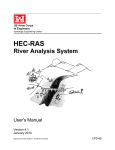
Chapter 3 Basic Data Requirements CHAPTER 3 Basic Data Requirements This chapter describes the basic data requirements for performing the onedimensional flow calculations within HEC-RAS. The basic data are defined and discussions of applicable ranges for parameters are provided. Contents ■ General ■ Geometric Data ■ Steady Flow Data ■ Unsteady Flow Data 3-1 Chapter 3 Basic Data Requirements General The main objective of the HEC-RAS program is quite simple - to compute water surface elevations at all locations of interest for either a given set of flow data (steady flow simulation), or by routing hydrographs through the system (unsteady flow simulation). The data needed to perform these computations are divided into the following categories: geometric data; steady flow data; unsteady flow data; and sediment data (not available yet). Geometric data are required for any of the analyses performed within HECRAS. The other data types are only required if you are going to do that specific type of analysis (i.e., steady flow data are required to perform a steady flow water surface profile computation). The current version of HECRAS can perform either steady or unsteady flow computations. Geometric Data The basic geometric data consist of establishing the connectivity of the river system (River System Schematic); cross section data; reach lengths; energy loss coefficients (friction losses, contraction and expansion losses); and stream junction information. Hydraulic structure data (bridges, culverts, spillways, weirs, etc...), which are also considered geometric data, will be described in later chapters. Study Limit Determination When performing a hydraulic study, it is normally necessary to gather data both upstream of and downstream of the study reach. Gathering additional data upstream is necessary in order to evaluate any upstream impacts due to construction alternatives that are being evaluated within the study reach (Figure 3.1). The limits for data collection upstream should be at a distance such that the increase in water surface profile resulting from a channel modification converges with the existing conditions profile. Additional data collection downstream of the study reach is necessary in order to prevent any user-defined boundary condition from affecting the results within the study reach. In general, the water surface at the downstream boundary of a model is not normally known. The user must estimate this water surface for each profile to be computed. A common practice is to use Manning’s equation and compute normal depth as the starting water surface. The actual water surface may be higher or lower than normal depth. The use of normal depth will introduce an error in the water surface profile at the boundary. In general, for subcritical flow, the error at the boundary will diminish as the computations proceed upstream. In order to prevent any computed errors within the study reach, the unknown boundary condition should be placed far enough downstream such that the computed profile will converge to a consistent answer by the time the computations reach the downstream limit of the study. 3-2 Chapter 3 Basic Data Requirements Starting Conditions Profile Errors Study Reach Project Induced Effect Levee Levee Plan View Modified profile Existing profile Profile View Figure 3.1 Example Study Limit Determination The River System Schematic The river system schematic is required for any geometric data set within the HEC-RAS system. The schematic defines how the various river reaches are connected, as well as establishing a naming convention for referencing all the other data. The river system schematic is developed by drawing and connecting the various reaches of the system within the geometric data editor (see Chapter 6 of the HEC-RAS User’s Manual for details on how to develop the schematic from within the user interface). The user is required to develop the river system schematic before any other data can be entered. Each river reach on the schematic is given a unique identifier. As other data are entered, the data are referenced to a specific reach of the schematic. For example, each cross section must have a “River”, “Reach” and “River Station” identifier. The river and reach identifiers defines which reach the cross section lives in, while the river station identifier defines where that cross section is located within the reach, with respect to the other cross sections for that reach. The connectivity of reaches is very important in order for the model to understand how the computations should proceed from one reach to the next. The user is required to draw each reach from upstream to downstream, in what is considered to be the positive flow direction. The connecting of reaches is considered a junction. Junctions should only be established at 3-3 Chapter 3 Basic Data Requirements locations where two or more streams come together or split apart. Junctions cannot be established with a single reach flowing into another single reach. These two reaches must be combined and defined as one reach. An example river system schematic is shown in Figure 3.2. Figure 3.2 Example River System Schematic. The example schematic shown in Figure 3.2 is for a dendritic river system. Arrows are automatically drawn on the schematic in the assumed positive flow direction. Junctions (red circles) are automatically formed as reaches are connected. As shown, the user is require to provide a river and reach identifier for each reach, as well as an identifier for each junction. HEC-RAS has the ability to model river systems that range from a single reach model to complicated networks. A “network” model is where river reaches split apart and then come back together, forming looped systems. An example schematic of a looped stream network is shown in Figure 3.3. 3-4 Chapter 3 Basic Data Requirements Figure 3.3 Example Schematic for a Looped Network of Reaches The river system schematic shown in Figure 3.3 demonstrates the ability of HEC-RAS to model flow splits as well as flow combinations. The current version of the steady flow model within HEC-RAS does not determine the amount of flow going to each reach at a flow split. It is currently up to the user to define the amount of flow in each reach. After a simulation is made, the user should adjust the flow in the reaches in order to obtain a balance in energy around the junction of a flow split. Cross Section Geometry Boundary geometry for the analysis of flow in natural streams is specified in terms of ground surface profiles (cross sections) and the measured distances between them (reach lengths). Cross sections are located at intervals along a stream to characterize the flow carrying capability of the stream and its adjacent floodplain. They should extend across the entire floodplain and 3-5 Chapter 3 Basic Data Requirements should be perpendicular to the anticipated flow lines. Occasionally it is necessary to layout cross-sections in a curved or dog-leg alignment to meet this requirement. Every effort should be made to obtain cross sections that accurately represent the stream and floodplain geometry. Cross sections are required at representative locations throughout a stream reach and at locations where changes occur in discharge, slope, shape, or roughness, at locations where levees begin or end and at bridges or control structures such as weirs. Where abrupt changes occur, several cross sections should be used to describe the change regardless of the distance. Cross section spacing is also a function of stream size, slope, and the uniformity of cross section shape. In general, large uniform rivers of flat slope normally require the fewest number of cross sections per mile. The purpose of the study also affects spacing of cross sections. For instance, navigation studies on large relatively flat streams may require closely spaced (e.g., 200 feet) cross sections to analyze the effect of local conditions on low flow depths, whereas cross sections for sedimentation studies, to determine deposition in reservoirs, may be spaced at intervals on the order of miles. The choice of friction loss equation may also influence the spacing of cross sections. For instance, cross section spacing may be maximized when calculating an M1 profile (backwater profile) with the average friction slope equation or when the harmonic mean friction slope equation is used to compute M2 profiles (draw down profile). The HEC-RAS software provides the option to let the program select the averaging equation. Each cross section in an HEC-RAS data set is identified by a River, Reach, and River Station label. The cross section is described by entering the station and elevation (X-Y data) from left to right, with respect to looking in the downstream direction. The River Station identifier may correspond to stationing along the channel, mile points, or any fictitious numbering system. The numbering system must be consistent, in that the program assumes that higher numbers are upstream and lower numbers are downstream. Each data point in the cross section is given a station number corresponding to the horizontal distance from a starting point on the left. Up to 500 data points may be used to describe each cross section. Cross section data are traditionally defined looking in the downstream direction. The program considers the left side of the stream to have the lowest station numbers and the right side to have the highest. Cross section data are allowed to have negative stationing values. Stationing must be entered from left to right in increasing order. However, more than one point can have the same stationing value. The left and right stations separating the main channel from the overbank areas must be specified on the cross section data editor. End points of a cross section that are too low (below the computed water surface elevation) will automatically be extended vertically and a note indicating that the cross section had to be extended will show up in the output for that section. The program adds additional wetted perimeter for any water that comes into contact with the extended walls. 3-6 Chapter 3 Basic Data Requirements Other data that are required for each cross section consist of: downstream reach lengths; roughness coefficients; and contraction and expansion coefficients. These data will be discussed in detail later in this chapter. Numerous program options are available to allow the user to easily add or modify cross section data. For example, when the user wishes to repeat a surveyed cross section, an option is available from the interface to make a copy of any cross section. Once a cross section is copied, other options are available to allow the user to modify the horizontal and vertical dimensions of the repeated cross section data. For a detailed explanation on how to use these cross section options, see chapter 6 of the HEC-RAS user's manual. Optional Cross Section Properties A series of program options are available to restrict flow to the effective flow areas of cross sections. Among these capabilities are options for: ineffective flow areas; levees; and blocked obstructions. All of these capabilities are available from the "Options" menu of the Cross Section Data editor. Ineffective Flow Areas. This option allows the user to define areas of the cross section that will contain water that is not actively being conveyed (ineffective flow). Ineffective flow areas are often used to describe portions of a cross section in which water will pond, but the velocity of that water, in the downstream direction, is close to zero. This water is included in the storage calculations and other wetted cross section parameters, but it is not included as part of the active flow area. When using ineffective flow areas, no additional wetted perimeter is added to the active flow area. An example of an ineffective flow area is shown in Figure 3.4. The cross-hatched area on the left of the plot represents what is considered to be the ineffective flow. Two alternatives are available for setting ineffective flow areas. The first option allows the user to define a left station and elevation and a right station and elevation (normal ineffective areas). When this option is used, and if the water surface is below the established ineffective elevations, the areas to the left of the left station and to the right of the right station are considered ineffective. Once the water surface goes above either of the established elevations, then that specific area is no longer considered ineffective. 3-7 Chapter 3 Basic Data Requirements The second option allows for the establishment of blocked ineffective flow areas. Blocked ineffective flow areas require the user to enter an elevation, a left station, and a right station for each ineffective block. Up to ten blocked ineffective flow areas can be entered at each cross section. Once the water surface goes above the elevation of the blocked ineffective flow area, the blocked area is no longer considered ineffective. Left Ineffective Flow Station Figure 3.4 Cross section with normal ineffective flow areas Levees. This option allows the user to establish a left and/or right levee station and elevation on any cross section. When levees are established, no water can go to the left of the left levee station or to the right of the right levee station until either of the levee elevations are exceeded. Levee stations must be defined explicitly, or the program assumes that water can go anywhere within the cross section. An example of a cross section with a levee on the left side is shown in Figure 3.5. In this example the levee station and elevation is associated with an existing point on the cross section. The user may want to add levees into a data set in order to see what effect a levee will have on the water surface. A simple way to do this is to set a levee station and elevation that is above the existing ground. If a levee elevation is placed above the existing geometry of the cross section, then a vertical wall is placed at that station up to the established levee height. Additional wetted perimeter is included when water comes into contact with the levee wall. An example of this is shown in Figure 3.6. 3-8 Chapter 3 Basic Data Requirements Left Levee Station Figure 3.5 Example of the Levee Option Obstructions. This option allows the user to define areas of the cross section that will be permanently blocked out. Obstructions decrease flow area and add wetted perimeter when the water comes in contact with the obstruction. A obstruction does not prevent water from going outside of the obstruction. Two alternatives are available for entering obstructions. The first option allows the user to define a left station and elevation and a right station and elevation (normal obstructions). When this option is used, the area to the left of the left station and to the right of the right station will be completely blocked out. An example of this type of obstruction is shown in Figure 3.7. 3-9 Chapter 3 Basic Data Requirements Left Levee Station and Eleveation Figure 3.6 Example Levee Added to a Cross Section Figure 3.7 Example of Normal Obstructions 3-10 Chapter 3 Basic Data Requirements The second option, for obstructions, allows the user to enter up to 20 individual blocks (Multiple Blocks). With this option the user enters a left station, a right station, and an elevation for each of the blocks. An example of a cross section with multiple blocked obstructions is shown in Figure 3.8. Figure 3.8 Example Cross Section With Multiple Blocked Obstructions Reach Lengths The measured distances between cross sections are referred to as reach lengths. The reach lengths for the left overbank, right overbank and channel are specified on the cross section data editor. Channel reach lengths are typically measured along the thalweg. Overbank reach lengths should be measured along the anticipated path of the center of mass of the overbank flow. Often, these three lengths will be of similar value. There are, however, conditions where they will differ significantly, such as at river bends, or where the channel meanders and the overbanks are straight. Where the distances between cross sections for channel and overbanks are different, a discharge-weighted reach length is determined based on the discharges in the main channel and left and right overbank segments of the reach (see Equation 2-3, of chapter 2). 3-11 Chapter 3 Basic Data Requirements Energy Loss Coefficients Several types of loss coefficients are utilized by the program to evaluate energy losses: (1) Manning’s n values or equivalent roughness “k” values for friction loss, (2) contraction and expansion coefficients to evaluate transition (shock) losses, and (3) bridge and culvert loss coefficients to evaluate losses related to weir shape, pier configuration, pressure flow, and entrance and exit conditions. Energy loss coefficients associated with bridges and culverts will be discussed in chapters 5 and 6 of this manual. Manning’s n. Selection of an appropriate value for Manning’s n is very significant to the accuracy of the computed water surface profiles. The value of Manning’s n is highly variable and depends on a number of factors including: surface roughness; vegetation; channel irregularities; channel alignment; scour and deposition; obstructions; size and shape of the channel; stage and discharge; seasonal changes; temperature; and suspended material and bedload. In general, Manning’s n values should be calibrated whenever observed water surface profile information (gaged data, as well as high water marks) is available. When gaged data are not available, values of n computed for similar stream conditions or values obtained from experimental data should be used as guides in selecting n values. There are several references a user can access that show Manning's n values for typical channels. An extensive compilation of n values for streams and floodplains can be found in Chow’s book “Open-Channel Hydraulics” [Chow, 1959]. Excerpts from Chow’s book, for the most common types of channels, are shown in Table 3.1 below. Chow's book presents additional types of channels, as well as pictures of streams for which n values have been calibrated. 3-12 Chapter 3 Basic Data Requirements Table 3.1 Manning's 'n' Values Type of Channel and Description Minimum Normal Maximum 0.025 0.030 0.033 0.035 0.040 0.030 0.035 0.040 0.045 0.048 0.033 0.040 0.045 0.050 0.055 0.045 0.050 0.070 0.050 0.070 0.100 0.060 0.080 0.150 0.025 0.030 0.030 0.035 0.035 0.050 0.020 0.025 0.030 0.030 0.035 0.040 0.040 0.045 0.050 0.035 0.035 0.040 0.045 0.070 0.050 0.050 0.060 0.070 0.100 0.070 0.060 0.080 0.110 0.160 0.030 0.050 0.080 0.040 0.060 0.100 0.050 0.080 0.120 0.100 0.120 0.160 0.110 0.150 0.200 0.030 0.040 0.040 0.050 0.050 0.070 A. Natural Streams 1. Main Channels a. Clean, straight, full, no rifts or deep pools b. Same as above, but more stones and weeds c. Clean, winding, some pools and shoals d. Same as above, but some weeds and stones e. Same as above, lower stages, more ineffective slopes and sections f. Same as "d" but more stones g. Sluggish reaches, weedy. deep pools h. Very weedy reaches, deep pools, or floodways with heavy stands of timber and brush 2. Flood Plains a. Pasture no brush 1. Short grass 2. High grass b. Cultivated areas 1. No crop 2. Mature row crops 3. Mature field crops c. Brush 1. Scattered brush, heavy weeds 2. Light brush and trees, in winter 3. Light brush and trees, in summer 4. Medium to dense brush, in winter 5. Medium to dense brush, in summer d. Trees 1. Cleared land with tree stumps, no sprouts 2. Same as above, but heavy sprouts 3. Heavy stand of timber, few down trees, little undergrowth, flow below branches 4. Same as above, but with flow into branches 5. Dense willows, summer, straight 3. Mountain Streams, no vegetation in channel, banks usually steep, with trees and brush on banks submerged a. Bottom: gravels, cobbles, and few boulders b. Bottom: cobbles with large boulders 3-13 Chapter 3 Basic Data Requirements Table 3.1 (Continued) Manning's 'n' Values Type of Channel and Description Minimum Normal Maximum 1. Concrete a. Trowel finish b. Float Finish c. Finished, with gravel bottom d. Unfinished e. Gunite, good section f. Gunite, wavy section g. On good excavated rock h. On irregular excavated rock 0.011 0.013 0.015 0.014 0.016 0.018 0.017 0.022 0.013 0.015 0.017 0.017 0.019 0.022 0.020 0.027 0.015 0.016 0.020 0.020 0.023 0.025 2. Concrete bottom float finished with sides of: a. Dressed stone in mortar b. Random stone in mortar c. Cement rubble masonry, plastered d. Cement rubble masonry e. Dry rubble on riprap 0.015 0.017 0.016 0.020 0.020 0.017 0.020 0.020 0.025 0.030 0.020 0.024 0.024 0.030 0.035 3. Gravel bottom with sides of: a. Formed concrete b. Random stone in mortar c. Dry rubble or riprap 0.017 0.020 0.023 0.020 0.023 0.033 0.025 0.026 0.036 4. Brick a. Glazed b. In cement mortar 0.011 0.012 0.013 0.015 0.015 0.018 5. Metal a. Smooth steel surfaces b. Corrugated metal 0.011 0.021 0.012 0.025 0.014 0.030 6. Asphalt a. Smooth b. Rough 0.013 0.016 0.013 0.016 7. Vegetal lining 0.030 B. Lined or Built-Up Channels 3-14 0.500 Chapter 3 Basic Data Requirements Table 3.1 (Continued) Manning's 'n' Values Type of Channel and Description Minimum Normal Maximum 0.016 0.018 0.022 0.022 0.018 0.022 0.025 0.027 0.020 0.025 0.030 0.033 0.023 0.025 0.030 0.025 0.030 0.035 0.030 0.033 0.040 0.028 0.025 0.030 0.030 0.035 0.040 0.035 0.040 0.050 3. Dragline-excavated or dredged a. No vegetation b. Light brush on banks 0.025 0.035 0.028 0.050 0.033 0.060 4. Rock cuts a. Smooth and uniform b. Jagged and irregular 0.025 0.035 0.035 0.040 0.040 0.050 5. Channels not maintained, weeds and brush a. Clean bottom, brush on sides b. Same as above, highest stage of flow c. Dense weeds, high as flow depth d. Dense brush, high stage 0.040 0.045 0.050 0.080 0.050 0.070 0.080 0.100 0.080 0.110 0.120 0.140 C. Excavated or Dredged Channels 1. Earth, straight and uniform a. Clean, recently completed b. Clean, after weathering c. Gravel, uniform section, clean d. With short grass, few weeds 2. Earth, winding and sluggish a. No vegetation b. Grass, some weeds c. Dense weeds or aquatic plants in deep channels d. Earth bottom and rubble side e. Stony bottom and weedy banks f. Cobble bottom and clean sides Other sources that include pictures of selected streams as a guide to n value determination are available (Fasken, 1963; Barnes, 1967; and Hicks and Mason, 1991). In general, these references provide color photos with tables of calibrated n values for a range of flows. Although there are many factors that affect the selection of the n value for the channel, some of the most important factors are the type and size of materials that compose the bed and banks of a channel, and the shape of the channel. Cowan (1956) developed a procedure for estimating the effects of these factors to determine the value of Manning’s n of a channel. In Cowan's procedure, the value of n is computed by the following equation: 3-15 Chapter 3 Basic Data Requirements n = ( nb + n1 + n2 + n3 + n4 ) m (3-1) where: nb = Base value of n for a straight uniform, smooth channel in natural materials n1 = Value added to correct for surface irregularities n2 = Value for variations in shape and size of the channel n3 = Value for obstructions n4 = Value for vegetation and flow conditions m = Correction factor to account for meandering of the channel A detailed description of Cowan’s method can be found in “Guide for Selecting Manning’s Roughness Coefficients for Natural Channels and Flood Plains” (FHWA, 1984). This report was developed by the U.S. Geological Survey (Arcement, 1989) for the Federal Highway Administration. The report also presents a method similar to Cowan’s for developing Manning’s n values for flood plains, as well as some additional methods for densely vegetated flood plains. Limerinos (1970) related n values to hydraulic radius and bed particle size based on samples from 11 stream channels having bed materials ranging from small gravel to medium size boulders. The Limerinos equation is as follows: n= where: R d84 (0.0926) R1 / 6 R 1.16 + 2.0 log d 84 = = (3-2) Hydraulic radius, in feet (data range was 1.0 to 6.0 feet) Particle diameter, in feet, that equals or exceeds that of 84 percent of the particles (data range was 1.5 mm to 250 mm) The Limerinos equation (3-2) fit the data that he used very well, in that the 2 coefficient of correlation R = 0.88 and the standard error of estimates for values of n R 1 / 6 = 0.0087. Limerinos selected reaches that had a minimum amount of roughness, other than that caused by the bed material. The Limerinos equation provides a good estimate of the base n value. The base n value should then be increased to account for other factors, as shown above in Cowen's method. 3-16 Chapter 3 Basic Data Requirements Jarrett (1984) developed an equation for high gradient streams (slopes greater than 0.002). Jarrett performed a regression analysis on 75 data sets that were surveyed from 21 different streams. Jarrett's equation for Manning's n is as follows: n = 0.39 S 0.38 R −0.16 where: S = (3-3) The friction slope. The slope of the water surface can be used when the friction slope is unknown. Jarrett (1984) states the following limitations for the use of his equation: 1. The equations are applicable to natural main channels having stable bed and bank materials (gravels, cobbles, and boulders) without backwater. 2. The equations can be used for slopes from 0.002 to 0.04 and for hydraulic radii from 0.5 to 7.0 feet (0.15 to 2.1 m). The upper limit on slope is due to a lack of verification data available for the slopes of high-gradient streams. Results of the regression analysis indicate that for hydraulic radius greater than 7.0 feet (2.1 m), n did not vary significantly with depth; thus extrapolating to larger flows should not be too much in error as long as the bed and bank material remain fairly stable. 3. During the analysis of the data, the energy loss coefficients for contraction and expansion were set to 0.0 and 0.5, respectively. 4. Hydraulic radius does not include the wetted perimeter of bed particles. 5. These equations are applicable to streams having relatively small amounts of suspended sediment. Because Manning’s n depends on many factors such as the type and amount of vegetation, channel configuration, stage, etc., several options are available in HEC-RAS to vary n. When three n values are sufficient to describe the channel and overbanks, the user can enter the three n values directly onto the cross section editor for each cross section. Any of the n values may be changed at any cross section. Often three values are not enough to adequately describe the lateral roughness variation in the cross section; in this case the “Horizontal Variation of n Value” should be selected from the “Options” menu of the cross section editor. If n values change within the channel, the criterion described in Chapter 2, under composite n values, is used to determine whether the n values should be converted to a composite value using Equation 2-5. Equivalent Roughness “k”. An equivalent roughness parameter “k”, 3-17 Chapter 3 Basic Data Requirements commonly used in the hydraulic design of channels, is provided as an option for describing boundary roughness in HEC-RAS. Equivalent roughness, sometimes called “roughness height,” is a measure of the linear dimension of roughness elements, but is not necessarily equal to the actual, or even the average, height of these elements. In fact, two roughness elements with different linear dimensions may have the same “k” value because of differences in shape and orientation [Chow, 1959]. The advantage of using equivalent roughness “k” instead of Manning’s “n” is that “k” reflects changes in the friction factor due to stage, whereas Manning’s “n” alone does not. This influence can be seen in the definition of Chezy's “C” (English units) for a rough channel (Equation 2-6, USACE, 1991): 12.2 R C = 32.6 log10 k where: C = Chezy roughness coefficient R = hydraulic radius (feet) k = equivalent roughness (feet) (3-4) Note that as the hydraulic radius increases (which is equivalent to an increase in stage), the friction factor “C” increases. In HEC-RAS, “k” is converted to a Manning’s “n” by using the above equation and equating the Chezy and Manning’s equations (Equation 2-4, USACE, 1991) to obtain the following: English Units: n= 1.486 R 1 / 6 R 32.6 log10 12.2 k (3-5) Metric Unit: R1/ 6 n= R 18 log10 12.2 k where: n = (3-6) Manning’s roughness coefficient Again, this equation is based on the assumption that all channels (even concrete-lined channels) are “hydraulically rough.” A graphical illustration of this conversion is available [USACE, 1991]. Horizontal variation of “k” values is described in the same manner as horizontal variation of Manning's “n” values. See chapter 6 of the HEC-RAS user’s manual, to learn how to enter k values into the program. Up to twenty 3-18 Chapter 3 Basic Data Requirements values of “k” can be specified for each cross section. Tables and charts for determining “k” values for concrete-lined channels are provided in EM 1110-2-1601 [USACE, 1991]. Values for riprap-lined channels may be taken as the theoretical spherical diameter of the median stone size. Approximate “k” values [Chow, 1959] for a variety of bed materials, including those for natural rivers are shown in Table 3.2. Table 3.2 Equivalent Roughness Values of Various Bed Materials k (Feet) Brass, Cooper, Lead, Glass Wrought Iron, Steel Asphalted Cast Iron Galvanized Iron Cast Iron Wood Stave Cement Concrete Drain Tile Riveted Steel Natural River Bed 0.0001 - 0.0030 0.0002 - 0.0080 0.0004 - 0.0070 0.0005 - 0.0150 0.0008 - 0.0180 0.0006 - 0.0030 0.0013 - 0.0040 0.0015 - 0.0100 0.0020 - 0.0100 0.0030 - 0.0300 0.1000 - 3.0000 The values of “k” (0.1 to 3.0 ft.) for natural river channels are normally much larger than the actual diameters of the bed materials to account for boundary irregularities and bed forms. Contraction and Expansion Coefficients. Contraction or expansion of flow due to changes in the cross section is a common cause of energy losses within a reach (between two cross sections). Whenever this occurs, the loss is computed from the contraction and expansion coefficients specified on the cross section data editor. The coefficients, which are applied between cross sections, are specified as part of the data for the upstream cross section. The coefficients are multiplied by the absolute difference in velocity heads between the current cross section and the next cross section downstream, which gives the energy loss caused by the transition (Equation 2-2 of Chapter 2). Where the change in river cross section is small, and the flow is subcritical, coefficients of contraction and expansion are typically on the order of 0.1 and 0.3, respectively. When the change in effective cross section area is abrupt such as at bridges, contraction and expansion coefficients of 0.3 and 0.5 are often used. On occasion, the coefficients of contraction and expansion around bridges and culverts may be as high as 0.6 and 0.8, respectively. These values may be changed at any cross section. For 3-19 Chapter 3 Basic Data Requirements additional information concerning transition losses and for information on bridge loss coefficients, see chapter 5, Modeling Bridges. Typical values for contraction and expansion coefficients, for subcritical flow, are shown in Table 3.3 below. Table 3.3 Subcritical Flow Contraction and Expansion Coefficients No transition loss computed Gradual transitions Typical Bridge sections Abrupt transitions Contraction Expansion 0.0 0.1 0.3 0.6 0.0 0.3 0.5 0.8 The maximum value for the contraction and expansion coefficient is one (1.0). In general, the empirical contraction and expansion coefficients should be lower for supercritical flow. In supercritical flow the velocity heads are much greater, and small changes in depth can cause large changes in velocity head. Using contraction and expansion coefficients that would be typical for subcritical flow can result in over estimation of the energy losses and oscillations in the computed water surface profile. In constructed trapezoidal and rectangular channels, designed for supercritical flow, the user should set the contraction and expansion coefficients to zero in the reaches where the cross sectional geometry is not changing shape. In reaches where the flow is contracting and expanding, the user should select contraction and expansion coefficients carefully. Typical values for gradual transitions in supercritical flow would be around 0.05 for the contraction coefficient and 0.10 for the expansion coefficient. As the natural transitions begin to become more abrupt, it may be necessary to use higher values, such as 0.1 for the contraction coefficient and 0.2 for the expansion coefficient. If there is no contraction or expansion, the user may want to set the coefficients to zero for supercritical flow. 3-20 Chapter 3 Basic Data Requirements Stream Junction Data Stream junctions are defined as locations where two or more streams come together or split apart. Junction data consists of reach lengths across the junction and tributary angles (only if the momentum equation is selected). Reach lengths across the junction are entered in the Junction Data editor. This allows for the lengths across very complicated confluences (e.g., flow splits) to be accommodated. An example of this is shown in Figure 3.9. Reach 1 Junction Reach 3 Reach 2 Figure 3.9 Example of a Stream Junction As shown in Figure 3.9, using downstream reach lengths, for the last cross section in Reach 1, would not adequately describe the lengths across the junction. It is therefore necessary to describe lengths across junctions in the Junction Data editor. For the example shown in Figure 3.9, two lengths would be entered. These lengths should represent the average distance that the water will travel from the last cross section in Reach 1 to the first cross section of the respective reaches. In general, the cross sections that bound a junction should be placed as close together as possible. This will minimize the error in the calculation of energy losses across the junction. 3-21 Chapter 3 Basic Data Requirements In HEC-RAS a junction can be modeled by either the energy equation (Equation 2-1 of chapter 2) or the momentum equation. The energy equation does not take into account the angle of any tributary coming in or leaving the main stream, while the momentum equation does. In most cases, the amount of energy loss due to the angle of the tributary flow is not significant, and using the energy equation to model the junction is more than adequate. However, there are situations where the angle of the tributary can cause significant energy losses. In these situations it would be more appropriate to use the momentum approach. When the momentum approach is selected, an angle for all tributaries of the main stem must be entered. A detailed description of how junction calculations are made can be found in Chapter 4 of this manual. Steady Flow Data Steady flow data are required in order to perform a steady water surface profile calculation. Steady flow data consist of: flow regime; boundary conditions; and peak discharge information. Flow Regime Profile computations begin at a cross section with known or assumed starting conditions and proceed upstream for subcritical flow or downstream for supercritical flow. The flow regime (subcritical, supercritical, or mixed flow regime) is specified on the Steady Flow Analysis window of the user interface. Subcritical profiles computed by the program are constrained to critical depth or above, and supercritical profiles are constrained to critical depth or below. In cases where the flow regime will pass from subcritical to supercritical, or supercritical to subcritical, the program should be run in a mixed flow regime mode. For a detailed discussion of mixed flow regime calculations, see Chapter 4 of this manual. Boundary Conditions Boundary conditions are necessary to establish the starting water surface at the ends of the river system (upstream and downstream). A starting water surface is necessary in order for the program to begin the calculations. In a subcritical flow regime, boundary conditions are only necessary at the downstream ends of the river system. If a supercritical flow regime is going to be calculated, boundary conditions are only necessary at the upstream ends of the river system. If a mixed flow regime calculation is going to be made, then boundary conditions must be entered at all ends of the river system. 3-22 Chapter 3 Basic Data Requirements The boundary conditions editor contains a table listing every reach. Each reach has an upstream and a downstream boundary condition. Connections to junctions are considered internal boundary conditions. Internal boundary conditions are automatically listed in the table, based on how the river system was defined in the geometric data editor. The user is only required to enter the necessary external boundary conditions. There are four types of boundary conditions available to the user: Known Water Surface Elevations - For this boundary condition the user must enter a known water surface elevation for each of the profiles to be computed. Critical Depth - When this type of boundary condition is selected, the user is not required to enter any further information. The program will calculate critical depth for each of the profiles and use that as the boundary condition. Normal Depth - For this type of boundary condition, the user is required to enter an energy slope that will be used in calculating normal depth (using Manning’s equation) at that location. A normal depth will be calculated for each profile based on the user-entered slope. In general, the energy slope can be approximated by using the average slope of the channel, or the average slope of the water surface in the vicinity of the cross section. Rating Curve - When this type of boundary condition is selected, a pop up window appears allowing the user to enter an elevation versus flow rating curve. For each profile, the elevation is interpolated from the rating curve given the flow, using linear interpolation between the user-entered points. Whenever the water surface elevations at the boundaries of the study are unknown; and a user defined water surface is required at the boundary to start the calculations; the user must either estimate the water surface, or select normal depth or critical depth. Using an estimated water surface will incorporate an error in the water surface profile in the vicinity of the boundary condition. If it is important to have accurate answers at cross sections near the boundary condition, additional cross sections should be added. If a subcritical profile is being computed, then additional cross sections need only be added below the downstream boundaries. If a supercritical profile is being computed, then additional cross sections should be added upstream of the relevant upstream boundaries. If a mixed flow regime profile is being computed, then cross sections should be added upstream and downstream of all the relevant boundaries. In order to test whether the added cross sections are sufficient for a particular boundary condition, the user should try several different starting elevations at the boundary condition, for the same discharge. If the water surface profile converges to the same answer, by the time the computations get to the cross sections that are in the study area, then enough sections have been added, and the boundary condition is not affecting the answers in the study area. 3-23 Chapter 3 Basic Data Requirements Discharge Information Discharge information is required at each cross section in order to compute the water surface profile. Discharge data are entered from upstream to downstream for each reach. At least one flow value must be entered for each reach in the river system. Once a flow value is entered at the upstream end of a reach, it is assumed that the flow remains constant until another flow value is encountered with the same reach. The flow rate can be changed at any cross section within a reach. However, the flow rate cannot be changed in the middle of a bridge, culvert, or stream junction. Flow data must be entered for the total number of profiles that are to be computed. Unsteady Flow Data Unsteady flow data are required in order to perform an unsteady flow analysis. Unsteady flow data consists of boundary conditions (external and internal), as well as initial conditions. Boundary Conditions Boundary conditions must be established at all of the open ends of the river system being modeled. Upstream ends of a river system can be modeled with the following types of boundary conditions: flow hydrograph; stage hydrograph; flow and stage hydrograph. Downstream ends of the river system can be modeled with the following types of boundary conditions: rating curve, normal depth (Manning’s equation); stage hydrograph; flow hydrograph; stage and flow hydrograph. Boundary conditions can also be established at internal locations within the river system. The user can specify the following types of boundary conditions at internal cross sections: lateral inflow hydrograph; uniform lateral inflow hydrograph; groundwater interflow. Additionally, any gated structures that are defined within the system (inline, lateral, or between storage areas) could have the following types of boundary conditions in order to control the gates: time series of gate openings; elevation controlled gate; navigation dam; or internal observed stage and flow. Initial Conditions In addition to boundary conditions, the user is required to establish the initial conditions (flow and stage) at all nodes in the system at the beginning of the simulation. Initial conditions can be established in two different ways. The most common way is for the user to enter flow data for each reach, and then have the program compute water surface elevations by performing a steady flow backwater analysis. A second method can only be done if a previous run was made. This method allows the user to write a file of flow and stage from 3-24 Chapter 3 Basic Data Requirements a previous run, which can then be used as the initial conditions for a subsequent run. In addition to establishing the initial conditions within the river system, the user must define the starting water surface elevation in any storage areas that are defined. This is accomplished from the initial conditions editor. The user must enter a stage for each storage area within the system. For more information on unsteady flow data, please review chapter 8 of the HEC-RAS User’s manual. 3-25