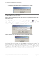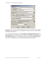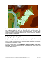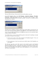
1
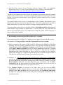
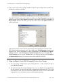
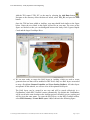
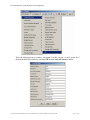
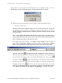
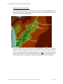
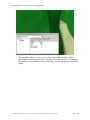
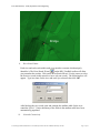
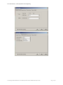
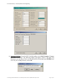
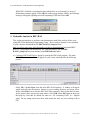
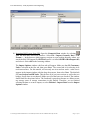
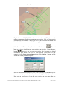
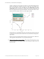
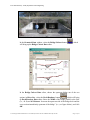
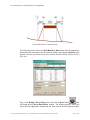
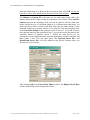
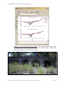
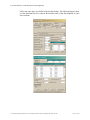
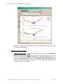
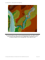
Texas A&M University – Zachry Department of Civil Engineering
Floodplain Mapping & Hydraulic Analysis with
HEC-GeoRAS 4.1.1 and ArcGIS 9.1
Prepared by Sarah Meyer1 and Francisco Olivera2, Ph.D., P.E.
May 2007
Contents:
1.
2.
3.
4.
5.
6.
7.
Goals of Exercise & Additional Resources
Downloading & Activating the HEC-GeoRAS 4.1.1 Extension
Using ArcMap to Create RAS (Geospatial) Layers for a Stream
Exporting GIS Data to HEC-RAS
Hydraulic Analysis in HEC-RAS
Importing Data from HEC-RAS
Mapping Floodplains Using GIS.
1. Goal of the exercise, additional resources and study area.
The purpose of this exercise is to familiarize the user with the floodplain mapping capabilities of
the extension HEC-GeoRAS developed by the Hydrologic Engineering Center (HEC) of the U.S.
Corps of Engineers. HEC-GeoRAS 4.1.1 requires ArcGIS 9.1 with the 3D Analyst and the
Spatial Analyst extensions. This tutorial was successfully completed using HEC-RAS 3.1.3. The
HEC-GeoRAS extension has many optional capabilities that will not be explored or do not apply
to the stream used in this tutorial.
Three manuals, prepared by the Hydrologic Engineering Center (HEC), were used extensively in
the preparation of this tutorial. The references for these manuals are listed below:
•
HEC-GeoRAS GIS Tools for Support of HEC-RAS Using ArcGIS, User’s Manual, CPD – 83,
Hydrologic Engineering Center, U.S. Army Corps of Engineers, Davis, California,
September 2005.
http://www.hec.usace.army.mil/software/hec-ras/hec-georas_downloads.html
•
HEC-RAS River Analysis System, User’s Manual, CPD – 68, Hydrologic Engineering Center,
U.S. Army Corps of Engineers, Davis, California, November 2002.
http://www.hec.usace.army.mil/software/hec-ras/hecras-document.html
1
Sarah Meyer is a Civil Engineering Graduate of Texas A&M University. She developed this exercise in partial
fulfillment of the requirements of the CVEN658 Civil Engineering Applications of GIS class taught the Fall 2006.
2
Francisco Olivera ([email protected]) is an Assistant Professor of Civil Engineering at Texas A&M
University. He teaches graduate and undergraduate courses and conducts research on the use of GIS in water
resources engineering.
Z:\Teaching\CVEN658\GISNewExercises\SarahMeyer\Final 2007 05 28\HECGeoRAS after FO.doc
Page 1 of 42
Texas A&M University – Zachry Department of Civil Engineering
•
HEC-RAS River Analysis System, Hydraulic Reference Manual, CPD – 69, Hydrologic
Engineering Center, U.S. Army Corps of Engineers, Davis, California, November 2002.
http://www.hec.usace.army.mil/software/hec-ras/hecras-document.html
The HEC-RAS manuals are useful to answer any questions you may have about the hydraulic
analysis portion of this tutorial. If you want to apply the procedures from this tutorial to a new
location or you need to trouble-shoot a specific problem, all three manuals will be a valuable
reference to you.
The region of study for this exercise is a small tributary to the Guadalupe River named Cypress
Rapids Creek, which is located in New Braunfels, TX. This creek is approximately one mile in
length, drains about 2.3 square miles, and has two bridge crossings within the study reach.
The required data for this exercise is stored in the folder TutorialDataGeoRAS. Maintaining the
folder structure, copy the folder to your hard drive. To be safe, make sure your folder name and
path do not contain blank spaces. You might need to change the folder and file properties to
remove the Read Only attribute.
2. Downloading and activating the HEC-GeoRAS 4.1.1 extension
If you already have HEC-GeoRAS 4.1.1 installed in your computer, you may skip this section
and continue at 3. Using ArcMap to create RAS (geospatial) layers for a stream.
a.) Make sure that any old versions of HEC-GeoRAS, APFramework, MSXML or XML Data
Exchange Tools are properly uninstalled. Remove these programs through the Windows
Control Panel using the Add/Remove Programs option. If you do not find APFramework
in the Add or Remove Programs list, run the program Unwise.exe, located in C:\Program
Files\ESRI\WaterUtils\APFrameworkX folder, to uninstall it. Note that the location of
Unwise.exe might change depending on where ArcGIS was installed in your computer.
Additionally, navigate to C:\Program Files\ESRI\WaterUtils, the default storage location of
APFramework and XML Data Exchange Tools, and delete the folder.
b.) Navigate to http://www.hec.usace.army.mil/software/hec-ras/hec-georas_downloads.html
and click on Primary Download Site under the heading HEC-GeoRAS 4.1.1 for ArcGIS
9.1. Select Save on the pop-up menu, navigate to the folder where you would like to store the
HEC-GeoRAS4.1.1.exe file, and click Save. For your convenience, the file HECGeoRAS4.1.1.exe has been included in the folder HECSoftware, so you do not have to
access the Internet and download it if you prefer not to do so.
c.) Use Windows Explorer to navigate to the folder where you just saved the HECGeoRAS4.1.1.exe file. Unzip it and save it in the same folder. Next, open the newly
unzipped folder HEC-GeoRAS 4.1.1 and open the text file Installation Instructions
4.1.1.txt. The instructions in this text file will guide you through the remainder of the file
installation process.
Z:\Teaching\CVEN658\GISNewExercises\SarahMeyer\Final 2007 05 28\HECGeoRAS after FO.doc
Page 2 of 42
Texas A&M University – Zachry Department of Civil Engineering
d.) You are now ready to start working with HEC-GeoRAS. Open ArcMap. HEC-GeoRAS will
be loaded as a toolbar in ArcMap.
If the HEC-GeoRAS toolbar is not loaded in ArcMap, select Tools/Customize from the main
interface menu, click on the Toolbars tab and place a checkmark in the box corresponding to
HEC-GeoRAS. While in this menu, you may also want to activate the Editor toolbar, as it
will be needed later.
You will also need to activate both the Spatial Analyst and 3D Analyst extensions for the
HEC-GeoRAS toolbar to properly work. In ArcMap, select Tools/Extensions from the main
interface menu. Place a checkmark in the box corresponding to the 3D Analyst and Spatial
Analyst extensions. If the 3D Analyst and Spatial Analyst toolbars are not loaded, select
Tools/Customize and click on the Toolbars tab as you did before and check the 3D Analyst
and Spatial Analyst boxes. You are now ready to work with HEC-GeoRAS.
3. Using ArcMap to Create RAS (Geospatial) Layers for a Stream
a.) Save your empty ArcMap map in your working directory. In this example the map is
named RASLayers.mxd.
b.) The main data input for creating floodplains for a river is a digital terrain model (DTM).
For this exercise, you have been provided a triangulated irregular network (TIN) of the
creek study area. This TIN was created from a DEM with cell size of 2-feet, which makes
it appropriate for use in hydraulic analyses and floodplain modeling.
Z:\Teaching\CVEN658\GISNewExercises\SarahMeyer\Final 2007 05 28\HECGeoRAS after FO.doc
Page 3 of 42
Texas A&M University – Zachry Department of Civil Engineering
.
Add the TIN, named “TIN_2ft”, to the map by selecting the Add Data button
Navigate to the directory where the data are stored, select TIN_2ft, and press the Add
button.
Once the TIN has been added to ArcMap, your map should look similar to the figure
below. Notice the river labels in this figure will not be on your map. The rivers on the
figure are labeled so that you can distinguish between the study reach Cypress Rapids
Creek and the larger Guadalupe River.
c.) We are now ready to create the RAS layers in ArcMap, which are used to create
geometric data sets that will be modeled in HEC-RAS. Only two RAS layers are needed
to map a floodplain (Stream Centerline and Cross Section Cutlines). All other layers
are optional. In this tutorial, we will use a few of the optional RAS layers.
The RAS layers can be created in one step and will be stored collectively in a
GeoDatabase, which HEC-GeoRAS creates automatically. By default, this GeoDatabase
will be saved in the same location as the ArcMap project with which you are working and
will be given the same name. To create the RAS layers, on the HEC-GeoRAS toolbar,
select RAS Geometry / Create RAS Layers / All, as shown in the following figure.
Z:\Teaching\CVEN658\GISNewExercises\SarahMeyer\Final 2007 05 28\HECGeoRAS after FO.doc
Page 4 of 42
Texas A&M University – Zachry Department of Civil Engineering
Then, the following pop-up window will appear. For this exercise, we will accept all of
the default RAS layer names by choosing OK on the Create All Layers window.
Z:\Teaching\CVEN658\GISNewExercises\SarahMeyer\Final 2007 05 28\HECGeoRAS after FO.doc
Page 5 of 42
Texas A&M University – Zachry Department of Civil Engineering
It may take a few seconds, but once the RAS layers are successfully created, you will see
the following message and the new layers will appear in the table of contents.
The following sections discuss how to create (digitize) each individual RAS layer.
i.
Stream Centerline Layer
This layer will be used to digitize (draw) the river reach network for the system you
are studying. For this tutorial, we will digitize only one stream with one reach. It is
possible, though, to model networks of streams with HEC-GeoRAS, but that will not
be discussed here.
Note: Always digitize the stream in the direction of flow. That is, you must begin at
the most upstream end of the stream, and work your way downstream ending at the
outlet or beginning of the next downstream reach.
In ArcMap, on the Editor toolbar, select Editor / Start Editing from the drop-down
menu. Select Create New Feature in the task window of the toolbar and River
(name of stream centerline) for the target feature class, as seen in the figure below.
Select the sketch tool
from the Editor toolbar to digitize the stream centerline in
the downstream direction. Left-clicking the mouse will drop a vertex point for the
line, and double-clicking the left mouse button will finish the line. You can pan
and zoom in and out
without interrupting your line drawing. After panning or
zooming you will have to select the sketch tool again, to resume drawing your line.
will remove the last point you placed and can be very
Selecting the undo tool
useful for erasing mistakes.When your centerline is complete, from the Editor toolbar,
select Editor / Save Edits and then Editor / Stop Editing to end your edit session.
Z:\Teaching\CVEN658\GISNewExercises\SarahMeyer\Final 2007 05 28\HECGeoRAS after FO.doc
Page 6 of 42
Texas A&M University – Zachry Department of Civil Engineering
Digitizing the Stream Centerline
The following picture shows a close-up view of the stream. Begin digitizing your
stream centerline at the downstream end of the railroad crossing and follow through
to the outlet into the Guadalupe River.
The next picture shows a close-up view of digitizing the stream. The stream
centerline will follow the path of lowest elevation, so care must be taken to find the
lowest elevations and then connect them with the streamline. You can find individual
elevation points on the TIN by selecting the Identity tool
, and then clicking on the
TIN layer in the map. A pop-up box will appear, listing the elevation at that point.
Z:\Teaching\CVEN658\GISNewExercises\SarahMeyer\Final 2007 05 28\HECGeoRAS after FO.doc
Page 7 of 42
Texas A&M University – Zachry Department of Civil Engineering
The next picture shows a close-up view of one of the bridge crossings. When
digitizing the stream follow from the centerline of the upstream side of the bridge to
the centerline of the downstream side of the bridge, passing through the center of the
bridge.
Z:\Teaching\CVEN658\GISNewExercises\SarahMeyer\Final 2007 05 28\HECGeoRAS after FO.doc
Page 8 of 42
Texas A&M University – Zachry Department of Civil Engineering
Bridge
ii.
River Reach Name
Each river and each reach within each river must have a name which uniquely
identifies it. The River Reach ID tool
on the HEC-GeoRAS toolbar will allow
you to number the reaches. Click on the River Reach ID tool. Use the cursor to select
the first river reach (in this tutorial we have only one reach). The following box will
appear. Type in a name for the river and reach you selected, then click OK.
After labeling the river reach, open and examine the attribute table for the river
centerline “River”. Notice that many of the fields in the attribute table have been
automatically populated.
iii.
Network Connectivity
Z:\Teaching\CVEN658\GISNewExercises\SarahMeyer\Final 2007 05 28\HECGeoRAS after FO.doc
Page 9 of 42
Texas A&M University – Zachry Department of Civil Engineering
Next, we will populate the “ToNode” and “FromNode” fields in the River centerline
attribute table. From the HEC-GeoRAS toolbar select RAS Geometry / Stream
Centerline Attributes / Topology. The following box will appear.
Select the name of your stream centerline and terrain TIN in the drop-down menus
and then select OK. After you do, the following message will appear.
Next, to determine the length of each reach and populate the “FromSta” and “ToSta”
fields in the attribute table, from the HEC-GeoRAS toolbar select RAS Geometry /
Stream Centerline Attributes / Lengths/Stations from the menu. You’ll receive
the following message.
iv.
Bank Lines Layer
The purpose of creating this layer is to distinguish between the main channel of the
river and the floodplains (overbanks) of the river. The bank lines will be created in
similar fashion as the river centerline and also starting from upstream.
On the Edit toolbar, select Editor / Start Editing. Make sure the task window of the
Edit toolbar says Create New Feature and that your target is now set to Banks.
Select the sketch tool
from the Editor toolbar and begin digitizing either the
right or left bank line in the downstream direction. Left-clicking the mouse will drop
Z:\Teaching\CVEN658\GISNewExercises\SarahMeyer\Final 2007 05 28\HECGeoRAS after FO.doc
Page 10 of 42
Texas A&M University – Zachry Department of Civil Engineering
a vertex point for the line, and double-clicking the left mouse button will finish the
and zoom in and out
without interrupting
line. You are allowed to pan
your line drawing. After panning or zooming you will have to select the sketch tool
again, to resume drawing your line. Selecting the undo tool
will remove the last
point you placed and can be very useful for erasing mistakes. When the bank line is
complete, from the Editor toolbar, select Editor / Save Edits and then Editor / Stop
Editing to end your edit session.
Digitizing the Bank Lines
Contours lines can help guide you digitize the bank lines. Two-foot contours are
provided in the data set and can be added to the map to assist you.
The following picture shows an example of drawing bank lines. You will have to
zoom in closely to the section of the river you are working with. You want the bank
lines to represent the edges of the main channel. In the following picture, you will
see that the bank line is drawn at what appears to be the edge of the creek, at the top
of the steepest grade from the creek and before the land planes out again on a more
gradual slope along the floodplain. Note that bank lines do not coincide with contour
lines.
v.
Flowpath Centerlines
Z:\Teaching\CVEN658\GISNewExercises\SarahMeyer\Final 2007 05 28\HECGeoRAS after FO.doc
Page 11 of 42
Texas A&M University – Zachry Department of Civil Engineering
The flowpath centerline layer is a set of lines that follows the center of mass of the
water flowing down the river. For the main channel, the stream centerline is the
flowpath centerline. For the channel overbanks (floodplains), the flowpath centerline
is located in the center of the overbank, and is set slightly outside the main channel
bank lines. Note that the widths of the floodplains are unknown thus far. The
flowpath centerlines are used to calculate the downstream reach lengths between
cross-sections. Flowpath centerlines are also created from upstream to downstream
according to the following instructions.
You have already created a Flowpaths feature class, but following these steps will
save you time. In the HEC-GeoRAS toolbar, select RAS Geometry / Create RAS
Layers / Flowpath Centerlines. The following menu will appear asking if you
would like to copy the stream centerline as your main channel flowpath line.
Select Yes. In the following window, select the Stream Centerline and Flowpath
Centerlines feature classes and click OK, and the following message window will
appear. Click OK.
You still need to digitize the overbank flowpath lines in the downstream direction.
Do this in an edit session, with Create New Feature as the task and Flowpaths as
the target in the Editor toolbar. Draw the flowpaths using the same methods described
above for digitizing the stream centerline and bank lines.
Next, you need to label each flowpath line using the Assign Line Type tool
.
After clicking on the Assign Line Type tool, click on a Flowpaths line, and then
select the correct option (i.e., right or left) in the window that pops up and click OK.
Repeat with all three flowpaths. Note the right flowpath is the line on your right if
you were looking downstream and water was hitting you in the back.
Z:\Teaching\CVEN658\GISNewExercises\SarahMeyer\Final 2007 05 28\HECGeoRAS after FO.doc
Page 12 of 42
Texas A&M University – Zachry Department of Civil Engineering
vi.
XS Cut Lines
Cross-sectional cut lines are used to define cross sections along the channel network
by using vertical planes (i.e., the XS cut lines) to cut the terrain TIN. There are a few
important rules to keep in mind when drawing cross-section cut lines.
•
Cut lines should be perpendicular to the direction of flow. You can use both the
river centerline and the flowpath lines to assist you in this task. You can dog-leg
cut lines if need be, to keep them perpendicular to the direction of flow.
•
Cut lines should be drawn directionally from left to right bank.
•
Cut lines should extend far enough on either side of the channel to encompass the
entire portion of the floodplain you want to model. They should end at the same
elevation at both ends.
•
Cut lines should not intersect each other.
•
Cut lines should be spaced close enough to account for notable changes in the
hydraulics or geometry of the stream, such as changes in discharge, slope, cross
section shape, roughness or presence of hydraulic structures (bridges, levees,
weirs.)
•
Each bridge intersection will require 4 cut lines, 2 upstream of the bridge and 2
downstream of the bridge. See the following figure for an illustration for spacing
these cross sections. In this figure, Lc represents the contraction reach length and
Le is the expansion reach length. Typically, Lc < Le as shown in the picture.
These distances can be determined by field investigation during high flows or by
examining the TIN to locate the point in the channel where the flowpath has fully
expanded or contracted. The flowpath lines should be parallel to each other where
cross-sections 1 and 4 are placed. Cross-sections 2 and 3 should be placed within
a short distance of the upstream and downstream ends of the bridge. The purpose
Z:\Teaching\CVEN658\GISNewExercises\SarahMeyer\Final 2007 05 28\HECGeoRAS after FO.doc
Page 13 of 42
Texas A&M University – Zachry Department of Civil Engineering
of placing these cross-sections near the bridge is to capture the natural ground
elevations directly next to the bridge. A good rule of thumb is to draw crosssections 2 and 3 at the toe of the bridge embankment on their respective sides of
the bridge.
Note: More information on this topic can be found on pages 6-23 to 6-26 in the
HEC-RAS User’s Manual. There is also an empirical method of determining the
distances Lc and Le based upon channel slope, ratios for bridge width opening to
the total floodplain width, and ratios of Manning’s roughness values (n) for the
main channel and floodplain explained in this section of the manual. This
approach, however, is not used in this tutorial.
(USACE HEC-RAS User’s Manual, 2002)
To draw cut lines, star an editing session and select Create New Feature from the
Task menu and XSCutLines from the Target menu. Draw all the cut lines (do not
forget to draw the bridge cross sections!) and save your edits. As you are drawing cut
lines you can preview the cross-section using the XS Plot tool
. After pressing the
XS Plot tool, left-click on the cross-section of interest, a plot will appear in a new
window. This feature will help you ensure you are drawing your cross-sections long
enough to capture the entire floodplain. After drawing the cut lines, they should look
similar to the following figure. Note the bridge location in the upper right corner.
Also note that, even though two of the cross sections might look like intersecting,
they are just very close to each other but do not intersect.
Z:\Teaching\CVEN658\GISNewExercises\SarahMeyer\Final 2007 05 28\HECGeoRAS after FO.doc
Page 14 of 42
Texas A&M University – Zachry Department of Civil Engineering
vii.
Attributing Cross-Section Cut Lines & Creating a 3D Feature Class
Now, we will populate the attribute table of the XSCutLines feature class we just
digitized. From the HEC-Geo RAS toolbar, select RAS Geometry / XS Cut Line
Attributes / All. The following pop-up window will be displayed. Use the dropdown menu to select the correct layer name for each item on the list. The first 5 items
on the list will be used to populate the empty fields in the attribute table of the
XSCutLines feature class. The last item (i.e., XS Cut Lines Profiles) is the name of a
new feature class that will be created. The 2D feature class XSCutLines will be
intersected with the TIN to create a feature class with 3D cross-section cut lines.
Accept the default name for this feature class XSCutLines3D.
Z:\Teaching\CVEN658\GISNewExercises\SarahMeyer\Final 2007 05 28\HECGeoRAS after FO.doc
Page 15 of 42
Texas A&M University – Zachry Department of Civil Engineering
Select OK on the All Cross-Section Tools window and the following message will
appear. Select OK again.
Open the attribute table of the new feature class XSCutLines3D and examine of the
populated fields.
viii.
Bridges/Culverts
Bridges and culverts are treated similarly to creating the cross-section layer. Begin an
editing session, and then select Create New Feature for the Task and Bridges as the
Target layer in the Editor toolbar. Digitize lines tracing each bridge/culvert crossing
for the stream. Bridges/culverts follow the same directional rules as the cross-section
layer. Remember to draw them from left overbank to right overbank. You can use the
TIN, the contours layer, or the aerial photo provided in the data folder to locate each
bridge and draw a line along the centerline of the bridge without intersecting the cross
sections. Extend your line beyond the ends of the bridge, so that you are sure to
capture the topography of the section. Once finished, save edits and end your edit
session.
ix.
Attributing Bridges/Culverts & Creating a 3D Feature Class
From the HEC-GeoRAS toolbar, select RAS Geometry / Bridges/Culverts / All.
The following window will pop-up menu. Use the drop-down menu to select the
correct layer name for each item on the list. The first 3 items on the list will populate
the empty fields in the attribute table of the Bridges/Culverts feature class. The last
item (i.e., Bridges/Culverts Profiles) will be the name of a new feature class that will
be created. The 2D feature class Bridges will be intersected with the TIN to create a
feature class of the bridges in 3D. In the window below, the default name for this
feature class Bridges3D is used.
Z:\Teaching\CVEN658\GISNewExercises\SarahMeyer\Final 2007 05 28\HECGeoRAS after FO.doc
Page 16 of 42
Texas A&M University – Zachry Department of Civil Engineering
Select OK on the All Bridge/Culverts Tools window and the following message will
appear.
x.
Optional RAS Layers
For the purpose of this tutorial, we are finished digitizing RAS layers. In the table of
contents window in ArcMap, you will notice that there are several empty feature
classes (SAConnections, StorageAreas, IneffAreas, BlockedObs, LandUse…) that
were created at the beginning, but we did not populate them. It is fine to not use all of
the optional RAS layers, but in the future you may come across a project where their
application is beneficial to you. The HEC-GeoRAS User’s Manual describes these
additional RAS layers, their use, and instructions for applying them to a scenario.
4. Exporting GIS Data to HEC-RAS
a.) Selecting Data for Export: From the HEC-GeoRAS toolbar, select RAS Geometry /
Layer Setup from the menu. The Layer Setup window with four tabs (Required
Surface, Required Layers, Optional Layers and Optional Tables) will appear. These
tabs are shown in the next four figures and include the preferences you should choose for
this tutorial. The purpose of the Layer Setup menu is to define which layers will be
exported to HEC-RAS. In this example, many of the menu items will show a Null value
because we did not use all of the optional RAS layers in this tutorial. Once you have
made all your selections in the Layer Setup tabs, select OK.
Z:\Teaching\CVEN658\GISNewExercises\SarahMeyer\Final 2007 05 28\HECGeoRAS after FO.doc
Page 17 of 42
Texas A&M University – Zachry Department of Civil Engineering
Z:\Teaching\CVEN658\GISNewExercises\SarahMeyer\Final 2007 05 28\HECGeoRAS after FO.doc
Page 18 of 42
Texas A&M University – Zachry Department of Civil Engineering
b.) Exporting GIS Data: From the HEC-GeoRAS toolbar, select RAS Geometry / Extract
GIS DATA menu item. The following window will appear. Choose a file name and
directory to save the data in. Here, we will call the file by its default name GIS2RAS and
save it in your working directory. Select OK.
Z:\Teaching\CVEN658\GISNewExercises\SarahMeyer\Final 2007 05 28\HECGeoRAS after FO.doc
Page 19 of 42
Texas A&M University – Zachry Department of Civil Engineering
While HEC-GeoRAS is exporting the data (which takes several seconds), a series of
information messages appear. Select OK for each message prompt. Finally, the following
message will appear signaling successful exporting of GIS data. Select OK.
5. Hydraulic Analysis in HEC-RAS
This section presents how to perform a one-dimensional steady flow analysis of the creek
using HEC-RAS (Hydrologic Engineering Center – River Analysis System). If not installed
in your computer, download the file HEC-RAS313_Setup.exe from
http://www.hec.usace.army.mil/software/hec-ras/hecras-download.html and install HECRAS 3.1.3 according to the instructions. For your convenience, the file HECRAS313_Setup.exe has been included in the HECSoftware folder.
a.) Creating a HEC-RAS Project: Begin by opening the HEC-RAS program. The main
HEC-RAS interface window will appear on your screen, and looks like the following
picture.
Select File / New Project from the main HEC-RAS interface. A window will appear
which looks like the next picture. Browse to your working directory and create a new
folder called RAS in it to store the HEC-RAS files separately. Enter a title and file name
for the project (they can have the same name). Select OK. Select OK again on the menu
that pops up. Note that by default the units are “US Customary Units” (i.e., English
units). Do not change them since these units match the ones we were working with in
GIS.
Z:\Teaching\CVEN658\GISNewExercises\SarahMeyer\Final 2007 05 28\HECGeoRAS after FO.doc
Page 20 of 42
Texas A&M University – Zachry Department of Civil Engineering
b.) Importing RAS Layers from GIS: Open the Geometric Data window by selecting
from the main HEC-RAS user interface. Select File / Import Geometry Data / GIS
Format …. In the browser which appears, navigate to your working directory where you
stored the RAS GIS import file GIS2RAS (notice it is called GIS2RAS.RASImport.sdf)
and select it. Select OK in the browsing window.
The Import Options window with four tabs will appear. Make sure that US Customary
Units is selected on the first tab, then press Next. The second tab is for selecting river
reach stream lines. For this tutorial, we have only one river and one reach – make sure it
appears in the import window with the drop-down arrow, then select Next. The third tab
is Cross Sections and IB Nodes. This tab lists all of our cross-sections as well as the two
bridges. Scroll down to see them all. Make sure all of the boxes are checked. The window
should look like the picture below. The fourth tab is grayed out because we did not create
any storage areas or storage connections in this tutorial. Therefore, we are finished
selecting the data we want to import, so select Finished – Import Data from the Import
Options window.
Z:\Teaching\CVEN658\GISNewExercises\SarahMeyer\Final 2007 05 28\HECGeoRAS after FO.doc
Page 21 of 42
Texas A&M University – Zachry Department of Civil Engineering
Note: If at any point you need to revise or add cross-sections or bridges to your data set,
you can add them in GIS (i.e., draw and attribute them), then return to the Import
Options menu in HEC-RAS and import only the sections which are new to your data set
by checking the appropriate boxes.
Now, your Geometric Data window should look similar to the following picture. A
georeferenced schematic of your river system will appear in the window. To save this
data, in the Geometric Data window, select File / Save Geometry Data and enter a
filename in the Title slot of the dialog box. I descriptively named my geometry data
Geometry.
Z:\Teaching\CVEN658\GISNewExercises\SarahMeyer\Final 2007 05 28\HECGeoRAS after FO.doc
Page 22 of 42
Texas A&M University – Zachry Department of Civil Engineering
c.) Entering Additional Data in the HEC-RAS Model: We will now use the Geometric Data
window to help us enter more data about the stream.
i. Cross-Section Points Filter: HEC-RAS allows a maximum of 500 data points per
cross-section. HEC-RAS has a cross-section points filter, which will allow us to
delete excess and duplicate points. In the Geometric Data window, select Tools /
Cross Section Points Filter. Once the Cross Section Points Filter window opens,
select the Multiple Locations tab and then the Minimize Area Change tab. In the
River option, select (All Rivers) and press the arrow
to slect them. Just for
practice, we will filter our cross-section to 250 points; but most of the crosssections already fall below this value. Enter 250 for the number of points to filter
down to and press the Filter Points on Selected XS button to complete this task.
The following picture shows all of the appropriate options selected.
Z:\Teaching\CVEN658\GISNewExercises\SarahMeyer\Final 2007 05 28\HECGeoRAS after FO.doc
Page 23 of 42
Texas A&M University – Zachry Department of Civil Engineering
A new window will appear showing the cross-sections that had more than 250
points or duplicate points, and were filtered. Select Close on this window, and then
select OK on the Cross Section Points Filter window. In the Geometric Data
window click on File / Save Geometry Data to keep these changes.
ii. Manning’s Roughness Values (n): Next, we need to enter Manning’s n values for
each cross-section. In the Geometric Data window select Tables / Manning’s n or
k values… . In the Edit Manning’s n or k Values window, select (All Rivers)
from the drop-down box in the River option. You will see all of your cross-sections
and two bridges listed in the table, with blank spaces where you will type in your n
values. The fields n#1 and n#3 are for the Manning’s n values for the overbanks
(floodplains). Enter 0.1 in these fields for all cross-sections, but not for the bridges.
Similarly, the field n#2 is for the main channel Manning’s n value. Enter 0.05 in
this field for all cross-sections, but not for the bridges. Once you’ve populated the
whole table, select OK. The window will close. Make sure you save your geometry
data again to retain this information.
Z:\Teaching\CVEN658\GISNewExercises\SarahMeyer\Final 2007 05 28\HECGeoRAS after FO.doc
Page 24 of 42
Texas A&M University – Zachry Department of Civil Engineering
Levees: Levees are linear features that contain the flow of water inside the
floodplain. Some channel scenarios may require levees to be defined in order to
maintain the true flowpath of the water. Usually, levees represent man-made
features in tended to constraint the floodplain, but can also represent other type of
high ground (such as roadway embankments or ridges in the natural topography of
the landscape) that blocks the flow until they are overtopped. Levees are only
required if the high ground prevents the stream from being hydraulically connected
to the terrain at the other side. If the terrain at the other side is hydraulically
connected to the stream upstream of the high ground, a levee should not be placed
on the cross-section.
In the example presented in this tutorial, the railroad track embankment, which runs
somewhat parallel to the creek, acts as a levee. The way the cross-sections have
been drawn in this tutorial, the most upstream cross-sections intersect the railroad
embankment, and require levees to be defined in HEC-RAS. Your cross-sections
may or may not cross the railroad tracks, so you will have to inspect your own
sections to make sure. In the data provided, Railroad.shp depicts the railroad
embankment. You may want to add it to your map to see if your cross-sections
extend across it. You can also look for topographical features in the landscape
intersected by your cross-sections for potential levee locations.
Z:\Teaching\CVEN658\GISNewExercises\SarahMeyer\Final 2007 05 28\HECGeoRAS after FO.doc
Page 25 of 42
Texas A&M University – Zachry Department of Civil Engineering
To place levees in HEC-RAS, follow these directions. Levees will be placed on the
roadway embankment for the most upstream cross-sections. Only one cross-section
is presented in this example to show you how to add levees, but you should add
levees for all the cross sections to which levees apply.
In the Geometric Data window, select the Cross Section button
. This will
bring up a window displaying your cross-sections one at a time. Using the arrow
buttons
, browse to one of your cross-sections that intersects the railroad
embankment (this tutorial will use the most upstream cross-section for this
example). On the Cross Section Data window, select Options / Levees and the
window in the next picture will appear.
Enter the station and elevation of the levee in this window. You can add two levees
in a cross-section (one on the left bank and one on the right bank) or just one levee.
Note that you need levees only in the cross sections that have more than one
Z:\Teaching\CVEN658\GISNewExercises\SarahMeyer\Final 2007 05 28\HECGeoRAS after FO.doc
Page 26 of 42
Texas A&M University – Zachry Department of Civil Engineering
channel. A simple way to locate the levee points is to click on them using the arrow
pointer and reading the coordinates in the lower right corner of the display area.
Once you entered the levee data, select OK. Next, select Apply Data in the Cross
Section Data window for the data to be added to the cross section information and
the levees to appear on the cross-section schematic. The next picture shows a crossstation used in this example with the levee on the right overbank.
In this specific case, the definition of the levee was unnecessary since the water will
overflow the cross section on the left end of the cross-section before flowing on the
right channel.
Inspect each cross-section and determine whether or not it needs levees. Add levees
where applicable. When finished, save your geometry data again.
iii. Bridge & Culvert Data: Upstream Bridge: This section will describe how to enter
the data to model the first bridge crossing. The following site photo shows the
upstream bridge.
Z:\Teaching\CVEN658\GISNewExercises\SarahMeyer\Final 2007 05 28\HECGeoRAS after FO.doc
Page 27 of 42
Texas A&M University – Zachry Department of Civil Engineering
In the Geometric Data window, select the Bridge/Culvert button
will bring up the Bridge Culvert Data editor.
, which
In the Bridge Culvert Data editor, choose the upstream bridge out of the two
options in River Sta., select the Deck/Roadway button
, which will bring
up Deck/Roadway Data editor. Enter the Width of the bridge parallel to the flow
(i.e., 44 ft) and the Distance “between the upstream side of the bridge deck and the
cross section immediately upstream of the bridge” (i.e., see figure below), and click
OK.
Z:\Teaching\CVEN658\GISNewExercises\SarahMeyer\Final 2007 05 28\HECGeoRAS after FO.doc
Page 28 of 42
Texas A&M University – Zachry Department of Civil Engineering
(USACE HEC-RAS User’s Manual, 2002)
The following picture shows the Deck/Roadway Data editor after the appropriate
information has been entered for the upstream bridge. Note that the Distance value
depends on where you located your cross sections and, most likely, will not be 38.4
ft for you.
Next, in the Bridge Culvert Data editor, select the Culvert button
. This
will bring up the Culvert Data Editor window. The following picture shows this
editor after the appropriate information has been entered for the upstream bridge.
Z:\Teaching\CVEN658\GISNewExercises\SarahMeyer\Final 2007 05 28\HECGeoRAS after FO.doc
Page 29 of 42
Texas A&M University – Zachry Department of Civil Engineering
Enter the information as is shown in the next picture, then select OK. Do not just
copy these values, they depend on the location of your cross sections.
The Distance to Upstrm XS is the same one you entered previously; that is, the
distance between the bridge and the next upstream cross section. The Centerline
Stations represent the centerlines of the two side by side box culverts. Since your
bridge cut-line may be of a different length or in a different place than mine, you
must enter these values yourself. Find what looks like the center station of your
upstream channel cross-section, subtract 5 feet from this value and enter this value
as the Centerline Station for the upstream section of culvert 1. If you add 10 feet to
the centerline station of the upstream culvert 1, you get the correct placement of the
centerline station of upstream culvert 2. Follow the same process for the
downstream culvert alignment based upon the downstream channel centerline and
make points 1 and 2 ten feet apart again. The Upstream Invert Elev. and
Downstream Invert Elev. will also depend on the specific location where you
defined your cross sections.
After clicking OK in the Culvert Data Editor window, the Bridge Culvert Data
window should look similar to the picture below.
Z:\Teaching\CVEN658\GISNewExercises\SarahMeyer\Final 2007 05 28\HECGeoRAS after FO.doc
Page 30 of 42
Texas A&M University – Zachry Department of Civil Engineering
iv. Bridge & Culvert Data: Downstream Bridge: This section describes how to enter
the data to model the bridge and culvert for the second bridge crossing. The
following site photo shows this bridge crossing.
Z:\Teaching\CVEN658\GISNewExercises\SarahMeyer\Final 2007 05 28\HECGeoRAS after FO.doc
Page 31 of 42
Texas A&M University – Zachry Department of Civil Engineering
Follow the same steps you followed for the first bridge. The following figures show
you the data that has to be entered. Recall that some of the data depends on your
cross sections.
Z:\Teaching\CVEN658\GISNewExercises\SarahMeyer\Final 2007 05 28\HECGeoRAS after FO.doc
Page 32 of 42
Texas A&M University – Zachry Department of Civil Engineering
When you are finished entering data, make sure you SAVE the geometry data file,
or all of this will disappear!
d.) Running the HEC-RAS Model:
i. Enter Steady Flow Data: From the main HEC-RAS window, select the Edit/Enter
. The Steady Flow Data Editor will open. In this
Steady Flow Data button
editor, enter 3 in the option Enter / Edit Number of Profiles (2000 max) and then
click on the Apply Data button. Next, select Options / Edit Profile Names from
the top menu and, in the table that pops up, enter the information displayed in the
following picture. Click on OK.
Z:\Teaching\CVEN658\GISNewExercises\SarahMeyer\Final 2007 05 28\HECGeoRAS after FO.doc
Page 33 of 42
Texas A&M University – Zachry Department of Civil Engineering
In the Steady Flow Data window, you will see that the most upstream station is
already listed. We will add a second “flow change location” at the cross section
immediately upstream of the second bridge. The river station of this second cross
section will vary based upon where you placed your cross sections. Use the network
schematic in the Geometric Data window to identify this cross section. Back to the
Steady Flow Data window, select the cross section from the drop-down menu next
to River Sta and then click on the Add a Flow Change Location button. A second
row will be added to your Steady Flow Data table with this river station listed.
Now, we want to enter the peak flows (in cfs) for these two river stations for the 10,
50, and 100 year events3. The following picture shows the peak flows listed for
these river stations. Select the Apply Data button after you enter all the flows.
3
These peak flows were obtained by running the HEC-HMS model for the 2003 FEMA mapping of the Guadalupe
River. For the purpose of this tutorial, these data is given to you.
Z:\Teaching\CVEN658\GISNewExercises\SarahMeyer\Final 2007 05 28\HECGeoRAS after FO.doc
Page 34 of 42
Texas A&M University – Zachry Department of Civil Engineering
Now, select the Reach Boundary Conditions button. Since a subcritical flow
analysis requires only a downstream boundary condition, click on the cell below the
word Downstream. Next, click the Normal Depth button and enter 0.009 in the
blank space as seen in the next picture. This slope value is approximately the
average slope of the entire channel. Click on OK.
The Steady Flow Boundary Conditions window should now look like the
following picture. Click on OK.
Z:\Teaching\CVEN658\GISNewExercises\SarahMeyer\Final 2007 05 28\HECGeoRAS after FO.doc
Page 35 of 42
Texas A&M University – Zachry Department of Civil Engineering
You are now finished entering steady flow data. Select File / Save Flow Data from
the Steady Flow Data window. Give this file a name, for example Steady_Flow,
and save it in your RAS file folder in your working directory. You can now close
the Steady Flow Data window.
ii. Run Steady Flow Analysis: We are now ready to do a steady flow hydraulic
analysis of the stream. In the main HEC-RAS user interface, press the Steady Flow
Simulation button
. You’ll see the following window appear. The names of
your Geometry File and Steady Flow File will be listed in the options. Choose the
Subcritical option as your Flow Regime.
Click on COMPUTE to run the steady flow analysis. If it is successful, you will
see the message below; if not, you may receive a warning/error message which you
will have to address before the model will run successfully.
Z:\Teaching\CVEN658\GISNewExercises\SarahMeyer\Final 2007 05 28\HECGeoRAS after FO.doc
Page 36 of 42
Texas A&M University – Zachry Department of Civil Engineering
e.) Exporting Data Back to GIS: Once our hydraulic model is run successfully, we are ready
to export the high water surface elevations for the three flow scenarios back to GIS.
From the main HEC-RAS window, select File / Export GIS Data. The following
window will appear. Save this file to your RAS folder in your working directory and let
it be saved with the default name “RASexport”. Choose the same options as shown in
this picture and then select Export Data.
Z:\Teaching\CVEN658\GISNewExercises\SarahMeyer\Final 2007 05 28\HECGeoRAS after FO.doc
Page 37 of 42
Texas A&M University – Zachry Department of Civil Engineering
If your data were successfully exported, the following message appears.
6. Importing Data from HEC-RAS
Return to your project in ArcMap and follow these directions to import the data from your HECRAS hydraulic model.
On the HEC-GeoRAS toolbar, click on the Import RAS SDF File button
. The following
window will appear. Use the browser to locate the RAS Output File you just created in HECRAS, probably stored in your RAS folder in your working directory. Select OK and this action
will convert the SDF file to and XML file, which GIS can read.
If you are successful in file conversion, you will receive the following message.
Next, from the HEC-GeoRAS toolbar, select RAS Mapping / Layer Setup from the menu. The
following dialog box will appear. Make the same selections as shown in the picture. You will
have to give your analysis a name, select the TIN option and browse to its location, select your
working directory for the output file location, and input 2 as the rasterization cell size since our
original DEM has a 2-foot cell size. When you’ve made these selections, select OK.
Z:\Teaching\CVEN658\GISNewExercises\SarahMeyer\Final 2007 05 28\HECGeoRAS after FO.doc
Page 38 of 42
Texas A&M University – Zachry Department of Civil Engineering
This action will create a new data frame with the name of your new analysis, in this example
SteadyFlow. Look at the bottom of the ArcMap table of contents and you will see the new data
frame with the TIN added to it.
Next, on the HEC-GeoRAS toolbar, select RAS Mapping / Read RAS GIS Export File. This
action will import the HEC-RAS results as feature classes (River2D, XS Cut Lines, and
Bounding Polygon) to your new data frame. It may take a few minutes to finish depending on
your computer. Additionally, a new geodatabase with you analysis name (SteadyFlow) will be
created in your working directory. Your map should look like the following picture.
Z:\Teaching\CVEN658\GISNewExercises\SarahMeyer\Final 2007 05 28\HECGeoRAS after FO.doc
Page 39 of 42
Texas A&M University – Zachry Department of Civil Engineering
Examine the attribute table of the new Bounding Polygon feature class. You will notice that
there are three rows in the table, one for each flood event (10, 50, and 100 year flows). The
purpose of the bounding polygon is to limit the extents of the floodplain. You’ll notice that the
bounding polygon will conform to the boundaries of any levees you placed in the model unless
they are overtopped by the flood flows.
7. Mapping Floodplains Using GIS
Floodplain mapping is completed in two steps. First, a water surface TIN will be constructed
from the cross section water surface elevations. We will have three TINs, one from each flood
frequency. Second, the water surface TIN is intersected with the digital terrain model to create
floodplain polygons for each flow scenario.
In the HEC-GeoRAS toolbar, select RAS Mapping / Inundation Mapping / Water Surface
Generation. The following window will appear. Select all three water surface profiles (hold
down Ctrl) and then select OK.
Z:\Teaching\CVEN658\GISNewExercises\SarahMeyer\Final 2007 05 28\HECGeoRAS after FO.doc
Page 40 of 42
Texas A&M University – Zachry Department of Civil Engineering
Three new TINs (t 100 year, t 50 year, and t 10 year) will be added to your map.
On the HEC-GeoRAS toolbar, select RAS Mapping / Inundation Mapping / Floodplain
Delineation / GRID Intersection from the menu. The following window will appear. Again,
select all three water surface profiles and then select OK. It may take a few minutes to finish
depending on your computer.
After this process is finished, several new feature classes will be added to your data frame. The
feature classes named b 10 year, b 50 Year, and b 100 Year are the floodplain boundary feature
classes. The grids d 10 Year, d 50 Year, and d 100 Year represent the water inundation depths
within the delineated floodplains.
You should examine your map with the following points in mind, and if something is not right
you may have to redo part of your analysis.
•
Does the cross section cut lines fully encompass the floodplain polygons? If not, you
may need to extend your cross-section cut-lines.
•
Does the placement of your levees make sense with the extents of the floodplains you
have mapped?
The following maps show some final results for this hydraulic analysis and floodplain
delineation using HEC-GeoRAS. Yours should look similar, but probably not identical. Note
that, in the following figure, the floodplain is wider than the cross sections in some places
(upstream of the first bridge). That implies that the XS Cut Lines have to be redefined and the
entire process repeated again!
Z:\Teaching\CVEN658\GISNewExercises\SarahMeyer\Final 2007 05 28\HECGeoRAS after FO.doc
Page 41 of 42
Texas A&M University – Zachry Department of Civil Engineering
These materials may be used for research and educational purposes only. Please credit the
authors and the Zachry Department of Civil Engineering at Texas A&M University.
All commercial rights reserved. Copyright 2007: Texas A&M University.
Z:\Teaching\CVEN658\GISNewExercises\SarahMeyer\Final 2007 05 28\HECGeoRAS after FO.doc
Page 42 of 42