1
MAVEN: Motion Analysis and Visualization of Elastic Networks and
Structure Ensembles
Version 1.1 User’s Manual
Contents:
1. Overview
1.1. What is MAVEN?
1.2. Major Features
- Parsing structure files
- Generating an ENM
- Analysis of the ENM
- Exporting and Visualization
1.3. Interface Overview
1.4. System Requirements
2. Model Generation (Prepare Files)
2.1. Selecting and reading a structure file
2.2. Using the atom type selector
2.3. Uniform coarse-graining
2.3.1. Alpha carbon models of proteins
2.3.2. Generate centroid positions (United Atoms) of proteins or nucleic acids
2.3.3. Reading electron density maps or image files and converting them to PDB files
2.3.4. Spherical coarse-graining
→ iteratively remove points that are within a cutoff distance of one another
2.4. Mixed resolution modeling (see 3.2.6 for running this type of model)
3. Running an ENM
3.1. Quick ENM buttons that automatically parse coarse-grained models from unprocessed files
3.2. Methods and parameter inputs for each ENM type
3.2.1. GNM
→ Gaussian Network Model
3.2.2. ANM
→ Anisotropic Network Model
3.2.3. Distance dependent springs
→ Connect all pairs of points and scale their interaction strength by a power of
their separation
3.2.4. STeM
→ An ENM which includes sequential bond lengths, angles, dihedral angles, and
nonbonded terms
3.2.5. Nearest Atom
→ Make a coarse-grained model where spring connections are assigned based on
an all atom representation
3.2.6. Mixed Resolution (see 2.4 for making the input PDB file)
4. Analysis
4.1. B-factors and their correlation with computed fluctuations
4.2. Calculating Anisotropy of motion and comparing to PDB ANISOU records
MAVEN 1.1
4.3. Fluctuations in internal distances
4.4. Correlated Motion between two parts of the structure
4.5. Compare one ENM to another
4.6. Overlap Matrices → Correlated motion within the structure
4.7. Compare modes to Principal Components of a structural ensemble
5. Exporting Data
5.1. Date to text file → ENM summary, B-factors, eigenvalues, and mode shapes
5.2. Molecular Viewers → how to visualize and animate the modes using PyMOL or VMD
5.3. Visualization Examples
6. References – Please also see the MAVEN publication in BMC Bioinformatics
Page 2 of 30
MAVEN 1.1
1) Overview
The structures of biomolecules have become increasingly important for new biological discoveries. Tens
of thousands of small to medium sized protein structures have been solved experimentally as well as a
growing number of polynucleotide systems and some larger entities. New methods for structure
determination of a wide range of biomolecules are under consideration across the world. A revolution in
biology occurred (and is still being felt) due to the availability of molecular structures and structure
determinations. This represents a true deepening of knowledge for biology. This was due to researchers
being able to explore mechanisms, active sites, and other topological properties that were otherwise
inaccessible.
Now that many static structures are available, much attention is focused on determining their dynamics.
Elastic Network Modeling has become a popular method in biophysics and molecular biology for
determining principal dynamics of biomolecules. It is a type of normal mode analysis where the structure
is typically (but not necessarily) treated in a coarse-grained way and a simple energy function is
employed. This may be as simple as the one parameter Gaussian Network Model (GNM) or more
complex methods as in the Spring Tensor model where three and four body interactions (bond and torsion
angles, respectively) are considered. Here we present MAVEN: a platform for generating and analyzing
ENMs.
1.1) What is MAVEN?
MAVEN is a freely available standalone application for generating and analyzing Elastic Network
Models (ENMs). It has been developed with the goal of bringing ENMs to a wider audience and easing
the steps of model generation and analysis.
MAVEN is freely available for download at
(http://maven.sourceforge.net).
1.2) Major Features
A major feature of this platform is the ability to construct many types of ENMs whereas other servers and
applications available are restricted to fewer types. These include the standard cutoff based models,
distance dependent springs, nearest neighbor, Spring Tensor [11], and mixed resolution. The nearest
neighbor method generates a coarse-grained model, but uses an atomic model for determining
connectivity. The Spring Tensor model expands the energy function of ENMs to account for bond and
torsion angle changes. Mixed coarse-graining represents a method for computing modes of motion in a
coarse-grained system, while still being able to analyze molecular effects on those motions such as
residue or base mutations, drug binding, proline isomerization, or post-translational modifications. A
second feature of this application is the ability to handle large systems through sparse matrix methods and
the ability to calculate only the lowest frequency modes. Since the contribution of each mode to the total
motion decreases quickly, calculating only the lowest frequency modes captures the majority of dynamics
while using considerably less computer resources. A further benefit of this platform is that it is setup to
accept protein, RNA, DNA, and ligand coordinates. One can generate a standard alpha carbon model in
only three clicks from an unprocessed PDB file, or our atom selector can be used to save a subset of atom
types for use in any ENM, points can be picked from electron density contours, united atoms representing
Page 3 of 30
MAVEN 1.1
the centroid of a set of atoms can be generated, or one may compile an initial model using other software
(such as a molecular viewer) and use MAVEN for ENM generation and analysis.
1.3) Interface Overview
In this section we will introduce the MAVEN interface and explain many of its features. Figure 1.3
(Figure numbers correspond to section numbers) provides an annotated screenshot and points to which
sections provide further explanation. Video tutorials are also available at the MAVEN web site
(http://maven.sourceforge.net). MAVEN only accepts PDB formatted files (see www.rcsb.org). Data
files of other types or formats will not be read properly. Density maps can be used by converting them
within the Prepare Files module (see Section 2.3.3).
Figure 1.3 Interface Overview. The MAVEN interface is shown and annotated with the corresponding section
number for further details about each component. Note that this User’s Guide was generated using the Windows
build of MAVEN. There may be some minor differences in the look of the interface on the other operating systems.
The selected file is displayed. Throughout the model preparation, building, analysis, and exporting processes the
Status Window will be continually updated to keep the user apprised of what MAVEN is doing. Results of
computations are often displayed here as well.
1.4) System Requirements
MAVEN has been built independently on Windows, Macintosh, and Linux operating systems. Be sure to
download the appropriate distribution for your system keeping in mind whether you have 32 bit or 64 bit
Page 4 of 30
MAVEN 1.1
architecture. MAVEN is coded in a mixture of MATLAB, Perl, and C++. The MCR should be the only
dependency required to run MAVEN, but a C compiler may be required to install the MCR. If your
system does not meet the requirements for installing the MCR, the installation dialog will alert you as
well as provide information on supported compilers. On Windows systems, this will likely be Microsoft
Visual Studio Express, which is free in Windows. Linux and Mac systems should have gcc installed as
part of the operating system.
Our source code is also made available with instructions for compiling or using the code outside of
MAVEN. This provides users on unsupported OS/Architecture combinations access to MAVEN in
addition to providing flexibility for extending MAVEN with user-made analysis routines. Source code
written in MATLAB will require MATLAB to be used, but Perl and C++ code can be executed with
appropriate compilers.
We do not recommend using MAVEN on a computer with less than 1GB of RAM unless only small
models will be generated (<500 points). As the size of systems increases, MAVEN will require more
memory. It is recommended to have at least 2 GB of RAM and a processor that operates at or above 2.5
GHz, but analysis of some structures may require more. If you run into memory barriers, most of the
ENM functions have an optional parameter that is the number of requested modes. Requesting a smaller
number of modes will decrease the required memory and computing time.
Disk Space
The MCR requires approximately 400 MB of disk space for use.
MAVEN requires only 1.5 MB of space. Documentation and examples total at worst 25 MB.
MAVEN depends on the MATLAB Component Runtime (MCR); a compiled library that interprets
compiled MATLAB code. It is likely that the MCR system requirements are similar to the MATLAB
system requirements (other than hard drive space – see below) which can be viewed, for all operating
systems and architectures, at: http://www.mathworks.com/products/matlab/requirements.html.
2) Model Generation - Prepare Files
The “Prepare Files” module will help you to take a raw PDB formatted file and prepare it for
computations. To learn more about PDB and the PDB file format, please see: www.rcsb.org. For
information regarding the MRC electron density maps that are able to be used by MAVEN, please consult
the Electron Microscopy Databank at www.emdatabank.org.
Page 5 of 30
MAVEN 1.1
Figure 2.0 Prepare Files Module Overview. The figure above displays the Prepare Files module, annotated by
which section further describes each part. From here, users can select atoms by type, perform spatial coarsegraining, convert density maps into PDB files, and more. Help files are accessible within MAVEN for each of the
methods described here.
2.1) Selecting a Structure file
Within the Prepare Files module, you should first select a file (PDB or MRC density map) to work with.
If a 4 character PDB structure ID is typed in the text box, then MAVEN will contact the PDB and retrieve
the file. In this manual, this file will be referred to as the “structure file” or occasionally the “base file.”
It may be a raw PDB file, or one that has been processed by other programs. As long as the PDB format
is maintained the file will be read properly.
The first item to note is that PDB files contain headers that give a lot of information about the experiment
that derived the given structure. The most critical information for MAVEN are the [x,y,z] coordinates of
all atoms in the structure. Commonly, a model based upon the alpha carbons of proteins (see CA model
in section 2.2 and/or 3.1), or the phosphate and/or O4' atoms of RNA and DNA backbones is used.
Electron density maps can be imported into MAVEN by converting regions of density into coordinate
points and saving those points as a PDB formatted file (see map2pdb in section 2.5).
Page 6 of 30
MAVEN 1.1
The original file will not be modified by any of these scripts. New files will be placed in the same
directory as the original structure file (base file). These processed files may be used for model generation
via “Select PDB File” in the initial MAVEN window (see section 1.3). Note that the analysis (section 4)
and export (section 5) modules assume that all relevant files (such as ANISOU files) are in the same
directory as the structure file. This is the default behavior of the Prepare Files module.
Segment IDs are not part of the official PDB file format, but are supported by MAVEN. The official
PDB file format does not accommodate structures with more than 99999 atoms. Molecular viewers such
as VMD and PyMOL, as well as many other programs, have added the Segment ID (columns 73-76) to
overcome this limitation. Each segment can include up to 99999 atoms.
2.2) Using the atom type selector
Launching the Atom Selector will read in the structure file, list all atom types in the structure file, and
initialize a simple molecular viewer (this may take a few moments). Atom types can be selected by
clicking on their names in the list (lower right of the Prepare Files module) and then pressing the [Select]
button. You may select as many types as you wish by holding the [shift] and [ctrl] keys while clicking.
Selected atom types are colored yellow in the viewer. Clicking the [Save] button will make a PDB file
containing only the selected atom types (all atoms that have been colored yellow). To clear the atoms
currently selected, use the [Reset Color] button.
Figure 2.2 Example
of selecting by atom
type. To the left we
show the PDB file
1T3R displayed in
the Atom Selector.
This view does not
look exactly like
the other images of
this
protease
structure as all
solvent atoms are
also displayed. No
atom types have
been
selected.
After
selecting
atom names N, CA,
C, and O (protein
backbone atoms)
and pressing the
[select] button, the
corresponding
atoms are displayed in yellow and we are informed that 1051 atoms are selected. Pressing the [Save] button would
make a PDB file consisting of only these selected atoms. The status window will display the name of the newly
generated file.
Page 7 of 30
MAVEN 1.1
2.3) Methods for Uniform Coarse-Graining
The next sections describe MAVEN’s methods for uniform coarse-graining (cg). The main advantage of
cg models is reduced computation time. It has been shown that the motions derived from coarse-grained
proteins are very similar to those of atomic systems. As packing density and shape are the primary
properties that ENMs depend on, it is important that the model points reflect that original density (spatial
distribution of points) and shape of the structure.
2.3.1) alpha carbon models
Figure 2.3.1 Examples of Protein Representations. A) PDB file 1T3R shown as “sticks.” This level of detail
does not show any solvent atoms or any of the system dynamics, yet it is complex. B) Structures are often shown in
simpler “cartoon” views that emphasize the path of the peptide backbone through space. C) We show spheres for
each Cα atom in the structure – a common way to represent proteins in coarse-grained ENMs.
Elastic Network Models consisting of alpha carbon (Cα atoms are given an atom type of “CA” in PDB
files) atoms from proteins are the most common type. This one point per residue level of coarse-graining
makes model generation fast and retains a one-to-one relationship with sequence information. Also, alpha
carbons are part of the protein backbone, so their position informs also about the overall fold.
For RNA or DNA systems, the counterpart is a model based on the backbone phosphate atoms (PDB
atom type “P”). Atoms from the sugar ring (most often “O4'” and occasionally “C2'”) ought to be
included so that the density of points is more similar to alpha carbon models of proteins, if both are
included in a structure. Thus, nucleotide systems can be represented likewise in a coarse-grained way to
preserve the backbone topology.
Please refer to section 3.1 for making these types of models quickly by bypassing the Prepare Files
module.
2.3.2) Generate centroid positions (United Atoms)
It may be of use to choose model points that do not correspond exactly to atomic points. For this reason,
we provide the capability to compute the centroid of a group of atoms. Possible selections include the
centroid of each residue, amino acid side chain, or of each nucleotide sugar and base. Note that running
this script on mixed DNA/RNA/protein systems may result in some inappropriate centroid atoms. For
example, asking for the ribose centroid of a protein is not meaningful. If MAVEN generates a cg point,
Page 8 of 30
MAVEN 1.1
the resulting centroid will not be for a ribose sugar ring (excluding the case of glycoproteins). Similarly,
Nucleotide bases are not normally thought of as having side chains.
The following atom name lists are used for determining which group an atom is in:
nucleotide sugar
nucleotide base
protein backbone
protein side chain
=
=
=
=
c1' c2' o2' c3' o3' c4' o4' c5' o5'
n1 c2 o2 n2 n3 c4 n4 o4 c5 c6 n6 o6 n7 c8 n9
n ca c o
not protein backbone
Figure 2.3.2i United Nucleotide Sugar
and Base. tRNA structure 1TRA is
shown in a lines representation with
backbone and ribose rings colored red
and the nucleotide base blue. United
atoms are shown as spheres. A close up
view is also given for one nucleotide.
Figure 2.3.2ii United residues and side
chains. Using the HIV-1 Protease 1T3R,
united side chains are shown as red
spheres and united residue positions in
blue. Notice that united residues also
generates a united atom point for the
inhibitor molecule (green).
2.3.3) Reading electron density maps
The function “map2pdb” is designed to read in an MRC formatted 3D density map and convert all grid
points that are at least "level" in value to a PDB file which contains a pseudo-atom for each density point.
Thus, "level" is used as density contour. All grid points with an associated density value greater than or
equal to "level" will be made into a pseudo-atom. The space between each grid point will be "grid" in
Angstroms. If the density map is downloaded from a database like the EMDB (www.emdatabank.org), a
suggested level will be given. See Figure 2.3.3i which uses EMDB structure 1800, the HIV-1 spike
(http://emsearch.rutgers.edu/atlas/1800_mapparams.html).
It is notable that the functions used will work for any MRC volume or density file. Thus any type of
tomographic reconstruction or image stack that is saved in the MRC file format can be analyzed using
MAVEN.
Page 9 of 30
MAVEN 1.1
Figure 2.3.3i EMDB entry 1800 Map Information. From this panel we can see the recommended density contour
as well as the grid spacing in the density map. This information is all the user needs to provide to convert the map
into PDB file format. The origin determines the coordinates of the first data point (in voxel spacing).
A
B
C
Figure 2.3.3ii Conversion from Density to coarse-grained pseudo-atoms. A) The map is visualized at the 2.3
density level. B) After selecting “EMD_1800.map” as the structure file within the Prepare Files module (this file is
provided in the Examples folder in the MAVEN distribution), we set the Grid to 3.5 and Level to 2.3 and run
map2pdb. The resulting PDB file is visualized as spheres. It is evident that many points are generated with this
method and the representation is dense. C) The PDB file from B) is coarse-grained using spherical coarse-graining
(see Section 2.3.4 for details). An approximate surface representation of the points in B) is shown for comparison.
This more sparse representation will require a longer ENM cutoff, but will be much less demanding for calculations
and still provide approximately the same motions.
We use readMRC.m which was downloaded from the MATLAB file exchange on Nov 9, 2010. The
function is free for academic use as long as the following legal text is retained with its distribution:
Page 10 of 30
MAVEN 1.1
readMRC
Copyright (c) 2010, Fred Sigworth
All rights reserved.
THIS SOFTWARE IS PROVIDED BY THE COPYRIGHT HOLDERS AND CONTRIBUTORS "AS IS" AND ANY EXPRESS OR IMPLIED
WARRANTIES, INCLUDING, BUT NOT LIMITED TO, THE IMPLIED WARRANTIES OF MERCHANTABILITY AND FITNESS FOR A
PARTICULAR PURPOSE ARE DISCLAIMED. IN NO EVENT SHALL THE COPYRIGHT OWNER OR CONTRIBUTORS BE LIABLE
FOR ANY DIRECT, INDIRECT, INCIDENTAL, SPECIAL, EXEMPLARY, OR CONSEQUENTIAL DAMAGES (INCLUDING, BUT NOT
LIMITED TO, PROCUREMENT OF SUBSTITUTE GOODS OR SERVICES; LOSS OF USE, DATA, OR PROFITS; OR BUSINESS
INTERRUPTION) HOWEVER CAUSED AND ON ANY THEORY OF LIABILITY, WHETHER IN CONTRACT, STRICT LIABILITY, OR
TORT (INCLUDING NEGLIGENCE OR OTHERWISE) ARISING IN ANY WAY OUT OF THE USE OF THIS SOFTWARE, EVEN IF
ADVISED OF THE POSSIBILITY OF SUCH DAMAGE.
2.3.4) Spherical coarse-graining
For many systems, we only want to consider a subset of the points available to us. Typically, we choose
alpha carbons since they represent the location of the peptide backbone and there is thus one point per
amino acid. This level of coarse-graining provides a straightforward correspondence between the
structure and sequence. Sometimes, either for a simpler view of the system, or for computational
requirements, one may wish to further reduce the number of points considered. For this purpose, we
provide a method to spherically coarse-grain a set of input points.
We begin with the seed point. This refers to the line number of the input file, if the file has been preprocessed. The coordinates in “Structure file” are looped through and all points within “Cutoff” of the
seed are discarded. The next (in the order of the input file) point is then added to the "seed." This is
repeated until all points have either been discarded or are in the seed. The seed is now a list of points that
are all at least the “Cutoff” distance away from one another. The "Seed" can be any MATLAB style
vector. "1" is the default, but you could use "1:10" or "1:5:100" or "[7,13,52:7:101,218]" all of which
describe valid MATLAB vectors.
This method helps to keep the distribution of points somewhat uniform, within the volume of space that
the original set occupied. Coarse-graining along the sequence of a protein, keeping every fifth residue for
example, will likely result in somewhat non-uniform spatial sampling – possibly a defective model. Since
packing density and the shape of the biomolecule are strong determinates of their motions, it is often
preferable to coarse grain spatially rather than along the sequence.
2.4) Mixed resolution modeling
One powerful tool in ENM analysis is the ability to run a mixed resolution system. What we mean by
mixed resolution is that part of the system is modeled in high detail (say all heavy non-hydrogen atoms)
while the rest of the system is modeled in a less detail (say only the alpha carbon atoms). To run such a
model, construct a PDB file where the lower resolution (coarser) atoms are listed first and the higher
resolution atoms are listed after (see Figure 2.4i). The scripts here can help you to build these two
components, but familiarity with a molecular viewer may be required.
Page 11 of 30
MAVEN 1.1
Select the completed mixed resolution PDB file as your [x,y,z] file and “ANM_mixed” as the ENM type.
The input parameter should then be three numbers, each separated by a coma. i.e. “100,13,7” would
indicate there are 100 atoms listed in the less detailed (lower resolution) section, a cutoff radius of 13Å
for the lower resolution section, and 7Å for the more detailed section.
In Figure 2.4i we show an image of the mixed resolution system. The PDB file used in this example is
located in the “examples” folder of the MAVEN distribution and named “1T3R_mixedModel.pdb” and is
also available on our web page.
A
B
Figure 2.4i: A) HIV Protease structure 1T3R with protease inhibitor TMC114 in red and protease atoms within 7Å
of the ligand in blue. The remainder of the structure is represented by Cα atoms and colored green. B) The elastic
network is exported to PyMOL. The default view colors the coarse-grained section green and fine-grained blue.
Figure 2.4ii MAVEN Interface for Mixed Models
Loading the model into MAVEN, we select an ENM type
of “ANM_mixedcg” and set the parameters to “163,13,7” to
tell MAVEN that we have 163 coarse-grained points, we
want to connect them with harmonic springs if they are
within 13Å of each other, and that points within the finegrained section should be connected if they are within 7Å.
Note that the cutoff length that bridges the two is
Å. The result is a model with much better agreement
with the experimental temperature factors; correlation
coefficient is 0.7. The correlation between experimental
and computed B-factors is 0.57 for only alpha carbon
coordinates and a cutoff of 13Å. Recalling that the first 163
atoms in the file are for the low resolution section, we can
see from the plot on the left that this region in particular has
excellent agreement with the experimental data.
Page 12 of 30
MAVEN 1.1
3) Running an ENM
One must select an input PDB file, ENM type, and proper parameters to run an ENM model. Help files
for each ENM type are available within MAVEN by pressing the
button with the ENM type selected.
Alternatively, quick ENM buttons exist that allow the user to select an unprocessed PDB file and directly
run an alpha carbon model.
Figure 3.0 Instructing MAVEN what ENM to use. A) Pressing the “
” button will bring up a file
selection dialog. Navigate to the directory where your PDB file of choice is located and select it. The panel to the
left will be updated to show the selected file and full path. If a 4 character PDB structure ID is typed in the text box,
then MAVEN will contact the PDB and retrieve the file. B) A list of implemented ENM types. “powerANM” is
currently selected. This is the model type that implements distance dependent springs. By clicking the
button
that is visible above, a help file explaining the currently selected ENM type as well as its parameters is displayed.
C) Parameter input. For this model, this parameter sets the distance dependence. Thus, points i and j will be
connected by springs of strength
. D) This button tells MAVEN to run the ENM defined by 1) the selected file
which contains the points to use, 2) ENM type, and 3) its parameters.
3.1) Quick ENM buttons
Section 1.3 shows the MAVEN interface and points out two quick
ENM buttons which are highlighted to the left with a red circle. The
buttons Qα and QPOα combine the “Parse CA Model” and “Parse PO4
Model” that are within the Prepare Files module with the “Run This
Model” button on the main interface. The result is that one can select
an unprocessed PDB file, press the Qα (QPOα) button, and compute a
standard alpha carbon (phosphate, O4’, and alpha carbon) model.
Thus, these two buttons facilitate the ease with which these models can
be computed for proteins alone or for proteins together with DNA or RNA.
One should exercise some caution when using this “quick” feature on diverse PDB structures as there
may be more atoms in a given file with Atom Name “CA” than the alpha carbons of the protein (similarly
for nucleotide atom types). A good example is that the QPOα will likely retain phosphate atoms positions
from any additional phosphate ions in the solvent or from ATP or ADP. Inspection of generated PDB
files will show which atoms have been used.
Page 13 of 30
MAVEN 1.1
3.2) Methods and parameter inputs for each ENM type
A list of the ENM types available and their parameters are provided below. Note that parameters are
separated by “,” and not whitespace. If a parameter is a vector, then spaces should separate the
components of the vector. i.e. [1 1 2 5] is a valid vector, but [1,1,2,5] will be interpreted as 4 parameters,
not one.
Most ENM types allow the user to designate the number of modes to solve for. We recommend not
asking for fewer than 50 as some of our numerical tests have resulted in poor convergence with fewer
modes. The main Status window will alert the user if the eigenvalues do not converge. If this happens,
the number of requested modes should be increased.
Figure 3.2 Help within MAVEN. The text of section
3.2 is available from within MAVEN by selecting the
given ENM type and then pressing the
button next
to the parameter input box.
3.2.1) GNM - Gaussian Network Model
This function computes the Gaussian Network Model for a given set of coordinates. Any points within a
cutoff value are connected by uniform harmonic springs. GNM returns amplitudes of motion within each
mode, but no directional information. See Bahar, et. al. (2) for more information.
PARAMETERS:
1) cutoff
Any two coordinates within 'cutoff' will be connected (we suggest a value
between 7 and 10Å for alpha carbon models)
3.2.2) ANM - Anisotropic Network Model
An ANM model is generated from a list of points and a cutoff value. Any points within a cutoff value are
connected by uniform harmonic springs. A basis set of motions for this system is then computed. Each
vector in this basis set is a Normal Mode. Thus, ANM returns directions and relative magnitudes of
motion. For more information, see Atilgan, et. al. (1) for more information.
PARAMETERS:
1) cutoff
2) numeigs
Any two coordinates within 'cutoff' will be connected (we suggest a value
between 11 and 15 for alpha carbon models)
(optional) number of eigen-pairs to solve for – default solves for all
Example: Cutoff set to 13Å and MAVEN will only compute the first 50 modes:
3.2.3) Distance dependent springs - powerANM
Page 14 of 30
MAVEN 1.1
We consider all pairs to be in contact, weighted by a power of the distance between them. This function
performs an 'all-pairs' ENM where spring strength is dependent upon the inverse power of the distance
between nodes.
PARAMETERS:
1) power
2) numeigs
distance dependence - spring constants are:
where
is the Euclidean
distance between nodes i and j. We suggest a power of 2 for proteins.
(optional) number of eigen-pairs to solve for – default solves for all
Example: Generating 100 modes with spring strength set to
:
NOTE: Rather than the parameter for the cutoff distance, we now have a parameter for the power
dependence. For more details including a performance comparison with cutoff based ANM, see Yang, e.
al. (4)
3.2.4) STeM – Spring Tensor Model
This is an ANM model that accounts for three and four body interactions; a Spring Tensor Model. See
the recent paper by Lin and Song (3).
PARAMETERS:
1) neigen
2) weight
number of eigen-pairs to solve for. We recommend solving for 50 or more.
(optional) the weights used to combine the 4 hessians (bonded pairs, bond angles,
tortion angles, and nonboned interactions). Default is [1 1 1 1]
NOTE: Only use spaces for separating the weights. Commas are used for separating parameters.
Example: Running STeM with 100 modes, with changes to bond length and angles weighted twice as
strongly as nonbonded, and torsion angle changes weighted by ten:
Figure 3.2.4 Effect on STeM performance with parameter choice. (left) Comparison between B-factors
deposited for Cα atoms in 1T3R and a STeM model with default weights and 50 computed modes. The
correlation coefficient is 0.66. (right) We increase the number of computed modes to 100 and change the
weights to [2 2 10 1]. These two changes together increase the correlation to 0.74 in addition to a noticeable
decrease in the magnitude of the residuals (difference between the curves).
Page 15 of 30
MAVEN 1.1
3.2.5) ANM_nearestAtom
This ANM model is much like the standard ANM, but the connectivity matrix is formed from an all atom
model. When choosing the PDB input file, select a file with (for example) all heavy atoms in it.
ANM_nearestAtom will then extract the alpha carbons and phosphate atoms and connect them with
uniform springs if any member of their residue or base is within the given cutoff. If the third input is
given an argument that evaluates to True (“1” is fine), then the spring strength is set to the number of
atom-atom contacts that fall within the cutoff.
PARAMETERS:
1) cutoff
2) numeigs
3) weighted
two coarse-grained points are considered in contact if any atom in their residue or
base is within 'cutoff' distance (Å)
(optional) number of eigen-pairs to solve for – default solves for all
(optional) If true (any positive non-zero number such as “1”), the spring strength
equals the number of atom-atom contacts between cg points. If false (“0”), then
all springs have a stiffness of 1 (unweighted). The default is unweighted.
3.2.6) ANM with mixed coarse-graining
See Section 2.4 for more information on constructing these models.
One powerful tool in ENM analysis is the ability to run a mixed resolution system. What we mean by
mixed resolution is that part of the system is modeled in greater detail (say all heavy non-hydrogen
atoms) while the rest of the system is modeled in less detail (say only the alpha carbon atoms). To run
such a model, construct a PDB file where the lower resolution (coarser) atoms are listed first and the
higher resolution atoms are listed afterwards. The scripts in "Prepare Files" can help build these two
components, but familiarity with a molecular viewer may be required.
See “Examples\
1T3R_mixedModel.pdb” in the MAVEN distribution files for an example mixed resolution file.
Select the completed mixed resolution PDB file as your structure file and “ANM_mixed” as the ENM
type. The input parameters should then be three numbers, each separated by a coma. i.e. “100,13,7”
would indicate that there are 100 atoms listed in the less detailed (coarser) section, a cutoff radius of 13
Angstroms for the lower resolution section, and 7 Angstroms is used for the more detailed section.
Parameters:
1) ncoarse
2) coarsecutoff
3) finecutoff
The number of coarse-grained points in IND
The cutoff for defining interactions within the coarse-grained points
The cutoff for defining interactions within the fine-grained points
*Note that the cutoff used for connecting fine resolution to coarse resolution is the geometric mean of the
two cutoff values (square root of their product).
Page 16 of 30
MAVEN 1.1
4) Analysis
Figure 4.0 Introducing the Analysis module. The analysis capabilities of MAVEN and the user interface. This
module is opened from the main MAVEN interface (see Figure 1.3) by pressing the [Run Further Analysis] button.
This figure will be referenced in the next subsections.
4.1) B-factors
During X-ray crystallography an electron density is computed for the system. Thermal noise as well as
internal motions of the molecule contributes to the “smearing” of this density. Thus, highly mobile atoms
may contribute to a relatively large area of electron density. This phenomenon is quantified in a metric
known as the Debye-Waller or B-factor and is recorded in the PDB file. Because thermal motions scale
with temperature, they are also referred to as temperature factors. It is vital to note that all B-factors can
have substantial contributions of rigid body motion, experimental noise, errors, heterogeneity in the
crystal, etc; which can all contribute to B-factors. Thus, it is not always clear a priori how well the Bfactors capture the actual solution dynamics of molecules. After calculating any ENM model, a
theoretical B-factor curve is calculated from the ENM and displayed on the main MAVEN interface along
with any B-factors in the input structure file (see Figure 1.3).
Understanding which parts of the structure are correlated in the dominant motions can be very
informative. The [Plot B-factor Correlation Matrix] button (see Figure 4.0) does this by computing:
The C matrix then represents the orientational cross-correlations between the fluctuations of ENM points.
Plots of C for individual modes, or a collection of modes will provide information about what parts of the
structure move collectively. For a more in-depth look at how specific regions of the structure move with
respect to each other see Section 4.2, Overlap Matrices.
Page 17 of 30
MAVEN 1.1
The normal mode fluctuations alter the relative position of atoms within the structure. This change in the
relative positions of atoms can be quantified by the internal distance changes:
These are computed directly from the pseudo inverse constructed as:
, where
is a
normal mode, the corresponding squared frequency, and c the largest mode index we wish to consider.
The first 6 modes correspond to rigid body translation and rotation of the whole system, and so their
contribution is neglected.
4.2 Anisotropy of Motion
This function is accessed by pressing the
button. To the
right of this button are two numbers. They are the scaling factors used for the two sets. If the numbers
are changed and the button pressed again, then the ellipsoids will be redrawn with the new scaling.
A
B
C
Figure 4.2 Visualizing Anisotropy A) Anisotropic temperature factors from C α atoms in 1T3R are shown as red
mesh ellipsoids. From ANM models, the concept of mean square fluctuations generalizes to a 3-by3 tensor that
describes more details of the directions of distortions. Anisotropy of motion is more difficult to model, but may be
important for function. Always keep in mind what the experimental data is, however. If anisotropies are strongly
influenced by crystal packing, then low agreement with the ANM results is not necessarily unwanted. A similar
metric can be derived from NMR ensembles by calculating the variance of each atom across the models. B) We
show a cartoon representation of the protein to show the orientation seen in A); inhibitor colored red and active site
flaps blue. This orientation was chosen to emphasize the differences in anisotropy between the ANM and ANISOU
records in the PDB file. C) In the case of this tRNA structure (1TRA), no experimental ANISOU records were
found. When this is the case, MAVEN will plot the ANM-derived fluctuations and color them by their relative
volume. We see that the terminal base on the acceptor arm dominates the motion (the so-called “tip effect” which is
usually lessened with the nearest atom or STeM methods).
4.3) Fluctuations in internal distances
ENMs allow us to efficiently compute not only mean square fluctuations, but also fluctuations in internal
distances. This quantity describes the average fluctuation in the distance between atom i and atom j
within the modes and is calculated using:
where kB is the Boltzmann constant, γ the spring constant between atom i and j, and ,
where the summation of normal modes,
, and square frequencies,
,
(the eigenvector and eigenvalues,
Page 18 of 30
MAVEN 1.1
respectively). We compute the pseudo-inverse because Γ has zero-value eigenvalues and is by definition
not invertible and requires the use of singular value decomposition.
Figure 4.3 Visualizing changing internal distances by using the [Plot Internal Distances] button (see Figure
4.0). We compute an alpha carbon ANM model and visualize the internal distance change matrix using all modes in
MAVEN. The structure is visualized in PyMOL with residues colored by the alpha carbon changes. A) The internal
distance changes upon mode deformation are computed from the above equation and visualized within MAVEN.
An arrow relates one of the two largest areas of change to the structure. B) The six residues in each chain with
target changes are colored and side chains displayed. C) Rotated view.
Page 19 of 30
MAVEN 1.1
4.4) Correlated Motion between two parts of the structure
Determining what the normal modes mean for the structure is not always a straightforward task and
analyzing the motion of subsets of the structure can be instructive. We have developed an analysis
module that compares how two parts (subsets of the structure - groups) move in one or a few modes in
order to better understand what the mode-motion means. Note that this type of analysis is, in some ways,
a simplification of the Overlap Matrix module described in section 4.6, but may be more meaningful for
looking at the relationship between two groups, as opposed to a larger number of groups. This type of
analysis is accessible using the
button, visible in Figure 4.0. In Figure 4.4.1 we show an
example of comparing the two termini of 1T3R. There are 198 Cα atoms in this structure and as such, the
atoms are indexed from 1 to 198. Thus, the N-terminal ten Cαs are chosen with the syntax 1:10 and the
ten C-terminal with 189:198. We choose modes 1 through 5 (1:5) for the comparison. When more than
one mode is chosen, an overlap matrix is constructed using the first selected mode (1 in this case) which
consists of a heatmap of pairwise dot products between the direction of each atoms motion in the given
mode. A second plot is made where the Mean Square Fluctuation (MSF) from ENM using only the
selected modes (here, 1 through 5) is plotted with the experimental B-factors from the PDB file for both
groups. Any status changes including errors thrown due to improper parameter syntax will be shown in
the main status window (see Figure 1.3).
Figure 4.4.1 Comparing Motion Within
an ENM. Here we show a comparison
between the motion of the N- and Cterminus of 1T3R using only the first
mode (Overlap) and the first 5 modes
(MSF calculated using 1:5). Here we
have used an ANM model with a cutoff
of 13Å. We see that the two termini are
well correlated with each other in the first
mode and that the MSF from ENMs is
very similar to the B-factors from X-ray
crystallography.
Pearson’s correlation
coefficients are displayed between the
MSF and experimental (PDB) values.
When the two parts of the structure
(groups) are of the same size, the
correlation between groups is also
displayed.
Page 20 of 30
MAVEN 1.1
4.5) Compare one ENM to Another
Another useful feature of MAVEN is the ability to compare one ENM to another. This dialog is initiated
using the
button, visible in Figure 4.0. To begin, we show a comparison between linear
distance dependent springs and quadratic distance dependence in Figure 4.5.1. The overall motion is not
changed, but there is a shuffling of the first 6 low-frequency modes between the two models. This type of
analysis can be used to help researchers decide what the effect of various ENM types are on their system.
The Cumulative Overlap is also shown. This quantity captures the total overlap between 3, 6, 10, or 20
modes in the initial ENM model, and a combination of modes from the new ENM whose parameters are
designated below. Note also that GNM does not contain directions of motion, so this type of analysis is
of less value for comparing to GNM. Any status changes including errors thrown due to improper
parameter syntax will be shown in the main status window (see Figure 1.3).
Figure 4.5.1 Comparing one ENM to
another – New Parameters. Here we
are comparing the distance dependent
springs model with a power dependence
of 2 (using 1T3R) with a linear power
dependence – in both cases, 100 modes
are calculated. We find that the mobility
of each atom is not significantly changed
for this structure (the MSF curves are
almost superimposed), but that there has
been a shuffling of the first 6 modes
(Overlap matrix). Pearson’s correlation
with the experimental values recorded in
the PDB file are also displayed.
Changing the parameters used can have a large effect on the model, but using a different ENM type may
be a more interesting comparison. The Motion Correlation Module also has the ability to perform this
type of comparison. In Figure 4.5.2 we compare a cutoff based ANM to a distance dependent springs
model. The “initial model” is the ENM model what is generated from the main MAVEN interface. The
parameters and ENM type for the new model (to which the initial is compared) are specified within the
Motion Correlation Module (see Figure 4.5.2).
Page 21 of 30
MAVEN 1.1
Figure 4.5.2 Comparing one ENM to
another – New ENM Type. In this case,
we are comparing ANMs of two different
types. We compare a cutoff based ANM
using a cutoff of 12Å with a distance
dependent model and a distance
dependence of 2. In both cases we use
the structure 1T3R and 100 modes are
calculated. Again, we do not find a large
difference in the patter of fluctuations, but
the extent of overlap between modes from
each model has decreased. The distance
dependent springs do offer an improved
agreement, which is indicated by an
improvement in the B-factor comparison
– the correlation increases from 0.57 to
0.65.
Page 22 of 30
MAVEN 1.1
4.6) Overlap Matrices → Correlated motion within the structure
Figure 4.6 Schematic of the Overlap Matrix dialog for computing directional correlations of computed
motions within the structure. This function computes pairwise overlap matrices for the specified modes and parts
(or subsets) of the structure. Access this module by pressing the [Generate Overlap Matrices] button in the Analysis
module (see Figure 4.0). Normal modes describe a vector of motion which we can superimpose onto the structure.
The normal mode then describes a 3x1 motion vector for each atom. If we make these 3x1 vectors unit length and
consider their pairwise dot product, we will end up with a matrix describing the amount of motion in the same
direction, opposite direction, or orthogonal. Matrices of this type are termed “overlap matrices.”
NOTE: As the number of “parts” and requested modes increases, the algorithm may generate a large
number of images. There will be one image made that compare motion within each mode and for each of
the pairwise “parts.” In addition to these, summary matrices will be made, one for each mode, that
display the dominant trends. See Figure 4.6.2 for a specific example. It is recommended that MAVEN
not be interrupted while the computation is in progress. Doing so has the potential to disrupt the image
saving script.
Defining the regions (Parts) within the structure that we wish to follow takes on MATLAB cell array
syntax where each cell describes one region. The description of a region is a vector of node indices. By
node indices, we mean the index of the node or geometric point as it is read into MAVEN. If records
other than ATOM and HETATM have been trimmed from the PDB file, then there will be a one-to-one
correspondence between node index and PDB line number. Depending on how the input PDB file was
generated, this many not necessarily correspond to the atom numbering.
Page 23 of 30
MAVEN 1.1
A directory for the output must be given. This module will generate a folder of data for each mode of
motion containing comparisons of all unique pair-wise combinations of the various “Parts.”
EXPLANATION OF VARIABLES
EXAMPLES ARE FOR 1T3R.pdb
part = {}
cell array where cells are vectors describing the subsets to use.
each cell should be a vector of induces from the parent structure
i.e. [{1:99},{100:198}]
→ 1T3R is a homodimer. Our first example (figure 4.6.1) simply compares the dimmers.
names = {}
cell array of names of the subsets
each cell is a string that names the corresponding "part"
i.e. [{'chainA'},{'chainB'}]
→ 1T3R is a dimer. We label each part by its PDB chain (see figure4.6.1)
Modes = 1:6
which normal modes to consider
the contribution of each mode to the total motion diminishes quickly as the mode index increases
between 6 and 20 modes are suggested for this type of analysis
threshold = 0.5 (±)
only overlaps above this magnitude will be counted in the summary matrices, for both positive
and negative correlations
outdir → the output directory
directory where the output is deposited
subdirectories will be made for each mode and all unique overlap matrices placed therein
each mode will also be summarized in two heatmaps (see Figure 4.6.2)
Example 1: HIV Protease 1T3R
Parts:
[{1:99},{100:198}]
Names:
[{'chainA'},{'chainB'}]
Page 24 of 30
MAVEN 1.1
Figure 4.6.1 Example of overlap matrix. The result of
this computation is a set of images and data files placed in
the output directory. This type of matrix will be referred to
as an Overlap Matrix and each point in the heatmap is the
overlap (dot product) between the directions of motion that
each point moves for the given mode (mode 1 shown). A
value of 1 means that the two points move parallel to each
other in the mode, and -1 is motions in opposite directions
or anti-correlation of motion.
Next, we consider eight subsections of the structure. The HIV-1 Protease is a homo dimer (the two
monomers are referred to as chain A and chain B) where each monomer contains a “flap” domain that
covers the substrate. A “shoulder” attaches this flap to the bulk of the structure (core). The N-Terminus
can also be considered as a unit. We compute overlap matrices for all unique combinations of these eight
(four per monomer) subsets of structure in the following.
Parts:
Names:
[{1:5},{44:58},{[36:43 59:62]},{[12:35 44:58 63:93]},
{100:104},{143:157},{[135:142 158:161]},{[111:134 143:157 162:192]}]
[{'TermA'},{'FlapA'},{'shoulderA'},{'CoreA'},
{'TermB'},{'FlapB'},{'shoulderB'},{'CoreB'}]
Figure 4.6.2 Heatmaps describing the details of motion
direction within the first mode of motion. With a larger
number of subsections of the structure defined (above), we
can better appreciate the dynamics of the structure. Two
example overlap matrices are shown on the left. From these
matrices we see that atoms in the flaps move in strong
positive correlations with each other, while flap A and
shoulder B are almost totally anti-correlated. For each
mode, images of this type will be made for all unique
pairwise combinations of the Parts. Matrices which
summarize all the overlap matrices for each mode are
also generated. The first type (visible to the left), has the
fraction of each overlap matrix that is above the threshold
value (0.5 used here) and positively correlated in the upper
triangle, while the lower triangle displays the fraction of
values within each overlap matrix whose magnitude is
greater than the threshold and are anti-correlated. To relate
the above two overlap matrices to this summary matrix, we
consider the “Flap A” row, move across to the “Flap B”
column, and see a white square. By the colorbar we see
that about half of the values in the “FlapA-FlapB” overlap matrix are positive and greater than 0.5. We also find
information such as (1) the termini exhibit the strongest positive overlap (2) both termini have strong negative
overlap with both shoulders (3) the cores are the largest subsection and have little discernable overlap pattern with
any other part of the structure in this mode of motion. The other type of summary matrix (not shown here) displays
Page 25 of 30
MAVEN 1.1
only an upper triangular matrix and records the fraction of each overlap matrix that has a magnitude greater than the
threshold (absolute value of the overlap), by combining correlations and anticorrelations. By choosing appropriate
subsets of points, detailed information about the mode shapes can be determined.
4.7) Compare modes to Principal Components of a structural ensemble
The goal of most ENM studies is to determine the dominant functional motions of biomolecules. With
the ever growing numbers of experimentally solved structures, homology modeling, and molecular
simulation, gathering a picture of the functional ensemble of conformations of a biomolecule is
increasingly a tractable problem. All three methods can either store the conformers as separate PDB files,
or as one multi-MODEL file. Both types of storage are supported by MAVEN.
A
B
C
D
E
Figure 4.7.1 Explanation of PC construction. A) When this button is pressed, the plot type that is selected will be
generated and displayed. B) Select a plot type. The options include the variance in each PC, the dot product
between modes and PCs (Overlap), the Cumulative Overlap, Root Mean Squared Inner Product (the percent of the
PC spanning space that is shared by the normal modes), and PC plots. The PC plots make a scatter plot where each
structure in the ensemble is a point. C) Pressing this button will open a “file select” dialog. The user should select
all PDB files that they wish to include in the structural ensemble, from which the PCs will be constructed. These
may be PDB files for one conformation or multi-MODEL files. One could even save frames from an MD trajectory
in PDB format and use them here. D) After processing the files and finding them to contain the same number of
points as the current ENM model, the number of conformers is displayed. E) This button helps the user to annotate
PC plots. Pressing it will turn the cursor into a selection crosshair. When points in the plot are clicked on with the
crosshair, up to the first 8 letters of its file name are displayed next to the point.
Figure 4.7.2 PCA analysis of 2KTD. A) Visualizing the structural ensemble of in PyMOL – coloring is blue-to-red
from the N-terminus to C-terminus. There are 15 models in the ensemble. B) MAVEN plot showing the percent of
ensemble variance that is captured by each PC as well as the cumulative. C) MAVEN plot showing the cumulative
overlap (dot product) of the first 3, 6, 10, or 20 modes with each of the first 3 PCs. In this case we have generated
200 modes from the STeM ANM model that accounts for changes in bond length, bond angle, and torsion angle.
Page 26 of 30
MAVEN 1.1
5) Exporting to Text or Molecular Viewers or Text Files
Often it is useful to visualize the normal modes moving the structure, or to save them for other uses. Both
of these options are available within MAVEN from the Export module. Access this module by pressing
the [Export to Text or Molecular Viewer] button on the MAVEN main interface (see Figure 1.3).
Figure 5.0 The Export Module Menue. Two main export features exist: plain text and PDB file. Text files can be
generated containing information about the ENM that was run (type, parameters, etc), the eigenvalues, or
eigenvectors. [Plot the ENM] will make a PDB file where bonds are explicitly added that correspond to the springs
used in the ENM. Animations take the form of a multi-MODEL PDB file where each MODEL describes one frame
(or state). If “Blocks” is set to a file name, then a one-to-one mapping from ENM point to residues in the block file
will be assumed. The residues (determined by residue ID) will then move as rigid blocks based on the motion of the
corresponding ENM point.
5.1) Exporting Data to a Text File
Select which data types you would like to export to a text file. The [ctrl] and [Shift] keys can be used to
select multiple options. The first six eigenvalues and eigenvectors are ignored since they represent the
degrees of freedom for rigid body rotation and translation. Note that the eigenvectors (normal modes) are
printed to the file in a comma separated format and each line has up to six numbers. Each mode is then
the concatenation of these rows.
Mode: 1
value1,value2,value3,value4,value5,value6
value7,…,value12
Page 27 of 30
MAVEN 1.1
5.2) Exporting the ENM model to a molecular viewer
This module provides options for exporting the active ENM model to a molecular viewer. Which viewer
(PyMOL, VMD, etc.) will be used and how the representations will appear when initially loaded is
defined in a configuration file. See MAVEN_Export.conf on our web page for examples of these
configuration files.
The model can be made into an animation. “Scale” is a scalar value describing the maximum amount of
deformation along the requested mode. This is usually chosen to be sufficiently large for viewing
purposes. The default value of 100 is a good starting point. The main Status window (see figure 1.3) will
report maximum RMSD in the animation. “Step” defines the step size that each frame (also the MODEL
number in the resulting PDB file) will take. If “Block” is a file name, then this file is read and then the
“blocks” are animated. More precisely, we will assume that each node in the ENM corresponds to one
residue in the “Block” file (a PDB file). Each residue will then move rigidly in the same way as its point
in the ENM. If one performs alpha carbon coarse-graining, then residues will move rigidly and the
animation can be displayed with cartoon representations, rather than simply the alpha carbon trace. Note
that the “Block” file must have the same number of residues as there are nodes in the ENM. If not,
MAVEN will not know which residues correspond to the modeled points.
Many resources exist for making interesting figures using VMD and PyMOL. Some of them are listed
here:
PyMOL wiki:
http://pymolwiki.org/index.php/Main_Page
PyMOL script library: http://pymolwiki.org/index.php/Category:Script_Library
http://pldserver1.biochem.queensu.ca/~rlc/work/pymol/
PyMOL community: http://sourceforge.net/mailarchive/forum.php?forum_name=pymol-users
VMD community:
http://www.ks.uiuc.edu/Research/vmd/mailing_list/vmd-l/
As these software and resources already exist, MAVEN does not need to reproduce them, but should
work seamlessly with them. Many scripts, plug-ins, and functions in VMD for trajectory analysis will
work with mode animations from MAVEN. Animation functions in most molecular viewers will
interpret the multi-MODEL PDB files as frames in an animation. Thus, MAVEN integrates into the
already powerful analysis and visual options within these systems.
5.3) Further examples of visualizations of MAVEN output in PyMOL:
Example 1: (left) the negative direction of mode 1
generated from distance dependent springs with a
square dependence and PDB 1T3R. (center) The
unaltered structure. (right) the positive direction of
the mode and (left) negative direction. Top down
view.
Generated with:
cartoon putty
Page 28 of 30
MAVEN 1.1
Color → Spectrum → B-Factors (CA)
Using “create” to make objects for individual frames
Using grid_mode and grid_slot to show the created objects next to each other
Example 2: We show the initial structure (same ENM model as mode 1) with mode 1 displayed using the
modevectors script available on the pymol wiki.
Example 3: Alpha carbon atoms from 1YYF tetramer (left) and hexamer (right) colored by their mean
square displacement computed from all ANM modes. This emphasizes the need to have the full structure
present when generating biologically meaningful motions. Also, one may interpret the highest mobility
of the tetramer as the regions that are “seeking” other binding partners with highest motions until the full
structure is formed. Then the motions shift from assembly dynamics to functional dynamics.
Example 4: Adenylate kinase shown as a cartoon with gray
bars indicating the springs from the ANM. Red arrows
indicate motions in the first mode – drawn with the
modevectors script from the pymol wiki. This is an open form
of the structure. The dominant mode describes a motion
where the open active site flap (top of the current view) moves
down toward the body of the structure, moving towards the
closed conformation.
Page 29 of 30
MAVEN 1.1
Please also see the MAVEN publication in BMC Bioinformatics
Reference List
1. Atilgan, A. R., S. R. Durell, R. L. Jernigan, M. C. Demirel, O. Keskin, and I. Bahar. 2001. Anisotropy of
fluctuation dynamics of proteins with an elastic network model. Biophys. J. 80: 505-515 PM:11159421.
2. Bahar, I., A. R. Atilgan, and B. Erman. 1997. Direct evaluation of thermal fluctuations in proteins using a
single-parameter harmonic potential. Fold. Des 2: 173-181 PM:9218955.
3. Lin, T. L., and G. Song. 2010. Generalized spring tensor models for protein fluctuation dynamics and
conformation changes. BMC Struct. Biol. 10 Suppl 1: S3 PM:20487510.
4. Yang, L., G. Song, and R. L. Jernigan. 2009. Protein elastic network models and the ranges of cooperativity.
Proc. Natl. Acad. Sci. U. S. A 106: 12347-12352 PM:19617554.
Page 30 of 30