Download user manual

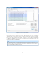
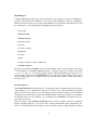
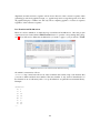
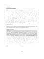
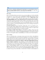
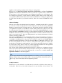
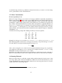
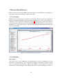
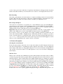
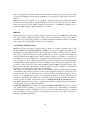
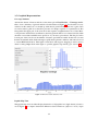
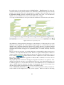
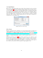
Hexicon 2
Quick start guide and user manual
Revision 12 JUN 2014
Robert Lindner
[email protected]
1
Contents
1 Quickstart
1.1 Prerequisites . . . . .
1.2 Walkthrough . . . . .
Data Import . . . . .
Protein Mixture Filter
Parameter Settings .
Run Hexicon . . . .
.
.
.
.
.
.
.
.
.
.
.
.
.
.
.
.
.
.
.
.
.
.
.
.
.
.
.
.
.
.
.
.
.
.
.
.
.
.
.
.
.
.
.
.
.
.
.
.
.
.
.
.
.
.
.
.
.
.
.
.
.
.
.
.
.
.
.
.
.
.
.
.
.
.
.
.
.
.
.
.
.
.
.
.
.
.
.
.
.
.
.
.
.
.
.
.
.
.
.
.
.
.
.
.
.
.
.
.
.
.
.
.
.
.
.
.
.
.
.
.
.
.
.
.
.
.
.
.
.
.
.
.
.
.
.
.
.
.
.
.
.
.
.
.
.
.
.
.
.
.
.
.
.
.
.
.
.
.
.
.
.
.
.
.
.
.
.
.
.
.
.
.
.
.
.
.
.
.
.
.
.
.
.
.
.
.
4
4
4
4
6
6
7
2 Hexicon Core
2.1 Prerequisites . . . . . . . . . . .
2.2 Input Data . . . . . . . . . . . .
LC-MS Maps . . . . . . . . . .
MS-MS Report . . . . . . . . .
Protein Sequences . . . . . . . .
Post Translational Modifications
2.3 Filters . . . . . . . . . . . . . .
Background Protein Filter . . . .
2.4 Parameters . . . . . . . . . . . .
Peptide / LC Settings . . . . . .
MS Settings . . . . . . . . . . .
Export Settings . . . . . . . . .
Advanced Settings . . . . . . .
Saving Parameters . . . . . . . .
2.5 Other Customizations . . . . . .
Protease Specificity Scores . . .
2.6 Running Hexicon 2 . . . . . . .
.
.
.
.
.
.
.
.
.
.
.
.
.
.
.
.
.
.
.
.
.
.
.
.
.
.
.
.
.
.
.
.
.
.
.
.
.
.
.
.
.
.
.
.
.
.
.
.
.
.
.
.
.
.
.
.
.
.
.
.
.
.
.
.
.
.
.
.
.
.
.
.
.
.
.
.
.
.
.
.
.
.
.
.
.
.
.
.
.
.
.
.
.
.
.
.
.
.
.
.
.
.
.
.
.
.
.
.
.
.
.
.
.
.
.
.
.
.
.
.
.
.
.
.
.
.
.
.
.
.
.
.
.
.
.
.
.
.
.
.
.
.
.
.
.
.
.
.
.
.
.
.
.
.
.
.
.
.
.
.
.
.
.
.
.
.
.
.
.
.
.
.
.
.
.
.
.
.
.
.
.
.
.
.
.
.
.
.
.
.
.
.
.
.
.
.
.
.
.
.
.
.
.
.
.
.
.
.
.
.
.
.
.
.
.
.
.
.
.
.
.
.
.
.
.
.
.
.
.
.
.
.
.
.
.
.
.
.
.
.
.
.
.
.
.
.
.
.
.
.
.
.
.
.
.
.
.
.
.
.
.
.
.
.
.
.
.
.
.
.
.
.
.
.
.
.
.
.
.
.
.
.
.
.
.
.
.
.
.
.
.
.
.
.
.
.
.
.
.
.
.
.
.
.
.
.
.
.
.
.
.
.
.
.
.
.
.
.
.
.
.
.
.
.
.
.
.
.
.
.
.
.
.
.
.
.
.
.
.
.
.
.
.
.
.
.
.
.
.
.
.
.
.
.
.
.
.
.
.
.
.
.
.
.
.
.
.
.
.
.
.
.
.
.
.
.
.
.
.
.
.
.
.
.
.
.
.
.
.
.
.
.
.
.
.
.
.
.
.
.
.
.
.
.
.
.
.
.
.
.
.
.
.
.
.
.
.
.
.
.
.
.
.
.
.
8
8
8
8
9
9
10
12
12
12
12
13
13
14
14
15
15
15
3 Hexicon 2 Result Browser
3.1 User Interface . . . . . . . .
3.2 File Handling . . . . . . . .
File Loading . . . . . . . . .
File Unloading . . . . . . .
File Saving and Export . . .
3.3 Dataset Navigation . . . . .
Selecting the Active Dataset
The Tree View . . . . . . . .
MDI Tabs . . . . . . . . . .
3.4 Filtering and Processing . .
3.5 Graphical Representations .
Coverage Statistics . . . . .
Peptide Map View . . . . . .
Time Series View . . . . . .
.
.
.
.
.
.
.
.
.
.
.
.
.
.
.
.
.
.
.
.
.
.
.
.
.
.
.
.
.
.
.
.
.
.
.
.
.
.
.
.
.
.
.
.
.
.
.
.
.
.
.
.
.
.
.
.
.
.
.
.
.
.
.
.
.
.
.
.
.
.
.
.
.
.
.
.
.
.
.
.
.
.
.
.
.
.
.
.
.
.
.
.
.
.
.
.
.
.
.
.
.
.
.
.
.
.
.
.
.
.
.
.
.
.
.
.
.
.
.
.
.
.
.
.
.
.
.
.
.
.
.
.
.
.
.
.
.
.
.
.
.
.
.
.
.
.
.
.
.
.
.
.
.
.
.
.
.
.
.
.
.
.
.
.
.
.
.
.
.
.
.
.
.
.
.
.
.
.
.
.
.
.
.
.
.
.
.
.
.
.
.
.
.
.
.
.
.
.
.
.
.
.
.
.
.
.
.
.
.
.
.
.
.
.
.
.
.
.
.
.
.
.
.
.
.
.
.
.
.
.
.
.
.
.
.
.
.
.
.
.
.
.
.
.
.
.
.
.
.
.
.
.
.
.
.
.
.
.
.
.
.
.
.
.
.
.
.
.
.
.
.
.
.
.
.
.
.
.
.
.
.
.
.
.
.
.
.
.
.
.
.
.
.
.
.
.
.
.
.
.
.
.
.
.
.
.
.
.
.
.
.
.
.
.
.
.
.
.
.
.
.
.
.
.
.
.
.
.
.
.
.
.
.
.
.
.
.
.
.
.
.
.
.
.
.
.
.
.
.
.
16
16
16
16
17
17
17
17
17
18
18
19
19
19
21
.
.
.
.
.
.
.
.
.
.
.
.
.
.
.
.
.
.
.
.
.
.
.
.
.
.
.
.
2
3.6
Graphics Export . . . . . . . . . . . . . . . . . . . . . . . . . . . . . . . . . .
B-Factor Export . . . . . . . . . . . . . . . . . . . . . . . . . . . . . . . . . .
3
22
22
1 Quickstart
This section is for the impatient who want to see what Hexicon 2 does to their data. We shall
assume that you have a complete and functional copy of Hexicon 2 binaries as well as the required runtime libraries for your operating system (cf. section 2.1). Furthermore, you have all
data at hand, know your experimental parameters and all you want to do is get results – fast. Be
warned that some tinkering with parameter settings and downstream postprocessing are required
for optimal results.
1.1 Prerequisites
Hexicon 2 is a reference-based bottom-up workflow which can run using one reference LC-MS
map, at least one map of deuterated protein and the corresponding protein sequences. More
formally, the files you need are:
• Reference dataset, one mzXML file per LC-MS map, line spectra
• Deuterated data, one mzXML file per LC-MS map (at least one), line spectra
• Protein sequence of your experimental construct
• Protein sequences of all significant other components in the mixture (if present)
While most parameter settings of Hexicon 2 are only needed for fine-tuning of the workflow, it
is essential that you know some parameters concerning data acquisition. This includes:
• Instrument resolution (FWHM)
• Instrument calibration accuracy
• Retention time range during which peptides elute
1.2 Walkthrough
Data Import
Hexicon 2 opens with the data import window (Figure 1). Hit Add to load your LC-MS maps.
After selecting a map in mzXML format, a dialog will pop up and ask you for incubation time
and group number. The group number is used to identify replicates: maps with the same incubation time and group number will be treated as experimental replicates. Enter 0 as incubation
time and group number of the reference.
For subsequent deuterated datasets, enter the respective D2 O incubation time in seconds and
assign the same (arbitrary) group number to each set of replicate maps. The example in Figure 1 shows two deuterated maps which consistute replicates of the 15 sec incubation time point,
hence they belong to the same group.
If you have an appropriately formatted MS/MS search report (cf. section 2.2), it is strongly recommended that you provide Hexicon 2 with this information. A protein sequence in plain text
4
Figure 1: Hexicon 2 data import window.
format always needs to be specified. If you used a 100 % labeling control, e.g., by labeling in
denaturing buffer, load that dataset and enter an arbitrary group number and time point higher
than for your longest-incubated actual sample. Check the box next to Use last time point
as 100 % D reference. When the location of all datasets has been specified, proceed to the
protein mixture filter by clicking Next
Tip
For optimal performance, some tinkering with parameter settings may be required. For your
convenience and for better reproducibility, the locations of the input files can be saved and
restored using Save and Open, respectively.
5
Protein Mixture Filter
This step is only required if your experiment contains nonnegligible amounts of more than
one protein. If this is not the case, proceed to the extraction parameters with Next.
Hexicon 2 is designed for the analysis of one protein of interest at a time. If other proteins
are present in the mixture at significant amounts (such that peptides originating from these proteins are detectable in the spectra), you need to provide their sequences as background set. Do
this with Add for each protein other than the protein of interest.
The optional reference map which can be loaded at the bottom of this window is currently not
used (build 12 JUN 2014) as it provided no measurable improvement of sensitvity in our test
data.
Parameter Settings
See section 2.4 for a detailed description of the available parameters. Only a few of these values
must be changed for Hexicon to produce useful data given that you are using a common LC-MS
experimental setup:
The Retention Time Range is crucial for sensitive feature extraction. It is highly discouraged to run Hexicon on the entire map. Much better performance can be achieved by entering
the time range at which your peptides elute from the chromatographic column. Make sure that
the time window not only accomodates the reference peptides but also the deuterated ones and
do not worry about adding a minute or so at each side of the window.
An estimate of the actual instrument Resolution (FWHM) ( ± 10 %) is required for Hexicon to get an estimate of the attainable mass precision. More importantly, if your detector tends
to drift over the course of an experiment, you should calibrate it regularly (at least before the
first and after the last injection, to know which errors to expect) and record the mass deviation.
Enter the largest relative mass deviation ( ∆mz
mz in ppm) that you expect for any of the analyzed
measurements as Calibration Error (ppm).
Tip
If calibration logs are not available and you cannot reproduce calibration errors experimentally, have a look at the precursor mass values reported for MS/MS sequenced peptides and
compare them to theoretically expected masses. This corresponds to the delta M field of
MASCOT reports.
The Export Settings are intuitive and should be adjusted. In addition to the specified output
file, Hexicon will create a number of other files in the same directory, including a runtime log
(Hexicon.log) and a subdirectory (deuteration), in which measured deuteration distributions for each identified peptide are stored. Is is therefore recommended to use one dedicated
directory for the result output of each Hexicon run.
6
Tip
Save parameter settings in the Hexicon result output directory for documentation and reproducibility. The resulting .hxpar file is a human-readable plain text file containing all
parameter settings.
If all parameters are set, proceed to the Run tab with Next.
Run Hexicon
If no error message is displayed in the status monitor, start Hexicon with Start Hexicon
Workflow. An approximate progress bar and the status monitor showing the contents of the
Hexicon.log file as it is created keep you informed about the progress and provide you with
key statistics. When the run has finished, a csv file containing one feature per line, as well as a
YAML file will be created. The YAML file can be read by hxviewer, Hexicon’s result browser,
which is the recommended way of postprocessing and viewing data.
7
2 Hexicon Core
This section describes the core of the Hexicon 2 workflow, upstream requirements, parametrization, the structure of the output as well as recommendations for quality control and downstream
processing.
2.1 Prerequisites
You have most likely received Hexicon 2 binaries in a zipped folder. The archive contains the
executables hexicon.exe and hxviever.exe, the libraries ms++.dll, hxcore.dll, sashimi.dll, yamlcpp.dll, zlib.dll as well as Qt libraries (QtXml4.dll, QtSvg4.dll, QtGui4.dll, QtCore4.dll, imageformats/qsvg4.dll). The text file pepsintable.txt contains protease cleavage score definitions (cf.
section 2.5).
It may be necessary to install Microsoft Visual Studio 2010 runtime libraries available free of
charge from Microsoft.
2.2 Input Data
LC-MS Maps
Hexicon 2 was designed for the analysis of high-resolution liquid chromatography mass spectrometry data generated from high-resolution TOF or ion trap based instruments. Since the
amount of data generated by such devices can be enormous and most of them provide sophisticated methods for peak picking, we leave this task to upstream processing by the user and start
with line spectra.
The open mzXML format is currently the most widely used and most flexible open data format
for mass spectrometry data. We are aware of the shortcomings of XML-based formats for data
storage and plan to provide support for other data formats as new open standards are emerging.
In order to run Hexicon 2, you will need exactly one reference map containing undeuterated peptides, at least one map containing deuterated peptides, and the protein sequence of the construct
used in your experiment.
Hexicon 2 is geared towards the analysis of continuous labeling experiments, i.e., the mass
difference over D2 O incubation time is analyzed. Therefore, each LC-MS map needs one associated time point. Maps with the same time point and group number are treated as replicates, i.e.
extracted deuteration values are averaged.
Relative deuteration centroid values can be corrected for back-exchange using a 100 % deuterated control sample measured under identical LC-MS conditions. You can provide such measurements as a set of additional maps. Give these maps an arbitrary group number and time
point that’s higher than the group numbers and time points of all other maps, then check the box
next to Use last time point as 100 % D reference.
8
MS-MS Report
Loading a MASCOT search report will greatly improve the quality of sequence assignment to
peptides contained therein. Furthermore, it helps resolving ambiguous sequence assignments.
The format is historically a copy of the peptide summary browser display, hence Hexicon 2 looks
for a whitespace or tab-separated file containing the following fields:
• Query ID
• Observed m/z
• Mr (measured)
• Mr (theoretical)
• delta m
• missed cleavages
• Ion Score
• E-value
• Rank
• Unique (letter U to denote uniqueness)
• Peptide sequence
Only the values printed in boldface are used, hence dummy values can be inserted in other fields
to create Hexicon 2 compatible MASCOT reports. Sequences must be provided in the format
X.YYYYY.X with YYYYY being the peptide sequence. Residues flanking the cleavage site are
not used in the current release (12 JUN 2014), however this behavior may change. We are planning on adding support for a simpler format for the specification of MS2 confirmed peptides in
the next release.
Protein Sequences
The Protein Sequence field is mandatory. Load a plain text file containing the protein sequence
corresponding to your experimental construct in one-letter code. Only standard proteinogenic
amino acids are allowed, however you may define some exotic amino acids as post translational
modifications, given that they contain only C,H,2 H,N,O,P,S and I atoms. Other atoms can likely
be included, however some elements, e.g., Selenium, throw NITPICK’s Averagine-based isotope pattern model off.
It may be useful to add a Reference Sequence if you want to compare constructs of different
length, containing mutations or just for the sake of using standardized sequence numbering. Positions of found peptides will be mapped to their reference position (using ungapped sequence
9
alignment) and the reference sequence will be shown instead of the construct sequence when
generating protein-level graphical output, i.e., peptide maps and coverage histograms. Note that
all graphical displays of Hexicon 2 will only allow comparing peptides of identical sequence
regardless of the reference sequence.
Post Translational Modifications
Hexicon 2 allows definition of simple fixed post translational modifications. Once the protein
sequence has been loaded, hit the Modifications button to open the corresponding dialog (Figure 2). You will need to define the modifications you want to apply to your protein in a YAML
Figure 2: Hexicon 2 Post translational modifications dialog.
file which is structured as follows:
elements map - must be the first node of the document and contain a map of all elements that
you want to define and their mass number. The mass number is only used for identification of
the element in our stoichiometry table - isotope distributions are pulled from an internal library.
Example:
elements:
H: 1
D: 2
C: 12
N: 14
O: 16
P: 30
S: 32
I: 53
---
10
This block can be followed by any number of nodes, each containing following tags:
modification: the name of the modification; short: a short identifier for display in the
peptide sequence; composition: a map of the elemental composition which will be added to
the modified amino acid’s stoichiometry (e.g., H: -2 means removal of two hydrogen atoms);
applyTo: List containing one-letter code of amino acids to which the defined modification
can be applied. Example:
modification: Phosphorylation
short: p
composition:
H: 2
O: 3
P: 1
applyTo:
- Y
- S
- T
--modification: Phosphopantetheinylation
short: ppt
composition:
H: 21
O: 6
P: 1
C: 11
N: 2
S: 1
applyTo:
- S
Once modifications have been loaded, use the mouse to highlight the parts of your protein sequence which you want modified, pick the corresponding modification from the list of available
modifications and hit >> to apply it.
Tip
Modifications can only include the elements listed in the above example since isotope patterns are only defined for these. Modifications with an elemental composition (more precisely: isotope distribution) that strongly differs from the isotope pattern of a peptide containing only standard amino acids may not be correctly identified by our NITPICK feature
detection algorithm. If your modified peptide made it through feature detection, full modeling of the isotope pattern is carried out in subsequent steps such that accuracy is no different
from unmodified peptides.
11
2.3 Filters
Background Protein Filter
Hexicon 2 can only analyze peptides corresponding to one protein at a time (referred to as protein
of interest). If your experiment contains other proteins (background proteins) in nonnegligible
amounts, there is a good chance of falsely assigning a sequence from the protein of interest
to a peptide derived from a background protein. In order to avoid this, Hexicon 2 allows you
to define the sequences of all background proteins in the filters tab. Import one plain text file
for each background protein in your experimental mixture. Peptides that match a background
sequence better than the protein of interest will be removed from the analysis after being used
for internal mass calibration and false assignment estimation.
In some cases, such filtering may be too strict and peptides of interest may be falsely assigned
to background sequences. If this is the case, you can load a reference map in mzXML format,
containing only the protein of interest measured under identical LC-MS conditions. Peptides
matching a background sequence but found in the reference map will be rescued from the filter.
Note: This feature has been disabled in the current release (12 JUN 2014) as it provided no
measurable performance gain in our benchmarking studies.
2.4 Parameters
Hexicon 2 provides a number of customizable parameters which can be used to tune the sensitivity of the analysis and to adjust it to your experimental conditions.
Peptide / LC Settings
NITPICK feature detection is applied in a divide-and-conquer scheme: feature detection is carried out in each scan independently and detected features with similar mass in subsequent scans
are merged. The fields Minimum / Maximum # Scans let you define in how many subsequent scans a peptide has has to be detected by NITPICK in order to be carried into further
analysis. The maximum scan number is rarely hit but if you have persisitent contaminations
consistently detected by NITPICK, this will remove them. The Maximum Gap Time setting
allows you to set a tolerance window in which a peptide need not be detected and still be merged
with a previous peptide signal. It is advisable to increase this setting when you notice fragmentation of your peptides, i.e., you get a large number of peptides with the same charge that
are detected in more than one contiguous region of the LC-MS map (another reason for this to
happen is too low mass precision tolerance in the FWHM setting).
Hexicon 2 will try to assign peptide sequences to any detected feature regardless of MS2 identification. For this purpose, exhaustive in-silico digestion is used to procude all peptides within a
given size range. Making the Peptide Length Range unnecessarily large will aversely affect
runtime and sequence assignment specificity.
12
Tip
A good way to determine a suitable peptide length range for your experiment is to have a
look at the peptides identified by MS2 or to do a discovery run with Hexicon 2 using a large
range (e.g. 5/45) and then to narrow down the range based on the results.
MS Settings
Since we are dealing with line spectra, there is no good way for Hexicon 2 to derive peak width
from input data. A good estimate of the scan Resolution (FWHM@400) is therefore required
for Hexicon 2 to estimate the attainable mass precision. A value of 40000 FWHM roughly
translates to a precision of 6 ppm. Using this setting, features from subsequent scans with a
relative mass difference ∆m/m of more than 6 ppm would be treated as two separate entities.
The Calibration Error parameter represents the accuracy of your measurement, i.e., how much
measured mass deviates from actual mass and how much two measurements of the same peptide
are allowed to differ in different maps. It is safe to set a fairly large value here since it is only
used as worst-case value and empirically narrowed down during the analysis. If you feel that
sequence assignment or chromatogram alignment perform poorly, try altering this parameter in
10 % intervals up or down.
The Noise Quantile defines the peak intensity quantile that is safe to be considered as noise.
It is used together with the SNR parameters (Advanced Settings) to pre-filter the spectrum. If
your data is heavily pre-filtered and no noise is present, set a very low value. Low values for this
parameter increase sensitivity, false discovery and mostly runtime.
m/z Range and Charge State Range are self-explanatory. Having a charge state range
that specificially matches your dataset will greatly accelerate feature detection and reduce false
positive rates. We stronly recommend using Positive Ionization for all experiments. Negative
ionization is incompatible with most current HDX protocols and was never tested in Hexicon.
Export Settings
There are several filters that you can apply for data export into the CSV file. The YAML file
for processing using hxviewer will not be filtered. Depending on your ionization settings, most
peptides will produce more than one charge state which can be detected by Hexicon 2. Finding
multiple charge states with similar deuteration increases the confidence in data extraction. It
may therefore be useful to discard results which have only one charge state, however it is
not recommended. For a quick discovery analysis, you may want to discard peptides with ambiguous sequence assignment. Such assignments occur when multiple theoretical peptide
sequences match the extracted mass within the attainable mass precision. Hexicon 2 provides
several means to resolve such sequence conflicts and to find the most likely correct assignment,
hence discarding ambiguous assignments up front is discouraged. As there are currently no
means to inspect individual replicates, we recomment discarding features with inconsistent
replicates. This filter will remove a peptide if the deuteration centroid standard deviation exceeds a certain percentage of its absolute value. This centroid deviation cutoff is set to 20 %
by default. If you get a very small number of results in the csv file but not in the YAML file, it
13
might be worth checking your filters and looking for a bad replicate.
Hexicon lets you Separately Export deuteration distributions or a list of ambiguous
peptides. The deuteration distributions will be exported into a separate directory with one csv
file per feature. It will contain deuteration state abundance distributions for each replicate. The
list of ambiguous peptides is a useful shortcut to defining peptides which you may want to have
re-sequenced by MS2 . Both the deuteration subdirectory and the list of ambiguous peptides will
be saved in the same directory as the main result list. This is also where the YAML file will be
saved.
Advanced Settings
The first section deals with feature detection parameters. A running median will be computed
for each scan to define a background noise level. Each peak is then smoothed using a Gaussian
Filter and compared against the background noise. The width of this filter determines whether
you emphasize local peaks or broad clusters to define which peaks lie above the noise level. The
two SNR parameters determine the intensity ratio of any raw (unsmoothed) peak over the
background and its smoothed counterpart over the background required to pass the filter. Only
if both smoothed and raw peak over background intensities exceed the set threshold values, the
peak is not treated as noise. These two SNR parameters are the main determinants of feature
detection sensitivity in Hexicon 2.
The runtime of NITPICK increases quadratically with model size, hence Hexicon 2 attempts to
fit models with independent (i.e., non-overlapping) isotope patterns separately. Busy spectra are
often highly overlapping and no split points can be found. In such cases, the Model Splitter
parameter determines the number of models after which Hexicon 2 forces the model set to split
in order to keep runtime low. We do our best to stitch split models together in a sensitive way
but the fits are subobtimal at such breakpoints. If you notice that feature detection is choking,
try reducing this setting. Better results are obtained with higher numbers here but significant
slowdown of feature extraction was observed at about 200 models.
The chromatogram alignment implemented in Hexicon 2 estimates two alignment tolerance
terms based on the data and thereby already extends the search space for deuterated peptides
generously. If you feel, however, that alignment fails, you may try to manually extend the
alignment window for deuterated peptides.
Tip
If you suspect that the chromatogram alignment is not doing a good job, try plotting reference retention times versus retention times of deuterated peptides (both listed in the csv
file). Large scatter will usually indicate alignment problems.
Saving Parameters
Parameters are not automatically saved and cannot be retrieved once Hexicon 2 has started processing data! Please save your paramter settings file for reproducibility and convenience. We
14
recommend using one directory per Hexicon 2 analysis run where you can also store the settings
used to generated the results contained therein.
2.5 Other Customizations
Protease Specificity Scores
Hexicon 2 assigns cleavage scores based on cleavage probabilities empirically determined by
Hamuro and colleagues1 . Table 2 of the corresponding publication was adapted (W-W cleavage
was not defined originally because the sequence WW had not been observed in the study) and
reformatted to match a shape which can be read by Hexicon 2: In a whitespace-separated text
file, N fields of the first line define the one-letter amino acid alphabet A (typically 20 letters). It
follows a N ×N square matrix of nonnegative real-valued cleavage probabilities [0,1] where the
value at position i, j (i denoting the row, j the column) stands for cleavage between A[j] (in P1)
and A[i] (in P10 ). Note the unconventional column-first notation which was kept for compliance
with Hamuro et al..
Consider the following example file defining an arbitrary four-letter alphabet:
A
0.06
0.15
0.2
0.21
C
0.18
0.8
0.31
0.83
D
0.07
0.1
0.01
0.03
E
0.2
0.3
0
0.08
Examples for cleavage scores would be AAC∧ DEACEDA (C/D): 0.31 or AACDEACED∧ A (D/A):
0.07. Internal peptides result from two cleavage events, hence a compound cleavage score must
be found. Hexicon 2 assigns an internal peptide cleavage score
s=
√
s1 s2
with s1 and s2 being the scores of the N- and C-terminal individual cleavage sites, respectively.
Accordingly, the subsequence DEACED from the above example (denoted C.DEACED.A using
MASCOT convention) would receive a score of 0.15.
Specificities are read from the plain text file "pepsintable.txt" which must be in the search path of
Hexicon 2. In the Windows release, this would be the same direcory as the hexicon.exe binary.
2.6 Running Hexicon 2
Hexicon 2 will produce a log file that contains much useful information about the state of data
processing. The log file is shown in the Run tab of Hexicon 2 and saved in the directory of run
output. Should Hexicon 2 quit unexpectedly without an error message, please have a look at the
log file which will contain debug output.
1
Hamuro Y. et al., Rapid Commun Mass Spectrom. 2008; 22(7):1041-6
15
3 Hexicon 2 Result Browser
Hexicon 2 writes its results in YAML format which can be read by HXViewer, a graphical tool
for postprocessing and visualization of Hexicon 2 results.
3.1 User Interface
HXViewer has a split graphical user interface (GUI) which contains file and result management
in the left column and a multiple document interface (MDI) area for various tasks related to visualization as well as interactive manipulation (Figure 3). Selecting the graphical representation
of a peptide in any of the views will select and highlight the peptide in the tree view on the left.
Modifications to either representation of the data will update the underlying model and affect
any other data displays.
Figure 3: Hexicon 2 Result Browser User Interface
3.2 File Handling
File Loading
You can load one or more YAML files containing Hexicon 2 results by drag&drop from your
filesystem browser into the tree view on the left, by clicking on the green + symbol above that
area or by using the menu item File > Open. Since YAML is a text-based format, loading of
data may take a while and happens in the background while you can start naming your datasets or
16
work on other, previously loaded data. Completely loaded datasets will appear in the dropdown
menu on the left from where you can select the active dataset to be displayed in the tree view.
File Unloading
Unload an opened dataset to free the memory it occupies by clicking on the red – button while it
is active. This will only succeed if no other views (graphical displays) of that dataset are open.
Note: Changes you made to the dataset will be lost unless you explicitly save it!
File Saving and Export
Your work is not saved unless you explicitly do so. Since HXViewer can only read YAML files,
you should save your progress. We recommend saving to a new YAML file using the File >
Save as menu item such that the original Hexicon 2 output is not lost. Peptides marked as
disabled will be saved as such and can be restored using HXViewer.
Important: Only the active dataset (in the dropdown menu on the left - not the graphics view)
will be saved. Make sure you save work in all your datasets before closing HXViewer.
If you wish to create a csv file similar to the output originally generated by Hexicon 2, you
can use the menu item File > Export to csv. The dialog will ask you whether you wish to
create a separate directory for deuteration files. Please note that answering Yes will create a
deuteration directory in the same location as the exported csv file. If this happens to be the
directory of the original Hexicon 2 output, it will be overwritten.
3.3 Dataset Navigation
Selecting the Active Dataset
Use the dropdown menu on the left to choose the active dataset. It will be displayed in the tree
view below and all filters or visualizations will be applied to this dataset. You can change the
active dataset while there are still graphical displays of it, however interactive manipulation is
only possible to the active dataset. It is not required to save your work before changing the
active dataset.
The Tree View
The tree view on the left side of HXViewer presents rich information about the results of a Hexicon 2 run. It groups the results by peptide and lists all peptides that were retrieved at least once in
each time point (i.e., have complete time series). Right-click the title bar to change how peptides
are sorted. The default is by position in the protein sequence. Expanding a peptide will show
all found ions (charge states) which you can view in further detail by expanding. Ions displayed
in red font have multiple sequence assignments which you can view by expanding their other
assignment(s) field. Right-click or double-click on the other assignment to jump to it in the
tree view. Ions displaed in boldface are confirmed by MS2 sequencing. Peptides that contain at
least one ambiguous or confirmed sequence are displayed in red or bold, respectively.
Double click on an ion to open a graphical display showing its deuterium incorporation over
17
time or on a peptide to show that display for all related ions. Other peptides or ions can be added
to the plot by dragging tree items and dropping them over an active plot. This can be done across
datasets.
Right-click on an ion to disable it or on a peptide to disable all related ions. Disabled items will
be removed from any statistics or graphical displays, they will not be listed as sequence conflicts
and not be exported to CSV. When saving the active dataset to a YAML file, disabled state is
preserved. Right-click on a disabled entitiy to re-enable it.
MDI Tabs
Graphical displays opened by a dataset will be grouped in one tab of the MDI area in the right
part of the viewport. While this helps you keep your work structured, closing a tab provides a
convenient way of destroying all views on a dataset and thereby making it ready for unloading
(unless there are open multi-dataset views open in other tabs).
3.4 Filtering and Processing
HXViewer provides two filter operations that we routine use as first-pass quality control: Filter by intensity and Resolve sequence conflicts. If you plan on applying both filters, we
recomment first applying the intensity filter and then proceeding to conflict resolution. Filters
will operate on the active dataset only. The intensity filter looks for ions with large deviation in
intensity extracted from different maps. This is usually an indicator for either poor extraction in
some datasets or for mis-alignment, i.e., assignment of a deuterated signal to a noncognate reference ion. It has two passes: The filter will remove all features which exceed a relative intensity
standard deviation larger than the first cutoff set regardless of total intensity in the first pass. The
second pass removes all ions with a given standard deviation and an absolute intensity lower
than a specfied quantile. This filter is of limited utility if you know that due to experimental
conditions, your samples show large variation in intensity.
The conflict resolution filter inspects all ions with multiple sequence assignments and attempts
to determine, solely based on sequence, if any of the suggested sequences is more likely to be
correct than the others. It allows the user to specify residues after which cleavage is not allowed to occur. Furthermore, cleavage scores computed by Hexicon 2 can be compared. If one
sequence is significantly more likely to be produced by the protease than another, it will be accepted as correct sequence. Check the box next to Extend MS/MS to related ions if you
want MS2 confirmation of an ion also to be applied to related ions and thus all related sequences
to be preferred over any conflicting sequences.
The Set all peptides menu contains two elements: Enable and Disable. This allows to (re-)set
your peptide selection quickly, e.g., if you want to consider only a small number of manually
selected peptides. Please note that hxviewer does not have an undo function, hence you should
save your dataset to preserve the state of any manual processing you may have done prior to
enabling or disabling all peptides.
18
3.5 Graphical Representations
Coverage Statistics
Activate the dataset of interest and choose the menu option Visualization > Coverage statistics to view a summary of general statistics about that dataset (Figure 4). Note that the recovery
statistics in this window do not match up with what is printed in the Hexicon 2 log file since
recoveries in the log file do not check for presence of a unique sequence for a particular ion. The
histogram in the upper part of the view shows the sequence assignment mass error. Since Hexicon 2 performs internal mass-recalibration, the histogram should be zero-centered and its width
should not exceed the attainable mass precision of your mass spectrometer. The bar plot in the
bottom part of the view shows the number of features per backbone amide. It takes into account
that the N-terminal amide back-exchanges rapidly under quench conditions and cannot be used
to extract HDX information. This figure is interactive and supports dragging as well as mouse
wheel zooming. Right-click on the figure to open the graphics export dialog (cf. section 3.6).
Figure 4: HXViewer Result Statistics View
Peptide Map View
The peptide map view can either display deuteration of all peptides in a single dataset (dynamics
mode, Figure 5) or compare deuteration differences between datasets (difference mode). Open
19
the peptide map view through the menu item Visualization > Peptide map. Choosing only
a reference dataset will open the dynamics view which shows deuterium incorporation of each
peptide color-coded from blue (low) through green to red (high). The scale begins at zero and
the Dynamic Range parameter determines the upper limit of the scale. You can adjust the
number of colors to obtain a more coarse or fine scale of color codings.
Choosing two different datasets will open a deuteration difference view which shows the deuter-
Figure 5: HXViewer Peptide Map View
ation difference of the target dataset with respect to the reference on a blue-gray-red color scale
running from the negative end of the dynamic range through zero to the positive end of the
dynamic range. Deuteration differences between two peptides take into account the standard
deviation of deuterium incorporation into the two displayed peptides, hence peptides with large
measurement uncertainty will appear less significantly blue or red than accurately measured
peptides.
Each box in the plot represents one peptide which may contain multiple charge states that are
combined to one compound deuteration value. Each box is split horizontally into a number of
segments which correspond to D2 O incubation time points. Therefore, the different colors in a
box, bottom-up
, indicate deuteration values or differences at each of the incubation
time points. A white diamond in a peptide box indicates MS2 confirmation of at least one ion
related to that peptide.
The peptide map view is interactive and supports drag and mousewheel zoom operations. Leftclicking a peptide will select the corresponding item in the tree view, right-clicking allows you
to disable a peptide or to view its time series. If you are in difference mode, you will have the
option to disable either the reference, the target or both peptides. In this case, the time series
will show both peptides’ deuterium incorporation over incubation time.
Click the Secondary Structure icon
to load a comma-separated secondaryi structure annotation which can be displayed above the protein sequence. Hexicon 2 reads the following
20
representation of secondary structure: line 1: protein sequence; line 2: secondary structure over
an alphabet of H, E, -; line 3: secondary structure prediction confidence on a scale of 0-9.
Data in the third line is ignored in the current release (12 JUN 2014) of HXViewer.
Click the Export icon
to open the graphics export dialog (cf. section 3.6).
Time Series View
The time series view shows deuterium incorporation into one or more peptides over D2 O incubation time. In order to open a time series view, double-click on an ion in the tree view. Double
clicking on a peptide will display all ions associated with the sequence. Each time a new item
is added to the time series view, you will be asked to specify a color. When a peptide with mutliple charge states is loaded, each charge state will be plotted as an individual line, the median
deuteration will be plotted as separate bold line and the deuteration range spanned by all related
ions will be shaded.
You can add further peptides to the time series view by dragging them from the tree view into
the plot area. HXViewer will try to construct a logical sequence from the peptides present in a
time series view such that loading one peptide from a dataset will allow you to browse through
all peptides of that dataset using either the scrollbar below the plot area or the mouse wheel
while over the plot area. When corresponding peptides from two or more datasets with identical
(reference) sequence are loaded, HXViewer will let you scroll through all peptides present in all
datasets (intersection mode)
or through all peptides present in any of the loaded datasets
(union mode)
.
Click the distribution button
to toggle the display of deuteration distribution estimates. If
multiple peptides are loaded, each peptide’s distribution will be plotted in a separate row.
HXViewer will automatically estimate the required Y-axis range to accomodate all peptides in
the current view. The field Required #D range lets you override this setting such that the
Y-axis range will never be less than specified here. This may be useful if you want to get all
plots in a series on the same scale.
There are three modes of interacting with the data plotted in the time series view: In Selection
Mode
, you can click on peptides and charge states to select them in the plot and in the tree
view. Selected peptides or charge states will be highlighted in blue and you can hit the Delete
key to disable the selected item. Right-clicking will open a context menu that lets you disable,
select or remove the selected item. Please note the difference between disabling an item and
removing it from the plot: a disabled item will still be associated with the time series view and
therefore influences how the sequence of peptides is constructed. Removed items on the other
hand remain active but are no longer associated with the plot. The latter corresponds to reversing
the drag-and-drop operation from the tree view.
In Marker Mode
, clicking on a graph value will display the corresponding deuteration
value. This value is transienly plotted and replotting, e.g., by scrolling back and forth in the
sequence or by disabling/activating a charge state, will remove the label.
Measurement Mode
lets you measure deuteration difference between two different data
points. Click on the first data point to initiate the measurement and click on a second point to
complete it. You can abort a measurement by hitting Escape.
21
3.6 Graphics Export
Hexicon 2 has a standardized graphics export scheme. Export parameters can be set up in the
export dialog (Figure 6). Export into a PNG file guarantees that the current view will be saved asis. Vector graphics can be obtained by exporting into PDF. Graphics exceeding the display width
can be saved as multi-page PDF files whereas HXViewer ensures correct breakpoints. There is
a bug in PDF export through Qt (Qt bug 23142, unresolved in Qt 4.x as of 2013/11/30) which
causes Adobe PDF readers to misinterpret the colorspace information of graphics containing
transparency. This is invisible to physical printing and can be easily fixed by opening and resaving the file in a vector graphics editor.
Figure 6: HXViewer File Export Dialog
B-Factor Export
Mapping of deuteration values or differences onto a crystal structure model is a popular way of
visualizing HDX data. One commonly used way of encoding such information in a structure is to
alter the B-Factors of a PDB file. PyMOL scripts like data2bfactor and color_b (http:
//pldserver1.biochem.queensu.ca/~rlc/work/pymol/, accessed 2013/12/04)
can be used to modify and color-code B-Factors according to a text file. Use the menu item Visualization > Create B-factor table to generate a text file compatible with the data2bfactor
script.
As with the peptide map (section 3.5), you can choose between one or two datasets to create
B-Factors from, to get B-factors corresponding to dynamics or difference output, respectively.
The task of integrating information from multiple peptides for each amide is resolved as follows:
for any amide, if MS2 -confirmed peptides are available to cover this amide, use the longest of
these. Otherwise, information from the longest MS-1 assigned peptide is used.
22
Tip
We are aware that there are multiple ways of mapping deuteration values from multiple
overlapping peptides onto each amide of a structure. While the presented approach consistently yielded the most faithful representation of our experimental data, this may not apply
to other datasets. We are planning to include other deuteration export policies in further
releases. In the meantime you can take full control of what is exported with this "hack":
Save your dataset first. Then disable all peptides using the Processing > Set all peptides
> Disabled menu item (cf section 3.4). Open the peptide map view (section 3.5) and go
through the peptide list (section 3.3) to activate only the peptides that you want exported.
The peptide map will visually assist you identifying the correct peptides.
23