Download 3D GeoModeller Tutorial Case Study G

GeoModeller User Manual
Contents | Help | Top
Tutorial case study G (Drillholes)
1
| Back |
Tutorial case study G (Drillholes)
Parent topic:
User Manual
and Tutorials
Author: Philip McInerney, Intrepid Geophysics
V2012: Des FitzGerald
Editor: David Stephensen, www.qdt.com.au
Using Drillholes in 3D GeoModeller – a Model-Building Strategy
In this case study:
Contents Help | Top
•
Case study G—Introduction
•
Tutorial G1—Building a model from drillholes (erosional series f5)
•
Tutorial G2—Building a model from drillholes (erosional series f2)
•
Tutorial G3—Building a model from drillholes (onlapping series f3)
•
Tutorial G4—Building a model from drillholes (onlapping series f4)
•
Tutorial G5—Building a model from drillholes (onlapping series f6)
© 2013 BRGM & Desmond Fitzgerald & Associates Pty Ltd
| Back |
GeoModeller User Manual
Contents | Help | Top
Tutorial case study G (Drillholes)
2
| Back |
Case study G—Introduction
Parent topic:
Tutorial case
study G
(Drillholes)
In this section:
•
Project data preparation
•
Topography of Case Study G
•
Geology of Case Study G
•
Strategy for Case Study G
Project data preparation
Parent topic:
Case study G—
Introduction
For this tutorial we have created a project area containing synthetic geology.
We have prepared a beginning project file for this case study. You open it at the start
of Tutorial G1—Building a model from drillholes (erosional series f5).
We have:
•
Contents Help | Top
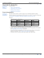
Defined the project dimensions.
Minimum
Maximum
Range
East
483,100
491,700
8,600 m
North
4,280,700
4,291,500
10,800 m
RL
–2000
4000
6000 m
•
Created a 3D GeoModeller project using these extents.
•
Loaded a digital terrain model (DTM) grid to create the topography for the project.
See Topography of Case Study G for details.
•
Created an initial stratigraphic pile. The top or bottom reference for the pile is
Bottom of formations. See Geology of Case Study G for details.
•
Created a series of sections: s81N, s83N, s85N, s87N, s89N, s91N.
© 2013 BRGM & Desmond Fitzgerald & Associates Pty Ltd
| Back |
GeoModeller User Manual
Contents | Help | Top
Tutorial case study G (Drillholes)
3
| Back |
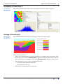
Topography of Case Study G
Parent topic:
Case study G—
Introduction
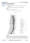
The following illustration shows the topography of the Case Study G region.
Geology of Case Study G
Parent topic:
Case study G—
Introduction
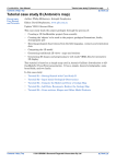
The following illustration shows the geology of the case study region.
Notes about the project:
•
There are six formations, f1 f2 f3 f4 f5 and f6 in a roughly layered sequence. Two
of the units are erosional (Relationship = Erode) across the older strata, and the
other units have an onlapping relationship (Relationship = Onlap) to older strata.
•
The formations are in a correct stratigraphic order
•
Contents Help | Top
•
f1 (oldest) at the bottom of the pile
•
f6 (youngest) at the top
This project uses Bottoms of formations
© 2013 BRGM & Desmond Fitzgerald & Associates Pty Ltd
| Back |
GeoModeller User Manual
Contents | Help | Top
Tutorial case study G (Drillholes)
4
| Back |
Strategy for Case Study G
Parent topic:
Case study G—
Introduction
We have found that a useful strategy for building any model in 3D GeoModeller is
to:
1
Work stratigraphically downwards through the erosional or cross-cutting events
(in this case study, first f5 and then f2).
2
Work stratigraphically upwards through any onlapping series occurring between
these (in this case study, f3, f4, f6).
We recommend this work order because, if you model the youngest, cross-cutting
event or geological surface and get get it right, all subsequent modelling work on all
other (older) events or surfaces has no impact on that earlier modelling of the younger
event.
Note that this tutorial follows one pathway towards building a 3D model of the Case
Study G project geology. There are several equally valid alternative approaches.
Tutorial G1—Building a model from drillholes (erosional series f5)
Parent topic:
Tutorial case
study G
(Drillholes)
According to our strategy (see Strategy for Case Study G), we model the youngest
erosional series first.
In this tutorial we:
1
Import drillhole data
2
Create, display and refine the model for one formation
Stages in the tutorial:
Contents Help | Top
•
G1 Stage 1—Open the prepared 3D GeoModeller Project for Case Study G
•
G1 Stage 2—Import the drillhole data
•
G1 Stage 3—Arrange the 2D Viewer windows
•
G1 Stage 4—Project the Drillholes in each 2D Section-View
•
G1 Stage 5—Prepare the project for modelling
•
G1 Stage 6—Comparing the model with drillhole observations
•
G1 Stage 7—Creating a 3D view
© 2013 BRGM & Desmond Fitzgerald & Associates Pty Ltd
| Back |
GeoModeller User Manual
Contents | Help | Top
Tutorial case study G (Drillholes)
5
| Back |
G1 Stage 1—Open the prepared 3D GeoModeller Project for Case Study G
Parent topic:
Tutorial G1—
Building a
model from
drillholes
(erosional
series f5)
G1 Stage 1—Steps
1
If required, save and close any project that you are currently working on.
2
From the main menu choose Project > Open OR
From the Project toolbar choose Open
Press CTRL+O.
OR
Open:
GeoModeller\tutorial\CaseStudyG\TutorialG1\Beginning_project
\TutorialG1_Start.xml
3
Save the project with a new name in the folder you are using for your tutorial
data.
From the main menu choose Project > Save As OR
From the Project toolbar choose Save As
Press CTRL+SHIFT+S.
OR
Note that a completed version of Stage 2 of the tutorial is available in
GeoModeller\tutorial\CaseStudyG\TutorialG1\Completed_project\
TutorialG1_1_Load_Holes\TutorialG1_1_Load_Holes.xml. Do not
overwrite it.
G1 Stage 1—Discussion and exploration
To view the formations, from the main menu choose Geology > Formations:
Create or Edit.
To view the whole stratigraphic pile, from the main menu choose Geology >
Stratigraphic Pile: Visualise.
Contents Help | Top
© 2013 BRGM & Desmond Fitzgerald & Associates Pty Ltd
| Back |
GeoModeller User Manual
Contents | Help | Top
Tutorial case study G (Drillholes)
6
| Back |
G1 Stage 2—Import the drillhole data
Parent topic:
Tutorial G1—
Building a
model from
drillholes
(erosional
series f5)
Our contractor has drilled a set of 40 deep vertical holes on the six sections. These
holes are 4500 m deep (nice drilling budget!) and there are about six holes per section.
The sections are 2000 m apart and the holes are at various spacings, 600 m – 1800 m.
The drillhole data are in a commonly used drillhole data file format. This is a set of
three files containing the drillhole collars, surveys, and geology.
For interest, you could examine these files in a text editor. For example, you could
examine:
GeoModeller\tutorial\CaseStudyG\TutorialG1\Data\Drilling
\VDH40Holes_Geology.csv
The first line of each file gives field names for each column of data. You need to set
these field names in 3D GeoModeller when you import the drillhole data. The
following table contains the field name list for each file.
File
Field names
VDH40Holes_Collars.csv
HoleID,X,Y,Z,EOH_Depth
VDH_s81N_01,483500,4281000,2755,4500
VDH_s81N_04,485300,4281000,2761,4500
...
VDH40Holes_Survey.csv
HoleID,Dip,Azimuth,Depth
VDH_s81N_01,90,0,0
VDH_s81N_01,90,0,4500
...
VDH40Holes_Geology.csv
HoleID,From,To,Lithology
VDH_s81N_01,0,743,f6
VDH_s81N_01,743,2380,f5
...
G1 Stage 2—Steps
1
Ensure that you are using your own saved version of the project according to G1
Stage 1—Open the prepared 3D GeoModeller Project for Case Study G.
Do not overwrite the completed version of this tutorial that we have supplied in
your 3D GeoModeller installation.
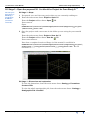
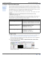
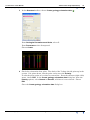
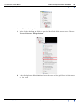
2
From the main menu choose Import > Import drillhole data > Import collars,
surveys, geology (3 files).
This starts the CSV Data Import - 3-table (Collar,Survey,Geology) Drillholes
wizard as shown below
Contents Help | Top
© 2013 BRGM & Desmond Fitzgerald & Associates Pty Ltd
| Back |
GeoModeller User Manual
Contents | Help | Top
Contents Help | Top
Tutorial case study G (Drillholes)
7
| Back |
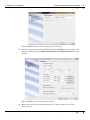
3
In the first page of the CSV Data Import - 3-table wizard dialog box, choose
Browse for the Collar Table and locate the drillhole collars file
GeoModeller\tutorial\CaseStudyG\TutorialG1\Data\Drilling
\VDH40Holes_Collars.csv
4
Repeat step 2 for Survey Table and Geology Table, correspondingly named.
© 2013 BRGM & Desmond Fitzgerald & Associates Pty Ltd
| Back |
GeoModeller User Manual
Contents | Help | Top
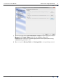
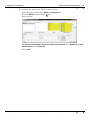
5
Tutorial case study G (Drillholes)
8
| Back |
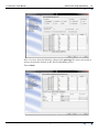
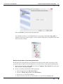
Select the correct data file field name from the drop-down lists for each 3D
GeoModeller field name in the dialog boxes, using the results of your
examination above or the names shown in the data preview panels shown below:
Choose Next.
Contents Help | Top
© 2013 BRGM & Desmond Fitzgerald & Associates Pty Ltd
| Back |
GeoModeller User Manual
Contents | Help | Top
Tutorial case study G (Drillholes)
9
| Back |
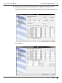
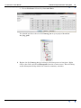
Choose Next.
Choose Next.
Choose Next.
Contents Help | Top
© 2013 BRGM & Desmond Fitzgerald & Associates Pty Ltd
| Back |
GeoModeller User Manual
Contents | Help | Top
Tutorial case study G (Drillholes)
10
| Back |
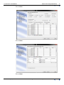
Note, of course, that the lithology coding in the geology file must correspond to
geology formations defined in the 3D GeoModeller project.
Choose Next.
Contents Help | Top
© 2013 BRGM & Desmond Fitzgerald & Associates Pty Ltd
| Back |
GeoModeller User Manual
Contents | Help | Top
Tutorial case study G (Drillholes)
11
| Back |
Choose Next.
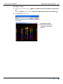
Choose Finish.
View the 40 drillholes in the 3D Viewer. (If not already displayed) In the Project
Explorer, from the Drillholes shortcut menu, choose Show.
Contents Help | Top
© 2013 BRGM & Desmond Fitzgerald & Associates Pty Ltd
| Back |
GeoModeller User Manual
Contents | Help | Top
Contents Help | Top
Tutorial case study G (Drillholes)
12
| Back |
© 2013 BRGM & Desmond Fitzgerald & Associates Pty Ltd
| Back |
GeoModeller User Manual
Contents | Help | Top
6
Tutorial case study G (Drillholes)
13
| Back |
Save your project
From the main menu choose Project > Save OR
From the Project toolbar choose Save
Press CTRL+S.
OR
Note that a completed version of Stage 2 of the tutorial is available in
\GeoModeller\tutorial\CaseStudyG\TutorialG1\Completed_project\
TutorialG1_1_Load_Holes\TutorialG1_1_Load_Holes.xml. Do not
overwrite it.
G1 Stage 3—Arrange the 2D Viewer windows
Parent topic:
Tutorial G1—
Building a
model from
drillholes
(erosional
series f5)
3D GeoModeller has a powerful window arrangement feature. For this project, it is
useful to view all six drill-sections in a tiled window arrangement.
G1 Stage 3—Steps
1
Expand the 2D Viewer so that it occupies about 75% of the main 3D GeoModeller
window
Drag the border between the 2D Viewer and the 3D Viewer to the right.
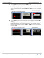
2
Drag the s91N tab so that it becomes a window above the rest of the 2D Viewer
tabs.
In the 2D Viewer, drag the s91N tab down in the 2D Viewer window. 3D
GeoModeller displays a grey rectangular drop spot. This shows the size and
position of the new window. Drop the s91N tab. s91N is now in its own window.
Drag s91N tab down and drop
Horizontal split
s91N
Contents Help | Top
© 2013 BRGM & Desmond Fitzgerald & Associates Pty Ltd
| Back |
GeoModeller User Manual
Contents | Help | Top
3
Tutorial case study G (Drillholes)
14
| Back |
Drag the s89N tab to become a tab in the s91N window
In the 2D Viewer, drag the s89N tab to the middle of the of the s91N window. 3D
GeoModeller displays a grey rectangular drop spot that covers the whole s91N
window. If a half-sized drop spot appears, drag the tab further up or down until
you see a full-sized drop spot. Drop the s89N tab. s89N is now a tab of the upper
window.
Two tabs in top window
Drag s89N tab to top window and drop
Drop spot is
anywhere in top
window
4
s91N & s89N
Drag the s91N tab into its own window at the right, separating it from the s89N
window.
In the 2D Viewer, drag the s91N tab to the right border of the upper window. 3D
GeoModeller displays a grey rectangular drop spot. This shows the size and
position of the new window. Drop the s91N tab. s91N now has its own window to
the right of s89N.
Drag s89N tab to right edge and drop
Top window split
Drop
spot
Contents Help | Top
© 2013 BRGM & Desmond Fitzgerald & Associates Pty Ltd
s89N
s91N
| Back |
GeoModeller User Manual
Contents | Help | Top
5
Tutorial case study G (Drillholes)
15
| Back |
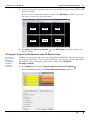
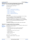
Continue using this technique and create the window arrangement shown in the
illustraton below.
You may need to adjust the relative widths of the 2D Viewer windows as you go
(see step 1 of this stage for instruction)
6
s87N
s89N
s91N
s81N
s83N
s85N
Use Zoom—Fit section to window
into its window.
in the 2D Toolbar to fit each section view
G1 Stage 4—Project the Drillholes in each 2D Section-View
Parent topic:
Tutorial G1—
Building a
model from
drillholes
(erosional
series f5)
Drillholes are separate data structures within 3D GeoModeller. They do not ‘belong’
to any particular section. You can project drillholes onto nearby sections. This shows
the drillhole geology intervals on the target section in the 2D Viewer.
G1 Stage 4—Steps
1
In the Model toolbar choose Project data onto section in 2D Viewer
.
3D GeoModeller displays the Project data onto section dialog box.
Contents Help | Top
© 2013 BRGM & Desmond Fitzgerald & Associates Pty Ltd
| Back |
GeoModeller User Manual
Contents | Help | Top
Tutorial case study G (Drillholes)
16
| Back |
From the Sections list select all sections s81N, s83N, s85N, s87N, s89N, and
s91N.
For Maximum distance of projection, enter 1. All of the drillholes are exactly on
these project sections, so this is an appropriate distance.
Clear from 2D Sections and from Hingelines.
Check From Drillholes Contacts, from3D Points, and fromDrillhole Trace.
Choose Apply.
Contents Help | Top
© 2013 BRGM & Desmond Fitzgerald & Associates Pty Ltd
| Back |
GeoModeller User Manual
Contents | Help | Top
Tutorial case study G (Drillholes)
17
| Back |
2
3D GeoModeller displays the projected drillholes.
3
Choose Close.
G1 Stage 5—Prepare the project for modelling
Parent topic:
Tutorial G1—
Building a
model from
drillholes
(erosional
series f5)
The first task in this tutorial is to model formation f5.
To model any geology surface, 3D GeoModeller requires the following:
•
At least one contact point for each formation within a series AND
•
At least one point of orientation data for one of the formations within the series.
In our case, we have no contact points as such. However, 3D GeoModeller
automatically extracts valid contact points from the geology intervals described in the
drillhole data. It turns out that there are numerous contact points in the assemblage
of 40 drillholes imported here. (Note: 3D GeoModeller may not necessarily find a
geology contact from drill hole data. If it cannot, then you must supply your own
contact points before it can compute the series.)
There are no orientation data in the project yet. 3D GeoModeller requires
orientation data before it can compute a series.
Perhaps you have some measured structural data for the f5 series. You could import
that data.
In the absence of measured data, we can provide an interpreted piece of orientation
data. We shall examine the drill-hole data made available to us in the section views
and decide where we can reasonably estimate the attitude of the (bottom of the) f5
boundary. After locating this we enter an orientation data point describing that
attitude.
In this tutorial we place the interpreted orientation data point on Section s81N.
Contents Help | Top
© 2013 BRGM & Desmond Fitzgerald & Associates Pty Ltd
| Back |
GeoModeller User Manual
Contents | Help | Top
Tutorial case study G (Drillholes)
18
| Back |
G1 Stage 5—Steps
1
Select the s81N section in the 2D Viewer.
In the Points List toolbar:
2
•
Choose Delete all Points
•
Choose Create
press C.
to erase any contents of the Points List
OR
Click the bottom of the f5 (pink) formation on the first drillhole. This is the
location of the orientation data point that you are creating.
Click the bottom of the f5 (pink) formation on the second drillhole. This indicates
the dip of the orientation point.
Click 1
Click 2
Contents Help | Top
© 2013 BRGM & Desmond Fitzgerald & Associates Pty Ltd
| Back |
GeoModeller User Manual
Contents | Help | Top
3
Tutorial case study G (Drillholes)
19
| Back |
In the Structural toolbar, choose Create geology orientation data
.
From Geological formations and faults, select f5.
From Provenance select Interpreted.
Choose Create.
4
Check the orientation data point. The shaft of the T shape should point up in the
section. If it points down, edit the point and reverse the Polarity.
To edit the point, point to it so that it turns white. From the shortcut (right click)
menu, choose Edit. In the Create geology orientation data dialog box, from the
Polarity options, select Normal or Reverse, whichever is not selected. Choose
Edit.
Close the Create geology orientation data dialog box.
Contents Help | Top
© 2013 BRGM & Desmond Fitzgerald & Associates Pty Ltd
| Back |
GeoModeller User Manual
Contents | Help | Top
5
Tutorial case study G (Drillholes)
20
| Back |
Compute the model with all series and sections.
From the main menu choose Model > Compute OR
From the Model toolbar choose
Press CTRL+M.
OR
For Series to interpolate, Sections to take into account, and, Drillholes to take
into account choose Select All.
Choose OK.
Contents Help | Top
© 2013 BRGM & Desmond Fitzgerald & Associates Pty Ltd
| Back |
GeoModeller User Manual
Contents | Help | Top
6
Tutorial case study G (Drillholes)
21
| Back |
Plot the model with lines in each of the section views
From the main menu choose, choose Model > Plot the model settings OR
From the Model toolbar, choose Plot the model settings
Pess CTRL+D.
OR
From the Section drop-down list, select a section.
Check Show lines and clear Show fill.
Choose OK.
3D GeoModeller plots the model on the selected section.
From the main menu choose, choose Model > Plot the model on all sections OR
From the Model toolbar, choose Plot the model on all sections
.
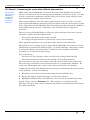
G1 Stage 5—Discussion
Note that 3D GeoModeller only calculates and plots the model for formation f5. To
calculate the model for a formation, 3D GeoModeller requires that there be at least
one orientation point associated with it. Currently, f5 is the only formation that
matches this criterion.
At these early stages of modelling a surface, you may get unexpected results.
This is mainly because there is very little orientation data to give information about
the attitude of the geology surfaces.
In the following stage, we shall work through the issues, dealing with the biggest
problems first.
Contents Help | Top
© 2013 BRGM & Desmond Fitzgerald & Associates Pty Ltd
| Back |
GeoModeller User Manual
Contents | Help | Top
Tutorial case study G (Drillholes)
22
| Back |
G1 Stage 6—Comparing the model with drillhole observations
Parent topic:
Tutorial G1—
Building a
model from
drillholes
(erosional
series f5)
Note: Using 3D GeoModeller’s ‘Compare the model with drillhole observations’
feature is a useful tool, but it is not required or obligatory in this case study. You may
be able to find and fix problems with the model just as easily using enlarged views
and examining the graphic representation.
When using drillholes, since the contact point from the data is certain, we would
expect 3D GeoModeller to place the geology boundary from the model exactly at this
point. Sometimes 3D GeoModeller places a geology boundary through the middle of
some drilled geology interval. Sometimes, also, the model surface appears to
‘meander’.
This is because 3D GeoModeller is using two other techniques that may, from its
viewpoint, conflict with the drillhole data:
•
It is trying to keep the model surface smooth.
•
It is using geological statistics to predict the course of the boundary.
These problems typically occur at the hole collar, and near the end-of-hole.
The problems are occurring at places where 3D GeoModeller does not have enough
information to generate the model properly. To fix the problems, add geology contact
or orientation points. As interpreters, we influence the modelling calculation
according to our belief about the geology.
We can do this by:
•
Tracing out a 'line-of-points' where we believe the geology should be OR
•
Add orientation data to influence the attitude of the geology horizons
Note that that we may not necessarily correct the data at the location of the error.
The error may result from lack of orientation data at a neighbouring drillhole. We
could even add mapping data on the surface that would resolve the problem.
Comparing the model with drillhole observations gives information about the location
of the problems. It does the following:
1
Examines each interval of observed geology from the drillhole data
2
Checks the model’s predicted geology over the same interval
3
Highlights drillholes where the difference error exceeds the specified precision.
Specify a large value for Precision first. This enables you to identify the big
problems. Fix those first. Often, fixing the big problems automatically fixes some of
the smaller problems.
Contents Help | Top
© 2013 BRGM & Desmond Fitzgerald & Associates Pty Ltd
| Back |
GeoModeller User Manual
Contents | Help | Top
Tutorial case study G (Drillholes)
23
| Back |
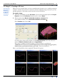
G1 Stage 6—Steps
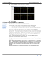
1
From the main menu choose Model > Compare model with drillhole observations
OR
From the Model toolbar choose Compare model with drillhole observations
2
.
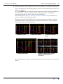
For Precision, enter 200.
Choose OK.
Highlighted drillholes
have model differences
compared to the drilled
intervals
Contents Help | Top
© 2013 BRGM & Desmond Fitzgerald & Associates Pty Ltd
| Back |
GeoModeller User Manual
Contents | Help | Top
3
Tutorial case study G (Drillholes)
24
| Back |
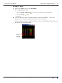
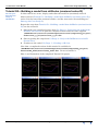
Fix the problems at the drillholes where 3D GeoModeller has identified a problem.
You can experiment with adding geology contact or orientation points yourself, or
follow our solution.
In section s81N, add an orientation point between the third and fourth drillholes
from the left, to guide the model away from the loop that it is mistakenly
generating through the fourth, fifth and sixth drillholes.
Use the steps in G1 Stage 5—Prepare the project for modelling to add the new
point, recalculate and replot the model.
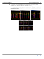
Compare the model with drillhole observations again with a distance of 200 m.
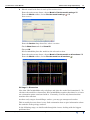
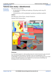
Add further points in other sections as required. Recalculate. The illustration
below shows the steps and the result.
1. Model has loop
4. Recalculate model
2. Click trace points
3. Create orientation
point
5. Add orientation points in other
sections as necessary and
recalculate.
In this illustration, we have removed discrepancies in the model to an accuracy of
200 m.
Contents Help | Top
© 2013 BRGM & Desmond Fitzgerald & Associates Pty Ltd
| Back |
GeoModeller User Manual
Contents | Help | Top
4
Tutorial case study G (Drillholes)
25
| Back |
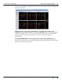
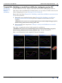
Compare the model with drillhole observations using progressively finer
precision, 50 m, then 15 m, then 5 m, repeating steps 1–3.
At 50 m, we added orientation points to s81N and s91N. When we recalculated
the model, we found another problem in s85N, which we fixed. The results are in
the illustration below.
Contents Help | Top
© 2013 BRGM & Desmond Fitzgerald & Associates Pty Ltd
| Back |
GeoModeller User Manual
Contents | Help | Top
Tutorial case study G (Drillholes)
26
| Back |
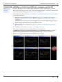
As you work through the problems in the model, the interpreted horizon begins to
look more plausible.
Important note about 3D GeoModeller’s ‘Compare the model with
drillhole observations’ feature: At larger Precision values, 3D GeoModeller
calculates genuine errors. You can review the project geology and add further
geology observations or interpretations to seek to resolve the reported
discrepancies.
At smaller Precision values, the 'errors' may be due to the mathematical
uncertainty in the model. You would gain very little from further interpretive
work to try and resolve such relatively small errors ('small' relative to the overall
dimensions of the model project).
Contents Help | Top
© 2013 BRGM & Desmond Fitzgerald & Associates Pty Ltd
| Back |
GeoModeller User Manual
Contents | Help | Top
Tutorial case study G (Drillholes)
27
| Back |
G1 Stage 7—Creating a 3D view
Parent topic:
Tutorial G1—
Building a
model from
drillholes
(erosional
series f5)
When you are satisfied that you have modelled the f5 surface in a credible geological
manner, and that the model is consistent with the drilled geology intervals, you can
quickly generate a 3D surface and view this in the 3D Viewer.
G1 stage8—Steps
1
View the 40 drillholes in the 3D Viewer. (If not already displayed) In the Project
Explorer, from the Drillholes shortcut menu, choose Show.
2
Choose main menu Model > Build 3D formations and faults OR
In the Model toolbar choose Build 3D formations and faults
Check Surface and choose OK.
To change the colour of the surface, in the Project Explorer, from the shortcut
menu of Model > Surface f1_f5, choose Appearance.
Note that a completed version of Stage 8 of the tutorial is available in
\GeoModeller\tutorial\CaseStudyG\TutorialG1\Completed_project\
TutorialG1_2_f5\TutorialG1_2_f5.xml. Do not overwrite it.
Here is an illustration of the completed Tutorial G2 project
Contents Help | Top
© 2013 BRGM & Desmond Fitzgerald & Associates Pty Ltd
| Back |
GeoModeller User Manual
Contents | Help | Top
Tutorial case study G (Drillholes)
28
| Back |
Tutorial G2—Building a model from drillholes (erosional series f2)
Parent topic:
Tutorial case
study G
(Drillholes)
In this tutorial we create, display and refine the model for (erosional) series f2
After series f5 (Tutorial G1—Building a model from drillholes (erosional series f5)),
series f2 is the next older erosional surface, and the next series for modelling (see
Strategy for Case Study G).
Repeat the steps from Tutorial G1—Building a model from drillholes (erosional series
f5), but for section f2.
1
Start with your completed project from G1 Stage 6—Comparing the model with
drillhole observations or open the completed version that we have supplied
\GeoModeller\tutorial\CaseStudyG\TutorialG1\Completed_project\
TutorialG1_2_f5\TutorialG1_2_f5.xml.
2
Start repeating the steps from G1 Stage 4—Project the Drillholes in each 2D
Section-View.
3
Continue to the end of G1 Stage 7—Creating a 3D view.
Note that a completed version of this tutorial is available in
\GeoModeller\tutorial\CaseStudyG\TutorialG2\Completed_project\
TutorialG2_f5f2\TutorialG2_f5f2.xml. Do not overwrite it.
Here is an illustration of the completed Tutorial G2 project
Contents Help | Top
© 2013 BRGM & Desmond Fitzgerald & Associates Pty Ltd
| Back |
GeoModeller User Manual
Contents | Help | Top
Tutorial case study G (Drillholes)
29
| Back |
Tutorial G3—Building a model from drillholes (onlapping series f3)
Parent topic:
Tutorial case
study G
(Drillholes)
In this tutorial we create, display and refine the model for (onlapping) series f3
Now that we have modelled the erosional series, we are ready to model serties f3, the
oldest onlapping series (see Strategy for Case Study G).
Repeat the steps from Tutorial G1—Building a model from drillholes (erosional series
f5), but for section f3.
1
Start with your completed project from Tutorial G2—Building a model from
drillholes (erosional series f2) or open the completed version that we have
supplied
\GeoModeller\tutorial\CaseStudyG\TutorialG2\Completed_project\
TutorialG2_f5f2\TutorialG2_f5f2.xml.
2
Start repeating the steps from G1 Stage 4—Project the Drillholes in each 2D
Section-View.
Note that a completed version of this tutorial is available in
\GeoModeller\tutorial\CaseStudyG\TutorialG3\Completed_project\
TutorialG3_f5f2f3\TutorialG3_f5f2f3.xml. Do not overwrite it.
Here is an illustration of the completed Tutorial G3 project
Contents Help | Top
© 2013 BRGM & Desmond Fitzgerald & Associates Pty Ltd
| Back |
GeoModeller User Manual
Contents | Help | Top
Tutorial case study G (Drillholes)
30
| Back |
Tutorial G4—Building a model from drillholes (onlapping series f4)
Parent topic:
Tutorial case
study G
(Drillholes)
In this tutorial we create, display and refine the model for (onlapping) series f4
After series f3, series f4 is the next youngest onlapping surface, and the recommended
next series for modelling (see Strategy for Case Study G).
Repeat the steps from Tutorial G1—Building a model from drillholes (erosional series
f5), but for section f4.
1
Start with your completed project from Tutorial G3—Building a model from
drillholes (onlapping series f3) or open the completed version that we have
supplied
\GeoModeller\tutorial\CaseStudyG\TutorialG3\Completed_project\
TutorialG3_f5f2f3\TutorialG3_f5f2f3.xml.
2
Start repeating the steps from G1 Stage 4—Project the Drillholes in each 2D
Section-View.
3
Continue to the end of G1 Stage 7—Creating a 3D view.
Note that a completed version of this tutorial is available in
\GeoModeller\tutorial\CaseStudyG\TutorialG4\Completed_project\
TutorialG4_f5f2f3f4\TutorialG4_f5f2f3f4.xml. Do not overwrite it.
Here is an illustration of the completed Tutorial G4 project
Contents Help | Top
© 2013 BRGM & Desmond Fitzgerald & Associates Pty Ltd
| Back |
GeoModeller User Manual
Contents | Help | Top
Tutorial case study G (Drillholes)
31
| Back |
Tutorial G5—Building a model from drillholes (onlapping series f6)
Parent topic:
Tutorial case
study G
(Drillholes)
In this tutorial we create, display and refine the model for the final (onlapping) series
f6
After series f4, series f6 is the next youngest onlapping surface, and the next series
for modelling (see Strategy for Case Study G).
Repeat the steps from Tutorial G1—Building a model from drillholes (erosional series
f5), but for section f4.
1
Start with your completed project from Tutorial G4—Building a model from
drillholes (onlapping series f4) or open the completed version that we have
supplied
\GeoModeller\tutorial\CaseStudyG\TutorialG4\Completed_project\
TutorialG4_f5f2f3f4\TutorialG4_f5f2f3f4.xml.
2
Start repeating the steps from G1 Stage 4—Project the Drillholes in each 2D
Section-View.
3
Continue to the end of G1 Stage 7—Creating a 3D view.
Note that a completed version of this tutorial is available in
\GeoModeller\tutorial\CaseStudyG\TutorialG5\Completed_project\
TutorialG5_f5f2f3f6\TutorialG5_f5f2f3f6.xml. Do not overwrite it.
Here is an illustration of the completed Tutorial G4 project
Contents Help | Top
© 2013 BRGM & Desmond Fitzgerald & Associates Pty Ltd
| Back |
GeoModeller User Manual
Contents | Help | Top
Tutorial G6: Import Drillhole Assay Data
32
| Back |
The following illustrations are of the final model, using line and filled mode.
Tutorial G6: Import Drillhole Assay Data
1
Choose Import > Drillhole > Assay Data into Existing Drillholes
2
The Import ASCII Wizard will pop up.
1
Contents Help | Top
On the first page, select the input file:
© 2013 BRGM & Desmond Fitzgerald & Associates Pty Ltd
| Back |
GeoModeller User Manual
Contents | Help | Top
Tutorial G6: Import Drillhole Assay Data
33
| Back |
\GeoModeller\tutorial\CaseStudyG\TutorialG5\Data\AssayImport
Example.csv
Contents Help | Top
2
On the second page you will see the file is formatted correctly already. Choose
Next to go to page 3.
3
Set the column mapping for the Hold ID.
3
Set the column mapping for the From and To in the same manner
4
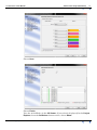
Set the Au field paraters. Set the Type to Real, set the name, description and
units as desired. The default NULL value can be used.
© 2013 BRGM & Desmond Fitzgerald & Associates Pty Ltd
| Back |
GeoModeller User Manual
Contents | Help | Top
5
Tutorial G6: Import Drillhole Assay Data
34
| Back |
Choose Finish to close the wizard and import the data.
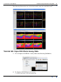
Tutorial G6 - Drillhole Properties Dialog
To view the assay field data for a drillhole you can use the Drillhole Properties
Dialog.
Contents Help | Top
1
Expand the Drillhole list in the Project Explorer tree
2
Find Drillhole VDH_s87N_07 in the list and open its context menu using the
© 2013 BRGM & Desmond Fitzgerald & Associates Pty Ltd
| Back |
GeoModeller User Manual
Contents | Help | Top
Tutorial G6: Import Drillhole Assay Data
35
| Back |
mouse.
3
Choose Edit to open the Drillhole Properties Dialog
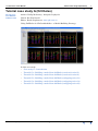
This dialog shows the drillhole log in the tree on the left hand side. The columns
next to this highlight the drillhole log/geological model misfit and the assay field
plot. As can be seen here there is now assay data in this drillhole.
Contents Help | Top
© 2013 BRGM & Desmond Fitzgerald & Associates Pty Ltd
| Back |
GeoModeller User Manual
Contents | Help | Top
Tutorial G6: Import Drillhole Assay Data
36
| Back |
Tutorial G6: Assay Data to Observation MeshGrid
Once assay data has been imported into drillholes you will generally want to
perform some sort of interpolation, analsysis or processing. To do this in
GeoModeller v2012 you must first create an Observation MeshGrid from Drillhole
fields.
Contents Help | Top
1
Right click on the Drillholes entry in the project tree to bring up the context
menu
2
Select Fields to Data Points Mesh to bring up the filter dialog.
3
Choose Select All for both the drillholes (left side) and Fields (right side). Then
choose OK to close the dialog and create the MeshGrid.
© 2013 BRGM & Desmond Fitzgerald & Associates Pty Ltd
| Back |
GeoModeller User Manual
Contents | Help | Top
Tutorial G6: Import Drillhole Assay Data
37
| Back |
You should now see the MeshGrid in the Project tree.
This tutorial will not cover the vast number of tools available when working with
MeshGrids. Instead a very simple “quick preview” interpolation of the assay data
using Inverse Distance Interpolation will be shown.
NOTE: GeoModeller v2012 now supports both traditional Kriging and domain
Kriging. Kriging can provide much better results than the Inverse Distance
interpolation.
Tutorial G7: Inverse Distance Interpolation
In this exercise you will:
•
Compute a new MeshGrid field using the MeshGrid calculator.
•
Interpolate data in a MeshGrid field using Inverse Distance Interpolation.
•
Add your Geological model as a field to an existing MeshGrid.
•
Use the calculator to threshold field data by unit.
It is common for Gold data to have a log-normal distribution. For interpolation it is
desirable to normalise the distribution first. Therefore, the first step in this exercise
is to use the MeshGrid calculator to take the LOG of the Gold field Au.
Contents Help | Top
© 2013 BRGM & Desmond Fitzgerald & Associates Pty Ltd
| Back |
GeoModeller User Manual
Contents | Help | Top
Tutorial G6: Import Drillhole Assay Data
38
| Back |
Compute the LOG of a MeshGrid field
1
Right click on the MeshGrid DrillholeFields and choose Compute New Field
from the context menu.
2
In the calculator dialog:
1
Choose ln (natural log) from the Function Keys
2
Choose Au from the Field List
3
Choose “)” from the Function Keys to close the brackets.
4
Change the Result Field Name to “log_au” or something appropraite.
5
Choose Evaluate to evaluate the expression and create the new field.
6
Choose Save and Exit to save the results into the Projet tree.
Important: You must always Evaluate the expression before choosing Save and
Exit. Otherwise the result will not be saved in the Project Tree.
You should now have two fields in the MeshGrid, as shown.
Contents Help | Top
© 2013 BRGM & Desmond Fitzgerald & Associates Pty Ltd
| Back |
GeoModeller User Manual
Contents | Help | Top
Tutorial G6: Import Drillhole Assay Data
39
| Back |
Inverse Distance Interpolation
Contents Help | Top
1
Right click on the log_au field to open the MeshGrid field context menu. Choose
Inverse Distance Interpolation.
2
In the dialog choose New Grid and enter the name of the grid. Here it is shown as
inv_log_gold.
© 2013 BRGM & Desmond Fitzgerald & Associates Pty Ltd
| Back |
GeoModeller User Manual
Contents | Help | Top
Tutorial G6: Import Drillhole Assay Data
40
| Back |
Choose Next to move to the next page of the wizard.
3
On the next page under Grid Definition choose Fixed and enter 250m cell
spacing. Then specify the Maximum Radius of Neighbourhood as 3000
metres.
Choose Next to go to page 3 of the wizard.
4
Contents Help | Top
Enter the name of the interpolation field. In this example it is called
interp_log_au.
© 2013 BRGM & Desmond Fitzgerald & Associates Pty Ltd
| Back |
GeoModeller User Manual
Contents | Help | Top
Tutorial G6: Import Drillhole Assay Data
41
| Back |
Choose Finish to perform the interpolation.
You should now have a new MeshGrid in your project called inv_log_gold, or
whatever name you chose of page 1 of the wizard. This grid is a regular voxet with
fixed cell size of 250m.
Remove linearisation of the interpolated field.
Recall that the interpolation was performed on the log of the gold assay data. Now
you will need to remove the linearisation to revert back to a log-normal distribution.
Contents Help | Top
1
Right click on the inv_log_gold and choose Compute New Field. This will open
the calculator dialog box again.
2
In the calculator perform the following steps:
1
Choose exp from the Function Keys,
2
Choose interp_log_au from the Field List
3
Choose “)” to close the brackets.
4
Enter the name for the new field. Here it is specified as interp_Au.
© 2013 BRGM & Desmond Fitzgerald & Associates Pty Ltd
| Back |
GeoModeller User Manual
Contents | Help | Top
5
Tutorial G6: Import Drillhole Assay Data
42
| Back |
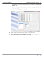
Choose Evaluate followed by Save and Exit.
You should now have the new field interp_Au in your project MeshGrid
inv_log_gold
3
Contents Help | Top
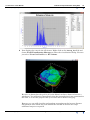
Explore the field interp_Au by looking at the histogram and statistics. Right
click on the field and choose Histogram from the context menu. This will bring
up the histogram dialog which also contains summary statistics.
© 2013 BRGM & Desmond Fitzgerald & Associates Pty Ltd
| Back |
GeoModeller User Manual
Contents | Help | Top
4
Tutorial G6: Import Drillhole Assay Data
43
| Back |
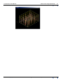
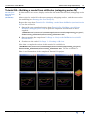
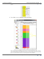
Now display the voxet in the 3D viewer. Right click on the interp_Au field and
choose Field Visualisation Manager to show the visualisation dialog. For now
just select View Grid in 3D as a 3D Volume.
Because we know that the gold is all in the f3 unit we have shown it here as a
wireframe. You will notice immediately that the interpolation is not contrained to
this unit. It is for this purpose that you would choose Domain Kriging.
However, we can still visualise and perform processing on the inverse distance
interpolated data which only falls within the unit f3. To do this two steps
additional steps are required.
Contents Help | Top
© 2013 BRGM & Desmond Fitzgerald & Associates Pty Ltd
| Back |
GeoModeller User Manual
Contents | Help | Top
Tutorial G6: Import Drillhole Assay Data
44
| Back |
1
Add a model field to the MeshGrid
2
Threshold the interp_Au field to only those voxels within the f3 unit using
the model field.
Adding a model field to a MeshGrid
Any MeshGrid can have a model field added to it. A model field is a lithology field
that contains the units at each cell in a MeshGrid. For example, a voxet model field
will the lithology unit number that each voxel is in, whereas, an observation
MeshGrid will contain the unit number at each point of the mesh grid.
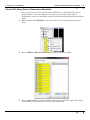
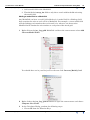
1
Right click on the inv_log_gold MeshGrid and from the context menu select Add
Current Model Field.
You should then see in your Project Tree the new field Current_Model_Grid.
2
Right click on the inv_log_gold MeshGrid to open the context menu and choose
Compute New Field.
3
In the Calculator Dialog, perform the following steps:
1
Contents Help | Top
Choose IF from the Function Keys
© 2013 BRGM & Desmond Fitzgerald & Associates Pty Ltd
| Back |
GeoModeller User Manual
Contents | Help | Top
Tutorial G6: Import Drillhole Assay Data
45
| Back |
2
Choose Current_Model_Grid from the Field List
3
Choose “==” from the Function Keys, followed by “3” from the Numeric Keys.
4
Choose “;” from the Numeric Keys
5
Choose interp_Au from the Field List
6
Choose “;” from the Numeric Keys
7
Choose NaN from the Numeric Keys
8
Chosoe “)” from the Function Keys.
9
Enter the result field name as interp_Au_f3
10 Choose Evaluate followed by Save and Exit.
The expression should look like the one above. It simply says:
IF voxel lithology is f3 THEN output interp_Au ELSE output null.
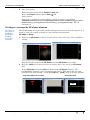
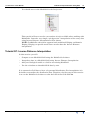
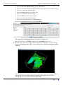
4
Visualise the new field using the Field Visualisation Manager, via the context
menu of the interp_Au_f3 field. In the dialog choose View Grid in 3D and 3D
Volume.
The visualisation now shows interpolated gold data within the lithology unit of
interest. You can view the colour map via the context menu for the field
interp_Au_f3. Choose Edit Colours and Clips.
Contents Help | Top
© 2013 BRGM & Desmond Fitzgerald & Associates Pty Ltd
| Back |
GeoModeller User Manual
Contents | Help | Top
Tutorial G6: Import Drillhole Assay Data
46
| Back |
Estimate the volume of gold within the f3 unit.
1
To get an estimate of the volume with the f3 unit you can use the MeshGrid
Calculator again. Open the calculator from the context menu of inv_log_gold.
2
Create the expression: IF(interp_Au_f3 <> NaN;Current_Model_Grid;NaN)
using the keys and field list.
3
Enter the name of the new field as interp_Au_f3_lithology.
4
Choose Evaluate followed by Save and Exit.
Check that the field was created in the project tree.
5
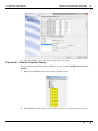
Right click on the new field interp_Au_f3_lithology and choose Properties.
This will open the properties dialog.
6
In the dialog change the Alias from none to Lithology.
Choose OK. GeoModeller will now recognise this field as a lithology field.
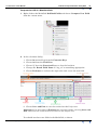
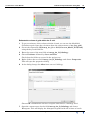
7
Contents Help | Top
Open the context menu for the field interp_Au_f3_lithology and choose
Histogram. This will display the histogram together with the volume of voxels
© 2013 BRGM & Desmond Fitzgerald & Associates Pty Ltd
| Back |
GeoModeller User Manual
Contents | Help | Top
Tutorial G6: Import Drillhole Assay Data
47
| Back |
which contain gold (interpolated) for the unit f3.
Compare this number with the value from the Current_Model_Grid field.
The volume of unit f3 is 4.604688E10 m
The volume of unit f3 which contains (interpolated) gold is 3.107812E10 m3.
This does not show an estimate of the grade of the gold in the f3 unit, just the cells
which contain gold.
Contents Help | Top
© 2013 BRGM & Desmond Fitzgerald & Associates Pty Ltd
| Back |