1
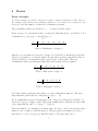
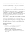
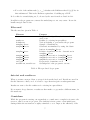
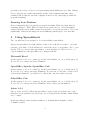
LOVEGROVE MATHEMATICALS GREAT LIKELINESSES Release B09 USER MANUAL R.Lovegrove GREAT LIKELINESSES is a program for calculating likelinesses, that is for finding best-estimates of probabilities. This is the manual for release B09, versions B09F and B09C. The recommended citation for this manual is Lovegrove,R.,(2015),‘Great Likelinesses (release B09) User Manual’, Lovegrove Mathematicals, London, Octber 2015 www.lovegrovemaths.co.uk London United Kingdom October 2015 [email protected] Contents 1 Introduction 3 2 There is no warranty 3 3 Releases and Versions 3.1 Changes implemented in this Release . . . . . . . . . . . . . . . . . . . . 3.2 Known Issues . . . . . . . . . . . . . . . . . . . . . . . . . . . . . . . . . 3 3 4 4 Basics 5 5 Using Spreadsheets 8 6 What you should do now 9 7 Running the program 9 8 Stopping 10 9 The given histogram 9.1 Basics of the specification . . . . . . . . . . . . . . . . . . . . . . . . . . 9.2 Merge Blocks . . . . . . . . . . . . . . . . . . . . . . . . . . . . . . . . . 11 11 11 10 The required integram 12 11 Percentile 11.1 Method of interpolation . . . . . . . . . . . . . . . . . . . . . . . . . . . 12 13 12 The underlying set 12.1 Components of the underlying set . . . . . . . . . 12.2 Fundamental types of underlying set . . . . . . . 12.2.1 Unstructured, S(N) . . . . . . . . . . . . . 12.2.2 Ranked, R(N) . . . . . . . . . . . . . . . . 12.2.3 Reverse-ranked, RR(N) . . . . . . . . . . . 12.2.4 Step-down, SD(c,N) . . . . . . . . . . . . . 12.2.5 Ranked step-down RSD(c,N) . . . . . . . . 12.2.6 High/Medium/Low, HML(c,d,N) . . . . . 12.2.7 Ranked High/Medium/Low, RHML(c,d,N) 12.2.8 Unimodal, M(A to B,N) . . . . . . . . . . 12.2.9 Bell-shaped, B(A to B,N) . . . . . . . . . 12.2.10 U-shaped, U(A to B,N) . . . . . . . . . . . 12.2.11 Multi-modal . . . . . . . . . . . . . . . . . 12.2.12 Plateau, PLAT(w,A to B,N) . . . . . . . . 12.2.13 Reverse-ranked with unimodal slope . . . . 12.2.14 Ranked with ranked slope . . . . . . . . . 12.2.15 Ranked with unimodal slope . . . . . . . . 14 14 14 14 14 14 15 15 16 16 16 18 19 19 22 23 23 23 1 . . . . . . . . . . . . . . . . . . . . . . . . . . . . . . . . . . . . . . . . . . . . . . . . . . . . . . . . . . . . . . . . . . . . . . . . . . . . . . . . . . . . . . . . . . . . . . . . . . . . . . . . . . . . . . . . . . . . . . . . . . . . . . . . . . . . . . . . . . . . . . . . . . . . . . . . . . . . . . . . . . . . . . . . . . . . . . . . . . . . . . . . . . . . . . . . . . . . . . . . . . . . . . . . . . . . . . . . . . . . . 13 Contractions 23 14 Frequency distributions and CDFs 24 15 data.txt 25 16 results.csv 27 17 The Sampling files 17.1 Introduction . . . . . . 17.2 CSV files . . . . . . . . 17.2.1 Basic Style . . . 17.2.2 Advanced Style 17.3 TXT files . . . . . . . . . . . . . . . . . . . . . . . . . . . . . . . . . . . . . . . . . . . . . . . . . . . . . . . . . . . . . . . . . . . . . . . . . . . . . . . . . . . . . . . . . . . . . . . . . . . . . . . . . . . . . . . . . . . . . . . . . . . . . . . . . . . . . . . . . . . . . . . . . . . 28 28 29 30 31 32 18 DEFAULTS.TXT 32 19 Odds and Ends 37 20 Troubleshooting 38 A Notation and Terminology 39 B The B.1 B.2 B.3 B.4 B.5 B.6 B.7 B.8 B.9 B.10 B.11 B.12 B.13 B.14 B.15 41 41 41 42 42 42 42 42 42 42 43 43 43 43 44 44 Algorithms The commoner underlying sets . . . . . . . . . . . . . . . Selection of f ∈ S(N ) . . . . . . . . . . . . . . . . . . . . Selection of r ∈ R(N ) . . . . . . . . . . . . . . . . . . . . Selection of f ∈ RR(N ) . . . . . . . . . . . . . . . . . . Selection of f ∈ RSD(c, N ) . . . . . . . . . . . . . . . . Selection of f ∈ SD(c, N ) . . . . . . . . . . . . . . . . . Selection of f ∈ RHM L(c, d, N ) . . . . . . . . . . . . . . Selection of f ∈ HM L(c, d, N ) . . . . . . . . . . . . . . . Selection of f ∈ M (m, N ) . . . . . . . . . . . . . . . . . Selection of f ∈ M (A to B, N ) . . . . . . . . . . . . . . . Selection of f ∈ U (m, N ) and f ∈ U (A to B, N ) . . . . . Selection of f ∈ P LAT (w, A to B, N ) . . . . . . . . . . . Merge Blocks . . . . . . . . . . . . . . . . . . . . . . . . Using a distribution to generate a simulated observation Expected frequency distributions and CDFs . . . . . . . C Standard analytically-solvable problems 2 . . . . . . . . . . . . . . . . . . . . . . . . . . . . . . . . . . . . . . . . . . . . . . . . . . . . . . . . . . . . . . . . . . . . . . . . . . . . . . . . . . . . . . . . . . . . . . . . . . . . . . . . . . . . . . . . . . . . . . . . . . . . . . . . . . . . . . . 44 1 Introduction GREAT LIKELINESSES (the name is a pun on that of Charles Dickens’s novel Great Expectations) is a program for calculating likelinesses, that is for finding best-estimates of probabilities. This is not a textbook about the theory of likelinesses. It is a guide to the use of the program Great Likelinesses. A summary of the notation and terminology is given in Appendix A; the algorithms are outlined in Appendix B. 2 There is no warranty This program is currently under development, and is not intended to be used in any situation where there are or might be deleterious consequences arising from that use. There is no warranty of any form. For example, there is no warranty against failure of the program, or against failure of the program to produce the correct result. By using the program, you accept full responsibility for all the consequences of that use. If you are not willing to accept that responsibility then do not use the program. 3 Releases and Versions This is the manual for Release B09. Each Release comes in two versions: the full version, signified by the suffix F, and the classical version, signified by the suffix C. The classical version might not be produced. but if it is then it is always produced first, and is usually withdrawn when the full version is released. In the full version, the degree is limited to a maximum of 102. In the classical version, the degree is restricted to values which have some significance in the classical problems to do with coins, dice and cards; these are 2,3,4,5,6,8,13,16,26,32,36,39,52 and 64. 3.1 Changes implemented in this Release • g and h are now set up before the underlying set, rather than after it. • The user may now specify a percentile to be best-estimated. • In a Multimodal analysis, if each essential domain extends over the whole of XN and the user has given permission in defaults.txt then the weights will be interpreted as being probabilities of selection rather than coefficients in linear combinations. • A new underlying set (Plateau distributions) has been introduced. 3 • (*) The layout of the basic .csv sampling files has been simplified. The nature of some of these changes is such that existing versions of data.txt and defaults.txt will be rendered unusable. 3.2 Known Issues General comments about over/underflow The number-crunching involved really can push your computer to its limits. The following should be avoided if possible:• High degree; • Large number of iterations; • Overly-complicated underlying set; • Merge block(s) • Given histogram with large sample size; • Required integram with large sample size. Any one of these, if taken to extremes, but especially any combination of more than one, can cause a run-time error. If this should happen to you then you will probably firstly want to reduce the number of iterations. Alternatively, or additionally:• You might consider reducing the degree, for example by measuring the independent variable in larger units (eg. 2Kg rather than 1Kg). • Ask yourself whether you really do need such a complicated underlying set. It is very easy to impose far more conditions than you would ever dream of using with a traditional closed, parametric analysis. Due to interactions between the various items, it is not possible to give precise guidance about the meanings of “High degree” etc. However, anything which increases the chances that the program will encounter a term f (i)g(i)+h(i) where f(i) is very small but g(i)+h(i) is large must be considered a bad idea. If there is any chance that you might run into difficulties of this type then you should use the sampling files, or some other technique, to model your observational or experimental program before carrying it out. 4 4 Basics Basic concepts A coin is of degree 2; a die is of degree 6; a pack of cards is of degree 52. The degree is the number of possibilities that something (tossing a coin; rolling a die; drawing a card) may take. It is the number of classes in a classification system. The possibilities/classes are labelled 1, 2, . . . , N where N is the degree. Given a degree, we can always define a distribution with that degree, as in Table 1. For N P a distribution f , each f (i) > 0 and f (i) = 1. i=1 i f(i) 1 0.2 2 0.1 3 0.35 4 0.05 5 0.25 6 0.5 Table 1: Distribution of degree 6 Likewise, we can define an histogram of degree N, as in Table 2. Each h(i)≥ 0 and the h(i) are not required to be integer-valued. If each h(i) is an integer then h is called an integram (Table 3); an integram is just a special type of histogram. There are circumstances where an integram, rather than just an histogram, is required. i h(i) 1 3.0 2 3 4.2 0 4 0.7 5 6 1.8 0 Table 2: Histogram of degree 6 i h(i) 1 3 2 4 3 0 4 0 5 1 6 0 Table 3: Integram of degree 6 Note that an histogram may take values of 0, but a distribution may not. The most important histogram is the zero integram, 0 = (0, 0, . . . , 0). If f is a distribution and g is an integram, both of degree N, then the probability of g given f is P r(g|f ) = M (g)f g , where M(g) is the multinomial coefficient associated with g (see Appendix A), and f g = f (1)g(1) . . . f (N )g(N ) . The best-estimate of something is its mean value. In order to have a mean value, there must be a set of values to find the mean of. This program best-estimates P r(g|f ) so there has to be a set of P r(g|f ) to find the mean of. We start with a set of 5 distributions, called the Underlying Set, calculate P r(g|f ) for each f in that set and then find the mean of those. The mean used is a weighted mean, where the weights depend upon available data in the form of an histogram (called the given histogram). The actual formula used is R g h f f f ∈P LP (g|h) = M (g) R h (1) f f ∈P where P is the underlying set, h is the given histogram and LP (g|h) is the likeliness (see Appendix A ). The expression for M (g) contains the product of factorials, N Q g(i)! (see Appendix A ), i=1 so each g(i) has to be integer-valued, so g has to be an integram. The weights, f h , started life as P r(h|f ), that is M (h)f h , but the M (h) has cancelled since it appeared in both the numerator and denominator of (1). The cancellation of the M (h) has taken with it any need for h to be integer-valued so h may be an histogram rather than specifically an integram. In a few simple cases, the main ones of which are listed in Appendix C, the integrals on the RHS can be evaluated theoretically. Usually, however, a numerical approach is needed; that is what this program does. The process is very simple: we replace the integrals by summations and the underlying set, P, by a sample of points (ie. distributions) selected at random from P. That sample can be surprisingly large: about a million points are often needed -the program defaults to 750,000- but 100 million or more can at times be necessary. It is only recently that improvements in computer technology have made it possible for such large problems to be tackled on home computers. What the program does The program:• Finds LP (g|h), and other standard likelinesses, by sampling from P. • Keeps track of convergence as the sampling process proceeds. • Produces a separate sample of distributions from P, and uses each as a generating distribution to generate simulated observations. • Calculates the best-estimate of the probability (ie. the likeliness) that P r(g|f ) < xi for a selection of xi equally spaced across some interval specified by the user. Likewise for P r(1|f ), . . . , P r(N |f ). This is the likeliness equivalent of building up a CDF. 6 • For each of the subintervals [xi , xi+1 ] calculates the Likeliness that P r(g|f ) lies in that subinterval. This is the likeliness equivalent of building up a PDF. It does this for an underlying set, P, chosen by the user from those listed in 12.2 In addition, the program can contract the underlying set onto any centre. It can also handle merged data-blocks. Files used The files used are given in Table 4. Filename data.txt results.csv defaults.txt sampling dis.csv sampling obs.csv sampling rfs.csv sampling dis.txt sampling obs.txt sampling rfs.txt errlog.txt scratch1.txt, scratch2.csv Purpose Keeps details of problem, for future editing and/or use Results, for viewing in spreadsheet Various defaults, to personalise the program Sample of distributions Observations simulated by using the distributions in sampling dis.csv Relative frequencies for the observations in sampling obs.csv simplified text version of sampling dis.csv simplified text version of sampling obs.csv simplified text version of sampling rfs.csv Keeps track of run-time errors Scratchpads for the program’s own use. Table 4: Files produced by program data.txt and results.csv When you start a new problem, you type it in from the keyboard. Details are saved in the file data.txt so that you do not have to type them in again on subsequent runs. Results are sent to the file results.csv for viewing in a spreadsheet. If you want to keep data.txt or results.csv then make a copy, under a different name, in the usual way. Countdown While the program is carrying out an analysis, a countdown-to-completion is sent to the screen so that you can see progress. The analysis is in two parts: a fast initial pass, during which various items are roughly estimated so as to improve the efficiency of the 7 program, followed by a slower second pass during which likelinesses are found. During the second pass, the countdown includes details of the estimated run-time: these estimates will be thrown out if the computer is used for any other purpose while the program is running. Running from Windows It is recommended that you run the program from within Windows rather than by switching, firstly, to DOS. This is because the program can be so fast with simpler analyses that the screen buffer cannot keep up and so forces the program to slow down significantly. Windows has improved screen-buffering which largely overcomes this. 5 Using Spreadsheets The .csv files have been designed to be viewed within a spreadsheet. Open your spreadsheet by right clicking on the icon for the file you want to open and selecting ‘open with’. You should then be offered the choice of programs to use to open the file. Choose your favourite spreadsheet: you should then be offered a choice of options defining how the spreadsheet is to interpret the file. Microsoft Excel As the separator, choose a comma (,). As the text delimiter, choose a double quote (”). Do not choose to merge successive delimiters. OpenOffice/Apache OpenOffice Calc As the separator, choose a comma (,). As the text delimiter, choose a double quote (”). Do not choose to merge successive delimiters. For versions 3.3 and later of Calc, select ‘detect special numbers’ (you will not be offered this option in earlier versions). LibreOffice Calc As the separator, choose a comma (,). As the text delimiter, choose a double quote (”). Do not choose to merge successive delimiters. Select ‘detect special numbers’. Lotus 1-2-3 Choose ‘Parse as CSV’. When the spreadsheet opens, it may seem that some of the fields have been asterisked out: they have not -it’s just that the default column widths are too small. In all spreadsheets, when viewing results.csv, you might find it helpful to widen Columns A and B. 8 6 What you should do now 1. Form a new folder to contain the files used by this program. 2. Transfer the .exe file and these notes into that folder. 3. Run the .exe file, and select item 999 from the opening menu. This will set up various defaults. You can now experiment with the program, to get a feel for what’s going on. 7 Running the program To start the program, run the .exe file. The opening screen gives you various options. If this is the first time that you have ever run this version then you must choose option 999 in order to set up various defaults. Otherwise, your choice will normally be between Option 1 if you are starting a completely new problem, or Option 2 if you are repeating a previous problem or running a modification of one. To start a new problem, choose Option 1. You will then be asked a number of questions, the answers to all of which will be numerical. For most of these, you will develop standard answers which you will soon get used to giving very quickly; with practice, your fingers will type most of the answers faster than you think of them. If you choose Option 2 then the computer will just take over and run the problem, giving you an on-screen progress report -which, for simpler problems, might flash past so quickly that you are unable to read it. 9 Figure 1: Opening screen 8 Stopping The program will normally come to a stop of its own accord. There are times, though, when you might want to stop it prematurely. You can choose ‘Stop’ from the opening menu. This will stop the program before it has really started. During data-input, when asked to answer ‘1 for YES or 2 for NO’ give one of the emergency numbers 911 or 999. The program will interpret this as a request to stop. However, data.txt will be partially written and will be unuseable; the next time you run the program, you will have to input the whole of the problem from the keyboard. Once the countdown has started, all you can really do is force a hard stop. If you are running the program in Windows then it should be enough to close the window in which it is running. Otherwise, try pressing CNTRL-C. Whichever method you use, the 10 program will be forced to stop immediately so it will not have the opportunity to close any open files. As a result, some files might not be closed properly –which could mean that you will need to restart your computer before you can use the program again. If you are analysing confidential or sensitive data then you should delete scratch1.txt and scratch2.csv manually. 9 The given histogram 9.1 Basics of the specification The given histogram, H, is specified in three parts, H=H1+H2+H3:1. H1 is specified as an histogram 2. H2 is specified as an ordered N’tuple of relative frequencies (which may be 0s) together with a sample size. The program finds H2 by multiplying the two together. 3. H3 is due to merge blocks, and will be discussed separately. Because an histogram will usually consist mostly of zeroes, when giving H1 (also the relative frequencies for H2), you specify a block about which you want to be asked, and the program defaults values outside that block to zero. To reduce errors, and also to make things easier for you, when you are specifying the relative frequencies for H2 you do not have to make them sum to 1: the program will normalise them for you. If you are specifying a multimodal problem then any H(I) less than 10−10 will be treated as zero when the program is checking whether the conditions have been met for treating the weights as probabilities. 9.2 Merge Blocks Table 5 gives three examples of Merge blocks. 4 5 6 7 8 2 0 3 3 1 1 2 3 4 5 6-8 2 1 6 2 0 7 (a) Merge block at left (b) Merge block at right 1-3 9 1-3 4 5 9 2 0 6-8 7 (c) Merge blocks at both ends Table 5: Merge blocks Each consists of a number of columns which have been merged together so that the detail has been lost of the entries in individual columns but the total of the entries is still known. 11 In practice, when data is collected in batches it sometimes happens that some batches contain a merge block but others do not. To cater for this, the program allows merge blocks to be entered independently of H1 and H2, and to overlap their non-zero entries. The degree is the number of columns that there would have been had the merging not taken place; it is 8 in each of the tables in Table 5. This means that merge blocks cannot be used as an artificial way to reduce the degree. The use of Merge Blocks introduces such vagueness into a problem that the resulting algorithms can be highly ill-conditioned. A significant increase in the number of iterations will be needed, but will not necessarily improve convergence to an acceptable extent; indeed, increasing the number of iterations could make convergence properties worse rather than better. For this reason, Merge Blocks should be used with caution. If there is no Merge Block then H1+H2 is the given histogram. If there is a Merge Block, however, the situation is more complicated since the program uses the information about the Merge Block to recreate the third histogram, H3. H3 is created every time that a new distribution is selected from the underlying set and will change as that distribution changes, so it is not possible to specify it. This continually-changing nature of H3 is a significant component of the vagueness which is introduced by the use of merge blocks. 10 The required integram The required integram, g, is specified in the same way as is H1: by giving a block about which you want to be asked, with values outside that block defaulting to zero. The calculated Likeliness of g is shown on-screen as part of the countdown display. This means that convergence can be monitored whilst the calculations are proceeding. 11 Percentile As part of the input routine, you are asked for a percentile for the program to estimate. You are not asked whether or not you want a percentile, since it takes as much effort to say “No” as it does to give one. If you don’t want a percentile then just reply “2 for No” and ignore the resulting 2nd percentile. Note the form of input. If you want the 5th percentile then input 5, not 0.05 . You are not restricted to integers, so you could ask for the 2.5th percentile, but this is not usual. Let’s say that you input p, then the program calculates 12 LP (p%|h) = Σf ∈P fp% f h Σf ∈P f h where fp% is the calculated p’th percentile of f. To find fp% it is necessary to interpolate the CDF of f -so the result depends upon the method of interpolation. Also, there is no universally-agreed definition of “percentile” when the domain is finite. Consequently, percentiles on finite domains -no matter how they are calculated- should always be treated with caution. 11.1 Method of interpolation Given a distribution f, the program firstly checks to find the value of J (J=1,...,N) for which 0.01*p lies between CDFf (J − 1) and CDFf (J), where CDFf (0) = 0. It does this by firstly checking J=1, then J=2 etc, ie by working from the left. Having found J, then program then uses linear interpolation between J-1 and J to find fp% . This models (see Fig 2) a distribution with domain [0,N] whose cumulative sums match those of f at 1,...,N. This is a classification of the interval into N subintervals, with the first subinterval being labelled “1”, the second “2”, etc. Figure 2: Linear interpolation, as used to find p’th percentile 13 12 12.1 The underlying set Components of the underlying set As a general rule, anything other than data (values of h(i) and g(i)) which has to be stated in order to define the problem forms part of the definition of the underlying set. Components include:• fundamental type • degree • contraction • essential domains of modal distributions • range of any mode • whether modal distributions are bell-shaped 12.2 Fundamental types of underlying set 12.2.1 Unstructured, S(N) S(N) is the set of all distributions of degree N. There is no relationship between the f(i) other than the requirement that they sum to 1. The fact that the domain, XN , is ordered is irrelevant. (a) LS(29) (b) Individual distribution Figure 3: Unstructured (general) distributions: S(29) 12.2.2 Ranked, R(N) A distribution, f , is ranked if f (1) > f (2) > ... > f (N ). 12.2.3 Reverse-ranked, RR(N) The mirror-images of ranked distributions, these increase to the right: f (1) < f (2) · · · < f (N ). 14 (a) LR(29) (b) Individual distribution (c) LR(N ) (i) for various N (semilog scales) Figure 4: Ranked distributions 12.2.4 Step-down, SD(c,N) There is a c such that the function values below c are all greater than the function values above c; that is, i ≤ c < k ⇒ f (i) > f (k). (a) LSD(6,29) (b) Individual distribution Figure 5: Step-down distributions: SD(6,29) 12.2.5 Ranked step-down RSD(c,N) The same as stepdown except that, in addition, the functions values below c are ranked; that is i < j ≤ c < k ⇒ f (i) > f (j) > f (k). c can be interpreted as a limit of discrimination for a ranked distribution. 15 (a) LRSD(6,29) (b) Individual distribution Figure 6: Ranked Step-down distributions: RSD(6,29) 12.2.6 High/Medium/Low, HML(c,d,N) An HML distribution is a step distribution with two steps. i 6 c < k 6 d < l ⇒ f (i) > f (k) > f (l) The degree must be at least 4. (a) LHM L(6,13,29) (b) Individual distribution Figure 7: High/Medium/Low: HML(6,13,29) 12.2.7 Ranked High/Medium/Low, RHML(c,d,N) A Ranked High/Medium/Low distribution is an HML distribution for which the ‘top step’ is ranked. i < j 6 c < k 6 d < l ⇒ f (i) > f (j) > f (k) > f (l) 12.2.8 Unimodal, M(A to B,N) Each distribution has precisely one mode. The mode does not have to be the same for every distribution used in the analysis, although it can be if so required. The program asks for a range of i which the mode may take; the smallest value is A and the largest is B. You will usually use one of two specific cases, here. 16 (a) LRHM L(6,13,29) (b) Individual distribution Figure 8: Ranked High/Medium/Low: RHML(6,13,29) (a) LM (6,29) (i) (b) LM (29) (i) Figure 9: Unimodal distributions 1. To use a specific mode, m say (Figure 9a has m=6), choose A=B=m. We then write M (m, N ) rather than M(m to m,N). 2. If A = 1 and B = N then M(A to B,N) becomes M(1 to N,N), which is written as M(N) and is the set of all unimodal distributions of degree N (Figure 9b). Despite the impression given by some mathematical texts, unimodal distributions are not usually bell-shaped (see Figure 9a): any bell-shape is due to vagueness in the mode (Figure 9b). You are offered the option to use only bell-shaped distributions, but you should not usually accept this offer. 17 There are two concepts of mode: the local and the global. Local modes i is a local mode of f if 1. i = 1 and f (1) > f (2); or 2. i = N and f (N − 1) < f (N ); or 3. 1 < i < N and f (i − 1) < f (i) > f (i + 1). Global modes i is a global mode of f if f (i) = max{f (j)|j ∈ XN }. This program uses local modes throughout. If you want to use M(A to B, N) as the underlying set but with a global, rather than local, mode then use PLAT(1,A to B,N) instead. 12.2.9 Bell-shaped, B(A to B,N) The notation used to refer to bell-shaped distributions follows that for Unimodal distributions, viz B(A to B,N), etc. The definition used by Great Likelinesses is “An unimodal distribution for which the absolute values of the first differences on either side of the mode are unimodal.” Figure 10a shows likelinesses over a set of Bell-shaped distributions, and Figure 10b shows their first differences. The platykurtic shape of 10a is due to the longer tail of the first differences on the right than on the left (because there is more room there). (a) LB(30,100) (b) First differences Figure 10: Bell-shaped distributions 18 12.2.10 U-shaped, U(A to B,N) (a) LU (6,29) (i) (b) LU (29) (i) Figure 11: U-shaped distributions The logical dual of unimodal distributions, U-shaped distributions have a single ‘trough’ rather than a single ‘mode’. Otherwise, there is no difference between the two. 12.2.11 Multi-modal The domain, XN , is covered by several (maximum, 9) ‘mini’ unimodal distributions, which may overlap. Each mini unimodal distribution has its own essential domain, over which that unimodal distribution takes non-zero values, and which is extended to cover the whole of XN by using values of zero elsewhere. During data-input, the user specifies the essential domain and the range of values that the mode make take. The combination of these two forms what is called a piece. If the degree is no more than 77 then a visual aide de memoire will appear on the screen during data-input (Figure 12) to help keep track of where the mini unimodal distributions are. This is switched off if the degree is more than 77 since a normal window would not be wide enough to contain it. Whenever a new multimodal distribution is needed, the program selects a mini unimodal distribution for each piece, and then uses them to produce the final distribution. The user can use defaults.txt to choose between two ways for using the mini distributions to produce the final distribution; both methods require the specification of a set of weights. That set is specified as part of the data-input; there are four possibilities. 1. S(p); 2. R(p); 3. SD(c,p) for some c; 19 Figure 12: Multi-modal distributions: aide de memoire 4. RSD(c,p). where p is the number of pieces. When a new multimodal distribution is being constructed, the program selects a single point from whichever of these sets the user has specified and then uses its co-ordinates as the weights. The two ways for using the weights are: 1. Weights used as coefficients in a linear combination; 2. Weights used as probabilities of selection Weights used as coefficients in linear combinations Having selected the mini unimodal distributions, the program forms a linear-combination by using the weights as the coefficients. The program labels the pieces in the order in which their details were typed into the computer, which need not be left-to-right and so gives flexibility when defining the problem. Figure 13 shows examples with weights selected from each of the four possible sets, where the details of the pieces were typed into the program in the order 1-2-3-4-5-6. 20 Figure 13: Multi-modal distributions: effects of different types of weights Weights used as probabilities of selection If:1. Each essential domain extends across the whole of XN , and 2. You have chosen the option in defaults.txt to make this happen then the weights, once chosen, will not be used as coefficients in a linear combination but, rather, as probabilities-of-selection. Every time a new distribution is needed, weights will be chosen and then one of the ‘mini’ unimodal distributions will be selected to be used as the required distribution, the weights being the probabilities-of-selection of the ‘mini’ distributions. If the program is using linear combinations, then all distributions will come from the same multimodal population, but if it is using probabilities-of-selection then some will come from Piece 1, some from Piece 2, etc so there will be a distinct population for each piece. The sample of 25 distributions given in RESULTS.CSV provide perhaps the most convenient way to see this, but the distributions in the sampling files allow a more thorough look. Consider the following example:Degree= 59 Multimodal In descending order of dominance the modes are:21 For Piece 1 the from 10 to 10. For Piece 2 the from 30 to 30. For Piece 3 the from 49 to 49. domain goes from 1 to 59. The Mode is allowed to vary A bell-shape has not been forced. domain goes from 1 to 59. The Mode is allowed to vary A bell-shape has been forced. domain goes from 1 to 59. The Mode is allowed to vary A bell-shape has not been forced. Using the weights as coefficients for linear combinations (option 2 in defaults.txt), the sample of 25 in results.csv was as in Figure 14a. Using weights as probabilities (option 1 in defaults.txt), the sample of 25 was as shown in Figure 14b. For all i, LP (00 i00 ) is the same in both cases: in Figure 14c, the two graphs are lying one-on-top of the other. However, although the LP (00 i00 )s coincide the distributions of the f(i)s do not (Figure 14d). (a) Weights used in linear combinations (b) Weights used as probabilities (c) Likelinesses (d) Distributions Figure 14: Alternative uses of weights 12.2.12 Plateau, PLAT(w,A to B,N) These are related to step-down distributions: take a step-down distribution and cycle it to the right. Plateau distributions need two numbers: the width and the start of the plateau. If the plateau has width w and starts at b then it finishes at c = b + (w − 1). 22 Figure 15: Plateau distribution The user specifies the width and a range of values A to B for the start, where B + (w − 1) ≤ N . The set of all plateau distributions of degree N with width w which start in the range A to B is denoted by PLAT(w,A to B,N). If B=A then we write PLAT(w,A,N) rather than PLAT(w,A to A,N). There are two special cases:1. PLAT(w,1,N) is SD(w,N); 2. PLAT(1,A to B,N) is equivalent to M(A to B,N) but using the global, rather than local, concept of mode. 12.2.13 Reverse-ranked with unimodal slope (As the name suggests) 12.2.14 Ranked with ranked slope (As the name suggests) 12.2.15 Ranked with unimodal slope (As the name suggests) 13 Contractions A contraction is a mapping of the form f 7→ q + α(f − q). These are useful for reducing the size of the underlying set. α is the magnitude, and q the centre, of the contraction Although the program gives you the opportunity just to type in the co-ordinates of the centre, if the degree is large then this can involve a lot of typing, which will be boring as well as increasing the chances of a typing mistake. The program therefore also gives you the choice of several standard cases. 23 (a) M (3) (b) Contraction centre 00 00 3 +00 100 2 (c) Contraction centre 00 00 2 +00 300 2 Figure 16: Two contractions of M(3) A contraction might cause the underlying set to fail to be of the fundamental type originally chosen; for example, the contraction of an unimodal distribution might not be unimodal. Figure 16 shows M(3) together with two contractions of magnitude 0.6. In Figures 16b & 16c, the shaded area, outside the boundary of M(3), shows the location of those distributions which are not unimodal. The contraction in 16b causes a significant number of distributions to move into this area and so fail to be unimodal. By contrast, every distribution in 16c remains in M(3) and so is still unimodal. 14 Frequency distributions and CDFs The expected frequency distribution of a probability can at times be useful. This will normally be concentrated in a fairly small region around the likeliness, so it would be inefficient to look at the whole of [0,1]; instead, we use a smaller interval to cover the range of interest, and then partition that interval into 20 cells. The difficulty is that that range of interest cannot be determined until the frequency distribution has been constructed, but the frequency distribution cannot be constructed until the range of interest has been chosen. To get round this, the program carries out a quick first-pass through the iterations during which it collects information to enable it to make a reasonable estimate of the 24 interval: which it then stores in data.txt. The intention is not to ‘get the interval right’, but, rather, to be able to present the user with enough information to make a better choice to suit his/her own needs, modifying data.txt accordingly. The program actually has very little too go on, so sometimes it does get things very wrong: but this is usually easily corrected by the User. When running a problem for the first time (ie. from the keyboard), you will usually not have the slightest idea which ranges to specify, so you will leave it to the program to make a choice. Sometimes the program will get a range right; sometimes it will be totally wrong. Nonetheless, the program will usually provide you with enough information to make a better second guess, which you should use to edit data.txt before running the program again. When entering information from the keyboard, the program will offer you the ability to specify the ranges of interest then-and-there. This is to cater for those circumstances where you are interested in a specific area regardless of the likeliness. You will not normally accept this offer and so will just leave everything to the program. 15 data.txt You may edit data.txt with any simple text editor: use of a wordprocessor is not recommended. You would edit data.csv if, for example, you wanted to change the values of some data without having to retype the whole of the problem-specification. There are two types of item in data.txt: structural and non-structural. Structural items affect the layout of the remainder of data.txt; non-structural items do not. You are strongly advised not to edit structural items because of the knock-on effects for the rest of the file (which are usually not as easy to predict as might be thought). Each item is preceded by a brief description. Descriptions of non-structural items are in CAPITALS and are enclosed in square brackets [ ]. To help you find your way around, items in a block of similar items are usually preceded by an indication of where you are, eg ‘h(11)’. These are not descriptions so the lower case and the round brackets should not be taken as indicating a structural item: the description is at the start of the block. If you make a syntactical mistake whilst typing the details of a new problem then the program can, and will, ask you to re-enter the information. If you make a syntactical mistake when editing data.txt, however, then the program cannot ask you to re-enter the information, because the program will not be running. The first you will know of the mistake is when you subsequently try running the program and a run-time error occurs; details of this will be sent to the screen and to the file errlog.txt. Behaviour is 25 similar to that of a compiler: the error might not be picked up immediately and the reported form of the error might not be the actual form. The contents of data.txt are in a standard layout chosen to make subsequent editing as easy as possible, and so are not simply a repetition of your typing. The basic idea is that it is easier -and less error-prone- to alter an existing value than it is to insert an omitted value, so everything is specifically given and nothing is implied. Examples are:– When specifying an histogram, you give a block about which you wish to be asked, and the program defaults values outside that block to zero. Regardless of which block you specify, the block stored in data.txt always runs from 1 to N and the defaulted zero values are all specifically given. – When specifying the subintervals to be used for the calculation of cdfs and pdfs, you are asked whether you want to specify them yourself or whether you want to leave that to the program. Regardless of how you reply, data.txt always contains the answer ‘do it myself’ followed by the intervals the program has chosen or were selected by you. – Regardless of whether or not you say that you want to use a contraction, the program always gives you one, albeit one which has no effect because it has a magnitude of 1. So the answer to the question ‘Do you want to use a contraction?’ is always stored as ‘1’ for ‘YES’, followed by the centre and magnitude of a contraction. If you say that you do want a contraction then the stored details will be as specified by you. If you say that you do not want a contraction then the magnitude will be 1 (and you don’t have to worry about where the centre is, because the contraction will have no effect). – When specifying the centre of a contraction, you are given the choice between various standard cases and specifying all the co-ordinates yourself. Regardless of how you reply, data.txt contains the answer ’specify them myself’, followed by all the co-ordinates. The two things you will most often want to alter are (a) the number of iterations and (b) the subintervals used for the calculation of distributions. For convenience, these have been placed together, and are preceded by a line of asterisks across the screen, terminating with the words FREQUENT CHANGES HERE (Figure 17). 26 Figure 17: Position of commonest changes 16 results.csv results.csv is in the form of various tables, as below. Table 1: Input Data This Table summarises the data as input by you. If you are not using any Merge blocks, then each will be shown as ‘not used’. For any Merge block that you are using, the column ‘size’ will show the number of observations you have specified for that block, and the extent of the block will be shown by the fields that have been ‘asterisked out’. If you are not using a contraction then the row ‘contraction’ will show a contraction of size 1 and centre 00 100 . If you are using a contraction, then its size and centre will be as specified by you. Table 2: Random selection of 25 distributions For convenience, either for your own interest or for use when writing a presentation, this section shows a random selection of 25 distributions. Also shown is P r(g|f ). Table 3: Convergence of Likelinesses This table shows convergence of the calculated likelinesses as the iterations proceed. Plotted points are concentrated towards the beginning and end of the iterative process. 27 Figure 18: Example of the convergence of calculations This table gives a very good indication of whether or not enough iterations had been used; it should always be checked, as a matter of routine. Table 4: Likelinesses This will be the main table of interest: it gives the likelinesses of the standard integrams (the required integram, g, and each of the integrams 00 i00 ). It also shows the Multinomial Consistency, which is an indication of how well the likelinesses obey the Multinomial Theorem. This will usually be just for the purposes of reporting, since the program itself makes use of the Multinomial Theorem unnecessary. Tables 5 & 6: Frequency and Cumulative distributions The program partitions each range of interest (see Section 14) into 20 subintervals and finds the likeliness that P r(g|f ) or P r(i|f ), as appropriate, is in each of those subintervals. The results are output as Table 5, which consists of a number of small tables, one for each of the standard integrams. The centres of the cells have been included to make graph-plotting easier. The cumulative sums of the likelinesses in each of the sub-tables of Table 5 are then formed, to give the best-estimated CDF for P r(g|f ) and for each P r(i|f ). These are output as Table 6. 17 17.1 The Sampling files Introduction Unless you choose otherwise, by making the appropriate selection in DEFAULTS.TXT, every time the program is run, it forms six files which are called the sampling files. 28 These come in two sets of three: three in CSV format and three in TXT format, as in Table 6. Filename sampling dis sampling obs sampling rfs Content Sample of distributions Observations simulated by using the distributions in sampling dis as generating distributions. Relative frequencies for the observations in sampling obs Table 6: The three types of sampling files The three in CSV format are intended to be used in a spreadsheet; the three in TXT format are intended to be read as data by some other program, possibly a future version of this one. DEFAULTS.TXT gives you the ability to switch off production of the TXT files if you wish; there would be no significant benefit to switching off the CSV files as well. How many distributions there are, and how many simulated observations there are per distribution, are controlled by altering the appropriate values in the DEFAULTS.TXT. In each of the CSV files, the data is divided into groups by blank lines. Two styles of CSV file are available: Basic and Advanced. Group-level data is included in Advanced Style, but not in Basic Style. You choose which style to use by setting the appropriate value in DEFAULTS.TXT . The TXT files are just solid blocks of data, separated by spaces, with no groups. Many users will not have any need for the sampling files, but for those who do they can be the most valuable part of the program. If a sample of distributions is needed just to show what distributions look like, eg in a report, then it should be remembered that results.csv contains a sample of 25 distributions intended for that purpose. Great Likelinesses does not place an upper limit on the number of distributions which may be produced. However, the user’s spreadsheet might: an older spreadsheet might have a maximum of about 65,000 rows. A more modern spreadsheet will normally cater for more than 1 million rows. 17.2 CSV files Each CSV file is split into groups (Figures 19,20), the size of which is set in defaults.txt. The CSV files are useful in modelling and in the design of experiments. Think of each row as representing the results of a test, where each test consists of a number of observations. Each group represents the results of an experiment, where each 29 experiment consists of a number of tests. The whole file consists of a number of repetitions of an experiment, and shows the variation which might be expected. 17.2.1 Basic Style (a) sampling dis.csv (b) sampling obs.csv (c) sampling rfs.csv Figure 19: Sampling CSV files - Basic Style In Basic Style, the files contain (Figure 19) basic data, split into groups by blank lines. There is an initial column containing either # or ##, depending on whether or not the line contains data: this is to aid navigation and sorting within a spreadsheet. There then follows P r(g|f ). The remainder of the line is as in Table 7. Filename sampling dis sampling obs sampling rfs Basic Content The values of a distribution: f(1),. . . , f(N) Observations simulated by using the corresponding distribution in sampling dis as a generating distribution. Relative frequencies for the observations in sampling obs Table 7: The contents of the CSV sampling files (Basic Style) 30 17.2.2 Advanced Style (a) sampling dis.csv (b) sampling obs.csv Figure 20: Sampling CSV files - Advanced Style At the top of the file, there is an initial header area, giving basic information about how the groups have been set up. Thereafter, each line (Figure 20) starts with a status field, which says what that line is all about. By sorting on this, a file can be split into its various components of individual results, group sums/averages and grand total. The first three characters of the status field correspond to the name of the file (DIS, OBS,RFS) and say what the line contains (distributions, observations, relative frequencies). The next three characters (IND,GRP,CUM) give the level of the data (individual, group, cumulative-so-far). Filename Group Content sampling dis Mean of the f(i)’s for that group sampling obs Total observations for that group sampling rfs RFs for the group Overall Content Mean of all the f(i)’s to date Total of all observations to date RFs for all observations to date Table 8: Group and Overall data (CSV files, Advanced Style) The next column enumerates the individual data or, in the case of group or cumulative data, contains the words ‘Group’ or ‘Overall’. The contents of these lines are shown in Table 8 31 (c) sampl 17.3 TXT files The TXT files are so simple (Figure 21) that they do not include even column headings. They contain only the f(i)’s, simulated observations and Relative Frequencies (no P r(g|f )). (a) sampling dis.txt (b) sampling obs.txt (c) sampling rfs.txt Figure 21: Sampling TXT files In the TXT files, observations are in I8 format, distributions and RFs are in E11.6, all with one space as a separator. 18 DEFAULTS.TXT defaults.txt is intended to contain the answers to questions which most people either would not be interested in, or would not usually want to alter. These questions could rapidly become annoying if asked every time the program was run. Because defaults.txt is much simpler than data.txt, error-reporting is minimal: either something works or it produces a run-time error. If the latter then the cause of the problem is easily spotted: usually either a text string has not been enclosed in quotes or a non-integer numerical value has been used. Some errors -usually involving nonsensical integer values- are easily detectable as errors; the program will use standard values if one of these is detected. 32 Some items could (at least in theory) take unlimited integer values. For these, there is no ‘nonsensical integer value’ which could be specified as part of the program. The user, however, could voluntarily place limits on these and so -to give protection against gross typing etc mistakes- is given the ability to give maximum acceptable values. Each item has a Factory Setting, which is hardwired into the program. All items can be reset to their factory settings by selecting item 999 from the opening menu. NUMBER OF ITERATIONS TO BE USED Each iteration corresponds to one distribution selected at random from the underlying set. Specify the number here. It is possible to alter the number of iterations within the program, but the number you put here should –if chosen correctly for the types of problem you are normally involved with– save you from having to do so most of the time. Just be careful not to use any thousands separators etc. If you rarely have an interest in anything apart from basic likelinesses then it should be possible to reduce the default number of iterations to substantially fewer than the Factory Setting: 100000 or fewer will often be good enough (for example, see Figure 18). However, if the program runs fast enough for you then you should ask yourself why you are bothering to reduce the number. On the other hand, if you are usually interested in PDFs then you might find that an increase to substantially more than the Factory Setting would be convenient. If defaults.txt contains a value ≤ 0 the program uses 999,999 to act as a warning that something is not right whilst still allowing the program to run. Factory Setting: 750000 SEEDING THE RANDOM NUMBER GENERATOR Option 1: Option 2: Same seed every time Different seed every time. There are two options:1. The program chooses the same seed every time it is run. This is always the same, but you have no control over its value. 2. The program chooses a different1 seed every time it is run. 1 Since computers work to a finite number of digits, there is always the remote chance that the program will choose the same seed twice in succession. Depending upon the circumstances, the chances of this happening could be as high as 1 in 200,000. 33 If defaults.txt contains any integer other than 1 then the program uses option 2. Factory Setting: 2 WHETHER .txt VERSIONS OF THE SAMPLING FILES ARE TO BE PRODUCED IN ADDITION TO THE .csv VERSIONS. Option 1: Option 2: Yes. Produce both the .txt and .csv files. No. Produce only the .csv files. Factory Setting: 2 This is a highly specialised requirement which very few people will ever need. Unless you are one of those people, just keep the Factory Setting. WHETHER THE csv SAMPLING FILES ARE TO BE BASIC OR ADVANCED Option 1: Option 2: Basic files, showing just the basic data Advanced files, showing Group totals etc. Sometimes you will want the sampling files to contain just the basic data (distributions, observations, relative frequencies); all the other information such as line numbers, status fields, group totals etc, can be a nuisance if you don’t really need them. This item gives you the option to switch off just about everything except the data. You will get:• column headings • P r(g|f ) • All the f(i) • blank lines between groups • An initial column of one (data line) or two (blank line) asterisks, to aid speedy navigation from top to bottom and to enable the blank lines to be easily sorted out. Choose Option 1 to get just the basic data; Option 2 if you want all the other stuff. Factory Setting: 2 THE MAXIMUM NUMBER OF DISTRIBUTIONS WHICH MAY BE SPECIFIED IN THE NEXT ITEM The next item asks for the number of distributions to be used in the sampling files. There is no natural upper limit to this, which makes that item particularly vulnerable to gross typing mistakes. 34 To give some protection, the user may specify an upper limit to the number of distributions which may be specified in the next item. If a number larger than that upper limit is entered, it will be reset to that upper limit. If the maximum entered here is 0 or negative then no upper limit is imposed. Factory Setting: 10000 THE NUMBER OF DISTRIBUTIONS WANTED IN THE SAMPLING FILES Each time the program is run, a number of distributions meeting the problem-definition is sent to the sampling files. This item specifies how many there should be. If defaults.txt contains an integer ≤ 0 the program sends 100 distributions to the sampling files. Factory Setting: 100 BROKEN INTO GROUPS OF The sampling files are broken into groups by the insertion of a blank line after every n’th distribution. In addition, the CSV files show group-level figures if the Advanced style is chosen. Insert the size of the groups (ie. the value of n) here. A group size of 0 or less, or of more than the number of distributions, forces a single group consisting of all the distributions. Factory Setting: 0 HOW FREQUENTLY A NEW DISTRIBUTION IS TO BE CHOSEN Option 1: Make every distribution a new distribution Option 2: Choose a new distribution only at the start of each group, so that all the distributions within a group are the same. The analysis of experiments often assumes that there is only one generating distribution. To model this, set all the distributions within each group to be the same (Option 2). If defaults.txt contains any integer other than 2 the program uses option 1. Factory Setting: 1 35 THE MAXIMUM NUMBER OF OBSERVATIONS GENERATED PER DISTRIBUTION WHICH MAY BE SPECIFIED IN THE NEXT ITEM The next item asks for the number of observations to be generated per distribution in the sampling files. There is no natural upper limit to this, but the user may voluntarily impose one here. If the code used in the next item is 0 or -1 then no upper limit is imposed. If the code used is negative (other than -1) then the negative of the same limit is applied. Factory Setting: 50 CODE GIVING THE NUMBER OF OBSERVATIONS GENERATED PER DISTRIBUTION Each distribution sent to sampling dis.csv is used as a generating distribution to simulate at least one observation. You specify the actual number of observations here by giving an integer, n, which has the effect given by Table 9. If n is negative, a random choice of the number of observations is made every time (ie. it is not a ‘once-and-for-all’ decision). n 1,2, . . . 0 -1 -2,-3, . . . Number of observations simulated per distribution n ω(g) chosen at random from {1,. . . , ω (g)} chosen at random from {1, . . . , -n} Table 9: Specifying the number of observations to be simulated. Factory Setting: 0 WHETHER THE WEIGHTS IN A MULTIMODAL DISTRIBUTION ARE TO BE USED AS PROBABILITIES-OF-SELECTION RATHER THAN COEFFICIENTS. Option 1: Option 2: YES. Use them as probabilities-of-selection. NO. Use them as the coefficients in a linear combination. By selecting Option 1, you will be forcing the weights to be used as probabilities-of-selection if the conditions are appropriate. Factory Setting: 1 36 19 Odds and Ends (An unordered list of things to remember and things which do not easily fit in elsewhere.) • If you are interested in only the sampling files then either specify the default number of iterations in DEFAULTS.TXT to be 1, or give the lowest possible multiple when asked during data-input. Doing so will produce the sampling files as per normal, but will give a speedy-but-meaningless data-analysis. • If you have been looking at any file but have forgotten to close it down before running the program again then you will receive a run-time error or be thrown back into Windows. Close the file and –if your system offers you the choice– choose Retry. If it does not offer you this choice then you may need to restart your computer. • For basic problems (no merging, contractions or Relative Frequencies; no given data; required integram =00 100 ; 750,000 iterations.), run times using a 64-bit laptop were as given in Table 10. Underlying Set B(N) S(N) R(N) M(N) U(N) 2 1 2 2 2 2 Degree, N 5 10 25 50 2 3 9 23 3 5 13 32 3 5 13 33 3 7 18 47 3 7 18 49 75 42 60 61 89 90 100 68 115 117 172 174 Table 10: Typical run times (seconds) • When using a spreadsheet to plot results, pay careful attention to the scale of the vertical axis. Spreadsheets usually choose the scale so as to maximise the vertical spread of the plotted points: this can cause the results to seem highly scattered when they are in fact in agreement to several sig figs. See Figure 18 for an example. • To investigate the effects of the sample size of the given data, take advantage of the fact that input relative frequencies are normalised before use, so they do not actually have to be relative frequencies provided they are not negative. Do not give any data as the input histogram but give it, instead, as input relative frequencies; varying the sample size then does just that. • In defaults.txt, if you choose to have a single group, by eg. selecting a group size of 0, and also choose to have a new distribution only at the start of a group then every entry in the sampling files will use the same distribution. However, that distribution will be selected at random and you will not have any say in its choice. 37 To have just a single distribution, specified by you, throughout the whole of the sampling files, when running the program, specify a contraction of magnitude zero, centred on the required distribution. 20 Troubleshooting The program freezes immediately after I have chosen Item 2 from the opening menu, leaving the menu on the screen You probably stopped the program on the previous run by using one of the emergency numbers 911 or 999. These make data.txt unusable (see 8, page 10) so the program has frozen while trying to read from it. You will firstly need to clear the computer by restarting it. Then open data.txt: if it starts with a message saying that it was formed when the previous run was finished early, then that is the problem. You will need to run the program from the keyboard. The program freezes soon after I have selected Item 2 from the opening menu, leaving the message *** downloading of samples now completed *** on the screen You probably forced the program to stop on the previous run. This makes data.txt unusable. Take the same action as for the previous problem. I get a run-time error with the error number M6101 This is an under/over-flow problem. There are various possible causes: 1. The given histogram has too large a sample size, causing underflow. The definition of likelinesses involves the factor f h (see Appendix A), so a large sample size can lead to very small numbers. The program has been written to handle numbers down to about 10−600 , but this is sometimes not small enough. If this should happen to you then the best you can probably do is reduce the sample size of the given data, by inputting it as relative frequencies and then reducing the sample size until you find one which works. 2. You have been experimenting with the program and have used a completely unrealistic example which has a large h(i) associated with a very unlikely i. This is equivalent to having a large number of observations of something that is very unlikely to happen. 3. The required integram has too large a sample size. The calculation of M(g) involves several factorials (again, see Appendix A), which can quickly exceed the limits of double precision in the intermediate calculations even if the final value is within limits. The program has been written to minimise this problem but it cannot be completely avoided. 38 A Notation and Terminology Let R+ be the non-negative reals, and N+ be the non-negative integers. For N ∈ N let XN = {1, . . . , N }. N is called the degree. Let G(N ) = {g|g : XN → N+ }, H(N ) = {h|h : XN → R+ }, so G(N ) ⊂ H(N ). The elements of H(N) are called histograms on XN and those of G(N) integer-valued histograms, shortened to integrams, on XN . The histogram h is identified with the point (h(1), . . . , h(N )). For h ∈ H(N ), the sample size of h is ω(h) = N P h(i). i=1 For n ∈ N+ , ΩN (n) = {g ∈ G(N )|ω(g) = n}. This is the set of all integrams of degree N and sample size n. In particular, ΩN (ω(g)) is the set of all integrams with the same sample size as g. For g ∈ G(N ), the Multinomial coefficient associated with g is M (g) = ω(g)! N Q . g(i)! i=1 Let f : XN → ]0, 1] be such that N P f (i) = 1. Then f is called a distribution on XN . i=1 S(N ) is the set of all such distributions. S(N ) ⊂ H(N ). For g∈G(N), h∈ H(N) and P ⊂ S(N ) where P 6= ∅, we define R g h f f f ∈P LP (g|h) = M (g) R h f f ∈P where R is the Daniell integral. LP (g|h) is called the likeliness, over P, of g given h. Since P, g or h will usually be clear from the context, this terminology is normally shortened by omitting appropriate terms. h is called the given histogram, g the required integram and P the underlying set. More generally, any non-empty subset of S(N) is called the underlying set in S(N). The integram of degree N and sample size 0 is (0, . . . , 0), which is denoted by 0, or –if greater clarity is needed– by 0N . We have LP (0|h) = 1 for all (h,P). LP (g|0) is written as LP (g) . If we roll a die and throw the number 2 then we have not only thrown a 2 once but have also thrown 1, 3, 4, 5 and 6 zero times each. So we can think of ourselves as having 39 thrown the integram (0,1,0,0,0,0). Also, we have not actually thrown the number 2 but have, rather, thrown the face labelled “2”. It is very convenient to adopt notation which associates the symbol “2” with (0,1,0,0,0,0). We define 00 i00N to be that integram (x1 , . . . , xN ) for which xi = 1 but xn = 0 otherwise; for example, 00 2006 = (0, 1, 0, 0, 0, 0). It is usually possible to write 00 i00 rather than 00 i00N 00 00 without introducing ambiguity. Importantly, f i = f (i) and M (00 i00 ) = 1. If P is a singleton set, P = {f }, then LP (g|h) = M (g) f g , which is denoted by P r (g|f, h): since this is independent of h the notation may be simplified to P r (g|f ); however, the presence of the h, although technically unnecessary, can sometimes add clarity. Now let V ⊂ S(N ). Then the likeliness of V, over P and given h, is R fh LP (V |h) = VR ∩P h . f P For x ∈ [0, 1] let Vx = {f ∈ S(N )|P r(g|f ) < x}. Then LP (Vx |h) is the likeliness, over P and given h, of the set of those f ∈ P for which P r(g|f ) < x. We denote this by LP (P r(g|f ) < x|h). The function [0, 1] → [0, 1] : x 7→ LP (P r(g|f ) ≤ x|h) is the expected CDF of P r(g|f ). Likewise, if 0 ≤ x0 ≤ x1 ≤ 1 then we define LP (P r(g|f ) ∈ [x0 , x1 ]|h) to be LP (V |h) where V = {f ∈ P |P r(g|f ) ∈ [x0 , x1 ]}. By covering [0,1] by cells in this way, we obtain an expected frequency distribution for P r(g|f ). 40 B B.1 The Algorithms The commoner underlying sets The symbols representing the commoner underlying sets are given in Table 11 Symbol S(N) R(N) Meaning The set of all distributions of degree N The set of all ranked distributions of degree N: f (1) > ... > f (N ) RR(N) The set of all reverse-ranked distributions of degree N: f (1) < · · · < f (N ) M(A to B,N) The set of all unimodal distributions of degree N with mode between A & B inclusive M(m,N) M(m to m,N) M(N) M(1 to N,N) U(A to B,N) The set of all U-shaped distributions of degree N with trough between A & B inclusive U(m,N) U(m to m,N) U(N) U(1 to N,N) B(m,N) The set of bell-shaped distributions of degree N with a mode at m. B(N) The set of bell-shaped distributions of degree N. SD(c,N) For c ∈ XN −1 , the set of all step-down distributions of degree N with step at c: i ≤ c < k ⇒ f (i) > f (k) RSD(c,N) The set of all ranked step-down distributions of degree N with step at c: i < j ≤ c < k ⇒ f (i) > f (j) > f (k) HML(c,d,N) The set of all High/Medium/Low distributions of degree N with steps at c and d. RHML(c,d,N) The set of elements of HML(c,d,N) with a ranked ‘top step’. Table 11: The commoner underlying sets B.2 Selection of f ∈ S(N ) Using the computer’s RAND function, select (N − 1) points in ]0, 1[, and use them to partition ]0, 1[, resulting in N subintervals. Use the subinterval-lengths as the f(i), randomising them, first, to reduce any biase in the selection process. 41 B.3 Selection of r ∈ R(N ) 1 2 1 2 1 Let AN = 1 3 1 3 1 3 . . . N1 . . . N1 . . . N1 . . . . . . . 1 N Then φN : S(N ) → R(N ) : f 7→ r where rT = AN f T is a linear bijection. Select f ∈ S(N ) and then, starting with r(N ) = construct r = φN (f ). B.4 1 f (N ) N and working upwards, Selection of f ∈ RR(N ) Select r ∈ R(N ) and then set f (i) = r(N + 1 − i). B.5 Selection of f ∈ RSD(c, N ) Select r ∈ R(N ) and randomise {r(c + 1), . . . , r(N )}. B.6 Selection of f ∈ SD(c, N ) Select f ∈ RSD(c, N ) and randomise {f (1), . . . , f (c)}. B.7 Selection of f ∈ RHM L(c, d, N ) Select f ∈ RSD(d, N ) and randomise {f (c + 1), . . . , f (d)} B.8 Selection of f ∈ HM L(c, d, N ) Select f ∈ RHM L(c, d, N ) and randomise {f (1), . . . , f (c)} B.9 Selection of f ∈ M (m, N ) The set of all injective unimodal distributions of degree N which have a mode of m is denoted by M(m,N). The practical underlying set, M (A to B, N ) is formed as the union of M (A, N ), . . . , M (B, N ). [The set of non-injective unimodal distributions has measure zero.] The basic procedure for forming f ∈ M (m, N ) is to select r ∈ R(N ) and then permute the r(i) to produce an unimodal distribution with mode m. The algorithm needs to determine how that permutation is to be carried out. By considering the selection of the (m-1) values to the left of m out of the (N-1) available (since r(1) 7→ m), it follows that there are N −1 Cm−1 unimodal permutations of r which have a mode at m. 42 Place r(1), then r(2), then r(3) etc as follows:1. Since it must be that r(1) 7→ m, place r(1) at m. 2. Since the distribution is to be unimodal, r(2) must be placed at either (m-1) or (m+1). In general, at each stage, the already-placed r(i)s must form a contiguous block, with the next value being placed at either end; we need to choose which end. Let there be L unfilled places to the left of the block and R unfilled places to the right. Then, of the L+R CL possible ways in which the remaining (L+R) values may be placed, the number which have the next value to the left is L+R−1 CL−1 , so the proportion which have the next value to the left is the ratio of L+R−1 CL−1 to L L+R . CL , which is L+R So, when deciding where to place the next value, use RANDOM() to select L Q ∈ ]0, 1[ and then place the value to the left if Q < . L+R B.10 Selection of f ∈ M (A to B, N ) Select r ∈ R(N ). Since we know the number of unimodal permutations with a given mode, we can count the total number which have a mode of at least A and at most B, and then find the proportions of that total which have each of the permissible modes in the range AtoB. We can then set those proportions as subintervals of [0, 1] and use RANDOM to select one of them as the mode, m. Having selected that mode, we can then proceed as with M(m,N). B.11 Selection of f ∈ U (m, N ) and f ∈ U (A to B, N ) The algorithms for the selection of U-shaped distributions are identical to those for Unimodal distributions with one exception. The construction of an Unimodal distribution starts with the selection of an element of R(N ), but that of a U-shaped distribution starts with the selection of an element of RR(N ). B.12 Selection of f ∈ P LAT (w, A to B, N ) Select f∈ SD(w,N). Set up a dummy array of maximum order. B.13 Merge Blocks Say the merge block covers columns M, . . . , N , so that we know h(1), . . . , h(M − 1). We reconstruct h(M ), . . . , h(N ) from the merge block. 43 Select f from the underlying set (of degree N), normalise (f (M ), . . . , f (N )) so that they become a distribution of degree N − M + 1. Use that distribution to generate the appropriate number of observations. Append those generated observations to (h(1), . . . , h(M − 1)) to form the given histogram, and then continue with the analysis. Do all of the above with every selection of a distribution. B.14 Using a distribution to generate a simulated observation Having selected f from the underlying set of degree N, use the points f (1), f (1) + f (2), . . . , f (1) + · · · + f (N − 1) to partition [0,1] into N subintervals. Label those subintervals 1, . . . , N from left to right, and use RAND to select one of them. B.15 Expected frequency distributions and CDFs The program reads the upper and lower limits of the interval of interest from data.txt, and partitions it into 20 subintervals by using 21 equally-spaced points. Those 21 points partition [0,1] into usually 22 subintervals (including the two, not of the same length, outside the interval of interest). Having found P r(g|h), the program looks to see which of those 22 intervals it falls into, and increases an accumulation-register for that interval by f h . At the end of the iterations, it normalises the contents of the accumulation-registers, to produce the expected frequency distribution. The expected CDF is the CDF of that expected frequency distribution. C Standard analytically-solvable problems a. The Multinomial Theorem gives the likeliness of g given h when the underlying set is singleton. b. The Law of Succession gives the likeliness, over S(N), of g given h when ω(g) = 1. c. The Combination Theorem gives the likeliness, over S(N), of g given h when h = 0. d. The Integram Theorem gives the likeliness, over S(N), of g given h when g & h are both integrams. For details of a-d, see [1]; for details of e, see [2]. References [1] Lovegrove,R.,(2013), ’The Fundamentals of Likelinesses’, Lovegrove Mathematical Services Research Report 2013-02, London, December 2013 [2] Lovegrove,R.,(2013), ’Ranked Distributions on Finite Domains’, Lovegrove Mathematical Services Research Report 2013-02, London, December 2013 44