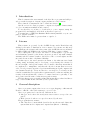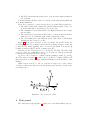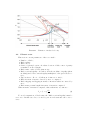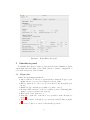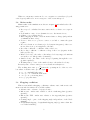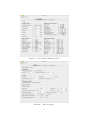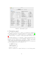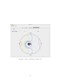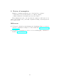
1
GyroRotor program : user manual
Jean Fourcade <[email protected]>
3 octobre 2015
1
1
Introduction
This document is the user manual of the GyroRotor program and will provide you with description of input/output parameters of the software.
The technical documentation can be found in reference [1].
GyroRotor is a free Java program to compute aerodynamic characteristics
of a rotor in uniform translation and rotation.
To use GyroRotor you have to download it to your computer, unzip the
program folder and simply double-click on GyroRotor.jar icon.
You must have a JRE (Java Runtime Environment) installed on your computer to run the software.
The JRE version must be greater than or equal to 7.
2
Licence
This software is governed by the CeCILL license under French law and
abiding by the rules of distribution of free software. You can use, modify and/
or redistribute the software under the terms of the CeCILL license as circulated
by CEA, CNRS and INRIA at the following URL http ://www.cecill.info
As a counterpart to the access to the source code and rights to copy, modify
and redistribute granted by the license, users are provided only with a limited
warranty and the software’s author, the holder of the economic rights, and the
successive licensors have only limited liability.
In this respect, the user’s attention is drawn to the risks associated with
loading, using, modifying and/or developing or reproducing the software by
the user in light of its specific status of free software, that may mean that it
is complicated to manipulate, and that also therefore means that it is reserved for developers and experienced professionals having in-depth computer and
aerodynamic knowledge. Users are therefore encouraged to load and test the
software’s suitability as regards their requirements in conditions enabling the
security of their systems and/or data to be ensured and, more generally, to use
and operate it in the same conditions as regards security.
The fact that you are presently reading this means that you have had knowledge of the CeCILL license and that you accept its terms
3
General discription
Gyrotor program computes the forces, rotor torque, flapping coefficients and
Fourier coefficient of the blade twist up to second order.
Gyrotor program can be used in two different modes :
• Autogyro mode where the steady state autorotative rotor speed is computed ;
• Helicopter mode where rotor speed is entered by the user.
The program has two menus :
• The ”GyroRotor” menu which describes the user license and defines the
system unit used for inputs and outputs data (Metric or British) ;
2
• The ”File” menu that allows the user to read and write input parameters
into text files.
Text files includes all data of the rotor and stores the unit system which was
used during simulation.
There are for panels to operate the GyroRotor program. Theses panels are :
• The ”Data” panel that contains the physical characteristics of the rotor
as well as atmosphere and induced velocity models ;
• The ”Simulation” panel that includes the flight parameters and computation results ;
• The ”Derivatives” panel that includes all rotor characteristics derivative
with respect to no-feathering plane frame and fuselage frame ;
• The ”Aoa distribution” panel that shows the blade angle of attack angle
distribution all over the rotor disc.
~S and X
~ S define the
Figure 1 shows forces and axes of the rotor frame. Y
~
~
no-feathering plane, YS pointing forward and XS pointing sideway to starboard
~ S is pointing upwards. Rotor forces are the thrust T along Z
~S , H
so that Z
~
~
pointing rearward along YS and Y pointing along XS .
~ is supposed to be in the Y
~S , Z
~ S plane. Incidence with
Aircraft velocity U
~ is the rotor lift (perpendicular
respect to plane of no-feathering is denote αS . L
~
to aircraft velocity) and D the rotor drag.
~ F lies to the body-fixed coordinate system pointing forward. Y
~F and Z
~F
X
(not represented on figure 1) complete the body-fixed coordinate system pointing respectively to starboard and downward. Finally αF is the incidence of the
fuselage.
When viewed from above, the rotor blades are supposed to spin counterclockwise so that starboard side is the advancing region and the port side is the
retreating region.
Figure 1 – Forces and rotor axes
4
Data panel
The data panel is shown figure 3. Values are for the Kelett KD-1 autogiro.
3
4.1
Atmosphere
Defines the atmosphere in order to calculate its density. Two model are
available :
• Standard atmosphere : this is the standard U.S. 76 where user have to
enter altitude where the rotor is operated and temperature increment,
the temperature deviation from the standard model.
• Density atmosphere where the user enter directly the value of the air
density.
4.2
Airfoil
Defines the characteristics of the blade airfoil profile.
• Lift curve slope : mean lift curve slope of the blade (derivative of lift
coefficient relative to angle of attack) 1/rad ;
• Profile drag : mean blade drag coefficient ;
• Moment coefficient : blade section moment coefficient ;
• Aerodynamic center location : chordwise location of aerodynamic center
from leading edge normalized on chord length.
The first two parameters must be considered as tuning parameters. By increasing the lift slope coefficient, the rotor thrust increased while the rotor
speed does not change significantly. By increasing the drag profile coefficient,
the rotation speed decreased as well as the amplitude of aerodynamics forces.
4.3
Induced velocity
Choice of rotor induced velocity model. There are two possible choices :
• Momentum theory : momentum theory or disk actuator theory ;
• Shaydakov theory : theory of Shaydakov.
It is preferable in most cases to use the Shaydakov theory (see technical
documentation [1]).
The figure 2 shows the variation of induced velocity and rotor state for the
momentum theory (red curve) and Shaydakov theory (blue curve) for different
values of advance ratio µ. The X axis is λ̄, the axial velocity normalized on
thrust velocity and the Y axis is v̄, the induced velocity normalized on thrust
velocity.
It is mandatory to use the Shaydakov theory when rotor incidence is greater than 30 degrees. Shaydakov theory allows to compute vertical descent in
autorotation where incidence is 90 degrees.
4
Figure 2 – Variation of induced velocity
4.4
Glauert rotor
This section concern parameters of the rotor itself :
• Number of blade ;
• Blade radius ;
• Blade chord ;
• Center of gravity location : chordwise location of blade center of gravity
normalized on chord length ;
• Blade twist : value of blade twist at tip ;
• Blade torsional rigidity : GJ where G is the modulus of rigidity (shear
modulus) and J the torsional rigidity multiplier for the given blade section ;
• Tip loss factor : B = 1 − C/2R most of time set to 0.975 ;
• Blade moment of inertia : entered by user or computed ;
• Blade flapping and lagging moments of inertia if values are entered by
user ;
• Blade mass per unit length if moment of inertia is computed.
When moment of inertia is computed, values taken into account are :
Ib = Ic = ml
R3
3
(1)
To avoid computation of blade twist, the ”Blade torsional rigidity” must be
set to zero. In this case, Cm, xac and xcg are non relevant and can be set to
zeros.
5
Figure 3 – Kelett KD-1 data panel
5
Simulation panel
To simulate the behavior of the rotor the user selects the ”Simulation” panel,
enters flight data and clicks on the ”Run” button to activate computation of
rotor state and get the desired results.
5.1
Flight data
Defines the input flight parameters :
• Autorotative mode : the rotor operates in autorotating mode (gyrocopter
flight) and the rotor speed is computed by the program ;
• Fixed rotation mode : the rotor speed is enter by the user (helicopter
mode) ;
• Flight Velocity : aircraft speed (must be positive or zero) ;
• Incidence NFP : incidence of the rotor relative to the no-feathering plane
(must be between -90 and +90 degrees) ;
• Blade pitch : blade pitch at root ;
~ S axis, see
• Pitch rate : pitch rate of the whole rotor (rotation on the X
figure 1) ;
~S axis, see figure
• Roll rate : roll rate of the whole rotor (rotation on the Y
1) ;
• Rotor speed : has to be entered only in helicopter mode.
6
When rotor is in autorotative mode, a too negative rotor incidence (beyond
a few degrees) will lead to non-convergence of the rotational speed.
5.2
Main results
Main results of the simulation are shown on figure 4 and includes the following parameters :
• Rotor speed : calculated in autorotation mode so that rotor torque is
zero ;
• Lock number : ratio of aerodynamic forces to the inertia forces ;
• Solidity : rotor solidity factor ;
• Blade flapping moment : blade moment relative to hinge (independent
of azimuth at first order) ;
• Power to drive rotor : power to sent to rotor hub to ensure the given
regime ;
• Rotor acceleration : acceleration (or deceleration if negative) of the rotor
in case there is no power supplied to the hub ;
• Rotor lift coefficient : coefficient of lift of the rotor ;
• Rotor drag coefficient : coefficient of drag of the rotor (negative in the
helicopter mode) ;
• Induced velocity : the value of the induced velocity supposed uniform
across the rotor disk (positive downward) ;
• Axial velocity : the value of the air speed passing through the rotor
(positive upward) ;
• Working state η : ratio of the axial velocity to the induced velocity.
In steady state of autorotation, rotor acceleration is always zero.
λ̄
The working state ratio η = defines the operating mode of the rotor for
v̄
low values of advance ratio (see the figure 2) :
• η < −2 : windmill brake state ;
• −2 < η < −1 : turbulent wake state ;
• −1 < η < 0 : vortex ring state ;
• 0 < η : propeller state.
5.3
Flapping coefficient
This section includes flapping coefficients, advance ratio, inflow ratio and
mean torsional deformation at 3/4 blade radius :
• Advance ratio : advance or tip-speed ratio ;
• Inflow ratio : inflow ratio relative to the no-feathering plane (positive
upward) ;
• Inflow ratio TPP : inflow ratio relative to the tip-path plane (positive
upward) ;
• Conning angle : part of the flapping angle independent of the blade
azimuth ;
• Longitudinal flapping : longitudinal flapping angle (positive when the
rotor tilts backward) ;
7
• Lateral flapping : lateral flapping, positive when the rotor tilts on the
advancing blade side ;
• 2nd longitudinal flapping : second order longitudinal flapping coefficient ;
• 2nd lateral flapping : second order lateral flapping coefficient ;
• 3/4 radius torsional deformation : angle of twist at 0.75 R.
5.4
Forces and torque
The last section includes forces and torque :
• Rotor Thrust : general aerodynamic force aligned with the hub axis or
rotor axis (T~ ) ;
• Lateral induced force : lateral force in the no-feathering plane induced
~ );
by the lift and in direction of the advancing blade (Y
• Lateral induced force TPP : the previous lateral force but expressed in
the tip-path plane ;
• Rear drag profile force : rear force in the no-feathering plane due to blade
profile drag ;
• Rear induced force : rear force in the no-feathering plane induced by the
lift.
~ ;
• Rear total force : total rear force in the no-feathering plane (H)
• Rear total force TPP : total rear force in the tip-path plane ;
• Profile drag torque : torque along the rotor hub due to blades profile
drag ;
• Induced torque : torque along the rotor hub induced by the lift ;
• Total torque : total torque ;
• Rotor lift : lift force generated by the rotor (perpendicular to airspeed
vector) ;
• Rotor drag : drag force generated by the rotor (along airspeed vector,
negative in helicopter mode).
In steady state of autorotation, rotor total torque is always zero.
Figure 5 and 6 show an another case of simulation for an R22 helicopter
flying at maximum power.
8
Figure 4 – Kelett KD-1 simulation panel
Figure 5 – R22 data panel
9
Figure 6 – R22 simulation panel
6
Derivatives panel
The derivatives panel allows to compute rotor derivatives for stability purpose. Analytic expression for derivatives formula can be found in reference [2].
These derivatives can be computed with respect to no-feathering coordinate
~ S, Y
~S , Z
~ S ) or body-fixed coordinate system (X
~F, Y
~F , Z
~ F ), see figure
system (X
1.
Derivatives with respect to no-feathering coordinate system includes derivatives of forces L, D, T, Y, H, rotor torque Q, flapping coefficient a0 , a1 , b1 , a2 , b2
and induced velocity vi with respect to u and w the coordinates of the aircraft
velocity, q and p, the pitch and roll rate and Ω the rotor speed.
These derivatives can be computed in dimensional form or non-dimensional
form. In non-dimensional form the scaling factor are :
• ρsAR2 Ω2 for forces ;
• ρsAR3 Ω2 for torque ;
• ΩR for velocity ;
• Ω for angular velocity.
A is the rotor disc area.
Therefore derivatives are computed with respect to the following parame-
10
ters :
û =
ŵ =
λi =
q̂ =
p̂ =
Ω̂ =
u
=µ
RΩ
w
RΩ
vi
RΩ
q
Ω
p
Ω
Ω
Ω
(2)
(3)
(4)
(5)
(6)
(7)
Derivatives with respect to body-fixed coordinate system includes derivatives of force X, Y, Z, moment L, M, N and rotor torque Q, with respect to u0
and w0 the coordinates of aircraft velocity, q and p0 , the pitch and roll rate and
Ω the rotor speed.
Theses derivatives, to be computed, require to enter the fuselage incidence
and the rotor hub coordinates expressed in the body-fixed coordinate.
Theses derivatives can be calculated in normalized or non-normalized form.
In normalized form the following factor are applied :
1
• on forces :
where m is the gross mass of the aircraft ;
m
1
• on moment : , where I is the body moment of inertia Ixx for L, Iyy for
I
M , Izz for N ;
1
• on rotor torque :
where IR is the rotor moment of inertia.
IR
Theses values have to be entered by the user. Once all parameters are entered
the user have to click on the ”Run” button to compute rotor derivatives.
7
Aoa distribution
The last panel is the blade angle of attack distribution panel. The user can
enter seven values of angle of attack to show the distribution. Le right side of
the chart (from 0 to 180 degrees azimuth) is the advancing region and the left
side (from 270 to 360 degrees azimuth) is the retreating region.
Figure 7 is the aoa distribution of the R22 helicopter rotor disc for the data
and flight parameters of figure 5 and 6.
11
Figure 7 – R22 aoa distribution at full power
12
8
Review of assumption
Mainly two assumptions limit the use of the GyroRotor software :
• The induced velocity through the rotor disk is constant ;
• Blade stall in the retreating region is not modelized.
These limitations leads to the fact that the results are valid only for low
values of the advance ratio µ and that computation during vortex ring state is
not accurate at all.
Références
[1] J. Fourcade : Calcul des caractéristiques aérodynamiques d’un rotor en mouvement de translation rectiligne et rotation uniformes ; www.volucres.fr ;
<download>
[2] J. Fourcade : Computation of the rotor forces and flapping coefficients derivatives ; www.volucres.fr.
13