Download LaTeX - Mathematical & Computer Sciences

LaTeX
by Wikibooks contributors
Created on Wikibooks,
the open content textbooks collection.
c 2005–2008 Wikibooks contributors.
Copyright Permission is granted to copy, distribute and/or modify this document under the terms
of the GNU Free Documentation License, Version 1.2 or any later version published by
the Free Software Foundation; with no Invariant Sections, no Front-Cover Texts, and
no Back-Cover Texts. A copy of the license is included in the section entitled “GNU
Free Documentation License”.
Contents
1 Introduction
9
2 Absolute Beginners
15
The LaTeX source . . . . . . . . . . . . . . . . . . . . . . . . . . . . . . . . . 15
Our first document . . . . . . . . . . . . . . . . . . . . . . . . . . . . . . . . . 18
3 Basics
21
4 Document Structure
27
The document environment . . . . . . . . . . . . . . . . . . . . . . . . . . . . 27
5 Errors and Warnings
Error messages . . . . . . . . . . . . . . . . . . . . . . . . . . . . . . . . . . .
Warnings . . . . . . . . . . . . . . . . . . . . . . . . . . . . . . . . . . . . . .
Examples . . . . . . . . . . . . . . . . . . . . . . . . . . . . . . . . . . . . . .
35
35
35
36
6 Title Creation
39
Create the title . . . . . . . . . . . . . . . . . . . . . . . . . . . . . . . . . . . 39
A practical example . . . . . . . . . . . . . . . . . . . . . . . . . . . . . . . . 41
Insert it in your document . . . . . . . . . . . . . . . . . . . . . . . . . . . . . 44
7 Bibliography Management
Embed system . . . . . . . . .
Citations . . . . . . . . . . . .
BibTeX . . . . . . . . . . . . .
Natbib . . . . . . . . . . . . . .
.
.
.
.
.
.
.
.
.
.
.
.
.
.
.
.
.
.
.
.
.
.
.
.
.
.
.
.
.
.
.
.
.
.
.
.
.
.
.
.
.
.
.
.
.
.
.
.
.
.
.
.
.
.
.
.
45
45
46
47
57
8 Tables
The tabular environment . . . . . . . . . . . . . . . .
The table environment — captioning etc . . . . . . .
The tabular* environment — controlling table width
The tabularx package — simple column stretching . .
Vertically centered images . . . . . . . . . . . . . . . .
Professional tables . . . . . . . . . . . . . . . . . . . .
Need more complicated features? . . . . . . . . . . . .
.
.
.
.
.
.
.
.
.
.
.
.
.
.
.
.
.
.
.
.
.
.
.
.
.
.
.
.
.
.
.
.
.
.
.
.
.
.
.
.
.
.
.
.
.
.
.
.
.
.
.
.
.
.
.
.
.
.
.
.
.
.
.
.
.
.
.
.
.
.
.
.
.
.
.
.
.
.
.
.
.
.
.
.
.
.
.
.
.
.
.
59
59
69
70
71
72
72
73
.
.
.
.
.
.
.
.
.
.
.
.
.
.
.
.
.
.
.
.
3
.
.
.
.
.
.
.
.
.
.
.
.
.
.
.
.
.
.
.
.
.
.
.
.
.
.
.
.
Summary . . . . . . . . . . . . . . . . . . . . . . . . . . . . . . . . . . . . . . 74
9 Importing Graphics
75
The graphicx package . . . . . . . . . . . . . . . . . . . . . . . . . . . . . . . 75
Xfig . . . . . . . . . . . . . . . . . . . . . . . . . . . . . . . . . . . . . . . . . 81
10 Floats, Figures and Captions
83
Floats . . . . . . . . . . . . . . . . . . . . . . . . . . . . . . . . . . . . . . . . 83
Captions . . . . . . . . . . . . . . . . . . . . . . . . . . . . . . . . . . . . . . . 85
11 Formatting
Text formatting . . . .
Paragraph Formatting
Special Paragraphs . .
List Structures . . . .
Footnotes . . . . . . .
Margin Notes . . . . .
Summary . . . . . . .
.
.
.
.
.
.
.
.
.
.
.
.
.
.
.
.
.
.
.
.
.
.
.
.
.
.
.
.
.
.
.
.
.
.
.
.
.
.
.
.
.
.
.
.
.
.
.
.
.
.
.
.
.
.
.
.
.
.
.
.
.
.
.
.
.
.
.
.
.
.
.
.
.
.
.
.
.
.
.
.
.
.
.
.
.
.
.
.
.
.
.
.
.
.
.
.
.
.
.
.
.
.
.
.
.
.
.
.
.
.
.
.
.
.
.
.
.
.
.
.
.
.
.
.
.
.
.
.
.
.
.
.
.
.
.
.
.
.
.
.
.
.
.
.
.
.
.
.
.
.
.
.
.
.
.
.
.
.
.
.
.
.
.
.
.
.
.
.
.
.
.
.
.
.
.
.
.
.
.
.
.
.
.
.
.
.
.
.
.
.
.
.
.
.
.
.
.
.
.
.
.
.
.
.
.
.
.
.
.
.
95
95
105
106
109
114
114
114
12 Page Layout
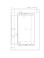
Page Dimensions . . . . .
Page Orientation . . . . .
Page Styles . . . . . . . .
Multi-column Pages . . .
Manual Page Formatting
Summary . . . . . . . . .
.
.
.
.
.
.
.
.
.
.
.
.
.
.
.
.
.
.
.
.
.
.
.
.
.
.
.
.
.
.
.
.
.
.
.
.
.
.
.
.
.
.
.
.
.
.
.
.
.
.
.
.
.
.
.
.
.
.
.
.
.
.
.
.
.
.
.
.
.
.
.
.
.
.
.
.
.
.
.
.
.
.
.
.
.
.
.
.
.
.
.
.
.
.
.
.
.
.
.
.
.
.
.
.
.
.
.
.
.
.
.
.
.
.
.
.
.
.
.
.
.
.
.
.
.
.
.
.
.
.
.
.
.
.
.
.
.
.
.
.
.
.
.
.
.
.
.
.
.
.
.
.
.
.
.
.
.
.
.
.
.
.
.
.
.
.
.
.
.
.
.
.
.
.
117
117
120
121
126
127
127
13 Mathematics
Basic Mathematics: plain LaTeX . . . . . . .
Advanced Mathematics: AMS Math package
List of Mathematical Symbols . . . . . . . . .
Notes . . . . . . . . . . . . . . . . . . . . . .
Further reading . . . . . . . . . . . . . . . . .
External links . . . . . . . . . . . . . . . . . .
.
.
.
.
.
.
.
.
.
.
.
.
.
.
.
.
.
.
.
.
.
.
.
.
.
.
.
.
.
.
.
.
.
.
.
.
.
.
.
.
.
.
.
.
.
.
.
.
.
.
.
.
.
.
.
.
.
.
.
.
.
.
.
.
.
.
.
.
.
.
.
.
.
.
.
.
.
.
.
.
.
.
.
.
.
.
.
.
.
.
.
.
.
.
.
.
.
.
.
.
.
.
.
.
.
.
.
.
129
129
140
149
151
151
151
14 Theorems
Basic theorems . .
Theorem counters
Proofs . . . . . . .
Theorem styles . .
External links . . .
.
.
.
.
.
.
.
.
.
.
.
.
.
.
.
.
.
.
.
.
.
.
.
.
.
.
.
.
.
.
.
.
.
.
.
.
.
.
.
.
.
.
.
.
.
.
.
.
.
.
.
.
.
.
.
.
.
.
.
.
.
.
.
.
.
.
.
.
.
.
.
.
.
.
.
.
.
.
.
.
.
.
.
.
.
.
.
.
.
.
.
.
.
.
.
153
153
153
154
154
155
15 Labels and Cross-referencing
Examples . . . . . . . . . . . . . . . . . . . .
The varioref package . . . . . . . . . . . . .
The hyperref package and \autoref{} . . .
The hyperref package and \phantomsection
.
.
.
.
.
.
.
.
.
.
.
.
.
.
.
.
.
.
.
.
.
.
.
.
.
.
.
.
.
.
.
.
.
.
.
.
.
.
.
.
.
.
.
.
.
.
.
.
.
.
.
.
.
.
.
.
.
.
.
.
.
.
.
.
.
.
.
.
.
.
.
.
157
158
161
161
162
.
.
.
.
.
.
.
.
.
.
.
.
.
.
.
.
.
.
.
.
.
.
.
.
.
.
.
.
.
.
.
.
.
.
.
.
.
.
.
.
.
.
.
.
.
.
.
.
.
.
.
.
.
.
.
.
.
.
.
.
.
.
.
.
.
.
.
4
.
.
.
.
.
.
.
.
.
.
16 Indexing
163
Abbreviation list . . . . . . . . . . . . . . . . . . . . . . . . . . . . . . . . . . 164
Multiple indexes . . . . . . . . . . . . . . . . . . . . . . . . . . . . . . . . . . 165
17 Algorithms and Pseudocode
Typesetting using the algorithmic package
The algorithm environment . . . . . . . .
An example from the manual . . . . . . . .
Code formating using the Listings package
.
.
.
.
.
.
.
.
.
.
.
.
.
.
.
.
.
.
.
.
.
.
.
.
.
.
.
.
.
.
.
.
.
.
.
.
.
.
.
.
.
.
.
.
.
.
.
.
.
.
.
.
.
.
.
.
.
.
.
.
.
.
.
.
.
.
.
.
.
.
.
.
18 Letters
The letter class . . . . . . . . . . . . . . . . . . . . . . . . . . . . . . . . .
Envelopes . . . . . . . . . . . . . . . . . . . . . . . . . . . . . . . . . . . . .
Sources . . . . . . . . . . . . . . . . . . . . . . . . . . . . . . . . . . . . . .
.
.
.
.
167
167
169
170
171
173
. 173
. 175
. 177
19 Packages
179
Using an existing package . . . . . . . . . . . . . . . . . . . . . . . . . . . . . 179
Package documentation . . . . . . . . . . . . . . . . . . . . . . . . . . . . . . 180
Packages list . . . . . . . . . . . . . . . . . . . . . . . . . . . . . . . . . . . . 181
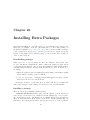
20 Installing Extra Packages
185
21 Color package
189
22 Hyperref package
Usage . . . . . . . . . . . . . . .
Customization . . . . . . . . . .
Problems with Links . . . . . . .
Problems with Bookmarks . . . .
Problems with tables and figures
.
.
.
.
.
.
.
.
.
.
.
.
.
.
.
.
.
.
.
.
.
.
.
.
.
.
.
.
.
.
.
.
.
.
.
.
.
.
.
.
.
.
.
.
.
.
.
.
.
.
.
.
.
.
.
.
.
.
.
.
.
.
.
.
.
.
.
.
.
.
.
.
.
.
.
.
.
.
.
.
.
.
.
.
.
.
.
.
.
.
.
.
.
.
.
.
.
.
.
.
.
.
.
.
.
.
.
.
.
.
.
.
.
.
.
.
.
.
.
.
.
.
.
.
.
191
191
192
194
195
196
23 Listings package
197
24 Rotating package
201
25 Beamer package: make your presentations in LaTeX
203
26 Xy-Pic package: create diagrams
205
A simple diagram . . . . . . . . . . . . . . . . . . . . . . . . . . . . . . . . . . 205
References . . . . . . . . . . . . . . . . . . . . . . . . . . . . . . . . . . . . . . 205
27 Producing Mathematical Graphics
Overview . . . . . . . . . . . . . . . . .
The picture Environment . . . . . . . .
XY-pic . . . . . . . . . . . . . . . . . . .
Alternatives . . . . . . . . . . . . . . . .
5
.
.
.
.
.
.
.
.
.
.
.
.
.
.
.
.
.
.
.
.
.
.
.
.
.
.
.
.
.
.
.
.
.
.
.
.
.
.
.
.
.
.
.
.
.
.
.
.
.
.
.
.
.
.
.
.
.
.
.
.
.
.
.
.
.
.
.
.
.
.
.
.
.
.
.
.
.
.
.
.
.
.
.
.
207
207
208
218
222
28 Advanced Topics
223
Using \includeonly . . . . . . . . . . . . . . . . . . . . . . . . . . . . . . . . . 226
Boxes . . . . . . . . . . . . . . . . . . . . . . . . . . . . . . . . . . . . . . . . 226
Rules and Struts . . . . . . . . . . . . . . . . . . . . . . . . . . . . . . . . . . 228
29 Fonts
229
Useful example . . . . . . . . . . . . . . . . . . . . . . . . . . . . . . . . . . . 229
XeTeX . . . . . . . . . . . . . . . . . . . . . . . . . . . . . . . . . . . . . . . . 230
Some useful websites . . . . . . . . . . . . . . . . . . . . . . . . . . . . . . . . 230
30 Customizing LaTeX
New commands . . . . .
New Environments . . .
Extra space . . . . . . .
Command-line LaTeX .
Creating your own style
Spacing . . . . . . . . .
.
.
.
.
.
.
.
.
.
.
.
.
.
.
.
.
.
.
.
.
.
.
.
.
.
.
.
.
.
.
.
.
.
.
.
.
.
.
.
.
.
.
.
.
.
.
.
.
.
.
.
.
.
.
.
.
.
.
.
.
.
.
.
.
.
.
.
.
.
.
.
.
.
.
.
.
.
.
.
.
.
.
.
.
.
.
.
.
.
.
.
.
.
.
.
.
231
231
232
233
234
235
235
31 Collaborative Writing of LaTeX Documents
Abstract . . . . . . . . . . . . . . . . . . . . . . . .
Introduction . . . . . . . . . . . . . . . . . . . . . .
Interchanging Documents . . . . . . . . . . . . . .
The Version Control System Subversion . . . . . .
Hosting LaTeX files in Subversion . . . . . . . . .
Subversion really makes the diff erence . . . . . . .
Managing collaborative bibliographies . . . . . . .
Conclusion . . . . . . . . . . . . . . . . . . . . . .
Acknowledgements . . . . . . . . . . . . . . . . . .
References . . . . . . . . . . . . . . . . . . . . . . .
Other Methods . . . . . . . . . . . . . . . . . . . .
.
.
.
.
.
.
.
.
.
.
.
.
.
.
.
.
.
.
.
.
.
.
.
.
.
.
.
.
.
.
.
.
.
.
.
.
.
.
.
.
.
.
.
.
.
.
.
.
.
.
.
.
.
.
.
.
.
.
.
.
.
.
.
.
.
.
.
.
.
.
.
.
.
.
.
.
.
.
.
.
.
.
.
.
.
.
.
.
.
.
.
.
.
.
.
.
.
.
.
.
.
.
.
.
.
.
.
.
.
.
.
.
.
.
.
.
.
.
.
.
.
.
.
.
.
.
.
.
.
.
.
.
.
.
.
.
.
.
.
.
.
.
.
.
.
.
.
.
.
.
.
.
.
.
.
.
.
.
.
.
.
.
.
.
.
237
237
237
238
238
239
241
243
246
246
247
247
32 Tips and Tricks
Add the Bibliography to the Table of Contents . .
id est & exempli gratia (i.e. & e.g.) . . . . . . . . .
Referencing Figures or Equations . . . . . . . . . .
Grouping Figure/Equation Numbering by Section
New Square Root . . . . . . . . . . . . . . . . . . .
A new oiint command . . . . . . . . . . . . . . . .
Generic header . . . . . . . . . . . . . . . . . . . .
Using graphs from gnuplot . . . . . . . . . . . . . .
.
.
.
.
.
.
.
.
.
.
.
.
.
.
.
.
.
.
.
.
.
.
.
.
.
.
.
.
.
.
.
.
.
.
.
.
.
.
.
.
.
.
.
.
.
.
.
.
.
.
.
.
.
.
.
.
.
.
.
.
.
.
.
.
.
.
.
.
.
.
.
.
.
.
.
.
.
.
.
.
.
.
.
.
.
.
.
.
.
.
.
.
.
.
.
.
.
.
.
.
.
.
.
.
.
.
.
.
.
.
.
.
.
.
.
.
.
.
.
.
249
249
250
250
250
251
251
252
253
33 General Guidelines
Project structure . . . . . . . . . .
The file mystyle.sty . . . . . . .
The main document document.tex
Writing your document . . . . . .
.
.
.
.
.
.
.
.
.
.
.
.
.
.
.
.
.
.
.
.
.
.
.
.
.
.
.
.
.
.
.
.
.
.
.
.
.
.
.
.
.
.
.
.
.
.
.
.
.
.
.
.
.
.
.
.
.
.
.
.
257
257
258
258
260
.
.
.
.
.
.
.
.
.
.
.
.
.
.
.
.
.
.
.
.
.
.
.
.
.
.
.
.
.
.
.
.
.
.
.
.
.
.
.
.
.
.
.
.
.
.
.
.
.
.
.
.
.
.
.
.
.
.
.
.
.
.
.
.
.
.
6
.
.
.
.
.
.
.
.
.
.
.
.
.
.
.
.
.
.
.
.
.
.
.
.
.
.
.
.
.
.
.
.
.
.
.
.
.
.
.
.
.
.
.
.
.
.
.
.
.
.
.
.
.
.
34 Export To Other Formats
Convert to PDF . . . . . . .
Convert to PostScript . . . .
Convert to RTF . . . . . . .
Conversion to HTML . . . . .
Conversion to image formats
.
.
.
.
.
.
.
.
.
.
.
.
.
.
.
.
.
.
.
.
.
.
.
.
.
.
.
.
.
.
.
.
.
.
.
.
.
.
.
.
.
.
.
.
.
.
.
.
.
.
.
.
.
.
.
.
.
.
.
.
.
.
.
.
.
.
.
.
.
.
.
.
.
.
.
.
.
.
.
.
.
.
.
.
.
.
.
.
.
.
.
.
.
.
.
.
.
.
.
.
.
.
.
.
.
.
.
.
.
.
.
.
.
.
.
.
.
.
.
.
.
.
.
.
.
.
.
.
.
.
.
.
.
.
.
261
261
262
263
263
263
35 Internationalization
Arabic script . . . . .
Cyrillic script . . . . .
Czech . . . . . . . . .
French . . . . . . . . .
German . . . . . . . .
Greek . . . . . . . . .
Hungarian . . . . . . .
Italian . . . . . . . . .
Korean . . . . . . . .
Polish . . . . . . . . .
Portuguese . . . . . .
Spanish . . . . . . . .
.
.
.
.
.
.
.
.
.
.
.
.
.
.
.
.
.
.
.
.
.
.
.
.
.
.
.
.
.
.
.
.
.
.
.
.
.
.
.
.
.
.
.
.
.
.
.
.
.
.
.
.
.
.
.
.
.
.
.
.
.
.
.
.
.
.
.
.
.
.
.
.
.
.
.
.
.
.
.
.
.
.
.
.
.
.
.
.
.
.
.
.
.
.
.
.
.
.
.
.
.
.
.
.
.
.
.
.
.
.
.
.
.
.
.
.
.
.
.
.
.
.
.
.
.
.
.
.
.
.
.
.
.
.
.
.
.
.
.
.
.
.
.
.
.
.
.
.
.
.
.
.
.
.
.
.
.
.
.
.
.
.
.
.
.
.
.
.
.
.
.
.
.
.
.
.
.
.
.
.
.
.
.
.
.
.
.
.
.
.
.
.
.
.
.
.
.
.
.
.
.
.
.
.
.
.
.
.
.
.
.
.
.
.
.
.
.
.
.
.
.
.
.
.
.
.
.
.
.
.
.
.
.
.
.
.
.
.
.
.
.
.
.
.
.
.
.
.
.
.
.
.
.
.
.
.
.
.
.
.
.
.
.
.
.
.
.
.
.
.
.
.
.
.
.
.
.
.
.
.
.
.
.
.
.
.
.
.
.
.
.
.
.
.
.
.
.
.
.
.
.
.
.
.
.
.
.
.
.
.
.
.
.
.
.
.
.
.
.
.
.
.
.
.
265
267
267
267
267
268
269
269
270
270
272
272
272
.
.
.
.
.
.
.
.
.
.
.
.
.
.
.
.
.
.
.
.
.
.
.
.
.
.
.
.
.
.
.
.
.
.
.
.
.
.
.
.
.
.
.
.
.
.
.
.
36 Links
275
37 Authors
279
Included books . . . . . . . . . . . . . . . . . . . . . . . . . . . . . . . . . . . 279
Wiki users . . . . . . . . . . . . . . . . . . . . . . . . . . . . . . . . . . . . . . 280
A Installation
TeX and LaTeX . . . . .
Editors . . . . . . . . . .
Bibliography management
Graphics tools . . . . . .
See also . . . . . . . . . .
.
.
.
.
.
.
.
.
.
.
.
.
.
.
.
.
.
.
.
.
.
.
.
.
.
.
.
.
.
.
.
.
.
.
.
.
.
.
.
.
.
.
.
.
.
.
.
.
.
.
.
.
.
.
.
.
.
.
.
.
.
.
.
.
.
.
.
.
.
.
.
.
.
.
.
.
.
.
.
.
.
.
.
.
.
.
.
.
.
.
.
.
.
.
.
.
.
.
.
.
.
.
.
.
.
.
.
.
.
.
.
.
.
.
.
.
.
.
.
.
.
.
.
.
.
.
.
.
.
.
281
281
282
282
283
283
B Useful Measurement Macros
Units . . . . . . . . . . . . . . . .
Length ’macros’ . . . . . . . . . .
Length manipulation macros . .
Samples . . . . . . . . . . . . . .
.
.
.
.
.
.
.
.
.
.
.
.
.
.
.
.
.
.
.
.
.
.
.
.
.
.
.
.
.
.
.
.
.
.
.
.
.
.
.
.
.
.
.
.
.
.
.
.
.
.
.
.
.
.
.
.
.
.
.
.
.
.
.
.
.
.
.
.
.
.
.
.
.
.
.
.
.
.
.
.
.
.
.
.
.
.
.
.
.
.
.
.
.
.
.
.
.
.
.
.
285
285
285
286
286
.
.
.
.
.
.
.
.
.
.
.
.
.
.
.
C Useful Size Commands
287
D Sample LaTeX documents
289
General examples . . . . . . . . . . . . . . . . . . . . . . . . . . . . . . . . . . 289
Semantics of Programming Languages . . . . . . . . . . . . . . . . . . . . . . 289
E Glossary
291
7
F Document Information
History . . . . . . . . . . . . . . . . . . . . . . . . . . . . . . . . . . . . . .
PDF Information & History . . . . . . . . . . . . . . . . . . . . . . . . . . .
Authors . . . . . . . . . . . . . . . . . . . . . . . . . . . . . . . . . . . . . .
G GNU Free Documentation License
8
301
. 301
. 301
. 301
303
Chapter 1
Introduction
What is TeX
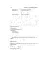
TeX (pronounced “Tech”, with “ch” like in the Scottish “Loch”; see below for details on pronunciation) is a markup language created by Donald Knuth to typeset
documents attractively and consistently. It’s also a Turing-complete programming
language, in the sense that it supports the if-else construct, it can calculate (the calculations are performed while compiling the document), etc., but you would find it
very hard to make anything else but typesetting with it. The fine control TeX offers
makes it very powerful, but also difficult and time-consuming to use. Knuth started
writing the TeX typesetting engine in 1977 to explore the potential of the digital printing equipment that was beginning to infiltrate the publishing industry at that time,
especially in the hope that he could reverse the trend of deteriorating typographical
quality that he saw affecting his own books and articles. TeX as we use it today was
released in 1982, with some slight enhancements added in 1989 to better support 8-bit
characters and multiple languages. TeX is renowned for being extremely stable, for
running on many different kinds of computers, and for being virtually bug free.
The version number of TeX is converging to π and is now at 3.1415926.
Its name originates from the Greek word τ χνoλoγια (technologı̀a, in English technology); its first syllable is τ χ, similar to TeX in the Latin alphabet.1 The name of
the language is thus upper-case τ χ: TEX, and the convention has arisen that the
name is also its own pronunciation when written in the International Phonetic Alphabet. Unfortunately, there is ambiguity among authors as to whether this transcription
is /tex/ or /tx/: the vowel is thus pronounced either as the “ay” of words such as
“way, hay, bay” (former case) or as the “e” of words such as “bet, met, let” (latter
and more frequent case).
What is LaTeX
LaTeX (pronounced either “Lah-tech” /la.tx/ or, less often, “Lay-tech” /le.tx/) is
a macro package based on TeX created by Leslie Lamport. Its purpose is to simplify
1 http://tex.loria.fr/general/texbook.tex
9
10
CHAPTER 1. INTRODUCTION
TeX typesetting, especially for documents containing mathematical formulae. It is
currently maintained by the LaTeX3 project. Many later authors have contributed
extensions, called packages or styles, to LaTeX. Some of these are bundled with most
TeX/LaTeX software distributions; more can be found in the Comprehensive TeX
Archive Network (CTAN).
Since LaTeX comprises a group of TeX commands, LaTeX document processing is
essentially programming. You create a text file in LaTeX markup. The LaTeX macro
reads this to produce the final document.
Clearly this has disadvantages in comparison with a WYSIWYG (What You See
Is What You Get) program such as Openoffice.org Writer or Microsoft Word:
• You can’t see the final result straight away.
• You need to know the necessary commands for LaTeX markup.
• It can sometimes be difficult to obtain a certain ’look’.
On the other hand, there are certain advantages to the markup language approach:
• The layout, fonts, tables and so on are consistent throughout.
• Mathematical formulae can be easily typeset.
• Indices, footnotes and references are generated easily.
• Your documents will be correctly structured.
The LaTeX-like approach can be called WYSIWYM, i.e. What You See Is What
You Mean: you can’t see how the final version will look like while typing. Instead you
see the logical structure of the document. LaTeX takes care of the formatting for you.
The LaTeX document is a plain text file containing the content of the document,
with additional markup. When the source file is processed by the macro package, it
can produce documents in several formats. LaTeX supports natively DVI and PDF,
but using other software you can easily create PostScript, PNG, JPG, etc.
Skills needed
LaTeX is a very easy system to learn, and requires no specialist knowledge, although
literacy and some familiarity with the publishing process is useful. It is, however,
assumed that you are completely fluent and familiar with using your computer before
you start. Specifically, effective use of this document requires that you already know
and understand the following very thoroughly:
• how to use a good plain-text editor (not a wordprocessor like OpenOffice, WordPerfect, or Microsoft Word).
• where to find all 95 of the printable ASCII characters on your keyboard and
what they mean, and how to type accents and symbols, if you use them.
11
• how to create, open, save, close, rename, move, and delete files and folders
(directories).
• how to use a Web browser and/or File Transfer Protocol (FTP) program to
download and save files from the Internet.
• how to uncompress and unwrap (unzip or detar) downloaded files.
If you don’t know how to do these things yet, it’s important to go and learn them
first. Trying to become familiar with the fundamentals of using a computer at the
same time as learning LaTeX is not likely to be as effective as doing them in order.
These are not specialist skills, they are all included in the European Computer Driving
Licence (ECDL) and the relevant sections of the ECDL syllabus are noted in the square
brackets above, so they are well within the capability of anyone who uses a computer.
Prerequisites
At a minimum, you’ll need the following programs to edit LaTeX:
• An editor (You can use a basic text editor like notepad, but a dedicated LaTeX
editor will be more useful).
– On Windows, TeXnicCenter(http://www.texniccenter.org/) is a popular free and open source LaTeX editor.
– On Unix-like (including Mac OS X) systems, Emacsen and gvim provide
powerful TeX enviroments for the tech-savvy, while Texmaker http://www.
xm1math.net/texmaker/index.html and Kile http://kile.sf.net provide more user-friendly development environments.
• The LaTeX binaries and style sheets — e.g. MiKTeX http://www.miktex.org/
for Windows, teTeX http://www.tug.org/teTeX/ for Unix/Linux and teTeX
for Mac OS X http://www.rna.nl/tex.html.
• A DVI viewer to view and print the final result. Usually, a DVI viewer is included
in the editor or is available with the binary distribution.
A distribution of LaTeX, with many packages, add-ins, editors and viewers for Unix,
Linux, Mac and Windows can be obtained from the TeX users group at http://www.tug.org/texlive/.
Applications within a distribution
Here are the main programs you expect to find in any (La)TeX distribution:
• tex: the simplest compiler: generates DVI from TeX source
• pdftex: generates PDF from TeX source
• latex: generates DVI from LaTeX source (the most used one)
• pdflatex: generates PDF from LaTeX source
12
CHAPTER 1. INTRODUCTION
• dvi2ps: converts DVI to PostScript
• dvipdf : converts DVI to PDF
• dvipdfm: an improved version of dvipdf
When LaTeX was created, the only format it could create was DVI; then the PDF
support was added by pdflatex, even if several people still don’t use it. As it is clear
from this short list, PDF files can be created with both pdflatex and dvipdfm; some
think that the output of pdflatex is better than the output of dvipdfm. DVI is an old
format, and it does not support hyperlinks for example, while PDF does, so passing
through DVI you will bring all the bad points of that format to PDF.
Strictly speaking, you would write your document slightly differently depending on
the compiler you are using (latex or pdflatex ). But as we will see later, it is possible
to add a sort of abstraction layer, to hide the details of which compiler you’re using,
and the compiler will handle the translation itself.
Note that, since LaTeX is just a collection of macros for TeX, if you compile a
plain TeX document with a LaTeX compiler (such as pdflatex ) it will work, while the
opposite is not true: if you try to compile a LaTeX source with a TeX compiler you
will get only a lot of errors.
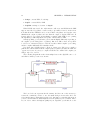
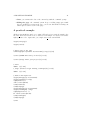
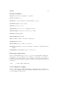
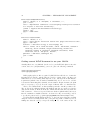
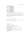
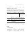
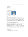
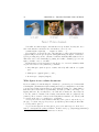
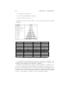
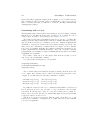
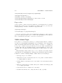
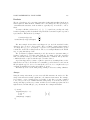
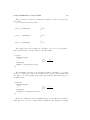
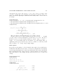
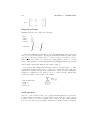
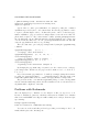
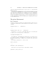
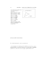
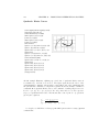
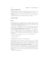
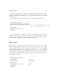
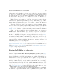
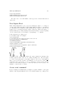
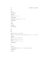
The following diagram shows the relationships between the (La)TeX source code
and all the formats you can create from it:
The boxed red text represents the file formats, the blue text on the arrows represents the commands you have to use, the small dark green text under the boxes
represents the image formats that are supported. Any time you pass through an arrow
you lose some information, which might decrease the quality of your document. Therefore, in order to achieve the highest quality in your output file, you should choose the
13
shortest route to reach your target format. This is probably the most convenient way
to obtain an output in your desired format anyway. Starting from a LaTeX source, the
best way is to use only latex for a DVI output or pdflatex for a PDF output, converting
to PostScript only when it is necessary to print the document.
Most of the programs should be already within your LaTeX distribution; the others
come with Ghostscript, which is a free and multi-platform software as well.
14
CHAPTER 1. INTRODUCTION
Chapter 2
Absolute Beginners
This tutorial is aimed at getting familiar with the bare bones of LaTeX. First, ensure
that you have LaTeX installed on your computer (see Installation for instructions of
what you will need). We will begin with creating the actual source LaTeX file, and
then take you through how to feed this through the LaTeX system to produce quality
output, such as postscript or PDF.
The LaTeX source
The first thing you need to be aware of is that LaTeX uses a markup language in order
to describe document structure and presentation. What LaTeX does is to convert
your source text, combined with the markup, into a high quality document. For the
purpose of analogy, web pages work in a similar way: the HTML is used to describe
the document, but it is your browser that presents it in its full glory — with different
colours, fonts, sizes, etc.
The input for LaTeX is a plain ASCII text file. You can create it with any text
editor. It contains the text of the document, as well as the commands that tell LaTeX
how to typeset the text.
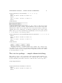
For the truly impatient, a minimal example looks something like the following (the
commands will be explained later):
\documentclass{article}
\begin{document}
Hello world!
\end{document}
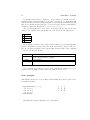
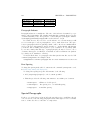
Spaces
“Whitespace” characters, such as blank or tab, are treated uniformly as “space” by
LaTeX. Several consecutive whitespace characters are treated as one “space”. Whitespace at the start of a line is generally ignored, and a single line break is treated as
15
16
CHAPTER 2. ABSOLUTE BEGINNERS
“whitespace.” An empty line between two lines of text defines the end of a paragraph.
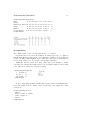
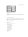
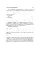
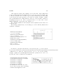
Several empty lines are treated the same as one empty line. The text below is an
example. On the left hand side is the text from the input file, and on the right hand
side is the formatted output.
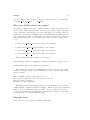
It does not matter whether you
enter one or several
after a word.
It does not matter whether you
enter one or several spaces after
spaces a word.
An empty line starts a new paragraph.
An empty line starts a new
paragraph.
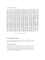
Special Characters
The following symbols are reserved characters that either have a special meaning under
LaTeX or are unavailable in all the fonts. If you enter them directly in your text, they
will normally not print, but rather make LaTeX do things you did not intend.
# $ % ^ & _ { } ~ \
As you will see, these characters can be used in your documents all the same by
adding a prefix backslash:
\# \$ \% \^{} \& \_ \{ \} \textbackslash
The other symbols and many more can be printed with special commands in mathematical formulae or as accents. The backslash character \ can not be entered by
adding another backslash in front of it (\\); this sequence is used for line breaking.
For introducing a backslash in math mode, you can use \backslash instead.
If you want to insert text that might contain several particular symbols (such as
URIs), you can consider using the \verb command, that will be discussed later in this
book.
LaTeX Commands
LaTeX commands are case sensitive, and take one of the following two formats:
• They start with a backslash \ and then have a name consisting of letters only.
Command names are terminated by a space, a number or any other “non-letter”.
• They consist of a backslash \ and exactly one non-letter.
Some commands need a parameter, which has to be given between curly braces
{ } after the command name. Some commands support optional parameters, which
are added after the command name in square brackets [ ]. The general syntax is:
\commandname[option1,option2,...]{argument1}{argument2}...
THE LATEX SOURCE
17
LaTeX environments
Environments in LaTeX have a role that is quite similar to commands, but they usually
have effect on a wider part of the document. Their syntax is:
\begin{environmentname}
text to be influenced
\end{environmentname}
between the \begin and the \end you can put other commands and nested environments. In general, environments can accept arguments as well, but this feature is not
commonly used and so it will be discussed in more advanced parts of the document.
Anything in LaTeX can be expressed in terms of commands and environments.
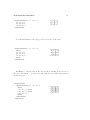
Comments
When LaTeX encounters a % character while processing an input file, it ignores the
rest of the present line, the line break, and all whitespace at the beginning of the next
line.
This can be used to write notes into the input file, which will not show up in the
printed version.
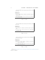
This is an % stupid
% Better: instructive <---example: Supercal%
ifragilist%
icexpialidocious
This is an example: Supercalifragilisticexpialidocious
The % character can also be used to split long input lines where no whitespace or
line breaks are allowed.
Input File Structure
When LaTeX processes an input file, it expects it to follow a certain structure. Thus
every input file must start with the command
\documentclass{...}
This specifies what sort of document you intend to write. After that, you can
include commands that influence the style of the whole document, or you can load
packages that add new features to the LaTeX system. To load such a package you use
the command
\usepackage{...}
When all the setup work is done, you start the body of the text with the command
\begin{document}
Now you enter the text mixed with some useful LaTeX commands. At the end of
the document you add the
18
CHAPTER 2. ABSOLUTE BEGINNERS
\end{document}
command, which tells LaTeX to call it a day. Anything that follows this command
will be ignored by LaTeX. The area between \documentclass and \begin{document}
is called the preamble.
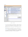
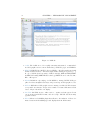
A Typical Command Line Session
LaTeX itself does not have a GUI (graphical user interface), since it is just a program
that crunches away at your input files, and produces either a DVI or PDF file. Some
LaTeX installations feature a graphical front-end where you can click LaTeX into
compiling your input file. On other systems there might be some typing involved,
so here is how to coax LaTeX into compiling your input file on a text based system.
Please note: this description assumes that a working LaTeX installation already sits
on your computer.
1. Edit/Create your LaTeX input file. This file must be plain ASCII text. On Unix
all the editors will create just that. On Windows you might want to make sure
that you save the file in ASCII or Plain Text format. When picking a name for
your file, make sure it bears a .tex extension.
2. Run LaTeX on your input file. If successful you will end up with a .dvi file. It
may be necessary to run LaTeX several times to get the table of contents and
all internal references right. When your input file has a bug LaTeX will tell you
about it and stop processing your input file.
Type ctrl-D to get back to the command line.
latex foo.tex
Now you may view the DVI file. On Unix with X11 you can type xdvi foo.dvi,
on Windows you can use a program called yap (yet another previewer).
You can run a similar procedure with pdflatex to produce a PDF document from
the original tex source. Similar to above, type the commands:
pdflatex foo.tex
Now you may view the PDF file, foo.pdf.
Our first document
Now we can create our first document. We will produce the absolute bare minimum
that is needed in order to get some output, the well known Hello World! approach
will be suitable here.
• Open your favourite text-editor. If you use vim or emacs, they also have syntax
highlighting that will help to write your files.
• Reproduce the following text in your editor. This is the LaTeX source.
OUR FIRST DOCUMENT
19
% hello.tex - Our first LaTeX example!
\documentclass{article}
\begin{document}
Hello World!
\end{document}
• Save your file as hello.tex.
What does it all mean?
% hello.tex - Our first LaTeX example!
\documentclass{article}
\begin{document}
Hello World!
\end{document}
The first line is a comment. This is because
it begins with the percent symbol (%); when
LaTeX sees this, it simply ignores the rest of
the line. Comments are useful for humans to
annotate parts of the source file. For example,
you could put information about the author
and the date, or whatever you wish.
This line is a command and tells LaTeX to
use the article document class. A document
class file defines the formatting, which in this
case is a generic article format. The handy
thing is that if you want to change the appearance of your document, substitute article
for another class file that exists.
This line is the beginning of the environment
called document; it alerts LaTeX that content
of the document is about to commence. Anything above this command is known generally
to belong in the preamble.
This was the only actual line containing real
content — the text that we wanted displayed
on the page.
The document environment ends here. It tells
LaTeX that the document source is complete,
anything after this line will be ignored.
As we have said before, each of the LaTeX commands begin with a backslash (\).
This is LaTeX’s way of knowing that whenever it sees a backslash, to expect some
commands. Comments are not classed as a command, since all they tell LaTeX is to
ignore the line. Comments never affect the output of the document.
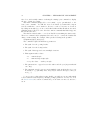
Generating the document
It is clearly not going to be the most exciting document you have ever seen, but we
want to see it nonetheless. I am assuming that you are at a command prompt, already
in the directory where hello.tex is stored.
20
CHAPTER 2. ABSOLUTE BEGINNERS
1. Type the command: latex hello (the .tex extension is not required, although
you can include it if you wish)
2. Various bits of info about LaTeX and its progress will be displayed. If all went
well, the last two lines displayed in the console will be:
Output written on hello.dvi (1 page, 232 bytes).
Transcript written on hello.log.
This means that your source file has been processed and the resulting document is
called hello.dvi, which takes up 1 page and 232 bytes of space. This way you created
the DVI file, but with the same source file you can create a PDF document. The steps
are exactly the same as before, but you have to replace the command latex with
pdflatex:
1. Type the command: pdflatex hello (as before, the .tex extension is not required)
2. Various bits of info about LaTeX and its progress will be displayed. If all went
well, the last two lines displayed in the console will be:
Output written on hello.pdf (1 page, 5548 bytes).
Transcript written on hello.log.
you can notice that the PDF document is bigger than the DVI, even if it contains
exactly the same information. The main differences between the DVI and PDF formats
are:
• DVI needs less disk space and it is faster to create. It does not include the
fonts within the document, so if you want the document to be viewed properly
on another computer, there must be all the necessary fonts installed. It does not
support any interactivity such as hyperlinks or animated images. DVI viewers
are not very common, so you can consider using it for previewing your document
while typesetting.
• PDF needs more disk space and it is slower to create, but it includes all the
necessary fonts within the document, so you will not have any problem of portability. It supports internal and external hyperlinks. Nowadays it is the de facto
standard for sharing and publishing documents, so you can consider using it for
the final version of your document.
About now, you saw you can create both DVI and PDF document from the same
source. This is true, but it gets a bit more complicated if you want to introduce images
or links. This will be explained in detail in the next chapters, about now assume you
can compile in both DVI and PDF without any problem.
Note, in this instance, due to the simplicity of the file, you only need to run the
LaTeX command once. However, if you begin to create complex documents, including
bibliographies and cross-references, etc, LaTeX needs to be executed multiple times to
resolve the references. But this will be discussed in the future when it comes up.
Chapter 3
Basics
Document Classes
The first information LaTeX needs to know when processing an input file is the type
of document the author wants to create. This is specified with the \documentclass
command.
\documentclass[options]{class}
Here class specifies the type of document to be created. The LaTeX distribution
provides additional classes for other documents, including letters and slides. The
options parameter customizes the behavior of the document class. The options have
to be separated by commas.
Example: an input file for a LaTeX document could start with the line
\documentclass[11pt,twoside,a4paper]{article}
which instructs LaTeX to typeset the document as an article with a base font size
of eleven points, and to produce a layout suitable for double sided printing on A4
paper.
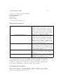
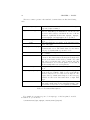
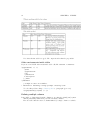
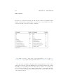
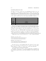
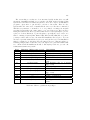
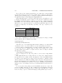
Here are some document classes that can be used with LaTeX:
article
proc
minimal
report
book
slides
memoir
letter
for articles in scientific journals, presentations, short reports, program
documentation, invitations, ...
a class for proceedings based on the article class.
is as small as it can get. It only sets a page size and a base font. It is
mainly used for debugging purposes.
for longer reports containing several chapters, small books, thesis, ...
for real books
for slides. The class uses big sans serif letters.
for changing sensibly the output of the document. It is based on the book
class, but you can create any kind of document with it http://www.
ctan.org/tex-archive/macros/latex/contrib/memoir/memman.pdf
for writing letters.
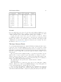
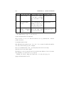
Table 3.1: Document Classes
21
22
CHAPTER 3. BASICS
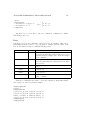
The most common options for the standard document classes are listed in following
table:
10pt, 11pt, 12pt
a4paper, letterpaper,...
fleqn
leqno
titlepage, notitlepage
onecolumn, twocolumn
twoside, oneside
landscape
openright, openany
draft
Sets the size of the main font in the document. If no option
is specified, 10pt is assumed.
Defines the paper size. The default size is letterpaper;
However, many European distributions of TeX now come
pre-set for A4, not Letter, and this is also true of all distributions of pdfLaTeX. Besides that, a5paper, b5paper,
executivepaper, and legalpaper can be specified.
Typesets displayed formulas left-aligned instead of centered.
Places the numbering of formulae on the left hand side instead of the right.
Specifies whether a new page should be started after the
document title or not. The article class does not start a
new page by default, while report and book do.
Instructs LaTeX to typeset the document in one column or
two columns.
Specifies whether double or single sided output should be
generated. The classes article and report are single sided
and the book class is double sided by default. Note that
this option concerns the style of the document only. The
option twoside does not tell the printer you use that it
should actually make a two-sided printout.
Changes the layout of the document to print in landscape
mode.
Makes chapters begin either only on right hand pages or
on the next page available. This does not work with the
article class, as it does not know about chapters. The
report class by default starts chapters on the next page
available and the book class starts them on right hand
pages.
makes LaTeX indicate hyphenation and justification problems with a small square in the right-hand margin of the
problem line so they can be located quickly by a human.
Table 3.2: Document Class Options
For example, if you want a report to be in 12pt type on A4, but printed one-sided
in draft mode, you would use:
\documentclass[12pt,a4paper,oneside,draft]{report}
23
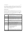
Packages
While writing your document, you will probably find that there are some areas where
basic LaTeX cannot solve your problem. If you want to include graphics, colored text
or source code from a file into your document, you need to enhance the capabilities of
LaTeX. Such enhancements are called packages. Packages are activated with the
\usepackage[options]{package}
command, where package is the name of the package and options is a list of keywords that trigger special features in the package. Some packages come with the
LaTeX base distribution. Others are provided separately.
Modern TeX distributions come with a large number of packages pre-installed. If
you are working on a Unix system, use the command texdoc for accessing package
documentation. For more information, see the Packages section.
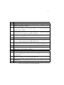
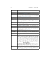
Files You Might Encounter
When you work with LaTeX you will soon find yourself in a maze of files with various
extensions and probably no clue. The following list explains the most common file
types you might encounter when working with TeX:
Big Projects
When working on big documents, you might want to split the input file into several
parts. LaTeX has three commands to insert a file into another when building the
document.
The simplest is the \input command:
\input{filename}
\input inserts the contents of another file, named filename.tex ; note that the .tex
extension is omitted. For all practical purposes, \input is no more than a simple,
automated cut-and-paste of the source code in filename.tex.
The other main inclusion command is \include:
\include{filename}
The \include command is different from </code>\input</code> in that it starts
a new page just before inclusion. Since a new page is started at every \include
command, it is appropriate to use it for large entities such as book chapters.
Very large documents (that usually include many files) take a very long time to
compile, and most users find it convenient to test their last changes by including
only the files they have been working on. One option is to hunt down all \include
commands in the inclusion hierarchy and to comment them out:
%\include{filename1}
\include{filename2}
\include{filename3}
%\include{filename4}
24
CHAPTER 3. BASICS
In this case, the user wants to include only filename2.tex and filename3.tex. If
the inclusion hierarchy is intricate, commenting can become error-prone: it is then
convenient to use the \includeonly command in the preamble:
\includeonly{filename2,filename3}
This way, only \include commands for the specified files will be executed, and
inclusion will be handled in only one place. Note that there must be no spaces between
the filenames and the commas.
Picking suitable filenames
Never, ever use directories (folders) or file names that contain spaces. Although your
operating system probably supports them, some don’t, and they will only cause grief
and tears with TeX. Make filenames as short or as long as you wish, but strictly avoid
spaces. Stick to upper- and lower-case letters without accents (A-Z and a-z), the digits
0-9, the hyphen (-), and the full point or period (.), (similar to the conventions for a
Web URL): it will let you refer to TeX files over the Web more easily and make your
files more portable.
25
.tex
.sty
.dtx
.ins
.cls
.fd
.dvi
.pdf
.log
.toc
.lof
.lot
.aux
.idx
.ind
.ilg
LaTeX or TeX input file. It can be compiled with latex.
LaTeX Macro package. This is a file you can load into your LaTeX document
using the \usepackage command.
Documented TeX. This is the main distribution format for LaTeX style files. If
you process a .dtx file you get documented macro code of the LaTeX package
contained in the .dtx file.
The installer for the files contained in the matching .dtx file. If you download
a LaTeX package from the net, you will normally get a .dtx and a .ins file.
Run LaTeX on the .ins file to unpack the .dtx file.
Class files define what your document looks like. They are selected with the
\documentclass command.
Font description file telling LaTeX about new fonts.
Device Independent File. This is the main result of a LaTeX compile run with
latex. You can look at its content with a DVI previewer program or you can
send it to a printer with dvips or a similar application.
Portable Document Format. This is the main result of a LaTeX compile run
with pdflatex. You can look at its content or print it with any PDF viewer.
Gives a detailed account of what happened during the last compiler run.
Stores all your section headers. It gets read in for the next compiler run and
is used to produce the table of content.
This is like .toc but for the list of figures.
And again the same for the list of tables.
Another file that transports information from one compiler run to the next.
Among other things, the .aux file is used to store information associated with
cross-references.
If your document contains an index. LaTeX stores all the words that go into
the index in this file. Process this file with makeindex.
The processed .idx file, ready for inclusion into your document on the next
compile cycle.
Logfile telling what makeindex did.
Table 3.4: Common file extensions in LaTeX
26
CHAPTER 3. BASICS
Chapter 4
Document Structure
The main point of writing a text is to convey ideas, information, or knowledge to the
reader. The reader will understand the text better if these ideas are well-structured,
and will see and feel this structure much better if the typographical form reflects the
logical and semantical structure of the content.
LaTeX is different from other typesetting systems in that you just have to tell it
the logical and semantical structure of a text. It then derives the typographical form of
the text according to the “rules” given in the document class file and in various style
files. LaTeX allows users to structure their documents with a variety of hierarchal
constructs, including chapters, sections, subsections and paragraphs.
The document environment
After the Document Class Declaration, the text of your document is enclosed between
two commands which identify the beginning and end of the actual document:
\documentclass[11pt,a4paper,oneside]{report}
\begin{document}
...
\end{document}
You would put your text where the dots are. The reason for marking off the
beginning of your text is that LaTeX allows you to insert extra setup specifications
before it (where the blank line is in the example above: we’ll be using this soon).
The reason for marking off the end of your text is to provide a place for LaTeX to be
programmed to do extra stuff automatically at the end of the document, like making
an index.
A useful side-effect of marking the end of the document text is that you can store
comments or temporary text underneath the \end{document} in the knowledge that
LaTeX will never try to typeset them:
27
28
CHAPTER 4. DOCUMENT STRUCTURE
...
\end{document}
Don’t forget to get the extra chapter from Jim!
Preamble
The preamble is everything from the start of the Latex source file until the \begin{document}
command. It normally contains commands that affect the entire document.
% simple.tex - A simple article to illustrate document structure.
\documentclass{article}
\usepackage{mathptmx}
\begin{document}
The first line is a comment (as denoted by the % sign). The \documentclass
command takes an argument, which in this case is article, because that’s the type
of document we want to produce. It is also possible to create your own, as is often
done by journal publishers, who simply provide you with their own class file, which
tells Latex how to format your content. But we’ll be happy with the standard article
class for now! \usepackage is an important command that tells Latex to utilize some
external macros. In this instance, I specified mathptmx which means Latex will use
the Postscript Times type 1 font instead of the default ComputerModern font. And
finally, the \begin{document}. This strictly isn’t part of the preamble, but I’ll put
it here anyway, as it implies the end of the preamble by nature of stating that the
document is now starting.
Top Matter
At the beginning of most documents there will be information about the document
itself, such as the title and date, and also information about the authors, such as
name, address, email etc. All of this type of information within Latex is collectively
referred to as top matter. Although never explicitly specified (there is no \topmatter
command) you are likely to encounter the term within Latex documentation.
A simple example:
\documentclass[11pt,a4paper,oneside]{report}
\begin{document}
\title{How to Structure a LaTeX Document}
\author{Andrew Roberts}
\date{December 2004}
\maketitle
\end{document}
THE DOCUMENT ENVIRONMENT
29
The \title, \author, and \date commands are self-explanatory. You put the
title, author name, and date in curly braces after the relevant command. The title
and author are usually compulsory (at least if you want LaTeX to write the title
automatically); if you omit the \date command, LaTeX uses today’s date by default.
You always finish the top matter with the \maketitle command, which tells LATEX
that it’s complete and it can typeset the title according to the information you have
provided and the class (style) you are using. If you omit \maketitle, the titling will
never be typeset (unless you write your own).
Here is a more complicated example:
\title{How to Structure a \LaTeX{} Document}
\author{Andrew Roberts\\
School of Computing,\\
University of Leeds,\\
Leeds,\\
United Kingdom,\\
LS2 1HE\\
\texttt{[email protected]}}
\date{\today}
\maketitle
as you can see, you can use commands as arguments of \title and the others. The
double backslash (\\) is the LaTeX command for forced linebreak. LaTeX normally
decides by itself where to break lines, and it’s usually right, but sometimes you need
to cut a line short, like here, and start a new one.
If there are two authors separate them with the \and command.
\title{Our Fun Document}
\author{John Doe \and Jane Doe}
\date{\today}
\maketitle
If you are provided with a class file from a publisher, or if you use the AMS
article class (amsart), then you can use several different commands to enter author
information. The email address is at the end, and the \texttt commands formats
the email address using a mono-spaced font. The built-in command called \today will
be replaced with the current date when processed by LaTeX. But you are free to put
whatever you want as a date, in no set order. If braces are left empty, then the date
is omitted.
Using this approach, you can create only basic output whose layout is very hard
to change. If you want to create your title freely, see the Title Creation section.
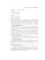
Abstract
As most research papers have an abstract, there are predefined commands for telling
LaTeX which part of the content makes up the abstract. This should appear in its
logical order, therefore, after the top matter, but before the main sections of the body.
This command is available for the document class article and report, but not book.
30
CHAPTER 4. DOCUMENT STRUCTURE
\documentclass{article}
\begin{document}
\begin{abstract}
Your abstract goes here...
...
\end{abstract}
...
\end{document}
By default, LaTeX will use the word “Abstract” as a title for your abstract, if you
want to change it into anything else, e.g. “Executive Summary”, add the following
line in the preamble:
\renewcommand{\abstractname}{Executive Summary}
Sectioning Commands
The commands for inserting sections are fairly intuitive. Of course, certain commands
are appropriate to different document classes. For example, a book has chapters but
an article doesn’t. Here is an edited version of some of the structure commands in use
from simple.tex.
\section{Introduction}
This section’s content...
\section{Structure}
This section’s content...
\subsection{Top Matter}
This subsection’s content...
\subsubsection{Article Information}
This subsubsection’s content...
As you can see, the commands are fairly intuitive. Notice that you do not need to
specify section numbers. LaTeX will sort that out for you! Also, for sections, you do
not need to markup which content belongs to a given block, using \begin and \end
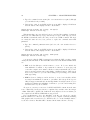
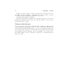
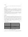
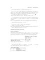
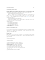
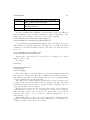
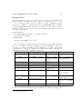
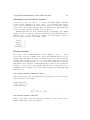
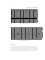
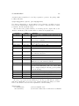
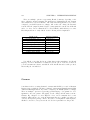
commands, for example. LaTeX provides 7 levels of depth for defining sections:
All the titles of the sections are added automatically to the table of contents (if
you decide to insert one). But if you make manual styling changes to your heading,
for example a very long title, or some special line-breaks or unusual font-play, this
would appear in the Table of Contents as well, which you almost certainly don’t want.
LATEX allows you to give an optional extra version of the heading text which only
gets used in the Table of Contents and any running heads, if they are in effect. This
optional alternative heading goes in [square brackets] before the curly braces:
THE DOCUMENT ENVIRONMENT
Command
\part{’’part’’}
\chapter{’’chapter’’}
\section{’’section’’}
\subsection{’’subsection’’}
\subsubsection{’’subsubsection’’}
\paragraph{’’paragraph’’}
\subparagraph{’’subparagraph’’}
31
Level
-1
0
1
2
3
4
5
comment
not in letters
only books and reports
not in letters
not in letters
not in letters
not in letters
not in letters
\section[Effect on staff turnover]{An analysis of the
effect of the revised recruitment policies on staff
turnover at divisional headquarters}
Section numbering
Numbering of the sections is performed automatically by LaTeX, so don’t bother
adding them explicitly, just insert the heading you want between the curly braces.
Parts get roman numerals (Part I, Part II, etc.); chapters and sections get decimal
numbering like this document, and appendices (which are just a special case of chapters, and share the same structure) are lettered (A, B, C, etc.). You can change the
depth to which section numbering occurs, so you can turn it off selectively. By default
it is set to 2. If you only want parts, chapters, and sections numbered, not subsections
or subsubsections etc., you can change the value of the secnumdepth counter using the
\setcounter command, giving the depth level from the previous table. For example,
if you want to change it to “1”:
\setcounter{secnumdepth}{1}
A related counter is tocdepth, which specifies what depth to take the Table of
Contents to. It can be reset in exactly the same way as secnumdepth. For example:
\setcounter{tocdepth}{3}
To get an unnumbered section heading which does not go into the Table of Contents,
follow the command name with an asterisk before the opening curly brace:
\subsection*{Introduction}
All the divisional commands from \part* to \subparagraph* have this “starred”
version which can be used on special occasions for an unnumbered heading when the
setting of secnumdepth would normally mean it would be numbered.
If you want the unnumbered section to be in the table of contents anyway, use the
\addcontentsline command like this:
\section*{Introduction}
\addcontentsline{toc}{section}{Introduction}
Appendices
The separate numbering of appendices is also supported by LaTeX. The \appendix
macro can be used to indicate that following sections or chapters are to be numbered
as appendices.
32
CHAPTER 4. DOCUMENT STRUCTURE
In the report or book classes this gives:
\appendix
\chapter{First Appendix}
For the article class use:
\appendix
\section{First Appendix}
Ordinary paragraphs
After section headings comes your text. Just type it and leave a blank line between
paragraphs. That’s all LaTeX needs. The blank line means “start a new paragraph
here”: it does not mean you get a blank line in the typeset output. The spacing
between paragraphs is a separately definable quantity, a dimension or length called
\parskip. This is normally zero (no space between paragraphs, because that’s how
books are normally typeset), but you can easily set it to any size you want with the
\setlength command in the Preamble:
\setlength{\parskip}{1cm}
This will set the space between paragraphs to 1cm. Leaving multiple blank lines
between paragraphs in your source document achieves nothing: all extra blank lines
get ignored by LaTeX because the space between paragraphs is controlled only by the
value of \parskip.
White-space in LaTeX can also be made flexible (what Lamport calls “rubber”
lengths). This means that values such as \parskip can have a default dimension plus
an amount of expansion minus an amount of contraction. This is useful on pages in
complex documents where not every page may be an exact number of fixed-height
lines long, so some give-and-take in vertical space is useful. You specify this in a
\setlength command like this:
\setlength{\parskip}{1cm plus4mm minus3mm}
Paragraph indentation can also be set with the \setlength command, although
you would always make it a fixed size, never a flexible one, otherwise you would have
very ragged-looking paragraphs.
\setlength{\parindent}{6mm}
By default, the first paragraph after a heading follows the standard Anglo-American
publishers’ practice of no indentation. Subsequent paragraphs are indented by the
value of \parindent (default 18pt). You can change this in the same way as any other
length.
To turn off indentation completely, set it to zero (but you still have to provide
units: it’s still a measure!).
\setlength{\parindent}{0in}
If you do this, though, and leave \parskip set to zero, your readers won’t be able
to tell easily where each paragraph begins! If you want to use the style of having no
indentation with a space between paragraphs, use the parskip package, which does it
for you (and makes adjustments to the spacing of lists and other structures which use
paragraph spacing, so they don’t get too far apart).
THE DOCUMENT ENVIRONMENT
33
Table of contents
All auto-numbered headings get entered in the Table of Contents (ToC) automatically. You don’t have to print a ToC, but if you want to, just add the command
\tableofcontents at the point where you want it printed (usually after the Abstract
or Summary).
Entries for the ToC are recorded each time you process your document, and reproduced the next time you process it, so you need to re-run LATEX one extra time
to ensure that all ToC pagenumber references are correctly calculated. We’ve already
seen how to use the optional argument to the sectioning commands to add text to the
ToC which is slightly different from the one printed in the body of the document. It
is also possible to add extra lines to the ToC, to force extra or unnumbered section
headings to be included.
The commands \listoffigures and \listoftables work in exactly the same way
as \tableofcontents to automatically list all your tables and figures. If you use them,
they normally go after the \tableofcontents command. The \tableofcontents
command normally shows only numbered section headings, and only down to the level
defined by the tocdepth counter, but you can add extra entries with the \addcontentsline
command. For example if you use an unnumbered section heading command to start
a preliminary piece of text like a Foreword or Preface, you can write:
\subsection*{Preface}
\addcontentsline{toc}{subsection}{Preface}
This will format an unnumbered ToC entry for “Preface” in the “subsection” style.
You can use the same mechanism to add lines to the List of Figures or List of Tables
by substituting lof or lot for toc.
Depth
The default ToC will list headings of level 3 and above. To change how deep the table
of contents displays automatically the following command can be used in the preamble:
\setcounter{tocdepth}{4}
This will make the table of contents include everything down to paragraphs. The
levels are defined above on this page.
The Bibliography
Any good research paper will have a whole list of references. Fortunately, LaTeX has a
slightly more intelligent approach to managing your references than the average word
processor where everything has to be input manually (unless you purchase a 3rd party
add-on). There are two ways to insert your references into LaTeX:
• you can embed them within the document itself. It’s simpler, but it can be
time-consuming if you are writing several papers about similar subjects so that
you often have to cite the same books.
34
CHAPTER 4. DOCUMENT STRUCTURE
• you can store them in an external BibTeX file and then link them via a command
to your current document and use a Bibtex style to define how they appear. This
way you can create a small database of the references you might use and simply
link them, letting LaTeX work for you.
In order to know how to add the bibliography to your document, see the Bibliography Management section.
Chapter 5
Errors and Warnings
LaTeX describes what it’s typesetting while it does it, and if it encounters something
it doesn’t understand or can’t do, it will display a message saying what’s wrong. It
may also display warnings for less serious conditions.
Don’t panic if you see error messages: it’s very common for beginners to mistype
or mis-spell commands, forget curly braces, type a forward slash instead of a backslash,
or use a special character by mistake. Errors are easily spotted and easily corrected
in your editor, and you can then run LaTeX again to check you have fixed everything.
Some of the most common errors are described in next sections.
Error messages
The format of an error message is always the same. Error messages begin with an
exclamation mark at the start of the line, and give a description of the error, followed
by another line starting with the number, which refers to the line-number in your
document file which LaTeX was processing when the error was spotted. Here’s an
example, showing that the user mistyped the \tableofcontents command:
! Undefined control sequence.
l.6 \tableofcotnetns
When LaTeX finds an error like this, it displays the error message and pauses. You
must type one of the following letters to continue:
Some systems (Emacs is one example) run LaTeX with a “nonstop” switch turned
on, so it will always process through to the end of the file, regardless of errors, or until
a limit is reached.
Warnings
Warnings don’t begin with an exclamation mark: they are just comments by LaTeX
about things you might want to look into, such as overlong or underrun lines (often
35
36
CHAPTER 5. ERRORS AND WARNINGS
Key
x
q
e
h
i
Meaning
Stop immediately and exit the program.
Carry on quietly as best you can and don’t bother me with any more
error messages.
Stop the program but re-position the text in my editor at the point
where you found the error (This only works if you’re using an editor
which LaTeX can communicate with).
Try to give me more help.
(followed by a correction) means input the correction in place of the
error and carry on (This is only a temporary fix to get the file processed.
You still have to make that correction in the editor).
caused by unusual hyphenations, for example), pages running short or long, and other
typographical niceties (most of which you can ignore until later). Unlike other systems,
which try to hide unevennesses in the text (usually unsuccessfully) by interfering with
the letterspacing, LaTeX takes the view that the author or editor should be able to
contribute. While it is certainly possible to set LaTeX’s parameters so that the spacing
is sufficiently sloppy that you will almost never get a warning about badly-fitting lines
or pages, you will almost certainly just be delaying matters until you start to get
complaints from your readers or publishers.
Examples
Only a few common error messages are given here: those most likely to be encountered
by beginners. If you find another error message not shown here, and it’s not clear what
you should do, ask for help.
Most error messages are self-explanatory, but be aware that the place where LaTeX
spots and reports an error may be later in the file than the place where it actually
occurred. For example if you forget to close a curly brace which encloses, say, italics,
LaTeX won’t report this until something else occurs which can’t happen until the curly
brace is encountered (e.g. the end of the document!) Some errors can only be righted
by humans who can read and understand what the document is supposed to mean or
look like.
Newcomers should remember to check the list of special characters: a very large
number of errors when you are learning LaTeX are due to accidentally typing a special
character when you didn’t mean to. This disappears after a few days as you get used
to them.
Too many }’s
! Too many }’s.
l.6 \date December 2004}
The reason LaTeX thinks there are too many }’s here is that the opening curly
brace is missing after the \date control sequence and before the word December, so
EXAMPLES
37
the closing curly brace is seen as one too many (which it is!). In fact, there are other
things which can follow the \date command apart from a date in curly braces, so
LaTeX cannot possibly guess that you’ve missed out the opening curly brace until it
finds a closing one!
Undefined control sequence
! Undefined control sequence.
l.6 \dtae
{December 2004}
In this example, LaTeX is complaining that it has no such command (“control
sequence”) as \dtae. Obviously it’s been mistyped, but only a human can detect that
fact: all LaTeX knows is that \dtae is not a command it knows about: it’s undefined.
Mistypings are the most common source of errors. If your editor has drop-down menus
to insert common commands and environments, use them!
Runaway argument
Runaway argument?
{December 2004 \maketitle
! Paragraph ended before \date was complete.
<to be read again>
\par
l.8
In this error, the closing curly brace has been omitted from the date. It’s the
opposite of the error of too many }’s, and it results in \maketitle trying to format
the title page while LaTeX is still expecting more text for the date! As \maketitle
creates new paragraphs on the title page, this is detected and LaTeX complains that
the previous paragraph has ended but \date is not yet finished.
Underfull hbox
Underfull \hbox (badness 1394) in paragraph
at lines 28--30
[][]\LY1/brm/b/n/10 Bull, RJ: \LY1/brm/m/n/10
Ac-count-ing in Busi[94]
This is a warning that LaTeX cannot stretch the line wide enough to fit, without
making the spacing bigger than its currently permitted maximum. The badness (010,000) indicates how severe this is (here you can probably ignore a badness of 1394).
It says what lines of your file it was typesetting when it found this, and the number in
square brackets is the number of the page onto which the offending line was printed.
The codes separated by slashes are the typeface and font style and size used in the
line. Ignore them for the moment.
38
CHAPTER 5. ERRORS AND WARNINGS
Overfull hbox
[101]
Overfull \hbox (9.11617pt too wide) in paragraph
at lines 860--861
[]\LY1/brm/m/n/10 Windows, \LY1/brm/m/it/10 see
\LY1/brm/m/n/10 X Win
And the opposite warning: this line is too long by a shade over 9pt. The chosen
hyphenation point which minimizes the error is shown at the end of the line (Win-).
Line numbers and page numbers are given as before. In this case, 9pt is too much to
ignore (over 3mm), and a manual correction needs making (such as a change to the
hyphenation), or the flexibility settings need changing.
If the “overfull” word includes a forward slash, such as “input/output”, this should
be properly typeset as “input\slash output”. The use of \slash has the same effect
as using the “/” character, except that it can form the end of a line (with the following
words appearing at the start of the next line). The “/” character is typically used in
units, such as “mm/year” character, which should not be broken over multiple lines.
Missing package
! LaTeX Error: File ’paralisy.sty’ not found.
Type X to quit or <RETURN> to proceed,
or enter new name. (Default extension: sty)
Enter file name:
When you use the \usepackage command to request LaTeX to use a certain package, it will look for a file with the specified name and the filetype .sty. In this case
the user has mistyped the name of the paralist package, so it’s easy to fix. However, if
you get the name right, but the package is not installed on your machine, you will need
to download and install it before continuing. If you don’t want to affect the global
installation of the machine, you can simply download from Internet the necessary .sty
file and put it in the same folder of the document you are compiling.
Chapter 6
Title Creation
There are several situations where you might want to vary the title from its default
format. For shorter documents such as basic articles, the output of \maketitle is
often adequate, but longer documents (such as books and reports) often require more
involved formatting. While it is possible to change the output of \maketitle, it can
be complicated even with minor changes to the title. In such cases it is often better
to create the title from scratch.
Create the title
Normally, the benefit of using LaTeX instead of traditional word processing programs
is that LaTeX frees you to concentrate on content by handling margins, justification,
and other typesetting concerns. On the other hand, if you want to write your own title
format, it is exactly the opposite: you have to take care of everything–this time LaTeX
will do nothing to help you. It can be challenging to create your own title format since
LaTeX was not designed to be graphically interactive in the adjustment of layout. The
process is similar to working with raw HTML with the added step that each time you
want to see how your changes look, you have to re-compile the source. While this may
seem like a major inconvenience, the benefit is that once the customized title format
has been written, it serves as a template for all other documents that would use the
title format you have just made. In other words, once you have a layout you like, you
can use it for any other documents where you would like the same layout without any
additional fiddling with layout.
First step: since you’ll be working only on the first page of your document and
you’ll have to compile very often, you don’t have to compile the whole document each
time, you only need to take a look at the first page. That is why we’ll first create a
dummy document for preparing the title and then we’ll simply include it within the
existing big document we are writing. Call the dummy document test title.tex
and put the following code in it:
\documentclass[pdftex,12pt,a4paper]{report}
39
40
CHAPTER 6. TITLE CREATION
\usepackage[pdftex]{graphicx}
\newcommand{\HRule}{\rule{\linewidth}{0.5mm}}
\begin{document}
\input{./title.tex}
\end{document}
It is meant to be compiled with pdflatex to create a PDF in output. It is a very
basic document, but take care that it has the same settings of the document you are
writing, so the output won’t change when you include the title in your document. In
this case (see the first line) the font size is set to 12pt and the paper size is an A4.
The package graphicx is included to insert an image in the title. Then a command is
defined called \HRule; it will just insert a horizontal line whose length is like the size
of the paper and whose thickness is 0.5 mm. If you want you can change its settings
in the definition. Finally the document starts and it simply includes the title.tex
file, that must be placed in the same directory of our dummy file test title.tex.
Now create the title.tex and write in it:
\begin{titlepage}
\end{titlepage}
all the things you want to put in the title must be inside the titlepage environment. Now if you compile test title.tex you will see a preview of your title in the
test title.pdf file. Here is what you need to know to write your title:
• Alignment: if you want to center some text just use \begin{center} ...
\end{center}. If you want to align it differently you can use the environment
flushright for right-alignment and flushleft for left alignment.
• Images: the command for including images is the following (the example is for a small logo, but you can introduce any image of any
size): \includegraphics[width=0.15\textwidth]{./logo}. There is no
\begin{figure} as you usually do because you don’t want it to be floating,
you just want it there where you placed it. When handling it, remember that it
is considered like a big box by the TeX engine.
• Text size: If you want to change the size of some text just place it within
brackets, {like this}, and you can use the following commands (in order of
size): \HUGE, \Huge, \LARGE, \Large, \large, \small, \tiny. So for example:
{\large this text is slightly bigger than normal}, this one is not
• New lines: you can force the start of a new line by \\. If you want to add more
vertical space you don’t need to use several new-line commands, just insert some
vertical space. For example, this way \\[1cm] you start a new line after having
left 1 cm of empty space.
A PRACTICAL EXAMPLE
41
• Date: you can insert the date of the current day with the command \today.
• Filling the page: the command \vfill keeps on adding empty spaces until
the page is full. If you put it in the page, you are sure that all the following text
will be placed at the bottom of the page.
A practical example
All these tips might have made you confused. Then, here is a practical example. Get
the test title.tex described above and here is an example of a title.tex. On the
right you can see the output after you compile test title.tex in PDF:
\begin{titlepage}
\begin{center}
% Upper part of the page
\includegraphics[width=0.15\textwidth]{./logo}\\[1cm]
\textsc{\LARGE University of Beer}\\[1.5cm]
\textsc{\Large Final year project}\\[0.5cm]
% Title
\HRule \\[0.4cm]
{ \huge \bfseries Lager brewing techniques}\\[0.4cm]
\HRule \\[1.5cm]
% Author and supervisor
\begin{minipage}{0.4\textwidth}
\begin{flushleft} \large
\emph{Author:}\\
John \textsc{Smith}
\end{flushleft}
\end{minipage}
\begin{minipage}{0.4\textwidth}
\begin{flushright} \large
\emph{Supervisor:} \\
Dr. Mark \textsc{Brown}
\end{flushright}
\end{minipage}
\vfill
42
% Bottom of the page
{\large \today}
\end{center}
\end{titlepage}
CHAPTER 6. TITLE CREATION
A PRACTICAL EXAMPLE
43
44
CHAPTER 6. TITLE CREATION
The picture is from a file called logo.png that is in the same directory of both
title.tex and test title.tex. Since I wanted to insert both the author and supervisor names properly aligned I used a trick: I created two small minipages, one on left
and one on the right. Their width is a bit less than half of page width (as you can see,
they are exactly 40% of the text width). Within the minipages I have used different
alignments. Using \vfill I could write the date exactly at the bottom of the page.
As you can see, the code looks “dirtier” than standard LaTeX source because you
have to take care of the output as well. If you start changing font’s output it will get
more confused, but you can do it: it’s only for the title and your complicated code will
be isolated from all the rest within its own file title.tex.
Insert it in your document
Once you have your title.tex ready, simply place it in the folder of your document and insert it with \input{./title.tex}. Don’t forget to add the commands
\usepackage[pdftex]{graphicx} and \newcommand{\HRule}{\rule{\linewidth}{0.5mm}},
otherwise you might get an error. So the beginning of your document should look like:
...
\usepackage[pdftex]{graphicx}
\newcommand{\HRule}{\rule{\linewidth}{0.5mm}}
\begin{document}
\input{./title.tex}
\tableofcontents
...
Chapter 7
Bibliography Management
For any academic/research writing, incorporating your references into your document
is an important task. Fortunately, as LaTeX was aimed for this sort of work, it has a
variety of features that make dealing with your references much simpler. LaTeX has
built in support for citing references. However, a much more powerful and flexible
solution is achieved thanks to an auxiliary tool called BibTeX (which comes bundled
as standard with LaTeX.)
BibTeX allows you to store all your references in an external, flat-file database.
You can then easily link this database to any LaTeX document, and cite any reference
that is contained within the file. This is often more convenient than embedding them
at the end of every document you write. You can have a centralized store of your
bibliography, that can be linked to as many documents as you wish (write once, read
many!). Of course, you can split your bibliographies over as many files as you wish, so
you could have a file of references concerning General Relativity, and another about
Quantum Mechanics. And if you were writing about Quantum Gravity (QG), which
tries to bridge the gap between the inconsistencies of these two theories, then you can
easily link both to your current document, as well another file of references about QG,
for example. It’s up to you how you store your references, of course.
Embed system
If you are writing only one or two documents and aren’t planning on writing more
on the same subject for a long time, maybe you don’t want to waste time creating a
database of references you are never going to use. In this case you should consider
using the basic and simple bibliography support that is embedded within LaTeX.
LaTeX provides an environment called thebibliography that you have to use
where you want the bibliography, that usually means at the very end of your document,
just before the \end{document} command. Here is a practical example:
\begin{thebibliography}{9}
45
46
CHAPTER 7. BIBLIOGRAPHY MANAGEMENT
\bibitem{lamport94}
Leslie Lamport,
\emph{\LaTeX: A Document Preparation System}.
Addison Wesley, Massachusetts,
2nd Edition,
1994.
\end{thebibliography}
OK, so what is going on here? The first thing to notice is the establishment of
the environment. thebibliography is a keyword that LaTeX recognizes as everything
between the begin and end tags as being data for the bibliography. The optional
argument which I supplied after the begin statement is telling LaTeX how wide the
item label will be when printed. Note however, that it is not a literal parameter, i.e the
number 9 in this case, but a text width. Therefore, I am effectively telling LaTeX that
I will only need reference labels of one character in width, which means no more than
nine references in total. If you want more than ten, then input a two-digit number,
such as ’99’ which permits less than 100 references.
Next is the actual reference entry itself. This is prefixed with the \bibitem{cite key}
command. The cite key should be a unique identifier for that particular reference,
and is often some sort of mnemonic consisting of any sequence of letters, numbers and
punctuation symbols (although not a comma). I often use the surname of the first
author, followed by the last two digits of the year (hence lamport94 ). If that author
has produced more than one reference for a given year, then I add letters after, ’a’,
’b’, etc. But, you should do whatever works for you. Everything after the key is the
reference itself. You need to type it as you want it to be presented. I have put the
different parts of the reference, such as author, title, etc., on different lines for readability. These linebreaks are ignored by LaTeX. I wanted the title to be in italics, so
I used the \emph{} command to achieve this.
Citations
To actually cite a given document is very easy. Go to the point where you want the
citation to appear, and use the following: \cite{cite key}, where the cite key is that
of the bibitem you wish to cite. When LaTeX processes the document, the citation
will be cross-referenced with the bibitems and replaced with the appropriate number
citation. The advantage here, once again, is that LaTeX looks after the numbering for
you. If it was totally manual, then adding or removing a reference can be a real chore,
as you would have to re-number all the citations by hand.
Instead of WYSIWYG editors, typesetting systems like
TeX or LaTeX \cite{lamport94} can be used.
BIBTEX
47
Multiple citations
When a sequence of multiple citations are needed, you should use a single \cite{}
command. The citations are then separated by commas. Here’s an example:
\cite{citation01,citation02,citation03}
The result will then be shown as citations inside the same brackets.
No Cite
If you only want a reference to appear in the bibliography, but not where it is referenced
in the main text, then the \nocite{} command can be used, for example:
Lamport showed in 1995 something... \nocite{lamport95}.
BibTeX
I have previously introduced the idea of embedding references at the end of the document, and then using the \cite command to cite them within the text. In this
tutorial, I want to do a little better than this method, as it’s not as flexible as it could
be. Which is why I wish to concentrate on using BibTeX.
A BibTeX database is stored as a .bib file. It is a plain text file, and so can be
viewed and edited easily. The structure of the file is also quite simple. An example of
a BibTeX entry:
@article{greenwade93,
author = "George D. Greenwade",
title
= "The {C}omprehensive {T}ex {A}rchive {N}etwork ({CTAN})",
year
= "1993",
journal = "TUGBoat",
volume = "14",
number = "3",
pages
= "342--351"
}
Each entry begins with the declaration of the reference type, in the form of @’’type’’.
BibTeX knows of practically all types you can think of, common ones such as book,
article, and for papers presented at conferences, there is inproceedings, etc. In this
example, I have referred to an article within a journal.
After the type, you must have a left curly brace ’{’ to signify the beginning of
the reference attributes. The first one follows immediately after the brace, which is
the citation key. This key must be unique for all entries in your bibliography. It is
with this identifier that you will use within your document to cross-reference it to this
entry. It is up to you as to how you wish to label each reference, but there is a loose
standard in which you use the author’s surname, followed by the year of publication.
This is the scheme that I use in this tutorial.
Next, it should be clear that what follows are the relevant fields and data for that
particular reference. The field names on the left are BibTeX keywords. They are
48
CHAPTER 7. BIBLIOGRAPHY MANAGEMENT
followed by an equals sign (=) where the value for that field is then placed. BibTeX
expects you to explicitly label the beginning and end of each value. I personally use
quotation marks (“), however, you also have the option of using curly braces (’{’, ’}’).
But as you will soon see, curly braces have other roles, within attributes, so I prefer
not to use them for this job as they can get more confusing.
Remember that each attribute must be followed by a comma to delimit one from
another. You do not need to add a comma to the last attribute, since the closing brace
will tell BibTeX that there are no more attributes for this entry, although you won’t
get an error if you do.
It can take a while to learn what the reference types are, and what fields each type
has available (and which ones are required or optional, etc). So, look at this entry
type reference and also this field reference for descriptions of all the fields. It may be
worth bookmarking or printing these pages so that they are easily at hand when you
need them.
Authors
BibTeX can be quite clever with names of authors. It can accept names in forename
surname or surname, forename. I personally use the former, but remember that the
order you input them (or any data within an entry for that matter) is customizable and
so you can get BibTeX to manipulate the input and then output it however you like.
If you use the forename surname method, then you must be careful with a few special
names, where there are compound surnames, for example ”John von Neumann“. In
this form, BibTeX assumes that the last word is the surname, and everything before
is the forename, plus any middle names. You must therefore manually tell BibTeX
to keep the ’von’ and ’Neumann’ together. This is achieved easily using curly braces.
So the final result would be ”John {von Neumann}“. This is easily avoided with
the surname, forename, since you have a comma to separate the surname from the
forename.
Secondly, there is the issue of how to tell BibTeX when a reference has more than
one author. This is very simply done by putting the keyword and in between every
author. As we can see from another example:
@book{goossens93,
author
= "Michel Goossens and Frank Mittlebach and Alexander Samarin",
title
= "The LaTeX Companion",
year
= "1993",
publisher = "Addison-Wesley",
address
= "Reading, Massachusetts"
}
This book has three authors, and each is separated as described. Of course, when
BibTeX processes and outputs this, there will only be an ’and’ between the penultimate
and last authors, but within the .bib file, it needs the and ’s so that it can keep track
of the individual authors.
BIBTEX
49
Standard templates
@article An article from a magazine or a journal.
@book A published book
@booklet A bound work without a named publisher or sponsor.
@conference Equal to inproceedings
@inbook A section of a book
@incollection A section of a book having its own title.
@inproceedings An article in a conference proceedings.
@manual Technical manual
@mastersthesis Master thesis
@misc Template useful for other kinds of publication
@phdthesis Ph.D. thesis
@proceedings The proceedings of a conference.
@techreport Technical report from educational, commercial or standardization institution.
@unpublished An unpublished article, book, thesis, etc.
Preserving capital letters
In the event that BibTeX has been set to not preserve all capitalization within titles,
problems can occur, especially if you are referring to proper nouns, or acronyms. To
tell BibTeX to keep them, use the good ol’ curly braces around the letter in question,
(or letters, if its an acronym) and all will be well! Or you can put the whole title in
curly braces:
title
= "{The LaTeX Companion}",
A few additional examples
Below you will find a few additional examples of bibliography entries. The first one
covers the case of multiple authors in the Surname, Firstname format, and the second
one deals with the incollection case.
50
CHAPTER 7. BIBLIOGRAPHY MANAGEMENT
@article{AbedonHymanThomas2003,
author = "Abedon, S. T. and Hyman, P. and Thomas, C.",
year = "2003",
title = "Experimental examination of bacteriophage latent-period evolution
as a response to bacterial availability",
journal = "Applied and Environmental Microbiology",
volume = "69",
pages = "7499--7506"
}
@incollection{Abedon1994,
author = "Abedon, S. T.",
title = "Lysis and the interaction between free phages and infected cells",
pages = "397--405",
booktitle = "Molecular biology of bacteriophage T4",
editor = "Karam, Jim D. Karam and Drake, John W. and Kreuzer, Kenneth N.
and Mosig, Gisela and Hall, Dwight and Eiserling, Frederick A.
and Black, Lindsay W. and Kutter, Elizabeth and Carlson, Karin
and Miller, Eric S. and Spicer, Eleanor",
publisher = "ASM Press, Washington DC",
year = "1994"
}
Getting current LaTeX document to use your .bib file
Actually this is not very difficult. At the end of your LaTeX file (that is, after the
content, but before \end{document}, you need to place the following commands:
\bibliographystyle{plain}
\bibliography{sample}
Bibliography styles are files recognized by BibTeX that tell it how to format the
information stored in the .bib file when processed for output. And so the first command listed above is declaring which style file to use. The style file in this instance
is plain.bst (which comes as standard with BibTeX). You do not need to add the
.bst extension when using this command, as it is assumed. Despite its name, the plain
style does a pretty good job (look at the output of this tutorial to see what I mean).
The second command is the one that actually specifies the .bib file you wish to use.
The one I created for this tutorial was called sample.bib, but once again, you don’t include the file extension. At the moment, the .bib file is in the same directory as the LaTeX document too. However, if your .bib file was elsewhere (which makes sense if you
intend to maintain a centralized database of references for all your research), you need
to specify the path as well, e.g \bibliography{$HOME/some/where/sample.bib}.
Now that LaTeX and BibTeX know where to look for the appropriate files, actually
citing the references is fairly trivial. The \cite{ref key} is the command you need,
making sure that the ref key corresponds exactly to one of the entries in the .bib
BIBTEX
51
file. If you wish to cite more that one reference at the same time, do the following:
\cite{ref key1, ref key2, ..., ref keyN}.
Why won’t LaTeX generate any output?
The addition of BibTeX adds extra complexity for the processing of the source to the
desired output. This is largely hidden to the user, but because of all the complexity
of the referencing of citations from your source LaTeX file to the database entries in
another file, you actually need multiple passes to accomplish the task. This means you
have to run LaTeX a number of times, where each pass, it will perform a particular
task until it has managed to resolve all the citation references. Here’s what you need
to type:
1. latex latex source code (doesn’t require .tex extension)
2. bibtex latex source code (Do NOT use .tex extension)
3. latex latex source code (doesn’t require .tex extension)
4. latex latex source code (doesn’t require .tex extension)
After the first LaTeX run, you will see errors such as:
LaTeX Warning: Citation ‘lamport94’ on page 1 undefined on input line 21.
...
LaTeX Warning: There were undefined references.
The next step is to run bibtex on that same LaTeX source (and not on the actual
.bib file) to then define all the references within that document. You should see output
like the following:
This is BibTeX, Version 0.99c (Web2C 7.3.1)
The top-level auxiliary file: latex_source_code.aux
The style file: plain.bst
Database file #1: sample.bib
The third step, which is invoking LaTeX for the second time will see more errors like
”LaTeX Warning: Label(s) may have changed. Rerun to get cross-references
right.”. Don’t be alarmed, it’s almost complete. As you can guess, all you have to
do is follow its instructions, and run LaTeX for the third time, and the document will
be output as expected, without further problems.
Biography styles
Below you can see three styles from available with LaTeX:
52
CHAPTER 7. BIBLIOGRAPHY MANAGEMENT
Figure 7.1: plain
Figure 7.2: abbrv
Figure 7.3: alpha
Web page http://www.cs.stir.ac.uk/~kjt/software/latex/showbst.html contains more examples.
BIBTEX
53
Including URLs in bibliography
As you can see, there is no field for URLs. One possibility is to include Internet
addresses in howpublished or note fields:
howpublished = "\url{http://www.example.com}"
Note the usage of \url command to ensure proper appearance of URLs.
Another way is to use special field url and make bibliography style recognise it.
url = "http://www.example.com"
Styles provided by Natbib (see below) handle this field, other styles can be modified
using urlbst program. Modifications of three standard styles (plain, abbrv and alpha)
are provided with urlbst.
If you need more help about URLs in bibliography, visit FAQ of UK List of TeX.
Customizing bibliography appearance
In my mind, one of the main advantages of BibTeX, especially for people who write
many research papers, is the ability to customize your bibliography to suit the requirements of a given publication. You will notice how different publications tend to have
their own style of formatting references, which authors must adhere to if they want
their manuscript published. In fact, established journals and conference organizers often will have created their own bibliography style (.bst file) for those users of BibTeX,
to do all the hard work for you.
It can achieve this because of the nature of the .bib database, where all the information about your references is stored in a structured format, but nothing about
style. This is a common theme in LaTeX in general, where it tries as much as possible
to keep content and presentation separate — as it should be!
A bibliography style file (.bst) will tell LaTeX how to format each attribute, what
order to put them in, what punctuation to use in between particular attributes etc.
Unfortunately, creating such a style by hand is not a trivial task. Which is why
Makebst (also known as custom-bib) is the tool we need.
Makebst can be used to automatically generate a .bst file based on your needs. It is
very simple, and actually asks you a series of questions about your preferences. Once
complete, it will then output the appropriate style file for you to use.
It should be installed with the LaTeX distribution (otherwise, you can download
it) and it’s very simple to initiate. At the command line, type:
latex makebst
LaTeX will find the relevant file and the questioning process will begin. You will
have to answer quite a few (although, note that the default answers are pretty sensible), which means it would be impractical to go through an example in this tutorial.
However, it is fairly straight-forward. And if you require further guidance, then there
is a comprehensive manual available. I’d recommend experimenting with it and seeing
what the results are when applied to a LaTeX document.
54
CHAPTER 7. BIBLIOGRAPHY MANAGEMENT
If you are using a custom built .bst file, it is important that LaTeX can find it!
So, make sure it’s in the same directory as the LaTeX source file, unless you are
using one of the standard style files (such as plain or plainnat, that come bundled
with LaTeX — these will be automatically found in the directories that they are
installed. Also, make sure the name of the .bst file you want to use is reflected in the
\bibliographystyle{style} command (but don’t include the .bst extension!).
Localizing bibliography appearance
When writing documents in languages other than English, you may find it desirable to
adapt the appearance of your bibliography to the document language. This concerns
words such as editors, and, or in as well as a proper typographic layout. The babelbib
package can be used here. For example, to layout the bibliography in German, add
the following to the header:
\usepackage[fixlanguage]{babelbib}
\selectbiblanguage{german}
Alternatively, you can layout each bibliography entry according to the language of
the cited document:
\usepackage{babelbib}
The language of an entry is specified as an additional field in the BibTeX entry:
@article{mueller08,
% ...
language = {german}
}
For babelbib to take effect, a bibliography style supported by it — one of babplain,
babplai3, babalpha, babunsrt, bababbrv, and bababbr3 — must be used:
\bibliographystyle{babplain}
\bibliography{sample}
Getting Bibliographic data
Many online databases provide bibliograhic data in BibTeX-Format, making it easy to
build your own database. For example, Google Scholar offers the option to return properly formatted output, but you must turn it on in the Preferences. Here is an example of such a BibTeX entry: http://scholar.google.com/scholar.bib?hl=en&lr=
&output=search&q=info:iOXAsGZMSHsJ:scholar.google.com/&output=citation&oe=
ASCII&oi=citation
Helpful Tools
• Referencer Referencer is a Gnome application to organise documents or references, and ultimately generate a BibTeX bibliography file.
BIBTEX
55
Figure 7.4: JabRef
• Citavi A free software which even searches libraries for citations and keeps all
your knowledge in a database. Export of the database to all kinds of formats is
possible. Works together with MS Word and Open Office Writer. Moreover plug
ins for browsers and Arcobat Reader exist to automatically include references to
your project.
• JabRef is a small Java program which lets you edit your BibTeX and other
bibliographic databases easily, letting you (mostly) forget about the details.
• bibliographer Bibliographer is a BibTeX bibliography database editor which aims
to be easy to use. Its features include linking files to your records with indexing
and searching support. The interface is designed for the easy navigation of your
bibliography, and double clicking a record will open the linked file.
56
CHAPTER 7. BIBLIOGRAPHY MANAGEMENT
Figure 7.5: BibDesk
• cb2Bib The cb2Bib is a tool for rapidly extracting unformatted, or unstandardized biblographic references from email alerts, journal Web pages, and PDF files.
• KBibTeX KBibTeX is a BibTeX editor for KDE to edit bibliographies used with
LaTeX. Features include comfortable input masks, starting web queries (e. g.
Google or PubMed) and exporting to PDF, PostScript, RTF and XML/HTML.
As KBibTeX is using KDE’s KParts technology, KBibTeX can be embedded into
Kile or Konqueror.
• Bibwiki Bibwiki is a Specialpage for MediaWiki to manage BibTeX bibliographies. It offers a straightforward way to import and export bibliographic records.
• BibDesk BibDesk is a bibliographic reference manager for Mac OS X. It features
a very usable user interface and provides a number of features like smart folders
based on keywords and live tex display.
• CiteULike CiteULike is a free online service to organise academic papers. It can
export citations in BibTeX format, and can “scrape” BibTeX data from many
popular websites.
• Bibtex Bibtex is a DokuWiki plugin that allows for the inclusion of bibtex formatted citations in DokuWiki pages and displays them in APA format.
NATBIB
57
• BibSonomy — A free social bookmark and publication management system based
on BibTeX.
Summary
Although it can take a little time to get to grips with BibTeX, in the long term, it’s
an efficient way to handle your references. It’s not uncommon to find .bib files on
websites that people compile as a list of their own publications, or a survey of relevant
works within a given topic, etc. Or in those huge, online bibliography databases, you
often find BibTeX versions of publications, so it’s a quick cut-and-paste into your own
.bib file, and then no more hassle!
Having all your references in one place can be a big advantage. And having them
in a structured form, that allows customizable output is another one. There are a
variety of free utilities that can load your .bib files, and allow you to view them in a
more efficient manner, as well as sort them and check for errors.
Natbib
Using the standard LaTeX bibliography support, you will see that each reference is
numbered and each citation corresponds to the numbers. The numeric style of citation
is quite common in scientific writing. In other disciplines, the author-year style, e.g.,
(Roberts, 2003), such as Harvard is preferred, and is in fact becoming increasingly
common within scientific publications. A discussion about which is best will not occur
here, but a possible way to get such an output is by the natbib package. In fact, it
can supersede LaTeX’s own citation commands, as Natbib allows the user to easily
switch between Harvard or numeric.
The first job is to add the following to your preamble in order to get LaTeX to use
the Natbib package:
\usepackage{natbib}
Citation command
\citet{goossens93}
\citep{goossens93}
\citet*{goossens93}
\citep*{goossens93}
\citeauthor{goossens93}
\citeauthor*{goossens93}
\citeyear{goossens93}
\citeyearpar{goossens93}
Output
Goossens et al. (1993)
(Goossens et al., 1993)
Goossens, Mittlebach, and Samarin (1993)
(Goossens, Mittlebach, and Samarin, 1993)
Goossens et al.
Goossens, Mittlebach, and Samarin
1993
(1993)
Table 7.1: Natbib commands
Also, you need to change the bibliography style file to be used, so edit the appropriate line at the bottom of the file so that it reads: \bibliographystyle{plainnat}.
58
CHAPTER 7. BIBLIOGRAPHY MANAGEMENT
Once done, it is basically a matter of altering the existing \cite commands to display
the type of citation you want.
The main commands simply add a t for ’textual’ or p for ’parenthesized’, to the
basic \cite command. You will also notice how Natbib by default will compress
references with three or more authors to the more concise 1st surname et al version.
By adding an asterisk (*), you can override this default and list all authors associated
with that citation. There are some other less common commands that Natbib supports,
listed in the table here.
The final area that I wish to cover about Natbib is customizing its citation style.
There is a command called \bibpunct that can be used to override the defaults and
change certain settings. For example, I have put the following in the preamble:
\bibpunct{(}{)}{;}{a}{,}{,}
The command requires six mandatory parameters.
1. The symbol for the opening bracket.
2. The symbol for the closing bracket.
3. The symbol that appears between multiple citations.
4. This argument takes a letter:
• n — numerical style.
• s — numerical superscript style.
• any other letter — author-year style.
5. The punctuation to appear between the author and the year (in parenthetical
case only).
6. The punctuation used between years, in multiple citations when there is a common author. e.g., (Chomsky 1956, 1957). If you want an extra space, then you
need {,~}.
So as you can see, this package is quite flexible, especially as you can easily switch
between different citation styles by changing a single parameter. Do have a look at
the Natbib manual, it’s a short document and you can learn even more about how to
use it.
Chapter 8
Tables
In academic writing, tables are a common feature, often for summarising results from
research. It is therefore a skill that needs mastering in order to produce good quality
papers.
However, if there is one area about LaTeX that I feel is the least intuitive, then I
am afraid that this is it. Basic tables are not too taxing, but you will quickly notice
that anything more advanced can take a fair bit of construction. So, we will start
slowly and build up from there.
The tabular environment
The tabular environment can be used to typeset beautiful tables with optional horizontal and vertical lines. LaTeX determines the width of the columns automatically.
The first line of the environment has the form: \begin{tabular}[pos]{table spec}
the table spec argument tells LaTeX the alignment to be used in each column and
the vertical lines to insert.
The number of columns does not need to be specified as it is inferred by looking
at the number of arguments provided. It is also possible to add vertical lines between
the columns here. The following symbols are available to describe the table columns
(some of them require that the package array has been loaded):
l
c
r
p{width}
m{width}
b{width}
|
||
left-justified column
centered column
right-justified column
paragraph column with text vertically aligned at the top
paragraph column with text vertically aligned in the middle (requires array package)
paragraph column with text vertically aligned at the bottom (requires array package)
vertical line
double vertical line
59
60
CHAPTER 8. TABLES
By default, if the text in a column is too wide for the page, LaTeX won’t automatically wrap it. Using p{width} you can define a special type of column which will
wrap-around the text as in a normal paragraph. You can pass the width using any unit
supported by LaTeX, such as pt and cm, or command lengths, such as \textwidth.You
can find a complete list in appendix Useful Measurement Macros.
The optional parameter pos can be used to specify the vertical position of the table
relative to the baseline of the surrounding text. You can use the following letters:
b
c
t
bottom
center
top
In the first line you have pointed out how many columns you want, their alignment
and the vertical lines to separate them. Once in the environment, you have to introduce
the text you want, separating between cells and introducing new lines. The commands
you have to use are the following:
&
\\
\hline
\cline{i-j}
column separator
start new row (additional space may be specified after \\ using
square brackets, such as \\[6pt])
horizontal line
partial horizontal line beginning in column i and ending in column
j
Note, any white space inserted between these commands is purely down to ones’
preferences. I personally add spaces between to make it easier to read.
Basic examples
This example shows how to create a simple table in LaTeX. It is a three-by-three table,
but without any lines.
\begin{tabular}{ l c r }
1 & 2 & 3 \\
4 & 5 & 6 \\
7 & 8 & 9 \\
\end{tabular}
Expanding upon that by including some vertical lines:
THE TABULAR ENVIRONMENT
61
\begin{tabular}{ l | c || r | }
1 & 2 & 3 \\
4 & 5 & 6 \\
7 & 8 & 9 \\
\end{tabular}
To add horizontal lines to the very top and bottom edges of the table:
\begin{tabular}{ l | c || r | }
\hline
1 & 2 & 3 \\
4 & 5 & 6 \\
7 & 8 & 9 \\
\hline
\end{tabular}
And finally, to add lines between all rows, as well as centering (notice the use of
the center environment — of course, the result of this is not obvious from the preview
on this web page):
\begin{center}
\begin{tabular}{ l | c || r | }
\hline
1 & 2 & 3 \\ \hline
4 & 5 & 6 \\ \hline
7 & 8 & 9 \\
\hline
\end{tabular}
\end{center}
62
CHAPTER 8. TABLES
\begin{tabular}{|r|l|}
\hline
7C0 & hexadecimal \\
3700 & octal \\ \cline{2-2}
11111000000 & binary \\
\hline \hline
1984 & decimal \\
\hline
\end{tabular}
Column specification using >{\cmd} and <{\cmd}
Using the array package, one is able to alter the column specification. This is done
in the argument of the tabular environment using >{\command} for commands executed right before each column element. The code <{\command} for commands to be
executed right after each column element. As an example: to get a column in math
mode enter: \begin{tabular}{|>{$}c<{$}}. Another example is changing the font:
\begin{tabular}{|>{\small}c} to print the column in a small font.
The argument of the > and < specifications must be correctly balanced when
it comes to { and } characters. This means that >{\bfseries} is valid, while
>{\textbf} will not work and >{\textbf{} is not valid. If there is the need to
use the text of the table as an argument (for instance, using the \underline to produce a line below the text), one should use the \bgroup and \egroup commands:
>{\underline\bgroup}c<{\egroup} produces the intended effect.
Text wrapping in tables
LaTeX’s algorithms for formatting tables have a few shortcomings. One is that it will
not automatically wrap text in cells, even if it has overrun the width of the page. For
columns that you know will contain a certain amount of text, then it is recommended
that you use the p attribute and specify the desired width of the column (although
it may take some trial-and-error to get the result you want). Use the m attribute to
have the lines aligned toward the middle of the box and the b attribute to align along
the bottom of the box.
Here is a practical example. The following code creates two tables with the same
code; the only difference is that the last column of the second one has a defined width
of 5 centimeters, while in the first one we didn’t specify any width. Compiling this
code:
\documentclass{article}
\usepackage[english]{babel}
\begin{document}
THE TABULAR ENVIRONMENT
63
Without specifying width for last column:
\begin{center}
\begin{tabular}{ | l | l | l | l |}
\hline
Day & Min Temp & Max Temp & Summary \\ \hline
Monday & 11C & 22C & A clear day with lots of sunshine.
However, the strong breeze will bring down the temperatures. \\ \hline
Tuesday & 9C & 19C & Cloudy with rain, across many northern regions. Clear spells
across most of Scotland and Northern Ireland,
but rain reaching the far northwest. \\ \hline
Wednesday & 10C & 21C & Rain will still linger for the morning.
Conditions will improve by early afternoon and continue
throughout the evening. \\
\hline
\end{tabular}
\end{center}
With width specified:
\begin{center}
\begin{tabular}{ | l | l | l | p{5cm} |}
\hline
Day & Min Temp & Max Temp & Summary \\ \hline
Monday & 11C & 22C & A clear day with lots of sunshine.
However, the strong breeze will bring down the temperatures. \\ \hline
Tuesday & 9C & 19C & Cloudy with rain, across many northern regions. Clear spells
across most of Scotland and Northern Ireland,
but rain reaching the far northwest. \\ \hline
Wednesday & 10C & 21C & Rain will still linger for the morning.
Conditions will improve by early afternoon and continue
throughout the evening. \\
\hline
\end{tabular}
\end{center}
\end{document}
You get the following output:
64
CHAPTER 8. TABLES
Note that the first table is cropped: The output is wider than the page width.
Other environments inside tables
If you use some LaTeX enviroments inside table cells, like verbatim or enumerate
\begintabular| c | c |
\hline
\beginverbatim
code
\endverbatim
& description
\\ \hline
\endtabular
you might encounter errors similar to
! LaTeX Error: Something’s wrong--perhaps a missing \item.
To solve this problem, change column specifier to “paragraph” (p, m or b).
\begin{tabular}{| m{5cm} | c |}
Defining multiple columns
It is possible to define many identical columns at once using the *{num}{str} syntax.
This is particularly useful when your table has many columns.
Here is a table with six centered columns flanked by a single column on each side:
THE TABULAR ENVIRONMENT
65
\begin{tabular}{l*{6}{c}r}
Team
& P & W & D & L & F & A & Pts \\
\hline
Manchester United & 6 & 4 & 0 & 2 & 10 & 5 & 12 \\
Celtic
& 6 & 3 & 0 & 3 & 8 & 9 & 9
\\
Benfica
& 6 & 2 & 1 & 3 & 7 & 8 & 7
\\
FC Copenhagen
& 6 & 2 & 1 & 2 & 5 & 8 & 7
\\
\end{tabular}
@-expressions
The column separator can be specified with the @{...} construct.
It typically takes some text as its argument, and when appended to a column, it
will automatically insert that text into each cell in that column before the actual data
for that cell. This command kills the inter-column space and replaces it with whatever
is between the curly braces. To add space, use @{\hspace{width}}.
Admittedly, this is not that clear, and so will require a few examples to clarify.
Sometimes, it is desirable in scientific tables to have the numbers aligned on the decimal
point. This can be achieved by doing the following:
\begin{tabular}{r@{.}l}
3
& 14159 \\
16 & 2
\\
123 & 456
\\
\end{tabular}
Its space suppressing qualities actually make it quite useful for manipulating the
horizontal spacing between columns. Given a basic table, and varying the column
descriptions:
\begin{tabular}{|l|l|}
\hline
stuff & stuff \\ \hline
stuff & stuff \\
\hline
\end{tabular}
66
CHAPTER 8. TABLES
{|l|l|}
{|@{}l|l@{}|}
{|@{}l@{}|l@{}|}
{|@{}l@{}|@{}l@{}|}
Spanning
To complete this tutorial, we take a quick look at how to generate slightly more complex
tables. Unsurprisingly, the commands necessary have to be embedded within the table
data itself.
Rows spanning multiple columns
The command for this looks like this: \multicolumn{num cols}{alignment}{contents}.
num cols is the number of subsequent columns to merge; alignment is pretty obvious,
either l, c, or r. And contents is simply the actual data you want to be contained
within that cell. A simple example:
\begin{tabular}{|l|l|}
\hline
\multicolumn{2}{|c|}{Team sheet} \\
\hline
GK & Paul Robinson \\
LB & Lucus Radebe \\
DC & Michael Duberry \\
DC & Dominic Matteo \\
RB & Didier Domi \\
MC & David Batty \\
MC & Eirik Bakke \\
MC & Jody Morris \\
FW & Jamie McMaster \\
ST & Alan Smith \\
ST & Mark Viduka \\
\hline
\end{tabular}
THE TABULAR ENVIRONMENT
67
Columns spanning multiple rows
The first thing you need to do is add \usepackage{multirow} to the preamble. This
then provides the command needed for spanning rows: \multirow{num rows}{width}{contents}.
The arguments are pretty simple to deduce (* for the width means the contents natural
width).
...
\usepackage{multirow}
...
\begin{tabular}{|l|l|l|}
\hline
\multicolumn{3}{|c|}{Team sheet} \\
\hline
Goalkeeper & GK & Paul Robinson \\ \hline
\multirow{4}{*}{Defenders} & LB & Lucus Radebe \\
& DC & Michael Duberry \\
& DC & Dominic Matteo \\
& RB & Didier Domi \\ \hline
\multirow{3}{*}{Midfielders} & MC & David Batty \\
& MC & Eirik Bakke \\
& MC & Jody Morris \\ \hline
Forward & FW & Jamie McMaster \\ \hline
\multirow{2}{*}{Strikers} & ST & Alan Smith \\
& ST & Mark Viduka \\
\hline
\end{tabular}
68
CHAPTER 8. TABLES
The main thing to note when using \multirow is that a blank entry must be
inserted for each appropriate cell in each subsequent row to be spanned.
If there is no data for a cell, just don’t type anything, but you still need the “&”
separating it from the next column’s data. The astute reader will already have deduced
that for a table of n columns, there must always be n − 1 ampersands in each row.
The exception to this is when \multicolumn and \multirow are used to create cells
which span multiple columns or rows.
Spanning in both directions simultaneously
Here is a nontrivial example how to use spanning in both directions simultaneously
and have the borders of the cells drawn correctly:
\usepackage{multirow}
\begin{tabular}{cc|c|c|c|c|l}
\cline{3-6}
& & \multicolumn{4}{|c|}{Primes} \\ \cline{3-6}
& & 2 & 3 & 5 & 7 \\ \cline{1-6}
\multicolumn{1}{|c|}{\multirow{2}{*}{Powers}} &
\multicolumn{1}{|c|}{504} & 3 & 2 & 0 & 1 &
\multicolumn{1}{|c|}{}
&
\multicolumn{1}{|c|}{540} & 2 & 3 & 1 & 0 &
\multicolumn{1}{|c|}{\multirow{2}{*}{Powers}} &
\multicolumn{1}{|c|}{gcd} & 2 & 2 & 0 & 0 & min
\multicolumn{1}{|c|}{}
&
\multicolumn{1}{|c|}{lcm} & 3 & 3 & 1 & 1 & max
\end{tabular}
\\ \cline{2-6}
\\ \cline{1-6}
\\ \cline{2-6}
\\ \cline{1-6}
THE TABLE ENVIRONMENT — CAPTIONING ETC
69
The dummy command \multicolumn{1}{|c|}{...} is just used to draw vertical borders both on the left and on the right of the cell. When combined with
\multirow{2}{*}{...} it draws vertical borders that span two rows. Note that we
cannot just use \hline to draw horizontal lines, since we do not want the line to be
drawn over the text that spans several rows. Instead we use the command \cline{2-6}
and opt out the first column that contains the text “Powers”.
Resize tables
The command \resizebox{width}{height}{object} can be used with \tabular to
specify the height and width of a table. The following example shows how to resize a
table to 8cm width while maintaining the original width/height ratio.
\resizebox{8cm}{!} {
\begin{tabular}...
\end{tabular}
}
Sideways tables
Tables can also be put on their side within a document using the rotating package
and the sidewaystable environments in place of the table environment. (NOTE:
most DVI viewers do not support displaying rotated text. Convert your document to
a PDF to see the result. Most, if not all, PDF viewers do support rotated text.)
\usepackage{rotating}
\begin{sidewaystable}
\begin{tabular}...
\end{tabular}
\end{sidewaystable}
The table environment — captioning etc
Although the tabular environment typesets tables brilliantly, it doesn’t cover all that
you need to do with tables. For example, you might want a caption for your table. For
this and other reasons, you should typically place your tabular environment inside a
table environment:
70
CHAPTER 8. TABLES
\begin{table}[h]
\caption{Performance at peak F-measure}
\begin{tabular}{| r | r || c | c | c |}
...
\end{tabular}
\end{table}
Why do the two different environments exist? Think of it this way: The tabular
environment is concerned with arranging elements in a tabular grid, while the table
environment represents the table more conceptually. This explains why it isn’t tabular
but table that provides for captioning (because the caption isn’t displayed in the gridlike layout).
A table environment has a lot of similarities with a figure environment, in the
way the “floating” is handled etc. For instance you can specify its placement in the
page with the option [placement], the valid values are:
h
t
b
p
where the table is declared (here, like in the example above)
at the top of the page (this is the default)
at the bottom of the page
on a dedicated page of floats
The table environment is also useful when you want to have a list of tables at
the beginning or end of your document with the command \listoftables; it enables
making cross-references to the table with:
You may refer to table~\ref{my_table} for an example.
...
\begin{table}
\begin{tabular}
...
\end{tabular}
\caption{An example of table}
\label{my_table}
\end{table}
The tabular* environment — controlling table width
This is basically a slight extension on the original tabular version, although it requires
an extra argument (before the column descriptions) to specify the preferred width of
the table.
THE TABULARX PACKAGE — SIMPLE COLUMN STRETCHING
71
\begin{tabular*}{0.75\textwidth}{ | c | c | c | r | }
\hline
label 1 & label 2 & label 3 & label 4 \\
\hline
item 1 & item 2 & item 3 & item 4 \\
\hline
\end{tabular*}
However, that doesn’t look quite as intended. The columns are still at their natural
width (just wide enough to fit their contents) whilst the rows are as wide as the table
width specified. This looks very ugly. The reason for the mess is that you must also
explicitly insert extra column space. Fortunately, LaTeX has rubber lengths, which
unlike others, are not fixed, and LaTeX can dynamically decide how long they should
be. So, the solution to the current problem is:
\begin{tabular*}{0.75\textwidth}{@{\extracolsep{\fill}} | c | c | c | r | }
\hline
label 1 & label 2 & label 3 & label 4 \\
\hline
item 1 & item 2 & item 3 & item 4 \\
\hline
\end{tabular*}
You will notice the @{...} construct added at the beginning of the column description. Within it is the \extracolsep command, which requires a width. A fixed width
could have been used, however, by using a rubber length, such as \fill, the columns
are automatically spaced evenly.
The tabularx package — simple column stretching
This package provides a table environment called tabularx which is similar to the
tabular* environment, except that it has a new column specifier X. The column(s)
specified with this specifier will be stretched to make the table as wide as specified.
\usepackage{tabularx}
...
\begin{tabularx}{\textwidth}{ |l|X|l|X| }
\hline
label 1 & label 2 & label 3 & label 4 \\
\hline
72
item 1 & item 2
\hline
\end{tabularx}
CHAPTER 8. TABLES
& item 3
& item 4
\\
The content provided for the boxes is treated as for a p column, except that the
width is calculated automatically. If you use the package array, you may also apply anytextgreater{\cmd} ortextless{\cmd} command to achieve specific behavior
(like \centering, or \raggedright\arraybackslash) as described previously.
Vertically centered images
Inserting images into a table row will align it at the top of the cell. By using the array
package this problem can be solved. Defining a new columntype will keep the image
vertically centered.
\newcolumntype{S}{>{\centering\arraybackslash} m{.4\linewidth} }
Professional tables
Many tables in professionally typeset books and journals feature simple tables, which
have appropriate spacing above and below lines, and almost never use vertical rules.
Many examples of LaTeX tables (including this Wikibook) showcase the use of vertical rules (using “|”), and double-rules (using \hline\hline“ or ”||“), which are
regarded as unnecessary and distracting in a professionally published form. The booktabs package is useful for easily providing this professionalism in LaTeX tables, and
the documentation also provides guidelines on what constitutes a ”good” table.
In brief, the package uses \toprule for the uppermost rule (or line), \midrule
for the rules appearing in the middle of the table (such as under the header), and
\bottomrule for the lowermost rule. This ensures that the rule weight and spacing
are acceptable. In addition, \cmidrule can be used for mid-rules that span specified
columns. The following example contrasts the use of booktabs and normal LaTeX implementations (the later example requires \usepackage{booktabs} in the preamble).
Normal LaTeX
\begin{tabular}{llr}
\hline
\multicolumn{2}{c}{Item} \\
\cline{1-2}
Animal & Description & Price (\$) \\
\hline
Gnat & per gram & 13.65 \\
& each
& 0.01 \\
Gnu
& stuffed & 92.50 \\
Emu
& stuffed & 33.33 \\
NEED MORE COMPLICATED FEATURES?
Armadillo & frozen & 8.99 \\
\hline
\end{tabular}
Using booktabs
\begin{tabular}{llr}
\toprule
\multicolumn{2}{c}{Item} \\
\cmidrule(r){1-2}
Animal & Description & Price (\$) \\
\midrule
Gnat & per gram & 13.65 \\
& each
& 0.01 \\
Gnu
& stuffed & 92.50 \\
Emu
& stuffed & 33.33 \\
Armadillo & frozen & 8.99 \\
\bottomrule
\end{tabular}
Need more complicated features?
Have a look at one of the following packages:
• hhline: do whatever you want with horizontal lines
• array: gives you more freedom on how to define columns
• colortbl: make your table more colorful
• supertab: for tables that need to stretch over several pages
73
74
CHAPTER 8. TABLES
• longtable: same as above. Note: footnotes do not work properly in a normal
tabular environment. If you replace it with a longtable environment, footnotes
work properly
• xtabular: Yet another package for tables that need to span many pages
• tabulary: modified tabular* allowing width of columns set for equal heights
Summary
This concludes discussion of basic tables. Experimentation quickly leads to mastery.
While the table syntax in LaTeX can look rather messy, seeing new examples can look
confusing. But hopefully, enough has been covered here so that a user can create any
table needed for your papers. Unsurprisingly, LaTeX has plenty more up its sleeve, so
expect a follow up tutorial covering more advanced features in the near future.
Chapter 9
Importing Graphics
Strictly speaking, LaTeX cannot manage pictures directly: in order to introduce graphics within documents, LaTeX just creates a box with the same size of the image you
want to include and embeds the picture, without any other processing. This means you
will have to take care that the images you want to include are in the right format to
be included. This is not such a hard task because LaTeX supports the most common
picture formats around.
The graphicx package
As stated before, LaTeX can’t manage pictures directly, so we will need some extra
help: we have to load the graphicx package in the preamble of our document:
\usepackage{graphicx}
This package accepts as an argument the external driver to be used to manage
pictures; luckily the recent version of this package takes care of everything by itself,
changing the driver according to the compiler you are using, so you don’t have to
worry about anything. Just in case you want to understand better how it works, here
are the possible options you can pass to the package:
• dvips (default if compiling with latex ), if you are compiling with latex to get a
DVI and you want to see your document with a DVI or PS viewer.
• dvipdfm, if you are compiling with latex to get a DVI that you want to convert
to PDF using dvipdfm, to see your document with any PDF viewer.
• pdftex (default if compiling with pdflatex ), if you are compiling with pdftex to
get a PDF that you will see with any PDF viewer.
but, again, you don’t need to pass any option to the package because the default
settings are fine most of the cases.
In many respects, importing your images into your document using LaTeX is fairly
simple... once you have your images in the right format that is! Therefore, I fear for
many people the biggest effort will be the process of converting their graphics files.
Now we will see which formats we can include and then we will see how to do it.
75
76
CHAPTER 9. IMPORTING GRAPHICS
Document Options
The graphics and graphicsx packages recognize the “draft” and “final” options given
in the \documentclass[...]{...} command at the start of the file. Using “draft” as
the option will suppress the inclusion of the image in the output file and will replace
the contents with the name of the image file that would have been seen. Using “final”
will result in the image being placed in the output file. The default is “draft”.
Supported image formats
As explained before, the image formats you can use depend on the driver that graphicx
is using but, since the driver is automatically chosen according to the compiler, then
the allowed image formats will depend on the compiler you are using.
Compiling with latex
The only format you can include while compiling with latex is Encapsulated PostScript
(EPS).
The EPS format was defined by Adobe Systems for making it easy for applications
to import postscript-based graphics into documents. Because an EPS file declares the
size of the image, it makes it easy for systems like LaTeX to arrange the text and the
graphics in the best way. EPS is a vector format—this means that it can have very
high quality if it is created properly, with programs that are able to manage vector
graphics. It is also possible to store bit-map pictures within EPS, but they will need
a lot of disk space.
Most decent graphics software has the ability to save images in the EPS format
(extension is normally .eps). Here are some examples of software that can output
EPS formats:
• Creating and converting vector graphics:
– Commercial vector graphics software, such as Adobe Illustrator, CorelDRAW, and FreeHand are commonly used and can read and write EPS
figues. However, these products are limited to Windows and Mac OS platforms.
– Inkscape can save in vector EPS format, and it can run on multiple platforms. However, it cannot open EPS figures—only export.
• Creating and converting raster-only graphics to EPS:
– GIMP, has a graphical user interface, and it is multi-platform.
– For command-line:
∗ ImageMagick (convert) or GraphicsMagick (gm convert). These two
programs operate much the same way, and can convert between most
graphics formats.
∗ imgtops. A lightweight graphics utility.
THE GRAPHICX PACKAGE
77
• Creating publication-quality vector-based plots and charts:
– Gnuplot, producing scientific graphics since 1986.
– R, statistical and scientific figures.
There are some tricks to be able to import other formats than EPS into your DVI
document, but they’re very complicated. On the other hand, converting any image to
EPS is very simple, so it’s not worth considering them.
Compiling with pdflatex
If you are compiling with pdflatex to get a PDF, you have a wider choice. You can
insert
• JPG, widely used on Internet, digital cameras, etc. They are the best choice if
you want to insert photos
• PNG, very common format (even if not as much as JPG), it’s a lossless format
and it’s the best choice for diagrams (if you were not able to generate a vector
version)
• PDF, it is widely used for documents but can be used to store images as well.
It supports both vector and bit-map images, but if you want to store bit-maps
you’d better use JPG or PNG, they need less disk space.
JPG and PNG are supported by any image processing program, so you just have
to use the one you prefer. If you want to create high quality vector PDF to embed
within your PDF document, you can use Inkscape: it supports many vector formats
and so you can use it convert from one to other. You could also create your graphics
directly with Inkscape. If you want to make mathematical plots, then Gnuplot can
save in any format.
Note, that EPS files can not be used with pdflatex, however they can be converted
to PDF using epstopdf, included in most LaTeX distributions. In Windows, multiple
files can be converted by placing the following line in a batch file (a text file with a .BAT
extension) in the same directory as the images: for %%f in (*.eps) do epstopdf %%f
which can then be run from the command line.
Images can be saved in multiple formats for different purposes. For example, a
directory can have “diagram.pdf” for high-resolution printing, while “diagram.png”
can be used for previewing on the monitor. You can specify which image file is to be
used by pdflatex through the preamble command:
\DeclareGraphicsExtensions{.pdf,.png,.jpg}
which specified the hierarchy of files to include in the document, if they exist and have
the same prefix.
78
CHAPTER 9. IMPORTING GRAPHICS
Including graphics
After we have seen which formats we can include and how we could manage those
formats, now it’s time to learn how to include them in our document. After you
have loaded the graphicx package in your preamble, you can include images with
\includegraphics, whose syntax is the following:
\includegraphics[attr1=val1, attr2=val2, ..., attrn=valn]{imagename}
As you should hopefully be aware by now, arguments in square brackets are optional, whereas curly braces are compulsory. The argument of the curly braces is the
name of the image, write it without the extension. This way the LaTeX compiler
will look for any supported image format in that directory and will take the best one
(EPS if the output is DVI; JPEG, PNG or PDF if the output is PDF). The variety of
possible attributes that can be set is fairly large, and so I shall cover the most useful:
width=xx
Specify the preferred width of the imported image to xx.
height=xx
Specify the preferred height of the imported image to xx.
This can be set to either true or false. When true, it will scale the
image according to both height and width, but will not distort
the image, so that neither width or height are exceeded.
Scales the image by the desired scale factor. e.g, 0.5 to reduce by
half, or 2 to double.
This option can rotate the image by xx degrees (anti-clockwise)
This option will crop the imported image by l from the left, b
from the bottom, r from the right, and t from the top. Where l,
b, r and t are lengths.
For the trim option to work, you must set clip=true.
keepaspectratio
scale=xx
angle=xx
trim=l b r t
clip
NB. Only specifying either
width or height will scale
the image whilst maintaining the aspect ratio.
In order to use more than one option at a time, simply separate with a comma.
Included graphics will be inserted just there, where you placed the code, and the
compiler will handle them as “big boxes”. As we will see in the next section, this may
lead to a bad output so you’d better place graphics inside floating objects.
Examples
OK, it’s time to see graphicx in action. Here are some examples:
\includegraphics{chick}
This simply imports the image, without any other processing. However, it is very
large (so I won’t display it here!). So, let’s scale it down:
This has now reduced by half. If you wish to be more specific and give actual
lengths of the image dimensions, this is how to go about it:
One can also specify the scale with respect to the width of a line in the local
environment (\linewidth), the width of the text on a page (\textwidth) or the
THE GRAPHICX PACKAGE
\includegraphics[scale=0.5]{chick}
\includegraphics[width=2.5cm]{chick}
height of the text on a page (\textheight) (pictures not shown):
\includegraphics[width=0.5\linewidth]{chick}
\includegraphics[width=0.75\textwidth]{chick}
\includegraphics[height=0.75\textheight]{chick}
To rotate (I also scaled the image down):
79
80
CHAPTER 9. IMPORTING GRAPHICS
\includegraphics[scale=0.5, angle=180]{chick}
And finally, an example of how to crop an image should you wish to focus in one
particular area of interest:
\includegraphics[trim = 10mm 80mm 20mm 5mm, clip,
width=3cm]{chick}
Note the presence of clip, as the trim operation will not work without it.
As you may have noticed, the file name of the picture is always without the extensions: the format of the picture does not matter, LaTeX will take care of getting the
right version for us. Consider the following situation: you have added some pictures to
your document in JPG and you have successfully compiled it in PDF. Now you want
to compile it in DVI, you run latex and you get a lot of errors... because you forgot to
provide the EPS versions of the pictures you want to insert. At the beginning of this
book, we have stated that the same LaTeX source can be compiled in both DVI and
PDF without any change. This is true, as long as you don’t use particular packages,
and graphicx is one of those. In any case, you can still use both compilers with documents with pictures as well, as long as you always remember to provide the pictures
in two formats (EPS and one of JPG, PNG and PDF).
Borders
It is possible to have LaTeX create a border around your image by using fbox:
\setlength\fboxsep{0pt}
\setlength\fboxrule{0.5pt}
\fbox{\includegraphics{chick}}
XFIG
81
You can control the border padding with the \setlength\fboxsep{0pt} command,
in this case I set it to 0pt to avoid any padding, so the border will be placed tightly
around the image. You can control the thickness of the border by adjusting the
\setlength\fboxrule{0.5pt} command.
Graphics storage
There is a way to tell LaTeX where to look for images: for example, it can be useful if
you had stored images centrally for use in many different documents. The answer is in
a command \graphicspath which you supply with an argument giving the name of an
additional directory path you want searched when a file uses the \includegraphics
command, here are some examples:
\graphicspath{{c:\mypict~1\camera}}
\graphicspath{{/var/lib/images/}}
\graphicspath{{./images/}}
\graphicspath{{images_folder/}{other_folder/}{third_folder/}}
please see http://www.ctan.org/tex-archive/macros/latex/required/graphics/grfguide.pdf
As you may have noticed, in the first example I’ve used the “safe” (MS-DOS)
form of the Windows MyPictures folder because it’s a bad idea to use directory names
containing spaces. Using absolute paths, \graphicspath does make your file less
portable, while using relative paths (like the last example), you shouldn’t have any
problem with portability, but remember not to use spaces in file-names.
Images as figures
There is one major topic missing from this chapter that is relevant, and that is to
do with making that image a figure. For this, you will want a caption, and maybe
cross-reference. However, this was deliberate, as it is not only images that are figures.
Therefore, this material is to be covered within its own tutorial (see Floats, Figures
and Captions).
Xfig
Vector graphics can be created using Xfig (see Installation), and exported for LaTeX. Once your graphic is saved as an test.fig file you need to export it using
the FILE>EXPORT drop down menu from the main Xfig window and then selecting
the “Combined PS/Latex (both parts)” in the language drop down list. If you don’t
change any other settings, two files will be created in the same directory as test.fig
file, such as: test.pstex t and test.pstex. The figure can then be placed in a
LaTeX document:
\begin{figure}
\begin{center}
\input{./xfig/test.pstex_t}
82
CHAPTER 9. IMPORTING GRAPHICS
\caption{This is the caption of my figure}
\label{fig:test}
\end{center}
\end{figure}
Chapter 10
Floats, Figures and Captions
In the previous chapter, the importing of graphics was introduced. However, just
having a picture stuck in-between paragraphs does not look professional. For starters,
we want a way of adding captions, and to be able to cross-reference. What we need is
a way of defining figures. It would also be good if Latex could apply similar principles
to when it arranges text to look its best, to arranging pictures too. This is where floats
come into play.
Floats
Floats are containers for things in a document that cannot be broken over a page.
LaTeX by default recognizes “table” and “figure” floats, but you can define new ones
of your own (see below). Floats are there to deal with the problem of the object that
won’t fit on the present page, and to help when you really don’t want the object here
just now.
Floats are not part of the normal stream of text, but separate entities, positioned
in a part of the page to themselves (top, middle, bottom, left, right, or wherever the
designer specifies). They always have a caption describing them and they are always
numbered so they can be referred to from elsewhere in the text. LaTeX automatically
floats Tables and Figures, depending on how much space is left on the page at the
point that they are processed. If there is not enough room on the current page, the
float is moved to the top of the next page. This can be changed by moving the Table
or Figure definition to an earlier or later point in the text, or by adjusting some of the
parameters which control automatic floating.
Authors sometimes have many floats occurring in rapid succession, which raises
the problem of how they are supposed to fit on the page and still leave room for text.
In this case, LaTeX stacks them all up and prints them together if possible, or leaves
them to the end of the chapter in protest. The skill is to space them out within your
text so that they intrude neither on the thread of your argument or discussion, nor on
the visual balance of the typeset pages.
83
84
CHAPTER 10. FLOATS, FIGURES AND CAPTIONS
Figures
To create a figure that floats, use the figure environment.
\begin{figure}[placement specifier]
... figure contents ...
\end{figure}
In the previous section, I was saying how floats are used to allow Latex to handle
figures, whilst maintaining the best possible presentation. However, there may be
times when you disagree, and a typical example is with its positioning of figures. The
placement specifier parameter exists as a compromise, and its purpose is to give the
author a greater degree of control over where certain floats are placed.
Specifier
h
t
b
p
!
H
Permission
Place the float here, i.e., approximately at the same point it occurs
in the source text (however, not exactly at the spot)
Position at the top of the page.
Position at the bottom of the page.
Put on a special page for floats only.
Override internal parameters Latex uses for determining “good”
float positions.
Places the float at precisely the location in the LaTeX code. Requires the float package,1 e.g., \usepackage{float}. This is
somewhat equivalent to h!.
What you do with these placement permissions is to list which of the options that
you wish to make available to Latex. These are simply possibilities, and Latex will
decide when typesetting your document which of your supplied specifiers it thinks is
best.
Use \listoffigures to add a list of the figures in the beginning of the document. To change the name used in the caption from Figure to Example, use
\renewcommand{\figurename}{Example}.
Tables
Although tables have already been covered, it was only the internal syntax that was
discussed. The tabular environment that was used to construct the tables is not a
float by default. Therefore, for tables you wish to float, wrap the tabular environment
within a table environment, like this:
\begin{table}
\begin{tabular}{...}
... table data ...
\end{tabular}
\end{table}
1 http://www.ctan.org/tex-archive/macros/latex/contrib/float/
CAPTIONS
85
You may feel that it is a bit long winded, but such distinctions are necessary,
because you may not want all tables to be treated as a float.
Use \listoftables to add a list of the tables in the beginning of the document.
Captions
It is always good practice to add a caption to any figure or table. Fortunately, this is
very simple in Latex. All you need to do is use the \caption{text} command within
the float environment. Because of how LaTeX deals sensibly with logical structure,
it will automatically keep track of the numbering of figures, so you do not need to
include this within the caption text.
The location of the caption is traditionally underneath the float. However, it is up
to you to therefore insert the caption command after the actual contents of the float
(but still within the environment). If you place it before, then the caption will appear
above the float. Try out the following example to demonstrate this effect:
\documentclass[a4paper,12pt]{article}
\usepackage[english]{babel}
\usepackage{graphicx}
\begin{document}
\begin{figure}[h!]
\caption{A picture of a gull.}
\centering
\includegraphics[width=0.5\textwidth]{gull}
\end{figure}
\begin{figure}[h!]
\centering
\reflectbox{%
\includegraphics[width=0.5\textwidth]{gull}}
\caption{A picture of the same gull
looking the other way!}
\end{figure}
\begin{table}[h!]
\begin{center}
\begin{tabular}{| l c r |}
\hline
1 & 2 & 3 \\
4 & 5 & 6 \\
7 & 8 & 9 \\
\hline
86
CHAPTER 10. FLOATS, FIGURES AND CAPTIONS
\end{tabular}
\end{center}
\caption{A simple table}
\end{table}
Notice how the tables and figures
have independent counters.
\end{document}
note that the command \reflectbox{...} flips horizontally its content.
CAPTIONS
87
Lists of figures and tables
Captions can be listed at the beginning of a paper or report in a “List of Tables” or a
“List of Figures” section by using the \listoftables or \listoffigures commands,
respectively. The caption used for each figure will appear in these lists, along with the
figure numbers, and page numbers that they appear on.
The \caption command also has an optional parameter, \caption[short]{long}
which is used for the List of Tables or List of Figures. Typically the short description
is for the caption listing, and the long description will be placed beside the figure or
table. This is particularly useful if the caption is long, and only a “one-liner” is desired
in the figure/table listing. Here is an example of this usage:
\documentclass[12pt]{article}
\usepackage{graphicx}
\begin{document}
\listoffigures
\section{Introduction}
\begin{figure}[hb]
\centering
\includegraphics[width=4in]{gecko}
\caption[Close up of \textit{Hemidactylus} sp.]%
{Close up of \textit{Hemidactylus} sp., which is
part the genus of the gecko family. It is the
second most speciose genus in the family.}
\end{figure}
\end{document}
88
CHAPTER 10. FLOATS, FIGURES AND CAPTIONS
Side captions
It is sometimes desirable to have a caption appear on the side of a float, rather than
above or below. The sidecap package can be used to place a caption beside a figure
or table. The following example demonstrates this for a figure by using a SCfigure
environment in place of the figure environment. SCfigure does not accept the usual
figure arguments.
\documentclass{article}
\usepackage[pdftex]{graphicx}
\usepackage{sidecap}
\begin{document}
\begin{SCfigure}
\centering
\includegraphics[width=0.55\textwidth]%
{Giraff_picture}% picture filename
\caption{ ... caption text ... }
\end{SCfigure}
\end{document}
CAPTIONS
89
Labels and Cross-referencing
Labels and cross-references work fairly similarly to the general case — see the Labels
and Cross-referencing section for more information.
Warning: If you want to label a figure so that you can reference it later, you have
to add the label after the caption but inside the floating environment. If it is
declared outside, it will give the section number. If the label picks up the section or
list number instead of the figure number, put the label inside the caption to ensure
correct numbering.
Wrapping text around figures
Although not normally the case in academic writing, an author may prefer that some
floats do not break the flow of text, but instead allow text to wrap around it. (Obviously, this effect only looks decent when the figure in question is significantly narrower
than the text width.)
A word of warning: Wrapping figures in LaTex will require a lot of manual adjustment of your document. There are several packages available for the task, but
none of them work perfectly. Before you make the choice of including figures with
text wrapping in your document, make sure you have considered all the options. For
example, you could use a layout with two columns for your documents and have no
text-wrapping at all.
Anyway, we will look at the package wrapfig.
To use wrapfig, you must first add \usepackage{wrapfig} to the preamble. This
then gives you access to:
\begin{wrapfigure}[lineheight]{alignment}{width}
Alignment can normally be either l for left, or r for right. Lowercase l or r forces the
figure to start precisely where specified (and may cause it to run over page breaks),
while capital L or R allows the figure to float. If you defined your document as
twosided, the alignment can also be i for inside or o for outside, as well as I or O. The
width is obviously the width of the figure. An example:
90
CHAPTER 10. FLOATS, FIGURES AND CAPTIONS
\begin{wrapfigure}{r}{0.5\textwidth}
\begin{center}
\includegraphics[width=0.48\textwidth]{gull}
\end{center}
\caption{A gull}
\end{wrapfigure}
Note that we have specified a size for both the wrapfigure environment and the
image we have included. We did it in terms of the text width: it is always better to use
relative sizes in LaTeX, let LaTeX do the work for you! The “wrap” is slightly bigger
than the picture, so the compiler will not return any strange warning and you will have
a small white frame between the image and the surrounding text. You can change it
to get a better result, but if you don’t keep the image smaller than the “wrap”, you
will see the image over the text, and this shouldn’t be the effect you want to get!
Tip for figures with too much white space
It happens that you’ll generate figures with too much (or too little) white space on
the top or bottom. In such a case, you can simply make use of the optional argument
[lineheight]. It specifies the height of the figure in number of lines of text.
Another possibility is adding space within the float using the \vspace{...} command. The argument is the size of the space you want to add, you can use any unit
you want, including pt, mm, in, etc. If you provide a negative argument, it will add
a negative space, thus removing some white space. Here is an example, the code is
exactly the one of the previous case, we just added some negative vertical spaces to
shrink everything up:
\begin{wrapfigure}{r}{0.5\textwidth}
\vspace{-20pt}
\begin{center}
\includegraphics[width=0.48\textwidth]{gull}
\end{center}
CAPTIONS
91
\vspace{-20pt}
\caption{A gull}
\vspace{-10pt}
\end{wrapfigure}
In this case it may look too shrunk, but you can manage spaces the way you like.
In general, you’d better not to add any space at all: let LaTeX do the formatting work!
you shouldn’t worry about appearance; moreover, if LaTeX decided to add some space,
there will be a reason considering that LaTeX is such an old and stable program, right?
Subfloats
A useful extension is the subfig package, which uses subfloats within a single float.
This gives the author the ability to have subfigures within figures, or subtables within
table floats. Subfloats have their own caption, and an optional global caption. An
example will best illustrate the usage of this package:
\begin{figure}
\centering
\subfloat[A gull]{\label{fig:gull}\includegraphics[width=0.3\textwidth]{gull}}
\subfloat[A tiger]{\label{fig:tiger}\includegraphics[width=0.3\textwidth]{tiger}}
\subfloat[A mouse]{\label{fig:mouse}\includegraphics[width=0.3\textwidth]{mouse}}
\caption{Pictures of animals}
\label{fig:animals}
\end{figure}
92
CHAPTER 10. FLOATS, FIGURES AND CAPTIONS
You will notice that the figure environment is set up as usual. You may also use a
table environment for subtables. For each subfloat, you need to use:
\subfloat[sub caption]{ ... figure or table ... }
If you intend to cross-reference any of the subfloats, see where the label is inserted;
\caption will provide the global caption. subfig will arrange the figures or tables sideby-side providing they can fit, otherwise, it will automatically shift subfloats below.
This effect can be added manually, by putting the newline command (\\) before the
figure you wish to move to a newline.
Horizontal spaces between figures is controlled by one of several commands, which
are placed in between each \subfloat{} command:
• Any whitespace (such as spaces, returns, and tabs) will result in one regular
space
• Math spaces: \qquad, \quad, \;, and \,
• Generic space: \hspace{length}
Wide figures in two column documents
If you are writing a document using two columns (i.e. you started your document with
something like \documentclass[twocolumn]{article}), you might have noticed that
you can’t use floating elements that are wider than the width of a column (using a
LaTeX notation, wider than 0.5\textwidth), otherwise you will see the image overlapping with text. If you really have to use such wide elements, the only solution is
to use the “starred” variants of the floating environments, that are {figure*} and
{table*}. Those “starred” versions work exactly like the standard ones, but they will
be as wide as the page, so you will get no overlapping.
A bad point of those environments is that they can be placed only at the top of
the page or on their own page. If you try to specify their position using modifiers like
b or h they will be ignored.
To prevent the figures from being placed out-of-order with respect to their “nonstarred” counterparts, the package fixltx2e 2 should be used (e.g. \usepackage{fixltx2e}).
2 http://www.tex.ac.uk/cgi-bin/texfaq2html?label=2colfltorder
CAPTIONS
93
Custom Floats
If tables and figures are not adequate for your needs, then you always have the option
to create your own! Examples of such instances could be source code examples, or
maps. For a program float example, one might therefore wish to create a float named
program. The package float is your friend for this task. All commands to set up the
new float must be placed in the preamble, and not within the document.
1. Add \usepackage{float} to the preamble of your document
2. Declare your new float using: \newfloat{type}{placement}{ext}[outer counter],
where:
• type — the new name you wish to call your float, in this instance, ’program’.
• placement — t, b, p, or h (as previously described in Placement), where
letters enumerate permitted placements.
• ext — the file name extension of an auxiliary file for the list of figures (or
whatever). Latex writes the captions to this file.
• outer counter — the presence of this parameter indicates that the counter
associated with this new float should depend on outer counter, for example
’chapter’.
3. The default name that appears at the start of the caption is the type. If you
wish to alter this use, \floatname{type}{floatname}
4. Changing float style can be issued with \floatstyle{style} (Works on all
subsequent \newfloat commands, therefore, must be inserted before \newfloat
to be effective).
• plain — the normal style for Latex floats, i.e., nothing!
• boxed — a box is drawn that surrounds the float, and the caption is printed
below.
• ruled — the caption appears above the float, with rules immediately above
and below. Then the float contents, followed by a final horizontal rule.
An example document using a new program float type:
\documentclassarticle
\usepackagefloat
\floatstyleruled
\newfloatprogramthplop
\floatnameprogramProgram
\begindocument
94
CHAPTER 10. FLOATS, FIGURES AND CAPTIONS
\beginprogram
\beginverbatim
class HelloWorldApp
public static void main(String[] args)
//Display the string
System.out.println("Hello World!");
\endverbatim
\captionThe Hello World! program in Java.
\endprogram
\enddocument
The verbatim environment is an environment that is already part of Latex. Although not introduced so far, its name is fairly intuitive! Latex will reproduce everything you give it, including new lines, spaces, etc. It is good for source code, but if
you want to introduce a lot of code you might consider using the listings package,
that was made just for it.
Summary
That concludes all the fundamentals of floats. You will hopefully see how much easier
it is to let Latex do all the hard work and tweak the page layouts in order to get your
figures in the best place. As always, the fact that Latex takes care of all caption and
reference numbering is a great time saver.
Chapter 11
Formatting
The term formatting is rather broad, but in this case it needs to be as this section
will guide you through the various text, paragraph and page formatting techniques.
Formatting tends to refer to most things to do with appearance, it makes the list
of possible topics quite eclectic: text style, font, size; paragraph alignment, interline
spacing, indents; special paragraph types; list structures; footnotes, margin notes, etc.
A lot of the formatting techniques are required to differentiate certain elements
from the rest of the text. It is often necessary to add emphasis to key words or
phrases. A numbered or bulleted list is also commonly used as a clear and concise
way of communicating an important issue. Footnotes are useful for providing extra
information or clarification without interrupting the main flow of text. So, for these
reasons, formatting is very important. However, it is also very easy to abuse, and a
document that has been over-done can look and read worse than one with none at all.
Text formatting
Hyphenation
LaTeX hyphenates words whenever necessary. If the hyphenation algorithm does not
find the correct hyphenation points, you can remedy the situation by using the following commands to tell TeX about the exception. The command
\hyphenation{word list}
causes the words listed in the argument to be hyphenated only at the points marked
by “-”. The argument of the command should only contain words built from normal
letters, or rather signs that are considered to be normal letters by LaTeX. The hyphenation hints are stored for the language that is active when the hyphenation command
occurs. This means that if you place a hyphenation command into the preamble of
your document it will influence the English language hyphenation. If you place the
command after the \begin{document} and you are using some package for national
language support like babel, then the hyphenation hints will be active in the language activated through babel. The example below will allow “hyphenation” to be
hyphenated as well as “Hyphenation”, and it prevents “FORTRAN”, “Fortran” and
95
96
CHAPTER 11. FORMATTING
“fortran” from being hyphenated at all. No special characters or symbols are allowed
in the argument. Example:
\hyphenation{FORTRAN Hy-phen-a-tion}
The command \ inserts a discretionary hyphen into a word. This also becomes the
only point hyphenation is allowed in this word. This command is especially useful for
words containing special characters (e.g., accented characters), because LaTeX does
not automatically hyphenate words containing special characters.
\begin{minipage}{2in}
I think this is: su\-per\-cal\-%
i\-frag\-i\-lis\-tic\-ex\-pi\-%
al\-i\-do\-cious
\end{minipage}
I think this is: supercalifragilisticexpialidocious
Several words can be kept together on one line with the command
\mbox{text}
It causes its argument to be kept together under all circumstances. Example:
My phone number will change soon. It will be \mbox{0116 291 2319}.
\fbox is similar to \mbox, but in addition there will be a visible box drawn around
the content.
Quotes
Latex treats left and right quotes as different entities. For single quotes, ‘ (on British
and American keyboards, this symbol is found on the key adjacent to the number
1) gives a left quote mark, and ’ is the right. For double quotes, simply double the
symbols, and Latex will interpret them accordingly. (Although, you can use the " for
right double quotes if you wish).
To ‘quote’ in Latex
To ‘‘quote’’ in Latex
To ‘‘quote" in Latex
‘‘Please press the ‘x’ key.’’
“Please press the ‘x’ key.”
The right quote is also used for apostrophe in Latex without trouble.
TEXT FORMATTING
97
Accents
It does not take long before you need to use an accented character within your document. Personally, I find it tends to be names of researchers whom I wish to cite which
contain accents. It’s easy to apply, although not all are easy to remember:
To place an accent on top of an i or a j, its dot has to be removed. This is
accomplished by typing \i and \j. If you have to write all your document in a foreign
language and you have to use particular accents several times, then using the right
configuration you can write those characters directly in your document. For more
information, see the Internationalization.
The Space Between Words
To get a straight right margin in the output, LaTeX inserts varying amounts of space
between the words. It inserts slightly more space at the end of a sentence, as this
makes the text more readable. LaTeX assumes that sentences end with periods, question marks or exclamation marks. If a period follows an uppercase letter, this is not
taken as a sentence ending, since periods after uppercase letters normally occur in
abbreviations.
Any exception from these assumptions has to be specified by the author. A backslash in front of a space generates a space that will not be enlarged. A tilde ‘˜’
character generates a space that cannot be enlarged and additionally prohibits a line
break. The command \@ in front of a period specifies that this period terminates a
sentence even when it follows an uppercase letter.
The additional space after periods can be disabled with the command
\frenchspacing
which tells LaTeX not to insert more space after a period than after ordinary
character. This is very common in non-English languages, except bibliographies. If
you use \frenchspacing, the command \@ is not necessary.
Some very long words, numbers or URLs may not be hyphenated properly and
move far beyond side margin. One solution for this problem is to use sloppypar
environment, which tells LaTeX to adjust word spacing less strictly. As result, some
98
CHAPTER 11. FORMATTING
spaces between words may be a bit too large, but long words will be placed properly.
This is a paragraph with
a very long word ABCDEFGHIJKLMNOPRST;
then we have an another bad thing
--- a long number 1234567890123456789.
\begin{sloppypar}
This is a paragraph with
a very long word ABCDEFGHIJKLMNOPRST;
then we have an another bad thing
--- a long number 1234567890123456789.
\end{sloppypar}
Ligatures
Some letter combinations are typeset not just by setting the different letters one after
the other, but by actually using special symbols (like “ff”), called ligatures. Ligatures
can be prohibited by inserting {} between the two letters in question. This might be
necessary with words built from two words. Here is an example:
\Large Not shelfful\\
but shelf{}ful
Slash marks
The normal typesetting of the / character in LaTeX does not allow following characters
to be “broken” on to new lines, which often create “overfull” errors in output (where
letters push off the margin). Words that use slash marks, such as “input/output”
should be typeset as “input\slash output”, which allow the line to “break” after
the slash mark (if needed). The use of the / character in LaTeX should be restricted
to units, such as “mm/year”, which should not be broken over multiple lines.
TEXT FORMATTING
99
Emphasizing Text
In order to add some emphasis to a word or phrase, the simplest way is to use the
\emph{text} command. That’s it! See, dead easy.
I want to \emph{emphasize} a word.
Font Styles and size
I will really only scratch the surface about this particular field. This section is not
about how to get your text in Verdana size 12pt! There are three main font families:
roman (such as Times), sans serif (eg Arial) and monospace (eg Courier). You can
also specify styles such as italic and bold:
The following table lists the commands you will need to access the typical font
styles:
LaTeX command
\textnormal{...}
Equivalent to
{\normalfont ...}
Output style
document font family
\emph{...}
\textrm{...}
\textsf{...}
\texttt{...}
{\em ...}
{\rmfamily ...}
{\sffamily ...}
{\ttfamily ...}
emphasis
roman font family
sans serif font family
teletypefont family
\textup{...}
{\upshape ...}
upright shape
\textit{...}
\textsl{...}
{\itshape ...}
{\slshape ...}
italic shape
slanted shape
\textsc{...}
\textbf{...}
\textmd{...}
{\scshape ...}
{\bfseries ...}
{\mdseries ...}
small capitals
bold
medium weight
Remarks
this is the default or normal font
typically italics
this is a fixed-width or
monospace font
the same as the normal
typeface
a skewed version of the
normal typeface (similar,
but slightly different than
italics)
a font weight in between
normal and bold
You may have noticed the absence of underline. Although this is available via
the \underline{...} command, text underlined in this way will not break properly.
This functionality has to be added with the ulem package. Stick \usepackage{ulem}
in your preamble. By default, this overrides the \emph command with the underline
rather than the italic style. It is unlikely that you wish this to be the desired effect,
so it is better to stop ulem taking over \emph and simply call the underline command
as and when it is needed.
• To disable ulem, add \normalem straight after the document environment begins.
100
CHAPTER 11. FORMATTING
• To underline, use \uline{...}.
• To add a wavy underline, use \uwave{...}.
• And for a strike-out \sout{...}.
Finally, there is the issue of size. This too is very easy, simply follow the commands
on this table:
size
\tiny
\scriptsize
\footnotesize
\small
\normalsize
\large
\Large
\LARGE
\huge
\Huge
10pt (default)
5pt
7pt
8pt
9pt
10pt
12pt
14pt
17pt
20pt
25pt
11pt option
6pt
8pt
9pt
10pt
11pt
12pt
14pt
17pt
20pt
25pt
12pt option
6pt
8pt
10pt
11pt
12pt
14pt
17pt
20pt
25pt
25pt
Table 11.1: Absolute Point Sizes in Standard Classes
Note that the font size definitions are set by the document style. Depending on the
document style the actual font size may differ from that listed above. And not every
document style has unique sizes for all 10 size commands.
Even if you can easily change the output of your fonts using those commands, you’re
better off not using explicit commands like this, because they work in opposition to
the basic idea of LaTeX, which is to separate the logical and visual markup of your
document. This means that if you use the same font changing command in several
places in order to typeset a special kind of information, you should use \newcommand
to define a “logical wrapper command” for the font changing command.
TEXT FORMATTING
101
\newcommand{\oops}[1]{\textbf{#1}}
Do not \oops{enter} this room,
it’s occupied by \oops{machines}
of unknown origin and purpose.
Do not enter this room, it’s occupied by machines of unknown
origin and purpose.
This approach has the advantage that you can decide at some later stage that you
want to use some visual representation of danger other than \textbf, without having
to wade through your document, identifying all the occurrences of \textbf and then
figuring out for each one whether it was used for pointing out danger or for some other
reason.
Text mode superscript and subscript
To superscript text in text-mode, you can use the \textsuperscript{} command.
This allows you to, for instance, typeset 6th as 6th :
Michelangelo was born on March 6\textsuperscript{th}, 1475.
The primary use of subscripts within the text environment is to typeset chemical
formulae. For this purposes, a highly recommend package is mhchem. This package
is easy to use, and works with your text fonts (rather than math fonts). To insert a
chemical forumula, use \ce{} with the text-equivalent formula, for example:
% In your preamble, add:
\usepackage[version=3]{mhchem}
...
% In your document:
Ammonium sulphate is \ce{(NH4)2SO4}.
Subscripting in text-mode is not supported by LaTeX alone, however, several packages allow the use of the \textsubscript{} command. For instance, bpchem, KOMAScript2 and, perhaps the most universal option since it is distributed with LaTeX,
fixltx2e all support this command.
% In your preamble, add:
\usepackage{fixltx2e}
...
% In your document:
It is found that height\textsubscript{apple tree} is
different than height\textsubscript{orange tree}.
102
CHAPTER 11. FORMATTING
It is found that heightappletree is different than heightorangetree .
If you do not load a package that supports \textsubscript{}, the math mode
must be used. This is easily accomplished in running text by bracketing your text
with the $ symbol. In math mode subscripting is done using the underscore: {}.
For example, the formula for water is written as:
H$_2$O is the formula for water
H2 O is the formula for water
Note that in math mode text will appear in a font suitable for mathematical variables. In math mode, to generate roman text, for example, one would use the \mathrm
command:
This is $\mathrm{normal\ roman\ and}_\mathrm{subscript\ roman}$ text
This is normal roman andsubscript
roman
text
Note the use of \<space> to insert a space in math mode.
Similarly, you can superscript using:
This is $\mathrm{normal\ roman\ and}^\mathrm{superscript\ roman}$ text
This is normal roman andsuperscript
roman
text
Symbols and special characters
Dashes and Hyphens
LaTeX knows four kinds of dashes: a hyphen (-), en dash (–), em dash (—), or a minus
sign (-). You can access three of them with different numbers of consecutive dashes.
The fourth sign is actually not a dash at all—it is the mathematical minus sign:
Hyphen: daughter-in-law, X-rated\\
En dash: pages 13--67\\
Em dash: yes---or no? \\
Minus sign: $0$, $1$ and $-1$
The names for these dashes are: ‘-’(-) hyphen , ‘–’(–) en-dash , ‘—’(—) em-dash
and ‘’(&minus;) minus sign. They have different purposes:
TEXT FORMATTING
Euro
103
e currency symbol
When writing about money these days, you need the Euro symbol. You have several
choices. If the fonts you are using have a euro symbol and you want to use that one,
first you have to load the textcomp package in the preamble:
\usepackage{textcomp}
then you can insert the euro symbol with the command \texteuro. If you want to
use the official version of the Euro symbol, then you have to use eurosym, load it with
the official option in the preamble:
\usepackage[official]{eurosym}
then you can insert it with the \euro command. Finally, if you want a Euro symbol
that’s matching with the current font style (e.g., bold, italics, etc.) but your current
font does not provide it, you can use the eurosym package again but with a different
option:
\usepackage[gen]{eurosym}
again you can insert the euro symbol with \euro
Ellipsis (. . . )
A sequence of three dots is known as an ellipsis, which is commonly used to indicate
omitted text. On a typewriter, a comma or a period takes the same amount of space
as any other letter. In book printing, these characters occupy only a little space and
are set very close to the preceding letter. Therefore, you cannot enter ‘ellipsis’ by just
typing three dots, as the spacing would be wrong. Instead, there is a special command
for these dots. It is called \ldots:
Not like this ... but like this:\\
New York, Tokyo, Budapest, \ldots
Ready-made strings
There are some very simple LaTeX commands for typesetting special text strings:
104
CHAPTER 11. FORMATTING
Other symbols
Latex has lots of symbols at its disposal. The majority of them are within the mathematical domain, and later chapters will cover how to get access to them. For the more
common text symbols, use the following commands:
Not mentioned in above table, tilde (˜) is used in LaTeX code to produce nonbreakable space. To get printed tilde sign, either make it verbatim text or write \~{}.
Of course, these are rather boring, and it just so happens that for some more interesting symbols, then the Postscript ZipfDingbats font is available thanks to the pifont.
Hopefully, you are beginning to notice now that when you want to use a package, you
need to add the declaration to your preamble, in this instance: \usepackage{pifont}.
Next, the command \ding{number}, will print the specified symbol. Here is a table
of the available symbols:
PARAGRAPH FORMATTING
105
Figure 11.1: ZapfDingbats symbols
.
Paragraph Formatting
Altering the paragraph formatting is not often required, especially in academic writing.
However, it is useful to know, and applications tend to be for formatting text in floats,
or other more exotic documents.
Paragraph Alignment
Paragraphs in Latex are usually fully justified (i.e., flush with both the left and right
margins). For whatever reason, should you wish to alter the justification of a paragraph, there are three environments at hand, and also Latex command equivalents.
All text between the \begin and \end of the specified environment will be justified appropriately. The commands listed are for use within other environments. For
example, p (paragraph) columns in tabular.
106
CHAPTER 11. FORMATTING
Alignment
Left justified
Right justified
Center
Environment
flushleft
flushright
center
Command
\raggedright
\raggedleft
\centering
Paragraph Indents
Paragraph indents are normally fine. The size of the indent is determined by a parameter called \parindent. The default length that this constant holds is set by the
document class that you use. It is possible to override using the \setlength command.
\setlength{\parindent}{length} will reset the indent to length.
Be careful, however, if you decide to set the indent to zero, then it means you will
need a vertical space between paragraphs in order to make them clear. The space
between paragraphs is held in \parskip, which could be altered in a similar fashion
as above. However, this parameter is used elsewhere too, such as in lists, which means
you run the risk of making various parts of your document look very untidy (that
is, even more untidy than this type of paragraph style!) It may be better to use a
document class typeset for this style of indentation, such as artikel3.cls (written
by a dutch person, translates to article3).
To indent all the lines of a paragraph other than just the first line, use the TeX
command \hangindent. An example follows.
\hangindent=0.7cm This paragraph has an extra indentation at the left.
Line Spacing
To change line spacing in the whole document use the command \linespread covered
in LaTeX/Customizing LaTeX#Spacing.
To change line spacing in specific environments do the following:
1. Add \usepackage{setspace} to the document preamble.
2. This then provides the following environments to use within your document:
• doublespace — all lines are double spaced.
• onehalfspace — line spacing set to one-and-half spacing.
• singlespace — normal line spacing.
Special Paragraphs
For those of you who have read most/all of the tutorials so far, you will have already
come across some of the following paragraph formats. Although seen before, it makes
sense to re-introduce here, for the sake of completeness.
SPECIAL PARAGRAPHS
107
Verbatim Text
There are several ways to introduce text that won’t be interpreted by the compiler.
If you use the verbatim environment, everything input between the begin and end
commands are processed as if by a typewriter. All spaces and new lines are reproduced
as given, and the text is displayed in an appropriate fixed-width font. Any LaTeX
command will be ignored and handled as plain text. Ideal for typesetting program
source code. This environment was used in an example in the previous tutorial. Here
is an example:
\beginverbatim
The verbatim environment
simply reproduces every
character you input,
including all s p a c e s!
\endverbatim
Note: once in the verbatim environment, the only command that will be recognized
is \end{verbatim}. Any others will be output, verbatim! If this is an issue, then you
can use the alltt package instead, providing an environment with the same name:
\begin{alltt}
Verbatim extended with the ability
to use normal commands. Therefore, it
is possible to \emph{emphasize} words in
this environment, for example.
\end{alltt}
Remember to add \usepackage{alltt} to your preamble to use it though! Within
the alltt environment, you can use the command \normalfont to get back the normal
font.
If you just want to introduce a short verbatim phrase, you don’t need to use the
whole environment, but you have the \verb command: \verb+my text+
The first character following \verb is the delimiter: here we have used “+”,
but you can use any character you like but * and space; \verb will print verbatim all the text after it until it finds the next delimiter. For example, the code:
\verb|\textbf{Hi mate!}| will print \textbf{Hi mate!}, ignoring the effect \textbf
should have on text.
For more control over formatting, however, you can try the fancyvrb package,
which provides a Verbatim environment (note the capital letter) which lets you draw
a rule round the verbatim text, change the font size, and even have typographic effects inside the Verbatim environment. It can also be used in conjunction with the
108
CHAPTER 11. FORMATTING
fancybox package and it can add reference line numbers (useful for chunks of data or
programming), and it can even include entire external files.
Typesetting URLs
One of either the hyperref or url packages provides the \url command, which properly typesets URLs, for example:
Go to \url{http://www.uni.edu/~myname/best-website-ever.html} for my website.
will show this URL exactly as typed (similar to the \verb command), but the \url
command also performs a hyphenless break at punctuation characters. It was designed
for Web URLs, so it understands their syntax and will never break mid-way through
an unpunctuated word, only at slashes and full stops. Bear in mind, however, that
spaces are forbidden in URLs, so using spaces in \url arguments will fail, as will using
other non-URL-valid characters.
When using this command through the hyperref package, the URL is “clickable”
in the PDF document, whereas it is not linked to the web when using only the url
package.
Listing Environment
This is also an extension of the verbatim environment provided by the moreverb package. The extra functionality it provides is that it can add line numbers along side the
text. The command: \begin{listing}[’’step’’]{’’first line’’}. The mandatory first line argument is for specifying which line the numbering shall commence.
The optional step is the step between numbered lines (the default is 1, which means
every line will be numbered).
To use this environment, remember to add \usepackage{moreverb} to the document preamble.
Multi-line comments
As we have seen, the only way LaTeX allows you to add comments is by using the
special character %, that will comment out all the rest of the line after itself. This
approach is really time-consuming if you want to insert long comments or just comment
out a part of your document that you want to improve later. Using the verbatim
package, to be loaded in the preamble as usual:
\usepackage{verbatim}
you can use an environment called comment that will comment out everything
within itself. Here is an example:
Note that this won’t work inside complex environments, like math for example.
You may be wondering, why should I load a package called verbatim to have the
possibility to add comments? The answer is straightforward: commented text is not
interpreted by the compiler just like verbatim text, the only difference is that verbatim
text is introduced within the document, while the comment is just dropped.
LIST STRUCTURES
This is another
\begin{comment}
rather stupid,
but helpful
\end{comment}
example for embedding
comments in your document.
109
This is another example for embedding comments in your document.
Quoting text
LaTeX provides several environments for quoting text, they have small differences and
they are aimed for different types of quotations. All of them are indented on either
margin, and you will need to add your own quotation marks if you want them. The
provided environments are:
quote for a short quotation, or a series of small quotes, separated by blank lines.
quotation for use with longer quotes, of more than one paragraph, because it indents
the first line of each paragraph.
verse is for quotations where line breaks are important, such as poetry. Once in, new
stanzas are created with a blank line, and new lines within a stanza are indicated
using the newline command, \\. If a line takes up more than one line on the
page, then all subsequent lines are indented until explicitly separated with \\.
Abstracts
In scientific publications it is customary to start with an abstract which gives the reader
a quick overview of what to expect. LaTeX provides the abstract environment for
this purpose. It is available in article and report document classes; it’s not available
in the book, but it’s quite simple to create your own if you really need it.
List Structures
Lists often appear in documents, especially academic, as their purpose is often to
present information in a clear and concise fashion. List structures in Latex are simply environments which essentially come in three flavors: itemize, enumerate and
description.
All lists follow the basic format:
\begin{list_type}
\item The first item
\item The second item
\item The third etc \ldots
110
CHAPTER 11. FORMATTING
\end{list_type}
All three of these types of lists can have multiple paragraphs per item: just type
the additional paragraphs in the normal way, with a blank line between each. So long
as they are still contained within the enclosing environment, they will automatically
be indented to follow underneath their item.
Itemize
This environment is for your standard bulleted list of items.
\begin{itemize}
\item The first item
\item The second item
\item The third etc \ldots
\end{itemize}
Enumerate
The enumerate environment is for ordered lists, where by default, each item is numbered sequentially.
\begin{enumerate}
\item The first item
\item The second item
\item The third etc \ldots
\end{enumerate}
Description
The description environment is slightly different. You can specify the item label by
passing it as an optional argument (although optional, it would look odd if you didn’t
include it!). Ideal for a series of definitions, such as a glossary.
Compacted lists using mdwlist
As you may have noticed, in standard LaTeX document classes, the vertical spacing between items, and above and below the lists as a whole, is more than between
LIST STRUCTURES
111
\begin{description}
\item[First] The first item
\item[Second] The second item
\item[Third] The third etc \ldots
\end{description}
paragraphs: it may look odd if the descriptions are too short. If you want tightlypacked lists, use the mdwlist package (included in the mdwtools bundle), which provides “starred” versions of the previous environments, i.e. itemize*, enumerate* and
description*. They work exactly in the same way, but the output is different.
Nested Lists
Latex will happily allow you to insert a list environment into an existing one (up to a
depth of four). Simply begin the appropriate environment at the desired point within
the current list. Latex will sort out the layout and any numbering for you.
\begin{enumerate}
\item The first item
\begin{enumerate}
\item Nested item 1
\item Nested item 2
\end{enumerate}
\item The second item
\item The third etc \ldots
\end{enumerate}
Customizing Lists
Customizing many things in LaTeX is not really within the beginners domain. While
not necessarily difficult in itself, because beginners are already overwhelmed with the
array of commands and environments, moving on to more advanced topics runs the
risk of confusion.
However, since the tutorial is on formatting, I shall still include a brief guide on
customizing lists. Feel free to skip!
112
CHAPTER 11. FORMATTING
Customizing Enumerated Lists
The thing people want to change most often with Enumerated lists are the counters. Therefore, to go any further, a brief introduction to LaTeX counters is required.
Anything that LaTeX automatically numbers, such as section headers, figures, and
itemized lists, there is a counter associated with it that controls the numbering. Each
counter also has a default format that dictates how it is displayed whenever LaTeX
needs to print it. Such formats are specified using internal LaTeX commands:
Command
\arabic
\alph
\Alph
\roman
\Roman
\fnsymbol
Example
1, 2, 3 ...
a, b, c ...
A, B, C ...
i, ii, iii ...
I, II, III ...
Aimed at footnotes (see below), but prints a sequence of symbols.
There are four individual counters that are associated with itemized lists, each one
represents the four possible levels of nesting, which are called: enumi, enumii, enumiii,
enumiv. Each counter entity holds various bits of information about itself. To get to
the numbered element, simply use \the followed immediately (i.e., no space) by the
name of the counter, e.g., \theenumi. This is often referred to as the representation of
a counter. Also, in order to reset any of these counters in the middle of an enumeration
simply use \setcounter. For example to reset enumi use: \setcounter{enumi}{0}
Now, that’s most of the technicalities out of the way. To make changes to the formatting of a given level: \renewcommand{\representation}{\format_command{counter}}
Admittedly, the generic version is not that clear, so a couple of examples will clarify:
%Redefine the first level
\renewcommand{\theenumi}{\Roman{enumi}}
\renewcommand{\labelenumi}{\theenumi}
%Redefine the second level
\renewcommand{\theenumii}{\Alph{enumii}}
\renewcommand{\labelenumii}{\theenumii}
The method used above first explicitly changes the format used by the counter.
However, the element that controls the label needs to be updated to reflect the change,
which is what the second line does. Another way to achieve this result is this:
\renewcommand{\labelenumi}{\Roman{enumi}}
This simply redefines the appearance of the label, which is fine, providing that you
do not intend to cross-reference to a specific item within the list, in which case the
reference will be printed in the previous format. This issue does not arise in the first
example.
LIST STRUCTURES
113
Customizing Itemised Lists
Itemized lists are not as complex as they do not need to count. Therefore, to customize, you simply change the labels. The itemize labels are accessed via \labelitemi,
\labelitemii, \labelitemiii, \labelitemiv, for the four respective levels.
\renewcommand{\labelitemi}{\textgreater}
The above example would set the labels for the first level to a greater than (>)
symbol. Of course, the text symbols available in Latex are not very exciting. Why
not use one of the ZapfDingbat symbols, as described in the Symbols section. Or use
a mathematical symbol:
\renewcommand{\labelitemi}{$\star$}
Itemized list with tightly set items, that is with no vertical space between two
consecutive items, can be created as follows.
\begin{itemize}
\setlength{\itemsep}{0cm}%
\setlength{\parskip}{0cm}%
\item Item opening the list
\item Item tightly following
\end{itemize}
Details of Customizing Lists
Note that it is necessary that the \renewcommand appears after the \begin{document}
instruction so the changes made are taken into account. This is needed for both
enumerated and itemized lists.
Inline lists
Inline lists are a special case as they require the use of the paralist package which
provides the inparaenum environment (with an optional formatting specification in
square brackets):
...
\usepackage{paralist}
\begin{document}
\textbf{\itshape Inline lists}, which are
sequential in nature, just like enumerated
lists, but are
\begin{inparaenum}[\itshape a\upshape)]
\item formatted within their paragraph;
\item usually labelled with letters; and
\item usually have the final item prefixed with
‘and’ or ‘or’,
\end{inparaenum} like this example.
...
114
CHAPTER 11. FORMATTING
Footnotes
Footnotes are a very useful way of providing extra information to the reader. Usually,
it is non-essential information which can be placed at the bottom of the page. This
keeps the main body of text concise.
The footnote facility is easy to use. The command you need is: \footnote{’’text’’}.
Do not leave a space between the command and the word where you wish the footnote
marker to appear, otherwise Latex will process that space and will leave the output
not looking as intended.
Creating a footnote is easy.\footnote{An example footnote.}
Latex will obviously take care of typesetting the footnote at the bottom of the
page. Each footnote is numbered sequentially — a process that, as you should have
guessed by now, is automatically done for you.
It is possible to customize the footnote marking. By default, they are numbered
sequentially (Arabic). However, without going too much into the mechanics of Latex
at this point, it is possible to change this using the following command (which needs
to be placed at the beginning of the document, or at least before the first footnote
command is issued).
Margin Notes
I dare say that this is not a commonly used function, however, I thought I’d include
it anyway, as it is simple to use command. \marginpar{’’margin text’’} will position the enclosed text on to the outside margin. To swap the default side, issue
\reversemarginpar and that moves margin notes to the opposite side.
Summary
Phew! What a busy tutorial! A lot of material was covered here, mainly because
formatting is such a broad topic. Latex is so flexible that we actually only skimmed
SUMMARY
\renewcommand{\thefootnote}{\arabic{footnote}}
\renewcommand{\thefootnote}{\roman{footnote}}
\renewcommand{\thefootnote}{\Roman{footnote}}
\renewcommand{\thefootnote}{\alph{footnote}}
\renewcommand{\thefootnote}{\Alph{footnote}}
\renewcommand{\thefootnote}{\fnsymbol{footnote}}
115
Arabic numerals, e.g., 1, 2,
3...
Roman numerals (lowercase),
e.g., i, ii, iii...
Roman numerals (uppercase), e.g., I, II, III...
Alphabetic (lowercase), e.g.,
a, b, c...
Alphabetic (uppercase), e.g.,
A, B, C...
A sequence of nine symbols
(try it and see!)
the surface, as you can have much more control over the presentation of your document
if you wish. Having said that, one of the purposes of Latex is to take away the stress of
having to deal with the physical presentation yourself, so you need not get too carried
away!
116
CHAPTER 11. FORMATTING
Chapter 12
Page Layout
Latex and the document class will normally take care of page layout issues for you.
For submission to an academic publication, this entire topic will be out of your hands,
as the publishers want to control the presentation. However, for your own documents,
there are some obvious settings that you may wish to change: margins, page orientation
and columns, to name but three. The purpose of this tutorial is to show you how to
configure your pages.
Page Dimensions
A page in Latex is defined by myriad internal parameters. Each parameter corresponds
to the length of an element of the page, for example, \paperheight is the physical
height of the page. Here you can see a diagram showing all the variables defining the
page:
117
118
CHAPTER 12. PAGE LAYOUT
PAGE DIMENSIONS
119
1. one inch + \hoffset
2. one inch + \voffset
3. \oddsidemargin = 31pt
4. \topmargin = 20pt
5. \headheight = 12pt
6. \headsep = 25pt
7. \textheight = 592pt
8. \textwidth = 390pt
9. \marginparsep = 10pt
10. \marginparwidth = 35pt
11. \footskip = 30pt
• \marginparpush = 7pt (not shown)
• \hoffset = 0pt
• \voffset = 0pt
• \paperwidth = 597pt
• \paperheight = 845pt
It will not have been immediately obvious — because it doesn’t really cause any
serious problems — that the default page size for all standard document classes is US
letter. This is shorter by 18 mm (about 3/4 inch), and slightly wider by 8 mm (about
1/4 inch), compared to A4 (which is the standard in almost all the rest of the world).
As I said, it’s not a great problem, and most printers will print the page without a
hiccup. However, it is possible to specify alternative sizes.
\documentclass[a4paper]{article}
The above example illustrates how to pass the optional argument to the \documentclass,
which will then modify the page dimensions accordingly. The standard document
classes that are a part of Latex are built to be fairly generic, which is why you have
the flexibility of specifying the page size. Other classes may have different options (or
none at all). Normally, 3rd party classes come with some documentation to let you
know.
Readers from a word processing background are probably thinking why there is so
much white space surrounding the text. There is a good reason, and it’s all down to
readability. Have a look in a few books, and pick a few lines at random. Count the
number of characters per line. I bet the average is about 66. Studies have shown that
it’s easier to read text when there are 60-70 characters per line — and it would seem
120
CHAPTER 12. PAGE LAYOUT
that 66 is the optimal number. Therefore, the page margins are set to ensure that
readability remains as good as possible. Also, white space is often left in the inner
margin for the assumption that the document will be bound.
If you wish to change the margins of your document, there are many ways to do
so:
• Simply use the fullpage package for somewhat standardized smaller margins:
\usepackage{fullpage}
• Use the a4wide package for a page with A4 document size with smaller margins.
• Use the geometry package. This package allows you to specify the 4 margins
without needing to remember the particular page dimensions commands. It may
be implemented as follows:
\usepackage[top=tlength,bottom=blength,left=llength,right=rlength]{geometry}
• Edit individual page dimension variables described above, using the \addtolength
and \setlength commands. For instance,
\oddsidemargin=-1cm
\setlength{\textwidth}{6.5in}
\addtolength{\voffset}{-5pt}
Additionally, there are several packages designed to solve the problem of varying
pages sizes, which override any defaults setup by the document class. One of the most
versatile packages for page layout is the geometry package. For instance, to set the
page size, add the following to your preamble:
\usepackage[a4paper]{geometry}
The geometry package has many pre-defined page sizes, like a4paper, built in.
Others include: a0paper, a1paper, ..., a6paper, b0paper, b1paper, ..., b6paper,
letterpaper, legalpaper, executivepaper.
Page Orientation
When you talk about changing page orientation, it usually means changing to landscape mode, since portrait is the default. I shall introduce two slightly different styles
of changing orientation.
The first is for when you want all of your document to be in landscape from the
very beginning. There are various packages available to achieve this, but the one I
prefer is the geometry package. All you need to do is call the package, with landscape
as an option:
\usepackage[landscape]{geometry}
Although, if you intend to use geometry to set your paper size, don’t add the
\usepackage commands twice, simply string all the options together, separating with
a comma:
PAGE STYLES
121
\usepackage[a4paper,landscape]{geometry}
The second method is for when you are writing a document in portrait, but you
have some contents, like a large diagram or table that would be displayed better on a
landscape page. However, you still want the consistency of your headers and footers
appearing the same place as the other pages.
The lscape package is for this very purpose. It supplies a landscape environment,
and anything inside is basically rotated. No actual page dimensions are changed. This
approach is more applicable to books or reports than to typical academic publications.
Using pdflscape instead of lscape when generating a PDF document will make the
page appear right side up when viewed: the single page that is in landscape format
will be rotated, while the rest will be left in portrait orientation.
Also, to get a table to appear correctly on a landscaped page, one must place the
tabular environment inside a table environment, which is itself inside the landscape
environment. e.g., it should look like this:
\begin{landscape}
\begin{table}
\centering
% optional, probably makes it look better to
have it centered on the page
\begin{tabular}{....}
.......
\end{tabular}
\end{table}
\end{landscape}
Page Styles
Page styles in Latex terms refers not to page dimensions, but to the running headers
and footers of a document. You may have noticed that in every example document
produced for these tutorials, each page has its respective number printed at the bottom,
even though not a single command has been issued to tell Latex to do it! That is
because the document class in use has already defined the page style for you. Of
course, you don’t need to stick with the defaults if you don’t want to.
There are two commands at your disposal for changing the page style. \pagestyle{style}
will apply the specified style to the current and all subsequent pages. \thispagestyle{style}
will only affect the current page. The possible styles are:
empty
plain
headings
myheadings
Both header and footer are clear
Header is clear, but the footer contains the page number.
Header displays page number and other information which
the document class deems important, e.g., section headers.
Similar to above, however, is possible to control the information in the header.
An issue to look out for is that the major sectioning commands (\part, \chapter
or \maketitle) specify a \thispagestyle{plain}. So, if you wish to suppress all
122
CHAPTER 12. PAGE LAYOUT
styles by inserting a \pagestyle{empty} at the beginning of your document, then the
style command at each section will override your initial rule, for those pages only. To
achieve your intended result, you will have to follow the offending commands with
\thispagestyle{empty}.
Customising with fancyhdr
The fancyhdr package, written by Piet van Oostrum, provides a few simple commands
that allow you to customize the header and footer lines of your document. For a more
complete guide, the author of the package produced this documentation.
The tricky problem when customizing headers and footers is to get things like
running section and chapter names in there. LaTeX accomplishes this with a two-stage
approach. In the header and footer definition, you use the commands \rightmark and
\leftmark to represent the current section and chapter heading, respectively. The
values of these two commands are overwritten whenever a chapter or section command
is processed. For ultimate flexibility, the \chapter command and its friends do not
redefine \rightmark and \leftmark themselves. They call yet another command
(\chaptermark, \sectionmark, or \subsectionmark) that is responsible for redefining
\rightmark and \leftmark.
If you want to change the look of the chapter name in the header line, you need
only “renew” the \chaptermark command.
To begin, add the following lines to your preamble:
\usepackage{fancyhdr}
\setlength{\headheight}{15.2pt}
\pagestyle{fancy}
The second line will prevent LaTeX from giving a warning. Both the header and
footer comprise three elements each according to its horizontal position (left, centre
or right). To set their values, the following commands are available:
\lhead[lh-even]{lh-odd }
\chead[ch-even]{ch-odd }
\rhead[rh-even]{rh-odd }
\lfoot[lf-even]{lf-odd }
\cfoot[cf-even]{cf-odd }
\rfoot[rf-even]{rf-odd }
Hopefully, the behaviour of the above commands is fairly intuitive: if it has head
in it, it affects the head etc, and obviously, l, c and r means left, centre and right
respectively. Documents can be either one- or two-sided. Articles are by default onesided, books are two-sided. Two-sided documents differentiate the left (even) and right
(odd) pages, whereas one-sided do not.
Watch out: if you give long text in two different “parts” only in the footer or only
in the header, you might see overlapping text, be careful. There are special commands
you can use as arguments:
PAGE STYLES
\thepage
\leftmark
\rightmark
\thesection
123
number of the current page
current chapter name printed like “CHAPTER 3.
THIS IS THE CHAPTER TITLE”
current section name printed like “1.6. THIS IS THE
SECTION TITLE”
current section number
Note that \leftmark and \rightmark convert the names to uppercase, whichever
was the formatting of the text. If you want them to print the actual name of the
chapter without converting it to uppercase use the following command:
\renewcommand{\chaptermark}[1]{\markboth{#1}{}}
\renewcommand{\sectionmark}[1]{\markright{#1}{}}
now \leftmark and \rightmark will just print the name of the chapter and section,
without number and without affecting the formatting. Moreover, with the following
commands you can define the thickness of the decorative lines on both the header and
the footer:
\renewcommand{\headrulewidth}{0.5pt}
\renewcommand{\footrulewidth}{0pt}
The first line for the header, the second for the footer. Setting it to zero means
that there will be no line.
An example:
\fancyhf{}
\lhead{Andrew Roberts}
\rhead{\today}
\rfoot{\thepage}
It is often necessary to clear any defaults or a previous style definition, and the first
line of the above example will do this. The commands are an alternative interface to
customising the headers/footers that fancyhdr offers, and so by not passing anything
to them, it assumes that you want it all blank.
The result of these commands will put my name at the top left, todays date at the
top right, and the current page number at the bottom right of the page. Even if the
document class was two-sided, because no optional text has been supplied for the even
pages, the style will be used for all pages.
This approach a serious bad point: some pages like the title or the beginning of
each chapter have no header or footer, but with the code we have shown every page
will get the same output. There is a way to solve this problem: you can use the
fancyplain style. If you do so, you can use the command \fancyplain{...}{...}
inside \lhead{...} etc.
When LaTeX wants to create a page with an empty style, it will insert the first
argument of fancyplain, in all the other cases it will use the second argument. So,
an improved version of the previous code would be:
124
CHAPTER 12. PAGE LAYOUT
\pagestyle{fancyplain}
\fancyhf{}
\lhead{\fancyplain{}{Andrew Roberts}}
\rhead{\fancyplain{}{\today}}
\rfoot{\fancyplain{}{\thepage}}
It has the same behavior of the previous code, but you will get empty header and
footer in the title and at the beginning of chapters.
For two-sided, it’s common to mirror the style of opposite pages, you tend to think
in terms of inner and outer. So, the same example as above for two-sided is:
\lhead[Andrew Roberts]{}
\rhead[]{Andrew Roberts}
\lhead[]{\today}
\rhead[\today]{}
\lfoot[\thepage]{}
\rfoot[]{\thepage}
This is effectively saying my name is top outer, todays date is top inner, and current
page number is bottom outer. You can use the fancyplain command within them for
two-sided documents, too.
As an example, here is the complete code of a basic configuration you could use
for a real document:
\usepackage{fancyhdr}
\setlength{\headheight}{15pt}
\pagestyle{fancyplain}
\renewcommand{\chaptermark}[1]{\markboth{#1}{}}
\lhead{\fancyplain{}{\thepage}}
\chead{}
\rhead{\fancyplain{}{\textit{\leftmark}}}
\lfoot{}
\cfoot{}
\rfoot{}
NB. If you want to make the article class two-sided, use
\documentclass[twoside]{article}.
Another approach with fancyhdr
If you want to get different style for even and odd pages, there is another possible way, still using fancyhdr. Start again with: \fancyhf{} it will just delete the
PAGE STYLES
125
current heading/footer configuration, so you can make your own. Now you can create what you want using the command \fancyhead for header and \fancyfoot for
footer. They work in the same way, so we’ll explain only the first one. The syntax is:
\fancyhead[selectors]{output you want}
The selectors are the following:
E
O
L
C
R
even page
odd page
left side
centered
right side
so CE will refer to the center of the even pages and RO to the right side of
the odd pages. Whether it is header or footer, depends if you are using \fancyhead
or \fancyfoot. You can use multiple selectors separated by a comma. Here is an
example:
\fancyhead[CE]{Author’s Name}
\fancyhead[CO]{\today}
\fancyfoot[LE,RO]{\thepage}
it will print author’s name on the center of the header of the even pages, the date
of the current day on the center of the odd pages and the current page number on the
left size of even pages and on the right size of the odd pages. Finally, in order to have
the pages at the beginning of any chapter really plain, you could redefine the plain
style, for example to have a really plain page when you want. The command to use
is \fancypagestyle{plain}{...} and the argument can contain all the commands
explained before. An example is the following:
\fancypagestyle{plain}{ %
\fancyhf{} % remove everything
\renewcommand{\headrulewidth}{0pt} % remove lines as well
\renewcommand{\footrulewidth}{0pt}}
Finally, here is the complete code of a possible style you could use for a two-sided
document:
\usepackage{fancyhdr}
\setlength{\headheight}{15pt}
\pagestyle{fancy}
\renewcommand{\chaptermark}[1]{\markboth{#1}{}}
\renewcommand{\sectionmark}[1]{\markright{#1}{}}
\fancyhf{}
\fancyhead[LE,RO]{\thepage}
\fancyhead[RE]{\textit{\nouppercase{\leftmark}}}
126
CHAPTER 12. PAGE LAYOUT
\fancyhead[LO]{\textit{\nouppercase{\rightmark}}}
\fancypagestyle{plain}{ %
\fancyhf{} % remove everything
\renewcommand{\headrulewidth}{0pt} % remove lines as well
\renewcommand{\footrulewidth}{0pt}}
Page n of m
Some people like to put the current page number in context with the whole document.
LaTeX only provides access to the current page number. However, you can use the
lastpage package to find the total number of pages, like this:
\usepackage{lastpage}
...
\cfoot{\thepage\ of \pageref{LastPage}}
Note the capital letters. Also, add a backslash after \thepage to ensure adequate
space between the page number and ’of’. And recall, when using references, that you
have to run LaTeX an extra time to resolve the cross-references.
Multi-column Pages
It is common to see articles and conference proceedings formatted with two columns of
text. However, such publishers will usually provide you with their own document class,
which automatically implements this format, without you having to do anything. It
is very easy to format your page in this way. If you are using a standard Latex
document class, then you can simply pass the optional argument twocolumn to the
document class: \documentclass[twocolumn]{article} which will give the desired
effect.
While this simple addition will do the job 9 out of 10 times, it is widely acknowledged that there are many limitations of this approach, and that the multicol package
is much more useful for handling multiple columns. It has several advantages:
• Can support up to ten columns.
• Implements a multicol environment, therefore, it is possible to mix the number
of columns within a document.
• Additionally, the environment can be nested inside other environments, such as
figure.
• Multicol outputs balanced columns, whereby the columns on the final page will
be of roughly equal length.
• Vertical rules between columns can be customised.
• Column environments can be easily customised locally or globally.
MANUAL PAGE FORMATTING
127
Floats are not fully supported by this environment. It can only cope if you use the
starred forms of the float commands (e.g., \begin{figure*} ) which makes the float
span all columns. This is not hugely problematic, since floats of the same width as a
column may be too small, and you would probably want to span them anyway.
To create a typical two-column layout:
\begin{multicols}{2}
lots of text
\ldots
\end{multicols}
The parameter \columnseprule holds the width of the vertical rules. By default,
the lines are omitted as this parameter is set to a length of 0pt. Do the following
before the beginning of the environment:
\setlength{\columnseprule}{1pt}
This will draw a thin line of 1pt in width. A thick line would not look very
pleasing, however, you are free to put in any length of your choosing. Also, to change
the horizontal space in between columns (the default is set at 10pt, which is quite
narrow) then you need to change the \columnsep parameter:
\setlength{\columnsep}{20pt}
Manual Page Formatting
There may be instances, especially in very long documents, such as books, that Latex
will not get all page breaks looking as good as it could. It may, therefore, be necessary
to manually tweak the page formatting. Of course, you should only do this at the very
final stage of producing your document, once all the content is complete. Latex offers
the following:
Summary
This tutorial is relatively short, largely due to the fact that the whole Latex ethos is
concentrate on the content, and let Latex (and/or other typographers who have developed suitable document classes) decide on the best presentation. The next step to
achieve greater control of page layout is to set about designing your own class. Unfortunately, that is not a straightforward task, and is often best left to the professionals!
128
CHAPTER 12. PAGE LAYOUT
\newline
\\
\\*
\linebreak[number]
\newpage
\pagebreak[number]
\nopagebreak[number]
\clearpage
Breaks the line at the point of the command.
Breaks the line at the point of the command, it’s a
shorter version of the previous command but it does
exactly the same
Breaks the line at the point of the command and
additionally prohibits a page break after the forced
line break
Breaks the line at the point of the command. The
number you provide as an argument represents the
priority of the command in a range from 0 (it will
be easily ignored) to 4 (do it anyway). LaTeX will
try to produce the best line breaks possible, meeting its high standards. If it cannot, it will decide
whether including the linebreak or not according to
the priority you have provided.
Ends the current page and starts a new one.
Breaks the current page at the point of the command.
The optional number argument sets the priority in a
scale from 0 to 4.
Stops the page being broken at the point of the command. The optional number argument sets the priority in a scale from 0 to 4.
Ends the current page and causes any floats encountered in the input, but yet to appear, to be printed.
Chapter 13
Mathematics
One of the greatest motivating forces for Donald Knuth when he began developing
the original TeX system was to create something that allowed simple construction
of mathematical formulas, whilst looking professional when printed. The fact that
he succeeded was most probably why TeX (and later on, LaTeX) became so popular
within the scientific community. Regardless of the history, typesetting mathematics is
one of LaTeX’s greatest strengths. However, it is also a large topic due to the existence
of so much mathematical notation.
If you are writing a document that needs only a few simple mathematical formulas,
then you can generally use plain LaTeX: it will give you all of the tools you need.
However, if you are writing a scientific document that contains numerous complicated
formulas, then you’ll most likely need to use the amsmath package. It introduces several
new commands that are more powerful and easy-to-use than the ones provided by plain
LaTeX.
Basic Mathematics: plain LaTeX
All the commands discussed in this section can be used in LaTeX without loading any
external package. What is here is enough if you just want to write a few formulas,
otherwise you’d better read the advanced section as well. In any case, this is a necessary
introduction to how LaTeX can manage mathematics.
Mathematics environments
LaTeX needs to know beforehand that the subsequent text does in fact contain mathematical elements. This is because LaTeX typesets maths notation differently than
normal text. Therefore, special environments have been declared for this purpose.
They can be distinguished into two categories depending on how they are presented:
• text — text formulas are displayed in-line, that is, within the body of text where
it is declared. e.g., I can say that a + a = 2a within this sentence.
129
130
CHAPTER 13. MATHEMATICS
• displayed — displayed formulas are separate from the main text.
As maths require special environments, there are naturally the appropriate environment names you can use in the standard way. Unlike most other environments,
however, there are some handy shorthands to declaring your formulas. The following
table summarizes them:
Type
Text
Displayed
Environment
\begin{math}...\end{math}
LaTeX shorthand
\(...\)
\[...\]
TeX shorthand
$...$
$$...$$
\begin{displaymath}...
\end{displaymath}
Note: Using the $$...$$ should be avoided, as it may cause problems, particularly with the AMS-LaTeX macros. Furthermore, should a problem occur, the error
messages may not be helpful.
Additionally, there is a second possible environment for the displayed type of formulas: equation. The difference between this and displaymath is that equation also
adds sequential equation numbers by the side.
If you are typing text normally, you are said to be in text mode, while you are
typing within one of those mathematical environments, you are said to be in math
mode, that has some differences compared to the text mode:
1. Most spaces and line breaks do not have any significance, as all spaces are either
derived logically from the mathematical expressions, or have to be specified with
special commands such as \quad
2. Empty lines are not allowed. Only one paragraph per formula.
3. Each letter is considered to be the name of a variable and will be typeset as such.
If you want to typeset normal text within a formula (normal upright font and
normal spacing) then you have to enter the text using dedicated commands.
Symbols
Mathematics has lots and lots of symbols! If there is one aspect of maths that is
difficult in Latex it is trying to remember how to produce them. There are of course
a set of symbols that can be accessed directly from the keyboard:
+ - = ! / ( ) [ ] < > | ’ :
Beyond those listed above, distinct commands must be issued in order to display the
desired symbols. And there are a lot! Greek letters, set and relations symbols, arrows,
binary operators, etc. Too many to remember, and in fact, they would overwhelm this
tutorial if I tried to list them all. Therefore, for a complete reference document, see
the external link at the bottom of the page.
BASIC MATHEMATICS: PLAIN LATEX
131
Greek letters
Greek letters are commonly used in mathematics, and they are very easy to type in
math mode. You just have to type the name of the letter after a backslash: if the first
letter is lowercase, you will get a lowercase Greek letter, if the first letter is uppercase
(and only the first letter), then you will get an uppercase letter. Note that some
uppercase Greek letters look like Latin ones, so they are not provided by LaTeX (e.g.
uppercase Alpha and Beta are just “A” and “B” respectively). Theta and Phi are
provided in two different versions:
\[
\alpha, \beta, \gamma, \mu,
\theta, \vartheta, \phi, \varphi, \omega,
\Gamma, \Theta, \Phi, \Omega
\]
α, β, γ, µ, θ, ϑ, φ, ϕ, ω, Γ, Θ, Φ, Ω
Set letters
Set letters are commonly used in Maths to name special sets like the set of natural
numbers. To create one, just type \mathbb{’’letter’’} and put the letter in the
brackets (using the amssymb package). It works only with capitals.
\[
\mathbb{N}, \mathbb{Z}, \mathbb{Q},
\mathbb{R}, \mathbb{C}
\]
N, Z, Q, R, C
If you prefer bold letters, so choose \mathbf{letter}.
\[
\mathbf{N}, \mathbf{Z}, \mathbf{Q},
\mathbf{R}, \mathbf{C}
\]
N, Z, Q, R, C
Note that you cannot bold greek letter using \mathbf. The bm package defines the
\bm command which can do this.
Fractions
To create a fraction, you must use the \frac{numerator}{denominator} command.
(For those who need their memories refreshed, that’s the top and bottom respectively!)
132
CHAPTER 13. MATHEMATICS
You can also embed fractions within fractions, as shown in the examples below:
x+y
y−z
\frac{x+y}{y-z}
\frac{\frac{1}{x}+\frac{1}{y}}{y-z}
1
1
x+y
y−z
It is also possible to produce a simple fraction of the form
x
/y
using the command:
^x/_y
Powers and indices
Powers and indices are mathematically equivalent to superscripts and subscripts in
normal text mode. The carat (ˆ) character is used to raise something, and the underscore ( ) is for lowering. How to use them is best shown by example:
Power
x^n
xn
x^{2n} x2n
Index
n_i
ni
n_{ij} nij
Note: if more than one character is to be raised (or lowered) then you must group
them using the curly braces ({ and }).
Also, if you need to assign both a power and an index to the same entity, then that
is achieved like this: x^{2i} {3j} (or x {3j}^{2i}, order is not significant).
x2i
3j
Roots
Typically, for the majority of times, you are after the square root, which is done easily
using the following command: \sqrt{x}. However, this can be generalized to produce
a root of any magnitude:
\sqrt[n]{x}
√
n
x
Latex will automatically ensure that the size of the root notation adjusts to the
size of the contents.
The n is optional, and without it will output a square root. Also, regardless of the
size of root you’re after, e.g., n=3, you still use the \sqrt command.
See also Tips and Tricks for another look of root.
BASIC MATHEMATICS: PLAIN LATEX
133
Brackets
The use of brackets soon becomes important when dealing with anything but the most
trivial equations. Without them, formulas can become ambiguous. Also, special types
of mathematical structures, such as matrices, typically rely on brackets to enclose
them.
You may recall that you have the ( ) [ ] { } | | symbols at your disposal, curly
brackets requiring a prefixed backslash. Larger structures sometimes require a specified
representation. This is shown by example:
(\frac{x^2}{y^3})
\left(\frac{x^2}{y^3}\right)
2
(x )
y32 x
y3
The first example shows what would happen if you used the standard bracket
characters. As you can see, they would be fine for a simple equation that remained
on a single line (e.g., (3 + 2) x (10-3) = 35) but not for equations that have greater
vertical size, such as those using fractions. The second example illustrates the LaTeX
way of coping with this problem.
The \left# and \right# commands provide the means for automatic sizing of
brackets, curly braces or absolute value symbols. You must enclose the expression
that you want in brackets (or absolute values) with these commands. The # after the
command should be replaced with the style of bracket desired.
A problem happens if you want to split the equation across multiple lines, as the
right bracket can only be used if there is a remaining open left bracket on the current
line (though the types do not need to match). If you need to force a right bracket you
can make an invisible left bracket and a full stop: \left.
Alternatively, check out the nath package, which provides auto-scaling delimiters.
Arrays
Using the array environment you can create table-like structures in math mode. The
array environment is basically equivalent to the tabular environment. For example,
if you want to create a matrix, Latex, by default, doesn’t have a specific command
to use, but you can create a similar structure using array. You can use the array to
arrange and align your data as you want, and then enclose it with appropriate left and
right brackets, and this will give you your matrix. For a simple 2x2 matrix:
\[ \left[
\begin{array}{ c c }
1 & 2 \\
3 & 4
\end{array} \right]
\]
1
3
2
4
134
CHAPTER 13. MATHEMATICS
Arrays are very flexible; here is an example of another matrix-like structure:
\[
\left( \begin{array}{c|c}
1 & 2 \\ \hline
3 & 4
\end{array} \right)
\]
Adding text to equations
The math environment differs from the text environment in the representation of text.
Here is an example of trying to represent text within the math environment:
\[
50 apples \times 100 apples = lots of apples^2
\]
50apples × 100apples = lotsof apples2
There are two noticeable problems. Firstly, there are no spaces between numbers
and text, nor spaces between multiple words. Secondly, the words don’t look quite
right—the letters are more spaced out than normal. Both issues are simply artifacts
of the maths mode, in that it doesn’t expect to see words. Any spaces that you type
in maths mode are ignored and Latex spaces elements according to its own rules. It is
assumed that any characters represent variable names. To emphasize that each symbol
is an individual, they are not positioned as closely together as with normal text.
There are a number of ways that text can be added properly. The typical way is to
wrap the text with the \mbox{...} command. This command hasn’t been introduced
before, however, its job is basically to create a text box just wide enough to contain
the supplied text. Text within this box cannot be broken across lines. Let’s see what
happens when the above equation code is adapted:
50apples × 100apples = lots of apples2
The text looks better. However, there are no gaps between the numbers and the
words. Unfortunately, you are required to explicitly add these. There are many ways
to add spaces between maths elements, however, for the sake of simplicity, I find it
easier, in this instance at least, just to literally add the space character in the affected
\mbox(s) itself (just before the text.)
\[
50 \mbox{ apples} \times 100 \mbox{ apples} =
\mbox{lots of apples}^2
\]
50 apples × 100 apples = lots of apples2
BASIC MATHEMATICS: PLAIN LATEX
135
Formatted text
Using the \mbox is fine and gets the basic result. Yet, there is an alternative that
offers a little more flexibility. You may recall the introduction of font formatting
commands, such as \textrm, \textit, \textbf, etc. These commands format the
argument accordingly, e.g., \textbf{bold text} gives bold text. These commands
are equally valid within a maths environment to include text. The added benefit here
is that you can have better control over the font formatting, rather than the standard
text achieved with \mbox.
\begin{equation}
50 \textrm{ apples} \times 100 \textbf{ apples} =
\textit{lots of apples}^2
\end{equation}
50 apples × 100 apples = lots of apples2
However, as is the case with Latex, there is more than one way to skin a cat! There
are a set of formatting commands very similar to the font formatting ones just used,
except they are aimed specifically for text in maths mode. So why bother showing
you \textrm and co if there are equivalents for maths? Well, that’s because they are
subtly different. The maths formatting commands are:
LaTeX command
Sample
Description
Common use
\mathnormal{...}
ABCDEF abcdef 123456
the default math most mathematical nofont
tation
\mathrm{...}
ABCDEFabcdef123456
this is the default or units of measurement,
normal font, unital- one word functions
icised
\mathit{...}
ABCDEFabcdef123456
italicised font
\mathbf{...}
ABCDEFabcdef123456 bold font
vectors
\mathsf{...}
ABCDEFabcdef123456
Sans-serif
\mathtt{...}
ABCDEFabcdef123456
Monospace (fixedwidth) font
\mathcal{...}
ABCDEFabcde{∞∈3456
calligraphy
often
used
for
sheaves/schemes
and categories
1
\mathfrak{...}
ABCDEFabcdef123456
Fraktur
Almost canonical font
for Lie algebras
\mathbb{...}1
ABCDEFaf123456
Blackboard bold
Used to denote special
sets (e.g. real numbers)
\mathscr{...}2
Script
The maths formatting commands can be wrapped around the entire equation, and
not just on the textual elements: they only format letters, numbers, and uppercase
1 requires
2 require
amsfonts or amssymb packages
mathrsfs package
136
CHAPTER 13. MATHEMATICS
Greek, and the rest of the maths syntax is ignored. So, generally, it is better to use the
specific maths commands if required. Note that the calligraphy example gives rather
strange output. This is because for letters, it requires upper case characters. The
remaining letters are mapped to special symbols.
Changing text size of equations
Probably a rare event, but there may be a time when you would prefer to have some
control of the size. For example, using text-mode maths, by default a simple fraction
will look like this: ab where as you may prefer to have it displayed larger, like when in
display mode, but still keeping it in-line, like this
a
b
.
A simple approach is to utilize the predefined sizes for maths elements:
\displaystyle
\textstyle
\scriptstyle
\scriptscriptstyle
Size for equations in display mode
Size for equations in text mode
Size for first sub/superscripts
Size for subsequent sub/superscripts
A classic example to see this in use is typesetting continued fractions. The following
code provides an example.
\begin{equation}
x = a_0 + \frac{1}{a_1 + \frac{1}{a_2 + \frac{1}{a_3 + a_4}}}
\end{equation}
x = a0 +
1
a1 +
1
a2 + a
1
3 +a4
As you can see, as the fractions continue, they get smaller (although they will not
get any smaller as in this example, they have reached the \scriptstyle limit. If you
wanted to keep the size consistent, you could declare each fraction to use the display
style instead, e.g.:
\begin{equation}
x = a_0 + \frac{1}{\displaystyle a_1
+ \frac{1}{\displaystyle a_2
+ \frac{1}{\displaystyle a_3 + a_4}}}
\end{equation}
BASIC MATHEMATICS: PLAIN LATEX
137
1
x = a0 +
1
a1 +
a2 +
1
a3 + a4
Another approach is to use the \DeclareMathSizes command to select your preferred sizes. You can only define sizes for \displaystyle, \textstyle, etc. One
potential downside is that this command sets the global maths sizes, as it can only be
used in the document preamble.
However, it’s fairly easy to use: \DeclareMathSizes{ds}{ts}{ss}{sss}, where ds
is the display size, ts is the text size, etc. The values you input are assumed to be
point (pt) size.
NB the changes only take place if the value in the first argument matches the
current document text size. It is therefore common to see a set of declarations in the
preamble, in the event of the main font being changed. E.g.,
\DeclareMathSizes{10}{18}{12}{8}
\DeclareMathSizes{11}{19}{13}{9}
\DeclareMathSizes{12}{20}{14}{10}
% For size 10 text
% For size 11 text
% For size 12 text
Plus and minus signs
Latex deals with the + and - signs in two possible ways. The most common is as
a binary operator. When two maths elements appear either side of the sign, it is
assumed to be a binary operator, and as such, allocates some space either side of the
sign. The alternative way is a sign designation. This is when you state whether a
mathematical quantity is either positive or negative. This is common for the latter,
as in maths, such elements are assumed to be positive unless a — is prefixed to it. In
this instance, you want the sign to appear close to the appropriate element to show
their association. If you put a + or a — with nothing before it but you want it to be
handled like a binary operator you can add an invisible character before the operator
using {}. This can be useful if you are writing multiple-line formulas, and a new line
could start with a = or a +, for example, then you can fix some strange alignments
adding the invisible character where necessary.
Controlling horizontal spacing
Latex is obviously pretty good at typesetting maths—it was one of the chief aims of
the core Tex system that Latex extends. However, it can’t always be relied upon to
accurately interpret formulas in the way you did. It has to make certain assumptions
when there are ambiguous expressions. The result tends to be slightly incorrect horizontal spacing. In these events, the output is still satisfactory, yet, any perfectionists
will no doubt wish to fine-tune their formulas to ensure spacing is correct. These are
generally very subtle adjustments.
138
CHAPTER 13. MATHEMATICS
There are other occasions where Latex has done its job correctly, but you just
want to add some space, maybe to add a comment of some kind. For example, in the
following equation, it is preferable to ensure there is a decent amount of space between
the maths and the text.
\[f(n) = \left\{
\begin{array}{l l}
n/2 & \quad \mbox{if $n$ is even}\\
-(n+1)/2 & \quad \mbox{if $n$ is odd}\\
\end{array} \right. \]
(
f (n) =
n/2
−(n + 1)/2
if n is even
if n is odd
Latex has defined two commands that can be used anywhere in documents (not
just maths) to insert some horizontal space. They are \quad and \qquad
A \quad is a space equal to the current font size. So, if you are using an 11pt
font, then the space provided by \quad will also be 11pt (horizontally, of course.)
The \qquad gives twice that amount. As you can see from the code from the above
example, \quads were used to add some separation between the maths and the text.
OK, so back to the fine tuning as mentioned at the beginning of the document. A
good example would be displaying the simple equation for the indefinite integral of y
with respect to x :
Z
y dx
If you were to try this, you may write:
Z
\[ \int y \mathrm{d}x \]
ydx
However, this doesn’t give the correct result. Latex doesn’t respect the white-space
left in the code to signify that the y and the dx are independent entities. Instead, it
lumps them altogether. A \quad would clearly be overkill is this situation—what is
needed are some small spaces to be utilized in this type of instance, and that’s what
Latex provides:
Command
\,
\:
\;
\!
Description
small space
medium space
large space
negative space
Size
3/18 of a quad
4/18 of a quad
5/18 of a quad
-3/18 of a quad
BASIC MATHEMATICS: PLAIN LATEX
139
NB you can use more than one command in a sequence to achieve a greater space
if necessary.
So, to rectify the current problem:
Z
y dx
\int y\, \mathrm{d}x
Z
\int y\:
y dx
\mathrm{d}x
Z
\int y\; \mathrm{d}x
y dx
The negative space may seem like an odd thing to use, however, it wouldn’t be
there if it didn’t have some use! Take the following example:
\[\left(
\begin{array}{c}
n \\
r
\end{array}
\right) = \frac{n!}{r!(n-r)!}
\]
n!
n
=
r
r!(n − r)!
The matrix-like expression for representing binomial coefficients is too padded.
There is too much space between the brackets and the actual contents within. This
can easily be corrected by adding a few negative spaces after the left bracket and before
the right bracket.
\[\left(\!
\begin{array}{c}
n \\
r
\end{array}
\!\right) = \frac{n!}{r!(n-r)!}
\]
n!
n
=
r
r!(n − r)!
In any case, adding some spaces manually should be avoided whenever possible: it
makes the source code more complex and it’s against the basic principles of a What
140
CHAPTER 13. MATHEMATICS
You See is What You Mean approach. The best thing to do is to define some commands
using all the spaces you want and then, when you use your command, you don’t have to
add any other space. Later, if you change your mind about the length of the horizontal
space, you can easily change it modifying only the command you defined before. Let us
use an example: you want the d of a dx in an integral to be in roman font and a small
space away from the rest. If you want to type an integral like \int x \; \mathrm{d}
x, you can define a command like this: \newcommand{\dd}{\; \mathrm{d}} in the
preamble of your document. We have chosen \dd just because it reminds the “d” it
replaces and it is fast to type. Doing so, the code for your integral becomes \int x
\dd x. Now, whenever you write an integral, you just have to use the \dd instead
of the “d”, and all your integrals will have the same style. If you change your mind,
you just have to change the definition in the preamble, and all your integrals will be
changed accordingly.
Argmax and argmin
LaTeX has no built-in “\argmax” command to typeset argmax. Some people get
around this by using \arg\max. This could be undesirable, because a subscripted
variable will appear centered beneath the word “max”, instead of centered beneath
the whole word.
The following command can be used to correctly display the argmax operator:
arg max
x
\underset{x}{\operatorname{arg\,max}}
Another way is to define the command:
arg max
x
\newcommand{\argmax}{\operatornamewithlimits{arg\,max}}
Advanced Mathematics: AMS Math package
The AMS (American Mathematical Society) mathematics package is a powerful package that creates an higher layer of abstraction over mathematical LaTeX language;
if you use it it will make your life easier. Some commands amsmath introduces will
make other plain LaTeX commands obsolete: in order to keep consistency in the final
output you’d better use amsmath commands whenever possible. If you do so, you will
get an elegant output without worrying about alignment and other details, keeping
your source code readable. If you want to use it, you have to add this in the preamble:
\usepackage{amsmath}
ADVANCED MATHEMATICS: AMS MATH PACKAGE
141
Introducing text and dots in formulas
You have been told to use \mbox{...} to insert text within formulas. Amsmath
provides another command for it, that is \text{...}. It works like \mbox, but it’s
better because it will adjust the size of the text according to the context. For example,
if you want to write text in a subscript, if you use \mbox the text will remain big, if
you use \text the text will look smaller, as you would expect.
Amsmath defines also the \dots command, that is a generalization of the existing
\ldots. You can use \dots in both text and math mode and LaTeX will replace it
with three dots “. . . ” but it will decide according to the context whether to put it on
the bottom (like \ldots) or centered (like \cdots).
\dot{x}
\ddot{x}
\hat{x}
\widehat{x}
ẋ
ẍ
x̂
x
b
Showing formulas
If you want to write a formula within the text, you still have to use $ ... $ but,
if you want to write a big formula on its own line, then amsmath introduces lots of
changes. In the following sections there are all the possible ways to insert an in-line
formula, with a description on how to do it. Any possible output can be expressed
in terms of the following structures. Do not use the environments introduced in the
plain LaTeX section: they have a different management of spaces before and after the
formula, so you’d better use only amsmath environments for consistency. Moreover,
amsmath prevents overlapping of the equation numbers with wide formula, while plain
LaTeX does not.
One centered formula, without any label
When you just want to show a formula without referencing it later, use the equation*
environment. Here is an example:
\begin{equation*}
a x^2 + b x + c = 0
\end{equation*}
One centered formula, with label
When you just want to show a formula and you want to reference it later, use the
equation environment. Here is an example
142
CHAPTER 13. MATHEMATICS
\begin{equation}
a x^2 + b x + c = 0
\end{equation}
Several centered formulas, without label
When you want to show several centered formulas without referencing them later use
gather*. It can be useful if you want to show the steps leading to a conclusion:
\begin{gather*}
a x + b = 0 \\
a x^2 + b x + c = 0 \\
a x^3 + b x^2 + c x + d = 0
\end{gather*}
Several centered formulas, one label for all of them
When you want to show several formulas on different lines, but you want to reference
all of them just with one number, then you have to use the gathered environment
within equation. Here is an example:
\begin{equation}
\begin{gathered}
a x + b = 0 \\
a x^2 + b x + c = 0 \\
a x^3 + b x^2 + c x + d = 0
\end{gathered}
\end{equation}
ADVANCED MATHEMATICS: AMS MATH PACKAGE
143
Several centered formulas, each with its own label
When you want to show several formulas on different lines, but you want to be able
to reference each of them by a different number, you have to use gather. Here is an
example:
\begin{gather}
a x + b = 0 \\
a x^2 + b x + c = 0 \\
a x^3 + b x^2 + c x + d = 0
\end{gather}
If you want to number all the lines but one or two, you can add the command
\notag on the line you want not to be numbered.
Several formulas, any alignment, without label
When you want to show one or several formulas with a particular alignment you want
to define, you have to use flalign*. Adding a \\ you start a new line, using & you
can manage the alignment. On each line you can add as many & as you want, but
there must be the same number of any line, otherwise LaTeX returns an error. On
each line, the alignment is managed as following:
\begin{flalign*}
right & left & right & left & right & left \\
right & left & right & left & right & left
\end{flalign*}
you can add multiple & without anything between them, for example:
\begin{flalign*}
& left & & left & & left \\
& left & & left & & left
\end{flalign*}
it’s quite hard to center a formula using flalign*, but it doesn’t matter since you
can use all the other environments defined above if you want to. Here is a practical
example:
\begin{flalign*}
10xy^2+15x^2y-5xy & = 5\left(2xy^2+3x^2y-xy\right) = \\
& = 5x\left(2y^2+3xy-y\right) = \\
& = 5xy\left(2y+3x-1\right)
\end{flalign*}
144
CHAPTER 13. MATHEMATICS
Several formulas, any alignment, each with its own label
If you want to align your formulas as you want, but you want each line to be numbered,
just use flalign. It works exactly like the starred version. Here is an example:
\begin{flalign}
10xy^2+15x^2y-5xy & = 5\left(2xy^2+3x^2y-xy\right) = \\
& = 5x\left(2y^2+3xy-y\right) = \\
& = 5xy\left(2y+3x-1\right)
\end{flalign}
Several formulas, any alignment, one label for all of them
If you want to manage the alignment as you like, but you want to be able to reference
all the lines just with one number, then you have to use split within equation. Here
is an example:
\begin{equation}
\begin{split}
10xy^2+15x^2y-5xy & = 5\left(2xy^2+3x^2y-xy\right) = \\
& = 5x\left(2y^2+3xy-y\right) = \\
& = 5xy\left(2y+3x-1\right)
\end{split}
\end{equation}
Splitting long formulas
LaTeX does not take care of splitting long formulas in several lines, you have to do
it by yourself. One possible approach is to separate the long formula into smaller
parts and align it manually; this way you will get the best approach according to your
needs. Anyway, if you want LaTeX to work for you, you’d better use the multline
ADVANCED MATHEMATICS: AMS MATH PACKAGE
145
environment. If you use it, all you have to do is to add \\ where you want to start
a new line. LaTeX will set the alignment automatically: the first line will be leftaligned, the last line right-aligned, all the lines in the middle will be centered. Here is
an example:
\begin{multline}
\left(1+x\right)^n = 1 + nx + \frac{n\left(n-1\right)}{2!}x^2 +\\
+ \frac{n\left(n-1\right)\left(n-2\right)}{3!}x^3 +\\
+ \frac{n\left(n-1\right)\left(n-2\right)\left(n-3\right)}{4!}x^4 + \dots
\end{multline}
There is a starred version multline* if you don’t want to label it.
Remember that, if you are using adapting brackets such as \left[ ... \right]
you cannot start a new line until all those brackets have been closed. The way to
fix this is to put a period (the invisible delimiter) to match – using e.g. \left( ...
\right.. To get the heights right, add an invisible object with height, using e.g.
\vphantom{\frac{1}{2}}. Another way to take care of this is to set the size yourself
with, for instance, one of \big( \Big( \bigg( \Bigg(.
Other options
If you want several formulas to be labeled with the same number, but you still want to
identify them with different letters, then you can use the subequations environments.
You put \begin{subequations} outside any mathematical environment; until LaTeX
finds \end{subequations}, all the labels for equations will have the same number
with a letter next to it. For example, they’ll be labeled 11a, 11b, 11c, etc. Here is an
example:
\begin{subequations}
\begin{gather}
a x + b = 0 \\
a x^2 + b x + c = 0 \\
a x^3 + b x^2 + c x + d = 0
\end{gather}
\end{subequations}
146
CHAPTER 13. MATHEMATICS
you can use any mathematical environment within subequations.
If you want to underline the importance of a formula, you can put it inside a box.
To do so, choose the mathematical environment you prefer and type your formula as
an argument of \boxed{...}. Here is an example:
\begin{equation*}
\boxed{a x^2 + b x + c = 0}
\end{equation*}
Matrix-like environments
Amsmath introduces several commands that will help you typing matrices. In plain
TeX, the only way is to use the array environment, but you have to define how many
columns you want and how you want them aligned, just like a table. If you use the
environments amsmath introduces, you don’t have to worry about it anymore, LaTeX
will take care of it. Those environments are:
\begin{environment}
a & b \\
c & d
\end{environment}
environment
matrix
pmatrix
bmatrix
Bmatrix
vmatrix
Vmatrix
output
a b
c d
a b
c d
a b
c d
a b
c d
a b c d
a b c d
As you can see, the syntax within the environment is just like array. Another
environment introduced by amsmath that is based on array is the cases environment,
that you can use to write “cases”:
ADVANCED MATHEMATICS: AMS MATH PACKAGE
u(x) =
\begin{cases}
1 & \text{if } x \geq 0 \\
0 & \text{if } x < 0
\end{cases}
(
u(x) =
147
1 if x ≥ 0
0 if x < 0
Just like before, you don’t have to take care of definition or alignment of columns,
LaTeX will do it for you.
Dots
LaTeX gives you several commands to insert dots in your formulas. This can be
particularly useful if you have to type big matrices omitting elements. First of all,
here are the main dots-related commands LaTeX provides:
Code
\dots
Output
...
\ldots
...
\cdots
···
\vdots
..
.
vertical dots
..
.
......
\ddots
\hdotsfor{’’n’’}
Comment
generic dots, to be used in text (outside formulas as
well). It automatically manages whitespaces before
and after itself according to the context, it’s a higher
level command.
the output is similar to the previous one, but there
is no automatic whitespace management; it works at
a lower level.
those dots are centered relative to the height of a
letter
diagonal dots
to be used in matrices, it creates a row of dots spanning n columns.
Using those commands it is possible to create any complicated output with a simple
and elegant code. Here is a practical example:
\begin{equation}
A_{m,n} =
\begin{pmatrix}
a_{1,1} & a_{1,2}
a_{2,1} & a_{2,2}
\vdots & \vdots
a_{m,1} & a_{m,2}
\end{pmatrix}
\end{equation}
&
&
&
&
\cdots
\cdots
\ddots
\cdots
&
&
&
&
a_{1,n}
a_{2,n}
\vdots
a_{m,n}
\\
\\
\\
\\
148
CHAPTER 13. MATHEMATICS

Am,n
a1,1
 a2,1

= .
 ..
a1,2
a2,2
..
.
···
···
..
.

a1,n
a2,n 

.. 
. 
am,1
am,2
···
am,n
Integrals and sums
Amsmath introduces more symbols for integrals:
\int
\iint
\iiint
\iiiint
R
RR
RRR
RRRR
\idotsint
this way the multiple integrals will look closer than simply using \int several times.
Moreover, if you add subscripts to an integral, in standard LaTeX they will look like
Rb
(\int {a}^{b}). If you want a and b to be placed on the bottom and top of those
a
symbols (this is the behavior you would expect using limits), you have to load the
package with intlimits: \usepackage[intlimits]{amsmath} this way, the integral
Rb
symbols will be handled like limits and they will look like .
a
If you want to write multiple-line subscripts you have to use \substack{...}. This
is particularly useful for sums, but you could need it for integrals as well. Just place
\substack as subscript and put in the argument the output you want. Within the
argument of \substack you are allowed to use \\ to start a new line. All the lines
you introduce will be centered. Here is an example:
\sum_{\substack{
0<i<m \\
0<j<n
}} P(i,j)
Math operators
There are operators such as \sin, \cos, \log that LaTeX handles in a special way:
it prints them in roman instead of italics and leaves the right space before and after them. There are lot but you might want to make your own. With amsmath
it is very easy, just use the following command (it is explained with an example):
LIST OF MATHEMATICAL SYMBOLS
149
\DeclareMathOperator{\ustep}{ustep} the first argument is the command you define, the second one is the text it will print. LaTeX will take care of font-formatting
and spacing. There is also a starred version \DeclareMathOperator*{...}{...}, it
works the same but the operator you define will be handled like \lim, so the subscripts
will be placed under the operator instead of the bottom right like all the others.
Fractions and binomials
Besides the standard \frac command to add fractions, amsmath adds two new commands. They use the same syntax but they have a sightly different meaning:
\dfrac
forces the fraction to be in display style
equivalent to \displaystyle \frac
x+1
y2
\tfrac
forces the fraction to be in text style
equivalent to \textstyle \frac
x+1
y2
for example, you could force the display style of a fraction within a matrix environment; using the amsmath shorter versions will keep your source code more readable.
For \binom the dual commands are defined: \dbinom and \tbinom.
Text over symbols
If you want to write something over a symbol you can easily do it with the following
command: \overset{top}{symbol} it will take top, resize it and put it over symbol. With this command you can easily create new symbols like , that are given by
\overset{!}{=} and \overset{?}{\leq}. If you want to write under a symbol, the
dual command is \underset, that works with the same syntax.
Anyway, if you want to write some text over an arrow, amsmath provides its own
command:
\xleftarrow{up}
\xleftarrow[down]{up}
up
←−
up
←−−−
down
it will create a left-pointing arrow of the right length and will write up over it and
optionally down under it. For right-pointing arrows use \xrightarrow with the same
syntax.
List of Mathematical Symbols
All the pre-defined mathematical symbols from the \TeX\ package are listed below.
More symbols are available from extra packages.
150
Symbol
≤
|=
∼
k
≈
⊇
A
v
_
∝
a
CHAPTER 13. MATHEMATICS
Script
\leq
\models
\sim
\succeq
\ll
\parallel
\approx
\supseteq
\sqsupset
\sqsubseteq
\frown
\propto
\dashv
Symbol
≥
≺
⊥
'
⊂
./
∼
=
6=
w
∈
=
<
Script
\geq
\prec
\perp
\simeq
\gg
\subset
\bowtie
\cong
\neq
\sqsupseteq
\in
=
<
Symbol
≡
|
⊃
⊆
@
^
.
=
3
`
>
Script
\equiv
\succ
\preceq
\mid
\asymp
\supset
\subseteq
\sqsubset
\smile
\doteq
\ni
\vdash
>
Table 13.1: Relation Symbols
Symbol
±
⊕
4
]
÷
.
∨
∧
\
o
Script
\pm
\oplus
\bigtriangleup
\uplus
\div
\oslash
\triangleright
\vee
\wedge
\setminus
\wr
Symbol
∩
∓
5
u
∗
†
‡
q
Script
\cap
\mp
\ominus ×
\bigtriangledown
\sqcap
\ast
\odot
\bigcirc
\dagger
\ddagger
\amalg
Symbol
∪
\times
⊗
/
t
?
◦
•
·
Script
\diamond
\cup
\otimes
\triangleleft
\sqcup
\star
\circ
\bullet
\cdot
Table 13.2: Binary Operations
Summary
As you can begin to see, typesetting maths can be tricky at times. However, because
Latex provides so much control, you can get professional quality mathematics typesetting for relatively little effort (once you’ve had a bit of practice, of course!). It would
be possible to keep going and going with maths topics because it seems potentially
limitless. However, with this tutorial, you should be able to get along sufficiently.
NOTES
151
Notes
Further reading
• meta:Help:Displaying a formula: Wikimedia uses a subset of LaTeX commands.
External links
• Latex maths symbols
• amsmath documentation
152
CHAPTER 13. MATHEMATICS
Chapter 14
Theorems
With “theorem” we can mean any kind of labelled enunciation that we want to look
separated from the rest of the text and with sequential numbers next to it. This
approach is commonly used for theorems in mathematics, but can be used for anything.
LaTeX provides a command that will let you easily define any theorem-like enunciation.
Basic theorems
The easiest is the following: \newtheorem{name}{Printed output} put it in the
preamble. The first argument is the name you will use to reference it, the second argument is the output LaTeX will print whenever you use it. For example:
\newtheorem{mydef}{Definition}
will define the mydef environment; if you use it like this:
\begin{mydef}
Here is a new definition
\end{mydef}
It will look like this:
Definition 3 Here is a new definition
with line breaks separating it from the rest of the text.
Theorem counters
Often the counters are determined by section, for example “Theorem 2.3” refers to the
3rd theorem in the 2nd section of a document. In this case, specify the theorem as
follows: \newtheorem{name}{Printed output}[numberby]
where numberby specifies the section level at which the numbering is to take place.
By default, each theorem uses its own counter. However it is common for similar
types of theorems (e.g. Theorems, Lemmas and Corollaries) to share a counter. In this
case, define subsequent theorems as: \newtheorem{name}[counter]{Printed output}
153
154
CHAPTER 14. THEOREMS
where counter is the name of the counter to be used. Usually this will be the name
of the master theorem.
You can also create a theorem environment that is not numbered by using the
newtheorem* command1 . For instance, \newtheorem*{mydef}{Definition} defines
the mydef environment, which will generate definitions without numbering. This requires amsthm package.
Proofs
The proof environment1 can be used for adding the proof of a theorem. The basic
usage is:
\begin{proof}
Here is my proof
\end{proof}
It just adds Proof in italics at the beginning of the text given as argument and a
white square (Q.E.D Symbol) at the end of it. If you are writing in another language
than English, just use babel with the right argument and the word Proof printed
in the output will be translated accordingly; anyway, in the source the name of the
environment remains proof.
If you would like to manually name the proof, include the name in square brackets:
\begin{proof}[Proof of important theorem]
Here is my important proof
\end{proof}
If the last line of the proof is displayed math then the Q.E.D. symbol will appear
on a subsequent empty line. To put the Q.E.D. symbol at the end of the last line, use
the \qedhere command:
\begin{proof}
Here is my proof:
\[
a^2 + b^2 = c^2 \qedhere
\]
\end{proof}
To use a custom Q.E.D. symbol, redefine the \qedsymbol command. To hide the
Q.E.D. symbol altogether, redefine it to be blank: \renewcommand{\qedsymbol}{}
Theorem styles
It adds the possibility to change the output of the environments defined by \newtheorem
using the \theoremstyle command1 command in the header: \theoremstyle{stylename}
the argument is the style you want to use. All subsequently defined theorems will use
this style. Here is a list of the possible pre-defined styles:
1 Requires
the amsthm package
EXTERNAL LINKS
stylename
plain
definition
remark
155
Description
Used for theorems, lemmas, propositions, etc. (default)
Used for definitions and examples
Used for remarks and notes
Custom styles
To define your own style, the use the \newtheoremstyle command1 :
\newtheoremstyle{stylename}% name of the style to be used
{spaceabove}% measure of space to leave above the theorem. E.g.: 3pt
{spacebelow}% measure of space to leave below the theorem. E.g.: 3pt
{bodyfont}% name of font to use in the body of the theorem
{indent}% measure of space to indent
{headfont}% name of head font
{headpunctuation}% punctuation between head and body
{headspace}% space after theorem head
{headspec}% Manually specify head
(Any arguments that are left blank will assume their default value). Here is an example headspec: \thmname{#1}\thmnumber{ #2}:\thmnote{ #3} which would look
something like:
Definition 2: Topology
for the following: \begin{definition}{Topology}... (The note argument, which in
this case is Topology, is always optional, but will not appear by default unless you
specify it as above in the head spec).
External links
• amsthm documentation
156
CHAPTER 14. THEOREMS
Chapter 15
Labels and Cross-referencing
Another good point of LaTeX is that you can easily reference almost anything that
is numbered (sections, figures, formulas), and LaTeX will take care of numbering,
updating it whenever necessary. The commands to be used do not depend on what
you are referencing, and they are:
\label{marker} you give the object you want to reference a marker, you can see it
like a name.
\ref{marker} you can reference the object you have marked before. This prints the
number that was assigned to the object
\pageref{marker} It will print the number of the page where the object is.
LaTeX will calculate the right numbering for the objects in the document, the
marker you have used to label the object will not be shown anywhere in the document.
Then LaTeX will replace the string “\ref{marker}” with the right number that was
assigned to the object. If you reference a marker that does not exist, the compilation
of the document will be successful but LaTeX will return a warning:
LaTeX Warning: There were undefined references.
and it will replace “\ref{unknown-marker}” with “??” (so it will be easy to find in
the document).
As you may have noticed reading how it works, it is a two-step process: first the
compiler has to store the labels with the right number to be used for referencing, then
it has to replace the \ref with the right number. That is why, when you use references,
you have to compile your document twice to see the proper output. If you compile it
only once, LaTeX will use the older information it collected in previous compilations
(that might be outdated), but the compiler will inform you printing on the screen
at the end of the compilation:
LaTeX Warning: Label(s) may have changed.
Rerun to get cross-references right.
Using the command \pageref{} you can help the reader to find the referenced
object by providing also the page number where it can be found. You could write
something like: See figure~\ref{fig:test} on page~\pageref{fig:test}.
157
158
CHAPTER 15. LABELS AND CROSS-REFERENCING
Since you can use exactly the same commands to reference almost anything, you
might get a bit confused after you have introduced a lot of references. It is common
practice among LaTeX users to add a few letters to the label to describe what you are
referencing. Here is an example:
chap:
sec:
fig:
tab:
eq:
chapter
section
figure
table
equation
Following this convention, the label of a figure will look like \label{fig:my figure},
etc. You are not obliged to use these prefixes. You can use any string as argument of
\label{...}, but these prefixes become increasingly useful as your document grows
in size.
Another suggestion: try to avoid using numbers within labels. You are better off
describing what the object is about. This way, if you change the order of the objects,
you will not be obliged to reference random pointless numbers.
If you want to be able to see the markers you are using in the output document as
well, you can use the showkeys package; this can be very useful while developing your
document. For more information see the Packages section.
Examples
Here are some practical examples, but you will notice that they are all the same
because they all use the same commands.
Sections
\section{Greetings}
\label{sec:greetings}
Hello!
\section{Referencing}
I greeted in section \ref{sec:greetings}.
EXAMPLES
159
you could place the label anywhere in the section; anyway, in order to avoid confusion, it is better to place it immediately after the beginning of the section. Note
how the marker starts with sec:, as suggested before. The label is then referenced in
a different section.
Pictures
You can reference a picture by inserting it in the figure floating environment.
\begin{figure}
\centering
\includegraphics[width=0.5\textwidth]{gull}
\caption{Close-up of a gull}
\label{gull}
\end{figure}
Figure \ref{gull} shows a photograph of a gull.
When a label is declared within a float environment, the \ref{...} will return
the respective fig/table number, but it must occur after the caption. When declared
outside, it will give the section number.
See the Floats, Figures and Captions section for more about the figure and related
environments.
Fixing wrong labels
A label may sometimes pick up the section or list number instead of the figure number.
In this case, put the label inside the caption to ensure correct numbering:
\begin{figure}
\begin{center}
\includegraphics[width=0.5\textwidth]{gull}
160
CHAPTER 15. LABELS AND CROSS-REFERENCING
\caption{Close-up of a gull \label{fig:gull} }
\end{center}
\end{figure}
Issues with links to tables and figures handled by hyperref
In case you use the package hyperref to create a PDF, the links to tables or figures
will point to the caption of the table or figure, which is always below the table or
figure itself1 . Therefore the table or figure will not be visible, it is above the pointer
and one has to scroll up in order to see it. If you want the link point to the top of the
image you can use the package hypcap http://www.ctan.org/tex-archive/macros/
latex/contrib/oberdiek/hypcap.pdf with: \usepackage[all]{hypcap} Be sure to
call this package after the package hyperref, which should otherwise be loaded last.
Formulas
Here is an example showing how to reference formulas:
\begin{equation} \label{eq:solve}
x^2 - 5 x + 6 = 0
\end{equation}
\begin{equation}
x_1 = \frac{5 + \sqrt{25 - 4 \times 6}}{2} = 3
\end{equation}
\begin{equation}
x_2 = \frac{5 - \sqrt{25 - 4 \times 6}}{2} = 2
\end{equation}
and so we have solved equation \ref{eq:solve}
1 http://www.ctan.org/tex-archive/macros/latex/contrib/hyperref/README
THE VARIOREF PACKAGE
161
as you can see, the label is placed soon after the beginning of the math mode.
In order to reference a formula, you have to use an environment that adds numbers.
Most of the times you will be using the equation environment, that is the best choice
for one-line formulas, if you are using amsmath or not. Note also the eq: prefix in the
label.
eqref
The amsmath package adds a new command for referencing formulas, it is \eqref{}.
It works exactly like \ref{}, but it adds brackets so that, instead of printing a plain
number as 5, it will print (5). This can be useful to help the reader distinguishing
between formulas and other things, without the need to repeat the word “formula”
before any reference. It’s output can be changed as you wish, for more information
see the amsmath documentation.
The varioref package
The varioref package introduces a new command called \vref{}. This command is
used exactly like the basic \ref, but it has a different output according to the context.
If the object to be referenced is in the same page, it works just like \ref; if the object
is far away it will print something like “5 on page 25”, i.e. it adds the page number
automatically. If the object is close, it can use more refined sentences like “on the
next page” or “on the facing page” automatically, according to the context and the
document class.
This command has to be used very carefully. It outputs more than one word, so it
may happen its output to stay between two different pages. In this case, the algorithm
can get confused and cause a loop. Let’s make an example. You label an object on
page 23 and the \vref output happens to stay between page 23 and 24. If it were
on page 23, it would print like the basic ref, if it were on page 24, it would print
“on the previous page”, but it is on both, and this may cause some strange errors at
compiling time that are very hard to be fixed. You could think that this happens very
rarely; unfortunately, if you write a long document you often edit with more than 100
references, situations like these are likely to happen. A possible way to avoid problems
is to use the standard ref all the time, and convert it to vref when you are close to
the final version of your document.
The hyperref package and \autoref{}
The hyperref package introduces another useful command; \autoref{}. This command creates a reference with additional text corresponding to the targets type, all of
which will be a hyperlink. For example, the command \autoref{sec:intro} would
create a hyperlink to the \label{sec:intro} command, wherever it is. Assuming that
this label is pointing to a section, the hyperlink would contain the text “section 3.4”,
or similar (capitalization rules will be followed, which makes this very convenient).
162
CHAPTER 15. LABELS AND CROSS-REFERENCING
You can customize the prefixed text by redefining \(type)autorefname to the prefix
you want, as in:
\def\subsectionautorefname{section}
If you would like a hyperlink reference, but do not want the predefined text that
\autoref{} provides, you can do this with a command such as
\hyperref[sec:intro]{Appendix~\ref*{sec:intro}}. Note that you can disable
the creation of hyperlinks in hyperref, and just use these commands for automatic
text.
The hyperref package also automatically includes the nameref package, and similarly named command. It is similar to \autoref{}, but inserts text corresponding to
the section name, for example.
The hyperref package and \phantomsection
When you define a \label outside a figure, a table, or other floating objects, the label
points to the current section. In some case, this behavior is not what you’d like and
you’d prefer the generated link to point to the line where the \label is defined. This
can be achieved with the command \phantomsection as in this example:
%The link location will be placed on the line below.
\phantomsection
\label{the_label}
Chapter 16
Indexing
A useful feature of many books, index is an alphabetical list of words and expressions
with the pages of the book upon which they are to be found. LaTeX supports the
creation of indices with its package makeidx, and its support program makeindex,
called on some systems makeidx.
To enable the indexing feature of LaTeX, the makeidx package must be loaded in
the preamble with: \usepackage{makeidx}
and the special indexing commands must be enabled by putting the \makeindex
command into the input file preamble. The content of the index is specified with
\index{key}
where key is the index entry. You enter the index commands at the points in the
text that you want the final index entries to point to.
Below are examples of index entries:
When the input file is processed with LaTeX, each \index command writes an
appropriate index entry, together with the current page number, to a special file. The
file has the same name as the LaTeX input file, but a different extension (.idx). This
.idx file can then be processed with the makeindex program. Type in the command
163
164
CHAPTER 16. INDEXING
line:
makeindex filename
Note that filename is without extension: the program will look for filename.idx
and use that. You can optionally pass filename.idx directly to the program as an
argument. The makeindex program generates a sorted index with the same base file
name, but this time with the extension .ind. If now the LaTeX input file is processed
again, this sorted index gets included into the document at the point where LaTeX
finds
\printindex
It is common to place it at the end of the document. The default index format is
two columns.
The showidx package that comes with LaTeX prints out all index entries in the
left margin of the text. This is quite useful for proofreading a document and verifying
the index.
Note that the \index command can affect your layout if not used carefully. Here
is an example:
My Word \index{Word}. As opposed
to Word\index{Word}. Note the
position of the full stop.
My Word . As opposed to Word. Note the
position of the full stop.
Abbreviation list
You can make a list of abbreviations with the package nomencl http://www.ctan.
org/tex-archive/macros/latex/contrib/nomencl/.
To enable the Nomenclature feature of LaTeX, the nomencl package must be loaded
in the preamble with:
\usepackage[<options>]{nomencl}
\makenomenclature
Issue the \nomenclature[<prefix>]{<symbol >}{<description>} command for
each symbol you want to have included in the nomenclature list. The best place for
this command is immediately after you introduce the symbol for the first time. Put
\printnomenclature at the place you want to have your nomenclature list.
Run LaTeX 2 times then
makeindex filename.nlo
-s nomencl.ist -o filename.nls
followed by running LaTeX once again.
MULTIPLE INDEXES
165
Multiple indexes
If you need multiple indexes you can use the package multind http://www.tex.ac.
uk/cgi-bin/texfaq2html?label=multind.
This package provides the same commands as makeidx, but now you also have to
pass a name as the first argument to every command.
\usepackage{multind}
\makeindex{books}
\makeindex{authors}
...
\index{books}{A book to index}
\index{authors}{Put this author in the index}
...
\printindex{books}{The Books index}
\printindex{authors}{The Authors index}
166
CHAPTER 16. INDEXING
Chapter 17
Algorithms and Pseudocode
LaTeX has a variety of packages that can help to format algorithms and “pseudocode”.
(Pseudocode is a loose way of expressing an algorithm in a way which resembles typical
computer programming languages. It doesn’t have much of a formal standardisation
but uses only very common programming structures such as “if-else” blocks and “for”
loops.)
Typesetting using the algorithmic package
The algorithmic environment provides a number of popular constructs for algorithm
designs. The command \begin{algorithmic} can be given the optional argument of
a positive integer, which if given will cause line numbering to occur at multiples of
that integer. E.g. \begin{algorithmic}[5] will enter the algorithmic environment
and number every fifth line.
Below is an example of typesetting a basic algorithm using the algorithmic package (remember to add the \usepackage{algorithmic} statement to your document
preamble):
\begin{algorithmic}
\IF {$i\geq maxval$}
\STATE $i\gets 0$
\ELSE
\IF {$i+k\leq maxval$}
\STATE $i\gets i+k$
\ENDIF
\ENDIF
\end{algorithmic}
The LaTeX source can be written to a format familiar to programmers so that it
is easy to read. This will not, however, affect the final layout in the document.
There are several constructs provided by algorithmic detailed below
167
168
CHAPTER 17. ALGORITHMS AND PSEUDOCODE
Single line statements
\STATE <text> A simple statement, e.g. for setting a variable
\begin{algorithmic}
\STATE i=0
\end{algorithmic}
would produce
i = 0
If-statements
There are three forms of this construct
\IF<condition> <text> \ENDIF
\IF<condition> <text> \ELSE <text> \ENDIF
\IF<condition> <text> \ELSIF<condition> <text> \ELSE <text> \ENDIF
The third form accepts as many \ELSIF{} clauses as required.
For-loops
There are two forms
\FOR<condition> <text> \ENDFOR
\FORALL<condition> <text> \ENDFOR A traditional “for” loop. The method
of iteration is usually described in the first argument,
e.g.
\FOR{$i$ = 1 to 10}
\STATE $i \leftarrow i + 1$
\ENDFOR
While-loops
\WHILE<condition> <text> \ENDWHILE
Repeat until condition
\REPEAT <text> \UNTIL<condition>
THE ALGORITHM ENVIRONMENT
169
Infinite loops
\LOOP <text> \ENDLOOP
Precondition
\REQUIRE <text>
Postcondition
\ENSURE <text>
Returning variables
\RETURN <text>
Printing variables
\PRINT <text> This is included because it is used so frequently it is considered
an operation in its own right.
Comments
\COMMENT<text>
Note that you can not use \COMMENT as the first statement of any closed structure, such as \IF..\ENDIF, \FOR..\ENDFOR, \FORALL..\ENDFORALL, \WHILE..\ENDWHILE,
and \begin{algorithmic}..\end{algorithmic}. An error “LaTeX Error: Something’s
wrong–perhaps a missing \item” will be reported (It does not make much sense).
There are two workaounds:
1. Use \STATE \COMMENT{<text>}.
2. Use the optional arguments in those closed structures.
For example, \WHILE[<comment-text>]{<condition>}
The algorithm environment
It is often useful for the algorithm produced by algorithmic to be “floated” to the
optimal point in the document to avoid it being split across pages. The algorithm
environment provides this and a few other useful features. Include it by adding the
\usepackage{algorithm} to your document’s preamble. It is entered into by
\begin{algorithm}
\caption{<your caption for this algorithm>}
\label{<your label for references later in your document>}
\begin{algorithmic}
<algorithmic environment>
170
CHAPTER 17. ALGORITHMS AND PSEUDOCODE
\end{algorithmic}
\end{algorithm}
Algorithm numbering
The default numbering system for the algorithm package is to number algorithms
sequentially. This is often not desirable, particularly in large documents where numbering according to chapter is more appropriate. The official documentation is not
very clear on how to change this, but it can be done by inserting a \numberwithin{}
into the preamble:
\usepackage{algorithmic}
\usepackage{algorithm}
\numberwithin{algorithm}{chapter}
% depending on what is required
% <--- chapter, section etc.
When using hyperref and referencing algorithms latex gives an error: ! Undefined
control sequence. <argument> algorithm.\theHalgorithm This can be solved
adding at the preamble: \newcommand{\theHalgorithm}{\arabic{algorithm}}
List of algorithms
When you use figures or tables, you can add a list of them close to the table of contents;
the algorithm package provides a similar command. Just put \listofalgorithms
anywhere in the document, and LaTeX will print a list of the “algorithm” environments
in the document with the corresponding page and the caption.
An example from the manual
This is an example taken from the manual (official manual, p.7)
\begin{algorithm}
\caption{Calculate $y = x^n$}
\label{alg1}
\begin{algorithmic}
\REQUIRE $n \geq 0 \vee x \neq 0$
\ENSURE $y = x^n$
\STATE $y \Leftarrow 1$
\IF{$n < 0$}
\STATE $X \Leftarrow 1 / x$
\STATE $N \Leftarrow -n$
\ELSE
\STATE $X \Leftarrow x$
\STATE $N \Leftarrow n$
\ENDIF
%
%
%
%
%
enter the algorithm environment
give the algorithm a caption
and a label for \ref{}
commands later in the document
enter the algorithmic environment
CODE FORMATING USING THE LISTINGS PACKAGE
\WHILE{$N \neq 0$}
\IF{$N$ is even}
\STATE $X \Leftarrow
\STATE $N \Leftarrow
\ELSE[$N$ is odd]
\STATE $y \Leftarrow
\STATE $N \Leftarrow
\ENDIF
\ENDWHILE
\end{algorithmic}
\end{algorithm}
171
X \times X$
N / 2$
y \times X$
N - 1$
More information about all possible commands available at the project page http:
//developer.berlios.de/docman/?group_id=3442
The official manual is located at http://developer.berlios.de/docman/display_
doc.php?docid=800&group_id=3442
Code formating using the Listings package
A complete reference manual can be found at http://tug.ctan.org/tex-archive/
macros/latex/contrib/listings/listings.pdf
This is a basic example for some Pascal code:
\documentclass{article}
\usepackage{listings}
% Include the listings-package
\begin{document}
\lstset{language=Pascal}
% Set your language (you can change
% the language for each code-block optionally)
\begin{lstlisting}
for i:=maxint to 0 do
begin
{ do nothing }
end;
Write(’Case insensitive ’);
WritE(’Pascal keywords.’);
\end{lstlisting}
\end{document}
% Start your code-block
172
CHAPTER 17. ALGORITHMS AND PSEUDOCODE
Chapter 18
Letters
Sometimes the mundane things are the most painful. However, it doesn’t have to be
that way because of evolved, user-friendly templates. Thankfully, LaTeX allows for
very quick letter writing, with little hassle.
The letter class
To write letters use the standard document class letter.
You can write multiple letters in one LaTeX file — start each one with \begin{letter}{recipient}
and end with \end{letter}. You can leave recipient blank. Each letter consists of
four parts:
1. opening (like \opening{Dear Sir or Madam,} or \opening{Dear Kate,})
2. main body — written as usual in LaTeX
3. closing (like \closing{Yours sincerely,})
4. LaTeX will leave some space after closing for your hand-written signature; then
it will put your name and surname, if you have declared them.
5. additional elements: post scriptum (\ps{}), carbon copy (\cc{}) and list of
enclosures (\encl{})
If you want your name, address and telephone number to appear in the letter, you
have to declare them first (with \signature{}, \address{} and \telephone{}).
The output letter will look like this:
173
174
CHAPTER 18. LETTERS
Figure 18.1: A sample letter.
Here is the example’s code:
\documentclass{letter}
\signature{Joe Bloggs}
\address{21 Bridge Street \\ Smallville \\ Dunwich DU3 4WE}
\begin{document}
\begin{letter}{Director \\ Doe \& Co \\ 35 Anthony Road
\\ Newport \\ Ipswich IP3 5RT}
ENVELOPES
175
\opening{Dear Sir or Madam:}
I am writing to you on behalf of the Wikipedia project
(http://www.wikipedia.org/), an endeavour to build a fully-fledged
multilingual encyclopaedia in an entirely open manner, to ask for
permission to use your copyrighted material.
\ldots % The \ldots command produces dots in a way that will not upset
% the typesetting of the document.
% Note that the % sign tells latex that whatever following it is
% a comment that should not be included in the compiled document.
That said, allow me to reiterate that your material will be used to
the noble end of providing a free collection of knowledge for everyone;
naturally enough, only if you agree. If that is the case, could you
kindly fill in the attached form and post it back to me? We shall
greatly appreciate it.
Thank you for your time and consideration.
I look forward to your reply.
\closing{Yours Faithfully,}
\ps{P.S. You can find the full text of GFDL license at
http://www.gnu.org/copyleft/fdl.html.}
\encl{Copyright permission form}
\end{letter}
\end{document}
Envelopes
Here is a relatively simple envelope which uses the geometry package which is used
because it vastly simplifies the task of rearranging things on the page (and the page
itself).
% envelope.tex
\documentclass{letter}
\usepackage[margin=0.15in,papersize={4.125in,9.5in},landscape,twoside=false]
{geometry}
\setlength\parskip{0pt}
\pagestyle{empty}
\begin{document}
176
CHAPTER 18. LETTERS
FROM-NAME
FROM-STREET ADDRESS
FROM-CITY, STATE, \ ZIP
\vspace{1.0in}\large
\setlength\parindent{3.6in}
TO-NAME
TO-STREET ADDRESS
TO-CITY, STATE, \ ZIP
\end{document}
Figure 18.2: A sample envelope to be printed in landscape mode.
This will certainly take care of the spacing but the actual printing is between you
and your printer. After all, different printers have different feeding mechanisms for
envelopes. You may find the following commands useful for printing the envelope.
In the first line, dvips command converts the .dvi file produced by latex into a .ps
(PostScript) file. In the second line, pdflatex converts the source .tex file into a pdf file
and xpdf opens that file (that is not necessary for the third line to work as expected).
In the third line, the PostScript file is sent to the printer.
latex envelope.tex && dvips -t unknown -T 9.5in,4.125in envelope.dvi
&& gv envelope.ps
SOURCES
177
pdflatex envelope.tex && xpdf envelope.pdf
lpr -o landscape envelope.ps
I have found that pdflatex creates the right page size but not dvips despite what
it says in the geometry manual. It will never work though unless your printer settings
are adjusted to the correct page style. These settings depend on the printer filter
you are using and in CUPS might be available on the lpr command line if you are
masochistic.
Sources
• Hypertext Help with LaTeX
178
CHAPTER 18. LETTERS
Chapter 19
Packages
Add-on features for LaTeX are known as packages. Dozens of these are pre-installed
with LaTeX and can be used in your documents immediately. They should all be
stored in subdirectories of texmf/tex/latex named after each package. To find out
what other packages are available and what they do, you should use the CTAN search
page which includes a link to Graham Williams’ comprehensive package catalogue.
A package is a file or collection of files containing extra LaTeX commands and programming which add new styling features or modify those already existing. Installed
package files all end with .sty (there may be ancillary files as well). When you try to
typeset a document which requires a package which is not installed on your system,
LaTeX will warn you with an error message that it is missing, and you can then download the package and install it using the instructions in the installing extra packages
section. You can also download updates to packages you already have (both the ones
that were installed along with your version of LaTeX as well as ones you added). There
is no limit to the number of packages you can have installed on your computer (apart
from disk space!), but there is probably a physical limit to the number that can be
used inside any one LaTeX document at the same time, although it depends on how
big each package is. In practice there is no problem in having even a couple of dozen
packages active.
Using an existing package
To use a package already installed on your system, insert a \usepackage command in
your document preamble with the package name in curly braces: \usepackage{package_name}
For example, to use the color package, which lets you typeset in colors, you would
type:
\documentclass[11pt,a4paper,oneside]{report}
\usepackage{color}
\begin{document}
179
180
CHAPTER 19. PACKAGES
...
\end{document}
You can include several package names in one \usepackage command by separating
the names with commas, like this:
\usepackage{package1,package2,package3}
and you can have more than one \usepackage command. Some packages allow
optional settings in square brackets. If you use these, you must give the package its
own separate \usepackage command, like geometry shown below:
\documentclass[11pt,a4paper,oneside]{report}
\usepackage{pslatex,palatino,avant,graphicx,color}
\usepackage[margin=2cm]{geometry}
\begin{document}
\title{\color{red}Practical Typesetting}
\author{\color{blue}Peter Flynn\\ Silmaril Consultants}
\date{\color{green}December 2005}
\maketitle
\end{document}
Many packages can have additional formatting specifications in optional arguments
in square brackets, in the same way as geometry does. Read the documentation for
the package concerned to find out what can be done. You can pass several options
together separated by a comma:
\usepackage[option1,option2,option3]{package_name}
Package documentation
To find out what commands a package provides (and thus how to use it), you need
to read the documentation. In the texmf/doc subdirectory of your installation there
should be directories full of .dvi files, one for every package installed. This location is
distribution-specific, but is typically found in:
Distribution
MiKTeX
teTeX
Path
C:\Program Files\MiKTeX 2.7\doc\latex
/usr/share/texmf-tetex/doc/latex
Generally, most of the packages are in the latex subdirectory, although other packages (such as BibTeX and font packages) are found in other subdirectories in doc. The
documentation directories have the same name of the package (e.g. amsmath), which
generally have one or more relevant documents in a variety of formats (dvi, txt, pdf,
etc.). The documents generally have the same name as the package, but there are exceptions (for example, the documentation for amsmath is found at latex/amsmath/amsdoc.dvi).
PACKAGES LIST
181
If your installation procedure has not installed the documentation, the DVI files can
all be downloaded from CTAN. Before using a package, you should read the documentation carefully, especially the subsection usually called “User Interface”, which
describes the commands the package makes available. You cannot just guess and hope
it will work: you have to read it and find out.
Packages list
Here is a (not complete) list of useful packages that can be used for a wide range of
different kind of documents. Each package has a short description next to it and, when
available, there is a link to a section describing such package in detail. All of them
(unless stated) should be included in your LaTeX distribution as package name.sty.
For more information, refer to the documentation of the single packages, as described
in the previous section. The list is in alphabetical order.
amsmath
amssymb
amsthm
array
babel
bm
boxedminipage
chngpage
it contains the advanced math extensions for LaTeX. The complete documentation should be in your LaTeX distribution; the
file is called amsdoc, and can be dvi or pdf. For more information,
see the chapter about Mathematics
it adds new symbols in to be used in math mode.
it introduces the proof environment and the theoremstyle command. For more information see the Theorems section.
it extends the possibility of LaTeX to handle tables, fixing some
bugs and adding new features. Using it, you can create very complicated and customized tables. For more information, see the
Tables section.
it provides the internationalization of LaTeX. It has to be loaded
in any document, and you have to give as an option the main
language you are going to use in the document.
allows use of bold greek letters in math mode using the \bm{...}
command. This supersedes the amsbsy package.
it introduces the boxedminipage environment, that works exactly
like minipage but adds a frame around it
to easily change the margins of pages. The syntax is
\changepage{textheight}{textwidth}%
{evensidemargin}{oddsidemargin}%
{columnsep}{topmargin}%
{headheight}{headsep}%
{footskip}
cite
All the arguments can be both positive and negative numbers;
they will be added (keeping the sign) to the relative variable.
assists in citation management
182
CHAPTER 19. PACKAGES
color
eucal
fancyhdr
fontenc
geometry
graphicx
hyperref
indentfirst
inputenc
latexsym
listings
mathrsfs
rotating
setspace
showkeys
showidx
it adds support for colored text. For more information, see the
relative section
other mathematical symbols
to change header and footer of any page of the document. It is
described in the Page Layout section
to choose the font encoding of the output text. You might need
it if you are writing documents in a language other than English.
Check in the Internationalization section.
for easy management of document margins
to manage external pictures
it gives LaTeX the possibility to manage links within the document or to any URL when you compile in PDF. For more information, see the relative section
once loaded, the beginning of any chapter/section is indented by
the usual paragraph indentation.
to choose the encoding of the input text. You might need it if you
are writing documents in a language other than English. Check
in the Internationalization section.
other mathematical symbols
to insert programming code within the document. Many languages are supported and the output can be customized. For
more information, see the relative section
other mathematical symbols
It lets you rotate any kind of object. It is particularly useful for
rotating tables. For more information, see the relative section
has the \doublespacing command for making double spaced documents
it is very useful while writing any document. If you want to reference an image or a formula, you have to give it a name using
\label{...} and then you can recall it using \ref{...}. When
you compile the document these will be replaced only with numbers, and you can’t know which label you had used unless you take
a look at the source. If you have loaded the showkeys package,
you will see the label just next or above the relative number in
the compiled version. An example of a reference to a section is
. This way you can easily keep track of the labels you add or use, simply looking at the
preview (both dvi or pdf ). Just before the final version, remove it
it prints out all index entries in the left margin of the text. This is
quite useful for proofreading a document and verifying the index.
For more information, see the Indexing section.
PACKAGES LIST
syntonly
183
if you add the following code in your preamble:
\usepackage{syntonly}
\syntaxonly
textcomp
theorem
units
url
verbatim
wrapfig
LaTeX skims through your document only checking for proper
syntax and usage of the commands, but doesn’t produce any (DVI
or PDF) output. As LaTeX runs faster in this mode you may save
yourself valuable time. If you want to get the output, you can
simply comment out the second line.
provides extra symbols, for example for different currencies
(\texteuro,...), things like \textcelsius and many other
you can change the style of newly defined theorems. For more
information see the Theorems section.
helps you typeset units correctly.
For example
\unitfrac[1]{C}{s}=\unit[1]{A}.
Automatically handles
the correct spacing between the number and the unit. Works in
math mode as well.
it defines the \url{...} command. URLs often contain special
character such as and &, in order to write them you should escape
them inserting a backslash, but if you write them as an argument
of \url{...}, you don’t need to escape any special character and
it will take care of proper formatting for you. If you are using the
hyperref, you don’t need to load url because it already provides
the \url{...} command.
it improves the verbatim environment, fixing some bugs. Moreover, it provides the comment environment, that lets you add
multiple-line comments or comment out easily big parts of the
code.
to insert images surrounded by text. It was discussed in section
Floats, Figures and Captions
184
CHAPTER 19. PACKAGES
Chapter 20
Installing Extra Packages
Most LaTeX installations come with a large set of pre-installed style packages, but
many more are available on the net. The main place to look for style packages on
the Internet is CTAN ( http://www.ctan.org/ ). Once you have identified a package
you need and haven’t already got (or you have got it and need to update it), use the
indexes on any CTAN server to find the package you need and the directory where it
can be downloaded from.
Downloading packages
What you need to look for is always two files, one ending in .dtx and the other
in .ins. The first is a DOCTeX file, which combines the package program and its
documentation in a single file. The second is the installation routine (much smaller).
You must always download both files. If the two files are not there, it means one of
two things:
• Either the package is part of a much larger bundle which you shouldn’t normally
update unless you change version of LaTeX;
• or it’s one of a few rare or unusual packages still supplied as a single .sty file
intended for the now obsolete LaTeX 2.09
Download both files to a temporary directory. There will often be a readme.txt
with a brief description of the package. You should of course read this file first.
Installing a package
There are four steps to installing a LaTeX package:
1. Extract the files Run LaTeX on the .ins file. That is, open the file in your
editor and process it as if it were a LaTeX document (which it is), or if you prefer,
type latex followed by the .ins filename in a command window in your temporary
directory. This will extract all the files needed from the .dtx file (which is why you
must have both of them present in the temporary directory). Note down or print the
185
186
CHAPTER 20. INSTALLING EXTRA PACKAGES
names of the files created if there are a lot of them (read the log file if you want to see
their names again).
2. Create the documentation Run LaTeX on the .dtx file. You might need
to run it twice or more, to get the cross-references right (just like any other LaTeX
document). This will create a .dvi file of documentation explaining what the package
is for and how to use it. If you prefer to create PDF then run pdfLaTeX instead. If you
created a .idx as well, it means that the document contains an index, too. If you want
the index to be created properly, follow the steps in the indexing section. Sometimes
you will see that a .glo (glossary) file has been produced. Run the following command
instead:
makeindex -s gglo.ist -o name.gls name.glo
3. Install the files While the documentation is printing, move or copy the files
created in step 1 from your temporary directory to the right place[s] in your TeX
local installation directory tree — always your ’local’ directory tree, a) to prevent
your new package accidentally overwriting files in the main TeX directories; and b)
to avoid your newly-installed files being overwritten when you next update your version of TeX. The “right place” sometimes causes confusion, especially if your TeX
installation is old or does not conform to the TeX Directory Structure. For a TDSconformant system, this is either a) for LaTeX packages, a suitably-named subdirectory
of texmf-local/tex/latex/; or b) a suitably-named sub-directory of texmf-local/
for files like BIBTeX styles which are not just for LaTeX but can be used in other TeX
systems. “Suitably-named” means sensible and meaningful (and probably short). For
a package like paralist, for example, I’d call the directory paralist. Often there is
just a .sty file to move but in the case of complex packages there may be more, and
they may belong in different locations. For example, new BibTeX packages or font
packages will typically have several files to install. This is why it is a good idea to
create a sub-directory for the package rather than dump the files into misc along with
other unrelated stuff. If there are configuration or other files, read the documentation
to find out if there is a special or preferred location to move them to.
4. Update your index Finally, run your TeX indexer program to update the
package database. This program comes with every modern version of TeX and is
variously called depending on the LaTeX distribution you use (Read the documentation
that came with your installation to find out which it is):
• teTeX, fpTeX: texhash
• web2c: mktexlsr
• MikTeX: initexmf -update-fndb (or use the GUI)
This last step is utterly essential, otherwise nothing will work.
187
The reason this process has not been automated widely is that there are still
thousands of installations which do not conform to the TDS, such as old shared Unix
systems and some Microsoft Windows systems, so there is no way for an installation
program to guess where to put the files: you have to know this. There are also
systems where the owner, user, or installer has chosen not to follow the recommended
TDS directory structure, or is unable to do so for political or security reasons (such
as a shared system where she cannot write to a protected directory). The reason for
having the texmf-local directory (called texmf.local on some systems) is to provide
a place for local modifications or personal updates, especially if you are a user on a
shared or managed system (Unix, Linux, VMS, Windows NT/2000/XP, etc.) where
you may not have write-access to the main TeX installation directory tree. You can
also have a personal texmf subdirectory in your own login directory. Your installation
must be configured to look in these directories first, however, so that any updates to
standard packages will be found there before the superseded copies in the main texmf
tree. All modern TeX installations should do this anyway, but if not, you can edit
texmf/web2c/texmf.cnf yourself.
Type
.cls
.sty
.bst
.mf
.fd
Directory (under texmf-local/)
tex/latex/base
tex/latex/packagename
bibtex/bst/packagename
fonts/source/public/typeface
tex/latex/mfnfss
.fd
tex/latex/psnfss
.pfb
.afm
.tfm
/fonts/type1/foundry/typeface
/fonts/afm/foundry/typeface
/fonts/tfm/foundry/typeface
.vf
.dvi
.pdf
others
/fonts/vf/foundry/typeface
/doc
/doc
tex/latex/packagename
Description
Document class file
Style file: the normal package content
BibTeX style
METAFONT outline
Font Definition files for METAFONT
fonts
Font Definition files for PostScript
Type 1 fonts
PostScript Type 1 outline
Adobe Font Metrics for Type 1 fonts
TeX Font Metrics for METAFONT and
Type 1 fonts
TeX virtual fonts
package documentation
package documentation
other types of file unless instructed otherwise
Table 20.1: Where to put files from packages
188
CHAPTER 20. INSTALLING EXTRA PACKAGES
Chapter 21
Color
The package color adds the support for colored text: LaTeX does not support it by
default. The best approach is to define the colors you want to use at the beginning
of your document and then you can reference them whenever you want. For example,
you can use them to type colored text or as an argument of another package that
supports colors as arguments (for example, see the listings package). There are some
standard colors that are already defined within the package, they are white, black,
red, green, blue, cyan, magenta, yellow; you can reference them simply typing
their name. You can define your own colors with:
\definecolor{name}{model}{color-spec}
• name is the name of the color; you can call it as you like
• model is the way you describe the color
• color-spec is the description of the color
The models you can use to describe the color are the following:
189
190
CHAPTER 21. COLOR PACKAGE
model:
gray
description:
you can only define
shades of gray
rgb
you refer to the
Red-Green-B lue
model
cmyk
you refer to the
C yan
M agenta
Y ellow
blacK
model
color-spec:
just one number between
0 (black) and 1 (white),
so 0.95 will be very light
gray, 0.30 will be dark
gray
three number given in the
form red,green,blue; the
quantity of each color is
represented with a number between 0 and 1
four
numbers
given
in
the
form
cyan,magenta,yellow,black
example:
\definecolor{lightgray}{gray}{0.95}
\definecolor{orange}
{rgb}{1,0.5,0}
\definecolor{orange}
{cmyk}{0,0.5,1,0}
The simplest way to type colored text is by:
\textcolor{declared-color}{text}
where declared-color is a color that was defined before by \definecolor. Another
possible way is by
\color{declared-color}
that will switch the standard text color to the color you want. It will work until the
end of the current TeX group. For example:
this is standard black text, {\color{red} this will look red},
and this will look black again.
The difference between \textcolor and \color is the same difference between \texttt
and \ttfamily, you can use the one you prefer.
Finally, you can also change the background color of the whole page by:
\pagecolor{declared-color}
Chapter 22
Hyperref
The package hyperref provides LaTeX the ability to create hyperlinks within the
document. It works with pdflatex and also with standard “latex” used with dvips and
ghostscript or dvipdfm to build a PDF file. If you load it, you will have the possibility
to include interactive external links and all your internal references will be turned to
hyperlinks. The compiler pdflatex makes it possible to create PDF files directly from
the LaTeX source, and PDF supports more features than DVI. In particular PDF
supports hyperlinks, and the only way to introduce them in LaTeX is using hyperref.
Moreover, PDF can contain other information about a document such as the title, the
author, etc., and you can edit those using this same package.
Usage
The basic usage with the standard settings is straightforward. Just load the package
in the preamble, at the end of all the other packages but prior to other settings:
\usepackage{hyperref}
This will automatically turn all your internal references into hyperlinks. It won’t
affect the way to write your documents: just keep on using the standard \label/\ref
system; with hyperref those “connections” will become links and you will be able to
click on them to be redirected to the right page. Moreover the table of contents, list
of figures/tables and index will be made of hyperlinks, too.
The package provides three useful commands for inserting links pointing outside
the document:
• \hyperref[label name]{link text}: this will have the same effect as
\ref{label name} but will make the text link text a full link, instead. The
two can be combined, for example in
we use \hyperref[mainlemma]{lemma \ref{mainlemma}}
If the lemma labelled as “mainlemma” was number 4.1.1, then the outputted text
would be “we use lemma 4.1.1” with the hyperlink as expected.
191
192
CHAPTER 22. HYPERREF PACKAGE
• \url{my url}: it will show the URL using a mono-spaced font and, if you click
on it, your browser will be opened pointing at it.
• \href{my url}{description}: it will show the string “description” using standard document font but, if you click on it, your browser will be opened pointing
at “my url”. Here is an example:
\url{http://www.wikibooks.org}
\href{http://www.wikibooks.org}{wikibooks home}
both point at the same page, but in the first case the URL will be shown, while in
the second case the URL will be hidden. Note that, if you print your document, the
link stored using \href will not be shown anywhere in the document. You can use
relative paths to link documents near the location of your current document; in order
to do so, use the standard unix-like notation (./ is the current directory, ../ is the
previous directory, etc.)
A possible way to insert emails is by
\textbackslash{}href\{mailto:my\[email protected]\}
\{my\[email protected]\}
it just shows your email address (so people can know it even if the document is
printed on paper) but, if the reader clicks on it, (s)he can easily send you an email.
Or, to incorporate the url package’s formatting and line breaking abilities into the
displayed text, use 1
\textbackslash{}href\{mailto:my\[email protected]\}
\{\textbackslash{}nolinkurl\{my\[email protected]\}\}
When using this form, note that the \nolinkurl command is fragile and if the hyperlink is inside of a moving argument, it must be preceeded by a \protect command.
Customization
The standard settings should be fine for most users, but if you want to change something, you can easily do it. There are several variables you can change and there are
two methods to pass those to the package. You can pass the options as an argument
of the package when you load it (that’s the standard way packages work), or you can
use the \hypersetup package:
\hypersetup{option1, option2}
you can pass as many options as you want, separate them with a comma. Those
options have to be in the form:
variable_name=new_value
1 Email
link with hyperref, url packages — comp.text.tex User Group
CUSTOMIZATION
193
exactly the same format has to be used if you pass those options to the package while
loading it, like this:
\usepackage[pdftex,option1, option2]{hyperref}
Note that you always have to use the pdftex option, otherwise you will get an error;
if you use the \hypersetup command, your code will be clearer and more readable
(even if the effect is exactly the same).
Here is a list of the possible variables you can change (for the complete list, see the
official documentation). The default values are written in an upright font:
variable
bookmarks
values
=true,false
unicode
=false,true
pdfborder
={text}
pdftoolbar
pdfmenubar
pdffitwindow
=true,false
=true,false
=true,false
pdftitle
={text}
pdfauthor
={text}
pdfsubject
pdfnewwindow
={text}
(=true,false)
pdfkeywords
colorlinks
={text}
(=false,true)
linkcolor
citecolor
filecolor
urlcolor
=red
=green
=magenta
=cyan
comment
show or hide the bookmarks bar when displaying the
document
allows to use characters of non-Latin based languages
in Acrobat’s bookmarks
set the style of the border around a link e.g. {0 0 0}
gives no border
show or hide Acrobat’s toolbar
show or hide Acrobat’s menu
adjust the initial magnification of the PDF when displayed
define the title that gets displayed in the “Document
Info” window of Acrobat
the name of the PDF’s author, it works like the one
above
subject of the document, it works like the one above
define if a new window should get opened when a
link leads out of the current document
list of keywords
surround the links by color frames (false) or colors
the text of the links (true). The color of these links
can be configured using the following options (default
colors are shown):
color of internal links (sections, pages, etc.)
color of citation links (bibliography)
color of file links
color of URL links (mail, web)
In order to speed up your customization process, here is a list with the variables
with their default value. Copy it in your document and make the changes you want.
Next to the variables, there is a short explanations of their meaning:
\hypersetup{
bookmarks=true,
unicode=false,
% show bookmarks bar?
% non-Latin characters in Acrobat’s bookmarks
194
CHAPTER 22. HYPERREF PACKAGE
pdftoolbar=true,
pdfmenubar=true,
pdffitwindow=true,
pdftitle={My title},
pdfauthor={Author},
pdfsubject={Subject},
pdfnewwindow=true,
pdfkeywords={keywords},
colorlinks=false,
linkcolor=red,
citecolor=green,
filecolor=magenta,
urlcolor=cyan
%
%
%
%
%
%
%
%
%
%
%
%
%
show Acrobat’s toolbar?
show Acrobat’s menu?
page fit to window when opened
title
author
subject of the document
links in new window
list of keywords
false: boxed links; true: colored links
color of internal links
color of links to bibliography
color of file links
color of external links
}
If you don’t need such a high customization, here are some smaller but useful
examples. When creating PDFs destined for printing, colored links are not a good
thing as they end up in gray in the final output, making it difficult to read. You can
use color frames, which are not printed:
\usepackage{hyperref}
\hypersetup{colorlinks=false}
or make links black:
\usepackage[pdftex]{hyperref}
\hypersetup{
colorlinks,%
citecolor=black,%
filecolor=black,%
linkcolor=black,%
urlcolor=black
}
When you just want to provide information for the Document Info section of the
PDF file:
\usepackage[pdfauthor={Author’s name},%
pdftitle={Document Title},%
pdftex]{hyperref}
By default, URLs are printed using mono-spaced fonts. If you don’t like it and you
want them to be printed with the same style of the rest of the text, you can use this:
\urlstyle{same}
Problems with Links
Messages like the following:
PROBLEMS WITH BOOKMARKS
195
! pdfTeX warning (ext4): destination with the same
identifier (name{page.1}) has been already used,
duplicate ignored
appear when a counter gets reinitialized, for example by using the command
\mainmatter provided by the book document class. It resets the page number counter
to 1 prior to the first chapter of the book. But as the preface of the book also has a page
number 1 all links to “page 1” would not be unique anymore, hence the notice that “duplicate has been ignored.” The counter measure consists of putting plainpages=false
into the hyperref options. This unfortunately only helps with the page counter. An
even more radical solution is to use the option hypertexnames=false, but this will
cause the page links in the index to stop working.
The best solution is to give each page a unique name by using the \pagenumbering
command:
\pagenumbering{alph}
% a, b, c, ...
... titlepage, other front matter ...
\pagenumbering{roman}
% i, ii, iii, iv, ...
\setcounter{page}{1}
... table of contents, table of figures, ...
\pagenumbering{arabic} % 1, 2, 3, 4, ...
\setcounter{page}{1}
... beginning of the main matter (chapter 1) ...
By changing the page numbering every time before the counter is reset, each page
gets a unique name. In this case, the pages would be numbered a, b, c, i, ii, iii, iv, v,
1, 2, 3, 4, 5, ...
If you don’t want the page numbers to be visible (for example, during the front matter part), use \pagestyle{empty} ... \pagestyle{plain}. The important point
is that although the numbers are not visible, each page will have a unique name.
The problem can also occur with the algorithms package: because each algorithm
uses the same line-numbering scheme, the line identifiers for the second and follow-on
algorithms will be duplicates of the first.
Problems with Bookmarks
The text displayed by bookmarks does not always look like you expect it to look.
Because bookmarks are “just text”, much fewer characters are available for bookmarks
than for normal LATEX text. Hyperref will normally notice such problems and put
up a warning:
Package hyperref Warning:
Token not allowed in a PDFDocEncoded string:
You can now work around this problem by providing a text string for the bookmarks, which replaces the offending text:
196
CHAPTER 22. HYPERREF PACKAGE
\texorpdfstring{TEX text}{Bookmark Text}
Math expressions are a prime candidate for this kind of problem:
\section{\texorpdfstring{$E=mc^2$}{E=mc2
which turns \section{$E=mc^2$} to E=mc2 in the bookmark area. Color changes
also do not travel well into bookmarks:
\section{\textcolor{red}{Red !
produces the string “redRed!”. The command \textcolor gets ignored but its
argument (red) gets printed. If you use:
\section{\texorpdfstring{\textcolor{red}{Red !{Red\ !
the result will be much more legible.
If you write your document in unicode and use the unicode option for the hyperref
package you can use unicode characters in bookmarks. This will give you a much larger
selection of characters to pick from when when using \texorpdfstring.
Problems with tables and figures
Since hyperref points to the caption created within the float environment, which
is always set below a figure or table, the figure or table itself will not be visible2 . A
workaround exists by using the package hypcap http://www.ctan.org/tex-archive/
macros/latex/contrib/oberdiek/hypcap.pdf with: \usepackage[all]{hypcap} Be
sure to call this package after loading hyperref, which should otherwise be loaded
last.
2 http://www.ctan.org/tex-archive/macros/latex/contrib/hyperref/README
Chapter 23
Listings
Using the package listings you can add non-formatted text as you would do with
\begin{verbatim} but its main aim is to include the source code of any programming
language within your document. It supports highlighting of all the most common
languages and it is highly customizable. If you just want to write code within your
document the package provides the lstlisting environment:
\begin{lstlisting}
put your code here
\end{lstlisting}
Another possibility, that is very useful if you created a program on several files and
you are still editing it, is to import the code from the source itself. This way, if you
modify the source, you just have to recompile the LaTeX code and your document
will be updated. The command is: \lstinputlisting{source_filename.py} in the
example there is a Python source, but it doesn’t matter: you can include any file
but you have to write the full file name. It will be considered plain text and it
will be highlighted according to your settings, that means it doesn’t recognize the
programming language by itself.
It supports the following programming languages:
ABAP
ACSL
Ada
Algol
Ant
Assembler
Awk
bash
Basic
C
C++
Caml
IDL
inform
Java
JVMIS
ksh
Lisp
Logo
make
Mathematica1
Matlab
Mercury
MetaPost
197
Plasm
POV
Prolog
Promela
Python
R
Reduce
Rexx
RSL
Ruby
S
SAS
198
CHAPTER 23. LISTINGS PACKAGE
Clean
Cobol
Comal
csh
Delphi
Eiffel
Elan
erlang
Euphoria
Fortran
GCL
Gnuplot
Haskell
HTML
Miranda
Mizar
ML
Modula-2
MuPAD
NASTRAN
Oberon-2
OCL
Octave
Oz
Pascal
Perl
PHP
PL/I
Scilab
sh
SHELXL
Simula
SQL
tcl
TeX
VBScript
Verilog
VHDL
VRML
XML
XSLT
For some of them, several dialects are supported. For more information, refer to
the documentation that comes with the package, it should be within your distribution
under the name listings-*.dvi.
Notes 1 — It supports Mathematica code only if you are typing in plain text format.
You can’t include *.NB files \lstinputlisting{...} as you could with any other
programming language, but Mathematica can export in a pretty-formatted LaTeX
source.
you can modify several parameters that will affect how the code is shown. You can
put the following code anywhere in the document (it doesn’t matter whether before or
after \begin{document}), change it according to your needs. The meaning is explained
next to any line.
\lstset{ %
language=Octave,
basicstyle=\footnotesize,
% choose the language of the code
% the size of the fonts that are
% used for the code
numbers=left,
% where to put the line-numbers
numberstyle=\footnotesize, % the size of the fonts that are
% used for the line-numbers
stepnumber=2,
% the step between two line-numbers.
% If it’s 1 each line will be numbered
numbersep=5pt,
% how far the line-numbers are from the code
backgroundcolor=\color{white}, % choose the background color. You must
% add \usepackage{color}
showspaces=false,
% show spaces adding particular underscores
showstringspaces=false,
% underline spaces within strings
showtabs=false,
% show tabs within strings adding
% particular underscores
frame=single,
% adds a frame around the code
tabsize=2,
% sets default tabsize to 2 spaces
captionpos=b,
% sets the caption-position to bottom
199
breaklines=true,
breakatwhitespace=false,
escapeinside={\%*}{*)}
%
%
%
%
%
sets automatic line breaking
sets if automatic breaks should
only happen at whitespace
if you want to add a comment
within your code
}
The last line needs an explanation. You need it if you want to add some text
within the code that will not be printed. Note that, by default, comments of the
language you are inserting will be printed; the command escapeinside={A}{B} will
define comments for listings only. All the code between the string “A” and “B” will
be ignored. In the example above, the comments for Octave start with %, and they
are going to be printed in the document unless they start with %*, but you have to
remember to “close” the comment with another “*”.
If you add the above paragraph, the following can be used to alter the settings
within the code:
\lstset{language=C,caption=Descriptive Caption Text,label=DescriptiveLabel}
A lot more detailed information can be found in a PDF by Carsten Heinz.
Details and documentation about the Listings package can be found at its CTAN
website.
200
CHAPTER 23. LISTINGS PACKAGE
Chapter 24
Rotating
The package rotating gives you the possibility to rotate any object of an arbitrary
angle. Once you have loaded it with the standard command in the preamble:
\usepackage{rotating}
you can use three new environments:
\begin{sideways}
it will rotate the whole argument by 90 degrees counterclockwise. Moreover:
\begin{turn}{30}
it will turn the argument of 30 degrees. You can give any angle as an argument, whether
it is positive or negative. It will leave the necessary space to avoid any overlapping of
text.
\begin{rotate}{30}
like turn, but it will not add any extra space.
NOTE: Many DVI viewers do not support rotating of text and tables. The text
will be displayed normally. You must convert your DVI file to a PDF document and
view it in a PDF viewer to see the rotation in effect.
201
202
CHAPTER 24. ROTATING PACKAGE
Chapter 25
Beamer
You can also make your presentation by using latex and the Beamer package.
The beamer package is provided with most of LaTeX distribution, but you can also
find it on CTAN. A very good documentation comes with the package, explaining the
usage of the package on more leveles of detail.
here is a simple template to create your first slide :
\documentclass{beamer}
\begin{document}
%the frame environnement creates a new slide
\begin{frame}
%put the slide title like this
\frametitle{My first Frame}
%items are classy for presentations !!
\begin{itemize}
\item you can
\item even put items
\end{itemize}
\end{frame}
\end{document}
You can do a lot more with beamer animations, table of contents ..
203
204CHAPTER 25. BEAMER PACKAGE: MAKE YOUR PRESENTATIONS IN LATEX
Chapter 26
Xy
Xy-pic is a package for typesetting graphs and diagrams developed by K.H. Rose and
R. Moore. There is already a number of tutorials and/or descriptions available at the
internet how to use the package; see for example Xy-pic — Typesetting graphs and
diagrams in TeX which contains further links.
A simple diagram
However, in my own daily work I just need a subset of commands to create the neccessary diagrams and therefore I will only describe those commands.
References
• Xy-pic — Typesetting graphs and diagrams in TeX
• K.H. Rose, Xy-pic User’s Guide
• K.H. Rose & R. Moore, Xy-pic Reference Manual
205
206
CHAPTER 26. XY-PIC PACKAGE: CREATE DIAGRAMS
Chapter 27
Producing Mathematical
Graphics
Most people use LaTeX for typesetting their text. But as the non content and structure
oriented approach to authoring is so convenient, LaTeX also offers the possibility for
producing graphical output from textual descriptions. Furthermore, quite a number
of LaTeX extensions have been created in order to overcome these restrictions. In this
chapter, you will learn about a few of them.
Overview
The picture environment allows programming pictures directly in LaTeX. On the one
hand, there are rather severe constraints, as the slopes of line segments as well as the
radii of circles are restricted to a narrow choice of values. On the other hand, the
picture environment of LaTeX2e brings with it the \qbezier command, “q” meaning
quadratic. Many frequently-used curves such as circles, ellipses, and catenaries can be
satisfactorily approximated by quadratic Bézier curves, although this may require some
mathematical toil. If a programming language like Java is used to generate \qbezier
blocks of LaTeX input files, the picture environment becomes quite powerful.
Although programming pictures directly in LaTeX is severely restricted, and often
rather tiresome, there are still reasons for doing so. The documents thus produced are
“small” with respect to bytes, and there are no additional graphics files to be dragged
along.
Packages like epic, eepic or pstricks enhance the original picture environment,
and greatly strengthen the graphical power of LaTeX.
While the former two packages just enhance the picture environment, the pstricks
package has its own drawing environment, pspicture. The power of pstricks stems
from the fact that this package makes extensive use of PostScript possibilities. In
addition, numerous packages have been written for specific purposes. One of them
is XY-pic, described at the end of this chapter. A wide variety of these packages is
207
208
CHAPTER 27. PRODUCING MATHEMATICAL GRAPHICS
described in detail in The LaTeX Graphics Companion (not to be confused with The
LaTeX Companion).
Perhaps the most powerful graphical tool related with LaTeX is MetaPost, the twin
of Donald E. Knuth’s METAFONT. MetaPost has the very powerful and mathematically sophisticated programming language of METAFONT. Contrary to METAFONT,
which generates bitmaps, MetaPost generates encapsulated PostScript files, which can
be imported in LaTeX. For an introduction, see A User’s Manual for MetaPost. A
very thorough discussion of LaTeX and TEX strategies for graphics (and fonts) can
be found in TEX Unbound.
The picture Environment
Basic Commands
A picture environment is available in any LaTeX distribution, without the need
of loading any external package. This environment is created with one of the two
commands
\begin{picture}(x, y) ... \end{picture}
or
\begin{picture}(x, y)(x0, y0) ... \end{picture}
The numbers x, y, x0, y0 refer to \unitlength, which can be reset any time (but
not within a picture environment) with a command such as
\setlength{\unitlength}{1.2cm}
The default value of \unitlength is 1pt. The first pair, (x, y), effects the reservation, within the document, of rectangular space for the picture. The optional second
pair, (x0 , y0 ), assigns arbitrary coordinates to the bottom left corner of the reserved
rectangle.
Most drawing commands have one of the two forms
\put(x, y){object}
or
\multiput(x, y)(dx, dy){n}{object}
Bézier curves are an exception. They are drawn with the command
\qbezier(x1, y1)(x2, y2)(x3, y3)
THE PICTURE ENVIRONMENT
209
Line Segments
Line segments are drawn with the command: \put(x, y){\line(x1, y1){length}}
The \line command has two arguments:
1. a direction vector,
2. a length.
The components of the direction vector are restricted to the integers (-6, -5, ... ,
5, 6 ) and they have to be coprime (no common divisor except 1). The figure below
illustrates all 25 possible slope values in the first quadrant. The length is relative to
\unitlength. The length argument is the vertical coordinate in the case of a vertical
line segment, the horizontal coordinate in all other cases.
\setlength{\unitlength}{5cm}
\begin{picture}(1,1)
\put(0,0){\line(0,1){1}}
\put(0,0){\line(1,0){1}}
\put(0,0){\line(1,1){1}}
\put(0,0){\line(1,2){.5}}
\put(0,0){\line(1,3){.3333}}
\put(0,0){\line(1,4){.25}}
\put(0,0){\line(1,5){.2}}
\put(0,0){\line(1,6){.1667}}
\put(0,0){\line(2,1){1}}
\put(0,0){\line(2,3){.6667}}
\put(0,0){\line(2,5){.4}}
\put(0,0){\line(3,1){1}}
\put(0,0){\line(3,2){1}}
\put(0,0){\line(3,4){.75}}
\put(0,0){\line(3,5){.6}}
\put(0,0){\line(4,1){1}}
\put(0,0){\line(4,3){1}}
\put(0,0){\line(4,5){.8}}
\put(0,0){\line(5,1){1}}
\put(0,0){\line(5,2){1}}
\put(0,0){\line(5,3){1}}
\put(0,0){\line(5,4){1}}
\put(0,0){\line(5,6){.8333}}
\put(0,0){\line(6,1){1}}
\put(0,0){\line(6,5){1}}
\end{picture}
210
CHAPTER 27. PRODUCING MATHEMATICAL GRAPHICS
Arrows
Arrows are drawn with the command
\put(x, y){\vector(x1, y1){length}}
For arrows, the components of the direction vector are even more narrowly restricted than for line segments, namely to the integers (-4, -3, ... , 3, 4 ). Components also have to be coprime (no common divisor except 1). Notice the effect of the
\thicklines command on the two arrows pointing to the upper left.
\setlength{\unitlength}{0.75mm}
\begin{picture}(60,40)
\put(30,20){\vector(1,0){30}}
\put(30,20){\vector(4,1){20}}
\put(30,20){\vector(3,1){25}}
\put(30,20){\vector(2,1){30}}
\put(30,20){\vector(1,2){10}}
\thicklines
\put(30,20){\vector(-4,1){30}}
\put(30,20){\vector(-1,4){5}}
\thinlines
\put(30,20){\vector(-1,-1){5}}
\put(30,20){\vector(-1,-4){5}}
\end{picture}
Circles
The command \put(x, y){\circle{diameter}}
draws a circle with center (x, y) and diameter (not radius) diameter. The picture
environment only admits diameters up to approximately 14mm, and even below this
limit, not all diameters are possible. The \circle* command produces disks (filled
circles). As in the case of line segments, one may have to resort to additional packages,
such as eepic or pstricks.
THE PICTURE ENVIRONMENT
211
\setlength{\unitlength}{1mm}
\begin{picture}(60, 40)
\put(20,30){\circle{1}}
\put(20,30){\circle{2}}
\put(20,30){\circle{4}}
\put(20,30){\circle{8}}
\put(20,30){\circle{16}}
\put(20,30){\circle{32}}
\put(40,30){\circle{1}}
\put(40,30){\circle{2}}
\put(40,30){\circle{3}}
\put(40,30){\circle{4}}
\put(40,30){\circle{5}}
\put(40,30){\circle{6}}
\put(40,30){\circle{7}}
\put(40,30){\circle{8}}
\put(40,30){\circle{9}}
\put(40,30){\circle{10}}
\put(40,30){\circle{11}}
\put(40,30){\circle{12}}
\put(40,30){\circle{13}}
\put(40,30){\circle{14}}
\put(15,10){\circle*{1}}
\put(20,10){\circle*{2}}
\put(25,10){\circle*{3}}
\put(30,10){\circle*{4}}
\put(35,10){\circle*{5}}
\end{picture}
There is also a possibility within the picture environment. If one is not afraid
of doing the necessary calculations (or leaving them to a program), arbitrary circles
and ellipses can be patched together from quadratic Bézier curves. See Graphics in
LaTeX2e for examples and Java source files.
Text and formulas
As this example shows, text and formulas can be written environment with the \put
command in the usual way:
212
CHAPTER 27. PRODUCING MATHEMATICAL GRAPHICS
\setlength{\unitlength}{0.8cm}
\begin{picture}(6,5)
\thicklines
\put(1,0.5){\line(2,1){3}}
\put(4,2){\line(-2,1){2}}
\put(2,3){\line(-2,-5){1}}
\put(0.7,0.3){$A$}
\put(4.05,1.9){$B$}
\put(1.7,2.95){$C$}
\put(3.1,2.5){$a$}
\put(1.3,1.7){$b$}
\put(2.5,1.05){$c$}
\put(0.3,4){$F=
\sqrt{s(s-a)(s-b)(s-c)}$}
\put(3.5,0.4){$\displaystyle
s:=\frac{a+b+c}{2}$}
\end{picture}
\multiput and \linethickness
The command \multiput(x, y)(dx, dy ){n}{object}
has 4 arguments: the starting point, the translation vector from one object to
the next, the number of objects, and the object to be drawn. The \linethickness
command applies to horizontal and vertical line segments, but neither to oblique line
segments, nor to circles. It does, however, apply to quadratic Bézier curves!
THE PICTURE ENVIRONMENT
213
\setlength{\unitlength}{2mm}
\begin{picture}(30,20)
\linethickness{0.075mm}
\multiput(0,0)(1,0){26}%
{\line(0,1){20}}
\multiput(0,0)(0,1){21}%
{\line(1,0){25}}
\linethickness{0.15mm}
\multiput(0,0)(5,0){6}%
{\line(0,1){20}}
\multiput(0,0)(0,5){5}%
{\line(1,0){25}}
\linethickness{0.3mm}
\multiput(5,0)(10,0){2}%
{\line(0,1){20}}
\multiput(0,5)(0,10){2}%
{\line(1,0){25}}
\end{picture}
Ovals
The command \put(x, y){\oval(w, h)}
or \put(x, y){\oval(w, h)[position]}
produces an oval centered at (x, y) and having width w and height h. The optional position arguments b, t, l, r refer to “top”, “bottom”, “left”, “right”, and
can be combined, as the example illustrates. Line thickness can be controlled by two
kinds of commands: \linethickness{’’length’’} on the one hand, \thinlines and
\thicklines on the other. While \linethickness{’’length’’} applies only to horizontal and vertical lines (and quadratic Bézier curves), \thinlines and \thicklines
apply to oblique line segments as well as to circles and ovals.
214
CHAPTER 27. PRODUCING MATHEMATICAL GRAPHICS
\setlength{\unitlength}{0.75cm}
\begin{picture}(6,4)
\linethickness{0.075mm}
\multiput(0,0)(1,0){7}%
{\line(0,1){4}}
\multiput(0,0)(0,1){5}%
{\line(1,0){6}}
\thicklines
\put(2,3){\oval(3,1.8)}
\thinlines
\put(3,2){\oval(3,1.8)}
\thicklines
\put(2,1){\oval(3,1.8)[tl]}
\put(4,1){\oval(3,1.8)[b]}
\put(4,3){\oval(3,1.8)[r]}
\put(3,1.5){\oval(1.8,0.4)}
\end{picture}
Multiple Use of Predefined Picture Boxes
A picture box can be declared by the command \newsavebox{name} then defined by
\savebox{name}(width,height)[position]{content}
and finally arbitrarily often be drawn by \put(x, y)\usebox{name}
The optional position parameter has the effect of defining the “anchor point” of
the savebox. In the example it is set to “bl” which puts the anchor point into the
bottom left corner of the savebox. The other position specifiers are top and right.
The name argument refers to a LaTeX storage bin and therefore is of a command
nature (which accounts for the backslashes in the current example). Boxed pictures
can be nested: In this example, \foldera is used within the definition of \folderb.
The \oval command had to be used as the \line command does not work if the
segment length is less than about 3 mm.
THE PICTURE ENVIRONMENT
\setlength{\unitlength}{0.5mm}
\begin{picture}(120,168)
\newsavebox{\foldera}
\savebox{\foldera}
(40,32)[bl]{% definition
\multiput(0,0)(0,28){2}
{\line(1,0){40}}
\multiput(0,0)(40,0){2}
{\line(0,1){28}}
\put(1,28){\oval(2,2)[tl]}
\put(1,29){\line(1,0){5}}
\put(9,29){\oval(6,6)[tl]}
\put(9,32){\line(1,0){8}}
\put(17,29){\oval(6,6)[tr]}
\put(20,29){\line(1,0){19}}
\put(39,28){\oval(2,2)[tr]}
}
\newsavebox{\folderb}
\savebox{\folderb}
(40,32)[l]{% definition
\put(0,14){\line(1,0){8}}
\put(8,0){\usebox{\foldera}}
}
\put(34,26){\line(0,1){102}}
\put(14,128){\usebox{\foldera}}
\multiput(34,86)(0,-37){3}
{\usebox{\folderb}}
\end{picture}
215
216
CHAPTER 27. PRODUCING MATHEMATICAL GRAPHICS
Quadratic Bézier Curves
\setlength{\unitlength}{0.8cm}
\begin{picture}(6,4)
\linethickness{0.075mm}
\multiput(0,0)(1,0){7}
{\line(0,1){4}}
\multiput(0,0)(0,1){5}
{\line(1,0){6}}
\thicklines
\put(0.5,0.5){\line(1,5){0.5}}
\put(1,3){\line(4,1){2}}
\qbezier(0.5,0.5)(1,3)(3,3.5)
\thinlines
\put(2.5,2){\line(2,-1){3}}
\put(5.5,0.5){\line(-1,5){0.5}}
\linethickness{1mm}
\qbezier(2.5,2)(5.5,0.5)(5,3)
\thinlines
\qbezier(4,2)(4,3)(3,3)
\qbezier(3,3)(2,3)(2,2)
\qbezier(2,2)(2,1)(3,1)
\qbezier(3,1)(4,1)(4,2)
\end{picture}
As this example illustrates, splitting up a circle into 4 quadratic Bézier curves is
not satisfactory. At least 8 are needed. The figure again shows the effect of the
\linethickness command on horizontal or vertical lines, and of the \thinlines and
the \thicklines commands on oblique line segments. It also shows that both kinds of
commands affect quadratic Bézier curves, each command overriding all previous ones.
Let P1 = (x1 , y1 ), P2 = (x2 , y2 ) denote the end points, and m1 , m2 the respective
slopes, of a quadratic Bézier curve. The intermediate control point S = (x, y) is then
given by the equations
(
1 x1 −(y2 −y1 )
x = m2 x2 −m
m2 −m1
y = yi + mi (x − xi ); (i = 1, 2)
See Graphics in LaTeX2e for a Java program which generates the necessary \qbezier
command line.
THE PICTURE ENVIRONMENT
217
Catenary
\setlength{\unitlength}{1cm}
\begin{picture}(4.3,3.6)(-2.5,-0.25)
\put(-2,0){\vector(1,0){4.4}}
\put(2.45,-.05){$x$}
\put(0,0){\vector(0,1){3.2}}
\put(0,3.35){\makebox(0,0){$y$}}
\qbezier(0.0,0.0)(1.2384,0.0)
(2.0,2.7622)
\qbezier(0.0,0.0)(-1.2384,0.0)
(-2.0,2.7622)
\linethickness{.075mm}
\multiput(-2,0)(1,0){5}
{\line(0,1){3}}
\multiput(-2,0)(0,1){4}
{\line(1,0){4}}
\linethickness{.2mm}
\put( .3,.12763){\line(1,0){.4}}
\put(.5,-.07237){\line(0,1){.4}}
\put(-.7,.12763){\line(1,0){.4}}
\put(-.5,-.07237){\line(0,1){.4}}
\put(.8,.54308){\line(1,0){.4}}
\put(1,.34308){\line(0,1){.4}}
\put(-1.2,.54308){\line(1,0){.4}}
\put(-1,.34308){\line(0,1){.4}}
\put(1.3,1.35241){\line(1,0){.4}}
\put(1.5,1.15241){\line(0,1){.4}}
\put(-1.7,1.35241){\line(1,0){.4}}
\put(-1.5,1.15241){\line(0,1){.4}}
\put(-2.5,-0.25){\circle*{0.2}}
\end{picture}
In this figure, each symmetric half of the catenary y = cosh x − 1 is approximated by
a quadratic Bézier curve. The right half of the curve ends in the point (2, 2.7622), the
slope there having the value m = 3.6269. Using again equation (*), we can calculate
the intermediate control points. They turn out to be (1.2384, 0) and (-1.2384, 0).
The crosses indicate points of the real catenary. The error is barely noticeable, being
less than one percent. This example points out the use of the optional argument of
the \begin{picture} command. The picture is defined in convenient “mathematical”
coordinates, whereas by the command \begin{picture}(4.3,3.6)(-2.5,-0.25)
its lower left corner (marked by the black disk) is assigned the coordinates (-2.5,0.25).
218
CHAPTER 27. PRODUCING MATHEMATICAL GRAPHICS
Plotting graphs
\setlength{\unitlength}{0.8cm}
\begin{picture}(6,4)(-3,-2)
\put(-2.5,0){\vector(1,0){5}}
\put(2.7,-0.1){$\chi$}
\put(0,-1.5){\vector(0,1){3}}
\multiput(-2.5,1)(0.4,0){13}
{\line(1,0){0.2}}
\multiput(-2.5,-1)(0.4,0){13}
{\line(1,0){0.2}}
\put(0.2,1.4)
{$\beta=v/c=\tanh\chi$}
\qbezier(0,0)(0.8853,0.8853)
(2,0.9640)
\qbezier(0,0)(-0.8853,-0.8853)
(-2,-0.9640)
\put(-3,-2){\circle*{0.2}}
\end{picture}
The control points of the two Bézier curves were calculated with formulas (*). The
positive branch is determined by P1 = (0, 0), m1 = 1 and P2 = (2, tanh 2), m2 =
1/ cosh2 2. Again, the picture is defined in mathematically convenient coordinates,
and the lower left corner is assigned the mathematical coordinates (-3,-2) (black disk).
The picture environment and gnuplot
The powerful scientific plotting package “gnuplot” has the capability to output directly
to a LaTeX picture environment. It is often far more convenient to plot directly to
LaTeX, since this saves having to deal with potentially troublesome postscript files.
Plotting scientific data (or, indeed, mathematical figures) this way gives much greater
control, and of course typesetting ability, than is available from other means (such
as postscript). Such pictures can then be added to a document by an \include{}
command.
N.B. gnuplot is a powerful piece of software with a vast array of commands. A full
discussion of gnuplot lies beyond the scope of this note.
XY-pic
xy is a special package for drawing diagrams. To use it, simply add the following line
to the preamble of your document: \usepackage[options]{xy} where options is a
list of functions from XY-pic you want to load. These options are primarily useful
XY-PIC
219
when debugging the package. I recommend you pass the all option, making LaTeX
load all the XY commands.
XY-pic diagrams are drawn over a matrix-oriented canvas, where each diagram
element is placed in a matrix slot:
\begin{displaymath}
\xymatrix{A & B \\
C & D }
\end{displaymath}
The \xymatrix command must be used in math mode. Here, we specified two lines
and two columns. To make this matrix a diagram we just add directed arrows using
the \ar command.
\begin{displaymath}
\xymatrix{ A \ar[r] & B \ar[d] \\
D \ar[u] & C \ar[l] }
\end{displaymath}
The arrow command is placed on the origin cell for the arrow. The arguments are
the direction the arrow should point to (up, down, right and left).
\begin{displaymath}
\xymatrix{
A \ar[d] \ar[dr] \ar[r] & B \\
D
& C }
\end{displaymath}
To make diagonals, just use more than one direction. In fact, you can repeat
directions to make bigger arrows.
220
CHAPTER 27. PRODUCING MATHEMATICAL GRAPHICS
\begin{displaymath}
\xymatrix{
A \ar[d] \ar[dr] \ar[drr] &
&
\\
B
& C & D }
\end{displaymath}
We can draw even more interesting diagrams by adding labels to the arrows. To
do this, we use the common superscript and subscript operators.
\begin{displaymath}
\xymatrix{
A \ar[r]^f \ar[d]_g & B \ar[d]^{g’} \\
D \ar[r]_{f’}
& C }
\end{displaymath}
As shown, you use these operators as in math mode. The only difference is that
that superscript means “on top of the arrow”, and subscript means “under the arrow”.
There is a third operator, the vertical bar: | It causes text to be placed in the arrow.
\begin{displaymath}
\xymatrix{
A \ar[r]|f \ar[d]|g & B \ar[d]|{g’} \\
D \ar[r]|{f’}
& C }
\end{displaymath}
To draw an arrow with a hole in it, use \ar[...]|\hole. In some situations, it
is important to distinguish between different types of arrows. This can be done by
putting labels on them, or changing their appearance
XY-PIC
\shorthandoff{"}
\begin{displaymath}
\xymatrix{
\bullet\ar@{->}[rr]
\bullet\ar@{.<}[rr]
\bullet\ar@{~)}[rr]
\bullet\ar@{=(}[rr]
\bullet\ar@{~/}[rr]
\bullet\ar@{^{(}->}[rr]
\bullet\ar@2{->}[rr]
\bullet\ar@3{->}[rr]
\bullet\ar@{=+}[rr]
\end{displaymath}
\shorthandon{"}
221
&&
&&
&&
&&
&&
&&
&&
&&
&&
\bullet\\
\bullet\\
\bullet\\
\bullet\\
\bullet\\
\bullet\\
\bullet\\
\bullet\\
\bullet }
Notice the difference between the following two diagrams:
\begin{displaymath}
\xymatrix{ \bullet \ar[r] \ar@{.>}[r] & \bullet }
\end{displaymath}
\begin{displaymath}
\xymatrix{
\bullet \ar@/^/[r]
\ar@/_/@{.>}[r] &
\bullet }
\end{displaymath}
The modifiers between the slashes define how the curves are drawn. XY-pic offers
many ways to influence the drawing of curves; for more information, check XY-pic
222
CHAPTER 27. PRODUCING MATHEMATICAL GRAPHICS
documentation.
If you are interested in a more thorough tutorial, see the XY-pic user’s guide.
Alternatives
In many cases, especially for more advanced diagrams, it may be easier to draw the
graphics using external vector graphics software, and then import the file into the
document (see Importing Graphics). However most software does not support LaTeX
fonts or mathematical notation, which can result in ugly and inconsistent graphics.
A solution is to use textext, a plug-in for Inkscape which allows one to insert small
LaTeX objects into .SVG images. These images can then be saved as .EPS (or .PDF)
files which may then be imported into the LaTeX document proper.
Chapter 28
Advanced Topics
Here are some topics that are not really necessary to write a proper document, but
could help you making your life easier and giving you some details to modify.
Splitting the document into multiple files
As the typing goes on, your LaTeX file could get big and confusing, so it could be
a good idea to split it into several other documents. For example, if you are writing
a book, you could consider writing every chapter in its own .tex file. LaTeX makes
this very easy thanks to the command: \input{filename.tex} While processing the
document, the compiler will simply read the content of filename.tex and put it within
the document instead of the input command. This way you can put all the formatting
options in your “root” document and then input other files containing only text and
very basic commands such as \section, etc. The code will be much cleaner and more
readable.
Another method of including a file is to use \include{filename}. However, you
cannot nest \include statements within a file added via \include, whereas you can
using input. Note that this will also have an effect on the number of compiles you’ll
need to do. Note that using \include will force a page break, whereas the input
command does not.
Adding your own counters
In LaTeX it is fairly easy to create new counters and even counters that reset automatically when another counter is increased (think subsection in a section for example).
With the command
\newcounter{TheNameForTheNewCounter}
you create a new counter that is automatically set to zero. If you want the counter to
be reset to zero every time another counter is increased, use:
\newcounter{TheNameForTheNewCounter}[TheNameOfTheOtherCounter]
223
224
CHAPTER 28. ADVANCED TOPICS
To increase the counter, either use
\stepcounter{TheNameForTheNewCounter}
or
\refstepcounter{TheNameForTheNewCounter} % used for labels and cross referencing
or
\addtocounter{TheNameForTheNewCounter}{number}
here the number can also be negative. For automatic reseting you need to use \stepcounter.
The values of the counters can be easily found by, for example:
\arabic{TheNameForTheNewCounter}
Instead of \arabic you could also use \alph, \Alph, \roman, or \Roman.
Here is an example for recreating something similar to a section and subsection
counter that already exist in LaTeX:
\newcounter{mysection}
\newcounter{mysubsection}[mysection]
\addtocounter{mysection}{2} % set them to some other numbers than 0
\addtocounter{mysection}{10} % same
%
\arabic{mysection}.\arabic{mysubsection}
bla bla
\stepcounter{mysection}
\arabic{mysection}.\arabic{mysubsection}
bla bla
\stepcounter{mysubsection}
\arabic{mysection}.\arabic{mysubsection}
bla bla
\addtocounter{mysubsection}{25}
\arabic{mysection}.\arabic{mysubsection}
bla bla and more bla bla
225
Creating your own package
As you know, you can easily include any package by the command: \usepackage{packagename}
but what if you want to create your own? It is very simple:
1. create a simple text file called mypack.sty and open it with any text editor
2. at the beginning of the text document just write\ProvidesPackage{mypack}
note: it has to have the same name of the file without the extension
1. write whatever you want in it using all the LaTeX commands you know. Normally you should define new commands or import other packages.
2. import your new package with the known command\usepackage{mypack}
the file mypack.sty and the LaTeX source you are compiling must be in the same
directory. It will be like that all you have written within your package were within the
document itself.
It is also possible to create your own style file. Similar to the creation of your
own package, you can call your own style file in the preamble of any document by the
command: \documentclass{mystyle} The name of the style file is then mystyle.cls
and can be opened with any text editor. At the beginning of this file, the following
lines have to be provided: \ProvidesClass{mystyle} again, withing the style files
other files or packages are imported by the requirepackage command.
See also: http://tex.loria.fr/general/new/clsguide.html
Using different paths
When referring to an external file in the LaTeX document source, if you just write a
filename the compiler will look for it in the same directory of the source. In general
you can refer to any document on your hardisk, using both relative and absolute paths.
In general, you might want to make your source portable (to another computer or to
a different location of you hardisk), so always use relative paths. A relative path is
always defined in terms of the current directory where you are running the compiler,
i.e. the directory where the source you are compiling is. LaTeX uses the standard
*nix notation: with a simple dot . you refer to the current directory, and by two dots
.. you refer to the previous directory, that is the upper one in the file system tree.
By a slash / you can separate names of different directories. So by ./ you refer to
the current directory, by ../ you refer to the previous directory, by ../../ you refer to
two upper directories in the filesystem tree. Writing \input{./filename.tex} will
have exactly the same effect as writing \input{filename.tex} but if you want to
put all your files in a different directory called myfiles, you can refer to that file by
\input{./myfiles/filename.tex} This lets you put your files wherever you want.
Do not leave empty spaces in the filenames: they can cause ambiguous behavior. Use
underscores instead.
It should be noted that LaTeX uses forward slashes / even when on a Microsoft
Windows platform that normally uses backslashes \.
226
CHAPTER 28. ADVANCED TOPICS
Using \includeonly
When writing a large document, it is sometimes useful to work on one section of the
document. In LaTeX, the command \includeonly{filename1, filename2, ...}
includes only the files specified between the brackets when used in the preamble of the
document.
This requires that there are \include commands in the document specifying these
files. The filename should be written without the .tex file extension
\include{filename1}
\include{filename2}
Boxes
LaTeX builds up its pages by pushing around boxes. At first, each letter is a little
box, which is then glued to other letters to form words. These are again glued to other
words, but with special glue, which is elastic so that a series of words can be squeezed
or stretched as to exactly fill a line on the page.
I admit, this is a very simplistic version of what really happens, but the point is
that TeX operates on glue and boxes. Letters are not the only things that can be
boxes. You can put virtually everything into a box, including other boxes. Each box
will then be handled by LATEX as if it were a single letter.
In the past chapters you have already encountered some boxes, although I did not
tell you. The tabular environment and the \includegraphics, for example, both
produce a box. This means that you can easily arrange two tables or images side by
side. You just have to make sure that their combined width is not larger than the
\textwidth.
You can also pack a paragraph of your choice into a box with either the
\parbox[pos]{width}{text}
command or the
\begin{minipage}[pos]{width} text \end{minipage}
environment. The pos parameter can take one of the letters c, t or b to control the
vertical alignment of the box, relative to the baseline of the surrounding text. width
takes a length argument specifying the width of the box. The main difference between
a minipage and a \parbox is that you cannot use all commands and environments
inside a parbox, while almost anything is possible in a minipage.
While \parbox packs up a whole paragraph doing line breaking and everything,
there is also a class of boxing commands that operates only on horizontally aligned
material. We already know one of them; it’s called \mbox. It simply packs up a series of
boxes into another one, and can be used to prevent LaTeX from breaking two words.
As you can put boxes inside boxes, these horizontal box packers give you ultimate
flexibility.
\makebox[width][pos]{text}
BOXES
227
width defines the width of the resulting box as seen from the outside (This means
it can be smaller than the material inside the box. You can even set the width to 0pt
so that the text inside the box will be typeset without influencing the surrounding
boxes). Besides the length expressions, you can also use \width, \height, \depth,
and \totalheight in the width parameter. They are set from values obtained by
measuring the typeset text. The pos parameter takes a one letter value: center,
flushleft, flushright, or spread the text to fill the box.
The command \framebox works exactly the same as \makebox, but it draws a box
around the text.
The following example shows you some things you could do with the \makebox and
\framebox commands:
\makebox[\textwidth]{%
c e n t r a l}\par
\makebox[\textwidth][s]{%
s p r e a d}\par
\framebox[1.1\width]{Guess I’m
framed now!} \par
\framebox[0.8\width][r]{Bummer,
I am too wide} \par
\framebox[1cm][l]{never
mind, so am I}
Can you read this?
Now that we control the horizontal, the obvious next step is to go for the vertical.
No problem for LaTeX. The \raisebox{lift}[extend-above-baseline][extend-below-baseline]{text}
command lets you define the vertical properties of a box. You can use \width,
\height, \depth, and \totalheight in the first three parameters, in order to act
upon the size of the box inside the text argument:
\raisebox{0pt}[0pt][0pt]{\Large%
\textbf{Aaaa\raisebox{-0.3ex}{a}%
\raisebox{-0.7ex}{aa}%
\raisebox{-1.2ex}{r}%
\raisebox{-2.2ex}{g}%
\raisebox{-4.5ex}{h}}}
he shouted but not even the next
one in line noticed that something
terrible had happened to him.
228
CHAPTER 28. ADVANCED TOPICS
Rules and Struts
The \rule command in normal use produces a simple black box: \rule[lift]{width}{height}
Here is an example:
\rule{3mm}{.1pt}%
\rule[-1mm]{5mm}{1cm}%
\rule{3mm}{.1pt}%
\rule[1mm]{1cm}{5mm}%
\rule{3mm}{.1pt}
This is useful for drawing vertical and horizontal lines.
A special case is a rule with no width but a certain height. In professional typesetting, this is called a strut. It is used to guarantee that an element on a page has a
certain minimal height. You could use it in a tabular environment to make sure a row
has a certain minimum height.
Chapter 29
Fonts
In order to select another than the default typeface in Latex environment, it is necessary to include some command in the preamble of the document.
Consider the following example:
\usepackage[T1]{fontenc}
\usepackage[light,math]{iwona}
Useful example
Following is an useful example found at google discussion groups http://groups.
google.com/group/latexlovers/browse_thread/thread/ecd10df0d05f0501/0d3192fb8e3826da?
#0d3192fb8e3826da . The example demonstrates how to select different fonts in a
simple document.
\documentclass{book}
\newcommand\blah{blah blah blah blah blah }
\begin{document}
\blah \blah \blah \blah
\renewcommand*\rmdefault{ppl}\normalfont\upshape
\blah \blah \blah \blah
\renewcommand*\rmdefault{iwona}\normalfont\upshape
\blah \blah \blah \blah
\end{document}
229
230
CHAPTER 29. FONTS
XeTeX
XeTeX and fontspec simplify font management considerably, additionaly enabling use
of advanced typographic features.
See XeTeX entry on Wikipedia for a visual example.
Some useful websites
The Latex Font Catalogue
LaTeX font commands
How to change fonts from Times Roman to Helvetica in Latex
LaTeX: Fonts
Chapter 30
Customizing LaTeX
Documents produced with the commands you have learned up to this point will look
acceptable to a large audience. While they are not fancy-looking, they obey all the
established rules of good typesetting, which will make them easy to read and pleasant
to look at. However, there are situations where LaTeX does not provide a command
or environment that matches your needs, or the output produced by some existing
command may not meet your requirements.
In this chapter, I will try to give some hints on how to teach LaTeX new tricks and
how to make it produce output that looks different from what is provided by default.
New commands
To add your own commands, use the \newcommand{name}[num]{definition} command. Basically, the command requires two arguments: the name of the command
you want to create, and the definition of the command. The num argument in square
brackets is optional and specifies the number of arguments the new command takes
(up to 9 are possible). If missing it defaults to 0, i.e. no argument allowed.
The following two examples should help you to get the idea. The first example
defines a new command called \wbal that will print “The Wikibook about LaTeX”.
Such a command could come in handy if you had to write the title of this book over
and over again.
\newcommand{\wbal}{The Wikibook about LaTeX}
This is “The Wikibook
This is ‘‘\wbal’’ \ldots{} ‘‘\wbal’’
about LaTeX” . . . “The
Wikibook about LaTeX”
The next example illustrates how to define a new command that takes one argument. The #1 tag gets replaced by the argument you specify. If you wanted to use
more than one argument, use #2 and so on, these arguments are added in an extra set
of brackets.
231
232
CHAPTER 30. CUSTOMIZING LATEX
\newcommand{\wbalsup}[1] {This is the Wikibook about LaTeX supported by #1}
\newcommand{\wbalTwo}[2] {This is the Wikibook about LaTeX supported by #1 #2}
% in the document body:
\begin{itemize}
\item \wbalsup{Wikimedia}
\item \wbalsup{lots of users!}
\item \wbalTwo{John}{Doe}
\end{itemize}
• This is the Wikibook about LaTeX supported by Wikimedia
• This is the Wikibook about LaTeX supported by lots of users!
• This is the Wikibook about LaTeX supported by John Doe
LaTeX will not allow you to create a new command that would overwrite an existing
one. But there is a special command in case you explicitly want this: \renewcommand.
It uses the same syntax as the \newcommand command.
In certain cases you might also want to use the \providecommand command. It
works like \newcommand, but if the command is already defined, LaTeX will silently
ignore it.
With LaTex2e, it is also possible to add a default parameter to a command with
the following syntax: \newcommand{name}[num][default]{definition} If the default parameter of \newcommand is present, then the first of the number of arguments
specified by num is optional with a default value of default; if absent, then all of the
arguments are required.
\newcommand{\wbalTwo}[2][Wikimedia]{This is the Wikibook about LaTeX
supported by {#1} and {#2}!}
% in the document body:
\begin{itemize}
\item \wbalTwo{John Doe}
\item \wbalTwo[a lots of users]{John Doe}
\end{itemize}
• This is the Wikibook about LaTeX supported by Wikimedia and John Doe!
• This is the Wikibook about LaTeX supported by a lots of users and John Doe!
NOTE: when the command is used with an explicit first parameter it is given
enclosed with brackets ( “[a lots of users]” ).
New Environments
Just as with the \newcommand command, there is a command to create your own
environments. The \newenvironment command uses the following syntax:
\newenvironment{name}[num]{before}{after}
EXTRA SPACE
233
Again \newenvironment can have an optional argument. The material specified
in the before argument is processed before the text in the environment gets processed.
The material in the after argument gets processed when the \end{’’name’’} command
is encountered.
The example below illustrates the usage of the \newenvironment command:
\newenvironment{king}
{\rule{1ex}{1ex}\hspace{\stretch{1}}}
{\hspace{\stretch{1}}\rule{1ex}{1ex}}
\begin{king}
My humble subjects \ldots
\end{king}
The num argument is used the same way as in the \newcommand command. LaTeX
makes sure that you do not define an environment that already exists. If you ever
want to change an existing command, you can use the \renewenvironment command.
It uses the same syntax as the \newenvironment command.
Extra space
When creating a new environment you may easily get bitten by extra spaces creeping
in, which can potentially have fatal effects. For example when you want to create a title
environment which suppresses its own indentation as well as the one on the following
paragraph. The \ignorespaces command in the begin block of the environment will
make it ignore any space after executing the begin block. The end block is a bit
more tricky as special processing occurs at the end of an environment. With the
\ignorespacesafterend LaTeX will issue an \ignorespaces after the special ‘end’
processing has occurred.
\newenvironment{simple}%
{\noindent}%
{\par\noindent}
\begin{simple}
See the space\\to the left.
\end{simple}
Same\\here.
See the space
to the left.
Same
here.
234
CHAPTER 30. CUSTOMIZING LATEX
\newenvironment{correct}%
{\noindent\ignorespaces}%
{\par\noindent%
\ignorespacesafterend}
\begin{correct}
No space\\to the left.
\end{correct}
Same\\here.
No space
to the left.
Same
here.
Command-line LaTeX
If you work on a Unix-like OS, you might be using Makefiles or any kind of script to
build your LaTeX projects. In that connection it might be interesting to produce different versions of the same document by calling LaTeX with command-line parameters.
If you add the following structure to your document:
\usepackage{ifthen}
\ifthenelse{\equal{\blackandwhite}{true}}{
% "black and white" mode; do something..
}{
% "color" mode; do something different..
}
Now you can call LaTeX like this:
latex ’\newcommand{\blackandwhite}{true}\input{test.tex}’
First the command \blackandwhite gets defined and then the actual file is read
with input. By setting \blackandwhite to false the color version of the document
would be produced.
Creating your own package
If you define a lot of new environments and commands, the preamble of your document
will get quite long. In this situation, it is a good idea to create a LaTeX package
containing all your command and environment definitions. You can then use the
\usepackage command to make the package available in your document. Writing a
package basically consists of copying the contents of your document preamble into a
separate file with a name ending in .sty.
It is very simple, just follow the steps:
1. create a simple text file called mypack.sty (or any other name you like) and open
it with any text editor
2. at the very beginning of the text document just write\ProvidesPackage{mypack}
CREATING YOUR OWN STYLE
235
3. note: it has to have the same name of the file without the extension. It tells
LaTeX the name of the package and will allow it to issue a sensible error message
when you try to include a package twice.
4. write whatever you want in it using all the LaTeX commands you know. Normally you should define new commands or import other packages.
5. import your new package with the known command\usepackage{mypack}
the file mypack.sty and the LaTeX source you are compiling must be in the same
directory. It will be like that all you have written within your package were within the
document itself.
Creating your own style
It is also possible to create your own style file. The process is similar to the creation
of your own package, you can call your own style file in the preamble of any document by the command: \documentclass{mystyle} The name of the style file is then
mystyle.cls and can be opened with any text editor. At the beginning of this file, the
following line has to be provided: \ProvidesClass{mystyle} again, within the style
files other files or packages are imported by the requirepackage command.
Spacing
Line Spacing
If you want to use larger inter-line spacing in a document, you can change its value by
putting the \linespread{factor}
command into the preamble of your document. Use \linespread{1.3} for “one
and a half” line spacing, and \linespread{1.6} for “double” line spacing. Normally
the lines are not spread, so the default line spread factor is 1.
Paragraph formatting
In LATEX, there are two parameters influencing paragraph layout. By placing a
definition like:
\setlength{\parindent}{0pt}
\setlength{\parskip}{1ex plus 0.5ex minus 0.2ex}
in the preamble of the input file, you can change the layout of paragraphs. These
two commands increase the space between two paragraphs while setting the paragraph
indent to zero.
The plus and minus parts of the length above tell TeX that it can compress
and expand the inter paragraph skip by the amount specified, if this is necessary to
properly fit the paragraphs onto the page. In continental Europe, paragraphs are often
236
CHAPTER 30. CUSTOMIZING LATEX
separated by some space and not indented. But beware, this also has its effect on the
table of contents. Its lines get spaced more loosely now as well. To avoid this, you
might want to move the two commands from the preamble into your document to
some place below the command \tableofcontents or to not use them at all, because
you’ll find that most professional books use indenting and not spacing to separate
paragraphs.
If you want to indent a paragraph that is not indented, you can use \indent at the
beginning of the paragraph. Obviously, this will only have an effect when \parindent
is not set to zero. If you want to indent the beginning of every section, you can use the
indentfirst package, see the chapter about LaTeX/Packages for more information.
To create a non-indented paragraph, you can use \noindent
as the first command of the paragraph. This might come in handy when you start
a document with body text and not with a sectioning command.
Horizontal Space
LATEX determines the spaces between words and sentences automatically. To add
horizontal space, use: \hspace{length}
If such a space should be kept even if it falls at the end or the start of a line,
use \hspace* instead of \hspace. The length in the simplest case is just a number
plus a unit, e.g. \hspace{1.5 cm}. For a list of the possible units, see the Useful
Measurement Macros appendix.
The command: \stretch{n} generates a special rubber space. It stretches until
all the remaining space on a line is filled up. If two \hspace{\stretch{n}} commands
are issued on the same line, they grow according to the stretch factor.
x\hspace{\stretch{1}}
x\hspace{\stretch{3}} x
x
x
x
Vertical Space
The space between paragraphs, sections, subsections, etc. is determined automatically
by LATEX. If necessary, additional vertical space between two paragraphs can be added
with the command: \vspace{length} This command should normally be used between two empty lines. If the space should be preserved at the top or at the bottom of
a page, use the starred version of the command, \vspace*, instead of \vspace. The
\stretch command, in connection with \pagebreak, can be used to typeset text on
the last line of a page, or to center text vertically on a page.
Additional space between two lines of the same paragraph or within a table is
specified with the \\[length] command.
Chapter 31
Collaborative Writing of
LaTeX Documents
Note: This Wikibook is based on the article Tools for Collaborative Writing of Scientific LaTeX Documents by Arne Henningsen that is published in The PracTeX Journal
2007, number 3 (http://www.tug.org/pracjourn/).
Abstract
Collaborative writing of documents requires a strong synchronisation among authors.
This Wikibook describes a possible way to organise the collaborative preparation of
LaTeX documents. The presented solution is primarily based on the version control
system Subversion (http://subversion.tigris.org). The Wikibook describes how
Subversion can be used together with several other software tools and LaTeX packages
to organise the collaborative preparation of LaTeX documents.
Introduction
The collaborative preparation of documents requires a considerable amount of coordination among the authors. This coordination can be organised in many different ways,
where the best way depends on the specific circumstances.
In this Wikibook, I describe how the collaborative writing of LaTeX documents
is organised at our department (Division of Agricultural Policy, Department of Agricultural Economics, University of Kiel, Germany). I present our software tools, and
describe how we use them. Thus, this Wikibook provides some ideas and hints that will
be useful for other LaTeX users who prepare documents together with their co-authors.
237
238
CHAPTER 31. COLLABORATIVE WRITING OF LATEX DOCUMENTS
Interchanging Documents
There are many ways to interchange documents among authors. One possibility is to
compose documents by interchanging e-mail messages. This method has the advantage that common users generally do not have to install and learn the usage of any
extra software, because virtually all authors have an e-mail account. Furthermore, the
author who has modified the document can easily attach the document and explain
the changes by e-mail as well. Unfortunately, there is a problem when two or more
authors are working, at the same time, on the same document. So, how can authors
synchronise these files?
A second possibility is to provide the document on a common file server, which is
available in most departments. The risk of overwriting each others’ modifications can
be eliminated by locking files that are currently edited. However, generally the file
server can be only accessed from within a department. Hence, authors, who are out
of the building, cannot use this method to update/commit their changes. In this case,
they will have to use another way to contour this problem. So, how can authors access
these files?
A third possibility is to use a version control system. A comprehensive list of
version control systems can be found at http://en.wikipedia.org/wiki/List_of_
revision_control_software Version control systems keep track of all changes in files
in a project. If many authors modify a document at the same time, the version control
system tries to merge all modifications automatically. Only if two (or more) authors
have modified the same line, the modifications cannot be merged automatically, but
the user has to resolve this ’conflict’ by deciding manually, which of the two changes
should be kept. Authors can also comment their modifications so that the co-authors
can easily understand the workflow of this file. As version control systems generally
communicate over the internet (e.g. through TCP/IP connections), they can be used
from different computers with internet connection. A restrictive firewall policy might
prevent the version control system from connecting to the internet. In this case, the
network administrator has to be asked to open the appropriate port. The internet is
only used for synchronising the files. Hence, a permanent internet connection is not
required. The only drawback of a version control system could be that a it has to be
installed and configured.
Moreover, a version control system is useful even if a single user is working on a
project. First, the user can track (and possibly revoke) all previous modifications.
Second, this is a convenient way to have a backup of the files on other computers (e.g.
on the version control server). Third, this allows the user to easily switch between
different computers (e.g. office, laptop, home).
The Version Control System Subversion
At our department, we decided to use the open source version control system Subversion (http://subversion.tigris.org/). This software is considered as an improvement of the popular version control system CVS. The Subversion (SVN) version
control system is based on a central Subversion server that hosts the ’repositories’.
HOSTING LATEX FILES IN SUBVERSION
239
A Repository can be thought of as a library, where authors keep successive revisions
of one or more documents. The version control systems acts as the librarian between
the author and the repository. For instance, the authors can ask the librarian to get
the latest version of their projects or to commit a new version to the librarian. (see
http://blogs.linux.ie/balor/2007/05/23/)
Each user has a local ’working copy’ of (a part of) a remote ’repository’. For instance, users can ’update’ changes from the repository to their working copy, ’commit’
changes from their own working copy to the repository, or (re)view the differences
between working copy and repository.
To set up a Subversion version control system, the Subversion server software
has to be installed on a (single) computer with permanent internet access. (If this
computer has no static IP address, one can use a service like DynDNS (http://www.
dyndns.com/) to be able to access the server with a static hostname.) It can run on
many Unix, modern MS Windows, and Mac OS X platforms.
Users do not have to install the Subversion server software, but a Subversion
client software. This is the unique way to access the ’repositories’ on the server.
Besides the basic Subversion command-line client, there are several Graphical User
Interface Tools (GUIs) and plug-ins for accessing the Subversion server (see http:
//subversion.tigris.org/links.html). Additionally, there are very good manuals
about Subversion freely available on the internet (e.g. http://svnbook.red-bean.com).
At our department, we run the Subversion server on a GNU-Linux system, because most Linux distributions include it. In this sense, installing, configuring, and
maintaining Subversion is a very simple task.
Most MS Windows users access the Subversion server by the TortoiseSVN client
(http://tortoisesvn.tigris.org/), because it provides the most usual interface for
common users. Linux users usually use the Subversion command-line client or eSvn
GUI (http://zoneit.free.fr/esvn/) with KDiff3 (http://kdiff3.sourceforge.
net/) for showing complex differences.
Hosting LaTeX files in Subversion
On our Subversion server, we have one repository for a common texmf tree. Its
structure complies with the TeX Directory Structure guidelines (TDS, http:
//www.tug.org/tds/tds.html, see figure 31.1). This repository provides LaTeX
classes, LaTeX styles, and BibTeX styles that are not available in the LaTeX distributions of the users, e.g. because they were bought or developed for the internal use at our department. All users have a working copy of this repository
and have configured LaTeX to use this as their personal texmf tree. For instance,
teTeX (http://www.tug.org/tetex/) users can edit their TeX configuration file (e.g.
/etc/texmf/web2c/texmf.cnf) and set the variable TEXMFHOME to the path of the
working copy of the common texmf tree (e.g. by TEXMFHOME = $HOME/texmf); MiKTeX (http://www.miktex.org/) users can add the path of the working copy of the
common texmf tree in the ’Roots’ tab of the MiKTeX Options.
If a new class or style file has been added (but not if these files have been modified),
the users have to update their ’file name data base’ (FNDB) before they can use these
240
CHAPTER 31. COLLABORATIVE WRITING OF LATEX DOCUMENTS
Figure 31.1: Common texmf tree shown in eSvn’s Repository Browser
classes and styles. For instance, teTeX users have to execute texhash; MiKTeX users
have to click on the button ’Refresh FNDB’ in the ’General’ tab of the MiKTeX
Options.
Furthermore, the repository contains manuals explaining the specific LaTeX software solution at our department (e.g. this document).
The Subversion server hosts a separate repository for each project of our department. Although branching, merging, and tagging is less important for writing text
documents than for writing source code for software, our repository layouts follow the
recommendations of the ’Subversion book’ (http://svnbook.red-bean.com). In this
sense, each repository has the three directories /trunk, /branches, and /tags.
The most important directory is /trunk. If a single text document belongs to the
project, all files and subdirectories of this text document are in /trunk. If the project
yields two or more different text documents, /trunk contains a subdirectory for each
text document. A slightly different version (a branch) of a text document (e.g. for
presentation at a conference) can be prepared either in an additional subdirectory of
/trunk or in a new subdirectory of /branches. When a text document is submitted
to a journal or a conference, we create a tag in the directory /tags so that it is easy
to identify the submitted version of the document at a later date. This feature has
been proven very useful. When creating branches and tags, it is important always to
use the Subversion client (and not the tools of the local file system) for these actions,
because this saves disk space on the server and it preserves information about the same
history of these documents.
Often the question arises, which files should be put under version control. Generally, all files that are directly modified by the user and that are necessary for compiling
the document should be included in the version control system. Typically, these are
the LaTeX source code (*.tex) files (the main document and possibly some subdocuments) and all pictures that are inserted in the document (*.eps, *.jpg, *.png, and
*.pdf files). All LaTeX classes (*.cls), LaTeX styles (*.sty), BibTeX data bases
(*.bib), and BibTeX styles (*.bst) generally should be hosted in the repository of
the common texmf tree, but they could be included in the respective repository, if
SUBVERSION REALLY MAKES THE DIFFERENCE
241
some (external) co-authors do not have access to the common texmf tree. On the
other hand, all files that are automatically created or modified during the compilation
process (e.g. *.aut, *.aux, *.bbl, *.bix, *.blg, *.dvi, *.glo, *.gls, *.idx, *.ilg,
*.ind, *.ist, *.lof, *.log, *.lot, *.nav, *.out, *.pdf, *.ps, *.snm, and *.toc
files) or by the (LaTeX or BibTeX) editor (e.g. *.bak, *.bib~, *.kilepr, *.prj,
*.sav, *.tcp, *.tmp, *.tps, and *.tex~ files) generally should be not under version
control, because these files are not necessary for compilation and generally do not include additional information. Furthermore, these files are regularly modified so that
conflicts are very likely.
Subversion really makes the diff erence
A great feature of a version control system is that all authors can easily trace the
workflow of a project by viewing the differences between arbitrary versions of the
files. Authors are primarily interested in ’effective’ modifications of the source code
that change the compiled document, but not in ’ineffective’ modifications that have
no impact on the compiled document (e.g. the position of line breaks). Software
tools for comparing text documents (’diff tools’) generally cannot differentiate between
’effective’ and ’ineffective’ modifications; they highlight both types of modifications.
This considerably increases the effort to find and review the ’effective’ modifications.
Therefore, ’ineffective’ modifications should be avoided.
In this sense, it is very important not to change the positions of line breaks without
cause. Hence, automatic line wrapping of the users’ LaTeX editors should be turned off
and line breaks should be added manually. Otherwise, if a single word in the beginning
of a paragraph is added or removed, all line breaks of this paragraph might change so
that most diff tools indicate the entire paragraph as modified, because they compare
the files line by line. The diff tools wdiff (http://www.gnu.org/software/wdiff/)
and dwdiff (http://os.ghalkes.nl/dwdiff.html) are not affected by the positions
of line breaks, because they compare documents word by word. However, their output
is less clear so that modifications are more difficult to track. Moreover, these tools
cannot be used directly with the Subversion command-line switch diff-cmd, but a
small wrapper script has to be used (http://textsnippets.com/posts/show/1033).
A reasonable convention is to add a line break after each sentence and start each
new sentence in a new line. Note that this has an advantage also beyond version
control: if you want to find a sentence in your LaTeX code that you have seen in a
compiled (DVI, PS, or PDF) file or on a printout, you can easily identify the first few
words of this sentence and screen for these words on the left border of your editor
window.
Furthermore, we split long sentences into several lines so that each line has at most
80 characters, because it is rather inconvenient to search for (small) differences in long
lines. (Note: For instance, the LaTeX editor Kile (http://kile.sourceforge.net/)
can assist the user in this task when it is configured to add a vertical line that marks the
80th column.) We find it very useful to introduce the additional line breaks at logical
breaks of the sentence, e.g. before a relative clause or a new part of the sentence starts.
An example LaTeX code that is formatted according to these guidelines is the source
242
CHAPTER 31. COLLABORATIVE WRITING OF LATEX DOCUMENTS
code of the article Tools for Collaborative Writing of Scientific LaTeX Documents by
Arne Henningsen that is published (including the source code) in The PracTeX Journal
2007, Number 3 (http://www.tug.org/pracjourn/2007-3/henningsen/).
If the authors work on different operating systems, their LaTeX editors will probably save the files with different newline (end-of-line) characters (http://en.wikipedia.
org/wiki/Newline). To avoid this type of ’ineffective’ modifications, all users can
agree on a specific newline character and configure their editor to use this newline character. Another alternative is to add the subversion property ’svn:eol-style’ and set it to
’native’. In this case, Subversion automatically converts all newline characters of this
file to the native newline character of the author’s operating system (http://svnbook.
red-bean.com/en/1.4/svn.advanced.props.file-portability.html#svn.advanced.
props.special.eol-style).
There is also another important reason for reducing the number of ’ineffective’
modifications: if several authors work on the same file, the probability that the same
line is modified by two or more authors at the same time increases with the number
of modified lines. Hence, ’ineffective’ modifications unnecessarily increase the risk of
conflicts (see section Interchanging Documents).
Figure 31.2: Reviewing modifications in KDiff3
Furthermore, version control systems allow a very effective quality assurance measure: all authors should critically review their own modifications before they commit
them to the repository (see figure 31.2). The differences between the user’s working
copy and the repository can be easily inspected with a single Subversion command or
with one or two clicks in a graphical Subversion client. Furthermore, authors should
verify that their code can be compiled flawlessly before they commit their modifications to the repository. Otherwise, the co-authors have to pay for these mistakes when
they want to compile the document. However, this directive is not only reasonable for
version control systems but also for all other ways to interchange documents among
authors.
Subversion has a feature called ’Keyword Substitution’ that includes dynamic version information about a file (e.g. the revision number or the last author) into the con-
MANAGING COLLABORATIVE BIBLIOGRAPHIES
243
tents of the file itself (see e.g. http://svnbook.red-bean.com, chapter 3). Sometimes, it
is useful to include these information not only as a comment in the LaTeX source code,
but also in the (compiled) DVI, PS, or PDF document. This can be achieved with the
LaTeX packages svn (http://www.ctan.org/tex-archive/macros/latex/contrib/svn/),
svninfo (http://www.ctan.org/tex-archive/macros/latex/contrib/svninfo/), or (preferably) svn-multi (http://www.ctan.org/tex-archive/macros/latex/contrib/svn-multi/).
The most important directives for collaborative writing of LaTeX documents with
version control systems are summarised in the following box.
Directives for using LaTeX with version control systems
1. Avoid ’ineffective’ modifications.
2. Do not change line breaks without good reason.
3. Turn off automatic line wrapping of your LaTeX editor.
4. Start each new sentence in a new line.
5. Split long sentences into several lines so that each line has at most 80 characters.
6. Put only those files under version control that are directly modified by the user.
7. Verify that your code can be compiled flawlessly before committing your modifications to the repository.
8. Use Subversion’s diff feature to critically review your modifications before committing them to the repository.
9. Add a meaningful and descriptive comment when committing your modifications
to the repository.
10. Use the Subversion client for copying, moving, or renaming files and folders that
are under revision control.
If the users are willing to let go of the built-in diff utility of SVN and use diff
tools that are local on their workstations, they can put to use such tools that are
more tailored to text documents. The diff tool that comes with SVN was designed
with source code in mind. As such, it is built to be more useful for files of short
lines. Other tools, such as Compare It! allows to conveniently compare text files
where each line can span hundreds of characters (such as when each line represents
a paragraph). When using a diff tool that allows convenient views of files with long
lines, the users can author the TeX files without a strict line-breaking policy.
Managing collaborative bibliographies
Writing of scientific articles, reports, and books requires the citation of all relevant
sources. BibTeX is an excellent tool for citing references and creating bibliographies
(Markey 2005, Fenn 2006). Many different BibTeX styles can be found on CTAN
(http://www.ctan.org) and on the LaTeX Bibliography Styles Database (http://
244
CHAPTER 31. COLLABORATIVE WRITING OF LATEX DOCUMENTS
jo.irisson.free.fr/bstdatabase/). If no suitable BibTeX style can be found, most
desired styles can be conveniently assembled with custombib/makebst (http://www.ctan.org/texarchive/macros/latex/contrib/custom-bib/). Furthermore, BibTeX style files can be
created or modified manually; however this action requires knowledge of the (unnamed)
postfix stack language that is used in BibTeX style files (Patashnik 1988).
At our department, we have a common bibliographic data base in the BibTeX
format (.bib file). It resides in our common texmf tree (see section ‘Hosting LaTeX
files in Subversion’) in the subdirectory /bibtex/bib/ (see figure 31.1). Hence, all
users can specify this bibliography by only using the file name (without the full path)
— no matter where the user’s working copy of the common texmf tree is located.
All users edit our bibliographic data base with the graphical BibTeX editor JabRef
(http://jabref.sourceforge.net/). As JabRef is written in Java, it runs on all
major operating systems. As different versions of JabRef generally save files in a
slightly different way (e.g. by introducing line breaks at different positions), all users
should use the same (e.g. last stable) version of JabRef. Otherwise, there would be
many differences between different versions of .bib files that solely originate from
using different version of JabRef. Hence, it would be hard to find the real differences
between the compared documents. Furthermore, the probability of conflicts would be
much higher (see section ’Subversion really makes the difference’). As JabRef saves the
BibTeX data base with the native newline character of the author’s operating system,
it is recommended to add the Subversion property ’svn:eol-style’ and set it to ’native’
(see section ’Subversion really makes the difference’).
Figure 31.3: Specify default key pattern in JabRef
JabRef is highly flexible and can be configured in many details. We make the
following changes to the default configuration of JabRef to simplify our work. First, we
specify the default pattern for BibTeX keys so that JabRef can automatically generate
keys in our desired format. This can be done by selecting Options &rarr; Preferences
&rarr; Key pattern and modifying the desired pattern in the field Default pattern.
For instance, we use [auth:lower][shortyear] to get the last name of the first author
in lower case and the last two digits of the year of the publication (see figure 31.3).
Second, we add the BibTeX field location for information about the location,
MANAGING COLLABORATIVE BIBLIOGRAPHIES
245
Figure 31.4: Set up general fields in JabRef
where the publication is available as hard copy (e.g. a book or a copy of an article).
This field can contain the name of the user who has the hard copy and where he has
it or the name of a library and the shelf-mark. This field can be added in JabRef
by selecting Options &rarr; Set up general fields and adding the word location
(using the semicolon (;) as delimiter) somewhere in the line that starts with General:
(see figure 31.4).
Figure 31.5: Specify ’Main PDF directory’ in JabRef
Third, we put all PDF files of publications in a specific subdirectory in our file
server, where we use the BibTeX key as file name. We inform JabRef about this
subdirectory by selecting Options &rarr; Preferences &rarr; External programs
and adding the path of the this subdirectory in the field Main PDF directory (see
figure 31.5). If a PDF file of a publication is available, the user can push the Auto
button left of JabRefs Pdf field to automatically add the file name of the PDF
file. Now, all users who have access to the file server can open the PDF
file of a publication by simply clicking on JabRef s PDF icon.
If we send the LaTeX source code of a project to a journal, publisher, or somebody else who has no access to our common texmf tree, we do not include our entire
bibliographic data base, but extract the relevant entries with the Perl script aux2bib
(http://www.ctan.org/tex-archive/biblio/bibtex/utils/bibtools/aux2bib/).
246
CHAPTER 31. COLLABORATIVE WRITING OF LATEX DOCUMENTS
Conclusion
This wikibook describes a possible way to efficiently organise the collaborative preparation of LaTeX documents. The presented solution is based on the Subversion version
control system and several other software tools and LaTeX packages. However, there
are still a few issues that can be improved.
First, we plan that all users install the same LaTeX distribution. As the TeX
Live distribution (http://www.tug.org/texlive/) is available both for Unix and MS
Windows operating systems, we might recommend our users to switch to this LaTeX
distribution in the future. (Currently, our users have different LaTeX distributions
that provide a different selection of LaTeX packages and different versions of some
packages. We solve this problem by providing some packages on our common texmf
tree.)
Second, we consider to simplify the solution for a common bibliographic data base.
Currently it is based on the version control system Subversion, the graphical BibTeX
editor JabRef, and a file server for the PDF files of publications in the data base. The
usage of three different tools for one task is rather challenging for infrequent users and
users that are not familiar with these tools. Furthermore, the file server can be only
accessed by local users. Therefore, we consider to implement an integrated server solution like WIKINDX (http://wikindx.sourceforge.net/), Aigaion (http://www.
aigaion.nl/), or refBASE (http://refbase.sourceforge.net/). Using this solution only requires a computer with internet access and a web browser, which makes
the usage of our data base considerably easier for infrequent users. Moreover, the
stored PDF files are available not only from within the department, but throughout
the world. (Depending on the copy rights of the stored PDF files, the access to the
server — or least the access to the PDF files — has to be restricted to members of
the department.) Even Non-LaTeX users of our department might benefit from a
server-based solution, because it should be easier to use this bibliographic data base
in (other) word processing software packages, because these servers provide the data
not only in BibTeX format, but also in other formats.
All readers are encouraged to contribute to this wikibook by adding further hints
or ideas or by providing further solutions to the problem of collaborative writing of
LaTeX documents.
Acknowledgements
Arne Henningsen thanks Francisco Reinaldo and Géraldine Henningsen for comments
and suggestions that helped him to improve and clarify this paper, Karsten Heymann
for many hints and advices regarding LaTeX, BibTeX, and Subversion, and Christian
Henning as well as his colleagues for supporting his intention to establish LaTeX and
Subversion at their department.
REFERENCES
247
References
1. Fenn, Jürgen (2006): Managing citations and your bibliography with BibTeX.
The PracTEX Journal, 4. http://www.tug.org/pracjourn/2006-4/fenn/.
2. Markey, Nicolas (2005): Tame the BeaST. The B to X of BibTeX. http://www.
ctan.org/tex-archive/info/bibtex/tamethebeast/ttb_en.pdf. Version 1.3.
3. Oren Patashnik. Designing BibTeX styles. http://www.ctan.org/tex-archive/
info/biblio/bibtex/contrib/doc/btxhak.pdf.
Other Methods
As the LaTeX system uses plain text, you can use collaborative editors like Gobby.
In Gobby you can write your documents in collaboration with anyone in real time.
It is strongly recommended that you use utf8 encoding (especially if there are users
on multiple operating systems collaborating) and a stable network (typically wired
networks). Google Documents also allows real-time editing of text files for anyone
with a Google account.
248
CHAPTER 31. COLLABORATIVE WRITING OF LATEX DOCUMENTS
Chapter 32
Tips and Tricks
Add the Bibliography to the Table of Contents
If you are writing a book or report, you’ll likely insert your bibliography using something
like:
\begin{thebibliography}{99}
\bibitem{bib:one_book} some information
\bibitem{bib:one_article} other information
\end{thebibliography}
This will create a chapter-like output showing properly all your references. Anyway, even if it looks like a chapter, it will not be handled like that so it will not appear
on the Table of Contents at the beginning of the document. If you want your bibliography to be in the table of contents, just add the following two lines just before the
thebibliography environment:
\clearpage
\addcontentsline{toc}{chapter}{Bibliography}
The first line just terminates the current paragraph and page. If you are writing a
book, you’d better use \cleardoublepage. The second line will add a line in the Table
of Contents (first option, toc), it will be like the ones created by chapters (second
option, chapter ), and the third argument will be printed on the corresponding line in
the Table of Contents; here Bibliography was chosen because it’s the same text the
thebibliography environment will automatically write when you use it, but you are free
to write whatever you like.
This trick is particularly useful when you have to insert the bibliography in the
Table of Contents, but it can work for anything. When LaTeX finds the code above,
it will record the info as described and the current page number, inserting a new line
in the Contents page.
249
250
CHAPTER 32. TIPS AND TRICKS
Add the Bibliography to the Table of Contents as numbered
item
If you instead want bibliography to be numbered section or chapter, you’ll likely use
this way:
\clearpage
\section{Bibliography}
\renewcommand*{\refname}{}
\begin{thebibliography}{99}
This will define heading of bibliography to be empty, so you can start normal
section before bibliography.
id est & exempli gratia (i.e. & e.g.)
If you simply use the forms
i.e.
or
e.g.
LaTeX will treat the periods as end of sentence periods. The correct syntax is
i.e.\
or
e.g.\
which tells LaTeX not to consider the period as an end of sentence period. This
syntax results in a shorter space.
Note:
1. In Chicago style, “i.e.” and “e.g.” are almost always followed by a comma.
2. If the command \frenchspacing has been given in the preamble, the space
between sentences is already short.
Referencing Figures or Equations
A reference to a figure/equation is normally done using the \ref{}-command.
The result is shown in Figure \ref{fig:result}.
To avoid that line break separated “Figure” and “\ref” use “˜” to glue the reference
to the description:
The result is shown in Figure~\ref{fig:result}.
Grouping Figure/Equation Numbering by Section
For long documents the numbering can become cumbersome as the numbers reach into
double and triple digits. To reset the counters at the start of each section and prefix
the numbers by the section number, include the following in the preamble.
NEW SQUARE ROOT
251
\usepackage{amsmath}
\numberwithin{equation}{section}
\numberwithin{figure}{section}
The same can be done with similar counter types and document units such as
“subsection”.
New Square Root
While writing Mathematics, some people prefer writing the square root “closing” it
over its content. This way it will look clearer what is inside the square root and what is
not. This habit is not normally used while writing with the computer because the text
is supposed to be clear anyway, but if you want to change the output of the square root
anyway, LaTeX gives you this possibility. Just add the following code at the beginning
of your document, where you would place a \usepackage{...} command:
% New definition of square root:
% it renames \sqrt as \oldsqrt
\let\oldsqrt\sqrt
% it defines the new \sqrt in terms of the old one
\def\sqrt{\mathpalette\DHLhksqrt}
\def\DHLhksqrt#1#2{%
\setbox0=\hbox{$#1\oldsqrt{#2\,}$}\dimen0=\ht0
\advance\dimen0-0.2\ht0
\setbox2=\hbox{\vrule height\ht0 depth -\dimen0}%
{\box0\lower0.4pt\box2}}
This is a TeX code that first renames the \sqrt command as \oldsqrt, then
redefines \sqrt in terms of the old one, adding something more. The new square
root can be seen in the picture on the right, compared to the old one. Unfortunately
√
this code won’t work if you want to use multiple roots: if you try to write b a as
\sqrt[b]{a} after you used the code above, you’ll just get a wrong output. In other
words, you can redefine the square root this way only if you are not going to use
multiple roots in the whole document.
A new oiint command
H
If you are writing about Mathematics you might need a symbol similar to \oint but
with the double integral within the circle. Some LaTeX packages (e.g. esint) provide
252
CHAPTER 32. TIPS AND TRICKS
this symbol by the command \oiint, but using such a package usually affect the output
of all the formulas within your document. Since you want to keep the elegant style of
LaTeX, you’d better find a way to have a new \oiint without using such packages.
The only way to do it is by defining it by your own. The best approach would be
to define another command using basic TeX, but by LaTeX is more straightforward.
Note that we will not use the AMSmath package, so everything will work in any LaTeX
document.
R
The symbols we will use are the integral \int and a big circle \bigcirc . More-
over we have to be able to move those symbols on the right or on the left; the command
\hspace{1cm} will introduce an horizontal space of 1 cm, it is possible to introduce
negative spaces, thus moving an object on the left. We’ll get the symbol we want with
the following command:
\bigcirc \hspace{-1.4em} \int \hspace{-.8em} \int
The value of the negative spaces to add have been chosen after several attempts;
By using the relative unit ’em’ it is quite flexible. It seems to work correctly for font
sizes 9 to 15 (with style extarticle) but it might not work properly for the particular
font or compiler you are using. Make some tests to find the best values for you.
The \int \hspace{-0.8em} \int creates the symbol of a double integral (we didn’t
use the standard \iint because we wanted the two integrals closer). The \bigcirc
\hspace{-1.4em} creates the circus and moves the integral over it.
Obviously you don’t want to type so much code whenever you need such a symbol,
so just define the new command \oiint:
\newcommand{\oiint}{\bigcirc \hspace{-1.4em} \int \hspace{-.8em} \int}
Put this before the \begin{document} of your document and you can use \oiint
whenever you want in Math mode. Since the last symbol within the definition is an
integral, you can freely add subscripts
R and superscripts, they will be handled just like
on the basic symbol of the integral according to the settings you are using.
Generic header
As explained in the previous sections, a LaTeX source can be used to generate both
a DVI and a PDF file. For very basic documents the source is the same but, if
the documents gets more complicated, it could be necessary to make some changes
USING GRAPHS FROM GNUPLOT
253
in the source so that it will work for a format but it will not for the other. For
example, all that is related to graphics has to be adapted according to the final format.
As discussed in the section about floating objects, even if you should use different
pictures according to the final format, you can override this limit putting in the same
folder pictures in different formats (e.g., EPS and PNG) with the same name and link
them without writing the extension. There is a simple way to solve this problem:
\usepackage{ifpdf} or, if you don’t have this package, you can add the following
text just after \documentclass[...]{...}:
\newif\ifpdf
\ifx\pdfoutput\undefined
\pdffalse
\else
\ifnum\pdfoutput=1
\pdftrue
\else
\pdffalse
\fi
\fi
this is plain TeX code. The ifpdf package and this code, both define a new if-else
you can use to change your code according to the compiler you are using. After you
have used this code, you can use whenever you want in your document the following
syntax:
\ifpdf
% we are running pdflatex
\else
% we are running latex
\fi
place after \ifpdf the code you want to insert if you are compiling with pdflatex,
place after \else the code you want to insert if you are compiling with latex. For
example, you can use this syntax to load different packages according to the compiler.
Using graphs from gnuplot
A simple method to include graphs and charts in LaTeX documents is to create it
within a common spreadsheet software (OpenOffice Calc or MS Office Excel etc.) and
include it in the document as a cropped screenshot. However, this produces poor
quality rasterized images.
It is much better is to render or draw the graphs in some vector image editor, like
Inkscape or Xfig. But even this way does not allow us to use the same font and text
size as the rest of the document has, not mentioning usage of mathematical formulae
in the legend.
254
CHAPTER 32. TIPS AND TRICKS
An excellent method to render graphs is through gnuplot, a free and versatile
plotting software, that has a special output filter directly for exporting files to LaTeX.
We assume, that the data is in a CSV file (comma separated text) in the first and
third column. A simple gnuplot script to plot the data can look like this:
set format "$%g$"
set title "Graph 3: Dependence of $V_p$ on $R_0$"
set xlabel "Resistance $R_0$ [$\Omega$]"
set ylabel "Voltage $V_p$ [V]"
set border 3
set xtics nomirror
set ytics nomirror
set terminal epslatex
set output "graph1.eps"
plot "graph1.csv" using 1:3
#Plot the data
Figure 32.1: GNUPlot can plot various numerical data, functions, error distribution
as well as 3D graphs and surfaces
Now gnuplot produces two files: the graph drawing in graph.eps and the text in
graph.tex. The second includes the EPS image, so that we only need to include the
file graph.tex in our document:
\input{graph1.tex}
The above steps can be automated by the package gnuplottex. By placing gnuplot commands inside \begin{gnuplot}\end{gnuplot}, and compiling with latex -shellescape, the graphs are created and added into your document.
USING GRAPHS FROM GNUPLOT
255
When using pdfLaTeX instead of simple LaTeX, we must convert the EPS image
to PDF and to substitute the name in the graph1.tex file. If we are working with a
Unix-like shell, it is simply done using:
eps2pdf graph1.eps
sed -i s/".eps"/".pdf"/g graph1.tex
With the included tex file we can work as with an ordinary image.
Instead of calling eps2pdf directly, we can also include the epstopdf package that
automates the process. If we include a graphics now and leave out the file extension,
epstopdf will automatically transform the .eps-file to PDF and insert it in the text.
\includegraphics{graph1}
This way, if we choose to output to PS or DVI, the EPS version is used and if we
output to PDF directly, the converted PDF graphics is used. Please note that usage
of epstopdf requires compiling with latex -shell-escape.
Note: Emacs AucTex users might want to check out Gnuplot-mode.
256
CHAPTER 32. TIPS AND TRICKS
Chapter 33
General Guidelines
During this guide we have seen what it is possible to do and how this can be achieved,
but the question is: I want to write a proper text with LaTeX, what to do then?
where should I start from? This is a short step-by-step guide about how to start a
document properly, keeping a good high-level structure. This way it will be very easy
to make modifications even when the document is almost finished. These are all just
suggestions, but you might take inspiration from that to create your own document.
Project structure
Create a clear structure of the whole project this way:
1. create a directory only for the project. We’ll refer to that in the following parts
as the root directory
2. create two other directories inside the root, one for LaTeX documents, the other
one for images. Since you’ll have to write their name quite often, choose short
names. A suggestion would be simply tex and img.
3. create your document (we’ll call it document.tex, but you can use the name you
prefer) and your own package (for example mystyle.sty); this second file will help
you to keep the code cleaner.
If you followed all those steps, these files should be in your root directory, using
“/” for each directory:
./document.tex
./mystyle.sty
./tex/
./img/
nothing else.
257
258
CHAPTER 33. GENERAL GUIDELINES
The file mystyle.sty
Instead of putting all the packages you need at the beginning of your document as you
could, the best way is to load all the packages you need inside another dummy package
called mystyle you will create just for your document. The good point of doing this is
that you will just have to add one single \usepackage in your document, keeping your
code much cleaner. Moreover, all the info about your style will be within one file, so
when you will start another document you’ll just have to copy that file and include it
properly, so you’ll have exactly the same style you have used.
Creating your own style is very simple: create a file called mystyle.sty (you
could name it as you wish, but it has to end with “.sty”). Write at the beginning:
\ProvidesPackage{mystyle} Then add all the packages you want with the standard
command \usepackage{...} as you would do normally, change the value of all the
variables you want, etc. It will work like the code you put here would be copied and
pasted within your document.
For a list of several packages you can use, see the List of Packages section.
The main document document.tex
Then create a file called document.tex; this will be the main file, the one you will
compile, even if you shouldn’t need to edit it very often because you will be working
on other files. It should be looking like this (it’s the sample code for a report, but you
might easily change it for an article or whatever else):
\ifx\pdfoutput\undefined % If you are running latex then:
\documentclass[12pt,a4paper]{report}
% put here packages only for the DVI:
\usepackage[dvips]{graphicx}
\else % else, you are running pdflatex:
\documentclass[pdftex,12pt,a4paper]{article}
% put here packages only for the PDF:
\usepackage[pdftex]{graphicx}
\DeclareGraphicsExtensions{.pdf,.png,.jpg,.mps}
\usepackage{hyperref}
\fi
% put all the other packages here:
\usepackage{mystyle}
\begin{document}
\input{./tex/title.tex}
%\maketitle
THE MAIN DOCUMENT DOCUMENT.TEX
259
\tableofcontents
\listoffigures
\listoftables
\input{./tex/intro.tex}
\input{./tex/main_part.tex}
\input{./tex/conclusions.tex}
\appendix
\input{./tex/myappendix.tex}
% Bibliography:
\clearpage
\addcontentsline{toc}{chapter}{Bibliography}
\input{./tex/mybibliography.tex}
\end{document}
Here a lot of code expressed in previous sections has been used. At the beginning
there is the header discussed in the Tips & Tricks section, so you will be able to
compile in both DVI and PDF. Then you import the only package you need, that is
your mystyle.sty (note that in the code it has to be imported without the extension),
then your document starts. Then it inserts the title: we don’t like the output of
\maketitle so we created our own, the code for it will be in a file called title.tex
in the folder called tex we created before. How to write it is explained in the Title
Creation section. Then tables of contents, figure and tables are inserted. If you don’t
want them, just comment out those lines. Then the main part of the document in
inserted. As you can see, there is no text in document.tex: everything is in other
files in the tex directory so that you can easily edit them. We are separating our text
from the structural code, so we are improving the “What You See is What You Mean”
nature of LaTeX. Then we can see the appendix and finally the Bibliography. It is in
a separated file and it is manually added to the table of contents using a tip suggested
in the Tips & Tricks.
Once you created your document.tex you won’t need to edit it anymore, unless
you want to add other files in the tex directory, but this is not going to happen very
often. Now you can write your document separating it in as many files as you want
and adding many pictures without getting confused: thanks to the rigid structure you
gave to the project, you will be able to keep track of all your edits clearly.
A suggestion: do not call your files like “chapter 01.tex” or “figure 03.png”, i.e.
try to avoid using numbers in file-names: if the numbering LaTeX gives them automatically is different from the one you gave (and this will likely happen) you will get
really confused. When naming a file, stop for a second, think about a short name that
can fully explain what is inside the file without being ambiguous, it will let you save
a lot of time as soon as the document gets larger.
260
CHAPTER 33. GENERAL GUIDELINES
Writing your document
While writing, whenever you have to take a decision about formatting, define your
own command for it and add it to your mystyle.sty:let LaTeX work for you. If you
do so, it will be very easy to change it if you change your mind. Here is an example:
if you are writing a book about Mathematics and you have to use vectors, you have
to decide how they will look like. There are several different standards, used in many
books. If a is a vector, some people like to add an arrow over it (~a), other people
write it underlined (a); another common version is to write it bold (a). Let us assume
you want to write your vectors with an arrow over them; then add the following line
in your mystyle.sty. \newcommand{\myvec}[1]{\vec{#1}} and write your vectors
inside the new \myvec{...} command. You can call it as you wish, but you’d better
choose a short name because you will probably write it very often. Then, if you change
your mind and you want your vectors to look differently you just have to change the
definition of your \myvec{...}. Use this approach whenever you can: this will save
you a lot of time.
Chapter 34
Export To Other Formats
Strictly speaking, LaTeX source can be used to directly generate two formats:
• DVI using latex, the first one to be supported
• PDF using pdflatex, more recent
Using other software freely available on Internet, you can easily convert DVI and
PDF to other document formats. In particular, you can obtain the PostScript version
using software coming within your LaTeX distribution. Some LaTeX IDE will give you
the possibility to generate the PostScript version directly (even if it uses internally a
DVI mid-step, e.g. LaTeX — DVI — PS). It is also possible to create PDF from
DVI and vice versa. It doesn’t seem logical to create a file with two steps when you
can create it straight away, but some users might need it because, as you remember
from the first chapters, the format you can generate depends upon the formats of the
images you want to include (EPS for DVI, PNG and JPG for PDF). Here you will find
sections about different formats with description about how to get it.
Other formats can be produced, such as RTF (which can be used in Microsoft
Word) and HTML. However, these documents are produced from software that parses
and interprets the LaTeX files, and do not implement all the features available for the
primary DVI and PDF outputs. Nonetheless, they do work, and can be crucial tools
for collaboration with colleague that do not edit documents with LaTeX.
Convert to PDF
DVI-> PDF
dvipdfm my_file.dvi will create my file.pdf. Another way is to pass through PS
generation:
dvi2ps myfile.dvi
ps2pdf myfile.ps
you will get also a file called my file.ps that you can delete.
261
262
CHAPTER 34. EXPORT TO OTHER FORMATS
Merging PDF
If you have created different PDF documents and you want to merge them into one
single PDF file you can use the following command-line command. You need to have
Ghostscript installed:
For Windows:
gswin32 -dNOPAUSE -sDEVICE=pdfwrite -sOUTPUTFILE=Merged.pdf
-dBATCH 1.pdf 2.pdf 3.pdf
For Linux:
gs -dNOPAUSE -sDEVICE=pdfwrite -sOUTPUTFILE=Merged.pdf
-dBATCH 1.pdf 2.pdf 3.pdf
Another option to check out is pdftk (or PDF toolkit), which is a command-line
tool that can manipulate PDFs in many ways. To merge one or more files, use:
pdftk 1.pdf 2.pdf 3.pdf cat output 123.pdf
Note: If you are merging external PDF documents into a Latex document which is
compiled with pdflatex, a much simpler option is to use the pdfpages package, e.g.:
\usepackage{pdfpages}
...
\includepdf[pages=-]{Document1.pdf}
\includepdf[pages=-]{Document2.pdf}
...
Three simple shell scripts using the pdfpages package are provided in the pdfjam
bundle by D. Firth. They include options for merge several pdf (pdfjoin), put several
pages in one physical sheet (pdfnup) and rotate pages (pdf90).
Convert to PostScript
from PDF
pdf2ps my_file.pdf
from DVI
dvi2ps my_file.dvi
CONVERT TO RTF
263
Convert to RTF
LaTeX can be converted into an RTF file, which in turn can be opened by Microsoft
Word and OpenOffice.org Writer. This conversion is done through latex2rtf, which
can run on any computer platform. The program operates by reading the LaTeX
source, and mimicking the behaviour of the LaTeX program. latex2rtf supports
most of the standard implementations of LaTeX, such as standard formatting, some
math typesetting, inclusion of EPS, PNG or JPG graphics, and tables. As well, it has
some limited support for packages, such as varioref, and natbib. However, many other
packages are not supported.
latex2rtf is simple to use. The Windows version has a GUI, which is straightforward
to use. The command-line version is offered for all platforms, and can be used on an
example mypaper.tex file:
latex mypaper
bibtex mypaper # if you use bibtex
latex2rtf mypaper
Both latex and (if needed) bibtex commands need to be run before latex2rtf,
because the .aux and .bbl files are needed to produce the proper output. The result
of this conversion will create myfile.rtf, which you may open in many modern word
processors. Microsoft Word users can save this file as a myfile.doc to use features
included with that program, such as “Track changes”.
Conversion to HTML
There are many converters to HTML. One option is the HEVEA program:
LaTeX
hevea mylatexfile
BibTeX
bibtex2html mybibtexfile
TeX4ht
TeX4ht is a very powerful conversion program, but its configuration is not straightforward. Basically a configuration file has to be prepared, and then the program is
called.
Conversion to image formats
PNG
To convert from PDF, open your file with GIMP. It will ask you which page you want
to convert, whether you want to use anti-aliasing (choose strong if you want to get
264
CHAPTER 34. EXPORT TO OTHER FORMATS
something similar to what you see on the screen). Try different resolutions to fit your
needs, but 100 dpi should be enough. Once you have the image within GIMP, you can
post-process it as you like and save it to any format supported by GIMP, as PNG for
example. A method for DVI files is dvipng (usage is the same as dvipdfm). Also, the
“convert” command from the ImageMagick suite can convert both DVI and PDF files
to PNG.
You can optimize the resulting image using optipng so that it will take up less
space.
SVG
Convert it to PS as described before, then use the bash script ps2svg.sh (it could be
possible to write a step-by-step guide for Windows as well; all the software it uses is
multiplatform).
One can also use dvisvgm, an open source utility that converts from DVI to SVG.
Chapter 35
Internationalization
When you write documents in languages other than English, areas where LaTeX has
to be configured appropriately:
1. All automatically generated text strings have to be adapted to the new language.
2. Language specific typographic rules. In French for example, there is a mandatory
space before each colon character (:).
3. LaTeX needs to know the hyphenation rules for the new language.
4. You want to be able to insert all the language-specific special characters directly,
without using any strange coding.
About the first, second and part of the third point, if your system is already
configured appropriately (and it is, unless your LaTeX distribution has a bug), the
babel package by Johannes Braams will take care of everything. You can use it
loading in your preamble, providing as an argument the language you want to use:
\usepackage[language]{babel}
you’d better place it soon after the \documentclass command, so that all the other
packages you will know the language you are using. A list of the languages built into
your LaTeX system will be displayed every time the compiler is started. Babel will
automatically activate the appropriate hyphenation rules for the language you choose.
If your LaTeX format does not support hyphenation in the language of your choice,
babel will still work but will disable hyphenation, which has quite a negative effect
on the appearance of the typeset document. Babel also specifies new commands for
some languages, which simplify the input of special characters. See the sections about
languages for more information
If you call babel with multiple languages:
\usepackage[languageA,languageB]{babel}
then the last language in the option list will be active (i.e. languageB) you can to
use the command \selectlanguage{languageA}
to change the active language.
265
266
CHAPTER 35. INTERNATIONALIZATION
Most of the modern computer systems allow you to input letter of national alphabets directly from the keyboard. In order to handle variety of input encoding used for
different groups of languages and/or on different computer platforms LaTeX employs
the inputenc package: \usepackage[encoding]{inputenc}
When using this package, you should consider that other people might not be able
to display your input files on their computer, because they use a different encoding.
For example, the German umlaut ä on OS/2 is encoded as 132, on Unix systems using
ISO-LATIN 1 it is encoded as 228, while in Cyrillic encoding cp1251 for Windows
this letter does not exist at all; therefore you should use this feature with care. The
following encodings may come in handy, depending on the type of system you are
working on:
Operating system
Mac
Unix
Windows
DOS, OS/2
Encodings
Western Latin
Cyrillic
applemac
macukr
latin1
koi8-ru
ansinew
cp1251
cp850
cp866nav
If you have a multilingual document with conflicting input encodings, you might
want to switch to unicode, using the ucs package.
\usepackage{ucs}
\usepackage[utf8x]{inputenc}
will enable you to create LaTeX input files in utf8x, a multi-byte encoding in which
each character can be encoded in as little as one byte and as many as four bytes.
Font encoding is a different matter. It defines at which position inside a TeXfont each letter is stored. Multiple input encodings could be mapped into one font
encoding, which reduces number of required font sets. Font encodings are handled
through fontenc package:
\usepackage[encoding]{fontenc}
where encoding is font encoding. It is possible to load several encodings simultaneously.
The default LaTeX font encoding is OT1, the encoding of the original Computer
Modern TeX font. It contains only the 128 characters of the 7-bit ASCII character
set. When accented characters are required, TeX creates them by combining a normal
character with an accent. While the resulting output looks perfect, this approach stops
the automatic hyphenation from working inside words containing accented characters.
Besides, some of Latin letters could not be created by combining a normal character
with an accent, to say nothing about letters of non-Latin alphabets, such as Greek or
Cyrillic.
To overcome these shortcomings, several 8-bit CM-like font sets were created. Extended Cork (EC) fonts in T1 encoding contains letters and punctuation characters
for most of the European languages based on Latin script. The LH font set contains
letters necessary to typeset documents in languages using Cyrillic script. Because of
ARABIC SCRIPT
267
the large number of Cyrillic glyphs, they are arranged into four font encodings—T2A,
T2B, T2C, and X2. The CB bundle contains fonts in LGR encoding for the composition of Greek text. By using these fonts you can improve/enable hyphenation in
non-English documents. Another advantage of using new CM-like fonts is that they
provide fonts of CM families in all weights, shapes, and optically scaled font sizes
Here is a collection of suggestions about writing a LaTeX document in a language
other than English. If you have experience in a language not listed below, please add
some notes about it.
Arabic script
For languages which use the Arabic script, including Arabic, Persian, Urdu, Pashto,
Kurdish, Uyghur, etc., add the following code to your preamble:
\usepackage{arabtex}
You can input text in either romanized characters or native Arabic script encodings.
Use any of the following commands/environment to enter in text:
\< ... >
\RL{ ... }
\begin{arabtext} ... \end{arabtext}.
See the ArabTeX Wikipedia article for further details.
Cyrillic script
See also the Bulgarian translation of the “Not so Short Introduction to LaTeX 2e” from
http://www.ctan.org/tex-archive/info/lshort/bulgarian/lshort-bg.pdf
Czech
Czech is fine using
\usepackage[czech]{babel}
\usepackage[T1]{fontenc}
\usepackage[utf8x]{inputenc}
You may use different encoding, but UTF-8 is becoming standard and it allows you
to have czech quotation marks“ directly in your text. Otherwise, there are macros
”
\glqq and \grqq to produce left and right quote.
French
Some hints for those creating French documents with LaTeX: you can load French
language support with the following command: \usepackage[frenchb]{babel}
268
CHAPTER 35. INTERNATIONALIZATION
There are multiple options for typesetting French documents, depending on the
flavor of French: french, frenchb, and francais for Parisian French, and acadian
and canadien for new-world French. All enable French hyphenation, if you have
configured your LaTeX system accordingly. All of these also change all automatic
text into French: \chapter prints Chapitre, \today prints the current date in French
and so on. A set of new commands also becomes available, which allows you to write
French input files more easily. Check out the following table for inspiration:
input code
\og guillemets \fg{}
M\up{me}, D\up{r}
1\ier{}, 1\iere{}, 1\ieres{}
2\ieme{} 4\iemes{}
\No 1, \no 2
20~\degres C, 45\degres
M. \bsc{Durand}
\nombre{1234,56789}
rendered output
guillemets Mme , Dr
1er , 1re , 1res
2e 4es
No 1, no 2
20 ◦ C, 45◦
M. Durand
1 234,567 89
You will also notice that the layout of lists changes when switching to the French
language. For more information on what the frenchb option of babel does and how
you can customize its behavior, run LaTeX on file frenchb.dtx and read the produced
file frenchb.pdf or frenchb.dvi.
German
Some hints for those creating German documents with LaTeX: you can load German
language support with the following command: \usepackage[german]{babel} This
enables German hyphenation, if you have configured your LaTeX system accordingly.
There are multiple options for typesetting german language. Use german for old or
ngerman for the new german orthography. It also changes all automatic text into
German. Eg. “Chapter” becomes “Kapitel.” A set of new commands also becomes
available, which allows you to write German input files more quickly even when you
don’t use the inputenc package. Check out table 2.5 for inspiration. With inputenc,
all this becomes moot, but your text also is locked in a particular encoding world.
GREEK
"a
"s
"‘ or \glqq
"’ or \grqq
"< or \flqq
"> or \frqq
\flq
\frq
\dq
269
ä
ß
”
“
<
>
”
Table 35.1: German Special Characters.
In German books you often find French quotation marks (guillemets). German
typesetters, however, use them differently. A quote in a German book would look like
this. In the German speaking part of Switzerland, typesetters use guillemets the
same way the French do. A major problem arises from the use of commands like \flq:
If you use the OT1 font (which is the default font) the guillemets will look like the
math symbol ”“, which turns a typesetter’s stomach. T1 encoded fonts, on the other
hand, do contain the required symbols. So if you are using this type of quote, make
sure you use the T1 encoding. (\usepackage[T1]{fontenc})
Greek
This is the preamble you need to write in the Greek language.
\usepackage[english,greek]{babel}
\usepackage[iso-8859-7]{inputenc}
This preamble enables hyphenation and changes all automatic text to Greek. A
set of new commands also becomes available, which allows you to write Greek input
files more easily. In order to temporarily switch to English and vice versa, one can use
the commands \textlatin{english text} and \textgreek{greek text} that both
take one argument which is then typeset using the requested font encoding. Otherwise
you can use the command \selectlanguage{...} described in a previous section.
Use \euro for the Euro symbol.
Hungarian
Similar to Italian, but use the following lines:
\usepackage[magyar]{babel}
\usepackage[latin2]{inputenc}
\usepackage[T1]{fontenc}
• More information in hungarian.
270
CHAPTER 35. INTERNATIONALIZATION
Italian
Italian is well supported by LaTeX. Just add \usepackage[italian]{babel} at the beginning of your document and the output of all the commands will be translated properly.
You can add letters with accents without any particular setting, just write \‘a \‘e
\’e \‘i \‘o \‘u and you will get à è é ı̀ ò ù (NB: the symbol changes if the inclination of the accent changes). Anyway, if you do so, it could be quite annoying since it’s
time-wasting. Moreover, if you are using any spell-checking program, ”città“ is correct, but ”citt\‘a” will be seen as a mistake. If you add \usepackage[latin1]{inputenc}
at the beginning of your document, LaTeX will include correctly all your accented
letters. To sum up, just add
\usepackage[italian]{babel}
\usepackage[latin1]{inputenc}
at the beginning of your document and you can write in Italian without being
worried of translations and fonts. If you are writing your document without getting
any error, then don’t worry about anything else. If you start getting some unknown
errors whenever you use an Italian letter, then you have to worry about the encoding
of your files. As known, any LaTeX source is just plain text, so you’ll have to insert
accented letters properly within the text file. If you write your document using always
the same program on the same computer, you should not have any problem. If you are
writing your document using different programs, if could start getting some strange
errors from the compiler. The reason could be that the accented letters were not
included properly within your source file and LaTeX can’t recognize them. The reason
is that an editor modified your document with a different encoding from the one that
was used when creating it. Most of the operating systems use UTF-8 as default, but
this could create problems if are using programs based on different libraries or different
operating systems. The best way to solve this problem is to change the encoding to
ISO-8859-1, that includes all the letters you need. Some text editors let you change
the encoding in the settings.
Korean
To use LATEX for typesetting Korean, we need to solve three problems:
1. We must be able to edit Korean input files. Korean input files must be in
plain text format, but because Korean uses its own character set outside the
repertoire of US-ASCII, they will look rather strange with a normal ASCII editor.
The two most widely used encodings for Korean text files are EUC-KR and its
upward compatible extension used in Korean MS-Windows, CP949/Windows949/UHC. In these encodings each US-ASCII character represents its normal
ASCII character similar to other ASCII compatible encodings such as ISO-8859x, EUC-JP, Big5, or Shift JIS. On the other hand, Hangul syllables, Hanjas
(Chinese characters as used in Korea), Hangul Jamos, Hiraganas, Katakanas,
Greek and Cyrillic characters and other symbols and letters drawn from KS
KOREAN
271
X 1001 are represented by two consecutive octets. The first has its MSB set.
Until the mid-1990’s, it took a considerable amount of time and effort to set
up a Korean-capable environment under a non-localized (non-Korean) operating
system. You can skim through the now much-outdated http://jshin.net/faq
to get a glimpse of what it was like to use Korean under non-Korean OS in mid1990’s. These days all three major operating systems (Mac OS, Unix, Windows)
come equipped with pretty decent multilingual support and internationalization
features so that editing Korean text file is not so much of a problem anymore,
even on non-Korean operating systems.
2. TEX and LATEX were originally written for scripts with no more than 256 characters in their alphabet. To make them work for languages with considerably
more characters such as Korean or Chinese, a subfont mechanism was developed. It divides a single CJK font with thousands or tens of thousands of glyphs
into a set of subfonts with 256 glyphs each. For Korean, there are three widely
used packages; HLATEX by UN Koaunghi, hLATEXp by CHA Jaechoon and
the CJK package byWerner Lemberg. HLATEX and hLATEXp are specific to
Korean and provide Korean localization on top of the font support. They both
can process Korean input text files encoded in EUC-KR. HLATEX can even
process input files encoded in CP949/Windows-949/UHC and UTF-8 when used
along with Λ, Ω. The CJK package is not specific to Korean. It can process
input files in UTF-8 as well as in various CJK encodings including EUC-KR and
CP949/Windows-949/UHC, it can be used to typeset documents with multilingual content (especially Chinese, Japanese and Korean). The CJK package has
no Korean localization such as the one offered by HLATEX and it does not come
with as many special Korean fonts as HLATEX.
3. The ultimate purpose of using typesetting programs like TEX and LATEX is to
get documents typeset in an ‘aesthetically’ satisfying way. Arguably the most
important element in typesetting is a set of welldesigned fonts. The HLATEX distribution includes UHC PostScript fonts of 10 different families and Munhwabu
fonts (TrueType) of 5 different families. The CJK package works with a set of
fonts used by earlier versions of HLATEX and it can use Bitstream’s cyberbit
True-Type font.
To use the HLATEX package for typesetting your Korean text, put the following
declaration into the preamble of your document: \usepackage{hangul} This command turns the Korean localization on. The headings of chapters, sections, subsections, table of content and table of figures are all translated into Korean and the
formatting of the document is changed to follow Korean conventions. The package
also provides automatic “particle selection.” In Korean, there are pairs of post-fix particles grammatically equivalent but different in form. Which of any given pair is correct
depends on whether the preceding syllable ends with a vowel or a consonant. (It is a
bit more complex than this, but this should give you a good picture.) Native Korean
speakers have no problem picking the right particle, but it cannot be determined which
particle to use for references and other automatic text that will change while you edit
272
CHAPTER 35. INTERNATIONALIZATION
the document. It takes a painstaking effort to place appropriate particles manually every time you add/remove references or simply shuffle parts of your document around.
HLATEX relieves its users from this boring and error-prone process.
In case you don’t need Korean localization features but just want to typeset Korean
text, you can put the following line in the preamble, instead. \usepackage{hfont}
For more details on typesetting Korean with HLATEX, refer to the HLATEX Guide.
Check out the web site of the Korean TEX User Group (KTUG) at http://www.ktug.or.kr/.
Polish
If you plan to use Polish in your UTF-8 encoded document, use the following code
\usepackage[utf8]{inputenc}
\usepackage{polski}
\usepackage[polish]{babel}
Portuguese
Add the following code to your preamble:
\usepackage[portuguese]{babel}
\usepackage[latin1]{inputenc}
\usepackage[T1]{fontenc}
if you are in Brazil, you can substitute the language for brazilian. The first line
is to get everything translated properly, the second is for being able to input text
correctly and the third one to get hyphenation right. Note that we are using the
latin1 input encoding here, so this will not work on a Mac or on DOS. Just use the
appropriate encoding for your system. If you are using Linux, use
\usepackage[utf8]{inputenc}
Spanish
To enable Spanish writing, besides installing the appropriate hyphenation patterns,
you type:
\usepackage[spanish]{babel}
The trick is that Spanish has several options and commands changing the layout.
The options may be loaded either at the call to Babel, after calling spanish, or before, defining the \spanishoptions macro. So the following commands are roughly
equivalent:
\def\spanishoptions{mexico}
\usepackage[spanish]{babel}
SPANISH
273
\usepackage[spanish,mexico]{babel}
On average, the former syntax should be preferred, as the latter is a deviation
from standard Babel behavior, and thus may break other programs (LyX, latex2rtf2e)
interacting with LaTeX.
Two particularly useful options are es-noquoting,es-nolists: some packages
and classes are known to collide with Spanish in the way they handle active characters,
and these options disable the internal workings of Spanish to allow you to overcome
these common pitfalls. Moreover, these options may simplify the way LyX customizes
some features of the Spanish layout from inside the GUI.
The options mexico,mexico-com provide support for local custom in Mexico: the
former using decimal dot, as customary, and the latter allowing decimal comma, as
required by the Mexican Official Norm (NOM) of the Department of Economy for
labels in foods and goods. More localizations are in the making.
Two particularly useful commands are \spanishoperators and \spanishdeactivate.
The macro \spanishoperators{list of operators} contains a list of spanish mathematical operators, and may be redefined at will. For instance, the command \def\spanishoperators{sen}
only defines sen, overriding all other definitions; the command \let\spanishoperators\relax
disables them all. This command supports accented or spaced operators. For instance,
the following operators are stated by default.
l\acute{i}m l\acute{i}m\,sup l\acute{i}m\,inf m\acute{a}x \acute{i}nf m\acute{i}n
sen tg arc\,sen arc\,cos arc\,tg cotg cosec senh tgh
The \acute{<letter >} command puts an accent, and the \, command adds a
small space.
Finally, the macro \spanishdeactivate{list of characters} disables some active
characters, to keep you out of trouble if they are redefined by other packages. The
candidates for deactivation are the set <>."’.
Please check the documentation for Babel or spanish.dtx for further details.
274
CHAPTER 35. INTERNATIONALIZATION
Chapter 36
Links
Here are some other online resources available:
See in Wikipedia: TeX
See in Wikipedia: LaTeX
Community
• The TeX Users Group Includes links to free versions of (La)TeX for many kinds
of computer.
• Newsgroup for (La)TeX related questions
• CTAN hundreds of add-on packages and programs
Tutorials/FAQs
• Tobias Oetiker’s Not So Short Introduction to LaTex2e: http://www.ctan.org/
tex-archive/info/lshort/english/lshort.pdf also at http://people.ee.
ethz.ch/~oetiker/lshort/lshort.pdf
• Peter Flynn’s beginner’s guide (formatting): http://www.ctan.org/tex-archive/
info/beginlatex/beginlatex-3.6.pdf
• The AMS Short Math Guide for LaTeX, a concise summary of math formula
typesetting features </br> http://www.ams.org/tex/amslatex.html
• amsmath users guide (PDF) and related files: http://www.ctan.org/tex-archive/
macros/latex/required/amslatex/math/
• LaTeX Primer from the Indian TeX Users Group: http://sarovar.org/projects/
ltxprimer/
• LaTeX Primer http://www.maths.tcd.ie/~dwilkins/LaTeXPrimer/
• PSTricks–fancy graphics exploiting PDF capabilities http://sarovar.org/projects/
pstricks/
275
276
CHAPTER 36. LINKS
• PDFScreen–create LaTeX PDF files that have navigation buttons used for presentations: http://sarovar.org/projects/pdfscreen/
• David Bausum’s list of TeX primitives (these are the fundamental commands
used in TeX): http://www.tug.org/utilities/plain/cseq.html
• Leslie Lamport’s manual for the commands that are unique to LaTeX (commands
not used in plain TeX): http://www.tex.uniyar.ac.ru/doc/latex2e.pdf
• The UK TeX FAQ List of questions and answers that are frequently posted at
comp.text.tex http://www.tex.ac.uk/faq
• TeX on Mac OS X: Guide to using TeX and LaTeX on a Mac http://www.rna.
nl/tex.html
• Text Processing using LaTeX http://www-h.eng.cam.ac.uk/help/tpl/textprocessing/
• The (La)TeX encyclopaedia http://tex.loria.fr/index.html
• Hypertext Help with LaTeX http://www.giss.nasa.gov/latex/
• EpsLatex: a very comprehensive guide to images, figures and graphics http:
//www.ctan.org/tex-archive/info/epslatex.pdf
• The Comprehensive LaTeX Symbol List (in PDF) http://www.ctan.org/tex-archive/
info/symbols/comprehensive/symbols-a4.pdf
• Getting to Grips with LaTeX (HTML) Collection of Latex tutorials taking you
from the very basics towards more advanced topics http://www.andy-roberts.
net/misc/latex/index.html
• Chapter 8 (about typesetting mathematics) of the LaTeX companion http://
www.macrotex.net/texbooks/latexcomp-ch8.pdf
Reference
• LaTeX Project Site
• The Comprehensive TeX Archive Network Latest (La)TeX-related packages and
software
• TeX Directory Structure, used by many (La)TeX distributions
• Natural Math converts natural language math formulas to LaTeX representation
• Obsolete packages and commands
• Lamport’s book LaTeX: A Document Preparation System
277
Templates
• LaTeX template for writing PhD thesis, 2007
• UCL computer department thesis template
• UT thesis template, 2006
278
CHAPTER 36. LINKS
Chapter 37
Authors
Included books
The following books have been included in this wikibook (or we are working on it!),
with permission of the author:
• Andy Roberts’ Getting to grips with Latex. (Done!)
• Not So Short Introduction to LaTex2e by Tobias Oetiker, Hubert Partl and Irene
Hyna. We have contacted the authors by email asking for permission: they
allowed us to use their material, but they never edited directly this wikibook.
That book is released under the GPL, that is not compatible with the GFDL
used here in Wikibooks. Anyway, we have the permission of the authors to use
their work. You can freely copy text from that guide to here. If you find text on
both the original book and here on Wikibooks, then that text is double licensed
under GPL and GFDL. For more information about Tobias Oetiker and Hubert
Partl, their websites are http://it.oetiker.ch/ and http://homepage.boku.
ac.at/partl/ respectively. (Done!)
• Peter Flynn’s Formatting information, a beginner’s guide to typesetting with
LaTeX. We have contacted him by email asking for permission to use his work.
The original book is released under the GNU Free Documentation License, the
same as Wikibooks. For more information, his personal website is http://
imbolc.ucc.ie/~pflynn/ (Working...)
• LaTeX Primer from the Indian TeX Users Group. Their document is released
under the GNU Free Documentation License, the same as Wikibooks, so we can
include parts of their document as we wish. In any case, we have contacted
Indian TeX Users Group and they allowed us to do it. (Working...)
• David Wilkins’ Getting started with LaTeX. The book is not released under any
free license, but we have contacted the author asking him for the permission
to use parts of his book on Wikibooks. He agreed: his work is still protected
279
280
CHAPTER 37. AUTHORS
but you are allowed to copy the parts you want on this Wikibook. If you see
text on both the original work and here, then that part (and only that part)
is released under the terms of GFDL, like any other text here on Wikibooks.
(Working...)
Wiki users
Major contributors to the book on Wikibooks are:
• Alessio Damato
• Jtwdog
Appendix A
Installation
Installing “LaTeX” is not a simple one-click download and install. Multiple programs
often need to be downloaded and installed in order to have a suitable computer system
that can be used to create publishable output, such as PDFs. The basic requirement is
to have TeX and LaTeX. Optional, and recommended installations include an attractive editor to write LaTeX source documents (this is probably where you will spend
most of your time), and a bibliographic management program to manage references.
TeX and LaTeX
TeX and LaTeX are available for most computer platforms, since they were programed
to be very portable. They are most commonly installed using a distribution, such as
teTeX, MiKTeX, or MacTeX. This, however, does not include any editor or advanced
graphical user interface. Other programs, that are not part of the distribution, are
used to write and prepare TeX and LaTeX files.
UNIX/Linux
UNIX and Linux users have a wide choice of distributions; the most common are
teTeX and TeX Live. Ubuntu and Debian users can install one (not both!) of these
systems using the system’s apt package manager.
Mac OS X
Mac OS X users may use the MacTeX, supporting TeX, LaTeX, AMSTeX, ConTeXt,
XeTeX and many other core packages.
Microsoft Windows
Microsoft Windows users can install MiKTeX onto their computer. This distribution
has advanced features, such as automatic installation of packages, and simple interfaces
to modify settings, such as default paper sizes.
281
282
APPENDIX A. INSTALLATION
Editors
TeX and LaTeX source documents (as well as related files) are all text files, and can be
opened and modified in almost any text editor. A few recommended editors include:
Cross-platform
• Texmaker
• Vim
Linux-only
• Kile
Mac OS X-only
• TeXShop
Windows-only
• LEd
• TeXnicCenter
• WinEdt
• WinShell
Bibliography management
Bibliography files (*.bib) are most easily edited and modified using a management
system. These graphical user interfaces all feature a database form, where information
is entered for each reference item, and the resulting text file can be used directly by
BibTeX.
Cross-platform
• JabRef
Mac OS X-only
• BibDesk
GRAPHICS TOOLS
283
Graphics tools
Xfig
Xfig is a basic program that can produce vector graphics, which can be exported
to PSTEX. It can be installed on UNIX/Linux platforms. With, Ubuntu or Debian
distributions, it can be easily installed using apt.
On Microsoft Windows systems, Xfig can only be installed using Cygwin-X; however, this will require a fast internet connection and about 2 gigabytes of space on you
computer. With Cygwin, to run Xfig, you need to first start the “Start X — Server”,
then launch “xterm” to bring up a terminal. In this terminal type “xfig” (without the
double quotes of course) and press return.
Inkscape
Inkscape is an open source vector graphics editor, which can export images to .EPS
files, which may then be imported into LaTeX (see Importing Graphics). It can run
natively under Windows, Linux or Mac OS.
An extremely useful plug-in is textext, which can import LaTeX objects. This can
be used for inserting mathematical notation or LaTeX fonts into graphics (which may
then be imported into LaTeX documents).
See also
• Installing Extra Packages
284
APPENDIX A. INSTALLATION
Appendix B
Useful Measurement Macros
A list of macros and their values
Units
First, we introduce the LaTeX measurement units. You can choose from a variety of
units.
pt
bp
mm
cm
in
ex
em
a point is 1/72.27 inch, that means about 0.0138 inch or 0.3515 mm.
a big point is 1/72 inch, that means about 0.0139 inch or 0.3527 mm.
a millimeter
a centimeter
inch
roughly the height of an ’x’ in the current font
roughly the width of an ’M’ (note the uppercase) of the current font
Length ’macros’
Some length commands are;
\baselineskip The normal vertical distance between lines in a paragraph
\baselinestretch Multiplies \baselineskip
\columnsep The distance between columns
\columnwidth The width of the column
\evensidemargin The margin for ’even’ pages (think of a printed booklet)
\linewidth The width of a line in the local environment
285
286
APPENDIX B. USEFUL MEASUREMENT MACROS
\oddsidemargin The margin for ’odd’ pages (think of a printed booklet)
\pagewidth The width of the page
\pageheight The height of the page
\parindent The normal paragraph indentation
\parskip The extra vertical space between paragraphs
\tabcolsep The default separation between columns in a tabular environment
\textheight The height of text on the page
\textwidth The width of the text on the page
\topmargin The size of the top margin!
\unitlength Units of length in Picture Environment
Length manipulation macros
You can change the values of the variables defining the page layout with two commands.
With this one you can set a new value:
\setlength{parameter}{length}
with this other one, you can add a value to the existing one:
\addtolength{parameter}{length}
See LaTeX/Page Layout for samples using these.
Samples
Resize an image to take exactly half the text width :
\includegraphics[width=0.5\textwidth]{mygraphic}
Make distance between items larger (inside an itemize environment) :
\addtolength{\itemsep}{0.5\baselineskip}
Appendix C
Useful Size Commands
The following type size commands, in order of increasing font size, are supported by
LaTeX.
• \tiny
• \scriptsize
• \footnotesize
• \small
• \normalsize (default)
• \large
• \Large (capital “l”)
• \LARGE (all caps)
• \huge
• \Huge (capital “h”)
The default for \normalsize is 10-point, but it may differ for some Document Styles
or their options. The actual size produced by these commands also depends on the
Document Style and, in some styles, more than one of these size commands may
produce the same actual size.
The new size takes effect immediately after the size command; if an entire paragraph or unit is set in a certain size, the size command should include the blank line
or the \end{} which delimites the unit. (See Declarations.)
These commands cannot be used in math mode. However, part of a formula may
be set in a different size by using an \mbox command containing the size command.
See also Formatting
287
288
APPENDIX C. USEFUL SIZE COMMANDS
Appendix D
Sample LaTeX documents
The easiest way to learn how to use latex is to look at how other people use it. Here
is a list of real world latex sources that are freely available on the internet. The
information here is sorted by application area, so that it is grouped by the scientific
communities that use similar notation and LaTeX constructs.
General examples
Tutorial examples, books, and real world uses of LaTeX.
• small2e.tex and sample2e.tex. The “official” sample documents...
• A short example of how to use LaTeX for scientific reports by Stephen J. Eglen.
• The not so Short Introduction to LaTeX by Tobias Oetiker is distributed with
full latex sources.
Semantics of Programming Languages
Articles on programming language research, from syntax to semantics, including source
code listings, type rules, proof trees, and even some category theory. A good place
to start is Mitchell Wand’s Latex Resources, including a sample file that also demonstrates Didier Remy’s mathpartir package. The following are latex sources of some
articles, books, or presentations from this field:
• Pugs: Bootstrapping Perl 6 with Haskell. This paper by Audrey Tang contains
nice examples on configuring the listings package to format source code.
289
290
APPENDIX D. SAMPLE LATEX DOCUMENTS
Appendix E
Glossary
List of commands (brackets “[]” are optional arguments and braces “{}” are required
arguments) :
#
/ see slash marks
\@ following period ends sentence
\\[* [extra-space]] new line. See Page Layout.
\, thin space, math mode
\; thick space, math mode
\: medium space, math mode
\! negative thin space, math mode
\- hyphenation; tabbing
\= set tab, see tabbing
\> tab, see tabbing
\< back tab, see tabbing
\+ see tabbing
\’ accent or tabbing
\‘ accent or tabbing
\| double vertical lines, math mode
\( start math environment
291
292
APPENDIX E. GLOSSARY
\) end math environment
\[ begin displaymath environment
\ ] end displaymath environment
A
\addcontentsline{file}{sec unit}{entry} adds an entry to the specified list or
table
\addtocontents{file}{text} adds text (or formatting commands) directly to the
file that generates the specified list or table
\addtocounter{counter}{value} increments the counter
\address{Return address}
\addtolength{len-cmd}{len} increments a length command, see Useful Measurement Macros
\addvspace adds a vertical space of a specified height
\alph causes the current value of a specified counter to be printed in alphabetic
characters
\appendix changes the way sectional units are numbered so that information after
the command is considered part of the appendix
\arabic causes the current value of a specified counter to be printed in Arabic numbers
\author declares the author(s). See Document Structure
B
\backslash prints a backslash
\baselineskip a length command (see Useful Measurement Macros), which specifies
the minimum space between the bottom of two successive lines in a paragraph
\baselinestretch scales the value of \baselineskip
\bf Boldface typeface
\bibitem generates a labeled entry for the bibliography
\bigskipamount
\bigskip equivalent to \vspace{\bigskipamount}
\boldmath bold font in math mode
293
C
\cal Calligraphic style in math mode
\caption generate caption for figures and tables
\cdots Centered dots
\centering Used to center align LaTeX environments
\chapter Starts a new chapter. See Document Structure.
\circle
\cite Used to make citations from the provided bibliography
\cleardoublepage
\clearpage Ends the current page and causes any floats to be printed. See Page
Layout.
\cline Adds horizontal line in a table that spans only to a range of cells. See \hline
and Tables/ chapter.
\closing
\copyright makes &copy; sign. See Formatting.
D
\dashbox
\date
\ddots
\documentclass[options {style}] Used to begin a latex document
\dotfill
E
\em Italicizes the text which is inside curly braces with the command. Such as {\em
This is in italics}. This command allows nesting.
\ensuremath (LaTeX2e)
\euro Prints euro &euro; symbol. Requires eurosym package.
294
APPENDIX E. GLOSSARY
F
\fbox
\flushbottom
\fnsymbol
\footnote Creates a footnote.
\footnotemark
\footnotesize Sets font size. See Formatting.
\footnotetext
\frac
\frame
\framebox
\frenchspacing
G
H
\hfill Abbreviation for \hspace{\fill}.
\hline adds a horizontal line in a tabular environment. See also \cline, Tables chapter.
\hrulefill
\hspace Produces horizontal space.
\huge Sets font size. See Formatting.
\Huge Sets font size. See Formatting.
\hyphenation
I
\include
\includegraphics Inserts an image. Requires graphicx package.
\includeonly
\indent
295
\input Used to read in LaTex files
\it Italicizes the text which is inside curly braces with the command. Such as {\it
This is in italics}. \em is generally preferred since this allows nesting.
\item Creates an item in a list. Used in list structures.
K
\kill
L
\label Used to create label which can be later referenced with \ref. See Labels and
Cross-referencing.
\large Sets font size. See Formatting.
\Large Sets font size. See Formatting.
\LARGE Sets font size. See Formatting.
\LaTeX Prints LaTeX logo. See Formatting.
\LaTeXe Prints current LaTeX version logo. See Formatting.
\ldots Prints sequence of three dots. See Formatting.
\left
\lefteqn
\line
\linebreak Suggests LaTeX to break line in this place. See Page Layout.
\linethickness
\linewidth
\listoffigures
\listoftables
\location
296
APPENDIX E. GLOSSARY
M
\makebox
\maketitle
\markboth \markright
\mathcal
\mathop
\mbox
\medskip
\multicolumn
\multiput
N
\newcommand
\newcounter
\newenvironment
\newfont
\newlength
\newline Ends current line and starts a new one. See Page Layout.
\newpage Ends current page and starts a new one. See Page Layout.
\newsavebox
\newtheorem
\nocite
\noindent
\nolinebreak
\normalsize Sets default font size. See Formatting.
\nopagebreak Suggests LaTeX not to break page in this place. See Page Layout.
\not
297
O
\onecolumn
\opening
\oval
\overbrace
\overline Draws a line over the argument.
P
\pagebreak Suggests LaTeX breaking page in this place. See Page Layout.
\pagenumbering
\pageref Used to reference to number of page where a previously declared \label is
located. See Floats, Figures and Captions.
\pagestyle
\par Starts a new paragraph
\paragraph Starts a new paragraph. See Document Structure.
\part Starts a new part of a book. See Document Structure.
\parbox
\parindent Normal paragraph indentation. See Useful Measurement Macros.
\parskip
\protect
\providecommand (LaTeX2e)
\put
R
\raggedbottom
\raggedleft
\raggedright
\raisebox
298
APPENDIX E. GLOSSARY
\ref Used to reference to number of previously declared \label. See Labels and
Cross-referencing.
\renewcommand
\right
\rm
\roman
\rule
S
\savebox Makes a box and saves it in a named storage bin.
\sbox The short form of \savebox with no optional arguments.
\sc
\scriptsize Sets font size. See Formatting.
\section Starts a new section. See Document Structure.
\setcounter
\setlength
\settowidth
\sf
\shortstack
\signature
\sl
\slash See slash marks
\small Sets font size. See Formatting.
\smallskip
\sout Strikes out text. Requires ulem package. See Formatting.
\space force ordinary space
\sqrt Creats a root (default square, but magnitude can be given as an optional parameter).
\stackrel
299
\subparagraph Starts a new subparagraph. See Document Structure.
\subsection Starts a new subsection. See Document Structure.
\subsubsection Starts a new sub-subsection. See Document Structure.
T
\tableofcontents
\telephone
\TeX Prints TeX logo. See Formatting.
\textbf{} Sets bold font style. See Formatting.
\textit{} Sets italic font style. See Formatting.
\textmd{} Sets medium weight of a font. See Formatting.
\textnormal{} Sets normal font. See Formatting.
\textrm{} Sets roman font family. See Formatting.
\textsc{} Sets font style to small caps. See Formatting.
\textsf{} Sets sans serif font family. See Formatting.
\textsl{} Sets slanted font style. See Formatting.
\texttt{} Sets typewriter font family. See Formatting.
\textup{} Sets upright shape of a font. See Formatting.
\textwidth
\textheight
\thanks
\thispagestyle
\tiny Sets font size. See Formatting.
\title
\today Writes current day. See Formatting.
\tt
\twocolumn
\typeout
\typein
300
APPENDIX E. GLOSSARY
U
\uline Underlines text. Requires ulem package. See Formatting.
\underbrace
\underline
\unitlength
\usebox
\usecounter
\uwave Creates wavy underline. Requires ulem package. See Formatting.
V
\value
\vbox{text} Encloses a paragraph’s text to prevent it from running over a page
break
\vdots
\vector
\verb
\vfill
\vline
\vphantom
\vspace
Appendix F
Document Information &
History
History
This book was started on January 2005 on the Wikibooks project and developed on
the project by the contributors listed below. For convenience, this PDF was created
for download from the project. The latest Wikibooks version may be found at http:
//en.wikibooks.org/wiki/LaTeX.
PDF Information & History
This PDF was complied by Derbeth from LATEX book on September 5, 2008, based on
the 3 September 2008 Wikibooks textbook. Source text from Wikibooks was translated
to LATEX code using javaLatex program, then manually corrected and finally compiled
into a PDF document using LATEX system.
The latest version of the PDF may be found at http://en.wikibooks.org/wiki/
Image:LaTeX.pdf.
Authors
3mta3, Abonnema, Alejo2083, Arnehe, Astrophizz, Az1568, Basenga, Blacktrumpeter,
Blob12, Borgg, Brendanarnold, Bsander, Cfailde, Collinpark, ConditionalZenith, Dan
Polansky, DavidMcKenzie, Derbeth, Dilaudid, Dingar, Dmb, Dncarley, Dporter, Drewbie, Edudobay, Eudoxos, Everlong, Filip Dominec, Flal, Fongs, Garoth, Geminatea,
Gggg, Graemeg, Gronau, Gyro Copter, HenrikMidtiby, Herbythyme, Hippasus, Hjsb,
Hokiehead, Hroobjartr, Iamunknown, Icc97, Igjimh, IrfanAli, JECompton, Jacho, Jacobrothstein, Jasu, Jguk, Jld, Joaospam, Jomegat, Jotomicron, Jraregris, Jtwdog, Kevang, Klusinyan, Kovianyo, Krischik, Krishnavedala, LaTeX, Louabill, Louisix, Madskaddie, Marozols, Marra, MartinSpacek, Mcld, Mhue, Mike’s bot account, Mintz l,
301
302
APPENDIX F. DOCUMENT INFORMATION
Morelight, Mwtoews, Neoptolemus, Nigels, Oomgosh, Orderud, Paxinum, Pdelong,
Qeny, Ramac, Raphael Ackermann, Rehoot, Robert Horning, Rogal, Rogerbrent, Sabalka, Schaber, Scruss, Sigbert, Skarakoleva, Spag85, Spelemann, Stephan Schneider,
SteveM82, Thefrankinator, Towsonu2003, Tuka, Tully, Unco, Urhixidur, Vadik wiki,
Vesal, Webinn, Whiteknight, Withinfocus, Wknight8111, Yez, Ysnikraz, and anonymous contributors.
Appendix G
GNU Free Documentation
License
Version 1.2, November 2002
c 2000,2001,2002 Free Software Foundation, Inc.
Copyright 51 Franklin St, Fifth Floor, Boston, MA 02110-1301 USA
Everyone is permitted to copy and distribute verbatim copies of this license
document, but changing it is not allowed.
Preamble
The purpose of this License is to make a manual, textbook, or other functional
and useful document “free” in the sense of freedom: to assure everyone the effective
freedom to copy and redistribute it, with or without modifying it, either commercially
or noncommercially. Secondarily, this License preserves for the author and publisher
a way to get credit for their work, while not being considered responsible for modifications made by others.
This License is a kind of “copyleft”, which means that derivative works of the
document must themselves be free in the same sense. It complements the GNU General
Public License, which is a copyleft license designed for free software.
We have designed this License in order to use it for manuals for free software,
because free software needs free documentation: a free program should come with
manuals providing the same freedoms that the software does. But this License is not
limited to software manuals; it can be used for any textual work, regardless of subject
matter or whether it is published as a printed book. We recommend this License
principally for works whose purpose is instruction or reference.
1. APPLICABILITY AND DEFINITIONS
303
304
APPENDIX G. GNU FREE DOCUMENTATION LICENSE
This License applies to any manual or other work, in any medium, that contains
a notice placed by the copyright holder saying it can be distributed under the terms
of this License. Such a notice grants a world-wide, royalty-free license, unlimited in
duration, to use that work under the conditions stated herein. The “Document”,
below, refers to any such manual or work. Any member of the public is a licensee, and
is addressed as “you”. You accept the license if you copy, modify or distribute the
work in a way requiring permission under copyright law.
A “Modified Version” of the Document means any work containing the Document or a portion of it, either copied verbatim, or with modifications and/or translated
into another language.
A “Secondary Section” is a named appendix or a front-matter section of the
Document that deals exclusively with the relationship of the publishers or authors of
the Document to the Document’s overall subject (or to related matters) and contains
nothing that could fall directly within that overall subject. (Thus, if the Document is
in part a textbook of mathematics, a Secondary Section may not explain any mathematics.) The relationship could be a matter of historical connection with the subject or
with related matters, or of legal, commercial, philosophical, ethical or political position
regarding them.
The “Invariant Sections” are certain Secondary Sections whose titles are designated, as being those of Invariant Sections, in the notice that says that the Document
is released under this License. If a section does not fit the above definition of Secondary
then it is not allowed to be designated as Invariant. The Document may contain zero
Invariant Sections. If the Document does not identify any Invariant Sections then
there are none.
The “Cover Texts” are certain short passages of text that are listed, as FrontCover Texts or Back-Cover Texts, in the notice that says that the Document is released
under this License. A Front-Cover Text may be at most 5 words, and a Back-Cover
Text may be at most 25 words.
A “Transparent” copy of the Document means a machine-readable copy, represented in a format whose specification is available to the general public, that is suitable
for revising the document straightforwardly with generic text editors or (for images
composed of pixels) generic paint programs or (for drawings) some widely available
drawing editor, and that is suitable for input to text formatters or for automatic translation to a variety of formats suitable for input to text formatters. A copy made in
an otherwise Transparent file format whose markup, or absence of markup, has been
arranged to thwart or discourage subsequent modification by readers is not Transparent. An image format is not Transparent if used for any substantial amount of text.
A copy that is not “Transparent” is called “Opaque”.
Examples of suitable formats for Transparent copies include plain ASCII without
markup, Texinfo input format, LaTeX input format, SGML or XML using a publicly
available DTD, and standard-conforming simple HTML, PostScript or PDF designed
for human modification. Examples of transparent image formats include PNG, XCF
and JPG. Opaque formats include proprietary formats that can be read and edited only
by proprietary word processors, SGML or XML for which the DTD and/or processing
tools are not generally available, and the machine-generated HTML, PostScript or
PDF produced by some word processors for output purposes only.
305
The “Title Page” means, for a printed book, the title page itself, plus such following pages as are needed to hold, legibly, the material this License requires to appear
in the title page. For works in formats which do not have any title page as such,
“Title Page” means the text near the most prominent appearance of the work’s title,
preceding the beginning of the body of the text.
A section “Entitled XYZ” means a named subunit of the Document whose title
either is precisely XYZ or contains XYZ in parentheses following text that translates XYZ in another language. (Here XYZ stands for a specific section name mentioned below, such as “Acknowledgements”, “Dedications”, “Endorsements”,
or “History”.) To “Preserve the Title” of such a section when you modify the
Document means that it remains a section “Entitled XYZ” according to this definition.
The Document may include Warranty Disclaimers next to the notice which states
that this License applies to the Document. These Warranty Disclaimers are considered
to be included by reference in this License, but only as regards disclaiming warranties:
any other implication that these Warranty Disclaimers may have is void and has no
effect on the meaning of this License.
2. VERBATIM COPYING
You may copy and distribute the Document in any medium, either commercially
or noncommercially, provided that this License, the copyright notices, and the license
notice saying this License applies to the Document are reproduced in all copies, and
that you add no other conditions whatsoever to those of this License. You may not
use technical measures to obstruct or control the reading or further copying of the
copies you make or distribute. However, you may accept compensation in exchange
for copies. If you distribute a large enough number of copies you must also follow the
conditions in section 3.
You may also lend copies, under the same conditions stated above, and you may
publicly display copies.
3. COPYING IN QUANTITY
If you publish printed copies (or copies in media that commonly have printed covers)
of the Document, numbering more than 100, and the Document’s license notice requires
Cover Texts, you must enclose the copies in covers that carry, clearly and legibly, all
these Cover Texts: Front-Cover Texts on the front cover, and Back-Cover Texts on
the back cover. Both covers must also clearly and legibly identify you as the publisher
of these copies. The front cover must present the full title with all words of the title
equally prominent and visible. You may add other material on the covers in addition.
Copying with changes limited to the covers, as long as they preserve the title of the
Document and satisfy these conditions, can be treated as verbatim copying in other
respects.
If the required texts for either cover are too voluminous to fit legibly, you should
put the first ones listed (as many as fit reasonably) on the actual cover, and continue
the rest onto adjacent pages.
306
APPENDIX G. GNU FREE DOCUMENTATION LICENSE
If you publish or distribute Opaque copies of the Document numbering more than
100, you must either include a machine-readable Transparent copy along with each
Opaque copy, or state in or with each Opaque copy a computer-network location from
which the general network-using public has access to download using public-standard
network protocols a complete Transparent copy of the Document, free of added material. If you use the latter option, you must take reasonably prudent steps, when you
begin distribution of Opaque copies in quantity, to ensure that this Transparent copy
will remain thus accessible at the stated location until at least one year after the last
time you distribute an Opaque copy (directly or through your agents or retailers) of
that edition to the public.
It is requested, but not required, that you contact the authors of the Document
well before redistributing any large number of copies, to give them a chance to provide
you with an updated version of the Document.
4. MODIFICATIONS
You may copy and distribute a Modified Version of the Document under the conditions of sections 2 and 3 above, provided that you release the Modified Version under
precisely this License, with the Modified Version filling the role of the Document, thus
licensing distribution and modification of the Modified Version to whoever possesses
a copy of it. In addition, you must do these things in the Modified Version:
A. Use in the Title Page (and on the covers, if any) a title distinct from that of the
Document, and from those of previous versions (which should, if there were any,
be listed in the History section of the Document). You may use the same title
as a previous version if the original publisher of that version gives permission.
B. List on the Title Page, as authors, one or more persons or entities responsible for
authorship of the modifications in the Modified Version, together with at least
five of the principal authors of the Document (all of its principal authors, if it
has fewer than five), unless they release you from this requirement.
C. State on the Title page the name of the publisher of the Modified Version, as
the publisher.
D. Preserve all the copyright notices of the Document.
E. Add an appropriate copyright notice for your modifications adjacent to the other
copyright notices.
F. Include, immediately after the copyright notices, a license notice giving the public
permission to use the Modified Version under the terms of this License, in the
form shown in the Addendum below.
G. Preserve in that license notice the full lists of Invariant Sections and required
Cover Texts given in the Document’s license notice.
H. Include an unaltered copy of this License.
307
I. Preserve the section Entitled “History”, Preserve its Title, and add to it an
item stating at least the title, year, new authors, and publisher of the Modified
Version as given on the Title Page. If there is no section Entitled “History” in
the Document, create one stating the title, year, authors, and publisher of the
Document as given on its Title Page, then add an item describing the Modified
Version as stated in the previous sentence.
J. Preserve the network location, if any, given in the Document for public access to
a Transparent copy of the Document, and likewise the network locations given
in the Document for previous versions it was based on. These may be placed
in the “History” section. You may omit a network location for a work that
was published at least four years before the Document itself, or if the original
publisher of the version it refers to gives permission.
K. For any section Entitled “Acknowledgements” or “Dedications”, Preserve the
Title of the section, and preserve in the section all the substance and tone of
each of the contributor acknowledgements and/or dedications given therein.
L. Preserve all the Invariant Sections of the Document, unaltered in their text and
in their titles. Section numbers or the equivalent are not considered part of the
section titles.
M. Delete any section Entitled “Endorsements”. Such a section may not be included
in the Modified Version.
N. Do not retitle any existing section to be Entitled “Endorsements” or to conflict
in title with any Invariant Section.
O. Preserve any Warranty Disclaimers.
If the Modified Version includes new front-matter sections or appendices that qualify as Secondary Sections and contain no material copied from the Document, you may
at your option designate some or all of these sections as invariant. To do this, add
their titles to the list of Invariant Sections in the Modified Version’s license notice.
These titles must be distinct from any other section titles.
You may add a section Entitled “Endorsements”, provided it contains nothing but
endorsements of your Modified Version by various parties–for example, statements of
peer review or that the text has been approved by an organization as the authoritative
definition of a standard.
You may add a passage of up to five words as a Front-Cover Text, and a passage
of up to 25 words as a Back-Cover Text, to the end of the list of Cover Texts in
the Modified Version. Only one passage of Front-Cover Text and one of Back-Cover
Text may be added by (or through arrangements made by) any one entity. If the
Document already includes a cover text for the same cover, previously added by you
or by arrangement made by the same entity you are acting on behalf of, you may not
add another; but you may replace the old one, on explicit permission from the previous
publisher that added the old one.
308
APPENDIX G. GNU FREE DOCUMENTATION LICENSE
The author(s) and publisher(s) of the Document do not by this License give permission to use their names for publicity for or to assert or imply endorsement of any
Modified Version.
5. COMBINING DOCUMENTS
You may combine the Document with other documents released under this License,
under the terms defined in section 4 above for modified versions, provided that you
include in the combination all of the Invariant Sections of all of the original documents,
unmodified, and list them all as Invariant Sections of your combined work in its license
notice, and that you preserve all their Warranty Disclaimers.
The combined work need only contain one copy of this License, and multiple identical Invariant Sections may be replaced with a single copy. If there are multiple
Invariant Sections with the same name but different contents, make the title of each
such section unique by adding at the end of it, in parentheses, the name of the original
author or publisher of that section if known, or else a unique number. Make the same
adjustment to the section titles in the list of Invariant Sections in the license notice of
the combined work.
In the combination, you must combine any sections Entitled “History” in the various original documents, forming one section Entitled “History”; likewise combine any
sections Entitled “Acknowledgements”, and any sections Entitled “Dedications”. You
must delete all sections Entitled “Endorsements”.
6. COLLECTIONS OF DOCUMENTS
You may make a collection consisting of the Document and other documents released under this License, and replace the individual copies of this License in the
various documents with a single copy that is included in the collection, provided that
you follow the rules of this License for verbatim copying of each of the documents in
all other respects.
You may extract a single document from such a collection, and distribute it individually under this License, provided you insert a copy of this License into the extracted
document, and follow this License in all other respects regarding verbatim copying of
that document.
7. AGGREGATION WITH INDEPENDENT
WORKS
A compilation of the Document or its derivatives with other separate and independent documents or works, in or on a volume of a storage or distribution medium,
is called an “aggregate” if the copyright resulting from the compilation is not used
to limit the legal rights of the compilation’s users beyond what the individual works
permit. When the Document is included in an aggregate, this License does not apply
to the other works in the aggregate which are not themselves derivative works of the
Document.
309
If the Cover Text requirement of section 3 is applicable to these copies of the
Document, then if the Document is less than one half of the entire aggregate, the
Document’s Cover Texts may be placed on covers that bracket the Document within
the aggregate, or the electronic equivalent of covers if the Document is in electronic
form. Otherwise they must appear on printed covers that bracket the whole aggregate.
8. TRANSLATION
Translation is considered a kind of modification, so you may distribute translations
of the Document under the terms of section 4. Replacing Invariant Sections with
translations requires special permission from their copyright holders, but you may
include translations of some or all Invariant Sections in addition to the original versions
of these Invariant Sections. You may include a translation of this License, and all the
license notices in the Document, and any Warranty Disclaimers, provided that you
also include the original English version of this License and the original versions of
those notices and disclaimers. In case of a disagreement between the translation and
the original version of this License or a notice or disclaimer, the original version will
prevail.
If a section in the Document is Entitled “Acknowledgements”, “Dedications”, or
“History”, the requirement (section 4) to Preserve its Title (section 1) will typically
require changing the actual title.
9. TERMINATION
You may not copy, modify, sublicense, or distribute the Document except as expressly provided for under this License. Any other attempt to copy, modify, sublicense
or distribute the Document is void, and will automatically terminate your rights under
this License. However, parties who have received copies, or rights, from you under this
License will not have their licenses terminated so long as such parties remain in full
compliance.
10. FUTURE REVISIONS OF THIS LICENSE
The Free Software Foundation may publish new, revised versions of the GNU Free
Documentation License from time to time. Such new versions will be similar in spirit
to the present version, but may differ in detail to address new problems or concerns.
See http://www.gnu.org/copyleft/.
Each version of the License is given a distinguishing version number. If the Document specifies that a particular numbered version of this License “or any later version”
applies to it, you have the option of following the terms and conditions either of that
specified version or of any later version that has been published (not as a draft) by
the Free Software Foundation. If the Document does not specify a version number of
this License, you may choose any version ever published (not as a draft) by the Free
Software Foundation.
310
APPENDIX G. GNU FREE DOCUMENTATION LICENSE
ADDENDUM: How to use this License for your
documents
To use this License in a document you have written, include a copy of the License
in the document and put the following copyright and license notices just after the title
page:
c YEAR YOUR NAME. Permission is granted to copy, disCopyright tribute and/or modify this document under the terms of the GNU Free Documentation License, Version 1.2 or any later version published by the Free
Software Foundation; with no Invariant Sections, no Front-Cover Texts,
and no Back-Cover Texts. A copy of the license is included in the section
entitled “GNU Free Documentation License”.
If you have Invariant Sections, Front-Cover Texts and Back-Cover Texts, replace
the “with . . . Texts.” line with this:
with the Invariant Sections being LIST THEIR TITLES, with the FrontCover Texts being LIST, and with the Back-Cover Texts being LIST.
If you have Invariant Sections without Cover Texts, or some other combination of
the three, merge those two alternatives to suit the situation.
If your document contains nontrivial examples of program code, we recommend
releasing these examples in parallel under your choice of free software license, such as
the GNU General Public License, to permit their use in free software.