Download ProVIEW User`s Guide - Applied Coherent Technology

ProVIEW
User’s
Manual
Table of Contents
OVERVIEW........................................................................................................................................................................7
WHAT IS PROVIEW ?............................................................................................................................................................7
WHO SHOULD USE PROVIEW? .............................................................................................................................................8
REFERENCES AND FURTHER READINGS .................................................................................................................................9
INSTALLATION ..............................................................................................................................................................10
SYSTEM REQUIREMENTS......................................................................................................................................................10
INSTALLING PROVIEW .......................................................................................................................................................10
TECHNICAL SUPPORT ...........................................................................................................................................................11
STARTING PROVIEW ...................................................................................................................................................13
START PROCEDURE ..............................................................................................................................................................13
COMMUNICATING WITH THE INTERPRETER ..........................................................................................................................13
IMAGE QUALITY ..................................................................................................................................................................14
USEFUL TIPS ........................................................................................................................................................................15
GRAPHICAL USER INTERFACE ................................................................................................................................16
PROVIEW’S WINDOWS ENVIRONMENT ...............................................................................................................................16
Command Shell Window .................................................................................................................................................17
Image Window ................................................................................................................................................................17
Script File Window..........................................................................................................................................................17
Plot Windows ..................................................................................................................................................................18
MENU COMMANDS ..............................................................................................................................................................18
File ..................................................................................................................................................................................18
Edit..................................................................................................................................................................................21
Search .............................................................................................................................................................................21
Image ..............................................................................................................................................................................21
ProVIEW User’s Manual
Table of Contents• iii
Plot................................................................................................................................................................................. 27
Data................................................................................................................................................................................ 28
Functions........................................................................................................................................................................ 29
Operators ....................................................................................................................................................................... 31
Window........................................................................................................................................................................... 32
Help................................................................................................................................................................................ 32
User................................................................................................................................................................................ 33
MSHELL INTERPRETER LANGUAGE ..................................................................................................................... 35
LANGUAGE SYNTAX ........................................................................................................................................................... 35
Introduction.................................................................................................................................................................... 35
Statements ...................................................................................................................................................................... 41
Calling Syntax for Numeric Functions........................................................................................................................... 41
Comments....................................................................................................................................................................... 41
Operator Precedence ..................................................................................................................................................... 42
Region of Interest Manipulation .................................................................................................................................... 42
Program Flow Control and Relational Operators......................................................................................................... 43
Look-Up-Table Manipulation ........................................................................................................................................ 45
PROVIEW SCRIPT FILES (.MSF,.MSH,.VSH)......................................................................................................................... 46
Function Files (.msf) ...................................................................................................................................................... 46
Include Files (.msh)........................................................................................................................................................ 47
Virtual Include Files (.vsh)............................................................................................................................................. 47
IMPORTING AND EXPORTING DATA..................................................................................................................................... 49
Importing Data into ProVIEW ....................................................................................................................................... 49
Exporting Data out of ProVIEW .................................................................................................................................... 49
INTERNAL FUNCTIONS ........................................................................................................................................................ 50
Classes of Built-in Functions ......................................................................................................................................... 50
MATH ERROR HANDLING.................................................................................................................................................... 52
EXTENDIBILITY OF THE ENVIRONMENT............................................................................................................................... 53
Dynamic Data Exchange................................................................................................................................................ 53
User Provided Functions as Dynamic Link Libraries (DLL)......................................................................................... 55
PROVIEW WEB INTERFACE ................................................................................................................................................ 58
Elements of Forms.......................................................................................................................................................... 58
RECENT CHANGES .............................................................................................................................................................. 61
Recent Changes that have been made to the ProVIEW functions will be documented here as well as a listing of their
date of effectiveness........................................................................................................................................................ 61
Added Functions ............................................................................................................................................................ 61
Updated Functions ......................................................................................................................................................... 61
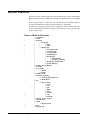
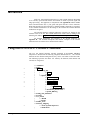
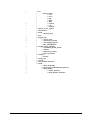
APPENDIX A : FUNCTION TREE............................................................................................................................. 63
INTRODUCTION ................................................................................................................................................................... 64
CATEGORIES OF PROVIEW’S MSHELL FUNCTIONS.......................................................................................................... 64
APPENDIX B : INTERNAL FUNCTIONS................................................................................................................. 67
PROVIEW’S MSHELL INTERNAL FUNCTIONS (BY CATEGORY): ....................................................................................... 68
Filtering ......................................................................................................................................................................... 68
Geo_Xform ..................................................................................................................................................................... 68
Intensity_Mapping ......................................................................................................................................................... 68
IO ................................................................................................................................................................................... 69
Matrix_Vector_Algebra ................................................................................................................................................. 69
Plot................................................................................................................................................................................. 70
Region_Ops.................................................................................................................................................................... 70
Satellite_Image_Mapping .............................................................................................................................................. 70
Statistics ......................................................................................................................................................................... 70
String_Ops ..................................................................................................................................................................... 71
System............................................................................................................................................................................. 71
iv • Table of Contents
ProView User’s Manual
Trigonometric Functions.................................................................................................................................................72
Useful ..............................................................................................................................................................................72
INTERNAL FUNCTIONS - ALPHABETICAL LIST......................................................................................................................74
- Symbols - ......................................................................................................................................................................75
- A - .................................................................................................................................................................................82
- B - .................................................................................................................................................................................84
- C - .................................................................................................................................................................................87
- D -.................................................................................................................................................................................92
- E - .................................................................................................................................................................................95
- F - .................................................................................................................................................................................97
- G -.................................................................................................................................................................................99
-H-.................................................................................................................................................................................102
- I - ................................................................................................................................................................................104
- L -................................................................................................................................................................................110
- M - ..............................................................................................................................................................................113
- N - ...............................................................................................................................................................................121
- O -...............................................................................................................................................................................125
- P - ...............................................................................................................................................................................126
- Q -...............................................................................................................................................................................129
- R - ...............................................................................................................................................................................130
- S -................................................................................................................................................................................137
- T -................................................................................................................................................................................157
- V - ...............................................................................................................................................................................159
- W - ..............................................................................................................................................................................163
- X - ...............................................................................................................................................................................166
- Z -................................................................................................................................................................................169
APPENDIX C : EXTERNAL FUNCTIONS ..............................................................................................................171
INTRODUCTION ..................................................................................................................................................................171
ProVIEW User’s Manual
Table of Contents• v
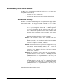
Overview
What Is ProVIEW ?
ProVIEW is an interactive command line and menu driven Image and Signal
Processing Environment which runs as a 32 bit application under Microsoft
Windows 3.x (utilizing Win32s) and Windows NT. ProVIEW provides powerful
scientific image and signal processing and visualization capability by affording you:
ProView User’s Manual
•
Algebraic and matrix operations using mathematically intuitive syntax.
•
Support of relational operators and flow control through the built-in
MSHELL image processing language interpreter.
•
Floating point image processing computations for high accuracy which
support both real and complex number operations.
•
Over 300 operators: FFT, convolution, edge detection....
•
Geometric operations: re-size and rotate images using unequal
horizontal and vertical scaling.
•
The ability to call your own functions as a Dynamic Link Library
(DLL).
•
The ability to query Microsoft Access databases using ProVIEW’s
DDE capabilities.
•
Flexible display of multiple images, plots, and scripts.
•
Contrast processing, linear stretching, intensity range remapping.
•
Pseudo Color Lookup Tables for each Image with as many colors as the
hardware permits.
•
Interactive 2D, 3D, and Contour Plots.
•
Multiple image format support: ASCII, 8 bits/pix, floating point, in
addition to key standard formats, such as TIFF, BMP, FITS, PGM,
PPM, and PDS.
•
Optimum use of the dynamic range of your display hardware by
providing optional automatic adjustment of pixel values prior to
display.
Overview • 7
•
Support of text attributes that are attached to an image, these attributes
can be used to store an image header or to store processing instructions
to be applied to the image.
•
Affordable real-time performance, when using i860 based floating
point array processors.
Expert or novice, independent of your experience, ProVIEW allows you to
manipulate images and signals in a simple manner, releasing you from the constant
tracking of image attributes such as image dimensionality.
ProVIEW permits you to process a large volume of images in a fully automatic
fashion, e.g. large scale reduction, calibration and analysis of satellite based digital
images.
IF you work with satellite imagery, ProVIEW enhances your productivity by
providing the following additional capabilities:
•
Using the SatVIEW module, the ability to:
⇒ Read ephemeris information following NASA’s SPICE kernel
format,
⇒ Compute an extensive set of viewing geometry related values, such
as phase angle, incidence angle, and
⇒ Compute the projection of any pixel on the planet surface or the
celestial sphere.
•
The ability to have a virtual image variable which can be as large as
your collective disk space! You can then read and write to selective
regions of interest in a very flexible manner.
•
The ability to perform simple automatic projections of satellite images
into the planet surface or the celestial sphere.
Who Should Use ProVIEW?
ProVIEW has been developed by and for professionals working in the areas of image
and signal processing who desire to concentrate on algorithmic development rather
than on low level programming.
ProVIEW can significantly reduce the time required for the development and
implementation of image and signal processing algorithms without sacrificing
computational performance. A single statement in ProVIEW’s interpreter language,
MSHELL, can be equivalent to a large number of statements in other languages,
such as C or FORTRAN.
Based on the understanding that both image processing and multi-dimensional signal
processing share the same mathematical foundations, MSHELL was developed from
the onset as an image and signal processing language. With MSHELL at it’s core,
ProVIEW is an Image and Signal Processing Environment that is powerful,
compact, and simple to use. This makes ProVIEW an excellent tool for work in
many diverse application areas, such as:
8 • Overview
•
Calibration and Reduction of Satellite Imagery, (coherent as well as
non-coherent image data),
•
Visualization of Multi-Spectral Image Data,
ProVIEW User’s Guide
•
Modeling of Electro-Optical Imaging Systems,
•
Machine Inspection,
•
Pattern Recognition, and
•
Neural Network modeling.
To effectivly use ProVIEW a working knowledge of Linear Algebra, Image
Processing, and Computer Programming is recommended. A listing of textbooks
which can provide such a working knowledge is given in “References and Further
Readings” below.
References and Further Readings
ProView User’s Manual
•
Applied Research Corporation, "A User's Guide for the Flexible Image
Transport System (FITS)", March 5, 1990
•
Erick Malaret - Applied Coherent Technology, "Clementine EDR
Archive SIS", October 1, 1994
•
Fukunaga, K., "Introduction to Statistical Pattern Recognition,"
Academic Press, 1972.
•
Harris, G. G., "On the Use of Windows for Harmonic Analysis with the
Discrete Fourier Transform," Proceedings of the IEEE, vol., 66, No. 1,
pp. 51-83, January 1978.
•
Kernighan, B. W., and Ritchie, D. M., "The C Programming
Language," Prentice-Hall, Englewood Cliffs, N.J.
•
Knuth, D. E., "Sorting and Searching," vol. 3, of The Art of Computer
Programming, Addison-Wesley, 1973.
•
Microsoft Windows User's Guide, Microsoft Corporation
•
Press, W. H., Flanney, B. P., Teukolsky, S. A., and Vettering, W. T.,
"Numerical Recipes in C," Cambridge University Press, 1988.
•
Rosenfeld, A., Kak, A. C., "Digital Picture Processing," second edition,
Academic Press, New York,New York, 1982
•
Strang, G., "Linear Algebra and Its Applications," Academic Press,
New York, 1980.
•
Newman, W. M., and Sproull, R F., "Principles of Interactive
Computer Graphics," McGraw-Hill Book Company, 1979.
Overview • 9
Installation
System Requirements
The system requirements to use ProVIEW are:
•
An 80386, 80486, or PENTIUM PC running Microsoft Windows 3.x
with Win32S or Windows/NT.
•
A hard drive with at least 10 Megabytes of available disk space.
•
A minimum of 4 Mbytes of RAM for Windows 3.1 and a minimum of
16 Mbytes for Windows/NT. (The more memory available the larger
the images that ProVIEW can handle).
•
A 3.5-inch high-density disk drive, CDROM, or internet connection
depending on the source of installation.
•
A Microsoft Windows supported High Resolution Video Graphics
Adapter Card. The image resolution and the number of brightness
levels (gray levels) that can be achieved in the display depend on the
video graphics card and monitor used.
•
A Microsoft or other compatible mouse.
•
A parallel port to install the ProVIEW electronic key.
Installing ProVIEW
ProVIEW must be installed on a hard disk in your computer that has at least 10
Mbytes of free space available.
To Install ProVIEW:
10 • Installation
•
While the computer is off, attached the ProVIEW electronic key to the
parallel port of your computer. This device will not interfere with your
printer in any way and is needed in order to access the full functionality
and capabilties of the ProVIEW environment..
•
Turn on the computer and the monitor, start Windows.
ProVIEW User’s Guide
•
Once in Windows insert the ProVIEW disk labled #1 in the 3.5 inch
floppy disk drive. (a: or b: as applicable) or place the CDROM in its
drive depending upon source of installation.
•
From the Program Manager, select File and then Run. (You can also
do this from the File Manager by double-clicking on the previously
mentioned file.)
•
When the dialog box appears, type in a:install and select OK. (or
b:install if applicable.)
•
Follow the instructions on the screen.
Once the installation is completed you will find the following new directories (e.g., if
installed in c:\ ) on your hard drive:
c:\ProVIEW
c:\ProVIEW\Bin
c:\ProVIEW\Images
c:\ProVIEW\Scripts
c:\ProVIEW\User
c:\ProVIEW\Temp
c:\ProVIEW\Wdb
In addition, you will find that a ProVIEW program group has been created in
Programs Start Menu. After this has been completed, you are now ready to start
ProVIEW.
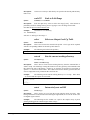
Technical Support
For Technical Support with ProVIEW please contact:
Applied Coherent Technology Corporation (ACT)
Phone:
(703) 742-0294
Fax:
(703) 742-0358
Between 9:00 AM to 6:00 PM EST, or
internet:
ProView User’s Manual
http://www.actgate.com
Installation • 11
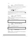
Starting ProVIEW
Start Procedure
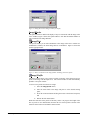
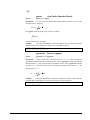
Once installed, ProVIEW can be started by double clicking on the ProVIEW icon
, located in the ProVIEW Program manager group.
Once ProVIEW is loaded in memory the ProVIEW prompt
[ready]:
will appear in the Command Line Window indicating that the command line
interpreter is ready to receive input.
For a quick test of
ProVIEW, select the
Help|Demo option from
the menubar.
To test if ProVIEW was properly installed you can run the script file ’mdemo.msh’.
This is done by typing the following line after the ProVIEW prompt,
[ready]: include "mdemo"
followed by Enter or Return.
This shell script can also be ran by choosing the Demo option below the Help menu
The ’mdemo.msh' script file tests many of ProVIEW’s capabilities, such as image
display, graphic display, multiple windows, script file and user defined function
execution.
Communicating with the Interpreter
You can communicate commands to MSHELL, ProVIEW’s built in command line
interpreter, in several different ways:
ProView User’s Manual
a.
Through the Graphical User Interface
selected under the graphical user
corresponding command line string
MSHELL interpreter for execution, see
on page 16.
- When a menu option is
interface it generates a
which is passed to the
"Graphical User Interface"
b.
Through the keyboard - With the Command Line Window active
you can interact directly with the interpreter by following the
Starting ProVIEW • 13
MSHELL language syntax, see "Command Shell Window " on
page 17.
c.
Through a ProVIEW script file - ProVIEW script files are user
generated text files consisting of sequences of MSHELL
statements and can be invoked through either the Graphical User
Interface or the keyboard as described above, see "ProVIEW Script
Files" on page 46. Note, that since a script file is just a collection
or sequence of MSHELL language statements, it is also referred to
as a MSHELL script file.
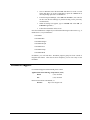
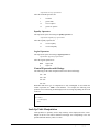
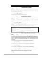
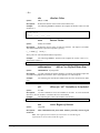
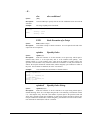
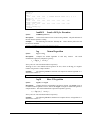
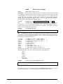
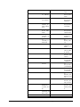
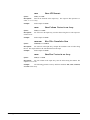
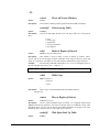
Image Quality
The spatial resolution in pixels and the number of gray levels and/or pseudo colors
that your system has while running ProVIEW is determined by the display driver
loaded in the Microsoft Windows environment and the graphics adapter hardware
installed in your computer. ProVIEW has been tested with the following graphic
adapter cards:
Graphics Card
Spatial Resolution
(columns X rows)
Number of Gray Levels
or Colors
Number 9
1280 X 1024
ATI Graphics Ultra Pro
1024 X 768
65,536 (16 bits)
800 X 600
16,777,216 (24 bits)
640 X 480
16,777,216 (24 bits)
1024 X 768
65,536 (16 bits)
Diamond Viper
2Mb
16,777,216 (24 bits)
800 X 600
16,777,216 (24 bits)
Diamond Stealth 64 2Mb
640 X 480
16,777,216 (24 bits)
VGA (generic)
640 X 480
16 ( 4 bits)
1024 X 768
256 ( 8 bits)
8514
When at least 65,536 gray levels or pseudo colors are used it is possible to display
gray scale images together with pseudo color images. See "Help|System Info" on
page 32 for how to get specific information about your video graphics card’s present
configuration.
14 • Starting ProVIEW
ProVIEW User’s Guide
Useful Tips
Specific information on how to navigate throughout the ProVIEW environment can
be found in the Graphical User Interface section. However, to help you get off to a
quick start we provide you with some useful tips and observations:
STOP ICON,
ProView User’s Manual
•
When a script file or function is executing, the word running appears
in the lower right portion of the screen.
•
To stop ProVIEW from executing an instruction, click on the STOP
icon, located on the tool bar, or press the ESC key
•
While in the Command Line Window any recently invoked command
can be re-invoked by using the UP and DOWN arrow keys on the
keyboard.
•
To exit ProVIEW select the File|Exit menu option.
Starting ProVIEW • 15
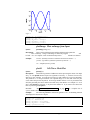
Graphical User Interface
ProVIEW’s Windows Environment
Since ProVIEW runs under Microsoft Windows, some familiarity with the Windows
Graphical User Interface (GUI) is assumed. For additional details or for a review of
the Windows environment we refer you to your Microsoft Windows manuals.
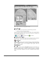
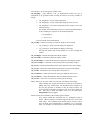
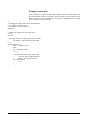
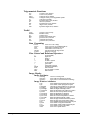
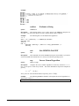
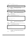
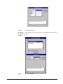
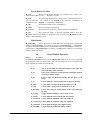
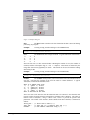
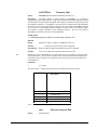
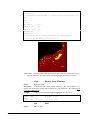
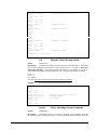
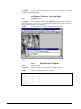
With ProVIEW you can have multiple windows open at the same time, each one
containing an image, a plot, text, or a script file. However, you will note that at any
given time only one of these windows will be the Active Window, i.e. the window
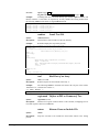
with the highlighted top bar. In Figure 1 the Command Shell Window is the active
window.
Figure 1 - Sample ProVIEW screen.
In addition, Figure 1 provides examples of some of the different types of ProVIEW
Windows: Command Line, Image, Script, and Plot. A description of each of the
different ProVIEW windows follows.
Command Shell Window
It is in this window that you can interact directly with MSHELL, ProVIEW’s
command line interpreter. Commands typed in this window are executed by the
MSHELL interpreter. It is from within this window that script files are normally
invoked, see "ProVIEW Script Files (.msf,.msh,.vsh)" on page 46. Also, any text
output is normally sent to this window. Note that in ProVIEW most of the menu item
or icon selections are converted directly to commands in the "MSHELL Interpreter
Language", see page 35.
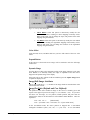
Image Window
Prior to enabling the
display of an image the
user can control many
attributes that will affect
how the image is to be
displayed; see section xx
for details.
An image window provides a visual representation of a two dimensional array of
numbers. In ProVIEW there are several different ways to enable an image window for
the display of an existing array variable:
•
from the Command Shell Window using the View command, see
Appendix B, following this section, on page B-87, or
•
from the menu by selecting the File|Open Image option.
Once the image is open, you can exercise a good deal of control over how it is
displayed, see "Image|Options" on page 24. Additionally, you can use the scroll bars
that are part of the image window to slide the image horizontally or vertically, or use
the cursor to travel over the image. Notice that as you move the cursor over the
image, it’s row position, column position, and corresponding pixel value are tracked
in the status bar at the bottom left of ProVIEW’s Main Window.
Script File Window
In a Script File Window you can create, edit, or display a text file of MSHELL
commands. The easy to use built in editor supports the standard Cut, Paste, Search,
and Replace operations found in most windows applications.
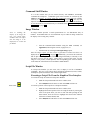
Executing a Script File From the Graphical User Interface
To execute the script file located in a Script File Window:
RUN ICON,
ProView User’s Manual
1.
Make the Script File Window the active window, then
2.
Select File|Run from the menu or click on the Run tool bar icon.
To execute a portion of the script file in a Script File Window:
1.
Make the Script File Window the active window, then
2.
Highlight the desired portion of the text using the mouse by moving the
cursor to the point where you want to start and while pressing the left
mouse button, move the cursor to highlight the selected area and then
release the left mouse button, then
3.
Select File|Run from the menu or click on the Run tool bar icon.
Graphical User Interface • 17
Plot Windows
The major types of plot windows in ProVIEW include 2D, 3D, Contour, and
Histogram. These plots can be generated:
•
From the GUI, see "Image|Plot Roi" on page 24,
•
From the Command Line Window using the PLOT, PLOT3D,
COUNTOUR, and HIST commands, see Appendix A (Listing of
internal Functions), or
Once a plot is generated its display can be changed through the Plot|Settings menu
option, see page 27.
To facilitate the handling of generated plots you will find that all plot windows are
numbered so that they may be updated or deleted from the command line.
Menu Commands
File
This menu allows you to control the input and output of images and script files,
printer output, script execution, and to end the ProVIEW work session.
File|New Script
Use this option to open a text window in which to create a new script file.
File|Open Script
Use this option to open an existing script file. Note that multiple script files can be
open simultaneously!
File|Save Script
Use this menu to save the script file in the active window.
File|Save Script As
Use this menu to save the script file in the active window to a new disk file.
File|Choose Font
Allows the user to modify the font used within the script file windows.
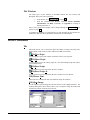
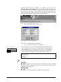
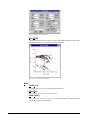
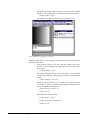
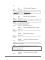
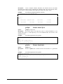
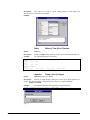
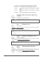
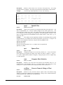
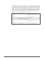
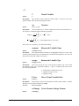
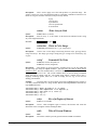
File|Open Image
Use this option to open an image data file stored in any of the supported formats. The
resulting Dialog Box, shown below, allows you to assign the image file format and
the directory location of the file to be retrived.
18 • Graphical User Interface
ProVIEW User’s Guide
Figure 2 - File|Open Image Dialog Box
File|Open Image - Browse Button
Select this option to keep the File|Image Open window active after selecting an
image file. This allows the selection of another image file for display without having
to open the Image File I/O window again.
File|Open Image - Movie
Select this option to display the images with the specified file format contained in the
selected directory in a movie-like manner.
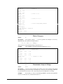
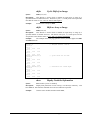
File|Open Image - File Formats
The following image file formats are supported:
•
ascii format (*.asc) is used for images whose data is stored in ASCII. A
sample ASCII image data file will look like,
3
3
0
-1
0
1
-2
0
2
-1
0
1
where the first row contains the number of rows, the number of columns,
and the real-complex flag (0 = real, 1 = complex). This is followed by
the image data stored in ASCII row by row starting from the top. Note
that the delimiter is the space character. This format is used for both the
reading and writing of image data.
ProView User’s Manual
•
bmp format (*.bmp) is the Windows Device Independent Bitmap
Format and is used both for the reading and writing of images.
•
char format (*.chr) is used for images stored using 1 byte/pixel data
prefixed by a simple 9 byte header, i.e. 4 bytes specifying the number of
rows, 4 bytes specifying the number of columns, and 1 byte specifying a
real or complex array. This format is used both for reading and writing
of data.
•
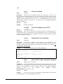
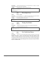
flex format (*.*) provides you significant flexibility in the reading of
data prefixed by an image header. When you select this format an input
dialog box, depicted below, opens allowing you to specify the
dimensions of the input image and the header size. The (flex) format is
only used for reading data.
Graphical User Interface • 19
Figure 3 - Flex Dialog Box
•
clemen_pds format (*.*) is the implementation of the PDS (Planetary
Data System) Format adopted by the Clementine mission. When an
image in this format is opened the ascii text header is attached to the
image. This header can be viewed from the image window using the
“Image|Header” option, see page 22. This format is used only for the
reading of data.
•
float format (*.flt) is one in which the data is stored in floating point
using 4 bytes/pixel. Similar to the char format above, a 9 byte header is
used. This format is used both for reading and writing of images.
•
tiff format (*.tif) can be used for both the reading and writing of data,
but please note that not all TIFF modes are supported.
•
fits format (*.fit) stands for the flexible interchange transfer system; this
is a format designed for the flexible trasnmission of varying image data
sets along with any extraneous required data such as history logs or any
other text info. This format can be read as well as written by ProVIEW.
•
jpeg format (*.jpg) is a image format primarily known for its extreme
ability of storing an image in a highly compressed state. This format
does however have one disadvantage; it is a lossy format meaning that
when written it loses all of the data in order to get its compression. This
format can be read, but not written.
•
pds format (*.pds) stands for the planetary data system; whereby, this
format involves the Huffman First Difference algorythm with no
compression. This format can be read but not written. Ongoing work is
being done at this time for the incorpoation of a pds writer within
ProVIEW.
File|Open Image - File Name
This option allows you to browse over a list of already defined variables or type in the
variable name to be used for the requested image I/O operation.
File|Save Image
This option, using a Dialog Box similar to that of the File|Open Image option
discussed earlier, saves an open image to disk in any of the supported formats.
File|Save Clipboard Bitmap
This option lets you save the contents of the clipboard to disk, in bmp format, while
specifying the output file name.
20 • Graphical User Interface
ProVIEW User’s Guide
File|Printer Setup
Use this option to change the printer configuration, e.g. orientation, paper size, output
quality, etc.
File|Print
Sends the contents of the active window, be it an image, a plot, or a script file to the
selected printer. Note that ProVIEW does not require any special printer drivers as
utilizes the Windows printer divers that you have already installed.
File|Print Screen
Sends an image of the ProVIEW screen to the printer
File|RunScript
Use this menu option to execute the script file in the active window or just the
highlighted portion of the script file in the active window. This very powerful feature
simplifies the interactive development of SCRIPT files.
File|Exit
Terminates execution of the current ProVIEW session.
Edit
This menu allows the user to select from any of the following options:
Undo
, Cut
, Copy
, Paste
, Delete, and Clear All.
Although these options are primarily for the editing of script files, the Copy and Paste
options can be used with Images.
Edit|Edit System Variables
This command runs the “sysedit.msh” script file which allows one to change all of the
system variables(M_~~~), which are described later in the internal functions section.
Search
This menu allows the user to select from any of the following options:
Find
, Replace
, and Next
.
All these options are primarily related to the editing of script files.
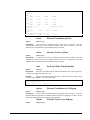
Image
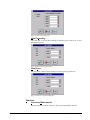
Image|Display
This menu option provides you with a means, using the Dialog Box of Figure 4, to
select which of the open Image Variables to display, see "Array Variables" on page
36.
ProView User’s Manual
Graphical User Interface • 21
Figure 4 - Dialog Box to Select Image Variable for Display
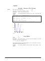
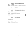
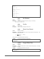
Image|Header
This option enables or disables the display of any text associated with the image in the
active window; Figure 5 shows this option enabled. Note that the Header Window is
fully contained in the Image Window
Image|Text
This option enables you to make annotations to the image in the active window in a
nondestructive manner; the actual image data is not modified. Figure 5 shows this
option’s popup window.
Figure 5 - This screen illustrates the Image|Header and Image|Text menu options.
Image|Profile
This menu options allows you to extract a profile of intensity values between any two
points in the image with the input focus. The extracted values are then automatically
plotted in a new plot window.
To select a new profile from the active image:
1
Select the Image|Profile menu,
2
Take the cursor back to the image and place it at the desired starting
point,
3
Press the left mouse button and drag the mouse to the desired end point,
and
4
Release the left mouse button.
While the extraction of the profile of intensity values is in progress the length of the
line (in pixels or user defined units) between the two selected points is shown in the
status bar at the bottom of ProVIEW’s main window.
22 • Graphical User Interface
ProVIEW User’s Guide
Image|Set ROI
The Graphical User Interface in ProVIEW allows you to define a rectangular region
of interest interactively using the mouse. Note that all array variables have an implicit
region of interest defined, see "Region of Interest Manipulation" on page 42. This
menu option allows you to define such a rectangular region of interest in the image
with the input focus in the following manner:
1
Select the Image|Set Roi menu option.
2
Take the cursor back to the image and place it at the desired starting
point of the rectangular window.
3
Press the left mouse button and drag the mouse to the desired end point.
4
Release the left mouse button.
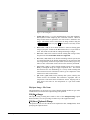
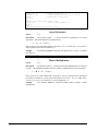
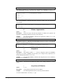
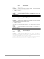
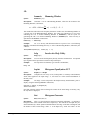
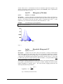
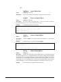
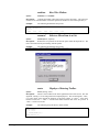
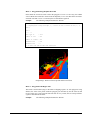
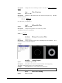
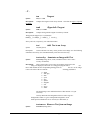
Image|Statistics
Using the Image|Statistics menu option the you can compute basic statistics over the
active region of interest (ROI) of the active image.
As illustrated in Figure 6, the statistics-window provides for the selected ROI:
ProView User’s Manual
•
An image of the ROI,
•
A normalized sum of the ROI’s columns,
•
A normalized sum of the ROI’s rows,
•
A Histogram of the image of the ROI,
•
The dimensions of the ROI,
•
The Minimum, Maximum, Mean, and Standard Deviation of the pixel
values within the ROI, and
•
The row and column Centroid of the ROI expressed in pixel coordinates
of the original image.
Graphical User Interface • 23
Figure 6 - This screen illustrates the Image|Statistics window.
Image|Plot Roi
Using this menu option you can generate any of the following types of plots:
PLOT3D, CONTOUR, and HISTOGRAM
for the active region of interest defined for the active image. Once a region of interest
has been defined, an alternative way to invoke these plot functions is through the set
of icons in the ProVIEW tool bar, i.e.,
use
for Plot3d, use
for Histogram, and use
for Contour.
Image|Spreadsheet View
This allows one to view the image values as they would appear within a spreadsheet
where each pixel is simply an entry within a table with the same dimensions.
Image|Zoom
This option allows the user to zoom over the active image. Zero order interpolation is
used for zooming into the image. As you move a rectangular window over the input
image a magnified version of the encompassed region appears within the
Image|Zoom popup window.
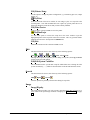
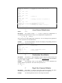
Image|Options
Selecting this menu item opens the Image|Options Dialog Box which affords you a
great deal of control over the way the image is displayed on screen. The options
available, as pictured in Figure 7, include: a choice of pre-defined or user-defined
Output Look-Up-Tables, adjustable Color Offset, and adjustable Dynamic Range
setting.
24 • Graphical User Interface
ProVIEW User’s Guide
Figure 7 - Image|Options Dialog Box
These options are discussed in more detail in the following:
Select LUT
This section gives you a selection of 4 different output Look-Up-Tables, (LUT), as
described below or the option to customize one to your particular needs.
LUT
wolut0
DESCRIPTION
gray scale LUT - low amplitudes display as dark (black) and high
amplitudes display as light (white)
wolut1
inverse gray scale LUT - low amplitudes display as light (white) and high
amplitudes display as dark (black)
wolut2
pseudo color LUT - intensity values are mapped to a pseudo color LUT
wolut3
pseudo color LUT - intensity values are mapped to a pseudo color LUT
wolut4
user defined LUT
The presently active LUT is displayed in the middle of the Image|Options dialog box
in the form of an intensity or color strip.
Modify LUT Box
Selecting the Modify LUT option in the Image|Option Dialog Box opens the Modify
GrayScale LUT Dialog Box, illustrated below. This dialog box allows you to
interactively modify the Gray Scale LUT that applies to the active image. Within this
dialog box changes to the gray scale LUT are displayed as a line plot superimposed on
a Histogram of the region of interest of the active image.
ProView User’s Manual
Graphical User Interface • 25
Figure 8 - Look Up Table Dialog Box
•
Linear Button. Select this option to interactively modify the user
defined LUT, wolut3, resulting in a linear mapping of intensity values.
While in this mode you can change the slope, and position of the linear
mapping using the slide bars.
•
Log Button. Select this option to interactively modify the user defined
LUT, wolut3, resulting in a logarithmic mapping of the intensity values.
While in this mode you can change the curvature of the logarithmic
mapping using the slide bars.
Color Offset
Using the Red, Green, and Blue slide bars you have full control of the LUT color
offset.
Expand Button
If this option is selected the active image will be stretched to take the full image
window size.
Dynamic Range
Use this option to either select automatic scaling of the image intensity levels (Auto
Scale Button) or to manually modify the range of amplitude levels that will be
mapped to the dynamic range of the display.
If the auto scale or max. and min. fields are modified, press the Update Image button
to update the display screen.
Image|Edit Image Attributes
This is used to edit the (m_~~~) variables of an image which are described later in the
internal functions section.
Image|Set Units (Default and User Defined)
The position of the cursor within an image on the screen is normally given with
respect to the upper left pixel in the image, i.e. (row,column) = (0,0). As you move
the cursor over the image, it’s row position, column position, and pixel value are
tracked in the status bar at the bottom left of ProVIEW’s Main Window. These are
reported as
row# col# val = #
[default mode]
row# = yval<units> col# = xval<units> val = # [user define mode]
In the user-defined mode, the cursor position is mapped into a user-defined
rectangular coordinate system, (row, col) ==> (yval, xval). To set user-defined
26 • Graphical User Interface
ProVIEW User’s Guide
interpixel distance from the Graphical User Interface you need use the
Image|Mensuration-User-Defined menu. This will bring an input box similar to the
one below where, x0 is the coordinate along the row axis for the first pixel on the
upper left corner of the image, y0 is the coordinate along the column axis for the first
pixel on the upper left corner of the image, dx is the interpixel distance along the
horizontal axis, and dy is the interpixel distance along vertical axis.
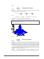
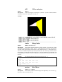
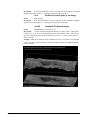
Figure 9 Partial Landsat Image of Ohare Airport.
Notice user defined units on the lower left corner.
Figure 10 Image Mensuration Dialog Box
The values of yvalue and xvalue are computed as:
xval = (col#)*dx+x0, and yval = (row#)*dy+y0
Given an image, say ’x’, the user can modify the image mensuration values
of this image directly from a script file by modifying the following intrinsic
image attributes: x.m_x0, x.m_y0, x.m_dx, x.m_dy. For example the
selection done through the user dialog box above could be done within a
script by typing the following lines: (here the image name is "eqohare")
For a discussion of
image attributes See
"Intrinsic
Attributes
Associated with Array
Variables".
eqohare.m_x0 = 300
eqohare.m_y0 = 4000
eqohare.m_dx = 25
eqohare.m_dy = 25
view eqohare
Plot
Plot|Plot
The plot menu allows you to generate plots used to modify the way that an existing
plot can be displayed. When the PLOT menu is selected it will work on the plot
window that has the input focus.
Plot|Settings
This selection is used for modifying the plot options and axis attributes.
ProView User’s Manual
Graphical User Interface • 27
Figure 10 Plot Settings Dialog Box
Plot|World
This menu item allows one to view any section of the word by double-clicking on the
map and then entering in the desired coordinates of interest.
Figure 11 Plot for World Coordinates
Data
Data|Load
This menu item allows one to load in a data set from a file.
Data|Save
This menu item allows one to save a data set as a file.
Data|Fitting
This menu item allows for the use of linear and bilinear interpolation when
constructing a curve from data points.
28 • Graphical User Interface
ProVIEW User’s Guide
Figure 12 Data Fitting Dialog Box
Data|Formatting
This menu item is used for the formatting of different types of data sets so as to be
manipulated correctly.
Figure 13 Data Formatting Dialog Box
Data|Series
This menu item is utilized for the creation of various specific type data sets.
Figure 14 Data Series Creation Dialog Box
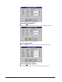
Functions
Functions|Mathematical
This menu option provides an interface to many of the mathematical functions.
ProView User’s Manual
Graphical User Interface • 29
Figure 15 Mathematical Functions Dialog Box
Functions|Trigonometric
This menu option provides an interface to many of the trigonometric functions.
Figure 16 Trigonometric Functions Dialog Box
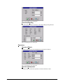
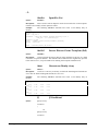
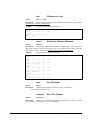
Functions|Statistical
This menu option provides an interface to many of the statistical functions.
Figure 17 Statistical Functions Dialog Box
Functions|Random Numbers
This menu option provides an interface to the random number generator.
30 • Graphical User Interface
ProVIEW User’s Guide
Figure 18 Random Generator Dialog Box
Functions|Ranking
This menu option provides an interface to the many ranking/sorting functions.
Figure 19 Ranking Functions Dialog Box
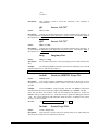
Operators
Operators|Matrix
This menu item is used for the manipulation and operation of matrices.
Figure 20 Ranking Functions Dialog Box
Operators|Transforms
This menu item is used for the operation of various transforms on data.
ProView User’s Manual
Graphical User Interface • 31
Figure 21 Transform Operators Dialog Box
Operators|Filtering
This menu item is used for the various filtering of data sets.
Figure 22 Filtering Operators Dialog Box
Window
This menu allows the user to select from any of the following options: Tile, Cascade,
Arrange Icons, and Close All. These menu options permits the control of the layout
of the different windows open within the ProVIEW environment.
Help
Help|Content
This option will bring up ProVIEW’s on-line help screen. This whole manual is
available under the help menu option.
Help|Keyword search
This option is activated when a script file window has the input focus. It allows the
user to highlight a word and do a search on ProVIEW’s on-line help file.
Help|About
Provides the version numbers for the ProVIEW shell and gui for your copy of
ProVIEW.
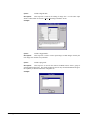
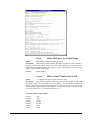
Help|System Info
Help System Info will display key system information in a window similar to the one
below. In the example below, the 2.12 Gbytes reported below include available swap
space to disk.
32 • Graphical User Interface
ProVIEW User’s Guide
Figure 23 System Info Dialog Box
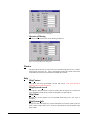
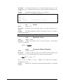
Help|Demo
This menu item invokes a series of demos which show some of ProVIEW’s
capabilities.
Figure 24 Demos Dialog Box
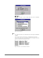
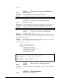
User
User defined menu items can be added under this menu using the addmenuitem
command.
The User option will show in the menu only if addmenuitem has been invoked.
The User menu along with its corresponding menu items will appear between the
Operators and Window menu headings once started.
Figure 25 Illustrative Use of the Addmenuitem Command
ProView User’s Manual
Graphical User Interface • 33
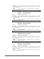
Figure
34 • Graphical User Interface
26
Corresponding
Menu
Creation
from
the
above
Command
List
ProVIEW User’s Guide
MSHELL Interpreter Language
Language Syntax
Introduction
At the heart of ProVIEW is the MSHELL interpreter developed by ACT. MSHELL is
a 32 bit image/signal processing language which allows you to perform complex
operations using a simple, almost intuitive syntax. In the following sections we will
introduce you to this language and discuss it’s syntax.
Variable Names and Types
In general, a variable name can be any alphanumeric string starting with a letter
followed by a combination of letters and/or digits. The following are legal
alphanumeric variable names,
x,
x10,
OutputImage
Note that variable names should be kept under 15 characters. Additionally there are a
number of reserved keywords and symbols, used by the interpreter, that cannot be
used as variable names. A list of these keywords together with a description of their
use is found in the section "Appendix A (List of Internal Functions).
There are four basic types of variables:
•
Array variables (holding floating point numbers),
•
String variables (holding character strings), and
•
System variables (which are used to control the interpreter environment).
•
Virtual Variable
Array Variables
Throughout most of this
manual the terms image,
array, or matrix can be
interchanged
without
loss of generality
The upper left element in
an image or array is
denoted as element
(row=0,col=0).
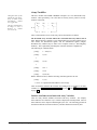
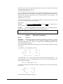
The basic variable in ProVIEW’s MSHELL interpreter is a two dimensional array
structure. More specifically, if 'a' is the name of an array, then it points to an array
structure of the form,
 a0,0

a1,0
a → 
M

 a J −1,0
a0,1
a1,1
M
a J −1,1
L a0 , I − 1 

L a1, I −1 
L
M 

L a J −1, I −1 
where J is the number of rows in the array, and I is the number of columns.
The ProVIEW array structure follows the convention that array indices start at
zero. Having the basic variable as a two dimensional array provides a unified way to
treat scalars, one dimensional signals, and two dimensional signals (images).
ProVIEW array variables may be either real or complex valued (i.e. hold imaginary
numbers). This is particularly advantageous in Fourier transform computations.
The following are valid statements:
[ready]:
x = ones(3,3)
[ready]:
x(2,2)
1
[ready]:
x(0,0)
1
[ready]:
row=1
[ready]:
col=2
[ready]:
x(row,col)
With 'x' defined as above, then the following statement generates an error
[ready]:
x(1,5)
>>>error= 6 -requested element address is out of range
There are different schemes that facilitate the reading from (or writing to) an array
variable, see: "Region of Interest Manipulation" on page 42, and "
on page 23.
Image|Set ROI"
Intrinsic Attributes Associated with Array Variables
There are many intrinsic attributes associated with array variables. For example,
these attributes can control the way a variable is displayed, and interpolated. Most of
these attributes can be inspected and changed by the user. The following presents all
the intrinsic attributes associated with array variables and their associated syntax.
36 • MSHELL Interpreter Language
ProVIEW User’s Guide
Let us denote ’x’ as an existing array variable. Then:
x.m_interpflag - (This function is not yet implemented.) Selects the type of
interpolation to be performed while accessing an element in an array variable by
setting:
•
x.m_interpflag=0 for zero order interpolation.
•
x.m_interpflag=1 for liner interpolation along the values of a row.
•
x.m_interpflag=2 for bi-linear interpolation when trying to access the
values in an array.
For example, in the following two lines of code the interpolation flag is
set to 2 resulting in a request to use bi-linear interpolation.
x.m_interpflag=2;
y = x(10.3, 12.7)
You can read the value of this attribute.
x.m_viewflag - Controls if an image is visible for display or not by setting:
•
x.m_viewFlag=1 which forces the image to be displayed.
•
x.m_viewFlag=0 which disables the display of the image.
Note that the default value for this atribute is zero, not to display the
variable.
x.m_viewheight - Controls the height of the display window.
x.m_viewwidth - Controls the width of the display window.
x.m_viewhscrollpos - Controls the horizontal scroll position of the display window.
x.m_viewvscrollpos - Controls the vertical scroll position of the display window.
x.m_viewx0 - Controls the horizontal position of the upper left corner on the display.
x.m_viewy0 - Controls the vertical position of the upper left corner on the display.
x.m_viewlut - Contains the active look-up-table to be used for ’x’.
x.m_viewmaxval - Controls the maximum value to be displayed on the screen.
x.m_viewminval - Controls the minimum value to be displayed on the screen.
x.m_viewtext - Allows one to view the text which is part of an image.
x.text - Allows you to access (either read or set) the text attribute of the image.
Image variables may contain associated text, which can be accessed by
adding ’.text’ to the variable name. The ProVIEW screen of Figure 5 on
the next page provides an example of this; the image ’myramp’ was
created, and its text attribute ’myramp.text’ was set to some simple text
line. Note that to enable the display of this text, the menu option
Image|Header must be toggled.
x.vroi - Extracts the coordinates of the variable region of interest.
Every image variable has associated with it a rectangular region of
interest. When a variable is created this region of interest is set to be the
whole image. The coordinates of the defined region of interest can be
easily accessed at the command line by appending ’.vroi’ to the image
name. For example, the following line of code extracts the coordinates
ProView User’s Manual
MSHELL Interpreter Language • 37
that define the variable region of interest (vroi) of an already defined
variable, say X, and assigns it to a user defined variable called ’regionc’,
[ready]: regionc = X.vroi
The notation X.vroi can be viewed as if vroi is an attribute of X.
Figure 5 Illustrates test attributes on an image
x.m_aoi - allows access to the actual pixel values defined by the region of interest
associated with an array.
Given an array variable, say X, the actual pixel values can be easily
accessed in the command line by appending ’.aoi’ to the image name.
For example,
[ready]: subimage = X.aoi
extracts the subimage defined by X.vroi and assigns it to a user defined
variable called ’subimage’. This could also be done using the following
notation
[ready]: subimage = X(X.vroi)
ProVIEW provides different ways to operate over regions of interest.
For example, to add 10 to all pixels falling within the defined region of
interest, and updating the display type
[ready]: X(X.vroi) = X.aoi + 10
[ready]: view X
This could also be done as follows,
[ready]: regionc = X.vroi
[ready]: X(regionc) = X(regionc)+10
[ready]: view X
38 • MSHELL Interpreter Language
ProVIEW User’s Guide
See "Region of Interest Manipulation" on page 42 for additional information on using
regions of interest.
See
Section
,
Image|Edit
Image
Attributes
This is used to edit
the (m_~~~) variables
of an image which are
described later in the
internal functions
section.
The following set of image attributes are related to image mensuration. They all start
with ’.m_’ just as the above intrinsic attribute commands did.
x.m_x0 - user defined horizontal position of upper left pixel in image
x.m_dx - user defined spacing between two adjacent horizontal pixels as you move
from left to right
Image|Set Units
(Default and User
Defined), for
examples on the
image mensuration
x.m_y0 - user defined vertical position of upper left pixel in image
x.m_dy - user defined spacing between two adjacent pixels in the same column as you
move from top to bottom
x.m_xunit - string describing the units of x.m_x0
x.m_yunit - string describing the units of x.m_y0
x.m_flag - if this flag is set to 1 the user defined image mensuration will be used
when viewing the ’x’ image
String Variables
A string is defined as a sequence of alpha numeric characters enclosed within quotes
(similar to the ’C’ language).
In general, string variable names start with ‘$’. For example, the string variable
‘$message’ can be assigned a string as follows,
$message = "hello world";
ProVIEW allows the use of control characters within a string, such as
\n
linefeed
\t
tabulation
\b
backspace
\\
backslash
The above control characters can be used to control the format of strings on the
output.
If $x is a string, its content can be accessed using the following syntax
$x(row)
$x(row,column)
$x(row, start_column : end_column)
For example,
$x(3)
ProView User’s Manual
// returns row 3 (starting at 0)
MSHELL Interpreter Language • 39
$x(3,4)
// returns character 4 at row 3
$x(3,4:10)
// returns substring at row 3
Relational Operations are permitted on strings. See Program Flow Control for more
info.
System Variables
Within the system variables there are plot, image display, and script related variables.
The majority of the system variables are used for plotting purposes by the ‘plot’ and
‘plot3d’ functions. A complete list of these variables can be found in the dictionary of
internal functions under M_.
Some of the ProVIEW system variables are strings while others are numbers. All
system variables are prefixed by 'M_'. String system variables do not require the ‘$’,
they are a special case. For example, to initialize the x-axis label to the string “Time”
use
M_xlabel="Time";
Virtual Variable ’V’
ProVIEW has a special variable, 'V', called the virtual variable. With this variable the
user can manipulate an image file which can be as large as the whole disk space
available in the system.
If the user has a huge image in a file or is going to be working with an image that can
not be easily held in memory, then he or she can still manipulate pieces of the large
image using ProVIEW's virtual variable.
The basic virtual related functions in ProVIEW are Vopen, Vclose, and Vnew().
Vopen - Links 'V' to a floating point or 1 byte/pixel type of file,
Vclose - Stops link between 'V' and a disk file,
Vnew - Creates a new virtual file.
(See Appendix B for detailed usage of the above virtual variable
manipulatory functions. - Pages B-87:88)
Once a link is established between a file in disk and the virtual variable 'V', then the
user can access rectangular regions of interest in the disk file for read or write
operations (the user must always provide a rectangular region of interest when writing
or reading from 'V').
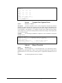
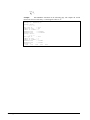
Example: The following script file illustrates the use of ProVIEW's virtual variable
'V'.
M_cwd = "/proview/images/clemen/moonbrus"
roi
= wdef(0,0,1,1)
V=Vopen("allmoon.chr",5760::11521::1::0,roi,0);
flyby = 0
view flyby;
i=0;
while(i<35){
meter("flyover virtual image",i/35*100);
angle= i/35*6.28
roi = wdef(2336+128*cos(angle),6926+128*sin(angle),256,256)
flyby = V(roi)
i = i+1
}
meter("",-1);
Vclose(V);
40 • MSHELL Interpreter Language
ProVIEW User’s Guide
Statements
A statement is, in general, an expression involving variables, internal functions, and
calls to script functions. Multiple statements can be typed in the same physical line if
they are separated by a semicolon. For example,
[ready]: x=4; y = x+4; z=cos(y);
is a legal statement.
A statement may expand over more than one physical line if a delimiter ‘\\’ is used in
the the continuation line, e.g.
x = cos(x+y) \\
+ sin(x-y)
Tabs, spaces, and linefeeds are ignored by the interpreter. An intuitive mathematical
syntax is followed by the interpreter, allowing you to input the expressions in a form
similar to the their actual mathematical representation.
In general, expressions which do not involve an assignment will print the result to the
screen, e.g.,
[ready]: 3+4
7
A broad representation of numbers consistent with most computer languages is
allowed. The following are valid number representations:
4
0.1
44.
0.44
34.89E4
34.89e10
Calling Syntax for Numeric Functions
The output of most of the numeric functions can be used as direct inputs to other
numeric function, e.g.
X = abs( log10(fft2(x)) )
Notice that you do not have to worry about the implicit dimensions of x and if it is
either real or complex. If a function can not handle a complex input it will return an
error message.
Unary Numeric Function Syntax
In general, when using a function with only one input argument, a ProVIEW unary
function, the following two statements are equivalent,
ufun(varname)
varname.ufun
For example, if x is an array variable the following two lines are equivalent,
y = cos(mean(x))
y = cos(x.mean)
The notation in the second line allows us to look at the mean value as an attribute of x.
Comments
Statements enclosed between /* and */ are ignored by the interpreter. This is used to
place comments in a script file or to prevent the execution of the line or lines between
the comment delimiters.
For example, a valid group of statements that make use of comment delimiters is,
ProView User’s Manual
MSHELL Interpreter Language • 41
/* Compute the magnitude of the FFT
on image x
*/
x = abs(fft2(x))
The delimiter ’//’ can be used to create single line comments in a script file, e.g.
x = fft2(x)
// note: compute the 2D FFT of x
Operator Precedence
The following operator symbols are defined within ProVIEW. Most of them are used
in algebraic operations. The precedence of operators increases as we move down the
list, with operators within the same line having the same precedence.
=
assignment operator
::
row augmentation or string concatenation
#
column augmentation
+ -
array addition and subtraction
* / *.
/.
multiplication and division (elemental)
^
a^b, "a to the power of b"
-
unary minus, e.g. -x
’
transpose operator, e.g. x’
f
an internal function, e.g. cos()
Hence, in the expression
c = a+b*x;
the multiplication is performed prior to the addition.
Proper
use
of
parenthesis can result in
a significantly faster
execution
The user can use parenthesis to force grouping of terms and override the operator
precedence. The use of parenthesis for grouping can result in faster code execution.
For example, consider the following two expressions,
x = (a/b)*c;
x = a*(c/b);
if a and b are scalars, and c is a large 2 dimensional or 1dimensional array, the
grouping, (a/b)*c , executes significantly faster since it involves fewer operations.
Region of Interest Manipulation
ProVIEW supports two types of regions of interest: rectangular regions of interest
(ROI), and non-connected regions of interest, also called generalized regions of
interest (GROI). ROIs provide a simple way to refer and access rectangular regions
within an image, while GROIs provide a simple way to refer to a list of pixels in an
image as an entity.
ROI
A rectangular region of interest can be constructed in the following ways:
42 • MSHELL Interpreter Language
ProVIEW User’s Guide
•
Using the window definition function, e.g.
roi = wdef(row0, col0, nrows, ncols);
•
Interactively, using the mouse.
IMAGE|SET-ROI menu option.
This option is selected using the
If the ROI is a valid region of interest, it can be used as an argument of a ProVIEW
variable. Regions of interest can be specified in any of the following operations,
•
Assignments,
x(wmove(roi,25,40)) = x(roi);
•
Within expressions,
x(roi) = y(roi)+z(roi)-q(roi);
GROI
Generalized regions of interest provide a powerful syntax to perform operations on
pixels that do not fall within a rectangular region in an image. A number of functions
can return generalized regions of interest, e.g., gtindex, ltindex, and eqindex. Once a
generalized region of interest has been defined it can be used as an argument in array
expressions.
Example 1.
The following statements will set all the pixels in an image X which fall within the
values of 100 and 110 to 0.
zroi = rindex(X,100,110);
X(zroi) = 0;
Example 2.
The following statements will compute the mean value of all those pixels in an image
X which have an amplitude less than or equal to the brightest pixel in X.
zroi = ltindex(X,X.max);
mean(X(zroi))
Generalized region of interest allows for the manipulation of disjoint regions of
interest in an image. In this method the pixel coordinates are stored as a complex row
vector. The length of the vector corresponds to the number of pixels identified within
the generalized region of interest. The real part of the row vector serves as a column
index to the pixels, while the complex part serves as a row index.
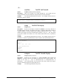
Program Flow Control and Relational Operators
The if, if-else, and while statements are used in ProVIEW to alter the flow within a
script file or to cause iteration. The range of each of these statements is a compound
statement consisting of statements enclosed in brackets.
IF Statement
if( expression ){
statements
}
if( expression ){
statements
ProView User’s Manual
MSHELL Interpreter Language • 43
} else {
statements
}
The if statement causes execution of its compound statements if and only if the
relation in the expression results in a non zero value.
The if-else has two groups of compound statements. If the relation in the expression
returns a non zero value , the first group of statements is executed otherwise the
second group of statements is executed.
An early exit from an ’if’’ block can be performed using the ’ifbreak’ statement.
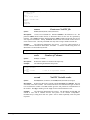
While Statement
while(expression){
statements
}
The while statement causes repeated execution of its statements as long as the
expression results in a non zero value. The relation is tested before each execution of
its range and if the relations is false, control passes to the next statement beyond the
range of the while statement.
The traditional ’for’ statement used in the C language, i.e.
for( expression1 ; relation ; expression2){
statements
}
can be constructed using the while statement as:
expression1
while(relation){
statements
expression2
}
An early exit from a while loop can be performed using the ’wbreak’ statement.
Control Expression with Numeric Values
The statements in an ’if’’ or ’while’ block are executed depending on the value returned
by the control expression. The control expression can include relational, equality, and
logical expressions.
Always use parenthesis
when using relational,
logical, or equality
operators. Do not
assume a specific
precedence.
Relational, logical, and equality operators all have the same precedence. Hence,
parenthesis should be used to obtain the desired groupings. For example, in the
following statement there is no ambiguity due to the use of parenthesis,
if( (i==4.8) && (p<3) ){
x=y ;
}
Relational Operators
The expression syntax when using a relational operator is:
44 • MSHELL Interpreter Language
ProVIEW User’s Guide
expression1 rel-op expression2
where the relational operators are:
<
less than
>
greater than
<=
less or equal to
>=
greater or equal to
Equality Operators
The expression syntax when using an equality operator is:
expression1 equality-op expression2
where the equality operators are:
==
test for equality
!=
test for inequality
Logical Operators
The expression syntax when using a logical operator is:
expression1 logical-op expression2
where the logical operators are:
&&
logical and
||
logical or
Control Expression with Strings
The following are the valid comparisons that can be done with strings:
$s1==$s2
$s1!=$s2
$s1<$s2
$s1>$s2
Remember that these type of comparisons are only meaningfull if used within the
control expression in a ’while’ or ’if’ statement. For example, the following code
performs a test on the string $a and displays itself as an image depending on the result
of the test:
$a="hello"
if($a=="hello"){
x = text2image($a);
view x;
}
Look-Up-Table Manipulation
Look-up-tables are primarily used to map intensity values displayed on the screen.
Output LUTs have 256 entries numbered 0 through 255 corresponding to the 256
possible different intensity values or colors.
ProView User’s Manual
MSHELL Interpreter Language • 45
Output LUTs
Before an image in memory is displayed on the screen, it goes through an output
LUT. The image’s pixel values are used as indices into the output look-up-table, the
output of which is displayed on the screen. Image data is transformed through the
currently selected output LUT whenever an image is being displayed on the screen.
Using the ‘select’ command, the user can select which is the active output look-uptable. For example, to select olut3 as the active LUT use the following command,
select wolut3
The user can read the first 3 output look-up-tables. For example,
x= wcolut0;
/* copy olut0 into x */
Inspecting x will show that it corresponds to 3 rows of data, each row with 256 entries
corresponding to the red, green, and blue components of the pseudo-color LUT.
Look up table wcolut3 is a user defined output look-up-table, e.g.
/* wcolut3 is set to the histogram equalization
LUT of image X
*/
wcolut3 = heqlut(X);
The following lines modify wcolut3 to provide intensities of red:
/* initialize wcolut3 */
red = (0,255,1);
green = (0,255,1);
blue = (0,255,1);
wcolut3 = red # 0*green # 0*blue;
ProVIEW Script Files (.msf,.msh,.vsh)
Script files provide a powerful tool to achieve repetitive processing tasks in a simple
manner.
There are two types of script files in ProVIEW, i.e. FUNCTION files and Include
files.
Function Files (.msf)
A ProVIEW FUNCTION file, or external function, permits the user to define its own
functions using the ProVIEW language syntax. Local variables defined within a
FUNCTION file are automatically erased by the ProVIEW interpreter when the script
file is finished.
Syntax
A valid ProVIEW FUNCTION must follow the following rules:
46 • MSHELL Interpreter Language
ProVIEW User’s Guide
•
function names must be limited to eight characters.
•
The instructions of a ProVIEW FUNCTION must be stored in a file with
the same name as the function, e.g. if the function name was MYFUNC,
then the file name must be MYFUNC.MSF. Notice the addition of the
’.msf’ extension.
•
Only one function per file.
•
Array and string variables can be used as input and output arguments.
•
If a variable is not defined at the present function level the interpreter
will look for it at the previous function level. If the variable is not found
there it will keep looking for it at the next function level until it
encounters the variable or stops with an error.
•
The first eight characters in the file must be the string FUNCTION
follow by the list of output arguments, equated to the function name,
and followed by the list of input arguments.
The following is a simple ProVIEW FUNCTION file.
FUNCTION [out1,out2]=MYFUNC[in1,in2,in3,$in4]
/* This is a dummy function */
LOCAL a b
a = 10*in1; b = 3*in2;
“The string passed was “::$in4
out1 = in1-in2
out2 = in1*.in2*.in3 - a + b
Notice that the variables ’a’ and ’b’ in the above example only exist during the duration
of subroutine.
Variables needed within the function must be passed to the function and new variables
not implicitly declared in the calling statement should then be declared within the
function using the LOCAL statement.
An actual call to the above example function could be,
x= hammiw(32,32)
y = gtclipto(x,0.5,0.5)
z = x-y
[res1, res2 ] = MYFUNC[ x,y,z]
where res1 and res2 will contain the result to the external function call.
Include Files (.msh)
Include files are not function files, hence they do not erase local variables upon
termination. Include files are simpler than ProVIEW Function files and are not
constrained by the FUNCTION rules. The user may think of an include file as a
sequence of commands that can be invoked with a simple include call. Typically
include files are saved to disk with the extension ’.msh’.
Virtual Include Files (.vsh)
A modification to the standard ‘.msh’ is the ‘.vsh’ extension; this allows ProVIEW to
automatically execute the entire contents of the script when opened using the
Image|Open menu item or ‘reada’ syntax of ProVIEW.
ProView User’s Manual
MSHELL Interpreter Language • 47
Example - movie.msh
Using a script file a sequence of image files residing in disk can be read, display, and
processed under the control of a script file. In this example a list of file names of type
’bmp’ is assumed to exit. This script file can be used as a building block for creating
more complex movie-like script files.
$
// read input list of image files, ’rm.lst’, from hard disk
list = readtext("../images/rm.lst");
// print number of lines in input list
nlines(list);
// initialize the variable ’out’ to zero and view it
out =0
view out
// start a loop to load every image in ’rm.lst’ for viewing
//
the variable ’i’ will be used as the loop index
i = 0;
while(i<nlines(list)-1){
infile ="../images/"::list(i,:);
infile
out = reada(infile,"char");
i = i+1;
// if at end of list reset ’i’ to start again. This
//
script file must be stopped using the
//
ESC key or the STOP sign icon.
if(i==nlines(list)-1){
i = 0;
}
}
48 • MSHELL Interpreter Language
ProVIEW User’s Guide
Importing and Exporting Data
Importing Data into ProVIEW
ProVIEW can read image or array data in a number of different output formats, see
"File|Open Image - File Format" on page 19.
Exporting Data out of ProVIEW
ProVIEW can write image or array data in a number of different output formats, see
"File|Open Image - File Format" on page 19.
Data stored in the ProVIEW’s char and float format contains a simple 9 byte header.
The first 4 bytes contain the number of rows, the next 4 bytes contain the number of
columns, and the last byte contains a flag indicating if the data is real or complex.
ProView User’s Manual
MSHELL Interpreter Language • 49
Internal Functions
The user can locate a specific function by first looking into the Classes of ProVIEW’s
Built-in Functions where commands are divided into functional areas, see Appendix
A.
Given a function name or symbol the user can locate specific information about its
use under the alphabetical listing of internal functions, see Appendix B.
ProVIEW array expressions can be used as arguments to other ProVIEW functions.
In most of the following functions the input to the functions are arrays and the output
result is another array.
Classes of Built-in Functions
*
*
*
*
*
*
*
*
*
*
*
*
*
*
*
50 • MSHELL Interpreter Language
+---Animation
+---Demo
+---Filtering
|
+---Freq_Ops
|
|
+---DCT
|
|
\---FFT
|
\---Spatial_Ops
|
+---Correlation_Ops
|
+---Gradient_Ops
|
+---Local_Statistics
|
+---Morphological
|
+---Resampling
|
|
+---Interpolation
|
|
\---Irregular_Sampling
|
+---Resolution_Enhancement
|
\---Spatial_Blurring
+---Fitting_and_Estimation
+---Fractals
+---Geo_Xform
|
+---Rot2D
|
\---Rot3D
+---HTML_Tools
+---Intensity_Mapping
+---Look-Up-Table Operators
|
\---Radiometric
+---IO
|
\---Data_Formats
|
+---aess
|
+---Ceos
|
+---pds
|
+---ppm
|
+---Raw
|
+---Virtual
|
+---vpf
|
\---NetCDF
+---Matrix_Vector_Algebra
+---Mensuration
+---PHIT
|
\---Hyperspectral
+---Plot
+---Region_Ops
ProVIEW User’s Guide
*
*
*
*
*
*
*
*
*
*
*
*
*
*
*
ProView User’s Manual
|
+---Groi_Logical
|
+---Interactive_Selection
|
+---Overlapping_Regions
|
\---Row_Manipulations
+---Satellite_Image_Mapping
|
+---Coordinate_System_Xform
|
+---Mosaics
|
+---Spherical_Geometry
|
\---Vector_Projection
+---Statistics
|
\---Sorting
+---String_Ops
+---System
+---Trigonometric Functions
\---Useful
+---Data_Formatting
+---Flow Control and Relational Operators
\---Image Display
+---Image Attributes
\---Image Window Attributes
MSHELL Interpreter Language • 51
Math Error Handling
In MSHELL floating point exceptions generate either results in the form of NOT-ANUMBER (NAN), infinity (+INF), or minus infinity (-INF). The user must inspect
an array for such an occurance to determine if invalid number are present in the array.
The example below illustrates manipulations that result in NAN or +INF or -INF.
The user can control how math related errors are reported using the system variable
‘M_matherrflag’ described under M_ in Appendix B.
[ready]: cos(1e38)
-NAN
[ready]: 1/0
+INF
[ready]: -1/0
-INF
[ready]: 0/0
-NAN
[ready]: x = 1/0 :: 0/0
[ready]: x(0,0)
+INF
[ready]: x(0,1)
-NAN
[ready]: log(0)
-INF
[ready]: log(-1)
0 + 3.14159i
[ready]: 0^0
1
[ready]: y = 0::1::2:: (0/0)
[ready]: y
(10^0) X
row 0 =
0.00
1.00
2.00
-NAN
[ready]: z = 0::1::2:: (1/0)
[ready]: z
(10^0) X
row 0 =
0.00
1.00
2.00
[ready]: eqindex(y,1/0)
3 + 0i
52 • MSHELL Interpreter Language
+INF
ProVIEW User’s Guide
Extendibility of the Environment
In addition to the internal funtions included and listed above you can further extend
the capabilities of ProVIEW by:
•
Accessing your own ’C’ funtions or by
•
Accessing other applications that support Dynamic Data Exchange.
Dynamic Data Exchange
ProVIEW is capable of communicating with other applications that support dynamic
data exchange (DDE). The following ProVIEW commands are used to establish
communications links with other applications via DDE.
DDEInit - this command is used to start a conversation on a particular topic
with the server application. Syntax: chan = DDEInit(“Application
Name”,”Topic”). “Application Name” is the name of the application
you want to communicate with (Ex. MSAccess), and “Topic” is the
name of the particular topic. This command returns a channel number
associated with the conversation you are requesting or -1 if the operation
fails.
DDETerm - this command terminates a conversation.
DDETerm(chan). chan is the number returned by DDEInit.
Syntax:
DDEExec - this command is used to send a command to the server
application once the DDE conversation is established. Syntax:
DDEExec(chan,cmd). chan is the channel number returned by DDEInit,
and cmd is a string you want the server to execute. DDEExec will return
0 if the server accepted the command, 1 otherwise.
DDEPoke - this command is used to request the server application to accept
an unsolicited data item value. Syntax: DDEPoke(chan,item,val). chan
is the channel number returned by DDEInit, item is a string that
identifies the data item you wish to send a value for, and val is a string
containing the value. DDEpoke will return 0 if the server accepted the
data item value, 1 otherwise.
DDEReqS - this command is used to request the server application to
provide the value of a data item. Syntax: $var = DDEReqS(chan,$item).
$var is a ProVIEW string variable, chan is the channel number returned
by DDEInit, and item is a string that identifies the data item you are
requesting the value of.
DDEReqV - this command is used to request the server application to
provide the value of a data item. Syntax: var = DDEReqV(chan,$item).
‘var’ is a ProVIEW array variable, chan is the channel number returned
by DDEInit, and item is a string that identifies the data item you are
requesting the value of.
Example: Using ProVIEW scripting language
ProView User’s Manual
MSHELL Interpreter Language • 53
$path = "M:\\NEWINDEX\\BYACCESS\\"
$database = "CL_0001"
/* Open Database */
chan1 = DDEInit("MSAccess","System")
$command = "[OpenDatabase "::$path::$database::".MDB]"
$command
DDEExec(chan1,$command)
DDETerm(chan1)
/* Query Database */
$topic = $database::";SQL"
chan1 = DDEInit("MSAccess",$topic);
$temp = "SELECT NEW_IMAGENAME";
status= DDEPoke(chan1,"SQLText",$temp);
$temp = " FROM header";
status=DDEPoke(chan1,"SQLText",$temp);
$temp = " WHERE ("
status=DDEPoke(chan1,"SQLText",$temp);
$temp = "([SENSOR_NAME]=\"UVVIS\")
status=DDEPoke(chan1,"SQLText",$temp);
$temp = " AND ([FILTER]=\"B\") AND ([MISSION_PHASE]=\"LUNAR AND MAPPING\")"
status=DDEPoke(chan1,"SQLText",$temp);
$temp = " AND (([CENTER_LATITUDE]>=14.0) AND ([CENTER_LATITUDE]<=35.0))"
status=DDEPoke(chan1,"SQLText",$temp);
$temp = " AND (([CENTER_LONGITUDE]>=25.0) AND ([CENTER_LONGITUDE]<=30.0))"
status=DDEPoke(chan1,"SQLText",$temp);
$temp = ");"
status=DDEPoke(chan1,"SQLText",$temp);
$res = DDEReqS(chan1,"Data");
if ( strlen($res) > 0 ) {
$query = $query::"\n"::$res
}
DDETerm(chan1);
54 • MSHELL Interpreter Language
ProVIEW User’s Guide
User Provided Functions as Dynamic Link Libraries (DLL)
ProVIEW permits the users to provide their own functions via dynamic link libraries.
Following are the steps required to make use of this capability.
First, write a C program containing the code you want to execute. Include user.h in
the header section; user.h is included as part of the installation. The functions that can
be called from ProVIEW must conform to the following declaration: ARRAY
*fname(ARRAY *, ARRAY *, ARRAY *, ARRAY *, ARRAY *), where ARRAY is
a data structure defined in user.h. Note that the declaration requires five ARRAY*
inputs but the user need not use the five inputs. The functions the user wants to call
from ProVIEW must be exportable.
Second, generate a 32-bit dynamic link library. The C compiler/linker you use must
be able to generate a 32-bit DLL. Consult your compiler reference manual.
Note: The memory allocation routines that ProVIEW uses are contained in mem.dll.
If you plan to use memory allocation routines in your code (i.e., malloc, calloc,
realloc, free, strdup) it is strongly recommended that you use instead the functions
contained in mem.dll (i.e., NewMalloc, NewCalloc, NewRealloc, NewFree,
NewStrdup). The file prvmem.h is provided with the ProVIEW installation. Include
it in your source code if you are going to make use of the mem.dll memory allocation
routines. If you are using Microsoft Visual C++, include the import library memvc.lib
in your project. If you are using Borland C/C++, include the import library membc.lib
in your project. Both memvc.lib and membc.lib are included as part of the ProVIEW
installation.
From within ProVIEW’s Command Shell Window register the DLL using the
following command: loadDLL($fullpath\\$dllname), where $fullpath is the path to the
DLL including drive letter, and $dllname is the name of the DLL. Note that loadDLL
will return 0 if the DLL is successfuly loaded and 1 otherwise.
Call the function in the DLL using the following ProVIEW command:
callDLL(“$dllname”,”$functionname”,arg1,arg2,arg3,arg4,arg5). “$functionname” is
the name of the function in the DLL you want to call; arg1, arg2, arg3, arg4 and arg5
are the arguments you want to pass to the function.
Example: On the next page.
ProView User’s Manual
MSHELL Interpreter Language • 55
Example of User Provided Functions as Dynamic Link Libraries
#include <stdio.h>
#include "user.h"
#ifdef __BORLANDC__
ARRAY* _export test(ARRAY *a1, ARRAY *a2, ARRAY *a3, ARRAY *a4, ARRAY *a5);
#endif
#ifdef _MSC_VER
__declspec( dllexport ) ARRAY* test(ARRAY *a1, ARRAY *a2, ARRAY *a3, ARRAY *a4, ARRAY
*a5);
#endif
/*********************************************************************/
--- Include the following two functions in your code. ProVIEW will call --- SetInitA and SetFree upon
loading the DLL to pass the addresses of --- the functions inside ProVIEW that InitA and Free will call. It is
--- very important that you initialize variables of type ARRAY* using --- InitA. You must pass to InitA a
name you want to assign to
--- the variable, the number of rows, the number of columns, and the
--- type (0-real, 1-complex).
**********************************************************************/
void SetInitA(void *fn)
{
_InitA = (ARRAY* (*)(char *ptr, unsigned long sizej, unsigned long
type))fn;
}
sizei,
unsigned
char
void SetFree(void *fn)
{
_Free = (void (*)(ARRAY *a))fn;
}
/*********************************************************************/
ARRAY* test(ARRAY *a1, ARRAY *a2, ARRAY *a3, ARRAY *a4, ARRAY *a5)
{
UN32 i, j;
ARRAY *c;
c = InitA("test",a1->sizej,a1->sizei,0);
if( c )
{
for(i=0; i<a1->sizej; i++)
{
for(j=0; j<a1->sizei; j++)
{
c->re[i][j] = a1->re[i][j] + 10.0;
}
}
}
return c;
}
56 • MSHELL Interpreter Language
ProVIEW User’s Guide
In ProVIEW Command Shell Window:
[ready]: loadDLL("d:\\proview.40\\user\\test.dll")
0
[ready]: x = hammiw(8,8)
[ready]: y = callDLL("test.dll","test",x,0,0,0,0)
[ready]: show x
--- x --data type is
: real
number of rows = 8
number of columns = 8
maximum value = 1
minimum value = 0.0064
[ready]: show y
--- y --data type is
: real
number of rows = 8
number of columns = 8
maximum value = 11
minimum value = 10.0064
[ready]: _
ProView User’s Manual
MSHELL Interpreter Language • 57
ProVIEW Web Interface
ProVIEW Web is a CGI application that parses and processes field = value pairs. ProVIEW Web can be invoked as a
result of an user submitting a form, or explicitly as
provweb.exe?_xtype=value&field1=value1&field2=value2&…&fieldn=valuen. The ‘&’ character is used to delimit
the various field = value pairs. Note that since the ‘=’ character is used to separate the field, value pair, you can not use it
explicitly in either the field or value parameters. If you need to use the ‘=’ character in the value parameter, for instance,
you must encode it using the ‘%’ character followed by the hexadecimal representation of its ASCII value (i.e., %3D).
Also the ‘+’ character is used to denote a white space, so if you need to use the ‘+’ character in the value parameter, you
must encode it as %2B. Below are examples of incorrect and correct usage.
Incorrect
provweb.exe?cmd1=x = 5
provweb.exe?cmd2=y = x + 5
provweb.exe?subject=”Hello World!”
Correct
provweb.exe?cmd1=x+%3D+5
provweb.exe?cmd2=y+%3D+x+%2B+5
provweb.exe?subject=”Hello+World!”
The table below shows how ProVIEW Web interprets various field = value instances. The _xtype=value is optional, and
is used to define the content type returned by ProVIEW Web. If omitted, the content type is text/html, with the <Title>,
<Head> and <Body> tags already predefined. If you specify _xtype=text/html when invoking provweb.exe, you are
expected to provide the <Title>, <Head> and <Body> tags as part of the output of ProVIEW Web.
Field = value
fieldname = value1
Internal Representation
$fieldname = value1
Example:
myname=Joe+Smith
cmd???… = value2
Example:
$myname = “Joe Smith”
value2
Example:
cmd1=x+%3D+5;+show+x;
name.x = value1
name.y = value2
Example:
x = 5; show x;
name_x = value1
name_y = value2
Example:
image1.x=100
image1.y=200
Example:
image1_x = 100
image1_y = 200
Description
ProVIEW Web internally creates a
string variable with the same name
as the field item and sets the value
to the value item
when the field item starts with
‘cmd’, ProVIEW Web uses the
value item as a command to be
executed
when the user clicks on an image
map the x and y values of the
location where the mouse clicked
are passed. ProVIEW Web creates
two variables using the name of the
image to store these values
ProVIEW Web also generates a string variable called $ipaddr which contains the ip address of the client submitting the
form. $ipaddr can be used in script files to keep track of users accessing ProVIEW Web.
Elements of Forms
There are three types of HTML tags you use to create fields in a form: TEXTAREA, SELECT, and INPUT.
TEXTAREA
With TEXTAREA you can provide a field for someone to enter multiple lines of information. NAME is a required option
for this tag. By setting the NAME to a name starting with ‘cmd’ you can use this field to enter multiple commands for
ProVIEW Web to execute.
58 • MSHELL Interpreter Language
ProVIEW User’s Guide
SELECT
The SELECT element shows a list of choices in either a pop-up menu or a scrollable list. Just like the TEXTAREA
element, the SELECT tag requires you to define a name. There are two possible courses of action depending upon the
name used in the NAME property: (a) if the name starts with ‘cmd’, ProVIEW Web uses the item selected from the list of
choices as a command to be executed; or (b) ProVIEW Web creates a string variable whose value is the item selected.
INPUT
INPUT is a single tag option for gathering information. INPUT contains other options for acquiring information including
simple text fields, radio buttons and checkboxes.
TEXT - the default input type, displays a simple line of text.
CHECKBOX - displays a simple checkbox that can be checked or empty.
RADIO - a more complex version of a checkbox, allows only one of a set to be chosen.
In all of the above INPUT types, by setting the NAME property to a name starting with ‘cmd’ you can instruct ProVIEW
Web to execute a command or set of commands depending on the value of the VALUE property of the INPUT type as
described previously. Otherwise, ProVIEW Web creates a string variable whose value depends on the INPUT type. In the
case of TEXT the value is the text entered by the user. In the case of a CHECKBOX or a RADIO the value is the string
assigned to the VALUE property.
EXAMPLE:
…
<PRE>
<FORM ACTION="http://www.acme.com/cgi-bin/provweb.exe" METHOD=GET Target=”South”>
Latitude: <INPUT NAME=lat VALUE=36.1216>
Longitude: <INPUT NAME=lon VALUE=-5.903>
<INPUT TYPE="HIDDEN" NAME=cmd VALUE='include "test"'>
<INPUT TYPE="SUBMIT" VALUE="Submit">
</FORM>
</PRE>
…
When the user clicks on the Submit button, the client browser will generate a call to provweb.exe as follows:
provweb.exe?lat=36.1216&lon=-5.903&cmd=include+”test”
ProVIEW Web will interpret the various field = value pairs as follows:
Field = Value
lat=36.1216
lon=-5.903
cmd=include+”test”
Translation
$lat = “36.1216”
$lon = “-5.903”
include “test”
If the contents of the script file ‘test.msh’ is as follows:
show all
$lat
$lon
$coord = "("::$lat::","::$lon::")"
"\nThe coordinate you selected is:"::$coord
"\n<H2>Thanks for using ProVIEW Web</H2>"
,then the output of ProVIEW Web (bottom frame) looks like this:
ProView User’s Manual
MSHELL Interpreter Language • 59
60 • MSHELL Interpreter Language
ProVIEW User’s Guide
Recent Changes
Recent Changes that have been made to the ProVIEW functions will be documented
here as well as a listing of their date of effectiveness.
Added Functions
At this time no new functions have been added to the ProVIEW Imaging System.
Further functions will be listed here.
Updated Functions
ProView User’s Manual
MSHELL Interpreter Language • 61
Appendix A : Function Tree
(By Category)
Of
ProVIEW’s MSHELL
Interpreter
Introduction
With over 140 internal functions and over 100 external functions, ProVIEW
is an extremely powerful and flexible environment in which to perform signal and
image processing. This appendix, in conjunction with Appendix B and the HTML
based external function list, is your guide and quick reference to these functions.
While this appendix lists the categories by which ProVIEW’s functions are organized,
it also contains information as to the listings of the internal and external functions
within these categories.
The internal functions contained within the categories are marked by the
asterisks below in the list. The external function list can be seen by linking to the
following web address: http://www.actgate.com/proview/help/msf/default.htm.
For detailed descriptions and examples of the internal functions, see
Appendix B. The detailed descriptions and realtime examples of the external
functions can be seen at the above mentioned web address.
Categories of ProVIEW’s MSHELL Functions
The over 140 internal functions currently supported by ProVIEW’s MSHELL
interpreter are divided into the following categories marked with an *. The external
functions are also divided among this list; they can be seen online via the above link.
The following represents the master tree whereby all functions, both internal and
external, are categorized.
*
*
*
*
*
*
*
*
*
A-64•Appendix A : Function Tree
+---Animation
+---Demo
+---Filtering
|
+---Freq_Ops
|
|
+---DCT
|
|
\---FFT
|
\---Spatial_Ops
|
+---Correlation_Ops
|
+---Gradient_Ops
|
+---Local_Statistics
|
+---Morphological
|
+---Resampling
|
|
+---Interpolation
|
|
\---Irregular_Sampling
|
+---Resolution_Enhancement
|
\---Spatial_Blurring
+---Fitting_and_Estimation
+---Fractals
+---Geo_Xform
|
+---Rot2D
|
\---Rot3D
+---HTML_Tools
+---Intensity_Mapping
+---Look-Up-Table Operators
|
\---Radiometric
ProVIEW User’s Manual
*
*
*
*
*
*
*
*
*
*
*
*
*
*
*
*
*
*
*
*
*
ProView User’s Manual
+---IO
|
\---Data_Formats
|
+---aess
|
+---Ceos
|
+---pds
|
+---ppm
|
+---Raw
|
+---Virtual
|
+---vpf
|
\---NetCDF
+---Matrix_Vector_Algebra
+---Mensuration
+---PHIT
|
\---Hyperspectral
+---Plot
+---Region_Ops
|
+---Groi_Logical
|
+---Interactive_Selection
|
+---Overlapping_Regions
|
\---Row_Manipulations
+---Satellite_Image_Mapping
|
+---Coordinate_System_Xform
|
+---Mosaics
|
+---Spherical_Geometry
|
\---Vector_Projection
+---Statistics
|
\---Sorting
+---String_Ops
+---System
+---Trigonometric Functions
\---Useful
+---Data_Formatting
+---Flow Control and Relational Operators
\---Image Display
+---Image Attributes
\---Image Window Attributes
Appendix A : Function Tree • 65
Appendix B : Internal Functions
(Alphabetical Listing)
Of
ProVIEW’s MSHELL
Interpreter
ProVIEW’s MSHELL Internal Functions (by Category):
A complete list, by category, of the the internal functions is presented on the following pages
Filtering
blackw
hammiw
Blackman-Harris window
Hamming window
Freq_Ops
DCT
dct2
dct8x8
idct2
idct8x8
computes the 2D DCT of each 8x8 block of an image
computes the DCT of each 8x8 block of an image
computes the inverse 2D DCT of a previous 2D DCT
computes the inverse DCT of a previous DCT
fft
fft2
ifft
ifft2
one dimensional Fourier transform
two dimensional Fourier transform
inverse one dimensional Fourier transform
inverse two dimensional Fourier transform
FFT
Spatial_Ops
Correlation_Ops
convol
convolt
spatf
xcorr
xcorrfft
xcorrt
convolutes an array with a kernel
truncated convolution
general spatial filter module
compute cross correlation between two arrays
computes the cross-correlation between FFT’s
truncated cross correlation between arrays
Local_Statistics
covm
gauss
hist
hist255
qgauss
qgaussinv
randg
randinit
randu
covariance matrix estimation
compute the Gaussian density function
histogram of array elements
histogram of array elements (255 levels)
area under Gaussian density function
inverse of qgauss
gaussian random number generator
initialize random number generator
uniform random number generator
Morphological
skeleton
a binary conversion filter
Resampling
Interpolation
blinterp
linterp
zinterp
bilinear interpolation
linear interpolation
zero-order interpolation
Geo_Xform
cmirror
rmirror
shiftc
shiftt
mirror image columns
mirror image rows
perform a cyclic translation
perform a non-cyclic translation
Intensity_Mapping
Look-Up-Table Operators
heqlut
hyplut
select
wcolut[#]
wolut[#]
B-68•Appendix B : Internal Functions
uniform histogram equalization look-up-table
hyperbolic histogram look-up-table
used to select an output look-up table for an image
complete user definition of output look-up-tables
user-defined output look-up-table
ProVIEW User’s Manual
xlut
transform input through a look-up-table
IO
callDLL
calls a DLL for execution after having been loaded
closef
close a file previously opened with ’openf’
dbclose
closes the connection to a database
dbconnect
creates a connection to a local or network database
dbsqltr
posts a formatted string to the database for submission
DDEExec
Dynamic Data Exchange execution
DDEInit
Dynamic Data Exchange initialization
DDEPoke
Dynamic Data Exchange polling
DDEReqS
Dynamic Data Exchange request returned as a string
DDEReqV
Dynamic Data Exchange request returned as a vector
DDETermDynamic Data Exchange termination
END
ends execution of a script
iboxlist
allows for choice of input options
include
invoke a ProVIEW script file
inputbox
input a value from keyboard into a list
load
load arrays from disk
loadDLL
loads a DLL into memory and registers it with ProVIEW
openf
open a file
print
print values to standard output
reada
read an array from disk
readf
read from a file
readtext
reads text from an ascii file
return
stops execution of a script file
save
save arrays to disk
writea
write an array to disk
writecolor
writes a color .bmp file from 3 ind. Arrays
writef
write to a file
Data_Formats
Virtual
V
Vclose
Vnew
Vopen
Virtual Variable
closes the above link between "V" and a disk file
allocates disk space for the above virtual link
links between the virtual variable "V" and the disk
vec2image
Vpftblinfo
converts a “.vec” format to a proview image
returns vpf table database info
VPF
Shapefile
getshpinfo
shp2contour
shp2fillimage
Get shapefile header information
Shapefile to contour image
Shapefile fill image
Matrix_Vector_Algebra
'
#
*
*.
/
/.
:
::
^
+
=
abs
ceil
complex
conj
exp
floor
fmod
ProVIEW User’s Guide
array subtraction
array transpose
column augmentation
array multiplication
corresponding elements array multiplication
array division
corresponding elements array division
select an interval of rows or columns
row augmentation
a^b , a raised a to power b
array addition
assignment operator
absolute value of array elements
returns the ceiling for each element of an array
used to define a complex vector (a,b)
conjugate of array elements
e raised to each array element
returns the floor for each element of an array
floating point modulus
Appendix B : Internal Functions
B-69
imag
int
invm
log
log10
makecmplx
nint
real
sign
sqrt
sum
sumc
sumcum
sumr
svd
trace
imaginary part of array elements
integer part of array elements
array inverse
natural log of array elements
log base 10 of array elements
makes a scalar into a complex vector
nearest integer of array elements
real part of array elements
sign of array elements
square root of array elements
sum of all array elements
sum columns
row wise cumulative sum of array elements
sum rows
computes the singular value decomp. of an array
sum diagonal elements
colplot
contour[#]
dworld[#]
plot
plot2image
plot3d
rowplot
view4d
plots a given column from an array
contour plot of an array
extracts a latlong region from the world database
plot a row vector, complex or real
uses coords. and intensity to form a shaded image
mesh plot or 3d plot of an array
plots a given row from an
produces a 3d image which is given height by another
Plot
Region_Ops
aoi
bresen
ladd2groi
pixval
rfill
text
vroi
wdef
wmove
wsize
xline
xlinec
xlinev
xpolyc
xpolyv
lists pixel values within active region of interest
compute line segment between two points
local addition to generalized region of interest
pixel value and mouse status in an image
fills determined polygons with roi’s
used to add text to an array for later display
variable region of interest
define a region of interest
move a region of interest
dimensions of a rectangular region of interest
extract values along a line
extract coordinate points of a line
extract vertices points (end points) of a line
extracts coordinate points of a polygon
extracts vertices of a polygon
Groi_Logical
regionand
defines a roi which is the common area of two roi's
Interactive_Selection
inputfocus
setroi
varname
puts focus to a specific variable for interactive selection
allows for interactive selection of an roi using the mouse
returns the variable name of a variable
Overlapping_Regions
cmplxoverlap
finds the overlapping locations within another roi
Satellite_Image_Mapping
SatVIEW
SatVIEWpix
computes spacecraft image geometry for the corners
computes spacecraft image geometry for listed points
Statistics
mean
median
medianr
momentr
B-70•Appendix B : Internal Functions
mean of array elements
median of array elements
median along the row of array elements
moment computations along rows
ProVIEW User’s Manual
rcoeff
stats
var
correlation coefficient between two arrays
computes basic statistics
variance of array elements
Sorting
bthresh
eqindex
geclipto
geindex
gtclipto
gtindex
index
leclipto
leindex
ltclipto
lthresh
ltindex
max
maxmin
maxof
maxr
min
minof
minr
rindex
sortr
binary threshold of array elements
index of elements with a specific value
clip values above and including threshold
index of array elements above a given value
clip values above threshold
index of array elements above a given value
index of non-zero elements in array
reset values below and equal to threshold
index elements less or equal to a given value
reset values below threshold
sets the values less than tresh to the thresh
index elements lower than a given value
maximum of array elements
maximum and minimum of array elements
element by element maximum
returns the maximum for each row
minimum of array elements
element by element minimum
returns the minimum for each row
index all elements within a specified range
sort array elements row wise
String_Ops
${string}
$str(#:#,#:#,)
/* ... */
//
\
\\
eqindexS
float2str
getline
getpos
int2str
itoa
nlines
smodify
str2float
str2int
strlow2up
strup2low
used to define a string variable
returns a subregion of a string
included multi-line comment
single-line comment
used as a control character within strings
line continuation
returns the complex position of each occcurence
convert a floating point number to a text string
returns the line # of of the desired text within a string
returns the index of the desired text within a string
convert an integer number to a text string
convert an integer number to ascii(text)
returns the number of lines contained within a string
used to perform a search and replace within a string
convert a number from ASCII to float
convert a number from ASCII to integer
outputs a string which is the “uupercase” of the input
outputs a string which is the “lowercase” of the input
System
addmenuitem
all
evaltext
exit
fileinfo
filesize
findfiles
free
getenv
help
M_(command)
mbox
menusel
meter
show
system
vartype
ProVIEW User’s Guide
used to add a user-defined menu to the menu bar
used with “free” and “show” for all variables
used to evaluate a string for functionality
exit the ProVIEW interpreter
returns detailed file information
returns the size of a file in bytes
used to find a particular file or group of files
erase an array from memory
returns desired environment variable value
used to call the ProVIEW help directory
System Variables
brings a dialog box onto the screen with the specified text
used to select a menu item within an iboxlist
used to show percent of completion within a loop
display variables information
calls a DOS shell from within ProVIEW
returns the type of the chosen variable
Appendix B : Internal Functions
B-71
Trigonometric Functions
acos
asin
atan{r}
atan2{x,y}
cos
cosh
sin
sinh
tan
tanh
arccosine of array elements
arcsine of array elements
arctangent of array elements
arctangent of value, preserving quadrant specifics
cosine of array elements
hyperbolic cosine of array elements
sine of array elements
hyperbolic sine of array elements
tangent of array elements
hyperbolic tangent of array elements
Useful
(a,b,d)
decimate
geo
ident
ones
sinc
zeros
generate a 1-d or 2-d ramp
decimate an array
geometric series
generate a square identity array
generate an array of all ones
compute the sinc function
generate an array of all zeroes
Data_Formatting
convtoi
convtov
ncols
nrows
scale255
zeropad
convert row vector to image
convert a 2-d array to a one dimensional one
return number of columns in an array
return number of rows in an array
scale input to fit in the range of 0-255
add zeroes to an array
Flow Control and Relational Operators
!=
&&
||
<
<=
==
>
>=
ifbreak
if-else
pause
while
test for inequality
logical and
logical or
less than
less than or equal to
test for equality
greater than
greater than or equal to
exit if-block immediately
if-else statement
pause ProVIEW’s execution
while statement
Image Display
Image Attributes
text2image
textoverlay
textremove
converts text to image form
used to add a text annotation to an image
used to remove a text annotation from an image
Image Window Attributes
m_dx
m_dy
m_interpflag
m_viewflag
m_viewheight
m_viewhscroll
m_viewlut
m_viewmaxval
m_viewminval
m_viewvscroll
m_viewwidth
m_viewx0
m_viewy0
m_x0
m_xunit
m_y0
m_yunit
wclose
B-72•Appendix B : Internal Functions
used to define horizontal spacing between pixels
used to define vertical spacing between pixels
selects the type of interpolation to use on an array
toggles whether an image is to be viewable or not
defines the height of the display window
defines the horizontal scroll position for a window
defines the active look-up table for an image
defines the maximum to be displayed
defines the minimum to be displayed
defines the vertical scroll position for a window
defines the width of the display window
defines the upper left horizontal window position
defines the upper left vertical window position
used to definehorizontal position of upper left pixel
used to define a string of horizontal units
used to define vertical position of upper left pixel
used to define a string of vertical units
used to close a specific window
ProVIEW User’s Manual
wtile
ProVIEW User’s Guide
used to tile the existing windows
Appendix B : Internal Functions
B-73
Internal Functions - Alphabetical List
Much of ProVIEW’s power resides in the MSHELL Interpreter. With over 140
internal commands, ProVIEW has a flexible structure that readily permits tailoring to
specific applications through User Defined external functions and script files
This appendix is an alphabetical listing with descriptions and examples of all the
current ProVIEW/MSHELL Internal Functions.
- Symbols (a,b,s[,n])
Syntax:
Generate a 1-D or 2-D ramp
(start_value, end_value, step_size)
1-D
(start_value, end_value, step_size, number_of_rows)
2-D
Description:
returns a 1-D or 2-D ramp of values
Example:
function.
The following applications illustrate the use of the 1-D and 2-D ramp
[ready]:
0.00
[ready]:
0.00
[ready]:
3.00
3.00
[ready]:
[ready]:
(0,3,1)
//generate a 1-D row
1.00
2.00
3.00
(0,1,0.2)
// generate 1-D row with fractional step size
0.20
0.40
0.60
0.80
(3,0,1,2)
// generate a 2-D matrix
2.00
1.00
0.00
2.00
1.00
0.00
pi = 3.14159;
// define PI
plot( 2 + cos( (0,4*pi, pi/4) ) )
// create a plot
Figure 1
+
Syntax:
Array Addition
a+b
Description:
The operator symbol + is used to perform the addition of two array
expressions. The actual sum is implemented as:
c j,i = a j ,i + b j,i ,for all j, i;
where j and i are, respectively, row and column indices. If ‘b’ is a scalar and ‘a’ is not, then ‘b’
will be added to each of the elements in ‘a’.
Example:
addition,
ProVIEW User’s Guide
The following MSHELL statements illustrate simple examples of array
Appendix B : Internal Functions
B-75
[ready]: a = (10,15,1)
//
[ready]: b = a
//
[ready]: c = a+b
//
[ready]: c
//
(10^0) X
row 0 =
20.00 22.00 24.00 26.00
[ready]: c+5
//
(10^0) X
row 0 =
25.00 27.00 29.00 31.00
Syntax:
creates row vector ‘a’
copies ‘a’ into ‘b’
add corresponding elements in ‘a’ and ‘b’
prints the ‘c’ row vector
28.00 30.00
add 5 to every element in ‘c’
33.00
35.00
Array Subtraction
a-b
Description:
The operator symbol - is used to perform the subtraction of two array
expressions. The actual subtraction is implemented as:
c j,i = a j ,i − b j,i ,for all j, i;
where j and i are row and column indices respectively. If ‘b’ is a scalar and ‘a’ is not, then ‘b’
will be subtracted from all the elements in ‘a’.
Example:
The following MSHELL statement will subtract array ‘b’ from ‘a’ and store
the result in ‘c’.
[ready]: c = a-b
*
Syntax:
Matrix Multiplication
a*b
Description:
The operator symbol * is used to perform the multiplication of two matrices
or arrays. The multiplication follows the rules of matrix multiplication used in linear algebra:
c j,i = ∑ a j ,n ⋅ bn, j ,for all j, i;
n
where j and i are row and column indices respectively. An error message will be generated if
the number of columns in 'a' is not equal to the number of rows in 'b'. If ‘a’ is a scalar and ‘b’
is not (or vice versa), every element in ‘b’ will be multiplied by ‘a’.
Example:
multiplication,
B-76•Appendix B : Internal Functions
The following MSHELL statements illustrate simple examples of array
ProVIEW User’s Manual
[ready]: a = ones(3,3)
//
[ready]: b = ones(1,3)
//
[ready]: a
//
row 0 =
1.00
1.00
1.00
row 1 =
1.00
1.00
1.00
row 2 =
1.00
1.00
1.00
[ready]: b
//
row 0 =
1.00
1.00
1.00
[ready]: b*a
//
(10^0) X
row 0 =
3.00
3.00
3.00
[ready]: a*b
//
>>>error = 4 ---incompatible
[ready]: b*4
//
row 0 =
4.00
4.00
4.00
*.
Syntax:
creates 3 x 3 matrix with all ones
creates 1 x 3 vector with all ones
prints ‘a’
prints ‘b’
multiply row vector ‘b’ by matrix ‘a’
an invalid multiplication
dimensions
multiply each element of ‘b’ by 4
Array Element Multiplication
a *. b
Description:
The operator symbol *. is used to perform the multiplication of
corresponding elements between two arrays. The multiplication is implemented as:
c j ,i = a j ,i ⋅ b j ,i
,for all j, i;
where j and i are row and column indices respectively. An error message will be generated if
‘a’ and ‘b’ do not have the same dimensions.
Example:
The following MSHELL statement will multiply corresponding elements in
array ‘a’ and ‘b’, and store the result in ‘c’,
[ready]:
[ready]:
row 0 =
1.00
[ready]:
[ready]:
[ready]:
row 0 =
1.00
a = 1::2::3
a
// creates a row vector
// print array
2.00
3.00
b = a
c = a*.b
c
// mult. corresponding elements
// print results
4.00
9.00
\\
Continuation Line delimiter
Description:
The symbol \\ tells the MSHELL interpreter that the present statement will
be continued on the next physical line. Continuation lines can only be used within MSHELL
script files (*.msf or *.msh)
Example:
The following 2 lines of code illustrate the use of the continuation line
delimiter within a script function. The result of the expression is 21.
x = 4*5 + \\
1
//
Single Line Comment Delimiter
Description:
The symbol // is used to specify that a single line comments will follow.
All characters that follow this symbol within a given physical line, will be ignored.
Example:
ProVIEW User’s Guide
The following illustrates the use of the single line delimiter.
Appendix B : Internal Functions
B-77
[ready]: pi = 4*atan(1.)
// this text will be ignored
/
Syntax:
Array Division by Scalar
a/b
Description:
The operator symbol / is used to perform the division of each element of an
array by a scalar. An error message will be generated if ‘b’ is not a scalar, i.e. a 1x1 array.
The actual division is implemented as:
c j ,i = a j ,i b
for all j, i;
where j and i are row and column indices respectively.
/.
Syntax:
Element Array Division
a /. b
Description:
The operator symbol /. is used to perform the division of corresponding
elements between two arrays. An error message will be generated if ‘a’ and ‘b’ do not have the
same dimensions. The actual division is implemented as:
c j , i = a j ,i b j ,i
for all j, i;
where j and i are row and column indices respectively.
Example:
The following MSHELL statement will divide the elements in array ‘a’ by
the elements in array ‘b’, and attempt to divide elements in array ‘a’ by a scalar.
[ready]:
[ready]:
[ready]:
row 0 =
1.00
[ready]:
>>>error
a = 1::3::5
b = a
a/.b
// generates a row vector
// divide corresponding elements
1.00
1.00
a/.4
// since ’x’ is not 1x1 an error occurs
= 4 ---incompatible dimensions
^
Syntax:
Raise Array Elements to a Power
a^b
Description:
The operator symbol ^ or caret is used to raise the elements of an array to a
given constant power, or the power specified by the corresponding elements of another array.
The above statement will raise the elements in array ‘a’ to the power specified by the elements
in array ‘b’, where ‘a’ and ‘b’ have the same dimensions. For ‘a’ and ‘b’ input arrays, we have
the following:
If ‘a’ and ‘b’ have the same dimension, the actual operation is implemented as:
c j,i = a j,ji,i for all j, i;
b
If ‘b’ is a scalar (i.e. a 1 x 1 array) and ‘a’ is not, the operation is implemented as,
c j,i = a j ,0i,0 for all j, i;
b
If ‘a’ is a scalar (i.e. a 1x1 array) and ‘b’ is not, the operation is implemented as,
c j ,i = a 0 , j0,i for all j, i;
b
where j and i are row and column indices respectively. Note that in each case the result ‘c’ is
an array; only in the case of both ‘a’ and ‘b’ scalars, will ‘c’ be a scalar.
Example:
B-78•Appendix B : Internal Functions
ProVIEW User’s Manual
[ready]: x = (1::3)#(4::5) // creates a 2 by 2 matrix
[ready]: x
// print ’x’
row 0 =
1.00
3.00
row 1 =
4.00
5.00
[ready]: 2^x
// raise 2 to ’x’
row 0 =
2.00
8.00
row 1 =
16.00 32.00
[ready]: x^0.5
// raises ’x’ to 0.5
row 0 =
1.00
1.73
row 1 =
2.00
2.24
[ready]: x^x
// raises corresponding elements
row 0 =
1.00 27.00
row 1 =
256.00 ###.##
[ready]: M_format = "00000.00"
[ready]: x^x
row 0 =
1.00
27.00
row 1 =
256.00 3125.00
’
Syntax:
Matrix Transpose
a’
Description:
The operator symbol ’ is used to generate the transpose of an array.
Mathematically, this operation is implemented as:
crow = i,col = j = arow = j,col = i for all j, i;
where j and i are row and column indices respectively in ‘a’.
Example:
These MSHELL statements assigns the transpose of ‘a’ to ‘c’.
[ready]: data = randg(3,3) // generate a 3x3 random array
[ready]: data
// print ’data’
row 0 =
-0.18
0.10
1.36
row 1 =
0.61
0.57
1.23
row 2 =
-1.10
1.55
-0.58
[ready]: data’
// transpose of ’data’
row 0 =
-0.18
0.61
-1.10
row 1 =
0.10
0.57
1.55
row 2 =
1.36
1.23
-0.58
::
Syntax:
Concatenate Arrays or Strings
a :: b
Description:
Given two arrays with the same number of rows, this operation will append
the corresponding rows of one array to the other array. Likewise, given two strings (which can
be considered one row arrays or row vectors) this operation will append the two strings.
Example:
For the arrays ‘a’ and ‘b’, the following MSHELL statement will append the
rows of ‘a’ to the rows of ‘b’, and store the result in ‘c’.
ProVIEW User’s Guide
Appendix B : Internal Functions
B-79
[ready]: c = a::b
The number of columns in ‘c’ is equal the sum of the number of columns in ‘a’ and ‘b’. The
following MSHELL commands will assign to the variable ‘y’ the concatenation of two arrays.
[ready]:
[ready]:
[ready]:
row 0 =
1.00
[ready]:
row 0 =
1.00
x = 1::2
y = x::x
x
// creates a row vector
// concatenates 2 vectors
2.00
y
2.00
1.00
2.00
The following MSHELL commands will assign to the string variable ‘$str1’ the concatenation
of two strings.
[ready]:
[ready]:
[ready]:
SSS last
$str = "SSS"
// creates a string
$str1 = $str::" last name" //concatenates another string
$str1
name
#
Syntax:
Column Augmentation
a#b
Description:
Given two arrays with the same number of columns, this operation will
append the corresponding columns of one array to the other array.
Example:
The following MSHELL statement will append the columns of ‘b’ to the
columns of ‘a’, and store the result in ‘c’.
[ready]: c = a#b
The number of rows in ‘c’ equals the sum of the number of rows in ‘a’ and ‘b’. The following
MSHELL commands illustrate the above,
[ready]: a = (0,3,1)’
[ready]: b = ones(2,1)
[ready]: c = a#b
// creates a column vector
// creates a 2-d identity column vector
// augments a with b and assigns result to c
=
Syntax:
Assignment
c=a
Description:
This operator symbol, = , is used to assign the output of an MSHELL
expression to a variable. MSHELL will not allow you to assign an array expression to an
already defined string variable, or vice versa.
Example:
The following MSHELL statement will assign the sum of two constants to
the newly defined variable ‘c’.
[ready]: c = 4 + sqrt(3.333)
If the variable ‘c’ has already been defined its content will be changed, otherwise it will be
created.
:
Array Interval Delimiter
Syntax:
x( : ,n)
Description:
Used to denote an interval of rows or columns.
Example:
The following illustrates the use of the array interval delimiter:
To extract column number 3 of an array ‘x’, type:
B-80•Appendix B : Internal Functions
ProVIEW User’s Manual
[ready]: x(:,3);
To extract row number 2 in ‘x’ and assign it to ‘y’, type:
[ready]: y = x(2,:);
To extract the sub array in ‘x’ defined by rows 3 to 5 and columns 2 to 10, and copy to ‘y’
type:
[ready]: y= x( 3:5 , 2:10 )
To insert the array ‘y’ into the array ‘x’ starting at row 8 and column 0 type:
[ready]: x( 8: , 0: ) = y
To extract an image block starting at row 9 and column 20 type
[ready]: x(9:, 20: )
Logical Relational Operators
<
Less Than Operator
>
Greater Than Operator
<=
Less Than or Equal To Operator
>=
Greater Than or Equal To Operator
==
Equivalent To Operator
!=
Inequivalent To Operator
&&
Logical AND Operator
||
Logical OR Operator
Syntax:
expression1 OPERATOR expression2
Description:
expressions.
These operators are used to perform logical checks on certain desired
Example:
Notice the use of separating parenthesis to establish precedence in the
example below:
if ( (I==4.8)
x=y;
}
ProVIEW User’s Guide
&&
(P>3) ){
Appendix B : Internal Functions
B-81
-Aabs
Absolute Value
Syntax:
abs(a) or a.abs
Description:
Returns the absolute value of each element in the array.
Example:
element of ‘a’.
The following MSHELL statement will compute the absolute values for each
[ready]: a=1::-2::3::-4
[ready]: abs(a)
row 0 =
1.00
2.00
3.00
acos
Syntax:
// stores these values on variable a
4.00
Inverse Cosine
acos(a) or a.acosor
Description:
Returns the inverse cosine of each array element. The output is in radians.
The actual mathematical expression computed is given by,
c j,i = acos( a j,i ) for all j, i;
where j and i are row and column indices respectively.
Example:
The following MSHELL statement will compute the inverse cosine of ‘a’,
and store the result in ‘c’.
[ready]: c = acos(a)
addmenuitem
Syntax:
Adds a User Defined Menu Item
addmenuitem "myscript.msh"
Description:
Use this command to add the capability of invoking user defined script files
from within the graphical user interface, where "myscript.msh" is a valid script file.
Example:
User
The following line will add the 'mdemo.msh' file to the menu item list under
[ready]: addmenuitem
"mdemo.msh"
all
Syntax:
Allows for “all” Variables to be included
free all
Description:
Use this command to access all variables at one time. It can be used with
show all, to free all variables, or with free all, to free all variables.
Example:
The following line will free all variables from memory
[ready]: free all
aoi
Active Region of Interest
Syntax:
image.aoi
Description:
of interest.
This command lists the pixel values within a previously selected region
Note: The region of interest must be of conservative size considering the
requirements to list all values within the region.
B-82•Appendix B : Internal Functions
ProVIEW User’s Manual
asin
Syntax:
Inverse Sine
asin(a) or a.asin
Description:
Compute the inverse sine of each array element. The output is in radians.
The actual mathematical expression computed is given by,
c j,i = a sin( a j ,i ) for all j, i;
where j and i are row and column indices respectively.
Example:
The following MSHELL statement will compute the inverse sine of ‘a’, and
store the result in ‘c’.
[ready]: c = asin(a);
atan
Syntax:
Inverse Tangent
atan(a) or a.atan
Description:
Compute the inverse tangent of each array element. The output is in radians.
The actual mathematical expression computed is given by,
c j,i = atan( a j,i ) for all j, i;
where j and i are row and column indices respectively. The returned values are between π/2
and +π/2.
Example:
The following MSHELL statement will compute the inverse tangent of ‘a’
and store the result in ‘c’.
[ready]: c = atan(x);
atan2
Syntax:
Inverse Tangent
atan2(y,x)
Description:
Computes the inverse tangent of each array element. The output is in
radians. Returns the arc tangent of y/x (in the range -π to +π); atan2 produces correct results
even when the resulting angle is near -π/2 or +π/2 (i.e. x near 0).
Note that the input values must be in the range of -1 to +1, otherwise incorrect results will be
generated, also note that if both x and y are set to 0, atan2(y,x) is set equal to 1.
ProVIEW User’s Guide
Appendix B : Internal Functions
B-83
-Bblackw
Syntax:
Blackman-Harris Window
blackw(n,m)
Description:
Generates a 2-D (4 coefficient) Blackman-Harris Window. The nth element
of the 1-D Blackman-Harris Window is defined as,
wn = c0 − c1 ⋅ cos(
2π
2π
2π
n) + c2 ⋅ cos( 2n) + c3 ⋅ cos( 3n)
N
N
N
where,
c 0 = 0.35875, c1 = 0. 48829, c 2 = 0.14128, and c 3 = 0.01168.
This window has side lobes that are -92dB below the main lobe.
Example:
[ready]:
[ready]:
[ready]:
[ready]:
[ready]:
The following generates a 256 x 256 Blackman-Harris Window.
y = blackw(256,256)
[YSpectrum] = spectrum[y]
view Yspectrum
roi = wdef(256-16,256-16,32,32)
plot3d(YSpectrum(roi))
Figure 2
blinterp
Syntax:
Bi-linear Interpolation
blinterp(f,z)
Description:
Blinterp will bi-linearly interpolate between data points located in a two
dimensional square grid, e.g. an image. Where ‘f’ is a 2-dimensional real data array containing
the input image. The data points in ‘f’ correspond to points in a square grid with an assumed
interpixel distance of 1 in the row or column axis and ‘z’ is a complex data array containing
the vertices at which the input image is to be bi-linearly interpolated. Specifically, the real part
of ‘z’ contains the fractional column positions and the imaginary part contains the fractional
row positions at which the input image is to be interpolated. Note that for every point that
extrapolation is attempted the result is set to zero
Example:
The following example generates a simple test pattern image over a 4x4 grid.
The image is then bilinearly interpolated at the row coordinate 2.2 and column coordinate 1.2.
B-84•Appendix B : Internal Functions
ProVIEW User’s Manual
[ready]: f = hammiw(4,4) // test image
[ready]: f
row 0 =
0.01
0.04
0.08
0.04
row 1 =
0.04
0.29
0.54
0.29
row 2 =
0.08
0.54
1.00
0.54
row 3 =
0.04
0.29
0.54
0.29
[ready]: x = complex( 2.2, 1.2)
[ready]: blinterp(f,x)
0.573856
bresen
Syntax:
Compute Line Segment Points
bresen(z) or z.bresen
Description:
Given the coordinates of two or more end points in the plane, this function
computes the points along the line segment between the points using the Bressenham’s Line
Drawing Algorithm. This function is particularly useful to define a region of interest make out
of line segments. The argument ‘z’ is a complex row data vector in which the nearest integer
of the real part of z is used as the column positions, and the nearest integer of the complex part
of z as the row positions.
Example:
The following uses bresen to compute the screen coordinates of the points
joining 5 vertices.
[ready]: x = (0,4,1);
[ready]: y = x^2
// generate points on a parabola
[ready]: xy = complex(x,y) // gen. vert. on the complex plane
[ready]: bresen(xy)
[ready]:image = zeros(30,30)
// create an array of zeroes
[ready]:image(bresen(xy)) = 255
// overlay computed line
[ready]:view image
// display the array
bthresh
Syntax:
Binary Threshold
bthresh(a,tval)
Description:
Given an input array, ‘a’, and a threshold value, ‘tval’, this function returns a
clipped version of the input array. That is, every element in the input array less than the real
threshold value is set to zero, and every element greater or equal than the threshold value is set
to 1.
Example:
ProVIEW User’s Guide
The following illustrates the use of bthresh.
Appendix B : Internal Functions
B-85
[ready]:
[ready]:
row 0 =
0.00
row 1 =
0.00
row 2 =
0.00
row 3 =
0.00
[ready]:
row 0 =
0.00
row 1 =
0.00
row 2 =
0.00
row 3 =
0.00
z = (0,5,1,4);
z
1.00
2.00
3.00
4.00
5.00
1.00
2.00
3.00
4.00
5.00
1.00
2.00
3.00
4.00
5.00
1.00
2.00
bthresh(z,3)
3.00
4.00
5.00
0.00
0.00
1.00
1.00
1.00
0.00
0.00
1.00
1.00
1.00
0.00
0.00
1.00
1.00
1.00
0.00
0.00
1.00
1.00
1.00
B-86•Appendix B : Internal Functions
ProVIEW User’s Manual
-CcallDLL
Syntax:
Calls a DLL for execution
callDLL($dllname,$function,returned_paramters);
Description:
This function is used to call a DLL for execution. It must have been
previously loaded with loadDLL. The dll must not return any more than 5 values. The syntax
is dll filename, function name, returns(comma delimited).
See Also:
loadDLL
Loads a DLL for Execution
Example:
The following line calls the delaunay.dll for execution after having been
loaded with loadDLL. There is only a ‘z’ variable being returned by this dll; therefore, one
must return zeros for all unused placeholders.
[ready]: callDLL("delaunay.dll","delaunay",z,0,0,0,0)
ceil
Syntax:
Find the Ceiling of an Array
ceil(array);
Description:
This function is used to find the ceiling of an array. The output has the same
dimensions as the original array. The output contains the ceiling for each element
Example:
[ready]: x = ceil(1.2::3.4)
row 0 =
2.00 4.00
centroid
Syntax:
Finds the centroid of an object
addmenuitem "myscript.msh"
Description:
Use this command to add the capability of invoking user defined script files
from within the graphical user interface, where "myscript.msh" is a valid script file.
Example:
User
The following line will add the 'mdemo.msh' file to the menu item list under
[ready]: addmenuitem
"mdemo.msh"
closef
Syntax:
Close a File
closef(unit);
Description:
This function is used to close a disk file previously opened using the openf
function. It’s argument, ‘unit’ is the integer file number assigned when openf was initially
invoked. Failure to close a file could result in a future error when doing disk i/o.
See Also:
openf on page 125
cmirror
ProVIEW User’s Guide
Mirrors an Image Column Wise
Syntax:
cmirror(a) or a.cmirror
Description:
Mirrors the columns of the input array or image, ‘a’.
See Also:
rmirror Row Mirror
Example:
The following illustrates the operation on the array ‘aa’.
Appendix B : Internal Functions
B-87
[ready]:
[ready]:
row 0 =
1.00
row 1 =
4.00
row 2 =
7.00
[ready]:
row 0 =
3.00
row 1 =
6.00
row 2 =
9.00
aa = (1::2::3)#(4::5::6)#(7::8::9)
aa
2.00
3.00
5.00
6.00
8.00
9.00
cmirror(aa)
2.00
1.00
5.00
4.00
8.00
7.00
// print mirror array of aa
colplot
Plots a Row from an Array
Syntax:
colplot(array,column#)
Description:
Used to plot a particular column from an array.
cmplxoverlap
Syntax:
Adds a User Defined Menu Item
addmenuitem "myscript.msh"
Description:
Use this command to add the capability of invoking user defined script files
from within the graphical user interface, where "myscript.msh" is a valid script file.
Example:
User
The following line will add the ’mdemo.msh’ file to the menu item list under
[ready]: addmenuitem
"mdemo.msh"
complex
Syntax:
Creates a Complex Array
complex(x,y)
Description:
Given 'x' and ‘y’ as real arrays with equal dimension, this function constructs
an array, ‘z’, of the form z = x+iy, where i = sqrt(-1).
Example:
The following is a simple application of the function.
[ready]: complex(0::3,4::3)
(10^0) X
row 0 =
0.00+ 4.00i
3.00+ 3.00i
conj
Syntax:
Array Conjugate
conj(a) or a.conj
Description:
This function returns the complex conjugate of each element in the input
array ‘a’ , i.e. it changes the sign of the complex part.
Example:
For example, if x = 4+3i, then conj(x) returns 4-3i.
contour
Syntax:
Generates a contour plot
contour[#](z,zlevels)
Description:
This function generates a contour plot of the image or sub image region
selected where: ‘z’ is a real array, with at least 2 rows and 2 columns; ‘zlevels’ is the row
vector with the contour levels that will be used; and ‘#’ is the Plot Screen Number.
B-88•Appendix B : Internal Functions
ProVIEW User’s Manual
Instead of ’zlevels’ you can use the following instruction to generate 11 different levels between
the maximum and minimum value of z:
z.min+(z.max-z.min)*(0,1,0.1)
.The ‘#’ parameter in the contour function is an optional integer number (between 0 and 255)
that selects the plot screen where the plot will be placed. If an integer number from 0 to 255 is
provided in this field the generated plot can be indexed from then on by that number. For
example, if x is an array, then
contour3(z,0.5::0.75)
will plot a contour plot of array ‘z’ on plot screen number 3, using for contour levels 0.5 and
0.75. If later on you want to free that screen type:
free plot3
See Also:
"M_
System Variables" on page 113 for a complete list of
system variables which affect the plot related functions.
Example:
The following MSHELL instructions generate a 32 x 32 hamming function,
which is then stored in ‘x’, and then used to generate a contour plot of ‘x’.
[ready]: M_xlabel = "row index"; M_ylabel = "column index"
[ready]: x = hammiw(32,32)
[ready]: contour10(x,x.min+(x.max-x.min)*(0,1,0.3))
convol
Syntax:
Discrete Convolution
convol(k,a)
Description:
This function performs the discrete convolution of a given array, ‘a’, with a
kernel array, ‘k’. The implementations used in convol and convolt are computationally
efficient for small kernel sizes. However, for large kernels, an FFT implementation of the
convolution should be considered.
Given an image and the right kernel this function can be used to change the spatial resolution
in the image.
Given that array ‘a’ has dimensions (N x M),
 a 0, 0

a1,0
a → 
M

 a N −1,0
a 0,1
a1,1
M
a N −1,1
L a 0, M −1 

L a1, M −1 
L
M 

L a N −1, M −1 
it is assumed that ‘a’ is zero for any index outside of the implicit range specified above. It is
required that the kernel, ‘k’, be of odd dimension, say (2P+1 x 2Q+1), where P and Q are nonnegative integers satisfying:
2 P + 1 ≤ N , and 2 Q + 1 ≤ M .
The input kernel samples are assumed to map into a row range of (-P to P) and a column range
of (-Q to Q) ,
 k − P,− Q L k − P ,+ Q 


k→ M
L
M 
k

 + P,− Q L k + P ,+ Q 
The result of the convolution is the array ‘g’,
ProVIEW User’s Guide
Appendix B : Internal Functions
B-89
 g − P,− Q

M
g→
g
 N + P −1, − Q
whose elements
g j ,i =
L g N − P, M + Q 

L
M

L g N + P, M + Q 
g j ,i are given by,
P
Q
∑ ∑ (k
p, q
p =− P q =− Q
⋅ a j − p, i − q ) ,
By construction, indices outside of the specified range of values in the above ‘g’ matrix are
zero. Note that the output of convol will have dimensions of (N+2P, M+2Q).
See Also:
“convolt” below
Example:
“convolt” below
convolt
Syntax:
Truncated Discrete Convolution
convolt(k,a)
Description:
This function is similar to convol; in many instances you may only be
interested in determining how the elements in the range of ‘a’ are affected by the convolution
operation. This function truncates the convolution results by only evaluating ‘g’ over the range
of ‘a’ , i.e., a row range of (0 to N-1) and a column range of (0 to M-1).
The implementations used in convol and convolt are computationally efficient for small kernel
sizes. However, for large kernels, an FFT implementation of the convolution should be
considered.
Example:
For arrays ‘a’ and ‘k’ as define, convol and convolt are given as:
[ready]: a = (1,3,1)
[ready]: k = (3,1,1)
[ready]: convol(a,k)
row 0 =
3.00
8.00 14.00
[ready]: convolt(a,k)
row 0 =
8.00 14.00
8.00
// example of convol
8.00
3.00
// example of convolt
convtoi
Syntax:
Convert Row Vector to Image
convtoi(a,ncols)
Description:
Converts a 1-D row array , ‘a’, to a 2-D array where you specify the column
dimension, ‘ncols’. The resulting number of rows must be an integer. That is, if the row
vector had dimensions (1 x M), and the you are questing a column dimension of N, the output
array will have dimensions of (( M/N ) x N ),i.e. N must be a factor of M.
Example:
[ready]:
[ready]:
row 0 =
1.00
row 1 =
1.00
The following converts the row array , ‘a’, to a 2-D array.
a = 1::2::1::2
convtoi(a,2)
// create row vector
// convert row vector to 2-col. array
2.00
2.00
convtov
Syntax:
B-90•Appendix B : Internal Functions
Convert Image to Row Vector
convtov(a) or a.convtov
ProVIEW User’s Manual
Description:
Converts the 2-D input array to a 1-D array containing only one row. That
is, if the input array, ‘a’, had dimensions (N x M), the output array will have dimensions of (1 x
(N * M)).
Example:
[ready]:
[ready]:
row 0 =
1.00
row 1 =
1.00
[ready]:
row 0 =
1.00
The following converts the 2-D array, ‘a’, to a row array.
a = (1,2,1,2)
a
// creates a 2x2 matrix
2.00
2.00
convtov(a)
2.00
1.00
// converts matrix to row vector
2.00
cos
Cosine
Syntax:
cos(a) or a.cos
Description:
radians.
Returns the cosine of each array element. The input is expected to be in
Example:
The following MSHELL statement will compute the cosine of ‘a’ divided by
2, and store the result in ‘c’.
[ready]: c = cos(a/2)
cosh
Syntax:
Hyperbolic Cosine
cosh(a) or a.cosh
Description:
Computes the hyperbolic cosine of each array element.
cosine of x is evaluated as:
cosh( x ) =
e x + e−x
2
covm
Syntax:
The hyperbolic
Covariance Matrix Estimation
covm(a) or a.covm
Description:
Computes an unbiased estimate of the covariance matrix established by the
column vectors in ‘a’. The actual estimation is done using the following equation,
1 I −1
⋅ ∑ (a i − a c )(a i − a c ) t
I − 1 i =0
where, ai is the ith column in ‘a’, and
averaging each row in ‘a’.
See Also:
definition.
ProVIEW User’s Guide
ac = sumc(a) is the column vector resulting by
Fukunaga, K., “Introduction to Statistical Pattern Recognition”, for a detailed
Appendix B : Internal Functions
B-91
-Ddbclose
Closes access to an external database
Syntax:
dbclose($database)
Description:
Use this command to close the alerady opened database.
Example:
The following line will close the connection to the database “Clemen”.
[ready]: status = dbclose(“Clemen”)
dbconnect Connects to an external database
Syntax:
dbconnect ($database)
Description:
Use this command to connect to an external datbase. The string passed is the
name which has been previouly defined for the database in the ODBC administration tool.
Example:
The following line connects to the external database “Clemen” for access.
[ready]: status = dbconnect("Clemen")
dbsqltr
Syntax:
Transacts with an external database
dbsqltr($query,<$filename>)
Description:
Use this command to post the passed string as the next query for the
previously connected database. The filename is an optional parameter which is for passing the
returned data to the named file.
Example:
The following example will query the database “Clemen” for VOLID and
NEW_IMAGENAME based upon the five passed conditionals.
The following is the file “test.sql”.
SELECT VOLID, NEW_IMAGENAME
FROM Clemen (INDEX = clemen_ACT_idx)
WHERE (
(SENSOR_NAME=’UVVIS’) AND
(MISSION_PHASE=’LUNAR MAPPING’) AND
(CENTER_LATITUDE>=86) AND
(CENTER_LATITUDE<=90) AND
(SLANT_DISTANCE<10000)
)
[ready]:
[ready]:
[ready]:
[ready]:
[ready]:
[ready]:
[ready]:
status = dbconnect(“Clemen”)
$query = readtext(“\\\\arctic\\mongo\\out.sql”)
$filename = “\\\\arctic\\mongo\\out.txt”
M_time
$result = dbsqltr($query,$filename)
M_time
status = dbclose(“Clemen”)
dct8x8
Syntax:
Discrete Cosine Transform (8x8)
dct8x8(a)
Description:
Computes the discrete cosine transform of each 8 x 8 block within the
specified array "a".
DDEExec Signal Decimation
Syntax:
B-92•Appendix B : Internal Functions
decimate(a,rowskip,columnskip)
ProVIEW User’s Manual
Description:
Extracts a sub-sampled version of the input signal, where: ‘a’ is the input
array, ‘rowskip’ and ‘columnskip’ are the number of rows and columns, respectively, to be
skipped in each direction.
Example:
A 512 x 512 input image, ‘a’, can be decimated to a 128 x 128 image, ‘b’,
using the following MSHELL statement,
[ready]: b = decimate(a,4,4);
DDEInit
Syntax:
Signal Decimation
decimate(a,rowskip,columnskip)
Description:
Extracts a sub-sampled version of the input signal, where: ‘a’ is the input
array, ‘rowskip’ and ‘columnskip’ are the number of rows and columns, respectively, to be
skipped in each direction.
Example:
A 512 x 512 input image, ‘a’, can be decimated to a 128 x 128 image, ‘b’,
using the following MSHELL statement,
[ready]: b = decimate(a,4,4);
DDEPoke Signal Decimation
Syntax:
decimate(a,rowskip,columnskip)
Description:
Extracts a sub-sampled version of the input signal, where: ‘a’ is the input
array, ‘rowskip’ and ‘columnskip’ are the number of rows and columns, respectively, to be
skipped in each direction.
Example:
A 512 x 512 input image, ‘a’, can be decimated to a 128 x 128 image, ‘b’,
using the following MSHELL statement,
[ready]: b = decimate(a,4,4);
DDEReqS Signal Decimation
Syntax:
decimate(a,rowskip,columnskip)
Description:
Extracts a sub-sampled version of the input signal, where: ‘a’ is the input
array, ‘rowskip’ and ‘columnskip’ are the number of rows and columns, respectively, to be
skipped in each direction.
Example:
A 512 x 512 input image, ‘a’, can be decimated to a 128 x 128 image, ‘b’,
using the following MSHELL statement,
[ready]: b = decimate(a,4,4);
DDEReqV Signal Decimation
Syntax:
decimate(a,rowskip,columnskip)
Description:
Extracts a sub-sampled version of the input signal, where: ‘a’ is the input
array, ‘rowskip’ and ‘columnskip’ are the number of rows and columns, respectively, to be
skipped in each direction.
Example:
A 512 x 512 input image, ‘a’, can be decimated to a 128 x 128 image, ‘b’,
using the following MSHELL statement,
ProVIEW User’s Guide
Appendix B : Internal Functions
B-93
[ready]: b = decimate(a,4,4);
DDETerm Signal Decimation
Syntax:
decimate(a,rowskip,columnskip)
Description:
Extracts a sub-sampled version of the input signal, where: ‘a’ is the input
array, ‘rowskip’ and ‘columnskip’ are the number of rows and columns, respectively, to be
skipped in each direction.
Example:
A 512 x 512 input image, ‘a’, can be decimated to a 128 x 128 image, ‘b’,
using the following MSHELL statement,
[ready]: b = decimate(a,4,4);
decimate
Syntax:
Signal Decimation
decimate(a,rowskip,columnskip)
Description:
Extracts a sub-sampled version of the input signal, where: ‘a’ is the input
array, ‘rowskip’ and ‘columnskip’ are the number of rows and columns, respectively, to be
skipped in each direction.
Example:
A 512 x 512 input image, ‘a’, can be decimated to a 128 x 128 image, ‘b’,
using the following MSHELL statement,
[ready]: b = decimate(a,4,4);
dworld
Syntax:
draws world contours
dworld(latmin::latmax::longmin::longmax,rowdim::coldim)
Description:
Generates a rowdimXcoldim image corresponding to the map of the world
for the selected range of latitudes and longitudes.
Example:
y = dworld(-90::90::-180::180,180::360)
y = 255-y
// negate the image to force white background
view y
B-94•Appendix B : Internal Functions
ProVIEW User’s Manual
-Eelse
else conditional
Syntax:
}else{
Description:
statement.
Used in an if loop to specify what to do if the conditional is not met in the if
Example:
The usage of }else{ in an if statement.
x = 0
if(x==1){
$string = “good”
}else{
$string = “bad”
}
END
Syntax:
Ends Execution of a Script
END (within a script)
Description:
Used within a script to end the execution. It is to be placed at the end of the
script when to be completed.
eqindex
Syntax:
Equality Index
eqindex(a,b)
Description:
Finds the locations of all the elements in an input array which equal a
constant value, where ‘a’ is the input array and ‘b’ is the constant scalar quantity. This
function returns a (1 x M) complex array, where M is the number of points equal to the
specified value and whose array elements contain the coordinates of each point encoded as
follows: the real part contains the column index, and the imaginary. part contains row index of
the point. If no elements are matched, the value -1 is returned.
Example:
[ready]:
[ready]:
3 + 0i
[ready]:
--- NULL
[ready]:
[ready]:
0
Cases with matches and without are illustrated below.
x = (0,5,1)
eqindex(x,3)
y = eqindex(x,10)
ARRAY --y = eqindex(x,10)
y.ncols
eqindexS
Syntax:
Equality Index String
eqindexS($a,$b)
Description:
Finds the locations of all the elements in an input string which equal a
defined substring, where ‘$a’ is the input string and ‘$b’ is the substring. This function returns
a (1 x M) complex array, where M is the number of points equal to the specified value and
whose array elements contain the coordinates of each string position encoded as follows: the
real part contains the column index, and the imaginary. part contains row index of the location.
If no elements are matched, the value -1 is returned.
ProVIEW User’s Guide
Appendix B : Internal Functions
B-95
Example:
evaltext
Syntax:
Evaluates a String
evaltext $str
Description:
This function allows you to send a string to the MSHELL interpreter for
execution. You can use this function to create variable names within a script file.
Example:
The following lines of code illustrate the application.
i = 1
$str = "x"::int2str(i)::"= hammiw(32,32)*255"
evaltext $str
view x1
num = 5
evaltext "$string = \"This is a very good manual.\""
$string
exit
Syntax:
Exit MSHELL/ProVIEW
exit
Description:
This command will exit the MSHELL Interpreter and confirm if you want to
exit the ProVIEW environment and, if so, return you to the host operating system.
exp
Syntax:
Inverse-Natural Logarithm
exp(a) or a.exp
Description:
Computes the inverse natural logarithm of each array element in ‘a’, i.e.,
raise e to the power of each array element. The actual mathematical expression computed is
given by,
c j ,i = e
a j ,i
for all j, i
where j and i are row and column indices respectively, and
e = ln(1) .
Example:
The following MSHELL statement will compute the inverse-logarithm of ‘a’
and store the result in ‘c’,
[ready]: c = exp(a)
B-96•Appendix B : Internal Functions
ProVIEW User’s Manual
-Ffft
Syntax:
1-D Fast Fourier Transform
fft(a) or a.fft
Description:
Computes the one dimensional Fourier transform of the rows of the input
array, ‘a’. The input as well as the output of this function may be a complex array. Note that
the row dimension of the input array must be a power of two.
Example:
If ‘a’ is an input array with dimensions of 64 x 64, then the one dimensional
Fourier transform of each row can be computed as, fft(a).
fft2
Syntax:
2-D Fast Fourier Transform
fft2(a) or a.fft2
Description:
Computes the two dimensional Fourier transform of the input array. The
input as well as the output of this function may be a complex array. It is expected that the
dimensions of the input array are a power of two.
Example:
If ‘x’ is an input array with dimensions of 64 x 64, then its power spectrum
in dB can be estimated using the following construction,
Power_spectrum = 20 * real(log10(fft2(x)))
See Also:
spectrum.msf; Appendix B External Function
fileinfo
Returns detailed information of a file
Syntax:
fileinfo($fname)
Description:
returns -1.
Returns the size of an existing file in bytes. If the file does not exist it
filesize
Returns the size of a file
Syntax:
filesize($fname)
Description:
returns -1.
Returns the size of an existing file in bytes. If the file does not exist it
findfiles
Syntax:
Locate Files in Directory Structure
findfiles($path,$type)
Description:
This function can be used to find all files starting at a given directory level,
‘$path’, and satisfying a matching criteria, ‘$type’. The function returns a string with all the
files that satisfy the matching criteria.
Example:
The following returns all files with extension “chr” in c:\proview.
[ready]: $str = findfiles("c:\proview","*.chr")
[ready]: $str
c:\proview\IMAGES\EQOHARE.CHR
c:\proview\IMAGES\MANDEL.CHR
c:\proview\IMAGES\MSHELL.CHR
c:\proview\IMAGES\RM000.CHR
float2str
Syntax:
ProVIEW User’s Guide
Converts Float Array to a String
float2str(a)
Appendix B : Internal Functions
B-97
Description:
Converts the input float array to a string which uses a comma as a column
delimiter and a carriage return as the row delimiter.
Example:
The following array will be converted to a string.
[reaqy]: x = (45.54::34.71::23.16)#(10.08::9.13::46.82)
[ready]: $x = float2str(x)
[ready]: $x
45.54,34.71,23.16
10.08, 9.13,46.82
floor
Syntax:
Floor of Input Array
floor(a) or a.floor
Description:
For each element in ‘a’ compute the largest integer not greater than that
element, i.e. returns the Greatest Integer Value for each element of the array.
Example:
The following illustrates the function.
[ready]: floor(3.3::4.5)
row 0 =
3.0
4.0
fmod
Floating-Point Modulus
Syntax:
fmod(a,b)
Description:
Compute the floating point modulus of every element in the input array.
Example:
The following illustrates the function.
[ready]: a = (4,6,1)
[ready]: fmod(a+.5,3)
row 0 =
1.50
2.50
0.50
free
Syntax:
// create row vector
Free Variable from Memory
free a b ... c
Description:
Used to erase a list of already defined variables from memory; also have free
all, free plot[#] plot[#] .... plot[#]. The variable list can contain array variables or string
variables. To erase all variables from memory use free all. As you delete image variables the
total memory available will increase. However, the amount of memory increase may not
correspond directly to the size of the object just released. This is due to the fact that MSHELL
can have two different variable names sharing the same array structure in memory as long as
they have an identical content.
B-98•Appendix B : Internal Functions
ProVIEW User’s Manual
-Ggauss
Syntax:
N-Dimensional Gaussian Density
gauss(a,invcov,det)
Description:
Given a covariance matrix, this function evaluates the Zero Mean MultiDimensional Gaussian Density Function. The gaussian density function is evaluated for each
column vector in ‘a’.
The actual mathematical expression evaluated for each column vector in ‘a’ is,
Zx c =
1
[2π ]
N /2
⋅Σ
1/ 2
1

⋅ exp x ct Σ −1 x c  ,
2

where: Σ is the covariance matrix of the Gaussian density function with dimensions N x N (N
is the dimension of the columns in ‘a’); xc is a column vector in the input array (the function is
−1
evaluated for each column in ‘x’); Σ is the matrix inverse of the covariance matrix; and Σ
is the determinant of the covariance matrix.
The output of this function is a row vector of length equal to number of columns present in the
input array ‘a’.
geclipto
Syntax:
Greater or Equal Clip to
geclipto(a,tval,newval)
Description:
Set all the values in the input array greater than or equal to a selected
threshold to a new desired value, where, ‘a’ is the input array, ‘tval’ is the threshold value, and
‘newval’ is the desired new value.
Example:
The following illustrates the operation.
[ready]: x = (0,3,1)
x
row0 =
0.00
1.00
2.00
3.00
[ready]: y = geclipto(x,2,999)
0.00
1.00 999.00 999.00
geindex
Greater than or Equal Index
Syntax:
geindex(a,b)
Description:
equal than ‘b’.
Similar to eqindex, but it returns an index to all elements in ‘a’ greater or
Example:
The following illustrates the operation.
[ready]: a = geo(-2,8)
[ready]: geindex(a,16)
row 0 =
4.00- 0.00i
6.00-
geo
Syntax:
0.00i
Geometric Series
geo(a,n)
Description:
Generates a vector whose elements are the first ‘n’ terms of the geometric
series of the input scalar, ‘a’. It is expected that ‘a’ be a real or complex scalar.
Mathematically, geo(a,n) generates the row vector,
ProVIEW User’s Guide
Appendix B : Internal Functions
B-99
(a
Example:
0
a 1 L a n −1
)
The following illustrates the operation.
[ready]: geo(-2,8)
row 0 =
1.00 -2.00
4.00
-8.00
getenv
Syntax:
16.00 -32.00
64.00 -128.00
Get Environment Variable
getenv($string)
Description:
Returns a string which is the currently held value for the $string passed in
parenthesis. This $string is the environment variable for which information is to be retreived.
[ready]: getenv(“PATH”)
C:\WINNT40\SYSTEM32;
getline
Syntax:
Finds Line Matching String Pattern
getline($str,$pattern)
Description:
Given a string variable, $str, this function can be used to find the line where
the string $pattern appears for the first time.
Example:
The following example illustrates the function.
[ready]: $a = "Now \n is the \n time \n for all..."
[ready]: $a
Now
is the
time
for all...
[ready]: line = getline($a,"time")
[ready]: $b = $a(line,:)
[ready]: $b
time
getpos
Syntax:
Finds String Position Within a Line
getpos($str,$pattern)
Description:
Given a string variable, $str, this function can be used to find the position
within a line where the string $pattern appeares for the first time.
Example:
The following example illustrates the function.
[ready]: $a = "Now \n is the \n time \n for all..."
[ready]:$b = $a(2,:)
[ready]:$b
time
[ready]: getpos($b,"i")
2
[ready]: getpos($b,"e")
4
getshpinfo Gets Shapefile Header Information
Syntax:
B-100•Appendix B : Internal Functions
getshpinfo($filename)
ProVIEW User’s Manual
Description:
Given a shapefile filename, $filename, this function retrieves the header
information and returns an array containing the following values: file code (normally 9994),
file size (bytes), version (normally 1000), shape type, Xmin, Ymin, Xmax, Ymax.
Example:
The following example illustrates the function.
a = getshpinfo("d:\\temp\\admin98.shp")
a
(10^0) X
row 0 =
9994.000000
12440280.000000
1000.000000
5.000000
-180.000000
-90.000000
180.000000
83.623596
gtclipto
Syntax:
Greater than Clip to
gtclipto(a,tval,newval)
Description:
Set all the values in the input array above a selected threshold to a new
desired value, where ‘a’ is the input array, ‘tval’ is the threshold value, and ‘newval’ is the
desired new value.
Example:
The following illustrates the operation.
[ready]: x = (0,3,1)
x
row0 =
0.00
1.00
2.00
3.00
[ready]: y = gtclipto(x,2,999)
0.00
1.00 2.00 999.00
gtindex
Syntax:
gtindex(a,b)
Description:
‘b’.
Similar to eqindex, but it returns an index to all elements in ‘a’ greater than
Example:
The following illustrates the operation.
[ready]: a = geo(-2,8)
[ready]: a
1.00 -2.00
4.00 -8.00
[ready]: gtindex(a,8)
4 + 0i
6 + 0i
ProVIEW User’s Guide
Greater than Index
16.00 -32.00
64.00 -128.00
Appendix B : Internal Functions
B-101
-Hhammiw
Syntax:
Hamming Window
hammiw(n [,m] )
Description:
Generates a 1-D or 2-D Hamming Window, where the nth element in the
Hamming Window, is defined as,
wn = 0.54 − 0.46 cos(
2π
⋅ n), n = 0,1,2,... N − 1
N
This window has side lobes in the frequency domain of -43dB. Note, the Hamming Window is
a special case of the Blackman-Harris Window. The syntax for generation of a row vector
containing the 1-D, n element Hamming Window is, hammiw(n), and the syntax for
generating the 2-D n x m element Hamming Window is, hammiw(n,m). This 2-D array is
equivalent to the MSHELL construction:
hammiw(n)’ * hammiw(m)
Example:
Let ‘a’ be an array with dimensions that are a power of two. The following
MSHELL command will multiply the array ‘a’ with a 2-D Hamming Window, followed by the
2-D FFT,
fft2(hammiw(nrows(a), ncols(a)) *. a)
help
Syntax:
Invokes the Help Utility
help [topic]
Description:
You can invoke the help utility directly from the command line. An optional
topic argument can be provided to search for help on that topic.
Example:
For help on the cos function, type from the command line,
help cos
heqlut
Syntax:
Histogram Equalization LUT
heqlut(a) or a.heqlut
Description:
Computes the 256 entry (8 bit) look-up-table (or intensity transformation)
which when applied to the input image, ‘a’, will result in a more uniform distribution of
intensity value.
Example:
An image x can be subjected to the heqlut intensity transformation, prior to
display, using the following MSHELL instructions,
wcolut3 = ones(1,3)*heqlut(X)
select wcolut3;
Note that selecting wcolut3 does not change the content of the actual image in memory, only
the way that it is displayed.
hist
Syntax:
Histogram Generator
hist(a,amin,amax,n)
Description:
This is a general purpose histogram generation subroutine. It performs a
histogram value of the element in the source input array. The elements on the input array are
first transformed by a linear equation which determines the range of the data to histogram, and
the number of bins on that range, where ‘a’ is the input array, ‘amin’ and ‘amax’ are the
B-102•Appendix B : Internal Functions
ProVIEW User’s Manual
extreme values, and ‘n’ is the number of levels over which the input will be grouped. This
function is particularly useful with floating point data, while "hist255", below, is optimized for
integer data in the range of 0 to 255.
hist255
Syntax:
Histogram of 8 bit data
hist255(a) or a.hist255
Description:
Generate a histogram of the distribution of intensity values in the input array.
The data values within the input array must assume only integer values in the range of 0 to 255
inclusive. The returned vector has 256 entries; where a k positive value in the ith -1 entry
implies there were k elements in the input array which assumed the ith value.
Example:
The following is a typical application.
[ready]:x = reada("eqohare.chr","char");
[ready]: plot(hist255(x))
Figure 3
hyplut
Syntax:
Hyperbolic Histogram LUT
hyplut(a,imin,imax)
Description:
Computes the 256 entries (8bit) look-up-table (or intensity transformation)
which when applied to the input image will result in a hyperbolic distribution of intensity
values. The input arguments are: the input image, ‘a’ and the intensity limits ‘imin’ and ‘imax’
, respectively, the minimum and the maximum values that any intensity value in ‘a’ can be map
to. Both ‘imin’ and ‘imax’ must be between 0 and 255 inclusive. It is expected that the input
image is representative of an image with 8 bits/pixel.
An advantage of using a hyperbolic lut is that it accounts for the assumed logarithmic or cube
root response of the photoreceptors of the human eye model, resulting in a perceived more
uniform distribution of intensity values. The actual intensity mapping utilized has the
following mathematical representation:
K
∑ Pa ( j )
 k  j =0
hyplut ( k ) = i min ⋅  max 
 k min 
Pa(j) = hist255(a)/(a.nrows*a.ncols)
ProVIEW User’s Guide
Appendix B : Internal Functions
B-103
-Iiboxlist
Syntax:
Input Box List
iboxlist(b)
Description:
This is used to create an input box on the screen with a list of vaious options.
It allows one to modify various options in a table.
Example:
memory,
The following MSHELL statement will create a 4x4 identity array in
[$title = "System Variables Editor"
$ilist = ""
$item = "M_cwd ="
$itemdesc = "Sets the current working directory.\r\n" \\
::"M_cwd = \"c:\\directory\""
$itemval = M_cwd
[list] = add2list[$ilist,$item,$itemdesc,$itemval]
$ilist = list.text
$list = iboxlist($title,40,$ilist)
idct8x8
Syntax:
Inverse Discrete Cosine Transform (8x8)
idct8x8(b)
Description:
Used to perform the inverse discrete cosine transform on an array "b" which
is the DCT of a previous function. The resultant will be identical to the original array previous
to the creation of "b", except for small errors resulting from computer roundoff errors.
ident
Syntax:
Generate an Identity Array
ident(n)
Description:
Create an N x N array in memory in which the main diagonal eleements are
set to value +1 and all off diagonal elements are set to zero.
Example:
memory,
The following MSHELL statement will create a 4x4 identity array in
[ready]: ident(4)
row 0 =
1.00
0.00
row 1 =
0.00
1.00
row 2 =
0.00
0.00
row 3 =
0.00
0.00
0.00
0.00
0.00
0.00
1.00
0.00
0.00
1.00
If
Syntax:
If Conditional
if(expression){
statements
}
or
if(expression){
statements
B-104•Appendix B : Internal Functions
ProVIEW User’s Manual
}else{
statements
}
Description:
This condition is used to execute the statements if the expression is
considered true.
ifft
Syntax:
Inverse 1-D FFT
ifft(a) or a.ifft
Description:
Compute the one dimensional inverse Fourier transform of the input array. It
is expected that the row dimension of the input array is a power of two. Note that the output of
this operation is a complex array.
ifft2
Syntax:
Inverse 2-D FFT
ifft2(a) or a.ifft2
Description:
Compute the two dimensional inverse Fourier transform of the input array. It
is expected that the dimensions of the input array are powers of two. Note that the output of
this operation is a complex array.
imag
Imaginary Part
Syntax:
imag(a) or a.imag
Description:
array.
For a complex input array, extract the imaginary part for each element in the
Example:
The following MSHELL statement will extract the imaginary part of the 2D
Fourier Transform of ‘a’, and store the result in ‘c’,
[ready]: c = imag( fft2(a) )
include
Syntax:
Invoke an MSHELL Script File
include "fname"
Description:
A file with a sequence of MSHELL commands can be invoked at any time
through the use of the include command, where “fname” is the name of the script file to be
executed.
Example:
Given an MSHELL script file named ‘test.msh’, the MSHELL instructions
contained in the file can be executed by simply typing: include "test" or include "test.msh".
In the first case above, the extension ".msh" was not included in the argument. In that case
MSHELL will try to open the file ‘test’, if that fails it will try again after adding the extension
‘.msh’. The system variable M_path establishes which directories, in addition to the present
directory, are to be searched.
See Also:
Syntax :
"M_
System Variables" on page 113.
Include
System Script Files
include “file2pds.msh”
Description:
This script file is used to convert an existing image file to a PDS image file
whereby the new image file now contains a keyed header.
ProVIEW User’s Guide
Appendix B : Internal Functions
B-105
Syntax:
include "imgedit.msh"
Description:
This script file is used for the editing of image files. It is the same script
which is called when one uses the “Image | Edit Image Attributes” menu.
Example:
Syntax :
include “img2pds.msh”
Description:
This script file is used to convert open images to PDS images whereby the
new image now contains a keyed header.
Syntax :
include “mpeg.msh”
Description:
This script file is used for the creation of MPEG movies from a group of
existing similar image files. This script prompts the user for any needed information and gives
the capability of advanced functions or beginner use.
Example:
B-106•Appendix B : Internal Functions
ProVIEW User’s Manual
Syntax :
include “pdsmap.msh”
Description:
This script file is used to map several or just one PDS formatted image onto a
lat-long annotated grid.
Example:
Syntax :
ProVIEW User’s Guide
include “sysedit.msh”
Appendix B : Internal Functions
B-107
Description:
This script file is used to convert existing images to PDS image files
whereby the now contained a keyed header.
Example:
index
Index of Non-Zero Elements
Syntax:
index(a,b)
Description:
Similar to eqindex, but it returns an index to all elements different than zero.
Example:
The following illustrates the indexing.
[ready]: a = (-2,2,2,2)
row 0 =
-2.00
0.00
2.00
row 1 =
-2.00
0.00
2.00
[ready]: index(a)
row 0 =
0.00 -0.00i
2.00 -0.00i
0.00 +1.00i
2.00 +1.00i
i
inputbox
Syntax:
Prompt User for Input
inputbox(prompt, title, default)
Description:
Prompts for input through a dialog box, where all the input arguments are
strings. This function returns a string which can be convert to a number. See Also:
str2int and str2float
Example:
The following illustrates the instructions and the Dialog Box.
[ready]: inputbox( "enter new value", "INPUT MENU", "1")
Figure 4
B-108•Appendix B : Internal Functions
ProVIEW User’s Manual
inputfocus Captures Array with Current Focus
Syntax:
x = inputfocus
Description:
focus.
Sets the defined variable equal to the variable whose window currently has
int
Integer part
Syntax:
int(a) or a.int
Description:
Computes the integer part for each element in the input array, ‘a’.
int2str
Syntax:
Converts an Integer Array to a String
int2str(a)
Description:
Converts the input integer array to a string which uses a comma as a column
delimiter and a carriage return as the row delimiter.
Example:
The following array will be converted to a string.
[reaqy]: x = (45::34::23)#(10::9::46)
[ready]: $x = int2str(x)
[ready]: $x
45,34,23
10,9,46
invm
Syntax:
Inverse of an Array
invm(a)
Description:
Computes the inverse of matrix "a", so that "a" multiplyed by its inverse
equals the identity matrix.
itoa
ProVIEW User’s Guide
Integer to Ascii
Syntax:
itoa(x)
Description:
Converts the integer ‘x’ to a string.
Appendix B : Internal Functions
B-109
-Lladd2groi
Local Add to Groi
Syntax:
ladd2groi(groi1,groi2)
Description:
This is used to add two local generalized regions of interest together.
leclipto
Syntax:
Lower or Equal Clip to
leclipto(a,tval,newval)
Description:
Set all the values in the input array, ‘a’, that are less than or equal to a
selected threshold value, ‘tval’, to a new desired value, ‘newval’.
Example:
[ready]:
[ready]:
row 0 =
0.43
[ready]:
row 0 =
1.00
The following illustrates the operation.
a = randu(1,7)
a
0.43
0.57
0.09
leclipto(a,.50,1)
0.78
0.56
0.74
1.00
0.78
0.56
0.74
0.57
1.00
leindex
Lower or Equal Index
Syntax:
leindex(a,b)
Description:
equal to ‘b’.
Similar to eqindex , but returns an index to all elements in ‘a’ lower than or
Example:
Using the array ‘a’, previously defined in leclipto,
[ready]: a = randu(1,7)
[ready]: leindex(a,.5)
row 0 =
0.00
-0.00i
1.00
-0.00i
linterp
Syntax:
3.00
-0.00i
Linear Interpolation
linterp(f,x)
Description:
Linearly interpolates between data points located on a one dimensional grid.
The function argument, ‘f’, is a 1-dimensional row vector with an assumed interpixel distance
of 1 along the axis, i.e. the element values of ‘f’ can be considered the ordinate values for some
function over a set of increasing (or decreasing) abscissa values. The argument ‘x’ is a real 1Dimensional row vector containing values of the abscissa for which ordinate values are to be
linearly interpolated. For every point that extrapolation is attempted the result is set to zero.
Example:
B-110•Appendix B : Internal Functions
The following two examples illustrate the function.
ProVIEW User’s Manual
[ready]: f = hammiw(1,4)
[ready]: f
(10^0) X
row 0 =
0.01
0.04
0.08
0.04
[ready]: x = (-1,7,1) * 0.5
[ready]: x
-0.50
0.00
0.50
1.00
[ready]: linterp(f,x)
0.00
0.01
0.02
0.04
[ready]: y = 0.2
[ready]: linterp(f,y)
0.01376
loadDLL
Syntax:
// assumed abscissa values of: 0, 1, 2, 3
1.50
2.00
2.50
3.00
3.50
0.06
0.08
0.06
0.04
0.00
Loads a DLL for Execution
loadDLL($pathname)
Description:
Used to load a DLL for later execution using callDLL. The path and name of
the DLL must be passed as a string.
Example:
The following will load the “delaunay.dll”. Notice that the path to this file
has also been included.
[ready]: loadDLL("c:/proview/bin/delaunay.dll")
log
Syntax:
Natural Logarithm
log(a) or a.log
Description:
Computes the natural logarithm of each array element.
mathematical expression computed is given by,
The actual
c j,i = log( a j,i ) for all j, i;
where j and i are row and column indices respectively.
The Log of zero is not defined and will generate an error, where as the Log of a negative
number will generate a complex number.
Example:
The following MSHELL statement will compute the natural logarithm of ‘a’
and store the result in ‘c’,
[ready]: c = log(a)
log10
Syntax:
Base 10 Logarithm
log10(a) or a.log10
Description:
Compute the base 10 logarithm of each array element. The Log10 of zero is
not defined and will generate an error, whereas the Log10 of a negative number will generate a
complex number. The actual mathematical expression computed is given by,
c j,i = log10 ( a j,i ) for all j, i;
where j and i are row and column indices respectively.
Example:
The following MSHELL statement will compute the base 10 logarithm of ‘a’
and store the result in ‘c’,
[ready]: c = log10(a)
ProVIEW User’s Guide
Appendix B : Internal Functions
B-111
ltclipto
Syntax:
Lower than Clip to
ltclipto(a,tval,newval)
Description:
Set all the values in the input array, ‘a’, below a selected threshold value,
‘tval’, to a new desired value, ‘newval’.
Example:
Using the array ‘a’, previously defined in leclipto,
[ready]: ltclipto(a,0.5,.0.2)
row 0 =
0.20
0.20
0.57
0.20
lthresh
0.78
0.56
0.74
Less than Threshold
Syntax:
lthresh(a,b)
Description:
the threshold.
This sets all values within "a" which are less than the treshold "b" equal to
ltindex
Lower Index
Syntax:
ltindex(a,b)
Description:
‘b’.
Similar to eqindex , but it returns an index to all elements in ‘a’ lower than
Example:
Using the array ‘a’, previously defined in leclipto,
[ready]: ltindex(a,.5)
row 0 =
0.00- 0.00i
1.00-
B-112•Appendix B : Internal Functions
0.00i
3.00-
0.00i
ProVIEW User’s Manual
-MM_
System Variables
Description:
System variables are used to control different functions within the MSHELL
environment. Some of the MSHELL system variables are strings while others are numbers.
All system variables are prefixed by ‘M_’. For example, to initialize the x-axis label to the
string "Time" use, M_xlabel = "Time".
Note that system string variables do not required the ‘$’ symbol normally associated with user
defined string variables. System variables can be read into other user defined variables, e.g.
$message = M_xlabel, is a legal construction.
Approximately three quarters of the system variables are used in controlling the plot and
plot3d function output.
The following list categorize and describes the various the system variables.
See include system files in this section for sysedit.msh which allows the user to change all
system variables at one time from a table. Also, under the Edit menu one can find the Edit
System Variables item which calls sysedit.msh.
Plot Related Variables
M_axis
When using plot3d you can control if a numeric axis is drawn or not
using the M_axis string; (string variable). If M_axis is set to "xyz" all the axis will be drawn.
If x,y, or z is omitted from the string the corresponding axis is also omitted.
M_blabel
Bottom label used in plots; (string variable).
M_device
Screen (default)
Output plot device, values: 0 = DT2861, 1 = AL860HRG, 2 = Windows
M_fxaxis
Used to control the number of digits used in the x-axis, see M_format
for more information.
M_fyaxis
Similar to M_fxaxis but for the y-axis.
M_fzaxis
Similar to M_fxaxis but for the z-axis.
M_hidden
If set to 0 hidden line removal will not be used in plot3d; default value
is 1 (use hidden line removal).
M_holdx
Sets axis display: if 0 display is the extent of the data, if 1 display is
limited by M_xmin and M_xmax
M_holdy
Similar to M_holdx but for y.
M_linetype
Sets plot line type style. Valid line styles are: 0, for symbol; 1, for solid
line; and 2, for spikes.
ProVIEW User’s Guide
M_panel
If set to 1 a side panel will be used in the plot3d; default value is 0.
M_phi1
(degrees).
Select rotation around z axis in 3dplot: values range between -90 and 90
M_phi2
(degrees).
Select out of plane angle in 3dplot: values range between -90 and 90
M_tlabel
Title label; (string variable).
M_xdir
default value is 1.
If set to 0 only the lines of constant x values will appear in a plot3d;
M_xlabel
X axis label; (string variable).
Appendix B : Internal Functions
B-113
M_xlog
Log scale of x-axis, valid values are 0, 1, 2, or 3. If set to: 0 the option
is disabled; 1, 2, or 3 yield logarithmic scaling with increasing resolution; applicable to plot
only.
M_xmax
restore.
Set maximum x-axis value, use M_holdx = 0 to cancel, M_holdx = 1 to
M_xmin
restore.
Set minimum x-axis value, use M_holdx = 0 to cancel, M_holdx = 1 to
M_xnice
If set to 1 the max. and min. for the x-axis are computedsuch that a nice
set of numbers is selected.
M_xtic
Used to control the spacing of tic marks along the x-axis; default value is
1. Only applies if M_xnice is set to zero.
M_ydir
Similar to M_xdir but for y.
M_ylabel
Similar to M_xlabel but for y.
M_ylog
Similar to M_xlog but for y-axis.
M_ymax
restore.
Set maximum y axis value, use M_holdy = 0 to cancel, M_holdy = 1 to
M_ymin
restore.
Set minimum y axis value, use M_holdy = 0 to cancel, M_holdy = 1 to
M_ynice
Similar to M_xnice but for y-axis.
M_ytic
Similar to M_xtic but for y-axis.
M_zlabel
Similar to M_xlable but for z.
M_zmax
Maximum z axis value.
M_zmin
Minimum z axis value.
M_znice
Similar to M_xnice but for z-axis.
M_ztic
Similar to M_xtic but for z-axis.
Image Display Related Variables
M_pframen
Contains the active image plane number; (only for the AL860HRG).
Text Output
M_format
Controls the number of digits used when printing values to the
Command Line Window screen. For example, M_format = "00.000" specifies that the largest
value that can be represented, excluding the exponent, is 99.999. Anything larger than this is
printed as ##.###.
M_ptsize
Controls the font size to be used when overlaying text to images using
the text2image commands; the available point sizes are: 9, 10, 12, 14, 18, and 24.
Time Related Variables
M_time
assigned.
Returns the system time; this variable is read only, no value is needed or
[ready]: M_time
Tue Apr 25 12:04:35 1995
B-114•Appendix B : Internal Functions
ProVIEW User’s Manual
System Related Variables
M_cwd
Sets the current working directory. For example, to set ’c:/mydir’ as the
current working directory type:
M_cwd = "c:/mydir"
M_path
The path string assigned to this variable will be searched when trying to
open an input file. For example, to set M_path to the directorys ’c:/mshell/bin’ &
’c:/mshell/msf’ type: M_path = "c:/mshell/bin; c:/mshell/msf".
M_wdb
This show the location of the world database.
M_windir
This is the windows root directory.
M_wwwroot
This is the root www directory, which is used for ProVIEW Web.
M_echo
This toggles the display of executed commands within a script file.
M_echo=1 causes all commands to be displayed as they are performed. M_echo=0 turns the
display of the commands off again.
Math Related
M_matherrflag
Selects the manner in which math errors or exceptions are reported and
handled. If M_matherrflag = 0, no errors are reported. If M_matherrflag = 1, mathematical
exceptions are reported and script file execution halted until you acknowledge by clicking in a
popup window. If M_matherrflag is set equal to 2, mathematical exceptions are reported and
script file execution is halted.
m_
Syntax:
Array Window Operators
m_xxxx(a)
See include system files in this section for imgedit.msh which allows the user to change all
image attributes at one time from a table. Also, under the Image menu one can find the Edit
Image Attributes item which calls imgedit.msh.
m_x0
This is used to define the horizontal position of the upper left
pixel of an image within a window.
m_y0
This is used to define the vertical position of the upper left pixel
of an image within a window.
m_dx
Used to define the horizontal spacing between pixels of an
image.
m_dy
Used to define the vertical spacing between pixels of an image.
m_xunit
Used to define a string of the horizontal units for m_x0
m_yunit
Used to define a string of the vertical units for m_y0.
m_interpflag
Used to select the type of interpolation to use when displaying
an array.
m_viewflag
Toggles whether an image is to be viewable or not.
m_viewlut
Used to define the active look-up table for an image.
m_viewminval Used to define the minimum value to be displayed.
m_viewmaxval Used to define the maximum value to be displayed.
ProVIEW User’s Guide
m_viewheight
Used to define the height of the display window.
m_viewwidth
Used to define the width of the display window.
Appendix B : Internal Functions
B-115
m_viewhscroll
Used to define the horizontal scroll position for a window.
m_viewvscroll
Used to define the vertical scroll position for a window.
m_viewx0
Used to define the upper-left horizontal position of the display
window.
m_viewy0
Used to define the upper-left vertical position of the display
window.
m_view2fit
Used to expand the image to the extents of the window
makecmplx Makes a scalar into a complex vector
Syntax:
makecmplx(x)
Description:
Makes the scalar ‘x’ into a complex vector.
Example:
The following demonstrates the operation.
[ready]: y = makecmplx(5)
[ready]: y
row 0 =
5 + 0i
max
Syntax:
Maximum in Array
max(a) or a.max
Description:
Find the maximum value of all the elements in the input array. Note that this
function is only valid for real input arrays.
Example:
The following demonstrates the operation.
[ready]: a = randu(1,8)
[ready]: a
row 0 =
0.02
0.46
0.64
0.96
[ready]: max(a)
0.95636
maxmin
Syntax:
0.34
0.57
0.08
0.60
Maximum and Minimum in Array
maxmin(a) or a.maxmin
Description:
Find the maximum and minimum values of all the elements in the input
array. Note that this function is only valid for real input arrays.
Example:
The following demonstrates the process.
[ready]: a = randu(1,100) //create a vector of random numbers
[ready]: maxmin(a)
row 0 =
1.00
0.01
maxof
Syntax:
Element by Element Maximum
maxof(a,b)
Description:
Computes the maximum on an element by element basis. In general, the two
input arrays must have the same dimensions. The only exception to this is when one of the
input arrays is a scalar. Note that this function is only valid for real input arrays.
Example:
B-116•Appendix B : Internal Functions
The following demonstrates the process.
ProVIEW User’s Manual
[ready]:
[ready]:
row 0 =
0.01
row 1 =
0.12
[ready]:
[ready]:
row 0 =
0.48
row 1 =
0.56
[ready]:
row 0 =
0.48
row 1 =
0.56
x = randu(2,2)
x
0.22
0.38
y = randu(2,2)
y
0.02
0.73
maxof(x,y)
0.22
0.73
maxr
Syntax:
Row Maximum
maxr(a)
Description:
Computes the maximum for each row of array "a" and strores
these values as a column vector.
mbox
Text Box
Syntax:
mbox($string)
Description:
Prints to string to a dialog box on the screen.
mean
Syntax:
Mean of Array Elements
mean(a) or a.mean
Description:
This module computes the mean of all the elements in the input array. The
formula used to compute the mean is
c0, 0 =
1 I −1 J −1
∑ ∑ a j ,i
I ⋅ J i=0 j =0
for all j, i
where j and i are row and column indices respectively.
Example:
The following demonstrates the application.
[ready]: a = randu(2,100) //create a matrix of ran. num.
[ready]: mean(a)
0.503304
median
Syntax:
Compute Median Value
median(a)
Description:
Compute the median value of all the elements in the input array. The output
is a scalar, i.e., a 1x1 array.
Example:
The following demonstrates the process.
[ready]: a = randu(2,100)
[ready]: median(a)
0.502454
ProVIEW User’s Guide
Appendix B : Internal Functions
B-117
medianr
Syntax:
Row Wise Median
medianr(a) or a.medianr
Description:
Compute the median value along each row of the input array. The output is a
column vector with the number of elements equal to the number of rows in the input array ‘a’.
Example:
The following demonstrates the process.
[ready]: a = randu(7,100)
[ready]: medianr(a)’
row 0 =
0.46
0.53
0.47
0.48
menusel
Syntax:
0.47
0.53
0.48
Selects a Menu Item in a List
menusel($title, $options)
Description:
Returns the row position for the desired option within the $options list. The
title of the menu must be passed along with the options.
Example:
The following demonstrates the process.
[ready]:menuv = menusel("Some ProVIEW Demos",$options)
meter
Syntax:
Displays a Metering Toolbar
meter( $string, value )
Description:
Draws a meter toolbar on the lower right hand corner of the screen. The first
argument, ‘$string’ is a text string used for description purposes. The second argumet, ‘value’,
is a scaler whose value controls the behavior of the meter toolbar. If ‘value’ < 0 the meter
toolbar is erased, if 0 <= ‘value’ <= 100 the meter toolbar is drawn with ‘value’ as a percent. If
‘value’ > 100 an error occurs.
Example:
The following script file draws a meter toolbar.
i=0
while(i<100){
i = i+1
meter("hello",i);
}
meter("hello",-1)
B-118•Appendix B : Internal Functions
ProVIEW User’s Manual
min
Syntax:
Minimum in Array
min(a) or a.min
Description:
Find the minimum value of all the elements in the input array. Note that this
function is only valid for real input arrays.
Example:
The following demonstrates the process.
[ready]: a = (-2,2,1,2)
row 0 =
-2.00 -1.00
0.00
1.00
row 1 =
-2.00 -1.00
0.00
1.00
[ready]: min(a)
-2
minof
Syntax:
2.00
2.00
Element by Element Minimum
minof(a,b)
Description:
Compute the minimum on an element by element basis. In general, the two
input arrays must have the same dimensions. The only exception to this is when one of the
input arrays is a scalar. Note that this function is only valid for real input arrays.
Example:
The following demonstrates the process.
[ready]: b = (-4,4,2,2)
[ready]: b
row 0 =
-4.00 -2.00
0.00
2.00
row 1 =
-4.00 -2.00
0.00
2.00
[ready]: a = (0,4,1,2)
[ready]: a
row 0 =
0.00
1.00
2.00
3.00
row 1 =
0.00
1.00
2.00
3.00
[ready]: minof(a,b)
row 0 =
-4.00 -2.00
0.00
2.00
row 1 =
-4.00 -2.00
0.00
2.00
minr
Syntax:
4.00
4.00
4.00
4.00
4.00
4.00
Row Minimum
minr(a)
Description:
Computes the minimum for each row of array "a" and strores
these values as a column vector.
momentr
Syntax:
Row Wise Moment
momentr(a,x)
Description:
Compute the xth moment along each row of the input array, where ‘x’ can be
real or complex. The moment of the jth row is defined as:
ProVIEW User’s Guide
Appendix B : Internal Functions
B-119
a .ncols −1
∑a
x
j ,i
i=0
Example:
The MSHELL statements on the following page will compute the second
moment of each row of the array ‘a’ and assign the values to ‘b’.
[ready]: a = randu(100,5)
[ready]: b = momentr(a,2)
[ready]: show a
--- a --data type is
: real
number of rows
= 100
number of columns = 5
maximum value
= 0.995382
minimum value
= 0.00161857
[ready]: show b
--- b --data type is
: real
number of rows
= 1
number of columns = 5
maximum value
= 7.25416
minimum value
= 5.92651
[ready]: b
6.48
7.25
7.18
6.13
5.93
B-120•Appendix B : Internal Functions
ProVIEW User’s Manual
-Nncaddvar
Syntax:
NetCDF Add Variable
ncaddvar($fname,$varname,$vardims)
Description:
Adds a new variable to an existing NetCDF file. The variable must use
existing dimensions from the NetCDF file, and specify them in order in $vardims.
Example:
The following demonstrates the process. The example NetCDF file has 3
dimensions: plane, lat, and lon.
[ready]: status = ncaddvar(“temp.nc”,”mydata”,”plane\nlat\nlon\n”)
[ready]: status = ncaddvar(“temp.nc”,”planeinfo”,”plane\n”)
ncinq
Syntax:
NetCDF File Inquiry
ncinq($fname)
Description:
Returns size and shape of NetCDF file $fname in a 1x4 array, and a list of
the variable names in the file. The format of the array is: Number of dimensions::Number of
Variables::Number of Global Attributes::The Unlimited Dimension ID (if any).
These
numbers come directly from call to NetCDF library function ‘nc_inq_var’. The .text portion
of the return variable will contain a list of the variable names from the file, separated by
newlines.
Example:
The following demonstrates the process. The example NetCDF file has 3
dimensions, 4 variables, no global attributes, and no variables with an unlimited dimension.
[ready]: netcdfinfo = ncinq(“temp.nc”)
[ready]: netcdfinfo
(10^0) X
row 0 =
3.00
4.00
0.00
-1.00
[ready]: netcdfinfo.text
Longitude
Latitude
Depth
Temperature
ncinqvar
Syntax:
NetCDF Variable Inquiry
ncinqvar($fname,$varname)
Description:
Returns the size and shape of variable $varname within NetCDF file
$fname in a 1xN array, where N is the number of dimensions of the requested variable. The
format of the array is:
Size of dimension#1::Size of dimension#2::Size of
dimension#3::…::Size of dimension#N. The text portion of the return variable will contain a
list of the N dimension names the variable makes use of.
Example:
ProVIEW User’s Guide
The following demonstrates the process.
Appendix B : Internal Functions
B-121
[ready]: varinfo = ncinqvar(“temp.nc”,”Temperature”)
[ready]: varinfo
(10^0) X
row 0 =
34.00 51.00 51.00
[ready]: varinfo.text
Depth
Latitude
Longitude
ncnew
Syntax:
Create new NetCDF file
ncnew($fname,$dims,varinfo,$varname)
Description:
Creates a new NetCDF file. Parameter $fname is the filename to use. The
parameter $dims should contain the list of dimension names for the new file separated by
newlines. The varinfo parameter should match the $dims variable and provide the size for
each respective dimension. Finally, $varname should contain the NetCDF variable name to
create in the new file. Currently, ProVIEW will only create a single variable NetCDF file.
Example:
The following demonstrates the process. A new file called newfile.nc is
created with two dimensions called dim1, and dim2. A 100x100 variable using these two
dimensions is created called myvariable.
[ready]: ncnew(“newfile.nc”,”dim1\ndim2”,100::100,”myvariable”)
0
ncols
Number of Columns
Syntax:
ncols(a) or a.ncols
Description:
Returns the number of columns in the input array.
Example:
The following demonstrates the process.
[ready]: a = (0,255,1,10356) create 10357x256 matrix
[ready]: ncols(a)
256
[ready]: a.ncols
// this is an equivalent command
256
ncread
Syntax:
NetCDF Variable reader
ncread($fname, $varname) or ncread($fname,$varname,start,edges)
Description:
Returns the data from a NetCDF variable $varname from $fname. The first
form reads in the entire variable. The second form allows an N-dimensional region of interest
to be read from the variable. The start variable gives the start position for each dimension of
the variable. The edges variable gives the length of each of the dimension to read.
Example:
The following demonstrates the process. The ProVIEW variable img will
contain 51 rows and 51 columns from the first “plane” of the variable “Temperature”.
ProVIEW arrays storing more than one “plane” will be filled sequentially with each plane
requested.
B-122•Appendix B : Internal Functions
ProVIEW User’s Manual
[ready]: img = ncread(“temp.nc”,”Temperature”,0::0::0,1::51::51)
[ready]: show img
--- img --data type is
: real
number of rows
= 51
number of columns = 51
maximum value
= 28.833
minimum value
= -1e+034
ncvarattstr
Syntax:
NetCDF Variable Attribute String
ncvarattstr($fname,$varname,$attname)
Description:
Returns the contents of the attribute $attname attached to variable
$varname from NetCDF file $fname as a string. An error will occur if the variable does not
exist. A blank string will be returned if the attribute does not exist.
See Also:
ncvarattval
NetCDF Variable Attribute Value
Example:
The following demonstrates the process.
[ready]: ncvarattstr(“temp.nc”,”Temperature”,”units”)
degC
ncvarattval
Syntax:
NetCDF Variable Attribute Value
ncvarattval($fname,$varname,$attname)
Description:
Returns the value of the attribute $attname attached to variable $varname
from NetCDF file $fname as an array. An error will occur if the variable does not exist. A
blank string will be returned if the attribute does not exist. Returns a Null string if attribute
contains an unknown numeric type.
See Also:
ncvarattstr
NetCDF Variable Attribute String
Example:
The following demonstrates the process.
[ready]: ncvarattval(“temp.nc”,”Temperature”,”dtgymd”)
19981012
ncwrite
Syntax:
NetCDF Write Variable
ncwrite($fname,$varname,img,ncstart,ncedges)
Description:
Writes array img to an existing variable $varname in NetCDF file $fname.
The parameters ncstart and ncedges determine what position to start writing in the variable,
and how much to write in each dimension. For an N dimensional NetCDF variable, ncstart and
ncedges must be 1xN.
Example:
The following demonstrates the process. The values 1::2::3 are written to the
beginning of the first row in the 2-D variable “myvariable” in NetCDF file “temp.nc”.
[ready]: ncwrite(“newfile.nc”,”myvariable”,1::2::3,0::0,1::3)
0
ncwriteatt
Syntax:
NetCDF Write Attribute
ncwriteatt($fname,$varname,$attname,value) or
ncwriteatt($fname,$varname,$attname,$strvalue)
ProVIEW User’s Guide
Appendix B : Internal Functions
B-123
Description:
Creates or modifies the value of attribute $attname associated with variable
$varname. If $varname is empty string, the attribute is added to the “global” attributes of the
NetCDF file. A floating point value (value), or a string ($strvalue) can be written.
Example:
The following demonstrates the process.
[ready]: ncwriteatt(“newfile.nc”,”myvariable”,”version”,3)
0
[ready]: ncwriteatt(“newfile.nc”,”myvariable”,”Units”,”degrees C”)
0
nint
Nearest Integer
Syntax:
nint(a) or a.nint
Description:
Compute the nearest integer for each element in the array.
Example:
The following MSHELL statement will compute the nearest integer for each
element of the input array, ‘a’, and store the result in ‘c’.
[ready]:
[ready]:
row 0 =
0.00
row 1 =
1.00
a = randu(2,4)
nint(a)
// create a random 2x4 matrix
1.00
1.00
0.00
1.00
0.00
0.00
nlines
Syntax:
Returns number of Lines
nlines($string)
Description:
This function returns the number of lines contained in the string
"$string".
nrows
Number of Rows
Syntax:
nrows(a) or a.nrows
Description:
Returns the number of rows in the input array.
Example:
The following demonstrates the process.
[ready]: a = (0,255,1,10356) //create 10357x256 matrix
[ready]: nrows(a)
10356
[ready]: a.nrows
// this command is equivalent
10356
B-124•Appendix B : Internal Functions
ProVIEW User’s Manual
-Oones
Initialize an Array to all ones
Syntax:
ones(n,m)
Description:
Create an array of the specified dimensions, with all elements set equal to 1.
Example:
entries set to 1,
The following MSHELL statement will create a 512 x 512 array with all
[ready]:a = ones(512,512)
[ready]: a(300,0:4)
// print first 5 elements in row 301
row 0 =
1.00
1.00
1.00
1.00
1.00
openf
Open a file for Formatted I/O
Syntax:
openf(unit,"fname","mode")
Description:
This function is used to open a disk file for formatted input or output. The
unit number can be any positive integer value. The selected integer value will identify the
opened file from then on. The file name, “fname” must be a valid file name in DOS. The
“mode” string must be one of the followings: "r" for read; "w" for write; or "a" for append.
If the write or append modes are tried on a non-existing file, the file will be created. The openf
returns a 0 into status if successful. The system variable M_path will determine which
directories, in addition to the current directory, to be searched, see "M_ System Variables" on
page 113.
See Also:
writef and closef
Example:
The following will open "test.out" for output as unit number 1, and "test.in"
for input as unit number 2,
[ready]: status = openf(1,"test.out","w");
[ready]: status = openf(2,"test.in","r");
ProVIEW User’s Guide
Appendix B : Internal Functions
B-125
-Ppause
Syntax:
Suspend Execution for N Seconds
pause(N)
Description:
Will causes MSHELL to stop execution for ‘N’ seconds. If the value of ‘N’
is negative a pause dialog box will be opened. Note that ‘N’ can be a fractional number.
pixval
Syntax:
Displays Pixel Status of Mouse
pixval(a)
Description:
This displays the pixel value and intensity corresponding with the
placement of the mouse when clicked within an image "a" ,after
having entered this command at the command line window.
Example:
pixval(x)
Now click in the image "x" where you would like placement and
intensity status.
The following is returned:
<row position>
<column position>
<intensity>
<button value>
The <button value> is 1 for a left click or 2 for a right click. Also, if the selection is made
outside of the image, then the first three values are all -1.
plot
Syntax:
plot[#](y)
Plot a Vector
or
plot[#](x,y)
Description:
Plots a row vector. The parameter ‘#’ in the plot function is an optional
integer (0 to 255) that selects the plot screen where the plot will be placed. If an integer
number from 0 to 255 is provided in this field, the generated plot can be indexed from then on
by that number. For example if ‘x’ is a row vector, then plot10( x ); will plot the vector on plot
screen number 10. If you would like to free that screen later on you can type free plot10.
Note that the plot function can have either one or two arguments.
Single Argument Case: When one argument is used in the plot function as in plot(y), the
row vector ‘y’ will be plotted against an internally generated ramp of integer values. If ‘y’ is a
complex vector then the real part of ‘y’ will be used as the abscissa and the imaginary part of
‘y’ as the ordinate.
Two Argument Case:
When two arguments are used with the plot function, as in
plot(x,y); the first argument, ‘x’ , corresponds to the abscissa values and the second argument,
‘y’, corresponds to the ordinate values, i.e. a plot of ‘y’ versus ‘x’ will result. Hence, for the
case that ‘y’ is complex, plot(y), is equivalent to plot(real(y), imag(y)).
See Also:
"M_
System Variables" on page 113 for a complete list of
system variables which affect the plot function.
Example:
The following MSHELL instructions generate two ramp vectors in memory,
‘x’ and ‘y’, and plot sin(y) as a function of cos(x); see Figure below and code following.
B-126•Appendix B : Internal Functions
ProVIEW User’s Manual
Figure 5
[ready]:
[ready]:
[ready]:
[ready]:
[ready]:
x = (0,3.14159*5,0.1);
y = 3.0 * x ;
M_ylabel = "sin(y)";
M_xlabel = "cos(x)"
plot(sin(y),cos(x));
plot2image Plots an Image from Input
Syntax:
plot2image(image,vec)
Description:
This is used to build polygons and then fill them with a particular
color or intensity. "image" is the image on which the polygons
will
be built. "vec" is a complex vector in which intensity and co
ordinates are defines.
Example:
xcoord = (intenisty::xcorner1::xcorner2::xcorner3::xcorner4::......)
ycoord = (0,ycorner1::ycorner2::ycorner3::ycorner4::......)
vec = complex(xcoord ,ycoord)
plot3d
Syntax:
3-D Plot or Mesh Plot
plot3d[#](z)
Description:
This function generates a hidden line surface plot using the values of an input
array, ‘z’. The plot3d function requires as arguments a real array, ‘z’, with two or more rows,
and two or more columns. You can also provide a row and column axis vector for annotation.
The parameter ‘#’ in the plot function is an optional integer (0 to 255) that selects the plot
screen where the plot will be placed. If an integer number from 0 to 255 is provided in this
field, the generated plot can be indexed from then on by that number For example if ‘x’ is an
array, then plot3d10(x) will plot ‘x’ on plot screen number 10. If you want to free that screen
later on you can type free plot10.
See Also:
"M_
System Variables" on page 113 for a complete list of
system variables which affect the plot functions.
Example:
The following MSHELL instructions generate a 32 x 32 Hamming function
and displays the function as a 3d plot.
[ready]:
[ready]:
[ready]:
[ready]:
[ready]:
[ready]:
ProVIEW User’s Guide
row = (0,15,1)
col = (0,19,1)+50
z = hammiw(16,20)
M_xlabel = "row index";
M_ylabel = "column index"
plot3d(z,row,col)
Appendix B : Internal Functions
B-127
polyfill
Fills an Image with Polygons
Syntax:
polyfill(image, complex(Index,fill)::outlist)
Description:
Fills and Image with Contained Polygons.
Example:
The following MSHELL expression illustrates the use of the polyfill function
[ready]: M_format = "000.000000"
[ready]: x = 3
[ready]: print "The value of x = " x "\n"
The value of x = 3.000000
print
Formatted Print
Syntax:
print "..."
Description:
Prints scalar values or strings to the standard output.
See Also:
"M_format" on page 114
Example:
The following MSHELL expression illustrates the use of the print statement
[ready]: M_format = "000.000000"
[ready]: x = 3
[ready]: print "The value of x = " x "\n"
The value of x = 3.000000
B-128•Appendix B : Internal Functions
ProVIEW User’s Manual
-Qqgauss
Syntax:
Area Under Gaussian Density
qgauss(a) or a.qgauss
Description:
Let Z(x) be the one dimensional Gaussian density function with zero mean
and unit variance, defined as
1
1 − 2 x2
e
,
2π
Z(x) =
then qgauss returns the integral of Z(x) from x to infinity,
∞
∫ Z ( x )dx
a j ,i
for each element in the input array.
Example:
The following MSHELL expressions compute the area under the Gaussian
density function (the probability) for values of 0 to 5 standard deviations.
[ready]: sigma = (0,5,0.1)
[ready]: plot(sigma,qgauss(sigma))
qgaussinv
Inverse of qgauss
Syntax:
qgaussinv(a) or a.qgaussinv
Description:
Given an input array with values, with 0.0 <
a j ,i < 1.0 that correspond to
probabilities under the normalized Gaussian density function, qgaussinv computes the decision
threshold values, t j ,i , that will generate those probability values. That is, qgaussinv computes
t j,i such that the area under the normalized Gaussian density between t j,i and
infinity equals a j ,i , i.e.
the values of
a j ,i =
∞
∫
t j ,i
2
1 − x2
e dx
2π
Example:
The following MSHELL expression computes the ordinate values under the
Gaussian density function for a row vector with values of 0.25, 0.50, and 0.75.
[ready]: qgaussinv( 0.25::0.50::0.75 )
0.67
0.00 -0.67
ProVIEW User’s Guide
Appendix B : Internal Functions
B-129
-Rrandg
Syntax:
Gaussian Random Number Generator
randg(n,m)
Description:
This function is similar to randu, except that it generates independent
identically distributed (i.i.d.) Gaussian random numbers with zero mean and unit variance,
where, ‘n’ and ‘m’ refer to the number of rows and columns in the array of Gaussian random
numbers to be generated.
Example:
Say, ‘a’ is an already existing array to which it is desired to add Gaussian
distributed random numbers with zero mean and standard deviation of 10. The following
MSHELL expression will add the Gaussian noise to ‘a’ and will save the result in c,
[ready]:
[ready]:
[ready]:
[ready]:
randinit(30) //initialize random number generator
a = (10,100,1)
c = a+10. * randg( a.nrows, a.ncols);
plot(a,c)
randinit
Syntax:
Random Number Seed Initializer
randinit(n)
Description:
As this function is used to initialize the MSHELL random number generators
it does not return any value. To initialize a random sequence, call randinit using a scalar
value greater than 1.
Example:
The initialization and subsequent use of a random generator,
[ready]: randinit(10)
// initialize random number generators
[ready]: x = randg(1,100) // call gaussian. rand. num. gnrtr
randu
Syntax:
Uniform Random Number Generator
randu(n, m)
Description:
This generator produces independent identically distributed (i.i.d.) random
numbers between 0 and 1. It returns a pointer to an (n x m) dimensioned array structure, where
n and m are, respectively, the number of rows and columns of uniformly distributed random
numbers generated.
The uniform random number generator itself is an adaptation of the RAN1( ) generator
presented in “Numerical Recipes in C”, see page 3, “References and Further Readings”.
This is a portable generator (given the same seed number it will generate the same random
sequence on all machines), which utilizes three linear congruential generators in producing
output.
Example:
The following MSHELL expressions will add uniform noise, with intensities
between 0 and 10, to the array, ‘a’, and save the result in ‘c’,
[ready]: randinit(20) //initialize random number generator
[ready]: c = a+10. * randu( nrows(a) , ncols(a) )
rcoeff
Syntax:
Correlation Coefficient
rcoeff(a,b)
Description:
Estimates the correlation coefficient between two arrays, ‘a’ and ‘b’ with the
same dimensions. The correlation coefficient is a scalar. Although the correlation coefficient is
an internal function,. it could also be computed in terms of other MSHELL instructions as,
rcoeff(a,b) = (mean(a*.b)-a.mean*b.mean )/sqrt(a.var*b.var) .
B-130•Appendix B : Internal Functions
ProVIEW User’s Manual
reada
Syntax:
Read Array or Image
reada("fname",$mode[, cntvec])
Description:
Reads an array or image from disk. The ‘$mode’ string specifies the format
of the data to be read from the disk. If the wrong mode is used with a given file the image will
not load properly. The image file formats (or modes) supported are: char, charflex, fits, tiff,
gif, pds, float, bmp, jpeg, asciiflex, and clemen_pds. Note that only the charflex and asciiflex
formats requires the additional argument ‘cntvec’, please see third and fourth examples.
Several examples using supported file formates follow.
See Also:
M_path under "M_
System Variables" on page 113.
chr
The char format stores images by using 1 byte/pixel prefixed by MSHELL's
9 byte header, i.e. 4 bytes specifying the number of rows, 4 bytes specifying the number of
columns, and 1 byte specifying if array elements real or complex . This format can be used
both for both the reading and writing of data.
Example:
Read eqohare.chr image.
[ready]:
[ready]:
x = reada("eqohare.chr","char");
view x
flex
The flex format provides you significant flexibility when reading various byte/pixel
types of data. You can read the whole image or just specified subregions of the image. This is
accomplished by using an additional argument, ‘cntvec’. This is a vector with specific data
read criteria, and is formated as follows:
in_sizej::
in_sizei::
hsize::
jstart::
istart::
jend::
iend::
jstep::
istep
/*
/*
/*
/*
/*
/*
/*
/*
/*
number of rows in input image */ \\
number of col. in input image */ \\
header size to skip (if any) */
\\
start row */ \\
start column */ \\
end row */ \\
end column */ \\
read every ’jstep’ row */ \\
read every ’istep’ column */ \\
The syntax for this format is then: reada("eqohare.chr","flex_type",cntvec)
The format specifier is “flex_type”; this string can be any of the following:
“char”
“PC16”
“PC32”
“SUN16”
“SUN32”
“PCFLOAT”
“SUNFLOAT”
Example:
Reading a portion of the eqohare.chr image.
[ready]: eqohare=reada("eqohare.chr","char", \\
256::256::9::128::128::255::255::3::1)
[ready]: view eqohare
This format is easier to use from the menu with the File|Image Open option since a dialog
box, illustrated in Figure 4, is provided to facilitate entery of the data read criteria.
ProVIEW User’s Guide
Appendix B : Internal Functions
B-131
Figure 4 - Charflex dialog box
float
The float format is similar to the char format but the data is stored in floating
point using 4 bytes/pixel.
Example:
Creating, writing, and then reading in a file in float format,
[ready]:
[ready]:
y = writea("out.flt", randu(3,3), "float")
x = reada("out.flt","float")
ascii
The ascii format stores images in ASCII. A typical ASCII file will look like:
3
-1
-2
-1
3
0
0
0
0
1
2
1
where the first row is a three element header containing the number of rows, the number of
columns, and the real-complex flag (0 = real, 1 = complex). This header is followed by the
image data stored lexico-graphically in ASCII. This format can be used for both the reading
and writing of data.
Example:
Creating, writing, and then reading in a file in ascii format,
[ready]: y = writea("out.asc", randu(3,3), "ascii")
[ready]: x = reada("out.asc","ascii")
asciiflex
The asciiflex format permits you to load selected rows and columns from an
ascii file. Note that the elements in the ascii file must be comma delimited. A typical
ASCII(flex) could look like test.asc, below:
This
3,
-1,
-2,
0,
This
is a sample user file
1, gain= 2, tint=3
0, gain= 22, tint=3
1, gain=n/a, tint=3
2, gain= 3, tint=0
is the end of the file
where ascii text can be mixed in with the numerical data to be extracted. Note that this read
process searches for and accepts the first number it encounters after a delimiter. The syntax is
similar to that of char(flex) , using a control vector, ’cntvec" to provide the specific read
parameters. The control vector structure, which is differs from that of charflex, is formated as
follows:
first_row::
last_row::
nnchar::
B-132•Appendix B : Internal Functions
/* first row to read */ \\
/* last row, if -1 read to last row */ \\
/* non numeric character flag */ \\
ProVIEW User’s Manual
hdrsubset:: /* vector of column numbers to read */ \\
cntvec = firstrow::lastrow::nnchar::colvec
cntvec.text = “,”
The text portion of the control vector contains the delimiter to use for ascii reading. Note that
the non-numeric charecter flag value, ’nnchar’ is assigned to any array entry encountered in the
read process that does not contain an ascii numeric data. The syntax for this format is then:
reada("test.asc","asciiflex",cntvec)
Example:
Reading a portion of the test.asc file.
[ready]: cntvec = 1::-1::-999::0::2 //read rows 1 to end,columns 0 and 2
[ready]: cntvec.text = “,”
[ready]: data = reada("test.asc","asciiflex”,cntvec)
[ready]: data
(10^0) X
row 0 =
3.00
2.00
row 1 =
-1.00 22.00
row 2 =
-2.00 -999.00
row 3 =
0.00
3.00
row 4 =
-999.00 -999.00
Note that in the above example, only the numeric data was extracted from the array entries of
column 2; in those cases, rows 3 and 5, that contained non numeric data the designated ’nnchar’
value has bee assigned. This flexability in extraction of numeric information from ascii text
commented data arrays is a very powerful processing tool.
bmp
The bmp format is the windows Bit Map Format (BMP). This format can be
used for both the reading and writing of images.
Example:
Reading a file in bmp format,
[ready]: x = reada("mandel.bmp","bmp")
PDS
The PDS format used is the implementation of the Planetary Data System
Format adopted by the Clementine mission.
Example:
[ready]:
[ready]:
[ready]:
[ready]:
[ready]:
[ready]:
Reading a file in PDS format,
// reads image object
x = reada("lua1472h.202","clemen_pds_image_uncorr")
// reads browse image object
x=reada("lua1472h.202","clemen_pds_browse_uncorr")
// reads histogram object
x=reada("lua1472h.202","clemen_pds_hist_uncorr")
readf
Syntax:
Formatted File Read
readf(unit,"format",arrayname) or
readf(unit,"format",stringname)
Description:
This function is used to perform a formatted read of a scalar or a string from
a file unit which has already been opened using the openf command. Only one value or string
can be read at a time. The format string follows a similar form to the “C” language formatting
options, where %s is used for strings, and %f, %g, %e are used for floating point numbers.
The first command above is used for reading a value into an already existing array. After
executing the readf the array will have dimensions of 1x1, i.e. a scalar. The second command
above is used for reading a string into an already existing string variable. If the readf is
successful it will return a value of 0. On end-of-file (eof) a value of -1 is returned.
ProVIEW User’s Guide
Appendix B : Internal Functions
B-133
See Also:
openf on page 125 and
M_path under "M_
System Variables" on page 113.
Example:
Assuming that unit 1 has been already open with an openf statement, and
that the variables ‘x’ and ‘name’ are respectively, an array variable and a string variable, then
the following MSHELL statements are legal readf statements,
[ready]:
[ready]:
[ready]:
[ready]:
[ready]:
status
status
status
status
status
=
=
=
=
=
readf(1,"%s",$name);
readf(1,"%f",x);
readf(1,"%4.2f",x);
readf(1,"%g",x);
readf(1,"%e",x); .
readtext
Loads Text File
Syntax:
readtext($fname)
Description:
This function is used to load a text file into memory.
Example:
Read then display the script file flyby.msh,
[ready]: $x = readtext("c:/proview/msh/flyby.msh")
[ready]: $x
V = Vopen("d:/clemen/mview/uvvisn/fe_0to18.chr" \\
5760::11521::1::0,wdef(0,0,1,1),0);
flyby = 0
view flyby;
time
i=0;
while(i<35){
meter("flyby demo completion",i/35*100);
angle = i/35*6.28
roi = wdef(2336+128*cos(angle),6926+128*sin(angle),256,256)
flyby = V(roi)
i = i+1
}
meter("",-1);
time
[ready]: evaltext $x
real
Real Part of an Array
Syntax:
real(a) or a.real
Description:
Returns real part for each element in the array ‘a’.
Example:
The following MSHELL statement will extract the real part of the Fourier
Transform of ‘a’ , and store the result in ‘c’,
c = real( fft2(a) );
[ready]: evaltext $x
regionand Defines a ROI as Common of Two
Syntax:
regionand(roi,roi2)
Description:
Defines a new region of interest which is the common (overlapping) area of
two other regions of interest (roi and roi2).
return
Returns From an Include File
Syntax:
return
Description:
process.
Stops the execution of an include file and returns control to the calling
B-134•Appendix B : Internal Functions
ProVIEW User’s Manual
rfill
Syntax:
Fills a subregion
rfill(a,b)
Description:
Finds the subregion of an image(’b’) which is all points contained within a
created groi from a list of polygonal vertices(’a’).
Example:
rindex
Syntax:
Range Index
rindex(a,minval,maxval)
Description:
This function finds the location of all the elements of an input array which
fall within a specified range of values, where ‘a’ is the input array, and ‘minval’ and ‘maxval’
are scalar values specifying the selection range. This function returns a (1 x M) complex array,
where M is the number of points equal to the specified value and whose array elements contain
the coordinates of each point encoded as follows: the real part contains the column index, and
the imaginary. part contains row index of the point. If no elements are matched, the value -1 is
returned.
Example:
[ready]:
[ready]:
row 0 =
0.08
row 1 =
0.79
[ready]:
3 + 0i
The following illustrates the function using the array ‘a’.
a = randu(2,6)
a
0.59
0.23
0.46
0.93
0.13
0.19
0.39
0.33
rindex(a,.4,.5)
0.71
0.67
rmirror
Syntax:
// create random 2x6 matrix
Row Mirror
rmirror(a) or a.rmirror
Description:
This function yields the mirror image of the input array over its rows, e.g.,
the last row will become the first row.
ProVIEW User’s Guide
Appendix B : Internal Functions
B-135
See Also:
cmirror
Example:
Creates array ‘a’ and then does the row reflection,
[ready]:
[ready]:
row 0 =
0.96
row 1 =
0.17
row 2 =
0.75
[ready]:
row 0 =
0.75
row 1 =
0.17
row 2 =
0.96
a = randu(3,3)
a
0.42
0.93
0.31
0.90
0.58
0.65
rmirror(a)
0.58
0.65
0.31
0.90
0.42
0.93
rowplot
Plots a Row from Array
Syntax:
rowplot(array,row#)
Description:
Used to plot a particular row from an array.
B-136•Appendix B : Internal Functions
ProVIEW User’s Manual
-S$string
String Access Control
Syntax:
$string(#:#,#:#)
Description:
This is used to extract a particular area of text out of a large string.
The first #:# identifies the line range, and the second #:# determines the column range within
the string.
Example:
SatVIEW
Syntax:
Geometry Info. for Satellite Images
SatVIEW($epoch,$camera,$centralbody,exposure)
Description:
ProVIEW provides the built-in function, SatVIEW, as a method of
computing spacecraft image geometry using the SPICE (Spacecraft Planet Instrument Camera
Events) formats developed by the Navigation and Ancillary Information Facility (NAIF) at the
Jet Propulsion Laboratory. SatVIEW, called from the command shell within ProVIEW,
requires a timestamp, instrument name (ID), and exposure duration, to return an array of
observation geometry parameters.
Calling Syntax:
y = SatVIEW($epoch,$camera,$centralbody,exposure)
[INPUT]
$epoch
$camera
$centralbody
exposure
Start time of image . Example: “27FEB94/20:12:34.513”
Camera for which the values will be computed.
Body for which all SUB_SPACECRAFT values are computed.
Time (in seconds) of the exposure duration for the sensor.
[OUTPUT]
Row vector with 59 entries containing image geometry values computed by SatVIEW.
The indices of the returned array correspond to the list given in Table1 on the next page.
If ProVIEW was installed in the ‘c:’ drive, SatVIEW will look for a SPICE kernel definition
file in 'c:/proview/satview/satview.ini', an example is illustrated below,
[LDPOOL]
; Text PCK file containing other planetary constants
kernel1=c:/proview/satview/pck00003.tpc
; Leapsecond Kernel File
kernel2=c:/proview/satview/naif0004.tls
; Clementine HIRES Instrument kernel
kernel3=c:/proview/satview/hires007.ti
; Clementine UV/Visible Instrument kernel
kernel4=c:/proview/satview/uvvis007.ti
; Clementine Near InfraRed Instrument kernel
kernel5=c:/proview/satview/nir007.ti
; Clementine Long Wave InfraRed Instrument kernel
kernel6=c:/proview/satview/lwir007.ti
; Clementine Star Tracker A Instrument kernel
ProVIEW User’s Guide
Appendix B : Internal Functions
B-137
kernel7=c:/proview/satview/astar005.ti
; Clementine Star Tracker B Instrument kernel
kernel8=c:/proview/satview/bstar005.ti
;
SC SCLK Kernel
kernel9=c:/proview/satview/dspse002.tsc
[SPKLEF]
; Clementine Binary SP-Kernel ( spacecraft ephemeris )
kernel1=c:/proview/satview/clemdef0.bsp
; Binary SP-Kernel of Planetary Ephemeris
kernel2=c:/proview/satview/de245.bsp
[CKLPF]
; Clementine Binary C-Kernel (spacecraft pointing info)
kernel1=c:/proview/satview/clemdef1.bck
[PCKLOF]
; Lunar Binary PC-Kernel (Euler angles of moon-Mean Earth Frame )
kernel1=c:/proview/satview/melib245.bpc
B-138•Appendix B : Internal Functions
Return
Vector
Description:
(continue)
00
RIGHT_ASCE
NSION
30
SMEAR_LEN
GTH
01
DECLINATIO
N
31
SMEAR_AZI
MUTH
02 RA1
32
NORTH_AZI
MUTH
03 DEC1
33
SUB_SPACEC
RAFT_LATIT
UDE
04 RA2
34
SUB_SPACEC
RAFT_LONGI
TUDE
05 DEC2
35
SPACECRAFT
_ALTITUDE
06 RA3
36
SUB_SPACEC
RAFT_AZIMU
TH
07 DEC3
37 X_SC
08 RA4
38 Y_SC
09 DEC4
39 Z_SC
10 X_TARGET
40 VX_SC
11 Y_TARGET
41 VY_SC
12 Z_TARGET
42 VZ_SC
13
43
SPACECRAFT
ProVIEW User’s Manual
VX_TARGET
_SOLAR_DIS
TANC
14
VY_TARGET
44
SOLAR_DIST
ANCE
15
VZ_TARGET
45
SUB_SOLAR_
AZIMUTH
16
TARGET_CE
NTER_DISTA
NCE
46
SUB_SOLAR_
LATITUDE
17
SLANT_DIST
ANCE
47
SUB_SOLAR_
LONGITUDE
18
CENTER_LAT
ITUDE
48
INCIDENCE_
ANGLE
19
CENTER_LO
NGITUDE
49
PHASE_ANG
LE
20 LAT1
50
EMISSION_A
NGLE
21 LON1
51
LOCAL_HOU
R_ANGLE
22 LAT2
52
SOURCE_DIS
TANCE
23 LON2
53
SUB_SOURCE
_AZIMUTH
24 LAT3
54
SUB_SOURCE
_LONGITUDE
25 LON3
55
SUB_SOURCE
_LATITUDE
26 LAT4
56
SOURCE_INC
IDENCE_ANG
LE
27 LON4
57
SOURCE_PH
ASE_ANGLE
28
HORIZONTA
L_PIXEL_SCA
LE
58
SOURCE_EMI
SSION_ANGL
E
29
VERTICAL_PI
XEL_SCALE
ProVIEW User’s Guide
Appendix B : Internal Functions
B-139
Table 1 - SatVIEW output array description
Example 1:
Below is an example script file that determines image geometry information
for all Clementine UVVIS images from revolution 68 in latitude bin “d” ( -60° to -50°
latitude).
// get a list of all uvvis images from revolution 68
$list = findfiles("g:/lun068/luxxxxxx/luxxxxxd","lu*.068")
n = nlines($list)
// loop through all images and calculate geometry
i=0;
while (i<n) {
// read file and get image header
$fname = $list(i,:)
x = reada($fname,"clemen_pds_image_uncorr");
$hdr = x.text
// parse the header to get the image timestamp
line = getline($hdr,"START_TIME")
$temp = $hdr(line,:)
eqoffset = getpos($temp,"=")
$epoch = $temp(0,eqoffset+2:eqoffset+24)
$nepoch = $epoch(0,0:9)::"/"::$epoch(0,11:22)
// parse the header to get the instrument id
line = getline($hdr,"INSTRUMENT_ID")
$temp = $hdr(line,:)
eqoffset = getpos($temp,"\"")
$cam = $temp(0,eqoffset+1:eqoffset+5)
// parse the header for the exposure duration
line = getline($hdr,"EXPOSURE_DURATION")
$temp = $hdr(line,:)
eqoffset = getpos($temp,"=")
$exposure = $temp(0,eqoffset+1:eqoffset+8)
// satview expects integration time in seconds....
tint = str2float($exposure) / 1000;
//
call SatVIEW with parameters calculated from header
y = SatVIEW($nepoch,$cam,"MOON",tint)
// display sample values from the returned values
y(0,33:35)
i=i+1;
}
Detailed Description of SatVIEW Computed Values:
VX_TARGET, VY_TARGET, VZ_TARGET <km/sec>
x-, y-, and z- components of velocity vector of target relative to observer, expressed in J2000
coordinates, and corrected for light time, evaluated at epoch at which image was taken. Units
are expressed in kilometers/second.
TARGET_CENTER_DISTANCE <km>
The target_center_distance element provides the distance between the spacecraft and the center
of the named target, expressed in kilometers.
SLANT_DISTANCE <km>
Distance from spacecraft to camera boresight intercept point on surface expressed in
kilometers.
CENTER_LATITUDE <deg>
CENTER_LONGITUDE <deg>
B-140•Appendix B : Internal Functions
ProVIEW User’s Manual
Planetocentric latitude and longitude of camera boresight intercept point.
LAT1, LON1, LAT2, LON2, LAT3, LON3, LAT4, LON4 <deg>
Latitudes and longitudes of the surface intercept points of the principle points of the camera.
HORIZONTAL_PIXEL_SCALE <km>
VERTICAL_PIXEL_SCALE <km>
Distance, measured along horizontal and vertical directions, along target surface between
intercept points defined by centers of left and right edges of pixel-sized region in FOV centered
at camera boresight. Defined only when boresight intercepts surface. Units are in kilometers.
SMEAR_LENGTH <pixels>
Norm of velocity vector of camera boresight intercept point projected on target, multiplied by
the exposure duration with the scale of the image factored to obtain the smear in pixels.
Spacecraft rotation is taken into account. (Units are in pixels.)
SMEAR_AZIMUTH = xxxxx.xx <deg>
Azimuth of smear velocity vector. The reference line for the angleextends from the center of
the image to the right edge of the image. The angle increases in the clock-wise direction. The
angle is measured to the "image" of the smear velocity vector in the camera’s focal plane. This
image is computed by orthogonally projecting the smear vector onto the image plane and then
applying whatever transformations are required to orient the result properly with respect to the
image. The specific transformations to be performed are given by the camera’s I-kernel.
NORTH_AZIMUTH = xxxxx.xxx <deg>
Analogs to smear azimuth, but applies to the target north poledirection vector.
SUB_SPACECRAFT_LATITUDE <deg>
SUB_SPACECRAFT_LONGITUDE <deg>
Planetocentric latitude and longitude of spacecraft-to-centerbody-center surface intercept
vector. These parameters and the SPACECRAFT_ALTITUDE and SUB_
SPACECRAFT_AZIMUTH parameters described below are relative to the central body for
which the spacecraft is orbiting and not the target of the observation.
SPACECRAFT_ALTITUDE <km>
Altitude of spacecraft above reference ellipsoid. Distance ismeasured to closest point on
ellipsoid.
SUB_SPACECRAFT_AZIMUTH <deg>
Azimuth angle of sub-spacecraft point in image. Method of measurement is same as for smear
azimuth (see above).
X_SC, Y_SC, Z_SC <km>
x-, y-, and z- components of position vector from observer to sun,center expressed in J2000
coordinates, and corrected for light timeand stellar aberration, evaluated at epoch at which
image was taken. Units are kilometers.
VX_SC, VY_SC, VZ_SC <km/sec>
x-, y-, and z- components of velocity vector of sun relative to observer, expressed in J2000
coordinates, and corrected for light time, evaluated at epoch at which image was taken. Units
are kilometers/second.
SPACECRAFT_SOLAR_DISTANCE <km>
Analogous to "target center distance," but Sun replaces target body in computation.
ProVIEW User’s Guide
Appendix B : Internal Functions
B-141
SOLAR_DISTANCE <km>
Distance from target body center to Sun. The Sun position used is that described above.
SUB_SOLAR_AZIMUTH <deg>
Azimuth of the apparent sub-solar point, as seen by the spacecraft. This point is the surface
intercept of the target-center-to-Sun vector, evaluated at the camera epoch minus one-way light
time from target to spacecraft at that epoch spacecraft at that epoch. Azimuth is measured as
described above. Target body position relative to the spacecraft is corrected for light-time and
stellar aberration. Target body orientation is corrected for light-time.
SUB_SOLAR_LATITUDE <deg>
SUB_SOLAR_LONGITUDE <deg>
Planetocentric latitude and longitude of the apparent sub-solar point.
INCIDENCE_ANGLE <deg>
PHASE_ANGLE<deg>
EMISSION_ANGLE <deg>
These angles are measured at the camera boresight intercept point. The target-Sun vector is the
same as that used in the sub-solar point computation. The spacecraft-target vector is the same
as that used in the camera boresight intercept computation. The INCIDENCE ANGLE is the
angle between the target-Sun vector and the local vertical vector at the boresight intercept. The
PHASE ANGLE is measured between the boresight intercept-to-Sun vector and the negative
of the boresight vector. The EMISSION ANGLE is measured between the negative of the
boresight vector and the local vertical vector at the boresight intercept.
LOCAL_HOUR_ANGLE <deg>
The angle from the negative of the target-body-to-Sun vector to the projection of the negative
of the spacecraft-to-target vector onto the target’s instantaneous orbital plane. Both vectors are
computed as in the sub-spacecraft point computation. The angle is measured in a
counterclockwise direction when viewed from North of the ecliptic plane.
SOURCE_DISTANCE <km>
Distance from target body center and secondary light source center.
SUB_SOURCE_AZIMUTH <deg>
Analogs to sub solar azimuth but using secondary light source instead of sun.
SUB_SOURCE_LONGITUDE <deg>
SUB_SOURCE_LATITUDE <deg>
Analogs to sub solar latitude and longitude but using secondary light source instead of sun.
SOURCE_INCIDENCE_ANGLE <deg>
SOURCE_PHASE_ANGLE<deg>
SOURCE_EMISSION_ANGLE <deg>
Analogs to incidence, phase and emission angles but using secondary light source instead of
sun.
TWIST_ANGLE = xxxx.xxx <deg>
The element TWIST_ANGLE provides the angle of rotation about optical axis relative to
celestial coordinates. The right ascension, declination, and twist angles define the pointing
direction of the scan platform.
B-142•Appendix B : Internal Functions
ProVIEW User’s Manual
SatVIEWpix
Syntax:
Geometry Info.
SatVIEW($epoch,$camera,$centralbody,exposure,roi)
Description:
ProVIEW provides a built-in function, SatVIEWpix, as a method of
computing spacecraft image geometry using the SPICE (Spacecraft Planet Instrument Camera
Events) formats developed by the Navigation and Ancillary Information Facility (NAIF) at the
Jet Propulsion Laboratory. SatVIEWpix is called from the command shell within ProVIEW.
Given a list of one or more points in the focal plane array of an image, SatVIEWpix computes
for each point its corresponding latitude, longitude, incidence, phase, and emission angles.
This function is highly dependent on the SatVIEW function. The first four inputs to
SatVIEWpix are similar to the ones used with SatVIEW.
Calling Syntax:
y = SatVIEWpix($epoch,$camera,$centralbody,exposure,roi)
[INPUT]
$epoch
Start time of image. example: “27FEB94/20:12:34.513”
$camera
roi
Camera for which the values will be computed.
$centralbody
Body for which all SUB_SPACECRAFT values are computed
exposure
Time (in seconds) of the exposure duration for the sensor
complex row vector with dimension 1 x N. Each entire in roi corresponds to a pixel position in
the focal plane array. The real part correspond to the column position and the imaginary part
correspond to the row position. The upper left corner pixel is referenced corresponds to row =
0 and column = 0.
[OUTPUT]
y
5 x N array.
The entries in the ith column of the return array are listed and described in Table 2.
Description:
latitude in deg.
longitude in deg.
incidence angle in deg.
phase angle in deg.
emission angle in deg.
Table 2 - SatVIEWpix return array description
save
Syntax:
ProVIEW User’s Guide
Saves an Array to Disk
save(path/array)
Appendix B : Internal Functions
B-143
Description:
name to use.
Used to save an array to disk wherby one specifies the desired path and array
scale255
Syntax:
Scale to 8-bit Range
scale255(a) or a.scale255
Description:
Scale the input array values to fall in the range [0,255]. This function is
particularly useful for scaling an array prior to copying it to an 8 bit image frame buffer.
Note that the input to scale255 must be real.
Example:
Given that ‘a’ is a valid array,
f = scale255(a);
will scale ‘a’ and copy it into image ‘f’.
select
Syntax:
Selects an Output Look-Up Table
select wolut#
Description:
This is used to select the desired look-up table. The # sign will be replaced
with the corresponding number for the look-up table desired.
Example:
The following will select look-up table 2.,
[ready]: select wolut2
setcwd
Syntax:
Sets the current working directory
setcwd($string)
status = setcwd($string)
Description:
This is used to set the current working directory from the command line or
within a script. The advantage of using this function over the typical M_cwd command is that
this captures the state of the change. If status is <0> then the cwd request was successful; if
equal to <-1> then it was unsuccessful. This could be because the directory specified does not
exist or simply that access permissions have not been met.
Example:
The following sets the current working directory to “C:\Temp”. Since status
= 0, we know that the request was successful.
[ready]: status = setcwd(“C:\\Temp”)
[ready]: status
0
[ready]:
setroi
Syntax:
Interactively sets an ROI
setroi(image)
Description:
This is used to set a roi from the screen using the mouse for input. After
having released the left mouse buton and clicking the right button, the roi will be saved as the
rectangular region selected.
Example:
The following sets the variable ‘roi’ equal to the complex array of pixels
defining the dragged out contained region within ‘image’.
[ready]: roi = setroi(image)
B-144•Appendix B : Internal Functions
ProVIEW User’s Manual
shiftc
Syntax:
Cyclic Shift of an Image
shiftc(a,row,col)
Description:
This function is used to shift or translate an input array or image by a
specified number of columns and rows. The shift is cyclic, i.e., border pixels will wrap around.
Note that the values of ‘row’' and ‘col’ must be non-negative.
Example:
Included with example of shiftt.
shiftt
Syntax:
Shift an Array or Image
shiftt(a,row,col)
Description:
This function is used to shift or translate an input array or image by a
specified number of columns and rows. The shift is non-cyclic, i.e., border pixels will not
wrap-around. Note that the values of ‘row’' and ‘col’ must be non-negative.
Example:
The example on the next page generates an array and then applies the shiftc
and shiftt functions.
[ready]: x = int(randu(3,3)*10)
[ready]: x
(10^0) X
row 0 =
3.00
1.00
2.00
row 1 =
9.00
3.00
1.00
row 2 =
2.00
5.00
8.00
[ready]: shiftc(x,1,0)
(10^0) X
row 0 =
2.00
5.00
8.00
row 1 =
3.00
1.00
2.00
row 2 =
9.00
3.00
1.00
[ready]: shiftt(x,0,1)
(10^0) X
row 0 =
0.00
3.00
1.00
row 1 =
0.00
9.00
3.00
row 2 =
0.00
2.00
5.00
show
Syntax:
// generate a 3 x 3 array of random
// integers between 1 and 10
// cyclic shift one row down
// translation one column right
Display Variables Information
show variable [ or list of variables]
Description:
Display basic parameters of a list of arrays, or of all arrays in memory. Also
have show all. Note that this command can not be used within an expression.
Example:
ProVIEW User’s Guide
Generate some variables and then invoke show,
Appendix B : Internal Functions
B-145
[ready]: ramp = (0,255,1,256)
[ready]: a = randg(3,100)
[ready]: name = "Carlos"
[ready]: x = 5.00
[ready]: show all
a
: 3
100 real
x
: 1
1
real
ramp
: 256 256 real
name
: 1
6
[ready]: show a
--- a --data type is
: real
number of rows
= 3
number of columns = 100
maximum value
= 2.75168
minimum value
= -2.92469
shp2contour
Syntax:
defined at level = 0
defined at level = 0
defined at level = 0
string
Shapefile to Contour Image
shp2contour($filename, bbox, size, recn)
Description:
This function generates an image containing a view of the shapefile for a
given region and number of records. ‘$filename’ is a string containing the name of the
shapefile file, ‘bbox’ is a 1x4 array containing the bounding box of the region of interest
(Xmin, Ymin, Xmax, Ymax), ‘size’ is a 1x2 array containing the desired image size (rows,
columns), and ‘recn’ is either a Nx2 array or 0. If ‘recn’ is a Nx2 array, the first column
contains the shapefile record id and the second column contains the value to use when drawing
the contour for that record; if it is 0, then all the shapefile records are used and the value
contained in the system variable M_plotcolor is used for the contour. The generated image can
be used as an overlay to another image.
Example:
The following example illustrates the function.
c = shp2contour("d:\\temp\\admin98.shp", -180::-90::180::90, 180::360, 0)
view c
Output image of shp2contour
shp2fillimage
Syntax:
Shapefile Image Fill
shp2fillimage($filename, image, bbox, recn)
Description:
This function is useful when performing polygon fill of shapefile records of
type 5 (polygons). ‘$filename’ is a string containing the name of the shapefile file, ‘image’ is
an array variable used as input to the polygon fill routine (it serves as a background image),
B-146•Appendix B : Internal Functions
ProVIEW User’s Manual
‘bbox’ is a 1x4 array containing the bounding box of the region of interest (Xmin, Ymin,
Xmax, Ymax), and ‘recn’ can be a Nx2 array, a Nx1 array or 0. If ‘recn’ is a Nx2 array, for
each row, the first column contains the shapefile record id and the second column contains the
value to use to fill in the corresponding polygon; if it is a Nx1 array, the column vector
contains the shapefile ids to extract from the shapefile; and if it is 0, then all the shapefile
records are extracted. The value used to fill in the polygons in the second and third case is
determined by the content of the system variable M_plotcolor. The returned image is a
combination of the input image and the filled in polygons.
Example:
The following example illustrates the function.
z = ones(180,360)*100
c = shp2fillimage("d:\\temp\\admin98.shp", z, -180::-90::180::90, 0)
view c
Background Image (z)
Output image of shp2fillimage
shp2image Shapefile to Image
Syntax:
shp2image($filename, image, bbox, recn, mode)
Description:
This function is useful when performing polygon fill of shapefile records of
type 5 (polygons). ‘$filename’ is a string containing the name of the shapefile file, ‘image’ is
an array variable used as input to the polygon fill routine (it serves as a background image),
‘bbox’ is a 1x4 array containing the bounding box of the region of interest (Xmin, Ymin,
Xmax, Ymax), ‘recn’ can be a Nx2 array, a Nx1 array or 0, and ‘mode’ is a value that
ProVIEW User’s Guide
Appendix B : Internal Functions
B-147
determines the type of output generated: ‘0’ – fill polygon, ‘1’ – fill polygon using shapefile
record id as the fill value, and ‘2’ – region add. The following examples show the different
modes in action.
Mode 0 – Polygon Fill
This mode works exactly as shp2fillimage. If ‘recn’ is a Nx2 array, for each row, the first
column contains the shapefile record id and the second column contains the value to use to fill
in the corresponding polygons; if it is a Nx1 array, the column vector contains the shapefile ids
to extract from the shapefile; and if it is 0, then all the shapefile records are extracted. The
value used to fill in the polygons in the second and third case is determined by the content of
the system variable M_plotcolor. The returned image is a combination of the input image and
the filled in polygons.
Example:
The following example illustrates the function.
z = ones(180,360)*100
c = shp2image("d:\\temp\\admin98.shp", z, -180::-90::180::90, 0, 0)
view c
Background Image (z)
Output image
B-148•Appendix B : Internal Functions
ProVIEW User’s Manual
Mode 1 – Polygon Fill using Shapefile Record Id
In this mode the record id is used to fill in the polygons. If ‘recn’ is a Nx1 array, the column
vector contains the record ids to extract from the shapefile; if ‘recn’ is 0 then all the records are
extracted. Note that if ‘recn’ is a Nx2 array the second column is ignored.
Example:
The following example illustrates the function.
z = ones(256,256)*100
c = shp2image("d:\\temp\\sed.shp", z, -78.015::33.001::-74.992::36.009, 0, 1)
view c
show c
--- c --data type is
: real
number of rows
= 256
number of columns = 256
maximum value
= 598
minimum value
= 0
// in this case 598 records were extracted
Output Image - Different colors represent different record ids
Mode 2 – Polygon Fill with Region Add
This mode is useful when trying to determine overlapping regions. As each polygon is being
filled in, the value of the pixels inside the polygon gets increment by the fill value for that
record. In this way if you assign the same fill value to every record, areas of overlap will have
a greater value than the fill value.
Example:
ProVIEW User’s Guide
The following example illustrates the function.
Appendix B : Internal Functions
B-149
z = ones(256,256)*100
M_plotcolor = 1
c = shp2image("d:\\temp\\sed.shp", z, -78.015::33.001::-74.992::36.009, 0, 2)
view c
show c
--- c --data type is
: real
number of rows
= 256
number of columns = 256
maximum value
= 6
minimum value
= 0
// the maximun value of 6 indicates there were overlapping regions;
// otherwise the maximum value would have been 1
Output image – regions in yellow color represent areas where there was overlap (there were no
plygons in the black area; there was no overlap of polygons in the darker red area)
sign
Syntax:
Sign of Array Elements
sign(a) or a.sign
Description:
Compute the sign of each element in the array. For every element in ‘a’ it
returns +1 if the element is greater than or equal to zero, and -1 otherwise. This function does
not accept complex inputs.
Example:
Generate a vector and then apply the sign function to the vector.
[ready]: a = geo(-2,7)
[ready]: sign(a)
row 0 =
1.00 -1.00
1.00 -1.00
sin
Syntax:
B-150•Appendix B : Internal Functions
// generate a row vector
// example of sign
1.00
-1.00
1.00
Sine
sin(a) or a.sin
ProVIEW User’s Manual
Description:
radians.
Compute the sine of each array element. Note that the input is expected in
sinc
Syntax:
Sinc Function
sinc(a) or a.sinc
Description:
Evaluates the sinc function for each element in the input array. The sinc
function is defined as
sinc( x ) =
sin( π ⋅ x )
.
π⋅x
Note that sinc(0) is evaluated as 1.
sinh
Hyperbolic Sine
Syntax:
sinh(a) or a.sinh
Description:
Computes the hyperbolic sine of each array element.
The hyperbolic sine of x is evaluated as
sinh( x ) =
e x − e−x
.
2
skeleton
Syntax:
Binary Conversion Filter
skeleton(array)
Description:
Converts an image to all 0’s and 1’s depending upon their amplitude. This is
used to show lines of maximum amplitude.
Example:
smodify
Syntax:
String Replace
smodify($string,$from,$to)
Description:
This replaces all occurrences of $from with $to in the string $string.
The output of this function can be set to a resultant string also.
Example:
This replaces the ‘F’ in ‘Fun’ with a ‘G’ to form “Gun’.
[ready]: smodify(“Fun”,”F”,”G”)
Gun
sortr
Syntax:
ProVIEW User’s Guide
// replaces “F” with “G”
Row Wise Sorting
sortr(a) or a.sortr
Appendix B : Internal Functions
B-151
Description:
Returns a sorted version, on a row basis, of the input array. The sorting
algorithm utilized is ’Heapsort’. The sorting is performed from small number to large number.
Example:
[ready]:
[ready]:
row 0 =
0.41
row 1 =
0.79
[ready]:
row 0 =
0.39
row 1 =
0.01
Create an array and then perform a row wise sort of the array.
a=randu(2,7)
a
0.72
// create random 2x7 matrix
0.63
0.39
0.62
0.17
0.01
sortr(a)
0.20
0.42
0.10
0.28
// example of sort
0.41
0.50
0.62
0.63
0.72
0.98
0.10
0.17
0.20
0.28
0.42
0.79
spatf
Syntax:
0.50
0.98
Spatial Filter
spatf(a,n,m,function)
Description:
Applies a user selected (or user defined) spatial filter to the input array . The
filter is implemented over a moving window through out the whole input array. The
dimensions of the window are (N x M ). The window must be able to fit within the dimensions
of ‘a’, otherwise an error message will be generated. The final argument, ‘function’, is the
name of a single argument internal MSHELL function which returns a scalar value, e.g., var,
mean, max, min, ...
Example:
This module provides significant flexibility for performing arbitrary spatial
filtering functions. For example, the local mean and variance over the array ‘a’, using a N x N
window, can be computed, respectively, using the following MSHELL calls,
spatf(a,N,N,mean)
spatf(a,N,N,var).
Likewise, the local maximum over a 9 x 9 window can be computed with
spatf(a,9,9,max).
sqrt
Syntax:
Square Root
sqrt(a) or a.sqrt
Description:
Computes the square root of each array element in ‘a’. If any of the entries
in the input array are negative the output of the square root will be complex, i.e. sqrt(-1) =
0+1i, where i implies that the number is imaginary. Taking the square root of a complex array
is a valid operation.
stats
Syntax:
Computes Basic Statistics
stats(a) or a.stats
Description:
Returns a row vector whose first element is the minimum value in ‘a’, its
second element is the maximum value in ‘a’, its third element is the mean value of the
elements of ‘a’, and its last element is the standard deviation of the elements of ‘a’.
str2float
Syntax:
Converts Numeric String to Float
str2float($string)
Description:
Returns an array with float value(s) equal to that of the numeric string
'$string' as if it had been evaluated at the command line. ‘$string’ can be comma delimited for
column separation and \n delimited for row signification.
See Also:
B-152•Appendix B : Internal Functions
str2int, strlen
ProVIEW User’s Manual
Example:
The following is an example of str2float usage with a 2x3 array creation.
ready]: $str = "4.56,34.25,67.02\n12.28,34.64,3.23"
variable
[ready]: str2float($str)
// example of str2float
(10^0) X
row 0 =
4.56 34.25
row 1 =
12.28 34.64
string
67.02
3.23
str2int
Syntax:
//define
Converts Numeric String to Integer
str2int($string)
Description:
Returns an array with integer value(s) equal to that of the numeric string
'$string' as if it had been evaluated at the command line. ‘$string’ can be comma delimited for
column separation and \n delimited for row signification.
See Also:
str2float, strlen
Example:
The following is an example of str2float usage with a 2x3 array creation.
ready]: $str = "4.56,34.25,67.02\n12.28,34.64,3.23"
variable
[ready]: str2int($str)
// example of str2int
(10^0) X
row 0 =
4.00 34.00
row 1 =
12.00 34.00
//define
string
67.00
3.00
strlen
Computes the Length of a String
Syntax:
strlen($string)
Description:
Returns a 1 x 1 array with the number of characters in a $string.
See Also:
str2float, str2ind
Example:
The following generates a string variable and then calculates str2float,
sstr2ind, and strlen of the variable.
[ready]: $str = "4.356"
// define string variable
[ready]: strlen($str)
// example of srtlen
5
strlow2up
Syntax:
strlow2up($lowercase)
Description:
uppercase.
The output is a string whereby all lowercase characters have been changed to
strup2low
ProVIEW User’s Guide
Converts lowercase to uppercase
Converts uppercase to lowercase
Syntax:
strlow2up($uppercase)
Description:
lowercase.
The output is a string whereby all uppercase characters have been changed to
Appendix B : Internal Functions
B-153
sum
Syntax:
Sum All Elements
sum(a) or a.sum
Description:
Sum all the elements in the input array. The output of this operation is a
scalar, i.e. a 1 x 1 array.
Example:
With example for sumr.
sumc
Sum Column Vectors in an Array
Syntax:
sumc(a) or a.sumc
Description:
column vector.
For each row in the input array, sum the values along the row. The output is a
Example:
With example for sumr.
sumcum
Syntax:
Row Wise Cumulative Sum
sumcum(a) or a.sumcm
Description:
For each row in the input array, compute the cumulative sum of values along
the row. The output will have the same dimensions as the input.
Example:
With example for sumr.
sumr
Syntax:
Sum Row Vectors in an Array
sumr(a) or a.sumr
Description:
For each column in the input array, sum the values along the column. The
output is a row vector.
Example:
The following generates an array and then calculates sum, sumc, sumcum,
and sumr of that array.
B-154•Appendix B : Internal Functions
ProVIEW User’s Manual
[ready]: x = randu(3,3)*10
[ready]: x = nint(x)
row 0 =
2.00
4.00
2.00
row 1 =
1.00
7.00 10.00
row 2 =
5.00
5.00
5.00
[ready]: sum(x)
41.00
[ready]:
[ready]: sumc(x)
row 0 =
8.00
row 1 =
18.00
row 2 =
15.00
[ready]:
[ready]: sumcum(x)
row 0 =
2.00
6.00
8.00
row 1 =
1.00
8.00 18.00
row 2 =
5.00 10.00 15.00
[ready]: sumr(x)
row 0 =
8.00 16.00 17.00 [ready]:
svd
Syntax:
// generate a 3 x 3 array of random
// integers in the range of 1 to 10
// example of sum(x)
// example of sumc(x)
// example of sumcum(x)
// example of sumr(x)
Singular Value Decomposition
svd(A,U,D,V)
Description:
Computes the singular value decomposition of an input matrix. The routine
used for this computation is derived from “Numerical Recipes in C”, see page 3, “References
and Further Readings”. This routine takes the input matrix, 'A', and returns 'U', 'D', and 'V',
which contain the singular value decomposition of 'A'. The following equalities will hold:
U’*U = 1
V’*V = 1
A = U*D*V’
Note that all the input variables must exist before calling this function.
Example:
[ready]:
[ready]:
row 0 =
0.23
row 1 =
0.16
[ready]:
[ready]:
[ready]:
row 0 =
0.23
row 1 =
0.16
Performs the operation and then checks the result.
a = randu(2,2)
a
// create a 2 x 2 random array
0.36
0.55
u=0; d=0; v=0
svd(a,u,d,v)
u*d*v’
// initialize u,d,v prior to svd call
// call svd function
// test output
0.36
0.55
system
Syntax:
Issues Operating System Command
system string
Description:
This function allows you to issue an operating system command. It invokes
the operating system command processor to execute an operating system command, batch file,
ProVIEW User’s Guide
Appendix B : Internal Functions
B-155
or other program named by the string command. To be located and executed, the program
must be in the current directory or in one of the directories listed in the PATH string in the
environment. In the case of the string consisting of a an executable command, batch file, or
program, you will be returned to the ProVIEW prompt upon completion of the executable. If
the the string consists of a non-executable statement or is nullthen return to ProView will
require you to type " exit" at the DOS prompt. The COMSPEC environment variable is used
to find the command processor program file, so that file need not be in the current directory.
Example:
The following operations illustrate the function.
[ready]: system "edit c:/autoexec.bat"
[ready]:
[ready]:
[ready]: system
c:\>rem
c:\>rem
c:\>rem
c:\>exit
// opens a DOS window:
at the DOS prompt you can execute operating
system commands, batch files, or other DOS
programs; when done type EXIT
rem
to return to the ProVIEW prompt
[ready]:
[ready]:
[ready]:
[ready]: system "dir/s/b > dir.lst"
[ready]: $list = readtext("dir.lst")
B-156•Appendix B : Internal Functions
// go to DOS, edit the file
// when done returns to the [ready]:
// ProVIEW prompt directly.
// ready to continue working
// in ProVIEW
// creats and stores a listing
// of files in a directory
ProVIEW User’s Manual
-Ttan
Tangent
Syntax:
tan(a) or a.tan
Description:
in radians.
Compute the tangent of each array element. Note that the input is expected
tanh
Hyperbolic Tangent
Syntax:
tanh(a) or a.tanh
Description:
Compute the hyperbolic tangent of each array element.
The hyperbolic tangent of ’a’ is evaluated as
tanh( a j ,i ) = sinh( a j ,i ) / cosh( a j ,i ) for all i, j;
where j and i are, respectively, row and column idices.
text
Syntax:
Adds Text to an Array
text(array,$text)
Description:
Used to add text to an array versus just the screen image as in the following
command "textoverlay"; this command actually writes the text to the array.
textoverlay Annotates an Image with Text
Syntax:
textoverlay(image, $text, "Font", PointSize::row#:: col#:: color::
overlay:: orientation)
Description:
This is used to place a text overlay on an image where $text is the
string to be displayed, and "Font" is a string specifying the font to
use.
Row # and column# are the corresponding starting pixels for
the text on the image.
Color is the color of the text with the
folowing possibilities:
0 = black
1 = dark gray
2 = blue
3 = cyan
4 = gray
5 = yellow
6 = magenta
7 = red
8 = green
9 = white
The actual image is not modified with use of this function. It is just
an overlay.
Overlay determines the background of the text where 0 gives a
background of white or 1 gives a transparent background. Orien
tation specifies whether the text is vertical (0) or horizontal (1).
textremove Removes Text from an Image
Syntax:
ProVIEW User’s Guide
textremove(image,$text)
Appendix B : Internal Functions
B-157
Description:
Used to remove the desired string ($text) from an image if it was created
using the command textoverlay.
text2image Converts Text to an Image
Syntax:
text2image( $sexpr )
Description:
Given a single line input string, text2image converts the input string into a
two dimensional array, where ’sexpr’ is a string expression Once the text exists in image form
it can be manipulated just as any other image.
Example:
The ProVIEW screen of Figure 5 illustrates this application.
Figure 5
trace
Sum Diagonal Elements
Syntax:
trace(a) or a.trace
Description:
Sums the elements on the diagonal of the input square array.
Example:
Generate a square array and calculate trace.
[ready]: x = randg(3,3)
[ready]: x
row 0 =
-0.85
0.94
0.16
row 1 =
1.23
-1.08
-0.46
row 2 =
-0.88
-0.80
0.41
[ready]: trace(x)
-1.52219
B-158•Appendix B : Internal Functions
ProVIEW User’s Manual
-VV
Syntax:
Virtual Variable
V
Description:
This variable is used to hold the virtual variable. All access to any array
opened virtually will be performed using this variable.
var
Syntax:
Variance
var(a) or a.var
Description:
Given an input array, ’a’, var(a) computes the variance of the elements in ’a’.
The variance is computed using the following expression,
var(a) =
a=
1
J⋅I
1
J ⋅I
I −1 J −1
∑∑ (a
i =0 j = 0
j ,i
− a ) 2 where,
I −1 J −1
∑ ∑ (a
j ,i
) is the sample mean of ’a’ ,for all j, i;
i =0 j = 0
where j and i are, respectively, row and column indices.
varname
Syntax:
Returns the Variable Name
varname(variable)
Description:
This command returns the name of the highlighted variable as a string. This
can be used after having used a user-defined menu command with an inputfocus call. This will
allow for the name of the variable to be known.
vartype
Syntax:
Returns the Variable Type
vartype(variable)
Description:
This is used to pass the "type" of the specified variable to the screen so that
the user knows what "type" a particular variable is. "Type" is a number which can be one of
the following possibilities:
0 = means that the variable does not exist
1 = signifies an integer or array
2 = signifies a string
Vclose
Syntax:
Closes Virtual Variable Link
Vclose(V)
Description:
This function is used to close the link between the virtual variable ’V’ and the
disk file it was previously attached to by Vopen.
See Also:
Vnew,and Vopen.
vec2image Vector Format to Image Format
Syntax:
ProVIEW User’s Guide
vec2image()
Appendix B : Internal Functions
B-159
Description:
From the command line or from a script file, use this command to enable the
display of any image variable, i.e. ’myimage’, that already exits in memory.
view
Syntax:
Enables Screen Display of an Image
view myimage
Description:
From the command line or from a script file, use this command to enable the
display of any image variable, i.e. ’myimage’, that already exits in memory.
view4d
Syntax:
Amplitude Enhanced Image
view4d(image,0,z,rot::tilt::nout::ns)
Description:
Use this command to amplitude enhance any ‘image’ with ‘z’ values with a
rotation of ‘rot’, a tilt of ‘tilt’, and with number of rows and columns of ‘nout’. Also, one can
specify the sampling accuracy using the parameter ‘ns’ from 1 - 8, where 1 is most accurate
and 8 is the least.
Example: Within the view4d entry in the script file below, the ‘uvvis750.flt’ file corresponds
to the lower image; in the top image this file has been altitude enhanced with the topography
image ‘luntopo/4’.
B-160•Appendix B : Internal Functions
ProVIEW User’s Manual
Vnew
Syntax:
Makes Disk Space for Virtual Image
Vnew($fname, nrows,ncols,bytes_per_pixel)
Description:
This function is used to allocate disk space in a disk file, where: ’$fname’ is
the string variable holding the file name to use, ’nrows’ is the number of rows in $fname, ’ncols’
is the number of columns in $fname, and ’bytes_per_Pixel’ is the number of bytes per pixel in
’$fname’. Returns status of 0 for good.
See Also:
Vclose, Vopen.
Vopen
Syntax:
Makes Virtual Variable Link to File
V = Vopen($fname,M::N::format::offset,roi,access);
Description:
This function establishes a link between the Virtual Variable ’V’ and a disk
file ’$fname’, where: M is the number of rows in ’$fname’, ’N’ is the number of columns in
’$fname’, byte ’format’ is determined by the list below, ’offset’ must be set to zero, and ’roi’ is a
valid rectangular region of interest within ’$fname’. Also the access parameter has been added
to allow just read (access = 0) or read and write (access = 1).
ProVIEW Virtual variable formats:
Format 1:
Format 2:
Format 3:
Format 4:
Format 5:
Format 6:
Format 7:
ProVIEW User’s Guide
Byte
PC16
Sun16
PC float
Sun float
PC32
Sun32
Appendix B : Internal Functions
B-161
Format 8:
Format 9:
PC16 unsigned
Sun16 unsigned
See Also:
Vclose, Vnew.
Note that ’V’ is a special variable in ProVIEW, a virtual variable. With this variable you can
manipulate an image file which can be as large as the whole disk space available in the system.
If the user has a huge image in a file or is going to be working with an image that can not be
easily hold in memory, then he or she can still manipulate pieces of the large image using
ProVIEW’s virtual variable.
Once a link is established between a file in disk and the virtual variable ’V’, then the user can
access rectangular regions of interest in the disk file for read or write operations (the user must
always provide a rectangular region of interest when writing or reading from the ’V’). The
following example illustrates the use of a virtual variable. It corresponds to the script file
flyby.msh located in the ProVIEW msh distribution directory.
M_cwd = "/proview/images/clemen/moonbrus"
roi = wdef(0,0,1,1)
V = Vopen("allmoon.chr",5760::11521::1::0,roi,0);
flyby = 0
view flyby
i=0
while(i<35){
meter("flyover virtual image",i/35*100)
angle = i/35*6.28
roi = wdef(2336+128*cos(angle), 6926+128*sin(angle), 256,256)
flyby = V(roi)
i = i+1
}
meter("",-1)
vpftblinfo
Virtual Region of Interest
Syntax:
image.vroi
Description:
Used to store a previously defined region of interest (make it virtual).
vroi
Virtual Region of Interest
Syntax:
image.vroi
Description:
Used to store a previously defined region of interest (make it virtual).
B-162•Appendix B : Internal Functions
ProVIEW User’s Manual
-Wwclose
Closes all Screen Windows
Syntax:
wclose
Description:
Closes all the windows presently opened in the ProVIEW environment.
wcolut[#]
Color Look up Table
Syntax:
wcolut[#]
Description:
table.
Used to list and define all three rows (red, green, blue) of a color look up
0=gray
1=inverse gray
2=pseudocolor
3=inverse pseudocolor
4=user defined
wdef
Syntax:
Define a Region of Interest
wdef(ul_row,ul_col,nrows,ncols)
Description:
This function is used to define a region of interest or window, where:
’ul_row’ and ’ul_col’ are the upper left pixel coordinates of the region of interest; ’nrows’ and
’ncols’ are, respectively, the number of rows and columns contained in the region of interest.
Example:
The following command defines roi1 to be a 16 x 16 rectangular region of
interest with upper left corner at row = 8 and col = 6.
[ready]: roi1 = wdef(8,6,16,16)
[ready]: froi = f(roi1)
// extracts subimage
while
Syntax:
While Loop
while (condition) {
statements
counter
}
Description:
This is a type of loop which runs until the condition stated is
nolonger met.
wmove
Syntax:
Move a Region of Interest
wmove(roi,row,col)
Description:
Given a valid rectangular region of interest, ’roi’, originally defined using
wdef this function will generate a new region of interest which is a translated version of the
input ROI, where ’row’ and ’col’ are the row and column coordinates of the upper left of the
translated region of interest, and ’roi’ is the input region of interest.
wolut[#]
Syntax:
ProVIEW User’s Guide
Wide Open Look Up Table
wolut[#]
Appendix B : Internal Functions
B-163
Description:
This is used to apply one of the look-up-tables to a particular image. The
wolut is a single row of 0 to 255 which then points to a particular combination of the three row
tables for red, green, and blue which have been previously defined.
0=gray
1=inverse gray
2=pseudocolor
3=inverse pseudocolor
4=user-defined
writea
Syntax:
Write Array to Disk
writea("fname",a,"mode")
Description:
Write an array, ’a’, to file ’fname’ on the disk in the indicated ’mode’, using
any of the supported formats
See Also:
reada on page 131
writecolor Writes a Color Image
Syntax:
writecolor("path/filename.ext", r, g ,b, "image type")
Description:
Used to write a color image to disk using the three red(r), green(g), blue(b)
image color arrays. The image type string is simply the type of image to be written (bmp, tiff,
or ppm).
writef
Syntax:
Formatted File Write
writef(unit,"format",arrayname) or
writef(unit,"format",stringname)
Description:
This function is used to perform a formatted write to a file unit which has
already being open using the openf command. Note that only one value or string can be
written at a time. The first command above is used for doing a formatted write of an already
existing 1 x 1 array into a file. The second command above is used for doing a formatted
string write into an already open file. The format string follows a similar form to the ’C’
language formatting options, where %s is used for strings, and %f, %g, %e are used for
floating point numbers.
Example:
Given that unit 1 has been already open with an openf statement, and that ’x’
is an array variable and ’name’ is a string variable, then the following MSHELL statements are
legal writef statements,
status=writef(1,"Hello my name is %s \n",name);
status=writef(1,"The temperature is %f degrees",x);
status=writef(1,"The value is \n %4.2f",x);
status=writef(1,"%g",x);
status=writef(1,"%e",x); .
wsize
Syntax:
Size of a Region of Interest
wsize(roi) or roi.wsize
Description:
Given a valid rectangular region of interest, this function will return the
dimensions of the rectangular window defining the ROI.
wtile
Tiles all Screen Windows
Syntax:
wtile
Description:
Tiles all the windows presently opened in the ProVIEW environment.
B-164•Appendix B : Internal Functions
ProVIEW User’s Manual
ProVIEW User’s Guide
Appendix B : Internal Functions
B-165
-Xxcorr
Syntax:
Cross Correlation
xcorr(a,b)
Description:
Perform the cross-correlation between two input arrays. There are no
specific restrictions on the two input arrays: they can be either real or complex and one or two
dimensional. If ’a’ has dimensions (N x M), and ’b’ has dimensions (P x Q) the resulting
ARRAY will have dimensions (N+P-1, M+Q-1). The implementation used in ’xcorr’ is
computationally efficient for small arrays. For large array sizes, an FFT implementation
should be considered.
See Also:
xcorrt
Example:
Example with xcorrt.
xcorrfft
Syntax:
Cross-Correlation of two FFT’s
xcorrfft(FFT1, FFT2)
Description:
This is used to find the cross-corrleation between two computed FFT’s of
certain previous arrays. This command is especially advantageous where a cross-correlation of
two large arrays would be processor comsumptive; therefore, an FFT (being much smaller)
would be much faster to compare.
xcorrt
Syntax:
Truncated Cross Correlation
xcorrt(a,b)
Description:
This function is similar to xcorr except that it only evaluates the cross
correlation in the range of the second array. This function, xcorrt, truncates the crosscorrelation results by only evaluating the cross-correlation over the range of ’b’. Note that ’a’ is
assumed to have odd dimensions.
Example:
[ready]:
[ready]:
[ready]:
row 0 =
0.00
[ready]:
[ready]:
row 0 =
2.00
The following illustrates the use of xcorr and xcorrt,
x = 2::4::2
y = (0,2,1)
z = xcorr(x,y)
2.00
8.00 10.00
zp = xcorrt(x,y)
zp
8.00
4.00
// example of xcorrt
10.00
xline
Syntax:
// example of xcorr
Extract Pixel Values along Line Segment
xline(a,row1,col1,row2,col2)
Description:
This function extracts the pixel values along a line segment in an array. The
coordinates (row1, col1) and (row2, col2) are, respectively, the start and end points of the line
segment. Note that xline(a,row1,col1,row2,col2) is equivalent to the following MSHELL
instruction
based
on
the
bresen
and
complex
funtions:
bresen(complex(col1::col2,row1::row2)).
See Also:
bresen.
Example:
For the given an array, the following will calculate both the xline and the
a(besen(complex(0::3, 0::3))) transformations of the array.
B-166•Appendix B : Internal Functions
ProVIEW User’s Manual
a = hammiw(4,4)
// generate a 4 x 4 array
a
(10^0) X
row 0 =
0.0064
0.0432
0.0800
0.0432
row 1 =
0.0432
0.2916
0.5400
0.2916
row 2 =
0.0800
0.5400
1.0000
0.5400
row 3 =
0.0432
0.2916
0.5400
0.2916
xline(a,0, 0, 3 ,3)
// example of xline
(10^0) X
row 0 =
0.0064
0.2916
1.0000
0.2916
0.0432
a(bresen(complex(0::3,0::3)))
0.0064
0.2916
1.0000
0.2916
xlinec
Syntax:
Extracts Coordinates of Line
xlinec(image)
Description:
Used to list the coordinates along a linear region of interest. Once the
command has been issued in the command window, then one is prompted to click the
endpoints of the desired linear region within the image of interest.
xlinev
Syntax:
Extracts Vertices of Line
xlinev(image)
Description:
Used to list the vertices or end point of a linear region of interest. Once the
command has been issued in the command window, then one is prompted to click the
endpoints of the desired linear region within the image of interest.
xlut
Syntax:
Look-Up-Table Transformation
xlut(a,lut)
Description:
Performs a permanent look up table transformation on the given input array
’a’ using a user supplied look-up-table, ’lut’.
Example:
Suppose it is desired to transform an array region of interest in image f using
an inverse ramp mapping. This can be done using,
f = reada("eqohare.chr","char")
roi = wdef(0,0,20,30)
f(roi) = xlut( f(roi) , (255,0,1) );
xpolyc
Syntax:
Extracts Coordinates of a Polygon
xpolyc(image)
Description:
Used to list the coordinates along a polygonal region of interest. Once the
command has been issued in the command window, then one is prompted to click the vertices
of the desired polygonal region within the image of interest.
Xpolyv
Syntax:
ProVIEW User’s Guide
Extracts Vertices of a Polygon
xpolyv(image)
Appendix B : Internal Functions
B-167
Description:
Used to list the vertices of a polygonal region of interest. Once the command
has been issued in the command window, then one is prompted to click the vertices of the
desired polygonal region within the image of interest.
B-168•Appendix B : Internal Functions
ProVIEW User’s Manual
-Zzeropad
Syntax:
Expand an Image with Zeroes
zeropad(a,n,m)
Description:
Add zeros to the input array ’a’, where n is the number of rows and m is the
number of columns.
Example:
[ready]:
[ready]:
row 0 =
1.00
row 1 =
3.00
[ready]:
[ready]:
row 0 =
1.00
row 1 =
3.00
row 2 =
0.00
Takes a 2 x 2 array and pads it to a 3 x 5 array.
x = (1::2)#(3::4)
x
2.00
4.00
y = zeropad(x,3,5)
y
2.00
0.00
0.00
0.00
4.00
0.00
0.00
0.00
0.00
0.00
0.00
0.00
zeros
Initialize Array to all Zeros
Syntax:
zeros(n,m)
Description:
Create an array in memory with all the elements set to 0.
Example:
The following MSHELL statement will create the 512 x 512 array ’c’ in
memory with all entries set to 0.
c = zeros(512,512);
zinterp
Syntax:
Zero Order Interpolation
zinterp(f,x)
Description:
This is used to perform zero-order interpolation on an array "f", by
expanding the data to a range specified by the "x" array which will list the abscissa and
ordinate indices for each new desired element.
ProVIEW User’s Guide
Appendix B : Internal Functions
B-169
Appendix C : External Functions
Introduction
The external function list can be seen by linking to the following web
address: http://www.actgate.com/proview/help/msf/default.htm.
The detailed descriptions and realtime examples of the external functions can
be seen at the above mentioned web address.