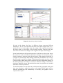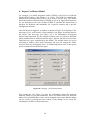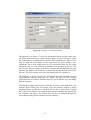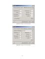
1
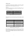
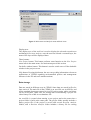
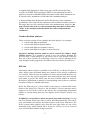
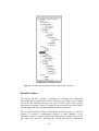
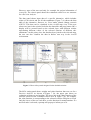
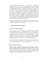
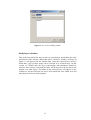
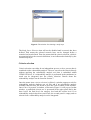
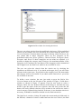
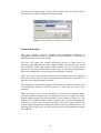
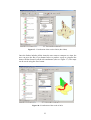
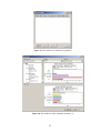
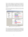
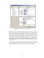
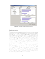
Project no. GOCE-CT-2003-505540
Project acronym: Euro-limpacs
Project full name: Integrated Project to evaluate the Impacts of Global Change on
European Freshwater Ecosystems
Instrument type: Integrated Project
Priority name: Sustainable Development
Deliverable (o. 407
Catchment Evaluation Decision Support System (CEDSS)
– User’s Manual (Task 9.4)
Due date of deliverable: 54
Actual submission date: 60
Start date of project: 1 February 2002
Duration: 5 Years
Organisation name of lead contractor for this deliverable: ULIV
Project co-funded by the European Commission within the Sixth Framework Programme (2002-2006)
Dissemination Level (tick appropriate box)
PU
PP
RE
CO
Public
Restricted to other programme participants (including the Commission Services)
Restricted to a group specified by the consortium (including the Commission Services)
Confidential, only for members of the consortium (including the Commission Services)
Revision : Final
0
v
Catchment Evaluation Decision Support System (CEDSS)
– User’s Manual
Version 1.0
Feb 20 2009
Hongyan Chen
Institute for Sustainable Water, Integrated Management and Ecosystem Research
SWIMMER, University of Liverpool, Liverpool L69 3GP, UK
EURO-LIMPACS Report
Deliverable 407
1
Table of Contents:
1.
2.
3.
Introduction ........................................................................................................... 3
Software installation.............................................................................................. 3
Overview of the program ...................................................................................... 3
Starting the program.................................................................................................. 3
CEDSS tool bar.......................................................................................................... 5
Data storage............................................................................................................... 6
Application steps ....................................................................................................... 7
4. Working with Project............................................................................................ 7
Create a new project.................................................................................................. 7
Load map................................................................................................................... 7
Conduct decision analyses ........................................................................................ 9
DSS tab ...................................................................................................................... 9
Dockable window.................................................................................................... 10
5. Working with decision analyses.......................................................................... 12
Start a new Decision Analysis................................................................................. 12
Delete a Decision Analysis ..................................................................................... 12
Study layer selection ............................................................................................... 13
Criteria selection ..................................................................................................... 14
Scenario definition .................................................................................................. 16
Multi-criteria analysis ............................................................................................. 20
Visualisation of the results ...................................................................................... 22
Sensitivity analysis.................................................................................................. 28
6. Export Coefficient Model.................................................................................... 30
7. Vulnerability analysis.......................................................................................... 34
Excel File Format .................................................................................................... 36
Long Text Entries.................................................................................................... 37
8. References ........................................................................................................... 38
9. Appendix A MCA implementation ..................................................................... 38
10.
Appendix B Export Co-efficient Model.......................................................... 40
2
1. Introduction
This CEDSS software is a generic tool to assist catchment managers with their
decision-making in the implementation of water framework directive (WFD)
in context of climate change. It enables the users to deal with their problems
by enabling them to compare different alternative management measures
under different climate change scenarios and therefore enabling them to select
an optimised management strategy.
This CEDSS software is developed as an ArcGIS extension so that the
advantages of the ArcGIS environment in spatial data processing and
visualisation etc. can be taken advantage of. The framework for the CEDSS
analysis is multi-criteria analysis (MCA) and with integrated interface, the user
can go implement the various steps of MCA, for example, criteria selection,
scenario definition and final evaluation calculation. Some simple models have
been integrated into the software and with them the user can work out the
values of some criteria for MCA.
2. Software installation
Software Requirements:
Operation System Windows NT, 2000 or XP
ArcGIS 9.2 and Microsoft .NET framework 2.0
Installing the program:
After following two steps, the CEDSS will be automatically installed to the
directory specified by the user (Administrator privileges are required).
•
•
Copy DSSSetup folder to your computer
Run the executable Setup.exe in the folder
3. Overview of the program
Starting the program
CEDSS is an ArcGIS extension and in order to use it, the user needs to activate
it within the ArcGIS platform. How to do it: go to the Tools menu in ArcGIS
and click on Extensions to get a list of extensions available and then check
on the CEDSS extension (see Figure 1). Once the extension is checked, the
CEDSS tool bar will appear on the screen, a DSS tab will display in the table
of contents (TOC) (left) and a dockable window will be embedded in the
middle (see Figure 2). The ArcGIS map view remains at the right.
3
Figure 1: The extension of CEDSS
Figure 2: The screen after CEDSS is checked on
4
CEDSS tool bar
The CEDSS tool bar consists of three components: a main menu, a research
layer display area and three buttons for starting a new project, displaying or
hiding the dockable window and getting help, respectively.
Main menu:
The main menu contains items for creating and managing projects. An
overview of the functions provided in the menu is shown in Table 1. It gives
the first level of functionality.
Menu Item
Function
ew Project
Map Load
Decision Analysis
Result Report
Create a new project
Add required maps
Perform a Decision Analysis
Create a final report
Help
Offer help information
Table 1: Functions in the main menu of the DSS
The item decision analysis in the main menu (see Table 1) leads to a second
level of functions and all of the functions included in this submenu are listed
in Table 2.
Menu Item
Function
ew Analysis
Delete Analysis
Study Layer Selection
Create a new analysis
Delete an analysis
Select a research layer that defines the
research objects and scale.
Select criteria for evaluation
Define the scenarios for comparison
Run the MCA model to calculate the
scores of all alternatives and visualise the
results in different ways.
Sensitivity analysis on weights and input
data of each criterion
Criteria Selection
Scenario Definition
Multi-criteria analysis
Sensitivity Analysis
Table 2: Functions for a Decision Analysis
Figure 3 shows the two menus embedded in the DSS tool bar, the relationship
between them reflects the hierarchy of the two levels of functionality. As each
stage of the CEDSS application is carried out successfully, subsequent menu
items are activated. The CEDSS analysis must be carried out in the order
of the menu items.
5
Figure 3: Main menu and analysis menu and their items
Display area:
The display area of the tool bar is used to display the selected research area
and during a Decision Analysis, once the user has selected a research layer, the
name of the layer will be displayed there.
Three buttons:
ew Project button: This button performs same function as the ew Project
menu item in the main menu. See main menu part of this section.
Dockable window button: This button is used to switch on or off the dockable
window in the project screen.
Help button: Pressing this button, the user can get help information relevant to
applications of CEDSS regarding environmental policies and management
measures in the EU and some member nations.
Data storage
Data are stored in different ways in CEDSS. Some data are stored in files for
later retrieval. The main file in the CEDSS is an .mxd file, an ArcGIS file, and
all the standard documents created in ArcGIS, such as maps, tables and charts
can be saved there. Other files for storing data created during a project are
either binary file or MS Access database file.
An .mxd file is created when starting a new project and at the same time a
project folder is built at the same path. The project folder usually includes a
binary project file (if the project is saved) and several Decision Analysis
folders, and a Decision Analysis folder includes a binary file for storing
6
evaluation criteria and a MS Access database file for holding all the
alternatives input data and the results from the MCA calculation.
Some temporary data stores are used for the sensitivity analysis and catchment
summary results display. All the calculated data are not saved in a file and
they are calculated in the memory and then displayed. When the procedure
ends, the values of the local variables holding these data will be lost and the
storage just lasts the time the procedure lasts. If the CEDSS analysis is
reloaded these data can be quickly regenerated.
Application steps
Generally, there are a few steps for an application of CEDSS. The user needs
to
• be clear what problem needs to be addressed with CEDSS;
• define potential alternatives to deal with that problem under potential
climate change scenarios;
• select evaluation criteria for comparison;
• upload the data for each alternative and if necessary, the data for a
specific model calculation;
• weight the importance among different criteria and to build the
relationship between the score each criterion contributes and its
physical value for preparing MCA calculation;
• perform MCA calculation and visualisation of results;
• perform sensitivity analysis;
• make a decision or provide information for decision-making support.
4. Working with Project
Create a new project
This function is used instead of the original new project command so that the
new project information can be recorded in the DSS tab in the Table of
Contents (TOC). When the ew Project button or the menu item ew Project
is selected, a window pops up to ask for a project name for the new project.
Once a name is given, the user can save it with the Save button on the window
and at the same time, an .mxd file and a new project folder are created at a
selected directory and the project name is displayed on the DSS tab.
Load map
Instead of the Add command in ArcGIS itself, a Load Map menu item is
offered for the user to load the required maps. If any other maps are needed,
the user can still load them with ArcGIS Add command.
A dialog window as shown in Figure 4 pops up once the Load Map item is
clicked. On this window, the user can select one from the list to load. The
maps in the list include maps of catchment boundary, sub-catchment, wetland,
lake, river network and land use. When one of the following Add buttons is
7
pressed, a Catchment Maps window like in Figure 5 appears and the user can
browse and select a corresponding map to add. For river network, a poly-line
layer or a network layer should be selected and for others a polygon layer is
needed. These layers can present either in individual shape files or as a part of
a dataset in a geo-database. Once the selected map is added, the red X will
change into green V indicating that the map now is available. Meanwhile a
predefined name will be given to that map, no matter what its original name is.
It is only necessary to load map layers that will be used in the subsequent
CEDSS application
Figure 4: Interface for adding required maps
Figure 5: The window for data adding
Maps represent the basic geographical entities in a catchment and are intended
to be used to deal with problems related to different water body types. In this
version of CEDSS, river sub-catchments are the only spatial unit available for
8
a complete DSS application. Other layer types will be activated in later
versions of CEDSS. When applying CEDSS to sub-catchments the MCA
applies to each sub-catchment and an assessment of the whole catchment can
be carried out by summation of individual sub-catchment analyses.
A data model has been designed to define the structure of the catchment
geodatabase. Since only the sub-catchment scale is addressed in the system at
this stage, there are few restrictions on the sub-catchment map. However, the
map selected to be used as a sub-catchment map must have a field called
‘ame’ in the attribute table that holds the name of individual subcatchments.
Conduct decision analyses
There are many reasons to have multiple decision analyses, for example:
• to deal with different problems,
• to deal with different spatial entities,
• to deal with different evaluation criteria,
• to deal with different weights or value functions.
Therefore, multiple decision analyses can be carried out within a single
CEDSS project. It is possible to create a new one without finishing the
previous ones. A built analysis in the project can be also deleted if the user
does not want it. Details of performing a Decision Analysis through all the
steps designed in the program are described in the next section, Section Five.
DSS tab
Information about analyses is outlined on the DSS tab, as shown in Figure 6,
where all the steps performed during two analyses in the project constitution
are recorded. These records are organised in a tree structure and therefore it is
easy to see how the project progresses: how many analyses have been already
built under a project and which step has been reached within an analysis.
Descriptive information is attached to corresponding items in the tree structure
and some of them are editable afterwards.
While the DSS tab gives a clear outline of the project, it cannot hold all the
details to the finest level. However, the leaf nodes of its tree structure can be
triggered via left click to lead to the details: the corresponding information
loaded or created during that step can display in the dockable window (see
below).
In addition, it is possible to delete unwanted steps and redo them. If a step
has to be deleted, all the steps after it will be deleted automatically. This rule is
only valid within one analysis and other analyses will not be influenced. The
Delete context menu appears only when the user right clicks on one of the
deleteable items, which include MCA, Scenarios, Decision Criteria, Selected
layer and individual climate change scenarios.
9
Figure 6: The DSS tab recording the analyses performed in a project
Dockable window
The project dockable window is designed to re-display the information
provided by the users during the Decision Analysis steps. There are five panels
in total in this window and only one panel will be visible when specific
information is required. These five panels are the text panel, the criteria panel,
the data panel, the MCA setting panel and the MCA result panel.
The text panel shows descriptive information about the project, or about an
analysis, a scenario, a management measure or other attributes of the
assessment. There is a textbox embedded in the panel and with it, the user can
type and save, therefore updating the existing description information.
10
However, some of the text read only, for example, the project information of
created by. The criteria panel shows the evaluation criteria in a tree structure
for a Decision Analysis.
The data panel shows input data of a specific alternative, which includes
values of all criteria and for all sub-catchments. Figure 7 (a) shows the data
table of the alternative, Business As Usual under climate change scenario
A2IPCC. This data can be visualised in the ArcGIS map view. If the user
selects one item in the criteria list below the data table and press button OK, a
display will be created based on the selected layer with different colours
representing different values of the selected criterion of different subcatchments. At this point, since the data has been joined to the selected map,
the user can also visualise the data in his/her own way in the ArcGIS
environment.
(a)
(b)
(c)
Figure 7: Three of the panels designed for the dockable window
The MCA setting panel shows weights and value functions that were set for a
Decision Analysis. As shown in Figure 7 (b), the upper part shows an
evaluation criteria tree and weights. The lower part is the value function of the
criterion selected in the evaluation criteria tree. In Figure 7 (b), for example,
the value function is corresponding to the selected criterion Phosphorus Load.
Only the leaves of the tree each have a value function for transformation. If a
non-leaf node is selected, a prompt will pop up to inform you of it.
11
The MCA results panel (see Figure 7 (c)) enables the visualisation of
calculation results of an MCA. It allows the user to select arbitrary
combinations among different scenarios, management measures and criteria
(including categories and the overall multi-criteria value) for comparison. The
user should ensure that logical combinations of results are selected for
interpretation. There are two types of maps available for displaying the results:
One is bar chart and the other is status map. Bar chart is good for comparison
among different combination items within one geographical entity, while
status map gives an image of spatial pattern of a specific item. All these maps
are displayed in the map view window and all existing tools in the ArcGIS
platform can be used to work with them. The Animation button allows the user
to create and play an animation with the selected map layers and the Summary
button enables the user to explore the whole catchment information and to
contrast it with that of individual sub-catchments.
This kind of information retrieval from the DSS tab to the dockable window is
allowed to shift from one analysis to another and this makes it possible to
compare among different decision analyses.
5. Working with decision analyses
Start a new Decision Analysis
The menu item ew Analysis is enabled after a required map layer has been
loaded. Selecting the menu item will display a window (see Figure 8) to ask
for a name for the new analysis and in the Existing Analyses listbox, the
existing analyses names are listed to avoid the same name as an existing
analysis being used. If the same name as an existing analysis is given, a
prompt will be given to request the user to change it. A default name like
AnalysisN is always given, where N is a number starting from 1 and which
automatically increases by 1 each time when a new analysis is created.
After the OK button is pressed on the window, the new analysis will be
created and added to the DSS tab tree view. Meanwhile, two menu items
Delete Analysis and Study Layer Selection will be enabled.
Delete a Decision Analysis
Even if the Delete Analysis item is enabled, you cannot delete an analysis
unless an analysis node in the DSS tab is selected. When the Delete
Analysis item is clicked, if an analysis node is not selected, a prompt will pop
up to ask you to select an analysis node. If an analysis node is selected, a
prompt will ask you to confirm it. Once an analysis has been deleted, the states
(disabled or enabled) of menu items will change accordingly.
12
Figure 8: ew Analysis dialog window
Study layer selection
This menu item allows the user to select a research layer that defines the scale
and objects of the analysis. When this item is clicked, a window, as shown in
Figure 9, will appear and the loaded maps (only the required ones) will be
listed there. One of these maps can be selected as a research layer. In this
version of CEDSS only the layer representing sub-catchments should be
selected. Once a layer is selected, the layer will be moved to the top and it will
display over other layers. The name of the selected layer will appear on the
combo box on the DSS tool bar and it will remind the user which area and
what objects the focus of the analysis.
13
Figure 9: The window for selecting a study layer
The Study Layer Selection item will not be disabled until a scenario has been
defined. That means the selected research layer can be changed before a
scenario has been defined. That also means that the criteria selection, which is
an operation before the scenario definition, is not influenced technically by the
selected map layer.
Criteria selection
Criteria selection can either be an independent process or be a process that is
combined with a vulnerability analysis. The user can select the criteria directly
without applying the vulnerability analysis tool that is embedded within
CEDSS. However, if a vulnerability analysis is performed in the catchment, its
result can be integrated into the criteria selection. Details about the
vulnerability analysis can be found in Section 7.
Once the menu item criteria selection is clicked, a window appears to ask for
vulnerability analysis database (an .xls file) and if no vulnerability analysis
available, then the user just needs to press the Cancel button on the window.
Once Cancel is pressed, a window, as shown in Figure 10, will pop up. In that
window, a predefined criteria tree is presented in the upper panel and it has
three levels: the final level, the category level and the criteria level. If no
vulnerability analysis has been carried out, the second panel is empty and no
criteria from a vulnerability analysis can be integrated.
14
Figure 10: The window for selecting the criteria
The user can select criteria from the predefined criteria tree. If the predefined
criteria are not suitable, the user can define new criteria with the Define ew
Criterion function. Criterion names may also be directly edited. However, the
user cannot add or delete categories. There are five categories in the
predefined criteria tree: Water Quantity, Chemical Status, Ecological Status,
Economic and Social. If these categories are not what are required, it is
possible to change the category name. However, the maximum number of the
categories is five and more are not allowed. The categories can be summarised
into a higher level, the final level, which is an overall MCA score.
The user can select the criteria from the criteria tree by checking the
checkboxes at different levels. If you check at the upper level, you will select
all items in the criteria tree. If you check at the category level, the items under
that category will be all selected. If you check at the criteria level, you select
one criterion at one time.
To define a new criterion, the user just needs to press the Define ew
Criterion button at the low-left part of the window in Figure 12 and then a
window as shown in Figure 11 appears. First the user needs to select a
category where the new defined criterion will belong to, and then the user
needs to type the name of the new criterion. Once the user presses the OK
button, the newly defined criterion will be written in the criteria tree under a
correct category without being checked. If the user is sure that that criterion is
necessary, it should be checked to include it in the final criteria list.
The final list is saved as a binary file under the current analysis folder and, in
the DSS tab, a branch of criteria is added and once the user clicks it, the final
15
criteria list will display again in the dockable window. The saved file will also
be used later for other operations, like data loading.
Figure 11: The window for defining a new criterion
Scenario definition
This step includes scenario definition and subsequent definition of
management measures under the scenario and data loading for each measure
immediately after it has been defined.
The user can repeat the scenario definition process as many times as
necessary, depending on how many climate change scenarios the user would
like to include. Under each climate change scenario, the user can also repeat
the process of measure definition as many times as necessary, depending on
how many management measures the user would like to include.
There are several ways available for the user to load data. One is to load data
from a file; the second is to derive data from model calculation. The third is to
type the value directly into the data table.
The following is a detailed description of the process to define a scenario and
its management measures and the process to load data for each of the
measures.
When the menu item scenario definition is pressed, the climate change
scenario definition window will be displayed to ask for a name for a new
climate change scenario and its description (see the window in Figure 12). The
default one is GCMN and the number N starts with 1 and will automatically
increase by 1 when a new scenario is defined. The user can give his/her own
scenario name and type the scenario description in the description text box. By
pressing OK, the user goes into the next step: define a management measure
and load data.
16
Figure 12: The window to define a climate change scenario
In the window shown in Figure 13, the user can define a management measure
by giving a measure name in the name text box and its description in the
description text box. Similarly, the default one is MeasureN and N starts with
1 and will increase automatically when a new measure is created.
The table in the middle part of the window needs to be filled with the data for
that measure. Each row of the table represents a geographic entity of the
research area and each column represents a criterion at the lowest level in the
final selected criteria tree. Once the table is populated, the Save at the bottom
will be enabled and with it the user will be able to save the data for that
measure. ew button lets the user start another measure definition and the
process is the same as the previous one. The buttons ‘<’ and ‘>’ allow the
user to check the data of the other defined measures. After all measures have
been defined, the user can press the Exit button to end this scenario definition.
17
Figure 13: The window to define a measure and to load data
As mentioned before, there are three ways to populating the table for each
measure defined there. With the button Load Data from File, the user can load
data from a .txt file. Once the button is clicked, a window pops up to allow the
user to select a .txt file. The data in the .txt file will be read in order from top
to bottom and from left to right. When preparing this .txt file, it is important to
have all the data in order and include a decision criteria name row and an
entity name column. The column names and names of the rows do not have to
be the same as in the table. Once the data table is filled, the user can save it for
later MCA calculation.
Data can also be generated using the modelling and guidance tools. The
structure of CEDSS has been designed to allow users to use models to
calculate one column of data for all the sub-catchments at one time. If the user
presses the button Calculation with Tools, a window shown in Figure 14 pops
up and all the modelling tools available for that decision criterion will be listed
in the listbox for selection. Once a tool is selected, the model interface will be
triggered and the user will be able to implement the model to calculate data for
a decision criterion and the result will be used to fill the corresponding
column. In the current version of CEDSS, the only tool available is an Export
Coefficient Modelling (ECM) used for calculating nitrogen load. The details of
the ECM are described in Section 6.
Another way to access help tools is to right-click the field name of a column
and to get a context menu as shown in Figure 15. The context menu includes
three items: Calculate Tool, Guidance and Help. If the Calculate Tool item is
clicked and if a tool is available for that column, then the tool interface will be
triggered directly and can be used in the same way as described above. The
18
Help option is designed to provide the user with some general quantitative or
qualitative information on important catchment management issues and the
outcomes of the application of certain catchment management measures in a
selection of EU member states. This information is intended to guide the user
in making expert judgements on the potential outcomes of implementing the
management measures defined on the decision criteria in the absence of
suitable modelling tools.
Figure 14: Tools for calculating criteria values
Figure 15: A context menu for each column
The user inputs to the scenario definitions are written to the DSS tree view in
the DSS tab. They are re-displayable in the dockable window by doubleclicking the corresponding nodes of the DSS tree view. If multiple scenarios
have been defined, all of them will be listed there in order and the data will be
saved in a MS Access database file in the folder of current analysis.
19
Multi-criteria analysis
In this step, the user is required to set weights for all the selected criteria
according to their importance and set value functions for each lowest level
criterion according their understanding of the relationship between the
criterion natural scales and their utilities in the evaluation system. These
settings will be applied to all the alternatives and the calculated result will be
visualised directly at the end of the step. Details about the MCA, additive
utility analysis are described in Appendix A.
Once the Multi-Criteria Analysis item is clicked, the window shown in Figure
16 appears for setting weights and value functions. The top drop-down menu
is used to select a criterion. The user can select an arbitrary one from the drop
down list of the decision criterion combo box or press the ext button to select
next one in order. For each selected criterion, the weights setting part will be
always enabled, but the right part of the window will be enabled only when
the selected criterion is one of the lowest level criteria.
Figure 16: Interface for MCA
In weight setting, any non- negative integer can be given as a weight for the
selected criterion. This non-negative integer should be typed in the textbox
below the criteria tree and when the Set is pressed, the weight will be written
in between brackets at the end of the criterion in the criteria tree. A cross will
disappear when that is done.
There are two crosses at the end of each lowest level criterion. The second
cross will disappear when its value function has been set. The user can press
the right Set button to finalise it. There are four kinds of curves to define a
value function: linear, exponential, parabola and customised. For each one,
there are two slopes: positive and negative. The range of the values of the
20
selected criterion is given automatically in the maximum and minimum
textboxes. Querying the database sets default values for the Maximum and
Minimum text boxes. It is possible to set manually a specific range of the
value by changing the maximum and minimum values and pressing the Set
button. The change will also reflect in the labels of the X-axis in the chart
panal. If the user wants the maximum and minimum of the current data as the
limits of the range, the Get button will get them back.
Linear curve is defined directly by the maximum and minimum and the slope.
If the slope is positive, then the maximum value will map to the highest score
1 and the minimum to the lowest score 0. If the slope is negative, the opposite
is true: that is the maximum value will map to the lowest score 0 and the
minimum to the highest score 0.
An exponential curve (see Appendix A for the formula) is defined by a given
user-defined point plus the maximum and minimum values and the slope. If
the slope is positive, the exponential curve will be completely determined by
the three points in the chart panel: the user defined point, the point at
(maximum, 1) and the point at (minimum, 0). If negative, the exponential
curve will be determined by the user-defined point, the point at (maximum, 0)
and the point at (minimum, 1). Clicking and dragging will change the userdefined point. The curve will change continuously during the mouse move.
The parabola curve (see Appendix A for the formula) is similarly defined to
the exponential curve. The user can determine a parabola curve by
determining a single user-defined point.
Multiple linear segments define the customised curve. The points to define
these segments are given by the user. To start with, there are three default user
defined points and the user can add more by double clicking within the chart
panel. The user can define 9 points at most. Together with two end points
there are therefore a maximum of ten segments available for the custom curve.
It is also possible to select a point, move a point, or delete a point and the
detailed operations are listed in Table 3. When selected, a point appears in red
and its coordinates appear in the X, Y textboxes. When a positive slope is
selected, the two end points are (minimum, 0) and (maximum, 1) and a
negative is selected, (minimum, 1) and (maximum, 0).
When all the required settings have been inputted (as indicated by all the
crosses disappearing), the Run button will be enabled and then the user can
press it to run the MCA model. The calculation results are saved in a results
table in the MS Access database and the overall values of the measures in the
last scenario are displayed as a bar chart map in the ArcGIS map view.
Meanwhile a window pops up for further exploration of the results through
visualisation.
21
Function
Add a point
Select a point
Move a point
Remove a point
Operations
Double click
Click on the point
Select the point and then click and drag the point
Select the point and then right-click the point
Table 3: Operational description in defining a customised curve for value function
Visualisation of the results
Visualisation of the results is considered as a part of the multi-criteria analysis
step as it allows the user to inspect the results from different perspectives. The
user interface for this process, which is the same as the one embedded in the
dockable window for visualisation (see Figure 7 (c)) is designed to allow
selection of arbitrary combinations of different scenarios, management
measures and criteria (including categories and the overall multi-criteria value)
for comparison. For example, it can be used to compare a single criterion but
under different climate change scenarios, or compare different criteria under
same climate change scenario but with different management measures, and so
on.
There are two types of maps available for display of the results: One is a bar
chart and the other is a status map. The bar chart option is good for
comparison of different combinations within one geographical entity, while
status map gives an image of the spatial pattern of a specific item. All these
maps display in the map view window and all existing tools in the ArcGIS
platform can be used to work with them.
The window designed for the visualisation (as shown in the middle window of
Figure 17) allows the user to select a scenario from the top scenario
combobox drop down list or with the ext button. Once a scenario is selected,
the management measures under it are added to the Measures combobox and
the user can select one of them from its drop down list or with the ext button.
A criterion can be selected from the criteria tree by clicking it.
With the + button pressed, a combination of the selection of scenario, measure
and criterion is added into the Selected items listbox as one of the items for
comparison. The user can add as many such combinations as required. If there
is one in the list unwanted, the user can use the X button to remove it and if
the user wants another comparison, the Reset button can be used to delete all
the items in the listbox.
22
Figure 17: Visualisation of the result of MCA (Bar Chart)
Once the listbox includes all the items the user wants to compare at a time, the
user can press the Bar Chart button below to produce a map to visualise the
items with bar charts for all the sub-catchments (also see Figure 17). The maps
can be saved using the Save button.
Figure 20: Visualisation of the result of MCA
23
Below the Bar chart button is a Status map button and it is used for the user to
display the items in the listbox one by one (see Figure 18). In a status map,
different colours are used to represent different categories of the values of the
selected item and there are five colour categories defined for all status maps:
light red, red, yellow, green and light green for scores at these following
ranges: 0-0.2, 0.2-0.4, 0.4-0.6, 0.6-0.8 and 0.8-1.0 respectively. If required, the
Save button next to the Map Status button can be used to save it.
Once a map is saved the Animation button will be enabled and the user is able
to select maps to make an animation. When Animation is clicked, a window as
shown in Figure 19 will display and when a layer or multiple layers are
selected on the Display tab in the TOC, the Add button will be enabled.
Clicking on the Add button will add the names of the selected layers to the
listbox in Figure 19. Once a layer is added, the Play button will be enabled
and the user can create an animation for these selected map layers and play it
automatically. With the Delete button, the user can delete a selected layer in
the list from the animation. The Reset button allows the user to clear all the
layers in the list.
When the Summary button is clicked, the window as shown in Figure 20 will
open with a default display. As in Figure 20, the default display shows the
total score of the first geographic entity under the first scenario and its first
measure in the upper panel and the area-weighted total score of the whole
catchment under the same scenario and same measure in the lower panel.
As we can see in Figure 20, the total MCA score is displayed in a segmented
bar at the bottom of each chart. The different colours of these segments
represent different categories that have contributed to the total score. The
scores of the individual categories are also given with the bars in a colour
corresponding to the components of the total scores. The lengths of the
component bars (representing their scores) are not necessarily proportional to
the lengths of the segments of the total bar. Their contributions are determined
not only by their own scores but also by their weights.
24
Figure 19: The window for animation preparation
Figure 20: The window for the catchment summary (1)
25
If the user wants to check the score of a category it can be selected in the
criteria tree and chart updated by pressing the OK button. The situation is
similar to the above, the difference being that the bottom bars, which are
segmented and coloured differently, represent the scores of the selected
category and other bars represent it contributing decision criteria (see Figure
21). If the user selects a lowest level criterion, then only one bar will be
displayed.
To check another geographic entity and/or another scenario and/or another
measure, it can be selected with the three combo boxes at the top and the OK
button pressed to update.
Figure 21: The window for the catchment summary (2)
There is an All Sub-Catchment option available in the sub-catchment combo
box. Once that option is selected, in the upper picture panel will display the
scores of all the sub-catchments in horizontal bars instead of a sub-catchment
specific score and the scores of its contributors. However, in the lower picture
panel, the display will be the same as in the situation described above. Figure
22 shows the situation when the All Sub-Catchment option is selected.
26
Figure 22: The window for Catchment summary 3
There are All Scenarios and All Measures options for the other two combo
boxes. Once they both are selected, all the alternatives of a specific criterion
value will be displayed in the upper panel for a specific sub-catchment and in
the lower panel for the whole catchment. It is possible to select one scenario
and All Measures and the result will be like that in Figure 23. However,
displaying All Scenarios and one measure, or All Sub-Catchments with All
Scenarios and All Measures is not possible because is too complex to be
displayed in the space available. However, the MCA results can be accessed
directly and exported to other data analysis packages to facilitate these types
of comparisons.
In the DSS tab, a branch called Results is added in the project tree after the
MCA calculation. Once the visualisation window is closed, it can be reopened
by right-clicking the Results node to reopen it in the dockable window.
27
Figure 23: The window for the catchment summary 4
Sensitivity analysis
The purpose of sensitivity analysis is to assess how robust the relative ranking
of alternatives is to changes in the weights of the decision criteria or changes
to the input data. In the case of variable weights, only one weight is varied at a
time, letting the relative weight change from 0 to 1. The change of the overall
values caused by the weight change is calculated and displayed. In the case of
variations in input data, only one attribute under a specific alternative is varied
at a time and the change of the overall value of the alternative is displayed as
the attribute changes from its minimum to its maximum. Other alternatives
will not be influenced and therefore remain unchanged but are displayed for
comparison (see Appendix A for the formula). The sensitivity analysis allows
an assessment of the uncertainty in the MCA results.
Once the MCA step is finished, the sensitivity analysis menu item is enabled.
Clicking on it displays a window as shown in Figure 24 with a default display.
In the default display, the first sub-catchment is selected and the first category
is selected, and therefore the upper panel displays the changes of the total
scores of all alternatives of that sub-catchment as the weight of the category
changes from 0 to 1. In the lower chart, the first sub-catchment is selected, the
first scenario and its first measure are selected and the first criterion is
selected, and therefore, the lower panel displays the impact as the input data of
the criterion changes from its minimum to its maximum.
28
Figure 24: Sensitivity analysis interface
In both of the charts, the lines in different colours represent different
alternatives. The Y axis represents the final score which ranges from 0 to 1
and the X axis is, for the upper chart, the weight of the criterion selected; for
the lower chart, it is the range of the selected criterion. Therefore the lines
show how the final scores change as the weight or the input value changes.
In the both situations, the intersection points of the lines are the points where
the preference order of different alternatives changes. If intersection points
appear frequently, then that means the preference order changes frequently as
a weight or criterion input data changes continually and therefore we can say
that the result is sensitive to change. If the intersection points are close to the
current weight or data input used in the MCA this shows that small changes in
the MCA parameters are likely to result in a different ranking of alternatives
and users should be aware that increased accuracy an precision are needed
with these for these parameters.
To use this tool the user can select any criterion and any geographic entity and
once any selection is made, the curves in the upper picture panel will be
redrawn automatically and immediately. If necessary, the graphics can be
exported for a report.
29
6. Export Coefficient Model
An example of a model integrated within CEDSS is the Export Coefficient
Model (ECM; Johnes, 1996; Johnes et al., 1996). The ECM is to calculate the
annual load of nitrogen delivered to a river from a specific area. The details
about the model as implemented in CEDSS are given in Appendix B and here
we just describe how to run it within CEDSS to calculate the annual load of
nitrogen for different sub-catchments for a specific scenario and a specific
management measure.
Once ECM tool is triggered, a window as shown in Figure 26 is displayed. The
main part of it is a tab control, which includes 6 tab pages for asking data for
the model. The first page (see Figure 25) is for information on nitrogen
fixation and deposition. As the nitrogen fixation rates are related to different
plants and therefore to different land use types, data are entered for each of the
eight land use types considered in the model. The default values are given
according to Johnes (1996) and if necessary, the user can change the values
and save them by pressing the Save. A default deposition value is also given
and is constant across all land use types.
Figure 25: Tab page 1 of ECM tab control
The second tab (see Figure 26) asks for information about the livestock
numbers within a given sub-catchment. There are default values for different
kinds of livestock and these values can be changed if necessary and the change
can be saved by pressing the Save button. If the change is not saved, the
calculation will still use the default ones.
30
Figure 26: Tab page 2 of ECM tab control
The third tab (see Figure 27) asks for information about fertiliser input rates
for different land use types. Again, default values are given and these values
are changeable by pressing the Save button. The fourth tab (see Figure 28) is
used to input the percentages of the eight land use types within a subcatchment. Since these eight types do not necessarily make up the entire
catchment area, the sum of these percentages does not have to be 100. The
user can save the percentages with the Save button and automatically the same
interface for another sub-catchment is shown and the data must be entered for
this one. The user can also select any sub-catchment in the combo box.
The fifth tab (see Figure 29) asks for information about the population of each
sub-catchment and the sixth tab (see Figure 30) asks for the nitrogen
production rate of livestock. Default values are given and the user can change
them if necessary.
In addition to typing data into the forms, the user can import data from a file
with the Import Data from File button. Once the button is clicked, a dialog
window pops up and the user is asked to select a file to import data. If a data
file of the correct format is selected the data will be automatically entered into
the respective tab pages. The loaded data can also be changed through the
screen and pressing the Save button saves the changes.
31
Figure 27: Tab page 3 of ECM tab control
Figure 28: Tab page 4 of ECM tab control
32
Figure 29: Tab page 5 of ECM tab control
Figure 30: Tab page 6 of ECM tab control
On finishing the data input through the tab control, the user can go to the next
step by clicking on the ext button. Figure 31 shows the window requesting
export coefficients. Default values are given and they can be changed if
necessary. If the values are satisfactory, the user can just press the Calculation
33
button to run the model with the given data and parameters and the result is
then written to the column in the data entry table.
Figure 31: ECM(N) parameter setting
7. Vulnerability analysis
The vulnerability analysis uses an Excel spreadsheet called table of database
III.xls at a default directory. This Excel file hold data a knowledge base for
assessing the vulnerability of different freshwater ecosystem types to climate
change and is described in full in Hering et al. (2008). If this file is not
available, a file browse dialog will be shown allowing you to choose an
alternative Excel file.
Once the Excel file has been read, the Select Ecosystem window will be
shown (see Figure 32). At the top of the window are some search terms and
below that is the Excel data in a tabular form. The columns in this table can be
resized to display the text or, if you hover your mouse over some text, a tooltip
will be shown with the full text. Clicking on the column heading sorts the data
in that column.
The data in the table can be selected (here, shown in green) using the usual
mouse controls. Click once on a row to select it. Multiple rows can be selected
by first clicking on a row and then, while holding down shift, clicking on a
second row. Extra rows can be selected by holding down control while
clicking on a row.
34
Figure 32: The window to show the Excel table for vulnerability analysis
Figure 33: The window to show how to add a new criterion from a vulnerability
analysis
35
If you have a large number of rows in the Excel file, then they can be reduced
by using the search terms are the top of the window. Next to the terms Climate
Region, Ecosystem type and Relevant ecoregion(s) are three drop down menus
which show the data from the corresponding columns of the Excel file.
Choose the appropriate region or ecosystem and then click the Refine button.
The text next to the Search: panel and the data in the table will be updated to
reflect your choice. Extra terms can be added to the search option by selecting
new options from the drop down menus and clicking Refine again. If your
search results in too few terms, you can start again by pressing the Clear
button.
Clicking on OK takes you to the Water Management Criteria Selection
window shown in Figure 33. The criteria are taken from the selected columns
Suggested indicator I, Suggested indicator II and Suggested indicator III. Any
duplicate entries are removed and invalid characters such as commas (“,”) or
brackets (“(“, “)”) are removed. In this example figure the criterion Flood
events in unusual seasons recorded by the gauging stations has been
successfully added to the category Water Quantity as indicated by the green
highlighting. To do this, click on the term Water Quantity and a criterion in
the lower window and click the Add button. To remove the term, highlight it
by clicking and press the Remove button. The term will be removed from the
criteria select tree in the top window and added to the list in the bottom
window.
Excel File Format
The Excel file should consist of a simple table on the first sheet with column
headings. Data appearing on other sheets will be ignored. As the file is read
directly without requiring Excel, then any formulas will be displayed as
entered rather than their results. The required column headings are:
•
Climate Region
•
Ecosystem type
•
Relevant ecoregion(s)1
•
Suggested indicator I
•
Justification of indicator I
•
Suggested indicator II
•
Justification of indicator II
•
Suggested indicator III
1
The sample Excel file has a space after the close bracket in “Relevant ecoregion(s)_“ which is
necessary.
36
•
Justification of indicator III
These will be displayed first in the table on the Select Ecoregion window. Any
other columns in the Excel file will be displayed as extra columns to the right.
These may be, for example,
•
Stressor type
•
Responding parameter group
•
Responding parameter
•
Response description
•
Secondary effects
•
Specification of relevant ecosystem type
•
Mitigation measures
•
Reference(s) (if any)
Long Text Entries
If the text within a cell occupies more than 256 characters, then there may be
problems with the Search and Refine options on the Select Ecosystems
window, even though the text is displayed correctly. This particularly affects
the Climate Region, Ecosystem type and Relevant ecoregion(s) columns. The
problem is cause by a Microsoft bug in the Excel ODBC driver which decides
the file format by scanning the first 8 lines of the Excel file, see
http://support.microsoft.com/kb/189897/EN-US/
The solutions are:
•
Ensure all cells are less than 256 characters.
•
Make sure there is a cell with more than 256 characters in the first
8 lines - these can just be spaces.
•
Use a registry fix. If you are confident in using regedit, change
HKLM\Software\Microsoft\Jet\4.0\Engines\Excel\TypeGuessRows
to 0 so it scans the whole file.
The problem was highlighted when many ecoregions were added to the
Relevant ecoregion(s) column. As a work around and to save typing, the
keyword All has been added. If you put All under Relevant ecoregion(s) then
the code will automatically fill in all of the ecoregions for you.
37
8. References
Hering et al 2008. Compilation of indicators of different types as the basis for
an indicator selection tool. Project deliverable Deliverable No. 277. Eurolimpacs Project.
Johnes, P.J. (1996). Evaluation and management of the impact of land use
change on the nitrogen and phosphorus load delivered to surface water: the
export coefficient modelling approach. Journal of Hydrology 183, 323-349.
Johnes, P. J., Moss, B. & Phillips, G. L. (1996). The determination of water
quality by land use, livestock numbers and population data - testing of a model
for use in conservation and water quality management. Freshwater Biology,
36, 451-473.
9. Appendix A MCA implementation
The formula of the linear additive model (see von Winterfeldt and Edwards,
1986) adopted in the CEDSS is given as follows:
n
V( Ai ) = ∑ w j v j ( xij )
j =1
A
Where V is the overall multi-attribute value and 0 ≤ V ≤ 1 ; i is the ith
v
( x , x ,..., xin )
as its attribute level vector; j is a value
alternative with i1 i 2
0 ≤ v j ≤ 1 wj
is a compound weight consisting of
function for attribute j and
;
two weights coming from different levels respectively of the value tree and
n
∑ j =1 w j = 1 .
To fix the model, weights and value functions have to be set. In CEDSS,
weights are set using direct numerical ratio judgement of relative attribute
importance and four types of value functions are available for selection: linear,
exponential, parabola and custom linear segment curves. The formula of
exponential and parabola curves adopted in the software is respectively
expressed in Equation 2 (Murphy et al., 2001) and 3.
v(r ) =
v(r ) =
exp (br ) − 1
exp (b) − 1
(2)
cosh (b(2r - 1)) − 1
cosh (b) − 1
(3)
38
where b is the parameter of the equation and r is a variable which is related to
attribute variable x and its nature scale (within a segment of any two real
x
numbers xmin and max ). The relationship is represented as follows:
r = ( x - xmin ) /( xmax − xmin )
(4)
These two curve equations guarantee that the v(r ) values are within a range
from 0 to 1, which is the requirement by the value functions in the MCA.
In the sensitivity analysis step, the purpose is to assess how robust the result
is, provided an uncertain situation. Two uncertain inputs are dealt with in the
CEDSS software: one is weights and the other is criterion natural scale input.
In the first case, only one weight is dealt with at a time and the change of the
overall values will be checked when letting the weight change from 0 to 1.
n
w =1
∑
j =1 j
Since
is required, the relevant weights are therefore let change
proportionally. The formula to reflect this change is expressed as follows:
V( Ai , wt ) = wt v t + ∑ (1 − wt )
j ≠t
wj
∑w
vj
j
j ≠t
(5)
(1 − wt )
wt
wj
∑w
j
j ≠t
is the adjusted weight for
is the addressed weight and
V( Ai , wt )
A
attribute j.
is the function of the overall value of alternative i with
wt
as its independent variable. Obviously, it is a linear function and for
A
different alternatives, A1 , A2 , ..., m the corresponding geometric straight lines
have different slopes and intercepts.
where
In the case of criterion natural scale input uncertainty, only one attribute under
a specific alternative is dealt with and the change of the overall value of the
alternative is checked as the attribute changes from its minimum to its
maximum and other alternatives will not be influenced and therefore remain
unchanged. The following formulas give a formal description of this
sensitivity analysis:
V( As , xsz ) = wz v z ( xsz ) + ∑ w j v j ( xsj )
j≠z
39
(6)
n
V( Ai ≠ s , xsz ) = ∑ w j v j ( x(i ≠ s ) j )
j =1
(7)
A
where the specific alternative is s and the addressed attribute is attribute z.
From above two formulas, we can see that the overall values of other
A
alternatives are unchanged and the one of the specific alternative s changes
x
as the specific attribute sz changes. It is not necessarily a linear change; it
changes depending on the value function v z .
10. Appendix B Export Co-efficient Model
Export coefficient modelling is a river basin scale, semi-distributed approach
that calculates mean annual total N (and total P) loading delivered to a water
body (freshwater or marine) as the sum of the nutrient loads exported from
each nutrient source in the river basin.
The model equation is as follows (Johnes, 1996):
n
L = ∑ Ei ( Ai ( I i )) + p
(8)
i =1
Where, L = Loss of nutrients
E = Export coefficient for the nutrient source i
A = Area of river basin occupied by land use type I, or number of
livestock type i, or of people
I = Input of nutrients to source i
p = Input of nutrients from precipitation
40