1
1
Volume
UNIVERSITY OF VICTORIA
Department of Computer Science
MATLAB
User Manual
DEPARTMENT OF COMPUTER SCIENCE
MATLAB User Manual
Lanjing Li
Department of Computer Science
University of Victoria
PO Box 3055, STN CSC
Victoria, BC
Canada V8W 3P6
Phone 250.721.7209 Fax 250.721.7292
Table of Content
Control Statements
CHAPTE R
15
1
Accessing and Quitting MATLAB
Accessing MATLAB
M-File Basics
18
1
Creating M-Files
18
In a UNIX Environment
1
Running M-Files
22
In a MS Windows Environment
2
Summary of Useful Commands
22
Quitting MATLAB
3
Some Useful Help Commands
4
CHAPTE R
2
Basics of MATLAB
MATLAB Environment
MATLAB Windows
5
5
Other Features of the MATLAB
Desktop
Data Structures and The Operators
6
Input/Output and Data Formatting
Input
23
Output
23
Format
25
Summary of Useful Commands
26
Graphics
26
Basic Plots
26
Graph of a Function
28
Define Titles, Labels and
7
Text in a Graph
Scalars
7
Commands for Controlling
Vectors
7
the Axes
Matrices
7
The Colon Notation and
Subscripting
Operators
8
23
29
30
Multiple Plots in One Figure
31
Save and Print a Figure
34
Commands for 2D Plotting
9
Functions
35
Precedence Rules for Operators 12
Character Strings
12
Chapter 3
13
Basic Functions for Linear Algebra and
Declaration
13
Numerical Analysis
Global Variables
14
Linear Algebra
Variables
Flow of Control
14
Relational and
Logical Operators
14
36
Vector and Matrix Norms
36
Inverses
37
Transposes
39
Determinants
40
Rank
40
Factorizations
40
Eigenvalues
42
Singular Value Decomposition
43
Sparse Matrices
44
Iterative Methods
46
Polynomial Roots and Interpolation
48
Polynomials
48
Polynomial Interpolation
50
Quadrature
56
Integrating Functions of
One Variable
Ordinary Differential Equations
Initial Value Problems
Partial Differential Equations
56
58
58
62
Parabolic and Elliptic Equations 62
Other Useful Functions
66
Functions for Nonlinear
Algebraic Equations
Functions for Data Analysis
References
66
66
69
M A T L A B
U S E R
1
Chapter
M A N U A L
Accessing and Quitting
MATLAB
Accessing MATLAB
M
ATLAB is available on both UNIX and MS Windows platforms in the
Department of Computer Science. MATLAB can be accessed from the
workstations located in ELW B215, B228 and B203 or from any UNIX
workstation that allows access to SHELL, where the UNIX version of
MATLAB is located. The PCs in ELW B228 and B203 can be used to access
MATLAB from a Windows Environment.
In a UNIX Environment
•
This is the environment
available in ELW B215. The basic steps to access MATLAB are as
follows.
Starting MATLAB on an X-Windows Desktop:
1.
Start Up A SSH Client Session to SHELL: In an X-Terminal, type ssh
at the prompt, and then enter your password. You
should get a UNIX prompt on the remote server after this step. For
example:
shell.csc.uvic.ca
mayne%
2.
Determine the Name of Your Computer: At the prompt, type
who am i
This command will give you a result back similar to the line below.
username termid date (hostname)
3.
Set Environment Variable for the Output Display:
UNIX command below.
1
Simply type the
M A T L A B
U S E R
M A N U A L
setenv DISPLAY hostname:0
For example, setenv DISPLAY boxter:0
4.
Start MATLAB: Type the command below.
matlab
In a Microsoft Windows Environment
•
MATLAB for Windows is
available in ELW B228 and B203. To start the Windows version of
MATLAB on a PC, click on the Start button on the taskbar at the bottom
of the desktop and then select Productivity/MATLAB 6.1.
•
Starting MATLAB Using X-Windows on the NT/2000 Workstations: This
is the environment available in ELW B228 and B203. The basic steps to
access the UNIX version of MATLAB on SHELL are as follows.
Starting MATLAB on a Windows Desktop:
1.
Start Up An X-Window Session:
Click on the Start button, and then
select network/X-Win32. An icon should appear on the taskbar at the
bottom of the desktop.
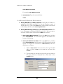
2.
Start Up An SSH Client to SHELL: Click on the Start button, and then
select network/SSH Client. After this step, a SSH Client window should
appear. To complete the connection to shell.csc.uvic.ca, follow the
steps from a to d below.
a. Click on Quick Connect on the menu bar at the top of the SSH
widow, or click on File on the menu bar and then select
Connect….
b. Type the name for the remote server and your user name in
the popup window as illustrated below. Then click on the
Connect button.
2
M A T L A B
U S E R
M A N U A L
c. When a popup window appears for Host Identification, just
click on the button No.
d. Type your password when the last popup window appears.
Note: After these steps, a command line prompt in the remote server
should appear in the SSH Client window. For example:
mayne%
3.
Determine the Name of Your Computer:
At the prompt in the SSH
Client window, type
who am i
This command will give you a result back similar to the line below.
username termid date (hostname)
4.
Set Environment Variable for the Output Display:
Simply type the
UNIX command below.
setenv DISPLAY hostname:0
For example, setenv DISPLAY boxter:0
5.
Start MATLAB: Type the command below.
matlab
Quitting MATLAB
S
elect Exit MATLAB from File on the menu bar to exit MATLAB. Alternatively,
type exit or quit in the Command Window to quit MATLAB. To quit
MATLAB on SHELL from the NT/2000 workstations in ELW B228 or B203,
do as follows.
1.
Quitting MATLAB: In the MATLAB Command Window, type exit or quit.
2.
Logout from SHELL: In the SSH Client window, type exit.
3.
Quitting SSH Client Session:
4.
Quitting X-Window Session:
Click on File on the menu bar at the top of the
SSH widow, and then select Exit.
Click on the icon X-Win32 on the taskbar at the
bottom of the desktop, and then select Close.
3
M A T L A B
U S E R
M A N U A L
Some Useful Help Commands
C O M M A N D
D E S C R I P T I O N
help
List all help topics in the Command Window
helpwin
List all help topics in the Help Window
help topic
Give help on the specified topic
quit
Terminate MATLAB
version
Version of MATLAB
type filename
Display the contents of the specified file
what
List MATLAB specific files in the current directory
more
Control paged output for the Command Window
4
M A T L A B
U S E R
2
Chapter
M A N U A L
Basics of MATLAB
The General Structure of the MATLAB
Environment
T
he Command Window, Graphics Window and Edit Window are the three
basic windows available in MATLAB .
MATLAB Windows
•
This is the primary and default window in which a
user interacts with MATLAB. Similar to any other command shells, the
prompt >> is displayed and a blinking cursor appears to the right of the
prompt. A user can type an individual command on the command line or
run a program in this window. For example, to create a vector e with two
elements, type
Command Window:
>> e = [ 1 0 ]
e=
1 0
•
Graphics Window:
•
This is a program editor where you create and modify your
own programs called 'M-files'. To invoke the editor, type edit in the
Command Window.
This is a graphics editor as well as an output window
for graphs or figures generated from commands entered in the Command
Window. To invoke the graphics editor, type figure in the Command
Window.
Edit Window:
5
M A T L A B
U S E R
M A N U A L
Other Features of the MATLAB Desktop
• MATLAB Desktop: In addition to the three basic windows above,
MATLAB also has a number of other windows, including Command
History, Launch Pad, Workspace, and Directory Browser. These
windows, which make up the MATLAB Desktop, are opened
automatically after MATLAB gets started. They can be closed or reopened
by clicking on the corresponding menu entry from the View menu on the
desktop.
•
The commands that you have previously entered
in the Command Window are listed in the Command History
Window. You can view and run the previous commands by selecting
and pasting them into the Command Window. Or you can use the uparrow key ↑ in the Command Window to recall previous commands.
•
Launch Pad:
•
The data and variables created in the Command Window
are stored in the system memory called the MATLAB Workspace. To
view the variables in the current Workspace, type who or whos in the
Command Window. Similarly, to clear the variables, type clear or
clear yourvariablename. The content of the Workspace Window is
equivalent of the whos command.
•
Directory Browser: This directory management system can be used to
Command History:
Launch Pad provides easy access to all of the MATLAB
products installed in your system. To view a list of all the products,
select Launch Pad from the View menu on the desktop. To run a
product, double click on the selected product listed in the Launch Pad
Window.
Workspace:
search, open, view, and edit files. To launch the Directory Browser,
select Current Directory from the View menu on the desktop or type
filebrowser in the Command Window. Alternatively, you can use the
following file management commands.
C O M M A N D
D E S C R I P T I O N
cd
Changes the current working directory
pwd
Shows the current working directory
dir
Lists contents of the current directory
ls
Lists contents of the current directory
mkdir
Creates a directory
6
M A T L A B
U S E R
M A N U A L
Data Structures and The Operators
A
matrix is the fundamental data structure in MATLAB; scalars and vectors are
special cases of a matrix. The entries of a matrix can be either real numbers or
complex numbers.
Scalars
•
A scalar is a number that can be either a real or complex
number. A scalar is a special case of a 1 × 1 matrix. For example:
Definition:
>> x = 0.75
x=
0.7500
>> y = 3 + 4i
y=
3.0000 + 4.0000i
Vectors
•
A vector is a special case of a matrix with one row or one
column. For example:
Definition:
>> u = [ 1 2 ]
u=
1 2
>> v = [ 1, -1.1, 0 ]
v=
1.0000 − 1.1000 0
>> w = [ 2; 3.6; - 1 ]
v=
2.0000
3.6000
− 1.0000
Matrices
•
An m × n matrix is a two dimensional array of scalars,
consisting m rows and n columns. A space or a comma separates
consecutive entries in a row, and a semicolon or a carriage return separates
consecutive rows. For example:
Definition:
7
M A T L A B
U S E R
M A N U A L
>> A = [ 1 2; 3 4 ]
A=
1 2
3 4
>> B = [ i, -1, 1 + i
2, -2 - i, 3 ]
B=
0 + 1.0000i - 1.0000
2.0000
1.0000 + 1.0000i
- 2.0000 - 1.0000i 3.0000
The Colon Notation and Subscripting
• The Colon Notation: The colon notation is useful for constructing
vectors with equally spaced entries. The syntax for using the colon
notation to generate a vector is m:s:n, which generates entries from m to n
with an increment for each step of s. If the required increment is 1, then
the syntax becomes m:n. Note that m, s and n need not be integers. For
example:
>> v = 1 : 4
v=
1 2 3 4
>> w = 12 : -3 : 0
w=
12 9 6 3 0
>> y = 5 : -2 : 0
y=
5 3 1
>> x = 0 : 2 : 5
x=
0 2 4
>> z = 0.2 : 0.3 : 1.2
z=
0.2000 0.5000 0.8000 1.1000
•
Each of the entries in a matrix A can be accessed by A (i, j),
where i ≥ 1 and j ≥ 1. If v is a vector of the row indices of a matrix A and
w is a vector of the column indices of A, then A (v, w) is the submatrix of
Subscripting:
8
M A T L A B
U S E R
M A N U A L
A from the selected rows and columns. If the row and column indices are
consecutive, then A(r : s, p : q) denotes the submatrix from rows r, …, s
and from columns p, …, q. A colon ( : ) can be used to select all of the
row or column indices. For example:
>> A = [ 1 2 3; 4 5 6; 7 8 9 ]
A=
1 2 3
4 5 6
7 8 9
>> A ( 3, 3 )
ans =
9
>> B = A ( [ 1 3 ], [ 2 3 ] )
B=
2 3
8 9
>> C = A ( 1 : 2, 2 : 3 )
C=
2 3
5 6
>> D = A ( :, 1 : 2 )
D=
1 2
4 5
7 8
Operators
•
Arithmetic Operators:
The table below lists all of the MATLAB
arithmetic operators. Other operators, such as logical and relational
operators, are described in the section Flow of Control.
9
M A T L A B
•
U S E R
M A N U A L
O P E R A T O R
D E S C R I P T I O N
+
Addition
-
Subtraction
*
Matrix multiplication
.*
Entry-wise multiplication
/
Matrix left division
./
Left entry-wise Division
\
Matrix right division
.\
Right entry-wise division
^
Matrix exponentiation
.^
Entry-wise exponentiation
'
Matrix transpose
.'
Nonconjugated transpose
Examples:
1
Suppose that x = 0.75, v = − 1.1 , w =
0
1 3
and B =
.
7 2
>> 2 * x / 5
ans =
0.3000
>> v – w
ans =
0
− 1.1000
0
>> x + 10 * v
ans =
10.7500
− 10.2500
0.7500
10
1
0 , u = 1 , A = 1 2
3
3 4
0
M A T L A B
U S E R
M A N U A L
>> 2 + A/2
ans =
2.5000 3.0000
3.5000 4.0000
>> A \ u
ans =
1
0
>> A * u
ans =
7
15
>> u * u'
ans =
1 3
3 9
>> u .* u
ans =
1
9
>> u' * u
ans =
10
>> A./B
ans =
1.0000 0.6667
0.4286 2.0000
>> A/B
ans =
0.6316 0.0526
1.1579 0.2632
11
M A T L A B
U S E R
M A N U A L
>> A * B
ans =
15 7
31 17
>> A( 1, 2 )^2 * B( 2, 2 )
ans =
8
Precedence Rules for Operators
• Operator precedence: The precedence rules for MATLAB operators are
summarized in the table below. They are ordered from the highest (Level
1) to the lowest (Level 9).
L E V E L
O P E R A T O R
1
Parentheses ( )
2
Transpose (.'), power (.^), complex conjugate transpose ( ' ), matrix power(^)
3
Unary plus (+), unary minus (-), logical negation (~)
4
Multiplication (.*), right division (./), left division (.\), matrix multiplication (*),
matrix right division (/), matrix left division (\)
5
Addition (+), subtraction (-)
6
Colon operator (:)
7
Less than (<), less than or equal to (<=), greater than (>),
greater than or equal to (>=), equal to (==), not equal to (~=)
8
Logical AND (&)
9
Logical OR (|)
Character Strings
• Definition: A character string, which is enclosed by a pair of single quotes,
is an array of characters. The internal representation of each character is a
numerical value, and requires 2 bytes for storage. For example,
>> myString = ' This is my first string.'
myString =
This is my first string.
•
The most common commands that manipulate
character strings are summarized in the table below.
String Functions:
12
M A T L A B
U S E R
M A N U A L
C O M M A N D
D E S C R I P T I O N
char
Create character array
blank(n)
A string of n blanks
deblank(s)
Strip trailing blanks from the end of a string
eval
Execute a string containing an expression
findstr (s1,s2)
Find one string within another
int2str(n)
Integer to string conversion
ischar(s)
True for character arrays
isletter (s)
True for alphabetical characters
isstring (s)
True for if the argument is a string (version 5)
lower
Convert string to lower case
mat2str
Convert a matrix into a string
num2str
Convert numbers to a string
strcmp(s1,s2)
Compare strings
strcmpi(s1,s2)
Compare strings ignoring case
strncmp(s1,s2,n)
Compare the first n characters of two strings
strncmpi(s1,s2,n)
Compare the first n characters of two strings ignoring case
strcat
String concatenation
strvcat
Vertical concatenation of strings
upper(s)
Convert string to upper case
Variables
A
s in other programming languages, you can use variables to store values in the
current session or in an M-file. There are two types of variables, local and
global.
Declaration
•
Implicit Declaration:
•
A variable name begins with a letter, optionally
followed by a number of letters, digits, or underscores to a maximum of
31 characters. Variable names are case sensitive.
MATLAB does not require explicit declarations for
its variables (with the exception of global variables used in MATLAB
functions; see 'Global Variables' below). When MATLAB encounters a
new variable name, it automatically creates the variable and allocates the
appropriate amount of storage.
Length of a Variable:
13
M A T L A B
U S E R
M A N U A L
Global Variables
•
Explicit Declaration: A global variable can be declared using the global
command so that more than one function can share a single copy of the
variable. You must declare the variable as global at the beginning of every
function that requires access to it. Similarly, you must declare it as global
from the command line to enable your active workspace to access it.
Using uppercase characters for a global variable name is recommended.
Flow of Control
I
n MATLAB, flow of control depends on the results of evaluating logical
expressions using relational and logical operators defined in the tables below.
These operators compare corresponding entries of matrices with the same
dimensions. The Boolean values true and false are stored and displayed as 1
and 0, respectively.
Relational and Logical Operators
•
•
•
Relational Operators:
O P E R A T O R
D E S C R I P T I O N
<
Less then
>
Greater then
<=
Less than or equal
>=
Greater than or equal
==
Equal
~=
Not equal
Logical Operators:
O P E R A T O R
D E S C R I P T I O N
&
And
|
Or
~
Not
Examples:
14
M A T L A B
U S E R
M A N U A L
>> ( 2^3 < 9 ) + ( 3^2 >= 9 )
ans =
2
>> [ 2 3 5 ] > [ 0 3 4 ]
ans =
1 0 1
>> [ 1 2; 3 4 ] <= [ 1 5; 6 2 ]
ans =
1 1
1 0
Note: To test if two matrices are identical, use isequal . For example, if A
1 2
1 2
=
and C =
, then
0 1
1 0
>> isequal( A,C )
ans =
0
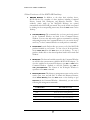
Control Statements
• if statement: The if statement executes a group of statements if the
evaluated expression is true. The optional elseif and else provide
alternatives for execution of different groups of statements.
•
Syntax:
if expression
statements
else
statements
end
if expression1
statements
elseif expression2
statements
…
else
statements
end
•
Example:
15
M A T L A B
U S E R
M A N U A L
>>if x > 10
z = 1;
else if y > 0
z = 2;
else
z = 3;
end
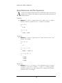
•
The switch statement evaluates an
expression and then executes a group of statements under the first
matching case statement. If no matching case statement is found, then the
statements under the optional otherwise statement are executed.
switch and case Statements:
•
Syntax:
switch expression
case test_expression1
statements
case test_expression2
statements
…
otherwise
statements
end
•
Example:
>>x = input( ' Enter a number: ' );
>>switch x
case 0
y = 0;
case 1
y = x + 2;
otherwise
y = 10;
end
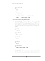
•
The for loop repeatedly executes a group of statements a
fixed and predetermined number of times.
for Statement:
•
Syntax:
for variable = expression
statements
end
16
M A T L A B
•
U S E R
M A N U A L
Example:
>> for n = 1 : 4
x( n ) = n/10 * pi;
end
>> x
x=
0.3142 0.6283 0.9425 1.2566
•
The while loop allows a group of statements to be
repeatedly executed as long as the evaluated expression is true.
while Loop Statement:
•
Syntax:
while expression
statements
end
•
Example:
>> p =1; u = 1;
while p < 16
p = p * 2;
u = [ u, p ];
end
>> u
u=
1 2 4 8 16
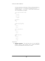
•
continue and break Statements: The continue statement causes
execution of a for or while loop to jump immediately to the next iteration
of the loop, and it skips any remaining statements in the loop. In contrast
to the continue statement, the break statement terminates the execution of
the loop.
•
Syntax:
while expression
statements
continue
statements
end
17
M A T L A B
U S E R
M A N U A L
for variable = expression
statements
continue
statements
end
while expression
statements
break
statements
end
for variable = expression
statements
break
statements
end
•
Example:
>> m = 1; n = 0;
>> while n <= 1000
m = m/3;
if ( 1 + m ) > 1
n = n + 1;
continue
end
m = m*3
break
end
m=
1.7989e-016
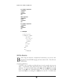
M-File Basics
B
esides using the interactive computational environment, you can also write
programs in the MATLAB language and store them in files. These files are
called M-files.
Creating M-Files
An M-file is just an ordinary text file and hence it can be created using any text
editor. As mentioned earlier, MATLAB provides a default M-file editor for all
platforms. To open the default editor, select New and then M-File from the File
menu, or type edit in the Command Window. To save an M-file, from the File
menu select Save for an existing file or Save as for a new file. An M-file name
18
M A T L A B
U S E R
M A N U A L
must have a '.m' extension after the file name. There are two types of M-files,
script files and function files.
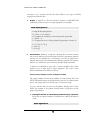
•
A script file is a file that contains a sequence of valid MATLAB
commands, and has no input or output arguments. For example:
Scripts:
M-file: myScriptFile.m
% Script M-file myScriptFile.m
% 1. Create a 3 × 3 matrix A
% 2. Compute the coefficients of the characteristic polynomial,
% det(λI – A)
% 3. Compute the roots of this polynomial (eigenvalues of matrix A)
A = [1 2 3; 4 5 6; 7 8 0]
p = poly (A)
r = roots (p)
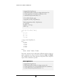
•
Similar to a script file, a function file is a file that contains
one or more functions. The first function in the file is the primary function
and the rest are subfunctions. A subfunction can only be called by the
primary function and other subfunctions within the same file. The primary
function or a subfunction can contain any valid MATLAB statements.
Function Files:
A function or subfunction starts with a function definition line, which
specifies a list of input and/or output arguments. The syntax of the
function definition line is defined as follows.
function [output variables] = function_name(input variables)
The output variables and the input variables are both optional. Note that
MATLAB function names are specified in the same way as variable names
(that is, they begin with a letter and are up to 31 characters long).
To save a function file, one must use the primary function name for the
M-file. For example, if the primary function name is EigValues, the file
name is EigValues.m
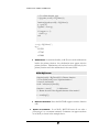
•
Passing Parameters to and Returning Parameters from a Function:
Below are two simple examples to illustrate how a MATLAB function
works.
M-file: EigValues.m
19
M A T L A B
U S E R
M A N U A L
% Script M-file EigValues.m
% This function takes a matrix A as input and returns a list
% of the eigenvalues of A and the coefficients of the
% characteristic polynomial, det(rI - A).
% To call this function, type:
% [eigvalues, coeffs] = EigValues(A);
function [eigvalues,coeffs] = EigValues(A)
p = poly (A);
eigvalues = roots (p);
coeffs = p;
>> C = [ 1 2 3; 4 5 6; 7 8 0 ]
C=
1 2 3
4 5 6
7 8 0
>> [eig, coef] = EigValues( C )
eig =
12.1229
- 5.7345
- 0.3884
coef =
1.0000 -6.0000 -72.0000 -27.0000
Note that a function can be called with a different number of input or
output arguments by using the built-in functions nargin and nargout.
The example below is the same function as EigValues above except the
output of the coefficients is optional.
M-file: EigValues.m
% Script M-file EigValues.m
% This function takes a matrix A as input, returns a list
% of the eigenvalues of A, and optionally returns the coefficients
% of the characteristic polynomial, det(rI - A).
20
M A T L A B
U S E R
M A N U A L
% To call this function, type:
% [eigvalues, coeffs] = EigValues(A);
function [eigvalues,coeffs] = EigValues(A)
p = poly (A);
eigvalues = roots (p);
if ( nargout == 2 )
coeffs = p;
end
>> eig = EigValues( C )
eig =
12.1229
- 5.7345
- 0.3884
•
Subfunctions: As mentioned earlier, an M-file can contain subfunctions
besides the primary function. Any subfunction must appear after the
primary function. Subfunctions are local and can be called only by the
primary function and other subfunctions in the same M-file.
M-file: BigTrace.m
function [result] = BigTrace(A,B) % Primary function
% The variable result is set to equal maximum of
% trace(A) and trace(B)
result = max(trace(A),trace(B));
function t = trace(C)
% Subfunction
% Return the sum of the diagonal elements of the matrix C.
t = sum(diag(C));
•
Recursive Functions: Note that MATLAB supports recursive function
calls.
•
Syntax of Comments: In an M-file, MATLAB treats all text after a
percent sign % as a comment statement. Comments can appear anywhere
in an M-file, as shown in the examples above.
21
M A T L A B
U S E R
M A N U A L
Running M-Files
•
To invoke an M-file (either a function file or a
script file), type the name of the file without the '.m' extension from the
command line in the Command Window. For example, you can call the
function BigTrace from the command line as follows.
From the Command Line:
Suppose A = [1 2 3; 4 5 6; 7 8 0] and B = [3 4; 5 6] .
>> BigTrace( A, B )
ans =
9
•
Within Another M-file:
A function or a script can similarly be called from
another M-file.
Summary of Useful Commands
C O M M A N D
D E S C R I P T I O N
type filename
Display the contents of a specified file
edit filename
Invoke the default editor
path
Display the current MATLAB search path.
tic/toc
tic starts a timer and toc returns elapsed time
profile
A debugging utility
lookfor
Search for the specified keyword in all help entries
dbstop
Set breakpoints in an M-file function
dbclear
Clear breakpoints in an M-file function
dbcont
Resume execution
dbquit
Quit debug mode
keyboard/return
Invoke and terminate the keyboard mode in an M-file
nargin
Number of input function arguments
nargout
Number of output function arguments
which
Locate functions and files
pcode
Create pre-parsed pseudocode file
22
M A T L A B
U S E R
M A N U A L
Input/Output and Data Formatting
M
ATLAB allows user input during runtime, saves a copy of a MATLAB
session in a file, and saves data files in a variety of formats. In addition,
there are commands to control how data are displayed.
Input
•
User input can be prompted and obtained interactively during
runtime. The syntax for the command input is given below. The value
entered by a user can be any valid MATLAB expression or a character
string if the second argument 's' is used.
User Input:
inValues = input(prompt_string)
inValues = input(prompt_string,'s')
•
Example:
>> isQuit = input( ' Do you want to exit the current session? Y/N [Y]: ',
's' );
>> if ( isQuit == 'Y' | isempty( isQuit ) )
save;
quit;
else
quit cancel;
end
Output
•
Save and Load Variables: Before you exit or quit the current workspace,
you can use the save command to save all the variables and their current
values. In a new session, you can use the load command to restore them.
For example:
>> save filename
To restore the variables, type
>> load filename
Note that if save and load are used without a specified file name, MATLAB
uses a default file name, matlab.mat.
•
Output to the Screen:
Several output functions are available. Here are a
few examples.
23
M A T L A B
U S E R
M A N U A L
When you type a variable name, MATLAB displays the variable name and its
value by default. Sometimes it is desirable to display only the value. For
example, suppose B = [3 4; 5 6] . Then to display the value of the
matrix B with column labels, type
>> disp( '
B1 B2
3 4
B1 B2 ' ), disp( B )
5 6
Similarly, if x = 0.756, then to display the formatted value of x, type
>> fprintf( '%7.2f\n', x )
0.76
Note that the number 7 in the format string is the field width, the number 2 is
the number of decimal digits after the decimal point, and the escape character
\n is a new line terminator.
•
Suppress Output from MATLAB Commands: If you place a semicolon (; )
at the end of a statement line, MATLAB executes the statement but does
not display any output. For example:
>> u = [ 1 2 ];
>> v = u + 3;
•
The diary command can be used to save the entire
working session. This command spools all the activities or events in the
Command Window to a text file. For example, to save the current session,
type
Keep a Session Log:
>> diary filename
To suspend the diary, type
>> diary off
If diary is used without a specified file name, then MATLAB uses a default file
name diary.
24
M A T L A B
U S E R
M A N U A L
Format
For online help
type help format or
select MATLAB Help
from Help menu.
MATLAB stores numbers to a relative precision of
approximately 16 decimal digits. By default MATLAB displays
numbers in the short format (4 decimal places). To print a value
in any of the formats given below, enter format type on the
command line. For example:
>> format long
The following table illustrates the additional format types supported by MATLAB.
F O R M A T
E X A M P L E S
format short
17.3205
format short e
1.7321e+001
format short g
17.321
format long
17.32050807568877
format long e
1.732050807568877e+001
format long g
17.3205080756888
format bank
17.32
format hex
4031520cd1372fea
format rat
1351/78
25
M A T L A B
U S E R
M A N U A L
Summary of Useful Commands
C O M M A N D
D E S C R I P T I O N
save filename
Save variables
load filename
Restore variables
clc
Clear the Command Window
disp
Display text or array
input
Wait for input from the keyboard
pause(n)
Halt execution temporarily
diary
Save a session to a disk file
format
Control the output format
Graphics
M
ATLAB has extensive tools for displaying various data as graphs. It also
provides facilities for annotating and printing graphs. In the following
section, some examples are presented to illustrate how a graph can be
created using these tools. To invoke the graphics editor, type figure in the
Command Window.
Basic Plots
The most basic graph is a simple 2-D plot. One form of the syntax for the plot
command is plot (x_values,y_values,'style-option'). x_values is a
For online help
vector that contains the points on the x-coordinate, while
type help graph2d
y_values contains the points on the y-coordinate. style-option is a
or select MATLAB
parameter that defines the line style, the marker, and the color
Help from Help
used in a graph. If this parameter is not entered, MATLAB uses
menu.
the default style. Style options are summarized in the following
table.
26
M A T L A B
U S E R
M A N U A L
C O L O R
L I N E
S T Y L E
M A R K E R
y
Yellow
-
Solid
o
Circle
m
magenta
--
Dashed
*
Asterisk
c
Cyan
:
Dotted
.
Point
r
Red
-.
Dash-dot
+
Plus
g
Green
none
No line
x
Cross
b
Blue
s
Square
w
White
d
Diamond
k
Black
^
Upward triangle
v
Downward triangle
>
Right triangle
<
Left triangle
p
Five-point star
h
Six-point start
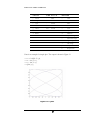
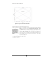
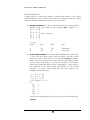
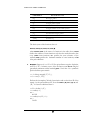
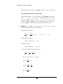
Here is an example of a simple plot. The output is shown in Figure 2.1
>> t = 0 : 0.001 : 2 * pi;
>> x = cos( 3 * t );
>> y = sin( 2 * t );
>> plot( x, y )
Figure 2.1: x-y Plot
27
M A T L A B
U S E R
M A N U A L
Graph of a Function
MATLAB provides commands ezplot and fplot for plotting mathematical functions.
The syntaxes for the commands are ezplot ('function', [xmin, xmax, ymin, ymax]) and fplot
('function', [xmin, xmax, ymin, ymax]), respectively. Both commands plot a function in a
specified range. However, if a line style different from the default is required, then fplot
( 'function', [xmin, xmax, ymin, ymax], 'style-option') should be used. For example, let us
first create a function in an M-file called myFunction.m and then use the command
ezplot ('myFunction',[ 0 2*pi 0 12 ]) to generate the graph on the specified range. The
output is shown in Figure 2.2a. To generate the same plot using a dotted line instead
of a solid line (default), use fplot ('myFunction',[ 0 2*pi 0 12 ], ' :xr '). Note that ':xr' means
a dotted red line with cross markers is used in the plot. The output is shown in Figure
2.2b.
M-file: myFunction.m
function y = myFunction(x)
y = exp( sqrt(x) .* sin(12 * x) );
>> ezplot( 'myFunction', [ 0 2*pi 0 12 ] )
Figure 2.2a: Plot of a Function Using ezplot
>> fplot( 'myFunction', [ 0 2*pi 0 12 ], ' :xr ' )
28
M A T L A B
U S E R
M A N U A L
Figure 2.2b: Plot of a Function Using fplot
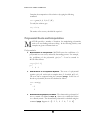
Define Titles, Labels and Text in a Graph
You can add a title to a graph and add labels to axes. The general syntax for the title
function is title('string'), and the syntax for the xlabel and ylabel commands are
xlabel('string') and ylabel('string'). Moreover, you can also add a text object to a graph.
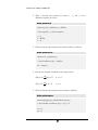
The syntax for the command text is text(x, y, 'string'). For example, we add a title,
labels and a text object to Figure 2.1. The output is shown in Figure 2.3.
>> plot( x, y )
>> title( 'X-Y Plot' )
>> ylabel( 'cos(2*t)' )
>> xlabel( 'sin(3*t)' )
>> text( -0.2, 0.4, 'A symmetry graph' )
29
M A T L A B
U S E R
M A N U A L
Figure 2.3: x-y Plot with Title and Labels
Commands for Controlling the Axes
After you generate a graph, you can modify or change an axis range with the command
axis. The most basic syntax is axis([xmin xmax ymin ymax]). xmin
For online help
and
xmax define the smallest and largest end points for x-axis;
type help axis or
similarly,
ymin and ymax define the smallest and largest end
select MATLAB
points for y-axis. For example, we can change the ranges for the
Help from Help
axes in Figure 2.2a to [ 0, 4 ] and [ 0, 8 ] as follows. The output
menu.
is shown in Figure 2.4.
>> ezplot( 'myFunction', [ 0 2*pi 0 12 ] )
>> axis( [ 0 4 0 8 ] )
30
M A T L A B
U S E R
M A N U A L
Figure 2.4: Plot of a Function: myFunction with Modified Axis Ranges
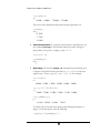
Multiple Plots in One Figure
There are three ways to create multiple plots on a single graph.
For online help
type help subplot
or select MATLAB
Help from Help
menu.
•
The MATLAB function
can be used to plot data into different subregions within the same graphics window. The
command subplot(m,n,i) divides the graphics window
into an m by n matrix of small sub-regions and
generates the next figure in the ith sub-region. The subregions are numbered row-wise.
Using the Command subplot:
subplot
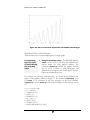
For example, the following statements plot a set of data in four different subregions of the graphics window in Figure 2.5. The command subplot(2,2,1) is set
for plot(t,z) to be generated in the first sub-region in first row. Similarly,
subplot(2,2,2) is set for plot(t,2*q) in the second sub-region in the first row, and so
on.
>> t = 0 : pi/20 : 2*pi;
>> z = cos( 3*t );
>> subplot( 2, 2, 1 )
>> plot( t, z )
>> subplot( 2, 2, 2 )
>> q = exp( -t );
>> plot( t, 2*q )
>> subplot( 2, 2, 3 )
>> fplot( 'myFunction',[ 0 2*pi ] )
31
M A T L A B
U S E R
M A N U A L
>> subplot( 2, 2, 4 )
>> fplot( '[ sin( x ), cos( 2*x ), 1/( 1+x ) ]',[ 0 5*pi -1.5 1.5 ] )
Figure 2.5: Generating Multiple Plots Using subplot
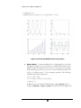
•
To create multiple plots in a single graph (as in the last
sub-region in Figure 2.5), one can also use a matrix. Each column of the
matrix contains the functional values that are to be plotted as one graph.
In the following, note that cos(x) is a row vector of functional values, and
cos(x)' is a column vector ( ' is the transpose operator). The following
example is illustrated in Figure 2.6a.
Using a Matrix:
>> x = 0 : 0.01 : 2*pi;
>> Y = [ cos( x )', cos( 2*x )', cos( 4*x )' ];
>> plot( x, Y )
If different styles are desired for different plots, replace plot(x,Y) with, for
example, plot(x,Y(:,1),'--',x,Y(:,2),'-.',x,Y(:,3)). The result is shown in Figure 2.6b.
32
M A T L A B
U S E R
M A N U A L
Figure 2.6a: Generating Multiple Plots Using a Matrix
Figure 2.6b: Multiple Plots with Different Styles
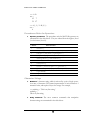
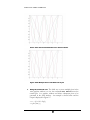
•
The third way to create multiple plots in the
same graphics window is to use the command hold. hold on freezes the
current plot in a graphics window and allows subsequent plots to be
generated in the same window. An example is shown below and the
output is displayed in Figure 2.7.
Using the Command hold:
>> t = [ 0 : 0.01 : 2*pi ];
>> plot( sin( t ) )
33
M A T L A B
U S E R
M A N U A L
>> hold on
>> plot( cos( t ) )
>> hold off
Figure 2.7: Generating Multiple Plots Using hold
Save and Print a Figure
To print a hardcopy of a graph, the simplest way is to select Print
For online help
from the File menu in a graphics window or alternatively type
type help print or
type help saveas
the print command directly in the Command Window. Similarly
select MATLAB Help to save a graph into a file, select Save from the File menu or
from Help menu.
enter the print command along with a file name in the
Command Window. The basic syntax of the print command is
defined as follows.
print –ddevicetype –options filename
For example, the following statement will save the current graph into a file named as
mygraph.eps.
>>print –deps mygraph.eps
You can export a graph with a specified format using the command
example, the command below saves the current graph in the jpg format.
>> saveas( gcf, 'myGraph.jpg' )
34
saveas.
For
M A T L A B
U S E R
M A N U A L
Commands for 2D Plotting Functions
C O M M A N D
D E S C R I P T I O N
area
Create an area graph
bar
Create a bar graph
barh
Create a horizontal bar graph
compass
Create an arrow graph for complex numbers
contour
Make a contour graph
hist
Create a histogram graph
pie
Create a pie graph
scatter
Create a scatter graph
stairs
Create a stair step graph
polar
Plot polar coordinates
plotmatrix
Draw scatter plots
plot
Create a 2-D plot
fplot
Plot a function between specified ranges ( with line styles)
ezplot
Plot a function between specified ranges
subplot
Create and control multiple axes
grid
Grid lines for two-dimensional plots
xlabel/ylabel
Create labels for x-axis and y-axis
title
Add titles to current axes
legend
Create a legend on a graph
hold
Hold current graph in a figure
text
Create text objects in current axes
fill
Filled two-dimensional polygons
line
Create a line object
axis
Set ranges for x-axis and y-axis
35
M A T L A B
U S E R
3
Chapter
M A N U A L
Basic Functions for Linear
Algebra and Numerical
Analysis
Linear Algebra
M
ATLAB has an extensive set of functions for computations in linear
algebra, such as functions for computing the inverse and the determinant of
a matrix. In the following section, several fundamental concepts from linear
algebra are defined and some examples are given to illustrate how to use
these MATLAB functions to solve linear algebra problems.
Vector and Matrix Norms
Norms, which are scalars, are measures of the size of vectors and matrices.
•
P-norm of a Vector: The p-norm of a vector x is
n
i =1
x p≡ ∑x
p
i
1/ p
for 1 ≤ p < ∞ .
The sum norm ( p = 1 ) and the Euclidean norm ( p = 2 ) are
particular cases of p-norms. In MATLAB, a norm is calculated by using
the function norm(x, p). Suppose x = [2 4 6 8] .
>> [ norm( x, 1 ) norm( x, 2 ) ]
ans =
20.0000 10.9545
Note that norm( x, 2 ) can be computed by norm( x ).
36
M A T L A B
U S E R
When p
→
M A N U A L
∞ , the p-norm becomes the max norm, defined as
x ∞ ≡ max { x 1 ,..., x n
}
For example, to compute the max norm of the vector x used in the
previous example, type
>> norm( x, inf )
ans =
8
•
P-norm of a Matrix: The p-norm of a matrix A is
Ax
A p ≡ max
x≠0
x
p
p
The maximum column sum matrix norm ( p = 1 ), the maximum row
sum matrix norm ( p = ∞ ), and the spectral norm ( p = 2 ) are
particular cases of the p-norms and they can be computed, respectively, by
n
A 1 ≡ max ∑ a ij ,
1≤ j ≤ n i =1
n
A ∞ ≡ max ∑ a ij , and
1≤ i ≤ n j =1
A 2 ≡ max{ λ : λ is an eigenvalue of A*A } .
Suppose matrix A = [1 2; 3 4] . To use the function
compute these matrix norms, type
norm(A, p)
to
>> [ norm(A, 1) norm(A, inf) norm(A, 2) ]
ans =
6.0000 7.0000 5.4650
Note that norm(A, 2) can be computed by norm(A).
Inverses
•
Inverse of a Square Matrix:
matrix A-1 such that
The inverse of a square matrix A is the
where I is the identity matrix. The
A-1A = AA-1 = I,
37
M A T L A B
U S E R
M A N U A L
function inv(A) is used to compute the inverse of a square matrix A. For
example:
>> A = [ 1 2; 3 4 ]
A=
1 2
3 4
>> B = inv( A )
B=
- 2.0000 1.0000
1.5000 - 0.5000
>> I = B * A
I=
1.0000
0
0.0000 1.0000
•
If a matrix A is a square and singular matrix, or a
rectangular matrix, it does not have an inverse. However, A has a unique
pseudo-inverse which can be computed using pinv(A). For example:
Pseudo-inverse:
>> A = [ 1 2 3; 5 7 9 ]
A=
1 2 3
5 7 9
>> B = pinv( A )
B=
- 1.3889 0.4444
- 0.2222
0.1111
0.9444 - 0.2222
>> B * A
ans =
0.8333 0.3333 - 0.1667
0.3333 0.3333 0.3333
- 0.1667 0.3333 0.8333
38
M A T L A B
U S E R
M A N U A L
>> A * B
ans =
1.0000 0.0000
- 0.0000 1.0000
>> A * B * A
ans =
1.0000 2.0000 3.0000
5.0000 7.0000 9.0000
>> B * A * B
ans =
- 1.3889 0.4444
- 0.2222
0.1111
0.9444 - 0.2222
Transposes
The transpose of a matrix A is obtained by interchanging the rows and columns of
A, and is computed by A' in MATLAB.
•
Transpose of a Real Matrix: For example:
>> A = [ 1 2; 3 4 ]
A=
1 2
3 4
>> A'
ans =
1 3
2 4
•
Conjugate Transpose of a Complex Matrix: In addition to interchanging
the rows and columns, the conjugate transpose of a complex matrix A also
replaces each entry by its complex conjugate. For example:
>> A = [ 1 + i, 2 - i; -3, -2i ]
A=
1.0000 + 1.0000i 2.0000 - 1.0000i
- 3.0000
0 - 2.0000i
39
M A T L A B
U S E R
M A N U A L
>> A'
ans =
1.0000 - 1.0000i
- 3.0000
2.0000 + 1.0000i 0 + 2.0000i
Determinants
•
Determinant of a Square Matrix: The determinant of a square matrix A is
calculated using the triangular factors obtained from Gaussian elimination
and can be computed by det(A). Suppose A = [1 2; 3 4] .
>> det( A )
ans =
-2
Rank
•
The rank of a matrix A is the largest number of
columns (or rows) of A that constitutes a linearly independent set. To
compute the rank of a matrix, use the function rank(A) in MATLAB. For
example, for the matrix A = [1 2; 3 4] :
Rank of a Matrix:
>> rank( A )
ans =
2
Factorizations
•
For every square matrix A, there exist a
lower triangular matrix L, an upper triangular matrix U, and a permutation
matrix P such that PA = LU. To compute the LU factors for a matrix by
Gaussian elimination with partial pivoting, use the function lu(A) in
MATLAB. For example, suppose A = [1 3; 2 4] .
LU Factorization of a Matrix:
>> [L, U, P] = lu( A )
L=
1.0000
0
0.5000 1.0000
U=
2 4
0 1
40
M A T L A B
U S E R
M A N U A L
P=
0 1
1 0
•
The Cholesky factorization is a
special case of LU factorization. Suppose A is a real symmetric matrix. If
A is positive definite (that is, x'Ax > 0 for all nonzero column vectors x),
then A can be factored as A = R'R, where R is an upper triangular matrix.
The function chol(A) in MATLAB is used to compute the Cholesky factor
for a matrix A. For example:
Cholesky Factorization of a Matrix:
>> A = [ 1 1 1; 1 2 3; 1 3 6 ]
A=
1 1 1
1 2 3
1 3 6
>> R = chol( A )
R=
1 1 1
0 1 2
0 0 1
>> R' * R
ans =
1 1 1
1 2 3
1 3 6
•
Any matrix A can be factored as a product
QR, where Q is orthogonal (or unitary) and R is upper triangular. This
decomposition is used, for example, to compute the eigenvalues of a
matrix and to solve least-squares problems. To compute the QR
factorization of a matrix A, use the function qr(A).
QR Factorization of a Matrix:
Suppose A = [1 0 1; 2 2 3; 0 1 3].
41
M A T L A B
U S E R
M A N U A L
>> [Q, R] = qr( A )
Q=
- 0.4472 0.5963 0.6667
- 0.8944 - 0.2981 - 0.3333
0 - 0.7454 0.6667
R=
- 2.2361 - 1.7889 - 3.1305
0 - 1.3416 - 2.5342
0
0 1.6667
Eigenvalues
•
If A is a square matrix and if
a scalar λ and a nonzero vector x satisfy the equation Ax = λx, then λ is
called an eigenvalue and x is called an eigenvector of the matrix A. The
function eig(A) allows you to compute eigenvalues and eigenvectors of a
matrix. Suppose A = [5 − 3 2; − 3 8 4; 1 3 − 9] .
Eigenvalues and Eigenvectors of a Matrix:
>> [V, D] = eig( A )
V=
- 0.4690 0.8714 - 0.1763
0.8760 0.4583 - 0.2421
0.1129 0.1751 0.9541
D=
10.1218
0
0
0 3.8243
0
0
0 - 9.9461
To verify that 10.1218 is an eigenvalue of A with corresponding
- 0.4690
eigenvector 0.8760 , enter the following.
0.1129
>> A * V( :, 1 )
ans =
- 4.7472
8.8666
1.1429
42
M A T L A B
U S E R
M A N U A L
>>D( 1, 1 ) * V( :, 1 )
ans =
- 4.7472
8.8666
1.1429
Singular Value Decomposition
• Singular Values of a Matrix: If A is an m × n matrix with rank r, then
there exist real numbers σ1 ≥ σ2 ≥ …≥ σr > 0, an orthonormal basis v1,…,
vm , and an orthonormal basis u1,…, un such that
Avi = σiui
Avi = 0
i = 1,…,r
A'ui = σivi
i = r + 1,…,m A'ui = 0
i = 1,…,r
i = r + 1,…,n
In MATLAB, the function svd(A) computes the singular value
decomposition for a matrix A.. Suppose A is the 2 × 3 matrix
[1 2 0; 2 0 2] .
>> [U D V] = svd( A )
U=
0.4472 0.8944
0.8944 - 0.4472
D=
3 0 0
0 2 0
V=
0.7454 - 0.0000 - 0.6667
0.2981
0.8944
0.3333
0.5963 - 0.4472
0.6667
The function returns two orthogonal matrices U and V, and a matrix D
that contains the singular values of A in its diagonal entries. To verify A =
UDV', enter the following statement.
>> U * D * V'
ans =
1.0000 2.0000 - 0.0000
2.0000 - 0.0000
2.0000
43
M A T L A B
U S E R
M A N U A L
Sparse Matrices
A sparse matrix is a matrix that contains a relatively large number of zero entries.
MATLAB provides a set of functions that stores only the nonzero entries of a sparse
matrix and eliminates arithmetic operations on the zero entries.
•
versions
1 0
0 0
0 1
0 0
•
To find out the information about sparse and full
of the same matrix, use the command whos. Suppose A =
0 0
0 2
and B = sparse (A).
5 0
3 0
Storage Information:
>> whos
Name
Size
Bytes
Class
A
B
4x4
4x4
128
80
double array
sparse array
For a sparse matrix, MATLAB uses three arrays
to store only the nonzero entries, their row indices, and their column
indices. To create a sparse matrix, use the command sparse( i, j, s, m, n ),
where i and j are the vectors that contain row and column indices for the
nonzero entries of the matrix; s is a vector that contains a list of nonzero
values whose indices are defined by the corresponding i, j pairs; m is the
row dimension of the sparse matrix; and similarly n is the column
dimension. To create a sparse matrix B of the above matrix A, for
example, enter the following.
Create a Sparse Matrix:
>> i = [ 1 2 3 3 4 ];
>> j = [ 1 4 2 3 3 ];
>> s =[ 1 2 1 5 3 ];
>> B = sparse( i, j, s, 4, 4 )
B=
(1,1)
1
(3,2)
1
(3,3)
5
(4,3)
3
(2,4)
2
Note that the resulting matrix above is the same as the one obtained using
sparse(A).
44
M A T L A B
•
U S E R
M A N U A L
There are a few useful commands to compute
additional information about a sparse matrix. For example, to find the
number of nonzero entries in the above sparse matrix B, use the
command nnz(B).
View Sparse Matrices:
>> nnz( B )
ans =
5
To obtain the list of nonzero entries of B, use the command nonzeros(B).
>> nonzeros( B )
ans =
1
1
5
3
2
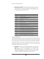
To view the distribution of the nonzero entries of B, use the command
spy(B).
>> spy( B )
45
M A T L A B
•
U S E R
M A N U A L
There are numerous sparse matrix functions in
MATLAB, e.g., for the solution of simultaneous linear equations, and for
factorizations such as LU, QR, and Cholesky. The table below lists a set
of commonly used sparse matrix functions.
Sparse Matrix Functions:
C O M M A N D
D E S C R I P T I O N
isspars
True if matrix is sparse
find
Find indices and values of nonzero entries
spalloc
Allocate space for sparse matrix
sprank
Structure rank
speys
Sparse identity matrix
svds
A few singular values
eigs
A few eigenvalues
cholinc
Incomplete Cholesky factorization
luinc
Incomplete LU factorization
bicg
Biconjugate gradient iterative linear equation solution
bicstab
Biconjugate gradient stabilized iterative linear equation solution
cgs
Conjugate gradient squared iterative linear equation solution
gmres
Generalized minimum residual iterative linear equation solution
minres
Minimum residual iterative linear equation solution
pcg
Preconditioned conjugate gradient iterative linear equation solution
qmr
Quasi-minimal residual iterative linear equation solution
Iterative Methods
Two classes of methods can be used to solve systems of simultaneous linear equations,
direct methods and iterative methods. Direct methods are more efficient for small
linear systems; however, they may be very costly in terms of storage and computational
time for large sparse linear systems. If convergent, iterative methods compute an
approximate solution to a linear system and this may be much more efficient than
using a direct method. In this section, we describe how to solve a linear system using
MATLAB functions based on iterative methods.
•
The functions in MATLAB are intended to solve Ax = b or
A linear system is usually replaced by an equivalent system
-1
-1
M Ax = M b, where M is a preconditioner that is chosen to make
computation of the solution more efficient. The goal is to find a simple
matrix M so that M-1Ax is near to the identity matrix. The table below lists a
set of MATLAB functions corresponding to iterative methods.
Description:
min | b – Ax |.
46
M A T L A B
U S E R
M A N U A L
C O M M A N D
D E S C R I P T I O N
bicg
Biconjugate gradient
bicgstab
Biconjugate gradient stabilized
cgs
Conjugate gradient squared
gmres
Generalized minimum residual
lsqr
Conjugate Gradients on the normal equations
minres
Minimum residual
pcg
Preconditioned conjugate gradient
qmr
Quasiminimal residual
symmlq
Symmetric LQ
The basic syntax of the functions above is
function_name (A, b, restart, tol, maxit, M)
where function_name is the name of a function in the table above; restart
defines the number of inner iterations such that the method restarts after
every restart inner iterations; tol specifies the error tolerance of the
method; maxit specifies the maximum number of outer iterations; and M
is the preconditioner.
•
Suppose A is a 139 × 139 five-point discrete negative Laplacian,
and b is a 139 × 1 column vector. Solve the linear system Ax = b using the
generalized minimum residual method gmres. Note that A is a symmetric
positive definite sparse matrix.
Example:
>> A =delsq( numgrid( 'C', 15 ) );
>> b = ones( 1, 139 )';
Perform the incomplete Cholesky factorization and use the factor R' of the
matrix A as the preconditioner M. Note that M-1Ax = ( R' )-1Ax = ( R' )-1b, and
( R' )-1A is better conditioned than A.
>> R = cholinc( A, '0' );
>> condest( A )
ans =
86.2192
>> condest( inv( R' ) * A )
ans =
31.8511
47
M A T L A B
U S E R
M A N U A L
Complete the computation of the solution x by typing the following
command.
>> x = gmres( A, b, 12, 1e-5, 3, R' );
To verify the solution, type
>> y = A * x;
The entries of the vector y should all be equal to 1.
Polynomial Roots and Interpolation
M
ATLAB provides a number of functions for manipulating polynomials,
such as for root finding and curve fitting. In the following section, some
examples are given to illustrate their use.
Polynomials
•
MATLAB stores the coefficients of a
polynomial in a row vector, ordered by descending powers. For example,
the coefficients of the polynomial p( x) = x 2 − 1 can be entered in
MATLAB as follows.
Representation of a Polynomial:
>> p = [ 1 0 -1 ]
p=
1 0 -1
•
The roots of a polynomial
equation p( x) = 0 are the real or complex values x̂ for which p ( xˆ ) = 0 .
The roots can be computed using the command roots(p). In the case of
the above polynomial, the roots are calculated as follows.
Find the Roots of a Polynomial Equation:
>> r = roots( p )
r=
−1
1
•
The characteristic polynomial of
an n × n matrix A is defined as det(rI - A), where r is a variable and I is the
n × n identity matrix . The characteristic polynomial is calculated using the
command poly(A). Suppose A = [1 2 3; 4 5 6; 7 8 0].
Characteristic Polynomial of a Matrix:
48
M A T L A B
U S E R
M A N U A L
>> p = poly ( A )
p=
1.0000 - 6.0000 - 72.0000 - 27.0000
The roots of this characteristic polynomial are the eigenvalues of A.
>> roots( p )
ans =
12.1229
- 5.7345
- 0.3884
•
To evaluate a polynomial at a specified point, use
the command polyval(p, x). This function returns the value of the given
polynomial p at the point x. Suppose p( x) = x 2 − 1 .
Polynomial Evaluation:
>> p = [ 1 0 -1 ];
>> polyval( p, 2 )
ans =
3
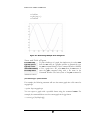
•
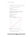
The function polyfit(x, y, n) determines the polynomial p(x)
of degree of n that best fits the given data ( x i , y i ) , 1 ≤ i ≤ n, in the least
squares sense. That is, p ( x) ≈ y i for i = 1, 2,…, n. For example:
Data Fitting:
>> x =1 : 0.2 : 2
x=
1.0000 1.2000 1.4000 1.6000 1.8000 2.0000
>> y = [ 2 1.7 1.3 1.28 1.11 1 ]
y=
2.0000 1.7000 1.3000 1.2800 1.1100 1.0000
>> p = polyfit( x, y, 3 )
p=
- 0.9144 4.9494 - 9.4616 7.4432
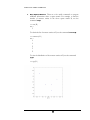
To obtain a plot of the best least squares polynomial approximation of
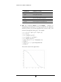
degree 3 to the data points, enter the following.
>> plot( x, y, '*', x, polyval(p, x), '--' )
49
M A T L A B
•
U S E R
M A N U A L
Other Useful Functions:
The table below lists some useful polynomial
functions.
C O M M A N D
D E S C R I P T I O N
conv
Polynomial multiplication
deconv
Polynomial division
polyder
Polynomial derivative
polyvalm
Matrix polynomial evaluation
residue
Partial fraction expansion
Polynomial Interpolation
• One Dimensional Interpolation: A polynomial p( x) in one variable x
interpolates a given set of values ( x i , y i ) , 1 ≤ i ≤ n, if p ( x i ) = y i for i
= 1, 2,…, n.
•
There are six methods available for one-dimensional
interpolation. The default interpolation method is linear.
Methods:
50
M A T L A B
•
U S E R
M A N U A L
M E T H O D
D E S C R I P T I O N
linear
Linear interpolation
spline
Cubic spline interpolation
nearest
Nearest neighbor interpolation
pchip
Piecewise cubic Hermite interpolation
cubic
Piecewise cubic Hermite interpolation
v5cubic
Cubic interpolation used in MATLAB 5
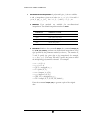
The command interp1( x, y, xx, method ) computes an
interpolating polynomial p(x) of the type specified by the parameter
method (see above) for the data specified in the vectors x and y, and
returns the interpolated values p(xx). For example:
Use:
>> x = [ 0 pi/4 3*pi/8 pi/2 3*pi/4 pi ];
>> y = cos( x );
>> xx = linspace( 0, pi, 40 )';
>> yy = interp1( x, y, xx, 'linear' );
>> z = linspace( 0, pi, 50 )';
>> plot( z, cos( z ), '-', x, y, '.', 'MarkerSize', 20 )
>> hold on
>> plot( xx, yy, '+' ) % plot interpolated data
>> hold off
The result is shown in the figure below.
51
M A T L A B
•
U S E R
M A N U A L
p ( x, y ) in two variables
x and y interpolates a given set of values ( x i , y j , z ij ) , 1 ≤ i ≤ n and 1 ≤
Two Dimensional Interpolation: A polynomial
j ≤ m, if p( x i , y j ) = z ij for i = 1, 2,…, n and j = 1, 2,…, m.
•
•
Four methods are available for two-dimensional
interpolation. The default interpolation method is linear.
Methods:
M E T H O D
D E S C R I P T I O N
linear
Bilinear interpolation
spline
Cubic spline interpolation
nearest
Nearest neighbor interpolation
cubic
Bicubic interpolation
Similar to the command interp1, the command interp2 ( X,
performs two-dimensional interpolation of the
type specified by the parameter method (see above). The matrices X,
Y and Z specify the given data to be interpolated; for example,
z ij = f ( x ij , y ij ) . The arrays XX and YY specify the points at which
the interpolating polynomial is evaluated. For example:
Functions:
Y, Z, XX, YY, method )
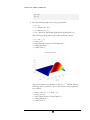
>> x = -4 : 0.5 : 4;
>> y = 0 : 0.5 : 8;
>> [X, Y] = meshgrid( x, y );
>> Z = peaks( X, Y );
>> xx = linspace( -4, 4, 50 );
>> yy = linspace( 0, 8, 50 );
>> [XX, YY] = meshgrid( xx, yy );
>> ZZ = interp2( X, Y, Z, XX, YX, 'bicubic' );
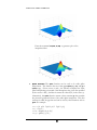
Enter the command surf( X, Y, Z ) to generate a plot of the original
data.
52
M A T L A B
U S E R
M A N U A L
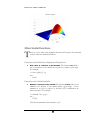
Enter the command surf( XX, YY, ZZ ) to generate a plot of the
interpolated data.
•
The spline function can be used to do cubic spline
interpolation. This function has two forms, yy = spline( x, y, xx ) and pp =
spline( x, y ). Given vectors x and y, the function computes the cubic
spline interpolating polynomial S that interpolates the given data specified
by the vectors x and y, and then it returns the values S(xx) in the vector yy.
Alternatively, the spline function returns a data structure pp that contains
the piecewise polynomial form of the cubic spline interpolant. This data
structure is called the pp-form and can be used by other functions such as
ppval. For example:
Spline Function:
>> x = [ 0 pi/4 3*pi/8 pi/2 3*pi/4 pi ];
>> y = cos( x );
>> xx = linspace( 0, pi, 40 )';
>> yy = spline( x, y, xx );
53
M A T L A B
U S E R
M A N U A L
>> z = linspace( 0, pi, 50 )';
>> plot( z, cos( z ), '-', x, y, '.', 'MarkerSize', 20 )
>> hold on
>> plot( xx, yy, '+' )
>> axis( [ 0 3.5 -1 1 ] )
>> hold off
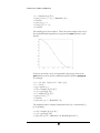
The resulting plot is shown below. This is the same example as the one in
the one-dimensional interpolation, except that the spline function is used
instead.
If there is more than one set of interpolated values, the pp-form of the
spline function can be used in combination with the function ppval(pp, xx).
For example:
>> x = [ 0 pi/4 3*pi/8 pi/2 3*pi/4 pi ];
>> y = cos( x );
>> pp = spline( x, y );
>> xx1 = linspace( 0, pi/2, 20 )';
>> yy1 = ppval( pp, xx1 );
>> z = linspace( 0, pi, 50 )';
>> plot( z, cos( z ), '-' )
>> hold on
>> plot( xx1, yy1, '+', 'MarkerSize', 10 )
The statements above compute interpolated values yy1 on the interval [ 0,
pi/2 ]. Similarly,
>> xx2 = linspace( pi/2, pi, 20 )';
>> yy2 = ppval( pp, xx2 );
>> plot( xx2, yy2, 'o', 'MarkerSize', 10, 'MarkerEdgeColor', 'r',
54
M A T L A B
U S E R
M A N U A L
'MarkerFaceColor', 'r' )
>> axis( [ 0 3.5 -1 1 ] )
>> hold off
compute interpolated values yy2 on the interval [ pi/2, pi ]. Note that
there is no need to recompute the same set of cubic spline coefficients a
second time; the previously computed pp-form can be used. The resulting
plot is shown below.
To get details of the piecewise polynomial or the pp-form, use the
function unmkpp(pp). For example, to print the knots and the coefficients
of the computed spline function above, type the commands below.
>> [breaks, coefs] = unmkpp(pp)
breaks =
0 0.7854 1.1781 1.5708 2.3562 3.1416
coefs =
0.1159 - 0.6123
0.1159 - 0.3392
0.1858 - 0.2026
0.1356 0.0163
0.1356 0.3357
0.0365 1.0000
- 0.7108 0.7071
- 0.9236 0.3827
- 0.9968 0.0000
- 0.7203 - 0.7071
Note that the values of the breaks are the entries of the vector x above,
and each row of the matrix coefs contains the coefficients of one of the
cubic polynomials of the spline function.
55
M A T L A B
U S E R
M A N U A L
Quadrature
M
ATLAB provides a set of functions for evaluating definite integrals. In the
following section, examples are given to illustrate the basic usage of these
functions.
Integrating Functions of One Variable
• Description: The numerical approximation of the definite integral
b
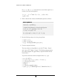
∫a f(x)dx
is called quadrature. The basic syntax of the MATLAB
quadrature functions is
q = quad( fun, a, b )
where fun is the function to be integrated;
integration.
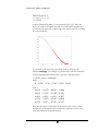
•
Example1:
F ( x) =
∫
b
a
a
and
b
specify the interval of
Consider the function below.
dx
2x 2 + 3
1. Write a MATLAB function for the function to be integrated. Note
that the MATLAB function should allow the argument x to be a
vector; that is, the ./ and .* operators are required in this function.
M-file: myIntegral.m
function y = myIntegral(x)
% Example for Quadrature
y = 1 ./ ( 2 .* x.^2 + 3 );
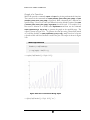
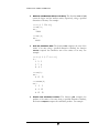
2. Run the following script to solve the given problem.
>> n = 15;
>> for m = 1 : n
b = m * 0.1;
Int(m) = quad( @myIntegral, 0, b );
end
3. View the result.
56
M A T L A B
U S E R
M A N U A L
>> x = linspace( 1, 1.5, 15 );
>> plot( x, Int )
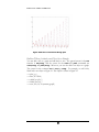
•
Another quadrature function in MATLAB is trapz(x, y). This
function computes a numerical approximation of the definite integral
Example2:
b
∫a f(x)dx by applying the trapezoidal rule.
Consider the example below.
dx
. An approximation of this integral using
1 x
can be obtained as follows.
Suppose F ( x) =
∫
2
trapz
>> format long
>> x = linspace ( 1, 2, 50 );
>> y = 1 ./ x;
>> area = trapz( x,y )
area =
0.69317321002551
Note that the exact solution is ln 2 = 0.69314718055995….
•
Summary of Quadrature Functions:
functions in MATLAB.
57
The table below lists the quadrature
M A T L A B
U S E R
M A N U A L
S O L V E R S
D E S C R I P T I O N
M E T H O D
quad
Adaptive Simpson quadrature
Simpson quadrature
quad l
Adaptive Lobatto quadrature
Lobatto quadrature
dblquad
Evaluate double integral
Double integral
trapz
Trapezoidal numerical integration
Trapezoidal Rule
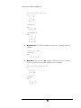
Ordinary Differential Equations
M
ATLAB provides software for solving both initial value and boundary value
problems. In the following section, examples are given to illustrate how to
solve initial value problems (a single differential equation and a system of
differential equations).
Initial Value Problems
• Description: These problems have the form
y ' = f (t , y ) subject to y (t 0 ) = y 0 ,
where t is a scalar variable (the independent variable), y = y (t ) , and the
initial condition is y (t 0 ) = y 0 . The functions y (t ) and f (t , y ) , and the
constant y 0 , can be vectors with more than one component.
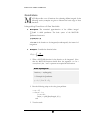
•
Example1: Solve the initial value problem
y' = y − t 2 + 1 ,
0 ≤ t ≤ 2,
y (0) = 0.5 .
First create the function myODE below and save the function in the file
myODE.m.
M-file: myODE.m
function dy = myODE(t,y)
% Initial Value Problem
% y' = y – t * t + 1, 0 ≤ t ≤ 2,
y( 0 ) = 0.5,
58
M A T L A B
U S E R
M A N U A L
dy = y - t * t + 1;
To run the function myODE, enter the following.
>> tspan = [ 0 2 ];
>> yzero = 0.5;
>> [t, y] = ode45( @myODE, tspan, yzero );
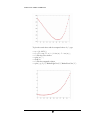
The exact solution to the problem is y (t ) = (t + 1) 2 − 0.5e t . The
following script generates a plot, which compares the (approximate)
computed solution with the exact solution.
>> w = [ 0 : .1 : 2 ];
>> f = ( w + 1 ) .^ 2 - 0.5 .* exp( w );
>> % Plot the exact solution
>> plot( w, f, '-' )
>> hold on
>> % Plot the computed solution
>> plot( t, y, 'o', 'MarkerEdgeColor', 'r', 'MarkerFaceColor', 'r' )
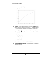
•
Example2: Solve the second order initial value problem
y ' '−2 y '+2 y = e 2t sin t , 0 ≤ x ≤ 1 , y (0) = −0.4 , y ' (0) = −0.6 .
1. Rewrite the problem as a first order system.
59
M A T L A B
U S E R
M A N U A L
Set y 1 = y and y 2 = y ' , and rewrite the second order equation as a
system of two first order equations:
y ' 1 = y 2 , y ' 2 = e 2t sin t + 2 y 2 − 2 y 1 ,
y 2 ( 0 ) = − 0 .6 .
y 1 ( 0 ) = − 0 .4 ,
2. Write a function that evaluates the differential equations as follows.
M-file: myODE2.m
function dy = myODE2(t,y)
% Initial Value Problem for a Second-order Equation
% y1' = y2, y2' = exp(2t)sin t + 2y2 - 2y1
% y1(0) = -0.4, y2(0) = -0.6
dy = [y(2); exp(2 * t) * sin(t) + 2 * y(2) - 2 * y(1)];
3. Run the following script to solve the given problem.
>> tspan = [ 0 1 ];
>> yzero =[ -0.4; -0.6 ];
>> [t, y] = ode45( @myODE2, tspan, yzero );
4. View the computed solutions.
The exact solution to the problem is y (t ) = 0.2e 2t (sin t − 2 cos t )
and y ' (t ) = 0.2e 2t (4 sin t − 3 cos t ) . The following script generates a
plot, which compares the (approximate) computed solution with the
exact solution.
To plot the actual values and the computed values of y , type
>> w = [ 0 : 0.05 :1 ];
>> f = 0.2 .* exp( 2 .* w ) .* ( sin( w ) - 2 .* cos( w ) );
>> % Plot the exact solution
>> plot( w, f, '-' )
>> hold on
>> % Plot the computed solution
>> plot( t, y(:, 1), 'o', 'MarkerEdgeColor', 'r', 'MarkerFaceColor', 'r' )
60
M A T L A B
U S E R
M A N U A L
To plot the actual values and the computed values of y ' , type
>> w = [ 0 : 0.05 :1 ];
>> f = 0.2 .* exp( 2 .* w ) .* ( 4 .* sin( w ) - 3 .* cos( w ) );
>> % Plot the exact solution
>> plot( w, f, '-' )
>> hold on
>> % Plot the computed solution
>> plot( t, y(:, 2), 'o', 'MarkerEdgeColor', 'r', 'MarkerFaceColor', 'r' )
61
M A T L A B
•
U S E R
M A N U A L
ODE Function Summary:
The table below lists the MATLAB initial value
problem solvers.
S O L V E R S
D E S C R I P T I O N
M E T H O D
ode45
Nonstiff differential equations
Runge-Kutta
ode23
Nonstiff differential equations
Runge-Kutta
ode113
Nonstiff differential equations
Adams
ode15s
Stiff differential equations and DAEs
NDFs (BDFs)
ode23s
Stiff differential equations
Rosenbrock
ode23t
Moderately stiff differential
ode23tb
equations and DAEs
Trapezoidal rule
Stiff differential equations
TR-BDF2
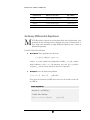
Partial Differential Equations
V
ersion 6 of MATLAB provides a solver for solving certain classes of
parabolic and elliptic partial differential equations. In the following section,
examples are given to illustrate how to use the solver.
Parabolic and Elliptic Equations
• Description: The class of parabolic and elliptic partial differential
equations that MATLAB can solve is of the form
∂u ∂u
∂
∂u
∂u
c x, t , u, = x − m x m f x, t , u , + s x, t , u, ,
∂x ∂t
∂x
∂x
∂x
where t 0 ≤ t ≤ t f , a ≤ x ≤ b , and m = 0, 1 or 2.
The vector-valued function u is a function of a space variable x and a
time variable t . At the initial time t = t 0 , the solution must satisfy initial
conditions of the form u ( x, t 0 ) = u 0 ( x) . In addition, at the boundaries
x = a and x = b , the solution must satisfy a boundary condition of the
form
∂u
p ( x, t , u ) + q ( x, t ) f x , t , u , = 0 .
∂x
62
M A T L A B
U S E R
M A N U A L
MATLAB provides a PDE solver pdepe. The basic syntax of this solver
is:
sol = pdepe(m, pdefun, icfun, bcfun, xmesh, tspan)
where m corresponds to m in the form of PDE; pdefun computes the
terms c , f , and s in the form of PDE; icfun evaluates the initial
conditions; bcfun evaluates the terms p and q in the form of the
boundary condition; xmesh is a vector specifying the points between a
and b ; and tspan is a vector specifying the points between t 0 and t f .
•
The example below illustrates the steps to solve a given
parabolic partial differential equation problem.
Example:
Consider the heat equation
∂u
∂ 2u
( x, t ) − 2 ( x , t ) = 0 ,
∂t
∂x
0 < x < 1,
with boundary conditions
u (0, t ) = u (1, t ) = 0 ,
t > 0,
and initial conditions
u ( x,0) = sin(πx),
0 ≤ x ≤ 1.
1. Rewrite the PDE in the required form.
∂u
∂ ∂u
= x0 x0
+0
∂x
∂x ∂x
Given the form above, m = 0 and
∂u
c x, t , u , = 1
∂x
∂u ∂u
f x, t , u , =
∂x ∂x
∂u
s x, t , u , = 0
∂x
63
t > 0,
M A T L A B
U S E R
M A N U A L
2. Write a function that evaluates the terms c , f , and s in the
differential equation as follows.
M-file: pdeHeat.m
function [c,f,s] = pdeHeat(x, t, u, DuDx)
% Set required c, f, s for the equation
c = 1;
f = DuDx;
s = 0;
3. Write the function that represents the initial conditions as follows.
M-file: pdeHeatic.m
function u0 = pdeHeatic (x)
% inital condition u(x,0) = sin(pi*x)
u0 = sin(pi*x);
4. Rewrite the boundary conditions in the required form.
u (0, t ) + 0 ⋅
∂u
(0, t ) = 0
∂x
at x = 0
u (1, t ) + 0 ⋅
∂u
(1, t ) = 0
∂x
at x = 1
5. Write the function that represents the boundary conditions.
M-file: pdeHeatbc.m
function [pl,ql,pr,qr] = pdeHeatbc(xl,ul,xr,ur,t)
% Set boundary conditions u(0,t) = u(1,t) = 0
pl = ul;
ql = 0;
64
M A T L A B
U S E R
M A N U A L
pr = ur;
qr = 0;
6. Run the following script to solve the given problem.
>> m = 0;
>> x = linspace( 0, 1, 20 );
>> t = linspace( 0, 2, 5 );
>> sol = pdepe( m, @pdeHeat, @pdeHeatic, @pdeHeatbc,x,t );
The following script generates a plot of the numerical solution.
>> u = sol( :, :, 1 );
>> surf( x, t, u )
>> title( 'Numerical solution to Heat Equation' )
>> xlabel( 'Distance x' )
>> ylabel( 'Time t' )
The actual solution to this problem is u ( x, t ) = e −π t sin(πx) . Run the
following script to generate a plot of this solution and compare the
two solutions.
2
>> ureal = exp( -pi .* t )' * sin( pi .* x );
>> surf( x, t, ureal )
>> title( 'Actual solution to Heat Equation' )
>> xlabel( 'Distance x' )
>> ylabel( 'Time t' )
65
M A T L A B
U S E R
M A N U A L
Other Useful Functions
T
here are a few other useful algebraic functions and functions for numerical
analysis, which are described as follows.
Functions for Nonlinear Algebraic Equations
• Find a Zero of a Function of One Variable: The function fzero finds a
zero of a function of one variable near a point x0 or within a given range.
For example:
>> fzero ( @sin, [ 2 4 ])
ans =
3.1416
Functions for Data Analysis
•
The function fminbnd finds a local
minimizer of a function of one variable within a given range. A local
minimizer x̂ of f (x) is a value of x such that f (xˆ ) is minimum in an
interval around x̂ . For example:
Minimize a Function of One Variable:
>> fminbnd ( 'sin', -pi, pi )
ans =
-1.5708
Note that the minimum value returned is -pi/2.
66
M A T L A B
•
U S E R
M A N U A L
Maximum and Minimum Entries of an Array: The functions max and min
return the largest and the smallest entries, respectively, along a specified
dimension of an array. For example:
>> w = [ 1 3 -3.56 4.1 ];
>> min ( w )
ans =
-3.5600
>> max ( w )
ans =
4.1000
•
The function sum computes the sum of the
entries of an array along a specified dimension. Similarly, the function
cumsum computes the cumulative sum of the entries of an array. For
example:
Sum and Cumulative Sum:
>> A = [ 1 2 3; 5 7 9; 0 4 1 ]
A=
1 2 3
5 7 9
0 4 1
>> sum( A )
ans =
6 13 13
>> cumsum( A )
ans =
1 2 3
6 9 12
6 13 13
•
The function prod computes the
product of the entries of an array along a specified dimension. Similarly,
the function cumprod computes the cumulative product. For example:
Product and Cumulative Product:
67
M A T L A B
U S E R
M A N U A L
>> A = [ 1 2 3; 5 7 9; 0 4 1 ]
A=
1 2 3
5 7 9
0 4 1
>> prod( A )
ans =
0 56 27
>> cumprod( A )
ans =
1 2 3
5 14 27
0 56 27
•
Sort Elements:
The function sort sorts elements in ascending order. For
example:
>> w = [ -1 6 -4 0 ];
>> sort( w )
ans =
− 4 −1 0 6
•
Differences: The function diff computes differences between adjacent
entries of an array along a specified dimension. For example:
>> C = [ 2 5 8; 1 6 10; 3 6 5 ]
C=
2 5 8
1 6 10
3 6 5
>> diff( C )
ans =
−1 1 2
2
0 −5
68
M A T L A B
U S E R
A
M A N U A L
References
[1] Desmond J. Higham and Nicholas J. Higham. MATLAB Guide. Society for
Industrial and Applied Mathematics, Philadelphia, PA, USA, 2000. ISBN 0-89871-4699.
[2] Getting Started with MATLAB Version 6. The Math Works, Inc., Natick, MA, USA,
2000.
[3] Duane Hanselman and Bruce Littlefield. Mastering MATLAB 6: a comprehensive
tutorial and reference. Prentice Hall, Upper Saddle River, New Jersey, USA, 2001. ISBN 013-019468-9
[4] Rudra Pratap. Getting Started with MATLAB 5: A Quick Introduction for Scientists and
Engineers. Oxford University Press, Inc., New York, New York, USA, 1999. ISBN 019-512947-4.
[5] Richard L. Burden and J. Douglas Faires. Numerical Analysis. PWS Publishing
Company, USA, 1993. ISBN 0-534-93219-3.
[6] Using MATLAB Version 6. The Math Works, Inc., Natick, MA, USA, 2000.
[7] Roger A. Horn. Matrix Analysis. Cambridge University Press, Cambridge, United
Kingdom, 1985. ISBN 0-521-38632-2.
[8] David S. Watkins. Fundamentals of Matrix Computations. Jon Wiley & Sons, Inc, New
York, New York, USA, 1991. ISBN 0-471-61414-9.
69
70