1
DAx Data Acquisition and Analysis Software 2014 PP van Mierlo Quick Start Guide www.dax.nl Contents Chapter 1. Installation __________________________ 3 Chapter 1.1 System Requirements ______________________ 3 Chapter 1.2 Installing the Software ______________________ 3 Chapter 2. Exercises ___________________________ 5 Chapter 2.1 First Exercise: Basics ______________________ 5 Chapter 2.1.1 Step 1: Starting DAx ______________________________ 5 Chapter 2.1.2 Step 2: Loading a Data Set _________________________ 6 Chapter 2.1.2.1 Data Tags ___________________________________ 8 Chapter 2.1.2.2 Data Tags: Moving Data ________________________ 9 Chapter 2.1.2.3 Which mouse button should I use? _______________ 10 Chapter 2.1.2.4 Data Tags: Other Uses ________________________ 10 Chapter 2.1.3 Step 3: Zooming In on the Graph ___________________ 11 Chapter 2.1.4 Step 4: Printing the Graph, or Exporting It_____________ 12 Chapter 2.1.5 Step 5: Analysing the Data Set _____________________ 13 Chapter 2.1.5.1 Manually Adjusting Peaks ______________________ 14 Chapter 2.1.6 Step 6: Displaying Peak Data ______________________ 15 Chapter 2.1.7 Step 7: Saving Your Work (End of first workout) ________ 16 Chapter 2.2 Second Exercise: Shortcuts and More ________ 17 Chapter 2.2.1 Step 1: Opening Several Data Files - and Analysing Them 17 Chapter 2.2.2 Step 2: Adjusting a Baseline _______________________ 19 Chapter 2.2.3 Step 3: Finding Peaks ____________________________ 22 Chapter 2.3 Third Exercise: Capillary Electrophoresis _____ 23 Chapter 2.3.1 Step 1: Calculating Apparent Mobilities _______________ 23 Chapter 2.3.2 Step 2: Calculating Effective Mobilities _______________ 25 Chapter 2.4 Fourth Exercise: Gel Permeation Chromatography _____________________________________ 27 Chapter 2.4.1 Step 1: Analysing the Calibration Sample _____________ 27 Chapter 2.4.2 Step 2: Setting the Flow Rate ______________________ 28 Chapter 2.4.3 Step 3: Creating the Calibration ____________________ 29 Chapter 2.5 Fifth Exercise: DNA Base Pair Count Determinations ______________________________________ 31 Chapter 2.5.1 Step 1: Analysing the Calibration Sample _____________ 32 Chapter 2.5.2 Step 3: Creating the Calibration ____________________ 33 Chapter 2.5.3 Step 4: Using the Calibration _______________________ 35 Chapter 2.6 Sixth Exercise: Qualifying & Quantifying Peaks 36 Chapter 2.6.1 Chapter 2.6.2 Chapter 2.6.3 Chapter 2.6.4 Step 1: Analysing the Sample with Known Components __ 37 Step 3: Creating the Identification Database ___________ 38 Step 4: Using the Identification Database _____________ 41 Step 5: Setting up a Comparison Sheet ______________ 42 1 Chapter 2.7 Seventh Exercise: Gradients ________________ 44 Chapter 2.7.1 Step 1: Defining the gradient _______________________ 44 Chapter 2.7.2 Step 2: Adjusting the gradient ______________________ 46 Chapter 2.7.3 Step 3: Adjusting gradient percentages_______________ 47 Chapter 3. Index ______________________________ 49 2 Chapter 1. Installation Chapter 1.1 System Requirements To install DAX, you must have permission to make changes to the system registry, and permission to create the DAx directory. If you are unsure whether or not you have these permissions, please ask your systems administrator. Chapter 1.2 Installing the Software 1. Insert the DAx distribution CD into the CD ROM drive. We will assume drive R: is being used. 2. From the Start menu, execute the Run... option. 3. In the Command Line box, type R:\autorun 4. Click the OK button. The set-up menu will now start. 5. Select DAx Master Setup, and follow the instructions on screen. 6. Run the Install USB dongle program that has been installed in the DAx program group. This should be run before the USB dongle is attached! Follow the instructions on screen. 7. Attach your USB dongle after installation completes. This completes the installation. Set-up has created a program group in the Start Menu containing the DAx icon; click this to start DAx. Refer to the Measurement window user’s manual for details on hardware installation, if applicable. 3 Chapter 2. Exercises This guide helps you make a quick start in using DAx. Chapter 2.1 First Exercise: Basics Chapter 2.1.1 Step 1: Starting DAx Start DAx using the DAx icon in the DAx program group in the Start Menu. This is what you will see: This screen contains the following items: • A caption with the program name, and buttons to minimise, maximise/restore, or close the program 5 • A menu bar. Initially this has only a limited number of options, depending on the version of DAx you’re using. Two options are always present: File and Help. • A toolbar, containing buttons that let you quickly access the most common menu options. The toolbar is also used to display tracking coordinates whenever the mouse cursor is over a graphics window . • A status bar (at the bottom). The status bar is used to display messages of varying importance. Normal messages are black on gray, and more important messages are black on yellow, or white on green or blue. Messages that require immediate attention are white on red. Click on the popup button at left of the status bar, and keep the mouse button depressed, to see up to 32 of the most recent important messages. When more than one important message has been added recently, the button will flash. • A waste barrel (bottom right). Data sets can be dragged to the waste barrel to remove them. However, they can also be retrieved back from the waste barrel. Refer to the chapter The Waste Barrel in the DAx manual for details on how to use the waste barrel. Now that you know a little more about the various items on the screen, enter your name in the Operator item, and your password in the Password item. If no-one else has changed it, the password is XYZZY. Press enter to start the program proper. Chapter 2.1.2 Step 2: Loading a Data Set Now that DAx is running, we need to load a data set. This is done using the File | Open menu option. However, the quick way to open a file is to click the file open button. Click here to open a file A dialog box appears, listing the available data files. Two or more example files have been installed along with DAx. The dialog box should look something like this: 6 Double click on test1.DAx to load it into memory. A data set graphic window will be opened. It will look like this: Most of this window is used to display the data set. Data tags representing the data sets are displayed at the top of the window. 7 Chapter 2.1.2.1 Data Tags At the top1 of each graph window, one or more data tags represent the data sets in the window. Data tags have the appearance of pushbuttons. • data tags can be clicked to display a data tag menu • data tags can be dragged and dropped, see the next section • data tags flash blue when a popup menu appears that pertains to the data set, such as when the right mouse cursor is clicked on a peak marker • data tags flash blue when a data set is changed, such as when a peak marker is dragged to a new location • data tags are depressed when the mouse cursor is placed over the data set’s curve • data tags are depressed when the mouse cursor is placed over a peak, tack or spline marker • data tags are depressed in stacked views (created using the Data | Stack data menu option) when the mouse cursor is in the vertical range of one or more of the stacked data sets The last three of these are tracking behaviour. Tracking behaviour is suppressed when the Shift key is held down. By default, up to three lines of tags are displayed at the top of graphic windows. For windows containing many tags, the number of lines of tags can be changed by placing the mouse cursor just below the data tags, where it will change shape to an up/down arrow. Click and drag the mouse to change the amount of space allocated to data tags. 1 The data tags can also be displayed at left, using the View | Tags left menu option. 8 Chapter 2.1.2.2 Data Tags: Moving Data Data tags can be moved around! Drag them to the waste barrel to remove the data (don’t try that now). Drag them to another data set window to move the data. If you press the Ctrl key while dragging, the data will not be moved, but will be copied. It’s also possible to drag a data tag to an empty part of DAx, where no window is being displayed. If you try that, a new data set graphic window will be created. Let’s try data copying. Move the mouse cursor over the data tag, click, now press the Ctrl key. While keeping both the mouse button and the ctrl key depressed, move the mouse cursor over an empty part of the DAx window. Now release the mouse button. A new window, containing a copy of the data, is created. You should get something like this: Note that the Waste Barrel has been moved out of the way - again by clicking the mouse button on it, then dragging it to a new position. 9 Chapter 2.1.2.3 Which mouse button should I use? When dragging data tags, you can use either the left or right mouse button. If you use the left button, only the data tag you clicked on will be moved2. If you use the right mouse button, the data set and any other data belonging to it will be moved. Now that you have created a copy of the data, try sending the copy to the waste barrel! Simply click and drag the data tag to the waste barrel. An empty window will be left. Chapter 2.1.2.4 Data Tags: Other Uses If, while trying to move a data tag, you inadvertently released the mouse button while the mouse cursor was still over the tag, you will have seen the data tag menu. This is a menu that contains a number of options that affect a single data set. The menu options in the main menu (displayed at the top of DAx) affect all data sets in a data set graphic window. If you execute the Info option in the data tag menu, you will see the data set information dialog box. Something like this: 2 You can also select multiple data tags by pressing the Ctrl key when clicking additional tags, then move all selected tags at once. 10 Refer to the chapter Data Set Information Dialog in the DAx manual for details. Chapter 2.1.3 Step 3: Zooming In on the Graph You may want to enlarge part of the graph being displayed for a data set. To do that, you must once again drag the mouse. Place the mouse cursor in the bottom left corner of the part of the graph you want to enlarge. Now, click the left mouse button, and, while keeping the mouse button depressed, move the mouse cursor to the top right corner of the part you want to enlarge. Then release the mouse button. 11 Some remarks: • Click the right mouse button to zoom out. • You do not have to go bottom left to top right - drag in any direction you like. • You can zoom in up to ten times. However, you may reach maximum zoom before then. • Press the Shift key and double click anywhere in the graph to set a relative origin for mouse tracking coordinates. Chapter 2.1.4 Step 4: Printing the Graph, or Exporting It To print the graph, use the File | Print menu option. More conveniently, click the print button3. Click here to print the contents of a window You may also put the contents of a data set graphic window on the clipboard. To do that, use the Edit | Copy Graph menu option. A so-called metafile picture is put on the clipboard. You can insert such a picture into a word processor document. That’s how the following picture was created. 3 The Print button actually prints a report, if a report definition has been set up. This can be done using the Report | Load Report menu option. 12 DAx 5.0: PP van Mierlo 07/02/96 21:42:37 Volt 6 4 2 0 100 200 300 time (s) Chapter 2.1.5 Step 5: Analysing the Data Set Now, let’s try to find some peaks. The quickest way to do this is to click the Baselines & Peaks button: Click here to create baselines for, and find peaks in, the data in a window This is what we get (provided the analysis parameters have not been changed since DAx was installed): 13 Chapter 2.1.5.1 Manually Adjusting Peaks It is possible to manually adjust peaks. In the example above, the triangular peak top markers are clearly visible. There are similar markers for peak begin and end (these markers are obscured by the signal in the example above, but are clearly visible on-screen). • To move any of these markers, place the mouse cursor on them, click the left mouse button, and drag the marker to its new position. • Press the Ctrl key, then double click the left mouse button, to add a new peak. • Remove a peak by moving its top past its begin or end marker. • Made a mistake? Press Alt + BackSpace to undo the operation (Alt+Shift+BackSpace redoes it) or use Edit | Undo (and Edit | Redo). • Place the mouse cursor over the top marker, then click the right mouse button, to display a popup dialog box. This dialog box let’s you enter a peak name or concentration. It also lets you remove the peak, or mark the peak as the reference or normalisation peak (cf. chapters Marking Normalisation Peaks and Marking Reference Peaks in the DAx manual). 14 Chapter 2.1.6 Step 6: Displaying Peak Data To display a list of peaks, click the Peak List window button on the left side of the data tag: Click here to open a peak list window Peak list windows can contain a variety of columns of information. Below is an example. The Component column is one of the columns in the peak list window that can be edited4. In the example, names for the peaks are being entered. Values entered in the annotations column are used in Capillary Electrophoresis to set the apparent mobility of a reference peak, and in Gel Permeation Chromatography to enter a molecular weight for the peak’s component. To enter a Component name or Annotation, simply click the mouse cursor in the peak list window. Use the cursor keys and the (Shift) Tab key to navigate. 4 The other columns that can be edited are the annotation and the concentration. 15 The contents of the peak list window can be printed. Use the print button! They can also be saved as a text file. Use the File | Export menu option for this. Finally, the peak list can be sent to the clipboard as a table using the Edit | Copy menu option. Note that the copy command will copy highlighted lines in the peak list window. Use Edit | Select All to highlight the entire window contents, or drag the mouse cursor over the lines you want to select, or press the Shift key and use the cursor keys to select lines. Chapter 2.1.7 Step 7: Saving Your Work (End of first workout) Use the File | Save As menu option to save your work. Better yet, use the Save button: Click here to save files The File Save dialog will appear. It will look like this: Enter a name in the File Name item, then click the OK button to save the data sets. By default DAx files will be written, but several other file types may be selected in the Save as type item. In the example, there are two data sets listed in the list box at left. If you try to deselect one of them, they will both be deselected! That’s because these data sets belong together (as indicated by 16 the line connecting them), which means they cannot be saved separately. You must use a new file name. If you try to use an existing file name, DAx will refuse to save the files. That’s because it’s not Good Laboratory Practice to overwrite any data5. This concludes the first exercise. Chapter 2.2 Second Exercise: Shortcuts and More The second exercise will show you some shortcuts, but it will also dig a little deeper. Chapter 2.2.1 Step 1: Opening Several Data Files - and Analysing Them Let’s begin the second exercise. We’ll assume you have opened DAx, the same way as before (chapter Chapter 2.1.1). Once again, click the File | Open button to start loading data. This time, we’ll use two shortcuts. You can select more than one file in the file open dialog box! Click on one file name, then press the Ctrl key, and click on another filename. You might get something like this: 5 This behaviour can be changed using the File | Customise > GLP menu option. 17 If you were to press the OK button now, both files would be loaded! • check the Multiple Windows box to load each data set into its own window. Otherwise, the data sets will be loaded into a single data set graphic window. • check the Add to Window box to add the selected data sets to an existing data set graphic window. Now, the second short-cut. Check the AutoAnalyse box in the lower right corner of the File Open dialog - the data files will automatically be analysed when they have been loaded! Depending on how AutoAnalysis has been set up various operations may be performed. • automatic baseline construction • automatic peak detection • automatic printing of the data as a graph • automatic printing of a peak list • automatically saving the peak list to a file Automatic analysis is set up using the Config button that is displayed next to the AutoAnalyse box in the File Open dialog. Refer to the chapter Setting up Automatic Analysis in the DAx manual for details. 18 To clean up DAx in preparation for the next step, use the Window | Close All menu option to close all data windows. If you were using automatic analysis two things can happen: • the contents of a window have not yet been analysed. DAx will see this, and ask if the analysis should be performed before the window is closed. • the contents have been analysed, but not saved. DAx will ask you to confirm the loss of the modified data. Chapter 2.2.2 Step 2: Adjusting a Baseline The file test2.DAx contains a pretty difficult measurement to analyse. It’s quite conceivable you’re not completely satisfied with the job DAx does of constructing a baseline. Simply adjust it yourself! Let’s see how this is done. First, load the file test2.DAx. Now, you can use the analysis button to analyse the data, or you may just want to create a baseline, without searching any peaks. To do that, use the Peaks | Construct Baselines menu option, or click a button: Click here to start constructing baselines You will get a baseline construction dialog box. For details, refer to the chapter Peaks | Construct Baselines in the DAx manual. For now, just click on the OK button. A baseline will be constructed. The resulting window may look something like this: 19 It seems likely the baseline needs to be a straight line beneath the two major peaks. To make this so, we need to add splines to the baseline. Click on the data tag for the baseline (the tag with the yellow B at left). Now, either execute the Splines | Add Spline menu option, or click the add spline button on the toolbar6: Click here to add a spline to a data set. A spline is a collection of nodes, connected by straight lines (or by curves). The nodes are drawn as squares in the same colour as the curve. You can change a spline in a number of ways: • put the mouse cursor over a node, then click the left mouse button, and drag the node to a new position. Keep the Ctrl key depressed to add a node! • If you drag a node past other nodes, those will be deleted. • Add a node by depressing the Shift and Ctrl keys, then double clicking the mouse at the position where you want to add a node. 6 It’s not enough to just click the add spline button if the data tag for the baseline is not the default data tag. The default data tag is the one with the thicker edge. Clicking the mouse button on a data tag makes it the default data tag. 20 • Use Alt + BackSpace to undo node modification operations (Alt+Shift+BackSpace redoes them). • Initially, the spline for the example may have looked something like this (the spline node markers have been enlarged for clarity): After you modified it, it might look something like this: Now, the spline has been modified, but the baseline hasn’t yet been updated! Click on the data tag for the baseline, and use the Splines | Replace Curve With Spline | Changed Nodes Only menu option to replace the baseline with the spline7. Only the parts of the baseline where you adjusted the spline will be changed. You can also use a toolbar button for this: 7 In fact, DAx offers to do this automatically as soon as the spline is first changed. 21 Click here to replace a data set with a spline. A menu appears to let you choose how much of the curve to replace with the spline. Now you can remove the spline, or, more accurately, hide it. Just click the add spline button on the toolbar again, or execute the Splines | Add Spline button in the data tag menu again. Now, your baseline should look like this: Now you’re ready to find some peaks! What if peaks had already been detected? DAx will notice the baseline has changed, and will recalculate the peaks. Chapter 2.2.3 Step 3: Finding Peaks To find peaks, use the Peaks | Find Peaks menu option to invoke the peak find dialog. You may also use a toolbar button: Click here to invoke the peak find dialog. 22 Refer to chapter Peaks | Find Peaks in the DAx manual for details on the peak find dialog box. For now, you might just click the OK button. This ends the second exercise. Chapter 2.3 Third Exercise: Capillary Electrophoresis The third exercise takes you through some aspects of Capillary Electrophoresis. If the menu option CE is not present, you need to use File | Customise > Extensions and check CE Options. Not all versions of DAx contain this option. Chapter 2.3.1 Step 1: Calculating Apparent Mobilities In capillary electrophoresis (CE), the apparent mobility of a l .l component is calculated as m app = tot det . t mig .V with mapp ltot ldet tmig V apparent mobility (10-9m2/Vs) length of capillary (m) length between injection point and detector (m) migration time (s) voltage drop over capillary (kV) The effective mobility is meff = mapp - EOF with meff effective mobility (10-9m2/Vs) EOF electro-osmotic flow (10-9m2/Vs) To be able to calculate apparent mobilities, DAx needs to be told the length of the capillary being used, the distance from injection to detector, and the voltage drop. To then be able to calculate effective mobilities, DAx needs to be told the electro-osmotic flow. Generally, instead of entering the electro-osmotic flow, you will mark a reference peak, and enter its effective mobility. Since the apparent mobility for the reference peak is also known, the electroosmotic flow can then be calculated. 23 Let’s assume the file test1.DAx contains a CE measurement. So, once again, start DAx. Load the file text1.DAx (refer to the first exercise for instructions). Now, invoke the CE | Calibrate menu option. The CE calibration dialog will be displayed: Enter the values shown into the dialog box. Now click the OK button to store these calibration parameters. You should realise that the parameters will only be stored in the data sets you select in the list displayed at left. What happens if no CE calibration parameters have been stored with a data set? The default parameters will be used. The default parameters are always equal to the last set of parameters stored with a data set. When you now move the mouse across the graph in the data set graphic window for test1.DAx, one of two things can happen: • the apparent mobility is tracked in the toolbar • the toolbar displays EffMob:<na>. That’s because no reference peak has been set yet, so the effective mobility cannot yet be calculated! To change between tracking apparent and effective mobilities, use the CE | Apparent Mobility and CE | Effective Mobility menu options. Use CE | Track Mobility to turn mobility tracking on and off. 24 Chapter 2.3.2 Step 2: Calculating Effective Mobilities Now, let’s mark a reference peak. First, analyse the data (use the Peaks | Baselines & Peaks menu option or the Baselines & Peaks button on the toolbar). Move the mouse cursor over the peak top of the third peak, and press the right mouse button. You’ll see something like this: Check the Reference Peak box to make the fourth peak the reference peak. The peak marker will change, and the toolbar will start tracking effective mobilities (if menu option CE | Effective Mobility has been checked - otherwise, you should do that now). In the first step of this exercise it was explained that to calculate effective mobilities, the effective mobility for the reference peak needs to be known. But we didn’t enter it! However, in the CE calibration dialog, we did enter a default reference mobility, and that’s now being used. If the effective mobility for the reference peak does not have the default value, you should enter the correct value as an annotation, in the peak top popup dialog, or in the annotations column in the peak list window. The peak list window might end up looking like this: 25 Notice the column with effective mobilities for the peaks. Naturally, the effective mobility listed there for the reference peak equals the value entered as the annotation! Would you like to print the effective mobilities for each peak in the graphic window? Invoke the File | Customise menu option. Select Plotting Peaks, and select Effective Mobility as the first or second peak label. Effective mobilities will now be displayed above the peak tops. You can also select a variety of other labels. Finally in this exercise, close the peak list window, and then use the CE | Mobility Axis menu option in the data set graphic window for file test1.DAx to display a graph where the time axis has been replaced by a mobility axis: 26 DAx 5.0: Mobility versus signal plot PP van Mierlo; printed 09/02/96 14:06:33 AU 6 4 2 200 300 400 Effective Mobility (10 Since mobility varies with the reciprocal of the migration time, the order of the peaks has been mirrored! Chapter 2.4 Fourth Exercise: Gel Permeation Chromatography The fourth exercise takes you through a Gel Permeation Chromatography Calibration. If the menu option GPC is not present, you need to use File | Customise > Extensions and check GPC Options. Not all versions of DAx contain this option. Chapter 2.4.1 Step 1: Analysing the Calibration Sample Once again, start DAx. Load the file test1.DAx, and analyse it (the first exercise took you through the steps required to do this). Make sure a peak list window is displayed. Now, we’ll assume we know the molecular weights for the first six peaks in this data set. Enter them into the annotations column in the peak list window. The peak list might end up containing something like this: 27 Peaks list: DAXSIM1.PRN * (not saved) Measured 00/00/00 00:00:00 by PP; RMS Noise (AU): 0.189; 0.189 Peak 1 2 3 4 5 6 7 8 9 10 Begin (s) 93.200 118.300 136.500 144.200 162.600 177.000 248.600 257.900 271.700 279.500 Top (s) End (s) 94.300 119.700 137.800 146.000 164.400 178.700 251.000 260.100 274.000 281.700 95.400 120.800 139.300 147.200 165.800 180.200 252.900 261.900 276.300 284.200 Top (AU) Annotation 5.9427 4.9746 4.6067 4.1538 3.6891 3.6716 1.97 1.8359 1.7433 1.6588 50000 45000 40000 35000 30000 25000 We’ll now use these data to create a GPC calibration. Chapter 2.4.2 Step 2: Setting the Flow Rate It is important to realise GPC calibrations work with elution volumes, not time coordinates. So, we must make sure the flow rate for our calibration measurement is correct. Click the data tag, and execute the Sizing | Sizing Dialog menu option. This is what you’ll see: 28 Change the Flow Rate to 300. The flow rate setting for the baseline will also change8. All data sets that belong together will always have the same flow rate. We’ve now made sure of the following crucial steps for creating a GPC calibration: • we have a data set with peaks • molecular weights have been entered as annotations for the peaks • the flow rate has been set Chapter 2.4.3 Step 3: Creating the Calibration Execute the GPC | Calibrate menu option. The GPC Calibration dialog box is displayed. For details, refer to the chapter GPC Calibration Dialog Box in the DAx manual. The dialog box looks like this: Now: • select the topmost data set in the list box at left • check the logarithmic Mw’s box • select a cubic spline curve 8 As soon as you change the flow rate for the top data set, the baseline will also become selected in the list at the left side of the dialog box. 29 • check both Derive from data boxes • and click the OK button A GPC calibration has been created! To see how it looks, execute the GPC | Calibration Curve menu option. To see a table, execute the GPC | Calibration List option. Let’s verify this calibration. Activate the data set graphic window for the file test1.DAx, and execute the GPC | Mw Axis menu option. You’ll get something like this: 30 DAx 1.0: Molecular Weight versus signal plot PP van Mierlo; printed 08/02/96 20:52:37 AU 6 4 2 4.4 4.5 4.6 4.7 log Molecular Weight The curve starts out and ends in peak tops! The reason is that valid elution volumes for molecular weight calculation were limited to the range of the calibration data points by checking the Derive from data box. Elution volumes smaller than the smallest elution volume in the calibration list, or larger than the largest volume, cannot be converted to molecular weights9. You may also notice that the curve has been flipped over in horizontal direction. This is because high molecular weights correspond to low elution volumes. Chapter 2.5 Fifth Exercise: DNA Base Pair Count Determinations The fifth exercise takes you through the steps needed to determine base pair counts in a DNA electropherogram. If the menu option Calibration is not present, you need to use File | Customise > Extensions and check Calibrations. Not all versions of DAx contain this option. 9 This is true for cubic spline calibrations even if the Derive from data boxes had not been checked in the GPC calibration dialog. This type of calibration does not support extrapolation beyond the data range. Multi-linear and polynomial calibrations do. 31 Chapter 2.5.1 Step 1: Analysing the Calibration Sample Once again, start DAx. Load the file test3.DAx, and analyse it (the first exercise took you through the steps required to do this). Zoom in on the part of the graph following the big peak. You should get something like this (but without the numbers on top of the peaks they are added in the next step): DAx 5.0: PP 09/03/96 16:01:55 AU 175 180 214 218 222 226 230 234 238 168 172 156 160 112 0.000 106 164 0.005 -0.005 4.5 5.0 5.5 time (min) Next, make sure a peak list window is displayed. We know the base pair counts for the peaks in this data set, and should enter them in the annotations column in the peak list window. NB we do not care about the earlier peaks in the peak list window! Only the peaks with migration times over 4 minutes are of interest. To locate a peak in the peak list window, simply move the mouse cursor over the top marker for the peak in the graph - the appropriate peak in the peak list window will be highlighted. The peak list might end up containing something like this: Peaks list: STAND-1.Da1 * (not saved) Measured 00/00/00 00:00:00 by PP; RMS Noise (AU): 0.00023251; 0.00011626 Peak Begin Top 1 0.168 0.182 2 1.433 1.442 <some peaks skipped> 13 3.770 3.808 14 4.155 4.170 32 End Top (AU) 0.245 1.450 0.0009542 -0.00028247 3.838 4.182 0.002147 0.00030184 Annotation 15 16 17 18 19 20 21 22 23 24 25 26 27 28 29 30 4.360 4.460 4.908 4.970 5.013 5.060 5.105 5.140 5.187 5.590 5.633 5.685 5.722 5.763 5.810 5.850 4.423 4.485 4.938 4.983 5.028 5.073 5.118 5.153 5.207 5.607 5.652 5.695 5.740 5.783 5.828 5.872 4.443 4.507 4.970 5.013 5.060 5.105 5.140 5.175 5.230 5.628 5.685 5.722 5.757 5.810 5.847 5.895 0.003394 0.0029842 0.0028615 0.0037159 0.0059983 0.0035568 0.0029702 0.0019518 0.0016548 0.0017969 0.0020277 0.0015195 0.0017602 0.0016279 0.0025198 0.0014169 106 112 156 160 164 168 172 175 180 214 218 222 226 230 234 238 We’ve now made sure of the following crucial steps for creating a DNA calibration: • we have a data set with peaks • base pair counts have been entered as annotations for the peaks Chapter 2.5.2 Step 3: Creating the Calibration Execute the Calibration | Calibrate menu option. The DNA Calibration dialog box is displayed. For details, refer to the chapter Calibration Dialog Box in the DAx manual. The dialog box looks like this: 33 Now: • check Derive main calibration from: • check the topmost data set in the list box at left • do not select Logarithmic Base Pair counts • select a Polynomial curve, with degree 1 • do not check the Derive from data boxes • and click the OK button A DNA calibration has been created! To see how it looks, execute the Calibration | Calibration Curve menu option. To see a table, execute the Calibration | Calibration List option. Here’s the curve: 34 DAx 8.1 18/03/2008 17:46:43 PP: DNA Calibration (not saved) Base pairs Linear order 1 Polynome; BP = -4.57757+0.0242333x ; Correlation 99.9965% ; Ave.Diff. 0.251134 250 200 150 100 4.5 5.0 5.5 Peak Top Coordinate The calibration does not seem to take the leftmost two points into account; this is because we double clicked the mouse on those points in the calibration curve window, to exclude them from the calibration. Now all that remains is to use the calibration to analyse some real data! Chapter 2.5.3 Step 4: Using the Calibration Load the file test4.DAx, and analyse it. Zoom in on the part of the graph following the big peak. You should get something like this: DAx 8.1 18/03/2008 17:51:04 PP 0.002 Y 0.000 -0.002 -0.004 4.5 5.0 5.5 Time (min) 35 As soon as you find peaks, the base pair counts are automatically calculated. But you don’t see them yet. To make them visible, you can either inspect the peak list window, or mark peaks with base pair counts. Use the File | Customise > Plotting Peaks menu option to do this. This will display a dialog box in which you can select “Base pairs” as one of the peak labels. This is what you get: DAx 8.1 18/03/2008 17:49:57 PP 0.002 Y 229.6 111.4 116.6 222.2 0.000 163.7 167.7 -0.002 -0.004 4.5 5.0 5.5 Time (min) Finally, try using the Calibration | Calibrated Axis menu option to display test4.DAx with base pair counts as the horizontal axis. Chapter 2.6 Sixth Exercise: Qualifying & Quantifying Peaks The sixth exercise takes you through the steps needed to set up an Identification Database, and to use the database to qualify peaks in an unknown sample, as well as determine the concentrations of the components. If the menu option Analysis is not present, you need to use File | Customise > Extensions and check Analysis Options. Standard analysis should be unchecked. 36 Chapter 2.6.1 Step 1: Analysing the Sample with Known Components Once again, start DAx. We’ll use the same test file as for the DNA calibrations. So, load the file test3.DAx, and analyse it (the first exercise took you through the steps required to do this). Zoom in on the part of the graph following the big peak. You should get something like this (but without the names on top of the peaks they are added in the next step): DAx 5.0: PP 03/04/96 15:31:25 AU 0.00 250 300 methanol ethanol propanol butanol pentanol hexanol heptanol methanal ethanal propanal butanal pentanal hexanal heptanal 0.02 350 time (s) Next, make sure a peak list window is displayed. We know the components in the data set, and should enter their names in the component name column in the peak list window10. We’ll also enter concentrations in the concentration column. NB we do not care about the earlier peaks in the peak list window! Only the peaks with retention times over 4 minutes are of interest. To locate a peak in the peak list window, simply move the mouse cursor over the top marker for the peak in the graph - the appropriate peak in the peak list window will be highlighted. The peak list might end up containing something like this: 10 Obviously, the names of the components have been pretty randomly picked. 37 Peaks list: STAND-1.Da1 * (not saved) Measured 00/00/00 00:00:00 by PP; RMS Noise (AU): 0.00023251; 0.00011626 Peak Top (s) Comp. 1 10.900 2 190.800 <some peaks skipped> 13 226.800 14 228.500 15 265.400 16 269.100 17 296.300 methanal 18 299.000 ethanal 19 301.700 propanal 20 304.400 butanal 21 307.100 pentanal 22 309.200 hexanal 23 312.400 heptanal 24 336.400 methanol 25 339.100 ethanol 26 341.700 propanol 27 344.400 butanol 28 347.000 pentanol 29 349.700 hexanol 30 352.300 heptanol Conc. 0.266 0.365 0.576 0.375 0.261 0.207 0.162 5.12 4.14 4.4 5.73 5.16 8.21 4.48 Area (AU.s) Area/Mig 0.0020676 0.004007 0.0017258 0.00020978 0.0013924 0.0034911 0.0039531 0.002658 0.0026634 0.0036532 0.0057591 0.0037514 0.0026055 0.0020745 0.0016157 0.0017238 0.0020816 0.0015037 0.0019723 0.0017918 0.002869 0.0015776 6.1429E-05 0.00015278 0.00014919 9.8766E-05 8.9883E-05 0.00012213 0.00019085 0.00012321 8.4843E-05 6.7091E-05 5.1711E-05 5.1231E-05 6.1378E-05 4.3998E-05 5.728E-05 5.1635E-05 8.2068E-05 4.4788E-05 As you may see, the alkanals have been assigned concentrations equaling 100 times the peak area, and the alkanols have a concentration equaling 100,000 times the migration time corrected peak area. We’ll now use these data to create an Identification Database. Chapter 2.6.2 Step 3: Creating the Identification Database Execute the Analysis | Edit Database menu option. The Identification Database edit dialog box is displayed. For details, refer to the chapter Identification Database Edit Dialog Box in the DAx manual. The dialog box looks like this: 38 Now: • select the topmost data set in the list box at left (is selected by default) • click on the Peak Top Time qualification coordinate • enter a value of 2 (seconds) for the tolerance • select the Quantification tab • select peak area as the quantifying parameter • select a polynomial calibration, with degree 1 • and click the OK button An Identification Database has been created! To see a table of the database, execute the Analysis | Display Database menu option. This will create an Identification Database list window. Note that in the Quant Points column the number of quantitative calibration points for each component is 2. This is because DAx automatically adds the point 0, 0 to each calibration - assuming that peak area is 0 if the concentration is 0. If more than one quantitative calibration point is found for a component (because several measurements, with different component concentrations, are being included in the Identification Database), the 0,0 point is de-activated. NB The procedure for adding quantitative calibration points is exactly the same as the procedure used above to set up the initial calibration points, with one exception: before clicking the OK button in the Identification Database Edit dialog box, you must check Add 39 to existing calibration. That way, the previous points are kept in memory, and new points are added. To see what the quantitative calibrations look like, click the right mouse button on a line in the Identification Database list window. Now execute the Draw Quantitative option, and a graph depicting the calibration will be displayed. It will look like this: DAx 5.0: propanal calibration PP; printed 10/04/96 14:57:14 Area (AU.s) 0.006 0.004 0.002 0.000 0.0 0.2 0.4 concentration 0.6 Remember that the concentrations for the alkanols were based on migration time corrected peak areas, rather than peak areas? For this reason, the quantitative calibration for the alkanols should use not the peak area, but the migration time corrected peak area, as the quantifying parameter. Go to the Identification Database list window. Click the left mouse button on the line containing the first alkanol (methanol), then, while keeping the mouse button depressed, drag the mouse cursor to the last line containing an alkanol. Now click the right mouse button. Execute the Config Quantification menu option in the popup menu. This is what you will see: 40 Change the quantification parameter to peak area / migration time, then click the OK button. You can also set lower and upper limits for the concentration. Concentrations outside this interval will still be calculated, but will get an L or H flag. This is useful in quality control situations. Now all that remains is to use the Identification Database to analyse some real data! Chapter 2.6.3 Step 4: Using the Identification Database Load the file test4.DAx, and analyse it. Zoom in on the part of the graph following the big peak. You should get something like this: 41 DAx 5.0: PP 03/04/96 15:42:11 AU 0.15 pentanol propanal butanal 0.05 propanol 0.10 0.00 250 300 350 time (s) To make the names visible, you can either inspect the peak list window, or mark peaks with component names. Use the File | Customise > Plotting Peaks menu option to display a dialog box in which you can select a peak label. To see which concentrations DAx has derived, again use the peak list window. Notice that the concentrations found for the alkanals are roughly equal to 100 times the peak area. The concentration found for the alkanols is roughly 100,000 times the migration time corrected peak area. You may wonder if DAx will overwrite any component names you have entered manually for a peak. It will not. Chapter 2.6.4 Step 5: Setting up a Comparison Sheet DAx has the option of creating a sheet that compares the peaks found in various data sets. Peaks with the same qualifying parameter are grouped, and the averages of all of their parameters, as well as standard deviations, are calculated. Let’s try it now. Load the files test3.dax and test4.dax into a single window, and analyse them (refer to chapter Chapter 2.2.1 for information on opening several data files at once). Make sure the data files are in a single window! If they are not, use the mouse cursor to drag the data tags to a single window. 42 Now, execute the Analysis | Comparison Sheet option. You will get a dialog box that looks like this: Now: • check the Only show matching peaks box. This will make sure a comparison sheet is created that only lists the peaks that occur in both data sets • select the peak top time as the qualifying parameter • set an absolute tolerance of 2 seconds Now click the OK button. A text window will be created with the following contents11 DAx 5.0: Comparison sheet; 17/04/96 19:57:54 Peak STAND-1.Da1 : 8 S158-4.Da1 *: 4 Average St.Dev. Top (s) Component Conc. Area (AU.s) 195.600 194.500 569.900 530.118 0.094012 0.012663 0.05943 0.058164 269.100 269.100 0.0027982 0.0018149 <some peaks skipped> STAND-1.Da1 : 23 S158-4.Da1 *: 19 11 The exact contents may vary, especially which data columns are present. 43 Average St.Dev. 269.100 0.000 0.0023065 0.00069536 STAND-1.Da1 : 26 S158-4.Da1 *: 20 Average St.Dev. 301.700 301.500 599.250 420.940 propanal propanal 0.58895 0.088674 0.66902 0.58585 0.0058905 0.00088191 0.0066915 0.0058645 STAND-1.Da1 : 27 S158-4.Da1 *: 21 Average St.Dev. 304.400 304.100 304.250 0.212 butanal butanal 0.38844 0.064189 0.22632 0.22928 0.0038913 0.00064033 0.0022658 0.0022988 STAND-1.Da1 : 33 S158-4.Da1 *: 22 Average St.Dev. 341.700 341.700 1143.799 1134.340 propanol propanol 4.4787 8.8621 11.693 7.7497 0.0015328 0.0030258 0.0075036 0.0074632 STAND-1.Da1 : 35 S158-4.Da1 *: 23 Average St.Dev. 347.000 346.800 519.100 243.527 pentanol pentanol 5.1775 11.001 11.006 5.8286 0.0017986 0.0038187 0.0038134 0.0020148 Chapter 2.7 Seventh Exercise: Gradients Some versions of DAx contain extensions that allow you to correct for signal drift in gradient HPLC and temperature programmed GC. You can also include a plot of the gradient percentage or programme temperature in your graphs. If the menu option HPLC / GC is not present, you need to use File | Customise > Extensions and check HPLC Options or GC Options. Not all versions of DAx contain this option. Chapter 2.7.1 Step 1: Defining the gradient As always, start DAx, then load the file test5.dax. There is no need to analyse the data yet. The data look like this: 44 DAx 5.1: uit dax (3) 04/08/96 15:43:28 AU % gradient 8 1.0 6 0.5 4 2 0.0 0 2 4 time (min) There is clearly a gradient, which runs from approximately 1 minute to approximately 2.5 minutes12. To tell DAx about this gradient, use the HPLC/GC | Set Gradient menu option. A dialog box appears. Enter the values shown above in the dialog box. That is, t0 = 1 minutes, t1 = 3 minutes. Derive signal values from data has been checked, so no values for Y0 and Y1 can be entered. In the example, an HPLC Gradient has been selected. The initial percentage has been entered as 0, and the final percentage as 30. Click the OK button. This is what you will see: 12 In most practical applications, you would know the exact timing of the gradient. In this example we assume the exact timing is unknown, to be better able to demonstrate how gradients can be modified. 45 Two new lines have been added. The lower one displays the gradient percentages that were entered, running from 0 to 30 percent. We will come back to this line later. For now, you may hide it using the View | Gradient Percentages menu option. Chapter 2.7.2 Step 2: Adjusting the gradient Clearly, the time coordinates for the gradient are not yet correct. To change them, move the mouse cursor over either of the triangles used to denote the beginning and end of the gradient. The mouse cursor will change to a four-pointed arrow . Click the left mouse button, and simply drag the gradient node to a new location. The exact time coordinates for test5.dax, by the way, are 50 and 150 seconds. You can now subtract the gradient from the date set. Invoke the HPLC/GC | Subtract Gradient menu option to do this. Put the new data set in a new window. You’ll probably end up with something like this: 46 DAx 5.1: uit dax (3) 04/08/96 16:09:42 AU % gradient 6 100 4 50 2 0 0 0 100 200 time (s) Initially, the gradient signal value curve was still displayed in the new window. You can use the data tag Gradient | Show Gradient menu option to hide it. This leaves only the data, and the gradient percentage curve, as shown above. Chapter 2.7.3 Step 3: Adjusting gradient percentages To change the gradient percentages, invoke the data set information dialog box, by clicking on the data tag and selecting the Info menu item. In the information dialog, click the HPLC button. This displays another dialog box, in which you can now change the gradient percentage values. 47 48 Chapter 3. Index adjusting baselines, 19 adjusting gradients, 46 adjusting peaks, 14 analysing data, 13 annotations, 15 apparent mobilities, 23 automatic analysis, 17 baselines, 13, 19 Capillary Electrophoresis, 23 changing peaks, 14 copying data, 9 data tags, 9, 10 displaying a peak list, 15 DNA analyses, 31 editing baselines, 19 editing gradients, 46 editing peaks, 14 effective mobilities, 25 finding peaks, 13, 22 flow rates, 28 GC gradients, 44 Gel Permeation Chromatography, 27 gradients, 44, 46 HPLC gradients, 44 installation, 3 loading data, 6 manually adjusting peaks, 14 mouse buttons, 10 moving data between windows, 9 opening more than one data file, 17 peaks, 13, 14, 15, 22, 36 annotations, 15 printing, 12 qualifying peaks, 36 quantifying peaks, 36 recognising peaks, 36 saving data, 16 shortcuts, 17 Size Exclusion Chromatography, 27 starting DAx, 5 status bar, 6 system requirements, 3 toolbar, 6 waste barrel, 6 zooming in, 11 49