Download Chapter 11 of User M..

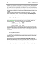
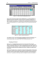
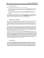
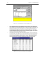
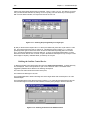
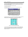
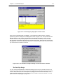
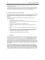
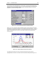
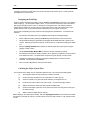
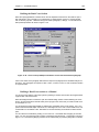
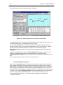
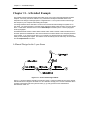
Chapter 11 – A Detailed Example
261
Chapter 11 - A Detailed Example
This chapter presents a simple example that makes use of many of the commands presented in earlier
chapters. For brevity, the size of network is very small but the techniques illustrated will be found
adequate for the design of drainage systems of significant size. You may find it useful to work through
this example on your computer while reading this chapter.
Two design sessions will be described. The first is in manual mode and will design the system for a 5year storm. The second session in automatic mode will test the design under the action of a more severe
storm. A final section describes how to use the Show/Graph command to plot 2 or more hyetographs
and/or hydrographs.
The MIDUSS 98 CD contains a folder called ‘Tutorials’ which holds a number of audio-visual lessons on
the basic operations in MIDUSS 98. Most of these lessons have been based on the examples presented
in this chapter. If you have a sound card on your computer you will find it useful to view these lessons
while you are reviewing this chapter. The lessons can be run directly from the CD or they can be invoked
from the Help/Tutorials menu item.
A Manual Design for the 5-year Storm
Figure 11-1 – A four-link drainage network
Figure 11.1 shows a network comprising 5 nodes and 4 links. Link #3 is intended to be an open channel,
links #4 and #2 are to be pipes and link #1 is to be a detention storage pond. The sub-catchments which
generate overland flow enter the system at nodes (1), (3) and (4) and have the characteristics
summarized in Table 11.1.
262
Chapter 11 – A Detailed Example
Table 11.1
Catchment data for the network of Figure 11.1
Catchment number
1
3
4
Percent impervious
65
20
30
Area (ha)
5.0
3.5
2.5
Overland flow length (m)
85
125
90
Surface gradient (%)
2.0
1.5
2.5
Manning ‘n’
0.20
0.25
0.25
SCS Curve Number CN
84
76
76
Initial abstraction (mm)
5.0
7.5
7.5
The impervious fractions in the three contributing sub- catchments are assumed to have roughness and
imperviousness values as indicated in Table 11.2. The runoff from these catchment areas is to be
computed using the SCS infiltration method and the triangular unit hydrograph method for overland flow.
Table 11.2
Characteristics of impervious areas
Catchment number
1
3
4
Manning ‘n’
0.015
0.020
0.020
SCS CN or Runoff coeff. C
0.95
98
98
Initial abstraction Ia – (mm)
1.5
2.0
2.0
Design Storms
The drainage system is to be designed for a 5-year design storm of the Chicago hyetograph type and
tested under a more severe historic storm. The 5-year synthetic storm is to be based on the intensityduration-frequency relation shown in equation [11.1], with a value or r = 0.35 and a storm duration of 2
hours.
[11.1]
i=
a
(t d + b )c
=
1140
(td + 6 )0.84
The historic storm is defined by the table of rainfall intensities in mm/hour at 5 minute intervals as shown
in Table 11.3. The total duration is 3 hours.
Chapter 11 – A Detailed Example
263
Table 11.3
Historic storm hyetograph in mm/hour for 5 minute intervals.
12
12
14
15
21
19
18
15
14
12
11
10
12
16
20
24
38
42
75
77
96
105
102
89
65
56
54
38
35
20
17
13
9
6
4
3
Setting the Initial Parameters
Three steps are required at the start of a MIDUSS 98 design session. These define:
•
The system of units to be used
•
The name of an output file to be used, and
•
The time step parameters for modelling.
These are detailed in the steps which follow and are also described in Chapter 2 – Structure and Scope
of the Main Menu.
Selecting the Units
When you launch MIDUSS 98 the Options/Units menu item is opened automatically and the mouse
pointer is moved over the Metric or Imperial choices. This is to force you to select from either Metric (S.I.)
or Imperial (U.S. Customary) units. In this example metric units are used. Note that your choice can be
changed up to the point where the time parameters are selected. After that, you cannot alter the
selection for the session.
When you click on your choice, MIDUSS 98 displays a prompt suggesting that the next step should be
define an output file for the session. For your convenience, the directory and name of the last used
output file is displayed. You can close these message boxes either by clicking with the mouse pointer on
the [OK] button or simply by tapping the space bar or any other printing key on the keyboard.
Specifying an Output File
When you accept the units, the menu item File/Output file/Create New file is opened automatically and
the mouse pointer is positioned over this item. A job specific output file is not a requirement but it is
strongly recommended. If you don’t specify one, all output will be written to a default file in the Miduss98
directory.
This is a good point at which to specify a special sub-directory for the project that will contain all of the
relevant files. When you click on the Create New file or Open existing file menu items, a file dialogue
box is displayed. If you want to create a new directory for this project, click on the ‘Create New Folder’
icon. A new directory with the temporary name ‘New Folder’ is displayed ready for editing. Type in an
appropriate name; for this example use a directory called ‘MyJobs’ in drive ‘C:\’. (Hint: You may have to
click anywhere on the ‘white space’ of the dialogue box to get Windows95 to recognize your new folder
name.)
264
Chapter 11 – A Detailed Example
Double click on the new directory or folder to open it. You can then type the name of the required output
file in the File name text box. For this example, use a filename ‘Chap11.out’ or another of your choice.
When you click on the [Open] command button, the file dialogue box closes and a message is displayed.
Typically, if a new file has been specified, MIDUSS 98 will ask you to confirm that you want to create this
file. If you select an existing file as the output file, the message will warn you that if you continue, the
existing contents of the file will be lost. Close the message box by clicking either [Yes] or [No]. If you
press [No] the Open file dialogue box is re-opened until an acceptable output filename has been selected
or defined.
The name of the output file will be displayed at the right-hand end of the status bar. If you want this
display to include the full path of the file, you can do this by selecting the Options/Other Options item
from the menu and click on the item Include Path on Status Bar. If you have used the suggested name,
you should see the path ‘C:\MyJobs\Chap11.out’ at the right end of the status bar..
Define the Time Parameters
The third required step is to define the time parameters. Click on the Hydrology item in the main menu.
Only the Time parameters item is enabled at this stage. Click on the command to open the Time
Parameters dialogue box. The three items to be defined and their default values are:
Time Step
5
minutes
Maximum Storm length
180
minutes
Maximum Hydrograph
1500
minutes
These are acceptable for the current example although you may prefer to reduce the hydrograph length
to (say) 1000 minutes. However, too short a hydrograph length may result in truncation of a long outflow
hydrograph from a detention pond that will result in continuity errors in hydrograph volume. For other
projects you can change these default values easily by clicking on a value to highlight it and then type in
the desired value.
Specifying the Design Storm
In the Hydrology menu the Hydrology/Storm item is enabled only after the time parameters have been
defined and accepted. On accepting the time parameters you may see a prompt that you can now define
a storm and on closing the message box the Storm command is opened automatically and the mouse
pointer is moved over it.
These two prompting features can be toggled off or on in the Options/Other Options menu. If you open
this menu you can see whether or not the options Show Prompt messages after each step and
Show Next logical menu item are checked. For the first few design sessions, you may find it useful to
use both options. After some experience with the program you may decide to omit the Prompt
messages.
Click the Storm command to open the Storm window. Using the Chicago tab of the form, enter the
parameters given in equation [11.1] above and press [Display]. The hyetograph is displayed in graphical
and tabular form.
Chapter 11 – A Detailed Example
265
Figure 11-2 – Table of the Chicago rainfall hyetograph
The resulting hyetograph is shown Figure 11-2. The peak intensity is 152.1 mm/hour at 45 minutes.
After you press the [Accept] button the storm descriptor window is opened as shown in Figure 11-3. The
default string of ‘005’ is for a 5-year storm. This is acceptable for the design storm so click on [Accept].
This means that any hydrograph files saved during the session will have a default extension of ‘005hyd’.
Figure 11-3 – Defining the storm descriptor
Runoff Analysis
The simulation and design does not need to follow the sequence of node numbers. You should first
design the channel and pipe conveying the runoff from areas 3 and 4 to the junction node 2.
Now that a design storm has been defined the Catchment command is enabled in the Hydrology menu.
Click the Hydrology/Catchment command to open the 3-tab Catchment form. On the Catchment tab,
enter the first 5 items of data given in Table 11.1 for area 3. On the same part of the form select the
Triangular SCS response as the routing method and select the Equal Lengths option which assumes that
the overland flow lengths on the pervious and impervious fractions are equal.
Select the Pervious tab. The area and flow length are shown and cannot be changed but the slope of
1.5% could be changed if necessary. For this example leave it at 1.5%.
Select the SCS method as the infiltration method and fill in the remaining three parameters from Table
9.1 to define the Manning ‘n’, SCS Curve Number and Initial Abstraction depth Ia. As you enter a CN of
76 you will see the runoff coefficient increase to 0.223 and the initial abstraction reduce to just over 8
mm. These changes are consistent with a less pervious soil type. When the initial abstraction is
reduced still further to 7.5 mm, the only change you will see is a slight reduction of the ratio Ia/S from the
default of 0.1 to 0.0935.
Now select the Impervious tab; note the area and flow length and leave the slope at 1.5%. Enter the
three parameters from Table 11.2. As with the Pervious parameters, you will see the ratio Ia/S increase
when you type in an initial abstraction of 2.0 mm.
266
Chapter 11 – A Detailed Example
Figure 11-4 – Table of the Runoff hydrograph for Area 3
Finally, select the Catchment tab again and press the [Display] button. The rainfall hyetographs are
displayed briefly followed by the graphs of runoff from the pervious, impervious and total areas. The
peak flow of 0.189 c.m/s is mainly from the impervious fraction. Press the [Show Details] button to
display the table shown in Figure 11-5. The pervious fraction contributes more than half the volume of
runoff. The table of runoff flows (Figure 11-4) shows zero runoff for the first 30 minutes; this is due to the
relatively high initial abstraction of 7.5 mm which is apparent if you click on the Pervious tab and press
[Display].
Figure 11-5 – Details of the Runoff from Area 3.
The contribution of area 3 to the drainage network is completed by pressing the [Accept] button to end
the Catchment command. Then use the Hydrograph/Add Runoff command which causes the
summary peak flow table to show a peak of 0.189 c.m/s in the Inflow (see Figure 11-10).
Designing the Channel
When you click on the Design/Channel command the form opens with the default trapezoidal
parameters of 3H:1V side-slopes, a base-width of 0.6 m and a roughness of n = 0.04. With the default
design of 1.0m depth with a slope of 0.5%, clicking on the [Design] button shows a depth of 0.262 m. If
you want to review alternate designs you can click on the [Depth Grade Velocity] button to display a table
of feasible values of depth and gradient. Velocity is also shown for information. You can ‘import’ any of
these designs by double clicking on the appropriate row of the grid. The gradient is rounded up to the
nearest 0.05%.
Flatten the channel grade to 0.25%. Notice that any change to the design parameters causes the plot of
water surface to be deleted and the [Accept] button is disabled until the [Design] button is pressed again.
The depth is increased to 0.308 m and the critical depth is just over half that, so the flow is tranquil or
sub-critical. Figure 11-6 shows a fragment of the Channel Design window. Press the [Accept] button to
close the form. The peak flows in the summary table are unchanged but another record is added for
Chapter 11 – A Detailed Example
267
information.
Figure 11-6 – A fragment of the Channel Design form.
If you have enabled the Options/Other Options/Show Next logical menu item, the mouse pointer will
automatically point to the Design/Route command. Click on this to open the Route window. The default
length (initially 500 m) is highlighted and you can type in the actual reach length of 300 m. This will
cause the values of the X-factor and K-lag to be reduced which means reduced attenuation of the outflow
hydrograph.
Press the [Route] button to show the graphical comparison of the inflow and outflow and also the tabular
display of the outflow hydrograph. The peak is reduced from 0.189 c.m/s to 0.160 c.m/s and lagged by 5
minutes. Since the hydrographs are plotted at 5 minute increments, very ‘peaky’ hydrographs may
sometimes show some truncation of the outflow. Press [Accept] to close the form. Another record is
added to the peak flow summary table showing the peak inflow and outflow.
Figure 11-7 – Final result of the Route command
268
Chapter 11 – A Detailed Example
Moving Downstream
When an outflow hydrograph is computed you can do one of two things:
1.
If this is the last link on a tributary you should probably use the Hydrograph/Combine command to
store the outflow at the junction node, adding it to any previous outflows which may have been
accumulated previously.
2.
If this is not the last link in the tributary, you should use the Hydrograph/Next Link command to
convert the computed outflow from the present link into the inflow to the next node and link
downstream.
In this example, the second case is true and we want to add the runoff from area 4 and design the pipe
to carry the total flow to the junction at node 2. Press the Hydrograph/Next Link menu item and note
the change in the peak flow summary table. With most of the Hydrograph/… commands a brief
explanatory message is displayed along with a table of the modified hydrograph.
Adding the Next Catchment
When you select the Hydrology/Catchment command to generate the runoff from area 4, the default
values reflect the values entered for the previous catchment area. From the data in Tables 11.1 and
11.2 the parameters for the pervious and impervious fractions are unchanged and only the first 5
parameters on the Catchment tab need to be changed. You may find it convenient to enter the top item
first (the ID number) and then press the Tab key on the keyboard to move down and highlight the next
item.
The increased impervious fraction and steeper slope more than compensates for the smaller area and
peak runoff is 0.216 c.m/s. Pressing [Show Details] reveals that the volume is just under 400 c.m and
that more than 60% of this is generated from the impervious fraction. You should also notice from the
graph and from the time of concentration shown in the details, that the time to peak is different for the
pervious and impervious fractions. As a result, the total flow peak of 0.216 is significantly less than the
sum of the two individual peaks (0.037 + 0.209 = 0.246).
Press [Accept] to close the Catchment form and select the Hydrograph/Add Runoff command to add
the runoff to the current inflow. A total peak flow of 0.256 c.m/s is shown in the peak flow summary grid
(see Figure 11-10). You may also note from the table of the new inflow hydrograph that the total volume
of 878.46 c.m is equal to the sum of the runoff volumes from the two catchment areas. You can confirm
this by using the Show/Output File command (or by pressing Ctrl+O) which lets you browse through the
output file to recall the details from each of the two Catchment commands. You can also see that the
time of concentration of the impervious runoff differs by almost 2 minutes. Because the hydrographs are
very ‘peaky’ this causes the total peak (0.256) to be over 35% smaller than the sum of the two
constituent runoff hydrographs (0.189 + 0.216 = 0.405 c.m/s).
Designing a Pipe
You can now use the Design/Pipe command to size the pipe leading to junction node 2. The Pipe
window shows the peak inflow and a table of diameter-gradient pairs that would carry this flow when
running full. Double click on the row containing the 525 mm diameter. The gradient is rounded up to
0.4% and pressing [Design] shows that this design will run just over ¾ full with an average velocity of
1.43 m/s. Figure 11-8 shows this result. You can, of course, experiment with different designs or
different roughness values until you have an acceptable design. Press [Accept] to close the window.
Chapter 11 – A Detailed Example
269
Figure 11-8 – Final result of the Pipe Design command
When you press the Design/Route command, the form opens with the length of 300 m previously used
for the channel. Change the highlighted value to 350 m and click on the [Route] button. The outflow
hydrograph table reports a peak flow of 0.242 c.m/s which represents 5% attenuation. This is a little high
for a pipe, and the reason is apparent if you look at the graph. Click on the horizontal scroll bar to reduce
the plotted time base to about 120 minutes. The inflow hydrograph has a double peak – due to the
difference in time to peak from areas 3 and 4 – and the outflow hydrograph tends to average out these
peaks despite the fact that the routing time step was only 2.5 minutes. However, the volume of outflow is
still correct.
Defining a Junction Node
You must now store this outflow hydrograph at junction node 2 while you design the highly impervious
area 1 and a detention pond. Use the Hydrograph/Combine command to open the Combine dialogue
window. Since this is the first use of the command the form contains no data. The procedure can be
followed fairly easily by responding to the prompts in the yellow box. Thus:
•
Press [New] and enter the number and description of a new node. When you press the
[New] button a text box is opened to define the Junction node number. Type ‘2’. As soon as a
node number is entered, another text box opens for a description. Type a brief description such
as “Node 2 – junction of links 1 and 4”. The textbox will expand to accommodate a second line.
•
After entering a description, press [Add] to add this to the List of Junction Nodes. The
[Add] button has been enabled. Click on it to cause the node number and description to appear
in columns 1 and 3 of the multiple list box. The middle column shows a value of 0.000. This will
be updated to hold the current peak value of the accumulated flows at the junction. If the
description is longer that the width of the descriptor column, a horizontal scroll bar is added to
column 3 of the list box.
•
Click on a node in ‘Junction Nodes Available’ to highlight the node to which the current
Outflow will be added. When you click anywhere on the desired row, the entire row is
highlighted and the [Combine] button is enabled.
270
Chapter 11 – A Detailed Example
Figure 11-9 – Final display of the Combine dialogue form.
•
Press [Combine] to add the current Outflow to the selected node. Click on the [Combine]
button. MIDUSS 98 shows a warning message to advise you that a new file HYD00002.JNC
will be created in the currently defined Job directory. Press the [Yes] button to confirm this. The
[No] option is provided in case you have made an error. When you press [Yes] the value of
0.242 is entered in the middle column of the list box as shown in Figure 11-9. Also, another
message is displayed showing the operation and the node number in the title bar, the name of
the file created and the peak flow and volume of the accumulated hydrograph. This is a modal
form and you must click on the [OK] button to continue.
•
Click [OK] and press [Accept] to finish the Combine operation. Press the [Accept] button
that is now enabled. The Combine form is closed and the peak flow summary table is updated
with another record showing the Combine operation, the node number and the updated peak
flow of the Junction hydrograph as shown in Figure 11-10 below. Note that the height of the
Peak Flows table has been increased by dragging the top edge of the window upwards.
Figure 11-10 – Peak flow summary for branch (3)-(4)-(2)
Chapter 11 – A Detailed Example
271
Adding Catchment Area 1
Before the new tributary branch from node 1 to junction node 2 can be designed, you must clear out the
Inflow hydrograph left over from the analysis of the previous branch. You can do this by clicking on the
Hydrograph/Start/New Tributary menu item. You can use this command either before or after
generating the runoff from catchment area 1.
The next logical command is the Hydrology/Catchment command, Because the parameter values are
different for both the pervious and impervious fractions you will have to edit the data on all three tabs of
the Catchment form. The impervious fraction is defined in terms of a runoff coefficient of 0.95 which, for
the currently defined storm, is equivalent to a Curve Number of 99.43.
The resulting peak runoff is 0.990 c.m/s with the peak occurring 50 minutes after the start of rainfall. This
peak flow will be routed through a detention pond before adding the runoff to Junction node 2. After
pressing the [Accept] key, use the Hydrograph/Add Runoff command to add it to the Inflow hydrograph.
If you have forgotten to set the Inflow to zero, MIDUSS 98 warns you that you may be double counting
the inflow hydrograph from the previous branch. However, there may be situations where a new tributary
runoff should be added to the previous inflow, so you must make the decision as to whether the warning
is legitimate or not.
Design the Pond
For this example assume that the following criteria will guide the design of the pond.
•
The pond will be a dry pond with no permanent storage.
•
The outflow peak should be approximately 0.3 c.m/s for the 5-year storm.
•
The maximum depth should be 2.0 m. with a top water elevation of 102.0 m.
•
Outflow control will comprise an orifice and an overflow, broad-crested weir with a trapezoidal
shape.
•
The ground available is roughly rectangular in plan with an aspect ratio of 2:1.
Click on the Design/Pond command to open the Pond form. The form shows the current peak inflow
and the hydrograph volume of 1410 c.m. The default peak outflow is 0.495 c.m/s and for this a storage
volume of approximately 439 c.m is required. Edit the Target outflow by typing a value of 0.3 c.m/s. The
required volume is increased to 590 c.m.
Enter the minimum and maximum levels as 100.0 and 102.0 m; leave the number of stages as 21 which
implies 20 depth increments. This will cause the Level – Discharge – Volume table to show levels
increasing by 0.1 m. Before you can route the inflow hydrograph through the pond, you must define two
characteristics of the proposed pond:
The storage geometry, and
The outflow control device.
Defining the Pond Storage Geometry
Select the Storage Geometry/Rectangular pond menu. This causes the Storage Geometry Data
window to be opened . Click once on the up-arrow of the spin button to open up a single row in the table.
This shows default data which will generate the required volume in a depth of roughly 2/3 of the
maximum depth of 2.0 m. You can test this by pressing the [Compute] button on the Geometry Data
form. The column of volumes is computed with a maximum value of almost 1150 c.m.
To check the size and shape of the surface area at elevation 102.0 open another row in the data table by
clicking again on the up-arrow of the spin-button. The computed area is just over 1000 sq.m but the
aspect ratio is only 1.4. To get the aspect ratio at elevation 102.0 to be 2:1 you must increase the aspect
ratio at elevation 100.0. To do this click on the cell containing the aspect ratio of 2.0 in the first row. The
272
Chapter 11 – A Detailed Example
outline of the cell is slightly thicker when it is selected. Type in a value – say 3.5. The effect is not shown
until you select another cell either by clicking on one or by using one of the arrow keys on the keyboard.
With 3.5 at the bottom elevation, the aspect ratio at level 102.0 is 1.84.
Figure 11-11 – Defining the pond geometry as a single layer.
By trial you will find that an aspect ratio of 4:1 at the pond bottom will yield a ratio of just under 2:1 at the
top. The surface area at level 102.0 is 1093 sq.m. This design is shown in Figure 11-11. Press the
[Compute] button again to refresh the column of volumes and enable the [Accept] button on the data
form. Click the [Accept] button to close the data form. It can be re-opened and edited later if you wish.
Note that it is more usual to have a number of ‘layers’ with different side-slopes but only one layer is used
at this stage for simplicity. MIDUSS 98 lets you define up to 10 layers.
Defining the Outflow Control Device.
To define the outflow control device select the menu item Outflow Control/Orifices. A similar data entry
form is displayed. Click on the spin-button to open a row to define an orifice. The default values
suggested by MIDUSS 98 are based on the following assumptions:
The invert of the orifice will be at the bottom of the pond,
The coefficient of discharge is 0.63, and
The suggested diameter is sized to discharge 25% of the target outflow with a head equal to 1/3 of the
maximum depth.
The suggested values for the orifice are shown in Figure 11-12, Press the [Compute] button to fill in the
column of discharge as a function of water elevation, and then press [Accept] to close the data form.
Figure 11-12 – Defining an Orifice for the Outflow Control
Chapter 11 – A Detailed Example
273
The outflow control should have a weir to pass the higher flows – particularly for the more severe historic
storm. Select the Outflow Control/Weirs menu item to open a data form for the weir specification.
When you open a data row by clicking on the spin-button, the default data is displayed. These data are
based on certain simple assumptions:
The crest elevation corresponds to 80% of the maximum depth.
The coefficient of discharge is 0.9.
The weir breadth is estimated to pass the peak inflow with a (critical depth/ breadth) ratio of 0.2.
The side-slopes are vertical.
Figure 11-13 – Defining a Weir for the Outflow Control
Change the side-slopes to 1H:1V (i.e. 45°) but leave the other parameters unchanged in the meantime as
shown in Figure 11-13. Press the [Compute] button. As shown in Figure 11-14, the column of
discharges is updated for elevations above 101.6. Press [Accept] to close the data form.
Figure 11-14 – The H-Q-V grid after defining a Weir.
You can plot a graph of the storage and/or discharge characteristics by selecting the Plot/V, Q = f(H)
menu item. You can enlarge the plot (Figure 11-15) by dragging the corners of the graph window. The
highly non-linear nature of the blue, stage-discharge curve is clear. You may notice a small convex
segment of the orifice discharge curve below an elevation of 100.2 which is caused by the orifice
operating as a circular weir.
274
Chapter 11 – A Detailed Example
Figure 11-15 – Plot of the functions V, Q = f(H).
Refining the Pond Design
You can now press the [Route] button to see how the pond performs. From the Pond Design form it is
clear that the design is very conservative. The peak outflow is only 0.129 c.m/s – well below the target
outflow of 0.3 c.m/s and the storage volume is too large at 857 c.m. The weir is overtopped by only a
very small head (101.614 – 101.6 or 14 mm) and only for about 15 minutes.
Of the various ways in which the outflow could be increased, reducing the land area required for the pond
will probably yield the greatest cost saving. Select the Storage Geometry/Rectangular pond menu item
to re-open the Storage Geometry Data form again. Reduce the base area to 150 sq.m and click on
another cell to see the result. The surface area is reduced to under 900 sq.m. Press [Compute] to
update the ‘Volumes’ column and then press [Route] again. The peak outflow increases to 0.233 c.m/s,
the volume is reduced to 725 c.m. and the head over the weir increases to 0.115 m.
Try reducing the base area still further – say to 115 sq.m. The surface area is reduced to 800 sq.m., the
maximum storage is 647 c.m. (which is within 10% of the initial estimate) and the peak outflow is still just
under 0.3 c.m/s. A fragment of the Pond Design form is shown in Figure 11-15. From the Outflow
hydrograph Table, you may notice a small error in the volume continuity as the pond outflow hydrograph
is longer than the maximum hydrograph length so that the tail of the recession limb is truncated. The
graph of the Inflow and Outflow hydrographs is shown in Figure 11-16.
Figure 11-16 – Results of the Pond Route operation.
Chapter 11 – A Detailed Example
275
Figure 11-17 – Graphical display of Pond Inflow and Outflow
Press the [Accept] button to close the Pond Design forms. Since this is the only Pond design in this
project, you can leave unchecked the box labelled ‘Keep all Design Data’. You can review the iterations
during this design in the Design log. If you want to keep a record of this you can use the
Design/Design Log/Print/Total Log File or Design…Current Design Log menu items to print a
hardcopy of the Design Log.
Saving the Inflow Hydrograph File.
As it is possible that you may want to revise the pond design when you subject it to the historic storm, it
might be useful to save the pond inflow file before continuing. Select the Hydrograph/File I/O command
to open the File Input/Output dialogue window. Perform the following steps, working in a clockwise
fashion around the form.
Confirm the File Operation as ‘Write to’ or ‘Save a file’ by selecting the lower radio button.
Set the Type of File as a Flow Hydrograph by selecting the lower radio button. This causes the Flow
Hydrograph frame to be displayed.
Select the desired Flow Hydrograph by clicking on the ‘Inflow’ radio button.
In the Drive and Directory list boxes, navigate to your Job directory
In the Hydrograph type drop-down list box, select the ‘Event Hydrograph (*.005hyd)’
The file-name box shows the default ‘*.005hyd’. Edit this to (say) ‘PondInflow.005hyd’. (Hint: click on the
default name to highlight it, press the ‘Home’ key on the keyboard to position the text entry marker in front
of the asterisk, type the desired name and finally delete the asterisk.)
Press the [View] command button to display the Graph and/or the table. This is necessary to enable the
[Accept] button.
Press [Accept]. Some default text “Enter a description…” is highlighted. Type in a description of at least
20 characters (about half the width of the text box) e.g. “Inflow to pond from area #1”.
Press [Accept] again to close the form.
276
Chapter 11 – A Detailed Example
Figure 11-18 – The File I/O form is used to save the Pond inflow.
Adding Flow from the Two Branches.
When the Pond Design form was closed, the peak flows summary table was updated with a new record
showing the value of 0.298 in the Outflow column. If you assume that the outflow from the pond is close
to the junction node 2, you can add the pond outflow to the junction by using the Hydrograph/Combine
command again.
The process is simpler this time as the junction node has been created. Follow the directions in the
yellow box as before to:
Click on the row describing Node 2 to highlight it, This enables the [Combine] button.
Click the [Combine] button to update the peak of the total junction hydrograph to 0.534 c.m/s.
MIDUSS 98 displays a message to confirm the junction file name, the peak flow and the total volume.
Click [OK] and then [Accept] to close the form.
Designing the Last Pipe
The final step in the design is to recover the accumulated flow from the Junction node 2 and design a
pipe to carry this flow over the last 400 m reach.
To recover the hydrograph at Junction node 2 select the Hydrograph/Confluence command. Notice
that in the Hydrograph menu, the Hydrograph/Combine command is disabled because a new Outflow
hydrograph has not been created since the last use of Combine. This is to protect you from making the
error of combining the same outflow twice.
The Confluence dialogue form in Figure 11-19 is similar in appearance to the Combine form. The [New]
and [Add] buttons are disabled as they have no relevance for the Confluence operation. The 3-column
list box shows the currently active junction nodes.
Chapter 11 – A Detailed Example
277
Figure 11-19 – Recovering the hydrograph at Junction node 2.
Click on the row describing Node 2 to highlight it. This enables the [Confluence] button. Pressing
[Confluence] causes a message box to be displayed as shown in Figure 11-20. This reports the file that
has been deleted. In fact, the file is not deleted but is renamed with the extension *.JNK. You may
therefore recover the file by renaming it prior to the end of the session at which point it will be erased.
Also reported is the peak flow and volume of the new Inflow hydrograph. Notice that if the current Inflow
hydrograph has not been used, MIDUSS98 will provide a warning message that you will lose some data if
you continue with the Confluence command.
Figure 11-20 – The information message following use of the Confluence command.
The Final Pipe Design
You can now select the Design/Pipe command and design a pipe to carry the peak flow of 0.534 c.m/s.
Assuming the default value of n = 0.013, a 675 mm diameter at 0.5% will carry the peak flow with a depth
of 0.5 m. Note, however, that the critical depth is only slightly less than the uniform flow depth. This
implies a Froude number close to 1.0 which is close to the condition of easy wave formation. You may
prefer to flatten the slope slightly to (say) 0.45%.
278
Chapter 11 – A Detailed Example
Finally, using the Route command again yields an Outflow peak flow of 0.530 c.m/s with almost
negligible attenuation and lag.
This finishes the design for the 5-year storm. You can now end the session by selecting the File/Exit
command. Before closing down MIDUSS 98 reminds you of the name of the output file. A copy of the
file ‘Chap11.out’ is provided for your information in sub-directory C:\…\Miduss98\Samples\.
An Automatic Design for a Historic Storm
When the design for the 5-year storm has been completed, you can check how this drainage system will
respond to the more extreme event described by the historic storm defined in Table 11-3. You can use
the Automatic mode to do this without having to re-enter all of the commands and data from the
keyboard.
The procedure is described in the topics that follow in the remainder of this chapter and can be
summarized as follows.
•
Run MIDUSS 98 and define a new output file.
•
Use the previous output file to create an Input Database called Miduss.Mdb that resides in the
MIDUSS 98 directory.
•
Run MIDUSS 98 in Automatic mode using the database as input.
•
Step through the database in EDIT mode to allow you to modify the design parameters as
desired.
•
When the previous Chicago hyetograph is displayed, reject this and replace it with a historic
storm.
•
Continue with the design, making any adjustments that you may feel are appropriate. These
may include some refinement of the Pond design and separation of major and minor flow
components if a pipe is surcharged under the more severe storm.
•
Complete the run and compare peak outflows for the two events.
First Steps
When you launch MIDUSS 98 and define the units, you will see a message prompting you to define an
output file and reminding you of the last output file used. When the File/Output file/Create New file
opens, reject this and move the mouse pointer to select instead the File/Open Input File command.
Two windows will open. One window titled ‘Create Miduss.Mdb’ is immediately overlain in part by an
‘Open’ file dialogue window that will show the previously selected Job Directory and the previous output
file as the defaults. You can select any output files available but in this case you will convert the contents
of the previous output file ‘Chap11.out’ to a database file called Miduss.Mdb which will be the Input for
this second run.
When you click on the [Open] command button the dialogue box closes and you will probably see a
standard warning message advising you that a file called Miduss.Mdb already exists in the Miduss98
folder. Click on the [Yes] button to proceed. After a few seconds processing the ‘Create Miduss.Mdb’
window (see Figure 11-21) will show the source data file, the number of commands processed and the
number of records in the data file. If the path of the source file is too long for the form you can re-size it
by dragging on the right edge. Close the form by clicking on the [FINISH] button that is now enabled.
Chapter 11 – A Detailed Example
279
Figure 11-21 – Creating an Input Database from an Output file.
Finally, in order to enable items on the main menu, you must use the File/Output file/Create New file
command once again to specify a new filename. If you are quite certain that you will not need the old
output file you can use the same filename again and ignore the warning that the current contents will be
lost. For this example, use a different filename such as ‘C:\MyJobs\Chap11B.out’.
Reviewing the Input Database
Before running the Input Database, it is worth taking a moment to review the file Miduss.Mdb. Obviously,
this is an essential first step if you want to edit any of the command parameters or even just make one of
the commands negative to force a continuous run to stop and revert to manual mode. Select the
Automatic/Edit Miduss.Mdb Database command. The window shown in Figure 11-22 Is displayed.
The Edit Panel controls let you navigate through the file to verify or change data.
Figure 11-22 – Reviewing the Input Database.
280
Chapter 11 – A Detailed Example
To provide an overview of the session, you can also review a subset of the records by clicking on the
down arrow and selecting a particular type of command. Figure 11-23 shows only the command lines for
the total database. This was done by clicking on ‘All COMMANDS’ on the drop down list.
Figure 11-23 – Displaying a sub-set of the Database in the Edit Panel
Starting the Automatic Run
Select and click on the Automatic/Run Miduss.Mdb menu item to start the run. The Control Panel
shown in Figure 11-24 Is displayed in the lower right of the screen. In its default size it displays only 9
records at a time but you can increase the height of the window by dragging on the top or bottom edge of
the form.
When initially displayed, only the first 3 records have been read and the current record – indicated by the
right arrow in the left margin of the grid – is about to read the units used. Note that if you have specified
the wrong type of units for this input file, MIDUSS 98 will change the units for this design session to
match these used when the previous run was made.
Figure 11-24 – The Control Panel for using Automatic Mode.
Chapter 11 – A Detailed Example
281
The default command button is [RUN] which processes the commands sequentially and continuously
without giving you a chance to change or even monitor the results. In this automatic run you will use the
[EDIT] button to pause after each command to display the result and give you a chance to modify the
parameters.
Click on [EDIT]. MIDUSS 98 displays the Time Parameters and the mouse pointer is automatically
positioned on the [Accept] button of the form. The maximum storm duration is 180 minutes, which is
enough for the historic storm. Click [Accept] to close the form.
Change the Storm Event
After you have accepted the time parameters, the mouse pointer is relocated over the [EDIT] button on
the Control Panel and the next record (number 14) is seen to be the Storm command. Click on [EDIT] to
show the Storm window with the 2-hour Chicago hyetograph.
To change the storm the first step is to click on the Historic tab on the Storms form to display the data for
the Historic storm. You should:
•
Check the box labelled ‘Check to set rainfall to zero’, and
•
Increase the duration from 120 to 180 minutes
•
Click on the [Display] command button.
The Historic tab should be similar to Figure 11-25 below, with the exception that the Rainfall depth will be
zero. The Graph window will be empty and the tabular form will have an extra row added with all the 36
cells having a value of ‘0.00’.
Figure 11-25 – The Historic tab of the Storms window with 21 values entered.
Defining the Historic Storm.
The Historic table is initially blank (unless you deliberately wanted to copy the previous storm intensities)
and the first cell should have a slightly heavier gray outline. If it does not show this, click on it with the
mouse ponter.
You can now start typing in the intensities shown in Table 11-3. As soon as you type a number (even the
first ‘1’) you will notice that the first bar of the storm hyetograph is plotted and the Rainfall depth in the
Storm window is updated. As each cell value is entered, use the Right-arrow key on the keyboard to
282
Chapter 11 – A Detailed Example
advance the active cell. When you are at the right end of a row, pressing the Right-arrow will ‘wrap’
around to the first cell of the next row.
Figures 11-26 And 11-27 show the Table and Graph respectively at a point where 21 values have been
entered. At this point the total rainfall depth is 47.833 mm as shown in Figures 11-25 and 11-26.
Figure 11-26 – The Historic Storm table after 21 intensities have been entered.
Figure 11-27 – The Rainfall Graph after 21 intensities have been entered.
After entry of the Historic storm is complete, the total rainfall depth should be 99.167 mm. Press [Accept]
to close all three forms. The Storm Descriptor window is opened and contains the value of ‘005’ used for
the minor storm. If not already highlighted, click on this text box to highlight the value and replace it with
‘100’. When you press the [Accept] key, MIDUSS 98 displays the message shown in Figure 11-28.
Chapter 11 – A Detailed Example
283
Figure 11-28 – The result of changing the Storm Descriptor.
The change in file extension means that if any hydrograph files are created they may have the same
name and share the same directory as previous hydrograph files but are distinguished by a unique file
extension. Click on the [OK] button to accept the default action of replacing the previous extension
‘.005hyd’ with the new file extension ‘.100hyd’.
Continuing with the New Storm
The Control Panel should now show the next record (#25) as the start of the Catchment command for
area 3. Click on the [EDIT] button to cause the results of this command to be displayed. The peak flow
is now 0.46 c.m/s. Click on [Accept] and then on [EDIT] to execute the Add Runoff command. Click on
the [OK] button and again on [EDIT] to run the Channel Design command. The depth in the channel has
increased from 0.308 m to 0.458 m.
Continue in this way to Route the flow through the channel, add the runoff from area 4 and check the
design of the pipe from node 4 to Junction node 2. When the Pipe Design form is displayed a message
is also shown warning you that the pipe is surcharged (see Figure 11-29). Click on the [Yes] button to
accept this design and return to the Pipe Design window. Then use the [Accept] command button to
close the form.
Figure 11-29 – A Warning of surcharge in Pipe 4-2.
284
Chapter 11 – A Detailed Example
Separating the Major System Flow
At this point you must split the Inflow hydrograph into two components:
•
A minor system fraction which does not exceed the capture capacity of the pipe, and
•
A major system fraction that is rejected by the minor system and which will flow on the surface –
typically on the street.
You can do this by introducing a diversion device that simulates one or more catchbasins at the
upstream end of the pipe. The following steps summarize the process.
(1)
Revert into Manual mode for steps (2) and (3) noted below. You may find this is not always
necessary but it is included here for completeness.
(2)
Design a diversion structure that will split the inflow hydrograph into two components. The
outflow should have a peak equal to the capacity of the pipe and the remainder will flow on the
major system – typically the street.
(3)
Make the Outflow from the diversion the Inflow to the pipe.
(4)
Return to Automatic mode and execute the next command that will Route the captured flow
through the pipe to node 2.
(5)
Continue in Automatic mode.
Figure 11_30 illustrates the technique of substituting a diversion structure plus a pipe when the pipe is
surcharged. At a later stage you can recover the diverted hydrograph and check the capacity of the road
system to convey this flow. The procedure is described in more detail in the topics which follow.
Figure 11_30 – Separating major and minor flow at a surcharged pipe.
Design of a Diversion Device.
After you have accepted the surcharged pipe design the next two commands should be executed in
Manual mode. Click on the [MANUAL] command on the Control Panel to close it and revert to Manual
mode.
Click on the Design/Diversion command. In the top two rows, the form displays the peak flow of the
current Inflow hydrograph and the type and capacity of the last conduit. The node number is copied from
the last Catchment area. This may not always be appropriate and you may want to edit this. In this
example it is correct because the runoff from area 4 enters at node 4. When used following the design of
a surcharged pipe, the Diversion sets the threshold flow equal to the pipe capacity and assumes that the
diverted fraction is 1.0 – i.e. 100% of the excess flow is diverted to the hydrograph file DIV00004.HYD.
Chapter 11 – A Detailed Example
285
You may prefer to set the diverted fraction to a value less than 1.0 to allow for the increased carrying
capacity of the pipe under surcharged conditions, i.e. when the hydraulic grade line is steeper than the
pipe gradient. Also, if the catchbasins are fitted with inflow control devices (ICDs) you may set the
threshold to a value less than the pipe capacity.
Figure 11_31 - The initial state of the Diversion Command window.
Figures 11-31 and 11-32 show the result of the Diversion operation. Before closing the form with the
[Accept] button you should enter a description such as “Major flow hydrograph at Node 4”. In Figure 1132 the Outflow hydrograph exhibits a plateau or constant value because 100% of the excess inflow is
diverted. If the diverted fraction is less than 1.0 the ‘plateau’ will show some increase above the
threshold flow rate.
Figure 11-32 – Graphical display of the Diversion operation.
The outflow from the diversion can now be converted to the inflow to the pipe by using the
Hydrograph/Next Link command. The result is seen in the Peak flow summary table of Figure 11-33.
286
Chapter 11 – A Detailed Example
Figure 11-33 – Peak flows summary after the Diversion
Continuing in Automatic Mode
You can now resume the automatic processing of the commands in the Input database file. Select the
Automatic/Run Miduss.Mdb command. The Control Panel will re-open at the point where it was
interrupted. Although the pipe-flow has been reduced to the full-pipe capacity, flood routing is not
physically possible. MIDUSS 98 displays a warning message that gives you the choice to simply copy
the Inflow to the Outflow (i.e. with neither attenuation nor lag) or cancel the route operation to re-design
the pipe. Click on the [Yes] button to choose the first option.
You can continue with the automatic processing (using the [EDIT] command to store the outflow from the
pipe at junction node 2, start the new tributary at node 1 and compute the runoff from area 1. The flow
entering the pond now has a peak of 1.154 c.m/sec. The peak flow is 16% greater than previously but,
at 4176 c.m the volume is almost three times larger. It is likely, therefore, that the outflow control can be
left unchanged but the storage will have to be increased by using more area.
Refining the pond Design.
When the Pond design is executed in automatic mode the concern expressed in the previous topic is
confirmed by MIDUSS 98 with a warning message in the Pond window to the effect that the upper limit of
either the discharge or storage is too small to route the increased hydrograph. The storage routing
function (Q + 2S/∆t) involves both discharge and storage volume and the design could be adjusted by
either increasing one or the other or both. Assume that you will provide more storage since the Pond
Design form shows that a required volume of over 2000 c.m. is necessary to reduce the outflow to less
than 0.6 c.m/sec.
Click on the Storage Geometry/Rectangular pond menu item to re-open the data table. Previously,
only one layer covering the total depth of 2.0 m was used. Make the changes shown in Figure 11-34.
This introduces a 15 m wide step in the side-slope at a level of 101.2. This greatly increases the land
area required (from 1094 to 2745 sq.m) but more than doubles the maximum volume from 1238 c.m. to
2516 c.m.
Chapter 11 – A Detailed Example
287
Figure 11-34 – Providing extra storage capacity in the pond.
The stage-discharge curve remains unchanged but the increase in storage is sufficient to enable routing
to be completed with a peak outflow of 0.623 c.m/sec and maximum storage of almost 2200 c.m. You
can experiment further with changes to both geometry and discharge control, but for this example you
should accept this design and continue with the automatic design session.
Completing the Automatic Design Session
If you check the next record in the Control Panel you will see that this was the point at which the 5-year
Inflow to the pond was saved as a file. You may wish to refine the design of the pond still further in a
separate design session, so it would be useful to save the Inflow for the historic storm as well. Should
this not be required you could easily avoid processing this command by pressing the [SKIP] button.
However, assume that this is not the case.
When the Hydrograph/FileI/O command is executed from the Input database, a message is displayed
as shown in Figure 11-35.
Figure 11-35 – MIDUSS 98 automatically changes the file extension.
MIDUSS 98 recognizes that the hydrograph file extension has been changed for the historic storm and
gives you the choice to accept the modified filename, keep the original name (most unlikely!) or enter a
special filename.
Click on the [Yes] button to accept the change in the file extension. The File Input/Output window
remains open to allow you to edit the description should you wish to do so. Add to the previous
288
Chapter 11 – A Detailed Example
description so that it now reads “Inflow to Pond from area #1 for the Historic storm”. Finally, press the
[Accept] button to close the form.
Designing the Final Pipe.
Continue with the automatic processing to use the Combine and Confluence commands. This yields an
inflow to Pipe (2) - (5) with a peak of 0.895 c.m/sec. You can see from record 276 in the Control Panel
that the pipe capacity is 0.564 c.m/sec, so this pipe is surcharged as well. If the capacity had been
greater than the inflow from Junction node 2 you would have had to check if any fraction of the major
system flow from reach (4)-(2) could have been captured by the minor system at this point.
The process of separating the major and minor flow hydrographs is repeated here. You should do the
following.
•
Run the Pipe command from the input database and accept the surcharged design
•
Revert to Manual mode by pressing the [MANUAL] command button in the Control Panel..
•
Use the Diversion design to generate the hydrograph file DIV00002.HYD with a peak of 0.331
c.m/sec. Note that you will need to specify a node number of ‘2’ instead of accepting the default
of ‘1’.
•
Select the Hydrograph/Next Link command to make the inflow to the pipe equal to the pipe
capacity of 0.564 c.m/sec.
•
Use the Automatic/Run Miduss.Mdb command to resume automatic processing.
•
Run the Route command and when prompted to do so, press the [Yes] button to copy the Inflow
to the Outflow at node 5. The peak outflow is equal to the pipe capacity of 0.564 c.m/sec.
•
Complete the automatic processing by pressing the [EDIT] button to execute the ‘EXIT’
command This closes the Input database.
•
Click on the [CLOSE] button to close the Control Panel.
Checking the Major System Flow.
The remainder of the design can be completed in Manual mode. This involves the following steps.
(1)
Save the pipe outflow at node (5) with the Combine command.
(2)
Recover the major system flow in the surface link from node (4) to (2).
(3)
Check the capacity of a typical road profile assuming a road grade of 0.5%.
(4)
Route this over some fraction of the reach length – say half of the length of 350 m .
(5)
Add the routed flow to the surface flow from file DIV00002.HYD
(6)
Check the total major system flow on the road cross-section from the junction node (2) to
the Outlet node (5).
(7)
Add the minor and major flows at node (5).
Before starting on the major system analysis, select the Hydrograph/Combine command and accumulate
the outflow from the pipe at node (5). The total volume of the minor flow is 5494 c.m. with a peak of 0.564
c.m/sec.
Chapter 11 – A Detailed Example
289
Defining the Road Cross-Section
Select the Hydrograph/FileI/O command and in the ‘File Operation’ frame click on the ‘Read or open a
File’ radio button. Next, navigate to your job directory by double clicking on Drive C: and then double
click on directory ‘MyJobs’. Select the File type of ‘Event Hydrograph (*.100hyd)’. You should see the
File Input/Output window as shown in Figure 11-36.
Figure 11-36 – Use the File Input/Output command to recover the Diverted flow hydrograph
Click on the ‘Inflow’ Flow hydrograph radio button to import the hydrograph in file ‘div00004.100hyd’ into
the Inflow. The hydrograph has a peak of 0.524 c.m/sec, a volume of 1501 c.m and an effective duration
of only 85 minutes.
Defining a Road Cross-section as a Channel
You can check the capacity of the major system by defining a channel cross-section which approximates
a typical urban road cross-section.
Select the Design/Channel command to open the Channel Design window. Before sketching the crosssection, set the horizontal and vertical scales (in the top right corner of the form) to contain a width of 20
m and a depth of 1.0 m.
You can sketch the shape approximately by watching the coordinates of the mouse pointer. Use 7 or 8
points to define boulevard slopes of around 2.5%, curb heights of 0.15 m and a road crossfall of 2% over
a road-width of 10 m between curbs. Remember to use the secondary mouse button to define the last
point.
You can refine the coordinates by clicking on one of the X or Y coordinate cells and typing an accurate
value. You can move the active cell by means of the left and right arrow keys. A trial section is shown in
Figure 11-37. Note that the [Design] command is not enabled until you press the [OK] button to indicate
290
Chapter 11 – A Detailed Example
that editing of the cross-section coordinates has been completed.
Figure 11-37 – Sketching the road cross-section for the major flow.
To complete the design you must specify a value for Manning’s ‘n’ and a longitudinal road gradient. Try n
= 0.02 and a grade of 0.5%. The final design is shown in the figure.
You can use the Design/Route command to get the Outflow from the major system at node (2). An
average reach length of (say) 175 m would be reasonable but in practice, the attenuation is negligible.
At junction node (2) the added contribution to the major flow can be obtained by using the
Hydrograph/Next Link command and then importing the file ‘div00002,100hyd’ into the Runoff flow
hydrograph.
To add the two hydrographs you can use the Hydrograph/Add Runoff command. This is one of the
situation in which MIDUSS 98 will issue a warning that perhaps you should have used the
Hydrograph/Start/New Tributary command. However, you can press [Yes] to force the addition in this
case.
The total major system flow is 0.845 c.m/sec with a volume of 2230 c.m.
A Second Channel Command
When you use the Design/Channel command to check the road section capacity from node (2) to the
outlet, it appears as though the previous cross-section has been lost. However, when you check the
‘Define arbitrary cross-section’ box, the data is restored. Pressing the [Design] button shows that for the
same roughness and gradient, the maximum depth is increased only slightly from 0.131 m to 0.161 m.
As with the previous routing operation, no significant attenuation occurs between node (2) and the outlet
at node (5). Then, using the Hydrograph/Combine command to add the outflow of the major system to
the minor flow, you will obtain a total outflow peak of 1.414 c.m/sec with a volume of 7724 c.m.
This concludes the design session. A copy of the output file ‘Chap11B.out’ is provided in the
…\Samples\ sub-directory.
Chapter 11 – A Detailed Example
291
Generating a Custom Plot
Once the design has been completed you may want to generate one or more figures for inclusion in the
report. During both the manual and automatic design sessions you have the opportunity to use the
File/Print/Miduss Window menu command to make a hard copy of any of the screens. However, you
will quite likely require a customized plot of one or more hydrographs, together with a storm hyetograph.
In addition, you may need to compare data from different design sessions – such as pre- and postdevelopment hydrographs – or add information to illustrate a point. This section will illustrate how you
can do this for the design which you have just completed using the Show/Graph menu command.
To do this you will run MIDUSS 98 a third time using the second output file in automatic mode. The
object is to produce a diagram to show the three runoff hydrographs from areas 1, 3 and 4 together with
hyetographs of storm rainfall and effective rainfall on the impervious and pervious fractions respectively..
This design session will use the previous output file to generate an input database and write the results to
a temporary file in the same Job directory. The procedure is described in the topics that follow. These
can be summarized as follows.
•
Run MIDUSS 98 and define a new output file. Use the previous output file to create an Input
Database called Miduss.Mdb that resides in the Miduss98 directory.
•
Run MIDUSS 98 in Automatic mode using the database as input.
•
Set one or more points in the input database where you want to carry out some manual
operations.
•
Run MIDUSS 98 in automatic mode using the [RUN] command button in the Control Panel,
•
Use the Show/Graph command to create one or more graphs to print out.
Setting up the Necessary Files
After MIDUSS 98 has started and you have selected Metric units, you should define a new output file
called ‘C:\MyJobs\Temp.out’. Next, generate a new input data base ‘Miduss.Mdb’ by selecting the
File/Open Input File command using the previous output file ‘C:\MyJobs\Chap11B.out’.
Once the database has been created, use the Automatic/Edit Miduss.Mdb Database to review the
commands. Assume that you want to display a figure showing all three runoff hydrographs from areas 1,
3 and 4 together with a plot of the historic storm hyetograph.
•
Using the [Next] command button on the Edit Panel, move the arrow indicating the active record
to record #65, immediately after the Catchment 3 command. Using the mouse pointer, click with
the primary mouse button on or in front of the Command 40 in column 2. If the ‘40’ is
highlighted, type in ‘-40’ in column 2 of the ‘HYDROGRAPH Add Runoff’ command. If the value
is not highlighted simply type ‘-‘ (negative) in front of the ‘40’,
•
Repeat the process at record #132, immediately after the ‘Catchment 4’ command.
•
Repeat the process again at record #214, after the ‘Catchment 1’ command. Note that this is
the largest of the three runoff peaks with a value of 1.154 c.m/sec.
You can now close the Edit Panel by clicking the [Close] command button. You are now ready to start
the second run in automatic mode.
A Second Automatic Run
Select the Automatic/Run Miduss.Mdb menu command to open the Control Panel. This time, instead
of using the [EDIT] button, click on the [RUN] command button. Depending on the speed of the
computer, you may see some of the detail as the commands are processed in sequence. When
MIDUSS 98 encounters the negative command number it does three things:
292
Chapter 11 – A Detailed Example
•
The negative command number is restored to the same positive value.
•
The automatic mode reverts to the [EDIT] mode instead of the continuous [RUN] mode.
•
MIDUSS 98 displays a message advising you what has been done as shown in Figure 11-38.
Figure 11-38 – Message displayed when MIDUSS 98 encounters a negative command number.
Plotting a Hyetograph and Hydrograph
You may prefer to revert to Manual mode by clicking on the [MANUAL] button on the Control Panel but
this is not necessary.
Select the Show/Graph menu command. A blank plotting form is displayed (approximately full screen
size for 640 x 480 screen resolution) together with a special menu. Assume that you want to plot the
hydrograph on the bottom edge and the inverted storm hyetograph on the top edge of the form.
Remember that you will want to plot two other hydrographs on this diagram so the vertical scaling should
be adjusted to suit the maximum flow rate which was 1.154 c.m/sec for catchment #1.
•
Select the menu item Scale/Plot Rainfall on… and click on Top Axis if this is not already the
default.
•
Select Scale/Lower fraction 0.650 . A small window opens prompting you to enter the desired
lower fraction of the plotting area on which the hydrographs will be plotted. Change the default
of 0.65 by typing in 0.75.
•
Select Scale/Maximum flow 0.500 c.m/sec and type in a peak flow rate of 1.2 in the text box.
When you have set the Scale factors the Scale menu should be as shown in Figure 11-39
Figure 11-39 – Setting the Scale factors
Chapter 11 – A Detailed Example
293
Select and click on the menu command Plot/Select Hydrograph…/Runoff. The menu items
Plot/View Selected Item and Plot/Draw Selected Item are enabled and modified to read
Plot/View Runoff hydrograph and Plot/Display Runoff Hydrograph respectively and the mouse
pointer is positioned between them. Move the mouse pointer down to highlight the
Display Runoff Hydrograph item. Click on it to draw the first hydrograph with a small text legend to
show the peak value of 0.460.
Adding the Rainfall Hyetographs
To add the storm hyetograph, select the menu command Plot/Select Rainfall…/Storm and click on it.
The bottom item on the Plot menu changes to Draw Storm Hyetograph. Click on it to draw the storm
rainfall inverted on the top edge of the window, with values of intensity shown on the right-hand vertical
axis. If you want to estimate the value of intensity at any point with greater accuracy, you can move the
mouse pointer with the primary button held down to display the cross-hairs. In this mode the title bar of
the GRAPH window displays the coordinates of the mouse pointer expressed in the units of the most
recently plotted object. Figure 11-40 shows a fragment of the window with this feature after plotting the
storm hyetograph. In the title bar, X is the time in minutes and Y is the intensity in mm/hr.
Figure 11-40 – Using the cross-hairs to interrogate the storm hyetograph.
If you want to add the effective rainfall hyetographs for the impervious and pervious fractions you can do
this easily by repeating the process for these items. Note that since each plotted item overlays the
previous one(s) you must draw the filled bar graphs in this order in order to see all of them.
In order to continue with the automatic run, you should use the File/Minimize Form command to reduce
the window to an icon. Later, you can use the Show/Graph menu command to restore it without loss of
data. Note that you cannot return to the main menu (with the File/Main Menu command) without losing
all of the data that has been plotted so far. Should you try to do this – either intentionally or in error – a
warning message is displayed.
Adding the Other Hydrographs to the Plot
Once the Graph window has been iconized you can press [RUN] on the Control Panel once again. There
are a few steps associated with the surcharged pipe which require you to confirm the action but
processing is otherwise automatic until the runoff from area #4 has been calculated.
Use the Show/Graph command to re-open the Graph window. From the graph menu select the Runoff
hydrograph with the Plot/Select Hydrograph/Runoff command and add it to the plot with the
Plot/Draw Runoff Hydrograph command.
294
Chapter 11 – A Detailed Example
You can repeat the process to:
•
Iconize the Graph window
•
Run the input database to compute the runoff from area #1
•
Re-open the Graph window
•
Select the third runoff hydrograph, and
•
Add it to the plot.
You should now have a plot showing three hydrographs and three hyetographs.
Adding Explanatory Text
Before printing it you should add some text to identify the area from which each hydrograph is generated.
The following steps describe the process.
(1)
Use the Edit/Erase a rectangle command to draw a space (i.e. erasing a portion of a grid line) to
the right of (say) the value of 1.154 on the hydrograph from area #1. You may clear similar
rectangles to the right of the other two values.
(2)
Select the Edit/Enter Text Mode command. The mouse pointer changes to a ‘writing hand’ as a
reminder. Click the primary mouse button at a location where you want to enter text. The mouse
pointer changes to a cross and any character you enter from the keyboard will be in the lower
right quadrant of this cross. You can position the cross and click again to adjust the location.
(3)
Type ‘Runoff from Area #1’. Be careful because errors can be corrected only by using the Erase
a rectangle tool.
(4)
You may relocate the cross pointer and enter other items of text.
(5)
Press either the Escape or End key to restore the ‘writing hand’ mouse pointer. At this stage, only
the Enter Text Mode and the Font items are enabled in the Edit menu. This allows you to alter
the style and colour of text.
(6)
To finish entering text, click on the checked menu item Enter Text Mode to return to the normal
mouse icon and re-enable the menu items.