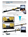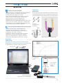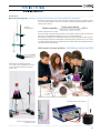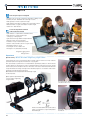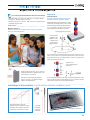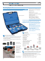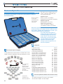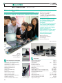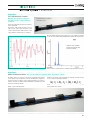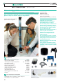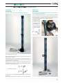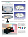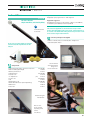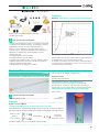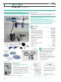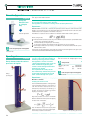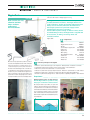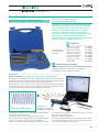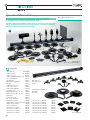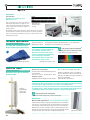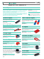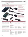
Download Catalogo Fisica Altay 1-40_r02.qxp

Physics Catalogue
Crafted for your world.
Crafted for your world.
ABOUT ALTAY
Since 1938, Altay Scientific has been a leading
company in the global market for science
and medical education equipment sold
through an extensive network of authorized
dealer and partners. Today, Altay operates
in five continents, employing more than 300
people.
Altay produces high quality and affordable
physics
and
chemistry
equipment,
anatomical models, medical simulators and
microscope slides.
NEW Altay’s Production Plant in Suzhou - China
OUR MISSION
The search for knowledge is a need that comes from human nature. To satisfy this need is
to overcome the social, economic and intellectual differences that can only divide us.
Our mission is to develop and market innovative, user-friendly and affordable products,
or “Instruments of Knowledge”, to allow and facilitate this search for knowledge.
Altay’s Manufacturing Facility and Warehouse
in San Cesareo - Italy
Altay will continue to support technology development, improving goods and services,
maximizing a humanistic vision of society and progress. In pursuing our corporate goals,
we will adhere to the most rigorous professional ethics regarding every aspect of our
business.
We will be part of and reinvest in all the communities where we do business.
OUR VISION
Altay Scientific is a leading company in the global market for science education sold
through a worldwide network of authorized dealer partners. Altay produces a full line of
innovative and user-friendly products based upon the highest technology research and
development married to high quality, low cost manufacturing techniques and processes.
The Altay brand stands for innovation, value and customer orientation.
The global Altay organization remains committed to investing the necessary human and
financial capital in the Altay Vision.
OUR R&D PHYSICS DEPT.
R&D Physics Dept.
from left to right: Francesco Cardarelli,
F.Zambolin, M.Pontesilli, M.Corio, Fabrizio
Cardarelli, L.Cozzi, F.Cordella
Thanks to our highly qualified scientists who work in our R&D Physics Dept., Altay has
become a leader in developing and crafting physics equipment specifically designed to
be safe, durable and easy to use.
Our dedicated, creative team of experts strives to develop a range of new products that
facilitate teaching and motivate learners by bringing science to life!
Dear Customer,
After many years teaching Physics, I truly believe that
effective learning comes from direct experiences.
With this in mind, Altay’s R&D Physics Dept. is engaged
in designing and developing a full range of products
that will both motivate students and help teachers
to convey theory in a stimulating and exciting way.
“If I hear, I forget. If I see, I remember.
If I do, I understand.”
(Confucius)
With Altay products, learning becomes an active
process- innovative and student friendly Physics
systems that allow in-depth exploration of mechanics,
optics, thermodynamics, electromagnetism…
In other words, crafted just for you!
CONTENTS
A Glance at Altay New Products. . . . . . . . . . . . . . . . . . . . . 2
Physics Systems . . . . . . . . . . . . . . . . . . . . . . . . . . . . . . . . . . . . 5
Single Items. . . . . . . . . . . . . . . . . . . . . . . . . . . . . . . . . . . . . . . 41
Best regards,
Datalogger & Sensors . . . . . . . . . . . . . . . . . . . . . . . . . . . . 115
General Accessories . . . . . . . . . . . . . . . . . . . . . . . . . . . . . . 131
Index . . . . . . . . . . . . . . . . . . . . . . . . . . . . . . . . . . . . . . . . . . . . 141
Fabrizio Cardarelli
Head
of Altay’s Physics
R&D Dept.
A GLANCE AT ALTAY NEW PRODUCTS
Magnetic Board
Mechanics Accessories Set
Optics Accessories Set
4114.30
4114.35
4114.37
Sturdy and versatile, Altay’s easy to set-up
Magnetic Board helps teachers to convey
Physics principles in a stimulating and
exciting way.
It is the idea visual aid that will enhance
teachers’ demonstrations while helping
students to clearly observe, understand
and assimilate scientific concepts with ease.
It is designed to be free
standing or wall mounted.
NEW
Force Table
4114.11
Our high quality New Force
Table is the ideal teaching aid
for an in depth study of vectors.
Thanks to its easy set-up and
innovative structure, the Altay
New Force Table guarantees
accurate results and is
compatible with a Dual Range
Force sensor.
Along with our new Mechanics Accessories Set (4114.35)
and Optics Accessories Set (4114.37), our Magnetic Board
is a must for your Physics lessons.
Full details on page 58
Rotating Coil
NEW
4640.60
Demonstrating and investigating principles of generating
electricity from a magnetic field, including the Earth’s magnetic
field, is easy thanks to Altay’s New Rotating Coil!
Sturdy structure, compatible with sensors and ready to use!
NEW
Full details on page 56
Inclined Plane
4115.10
This most famous simple machine, revisited
by Altay, includes some engaging
features such as: easy set-up,
NEW
clearly visible scales and
sensor attachments.
Sturdy and reliable,
the Altay New Inclined
Full details
Plane can be used for
on page 61
demonstration purposes or by
students, providing extensive handson experimentation in the study of
simple machines.
Full details
on page 104
Gimbals Magnetic Field Sensor 4640.70
An easy and intuitive way to explore magnetic
fields and study magnetism!
Full details on page 103
NEW
2
Barlow’s Wheel
4645.02
Investigate the
interaction of currents
and a magnetic field
without using mercury!
Variable Inductance
4731.00
The Altay New Variable Inductance apparatus is designed
to demonstrate the generation of magnetic fields and the
basic principles of inductance.
Full details on page 106
Full details
on page 105
NEW
NEW
Altay Docking Station
2236.65
This easy to use, upgradeable Docking Station is a low-cost
data acquisition system that is compatible with an increasing
range of sensors.
V, I, P and Phase Shift Meter 2276.10
The Altay V,I,P and Phase Shift Meter is a very useful
instrument for conducting all types of electrical measurements.
Full details
on page 129
Easy and practical, it includes a built-in connection to the Altay
New Digital Large Display (2236.60).
NEW
Full details
on page 129
Buoyancy Balance
4184.93
NEW
NEW
Full details
on page 77
Millikan Apparatus
4836.60
Originally designed by Robert Millikan (1909), the Altay New
Millikan Apparatus recalls the classic experiment to measure
the electric charge of the electron- it’s an ideal instrument to
begin to explore the basic principles of Modern Physics!
The Altay New Buoyancy Balance is an effective instrument
to experience buoyancy of air- when the Balance is located
inside a vacuum jar and the air is evacuated, you clearly
demonstrate the lack of pressure, as the balance inclines.
Digital Large Display
Full details on page 114
NEW
2236.60
Easily show the results of
classroom experiments in any
unit of measurement with the
New Digital Large Display.
NEW
Full details
on page 129
3
PHYSICS
SYSTEMS
With Altay Physics Systems, teachers have everything
they need to easily demonstrate all the main scientific
principles within Optics, Electricity, Electrostatics,
Mechanics, Magnetism and Thermodynamics.
Our flexible, time-saving and easy to set-up systems
cover a wide range of experiments interfacing with
dataloggers, loggers and sensors.
They are supplied in a sturdy portable case guaranteeing
durability, safety and simple storage.
User-friendly instruction manuals provide the guidance
necessary to assure a successful learning experiencescience principles become simple and clear to
understand while enhancing students’ curiosity and
learning.
Altay’s full line of Physics Systems offer you quality,
precision and economy in one package – designed
by teachers, for teachers.
•
Mechanics . . . . . . . . . . . . . . . . . . . . . . . . . . . . . . . . . . . . . . . . . 6
•
Thermodynamics . . . . . . . . . . . . . . . . . . . . . . . . . . . . . . . . . 15
•
Optics . . . . . . . . . . . . . . . . . . . . . . . . . . . . . . . . . . . . . . . . . . . . 18
•
Electrostatics. . . . . . . . . . . . . . . . . . . . . . . . . . . . . . . . . . . . . . 26
•
Magnetism & Electromagnetism . . . . . . . . . . . . . . . . . . . 28
•
Electricity & Electronics. . . . . . . . . . . . . . . . . . . . . . . . . . . . 32
Mechanics System 1
Specifications
4861.10
An introductory system to study basic mechanics
Size: 83 x 28 x 12 cm – Weight: approx. 6 kg
Packing: external suitcase in hard ABS,
internal foam for prevention accidental
breakage.
Equipment suggested
Electronic Balance (code 2219.30)
Dual Range Force Sensor (code 2311.10)
Motion Detector (code 2310.10)
or Go!Motion (code 2320.10)
LabPro (code 2300.10)
or LabQuest (code 2300.30)
or Go!Link (code 2320.30)
Mechanics System 1.
Our high quality Mechanics System 1
comes in a heavy duty ABS plastic
carry-case for ease of storage.
Simple to set-up with all components easily accessible.
The system consists of: balance, inclined plane, friction block,
weights, simple machines, pulleys, levers, springs and scales.
A variety of experiments can be carried out using this kit.
Components
• Sectional universal base with 3 knob
(2x)
5405.71
• Pulley with hook
(2x)
4112.10
• Plastic Pulley, with metal rod
4112.05
• Scale pan hooked, with metal suspension
(2x)
4113.27
• Friction block
4114.71
• Tubular Spring Balance (Metal) 3N
4110.03
• Tubular Spring Balance (Metal) 6N
4110.05
• Tubular Spring Balance (Metal) 10N
4110.07
• Lever, Holed Rod, with pair of threaded cylinders
4114.13
• Double Side Scale, silk screen printed
2208.20
• Inclined plane, with 3 different track terminals
5491.11
• Multifunction Support Rod, rounded ends,
with holes, length 35 cm
5408.91
• Support Rod, rounded ends, length 35 cm
(2x) 5408.81.L350
• Support Rod, rounded ends, length 50 cm
(3x) 5408.81.L500
• Spring leaf, length 30 cm, width 1 cm
4110.91
• Spring leaf, length 30 cm, width 2 cm
4110.92
• Extension Clamp with Rod, diameter 1 cm
5416.20
• Cart for Inclined Plane
4114.82
• Differential pulley (30, 60, and 90 mm diameters)
4112.40
• Differential pulley with two handles
(40, 80, and 120 mm diameters)
4112.42
• Goniometric Circle
2216.10
• Tape Measure, 2 m
2211.10
• Vernier caliper, scale 0÷160 mm, accuracy 0.05 mm
2213.10
• Cylindrical mass 10 g
(5x)
4111.08
• Cylindrical mass 25 g
(8x)
4111.10
• Cylindrical mass 50 g
(4x)
4111.12
• Mass 100 g
2221.32
• Mass 50 g
(2x)
2221.30
• Mass 20 g
(2x)
2221.28
• Mass 10 g
2221.26
• Mass 5 g
2221.24
• Mass 2 g
(2x)
2221.22
• Mass 1 g
2221.20
• Flat mass 500 mg
2221.18
6
Accessory box with part of its contents.
• Flat mass 300 mg
2221.16
• Steel spring with pointer
(2x)
4110.81
• Hook for Cart
4114.80-011
• Rod with clip
(2x)
4113.50
• Rod diam. 10 mm, length 127 mm, with hook
(2x)
4113.53
• Red pointer with clip
4113.54
• Suspension ring
5401.60
DGAKNB.M4X10
• Knob (Inox, Blue M4 x 10 mm)
• Axel with fixing screw for differential pulley
(2x)
4112.45
• Metal bosshead 20 x 20 x 40 mm, with knobs
(2x)
5401.20
• Bosshead
(3x)
5401.22
• Polyester inelastic cord, diam. 0.8 mm, length 10 m
4113.20
• Mass hanger, 10 g
4111.56
• Slotted mass, 10 g
(5x)
4111.51
• Metal ring dia. 20 mm
4861.10-024
• Brass hook diam. 3 mm, length 50 mm
(2x) 4861.10-026
• Brass hook diam. 3 mm, length 40 mm
(7x) 4861.10-027
• “S” Hook
(2x)
4113.35
• Balance hook
(2x) 4861.10-029
• Rubber band
(2x) 4861.10-030
• Rod diam. 3 mm, length 72.5 mm with cylinder
4861.10-020
4861.10-021
• Rod diam. 8 mm, length 70 mm with threaded stem M3
Laws and principles investigated
Inclined plane with cart, pulleys, friction block and scale pans.
• Balance oscillation measurements • Balance sensitivity
• Belt wheel drive • Composition and decomposition of forces
• Concurrent forces • Decomposition of a force into its components
• Determination of the acceleration due to gravity by means of the
simple pendulum
• Elongation of a leaf spring • Elongation of a spring
• First-class levers • Fixed pulley • Hooke’s Law • Inclined plane
• Investigation of an oscillation of a simple pendulum
• Measurement of length • Mobile and fixed pulley
• Momentum of a force • Parallelogram of forces
• Second and third-class levers • Static and dynamic friction
• Spring pendulum • Springs in series and parallel
• Static measurement of a force • The concept of kinetic energy
• The concept of potential energy
• Transmission of a force along a cable • Weight as a force
Many of these experiments will also be suitable for applied mathematics.
Full set of basic
measuring instruments.
List of the experiments detailed in the instruction manual
• Belt drive systems
• Composition, decomposition and transmission of forces including the
parallelogram law
• Analytical balance and the investigation of weight as a force
• Levers: including first, second and third class type
• Pulley systems: including fixed, mobile and differential pulleies
• Simple pendulum and spring pendulum
• Hooke’s Law with spring and with spring leaf
• Inclined plane and friction • Kinetic and potential energy
• The concept of experimental error • Springs in series and in parallel
General hardware
for experiments.
Experiment
Analytic Balance • In-depth investigation of the analytical balance
The balance is an instrument that allows, in a
gravitational field, to measure the unknown
masses by comparison with sample masses.
One sample experiment is the determination of
the sensitivity of a balance which has arms of
equal length.
The more sensitive a balance is, the smaller
the variation in a mass (m) the balance can
detect and measure.
If the test mass (m) is lesser in magnitude than
the sensitivity of the balance, it will not be
detected.
With reference to the diagram, if load a test
mass (M) on each pan of the balance and
assuming that the distance between each of
the pans is equidistant and represented by “a”,
we can vary weight on one of the pans which
will result in a displacement through an angle
defined by α.
Formula defining
balance sensitivity.
Schematic of analytical balance.
Therefore, we can see that the sensitivity of a
balance depends on several design characteristics
as well as the patience of the experimenter.
For example, the more stable the design of a
balance, the more mass is needed to move the
balance noticeably.
Additionally, the more friction at the locations
where movement is required, the less sensitive
the balance will be.
Assembled analytical balance.
7
Experiment
The Spring Pendulum
Calculate the elastic constant of a spring by means of a spring pendulum
When the forces acting on the oscillating spring
are examined it is possible to find a useful
relationship between the spring elastic constant,
the loaded mass and the oscillation period.
Further examples of classical experiments
Two more examples on the experimental
possibilities offered by this system
Example of
spring pendulum
forces.
Starting from Newton’s Second Law and neglecting
the mass of the spring, it is easy to deduce the
following relation:
Parallelogram of forces.
Mechanics System 1 assembled in the spring
pendulum configuration.
Formula defining the oscillation period of the
spring pendulum loaded with a mass (m) and
with an unknown elastic constant (k).
Students experience the spring
pendulum, acquiring data
with the datalogger.
Mobile and fixed pulley.
Using a motion detector it is easy to acquire position data.
This way, it is possible to calculate the oscillation period of the pendulum
with the Fast Fourier Transform, a feature of the software.
The histogram represents all the frequency range, the highest bar refers
to the main oscillation frequency of the system.
Frequency analysis of the spring pendulum motion.
8
Mechanics System 2
Specifications
4861.20
An advanced low friction dynamics system to study elastic and inelastic
collisions between carts
Size: 124 x 28 x 12 cm – Weight: approx. 7 kg
Packing: external suitcase in hard ABS,
internal foam to prevent accidental shock
Equipment suggested
Electronic Balance (code 2219.30)
Motion Detector (code 2310.10)
or Go!Motion (code 2320.10)
LabPro (code 2300.10) or LabQuest
(code 2300.30) or Go!Link (code 2320.30)
Mechanics System 2.
The Mechanics System 2 allows us to
verify many kinematics and dynamics
principles by using a low friction system.
The basic theory involves topics such as Newton’s Laws
of Motion, Conservation of Energy and Momentum, Friction
and many others.
Components
• Aluminium Track
• Electronic Timer
• Power Supply 12V
• Cart
• Reflection Photogate
• Release Electromagnet
• Brake/Bumper for Cart
• Fixed Support for Track
• Adjustable Support for Track
• Pulley with metal rod
• Aluminium Flag for Cart
• Bubble Level
• Neodymium-Iron-Boron Button Magnet
• Polyester inelastic cord, length 10 m
• Knob (Inox, Blue) M4x10
• Knob (Inox, Blue) M5x14
• Knob (Inox, Blue) M5x20
• Knob (Inox, Blue) M5x35
• Massholder for Cart
• Slotted Masses Set
• Plumb Line on Scale
• Spring Bumper
• Spring Bumper for Electromagnet
• Trigger for Cart
• Pair of Velcro Bumpers
• Hook for Cart
(2x)
(2x)
(2x)
(2x)
(2x)
(3x)
(2x)
(2x)
(2x)
4114.81
2232.50
2402.54
4114.83
2232.54
4114.88
4114.87
4114.84
4114.85
4112.05
4114.80-004
4180.70
4611.86
4113.20
DGAKNB.M4X10
DGAKNB.M5X14
DGAKNB.M5X20
DGAKNB.M5X35
4114.80-003
4111.74
4114.86
4114.80-006
4114.80-007
4114.80-008
4114.80-010
4114.80-011
Electronic timer
with electromagnet
and photogates.
Contents of accessories boxes.
Laws and principles investigated
• Conservation of momentum and energy • Acceleration and velocity
• Eddy currents • Elastic and inelastic collisions • Friction • Law of Inertia
• Kinetic and potential energy • Newton’s 1st Law • Newton’s 2nd Law
• Rectilinear uniform motion • Rolling friction
• Uniform accelerated rectilinear motion
List of the experiments detailed in the instruction manual
• Concept of inertia • Conservation of momentum and energy
• Determination of velocity and acceleration • Laws of dynamic
• Elastic and inelastic collisions • Energy conservation
• Inclined plane • Kinetic and potential energy
• Laws of motion (accelerated, linear uniform) • Rolling friction
• Eddy currents in an aluminium track
Aluminium track with carts.
9
Uniform accelerated rectilinear motion
Experiment
A cart of mass (M) on a horizontal plane is connected, via a string, over a
pulley to an object of mass m.
Mass M + m, is accelerated due to gravity and defined by W = mg.
The value for g is determined using photogates and an Altay timer system.
Rolling friction
Quantitative measurement of the rolling friction acting on the
cart’s wheels
When you incline the plane at a set angle and then release the compressed
spring the cart gets an initial velocity.
During the upward motion of the cart, gravity and friction act in the same
direction. When the cart reaches the highest point on the inclined plane,
it starts to return down the track again. In this instance, gravity and friction
act in opposite directions.
A teacher explains how to quantitatively measure
the rolling friction.
Setup example for study the uniform accelerated rectilinear motion.
Inclined plane angle measurement.
Detail of the elastic
collision between
cart and bumper.
Velocity vs. time graph
of the same system.
Position vs. time graph of a cart bouncing with
a spring on an inclined plane.
The difference in slope is due to the change of the rolling friction forces
and gravity acceleration from concordant to discordant forces when
crossing the x-axis.
10
Experiment
Impulse – momentum theorem • Experimental verification of the theorem
Using the Altay Mechanics System 2 we can induce a collision between two carts.
The carts experience a force for a given amount of time, resulting in its mass undergoing a
change in velocity. Another way of expressing this is to say that this results in
a change of momentum.
An example of how to assemble the experiment.
There are four physical quantities which can be investigated: force, time, mass and velocity
change. The force multiplied by the time is known as the impulse and the mass multiplied by
the velocity change is known as the change in momentum.
The impulse experienced by the cart is always equal to the change in its momentum.
This can be approximated as follows:
Impulse – momentum theorem.
Further examples of workable experiments
The area enclosed by the curve
represents the rate of change of
momentum.
Experimental data acquired with a datalogger.
Inelastic collision between two carts.
Setup for study different
types of collisions.
Different graphs, with and without
magnet acting as a friction force.
Elastic collision between two carts.
Magnet
An example of a basic dynamic set-up.
11
Mechanics System 3
Specifications
4861.30
A basic introductory mechanics system for mechanics of fluids
Mechanics System 3 introduces the
basic concepts of fluid dynamics.
The system provides a useful
framework to understand and study
quantitatively many fluid dynamics
experiments.
Mechanics System 3 case 1, hardware case.
Mechanics System 3 case 2, glassware case.
Case 1
Size: 73 x 50 x 16 cm – Weight: approx. 8 kg
Packing: external suitcase in hard ABS, internal
foam for prevention of accidental breakage
Case 2
Size: 124 x 28 x 12 cm – Weight: approx. 4 kg
Equipment suggested
Gas Pressure Sensor (code 2311.40)
Dual Range Force Sensor (code 2311.10)
LabPro (code 2300.10) or LabQuest
(code 2300.30) or Go!Link (code 2320.30)
Vernier Caliper (code 2213.10)
Tape Measure (code 2211.10)
Mercury (code 4207.55)
Hardware
case content.
Components
• Universal base
• Support Rod, rounded ends, length 35 cm
• Support Rod, rounded ends, length 50 cm
• Bosshead
• Swivel bosshead
• Extension Clamp with Rod
• G Clamp
• U-Tube manometer
• Air Blower
• Voltage Regulator for Air Blower
• Pascal Apparatus Ball
• Potassium Permanganate (5 g)
• Silicone Grease
• Styrofoam Ball
• Ping Pong Ball
• Silicone Tubing
• PVC transparent tube
• Viscosity Tube, Ostwald
• Plastic Funnel
• Mariotte’s Bottle
• Tube for Mariotte’s Bottle
• Cartesian Diver
• Centrifuge Tube
• Rubber Stopper, 1 hole
• Rubber Stopper, solid
• Rubber Stopper, 1 hole
• Communicating Vessels
• Capillary Tubes
12
(2x)
5405.71
(2x) 5408.81.L350
(2x) 5408.81.L500
(4x)
5401.23
(2x)
5401.43
(2x)
5416.20
5402.22
2242.10
4132.50
4132.52
4180.13
4207.56
5424.50
4625.05
4625.06
5449.25.L2000
5449.41.L250
1485.00
1640.64
1476.51
1465.05.L330
4181.16
1480.00
5450.43
5450.12
5450.35
4180.60
4182.20
Force pump, capillary tubes, communicating vessels, Venturi’s tube
and Ostwald viscometer.
Mariotte’s bottle, cartesian diver, Hare’s apparatus.
• Drying Tube, U shaped
• Force Pump
• Plastic beaker, 250 ml
• Hare’s apparatus
• Perspex tube
• Venturi’s tube
• Syringe 5 ml
• Syringe 20 ml
• Base for Capillary Tube and Communicating Vessels
1274.00
4183.20
(2x) 1610.20
4181.57
DPX001
4183.51
4180.16
4180.17
5405.30
Laws and principles investigated
Experiment
Relative density
• Adhesion and cohesion • Archimedes’ principle • Bernoulli’s theorem
• Boyle’s Law • Buoyant force • Capillarity • Cartesian diver
• Communicating vessels • Density of a solid body
• Density of two immiscible liquids • Drag coefficient • Force pump
• Hagen-Poiseuille Law • Hare’s apparatus • Hydraulic brake
• Hydrostatic pressure • Jurin’s Law • Mariotte’s bottle
• Ostwald viscometer • Pascal’s Law • Perfect gas Law
• Relative density of two non-mixable fluids • Reynold’s number • Siphon
• Stevino’s Law • Stoke’s formula • Surface tension • Terminal velocity
• The Archimedes’ principle • The Gamow, Oppenheimer, Bloch puzzle
• Torricelli’s theorem • U-tube manometer • Venturi tube
The pressure exerted within a liquid depends only from the free surface
and from the liquid density. Using two non-mixable fluids inside the U-tube
(e.g. water and oil) it is possible to verify the equation for the relative density.
Schema for
the relative density
determination.
List of the experiments detailed in the instruction manual
• Principles of the manometer • Communicating vessels
• Hydrostatic pressure and Pascal’s Law • Stevino’s Law
• Archimedes’ Law • Bernoulli’s equation • Torricelli’s theorem
• Determination of the volume of a solid body
• Determination of density and of specific weight of a solid body
• Determination of density of immiscible liquids • Capillarity
• Boyle’s Law • Pumps and siphons • Adhesion and cohesion
• Cartesian diver • Measurement of surface tension • Viscosity
Relative density of two non-mixable fluids.
Experiment
Perfect gas law
Application of the perfect gas law to an air filled syringe
By measuring the force needed to pull the piston at a certain distance with
an air-filled syringe, it’s possible to verify the perfect gas law.
Perfect gas law.
Pressure force graph
vs. syringe piston
position.
Force schematic
of the perfect
gas law
experiment.
Experiment setup using
gas pressure sensor and datalogger.
13
Experiment
Hare’s apparatus • Find the relative density of a liquid
Hare’s apparatus consists of an inverted U-Tube
immersed in two vessels of fluid.
One vessel is filled with water and the other with
a fluid of unknown density.
By pinching the tube at any point higher than
the Y Piece, you will notice both liquids rise to
a certain height in each tube.
Therefore, when air is removed from the top of
the apparatus, the liquids rise in the tubes to
heights which are inversely proportional to their
densities.
Therefore, Hare’s apparatus is used to compare
the density of two liquids.
Formula of the relative density of a liquid with
respect to another.
Students acquiring data
from Hare’s apparatus.
Other apparatus and setups for this system • Examples of various experiments on the mechanics of fluids
Force pump.
14
Venturi’s tube.
Capillary tube apparatus.
Bernoulli Blower.
Communicating vessels apparatus.
Heat System
Specifications
4862.10
Study thermology with this compact and easy to use system
Size: 73 x 50 x 16 cm – Weight: approx. 6 kg
Packing: durable ABS plastic carry case with
foam inserts
Equipment needed
Methane/Butane Cylinder
Power Supply 10 A (code 2407.60)
Equipment suggested
Heat System in case.
Stainless Steel Temperature Probe (code
2314.20) or Thermocouple (code 2314.10)
Go!Temp (code 2320.20)
Gas Pressure Sensor (code 2311.40)
LabPro (code 2300.10) or LabQuest
(code 2300.30) or Go!Link (code 2320.30)
This system introduces basic concepts
of thermodynamics and heat
experiments. It provides a framework
for understanding and quantitatively
assessing introductory thermodynamics questions and problems.
Hardware
components for
experiments.
Components
• Universal base
(2x)
5405.71
• Support Rod, length 35 cm
(2x) 5408.81.L350
• Support Rod, length 50 cm
(2x) 5408.81.L500
• Bosshead
(4x)
5401.23
• Swivel bosshead
(2x)
5401.43
• Digital multimeter
2275.10
• Thermocouple type T
4672.00
• Beaker, low form 500 ml
1118.50
• Beaker, low form 250 ml
1118.35
• Beaker, low form 100 ml
1118.20
• Cylinder graduated 100 x 1 ml
1226.15
• Centrifuge Tube 100 ml
1481.05
• Filtering Flask 500 ml
1331.05
• Silicone Tubing
5449.25.L2000
• Drying Tube
1274.00
• Extension clamp with rod
(2x)
5416.20
• Mercury thermometer, range: -10°C/+110°C x 1°C (2x)
2240.15
• Calorimeter
4230.71
• Joule’s law unit
4230.66
• Stackable Plug Lead, 50 cm, red colour, plug 4 mm
2522.03
2522.08
• Stackable Plug Lead, 50 cm, black colour, plug 4 mm
• Silicone grease
5424.50
• Rubber stopper with one hole (37 x 28 x 5 mm)
5450.42
• Rubber stopper, solid
5450.23
• Rubber stopper with one hole (23 x 16 x 4 mm)
5450.38
• Paraffin block
(4x)
5424.52
• Set of two cylinders (stainless steel and aluminium)
4200.95
• Sponge piece
4200.97
• Set U-shaped rod
4200.96
• Specific heat cylinders
4230.96
Centrifuge tube, beakers, filtering flask and graduated cylinder.
Calorimeter
with Joule’s Law
Apparatus.
• Wire gauzes with round ceramic centre
• Bunsen Burner
• Tripod Stand for Bunsen Burner
• Gas Burner Tubing, for butane/propane gas
• Micrometer Dial Gauge, range: 0 ÷ 10 mm
sensitivity: 0.01 mm
• Support for Micrometer Dial Gauge with knob
• Pulse glass
• Potassium Permanganate
• Bimetallic strip with electric contact
(2x)
5534.25
5511.10
5533.10
5449.95
2214.00
2214.01
4210.50
4207.56
4200.80
15
Laws and principles investigated
List of the experiments detailed in the instruction manual
• Thermal radiation • Boiling and condensation
• Calorimeter and Joule’s Law • Dalton’s Law of Partial Pressures
• Equilibrium temperature of mixed liquids
• Evaporation of two different liquids • Expansion of ice
• Thermometer’s time constant and fixed points of a thermometer
• Fourier’s Equation and Fourier’s Law
• Heat sensitivity and Locke’s Law • Linear expansion of a solid
• Wet and dry bulb hygrometer, relative humidity, psychrometry and
moisture content
• Newton’s Law of Heating or Cooling • Phase transition
• Pulse glass functioning principle • Saturated and supersaturated solutions
• Different solution phenomena at different temperatures • Specific Heat
• Thermal agitation, conduction and expansion
• Thermostat and thermocouple • Peltier-Seebeck effect
In holding a pulse
glass in your hand,
you can observe
some surprising
phenomena and
experience the
effects of
Thermal Energy.
• Heat sensitivity and thermal equilibrium
• Measurement of the coefficient of volume expansion of water
• Fixed points of a thermometer
• Temperature measurement with a T type thermocouple
• Linear expansion of a solid • Coefficient of expansions of iron and brass
• Example of the use of a thermostat
• Measurement of the boiling point of alcohol
• Boiling at below and above atmospheric pressure
• Measurement of the heat of evaporation of water
• The graph for the solidification of paraffin
• Saturated and supersaturated solutions • Wet and dry bulb hygrometer
• Expansion of air at constant pressure and volume
• Thermal convection in fluids
• Thermal conductivity of iron, brass, aluminium and copper
• Conduction of heat by water • Absorption of thermal radiation
• Thermal insulation • Construction of a simple Dewar vessel
• Heating different quantities of liquid
• Specific heat capacity of liquids and solid bodies
• Equilibrium temperature of mixed liquids
• Heat capacity of the calorimeter
• Conversion of mechanical energy into thermal energy • Joule’s effect
• Expansion of ice • Latent heat of fusion of ice
• Latent heat of vaporisation of water
• Evaporation of two different liquids • Boiling point elevation
Experiment
Time constant of a thermometer • To study the thermal sensitivity of a mercury thermometer and a thermocouple
An experiment to give a quantitative explanation
of the thermometer’s time constant.
This is important as it gives insight to the heat
sensitivity of the thermometer.
Newton stated that a hot object cools down at a
rate proportional to the difference between its
temperature and that of its surroundings.
An easy demonstration of this would be to place
a mercury thermometer in hot water and observe
the effect on the glass of the thermometer and
the mercury inside it. The graph below can be
described using the following equation:
Newton’s Law of heating and cooling.
Where T(t) is the temperature of the system,
T1 is the temperature of hot water, T0 is the
temperature of the thermometer and τ is the
time constant.
With just a beaker, boiling water and a
thermometer it is possible to measure thermal
sensitivity.
16
Temperature vs. time
diagram of a mercury
thermometer placed
in an environment
with higher
temperature.
Experimental data
showing the heating
for a temperature
sensor immersed
in a beaker with
hot water.
Experiment
Wet and dry bulb hygrometer • The basics concepts of psychrometry can be demonstrated in this experiments
The amount of water vapour in the air at any given time is usually less than that is required to saturate
the air. The relative humidity is the percent of saturation humidity, generally calculated in relation to
saturated vapour density.
Setup for
the experiment.
Relative humidity definition formula.
The psychrometer or Wet & Dry bulb hygrometer is an important instrument used for measuring the
water vapour content (Relative Humidity) per unit of air at a given temperature.
The instrument is made up of two identical thermometers: one being a wet bulb, the other a dry bulb.
The wet bulb thermometer has its bulb wrapped in a tight fitting wicking material such as cotton, which
is soaked in distilled water. When the thermometers are ventilated, the wet bulb temperature will be
lower than the dry bulb temperature.
Further examples of possible experiments • Some experiments using the Heat System
With minimal experimental setup time,
it is possible to show qualitatively how the air
is expanded when heated and contracted
when cooled.
Students involved in the thermocouple experiment.
Calorimeter with Joule’s Law unit.
Detail of the air expansion in the
U-Tube manometer.
17
Optics System 1
Specifications
4864.10
A complete system to study the principal laws of geometric optics
Size: 124 x 28 x 12 cm – Weight: approx. 6 kg
Packing: durable ABS plastic carry case
with foam inserts
Equipment suggested
Light Sensor (code 2315.10)
LabPro (code 2300.10) or LabQuest
(code 2300.30) or Go!Link (code 2320.30)
Optics System 1.
Components
• Stackable Plug Lead
• Lampholder, single
• Lampholder, quadruple
• Slider for holder, with knob
• Slider for projector, with knob
• Holder for 50 mm diam. lenses and mirrors
• Transformer, 12 V 2.5 A
• Prism table
• Projector with 12 V 20 W halogen lamp
• Halogen lamp 12 V 20 W, spare
• White metal screen (140 x 140 mm)
• Set of 4 Biconvex Spherical lenses (dia. 50 mm)
• Set of 4 Biconcave Spherical lenses (diam. 50 mm)
• Set of 4 Concave Spherical mirrors (diam. 50 mm)
• Set of 4 Convex Spherical mirrors (diam. 50 mm)
• Optical bench with supports
• Shadow rod
• Joly photometer on stem
• Bulb lamp, 12 V 2 W
• Set of seven diaphragms
• Holder for slides and diaphragms
• Millimetre graph paper
• Equilateral glass prism (side 25 mm)
(4x)
2522.14
4418.19
4418.20
(6x)
4414.01
4414.17
(4x)
4414.02
2403.14
4418.29
4414.18
4414.19
4418.35
4445.00
4441.00
4431.00
4435.00
4414.00
4864.10-001
4422.01
(6x)
2505.65
4414.12
4414.03
4864.10-002
4450.10
Set of mirrors, lenses
and prism holder.
A complete
set of diaphragms.
Set of lens – mirror
holder.
Laws and principles investigated
• Concave and convex mirror
• Convergent and divergent lens
• Focal length • Gauss approximation
• The eye, hyperopic and myopic eye
• Inverse square law • Joly photometer
• Lens power • Luminous intensity
• Magnifier and magnifying power • Photometry
• Prism • Ray tracing • Refractive index
• Umbra and penumbra • System of lenses
• The microscope • The telescope
• Thin lens equation
18
General hardware of the System.
The Optics System 1 can be used for
the study of many aspects of
geometric optics, including
photometry, luminous intensity, focal
length of a lens and
many other experiments.
List of the experiments detailed
in the instruction manual
Experiment
Inverse square law • A classical experiment on the inverse square law
• Photometry • Luminous intensity
• Shadow and penumbra • Magnifier • Lenses
• Mirrors • Thin lens equation • Focal length
• System of lenses • Prism • The eye
• Microscope • Telescope
Experimental data collected with a datalogger.
J oly photometer
Setup for the Joly photometer experiment.
Simple explanation of
inverse square law:
According to the photometric law of distance,
the irradiance (E) of a point light source decreases
in inverse proportion to the square of distance
(r) for constant radiant intensity (I).
Experiment
Focal length of a diverging lens • How to find the exact focal length of a diverging lens
Assembly for the determination
of the focal length of a
diverging lens.
If the converging lens has a focal length such
that the system of the converging plus diverging
lenses is still converging, it is possible to recover
the focal length of the system by using the thin
lens equation (valid in the “Gauss approximation”).
Thin lens equation: u is the object distance, v is
the image distance and f is the focal length.
Schematic view of symbols and sign.
19
Experiment
Refraction index of a glass prism • By measuring the minimum deviation angle it is possible to get the refraction index of a prism
Optical bench assembly
for the determination
of the refraction index of a prism.
Further examples of classical experiments
A quick look at the experimental possibilities offered by this system
Joly photometer.
Geometrical representation of Snell’s Law.
The above diagram is a simple representation of Snell’s Law, which is
represented by the following formula.
Snell’s Law.
Where n is also known as a refraction index of a given material.
20
Umbra and penumbra.
Optics System 2
Specifications
4864.21
An intermediate system for geometrical and physical optics
Size: 83 x 28 x 12 cm – Weight: approx. 5.5 kg
Packing: durable ABS plastic carry case
with foam inserts
Equipment needed
Optics System 2.
Dextrose
Equipment suggested
Light Sensor (code 2315.10)
LabPro (code 2300.10) or LabQuest
(code 2300.30) or Go!Link (code 2320.30)
The Optics System 2 is designed to
study composition of light, light
polarization, refraction index as well as
many additional aspects of light
reflection and refraction.
Components
• Hartl Disk
• Optical Bench
• Universal Base with knob
• Thread adapter for Universal Base
• Slider for Holder with knob
• Slider for Projector with knob
• Biconvex Lens for Hartl Disk (f = +85 mm)
• Biconvex Lens for Hartl Disk (f = +135 mm)
• Biconcave Lens for Hartl Disk (f= -135 mm)
• Trapezoidal Prism for Hartl Disk
• Triangular Prism for Hartl Disk (90°, 45°, 45°)
• Deformable Mirror for Hartl Disk
• Plane Mirror for Hartl Disk
• Refraction Index Vessel for Hartl Disk, (60 mm dia.)
• Polarization Tank, with two Rubber Stopper
• Support for Polarization Tank
• Pair of polarizing filter
• Photometer
• Transformer, 12 V 2.5 A
• Ray optics and colour mixing box with lamp,
coloured filters, slits, mirrors
• Base support for ray optics box
• White metal screen
4419.01
4413.92
(2x) 5405.73
(2x) DBR007
(4x) 4414.01
4414.17
4419.06
4419.07
4419.08
4419.09
4419.10
4419.11
4419.12
4419.13
4454.11
4454.15
4453.90
4486.20
2403.14
The system contains a Hartl apparatus, which allows the
student to perform many experiments related to the
reflection of light on mirrors and to the refraction through
transparent bodies.
Also included is our specially designed Altay Optics Box,
designed to investigate polarisation in various solutions.
Additionally you can study photoresistance, photometry and
verification of Malus’ Law.
Ray box with coloured filters, slits, two
side parts with mirror and transformer.
4402.30
4402.35
4418.35
Lens set with flexible mirror and Hartl disk.
Pair of polarising
filters, photometer,
screen and plexiglas
cylinder with support.
Optical bench with
accessories.
21
Laws and principles investigated
• Principles of bi-concave, bi-convex lenses and mirrors • Mixing colours
• Fermat’s principle • Determine the focal length of a lens
• Hartl apparatus • Inverse square law of light
• Light reflection and refraction • Malus’ Law • Photometry • Prism
• Refraction index of a glass and a liquid • Rotation of light
• Snell’s Law • Total reflection
List of the experiments detailed
in the instruction manual
• Light reflection of a plane mirror and flexible mirror
• Light refraction in a prism and through a
converging or a diverging lens
• Light refraction through different shaped materials
• Refraction index of a liquid and glass
• Polarisation of light • Total refraction prism
• Rotation of the polarisation plane in a sugar solution
• Investigating mixing of colours
• Focal length of a lens • Malus’ Law
• Investigations in quantitative photometry
Using data logging system
with light sensor.
Experiment
Optical activity • Observe the rotation of light using a sugar solution
Some substances such as sugar will react when a beam of light is incident on it. They rotate the
polarisation plane of the light around its direction of propagation.
This optical activity is a phenomenon connected with the “asymmetry by reflection” of the molecules
of many substances. The degree of rotation is determined by the rotational power of the optically
active solution present and by the amount of molecules of the solution that interact with the beam
of light. The directional change of the light is also affected by degree of concentration of the solution
and distance the light must travel through it.
Other features such as temperature and wavelength of light
are also important.
Optics System 2 experimental setup
to show rotation of light using
a sugar solution.
For a given angle, all the polarised light is
collected on the screen.
The above formula defines the specific rotatory
power of a substance at a given temperature
and wavelength.
22
The angle is adjusted until all light is
blocked out.
Experiment
Malus’ Law • Explanation and verification of Malus’ Law
If we consider the polarised light coming from the first polariser, we can analyze
how much of this light is transmitted through the second polariser.
Let (A) be the amplitude of plane polarised light incident on the second polariser.
The light is incident at angle to direction of the first polariser.
The component of A (A cosθ) is transmitted and whilst A sinθ is not transmitted.
Photometer assembly
for the Malus’ Law
experiment.
The resistance value is dependent on the
angle between the polarisers.
The intensity is proportional to the square of amplitude, so that the intensity
transmitted is IT = I cos2θ: where (I) is the intensity of light incident on
polariser. This is called “Malus’ Law”.
An example
of experimental data
collected using a digital
multimeter.
Experimental data collected using a light sensor and a datalogger.
Experiment
Further examples of experiments
A quick look at further experiments of the Optics System 2
A biconvex lens placed
on the Hartl disk.
Composition of colours.
Using a flexible mirror.
23
Optics System 3
Specifications
4864.30
An advanced optics system with diode laser
Optics System 3
in its own box.
Size: 30 x 23 x 7 cm – Weight: approx. 1 kg
Packing: comes with a durable ABS plastic
carry case with foam inserts
Equipment needed
Vernier Caliper (code 2213.10)
Tape Measure (code 2211.10)
The Optics System 3 includes everything needed for a
complete course in advanced optics.
Our system will take students through reflection, lens
theory, diffraction, interference, diffraction grating and
multiple slit diffraction.
You can also study many aspects of modern optical
technology. The equipment is easy to use and durable,
and the experiments are substantive, yet conceptually
easy to conduct.
Areas of study including geometric
principles of optics, polarisation of
laser beams, investigating basic and
study advanced diffraction
principles.
The results will be accurate and
repeatable every time!
Components
Grating
on plastic
holder.
Multiple diffraction
grating mounted
on holder.
Laws and principles investigated
• Laser on stem (630 – 670 nm)
• Rechargeable accumulators
(2x)
• Plug-in power supply
• Cylindrical lens
• Polaroid filter
• Holder for slides and diaphragms
• Plastic base
(2x)
• Slide with 1 slit (width 0.06 mm, separation 0.20 mm)
• Slide with 2 slit (width 0.06 mm, separation 0.20 mm)
• Slide with 3 slit (width 0.06 mm, separation 0.20 mm)
• Slide with 4 slit (width 0.06 mm, separation 0.20 mm)
• Slide with 5 slit (width 0.06 mm, separation 0.20 mm)
• Slide with 6 slit (width 0.06 mm, separation 0.20 mm)
• Coarse grating 1 (4 lines per mm, line/space ratio 3:1)
• Coarse grating 2 (4 lines per mm, line/space ratio 6:1)
• Coarse grating 3 (8 lines per mm, line/space ratio 3:1)
• Metal gauze 300 mesh for bidimensional diffraction grating
• Diffraction grating with three different rulings
(100, 300 and 600 lines per mm)
4478.01
2402.30
2402.52
4478.03
4478.05
4414.03
4417.17
4485.29
4485.30
4485.31
4485.32
4485.33
4485.34
4485.25
4485.26
4485.27
4485.23
4455.20
• Diffraction • Diffraction grating • Interference • Multiple slit diffraction
• Optical activity • Single slit diffraction
List of the experiments detailed in the instruction manual
• Introduction to Ray Optics • The Law of Refraction
• The Diffraction Grating • Single-slit Diffraction • General Diffraction
• Using Diffraction gratings
• The effects of Double slit on diffraction (Two-slit Interference)
• Investigating Optical activity • Overview of interference and diffraction
• Single slit diffraction • Polarization • Introduction to Optical Instruments
24
Solid state laser
with cylindrical
lens and
polariser.
Experiment
Fraunhofer diffraction • Using a Diffraction grating to create a diffraction pattern
Diffraction of light occurs when a light wave passes by a corner or through
an opening or slit that is physically the approximate size of, or even
smaller than that light’s wavelength.
Diffraction describes a specialized case of light scattering in which an
object with regularly repeating features (such as a diffraction grating)
produces an orderly diffraction of light in a diffraction pattern.
These phenomena can be described through the Huygens-Fresnel’s
Principle. Huygens postulated that as a wave propagates through a
medium, each point on the advancing wavefront acts as a new point
source of the wave.
For instance, the points inside a slit become sources of virtual elementary
spherical waves. The observed real wave is the result of the interference
of the elementary waves.
This suggests that diffraction and interference
are phenomena that can be referred to only in
a theoretical interpretation.
Assembly example
for the diffraction
grating experiment.
Diagram shows
constructive and
destructive
interference of the
light coming from the
diffraction grating.
By using a motion detector and a light sensor
you can show a graph of the light intensity
vs. the light sensor position (i.e., distance).
This is possible by moving the light sensor
around the positions of maximum intensity
while sampling its position with the motion
detector.
For a distance x = 173 cm and a diffraction
grating with a pitch (p) of 0.13 mm we get the
following result.
Experimental data
of luminous intensity
vs. position for a
diffraction grating.
Constructive interference.
Where (p) is the pitch of the diffraction grating.
Further examples of possible experiments • Additional experiments with Optics System 3
The effect of
using a diffraction
grating.
Coarse grating interference.
Bi-dimensional
diffraction grating.
25
Electrostatics System
Specifications
4865.10
A qualitative and quantitative overview of the concepts of electrostatics
Electrostatics
System in its case.
Size: 73 x 50 x 16 cm – Weight: approx. 5.5 kg
Packing: ABS plastic carry case with foam inserts
Equipment suggested
Charge Sensor (code 2313.10)
LabPro (code 2300.10) or LabQuest
(code 2300.30) or Go!Link (code 2320.30)
The Electrostatics System introduces basic concepts of
electrostatics and provides a good basis for understanding
and quantitatively assessing electrostatics.
A full set of accessories are supplied to study charge by
friction, conduction and induction.
Components
Full set of materials
for electrostatics
experiments.
Laws and principles investigated
Hollow sphere,
conductive sphere,
pith ball
electroscope
and Volta’s
electrophorus.
• Charging by conduction • Charging by friction • Charging by induction
• Conducting sphere • Investigating electric charge
• Principles of the electroscope • Faraday ice pail experiment
• Volta’s electrophorus experiment
List of the experiments detailed in the instruction manual
• Concept of static charge • How to use the electroscope
• Charges on an electroscope
• Electrophorus principles using electrostatic induction
• Investigating different kinds of electric charge
• Production of charges, equal and opposite • Charge transfer
• Charging by conduction, friction and induction • Hollow sphere
• Charge distribution in electric fields
• Charge distribution in a hollow sphere and in a conducting sphere
26
Leaf electroscope
with accessories.
• Leaf Electroscope
• Hollow sphere
• Conductive sphere
• Pith Ball Electroscope
• Neon Tube
• Reel of nylon filament, 25 m
• Polyethylene strip
• Wire stirrup to support items
• Wool cloth
• Silk cloth
• Glass rod
• Ebonite rod
• Perspex rod
• Electrophorus disk with handle
• Proof plane with handle
• Polyethylene tile
• Faraday’s Well
• Aluminium can
(2x)
4625.50
4627.80
4627.60
4625.00
4627.90
4620.90
4620.31
4612.50
4620.40
4620.50
4620.10
4620.13
4620.14
4621.11
4627.22
4621.14
4627.50
4627.23
Experiment
There are three modes of electrifying an
object: friction, conduction and
induction. A positive charge means that
the object has lost electrons, a negative
charge means that the
object has gained
electrons. The picture
shows how to induce a
charge using friction by rubbing
two surfaces together.
Electroscope usage
Using the electroscope
to measure the charges
by induction
and conduction
Charging by friction.
An electroscope is an instrument for detecting
the presence of static electricity. It consists of
two thin metal leaves suspended from a metal
hook. When the hook is brought near a source
of static electricity, some of the electrons in the
hook are pushed to the leaves (if the source is
negative) or pulled up to the hook from the leaves
(if the source is positive). Either way, the leaves
are now charged the same way as each other
or so they repel each other. The amount they
open up is proportional to the charge of the
source (if the sources are always held at the
same distance from the hook).
Induction charging is a method
used to charge an object without
actually touching the object to
any other charged object. If such
a charged rod is brought near
to the hook of an electroscope,
Induction.
it will induce the similarly charged
electrons to move away from the rod and the
leaves. Since both leaves will have the same
charge they will repel each other and move apart.
Measuring charge
in a hollow sphere
with electroscope
and datalogger.
Charging by conduction
means that the charging rod
actually touches the
electroscope’s hook.
Since there is contact,
electrons from the knob
would flow onto a positive
Conduction.
rod or off of a negative rod.
Charging by conduction leaves the electroscope,
with a residual charge identical to that of the
charging rod.
When the electrified rod touches the electroscope,
it is possible to observe that the leaves of the
instrument move apart one from the other.
The negative charge induced by the metallic rod
causes a repulsive action that moves them apart.
Using the graduated scale we can measure the
size of this charge.
Experiment
Further examples of experiments performed using the Electrostatics System
A quick look at the possibilities offered by this system
Sample use
of the pith ball
electroscope.
Different charges induced by rubbing ebonite,
Perspex and glass with wool.
Experiment
Conductive sphere and hollow sphere
How the charge is distributed
in different shapes
Charging
the conductive
sphere.
This experiment shows how the shape of the
conductor influences the surface charge on it.
The first experiment shows that the surface
charge in a conductive sphere depends on the
quantity of charge you put in it.
In the second case, despite the amount of charge
placed on the hollow sphere, the inner surface
remains uncharged.
The electrostatic charge causes
the neon tube to light.
Measuring
the inner
charge of a
hollow
sphere.
Measuring
the surface
charge of a
conductive
sphere.
27
Magnetics System 1
Specifications
4867.10
A basic introductory system to study the magnetism produced by
various permanent magnets
Magnetics System 1
in durable ABS
carry case.
Size: 50 x 42 x 12 cm – Weight: approx. 4 kg
Packing: external suitcase in durable ABS plastic,
internal foam to prevent accidental shock
Equipment suggested
Overhead Projector
Magnetic Field Sensor (code 2313.50)
LabPro (code 2300.10) or LabQuest
(code 2300.30) or Go!Link (code 2320.30)
The Magnetics System 1 permits the demonstration of the
characteristics of various shaped magnets.
In this system we study basic magnetic flux lines (of various
shaped permanent magnets in 2D and 3D), deflection
of a magnetic needle, compasses, magnetic dipoles,
magnetic hysteresis, eddy currents, Earth’s magnet, etc.
Plastic coated bar magnets
with plotting compasses.
Magnetic field
lines of force
demonstrated by
series of plotting
compasses.
Magnet system with all components.
Components
Laws and principles investigated
• Ampère’s Equivalence Theorem • Attractive-Repulsive magnetic forces
• Biot-Savart Law • Earth’s magnetic field • Eddy currents • Faraday’s Law
• Image charge method • Lenz’s Law • Magnetic dipole and its interactions
• Magnetic dipole vs. magnetic monopole • Magnetic field
• Magnetic force • Magnetic hysteresis • Magnetic moment determination
• Magnetic and Electrostatic Mapping • Ohm’s Law
• Magnetisation and demagnetisation of steel and iron
28
• Floating magnets with base support
• Neodymium magnet
• Aluminium foil for eddy currents
• Magnetic field chamber 2D
• Magnetic field chamber 3D
• Pocket compass, diam. 38 mm
• Plotting compass
• U-shaped magnet (with keeper)
• Horseshoe magnet (with keeper)
• Horseshoe magnet (with keeper)
• Pair of cylindrical magnets
• Earth’s magnetic model (diam. 55 mm)
• Pair of plastic cased bar magnets
• Pair of bar magnets (Chrome Steel)
• Pair of bar magnets (Alnico)
• Pair of bar magnets (Ferrite)
• Ring magnets
• Cylindrical iron bar
• Cylindrical steel bar
• Hook
• Ferromagnetic chain (length 200 cm)
• Iron filings (package of 300 g)
• Stainless steel sphere
4612.00
4611.86
4612.63
4611.10
4611.12
4614.40
(10x)
4614.31
4611.71
4611.72
4611.81
4611.18
4614.70
4611.40
4611.50
4611.65
4612.09
(5x)
4612.03
4867.10-004
4867.10-005
4867.10-006
4867.10-007
4612.12
4230.85
(5x)
List of the experiments detailed in the instruction manual
• Magnetic field lines in 2D and 3D • Deflection of a magnetic needle
• Compasses • Magnetic dipole interactions
• Magnetic hysteresis of a steel bar • Eddy currents in an aluminium tube
• The Earth’s magnetic field
Experiment
Magnetic drag force
Observe the effect of the eddy currents acting on a magnet
falling in an aluminium tube
Experiment
Floating magnets
A simple experiment demonstrating the
interaction between magnetic dipoles
Andre Marie Ampère hypothesised (the so called
“elementary current hypothesis”), that a small
permanent magnet (magnetic dipole) behaves
as a coil in which is flowing a direct electric
current (Ampère’s Equivalence Theorem).
Floating magnets experiment.
Biot and Savart
diagram for the
calculation of the
magnetic field
produced by a
magnetic dipole.
A force experienced an intermediate magnetic dipole is defined as the
inverse of the fourth power of the distance between the lower and upper
dipole. We can then use a near approximation of this force and ignore the
interactions between the dipoles.
Variables used
in the floating magnets
experiment.
Students demonstrating the effect of the eddy current (Lenz’s Law).
A falling magnet inducing a force inside an
aluminium tube which is against itselfs. A nice
demonstration of Lenz’s Law.
Experiment demonstrating the magnetic
drag force acting on a permanent magnet
falling in an aluminium pipe.
A very interesting result since the ratio is evidently independent of the
mass and dipole moment of the magnets (as long as all three are the
same and by using the next nearest approximation).
Further examples of classical experiments • A quick look at further experiments of the Magnetic System 1
Experimental data showing the
magnetic hysteresis experiment, using a
datalogger with a magnetic field sensor
(y-axis) and a current sensor (x-axis).
Assembly
for magnetic
hysteresis
experiment.
2D magnetic field viewer.
29
Magnetics System 2
Specifications
4867.20
An intermediate lab system to investigate the magnetic field produced
by permanent magnets and electric currents
Size: 50 x 42 x 12 cm – Weight: approx. 4 kg
Packing: comes with a durable ABS plastic
carry case
Equipment needed
Power Supply 30 A (code 2407.60)
Magnetics System 2
comes in a durable
ABS plastic case
with foam inserts.
Equipment suggested
Overhead Projector
Magnetic Field Sensor (code 2313.50)
LabPro (code 2300.10) or LabQuest
(code 2300.30) or Go!Link (code 2320.30)
The Magnetics System 2 is designed to demonstrate the
basic principles electromagnetic flux lines (of current
carrying conductors), deflection of a magnetic needle,
the magnetic field produced by a permanent magnet and
paramagnetic and ferromagnetic
substances, etc. The Magnetics
System 2 is also suitable for use
with an overhead projector.
Magnetics System 2
components.
Components
Example of the use of the carrying current conductor
• Pair of bar magnets
• Iron filings (package of 300 g)
• Support for acrylic discs
• Clear acrylic disc for permanent magnet experience
• Magnetic needle probe
• Plastic funnel
• Clear acrylic disc with straight wire conductor
• Clear acrylic disc with long solenoid conductor
• Clear acrylic disc vertical coil conductor
• Pair of ferromagnetic bars
• Aluminium ring
4867.20-001
4612.12
4867.20-002
4867.20-003
4615.10
1640.60
4867.20-006
4867.20-007
4867.20-008
4610.50
4867.20-010
Laws and principles investigated
• Ampère’s Law • Biot-Savart Law
• Investigation of Magnetic circuits
• Magnetic field produced by permanent magnets
• Magnetic field produced by a current • North-south poles of a magnet
• Investigation of paramagnetic and ferromagnetic substances
List of the experiments detailed in the instruction manual
• Magnetic field produced by permanent magnets • Magnetic poles
• Magnetic field produced by an electric current in a coil
• Magnetic field produced by an electric current in a wire
• Magnetic field produced by an electric current in a solenoid
• Paramagnetic and ferromagnetic substances
30
Experiment data being taken using a magnetic field sensor.
With a datalogger and a magnetic field sensor it is easy to gather and
manipulate data with a computer.
Experiment
Experiment
Magnetic field produced by
a permanent magnet
This classic experiment shows magnetic
lines of force produced by various
combinations of bar-shaped magnets
Magnetic field produced by a current
Experiment to show the magnetic lines of force produced by a current flowing in a
circular shape conductor
One of the simplest ways for showing the behaviour
of the lines of force of a magnetic field is the use
of iron filings.
The small iron fragments orient themselves like
small magnetic needles along the direction of
the field, demonstrating the actual lines of force.
When the current is turned off, the magnetic
field probe is aligned with the earth’s
magnetic field.
Magnetic field produced by two bar-shape
magnets with same polarity.
When the current is turned on, the magnetic
field probe is aligned with the magnetic field
produced by the coil.
Magnetic field measured at the centre of a
circular coil (z = 0) when the current is turned
on at roughly two seconds and turned off
at roughly six seconds from the beginning
of the experiment.
Magnetic field
graph.
Magnetic field produced by two bar shape
magnets with opposite polarities.
This is a very interesting demonstration showing
the lines of force of a magnet using iron filings.
Students can easily see where lines of force
are greater, simply by the greater density of the
iron filings and how they line up, and a very
simple way to show how the North and South
poles of a magnet differ.
The screen shot shows a nice approximation of Ampère’s hypothesis. By utilizing the BiotSavart Law we can also demonstrate the magnetic field in the centre of a given coil.
Further experiments • Some examples performed with this system
Solenoid shape
conductor prepared
with iron filings.
Straight wire conductor
prepared with iron filings.
31
Electricity System 1
Specifications
4866.10
This comprehensive system provides a strong foundation for studies
in electricity and electronics
Size: 50 x 42 x 12 cm – Weight: approx. 4.5 kg
Packing: durable carry case in ABS
with internal foam
Equipment needed
Regulated DC Power Supply Unit (code 2409.20)
Electricity System 1
in a durable
carry case.
Equipment suggested
Oscilloscope (code 2280.70)
Magnetic Field Sensor (code 2313.50)
LabPro (code 2300.10) or LabQuest
(code 2300.30) or Go!Link (code 2320.30)
Electricity System 1 is designed as a perfect introduction
to the basic fundamentals of electricity and provides a
good platform for more advanced study. The system is
designed to be assembled quickly and with ease.
Each connection block contains a
description of the component
housed inside it.
Connectors are made of special
metal alloys that allow excellent
conduction of current to give
accurate results.
Electricity System 1 can be mounted
on the Altay Magnetic Board (code
4114.30), for class demonstration
experiments.
Laws and principles investigated
• Voltage and current measurement • Ohm’s Law
• Kirchhoff’s Laws • Resistance, capacitance and inductance in circuits
• Investigating the Potentiometer
• Charge and discharge of a capacitors in circuits • RC, RL and RLC circuits
• Magnetic energy and mechanical forces in circuits
• Mutual-induction in circuits • Series parallel circuit
• Electromagnetism in circuits
Voltmeter,
ammeter,
cell holders,
switches
and bridging
plugs.
List of the experiments detailed in the instruction manual
• Investigating the Voltmeter • Investigating the Ammeter
• Electric resistance • Ohm’s Laws • Series versus Parallel Circuits
• Kirchhoff’s Laws (nodes and loops) • Investigating the Capacitor
• Charging and discharging of a capacitor in a circuit
• Investigating capacitors in series and in parallel in a circuit
• Investigating electric cells • Investigating the electric bulb
• A study of the electromagnet
32
Components
• Board (for Electricity and Electronics)
• Voltmeter, 0÷15 V and 0÷1.5 V (4 plug)
• Ammeter, 0÷500 mA and 0÷50 mA (4 plug)
• Resistor 100 Ω 2 W (2 plug)
• Resistor 220 Ω 2 W (2 plug)
• Resistor 470 Ω 2 W (2 plug)
• Resistor 1 kΩ 2 W (2 plug)
• Resistor 4.7 kΩ 0.25 W (2 plug)
• Resistor 10 kΩ 0.25 W (2 plug)
• Potentiometer 100 Ω 5 W (4 plug)
• Lamp holder for E10 bulbs (2 plug)
• Capacitor 1000 μF (2 plug)
• Two cell holder (4 plug)
• Coil 10 mH (2 plug)
• Compass
• Bridging plugs (2 plug)
• Push-button switch (2 plug)
• Toggle switch, single pole (2 plug)
• Lamp bulb E10, 2.8 V
• Lamp bulb E10, 6 V
• Lamp bulb E10, 12 V
• Cylindrical magnet
• Ferromagnetic core
• Stackable plug lead, length 25 cm, red
• Stackable plug lead, length 25 cm, black
• Stackable plug lead, length 50 cm, red
• Stackable plug lead, length 50 cm, black
(4x)
(2x)
(2x)
(2x)
(2x)
(2x)
(4x)
(2x)
(2x)
(4x)
(4x)
(4x)
(4x)
(2x)
(2x)
4762.02
4762.60
4762.62
4763.18
4763.20
4763.24
4763.26
4763.32
4763.34
4763.81
4762.36
4764.28
4762.28
4764.42
4614.40
4762.20
4762.70
4762.72
2505.61
2505.64
2505.65
4764.44
4764.46
2522.02
2522.07
2522.03
2522.08
The circuit experiment board for the Electricity
System is designed to be easy to use and
intuitive. The circuit experiment board consists
of a series of sockets which are designed to fit
the connector blocks.
The blocks are easily identified by schematic
diagram of the component printed on top, so
that the student can have a clearly defined view
of the circuit or experiment being built.
Experiment
Ohm’s Law • The fundamental principle of electricity
The Ohm’s Law is the fundamental law of electricity
and it helps us understand the relational between
current, voltage and resistance.
Ohm’s Law explains that the amount of electrical
current flowing through a metal conductor of a
circuit is directly proportional to the voltage across
it, for any given temperature.
Ohm derived this relationship in a simple
mathematical form as follows: (current (I), voltage
(V) and resistance (R):
Ohm’s Law.
The setup used
to explain Ohm’s Law.
This law can be verified by means of the circuit
above. The student can calculate the value of
the resistance by applying a voltage value and
measuring the corresponding current value and
their results can be graphed.
The student can also vary the value of the
resistance and verify investigate the consistency
of Ohm’s Law.
Circuit schematics.
Experiment
The Kirchhoff’s Laws • Two practical principles for describing electrical circuits
Series and parallel sample circuits
experimental setup.
The two Kirchhoff’s Laws are very useful tools
for solving simple and complex electrical circuits.
The First Kirchhoff’s Law (or Kirchhoff’s Current
Law) states that in every node of a circuit in
which two or more branches are connected, the
algebraic sum of all currents entering and exiting
the junction must be equal to zero.
The Second Kirchhoff’s Law (or Kirchhoff’s Voltage
Law) establishes that in every loop of a circuit
the algebraic sum of all voltages in a loop must
be equal to zero.
Example of a more complex circuit explaining
the application of both Kirchhoff’s Laws.
Further examples of classical experiments • More circuits experiments performed with this system
Case can also be used to setup experiments.
A simple circuit for explain the
effect of a potentiometer.
A sample circuit with resistance,
capacitance and inductance.
33
Electricity System 2
Specifications
4866.20
An advanced electricity lab for electrical circuit projects
Size: 50 x 42 x 12 cm – Weight: approx. 4 kg
Packing: external suitcase in a durable ABS
plastic carry case
Equipment needed
Electricity System 1 (code 4866.10)
Regulated DC Power Supply Unit (code 2409.20)
Equipment suggested
Electricity System 2.
Digital Multimeter (code 2275.10)
Magnetic Field Sensor (code 2313.50)
LabPro (code 2300.10) or LabQuest
(code 2300.30) or Go!Link (code 2320.30)
The Electricity System 2 is an advanced system designed
to teach practical applications in circuits. The system
completes and can be used with our Electricity System 1.
Our system consists of a set of plastic blocks which house
the electrical components (such as
motors, buzzers, etc).
Each block connects to the base by
two or four plugs with 4 mm sockets.
Once inserted into the board, the
circuit starts to build.
All the components of the kit are
stored in a foam cushioned durable
plastic storage case.
Components
Laws and principles investigated
• What is a transformer • Investigating the behaviour of electric motors
• Looking at electric energy transformation into mechanical energy
• The principle of the dynamo
• Looking at mechanical energy transformation into electrical energy
• Experiments with luminosity
The transformer
model components.
Electricity System 2
is easy to use and
quick to set up.
Using the experiment
circuit board in
System 1, you can
now perform
advanced electricity
experiments.
Mounting detail for a
sample experiment.
34
• Relay, 6÷12 V (4 plug)
• Motor Unit, 3÷12 V (4 plug)
• Plastic Propeller
• Motor Model (4 plug)
• Double C core
• Spring Steel Clip
• Coil, 400 turns
• Coil, 1600 turns
• Toggle switch, single pole (2 plug)
• Push-button switch (2 plug)
• Reversing switch (4 plug)
• Bridging plugs (2 plug)
• Buzzer, 3÷12 V (2 plug)
4764.70
(2x) 4764.90
4764.91
4764.94
4730.80
4730.81
(2x) 4730.91
4730.87
4762.72
4762.70
(2x) 4762.74
(2x) 4762.20
4764.74
Plug in block
components.
List of the experiments detailed in the instruction manual
• Using a transformer • Experiments with a relay • The electric motor
• Electric energy transformation into mechanical energy
• Mechanical energy transformation into electrical energy e.g. the dynamo
• Controlling the luminous intensity of a lamp
• Controlling the speed and direction of an electric motor
• Using a buzzer in a circuit • Use of a relay in a circuit
Experiment
Dynamo • How to transform mechanical into electrical energy
A dynamo can be described as a kind of DC motor used in reverse.
Also known as an electrical generator, it is a device for converting mechanical
energy into electrical energy.
There are two types of generator or dynamo. Both turn rotational energy
into electrical energy. One type involves rotating a coil inside a magnet.
The other involves rotating a magnet inside a coil (like a dynamo found
on a bicycle). Both types produce alternating current.
Therefore, a DC motor is a dynamo operating in reverse.
The electrical
energy can then be
used to power
a buzzer.
In this experiment, the student can verify that the first motor is supplied
with an electric voltage and transfers the mechanical motion to the second
motor by means of a rubber band.
The motion produced by this motor is then used to produce an electric
voltage which in turn can power the buzzer.
The buzzer will then produce an audible sound.
Transforming energy using a dynamo.
Experiment
Transformers • How to obtain a different voltage
The transformer is an electric machine able to change (transform) an AC input voltage to another
AC output voltage. It consists of two coils (primary and secondary) wrapped around the same
ferromagnetic core, as shown in the picture.
Using a Transformer.
Experiment using a
transformer to change
the voltage provided
by a power supply.
Let us indicate with N1 the number of turns of the
primary coil and with N2 the number of turns of
the secondary coil, therefore we can define a coil
turn ratio as:
Further examples of classical experiments
Sample setup offered by this system
It can be proved that:
while we define a voltage
transformation ratio as:
That is the
transformation ratio
is equal to the turn
coil ratio.
Motor model.
If N1>N2, then the voltage on the primary will be greater than the one on
the secondary (step-down transformer).
Otherwise, if N1< N2, then the voltage on the secondary will be greater
than the one on the primary (step-up transformer).
Students can try to measure (with a digital multimeter) both the voltage at
the primary and the voltage at the secondary, for different coil turn ratios,
as shown in the picture above.
35
Electronics System 1
Specifications
4868.10
A comprehensive system introducing the principles of electronics
Size: 50 x 42 x 12 cm – Weight: approx. 3.5 kg
Packing: external suitcase in hard ABS,
internal foam for prevent accidental shock
Equipment needed
Electronics System 1
in durable ABS
carry case.
Electricity System 1 (code 4866.10)
Regulated DC Power Supply Unit (code 2409.20)
Equipment suggested
Digital Multimeter (code 2275.10)
The Electronics System 1 is designed to be rugged and easy
to use. Assemble and teach electronic circuits and principles
with the minimum of fuss using our easy to use electronic
blocks. Each block contains a fully functional electronic
component encased; everything from a potentiometer to a
photo resistor. Using this kit, you can
observe and understand how semiconductor components work and their
characteristic behaviour in static and
dynamic circuits. Electronics System 1
can be mounted on the Altay Magnetic
Board (code 4114.30), for class
demonstration experiments.
The system includes a durable ABS
plastic carry case with foam inserts.
Laws and principles investigated
• Characteristics of diode • Investigating transistors
• Comparing PNP and NPN transistors
• Characteristics LED diodes and Infrared LEDs
• Looking at photoresistors versus phototransistors
• Experiments on power dissipation
• Investigating Signal versus Power transistors
• Transistors in power applications: thyristors (SCR, UJT and TRIAC)
• Theory of rectification in circuits • Theory of reflection in circuits
• Temperature and the use of thermistors in circuits
• Looking at Zener diodes in circuits
• The astable multivibrator (or flip-flop circuit)
Experiment Board.
List of the experiments detailed in the instruction manual
• Investigating the diode and the PN junction • LED diodes
• Experiments with rectifier diodes • Working with Zener diodes
• Experiments with the PNP transistor • Experiments with the NPN transistor
• Comparison between the signal and power transistor
• Experiments with the unijunction transistor UJT
• Experiments with the silicon controlled rectifier SCR
• Investigating the TRIAC • Working with the phototransistor
• What is photoresistance?
• Experiments with the PTC (positive temperature coefficient) resistor
• Experiments with the NTC (negative temperature coefficient) resistor
• Experiments with the astable multivibrator
36
Components
• Board (for electricity and electronics)
• Si diode (2 plug)
• Signal transistor PNP (4 plug)
• Signal transistor NPN (4 plug)
• Power transistor PNP (4 plug)
• Power transistor NPN (4 plug)
• LED, red colour (2 plug)
• LED, green colour (2 plug)
• Infrared LED diode (2 plug)
• Unijunction transistor UJT (4 plug)
• Silicon controlled rectifier SCR (4 plug)
• Triac (4 plug)
• Photo transistor (2 plug)
• Photoresistance LDR (2 plug)
• Zener diode 6.2 V (2 plug)
• PTC resistor (2 plug)
• NTC resistor (2 plug)
• Potentiometer 1kΩ 0.25 W (4 plug)
4762.02
(2x) 4765.44
4766.06
4766.02
4766.08
4766.04
4765.20
4765.22
4765.28
4766.20
4766.22
4766.24
4765.08
4763.76
4765.48
4763.72
4763.74
4763.85
Components included with the system.
Experiment
The Astable Multivibrator • Building a flip-flop circuit
An astable multivibrator is a two-stage switching
circuit where the output of the first stage is
connected to the input of the second and viceversa. The outputs of both stages are
complementary. This multivibrator generates
square waves without any external triggering
pulse. The circuit has two stable states and
switches back and forth from one state to another,
remaining in each state for a period depending
upon the discharging of the capacitive circuit.
Students mounting
the circuit.
The multivibrator is an example of a relaxation oscillator, whose frequency may be controlled by
external synchronizing pulses.
Flip-flop circuit.
Experiment
Transistors as current amplifiers
A low-power input signal allows you to control a highpower output signal
A bipolar transistor works as a current regulator.
In a NPN transistor, the main current goes from
the collector to the emitter, while the small current
goes from the base to the emitter.
Circuit setup.
Further examples of experiments with the Electronics System 1
Circuit diagram for
a current amplifier
using a NPN
transistor.
A circuit mounted
in the case.
For example, this experiment highlights the effect of the current amplification
using an LED diode. A light-emitting diode (LED) is a diode that glows
when a current flows into it in a forward direction.
In our circuit, a resistance R = 100 Ω has been inserted in order to limit
the current flowing through the LED. Once the NPN transistor has been
properly connected, a current that flows through the LED will glow red.
This means that the small current injected through the base of the transistor
has been amplified into a higher current through the collector and the LED.
37
Electronics System 2
Specifications
4868.20
An advanced electronics system for circuit projects, analysis
and circuit testing
Electronics System
2 comes with
durable ABS plastic
carry case with
foam inserts.
Size: 50 x 42 x 12 cm – Weight: approx. 3 kg
Packing: comes with a durable ABS plastic
carry case with foam inserts
Equipment needed
Electronics System 1 (code 4868.10)
Regulated DC Power Supply Unit (code 2409.20)
Equipment suggested
Digital Multimeter (code 2275.10)
Voltage Probe (code 2313.30)
LabPro (code 2300.10) or LabQuest
(code 2300.30) or Go!Link (code 2320.30)
Electronics System 2 consists of a set of components
mounted in handy to use plug-in “blocks” with two or four
plug sockets. Together with our Electronics System 1, you
can perform many advanced experiments.
The system allows the student to
quickly setup and assemble circuits
by simply plugging each electrical
circuit “blocks” into the lab circuit
board. Using our System 2 upgrade,
you take students from the basic
properties of transistors right
through to practical applications of
electronic amplifiers.
Components
Laws and principles investigated
• Investigating the diode’s physical behaviour in a circuit
• Looking at the transistor’s physical behaviour • Polarization within a circuit
• Stability of a transistor • Experiments looking at the amplification in a circuit
Each component
can easily
be interconnected
with each other
through our specially
developed
lab circuit board.
• Microphone with cable
• Loudspeaker (4 plug)
• Bridge rectifier (4 plug)
• Signal transistor NPN (4 plug)
• Power transistor NPN (4 plug)
• Capacitor 500 μF not polarized (2 plug)
• Capacitor 50 μF not polarized (2 plug)
• Capacitor 10 μF not polarized (2 plug)
• Capacitor 1 μF not polarized (2 plug)
• Resistor 47 Ω 2 W (2 plug)
• Resistor 2.2 kΩ 2 W (2 plug)
• Resistor 3.3 kΩ 2 W (2 plug)
• Resistor 10 kΩ 0.25 W (2 plug)
• Resistor 47 kΩ 0.25 W (2 plug)
• Resistor 100 kΩ 0.25 W (2 plug)
• Resistor 1 MΩ 0.25 W (2 plug)
• Bridging plugs (2 plug)
• Plugs, 90°
• Potentiometer, 100 kΩ 0.25W (4 plug)
• Stackable plug lead, length 25 cm, red
• Stackable plug lead, length 25 cm, black
• Stackable plug lead, length 50 cm, red
• Stackable plug lead, length 50 cm, black
(2x)
(2x)
(2x)
(2x)
(2x)
(2x)
(2x)
(2x)
(2x)
(2x)
(2x)
(2x)
(2x)
(2x)
(2x)
(2x)
(2x)
(2x)
4766.50
4766.54
4765.42
4766.02
4766.04
4764.12
4764.06
4764.26
4764.22
4763.16
4763.28
4763.30
4763.34
4763.40
4763.42
4763.44
4762.20
4762.22
4763.92
2522.02
2522.07
2522.03
2522.08
List of the experiments detailed in the instruction manual
Components
included into the
Electronics System 2.
38
• The bridge rectifier • The voltage follower • The common emitter amplifier
• The common base amplifier • The common collector amplifier
• The current mirror amplifier • The audio amplifier
Experiment
Bridge rectifier • Using a diode as a full-wave rectifier
One of the most famous applications of the diode is rectification, which is the conversion of an
alternating current (AC) to a direct current (DC). The simplest rectifier is the half-wave rectifier; a
single diode allows only one half of an AC waveform to be transferred to the load. In some applications,
half-wave rectification has a high inefficiency due to the large harmonic content and to the limitation
of supplying power to the load once every half-cycle.
If one needs to rectify AC power in order to obtain the full usage of both half-cycles of the sine
wave, a more efficient circuit can be obtained by simply doubling the half-wave rectifier.
The resulting circuit is called full-wave rectifier; one diode only works
during the first half-wave, the other in the next half-wave, and so on.
But this two-diode rectifier has a large disadvantage: the necessity to
use a transformer with a centre-tapped secondary winding, which is
generally cumbersome and expensive, especially in high-power applications.
Usually, a four-diode bridge configuration is preferred. While one set of
two parallel diodes is forward biased, the other
set is reverse biased and can be considered
as eliminated from the circuit.
Example of using
a diode to rectify an
input signal.
How to use four
diodes in a bridge
rectifier configuration.
By using a datalogger we can easily study
rectification in a circuit.
The datalogger is used for recording the signal
traces of the input and output.
Example of a screenshot
(resistance R = 100 Ω, voltage amplitude A
input = 2 V, frequency f = 50 Hz).
The blue line is the input signal, while the red
line is the output, rectified signal.
Experiment
Audio amplifier • How to design a basic amplifier
With Electronics System 2 it is possible to design a basic audio amplifier.
This is a simple circuit that will boost the input audio signal then generating
an output signal by means of a speaker. The circuit is composed of two
transistors, one being the driver, the other being the power transistor.
Simple circuit design
of basic audio
amplifier.
Students using the amplifier.
The input audio signal, generated by a microphone,
is boosted by the circuit and is picked up at the
output by means of a speaker.
The circuit provides the student with a good way
to observe the practical behaviour of an amplifier.
Audio amplifier circuit setup.
39
SINGLE
ITEMS
Our belief in hands-on science has been the inspiration
behind the development of Altay’s Single Items.
As the result of a unique modular design, the Altay
Multiuse System and the Altay Magnetic Board
can be used to perform multiple experiments using
common elements – in other words, flexibility and
affordability guaranteed.
In addition, our single items focus on selective
experiments to demonstrate scientific principles in
depth while capable of working with a complete
range of data loggers and sensors assuring consistent
accuracy.
Carefully designed and crafted with significant input
from teachers, our single items guarantee high quality
at competitive prices.
•
Multiuse System . . . . . . . . . . . . . . . . . . . . . . . . . . . . . . . . . . 42
•
Mechanics . . . . . . . . . . . . . . . . . . . . . . . . . . . . . . . . . . . . . . . . 56
•
Thermodynamics . . . . . . . . . . . . . . . . . . . . . . . . . . . . . . . . . 85
•
Optics . . . . . . . . . . . . . . . . . . . . . . . . . . . . . . . . . . . . . . . . . . . . 91
•
Electrostatics. . . . . . . . . . . . . . . . . . . . . . . . . . . . . . . . . . . . . . 97
•
Magnetism & Electromagnetism. . . . . . . . . . . . . . . . . . 100
•
Electricity & Electronics . . . . . . . . . . . . . . . . . . . . . . . . . . 104
•
Radioactivity. . . . . . . . . . . . . . . . . . . . . . . . . . . . . . . . . . . . . 113
•
Fundamental Constants . . . . . . . . . . . . . . . . . . . . . . . . . . 114
The Altay Multiuse System
Multiuse System overview.
A new and unique Altay physics
bench that can be used
for mechanics and optics
experiments.
The Multiuse System has been devised as a multipurpose system that can be
used for kinematics, pendulum, free fall and optics experiments.
As the result of a modular design, multiple experiments can be set up easily and
quickly. All you need is one Multiuse System, then purchase whatever upgrade
kit you require.
You need only to buy the bench once!
Components
With Altay Multiuse System you can add the
following upgrades and convert your bench to a
complete dynamics, mechanics or optics system:
Multiuse System used as a dynamics track.
Laws and principles investigated
• Altay Track Set (code 4954.12)
Aluminium track with accessories
• Mechanics Upgrade 1 (code 4941.14)
Two Altay Carts, new design,
track’s terminals and accessories
• Mechanics Upgrade 2 (code 4941.21)
Spheres for free fall and pendulum
experiments, electromagnet and accessories
• Optics Upgrade 1 (code 4944.11)
Lenses, mirrors, prism and general hardware
for the optical bench
• Optics Upgrade 2 (code 4944.20)
Hartl disk, optical bodies for geometric optics
experiments and accessories
• Optics Upgrade 3 (code 4944.30)
Laser, diffraction gratings and accessories
Additional items
• Timing Set (code 4922.10)
Electronic timer with photogates
• Ball Launcher for Cart (code 4941.60)
Ball Launcher for Altay Cart, with accessories
• Altay Cart without Plunger (code 4941.12)
• Altay Cart with Plunger (code 4941.13)
• Eddy Current Set (code 4941.51)
A powerful magnet and a set of solid and
slitted flags to discover the eddy currents
• Coupled Pendulum Set (code 4941.16)
• EM Trigger&Launcher for Cart (code 4941.17)
Using our Upgrade Systems and the Track Set you can perform many experiments in mechanics
and optics. Some of the experiments are as follows:
Mechanics
• Conservation of momentum and energy • Laws of dynamics
• Determination of velocity in dynamics systems • Determination of acceleration in dynamics systems
• Elastic and inelastic collisions • Impulse - momentum theorem • Concept of inertia
• Investigating kinetic and potential energy • Newton’s 1st Law of Motion • Newton’s 2nd Law of Motion
• Newton’s 3rd Law of Motion • Rolling friction • Rectilinear uniform motion
• Uniform accelerated rectilinear motion • Projectile motion • Free fall motion • Law of the pendulum
• Drag force • Determination of the earth’s gravity acceleration with free fall using the pendulum
Optics
• Convergent and divergent lenses • Concave and convex mirrors • Magnifier and magnifying power
• Focal length • Gauss approximation • Hyperopic eye • Myopic eye • Inverse square law of light
• Lens power • Luminous intensity • The prism • Ray tracing • Refractive index
• System of lenses • The microscope • The eye • The telescope • Thin lens equation
• Light reflection and refraction • Colours mixing
42
Multiuse System used as an optical bench.
Track Set
Specifications
4954.12
The Altay Multipurpose Track Set
Designed to produce an almost frictionless track for the
Altay Carts, it is also an Optical Bench, a Free Fall Stand for
determination of “g” and a Pendulum Stand.
The Track Set has clearly defined scales printed
on an attractive black anodised base.
Length: 116 cm – Size: 116 x 7 x 4 cm – Weight: approx. 1.5 kg
Also available: Altay Track Set, length 145 cm (code 4954.11)
Altay Track.
The Altay Track is designed to be easily
integrated with data logging sensors, such as
motion sensors and photogate sensors.
This is truly a versatile addition to any physics
lab and underlines Altay’s commitment to
quality products at affordable prices.
Altay Track
showing the Dynamics Scale.
Components
• Altay Track • Track terminals • Fixing nuts
Altay Track
showing Free Fall and
Pendulum scales.
Altay Track
with Optical Bench scale.
Our Multiuse Track solution is designed to use
only one track in multiple setups as a track
in mechanics
experiments,
as an operating
desk in free fall
and pendulum
experiences
and as an
optical bench.
Free Fall mount
schema.
Optical bench mount schema.
Dynamics mount schema.
The Altay Multiuse System allows you perform
dynamics as well as optics experiments.
If you already have the bench, you can obtain
our “Upgrade Systems” to convert from optics
to dynamics and vice-versa.
43
Mechanics Upgrade 1
Equipment needed
4941.14
The Mechanics Upgrade 1 will give you a complete Dynamics System
Altay Track Set (code 4954.12)
Timing Set (code 4922.10)
or LoggerPro Data Logger (code 2300.10)
or Labquest (code 2300.30) with Two Motion
Sensors (code 2310.10)
The Mechanics Upgrade 1 will give
you a complete Dynamics System,
with low friction carts and full
accessories.
It is designed to perform experiments
such as energy and/or momentum
conservation, elastic and inelastic
collisions, rolling friction, coupled
harmonic oscillators, etc.
If you add further accessories to the
Altay Carts, you can perform many
more experiments as well as
interesting demonstrations.
Multiuse System used
with the Mechanics Upgrade 1
and a datalogger
with two motion detectors.
Main components.
Example
of use of the
Mechanics Upgrade 1
with the Timing Set.
Components
Laws and principles investigated
• Conservation of momentum and energy
• Coupled harmonic oscillators
• Determination of acceleration and velocity
• Elastic and inelastic collisions
• Impulse-momentum theorem
• Law of Inertia
• Kinetic and potential energy
• Acceleration
• Newton’s 1st Law of Motion
• Newton’s 2nd Law of Motion
• Newton’s 3rd Law of Motion
• Qualitative and quantitative rolling friction
• Rectilinear uniform motion
• Uniform accelerated rectilinear motion
44
Altay Cart passing
under the Photogate.
• Altay Cart without Plunger
• Altay Cart with Plunger
• Track Terminal
• Plumb Line on Scale
• Polyester Inelastic Cord
• Slotted Masses with Hanger 250 g
• Bubble Level
• Metal Mask Adapter
• Additional Weight for Cart - Same Mass as Cart
• Additional Weight for Cart - Double Mass of Cart
• Low Friction Pulley with Screw
• Ziggurrat Flag
• Spring Holder for Cart
• Spring, length 65 mm, diam. 10 mm
• Spring, length 20 mm, diam. 20 mm
• Support for Photogates
(2x)
(2x)
(2x)
(3x)
(2x)
4941.12
4941.13
4941.18
4114.86
4113.20
4111.74
4180.70
4941.10-001
4941.10-002
4941.10-003
4112.55
4941.10-005
4941.10-006
DST029
DST030
4941.10-007
Experiment
Two coupled harmonic oscillators
With two carts and three springs it is
possible to produce coupled harmonic
oscillators
Coupled harmonic oscillators
experiment setup.
The motion of Dynamics Carts in this system is
quite complicated.
The motion of the system as a whole, can be
split up in two components: the motion of the
centre of mass and the relative motion of the
carts (called the normal modes of oscillation).
By using a datalogger and a motion detector you can graph the movement
of one cart. You can then quickly determine the normal modes of the system.
Analysis of the oscillation
frequencies using the FFT
function on LabPro.
Position vs. time for a cart in this configuration.
We can see two coupled harmonic oscillators (neglecting effects of friction).
Experiment
Elastic and Inelastic Collisions • Discover the differences between elastic and inelastic collision
An elastic collision is a “bounce” of two objects, where the kinetic energy
is the same before and after the collision; with Mechanics Upgrade 1
everyone can discover elastic collisions with a minimum loss of accuracy,
thanks to the pair of powerful magnet embedded in the Altay Carts and
due to their low friction wheels.
Elastic collision with Altay Carts.
Instead, in an inelastic collisions between two masses, the kinetic energy
is not conserved, following the equation
To perform this experiment, Altay Carts are provided with Velcro strips, to
stick together in the collision.
45
Mechanics Upgrade 2
4941.21
With our Mechanics Upgrade 2 you can use the Altay Track in a vertical
plane to study free fall and motion of the pendulum
Students acquiring data from Multiuse
System in free fall configuration.
Also available with Remote Control
(code 4941.21-RC)
Equipment needed
Track Set (code 4954.12)
Timing Set (code 4922.10)
Electronic Oscillation Counter (code 2237.12)
The study of free fall and the
pendulum is one of the most
fundamental studies in mechanics.
A free-falling object is an object
which is falling under the influence of
gravity. That is to say that any object
which is moving and being acted upon
only be the force of gravity is said to
be “in a state of free fall”.
Determining and measuring free fall is
made easy with our Mechanics
Upgrade 2. You simply mount the
Track in the vertical position and
gather your data.
The acceleration of gravity is studied
by measuring the time necessary for a
falling body to travel a fixed distance
on the graduated scale.
With this upgrade you can also verify
the Pendulum Law.
Using the Altay Oscillations Counter
and Electronic Timer the period of the
pendulum can be easily and accurately
measured.
Components
• Bench Clamp for vertical mount support
• Support for Vertical Mount
• Track Supports for Magnetics attachment
• Free Fall Electromagnet
• RCA Cable for electromagnet
• Basket for Falling Spheres
• Stainless Steel Sphere, 19 mm
• Stainless Steel Sphere, 25 mm
• Polyester inelastic cord
• Three Spheres with Hook set
• Magnetic Support for Pendulum Cord
• Plasticine®
5402.05
4941.20-001
(2x) 4941.20-002
4941.20-003
2526.30
DAB134
4230.85
4230.87
4113.20
4137.00
4941.20-005
4941.20-006
Free fall accessories.
Laws and principles investigated
• Determination of the acceleration of gravity • Drag force
• Free fall motion • Law of the Pendulum
46
Pendulum accessories.
Experiment
Experiment
Free fall motion
Explore free fall motion with Altay Mechanics Upgrade 2
The Pendulum
To investigate the relationship between period, length and the
effect of gravity of a pendulum
To set up a simple gravity pendulum you can place the support for pendulum
at the zero position on the scale and suspend a mass from this point a
chosen length. Giving it an initial push, the sphere will swing back and forth
under the influence of gravity over its central (lowest) point.
Measuring the period
of oscillation through
the oscillation counter;
knowing the length
of the pendulum, it is
easy to calculate the
acceleration of gravity
using the Pendulum
Law.
Pendulum Law.
Free fall experiment ready to go.
When the Altay Track is placed vertically you simply mount the photogate
and connect it to the timer.
By placing the photogate at a chosen distance from the electromagnet, you
can quickly measure the speed at which the body falls through the photogate
and verify that the body is in free fall.
Whether the object is falling downward or rising upward towards its peak,
if it is under the sole influence of gravity, its acceleration value is 9.8 m/s2.
This value is usually referred to as ‘g’.
Free fall motion equations.
From this law you can experimentally determine the acceleration due
to gravity ‘g’.
We can simply solve the formula to determine ‘g’ as a function of time (t).
The pendulum experiment setup.
47
Coupled Pendulum Set
Prerequisites
4941.16
Studying the coupled oscillators effect
Mechanics Upgrade 1 (code 4941.14)
Simple to set up and highly effective, the coupled pendulums
transfer energy one to the other thanks to a thin string that
couples them. This system allows teachers to introduce the
normal modes of oscillation. The resultant motion
corresponds to the composition of two oscillations: the centre
of mass motion and the relative motion of the pendulums.
Coupled pendulums
at work.
Components
• Threatened rod
• Sphere with Hook
• Polyester inelastic Cord
(2x) 5408.31
(2x) 4941.16-001
4113.20
Coupled oscillators
components.
Laws and principles investigated
• Pendulums • Energy transfer • Harmonic motion • Couplement • Resonance
Experiment
Normal modes
Introduce the normal modes in the simplest way, the coupled pendulum motion
The normal modes of oscillations is a milestone concept in physics. The behaviour of the system
can be deduced from the data plot.At first sight, students can notice that the motion of pendulum
one (red plot) is symmetric to the motion of pendulum two (blue plot). After, we should see that the
maximum amplitude of the first one corresponds to the second staying still and vice-versa.
From our plot (e.g. the red one) we immediately note the presence of two frequencies superimposed
which are related to the normal modes of oscillation.
Data from the coupled motion of pendulums.
Eddy Current Set
Equipment Needed
4941.51
Studying
the Foucault Currents
Eddy Current Set.
NEW
Track Set (code 4954.12) – Mechanics Upgrade 1 (code 4941.14)
or Altay Cart with Plunger (code 4941.13)
The Altay Eddy Current Set is the simplest and more
effective way to study Eddy Currents and all the principles
concerning them.
Components
An eddy current is
reproduced by using
a “C” shaped
magnet affixed to
the track and then
pass once of the kits
screens through it.
Eddy current (also known as Foucault current) is a phenomenon caused by a moving magnetic field
intersecting a conductor or vice-versa. The relative motion causes a circulating flow of electrons, or
currents, within the conductor. With this kit, students can easily study “electromagnetic brakes” (also
called eddy current brakes), to retard motion or cause deceleration in a moving system.
This type of brake converts kinetic energy to heat without contact between the moving parts.
Heat is generated in the screen as a direct result of the electrical resistance of the material and the
current flow induced in it; this heat represents the kinetic energy being absorbed, and it’s analogous
to heat generation in a friction brake.
Observe the different behaviour of the slitted and the solid flag.
48
• Aluminium flag with slits
• Aluminium flag without slits (1 mm)
• Aluminium flag without slits (3 mm)
• Magnetic poles “C” shaped
• Metallic flag for motion sensor
• Support for Magnet
4941.51-001
4941.51-002
4941.51-003
4941.51-004
4941.51-005
W116A1
Optics Upgrade 1
Equipment needed
4944.11
The Optics Upgrade 1 is designed to convert the Altay Track
into an optical bench
Altay Track Set (code 4954.12)
Transformer 12 V (code 2403.14)
The Optics Upgrade 1 allows students
to configure the Altay Track as an
optical bench.
The Optical Bench
using Altay Track.
You will have all you need to study
geometric optics, photometry, focal
length of lenses, mirrors and
much more.
Components
Laws and principles investigated
• Convergent and divergent lenses • Concave and convex mirrors
• Focal length • Gauss approximation
• The eye (hyperopic and myopic eye) • Inverse square law for light
• Lens power • Luminous intensity
• Magnifier and magnifying power
• Photometry • The prism
• System of lenses
• The compound microscope
• The telescope
• Thin lens equation
• Set of 4 Biconvex Spherical Lenses
• Set of 4 Biconcave Spherical lenses
• Set of 4 Concave Spherical Mirrors
• Set of 4 Convex Spherical Mirrors
• Equilateral glass prism
• Set of seven diaphragms
• White metal screen
• Holder for slides and diaphragms
• Projector with 12V 20W halogen lamp
• Halogen lamp 12V 20W
• Prism table
• Holder for lenses and mirrors
• Slider for Holders
• Slider for Projectors
4445.00
4441.00
4431.00
4435.00
4450.10
4414.12
4418.35
4414.03
4414.18
4414.19
4418.29
(4x) 4414.02
(4x) 4417.01
4417.17
Mirror holders.
Lenses and mirrors.
Detail of the holder.
Projector and optical bench accessories.
49
Experiment
Focal length of a lens
An experiment illustrating how
to determine the focal length of a
converging lens
The mirror equation expresses the relationship
between the object distance (u), the image
distance (v) and the focal length (f).
The equation is stated as follows and is known
as the Gauss approximation.
Thin lens equation, where u is the object
distance, v is the image distance and f is the
focal length.
Optical bench setup for converging lens experiment.
The example below shows an experimental setup to determine focal
length of a lens.
Once the image is clearly focussed on the screen the measurement you
can easily measure the distance of the object from the lens and the distance
of the screen to the lens using of the graduations on the bench.
Light propagation through a converging lens.
Thanks to this simple law, involving only three variables, it is easy to
calculate f. The Altay Optics Bench makes it easy to set up an experiment
to determine a value for f.
Further examples of experiments
A quick look at further experiments of the Optics Upgrade 1
Focal length experiment detail.
Detail of the equilateral prism mounted on the optical bench.
50
Convergent mirror.
Optics Upgrade 2
Equipment needed
4944.20
The advanced upgrade on geometric optics
The Optics Upgrade 2 completes
the equipment for geometric
optics studies.
The kit demonstrates refraction
and reflection of light using an
Hartl disk, and introduces
composition of the colours of light.
The optical bench is based
on Altay Track.
Altay Track Set (code 4954.12)
Transformer 12 V (code 2403.14)
Optics Upgrade 2 components
on the optical bench.
Components
Laws and principles investigated
• Principles of biconcave, biconvex lenses and mirrors • Mixing of colours
• Fermat’s principle • Determination of the focal length of a lens
• Hartl apparatus • Inverse square law of light • Light reflection and refraction
Raybox, coloured filters,
slits, two side parts
with mirror and filter holders.
• Hartl Disk on stem
• Biconvex Lens for Hartl Disk, (f = + 85 mm)
• Biconvex Lens for Hartl Disk, (f = +135 mm)
• Biconcave Lens for Hartl Disk, (f= -135 mm)
• Trapezoidal Prism for Hartl Disk
• Triangular Prism for Hartl Disk, (90°, 45°, 45°)
• Deformable Mirror for Hartl Disk
• Plane Mirror for Hartl Disk
• Refraction Index Vessel for Hartl Disk
• Ray optics and colour mixing box
• Halogen lamp
• Base support for ray optics box
• Slider for Holders
• Slider for Projectors
4419.01
4419.06
4419.07
4419.08
4419.09
4419.10
4419.11
4419.12
4419.13
4402.30
4414.19
4402.35
4417.01
4417.17
Lenses set with flexible mirror and Hartl disk.
Experiment
Hartl Disk
How to use the Hartl disk for geometric
optics studies
The Hartl disk is designed to demonstrate many
optical principles such as reflection, refraction,
critical angle, principle rays, dispersion and how
a rainbow is made.
The light coming from the raybox provides a
bright point source and is parallel to the disc.
The raybox is for stand alone use or with the
optical bench. When mounted on the linear
bench, it provides an accurate and stable
experimental setup.
A triangular prism showing total reflection.
51
The protractor scale allows students to measure the reflection and
refraction angles.
Path of a ray of light through a biconcave lens.
Path of light from raybox.
Path of light through a biconvex lens on the Hartl disk.
A biconvex lens placed
on the Hartl disk.
The Optics Upgrade 2 supplies various lenses of different shapes.
Every lens shows a different behaviour of light rays.
The behaviour of rays of light passing through the various lenses can be seen readily.
Using the diaphragms set in front of the raybox, it is possible to obtain multiple rays of light in order
to easily measure the refraction effects on the Hartl disk.
Experiment
Colour mixing • How to use the raybox for experiments with coloured filters
White light is composed by the mixture of the
three primary colours: red, green and blue.
Mixing colours of light, usually red – green –
blue, is done using the additive colour system
(also referred to as the “RGB Model” or “RGB
colour space”).
Different combinations of colours produced
by red, green and blue.
The addition of the primary colours of light can
be demonstrated in class using the Altay raybox.
The raybox illuminates a screen (shown above)
with the primary colours red (R), green (G) and
blue (B).
The result of adding two primary colours of light
is easily seen by viewing the overlap on a screen.
Raybox with mirrors for colour composition.
52
Optics Upgrade 3
Equipment needed
4944.30
Diffraction using a laser
Optics Upgrade 1 (code 4944.11)
Track Set (code 4954.12)
Equipment suggested
With the Altay Optics Upgrade 3 you will complete your advanced optics
experiments. Optics Upgrade 3 introduces further concepts of physical optics
and allows study in advanced optics. The diode laser allows you to study light as
an electromagnetic wave and introduces the concept
of diffraction. As in Optics Upgrade 2
all components are designed
to work with the
optical bench.
White Metal Screen
(code 4418.35)
Diffraction theory
using the optical bench.
Components
Optics Upgrade 3 components.
Laws and principles investigated
• The Laser - principles of operation • Investigating diffraction
• Experiments with interference patterns
• Laser on stem (630 – 670 nm), with rechargeable accumulators
• Plug-in power supply
• Holder for slides and diaphragms
• Slider for Holder
• Slider for projector
• Slide with 1 slit (width 0.06 mm)
• Slide with 2 slit (width 0.06 mm, separation 0.20 mm, pitch 0.26 mm)
• Slide with 3 slit (width 0.06 mm, separation 0.20 mm, pitch 0.26 mm)
• Slide with 4 slit (width 0.06 mm, separation 0.20 mm, pitch 0.26 mm)
• Slide with 5 slit (width 0.06 mm, separation 0.20 mm, pitch 0.26 mm)
• Slide with 6 slit (width 0.06 mm, separation 0.20 mm, pitch 0.26 mm)
• Coarse grating 1 (4 lines per mm, line/space ratio 3:1)
• Coarse grating 2 (4 lines per mm, line/space ratio 6:1)
• Coarse grating 3 (8 lines per mm, line/space ratio 3:1)
• Metal gauze 300 mesh for bidimensional diffraction grating
• Diffraction grating
4478.01
2402.52
4414.03
4417.01
4417.17
4485.29
4485.30
4485.31
4485.32
4485.33
4485.34
4485.25
4485.26
4485.27
4485.23
4455.20
Experiment
Light diffraction
Study the laser behaviour in a diffraction grating
A diffraction grating is a set of parallel slits used to disperse light.
It is ruled with closely-spaced, fine, parallel grooves, typically several
thousand per cm. It produces interference patterns in a way that separates
all components of the incoming light.
Optical bench helps measuring distances.
The Optics Upgrade 3 contains all that you need to study diffraction principles
from single and multiple slits.
With the help of the optical bench it is easy to verify optics laws measuring
the distances between the diffraction grating and the screen.
Laser
diffraction
detail.
53
Timing Set
4922.10
The Timing Set is an accessory pack for time measurements
in dynamics experiments and can be an alternative to data logging
Timing Set components.
The Timing Set is a complete solution
for measuring time in dynamics
experiments such as cart collisions
and free fall. The system can be used
with our Mechanics Upgrades 1 and 2.
It can also be used in conjunction
with the Altay Oscillation Counter.
These accessories can be used as an
alternative to a data logger and a
motion sensor.
Components
• Electronic Timer
2232.50
• Photogate
(2x) 2232.52
• Power Supply 12 V DC 220 AC
2402.56
Ball Launcher for Cart
Equipment needed
4941.60
Ball Launcher for Cart can be used with Mechanics Upgrade 1 or with
Altay Cart with Plunger
Altay Track Set (code 4954.12)
Mechanics Upgrade 1 (code 4941.14)
or Altay Cart with Plunger (code 4941.13)
An ideal accessory for the Mechanics
Upgrade 1 to demonstrate the
independence of vertical and linear
motion.
Ball Launcher for Cart.
Components
• Ball launcher
• PVC ball
• Trigger flag with knob
• Magnetic anchor with hook
W142A1
(2x) DPV038
4941.60-001
4941.60-002
Laws and principles investigated
Ball Launcher on Altay Cart.
• Projectile motion equation
• Resolution of component motions
• Determination of gravity acceleration
Experiment
Composition of motion
Study the rectilinear uniform motion of the cart with the projectile motion in a unique way
Perform an interesting experiment that is not
always intuitive. The Ball Launcher is designed
to fit onto our low friction carts.
The Launcher is triggered at a certain point to
release the ball and assuming that the motion
is a constant velocity the ball should then
land back on the Launcher.
This shows that vertical and horizontal
motion are independent. The motion of
the ball is a parabolic trajectory no
matter how hard you push the cart.
The ball has the same constant velocity of the cart on the x axis and is subjected
to gravity acceleration in the vertical direction.
At the end of the horizontal motion (x) the projectile falls again into the launcher
because the vertical motion (y) remains the same.
Ball motion.
54
Ball Launcher
experiment schema.
Altay Cart without Plunger
Specifications
4941.12
Elastic and inelastic collisions with our new cart
Altay Cart
without Plunger.
VelcroTM
for inelastic collisions.
Size: 14 x 7 x 4 cm – Weight: approx. 450 g
Ideal for all dynamics experiments, the all new Altay Cart is
an ideal companion for the Plunger Cart.
Designed to be robust yet almost friction free, we have
designed our cart so that it will withstand the rigours of any
school laboratory. Manufactured from solid aluminium, we
have used a special low friction wheel system.
This system gives almost friction free movement and results
which are accurate and repeatable time and time again.
Inelastic collision.
Magnets for elastic collisions.
One side of the cart is fitted with Velcro™ strips, which are ideal for inelastic
collisions, and on the other side, a pair of powerful neodymium magnets,
which are ideal for elastic collisions.
The cart is also designed to easily accommodate extra masses as well as
mounting for data logging sensors.
Altay Cart with Plunger
Specifications
4941.13
Explosions and collisions with our new cart
Altay Cart
with Plunger.
Plunger.
Magnets and VelcroTM
for elastic and
inelastic collisions.
Size: 14 x 7 x 4 cm – Weight: approx. 450 g
The Altay Plunger Cart has been designed specifically for
accurate and repeatable experiments results in kinematics.
Manufactured from solid aluminium, the sturdy design
prevents any accidental damage in the classroom.
The Altay Plunger Cart has been designed specifically with
ruggedness and experimental accuracy in mind.
The cart’s wheels are mounted on almost frictionless
bearings to give a smooth and effortless motion on the
dynamics track.
The cart includes a spring loaded plunger mechanism that can be released
to provide an immediate impulse to set another cart in motion and to provide
an initial impulse velocity.
The plunger has two settings to allow a lesser or greater impulse depending
on the mass of the adjacent cart. The other side of the cart contains two
strips of Velcro™ and a pair of powerful neodymium magnets, which are
designed for alternate elastic and inelastic collisions.
EM Trigger & Launcher for Cart
4941.17
An automatic trigger/launcher for dynamics
experiments
EM Trigger & Launcher for Cart.
Elastic collision, magnets-magnets sides.
Specifications
Available from September 2008
Specially designed to fit on Altay Track Set (code 4954.12)
Equipment needed
Altay Track Set (code 4954.12) – Mechanics Upgrade 1 (code 4941.14)
Timing Set (code 4922.10)
The new Altay EM Trigger & Launcher for Cart is an ideal complement to the
Mechanics Upgrade 1. It allows a repeatability impossible to achieve by hand or
any other method. The EM Trigger & Launcher for Cart can be used in dynamics
experiments to investigate acceleration as a function of the impressed force and
as a trigger for studying the motion on an inclined plane.
Our specially designed, easy release mechanism, can give an impulse to the cart
in an almost frictionless way, thus allowing repeatable and accurate results each
time. Ideal for use with our Timing Set (code 4922.10).
55
Force Table
Specifications
4114.11
Discover the addition of forces in an easy way
Height: approx. 40 cm
Equipment suggested
Dual Range Force Sensor (code 2311.10)
LabPro (code 2300.10) or LabQuest (code 2300.30)
or Go!Link (code 2320.30)
NEW
Force Table.
The Altay Force Table is ideal for teaching composition and
addition of vectors and provides an ideal platform for
determination and addition of forces.
Also known as a Varignon Table, our quality Force Table
comes complete with a set of weights and self clamping low
friction pulleys to allow accurate measurement of resultant
vectors sums and associated angle measurements.
The Altay Force Table is easy to set up; simple attach
weights (forces) to the mass holder and attach to central
ring, which then hangs over the edge of the table through the
pulleys. By varying the magnitude the forces and moving the
pulleys to adjust the angles, you can easily measure the
resolving angles using the printed protractor on top of table
A bubble level bob is also supplied for increased accuracy.
Components
• Force Table Stand
• Low Friction Pulley for Force Table
• Dual Range Force Sensor Adapter
• Slotted Masses 250g
• Polyester String
• Rings set
Experiment
4114.11-001
(3x) 4114.11-002
4114.11-003
(3x)
4111.74
4113.20
4114.11-004
Laws and principles investigated
The Rule of the Parallelogram
Consider two vectors a and b, with e1, e2 and e3 orthogonal unit vectors:
• Balancing force • Concept of force • Direction of a force
• Equilibrium of a material point • Intensity of different forces
• Measure the intensity of a force • Rule of the parallelogram
The sum of a and b is:
This result can be graphically represented using arrows, placing the end
of the b arrow on the tip of the a arrow. Drawing another arrow from the
end of the a to the tip of the b, we obtain the sum a+b of the two vectors.
Example of set-up
experiment.
Graphical representation of the sum of vectors.
This is usually called “rule of the parallelogram”
for the shape of the graph.
With the Force Table we can vary the angle
between different forces, to observe how the
resultant changes.
56
Use the Force Table
with the Dual Range
Force Sensor.
Demonstration Balance Model
Specifications
4114.18
Height: 50 cm – Arm length: 45 cm – With bench clamp for table mount
Designed to demonstrate levers, static forces and
the analytic balance
We developed this as more than just a balance.
It is easy to mount thanks to the bench clamp.
With the graduated scale you can demonstrate the effects of
different static forces and equilibrium.
Predict what the result might be and see if you are correct!
Laws and principles investigated
Altay’s
Demonstration
Balance Model.
• Calibration of a balance • Using the Analytical Balance
• Mass determination by comparison • Moment of a force • Levers
Analytic balance components.
Experiment
Static equilibrium • How to balance different weights at different arms lengths
Place some weights on one pan and let students guess or calculate how
many weights should be placed on the other pan in order take back the
balance to equilibrium.
Altay’s Analytic Balance Model in static equilibrium.
Easy to use and set up, the balance introduces the principles of static
friction. Set up the system including scale pans and hooks, then tare (or
“zero”) the apparatus with masses.
When the needle matches the zero-offset rod, you are ready to start.
Tare the balance.
57
Magnetic Board
Specifications
4114.30
A versatile solution to demonstrate mechanics, optics, electricity,
electronics and radioactivity using a unique magnetic display board
Components
• Magnetic Board
• External Power Supply 220 AC, 50 Hz
W146A1
2402.56
Mechanics Accessories Set
Using Magnetic Board with mechanics accessories.
58
The Altay Magnetic Display Board
provides an excellent sturdy support for
class demonstration of a wide variety
Magnetic Board
of experiments in mechanics, optics,
power supply.
electricity, electronics and radioactivity.
Consisting of a large white magnetic board, all components
in the Upgrade kits are fitted with a strong magnet which
allows easy attachment to theboard.
The board is printed with a graduated x-y axis to allow each
experiment to be easily quantified and measured.
The board can be free standing or affixed to a wall with
enclosed wall brackets.
An integrated power supply is also included to allow
attachment to accessories, such as a laser for example.
Equipment needed
4114.35
Discover static forces
with the Magnetic Board
Compatible equipment
Mechanics Accessories Set (code 4114.35)
Falling Bodies Upgrade (code 4114.36)
Optics Accessories Set (code 4114.37)
Electricity System 1 (code 4866.10)
Electronics System 1 (code 4868.10)
Radioactivity Bench (code 4832.00)
NEW
Altay’s Magnetic Board.
Size: 95 x 81 x 41 cm – Approx weight: 12 kg
Embedded power supply:
output 3,3 V – 5 V – 12 V DC, 1A
NEW
Magnetic Board (code 4114.30)
Together with the magnetic board, the Mechanics Accessories
Set allows working demonstrations on: equilibrium, inclined
plane, levers, pulley systems, simple machines and much more.
Laws and principles investigated
Components
• Cart for inclined plane
• Inclined Plane, with Magnetic Pins
• Centimetre Rule with Holes
• Weinhold’s Disk, with Magnetic Support
• Tubular Spring Balance (Metal) Range 3N
• Tubular Spring Balance (Metal) Range 6N
• Pulley with Hook
• Triple-In-Line Pulley Block (block and tackle)
• Triple-In-Axis Pulley Block (block and tackle)
• Goniometric Circle, Magnetic
• Protractor 0-60°, Magnetic
• Rule 25 cm, Magnetic
• Steel Spring with Pointer
• Closing Cap for Magnetic Pins
• Hook for Cart
• Cylindrical Mass 10 g
• Cylindrical Mass 25 g
• Cylindrical Mass 50 g
• Magnetic Pin (long)
• Magnetic Pin (short)
• Pulley
• Ring
• “S” Shaped Hook
• Plumb-line Bob
• Set of 3 Geometric Objects
• Polyester cord 10 m
(2x)
(2x)
(2x)
(6x)
(3x)
(7x)
(4x)
(7x)
(3x)
(3x)
(5x)
4114.83
4114.60-06
4114.60-05
4114.60-08
4110.03
4110.05
4112.10
4112.30
4112.24
2216.15
4114.60-14
2216.15
4110.81
4114.60-03
4114.80-11
4111.08
4111.10
4111.12
4114.60-02
4114.60-16
4114.60-07
4114.60-09
4113.35
4114.60-10
4114.60-11
4113.20
• Investigating balancing forces • Balance of a heavy body on an inclined plane
• Determine the centre of gravity of a rod • Build a block and tackle hoist
• Build a dynamometer, calibrate and use it to determine the torque and power
• Determining the centre of mass of a rod
• Understanding the concept of force, direction and intensity
• Measurement of the intensity of a force
• Equivalence between force couples of equal and different arm lengths
• Equilibrium of a material point • Forces applied to a rigid body with fixed axes
• Build a Galileo Pendulum
• Investigate the resultant force of a system of convergent forces
• Determine the resultant force of two convergent forces
• Determine the resultant forces of two convergent forces applied to a rigid body
• Investigate a rigid and a heavy body suspended from a point
• Investigating Parallelogram Law • Triple-in-axis pulley block
• Triple-in-line pulley block • Study two forces applied to a fixed pulley
• Study two parallel forces applied to a mobile pulley
• Investigation forces applied to a material point suspended over an inclined plane
Sample set up.
Various pulleys,
pins and
closing caps.
The Mechanics Accessories Set give teachers and students the freedom
to set up experiments with their own fashion.
Thanks to the magnetic pins it’s easy to place the inclined plane, pulleys,
and all the other objects everywhere on the board and perform experiments
in any configuration.
Track, cart, Weinhold’s
disk, protractor,
rule and
goniometer.
Triple-in-line
pulley block
experiment.
Rule with holes,
masses, spring,
dynamometers,
geometric objects
and cord.
The set contains also multiple in-line and in-axis pulleys to study the
mechanical advantage of a system of pulleys like the block and tackle as
in the particular configuration of the triple-in-line pulley block.
59
Falling Bodies Upgrade
Equipment needed
4114.36
A simple and affordable way to observe laws of
motion and energy conservation
Magnetic Board (code 4114.30)
With this accessory set the laws of motion and conservation
became an easy subject.
By using the silk-screen scale on the board and a videocamera
it’s possible to compare theory and experiments.
This set can also be used to study elastic collisions.
NEW
Falling Bodies
Upgrade for
Magnetic Board.
Example of use.
Laws and principles investigated
Components
• Diving Board with Screw
W145A1
• Stainless Steel Sphere diam. 25 mm 4230.87
• Stainless Steel Sphere diam. 19 mm 4230.85
• Conservation of energy in elastic collisions
• Momentum conservation in elastic collisions
• Laws of motion
Optics Accessories Set
Equipment needed
4114.37
Show to the whole class interesting optics experiments
NEW
Magnetic Board (code 4114.30)
A five beam laser, a magnetic protractor and 5 optical
bodies are the components of the optics accessories set.
With all this geometric optics is a child’s play.
Components
• Five Beam Laser
4114.37-001
• Magnetic Protractor
2216.15
• Triangular Optical Body
4419.10
• Biconvex Optical Body (f= +85 mm) 4419.06
• Biconvex Optical Body (f= +135 mm) 4419.07
• Biconcave Optical Body (f= -135 mm) 4419.08
• Trapezoidal Optical Body
4419.09
Example of set up.
Laws and principles investigated
Optics Accessories Set.
• Bi-concave and bi-convex lenses • Focal length • Refraction • Refraction index
• Total reflection • Snell’s law
Experiment
Snell’s Law
Snell’s Law describes the relationship between
the angles of incidence and refraction of light,
when it passes through a two different media (in
example, air and glass).
The law shows that the ratio of the sines of the
angles of incidence and of refraction is a constant
and that it depends on the media.
60
Snell’s Law.
Refraction
of light.
In optics, the law is used in ray tracing to compute
the angles of incidence or refraction, and in
experimental optics to find the refractive index
of a material.
Inclined Plane
Specifications
4115.10
The most famous
simple machine, revisited by Altay
NEW
Inclined Plane with
accessories.
Height (fully open): approx. 40 cm – Max angle: 45°
Equipment suggested
Dual Range Force Sensor (code 2311.10) – LabPro (code 2300.10)
or LabQuest (code 2300.30) or Go!Link (2320.30)
One of the classical simple machines.
This classical apparatus is devoted to the study of static
friction and tangential/normal components of the weight force.
It consists of an aluminium folding track and a protractor scale
to be used for angle measurements.
Laws and principles investigated
• Balance of a heavy body on an inclined plane • Weight force
• Static and dynamic friction
A set of accessories allows to perform
several classical experiments on this
subject.
Components
• Inclined plane with pulleys, protractor and screws
• Bottle for adding liquid weight
• Balance pan with hook
• Cylindrical mass
• Polyester cord
• “S” shaped hook
• Hook for cart
• Cart
• Masshanger for cart
• Massholder with masses (total weight 250 g)
• Bubble level
• Friction box
4115.10-001
1616.05
4113.27
4115.10-002
4113.20
(2x)
4113.36
4114.80-011
4114.83
4114.80-003
4111.74
4180.70
4114.71
Use the Inclined
Plane with the Dual
Range Force
Sensor and the PC.
Students using the
Inclined Plane.
Discover how
friction changes
depending on the
surface
smoothness.
61
Hooke’s Law Apparatus
Specifications
4163.10
The Hooke’s Law experiment set allows students to investigate the
relationship between the force applied to a spring and the amount of
stretch on the spring
Hooke’s Law
Apparatus.
This rugged experiment features a
heavy base to allow student to stretch
springs without toppling the unit.
We have printed an easy to read
measuring scale on the side for easy
reading.
Size: 30 x 20 x 80 cm – Weight: approx. 2 kg
Components
• Hooke’s Law Apparatus Stand
• Cylindrical Mass with Hook (25 g)
• Cylindrical Mass with Hook (50 g)
• Spring (length 150 mm)
• Spring (length 75 mm)
• Spring (length 122 mm)
• Weight Holder
• Sliding Support with Pivot
(2x)
4163.10-001
(2x) 4111.10
(2x) 4111.12
DST002
DST003
DST004
4163.10-002
4163.10-003
Laws and principles investigated
• Hooke’s Law • Determination of the elastic constant of a spring • Hydrostatic balance
Experiment
Hooke’s Law Experiment
The force applied to a spring is directly proportional
to the distance it will stretch.
This behaviour is regulated by Hooke’s Law,
valid in a limited range of elongation of the spring.
The same law allows for the estimation of the
spring constant.
Theoretic plot showing
the Hooke’s Law.
Elastic constant
formula.
Our Hooke’s Law Apparatus contains a tightly
wound spring designed for easy determination
of the formula. Graph the force needed to slightly
stretch the spring and from the slope of the graph
“force vs. elongation” we can determine the
spring’s constant.
Different Bodies with Equal Mass
4230.97
A set of
cylinders to
perform various
experiments
NEW
Different Bodies with Equal Mass.
62
The elongation is proportional to the strain.
Specifications
Diameter: 16 mm – Mass: 100 g
Set of five cylinders of equal diameter and mass but
different height in iron, brass, lead, copper, and zinc for
experiments on calorimetry and for density measurements.
Laws and principles investigated
• Density • Specific heat
Small Cubes with Equal Volume
4230.98
A simple way to
study density
Specifications
Size: 20 x 20 x 20 mm
Set of seven cubes of equal side (20 mm) and different
mass in iron, brass, lead, copper, tin, aluminium and zinc
for experiments on density measurements.
NEW
Laws and principles investigated
Small Cubes
with Equal volume.
Elastic and Inelastic Collision in 2D
4130.20
Discover energy and momentum conservation
laws during collisions
• Density
Specifications
Track length: 28.5 cm
Using our simple apparatus you can demonstrate the
conservation of momentum and conservation of energy by
showing elastic and inelastic collision experiments.
Components
Elastic and Inelastic
Collision in 2D
apparatus.
• Aluminium ramp with attached
set screw and nut set
• Steel ball, 13 mm
(2x)
• Glass ball, 13 mm
• Wood ball, 25 mm drilled
• Plumb line and bob
4130.20-001
4130.20-002
4130.20-003
4130.20-004
4130.20-005
Laws and principles investigated
• Conservation of energy in elastic collisions
• Conservation momentum in elastic collisions
• Conservation of momentum and loss of energy
in inelastic and perfectly inelastic collisions
Elastic and Inelastic
Collision in 2D
apparatus
components.
Experiment
Example of elastic collision
Inelastic Collision
In order to investigate the elastic collision effect, choose two steel balls of
equal mass; make one roll down the inclined ramp and collide with the
second one at the rest on the support. The kinetic energy and momentum
of the balls before collision can be easily determined as their masses and
the height of the ramp are already known. What will happen to the balls
after impact? What would happen if we changed the angle of impact?
Use carbon and tracing papers to estimate the final velocity of the balls.
Just before collision of balls.
Using the drilled wooden ball to perform perfectly inelastic collisions.
As you know, perfectly inelastic collisions do not conserve energy but only
the total momentum of the system.
The drilled wooden ball placed at the end of the ramp with the hollow facing
the track, will catch the rolling ball at the end of the fall. After the collision,
they move on together as a one system.
Use carbon and tracing papers to empirically verify the conservation laws.
63
Linear Air Track System
Specifications
4132.00
Linear Air Track length: 200 cm
A frictionless system to explore kinematics
The most fundamental laws of physics states that a moving
object will continue forever at a constant velocity unless it
is acted on by an external force.
With our near frictionless linear
motion track, this incredible
observation is made easy
to understand.
The Linear Air Track
System.
An air track glider provides for highly
accurate investigations into the laws of motion.
Students can investigate inelastic collisions, impulse
and change in momentum, conservation of momentum,
conservation of energy and more in our 2 m long track.
Because the frictional forces are negligible the data derived
will always be accurate.
Components
Basic accessories:
gliders, slides,
photogates
and bumpers.
Electronic Digital
Timer.
Air blower and
voltage regulator.
64
• Air track - Assembly
• Pendulum for Air Track
• Needle with Support
• Sewing needle
• Slider for Air Track (long)
• Long flag for Air Track
• Small Stirrup
• Large Stirrup
• Slider for Air Track (short)
• ABS Bush
• Swan shaped hook
• Clip with ring
• Bumper for Air Track
• Masses with support
• Cord with rings
• Black cardboard 50 x 70 x 0,2 mm
• Black cardboard 70 x 100 x 0,2 mm
• Painted aluminium flag
• White cardboard 150 x 100
• Red PVC rod
• Sewing thread (reel)
• PVC Sheet
• Aluminium threaded bush (M3)
• Magnet with rod
• Electromagnet
• Electronic Digital Timer
• Photogate (Altay Brand)
• Power Supply 12 V DC 220 V AC
• Pulley for Inclined Plane
• Air Blower
• Voltage Regulator for Air Blower
• Stainless Steel Sphere, diam. 12 mm
• Reel of Nylon Filament
• Cylindrical Magnet
• Plasticine®
(20x)
(2x)
(2x)
(4x)
(2x)
(2x)
(2x)
(4x)
(2x)
(20x)
(2x)
(2x)
(2x)
(2x)
(2x)
(2x)
(2x)
4132.00-001
4132.00-002
4132.00-003
4132.00-004
4132.00-005
4132.00-006
4132.00-007
4132.00-008
4132.00-009
4132.00-010
4132.00-011
4132.00-012
4132.00-013
4132.00-014
4132.00-015
4132.00-016
4132.00-017
4132.00-018
4132.00-019
4132.00-020
4132.00-021
4132.00-022
4132.00-023
4132.00-024
4132.00-025
2232.50
2232.52
2402.56
4112.05
4132.50
4132.52
4230.83
4620.90
4764.44
4941.20-006
Experiment
Dynamics • Verify the law of the uniformly accelerated motion
Various air track accessories to perform a wide range
of dynamics experiments.
Laws and principles investigated
• Principles of the inertial mass systems • Conservation of momentum
• Conservation of momentum and energy • Investigating acceleration
• Determination of the velocity of the constant linear motion
• Effect of a force on the motion of an object • Elastic collisions
• Inelastic collisions • Experiments with kinetic and potential energy
• Mixed motions: medium range speed, instantaneous speed,
parabolic time chart
• Investigating Newton’s 1st Law of Motion
• Investigating Newton’s 2nd Law of Motion
• Looking at linear oscillating systems on a track • Principle of Inertia
• Rectilinear uniform motion on a track • Description of a trajectory
• Uniform accelerated rectilinear motion
• Uniformly mixed motion, speed and acceleration
Newton’s Tube
Data acquisition for uniformly accelerated motion.
Using the Altay’s Linear Air Track System students can demonstrate precise
accelerated motion, due to the near frictionless system.
For example, we can attach a mass via a pulley to a glider and watch its
accelerated motion as detected by a position sensor that shows the
characteristic parabolic trend in time.
Specifications
4134.00
A falling body is independent of its mass and shape
Size: 5 x 105 cm (dia. x height) – Weight: 0.7 kg
Equipment needed
Vacuum pump (code 4184.21)
Using Newton’s Tube we can demonstrate the
independence of mass and shape of a falling body.
The apparatus consists of a vacuum tube containing a
feather and a piece of metal. We can visually demonstrate
both bodies falling together inside the evacuated tube.
Newton’s Tube.
Laws and principles investigated
Detail of
the falling bodies.
• Free fall motion in vacuum
Experiment
Newton’s 2nd Law of Motion
To verify that the falling velocity is independent of mass and shape
A force will produce an acceleration proportional to the mass of the body, as stated by 2nd Newton’s
Law of Motion. We can show that acceleration due to gravity (g) is independent of mass (m) as follows:
Gravity force and
Newton’s
2nd Law of Motion.
which will make:
Theory tells
acceleration is
independent of mass.
The masses simplify, as we can observe thanks to Newton’s Tube.
65
Free Fall and Pendulum Apparatus
4134.70
A complete solution for the study of free fall and
pendulum motion
Also available with Remote Control (code 4134.70-RC)
Specifications
Vertical column height: 170 cm – Scaled surface length: 150 cm
The apparatus is designed specifically for the study of free fall due to gravity
and the study of the Law of the Pendulum. It consists of a vertical column with
a graduated scale and an electromagnet, mounted on a triangular base with
levelling screws and a basket for the falling spheres.
The acceleration of free falling bodies, defined as “g”, is studied by measuring
the time necessary for a falling body to move a fixed distance on the graduated
scale. The apparatus can be used with Electronic Timer.
To use a large LED display for classroom use, the Altay Large Display (code
2236.50) is an ideal choice.
Components
Vertical column
constructive detail.
• Base for Free Fall and Pendulum Apparatus
• Profile for Free Fall and Pendulum Apparatus
• Electronic Digital Timer
• Photogate
(2x)
• Electronic Oscillation Counter
• Power Supply 12 V DC 220 V AC
• RCA Cable length
• Stereo Jack In/Jack Out Cable
• Polyester inelastic String
• Set of Three Spheres with Hook (PVC, Brass, Wood)
• Stainless Steel Sphere diam. 19 mm
• Stainless Steel Sphere diam. 25 mm
• Free fall electromagnet cap for track
• Magnetic Support for Pendulum Cord
• Plasticine®
• Support for Magnet (Short)
(2x)
Free Fall Apparatus components.
Free Fall
and Pendulum
Apparatus
general view.
66
4134.70-001
4134.70-002
2232.50
2232.52
2237.12
2402.56
2526.30
2526.31
4113.20
4137.00
4230.85
4230.87
4941.20-003
4941.20-005
4941.20-006
W026A1
Pendulum accessories.
Laws and principles investigated
• Investigating motion of different objects with free fall
• Experiment to demonstrate the Law of the Pendulum
• Acceleration of a free fall objects of different masses
• Determination of “g” and acceleration by means of the free fall
• Determination of “g” by means of the pendulum
• Drag or frictional force on a pendulum
• Study the oscillations or periods of a pendulum
• Determination of the drag force acting on a body in motion
Experiment
Experiment
Free fall motion
Study of the motion of acceleration due to gravity “g”
The Laws of the Pendulum
Study of the oscillations in a pendulum
If we neglect the friction of the air, the falling sphere is subject only to the
acceleration due to gravity defined by ‘g’.
Using the Altay Free Fall and Pendulum Apparatus, the formula is straight
forward since there is no initial velocity and the starting position is zero.
Free fall motion formula.
Using the Altay Free Fall and Pendulum Apparatus, acceleration due to
gravity (g) can be easily and accurately determined by fixing a photogate
at a defined distance along the scale.
Pendulum configuration.
Timing accessories detail.
Determination of the
free fall motion.
Time needed for the
free fall through
one metre.
The Electronic Digital Timer is an ideal tool to study of the Laws of the
Pendulum. We can also use the Electronic Oscillation Counter to measure
the period of the pendulum (T) to easily verify the following formula.
The Law of the Pendulum.
67
Projectile Launcher
4135.10
Specifications
Equipment needed
Screen size: 30 x 20 cm
Photogates (code 2232.52)
Electronic Digital Timer (code 2232.50)
The ideal tool to study projectile motion
The Altay Projectile Launcher is an ideal demonstrator
showing that motion in different planes are independent of
each other. The Altay Projectile Launcher not only illustrates
this non-intuitive idea, but it can be used to describe the
exact motion of the projectile as well.
Projectile Launcher
with photogates.
Having seven different launch angles (in 15° increments) from 0° to 90°,
it gives you the option of horizontal and variable angle launching positions.
The Altay Projectile Launcher is designed with safety in mind, having our
four setting spring mechanism fully enclosed.
Each of the four launch positions are released by means of a simple arm
release mechanism which ensures minimal contact and hence repeatable
launches time and time again. Our unique piston design means that we
have minimised projectile spin so that we can ensure the highest accuracy
in hitting the exact stop each time.
Also featured is a sturdy bench top clamp which can be rigidly secured to
any table surface to ensure repeatable results each time the projectile is
launched. Our launcher can also be fitted with photogates, which allows
precise calculations of launch velocities, acceleration and for “monkey and
hunter” experiments. With the help of a simple digital camera and a motion
analysis software, it is also possible to study the motion in great detail.
Components
• Millimetred sheet
• Carbon sheet
• Projectile Launcher Assembly
• Stainless Steel Sphere
• Landing Base
Projectile Launcher
components.
(5x) 4135.10-001
(5x) 4135.10-002
4135.11
(2x)
4230.85
DAB022
Laws and principles investigated
• Projectile motion • Decomposition of motions • Acceleration of gravity
Experiment
Study of motion of a projectile • An experiment to analyse the motion of a projectile
The projectile fired by a gun is a good example of motion; there will always
be constant acceleration (acceleration due to gravity, (g)) as described below:
Projectile motion showing
constant acceleration.
Using this graph, it is possible to draw the trajectory of motion and deduce
the following equations:
General equation of motion of the projectile.
68
Plot of trajectory
of the projectile
using datalogging.
In the formula the motion along x axis is rectilinear uniform, along the y
axis is determined by the acceleration of gravity (g) and is negative in the
first half of motion and positive in the final trajectory.
There are four spring launch positions and one arm for the release.
By using one or two photogates it is possible to measure the launch velocity.
With the help of a simple digital camera and motion analysis software it is
possible to study the motion in great detail.
Simple Pendulum
Specifications
Height: approx. 765 mm
4136.50
The simplest way
to discover pendulum
Simple Pendulum is made of strong and lasting materials.
Two different diameter balls show that the period
of oscillation of pendulum depends only from the length
of the cord.
NEW
Altay Simple Pendulum is created to
show to the whole class the
fundamental experiments concerning
pendulum and its laws.
Laws and principles investigated
The Simple Pendulum.
• The Law of the Pendulum • Independency of the period from the mass
Multiple Pendulum Apparatus
Specifications
4137.40
Understanding the Laws of the Pendulum
Size: 104 x 30 x 35 cm – Weight: approx. 2 kg
This apparatus has been developed for the specific purpose
of studying the Laws of the Pendulum.
Using a set of spheres of different masses we can demonstrate
the how influential mass can be on a pendulum system.
The apparatus can also be used to measure gravity
and acceleration.
Components
• Polyester inelastic String
• Multiple Pendulum Apparatus Stand
• Set of four Brass Spheres with Hook
• Set of four PVC Spheres with Hook
• Set of four Wood Spheres with Hook
4113.20
4137.40-001
4137.40-002
4137.40-003
4137.40-004
Laws and principles investigated
• The Laws of the Pendulum
• Determination of the acceleration due to gravity
The Multiple Pendulum Apparatus.
Multiple Pendulum
Apparatus
components.
Experiment
The Law of the Pendulum
Sample experiments with the pendulum
A simple pendulum can be thought as a point
mass suspended on a wire of negligible weight.
Two forces act on the mass: the centripetal force
due to the wire and the force of gravity.
In small oscillations the period (T) depends on
the wire extension (l) and the gravity constant
(g) defined as:
Simple pendulum
formula.
Pendulum detail with bifilar suspension.
69
Moment of Inertia Apparatus
Specifications: disks diam. 36 cm and 20 cm – Rod lenght 65 cm
4138.50
An experimental approach to the moment of inertia
Equipment needed
Digital Chronometer (code 2231.52) – Vernier Photogate (code 2312.10)
or Motion Detector (code 2310.10) – LabPro (code 2300.10)
The Moment of Inertia Apparatus allows students to verify the
laws of the moment of inertia.
Discs of different masses and hollow cylinders, can be
mounted on a low friction system in order to perform
qualitative and quantitative observations. The apparatus can
be used both with an electronic timer and photogates, or
with a datalogger system and a computer interface.
Moment of Inertia
Apparatus.
Components
• Graduated Rod
• Air Cushion
• Differential Pulley (demountable)
• Aluminium Disk (diam. 360 mm)
• Aluminium Disk (diam. 200 mm)
• Pair of Hollow Cylinder, 40 g each
• Pair of Hollow Cylinder, 20 g each
• Plastic Disk
• Cylindrical Masses 50 g with Pin
• Massholder (overall mass 100 g)
• Low friction pulley
• Polyester string
• Air Blower
• Voltage Regulator for Air Blower
• Swivel bosshead
• Clamp
• Support Rod
Hardware components.
Air blower set.
Disks for moment
of inertia
experiments.
(2x)
(8x)
(2x)
4138.50-001
4138.50-002
4138.50-004
4138.50-005
4138.50-006
4138.50-007
4138.50-008
4138.50-010
4138.50-012
4111.42
4112.06
4113.20
4132.50
4132.52
5401.43
5402.05
5408.81.L500
Laws and principles investigated
• Disk’s moment of inertia, experimental
approach and theoretical approach
• Eddy currents and magnetic friction
• Friction’s moment
• Hollow cylinder’s moment of inertia,
experimental approach, theoretical approach
• Moment of inertia, experimental approach
and theoretical approach
• Parallel axis theorem
Experiment
Moment of Inertia
A nice demonstration of the important
concept of Inertia
The moment of inertia of a solid body corresponds
to its tendency to resist angular acceleration.
It is specified with respect to a chosen axis of
rotation and generally has an integral form.
For a point mass, it simplifies to the product of
the mass (m) times the square of the distance
(r) from the rotation axis.
Sample assembly for the Moment of Inertia Apparatus.
70
Moment of Inertia of a point mass.
The point mass relationship is the
basis for all other moments of inertia,
since any object can be built from
a collection of point masses.
Data acquired to estimate
the moment of inertia of a hollow
cylinder.
Centrifugal Force Apparatus
Specifications
4142.70
An experimental insight
into centrifugal forces
and the flattening of the
“Earth’s poles”
Size: 16 x 16 x 45 cm – Weight: approx. 2.5 kg – Mounted on base
Equipment needed
Vernier Photogate (code 2312.10)
Dual-Range Force Sensor (code 2311.10) – LabPro (code 2300.10)
Regulated DC Power Supply Unit (code 2409.20)
Components
The apparatus is designed
to study centrifugal forces.
It can also be used to study
the phenomena of the
“Earth’s poles flattening”.
Centrifugal Forces and
“Earth’s poles flattening”
Apparatus.
• Motor for Centrifugal Force Apparatus
• Stackable plug lead, length 50 cm, red
• Stackable plug lead, length 50 cm, black
• Bench Clamp
• Rolling wire suspension
• Centrifugal force rotator
• “Earth’s poles flattering” demonstrator
• Support Rod, rounded ends, length 500mm
• Support Rod, rounded ends, length 350mm
• Metal Bosshead with knobs
• Reel of nylon filament
4142.71
2522.03
2522.08
(2x)
5402.05
4142.72
4142.73
4142.74
(2x) 5408.81.L500
5408.81.L350
(3x)
5401.20
4620.90
Laws and principles investigated
• Centrifugal and centripetal force • Model of Earth’s pole flattering
Experiment
Centrifugal force • How to measure the intensity of the centrifugal force
Experiment
Earth’s poles flattening demonstrator
By using the Earth’s poles flattening demonstrator
mounted on the electric motor, it is possible to
observe the effect of the centrifugal force on the
shape of Earth.
According to Newton’s 3rd Law of Motion, for
every action there is an equal and opposite
reaction.
In centripetal forces, the action is balanced by
a reaction force and the centrifugal (“centrefleeing”) force. The two forces are equal in
magnitude and opposite in direction.
The rotating mass is held in its path by a string
which transmits the centrifugal force to the force
sensor, meanwhile the photogate detects the
passage of the mass at every revolution.
The measurements collected through the
datalogger readily allow us to relate the centrifugal
force to the angular velocity of the mass.
Data of the
centrifugal force.
Observing the role of centrifugal force
on Earth’s shape.
We can readily see that the squeezing of the
poles is a balance of the centrifugal force, due
to the rotation of the Earth, and a centripetal
force due to the elastic deformation of the Earth.
In the graph, experimental data is plotted in red
and predicted data in green.
The dataplot shows different values of the intensity
of the centrifugal force for various angular velocities.
Centrifugal Force Apparatus setup.
71
Torsion Balance
Specifications
4170.00
Size: 37 x 35 x 100 cm – Weight: approx. 2.5 kg
Equipment needed
Static and dynamical measurement of the torsional
modulus of a metal wire
Digital Chronometer (code 2231.52)
or Vernier Photogate (code 2312.10)
or Motion Detector (code 2310.10)
LabPro (code 2300.10)
Altay’s Torsion Balance
ready to work.
Precise and simple, the Altay’s
Torsion Balance is designed to study
the torsional elasticity of a metal wire.
Using pendulum’s movement, the
measurement of the balance
oscillating period allows us to
estimate the modulus of torsion.
Components
• Torsion balance (with protractor and clamp)
• Pan for weights
• Reference index
• Mass (10 g)
• Balance Arm with nylon string and weights
• Metal wire diam. 0,4 mm (length 40 cm)
• Metal wire diam. 0,6 mm (length 40 cm)
• Metal wire diam. 0,8 mm (length 40 cm)
Balance arm with cylindrical
weights housed in the wire clamp’s
plughole; metal wires of different diameters.
Protractor.
4170.00-001
4170.00-002
W133A1
(8x)
DBR047
W130A1
RSSNCD.0,4
RSSNCD.0,6
RSSNCD.0,8
Pan and weights.
Reference index.
Laws and principles investigated
• Moment of inertia • Torsional modulus • Oscillation’s period • Moment of a force
Experiment
Torsional modulus
The measurement of the torsional modulus of a metal wire
Place the torsional balance vertically to measure the torsional modulus.
First, proceed to estimate the inertia momentum according to the weights’
position on the balance arm; then set on moving the balance and record
the number of oscillations and the time period in your logbook.
Apply the empirical formula relating the oscillation period, the momentum
of inertia and the torsional modulus:
Set the apparatus horizontal and take a static measure of the torsional
modulus, then compare the two.
Setup for the dynamical measure of the torsional modulus.
72
Pellat Apparatus
Specifications
4180.20
A simple experiment to study
hydrostatic pressure
Size: 24 x 28 x 55 cm – Weight: approx. 4.5 kg
The Pellat Apparatus is specifically designed to study the independence of
hydrostatic pressure from the shape of the vessel.
The apparatus is provided with glass cones of different shapes in order to study
this principle. A specifically designed pump system allows us to compare the
pressures of different shapes. The apparatus is composed of a supporting panel
on which a cylindrical support is used to hold the various shaped containers.
Components
• Hoffman clip
• Support for Vesseles Spare
• Membrane Set
• Glassworks Set
• Tubes Set
• Carrier Structure
• U-Tube Manometer
5432.05
DRB004
4180.20-001
4180.20-002
4180.20-003
W004A1
W006A1
Laws and principles investigated
• Hydrostatic pressure
• Communicating vessels principle
Pellat Apparatus
components.
Pellat Apparatus.
The bottom of the support is made of an elastic membrane which is the moving part
of a capsule connected with an air gauge.
A small vertical tube is used for checking the level and the discharge of the vessels.
Experiment
Hydrostatic pressure • Independence of the pressure on the shape of the vessel
With this easy to use apparatus, it is possible to demonstrate that the
hydrostatic pressure on the bottom of a vessel does not depend on the
shape of the vessel but only on the specific weight and on the level of the
liquid. The effect can be shown through a vessel whose bottom is the
membrane of a manometer capsule.
If water is poured in the vessel it can be observed that as the level increases
the pressure shown by the gauge increases. This is because the pressure
on the flexible wall of the manometer capsule at the bottom increases.
Balanced
pressure in
an empty vessel.
Once a predetermined level (say 28 cm) has
been reached, the level of the liquid contained
in the left limb of the gauge is marked before
turning the vessel over and substituting it with
another of different shape.
By filling a different vessel up to the same level
as the first, it can be observed that the pressure
at the bottom of the membrane will still remain
the same. A similar result will be seen with a
third different vessel.
Conical shape vessel mounted
on Pellat Apparatus.
Thin shape vessel with 28 cm
water height shows the same 13 cm
pressure column height.
73
SINGLE ITEMS
Pascal’s Apparatus
4180.12
Verify the
Pascal’s Law
in a simple
way
Specifications
Size: approx 150 x 200 x 250 mm
Our Pascal’s Apparatus has been designed to easily demonstrate that the pressure
in a vessel is the same in every direction.
The apparatus is mounted in a strong shock resistant plastic base.
Experiment
Pascal’s Law • Pascal’s law or Pascal’s principle states that for all points at the same absolute
NEW
Pascal’s Apparatus.
Laws and principles investigated
• Pascal’s Law
Spouting Jar
4180.42
Easily demonstrate the various
pressures of liquids
Altay’s
Spouting Jar.
height in a connected body of an incompressible fluid at rest, the fluid pressure is the same, even
if additional pressure is applied on the fluid at some place.
The difference of pressure due to a difference in elevation within a fluid column is given by:
where, using SI units,
ΔP is the hydrostatic pressure (in pascals), or the difference in pressure at two points within a fluid
column, due to the weight of the fluid;
ρ is the fluid density (in kilograms per cubic meter);
g is sea level acceleration due to Earth’s gravity (in meters per second squared);
Δh is the height of fluid above (in meters), or the difference in elevation between the two points
within the fluid column.
Pascal’s law can be interpreted as saying that any change in pressure applied at any given point
of the fluid is transmitted undiminished throughout the fluid.
The Spouting Jar Apparatus gives a
very nice classroom demonstration of
the laws governing pressure in fluids.
The apparatus consists of a metal
column filled with water with spout out
water at different height along the
vertical column through rubber tubes
fixed along its length.
The experiment will clearly see the
direct relationship between the pressure
of the liquid and length of the ejected
water column through each spout.
Specifications
Size: 25 x 28 x 52 cm – Weight: approx. 1.8 kg
Components
• Spouting Jar Stand
• Tube
• Mohr Clip
4180.42-001
(4x) 4180.42-002
(4x)
5431.05
Laws and principles investigated
• Stevino’s Law
Experiment
Mechanics of fluids
Verifying the Stevino’s Law
The most immediate application of this apparatus
is the quantitative verification of the Stevino’s
Law. This law relates liquid pressure to the
atmospheric pressure (Patm), the density (ρ) of
the fluid, the gravity acceleration (g) and the
height (h) of the water column:
Right away students can notice a remarkable
difference between the three spouts and applying
the basic laws of kinematics,
they can relate the velocity of the outgoing water
with the pressure (P) of the liquid at that height.
The linearity of Stevino’s Law follows.
74
Snapshot of the Spouting Jar at work.
Communicating Vessels
Specifications
4180.60
An interesting experiment with connecting vessels
The apparatus is an ideal experiment
platform to study the principles of
connecting fluid vessels.
It consists of a set of four intercommunicating glass tubes of different
diameters and shapes.
This is an ideal demonstration tool for
the observation of fluid dynamics.
Size: 20 x 18 x 20 cm – Weight: approx. 150 g
Mounted on base
Components
• Communicating Vessels Glasswork 4180.60-001
• Base
5405.30
Laws and principles investigated
• Communicating vessels principle
Experiment
Fluid Dynamics • Take an insight of this interesting behaviour of liquids
The level reached by the liquid in each of the four glass tubes of the apparatus is the same and it
remains so even if the apparatus is inclined!
If you add a non-miscible fluid to one of the tubes by replacing the same amount of the fluid already
there, the level containing the non-miscible fluid will be different from the other levels.
Students peering
at the principle of
communicating
vessels.
Communicating Vessels with coloured water.
Capillary Tubes
4182.20
Exploring capillarity of various fluids
The Capillary
Tubes apparatus
Specifications
Size: 20 x 18 x 20 cm
Weight: approx.190 g
Mounted on base
An easy to use apparatus to
investigate capillarity and surface
tension in fluids.
The apparatus consists of a set of five
interconnecting glass tubes of different
diameters which give students a unique
experimental insight to the phenomena
of capillarity and surface tension.
Components
• Capillary Tubes Glasswork
• Base
4182.20-001
5405.30
Laws and principles investigated
• Capillarity • Jurin’s Law
Experiment
Capillarity • Narrow tubes and fluid behaviour
Capillary action is a physical effect caused by the interactions of a liquid
with the walls of a thin tube. The capillary effect is a function of the ability
of the liquid to wet a particular material.
It is due to surface tension by which the portion of the surface of a liquid
coming in contact with a solid is elevated or depressed, depending on the
adhesive or cohesive properties of the liquid.
The liquid reaches different levels depending on the size of the capillary
tube and the difference in height increases as the radius decreases according
to Jurin’s Law.
Jurin’s Law.
h is the height, r is the capillary radius, τ is the surface tension of the liquid.
75
SINGLE ITEMS
Lift Pump on Stand
4183.11
Specifications
NEW
Size: 14 x 14 x 30 cm – Weight: 1,5 kg – Mounted on base
Discover how pumps work
Components
This striking demonstration glass
apparatus, mounted on a strong iron
base, allows to the students to
understand basic principles of
mechanics of fluid. The transparency
of the glasswork allows an in-depth
comprehension of the mechanism,
thanks to the view of valves.
The Lift Pump
on Stand Apparatus.
Vacuum Bell with Plate
Specifications
• Lift Pump Glasswork
• Base
• Basket
4315.60
4183.11-001
4183.11-002
4183.11-003
Laws and principles investigated
• Pump functioning • Concept of Pressure
Dimensions: diam. approx 20 cm, height approx 30 cm
Equipment Needed
The classic vacuum bell,
for acoustic and mechanics
of fluid experiments
Vacuum Pump (code 4184.21) – Silicone Grease (code 5424.52)
This bell is the ideal solution for every experiment involving
vacuum, like propagation of sound or experiments with the
Buoyancy Balance (code 4184.93).
The Vacuum Bell.
Vacuum Bell Plate.
Magdeburg Hemispheres
Specifications
4184.48
The clearest and funniest experiment to explain the
concept of pressure
Dimensions: diam. approx 13 cm
Equipment Needed
Vacuum Pump (code 4184.21) or Manual Vacuum Pump (code 4184.12)
NEW
Magdeburg
Hemispheres.
The Magdeburg hemispheres were designed by German
scientist Otto von Guericke in 1650 to demonstrate the air
pump he had invented and the concept of air pressure.
A pair of large PVC hemispheres with mating rims.
When the the air is pumped out, the sphere contains a vacuum
and could not be pulled apart by hands.
To power the machine, connect it to the Altay Vacuum Pump
(code 4184.21).
Laws and principles investigated
• Concept of pressure • Air pressure
76
Try to open the hemispheres!
Sphere with Two Stopcocks
Specifications: capacity 1 l
4184.90
A simple experiment to measure air density
Equipment Needed
Vacuum Pump (Code: 4184.21) - Electronic Balance (code 2219.30)
or Ohaus Scout® Pro Balance 400 ± 0.01 g (code 2219.61)
The purpose of this item is to measure air density making
use of a vacuum pump and a sensitive balance.
NEW
Laws and principles investigated
• Air density • Vacuum
Sphere with
Two Stopcocks.
This item consists of a Pyrex glass sphere with two
stopcocks. The blown glass can hold low-vacuum and has
a capacity of roughly 1 litre.
The sphere is equipped with two stopcocks and glass
connections for rubber tubes.
Buoyancy Balance
The Sphere with
Two Stopcocks with
the Vacuum Pump.
Specifications
4184.93
Simple and effective instrument to experience
buoyancy of air
Available from July 2008 – Dimensions: 17 x 17 x 13 cm
Equipment needed
Vacuum Pump (code 4184.21)
Vacuum Bell with Plate (code 4315.60)
Silicon Grease (code 5424.52)
This apparatus is constituted of a polystyrene foam ball
suspended on a balance arm and mounted on a PVC stand.
When located in a vacuum jar and evacuated, the balance
inclines as the buoyancy force diminishes.
NEW
Altay Buoyancy
Balance with
inclination index.
Altay Buoyancy balance is equipped with inclination
index to recover the buoyancy force and the level of
vacuum in the bell.
Components
• Balance
• Sphere with Hook
4184.93-001
4184.93-002
The Buoyancy
Balance inside the
Vacuum Bell, with
the Vacuum Pump
Laws and principles investigated
• Buoyancy of air • Air Pressure and level of vacuum
77
SINGLE ITEMS
Aluminium Cuboid for Buoyancy
Specifications
Available from July 2008
Dimensions: approx. 15 x 3 x 3 cm
4184.95
The perfect partner for the Buoyancy Balance
Equipment needed
Aluminium parallelogram ideal
for the study of the hydrostatic pressure.
Buoyancy Balance (code 4184.93)
Laws and principles investigated
NEW
• Hydrostatic pressure • Buoyancy
• Weight force
Aluminium Cuboid.
Boyle’s Law Apparatus
4187.19
Get started with mechanics
of fluids
Specifications
Equipment needed
Size: 20 x 14 x 125 cm – Weight: approx. 4 kg
Mercury (code 4207.55)
The essential form of the apparatus gives a natural approach to the empirical basis
of Boyle’s Law. It becomes a simple way to approach the experimental side of
physics and to introduce at sight the concepts of vacuum, pressure, density, etc.
Components
• Graduated Burette
• Reservoir tube
• Hookup for pipe
• Knob (Policarbonate, Yellow) M5 x 10mm
• Tube for Boyle apparatus
• Sliding support for profile
• Stand for Boyle’s law apparatus
Boyle’s Law
Apparatus.
4187.20
4187.21
(4x)
DDL001
(2x) DGAKNR.M5X10
DSR001
(2x)
W012A1
W115A1
Laws and principles investigated
• Boyle’s Law • Atmospheric pressure
Experiment
Boyle-Mariotte Law
An experimental approach to this
physical phenomena
The tube filled with mercury and connected to
a closed reservoir allows to study the aeriform
substance in the expansion container.
By raising or lowering the other end of the tube,
compression or rarefaction of the gas is obtained.
Boyle-Mariotte
empirical law.
The product of pressure and volume of a gas is
constant when temperature is fixed.
The variation of the height of the mercury column
implies a simultaneous change of the volume
occupied by the substance.
Example showing the compression of gas.
Particular showing the expansion of gas.
This apparatus can also be used to estimate the atmospheric pressure. Thanks to the high density
and the very low saturated vapour pressure of mercury at normal temperatures, it allows an immediate
measure of the atmospheric pressure: the world famous Torricelli’s barometer.
78
Ripple Tank
Specifications
Size: 52 x 44 x 40 cm – Weight: approx. 6.5 kg
4311.80
New version of a very
effective tool that
helps students
understand
wave mechanics
The Ripple Tank is a very effective tool that helps students
to understand wave mechanics. The Ripple Tank is also
used to introduce, develop and visually demonstrate wave
theory such as refraction, diffraction and interference.
Our unique system uses a pulsed air supply so that
standing waves are easy to reproduce.
No more difficult phase change oscillators to worry about!
As with all Altay products, the Ripple Tank is supplied with
all accessories, including connecting cables and
instruction manual.
Ripple Tank.
Components
• Tank
W057A1
• Ripple Tank Controller
W060A1
• Woofer
W065A1
• Strobe lamp for ripple tank
4311.80-001
• Tubing Set
4311.80-005
• Figures Set
4311.80-006
• Mohr spring
5431.10
• Bush with Brass Insert
(8x)
DAB122
• Panels Set
4311.80-007
• Profiles Set
4311.80-008
• Beater Set
4311.80-009
We use a unique pulsed air system to produce
accurate and repeatable waves with our Ripple
Tank. The electronic controller allows you to
control the frequency of the pulses and hence
the value of the wavelength. The controller also
coordinates the same pulsed air frequency to
the stroboscope so that the waves appear to be
static and therefore easily measurable. The
system also includes a bright light source which
is easily moveable to the side of the Ripple Tank.
Laws and principles investigated
• Diffraction of plane waves through a slit • Dispersion • Gravity waves • Interference of waves
• Liquid depth and waves propagation speed • Periodic waves • Pulses diffraction
• Reflection of plane and circular waves on a curved obstacle
• Reflection of plane waves by angle shaped obstacle • Reflection of plane waves on a flat obstacle
• Refraction of plane waves • Refraction of plane waves through a plate with parallel faces
• Refraction of plane waves through lenses • Stationary waves • Superimposed pulses • Total refraction
Experiment
Reflected wave from a circular obstacle
With the Ripple Tank it is possible to study
many types of interference between waves
By using the stroboscopic effect, it is quick and
simple to have a fixed image of the interference
of a plane wave on an obstacle and constructive
and destructive interference phenomena between
two circular waves. All this is due to the ripple
tank controller that synchronises the stroboscopic
flash and the air pulse with a selectable frequency
and amplitude.
Ripple Tank Controller detail.
Relationship between depth and phase velocity.
Focus of a circular mirror.
79
Experiment
Wavelength
Measure the wavelength of a plane wave
With the Ripple Tank it is easy to teach students
concepts such as wavelength, period, frequency,
amplitude and so on.
The screen is also very useful in taking direct
measures of quantities. With a calliper, it is easy
to measure the wavelength of a plane wave and
verify the relation between other quantities such
as period and frequency.
Student measuring the wavelength of a plane wave.
Spring Set
Specifications
4315.16
Longitudinal and transversal waves
Wave Form Helix (Slinky), diameter 8 cm, unstretched length 13 cm,
may be stretched to approximately 5 m
Helix Spring, diameter 2 cm, unstretched length 1 m
These springs are ideal for demonstrating longitudinal
and transverse waves.
Altay’s Spring Set
includes
Wave Form Helix
and Helix Spring,
that can be sold
separately.
Components
• Wave Form Helix (Slinky)
• Helix Spring
• Cord
4315.00
4315.02
4315.16-001
Laws and principles investigated
• Logitudinal and transversal waves
Experiment
Waves
An introduction to a wide range of
teaching involving longitudinal waves
Altay’s Spring Set allows teachers to literally
introduce a hands on approach to the teaching
of waves. The motion of the coil compressions
of the springs resemble sound waves.
You can observe reflection and interference on
the slinky created by students themseves.
Wave Form Helix
Helix Spring
4315.00
4315.02
Explore longitudinal waves
Discover transversal waves
The Wave Form Helix is the best way to figure out how
longitudinal waves work.
Try the Helix Spring to discover transversal waves.
Laws and principles investigated
Laws and principles investigated
• Logitudinal waves
• Transversal waves
Specifications
Specifications
Diameter: 8 cm – Unstretched length: 13 cm, stretched length: approx 5 m
Diameter: 2 cm – Unstretched length: 1 m
80
Melde’s Apparatus
Specifications
4315.35
A simple experiment to study standing waves
on a string
Size: 25 x 18 x 7 cm – Weight: approx. 1.6 kg
Equipment Suggested
Stroboscope (code 2238.10)
The Melde’s Apparatus is a simple way to introduce
students to the concept of standing waves.
The apparatus consists of a string and an oscillator to
generate different frequencies. Melde’s experiment is
ideal to study the behaviour of standing waves.
You can even visually determine wavelength, period and
amplitude of waves.
Melde’s Apparatus
components.
Melde’s Apparatus detail.
Laws and principles investigated
• Standing waves on a string
Components
• Wave generator base
• Metal rod with hook
• U-shaped magnet
• Clamp
• Weight holder
• String
• Mass, 50 g
4315.35-001
4315.35-002
4611.71
4315.35-003
4315.35-004
4315.35-005
(4x)
2221.30
Experiment
Standing waves
Easy determination of amplitude and
wavelength in a standing wave
Simply connect a string with a hanging mass
attached to the wave generator and turn on the
apparatus.
You can start observing the standing waves, in
particular, the distance between two nodes
corresponds to half the wavelength.
Standing waves schema.
Using a simple tape meter, it is possible to
measure the wavelength and the amplitude.
With some basic calculations, you will verify the
relation between the frequency of the vibrating
string, its wavelength, the tension applied and
the density of the string.
Measuring a standing wave.
Three-Wire Sonometer
Specifications
4316.05
Enquiring the laws of the vibrating string
Size: 67 x 10 x 10 cm
Weight: approx. 1.5 kg
Appealing and elegant, the Sonometer
is a classical device developed in
order to study vibrating strings.
With this apparatus it is possible
to investigate the dependence of the
pitch on the length, tension
and thickness of a vibrating string.
Three-Wire Sonometer
apparatus.
Laws and principles investigated
• Vibration frequency of a stretched string as a function of the length, tension and density of the string
• Frequency versus length • Frequency versus tension • Frequency versus mass per unit of length
81
Experiment
Vibrating strings • How to visualize the normal modes of a string
Students can readily verify the dependence of the pitch on the length of
the string, by just inserting a bridge under the string so to choose such
length. Moreover, two strings of different diameters are put under tension
with an endless screw device; weights or a dynamometer can be attached
to the other string. The excitation of the strings is obtained with a bass
bow or by simply plucking them.
Pair of LA3 Tuning Forks
Examples of normal modes of a vibrating string.
Specifications
4317.40
A pair of mounted tuning forks for interference
and resonance experiments
Tuning forks.
Size: approx. 14 x 7 x 20 cm each – Weight: approx. 0.4 kg each
Tuning forks are a standard tool in school laboratories
helping students to understand the relationship between
wave frequency and pitch.
The Altay tuning forks can be used to perform several
experiments. Ideal for determining the wave frequency (can
be used with a data logger and sound sensor) and the pitch.
These high quality aluminium forks are mounted on a base to
enhance the resonant sounds. Complete with rubber mallet.
Components
• LA3 tuning fork
• Resonance box for tuning forks
• Rubber mallet
• Sliding masses on fork
(2x)
(2x)
(2x)
4317.40-001
4317.40-002
4317.40-003
4317.40-004
Laws and principles investigated
• Use of the tuning forks • Resonance • Interference • Beats
The tuning fork is a sound generator. It was invented by John Shore in 1711, and it is used for
determining musical pitch and also in sound experiments.
The tuning fork generates a pure sound of a determined frequency. Each fork is a metallic elastic
body which vibrates and then generates longitudinal elastic waves of acoustic frequencies.
Experiment
Pure tone • LA3 sound and resonance
Tuning fork in use.
When the tuning fork is mounted on the resonance box and is hit with the mallet, it will transmit a
vibrational energy to the walls of the resonance box and then to the air inside the box.
The box is also an oscillating system and therefore can resonate both on the fundamental frequency
as well as on higher harmonics. The tuning forks will produce a note at a frequency of 440 Hz.
Two adjustable masses can be fitted to the tuning fork and can modify the frequency of each one
by moving the arm up and down.
Experiment
Resonance
Excitation of a tuning fork by resonance
You can vibrate a tuning fork without even touching
it. By resonance.
This is done by striking another tuning fork facing
the one you want to resonate.
You will notice that the maximum resonance is
experienced when both the open resonant boxes
face each other.
Setup for resonance experiment.
82
Set of Tuning Forks
Specifications
4317.90
Set of Tuning Forks for a wide range of experiments
Size: 25 x 21 x 7 cm – Weight: approx. 0.8 kg
Packing: ABS carry case with foam inserts
The Altay Set of Tuning Forks contains eight tuning forks
representing a full octave of frequencies, a soft protective
case and a rubber mallet. You can also study resonance,
interference, beats and the relationship among them.
The set also contains tuning forks of exact multiple
frequencies of each other (for example 256 Hz and 512 Hz),
allowing you to perform interesting experiments in
harmonics. Ideal for use with the LabPro software and data
logging sound sensor to demonstrate beats.
Components
Set of Tuning Forks
in its ABS case with
foam inserts.
• Tuning fork c1, 256 Hz
• Tuning fork d1, 288 Hz
• Tuning fork e1, 320 Hz
• Tuning fork f1, 341.3 Hz
• Tuning fork g1, 384 Hz
• Tuning fork a1, 426.6 Hz
• Tuning fork h1, 480 Hz
• Tuning fork c 2, 512 Hz
• Rubber mallet
4317.90-001
4317.90-002
4317.90-003
4317.90-004
4317.90-005
4317.90-006
4317.90-007
4317.90-008
4317.90-009
Laws and principles investigated
• Measure the frequency and period of sound waves from tuning forks
• Measure the amplitude of sound waves from tuning forks
• Investigating resonance, interference and beats
Experiment
Resonance frequencies • Determine the sound frequency of the tuning forks
When tuning forks are vibrated, the forks create a compression and a rarefaction of the surrounding air.
Periodically vibrating the tuning fork alternatively compresses and rarefies the surrounding air that
transmits this in the form of longitudinal waves that move away from the source.
When these waves reach the ear, they cause us to hear a sound. This set of tuning forks is ideal in
all the experiments useful to illustrate acoustic phenomenon, particularly with the Three-Wire
Sonometer (code 4316.05), and the Resonance Apparatus (code 4331.27).
Sound pressure data acquisition.
Sample use of a
datalogger to determine
the frequency of tuning forks.
The diaphragm of a microphone sensor records these variations by moving
in response to the pressure changes.
The diaphragm motion is then converted to an electrical signal.
Using a microphone and a computer interface, you can explore the properties
of common sounds such as period, frequency and amplitude.
When two sound waves overlap, their air pressure variations will combine.
For sound waves, this combination is additive. We say that sound follows
the principle of linear superposition.
Beats are an example of superposition.
Two sounds of nearly the same frequency will create a distinctive variation
of sound amplitude, which we call beats. You can study this phenomenon
with a microphone, lab interface, and computer.
83
Resonance Apparatus
4331.27
Demonstrating standing waves
Specifications
Equipment needed
Size: 30 x 20 x 104 cm – Weight: approx. 3.2 kg
Mounted on base
Set of Tuning forks (code 4317.90)
The Resonance Apparatus allows you to observe the resonance phenomena and
to measure the speed of sound in air by exploiting standing wave and resonance
effects in longitudinal waves.
Components
The Resonance
Apparatus.
• Stand for Resonance Apparatus
• Levelling Bulb (1000ml)
• Rubber tube
• Resonance tube
• Knob (Policarbonate, Yellow) M5 x 10 mm
• Sliding Support with 2 holes
(2x)
4331.27-001
4331.27-002
4331.27-003
4331.27-004
DGAKNR.M5X10
W012A2
Laws and principles investigated
• Resonance • Resonance points for a certain frequency and their relation with the standing wavelength
• Measurement of the speed of sound in air • Measurement of the wavelength of the incoming wave
Experiment
Resonance phenomena
How to visually determine the wavelength of a standing wave
This apparatus allows us to introduce the concepts and the main features
of resonance. By raising or lowering the water-filled bulb, the length of the
air column in the tube can be adjusted to correspond to the wavelength
of the sound source placed near the mouth of the tube.
The resonance
tube matching the
wavelength of the
incoming sound wave.
The Resonance
Apparatus ready
to use.
84
Air in a tube can be regarded as an oscillating
system with its own vibration frequencies.
When an exciting frequency is equal to one of
the apparatus, stationary waves can be observed
in the oscillating air cylinder.
An audible sound is detected because the vibrating
air volume is now larger than the volume excited
by the tuning fork.
For a sound of given frequency, the tube length
has to be a multiple of a quarter of the wavelength
of the incoming wave, which is the shortest
measure a standing wave can form.
Gravesande Ball and Ring
Specifications
4200.10
Simple and effective piece of equipment for
qualitative experiments
Length of the bar 130 mm – Length of the chain 100 mm
Equipment needed
Bunsen Burner (code 5511.00)
A concrete demonstration of the cubic thermal expansion
of a solid. Ring and ball on chain with 2 wooden handles.
The ball passes through the ring when cold but will not
pass through after being heated.
Laws and principles investigated
NEW
• Cubic thermal expansion of solids
Altay’s Ball and Ring.
Bar and Gauge
4200.15
Simple instrument to show
thermal expansion of solids
Specifications
Equipment needed
Steel bar: length 110 mm, diam. 12 mm
Rod with wooden handle: length 200 mm
Bunsen Burner
(code 5511.00)
For demonstration of solids expansion.
Steel bar on rod with wooden handle. U-shaped gauge,
sliding fit over ends of bar, with holes 12 mm bore.
NEW
Bar and Gauge.
Thermal Expansion Bar
4200.18
Simple and effective piece of
equipment to
show thermal
expansion
Laws and principles investigated
• Solid expansion
Specifications
Equipment needed
Plastic base: dimensions approx. 12 x12 cm
Bunsen Burner (code 5511.00)
A model to demonstrate the change of diameter of a metal
rod when heated including brass rod with insulated handle.
Mounted on sturdy shock resistant plastic base.
NEW
Altay’s Thermal Expansion Bar.
Components
Laws and principles investigated
• Brass Rod (with insulated handle) 4200.18-001
• Metal Plate with Base
4200.18-002
• Thermal expansion
Pin Shearing Apparatus
4200.30
Simple instrument to show forces
of thermal contraction
Specifications
Equipment needed
Dimensions: approx. 40 x 9 x 6 cm
Cotton wool – Alcohol
This effective piece of equipment shows dramatically the
forces of thermal contraction.
Constituted of a metal bar mounted on a sturdy metal base;
the bar extends when heated and offers room to place the cast
iron pin; the pin will break during cooling (i.e. contraction).
Equipped with a set of cast iron pins.
NEW
Laws and principles investigated
• Thermal expansion • Tensions due to expansion and contraction
Altay’s Pin Shearing
Apparatus with cast
iron bars.
Components
• Metal Base
4200.30-001
• Metal Bar (with hole and screw) 4200.30-002
• Cast iron pins set
4200.30-003
85
Gunther Expansion Apparatus
4200.22
With Altay’s Gunther Expansion Apparatus, students can
accurately and easily investigate the expansion
of metals with increasing temperature
Specifications
Size: 62 x 8 x 12 cm – Weight: approx. 2.2 kg
Equipment needed
Gunther Expansion Apparatus.
Components
• Gunther Apparatus
• Metal Rods Set
(Brass, Aluminium, Iron)
• Thermometer (-10 to 110°C )
4200.22-001
4200.22-002
2240.15
Laws and principles investigated
• Linear thermal expansion
Filtering Flask (code 1331.05)
Bunsen Burner with Accessories (code 5511.00)
Digital Multimeter (code 2275.10)
This is an ideal apparatus for determinating the coefficient of the linear
expansion of a solid.
The apparatus comprises of a double metal plastic jacket containing the rods
which will be raised to a temperature of 100°C. A micrometer screw gauge is
mounted at one end and will show any expansion of the rods.
We make temperature measurement simple, yet accurate.
We directly measure the temperature of each tube with a mercury thermometer.
A digital multimeter can be used together with the micrometer screw gauge.
Comes complete with one brass, one aluminium and one iron rod of length 50 cm approx, mounted
in the double jacket.
Experiment
Apparatus ready to use.
Linear thermal expansion
How to measure the expansion of solids due to heat
All bodies undergo variations in volume when their temperature increases
or decreases.
For a body with length much greater than its width, the expansion and
contraction are very evident and dependent on the material of the body.
The forces associated with the thermal expansion and contraction are very
powerful and are used widely in engineering and other applications.
Suppose an object of length (L) undergoes a temperature change of magnitude
(ΔT). If ΔT is reasonably small the change in length, (ΔL), is generally
proportional to L and to ΔT. Therefore we can say:
Linear Thermal Expansion Law.
Where α is called the coefficient of linear expansion
for the material.
For an isotropic material, α will be the same in
all directions, so we can measure α simply by
measuring the change in length of the material.
The values obtained for the coefficient of linear
expansion will be compared with accepted values
to determine the composition of each rod.
86
Compound Bar
4200.60
Simple instrument to study
thermal expansion
NEW
Specifications
Equipment needed
Length 300 mm
Bunsen Burner (code 5511.00)
Demonstrates how the unequal expansion of different
metals may be used for practical applications (principle of
bimetallic thermostats, switches, etc.).
With wooden handle.
Laws and principles investigated
Altay Compound Bar.
Bimetal Strip with Electric Contact
Specifications
4200.80
Simple demonstrator for thermal
expansion
• Expansion of solids • Functioning of thermostats
Size: 10 x 10 x 12 cm – Weight: approx. 150 g
Mounted on base, with electrical plugs for electric contacts
A simple device that shows how we can use two different metals joined together
to produce a thermostat.
The apparatus consists of a bimetal strip that expands differently on both sides
due to two different materials. Once heated, it will bend to one side as one of the
metals will expand faster than the other.
Laws and principles investigated
• Thermal expansion
• Demonstraton model of thermostat
Experiment
Thermal expansion
Demonstration of a Bimetal Strip in action
Bimetal strip detail.
Many of today’s thermostats are based on the
differential expansion of two different metals
(brass and iron, for example), which was discovered
in the 18th century.
Differential expansion causes the metals to change shape when heated. This metal bending can
then be used to turn off a switch. With our Bimetal Strip it is possible to demonstrate this behaviour
by just connecting a multimeter to the electric contacts.
Before it is heated, you will see that the Bimetal Strip will make a closed circuit. When it starts to
heat up, the circuit will open as the Bimetal Strip will visibly bend way.
Once cooled, it will revert back to its original position, closing the circuit once more.
Bimetal strip in use.
Thermal Conductivity Apparatus
4210.73
Simple apparatus to show thermal expansions
in introductory physics courses
NEW
Specifications
Equipment needed
Total length:
approx. 35 cm
Bunsen Burner (code 5511.00)
Demonstrates the different thermal conductivity of four
different metal rods (brass, copper, aluminium, iron).
With wooden handle.
Altay Thermal
Conductivity
Apparatus.
Laws and principles investigated
• Conductivity of different materials
87
Convection Apparatus
4210.91
Tubular chamber to visualize
convection motions
Specifications
Dimensions: approx. 30 x 20 cm
External diameter 15 mm.
Heat resistant borosilicate glass
Gentle heating one of the lower
corners of the tube creates convection
currents in the liquid.
The currents are demonstrated by the
addition of a small amount of
potassium permanganate crystals or
food colorant.
Equipment needed
Bunsen Burner (code 5511.00)
Food colorant or potassium permanganate
crystals
Laws and principles investigated
NEW
• Convection
Altay Convection Apparatus.
Expansion of Liquids Apparatus
4210.32
Discover the relative coefficient of expansion of
different liquids easily
Specifications
Overall dimensions: approx. 38 x 9.5 x 36 cm
Equipment needed
Alcohol Thermometer -10°C ÷ 110°C (code 2245.15)
or Mercury Thermometer -10°C ÷ 110°C (code 2240.15)
Equipment suggested
NEW
Stainless Steel Temperature Probe (code 2314.20)
LabPro (code 2300.10) or LabQuest (code 2300.30)
or Go!Link (code 2320.30)
Altay’s Expansion
of Liquids
Apparatus.
Illustrates the different expansion
of liquids and allows for
the determination of the relative
coefficient of expansion.
Constituted of five glass bulbs with stem, total height 400
mm; mounted against a plastic stand, with 5 scales
graduated in mm.
Complete with metal trough for the uniform and
simultaneous heating of the 5 glass bulbs.
Components
• Stand with 5 Scales
• Metal Trough
• Glass Bulb with Stem
• Syringe
W150A1
W149A1
(5x) DGL015
4180.17
Laws and principles investigated
• Expansion of liquids (relative expansion) • Coefficient of expansion
88
Hope’s Apparatus
Specifications
4210.10
Hope’s
Apparatus is
the simplest
way to verify
maximum
water density
at 4°C.
Height approx: 30 cm
Equipment needed
Alcohol Thermometer -10°C ÷ 110°C (code 2245.15)
or Mercury Thermometer -10°C ÷ 110°C (code 2240.15)
Equipment suggested
Stainless Steel Temperature Probe (code 2314.20) (2x or 3x)
LabPro (code 2300.10) or LabQuest (code 2300.30)
or Go!Link (code 2320.30)
The solid form of most substances is more dense than the
liquid phase. But water plays an exception and with this
apparatus you can determine the temperature at which
water attains its maximum density.
NEW
Requires two thermometers for measurement of the temperature of the water, and eventually a
third thermometer for the measurement of the temperature of the refrigerant mixture.
Thermometers are not supplied.
Altay Hope’s
Apparatus to study
anomaly of
water density.
Laws and principles investigated
• Determination of water maximum density at 4°C
• Determination of sea water density maximum at 2°C
Mixing Calorimeter
Specifications
4230.60
Ideal apparatus for simple experiments in thermodynamics
Mixing Calorimeter.
Size: 12 x 20 cm (dia. x height)
Weight: approx. 250 g
The Mixing Calorimeter is used for the
study of heat characteristics of masses.
The apparatus has been insulated
from the surrounding environment
with a felt cover in order to perform
experiments in a state of thermal
equilibrium.
Components
• Copper Calorimeter
• Lid with Stirrer
• Thermometer (-10 ÷ 110°C)
4230.60-001
4230.60-002
2240.15
Experiment
Thermodynamics of equilibrium
How to determine the specific heat
of a body
Laws and principles investigated
• Determination of the water equivalent
of a mixing calorimeter
• Specific heat of bodies
• Time constant of a thermometer
A heat quantity is lost or gained by a material
when in contact with another body of a different
temperature.
Specific heat in general depends on temperature.
Estimating the specific heat
of aluminium.
89
Joule’s Law Unit for Calorimeter
4230.65
Joule’s Law: electricity and thermodynamics
Joule's Law
Unit for Calorimeter.
Specifications
Specifically developed for our Mixing Calorimeter – Resistances: 1, 2, 3 Ω
4 mm jacks for power supply
Equipment needed
Mixing Calorimeter (code 4230.60)
Regulated DC Power Supply Unit (code 2409.20)
The Joule’s Law Unit for Calorimeter is used to demonstrate the thermal effect of
currents and the specific heat of a fluid. Add this attachment to the Altay
Calorimeter to perform experiments involving electricity and thermal energy.
Laws and principles investigated
• Joule’s Law
• Time dependence of the heat quantity
generated in the spiral
• Resistance’s value dependence of the heat
quantity generated in the spiral
• Current intensity value dependence of the
heat quantity generated in the spiral
Experiment
Joule’s Law • How to convert electrical energy to heat
Joule’s Law describes how the amount of heat per second (Q) that develops in a wire carrying a
current (I) is proportional to the electrical resistance of the wire (R) and the square of the current.
The heat evolved per second is equivalent to the electric power absorbed, or the power loss.
With this apparatus you can determine the
Joule’s Law.
relationship between calories and joules.
Mechanical Equivalent of Heat Apparatus
4235.10
Joule’s most important experiment, converting
mechanical work to thermal energy
Mechanical Equivalent
of Heat Apparatus
components.
Specifications
Size: 26 x 22 x 20 cm – Inclusive of clamp for table mounting
The apparatus is a simple and accurate demonstration of
how to turn mechanical energy into heat. Using the
rotation-counter and a falling mass it is possible, using a
thermometer, to calculate the mechanical effect of friction
and the increase in temperature of the calorimeter.
Mechanical
Equivalent of Heat
Apparatus in use.
Components
Laws and principles investigated
• Conversion factor between joules and calories
• Base
• Pin with cord and spring
• Weight (5 Kg)
• Thermometer (-10 ÷ 110°C)
4235.10-001
4235.10-002
4235.10-003
2240.15
Experiment
Converting joules into calories
Experimental determination of the conversion factor between joules and calories
The apparatus is quick and easy to set up and will give an excellent approximation of the work done
by a falling mass and the produced energy. We can compare the difference in temperature and the
mass of water with the number of turns of the calorimeter and the mass of the hanging weight.
The ratio term between the work performed and the thermal energy produced and transmitted to the
cylinder determines the mechanical equivalent of heat.
90
Joule’s Law Unit setup with the Calorimeter.
Stroboscope
Specifications
2238.10
Light from a timing source
Size: 20 x 12 x 14 cm – Frequency range: 1÷ 300 Hz – External input for trigger
A Stroboscope is a pulsed lamp which is used to observe rapidly moving
phenomena, such a vibrating string or waves in a Ripple Tank.
If the frequency of “flashes” from the Stroboscope matches the frequency of the
object being observed, it causes the
eye to see the image as having been
frozen at that matched frequency.
Hence, useful measurements can be
made and observations made easy.
Laws and principles investigated
• Frequency determination in various contexts
Altay’s Stroboscope.
Experiment
Slow down motion
Decomposition of colours
Make the Newton’s Disk rotate and note that the
colours merge and fuse to white.
Now direct the strobo light towards the Newton’s
Disk and observe that at a certain frequency of
flashing, the Newton’s Disk appears still and the
colours do not change.
Stroboscope with frequency selector.
Crooke’s Radiometer
4215.20
Investigating the energy and impulse
of an electromagnetic wave
Altay’s Crooke’s
Radiometer.
Strobo light over the Newton’s Disk.
Specifications
Size: 10 x 15 cm (dia. x height) – Weight: approx. 250 g – Mounted on base
Invented by Sir William Crooke, the vanes in the highly effective radiometer
rotate when exposed to solar radiation.
The cause for this rotation can open up much debate for which students should
be encouraged to develop their own explanations.
Some will state that the device relies upon the difference in absorption of
impulse between the black and metal vanes.
Others may think there is a difference in temperature of the vanes.
This device has been designed with black vanes that absorb electromagnetic
radiation and reflective metal vanes. Students need also remember that black
painted sides getwarmer than metallic ones.
Laws and principles investigated
• Energy conversion
Experiment
Black body • Heating up the vanes
The correct solution of the puzzle concerns heat considerations. We know that the black surface is
warmer than the shiny one and that gas molecules will recoil faster from a hot surface.
The slight difference in molecule recoil is what causes the device to spin.
The other proposal involving photon absorption by the black vane and reflection by the metal side
is physically correct, but negligible with respect to the main effect described above.
With a light sensor, it is also possible to measure the frequency of rotation and calculate the angular
speed of the radiometer.
Investigate light reflection using a light sensor.
91
Optical Bench Deluxe Edition
Specifications
4417.50
Optical Bench: length 116 cm
A complete set for exploring geometrical optics
The Altay’s Optical Bench Deluxe Edition allows the student to investigate a wide
variety of optical phenomena. These include: reflection, lens theory, polarization,
interference, diffraction and optical instruments.
NEW
Optical Bench
with Accessories Deluxe Edition.
Components
• Optical bench
4417.50-001
• Slider for holders
(6x) W108A1
• Slider for projector
W107A1
• Slides and diaphragm holders (2x) 4414.03
• Set of 7 diaphragms
4414.12
• Iris diaphragm
4418.13
• Adjustable slit diaphragm
4418.15
• Projector
4414.18
• Transformer 12 V 2.5 A
2403.14
• Lamp Holder Single
4418.19
• Lamp Holder Quadruple
4418.20
• Equilateral Prism
4450.14
• Right-angle prism (90°, 45°, 45°)
4450.21
• Right angle prism (90°, 60°, 30°)
4450.32
• Prism table
4418.29
• Translucent screen
4418.31
• Two colour metal screen
4418.34
• Plane mirror on mount
4430.05
• Double-sided concave-convex mirror 4430.10
• Grease spot photometer
4423.00
• Pair of polaroid filters
4453.90
• Biconvex lens f = 50 mm
4448.01
• Biconvex lens f = 100 mm
4448.02
• Biconvex lens f = 150 mm
4448.03
• Biconvex lens f = 200 mm
4448.04
92
Optical Bench
with supports and
holders.
Iris diaphragm, adjustable slit
diaphragm
and mirror.
• Biconvex lens f = 300 mm
• Biconvex lens f = 500 mm
• Biconcave lens f = 50 mm
• Biconcave lens f = 100 mm
• Biconcave lens f = 150 mm
• Biconcave lens f = 200 mm
• Biconcave lens f = 300 mm
• Biconcave lens f = 500 mm
4448.06
4448.07
4449.01
4449.02
4449.03
4449.04
4449.06
4449.07
Set of diaphragms.
Two colour metal
screen, translucent
screen and
plane mirror.
Projector with transformer, cables and lamp holders.
Laws and principles investigated
• Concave and convex mirror • Convergent and divergent lens
• Focal length • Gauss approximation
• The eye, hyperopic and myopic eye • Inverse square law
• Lens power • Luminous intensity • Magnifier and magnifying power
• Photometry • Prism • Ray tracing
• Refraction index • System of lenses • The compound microscope
• The telescope • Thin lens equation
• Principles of biconcave, biconvex lenses and mirrors
• Determine the focal length of a lens • Inverse square law of light
• Rotation of light • Grease spot photometer • Polarization
Lenses with lens holders.
Experiment
Polarization of light • Discover the principle of sunglasses
In electrodynamics, polarization is the property of electromagnetic waves such as light, which describes the direction of their transverse electric field.
More generally, the polarization of a transverse wave describes the direction of oscillation in the plane perpendicular to the direction of travel.
A polarizing filter, such as a pair of polarizing sunglasses, can be used to observe this by rotating the filter while looking through. At certain angles, the
reflected light will be reduced or eliminated. Polarizing filters remove light polarized at 90° to the filter’s polarization axis.
If two polarizers are placed atop one another at 90° angles to one another, no light passes through.
Polarization experiment setup.
93
Optical Bench Standard Edition
Specifications
4417.60
Optical Bench: length 116 cm
A simple and affordable way to begin exploring optics
The Optical Bench Standard Edition is the most easy and complete way to begin
the exploration of the optics. Simple, complete and affordable.
Optical bench Standard Edition.
NEW
Components
• Optical bench
4417.50-001
• Slider for holders
(6x) W108A1
• Slider for projector
W107A1
• Slides and diaphragm holders (2x) 4414.03
• Set of 7 diaphragms
4414.12
• Projector
4414.18
• Transformer 12 V 2.5 A
2403.14
• Lamp Holder Single
4418.19
• Lamp Holder Quadruple
4418.20
• Equilateral Prism
4450.14
• Prism table
4418.29
• Two colour metal screen
4418.34
• Set of colour Filters
4453.10
• Halogen Lamp (spare)
(2x) 4414.19
• Joly Photometer
4422.01
• Holder for Lenses and Mirrors (4x) 4414.02
• Set of 4 Biconvex Spherical Lenses 4445.00
• Set of 4 Biconcave Spherical Lenses 4441.00
• Set of 4 Convex Spherical Mirrors
4435.00
• Set of 4 Convex Spherical Mirrors
4431.00
Projector, lamp holders
and supports.
Slits, coloured
screens, holders,
prism table.
Lens and mirror
with holders.
Laws and principles investigated
• Concave and convex mirror • Convergent and divergent lens
• Focal length • Gauss approximation
• The eye, hyperopic and myopic eye • Inverse square law
• Joly photometer • Lens power • Luminous intensity
• Magnifier and magnifying power • Photometry • Prism
• Refraction index • System of lenses • The compound microscope
• The telescope • Thin lens equation
• Principles of Bi-concave, bi-convex lenses and mirrors
• Determine the focal length of a lens
94
Experiment
Prism • Separate white light into its different components
A prism is a wedge-shaped transparent body which causes incident light
to be separated into its constituent colours when it exits the prism.
The separation by colour occurs because different colours (corresponding
to different wavelengths) of light travel at different speeds in the prism
(although they travel at the same speed, namely
the speed of light, in a vacuum).
As a result, refraction causes the wavefronts of
different wavelengths to be deflected by different
angular amounts. Since "white" light is really a
superposition of many different wavelengths, the
prism therefore has the effect of angularly separating
the incident light by colour.
Spectrum of white light.
Newton’s Disk
Specifications
4453.22
The human perception of colours
Newton’s
Disk.
Size: 20 x 30 x 12 cm – Weight: approx. 1 kg – Mounted on base
The Newton’s Disk consists of an aluminium platform with coloured segments
printed on it. The colours represent the primary colours of the spectrum (red,
orange, yellow, green, blue, indigo and violet).
When the disk is rotated, the colours blur together and the eye, unable to respond
rapidly enough, sees the colours mixed together to form white.
Since the eye is more sensitive to colours in the middle of the visible spectrum,
the wedges with yellow and green often become narrower, while those for red and
violet become wider. When the disk is rotated, the colours fuse together resulting
in the effect of “white light”.
Experiment
Colour mixing • By rotating the disk all colours mix together becoming white
Laws and principles investigated
Using the handle on the back of the apparatus,
the disk is soon set in motion.
Observe how the eye, from a certain speed,
can no longer follow the rotation of a particular
coloured section but rather it sees a fusion of
the various colours on the disk.
As the rotation frequency increases, the edges
of the sections begin to blur and the colours
start to mix.
Rotating disk at low speed.
• Colour mixing • Human perception of colours
Spectrometer
Newton’s Disk turns
white at a higher
rotation.
Specifications
4455.02
Studying the spectral lines of a light source
Size: 44 x 30 x 30 cm in wooden box – Weight: approx. 12 kg
Equipment needed
Spectrum Tubes Holder (code 4470.50)
Regulated 5 kV Power Supply Unit (code 2407.01)
Prism (code 4450.14) – Diffraction Grating 600 Lines
Gas tubes
Helium (code 4470.10) – Neon (code 4470.11) – Argon (code 4470.12)
Mercury (code 4470.13) – Hydrogen (code 4470.14) – Oxygen (code 4470.15)
Nitrogen (code 4470.16) – Carbon Dioxide (code 4470.17)
The Spectrometer is used to study the spectral lines of a
light source. Altay’s Spectrometer allows you to detect the
spectral lines with precision and to measure the
corresponding wavelength.
Easy to use and robust, this instrument
is particularly suitable for classrooms.
Altay’s Spectrometer with accessories.
Laws and principles investigated
• Dispersion of light from a prism • Diffraction of light from a diffraction grating
• Measurement of a dispersion power of a prism • Refraction index of a prism
• Measurement of the diffraction power of a grating • Visualizing atomic spectra for different kind of lamps
• Light emission by excitation of electrons • Measurement of the wavelength of the spectral lines
• Quantum energy levels • Intensity of a spectral line
95
Experiment
Spectral Lines
Measuring the wavelength of the
hydrogen spectra
Placing a lamp in
front of the
collimator.
The spectrometer is an ideal instrument for
Hydrogen and
analysing the spectral lines of a light source. In
Helium emission
order to perform the experiment, set the position
spectra.
of the sodium lamp so that the collimator is
properly aligned.
The diffraction grating is then placed in its holder, allowing you to observe
the spectral lines of sodium. The full spectra can be seen by rotating the
telescope. By knowing the diffraction angle, we can then work out the
wavelength of the light.
Handheld Spectrometer
4455.30
A simple and affordable way to
begin studying the spectral lines
NEW
Altay’s Handheld Spectrometer.
Spectrum Tubes
4470.10 - 50
Excitation of the gas in the tube
produces light
Specifications
Equipment needed
Size: approx 28 x 22 cm
Weight: approx 100 g
Spectrum Tubes Holder (code 4470.50) with one or more Gas Tubes
Regulated 5 kV Power Supply Unit (code 2407.01)
Altay Handheld Spectrometer is the
best solution to begin studying the
spectral lines of a light source.
With this instrument every single
student could explore spectrometry
by his own. Altay’s Handheld
Spectrometer allows to detect the
spectral lines with precision.
• Visualizing atomic spectra for different kind of lamps
• Light emission by excitation of electrons
Handheld Spectrometer at work.
Specifications
Gas tubes
All items are sold separately
Spectrum Tubes Holder with Ballast Resistance
(code 4470.50)
Size: 12 x 12 x 36 cm – Weight: approx. 260 g
Size: 1 x 10 x 23 cm – Weight: approx. 20 g
Equipment needed
Regulated 5 kV Power Supply Unit (code 2407.01)
Hydrogen
Spectrum Tube
on Spectrum
Tubes Holder.
Laws and principles investigated
Helium (code 4470.10) – Neon (code 4470.11)
Argon (code 4470.12) – Mercury (code 4470.13)
Hydrogen (code 4470.14) – Oxygen (code 4470.15)
Nitrogen (code 4470.16)
Carbon Dioxide (code 4470.17)
Spectrum Tubes are an effective tool to teach the effect of gas excitation and visible
light emission. Our Spectrum Tubes can also be used together with the Spectrometer
(code 4455.02) to analyse the spectra of gases in the different tubes.
Spectrum Tubes can easily be mounted on our Tube Holder that protect them against
accidental shocks. Tubes of different gas types are available. Altay designed to be
capillary thin at their centre point to produce a sharp and bright spectra.
Laws and principles investigated
• Light from excited energy levels • Monochromatic light
Experiment
Monochromatic light emission • The principle behind neon lamps
A Hydrogen vapour lamp is a gas discharge lamp which uses the excitation
of the atoms to produce light. Very high voltage between the anode and
cathode plates causes the hydrogen atoms to move to an excited state.
When the atom reverts to its stable condition, a definite quanta of light is
emitted. This observed spectral line is the energy associated with the first
energy level state of the atom and its normal fundamental state.
96
Hydrogen
light emission detail.
Wimshurst Machine
4622.20
One of the classic electrostatic
generator experiment
Specifications
Size: 40 x 24 x 43 cm – Weight: approx. 4.4 kg
The Wimshurst Machine is an electrical generator with a distinctive appearance.
With its two large contra-rotating disks mounted in a vertical plane and a spark
gap within two metal spheres, the Wimshurst Machine is a historical electrostatic machine used for generating high voltages.
Constructed according to the
classical model, this generator is safe
to use and robustly built. Structural
elements are in cast metal, with all
insulating components constructed
from high dielectric strength plastic.
Particular attention has been paid to
the collection combs and supports so
as to prevent damage to the radial
aluminium strips.
The Wimshurst Machine ready to run.
Laws and principles investigated
• Electrostatic charge • Electrical sparks
Experiment
Electrical sparks • How to generate high potential differences between conductors
High voltages break down air and produce a
spark. The dielectric strength of air is 10.000
volts/cm; when this is exceeded we can create
sparks of lightning.
The generator simply requires mechanical power
to run the disks. The output is a constant current
and the spark energy can be increased by adding
a Leyden jar.
Van de Graaff Generator
Wimshurst Machine at work.
Specifications
4623.20
Get excited with the Van de Graaff Generator
Van de Graaff
components.
Size: 30 x 20 x 77 cm – Weight: approx. 4.4 kg
The Van de Graaff Generator is considered an important
and powerful apparatus to perform electricity
experiments. Its great appeal and dramaticity attracts
students into the amazing world of physics.
Historically developed to accelerate particles in high
energy physics experiments, our Van de Graaff Generator
has been redesigned to perform demonstrations and
experiments in schools.
Laws and principles investigated
• Potential difference • Electrostatic repulsion and attraction
• Dielectric strength • Point effect
97
Experiment
Students having fun learning electricity with the Van de Graaff device.
Breakdown field strength
Visualise the electric spark when the electric current flows through
a dielectric
The Van de Graaff Generator uses a belt to strip electrons from the base
to the metal head of the system. This transfer of charges creates a potential
difference between the base and the head.
The static electricity produced with Van de Graaff Generator is used to
empirically study the effects of charges on metals and dielectrics.
The finite dielectric strength of air allows the production of an electric spark
through the gas, showing the outstanding phenomena resembling a
thunderbolt. The dielectric strength air is roughly 10,000 volts/cm, which
means that the spark shown in the picture reveals a potential difference
of at least 50,000 volts.
Detail of the spark of several thousands volts.
Pith Ball Electroscope
Specifications
4625.00
High impact electrostatic force experiment
Pith Ball
Electroscope
in detail.
Size: 11 x 13 x 26 cm – Weight: approx. 100 g
The Pith Ball Electroscope is a simple instrument for
demonstrating electrostatic force. With some simple rods
of different materials such as perspex, PVC or glass and a
piece wool or silk surface, you can charge one of the
spheres in the electroscope. After, the spheres will have
different charges and will repel each other.
Laws and principles investigated
• Electrostatic charge • Electrical sparks
Experiment
Electrostatic force of repulsion
Charging the spheres
By rubbing a PVC rod on a wool surface it is
possible to charge the rod by friction.
If you place the rod near one of the spheres it
will be electrified by induction; touching it with
the rod you will charge the sphere by conduction.
It is therefore possible to charge the electroscope
positively or negatively depending on the electrifying
properties of the rod.
98
Charging the electroscope by conduction.
Leaf Electroscope
4625.50
A classical instrument for measure
static charges
Altay’s Leaf Electroscope.
Specifications
Size: 20 x 15 x 20 cm – Weight: approx. 1 kg – Mounted on base
Simple and functional, Altay’s Leaf Electroscope allows us to measure the amount
of excessive electric charges of one sign over the other.
Place a dielectric material to induce or bank charges on top of the electroscope
box and observe a permanent or temporary displacement of the thin metallic leaf
from the vertical metal rod.
If you introduce a charge on the metal
Laws and principles investigated
cap of the electroscope, you will see
• Electrostatic charge measure
the displacement of the leaf.
Experiment
Electrostatics
Detect the excess of charges of one sign
When electrons are removed or added on the
metal top, the excess of charges spread over
the whole metal surface, producing an electrostatic repulsion between the leaf and the
vertical rod.
Leaf detail with back lighting.
Aepinus Air Condenser
4628.32
A demonstration model
of a condenser
Specifications
Size: 34 x 20 x 25 cm – Weight: approx. 3 kg
A condenser is a device that allows the storage of energy in the electric field
created between a pair of conductors on which electric charges of equal
magnitude, but opposite sign, have been placed.
With our Aepinus Air Condenser, it is possible to show the dependence on
capacity of a parallel plate condenser and the distance between the plates and
the nature of the medium between them.
Aepinus Air
Condenser.
Laws and principles investigated
• Plane face condenser • Dielectric effect
Experiment
Condenser principles • Verify the law of capacitors
In order to verify the laws governing charge and potential in the two condensers, the first
step is to charge one of the discs. With a differential voltage sensor, it is possible to acquire
data on the computer and verify the dependence of the potential difference on the distance
between the two disks. The plates can be manually adjusted by means of a micrometer screw gauge.
A set of three dielectric plates of
bakelite, glass and wood is supplied in
order to verify the dependence of
capacity on the medium between the
two disks.
Students
charging the
condenser.
99
Various Magnets
Different shape magnets for a wide number of magnetism experiments
Specifications
In physics, magnetism is one of the phenomena by which materials exert an
attractive or repulsive force on other materials.
Some well known materials that easily exhibit detectable magnetic properties are
iron, some steels and the mineral lodestone; however, all materials are influenced
to a greater or lesser degree by the presence of a magnetic field.
Altay offers a wide variety of permanent magnets.
All items can be bought separately
Cylindrical Magnets
Laws and principles investigated
• Magnetic poles • Magnetic field • Lines of force
Plastic Cased Bar Magnets
4611.18
Cylindrical magnets, supplied in pairs.
4611.40
Ideal for demonstrating attraction and repulsion.
Supplied in pairs, with different colours for North
and South.
Specifications
Material: ALNICO
Size: 0.8 x 2.5 cm (dia. x length)
Specifications
Size: 8 x 2.2 x 1 cm
Chrome Steel Bar Magnets
4611.50
Bar Magnets
Painted in two colours for North and South, with
keeper. Supplied by pair, in plastic case.
4611.65
Red in colour, with north pole marked with dimple.
Boxed in pairs with keepers.
Specifications
Size: 5 x 1 x 0.5 cm
Specifications
Material: ALNICO
Size: 5 x 1.5 x 1 cm (code 4611.65)
U-Shaped Magnet
4611.71
Horseshoe Flat Magnet
Strongly magnetized, with keeper.
4611.72
Specifications
Size: 6 x 5 x 2.5 cm
Painted, with keeper, in plastic case.
Horseshoe Magnet
4611.81
Specifications
Material: chrome steel
Size: 10 x 5 x 0.5 cm
With keeper, painted red.
Ring Magnet
Specifications
Material: ALNICO – Size: 3 x 3 x 1 cm
4612.03
Anular magnets with face poles.
Neodymium-Iron-Boron Magnet
4611.86
Specifications
Size: 2.4 x 0.7 x 0.5 cm
Face-polarised disc shaped magnets.
May be used for many magnetic demonstrations
where intense field strength is an important
criterion. Protected against corrosion and can
be used up to 80 °C; are not suitable in situations
involving impact or significant vibration.
Ferrite Magnet
Specifications
Material: NdFeB – Size: 2.5 x 0.5 cm (dia.x height)
Specifications
Size: 5 x 1.9 x 0.6 cm
100
4612.09
Magnetised through thickness.
Magnetic Needle on Stand
4613.80
A simple magnetic needle compass
Magnetic Needle
on Stand.
Specifications
Needle: 10 cm length – Support rod: 11 cm length – Mounted on base: 6 cm dia.
Our Magnetic Needle provides a simple demonstration model of how a compass
works. It is simply constructed with a magnetic needle finely balanced on a
needle on top of a supporting stand.
The pointer is alternately coloured in
red and blue, allowing the user to
easily identify the direction of North
and South Poles.
Laws and principles investigated
Magnetic
Needle components.
• Earth magnetic field • North and cardinal points
Experiment
The North • To determine the position of cardinal points
World map in:
“Tabulae Rudolphinae: quibus astronomicae...”
by Johannes Kepler.
The compass was developed in China in the 4th century and it was mainly used as a navigational
instrument to find a travellers’ direction on the Earth:
“The navigator knows the geography, he watches the stars at night, watches the sun at day; when
it is dark and cloudy, he watches the compass.” (Pingzhou Ke Tan, Zhu Yu).
The simplest compass consists of a magnetised
pointer that aligns itself accurately with Earth’s
magnetic field.
In our Magnetic Needle, you will find a simple
compass useful to determine the position of the
cardinal points of every location.
The red side points to North (0°), the blue to
South (180°). Earth’s rotation defines the
orientation of East (90°) and West (270°).
Demonstration Compass
Specifications
4614.50
Study the cardinal points with a
compass
Size: 16 x 3 cm (dia. x height) – Magnetic needle: 10 cm length
Our Demonstration Compass consists
of a simple magnetic needle on a
compass map.
Our compass makes it extremely easy
to demonstrate the cardinal points of
a compass and determine all their
directions.
Laws and principles investigated
Demonstration Compass.
• Investigating Earth’s magnetic field
• What are the cardinal points?
• The compass point and winds direction
experiments
Demonstration Compass
unmounted.
Experiment
The cardinal points • How to read the compass
Compass rose example.
A compass or “wind rose” is a figure that displays the orientation of the cardinal directions: North, South, East and West on
a map or nautical chart. Today the use of a compass rose is used in almost all navigational systems, including nautical
charts, NDB and VOR systems and in some GPS systems.
Placing our Demonstration Compass on a table the magnetic needle orientates itself with Earth’s magnetic field.
The red part of the needle points to North; this way all other cardinal points are immediately defined.
101
Circular Coil
Specifications
4640.50
Size: 30 x 20 x 20 cm – Weight: approx. 1.2 kg
This equipment has been developed for students’
demonstrations on static magnetic fields generated by a
constant flowing current.
The evident results can be visualised by the more
classical iron filings’ disposition along the magnetic lines
of a force or with a magnetic field sensor and a datalogger.
The easiest way
to observe static
magnetic fields
Circular Coil.
Laws and principles investigated
• Magnetic field by electric current
Teacher
demonstrating
how the Circular
Coil works.
Experiment
Magnetic fields generated by currents
A Circular Coil with a constant current
passing through it generates a static
magnetic field
Connecting the Circular Coil to a power supply
and allowing current to flow, a low magnetic field
starts to appear in the vicinity of the coil. With a
datalogger and a magnetic field sensor it is
possible to measure even a slight magnetic force.
If the power supply is able to produce more
current (up to 10 A), the iron filings will start to
align on the magnetic field lines.
Magnetic field data acquisition.
U-Shaped Electromagnet
4652.10
Magnetic and electric fields
Specifications
Size: 10 x 12 x 4 cm – Weight: approx. 350 g
Resistance: approx. 30 Ω – Impedance at 50 Hz: approx. 50 Ω without keeper
Equipment needed
Altay’s U-Shaped
Electromagnet.
Regulated DC Power Supply Unit (code 2409.20) – Iron Filings (code 4612.12)
Specifically designed to perform experiments of electromagnetism, Altay’s UShaped Electromagnet encourages students to learn the relationship between
electricity and magnetism.
Experiment
Electricity and magnetic fields • Visualize the magnetic lines of force
The electromagnet is used in many electric devices such as: electric bells, relays, circuit breakers,
loudspeakers and microphones. Strong magnetic fields can be achieved by coiling a wire around
a piece of soft iron. The soft iron becomes a magnet itself when the current begins to flow, and
makes the magnetic field stronger.
Laws and principles investigated
• Magnetic effect of a flowing current
• Magnetic strength and its dependence on the
intensity of the electric current
• Magnetic lines of force
102
U-Shaped
Electromagnet
at work.
Gimbals Magnetic Field Sensor
Specifications
4640.70
The simplest way to explore
magnetic fields
NEW
Altay’s Gimbals Magnetic Field Sensor.
Laws and principles investigated
• Detection of lines of magnetic field like earth
magnetic field, permanent magnets magnetic
fields etc.
Induction Coils
4640.75
Induction coils are essential
laboratory equipment for a wide
range of electromagnetism
experiments.
Available from July 2008 – Dimensions: approx. 15 cm
Altay Gimbals Magnetic Field Sensor is
an effective piece of equipment for
pupils’ first approach to magnetism.
The gimbals magnetic field sensor is
useful to demonstrate the 3-D nature
of magnetic fields.
The probe features a gimbals-mounted
magnet which is free to move in space.
As the gimbals magnetic field sensor is brought
near a magnetic field, the magnet aligns itself
with the field.
Investigations of various geometries of magnets
or magnetic fields are quick and easy.
Example of use of the Gimbals Magnetic
Field Sensor.
Specifications
Equipment needed
Available from July 2008
Coil 180 Turns: wire length 15 m, wire diam. 0,5 mm, turns 180
Coil 1600 Turns: wire length 300 m, wire diam. 0,25 mm, turns 1600
4 mm safety
connecting leads (2x)
Equipment suggested
Current probe (code 2313.20)
LabPro (code 2300.10) or LabQuest (code 2300.30) or Go!Link (code 2320.30)
Chrome Steel Bar Magnets (code 4611.50) – Low Tension Power Supply Unit (code 2407.01)
NEW
Altay Induction Coils are a simple and
versatile piece of equipment for the
study of electromagnetism, magnetic
induction and generation of static and
dynamic magnetic fields.
Suggested for all physics introductory
laboratory courses.
• Coil 180 Turns
• Coil 1600 Turns
Altay Induction Coils.
• Magnetic induction • Inductance
Waltenhofen’s Pendulum
This piece of equipment was designed
by Adalbert Carl von Waltenhofen
(1828-1914) for the study of Foucault’s
currents.
Laws and principles investigated
• Foucault’s (or Eddy) currents
• Faraday-Neumann-Lenz’s law
Altay Waltenhofen’s
Pendulum.
4640.75-001
4640.75-002
Laws and principles investigated
Specifications
Available from July 2008
Dimensions: approx. 30 x 15 x 10 cm
4640.80
Altay Waltenhofen’s Pendulum
recalls the historical instrument
for the study of Foucault’s
currents.
Components
NEW
It is constituted of a plate of a
diamagnetic material free to oscillate
between the polar expansions of an
electromagnet. Oscillations are
slightly damped when the
electromagnet is off and dramatically
damped when the electromagnet is
turned on. Damping is due to currents
induced in the plate (Foucault currents
or Eddy currents) and to their verse
that opposes to the variation of
magnetic flux through the plate.
Substituting the solid disc with a
brush disc, we see that the damping
decreases because the eddy currents
are no more enabled to flow.
103
Rotating Coil
Specifications
4640.60
Rotating Coil is an interesting device to study
Faraday-Neumann-Lenz’s law.
NEW
Altay’s Rotating coil.
Dimensions: approx. 20 x 20 x 35 cm
Weight: approx. 3 kg
Equipment needed
Vernier Differential Voltage Sensor (code 2313.40)
LabPro (code 2300.10)
or LabQuest (code 2300.30)
or Go!Link (code 2320.30)
Generation of currents when a coil
rotates in a magnetic filed is a basic
concept of hundreds of crucial
applications in physics, engineering
and everyday life (e.g. this is the
principle of the dynamo).
This apparatus is comprised of a
suspended coil free to rotate and
magnets beneath; a crank will help to
rotate the coil; two 4 mm sockets
allow to measure the differential
voltage generated by the coil or to
mount a circuit. The Rotating Coil
has a sturdy base with rubber feet
and a security shield for safe usage.
Using the coil in vertical position and taking
away the magnet, it is possibleto find the NorthSouth direction of the Earth’s magnetic field.
Using the Rotating Coil with LabQuest.
Laws and principles investigated
The Rotating Coil in standing position
• Faraday-Neumann-Lenz’s law
• Earth magnetic field
Experiment
Faraday-Newmann-Lenz Law • Generate electric current
It is possible to generate electric currents in a circuit, without generators.
Those currents are called “induced currents” and the phenomenon is called “magnetic induction”.
The Faraday-Newmann Law describes this phenomenon, asserting that when a magnetic field
varies in a certain point of a conductor, there an electric field is created.
Lenz showed that the electromotive force generated in this way, produces a current generating a
magnetic field opposite to the one which generated the current.
So the Faraday-Newmann Law can be written as:
The negative sign shows that the f.e.m. oppose itself to the variations of the flux.
104
Barlow’s Wheel
Specifications
4645.02
Dimensions: approx. 25 x 18 x 20 cm – Weight: approx. 0,7 kg
Equipment needed
Discover Lorentz force without using mercury
NEW
Low Tension Power Supply Unit (code 2407.01)
Connecting leads (code 2522.00) (2x)
Altay Barlow’s
Wheel works without
mercury.
Barlow’s Wheel is an historical demonstration experiment
of Lorentz force generated by currents flowing between
the polar expansions of a magnet.
Barlow’s Wheels is an impressive piece of apparatus constituted by a wheel on
low friction suspensions. The item is equipped with neodinium-iron-boron
magnets that generate a strong magnetic field over the wheel that is therefore
set on motion when crossed by currents. Students are challenged to find an
explanation to the phenomenon making use of the concept of Lorentz force.
Laws and principles investigated
• Lorentz force • Interaction of currents with magnetic field
Barlow’s Wheel
at work.
Experiment
Lorentz force • How force acts on a single particle
Lorentz force is the force exerted on a charged particle in an electromagnetic field.
The particle will experience a force due to electric field of q E, and due to the magnetic field q v x B.
Combined they give the Lorentz force equation (or law):
where
F is the force (in newtons)
E is the electric field (in volts per meter)
B is the magnetic field (in teslas)
q is the electric charge of the particle (in coulombs)
v is the instantaneous velocity of the particle (in meters per second), and x is the cross product.
Thus a positively charged particle will be accelerated in the same linear orientation as the E field,
but will curve perpendicularly to both the instantaneous velocity vector v and the B field according
to the right-hand rule (i.e., if the thumb of the right hand points along v and the index finger along
B, then the middle finger points along F).
Students discovering the Lorenz Force.
Laplace Apparatus
4646.10
Laplace Apparatus works
without mercury
The study of Lorentz’s force is a
crucial topic of introductory physics
courses and interaction between
electric currents and magnetic fields
is a major issue of electromagnetism.
Laws and principles investigated
• Laplace’s Law • Lorentz’s Force
Altay’s Laplace Apparatus
works without mercury.
Specifications
Dimensions: approx. 25 x 18 x 45 cm
NEW
Equipment needed
Low Tension Power Supply Unit (code 2407.01)
Connecting leads 50 cm (code 2522.00) (3x)
Laplace Apparatus shows the dramatic
effect of displacement of a tensioned
conductor in a magnetic field.
Altay’s Laplace Apparatus doesn’t need
for mercury.
Components
• Laplace Apparatus Stand
• U-Shaped magnet
4646.10-001
4611.78
105
Laplace Rail
Specifications
4646.15
Discover easily the abstract concepts of
electromagnetism
Dimensions: approx. 25 x 18 x 8 cm
Equipment needed
NEW
Low Tension Power Supply Unit (code 2407.01)
Connecting leads (code 2522.00) (2x)
The electromagnetism is one of the most abstract theory of
classical physics. This apparatus allows students to
approach with fun the concepts of interaction between
electric charges and magnetic fields.
The sliding bar that closes the circuit can be set on motion
moving a few permanent magnets (or other sources of
magnetic field) in the surroundings of the rail; students will
see the sliding bar moving and electric currents flowing if
the apparatus is connected to a current probe.
Altay’s Laplace Rail.
Components
• Rail
• Sliding bar
• Neodinium-Iron-Boron magnet
4646.15-001
4646.15-002
(5x) 4611.86
Laws and principles investigated
• Laplace’s Law • Lorentz’s Force
Students enjoying
with the Laplace Rail.
The links between
electrical and
magnetic fields will be
easily explained by
this apparatus.
Variable Inductance
Specifications
4731.00
A unique apparatus to discover inductance
NEW
Altay’s
Variable Inductance.
Available from September 2008 – Weight: approx. 8 kg
Dimensions: approx. 25 x 11 x 22 cm
Equipment needed
Low Tension Power Supply Unit (code 2407.01)
Connecting leads (code 2522.00) (2x)
Equipment suggested
Magnetic Field Sensor (code 2313.50)
Digital Multimeter (code 2275.10)
Learning of magnetism and especially
the topic of electric generation of
magnetic fields, necessarily passes
through the experimental study of
tensioned coils whose inductance can
be measured and related to theory when
Altay’s Variable Inductance is used.
Two iron cores are also supplied; solid
iron core when DC supplied and
laminated core when AC supplied.
Components
Laws and principles investigated
• Generation of magnetic fields by flowing currents • Study of a variable inductance
• Role of iron cores • Study of RL, RLC circuits
106
• Variable Inductance
• Solid Iron Core
• Laminated Iron Core
4731.00-001
4731.00-002
4731.00-003
Bridge Rectifier
Specifications
2404.13
The Altay Bridge Rectifier
transforms alternate current (AC)
in direct current (DC)
Size: 13.5 x 9 x 5.5 cm – Weight: approx. 150 g
The Altay Bridge Rectifier consists of four diodes connected in a bridge circuit.
The most common application of this circuit is the conversion of alternating
current (AC) input into direct current (DC) output. The unit has a circuit
diagram printed so that student may gain an appreciation of the importance of
diodes and how they can rectify alternating current to direct current.
Laws and principles investigated
• AC-DC Convertion • Diode principle
The Altay
Bridge Rectifier.
Bridge Rectifier ready to be used with
Go!Link and a Differential Voltage Probe.
Experiment
AC – DC Converter • How to transform an alternate current in direct current
A bridge rectifier makes use of four diodes in a bridge arrangement to achieve full-wave rectification.
This is a widely used configuration, both with individual diodes wired as shown and single component
bridges where the diode bridge is wired internally. For both positive and negative swings of the
transformer, there is a forward path through the diode bridge. Both conduction paths cause current
to flow in the same direction through the load resistor, achieving full-wave rectification.
By simply placing a capacitor in parallel to the output of the bridge rectifier, it is possible to stabilize
the tension of the DC current. While one set of diodes is forward biased, the other set is reverse
biased and effectively eliminated from the circuit.
Full wave
rectification schema.
Capacitance Box
4690.00 - 04
A didactic solution for students to
handle capacitances at site
Capacitance
Box detail.
As with all our products, it is easy to set up a
configuration to acquire data directly on the
computer.
Positive current flow.
Negative current flow.
Specifications
Also available
Size: 135 x 90 x 55 mm – Weight: approx. 150 g
11-position switch – 4 mm sockets
Max. voltage: 50 V – Accuracy 10%
Capacitance: 1 - 2.2 - 4.7 - 10 - 22 - 47 - 100 220 - 470 - 1000 nF.
Capacitance: 1 - 2.2 - 4.7 - 10 - 22 - 47 - 100 220 - 470 - 1000 μF (code 4690.02)
Capacitance: 100 pF - 470 pF - 1 nF - 4.7 nF 10 nF - 47 nF - 100 nF - 1 μF - 4.7 μF - 10 μF
(code 4690.04)
Altay Capacitance Boxes are designed
to be sturdy and are also very useful in
laboratories. The strong ABS case
prevents damage and is printed with
large easy to read capacitance value to
facilitate experimenting in a circuit
without having to disconnect.
Laws and principles investigated
• Capacitor laws
Experiment
Capacitances in series and in parallel • Verify the laws of capacitances in circuits
Capacitors are different from resistors connected in series. Capacitors in series can be shown as:
Capacitances
in parallel.
Ceq in series mounting.
Two or more capacitors are rarely deliberately
connected in series in real circuits, but it can be
useful to connect capacitors in parallel to obtain
a very large capacitance, for example, to smooth
a power supply.
Capacitances
in series.
Capacitances connected in parallel offer an
equivalent resistance equal to the sum of the two.
In this case, is also easy to setup the experiment.
Ceq in parallel mounting.
107
Decade Resistance Box
Specifications
4693.00 - 50
An easy to use, multiple value resistances with
4 mm jacks.
Resistance Boxes.
Laws and principles investigated
• Resistance laws
Size: 13.5 x 9 x 5.5 cm – Weight: approx. 150 g – 11 position switch
4 mm sockets – Max voltage: 50 V – Power permitted: 1 W
Decade Resistance Box: 0.1 Ω ÷ 1, accuracy 2% (code 4693.00)
Decade Resistance Box: 1 Ω ÷ 10 Ω, accuracy 2% (code 4693.10)
Decade Resistance Box: 10 Ω ÷ 100 Ω, accuracy 2% (code 4693.20)
Decade Resistance Box: 100 Ω ÷ 1 kΩ, accuracy 2% (code 4693.30)
Decade Resistance Box: 1 kΩ ÷ 10 kΩ, accuracy 2% (code 4693.40)
Decade Resistance Box: 10 kΩ ÷ 100 kΩ, accuracy 2% (code 4693.50)
The Altay Decade Resistance Boxes are a robust solution in
any electronics laboratory and ideal for testing circuits with
different resistances.
The high impact angled plastic housing case allows an easy
reading of resistance values and easy changing of resistance
values without having to remove them from the circuit.
Experiment
Resistance in series and in parallel • Ohm’s Law and its concequences
Resistors connected in parallel
The most fundamental law of electrical circuits is known as Ohm’s Law:
“To make a current flow through a resistance there must be a voltage across that resistance.
Ohm’s Law shows the relationship between the voltage (V), current (I) and resistance (R)”
Ohm’s Law.
Using Ohm’s Law, we can look at how a circuit
differs as to whether it is in series or parallel.
Resistors connected in series
When resistors are connected in series, their
combined resistance is equal to the individual
resistances added
together.
Resistance boxes in parallel.
When resistors are connected in parallel, their
combined resistance is less than any of the individual
resistances. There is a special equation for the
combined resistance of two resistors R1 and R2.
Req in series.
Req in parallel.
Resistance boxes
in series.
Sliding Contact Rheostat
Specifications
4694.11 - 61
Changing the resistance value with a Sliding Contact
Rheostat
Size: 30 x 10 x 15 cm – Weight: approx. 2.5 kg
Sliding Contact Rheostat, 2.9 Ω, max 9 A (code 4694.11)
Sliding Contact Rheostat, 10 Ω, max 5 A (code 4694.21)
Sliding Contact Rheostat, 50 Ω, max 2.2 A (code 4694.31)
Sliding Contact Rheostat, 120 Ω, max 1.4 A (code 4694.41)
Sliding Contact Rheostat, 300 Ω, max 0.9 A (code 4694.51)
Sliding Contact Rheostat, 1400 Ω, max 0.4 A (code 4694.61)
A rheostat is similar to a potentiometer as they both control
the input voltage by varying the level of resistance.
Available in different resistance values.
Laws and principles investigated
• Variable resistance
Altay’s Sliding Contact Rheostats.
108
Experiment
Variable resistance • Suitable for use in many electricity experiments
Each rheostat is fitted with three terminals that allow it to be used as a fixed or a variable resistance or a potentiometer.
Connecting the two black plugs to the circuit, the rheostat
works as a fixed resistance.
Rheostat used as a fixed resistance.
Connecting the black and red plugs to the circuit, the rheostat
works as a variable resistance.
Rheostat used as a variable resistance.
With a more complex circuit schema is possible to realise
a potentiometer.
Resistance measurement.
Rheostat used as a potentiometer.
Specifications
Potentiometer Bridge
4697.00
Size: 110 x 12 x 3 cm – Weight: approx. 1.6 kg
The most effective way to introduce the concept of resistance
We have developed our Potentiometer Bridge specifically for the teaching
laboratory. This apparatus allows to study the resistance
easily and quickly and determine the value
of an unknown resistance.
Altay’s Potentiometer Bridge.
Components
• Graduated metal scale
• Metal wire with jockey
4697.00-001
4697.00-002
Laws and principles investigated
• Resistance dependence from geometrical quantities
Experiment
Investigating the principles of variable resistance
How to build a potentiometer
A metal wire of known linear resistance is connected between the two
extremes of the scaled surface.
Potentiometer Bridge schema.
If tension is applied between A and B, the current flowing on the wire will
depend on the resistance of the whole wire.
If we now connect our circuit at point C, the resistance of the circuit will
be less, and can be shown that it is directly proportional to the wire length.
By simply using a voltmeter and applying Ohm’s Law, is possible to verify
the linear increasing of the resistance with length.
Students using the Potentiometer Bridge.
109
Demonstration Transformer
Specifications
4729.00
Demonstration of the voltage transformation in an
alternate current
Size: 20 x 15 x 20 cm – Weight: approx. 10 kg – Power output: 2 A max.
Equipment needed
Digital Multimeter (code 2275.10)
With our Demonstration Transformer, students will learn how to change the
voltage of an alternate current at a certain frequency to a different value.
Ideal for use in many experiments such as plotting a hysteresis of a ferro-magnet.
Demonstration
Transformer
components.
Components
• Laminated iron U-core, with locking system
• Laminated iron base
• Main coil, 2400 turns
• Interchangeable secondary coil, 65 turns
• Interchangeable secondary coil, 130 turns
• Plastic base with coil support
4729.00-001
4729.00-002
4729.00-003
4729.00-004
4729.00-005
4729.00-006
Laws and principles investigated
• Voltage transformation • Current transformation
• Resistance in an ideal transformer
• Magnetic hysteresis
Experiment
Voltage transformation
How to obtain 12 V power supply from 220 V line power
A transformer is an electrical device that is used to convert AC power at
a certain voltage to a different voltage at the same frequency.
The Demonstration Transformer had been specifically developed to aid
the understanding of AC power and frequency relationships.
The apparatus is easy to setup whilst still safe and secure to use.
Students realizing a voltage transformation.
Generator Model
Specifications
4739.20
Demonstration model of
dynamo for easy understanding
of the functioning
Base dimensions approx. 12 x 12 cm
The dynamo is driven by a crank,
transmission ratio 1:4.
Complete with spare bulb.
NEW
Bicycle dynamo on plastic base
dimensions 12 x 12 cm, complete
with a E10 (MES) bulb on bulb holder,
and two 4 mm sockets for the
dynamo output.
110
Laws and principles investigated
• Motor spinning • Dynamo
• Current generation
Altay’s Generator Model.
Demonstration Dynamo
Specifications
4739.40
Open demonstration model of dynamo for easy
understanding of
NEW
the functioning
Altay’s
Demonstration
Dynamo
side view.
Base dimensions approx. 150 x 200 mm
Completely exposed demonstration model.
An armature comprising two coils of copper wire is mounted
to rotate about a horizontal axis.
The spin of the armature is obtained for means of one hand
cranked driving wheel, diameter 140 mm, coupled via a belt.
Transmission ratio 1:4.
The magnetic field is generated by means of one permanent
U-magnet supplied with the unit. Mounted on plastic base,
dimensions 150x200 mm, with two 4 mm sockets for
connection to measuring instruments and a LED.
Complete with 5 spare.
Laws and principles investigated
• Motor spinning • Dynamo • Current generation
• Interaction between currents and magnetic fields
Motor Unit
Specifications
4743.05
Dimensions approx. 12 x 12 cm
Electrical supply: 4-6 V DC or AC
NEW
Open demonstration model of
motor for easy understanding of
the functioning
Completely exposed demonstration
model. The magnetic field is
generated by means of the permanent
magnet supplied with the unit.
Motor Unit front side.
Laws and principles investigated
Mounted on a sturdy shock resistant
plastic base with 4mm sockets for
connection to power source.
• Motor spinning • Dynamo
• Interaction between currents and magnetic fields
Logic Circuit Board
Specifications
4781.00
Easy to use digital circuits project and testing board
Available from July 2008 – Size: 35 x 25 x 6 cm – Weight: approx. 1.2 kg
Packing: plastic case with transparent cover
Equipment needed
Digital Multimeter (code 2275.10)
The Logic Circuit Board is a complete solution for the
study of logic gates.
A logic gate is an arrangement of controlled switches used
to calculate operations using Boolean logic in digital
circuits. The board features AND, NAND, OR, EXOR and
two different types of NOT gates.
The kit is supplied in sturdy plastic storage case with
power supply and connection cables.
Laws and principles investigated
• Logic gates • Truth table • Boolean algebra
Logic Circuit Board in case
with accessories.
111
Experiment
Boolean algebra • How to realise logic circuits in a easy way
The three types logic gates are the AND, OR and NOT gates. Using the array of gates, we can
demonstrate any boolean equation.
The kit also includes NAND, NOR, XOR and XNOR gates for convenience.
A
1
1
0
0
B
1
0
1
0
A AND B
1
0
0
0
Truth table of the AND gate.
The board is an ideal base to demonstrate and
introduce students to truth tables.
After compiling the truth table, students can then
verify the result on the Altay Logic Circuit Board.
Demonstration shows how
an AND gate goes high when
the inputs are both high.
Truth table of the EXOR Gate.
A
1
1
0
0
B
1
0
1
0
A EXOR B
0
1
1
0
The EXOR gate (for ‘EXclusive OR’ gate) is a
logic gate that gives an output of ‘1’ when only
one of its inputs is ‘1’. It is one of the most difficult
for students to understand.
With the Altay Logic Circuit Board, it is made easy!
A Truth table of the EXOR Gate
explained on the Altay Logic Circuit Board.
Students can easily verify a Truth Table for a high and low level input to the EXOR gate.
The Altay Logic Board has many inputs for high and low values; all the gates can be used in series
or parallel to mount more complex circuits. This feature allows students to test particular boolean
equations such as De Morgan’s Laws. By using
De Morgan’s Laws
De Morgan’s Theorem, an AND gate can be
(in Boolean formal
turned into an OR gate by inverting the sense
logic notation).
of the logic at its inputs and outputs
Other examples of gates using the Altay Logic Board
The OR Gate is high if one input is high and
the other is low.
112
NOT Gate (NPN-Si Type).
NOT Gate (integrated type).
Radioactivity Bench
Specifications
4832.00
An easy to set up apparatus for radioactivity
experiments
Radioactivity Bench: length 35 cm
Geiger Müller Counter: size 20 x 12 x 7 cm
With our Radioactivity Bench it is easy
to measure the number of radioactive
particles emitted by alfa, beta and
gamma sources.
Is also possible to verify the principle of radioactive decay
that is the set of various processes by which unstable
atomic nuclei emit subatomic particles.
Radioactivity Bench can be mounted on Altay Magnetic
Board (code 4114.30)
Altay’s Radioactivity
Bench.
Components
Laws and principles investigated
• Radioactive decay • Alfa, beta and gamma sources
• Radiation absorption from metallic screens • Geiger Müller detection
Radioactivity Bench with holders
for sources and screens.
GM Counter
with particle detector.
• Radioactivity Bench (Base)
• Slider for Holders
• Slider for Projectors
• Support for Radioactivity Sources
• Container for Absorbers
• Geiger Müller Rate Counter
• Geiger Müller Probe
• Power Supply 9 V
• Stereo Cable
• Radioactivity Sources (Alpha, Beta, Gamma)
• Metal Screen (Lead, 30 x 1 mm )
• Metal Screen (Lead, 30 x 5 mm )
• Metal Screen (Lead, 30 x 10 mm )
• Metal Screen (Brass, 30 x 1 mm )
• Metal Screen (Galvanized Iron, 30 x 1 mm)
• Metal Screen (Aluminium, 30 x 1 mm)
(2x)
(5x)
(5x)
(5x)
(5x)
4832.00-001
W107A1
W108A1
DAB023
DAB025
2236.01
4825.00
2402.54
2526.31
4822.50
DLE001
DLE002
DLE003
DBR012
DIR006
DAL015
Radioactive sources
and metallic
screens.
Experiment
Radioactive sources and effect of metal screens
Determination of Radioactive alfa, beta and gamma decay and
study of shielding effect of metal screens
Altay Radioactivity bench is suited for an easy measure of the radioactive
decay of the different sources supplied.
Setting up the time interval to a specified value can be quickly measured
the radioactive activity in becqerel (Bq) applying the know physics laws.
If a quantity of radioactive material produces one decay event per second,
it has an activity of one Bq.
Since any reasonably – sized sample of radioactive material contains
many atoms, one becquerel is a tiny level of activity, numbers on the order
of gigabecquerels are commonly seen.
With the different metal screens supplied is also possible to study the
shielding due to different materials, for example lead, interposed between
the radioactive source and the detector. In this way it is possible to verify
the behaviour of various radioactive source in presence of different metal
screening and understand, for examples, the principles behind the
construction of bunkers.
Effect of lead screen.
113
Millikan Apparatus
Specifications
4836.60
Measure electron charge following the experimental steps of the great
scientist Robert Millikan
NEW
Millikan Apparatus is
self contained and
simple to use.
Dimensions: 26 x 20 x 9 cm
Mains supply: 110 V / 230 V, 50 ÷ 60 Hz
The quantization of electric charge is
still as mysterious as it was over 90
years ago when it was discovered by
Robert Millikan in his groundbreaking
oil-drop experiment.
With this apparatus all the obstacles to
the focus of the experiment are
removed. The charge of an electron
will be measured by observing the
rising and falling of latex microspheres
in an electric field.
Laws and principles investigated
• Electric charge • Air buoyancy • Air viscosity
• Reynolds number
Experiment
Oil drop experiment
Measure the electric charge of the electron
The purpose of Robert Millikan and Harvey Fletcher’s oil-drop experiment
(1909) was to measure the electric charge of the electron.
They did this by carefully balancing the gravitational and electric forces
on tiny charged droplets of oil suspended between two metal electrodes.
Knowing the electric field, the charge on the oil droplet could be determined.
Repeating the experiment for many droplets, they found that the values
measured were always multiples of the same number. They interpreted
this as the charge on a single electron: 1.602 x 10-19 coulomb.
Student using the Millikan Apparatus.
114
DATALOGGER
& SENSORS
Our comprehensive range of dataloggers and
sensors can work with a variety of Altay Physics
apparatus providing accurate acquisition and
manipulation of data.
Our sensors are portable, versatile and easy to use
guaranteeing consistent accuracy in all circumstances
– whether in the classroom or on a field trip, learning
physics becomes meaningful and fun.
•
Interfaces. . . . . . . . . . . . . . . . . . . . . . . . . . . . . . . . . . . . . . . . 116
•
Software. . . . . . . . . . . . . . . . . . . . . . . . . . . . . . . . . . . . . . . . . 121
•
Packages . . . . . . . . . . . . . . . . . . . . . . . . . . . . . . . . . . . . . . . . 122
•
Sensors . . . . . . . . . . . . . . . . . . . . . . . . . . . . . . . . . . . . . . . . . . 123
•
Interfaceless Sensors . . . . . . . . . . . . . . . . . . . . . . . . . . . . . 128
•
Tabletop & Visualization Systems . . . . . . . . . . . . . . . . . 129
LabPro
2300.10
Get Started with Datalogging: Data Collection Technology
LabPro interface.
The Vernier LabPro offers data
logging in a new level of affordability
and flexibility.
The LabPro is very versatile as it can
be used directly with a USB or Serial
Port on your computer and has four
digital and two analogue inputs.
LabPro can be used directly with a
computer (using the award winning
LoggerPro software)
or with a Texas Instruments graphing
calculator, Palm OS® PDA*, or as a
stand-alone data collector.
To collect data, simply connect the
LabPro to your computer or hand-held
device, plug in one of our sensors,
and start the data-collection program.
The program automatically detects
which sensors are connected.
This datalogger has been classroom
tested by hundreds of thousands of
students around the world.
Main components
Compatibility
• Windows or Macintosh OS, serial or USB port, with Logger Pro software (sold separately)
• TI handhelds: TI-73, TI-82, TI-83, TI-83 Plus, TI-83 Plus Silver Edition, TI-84 Plus, TI-84 Plus
Silver Edition, TI-86, TI-89, TI-92, TI-92 Plus, Voyage 200
• Palm® Handhelds: Palm T|X, Tungsten E2, T5, T3, C, W, T2, T, Zire 71, m515, m130, m125,
m500, i705, and many legacy, Palm, and Visor handhelds
• Sony Handhelds: PEG-TJ25, TJ35, TJ27, TJ37
• Garmin® iQue™ 3600, 3200
Six data collection channels
• Four analogue channels for over 40 different sensors, for physics, chemistry, environmental
science, mathematics, biology and physiology
• Two digital channels (DIG/SONIC 1, DIG/SONIC 2) for motion detectors, photogates, radiation
monitors and rotary motion sensors
• Samples up to 50,000 readings per second • 12-bit A/D conversion
• Internally stores 12,000 data points
• Four analogue input channels (CH1÷CH4)
• Analogue Output, 1 channel (CH4), ±3 volts, 100 mA (with function generator)
Datalogger with
motion detector used
to acquire collision
data with the
Altay Mechanics
Upgrade 1.
Easily and
immediate field
data acquisition to
the computer.
116
• LabPro Interface • Voltage Probe
• Computer cables (USB & serial)
• Calculator cradles
• DataMate calculator program
• Calculator link cable • User’s manual
• AC power supply
The datalogger can be easily connected to:
Examples of datalogger in use
• Computers: Windows or Macintosh computers (serial or USB).
Using the LabPro3 software (sold separately)
• Texas Instruments Handhelds: the datalogger can be directly
connected to many TI graphic calculators for field data acquisition
• Palm® Handhelds: with the Palm data collection kit (sold separately)
and a Palm Powered™ handheld, you get the same portability as a
calculator on the highly popular Palm OS. For further analysis, it is
always possible to uploading data to a computer
• As a Stand-Alone Data Logger: in remote mode, you can take LabPro
to an amusement park or a local stream and collect data without a
computer or handheld attached
Mechanics experiments with datalogger.
The Motion Sensor is ideal for most Kinematics
Experiments. Using LoggerPro software and the
Altay Mechanics System 1, we can use the
powerful LoggerPro software to easily determine
the elastic constant of a spring.
This is done by using the FFT (Fast Fourier
Transform function in real time).
The Motion Sensor can be also used in collision experiments to acquire
data of elastic and inelastic collisions in real time with incredible accuracy.
Spring pendulum experiment using LoggerPro data logging software.
A Differential Voltage
Sensor can be used
together with the
Bimetal Strip and a
Stainless Steel
Temperature Probe
to determine the
instantaneous
temperature of the
circuit when it opens.
Using the Bimetal
Strip and the
Differential Voltage
Probe.
Investigating
collisions using a
datalogger.
Collision graphs
with the datalogger
and motion
sensors.
With the datalogger and software it is easy to study collision between carts.
It is very easy to set up an experiment by combining two motion sensors
to acquire position, velocity and acceleration data for two carts in real time.
Using LoggerPro, it is possible to graph simultaneously the positions of the
two carts and see what happens during the collision in real time.
117
Calorimeter and
Stainless Steel
Temperature Probe.
The Light Sensor is ideal for use with the Altay Optics Systems 1 and 2
for accurate data on a very wide range of experiments.
Using a Light Sensor we can acquire extremely accurate interference
fringes and other diffraction patterns.
The Light Sensor and the
Altay Optics System 2.
Copper specific
heat measurement.
With a calorimeter and a temperature
probe is easy to acquire data and
determine the specific heat of materials.
Wireless Dynamics Sensor System
2300.20
Force, acceleration, altitude. All in one, all wireless
Wireless Dynamics Sensor System,
the wireless solution for
datalogging.
• LoggerPro 3.4.5 software
• Windows XP SP2 (or newer) or Macintosh OS X 10.3 (or newer)
• Bluetooth® wireless technology enabled computer
All in one, all wireless. Ideal for use with the Altay
Multiuse Systems, this new sensor offers true portability.
Using Bluetooth® technology it is useful for both
experiments inside the physics lab as well as on
amusement park rides!
The new Wireless Dynamics Sensor System combines a
3-axis accelerometer, force sensor and altimeter into one
unit that communicates wirelessly with your computer
via Bluetooth®.
You can also use it as a stand-alone data logger.
It is more than just a wireless sensor; it is a complete data-collection system
completely free of friction due to cables.
A complete system
The Wireless Dynamics Sensor System includes a high capacity lithiumion rechargeable battery and charger, AAA alkaline battery holder (allows
you to use AAA batteries instead of the rechargeable battery), bumpers
for collisions, hooks for mounting the unit in different positions, mounting
hardware for Vernier and other dynamics carts and user manual.
Specifications
• Internal data storage capacity: 50,000 points
• Maximum sampling rate: 1,000 samples/sec
• Force Sensor: Range ±50 N – Resolution 0.006 N (<10 N), 0.03 N (>10 N)
• Accelerometer: Range (for each axis) ±50 m/s2 (±5 g)
Resolution 0.04 m/s2
• Altimeter: Altitude Change Range ±200 m – Resolution 1 m
118
Equipment needed
• Force Sensor, custom load cell provides accurate, repeatable results
• Altimeter, record changes in altitude for roller-coaster physics
• 3-Axis Accelerometer, three orthogonally mounted sensors let you
measure acceleration in all directions
• Wireless Communication, Bluetooth® wireless technology transmits data
to a supported device
• Start/Stop Button, one-button operation allows you to start and stop data
collection when away from the computer
• Multiple Mounting Options, mount the device in almost any orientation
using standard hardware
• On-Board Memory, retains data even after the unit is turned off
• Additional Hook, allows the device to be mounted in-line for tension and
pendulum experiments
LabQuest
2300.30
The freedom to inquire. The technology to excel
NEW
LabQuest, the most
powerful and intuitive
interface for science
education.
One-touch simplicity for real-time data analysis at your
fingertips, the Vernier LabQuest is as easy to use as point
and touch. Vernier LabQuest offers a durable, color, touchscreen interface with powerful built-in software.
It provides intuitive data collection in the field, as well as in
the classroom. The new LabQuest can be used with your
existing Vernier sensors.
Also for good measure, a handy touch screen display was
added, so the students do not have to work with messy and
hard to use menus or a complicated array of buttons.
Features of LabQuest
• High-speed data collection with color graphs and powerful analysis • Linear and curve fits
• Draw a prediction before taking data • Display a tangent line on the graph
• Color-coded periodic table, on-screen keyboard, scientific calculator, and stopwatch
• Export data to Logger Pro software
Specifications
LabQuest is the most powerful and intuitive
interface designed specifically for science
education. Combined with Vernier sensors,
LabQuest will engage your students in handson science and provide real-time graphing and
analysis. Use it stand-alone or with a PC!
Use your LabQuest
stand-alone.
• Dimensions: 165 x 100 x 40 mm • Weight: 350 g • CPU: 416 MHz Processor
• Display: 320 x 240 pixel color touch screen 7 cm x 5.3 cm
• Input Method: Touch Screen, On-Screen Display, Buttons • Battery: Lithium Ion, rechargeable
• Sensors: 6 Channels (4 Analogue – 2 Digital) • Resolution: 12 bit
• Sampling Rate: 100000 samples per second
• Other Ports: USB Standard-A, USB Mini-AB, DC Power Jack, Audio In – Speaker Out
• Memory: 40 MB built-in storage – SD/MMC card slot for expandability
• Built-in temperature sensor and microphone • Splash proof
• Rugged enclosure with rubber molding for shock absorption
The LabQuest Graphing and Analysis Application
gives your students real-time graphing capabilities
in a handheld device.
It’s powerful-yet beautifully simple.
Built-in Applications
Use your LabQuest
with a PC.
Analisys Features
• Perform linear and curve fits
• Draw a prediction before taking data
• Display two graphs at once
• Display a tangent line on the graph
• Autoscale • Integral function • Statistics
• Stopwatch • Periodic table
• On-screen keyboard • Scientific calculator
Built-In Curriculum
Vernier has embedded over 50 science labs into
LabQuest.
These well-designed labs have been tested by
science educators and make it easy for your
students to follow along.
LabQuest works with over 50 Vernier sensors.
Use your LabQuest in any condition.
The Vernier LabQuest interface is build with
rugged reliability in mind.
The Vernier LabQuest is designed to withstand
a fall from a lab bench. It is water resistant, and
holds a battery charge for your entire school day.
Lab Books
Written by science teachers, each lab book
guides you through core science labs.
Our popular lab books have been updated with
instructions for LabQuest:
• Biology with Vernier
• Middle School Science with Vernier
• Physics with Vernier
• Water Quality with Vernier
• Chemistry with Vernier
• Advanced Chemistry with Vernier
• Earth Science with Vernier
• Physical Science with Vernier
• Investigating Environmental Science
through Inquiry
Discover the LabQuest graphic features.
LabQuest data collection capabilities are the
state of the art in datalogging.
119
TI-84 Plus Calculator
2300.40
The ideal instrument for High School calculus and
data collection
TI-84 Plus calculator is learning tool designed to help
students visualize concepts and make connections in math
and science, offering advanced data collection features.
Features of TI-84 Plus
• Three times the memory of the TI-83 Plus model
• More than twice the speed of the TI-83 Plus model
• USB cable included with purchase (built-in USB port)
• Preloaded Apps: Cabri® Jr., Vernier EasyData™, StudyCards™ and more
• Compatible with TI presentation
• One-year limited manufacturer’s warranty
NEW
Use easily the TI-84 Plus calculator
with the Vernier sensors.
Specifications
The TI-84 Plus, with Easy Link (code 2300.41), provides an easy to use
and versatile system to acquire data from any type of Vernier Sensor,
offering, at the same time, all the powerful capabilities in calculus of the
TI calculators. Simply connect the EasyLink to your TI-84 Plus, plug the
sensor you need to use in the EasyLink and start acquiring!
• Electronically upgradeable graphing calculator allows you to have the
most up-to-date functionality and software applications (Apps)
• 480 KB Flash ROM memory for data archive and storage of Apps
• 24KB of available RAM memory
• USB port for computer connectivity, unit-to-unit communication with
TI-84 Plus and TI-84 Plus Silver Edition graphing calculators, and more
• I/O port for communication with other TI products
• Internal Clock with date and time display
• 8-line by 16-character display
• Real and complex numbers calculated to 14- digit accuracy and
displayed with 10 digits plus a 2-digit exponent
• Compatible with Vernier EasyLink™, and Vernier EasyTemp™ systems
to allow collection and analysis of real-world data
EasyLink
TI USB Graph Link Connectivity Kit
2300.41
Easy Data Collection for Math and Science
2300.42
Easy connection between TI-84 Plus and Windows
and Macintosh Computers
NEW
NEW
The Vernier EasyLink is the least expensive way to collect data
using a single sensor and a TI-84 Plus graphing calculator.
Connect one of 42 compatible sensors to your TI-84 Plus calculator using
an EasyLink interface. Use EasyLink to explore math and science concepts
found in real-world phenomena such as light, pressure, force, and more.
EasyLink simplifies data-collection because it plugs directly into the USB
port of a TI-84 Plus calculator.
This action launches the preloaded Vernier EasyData Application on your
calculator. Simply press “Start” and you are collecting data.
The TI USB Graph Link Connectivity Kit allows easy connections between
your TI-84 Plus and your PC, to download and share your data.
Easy to use as the others Texas Instruments products, includes a USB
TI-Graph Link cable that works on Windows or Macintosh computers to
be immediately ready to work.
Features of EasyLink
• Easy to use USB connection
• Compatible with 42 Vernier sensors, as Dual Range Force Sensor,
25-g Accellerometer, Barometer, Gas Pressure Sensor, etc.
Equipment needed
TI-84 Plus – Calculator Operating System 2.30 or higher
EasyData (1.0 or higher)
120
Features of TI USB GRAPH LINK Connectivity Kit
• Capture multiple screen images and use them in tests, presentations
and quizzes
• Drag and drop all data types in one consistent manner
• Download calculator Software Applications to use your TI calculator
in more classes
• Back up the data from your TI calculator to your computer
LoggerPro 3
2300.50
Real-time graphing and powerful analytical tools
The award winning LoggerPro software is used by many
schools worldwide and has become the basic programme
for data logging experiments.
It is both powerful and extremely intuitive. Its ease of use
has made it the standard across the world and is used in
more schools than any other programme of its type.
LoggerPro 3 Software.
Features of LoggerPro
• One program does it all for your computers and your students’
personal computers
• Think of LoggerPro as the digital data hub of your classroom and lab.
It can gather data from a variety of sources: Vernier LabPro,
Go! devices, Ohaus balances, TI graphing calculators, Palm PoweredTM
handhelds, manual entry, movies and more
• Easily export data and graphs from LoggerPro to Microsoft® Word
documents or Excel spreadsheets. Students can even use the multiple
page feature to write lab reports in LoggerPro
• LoggerPro will be your students’ favourite graphing program.
Our generous LoggerPro site license allows your students to continue
working with lab data on their home computers
• LoggerPro includes over 1,000 experiment files
Specifications
LoggerPro can also be used as a basis for student’s lab books, being able
to create multiple pages to their lab reports.
They can incorporate data from other students, enter text for their report,
and show step-by-step analysis. It is also free for their home computers!
• Designed for Windows XP • Mac OS X Native
• Software of choice for Apple® Mobile Science Labs
• Available in multiple languages
Analysis tools
• Draw predictions on graphs prior to collecting data
• Determine statistical information about data
• Perform a linear regression
• Fit a curve to data • Model data with an equation
Elastic collision
between two carts
plotted in LoggerPro
software.
Compatibility
• LabPro
• Go!Temp • Go!Link • Go!Motion
• Vernier Spectrometer
• Garmin GPS
• Wireless Dynamics Sensor System
• Ohaus Balances
Features
Centrifugal forces
apparatus data
plotted in multiple
graphs.
With LoggerPro, it is possible to compare experimental data with theoretical predictions.
In the above plot the theoretical centrifugal force (red line) is compared with the actual experimental
data (blue line).
• Video capture
• GPS data collection
• Vernier Spectrometer and Ocean Optics
support
• Date and time stamps for long-term collection
• User-adjustable parameters for total control
over calculations
• Double y-axis graphs for plotting unlike units
on the same graph
• Collect data from multiple LabPros, Go!
devices, or Ohaus balances
• Synchronize videos to sensor data
• Easy unit switching
• Log graphs
• Auto-save feature to protect data during long
collections
121
Physics Data Logging Packages
2300.61 - 63
Three levels of data logging for different levels of study
We offer three levels of data logging
bundles for physics.
All bundles are ideal for use with
Altay apparati. We offer Starter,
Standard and Deluxe Bundles aimed
at different levels of study.
Combine the award winning Vernier
software and the largest range of
sensors in the world with our high
quality and affordable physics
apparatus.
The bundles include all you need
to perform a wide variety of
experiments.
Concepts such as velocity,
acceleration, Newton’s Laws, and
momentum will be more clearly
understood by your students using
both data logging and physics
apparatus.
Starter Bundle detail.
Starter Bundle (code 2300.61)
The ideal starter package for data logging in
physics. The bundle consists of a LabPro Interface
with a voltage sensor, motion detector, dual-range
force sensor and microphone.
Standard Bundle (code 2300.62)
Great companion for the study of Kinematics
experiments including motion and momentum.
Also included is a sound sensor for determination
of sound wave experiments plus a light sensor
for optics.
We also include the Low-g Accelerometer so that
students can gain an understanding into g forces.
Deluxe Bundle (code 2300.63)
Our advanced bundle allows for over fifty different
experiments in kinematics, optics, electricity,
magnetism, thermodynamics and much more.
122
Components
LabPro Interface
Voltage Probe
Motion Detector
(code 2300.10)
(code 2313.30)
(code 2310.10)
Dual-Range Force Sensor
Microphone
(code 2311.10)
(code 2313.60)
(code 2300.10)
(code 2313.30)
(code 2310.10)
(code 2311.10)
(code 2313.60)
Picket Fence
Light Sensor
Low-g Accelerometer
Vernier Photogate
Ultra Pulley Attachment
(code 2312.11)
(code 2315.10)
(code 2311.21)
(code 2312.10)
(code 2312.12)
(code 2300.10)
(code 2313.30)
(code 2310.10)
(code 2311.10)
(code 2313.60)
(code 2312.11)
(code 2315.10)
(code 2311.21)
Vernier Photogate
Ultra Pulley Attachment
Magnetic Field Sensor
Differential Voltage Probe
Current Probe
Stainless Steel
Temperature Probe
(code 2312.10)
(code 2312.12)
(code 2313.50)
(code 2313.40)
(code 2313.20)
Components
LabPro Interface
Voltage Probe
Motion Detector
Dual-Range Force Sensor
Microphone
Components
LabPro Interface
Voltage Probe
Motion Detector
Dual-Range Force Sensor
Microphone
Picket Fence
Light Sensor
Low-g Accelerometer
(code 2314.20)
Motion Detector
2310.10
The most versatile instrument for dynamics experiments
The Motion Detector uses the Doppler Effect to take
accurate and real time measurements.
The Motion Detector uses ultrasound to measure distance.
Ultrasonic pulses are emitted by the Motion Detector,
reflected from a target and then detected by the device.
The time it takes for the reflected pulses to return is used
to calculate position, velocity, and acceleration.
This allows you to study the motion of objects such
as a person walking, a ball in free fall or a cart on a ramp.
These three measurements are calculated in real time
by the data logger and shown simultaneously
on the computer.
Our Motion Detector can measure
objects as close as 15 cm to the
detector and as far away as 6 m.
The short minimum target distance
allows objects to get closer to the
detector, which reduces stray
reflections.
A special track mode switch controls
the sensitivity for dynamics carts
on tracks for lower noise and higher
quality data.
The Motion Detector easily attaches
to the Altay dynamics systems and
has a pivoting head and rubber feet
for ease of use when not attached
to a dynamics track.
The cable is removable, so you can
use the Motion Detector with other
interfaces with an alternate cable.
Specifications
Range: 0.15 ÷ 6.0 m – Resolution: 1 mm
Sensitivity: 2 settings
Rotary Motion Sensor
2310.20
Ideal for linear and rotary motion
measurements
Dual-Range Force Sensor
2311.10
For studies in force and dynamics
experiments
Using the Rotary Motion Sensor you can monitor
directional angular motion with ease and accuracy
to graph angular displacement, angular velocity
and angular acceleration.
Typical experiments include measuring moments
of inertia, torque, transmission of light through
polarizing materials (as a function of angle),
pendulum and Atwood’s machine.
The Rotary Motion Sensor can also be used to
measure precise linear position by rolling the
pulley of the sensor along a table.
Specifications
Standard Resolution:
1.0° (angular velocity up to 13 rev/sec)
High Resolution:
0.25° (angular velocity up to 3.25 rev/sec)
25-g Accelerometer
2311.20
Measurement of g forces in
dynamics experiments
This is great for studying one-dimensional
collisions or any motion with larger accelerations.
The Force Sensor can be easily mounted on a
ring stand or dynamics cart or can used as a
replacement for a hand-held spring scale.
Use it to study friction, simple harmonic motion,
impact in collisions, or centripetal force.
Specifications
Ranges: -10 ÷ +10 N, -50 ÷ +50 N
Specifications
Range: -250 ÷ +250 m/s2
Typical Accuracy: ±1 m/s2
Also available:
Low-g Accelerometer (code 2311.21)
Range: -50 ÷ +50 m/s2
Typical Accuracy: ±0.1 m/s2
123
Barometer
Gas Pressure Sensor
2311.30
Ideal for use it for environmental
monitoring
2311.40
A complete kit for your pressure-temperature experiments
Components
• 20 mL syringe
• Plastic tubing with two
Luer-lock connectors
• Two-hole rubber stopper with
• Two Luer-lock adapters
• Two-way valve
• One-hole rubber stopper with one adapter
• Two airtight tubing clamps
The Barometer can be used for barometric
pressure in weather studies or for lab experiments
involving pressures close to normal air pressure.
Specifications
Ranges: 25.0 ÷ 31.5 in. Hg, 0.80 ÷ 1.05 atm,
81 ÷ 106 kPa, 608 ÷ 798 mm Hg
12-bit Resolution
(LabPro, Go!Link): 0.003 in. Hg
10-bit Resolution
(CBL, CBL 2): 0.01 in. Hg
An ideal sensor for experiments in physics,
biology and chemistry.
The Gas Pressure Sensor is accurate and has
a good range to work within all subject areas.
Photogate
2312.10
The ideal sensor for dynamics experiments
Ideal for Boyle’s Law experiments and also suitable for vapour-pressure
or pressure-temperature experiments.
The sensor also includes airtight tubing clamps for transpiration experiments,
as well as fittings for respiration experiments in small containers.
Specifications
Range: 0 ÷ 210 kPa, (0 ÷ 2.1 atm or 0 ÷ 1,600 mm Hg)
12-bit Resolution (LabPro, Go!Link): 0.05 kPa (0.0005 atm or 0.40 mm Hg)
10-bit Resolution (CBL or CBL 2): 0.2 kPa (0.002 atm or 1.6 mm Hg)
Picket Fence
2312.11
Accessory for free fall studies
The Photogate can be used to study free fall, rolling objects, collisions,
and pendulum motion, to name but a few.
The sensor also includes a built-in laser to allow detection of objects much
greater than dynamic carts on a track. You can also connect up to four
gates in a chain.
The Photogate comes with an accessory rod for attachment to a ring
stand or for adding the Ultra Pulley Attachment.
The Picket Fence has eight opaque bars silk-screened at intervals of 5
cm directly onto clear plastic.
These devices are especially good for dropping through a photogate to
study free fall. A very accurate value for g can be achieved using this
simple accessory and a photogate.
Ultra Pulley Attachment
Bar Tape
2312.12
Accessory for motion detection
Add an Ultra Pulley to your Photogate
to monitor motion as a string passes
over the pulley, or as the pulley rolls
along a table. Ideal for F=ma.
124
2312.13
Accessory for mechanics experiments
Our Bar Tape is a flexible strip 3 m long and 1.6 cm wide with opaque
bars spaced every 1.525 cm.
This strip can be attached to a dynamics cart and pulled through a
photogate, taking the place of a “ticker tape” in many mechanics experiments.
Charge Sensor
Current Probe
2313.10
Ideal for quantitative measurements
The Charge Sensor is used as an electronic
electroscope.
Unlike a traditional electroscope, the Charge
Sensor can make quantitative measurements.
Numerical measurements improve many
electrostatics experiments, such as charging
by induction, charging by friction and charging
by contact. The sensor can also be used to
measure charge polarities.
An extremely high impedance voltage sensor
with a 0.01F input capacitor makes these
measurements possible.
The sensor has three operating ranges and a
zeroing switch to discharge the input capacitor.
Specifications
Ranges: ±0.5 V (+/- 5 nC), ±2 V (+/- 20 nC),
±10 V (+/- 97 nC)
Typical bias current: 0.005 pA
Input capacitance: 0.01 μF
Voltage Probe
2313.20
2313.30
A practical sensor for current
measurements
A simple sensor for tension
measurements
Use the Current Probe to measure currents in
low-voltage AC and DC circuits.
With a range of ±0.6 A, this probe is ideal for
use in most battery and bulb circuits.
Use it with a voltage probe to explore Ohm’s
Law, phase relationships in reactive components
and much more.
Use multiple sensors to explore series and
parallel circuits.
Can also be used in electrochemistry experiments.
This Voltage Probe is included with each Vernier
LabPro and TI CBL 2.
It can be used to measure the potential in directcurrent or alternating current circuits. In chemistry,
physical science or middle school science classes,
the Voltage Probe can be used to measure
voltages developed in a variety of electrochemical
(voltaic) cells.
Specifications
Range: -0.6 ÷ +0.6 A
Specifications
Range: -10 ÷ +10 V
12-bit Resolution (LabPro): 0.005 V (5 mV)
10-bit Resolution (CBL, CBL 2): 0.020 V (20 mV)
Magnetic Field Sensor
2313.50
Ideal sensor for magnetic field measurements
Differential Voltage Probe
2313.40
Used for voltage measurements
Specifications
Low Sensitivity: -6.4 ÷ +6.4 mT
High Sensitivity: -0.32 ÷ +0.32 mT
Use the Differential Voltage Probe to measure
voltages in low-voltage AC and DC circuits.
With a range of ±6.0 V, this system is ideal for
use in most battery and bulb circuits.
Use it with the Current Probe to explore Ohm’s
Law, phase relationships in reactive components
and much more.
This differs from the Voltage Probe that comes
with your interface in that neither clip is connected
to the ground.
Use multiple sensors to explore series and
parallel circuits.
This sensor, which uses a Hall Effect transducer, is sensitive enough to measure the Earth’s magnetic
field. It can also be used to study the field around permanent magnets, coils, and electrical devices.
Our newly designed sensor has a rotating sensor tip which allows you to measure both transverse
and longitudinal magnetic fields.
Microphone
2313.60
Great for sound experiments
The Microphone sensor can be used to display
and study the waveforms of sounds from a
human voice and musical instruments.
It is also ideal for speed of sound experiments.
Specifications
Range: -6.0 ÷ +6.0 V
Input Impedance: 10 MOhm
125
Electrode Amplifier
Instrumentation Amplifier
2313.70
Sensor which is used to amplify
BNC connector
2313.80
Sensor to amplify chart recorder and many other instruments
The Instrumentation Amplifier monitors voltages
from 20 mV to 1 V (DC or AC).
It has several switch settings to allow you to
select the best gain. It is typically used to amplify
the chart recorder or analogue output of any
instrument (such as a Gas Chromatograph).
The Electrode Amplifier is an mV/pH/ORP amplifier
that accepts an electrode with a standard BNC
connector. It amplifies a -450 mV ÷ +1,100 mV
signal to the 0 ÷ 5 V range of the LabPro.
Thermocouple
This sensor uses type-K thermocouple wire to
measure temperatures over the range of -200
2314.10
to 1,400°C.
It can be used to measure flame temperatures
as high as 1,400°C, or liquid nitrogen temperatures
at -196°C.
The Thermocouple has an internal ice-point compensation chip, so you
do not need to place a reference wire in an ice-water bath.
You can simply use one measuring lead to take temperature readings.
Each Thermocouple is individually calibrated.
Sensor for temperature measurements
Specifications
Range: -200 ÷ 1,400°C
Typical Accuracy: 0 ÷ 900°C: ±2°C,
-200 ÷ 0°C: ±5°C, 900 ÷ 1,400°C: ±15°C
Stainless Steel Temperature Probe
Surface Temperature Sensor
2314.20
Rugged sensor for temperature measurements
This rugged and durable temperature probe has
a sealed stainless steel shaft and tip that can
be used in organic liquids, salt solutions, acids
and bases.
Specifications
Range: -40 ÷ 130°C
12-bit Resolution (LabPro, Go!Link): 0.17°C (-40 ÷ 0°C), 0.03°C (0 ÷ 40°C),
0.1°C (40 ÷ 100°C), 0.25°C (100 ÷ 135°C)
10-bit Resolution (CBL, CBL 2): 0.68°C (-40 ÷ 0°C), 0.12°C (0 ÷ 40°C),
0.4°C (40 ÷ 100°C)
126
2314.30
Versatile temperature sensor
Featuring an exposed Thermistor that results in
an extremely rapid response time, the Surface
Temperature Sensor is ideal for situations in
which low thermal mass or flexibility is required
or for a skin temperature measurement.
For use in air only.
Specifications
Range: -25 ÷ 125°C
12-bit Resolution (LabPro, Go!Link): 0.08°C (-25 ÷ 0°C), 0.03°C (0 ÷ 40°C),
0.1°C (40 ÷ 100°C), 0.25°C (100 ÷ 125°C)
10-bit Resolution (CBL, CBL 2): 0.3°C (-25 ÷ 0°C), 0.12°C (0 ÷ 40°C),
0.4°C (40 ÷ 100°C), 1.0°C (100 ÷ 125°C)
Relative Humidity Sensor
Light Sensor
2314.40
Ideal for environmental measurements
2315.10
Sensor for experiments involving light
The Relative Humidity Sensor contains an
integrated circuit that can be used to monitor
relative humidity over the range of 0 to 95%
(±5%). Use this sensor for weather studies,
monitoring greenhouses or for determining
days when static electrical discharges could
be a problem.
The Light Sensor emulates the human eye in spectral response and can
be used over three different illumination ranges, which you select with a
switch. Use it for inverse-square law experiments, studying polarizer,
reflectivity, or solar energy.
Specifications
Low Range: 0 ÷ 600 lux – Medium Range: 0 ÷ 6,000 lux
High Range: 0 ÷ 150,000 lux
Specifications
Range: 0 ÷ 100% – Typical Accuracy: ±5%
UVA and UVB Sensor
2315.20 - 21
Devices for measurements in the radiation field
Specifications
UVA Sensor (code 2315.20) – Range: 0 ÷ 18,000 mW/m2
Wavelength sensitivity region: approx. 320 to 390 nm
UV peak sensitivity: one volt per 3,940 mW/m2 at 340 nm
12-bit Resolution (LabPro, Go!Link): 5 mW/m2
10-bit Resolution (CBL, CBL 2): 20 mW/m2
UVB Sensor (code 2315.21) – Range: 0 ÷ 900 mW/m2
Wavelength sensitivity region: approx. 290 to 320 nm
UV peak sensitivity: one volt per 204 mW/m2 at 315 nm
12-bit Resolution (LabPro, Go!Link): 0.3 mW/m2
10-bit Resolution (CBL, CBL 2): 1 mW/m2
We have two different sensors for measuring
the intensity of ultraviolet radiation.
One responds primarily to UVA radiation (320
to 390 nm), and another responds primarily to
UVB radiation (290-320 nm).
UVB radiation is commonly associated with
sunburns, cataracts and skin cancer.
UVA radiation, while responsible for suntans, is
also a cause of premature aging of the skin and
some types of skin cancer.
The particular sensor you use will depend upon
the particular experiment you want to perform.
For example, you can perform the following
experiments:
• Compare ultraviolet transmission of various
plastics and glasses
• Compare ultraviolet intensity on cloudy and
sunny days
• Study the absorption of ultraviolet by sunscreen
lotions and clothing
Radiation Monitor (alpha, beta, gamma)
2316.10
For your radioactivity experiments
The Radiation Monitor consists of a Geiger-Müller tube and rate meter mounted in a small, rugged,
plastic case with an analogue meter. The unit is battery operated and can be used without a computer
for measurement of alpha, beta and gamma radiation. It can be used to explore radiation statistics,
measure the rate of nuclear decay and monitor radon progenies.
pH Sensor
2317.10
The ideal sensor for pH measuring
NEW
The pH Sensor is a Ag-AgCl combination electrode with a range of 0 to
14 pH units. This high quality electrode has many uses in chemistry, biology,
and middle school classes, as well as water quality monitoring.
Included is a convenient soaking bottle with storage solution.
Specifications
Response time: 90% of full reading in 1 sec. – Temp. range: 5 to 80°C
12-bit resolution: 0.005 pH units – Smart Sensor as of 5/2000
127
Conductivity Probe
2317.20
The ideal probe for environmental testing for salinity,
total dissolved solids (TDS), or conductivity in water samples
Biology students can use this probe to demonstrate
diffusion of ions through membranes or to monitor
changes in ion levels in aquatic systems.
Chemistry students can use it to investigate the
difference between ionic and molecular compounds,
strong and weak acids, or ionic compounds that
yield different ratios of ions. The Conductivity
Probe can monitor concentration or conductivity
at three different sensitivity settings.
NEW
Specifications
Automatic Temp. Compensation 5° C ÷ 35 °C
Low Range: 0-200 μS/cm (0-100 mg/L TDS)
12-bit Resolution (LabPro, Go!Link): 0.1 μS/cm – 10-bit Resolution (CBL, CBL 2): 0.4 μS/cm
Medium Range: 0-2000 μS/cm (0-1000 mg/L TDS)
12-bit Resolution (LabPro, Go!Link): 1 μS/cm – 10-bit Resolution (CBL, CBL 2): 4 μS/cm
High Range: 0-20000 μS/cm (0-10000 mg/L TDS)
12-bit Resolution (LabPro, Go!Link): 10 μS/cm – 10-bit Resolution (CBL, CBL 2): 40 μS/cm
Go!Motion
2320.10
Easy to use and can connect direct to a USB port
Go!Motion is the next-generation motion detector from Vernier. Go!Motion connects directly to a
computer’s USB port, eliminating the need for a data-collection interface.
Go!Motion comes bundled with free LoggerLite software, which supports data collection on Windows
or Macintosh computers.
• Teach important concepts in physics and physical science, such as position, velocity and acceleration
• Engage your students with hands-on activities
• Study the motion of a ball tossed in the air or a cart on a ramp
• Study the motion of a student walking, a toy car and much more… without an additional interface!
Specifications
Sensitivity switch lets you customise settings to your experiment – Objects can be as close as 15 cm and as far away as 6 m
Go!Temp
2320.20
USB temperature sensor
Go!Temp plugs directly into the USB port of your Windows or Macintosh computer’s USB port without
the need for an additional interface. This rugged, stainless-steel temperature probe will engage your
students in hands-on science as they explore temperature investigations.
Collect temperature data on your computer with our award-winning
USB temperature sensor!
Go!Link
2320.30
Easy to connect and collect data
128
A quick and affordable way to get started with
data-collection technology.
This single-channel USB interface is used by
students to perform their own engineering
experiments on or off campus. Students can use
a Go!Link instead of a textbook for their course
on sensors and data acquisition.
Use our LabVIEW drivers or LoggerPro software
for data collection and analysis.
Sensors can be automatically recognized and
calibrations automatically loaded.
Dozens of experiments from our popular lab
books may be conducted using Go!Link.
Connect any one of the sensors to your computer
and collect data such as light, pH, and more!
Logger Lite software, included in Go!
sensors for a quick datalogging.
Digital Large Display
2236.60
A new way to show experiment results
NEW
The Digital Large Display is very useful in classroom experiments.
The first data visualization line with its four digit, 4 inch. height display has good visibility even from
the back of the classroom. The measure units visualization line is a dot matrix assembly that can
visualize every measure unit (e.g. μS/cm)
Main features
Two visualization lines - top line: Data (4 digits - 7 segments - 4 inch. high)
- bottom line: Measure Units (dot matrix segment - 3 inch. high)
Altay Docking Station
2236.65
Specifications
Available from November 2008
Dimensions: 40 x 26 cm
Mains supply: 110 V / 230 V, 50 ÷ 60 Hz
The Altay Docking Station has been
designed as a low cost solution to a
data logging system.
Low cost, high performance
Altay Docking Station works with:
- Vernier Dual-Range Force Sensor (code 2311.10)
- Vernier Gas Pressure Sensor (code 2311.40)
- Vernier Thermocouple (code 2314.10)
- Vernier Stainless Steel Temperature Probe
(code 2314.20)
- Venier pH Sensor (code 2317.10)
- Vernier Conductivity Probe (code 2317.20)
Its easy-to-upgrade firmware will allow the adding
of more compatible sensors.
NEW
Main features
• Large screen LCD for easy viewing of data
• Zero function
• Connectivity with Vernier sensors and all new
future Altay Sensors
• ZIF Microprocessor easily replaceable by user
• Built in connection with Altay Digital Large
Display (code 2336.60)
Specifications
Available from November 2008 – Mains supply: 110 V / 230 V, 50 ÷ 60 Hz
V, I, P and Phase Shift Meter
2276.10
A unique solution for electrical measurements needs
NEW
This table-top measuring instrument is the best solution you could have for a variety of
electrical measurements: a unique apparatus with voltmeter, amperometer, wattmeter, frequency
meter and phase shift meter. With its lcd display 16 x 2 and its robust plastic case, it’s the easiest
and most practical way to carry out a lot of experiments that normally require many different devices.
Moreover a connection to the Digital Large Display (code 2236.60) is already built-in.
Specifications
Available from November 2008
Voltage: range 0 ÷ 30 V, resolution 0.04 V, frequency 20 ÷ 1000 Hz – Current: range 0 ÷ 10 A, resolution: 0.01 A, frequency 20 ÷ 1000 Hz
Phase angle: -90° ÷ +90° – Mains supply: 110 V / 230 V, 50 ÷ 60 Hz
129
GENERAL
ACCESSORIES
•
Measuring Instruments . . . . . . . . . . . . . . . . . . . . . . . . . . 132
•
Power Supply & Function Generator . . . . . . . . . . . . . . 137
•
Laboratory General Accessories . . . . . . . . . . . . . . . . . . 139
Tape Measure
Vernier Caliper
2211.10 - 15
Basic measuring tools for the
school lab
Goniometric Circle
2213.10
2216.10
The original accurate measuring tool
Angle measurement instrument
Specifications
Length: 2 m (code 2211.10)
Length: 3 m (code 2211.12)
Length: 5 m (code 2211.15)
The Vernier Caliper is an extremely precise
measuring instrument; the reading error is
0.05 mm.
The Vernier Caliper is easy to use and is very
similar to a slide rule. You simply move the sliding
scale against the fixed and as the graduations
match up and align, this is your reading!
The Goniometric Circle is an useful device for
measure angles. The yellow - blue scale facilitates
the measure. For example, this instrument is
used in Mechanics System 1 for the parallelogram
of forces experiment. Also available Magnetic
Goniometric Circle (code 2216.15).
Micrometer Screw Gauge
Specifications
Range: 0 ÷ 160 mm – Sensitivity: 0.05 mm
Specifications
Range: 0 ÷ 360° – Sensitivity: 1°
A low cost flexible steel ruler ideal for any school
laboratory.
Comes in different lengths with thumb lock.
2213.15
A precise instrument to measure
thickness of a material
Spherometer
2215.01
Precisely
measure curve
surfaces
A Micrometer Screw Gauge, also called external
micrometer, is typically used to measure wires,
spheres, shafts and blocks. This instrument will
give measurement of extremely high accuracy.
Specifications
Range: 0 ÷ 25 mm – Sensitivity: 0.01 mm
Micrometer Dial Gauge
2214.00
Length comparator
The Micrometer Dial Gauge allows precise
measurements of differences in length.
It is very useful in the study of the thermal
expansion in solids.
Specifications
Range: 0 ÷ 10 mm – Sensitivity: 0.01 mm
132
The Spherometer is used for the precise
measurement of the radius of a sphere or the
thickness of a thin plate. It consists of a fine
screw moving in a nut carried on the centre of
a small three-legged table. In order to measure
the curvature of the surface, the object is placed
centred under the Spherometer and the screw
turned until the point just touches it.
Specifications
Range: -10 ÷ +10 mm – Sensitivity: 0.005 mm
Ohaus Dial-O-Gram® Balance
2218.00
Mechanical balance
Features include:
• Two graduated, notched beams with centre
indicating sliding poise
• Undivided tare beam with sliding poise
• Magnetic damping
• Zero adjust compensator equipped for specific
gravity weighing – 1/2" hole in base for lab rod,
provision for suspending sample below platform
• Die cast aluminium box and beam.
Ideal for school laboratories, the convenience and speed of a direct reading dial calibrated 10 g x
0.1 g, makes this balance one of the most popular in schools worldwide.
The Dial-O-Gram® Balance provides the convenience of a top loading balance with the durability
and versatility to accommodate a range of lab applications.
All models have a tare beam to allow containers up to 225 g to be weighed accurately.
The Dial-O-Gram ® Balance combines the versatility of even arm balance and the speed and
convenience of a dial reading of up to 100 g.
Specifications
Capacity: with optional attachment weight set, 2,610 g; without, 610 g – Sensitivity: 0.1 g
Graduations: centre beam 500 g x 100 g; rear beam 100 g x 10 g; dial 10 g x 0.1 g – Tare: 225 g
Ohaus Cent-O-Gram®
Balance
2218.10
All day use mechanical balance
The Ohaus Cent-O-Gram® Balance is a favorite
in classrooms and industries worldwide.
The Cent-O-Gram® Balance offers high precision
and remarkable value. The three-point base,
special floating bearing principle and beam design
eliminates the need for level adjustment.
Zeroing is quickly achieved by means of a zero
adjust knob at the end of the beam. With aluminum
pressure castings for the base and beam assembly,
agate bearings, steel knife-edges, and stainless
steel pan, everything about the Cent-O-Gram®
Balance ensures a high standard of quality.
Ohaus Triple Beam Balance
2218.20
Classical mechanical balance
Whether you're weighing solids, liquids, powders
or even animals, an Ohaus Triple Beam balance
is well-equipped to handle the job.
This series provides the convenience of a top
loading balance with the durability and versatility
to accommodate a range of lab applications.
The Triple Beam Balance Series is known world
wide for its durability and versatility to accommodate
a range of lab applications.
Main characteristics are: removable stainless steel pan, three notched and tiered beams with centre
reading and spring loaded zero adjust compensator.
Specifications
Capacity: with optional attachment weight set, 2,610 g; without 610 g – Sensitivity: 0.1 g
Graduations: front beam 10 g x 0.1 g; second beam 500 g x 100 g; rear beam 100 g x 10 g
Platform size: 6 x 0.8 cm (dia. x depth)
Altay Electronic Balance
2219.30 - 34
Higher accuracy balance
A high quality electronic balance for schools
laboratory usage. Simple to use and calibrate,
provides high-precision measurements.
Specifications
Capacity: 300 g – Sensitivity: 0.01 g
Specifications
Capacity: 311 g – Sensitivity: 0.01 g
Graduations: front beam 1 g x 0.01 g;
second beam 10 g x 1 g; third beam 100 g x 10 g;
rear beam 200 g x 100 g
Also available:
Capacity 200 g – Sensitivity 0.01 g (code 2219.31)
Capacity 500 g – Sensitivity 0.01 g (code 2219.32)
Capacity 1 kg – Sensitivity 0.01 g (code 2219.33)
Capacity 2 kg – Sensitivity 0.01 g (code 2219.34)
Ohaus Scout® Pro Balance
Precision Mass Set
2219.60 - 66
Top quality balance
Accurate and immediate weight measures in
laboratory, industrial or education applications,
the Ohaus Scout Pro continues the tradition set
by the Ohaus Scout and Scout II products.
Featuring easy-to-use two-button operation, a
high-contrast LCD display, multiple weighing
units, four application modes, and the option of
either RS232 or USB connectivity, the Scout
Pro Balance is the high quality portable balance
for daily use.
Specifications
Capacity: 200 g – Sensitivity: 0.01 g
Also available:
Capacity 400 g – Sensitivity 0.01 g (code 2219.61)
Capacity 400 g – Sensitivity 0.1 g (code 2219.62)
Capacity 600 g – Sensitivity 0.1 g (code 2219.63)
Capacity 2 kg – Sensitivity 0.1 g (code 2219.64)
Capacity 4 kg – Sensitivity 0.1 g (code 2219.65)
Capacity 6 kg – Sensitivity 1 g (code 2219.66)
2220.60 - 66
Precision Mass Sets
A complete set of masses for daily use in
laboratory. Available with different masses set,
from 1 mg to 1 kg.
Specifications
Range: 1 mg ÷ 50 g
Also available:
Range 10 mg ÷ 100 g (code 2220.61)
Range 1 g ÷ 500 g (code 2220.64)
Range 1 g ÷ 1 kg (code 2220.66)
133
U-Tube Manometer
Mercury Barometer
2242.20
2242.50
A classical instrument for air pressure mesurements
NEW
For exact measurements of air pressure and for calibrating aneroid barometers.
Consists of a barometer tube mounted on wooden backboard, with one fixed scale and
one sliding scale.The fixed scale indicates the height above the sea level (from 0 to
1700 m), mmHg values (from 620 to 800) and millibar (from 820 to 1070).
The sliding scale, that allows the calibration of the instrument according to the height
above sea level, indicates mmHg (from 700 to 790) and millibar (from 930 to 1050).
A pointer sliding on the tube may be set at the pressure most recently observed.
Range -10 to +60°C with 1°C divisions.
Specifications
Height: 940 mm
Fixed scale: Height 0 ÷ 1700 m – Pressure 620 ÷ 800 mmHg (820 ÷ 1070 millibar)
Sliding scale: Pressure 700 ÷ 790 mmHg (930 ÷ 1050 millibar)
Range: -10°C ÷ +60°C – Accuracy 1°C
A manometer made from a glass U-tube, with a
valve attached to a metric scale plate mounted
on a secure base.
The measured pressure is applied to one side
of the tube whilst the reference pressure (which
may be atmospheric) is applied to the other.
The difference in liquid level represents the
applied pressure.
Barometer
2242.62
NEW
A complete solution for measuring pressure,
temperature and humidity
Complete with thermometer and hygrometer with wooden frame.
Specifications
Dial diameter: 140 mm – Pressure: 973 ÷ 1053 millibar
Temperature: -25° ÷ 65° C – Humidity: 0% ÷ 100%
Specifications
Range: 0 ÷ 100 mm – Sensitivity: 1 mm
Tubular Spring Balances (Metal)
4110.01 - 07
Dynamometer
A range of spring balances constructed with high quality tubular metal
case, with load hook and suspension ring.
Each balance is dual scaled in Newton and grams, with zero adjustment
and protection against over load.
Available in different ranges and colour coded for convenience.
Specifications
Range: 1 N (code 4110.01, available from July 2008) – Range: 3 N (code 4110.03) – Range: 6 N (code 4110.05) – Range: 10 N (code 4110.07)
For additional ranges, please contact our sales department
Tubular Spring Balances (Plastic)
4110.20 - 24
Dynamometer
A range of spring balances constructed with high quality and attractive
clear plastic case, with load hook and suspension ring.
Each balance is dual scaled in Newtons and grams, with zero adjustment
and protection against over load.
Available in different ranges and colour coded for convenience.
Specifications
Range: 1 N (code 4110.20) – Range: 2.5 N (code 4110.21) – Range: 5 N (code 4110.22) – Range: 10 N (code 4110.23) – Range: 20 N (code 4110.24)
For additional ranges, please contact our sales department
134
Stopwatch
Analogue Chronometer
2231.25
Digital Chronometer
2231.05
2231.52
Mechanical stopwatch for time measurement.
The best solution for schools and laboratories.
Easy to use and accurate.
Specifications
Range: 0 ÷ 60 sec, 1 ÷ 100 min – Accuracy: 1 sec
Handy to use LCD stopwatch with single memory
function.
Specifications
Main quadrant: 0 ÷ 60 sec
Secondary quadrant: 0 ÷ 30 min
Sensitivity: 0.1 sec
Specifications
Accuracy: 0.01 sec
Electronic Digital Timer
2232.50
For dynamics experiments
Designed as a portable smart timer for kinematics experiments, the accuracy is crystal controlled
giving 0.01% accuracy for timing experiments. Timer system can be used with up to two photogates, or additional inputs from a GM Tube, Time of Flight accessory, pulley systems and so on.
The Timer is easy to set up and can measure speed and acceleration as well as time.
The Electronic Digital Timer is compatible with Altay Docking Station (code 2236.65) and Digital
Large Display (code 2236.60).
Specifications
• Two function modes: measurement of the time interval between two pulses (determination of average velocity) or the duration of a pulse
(determination of instantaneous velocity) • Two input gates • Three timing ranges: 1/10 s (up to 999.9 s), 1/100 s (up to 99.99 s), 1/1000 s (up to 9.999 s)
• Large (20 mm) four digit display with over range indicator • Automatic or manual reset feature • Two start mode: chronometer and simultaneous
electromagnet release or only electromagnet release • Auxiliary 12 V DC power supply unit for use with release electromagnet • Input: 220 V, 50 - 60 Hz
Photogate
Large Display
2232.52
2236.50
The Altay Large LED Display is very useful in
classroom experiments. This four digit, 10 cm
height display has good visibility even from the
back of classroom. Ready to use, with bases
and suspension cord. To be used with the Electronic
Digital Timer (code 2232.50).
Photogate to be used with the Electronic Digital
Timer (code 2232.50).
(Comes with Varec magnet for an easy setup).
Specifications
Power Supply: AC Adaptor (supplied)
Connection cable (supplied) to connect Electronic Digital Timer (code 2232.50)
Electronic Oscillation Counter
2237.12
The Electronic Oscillation Counter can be used with the Electronic Digital Timer (code 2232.50).
You can control oscillations for pendulum experiments, allowing you to easily measure the mean
oscillation period of a pendulum.
Specifications
Range: 0 ÷ 100 periods – Manual stop function
Automatic stop function after: 1, 2, 5, 10, 20, 50, 100 oscillations – Power Supply: Digital Electronic Timer (code 2232.50)
135
Mounted Electric Meters
2264.40 - 45
A complete set of ammeters and voltmeters for every necessity in measuring
electrical quantities on low voltage circuits (max 50 V). Based on a moving
coil, this instrument allows an easy read of the measure value.
The ABS plastic boxes are of practical use in laboratory and the 4 mm
sockets allow an easy mount to circuits with simple connection wires.
The code refers to the category, please contact our sales department.
Main ranges are 0 ÷ 1 A, 0 ÷ 1 V, 0 ÷ 5 A, 0 ÷ 5 V, 0 ÷ 15 A, 0 ÷ 15 V
Available all in AC and DC modes.
Specifications
Dimensions: 13.5 x 10 x 5.5 cm – Plugs: 4 mm sockets
Analogue Multimeter
Digital Multimeter
2274.10
2275.10
Specifications
Ranges: AC: 20 mA, 200 mA, 10 A – 2 V, 20 V, 200 V, 700 V
DC: 2 mA, 20 mA, 200 mA, 10 A – 200 mV, 2 V, 20 V, 200 V, 1 kV
Ohm: 200 Ω, 2 kΩ, 20 kΩ, 200 kΩ, 2 MΩ, 20 MΩ, 200 MΩ
Farad: 2 nF, 20 nF, 200 nF, 2 μF, 20 μF
Analogue Multimeter, perfect for laboratory use.
Specifications
Ranges:
DC Volts: 0 ÷ 0,6 V, 3 V,12 V, 60 V, 300 V,1 kV, ±3%
AC Volts: 0 ÷ 12 V, 30 V, 120 V, 300 V, 1 kV, ±4%
Resistance: 0 ÷ 50 MΩ, ±3
Transistor check: NPN or PNP
Digital Teslameter
2280.50
Designed according to IEC – 1010, Cat II, Pollution
2, this multimeter is capable of performing
functions such as: • DC and AC voltage and
current measurement • Resistance, capacitance
measurement • Diode, transistor and audible
continuity test • Frequency and temperature
measurement
Oscilloscope
2280.70 - 90
This cathode ray Oscilloscope is fundamental in all electronic labs for circuit tests.
The Oscilloscope allows signal voltages to be viewed, as a two-dimensional graph of one or more
electrical potential differences (vertical axis) plotted as a function of time or of some other voltage
(horizontal axis).
Technical datasheet available on request.
Specifications
• 20 Mhz max operating frequency
• Two Channels, Four Traces
• x5 Magnifier • X-Y Operation
Also available:
40 Mhz Oscilloscope (code 2280.80)
100 Mhz Oscilloscope (code 2280.90)
All in one solution for measuring alternating and
direct magnetic fields. With digital display, zero
point adjustment, analogue output. Supplied with
probe, and power supply.
The Digital Teslameter is compatible with Altay
Docking Station (code 2236.65) and Digital Large
Display (code 2236.60).
Specifications
Ranges: 20 mT, 200 mT, 2,000 mT
136
Maximum and Minimum
Thermometer
2241.32
Ideal for study
of outdoor
temperatures
over time
A simple thermometer for measuring temperatures
Specifications
of both maximum and minimum levels over a
Range: -40°C ÷ +50°C
period of time.
Mounted on a plastic base, with max/min indicators and a reset push button.
Geiger Müller Counter
Mercury Thermometer
2236.00
A simple radiation measuring instrument
2240.10 - 50
Measure temperature (-10° to + 110° and over)
This thermometer consists of mercury in a glass tube.
Calibrated marks on the tube allow the temperature to be read by the
length of the mercury within the tube, which varies directly with temperature.
All thermometers are supplied with a plastic case in many different ranges.
The Altay Geiger Müller Counter detects radioactivity data from alpha,
beta and gamma sources. You can also analyse the data received with
our all in one unit. The probe contains a Geiger-Müller tube which briefly
conducts electricity when a particle or photon of radiation is detected.
An audible sound is released and the rate counter records the reading.
The Geiger-Müller Counter is compatible with Altay Docking Station (code
2236.65) and Digital Large Display (code 2236.60).
Specifications
Range: -10°C ÷ +50°C
Accuracy: 1°C
(code 2240.10)
Range: -10°C ÷ +110°C
Accuracy: 1°C
(code 2240.15)
Range: -10°C ÷ +150°C
Accuracy: 1°C
(code 2240.20)
Range: -10°C ÷ +250°C
Accuracy: 1°C
(code 2240.25)
Range: -10°C ÷ +420°C
Accuracy: 1°C
(code 2240.28)
Range: -10°C ÷ +50°C
Accuracy: 0.1°C
(code 2240.30)
Specifications
• On-off switch • Manual start • x1, x2, x3, x4, x5 acquisition time multipliers
• Automatic stop after 10 and 60 sec intervals or manual stop
Range: -10°C ÷ +110°C
Accuracy: 0.1°C
(code 2240.37)
Range: -5°C ÷ +5°C
Accuracy: 0.05°C
(code 2240.50)
Alcohol Thermometer
Specifications
2245.10 - 25
Measure temperature
NEW
Other types available on request, please call sales office.
Range: -10°C ÷ +110°C
Accuracy: 1°C
(code 2245.15)
Range: -10°C ÷ +200°C
Accuracy: 2°C
(code 2245.25)
Other types available on request, please call sales office.
Those mercury-free thermometers allow simply and accurate
temperature measurements. The use of alcohol instead of mercury
guarantees safety and non-toxicity even in case of accidental breakage
of the thermometer. Available with different ranges and accuracies.
Function Generator
2290.10
Advanced functions generator
for circuit tests
This Function Generator is a crucial part of any
electronics lab for testing circuits.
This unit offers a complete solution in generating
sine, triangle, square, ramp and pulse signals.
Features include: gate and trigger outputs, burst
waveform outputs, sweep functions, VCG inputs,
GCV functions, AM modulations, frequency
counters and much more.
Specifications
Input: 220 V, 50 Hz
Output: Frequency Range: 0.01 ÷ 10 Mhz
Amplitude Range: 10 Vpp 50 Ω
Output Impedance: 50 Ω ± 10%
Complete datasheet available on request
Audio Frequency Generator
Transformer (12 V)
2290.50
Ideal for generating different
frequencies
in circuits
The versatile Audio Frequency Generator is
indispensable in electronics labs.
Ideal for testing circuits, with its multiple function
and frequency outputs it is an absolute must to
teaching labs.
Specifications
Input: 220 V, 50 Hz
Waveform: sine, square, triangular
Frequency Range: 10 ÷ 200 Hz, 100 ÷ 2 kHz,
1 kHz ÷ 20 kHz
Amplitude Range: 0 ÷ 20 Vpp – Output
Impedance: 4 Ω, 600 Ω
2403.14 - 24
AC Transformer for multiple
applications
This general purpose 12 V AC Transformer is
useful in many applications in schools, as supply
unit for lamps, circuits and so on.
Enclosed in a sturdy ABS box, it has 4 mm sockets
for connections, an on-off switch and fuse for
high current protection.
Specifications
Input: 220 V AC 50 Hz
Output: 12 V AC 2.5 A Max
Also available:
Input: 110 V AC, 60 Hz (code 2403.24)
137
GENERAL ACCESSORIES
Multitap Transformer
2403.50
A general purpose laboratory
transformer
This transformer is very useful in physics, electricity
and electronics laboratories for multiple outputs
at different voltages.
Regulated 5 kV Power
Supply Unit
2407.01
Designed for power supply to
spectrum lamps
This power supply unit has been specially designed
as a power source for spectrum lamps and
discharge tubes. It supplies high tension up to 5
kV, or even more if used in combination with a
controlled AC-DC converter.
Both the LT and HT outputs are floating and the
current from the HT output is limited to safe levels
by the unit.
Specifications
Input: 220 V, 50 Hz
Outputs: 0, 4, 6, 9,12 V AC
Current output 2 A Max
In plastic case, with on-off switch, 4 mm output
sockets, fuse and cables
Low Tension Power
Supply Unit
2408.00
Low tension laboratory power
supply unit
This unit supplies the voltages most commonly
used in laboratories.
In the front panel you can find a current or tension
regulator, 4 mm plugs for variable AC, DC and
fixed AC outputs, voltmeter and ammeter for
output current and tension measures.
Specifications
Input: 220 V, 50 Hz
Output ranges: 0 ÷ 30 V DC, 10 A,
continuously adjustable
0 ÷ 22 V AC, 10 A,
continuously adjustable
6 V, 5 A AC, fixed
Protection: Magnetothermic circuit breaker
1.5 A fuse for variable outputs
6.3 A fuse for fixed outputs
138
Specifications
Input: 220 V, 50 Hz
Output ranges: HT 0 ÷ 5 kV DC, 3 mA,
continuously variable
LT 6 V AC, insulated from 5 kV
Electronic with 1 A fuse protection
Comes complete with high tension cables
Power Supply 30 A
2407.60
The ideal solution for high
current requests
NEW
This power supply is great for powering all kinds
of electronic projects, providing a well filtered 5
V at 30 A current.
Really useful for those items needing high currents,
like Barlow’s Wheel (code 4645.02) or Magnetics
System 2 (code 4867.20).
Specifications
Input: 110/220 V, 50/60 Hz
Output: 5 V DC, 30 A, 150 W
Overload protection
Low ripple and noise
Regulated AC/DC Power
Supply Unit
2409.20
Low Voltage Power Supply
2408.10
A low tension power supply
unit for laboratory needs
NEW
Supplies the low voltages most commonly used
in the laboratory. Protected against overload.
The front panel of the metal case has two meters
indicating output current and voltage of output 2.
The front panel also houses output sockets. Reset
and ON-OFF switch.
Specifications
Input: 220 V, 50 Hz
Output ranges: 2- 4- 6- 8 -10 -12 -14 -18 V AC, 10 A
2 - 4 - 6 - 8 - 10 - 12 - 14 - 18 V DC, 10 A
6 V, 10 A AC, fixed
Stabilised current and tension
in labs
Specially designed for use in physics and
electronics labs, this power supply unit has 1.5
A Max current stabilised output.
Voltage and current are displayed on the two
dial indicators.
The front panel contains outputs for circuits and
electromagnets.
Specifications
DC Output: Range: 0 ÷ 12 V, 0 ÷ 1.5 A
AC Output: Range: 6 V, 12 V
4 mm sockets outputs
Housed in box with on-off switch and fuse
Also available with large four digit LED display
instead of analogue meters
Connecting Leads
Universal Base
2522.02 - 14
Fundamental to all electrical and electronics experiments
These flexible leads allow rapid connection with
low contact resistance between laboratory
equipment.
Fitted with four mm stackable plugs at each end.
Available in different lengths and terminals, also
crocodile clips and banana plugs.
5405.70 - 74
Universal base designed for a wide
variety of uses
Single base.
Specifications
Red
Length 25 cm
(code 2522.02)
Red
Length 50 cm
(code 2522.03)
Red
Length 100 cm
(code 2522.04)
Black
Length 25 cm
(code 2522.07)
Black
Length 50 cm
(code 2522.08)
Black
Length 100 cm
(code 2522.09)
Yellow
Length 25 cm
(code 2522.12)
Yellow
Length 50 cm
(code 2522.13)
Yellow
Length 100 cm
(code 2522.14)
Base mount sample.
Universal Retort Stand
5404.52 - 60
General purpose retort stand with a single vertical rod
High quality enamel finished cast iron stands provided with a threaded
chromium-plated rod, are particularly suitable for use with ring supports,
burette clamps or other similar supports.
Very stable and versatile, this base allows the
simultaneous use of two vertical rods of variable
height between 20 and 300 mm.
Very easy and fast to use, simple to break down
and store away.
Specifications
Complete Universal Base
(code 5405.70)
Universal Base with 3 Knobs (code 5405.71)
Specifications
Base 170 x 150 mm
Rod lenght 500 mm
(code 5404.52)
Universal Base with 2 Knobs (code 5405.72)
Base 252 x 163 mm
Rod lenght 650 mm
(code 5404.55)
Universal Base with 1 Knobs (code 5405.73)
Base 317 x 200 mm
Rod lenght 800 mm
(code 5404.60)
Universal Base
(code 5405.74)
Laboratory Jack
Metal Bosshead
5406.30 - 34
5401.20
Specifications
NEW
10 x 10 cm, 4.5 ÷ 14 cm height (code 5406.30)
15 x 15 cm, 5.5 ÷ 26 cm height (code 5406.32)
20 x 20 cm, 6 ÷ 29.5 cm height (code 5406.34)
The laboratory jacks, are designed with strength, precision, safety, easy handling, stability and
resistance to chemical aggression in mind.
They can be used as ideal supports for precise vertical adjustment of laboratory equipment, hot
plates, baths, flasks and other glassware in general.
Metal bosshead allows the clamping of two rods
(diameter up to 10 mm) with an angle of 0° or 90°.
Easy to use and strong, for heavy duty purposes.
Specifications
Measures: 40 x 20 x 20 mm
Allows clamping of rods up to 10 mm diam.
Bosshead
5401.22
NEW
This Bosshead is the simplest solution to clamp
10 mm diameter rods.
Made of hard PVC, is inexpensive but really
durable.
139
Squared Bosshead
Swivel Bosshead
5401.23
Manual Vacuum Pump
5401.43
4184.12
This simple and low-cost pump is capable of
handling all laboratory experiments not requiring
a vacuum below a few millimetres of mercury.
Since the pump is hand operated and of sturdy
construction, it can be easily used by students
and presents no maintenance problems.
ABS plastic. Only one securing screw for
simultaneous clamping of two pairs of rods, 10
mm diameter, at 90°.
This item is specifically designed to be used with
the multiuse Universal Base (code 5405.70) for
a quick set up of experimental environment.
Rods
ABS plastic. Only one securing screw for
simultaneous clamping and varying inclination
of two rods, 10 mm diameter.
This item is specifically designed to be used with
the multiuse Universal Base (code 5405.70) for
a quick set up of an experimental environment.
Specifications
5408.81.L350 - L1000
Length 35 cm
(code 5408.81.L350)
Length 50 cm
(code 5408.81.L500)
Length 100 cm
(code 5408.81.L1000)
Specifications
Dimensions: length 395 mm, diam. 38 mm
Chamber volume: approx. 350 cm3
Weight: 4,5 kg
Mercury
4207.55
Used with the U-Tube manometer for measuring
pressure. Mercury is needed in many laboratory
experiments.
WARNING: Handle with care and always secure
container to avoid spills and evaporation. Mercury
vapour is toxic, carry out experiments with adequate
ventilation in order to avoid human exposure.
Specifications: weight 500 g
Altay offers a wide range of support rods. They are robust and perfect to use with the Multiuse
Universal Base (code 5405.70) or Squared and Swivel Bossheads (code 5401.23 – 5401.43) for a
quick set up of an experimental environment.
Iron Filings
4612.12
Iron Filings are essential to every magnetic
experiment.
Vacuum Pump
4184.21
Specially designed pump that removes gas
molecules from a sealed volume in order to leave
behind a partial vacuum.
Specifications: weight: 300 g
Extension Clamp with Rod
5416.20
Specifications
Air bleeding speed: 1.5 m3/h
Pressure limit: 10 ÷ 30 Pa
Noise: ≤ 65 dB
Size: 27 x 11 x 22 cm
Weight: approx. 7.5 kg
Bunsen Burner with Accessories
5511.00
General purpose Bunsen Burner for thermology
experiments
The multigas Bunsen Burner is available in nickelplated brass on a chromium plated steel base.
The unit also comes with a gas control stopcock
and air regulator. Supplied with tripod stand, wire
gauze and connecting tube.
140
Extension clamps are available in painted
aluminium in various sizes. Ranging from a
minimum of 5 mm to a maximum of 80 mm.
Clamps have cork-lined jaws that make them
particularly suitable when holding glassware.
This item is available in different lengths and
diameter, and is perfect for use with the Squared
and Swivel Bossheads (code 5401.23 – 5401.43).
The code refers to the category.
INDEX
•
Alphabetical Index . . . . . . . . . . . . . . . . . . . . . . . . . . . . . . . 142
•
Numerical Index . . . . . . . . . . . . . . . . . . . . . . . . . . . . . . . . . 145
Description
Code
Page
A
Accelerometer 25-g
Description
Code
Page
Crooke’s Radiometer
4215.20
91
Current Probe
2313.20
125
2311.20
123
Accelerometer Low-g
2311.21
123
Aepinus Air Condenser
4628.32
99
Aluminium Cuboid for Buoyancy
4184.95
78
Data Logging Packages
2300.61 - 63
122
137
Decade Resistance Box
4693.00 - 50
108
Different Bodies with Equal Mass
4230.97
62
Differential Voltage Probe
2313.40
125
Digital Timer, Electronic
2232.50
135
Docking Station
2236.65
129
Dynamics Sensor System, Wireless
2300.20
118
Dynamo, Demonstration
4739.40
111
120
Audio Frequency Generator
2290.50
B
Balance, Demonstration Model
4114.18
57
Balance, Electronic
2219.30 - 34
133
Balance, Ohaus Dial-O-Gram®
2218.00
132
Balance, Ohaus Cent-O-Gram®
2218.10
133
D
Balance, Ohaus Scout® Pro
2219.60 - 66
133
Balance, Ohaus Triple Beam
2218.20
133
Ball Launcher for Cart
4941.60
54
EasyLink
2300.41
Bar and Gauge
4200.15
85
Eddy Current Set
4941.51
48
Barlow’s Wheel
4645.02
105
Elastic and Inelastic Collision in 2D
4130.20
63
E
Barometer
2242.62
134
Electric Meter, Mounted
2264.40 - 45
Barometer, Mercury
2242.50
134
Electricity System 1
4866.10
32
Barometer Vernier
2311.30
124
Electricity System 2
4866.20
34
Bar Tape
2312.13
124
Electrode Amplifier
2313.70
126
Base, Universal
5405.70 - 74
139
Electromagnet, U-Shaped
4652.10
102
Bimetal Strip with Electric Contact
4200.80
87
Electronics System 1
4868.10
36
Bosshead
5401.22
139
Electronics System 2
4868.20
38
Bosshead, Metal
5401.20
139
Electroscope, Leaf
4625.50
99
Bosshead, Squared
5401.23
140
Electroscope, Pith Ball
4625.00
98
Bosshead, Swivel
5401.43
140
Electrostatics System
4865.10
26
Boyle’s Law Apparatus
4187.19
78
EM Trigger & Launcher for Cart
4941.17
55
Bridge Rectifier
2404.13
107
Expansion of Liquids Apparatus
4210.32
88
Bunsen Burner with Accessories
5511.00
140
Extension Clamp with Rod
5416.20
140
Buoyancy Balance
4184.93
77
136
F
C
Falling Bodies Upgrade for Magnetic Board 4114.36
60
Caliper, Vernier
2213.10
132
Force Sensor, Dual-Range
2311.10
123
Capacitance Box
4690.00 - 04
107
Force Table
4114.11
56
Capillary Tubes
4182.20
75
Free Fall and Pendulum Apparatus
4134.70
66
Cart without Plunger
4941.12
55
Function Generator
2290.10
137
Cart with Plunger
4941.13
55
Centrifugal Force Apparatus
4142.70
71
Charge Sensor
2313.10
125
Chronometer, Analogue
2231.05
135
Gas Pressure Sensor
2311.40
124
Chronometer, Digital
2231.52
135
Generator Model
4739.20
110
Circular Coil
4640.50
102
Geiger Müller Counter
2236.00
137
Communicating Vessels
4180.60
75
Gimbals Magnetic Field Sensors
4640.70
103
Compass, Demonstration
4614.50
101
Go!Link
2320.30
128
Compound Bar
4200.60
87
Go!Motion
2320.10
128
Conductivity Probe
2317.20
128
Go!Temp
2320.20
128
Connecting Leads
2522.02 - 14
139
Goniometric Circle
2216.10
132
Convection Apparatus
4210.91
88
Gravesande Ball and Ring
4200.10
85
Coupled Pendulum Set
4941.16
48
Gunther Expansion Apparatus
4200.22
86
142
G
Description
Code
Page
H
Description
Code
Page
Mechanics System 1
4861.10
6
Mechanics System 2
4861.20
9
Heat System
4862.10
15
Mechanics System 3
4861.30
12
Hooke’s Law Apparatus
4163.10
62
Mechanics Upgrade 1
4941.14
44
Hope’s Apparatus
4210.10
89
Mechanics Upgrade 2
4941.21
46
Melde’s Apparatus
4315.35
81
Mercury
4207.55
140
Millikan Apparatus
4836.60
114
Micrometer Dial Gauge
2214.00
132
I
Inclined Plane
4115.10
61
Induction Coils
4640.75
103
Instrumentation Amplifier
2313.80
126
Iron Filings
4612.12
140
J
Joule’s Law Unit for Calorimeter
4230.65
90
L
Micrometer Screw Gauge
2213.15
132
Microphone
2313.60
125
Mixing Calorimeter
4230.60
89
Moment of Inertia Apparatus
4138.50
70
Motion Detector
2310.10
123
Motor Unit
4743.05
111
Multimeter, Analogue
2274.10
136
Multimeter, Digital
2275.10
136
Laboratory Jack
5406.30 - 34
139
LabPro
2300.10
116
LabQuest
2300.30
119
Newton’s Disk
4453.22
95
105
Newton’s Tube
4134.00
65
Optical Bench Deluxe Edition
4417.50
92
Optical Bench Standard Edition
4417.60
94
Optics Accessories Set
4114.37
60
Optics System 1
4864.10
18
Optics System 2
4864.21
21
Optics System 3
4864.30
24
Optics Upgrade 1
4944.11
49
Optics Upgrade 2
4944.20
51
Optics Upgrade 3
4944.30
53
Oscillation Counter, Electronic
2237.12
135
Oscilloscope
2280.70 - 90
136
Laplace Apparatus
4646.10
Laplace Rail
4646.15
106
Large Display
2236.50
135
Large Display, Digital
2236.60
129
Lift Pump on Stand
4183.11
76
Light Sensor
2315.10
127
Linear Air Track System
4132.00
64
LoggerPro 3
2300.50
121
Logic Circuit Board
4781.00
111
M
Magdeburg Hemispheres
4184.48
76
N
O
Magnet, Ferrite
4612.09
100
Magnet, Horseshoe
4611.81
100
Magnet, Horseshoe - Flat
4611.72
100
Magnet, U-Shaped
4611.71
100
Magnetic Board
4114.30
58
Pascal’s Apparatus
4180.12
Magnetic Field Sensor
2313.50
125
Pellat Apparatus
4180.20
73
Magnetic Needle on Stand
4613.80
101
Pendulum, Multiple
4137.40
69
Magnetics System 1
4867.10
28
Pendulum, Simple
4136.50
69
Magnetics System 2
4867.20
30
Ph Sensor
2317.10
127
P
74
Magnets, Bar
4611.65
100
Photogate
2232.52
135
Magnets, Chrome Steel Bar
4611.50
100
Photogate, Vernier
2312.10
124
Magnets, Cylindrical
4611.18
100
Picket Fence
2312.11
124
Magnets, Neodymium-Iron-Boron
4611.86
100
Pin Shearing Apparatus
4200.30
85
Magnets, Plastic Cased Bar
4611.40
100
Potentiometer Bridge
4697.00
109
Magnets, Ring
4612.03
100
Power Supply, Low Voltage
2408.10
138
Manometer, U-Tube
2242.20
134
Power Supply, Low Tension
2408.00
138
Mechanical Equivalent of Heat Apparatus 4235.10
90
Power Supply, Regulated AC/DC
2409.20
138
Mechanics Accessories Set
58
Power Supply, Regulated 5 kV
2407.01
138
4114.35
143
Description
Code
Page
Description
Code
Page
Power Supply 30 A
2407.60
138
Tubular Spring Balance (Metal)
4110.01 - 07
134
Precision Mass Set
2220.60 - 66
133
Tubular Spring Balance (Plastic)
4110.20 - 24
134
Projectile Launcher
4135.10
68
Tuning Forks, Pair of LA3
4317.40
82
Tuning Forks, Set
4317.90
83
R
Radiation Monitor (alpha, beta, gamma) 2316.10
127
U
Radioactivity Bench
4832.00
113
Ultra Pulley Attachment
2312.12
124
Relative Humidity Sensor
2314.40
127
UVA Sensor
2315.20
127
Rheostat, Sliding Contact
4694.11 - 61
108
UVB Sensor
2315.21
127
Resonance Apparatus
4331.27
84
Ripple Tank
4311.80
79
Rods
5408.81.L350 - L1000 140
Rotary Motion Sensor
2310.20
123
V, I, P and Phase Shift Meter
2276.10
129
Rotating Coil
4640.60
104
Vacuum Bell with Plate
4315.60
76
Vacuum Pump, Manual
4184.12
140
Vacuum Pump with Accessories
4184.21
140
Van de Graaff Generator
4623.20
97
Variable Inductance
4731.00
106
Voltage Probe
2313.30
125
103
S
V
Small Cubes with Equal Volume
4230.98
63
Sonometer, Three-Wire
4316.05
81
Spectrometer
4455.02
95
Spectrometer, Handheld
4455.30
96
Spectrum Tubes
4470.10 - 17
96
W
Spectrum Tubes Holder
4470.50
96
Waltenhofen’s Pendulum
4640.80
Sphere with Two Stopcocks
4184.90
77
Wave Form Helix
4315.00
80
Spherometer
2215.01
132
Wimshurst Machine
4622.20
97
Spouting Jar
4180.42
74
Spring, Helix
4315.02
80
Spring Set
4315.16
Stand, Universal Retort
5404.52 - 60
139
80
Stopwatch
2231.25
135
Stroboscope
2238.10
91
Surface Temperature Sensor
2314.30
126
T
Tape Measure
2211.10 - 15
132
Temperature Probe, Stainless Steel
2314.20
126
Teslameter, Digital
2280.50
136
Thermal Conductivity Apparatus
4210.73
87
Thermal Expansion Bar
4200.18
85
Thermocouple
2314.10
126
Thermometer, Maximum and Minimum
2241.32
136
Thermometers, Alchool
2245.10 - 25
137
Thermometers, Mercury
2240.10 - 50
137
TI USB Graph Link Connectivity Kit
2300.42
120
Timing Set
4922.10
54
TI-84 Plus Calculator
2300.40
120
Torsion Balance
4170.00
72
Track Set
4954.12
43
Transformer, Demonstration
4729.00
110
Transformer, Multitap
2403.50
138
Transformer (12 V)
2403.14 - 24
137
144
Code
Description
Page
Code
2211.10 - 15
2213.10
Tape Measure
132
2312.10
Photogate, Vernier
124
Caliper, Vernier
132
2312.11
Picket Fence
124
2213.15
Micrometer Screw Gauge
132
2312.12
Ultra Pulley Attachment
124
2214.00
Micrometer Dial Gauge
132
2312.13
Bar Tape
124
2215.01
Spherometer
132
2313.10
Charge Sensor
125
2216.10
Goniometric Circle
132
2313.20
Current Probe
125
132
2313.30
Voltage Probe
125
133
2313.40
Differential Voltage Probe
125
Dial-O-Gram®
2218.00
Balance, Ohaus
2218.10
Balance, Ohaus Cent-O-Gram®
Description
Page
2218.20
Balance, Ohaus Triple Beam
133
2313.50
Magnetic Field Sensor
125
2219.30 - 34
Balance, Electronic
133
2313.60
Microphone
125
Scout®
2219.60 - 66
Balance, Ohaus
133
2313.70
Electrode Amplifier
126
2220.60 - 66
Precision Mass Set
133
2313.80
Instrumentation Amplifier
126
2231.05
Chronometer, Analogue
135
2314.10
Thermocouple
126
2231.25
Stopwatch
135
2314.20
Temperature Probe, Stainless Steel
126
Pro
2231.52
Chronometer, Digital
135
2314.30
Surface Temperature Sensor
126
2232.50
Digital Timer, Electronic
135
2314.40
Relative Humidity Sensor
127
2232.52
Photogate
135
2315.10
Light Sensor
127
2236.00
Geiger Müller Counter
137
2315.20
UVA Sensor
127
2236.50
Large Display
135
2315.21
UVB Sensor
127
2236.60
Large Display, Digital
129
2316.10
Radiation Monitor (alpha, beta, gamma) 127
2236.65
Docking Station
129
2317.10
Ph Sensor
127
2237.12
Oscillation Counter, Electronic
135
2317.20
Conductivity Probe
128
2238.10
Stroboscope
91
2320.10
Go!Motion
128
2240.10 - 50
Thermometers, Mercury
137
2320.20
Go!Temp
128
2241.32
Thermometer, Maximum and Minimum
136
2320.30
Go!Link
128
2242.20
Manometer, U-Tube
134
2403.14 - 24
Transformer (12 V)
137
2242.50
Barometer, Mercury
134
2403.50
Transformer, Multitap
138
2242.62
Barometer
134
2404.13
Bridge Rectifier
107
2245.10 - 25
Thermometers, Alchool
137
2407.01
Power Supply, Regulated 5 kV
138
2264.40 - 45
Electric Meter, Mounted
136
2407.60
Power Supply 30 A
138
2274.10
Multimeter, Analogue
136
2408.00
Power Supply, Low Tension
138
2275.10
Multimeter, Digital
136
2408.10
Power Supply, Low Voltage
138
2276.10
V, I, P and Phase Shift Meter
129
2409.20
Power Supply, Regulated AC/DC
138
2280.50
Teslameter, Digital
136
2522.02 - 14
Connecting Leads
139
2280.70 - 90
Oscilloscope
136
4110.01 - 07
Tubular Spring Balance (Metal)
134
134
2290.10
Function Generator
137
4110.20 - 24
Tubular Spring Balance (Plastic)
2290.50
Audio Frequency Generator
137
4114.11
Force Table
56
2300.10
LabPro
116
4114.18
Balance, Demonstration Model
57
2300.20
Dynamics Sensor System, Wireless
118
4114.30
Magnetic Board
58
2300.30
LabQuest
119
4114.35
Mechanics Accessories Set
58
2300.40
TI-84 Plus Calculator
120
4114.36
Falling Bodies Upgrade for Magnetic Board 60
2300.41
EasyLink
120
4114.37
Optics Accessories Set
2300.42
TI USB Graph Link Connectivity Kit
120
4115.10
Inclined Plane
61
2300.50
LoggerPro 3
121
4130.20
Elastic and Inelastic Collision in 2D
63
2300.61 - 63
Data Logging Packages
122
4132.00
Linear Air Track System
64
2310.10
Motion Detector
123
4134.00
Newton’s Tube
65
2310.20
Rotary Motion Sensor
123
4134.70
Free Fall and Pendulum Apparatus
66
2311.10
Force Sensor, Dual-Range
123
4135.10
Projectile Launcher
68
2311.20
Accelerometer 25-g
123
4136.50
Pendulum, Simple
69
2311.21
Accelerometer Low-g
123
4137.40
Pendulum, Multiple
69
60
2311.30
Barometer, Vernier
124
4138.50
Moment of Inertia Apparatus
70
2311.40
Gas Pressure Sensor
124
4142.70
Centrifugal Force Apparatus
71
145
Code
Description
4163.10
Hooke’s Law Apparatus
4170.00
Torsion Balance
4180.12
4180.20
4180.42
4180.60
Page
Code
Description
Page
62
4611.50
Magnets, Chrome Steel Bar
100
72
4611.65
Magnets, Bar
100
Pascal’s Apparatus
74
4611.71
Magnet, U-Shaped
100
Pellat Apparatus
73
4611.72
Magnet, Horseshoe - Flat
100
Spouting Jar
74
4611.81
Magnet, Horseshoe
100
Communicating Vessels
75
4611.86
Magnets, Neodymium-Iron-Boron
100
4182.20
Capillary Tubes
75
4612.03
Magnets, Ring
100
4183.11
Lift Pump on Stand
76
4612.09
Magnet, Ferrite
100
4184.12
Vacuum Pump, Manual
140
4612.12
Iron Filings
140
4184.21
Vacuum Pump with Accessories
140
4613.80
Magnetic Needle on Stand
101
4184.48
Magdeburg Hemispheres
76
4614.50
Compass, Demonstration
101
4184.90
Sphere with Two Stopcocks
77
4622.20
Wimshurst Machine
97
4184.93
Buoyancy Balance
77
4623.20
Van de Graaff Generator
97
4184.95
Aluminium Cuboid for Buoyancy
78
4625.00
Electroscope, Pith Ball
98
4187.19
Boyle’s Law Apparatus
78
4625.50
Electroscope, Leaf
99
4200.10
Gravesande Ball and Ring
85
4628.32
Aepinus Air Condenser
99
4200.15
Bar and Gauge
85
4640.50
Circular Coil
102
4200.18
Thermal Expansion Bar
85
4640.60
Rotating Coil
104
4200.22
Gunther Expansion Apparatus
86
4640.70
Gimbals Magnetic Field Sensors
103
4200.30
Pin Shearing Apparatus
85
4640.75
Induction Coils
103
4200.60
Compound Bar
87
4640.80
Waltenhofen’s Pendulum
103
4200.80
Bimetal Strip with Electric Contact
4207.55
Mercury
87
4645.02
Barlow’s Wheel
105
140
4646.10
Laplace Apparatus
105
4210.10
4210.32
Hope’s Apparatus
89
4646.15
Laplace Rail
106
Expansion of Liquids Apparatus
88
4652.10
Electromagnet, U-Shaped
102
4210.73
Thermal Conductivity Apparatus
87
4690.00 - 04
Capacitance Box
107
4210.91
Convection Apparatus
88
4693.00 - 50
Decade Resistance Box
108
4215.20
Crooke’s Radiometer
91
4694.11 - 61
Rheostat, Sliding Contact
108
4230.60
Mixing Calorimeter
89
4697.00
Potentiometer Bridge
109
4230.65
Joule’s Law Unit for Calorimeter
90
4729.00
Transformer, Demonstration
110
4230.97
Different Bodies with Equal Mass
62
4731.00
Variable Inductance
106
4230.98
Small Cubes with Equal Volume
63
4739.20
Generator Model
110
4235.10
Mechanical Equivalent of Heat Apparatus 90
4739.40
Dynamo, Demonstration
111
4311.80
Ripple Tank
79
4743.05
Motor Unit
111
4315.00
Wave Form Helix
80
4781.00
Logic Circuit Board
111
4315.02
Spring, Helix
80
4832.00
Radioactivity Bench
113
4315.16
Spring Set
80
4836.60
Millikan Apparatus
114
4315.35
Melde’s Apparatus
81
4861.10
Mechanics System 1
6
4315.60
Vacuum Bell with Plate
76
4861.20
Mechanics System 2
9
4316.05
Sonometer, Three-Wire
81
4861.30
Mechanics System 3
12
4317.40
Tuning Forks, Pair of LA3
82
4862.10
Heat System
15
4317.90
Tuning Forks, Set
83
4864.10
Optics System 1
18
4331.27
Resonance Apparatus
84
4864.21
Optics System 2
21
4417.50
Optical Bench Deluxe Edition
92
4864.30
Optics System 3
24
4417.60
Optical Bench Standard Edition
94
4865.10
Electrostatics System
26
4453.22
Newton’s Disk
95
4866.10
Electricity System 1
32
4455.02
Spectrometer
95
4866.20
Electricity System 2
34
4455.30
Spectrometer, Handheld
96
4867.10
Magnetics System 1
28
4470.10 - 17
Spectrum Tubes
96
4867.20
Magnetics System 2
30
4470.50
Spectrum Tubes Holder
96
4868.10
Electronics System 1
36
4611.18
Magnets, Cylindrical
100
4868.20
Electronics System 2
38
4611.40
Magnets, Plastic Cased Bar
100
4922.10
Timing Set
54
146
Code
Description
Page
4941.12
Cart without Plunger
55
4941.13
Cart with Plunger
55
4941.14
Mechanics Upgrade 1
44
4941.16
Coupled Pendulum Set
48
4941.17
EM Trigger & Launcher for Cart
55
4941.21
Mechanics Upgrade 2
46
4941.51
Eddy Current Set
48
4941.60
Ball Launcher for Cart
54
4944.11
Optics Upgrade 1
49
4944.20
Optics Upgrade 2
51
4944.30
Optics Upgrade 3
53
4954.12
Track Set
5401.20
Bosshead, Metal
139
5401.22
Bosshead
139
5401.23
Bosshead, Squared
140
5401.43
Bosshead, Swivel
140
5404.52 - 60
Stand, Universal Retort
139
5405.70 - 74
Base, Universal
139
5406.30 - 34
Laboratory Jack
139
43
5408.81.L350 - L1000 Rods
140
5416.20
Extension Clamp with Rod
140
5511.00
Bunsen Burner with Accessories
140
147
OUR FOCUS ON QUALITY
STRATEGIC PARTNER
All Altay products are built to the most demanding quality
standards. We combine high level R&D with low cost manufacturing
to develop and market products that fully satisfy our customers’
performance and budget requirements.
We have been granted the ISO 9001 quality standard certification
by SGS and the Worlddidac Quality Certificate Award a documented
quality assurance of our products and services.
To learn more about Altay
visit altayscientific.com
Headquarters:
Via Tuscolana, 242 - 00046 Grottaferrata (Rome) Italy
Tel.: + 39 06 945 501 - Fax: +39 06 945 50015
[email protected]
Altay Ireland Ltd
Altay Scientific Romania
Unit 2, Johnston Business Park, Athlone Road
35 Alexandru Constantinescu Street
Longford, Co. Longford
Bucharest, Romania
Phone: +353 43 36 685 - Fax: +353 43 36 687
[email protected] - www.altayscientific.ie
Phone: + 40 21 225 00 60 - Fax: + 40 21 225 00 61
[email protected] - www.altay.ro
Altay Scientific USA Inc.
Altay East Europe Sp. z o.o.
67 Walnut Avenue,
ul. Młynarska 7
Suite 207, Clark - New Jersey, 07066,USA
01-205 Warszawa, Poland
Phone +1 732 381 4380 -Fax +1 732 381 4381
[email protected]
Phone: + 48 22 331 82 29 - Fax +48 22-331-82-30
[email protected] - www.altayeasteurope.pl
Printed - April 2008
Copyright © 2008 Altay Scientific SpA, Italy Unauthorized reproduction and publication is strictly forbidden.
Altay Scientific S.p.A
Headquarters:
Via Tuscolana, 242
00046 Grottaferrata (Rome) Italy
Tel.: + 39 06 945 501 - Fax: +39 06 945 50015
[email protected]
www.altayscientific.com