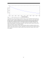
1
A vision based on surveillance system
using a wireless sensor network
NIKLAS LUNDELL
Masters’ Degree Project
Stockholm, Sweden March 2010
XR-EE-RT 2010:006
A VISION BASED
SURVEILLANCE SYSTEM
USING A WIRELESS
SENSOR NETWORK
Niklas Lundell
[email protected]
Masters degree project
Supervisor: Mikael Johansson
Stockholm, Sweden 2009
II
A Vision based surveillance system using a
wireless sensor network
Abstract
The aim of this thesis project is to implement a vision based surveillance system in a wireless
sensor network running the Contiki operating system.
After a comparative review of experimental cameras the decision fell on the Cmucam3.
Hardware and software to integrate the camera with a Tmote Sky mote were created. In this
way, the camera can be controlled with the Contiki operation system and images can be
transferred to the sensors memory for further processing and forwarding to other network nodes.
Due to the lack of memory on the sensor nodes, the prospect of image compression was
investigated.
To save energy, the system uses an energy efficient onboard light sensor to detect ambivalent
changes that would occur in the presence of, for instance, intruders or fire. When these sensors
detect changes, the more energy consuming camera gets activated. The detection mechanism
uses a Cusum algorithm which filters out irrelevant disturbances while maintaining high
sensitivity to unexpected changes. An evaluation of the system using multiple motes running the
energy efficient detection algorithm demonstrates rapid detection and transmission times of
about 2 seconds.
III
IV
Preface
Wireless sensor networks, referred to as WSNs, are being used to monitor and regulate areas
and processes. This could in many cases be done with much more confidence if visional
confirmation can be achieved with just the push of a button. The ability to send images within a
WSN is therefore a vital part of its desired functionalities. There are two main operating
systems that can be implemented on the motes; the well established TinyOS, and Contiki which
is more of a work in progress. Creating the hardware and software needed for image transfer
within WSNs is the main purpose of this report. How to detect abnormal changes in an area for
automatic surveillance will also be reviewed.
This report concludes my Master of Science degree project at the Royal Institute of Technology
in Stockholm.
V
VI
Acknowledgements
I would like thank Mikael Johansson for his fine support and mentorship throughout this degree
project.
I would also like to thank António Gonga for the expertise he shared and José Araújo for the
energy he provided. My good friend Ludvig Nyberg has also been of great help regarding his
proofreading and Thomas Lirén has been an invaluable source of never ceasing advice.
VII
VIII
Contents
1 Introduction................................................................................................................................ 1
1.1 Motivation........................................................................................................................... 2
1.2 Outline................................................................................................................................. 2
2 Problem formulation .................................................................................................................. 3
2.1 Scenario............................................................................................................................... 3
2.2 Problem formulation ........................................................................................................... 3
2.3 A possible architecture and its challenges........................................................................... 4
3 Camera selection ........................................................................................................................ 6
4 Transmission architecture .......................................................................................................... 9
4.1 Hardware interface .............................................................................................................. 9
4.2 Software interface ............................................................................................................. 11
4.2.1 Camera ....................................................................................................................... 11
4.2.2 Mote ........................................................................................................................... 12
4.2.3 Server ......................................................................................................................... 13
5 Change detection...................................................................................................................... 16
5.1 Cusum ............................................................................................................................... 16
5.2 Implementation ................................................................................................................. 19
6 Evaluation ................................................................................................................................ 21
6.1 MAC Protocol ................................................................................................................... 21
6.2 Quality of service .............................................................................................................. 21
6.3 Cusum ............................................................................................................................... 22
7 Final remarks............................................................................................................................ 23
7.1 Experiences ....................................................................................................................... 23
7.2 Future work ....................................................................................................................... 23
7.3 Conclusions....................................................................................................................... 23
Biography.................................................................................................................................... 25
Literature references ........................................................................................................... 25
Figure, table and algorithm references................................................................................ 26
IX
X
Chapter 1
Introduction
Surveillance applications, like most process control applications, use sensors to measure
temperature, moisture, light, pressure, vibrations etcetera. When the optimal locations for these
sensors are places where cables would run the risk of getting damaged, being in the way, or take
a lot of effort to apply, the communication would be preferred to be handled wirelessly.
An example of a potential application is the motion triggered wireless burglar alarm illustrated
in figure 1.1. Motion sensors with wireless transceivers are placed in each room and forward
alarm messages wirelessly to the other nodes when an intrusion is detected. In this way, an
efficient alarm system is created without the need for any wiring.
Figure 1.1. Floor plan.
While samples collected through the WSN can describe the surrounding environment quite
well, visual confirmation is often desired. For instance, even if a motion sensor detects changes
in its environment, an image might reveal if there is in fact a non authorized entry or not. In this
way, a single operator, whose attention is driven by the simple motion sensors, could watch
over a large number of buildings, spread over a large area. Remote communication with the
buildings could be performed via a gateway over a GSM or 3G network. New installations
could then be commissioned quickly without any wiring.
The wireless sensors do not need fast processors, high bandwidth or large onboard memory and
can therefore have a focus on a low power consumption, which allows them to operate for
extended periods of time without any external power supply. Moreover, the IEEE 802.15.4
standard for low power wireless communication allows nodes to communicate on an unlicensed
spectrum at a rate of up to 250 kbps with a very limited transmit power. This transmission rate
allows collecting sensor measurements from a rather large number of nodes without saturating
the wireless medium. However, the 802.15.4 standard was not designed to support large data
transfer, such as high resolution video or images. Large bulk transfers of data will occupy the
wireless medium for a long time and consumes a lot of energy, which could lead to quick
depletion of onboard batteries and short system life times. Furthermore, the limited memory of
current wireless sensor network platforms creates challenges for storing and processing the
large files that result from high resolution image capture.
1
The purpose of this Master Thesis is to design a vision based surveillance system based on
commodity wireless sensor network nodes, including camera selection, hardware integration,
system design, and software implementation.
1.1 Motivation
If a sensor triggers an alarm it can be both time consuming and expensive to manually check
what caused it and can therefore lead to wrongful decisions. Supplying images is therefore a
vital function for many surveillance implementations, which has not yet been made possible
with the Contiki operating system.
Sending an image occupies the radio channel for a long period of time and uses, in this context,
a lot of energy. To minimize the number of unnecessary transmissions an alarm can be set to
automatically send images when they are desired. Such an alarm would diminish the need for
unnecessary image updates. Two methods for realizing such an alarm will get evaluated.
1.2 Outline
The thesis is organized as follows. In chapter two the problem is formulated, and in the
following chapter a range of cameras are evaluated considering interface, onboard functions and
cost. In chapter four the architecture for an image carrying WSN is created; problems faced
during the construction of it are described as well as how to get past them. The fifth chapter
examines a couple of ways of detecting the presence of an intruder with a focus on a Cusum
algorithm, weighing pros and cons. The system is tuned and evaluated in chapter six. The
seventh and final chapter discusses the performance of the system and the experiences gathered
during the construction of it; the conclusions drawn from them are also presented here, as well
as what the most important upcoming work is considered to be.
2
Chapter 2
Problem formulation
2.1 Scenario
One application for the surveillance system is to monitor an office space for trespassers. When
someone enters, simple low energy sensors detect motion, vibration or perhaps changes in the
light condition, triggering a camera to capture an image and transmitting this over a WSN to a
gateway for further forwarding over the internet. If the image confirms an intrusion appropriate
action can be taken, such as contacting a security company. If an intrusion is not confirmed, the
action can be called of, saving time and thereby money.
Figure 2.1. Intrusion in an office space.
As an example, the scenario in Figure 2.1 results in a slight deviation in light conditions which
the sensors can pick up on. The difference from the expected values might be too small to be
certain that an intrusion is taking place, while an image easily verifies it.
2.2 Problem formulation
Based on our discussion so far, we are now ready to formulate and motivate our problem more
detailed.
A lot of dangerous, hard to reach, or simply unmanned places needs visual surveillance.
Drawing wires to these places can be difficult or expensive. The main objective of this thesis is
therefore to
1. Design and implement a wireless surveillance system, allowing remote image
acquisition.
To relief the WSN and a potential system operator from a flood of unnecessary images the
system can be equipped with an alarm, based on simple low energy sensors, which would
trigger the camera when activity out of the ordinary is detected. If this alarm is too sensitive
unnecessary images would still get sent, while if it is not sensitive enough it could create a false
sense of security. Hence,
2. The system should be atomized and sensitive, while keeping false alarms to a
minimum.
A large part of the advantage with a wireless system is that it can be used in places where wires
would be in the way or hard to draw. For this system to be suitable for such places it needs to be
3
independent of an external power supply, and therefore power efficient. Wireless sensor motes
have low power consumption and can be run on various operating systems. Contiki is a young
and interesting operating system which lacks the source code to communicate with an external
camera.
3. The base for the system should be a low power sensor mote running the Contiki
operating system.
A suitable camera has to be low power, possible to integrate with current sensor network
hardware, and preferably also offer onboard functionality to simplify image acquisition and
image transfer. Hence,
4. Selecting an appropriate camera and creating the hardware and software needed to
integrate it with the mote is an integral part of the thesis.
2.3 A possible architecture and its challenges.
Figure 2.2. Room with surveillance.
Figure 2.2 illustrates the system architecture. Rooms are equipped with wireless camera nodes,
combining low power camera hardware with commodity wireless sensor platforms. The rather
heavyweight camera nodes are complemented with small low power sensor nodes, tuned to
detect changes in ambient conditions (such as temperature, light, vibration or motion). These
smaller nodes provide better sensor coverage while keeping hardware costs low. When the low
power sensor nodes detect changes, they trigger the camera to acquire and process an image, for
further forwarding over the wireless sensor network to the gateway.
The design and implementation of such a system poses several challenges, including the
following.
A lot of different parameters can be used as indicators for an intrusion; for instance sound, heat,
light or vibrations. One of the fastest changing and easiest to measure is the light conditions.
However, if the premises have windows the light will not only change when someone enters but
also at sunsets, sunrises, streetlights turning on and off, amongst other irrelevant events; the
light changes caused by these events have to be filtered out. Similar issues happen also with
other sensors. When it is an event outside the office that causes the change, it will most often be
slower then if it would derive from within, and a model based detection algorithm could
possibly discern between the expected slow changes in the environment and sudden unexpected
changes associated with the burglary. Different algorithms for change detection have to be
designed and evaluated.
4
Camera network hardware is in its infancy and no current wireless sensor platforms have
integrated camera support. Hence, the selection of appropriate camera hardware and integration
with the sensor network platform is nontrivial. For example, the ports on the mote and the
otherwise attractive Cmucam3 camera have different voltage levels [3] [4] and connecting them
straight to one another would not enable communication and could damage the mote, since it is
the one operating on the lowest voltage. A circuit has to be designed to enable the
communication on the physical level.
The hardware integration needs to be accompanied by software for controlling the camera
hardware. This includes isolating and implementing low level commands for triggering image
acquisition, changing image resolution, format, etc. Unless the camera can transfer parts of the
picture to the mote, the image has to be compressed before it can be stored into the memory of
the sensor nodes.
Packet formats and communication protocols for communicating between the different devices
must also be designed. This includes the interaction between the low power sensor nodes and
the camera node, and the image transfer between the camera node and the server. Decreasing
the time consumed to retrieve an image would be a valuable contribution to lower the demand
for bandwidth and make the process more energy efficient.
When the server receives an image it often has lost parts and accumulated pixel errors; these
problems has to be solved by the server to get a decent quality. Hence, the appropriate image
processing algorithm for the server has to be designed.
Figure 2.3. Command center.
There are a lot of different tasks for which the system can be implemented. One is shown in
figure 2.3, where sensor and camera nodes have been placed in offices which are monitored by
a command center. If ambivalent changes are detected in one of the offices, an image will
automatically be sent to the command center, and a decision can be made if any action needs to
be taken.
5
Chapter 3
Camera selection
When determining which camera would be best suited for the task at hand the first step is to
define which features should be prioritized.
When connecting the camera to the mote, it must have an interface which enables them to
communicate on the physical level. Such interfaces could be i²c or RS-232 while using USB
runs the risk of getting too complicated.
A large part of the advantages with WSNs compared to other wireless networks lays in the low
power consumption which enables them to be independent of an external power supply. Low
power consumption will also be a requirement for the camera so this advantage does not get
wasted.
Not to take up more than necessary of the WSN bandwidth, image sending should be kept to a
minimum. The number of sent images can be reduced if as much as possible of the image
processing is done on the camera. For instance would colour tracking onboard the camera result
in a couple of coordinates instead of having to send multiple images to a server, which then
would extract the coordinates. Although this report does not cover image processing on the
camera it is important to keep in mind for future work while choosing a camera.
The report “The evolution from single to pervasive smart cameras” [15] has gathered a range
of cameras with onboard image processing capabilities, displayed in table 3.1.
6
Table 3.1. A range of smart cameras. From reference [15].
7
Comparing the cameras in table 3.1 and a few others considering power consumption, onboard
functionalities and what interfaces they offer resulted in two prospects; Cmucam3 [2] and
Cognachrome [16]. Both cameras has RS-232 interface, low power consumption, open source
code and offers a range of onboard functionalities.
While they have similar technical specifications the price separates them a bit more.
Cognachrome has a ten times higher price tag [16] [17] then the Cmucam3; which forms the
decision to proceed with the Cmucam3.
Figure 3.1a and b. Cognachrome [16] and Cmucam3.
The Cmucam3 can provide images in RGB format or compressed to JPEG and has a resolution
of up to 352*288 pixels [3] with the possibility to scale down the quality [4]. It operates on 5 V
and uses only 650 mW.
8
Chapter 4
Transmission architecture
The architecture has been divided into four parts: the hardware interface between the camera
and the transmitting mote, the software implemented into the motes, the camera settings and
finally the image processing done by the server. To scale down the complexity of the
architecture the source code of the camera will be left untouched.
The hardware interface enables the camera and the mote to communicate on a physical level. It
is a circuit that changes the voltage levels in the communication channel and uses an IC to RS232 converter.
The chapter about the software interface, describes how to acquire images from the camera,
sending them though the WSN, and restoring them on a server.
4.1 Hardware interface
The chosen mote, Tmote Sky, has a couple of options for serial communication [5]; either to
use the i²c bus (port six and eight), or the pair of UART ports (port two and four) that has not
yet been allocated in Contiki. For both options the voltage levels are 3 V which represents one
and 0 V which represents zero.
Figure 4.1. Tmote Sky 10 pin expansion connector.
Attempts to allocate the UART ports have been done, unfortunately without success. The i²c
bus on the other hand is connected to the radio [5] and might cause problems if it is used in
some other way then in standard i²c communication. The camera also has an i²c bus [6] which
could be connected directly to the one on the mote. Unfortunately the camera has not been
programmed to enable communicate with outside units via this bus and it has turned out to be
quite difficult to write such a function [9] [13]; therefore the cameras standard I/O ports will be
used.
9
Figure 4.2. Cmucam3’s serial port.
Figure 4.2 shows the Cmucam3’s serial port which uses the RS-232 standard [6]. Here 13 V
represents zero and -13 V represents one. If such voltage levels would be sent to the motes i²c
bus it might damage the mote besides not being able to establish communication; therefore a
pair of amplifiers is needed between them. There are integrated circuits designed for this task
and one of them is the Maxim MAX202ECPE [8].
1.5 kOhm
To Tmote sky
1.5 kOhm
From Cmucam
13
8
From Tmote sky
11
10
1µF
1
3
4
5
2
6
1µF
1µF
R1IN
R2IN
R1OUT
R2OUT
T1IN
T2IN
T1OUT
T2OUT
12
9
14
7
To Cmucam
C1+
C1C2+
C2V+
V-
1µF
MAX202ECPE
6V
Figure 4.3. ±13 V to 0-3 V converter.
With the schematics in figure 4.3 -13 V from the camera will result in 3 V to the mote and +13
V results in 0 V, and vice versa in the other direction.
10
The Cmucam3 has a circuit like the one in figure 4.3 [2] to enable its RS-232 communication.
If the mote were to be connected prior to it, the external one would not be needed; this on the
other hand would require soldering on the camera.
Connecting the mote to the camera via its i²c bus in this way will result in a few pixel errors
generated by the radio; these can then be corrected by filtering the image on the server.
4.2 Software interface
This chapter explains the software architecture which in most part is implemented into the mote
connected to the camera. One of the results from this chapter is the cmucam3.h file which
includes the functions needed to communicate with the Cmucam3.
To enable the communication the enable_camera() function awakens the camera if it is in
sleep mode and sets the right resolution for the forthcoming images. After the options for the
camera in set, images can be acquired and sent to the server; this is done with the
receive_trigger( c, from, unicast_conn) function. The trigger receiver is to be
paced in the motes recv() function and do not need any adjustments, in conformity with the
rest of the functions. When a message is received on the camera node an image is captured and
forwarded to the server if it is a trigger message, otherwise the message is discarded.
4.2.1 Camera
Figure 4.4. Cmucam3.
The Cmucam3 can provide images in JPEG or RGB format [1]. The preferred format would be
JPEG since it is compressed and enables good quality images to be stored on the mote;
unfortunately it can not be used due to the sensibility to bit errors and packet losses. RGB is not
as sensitive to bit errors; a false bit only impacts one pixel, while it could destroy a JPEG image
completely. Furthermore if a package were to be lost during its transmission an RGB image
would loose an equivalent amount of pixels as the number of bytes the package withheld if it is
in grayscale, while an image in JPEG format could be incomprehensible from there on.
11
Command Clarification
Camera_Power CP x
Turn the camera on or off depending on the x value (1 or 0).
Down Sample
DS x y
Decrease the resolution in x and y axels in the forthcoming
images.
Send JPEG
SJ
Retrieve an image compressed in JPEG format.
Send Frame
SF x
Retrieve one or all colours from an image, in RGB format. The
value of x determines which colour will be retrieve.
Table 4.1. A range of commands for the Cmucam3 [2] [4].
All of the commands in the table have to be followed by carriage return, represented by the
enter key on a keyboard and “\r” or 0x0D in the ASCII table.
The standard image size provided by the camera is 88*144 pixels and 38 kb which is far too
much to be stored on the mote. Sending the command “DS 2 2\r” will scale down the image [4]
size to 88*72 pixels and 19 kb; this is still too large for the mote but scaling it down even
further would result in an image with too low quality for recognizing for instance people. The
solution is to get it in grayscale. Sending “SF 0\r” to the camera will return the images red scale
and displaying it in grayscale will result in a nice black and white image. The image will now be
about 6 kb and thereby being able to fit on the mote. Meanwhile images with better quality can
be stored on an MMC/SD memory which the Cmucam3 has a slot for.
4.2.2 Mote
Figure 4.5. Tmote Sky.
The mote initializes the connection to the camera by sending “DS 2 2\r” to scale down the
amount of pixels in the forthcoming images requested by it and thereby enabling them to be
stored on the mote. The images are requested by sending “SF 0\r”; the camera then returns a
grayscale image which is saved on the mote. The image can not be sent in one large package
due to the lack of memory on the radio [10]; therefore it has to be divided into smaller packages.
It is not only the radios limited memory that needs to be considered. The risk for bit errors in a
package increases with its size and the receiving radio will discard packages including such,
with the use of a CRC (Cyclic Redundancy Check). Setting the payload sizes to the maximum
amount of space available on the radio would therefore, under bad conditions with an increased
risk for bit errors, run the risk of resulting in a large number of lost packages.
There are two ways to approach this issue; one is to maximize the package sizes to fit the
memory on the radio and retransmitting lost ones, and another is to send the image in smaller
packages and letting the server compensate for those who got lost.
12
4.2.2.1 With retransmission
Figure 4.6. Package with sequence number.
The radio has a 128 byte memory, of which about 100 bytes can be used for the payload. A
sequence number will get assigned to each package. When an image has been acquired it is
stored on the mote connected to the camera until a new image is requested. If packages have
been lost in the WSN they are requested for retransmission via their sequence number.
4.2.2.2 Without retransmission
Figure 4.7. Package without sequence number.
The larger the packages are, the harder it will be for the server to compensate for lost packages.
Experiments have proven 10 bytes to be a good package size, considering transmission time and
complexity to reassemble the images; more about this in chapter 4.2.3.2.
The receiving mote, connected to the server, waits for an initiation message and then simply
flushes all the packages one by one via its USB port to the server.
4.2.3 Server
The server reassembles and filters image to get rid of pixel errors. If retransmission has not
been utilized the server also has to compensate for lost packages.
4.2.3.1 With retransmission
If packages have been lost the receiving mote will request the lost packages again after the last
package has been sent. The server is not involved in this process but the payloads will be
flushed to the server in a different order then in which the image were divided into.
After the receiving mote has flushed the payloads and their sequence numbers to the server via
its USB port the payloads are arranged in order of their sequence numbers and stored into a file.
The file will now contain the image and some bit errors. The bit errors descend from the
communication between the camera and the transmitting mote, where the motes radio disturbs
the communication when it cyclically tries to send updates to the processor. The image quality
is sufficient enough to be used for surveillance purposes and can be further improved. To
increase the quality the image can be filtered so that it gets rid of the odd pixels; such a filter is
described in chapter 4.2.3.3.
The bit errors can affect the row changes as well. The row changes are represented by the
number 2, and should occur every 88th byte in an image with 87 pixels per row and every pixel
is represented by one byte. This can easily be managed by storing 2 in every 88th byte.
4.2.3.2 Without retransmission
The server reassembles the incoming packages from the receiving mote and synchronizes the
pixel rows, thereby creating an image. The result is then run through a smoothening filter
creating an image close to the one sent from the camera.
The incoming packages get stored into a file where the image is represented as one long row of
pixels. The next step is to achieve row changes at the right time. Every pixel is represented by
one byte with values ranging from 16 to 240, depending on its brightness¹. The image is 88*72
pixels. Every row gets initiated with a byte containing the value 2 [4].
¹How red the pixel should be.
13
Byte_number
80
81
82
83
84
85
86
87
88
89
1
2
3
Value
134
142
151
123
122
142
139
155
176
2
54
49
63
Figure 4.8. A row of pixels without package losses or significant bit errors.
In figure 4.8 the byte number represents the number of bytes since the last row change. The
figure displays a row that has been received without any package loss. If no packages have been
lost during the whole transmission the rows can be synchronized by starting a new one every
89th byte.
Although, if packages have been lost, changing lines every 89th byte would result in the rows
being unsynchronized for the rest of the image and the error would increase for every lost
package. With package sizes of 10 bytes the byte containing the value 2 would be located 79
bytes after the last row change; this is displayed in figure 4.9.
Byte_number
78
79
80
81
82
83
84
85
86
87
88
89
1
Value
134
2
38
45
64
72
31
44
43
45
54
49
63
Figure 4.9. A row missing a package.
If on the other hand the row changers would be based on the location of the 2 the image would
be sensitive to bit errors. In figure 4.10 a bit error has changed the 2 to a 9 and thereby created a
177 byte (89+88) long row.
Byte_number
80
81
82
83
84
85
86
87
88
89
90
91
92
Value
134
142
151
123
122
142
139
155
176
9
54
49
63
Figure 4.10. A bit error in byte number 89.
Combining these two methods would give a good synchronization amongst the rows. Searching
for the value 2 between the 79th and 89th byte, if it is not found a new row gets created after the
89th byte. This will allow every row to have a missing package or a bit error in byte number 89.
The motes include checksums (CRC) in their communication with each other and if a package
has accumulated bit errors it gets discarded. If the packages were to be larger they would run a
greater risk of containing bit errors generated in the WSN communication causing them to get
discarded. Large packages would also mean a wider span to search for the row changes,
increasing the risk to find false 2:s created in the communication between the camera and the
mote.
The synchronization will create blank lines at the end of the rows where a package has been
lost and bit errors from the camera to mote communication will result in odd pixels. Such an
image is shown in figure 4.12a.
4.2.3.3 Filter
To get rid of unwanted lines and odd pixels a smoothening filter is applied. The filter compares
every pixel with the ones surrounding it and if it is one of the three brightest or darkest it is
assumed to be faulty and gets assigned the median value of the eight surrounding pixels.
14
Figure 4.11a and b. Smoothening filter.
The center pixel in figure 4.11a is evaluated by the smoothening filter and since it is one of the
three darkest it is assumed faulty and is assigned the median value of the eight surrounding
ones. The result is illustrated by figure 4.11b.
Figure 4.12a and b. Image recovery.
When the image in figure 4.12a where sent, retransmission was not utilized, and lost packages
have resulted in the rows not being synchronized in a couple of places. There are also odd pixels
due to problems in the communication with the camera. After the filter have been applied to the
image it has gotten rid of the odd pixels, solved the problem with the synchronization amongst
the rows, but become a bit blurry. The result is shown in figure 4.12b.
15
Chapter 5
Change detection
Detecting for instance fires or intrusions is an important part of the surveillance system and
there are a couple of ways to approach it; having a person updating and reviewing the images is
for obvious reasons not an option. The same approach with the difference to let the server
handle the image comparison could be implemented; this would not take any man hours, but
would use a lot of energy and lead to congestion in the WSN. Letting the camera handle the
detection would relieve the radio channel from the extra traffic and use a lot less energy. To
save even more energy the camera can be completely turned off during the detection period by
letting the sensors on the mote search for differences that would occur in case of an intrusion;
these differences could for instance be in heat, moisture, vibration, sound, light or a
combination of them. Moisture and heat changes quite slowly while sounds and vibrations have
a tendency to include a lot of white noise, which leaves light detection.
The easiest way to sense differences is to have an interval of for instance one second where the
current light conditions are compared to what it was the previous cycle, and if it differs more
then a predetermined threshold the camera is triggered to send an image. A more sophisticated
way is to use a weighted average [14], which is then compared to the current condition; using
such method the camera can be triggered by differences occurring over more then one cycle and
enables it to be more sensitive without increasing the risk for false alarms.
5.1 Cusum
To detect out of the ordinary changes, a comparison to the average is preferential. Creating an
average for the whole time the detection algorithm have been running would trigger the alarm
on all variances from it, no matter how slow they are. The alarm would therefore be triggered at
sunsets, sun downs etcetera. To allow slow changes the average can be weighted, so that the
average is more dependent on new values then of old ones.
Figure 5.1. Signal versus noise.
In figure 5.1 the signal is represented by the line, and the stars shows the measured values out
of which the signal is to be determined. The figure is an example of how measured values
changes with the signal. The signal is influenced by white noise and can therefore not be read
straight from the measured values. A good estimate of the signal can be calculated with a
weighted average algorithm, and works like a low pass filter.
16
To create a weighted average, the current signal value and the previous average are added
together after they have been weighted with a value ranging from zero to one. The weight is
represented by λ, and the signal is given by y(t).
qt = lqt-1 + H1 - lL yt
Algorithm 5.1. Weighted average [11].
The current value for the signal can be described by algorithm 5.2 [11], where θ(t) is the
weighted average and Æ(t) is the noise. That is if the signal is static.
yt = qt-1 + ‰t
Algorithm 5.2. Current signal value [11].
If the noise Æ from algorithm 5.2 is replaced with ε(t), which includes not only the noise but
also the change in signal value, the difference between the current value and the weighted
average will be given by algorithm 5.3.
¶ t = yt - qt-1
Algorithm 5.3. Difference from the weighted average.
Now that the difference between the signal value and the weighted average can be found, a
method for deciding when to trigger the camera based on it needs to be created. This method is
called stopping rule; the process is quantified in figure 5.2.
Figure 5.2. Detection process.
The stopping rule can for instance be set to trigger on a large ε(t) value. Another way to go is to
use a simple yet effective Cusum algorithm, which can trigger on a continuously high ε(t) value,
as well one single large ε(t) value.
qt = lqt-1 + H1 - l L yt
¶ t = yt - qt-1
sHt1L = ¶ t
sHt2L = -¶ t
gHt1L = max Igt-1 + s Ht1L - n , 0M
H1L
gHt2L = max Igt-1 + s Ht2L - n , 0M
H2L
Alarm if gHt1L or gHt2L > h.
Algorithm 5.4. Cusum RLS filter.
A Cusum RLS filter has been chosen for the task and is shown in algorithm 5.4. θ(t) is the
weighted average, y(t) the current value, and λ the weight for how much the old and new values
are going to influence the average. ε(t) represents the difference between the weighted average
and the current value. G1(t) and g2(t) are the accumulated difference (positive and negative)
exceeding ν, between the measured values and the weighted average, where ν is an empirically
chosen constant. When g1(t) or g2(t) exceeds the threshold h the camera node is triggered to
capture and send an image.
To increase the sensitivity even further the algorithm is implemented into external motes,
connected neither to the camera nor the server; these will then trigger the camera node via the
WSN.
17
Figure 5.3a, b and c. Cusum example.
Figure 5.3 shows an example of how the Cusum algorithm might be used. Figure 5.3a displays
values collected from the motes light sensor. The sensor registers small variations until 16
seconds has passed and a person casts a shadow in front of the light sensor which results in
decreased values. In this case λ has been set to 0.7 and ν to 0.4; an analyze of figure 5.3b and
5.3c concludes that a threshold of about three would in this case filter out the irrelevant
variations while triggering the alarm in the presence of an intruder. The variation in brightness
after three seconds could very well be that the sensor is balancing between two values, while the
change after 14 seconds is more likely caused by the presence of an intruder or a fire.
18
Figure 5.4a, b and c. Cusum example.
If the values for λ and ν is changed, g1(t) and g2(t) will do so as well. In figure 5.4 both λ and ν
has been set to 0.9. The increased value for ν lowers the effect a change in brightness has on
g1(t) and g2(t), while the increased λ preserves the accumulated g1(t) and g2(t) values for a
longer period of time. To quantify this; the change in brightness after four seconds gives a very
limited effect on g2(t), due to the high ν value, while the value for g2(t) after 30 seconds is
higher then in figure 5.3c, due to the increased λ.
Appropriate values for λ and ν will differ depending on where the light sensors are placed and
what they are supposed to detect.
5.2 Implementation
The Cusum algorithm is implemented into one or several motes. The advantage with having
more then one mote lays in the increased sensibility and that the system gets less dependent on
each mote. If cost is a major issue, the algorithm can be implemented on the camera node.
However, if sensibility is of greater concern the Cusum algorithm should run on external motes.
The external motes can be placed where they have an increased chance to detect what they are
suppose to while being shielded from outside events.
19
Figure 5.5 Chain of events.
The algorithm runs quietly on the sensor motes until either the positive or negative accumulated
variation from weighted average exceeds its threshold and thereby setting off the alarm. When
the alarm is set off the sensor mote sends a message to the camera node, triggering it to capture
an image which is then sent to the server. This chain of events is illustrated in figure 5.3. In the
figure three external motes are running the Cusum algorithm quietly until one of there alarms is
set off and starts the chain of events.
20
Chapter 6
Evaluation
6.1 MAC Protocol
The MAC protocol defines the characteristics of the radio [1]; for instance whether or not it
will synchronize with the receiver before starting to transmit. The X-MAC protocol has been
compared with what the result would be if no MAC protocol were being used, called
NULLMAC. X-MAC is the default protocol and will wait for the radio channel to clear before
starting to transmit; this will decrease the risk for collisions with packages sent from other
motes. NULLMAC will flush out everything without synchronizing with the receiver; this will
decrease the time required to send the image but increase the risk for packages colliding.
Transmitting images will occupy the radio channel for quite some time which makes it an
option to allocate a channel only used for this purpose.
Measurements have shown transmission times for images to be between 2.2 and 4.8 seconds,
depending on the payload size, with a 0.3 % time difference between NULLMAC and X-MAC,
to NULLMAC advantage. The time difference is so small that it could be coincidental and is not
nearly enough to compensate for the advantages brought with X-MAC; which therefore is
preferred.
6.2 Quality of service
With retransmission and payload sizes of 100 byte, the total time, from an image is requested
from the server until it arrives, is 2.2 seconds. That is if no packages have been lost.
If retransmission is not applied and the package sizes are set to 10 byte, it is possible for the
server to synchronize the image even though a few packages have been lost. It is also important
to have small packages if bit errors would occur in the WSN since packages including such will
get discarded. The large number of packages (almost 650) will affect the transfer time
considerably and result in a total time of 4.8 seconds, from an image is requested from the
server until it arrives.
Most of the difference in transmission time between various payload sizes is a result of the
transmitting mote waiting for a free timeslot every time a package is to be sent. The waiting
period is called Mac delay.
21
Figure 6.1. Total retrieval time correlating with payload size.
Figure 6.1 illustrates how the time to retrieve an image correlates with the size of the payload.
The curve is the result of experiments which have been interpolated. The diagram shows the
benefit of large packages, while proving that a larger radio memory would not have a significant
impact on the retrieval time since the curve is quite flat when the payload is 100 bytes.
To get a better idea of how the payload size influence the total time the theoretical principle can
be advised.
Payload1 + Over_head1 y
i
z
j Mac_delay1 +
z + Camera_delay +
Time = j
k
{
Bit_rate
Payload2 + Over_head2 y
i
File_size
j
z
j Mac_delay2 +
z
k
{ Payload_size2
Bit_rate
Algorithm 6.1. Theoretical principle of the retrieval time.
The first part of the algorithm is the message that triggers the camera node. The message is sent
either from a sensor mote or the mote connected to the server. The second part consists of the
capturing of an image and the communication between the camera and mote connected to it.
The first two parts are static while the third changes depending on the payload sizes in which
the image is divided into. It is the payload size in the denominator, in the last part of the
algorithm, that gives the curve its convex shape.
In a day and age when it is not unusual to have a 100 Mbps internet connection at home and an
ordinary digital camera recognizes millions of colours in tens of millions of pixels, the system
described here, where a bit over 6000 grayscale pixels are recovered in approximately 2
seconds, seems almost ancient. Although it is far from being able to uphold a videoconference it
is still sufficient enough for many surveillance purposes and has the possibility to take images
with higher quality which can be stored on the camera for manual collection.
6.3 Cusum
The Cusum algorithm described in chapter five is superior for detecting intrusions compared to
simply weighing the current value against an old one, but takes time and effort to calibrate.
Values for ν and λ have to be tested out and when that is done it has become much of an ad hoc
system, tuned to the conditions inside and outside the premises. For the system to be easily
implemented in various locations the simpler solution could be a practical option and preferably
with a combination of e.g. light and sound detection.
22
Chapter 7
Final remarks
7.1 Experiences
My experience is that there are many functions included in Contiki that need to be reedited due
to various bugs. Comments to the source code and an increased number of examples would also
be appreciated. Contiki simply needs to mature a bit more.
I have put in a lot of time and effort to get the i²c communication to work and still did not
manage due to the complexity to implement it on the Cmucam3; i²c is a good way for the mote
to communicate but is very time consuming with the Cmucam3. In the final solution the camera
has its original software.
Effort was also put into getting the motes UART to function (port 2 and 4 in figure 4.1). The
lesson here is that port allocation can take a lot of time and effort.
The JPEG format uses Fourier transforms to compress the images to just a fraction of the size it
would have in RGB format; it were unfortunately too sensitive to the bit errors originated
between the mote and the camera. It is possible to evolve the system so that the JPEG format
can be utilized. The easiest way to get this done is to allocate the UART ports on the mote.
7.2 Future work
A more user friendly way to acquire images would be nice; it now takes three steps and should
be automated.
The most important future work would, without a doubt, be to enable either the i²c on the
camera or the UART on the mote, so that they can communicate with each other without having
their communication tainted by bit errors. If the communication between the mote and the
camera would be relieved from bit errors the images can be compressed to JPEG format,
enabling higher resolution and colour vision.
7.3 Conclusions
With large payload sizes and retransmission of lost packages, the transmission times are
shorter, the communication is more reliable, and the complexity is scaled down. This approach
is therefore preferred.
Even though the optimal solution is to have large payloads and retransmit lost packages, it is
not certain that the payloads should be as large as possible at all time.
23
Figure 7.1. Total transmission time correlated with payload size.
Experiments have shown that larger payloads result in a lower transmission time, but the risk
for bit errors increase and if packages are lost or discarded due to bit errors, more data needs to
be resent. Figure 7.1 shows the transmission times for images sent with payloads between 50
and 100 bytes. The difference in time is only about a third of a second per image and in an
environment where packages often are lost, smaller payload sizes should be considered. The
default setting should be a maximized payload size, while large distances between the motes or
a noisy environment, calls for smaller payloads.
WSNs have a huge potential as image carrying networks and will, combined with the sensors
mounted on the motes and the low power consumption, be ideal for many surveillance purposes;
such as various forms of process control, animal research and control, logistics and of course
crime fighting.
24
Biography
Literature references
[1] www.sics.se/contiki
The publishers of Contiki.
[2] www.cmucam.org
The creators of the Cmucam3.
[3] www.cmucam.org/attachment/wiki/Documentation/CMUcam3_datasheet.pdf?format=raw
The datasheet for the Cmucam3.
[4] www.cmucam.org/attachment/wiki/Documentation/CMUcam3_datasheet.pdf?format=raw
The user manual for Cmucam2.
[5] www.snm.ethz.ch/pub/uploads/Projects/tmote_sky_datasheet.pdf
The datasheet for the Tmote Sky.
[6] www.nxp.com/acrobat_download/datasheets/LPC2104_2105_2106_7.pdf
The datasheet for the processor on the Cmucam3.
[7] focus.ti.com/lit/ds/symlink/msp430f1611.pdf
The datasheet for the processor on the Tmote Sky.
[8] pdf1.alldatasheet.com/datasheet-pdf/view/73057/MAXIM/
MAX202ECPE/+431WJupNuhLaxDatAYlKZx+/datasheet.pdf
The datasheet for the Maxim MAX202ECPE.
[9] www.nxp.com/documents/application_note/AN10369.pdf
User guide for implementing i²c communication on the Cmucam3’s processor.
[10] focus.ti.com/lit/ds/symlink/cc2420.pdf
The datasheet for the mote’s radio.
[11] GUSTAFSSON F. 2001. Adaptive Filtering and Change Detection. John Wiley & Sons Ltd.
ISBN 0-471-49287-6.
Describes various adaptive filters e.g. Cusum filters.
[12] BOYLESTAD R. 2000. Introductory Circuit Analysis. Prentice Hall. ISBN 0-13-192187-2.
Explains the behavior of electrical components and circuits.
[13] FALK C. 2002. Datorteknik med Imsys.
Teaches low level programming in Assembler and covers e.g. interruption routines.
[14] GONZALEZ R. AND WOODS R. 2002. Digital Image Processing. Prentice Hall.
ISBN 0-13-094650-8.
Describes various ways to increase image quality.
25
[15] RINNER B. AND WOLF W. 2008. The evolution from single to pervasive smart cameras.
Universität Klagenfurt. ieeexplore.ieee.org/stamp/stamp.jsp?arnumber=04635674
A report comparing various cameras suitable for WSN.
[16] www.newtonlabs.com/cognachrome
The creators of Cognachrome.
[17] www.probyte.fi
A distributor of Cmucam3, others can be found at [2].
Figure, table and algorithm references
F 1.1. System overview. Created with ArchiCAD.
F 2.1. Intrusion scenario.
F 2.2. Room with surveillance. Created in ArchiCAD.
F 2.3. System with a command center. Created in ArchiCAD.
T 3.1. From “The evolution from single to pervasive smart cameras”. Reference [15].
F 3.1a. The Cognachrome camera. From Newton labs homepage. Reference [16].
F 3.1b. Image taken of the Cmucam3.
F 4.1. From the Tmote Sky’s datasheet. Reference [5].
F 4.2. From the Cmucam3’s homepage. Reference [2].
F 4.3. Created using Orcad Family Capture. Reference [8] and [12].
F 4.4. From the Cmucam3’s datasheet. Reference [3].
T 4.1. From the Cmucam2’s user manual and Cmucam3’s homepage. Reference [2] and [4].
F 4.5. From the Tmote Sky’s datasheet. Reference [5].
F 4.6. Package with sequence number. Created in Paint.
F 4.7. Package without sequence number. Created in Paint.
F 4.8. Example of a row without package losses or bit errors.
F 4.9. Example of a row missing a package.
F 4.10. Example of a bit error in byte number 89.
F 4.11a. Unfiltered center pixel. Created using Microsoft Paint.
F 4.11b. Filtered center pixel. Created using Microsoft Paint.
F 4.12a. Unfiltered image. Created on the server using Matlab.
F 4.12b. Filtered image. Created on the server using Matlab.
F 5.1. Example of a signal influenced by white noise. Created in Matlab.
A 5.1. From “Adaptive Filtering and Change Detection”. Reference [11].
A 5.2. From “Adaptive Filtering and Change Detection”. Reference [11].
A 5.3. From “Adaptive Filtering and Change Detection”. Reference [11].
F 5.2. Block diagram over the detection mechanism. Created in Paint. Reference [11].
A 5.4. From “Adaptive Filtering and Change Detection”. Reference [11].
F 5.3a. Example of values from a light sensor. Plotted in Matlab.
26
F 5.3b. Accumulated positive deviance from the weighted average. Plotted in Matlab.
F 5.3c. Accumulated negative deviance from the weighted average. Plotted in Matlab.
F 5.4a. Example of values from a light sensor. Plotted in Matlab.
F 5.4b. Accumulated positive deviance from the weighted average. Plotted in Matlab.
F 5.4c. Accumulated negative deviance from the weighted average. Plotted in Matlab.
F 5.5. The chain of events when a Cusum threshold is exceeded. Created in Paint.
F 6.1. Times measured by the mote connected to the server. Interpolated with Matlab.
A 6.1. Theoretical time delay.
F 7.1. Times measured by the mote connected to the server. Interpolated with Matlab.
27