Download Implementation of an executable graphical representation of GAPs

Implementation of an executable graphical
representation of GAPs based on Petri-nets
Sebastian Jekutsch
Project work report
Institute for Algorithms and Cognitive Systems
University Karlsruhe
Contents
1 Introduction
3
2 Prerequisites
3
2.1 Generalized Annotated Programs : : : : : : : : : : :
2.2 Well-founded semantics : : : : : : : : : : : : : : : :
2.2.1 Alternating xpoint : : : : : : : : : : : : : :
2.2.2 Annotated logic and the well-founded model
2.3 Coloured Petri-nets : : : : : : : : : : : : : : : : : : :
:
:
:
:
:
:
:
:
:
:
:
:
:
:
:
:
:
:
:
:
:
:
:
:
:
:
:
:
:
:
:
:
:
:
:
:
:
:
:
:
:
:
:
:
:
:
:
:
:
:
:
:
:
:
:
:
:
:
:
:
:
:
:
:
:
3 An extended Petri-net Model
3.1 Negation-free GAPs : : : : : : : : : : : : : : : : : : : : : : : : : : : : : : :
3.1.1 Algorithms for the extended Petri-net model : : : : : : : : : : : : :
3.2 Normal GAPs : : : : : : : : : : : : : : : : : : : : : : : : : : : : : : : : : : :
3
5
6
7
8
9
9
12
15
4 GAPCAD - Architecture
17
5 Further issues
20
5.1 Control ow specication : : : : : : : : : : : : : : : : : : : : : : : : : : : :
5.2 GAPCAD as a knowledge acquisition tool : : : : : : : : : : : : : : : : : : :
6 Conclusion
20
22
23
1 INTRODUCTION
3
1 Introduction
The contents of this work is the implementation of the bottom-up evaluation procedure of
Generalized Annotated Programs (GAPs). A related procedure was presented in 2] (Chapter 3.3) and 13]. The procedure has been formulated in terms of Coloured Petri-nets 6].
Also the extension to GAP-clauses with negated body literals has been examined. The
developed tool, called GAPCAD (Generalized Annotated Program Construction And Debugging), allows the interactive graphical entering of the Petri-net representation of GAPs
and therefore serves as an front-end to DAEDALUS 9]. GAPCAD also permits the monitoring and step-by-step execution of GAPs. In contrast to DAEDALUS, which performs
a query initiated backward chaining (SLG-resolution), the forward chaining procedure in
GAPCAD computes the whole model of the GAP based on the xpoint semantics. To
compute normal GAPs, i.e. clauses with negated literals in the body, an algorithmical proposal for the computation of the well-founded model according to the alternating xpoint
characterisation 20] is presented. This will ensure answer compatibility to DAEDALUS.
The implementation uses DAEDALUS routines, a generic graph editor 5] and inbetween code for representing the Petri-net and computing the xpoint. It was taken care
to dene a useful interface between the GAPCAD core and the graph editor for possibly
exchange with a dierent editor.
The outline of this report is as follows: Firstly, the generalized annotated logic, the
well-founded semantics and the Coloured Petri-net formalisms are described shortly. Next,
the extended Petri-net model is presented, in the rst instance without negated literals
and subsequently including them. Chapter 4 addresses the architecture of GAPCAD, and
the nal chapter discusses some further issues and an outlook. This text does not cover
GAPCADs actual purpose: To serve as a front-end for developing mediatory knowledge
bases for the integration of heterogeneous and inconsistent information sources.
2 Prerequisites
2.1 Generalized Annotated Programs
In this section the generalized annotated logic, introduced by M. Kifer and coworkers 7],
is sketched. It provides an universal language for dealing with temporal, uncertain and
inconsistent information or in general with parametric data with provides the algebraic
structure of a lattice. For a comprehensive description of the language the reader may refer
to 10, 7].
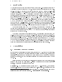
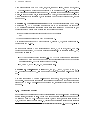
Salient features of the language are the so-called annotations which are constants, variables and terms over a complete lattice T 1. Figure 1 presents some examples for complete
lattices. The following denitions are from 7]:
Denition 2.1 An annotation is either an element of T (c-annotation), an annotation
variable (v-annotation) or a complex annotation term (t-annotation). Annotation terms are
1
A complete lattice (T ) is a partial ordering with respect to , a least upper bound (lub) t and a
greatest lower bound (glb) u for every subset of T . A lattice is linear if is a total ordering.
2 PREREQUISITES
4
1:0
>
f
t
f
?
FOUR
0:0
0 1]
df
>
d>
?
DEFA ULT
t
dt
Figure 1: Some lattices used in this report
dened recursively as follows: Members of T and variable annotations are annotation terms.
In addition, if 1 : : : n are annotation terms, then f (1 : : : n ) is a complex annotation
term.
If A is a usual atomic formula of datalog (in 7] predicate calculus) and is an annotation,
then A : is an annotated atom. An annotated atom containing no occurrence of object
variables is ground. A is called the object part and is called the annotation part of A : .
Denition 2.2 (Annotated clause) If A : is an annotated atom and B1 : 1 : : : Bk :
k are c- or v- annotated atoms, then
A : B1 : 1 ^ : : : ^ Bk : k
is an annotated clause. A : is called the head of this clause, whereas B1 : 1 : : : Bk : k
is called the body. All variables (object or annotation) are implicitly universally quantied.
Any set of annotated clauses is called a Generalized Annotated Program (GAP).
Denition 2.3 (Strictly ground instance) Suppose that C is an annotated clause. A
strictly ground instance of C is any ground instance of C that contains only c-annotations.
Let H be the Herbrand base of the program. An annotated logic interpretation I is a
mapping I : H ! T from the base onto a lattice.
Denition 2.4 (Satisability) Let I be an interpretation, 2 T a c-annotation, F1 and
F2 formulae, and A a ground atom:
1.
2.
3.
4.
5.
I j= A : i I (A) .
I j= :A : i :() I (A).
I j= F1 ^ F2 i I j= F1 and I j= F2 .
I j= F1 _ F2 i I j= F1 or I j= F2.
I j= F1 F2 i I j= F1 or I 6j= F2.
2 PREREQUISITES
5
6. I j= F1 $ F2 i I j= F1 F2 and I j= F2 F1 .
7. I j= (8x)F i I j= fx=tgF for all ground terms t where x is an object- or annotation
variable.
8. I j= (9x)F i I j= fx=tgF for some ground term t where x is an object- or annotation
variable.
9. If F is not a closed formula, then I j= F i I j= (8)F , where (8)F denotes the
universal closure of F .
There are two dierent kinds of negation in GAP, the so-called epistemic (or explicit)
negation : and the non-monotonic not. : requires symmetry between true and false, e.g.
:A : t = A : f in FOUR. The topic of non-monotonic negation will be discussed in section
2.2. For GAPs without non-monotonic negation the xpoint operator has the following
form:
Denition 2.5 (Fixpoint-operator) Let P be a generalized annotated logic program
(GAP), I a GAP interpretation and T a complete lattice. Then a xpoint operator RP (I )
for bottom-up computation of GAPs is dened as follows: RP (I )(p) := tf j p : p1 :
1 : : :pn : n is a strict ground instance of a clause in P and I j= p1 : 1 : : :pn : n g.
RP may reach the least xpoint (lfp) if for all strict ground instances A, lfp(RP (A))
is reached after a nite number of iterations. This condition, called xpoint reachability
property 7], holds for many GAP knowledge bases: If the clause bodies of a program
contain only variable (v-) or only constant (c-) annotations, or if only nite or decreasing
monotone functions2 appear in the program. For instance, if the knowledge base consists
of Rains(Monday ) : 0:5 and Rains(Monday ) : 0:8 the least upper bound computed by the
xpoint operator would be Rains(Monday ) : 0:8 = tf0:5 0:8g.
2.2 Well-founded semantics
For simplicity we dene the well-founded semantics for classical logic in the rst case,
according to 19].
Denition 2.6 (Normal program) A normal program is a set of clauses of the form
A B1 ^ : : : ^ Bn ^ not Bn+1 ^ : : : ^ not Bm
where A B1 : : :Bm are atoms.
Let P be a normal program and HP its Herbrand base consisting of all atoms that are
grounded in every possible way using all predicates, functions and constants that appear
in P . For a set of literals S the expression : S denotes the set formed by taking the
complement of each literal in S . Consider as an example the following program P :
p(a) not q (b)
q(b)
2
A function f is nite if ff (x)jx 2 DOM (f )g is nite and f is decreasing if for arbitrary arguments
x1 : : : xn f (x1 : : : xn ) xi for all 1 i n.
2 PREREQUISITES
6
P is a normal program with HP = fp(a) p(b) q(a) q (b)g and :fp(a) :q (a)g=f:p(a) q (b)g.
The well-founded model of a normal program P is a partial model3 , i.e. a set of literals
which contains not necessarily all atoms of HP . Therefore it can be seen as a three-valued
model. In the above example, an interpretation I = fq (b) :q (a)g states that q (b) is true in
I (and therefore :q (b) is false in I ), q (a) is false in I and the truth values of p(a) p(b) are
unknown in I .
Denition 2.7 (Greatest unfounded set) Given a partial interpretation I and a normal program P , A HP is called an unfounded set of P with respect to I if each atom
p 2 A satises the following condition: Either there is no clause in P whose head is p, or
there exists such a clause c and at least one of the following holds:
(a) some (positive or negative) subgoal of the body of c is false
in I
(b) some positive subgoal of the body of c occurs in A.
The greatest unfounded set of P with respect to I , denoted UP (I ), is the union of all unfounded sets of P w.r.t I .
In the example program P and interpretation I above, UP (I ) is fp(b) p(a)g. The wellfounded semantics uses UP (I ) to draw negative conclusions. The transformations TP , WP
are dened as follows:
TP (I ) is the usual xpoint operator, i.e. p 2 TP (I ) i there is some instantiated
clause c of P such that c has head p and each subgoal literal in the body of c is true
in interpretation I . TP (I ) is called the inner xpoint.
WP (I ) := TP (I ) : UP (I ). WP is monotonic 19].
Denition 2.8 (Well-founded model) Let I0 := , I+1 := WP (I) and I 1 := S I.
I 1 { the least xpoint of WP , also named outer xpoint { denes the well-founded model
of P .
The example program P has the well-founded model fq (b) :p(a) :q (a) :p(b)g which is
not partial. As an example for partial model consider the program which only contains the
clause p(a) :p(a): The well-founded model is empty, therefore the truth value of p(a) is
unknown.
2.2.1 Alternating xpoint
In the following the alternating xpoint characterisation of the well-founded model is presented shortly, according to 20]. Let I~ be a set of negative literals of atoms known to
be false and P 0 := HP I~. We dene SP (I~) := TP1 () where TP1 is the least xpoint of
TP , which was already dened above. SP (I~) is the set of positive facts that are derivable
0
0
0
3
An interpretation or model I is seen as the set of all literals that are true in I , i.e. fp 2 HP :HP j I j= pg
2 PREREQUISITES
7
from P and I~. Let S~P (I~) := : (HP n SP (I~)). The iteration steps I~+1 = S~P (I~) alternate between subsets (underestimation) of the positive portion of the partial well-founded
model and supersets (overestimation) of the undened and negative portion. The alternation converges: Let AP (I~) := S~P (S~P (I~)), then AP is monotone, therefore A~ := A1
P exists.
Finally SP (A~) A~ is the well-founded model of P. The reader may refer to 20] for a deeper
treatment.
Consider as an example for the alternating xpoint computation of the well-founded
model the following program taken from 20]. It describes a game where one wins if the
opponent has no moves left.
Example 1
wins(X ) move(X Y ) ^ not wins(Y )
move(a b)
move(b a)
move(b c)
move(c d)
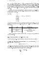
The table shows the sets SP and S~P at consecutive stages of the computation. They are
restricted to the atoms of the wins-predicate, since the move-facts do not change during
computation.
SP (I~t)
S~P (I~t) = I~t+1
Step t
0
f:wins(a) :wins(b) :wins(c) :wins(d)g
fwins(c) wins(b) wins(a)g
f:wins(d)g
1
2
fwins(c)g
f:wins(a) :wins(b) :wins(d)g
fwins(c) wins(b) wins(a)g
Fixpoint reached
3
Finally the well founded model is SP (I~4) S~P (I~3 ) = fwins(c) :wins(d)g, restricted to
the wins predicates.
2.2.2 Annotated logic and the well-founded model
The semantics of the non-monotonic negation in annotated logic is dened as follows:
Denition 2.9 (Satisability of negated atoms) Let I be an interpretation, 2 T a
c-annotation and A a ground atom:
I j= not A : i I (A) 6 The well-founded semantics can be generalized to annotated programs. Since the semantics
of the satisability relation j= changed in annotated logic, a partial model can have a
dierent form. Consider the following program with the lattice 0 1]:
p : 0:7 not p : 0:5
p : 0:3
2 PREREQUISITES
8
The partial well-founded model evaluates to fp : 0:3 not p : 0:7g, i.e. p : is true for all
0:3, false for all 0:7 and unknown for all 0:3 0:7, where a b i a 6 b.
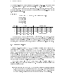
Example 2 reviews example 1 with annotated atoms. In the table, again only the wins
atoms are presented. They are abbreviated in a straightforward manner, e.g. not wins(a) :
0:3 is represented as :a : 0:3.
Example 2
Step t
0
1
2
3
4
wins(X ) : W move(X Y ) : W ^ not wins(Y ) : 0:5
move(a b) : 0:3
move(b a) : 0:4
move(b c) : 0:6
move(c d) : 0:7
fa : 0:0
fa : 0:3
fa : 0:0
fa : 0:3
fa : 0:3
SP (I~t)
b : 0:0 c : 0:0
b : 0:6 c : 0:7
b : 0:4 c : 0:7
b : 0:6 c : 0:7
b : 0:6 c : 0:7
d : 0:0g
d : 0:0g
d : 0:0g
d : 0:0g
d : 0:0g
f:a : 0:0
f:a : 0:3
f:a : 0:0
f:a : 0:3
S~P (I~t ) = I~t+1
:b : 0:0 :c : 0:0
:b : 0:6 :c : 0:7
:b : 0:4 :c : 0:7
:b : 0:4 :c : 0:7
Fixpoint reached
:d : 0:0g
:d : 0:0g
:d : 0:0g
:d : 0:0g
The well founded model is SP (I~5) S~P (I~4) = SP (I~3 ) S~P (I~3). This model is { dierent
to the one in example 1 { not partial. Note that the xpoint was reached, because step 4
results in the same sets as step 3, leading to a total model. Due to the alternating xpoint
denition, step 5 needs also be computed, because AP evaluates two S~P -steps at a time.
2.3 Coloured Petri-nets
A coloured Petri-net is a triple N = (P T A) consisting of disjoint sets P (places) and T
(transitions) and a multiset A (arcs) over (P T ) (T P ) forming a bipartite graph.
Each place p 2 P is assigned a colourset C (p) and a multiset M (p) of tokens, each of
colour C (p). Coloursets can be viewed as data types, and tokens are instances having a
specic colour. Each arc a = hp ti 2 A or ht pi 2 A is attached a label L(a) of type C (p).
Note that tokens as well as labels may contain variables of suitable type. A marking is the
distribution of tokens over all places of the net. Each transition t 2 T is assigned a Boolean
guard G(t) expressing constraints on the variables binded to t. For an extended and more
formal denition of coloured Petri-nets, the reader may refer to 6].
Let IN (t) := fhp ti 2 A j p 2 P g, OUT (t) := fht pi 2 A j p 2 P g, t := fp jhp ti 2 Ag
and t := fp jht pi 2 Ag denote the vicinity of t 2 T . A transition t is called enabled i the
following conditions hold:
For each incoming arc ai = hp ti 2 IN (t) there is at least one variable substitution
i , such that a token s 2 M (p) exists with i(s) = i (L(ai)). This particular token s
must not serve again as a resource for another substitution j for j =
6 i. Recall that
M (p) is a multiset, therefore more than one token of this kind may be present.
3 AN EXTENDED PETRI-NET MODEL
9
All substitutions i (1 i jIN (t)j) are compatible. i and j are compatible if
their concatenation i j is dened. In other words, there is no assignment of two
dierent values to the same variable.
G(t) evaluates to true under = 12 m. In this case, is called an enabling
substitution.
There could be more than one enabling substitution under the same marking. A transition
could re, if it is enabled under a substitution . If a transition t res, the tokens Mi of
the places are updated to Mi+1 as follows:
8>
i (p) n (L(hp ti))
>< M
M
Mi+1 (p) := > fMi (p()p)n((LL((hhtpptii))))g (L(ht pi))
>: M (ip)
i
if p 2 t n t
if p 2 t n t
if p 2 t \ t
otherwise
Given a marking M0 , a sequence t1 : : :tn is called a ring sequence, if for each i (1 i n),
it holds that ti 2 T is enabled under the marking Mi;1 and ti 's ring results in the marking
Mi . The ring sequence changes the marking M0 into Mn.
3 An extended Petri-net Model
3.1 Negation-free GAPs
A GAP knowledge base is transformed into an extended Petri-net N = (P T A) according
to the subsequent rules (suppose the clauses are enumerated from 1 to n):
Each predicate p is a place p 2 P in the net.
Each clause c (1 c n) is a transition c 2 T in the net.
Let O be the type of the object part and T the annotational lattice of predicate p.
Then C (p) := O T .
For every clause c of the form
p0 (o0) : 0 p1(o1) : 1 ^ : : : ^ pm (om) : m
and 1 i m, the net contains the arcs ai := hpi ci with the labels L(ai) := (oi i ),
where i is a new variable annotation. If i is a c-annotation, then i i is added
as a conjunctional condition to the guard of transition c. In addition, the net contains
the arc a0 := hc p0i with the label L(a0) := (o0 0 ), where
8>
if 0 is c-annotation
< 0
0 := > ufi ji is the same variable as 0 g if 0 is v-annotation
: f (1 : : : n)
if 0 = f (1 : : :n )
The 1 : : : n are dened recursively in the same way. Note that ufag = a for every
a 2 T and ufg := uT .
3 AN EXTENDED PETRI-NET MODEL
10
The initial marking is 8p 2 P : M0(p) = f(X uT )g, where X is a new variable for all
p and (X uT ) 2 C (p).
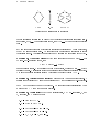
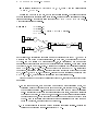
Queries can be added to the net, as they are headless clauses. The following abstract
example illustrates the transformation in its details. Places are drawn as circles and transitions as rectangles. Typing information is omitted and C (p) = C (q ) = C (r) = fag 0 1].
All uppercase letters are variables.
(1) p(a) : 0:5 (2) q (a) : 0:6 (3) r(X ) : 21 V p(a): V ^ q (X ): V ^ q (a):0:3
(4) r(X ) : 0:2
Example 3
1
2
(a 0:5)(a 0:6)-
p
(a V1)
(a V3)
q
(X V2)
j
:3
(X 12 ufV1 V2g)-
V3 0:3
r
(X V ) -
4
V 0:2
In the following, a substitution is written as a set of bindings of the form X=t, where X is
a variable and t is a term of appropriate colour. In example 3, the answering of the query
r(X ) : 0:2 can be modelled by a ring sequence 1 2 3 4: Transitions 1 and 2 are always
enabled since their guards are true and no variable binding is necessary. Their ring places
the token (a 0:5) in p and (a 0:6) in q . Consider now transition 3: A possible substitution
is = fV1=0:5 V2=0:6 V3=0:6 X=ag. Due to the fact that the guard V3 0:3 evaluates to
true under , transition 3 is enabled. Its ring (see below for problems here) adds the token
((X 0:5 ufV1 V2g)) = (a 0:25) to place r. Finally the query transition 4 is enabled with
= fX=a V=0:25g, which is also the substitution for the successful query.
We need to extend the model in the following three ways, in order to capture the xpoint
semantics:
1. In the example above, only one token was in place q after transition 2 red, but
transition 3 needed this token two times to be enabled, one for every arc hq 3i. Unlike
the denition in section 2.3, tokens will not be removed in our model if a transition
res. This reects the fact that the tokens represent knowledge, rather than resources
that cannot be shared. In other words, our Petri-net model caches all facts necessary
for answering a query, which could lead to a large number of tokens to be kept within
the net. Such an extension avoids conicts between transitions which need the same
token to be enabled, as encountered in the example.
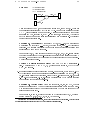
2. The model presented so far only works with linear annotation lattices. Consider the
following example using the non-linear lattice FOUR.
3 AN EXTENDED PETRI-NET MODEL
Example 4
11
(1) buy (yen) : t (2) buy (yen) : f (3) buy (yen) : >
1
2
(yen t)-
*
(yen f )
buy
(yen V ) -
3
V >
After the rings of 1 and 2, buy contains the tokens (yen t) and (yen f ). There are
two possible substitutions for V : fV=tg and fV=f g. None of them satises the guard
V >, hence transition 3 is not enabled. This is a contradiction to the xpoint
semantics of GAPs, because tft f g = >. In the example, a token (yen >) should be
in M (p) although none of the incoming transitions 1 and 2 delivered it. We call such
derived tokens reductants 7]4.
Denition 3.1 (Reductants) Given a set M = f(o1 1) : : : (on n)g of tokens and
a unication with (o1) = : : : = (on ), the token ( (o1) tf1 : : :n g) is called a
reductant. The function reductants(M) computes the set of reductants derived from
all subsets of M for which is dened.
For example ((a b) >) is a reductant of the set f((X,b),t), ((a,Y),f)g. It is important
that every annotation in M is a c-annotation to ensure that the least upper bound t
is dened. For markings M (p) this is always the case according to the next theorem.
A proof has appeared in 2].
Theorem 1 (Possible tokens of a place) Let P be a GAP and N its transformation. At all places p 2 P of N = (T P A), there are only tokens (o ) 2 M (p) with
2 T , if P is nite.
3. It is also possible to delete tokens from a place. For example, every time (a 0:5) 2
M (p) serves as a token for an enabling substitution of transition t (with hp ti 2 A),
(a 0:6) will as well but not vice versa. We say that (a 0:6) subsumes (a 0:5), because
0:6 0:5 in the lattice 0 1]. (a 0:5) might be deleted from M (p) without changing
the behaviour of the extended Petri-net.
Denition 3.2 (Subsumption) Given two tokens (o1 1) (o2 2) 2 M , the rst
subsumes the second if 1 2 and there exists a substitution such that o2 = (o1).
The function subsumption(M) computes all tokens in M which are subsumed by at
least one other token in M .
For example (a t) and (a f ) are both subsumed by their reductant (a >), whereas
subsumption(f((X b) t) ((a Y ) f ) ((a b)>)g) is empty.
Dierent from the denition provided here, in 7] derived rules are named reductants. Note that tokens
are representations for annotated atoms due to the presented transformation.
4
3 AN EXTENDED PETRI-NET MODEL
12
To summarize the three extensions presented above, we redene the update Mi+1 of the
marking Mi due to the ring of transition t 2 T :
(
Mi (p) (L(ht pi)) if p 2 t
Mi (p)
otherwise
up
up
(2) Mired
+1 (p) := Mi+1 (p) reductants(Mi+1 (p))
red
(3) Mi+1 (p) := Mired
+1 (p) n subsumption(Mi+1 (p))
(1)
Miup+1(p)
:=
With this extension, example 4 works as expected: Transitions 1 and 2 place the tokens
(yen t) and (yen f ) in p respectively. M red (p) evaluates to f(yen t), (yen f ), (yen >)g
and M (p) to f(yen >)g, which enables transition 3, since > >.
It is worth noting that our model captures the operational semantics of a GAP, which
means that if there is a GAP for which the least xedpoint reachability property does not
hold (e.g. from fp : 0 p : 1+2 x p : x q : 1 p : 1g it is never possible to answer the query
q : 1) the corresponding Petri-net cannot answer this query as well and runs forever.
The following theorems have been proven in 2] and capture the soundness and completeness of the proposed extended Petri-net model with respect to the semantics of GAPs:
Theorem 2 (Soundness) Let P be a GAP with clauses c1 : : :cn, cn a query and N
the extended Petri-net dened on P . If there is a successful ring sequence in N then
c1 : : :cn;1 j= cn.
Theorem 3 (Completeness) Let P be a GAP with clauses c1 : : :cn, cn a query and N
the extended Petri-net dened on P . If c1 : : :cn;1 j= cn , then there is a successful ring
sequence in N .
3.1.1 Algorithms for the extended Petri-net model
Before presenting algorithms for the testing for reability of a transition and updating of
the net marking, some more denitions are required.
Denition 3.3 (Unier mgua() of tokens) Tokens s = (o ) as well as arc labels con-
sist of two parts, its rst being the object part sobj = o and its second being the annotation
part sann = . Let mgu(o1 o2) denote the usual most general unier of o1 and o2 . Given
two tokens/labels s1 s2 , the most general annotational unier, denoted mgua (s1 s2), is
dened as follows:
8>
obj obj
ann ann
ann
>< mgu(s1obj s2obj ) fs2 =s1 g if s2ann is v-annotation
if s1 and sann
are c-annotations
2
mgua(s1 s2) := mgu(s1 s2 )
ann
and sann
s
>:
1
2
undefined
otherwise
obj
If mgu(sobj
1 s2 ) is not dened, mgua (s1 s2) is not dened either. Note that mgua () is not
symmetric. If mgua(s1 s2) is dened, then s1 and s2 are said to be uniable.
3 AN EXTENDED PETRI-NET MODEL
13
For example, mgua (((X a) 0:5) ((b Y ) 0:4)) = fX=b Y=ag and mgua ((a t) (a f )) is not
dened.
Denition 3.4 (Compatibility of annotation substitutions) Two substitutions
fV=ag and fV=bg, which assign dierent c-annotations a and b to the same annotation
variable V , are compatible if a and b are comparable due to the ordering of the underling
lattice. In this case their concatenation fV=agfV=bg is dened as fV= ufa bgg. This
denition is easily extended to cases with more than two substitutions.
Denition 3.5 (Concatenation of mguas) The substitutions in mguas may be divided
in object variable substitutions and annotation variable substitutions. The concatenation
1 2 n of n mgua s 1 : : :n is dened as the usual concatenation of the object variable substitutions unioned with the above dened concatenation of the annotation variable
substitutions.
The following algorithms do not use the notion of transition guards. Instead they are
specialized for the bottom-up evaluation of annotated programs encoded in Petri-nets. The
guards are implicitly checked in the mgua -routine dened above.
Testing for reability of a transition
Input: Extended Petri-net N = (P T A)
Transition c 2 T
Output: Maximal set of mguas each enabling c. c is not enabled if the set is empty.
:= fg
( is a set of sets of possible substitutions for c)
for all arcs a 2 IN (c) do
a be (p c) 2 A)
'a := fg ('a is the set of all possible substitutions according to a)
(Let
for all tokens s 2 M (p) do
if unifiable(s L(a)) then 'a := 'a mgua(s L(a))
if 'a = fg then return fg
:= 'a
(Let
be f'1 : : : ' g)
:= fg
( is a set of all enabling substitutions for c)
for all permutations (1 : : :jj) with i 2 'i 2 (1 i jj) do
if 1 : : :jj are compatible in pairs then := 12 jj
return j
j
Firing of a transition
Input: Extended Petri-net N = (P T A)
Transition c 2 T Set of c-enabling substitutions
Output: N with updated marking using every 2 3 AN EXTENDED PETRI-NET MODEL
14
for all arcs a 2 OUT (c) do
(Let
a be (c p) 2 A)
for all 2 do
M (p) := M (p) f(L(a))g
M (p) := M (p) reductants(M (p))
M (p) := M (p) n subsumption(M (p))
See 9] for algorithms implementing reductants() and subsumption(). The algorithms
are based on the rather descriptive than procedural algorithms in 2], which need two minor
corrections: Firstly, in 2] the initial marking is empty. This leads to incompleteness,
because even without any fact, the bottom element P : uT of any predicate p is derivable.
Secondly, the testing for reability on page 19 needs to be modied in step 2 in the following
way:
2. Compute for all i (1 i n) sets Mij = f(tP1 i P1 i : : : (tPnji Pnji )g of tokens of the
i
i
place Pi (ei = hPi ki) and a substitution ji for every set Mij such that the following
conditions hold:
(a) ji = unifier(ti tP1 i : : :tPnii )
(b) ci t(P1 i : : :Pnii )
(c) i = 1i ji if 1i : : : ji are compatible in pairs.
(d) = 1 i if 1 : : : i are compatible in pairs.
(e) There is no 0 > which satises (a)-(d).
The main procedure checks in each step for an arbitrary transition t whether any of its
input places p 2 t contains new tokens relative to the last step. If not, it checks another
transition and stops, if no transition satises this condition, because this means, that no
new useful token was produced in the last step, therefore the xpoint is reached. If on the
other hand a transition is found, it is red if it is enabled. Then the next step is taken.
There is an indeterminism in choosing an arbitrary transition in the beginning of each new
step. This choice should be fair, i.e. every transition is checked a nite count of steps after
it has been checked last. See also section 5.1 for a discussion of this point.
Main procedure
Input: Extended Petri-net N = (P T A) with initial marking
Output: N with marking which represents the xpoint
iterate through all t 2 T
if 9p 2 t with new tokens since last ring of a transition then
if t is enabled then
re t
restart iteration
3 AN EXTENDED PETRI-NET MODEL
15
3.2 Normal GAPs
This section describes a method how to handle non-monotonic modes of negation based
upon the well-founded semantics in the extended Petri-net formalism, using a direct implementation of the alternating xpoint computation. The reader may also refer to 8] for a
similar presentation not based on Petri-nets.
The transformation of a normal GAP to an extended Petri-net N = (P T A) is performed as follows: Every negated atom of the form not p is treated as a new, not negated
atom `not p`, i.e. for every predicate a dual negative predicate is added to the vocabulary.
This transforms the normal GAP into a negation-free GAP. The set of places P is therefore
divided into two sets: P + , containing the positive literals, and P ; , containing the previously negative literals, such that P = P + P ; . The transformation process is similar to
the one described in section 3.1, but with the following dierences:
For every clause c of the form
p0 (o0) : 0 p1(o1) : 1 ^ : : : ^ pm (om) : m
and 1 i m, the net contains the arcs ai := hpi ci with the labels L(ai) := (oi i)
where i is a new variable annotation. In case that i is a c-annotation: If pi 2 P + ,
then i i is added as a conjunctional condition to the guard of transition c
otherwise if pi 2 P ; , then i i is added to the guard. In addition, the net
contains the arc a0 := hc p0i with the label L(a0) := (o0 0) where 0 is dened as
in section 3.1.
The initial marking is 8p 2 P + : M0(p) = f(X uT )g, and 8p 2 P ; : M0(p) =
f(X tT )g, where X is a new variable for each p.
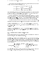
Additionally, new transitions T will be introduced, as shown in example 5:
Given two dual places p 2 P + and not p 2 P ; , a transition c 2 T is added to T
with an empty guard. The arcs hp ci and hc not pi, both with labels (X V ) with
new variables X and V , are added to A. If such a transition res, all tokens from p
are moved to not p.
Example 5
(1) p(a) : 0:3 (2) p(a) : 0:7 not p(a) : 0:5 ^ p(a) : 0:2
not p
(X V )
c
(X V )
(a 0:3)
1
(a V )
(a W )
p
(a 0:7)
2
V 0:5
W 0:2
3 AN EXTENDED PETRI-NET MODEL
16
The following algorithm schema describes, how to compute the well-founded model:
1. Compute the xpoint as described in section 3.1 without ring any transition from
T . This realizes SP .
2. Transfer all tokens along the transitions in T , i.e.:
Delete all tokens out of places in P ; .
Fire every transition in T .
Delete all tokens out of places in P + and restore the initial marking in these
places.
This performs S~P .
3. Redo these two steps. This results in S~P (S~P ).
4. If the outer xpoint is not reached, go to step 1. To test this, the marking needs to
be saved to compare it to the new marking after step 1.
5. The xpoint is reached. Take step 1 one more time. The resulting marking represents
the well-founded model.
The following table demonstrates the algorithm referring to example 5:
Step Marking
p(X ) : 0:0 not p(X ) : 1:0
1 p(a) : 0:3 not p(X ) : 1:0
2 p(X ) : 0:0 not p(a) : 0:3
1 p(a) : 0:7 not p(a) : 0:3
2 p(X ) : 0:0 not p(a) : 0:7
1 p(a) : 0:3 not p(X ) : 1:0
2 p(X ) : 0:0 not p(a) : 0:3
1 p(a) : 0:7 not p(a) : 0:3
2 p(X ) : 0:0 not p(a) : 0:7
1 p(a) : 0:3 not p(a) : 0:7
Initialisation
(1) res
(c) res
(1)+(2) re
No xpoint
The same four steps repeated
Fixpoint reached
Well-founded model
This procedure has some problems: Tokens need to be deleted explicitly and two dierent
ring semantics need to be observed. Also transitions are locked and unlocked periodically.
After all, this results in something very dierent from Petri-nets. To check whether the
xpoint was reached, many tokens need to be remembered and compared. To implement
this, it will be best to divide every place from P + in two parts, one storing S~, the other
S~(S~). The solution in 8] bares the same disadvantages.
An alternative solution is described in 16]. This is more closely to Petri-nets, but adds
inhibitor arcs and requires the explicit computation of the greatest deadlock of the net to
obtain the unfounded set of a program: A non-empty subset S P of places in a Petri-net
is called a deadlock, if every transition having an output place in S has an input place in S .
Note that in this approach enabling tokens will be removed if a transition res, according to
the denition of the update of markings in ordinary Petri-nets. The greatest disadvantage
4 GAPCAD - ARCHITECTURE
17
of the approach in 16] is the translation schema: Every place represents a ground atom
rather than a predicate, which makes it of little use for graphical applications addressed in
this report.
To summarize, there is no known elegant method for Petri-net computation of the wellfounded model of normal programs. In the next section, a tool implementing the routines
in section 3.1 is presented. It does not allow normal programs and therefore does not
implement the well-founded semantics, due to the problems encountered above.
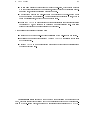
4 GAPCAD - Architecture
GAPCAD is the implementation of the procedures presented in section 3.1. This chapter
briey reviews the concepts behind GAPCAD.
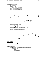
Figure 2: Screendump of the GAPCAD user interface with a well-known problem. The
current tokens in place flies are shown at the right bottom. At the top, a control panel
presents the features described in the text
GAPCAD oers the following features:
One can draw a Petri-net and save it as a kind of painting, or load a GAP-program
4 GAPCAD - ARCHITECTURE
18
in DAEDALUS syntax. In the latter case the net is automatically being drawn in the
window as a Petri-net. Guards need not be typed. They are automatically derived
from the arc labels.
After nishing the drawing, the graph needs to be compiled into the internal extended
Petri-net structure. Syntax errors are located.
After compiling, one can
{ start the bottom-up procedure described in chapter 3.
{ start DAEDALUS, assuming a query (transitions without outgoing arcs) was
entered.
{ save the net as a GAP in DAEDALUS syntax.
During the bottom-up procedure
{ every ring transition highlights.
{ the tokens in any place are shown, if requested.
{ a transition can manually be forced to re.
The features of the graph editor are preserved.
See the GAPCAD manual included in the distribution for detailed descriptions.
Gapcad-Extensions
(Frames, Menus, etc.)
Graph editor
(GraphEd)
gapcad2ui
ui2gapcad
GAPCADcore
inheritance
DAEDALUS
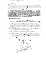
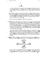
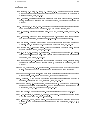
Figure 3: The GAPCAD architecture
GAPCAD is a graphical user interface to DAEDALUS. Therefore the system can be
divided in three parts as illustrated in gure 3:
1. DAEDALUS 9] provides generic object data classes and lattice classes, and concepts
like predicates, literals, substitutions, etc. GAPCAD uses heavily DAEDALUS-code
for those basic GAP-functions like unifying, computing the least upper bound and so
on.
2. The graph editor provides a front-end for entering Petri-nets. GraphEd 5] was chosen,
because
4 GAPCAD - ARCHITECTURE
19
it is generic in the sense that it provides application interfaces for adding domain
specic functionality.
it is easy to use.
it is public domain.
Unfortunately some code had to be added in the core of GraphEd to provide an even
easier entering of Petri-nets, for example using the left and right mouse buttons to
create places and transitions or suppressing attempts to connect two places. It was
also important to ensure consistency between the GraphEd- and the GAPCAD data
structures, for example token windows need to be deleted as soon as the corresponding
place is deleted.
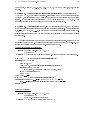
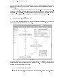
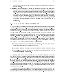
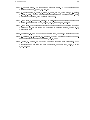
3. The GAPCAD-core itself has its own data structure. While running the bottom-up
procedure it needs to be consistent with the GraphEd data structure (for example to
highlight a transition) as well as the DAEDALUS data structure (for example to use
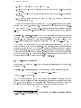
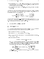
the routines for unifying). Figure 4 shows the relevant classes.
ISA
HAS-A (with cardinality)
Points-to
Net
Graph
Node
Node
n
Xclause
Transition
1
n
Pred
Place
1
n
Literal
Arc
Edge
1
QSolRoot
DAEDALUS
Tokenlist
GAPCAD-Core
GraphEd
Figure 4: The GAPCAD class structure
One goal was to separate the graph editor from the GAPCAD-core as far as possible to
make it easily possible to use another editor. Two interfaces were dened:
gapcad2ui:
This contains procedures which GAPCAD provides for the editor such as creating and deleting nets/places/transitions/arcs, ring of transitions, starting Daedalus/
bottom-up evaluation, loading/saving/printing the GAP, etc.
ui2gapcad: This species services which the editor needs to provide, such as displaying new
nodes and edges, highlighting of a node, setting labels or refreshing token windows.
Some extensions of GAPCAD would be useful:
5 FURTHER ISSUES
20
Currently no parallelizing is supported. Every enabled transition is immediately red.
It would be interesting to compute the conict set of transitions which are enabled see
also chapter 5.1. It would be easy to implement this, because there are two dierent
procedures for checking for reability and ring of a transition.
For a more e"cient computation, it would be useful to switch of the graphical representation completely.
It could be interesting to examine the ring sequence as a list.
In 23] and 12] a Petri-net based validation check of rule-based programs is described.
Integration in GAPCAD should be easy because of the simple class structure.
Unfortunately GraphEd provides no graph overview facility. For large GAPs the
graph becomes too complicated. Also the automated graph drawing of a loaded GAP
is far from optimal.
For more easy entering of graphs, it would be useful to implement hierarchical coloured
Petri nets 6].
5 Further issues
In this chapter, two further subjects are addressed: 1. control ow specication and 2.
GAPCAD as a knowledge acquisition tool.
5.1 Control ow specication
From a software engineering point of view, the extended Petri-net model species the data
ow. The places are data containers and the transitions represent the operations on the
data, especially if the guards contain more complex functions. On the other side no control
ow specication is given. Each enabled transition may (but need not) re, which causes
indeterminism. This is sound according to the xpoint-semantics 2]. A specication of
the control ow, i.e. the determination which of the enabled transition re in any state of
the net, is not necessary. It could even make the extended Petri-net model incomplete, if
it never allows a particular transition to re, which contribution to the xpoint set is not
empty. This shows that a control ow specication needs to satisfy some conditions. For
example it needs to be fair, i.e. every enabled transition res sometime until the xpoint
is reached.
However, explicitly specifying the control ow has two advantages:
1. E"ciency: Even if a transition is enabled, its ring does not necessarily enlarge the
xpoint set. If a query has been stated, the point becomes obvious. Consider as an
example the following program:
p(X ) q (X )
q (a)
q(b)
()
5 FURTHER ISSUES
21
q (c)
..
.
Query : p(a)
The query is answered in two steps, but a pure bottom-up procedure computes the
whole model. A possible way to resolve this overhead is the magic set approach 1],
where the clause () would be rewritten to p(a) q (a), depending on the known
query.
2. Side eects: Consider the case where the ring of a transition causes a side eect
output to the screen. In the most cases the user is only interested in the nal solution,
not in several in-between results, so this transition should re as late as possible. This
can only be achieved if the control ow is explicitly specied. Of course, this argument
is not a theoretical but a practical one.
There are at least three possibilities to describe the control ow:
Firm strategy Production systems, which also work in a bottom-up manner, usually re-
solve the conict that arises if more then one rule at the time is ready to re, via some
heuristics like "Take the most recent enabled rule" or "Take the rule with the largest
number of premises" or so. In GAPCAD a rather simple conict resolution is implemented: It iterates through the set of transitions. If the current transition t is enabled
and some new token is in any of the places in t, it res and the iteration restarts.
This algorithm terminates because the xpoint is reachable and its occurrence causes
no new token being in any place.
There is one major disadvantage in completely specifying the control ow: Two transitions being enabled at the same time express the possibility to re them in parallel.
There is not always the need to completely sequentialize the order of ring. In the
case of Petri-nets, a control specication should be better viewed as a restriction of
freedom, rather than a total sequentialisation. The next two techniques take this into
account.
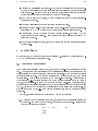
Petri-nets We used the Petri-net model to dene the data ow, although Petri-nets usually
specify the control ow. It is possible to unify both applications: Orthogonally to the
controlplace
control flow
dataplace
data
flow
dataplace
controlplace
data ow we embed the transitions in a second Petri-net where the places contain
control tokens. A transition may be enabled only if its input control-places contain
tokens. In 3] it is shown that as soon as the control ow gets more complex, Petri-nets
5 FURTHER ISSUES
22
tend to be di"cult to survey, so this kind of control ow specication appears to be
not very natural.
Priorities In 3] it is suggested to express the control ow through dynamically given
priorities between transitions or temporally locks of transitions. If two transitions are
enabled, the one with the higher priority res (if it is not locked), while the other has to
wait. If the two have the same priority they do both re in parallel. These priorities
may change on certain events like a counter reaching zero, an external condition
becoming true, time constraints, etc. The reader may refer to 3] for more ideas.
This seems to me the most promising approach for control specication, although
dynamically changing priorities may lead to confusion about what state the net is
currently in.
5.2 GAPCAD as a knowledge acquisition tool
KADS (Knowledge Acquisition and Design Structuring) 22] is a methodology for developing
knowledge-based systems (KBS). Its emphasis lies on dening a language for semi-formal
specication of KBS. Neither any knowledge elicitation technique nor implementational
details are covered. KADS oers some abstract templates (called models) which need to
be lled during the specication phase. A central model is the model of expertise which
describes the contents of the knowledge base of the KBS in (essentially) three parts, called
layers: 1. Inference Layer, specifying the data ow, 2. Task Layer, specifying the control
ow, and 3. Domain Layer, specifying the kinds of data. The KADS methodology is widely
used for new developments in the eld of knowledge based systems. Many knowledge
acquisition tools are based on the KADS methodology. It would be interesting to examine,
how well GAPCAD meets the requirements of KADS-tools, since
annotated programs form a logic programming language, which are widely used as
prototyping languages for the development of KBS,
the institute is looking for tools which aid in developing mediatory knowledge bases,
the Petri-net model is very similar to the description of the inference layer in KADS.
This point is discussed in the sequel.
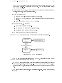
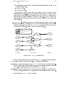
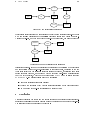
The inference layer of the model of expertise in KADS contains a description of the data
ow in the KBS to be developed. Its graphical representation (called inference structure)
contains meta-classes (squares) { the data and knowledge sources or inference steps (circles)
{ the operations on the data. See Figure 5 as an example for an inference structure. It
shows the data ow in a generic conguration task 15]. Notice the similarity to Petri-nets:
meta-classes are places and knowledge sources are transitions, but one should notice the
dual graphical syntax: circles are squares and vice versa. The semantics of the inference
structure is not formally specied in KADS. The syntactical equivalence between the two
was used in MoMo 21].
However, as our extended Petri-net model represents specic program clauses on the
symbol level, the inference structure in KADS describes "only" the very idea, how the
expert performs the (conguration) task on the knowledge level 14]. Further renement of
6 CONCLUSION
23
user
specs
skeletal
model
propose
design
extensions
init
extended
model
verify
violation
revise
Figure 5: A top level inference structure
the inference structure leads to more special and nally to atomic inference steps. In Figure
6 a more detailed description of the propose knowledge source from Figure 5 is shown.
Coloured Petri-nets, on which the extended Petri-net model is based, can also be dened as
parameter
select
specify
extended
model
skeletal
model
design
extensions
Figure 6: Renement of inference step 'propose'
hierarchical nets 6]. It would be interesting to investigate the possibility of a graphically
and semantically unied top-down-construction of knowledge bases, beginning at the top
(knowledge level) with the inference structure similar to Figure 5, applicating some local
renements as in Figure 6, and ending up with an extended Petri-net as a representation
for GAPs (symbol level), which can be debugged using GAPCAD and e"ciently executed
by DAEDALUS. Some related issues need to be addressed:
Are atomic inference steps really clauses?
Where do the arc labels t in? What is their interpretation on the knowledge level?
How can nets with non-atomic transitions be executed? 11]
6 Conclusion
This report described the theory and the implementation of an executable graphical representation of generalized annotated programs using the notation and semantic of Petri-nets.
The following topics were addressed the rst time:
6 CONCLUSION
24
The formalism presented here is based on Coloured Petri-nets, which provide a natural
way to express constraints on the annotations, using the concept of transition guards.
In 2] and 13], predicate/transition nets 4] were used.
An execution model for the Petri-net based computation of the well-founded model
of normal programs was presented. Another alternative is described in 16], which is
based on classical logic, rather than on annotated logic.
Finally the GAPCAD implementation provides an interesting graphical user interface
for entering GAPs, and serves as an basis for a more sophisticated tool. Promising
ideas in this direction were also presented in this report.
Three possible future research direction are:
Development of a better Petri-net based realisation of the well-founded semantics.
Provision of more support for entering GAPs for DAEDALUS (especially for the sorts
of the predicates).
Viewing GAPCAD in a more general frame for support of knowledge acquisition along
the lines of 21] and 22].
Acknowledgements I'd like to thank Joachim for supervising and supporting this
work, Michael Himsoldt for providing GraphEd and especially Peter for many quick respondings to my never-ending wishes, remarks and misunderstandings concerning DAEDALUS.
REFERENCES
25
References
1] Bancilhon, F., Maier, D., Sagiv, Y., Ullman, D.D. Magic Sets and other strange
ways to implement logic programs Proceedings of ACM Symposium on Principles of
Database Systems, 1986, pp. 1-15
2] D. Debertin. Parallizing inference in distributed knowledge based systems. Master's
thesis, Institute of Algorithms and Cognitive Systems, University of Karlsruhe (in
German)
3] F. Gebhardt, E. Gro%, H. Vo%. Concurrency constraints as control specications for
the MoMo language FABEL Report No.21, GMD Sankt Augustin, 1994
4] H.J. Genrich. Predicate/Transition nets. LNCS 254, Springer-Verlag, 1987 pp. 207247
5] M. Hemsoldt. GraphEd User Manual, and Sgraph 3.1 Programmers Manual Included
in GraphEd distribution, available at ftp.uni-passau.de in pub/local/graphed.
6] Kurt Jensen. Coloured Petri Nets: A High Level Language for System Design and
Analysis. in: G. Rozenberg (Ed.): Advances in Petri Nets 1990, pp. 342-416
7] Michael Kifer, V.S. Subrahmanian. Theory of Generalized Annotated Logic. Journal
of Logic Programming 12, 1992, pp. 335-367
8] D.B. Kemp, P.J. Stuckey, D. Scrivastava. Magic Sets and the Bottom-up Evaluation of the Well-founded Model. Logic Programming: Proceedings 1991 International
Symposium, San Diego, pp. 337-351
9] Peter Kullmann. SLG-Resolution for Generalized Annotated Logic. Master's thesis,
Institute for Algorithms and Cognitive Systems, University of Karlsruhe, 1995 (in
German)
10] Jim Lu, Anil Nerode, V.S. Subrahmanian. Towards a Theory of Hybrid Knowledge
Bases. To appear in IEEE Transactions on Knowledge and Data Engineering
11] Frank Maurer. Hypermedia-based Knowledge Engineering for Distributed Knowledge
Based Systems. Diss. thesis (in German), inx Sankt Augustin 1993
12] P. Meseguer. A new method to checking rule bases for inconsistency: a Petri Net
approach. Proceedings of ECAI, Stockholm, 1990, pp. 437-442
13] Tadao Murata, V.S. Subrahmanian, Toshiro Wakayama. A Petri Net Model for Reasoning in the Presence of Inconsistency. IEEE Transactions on Knowledge and Data
Engineering, Vol3, No.3, September 1991, pp.281-292
14] Allen Newell. The Knowledge Level. Articial Intelligence 18(1982) pp.82-127
15] A. Th. Schreiber, P. Terpstra, P. Magni, M. van Velzen. Analysing and Implementing
VT Using CommonKADS. KADS-Workshop.
16] T. Shimura, J. Lobo, Tadao Murata. An Extended Petri Net Model for Normal Logic
Programs. IEEE Transactions on Knowledge and Data Engineering, Vol. 7, No. 1,
Feb. 1995
REFERENCES
26
17] V.S. Subrahmanian. Amalgamating Knowledge Bases. ACM Transactions on
Database Systems 19,2, 1994, pp. 291-331
18] V.S. Subrahmanian, S. Adali, A. Brink, R. Emery, Jim Lu, Adil Rajput, T.J. Rogers,
R. Ross, C.Ward. HERMES Heterogeneous Reasoning and Mediator System. Draft,
University of Maryland, 1995 Available via WWW.
19] A. van Gelder, K. Ross and J. Schlipf. The Well-founded Semantics for General Logic
Programs. Journal of the ACM, Vol. 38, No. 3, July 1991, pp. 620-650
20] A. van Gelder. The Alternating Fixpoint of Logic Programs with Negation (Extended
Abstract) Proc. 8th Symposium on Principles of Database Systems, March 29-31,
Philadelphia 1989
21] J. Walther et. al. MoMo GMD Sankt Augustin 1993, Germany. Available via WWW
22] B.J. Wielinga, A.T. Schreiber, J.A. Breuker. KADS: A Modelling Approach to Knowledge Engineering Knowledge Acquisition, 4:5-53, 1992
23] D. Zhang, D. Nguyen. PREPARE: A Tool for Knowledge Base Verication. IEEE
Transactions on Knowledge and Data Engineering, December 1994, Vol. 6, Number
6, pp. 983-989