Download Improving Throughput in Network Analyzer Applications

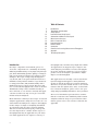
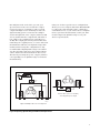
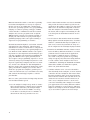
Agilent AN 1287-5
Improving Throughput in Network
Analyzer Applications
Application Note
Table of Contents
2
3
5
12
13
15
18
20
20
20
21
22
23
Introduction
In today’s competitive environment, prices for
electronic components are continually decreasing.
Reducing manufacturing cost by improving throughput, while maintaining product quality, is an important goal for many production test engineers and
managers. The topic of improving throughput is
very broad, and it can span methods from how to
minimize testing and the number of specifications
to using just-in-time (JIT) manufacturing with a
Kanban inventory-control system. This note will
not cover broad throughput issues such as whether
distributed testing versus centralized testing is
more efficient or cost effective. Instead, this application note will focus only on test processes that
include network analyzers.
Even within the relatively focused topic of network
analyzer applications, many factors need to be considered when deciding how to improve throughput.
It isn’t always as simple as analyzing instrument
specifications and choosing a network analyzer
with the best measurement speed per data point.
It is also important to consider all the aspects of
throughput that may be applicable for your situation. This application note explores a variety of
2
Introduction
Throughput Considerations
Sweep Speed
Instrument State Recall Speed
Automation and Data Transfer Speed
Measurement Accuracy
Device Connection Time
Instrument Uptime
Product Quality
Conclusion
Checklist for Increasing Measurement Throughput
Appendix
Third-Party Companies
throughput issues and how they might affect different applications. It suggests ways to improve network analyzer performance for better throughput
in specific situations, and how to get an accurate
picture of how an analyzer’s performance might
impact overall throughput.
This application note broadly covers network analyzer throughput and applies to many different
models of Agilent Technologies network analyzers.
Therefore, for specific details on how to use certain
features with the Agilent 8753, 8711, or 8720 families of network analyzers, please refer to the operating and programming manuals for these products.
The level of information presented here assumes
that the reader has some familiarity with network
analyzers and their usage. If you need basic information, please refer to the references listed in the
appendix.
Throughput Considerations
When considering throughput, it is important to
examine the overall measurement process, which is
likely to consist of a number of steps. For example,
a production line might have a process where operators use network analyzers to perform manual
tuning on filters. The process might include connecting a filter, recalling a test setup (or instrument
state) on the analyzer, tuning, and watching for a
desired result (indicated perhaps by markers that
display values, or limit lines that display whether
a device passes or fails). More tuning might be necessary, then the operator might move on to a different instrument state to tune another parameter,
and so on. (See Figure 1.)
Connect Tx, Ant filter
ports to analyzer
15 sec
Recall instrument
state and calibration
3 sec
Total for multiple
measurements
and adjustments:
90 sec meas. time
210 sec adjust. time
Adjust screws to
tune Tx -> Ant path
Connect Ant, Rx ports to analyzer;
Recall new state and calibration
Total for all measurements
and adjustments:
90 sec meas. time
210 sec adjust. time
Adjust screws to
tune Ant->Rx path
Connect Tx, Ant ports to analyzer;
Recall Tx->Ant state and cal
Measurement
OK?
15 sec connection
3 sec recall
This is a simplified example of a
manual tuning process for a base
station duplexer filter. The filter
is a 3-port device with two main
signal paths of interest: the one
between the transmit (Tx) and
antenna (Ant) ports, and the one
between the Ant and receive (Rx)
ports. With a standard two-port
network analyzer, two filter ports
are measured at a time, with a
load (termination) connected to
the unused port. Some steps have
been left out for simplicity.
15 sec connection
3 sec
NO
Measurement time
28%
Recall 2%
Connection
YES
Lock adjustment
screws
Verify Tx -> Ant measurements
Recall instrument state
and cal for Ant -> Rx
Verify Ant -> Rx measurements
Disconnect filter
Another example is an automated final test that
uses a part handler. Here the process might include
the part handler placing a part in a test fixture,
setting up an instrument state, taking data, transferring data to a PC, having a PC perform calculations or store data to a file, and then setting up
an analyzer for the next test. The instrument-state
setup might be done by recalling an instrumentstate file that had previously been set up and stored,
or the PC could issue commands to the analyzer
to set up the desired conditions.
8%
60 sec
Total for all tests:
20 sec
Adjustment
62%
3 sec
Total for all tests:
20 sec
15 sec
This pie chart shows that with
one pass of tuning, measurement
time is only about one-quarter of
the total throughput time.
Figure 1. Example Manual-Tuning Process for a Base-Station Filter
3
These two examples demonstrate how throughput
issues might be different in various applications.
For manual tuning, faster sweep speed is important. However, once the user perceives a continuous update of data (approximately 30 updates per
second), any faster update speed would not be
noticeable or result in a increase in filter throughput. Conversely, faster sweep speed could be useful
in automated testing where a computer is faster
than an analyzer. Part-handler speed and datatransfer speed are not relevant to the manual tuning application, but the time needed to manually
connect the test device is relevant. The time
required to recall or set up an instrument state
is important in both applications.
It is also important to consider the relative importance and value of improving each part of the
process. Many people focus on the sweep time of a
network analyzer when trying to improve throughput, but improving sweep time alone does not
always provide the best throughput improvement.
For example, in a multiport test application, if it
takes the operator 1.5 minutes to connect a new
device into place, while the analyzer takes 10 seconds to perform the test, then cutting the analyzer
test time in half only reduces the total test time
from 100 seconds to 95 seconds for a 5% improvement. However, reducing the device connection
time to 1 minute will reduce the total test time
to 70 seconds, which is a 30% improvement.
4
The complete test process might include additional
items such as calibration time that are not part of
testing every device, but they might need to be done
occasionally and will affect the overall throughput.
Calibration time can range from a few minutes for
a simple one-port calibration to several hours for
a series of two-port calibrations for testing a high
dynamic-range multiport device.
For this application note, throughput considerations are divided into the following topics:
•
•
•
•
•
•
•
Sweep speed
Instrument state recall speed
Automation and data transfer speed
Measurement accuracy
Device connection time
Instrument uptime
Product quality
Each topic will be described in greater detail and
suggestions for improving throughput in each area
will be provided.
Sweep Speed
Sweep speed (also referred to as sweep time) can
be a confusing term; not everyone means the same
thing when referring to sweep speed. In general,
sweep speed refers to the amount of time needed
for the analyzer to take one sweep of the source
and acquire data over the defined range. Many
analyzers’ technical specifications report a number in the form of time per data point, which one
might assume would yield the sweep time when
multiplied by the number of points in a trace. Many
instruments also have a function that reports
a value for hardware sweep time. However, users
may never get this sweep time in their measurements, because in reality what they will get is
the “cycle time.” This cycle time includes sweep
(hardware) set-up time, band-switch times (when
the source or receiver crosses frequency bands),
data-acquisition time, retrace time (for the source
to move from the end of one sweep to the start
of the next one), data-calculation and formatting
time, and display update time (see Figure 2). Also,
error-correction time might not be included, and
if two-port calibration is used, the analyzer might
need to take two sweeps instead of one for each
display update (see the “Measurement Accuracy”
section for more details on calibration). So, for
the purpose of consistency in this application
note, “sweep speed” refers to “cycle time” unless
otherwise stated.
,,,
,
,,,,
Data calculation
and formatting
Sweep and data acquisition
Also, it is important not to assume that an
analyzer’s sweep speed under actual test conditions will be the same as the time-per-point number published in the technical specifications. In
most technical specifications, the value reported
is a best-case number. Often it is measured at the
instrument’s widest IF bandwidth (which might
have too much trace noise and too little dynamic
range to be useful), with a single-band sweep to
avoid band switch delays, and with the highest
number of points (to spread out the effects of overhead items such as sweep set-up time and obtain
the smallest time value per point). Actual sweep
speed is closely tied to an instrument’s set-up
parameters, including the number of points and
frequency range, and the degree of accuracy and
amount of dynamic range required (which also
impact the type of calibration necessary).
Display
update
Band switches
Retrace
(Diagram not to scale)
Figure 2. Components of Cycle Time
5
Here are some ideas to optimize sweep speed and
cycle time.
IF Bandwidth: Use the widest IF bandwidth with
acceptable dynamic range and trace noise.
Wider IF bandwidths result in faster measurements, but they also give you more trace noise
(ripples in high-power-level measurements) and
higher noise floor (less dynamic range). Typically,
a ten-fold reduction in IF bandwidth will give
you a 10 dB reduction in the noise floor. Use the
widest IF bandwidth that will give you reasonable
results, especially with regard to trace noise and
dynamic range. Figure 3 shows an example of
some typical relationships between IF bandwidth,
trace noise, and sweep speed for the Agilent 8753E
RF network analyzer.
Note that narrowing the IF bandwidth in some
Agilent network analyzers such as those in the
8753 and 8720 families has the same effect as
increasing point-by-point averaging in other analyzers such as the 8510. In the 8753 and 8720
families, the averaging feature performs a traceby-trace average. Refer to the operating manuals
for these analyzers for more details.
Test Set Changes: Consider special test set configurations
for higher dynamic range.
If a lower noise floor is required only in the forward direction, you can configure the test set to
bypass the usual coupler loss on port 2 for transmitted signals. The Agilent 8720D family provides
this capability with Option 012, direct sampler
access. As shown in Figure 4, you can connect the
output of your device under test directly into the
B sampler, instead of to port 2. This direct connection increases your dynamic range by about 20 dB,
which is the amount of the coupling loss.
Agilent 8753E Full 2-port Cal Sweep Update Time (201 points)
Sweeps per second
8
6 kHz
IF BW
7.5
7
6.5
3.7 kHz
IF BW
6
5.5
5
4.5
4
0.015
3 kHz
IF BW
0.02
0.025
0.03
0.035
Typical Trace Noise (dB peak-to-peak)
0.04
Figure 3. IF Bandwidth vs. Trace Noise and Sweep Speed
6
0.045
For analyzers such as the 8753, you can get a
special version of the test set with the coupler
reversed on port 2 (see Figure 5). The reversed
coupler will improve the sensitivity because the
signal entering port 2 is routed to the sampler
via the through arm of the coupler (with a few dB
of loss) rather than the coupled arm, which has a
loss equal to the coupling factor (typically 15 to
20 dB). The output power from port 2 will now be
reduced by the coupling factor, so reverse direction
measurements will have less dynamic range than
normal, which is why this configuration is only
recommended if high dynamic range is needed in
one direction. The same noise floor improvement
can be obtained for measurements in the reverse
direction by reversing the port 1 coupler (with the
corresponding loss of dynamic range for forward
measurements).
Using one of these special test set configurations
allows you to use a higher and faster IF bandwidth
to achieve the same dynamic range compared to
a standard test set, so you can use these configurations to get faster measurements even if you don’t
need the improved dynamic range to test your
device’s specifications.
Source
R
A
Transfer
switch
B
Samplers
R
A
B
Measure filter rejection to -120 dB by
connecting directly to B sampler
Samplers
Port 1
Port 2
R Channel
Jumper
Agilent 8720D Option 012 Test Set Configuration
Figure 4. Improving Dynamic Range with Direct Sampler Access
7
Source power: Use the highest source power that does
not overload the device or network analyzer.
To extend the upper limit on dynamic range, use
the highest source power from the network analyzer
that will not overload the device under test or
cause the analyzer’s receiver to overload.
Frequency span: Choose smaller frequency spans that
minimize the number of band switches.
Test only the frequency spans that are necessary
for your device. Information on the band switch
frequencies for each network analyzer can usually
be found in the operating or service manual.
Number of points: Use the minimum number of points
required for the measurement.
For most analyzers, sweeping fewer points results
in less time per sweep. However, network analyzer
sources have a maximum sweep rate limited by
the hardware. Once this limit is reached, reducing
the number of points will not further reduce the
sweep time.
List frequency sweep: Use list mode to focus test data
where you want it.
List frequency sweep allows you to define an arbitrary list of frequency points at which the analyzer
makes measurements. This capability is useful for
optimizing sweep time, because you can choose a
larger number of sweep points in frequency ranges
of interest, while minimizing the number of points
for ranges that are not as important.
Source
Source
Transfer
switch
Transfer
switch
R
R
A
A
B
Samplers
Samplers
Port 1
Port 2
R Channel
Jumper
Port 1
Typical standard test set configuration
Figure 5. Improving Dynamic Range with a Reversed Port-2 Coupler
8
B
Port 2
Test set with port 2 coupler reversed
R Channel
Jumper
For example, in a filter measurement, you might
choose to measure many points in the reject bands
and in the passband, but very few points on the
skirts of the filter. The frequency list can even
skip over frequency ranges where no data is needed.
This will enable you to get the detail you want,
with fewer total points measured. Also, you can
choose to sweep a single segment in the list without losing calibration or needing to interpolate
the calibration data.
Some network analyzers such as the Agilent 8753E
also offer an enhanced version of this mode that
provides two additional features:
a. Swept list mode: Many network analyzers normally
default to a stepped sweep mode when list frequency is used, which slows the analyzer down.
In swept list mode, the network analyzer sweeps
a segment instead of stepping the source, resulting in a faster measurement.
b. Ability to change IF bandwidth and power level for
each segment: For regular list frequency mode,
the same IF bandwidth and power level are used
for all segments in the sweep. Swept list mode
includes a feature that allows you to choose a
higher power level and smaller IF bandwidth in
segments where better dynamic range is needed,
such as in the reject bands of a filter. You can
use a wider IF bandwidth and lower power for
faster measurements in segments with high-level
(low loss) signals, such as in the passband of a
filter. The ability to change power levels can be
especially helpful for a device such as a filter
combined with a low-noise amplifier, where high
power is desired for measuring the reject bands,
but lower power is needed in the passband to
avoid damaging the amplifier or the analyzer’s
receiver. When the best dynamic range is not
needed, you can also use higher power with a
wider IF bandwidth for measuring filter stopbands to provide adequate dynamic range while
sweeping more quickly.
Segment 3: 29 ms
(108 points, -10 dBm, 6000 Hz)
CH1 S 21
log MAG
12 dB/
REF 0 dB
PRm
Swept-list sweep: 349 ms
(201 pts., variable BW's & power)
Linear sweep: 676 ms
(201 pts., 300 Hz, -10 dBm)
PASS
Segment 5: 129 ms
(38 points, +10 dBm, 300 Hz)
Segment 1: 87 ms
(25 points, +10 dBm, 300 Hz)
START 525.000 000 MHz
No specs here, so no points
measured in this span
STOP 1 275.000 000 MHz
Segments 2,4: 52 ms
(15 points, +10 dBm, 300 Hz)
No specs here, so no points
measured in this span
Figure 6. Linear Sweep vs. Swept List Frequency Filter Measurement
9
Averaging: Use the minimum number of averages
necessary for the measurement.
Averaging can be useful for reducing noise and
improving dynamic range. But it might also be
helpful to compare the effects of using a narrower
IF bandwidth versus averaging to achieve the
same noise reduction to see which yields a faster
measurement.
Type of calibration: Choose the fastest type of calibration
for the required level of accuracy.
For most network analyzers, sweep speed is about
the same for uncorrected measurements and
measurements done using a response calibration,
enhanced response calibration, or one-port calibration. However, sweep speed might be at least twice
as slow for a full two-port calibration. A full twoport calibration requires both forward and reverse
sweeps to update all four S-parameters for error
correction, even when only a single S-parameter is
displayed. So, use the calibration that yields the
fastest sweep speed for the desired level of accuracy.
See the section on Measurement Accuracy for
more details.
Fast two-port mode: For faster tuning with full two-port
calibration, minimize reverse sweeps.
If a full two-port calibration is used for a tuning
application, the sweep speed and trace update
time can be improved by using a feature in some
Agilent network analyzers called fast two-port
mode. Normally, the analyzer will switch the output power sequentially between port one and port
two in order to measure all four S-parameters,
which is necessary for calculating the corrected
results with two-port calibration. This means it
takes the analyzer two sweeps (one forward, one
reverse) before it can update the trace. With fast
two-port mode, you can specify how many forward
sweeps the analyzer should take before it switches
the power to port two to take the reverse sweep.
The analyzer will then update the trace on every
forward sweep (using data from the last reverse
sweep), until it takes the next reverse sweep. This
makes it twice as fast until the reverse sweep is
taken. Fast two-port mode can also be used to tune
reverse parameters by specifying the number of
reverse sweeps to take before the analyzer takes
a single forward sweep.
Fast two-port mode provides a more real-time
response for tuning. It gives good results because
the reverse S-parameters only have a secondary
effect on the corrected forward S-parameters.
Generally, updating the reverse parameters less
often will not cause large errors on the forward
parameters. All data is fully error-corrected immediately after the reverse sweep is taken.
10
Sweep modes
Chopped vs. alternate mode: Use alternate sweep
instead of chopped mode for better dynamic range.
The default sweep mode in most Agilent network analyzers is chopped mode, in which both
input ports are measured when active (using
their corresponding samplers) during one sweep
by measuring on one sampler and then switching to the other at each point. Chopped mode
provides the fastest measurements, but it might
not be the best mode in all situations. There
is also a mode called alternate sweep, in which
only one sampler is measured during a sweep.
The analyzer measures the other sampler during
the next sweep. Alternate mode is slower, but
it provides the best dynamic range by turning
off the unused sampler to reduce crosstalk. It
is also selected automatically when the measurement channels are uncoupled, so two different
instrument states can be measured on the two
channels sequentially. Using alternate mode can
yield faster results than using a lower IF bandwidth (with chopped mode) to get better dynamic range, or recalling an additional instrument
state to make another measurement.
Swept vs. stepped sweep: Use swept mode to
minimize sweep time when possible.
Many analyzers can also do a frequency sweep
in swept mode, stepped mode, or a combination
of both, depending on the instrument state
settings. Setting the sweep time to “auto” mode
(usually the default) causes the analyzer to
sweep as quickly as possible for the current settings. Some analyzers also allow you to specifically select either swept mode or stepped mode.
Use swept mode when possible, since this will
be faster. However, some measurements might
require slower sweep time, especially measurements through devices with long electrical delay
such as cables or surface acoustic wave (SAW)
devices. The slower sweep time can be set either
by selecting stepped mode, or by entering a
longer sweep time value. You can verify if the
device needs a slower sweep time by examining
the measurement results using both the faster
and slower sweep speeds. If there is no significant difference, then it is acceptable to use the
faster setting for that measurement.
Unnecessary functions: Turn off unnecessary functions
to reduce sweep time.
Sometimes you turn on a feature when designing
a test, but later on you might forget to turn it off
when the feature is no longer needed. This might
cause the analyzer to take extra time to update information that’s not being used. For example, turn off
unused markers, averaging, smoothing, limit tests,
or measurements of other parameters if they are
not needed. For some analyzers, turning off the
display in an automated environment might result
in faster measurements.
11
Instrument State Recall Speed
An instrument state is a particular set of stimulus
and response parameters that controls how an
analyzer makes a specific measurement. It includes
the frequency range, number of points, IF bandwidth, power level, and other front panel settings.
It may also include calibration data and memory
traces. Recalling an instrument state is a quick
way to set up an instrument for a particular measurement. The fastest recalls are done from the analyzer’s internal memory, but recalls can also be
done from a floppy or hard disk file, or from an
external controller.
Recall speed depends greatly on the content of
the memory register or instrument state that’s
being recalled. More complicated states will take
longer. For example, a simple instrument state
with a measurement on one channel only and no
calibration can be recalled much faster than one
with measurements set up on both channels with
full two-port calibration, and limit lines and limit
testing turned on. For the Agilent 8753E network
analyzer, the recall times for these two states are
about 0.5 seconds and 0.9 seconds, respectively
(with mostly preset conditions and no optimization). Therefore, it is very difficult to specify a
single number for instrument state recall speed.
It is best to examine the recall time for the instrument state that is needed for the application.
In many cases, you might see times given for
just “recall,” rather than “recall with single sweep.”
These times may be quite different, because at some
point, the analyzer needs to take time to actually
set up the source and receiver to take a data sweep.
If the analyzer is in “hold” mode while the recall is
12
being done, it usually won’t take the time to set
up for a new sweep. However, as soon as you trigger the analyzer to take a sweep, the analyzer has
to do the setup, so the time for a recall with single
sweep is often significantly longer than the time
for just a recall. Realistically, you will need to know
the time for recall with single sweep to approximate your real measurement conditions.
One way to reduce recall time in some network
analyzers is to turn off spur avoidance before storing the instrument state. This is a feature in many
network analyzers to reduce low-level spurious
signals. You can check if this is needed for your
measurement by seeing if your data changes with
spur avoidance on or off. Turning spur avoidance
off allows the analyzer to bypass the calculations
and setup that are needed during an instrument
state recall, making the recall faster. Similarly, you
can turn off other hardware corrections such as
sampler correction. If you do, you should calibrate
and make measurements under the same conditions so that the calibration can compensate for
the lack of hardware correction.
On some newer network analyzers, a very effective
way to reduce recall time is to turn the display off,
since the analyzer does not spend processing time
to display the new instrument state. For example,
a typical simple instrument state that takes an
8753E about 0.4 seconds to recall with the display
on takes only 0.2 seconds to recall with the display
turned off. The amount of speed improvement will
vary depending on the instrument state conditions.
If an external controller is being used to control
the test, it might be faster or more convenient to
use the analyzer’s learn string to quickly save the
current instrument state or restore a previous
state. The learn string is a compact data string that
includes the front panel settings, but not calibration or memory trace data. Learn strings might not
be compatible between different models of network
analyzers, so you need to be careful if your environment includes a mix of network analyzers. For
more details, consult the programming manual
for your network analyzer.
Recalling an instrument state might not be the
fastest way to set up and make a new measurement. For example, with a two-channel network
analyzer, you can uncouple the channels and set
up two different instrument states on the two
channels, such as two frequency ranges or different numbers of points. You will need to check
whether it is faster to switch from one channel
to the other, or to do an instrument state recall
to obtain the second instrument state. Another
example is when two instrument states only differ
slightly from each other (for example, when you
only need to change a few settings from the factory
preset state). It might be faster to just change those
settings instead of recalling a new instrument state.
Automating these changes, with remote commands
via GPIB or built-in automation features such as
test sequencing, can help make changes easy and
repeatable.
Automation and Data Transfer Speed
Sooner or later, most production managers consider
automating part or all of their test processes to
improve throughput. An important part of test
process development is deciding what and how
much to automate, and deciding on the method of
automation. The first decision is whether to use
some form of automation internal to the network
analyzer or to use some type of external controller.
The main choices are:
1. External controller (for example, a PC or
workstation)
2. Internal programming language (for example,
built-in IBASIC in the Agilent 8711 family of
network analyzers)
3. Other internal automation (for example, test
sequencing in the Agilent 8752, 8753, or 8720
network analyzer families)
If an application requires measurements over
a series of different frequency ranges, consider
using list-frequency mode instead of instrument
state recalls. Each desired frequency range can
be set up as a segment in the frequency list. All
of the segments can be calibrated at once, and
afterwards you can choose to sweep any one of
the segments individually, without losing the
calibration, instead of having to recall a series
of different instrument states.
13
External automation with a controller is probably
best if data manipulation or storage is required.
In this case there are additional considerations,
such as the operating system to use, programming
language or software package, and type of GPIB
card to install to communicate with the network
analyzer. You can use programs such as Agilent
VEE that help you write test software quickly, or
design your own software in your preferred programming language. This can require training or
experience in programming or software.
Internal automation might be easier than external
automation in some situations. Often internal
automation is easier to learn if there is a keystrokerecording mode that lets a user quickly duplicate a
test. Both the 8711’s IBASIC and the test sequencing feature in other Agilent network analyzers provide this capability. An internal programming language like IBASIC can be quite powerful, but it
does require some programming expertise to use it
effectively and go beyond simple keystroke recording. Test sequencing is simpler, but also less extensive, and it is not suitable for data manipulation.
However, both forms of internal automation can be
quite powerful. For example, you can use either
method to program the analyzer’s parallel port to
control an external test set, read a limit test result,
and send an external trigger signal to control a
part handler.
Here are some general ideas for improving automation and data transfer speed:
1. Use the analyzer’s single sweep mode to ensure
that a measurement is complete before starting
data transfer. Otherwise, the analyzer might
send data to the PC in the middle of a sweep,
so the data received by the PC is a mixture of
data from the old sweep and the new one.
14
2. Pick a data format and the associated commands
that provide the fastest transfer speeds for the
application. The number of bytes per data point
that need to be transferred depends on the format. The analyzer’s internal format is usually
the fastest, but it requires reformatting in a PC
to be interpreted. ASCII data transfers are the
slowest.
3. Use the fastest data transfer method available.
Many Agilent network analyzers have “fast data
transfer” commands that may be helpful in certain cases, because they transfer an array as a
block compared to the usual byte-by-byte transfer.
4. Transfer the minimum amount of data needed.
Users should try different methods to see what
yields the fastest results in their application.
For example, it might be faster to transfer a
trace with a only a few points in it (possibly
using a frequency list) instead of using markers
to read out data. Some analyzers also have a
command for obtaining the maximum and minimum values within each limit line segment,
which can yield sufficient data.
5. Consider whether error correction should be
done internally in the analyzer, or in an external
controller. In newer analyzers with faster CPUs,
internal calculation time can be faster than the
time needed to transfer data out and do the calculation in an external controller. However, in
some cases, it might be better to do the error
correction externally. One example is for multiport applications where many different calibrations are required for each test device, and there
might not be enough room in the analyzer’s memory to store all the required correction arrays.
Measurement Accuracy
This application note assumes that the reader has
some familiarity with the concepts of measurement
errors and error correction or calibration in network
analyzers. For more details, refer to Application
Note 1287-3, “Applying Error Correction to Network
Analyzer Measurements.” The appendix also lists
other references on calibration.
To review briefly, measurement accuracy (or
uncertainty) can be thought of as how close a
measurement is to the true or correct value you
are trying to measure. No network analyzer is perfect. The factors that contribute to measurement
uncertainty can be grouped into the following
types of errors:
• Systematic: Caused by imperfections in the
test equipment and test setup. These are generally repeatable and can be characterized and
removed through calibration (also called error
correction).
• Random: Errors that vary randomly as a function of time, including connector repeatability
and changes from movements of cables. These
cannot be removed by calibration.
How often to calibrate is another issue. Recalibration
will correct for drift errors, which may be caused
by changes in the hardware over time, temperature
changes in the environment, or changes in the test
setup such as movement of cables. How often a
new calibration is required will depend mostly on
the environment and the desired level of accuracy.
Many users perform validation checks by measuring a verification device. If the measurement falls
within acceptable limits, the previous calibration is
still considered good. Agilent provides verification
kits that contain devices with factory-measured
data that can be used for this purpose.
The level of accuracy that is required depends
on the application (tuning vs. final test) and the
specifications of the device under test. Better accuracy means lower measurement uncertainty, so
you can reduce guard bands and still have less
likelihood of incorrect pass/fail results. Tighter
guard bands improve throughput by allowing more
devices to pass without sacrificing quality. These
same devices might have failed test limits based
on wider guard bands when they were actually
good devices.
• Drift: Errors due to temperature changes or
drift over time. These errors can be removed
by repeating the calibration.
Network analyzers offer a variety of calibration
methods that remove some or all of the systematic
errors. Calibration methods that correct more
errors also take more time to perform, since more
calibration standards need to be measured. More
accurate calibrations can also slow down the measurement time, so the user needs to compromise
between the desired measurement accuracy and
the test process speed (including calibration time).
15
For applications that do not require the highest
accuracy, analyzers with transmission/reflection
test sets, such as the 8711C family or the 8752C,
can be an economical solution. These analyzers
offer the types of calibration methods listed in the
table below. The time required for performing the
calibration will vary depending on the number of
calibration standards that need to be measured.
Calibration Type
Errors Corrected
Number of
Standards
Required
Response
Reflection OR transmission:
Frequency response/tracking
1
Response and Isolation
Reflection: Tracking and directivity
OR
Transmission: Tracking and crosstalk
2
One-port
Reflection only: directivity, source match,
and reflection tracking
3
Enhanced Response
(Available only in newer
Agilent network analyzers
such as the 8711C family)
Transmission: tracking and source match
AND
Reflection: directivity, source match,
and reflection tracking
4
These calibration methods are good for improving
throughput because they have almost no impact
on sweep speed, and the calibrations themselves
are quick and easy to perform. Since these methods only correct for some of the errors that might
be present in a measurement, they are best suited
to certain types of devices. For example, devices
that have very good input and output match will
be less affected by source and load match errors,
so response or one-port calibrations can yield good
results. One-port calibrations can also yield good
results for devices with high loss in the transmission path or high isolation between ports. However,
a device that has low insertion loss will have its
16
measurements affected by source and load match
errors. For example, a filter that has low insertion
loss in its passband will show ripples in the measurement due to these errors. Some of these ripples
might have peaks with magnitudes greater than
0 dB, indicating gain in a passive device, which is
clearly an error.
For better accuracy, a network analyzer with an
S-parameter test set is needed, such as the 8753
or 8720 families. These systems can provide full
two-port error correction such as short-open-loadthru (SOLT) calibration. SOLT calibration corrects
for twelve errors: reflection tracking, directivity,
source match, transmission tracking, load match,
and crosstalk, in both the forward and reverse
directions. Twelve measurements need to be made
(using four known standards) to correct for all of
these errors, so it takes longer to perform a calibration (although the two measurements required
for the crosstalk correction can be omitted if the
measurement does not require a low noise floor).
This type of calibration provides the best accuracy,
but it does require the analyzer to take both a
forward and reverse sweep to update all four Sparameters for each updated measurement display.
Two-port calibration will slow down the perceived
sweep speed, since it effectively takes two sweeps
for every trace update instead of one.
faster conditions (with no averaging) without
the analyzer indicating that conditions have been
changed after the calibration was complete.
Another form of two-port calibration uses throughreflect-line (TRL) standards. This method is primarily used in noncoaxial environments such as
measurements in test fixtures or on-wafer. It requires
a network analyzer with four receivers, such as the
Agilent 8720D with Option 400 or 8510C. There are
a number of variations of TRL calibration, including TRL* for network analyzers with only three
receivers, LRM using line-reflect-match standards,
or TRM using through-reflect-match standards. From
a throughput standpoint, TRL calibration (and its
variations) have the same effect on sweep speed as
a full two-port calibration, because it also requires
measurement of all four S-parameters to calculate
corrected data for each displayed sweep update.
A quick check on whether accuracy is being compromised for sweep speed can be done by making
a measurement with the settings for the best accuracy, saving the results as a memory trace, then
changing the settings or calibration type, and comparing the new results with the memory trace.
Note that for the best accuracy, it is necessary to
perform a calibration as close to the actual measurement plane as possible. For example, for an onwafer measurement, the setup might include an
S-parameter test set, test port cables, and a wafer
probe station. The calibration should be performed
on-wafer using a calibration substrate in order to
remove systematic errors caused by all the components between the network analyzer and the wafer
probe tips.
When performing two-port calibrations, you may
need to perform the isolation portion of the calibration for the best dynamic range. For isolation,
at least 16 averages are recommended. Turn averaging on only during the isolation portion if you
do not need it for other calibration standards. Turn
averaging off prior to finishing the calibration.
This will allow you to make measurements at the
Calibration Summary
Reflection
Test Set (cal type)
T/R
S-parameter
(one-port)
SHORT
(two-port)
OPEN
Reflection tracking
Directivity
LOAD
Source match
Load match
Test Set (cal type)
T/R
S-parameter
Transmission
(response,
isolation)
error can be corrected
error cannot be corrected
*
8711C enhanced response cal
can correct for source match during
transmission measurements
(two-port)
Transmission Tracking
Crosstalk
Source match
(
*)
Load match
Figure 7. Correctable Errors for Different Test Sets and Calibration Types
17
Some devices have connectors that make them
“noninsertable,” meaning that the connectors are
the wrong type to fit in place of a zero-length
through connection between the test-port cables.
The connectors can have the same type and sex
on each port, or they can be different types, such
as type-N on one side and 3.5 mm on the other.
One way to calibrate in this situation is the swapequal-adapters method, which uses one adapter
to perform the transmission calibration, but a different adapter for the reflection calibration and
actual measurement. The two adapters need to be
as equal as possible, especially in loss, electrical
length, and match.
Port 1
DUT
Cal
Adapter
Port 1
Port 2
Use cal adapter with the same connectors as
the device under test (DUT).
Port 2
1. Perform 2-port cal with adapter on port 2.
Save in cal set 1.
Cal Set 1
Port 1
Cal
Adapter
Port 2
Cal Set 2
[CAL] [MORE] [ADAPTER REMOVAL]
[REMOVE ADAPTER]
Port 1
DUT
2. Perform 2-port cal with adapter on port 1.
Save in cal set 2.
3. Perform ADAPTER REMOVAL
to generate new cal set.
Port 2
4. Measure DUT without cal adapter.
Measurement
Figure 8. Adapter-Removal Calibration Procedure
A more accurate way to perform calibrations for
noninsertable devices is to use adapter-removal
calibration. Figure 8 outlines the main steps for
performing this procedure. The electrical length of
the adapter must be specified within one-quarter
wavelength (entered as a time value, similar to
electrical delay). Type-N, 3.5-mm, and 2.4-mm calibration kits for the Agilent 8510 and 8720 family
network analyzers contain adapters that are specified for this purpose. Refer to the operating manual
or on-screen help text (for the 8753 and 8720 network analyzers) for more information.
18
Device Connection Time
The time needed to disconnect a device and connect a new one can be a significant portion of the
total test process time, especially for multiport
test devices. Most test processes will include one
or more of the following:
• Manual connections
• Part handlers
• Multiport devices
For two-port devices that are measured with a
transmission/reflection test set, the user must
manually turn the device around in order to make
measurements in the reverse direction. Users can
save time by using switching test sets, which can
switch the output power to either port so both
forward and reverse measurements can be made
with a single connection. (Note that switching
test sets generally do not offer additional error
correction capability, so these measurements
are still less accurate than those made with an
S-parameter test set.)
If manual connections are being used for a twoport device, it is possible to speed up the connection time using a part handler to automate the
process. Gravity-feed part handlers tend to be
faster and less expensive than pick-and-place
part handlers, but they are more limited in the
types of device packages they can handle. Using
a part handler generally requires a custom test
fixture, which adds development time and can
also add calibration time, so this might not be
helpful in all situations. For devices that require
coaxial connections, push-on connectors can
make the connection faster, but they will be less
repeatable and can result in more measurement
uncertainty.
Special test fixtures that allow a user to connect
devices more quickly can be useful, with or without a part handler. Many companies make their own
fixtures since they have many custom packages for
their devices. When designing a test fixture, it is
important to have good RF performance (low loss
and low parasitics), and ease of calibration within
the fixture should be considered. Because of the
difficulty in making good RF fixtures, full two-port
calibration is generally required, requiring a set
of in-fixture calibration standards. There are some
vendors who specialize in making test fixtures and
calibration standards. The appendix contains some
references for vendors and more information on
designing and calibrating fixtures.
For multiport devices, some operators use the
analyzer to test two ports at a time, with terminations at the unused ports, and then switch the cable
connections around to make the other necessary
measurements. For devices with many ports, this
process can be very tedious and time-consuming,
and it can also contribute to operator fatigue.
One alternative is to use a multiport test set that
allows the operator to make connections to all of
the ports once, and then have the analyzer make
all necessary tests without changing connections.
Agilent provides a variety of test sets for its network analyzers, including the 8753D Option K36
three-port duplexer test set (also available for
the 8711, 8752C, and 8720 families), the 87075C
75 ohm multiport test sets with the innovative
“SelfCal” feature for the 8711C family, and the
87050A/B series of 50 ohm test sets for the 8711,
8753, or 8720 families. Other test set designs
provide two sets of test ports for one network
analyzer, so that the operator can connect a new
device while another device is being tested.
Some vendors offer multiport solutions for
Agilent network analyzers. For example, the
SPTS-4 four-port S-parameter test system from
ATN Microwave (see Appendix) provides full fourport error-corrected measurements with an 8753
network analyzer. Users can also build their own
test sets to switch signals to and from the network
analyzer to the proper ports of the test device.
If you already use a part handler, the easiest way
to speed up connection time is to use a faster part
handler, although that will probably be more expensive. Another improvement is to consider using
the analyzer’s internal automation capability to
control the part handler, instead of relying on an
external controller, as described in the section
on “Automation and Data Transfer Speed.” Using
internal automation can be faster since no data
has to be transferred outside of the analyzer before
a decision can be made and a command sent to
the part handler.
19
Instrument Uptime
Many people overlook an instrument’s availability
when considering throughput, but it is actually a
very important part. A fast network analyzer has
little value if the analyzer breaks or has to be sent
out for service or maintenance frequently, causing
a production line to shut down, or requiring arrangements for spare instruments. When making a purchase, consider instrument quality, expected failure rate, calibration interval, and turn-around time
for repair or calibration, all of which add to the
maintenance cost. The location of the nearest service center and the availability of on-site repair are
some of the factors in the turn-around time.
Product Quality
Making measurements faster and increasing
throughput is not the only concern for manufacturing companies. Many companies are also using
techniques like statistical quality control (SQC) or
continuous process improvement (CPI) to improve
the quality of their products and to reduce waste
(and lower costs) by finding problems earlier in
the manufacturing process. Network analyzers can
help with this task by providing an efficient interface for data collection. Examples include providing hardcopy printouts, saving data to disk files
in easy-to-use formats, or fast transfers of data to
an external controller.
Traceability of a test instrument’s performance
is important to ensure quality, especially if your
company is ISO-9000 compliant. If you are relying
on a certain level of performance from the analyzer
in order to make your measurements, it is important to note whether these are guaranteed instrument specifications or only “typical” instrument
performance values that might vary from one analyzer to another. Variation in instrument performance will affect the consistency and repeatability
of measurements made on different production lines.
20
Another issue is whether the network analyzer’s
specifications are sufficiently complete to determine the accuracy of your measurements. Some
network analyzers only specify the dynamic accuracy, the uncorrected systematic errors, or the
residual errors after a calibration. However, having
only one of these specifications is not enough to
determine total measurement uncertainty. To get
the total measurement uncertainty for a calibrated
transmission or reflection measurement, you need
to combine the effects of dynamic accuracy with
other system errors such as the residual systematic
errors. Most Agilent network analyzers provide
graphs of the total measurement uncertainties
for a test system based on particular test port
connectors.
Conclusion
The task of improving throughput while maintaining product quality requires the consideration of
many different aspects of the network analyzer
and the test device, besides the most obvious data
sheet items such as the microseconds per point
sweep speed. Optimizing the important areas for
each application can provide a more thorough and
effective way to improve overall throughput. The
following checklist is a brief summary of the key
points presented in this application note.
A Checklist for Increasing Measurement Throughput
Sweep Speed
Use the widest IF bandwidth with acceptable
dynamic range and trace noise
For better dynamic range, change setup to
bypass coupler loss
Use the highest source power that does not
overload the device or network analyzer
Choose smaller frequency spans to minimize
band switches
Use the minimum number of points
Use swept list mode, including setting IF
bandwidth and power for each segment
Minimize use of averaging, and compare
speed of averaging vs. using smaller IF
bandwidth
Choose the fastest type of calibration for
required level of accuracy
For tuning while using full two-port calibration, try fast two-port mode to minimize
reverse sweeps
Try using alternate sweep instead of chopped
mode for improving dynamic range
Use swept mode instead of stepped mode and
minimize sweep time when possible
Turn off unnecessary functions like markers,
averaging, smoothing, limit tests, unused
parameters
Instrument State Recall
Turn off spur avoidance and hardware
corrections
Turn off display (for newer network analyzers)
For automated test, try using learn strings
instead of recalling instrument states
Consider using uncoupled channels to set up
two instrument states instead of using a
recall
Consider using list frequency mode instead
of recalling instrument states with different
frequency ranges
Automation and Data Transfer
Consider using internal automation where
possible
Use fastest data format for data transfers
Use any available fast data transfer commands
Transfer minimum amount of data needed
Consider whether to use internal error correction or to use an external computer for
calculations
Measurement Accuracy
Use calibration type that gives you the best
compromise between measurement speed
and accuracy
Calibrate as close to the device under test
as possible
Use adapter-removal calibration where
appropriate
Device Connection
Part handlers may speed connection time,
but will probably require test fixtures
Be aware of fixture design and calibration
considerations
Consider using multiport test sets to simplify
connections
Instrument Uptime
Choose analyzer with low failure rate, fast
turn-around time, and reasonable cost for
repairs and calibrations
Maintaining Product Quality
Use easiest ways to collect necessary data
from the analyzer (printouts, data transfers
to PCs, etc.)
Make sure analyzer has necessary specifications to guarantee the desired level of
accuracy
21
Appendix
Related Agilent Application and Product Notes
Understanding the Fundamental Principles of
Vector Network Analysis, Application Note 1287-1
Exploring the Architectures of Network Analyzers,
Application Note 1287-2
Applying Error Correction to Network Analyzer
Measurements, Application Note 1287-3
Network Analyzer Measurements: Filter and
Amplifier Examples, Application Note 1287-4
In-fixture Microstrip Device Measurements Using
TRL* Calibration, Product Note 8720-2
Specifying Calibration Standards for the Agilent
8510 Network Analyzer, Product Note 8510-5A
Applying the Agilent 8510 TRL Calibration for
Non-Coaxial Measurements, Product Note 8510-8A
Measuring Noninsertable Devices, Product Note
8510-13
22
Suggested Reading
“Design of an Enhanced Vector Network
Analyzer,” Frank David et al., Hewlett-Packard
Journal, April 1997.
“Calibration for PC Board Fixtures and Probes,”
Joel Dunsmore, 45th ARFTG Conference Digest,
Spring 1995.
“Techniques Optimize Calibration of PCB Fixtures
and Probes,” Joel Dunsmore, Microwaves & RF,
October 1995, pp. 96–108, November 1995, pp. 93–98.
“Improving TRL* Calibrations of Vector Network
Analyzers,” Don Metzger, Microwave Journal,
May 1995, pp. 56–68.
“The Effect of Adapters on Vector Network
Analyzer Calibrations,” Doug Olney, Microwave
Journal, November 1994.
Third-Party Companies
Test Fixtures
Inter-Continental Microwave
1515 Wyatt Drive
Santa Clara, CA 95054-1524
USA
E-mail: [email protected]
Phone: (408) 727-1596
Fax: (408) 727-0105
Multiport Test Sets
ATN Microwave, Inc.
85 Rangeway Road
North Billerica, MA 01862-2105
USA
E-mail: [email protected]
Phone: (978) 667-4200
Fax: (978) 667-8548
www.atn-microwave.com
Wafer Probes and Stations
Cascade Microtech
14255 SW Brigadoon Court
Beaverton, OR 97005
USA
E-mail: [email protected]
Phone: (503) 626-8245
Fax: (503) 626-6023
23
By internet, phone, or fax, get assistance with all your
test and measurement needs.
Online Assistance
www.agilent.com/find/assist
Phone or Fax
United States:
(tel) 1 800 452 4844
Canada:
(tel) 1 877 894 4414
(fax) (905) 206 4120
Europe:
(tel) (31 20) 547 2323
(fax) (31 20) 547 2390
Japan:
(tel) (81) 426 56 7832
(fax) (81) 426 56 7840
Latin America:
(tel) (305) 269 7500
(fax) (305) 269 7599
Australia:
(tel) 1 800 629 485
(fax) (61 3) 9272 0749
New Zealand:
(tel) 0 800 738 378
(fax) (64 4) 495 8950
Asia Pacific:
(tel) (852) 3197 7777
(fax) (852) 2506 9284
Product specifications and descriptions in this
document subject to change without notice.
Copyright © 1998, 2000 Agilent Technologies
Printed in U.S.A. 5/00
5966-3317E