1
Notice
Hewlett-Packard to Agilent Technologies Transition
This documentation supports a product that previously shipped under the HewlettPackard company brand name. The brand name has now been changed to Agilent
Technologies. The two products are functionally identical, only our name has changed. The
document still includes references to Hewlett-Packard products, some of which have been
transitioned to Agilent Technologies.
Printed in USA
March 2000
User's Guide
HP 8753D Network Analyzer
ABCDE
HP Part No. 08753-90257 Supersedes October 1997
Printed in USA December 1997
Notice.
The information contained in this document is subject to change without notice.
Hewlett-Packard makes no warranty of any kind with regard to this material, including
but not limited to, the implied warranties of merchantability and tness for a particular
purpose. Hewlett-Packard shall not be liable for errors contained herein or for incidental or
consequential damages in connection with the furnishing, performance, or use of this material.
c Copyright Hewlett-Packard Company 1994, 1995, 1997
All Rights Reserved. Reproduction, adaptation, or translation without prior written permission
is prohibited, except as allowed under the copyright laws.
1400 Fountaingrove Parkway, Santa Rosa, CA 95403-1799, USA
Certication
Hewlett-Packard Company certies that this product met its published specications at the
time of shipment from the factory. Hewlett-Packard further certies that its calibration
measurements are traceable to the United States National Institute of Standards and
Technology, to the extent allowed by the Institute's calibration facility, and to the calibration
facilities of other International Standards Organization members.
Warranty
This Hewlett-Packard instrument product is warranted against defects in material and
workmanship for a period of one year from date of shipment. During the warranty period,
Hewlett-Packard Company will, at its option, either repair or replace products which prove to
be defective.
For warranty service or repair, this product must be returned to a service facility designated by
Hewlett-Packard. Buyer shall prepay shipping charges to Hewlett-Packard and Hewlett-Packard
shall pay shipping charges to return the product to Buyer. However, Buyer shall pay all
shipping charges, duties, and taxes for products returned to Hewlett-Packard from another
country.
Hewlett-Packard warrants that its software and rmware designated by Hewlett-Packard for
use with an instrument will execute its programming instructions when properly installed on
that instrument. Hewlett-Packard does not warrant that the operation of the instrument, or
software, or rmware will be uninterrupted or error-free.
Limitation of Warranty
The foregoing warranty shall not apply to defects resulting from improper or inadequate
maintenance by Buyer, Buyer-supplied software or interfacing, unauthorized modication or
misuse, operation outside of the environmental specications for the product, or improper
site preparation or maintenance.
NO OTHER WARRANTY IS EXPRESSED OR IMPLIED. HEWLETT-PACKARD SPECIFICALLY
DISCLAIMS THE IMPLIED WARRANTIES OF MERCHANTABILITY AND FITNESS FOR A
PARTICULAR PURPOSE.
Exclusive Remedies
THE REMEDIES PROVIDED HEREIN ARE BUYER'S SOLE AND EXCLUSIVE REMEDIES.
HEWLETT-PACKARD SHALL NOT BE LIABLE FOR ANY DIRECT, INDIRECT, SPECIAL,
INCIDENTAL, OR CONSEQUENTIAL DAMAGES, WHETHER BASED ON CONTRACT, TORT,
OR ANY OTHER LEGAL THEORY.
iii
Maintenance
Clean the cabinet, using a damp cloth only.
Assistance
Product maintenance agreements and other customer assistance agreements are available for
Hewlett-Packard products.
For any assistance, contact your nearest Hewlett-Packard Sales and Service Oce.
iv
Contacting Agilent
By internet, phone, or fax, get assistance with all your test and measurement needs.
Table 1-1 Contacting Agilent
Online assistance: www.agilent.com/find/assist
United States
(tel) 1 800 452 4844
Latin America
(tel) (305) 269 7500
(fax) (305) 269 7599
Canada
(tel) 1 877 894 4414
(fax) (905) 282-6495
New Zealand
(tel) 0 800 738 378
(fax) (+64) 4 495 8950
Japan
(tel) (+81) 426 56 7832
(fax) (+81) 426 56 7840
Australia
(tel) 1 800 629 485
(fax) (+61) 3 9210 5947
Europe
(tel) (+31) 20 547 2323
(fax) (+31) 20 547 2390
Asia Call Center Numbers
Country
Phone Number
Fax Number
Singapore
1-800-375-8100
(65) 836-0252
Malaysia
1-800-828-848
1-800-801664
Philippines
(632) 8426802
1-800-16510170 (PLDT
Subscriber Only)
(632) 8426809
1-800-16510288 (PLDT
Subscriber Only)
Thailand
(088) 226-008 (outside Bangkok)
(662) 661-3999 (within Bangkok)
(66) 1-661-3714
Hong Kong
800-930-871
(852) 2506 9233
Taiwan
0800-047-866
(886) 2 25456723
People’s Republic
of China
800-810-0189 (preferred)
10800-650-0021
10800-650-0121
India
1-600-11-2929
000-800-650-1101
2
Chapter 1
Safety Symbols
The following safety symbols are used throughout this manual. Familiarize yourself with each
of the symbols and its meaning before operating this instrument.
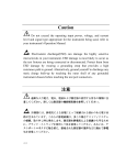
Caution
Caution denotes a hazard. It calls attention to a procedure that, if not
correctly performed or adhered to, would result in damage to or destruction
of the instrument. Do not proceed beyond a caution note until the indicated
conditions are fully understood and met.
Warning
Warning denotes a hazard. It calls attention to a procedure which, if not
correctly performed or adhered to, could result in injury or loss of life.
Do not proceed beyond a warning note until the indicated conditions are
fully understood and met.
L
Instrument Markings
The instruction documentation symbol. The product is marked with this symbol when it
is necessary for the user to refer to the instructions in the documentation.
\CE" The CE mark is a registered trademark of the European Community. (If accompanied by
a year, it is when the design was proven.)
\ISM1-A" This is a symbol of an Industrial Scientic and Medical Group 1 Class A product.
\CSA" The CSA mark is a registered trademark of the Canadian Standards Association.
vi
General Safety Considerations
Warning
This is a Safety Class I product (provided with a protective earthing
ground incorporated in the power cord). The mains plug shall only be
inserted in a socket outlet provided with a protective earth contact. Any
interruption of the protective conductor, inside or outside the instrument,
is likely to make the instrument dangerous. Intentional interruption is
prohibited.
Warning
No operator serviceable parts inside. Refer servicing to qualied
personnel. To prevent electrical shock, do not remove covers.
Caution
Before switching on this instrument, make sure that the line voltage selector
switch is set to the voltage of the power supply and the correct fuse is
installed.
Warning
The opening of covers or removal of parts is likely to expose dangerous
voltages. Disconnect the instrument from all voltage sources while it is
being opened.
Warning
The power cord is connected to internal capacitors that may remain live
for 10 seconds after disconnecting the plug from its power supply.
Warning
For continued protection against re hazard replace line fuse only with
same type and rating (F 3A/250V). The use of other fuses or material is
prohibited.
Warning
If this instrument is used in a manner not specied by Hewlett-Packard
Co., the protection provided by the instrument may be impaired.
Note
This instrument has been designed and tested in accordance with IEC
Publication 348, Safety Requirements for Electronics Measuring Apparatus, and
has been supplied in a safe condition. This instruction documentation contains
information and warnings which must be followed by the user to ensure safe
operation and to maintain the instrument in a safe condition.
vii
User's Guide Overview
Chapter 1, \HP 8753D Description and Options," describes features, functions, and available
options.
Chapter 2, \Making Measurements," contains step-by-step procedures for making
measurements or using particular functions.
Chapter 3, \Making Mixer Measurements," contains step-by-step procedures for making
calibrated and error-corrected mixer measurements.
Chapter 4, \Printing, Plotting, and Saving Measurement Results," contains instructions
for saving to disk or the analyzer internal memory, and printing and plotting displayed
measurements.
Chapter 5, \Optimizing Measurement Results," describes techniques and functions for
achieving the best measurement results.
Chapter 6, \Application and Operation Concepts," contains explanatory-style information
about many applications and analyzer operation.
Chapter 7, \Specications and Measurement Uncertainties," denes the performance
capabilities of the analyzer.
Chapter 8, \Menu Maps," shows softkey menu relationships.
Chapter 9, \Key Denitions," describes all the front panel keys, softkeys, and their
corresponding HP-IB commands.
Chapter 10, \Error Messages," provides information for interpreting error messages.
Chapter 11, \Compatible Peripherals," lists measurement and system accessories, and
other applicable equipment compatible with the analyzer. Procedures for conguring the
peripherals, and an HP-IB programming overview are also included.
Chapter 12, \Preset State and Memory Allocation," contains a discussion of memory
allocation, memory storage, instrument state denitions, and preset conditions.
Appendix A, \The CITIle Data Format and Key Word Reference," contains information on
the CITIle data format as well as a list of CITIle keywords.
viii
Network Analyzer Documentation Set
The Installation and Quick Start Guide
familiarizes you with the network analyzer's
front and rear panels, electrical and
environmental operating requirements, as well
as procedures for installing, conguring, and
verifying the operation of the analyzer.
The User's Guide shows how to make
measurements, explains commonly-used
features, and tells you how to get the most
performance from your analyzer.
The Quick Reference Guide provides a
summary of selected user features.
The Programmer's Guide provides
programming information including an HP-IB
programming and command reference as well
as programming examples.
The System Verication and Test Guide
provides the system verication and
performance tests and the Performance Test
Record for your analyzer.
ix
x
Contents
1. HP 8753D Description and Options
Where to Look for More Information . . . . . . . . .
Analyzer Description . . . . . . . . . . . . . . . . .
Front Panel Features . . . . . . . . . . . . . . . . .
Analyzer Display . . . . . . . . . . . . . . . . . .
Rear Panel Features and Connectors . . . . . . . . .
Analyzer Options Available . . . . . . . . . . . . . .
Option 1D5, High Stability Frequency Reference . . .
Option 002, Harmonic Mode . . . . . . . . . . . .
Option 006, 6 GHz Operation . . . . . . . . . . . .
Option 010, Time Domain . . . . . . . . . . . . .
Option 011, Receiver Conguration . . . . . . . . .
Option 075, 75
Impedance . . . . . . . . . . . . .
Option 1CM, Rack Mount Flange Kit Without Handles
Option 1CP, Rack Mount Flange Kit With Handles . .
Service and Support Options . . . . . . . . . . . . .
On-Site System Verication (+23G) . . . . . . . . .
Standard System Maintenance Service (+02A) . . . .
Basic System Maintenance Service (+02B) . . . . . .
Return to HP Full Service Agreement (+22A) . . . .
Return to HP Repair Agreement (+22B) . . . . . . .
Return to HP Calibration Agreement (+22C) . . . . .
Return to HP Calibration (+22G) . . . . . . . . . .
Changes between the HP 8753 Network Analyzers . . .
.
.
.
.
.
.
.
.
.
.
.
.
.
.
.
.
.
.
.
.
.
.
.
.
.
.
.
.
.
.
.
.
.
.
.
.
.
.
.
.
.
.
.
.
.
.
.
.
.
.
.
.
.
.
.
.
.
.
.
.
.
.
.
.
.
.
.
.
.
.
.
.
.
.
.
.
.
.
.
.
.
.
.
.
.
.
.
.
.
.
.
.
.
.
.
.
.
.
.
.
.
.
.
.
.
.
.
.
.
.
.
.
.
.
.
.
.
.
.
.
.
.
.
.
.
.
.
.
.
.
.
.
.
.
.
.
.
.
.
.
.
.
.
.
.
.
.
.
.
.
.
.
.
.
.
.
.
.
.
.
.
.
.
.
.
.
.
.
.
.
.
.
.
.
.
.
.
.
.
.
.
.
.
.
.
.
.
.
.
.
.
.
.
.
.
.
.
.
.
.
.
.
.
.
.
.
.
.
.
.
.
.
.
.
.
.
.
.
.
.
.
.
.
.
.
.
.
.
.
.
.
.
.
.
.
.
.
.
.
.
.
.
.
.
.
.
.
.
.
.
.
.
.
.
.
.
.
.
.
.
.
.
.
.
.
.
.
.
.
.
.
.
.
.
.
.
1-1
1-2
1-4
1-6
1-10
1-12
1-12
1-12
1-12
1-12
1-12
1-12
1-12
1-12
1-13
1-13
1-13
1-13
1-13
1-13
1-13
1-13
1-14
2. Making Measurements
Where to Look for More Information . . . . . . . . . . . . . . . . . . .
Principles of Microwave Connector Care . . . . . . . . . . . . . . . . .
Basic Measurement Sequence and Example . . . . . . . . . . . . . . . .
Basic Measurement Sequence . . . . . . . . . . . . . . . . . . . . . .
Basic Measurement Example . . . . . . . . . . . . . . . . . . . . . .
Step 1. Connect the device under test and any required test equipment.
Step 2. Choose the measurement parameters. . . . . . . . . . . . . .
Setting the Frequency Range . . . . . . . . . . . . . . . . . . . .
Setting the Source Power . . . . . . . . . . . . . . . . . . . . . .
Setting the Measurement . . . . . . . . . . . . . . . . . . . . . .
Step 3. Perform and apply the appropriate error-correction. . . . . . .
Step 4. Measure the device under test. . . . . . . . . . . . . . . . .
Step 5. Output the measurement results. . . . . . . . . . . . . . . .
Using the Display Functions . . . . . . . . . . . . . . . . . . . . . . .
To View Both Measurement Channels . . . . . . . . . . . . . . . . . .
To Save a Data Trace to the Display Memory . . . . . . . . . . . . . .
To View the Measurement Data and Memory Trace . . . . . . . . . . .
To Divide Measurement Data by the Memory Trace . . . . . . . . . . .
To Subtract the Memory Trace from the Measurement Data Trace . . . . .
To Ratio Measurements in Channel 1 and 2 . . . . . . . . . . . . . . .
.
.
.
.
.
.
.
.
.
.
.
.
.
.
.
.
.
.
.
.
.
.
.
.
.
.
.
.
.
.
.
.
.
.
.
.
.
.
.
.
2-1
2-2
2-3
2-3
2-3
2-3
2-3
2-3
2-4
2-4
2-4
2-4
2-4
2-5
2-5
2-6
2-6
2-7
2-7
2-7
Contents-1
To Title the Active Channel Display . . . . . . . . . . . . . . . . . . .
Using Analyzer Display Markers . . . . . . . . . . . . . . . . . . . . .
To Use Continuous and Discrete Markers . . . . . . . . . . . . . . . .
To Activate Display Markers . . . . . . . . . . . . . . . . . . . . . .
To Use Delta (1) Markers . . . . . . . . . . . . . . . . . . . . . . . .
To Activate a Fixed Marker . . . . . . . . . . . . . . . . . . . . . . .
Using the 1REF=1FIXED MKR Key to activate a Fixed Reference Marker
Using the MKR ZERO Key to Activate a Fixed Reference Marker . . . .
To Couple and Uncouple Display Markers . . . . . . . . . . . . . . . .
To Use Polar Format Markers . . . . . . . . . . . . . . . . . . . . . .
To Use Smith Chart Markers . . . . . . . . . . . . . . . . . . . . . .
To Set Measurement Parameters Using Markers . . . . . . . . . . . . .
Setting the Start Frequency . . . . . . . . . . . . . . . . . . . . .
Setting the Stop Frequency . . . . . . . . . . . . . . . . . . . . . .
Setting the Center Frequency . . . . . . . . . . . . . . . . . . . . .
Setting the Frequency Span . . . . . . . . . . . . . . . . . . . . .
Setting the Display Reference Value . . . . . . . . . . . . . . . . . .
Setting the Electrical Delay . . . . . . . . . . . . . . . . . . . . . .
Setting the CW Frequency . . . . . . . . . . . . . . . . . . . . . . .
To Search for a Specic Amplitude . . . . . . . . . . . . . . . . . . .
Searching for the Maximum Amplitude . . . . . . . . . . . . . . . .
Searching for the Minimum Amplitude . . . . . . . . . . . . . . . .
Searching for a Target Amplitude . . . . . . . . . . . . . . . . . . .
Searching for a Bandwidth . . . . . . . . . . . . . . . . . . . . . .
Tracking the Amplitude that You are Searching . . . . . . . . . . . .
To Calculate the Statistics of the Measurement Data . . . . . . . . . . .
Measuring Magnitude and Insertion Phase Response . . . . . . . . . . . .
Measuring the Magnitude Response . . . . . . . . . . . . . . . . . . .
Measuring Insertion Phase Response . . . . . . . . . . . . . . . . . .
Measuring Electrical Length and Phase Distortion . . . . . . . . . . . . .
Measuring Electrical Length . . . . . . . . . . . . . . . . . . . . . .
Measuring Phase Distortion . . . . . . . . . . . . . . . . . . . . . . .
Deviation From Linear Phase . . . . . . . . . . . . . . . . . . . . .
Group Delay . . . . . . . . . . . . . . . . . . . . . . . . . . . . .
Testing A Device with Limit Lines . . . . . . . . . . . . . . . . . . . .
Setting Up the Measurement Parameters . . . . . . . . . . . . . . . .
Creating Flat Limit Lines . . . . . . . . . . . . . . . . . . . . . . . .
Creating a Sloping Limit Line . . . . . . . . . . . . . . . . . . . . . .
Creating Single Point Limits . . . . . . . . . . . . . . . . . . . . . .
Editing Limit Segments . . . . . . . . . . . . . . . . . . . . . . . . .
Deleting Limit Segments . . . . . . . . . . . . . . . . . . . . . . .
Running a Limit Test . . . . . . . . . . . . . . . . . . . . . . . . . .
Reviewing the Limit Line Segments . . . . . . . . . . . . . . . . . .
Activating the Limit Test . . . . . . . . . . . . . . . . . . . . . . .
Osetting Limit Lines . . . . . . . . . . . . . . . . . . . . . . . . .
Measuring Gain Compression . . . . . . . . . . . . . . . . . . . . . . .
Measuring Gain and Reverse Isolation Simultaneously . . . . . . . . . . .
Measurements Using the Tuned Receiver Mode . . . . . . . . . . . . . .
Typical test setup . . . . . . . . . . . . . . . . . . . . . . . . . . .
Tuned receiver mode in-depth description . . . . . . . . . . . . . . . .
Frequency Range . . . . . . . . . . . . . . . . . . . . . . . . . .
Compatible Sweep Types . . . . . . . . . . . . . . . . . . . . . . .
External Source Requirements . . . . . . . . . . . . . . . . . . . .
Test Sequencing . . . . . . . . . . . . . . . . . . . . . . . . . . . . .
NNNNNNNNNNNNNNNNNNNNNNNNNNNNNNNNNNNNNNNNNNNNNNN
NNNNNNNNNNNNNNNNNNNNNNNNNN
Contents-2
.
.
.
.
.
.
.
.
.
.
.
.
.
.
.
.
.
.
.
.
.
.
.
.
.
.
.
.
.
.
.
.
.
.
.
.
.
.
.
.
.
.
.
.
.
.
.
.
.
.
.
.
.
.
.
.
.
.
.
.
.
.
.
.
.
.
.
.
.
.
.
.
.
.
.
.
.
.
.
.
.
.
.
.
.
.
.
.
.
.
.
.
.
.
.
.
.
.
.
.
.
.
.
.
.
.
.
.
2-8
2-9
2-9
2-10
2-11
2-11
2-12
2-13
2-14
2-14
2-15
2-16
2-17
2-17
2-18
2-19
2-20
2-21
2-21
2-22
2-22
2-23
2-24
2-25
2-25
2-26
2-27
2-27
2-28
2-30
2-30
2-32
2-32
2-33
2-36
2-36
2-37
2-39
2-41
2-42
2-42
2-43
2-43
2-43
2-44
2-45
2-49
2-51
2-51
2-51
2-51
2-51
2-52
2-53
Creating a Sequence . . . . . . . . . . . . . . . . . .
Running a Sequence . . . . . . . . . . . . . . . . .
Stopping a Sequence . . . . . . . . . . . . . . . . .
Editing a Sequence . . . . . . . . . . . . . . . . .
Deleting Commands . . . . . . . . . . . . . . . .
Inserting a Command . . . . . . . . . . . . . . .
Modifying a Command . . . . . . . . . . . . . . .
Clearing a Sequence from Memory . . . . . . . . . .
Changing the Sequence Title . . . . . . . . . . . . .
Naming Files Generated by a Sequence . . . . . . . . .
Storing a Sequence on a Disk . . . . . . . . . . . . .
Loading a Sequence from Disk . . . . . . . . . . . .
Purging a Sequence from Disk . . . . . . . . . . . .
Printing a Sequence . . . . . . . . . . . . . . . . .
Cascading Multiple Example Sequences . . . . . . . .
Loop Counter Example Sequence . . . . . . . . . . .
Generating Files in a Loop Counter Example Sequence .
Limit Test Example Sequence . . . . . . . . . . . . .
Measuring Swept Harmonics . . . . . . . . . . . . . .
Measuring a Device in the Time Domain (Option 010 Only)
Transmission Response in Time Domain . . . . . . . .
Reection Response in Time Domain . . . . . . . . .
Non-coaxial Measurements . . . . . . . . . . . . . . .
.
.
.
.
.
.
.
.
.
.
.
.
.
.
.
.
.
.
.
.
.
.
.
.
.
.
.
.
.
.
.
.
.
.
.
.
.
.
.
.
.
.
.
.
.
.
.
.
.
.
.
.
.
.
.
.
.
.
.
.
.
.
.
.
.
.
.
.
.
.
.
.
.
.
.
.
.
.
.
.
.
.
.
.
.
.
.
.
.
.
.
.
.
.
.
.
.
.
.
.
.
.
.
.
.
.
.
.
.
.
.
.
.
.
.
.
.
.
.
.
.
.
.
.
.
.
.
.
.
.
.
.
.
.
.
.
.
.
.
.
.
.
.
.
.
.
.
.
.
.
.
.
.
.
.
.
.
.
.
.
.
.
.
.
.
.
.
.
.
.
.
.
.
.
.
.
.
.
.
.
.
.
.
.
.
.
.
.
.
.
.
.
.
.
.
.
.
.
.
.
.
.
.
.
.
.
.
.
.
.
.
.
.
.
.
.
.
.
.
.
.
.
.
.
.
.
.
.
.
.
.
.
.
.
.
.
.
.
.
.
.
.
.
.
.
.
.
.
.
.
.
.
.
2-54
2-55
2-55
2-56
2-56
2-56
2-57
2-57
2-58
2-58
2-59
2-60
2-60
2-60
2-61
2-62
2-63
2-64
2-66
2-68
2-68
2-73
2-76
3. Making Mixer Measurements
Where to Look for More Information . . . . . . . . . . . .
Measurement Considerations . . . . . . . . . . . . . . . .
Minimizing Source and Load Mismatches . . . . . . . . .
Reducing the Eect of Spurious Responses . . . . . . . .
Eliminating Unwanted Mixing and Leakage Signals . . . . .
How RF and IF Are Dened . . . . . . . . . . . . . . .
Frequency Oset Mode Operation . . . . . . . . . . . . .
Dierences Between Internal and External R-Channel Inputs
Power Meter Calibration . . . . . . . . . . . . . . . . .
Conversion Loss Using the Frequency Oset Mode . . . . . .
High Dynamic Range Swept RF/IF Conversion Loss . . . . .
Fixed IF Mixer Measurements . . . . . . . . . . . . . . .
Tuned Receiver Mode . . . . . . . . . . . . . . . . . .
Sequence 1 Setup . . . . . . . . . . . . . . . . . . . .
Sequence 2 Setup . . . . . . . . . . . . . . . . . . . .
Phase or Group Delay Measurements . . . . . . . . . . . .
Amplitude and Phase Tracking . . . . . . . . . . . . . . .
Conversion Compression Using the Frequency Oset Mode . .
Isolation Example Measurements . . . . . . . . . . . . . .
LO to RF Isolation . . . . . . . . . . . . . . . . . . . .
RF Feedthrough . . . . . . . . . . . . . . . . . . . . .
.
.
.
.
.
.
.
.
.
.
.
.
.
.
.
.
.
.
.
.
.
.
.
.
.
.
.
.
.
.
.
.
.
.
.
.
.
.
.
.
.
.
.
.
.
.
.
.
.
.
.
.
.
.
.
.
.
.
.
.
.
.
.
.
.
.
.
.
.
.
.
.
.
.
.
.
.
.
.
.
.
.
.
.
.
.
.
.
.
.
.
.
.
.
.
.
.
.
.
.
.
.
.
.
.
.
.
.
.
.
.
.
.
.
.
.
.
.
.
.
.
.
.
.
.
.
.
.
.
.
.
.
.
.
.
.
.
.
.
.
.
.
.
.
.
.
.
.
.
.
.
.
.
.
.
.
.
.
.
.
.
.
.
.
.
.
.
.
.
.
.
.
.
.
.
.
.
.
.
.
.
.
.
.
.
.
.
.
.
3-1
3-2
3-2
3-2
3-2
3-2
3-4
3-4
3-6
3-7
3-12
3-17
3-17
3-17
3-21
3-24
3-27
3-28
3-33
3-33
3-35
Contents-3
4. Printing, Plotting, and Saving Measurement Results
Where to Look for More Information . . . . . . . . . . . . . . . . . .
Printing or Plotting Your Measurement Results . . . . . . . . . . . . . .
Conguring a Print Function . . . . . . . . . . . . . . . . . . . . . .
Dening a Print Function . . . . . . . . . . . . . . . . . . . . . . .
If You are Using a Color Printer . . . . . . . . . . . . . . . . . . . .
To Reset the Printing Parameters to Default Values . . . . . . . . . . .
Printing One Measurement Per Page . . . . . . . . . . . . . . . . . .
Printing Multiple Measurements Per Page . . . . . . . . . . . . . . . .
Conguring a Plot Function . . . . . . . . . . . . . . . . . . . . . .
If You are Plotting to an HPGL/2 Compatible Printer . . . . . . . . . .
If You are Plotting to a Pen Plotter . . . . . . . . . . . . . . . . . .
If You are Plotting to a Disk Drive . . . . . . . . . . . . . . . . . .
Dening a Plot Function . . . . . . . . . . . . . . . . . . . . . . . .
Choosing Display Elements . . . . . . . . . . . . . . . . . . . . . .
Selecting Auto-Feed . . . . . . . . . . . . . . . . . . . . . . . . .
Selecting Pen Numbers and Colors . . . . . . . . . . . . . . . . . .
Selecting Line Types . . . . . . . . . . . . . . . . . . . . . . . . .
Choosing Scale . . . . . . . . . . . . . . . . . . . . . . . . . . . .
Choosing Plot Speed . . . . . . . . . . . . . . . . . . . . . . . . .
To Reset the Plotting Parameters to Default Values . . . . . . . . . . .
Plotting One Measurement Per Page Using a Pen Plotter . . . . . . . . .
Plotting Multiple Measurements Per Page Using a Pen Plotter . . . . . . .
If You are Plotting to an HPGL Compatible Printer . . . . . . . . . . .
Plotting a Measurement to Disk . . . . . . . . . . . . . . . . . . . . .
To Output the Plot Files . . . . . . . . . . . . . . . . . . . . . . .
To View Plot Files on a PC . . . . . . . . . . . . . . . . . . . . . . .
Using AmiPro . . . . . . . . . . . . . . . . . . . . . . . . . . . .
Using Freelance . . . . . . . . . . . . . . . . . . . . . . . . . . .
Outputting Plot Files from a PC to a Plotter . . . . . . . . . . . . . . .
Outputting Plot Files from a PC to an HPGL Compatible Printer . . . . .
Step 1. Store the HPGL initialization sequence. . . . . . . . . . . . .
Step 2. Store the exit HPGL mode and form feed sequence. . . . . . .
Step 3. Send the HPGL initialization sequence to the printer. . . . . . .
Step 4. Send the plot le to the printer. . . . . . . . . . . . . . . . .
Step 5. Send the exit HPGL mode and form feed sequence to the printer.
Outputting Single Page Plots Using a Printer . . . . . . . . . . . . . . .
Outputting Multiple Plots to a Single Page Using a Printer . . . . . . . .
Plotting Multiple Measurements Per Page From Disk . . . . . . . . . . .
To Plot Multiple Measurements on a Full Page . . . . . . . . . . . . .
To Plot Measurements in Page Quadrants . . . . . . . . . . . . . . .
Titling the Displayed Measurement . . . . . . . . . . . . . . . . . . .
Conguring the Analyzer to Produce a Time Stamp . . . . . . . . . . .
Aborting a Print or Plot Process . . . . . . . . . . . . . . . . . . . .
Printing or Plotting the List Values or Operating Parameters . . . . . . .
If You want a Single Page of Values . . . . . . . . . . . . . . . . . .
If You Want the Entire List of Values . . . . . . . . . . . . . . . . .
Solving Problems with Printing or Plotting . . . . . . . . . . . . . . .
Saving and Recalling Instrument States . . . . . . . . . . . . . . . . .
Places Where You Can Save . . . . . . . . . . . . . . . . . . . . .
What You Can Save to the Analyzer's Internal Memory . . . . . . . . .
What You Can Save to a Floppy Disk . . . . . . . . . . . . . . . . .
What You Can Save to a Computer . . . . . . . . . . . . . . . . . .
Saving an Instrument State . . . . . . . . . . . . . . . . . . . . . . .
Saving Measurement Results . . . . . . . . . . . . . . . . . . . . . .
Contents-4
.
.
.
.
.
.
.
.
.
.
.
.
.
.
.
.
.
.
.
.
.
.
.
.
.
.
.
.
.
.
.
.
.
.
.
.
.
.
.
.
.
.
.
.
.
.
.
.
.
.
.
.
.
.
.
.
.
.
.
.
.
.
.
.
.
.
.
.
.
.
.
.
.
.
.
.
.
.
.
.
.
.
.
.
.
.
.
.
.
.
.
.
.
.
.
.
.
.
.
.
.
.
.
.
.
.
.
.
.
.
.
.
.
.
.
.
.
.
.
.
.
.
.
.
.
.
.
.
.
.
.
.
.
.
.
.
.
.
.
.
.
.
.
.
.
.
.
.
.
.
.
.
.
.
.
.
.
.
.
.
.
.
4-2
4-3
4-3
4-5
4-6
4-6
4-6
4-7
4-8
4-8
4-10
4-11
4-12
4-12
4-12
4-13
4-14
4-15
4-15
4-16
4-16
4-17
4-18
4-19
4-20
4-20
4-21
4-22
4-22
4-23
4-23
4-24
4-24
4-24
4-24
4-24
4-25
4-26
4-26
4-28
4-29
4-30
4-30
4-30
4-30
4-31
4-32
4-33
4-33
4-33
4-33
4-34
4-35
4-36
ASCII Data Formats . . . . . . . . . . . .
CITIle . . . . . . . . . . . . . . . . .
S2P Data Format . . . . . . . . . . . . .
Re-Saving an Instrument State . . . . . . . .
Deleting a File . . . . . . . . . . . . . . . .
To Delete an Instrument State File . . . . .
To Delete all Files . . . . . . . . . . . . .
Renaming a File . . . . . . . . . . . . . . .
Recalling a File . . . . . . . . . . . . . . .
Formatting a Disk . . . . . . . . . . . . . .
Solving Problems with Saving or Recalling Files
If You are Using an External Disk Drive . . .
.
.
.
.
.
.
.
.
.
.
.
.
.
.
.
.
.
.
.
.
.
.
.
.
.
.
.
.
.
.
.
.
.
.
.
.
.
.
.
.
.
.
.
.
.
.
.
.
.
.
.
.
.
.
.
.
.
.
.
.
.
.
.
.
.
.
.
.
.
.
.
.
.
.
.
.
.
.
.
.
.
.
.
.
.
.
.
.
.
.
.
.
.
.
.
.
.
.
.
.
.
.
.
.
.
.
.
.
.
.
.
.
.
.
.
.
.
.
.
.
.
.
.
.
.
.
.
.
.
.
.
.
.
.
.
.
.
.
.
.
.
.
.
.
.
.
.
.
.
.
.
.
.
.
.
.
.
.
.
.
.
.
.
.
.
.
.
.
.
.
.
.
.
.
.
.
.
.
.
.
.
.
.
.
.
.
.
.
.
.
.
.
4-39
4-39
4-39
4-41
4-41
4-41
4-41
4-42
4-42
4-43
4-43
4-43
5. Optimizing Measurement Results
Where to Look for More Information . . . . . . . . . . . . . . . . . .
Increasing Measurement Accuracy . . . . . . . . . . . . . . . . . . .
Connector Repeatability . . . . . . . . . . . . . . . . . . . . . . .
Interconnecting Cables . . . . . . . . . . . . . . . . . . . . . . . .
Temperature Drift . . . . . . . . . . . . . . . . . . . . . . . . . .
Frequency Drift . . . . . . . . . . . . . . . . . . . . . . . . . . .
Performance Verication . . . . . . . . . . . . . . . . . . . . . . .
Reference Plane and Port Extensions . . . . . . . . . . . . . . . . .
Measurement Error-Correction . . . . . . . . . . . . . . . . . . . . .
Conditions Where Error-Correction is Suggested . . . . . . . . . . . .
Types of Error-Correction . . . . . . . . . . . . . . . . . . . . . .
Error-Correction Stimulus State . . . . . . . . . . . . . . . . . . . .
Calibration Standards . . . . . . . . . . . . . . . . . . . . . . . .
Compensating for the Electrical Delay of Calibration Standards . . . .
Clarifying Type-N Connector Sex . . . . . . . . . . . . . . . . . .
When to Use Interpolated Error-Correction . . . . . . . . . . . . . .
Procedures for Error-Correcting Your Measurements . . . . . . . . . . .
Frequency Response Error-Corrections . . . . . . . . . . . . . . . . .
Response Error-Correction for Reection Measurements . . . . . . . .
Response Error-Correction for Transmission Measurements . . . . . . .
Receiver Calibration . . . . . . . . . . . . . . . . . . . . . . . . .
Frequency Response and Isolation Error-Corrections . . . . . . . . . . .
Response and Isolation Error-Correction for Reection Measurements . .
Response and Isolation Error-Correction for Transmission Measurements
One-Port Reection Error-Correction . . . . . . . . . . . . . . . . . .
Full Two-Port Error-Correction . . . . . . . . . . . . . . . . . . . . .
TRL* and TRM* Error-Correction . . . . . . . . . . . . . . . . . . . .
TRL Error-Correction . . . . . . . . . . . . . . . . . . . . . . . .
TRM Error-Correction . . . . . . . . . . . . . . . . . . . . . . . .
Modifying Calibration Kit Standards . . . . . . . . . . . . . . . . . . .
Denitions . . . . . . . . . . . . . . . . . . . . . . . . . . . . .
Outline of Standard Modication . . . . . . . . . . . . . . . . . . .
Modifying Standards . . . . . . . . . . . . . . . . . . . . . . . . .
Modifying TRL Standards . . . . . . . . . . . . . . . . . . . . . . .
Modifying TRM Standards . . . . . . . . . . . . . . . . . . . . . .
Power Meter Measurement Calibration . . . . . . . . . . . . . . . . .
Entering the Power Sensor Calibration Data . . . . . . . . . . . . . .
Editing Frequency Segments . . . . . . . . . . . . . . . . . . . .
Deleting Frequency Segments . . . . . . . . . . . . . . . . . . .
Compensating for Directional Coupler Response . . . . . . . . . . . .
Using Sample-and-Sweep Correction Mode . . . . . . . . . . . . . . .
.
.
.
.
.
.
.
.
.
.
.
.
.
.
.
.
.
.
.
.
.
.
.
.
.
.
.
.
.
.
.
.
.
.
.
.
.
.
.
.
.
.
.
.
.
.
.
.
.
.
.
.
.
.
.
.
.
.
.
.
.
.
.
.
.
.
.
.
.
.
.
.
.
.
.
.
.
.
.
.
.
.
.
.
.
.
.
.
.
.
.
.
.
.
.
.
.
.
.
.
.
.
.
.
.
.
.
.
.
.
.
.
.
.
.
.
.
.
.
.
.
.
.
5-2
5-2
5-2
5-2
5-2
5-3
5-3
5-3
5-4
5-4
5-4
5-5
5-6
5-6
5-6
5-6
5-7
5-8
5-8
5-10
5-11
5-13
5-13
5-15
5-17
5-20
5-23
5-23
5-24
5-26
5-26
5-26
5-26
5-28
5-30
5-33
5-34
5-34
5-35
5-35
5-36
Contents-5
Using Continuous Correction Mode . . . . . . . . . . . . . .
To Calibrate the Analyzer Receiver to Measure Absolute Power
Matched Adapters . . . . . . . . . . . . . . . . . . . . . .
Modify the Cal Kit Thru Denition . . . . . . . . . . . . . .
Calibrating for Noninsertable Devices . . . . . . . . . . . . . .
Adapter Removal . . . . . . . . . . . . . . . . . . . . . .
Perform the 2-port Error Corrections . . . . . . . . . . . .
Remove the Adapter . . . . . . . . . . . . . . . . . . . .
Verify the Results . . . . . . . . . . . . . . . . . . . . .
Example Program . . . . . . . . . . . . . . . . . . . . .
Making Accurate Measurements of Electrically Long Devices . . .
The Cause of Measurement Problems . . . . . . . . . . . . .
To Improve Measurement Results . . . . . . . . . . . . . . .
Decreasing the Sweep Rate . . . . . . . . . . . . . . . . .
Decreasing the Time Delay . . . . . . . . . . . . . . . . .
Increasing Sweep Speed . . . . . . . . . . . . . . . . . . . .
To Decrease the Frequency Span . . . . . . . . . . . . . . .
To Set the Auto Sweep Time Mode . . . . . . . . . . . . . .
To Widen the System Bandwidth . . . . . . . . . . . . . . .
To Reduce the Averaging Factor . . . . . . . . . . . . . . .
To Reduce the Number of Measurement Points . . . . . . . . .
To Set the Sweep Type . . . . . . . . . . . . . . . . . . . .
To View a Single Measurement Channel . . . . . . . . . . . .
To Activate Chop Sweep Mode . . . . . . . . . . . . . . . .
To Use External Calibration . . . . . . . . . . . . . . . . .
To Use Fast 2-Port Calibration . . . . . . . . . . . . . . . .
Increasing Dynamic Range . . . . . . . . . . . . . . . . . . .
To Increase the Test Port Input Power . . . . . . . . . . . . .
To Reduce the Receiver Noise Floor . . . . . . . . . . . . . .
Changing System Bandwidth . . . . . . . . . . . . . . . .
Changing Measurement Averaging . . . . . . . . . . . . .
Reducing Trace Noise . . . . . . . . . . . . . . . . . . . . .
To Activate Averaging . . . . . . . . . . . . . . . . . . . .
To Change System Bandwidth . . . . . . . . . . . . . . . .
Reducing Receiver Crosstalk . . . . . . . . . . . . . . . . . .
Reducing Recall Time . . . . . . . . . . . . . . . . . . . . .
Understanding Spur Avoidance . . . . . . . . . . . . . . . .
6. Application and Operation Concepts
Where to Look for More Information .
HP 8753D System Operation . . . . .
The Built-In Synthesized Source . .
The Source Step Attenuator . . .
The Built-In Test Set . . . . . . . .
The Receiver Block . . . . . . . .
The Microprocessor . . . . . . . .
Required Peripheral Equipment . . .
Data Processing . . . . . . . . . . .
Processing Details . . . . . . . . .
The ADC . . . . . . . . . . . .
IF Detection . . . . . . . . . . .
Ratio Calculations . . . . . . . .
Sampler/IF Correction . . . . . .
Sweep-To-Sweep Averaging . . . .
Pre-Raw Data Arrays . . . . . .
Contents-6
.
.
.
.
.
.
.
.
.
.
.
.
.
.
.
.
.
.
.
.
.
.
.
.
.
.
.
.
.
.
.
.
.
.
.
.
.
.
.
.
.
.
.
.
.
.
.
.
.
.
.
.
.
.
.
.
.
.
.
.
.
.
.
.
.
.
.
.
.
.
.
.
.
.
.
.
.
.
.
.
.
.
.
.
.
.
.
.
.
.
.
.
.
.
.
.
.
.
.
.
.
.
.
.
.
.
.
.
.
.
.
.
.
.
.
.
.
.
.
.
.
.
.
.
.
.
.
.
.
.
.
.
.
.
.
.
.
.
.
.
.
.
.
.
.
.
.
.
.
.
.
.
.
.
.
.
.
.
.
.
.
.
.
.
.
.
.
.
.
.
.
.
.
.
.
.
.
.
.
.
.
.
.
.
.
.
.
.
.
.
.
.
.
.
.
.
.
.
.
.
.
.
.
.
.
.
.
.
.
.
.
.
.
.
.
.
.
.
.
.
.
.
.
.
.
.
.
.
.
.
.
.
.
.
.
.
.
.
.
.
.
.
.
.
.
.
.
.
.
.
.
.
.
.
.
.
.
.
.
.
.
.
.
.
.
.
.
.
.
.
.
.
.
.
.
.
.
.
.
.
.
.
.
.
.
.
.
.
.
.
.
.
.
.
.
.
.
.
.
.
.
.
.
.
.
.
.
.
.
.
.
.
.
.
.
.
.
.
.
.
.
.
.
.
.
.
.
.
.
.
.
.
.
.
.
.
.
.
.
.
.
.
.
.
.
.
.
.
.
.
.
.
.
.
.
.
.
.
.
.
.
.
.
.
.
.
.
.
.
.
.
.
.
.
.
.
.
.
.
.
.
.
.
.
.
.
.
.
.
.
.
.
.
.
.
.
.
.
.
.
.
.
.
.
.
.
.
.
.
.
.
.
.
.
.
.
.
.
.
.
.
.
.
.
.
.
.
.
.
.
.
.
.
.
.
.
.
.
.
.
.
.
.
.
.
.
.
.
.
.
.
.
.
.
.
.
.
.
.
.
.
.
.
.
.
.
.
5-37
5-38
5-39
5-40
5-41
5-42
5-43
5-44
5-45
5-47
5-48
5-48
5-48
5-48
5-49
5-50
5-50
5-51
5-52
5-52
5-52
5-53
5-53
5-54
5-54
5-54
5-56
5-56
5-56
5-56
5-56
5-57
5-57
5-57
5-57
5-58
5-59
.
.
.
.
.
.
.
.
.
.
.
.
.
.
.
.
.
.
.
.
.
.
.
.
.
.
.
.
.
.
.
.
.
.
.
.
.
.
.
.
.
.
.
.
.
.
.
.
.
.
.
.
.
.
.
.
.
.
.
.
.
.
.
.
.
.
.
.
.
.
.
.
.
.
.
.
.
.
.
.
.
.
.
.
.
.
.
.
.
.
.
.
.
.
.
.
.
.
.
.
.
.
.
.
.
.
.
.
.
.
.
.
6-1
6-2
6-2
6-2
6-3
6-3
6-3
6-3
6-4
6-5
6-5
6-5
6-5
6-5
6-5
6-6
Raw Arrays . . . . . . . . . . . . . . . . . .
Vector Error-correction (Accuracy Enhancement)
Trace Math Operation . . . . . . . . . . . . .
Gating (Option 010 Only) . . . . . . . . . . . .
The Electrical Delay Block . . . . . . . . . . .
Conversion . . . . . . . . . . . . . . . . . .
Transform (Option 010 Only) . . . . . . . . . .
Format . . . . . . . . . . . . . . . . . . . .
Smoothing . . . . . . . . . . . . . . . . . . .
Format Arrays . . . . . . . . . . . . . . . . .
Oset and Scale . . . . . . . . . . . . . . . .
Display Memory . . . . . . . . . . . . . . . .
Active Channel Keys . . . . . . . . . . . . . . . .
Dual Channel . . . . . . . . . . . . . . . . . .
Uncoupling Stimulus Values Between Channels . .
Coupled Markers . . . . . . . . . . . . . . . . .
Entry Block Keys . . . . . . . . . . . . . . . . .
Units Terminator . . . . . . . . . . . . . . . . .
Knob . . . . . . . . . . . . . . . . . . . . . .
Step Keys . . . . . . . . . . . . . . . . . . . .
4ENTRY OFF5 . . . . . . . . . . . . . . . . . . .
45 . . . . . . . . . . . . . . . . . . . . . . .
415 . . . . . . . . . . . . . . . . . . . . . . . .
405 . . . . . . . . . . . . . . . . . . . . . . .
Stimulus Functions . . . . . . . . . . . . . . . .
Dening Ranges with Stimulus Keys . . . . . . .
Stimulus Menu . . . . . . . . . . . . . . . . . .
The Power Menu . . . . . . . . . . . . . . . . . .
Understanding the Power Ranges . . . . . . . . .
Automatic mode . . . . . . . . . . . . . . . .
Manual mode . . . . . . . . . . . . . . . . .
Power Coupling Options . . . . . . . . . . . . .
Channel coupling . . . . . . . . . . . . . . .
Test port coupling . . . . . . . . . . . . . . .
Sweep Time . . . . . . . . . . . . . . . . . . . .
Manual Sweep Time Mode . . . . . . . . . . . .
Auto Sweep Time Mode . . . . . . . . . . . . .
Minimum Sweep Time . . . . . . . . . . . . . .
Trigger Menu . . . . . . . . . . . . . . . . . . .
Source Attenuator Switch Protection . . . . . . . .
Allowing Repetitive Switching of the Attenuator .
Channel Stimulus Coupling . . . . . . . . . . . . .
Sweep Type Menu . . . . . . . . . . . . . . . . .
Linear Frequency Sweep (Hz) . . . . . . . . . . .
Logarithmic Frequency Sweep (Hz) . . . . . . . .
List Frequency Sweep (Hz) . . . . . . . . . . . .
Segment Menu . . . . . . . . . . . . . . . . .
Power Sweep (dBm) . . . . . . . . . . . . . . .
CW Time Sweep (Seconds) . . . . . . . . . . . .
Selecting Sweep Modes . . . . . . . . . . . . . .
Modifying List Frequencies . . . . . . . . . . . .
Edit list menu . . . . . . . . . . . . . . . . .
Edit subsweep menu . . . . . . . . . . . . . .
Response Functions . . . . . . . . . . . . . . . .
S-Parameters . . . . . . . . . . . . . . . . . . .
.
.
.
.
.
.
.
.
.
.
.
.
.
.
.
.
.
.
.
.
.
.
.
.
.
.
.
.
.
.
.
.
.
.
.
.
.
.
.
.
.
.
.
.
.
.
.
.
.
.
.
.
.
.
.
.
.
.
.
.
.
.
.
.
.
.
.
.
.
.
.
.
.
.
.
.
.
.
.
.
.
.
.
.
.
.
.
.
.
.
.
.
.
.
.
.
.
.
.
.
.
.
.
.
.
.
.
.
.
.
.
.
.
.
.
.
.
.
.
.
.
.
.
.
.
.
.
.
.
.
.
.
.
.
.
.
.
.
.
.
.
.
.
.
.
.
.
.
.
.
.
.
.
.
.
.
.
.
.
.
.
.
.
.
.
.
.
.
.
.
.
.
.
.
.
.
.
.
.
.
.
.
.
.
.
.
.
.
.
.
.
.
.
.
.
.
.
.
.
.
.
.
.
.
.
.
.
.
.
.
.
.
.
.
.
.
.
.
.
.
.
.
.
.
.
.
.
.
.
.
.
.
.
.
.
.
.
.
.
.
.
.
.
.
.
.
.
.
.
.
.
.
.
.
.
.
.
.
.
.
.
.
.
.
.
.
.
.
.
.
.
.
.
.
.
.
.
.
.
.
.
.
.
.
.
.
.
.
.
.
.
.
.
.
.
.
.
.
.
.
.
.
.
.
.
.
.
.
.
.
.
.
.
.
.
.
.
.
.
.
.
.
.
.
.
.
.
.
.
.
.
.
.
.
.
.
.
.
.
.
.
.
.
.
.
.
.
.
.
.
.
.
.
.
.
.
.
.
.
.
.
.
.
.
.
.
.
.
.
.
.
.
.
.
.
.
.
.
.
.
.
.
.
.
.
.
.
.
.
.
.
.
.
.
.
.
.
.
.
.
.
.
.
.
.
.
.
.
.
.
.
.
.
.
.
.
.
.
.
.
.
.
.
.
.
.
.
.
.
.
.
.
.
.
.
.
.
.
.
.
.
.
.
.
.
.
.
.
.
.
.
.
.
.
.
.
.
.
.
.
.
.
.
.
.
.
.
.
.
.
.
.
.
.
.
.
.
.
.
.
.
.
.
.
.
.
.
.
.
.
.
.
.
.
.
.
.
.
.
.
.
.
.
.
.
.
.
.
.
.
.
.
.
.
.
.
.
.
.
.
.
.
.
.
.
.
.
.
.
.
.
.
.
.
.
.
.
.
.
.
.
.
.
.
.
.
.
.
.
.
.
.
.
.
.
.
.
.
.
.
.
.
.
.
.
.
.
.
.
.
.
.
.
.
.
.
.
.
.
.
.
.
.
.
.
.
.
.
.
.
.
.
.
.
.
.
.
.
.
.
.
.
.
.
.
.
.
.
.
.
.
.
.
.
.
.
.
.
.
.
.
.
.
.
.
.
.
.
.
.
.
.
.
.
.
.
.
.
.
.
.
.
.
.
.
.
.
.
.
.
.
.
.
.
.
.
.
.
.
.
.
.
.
.
.
.
.
.
.
.
.
.
.
.
.
.
.
.
.
.
.
.
.
.
.
.
.
.
.
.
.
.
.
.
.
.
.
.
.
.
.
.
.
.
.
.
.
.
.
.
.
.
.
.
.
6-6
6-6
6-6
6-6
6-6
6-6
6-6
6-7
6-7
6-7
6-7
6-7
6-8
6-8
6-8
6-8
6-9
6-9
6-10
6-10
6-10
6-10
6-10
6-10
6-11
6-11
6-12
6-13
6-13
6-13
6-13
6-15
6-15
6-15
6-16
6-16
6-16
6-16
6-18
6-19
6-19
6-20
6-21
6-21
6-22
6-22
6-22
6-23
6-23
6-23
6-23
6-23
6-24
6-25
6-26
Contents-7
Understanding S-Parameters . . . . . . . . . . . .
The S-Parameter Menu . . . . . . . . . . . . . . .
Analog In Menu . . . . . . . . . . . . . . . . .
Conversion Menu . . . . . . . . . . . . . . . .
Input Ports Menu . . . . . . . . . . . . . . . .
The Format Menu . . . . . . . . . . . . . . . . . .
Log Magnitude Format . . . . . . . . . . . . . . .
Phase Format . . . . . . . . . . . . . . . . . . .
Group Delay Format . . . . . . . . . . . . . . . .
Smith Chart Format . . . . . . . . . . . . . . . .
Polar Format . . . . . . . . . . . . . . . . . . .
Linear Magnitude Format . . . . . . . . . . . . . .
SWR Format . . . . . . . . . . . . . . . . . . . .
Real Format . . . . . . . . . . . . . . . . . . . .
Imaginary Format . . . . . . . . . . . . . . . . .
Group Delay Principles . . . . . . . . . . . . . . .
Scale Reference Menu . . . . . . . . . . . . . . . .
Electrical Delay . . . . . . . . . . . . . . . . . .
Display Menu . . . . . . . . . . . . . . . . . . . .
Dual Channel Mode . . . . . . . . . . . . . . . .
Dual Channel Mode with Decoupled Channel Power
Memory Math Functions . . . . . . . . . . . . . .
Adjusting the Colors of the Display . . . . . . . . .
Setting Display Intensity . . . . . . . . . . . . .
Setting Default Colors . . . . . . . . . . . . . .
Blanking the Display . . . . . . . . . . . . . . .
Saving Modied Colors . . . . . . . . . . . . . .
Recalling Modied Colors . . . . . . . . . . . . .
The Modify Colors Menu . . . . . . . . . . . . .
Averaging Menu . . . . . . . . . . . . . . . . . . .
Averaging . . . . . . . . . . . . . . . . . . . . .
Smoothing . . . . . . . . . . . . . . . . . . . . .
IF Bandwidth Reduction . . . . . . . . . . . . . .
Markers . . . . . . . . . . . . . . . . . . . . . . .
Marker Menu . . . . . . . . . . . . . . . . . . .
Delta Mode Menu . . . . . . . . . . . . . . . .
Fixed Marker Menu . . . . . . . . . . . . . .
Marker Function Menu . . . . . . . . . . . . . . .
Marker Search Menu . . . . . . . . . . . . . . .
Target Menu . . . . . . . . . . . . . . . . . .
Marker Mode Menu . . . . . . . . . . . . . . .
Polar Marker Menu . . . . . . . . . . . . . .
Smith Marker Menu . . . . . . . . . . . . . .
Measurement Calibration . . . . . . . . . . . . . . .
What is Accuracy Enhancement? . . . . . . . . . .
What Causes Measurement Errors? . . . . . . . . .
Directivity . . . . . . . . . . . . . . . . . . .
Source Match . . . . . . . . . . . . . . . . . .
Load Match . . . . . . . . . . . . . . . . . . .
Isolation (Crosstalk) . . . . . . . . . . . . . . .
Frequency Response (Tracking) . . . . . . . . . .
Characterizing Microwave Systematic Errors . . . . .
One-Port Error Model . . . . . . . . . . . . . .
Device Measurement . . . . . . . . . . . . . . .
Two-Port Error Model . . . . . . . . . . . . . .
Contents-8
.
.
.
.
.
.
.
.
.
.
.
.
.
.
.
.
.
.
.
.
.
.
.
.
.
.
.
.
.
.
.
.
.
.
.
.
.
.
.
.
.
.
.
.
.
.
.
.
.
.
.
.
.
.
.
.
.
.
.
.
.
.
.
.
.
.
.
.
.
.
.
.
.
.
.
.
.
.
.
.
.
.
.
.
.
.
.
.
.
.
.
.
.
.
.
.
.
.
.
.
.
.
.
.
.
.
.
.
.
.
.
.
.
.
.
.
.
.
.
.
.
.
.
.
.
.
.
.
.
.
.
.
.
.
.
.
.
.
.
.
.
.
.
.
.
.
.
.
.
.
.
.
.
.
.
.
.
.
.
.
.
.
.
.
.
.
.
.
.
.
.
.
.
.
.
.
.
.
.
.
.
.
.
.
.
.
.
.
.
.
.
.
.
.
.
.
.
.
.
.
.
.
.
.
.
.
.
.
.
.
.
.
.
.
.
.
.
.
.
.
.
.
.
.
.
.
.
.
.
.
.
.
.
.
.
.
.
.
.
.
.
.
.
.
.
.
.
.
.
.
.
.
.
.
.
.
.
.
.
.
.
.
.
.
.
.
.
.
.
.
.
.
.
.
.
.
.
.
.
.
.
.
.
.
.
.
.
.
.
.
.
.
.
.
.
.
.
.
.
.
.
.
.
.
.
.
.
.
.
.
.
.
.
.
.
.
.
.
.
.
.
.
.
.
.
.
.
.
.
.
.
.
.
.
.
.
.
.
.
.
.
.
.
.
.
.
.
.
.
.
.
.
.
.
.
.
.
.
.
.
.
.
.
.
.
.
.
.
.
.
.
.
.
.
.
.
.
.
.
.
.
.
.
.
.
.
.
.
.
.
.
.
.
.
.
.
.
.
.
.
.
.
.
.
.
.
.
.
.
.
.
.
.
.
.
.
.
.
.
.
.
.
.
.
.
.
.
.
.
.
.
.
.
.
.
.
.
.
.
.
.
.
.
.
.
.
.
.
.
.
.
.
.
.
.
.
.
.
.
.
.
.
.
.
.
.
.
.
.
.
.
.
.
.
.
.
.
.
.
.
.
.
.
.
.
.
.
.
.
.
.
.
.
.
.
.
.
.
.
.
.
.
.
.
.
.
.
.
.
.
.
.
.
.
.
.
.
.
.
.
.
.
.
.
.
.
.
.
.
.
.
.
.
.
.
.
.
.
.
.
.
.
.
.
.
.
.
.
.
.
.
.
.
.
.
.
.
.
.
.
.
.
.
.
.
.
.
.
.
.
.
.
.
.
.
.
.
.
.
.
.
.
.
.
.
.
.
.
.
.
.
.
.
.
.
.
.
.
.
.
.
.
.
.
.
.
.
.
.
.
.
.
.
.
.
.
.
.
.
.
.
.
.
.
.
.
.
.
.
.
.
.
.
.
.
.
.
.
.
.
.
.
.
.
.
.
.
.
.
.
.
.
.
.
.
.
.
.
.
.
6-26
6-27
6-27
6-27
6-28
6-29
6-29
6-30
6-30
6-31
6-32
6-33
6-33
6-34
6-34
6-35
6-38
6-38
6-39
6-40
6-40
6-41
6-41
6-41
6-42
6-42
6-42
6-42
6-42
6-44
6-44
6-45
6-45
6-47
6-48
6-48
6-48
6-49
6-49
6-49
6-49
6-49
6-49
6-50
6-50
6-51
6-51
6-52
6-52
6-53
6-53
6-53
6-53
6-59
6-59
Calibration Considerations . . . . . . . . . . . . . . . . . . . . . . . .
Measurement Parameters . . . . . . . . . . . . . . . . . . . . . . . .
Device Measurements . . . . . . . . . . . . . . . . . . . . . . . . .
Omitting Isolation Calibration . . . . . . . . . . . . . . . . . . . . . .
Saving Calibration Data . . . . . . . . . . . . . . . . . . . . . . . .
The Calibration Standards . . . . . . . . . . . . . . . . . . . . . . .
Frequency Response of Calibration Standards . . . . . . . . . . . . . .
Electrical Oset . . . . . . . . . . . . . . . . . . . . . . . . . . .
Fringe Capacitance . . . . . . . . . . . . . . . . . . . . . . . . .
How Eective Is Accuracy Enhancement? . . . . . . . . . . . . . . . . .
Correcting for Measurement Errors . . . . . . . . . . . . . . . . . . . .
Ensuring a Valid Calibration . . . . . . . . . . . . . . . . . . . . . .
Interpolated Error-correction . . . . . . . . . . . . . . . . . . . . . .
The Calibrate Menu . . . . . . . . . . . . . . . . . . . . . . . . . . .
Response Calibration . . . . . . . . . . . . . . . . . . . . . . . . . .
Response and Isolation Calibration . . . . . . . . . . . . . . . . . . .
S11 and S22 One-Port Calibration . . . . . . . . . . . . . . . . . . . .
Full Two-Port Calibration . . . . . . . . . . . . . . . . . . . . . . . .
TRL*/LRM* Two-Port Calibration . . . . . . . . . . . . . . . . . . . .
Restarting a Calibration . . . . . . . . . . . . . . . . . . . . . . . . .
Cal Kit Menu . . . . . . . . . . . . . . . . . . . . . . . . . . . . . .
The Select Cal Kit Menu . . . . . . . . . . . . . . . . . . . . . . . .
Modifying Calibration Kits . . . . . . . . . . . . . . . . . . . . . . . .
Denitions . . . . . . . . . . . . . . . . . . . . . . . . . . . . . .
Procedure . . . . . . . . . . . . . . . . . . . . . . . . . . . . . . .
Modify Calibration Kit Menu . . . . . . . . . . . . . . . . . . . . . .
Dene Standard Menus . . . . . . . . . . . . . . . . . . . . . . . .
Specify Oset Menu . . . . . . . . . . . . . . . . . . . . . . . . .
Label Standard Menu . . . . . . . . . . . . . . . . . . . . . . . .
Specify Class Menu . . . . . . . . . . . . . . . . . . . . . . . . .
Label Class Menu . . . . . . . . . . . . . . . . . . . . . . . . . .
Label Kit Menu . . . . . . . . . . . . . . . . . . . . . . . . . . .
Verify performance . . . . . . . . . . . . . . . . . . . . . . . . . .
TRL*/LRM* Calibration . . . . . . . . . . . . . . . . . . . . . . . . .
Why Use TRL Calibration? . . . . . . . . . . . . . . . . . . . . . . .
TRL Terminology . . . . . . . . . . . . . . . . . . . . . . . . . . . .
How TRL*/LRM* Calibration Works . . . . . . . . . . . . . . . . . . .
TRL* Error Model . . . . . . . . . . . . . . . . . . . . . . . . . .
Isolation . . . . . . . . . . . . . . . . . . . . . . . . . . . . . .
Source match and load match . . . . . . . . . . . . . . . . . . . .
Improving Raw Source Match and Load Match For TRL*/LRM* Calibration
The TRL Calibration Procedure . . . . . . . . . . . . . . . . . . . . .
Requirements for TRL Standards . . . . . . . . . . . . . . . . . . .
Fabricating and dening calibration standards for TRL/LRM . . . . . .
TRL Options . . . . . . . . . . . . . . . . . . . . . . . . . . . . .
Power Meter Calibration . . . . . . . . . . . . . . . . . . . . . . . . .
Primary Applications . . . . . . . . . . . . . . . . . . . . . . . . . .
Calibrated Power Level . . . . . . . . . . . . . . . . . . . . . . . .
Compatible Sweep Types . . . . . . . . . . . . . . . . . . . . . . . .
Loss of Power Meter Calibration Data . . . . . . . . . . . . . . . . . .
Interpolation in Power Meter Calibration . . . . . . . . . . . . . . . .
Power Meter Calibration Modes of Operation . . . . . . . . . . . . . .
Continuous Sample Mode (Each Sweep) . . . . . . . . . . . . . . . .
Sample-and-Sweep Mode (One Sweep) . . . . . . . . . . . . . . . . .
Power Loss Correction List . . . . . . . . . . . . . . . . . . . . . .
.
.
.
.
.
.
.
.
.
.
.
.
.
.
.
.
.
.
.
.
.
.
.
.
.
.
.
.
.
.
.
.
.
.
.
.
.
.
.
.
.
.
.
.
.
.
.
.
.
.
.
.
.
.
.
.
.
.
.
.
.
.
.
.
.
.
.
.
.
.
.
.
.
.
.
.
.
.
.
.
.
.
.
.
.
.
.
.
.
.
.
.
.
.
.
.
.
.
.
.
.
.
.
.
.
.
.
.
.
.
6-65
6-65
6-65
6-65
6-65
6-66
6-66
6-67
6-67
6-69
6-71
6-71
6-72
6-73
6-73
6-73
6-73
6-73
6-74
6-75
6-75
6-75
6-76
6-76
6-76
6-77
6-78
6-80
6-81
6-81
6-83
6-83
6-84
6-85
6-85
6-85
6-86
6-86
6-87
6-88
6-88
6-90
6-90
6-91
6-93
6-95
6-95
6-95
6-95
6-96
6-96
6-96
6-96
6-97
6-98
Contents-9
Power Sensor Calibration Factor List . . . . . . . . . . . . . .
Speed and Accuracy . . . . . . . . . . . . . . . . . . . . . .
Test Equipment Used . . . . . . . . . . . . . . . . . . . .
Stimulus Parameters . . . . . . . . . . . . . . . . . . . . .
Notes On Accuracy . . . . . . . . . . . . . . . . . . . . . .
Alternate and Chop Sweep Modes . . . . . . . . . . . . . . . .
Alternate . . . . . . . . . . . . . . . . . . . . . . . . . . .
Chop . . . . . . . . . . . . . . . . . . . . . . . . . . . . .
Calibrating for Non-Insertable Devices . . . . . . . . . . . . . .
Adapter Removal . . . . . . . . . . . . . . . . . . . . . . .
Matched Adapters . . . . . . . . . . . . . . . . . . . . . . .
Modify the Cal Kit Thru Denition . . . . . . . . . . . . . . .
Using the Instrument State Functions . . . . . . . . . . . . . . .
HP-IB Menu . . . . . . . . . . . . . . . . . . . . . . . . . . .
4LOCAL5 Key . . . . . . . . . . . . . . . . . . . . . . . . . .
HP-IB STATUS Indicators . . . . . . . . . . . . . . . . . . . .
System Controller Mode . . . . . . . . . . . . . . . . . . . .
Talker/Listener Mode . . . . . . . . . . . . . . . . . . . . . .
Pass Control Mode . . . . . . . . . . . . . . . . . . . . . . .
Address Menu . . . . . . . . . . . . . . . . . . . . . . . . .
Using the Parallel Port . . . . . . . . . . . . . . . . . . . . .
The Copy Mode . . . . . . . . . . . . . . . . . . . . . . .
The GPIO Mode . . . . . . . . . . . . . . . . . . . . . . .
The System Menu . . . . . . . . . . . . . . . . . . . . . . . .
The Limits Menu . . . . . . . . . . . . . . . . . . . . . . . .
Edit Limits Menu . . . . . . . . . . . . . . . . . . . . . .
Edit Segment Menu . . . . . . . . . . . . . . . . . . . . .
Oset Limits Menu . . . . . . . . . . . . . . . . . . . . . .
Knowing the Instrument Modes . . . . . . . . . . . . . . . . . .
Network Analyzer Mode . . . . . . . . . . . . . . . . . . . .
External Source Mode . . . . . . . . . . . . . . . . . . . . .
Primary Applications . . . . . . . . . . . . . . . . . . . . .
Typical Test Setup . . . . . . . . . . . . . . . . . . . . . .
External Source Mode In-Depth Description . . . . . . . . . .
External Source Auto . . . . . . . . . . . . . . . . . . .
External Source Manual . . . . . . . . . . . . . . . . . .
CW Frequency Range in External Source Mode . . . . . . .
Compatible Sweep Types . . . . . . . . . . . . . . . . . .
External Source Requirements . . . . . . . . . . . . . . .
Capture Range . . . . . . . . . . . . . . . . . . . . . . .
Locking onto a signal with a frequency modulation component
Tuned Receiver Mode . . . . . . . . . . . . . . . . . . . . .
Frequency Oset Menu . . . . . . . . . . . . . . . . . . . .
Primary Applications . . . . . . . . . . . . . . . . . . . . .
Typical Test Setup . . . . . . . . . . . . . . . . . . . . . .
Frequency Oset In-Depth Description . . . . . . . . . . . .
The Receiver Frequency . . . . . . . . . . . . . . . . . .
The Oset Frequency (LO) . . . . . . . . . . . . . . . . .
Frequency Hierarchy . . . . . . . . . . . . . . . . . . . .
Frequency Ranges . . . . . . . . . . . . . . . . . . . . .
Compatible Instrument Modes and Sweep Types . . . . . . .
Receiver and Source Requirements . . . . . . . . . . . . .
Display Annotations . . . . . . . . . . . . . . . . . . . .
Error Message . . . . . . . . . . . . . . . . . . . . . . .
Spurious Signal Passband Frequencies . . . . . . . . . . . .
Contents-10
.
.
.
.
.
.
.
.
.
.
.
.
.
.
.
.
.
.
.
.
.
.
.
.
.
.
.
.
.
.
.
.
.
.
.
.
.
.
.
.
.
.
.
.
.
.
.
.
.
.
.
.
.
.
.
.
.
.
.
.
.
.
.
.
.
.
.
.
.
.
.
.
.
.
.
.
.
.
.
.
.
.
.
.
.
.
.
.
.
.
.
.
.
.
.
.
.
.
.
.
.
.
.
.
.
.
.
.
.
.
.
.
.
.
.
.
.
.
.
.
.
.
.
.
.
.
.
.
.
.
.
.
.
.
.
.
.
.
.
.
.
.
.
.
.
.
.
.
.
.
.
.
.
.
.
.
.
.
.
.
.
.
.
.
.
.
.
.
.
.
.
.
.
.
.
.
.
.
.
.
.
.
.
.
.
.
.
.
.
.
.
.
.
.
.
.
.
.
.
.
.
.
.
.
.
.
.
.
.
.
.
.
.
.
.
.
.
.
.
.
.
.
.
.
.
.
.
.
.
.
.
.
.
.
.
.
.
.
.
.
.
.
.
.
.
.
.
.
.
.
.
.
.
.
.
.
.
.
.
.
.
.
.
.
.
.
.
.
.
.
.
.
.
.
.
.
.
.
.
.
.
.
.
.
.
.
.
.
.
.
.
.
.
.
.
.
.
.
.
.
.
.
.
.
.
.
.
.
.
.
.
.
.
.
.
.
.
.
.
.
.
.
.
.
.
.
.
.
.
.
6-98
6-98
6-98
6-98
6-99
6-100
6-100
6-100
6-101
6-101
6-101
6-101
6-102
6-103
6-103
6-104
6-104
6-104
6-104
6-104
6-105
6-105
6-105
6-106
6-106
6-107
6-107
6-108
6-109
6-109
6-109
6-109
6-110
6-110
6-110
6-110
6-111
6-111
6-111
6-111
6-111
6-111
6-112
6-112
6-112
6-113
6-113
6-113
6-113
6-113
6-113
6-114
6-114
6-114
6-114
Harmonic Operation (Option 002 only) . . . . . . . . . . . . . . . . . . .
Typical Test Setup . . . . . . . . . . . . . . . . . . . . . . . . . . . .
Single-Channel Operation . . . . . . . . . . . . . . . . . . . . . . . . .
Dual-Channel Operation . . . . . . . . . . . . . . . . . . . . . . . . .
Coupling Power Between Channels 1 and 2 . . . . . . . . . . . . . . . .
Frequency Range . . . . . . . . . . . . . . . . . . . . . . . . . . . .
Accuracy and input power . . . . . . . . . . . . . . . . . . . . . . . .
Time Domain Operation (Option 010) . . . . . . . . . . . . . . . . . . . . .
The Transform Menu . . . . . . . . . . . . . . . . . . . . . . . . . . . .
General Theory . . . . . . . . . . . . . . . . . . . . . . . . . . . . . .
Time Domain Bandpass . . . . . . . . . . . . . . . . . . . . . . . . . .
Adjusting the Relative Velocity Factor . . . . . . . . . . . . . . . . . . .
Reection Measurements Using Bandpass Mode . . . . . . . . . . . . . .
Interpreting the bandpass reection response horizontal axis . . . . . . .
Interpreting the bandpass reection response vertical axis . . . . . . . .
Transmission Measurements Using Bandpass Mode . . . . . . . . . . . . .
Interpreting the bandpass transmission response horizontal axis . . . . .
Interpreting the bandpass transmission response vertical axis . . . . . . .
Time domain low pass . . . . . . . . . . . . . . . . . . . . . . . . . . .
Setting frequency range for time domain low pass . . . . . . . . . . . . .
Minimum allowable stop frequencies . . . . . . . . . . . . . . . . . .
Reection Measurements In Time Domain Low Pass . . . . . . . . . . . .
Interpreting the low pass response horizontal axis . . . . . . . . . . . .
Interpreting the low pass response vertical axis . . . . . . . . . . . . .
Fault Location Measurements Using Low Pass . . . . . . . . . . . . . . .
Transmission Measurements In Time Domain Low Pass . . . . . . . . . . .
Measuring small signal transient response using low pass step . . . . . .
Interpreting the low pass step transmission response horizontal axis . . .
Interpreting the low pass step transmission response vertical axis . . . . .
Measuring separate transmission paths through the test device using low
pass impulse mode . . . . . . . . . . . . . . . . . . . . . . . . .
Time Domain Concepts . . . . . . . . . . . . . . . . . . . . . . . . . . .
Masking . . . . . . . . . . . . . . . . . . . . . . . . . . . . . . . . .
Windowing . . . . . . . . . . . . . . . . . . . . . . . . . . . . . . .
Range . . . . . . . . . . . . . . . . . . . . . . . . . . . . . . . . . .
Resolution . . . . . . . . . . . . . . . . . . . . . . . . . . . . . . . .
Response resolution . . . . . . . . . . . . . . . . . . . . . . . . . .
Range resolution . . . . . . . . . . . . . . . . . . . . . . . . . . . .
Gating . . . . . . . . . . . . . . . . . . . . . . . . . . . . . . . . .
Setting the gate . . . . . . . . . . . . . . . . . . . . . . . . . . . .
Selecting gate shape . . . . . . . . . . . . . . . . . . . . . . . . . .
Transforming CW Time Measurements Into the Frequency Domain . . . . . .
Forward Transform Measurements . . . . . . . . . . . . . . . . . . . .
Interpreting the forward transform vertical axis . . . . . . . . . . . . .
Interpreting the forward transform horizontal axis . . . . . . . . . . . .
Demodulating the results of the forward transform . . . . . . . . . . .
Forward transform range . . . . . . . . . . . . . . . . . . . . . . . .
Test Sequencing . . . . . . . . . . . . . . . . . . . . . . . . . . . . . . .
In-Depth Sequencing Information . . . . . . . . . . . . . . . . . . . . . .
Features That Operate Dierently When Executed In a Sequence . . . . . .
Commands That Sequencing Completes Before the Next Sequence Command
Begins . . . . . . . . . . . . . . . . . . . . . . . . . . . . . . . .
Commands That Require a Clean Sweep . . . . . . . . . . . . . . . . . .
Forward Stepping In Edit Mode . . . . . . . . . . . . . . . . . . . . . .
Titles . . . . . . . . . . . . . . . . . . . . . . . . . . . . . . . . . .
6-115
6-115
6-115
6-115
6-115
6-116
6-116
6-117
6-117
6-118
6-119
6-119
6-119
6-120
6-120
6-121
6-121
6-121
6-122
6-122
6-123
6-123
6-123
6-123
6-123
6-125
6-125
6-126
6-126
6-126
6-127
6-127
6-128
6-130
6-131
6-131
6-132
6-133
6-133
6-134
6-134
6-135
6-135
6-135
6-135
6-136
6-138
6-138
6-138
6-138
6-139
6-139
6-139
Contents-11
Sequence Size . . . . . . . . . . . . . . . . . . . . . . . . . . .
Embedding the Value of the Loop Counter In a Title . . . . . . . . .
Autostarting Sequences . . . . . . . . . . . . . . . . . . . . . .
The GPIO Mode . . . . . . . . . . . . . . . . . . . . . . . . . .
The Sequencing Menu . . . . . . . . . . . . . . . . . . . . . . . .
Gosub Sequence Command . . . . . . . . . . . . . . . . . . . . . .
TTL I/O Menu . . . . . . . . . . . . . . . . . . . . . . . . . . . .
TTL Output for Controlling Peripherals . . . . . . . . . . . . . . .
TTL Input Decision Making . . . . . . . . . . . . . . . . . . . . .
TTL Out Menu . . . . . . . . . . . . . . . . . . . . . . . . . . .
Sequencing Special Functions Menu . . . . . . . . . . . . . . . . . .
Sequence Decision Making Menu . . . . . . . . . . . . . . . . . . .
Decision Making Functions . . . . . . . . . . . . . . . . . . . . . .
Decision making functions jump to a softkey location, not to a specic
sequence title . . . . . . . . . . . . . . . . . . . . . . . . .
Having a sequence jump to itself . . . . . . . . . . . . . . . . . .
TTL input decision making . . . . . . . . . . . . . . . . . . . . .
Limit test decision making . . . . . . . . . . . . . . . . . . . . .
Loop counter decision making . . . . . . . . . . . . . . . . . . .
Naming Files Generated by a Sequence . . . . . . . . . . . . . . . . .
HP-GL Considerations . . . . . . . . . . . . . . . . . . . . . . . .
Entering HP-GL Commands . . . . . . . . . . . . . . . . . . . . .
Special Commands . . . . . . . . . . . . . . . . . . . . . . . . .
Entering Sequences Using HP-IB . . . . . . . . . . . . . . . . . .
Reading Sequences Using HP-IB . . . . . . . . . . . . . . . . . .
Amplier Testing . . . . . . . . . . . . . . . . . . . . . . . . . . .
Amplier parameters . . . . . . . . . . . . . . . . . . . . . . . .
Gain Compression . . . . . . . . . . . . . . . . . . . . . . . . . .
Metering the power level . . . . . . . . . . . . . . . . . . . . . . .
Mixer Testing . . . . . . . . . . . . . . . . . . . . . . . . . . . . .
Frequency Oset . . . . . . . . . . . . . . . . . . . . . . . . . .
Tuned Receiver . . . . . . . . . . . . . . . . . . . . . . . . . . .
Mixer Parameters That You Can Measure . . . . . . . . . . . . . . .
Accuracy Considerations . . . . . . . . . . . . . . . . . . . . . . .
Attenuation at Mixer Ports . . . . . . . . . . . . . . . . . . . . .
Filtering . . . . . . . . . . . . . . . . . . . . . . . . . . . . . .
Frequency Selection . . . . . . . . . . . . . . . . . . . . . . . .
LO Frequency Accuracy and Stability . . . . . . . . . . . . . . . .
Up-Conversion and Down-Conversion Denition . . . . . . . . . . .
Conversion Loss . . . . . . . . . . . . . . . . . . . . . . . . . . .
Isolation . . . . . . . . . . . . . . . . . . . . . . . . . . . . . .
LO Feedthru / LO to RF Leakage . . . . . . . . . . . . . . . . . .
RF Feedthru . . . . . . . . . . . . . . . . . . . . . . . . . . . .
SWR / Return Loss . . . . . . . . . . . . . . . . . . . . . . . . . .
Conversion Compression . . . . . . . . . . . . . . . . . . . . . . .
Phase Measurements . . . . . . . . . . . . . . . . . . . . . . . . .
Amplitude and Phase Tracking . . . . . . . . . . . . . . . . . . . .
Phase Linearity and Group Delay . . . . . . . . . . . . . . . . . . .
Connection Considerations . . . . . . . . . . . . . . . . . . . . . . .
Adapters . . . . . . . . . . . . . . . . . . . . . . . . . . . . . .
Fixtures . . . . . . . . . . . . . . . . . . . . . . . . . . . . . . .
If You Want to Design Your Own Fixture . . . . . . . . . . . . . . .
Reference Documents . . . . . . . . . . . . . . . . . . . . . . . . .
General Measurement and Calibration Techniques . . . . . . . . . . .
Fixtures and Non-Coaxial Measurements . . . . . . . . . . . . . . .
Contents-12
.
.
.
.
.
.
.
.
.
.
.
.
.
.
.
.
.
.
.
.
.
.
.
.
.
.
.
.
.
.
.
.
.
.
.
.
.
.
.
6-139
6-139
6-139
6-139
6-140
6-140
6-140
6-140
6-140
6-142
6-142
6-142
6-142
.
.
.
.
.
.
.
.
.
.
.
.
.
.
.
.
.
.
.
.
.
.
.
.
.
.
.
.
.
.
.
.
.
.
.
.
.
.
.
.
.
.
.
.
.
.
.
.
.
.
.
.
.
.
.
.
.
.
.
.
.
.
.
.
.
.
.
.
.
.
.
.
.
.
.
.
.
.
.
.
.
.
.
.
.
.
.
.
.
.
.
.
.
.
.
.
.
.
.
.
.
.
.
.
.
.
.
.
.
.
.
.
.
.
.
.
.
.
.
.
.
.
.
6-142
6-142
6-142
6-142
6-143
6-143
6-143
6-143
6-144
6-144
6-144
6-145
6-145
6-146
6-148
6-149
6-149
6-149
6-150
6-150
6-151
6-152
6-153
6-153
6-153
6-156
6-156
6-156
6-157
6-157
6-158
6-158
6-159
6-159
6-161
6-161
6-162
6-162
6-163
6-163
6-163
On-Wafer Measurements . . . . . . . . . . . . . . . . . . . . . . . . . .
7. Specications and Measurement Uncertainties
Dynamic Range . . . . . . . . . . . . . . . . . . . . . . . . .
HP 8753D Network Analyzer Specications . . . . . . . . . . . .
HP 8753D (50
) with 7 mm Test Ports . . . . . . . . . . . . . .
Measurement Port Characteristics . . . . . . . . . . . . . . .
Transmission Measurement Uncertainties . . . . . . . . . . .
Reection Measurement Uncertainties . . . . . . . . . . . .
HP 8753D (50
) with Type-N Test Ports . . . . . . . . . . . . .
Measurement Port Characteristics . . . . . . . . . . . . . . .
Transmission Measurement Uncertainties . . . . . . . . . . .
Reection Measurement Uncertainties . . . . . . . . . . . .
HP 8753D (50
) with 3.5 mm Test Ports . . . . . . . . . . . . .
Measurement Port Characteristics . . . . . . . . . . . . . . .
Transmission Measurement Uncertainties . . . . . . . . . . .
Reection Measurement Uncertainties . . . . . . . . . . . .
HP 8753D (75
) with Type-N Test Ports . . . . . . . . . . . . .
Measurement Port Characteristics . . . . . . . . . . . . . . .
Transmission Measurement Uncertainties . . . . . . . . . . .
Reection Measurement Uncertainties . . . . . . . . . . . .
HP 8753D (75
) with Type-F Test Ports . . . . . . . . . . . . .
Measurement Port Characteristics . . . . . . . . . . . . . . .
Transmission Measurement Uncertainties . . . . . . . . . . .
Reection Measurement Uncertainties . . . . . . . . . . . .
Transmission Measurement Uncertainties . . . . . . . . . . .
Reection Measurement Uncertainties . . . . . . . . . . . .
Transmission Measurement Uncertainties . . . . . . . . . . .
Reection Measurement Uncertainties . . . . . . . . . . . .
Transmission Measurement Uncertainties . . . . . . . . . . .
Reection Measurement Uncertainties . . . . . . . . . . . .
Instrument Specications . . . . . . . . . . . . . . . . . . . . .
HP 8753D Network Analyzer General Characteristics . . . . . . . .
Measurement Throughput Summary . . . . . . . . . . . . . . .
Remote Programming . . . . . . . . . . . . . . . . . . . . .
Interface . . . . . . . . . . . . . . . . . . . . . . . . . .
Transfer Formats . . . . . . . . . . . . . . . . . . . . . .
Interface Function Codes . . . . . . . . . . . . . . . . . . .
Front Panel Connectors . . . . . . . . . . . . . . . . . . . .
Probe Power . . . . . . . . . . . . . . . . . . . . . . . . .
Rear Panel Connectors . . . . . . . . . . . . . . . . . . . . .
External Reference Frequency Input (EXT REF INPUT) . . . .
High-Stability Frequency Reference Output (10 MHz)(Option 001)
External Auxiliary Input (AUX INPUT) . . . . . . . . . . . .
External AM Input (EXT AM) . . . . . . . . . . . . . . . . .
External Trigger (EXT TRIGGER) . . . . . . . . . . . . . . .
Test Sequence Output (TEST SEQ) . . . . . . . . . . . . . .
Limit Test Output (LIMIT TEST) . . . . . . . . . . . . . . . .
Test Port Bias Input (BIAS CONNECT) . . . . . . . . . . . . .
Video Output (EXT MON) . . . . . . . . . . . . . . . . . . .
HP-IB . . . . . . . . . . . . . . . . . . . . . . . . . . . . .
Parallel Port . . . . . . . . . . . . . . . . . . . . . . . . . .
RS-232 . . . . . . . . . . . . . . . . . . . . . . . . . . . .
DIN Keyboard . . . . . . . . . . . . . . . . . . . . . . . . .
Line Power . . . . . . . . . . . . . . . . . . . . . . . . . .
.
.
.
.
.
.
.
.
.
.
.
.
.
.
.
.
.
.
.
.
.
.
.
.
.
.
.
.
.
.
.
.
.
.
.
.
.
.
.
.
.
.
.
.
.
.
.
.
.
.
.
.
.
.
.
.
.
.
.
.
.
.
.
.
.
.
.
.
.
.
.
.
.
.
.
.
.
.
.
.
.
.
.
.
.
.
.
.
.
.
.
.
.
.
.
.
.
.
.
.
.
.
.
.
.
.
.
.
.
.
.
.
.
.
.
.
.
.
.
.
.
.
.
.
.
.
.
.
.
.
.
.
.
.
.
.
.
.
.
.
.
.
.
.
.
.
.
.
.
.
.
.
.
.
.
.
.
.
.
.
.
.
.
.
.
.
.
.
.
.
.
.
.
.
.
.
.
.
.
.
.
.
.
.
.
.
.
.
.
.
.
.
.
.
.
.
.
.
.
.
.
.
.
.
.
.
.
.
.
.
.
.
.
.
.
.
.
.
.
.
.
.
.
.
.
.
.
.
.
.
.
.
.
.
.
.
.
.
.
.
.
.
.
.
.
.
.
.
.
.
.
.
.
.
.
.
.
.
.
.
.
.
.
.
.
.
.
.
.
.
.
.
.
.
.
.
.
.
.
.
.
.
.
.
.
.
.
.
.
.
.
.
.
.
.
.
.
.
.
.
.
.
.
.
.
.
.
.
.
.
.
.
6-164
7-1
7-2
7-2
7-2
7-3
7-4
7-5
7-5
7-6
7-7
7-8
7-8
7-9
7-10
7-11
7-11
7-12
7-13
7-14
7-14
7-15
7-16
7-18
7-19
7-21
7-22
7-24
7-25
7-26
7-33
7-33
7-33
7-33
7-33
7-33
7-34
7-34
7-34
7-34
7-34
7-34
7-34
7-35
7-35
7-35
7-35
7-35
7-35
7-36
7-36
7-36
7-36
Contents-13
Environmental Characteristics . . .
General Conditions . . . . . . . .
Operating Conditions . . . . . . .
Non-Operating Storage Conditions
Weight . . . . . . . . . . . . . .
Cabinet Dimensions . . . . . . . .
Internal Memory . . . . . . . . . .
.
.
.
.
.
.
.
.
.
.
.
.
.
.
.
.
.
.
.
.
.
.
.
.
.
.
.
.
.
.
.
.
.
.
.
.
.
.
.
.
.
.
.
.
.
.
.
.
.
.
.
.
.
.
.
.
.
.
.
.
.
.
.
.
.
.
.
.
.
.
.
.
.
.
.
.
.
.
.
.
.
.
.
.
.
.
.
.
.
.
.
.
.
.
.
.
.
.
.
.
.
.
.
.
.
.
.
.
.
.
.
.
.
.
.
.
.
.
.
.
.
.
.
.
.
.
.
.
.
.
.
.
.
.
.
.
.
.
.
.
7-36
7-36
7-36
7-36
7-37
7-37
7-37
9. Key Denitions
Where to Look for More Information . . . . . . . . . . .
Guide Terms and Conventions . . . . . . . . . . . . . .
Analyzer Functions . . . . . . . . . . . . . . . . . . .
Cross Reference of Key Function to Programming Command
Softkey Locations . . . . . . . . . . . . . . . . . . . .
.
.
.
.
.
.
.
.
.
.
.
.
.
.
.
.
.
.
.
.
.
.
.
.
.
.
.
.
.
.
.
.
.
.
.
.
.
.
.
.
.
.
.
.
.
.
.
.
.
.
9-1
9-2
9-2
9-48
9-69
10. Error Messages
Where to Look for More Information . . . . . . . . . . . . . . . . . . . . .
Error Messages in Alphabetical Order . . . . . . . . . . . . . . . . . . . . .
Error Messages in Numerical Order . . . . . . . . . . . . . . . . . . . . . .
10-1
10-2
10-26
8. Menu Maps
11. Compatible Peripherals
Where to Look for More Information . . . . . . . . . .
Measurement Accessories Available . . . . . . . . . . .
Calibration Kits . . . . . . . . . . . . . . . . . . .
Verication Kit . . . . . . . . . . . . . . . . . . .
HP 85029B 7 mm Verication Kit . . . . . . . . . .
Test Port Return Cables . . . . . . . . . . . . . . .
HP 11857D 7 mm Test Port Return Cable Set . . . .
HP 11857B 75 Ohm Type-N Test Port Return Cable Set
Adapter Kits . . . . . . . . . . . . . . . . . . . . .
HP 11852B 50 to 75 Ohm Minimum Loss Pad. . . . .
Transistor Test Fixtures . . . . . . . . . . . . . . .
HP 11600B and 11602B Transistor Fixtures. . . . . .
HP 11608A Option 003 Transistor Fixture. . . . . . .
HP 11858A Transistor Fixture Adapter. . . . . . . .
System Accessories Available . . . . . . . . . . . . . .
System Cabinet . . . . . . . . . . . . . . . . . . .
System Testmobile . . . . . . . . . . . . . . . . . .
Plotters and Printers . . . . . . . . . . . . . . . . .
These plotters are compatible: . . . . . . . . . . .
These printers are compatible: . . . . . . . . . . .
Mass Storage . . . . . . . . . . . . . . . . . . . .
HP-IB Cables . . . . . . . . . . . . . . . . . . . .
Interface Cables . . . . . . . . . . . . . . . . . . .
Keyboards . . . . . . . . . . . . . . . . . . . . . .
Controller . . . . . . . . . . . . . . . . . . . . . .
Sample Software . . . . . . . . . . . . . . . . . . .
External Monitors . . . . . . . . . . . . . . . . . .
Connecting Peripherals . . . . . . . . . . . . . . . . .
Connecting the Peripheral Device . . . . . . . . . . .
Conguring the Analyzer for the Peripheral . . . . . . .
If the Peripheral is a Printer . . . . . . . . . . . . .
If the Peripheral is a Plotter . . . . . . . . . . . . .
Contents-14
.
.
.
.
.
.
.
.
.
.
.
.
.
.
.
.
.
.
.
.
.
.
.
.
.
.
.
.
.
.
.
.
.
.
.
.
.
.
.
.
.
.
.
.
.
.
.
.
.
.
.
.
.
.
.
.
.
.
.
.
.
.
.
.
.
.
.
.
.
.
.
.
.
.
.
.
.
.
.
.
.
.
.
.
.
.
.
.
.
.
.
.
.
.
.
.
.
.
.
.
.
.
.
.
.
.
.
.
.
.
.
.
.
.
.
.
.
.
.
.
.
.
.
.
.
.
.
.
.
.
.
.
.
.
.
.
.
.
.
.
.
.
.
.
.
.
.
.
.
.
.
.
.
.
.
.
.
.
.
.
.
.
.
.
.
.
.
.
.
.
.
.
.
.
.
.
.
.
.
.
.
.
.
.
.
.
.
.
.
.
.
.
.
.
.
.
.
.
.
.
.
.
.
.
.
.
.
.
.
.
.
.
.
.
.
.
.
.
.
.
.
.
.
.
.
.
.
.
.
.
.
.
.
.
.
.
.
.
.
.
.
.
.
.
.
.
.
.
.
.
.
.
.
.
.
.
.
.
.
.
.
.
.
.
.
.
.
.
.
.
.
.
.
.
.
.
.
.
.
.
.
.
.
.
.
.
.
.
.
.
.
.
.
.
.
.
.
.
.
.
.
.
.
.
.
.
.
.
.
.
.
.
.
.
.
.
.
.
.
.
.
.
.
.
.
.
.
.
.
.
.
.
.
.
.
.
.
.
.
.
.
.
.
.
.
.
.
.
.
.
.
.
11-1
11-1
11-1
11-2
11-2
11-2
11-2
11-2
11-2
11-2
11-3
11-3
11-3
11-3
11-4
11-4
11-4
11-4
11-4
11-4
11-5
11-5
11-5
11-6
11-6
11-6
11-6
11-7
11-7
11-8
11-8
11-9
HPGL/2 Compatible Printer (used as a plotter) .
Pen Plotter . . . . . . . . . . . . . . . . .
If the Peripheral is a Power Meter . . . . . . .
If the Peripheral is an External Disk Drive . . .
If the Peripheral is a Computer Controller . . . .
Conguring the Analyzer to Produce a Time Stamp
HP-IB Programming Overview . . . . . . . . . .
HP-IB Operation . . . . . . . . . . . . . . . . .
Device Types . . . . . . . . . . . . . . . . .
Talker . . . . . . . . . . . . . . . . . . . .
Listener . . . . . . . . . . . . . . . . . . .
Controller . . . . . . . . . . . . . . . . . .
HP-IB Bus Structure . . . . . . . . . . . . . .
Data Bus . . . . . . . . . . . . . . . . . .
Handshake Lines . . . . . . . . . . . . . .
Control Lines . . . . . . . . . . . . . . . .
HP-IB Requirements . . . . . . . . . . . . . .
HP-IB Operational Capabilities . . . . . . . . .
HP-IB Status Indicators . . . . . . . . . . .
Bus Device Modes . . . . . . . . . . . . . . .
System-Controller Mode . . . . . . . . . . .
Talker/Listener Mode . . . . . . . . . . . . .
Pass-Control Mode . . . . . . . . . . . . . .
Setting HP-IB Addresses . . . . . . . . . . . .
Analyzer Command Syntax . . . . . . . . . . . .
Code Naming Convention . . . . . . . . . . .
Valid Characters . . . . . . . . . . . . . . . .
Units . . . . . . . . . . . . . . . . . . . . .
HP-IB Debug Mode . . . . . . . . . . . . . . . .
.
.
.
.
.
.
.
.
.
.
.
.
.
.
.
.
.
.
.
.
.
.
.
.
.
.
.
.
.
.
.
.
.
.
.
.
.
.
.
.
.
.
.
.
.
.
.
.
.
.
.
.
.
.
.
.
.
.
.
.
.
.
.
.
.
.
.
.
.
.
.
.
.
.
.
.
.
.
.
.
.
.
.
.
.
.
.
.
.
.
.
.
.
.
.
.
.
.
.
.
.
.
.
.
.
.
.
.
.
.
.
.
.
.
.
.
.
.
.
.
.
.
.
.
.
.
.
.
.
.
.
.
.
.
.
.
.
.
.
.
.
.
.
.
.
.
.
.
.
.
.
.
.
.
.
.
.
.
.
.
.
.
.
.
.
.
.
.
.
.
.
.
.
.
.
.
.
.
.
.
.
.
.
.
.
.
.
.
.
.
.
.
.
.
.
.
.
.
.
.
.
.
.
.
.
.
.
.
.
.
.
.
.
.
.
.
.
.
.
.
.
.
.
.
.
.
.
.
.
.
.
.
.
.
.
.
.
.
.
.
.
.
.
.
.
.
.
.
.
.
.
.
.
.
.
.
.
.
.
.
.
.
.
.
.
.
.
.
.
.
.
.
.
.
.
.
.
.
.
.
.
.
.
.
.
.
.
.
.
.
.
.
.
.
.
.
.
.
.
.
.
.
.
.
.
.
.
.
.
.
.
.
.
.
.
.
.
.
.
.
.
.
.
.
.
.
.
.
.
.
.
.
.
.
.
.
.
.
.
.
.
.
.
.
.
.
.
.
.
.
.
.
.
.
.
.
.
.
.
.
.
.
.
.
.
.
.
.
.
.
.
.
.
.
.
.
.
.
.
.
.
.
.
.
.
.
.
.
.
.
.
.
.
.
.
.
.
.
.
.
.
.
.
.
.
.
11-9
11-11
11-12
11-12
11-12
11-13
11-14
11-15
11-15
11-15
11-15
11-15
11-16
11-16
11-16
11-16
11-17
11-18
11-19
11-19
11-20
11-20
11-20
11-20
11-21
11-21
11-22
11-23
11-23
.
.
.
.
.
.
.
.
.
.
.
.
.
.
.
.
.
.
.
.
.
.
.
.
.
.
.
.
.
.
.
.
.
.
.
.
.
.
.
.
.
.
.
.
.
.
.
.
.
.
.
.
.
.
.
.
.
.
.
.
.
.
.
.
.
.
.
.
.
.
.
.
.
.
.
.
.
.
.
.
.
.
.
.
.
.
.
.
.
.
.
.
.
.
.
.
.
.
.
.
.
.
.
.
.
.
.
.
.
.
.
.
12-1
12-1
12-1
12-2
12-4
12-5
12-5
12-6
A. The CITIle Data Format and Keyword Reference
The CITIle Data Format . . . . . . . . . . . . . . .
Description and Overview . . . . . . . . . . . . .
Data Formats . . . . . . . . . . . . . . . . . .
File and Operating System Formats . . . . . . . .
Denition of CITIle Terms . . . . . . . . . . . . .
A CITIle Package . . . . . . . . . . . . . . . .
The CITIle Header . . . . . . . . . . . . . . .
An Array of Data . . . . . . . . . . . . . . . .
CITIle Keyword . . . . . . . . . . . . . . . .
CITIle Examples . . . . . . . . . . . . . . . . .
Example 2, An 8510 Display Memory File . . . . .
Example 3, 8510 Data le . . . . . . . . . . . .
Example 4, 8510 3-Term Frequency List Cal Set File
Conclusion . . . . . . . . . . . . . . . . . . . .
.
.
.
.
.
.
.
.
.
.
.
.
.
.
.
.
.
.
.
.
.
.
.
.
.
.
.
.
.
.
.
.
.
.
.
.
.
.
.
.
.
.
.
.
.
.
.
.
.
.
.
.
.
.
.
.
.
.
.
.
.
.
.
.
.
.
.
.
.
.
.
.
.
.
.
.
.
.
.
.
.
.
.
.
.
.
.
.
.
.
.
.
.
.
.
.
.
.
.
.
.
.
.
.
.
.
.
.
.
.
.
.
.
.
.
.
.
.
.
.
.
.
.
.
.
.
.
.
.
.
.
.
.
.
.
.
.
.
.
.
.
.
.
.
.
.
.
.
.
.
.
.
.
.
.
.
.
.
.
.
.
.
.
.
.
.
.
.
A-1
A-1
A-1
A-1
A-2
A-2
A-2
A-2
A-3
A-4
A-4
A-4
A-5
A-6
12. Preset State and Memory Allocation
Where to Look for More Information .
Types of Memory and Data Storage . .
Volatile Memory . . . . . . . . . .
Non-Volatile Memory . . . . . . . .
Storing Data to Disk . . . . . . . .
Conserving Memory . . . . . . . . .
Using Saved Calibration Sets . . . . .
Preset State . . . . . . . . . . . . .
.
.
.
.
.
.
.
.
.
.
.
.
.
.
.
.
.
.
.
.
.
.
.
.
.
.
.
.
.
.
.
.
.
.
.
.
.
.
.
.
.
.
.
.
.
.
.
.
Contents-15
The CITIle Keyword Reference . . . . . . . . . . . . . . . . . . . . . . .
Index
Contents-16
A-7
Figures
1-1.
1-2.
1-3.
2-1.
2-2.
2-3.
2-4.
2-5.
2-6.
2-7.
2-8.
2-9.
2-10.
2-11.
2-12.
2-13.
2-14.
2-15.
2-16.
2-17.
2-18.
2-19.
2-20.
2-21.
2-22.
2-23.
2-24.
2-25.
2-26.
2-27.
2-28.
2-29.
2-30.
2-31.
2-32.
2-33.
2-34.
2-35.
2-36.
2-37.
2-38.
2-39.
2-40.
2-41.
2-42.
HP 8753D Front Panel . . . . . . . . . . . . . . . . . . . . . . . .
Analyzer Display (Single Channel, Cartesian Format) . . . . . . . . . .
HP 8753D Rear Panel . . . . . . . . . . . . . . . . . . . . . . . .
Basic Measurement Setup . . . . . . . . . . . . . . . . . . . . . .
Example of Viewing Both Channels Simultaneously . . . . . . . . . .
Example Dual Channel With Split Display On . . . . . . . . . . . . .
Example of a Display Title . . . . . . . . . . . . . . . . . . . . . .
Active Marker Control Example . . . . . . . . . . . . . . . . . . . .
Active and Inactive Markers Example . . . . . . . . . . . . . . . . .
Marker 1 as the Reference Marker Example . . . . . . . . . . . . . .
Example of a Fixed Reference Marker Using 1REF=1FIXED MKR . . . .
Example of a Fixed Reference Marker Using MKR ZERO . . . . . . . .
Example of Coupled and Uncoupled Markers . . . . . . . . . . . . .
Example of a Log Marker in Polar Format . . . . . . . . . . . . . . .
Example of Impedance Smith Chart Markers . . . . . . . . . . . . .
Example of Setting the Start Frequency Using a Marker . . . . . . . .
Example of Setting the Stop Frequency Using a Marker . . . . . . . .
Example of Setting the Center Frequency Using a Marker . . . . . . .
Example of Setting the Frequency Span Using Markerj . . . . . . . . .
Example of Setting the Reference Value Using a Marker . . . . . . . .
Example of Setting the Electrical Delay Using a Marker . . . . . . . .
Example of Searching for the Maximum Amplitude Using a Marker . . .
Example of Searching for the Minimum Amplitude Using a Marker . . .
Example of Searching for a Target Amplitude Using a Marker . . . . . .
Example of Searching for a Bandwidth Using Markers . . . . . . . . .
Example Statistics of Measurement Data . . . . . . . . . . . . . . .
Device Connections for Measuring a Magnitude Response . . . . . . . .
Example Magnitude Response Measurement Results . . . . . . . . . .
Example Insertion Phase Response Measurement . . . . . . . . . . .
Phase Samples . . . . . . . . . . . . . . . . . . . . . . . . . . . .
Device Connections for Measuring Electrical Length . . . . . . . . . .
Linearly Changing Phase . . . . . . . . . . . . . . . . . . . . . . .
Example Best Flat Line with Added Electrical Delay . . . . . . . . . .
Deviation From Linear Phase Example Measurement . . . . . . . . . .
Group Delay Example Measurement . . . . . . . . . . . . . . . . .
Group Delay Example Measurement with Smoothing . . . . . . . . . .
Group Delay Example Measurement with Smoothing Aperture Increased
Connections for SAW Filter Example Measurement . . . . . . . . . . .
Example Flat Limit Line . . . . . . . . . . . . . . . . . . . . . . .
Example Flat Limit Lines . . . . . . . . . . . . . . . . . . . . . . .
Sloping Limit Lines . . . . . . . . . . . . . . . . . . . . . . . . .
Example Single Points Limit Line . . . . . . . . . . . . . . . . . . .
Example Stimulus Oset of Limit Lines . . . . . . . . . . . . . . . .
Diagram of Gain Compression . . . . . . . . . . . . . . . . . . . .
Gain Compression Using Linear Sweep and D2/D1 to D2 ON . . . . .
NNNNNNNNNNNNNNNNNNNNNNNNNNNNNNNNNNNNNNNNNNNNNNN
NNNNNNNNNNNNNNNNNNNNNNNNNN
NNNNNNNNNNNNNNNNNNNNNNNNNNNNNNNNNNNNNNNNNNNN
.
.
.
.
.
.
.
.
.
.
.
.
.
.
.
.
.
.
.
.
.
.
.
.
.
.
.
.
.
.
.
.
.
.
.
.
.
.
.
.
.
.
.
.
.
.
.
.
.
.
.
.
.
.
.
.
.
.
.
.
.
.
.
.
.
.
.
.
.
.
.
.
.
.
.
.
.
.
.
.
.
.
.
.
.
.
.
.
.
.
.
.
.
.
.
.
.
.
.
.
.
.
.
.
.
.
.
.
.
.
.
.
.
.
.
.
.
.
.
.
.
.
.
.
.
.
.
.
.
.
.
.
.
.
.
1-4
1-6
1-10
2-3
2-5
2-6
2-8
2-10
2-10
2-11
2-12
2-13
2-14
2-15
2-16
2-17
2-17
2-18
2-19
2-20
2-21
2-22
2-23
2-24
2-25
2-26
2-27
2-28
2-28
2-29
2-30
2-31
2-32
2-33
2-34
2-34
2-35
2-36
2-38
2-39
2-40
2-41
2-44
2-45
2-46
Contents-17
2-43.
2-44.
2-45.
2-46.
2-47.
2-48.
2-49.
2-50.
2-51.
2-52.
2-53.
2-54.
2-55.
2-56.
3-1.
3-2.
3-3.
3-4.
3-5.
3-6.
3-7.
3-8.
3-9.
3-10.
3-11.
3-12.
3-13.
3-14.
3-15.
3-16.
3-17.
3-18.
3-19.
3-20.
3-21.
3-22.
3-23.
3-24.
3-25.
3-26.
3-27.
3-28.
3-29.
3-30.
4-1.
4-2.
4-3.
4-4.
4-5.
4-6.
4-7.
4-8.
4-9.
4-10.
Gain Compression Using Power Sweep . . . . . . . . . . . . . . . . . . .
Gain and Reverse Isolation . . . . . . . . . . . . . . . . . . . . . . . . .
Typical Test Setup for Tuned Receiver Mode . . . . . . . . . . . . . . . . .
Test Sequencing Help Instructions . . . . . . . . . . . . . . . . . . . . . .
Fundamental and 2nd Harmonic Power Levels in dBm . . . . . . . . . . . .
2nd Harmonic Power Level in dBc . . . . . . . . . . . . . . . . . . . . .
Device Connections for Time Domain Transmission Example Measurement . .
Time Domain Transmission Example Measurement . . . . . . . . . . . . . .
Gating in a Time Domain Transmission Example Measurement . . . . . . . .
Gate Shape . . . . . . . . . . . . . . . . . . . . . . . . . . . . . . . .
Gating Eects in a Frequency Domain Example Measurement . . . . . . . .
Device Connections for Reection Time Domain Example Measurement . . . .
Device Response in the Frequency Domain . . . . . . . . . . . . . . . . .
Device Response in the Time Domain . . . . . . . . . . . . . . . . . . . .
Down Converter Port Connections . . . . . . . . . . . . . . . . . . . . .
Up Converter Port Connections . . . . . . . . . . . . . . . . . . . . . . .
R-Channel External Connection . . . . . . . . . . . . . . . . . . . . . . .
An Example Spectrum of RF, LO, and IF Signals Present in a Conversion Loss
Measurement . . . . . . . . . . . . . . . . . . . . . . . . . . . . . .
Connections for R Channel and Source Calibration . . . . . . . . . . . . . .
Connections for a One-Sweep Power Meter Calibration for Mixer Measurements
Diagram of Measurement Frequencies . . . . . . . . . . . . . . . . . . . .
Measurement Setup from Display . . . . . . . . . . . . . . . . . . . . . .
Conversion Loss Example Measurement . . . . . . . . . . . . . . . . . . .
Connections for Broad Band Power Meter Calibration . . . . . . . . . . . .
Connections for Receiver Calibration . . . . . . . . . . . . . . . . . . . .
Connections for a High Dynamic Range Swept IF Conversion Loss Measurement
Example of Swept IF Conversion Loss Measurement . . . . . . . . . . . . .
Connections for a Response Calibration . . . . . . . . . . . . . . . . . . .
Connections for a Conversion Loss Using the Tuned Receiver Mode . . . . . .
Example Fixed IF Mixer Measurement . . . . . . . . . . . . . . . . . . .
Connections for a Group Delay Measurement . . . . . . . . . . . . . . . .
Group Delay Measurement Example . . . . . . . . . . . . . . . . . . . .
Conversion Loss and Output Power as a Function of Input Power Level Example
Connections for the First Portion of Conversion Compression Measurement . .
Connections for the Second Portion of Conversion Compression Measurement .
Measurement Setup Diagram Shown on Analyzer Display . . . . . . . . . . .
Example Swept Power Conversion Compression Measurement . . . . . . . .
Signal Flow in a Mixer Example . . . . . . . . . . . . . . . . . . . . . .
Connections for a Response Calibration . . . . . . . . . . . . . . . . . . .
Connections for a Mixer Isolation Measurement . . . . . . . . . . . . . . .
Example Mixer LO to RF Isolation Measurement . . . . . . . . . . . . . . .
Connections for a Response Calibration . . . . . . . . . . . . . . . . . . .
Connections for a Mixer RF Feedthrough Measurement . . . . . . . . . . . .
Example Mixer RF Feedthrough Measurement . . . . . . . . . . . . . . . .
Printer Connections to the Analyzer . . . . . . . . . . . . . . . . . . . .
Printing Two Measurements . . . . . . . . . . . . . . . . . . . . . . . .
Peripheral Connections to the Analyzer . . . . . . . . . . . . . . . . . . .
Plot Components Available through Denition . . . . . . . . . . . . . . . .
Line Types Available . . . . . . . . . . . . . . . . . . . . . . . . . . . .
Locations of P1 and P2 in SCALE PLOT [GRAT] Mode . . . . . . . . . . . .
Plot Quadrants . . . . . . . . . . . . . . . . . . . . . . . . . . . . . .
Automatic File Naming Convention for LIF Format . . . . . . . . . . . . . .
Plot Filename Convention . . . . . . . . . . . . . . . . . . . . . . . . .
Plotting Two Files on the Same Page . . . . . . . . . . . . . . . . . . . .
Contents-18
NNNNNNNNNNNNNNNNNNNNNNNNNNNNNNNNNNNNNNNNNNNNNNNNNNNNN
2-48
2-50
2-51
2-54
2-66
2-67
2-68
2-69
2-70
2-71
2-72
2-73
2-74
2-75
3-3
3-3
3-4
3-7
3-8
3-9
3-10
3-10
3-11
3-13
3-14
3-15
3-16
3-18
3-22
3-23
3-25
3-26
3-28
3-29
3-30
3-31
3-32
3-33
3-34
3-34
3-35
3-36
3-36
3-37
4-3
4-7
4-8
4-12
4-14
4-15
4-17
4-19
4-26
4-27
4-11. Plot Quadrants . . . . . . . . . . . . . . . . . . . . . . . . . . .
4-12. Data Processing Flow Diagram . . . . . . . . . . . . . . . . . . . .
5-1. Standard Connections for a Response Error-Correction for Reection
Measurement . . . . . . . . . . . . . . . . . . . . . . . . . . .
5-2. Standard Connections for Response Error-Correction for Transmission
Measurements . . . . . . . . . . . . . . . . . . . . . . . . . .
5-3. Standard Connections for Receiver Calibration . . . . . . . . . . . . .
5-4. Standard Connections for a Response and Isolation Error-Correction for
Reection Measurements . . . . . . . . . . . . . . . . . . . . .
5-5. Standard Connections for a Response and Isolation Error-Correction for
Transmission Measurements . . . . . . . . . . . . . . . . . . . .
5-6. Standard Connections for a One Port Reection Error-Correction . . . .
5-7. Standard Connections for Full Two port Error-Correction . . . . . . .
5-8. Sample-and-Sweep Mode for Power Meter Calibration . . . . . . . . .
5-9. Continuous Correction Mode for Power Meter Calibration . . . . . . .
5-10. Calibrating for Noninsertable Devices . . . . . . . . . . . . . . . . .
5-11. Noninsertable Device . . . . . . . . . . . . . . . . . . . . . . . .
5-12. Adapters Needed . . . . . . . . . . . . . . . . . . . . . . . . . .
5-13. Two-Port Cal Set 1 . . . . . . . . . . . . . . . . . . . . . . . . . .
5-14. Two-Port Cal Set 2 . . . . . . . . . . . . . . . . . . . . . . . . . .
5-15. Calibrated Measurement . . . . . . . . . . . . . . . . . . . . . . .
6-1. Simplied Block Diagram of the Network Analyzer System . . . . . . .
6-2. Data Processing Flow Diagram . . . . . . . . . . . . . . . . . . . .
6-3. Active Channel Keys . . . . . . . . . . . . . . . . . . . . . . . . .
6-4. Entry Block . . . . . . . . . . . . . . . . . . . . . . . . . . . . .
6-5. Stimulus Function Block . . . . . . . . . . . . . . . . . . . . . . .
6-6. Power Range Transitions in the Automatic Mode . . . . . . . . . . . .
6-7. Response Function Block . . . . . . . . . . . . . . . . . . . . . . .
6-8. S-Parameters of a Two-Port Device . . . . . . . . . . . . . . . . . .
6-9. Reection Impedance and Admittance Conversions . . . . . . . . . .
6-10. Transmission Impedance and Admittance Conversions . . . . . . . . .
6-11. Log Magnitude Format . . . . . . . . . . . . . . . . . . . . . . . .
6-12. Phase Format . . . . . . . . . . . . . . . . . . . . . . . . . . . .
6-13. Group Delay Format . . . . . . . . . . . . . . . . . . . . . . . . .
6-14. Standard and Inverse Smith Chart Formats . . . . . . . . . . . . . .
6-15. Polar Format . . . . . . . . . . . . . . . . . . . . . . . . . . . .
6-16. Linear Magnitude Format . . . . . . . . . . . . . . . . . . . . . . .
6-17. Typical SWR Display . . . . . . . . . . . . . . . . . . . . . . . . .
6-18. Real Format . . . . . . . . . . . . . . . . . . . . . . . . . . . . .
6-19. Constant Group Delay . . . . . . . . . . . . . . . . . . . . . . . .
6-20. Higher Order Phase Shift . . . . . . . . . . . . . . . . . . . . . . .
6-21. Rate of Phase Change Versus Frequency . . . . . . . . . . . . . . .
6-22. Variations in Frequency Aperture . . . . . . . . . . . . . . . . . . .
6-23. Dual Channel Displays . . . . . . . . . . . . . . . . . . . . . . . .
6-24. Eect of Averaging on a Trace . . . . . . . . . . . . . . . . . . . .
6-25. Eect of Smoothing on a Trace . . . . . . . . . . . . . . . . . . . .
6-26. IF Bandwidth Reduction . . . . . . . . . . . . . . . . . . . . . . .
6-27. Markers on Trace . . . . . . . . . . . . . . . . . . . . . . . . . .
6-28. Directivity . . . . . . . . . . . . . . . . . . . . . . . . . . . . .
6-29. Source Match . . . . . . . . . . . . . . . . . . . . . . . . . . . .
6-30. Load Match . . . . . . . . . . . . . . . . . . . . . . . . . . . . .
6-31. Sources of Error in a Reection Measurement . . . . . . . . . . . . .
6-32. Reection Coecient . . . . . . . . . . . . . . . . . . . . . . . .
6-33. Eective Directivity EDF . . . . . . . . . . . . . . . . . . . . . . .
6-34. Source Match ESF . . . . . . . . . . . . . . . . . . . . . . . . . .
. . .
. . .
4-28
4-37
. . .
5-9
. . .
. . .
5-10
5-11
. . .
5-14
.
.
.
.
.
.
.
.
.
.
.
.
.
.
.
.
.
.
.
.
.
.
.
.
.
.
.
.
.
.
.
.
.
.
.
.
.
.
.
.
.
.
.
.
.
5-16
5-18
5-20
5-36
5-37
5-39
5-41
5-42
5-43
5-44
5-45
6-2
6-4
6-8
6-9
6-11
6-14
6-25
6-26
6-28
6-28
6-30
6-30
6-31
6-32
6-32
6-33
6-33
6-34
6-35
6-35
6-36
6-36
6-40
6-44
6-45
6-46
6-47
6-51
6-52
6-52
6-54
6-54
6-55
6-55
.
.
.
.
.
.
.
.
.
.
.
.
.
.
.
.
.
.
.
.
.
.
.
.
.
.
.
.
.
.
.
.
.
.
.
.
.
.
.
.
.
.
.
.
.
.
.
.
.
.
.
.
.
.
.
.
.
.
.
.
.
.
.
.
.
.
.
.
.
.
.
.
.
.
.
.
.
.
.
.
.
.
.
.
.
.
.
.
.
.
Contents-19
6-35.
6-36.
6-37.
6-38.
6-39.
6-40.
6-41.
6-42.
6-43.
6-44.
6-45.
6-46.
6-47.
6-48.
6-49.
6-50.
6-51.
6-52.
6-53.
6-54.
6-55.
6-56.
6-57.
6-58.
6-59.
6-60.
6-61.
6-62.
6-63.
6-64.
6-65.
6-66.
6-67.
6-68.
6-69.
6-70.
6-71.
6-72.
6-73.
6-74.
6-75.
6-76.
6-77.
6-78.
6-79.
6-80.
6-81.
6-82.
6-83.
6-84.
Reection Tracking ERF . . . . . . . . . . . . . . . . . . . . . . . . . .
\Perfect Load" Termination . . . . . . . . . . . . . . . . . . . . . . . .
Measured Eective Directivity . . . . . . . . . . . . . . . . . . . . . . .
Short Circuit Termination . . . . . . . . . . . . . . . . . . . . . . . . .
Open Circuit Termination . . . . . . . . . . . . . . . . . . . . . . . . . .
Measured S11 . . . . . . . . . . . . . . . . . . . . . . . . . . . . . . .
Major Sources of Error . . . . . . . . . . . . . . . . . . . . . . . . . . .
Transmission Coecient . . . . . . . . . . . . . . . . . . . . . . . . . .
Load Match ELF . . . . . . . . . . . . . . . . . . . . . . . . . . . . . .
Isolation EXF . . . . . . . . . . . . . . . . . . . . . . . . . . . . . . .
Full Two-Port Error Model . . . . . . . . . . . . . . . . . . . . . . . . .
Full Two-Port Error Model Equations . . . . . . . . . . . . . . . . . . . .
Typical Responses of Calibration Standards after Calibration . . . . . . . . .
Response versus S11 1-Port Calibration on Log Magnitude Format . . . . . . .
Response versus S11 1-Port Calibration on Smith Chart . . . . . . . . . . . .
Response versus Full Two-Port Calibration . . . . . . . . . . . . . . . . .
HP 8753D functional block diagram for a 2-port error-corrected measurement
system . . . . . . . . . . . . . . . . . . . . . . . . . . . . . . . . .
8-term TRL error model and generalized coecients . . . . . . . . . . . . .
Typical Measurement Set up . . . . . . . . . . . . . . . . . . . . . . . .
Test Setup for Continuous Sample Mode . . . . . . . . . . . . . . . . . . .
Test Setup for Sample-and-Sweep Mode . . . . . . . . . . . . . . . . . . .
Alternate and Chop Sweeps Overlaid . . . . . . . . . . . . . . . . . . . .
Instrument State Function Block . . . . . . . . . . . . . . . . . . . . . .
Typical Setup for the External Source Mode . . . . . . . . . . . . . . . . .
Typical Test Setup for a Frequency Oset Measurement . . . . . . . . . . .
Typical Harmonic Mode Test Setup . . . . . . . . . . . . . . . . . . . . .
Device Frequency Domain and Time Domain Reection Responses . . . . . .
A Reection Measurement of Two Cables . . . . . . . . . . . . . . . . . .
Transmission Measurement in Time Domain Bandpass Mode . . . . . . . . .
Time Domain Low Pass Measurements of an Unterminated Cable . . . . . . .
Simulated Low Pass Step and Impulse Response Waveforms (Real Format) . . .
Low Pass Step Measurements of Common Cable Faults (Real Format) . . . . .
Time Domain Low Pass Measurement of an Amplier Small Signal Transient
Response . . . . . . . . . . . . . . . . . . . . . . . . . . . . . . .
Transmission Measurements Using Low Pass Impulse Mode . . . . . . . . . .
Masking Example . . . . . . . . . . . . . . . . . . . . . . . . . . . . .
Impulse Width, Sidelobes, and Windowing . . . . . . . . . . . . . . . . . .
The Eects of Windowing on the Time Domain Responses of a Short Circuit . .
Response Resolution . . . . . . . . . . . . . . . . . . . . . . . . . . . .
Range Resolution of a Single Discontinuity . . . . . . . . . . . . . . . . .
Sequence of Steps in Gating Operation . . . . . . . . . . . . . . . . . . .
Gate Shape . . . . . . . . . . . . . . . . . . . . . . . . . . . . . . . .
Amplier Gain Measurement . . . . . . . . . . . . . . . . . . . . . . . .
Combined Eects of Amplitude and Phase Modulation . . . . . . . . . . . .
Separating the Amplitude and Phase Components of Test-Device-Induced
Modulation . . . . . . . . . . . . . . . . . . . . . . . . . . . . . . .
Range of a Forward Transform Measurement . . . . . . . . . . . . . . . .
Parallel Port Input and Output Bus Pin Locations in GPIO Mode . . . . . . .
Amplier Parameters . . . . . . . . . . . . . . . . . . . . . . . . . . . .
Swept Frequency Amplier Measurement of Absolute Fundamental, 2nd and 3rd
Harmonic Output Levels . . . . . . . . . . . . . . . . . . . . . . . .
Swept Frequency Amplier Measurement of 2nd and 3rd Harmonic Distortion
(dBc) . . . . . . . . . . . . . . . . . . . . . . . . . . . . . . . . .
Diagram of Gain Compression . . . . . . . . . . . . . . . . . . . . . . .
Contents-20
6-56
6-56
6-57
6-57
6-58
6-59
6-60
6-60
6-61
6-62
6-63
6-64
6-68
6-69
6-70
6-70
6-86
6-87
6-89
6-97
6-97
6-100
6-102
6-110
6-113
6-115
6-118
6-120
6-121
6-123
6-124
6-125
6-126
6-127
6-128
6-128
6-130
6-132
6-132
6-133
6-134
6-135
6-136
6-136
6-137
6-141
6-145
6-145
6-146
6-147
6-85. Swept Power Measurement of Amplier's Fundamental Gain Compression and
2nd Harmonic Output Level . . . . . . . . . . . . . . . . . . . . . . .
6-86. Test Conguration for Setting RF Input using Automatic Power Meter Calibration
6-87. Mixer Parameters . . . . . . . . . . . . . . . . . . . . . . . . . . . . .
6-88. Conversion Loss versus Output Frequency Without Attenuators at Mixer Ports
6-89. Example of Conversion Loss versus Output Frequency Without Correct IF Signal
Path Filtering . . . . . . . . . . . . . . . . . . . . . . . . . . . . .
6-90. Example of Conversion Loss versus Output Frequency With Correct IF Signal
Path Filtering and Attenuation at all Mixer Ports . . . . . . . . . . . . .
6-91. Examples of Up Converters and Down Converters . . . . . . . . . . . . . .
6-92. Down Converter Port Connections . . . . . . . . . . . . . . . . . . . . .
6-93. Up Converter Port Connections . . . . . . . . . . . . . . . . . . . . . . .
6-94. Example Spectrum of RF, LO, and IF Signals Present in a Conversion Loss
Measurement . . . . . . . . . . . . . . . . . . . . . . . . . . . . . .
6-95. Main Isolation Terms . . . . . . . . . . . . . . . . . . . . . . . . . . . .
6-96. Conversion Loss and Output Power as a Function of Input Power Level . . . .
6-97. Connections for an Amplitude and Phase Tracking Measurement Between Two
Mixers . . . . . . . . . . . . . . . . . . . . . . . . . . . . . . . . .
6-98. Adapter Considerations . . . . . . . . . . . . . . . . . . . . . . . . . .
7-1. External Trigger Circuit . . . . . . . . . . . . . . . . . . . . . . . . . .
11-1. Peripheral Connections to the Analyzer . . . . . . . . . . . . . . . . . . .
11-2. HP-IB Bus Structure . . . . . . . . . . . . . . . . . . . . . . . . . . . .
11-3. Analyzer Single Bus Concept . . . . . . . . . . . . . . . . . . . . . . . .
6-147
6-148
6-150
6-151
6-152
6-152
6-153
6-154
6-155
6-156
6-156
6-158
6-159
6-161
7-35
11-7
11-16
11-19
Contents-21
Tables
0-1.
1-1.
2-1.
2-2.
4-1.
4-2.
4-3.
4-4.
4-5.
4-6.
4-7.
5-1.
5-2.
5-3.
5-4.
5-5.
5-6.
6-1.
6-2.
6-3.
6-4.
6-5.
6-6.
6-7.
6-8.
6-9.
6-10.
6-11.
6-12.
7-1.
7-2.
7-3.
7-4.
7-5.
7-6.
7-7.
7-8.
7-9.
Hewlett-Packard Sales and Service Oces . . . . . . . . . . . . . . . . . .
Comparing the HP 8753A/B/C/D . . . . . . . . . . . . . . . . . . . . . .
Connector Care Quick Reference . . . . . . . . . . . . . . . . . . . . . .
Gate Characteristics . . . . . . . . . . . . . . . . . . . . . . . . . . . .
Default Values for Printing Parameters . . . . . . . . . . . . . . . . . . .
Default Pen Numbers and Corresponding Colors . . . . . . . . . . . . . . .
Default Pen Numbers for Plot Elements . . . . . . . . . . . . . . . . . . .
Default Line Types for Plot Elements . . . . . . . . . . . . . . . . . . . .
Plotting Parameter Default Values . . . . . . . . . . . . . . . . . . . . .
HPGL Initialization Commands . . . . . . . . . . . . . . . . . . . . . . .
HPGL Test File Commands . . . . . . . . . . . . . . . . . . . . . . . . .
Dierences between PORT EXTENSIONS and ELECTRICAL DELAY . . . . .
Purpose and Use of Dierent Error-Correction Procedures . . . . . . . . . .
Typical Calibration Kit Standard and Corresponding Number . . . . . . . . .
Characteristic Power Meter Calibration Sweep Speed and Accuracy . . . . . .
Band Switch Points . . . . . . . . . . . . . . . . . . . . . . . . . . . .
Typical Recall State Times . . . . . . . . . . . . . . . . . . . . . . . . .
Minimum Cycle Time (in seconds) . . . . . . . . . . . . . . . . . . . . . .
Display Colors with Maximum Viewing Angle . . . . . . . . . . . . . . . .
Calibration Standard Types and Expected Phase Shift . . . . . . . . . . . .
Standard Denitions . . . . . . . . . . . . . . . . . . . . . . . . . . . .
Standard Class Assignments . . . . . . . . . . . . . . . . . . . . . . . .
Characteristic Power Meter Calibration Sweep Speed and Accuracy . . . . . .
External Source Capture Ranges . . . . . . . . . . . . . . . . . . . . . .
Maximum Fundamental Frequency using Harmonic Mode . . . . . . . . . .
Time Domain Reection Formats . . . . . . . . . . . . . . . . . . . . . .
Minimum Frequency Ranges for Time Domain Low Pass . . . . . . . . . . .
Impulse Width, Sidelobe Level, and Windowing Values . . . . . . . . . . . .
Gate Characteristics . . . . . . . . . . . . . . . . . . . . . . . . . . . .
HP 8753D Dynamic Range . . . . . . . . . . . . . . . . . . . . . . . . .
Measurement Port Characteristics (Corrected*) for HP 8753D (50
) with 7 mm
Test Ports . . . . . . . . . . . . . . . . . . . . . . . . . . . . . . .
Measurement Port Characteristics (Uncorrected*) for HP 8753D (50
) with 7 mm
Test Ports . . . . . . . . . . . . . . . . . . . . . . . . . . . . . . .
Measurement Port Characteristics (Corrected)* for HP 8753D (50
) with Type-N
Test Ports . . . . . . . . . . . . . . . . . . . . . . . . . . . . . . .
Measurement Port Characteristics (Corrected)* for HP 8753D (50
) with 3.5 mm
Test Ports . . . . . . . . . . . . . . . . . . . . . . . . . . . . . . .
Measurement Port Characteristics (Corrected)* for HP 8753D (75
) with Type-N
Test Ports . . . . . . . . . . . . . . . . . . . . . . . . . . . . . . .
Measurement Port Characteristics (Uncorrected)* y for HP 8753D (75
) with
Type-N Test Ports . . . . . . . . . . . . . . . . . . . . . . . . . . . .
Measurement Port Characteristics (Corrected)* for HP 8753D (75
) using HP
85039A F-M Test Ports . . . . . . . . . . . . . . . . . . . . . . . . .
Measurement Port Characteristics (Corrected)* for HP 8753D (75
) using HP
85039A F-F Testports . . . . . . . . . . . . . . . . . . . . . . . . . .
Contents-22
v
1-14
2-2
2-71
4-6
4-13
4-13
4-14
4-16
4-23
4-24
5-3
5-5
5-27
5-33
5-50
5-58
6-17
6-43
6-67
6-78
6-82
6-99
6-111
6-116
6-121
6-122
6-129
6-134
7-1
7-2
7-2
7-5
7-8
7-11
7-11
7-14
7-17
7-10. Measurement Port Characteristics (Corrected)* for HP 8753D (75
) using HP
85039A M-M Testports . . . . . . . . . . . . . . . . . . . . . . . .
7-11. Measurement Port Characteristics (Corrected)* for HP 8753D (75
) using HP
85039A M-F Testports . . . . . . . . . . . . . . . . . . . . . . . . .
9-1. Cross Reference of Key Function to Programming Command . . . . . . . .
9-2. Softkey Locations . . . . . . . . . . . . . . . . . . . . . . . . . . . .
11-1. Code Naming Convention . . . . . . . . . . . . . . . . . . . . . . . .
12-1. Memory Requirements of Calibration and Memory Trace Arrays . . . . . .
12-2. Sux Character Denitions . . . . . . . . . . . . . . . . . . . . . . .
12-3. Preset Conditions (1 of 5) . . . . . . . . . . . . . . . . . . . . . . . .
12-4. Power-on Conditions (versus Preset) . . . . . . . . . . . . . . . . . . .
12-5. Results of Power Loss to Non-Volatile Memory . . . . . . . . . . . . . . .
.
7-20
.
.
.
.
.
.
.
.
.
7-23
9-48
9-70
11-22
12-3
12-4
12-7
12-10
12-11
Contents-23
1
HP 8753D Description and Options
This chapter contains information on the following topics:
Analyzer overview
Analyzer description
Front panel features
Analyzer display
Rear panel features and connectors
Analyzer options available
Service and support options
Changes between the HP 8753 network analyzers
Where to Look for More Information
Additional information about many of the topics discussed in this chapter is located in the
following areas:
Chapter 2, \Making Measurements," contains step-by-step procedures for making
measurements or using particular functions.
Chapter 4, \Printing, Plotting, and Saving Measurement Results," contains instructions
for saving to disk or the analyzer internal memory, and printing and plotting displayed
measurements.
Chapter 5, \Optimizing Measurement Results," describes techniques and functions for
achieving the best measurement results.
Chapter 6, \Application and Operation Concepts," contains explanatory-style information
about many applications and analyzer operation.
HP 8753D Description and Options 1-1
Analyzer Description
The HP 8753D is a high performance vector network analyzer for laboratory or production
measurements of reection and transmission parameters. It integrates a high resolution
synthesized RF source, an S-parameter test set, and a dual channel three-input receiver to
measure and display magnitude, phase, and group delay responses of active and passive RF
networks.
Two independent display channels and a large screen color display show the measured results
of one or both channels, in rectangular or polar/Smith chart formats.
For information on options, refer to \Options Available" later in this chapter.
The analyzer has the additional following features:
Control
Measurement functions selection with front panel keys and softkey menus.
External keyboard compatibility that allows you to title les and control the analyzer.
Internal automation, using test sequencing to program analyzer measurements and control
other devices without an external controller.
Test system automation with the addition of an external controller. This allows all of the
analyzer's measurement capabilities to be programmed over the Hewlett-Packard Interface
Bus (HP-IB). (Refer to Chapter 11, \Compatible Peripherals"or the HP 8753D Network
Analyzer Programming Guide.)
A general purpose input/output (GPIO) bus that can control eight output bits and read ve
input bits through test sequencing. This can be useful for interfacing to material handlers
or custom test sets.
Performance
Automatic sweep time that selects the minimum sweep time for the given IF bandwidth,
number of points, averaging mode, frequency range, and sweep type.
Built-in service diagnostics are available to simplify troubleshooting procedures.
Measurement exibility through trace math, data averaging, trace smoothing, electrical
delay, and accuracy enhancement.
External source mode capability that allows you to phase lock the analyzer's receiver to an
external source. Refer to Chapter 6, \Applications and Operation Concepts."
Tuned receiver mode that allows you to use the receiver as a stand-alone device. Refer to
Chapter 6, \Applications and Operation Concepts."
Complete reection and transmission measurements in either 50 or 75 ohm impedance
environments.
Receiver/source frequency oset mode that allows you to set the analyzer's receiver and
source with a xed frequency oset for mixer test applications.
1-2 HP 8753D Description and Options
Accuracy
Accuracy enhancement methods that range from normalizing data to complete one or two
port vector error correction with up to 1601 measurement points, and TRL*/LRM*. (Vector
error correction reduces the eects of system directivity, frequency response, source and
load match, and crosstalk.)
Power meter calibration that allows you to use an HP-IB compatible power meter to
monitor and correct the analyzer's output power at each data point. (The analyzer stores a
power correction table that contains the correction values.)
Printing, Plotting, and Saving
Direct print or plot output of displayed measurement results, with a time stamp if desired,
to a compatible peripheral with a serial, parallel, or HP-IB interface.
Instrument states storage in internal memory for the following times, or on disk
indenitely.
Temperature at 70 C : : : : : : : : : : : : : : : : : : : : : : : : : : : : : : : 250 days (0.68 year) characteristically
Temperature at 40 C : : : : : : : : : : : : : : : : : : : : : : : : : : : : : : 1244 days (3.4 years) characteristically
Temperature at 25 C : : : : : : : : : : : : : : : : : : : : : : : : : : : : : : : : : : : : : : : : : : : 10 years characteristically
LIF/DOS disk formats for saving instrument states and measurement data.
Integration of a high capacity micro-oppy disk drive.
HP 8753D Description and Options 1-3
Front Panel Features
Figure 1-1. HP 8753D Front Panel
Figure 1-1 shows the location of the following front panel features and key function blocks.
These features are described in more detail later in this chapter, and in Chapter 9, \Key
Denitions."
1. LINE switch. This switch controls ac power to the analyzer. 1 is on, 0 is o.
2. Display. This shows the measurement data traces, measurement annotation, and softkey
labels. The display is divided into specic information areas, illustrated in Figure 1-2.
3. Softkeys. These keys provide access to menus that are shown on the display.
4. STIMULUS function block. The keys in this block allow you to control the analyzer
source's frequency, power, and other stimulus functions.
5. RESPONSE function block. The keys in this block allow you to control the measurement
and display functions of the active display channel.
6. ACTIVE CHANNEL keys. The analyzer has two independent display channels. These
keys allow you to select the active channel. Then any function you enter applies to this
active channel.
1-4 HP 8753D Description and Options
7.
8.
9.
10.
11.
12.
13.
The ENTRY block. This block includes the knob, the step 4*5 4+5 keys, and the number
pad. These allow you to enter numerical data and control the markers.
You can use the numeric keypad to select digits, decimal points, and a minus sign for
numerical entries. You must also select a units terminator to complete value inputs.
INSTRUMENT STATE function block. These keys allow you to control
channel-independent system functions such as the following:
copying, save/recall, and HP-IB controller mode
limit testing
external source mode
tuned receiver mode
frequency oset mode
test sequence function
harmonic measurements (Option 002)
time domain transform (Option 010)
HP-IB STATUS indicators are also included in this block.
4PRESET5 key. This key returns the instrument to either a known factory preset state, or
a user preset state that can be dened. Refer to Chapter 12, \Preset State and Memory
Allocation," for a complete listing of the instrument preset condition.
PORT 1 and PORT 2. These ports output a signal from the source and receive input
signals from a device under test. PORT 1 allows you to measure S12 and S11 . PORT 2
allows you to measure S21 and S22 .
PROBE POWER connector. This connector (fused inside the instrument) supplies power
to an active probe for in-circuit measurements of ac circuits.
R CHANNEL connectors. These connectors allow you to apply an input signal to the
analyzer's R channel, for frequency oset mode.
Disk drive. This 3.5 inch drive allows you to store and recall instrument states and
measurement results for later analysis.
HP 8753D Description and Options 1-5
Analyzer Display
Figure 1-2. Analyzer Display (Single Channel, Cartesian Format)
The analyzer display shows various measurement information:
The grid where the analyzer plots the measurement data.
The currently selected measurement parameters.
The measurement data traces.
Figure 1-2 illustrates the locations of the dierent information labels described below.
In addition to the full-screen display shown in Figure 1-2, a split display is available, as
described in Chapter 2, \Making Measurements." In the split display mode, the analyzer
provides information labels for each half of the display.
Several display formats are available for dierent measurements, as described under
\4FORMAT5" in Chapter 9, \Key Denitions."
1. Stimulus Start Value. This value could be any one of the following:
The start frequency of the source in frequency domain measurements.
The start time in CW mode (0 seconds) or time domain measurements.
The lower power value in power sweep.
When the stimulus is in center/span mode, the center stimulus value is shown in this
space.
1-6 HP 8753D Description and Options
2.
Stimulus Stop Value. This value could be any one of the following:
The stop frequency of the source in frequency domain measurements.
The stop time in time domain measurements or CW sweeps.
The upper limit of a power sweep.
When the stimulus is in center/span mode, the span is shown in this space. The stimulus
values can be blanked, as described under \ FREQUENCY BLANK Key" in Chapter 9, \Key
Denitions."
(For CW time and power sweep measurements, the CW frequency is displayed centered
between the start and stop times or power values.)
Status Notations. This area shows the current status of various functions for the active
channel.
The following notations are used:
Avg = Sweep-to-sweep averaging is on. The averaging count is shown immediately
below. (See \4AVG5 Key" in Chapter 9, \Key Denitions.")
Cor = Error correction is on. (For error-correction procedures, refer to Chapter 5,
\Optimizing Measurement Results." For error correction theory, refer to Chapter
6, \Application and Operation Concepts.")
C? = Stimulus parameters have changed from the error-corrected state, or interpolated
error correction is on. (For error-correction procedures, refer to Chapter 5,
\Optimizing Measurement Results." For error correction theory, refer to Chapter
6, \Application and Operation Concepts.")
C2 = Full two-port error-correction is active and either the power range for each port
is dierent (uncoupled), or the TESTSET SW HOLD is activated. The annotation
occurs because the analyzer does not switch between the test ports every sweep
under these conditions. The measurement stays on the active port after an
initial cycling between the ports. (The active port is determined by the selected
measurement parameter.) You can update all the parameters by pressing 4MENU5
MEASURE RESTART ,or 4MEAS5 key.
NNNNNNNNNNNNNNNNNNNNNNNNNNNNNNNNNNNNNNNNNNNNNNN
3.
NNNNNNNNNNNNNNNNNNNNNNNNNNNNNNNNNNNNNNNNNNNNNNN
NNNNNNNNNNNNNNNNNNNNNNNNNNNNNNNNNNNNNNNNNNNNNNN
Del =
ext =
Ofs =
Of? =
Gat =
Electrical delay has been added or subtracted, or port extensions are active.
(See Chapter 6, \Application and Operation Concepts"and \4SCALE REF5 Key" in
Chapter 9, \Key Denitions.")
Waiting for an external trigger.
Frequency oset mode is on. (See \Frequency Oset Operation" in Chapter 6,
\Application and Operation Concepts.")
Frequency oset mode error, the IF frequency is not within 10 MHz of expected
frequency. LO inaccuracy is the most likely cause. (See \Frequency Oset
Operation" in Chapter 6, \Application and Operation Concepts.")
Gating is on (time domain Option 010 only). (For time domain measurement
procedures, refer to Chapter 2, \Making Measurements." For time domain theory,
refer to Chapter 6 \Application and Operation Concepts.")
HP 8753D Description and Options 1-7
H=2 = Harmonic mode is on, and the second harmonic is being measured (harmonics
Option 002 only). See \Analyzer Options Available" later in this chapter.)
H=3 = Harmonic mode is on, and the third harmonic is being measured (harmonics
Option 002 only). (See \Analyzer Options Available" later in this chapter.)
Hld = Hold sweep. (See HOLD in Chapter 9, \Key Denitions.")
NNNNNNNNNNNNNN
man = Waiting for manual trigger.
PC = Power meter calibration is on. (For power meter calibration procedures, refer
to Chapter 5, \Optimizing Measurement Results." For power meter calibration
theory, refer to Chapter 6, \Application and Operation Concepts.")
PC? = The analyzer's source could not be set to the desired level, following a power
meter calibration. (For power meter calibration procedures, refer to Chapter 5,
\Optimizing Measurement Results." For power meter calibration theory, refer to
Chapter 6, \Application and Operation Concepts.")
P? = Source power is unleveled at start or stop of sweep. (Refer to the
HP 8753D Network Analyzer Service Guide for troubleshooting.)
P# = Source power has been automatically set to minimum, due to receiver overload.
(See POWER in Chapter 9, \Key Denitions.")
NNNNNNNNNNNNNNNNN
PRm = Power range is in manual mode.
Smo = Trace smoothing is on. (See \4AVG5" in Chapter 9, \Key Denitions,")
tsH = Indicates that the test set hold mode is engaged.
That is, a mode of operation is selected which would cause repeated switching of
the step attenuator. This hold mode may be overridden. See MEASURE RESTART
or NUMBER OF GROUPS in Chapter 9, \Key Denitions."
NNNNNNNNNNNNNNNNNNNNNNNNNNNNNNNNNNNNNNNNNNNNNNN
NNNNNNNNNNNNNNNNNNNNNNNNNNNNNNNNNNNNNNNNNNNNNNNNNN
"=
Fast sweep indicator. This symbol is displayed in the status notation block when
sweep time is less than 1.0 second. When sweep time is greater than 1.0 second,
this symbol moves along the displayed trace.
*=
Source parameters changed: measured data in doubt until a complete fresh
sweep has been taken.
4. Active Entry Area. This displays the active function and its current value.
5. Message Area. This displays prompts or error messages.
6. Title. This is a descriptive alpha-numeric string title that you dene and enter through
an attached keyboard or as described in Chapter 4, \Printing, Plotting, and Saving
Measurement Results."
7. Active Channel. This is the number of the current active channel, selected with the
4CHAN 15 and 4CHAN 25 keys. If dual channel is on with an overlaid display, both channel 1
and channel 2 appear in this area.
8. Measured Input(s). This shows the S-parameter, input, or ratio of inputs currently
measured, as selected using the 4MEAS5 key. Also indicated in this area is the current
display memory status.
9. Format. This is the display format that you selected using the 4FORMAT5 key.
10. Scale/Div. This is the scale that you selected using the 4SCALE REF5 key, in units
appropriate to the current measurement.
1-8 HP 8753D Description and Options
11. Reference Level. This value is the reference line in Cartesian formats or the outer circle
in polar formats, whichever you selected using the 4SCALE REF5 key. The reference level is
also indicated by a small triangle adjacent to the graticule, at the left for channel 1 and at
the right for channel 2 in Cartesian formats.
12. Marker Values. These are the values of the active marker, in units appropriate to the
current measurement. (Refer to \Using Analyzer Display Markers" in Chapter 2, \Making
Measurements.")
13. Marker Stats, Bandwidth. These are statistical marker values that the analyzer
calculates when you access the menus with the 4MARKER FCTN5 key. (Refer to \Using
Analyzer Display Markers" in Chapter 2, \Making Measurements.")
14. Softkey Labels. These menu labels redene the function of the softkeys that are located
to the right of the analyzer display.
15. Pass Fail. During limit testing, the result will be annunciated as PASS if the limits are not
exceeded, and FAIL if any points exceed the limits.
HP 8753D Description and Options 1-9
Rear Panel Features and Connectors
Figure 1-3. HP 8753D Rear Panel
Figure 1-3 illustrates the features and connectors of the rear panel, described below.
Requirements for input signals to the rear panel connectors are provided in Chapter 7,
\Specications and Measurement Uncertainties."
1. Serial number plate. The serial number of the instrument is located on this plate.
2. EXTERNAL MONITOR: RED, GREEN, BLUE Video output connectors provide analog
red, green, and blue video signals which you can use to drive an analog multi-sync
external monitor. The monitor must be compatible with the analyzer's 25.5 kHz scan rate
and video levels: 1 Vp-p, 0.7 V=white, 0 V=black, 00.3 V sync, sync on green.
3. HP-IB connector. This allows you to connect the analyzer to an external controller,
compatible peripherals, and other instruments for an automated system. Refer to Chapter
11, \Compatible Peripherals," in this document for HP-IB information, limitations, and
congurations.
4. PARALLEL interface. This connector allows the analyzer to output to a peripheral
with a parallel input. Also included, is a general purpose input/output (GPIO) bus that
can control eight output bits and read ve input bits through test sequencing. Refer to
Chapter 11, \Compatible Peripherals," for information on conguring a peripheral. Also
refer to \Application and Operation Concepts" for information on GPIO.
5. RS-232 interface. This connector allows the analyzer to output to a peripheral with an
RS-232 (serial) input.
6. KEYBOARD input (DIN). This connector allows you to connect an external keyboard.
This provides a more convenient means to enter a title for storage les, as well as
substitute for the analyzer's front panel keyboard.
7. Power cord receptacle, with fuse. For information on replacing the fuse, refer to the
HP 8753D Network Analyzer Installation and Quick Start Guide or the
HP 8753D Network Analyzer Service Guide.
8. Line voltage selector switch. For more information refer to the HP 8753D Network
Analyzer Installation and Quick Start Guide.
9. 10 MHZ REFERENCE ADJUST. (Option 1D5)
1-10 HP 8753D Description and Options
10. 10 MHZ PRECISION REFERENCE OUTPUT. (Option 1D5)
11. EXTERNAL REFERENCE INPUT connector. This allows for a frequency reference signal
input that can phase lock the analyzer to an external frequency standard for increased
frequency accuracy.
The analyzer automatically enables the external frequency reference feature when a
signal is connected to this input. When the signal is removed, the analyzer automatically
switches back to its internal frequency reference.
12. AUXILIARY INPUT connector. This allows for a dc or ac voltage input from an external
signal source, such as a detector or function generator, which you can then measure, using
the S-parameter menu. (You can also use this connector as an analog output in service
routines, as described in the service manual.)
13. EXTERNAL AM connector. This allows for an external analog signal input that is
applied to the ALC circuitry of the analyzer's source. This input analog signal amplitude
modulates the RF output signal.
14. EXTERNAL TRIGGER connector. This allows connection of an external negative-going
TTL-compatible signal that will trigger a measurement sweep. The trigger can be set to
external through softkey functions.
15. TEST SEQUENCE. This outputs a TTL signal that can be programmed in a test sequence
to be high or low, or pulse (10 seconds) high or low at the end of a sweep for robotic part
handler interface.
16. LIMIT TEST. This outputs a TTL signal of the limit test results as follows:
Pass: TTL high
Fail: TTL low
17. BIAS INPUTS AND FUSES. These connectors bias devices connected to port 1 and
port 2. The fuses (1 A, 125 V) protect the port 1 and port 2 bias lines.
18. TEST SET INTERCONNECT. This allows you to connect an HP 8753D Option 011
analyzer to an HP 85046A/B or 85047A S-parameter test set using the interconnect
cable supplied with the test set. The S-parameter test set is then fully controlled by the
analyzer.
19. Fan. This fan provides forced-air cooling for the analyzer.
HP 8753D Description and Options 1-11
Analyzer Options Available
Option 1D5, High Stability Frequency Reference
Option 1D5 oers 60.05 ppm temperature stability from 0 to 60 C (referenced to 25 C).
Option 002, Harmonic Mode
Provides measurement of second or third harmonics of the test device's fundamental output
signal. Frequency and power sweep are supported in this mode. Harmonic frequencies can be
measured up to the maximum frequency of the receiver. However, the fundamental frequency
may not be lower than 16 MHz.
Option 006, 6 GHz Operation
Option 006 extends the maximum source and receiver frequency of the analyzer to 6 GHz.
Option 010, Time Domain
This option displays the time domain response of a network by computing the inverse Fourier
transform of the frequency domain response. It shows the response of a test device as a
function of time or distance. Displaying the reection coecient of a network versus time
determines the magnitude and location of each discontinuity. Displaying the transmission
coecient of a network versus time determines the characteristics of individual transmission
paths. Time domain operation retains all accuracy inherent with the correction that is active in
the frequency domain. The time domain capability is useful for the design and characterization
of such devices as SAW lters, SAW delay lines, RF cables, and RF antennas.
Option 011, Receiver Conguration
Option 011 allows front panel access to the R, A, and B samplers and receivers. The transfer
switch, couplers, and bias tees have been removed. Therefore, external accessories are
required to make most measurements.
Option 075, 75
Impedance
Option 075 oers 75 ohm impedance bridges with type-N test port connectors.
Option 1CM, Rack Mount Flange Kit Without Handles
Option 1CM is a rack mount kit containing a pair of anges and the necessary hardware to
mount the instrument, with handles detached, in an equipment rack with 482.6 mm (19 inches)
horizontal spacing.
Option 1CP, Rack Mount Flange Kit With Handles
Option 1CP is a rack mount kit containing a pair of anges and the necessary hardware to
mount the instrument with handles attached in an equipment rack with 482.6 mm (19 inches)
spacing.
1-12 HP 8753D Description and Options
Service and Support Options
The analyzer automatically includes a one-year on-site service warranty, where available. The
following service and support products are available with an HP 8753D network analyzer at
any time during or after the time of purchase. Additional service and support options may be
available at some sites. Consult your local HP customer engineer for details.
On-Site System Verication (+23G)
On-site system verication (performed by a Hewlett-Packard customer engineer), conrms
the system's error-corrected uncertainty performance by measuring traceable 7 mm devices.
It provides a hardcopy listing of both ideal and actual data, together with a certicate of
traceability. Preventive maintenance is performed at the time of system verication. Travel
through Zone 3 (up to 100 miles/160 km from Hewlett-Packard's nearest service-responsible
oce) is included.
Standard System Maintenance Service (+02A)
This option provides four-hour, on-site response through Travel Zone 3 on all service requests
for the HP 8753D (and a 50 ohm test set for Option 011), by a Hewlett-Packard customer
engineer.
Basic System Maintenance Service (+02B)
This option provides next day on-site response through Travel Zone 3 on all service requests for
the HP 8753D (and a 50 ohm test set for Option 011), by a Hewlett-Packard customer engineer.
Return to HP Full Service Agreement (+22A)
This option is a one-year service contract for any repair of the HP 8753D at a Hewlett-Packard
repair facility. One complete calibration procedure is included.
Return to HP Repair Agreement (+22B)
This option provides repair of the HP 8753D at a Hewlett-Packard repair facility for one year.
Following repair, the instrument is tested functionally but is not fully calibrated.
Return to HP Calibration Agreement (+22C)
This option provides a once-a-year complete calibration procedure at a Hewlett-Packard facility.
Return to HP Calibration (+22G)
This option is a one-time complete calibration procedure performed at a Hewlett-Packard
facility. The procedure veries that the HP 8753D is performing according to its published
specications.
HP 8753D Description and Options 1-13
Changes between the HP 8753 Network Analyzers
Table 1-1. Comparing the HP 8753A/B/C/D
Feature
8753A
8753B
8753C
8753D
Fully integrated measurement system (built-in
No
No
No
Yes
test set)
y
y
y
+10 to 085
Test port power range (dBm)
No
No
No
Yes
Auto/manual power range selecting
No
No
No
Yes
Port power coupling/uncoupling
No
No
No
Yes
Internal disk drive
No
No
No
Yes
Precision frequency reference (Option 1D5)
300 kHz 300 kHz 300 kHz
30 kHz
Frequency range - low end
No
Yes
Yes
Yes
Ext. freq. range to 6 GHz (Option 006)
y
y
y
Yes
75
system impedance (Option 075)
TRL*/LRM* correction
No
No
No
Yes
No
Yes
Yes
Yes
Power meter calibration
Interpolated error correction
No
Yes
Yes
Yes
801
1601
1601
1601
Max. error corrected measurement points
No
No
Yes
Yes
Segmented error correction in freq. list mode
Color CRT
No
No
Yes
Yes
Test sequencing
No
Yes
Yes
Yes
No
Yes
Yes
Yes
Automatic sweep time
No
Yes
Yes
Yes
External source capability
Tuned receiver mode
No
Yes
Yes
Yes
Printer/plotter buer
No
Yes
Yes
Yes
No
Yes
Yes
Yes
Harmonic measurements (Option 002)
No
Yes
Yes
Yes
Frequency oset mode (mixer measurements)
y
y
y
Yes
dc bias to test device
No
No
No
Yes
Interfaces: RS-232, parallel, and DIN
keyboard
User-dened preset
No
No
No
Yes
Non-volatile memory
16 Kbytes 16 Kbytes 16 Kbytes 512 Kbytes
Dynamic range
100 dB
100 dB
100 dB
110 dBz
30 kHz to 3 GHz
3 GHz to 6 GHz
N/A
80 dB
80 dB
105 dB
Real time clock
No
No
No
Yes
* 300 kHz to 3 GHz, without Option 006, or 30 kHz to 6 GHz, with Option 006.
y For this network analyzer, the feature is dependent on the test set being used.
z 90 dB from 30 kHz to 50 kHz, 100 dB from 300 kHz to 16 MHz.
1-14 HP 8753D Description and Options
8753D Opt
011
No
y
No
No
Yes
Yes
30/300 kHz*
Yes
y
Yes
Yes
Yes
1601
Yes
Yes
Yes
Yes
Yes
Yes
Yes
Yes
Yes
y
Yes
Yes
512 Kbytes
100 dB
110 dB
Yes
2
Making Measurements
This Chapter contains the following example procedures for making measurements or using
particular functions:
Basic measurement sequence and example
Setting frequency range
Setting source power
Analyzer display functions
Analyzer marker functions
Magnitude and insertion phase response
Electrical length and phase distortion
Deviation from linear phase
Group delay
Limit testing
Gain compression
Gain and reverse isolation
High Power Measurements
Tuned Receiver Mode
Test sequencing
Time domain
Transmission response
Reection response
Non-Coaxial Measurements
Where to Look for More Information
Additional information about many of the topics discussed in this Chapter is located in the
following areas:
Chapter 4, \Printing, Plotting, and Saving Measurement Results," contains instructions
for saving to disk or the analyzer internal memory, and printing and plotting displayed
measurements.
Chapter 5, \Optimizing Measurement Results," describes techniques and functions for
achieving the best measurement results.
Chapter 6, \Application and Operation Concepts," contains explanatory-style information
about many applications and analyzer operation.
Chapter 9, \Key Denitions," describes all the front panel keys and softkeys.
Chapter 11, \Compatible Peripherals," lists measurement and system accessories, and other
applicable equipment compatible with the analyzer.
Making Measurements 2-1
Principles of Microwave Connector Care
Proper connector care and connection techniques are critical for accurate, repeatable
measurements.
Refer to the calibration kit documentation for connector care information. Prior to making
connections to the network analyzer, carefully review the information about inspecting,
cleaning and gaging connectors.
Having good connector care and connection techniques extends the life of these devices. In
addition, you obtain the most accurate measurements.
This type of information is typically located in Chapter 3 of the calibration kit manuals.
For additional connector care instruction, contact your local Hewlett-Packard Sales and Service
Oce about course numbers HP 85050A+24A and HP 85050A+24D.
See the following table for quick reference tips about connector care.
Table 2-1. Connector Care Quick Reference
Do
Handling and Storage
Keep connectors clean
Extend sleeve or connector nut
Use plastic end-caps during storage
Do
Do Not
Touch mating-plane surfaces
Set connectors contact-end down
Visual Inspection
Do Not
Use a damaged connector - ever
Inspect all connectors carefully
Look for metal particles, scratches, and dents
Do
Connector Cleaning
Do
Gaging Connectors
Clean and zero the gage before use
Use the correct gage type
Use correct end of calibration block
Gage all connectors before rst use
Do
Do Not
Use an out-of-spec connector
Making Connections
Align connectors carefully
Make preliminary connection lightly
Turn only the connector nut
Use a torque wrench for nal connect
2-2 Making Measurements
Do Not
Use any abrasives
Get liquid into plastic support beads
Try compressed air rst
Use isopropyl alcohol
Clean connector threads
Do Not
Apply bending force to connection
Over tighten preliminary connection
Twist or screw any connection
Tighten past torque wrench \break" point
Basic Measurement Sequence and Example
Basic Measurement Sequence
There are ve basic steps when you are making a measurement.
1. Connect the device under test and any required test equipment.
Caution
2.
3.
4.
5.
Damage may result to the device under test if it is sensitive to analyzer's
default output power level. To avoid damaging a sensitive DUT, perform step 2
before step 1.
Choose the measurement parameters.
Perform and apply the appropriate error-correction.
Measure the device under test.
Output the measurement results.
Basic Measurement Example
This example procedure shows you how to measure the transmission response of a bandpass
lter.
Step 1. Connect the device under test and any required test equipment.
1. Make the connections as shown in Figure 2-1.
Figure 2-1. Basic Measurement Setup
Step 2. Choose the measurement parameters.
2. Press 4PRESET5.
To set preset to \Factory Preset," press:
NNNNNNNNNNNNNNNNNNNNNNNNNNNNNNNNNNNNNNNNNNNNNNN
PRESET: FACTORY 4PRESET5
Setting the Frequency Range.
3. To set the center frequency to 134 MHz, press:
4CENTER5 41345 4M/5
Making Measurements 2-3
4. To set the span to 30 MHz, press:
4SPAN5 4305 4M/5
Note
You could also press the 4START5 and 4STOP5 keys and enter the frequency range
limits as start frequency and stop frequency values.
Setting the Source Power.
5. To change the power level to 05 dBm, press:
4MENU5
Note
NNNNNNNNNNNNNNNNN
POWER 4-55 4x15
NNNNNNNNNNNNNNNNNNNNNNNNNNNNNNNNNNNNNNNNNNNNNNN NNNNNNNNNNNNNNNNNNNNNNNNNNNNNNNNNNNNNN
You could also press POWER RANGE MAN POWER RANGES and select one of the
power ranges to keep the power setting within the dened range.
Setting the Measurement.
6. To change the number of measurement data points to 101, press:
4MENU5
NNNNNNNNNNNNNNNNNNNNNNNNNNNNNNNNNNNNNNNNNNNNNNNNNN
NUMBER OF POINTS
+
4 5
7. To select the transmission measurement, press:
4MEAS5
NNNNNNNNNNNNNNNNNNNNNNNNNNNNNNNNNNNNNNNNNNNNNNNNNNNNNNNNNNN
Trans:FWD S21 (B/R)
8. To view the data trace, press:
4SCALE
NNNNNNNNNNNNNNNNNNNNNNNNNNNNN
REF5 AUTOSCALE
Step 3. Perform and apply the appropriate error-correction.
9. Refer to the \Optimizing Measurement Results" Chapter for procedures on correcting
measurement errors.
10. To save the instrument state and error-correction in the analyzer internal memory, press:
4SAVE/RECALL5
NNNNNNNNNNNNNNNNNNNNNNNNNNNNNNNNNNN NNNNNNNNNNNNNNNNNNNNNNNNNNNNNNNNNNNNNNNNNNNNNNN NNNNNNNNNNNNNNNNNNNN NNNNNNNNNNNNNNNNNNNNNNNNNNNNNNNN
SELECT DISK INTERNAL MEMORY RETURN SAVE STATE
Step 4. Measure the device under test.
11. Replace any standard used for error-correction with the device under test.
12. To measure the insertion loss of the bandpass lter, press:
4MARKER5 41345 4M/5
Step 5. Output the measurement results.
13. To create a hardcopy of the measurement results, press:
4COPY5
NNNNNNNNNNNNNNNNNNNNNNNNNNNNNNNNNNNNNNNNNNNNNNNNNN
NNNNNNNNNNNNNN
PRINT MONOCHROME (or PLOT )
Refer to Chapter 4, \Printing, Plotting, and Saving Measurement Results," for procedures
on how to dene a print, plot, or save. For information on conguring a peripheral, refer
to Chapter 11, \Compatible Peripherals."
2-4 Making Measurements
Using the Display Functions
To View Both Measurement Channels
In some cases, you may want to view more than one measured parameter at a time.
Simultaneous gain and phase measurements for example, are useful in evaluating stability in
negative feedback ampliers. You can easily make such measurements using the dual channel
display.
1. To see both channels simultaneously, press:
4DISPLAY5
NNNNNNNNNNNNNNNNNNNNNNNNNNNNNNNNNNNNNN
DUAL CHAN ON
Figure 2-2. Example of Viewing Both Channels Simultaneously
Making Measurements 2-5
2. You can view the measurements on separate displays, press: MORE SPLIT DISP ON The
analyzer shows channel 1 on the upper half of the display and channel 2 on the lower half
of the display. The analyzer also defaults to measuring S11 on channel 1 and S21 on channel
2.
NNNNNNNNNNNNNN NNNNNNNNNNNNNNNNNNNNNNNNNNNNNNNNNNNNNNNNN
Figure 2-3. Example Dual Channel With Split Display On
3. To return to one display, press: SPLIT DISPLAY OFF
NNNNNNNNNNNNNNNNNNNNNNNNNNNNNNNNNNNNNNNNNNNNNNNNNNNNN
Note
You can control the stimulus functions of the two channels independent of each
other, by pressing 4MENU5 COUPLED CH OFF .
NNNNNNNNNNNNNNNNNNNNNNNNNNNNNNNNNNNNNNNNNNNN
To Save a Data Trace to the Display Memory
Press 4DISPLAY5 DATA!MEMORY to store the current active measurement data in the memory of
NNNNNNNNNNNNNNNNNNNNNNNNNNNNNNNNNNNNN
the active channel.
The data trace is now also the memory trace. You can use a memory trace for subsequent math
manipulations.
To View the Measurement Data and Memory Trace
The analyzer default setting shows you the current measurement data for the active channel.
1. To view a data trace that you have already stored to the active channel memory, press:
4DISPLAY5
NNNNNNNNNNNNNNNNNNNN
MEMORY
This is the only memory display mode where you can change the smoothing and gating of
the memory trace.
2. To view both the memory trace and the current measurement data trace, press:
4DISPLAY5
NNNNNNNNNNNNNNNNNNNNNNNNNNNNNNNNNNNNNNNNNNNNNNN
DATA and MEMORY
2-6 Making Measurements
To Divide Measurement Data by the Memory Trace
You can use this feature for ratio comparison of two traces, for example, measurements of gain
or attenuation.
1. You must have already stored a data trace to the active channel memory, as described in \To
Save a Data Trace to the Display Memory."
2. Press 4DISPLAY5 DATA/MEM to divide the data by the memory.
NNNNNNNNNNNNNNNNNNNNNNNNNN
The analyzer normalizes the data to the memory, and shows the results.
To Subtract the Memory Trace from the Measurement Data Trace
You can use this feature for storing a measured vector error, for example, directivity. Then,
you can later subtract it from the device measurement.
1. You must have already stored a data trace to the active channel memory, as described in \To
Save a Data Trace to the Display Memory."
2. Press 4DISPLAY5 DATA-MEM to subtract the memory from the measurement data.
NNNNNNNNNNNNNNNNNNNNNNNNNN
The analyzer performs a vector subtraction on the complex data.
To Ratio Measurements in Channel 1 and 2
You may want to use this feature when making amplier measurements to produce a trace that
represents gain compression. For example, with the channels uncoupled, you can increase the
power for channel 2 while channel 1 remains unchanged. This will allow you to observe the
gain compression on channel 2 .
1. Press 4MENU5 COUPLED CH OFF to uncouple the channels.
NNNNNNNNNNNNNNNNNNNNNNNNNNNNNNNNNNNNNNNNNNNN
2. Make sure that both channels must have the same number of points.
a. Press 4CHAN 15 4MENU5 NUMBER OF POINTS and notice the number of points setting, shown
on the analyzer display.
b. Press 4CHAN 25 4MENU5 NUMBER OF POINTS and enter the same value that you observed
for the channel 1 setting.
3. Press 4DISPLAY5 DUAL CHAN ON MORE D2/D1 TO D2 ON to ratio channels 1 and 2, and put
the results in the channel 2 data array. This ratio is applied to the complex data.
4. Refer to Chapter \Measuring Gain Compression" for the procedure on identifying the 1 dB
compression point.
NNNNNNNNNNNNNNNNNNNNNNNNNNNNNNNNNNNNNNNNNNNNNNNNNN
NNNNNNNNNNNNNNNNNNNNNNNNNNNNNNNNNNNNNNNNNNNNNNNNNN
NNNNNNNNNNNNNNNNNNNNNNNNNNNNNNNNNNNNNN NNNNNNNNNNNNNN NNNNNNNNNNNNNNNNNNNNNNNNNNNNNNNNNNNNNNNNNNNN
Making Measurements 2-7
To Title the Active Channel Display
1. Press 4DISPLAY5 MORE TITLE to access the title menu.
NNNNNNNNNNNNNN NNNNNNNNNNNNNNNNN
2. Press ERASE TITLE and enter the title you want for your measurement display.
NNNNNNNNNNNNNNNNNNNNNNNNNNNNNNNNNNN
If you have a DIN keyboard attached to the analyzer, type the title you want from the
keyboard. Then press 4ENTER5 to enter the title into the analyzer. You can enter a title
that has a maximum of 50 characters.
If you do not have a DIN keyboard attached to the analyzer, enter the title from the
analyzer front panel.
a. Turn the front panel knob to move the arrow pointer to the rst character of the title.
b. Press SELECT LETTER .
NNNNNNNNNNNNNNNNNNNNNNNNNNNNNNNNNNNNNNNNN
c. Repeat the previous two steps to enter the rest of the characters in your title. You can
enter a title that has a maximum of 50 characters.
d. Press DONE to complete the title entry.
NNNNNNNNNNNNNN
Figure 2-4. Example of a Display Title
2-8 Making Measurements
Using Analyzer Display Markers
The analyzer markers provide numerical readout of trace data. You can control the marker
search, the statistical functions, and the capability for quickly changing stimulus parameters
with markers, from the 4MARKER FCTN5 key.
Markers have a stimulus value (the x-axis value in a Cartesian format) and a response value
(the y-axis value in a Cartesian format). In a polar or Smith chart format, the second part of
a complex data pair is also provided as an auxiliary response value. When you switch on a
marker, and no other function is active, the analyzer shows the marker stimulus value in the
active entry area. You can control the marker with the front panel knob, the step keys, or the
front panel numeric keypad.
If you activate both data and memory traces, the marker values apply to the data trace.
If you activate only the memory trace, the marker values apply to the memory trace.
If you activate a memory math function (data/memory or data-memory), the marker values
apply to the trace resulting from the memory math function.
The examples in this section are shown with lter measurement results. The measurement
parameters are set as follows:
4MEAS5
NNNNNNNNNNNNNNNNNNNNNNNNNNNNNNNNNNNNNNNNNNNNNNNNNNNNNNNNNNNNNN
Trans: FWD S21 (B/R)
4CENTER5 41345 4M/5
4SPAN5 4255 4M/5
To Use Continuous and Discrete Markers
The analyzer can either place markers on discrete measured points, or move the markers
continuously along a trace by interpolating the data value between measured points.
NNNNNNNNNNNNNNNNNNNNNNNNNNNNNNNNNNNNNNNNNNNNNNNNNN
Press 4MARKER FCTN5 MARKER MODE MENU and select one of the following choices:
NNNNNNNNNNNNNNNNNNNNNNNNNNNNNNNNNNNNNNNNNNNNNNNNNNNNNNNNNNN
Choose MARKERS: CONTINUOUS if you want the analyzer to place markers at any point
on the trace, by interpolating between measured points. This default mode allows you to
conveniently obtain round numbers for the stimulus value.
NNNNNNNNNNNNNNNNNNNNNNNNNNNNNNNNNNNNNNNNNNNNNNNNNNNNN
Choose MARKERS: DISCRETE if you want the analyzer to place markers only on measured
trace points determined by the stimulus settings. This may be the best mode to use with
automated testing, using a computer or test sequencing because the analyzer does not
interpolate between measured points.
Note
NNNNNNNNNNNNNNNNNNNNNNNNNNNNNNNNNNNNNNNNNNNNNNNNNNNNN
Using MARKERS: DISCRETE will also aect marker search and positioning
functions when the value entered in a search or positioning function does not
exist as a measurement point.
Making Measurements 2-9
To Activate Display Markers
To switch on marker 1 and make it the active marker, press:
4MARKER5
NNNNNNNNNNNNNNNNNNNNNNNNNN
MARKER 1
The active marker appears on the analyzer display as r. The active marker stimulus value is
displayed in the active entry area. You can modify the stimulus value of the active marker,
using the front panel knob or numerical keypad. All of the marker response and stimulus
values are displayed in the upper right corner of the display.
Figure 2-5. Active Marker Control Example
To switch on the corresponding marker and make it the active marker, press:
NNNNNNNNNNNNNNNNNNNNNNNNNN
NNNNNNNNNNNNNNNNNNNNNNNNNN
NNNNNNNNNNNNNNNNNNNNNNNNNN
NNNNNNNNNNNNNNNNNNNNNNNNNN
MARKER 2 , MARKER 3 , MARKER 4 , or MARKER 5
All of the markers, other than the active marker, become inactive and are represented on the
analyzer display as 1.
Figure 2-6. Active and Inactive Markers Example
2-10 Making Measurements
To switch o all of the markers, press:
NNNNNNNNNNNNNNNNNNNNNNN
ALL OFF
To Use Delta (1) Markers
This is a relative mode, where the marker values show the position of the active marker
relative to the delta reference marker. You can switch on the delta mode by dening one of the
ve markers as the delta reference.
1. Press 4MARKER5 1 MODE MENU 1 REF=1 to make marker 1 a reference marker.
NNNNNNNNNNNNNNNNNNNNNNNNNNNNNNNNNNN NNNNNNNNNNNNNNNNNNNNNNN
2. To move marker 1 to any point that you want to reference:
a. Turn the front panel knob.
OR
a. Enter the frequency value (relative to the reference marker) on the numeric keypad.
3. Press MARKER 2 and move marker 2 to any position that you want to measure in reference
to marker 1.
NNNNNNNNNNNNNNNNNNNNNNNNNN
Figure 2-7. Marker 1 as the Reference Marker Example
4. To change the reference marker to marker 2, press:
NNNNNNNNNNNNNNNNNNNNNNNNNNNNNNNNNNN NNNNNNNNNNNNNNNNNNNNNNN
1 MODE MENU 1 REF=2
To Activate a Fixed Marker
When a reference marker is xed, it does not rely on a current trace to maintain its xed
position. The analyzer allows you to activate a xed marker with one of the following key
sequences:
4MARKER5
4MARKER5
NNNNNNNNNNNNNNNNNNNNNNNNNNNNNNNNNNN NNNNNNNNNNNNNNNNNNNNNNNNNNNNNNNNNNNNNNNNNNNNNNN
1 MODE MENU 1REF=1FIXED MKR
NNNNNNNNNNNNNNNNNNNNNNNNNN
MKR ZERO
Making Measurements 2-11
Using the 1REF=1FIXED
NNNNNNNNNNNNNNNNNNNNNNNNNNNNNNNNNNNNNNNNNNNNNNNNNNN
MKR
Key to activate a Fixed Reference Marker
1. To set the frequency value of a xed marker that appears on the analyzer display, press:
NNNNNNNNNNNNNNNNNNNNNNNNNNNNNNNN NNNNNNNNNNNNNNNNNNNNNNNNNNNNNNNNNNNNNNNNNNNNNNN NNNNNNNNNNNNNNNNNNNNNNNNNNNNNNNN NNNNNNNNNNNNNNNNNNNNNNNNNNNNNNNNNNNNNNNNNNNNNNNNNNNNNNNN
1MODE MENU 1REF=1FIXED MKR 1MODE MENU FIXED MKR POSITION
FIXED MKR STIMULUS and turn the front panel knob or enter a value from the front panel
keypad.
4MARKER5
NNNNNNNNNNNNNNNNNNNNNNNNNNNNNNNNNNNNNNNNNNNNNNNNNNNNNNNN
The marker is shown on the display as a small delta (1), smaller than the inactive marker
triangles.
2. To set the response value (dB) of a xed marker, press:
NNNNNNNNNNNNNNNNNNNNNNNNNNNNNNNNNNNNNNNNNNNNNNN
FIXED MKR VALUE and turn the front panel knob or enter a value from the front panel
keypad.
In a Cartesian format the setting is the y-axis value. In polar or Smith chart format, with a
magnitude/phase marker, a real/imaginary marker, an R+jX marker, or a G+jB marker, the
setting applies to the rst part of the complex data pair. (Fixed marker response values are
always uncoupled in the two channels.)
3. To set the auxiliary response value of a xed marker when you are viewing a polar or Smith
format, press:
NNNNNNNNNNNNNNNNNNNNNNNNNNNNNNNNNNNNNNNNNNNNNNNNNNNNNNNNNNN
FIXED MKR AUX VALUE and turn the front panel knob or enter a value from the front panel
keypad.
This value is the second part of complex data pair, and applies to a magnitude/phase marker,
a real/imaginary marker, an R+jX marker, or a G+jB marker. (Fixed marker auxiliary
response values are always uncoupled in the two channels.)
Figure 2-8.
Example of a Fixed Reference Marker Using 1REF=1FIXED MKR
NNNNNNNNNNNNNNNNNNNNNNNNNNNNNNNNNNNNNNNNNNNNNNN
2-12 Making Measurements
Using the MKR
NNNNNNNNNNNNNNNNNNNNNNNNNNNN
ZERO
Key to Activate a Fixed Reference Marker
Marker zero enters the position of the active marker as the 1 reference position. Alternatively,
you can specify the xed point with FIXED MKR POSITION . Marker zero is canceled by
switching delta mode o.
1. To place marker 1 at a point that you would like to reference, press:
4MARKER5 and turn the front panel knob or enter a value from the front panel keypad.
2. To measure values along the measurement data trace, relative to the reference point that
you set in the previous step, press:
NNNNNNNNNNNNNNNNNNNNNNNNNNNNNNNNNNNNNNNNNNNNNNNNNNNNNNNN
NNNNNNNNNNNNNNNNNNNNNNNNNN
MKR ZERO and turn the front panel knob or enter a value from the front panel keypad.
3. To move the reference position, press:
NNNNNNNNNNNNNNNNNNNNNNNNNNNNNNNN NNNNNNNNNNNNNNNNNNNNNNNNNNNNNNNNNNNNNNNNNNNNNNNNNNNNNNNN NNNNNNNNNNNNNNNNNNNNNNNNNNNNNNNNNNNNNNNNNNNNNNNNNNNNNNNN
1MODE MENU FIXED MKR POSITION FIXED MKR STIMULUS and turn the front panel knob
or enter a value from the front panel keypad.
NNNNNNNNNNNNNNNNNNNNNNNNNN
Figure 2-9. Example of a Fixed Reference Marker Using MKR ZERO
Making Measurements 2-13
To Couple and Uncouple Display Markers
At a preset state, the markers have the same stimulus values on each channel, but they can be
uncoupled so that each channel has independent markers.
1. Press 4MARKER FCTN5 MARKER MODE MENU and select from the following keys:
NNNNNNNNNNNNNNNNNNNNNNNNNNNNNNNNNNNNNNNNNNNNNNNNNN
NNNNNNNNNNNNNNNNNNNNNNNNNNNNNNNNNNNNNNNNNNNNNNNNNN
Choose MARKERS: COUPLED if you want the analyzer to couple the marker stimulus values
for the two display channels.
NNNNNNNNNNNNNNNNNNNNNNNNNNNNNNNNNNNNNNNNNNNNNNNNNNNNNNNN
Choose MARKERS: UNCOUPLED if you want the analyzer to uncouple the marker stimulus
values for the two display channels. This allows you to control the marker stimulus values
independently for each channel.
Figure 2-10. Example of Coupled and Uncoupled Markers
To Use Polar Format Markers
The analyzer can display the marker value as magnitude and phase, or as a real/imaginary pair:
LIN MKR gives linear magnitude and phase, LOG MKR gives log magnitude and phase, Re/Im
gives the real value rst, then the imaginary value.
You can use these markers only when you are viewing a polar display format. (The format is
available from the 4FORMAT5 key.)
NNNNNNNNNNNNNNNNNNNNNNN
NNNNNNNNNNNNNNNNNNNNNNN
Note
For greater accuracy when using markers in the polar format, it is
recommended to activate the discrete marker mode. Press 4MARKER FCTN5
MKR MODE MENU MARKERS:DISCRETE .
NNNNNNNNNNNNNNNNNNNNNNNNNNNNNNNNNNNNNNNNN NNNNNNNNNNNNNNNNNNNNNNNNNNNNNNNNNNNNNNNNNNNNNNNNNN
1. To access the polar markers, press:
NNNNNNNNNNNNNNNNN
POLAR
4MARKER FCTN5 MARKER MODE MENU POLAR MKR MENU
4FORMAT5
NNNNNNNNNNNNNNNNN
NNNNNNNNNNNNNNNNNNNNNNNNNNNNNNNNNNNNNNNNNNNNNNNNNN NNNNNNNNNNNNNNNNNNNNNNNNNNNNNNNNNNNNNNNNNNNN
2-14 Making Measurements
2. Select the type of polar marker you want from the following choices:
NNNNNNNNNNNNNNNNNNNNNNN
Choose LIN MKR if you want to view the magnitude and the phase of the active marker.
The magnitude values appear in units and the phase values appear in degrees.
NNNNNNNNNNNNNNNNNNNNNNN
Choose LOG MKR if you want to view the logarithmic magnitude and the phase of the
active marker. The magnitude values appear in dB and the phase values appear in
degrees.
NNNNNNNNNNNNNNNNNNNNNNNNNNNNN
Choose Re/Im MKR if you want to view the real and imaginary pair, where the complex
data is separated into its real part and imaginary part. The analyzer shows the rst
marker value the real part (M cos ), and the second value is the imaginary part
(M sin , where M=magnitude).
Figure 2-11. Example of a Log Marker in Polar Format
To Use Smith Chart Markers
The amount of power reected from a device is directly related to the impedance of the device
and the measuring system. Each value of the reection coecient (0) uniquely denes a device
impedance; 0 = 0 only occurs when the device and analyzer impedance are exactly the same.
The reection coecient for a short circuit is: 0 = 1 6 180 . Every other value for 0 also
corresponds uniquely to a complex device impedance, according to the equation:
ZL = [( 1 + 0) / (1 0 0)]2Z0
where ZL is your test device impedance and Z0 is the measuring system's characteristic
impedance.
Note
For greater accuracy when using markers in the Smith chart format, it is
recommended to activate the discrete marker mode. Press 4MARKER FCTN5
MKR MODE MENU MARKERS:DISCRETE .
NNNNNNNNNNNNNNNNNNNNNNNNNNNNNNNNNNNNNNNNN NNNNNNNNNNNNNNNNNNNNNNNNNNNNNNNNNNNNNNNNNNNNNNNNNN
NNNNNNNNNNNNNNNNNNNNNNNNNNNNNNNNNNN
1. Press 4FORMAT5 SMITH CHART .
2. Press 4MARKER FCTN5 MARKER MODE MENU SMITH MKR MENU and turn the front panel knob or
enter a value from the front panel keypad to read the resistive and reactive components of
the complex impedance at any point along the trace. This is the default Smith chart marker.
NNNNNNNNNNNNNNNNNNNNNNNNNNNNNNNNNNNNNNNNNNNNNNNNNN NNNNNNNNNNNNNNNNNNNNNNNNNNNNNNNNNNNNNNNNNNNN
Making Measurements 2-15
The marker annotation tells that the complex impedance is capacitive in the bottom half of
the Smith chart display and is inductive in the top half of the display.
NNNNNNNNNNNNNNNNNNNNNNN
Choose LIN MKR if you want the analyzer to show the linear magnitude and the phase of
the reection coecient at the marker.
Choose LOG MKR if you want the analyzer to show the logarithmic magnitude and the
phase of the reection coecient at the active marker. This is useful as a fast method of
obtaining a reading of the log magnitude value without changing to log magnitude format.
NNNNNNNNNNNNNNNNNNNNNNN
NNNNNNNNNNNNNNNNNNNNNNNNNNNNN
Choose Re/Im MKR if you want the analyzer to show the values of the reection
coecient at the marker as a real and imaginary pair.
NNNNNNNNNNNNNNNNNNNNNNNNNN
Choose R+jX MKR to show the real and imaginary parts of the device impedance at
the marker. Also shown is the equivalent series inductance or capacitance (the series
resistance and reactance, in ohms).
NNNNNNNNNNNNNNNNNNNNNNNNNN
Choose G+jB MKR to show the complex admittance values of the active marker in
rectangular form. The active marker values are displayed in terms of conductance (in
Siemens), susceptance, and equivalent parallel circuit capacitance or inductance. Siemens
are the international unit of admittance and are equivalent to mhos (the inverse of ohms).
Figure 2-12. Example of Impedance Smith Chart Markers
To Set Measurement Parameters Using Markers
The analyzer allows you to set measurement parameters with the markers, without going
through the usual key sequence. You can change certain stimulus and response parameters to
make them equal to the current active marker value.
2-16 Making Measurements
Setting the Start Frequency
1. Press 4MARKER FCTN5 and turn the front panel knob or enter a value from the front panel
keypad to position the marker at the value that you want for the start frequency.
2. Press MARKER!START to change the start frequency value to the value of the active marker.
NNNNNNNNNNNNNNNNNNNNNNNNNNNNNNNNNNNNNNNN
Figure 2-13. Example of Setting the Start Frequency Using a Marker
Setting the Stop Frequency
1. Press 4MARKER FCTN5 and turn the front panel knob or enter a value from the front panel
keypad to position the marker at the value that you want for the stop frequency.
2. Press MARKER!STOP to change the stop frequency value to the value of the active marker.
NNNNNNNNNNNNNNNNNNNNNNNNNNNNNNNNNNNNN
Figure 2-14. Example of Setting the Stop Frequency Using a Marker
Making Measurements 2-17
Setting the Center Frequency
1. Press 4MARKER FCTN5 and turn the front panel knob or enter a value from the front panel
keypad to position the marker at the value that you want for the center frequency.
2. Press MARKER!CENTER to change the center frequency value to the value of the active
marker.
NNNNNNNNNNNNNNNNNNNNNNNNNNNNNNNNNNNNNNNNNNN
Figure 2-15. Example of Setting the Center Frequency Using a Marker
2-18 Making Measurements
Setting the Frequency Span
You can set the span equal to the spacing between two markers. If you set the center
frequency before you set the frequency span, you will have a better view of the area of
interest.
1. Press 4MARKER5 1MODE MENU 1REF=1 MARKER 2 .
NNNNNNNNNNNNNNNNNNNNNNNNNNNNNNNN NNNNNNNNNNNNNNNNNNNN NNNNNNNNNNNNNNNNNNNNNNNNNN
2. Turn the front panel knob or enter a value from the front panel keypad to position the
markers where you want the frequency span.
NNNNNNNNNNNNNNNNNNNNNNNNNN
NNNNNNNNNNNNNNNNNNNNNNNNNN
Iterate between marker 1 and marker 2 by pressing Marker 1 and MARKER 2 , respectively,
and turning the front panel knob or entering values from the front panel keypad to position
the markers around the center frequency. When nished positioning the markers, make sure
that marker 2 is selected as the active marker.
Note
NNNNNNNNNNNNNNNNNNNNNNNNNN
NNNNNNNNNNNNNNNNNNNNNNNNNN
Step 2 can also be performed using MKR ZERO and MARKER 1 . However, when
using this method, it will not be possible to iterate between marker zero and
marker 1.
3. Press 4MARKER FCTN5 MARKER!SPAN to change the frequency span to the range between
marker 1 and marker 2.
NNNNNNNNNNNNNNNNNNNNNNNNNNNNNNNNNNNNN
Figure 2-16. Example of Setting the Frequency Span Using Markerj
Making Measurements 2-19
Setting the Display Reference Value
1. Press 4MARKER FCTN5 and turn the front panel knob or enter a value from the front panel
keypad to position the marker at the value that you want for the analyzer display reference
value.
2. Press MARKER!REFERENCE to change the reference value to the value of the active marker.
NNNNNNNNNNNNNNNNNNNNNNNNNNNNNNNNNNNNNNNNNNNNNNNNNNNN
Figure 2-17. Example of Setting the Reference Value Using a Marker
2-20 Making Measurements
Setting the Electrical Delay
This feature adds phase delay to a variation in phase versus frequency, therefore it is only
applicable for ratioed inputs.
1. Press 4FORMAT5 PHASE .
NNNNNNNNNNNNNNNNN
2. Press 4MARKER FCTN5 and turn the front panel knob or enter a value from the front panel
keypad to position the marker at a point of interest.
3. Press MARKER!DELAY to automatically add or subtract enough line length to the receiver
input to compensate for the phase slope at the active marker position. This eectively
attens the phase trace around the active marker. You can use this to measure the electrical
length or deviation from linear phase.
Additional electrical delay adjustments are required on devices without constant group delay
over the measured frequency span.
NNNNNNNNNNNNNNNNNNNNNNNNNNNNNNNNNNNNNNNN
Figure 2-18. Example of Setting the Electrical Delay Using a Marker
Setting the CW Frequency
1. To place a marker at the desired CW frequency, press:
4MARKER5 and either turn the front panel knob or enter the value, followed by 4x15 FRE
2. Press 4SEQ5 SPECIAL FUNCTIONS MKR!CW .
NNNNNNNNNNNNNNNNNNNNNNNNNNNNNNNNNNNNNNNNNNNNNNNNNNNNN NNNNNNNNNNNNNNNNNNNNNN
You can use this function to set the marker to a gain peak in an amplier. After pressing
MKR!CW FREQ , activate a CW frequency power sweep to look at the gain compression with
increasing input power.
NNNNNNNNNNNNNNNNNNNNNNNNNNNNNNNNNNNNN
Making Measurements 2-21
To Search for a Specic Amplitude
These functions place the marker at an amplitude-related point on the trace. If you switch on
tracking, the analyzer searches every new trace for the target point.
Searching for the Maximum Amplitude
1. Press 4MARKER FCTN5 MKR SEARCH to access the marker search menu.
NNNNNNNNNNNNNNNNNNNNNNNNNNNNNNNN
2. Press SEARCH: MAX to move the active marker to the maximum point on the measurement
trace.
NNNNNNNNNNNNNNNNNNNNNNNNNNNNNNNNNNN
Figure 2-19.
Example of Searching for the Maximum Amplitude Using a Marker
2-22 Making Measurements
Searching for the Minimum Amplitude
1. Press 4MARKER FCTN5 MKR SEARCH to access the marker search menu.
NNNNNNNNNNNNNNNNNNNNNNNNNNNNNNNN
2. Press SEARCH: MIN to move the active marker to the minimum point on the measurement
trace.
NNNNNNNNNNNNNNNNNNNNNNNNNNNNNNNNNNN
Figure 2-20.
Example of Searching for the Minimum Amplitude Using a Marker
Making Measurements 2-23
Searching for a Target Amplitude
1. Press 4MARKER FCTN5 MKR SEARCH to access the marker search menu.
NNNNNNNNNNNNNNNNNNNNNNNNNNNNNNNN
2. Press SEARCH: TARGET to move the active marker to the target point on the measurement
trace.
3. If you want to change the target amplitude value (default is 03 dB), press TARGET and
enter the new value from the front panel keypad.
4. If you want to search for multiple responses at the target amplitude value, press
SEARCH LEFT and SEARCH RIGHT .
NNNNNNNNNNNNNNNNNNNNNNNNNNNNNNNNNNNNNNNNNNNN
NNNNNNNNNNNNNNNNNNNN
NNNNNNNNNNNNNNNNNNNNNNNNNNNNNNNNNNN
NNNNNNNNNNNNNNNNNNNNNNNNNNNNNNNNNNNNNN
Figure 2-21.
Example of Searching for a Target Amplitude Using a Marker
2-24 Making Measurements
Searching for a Bandwidth
The analyzer can automatically calculate and display the 03 dB bandwidth (BW:), center
frequency (CENT:), Q, and loss of the device under test at the center frequency. (Q stands for
\quality factor," dened as the ratio of a circuit's resonant frequency to its bandwidth.) These
values are shown in the marker data readout.
1. Press 4MARKER5 and turn the front panel knob or enter a value from the front panel keypad
to place the marker at the center of the lter passband.
2. Press MKR ZERO 4MARKER FCTN5 MKR SEARCH to access the marker search menu.
NNNNNNNNNNNNNNNNNNNNNNNNNNNNNNNN
NNNNNNNNNNNNNNNNNNNNNNNNNN
3. Press WIDTHS ON to calculate the center stimulus value, bandwidth, and the Q of a
bandpass or band reject shape on the measurement trace.
4. If you want to change the amplitude value (default is 03 dB) that denes the passband or
rejectband, press WIDTH VALUE and enter the new value from the front panel keypad.
NNNNNNNNNNNNNNNNNNNNNNNNNNNNN
NNNNNNNNNNNNNNNNNNNNNNNNNNNNNNNNNNN
Figure 2-22. Example of Searching for a Bandwidth Using Markers
Tracking the Amplitude that You are Searching
1. Set up an amplitude search by following one of the previous procedures in \To Search for a
Specic Amplitude."
2. Press 4MARKER FCTN5 MKR SEARCH TRACKING ON to track the specied amplitude search
with every new trace and put the active marker on that point.
When tracking is not activated, the analyzer nds the specied amplitude on the current
sweep and the marker remains at same stimulus value, regardless of changes in the trace
response value with subsequent sweeps.
NNNNNNNNNNNNNNNNNNNNNNNNNNNNNNNN NNNNNNNNNNNNNNNNNNNNNNNNNNNNNNNNNNN
Making Measurements 2-25
To Calculate the Statistics of the Measurement Data
This function calculates the mean, standard deviation, and peak-to-peak values of the section
of the displayed trace between the active marker and the delta reference. If there is no delta
reference, the analyzer calculates the statistics for the entire trace.
1. Press 4MARKER5 1 MODE MENU 1 REF=1 to make marker 1 a reference marker.
NNNNNNNNNNNNNNNNNNNNNNNNNNNNNNNNNNN NNNNNNNNNNNNNNNNNNNNNNN
2. Move marker 1 to any point that you want to reference:
Turn the front panel knob.
OR
Enter the frequency value on the numeric keypad.
3. Press MARKER 2 and move marker 2 to any position that you want to measure in reference
to marker 1.
4. Press 4MARKER FCTN5 MKR MODE MENU STATS ON to calculate and view the mean, standard
deviation, and peak-to-peak values of the section of the measurement data between the
active marker and the delta reference marker.
An application for this feature is to nd the peak-to-peak value of passband ripple without
searching separately for the maximum and minimum values.
If you are viewing a measurement in the polar or Smith Chart format, the analyzer
calculates the statistics using the rst value of the complex pair (magnitude, real part,
resistance, or conductance).
NNNNNNNNNNNNNNNNNNNNNNNNNN
NNNNNNNNNNNNNNNNNNNNNNNNNNNNNNNNNNNNNNNNN NNNNNNNNNNNNNNNNNNNNNNNNNN
Figure 2-23. Example Statistics of Measurement Data
2-26 Making Measurements
Measuring Magnitude and Insertion Phase Response
The analyzer allows you to make two dierent measurements simultaneously. You can make
these measurements in dierent formats for the same parameter. For example, you could
measure both the magnitude and phase of transmission. You could also measure two dierent
parameters (S11 and S22 ).
This measurement example shows you how to measure the maximum amplitude of a SAW lter
and then how to view the measurement data in the phase format, which provides information
about the phase response.
Measuring the Magnitude Response
1. Connect your test device as shown in Figure 2-24.
Figure 2-24. Device Connections for Measuring a Magnitude Response
2. Press 4PRESET5 and choose the measurement settings. For this example the measurement
parameters are set as follows:
4MEAS5
NNNNNNNNNNNNNNNNNNNNNNNNNNNNNNNNNNNNNNNNNNNNNNNNNNNNNNNNNNNNNN
Trans: FWD S21 (B/R)
4CENTER5 41345 4M/5
4SPAN5 4505 4M/5
4MENU5
4SCALE
NNNNNNNNNNNNNNNNN
POWER
035 4x15
4
NNNNNNNNNNNNNNNNNNNNNNNNNNNNNNNN
REF5 AUTO SCALE
4CHAN 25
4MEAS5
4SCALE
NNNNNNNNNNNNNNNNNNNNNNNNNNNNNNNNNNNNNNNNNNNNNNNNNNNNNNNNNNNNNN
Trans: FWD S21 (B/R)
NNNNNNNNNNNNNNNNNNNNNNNNNNNNNNNN
REF5 AUTO SCALE
You may also want to select settings for the number of data points, averaging, and IF
bandwidth.
3. Substitute a thru for the device and perform a response calibration for both channel 1 and
channel 2.
Press 4CAL5 CALIBRATE MENU RESPONSE THRU .
Press 4CHAN 15 RESPONSE THRU .
NNNNNNNNNNNNNNNNNNNNNNNNNNNNNNNNNNNNNNNNNNNN NNNNNNNNNNNNNNNNNNNNNNNNNN NNNNNNNNNNNNNN
NNNNNNNNNNNNNNNNNNNNNNNNNN NNNNNNNNNNNNNN
Making Measurements 2-27
4. Reconnect your test device.
5. To better view the measurement trace, press:
4SCALE
NNNNNNNNNNNNNNNNNNNNNNNNNNNNNNNN
REF5 AUTO SCALE
6. To locate the maximum amplitude of the device response, as shown in Figure 2-25, press:
4MARKER
NNNNNNNNNNNNNNNNNNNNNNNNNNNNNNNN NNNNNNNNNNNNNNNNNNNNNNNNNNNNNNNNNNN
FCTN5 MKR SEARCH SEARCH: MAX
Figure 2-25. Example Magnitude Response Measurement Results
Measuring Insertion Phase Response
7. To view both the magnitude and phase response of the device, as shown in Figure 2-26,
press:
4CHAN 25
4DISPLAY5
4FORMAT5
NNNNNNNNNNNNNNNNNNNNNNNNNNNNNNNNNNNNNN
DUAL CHAN ON
NNNNNNNNNNNNNNNNN
PHASE
The channel 2 portion of Figure 2-26 shows the insertion phase response of the device under
test. The analyzer measures and displays phase over the range of 0180 to +180 . As phase
changes beyond these values, a sharp 360 transition occurs in the displayed data.
Figure 2-26. Example Insertion Phase Response Measurement
2-28 Making Measurements
The phase response shown in Figure 2-27 is undersampled; that is, there is more than
180 phase delay between frequency points. If the 1 = >180 , incorrect phase and delay
information may result. Figure 2-27 shows an example of phase samples being with 1 less
than 180 and greater than 180 .
Figure 2-27. Phase Samples
Undersampling may arise when measuring devices with long electrical length. To correct this
problem, the frequency span should be reduced, or the number of points increased until 1 is
less than 180 per point. Electrical delay may also be used to compensate for this eect (as
shown in the next example procedure).
Making Measurements 2-29
Measuring Electrical Length and Phase Distortion
Electrical Length
The analyzer mathematically implements a function similar to the mechanical \line stretchers"
of earlier analyzers. This feature simulates a variable length lossless transmission line, which
you can add to or remove from the analyzer's receiver input to compensate for interconnecting
cables, etc. In this example, the electronic line stretcher measures the electrical length of a
SAW lter.
Phase Distortion
The analyzer allows you to measure the linearity of the phase shift through a device over a
range of frequencies and the analyzer can express it in two dierent ways:
deviation from linear phase
group delay
Measuring Electrical Length
1. Connect your test device as shown in Figure 2-28.
Figure 2-28. Device Connections for Measuring Electrical Length
2. Press 4PRESET5 and choose the measurement settings. For this example, the measurement
settings include reducing the frequency span to eliminate under sampled phase response.
Press the following keys as shown:
4MEAS5
NNNNNNNNNNNNNNNNNNNNNNNNNNNNNNNNNNNNNNNNNNNNNNNNNNNNNNNNNNNNNN
Trans: FWD S21 (B/R)
4CENTER5 41345 4M/5
4SPAN5 425 4M/5
4MENU5
NNNNNNNNNNNNNNNNN
POWER 455 4x15
4FORMAT5
4SCALE
NNNNNNNNNNNNNNNNN
PHASE
NNNNNNNNNNNNNNNNNNNNNNNNNNNNNNNN
REF5 AUTO SCALE
You may also want to select settings for the number of data points, averaging, and IF
bandwidth.
2-30 Making Measurements
3. Substitute a thru for the device and perform a response calibration by pressing:
4CAL5
NNNNNNNNNNNNNNNNNNNNNNNNNNNNNNNNNNNNNNNNNNNN NNNNNNNNNNNNNNNNNNNNNNNNNN NNNNNNNNNNNNNN
CALIBRATE MENU RESPONSE THRU
4. Reconnect your test device.
5. To better view the measurement trace, press:
4SCALE
NNNNNNNNNNNNNNNNNNNNNNNNNNNNNNNN
REF5 AUTO SCALE
Notice that in Figure 2-29 the SAW lter under test has considerable phase shift within only
a 2 MHz span. Other lters may require a wider frequency span to see the eects of phase
shift.
The linearly changing phase is due to the device's electrical length. You can measure this
changing phase by adding electrical length (electrical delay) to compensate for it.
Figure 2-29. Linearly Changing Phase
6. To place a marker at the center of the band, press:
4MARKER5 and turn the front panel knob or enter a value from the front panel keypad.
7. To activate the electrical delay function, press:
4MARKER
FCTN5 MARKER!DELAY
NNNNNNNNNNNNNNNNNNNNNNNNNNNNNNNNNNNNNNNN
This function calculates and adds in the appropriate electrical delay by taking a 610%
span about the marker, measuring the 1, and computing the delay as the negative of
1/1frequency.
Making Measurements 2-31
8. Press 4SCALE REF5 ELECTRICAL DELAY and turn the front panel knob to increase the
electrical length until you achieve the best at line, as shown in Figure 2-30.
The measurement value that the analyzer displays represents the electrical length of your
device relative to the speed of light in free space. The physical length of your device is
related to this value by the propagation velocity of its medium.
NNNNNNNNNNNNNNNNNNNNNNNNNNNNNNNNNNNNNNNNNNNNNNNNNN
Note
Velocity factor is the ratio of the velocity of wave propagation in a coaxial
cable to the velocity of wave propagation in free space. Most cables have a
relative velocity of about 0.66 the speed in free space. This velocity depends
on the relative permittivity of the cable dielectric (r) as
1
V elocityF actor = p
"r
where r is the relative permittivity of the cable dielectric
You could change the velocity factor to compensate for propagation velocity by
pressing 4CAL5 MORE VELOCITY FACTOR (enter the value) 4x15. This will help
the analyzer to accurately calculate the equivalent distance that corresponds to
the entered electrical delay.
NNNNNNNNNNNNNN NNNNNNNNNNNNNNNNNNNNNNNNNNNNNNNNNNNNNNNNNNNNNNN
Figure 2-30. Example Best Flat Line with Added Electrical Delay
9. To display the electrical length, press:
4SCALE
NNNNNNNNNNNNNNNNNNNNNNNNNNNNNNNNNNNNNNNNNNNNNNNNNN
REF5 ELECTRICAL DELAY
In this example, there is a large amount of electrical delay due to the long electrical length
of the SAW lter under test.
Measuring Phase Distortion
This portion of the example shows you how to measure the linearity of the phase shift over
a range of frequencies. The analyzer allows you to measure this linearity and read it in two
dierent ways: deviation from linear phase, or group delay.
Deviation From Linear Phase
By adding electrical length to \atten out" the phase response, you have removed the linear
phase shift through your device. The deviation from linear phase shift through your device is
all that remains.
2-32 Making Measurements
1. Follow the procedure in \Measuring Electrical Length."
2. To increase the scale resolution, press:
NNNNNNNNNNNNNNNNNNNNNNNNNNNNN
and turn the front panel knob or enter a value from the front panel
keypad.
3. To use the marker statistics to measure the maximum peak-to-peak deviation from linear
phase, press:
4SCALE
REF5 SCALE DIV
4MARKER
NNNNNNNNNNNNNNNNNNNNNNNNNNNNNNNNNNNNNNNNN NNNNNNNNNNNNNNNNNNNNNNNNNN
FCTN5 MKR MODE MENU STATS ON
4. Activate and adjust the electrical delay to obtain a minimum peak-to-peak value.
Note
It is possible to use delta markers to measure peak-to-peak deviation in only
one portion of the trace, see \To Calculate the Statistics of the Measurement
Data" located earlier in this Chapter.
Figure 2-31. Deviation From Linear Phase Example Measurement
Group Delay
The phase linearity of many devices is specied in terms of group or envelope delay.
The analyzer can translate this information into a related parameter, group delay. Group
delay is the transmission time through your device under test as a function of frequency.
Mathematically, it is the derivative of the phase response which can be approximated by the
following ratio:
01/(360 * 1F)
where 1 is the dierence in phase at two frequencies separated by 1F. The quantity 1F is
commonly called the \aperture" of the measurement. The analyzer calculates group delay from
its phase response measurements.
The default aperture is the total frequency span divided by the number of points across the
display (i.e. 201 points or 0.5% of the total span in this example).
1. Continue with the same instrument settings and measurements as in the previous procedure,
\Deviation from Linear Phase."
2. To view the measurement in delay format, as shown in Figure 2-32, press:
4FORMAT5
NNNNNNNNNNNNNNNNN
NNNNNNNNNNNNNNNNNNNNNNNNNNNNN
DELAY 4SCALE REF5 SCALE DIV
* *
4 5 4 5
Making Measurements 2-33
3. To activate a marker to measure the group delay at a particular frequency, press:
4MARKER5 and turn the front panel knob or enter a value from the front panel keypad.
Figure 2-32. Group Delay Example Measurement
Group delay measurements may require a specic aperture (1f) or frequency spacing between
measurement points. The phase shift between two adjacent frequency points must be less than
180 , otherwise incorrect group delay information may result.
4. To vary the eective group delay aperture from minimum aperture (no smoothing) to
approximately 1% of the frequency span, press: 4AVG5 SMOOTHING ON .
NNNNNNNNNNNNNNNNNNNNNNNNNNNNNNNNNNNNNN
When you increase the aperture, the analyzer removes ne grain variations from the
response. It is critical that you specify the group delay aperture when you compare group
delay measurements.
Figure 2-33. Group Delay Example Measurement with Smoothing
2-34 Making Measurements
5. To increase the eective group delay aperture, by increasing the number of measurement
points over which the analyzer calculates the group delay, press:
NNNNNNNNNNNNNNNNNNNNNNNNNNNNNNNNNNNNNNNNNNNNNNNNNNNNNNNN
SMOOTHING APERTURE 455 4x15
As the aperture is increased the \smoothness" of the trace improves markedly, but at the
expense of measurement detail.
Figure 2-34.
Group Delay Example Measurement with Smoothing Aperture Increased
Making Measurements 2-35
Testing A Device with Limit Lines
Limit testing is a measurement technique that compares measurement data to constraints that
you dene. Depending on the results of this comparison, the analyzer will indicate if your
device either passes or fails the test.
Limit testing is implemented by creating individual at, sloping, and single point limit lines on
the analyzer display. When combined, these lines can represent the performance parameters
for your device under test. The limit lines created on each measurement channel are
independent of each other.
This example measurement shows you how to test a bandpass lter using the following
procedures:
creating at limit lines
creating sloping limit lines
creating single point limit lines
editing limit segments
running a limit test
Setting Up the Measurement Parameters
1. Connect your test device as shown in Figure 2-35.
Figure 2-35. Connections for SAW Filter Example Measurement
2. Press 4PRESET5 and choose the measurement settings. For this example the measurement
settings are as follows:
4MEAS5
NNNNNNNNNNNNNNNNNNNNNNNNNNNNNNNNNNNNNNNNNNNNNNNNNNNNNNNNNNNNNN
Trans: FWD S21 (B/R)
4CENTER5 41345 4M/5
4SPAN5 4505 4M/5
4SCALE
NNNNNNNNNNNNNNNNNNNNNNNNNNNNNNNN
REF5 AUTO SCALE
You may also want to select settings for the number of data points, power, averaging, and IF
bandwidth.
3. Substitute a thru for the device and perform a response calibration by pressing:
4CAL5
NNNNNNNNNNNNNNNNNNNNNNNNNNNNNNNNNNNNNNNNNNNN NNNNNNNNNNNNNNNNNNNNNNNNNN NNNNNNNNNNNNNN
CALIBRATE MENU RESPONSE THRU
2-36 Making Measurements
4. Reconnect your test device.
5. To better view the measurement trace, press:
4SCALE
NNNNNNNNNNNNNNNNNNNNNNNNNNNNNNNN
REF5 AUTO SCALE
Creating Flat Limit Lines
In this example procedure, the following at limit line values are set:
Frequency Range : : : : : : : : : : : : : : : : : : : : : : : : : : : : : : : : : : : : : : : : : : : : : : : : : : : : : : : : : : : : : : : : : Power Range
127 MHz to 140 MHz : : : : : : : : : : : : : : : : : : : : : : : : : : : : : : : : : : : : : : : : : : : : : : : : : : : : : : : : : : 027 dB to 021 dB
100 MHz to 123 MHz : : : : : : : : : : : : : : : : : : : : : : : : : : : : : : : : : : : : : : : : : : : : : : : : : : : : : : : : : 0200 dB to 065 dB
146 MHz to 160 MHz : : : : : : : : : : : : : : : : : : : : : : : : : : : : : : : : : : : : : : : : : : : : : : : : : : : : : : : : : 0200 dB to 065 dB
Note
The minimum value for measured data is 0200 dB.
1. To access the limits menu and activate the limit lines, press:
4SYSTEM5
NNNNNNNNNNNNNNNNNNNNNNNNNNNNNNNN NNNNNNNNNNNNNNNNNNNNNNNNNNNNNNNNNNNNNNNNN NNNNNNNNNNNNNNNNNNNNNNNNNNNNNNNNNNNNNNNNNNNNNNN NNNNNNNNNNNNNNNNNNNNNNNNNNNNNNNN NNNNNNNNNNN
LIMIT MENU LIMIT LINE ON EDIT LIMIT LINE CLEAR LIST YES
2. To create a new limit line, press:
NNNNNNNNNNN
ADD
The analyzer generates a new segment that appears on the center of the display.
3. To specify the limit's stimulus value, test limits (upper and lower), and the limit type, press:
NNNNNNNNNNNNNNNNNNNNNNNNNNNNNNNNNNNNNNNNNNNN
STIMULUS VALUE 41275 4M/5
UPPER LIMIT 40215 4x15
LOWER LIMIT 40275 4x15
DONE
NNNNNNNNNNNNNNNNNNNNNNNNNNNNNNNNNNN
NNNNNNNNNNNNNNNNNNNNNNNNNNNNNNNNNNN
NNNNNNNNNNNNNN
Note
NNNNNNNNNNNNNNNNNNNNNNNNNNNNNNNNNNNNNN
You could also set the upper and lower limits by using the MIDDLE VALUE and
DELTA LIMITS keys. To use these keys for the entry, press:
NNNNNNNNNNNNNNNNNNNNNNNNNNNNNNNNNNNNNN
MIDDLE VALUE 40245 4x15
DELTA LIMITS 435 4x15
NNNNNNNNNNNNNNNNNNNNNNNNNNNNNNNNNNNNNN
NNNNNNNNNNNNNNNNNNNNNNNNNNNNNNNNNNNNNN
This would correspond to a test specication of 024 63 dB.
4. To dene the limit as a at line, press:
NNNNNNNNNNNNNNNNNNNNNNNNNNNNNNNN NNNNNNNNNNNNNNNNNNNNNNNNNNNNN NNNNNNNNNNNNNNNNNNNN
LIMIT TYPE FLAT LINE RETURN
Making Measurements 2-37
5. To terminate the at line segment by establishing a single point limit, press:
NNNNNNNNNNN
ADD
STIMULUS VALUE 41405 4M/5
DONE
LIMIT TYPE SINGLE POINT RETURN
NNNNNNNNNNNNNNNNNNNNNNNNNNNNNNNNNNNNNNNNNNNN
NNNNNNNNNNNNNN
NNNNNNNNNNNNNNNNNNNNNNNNNNNNNNNN NNNNNNNNNNNNNNNNNNNNNNNNNNNNNNNNNNNNNN NNNNNNNNNNNNNNNNNNNN
Figure 2-36 shows the at limit lines that you have just created with the following
parameters:
stimulus from 127 MHz to 140 MHz
upper limit of 021 dB
lower limit of 027 dB
Figure 2-36. Example Flat Limit Line
6. To create a limit line that tests the low side of the lter, press:
NNNNNNNNNNN
ADD
NNNNNNNNNNNNNNNNNNNNNNNNNNNNNNNNNNNNNNNNNNNN
STIMULUS VALUE 41005 4M/5
NNNNNNNNNNNNNNNNNNNNNNNNNNNNNNNNNNN
UPPER LIMIT
NNNNNNNNNNNNNNNNNNNNNNNNNNNNNNNNNNN
LOWER LIMIT
NNNNNNNNNNNNNN
0655 4x15
402005 4x15
4
DONE
NNNNNNNNNNNNNNNNNNNNNNNNNNNNNNNN NNNNNNNNNNNNNNNNNNNNNNNNNNNNN NNNNNNNNNNNNNNNNNNNN
LIMIT TYPE FLAT LINE RETURN
NNNNNNNNNNN
ADD
NNNNNNNNNNNNNNNNNNNNNNNNNNNNNNNNNNNNNNNNNNNN
STIMULUS VALUE 41235 4M/5
NNNNNNNNNNNNNN
DONE
NNNNNNNNNNNNNNNNNNNNNNNNNNNNNNNN NNNNNNNNNNNNNNNNNNNNNNNNNNNNNNNNNNNNNN NNNNNNNNNNNNNNNNNNNN
LIMIT TYPE SINGLE POINT RETURN
2-38 Making Measurements
7. To create a limit line that tests the high side of the bandpass lter, press:
NNNNNNNNNNN
ADD
NNNNNNNNNNNNNNNNNNNNNNNNNNNNNNNNNNNNNNNNNNNN
STIMULUS VALUE 41465 4M/5
NNNNNNNNNNNNNNNNNNNNNNNNNNNNNNNNNNN
UPPER LIMIT
NNNNNNNNNNNNNNNNNNNNNNNNNNNNNNNNNNN
LOWER LIMIT
NNNNNNNNNNNNNN
0655 4x15
402005 4x15
4
DONE
NNNNNNNNNNNNNNNNNNNNNNNNNNNNNNNN NNNNNNNNNNNNNNNNNNNNNNNNNNNNN NNNNNNNNNNNNNNNNNNNN
LIMIT TYPE FLAT LINE RETURN
NNNNNNNNNNN
ADD
NNNNNNNNNNNNNNNNNNNNNNNNNNNNNNNNNNNNNNNNNNNN
STIMULUS VALUE 41605 4M/5
NNNNNNNNNNNNNN
DONE
NNNNNNNNNNNNNNNNNNNNNNNNNNNNNNNN NNNNNNNNNNNNNNNNNNNNNNNNNNNNNNNNNNNNNN NNNNNNNNNNNNNNNNNNNN
LIMIT TYPE SINGLE POINT RETURN
Figure 2-37. Example Flat Limit Lines
Creating a Sloping Limit Line
This example procedure shows you how to make limits that test the shape factor of a SAW
lter. The following limits are set:
Frequency Range : : : : : : : : : : : : : : : : : : : : : : : : : : : : : : : : : : : : : : : : : : : : : : : : : : : : : : : : : : : : : : : : : Power Range
123 MHz to 125 MHz : : : : : : : : : : : : : : : : : : : : : : : : : : : : : : : : : : : : : : : : : : : : : : : : : : : : : : : : : : 065 dB to 026 dB
144 MHz to 146 MHz : : : : : : : : : : : : : : : : : : : : : : : : : : : : : : : : : : : : : : : : : : : : : : : : : : : : : : : : : : 026 dB to 065 dB
1. To access the limits menu and activate the limit lines, press:
4SYSTEM5
NNNNNNNNNNNNNNNNNNNNNNNNNNNNNNNN NNNNNNNNNNNNNNNNNNNNNNNNNNNNNNNNNNNNNNNNN NNNNNNNNNNNNNNNNNNNNNNNNNNNNNNNNNNNNNNNNNNNNNNN NNNNNNNNNNNNNNNNNNNNNNNNNNNNNNNN NNNNNNNNNNN
LIMIT MENU LIMIT LINE ON EDIT LIMIT LINE CLEAR LIST YES
2. To establish the start frequency and limits for a sloping limit line that tests the low side of
the lter, press:
NNNNNNNNNNN
ADD
STIMULUS VALUE 41235 4M/5
UPPER LIMIT 40655 4x15
LOWER LIMIT 402005 4x15
DONE
LIMIT TYPE SLOPING LINE RETURN
NNNNNNNNNNNNNNNNNNNNNNNNNNNNNNNNNNNNNNNNNNNN
NNNNNNNNNNNNNNNNNNNNNNNNNNNNNNNNNNN
NNNNNNNNNNNNNNNNNNNNNNNNNNNNNNNNNNN
NNNNNNNNNNNNNN
NNNNNNNNNNNNNNNNNNNNNNNNNNNNNNNN NNNNNNNNNNNNNNNNNNNNNNNNNNNNNNNNNNNNNN NNNNNNNNNNNNNNNNNNNN
Making Measurements 2-39
3. To terminate the lines and create a sloping limit line, press:
NNNNNNNNNNN
ADD
STIMULUS VALUE 41255 4M/5
UPPER LIMIT 40265 4x15
LOWER LIMIT 402005 4x15
DONE
LIMIT TYPE SINGLE POINT RETURN
NNNNNNNNNNNNNNNNNNNNNNNNNNNNNNNNNNNNNNNNNNNN
NNNNNNNNNNNNNNNNNNNNNNNNNNNNNNNNNNN
NNNNNNNNNNNNNNNNNNNNNNNNNNNNNNNNNNN
NNNNNNNNNNNNNN
NNNNNNNNNNNNNNNNNNNNNNNNNNNNNNNN NNNNNNNNNNNNNNNNNNNNNNNNNNNNNNNNNNNNNN NNNNNNNNNNNNNNNNNNNN
4. To establish the start frequency and limits for a sloping limit line that tests the high side of
the lter, press:
NNNNNNNNNNN
ADD
STIMULUS VALUE 41445 4M/5
UPPER LIMIT 40265 4x15
LOWER LIMIT 402005 4x15
DONE
LIMIT TYPE SLOPING LINE RETURN
NNNNNNNNNNNNNNNNNNNNNNNNNNNNNNNNNNNNNNNNNNNN
NNNNNNNNNNNNNNNNNNNNNNNNNNNNNNNNNNN
NNNNNNNNNNNNNNNNNNNNNNNNNNNNNNNNNNN
NNNNNNNNNNNNNN
NNNNNNNNNNNNNNNNNNNNNNNNNNNNNNNN NNNNNNNNNNNNNNNNNNNNNNNNNNNNNNNNNNNNNN NNNNNNNNNNNNNNNNNNNN
5. To terminate the lines and create a sloping limit line, press:
NNNNNNNNNNN
ADD
STIMULUS VALUE 41465 4M/5
UPPER LIMIT 40655 4x15
LOWER LIMIT 402005 4x15
DONE
LIMIT TYPE SINGLE POINT RETURN
NNNNNNNNNNNNNNNNNNNNNNNNNNNNNNNNNNNNNNNNNNNN
NNNNNNNNNNNNNNNNNNNNNNNNNNNNNNNNNNN
NNNNNNNNNNNNNNNNNNNNNNNNNNNNNNNNNNN
NNNNNNNNNNNNNN
NNNNNNNNNNNNNNNNNNNNNNNNNNNNNNNN NNNNNNNNNNNNNNNNNNNNNNNNNNNNNNNNNNNNNN NNNNNNNNNNNNNNNNNNNN
You could use this type of limit to test the shape factor of a lter.
Figure 2-38. Sloping Limit Lines
2-40 Making Measurements
Creating Single Point Limits
In this example procedure, the following limits are set:
from 023 dB to 028.5 dB at 141 MHz
from 023 dB to 028.5 dB at 126.5 MHz
1. To access the limits menu and activate the limit lines, press:
4SYSTEM5
NNNNNNNNNNNNNNNNNNNNNNNNNNNNNNNN NNNNNNNNNNNNNNNNNNNNNNNNNNNNNNNNNNNNNNNNN NNNNNNNNNNNNNNNNNNNNNNNNNNNNNNNNNNNNNNNNNNNNNNN NNNNNNNNNNNNNNNNNNNNNNNNNNNNNNNN NNNNNNNNNNN
LIMIT MENU LIMIT LINE ON EDIT LIMIT LINE CLEAR LIST YES
2. To designate a single point limit line, as shown in Figure 2-39, you must dene two pointers;
downward pointing, indicating the upper test limit
upward pointing, indicating the lower test limit
Press:
ADD
STIMULUS VALUE 41415 4M/5
UPPER LIMIT 40235 4x15
LOWER LIMIT 4028.55 4x15
DONE
LIMIT TYPE SINGLE POINT
RETURN
ADD
STIMULUS VALUE 4126.55 4M/5
UPPER LIMIT 40235 4x15
LOWER LIMIT 4028.55 4x15
DONE
LIMIT TYPE SINGLE POINT
RETURN
NNNNNNNNNNN
NNNNNNNNNNNNNNNNNNNNNNNNNNNNNNNNNNNNNNNNNNNN
NNNNNNNNNNNNNNNNNNNNNNNNNNNNNNNNNNN
NNNNNNNNNNNNNNNNNNNNNNNNNNNNNNNNNNN
NNNNNNNNNNNNNN
NNNNNNNNNNNNNNNNNNNNNNNNNNNNNNNN NNNNNNNNNNNNNNNNNNNNNNNNNNNNNNNNNNNNNN
NNNNNNNNNNNNNNNNNNNN
NNNNNNNNNNN
NNNNNNNNNNNNNNNNNNNNNNNNNNNNNNNNNNNNNNNNNNNN
NNNNNNNNNNNNNNNNNNNNNNNNNNNNNNNNNNN
NNNNNNNNNNNNNNNNNNNNNNNNNNNNNNNNNNN
NNNNNNNNNNNNNN
NNNNNNNNNNNNNNNNNNNNNNNNNNNNNNNN NNNNNNNNNNNNNNNNNNNNNNNNNNNNNNNNNNNNNN
NNNNNNNNNNNNNNNNNNNN
Figure 2-39. Example Single Points Limit Line
Making Measurements 2-41
Editing Limit Segments
This example shows you how to edit the upper limit of a limit line.
1. To access the limits menu and activate the limit lines, press:
4SYSTEM5
NNNNNNNNNNNNNNNNNNNNNNNNNNNNNNNN NNNNNNNNNNNNNNNNNNNNNNNNNNNNNNNNNNNNNNNNN NNNNNNNNNNNNNNNNNNNNNNNNNNNNNNNNNNNNNNNNNNNNNNN
LIMIT MENU LIMIT LINE ON EDIT LIMIT LINE
2. To move the pointer symbol (>) on the analyzer display to the segment you wish to modify,
press:
SEGMENT 4*5 or 4+5 repeatedly
OR
SEGMENT and enter the segment number followed by 4x15
NNNNNNNNNNNNNNNNNNNNNNN
NNNNNNNNNNNNNNNNNNNNNNN
3. To change the upper limit (for example, 020) of a limit line, press:
NNNNNNNNNNNNNN NNNNNNNNNNNNNNNNNNNNNNNNNNNNNNNNNNN
NNNNNNNNNNNNNN
EDIT UPPER LIMIT 4-205 4x15 DONE
Deleting Limit Segments
1. To access the limits menu and activate the limit lines, press:
4SYSTEM5
NNNNNNNNNNNNNNNNNNNNNNNNNNNNNNNN NNNNNNNNNNNNNNNNNNNNNNNNNNNNNNNNNNNNNNNNN NNNNNNNNNNNNNNNNNNNNNNNNNNNNNNNNNNNNNNNNNNNNNNN
LIMIT MENU LIMIT LINE ON EDIT LIMIT LINE
2. To move the pointer symbol (>) on the analyzer display to the segment you wish to delete,
press:
SEGMENT 4*5 or 4+5 repeatedly
OR
SEGMENT and enter the segment number followed by 4x15
NNNNNNNNNNNNNNNNNNNNNNN
NNNNNNNNNNNNNNNNNNNNNNN
3. To delete the segment that you have selected with the pointer symbol, press:
NNNNNNNNNNNNNNNNNNNN
DELETE
2-42 Making Measurements
Running a Limit Test
1. To access the limits menu and activate the limit lines, press:
4SYSTEM5
NNNNNNNNNNNNNNNNNNNNNNNNNNNNNNNN NNNNNNNNNNNNNNNNNNNNNNNNNNNNNNNNNNNNNNNNN NNNNNNNNNNNNNNNNNNNNNNNNNNNNNNNNNNNNNNNNNNNNNNN
LIMIT MENU LIMIT LINE ON EDIT LIMIT LINE
Reviewing the Limit Line Segments
The limit table data that you have previously entered is shown on the analyzer display.
2. To verify that each segment in your limits table is correct, review the entries by pressing:
NNNNNNNNNNNNNNNNNNNNNNN
SEGMENT
*
4 5
and 4+5
3. To modify an incorrect entry, refer to the \Editing Limit Segments" procedure, located
earlier in this section.
Activating the Limit Test
4. To activate the limit test and the beep fail indicator, press:
4SYSTEM5
Note
NNNNNNNNNNNNNNNNNNNNNNNNNNNNNNNN NNNNNNNNNNNNNNNNNNNNNNNNNNNNNNNNNNNNNNNNN NNNNNNNNNNNNNNNNNNNNNNNNNNNNNNNNNNNNNN
LIMIT MENU LIMIT TEST ON BEEP FAIL ON
NNNNNNNNNNNNNNNNNNNNNNNNNNNNNNNNNNNNNN
Selecting the beep fail indicator BEEP FAIL ON is optional and will add
approximately 50 ms of sweep cycle time. Because the limit test will still work
if the limits lines are o, selecting LIMIT LINE ON is also optional.
NNNNNNNNNNNNNNNNNNNNNNNNNNNNNNNNNNNNNNNNN
The limit test results appear on the right side on the analyzer display. The analyzer indicates
whether the lter passes or fails the dened limit test:
The message FAIL will appear on the right side of the display if the limit test fails.
NNNNNNNNNNNNNNNNNNNNNNNNNNNNNNNNNNNNNN
The analyzer beeps if the limit test fails and if BEEP FAIL ON has been selected.
The analyzer alternates a red trace where the measurement trace is out of limits.
A TTL signal on the rear panel BNC connector \LIMIT TEST" provides a pass/fail (5 V/0 V)
indication of the limit test results.
Making Measurements 2-43
Osetting Limit Lines
The limit oset functions allow you to adjust the limit lines to the frequency and output level
of your device. For example, you could apply the stimulus oset feature for testing tunable
lters. Or, you could apply the amplitude oset feature for testing variable attenuators, or
passband ripple in lters with variable loss.
This example shows you the oset feature and the limit test failure indications that can appear
on the analyzer display.
1. To oset all of the segments in the limit table by a xed frequency, (for example, 3 MHz),
press:
4SYSTEM5
NNNNNNNNNNNNNNNNNNNNNNNNNNNNNNNN NNNNNNNNNNNNNNNNNNNNNNNNNNNNNNNNNNNNNNNNNNNNNNNNNNNNNNNN
LIMIT MENU LIMIT LINE OFFSETS
STIMULUS OFFSET 435 4M/5
NNNNNNNNNNNNNNNNNNNNNNNNNNNNNNNNNNNNNNNNNNNNNNN
The analyzer beeps and a FAIL notation appears on the analyzer display, as shown in
Figure 2-40.
Figure 2-40. Example Stimulus Oset of Limit Lines
2. To return to 0 Hz oset, press:
NNNNNNNNNNNNNNNNNNNNNNNNNNNNNNNNNNNNNNNNNNNNNNN
STIMULUS OFFSET 405 4x15
3. To oset all of the segments in the limit table by a xed amplitude, press:
NNNNNNNNNNNNNNNNNNNNNNNNNNNNNNNNNNNNNNNNNNNNNNNNNN
AMPLITUDE OFFSET 455 4x15
The analyzer beeps and a FAIL notation appears on the analyzer display.
4. To return to 0 dB oset, press:
NNNNNNNNNNNNNNNNNNNNNNNNNNNNNNNNNNNNNNNNNNNNNNNNNN
AMPLITUDE OFFSET 405 4x15
2-44 Making Measurements
Measuring Gain Compression
Gain compression occurs when the input power of an amplier is increased to a level that
reduces the gain of the amplier and causes a nonlinear increase in output power. The point at
which the gain is reduced by 1 dB is called the 1 dB compression point. The gain compression
will vary with frequency, so it is necessary to nd the worst case point of gain compression in
the frequency band.
Once that point is identied, you can perform a power sweep of that CW frequency to measure
the input power at which the 1 dB compression occurs and the absolute power out (in dBm) at
compression. The following steps provide detailed instruction on how to apply various features
of the analyzer to accomplish these measurements.
Figure 2-41. Diagram of Gain Compression
1. Set up the stimulus and response parameters for your amplier under test. To reduce the
eect of noise on the trace, press:
4AVG5
NNNNNNNNNNNNNNNNN NNNNNNNNNNNNNN
IF BW 1000
215
4
2. Perform the desired error correction procedure. Refer to Chapter 5, \Optimizing
Measurement Results," for instructions on how to make a measurement correction.
3. Hook up the amplier under test.
4. To produce a normalized trace that represents gain compression, perform either step 5
or step 6. (Step 5 uses trace math and step 6 uses uncoupled channels and the display
function D1/D2 to D2 ON .)
NNNNNNNNNNNNNNNNNNNNNNNNNNNNNNNNNNNNNNNNNNNN
5. Press 4DISPLAY5 DATA
!MEMORY
NNNNNNNNNNNNNNNNNNNNNNNNNNNNNNNNNNNNNNNN NNNNNNNNNNNNNNNNNNNNNNNNNN
DATA/MEM to produce a normalized trace.
6. To produce a normalized trace, perform the following steps:
a. Press 4DISPLAY5 and select DUAL CHANNEL ON to view both channels simultaneously.
NNNNNNNNNNNNNNNNNNNNNNNNNNNNNNNNNNNNNNNNNNNNNNN
Making Measurements 2-45
b. To uncouple the channel stimulus so that the channel power will be uncoupled, press:
4MENU5
NNNNNNNNNNNNNNNNNNNNNNNNNNNNNNNNNNNNNNNNNNNN
COUPLED CH OFF
This will allow you to separately increase the power for channel 2 and channel 1,
so that you can observe the gain compression on channel 2 while channel 1 remains
unchanged.
c. To display the ratio of channel 2 data to channel 1 data on the channel 2 display, press:
4CHAN 25
NNNNNNNNNNNNNNNNNNNNNNN NNNNNNNNNNNNNN NNNNNNNNNNNNNNNNNNNNNNNNNNNNNNNNNNNNNNNNNNNN
DISPLAY MORE D2/D1 to D2 ON
This produces a trace that represents gain compression only.
7. Press 4MARKER5 MARKER 1 and position the marker at approximately mid-span.
NNNNNNNNNNNNNNNNNNNNNNNNNN
8. Press 4SCALE REF5 SCALE/DIV 415 4x15 to change the scale to 1 dB per division.
NNNNNNNNNNNNNNNNNNNNNNNNNNNNN
9. Press 4MENU5 POWER .
NNNNNNNNNNNNNNNNN
10. Increase the power until you observe approximately 1 dB of compression on channel 2,
using the step keys or the front panel knob.
11. To locate the worst case point on the trace, press:
4MARKER
NNNNNNNNNNNNNNNNNNNNNNNNNNNNNNNN NNNNNNNNNNNNNNNNNNNNNNNNNNNNNNNN
FCTN5 MKR SEARCH SEARCH:MIN
NNNNNNNNNNNNNNNNNNNNNNNNNNNNNNNNNNNNNNNNNNNN
Figure 2-42. Gain Compression Using Linear Sweep and D2/D1 to D2 ON
12. If COUPLED CH OFF was selected, recouple the channel stimulus by pressing:
NNNNNNNNNNNNNNNNNNNNNNNNNNNNNNNNNNNNNNNNNNNN
4MENU5
NNNNNNNNNNNNNNNNNNNNNNNNNNNNNNNNNNNNNNNNN
COUPLED CH ON
13. To place the marker exactly on a measurement point, press:
4MARKER
NNNNNNNNNNNNNNNNNNNNNNNNNNNNNNNNNNNNNNNNNNNNNNNNNN NNNNNNNNNNNNNNNNNNNNNNNNNNNNNNNNNNNNNNNNNNNNNNNNNN
FCTN5 MARKER MODE MENU MARKERS:DISCRETE
2-46 Making Measurements
14. To set the CW frequency before going into the power sweep mode, press:
4SEQ5
!
NNNNNNNNNNNNNNNNNNNNNNNNNNNNNNNNNNNNNNNNNNNNNNNNNNNNN NNNNNNNNNNNNNNNNNNNNNNNNNNNNNNNNNNNNN
SPECIAL FUNCTIONS MARKER
CW
15. Press 4MENU5 SWEEP TYPE MENU POWER SWEEP .
NNNNNNNNNNNNNNNNNNNNNNNNNNNNNNNNNNNNNNNNNNNNNNN NNNNNNNNNNNNNNNNNNNNNNNNNNNNNNNNNNN
16. Enter the start and stop power levels for the sweep.
Now channel 1 is displaying a gain compression curve. (Do not pay attention to channel 2
at this time.)
17. To maintain the calibration for the CW frequency, press:
4CAL5
NNNNNNNNNNNNNNNNNNNNNNNNNNNNNNNNNNN NNNNNNNNNNNNNNNNNNNNNNNNNNNNNNNNNNNNNNNNN
INTERPOL ON CORRECTION ON
18. Press 4CHAN 25 4DISPLAY5 DUAL CHANNEL ON .
NNNNNNNNNNNNNNNNNNNNNNNNNNNNNNNNNNNNNNNNNNNNNNN
19. If D2/D1 to D2 ON was selected, press MORE D2/D1 to D2 OFF .
NNNNNNNNNNNNNN NNNNNNNNNNNNNNNNNNNNNNNNNNNNNNNNNNNNNNNNNNNNNNN
NNNNNNNNNNNNNNNNNNNNNNNNNNNNNNNNNNNNNNNNNNNN
20. Press 4MEAS5 INPUT PORTS B .
NNNNNNNNNNNNNNNNNNNNNNNNNNNNNNNNNNN NNNNN
Now channel 2 displays absolute output power (in dBm) as a function of power input.
21. Press 4SCALE REF5 SCALE/DIV 4105 4x15 to change the scale of channel 2 to 10 dB per division.
NNNNNNNNNNNNNNNNNNNNNNNNNNNNN
22. Press 4CHAN 15 415 4x15 to change the scale of channel 1 to 1 dB per division.
Note
A receiver calibration will improve the accuracy of this measurement. Refer to
Chapter 5, \Optimizing Measurement Results."
NNNNNNNNNNNNNNNNNNNNNNNNNNNNNNNNNNNNNNNNNNNNNNNNNN NNNNNNNNNNNNNNNNNNNNNNNNNNNNNNNNNNNNNNNNNNNNNNN
23. Press 4MARKER FCTN5 MARKER MODE MENU MARKERS:COUPLED .
24. To nd the 1 dB compression point on channel 1, press:
4MARKER
NNNNNNNNNNNNNNNNNNNNNNNNNNNNNNNN NNNNNNNNNNNNNNNNNNNNNNNNNNNNNNNN
FCTN5 MKR SEARCH SEARCH:MAX
NNNNNNNNNNNNNNNNNNNNNNNNNN
MKR ZERO
4MARKER FCTN5 MKR SEARCH SEARCH:TARGET
4MARKER5
NNNNNNNNNNNNNNNNNNNNNNNNNNNNNNNN NNNNNNNNNNNNNNNNNNNNNNNNNNNNNNNNNNNNNNNNN
015 4215
4
Notice that the marker on channel 2 tracked the marker on channel 1.
25. Press 4CHAN 25 4MARKER5 MKR MODE MENU MARKERS:UNCOUPLED .
NNNNNNNNNNNNNNNNNNNNNNNNNNNNNNNNNNNNNNNNN NNNNNNNNNNNNNNNNNNNNNNNNNNNNNNNNNNNNNNNNNNNNNNNNNNNNN
26. To take the channel 2 marker out of the 1 mode so that it reads the absolute output power
of the amplier (in dBm), press:
4MARKER5
NNNNNNNNNNNNNNNNNNNNNNNNNNNNNNNNNNN NNNNNNNNNNNNNNNNNNNNNNNNNNNNNNNN
1 MODE MENU 1 MODE OFF
Making Measurements 2-47
Figure 2-43. Gain Compression Using Power Sweep
2-48 Making Measurements
Measuring Gain and Reverse Isolation Simultaneously
Since an amplier will have high gain in the forward direction and high isolation in the reverse
direction, the gain (S21 ) will be much greater than the reverse isolation (S12 ). Therefore, the
power you apply to the input of the amplier for the forward measurement (S21 ) should be
considerably lower than the power you apply to the output for the reverse measurement
(S12 ). By applying low power in the forward direction, you'll prevent the amplier from being
saturated. A higher power in the reverse direction keeps noise from being a factor in the
measurement and accounts for any losses caused by attenuators or couplers on the amplier's
output needed to lower the output power into the analyzer. The following steps demonstrate
the features that best accomplish these measurements.
1. Press 4MENU5 COUPLED CH ON .
NNNNNNNNNNNNNNNNNNNNNNNNNNNNNNNNNNNNNNNNN
Coupling the channels allows you to have the same frequency range and calibration applied
to channel 1 and channel 2.
2. Press POWER PORT POWER [UNCOUPLED] .
NNNNNNNNNNNNNNNNN NNNNNNNNNNNNNNNNNNNNNNNNNNNNNNNNNNNNNNNNNNNNNNNNNNNNNNNNNNNNNNNNNNNN
Uncoupling the port power allows you to apply dierent power levels at each port. In
Figure 2-44, the port 1 power is set to 025 dBm for the gain measurement (S21) and the
port 2 power is set to 0 dBm for the reverse isolation measurement (S12).
3. Press 4CHAN 15 4MEAS5 Trans: FWD S21 (B/R) 4MENU5 POWER and set the power level for
port 1.
4. Press 4CHAN 25 4MEAS5 Trans: REV S12 (A/R) 4MENU5 POWER and set the power level for
port 2.
5. Perform an error-correction and connect the amplier to the network analyzer. Refer to the
\Optimizing Measurement Results" Chapter for error-correction procedures.
6. Press 4DISPLAY5 DUAL CHAN ON .
NNNNNNNNNNNNNNNNNNNNNNNNNNNNNNNNNNNNNNNNNNNNNNNNNNNNNNNNNNNNNN
NNNNNNNNNNNNNNNNN
NNNNNNNNNNNNNNNNNNNNNNNNNNNNNNNNNNNNNNNNNNNNNNNNNNNNNNNNNNNNNN
NNNNNNNNNNNNNNNNN
NNNNNNNNNNNNNNNNNNNNNNNNNNNNNNNNNNNNNN
You can view both measurements simultaneously by using the dual channel display mode.
Refer to Figure 2-44. If the port power levels are in dierent power ranges, one of the
displayed measurements will not be continually updated and the annotation tsH will appear
on the left side of the display. Refer to \Source Attenuator Switch Protection"section in
Chapter 6, \Application and Operation Concepts," for information on how to override this
state.
Making Measurements 2-49
Note
To obtain best accuracy, you should set the power levels prior to performing
the calibration. However, the analyzer compensates for nominal power changes
you make during a measurement, so that the error correction still remains
approximately valid. In these cases, the Cor annunciator will change to C?.
Figure 2-44. Gain and Reverse Isolation
2-50 Making Measurements
Measurements Using the Tuned Receiver Mode
In the tuned receiver mode, the analyzer's receiver operates independently of any signal
source. This mode is not phase-locked and functions in all sweep types. The analyzer tunes
the receiver to a synthesized CW input signal at a precisely specied frequency. All phase
lock routines are bypassed, increasing sweep speed signicantly. The external source must
be synthesized, and must drive the analyzer's external frequency reference. The analyzer's
internal source frequency is not accurate, and the internal source should not be used in the
tuned receiver mode.
Using the analyzer's tuned receiver mode is useful for automated test applications where an
external synthesized source is available and applications where speed is important. Although
the tuned receiver mode can function in all sweep types, it is typically used in CW applications.
Typical test setup
1. Activate the tuned receiver mode by pressing 4SYSTEM5 INSTRUMENT MODE
TUNED RECEIVER .
NNNNNNNNNNNNNNNNNNNNNNNNNNNNNNNNNNNNNNNNNNNNNNN
NNNNNNNNNNNNNNNNNNNNNNNNNNNNNNNNNNNNNNNNNNNN
2. Connect the equipment as shown in Figure 2-45 to perform a CW measurement using the
tuned receiver mode.
Figure 2-45. Typical Test Setup for Tuned Receiver Mode
Tuned receiver mode in-depth description
Frequency Range
30 kHz to 3 GHz (6 GHz for Option 006)
Compatible Sweep Types
All sweep types may be used.
Making Measurements 2-51
External Source Requirements
An analyzer in tuned receiver mode can receive input signals into PORT 1, PORT 2, or R
CHANNEL IN.
Input power range specications are provided in Chapter 7, \Specications and Measurement
Uncertainties."
2-52 Making Measurements
Test Sequencing
Test sequencing allows you to automate repetitive tasks. As you make a measurement, the
analyzer memorizes the keystrokes. Later you can repeat the entire sequence by pressing a
single key. Because the sequence is dened with normal measurement keystrokes, you do not
need additional programming expertise. Subroutines and limited decision-making increases the
exibility of test sequences. In addition, the GPIO outputs can be controlled in a test sequence,
and the GPIO inputs can be tested in a sequence for conditional branching. For in-depth
sequencing information, refer to \Test Sequencing" in Chapter 6, \Application and Operation
Concepts."
The test sequence function allows you to create, title, save, and execute up to six independent
sequences internally.
You can also save sequences to disk and transfer them between the analyzer and an external
computer controller.
The following procedures are based on an actual measurement example, that shows you how to
do the following:
create a sequence
title a sequence
edit a sequence
clear a sequence
change a sequence title
name les generated by a sequence
store a sequence
load a sequence
purge a sequence
print a sequence
There are also three example sequences:
cascading multiple sequences
loop counter sequence
limit test sequence
Making Measurements 2-53
Creating a Sequence
1. To enter the sequence creation mode, press:
4SEQ5
d
NNNNNNNNNNNNNNNNNNNNNNNNNNNNNNNNNNNNNNNNNNNNNNNNNNNNNNNN
NEW SEQ/MODIFY SEQ
As shown in Figure 2-46, a list of instructions appear on the analyzer display to help you
create or edit a sequence.
c
a
b
Figure 2-46. Test Sequencing Help Instructions
2. To select a sequence position in which to store your sequence, press:
NNNNNNNNNNNNNNNNNNNNNNNNNNNNNNNNNNNNNNNNNNNNNNN
SEQUENCE 1 SEQ1
This choice selects sequence position #1. The default title is SEQ1 for this sequence.
Refer to \Changing the Sequence Title," (located later in this Chapter) for information on
how to modify a sequence title.
2-54 Making Measurements
3. To create a test sequence, enter the parameters for the measurement that you wish to make.
For this example, a SAW lter measurement is set up with the following parameters:
4SAVE/RECALL5
NNNNNNNNNNNNNNNNNNNNNNNNNNNNNNNNNNN NNNNNNNNNNNNNNNNNNNNNNNNNNNNNNNNNNNNNNNNNNNNNNN
SELECT DISK INTERNAL MEMORY
NNNNNNNNNNNNNNNNNNNN NNNNNNNNNNNNNNNNNNNNNNNNNNNNNNNNNNNNNN
RETURN RECALL STATE
4MEAS5
NNNNNNNNNNNNNNNNNNNNNNNNNNNNNNNNNNNNNNNNNNNNNNNNNNNNNNNNNNNNNN
Trans: FWD S21 (B/R)
4FORMAT5
NNNNNNNNNNNNNNNNNNNNNNN
LOG MAG
4CENTER5 41345 4M/5
4SPAN5 4505 4M/5
4SCALE
NNNNNNNNNNNNNNNNNNNNNNNNNNNNN
REF5 AUTOSCALE
The above keystrokes will create a displayed list as shown:
Start of Sequence
RECALL PRST STATE
Trans: FWD S21 (B/R)
LOG MAG
CENTER
134 M/u
SPAN
50 M/u
SCALE/DIV
AUTO SCALE
4. To complete the sequence creation, press:
4SEQ5
NNNNNNNNNNNNNNNNNNNNNNNNNNNNNNNNNNNNNNNNNNNNNNN
DONE SEQ MODIFY
Caution
When you create a sequence, the analyzer stores it in volatile memory where
it will be lost if you switch o the instrument power (except for sequence #6
which is stored in the analyzer non-volatile memory). However, you may store
sequences to a oppy disk.
Running a Sequence
To run a stored test sequence, press:
4PRESET5 and the softkey labeled with desired sequence number
or, press:
4SEQ5
NNNNNNNNNNNNNNNNNNNNNNNNNNNNNNNNNNN
DO SEQUENCE and the softkey labeled with the desired sequence number.
Stopping a Sequence
To stop a sequence before it has nished, press 4LOCAL5.
Making Measurements 2-55
Editing a Sequence
Deleting Commands
1. To enter the creation/editing mode, press:
4SEQ5
NNNNNNNNNNNNNNNNNNNNNNNNNNNNNNNNNNNNNNNNNNNNNNNNNNNNNNNN
NEW SEQ/MODIFY SEQ
2. To select the particular test sequence you wish to modify (sequence 1 in this example),
press:
NNNNNNNNNNNNNNNNNNNNNNNNNNNNNNNNNNNNNNNNNNNNNNN
SEQUENCE 1 SEQ1
3. To move the cursor to the command that you wish to delete, press:
4*5 or 4+5
If you use the 4*5 key to move the cursor through the list of commands, the commands are
actually performed when the cursor points to them. This feature allows the sequence to
be tested one command at a time.
If you wish to scroll through the sequence without executing each line as you do so, you
can press the 4+5 key and scroll through the command list backwards.
4. To delete the selected command, press:
45 (backspace key)
5. Press 4SEQ5 DONE SEQ MODIFY to exit the modify (edit) mode.
NNNNNNNNNNNNNNNNNNNNNNNNNNNNNNNNNNNNNNNNNNNNNNN
Inserting a Command
1. To enter the creation/editing mode, press:
4SEQ5
NNNNNNNNNNNNNNNNNNNNNNNNNNNNNNNNNNNNNNNNNNNNNNNNNNNNNNNN
NEW SEQ/MODIFY SEQ
2. To select the particular test sequence you wish to modify (sequence 1 in this example),
press:
NNNNNNNNNNNNNNNNNNNNNNNNNNNNNNNNNNNNNNNNNNNNNNN
SEQUENCE 1 SEQ1
3. To insert a command, move the cursor to the line immediately above the line where you
want to insert a new command, by pressing:
4*5 or 4+5
If you use the 4*5 key to move the cursor through the list of commands, the commands are
actually performed when the cursor points to them. This feature allows the sequence to
be tested one command at a time.
If you wish to scroll through the sequence without executing each line as you do so, you
can press the 4+5 key and scroll through the command list backwards.
4. To enter the new command, press the corresponding analyzer front panel keys. For example,
if you want to activate the averaging function, press:
4AVG5
NNNNNNNNNNNNNNNNNNNNNNNNNNNNNNNNNNNNNN
AVERAGING ON
5. Press 4SEQ5 DONE SEQ MODIFY to exit the modify (edit) mode.
NNNNNNNNNNNNNNNNNNNNNNNNNNNNNNNNNNNNNNNNNNNNNNN
2-56 Making Measurements
Modifying a Command
1. To enter the creation/editing mode, press:
4PRESET5 4SEQ5
NNNNNNNNNNNNNNNNNNNNNNNNNNNNNNNNNNNNNNNNNNNNNNNNNNNNNNNN
NEW SEQ/MODIFY SEQ
2. To select the particular test sequence you wish to modify, (sequence 1 in this example),
press:
NNNNNNNNNNNNNNNNNNNNNNNNNNNNNNNNNNNNNNNNNNNNNNN
SEQUENCE 1 SEQ1
The following list is the commands entered in \Creating a Sequence." Notice that for longer
sequences, only a portion of the list can appear on the screen at one time.
Start of Sequence
RECALL PRST STATE
Trans: FWD S21 (B/R)
LOG MAG
CENTER
134 M/u
SPAN
50 M/u
SCALE/DIV
AUTO SCALE
3. To change a command (for example, the span value from 50 MHz to 75 MHz) move the
cursor (!) next to the command that you wish to modify, press:
4*5 or 4+5
If you use the 4*5 key to move the cursor through the list of commands, the commands are
actually performed when the cursor points to them. This feature allows the sequence to
be tested one command at a time.
If you wish to scroll through the sequence without executing each line as you do so, you
can press the 4+5 key and scroll through the command list backwards.
4. To delete the current command (for example, span value), press:
45
5. To insert a new value (for example, 75 MHz), press:
4755 4M/5
6. Press 4SEQ5 DONE SEQ MODIFY to exit the modify (edit) mode.
NNNNNNNNNNNNNNNNNNNNNNNNNNNNNNNNNNNNNNNNNNNNNNN
Clearing a Sequence from Memory
1. To enter the menu where you can clear a sequence from memory, press:
4SEQ5
NNNNNNNNNNNNNN NNNNNNNNNNNNNNNNNNNNNNNNNNNNNNNNNNNNNNNNNNNN
MORE CLEAR SEQUENCE
2. To clear a sequence, press the softkey of the particular sequence.
Making Measurements 2-57
Changing the Sequence Title
If you are storing sequences on a disk, you should replace the default titles (SEQ1, SEQ2 . . . ).
1. To select a sequence that you want to retitle, press:
4SEQ5
NNNNNNNNNNNNNN NNNNNNNNNNNNNNNNNNNNNNNNNNNNNNNNNNNNNNNNNNNNNNN
MORE TITLE SEQUENCE and select the particular sequence softkey.
The analyzer shows the available title characters. The current title is displayed in the
upper-left corner of the screen.
2. You can create a new lename in two ways:
If you have an attached DIN keyboard, you can press 4f65 and then type the new lename.
NNNNNNNNNNNNNNNNNNNNNNNNNNNNNNNNNNN
If you do not have an attached DIN keyboard, press ERASE TITLE and turn the front
panel knob to point to the characters of the new lename, pressing SELECT LETTER as
you stop at each character.
The analyzer cannot accept a title (le name) that is longer than eight characters. Your titles
must also begin with a letter, and contain only letters and numbers.
NNNNNNNNNNNNNNNNNNNNNNNNNNNNNNNNNNNNNNNNN
3. To complete the titling, press DONE .
NNNNNNNNNNNNNN
Naming Files Generated by a Sequence
The analyzer can automatically increment the name of a le that is generated by a sequence
using a loop structure. (See example ''Generating Files in a Loop Counter Example Sequence''
later in this chapter.)
To access the sequence lename menu, press:
4SAVE/RECALL5
NNNNNNNNNNNNNNNNNNNNNNNNNNNNNNNNNNNNNNNNNNNN
FILE UTILITIES
NNNNNNNNNNNNNNNNNNNNNNNNNNNNNNNNNNNNNNNNNNNNNNNNNNNNNNNNNNN
SEQUENCE FILENAMING
This menu presents two choices:
NNNNNNNNNNNNNNNNNNNNNNNNNNNNNNNNNNNNNNNNNNNNNNN
FILE NAME FILE0 supplies a name for the saved state and/or data le. This also brings up
the Title File Menu.
PLOT NAME PLOTFILE supplies a name for the plot le generated by a plot-to-disk command.
This also brings up the Title File Menu.
The above keys show the current lename in the 2nd line of the softkey.
When titling a le for use in a loop function, you are restricted to only 2 characters in the
lename due to the 6 character length of the loop counter keyword \[LOOP]." When the le is
actually written, the [LOOP] keyword is expanded to only 5 ASCII characters (digits), resulting
in a 7 character lename.
After entering the 2 character lename, press:
NNNNNNNNNNNNNNNNNNNNNNNNNNNNNNNNNNNNNNNNNNNNNNNNNNNNNNNN
NNNNNNNNNNNNNNNNNNNNNNNNNNNNNNNNNNNNNN NNNNNNNNNNNNNN
LOOP COUNTER DONE
2-58 Making Measurements
Storing a Sequence on a Disk
1. To format a disk, refer to Chapter 4, \Printing, Plotting, and Saving Measurement Results."
2. To save a sequence to the internal disk, press:
4SEQ5
NNNNNNNNNNNNNN NNNNNNNNNNNNNNNNNNNNNNNNNNNNNNNNNNNNNNNNNNNNNNNNNNNNN
MORE STORE SEQ TO DISK and select the particular sequence softkey.
The disk drive access light should turn on briey. When it goes out, the sequence has been
saved.
Caution
The analyzer will overwrite a le on the disk that has the same title.
Making Measurements 2-59
Loading a Sequence from Disk
For this procedure to work, the desired le must exist on the disk in the analyzer drive.
1. To view the rst six sequences on the disk, press:
4SEQ5
NNNNNNNNNNNNNN NNNNNNNNNNNNNNNNNNNNNNNNNNNNNNNNNNNNNNNNNNNNNNNNNNNNNNNN NNNNNNNNNNNNNNNNNNNNNNNNNNNNNNNNNNNNNNNNNNNNNNNNNNNNNNNNNNN
MORE LOAD SEQ FROM DISK READ SEQ FILE TITLS
If the desired sequence is not among the rst six les, press:
NNNNNNNNNNNNNNNNNNNNNNNNNNNNNNNNNNNNNNNNNNNNNNNNNNNNNNNNNNN
READ SEQ FILE TITLS until the desired le name appears.
2. Press the softkey next to the title of the desired sequence. The disk access light should
illuminate briey.
Note
If you know the title of the desired sequence, you can title the sequence (1-6)
with the name, and load the sequence. This is also how you can control the
sequence number of an imported titled sequence.
Purging a Sequence from Disk
1. To view the contents of the disk (six titles at a time), press:
4SEQ5
NNNNNNNNNNNNNN NNNNNNNNNNNNNNNNNNNNNNNNNNNNNNNNNNNNNNNNNNNNNNNNNNNNN NNNNNNNNNNNNNNNNNNNNNNNNNNNNNNNNNNNNNNNNNNNNNNN NNNNNNNNNNNNNNNNNNNNNNNNNNNNNNNNNNNNNNNNNNNNNNNNNNNNNNNNNNN
MORE STORE SEQ TO DISK PURGE SEQUENCES READ SEQ FILE TITLS
If the desired sequence is not among the rst six les, press:
NNNNNNNNNNNNNNNNNNNNNNNNNNNNNNNNNNNNNNNNNNNNNNNNNNNNNNNNNNN
READ SEQ FILE TITLS until the desired le name appears.
2. Press the softkey next to the title of the desired sequence. The disk access light should
illuminate briey.
Printing a Sequence
1. Congure a compatible printer to the analyzer. (Refer to Chapter 11, \Compatible
Peripherals.")
2. To print a sequence, press:
4SEQ5
Note
NNNNNNNNNNNNNN NNNNNNNNNNNNNNNNNNNNNNNNNNNNNNNNNNNNNNNNNNNN
MORE PRINT SEQUENCE and the softkey for the desired sequence.
If the sequence is on a disk, load the sequence (as described in a previous
procedure) and then follow the printing sequence.
2-60 Making Measurements
Cascading Multiple Example Sequences
By cascading test sequences, you can create subprograms for a larger test sequence. You can
also cascade sequences to extend the length of test sequences to greater than 200 lines.
In this example, you are shown two sequences that have been cascaded. You can do this by
having the last command in sequence 1 call sequence position 2, regardless of the sequence
title. Because sequences are identied by position, not title, the call operation will always go to
the sequence loaded into the given position.
1. To create the example multiple sequences, press:
4SEQ5
NNNNNNNNNNNNNNNNNNNNNNNNNNNNNNNNNNNNNNNNNNNNNNNNNNNNNNNN NNNNNNNNNNNNNNNNNNNNNNNNNNNNNNNNNNNNNNNNNNNNNNN
NEW SEQ/MODIFY SEQ SEQUENCE 1 SEQ1
4CENTER5 41345 4M/5
4SPAN5 4505 4M/5
4SEQ5
NNNNNNNNNNNNNNNNNNNNNNNNNNNNNNNNNNN NNNNNNNNNNNNNNNNNNNNNNNNNNNNNNNN
DO SEQUENCE SEQUENCE 2
NNNNNNNNNNNNNNNNNNNNNNNNNNNNNNNNNNNNNNNNNNNNNNN
DONE SEQ MODIFY
NNNNNNNNNNNNNNNNNNNNNNNNNNNNNNNNNNNNNNNNNNNNNNNNNNNNNNNN NNNNNNNNNNNNNNNNNNNNNNNNNNNNNNNNNNNNNNNNNNNNNNN
NEW SEQ/MODIFY SEQ SEQUENCE 2 SEQ2
4MEAS5
NNNNNNNNNNNNNNNNNNNNNNNNNNNNNNNNNNNNNNNNNNNNNNNNNNNNNNNNNNNNNN
Trans: FWD S21 (B/R)
4FORMAT5
4SCALE
4SEQ5
NNNNNNNNNNNNNNNNNNNNNNN
LOG MAG
NNNNNNNNNNNNNNNNNNNNNNNNNNNNN
REF5 AUTOSCALE
NNNNNNNNNNNNNNNNNNNNNNNNNNNNNNNNNNNNNNNNNNNNNNN
DONE SEQ MODIFY
The following sequences will be created:
SEQUENCE SEQ1
Start of Sequence
CENTER
134 M/u
SPAN
50 M/u
DO SEQUENCE
SEQUENCE 2
SEQUENCE SEQ2
Start of Sequence
Trans: FWD S21 (B/R)
LOG MAG
SCALE/DIV
AUTO SCALE
You can extend this process of calling the next sequence from the last line of the present
sequence to 6 internal sequences, or an unlimited number of externally stored sequences.
2. To run both sequences, press:
4PRESET5
NNNNNNNNNNNNNNNNNNNNNNNNNNNNNNNNNNNNNNNNNNNNNNN
SEQUENCE 1 SEQ1
Making Measurements 2-61
Loop Counter Example Sequence
This example shows you the basic steps necessary for constructing a looping structure within
a test sequence. A typical application of this loop counter structure is for repeating a specic
measurement as you step through a series of CW frequencies or dc bias levels. For an example
application, see \Fixed IF Mixer Measurements" in Chapter 3.
1. To create a sequence that will set the initial value of the loop counter, and call the sequence
that you want to repeat, press:
4SEQ5
NNNNNNNNNNNNNNNNNNNNNNNNNNNNNNNNNNNNNNNNNNNNNNNNNNNNNNNN NNNNNNNNNNNNNNNNNNNNNNNNNNNNNNNNNNNNNNNNNNNNNNN
NEW SEQ/MODIFY SEQ SEQUENCE 1 SEQ1
NNNNNNNNNNNNNNNNNNNNNNNNNNNNNNNNNNNNNNNNNNNNNNNNNNNNN NNNNNNNNNNNNNNNNNNNNNNNNNNNNNNNNNNNNNNNNNNNNNNN
SPECIAL FUNCTIONS DECISION MAKING
NNNNNNNNNNNNNNNNNNNNNNNNNNNNNNNNNNNNNN
LOOP COUNTER 4105 4x15
4SEQ5
NNNNNNNNNNNNNNNNNNNNNNNNNNNNNNNNNNN NNNNNNNNNNNNNNNNNNNNNNNNNNNNNNNN
DO SEQUENCE SEQUENCE 2
NNNNNNNNNNNNNNNNNNNNNNNNNNNNNNNNNNNNNNNNNNNNNNN
DONE SEQ MODIFY
This will create a displayed list as shown:
SEQUENCE LOOP 1
Start of Sequence
LOOP COUNTER
10x1
DO SEQUENCE
SEQUENCE 2
To create a second sequence that will perform a desired measurement function,
decrement the loop counter, and call itself until the loop counter value is equal to zero,
press:
4SEQ5 NEW SEQ/MODIFY SEQ SEQUENCE 2 SEQ2
4MEAS5 Trans: FWD S21 (B/R)
4SCALE REF5 AUTO SCALE
4MARKER FCTN5 MKR SEARCH SEARCH: MAX
4SEQ5 SPECIAL FUNCTIONS DECISION MAKING
DECR LOOP COUNTER IF LOOP COUNTER<> 0
SEQUENCE 2 SEQ2
4SEQ5 DONE SEQ MODIFY
NNNNNNNNNNNNNNNNNNNNNNNNNNNNNNNNNNNNNNNNNNNNNNNNNNNNNNNN NNNNNNNNNNNNNNNNNNNNNNNNNNNNNNNNNNNNNNNNNNNNNNN
NNNNNNNNNNNNNNNNNNNNNNNNNNNNNNNNNNNNNNNNNNNNNNNNNNNNNNNNNNNNNN
NNNNNNNNNNNNNNNNNNNNNNNNNNNNNNNN
NNNNNNNNNNNNNNNNNNNNNNNNNNNNNNNN NNNNNNNNNNNNNNNNNNNNNNNNNNNNNNNNNNN
NNNNNNNNNNNNNNNNNNNNNNNNNNNNNNNNNNNNNNNNNNNNNNNNNNNNN NNNNNNNNNNNNNNNNNNNNNNNNNNNNNNNNNNNNNNNNNNNNNNN
NNNNNNNNNNNNNNNNNNNNNNNNNNNNNNNNNNNNNNNNNNNNNNNNNNNNN NNNNNNNNNNNNNNNNNNNNNNNNNNNNNNNNNNNNNNNNNNNNNNNNNNNNNNNNNNN
NNNNNNNNNNNNNNNNNNNNNNNNNNNNNNNNNNNNNNNNNNNNNNN
NNNNNNNNNNNNNNNNNNNNNNNNNNNNNNNNNNNNNNNNNNNNNNN
This will create a displayed list as shown:
SEQUENCE LOOP 2
Start of Sequence
Trans: FWD S21 (B/R)
SCALE/DIV
AUTO SCALE
MKR Fctn
SEARCH MAX
DECR LOOP COUNTER
IF LOOP COUNTER <> 0 THEN DO
SEQUENCE 2
To run the loop sequence, press:
4PRESET5
NNNNNNNNNNNNNNNNNNNNNNNNNNNNNNNNNNNNNNNNNNNNNNN
SEQUENCE 1 SEQ1
2-62 Making Measurements
Generating Files in a Loop Counter Example Sequence
This example shows how to increment the names of tiles that are generated by a sequence with
a loop structure.
NNNNNNNNNNNNNNNNNNNNNNNNNNNNNNNNNNNNNNNNNNNNNNNNNNNNNNNN NNNNNNNNNNNNNNNNNNNNNNNNNNNNNNNNNNNNNNNNNNNNNNNNNN
4SEQ5 NEW
SEQ/MODIFY SEQ SEQUENCE 1 SEQ 1
NNNNNNNNNNNNNNNNNNNNNNNNNNNNNNNNNNNNNNNNNNNNNNNNNNNNN NNNNNNNNNNNNNNNNNNNNNNNNNNNNNNNNNNNNNNNNNNNNNNN
SPECIAL FUNCTIONS DECISION MAKING
NNNNNNNNNNNNNNNNNNNNNNNNNNNNNNNNNNNNNN
LOOP COUNTER 475 4x15
4SAVE/RECALL5
NNNNNNNNNNNNNNNNNNNNNNNNNNNNNNNNNNN NNNNNNNNNNNNNNNNNNNNNNNNNNNNNNNNNNNNNNNNN
SELECT DISK INTERNAL DISK
NNNNNNNNNNNNNNNNNNNN NNNNNNNNNNNNNNNNNNNNNNNNNNNNNNNNNNNNNNNNNNNNNNNNNN NNNNNNNNNNNNNNNNNNNNNNNNNNNNNNNNNNNNNN
RETURN DEFINE DISK-SAVE DATA ONLY ON
4LOCAL5
4SEQ5
NNNNNNNNNNNNNNNNNNNNNNNNNNNNNNNNNNNNNNNNN NNNNNNNNNNNNNNNNNNNNNNNNNNNNNNNNNNNNNN NNNNNNNNNNNNNN
SET ADDRESSES PLOTTER PORT DISK
NNNNNNNNNNNNNNNNNNNNNNNNNNNNNNNNNNN NNNNNNNNNNNNNNNNNNNNNNNNNNNNNNNN
DO SEQUENCE SEQUENCE 2
NNNNNNNNNNNNNNNNNNNNNNNNNNNNNNNNNNNNNNNNNNNNNNN
DONE SEQ MODIFY
NNNNNNNNNNNNNNNNNNNNNNNNNNNNNNNNNNNNNNNNNNNNNNNNNNNNNNNN NNNNNNNNNNNNNNNNNNNNNNNNNNNNNNNNNNNNNNNNNNNNNNNNNN
NEW SEQ/MODIFY SEQ SEQUENCE 2 SEQ 2
4Save/Recall5
NNNNNNNNNNNNNNNNNNNNNNNNNNNNNNNNNNNNNNNNNNNN NNNNNNNNNNNNNNNNNNNNNNNNNNNNNNNNNNNNNNNNNNNNNNNNNNNNNNNNNNNNNN
FILE UTILITIES SEQUENCE FILE NAMING
NNNNNNNNNNNNNNNNNNNNNNNNNNNNNNNNNNNNNNNNNNNNNNN NNNNNNNNNNNNNNNNNNNNNNNNNNNNNNNNNNN
FILE NAME FILE0 ERASE TITLE
NNNNN NNNNN NNNNNNNNNNNNNNNNNNNNNNNNNNNNNNNNNNNNNN NNNNNNNNNNNNNN
D T LOOP COUNTER DONE
NNNNNNNNNNNNNNNNNNNNNNNNNNNNNNNNNNNNNNNNNNNNNNNNNNNNNNNNNNNNNNNNNNNNNNNNNNNNNNNNNNNNNNNNNNN
PLOT NAME PLOTFILE ERASE TITLE
NNNNN NNNNN NNNNNNNNNNNNNNNNNNNNNNNNNNNNNNNNNNNNNN NNNNNNNNNNNNNN NNNNNNNNNNNNNNNNNNNN
P L LOOP COUNTER DONE RETURN
4MENU5
NNNNNNNNNNNNNNNNNNNNNNNNNNNNNNNNNNNNNN NNNNNNNNNNNNNNNNNNNN
TRIGGER MENU SINGLE
4SAVE/RECALL5
4COPY5
4SEQ5
NNNNNNNNNNNNNNNNNNNNNNNNNNNNNNNN
SAVE STATE
NNNNNNNNNNNNNN
PLOT
NNNNNNNNNNNNNNNNNNNNNNNNNNNNNNNNNNNNNNNNNNNNNNNNNNNNN NNNNNNNNNNNNNNNNNNNNNNNNNNNNNNNNNNNNNNNNNNNNNNN
SPECIAL FUNCTIONS DECISION MAKING
NNNNNNNNNNNNNNNNNNNNNNNNNNNNNNNNNNNNNNNNNNNNNNNNNNNNN NNNNNNNNNNNNNNNNNNNNNNNNNNNNNNNNNNNNNNNNNNNNNNNNNNNNNNNNNNNNNNNNN
DECR LOOP COUNTER IF LOOP COUNTER < > 0
NNNNNNNNNNNNNNNNNNNNNNNNNNNNNNNNNNNNNNNNNNNNNNNNNN
SEQUENCE 2 SEQ 2
4SEQ5
NNNNNNNNNNNNNNNNNNNNNNNNNNNNNNNNNNNNNNNNNNNNNNN
DONE SEQ MODIFY
This will create the following displayed lists:
Start of Sequence
LOOP COUNTER
7 x1
INTERNAL DISK
DATA ONLY
ON
DO SEQUENCE
SEQUENCE 2
Making Measurements 2-63
Start of Sequence
FILE NAME
DT[LOOP]
PLOT NAME
PL[LOOP]
SINGLE
SAVE FILE 0
PLOT
DECR LOOP COUNTER
IF LOOP COUNTER 0 THEN DO
SEQUENCE 2
Sequence 1 initializes the loop counter and calls sequence 2. Sequence 2 repeats until the loop
counter reaches 0. It takes a single sweep, saves the data le and plots the display.
The data le names generated by this sequence will be:
DT00007.D1
through
DT000001.D1
The plot le names generated by this sequence will be:
PL00007.FP
through
PL00001.FP
To run the sequence, press:
4PRESET5
NNNNNNNNNNNNNNNNNNNNNNNNNNNNNNNNNNNNNNNNNNNNNNNNNN
SEQUENCE 1 SEQ 1
Limit Test Example Sequence
This measurement example shows you how to create a sequence that will branch the sequence
according to the outcome of a limit test. Refer to \Testing a Device with Limit Lines," located
earlier in this Chapter, for a procedure that shows you how to create a limit test.
For this example, you must have already saved the following in register 1:
device measurement parameters
a series of active (visible) limit lines
an active limit test
1. To create a sequence that will recall the desired instrument state, perform a limit test, and
branch to another sequence position based on the outcome of that limit test, press:
4SEQ5
NNNNNNNNNNNNNNNNNNNNNNNNNNNNNNNNNNNNNNNNNNNN NNNNNNNNNNNNNNNNNNNNNNNNNNNNNNNNNNNNNNNNNNNNNNN
NEW SEQ MODIFY SEQUENCE 1 SEQ1
4SAVE/RECALL5
4SEQ5
NNNNNNNNNNNNNNNNNNNNNNNNNNNNNNNNNNNNNNNNNNNNNNNNNN NNNNNNNNNNNNNNNNNNNNNNNNNNNNNNNNNNN
RECALL KEYS MENU RECALL REG1
NNNNNNNNNNNNNNNNNNNNNNNNNNNNNNNNNNNNNNNNNNNNNNNNNNNNN NNNNNNNNNNNNNNNNNNNNNNNNNNNNNNNNNNNNNNNNNNNNNNN
SPECIAL FUNCTIONS DECISION MAKING
NNNNNNNNNNNNNNNNNNNNNNNNNNNNNNNNNNNNNNNNNNNNNNNNNNNNNNNN NNNNNNNNNNNNNNNNNNNNNNNNNNNNNNNNNNNNNNNNNNNNNNN
IF LIMIT TEST PASS SEQUENCE 2 SEQ2
NNNNNNNNNNNNNNNNNNNNNNNNNNNNNNNNNNNNNNNNNNNNNNNNNNNNNNNN NNNNNNNNNNNNNNNNNNNNNNNNNNNNNNNNNNNNNNNNNNNNNNN
IF LIMIT TEST FAIL SEQUENCE 3 SEQ3
4SEQ5
NNNNNNNNNNNNNNNNNNNNNNNNNNNNNNNNNNNNNNNNNNNNNNN
DONE SEQ MODIFY
This will create a displayed list for sequence 1, as shown:
Start of Sequence
2-64 Making Measurements
RECALL REG 1
IF LIMIT TEST PASS THEN DO
SEQUENCE 2
IF LIMIT TEST FAIL THEN DO
SEQUENCE 3
2. To create a sequence that stores the measurement data for a device that has passed the limit
test, press:
4SEQ5
NNNNNNNNNNNNNNNNNNNNNNNNNNNNNNNNNNNNNNNNNNNN NNNNNNNNNNNNNNNNNNNNNNNNNNNNNNNNNNNNNNNNNNNNNNN
NEW SEQ MODIFY SEQUENCE 2 SEQ2
4SAVE/RECALL5
NNNNNNNNNNNNNNNNNNNNNNNNNNNNNNNNNNN NNNNNNNNNNNNNNNNNNNNNNNNNNNNNNNNNNNNNNNNN NNNNNNNNNNNNNNNNNNNN
SELECT DISK INTERNAL DISK RETURN
NNNNNNNNNNNNNNNNNNNNNNNNNNNNNNNNNNNNNNNNNNNNNNNNNN NNNNNNNNNNNNNNNNNNNNNNNNNNNNNNNNNNNNNNNNN NNNNNNNNNNNNNNNNNNNN NNNNNNNNNNNNNNNNNNNNNNNNNNNNNNNN
DEFINE DISK-SAVE DATA ARRAY ON RETURN SAVE STATE
4SEQ5
NNNNNNNNNNNNNNNNNNNNNNNNNNNNNNNNNNNNNNNNNNNNNNN
DONE SEQ MODIFY
This will create a displayed list for sequence 2, as shown:
Start of Sequence
INTERNAL DISK
DATA ARRAY
ON
FILENAME
FILE 0
SAVE FILE
3. To create a sequence that prompts you to tune a device that has failed the limit test, and
calls sequence 1 to retest the device, press:
4SEQ5
NNNNNNNNNNNNNNNNNNNNNNNNNNNNNNNNNNNNNNNNNNNNNNNNNNNNNNNN NNNNNNNNNNNNNNNNNNNNNNNNNNNNNNNNNNNNNNNNNNNNNNN
NEW SEQ/MODIFY SEQ SEQUENCE 3 SEQ3
4DISPLAY5
NNNNNNNNNNNNNN NNNNNNNNNNNNNNNNN
MORE TITLE
NNNNN NNNNN NNNNN NNNNN NNNNN NNNNN NNNNN NNNNN NNNNN NNNNN NNNNNNNNNNNNNN
T U N E D E V I C E DONE
4SEQ5
NNNNNNNNNNNNNNNNNNNNNNNNNNNNNNNNNNNNNNNNNNNNNNNNNNNNN NNNNNNNNNNNNNNNNN NNNNNNNNNNNNNNNNNNNN
SPECIAL FUNCTIONS PAUSE RETURN
NNNNNNNNNNNNNNNNNNNNNNNNNNNNNNNNNNN NNNNNNNNNNNNNNNNNNNNNNNNNNNNNNNNNNNNNNNNNNNNNNN
DO SEQUENCE SEQUENCE 1 SEQ1
4SEQ5
NNNNNNNNNNNNNNNNNNNNNNNNNNNNNNNNNNNNNNNNNNNNNNN
DONE SEQ MODIFY
This will create a displayed list for sequence 3, as shown:
Start of Sequence
TITLE
TUNE DEVICE
SEQUENCE
PAUSE
DO SEQUENCE
SEQUENCE 1
Making Measurements 2-65
Measuring Swept Harmonics
The analyzer has the unique capability of measuring swept second and third harmonics as a
function of frequency in a real-time manner. Figure 2-47 displays the absolute power of the
fundamental and second harmonic in dBm. Figure 2-48 shows the second harmonic's power
level relative to the fundamental power in dBc. Follow the steps listed below to perform these
measurements.
1. Press 4CHAN 15 4MEAS5 Trans: FWD S21 (B/R) INPUT PORTS B to measure the power for
the fundamental frequencies.
2. Press 4CHAN 25 4MEAS5 INPUT PORTS B to measure the power for the harmonic frequencies.
NNNNNNNNNNNNNNNNNNNNNNNNNNNNNNNNNNNNNNNNNNNNNNNNNNNNNNNNNNNNNN NNNNNNNNNNNNNNNNNNNNNNNNNNNNNNNNNNN NNNNN
NNNNNNNNNNNNNNNNNNNNNNNNNNNNNNNNNNN NNNNN
3. Set the start frequency to a value greater than 16 MHz.
4. Press 4MENU5 and select COUPLED CH OFF . Uncoupling the channels allows you to have the
separate sweeps necessary for measuring the fundamental and harmonic frequencies.
5. Press POWER and select CHAN POWER [COUPLED] . Coupling the channel power allows you
to maintain the same fundamental frequency power level for both channels.
6. Press 4MENU5 POWER and set the power level for both channels.
NNNNNNNNNNNNNNNNNNNNNNNNNNNNNNNNNNNNNNNNNNNN
NNNNNNNNNNNNNNNNNNNNNNNNNNNNNNNNNNNNNNNNNNNNNNNNNNNNNNNNNNNNNN
NNNNNNNNNNNNNNNNN
NNNNNNNNNNNNNNNNN
7. Press 4DISPLAY5 and select DUAL CHAN ON .
NNNNNNNNNNNNNNNNNNNNNNNNNNNNNNNNNNNNNN
8. Press 4MARKER5 and position marker to desired frequency.
Figure 2-47. Fundamental and 2nd Harmonic Power Levels in dBm
NNNNNNNNNNNNNNNNNNNNNNNNNNNNNNNNNNNNNNNNN NNNNNNNNNNNNNNNNNNNN
Press 4SYSTEM5 HARMONIC MEAS SECOND . You can view both the fundamental power and
harmonic power levels at the same time. (Refer to Figure 2-47.)
9. Press 4CHAN 25 4DISPLAY5 MORE and select D2/D1 toD2 ON . This display mode lets you see
the relationship between the fundamental and second or third harmonic in dBc. (Refer to
Figure 2-48.)
NNNNNNNNNNNNNN
2-66 Making Measurements
NNNNNNNNNNNNNNNNNNNNNNNNNNNNNNNNNNNNNNNNN
Figure 2-48. 2nd Harmonic Power Level in dBc
Making Measurements 2-67
Measuring a Device in the Time Domain (Option 010 Only)
The HP 8753D Option 010 allows you to measure the time domain response of a device. Time
domain analysis is useful for isolating a device problem in time or in distance. Time and
distance are related by the velocity factor of your device under test. The analyzer measures
the frequency response of your device and uses an inverse Fourier transform to convert the
data to the time domain.
Gating
Time domain analysis allows you to mathematically remove individual parts of the time domain
response to see the eect of potential design changes. You can accomplish this by \gating" out
the undesirable responses.
This section shows you how to use the time domain function to measure a device response by
the following measurement examples:
transmission measurement of RF crosstalk and multi-path signal through a surface acoustic
wave (SAW) lter
reection measurement that locates reections along a terminated transmission line
Transmission Response in Time Domain
In this example measurement there are three components of the transmission response:
RF leakage at near zero time
the main travel path through the device (1.6 s travel time)
the \triple travel" path (4.8 s travel time)
This example procedure also shows you how time domain analysis allows you to mathematically
remove individual parts of the time domain response to see the eect of potential design
changes. This is accomplished by \gating" out the undesirable responses. With the \gating"
capability, the analyzer time domain allows you perform \what if" analysis by mathematically
removing selected reections and seeing the eect in the frequency domain.
1. Connect the device as shown in Figure 2-49.
Figure 2-49. Device Connections for Time Domain Transmission Example Measurement
2-68 Making Measurements
2. To choose the measurement parameters, press:
4PRESET5
4MEAS5
NNNNNNNNNNNNNNNNNNNNNNNNNNNNNNNNNNNNNNNNNNNNNNNNNNNNNNNNNNN
Trans:FWD S21 (B/R)
4START5 41195 4M/5
4STOP5 41495 4M/5
4SCALE
NNNNNNNNNNNNNNNNNNNNNNNNNNNNNNNN
REF5 AUTO SCALE
3. Substitute a thru for the device under test and perform a frequency response correction.
Refer to \Calibrating the Analyzer," located at the beginning of this Chapter, for a detailed
procedure.
4. Reconnect your device under test.
5. To transform the data from the frequency domain to the time domain and set the sweep
from 0 s to 6 s, press:
4SYSTEM5
NNNNNNNNNNNNNNNNNNNNNNNNNNNNNNNNNNNNNNNNNNNN NNNNNNNNNNNNNNNNNNNNNNNNNN NNNNNNNNNNNNNNNNNNNNNNNNNNNNNNNNNNNNNN
TRANSFORM MENU BANDPASS TRANSFORM ON
4START5 405 4G/n5
4STOP5 465 4M/5
The other time domain modes, low pass step and low pass impulse, are described in
Chapter 6, \Application and Operation Concepts."
6. To better view the measurement trace, press:
NNNNNNNNNNNNNNNNNNNNNNNNNNNNNNNNNNNNNNNNNNNNNNN
and turn the front panel knob or enter a value from the
front panel keypad.
7. To measure the peak response from the main path, press:
4SCALE
REF5 REFERENCE VALUE
4MARKER
NNNNNNNNNNNNNNNNNNNNNNNNNNNNNNNN NNNNNNNNNNNNNNNNNNNNNNNNNNNNNNNNNNN
FCTN5 MKR SEARCH SEARCH: MAX
The three responses shown in Figure 2-50 are the RF leakage near zero seconds, the
main travel path through the lter, and the triple travel path through the lter. Only the
combination of these responses was evident to you in the frequency domain.
Figure 2-50. Time Domain Transmission Example Measurement
Making Measurements 2-69
8. To access the gate function menu, press:
4SYSTEM5
NNNNNNNNNNNNNNNNNNNNNNNNNNNNNNNNNNNNNNNNNNNN NNNNNNNNNNNNNNNNNNNNNNNNNNNNNNNNNNNNNN NNNNNNNNNNNNNNNNNNNN
TRANSFORM MENU SPECIFY GATE CENTER
9. To set the gate parameters, by entering the marker value, press:
41.65 4M/5, or turn the front panel knob to position the \>" center gate marker.
10. To set the gate span, press:
NNNNNNNNNNNNNN
SPAN 41.25 4M/5 or turn the front panel knob to position the \ag" gate markers.
11. To activate the gating function to remove any unwanted responses, press:
NNNNNNNNNNNNNNNNNNNNNNN
GATE ON
As shown in Figure 2-51, only response from the main path is displayed.
Note
You may remove the displayed response from inside the gate markers by
pressing SPAN and turning the front panel knob to exchange the \ag" marker
positions.
NNNNNNNNNNNNNN
Figure 2-51.
Gating in a Time Domain Transmission Example Measurement
12. To adjust the gate shape for the best possible time domain response, press GATE SHAPE and
select between minimum, normal, wide, and maximum. Each gate has a dierent passband
atness, cuto rate, and sidelobe levels.
NNNNNNNNNNNNNNNNNNNNNNNNNNNNNNNN
2-70 Making Measurements
Table 2-2. Gate Characteristics
Gate
Shape
Passband
Ripple
Sidelobe
Levels
Cuto
Time
Minimum
Gate Span
Gate Span Minimum
60.1 dB
60.1 dB
60.1 dB
60.01 dB
048 dB
068 dB
057 dB
070 dB
1.4/Freq Span
2.8/Freq Span
2.8/Freq Span
5.6/Freq Span
4.4/Freq Span
8.8/Freq Span
12.7/Freq Span
25.4/Freq Span
Normal
Wide
Maximum
NOTE: With 1601 frequency points, gating is available only in the bandpass mode.
The passband ripple and sidelobe levels are descriptive of the gate shape. The cuto time is the
time between the stop time (06 dB on the lter skirt) and the peak of the rst sidelobe, and
is equal on the left and right side skirts of the lter. Because the minimum gate span has no
passband, it is just twice the cuto time.
Figure 2-52. Gate Shape
13. To see the eect of the gating in the frequency domain, press:
NNNNNNNNNNNNNNNNNNNNNNNNNNNNNNNNNNNNNNNNNNNN NNNNNNNNNNNNNNNNNNNNNNNNNNNNNNNNNNNNNNNNN
TRANSFORM MENU TRANSFORM OFF
4SCALE REF5 AUTO SCALE
4DISPLAY5 DATA!MEM DISPLAY: DATA AND MEMORY
4SYSTEM5 TRANSFORM MENU SPECIFY GATE GATE OFF
4SYSTEM5
NNNNNNNNNNNNNNNNNNNNNNNNNNNNNNNN
NNNNNNNNNNNNNNNNNNNNNNNNNNNN NNNNNNNNNNNNNNNNNNNNNNNNNNNNNNNNNNNNNNNNNNNNNNNNNNNNNNNNNNNNNNNNNNNNNNNNNN
NNNNNNNNNNNNNNNNNNNNNNNNNNNNNNNNNNNNNNNNNNNN NNNNNNNNNNNNNNNNNNNNNNNNNNNNNNNNNNNNNN NNNNNNNNNNNNNNNNNNNNNNNNNN
This places the gated response in memory. Figure 2-53 shows the eect of removing the RF
leakage and the triple travel signal path using gating. By transforming back to the frequency
domain we see that this design change would yield better out-of-band rejection.
Making Measurements 2-71
Figure 2-53.
Gating Eects in a Frequency Domain Example Measurement
2-72 Making Measurements
Reection Response in Time Domain
The time domain response of a reection measurement is often compared with the time
domain reectometry (TDR) measurements. Like the TDR, the analyzer measures the size of
the reections versus time (or distance). Unlike the TDR, the time domain capability of the
analyzer allows you to choose the frequency range over which you would like to make the
measurement.
1. To choose the measurement parameters, press:
4PRESET5
4MEAS5
NNNNNNNNNNNNNNNNNNNNNNNNNNNNNNNNNNNNNNNNNNNNNNNNNNNNNNNNNNN
Refl: FWD S11 (A/R)
4START5 4505 4M/5
4STOP5 435 4G/n5
2. Perform an S11 1-port correction on PORT 1. Refer to Chapter 5, \Optimizing Measurement
Results," for a detailed procedure.
3. Connect your device under test as shown in Figure 2-54.
Figure 2-54. Device Connections for Reection Time Domain Example Measurement
Making Measurements 2-73
4. To better view the measurement trace, press:
4SCALE
NNNNNNNNNNNNNNNNNNNNNNNNNNNNNNNN
REF5 AUTO SCALE
Figure 2-55 shows the frequency domain reection response of the cables under test. The
complex ripple pattern is caused by reections from the adapters interacting with each
other. By transforming this data to the time domain, you can determine the magnitude of
the reections versus distance along the cable.
Figure 2-55. Device Response in the Frequency Domain
5. To transform the data from the frequency domain to the time domain, press:
4SYSTEM5
NNNNNNNNNNNNNNNNNNNNNNNNNNNNNNNNNNNNNNNNNNNN NNNNNNNNNNNNNNNNNNNNNNNNNN NNNNNNNNNNNNNNNNNNNNNNNNNNNNNNNNNNNNNN
TRANSFORM MENU BANDPASS TRANSFORM ON
6. To view the time domain over the length (<4 meters) of the cable under test, press:
4FORMAT5
NNNNNNNNNNNNNNNNNNNNNNN
LIN MAG
4START5 405 4x15
4STOP5 4355 4G/n5
The stop time corresponds to the length of the cable under test. The energy travels about
1 foot per nanosecond, or 0.3 meter/ns, in free space. Most cables have a relative velocity of
about 0.66 the speed in free space. Calculate about 3 ns/foot, or 10 ns/meter, for the stop
time when you are measuring the return trip distance to the cable end.
2-74 Making Measurements
7. To enter the relative velocity of the cable under test, press:
NNNNNNNNNNNNNN NNNNNNNNNNNNNNNNNNNNNNNNNNNNNNNNNNNNNNNNNNNNNNN
MORE VELOCITY FACTOR
and enter a velocity factor for your cable under test.
4CAL5
Note
Most cables have a relative velocity of 0.66 (for polyethylene dielectrics) or 0.7
(for teon dielectrics). If you would like the markers to read actual one-way
distance rather than return trip distance, enter one-half the actual velocity
factor. Then the markers will read the actual round trip distance to the
reection of interest rather than the \electrical length" that assumes a relative
velocity of 1.
1
V elocityF actor = p
"r
where r is the relative permittivity of the cable dielectric.
8. To position the marker on the reection of interest, press:
4MARKER5 and turn the front panel knob or enter a value from the front panel keypad.
In this example, the velocity factor was set to one-half the actual value, so the marker reads
the time and distance to the reection.
9. To position a marker at each reection of interest, as shown in Figure 2-56, press:
NNNNNNNNNNNNNNNNNNNNNNNNNN NNNNNNNNNNNNNNNNNNNNNNNNNN NNNNNNNNNNNNNNNNNNNNNNNNNN
MARKER 2 MARKER 3 MARKER 4 , turning the front panel knob or entering a value from the
front panel keypad after each key press.
Figure 2-56. Device Response in the Time Domain
Making Measurements 2-75
Non-coaxial Measurements
The capability of making non-coaxial measurements is available with the HP 8753 family of
analyzers with TRL* (thru-reect-line) or LRM* (line-reect-match) calibration. For indepth
information on TRL*/LRM* calibration, refer to Chapter 6, \Application and Operation
Concepts."
Non-coaxial, on-wafer measurements present a unique set of challenges for error correction in
the analyzer:
The close spacing between the microwave probes makes it dicult to maintain a high degree
of isolation between the input and the output.
The type of device measured on-wafer is often not always a simple two-port.
It may be dicult to make repeatable on-wafer contacts due to the size of the device contact
pads.
Due to the simplicity of the calibration standards, TRL* or LRM* calibrations may be used
for non-coaxial applications such as on-wafer measurements. This type of calibration with
time domain gating and a variety of probe styles can provide optimal accuracy in on-wafer
measurements. At frequencies where on-wafer calibration standards are available, SOLT
calibrations can also be done and may be preferred due to the better accuracy of the SOLT
calibration method.
For information on how to perform TRL* or LRM* calibrations, refer to the section \TRL* and
TRM* Error-Correction" in Chapter 5, \Optimizing Measurement Results."
2-76 Making Measurements
3
Making Mixer Measurements
This chapter contains information and example procedures on the following topics:
Measurement considerations
Minimizing Source and Load Mismatches
Reducing the Eect of Spurious Responses
Eliminating Unwanted Mixing and Leakage Signals
How RF and IF Are Dened
Frequency Oset Mode Operation
Dierences Between Internal and External R-Channel Inputs
Power Meter Calibration
Conversion loss using the frequency oset mode
High dynamic range swept RF/IF conversion loss
Fixed IF measurements
Group delay measurements
Conversion compression using the frequency oset mode
Isolation
LO to RF isolation
RF feedthrough
Where to Look for More Information
Additional information about many of the topics discussed in this chapter is located in the
following areas:
Chapter 2, \Making Measurements," contains step-by-step procedures for making
measurements or using particular functions.
Chapter 4, \Printing, Plotting, and Saving Measurement Results," contains instructions
for saving to disk or the analyzer internal memory, and printing and plotting displayed
measurements.
Chapter 5, \Optimizing Measurement Results," describes techniques and functions for
achieving the best measurement results.
Chapter 6, \Application and Operation Concepts," contains explanatory-style information
about many applications and analyzer operation.
Making Mixer Measurements 3-1
Measurement Considerations
To ensure successful mixer measurements, the following measurement challenges must be taken
into consideration:
Mixer Considerations
Minimizing Source and Load Mismatches
Reducing the Eect of Spurious Responses
Eliminating Unwanted Mixing and Leakage Signals
Analyzer Operation
How RF and IF Are Dened
Frequency Oset Mode Operation
Dierences Between Internal and External R-Channel Inputs
Power Meter Calibration
Minimizing Source and Load Mismatches
When characterizing linear devices, you can use vector accuracy enhancement to
mathematically remove all systematic errors, including source and load mismatches, from your
measurement. This is not possible when the device you are characterizing is a mixer operating
over multiple frequency ranges. Therefore, source and load mismatches are not corrected for
and will add to overall measurement uncertainty.
You should place attenuators at all of the test ports to reduce the measurement errors
associated with the interaction between mixer port matches and system port matches. To avoid
overdriving the receiver, you should give extra care to selecting the attenuator located at the
mixer's IF port. For best results, you should choose the attenuator value so that the power
incident on the analyzer R-channel input is less than 010 dBm and greater than 035 dBm.
Reducing the Eect of Spurious Responses
By choosing test frequencies (frequency list mode), you can reduce the eect of spurious
responses on measurements by avoiding frequencies that produce IF signal path distortion.
Eliminating Unwanted Mixing and Leakage Signals
By placing lters between the mixer's IF port and the receiver's input port, you can eliminate
unwanted mixing and leakage signals from entering the analyzer's receiver. Filtering is
required in both xed and broadband measurements. Therefore, when conguring broad-band
(swept) measurements you may need to trade some measurement bandwidth for the ability to
more selectively lter signals entering the analyzer receiver.
How RF and IF Are Dened
In standard mixer measurements, the input of the mixer is always connected to the analyzer's
RF source, and the output of the mixer always produces the IF frequencies that are received by
the analyzer's receiver.
However, the ports labeled RF and IF on most mixers are not consistently connected to the
analyzer's source and receiver ports, respectively. These mixer ports are switched, depending
on whether a down converter or an up converter measurement is being performed.
It is important to keep in mind that in the setup diagrams of the frequency oset mode, the
analyzer's source and receiver ports are labeled according to the mixer port that they are
connected to.
3-2 Making Mixer Measurements
NNNNNNNNNNNNNNNNNNNNNNNNNNNNNNNNNNNNNNNNNNNN
In a down converter measurement where the DOWN CONVERTER softkey is selected, the
notation on the analyzer's setup diagram indicates that the analyzer's source frequency is
labeled RF, connecting to the mixer RF port, and the analyzer's receiver frequency is labeled
IF, connecting to the mixer IF port.
Because the RF frequency can be greater or less than the set LO frequency in this type of
measurement, you can select either RF > LO or RF < LO .
NNNNNNNNNNNNNNNNNNNNNNN
NNNNNNNNNNNNNNNNNNNNNNN
Figure 3-1. Down Converter Port Connections
NNNNNNNNNNNNNNNNNNNNNNNNNNNNNNNNNNNNNN
In an up converter measurement where the UP CONVERTER softkey is selected, the notation
on the setup diagram indicates that the analyzer's source frequency is labeled IF, connecting
to the mixer IF port, and the analyzer's receiver frequency is labeled RF, connecting to the
mixer RF port.
Because the RF frequency will always be greater than the set LO frequency in this type of
measurement, you must select only RF > LO .
NNNNNNNNNNNNNNNNNNNNNNN
Figure 3-2. Up Converter Port Connections
Making Mixer Measurements 3-3
Frequency Oset Mode Operation
Frequency oset measurements do not begin until all of the frequency oset mode parameters
are set. These include the following:
Start and Stop IF Frequencies
LO frequency
Up Converter / Down Converter
RF > LO / RF < LO
The LO frequency for frequency oset mode must be set to the same value as the external LO
source. The oset frequency between the analyzer source and receiver will be set to this value.
When frequency oset mode operation begins, the receiver locks onto the entered IF signal
frequencies and then osets the source frequency required to produce the IF. Therefore, since
it is the analyzer receiver that controls the source, it is only necessary to set the start and stop
frequencies from the receiver.
Dierences Between Internal and External R-Channel Inputs
Due to internal losses in the analyzer's test set, the power measured internally at the
R-Channel is 16 dB lower than that of the source. To compensate for these losses, the traces
associated with the R-Channel have been oset 16 dB higher. As a result, power measured
directly at the R-Channel via the R CHANNEL IN port will appear to be 16 dB higher than its
actual value. If power meter calibration is not used, this oset in power must be accounted for
with a receiver calibration before performing measurements.
The following steps can be performed to observe this oset in power:
1. To set the power range to manual, press:
4MENU5
NNNNNNNNNNNNNNNNN
POWER
NNNNNNNNNNNNNNNNNNNNNNNNNNNNNNNNNNNNNNNNN
PWR RANGE MAN 405 4x15
Setting the power range to manual prevents the internal source attenuator from switching
when changing power levels. If you choose a dierent power range, the R-channel oset
compensation and R-channel measurement changes by the amount of the attenuator setting.
2. Connect the analyzer source output, port 1, directly to the R-channel input as shown in
Figure 3-3.
Caution
To prevent connector damage, use an adapter (HP part number 1250-1462) as a
connector saver for R CHANNEL IN.
Figure 3-3. R-Channel External Connection
3-4 Making Mixer Measurements
3. To activate the frequency oset mode, press:
4SYSTEM 5
NNNNNNNNNNNNNNNNNNNNNNNNNNNNNNNNNNNNNNNNNNNNNNN
INSTRUMENT MODE
NNNNNNNNNNNNNNNNNNNNNNNNNNNNNNNNNNNNNNNNNNNN
FREQ OFFS MENU
NNNNNNNNNNNNNNNNNNNNNNNNNNNNNNNNNNNNNN
FREQ OFFS ON
Since the LO (oset) frequency is still set to the default value of 0 Hz, the analyzer will
operate normally.
4. Measure the output power in the R-channel by pressing:
4MEAS5
NNNNNNNNNNNNNNNNNNNNNNNNNNNNNNNNNNN
INPUT PORTS
NNNNN
R
Observe the 13 to 16 dB oset in measured power. The actual input power level to the
R-channel input must be 0 dBm or less, 010 dBm typical, to avoid receiver saturation
eects. The minimum signal level must be greater than 035 dBm to provide sucient signal
for operation of the phaselock loop.
5. You cannot trust R channel power settings without knowing about the oset involved.
Perform a receiver calibration to remove any power osets by pressing:
4CAL5
NNNNNNNNNNNNNNNNNNNNNNNNNNNNNNNNNNNNNN
RECEIVER CAL
NNNNNNNNNNNNNNNNNNNNNNNNNNNNNNNNNNNNNNNNNNNNNNNNNNNNNNNNNNN
TAKE RCVR CAL SWEEP
Once completed, the R-channel should display 0 dBm. Changing power ranges will require a
recalibration of the R-channel.
Making Mixer Measurements 3-5
Power Meter Calibration
Mixer transmission measurements are generally congured as follows:
measured output power (Watts) / set input power (Watts)
OR
measured output power (dBm) 0 set input power (dBm)
For this reason, the set input power must be accurately controlled in order to ensure
measurement accuracy.
The amplitude variation of the analyzer is specied 61 dB over any given source frequency.
This may give a maximum 2 dB error for a mixer transmission test setup: 61 dB for the source
over the IF range during measurement and 61 dB over the RF range during measurement.
Higher measurement accuracy may be obtained through the use of power meter calibration.
You can use power meter calibration to correct for power osets, losses, and atness variations
occurring between the analyzer source and the input to the mixer under test.
3-6 Making Mixer Measurements
Conversion Loss Using the Frequency Oset Mode
Conversion loss is the measure of eciency of a mixer. It is the ratio of side-band IF power
to RF signal power, and is usually expressed in dB. (Express ratio values in dB amounts to a
subtraction of the dB power in the denominator from the dB power in the numerator.) The
mixer translates the incoming signal, (RF), to a replica, (IF), displaced in frequency by the
local oscillator, (LO). Frequency translation is characterized by a loss in signal amplitude and
the generation of additional sidebands. For a given translation, two equal output signals are
expected, a lower sideband and an upper sideband.
Figure 3-4.
An Example Spectrum of RF, LO, and IF Signals Present in a
Conversion Loss Measurement
The analyzer allows you to make a swept RF/IF conversion loss measurement holding the LO
frequency xed. You can make this measurement by using the analyzer's frequency oset
measurement mode. This mode of operation allows you to oset the analyzer's source by a
xed value, above or below the analyzer's receiver. That is, this allows you to use a device
input frequency range that is dierent from the receiver input frequency range.
The following procedure describes the swept IF frequency conversion loss measurement of a
broadband component mixer:
1. Set the LO source to the desired CW frequency and power level.
CW frequency = 1000 MHz
Power = 13 dBm
2. Set the desired source power to the value which will provide 010 dBm or less to the
R-channel input. Press:
4MENU5
NNNNNNNNNNNNNNNNN NNNNNNNNNNNNNNNNNNNNNNNNNNNNNNNNNNNNNNNNN
POWER PWR RANGE MAN 405 4x15
3. Calibrate and zero the power meter.
4. Connect the measurement equipment as shown in Figure 3-5.
The low pass lter is required to limit the range of frequencies passed into the R-channel
input port. The lter is selected to pass the IF frequencies for the measurement but
prevent the LO feedthrough and unwanted mixer products from confusing the phase lock
loop operation.
A pad is used to isolate the lter and improve the IF port match for the mixer.
The attenuation of the power splitter is used to improve the RF port match for the mixer.
Making Mixer Measurements 3-7
Caution
To prevent connector damage, use an adapter (HP part number 1250-1462) as a
connector saver for R CHANNEL IN.
Figure 3-5. Connections for R Channel and Source Calibration
5. From the front panel of the HP 8753D or analyzer, set the desired receiver frequency and
source output power, by pressing:
4SYSTEM5
NNNNNNNNNNNNNNNNNNNNNNNNNNNNNNNNNNNNNNNNNNNNNNN NNNNNNNNNNNNNNNNNNNNNNNNNNNNNNNNNNNNNNNNNNNN
INSTRUMENT MODE FREQ OFFS MENU
4START5 41005 4M/5
4STOP5 43505 4M/5
NNNNNNNNNNNNNNNNNNNNNNNNNNNNNNNNNNNNNN
FREQ OFFS ON
NNNNNNNNNNNNNNNNN
POWER 405 4 x15
4MENU5
6. To view the measurement trace, press:
4MEAS5
NNNNNNNNNNNNNNNNNNNNNNNNNNNNNNNNNNN NNNNN
INPUT PORTS R
7. Select the HP 8753D as the system controller:
4LOCAL5
NNNNNNNNNNNNNNNNNNNNNNNNNNNNNNNNNNNNNNNNNNNNNNNNNNNNN
SYSTEM CONTROLLER
8. Set the power meter's address:
NNNNNNNNNNNNNNNNNNNNNNNNNNNNNNNNNNNNNNNNN
SET ADDRESSES
NNNNNNNNNNNNNNNNNNNNNNNNNNNNNNNNNNNNNNNNNNNNNNNNNNNNNNNNNNN
ADDRESS: P MTR/HPIB 4##5 4x15
9. Select the appropriate power meter by pressing POWER MTR [ ] until the correct model
number is displayed (HP 436A or HP 438A/437).
10. Press 4CAL5 PWRMTR CAL LOSS/SENSR LISTS CAL FACTOR SENSOR A and enter the
NNNNNNNNNNNNNNNNNNNNNNNNNNNNNNNNNNNNNNNNNNNN
NNNNNNNNNNNNNNNNNNNNNNNNNNNNNNNN NNNNNNNNNNNNNNNNNNNNNNNNNNNNNNNNNNNNNNNNNNNNNNNNNN NNNNNNNNNNNNNNNNNNNNNNNNNNNNNNNNNNNNNNNNNNNNNNNNNNNNNNNNNNN
NNNNNNNNNNN NNNNNNNNNNNNNNNNNNNNNNNNNNNNN
correction factors as listed on the power sensor. Press ADD FREQUENCY 4XX5 4M/5
CAL FACTOR 4XX5 4x15 DONE for each correction factor. When nished, press DONE .
NNNNNNNNNNNNNNNNNNNNNNNNNNNNNNNN
NNNNNNNNNNNNNN
3-8 Making Mixer Measurements
NNNNNNNNNNNNNN
11. To perform a one sweep power meter calibration over the IF frequency range at 0 dBm,
press:
4CAL5
NNNNNNNNNNNNNNNNNNNNNNNNNNNNNNNN
PWRMTR CAL
NNNNNNNNNNNNNNNNNNNNNNNNNNNNN
ONE SWEEP
405 4x15
NNNNNNNNNNNNNNNNNNNNNNNNNNNNNNNNNNNNNNNNNNNN
TAKE CAL SWEEP
Note
Because power meter calibration requires a longer sweep time, you may want
to reduce the number of points before pressing TAKE CAL SWEEP . After the
power meter calibration is nished, return the number of points to its original
value and the analyzer will automatically interpolate this calibration.
NNNNNNNNNNNNNNNNNNNNNNNNNNNNNNNNNNNNNNNNNNNN
12. To calibrate the R-channel over the IF range, press:
4CAL5
NNNNNNNNNNNNNNNNNNNNNNNNNNNNNNNNNNNNNN
RECEIVER CAL
NNNNNNNNNNNNNNNNNNNNNNNNNNNNNNNNNNNNNNNNNNNNNNNNNNNNNNNNNNN
TAKE RCVR CAL SWEEP
Once completed, the display should read 0 dBm.
13. Make the connections as shown in Figure 3-6 for the one-sweep power meter calibration
over the RF range.
Figure 3-6.
Connections for a One-Sweep Power Meter Calibration for Mixer Measurements
14. To set the frequency oset mode LO frequency from the analyzer, press:
4SYSTEM5
NNNNNNNNNNNNNNNNNNNNNNNNNNNNNNNNNNNNNNNNNNNNNNN
INSTRUMENT MODE
NNNNNNNNNNNNNNNNNNNNNNNNNNNNNNNNNNNNNNNNNNNN
FREQ OFFS MENU
NNNNNNNNNNNNNNNNNNNNNNN NNNNNNNNNNNNNNNNNNNNNNNNNNNNNNNNNNNNNN
LO MENU FREQUENCY:CW 410005 4M/5
Making Mixer Measurements 3-9
15. To select the converter type and a high-side LO measurement conguration, press:
NNNNNNNNNNNNNNNNNNNN
RETURN
NNNNNNNNNNNNNNNNNNNNNNNNNNNNNNNNNNNNNNNNNNNN
DOWN CONVERTER
NNNNNNNNNNNNNNNNN
RF<LO
Notice, in this high-side LO, down conversion conguration, the analyzer's source is
actually sweeping backwards, as shown in Figure 3-7. The measurements setup diagram is
shown in Figure 3-8.
Figure 3-7. Diagram of Measurement Frequencies
Figure 3-8. Measurement Setup from Display
16. To view the measurement trace, press:
NNNNNNNNNNNNNNNNNNNNNNNNNNNNNNNNNNNNNN
VIEW MEASURE
17. To perform a one-sweep power meter calibration over the RF frequency range, press:
4CAL5
Note
NNNNNNNNNNNNNNNNNNNNNNNNNNNNNNNN NNNNNNNNNNNNNNNNNNNNNNNNNNNNN
NNNNNNNNNNNNNNNNNNNNNNNNNNNNNNNNNNNNNNNNNNNN
PWRMTR CAL ONE SWEEP 405 4x15 TAKE CAL SWEEP
Do not reduce the number of points to perform this power meter calibration.
Reducing the number of points will turn o the receiver calibration.
The analyzer is now displaying the conversion loss of the mixer calibrated with power
meter accuracy.
3-10 Making Mixer Measurements
18. To view the conversion loss in the best vertical resolution, press:
4SCALE
NNNNNNNNNNNNNNNNNNNNNNNNNNNNN
REF5 AUTOSCALE
Figure 3-9. Conversion Loss Example Measurement
= output power 0 input power
In this measurement, you set the input power and measured the output power. Figure 3-9
shows the absolute loss through the mixer versus mixer output frequency. If the mixer
under test contained built-in amplication, then the measurement results would have shown
conversion gain.
Conversion loss=gain
Making Mixer Measurements 3-11
High Dynamic Range Swept RF/IF Conversion Loss
The HP 8753D's frequency oset mode enables the testing of high dynamic range frequency
converters (mixers), by tuning the analyzer's high dynamic range receiver above or below its
source, by a xed oset. This capability allows the complete measurement of both pass and
reject band mixer characteristics.
The analyzer has a 35 dB dynamic range limitation on measurements made directly with its R
(phaselock) channel. For this reason, the measurement of high dynamic range mixing devices
(such as mixers with built in amplication and ltering) with greater than 35 dB dynamic range
must be made on either the analyzer's A or B channel, with a reference mixer providing input
to the analyzer's R-channel for phaselock.
This example describes the swept IF conversion loss measurement of a mixer and lter. The
output ltering demonstrates the analyzer's ability to make high dynamic range measurements.
To avoid the complexity of performing a separate power meter calibration over the RF
frequency range while the mixer under test and reference mixer are operating, a broad band
power meter calibration is used. The broad band calibration covers the entire range of IF and
RF frequencies.
1. Set the following analyzer parameters:
4PRESET5
4START5 41005 4M/5
4STOP5 42.55 4G/n5
4MENU5
NNNNNNNNNNNNNNNNN NNNNNNNNNNNNNNNNNNNNNNNNNNNNNNNNNNNNNNNNN
POWER PWR RANGE MAN 405 4x15
2. Calibrate and zero the power meter.
3. Connect the measurement equipment as shown in Figure 3-10.
Caution
To prevent connector damage, use an adapter (HP part number 1250-1462) as a
connector saver for R CHANNEL IN.
3-12 Making Mixer Measurements
Figure 3-10. Connections for Broad Band Power Meter Calibration
4. Select the HP 8753D as the system controller:
4LOCAL5
NNNNNNNNNNNNNNNNNNNNNNNNNNNNNNNNNNNNNNNNNNNNNNNNNNNNN
SYSTEM CONTROLLER
5. Set the power meter's address:
NNNNNNNNNNNNNNNNNNNNNNNNNNNNNNNNNNNNNNNNN
SET ADDRESSES
NNNNNNNNNNNNNNNNNNNNNNNNNNNNNNNNNNNNNNNNNNNNNNNNNNNNNNNNNNN
ADDRESS: P MTR/HPIB 4##5 4x15
6. Select the appropriate power meter by pressing POWER MTR [ ] until the correct model
number is displayed (HP 436A or HP 438A/437).
7. Press 4CAL5 PWRMTR CAL LOSS/SENSR LISTS CAL FACTOR SENSOR A and enter the
NNNNNNNNNNNNNNNNNNNNNNNNNNNNNNNNNNNNNNNNNNNN
NNNNNNNNNNNNNNNNNNNNNNNNNNNNNNNN NNNNNNNNNNNNNNNNNNNNNNNNNNNNNNNNNNNNNNNNNNNNNNNNNN NNNNNNNNNNNNNNNNNNNNNNNNNNNNNNNNNNNNNNNNNNNNNNNNNNNNNNNNNNN
NNNNNNNNNNN NNNNNNNNNNNNNNNNNNNNNNNNNNNNN
correction factors as listed on the power sensor. Press ADD FREQUENCY 4XX5 4M/5
CAL FACTOR 4XX5 4x15 DONE for each correction factor. When nished, press DONE
RETURN .
NNNNNNNNNNNNNNNNNNNNNNNNNNNNNNNN
NNNNNNNNNNNNNN
NNNNNNNNNNNNNN
NNNNNNNNNNNNNNNNNNNN
8. 4MEAS5 INPUT PORTS B
NNNNNNNNNNNNNNNNNNNNNNNNNNNNNNNNNNN NNNNN
9. 4CAL5 PWRMTR CAL
NNNNNNNNNNNNNNNNNNNNNNNNNNNNNNNN
10. Perform a one sweep power meter calibration over the IF frequency range at 0 dBm:
NNNNNNNNNNNNNNNNNNNNNNNNNNNNN
ONE SWEEP
405 4x15
NNNNNNNNNNNNNNNNNNNNNNNNNNNNNNNNNNNNNNNNNNNN
TAKE CAL SWEEP
Making Mixer Measurements 3-13
Note
Because power meter calibration requires a longer sweep time, you may want
to reduce the number of points before pressing TAKE CAL SWEEP . After the
power meter calibration is nished, return the number of points to its original
value and the analyzer will automatically interpolate this calibration.
NNNNNNNNNNNNNNNNNNNNNNNNNNNNNNNNNNNNNNNNNNNN
11. Connect the measurement equipment as shown in Figure 3-11.
Figure 3-11. Connections for Receiver Calibration
12. Set the following analyzer parameters:
4START5 41005 4M/5
4STOP5 415 4G/n5
13. To calibrate the B-channel over the IF range, press:
4CAL5
NNNNNNNNNNNNNNNNNNNNNNNNNNNNNNNNNNNNNN NNNNNNNNNNNNNNNNNNNNNNNNNNNNNNNNNNNNNNNNNNNNNNNNNNNNNNNNNNN
RECEIVER CAL TAKE RCVR CAL SWEEP
Once completed, the analyzer should display 0 dBm.
14. Make the connections shown in Figure 3-12.
15. Set the LO source to the desired CW frequency and power level. For this example the
values are as follows:
CW frequency = 1500 MHz
source power = 13 dBm
3-14 Making Mixer Measurements
Figure 3-12.
Connections for a High Dynamic Range Swept IF Conversion Loss Measurement
Making Mixer Measurements 3-15
16. To set the frequency oset mode LO frequency, press:
NNNNNNNNNNNNNNNNNNNNNNNNNNNNNNNNNNNNNNNNNNNNNNN NNNNNNNNNNNNNNNNNNNNNNNNNNNNNNNNNNNNNNNNNNNN
INSTRUMENT MODE FREQ OFFS MENU
LO MENU FREQUENCY:CW 415005 4M/5
4SYSTEM5
NNNNNNNNNNNNNNNNNNNNNNN NNNNNNNNNNNNNNNNNNNNNNNNNNNNNNNNNNNNNN
17. To select the converter type and low-side LO measurement conguration, press:
NNNNNNNNNNNNNNNNNNNN
RETURN
NNNNNNNNNNNNNNNNNNNNNNNNNNNNNNNNNNNNNNNNNNNN NNNNNNNNNNNNNNNNN NNNNNNNNNNNNNNNNNNNNNNNNNNNNNNNNNNNNNN
DOWN CONVERTER RF>LO FREQ OFFS ON
In this low-side LO, down converter measurement, the analyzer's source frequency range
will be oset higher than the receiver frequency range. The source frequency range can be
determined from the following equation:
receiver frequency range (100 { 1000 MHz) + LO frequency (1500 MHz) = 1.6-2.5 GHz
18. To view the conversion loss in the best vertical resolution, press:
NNNNNNNNNNNNNNNNNNNNNNNNNNNNNNNNNNNNNN
VIEW MEASURE
4SCALE REF5 AUTOSCALE
NNNNNNNNNNNNNNNNNNNNNNNNNNNNN
Figure 3-13 shows the conversion loss of this low-side LO, mixer with output ltering.
Notice that the dynamic range from the pass band to the noise oor is well above the
dynamic range limit of the R Channel. If the mixer under test also contained amplication,
then this dynamic range would have been even greater due to the conversion gain of the
mixer.
Figure 3-13. Example of Swept IF Conversion Loss Measurement
3-16 Making Mixer Measurements
Fixed IF Mixer Measurements
A xed IF can be produced by using both a swept RF and LO that are oset by a certain
frequency. With proper ltering, only this oset frequency will be present at the IF port of the
mixer.
This measurement requires two external RF sources as stimuli. Figure 3-15 shows the hardware
conguration for the xed IF conversion loss measurement. This example measurement
procedure uses the analyzer's test sequence function for automatically controlling the two
external synthesizers (with SCPI commands), and making a conversion loss measurement in
tuned receiver mode. The test sequence function is an instrument automation feature internal
to the analyzer. For more information on the test sequence function refer to \Test Sequencing"
located in Chapter 2.
Tuned Receiver Mode
The analyzer's tuned receiver mode allows you to tune its receiver to an arbitrary frequency
and measure signal power. This is only possible if the signal you wish to analyze is at an exact
known frequency. Therefore, the RF and LO sources must be synthesized and synchronized
with the analyzer's time base.
Sequence 1 Setup
The following sequence initializes and calibrates the network analyzer. It then initializes the
two external sources prior to measurement. This sequence includes:
putting the network analyzer into tuned receiver mode
setting up a frequency list sweep of 26 points
performing a response calibration
prompting the user to connect a mixer to the test set up
initializing a loop counter value to 26
addressing and conguring the two sources
calling the next measurement sequence
1. Make the following connections as shown in Figure 3-14. Set the HP-IB address of the
external RF source to 19 and the external LO source to 21.
2. Conrm that the external sources are congured to receive commands in the SCPI
programming language and that their output power is switched on.
Note
You may have to consult the User's Guide of the external source being used to
determine how to set the source to receive SCPI commands.
3. Be sure to connect the 10 MHz reference signals of the external sources to the EXT REF
connector on the rear panel of the analyzer (a BNC tee must be used).
Note
If the 10 MHz reference signals of the external sources are connected together,
then it will only be necessary to connect one reference signal from one of the
sources to the EXT REF connector of the analyzer.
Making Mixer Measurements 3-17
Figure 3-14. Connections for a Response Calibration
4. Press the following keys on the analyzer to create sequence 1:
Note
4SEQ5
To enter the following sequence commands that require titling, an external
keyboard may be used for convenience.
NNNNNNNNNNNNNNNNNNNNNNNNNNNNNNNNNNNNNNNNNNNNNNNNNNNNNNNN NNNNNNNNNNNNNNNNNNNNNNNNNNNNNNNNNNNNNNNNNNNNNNN
NEW SEQ/MODIFY SEQ SEQUENCE 1 SEQ1
Presetting the Instrument
4SAVE/RECALL5
NNNNNNNNNNNNNNNNNNNNNNNNNNNNNNNNNNN NNNNNNNNNNNNNNNNNNNNNNNNNNNNNNNNNNNNNNNNNNNNNNN
SELECT DISK INTERNAL MEMORY
NNNNNNNNNNNNNNNNNNNNNNNNNNNNNNNNNNNNNN
NNNNNNNNNNNNNNNNNNNN
RETURN (Select the preset state.) RECALL STATE
Putting the Analyzer into Tuned Receiver Mode
4LOCAL5
NNNNNNNNNNNNNNNNNNNNNNNNNNNNNNNNNNNNNNNNNNNNNNNNNNNNN
SYSTEM CONTROLLER
4SYSTEM5
NNNNNNNNNNNNNNNNNNNNNNNNNNNNNNNNNNNNNNNNNNNNNNN NNNNNNNNNNNNNNNNNNNNNNNNNNNNNNNNNNNNNNNNNNNN
INSTRUMENT MODE TUNED RECEIVER
Setting Up a Frequency List Sweep of 26 Points
4MENU5
NNNNNNNNNNNNNNNNNNNNNNNNNNNNNNNNNNNNNNNNNNNNNNN NNNNNNNNNNNNNNNNNNNNNNNNNNNNN NNNNNNNNNNN
SWEEP TYPE MENU EDIT LIST ADD
NNNNNNNNNNNNNNNNNNNNNNN
CW FREQ 41005 4M/5
NNNNNNNNNNNNNNNNNNNNNNNNNNNNNNNNNNNNNNNNNNNNNNNNNN
NNNNNNNNNNNNNN NNNNNNNNNNNNNN
NUMBER OF POINTS 4265 4x15 DONE DONE
NNNNNNNNNNNNNNNNNNNNNNNNNNNNN
LIST FREQ
Performing a Response Calibration
4MEAS5
NNNNNNNNNNNNNNNNNNNNNNNNNNNNNNNNNNN NNNNN
INPUT PORTS B
4DISPLAY5
NNNNNNNNNNNNNN NNNNNNNNNNNNNNNNN NNNNNNNNNNNNNNNNNNNNNNNNNNNNNNNNNNN
MORE TITLE ERASE TITLE
3-18 Making Mixer Measurements
POW:LEV 6DBM
DONE
4SEQ5 SPECIAL FUNCTIONS PERIPHERAL HPIB ADDR 4195 4x15
TITLE TO PERIPHERAL
4DISPLAY5 MORE TITLE ERASE TITLE
FREQ:MODE CW;CW 100MHZ
DONE
4SEQ5 SPECIAL FUNCTIONS PERIPHERAL HPIB ADDR 4195 4x15
TITLE TO PERIPHERAL
4CAL5 CALIBRATE MENU RESPONSE
THRU
NNNNNNNNNNNNNN
NNNNNNNNNNNNNNNNNNNNNNNNNNNNNNNNNNNNNNNNNNNNNNNNNNNNN NNNNNNNNNNNNNNNNNNNNNNNNNNNNNNNNNNNNNNNNNNNNNNNNNNNNNNNNNNNNNN
NNNNNNNNNNNNNNNNNNNNNNNNNNNNNNNNNNNNNNNNNNNNNNNNNNNNNNNNNNN
NNNNNNNNNNNNNN NNNNNNNNNNNNNNNNN NNNNNNNNNNNNNNNNNNNNNNNNNNNNNNNNNNN
NNNNNNNNNNNNNN
NNNNNNNNNNNNNNNNNNNNNNNNNNNNNNNNNNNNNNNNNNNNNNNNNNNNN NNNNNNNNNNNNNNNNNNNNNNNNNNNNNNNNNNNNNNNNNNNNNNNNNNNNNNNNNNNNNN
NNNNNNNNNNNNNNNNNNNNNNNNNNNNNNNNNNNNNNNNNNNNNNNNNNNNNNNNNNN
NNNNNNNNNNNNNNNNNNNNNNNNNNNNNNNNNNNNNNNNNNNN NNNNNNNNNNNNNNNNNNNNNNNNNN
NNNNNNNNNNNNNN
Prompting the User to Connect a Mixer to the Test Set Up
NNNNNNNNNNNNNN NNNNNNNNNNNNNNNNN NNNNNNNNNNNNNNNNNNNNNNNNNNNNNNNNNNN
MORE TITLE ERASE TITLE
CONNECT MIXER
DONE
4DISPLAY5
NNNNNNNNNNNNNN
4SEQ5
NNNNNNNNNNNNNNNNNNNNNNNNNNNNNNNNNNNNNNNNNNNNNNNNNNNNN
SPECIAL FUNCTIONS
NNNNNNNNNNNNNNNNN
PAUSE
Initializing a Loop Counter Value to 26
4SEQ5
NNNNNNNNNNNNNNNNNNNNNNNNNNNNNNNNNNNNNNNNNNNNNNNNNNNNN NNNNNNNNNNNNNNNNNNNNNNNNNNNNNNNNNNNNNNNNNNNNNNN
SPECIAL FUNCTIONS DECISION MAKING
NNNNNNNNNNNNNNNNNNNNNNNNNNNNNNNNNNNNNN
LOOP COUNTER 4265 4x15
4SCALE
REF5 425 4x15
NNNNNNNNNNNNNNNNNNNNNNNNNNNNNNNNNNNNNNNNNNNNNNNNNNNNNNNN
REFERENCE POSITION 405 4x15
NNNNNNNNNNNNNNNNNNNNNNNNNNNNNNNNNNNNNNNNNNNNNNN
REFERENCE VALUE
4MENU5
0205 4x15
4
NNNNNNNNNNNNNNNNNNNNNNNNNNNNNNNNNNNNNN NNNNNNNNNNNNNNNNNNNNNNNNNNNNNNNNNNNNNNNNNNNNNNNNNNNNNNNNNNN
TRIGGER MENU MANUAL TRG ON POINT
Addressing and Conguring the Two Sources
NNNNNNNNNNNNNN NNNNNNNNNNNNNNNNN NNNNNNNNNNNNNNNNNNNNNNNNNNNNNNNNNNN
MORE TITLE ERASE TITLE
FREQ:MODE CW;CW 500MHZ;:FREQ:CW:STEP 100MHZ
DONE
4DISPLAY5
NNNNNNNNNNNNNN
4SEQ5
NNNNNNNNNNNNNNNNNNNNNNNNNNNNNNNNNNNNNNNNNNNNNNNNNNNNN NNNNNNNNNNNNNNNNNNNNNNNNNNNNNNNNNNNNNNNNNNNNNNNNNNNNNNNNNNNNNN
SPECIAL FUNCTIONS PERIPHERAL HPIB ADDR 4195 4x15
NNNNNNNNNNNNNNNNNNNNNNNNNNNNNNNNNNNNNNNNNNNNNNNNNNNNNNNNNNN
TITLE TO PERIPHERAL
NNNNNNNNNNNNNN NNNNNNNNNNNNNNNNN NNNNNNNNNNNNNNNNNNNNNNNNNNNNNNNNNNN
MORE TITLE ERASE TITLE
POW:LEV 13DBM
DONE
4DISPLAY5
NNNNNNNNNNNNNN
4SEQ5
NNNNNNNNNNNNNNNNNNNNNNNNNNNNNNNNNNNNNNNNNNNNNNNNNNNNN NNNNNNNNNNNNNNNNNNNNNNNNNNNNNNNNNNNNNNNNNNNNNNNNNNNNNNNNNNNNNN
SPECIAL FUNCTIONS PERIPHERAL HPIB ADDR 4215 4x15
NNNNNNNNNNNNNNNNNNNNNNNNNNNNNNNNNNNNNNNNNNNNNNNNNNNNNNNNNNN
TITLE TO PERIPHERAL
NNNNNNNNNNNNNN NNNNNNNNNNNNNNNNN NNNNNNNNNNNNNNNNNNNNNNNNNNNNNNNNNNN
MORE TITLE ERASE TITLE
FREQ:MODE CW;CW 600MHZ;:FREQ:CW:STEP 100MHZ
DONE
4DISPLAY5
NNNNNNNNNNNNNN
4SEQ5
NNNNNNNNNNNNNNNNNNNNNNNNNNNNNNNNNNNNNNNNNNNNNNNNNNNNN NNNNNNNNNNNNNNNNNNNNNNNNNNNNNNNNNNNNNNNNNNNNNNNNNNNNNNNNNNNNNN
SPECIAL FUNCTIONS PERIPHERAL HPIB ADDR 4215 4x15
NNNNNNNNNNNNNNNNNNNNNNNNNNNNNNNNNNNNNNNNNNNNNNNNNNNNNNNNNNN
TITLE TO PERIPHERAL
Making Mixer Measurements 3-19
Calling the Next Measurement Sequence
4SEQ5
4SEQ5
NNNNNNNNNNNNNNNNNNNNNNNNNNNNNNNNNNN NNNNNNNNNNNNNNNNNNNNNNNNNNNNNNNNNNNNNNNNNNNNNNN
DO SEQUENCE SEQUENCE 2 SEQ2
NNNNNNNNNNNNNNNNNNNNNNNNNNNNNNNNNNNNNNNNNNNNNNN
DONE SEQ MODIFY
NNNNNNNNNNNNNNNNNNNNNNNNNNNNNNNNNNNNNNNNNNNNNNNNNNNNNNNN NNNNNNNNNNNNNNNNNNNNNNNNNNNNNNNNNNNNNNNNNNNNNNNNNN
Press 4SEQ5 NEW SEQ/MODIFY SEQ SEQUENCE 1 SEQ 1 and the analyzer will display the
following sequence commands:
SEQUENCE SEQ1
Start of Sequence
RECALL PRST STATE
SYSTEM CONTROLLER
TUNED RECEIVER
EDIT LIST
ADD
CW FREQ
100M/u
NUMBER OF POINTS
26x1
DONE
DONE
LIST FREQ
B
TITLE
POW:LEV 6DBM
PERIPHERAL HPIB ADDR
19x1
TITLE TO PERIPHERAL
TITLE
FREQ:MODE CW;CW 100MHZ
TITLE TO PERIPHERAL
CALIBRATE: RESPONSE
CAL STANDARD
DONE CAL CLASS
TITLE
CONNECT MIXER
PAUSE
LOOP COUNTER
26x1
SCALE/DIV
2 x1
REFERENCE POSITION
0 x1
REFERENCE VALUE
020x1
MANUAL TRG ON POINT
TITLE
FREQ:MODE CW;CW 500MHZ;:FREQ:CW:STEP 100MHZ
TITLE TO PERIPHERAL
TITLE
POW:LEV 13DBM
PERIPHERAL HPIB ADDR
21x1
TITLE TO PERIPHERAL
TITLE
3-20 Making Mixer Measurements
FREQ:MODE CW;CW 600MHZ;:FREQ:CW:STEP 100MHZ
TITLE TO PERIPHERAL
DO SEQUENCE
SEQUENCE 2
Sequence 2 Setup
The following sequence makes a series of measurements until all 26 CW measurements are
made and the loop counter value is equal to zero. This sequence includes:
taking data
incrementing the source frequencies
decrementing the loop counter
labeling the screen
1. Press the following keys on the analyzer to create sequence 2:
Note
4SEQ5
4SEQ5
To enter the following sequence commands that require titling, an external
keyboard may be used for convenience.
NNNNNNNNNNNNNNNNNNNNNNNNNNNNNNNNNNNNNNNNNNNNNNN
DONE SEQ MODIFY
NNNNNNNNNNNNNNNNNNNNNNNNNNNNNNNNNNNNNNNNNNNNNNNNNNNNNNNN NNNNNNNNNNNNNNNNNNNNNNNNNNNNNNNNNNNNNNNNNNNNNNN
NEW SEQ/MODIFY SEQ SEQUENCE 2 SEQ2
Taking Data
4SEQ5
NNNNNNNNNNNNNNNNNNNNNNNNNNNNNNNNNNNNNNNNNNNNNNNNNNNNN NNNNNNNNNNNNNNNNNNNN
SPECIAL FUNCTIONS WAIT x 4.15 4x15
4MENU5
NNNNNNNNNNNNNNNNNNNNNNNNNNNNNNNNNNNNNN NNNNNNNNNNNNNNNNNNNNNNNNNNNNNNNNNNNNNNNNNNNNNNNNNNNNNNNNNNN
TRIGGER MENU MANUAL TRG ON POINT
Incrementing the Source Frequencies
NNNNNNNNNNNNNN NNNNNNNNNNNNNNNNN NNNNNNNNNNNNNNNNNNNNNNNNNNNNNNNNNNN
MORE TITLE ERASE TITLE
FREQ:CW UP
DONE
4SEQ5 SPECIAL FUNCTIONS PERIPHERAL HPIB ADDR 4195 4x15
TITLE TO PERIPHERAL
PERIPHERAL HPIB ADDR 4215 4x15 TITLE TO PERIPHERAL
4DISPLAY5
NNNNNNNNNNNNNN
NNNNNNNNNNNNNNNNNNNNNNNNNNNNNNNNNNNNNNNNNNNNNNNNNNNNN NNNNNNNNNNNNNNNNNNNNNNNNNNNNNNNNNNNNNNNNNNNNNNNNNNNNNNNNNNNNNN
NNNNNNNNNNNNNNNNNNNNNNNNNNNNNNNNNNNNNNNNNNNNNNNNNNNNNNNNNNN
NNNNNNNNNNNNNNNNNNNNNNNNNNNNNNNNNNNNNNNNNNNNNNNNNNNNNNNNNNNNNN
NNNNNNNNNNNNNNNNNNNNNNNNNNNNNNNNNNNNNNNNNNNNNNNNNNNNNNNNNNN
Decrementing the Loop Counter
NNNNNNNNNNNNNNNNNNNNNNNNNNNNNNNNNNNNNNNNNNNNNNN NNNNNNNNNNNNNNNNNNNNNNNNNNNNNNNNNNNNNNNNNNNNNNNNNNNNN NNNNNNNNNNNNNNNNNNNNNNNNNNNNNNNNNNNNNNNNNNNNNNNNNNNNNNNN NNNNNNNNNNNNNNNNNNNNNNNNNNNNNNNNNNNNNNNNNNNNNNN
DECISION MAKING DECR LOOP COUNTER IF LOOP COUNTER<>0 SEQUENCE 2 SEQ2
Labeling the Screen
NNNNNNNNNNNNNN NNNNNNNNNNNNNNNNN NNNNNNNNNNNNNNNNNNNNNNNNNNNNNNNNNNN
MORE TITLE ERASE TITLE
MEASUREMENT COMPLETED
DONE
4DISPLAY5
NNNNNNNNNNNNNN
4SEQ5
NNNNNNNNNNNNNNNNNNNNNNNNNNNNNNNNNNNNNNNNNNNNNNN
DONE SEQ MODIFY
NNNNNNNNNNNNNNNNNNNNNNNNNNNNNNNNNNNNNNNNNNNNNNNNNNNNNNNN NNNNNNNNNNNNNNNNNNNNNNNNNNNNNNNNNNNNNNNNNNNNNNNNNN
Press 4SEQ5 NEW SEQ/MODIFY SEQ SEQUENCE 2 SEQ 2 and the analyzer will display the
following sequence commands:
SEQUENCE SEQ2
Start of Sequence
WAIT x
.1 x1
Making Mixer Measurements 3-21
MANUAL TRG ON POINT
TITLE
FREQ:CW UP
PERIPHERAL HPIB ADDR
19x1
TITLE TO PERIPHERAL
PERIPHERAL HPIB ADDR
21x1
TITLE TO PERIPHERAL
DECR LOOP COUNTER
IF LOOP COUNTER <>0 THEN DO
SEQUENCE 2
TITLE
MEASUREMENT COMPLETED
2. Press the following keys to run the sequences:
4SEQ5
NNNNNNNNNNNNNNNNNNNNNNNNNNNNNNNNNNNNNNNNNNNNNNN NNNNNNNNNNNNNNNNNNNNNNNNNNNNNNNNNNN NNNNNNNNNNNNNNNNNNNNNNNNNNNNNNNNNNNNNNNNNNNN
DONE SEQ MODIFY DO SEQUENCE SEQUENCE2 SEQ2
When the prompt CONNECT MIXER appears, connect the equipment as shown in Figure 3-15.
Figure 3-15. Connections for a Conversion Loss Using the Tuned Receiver Mode
When the sequences are nished you should have a result as shown in Figure 3-16.
3-22 Making Mixer Measurements
Figure 3-16. Example Fixed IF Mixer Measurement
The displayed trace represents the conversion loss of the mixer at 26 points. Each point
corresponds to one of the 26 dierent sets of RF and LO frequencies that were used to create
the same xed IF frequency.
Making Mixer Measurements 3-23
Phase or Group Delay Measurements
For information on group delay principles, refer to \Group Delay Principles" in Chapter 6.
The accuracy of this measurement depends on the quality of the mixer that is being used for
calibration and how well this mixer has been characterized. The following measurement must
be performed with a broadband calibration mixer that has a known group delay. The following
table lists the specications of two mixers that may be used for calibration:
Model
Number
Useful
Frequency Range
Group
Delay
.03 to 3 GHz
.5 ns
dc to 1250 MHz
.6 ns
ANZAC
MCD-123
Mini-Circuits
ZFM-4
1. Set the LO source to the desired CW frequency and power level. For this example the LO
source is set to the following values:
CW frequency = 1000 MHz
power = 13 dBm
2. Initialize the analyzer by pressing 4PRESET5.
3. From the front panel of the HP 8753D, set the desired receiver frequency and source
output power by pressing:
4CENTER5 43005 4M/5
4SPAN5 41005 4M/5
4MENU5
NNNNNNNNNNNNNNNNN NNNNNNNNNNNNNNNNNNNNNNNNNNNNNNNNNNNNNNNNN
POWER PWR RANGE MAN 405 4x15
4. Connect the instruments as shown in Figure 3-17, placing a broadband \calibration" mixer
(ZFM-4) between PORT 1 and PORT 2.
Caution
To prevent connector damage, use an adapter (HP part number 1250-1462) as a
connector saver for R CHANNEL IN.
3-24 Making Mixer Measurements
Figure 3-17. Connections for a Group Delay Measurement
5. To set the frequency oset mode LO frequency from the analyzer, press:
4SYSTEM5
NNNNNNNNNNNNNNNNNNNNNNNNNNNNNNNNNNNNNNNNNNNNNNN
INSTRUMENT MODE
NNNNNNNNNNNNNNNNNNNNNNNNNNNNNNNNNNNNNNNNNNNN
FREQ OFFS MENU
NNNNNNNNNNNNNNNNNNNNNNNNNNNNNNNNNNNNNN
VIEW MEASURE
NNNNNNNNNNNNNNNNNNNNNNN NNNNNNNNNNNNNNNNNNNNNNNNNNNNNNNNNNNNNN
LO MENU FREQUENCY:CW 410005 4M/5
6. To select the converter type and a high-side LO measurement conguration, press:
NNNNNNNNNNNNNNNNNNNN
RETURN
NNNNNNNNNNNNNNNNNNNNNNNNNNNNNNNNNNNNNNNNNNNN
DOWN CONVERTER
NNNNNNNNNNNNNNNNN
RF<LO
NNNNNNNNNNNNNNNNNNNNNNNNNNNNNNNNNNNNNN
FREQ OFFS ON
7. To select the format type, press:
4FORMAT5
NNNNNNNNNNNNNNNNN
DELAY
Making Mixer Measurements 3-25
8. To make a response error-correction, press:
4MEAS5
4CAL5
NNNNNNNNNNNNNNNNNNNNNNNNNNNNNNNNNNN NNNNNNNNNNN
INPUT PORTS B/R
NNNNNNNNNNNNNNNNNNNNNNNNNNNNNNNNNNNNNNNNNNNN NNNNNNNNNNNNNNNNNNNNNNNNNN NNNNNNNNNNNNNN
CALIBRATE MENU RESPONSE THRU
9. Replace the \calibration" mixer with the device under test. If measuring group delay, set
the delay equal to the \calibration" mixer delay (for example 00.6 ns) by pressing:
4SCALE
REF5
NNNNNNNNNNNNNNNNNNNNNNNNNNNNNNNNNNNNNNNNNNNNNNNNNN
ELECTRICAL DELAY
00.65 4G/n5
4
10. Scale the data for best vertical resolution.
4SCALE
REF5
NNNNNNNNNNNNNNNNNNNNNNNNNNNNN
AUTOSCALE
Figure 3-18. Group Delay Measurement Example
The displayed measurement trace shows the device under test delay, relative to the
\calibration" mixer. This measurement is also useful when the device under test has built-in
ltering, which requires >30 dB range (the maximum of R input). PORT 1 to PORT 2 range is
>100 dB.
3-26 Making Mixer Measurements
Amplitude and Phase Tracking
Using the same measurement set-up as in \Phase or Group Delay Measurements," you can
determine how well two mixers track each other in terms of amplitude and phase.
1. Repeat steps 1 through 8 of the previous \Group Delay Measurements" section with the
following exception:
NNNNNNNNNNNNNNNNN
In step 7, select 4FORMAT5 PHASE .
2. Once the analyzer has displayed the measurement results, press 4DISPLAY5 DATA!MEM .
NNNNNNNNNNNNNNNNNNNNNNNNNNNN
3. Replace the calibration mixer with the mixer under test.
4. Press DATA/MEM .
NNNNNNNNNNNNNNNNNNNNNNNNNN
The resulting trace should represent the amplitude and phase tracking of the two mixers.
Making Mixer Measurements 3-27
Conversion Compression Using the Frequency Oset Mode
Conversion compression is a measure of the maximum RF input signal level, where the mixer
provides linear operation. The conversion loss is the ratio of the IF output level to the RF input
level. This value remains constant over a specied input power range. When the input power
level exceeds a certain maximum, the constant ratio between IF and RF power levels will begin
to change. The point at which the ratio has decreased 1 dB is called the 1 dB compression
point. See Figure 3-19.
Figure 3-19.
Conversion Loss and Output Power as a Function of Input Power Level Example
Notice that the IF output power increases linearly with the increasing RF signal, until mixer
compression begins and the mixer saturates.
The following example uses a ratio of mixer output to input power and a marker search
function to locate a mixer's 1 dB compression point.
1. Set the LO source to the desired CW frequency and power level.
CW frequency = 600 MHz
Power = 13 dBm
2. Initialize the analyzer by pressing 4PRESET5.
3. To set the desired CW frequency and power sweep range, press:
4MENU5
NNNNNNNNNNNNNNNNNNNNNNNNNNNNNNNNNNNNNNNNNNNNNNN NNNNNNNNNNNNNNNNNNNNNNNNNNNNNNNNNNN NNNNNNNNNNNNNNNNNNNN
SWEEP TYPE MENU POWER SWEEP RETURN
NNNNNNNNNNNNNNNNNNNNNNN
CW FREQ
48005 4M/5
NNNNNNNNNNNNNNNNN NNNNNNNNNNNNNNNNNNNNNNNNNNNNNNNNNNNNNNNNN
POWER PWR RANGE MAN
NNNNNNNNNNNNNNNNNNNNNNNNNNNNNNNNNNNNNN NNNNNNNNNNNNNNNNNNNNNNN
POWER RANGES RANGE 0
0105 4x15
4START5 4
4STOP5 4105 4x15
4. Make the connections, as shown in Figure 3-20.
3-28 Making Mixer Measurements
Caution
To prevent connector damage, use an adapter (HP part number 1250-1462) as a
connector saver for R CHANNEL IN.
Figure 3-20. Connections for the First Portion of Conversion Compression Measurement
5. To view the absolute input power to the analyzer's R-channel, press:
4MEAS5
NNNNNNNNNNNNNNNNNNNNNNNNNNNNNNNNNNN NNNNN
INPUT PORTS R
6. To store a trace of the receiver power versus the source power into memory and view
data/memory, press:
4DISPLAY5
!
NNNNNNNNNNNNNNNNNNNNNNNNNNNNNNNNNNNNNNNNNNN
DATA
MEMORY
NNNNNNNNNNNNNNNNNNNNNNNNNN
DATA/MEM
This removes the loss between the output of the mixer and the input to the receiver, and
provides a linear power sweep for use in subsequent measurements.
7. Make the connections as shown in Figure 3-21.
Making Mixer Measurements 3-29
Caution
To prevent connector damage, use an adapter (HP part number 1250-1462) as a
connector saver for R CHANNEL IN.
Figure 3-21.
Connections for the Second Portion of Conversion Compression Measurement
8. To set the frequency oset mode LO frequency, press:
4SYSTEM5
NNNNNNNNNNNNNNNNNNNNNNNNNNNNNNNNNNNNNNNNNNNNNNN NNNNNNNNNNNNNNNNNNNNNNNNNNNNNNNNNNNNNNNNNNNN
INSTRUMENT MODE FREQ OFFS MENU
NNNNNNNNNNNNNNNNNNNNNNN NNNNNNNNNNNNNNNNNNNNNNNNNNNNNNNNNNNNNN
LO MENU FREQUENCY:CW 46005 4M/5
9. To select the converter type, press:
NNNNNNNNNNNNNNNNNNNN
RETURN
NNNNNNNNNNNNNNNNNNNNNNNNNNNNNNNNNNNNNN
UP CONVERTER
10. To select a low-side LO measurement conguration, press:
NNNNNNNNNNNNNNNNN
RF>LO
NNNNNNNNNNNNNNNNNNNNNNNNNNNNNNNNNNNNNN
FREQ OFFS ON
In this low-side LO, up converter measurement, the analyzer source frequency is oset lower
than the receiver frequency. The analyzer source frequency can be determined from the
following equation:
receiver frequency (800 MHz) 0 LO frequency (600 MHz) = 200 MHz
3-30 Making Mixer Measurements
The measurements setup diagram is shown in Figure 3-22.
Figure 3-22. Measurement Setup Diagram Shown on Analyzer Display
11. To view the mixer's output power as a function of its input power, press:
NNNNNNNNNNNNNNNNNNNNNNNNNNNNNNNNNNNNNN
VIEW MEASURE
12. To set up an active marker to search for the 1 dB compression point of the mixer, press:
4SCALE
REF5
NNNNNNNNNNNNNNNNNNNNNNNNNNNNNNNN
AUTO SCALE
4MARKER
NNNNNNNNNNNNNNNNNNNNNNNNNNNNNNNNNNNNNNNNN NNNNNNNNNNNNNNNNNNNNNNNNNNNNNNNN
FCTN5 MKR SEARCH ON SEARCH:MAX
13. Press:
4MARKER5
4MARKER
NNNNNNNNNNNNNNNNNNNNNNNNNN
MKR ZERO
FCTN5
NNNNNNNNNNNNNNNNNNNNNNNNNNNNNNNNNNNNNNNNN NNNNNNNNNNNNNNNNNNNN
MKR SEARCH ON TARGET
015 4x15
4
The measurement results show the mixer's 1 dB compression point. By changing the target
value, you can easily locate other compression points (for example, 0.5 dB, 3 dB). See
Figure 3-22.
14. Read the compressed power on by turning marker 1 o.
4MARKER5
NNNNNNNNNNNNNNNNNNNN NNNNNNNNNNNNNNNNNNNNNNNNNNNNNNNN
1 MODE 1 MODE OFF .
Making Mixer Measurements 3-31
Figure 3-23.
Example Swept Power Conversion Compression Measurement
j
3-32 Making Mixer Measurements
Isolation Example Measurements
Isolation is the measure of signal leakage in a mixer. Feedthrough is specically the forward
signal leakage to the IF port. High isolation means that the amount of leakage or feedthrough
between the mixer's ports is very small. Isolation measurements do not use the frequency
oset mode. Figure 3-24 illustrates the signal ow in a mixer.
Figure 3-24. Signal Flow in a Mixer Example
The RF and LO feedthrough signals may appear at the mixer IF output, together with the
desired IF signal.
The LO to RF isolation and the LO feedthrough are typically measured with the third port
terminated in 50 ohms. Measurement of the RF feedthrough is made as the LO signal is being
applied to the mixer.
LO to RF Isolation
1. Initialize the analyzer by pressing 4PRESET5.
2. To select the analyzer frequency range and source power, press:
4START5 4105 4M/5
4STOP5 430005 4M/5
4MENU5
NNNNNNNNNNNNNNNNN NNNNNNNNNNNNNNNNNNNNNNNNNNNNNNNNNNNNNNNNN
POWER PWR RANGE MAN 405 4x15
This source stimulates the mixer's LO port.
3. To select a ratio B/R measurement, press:
4MEAS5
NNNNNNNNNNNNNNNNNNNNNNNNNNNNNNNNNNN NNNNNNNNNNN
INPUT PORTS B/R
4. Make the connections as shown in Figure 3-25.
Making Mixer Measurements 3-33
Figure 3-25. Connections for a Response Calibration
5. Perform a response calibration by pressing 4CAL5 CALIBRATE MENU RESPONSE THRU .
NNNNNNNNNNNNNNNNNNNNNNNNNNNNNNNNNNNNNNNNNNNN NNNNNNNNNNNNNNNNNNNNNNNNNN NNNNNNNNNNNNNN
Note
A full 2 port calibration will increase the accuracy of isolation measurements.
Refer to Chapter 5, \Optimizing Measurement Results."
6. Make the connections as shown in Figure 3-26.
Figure 3-26. Connections for a Mixer Isolation Measurement
7. To adjust the display scale, press:
4SCALE
REF5
NNNNNNNNNNNNNNNNNNNNNNNNNNNNNNNN
AUTO SCALE
The measurement results show the mixer's LO to RF isolation.
3-34 Making Mixer Measurements
Figure 3-27. Example Mixer LO to RF Isolation Measurement
RF Feedthrough
The procedure and equipment conguration necessary for this measurement are very similar
to those above, with the addition of an external source to drive the mixer's LO port as we
measure the mixer's RF feedthrough. RF feedthrough measurements do not use the frequency
oset mode.
1. Select the CW LO frequency and source power from the front panel of the external source.
CW frequency = 300 MHz
Power = 10 dBm
2. Initialize the analyzer by pressing 4PRESET5.
3. To select the analyzer's frequency range and source power, press:
4START5 4105 4M/5
4STOP5 430005 4M/5
4MENU5
NNNNNNNNNNNNNNNNN NNNNNNNNNNNNNNNNNNNNNNNNNNNNNNNNNNNNNNNNN
POWER PWR RANGE MAN 405 4x15
This signal stimulates the mixer's RF port.
4. To select a ratio measurement, press:
4MEAS5
Note
NNNNNNNNNNNNNNNNNNNNNNNNNNNNNNNNNNN NNNNNNNNNNN
INPUT PORTS B/R
Isolation is dependent on LO power level and frequency. To ensure good
test results, you should choose these parameters as close to actual operating
conditions as possible.
5. Make the connections as shown in Figure 3-28.
Making Mixer Measurements 3-35
Figure 3-28. Connections for a Response Calibration
6. Perform a response calibration by pressing 4CAL5 CALIBRATE MENU RESPONSE THRU
NNNNNNNNNNNNNNNNNNNNNNNNNNNNNNNNNNNNNNNNNNNN NNNNNNNNNNNNNNNNNNNNNNNNNN NNNNNNNNNNNNNN
7. Make the connections as shown in Figure 3-29.
Figure 3-29. Connections for a Mixer RF Feedthrough Measurement
8. Connect the external LO source to the mixer's LO port.
9. The measurement results show the mixer's RF feedthrough.
Note
You may see spurious responses on the analyzer trace due to interference
caused by LO to IF leakage in the mixer. This can be reduced with averaging or
by reducing the IF bandwidth.
3-36 Making Mixer Measurements
Figure 3-30. Example Mixer RF Feedthrough Measurement
You can measure the IF to RF isolation in a similar manner, but with the following
modications:
use the analyzer source as the IF signal drive
view the leakage signal at the RF port
Making Mixer Measurements 3-37
Printing, Plotting, and Saving Measurement
Results
4
This chapter contains instructions for the following tasks:
Printing or plotting your measurement results
Conguring a print function
Dening a print function
Printing one measurement per page
Printing multiple measurements per page
Printing time
Conguring a plot function
Dening a plot function
Plotting one measurement per page using a pen plotter
Plotting multiple measurements per page using a pen plotter
Plotting time
Plotting a measurement to disk
Outputting plot les from a PC to a plotter
Outputting plot les from a PC to an HPGL compatible printer
Outputting single page plots using a printer
Outputting multiple plots to a single page using a printer
Plotting Multiple Measurements per page from disk
Titling the displayed measurement
Conguring the analyzer to produce a time stamp
Aborting a print or plot process
Printing or plotting the list values or operating parameters
Solving problems with printing or plotting
Saving and recalling instrument states
Saving an instrument state
Saving measurement results
Re-saving an instrument state
Deleting a le
Renaming a le
Recalling a le
Formatting a disk
Solving problems with saving or recalling les
Printing, Plotting, and Saving Measurement Results 4-1
Where to Look for More Information
Additional information about many of the topics discussed in this chapter is located in the
following areas:
Chapter 2, \Making Measurements," contains step-by-step procedures for making
measurements or using particular functions.
Chapter 8, \Menu Maps," shows softkey menu relationships.
Chapter 9, \Key Denitions," describes all the front panel keys, softkeys, and their
corresponding HP-IB commands.
Chapter 11, \Compatible Peripherals," lists measurement and system accessories, and other
applicable equipment compatible with the analyzers. An HP-IB programming overview is also
included.
4-2 Printing, Plotting, and Saving Measurement Results
Printing or Plotting Your Measurement Results
You can print your measurement results to the following peripherals:
printers with HP-IB interfaces
printers with parallel interfaces
printers with serial interfaces
You can plot your measurement results to the following peripherals:
HPGL compatible printers with HP-IB interfaces
HPGL compatible printers with parallel interfaces
plotters with HP-IB interfaces
plotters with parallel interfaces
plotters with serial interfaces
Refer to the \Compatible Peripherals" chapter for a list of recommended peripherals.
Conguring a Print Function
All copy conguration settings are stored in non-volatile memory. Therefore, they are not
aected if you press 4PRESET5or switch o the analyzer power.
1. Connect the printer to the interface port.
Printer Interface Recommended Cables
Parallel
HP 92284A
HP-IB
HP 10833A/B/D
Serial
HP 24542G
Figure 4-1. Printer Connections to the Analyzer
Printing, Plotting, and Saving Measurement Results 4-3
2. Press 4LOCAL5 SET ADDRESSES PRINTER PORT PRNTR TYPE until the correct printer choice
appears:
NNNNNNNNNNNNNNNNNNNNNNNNNNNNNNNNNNNNNNNNN NNNNNNNNNNNNNNNNNNNNNNNNNNNNNNNNNNNNNN NNNNNNNNNNNNNNNNNNNNNNNNNNNNNNNN
NNNNNNNNNNNNNNNNNNNNNNNNNN
ThinkJet (QuietJet)
NNNNNNNNNNNNNNNNNNNNNNN
DeskJet (except for HP DeskJet 540 and DeskJet 850C)
NNNNNNNNNNNNNNNNNNNNNNNNNN
LaserJet
NNNNNNNNNNNNNNNNNNNNNNNNNN
PaintJet
NNNNNNNNNNNNNNNNNNNNNNNNNN
Epson-P2 (printers that conform to the ESC/P2 printer control language)
NNNNNNNNNNNNNNNNNNNN
DJ 540 (for use with the HP DeskJet 540 and DeskJet 850C)
Note
NNNNNNNNNNNNNNNNNNNN
Selecting DJ 540 converts 100 dpi raster information to 300 dpi raster format.
If your DeskJet printer does not support the 100 dpi raster format and your
printing results seem to be less than normal size, select DJ 540 .
NNNNNNNNNNNNNNNNNNNN
3. Select one of the following printer interfaces:
NNNNNNNNNNNNNNNNNNNNNNNNNNNNNNNNNNNNNNNNNNNNNNN
Choose PRNTR PORT HPIB if your printer has an HP-IB interface, and then congure the
print function as follows:
a. Enter the HP-IB address of the printer, followed by 4x15.
b. Press 4LOCAL5 and SYSTEM CONTROLLER if there is no external controller connected to
the HP-IB bus.
c. Press 4LOCAL5 and USE PASS CONTROL if there is an external controller connected to
the HP-IB bus.
Choose PARALLEL if your printer has a parallel (centronics) interface, and then congure
the print function as follows:
NNNNNNNNNNNNNNNNNNNNNNNNNNNNNNNNNNNNNNNNNNNNNNNNNNNNN
NNNNNNNNNNNNNNNNNNNNNNNNNNNNNNNNNNNNNNNNNNNNNNNNNN
NNNNNNNNNNNNNNNNNNNNNNNNNN
NNNNNNNNNNNNNNNNNNNNNNNNNN
Press 4LOCAL5 and then select the parallel port interface function by pressing PARALLEL
until the correct function appears.
NNNNNNNNNNNNNNNNNNNNNNNNNNNNNNNNNNNNNNNNNNNNNNN
If you choose PARALLEL [COPY] , the parallel port is dedicated for normal copy
device use (printers or plotters).
NNNNNNNNNNNNNNNNNNNNNNNNNNNNNNNNNNNNNNNNNNNNNNN
If you choose PARALLEL [GPIO] , the parallel port is dedicated for general purpose
I/O, and cannot be used for printing or plotting.
4-4 Printing, Plotting, and Saving Measurement Results
NNNNNNNNNNNNNNNNNNNN
Choose SERIAL if your printer has a serial (RS-232) interface, and then congure the print
function as follows:
a. Press PRINTER BAUD RATE and enter the printer's baud rate, followed by 4x15.
NNNNNNNNNNNNNNNNNNNNNNNNNNNNNNNNNNNNNNNNNNNNNNNNNNNNN
b. To select the transmission control method that is compatible with your printer, press
XMIT CNTRL (transmit control - handshaking protocol) until the correct method
appears.
NNNNNNNNNNNNNNNNNNNNNNNNNNNNNNNN
NNNNNNNNNNNNNNNNNNNNNNNNNN
If you choose Xon-Xoff , the handshake method allows the printer to control the
data exchange by transmitting control characters to the network analyzer.
NNNNNNNNNNNNNNNNNNNNNNN
If you choose DTR-DSR , the handshake method allows the printer to control the data
exchange by setting the electrical voltage on one line of the RS-232 serial cable.
Note
NNNNNNNNNNNNNNNNNNNNNNN
Because the DTR-DSR handshake takes place in the hardware rather than the
rmware or software, it is the fastest transmission control method.
Dening a Print Function
Note
The print denition is set to default values whenever the power is cycled.
However, you can save the print denition by saving the instrument state.
NNNNNNNNNNNNNNNNNNNNNNNNNNNNNNNNNNNNNN
1. Press 4COPY5 DEFINE PRINT .
2. Press PRINT: MONOCHROME or PRINT: COLOR .
NNNNNNNNNNNNNNNNNNNNNNNNNNNNNNNNNNNNNNNNNNNNNNNNNNNNN
NNNNNNNNNNNNNNNNNNNNNNNNNNNNNNNNNNNNNN
NNNNNNNNNNNNNNNNNNNNNNNNNNNNNNNNNNNNNNNNNNNNNNNNNNNNN
Choose PRINT: MONOCHROME if you are using a black and white printer, or you want just
black and white from a color printer.
NNNNNNNNNNNNNNNNNNNNNNNNNNNNNNNNNNNNNN
Choose PRINT: COLOR if you are using a color printer.
3. Press AUTO-FEED until the correct choice (ON or OFF) is high-lighted.
NNNNNNNNNNNNNNNNNNNNNNNNNNNNN
NNNNNNNNNNNNNNNNNNNNNNNNNNNNNNNNNNNNNN
Choose AUTO-FEED ON if you want to print one measurement per page.
NNNNNNNNNNNNNNNNNNNNNNNNNNNNNNNNNNNNNNNNN
Choose AUTO-FEED OFF if you want to print multiple measurements per page.
Note
Laser printers and some DeskJet printers do not begin to print until a full page,
or a partial page and a form feed, have been received.
Printing, Plotting, and Saving Measurement Results 4-5
If You are Using a Color Printer
1. Press PRINT COLORS .
NNNNNNNNNNNNNNNNNNNNNNNNNNNNNNNNNNNNNN
2. If you want to modify the print colors, select the print element and then choose an available
color.
Note
You can set all the print elements to black to create a hardcopy in black and
white.
Since the media color is white or clear, you could set a print element to white if
you do not want that element to appear on your hardcopy.
To Reset the Printing Parameters to Default Values
1. Press 4COPY5 DEFINE PRINT DEFAULT PRNT SETUP .
NNNNNNNNNNNNNNNNNNNNNNNNNNNNNNNNNNNNNN NNNNNNNNNNNNNNNNNNNNNNNNNNNNNNNNNNNNNNNNNNNNNNNNNNNNNNNN
Table 4-1. Default Values for Printing Parameters
Default
Printing Parameter
Printer Mode
Monochrome
Auto Feed
ON
Printer Colors
Channel 1 Data
Magenta
Channel 1 Memory
Green
Channel 2 Data
Blue
Channel 2 Memory
Red
Graticule
Cyan
Warning
Black
Text
Black
Printing One Measurement Per Page
1. Congure and dene the print function, as explained in \Conguring a Print Function" and
\Dening a Print Function" located earlier in this chapter.
2. Press 4COPY5 PRINT MONOCHROME .
NNNNNNNNNNNNNNNNNNNNNNNNNNNNNNNNNNNNNNNNNNNNNNNNNN
NNNNNNNNNNNNNNNNNNNNNNNNNNNNNNNNNNNNNNNNN
NNNNNNNNNNNNNNNNNNNNNNNNNNNNNNNNNNNNNNNNNNNNNNNNNNNNN
If you dened the AUTO-FEED OFF , press PRINTER FORM FEED after the message COPY
OUTPUT COMPLETED appears.
4-6 Printing, Plotting, and Saving Measurement Results
Printing Multiple Measurements Per Page
1. Congure and dene the print function, as explained in \Conguring a Print Function" and
\Dening a Print Function" located earlier in this chapter.
2. Press 4COPY5 DEFINE PRINT and then press AUTO-FEED until the softkey label appears as
AUTO-FEED OFF .
NNNNNNNNNNNNNNNNNNNNNNNNNNNNNNNNNNNNNN
NNNNNNNNNNNNNNNNNNNNNNNNNNNNN
NNNNNNNNNNNNNNNNNNNNNNNNNNNNNNNNNNNNNNNNN
3. Press RETURN PRINT MONOCHROME to print a measurement on the rst half page.
NNNNNNNNNNNNNNNNNNNN NNNNNNNNNNNNNNNNNNNNNNNNNNNNNNNNNNNNNNNNNNNNNNNNNN
4. Make the next measurement that you want to see on your hardcopy. Figure 4-2 shows an
example of a hardcopy where two measurements appear.
5. Press 4COPY5 PRINT MONOCHROME to print a measurement on the second half page.
NNNNNNNNNNNNNNNNNNNNNNNNNNNNNNNNNNNNNNNNNNNNNNNNNN
Note
This feature will not work for all printers due to dierences in printer
resolution.
Figure 4-2. Printing Two Measurements
Printing, Plotting, and Saving Measurement Results 4-7
Conguring a Plot Function
All copy conguration settings are stored in non-volatile memory. Therefore, they are not
aected if you press 4PRESET5 or switch o the analyzer power.
1. Connect the peripheral to the interface port.
Peripheral Interface Recommended Cables
Parallel
HP 92284A
HP-IB
HP 10833A/33B/33D
Serial
HP 24542G
Figure 4-3. Peripheral Connections to the Analyzer
If You are Plotting to an HPGL/2 Compatible Printer
2. Press 4LOCAL5 SET ADDRESSES PRINTER PORT and then press PRNTR TYPE until the correct
printer choice appears:
NNNNNNNNNNNNNNNNNNNNNNNNNNNNNNNNNNNNNNNNN NNNNNNNNNNNNNNNNNNNNNNNNNNNNNNNNNNNNNN
NNNNNNNNNNNNNNNNNNNNNNNNNNNNNNNN
NNNNNNNNNNNNNNNNNNNNNNNNNN
ThinkJet (QuietJet)
NNNNNNNNNNNNNNNNNNNNNNN
DeskJet (only DeskJet 1200C and DeskJet 1600C)
NNNNNNNNNNNNNNNNNNNNNNNNNN
LaserJet (only LaserJet III and IV)
NNNNNNNNNNNNNNNNNNNNNNNNNN
PaintJet
NNNNNNNNNNNNNNNNNNNNNNNNNN
Epson-P2 (printers that conform to the ESC/P2 printer control language)
4-8 Printing, Plotting, and Saving Measurement Results
3. Congure the analyzer for one of the following printer interfaces:
NNNNNNNNNNNNNNNNNNNNNNNNNNNNNNNNNNNNNNNNNNNNNNN
Choose PRNTR PORT HPIB if your printer has an HP-IB interface, and then congure the
print function as follows:
a. Enter the HP-IB address of the printer (default is 01), followed by 4x15.
b. Press 4LOCAL5 and SYSTEM CONTROLLER if there is no external controller connected to
the HP-IB bus.
c. Press 4LOCAL5 and USE PASS CONTROL if there is an external controller connected to
the HP-IB bus.
Choose PARALLEL if your printer has a parallel (centronics) interface, and then congure
the print function as follows:
NNNNNNNNNNNNNNNNNNNNNNNNNNNNNNNNNNNNNNNNNNNNNNNNNNNNN
NNNNNNNNNNNNNNNNNNNNNNNNNNNNNNNNNNNNNNNNNNNNNNNNNN
NNNNNNNNNNNNNNNNNNNNNNNNNN
NNNNNNNNNNNNNNNNNNNNNNNNNN
Press 4LOCAL5 and then select the parallel port interface function by pressing PARALLEL
until the correct function appears.
NNNNNNNNNNNNNNNNNNNNNNNNNNNNNNNNNNNNNNNNNNNNNNN
If you choose PARALLEL [COPY] , the parallel port is dedicated for normal copy
device use (printers or plotters).
NNNNNNNNNNNNNNNNNNNNNNNNNNNNNNNNNNNNNNNNNNNNNNN
If you choose PARALLEL [GPIO] , the parallel port is dedicated for general purpose
I/O, and cannot be used for printing or plotting.
NNNNNNNNNNNNNNNNNNNN
Choose SERIAL if your printer has a serial (RS-232) interface, and then congure the print
function as follows:
a. Press PRINTER BAUD RATE and enter the printer's baud rate, followed by 4x15.
NNNNNNNNNNNNNNNNNNNNNNNNNNNNNNNNNNNNNNNNNNNNNNNNNNNNN
b. To select the transmission control method that is compatible with your printer, press
XMIT CNTRL (transmit control - handshaking protocol) until the correct method
appears.
NNNNNNNNNNNNNNNNNNNNNNNNNNNNNNNN
NNNNNNNNNNNNNNNNNNNNNNNNNN
If you choose Xon-Xoff , the handshake method allows the printer to control the
data exchange by transmitting control characters to the network analyzer.
NNNNNNNNNNNNNNNNNNNNNNN
If you choose DTR-DSR , the handshake method allows the printer to control the data
exchange by setting the electrical voltage on one line of the RS-232 serial cable.
Note
NNNNNNNNNNNNNNNNNNNNNNN
Because the DTR-DSR handshake takes place in the hardware rather than the
rmware or software, it is the fastest transmission control method.
NNNNNNNNNNNNNNNNNNNNNNNNNNNNNNNNNNNNNNNNN NNNNNNNNNNNNNNNNNNNNNNNNNNNNNNNNNNNNNN
NNNNNNNNNNNNNNNNNNNNNNNNNNNNN
4. Press 4LOCAL5 SET ADDRESSES PLOTTER PORT and then PLTR TYPE until
PLTR TYPE [HPGL PRT] appears.
NNNNNNNNNNNNNNNNNNNNNNNNNNNNNNNNNNNNNNNNNNNNNNNNNNNNNNNNNNNNNN
Printing, Plotting, and Saving Measurement Results 4-9
If You are Plotting to a Pen Plotter
1. Press 4LOCAL5 SET ADDRESSES PLOTTER PORT and then PLTR TYPE until
PLTR TYPE [PLOTTER] appears.
NNNNNNNNNNNNNNNNNNNNNNNNNNNNNNNNNNNNNNNNN NNNNNNNNNNNNNNNNNNNNNNNNNNNNNNNNNNNNNN
NNNNNNNNNNNNNNNNNNNNNNNNNNNNN
NNNNNNNNNNNNNNNNNNNNNNNNNNNNNNNNNNNNNNNNNNNNNNNNNNNNNNNNNNN
2. Congure the analyzer for one of the following plotter interfaces:
NNNNNNNNNNNNNNNNNNNNNNNNNNNNNNNNNNNNNNNNNNNN
Choose PLTR PORT HPIB if your plotter has an HP-IB interface, and then congure the
plot function as follows:
a. Enter the HP-IB address of the printer (default is 05), followed by 4x15.
b. Press 4LOCAL5 and SYSTEM CONTROLLER if there is no external controller connected to
the HP-IB bus.
c. Press 4LOCAL5 and USE PASS CONTROL if there is an external controller connected to
the HP-IB bus.
Choose PARALLEL if your printer has a parallel (centronics) interface, and then congure
the print function as follows:
NNNNNNNNNNNNNNNNNNNNNNNNNNNNNNNNNNNNNNNNNNNNNNNNNNNNN
NNNNNNNNNNNNNNNNNNNNNNNNNNNNNNNNNNNNNNNNNNNNNNNNNN
NNNNNNNNNNNNNNNNNNNNNNNNNN
NNNNNNNNNNNNNNNNNNNNNNNNNN
Press 4LOCAL5 and then select the parallel port interface function by pressing PARALLEL
until the correct function appears.
NNNNNNNNNNNNNNNNNNNNNNNNNNNNNNNNNNNNNNNNNNNNNNN
If you choose PARALLEL [COPY] , the parallel port is dedicated for normal copy
device use (printers or plotters).
NNNNNNNNNNNNNNNNNNNNNNNNNNNNNNNNNNNNNNNNNNNNNNN
If you choose PARALLEL [GPIO] , the parallel port is dedicated for general purpose
I/O, and cannot be used for printing or plotting.
NNNNNNNNNNNNNNNNNNNN
Choose SERIAL if your printer has a serial (RS-232) interface, and then congure the print
function as follows:
a. Press PRINTER BAUD RATE and enter the printer's baud rate, followed by 4x15.
NNNNNNNNNNNNNNNNNNNNNNNNNNNNNNNNNNNNNNNNNNNNNNNNNNNNN
b. To select the transmission control method that is compatible with your printer, press
XMIT CNTRL (transmit control - handshaking protocol) until the correct method
appears.
NNNNNNNNNNNNNNNNNNNNNNNNNNNNNNNN
NNNNNNNNNNNNNNNNNNNNNNNNNN
If you choose Xon-Xoff , the handshake method allows the printer to control the
data exchange by transmitting control characters to the network analyzer.
NNNNNNNNNNNNNNNNNNNNNNN
If you choose DTR-DSR , the handshake method allows the printer to control the data
exchange by setting the electrical voltage on one line of the RS-232 serial cable.
Note
NNNNNNNNNNNNNNNNNNNNNNN
Because the DTR-DSR handshake takes place in the hardware rather than the
rmware or software, it is the fastest transmission control method.
4-10 Printing, Plotting, and Saving Measurement Results
If You are Plotting to a Disk Drive
1. Press 4LOCAL5 SET ADDRESSES PLOTTER PORT DISK .
NNNNNNNNNNNNNNNNNNNNNNNNNNNNNNNNNNNNNNNNN NNNNNNNNNNNNNNNNNNNNNNNNNNNNNNNNNNNNNN NNNNNNNNNNNNNN
2. Press 4SAVE/RECALL5 SELECT DISK and select the disk drive that you will plot to.
NNNNNNNNNNNNNNNNNNNNNNNNNNNNNNNNNNN
NNNNNNNNNNNNNNNNNNNNNNNNNNNNNNNNNNNNNNNNN
Choose INTERNAL DISK if you will plot to the analyzer internal disk drive.
Choose EXTERNAL DISK if you will plot to a disk drive that is external to the analyzer.
Then congure the disk drive as follows:
a. Press CONFIGURE EXT DISK ADDRESS: DISK and enter the HP-IB address to the disk
drive (default is 00) followed by 4x15.
b. Press 4LOCAL5 DISK UNIT NUMBER and enter the drive where your disk is located,
followed by 4x15.
c. If your storage disk is partitioned, press VOLUME NUMBER and enter the volume number
where you want to store the instrument state le.
NNNNNNNNNNNNNNNNNNNNNNNNNNNNNNNNNNNNNNNNN
NNNNNNNNNNNNNNNNNNNNNNNNNNNNNNNNNNNNNNNNNNNNNNNNNNNNNNNN NNNNNNNNNNNNNNNNNNNNNNNNNNNNNNNNNNNNNNNNN
NNNNNNNNNNNNNNNNNNNNNNNNNNNNNNNNNNNNNNNNNNNNNNNNNN
NNNNNNNNNNNNNNNNNNNNNNNNNNNNNNNNNNNNNNNNN
Printing, Plotting, and Saving Measurement Results 4-11
Dening a Plot Function
Note
The plot denition is set to default values whenever the power is cycled.
However, you can save the plot denition by saving the instrument state.
NNNNNNNNNNNNNNNNNNNNNNNNNNNNNNNNNNN
1. Press 4COPY5 DEFINE PLOT .
Choosing Display Elements
2. Choose which of the following measurement display elements that you want to appear on
your plot:
NNNNNNNNNNNNNNNNNNNNNNNNNNNNNNNNNNNNNN
Choose PLOT DATA ON if you want the measurement data trace to appear on your plot.
NNNNNNNNNNNNNNNNNNNNNNNNNNNNNNNNNNN
Choose PLOT MEM ON if you want the displayed memory trace to appear on your plot.
NNNNNNNNNNNNNNNNNNNNNNNNNNNNNNNNNNNNNN
Choose PLOT GRAT ON if you want the graticule and the reference line to appear on your
plot.
NNNNNNNNNNNNNNNNNNNNNNNNNNNNNNNNNNNNNN
Choose PLOT TEXT ON if you want all of the displayed text to appear on your plot. (This
does not include the marker values or softkey labels.)
NNNNNNNNNNNNNNNNNNNNNNNNNNNNNNNNNNN
Choose PLOT MKR ON if you want the displayed markers, and marker values, to appear on
your plot.
Figure 4-4. Plot Components Available through Denition
Selecting Auto-Feed
3. Press AUTO-FEED until the correct choice is high-lighted.
NNNNNNNNNNNNNNNNNNNNNNNNNNNNN
NNNNNNNNNNNNNNNNNNNNNNNNNNNNNNNNNNNNNN
Choose AUTO-FEED ON if you want a \page eject" sent to the plotter or HPGL compatible
printer after each time you press PLOT .
NNNNNNNNNNNNNN
NNNNNNNNNNNNNNNNNNNNNNNNNNNNNNNNNNNNNNNNN
Choose AUTO-FEED OFF if you want multiple plots on the same sheet of paper.
4-12 Printing, Plotting, and Saving Measurement Results
Note
NNNNNNNNNNNNNNNNNNNNNNNNNNNNNNNNNNNNNN
The peripheral ignores AUTO-FEED ON when you are plotting to a quadrant.
Selecting Pen Numbers and Colors
4. Press MORE and select the plot element where you want to change the pen number. For
example, press PEN NUM DATA and then modify the pen number. The pen number selects
the color if you are plotting to an HPGL/2 compatible color printer.
Press 4x15 after each modication.
NNNNNNNNNNNNNN
NNNNNNNNNNNNNNNNNNNNNNNNNNNNNNNNNNNNNN
Note
The following color assignments are valid for HPGL/2 compatible color printers
only. When using word processor or graphics presentation programs, dierent
colors may be assigned to the pen numbers.
Table 4-2. Default Pen Numbers and Corresponding Colors
Pen
Number
Color
0
white
1
cyan
2
magenta
3
blue
4
yellow
5
green
6
red
7
black
Table 4-3. Default Pen Numbers for Plot Elements
Corresponding Key
FFFFFFFFFFFFFFFFFFFFFFFFFFFFFFF
PEN NUM DATA
FFFFFFFFFFFFFFFFFFFFFFFFFFFFFFFFFFFF
PEN NUM MEMORY
Plot Element
Measurement Data Trace
2
3
Displayed Memory Trace
5
6
1
1
Displayed Text
7
7
Displayed Markers and Values
7
7
FFFFFFFFFFFFFFFFFFFFFFFFFFFFFFFFFFFFFFFFFFF
PEN NUM GRATICULE Graticule and Reference Line
FFFFFFFFFFFFFFFFFFFFFFFFFFFFFFF
PEN NUM TEXT
FFFFFFFFFFFFFFFFFFFFFFFFFFFFFFFFFFFF
PEN NUM MARKER
Note
Channel 1 Channel 2
Pen Numbers Pen Numbers
You can set all the pen numbers to black for a plot in black and white.
You must dene the pen numbers for each measurement channel (channel 1
and channel 2).
Printing, Plotting, and Saving Measurement Results 4-13
Selecting Line Types
5. Press MORE and select each plot element line type that you want to modify.
NNNNNNNNNNNNNN
NNNNNNNNNNNNNNNNNNNNNNNNNNNNNNNNNNNNNNNNNNNN
Select LINE TYPE DATA to modify the line type for the data trace. Then enter the new
line type (see Figure 4-5), followed by 4x15.
NNNNNNNNNNNNNNNNNNNNNNNNNNNNNNNNNNNNNNNNNNNNNNNNNN
Select LINE TYPE MEMORY to modify the line type for the memory trace. Then enter the
new line type (see Figure 4-5), followed by 4x15.
Table 4-4. Default Line Types for Plot Elements
Plot Elements
Note
Channel 1
Channel 2
Line Type Numbers Line Type Numbers
Data Trace
7
7
Memory Trace
7
7
Figure 4-5. Line Types Available
You must dene the line types for each measurement channel (channel 1 and
channel 2).
4-14 Printing, Plotting, and Saving Measurement Results
Choosing Scale
6. Press SCALE PLOT until the selection appears that you want.
NNNNNNNNNNNNNNNNNNNNNNNNNNNNNNNN
NNNNNNNNNNNNNNNNNNNNNNNNNNNNNNNNNNNNNNNNNNNNNNNNNNNNN
Choose SCALE PLOT [FULL] if you want the normal scale selection for plotting. This
includes space for all display annotations such as marker values and stimulus values. The
entire analyzer display ts within the dened boundaries of P1 and P2 on the plotter,
while maintaining the exact same aspect ratio as the display.
NNNNNNNNNNNNNNNNNNNNNNNNNNNNNNNNNNNNNNNNNNNNNNNNNNNNN
Choose SCALE PLOT [GRAT] if you want the outer limits of the graticule to correspond to
the dened P1 and P2 scaling point on the plotter. (Intended for plotting on preprinted
rectangular or polar) forms.
NNNNNNNNNNNNNNNNNNNNNNNNNNNNNNNNNNNNNNNNNNNNNNNNNNNNN
Figure 4-6. Locations of P1 and P2 in SCALE PLOT [GRAT] Mode
Choosing Plot Speed
7. Press PLOT SPEED until the plot speed appears that you want.
NNNNNNNNNNNNNNNNNNNNNNNNNNNNNNNN
NNNNNNNNNNNNNNNNNNNNNNNNNNNNNNNNNNNNNNNNNNNNNNNNNNNNN
Choose PLOT SPEED [FAST] for normal plotting.
NNNNNNNNNNNNNNNNNNNNNNNNNNNNNNNNNNNNNNNNNNNNNNNNNNNNN
Choose PLOT SPEED [SLOW] for plotting directly on transparencies.(The slower speed
provides a more consistent line width.)
Printing, Plotting, and Saving Measurement Results 4-15
To Reset the Plotting Parameters to Default Values
NNNNNNNNNNNNNNNNNNNNNNNNNNNNNNNNNNN NNNNNNNNNNNNNN NNNNNNNNNNNNNN NNNNNNNNNNNNNNNNNNNNNNNNNNNNNNNNNNNNNNNNNNNNNNNNNNNNNNNN
Press 4COPY5 DEFINE PLOT MORE MORE DEFAULT PLOT SETUP .
Table 4-5. Plotting Parameter Default Values
Plotting Parameter
Select Quadrant
Default
Full page
Auto Feed
ON
Dene Plot
All plot elements on
Plot Scale
Full
Plot Speed
Fast
Line Type
7 (solid line)
Pen Numbers: Channel 1
Data
2
Memory
5
Graticule
1
Text
7
Marker
7
Pen Numbers: Channel 2
Data
3
Memory
6
Graticule
1
Text
7
Marker
7
Plotting One Measurement Per Page Using a Pen Plotter
1. Congure and dene the plot, as explained in \Conguring a Plot Function" and \Dening a
Plot Function" located earlier in this chapter.
2. Press 4COPY5 PLOT .
NNNNNNNNNNNNNN
NNNNNNNNNNNNNNNNNNNNNNNNNNNNNNNNNNNNNNNNN
NNNNNNNNNNNNNNNNNNNNNNNNNNNNNNNNNNNNNNNNNNNNNNNNNNNNN
If you dened the AUTO-FEED OFF , press PLOTTER FORM FEED after the message COPY
OUTPUT COMPLETED appears.
4-16 Printing, Plotting, and Saving Measurement Results
Plotting Multiple Measurements Per Page Using a Pen Plotter
1. Congure and dene the plot, as explained in \Conguring a Plot Function" and \Dening a
Plot Function" located earlier in this chapter.
2. Press 4COPY5 SEL QUAD .
NNNNNNNNNNNNNNNNNNNNNNNNNN
3. Choose the quadrant where you want your displayed measurement to appear on the
hardcopy. The following quadrants are available:
NNNNNNNNNNNNNNNNNNNNNNNNNNNNNNNN
LEFT UPPER
NNNNNNNNNNNNNNNNNNNNNNNNNNNNNNNN
LEFT LOWER
NNNNNNNNNNNNNNNNNNNNNNNNNNNNNNNNNNN
RIGHT UPPER
NNNNNNNNNNNNNNNNNNNNNNNNNNNNNNNNNNN
RIGHT LOWER
NNNNNNNNNNNNNNNNNNNNNNNNNN
The selected quadrant will appear in the brackets under SEL QUAD .
Figure 4-7. Plot Quadrants
4. Press PLOT .
NNNNNNNNNNNNNN
5. Make the next measurement that you want to see on your hardcopy.
6. Press 4COPY5 SEL QUAD and choose another quadrant where you want to place the displayed
measurement.
7. Repeat the previous three steps until you have captured the results of up to four
measurements.
NNNNNNNNNNNNNNNNNNNNNNNNNN
Printing, Plotting, and Saving Measurement Results 4-17
If You are Plotting to an HPGL Compatible Printer
1. Congure and dene the plot, as explained in \Conguring a Plot Function" and \Dening a
Plot Function" located earlier in this chapter.
2. Press 4COPY5 PLOT PLOTTER FORM FEED to print the data the printer has received.
NNNNNNNNNNNNNN NNNNNNNNNNNNNNNNNNNNNNNNNNNNNNNNNNNNNNNNNNNNNNNNNNNNN
Hint
Use test sequencing to automatically plot all four S-parameters.
1. Set all measurement parameters.
2. Perform a full 2-port calibration.
3. Enter the test sequence:
4SEQ5
NNNNNNNNNNNNNNNNNNNNNNNNNNNNNNNNNNNNNNNNNNNNNNNNNNNNNNNN NNNNNNNNNNNNNNNNNNNNNNNNNNNNNNNNNNNNNNNNNNNNNNN
NEW SEQ/MODIFY SEQ SEQUENCE 1 SEQ1
4MEAS5
4COPY5
4MEAS5
4COPY5
4MEAS5
4COPY5
4MEAS5
4COPY5
4SEQ5
NNNNNNNNNNNNNNNNNNNNNNNNNNNNNNNNNNNNNNNNNNNNNNNNNNNNNNNNNNN
Refl: FWD S11 (A/R)
NNNNNNNNNNNNNNNNNNNNNNNNNN NNNNNNNNNNNNNNNNNNNNNNNNNNNNNNNN NNNNNNNNNNNNNN
SEL QUAD LEFT UPPER PLOT
NNNNNNNNNNNNNNNNNNNNNNNNNNNNNNNNNNNNNNNNNNNNNNNNNNNNNNNNNNNNNN
Trans: FWD S21 (B/R)
NNNNNNNNNNNNNNNNNNNNNNNNNN NNNNNNNNNNNNNNNNNNNNNNNNNNNNNNNN NNNNNNNNNNNNNN
SEL QUAD LEFT LOWER PLOT
NNNNNNNNNNNNNNNNNNNNNNNNNNNNNNNNNNNNNNNNNNNNNNNNNNNNNNNNNNN
Refl: REV S22 (B/R)
NNNNNNNNNNNNNNNNNNNNNNNNNN NNNNNNNNNNNNNNNNNNNNNNNNNNNNNNNNNNN NNNNNNNNNNNNNN
SEL QUAD RIGHT UPPER PLOT
NNNNNNNNNNNNNNNNNNNNNNNNNNNNNNNNNNNNNNNNNNNNNNNNNNNNNNNNNNNNNN
Trans: REV S12 (B/R)
NNNNNNNNNNNNNNNNNNNNNNNNNN NNNNNNNNNNNNNNNNNNNNNNNNNNNNNNNNNNN NNNNNNNNNNNNNN
SEL QUAD RIGHT LOWER PLOT
NNNNNNNNNNNNNNNNNNNNNNNNNNNNNNNNNNNNNNNNNNNNNNN
DONE SEQ MODIFY
4. Run the test sequence by pressing:
4SEQ5
NNNNNNNNNNNNNNNNNNNNNNNNNNNNNNNNNNN NNNNNNNNNNNNNNNNNNNNNNNNNNNNNNNNNNNNNNNNNNNNNNN
DO SEQUENCE SEQUENCE 1 SEQ1
4-18 Printing, Plotting, and Saving Measurement Results
Plotting a Measurement to Disk
The plot les that you generate from the analyzer, contain the HPGL representation of the
measurement display. The les will not contain any setup or formfeed commands.
1. Congure the analyzer to plot to disk.
a. Press 4LOCAL5 SET ADDRESSES PLOTTER PORT DISK .
NNNNNNNNNNNNNNNNNNNNNNNNNNNNNNNNNNNNNNNNN NNNNNNNNNNNNNNNNNNNNNNNNNNNNNNNNNNNNNN NNNNNNNNNNNNNN
b. Press 4SAVE/RECALL5 SELECT DISK and select the disk drive that you will plot to.
NNNNNNNNNNNNNNNNNNNNNNNNNNNNNNNNNNN
NNNNNNNNNNNNNNNNNNNNNNNNNNNNNNNNNNNNNNNNN
Choose INTERNAL DISK if you will plot to the analyzer internal disk drive.
Choose EXTERNAL DISK if you will plot to a disk drive that is external to the analyzer.
Then congure the disk drive as follows:
i. Press CONFIGURE EXT DISK ADDRESS: DISK and enter the HP-IB address to the
disk drive (default is 00) followed by 4x15.
ii. Press 4LOCAL5 DISK UNIT NUMBER and enter the drive where your disk is located,
followed by 4x15.
iii. If your storage disk is partitioned, press VOLUME NUMBER and enter the volume
number where you want to store the instrument state le.
NNNNNNNNNNNNNNNNNNNNNNNNNNNNNNNNNNNNNNNNN
NNNNNNNNNNNNNNNNNNNNNNNNNNNNNNNNNNNNNNNNNNNNNNNNNNNNNNNN NNNNNNNNNNNNNNNNNNNNNNNNNNNNNNNNNNNNNNNNN
NNNNNNNNNNNNNNNNNNNNNNNNNNNNNNNNNNNNNNNNNNNNNNNNNN
NNNNNNNNNNNNNNNNNNNNNNNNNNNNNNNNNNNNNNNNN
2. Press 4COPY5 PLOT .
NNNNNNNNNNNNNN
The analyzer assigns the rst available default lename for the displayed directory. For
example, the analyzer would assign PLOT00FP for a LIF format (PLOT00.FP for a DOS
format) if there were no previous plot les saved to the disk.
The gure below shows the three parts of the le name that is generated automatically by
the analyzer whenever a plot is requested. The two digit sequence number is incremented
by one each time a le with a default name is added to the directory.
Figure 4-8. Automatic File Naming Convention for LIF Format
Printing, Plotting, and Saving Measurement Results 4-19
To Output the Plot Files
You can plot the les to a plotter from a personal computer.
You can output your plot les to an HPGL compatible printer, by following the sequence
in \Outputting Plot Files from a PC to an HPGL Compatible Printer" located later in this
chapter.
You can run a program that plots all of the les, with the root lename of PLOT, to an
HPGL compatible printer. This program is provided on the \Example Programs Disk" that is
included in the HP 8753D Network Analyzer Programmer's Guide. However, this program is
for use with LIF formatted disks and is written in HP BASIC.
To View Plot Files on a PC
Plot les can be viewed and manipulated on a PC using a word processor or graphics
presentation program. Plot les contain a text stream of HPGL (Hewlett-Packard Graphics
Language) commands. In order to import a plot le into an application, that application must
R
have an import lter for HPGL (often times call HGL). Two such applications from the Lotus
suite of products are the word processor \AmiPro" and the graphics presentation package
\Freelance Graphics."
Note
Lotus applications are not supported by Hewlett-Packard. The following
procedures are provided for informational use only. Other applications or other
versions of the same application may function dierently.
When viewed in such programs, the color and font size of the plot may vary from the output
of an HPGL/2 compatible color printer. The following table shows the dierences between
the color assignments of HPGL/2 compatible printers and Lotus applications. Also refer to
\Selecting Pen Numbers and Colors" located earlier in this chapter.
HPGL/2 Printer
Pen
Color
No.
Lotus Applications
Pen
Color
No.
0
white
1
cyan
(aqua)
1
black
2
magenta
(red-violet)
2
red
3
blue
3
green
4
yellow
4
yellow
5
green
5
blue
6
red
6
red-violet
(magenta)
7
black
7
aqua
(cyan)
To modify the color or font size, consult the documentation for the particular application being
used.
4-20 Printing, Plotting, and Saving Measurement Results
Using AmiPro
To view plot les in AmiPro, perform the following steps:
1. From the FILE pull-down menu, select IMPORT PICTURE.
2. In the dialog box, change the File Type selection to HPGL. This automatically changes the
le sux in the lename box to *.PLT.
Note
The network analyzer does not use the sux *.PLT, so you may want to change
the lename lter to *.* or some other pattern that will allow you to locate the
les you wish to import.
3. Click OK to import the le.
4. The next dialog box allows you to select paper type, rotation (landscape or portrait), and pen
colors. You will probably need to change pen colors.
Note
The network analyzer uses pen 7 for text. The default color in Ami Pro for pen
7 is aqua, which is not very readable against the typical white background. You
may want to change pen 7 to black.
5. After all selections have been made, the le is imported and rendered in a small graphics
frame which can be sized to the page by grabbing one of the nodes and stretching the box as
required.
You will notice that the annotation around the display is not optimum, as the Ami Pro
lter does not accurately import the HPGL command to render text.
Printing, Plotting, and Saving Measurement Results 4-21
Using Freelance
To view plot les in Freelance, perform the following steps:
1. From the FILE pull-down menu, select IMPORT.
2. Set the le type in the dialog box to HGL.
Note
The network analyzer does not use the sux *.HGL, so you may want to
change the lename lter to *.* or some other pattern that will allow you to
locate the les you wish to import.
3. Click OK to import the le.
You will notice that when the trace is displayed, the text annotation will be illegible. You
can easily x this with the following steps:
a. From the TEXT pull-down menu select FONT.
b. Select the type face and size. (Fourteen point text is a good place to start.)
c. Click OK to resize the font.
If you wish to modify the color of the displayed text, perform the following steps:
a. From the ARRANGE pull-down menu select UNGROUP.
b. Highlight a piece of text.
c. From the STYLE pull-down menu select ATTRIBUTES.
d. Select the desired text color and click OK.
e. Repeat steps b through d for each piece of text.
Outputting Plot Files from a PC to a Plotter
1. Connect the plotter to an output port of the computer (for example, COM1).
2. If using the COM1 port, output the le to the plotter by using the following command:
C:> TYPE PLOT00.FP > COM1
4-22 Printing, Plotting, and Saving Measurement Results
Outputting Plot Files from a PC to an HPGL Compatible Printer
To output the plot les to an HPGL compatible printer, you can use the HPGL initialization
sequence linked in a series as follows:
Step 1. Store the HPGL initialization sequence in a le named hpglinit.
Step 2. Store the exit HPGL mode and form feed sequence in a le named exithpgl.
Step 3. Send the HPGL initialization sequence to the printer.
Step 4. Send the plot le to the printer.
Step 5. Send the exit HPGL mode and form feed sequence to the printer.
Step 1. Store the HPGL initialization sequence.
1. Create a test le, by typing in each character as shown in the left hand column of Table 4-6.
Do not insert spaces or linefeeds. Most editors allow the inclusion of escape sequences.
For example, in the MS-DOS editor (DOS 5.0 or greater), press CNTRL-P (hold down the
CTRL key and press P) followed by the ESCape key to create the escape character.
2. Name the le hpglinit.
Table 4-6. HPGL Initialization Commands
Command
Remark
<esc>E
conditional page eject
<esc>&12A
page size 8.5 x 11
<esc>&l1O
landscape orientation
(lower case l, one, capital O)
<esc>&a0L
no left margin
(a, zero, capitol L)
<esc>&a400M
no right margin
(a, 4, zero, zero, capitol M)
<esc>&l0E
no top margin
(lower case l, zero, capitol E)
<esc>*c7680x5650Y frame size 10.66\x 7.847"
(720 decipoints/inch)
<esc>*p50x50Y
move cursor to anchor point
<esc>*c0T
set picture frame anchor point
<esc>*r-3U
set CMY palette
<esc>%1B
enter HPGL mode; cursor at PCL
Note
As shown in Table 4-6, the <esc> is the symbol used for the escape character,
decimal value 27.
Printing, Plotting, and Saving Measurement Results 4-23
Step 2. Store the exit HPGL mode and form feed sequence.
1. Create a test le by typing in each character as shown in the left hand column of Table 4-7.
Do not insert spaces or linefeeds.
2. Name the le exithpgl.
Table 4-7. HPGL Test File Commands
Command
Remark
<esc>%0A
exit HPGL mode
form feed
<esc>E
Step 3. Send the HPGL initialization sequence to the printer.
Step 4. Send the plot le to the printer.
Step 5. Send the exit HPGL mode and form feed sequence to the printer.
Outputting Single Page Plots Using a Printer
You can output plot les to an HPGL compatible printer, using the DOS command line and the
les created in the previous steps. This example assumes that the escape sequence les and the
plot les are in the current directory and the selected printer port is PRN.
Command
C:>
C:>
C:>
Remark
type hpglinit > PRN
type PLOT00.FP > PRN
type exithpgl > PRN
4-24 Printing, Plotting, and Saving Measurement Results
Outputting Multiple Plots to a Single Page Using a Printer
Refer to the \Plotting Multiple Measurements Per Page Using a Disk Drive," located earlier in
this chapter, for the naming conventions for plot les that you want printed on the same page.
You can use the following batch le to automate the plot le printing. This batch le must be
saved as \do plot.bat."
rem
rem
rem
rem
rem
rem
rem
rem
rem
rem
rem
rem
rem
rem
rem
Name: do plot
Description:
output HPGL initialization sequence to a le:spooler
append all the requested plot les to the spooler
append the formfeed sequence to the spooler
copy the le to the printer
(This routine uses COPY instead of PRINT because COPY
will not return until the action is completed. PRINT
will queue the le so the subsequent DEL will likely
generate an error. COPY avoids this.)
echo o
type hpglinit > spooler
for %%i in (%1) do type %%i >> spooler
type exithpgl >> spooler
copy spooler LPT1
del spooler
echo on
For example, you have the following list of les to plot:
PLOT00.LL
PLOT00.LU
PLOT00.RL
PLOT00.RU
You would invoke the batch print as follows:
C:> do_plot PLOT00.*
Printing, Plotting, and Saving Measurement Results 4-25
Plotting Multiple Measurements Per Page From Disk
The following procedures show you how to store plot les on a LIF formatted disk. A naming
convention is used so you can later run an HP BASIC program on an external controller that
will output the les to the following peripherals:
a plotter with auto-feed capability, such as the HP 7550B
an HP-GL/2 compatible printer, such as the LaserJet 4 series (monochrome) or the DeskJet
1200C or DeskJet 1600C (color)
The program is contained on the \Example Programs Disk" that is provided with the
HP 8753D Network Analyzer Programmer's Guide. The le naming convention allows the
program to initiate the following:
to initialize the printer for HP-GL/2 at the beginning of a page
to plot multiple plot les on the same page
to send a page eject (form feed) to the hardcopy device, when all plots to the same page have
been completed
The plot le name is made up of four parts, the rst three are generated automatically by the
analyzer whenever a plot is requested. The two digit sequence number is incremented by one
each time a le with a default name is added to the directory.
Figure 4-9. Plot Filename Convention
To Plot Multiple Measurements on a Full Page
You may want to plot various les to the same page, for example, to show measurement data
traces for dierent input settings, or parameters, on the same graticule.
1. Dene the plot, as explained in \Dening the Plot Function" located earlier in this chapter.
2. Press 4COPY5 PLOT . The analyzer assigns the rst available default lename for the
displayed directory. For example, the analyzer would assign PLOT00FP if there were no
previous plot les on the disk.
3. Press 4SAVE/RECALL5 and turn the front panel knob to high-light the name of the le that
you just saved.
4. Press FILE UTILITIES RENAME FILE and turn the front panel knob to place the " pointer
to the A character.
NNNNNNNNNNNNNN
NNNNNNNNNNNNNNNNNNNNNNNNNNNNNNNNNNNNNNNNNNNN NNNNNNNNNNNNNNNNNNNNNNNNNNNNNNNNNNN
4-26 Printing, Plotting, and Saving Measurement Results
NNNNNNNNNNNNNNNNNNNNNNNNNNNNNNNNNNNNNNNNN NNNNNNNNNNNNNN
5. Press SELECT LETTER DONE .
6. Dene the next measurement plot that you will be saving to disk.
For example, you may want only the data trace to appear on the second plot for
measurement comparison. In this case, you would press 4COPY5 DEFINE PLOT and choose
PLOT DATA ON PLOT MEM OFF PLOT GRAT OFF PLOT TEXT OFF PLOT MKR OFF .
NNNNNNNNNNNNNNNNNNNNNNNNNNNNNNNNNNN
NNNNNNNNNNNNNNNNNNNNNNNNNNNNNNNNNNNNNN NNNNNNNNNNNNNNNNNNNNNNNNNNNNNNNNNNNNNN NNNNNNNNNNNNNNNNNNNNNNNNNNNNNNNNNNNNNNNNN NNNNNNNNNNNNNNNNNNNNNNNNNNNNNNNNNNNNNNNNN NNNNNNNNNNNNNNNNNNNNNNNNNNNNNNNNNNNNNN
7. Press 4COPY5 PLOT . The analyzer will assign PLOT00FP because you renamed the last le
saved.
8. Press 4SAVE/RECALL5 and turn the front panel knob to high-light the name of the le that
you just saved.
9. Press FILE UTILITIES RENAME FILE and turn the front panel knob to place the " pointer
to the B character.
10. Press SELECT LETTER DONE .
NNNNNNNNNNNNNN
NNNNNNNNNNNNNNNNNNNNNNNNNNNNNNNNNNNNNNNNNNNN NNNNNNNNNNNNNNNNNNNNNNNNNNNNNNNNNNN
NNNNNNNNNNNNNNNNNNNNNNNNNNNNNNNNNNNNNNNNN NNNNNNNNNNNNNN
11. Continue dening plots and renaming the saved le until you have saved all the data
that you want to put on the same page. Renaming the les as shown below allows you to
use the provided program, that organizes and plots the les, according to the le naming
convention.
Plot File
Recognized Filename
First File Saved
PLOT00FPA
Second File Saved
PLOT00FPB
Third File Saved
PLOT00FPC
Fourth File Saved
PLOT00FPD
The gure below shows plots for both the frequency and time domain responses of the same
device.
Figure 4-10. Plotting Two Files on the Same Page
Printing, Plotting, and Saving Measurement Results 4-27
To Plot Measurements in Page Quadrants
1. Dene the plot, as explained in \Dening the Plot Function" located earlier in this chapter.
2. Press 4COPY5 SEL QUAD .
NNNNNNNNNNNNNNNNNNNNNNNNNN
3. Choose the quadrant where you want your displayed measurement to appear on the
hardcopy. The selected quadrant appears in the brackets under SEL QUAD .
NNNNNNNNNNNNNNNNNNNNNNNNNN
Figure 4-11. Plot Quadrants
4. Press PLOT . The analyzer assigns the rst available default lename for the selected
quadrant. For example, the analyzer would assign PLOT01LU if there were no other left
upper quadrant plots on the disk.
5. Make the next measurement that you want to see on your hardcopy.
6. Repeat this procedure for the remaining plot les that you want to see as quadrants on a
page. If you want to see what quadrants you have already saved, press 4SAVE/RECALL5 to
view the directory.
NNNNNNNNNNNNNN
4-28 Printing, Plotting, and Saving Measurement Results
Titling the Displayed Measurement
You can create a title that is printed or plotted with your measurement result.
1. Press 4DISPLAY5 MORE TITLE to access the title menu.
NNNNNNNNNNNNNN NNNNNNNNNNNNNNNNN
2. Press ERASE TITLE .
NNNNNNNNNNNNNNNNNNNNNNNNNNNNNNNNNNN
3. Turn the front panel knob to move the arrow pointer to the rst character of the title.
4. Press SELECT LETTER .
NNNNNNNNNNNNNNNNNNNNNNNNNNNNNNNNNNNNNNNNN
5. Repeat the previous two steps to enter the rest of the characters in your title. You can enter
a title that has a maximum of 50 characters. Press BACK SPACE if you enter an incorrect
character.
6. Press DONE to complete the title entry.
NNNNNNNNNNNNNNNNNNNNNNNNNNNNNNNN
NNNNNNNNNNNNNN
Note
Titles may also be entered using the optional external keyboard.
Caution
The NEWLINE and FORMFEED keys are not intended for creating display titles.
Those keys are for creating commands to send to peripherals during a sequence
program.
NNNNNNNNNNNNNNNNNNNNNNN
NNNNNNNNNNNNNNNNNNNNNNNNNN
Printing, Plotting, and Saving Measurement Results 4-29
Conguring the Analyzer to Produce a Time Stamp
You can set a clock, and then activate it, if you want the time and date to appear on your
hardcopies.
1. Press 4SYSTEM5 SET CLOCK .
NNNNNNNNNNNNNNNNNNNNNNNNNNNNN
2. Press SET YEAR and enter the current year (four digits), followed by 4x15.
NNNNNNNNNNNNNNNNNNNNNNNNNN
3. Press SET MONTH and enter the current month of the year, followed 4x15.
NNNNNNNNNNNNNNNNNNNNNNNNNNNNN
4. Press SET DAY and enter the current day of the month, followed by 4x15.
NNNNNNNNNNNNNNNNNNNNNNN
5. Press SET HOUR and enter the current hour of the day (0-23), followed by 4x15.
NNNNNNNNNNNNNNNNNNNNNNNNNN
6. Press SET MINUTES and enter the next immediate minute, followed by 4x15.
NNNNNNNNNNNNNNNNNNNNNNNNNNNNNNNNNNN
7. Press ROUND SECONDS when the current time is exactly as you have set it.
NNNNNNNNNNNNNNNNNNNNNNNNNNNNNNNNNNNNNNNNN
8. Press TIME STAMP until TIME STAMP ON appears on the softkey label.
NNNNNNNNNNNNNNNNNNNNNNNNNNNNNNNN
NNNNNNNNNNNNNNNNNNNNNNNNNNNNNNNNNNNNNNNNN
Aborting a Print or Plot Process
1. Press the 4LOCAL5 key to stop all data transfer.
2. If your peripheral is not responding, press 4LOCAL5 again or reset the peripheral.
Printing or Plotting the List Values or Operating Parameters
NNNNNNNNNNNNNN
Press 4COPY5 LIST and select the information that you want to appear on your hardcopy.
NNNNNNNNNNNNNNNNNNNNNNNNNNNNNNNNNNN
Choose LIST VALUES if you want a tabular listing of the measured data points, and
their current values, to appear on your hardcopy. This list will also include the limit test
information, if you have the limits function activated.
NNNNNNNNNNNNNNNNNNNNNNNNNNNNNNNNNNNNNNNNNNNNNNNNNNNNNNNNNNN
Choose OP PARMS (MKRS etc) if you want a tabular listing of the parameters for both
measurement channels to appear on your hardcopy. The parameters include: operating
parameters, marker parameters, and system parameters that relate to the control of
peripheral devices.
If You want a Single Page of Values
1. Choose PRINT MONOCHROME for a printer or PLOT for a plotter peripheral, to create a
hardcopy of the displayed page of listed values.
2. Press NEXT PAGE to display the next page of listed values. Press PREVIOUS PAGE to display
the previous page of listed values. Or, you can press NEXT PAGE or PREVIOUS PAGE
repeatedly to display a particular page of listed values that you want to appear on your
hardcopy. Then repeat the previous step to create the hardcopy.
NNNNNNNNNNNNNNNNNNNNNNNNNNNNNNNNNNNNNNNNNNNNNNNNNN
NNNNNNNNNNNNNN
NNNNNNNNNNNNNNNNNNNNNNNNNNNNN
NNNNNNNNNNNNNNNNNNNNNNNNNNNNNNNNNNNNNNNNN
NNNNNNNNNNNNNNNNNNNNNNNNNNNNN
4-30 Printing, Plotting, and Saving Measurement Results
NNNNNNNNNNNNNNNNNNNNNNNNNNNNNNNNNNNNNNNNN
3. Repeat the previous two steps until you have created hardcopies for all the desired pages of
listed values.
If you are printing the list of measurement data points, each page contains 30 lines of data.
The number of pages is determined by the number of measurement points that you have
selected under the 4MENU5 key.
If You Want the Entire List of Values
NNNNNNNNNNNNNNNNNNNNNNNNNNNNN
Choose PRINT ALL to print all pages of the listed values.
Note
If you are printing the list of operating parameters, only the rst four pages are
printed. The fth page, system parameters, is printed by displaying that page
and then pressing PRINT .
NNNNNNNNNNNNNNNNN
Printing, Plotting, and Saving Measurement Results 4-31
Solving Problems with Printing or Plotting
If you encounter a problem when you are printing or plotting, check the following list for
possible causes:
Look in the analyzer display message area. The analyzer may show a message that will
identify the problem. Refer to the \Error Messages" chapter if a message appears.
If necessary, refer to the conguration procedures in this chapter to check that you have
done the following:
connected an interface cable between the peripheral and the analyzer
connected the peripheral to ac power
switched on the power
switched the peripheral on line
selected the correct printer or plotter type
If you are using a laser printer for plotting, and the printer is outputting partial plots, the
printer may require more memory and/or the page protection activated.
Note
Consult your printer manual for information on upgrading memory and how to
activate page protection.
Make sure that the analyzer address setting for the peripheral corresponds to the actual
HP-IB address of the peripheral. The procedure is explained earlier in this chapter.
Make sure that the analyzer is in system controller mode, by pressing 4LOCAL5
SYSTEM CONTROLLER , if the analyzer is not connected to an external controller. Otherwise,
the analyzer must be in the pass control mode.
Substitute the interface cable.
Substitute a dierent printer or plotter.
NNNNNNNNNNNNNNNNNNNNNNNNNNNNNNNNNNNNNNNNNNNNNNNNNNNNN
4-32 Printing, Plotting, and Saving Measurement Results
Saving and Recalling Instrument States
Places Where You Can Save
analyzer internal memory
oppy disk using the analyzer's internal disk drive
oppy disk using an external disk drive
IBM compatible personal computer using HP-IB mnemonics
What You Can Save to the Analyzer's Internal Memory
The number of registers that the analyzer allows you to save depends on the size of associated
error-correction sets, and memory traces. Refer to the \Preset State and Memory Allocation"
chapter for further information.
You can save instrument states in the analyzer internal memory, along with the following list of
analyzer settings. The default lenames are REG<01-31>.
error-corrections on channels 1 and 2
displayed memory trace
print/plot denitions
measurement setup
frequency range
number of points
sweep time
output power
sweep type
measurement parameter
Note
When the ac line power is switched o, the internal non-volatile memory is
retained by a battery. The data retention time with the 3 V, 1.2 Ah battery is
as follows:
Temperature at 70 C : : : : : : : : : : : : : : : : : : : 250 days (0.68 year) characteristically
Temperature at 40 C : : : : : : : : : : : : : : : : : : 1244 days (3.4 years) characteristically
Temperature at 25 C : : : : : : : : : : : : : : : : : : : : : : : : : : : : : : : 10 years characteristically
What You Can Save to a Floppy Disk
You can save an instrument state and/or measurement results to a disk. The default lenames
are FILEn, where n gets incremented by one each time a le with a default name is added to
the directory. The default lenames for data-only les are DATAnDn (DATAn.Dn for DOS),
where the rst n is incremented by one each time a le with a default name is added to the
directory. The second n is the channel where the measurement was made. When you save a
le to disk, you can choose to save some or all of the following:
all settings listed above for internal memory
active error-correction for the active channel only
displayed measurement data trace
displayed user graphics
data only
HPGL plots
Printing, Plotting, and Saving Measurement Results 4-33
What You Can Save to a Computer
Instrument states can be saved to and recalled from an external computer (system controller)
using HP-IB mnemonics. For more information about the specic analyzer settings that can be
saved, refer to the output commands located in the \Command Reference" chapter of the
HP 8753D Network Analyzer Programmer's Guide. For an example program, refer to \Saving
and Recalling Instruments States" in the \Programming Examples" chapter of the
HP 8753D Network Analyzer Programmer's Guide.
4-34 Printing, Plotting, and Saving Measurement Results
Saving an Instrument State
1. Press 4SAVE/RECALL5 SELECT DISK and select one of the storage devices:
NNNNNNNNNNNNNNNNNNNNNNNNNNNNNNNNNNN
NNNNNNNNNNNNNNNNNNNNNNNNNNNNNNNNNNNNNNNNNNNNNNN
INTERNAL MEMORY
NNNNNNNNNNNNNNNNNNNNNNNNNNNNNNNNNNNNNNNNN
INTERNAL DISK
NNNNNNNNNNNNNNNNNNNNNNNNNNNNNNNNNNNNNNNNN
EXTERNAL DISK and then congure as follows:
a. Connect an external disk drive to the analyzer's HP-IB connector, and congure as
follows:
b. Press 4LOCAL5 DISK UNIT NUMBER and enter the drive where your disk is located,
followed by 4x15.
c. If your storage disk is partitioned, press VOLUME NUMBER and enter the volume number
where you want to store the instrument state le.
d. Press SET ADDRESSES ADDRESS: DISK .
NNNNNNNNNNNNNNNNNNNNNNNNNNNNNNNNNNNNNNNNNNNNNNNNNN
NNNNNNNNNNNNNNNNNNNNNNNNNNNNNNNNNNNNNNNNN
NNNNNNNNNNNNNNNNNNNNNNNNNNNNNNNNNNNNNNNNN NNNNNNNNNNNNNNNNNNNNNNNNNNNNNNNNNNNNNNNNN
e. Enter the HP-IB address of the peripheral, if the default address is incorrect
(default = 00). Follow the entry by pressing 4x15.
f. Press 4LOCAL5 and select one of the following:
NNNNNNNNNNNNNNNNNNNNNNNNNNNNNNNNNNNNNNNNNNNNNNNNNNNNN
Choose SYSTEM CONTROLLER to allow the analyzer to control peripherals directly.
NNNNNNNNNNNNNNNNNNNNNNNNNNNNNNNNNNNNNNNNNNNNNNN
Choose TALKER/LISTENER to allow the computer controller to be involved in all
peripheral access operations.
NNNNNNNNNNNNNNNNNNNNNNNNNNNNNNNNNNNNNNNNNNNNNNNNNN
Choose USE PASS CONTROL to allow yourself to control the analyzer over HP-IB and
also allows the analyzer to take or pass control.
2. Press 4SAVE/RECALL5 SAVE STATE .
NNNNNNNNNNNNNNNNNNNNNNNNNNNNNNNN
The analyzer saves the state in the next available register, if you are saving to internal
memory, or saves the state to disk. Although one le is shown to represent an instrument
state on the analyzer display, each instrument state is composed of numerous les (which
can be viewed on a PC).
Note
If you have saved enough les that you have used all the default names
(FILE00 - FILE31 for disk les, or REG1 - REG31 for memory les), you must
do one of the following in order to save more states:
use another disk
rename an existing le to make a default name available
re-save a le/register
delete an existing le/register
Printing, Plotting, and Saving Measurement Results 4-35
Saving Measurement Results
Instrument states combined with measurements results can only be saved to disk. Files that
contain data-only, and the various save options available under the DEFINE DISK SAVE key,
are also only valid for disk saves.
The analyzer stores data in arrays along the processing ow of numerical data, from IF
detection to display. These arrays are points in the ow path where data is accessible, usually
via HP-IB. You can choose from three dierent arrays which vary in modication exibility
when they are recalled.
raw data
data (raw data with error-correction applied)
format (data processed to the display format)
If you choose to save the raw data array, you will have the most exibility in modifying the
recalled measurement (including the ability to view all four S-parameters). This is because the
raw data array has the least amount of processing associated with it. Conversely, if you choose
to save the format array, your modication of the recalled measurement will be limited by all
the processes that are associated with that measurement result. However, the format array is
appropriate if you want to retrieve data traces that look like the currently displayed data.
NNNNNNNNNNNNNNNNNNNNNNNNNNNNNNNNNNNNNNNNNNNNNNNNNN
Dene Save
Modication Flexibility
During Recall
Raw Data Array
Most
Data Array
Format Array
Medium
Least
You can also save data-only. This is saved to disk with default lenames DATA00D1 to
DATA31D1, for channel 1, or DATA00D2 to DATA31D2, for channel 2. However, these les are
not instrument states and cannot be recalled.
4-36 Printing, Plotting, and Saving Measurement Results
Figure 4-12. Data Processing Flow Diagram
Note
If the analyzer has an active two-port measurement calibration, all
four S-parameters will be saved with the measurement results. All four
S-parameters may be viewed if the raw data array has been saved.
1. If you want to title the displayed measurement, refer to \Titling the Displayed
Measurement," located earlier in this chapter.
2. Press 4SAVE/RECALL5 SELECT DISK .
NNNNNNNNNNNNNNNNNNNNNNNNNNNNNNNNNNN
3. Choose one of the following disk drives:
NNNNNNNNNNNNNNNNNNNNNNNNNNNNNNNNNNNNNNNNN
INTERNAL DISK
NNNNNNNNNNNNNNNNNNNNNNNNNNNNNNNNNNNNNNNNN
EXTERNAL DISK and then congure as follows:
a. Connect an external disk drive to the analyzer's HP-IB connector, and congure as
follows:
b. Press 4LOCAL5 DISK UNIT NUMBER and enter the drive where your disk is located,
followed by 4x15.
c. If your storage disk is partitioned, press VOLUME NUMBER and enter the volume number
where you want to store the instrument state le.
d. Press SET ADDRESSES ADDRESS: DISK .
NNNNNNNNNNNNNNNNNNNNNNNNNNNNNNNNNNNNNNNNNNNNNNNNNN
NNNNNNNNNNNNNNNNNNNNNNNNNNNNNNNNNNNNNNNNN
NNNNNNNNNNNNNNNNNNNNNNNNNNNNNNNNNNNNNNNNN NNNNNNNNNNNNNNNNNNNNNNNNNNNNNNNNNNNNNNNNN
e. Enter the HP-IB address of the peripheral, if the default address is incorrect
(default = 00). Follow the entry by pressing 4x15.
Printing, Plotting, and Saving Measurement Results 4-37
f. Press 4LOCAL5 and select one of the following:
NNNNNNNNNNNNNNNNNNNNNNNNNNNNNNNNNNNNNNNNNNNNNNNNNNNNN
Choose SYSTEM CONTROLLER to allow the analyzer to control peripherals directly.
NNNNNNNNNNNNNNNNNNNNNNNNNNNNNNNNNNNNNNNNNNNNNNN
Choose TALKER/LISTENER to allow the computer controller to be involved in all
peripheral access operations.
NNNNNNNNNNNNNNNNNNNNNNNNNNNNNNNNNNNNNN
Choose PASS CONTROL to allow yourself to control the analyzer over HP-IB and also
allows the analyzer to take or pass control.
4. Press 4SAVE/RECALL5 DEFINE DISK-SAVE .
NNNNNNNNNNNNNNNNNNNNNNNNNNNNNNNNNNNNNNNNNNNNNNNNNN
5. Dene the save by selecting one of the following choices:
NNNNNNNNNNNNNNNNNNNNNNNNNNNNNNNNNNNNNNNNN
DATA ARRAY ON
NNNNNNNNNNNNNNNNNNNNNNNNNNNNNNNNNNNNNN
RAW ARRAY ON
NNNNNNNNNNNNNNNNNNNNNNNNNNNNNNNNNNNNNNNNNNNNNNN
FORMAT ARRAY ON
NNNNNNNNNNNNNNNNNNNNNNNNNNNNNNNNNNN
GRAPHICS ON
NNNNNNNNNNNNNNNNNNNNNNNNNNNNNNNNNNNNNN
DATA ONLY ON (see note below)
NNNNNNNNNNNNNNNNNNNNNNNNNNNNNNNNNNNNNNNNN
NNNNNNNNNNNNNNNNNNNNNNNNNNNNNNNNNNNNNN
NNNNNNNNNNNNNNNNNNNNNNNNNNNNNNNNNNNNNNNNNNNNNNN
If you select DATA ARRAY ON , RAW ARRAY ON , or FORMAT ARRAY ON , the data is stored
to disk in IEEE-64 bit real format (for LIF disks), and 32 bit PC format for DOS disks. This
makes the DOS data les half the size of the LIF les.
Note
NNNNNNNNNNNNNNNNNNNNNNNNNNNNNNNNNNNNNNNNN
Selecting DATA ARRAY ON may store data to disk in the S2P ASCII data format.
See \ASCII Data Formats."
NNNNNNNNNNNNNNNNNNNNNNNNNNNNNNNNNNN
If you select GRAPHICS ON , the user graphics area is saved. (Refer to the
HP 8753D Network Analyzer Programmer's Guide for information on using display
graphics.) The measurement display is not saved with this selection. (Refer to the
information located earlier in this chapter for a procedure that shows you how to plot
measurement displays to disk.)
Note
NNNNNNNNNNNNNNNNNNNNNNNNNNNNNNNNNNNNNN
Selecting DATA ONLY ON will override all of the other save options. Because
this type of data is only intended for computer manipulation, the le contents
of a DATA ONLY ON save cannot be recalled and displayed on the analyzer.
NNNNNNNNNNNNNNNNNNNNNNNNNNNNNNNNNNNNNN
6. Choose the type of format you want:
NNNNNNNNNNNNNNNNNNNNNNNNNNNNNNNNNNNNNNNNNNNNNNNNNNNNN
Choose SAVE USING BINARY for all applications except CITIle, S2P, or CAE applications.
NNNNNNNNNNNNNNNNNNNNNNNNNNNNNNNNNNNNNNNNNNNNNNNNNN
Choose SAVE USING ASCII for CITIle, S2P, and CAE applications or when you want to
import the information into a spread sheet format.
7. Press RETURN SAVE STATE .
NNNNNNNNNNNNNNNNNNNN NNNNNNNNNNNNNNNNNNNNNNNNNNNNNNNN
4-38 Printing, Plotting, and Saving Measurement Results
ASCII Data Formats
CITIle
CITIle (Common Instrumentation Transfer and Interchange le) is an ASCII data format
that is useful when exchanging data between dierent computers and instruments. For more
information on the CITIle data format as well as a list of CITIle keywords, refer to Appendix
A, \The CITIle Data Format and Keyword Reference."
S2P Data Format
Component data les contain small signal S-parameters described by frequency dependent
linear network parameters for 2 port components. These les are assigned a lename with the
sux S1 or S2 depending on which measurement channel generated the data. These les are
output only. (They cannot be read in by the analyzer.)
An S2P le is output only when the user has either a full 2-port or TRL 2-port error correction
turned on, and has selected it under 4SAVE/RECALL5:
NNNNNNNNNNNNNNNNNNNNNNNNNNNNNNNNNNNNNNNNNNNNNNNNNN
DEFINE DISK-SAVE
NNNNNNNNNNNNNNNNNNNNNNNNNNNNNNNNNNNNNNNNN
NNNNNNNNNNNNNNNNNNNNNNNNNNNNNNNNNNNNNN
DATA ARRAY ON or DATA ONLY ON
NNNNNNNNNNNNNNNNNNNNNNNNNNNNNNNNNNNNNNNNNNNNNNNNNN
SAVE USING ASCII
NNNNNNNNNNNNNNNNNNNNNNNNNNNNNNNN
SAVE STATE
The template for component data les is as follows:
! comment line
# <frequency units> <parameter> <format> <Rn>
<data line>
...
<data line>
where
!
indicates that all following on this line is a comment
#
indicates that entries following on this line are parameters that are being
specied
frequency
GHz, MHz, kHz, Hz
units
parameter
S for S-parameters
format
DB for dB magnitude and angle in degrees
MA for linear magnitude and angle in degrees
RI for real and imaginary pair
Rn
the reference impedance in ohms for the analyzer making the measurement
(R 50 or R 75)
The \format" above is selected by the current selection under the FORMAT menu. To select the
DB format, the FORMAT must be LOG MAG. For MA, the FORMAT must be LIN MAG, and all
other FORMAT selections will output RI data. The S2P data will always represent the format
array data, including eects of electrical delay and port extensions. A CITI le will be saved at
the same time. To be consistent with previous versions, the CITI le data saved will represent
the DATA array (corrected data) without eects of electrical delay or port extensions.
Printing, Plotting, and Saving Measurement Results 4-39
Here is an S2P example le for an 21 point measurement of a 20 dB attenuator:
! Network Analyzer HP 8753D.06.11 Serial No. US31240052
! <Title line for current channel>
! 23 May 1997 15:26:54
# HZ S DB
R 50
50000000
1050000000
2050000000
3050000000
4050000000
5050000000
6050000000
7050000000
8050000000
9050000000
10050000000
11050000000
12050000000
13050000000
14050000000
15050000000
16050000000
17050000000
18050000000
19050000000
20050000000
056.404
068.761
064.108
060.125
061.224
059.429
056.035
054.229
061.411
052.49
064.291
052.096
049.648
048.431
045.984
052.703
050.548
057.776
056.256
076.33
059.269
0145.38 0.0083 0.3337 0.0079 0.1606 058.034
065.356 .0142 .0137 .0042 .1043 064.085
41.723 .0253 .0068 .0147 .1675 061.954
119.38 .0358
0.0 .0279 .1455 060.338
032.686 .0474 0.0137 .0384 .1249 061.743
38.486 .0596 0.0494 .0448 .0700 055.876
70.648 .0681 0.0975 .0553 .0315 063.449
88.746 .0749 0.1139 .0633 0.0068 055.804
111.97 .0802 0.1977 .0712 0.0521 051.102
103.21 .0828 0.2952 .0764 0.1249 052.406
35.461 .0875 0.3213 .0775 0.2252 059.417
46.505 .0918 0.4298 .0770 0.2774 048.868
78.573 .0878 0.5232 .0787 0.3364 050.699
25.793 .0805 0.5616 .0751 0.4229 048.461
36.612 .0717 0.6097 .0651 0.4202 044.971
09.3823 .0748 0.6001 .0614 0.3749 046.822
063.182 .0863 0.5685 .0849 0.3364 053.049
19.931 .0973 0.5877 .0971 0.4229 048.105
098.687 .1022 0.7045 .0993 0.5081 054.446
149.78 .0965 0.7635 .1004 0.5644 048.489
163.78 .1050 0.7951 .1078 0.6083 044.865
4-40 Printing, Plotting, and Saving Measurement Results
5.0084
083.573
0173.75
56.346
169.73
156.44
39.47
30.247
97.546
126.36
85.038
68.46
77.157
60.445
37.711
023.128
11.283
034.254
067.992
48.591
2.8304
Re-Saving an Instrument State
If you re-save a le, the analyzer overwrites the existing le contents.
Note
You cannot re-save a le that contains data only. You must create a new le.
NNNNNNNNNNNNNNNNNNNNNNNNNNNNNNNNNNN
1. Press 4SAVE/RECALL5 SELECT DISK and select the storage device.
NNNNNNNNNNNNNNNNNNNNNNNNNNNNNNNNNNNNNNNNNNNNNNN
INTERNAL MEMORY
NNNNNNNNNNNNNNNNNNNNNNNNNNNNNNNNNNNNNNNNN
INTERNAL DISK
NNNNNNNNNNNNNNNNNNNNNNNNNNNNNNNNNNNNNNNNN
EXTERNAL DISK
2. Press RETURN and then use the 4+5 4*5 keys or the front panel knob to high-light the name
of the le that you want to re-save.
3. Press RE-SAVE STATE YES .
NNNNNNNNNNNNNNNNNNNN
NNNNNNNNNNNNNNNNNNNNNNNNNNNNNNNNNNNNNNNNN NNNNNNNNNNN
Deleting a File
1. Press 4SAVE/RECALL5 SELECT DISK .
NNNNNNNNNNNNNNNNNNNNNNNNNNNNNNNNNNN
2. Choose from the following storage devices:
NNNNNNNNNNNNNNNNNNNNNNNNNNNNNNNNNNNNNNNNNNNNNNN
INTERNAL MEMORY
NNNNNNNNNNNNNNNNNNNNNNNNNNNNNNNNNNNNNNNNN
INTERNAL DISK
NNNNNNNNNNNNNNNNNNNNNNNNNNNNNNNNNNNNNNNNN
EXTERNAL DISK
3. Press RETURN .
NNNNNNNNNNNNNNNNNNNN
To Delete an Instrument State File
Press the 4+5 4*5 keys or the front panel knob to high-light the name of the le that you want
to delete.
Press FILE UTILITIES DELETE FILE YES to delete all of the les that make up the
selected instrument state.
NNNNNNNNNNNNNNNNNNNNNNNNNNNNNNNNNNNNNNNNNNNN NNNNNNNNNNNNNNNNNNNNNNNNNNNNNNNNNNN NNNNNNNNNNN
To Delete all Files
NNNNNNNNNNNNNNNNNNNNNNNNNNNNNNNNNNNNNNNNNNNN NNNNNNNNNNNNNNNNNNNNNNNNNNNNNNNNNNNNNNNNNNNNNNNNNN NNNNNNNNNNN
Press FILE UTILITIES DELETE ALL FILES YES to delete all of the les that are on the
selected storage device.
Printing, Plotting, and Saving Measurement Results 4-41
Renaming a File
1. Press 4SAVE/RECALL5 SELECT DISK .
NNNNNNNNNNNNNNNNNNNNNNNNNNNNNNNNNNN
2. Choose from the following storage devices:
NNNNNNNNNNNNNNNNNNNNNNNNNNNNNNNNNNNNNNNNNNNNNNN
INTERNAL MEMORY
NNNNNNNNNNNNNNNNNNNNNNNNNNNNNNNNNNNNNNNNN
INTERNAL DISK
NNNNNNNNNNNNNNNNNNNNNNNNNNNNNNNNNNNNNNNNN
EXTERNAL DISK
3. Press RETURN and then use the 4+5 4*5 keys or the front panel knob to high-light the name
of the le that you want to rename.
4. Press RETURN FILE UTILITIES RENAME FILE ERASE TITLE .
NNNNNNNNNNNNNNNNNNNN
NNNNNNNNNNNNNNNNNNNN NNNNNNNNNNNNNNNNNNNNNNNNNNNNNNNNNNNNNNNNNNNN NNNNNNNNNNNNNNNNNNNNNNNNNNNNNNNNNNN NNNNNNNNNNNNNNNNNNNNNNNNNNNNNNNNNNN
5. Turn the front panel knob to point to each character of the new lename, pressing
SELECT LETTER when the arrow points to each character. Press BACK SPACE if you enter
an incorrect character. After you have selected all the characters in the new lename, press
DONE .
NNNNNNNNNNNNNNNNNNNNNNNNNNNNNNNN
NNNNNNNNNNNNNNNNNNNNNNNNNNNNNNNNNNNNNNNNN
NNNNNNNNNNNNNN
Note
Renaming les may also be done by using the optional external keyboard.
Recalling a File
1. Press 4SAVE/RECALL5 SELECT DISK .
NNNNNNNNNNNNNNNNNNNNNNNNNNNNNNNNNNN
2. Choose from the following storage devices:
NNNNNNNNNNNNNNNNNNNNNNNNNNNNNNNNNNNNNNNNNNNNNNN
INTERNAL MEMORY
NNNNNNNNNNNNNNNNNNNNNNNNNNNNNNNNNNNNNNNNN
INTERNAL DISK
NNNNNNNNNNNNNNNNNNNNNNNNNNNNNNNNNNNNNNNNN
EXTERNAL DISK
3. Press the 4+5 4*5 keys or the front panel knob to high-light the name of the le that you
want to recall.
4. Press RETURN RECALL STATE .
NNNNNNNNNNNNNNNNNNNN NNNNNNNNNNNNNNNNNNNNNNNNNNNNNNNNNNNNNN
4-42 Printing, Plotting, and Saving Measurement Results
Formatting a Disk
1. Press 4SAVE/RECALL5 FILE UTILITIES FORMAT DISK .
NNNNNNNNNNNNNNNNNNNNNNNNNNNNNNNNNNNNNNNNNNNN NNNNNNNNNNNNNNNNNNNNNNNNNNNNNNNNNNN
2. Choose the type of format you want:
NNNNNNNNNNNNNNNNNNNNNNNNNNNNNNNN
FORMAT:LIF
NNNNNNNNNNNNNNNNNNNNNNNNNNNNNNNN
FORMAT:DOS
3. Press FORMAT EXT DISK YES .
NNNNNNNNNNNNNNNNNNNNNNNNNNNNNNNNNNNNNNNNNNNNNNN NNNNNNNNNNN
Solving Problems with Saving or Recalling Files
If you encounter a problem when you are storing les to disk, or the analyzer internal memory,
check the following list for possible causes:
Look in the analyzer display message area. The analyzer may show a message that will
identify the problem. Refer to the \Error Messages" chapter if you view a message.
Make sure that you are NOT using a single-sided oppy disk in the analyzer disk drive.
Make sure that you are using a formatted disk.
Make sure that the disk has not been formatted with the LIF-1 (hierarchical le system)
extensions as the analyzer does not support this format.
If You are Using an External Disk Drive
Make sure that the analyzer is in system controller mode, by pressing 4LOCAL5
SYSTEM CONTROLLER .
NNNNNNNNNNNNNNNNNNNNNNNNNNNNNNNNNNNNNNNNNNNNNNNNNNNNN
Make sure that you have connected the disk drive to ac power, switched on the power, and
connected an HP-IB cable between the disk drive and the analyzer.
Make sure that the analyzer recognizes the disk drive's HP-IB address, as explained earlier in
this chapter.
Make sure that the analyzer recognizes the disk (drive) unit that you selected (0 or 1).
If the external disk is a hard disk, make sure that the disk volume number is set correctly.
If the disk drive is an older HP 9122, it may not recognize the newer high density disks.
Substitute the HP-IB cable.
Substitute the disk drive.
Printing, Plotting, and Saving Measurement Results 4-43
5
Optimizing Measurement Results
This chapter describes techniques and analyzer functions that help you achieve the best
measurement results. The following topics are included in this chapter:
Increasing measurement accuracy
Connector repeatability
Interconnecting cables
Temperature drift
Frequency drift
Performance verication
Reference plane and port extensions
Measurement error-correction
Frequency response correction
Frequency response and isolation correction
One-port reection correction
Full two-port correction
TRL* and TRM* error-correction
Modifying calibration kit standards
Power meter measurement calibration
Calibrating for noninsertable devices
Adapter removal
Matched adapters
Modify the cal kit thru denition
Maintaining testport output power during sweep retrace
Making accurate measurements of electrically long devices
Increasing sweep speed
Increasing dynamic range
Reducing trace noise
Reducing receiver crosstalk
Reducing recall time
Optimizing Measurement Results 5-1
Where to Look for More Information
Additional information about many of the topics discussed in this chapter is located in the
following areas:
Chapter 2, \Making Measurements," contains step-by-step procedures for making
measurements or using particular functions.
Chapter 4, \Printing, Plotting, and Saving Measurement Results," contains instructions
for saving to disk or to the analyzer internal memory, and printing and plotting displayed
measurements.
Chapter 6, \Application and Operation Concepts," contains explanatory-style information
about many applications and analyzer operation.
Increasing Measurement Accuracy
Connector Repeatability
Connector repeatability is a source of random measurement error. Measurement
error-corrections do not compensate for these errors. For all connectors, you should frequently
do the following:
inspect the connectors
clean the connectors
gauge the connectors
use correct connection techniques (See Chapter 2, Table 2-1.)
Interconnecting Cables
Cables connecting the device under test to the analyzer can contribute random errors to your
measurement. You should frequently do the following:
inspect for lossy cables
inspect for damaged cable connectors
practice good connector care techniques
minimize cable position changes between error-correction and measurements
inspect for cables which dramatically change magnitude or phase response when exing (This
may indicate an intermittent problem.)
Temperature Drift
Electrical characteristics will change with temperature due to the thermal expansion
characteristics of devices within the analyzer, calibration devices, test devices, cables, and
adapters. Therefore, the operating temperature is a critical factor in their performance. During
a measurement calibration, the temperature of the calibration devices must be stable and
within 25 65 C.
use a temperature-controlled environment
ensure the temperature stability of the calibration devices
avoid handling the calibration devices unnecessarily during calibration
ensure the ambient temperature is 61 C of measurement error-correction temperature
5-2 Optimizing Measurement Results
Frequency Drift
Minute changes in frequency accuracy and stability can occur as a result of temperature and
aging (on the order of parts per million). If you require greater frequency accuracy, do the
following:
Override the internal crystal with a high-stability external source, frequency standard, or (if
your analyzer is equipped with Option 1D5) use the internal frequency standard.
Performance Verication
You should periodically check the accuracy of the analyzer measurements, by doing the
following:
perform a measurement verication at least once per year
Refer to the HP 8753D Service Guide for the measurement verication procedure.
Reference Plane and Port Extensions
Use the port extension feature to compensate for the phase shift of an extended measurement
reference plane, due to such additions as cables, adapters, and xtures, after completing an
error-correction procedure (or when there is no active correction).
Using port extensions is similar to using electrical delay. However, using port extensions is the
preferred method of compensating for test xture phase shift. Table 5-1 explains the dierence
between port extensions and electrical delay.
Table 5-1.
Dierences between PORT EXTENSIONS and ELECTRICAL DELAY
FFFFFFFFFFFFFFFFFFFFFFFFFFFFFFFFFFFFFFFFF
FFFFFFFFFFFFFFFFFFFFFFFFFFFFFFFFFFFFFFF
ELECTRICAL DELAY
PORT EXTENSIONS
Main Eect
The end of a cable becomes the test port plane Compensates for the electrical length of a
cable.
for all S-parameter measurements.
Set the cable's electrical length x 1 for
transmission.
Set the cable's electrical length x 2 for
reection.
Measurements
Aected
Electrical
Compensation
All S-parameters.
Only the currently selected S-parameter.
Intelligently compensates for 1 times or 2
times the cable's electrical delay, depending
on which S-parameter is computed.
Only compensates for electrical length.
NNNNNNNNNNNNNN NNNNNNNNNNNNNNNNNNNNNNNNNNNNNNNNNNNNNNNNNNNNNNN NNNNNNNNNNNNNNNNNNNNNNNNNNNNNNNNNNNNNNNNN
You can activate a port extension by pressing 4CAL5 MORE PORT EXTENSIONS EXTENSIONS ON .
Then enter the delay to the reference plane.
Optimizing Measurement Results 5-3
Measurement Error-Correction
The accuracy of network analysis is greatly inuenced by factors external to the network
analyzer. Components of the measurement setup, such as interconnecting cables and adapters,
introduce variations in magnitude and phase that can mask the actual response of the device
under test.
Error-correction is an accuracy enhancement procedure that removes systematic errors
(repeatable measurement variations) in the test setup. The analyzer measures known standard
devices, and uses the results of these measurements to characterize the system.
Conditions Where Error-Correction is Suggested
Measurement accuracy and system characteristics can be aected by the following factors:
Adapting to a dierent connector type or impedance.
Connecting a cable between the test device and an analyzer test port.
Connecting any attenuator or other such device on the input or output of the test device.
If your test setup meets any of the conditions above, the following system characteristics may
be aected:
amplitude at device input
frequency response accuracy
directivity
crosstalk (isolation)
source match
load match
Types of Error-Correction
Several types of error correction are available that remove from one to twelve systematic
errors. The full 2-port correction eectively removes all twelve correctable systematic errors.
Some measurements do not require correction for all twelve errors. The following table
explains each correction and its uses.
5-4 Optimizing Measurement Results
Table 5-2. Purpose and Use of Dierent Error-Correction Procedures
Correction
Procedure
Corresponding
Measurement
Response
Transmission or reection
measurement when the highest
accuracy is not required.
Response & isolation
Errors Corrected
Frequency response.
Standard
Devices
Thru for transmission, open
or short for reection.
Transmission of high insertion loss Frequency response plus
devices or reection of high return isolation in transmission or
directivity in reection.
loss devices. Not as accurate as
1-port or 2-port correction.
Same as response plus
isolation standard. (load)
S11 1-port
Reection of any one-port device
or well terminated two-port
device.
Directivity, source match,
frequency response.
Short and open and load.
S22 1-port
Reection of any one-port device
or well terminated two-port
device.
Directivity, source match,
frequency response.
Short and open and load.
Full 2-port
Transmission or reection of
highest accuracy for two-port
devices.
Directivity, source match,
load match, isolation,
frequency response,
forward and reverse.
Short and open and load and
thru. (2 loads for isolation)
Transmission or reection when
highest accuracy is not required.
Directivity, isolation,
frequency response.
(forward and reverse)
Thru, reect, line, or line,
reect, match, or thru,
reect, match.
TRL* /LRM*
Note
Frequency response calibration is not as accurate as other calibration methods.
Error-Correction Stimulus State
Error-correction is only valid for a specic stimulus state, which you must select before you
start a correction. If you change any of the following parameters, you will invalidate the
correction and the analyzer will switch the correction o (unless the interpolated error
correction feature is activated):
frequency range
number of points
sweep type
The error-correction quality may be degraded (Cor changes to C?), if you change the following
stimulus state parameters:
sweep time
system bandwidth
output power
Note
If you activate averaging, the analyzer may increase the sweep time if more
time is needed to calculate the averages. If the sweep time changes, you will
see Cor change to C?. The number of averages does not aect a sweep cycle
time. Therefore, if you use averaging for error-correction, leave it on for the
measurement and set the averaging factor to 1, for a faster sweep.
Optimizing Measurement Results 5-5
Calibration Standards
The quality of the error-correction is limited by two factors: (1) the dierence between the
model of the calibration standards and the actual electrical characteristics of those standards,
and (2) the condition of the calibration standards. To make the highest quality measurement
calibration, follow the suggestions below:
use the correct standard model
inspect the calibration standards
clean the calibration standards
gauge the calibration standards
use correct connection techniques
If you want to use calibration standards other than the default sets, you must change the
standard model. (Refer to \Modifying Calibration Kit Standards" located later in this chapter.)
After you enter the mathematical model for the new calibration standards, the analyzer can
then use the model that corresponds to the new standards.
Compensating for the Electrical Delay of Calibration Standards
Short and open calibration standards in the 3.5 mm, 2.4 mm, and 2.92 mm connector types
have a certain amount of electrical delay. The analyzer compensates for this delay by osetting
the calibration results by the total amount of electrical delay caused by the calibration standard
in both the forward and reverse direction. As a result, if these standards are measured after a
calibration, they will not appear to be \perfect" shorts or opens. This is an indication that your
analyzer is working properly and that it has successfully performed a calibration.
Note
If you enter the opposite amount of electrical delay that was used by the
analyzer during calibration, then the short calibration standard will appear
to be \perfect." The open calibration standard has additional phase shift
caused by fringing capacitance. See \Calibration Considerations" in Chapter 6,
\Application and Operation Concepts."
Clarifying Type-N Connector Sex
When you are performing error-correction for a system that has type-N test port connectors,
the softkey menus label the sex of the test port connector - not the calibration standard
connector. For example, the label SHORT (F) refers to the short that will be connected to the
female test port.
NNNNNNNNNNNNNNNNNNNNNNNNNNNNN
When to Use Interpolated Error-Correction
You may want to use interpolated error-correction when you choose a subset of a frequency
range that you already corrected, when you change the number of points, or when you change
to CW. This feature also allows you to change the parameters in a 2-port correction, such as IF
bandwidth, power, or sweep time. The analyzer calculates the systematic errors from the errors
of the original correction.
The quality of the interpolated error-correction depends on the amount of phase shift and
amplitude change of the error coecients between measurement points. If the phase shift
is <180 per ve measurement points, the interpolated error-correction can be a great
improvement over uncorrected measurement.
NNNNNNNNNNNNNNNNNNNNNNNNNNNNNNNNNNN NNNNNNNNNNNNNNNNNNNNNNNNNNNNNNNNNNNNNNNNN
To activate interpolated measurement correction, press 4CAL5 INTERPOL ON CORRECTION ON .
When interpolation is in use, the notation C? will appear on the analyzer display.
5-6 Optimizing Measurement Results
Procedures for Error-Correcting Your Measurements
This section has example procedures or information on the following topics:
frequency response correction
frequency response and isolation correction
one-port reection correction
full two-port correction
TRL*/LRM* correction
modifying calibration kit standards
power meter measurement calibration procedure
Note
If you are making measurements on uncoupled measurement channels, you
must make a correction for each channel.
Optimizing Measurement Results 5-7
Frequency Response Error-Corrections
You can remove the frequency response of the test setup for the following measurements.
reection measurements
transmission measurements
combined reection and transmission measurements
Response Error-Correction for Reection Measurements
1. Press 4PRESET5.
2. Select the type of measurement you want to make.
If you want to make a reection measurement on PORT 1 (in the forward direction, S11 ),
leave the instrument default setting.
If you want to make a reection measurement on PORT 2 (in the reverse direction S22 ),
press:
4MEAS5
NNNNNNNNNNNNNNNNNNNNNNNNNNNNNNNNNNNNNNNNNNNNNNNNNNNNNNNNNNN
Refl: REV S22 (B/R)
Set any other measurement parameters that you want for the device measurement:
power, sweep type, number of points, or IF bandwidth.
To access the measurement error-correction menus, press:
4CAL5
NNNNNNNNNNNNNNNNNNNNNNNNNNNNNNNNNNNNNN
If your calibration kit is dierent than the kit specied under the CAL KIT [ ] softkey,
press:
NNNNNNNNNNNNNNNNNNNNNNN NNNNNNNNNNNNNNNNNNNNNNNNNNNNNNNNNNNNNNNNNNNN
CAL KIT SELECT CAL KIT (select your type of kit)
RETURN
NNNNNNNNNNNNNNNNNNNN
If your type of calibration kit is not listed in the displayed menu, refer to the \Modifying
Calibration Standards" procedure, located later in this chapter.
To select a response correction, press:
4CAL5
NNNNNNNNNNNNNNNNNNNNNNNNNNNNNNNNNNNNNNNNNNNN NNNNNNNNNNNNNNNNNNNNNNNNNN
CALIBRATE MENU RESPONSE
Connect the short or open calibration standard to the port you selected for the test port
(PORT 1 for S11 or PORT 2 for S22 ).
Note
Include any adapters or cables that you will have in the device measurement.
That is, connect the standard device to the particular connector where you will
connect your device under test.
5-8 Optimizing Measurement Results
Figure 5-1.
Standard Connections for a Response Error-Correction for Reection Measurement
To measure the standard when the displayed trace has settled, press:
NNNNNNNNNNNNNNNNN
NNNNNNNNNNNNNN
SHORT or OPEN
If the calibration kit you selected has a choice between male and female calibration
standards, remember to select the sex that applies to the test port and not the standard.
The analyzer displays WAIT - MEASURING CAL STANDARD during the standard measurement.
The analyzer underlines the softkey that you selected after it nishes the measurement,
and computes the error coecients.
Note
This calibration allows only one standard to be measured. If you press the
wrong key for a standard, start over with step 6. Do not use a thru standard
for a reection response correction.
Note
You can save or store the measurement correction to use for later
measurements, that use the same measurement parameters. Refer to the
\Printing, Plotting, and Saving Measurement Results" chapter for procedures.
This completes the response correction for reection measurements. You can connect and
measure your device under test.
Optimizing Measurement Results 5-9
Response Error-Correction for Transmission Measurements
1. Press 4PRESET5.
2. Select the type of measurement you want to make.
If you want to make a transmission measurement in the forward direction (S21 ), press:
4MEAS5
NNNNNNNNNNNNNNNNNNNNNNNNNNNNNNNNNNNNNNNNNNNNNNNNNNNNNNNNNNNNNN
Trans: FWD S21 (B/R)
If you want to make a transmission measurement in the reverse direction (S12 ), press:
4MEAS5
NNNNNNNNNNNNNNNNNNNNNNNNNNNNNNNNNNNNNNNNNNNNNNNNNNNNNNNNNNNNNN
Trans: REV S12 (A/R)
3. Set any other measurement parameters that you want for the device measurement: power,
number of points, IF bandwidth.
4. To select a response correction, press:
4CAL5
NNNNNNNNNNNNNNNNNNNNNNNNNNNNNNNNNNNNNNNNNNNN NNNNNNNNNNNNNNNNNNNNNNNNNN
CALIBRATE MENU RESPONSE
5. Make a \thru" connection between the points where you will connect your device under
test.
Note
Include any adapters or cables that you will have in the device measurement.
That is, connect the standard device where you will connect your device under
test.
Figure 5-2.
Standard Connections for Response Error-Correction for Transmission Measurements
6. To measure the standard, press:
NNNNNNNNNNNNNN
THRU
The analyzer displays WAIT - MEASURING CAL STANDARD during the standard measurement.
The analyzer underlines the THRU softkey after it measures the calibration standard, and
computes the error coecients.
NNNNNNNNNNNNNN
5-10 Optimizing Measurement Results
Note
Do not use an open or short standard for a transmission response correction.
Note
You can save or store the measurement correction to use for later
measurements. Refer to the \Printing, Plotting, and Saving Measurement
Results" chapter for procedures.
7. This completes the response correction for transmission measurements. You can connect and
measure your device under test.
Receiver Calibration
Receiver calibration provides a frequency response error-correction that also indicates absolute
power in dBm. This calibration is most useful when performed with a power meter calibration.
1. Perform a power meter calibration. See \Power Meter Measurement Calibration," located
later in this chapter.
2. To set the analyzer test port power to 0 dBm, press:
4MENU5
NNNNNNNNNNNNNNNNN
POWER 405 4x15
3. Make a \thru" connection between the points where you will connect your device under
test.
Note
Include any adapters or cables that you will have in the device measurement.
That is, connect the standard device where you will connect your device under
test.
Figure 5-3. Standard Connections for Receiver Calibration
4. To choose a non-ratioed measurement, press:
4MEAS5
NNNNNNNNNNNNNNNNNNNNNNNNNNNNNNNNNNN NNNNN NNNNNNNNNNNNNNNNNNNNNNNNNNNNNNNNNNN
INPUT PORTS B TEST PORT 1
This sets the source at PORT 1, and the measurement receiver to PORT 2, or B channel.
5. Set any other measurement parameters that you want for the device measurement: power,
number of points, IF bandwidth.
6. To perform a receiver error-correction, press:
4CAL5
NNNNNNNNNNNNNNNNNNNNNNNNNNNNNNNNNNNNNN
NNNNNNNNNNNNNNNNNNNNNNNNNNNNNNNNNNNNNNNNNNNNNNNNNNNNNNNNNNN
RECEIVER CAL 405 4x15 TAKE RCVR CAL SWEEP
Optimizing Measurement Results 5-11
Note
You can save or store the measurement correction to use for later
measurements. Refer to the \Printing, Plotting, and Saving Measurement
Results" chapter for procedures.
7. This completes the receiver calibration for transmission measurements. You can connect and
measure your device under test.
Note
The accuracy of the receiver calibration will be nearly the same as the test
port power accuracy; and the test port power accuracy can be signicantly
improved by performing a power meter source calibration, as described later in
this chapter
5-12 Optimizing Measurement Results
Frequency Response and Isolation Error-Corrections
removes frequency response of the test setup
removes isolation in transmission measurements
removes directivity in reection measurements
You can make a response and isolation correction for the following measurements.
reection measurements
transmission measurements
combined reection and transmission measurements
Response and Isolation Error-Correction for Reection Measurements
Although you can perform a response and isolation correction for reection measurements,
Hewlett-Packard recommends that you perform an S11 one-port error-correction; it is more
accurate and just as convenient.
1. Press 4PRESET5.
2. Select the type of measurement you want to make.
If you want to make a reection measurement on PORT 1 (in the forward direction, S11 ),
leave the instrument default setting.
If you want to make a reection measurement on PORT 2 (in the reverse direction, S22 ),
press:
4MEAS5
NNNNNNNNNNNNNNNNNNNNNNNNNNNNNNNNNNNNNNNNNNNNNNNNNNNNNNNNNNN
Refl: REV S22 (B/R)
3. Set any other measurement parameters that you want for the device measurement: power,
sweep type, number of points, IF bandwidth.
4. To access the measurement correction menus, press:
4CAL5
5. If your calibration kit is dierent than the kit specied under the CAL KIT [ ] softkey,
press:
NNNNNNNNNNNNNNNNNNNNNNNNNNNNNNNNNNNNNN
NNNNNNNNNNNNNNNNNNNNNNN NNNNNNNNNNNNNNNNNNNNNNNNNNNNNNNNNNNNNNNNNNNN
NNNNNNNNNNNNNNNNNNNN
CAL KIT SELECT CAL KIT (select your type of kit) RETURN
If your type of calibration kit is not listed in the displayed menu, refer to the \Modifying
Calibration Kit Standards" procedure, located later in this chapter.
6. To select a response and isolation correction, press:
NNNNNNNNNNNNNNNNNNNNNNNNNNNNNNNNNNNNNNNNNNNN NNNNNNNNNNNNNNNNNNNNNNNNNNNNNNNNNNNNNNNNNNNNNNNNNNNNN NNNNNNNNNNNNNNNNNNNNNNNNNN
CALIBRATE MENU RESPONSE & ISOL'N RESPONSE
7. Connect the short or open calibration standard to the port you selected for the test port
(PORT 1 for S11 or PORT 2 for S22 ).
Note
Include any adapters that you will have in the device measurement. That is,
connect the standard device to the particular connector where you will connect
your device under test.
Optimizing Measurement Results 5-13
Figure 5-4.
Standard Connections for a Response and Isolation Error-Correction for Reection
Measurements
8. To measure the standard, press:
NNNNNNNNNNNNNNNNN
NNNNNNNNNNNNNN
SHORT or OPEN
If the calibration kit you selected has a choice between male and female calibration
standards, remember to select the sex that applies to the test port and not the standard.
The analyzer displays WAIT - MEASURING CAL STANDARD during the standard measurement.
The analyzer underlines the softkey that you selected after it nishes the measurement,
and computes the error coecients.
9. Connect the load calibration standard to the test port.
10. To measure the standard for the isolation portion of the correction, press:
NNNNNNNNNNNNNNNNNNNNNNNNNNNNNNNN
ISOL'N STD
11. To compute the response and directivity error coecients, press:
NNNNNNNNNNNNNNNNNNNNNNNNNNNNNNNNNNNNNNNNNNNNNNNNNNNNNNNNNNNNNN
DONE RESP ISOL'N CAL
The analyzer displays the corrected S11 (or S22 ) data. The analyzer also shows the notation
Cor to the left of the screen, indicating that the correction is switched on for this channel.
Note
You can save or store the error-correction to use for later measurements.
Refer to the \Printing, Plotting, and Saving Measurement Results" chapter for
procedures.
12. This completes the response and isolation error-correction for reection measurements. You
can connect and measure your device under test.
5-14 Optimizing Measurement Results
Response and Isolation Error-Correction for Transmission Measurements
This procedure is intended for measurements that have a measurement range of greater than
90 dB.
1. Press 4PRESET5.
2. Select the type of measurement you want to make.
If you want to make a transmission measurement in the forward direction (S21 ), press:
4MEAS5
NNNNNNNNNNNNNNNNNNNNNNNNNNNNNNNNNNNNNNNNNNNNNNNNNNNNNNNNNNNNNN
Trans: FWD S21 (B/R)
If you want to make a transmission measurement in the reverse direction (S12 ), press:
4MEAS5
NNNNNNNNNNNNNNNNNNNNNNNNNNNNNNNNNNNNNNNNNNNNNNNNNNNNNNNNNNNNNN
Trans: REV S12 (A/R)
3. Set any other measurement parameters that you want for the device measurement: power,
number of points, IF bandwidth.
4. To access the measurement correction menus, press:
4CAL5
5. If your calibration kit is dierent than the kit specied under the CAL KIT [ ] softkey,
press:
NNNNNNNNNNNNNNNNNNNNNNNNNNNNNNNNNNNNNN
NNNNNNNNNNNNNNNNNNNNNNN NNNNNNNNNNNNNNNNNNNNNNNNNNNNNNNNNNNNNNNNNNNN
CAL KIT SELECT CAL KIT (select your type of kit)
If your type of calibration kit is not listed in the displayed menu, refer to the \Modifying
Calibration Kit Standards" procedure, located later in this chapter.
6. To select a response and isolation correction, press:
NNNNNNNNNNNNNNNNNNNNNNNNNNNNNNNNNNNNNNNNNNNN NNNNNNNNNNNNNNNNNNNNNNNNNNNNNNNNNNNNNNNNNNNNNNNNNNNNN NNNNNNNNNNNNNNNNNNNNNNNNNN
CALIBRATE MENU RESPONSE & ISOL'N RESPONSE
7. Make a \thru" connection between the points where you will connect your device under
test.
Note
Include any adapters that you will have in the device measurement. That is,
connect the standard device to the particular connector where you will connect
your device under test.
8. To measure the standard, when the displayed trace has settled, press:
NNNNNNNNNNNNNN
THRU
The analyzer displays WAIT - MEASURING CAL STANDARD during the standard measurement.
The analyzer underlines the THRU softkey after it measures the calibration standard, and
computes the error coecients.
9. Connect impedance-matched loads to PORT 1 and PORT 2, as shown in Figure 5-5. Include
the adapters that you would include for your device measurement.
NNNNNNNNNNNNNN
Optimizing Measurement Results 5-15
Figure 5-5.
Standard Connections for a Response and Isolation Error-Correction for Transmission
Measurements
If you will be measuring highly reective devices, such as lters, use the test
Note
device, connected to the reference plane and terminated with a load, for the
isolation standard.
10. To help remove crosstalk noise, set the analyzer as follows:
a. Press 4AVG5 AVERAGING ON AVERAGING FACTOR and enter at least four times more
averages than desired during the device measurement.
b. Press 4CAL5 MORE ALTERNATE A and B to eliminate one crosstalk path.
NNNNNNNNNNNNNNNNNNNNNNNNNNNNNNNNNNNNNN NNNNNNNNNNNNNNNNNNNNNNNNNNNNNNNNNNNNNNNNNNNNNNNNNN
NNNNNNNNNNNNNN NNNNNNNNNNNNNNNNNNNNNNNNNNNNNNNNNNNNNNNNNNNNNNNNNNNNN
11. To measure the calibration standard, press:
4CAL5
NNNNNNNNNNNNNNNNNNNNNNNNNNNNNNNNNNNNNNNNNNNNNNNNNNNNNNNNNNN NNNNNNNNNNNNNNNNNNNNNNNNNNNNNNNN
RESUME CAL SEQUENCE ISOL'N STD
12. Return the averaging to the original state of the measurement. For example, reduce the
averaging factor by at least four times or turn averaging o.
13. To compute the isolation error coecients, press:
4CAL5
NNNNNNNNNNNNNNNNNNNNNNNNNNNNNNNNNNNNNNNNNNNNNNNNNNNNNNNNNNN NNNNNNNNNNNNNNNNNNNNNNNNNNNNNNNNNNNNNNNNNNNNNNNNNNNNNNNNNNNNNN
RESUME CAL SEQUENCE DONE RESP ISOL'N CAL
The analyzer displays the corrected data trace. The analyzer also shows the notation Cor at
the left of the screen, indicating that the correction is switched on for this channel.
Note
You can save or store the measurement correction to use for later
measurements. Refer to the \Printing, Plotting, and Saving Measurement
Results" chapter for procedures.
14. This completes the response and isolation correction for transmission measurements. You
can connect and measure your device under test.
5-16 Optimizing Measurement Results
One-Port Reection Error-Correction
removes directivity errors of the test setup
removes source match errors of the test setup
removes frequency response of the test setup
You can perform a 1-port correction for either an S11 or an S22 measurement. The only
dierence between the two procedures is the measurement parameter that you select.
Note
This is the recommended error-correction process for all reection
measurements, when full two-port correction is not used.
1. Press 4PRESET5.
2. Select the type of measurement you want to make.
If you want to make a reection measurement on PORT 1 (in the forward direction, S11 ),
leave the instrument default setting.
If you want to make a reection measurement on PORT 2 (in the reverse direction, S22 ),
press:
4MEAS5
NNNNNNNNNNNNNNNNNNNNNNNNNNNNNNNNNNNNNNNNNNNNNNNNNNNNNNNNNNN
Refl: REV S22 (B/R)
3. Set any other measurement parameters that you want for the device measurement: power,
number of points, IF bandwidth.
4. To access the measurement correction menus, press:
4CAL5
5. If your calibration kit is dierent than the kit specied under the CAL KIT [ ] softkey,
press:
NNNNNNNNNNNNNNNNNNNNNNNNNNNNNNNNNNNNNN
NNNNNNNNNNNNNNNNNNNNNNN NNNNNNNNNNNNNNNNNNNNNNNNNNNNNNNNNNNNNNNNNNNN
NNNNNNNNNNNNNNNNNNNN
CAL KIT SELECT CAL KIT (select your type of kit) RETURN
If your type of calibration kit is not listed in the displayed menu, refer to the \Modifying
Calibration Kit Standards" procedure, located later in this chapter.
6. To select the correction type, press:
NNNNNNNNNNNNNNNNNNNNNNNNNNNNNNNNNNNNNNNNNNNN
CALIBRATE MENU and select the correction type
If you want to make a reection measurement at PORT 1 press:
NNNNNNNNNNNNNNNNNNNNNNNNNNNNNNNN
S11 1-PORT
If you want to make a reection measurement at PORT 2, press:
NNNNNNNNNNNNNNNNNNNNNNNNNNNNNNNN
S22 1-PORT
7. Connect a shielded open circuit to PORT 1 (or PORT 2 for an S22 measurement).
Note
Include any adapters that you will have in the device measurement. That is,
connect the calibration standard to the particular connector where you will
connect your device under test.
Optimizing Measurement Results 5-17
Figure 5-6. Standard Connections for a One Port Reection Error-Correction
8. To measure the standard, when the displayed trace has settled, press:
NNNNNNNNNNNNNN
OPEN
Note
If the calibration kit that you selected has a choice between male or female
calibration standards, remember to select the sex that applies to the test port
and not the standard.
The analyzer displays WAIT - MEASURING CAL STANDARD during the standard measurement.
The analyzer underlines the OPEN softkey after it measures the calibration standard.
NNNNNNNNNNNNNN
9. Disconnect the open, and connect a short circuit to the test port.
10. To measure the standard when the displayed trace has settled, press:
NNNNNNNNNNNNNNNNN
SHORT
NNNNNNNNNNNNNNNNN
The analyzer measures the short circuit and underlines the SHORT softkey.
11. Disconnect the short, and connect an impedance-matched load to the test port.
12. When the displayed trace settles, press LOAD .
NNNNNNNNNNNNNN
NNNNNNNNNNNNNN
The analyzer measures the load and underlines the LOAD softkey.
13. To compute the error coecients, press:
NNNNNNNNNNNNNNNNNNNNNNNNNNNNNNNNNNNNNNNNNNNNNNNNNN
DONE: 1-PORT CAL
The analyzer displays the corrected data trace. The analyzer also shows the notation Cor to
the left of the screen, indicating that the correction is switched on for this channel.
Note
The open, short, and load could be measured in any order, and need not follow
the order in this example.
5-18 Optimizing Measurement Results
Note
You can save or store the error-correction to use for later measurements.
Refer to the \Printing, Plotting, and Saving Measurement Results" chapter for
procedures.
14. This completes the one-port correction for reection measurements. You can connect and
measure your device under test.
Optimizing Measurement Results 5-19
Full Two-Port Error-Correction
removes directivity errors of the test setup in forward and reverse directions
removes source match errors of the test setup in forward and reverse directions
removes load match errors of the test setup in forward and reverse directions
removes isolation errors of the test setup in forward and reverse directions (optional)
removes frequency response of the test setup in forward and reverse directions
Note
This is the most accurate error-correction procedure. Since the analyzer takes
both forward and reverse sweeps, this procedure takes more time than the
other correction procedures.
1. Set any measurement parameters that you want for the device measurement: power,
format, number of points, IF bandwidth.
2. To access the measurement correction menus, press:
4CAL5
3. If your calibration kit is dierent than the kit specied under the CAL KIT [ ] softkey,
press:
NNNNNNNNNNNNNNNNNNNNNNNNNNNNNNNNNNNNNN
NNNNNNNNNNNNNNNNNNNNNNN NNNNNNNNNNNNNNNNNNNNNNNNNNNNNNNNNNNNNNNNNNNN
NNNNNNNNNNNNNNNNNNNN
CAL KIT SELECT CAL KIT (select your type of kit) RETURN
If your type of calibration kit is not listed in the displayed menu, refer to the \Modifying
Calibration Kit Standards" procedure, located later in this chapter.
4. To select the correction type, press:
NNNNNNNNNNNNNNNNNNNNNNNNNNNNNNNNNNNNNNNNNNNN NNNNNNNNNNNNNNNNNNNNNNNNNNNNNNNNNNN NNNNNNNNNNNNNNNNNNNNNNNNNNNNNNNN
CALIBRATE MENU FULL 2-PORT REFLECTION
5. Connect a shielded open circuit to PORT 1.
Note
Include any adapters that you will have in the device measurement. That is,
connect the standard to the particular connector where you will connect your
device under test.
Figure 5-7. Standard Connections for Full Two port Error-Correction
5-20 Optimizing Measurement Results
6. To measure the standard, when the displayed trace has settled, press:
NNNNNNNNNNNNNNNNNNNNNNNNNNNNNNNNNNNNNNNNN
FORWARD: OPEN
The analyzer displays WAIT - MEASURING CAL STANDARD during the standard measurement.
The analyzer underlines the OPEN softkey after it measures the standard.
NNNNNNNNNNNNNN
7. Disconnect the open, and connect a short circuit to PORT 1.
8. To measure the device, when the displayed trace has settled, press:
NNNNNNNNNNNNNNNNNNNNNNNNNNNNNNNNNNNNNNNNNNNN
FORWARD: SHORT
NNNNNNNNNNNNNNNNN
The analyzer measures the short circuit and underlines the SHORT softkey.
9. Disconnect the short, and connect an impedance-matched load to PORT 1.
10. To measure the standard, when the displayed trace has settled, press:
NNNNNNNNNNNNNNNNNNNNNNNNNNNNNNNNNNNNNNNNN
FORWARD: LOAD
NNNNNNNNNNNNNN
The analyzer measures the load and underlines the LOAD softkey.
11. Repeat the open-short-load measurements described above, but connect the devices in turn
to PORT 2, and use the REVERSE: OPEN , REVERSE: SHORT , and REVERSE: LOAD softkeys.
Include any adapters that you would include in your device measurement.
12. To compute the reection correction coecients, press:
NNNNNNNNNNNNNNNNNNNNNNNNNNNNNNNNNNNNNNNNN
NNNNNNNNNNNNNNNNNNNNNNNNNNNNNNNNNNNNNNNNNNNN
NNNNNNNNNNNNNNNNNNNNNNNNNNNNNNNNNNNNNNNNN
NNNNNNNNNNNNNNNNNNNNNNNNNNNNNNNNNNNNNNNNNNNN
STANDARDS DONE
13. To start the transmission portion of the correction, press: TRANSMISSION
NNNNNNNNNNNNNNNNNNNNNNNNNNNNNNNNNNNNNN
14. Make a \thru" connection between the points where you will connect your device under
test as shown in Figure 5-7.
Note
Include any adapters or cables that you will have in the device measurement.
That is, connect the standard device where you will connect your device under
test.
Optimizing Measurement Results 5-21
Note
The thru in most calibration kits is dened with zero length. The correction
will not work properly if a non-zero length thru is used, unless the calibration
kit is modied to change the dened thru to the length used. This is important
for measurements of noninsertable devices (devices having ports that are both
male or both female). The modied calibration kit must be saved as the user
calibration kit, and the USER KIT must be selected before the calibration is
started.
NNNNNNNNNNNNNNNNNNNNNNNNNN
15. To measure the standard, when the trace has settled, press:
NNNNNNNNNNNNNNNNNNNNNNNNNNNNNNNNNNNNNNNNNNNNNNN
DO BOTH FWD+REV
The analyzer underlines the softkey label after it makes each measurement.
16. Press ISOLATION and select from the following two options:
NNNNNNNNNNNNNNNNNNNNNNNNNNNNN
If you will be measuring devices with a dynamic range less than 90 dB, press:
NNNNNNNNNNNNNNNNNNNNNNNNNNNNNNNNNNNNNNNNNNNN
OMIT ISOLATION
If you will be measuring devices with a dynamic range greater than 90 dB, follow these
steps:
a. Connect impedance-matched loads to PORT 1 and PORT 2. Include the adapters that
you would include for your device measurement.
Note
If you will be measuring highly reective devices, such as lters, use the test
device, connected to the reference plane and terminated with a load, for the
isolation standard.
b. Activate at least four times more averages than desired during the device
measurement.
Note
If loads can be connected to both port 1 and port 2 simultaneously, then the
following step can be performed using the DO BOTH FWD + REV softkey.
NNNNNNNNNNNNNNNNNNNNNNNNNNNNNNNNNNNNNNNNNNNNNNNNNNNNN
NNNNNNNNNNNNNNNNNNNNNNNNNNNNNNNNNNNNNNNNNNNNNNNNNNNNNNNNNNN NNNNNNNNNNNNNNNNNNNNNNNNNNNNN NNNNNNNNNNNNNNNNNNNNNNNNNNNNNNNNNNNNNNNNNNNNNNNNNNNNNNNNNNNNNNNNN
c. Press 4CAL5 RESUME CAL SEQUENCE ISOLATION FWD ISOL'N ISOL'N STD
REV ISOL'N ISOL'N STD ISOLATION DONE .
NNNNNNNNNNNNNNNNNNNNNNNNNNNNNNNNNNNNNNNNNNNNNNNNNNNNNNNNNNNNNNNNN NNNNNNNNNNNNNNNNNNNNNNNNNNNNNNNNNNNNNNNNNNNN
d. Return the averaging to the original state of the measurement, and press 4CAL5
RESUME CAL SEQUENCE .
NNNNNNNNNNNNNNNNNNNNNNNNNNNNNNNNNNNNNNNNNNNNNNNNNNNNNNNNNNN
17. To compute the error coecients, press:
NNNNNNNNNNNNNNNNNNNNNNNNNNNNNNNNNNNNNNNNNNNNNNN
DONE 2-PORT CAL
The analyzer displays the corrected measurement trace. The analyzer also shows the
notation Cor at the left of the screen, indicating that error correction is on.
Note
You can save or store the measurement correction to use for later
measurements. Refer to the \Printing, Plotting, and Saving Measurement
Results" chapter for procedures.
18. This completes the full two-port correction procedure. You can connect and measure your
device under test.
5-22 Optimizing Measurement Results
TRL* and TRM* Error-Correction
The HP 8753D analyzer has the capability of making calibrations using the TRL*/LRM* method.
TRL Error-Correction
1. You must have a TRL calibration kit dened and saved in the USER KIT , as shown in
\Modifying Calibration Kit Standards," located later in this section.
2. Press 4CAL5 CAL KIT SELECT CAL KIT USER KIT RETURN RETURN CALIBRATE MENU
TRL*/LRM* 2-PORT .
NNNNNNNNNNNNNNNNNNNNNNNNNN
NNNNNNNNNNNNNNNNNNNNNNN NNNNNNNNNNNNNNNNNNNNNNNNNNNNNNNNNNNNNNNNNNNN NNNNNNNNNNNNNNNNNNNNNNNNNN NNNNNNNNNNNNNNNNNNNN NNNNNNNNNNNNNNNNNNNN NNNNNNNNNNNNNNNNNNNNNNNNNNNNNNNNNNNNNNNNNNNN
NNNNNNNNNNNNNNNNNNNNNNNNNNNNNNNNNNNNNNNNNNNNNNNNNN
3. To measure the \TRL THRU," connect the \zero length" transmission line between the two
test ports.
4. To make the necessary four measurements, press:
NNNNNNNNNNNNNNNNNNNNNNNNNNNNNNNNNNNNNN
THRU TRLTHRU
5. To measure the \TRL SHORT," connect the short to PORT 1, and press:
NNNNNNNNNNNNNNNNNNNNNNNNNNNNNNNNNNNNNNNNNNNNNNNNNNNNNNNN
S11 REFL: TRLSHORT
6. Connect the short to PORT 2, and press:
NNNNNNNNNNNNNNNNNNNNNNNNNNNNNNNNNNNNNNNNNNNNNNNNNNNNNNNNNNN
S22 REFL: TRLSHORT
7. To measure the \TRL LINE," disconnect the short and connect the TRL line from PORT 1 to
PORT 2.
8. Press LINE/MATCH DO BOTH FWD+REV .
NNNNNNNNNNNNNNNNNNNNNNNNNNNNNNNN NNNNNNNNNNNNNNNNNNNNNNNNNNNNNNNNNNNNNNNNNNNNNNN
9. The line data is measured and the LN/MATCH1 TRLLINE and LN/MATCH2 TRLLINE softkey
labels are underlined.
10. To measure the \ISOLATION" class, press:
NNNNNNNNNNNNNNNNNNNNNNNNNNNNNNNNNNNNNNNNNNNNNNNNNNNNN
NNNNNNNNNNNNNNNNNNNNNNNNNNNNNNNNNNNNNNNNNNNNNNNNNNNNN
NNNNNNNNNNNNNNNNNNNNNNNNNNNNN
ISOLATION
You could choose not to perform the isolation measurement by pressing
OMIT ISOLATION DONE TRL/LRM .
NNNNNNNNNNNNNNNNNNNNNNNNNNNNNNNNNNNNNNNNNNNN NNNNNNNNNNNNNNNNNNNNNNNNNNNNNNNNNNNNNN
Note
You should perform the isolation measurement when the highest dynamic range
is desired.
To perform the best isolation measurements, you should reduce the system
bandwidth, and/or activate the averaging function.
A poorly measured isolation class can actually degrade the overall
measurement performance. If you are in doubt of the isolation measurement
quality, you should omit the isolation portion of this procedure.
Note
If loads can be connected to both port 1 and port 2 simultaneously, then the
following measurement can be performed using the DO BOTH FWD + REV
softkey.
NNNNNNNNNNNNNNNNNNNNNNNNNNNNNNNNNNNNNNNNNNNNNNNNNNNNN
Optimizing Measurement Results 5-23
11. Connect a load to PORT 2, and press:
NNNNNNNNNNNNNNNNNNNNNNNNNNNNNNNNNNNNNNNNNNNNNNNNNNNNNNNNNNNNNNNNN
REV ISOL'N ISOL'N STD
12. Connect the load to PORT 1, and press:
NNNNNNNNNNNNNNNNNNNNNNNNNNNNNNNNNNNNNNNNNNNNNNNNNNNNNNNNNNNNNNNNN
FWD ISOL'N ISOL'N STD
NNNNNNNNNNNNNNNNNNNNNNNNNNNNNNNNNNNNNNNNNNNN
ISOLATION DONE
13. You may repeat any of the steps above. There is no requirement to go in the order of
steps. When the analyzer detects that you have made all the necessary measurements, the
message line will show PRESS 'DONE' IF FINISHED WITH CAL. Press DONE TRL/LRM .
NNNNNNNNNNNNNNNNNNNNNNNNNNNNNNNNNNNNNN
The message COMPUTING CAL COEFFICIENTS will appear, indicating that the analyzer is
performing the numerical calculations of error coecients.
Note
You can save or store the measurement correction to use for later
measurements. Refer to the \Printing, Plotting, and Saving Measurement
Results" chapter for procedures.
14. Connect the device under test. The device S-parameters are now being measured.
TRM Error-Correction
1. You must have a TRM calibration kit dened and saved in the USER KIT , as shown in
\Modifying Calibration Kit Standards," located later in this section.
NNNNNNNNNNNNNNNNNNNNNNNNNN
Note
This must be done before performing the following sequence.
NNNNNNNNNNNNNNNNNNNNNNN NNNNNNNNNNNNNNNNNNNNNNNNNNNNNNNNNNNNNNNNNNNN NNNNNNNNNNNNNNNNNNNNNNNNNN NNNNNNNNNNNNNNNNNNNN NNNNNNNNNNNNNNNNNNNN NNNNNNNNNNNNNNNNNNNNNNNNNNNNNNNNNNNNNNNNNNNN
2. Press 4CAL5 CAL KIT SELECT CAL KIT USER KIT RETURN RETURN CALIBRATE MENU
TRL*/LRM* 2-PORT .
NNNNNNNNNNNNNNNNNNNNNNNNNNNNNNNNNNNNNNNNNNNNNNNNNN
3. To measure the \TRM THRU," connect the \zero length" transmission line between the two
test ports.
4. To make the necessary four measurements, press:
NNNNNNNNNNNNNNNNNNNNNNNNNNNNNNNNNNNNNN
THRU TRMTHRU
5. To measure the \TRM SHORT," connect the short to PORT 1, and press:
NNNNNNNNNNNNNNNNNNNNNNNNNNNNNNNNNNNNNNNNNNNNNNNNNNNNNNNN
S11 REFL: TRMSHORT
6. Connect the short to PORT 2, and press:
NNNNNNNNNNNNNNNNNNNNNNNNNNNNNNNNNNNNNNNNNNNNNNNNNNNNNNNNNNN
S22 REFL: TRMSHORT
Note
If loads can be connected to both port 1 and port 2 simultaneously,
then the following TRM load measurement can be performed using the
DO BOTH FWD + REV softkey.
NNNNNNNNNNNNNNNNNNNNNNNNNNNNNNNNNNNNNNNNNNNNNNNNNNNNN
7. To measure the \TRM LOAD," disconnect the short and connect the TRM load to PORT1.
Refer to \Choosing Calibration Load Standards."
5-24 Optimizing Measurement Results
8. Press LINE/MATCH LN/MATCH1 TRMLOAD to access the Loads menu. When the displayed
trace settles, press the softkey corresponding to the load used. If a sliding load is
used, press SLIDING to access the Sliding Load menu. Position the slide and press
SLIDE IS SET .
NNNNNNNNNNNNNNNNNNNNNNNNNNNNNNNN NNNNNNNNNNNNNNNNNNNNNNNNNNNNNNNNNNNNNNNNNNNNNNNNNNNNN
NNNNNNNNNNNNNNNNNNNNNNN
NNNNNNNNNNNNNNNNNNNNNNNNNNNNNNNNNNNNNN
9. When all the appropriate load measurements are complete, the load data is measured and
the LN/MATCH1 TRMLOAD softkey label is underlined.
NNNNNNNNNNNNNNNNNNNNNNNNNNNNNNNNNNNNNNNNNNNNNNNNNNNNN
10. Connect the load to PORT 2 and press LN/MATCH2 TRMLOAD .
NNNNNNNNNNNNNNNNNNNNNNNNNNNNNNNNNNNNNNNNNNNNNNNNNNNNN
11. Repeat the previous TRM load measurement steps for PORT 2.
12. After the measurement is complete, press:
NNNNNNNNNNNNNNNNNNNNNNNNNNNNNNNNNNNNNNNNNNNNNNN
DONE LINE/MATCH
13. To measure the \ISOLATION" class, press:
NNNNNNNNNNNNNNNNNNNNNNNNNNNNN
ISOLATION
You could choose not to perform the isolation measurement by pressing
OMIT ISOLATION DONE TRL/LRM .
NNNNNNNNNNNNNNNNNNNNNNNNNNNNNNNNNNNNNNNNNNNN NNNNNNNNNNNNNNNNNNNNNNNNNNNNNNNNNNNNNN
Note
You should perform the isolation measurement when the highest dynamic range
is desired.
To perform the best isolation measurements, you should reduce the system
bandwidth, and/or activate the averaging function.
A poorly measured isolation class can actually degrade the overall
measurement performance. If you are in doubt of the isolation measurement
quality, you should omit the isolation portion of this procedure.
14. You may repeat any of the steps above. There is no requirement to go in the order of
steps. When the analyzer detects that you have made all the necessary measurements, the
message line will show PRESS 'DONE' IF FINISHED WITH CAL. Press DONE TRL/LRM .
NNNNNNNNNNNNNNNNNNNNNNNNNNNNNNNNNNNNNN
The message COMPUTING CAL COEFFICIENTS will appear, indicating that the analyzer is
performing the numerical calculations of error coecients.
Note
You can save or store the measurement correction to use for later
measurements. Refer to the \Printing, Plotting, and Saving Measurement
Results" chapter for procedures.
15. Connect the device under test. The device S-parameters are now being measured.
Note
When making measurements using the same port with uncoupled channels, the
power level for each channel must fall within the same power range setting of
that single port. An error message will be displayed if you enter two power
levels that do not fall within the same power range.
Optimizing Measurement Results 5-25
Modifying Calibration Kit Standards
Note
Numerical data for most Hewlett-Packard calibration kits is provided in the
calibration kit manuals.
The following section provides a summary of the information in the 8510-5A application note,
as well as HP 8753D menu-specic information. For a detailed description of the menus and
softkeys located in this section, as well as information about when user-dened calibration kits
should be used, refer to Chapter 6, \Application and Operation Concepts."
Denitions
The following are denitions of terms:
A \standard" (represented by a number 1-8) is a specic, well-dened, physical device used
to determine systematic errors. For example, standard 1 is a short in the 3.5 mm calibration
kit.
A standard \type" is one of ve basic types that dene the form or structure of the model to
be used with that standard (short, open, load, delay/thru, and arbitrary impedance); standard
1 is of the type short in the 3.5 mm calibration kit.
Standard \coecients" are numerical characteristics of the standards used in the model
selected. For example, the oset delay of the short is 32 ps in the 3.5 mm calibration kit.
A standard \class" is a grouping of one or more standards that determines which of the eight
standards are used at each step of the calibration. For example, standard number 2 makes up
the S11 A reection class.
Outline of Standard Modication
The following steps are used to modify or dene user kit standard models, contained in the
analyzer memory. It is not possible to alter the built-in calibration kits; all modications will be
saved in the user kit.
1. To modify a cal kit, rst select the predened kit to be modied. This is not necessary for
dening a new cal kit.
2. Dene the standards. For each standard, dene which \type" of standard it is and its
electrical characteristics.
3. Specify the class where the standard is to be assigned.
4. Store the modied cal kit.
Modifying Standards
1. Press 4CAL5 CAL KIT SELECT CAL KIT .
NNNNNNNNNNNNNNNNNNNNNNN NNNNNNNNNNNNNNNNNNNNNNNNNNNNNNNNNNNNNNNNNNNN
2. Select the softkey that corresponds to the kit you want to modify.
3. Press RETURN MODIFY DEFINE STANDARD .
NNNNNNNNNNNNNNNNNNNN NNNNNNNNNNNNNNNNNNNN NNNNNNNNNNNNNNNNNNNNNNNNNNNNNNNNNNNNNNNNNNNNNNN
4. Enter the number of the standard that you want to modify, followed by 4x15. Refer to your
calibration kit manual for the numbers of the specic standards in your kit. For example,
to select a short press 415 4x15.
5-26 Optimizing Measurement Results
Table 5-3. Typical Calibration Kit Standard and Corresponding Number
Typical
Default
Standard Type Standard Number
short (m)
1
open (m)
2
broadband load
3
delay/thru
4
sliding load
5
lowband load
6
short (f)
7
open (f)
8
5. Press the underlined softkey. For example, if you selected 415 4x15 in the previous step,
SHORT should be the underlined softkey.
NNNNNNNNNNNNNNNNN
Note
Do not press a softkey that is not underlined unless you want to change the
\type" of standard.
6. This step applies only to the open. Go to the next step if you selected any other standard.
a. Press OPEN C0 . Observe the value on the analyzer screen. Use the entry keys on the
analyzer front panel to change the value.
b. Repeat the modication for C1 , C2 , and C3 .
NNNNNNNNNNNNNN NNNNNNNN
NNNNNNNN
NNNNNNNN
NNNNNNNN
7. This step applies only to the load. Go to the next step if you selected any other standard.
NNNNNNNNNNNNNNNNN
NNNNNNNNNNNNNNNNNNNNNNN
NNNNNNNNNNNNNNNNNNNN
Ensure that the correct load type is underlined: FIXED , SLIDING , or OFFSET .
8. Press SPECIFY OFFSET OFFSET DELAY and observe the value on the analyzer screen. To
change the value, use the entry keys on the front panel.
9. Repeat the value modication for the characteristics listed below:
NNNNNNNNNNNNNNNNNNNNNNNNNNNNNNNNNNNNNNNNNNNN NNNNNNNNNNNNNNNNNNNNNNNNNNNNNNNNNNNNNN
NNNNNNNNNNNNNNNNNNNNNNNNNNNNNNNNNNN
OFFSET LOSS
NNNNNNNNNNNNNNNNNNNNNNNNNNNNN
OFFSET Z0
NNNNNNNNNNNNNNNNNNNNNNNNNNNNNNNNNNNNNNNNNNNNNNNNNNNNN
MINIMUM FREQUENCY
NNNNNNNNNNNNNNNNNNNNNNNNNNNNNNNNNNNNNNNNNNNNNNNNNNNNN
MAXIMUM FREQUENCY
10. Ensure that the correct transmission line is underlined: COAX or WAVEGUIDE .
NNNNNNNNNNNNNN
NNNNNNNNNNNNNNNNNNNNNNNNNNNNN
11. Press STD OFFSET DONE STD DONE (DEFINED) .
NNNNNNNNNNNNNNNNNNNNNNNNNNNNNNNNNNNNNNNNNNNNNNN NNNNNNNNNNNNNNNNNNNNNNNNNNNNNNNNNNNNNNNNNNNNNNNNNNNNNNNN
12. Repeat steps 4 through 11 for the remaining standards.
Optimizing Measurement Results 5-27
Saving the modied calibration constants
If you made modications to any of the standard denitions, follow the remaining steps in this
procedure to assign a kit label, and store them in the non-volatile memory. The new set of
standard denitions will be available under USER KIT until you save another user kit.
NNNNNNNNNNNNNNNNNNNNNNNNNN
13. Press 4CAL5 CAL KIT MODIFY LABEL KIT ERASE TITLE . Use the front panel knob to
move the pointer to a character and press SELECT LETTER .
NNNNNNNNNNNNNNNNNNNNNNN NNNNNNNNNNNNNNNNNNNN NNNNNNNNNNNNNNNNNNNNNNNNNNNNN NNNNNNNNNNNNNNNNNNNNNNNNNNNNNNNNNNN
NNNNNNNNNNNNNNNNNNNNNNNNNNNNNNNNNNNNNNNNN
Note
To enter titles, you may also use the optional external keyboard.
NNNNNNNNNNNNNN NNNNNNNNNNNNNNNNNNNNNNNNNNNNNNNNNNNNNNNNNNNNNNNNNNNNNNNNNNN NNNNNNNNNNNNNNNNNNNNNNNNNNNNNNNNNNNNNNNNN
14. Press DONE KIT DONE (MODIFIED) SAVE USER KIT .
Note
You may also save the user kit to disk, by selecting the particular kit at the
time you save a measurement result.
Modifying TRL Standards
In order to use the TRL technique, the calibration standards characteristics must be entered
into the analyzer's user dened calibration kit.
This example procedure shows you how to dene a calibration kit to utilize a set of TRL
(THRU, REFLECT, LINE) standards. This example TRL kit contains the following:
zero length THRU
\ush" short for the REFLECT standard (0 second oset)
50 ohm transmission line with 80 ps of oset delay for the LINE
Note
Hewlett-Packard strongly recommends that you read product note 8510-8A
before you attempt to modify the standard denitions. The part number of this
product note is 5091-3645E. Although the product note was written for the HP
8510 family of network analyzers, it also applies to the HP 8753D.
For a discussion on TRL calibration, refer to \TRL/LRM Calibration" in
Chapter 6, \Application and Operation Concepts."
Modify the Standard Denitions
1. Press the following keys to start modifying the standard denitions:
4PRESET5
4CAL5
NNNNNNNNNNNNNNNNNNNNNNN NNNNNNNNNNNNNNNNNNNN NNNNNNNNNNNNNNNNNNNNNNNNNNNNNNNNNNNNNNNNNNNNNNN
CAL KIT MODIFY DEFINE STANDARD
2. To select a short, press 415 4x15. (In this example the REFLECT standard is a SHORT.)
3. Press the following keys:
NNNNNNNNNNNNNNNNN NNNNNNNNNNNNNNNNNNNNNNNNNNNNNNNNNNNNNNNNNNNN NNNNNNNNNNNNNNNNNNNNNNNNNNNNNNNNNNNNNN
SHORT SPECIFY OFFSET OFFSET DELAY
405 4x15 STD OFFSET DONE STD DONE (DEFINED)
NNNNNNNNNNNNNNNNNNNNNNNNNNNNNNNNNNNNNNNNNNNNNNN NNNNNNNNNNNNNNNNNNNNNNNNNNNNNNNNNNNNNNNNNNNNNNNNNNNNNNNN
5-28 Optimizing Measurement Results
4. To dene the THRU/LINE standard, press:
NNNNNNNNNNNNNNNNNNNNNNNNNNNNNNNNNNNNNNNNNNNNNNN
DEFINE STANDARD 445 4x15
DELAY/THRU SPECIFY OFFSET OFFSET DELAY 405 4x15
STD OFFSET DONE STD DONE (DEFINED)
NNNNNNNNNNNNNNNNNNNNNNNNNNNNNNNN NNNNNNNNNNNNNNNNNNNNNNNNNNNNNNNNNNNNNNNNNNNN NNNNNNNNNNNNNNNNNNNNNNNNNNNNNNNNNNNNNN
NNNNNNNNNNNNNNNNNNNNNNNNNNNNNNNNNNNNNNNNNNNNNNN NNNNNNNNNNNNNNNNNNNNNNNNNNNNNNNNNNNNNNNNNNNNNNNNNNNNNNNN
5. To dene the LINE/MATCH standard, press:
NNNNNNNNNNNNNNNNNNNNNNNNNNNNNNNNNNNNNNNNNNNNNNN
DEFINE STANDARD 465 4x15
DELAY/THRU SPECIFY OFFSET OFFSET DELAY 4.085 4G/n5
STD OFFSET DONE
NNNNNNNNNNNNNNNNNNNNNNNNNNNNNNNN NNNNNNNNNNNNNNNNNNNNNNNNNNNNNNNNNNNNNNNNNNNN NNNNNNNNNNNNNNNNNNNNNNNNNNNNNNNNNNNNNN
NNNNNNNNNNNNNNNNNNNNNNNNNNNNNNNNNNNNNNNNNNNNNNN
6. For the purposes of this example, change the name of the standard by pressing LABEL STD
and modifying the name to \LINE."
7. When the title area shows the new label, press:
NNNNNNNNNNNNNNNNNNNNNNNNNNNNN
NNNNNNNNNNNNNN NNNNNNNNNNNNNNNNNNNNNNNNNNNNNNNNNNNNNNNNNNNNNNNNNNNNNNNN
DONE STD DONE (DEFINED)
Assign the Standards to the Various TRL Classes
8. To assign the calibration standards to the various TRL calibration classes, press:
NNNNNNNNNNNNNNNNNNNNNNNNNNNNNNNNNNNNNNNNN NNNNNNNNNNNNNN NNNNNNNNNNNNNN NNNNNNNNNNNNNNNNNNNNNNNNNNNNNNNNNNN
SPECIFY CLASS MORE MORE TRL REFLECT
9. Since you previously designated standard #1 for the REFLECT standard, press:
415 4x15
10. Since you previously designated standard #6 for the LINE/MATCH standard, press:
NNNNNNNNNNNNNNNNNNNNNNNNNNNNNNNNNNNNNNNNNNNNNNNNNNNNN
TRL LINE OR MATCH 465 4x15
11. Since you previously designated standard #4 for the THRU/LINE standard, press:
NNNNNNNNNNNNNNNNNNNNNNNNNN
TRL THRU 445 4x15
12. To complete the specication of class assignments, press:
NNNNNNNNNNNNNNNNNNNNNNNNNNNNNNNNNNNNNNNNNNNNNNNNNNNNNNNN
SPECIFY CLASS DONE
Optimizing Measurement Results 5-29
Label the Classes
Note
To enter the following label titles, an external keyboard may be used for
convenience.
NNNNNNNNNNNNNNNNNNNNNNNNNNNNNNNN NNNNNNNNNNNNNN NNNNNNNNNNNNNN
13. Press LABELCLASS MORE MORE .
14.
15.
16.
17.
Change the label of the \TRL REFLECT" class to \TRLSHORT."
Change the label of the \TRL LINE OR MATCH" class to \TRLLINE."
Change the label of the \TRL THRU" class to \TRLTHRU."
NNNNNNNNNNNNNNNNNNNNNNNNNNNNNNNNNNNNNNNNNNNNNNNNNN
Press LABEL CLASS DONE .
Label the Calibration Kit
18. Press LABELKIT and create a label up to 8 characters long. For this example, enter \TRL
KIT1" DONE .
NNNNNNNNNNNNNNNNNNNNNNNNNN
NNNNNNNNNNNNNN
19. To save the newly dened kit into nonvolatile memory, press:
NNNNNNNNNNNNNNNNNNNNNNNNNNNNNNNNNNNNNNNNNNNNNNNNNNNNNNNNNNN NNNNNNNNNNNNNNNNNNNNNNNNNNNNNNNNNNNNNNNNN
KIT DONE (MODIFIED) SAVE USER KIT
Modifying TRM Standards
In order to use the TRL technique, the calibration standards characteristics must be entered
into the analyzer's user dened calibration kit.
This example procedure shows you how to dene a calibration kit to utilize a set of TRM
(THRU, REFLECT, MATCH) standards. This example TRM kit contains the following:
zero length THRU
\ush" short for the REFLECT standard (0 second oset)
50 ohm termination for the MATCH (innite length line)
Note
Hewlett-Packard strongly recommends that you read product note 8510-8A
before you attempt to modify the standard denitions. The part number of this
product note is 5091-3645E. Although the product note was written for the
HP 8510 family of network analyzers, it also applies to the HP 8753D.
For a discussion on TRL calibration, refer to \TRL/LRM Calibration" in
Chapter 6, \Application and Operation Concepts."
Modify the Standard Denitions
1. Press the following keys to start modifying the standard denitions:
4PRESET5
4CAL5
NNNNNNNNNNNNNNNNNNNNNNN NNNNNNNNNNNNNNNNNNNN NNNNNNNNNNNNNNNNNNNNNNNNNNNNNNNNNNNNNNNNNNNNNNN
CAL KIT MODIFY DEFINE STANDARD
2. To select a short, press 415 4x15. (In this example the REFLECT standard is a SHORT.)
3. Press the following keys:
NNNNNNNNNNNNNNNNN NNNNNNNNNNNNNNNNNNNNNNNNNNNNNNNNNNNNNNNNNNNN NNNNNNNNNNNNNNNNNNNNNNNNNNNNNNNNNNNNNN
SHORT SPECIFY OFFSET OFFSET DELAY
405 4x15 STD OFFSET DONE STD DONE (DEFINED)
NNNNNNNNNNNNNNNNNNNNNNNNNNNNNNNNNNNNNNNNNNNNNNN NNNNNNNNNNNNNNNNNNNNNNNNNNNNNNNNNNNNNNNNNNNNNNNNNNNNNNNN
5-30 Optimizing Measurement Results
4. To dene the THRU/LINE standard, press:
NNNNNNNNNNNNNNNNNNNNNNNNNNNNNNNNNNNNNNNNNNNNNNN
DEFINE STANDARD 445 4x15
DELAY/THRU SPECIFY OFFSET OFFSET DELAY 405 4x15
STD OFFSET DONE STD DONE (DEFINED)
NNNNNNNNNNNNNNNNNNNNNNNNNNNNNNNN NNNNNNNNNNNNNNNNNNNNNNNNNNNNNNNNNNNNNNNNNNNN NNNNNNNNNNNNNNNNNNNNNNNNNNNNNNNNNNNNNN
NNNNNNNNNNNNNNNNNNNNNNNNNNNNNNNNNNNNNNNNNNNNNNN NNNNNNNNNNNNNNNNNNNNNNNNNNNNNNNNNNNNNNNNNNNNNNNNNNNNNNNN
5. To dene the LINE/MATCH standard, press:
NNNNNNNNNNNNNNNNNNNNNNNNNNNNNNNNNNNNNNNNNNNNNNN
DEFINE STANDARD 435 4x15
LOAD
NNNNNNNNNNNNNN
6. For the purposes of this example, change the name of the standard by pressing LABEL STD
ERASE TITLE , if a previous title exists, and then modify the name to \MATCH".
NNNNNNNNNNNNNNNNNNNNNNNNNNNNN
NNNNNNNNNNNNNNNNNNNNNNNNNNNNNNNNNNN
7. When the title area shows the new label, press:
NNNNNNNNNNNNNN NNNNNNNNNNNNNNNNNNNNNNNNNNNNNNNNNNNNNNNNNNNNNNNNNNNNNNNN
DONE STD DONE (DEFINED)
Assign the Standards to the Various TRM Classes
8. To assign the calibration standards to the various TRL calibration classes, press:
NNNNNNNNNNNNNNNNNNNNNNNNNNNNNNNNNNNNNNNNN NNNNNNNNNNNNNN NNNNNNNNNNNNNN NNNNNNNNNNNNNNNNNNNNNNNNNNNNNNNNNNN
SPECIFY CLASS MORE MORE TRL REFLECT
9. Since you previously designated standard #1 for the REFLECT standard, press:
415 4x15
10. Since you previously designated standard #3 for the LINE/MATCH standard, press:
NNNNNNNNNNNNNNNNNNNNNNNNNNNNNNNNNNNNNNNNNNNNNNNNNNNNN
TRL LINE OR MATCH 435 4x15
11. Since you previously designated standard #4 for the THRU/LINE standard, press:
NNNNNNNNNNNNNNNNNNNNNNNNNN
TRL THRU 445 4x15
12. To complete the specication of class assignments, press:
NNNNNNNNNNNNNNNNNNNNNNNNNNNNNNNNNNNNNNNNNNNNNNNNNNNNNNNN
SPECIFY CLASS DONE
Optimizing Measurement Results 5-31
Label the Classes
Note
To enter the following label titles, an external keyboard may be used for
convenience.
NNNNNNNNNNNNNNNNNNNNNNNNNNNNNNNN NNNNNNNNNNNNNN NNNNNNNNNNNNNN
13. Press LABELCLASS MORE MORE .
14.
15.
16.
17.
Change the label of the \TRL REFLECT" class to \TRMSHORT."
Change the label of the \TRL LINE OR MATCH" class to \TRMLOAD."
Change the label of the \TRL THRU" class to \TRMTHRU."
NNNNNNNNNNNNNNNNNNNNNNNNNNNNNNNNNNNNNNNNNNNNNNNNNN
Press LABEL CLASS DONE .
Label the Calibration Kit
18. Press LABELKIT and create a label up to 8 characters long. For this example, enter \TRM
KIT1". DONE
NNNNNNNNNNNNNNNNNNNNNNNNNN
NNNNNNNNNNNNNN
19. To save the newly dened kit into nonvolatile memory, press:
NNNNNNNNNNNNNNNNNNNNNNNNNNNNNNNNNNNNNNNNNNNNNNNNNNNNNNNNNNN NNNNNNNNNNNNNNNNNNNNNNNNNNNNNNNNNNNNNNNNN
KIT DONE (MODIFIED) SAVE USER KIT
5-32 Optimizing Measurement Results
Power Meter Measurement Calibration
You can use the power meter to monitor and correct the analyzer source power to achieve
calibrated absolute power at the test port. You can also use this calibration to set a reference
power for receiver power calibration, and mixer measurement calibration. The power meter
can measure and correct power in two ways:
continuous correction | each sweep mode
sample-and-sweep correction | single sweep mode
The time required to perform a power meter calibration depends on the source power,
number of points tested, and number of readings taken. The parameters used to derive the
characteristic values in Table 5-4 are as follows:
number of points: 51, 100 kHz to 3 GHz
test port power: equal to calibration power
Table 5-4.
Characteristic Power Meter Calibration Sweep Speed and Accuracy
Power Desired Number of Readings Sweep Time Characteristic
at Test Port (dBm)
(seconds)1 Accuracy (dB)2
+5
015
030
1
33
2
64
3
95
1
48
2
92
3
123
1
194
2
360
3
447
60.7
60.2
60.1
60.7
60.2
60.1
60.7
60.2
60.1
1 Sweep speed applies to every sweep in continuous correction mode, and
to the rst sweep in sample-and-sweep mode. Subsequent sweeps in
sample-and-sweep mode will be much faster.
2 The accuracy values were derived by combining the accuracy of the
power meter and linearity of the analyzer's internal source, as well as
the mismatch uncertainty associated with the power sensor.
Note
Loss of Power Calibration Data
If your instrument state has not been saved after a power meter calibration,
the power correction data will be lost if any of the following circumstances
exists:
if you switch o the analyzer ac power and you haven't saved the correction
in an internal register
if you press 4PRESET5 and you haven't saved the correction in an internal
register
if you change the sweep type (linear, log, list, CW, power) when the power
meter correction is activated
if you change the frequency when the sweep type is in log or list mode
Optimizing Measurement Results 5-33
Entering the Power Sensor Calibration Data
Entering the power sensor calibration data compensates for the frequency response of the
power sensor, thus ensuring the accuracy of power meter calibration.
1. Make sure that your analyzer and power meter are congured. Refer to the \Compatible
Peripherals" chapter for conguration procedures.
2. Press 4CAL5 PWRMTR CAL LOSS/SENSR LISTS CAL FACTOR SENSOR A .
NNNNNNNNNNNNNNNNNNNNNNNNNNNNNNNN NNNNNNNNNNNNNNNNNNNNNNNNNNNNNNNNNNNNNNNNNNNNNNNNNN NNNNNNNNNNNNNNNNNNNNNNNNNNNNNNNNNNNNNNNNNNNNNNNNNNNNNNNNNNN
The analyzer shows the notation EMPTY, if you have not entered any segment information.
3. To create the rst segment, press:
NNNNNNNNNNN NNNNNNNNNNNNNNNNNNNNNNNNNNNNN
ADD FREQUENCY
4. Enter the frequency of a correction factor data point, as listed on the power sensor,
followed by the appropriate key: 4G/n5 4M/5 4k/m5.
5. Press CAL FACTOR and enter the correction factor that corresponds to the frequency that
you have entered in the previous step. Complete the correction factor entry by pressing 4x15
DONE .
NNNNNNNNNNNNNNNNNNNNNNNNNNNNNNNN
NNNNNNNNNNNNNN
6. Repeat the previous two steps to enter up to 55 frequency segments.
You may enter multiple segments in any order because the analyzer automatically sorts
them and lists them on the display by frequency value. The analyzer also automatically
interpolates the values between correction factor data points.
If you only enter one frequency segment the analyzer assumes that the single value is valid
over the entire frequency range of the correction.
7. After you have entered all the frequency segments, press DONE .
NNNNNNNNNNNNNN
Editing Frequency Segments
1. Access the \Segment Modify Menu" by pressing 4CAL5 PWRMTR CAL LOSS/SENSR LISTS
CAL FACTOR SENSOR A (or CAL FACTOR SENSOR B , depending on where the segment is
that you want to edit).
2. Identify the segment that you want to edit by pressing SEGMENT and using the 4*5 and 4+5
keys to locate and position the segment next to the pointer (>), shown on the display. Or
press SEGMENT and enter the segment number followed by 4x15.
NNNNNNNNNNNNNNNNNNNNNNNNNNNNNNNN NNNNNNNNNNNNNNNNNNNNNNNNNNNNNNNNNNNNNNNNNNNNNNNNNN
NNNNNNNNNNNNNNNNNNNNNNNNNNNNNNNNNNNNNNNNNNNNNNNNNNNNNNNNNNN
NNNNNNNNNNNNNNNNNNNNNNNNNNNNNNNNNNNNNNNNNNNNNNNNNNNNNNNNNNN
NNNNNNNNNNNNNNNNNNNNNNN
NNNNNNNNNNNNNNNNNNNNNNN
3. Press EDIT and then press either the FREQUENCY or CAL FACTOR key, depending of which
part of the segment you want to edit.
If you are modifying the frequency, enter the new value, followed by a 4G/n5, 4M/5, or
4k/m5 key.
If you are modifying the correction factor, enter the new value, followed by the 4x15 key.
4. Press DONE after you have nished modifying the segment.
NNNNNNNNNNNNNN
NNNNNNNNNNNNNNNNNNNNNNNNNNNNN
NNNNNNNNNNNNNNNNNNNNNNNNNNNNNNNN
NNNNNNNNNNNNNN
5. If you want to edit any other segments, press SEGMENT and follow the previous steps,
starting with step 2.
NNNNNNNNNNNNNNNNNNNNNNN
5-34 Optimizing Measurement Results
Deleting Frequency Segments
1. Access the \Segment Modify Menu" by pressing 4CAL5 PWRMTR CAL LOSS/SENSR LISTS
CAL FACTOR SENSOR A (or CAL FACTOR SENSOR B , depending on where the segment is
that you want to delete).
2. Identify the segment that you want to delete by pressing SEGMENT and using the 4*5 and 4+5
keys to locate and position the segment next to the pointer (>), shown on the display. Or
press SEGMENT and enter the segment number followed by 4x15.
NNNNNNNNNNNNNNNNNNNNNNNNNNNNNNNN NNNNNNNNNNNNNNNNNNNNNNNNNNNNNNNNNNNNNNNNNNNNNNNNNN
NNNNNNNNNNNNNNNNNNNNNNNNNNNNNNNNNNNNNNNNNNNNNNNNNNNNNNNNNNN
NNNNNNNNNNNNNNNNNNNNNNNNNNNNNNNNNNNNNNNNNNNNNNNNNNNNNNNNNNN
NNNNNNNNNNNNNNNNNNNNNNN
NNNNNNNNNNNNNNNNNNNNNNN
3. Press DELETE .
NNNNNNNNNNNNNNNNNNNN
The analyzer deletes the segment and moves the remainder of the segments up one number.
4. You could also delete all the segments in a list by pressing CLEAR LIST YES .
NNNNNNNNNNNNNNNNNNNNNNNNNNNNNNNN NNNNNNNNNNN
5. Press DONE when you are nished modifying the segment list.
NNNNNNNNNNNNNN
Compensating for Directional Coupler Response
If you use a directional coupler to sample power in your measurement conguration, you
should enter the coupled arm power loss value into the power loss table, using the following
procedure. You can enter the loss information in a single segment, and the analyzer will assume
that the value applies to the entire frequency range of the instrument. Or, you can input actual
measured power loss values at several frequencies using up to 55 segments, enhancing power
accuracy.
1. Press 4CAL5 PWRMTR CAL LOSS/SENSR LISTS POWER LOSS .
NNNNNNNNNNNNNNNNNNNNNNNNNNNNNNNN NNNNNNNNNNNNNNNNNNNNNNNNNNNNNNNNNNNNNNNNNNNNNNNNNN NNNNNNNNNNNNNNNNNNNNNNNNNNNNNNNN
The analyzer shows the notation EMPTY, if you have not entered any segment information.
2. To create the rst segment, press ADD FREQUENCY and enter a frequency of a correction
factor data point, followed by the appropriate key: 4G/n5 4M/5 4k/m5.
3. Press LOSS and enter the power loss that corresponds to the attenuation of the directional
coupler (or power splitter) at the frequency that you have entered in the previous step.
Complete the power loss entry by pressing 4x15 DONE .
NNNNNNNNNNN NNNNNNNNNNNNNNNNNNNNNNNNNNNNN
NNNNNNNNNNNNNN
NNNNNNNNNNNNNN
Note
Remember to subtract the through arm loss from the coupler arm loss before
entering it into the power loss table, to ensure the correct power at the output
of the coupler.
4. Repeat the previous two steps to enter up to 55 frequency segments, depending on the
required accuracy.
You may enter multiple segments in any order because the analyzer automatically sorts them
and lists them on the display in increasing order of frequency.
If you only enter one frequency segment, the analyzer assumes that the single value is valid
over the entire frequency range of the correction.
5. After you have entered all the segments, press DONE .
NNNNNNNNNNNNNN
6. Press 4CAL5 PWRMTR CAL PWR LOSS ON to activate the power loss compensation.
NNNNNNNNNNNNNNNNNNNNNNNNNNNNNNNN NNNNNNNNNNNNNNNNNNNNNNNNNNNNNNNNNNN
Optimizing Measurement Results 5-35
Using Sample-and-Sweep Correction Mode
You can use the sample-and-sweep mode to correct the analyzer output power and update
the power meter correction data table, during the initial measurement sweep. Because the
analyzer measures the actual power at each frequency point during the initial sweep, the initial
sweep time is signicant. However, in this mode of operation the analyzer does not require the
power meter for subsequent sweeps. Therefore, this mode sweeps considerably faster than the
continuous correction mode.
Figure 5-8. Sample-and-Sweep Mode for Power Meter Calibration
1. Calibrate and zero the power meter.
2. Connect the equipment as shown in Figure 5-8.
3. Select the HP 8753D as the system controller:
4LOCAL5
NNNNNNNNNNNNNNNNNNNNNNNNNNNNNNNNNNNNNNNNNNNNNNNNNNNNN
SYSTEM CONTROLLER
4. Set the power meter's address:
NNNNNNNNNNNNNNNNNNNNNNNNNNNNNNNNNNNNNNNNN
SET ADDRESSES
NNNNNNNNNNNNNNNNNNNNNNNNNNNNNNNNNNNNNNNNNNNNNNNNNNNNNNNNNNN
ADDRESS: P MTR/HPIB 4##5 4x15
5. Select the appropriate power meter by pressing POWER MTR [ ] until the correct model
number is displayed (HP 436A or HP 438A/437).
6. Set test port power to the approximate desired corrected power.
7. Press 4CAL5 PWRMTR CAL and enter the test port power level that you want at the input to
your test device. For example, if you enter 40105 4x15, the display will read CAL POWER 010.
8. If you want the analyzer to make more than one power measurement at each frequency
data point, press:
NNNNNNNNNNNNNNNNNNNNNNNNNNNNNNNNNNNNNNNNNNNN
NNNNNNNNNNNNNNNNNNNNNNNNNNNNNNNN
NNNNNNNNNNNNNNNNNNNNNNNNNNNNNNNNNNNNNNNNNNNNNNNNNNNNNNNN
NUMBER OF READINGS 4n5 4x15, (where n = the number of desired iterations).
If you increase the number of readings, the power meter correction time will substantially
increase.
5-36 Optimizing Measurement Results
NNNNNNNNNNNNNNNNNNNNNNNNNNNNNNNN NNNNNNNNNNNNNNNNNNNNNNNNNNNNN NNNNNNNNNNNNNNNNNNNNNNNNNNNNNNNNNNNNNNNNNNNN
9. Press 4CAL5 PWRMTR CAL ONE SWEEP TAKE CAL SWEEP .
Note
Because power meter calibration requires a longer sweep time, you may want
to reduce the number of points before pressing TAKE CAL SWEEP . After the
power meter calibration is nished, return the number of points to its original
value and the analyzer will automatically interpolate this calibration. Some
accuracy will be lost for the interpolated points.
NNNNNNNNNNNNNNNNNNNNNNNNNNNNNNNNNNNNNNNNNNNN
The analyzer will use the data table for subsequent sweeps to correct the output power
level at each measurement point. Also, the status annunciator PC will appear on the
analyzer display.
Note
NNNNNNNNNNNNNNNNNNNNNNNNNNNNNNNNNNNNNNNNNNNN
You can abort the calibration sweep by pressing PWRMTR CAL OFF .
10. Remove the power sensor from the analyzer test port and connect your test device.
Using Continuous Correction Mode
You can set the analyzer to update the correction table at each sweep (as in a leveling
application), using the continuous sample mode. When the analyzer is in this mode, it
continuously checks power at every point in each sweep. You must keep the power meter
connected as shown in Figure 5-9. This mode is also known as power meter leveling, and the
speed is limited by the power meter.
Note
You may level at the input of a device under test, using a 2-resistor power
splitter or a directional coupler before the device; or level at the output of
the device using a 3-resistor power splitter or a bidirectional coupler after the
device.
Figure 5-9. Continuous Correction Mode for Power Meter Calibration
1. Connect a power splitter or directional coupler to the port supplying RF power to your test
device, as shown in Figure 5-9.
2. Set test port power to approximate desired leveled power.
Optimizing Measurement Results 5-37
3. Press 4CAL5 PWRMTR CAL and enter the test port power level that you want the analyzer
to maintain at the input to your test device. Compensate for the power loss of the power
splitter or directional coupler in the setup.
4. If you want the analyzer to make more than one power measurement at each frequency
data point, press NUMBER OF READINGS 4n5 4x15, (where n = the number of desired
iterations).
If you increase the number of readings, the power meter correction time will substantially
increase.
5. Press 4CAL5 PWRMTR CAL EACH SWEEP TAKE CAL SWEEP to activate the power meter
correction.
NNNNNNNNNNNNNNNNNNNNNNNNNNNNNNNN
NNNNNNNNNNNNNNNNNNNNNNNNNNNNNNNNNNNNNNNNNNNNNNNNNNNNNNNN
NNNNNNNNNNNNNNNNNNNNNNNNNNNNNNNN NNNNNNNNNNNNNNNNNNNNNNNNNNNNNNNN NNNNNNNNNNNNNNNNNNNNNNNNNNNNNNNNNNNNNNNNNNNN
To Calibrate the Analyzer Receiver to Measure Absolute Power
You can use the power meter calibration as a reference to calibrate the analyzer receiver to
accurately measure absolute power. The following procedure shows you how to calibrate the
receiver to any power level.
1. Set the analyzer test port power to the desired level:
4MENU5
NNNNNNNNNNNNNNNNN
POWER (enter power level) 4x15
2. Connect the power sensor to the analyzer test port 1.
3. To apply the one sweep mode, press:
4CAL5
NNNNNNNNNNNNNNNNNNNNNNNNNNNNNNNN
NNNNNNNNNNNNNNNNNNNNNNNNNNNNN NNNNNNNNNNNNNNNNNNNNNNNNNNNNNNNNNNNNNNNNNNNN
PWRMTR CAL (enter power level) 4x15 ONE SWEEP TAKE CAL SWEEP
Note
Because power meter calibration requires a longer sweep time, you may want
to reduce the number of points before pressing TAKE CAL SWEEP . After the
power meter calibration is nished, return the number of points to its original
value and the analyzer will automatically interpolate this calibration.
NNNNNNNNNNNNNNNNNNNNNNNNNNNNNNNNNNNNNNNNNNNN
The status notation PC will appear on the analyzer display. Port 1 is now a calibrated source
of power.
4. Connect the test port 1 output to the test port 2 input.
5. Choose a non-ratioed measurement by pressing:
4MEAS5
NNNNNNNNNNNNNNNNNNNNNNNNNNNNNNNNNNN NNNNN NNNNNNNNNNNNNNNNNNNNNNNNNNNNNNNNNNN
INPUT PORTS B TEST PORT 1
This sets the source at PORT 1, and the measurement receiver to PORT 2, or input port B.
6. To perform a receiver error-correction, press:
4CAL5
NNNNNNNNNNNNNNNNNNNNNNNNNNNNNNNNNNNNNN
NNNNNNNNNNNNNNNNNNNNNNNNNNNNNNNNNNNNNNNNNNNNNNNNNNNNNNNNNNN
RECEIVER CAL (enter power level) 4x15 TAKE RCVR CAL SWEEP
The receiver channel now measures power to a characteristic accuracy of 0.35 dB or better.
The accuracy depends on the match of the power meter, the source, and the receiver.
5-38 Optimizing Measurement Results
Matched Adapters
With this method, you use two precision matched adapters which are \equal." To be equal,
the adapters must have the same match, Z0 , insertion loss, and electrical delay. The adapters
in most HP calibration kits have matched electrical length, even if the physical lengths appear
dierent.
Figure 5-10. Calibrating for Noninsertable Devices
To use this method, refer to Figure 5-10 and perform the following steps:
1. Perform a transmission calibration using the rst adapter.
2. Remove adapter A, and place adapter B on port 2. Adapter B becomes the eective test
port.
3. Perform a reection calibration.
4. Measure the test device with adapter B in place.
The errors remaining after calibration with this method are equal to the dierences between
the two adapters that are used.
Optimizing Measurement Results 5-39
Modify the Cal Kit Thru Denition
With this method it is only necessary to use adapter B. The calibration kit thru denition is
modied to compensate for the adapter and then saved as a user kit. However, the electrical
delay of the adapter must rst be found.
1. Perform a 1-port calibration on PORT 2.
2. Connect adapter B to the test port.
3. Add a short to the open end of the B adapter.
4. Measure the delay of the adapter by pressing 4FORMAT5 DELAY .
NNNNNNNNNNNNNNNNN
5. Divide the resulting delay measurement by 2.
6. Determine the oset delay of the calibration short by examining the dene standard menu
(see \Dene Standard Menus").
7. Subtract the short oset delay from the value calculated in step 5. This corresponds to the
delay of adapter B.
8. Modify the calibration kit thru denition by entering in the electrical delay of adapter B.
Save this as a user kit.
9. Perform the desired calibration with this new user kit.
10. Measure the test device.
5-40 Optimizing Measurement Results
Calibrating for Noninsertable Devices
A test device having the same sex connector on both the input and output cannot be connected
directly into a transmission test conguration. Therefore, the device is considered to be
noninsertable, and one of the following calibration methods must be performed:
adapter removal
matched adapters
modify the cal kit thru denition
Figure 5-11. Noninsertable Device
Optimizing Measurement Results 5-41
Adapter Removal
The adapter removal technique provides a means to accurately measure noninsertable devices.
The following adapters are needed:
Adapter A1, which mates with port 1 of the device, must be installed on test set port 1.
Adapter A2, which mates with port 2 of the device, must be installed on test set port 2.
Adapter A3 must match the connectors on the test device. The eects of this adapter will be
completely removed with this calibration technique.
Figure 5-12. Adapters Needed
The following requirements must also be met:
Calibration standards for performing a 2-port error correction for each connector type.
Specied electrical length of adapter A3 within 6 1/4 wavelength for the measurement
frequency range.
For each port, a separate 2-port error correction needs to be performed to create two
calibration sets. The adapter removal algorithm uses the resultant data from the two
calibration sets and the nominal electrical length of the adapter to compute the adapter's
actual S-parameters. This data is then used to generate a separate third calibration set in
which the forward and reverse match and tracking terms are as if port 1 and port 2 could be
connected. This is possible because the actual S-parameters of the adapter are measured with
great accuracy, thus allowing the eects of the adapter to be completely removed when the
third cal set is generated.
5-42 Optimizing Measurement Results
Perform the 2-port Error Corrections
1. Connect adapter A3 to adapter A2 on port 2. (See Figure 5-12)
Figure 5-13. Two-Port Cal Set 1
2. Perform the 2-port error correction using calibration standards appropriate for the
connector type at port 1.
Note
When using adapter removal calibration, you must save calibration sets to the
internal disk, not to internal memory.
3. Save the results to disk. Name the le \PORT1."
4. Connect adapter A3 to adapter A1 on port 1. (See Figure 5-13)
Optimizing Measurement Results 5-43
Figure 5-14. Two-Port Cal Set 2
5. Perform the 2-port error correction using calibration standards appropriate for the
connector type at port 2.
6. Save the results to disk. Name the le \PORT2."
7. Determine the electrical delay of adapter A3 by performing steps 1 through 7 of \Modify
the Cal Kit Thru Denition."
Remove the Adapter
When the two sets of error correction les have been created (now referred to as \cal sets"),
the adapter may be removed.
8. Press 4CAL5 MORE ADAPTER REMOVAL . This brings up the following menu:
NNNNNNNNNNNNNN NNNNNNNNNNNNNNNNNNNNNNNNNNNNNNNNNNNNNNNNNNNNNNN
NNNNNNNNNNNNNNNNNNNNNNNNNNNNNNNNNNNNNNNNNNNNNNNNNNNNNNNN
HELP ADAPT REMOVAL (This provides a quick reference guide to using the adapter
removal technique.)
RECALL CAL SETS
ADAPTER DELAY
ADAPTER COAX
ADAPTER WAVEGUIDE
REMOVE ADAPTER
NNNNNNNNNNNNNNNNNNNNNNNNNNNNNNNNNNNNNNNNNNNNNNN
NNNNNNNNNNNNNNNNNNNNNNNNNNNNNNNNNNNNNNNNN
NNNNNNNNNNNNNNNNNNNNNNNNNNNNNNNNNNNNNN
NNNNNNNNNNNNNNNNNNNNNNNNNNNNNNNNNNNNNNNNNNNNNNNNNNNNN
NNNNNNNNNNNNNNNNNNNNNNNNNNNNNNNNNNNNNNNNNNNN
9. Press RECALL CAL SETS to bring up the following two choices:
NNNNNNNNNNNNNNNNNNNNNNNNNNNNNNNNNNNNNNNNNNNNNNN
NNNNNNNNNNNNNNNNNNNNNNNNNNNNNNNNNNNNNNNNNNNNNNNNNNNNN
RECALL CAL PORT 1
NNNNNNNNNNNNNNNNNNNNNNNNNNNNNNNNNNNNNNNNNNNNNNNNNNNNN
RECALL CAL PORT 2
NNNNNNNNNNNNNNNNNNNNNNNNNNNNNNNNNNNNNNNNNNNNNNN
RECALL CAL SETS also brings up the internal (or external if internal not used) disk le
directory.
5-44 Optimizing Measurement Results
Note
In the following two steps, calibration data is recalled, not instrument states.
10. From the disk directory, choose the le associated with the port 1 error correction, then
press RECALL CAL PORT 1 .
NNNNNNNNNNNNNNNNNNNNNNNNNNNNNNNNNNNNNNNNNNNNNNNNNNNNN
11. When this is complete, choose the le for the port 2 error correction and press
RECALL CAL PORT 2 .
NNNNNNNNNNNNNNNNNNNNNNNNNNNNNNNNNNNNNNNNNNNNNNNNNNNNN
12. When complete, press RETURN .
NNNNNNNNNNNNNNNNNNNN
13. Enter the value of the electrical delay of adapter A3.
NNNNNNNNNNNNNNNNNNNNNNNNNNNNNNNNNNNNNNNNN
Press ADAPTER DELAY and enter the value.
14. Select the appropriate key: ADAPTER COAX or ADAPTER WAVEGUIDE .
NNNNNNNNNNNNNNNNNNNNNNNNNNNNNNNNNNNNNN
NNNNNNNNNNNNNNNNNNNNNNNNNNNNNNNNNNNNNNNNNNNNNNNNNNNNN
15. Press REMOVE ADAPTER to complete the technique for calculating the new error
coecients and overwrite the current active calibration set in use.
16. To save the results of the new cal set, press 4SAVE/RECALL5 SELECT DISK INTERNAL DISK
(or EXTERNAL DISK ) RETURN SAVE STATE .
NNNNNNNNNNNNNNNNNNNNNNNNNNNNNNNNNNNNNNNNNNNN
NNNNNNNNNNNNNNNNNNNNNNNNNNNNNNNNNNN NNNNNNNNNNNNNNNNNNNNNNNNNNNNNNNNNNNNNNNNN
NNNNNNNNNNNNNNNNNNNNNNNNNNNNNNNNNNNNNNNNN
Verify the Results
NNNNNNNNNNNNNNNNNNNN NNNNNNNNNNNNNNNNNNNNNNNNNNNNNNNN
Figure 5-15. Calibrated Measurement
Since the eect of the adapter has been removed, it is easy to verify the accuracy of the
technique by simply measuring the adapter itself. Because the adapter was used during the
creation of the two cal sets, and the technique removes its eects, measurement of the adapter
itself should show the S-parameters.
Optimizing Measurement Results 5-45
If unexpected phase variations are observed, this indicates that the electrical delay of the
adapter was not specied within a quarter wavelength over the frequency range of interest.
To correct this, recall both cal sets, since the data was previously stored to disk, change the
adapter delay, and press REMOVE ADAPTER .
NNNNNNNNNNNNNNNNNNNNNNNNNNNNNNNNNNNNNNNNNNNN
5-46 Optimizing Measurement Results
Example Program
The following is an example program for performing these same operations over HP-IB:
10 ! File:
adaptrm.bas
20 !
30 ! This demonstrates how to do adapter removal over HP--IB.
40 !
50 ASSIGN
@Na TO 716
60 !
70 ! Select internal disk.
80 !
90 OUTPUT @Na;"INTD;"
100 !
110 ! Assign file #1 to the filename that has a 2-port
120 ! cal previously performed for Port 1's connector.
130 !
140 OUTPUT @Na;"TITF1""F10DCAL1"";"
150 !
160 ! Recall the cal set for Port 1.
170 !
180 OUTPUT @Na;"CALSPORT1;"
190 !
200 ! Assign file #2 to the filename that has a 2-port
210 ! cal previously performed for Port 2's connector.
220 !
230 OUTPUT @Na;"INTD;TITF2""F20DCAL2"";"
240 !
250 ! Recall the cal set for Port 2.
260 !
270 OUTPUT @Na;"CALSPORT2;"
280 !
290 ! Set the adapter electrical delay.
300 !
310 OUTPUT @Na;"ADAP158PS;"
320 !
330 ! Perform the "remove adapter" computation.
340 !
350 !OUTPUT @Na;"MODS;"
360 END
Optimizing Measurement Results 5-47
Making Accurate Measurements of Electrically Long Devices
A device with a long electrical delay, such as a long length of cable or a SAW lter, presents
some unusual measurement problems to a network analyzer operating in swept frequency
mode. Often the measured response is dependent on the analyzer's sweep time, and incorrect
data may be obtained. At faster sweep rates, the magnitude of the response may seem to drop
and look distorted, while at slower sweep rates it looks correct. The results may indicate that a
cable has more loss than it truly does, or that a lter has some unusual ripple in the passband
which isn't really there.
This section describes the cause of this behavior, and how to accurately measure these
electrically long devices.
The Cause of Measurement Problems
When using a vector network analyzer to measure a device that has a long electrical delay
(1T), the device's time delay causes a frequency shift between its input and output signals. The
frequency shift, 1F, equals the product of the sweep rate and the time delay:
1F= dF/dt * 1T
Since frequency is changing with time as the analyzer sweeps, the time delay of the DUT
causes a frequency oset between its input and output. In the analyzer receiver, the test and
reference input signals will dier in frequency by 1F. Because the test signal frequency is
slightly dierent than the receiver frequency, the analyzer will err in measuring its magnitude
or phase. The faster the analyzer's sweep rate, the larger 1F becomes, and the larger the error
in the test channel.
The HP 8753D network analyzers do not sweep at a constant rate. The frequency range is
covered in several bands, and the sweep rate may be dierent in each band. So if an operator
sets up a broadband sweep with the minimum sweep time, the error in measuring a long device
will be dierent in each band, and the data will be discontinuous at each band edge. This can
produce confusing results which make it dicult to determine the true response of the device.
To Improve Measurement Results
To reduce the error in these measurements, the frequency shift, 1F, must be reduced. 1F can
be reduced by using the following three methods:
decreasing the sweep rate
decreasing the time delay (1T)
Decreasing the Sweep Rate
The sweep rate can be decreased by increasing the analyzer's sweep time. To increase the
analyzer's sweep time, press 4MENU5 SWEEP TIME [MANUAL] and use the front panel knob, the
step 4*5 4+5 keys, or the front panel keypad enter in the appropriate sweep time.
Selection of the appropriate sweep time depends on the device being measured; the longer the
electrical delay of the device under test, the slower the sweep rate must be. A good way to tell
when the sweep rate is slow enough is to put the vector network analyzer into a list frequency
mode of sweeping, and compare the data. In this mode, the vector network analyzer does not
sweep the frequency, but steps to each listed frequency point, stops, makes a measurement,
then goes on to the next point. Because errors do not occur in the list frequency mode, it can
be used to check the data. The disadvantage of the list frequency mode is that it is slower than
sweeping.
NNNNNNNNNNNNNNNNNNNNNNNNNNNNNNNNNNNNNNNNNNNNNNNNNNNNNNNNNNN
5-48 Optimizing Measurement Results
Decreasing the Time Delay
The other way to reduce 1F is by decreasing the time delay, 1T. Since 1T is a property of
the device that is being measured, it cannot literally be decreased. However, what can be
decreased is the dierence in delay times between the paths to the R channel and the B
channel. These times can be equalized by adding a length of cable to the R channel which has
approximately the same delay as the device under test.
This length of cable can be inserted between the R CHANNEL IN and OUT connectors on the
front panel of the analyzer. The delay of this cable must be less than 5s.
Optimizing Measurement Results 5-49
Increasing Sweep Speed
You can increase the analyzer sweep speed by avoiding the use of some features that require
computational time for implementation and updating, such as bandwidth marker tracking.
You can also increase the sweep speed by making adjustments to the measurement settings.
The following suggestions for increasing sweep speed are general rules that you should
experiment with:
decrease the frequency span
set the auto sweep time mode
widen the system bandwidth
reduce the averaging factor
reduce the number of measurement points
set the sweep type
use chop sweep mode
use external calibration
fast 2-port calibration mode
To Decrease the Frequency Span
The hardware of the network analyzer sweeps the frequency range in separate bands, where
switching from band to band takes time. Modify the frequency span to eliminate as many band
switches as possible while maintaining measurement integrity. Refer to the following table to
identify the analyzer's band switch points:
Table 5-5. Band Switch Points
Band
Frequency Span
0
.01 MHz to .3 MHz
1
.3 MHz to 3.3 MHz
2
3.3 MHz to 16 MHz
3
16 MHz to 31 MHz
4
31 MHz to 61 MHz
5
61 MHz to 121 MHz
6
121 MHz to 178 MHz
7
178 MHz to 296 MHz
8
296 MHz to 536 MHz
9
536 MHz to 893 MHz
10
893 MHz to 1.607 GHz
11
1.607 GHz to 3 GHz
12 (Option 006)
3 GHz to 4.95 GHz
13 (Option 006)
4.95 GHz to 6 GHz
5-50 Optimizing Measurement Results
To Set the Auto Sweep Time Mode
Auto sweep time mode is the default mode (the preset mode). This mode maintains the fastest
sweep speed possible for the current measurement settings.
NNNNNNNNNNNNNNNNNNNNNNNNNNNNNNNN
Press 4MENU5 SWEEP TIME 405 4x15, to re-enter the auto mode.
Optimizing Measurement Results 5-51
To Widen the System Bandwidth
1. Press 4AVG5 IF BW .
NNNNNNNNNNNNNNNNN
2. Set the IF bandwidth to change the sweep time.
The following table shows the relative increase in sweep time as you decrease system
bandwidth. The characteristic values in the following table were derived using 201
measurement points.
IF BW
Cycle Time (Seconds)1
Full Span Narrow Sweep
3700 Hz
.446
.150
3000 Hz
.447
.176
1000 Hz
.511
.312
300 Hz
.944
.980
100 Hz
2.25
2.070
30 Hz
7.57
7.240
10 Hz
21.98
21.600
1 The listed sweep times correspond
to an HP 8753D analyzer being set
to a preset state for the full span,
and 2 GHz to 3 GHz for the narrow
span.
To Reduce the Averaging Factor
By reducing the averaging factor (number of sweeps) or switching o averaging, you can
increase the analyzer's measurement speed. The time needed to compute averages can also
slow the sweep time slightly, in narrow spans.
1. Press 4AVG5 AVG FACTOR .
NNNNNNNNNNNNNNNNNNNNNNNNNNNNNNNN
2. Enter an averaging factor that is less than the value displayed on the analyzer screen and
press 4x15.
3. If you want to switch o averaging, press 4AVG5 AVERAGING OFF .
NNNNNNNNNNNNNNNNNNNNNNNNNNNNNNNNNNNNNNNNN
To Reduce the Number of Measurement Points
1. Press 4MENU5 NUMBER OF POINTS .
NNNNNNNNNNNNNNNNNNNNNNNNNNNNNNNNNNNNNNNNNNNNNNNNNN
2. Enter a number of points that is less than the value displayed on the analyzer screen and
press 4x15.
5-52 Optimizing Measurement Results
The analyzer sweep time does not change proportionally with the number of points, but as
indicated below.
Number of
Points
Sweep Time (Seconds)1
Full Span Narrow Span
LIN LIST/LOG LIN LIST
51
0.35
0.57
0.09
0.25
101
0.39
0.77
0.12
0.43
201
0.43
1.11
0.17
0.78
401
0.49
1.73
0.27
1.33
801
0.69
3.04
0.47
2.64
1601
1.09
5.7
0.87
5.30
1 The listed sweep times correspond to the
analyzer being set to a preset state, with a
6 GHz span. A 3 GHz span would have
faster sweep times.
To Set the Sweep Type
Dierent sweep speeds are associated with the following three types of non-power sweeps.
Choose the sweep type that is most appropriate for your application.
1. Press 4MENU5 SWEEP TYPE MENU .
NNNNNNNNNNNNNNNNNNNNNNNNNNNNNNNNNNNNNNNNNNNNNNN
2. Select the sweep type:
NNNNNNNNNNNNNNNNNNNNNNNNNN
Select LIN FREQ for the fastest sweep for a given number of xed points.
Select LIST FREQ for the fastest sweep when specic non-linearly spaced frequency
points are of interest.
Select LOG FREQ for the fastest sweep when the frequency points of interest are in the
lower part of the frequency span selected.
NNNNNNNNNNNNNNNNNNNNNNNNNNNNN
NNNNNNNNNNNNNNNNNNNNNNNNNN
To View a Single Measurement Channel
Viewing a single channel will increase the measurement speed if the analyzer's channels are in
alternate, or uncoupled mode.
1. Press 4DISPLAY5] DUAL CHAN OFF .
NNNNNNNNNNNNNNNNNNNNNNNNNNNNNNNNNNNNNNNNN
2. Press 4CHAN 15 and 4CHAN 25 to alternately view the two measurement channels.
If you must view both measurement channels simultaneously (with dual channel), use the
chop sweep mode, explained next.
Optimizing Measurement Results 5-53
To Activate Chop Sweep Mode
You can use the chop sweep mode to make two measurements at the same time. For example,
the analyzer can measure A/R and B/R simultaneously. You can activate the chop mode by
pressing 4PRESET5 or by the following the sequence below.
NNNNNNNNNNNNNN NNNNNNNNNNNNNNNNNNNNNNNNNNNNNNNNNNNNNN
Press 4CAL5 MORE CHOP A and B .
For more information, refer to \Alternate and Chop Sweep Modes" in Chapter 6.
To Use External Calibration
Ooading the error correction process to an external PC increases throughput on the network
analyzer. This can be accomplished with remote only commands. Refer to the HP 8753D
Programmer's Guide for information on how to use external calibration.
To Use Fast 2-Port Calibration
With the 2-port calibration on, faster measurements may be made by not measuring the reverse
path for every forward sweep. This is controlled by the test set switch command.
When making measurements using full two-port error-correction, the following types of test set
switching can be dened by the user:
Hold: In this mode the analyzer does not switch between the test ports on every sweep. The
measurement stays on the active port after an initial cycling between the ports. The fastest
measurements can be made by using this type of test set switching. Pressing the 4MEAS5 key
or changing to a dierent S-parameter measurement will cause the test set to switch and
cycle between the ports.
Continuous: In this mode the analyzer will switch between the test ports on every sweep.
Although this type of test set switching provides the greatest measurement accuracy, it also
takes the longest amount of time.
Number of Sweeps: In this mode there is an initial cycling between the test ports and
then the measurement stays on the active port for a user-dened number of sweeps. After
the specied number of sweeps have been executed, the analyzer switches between the
test ports and begins the cycle again. This type of test set switching can provide improved
measurement accuracy over the hold mode and faster measurement speeds than continuous
mode.
1. To access the test set switch functions, press:
4CAL5
NNNNNNNNNNNNNN NNNNNNNNNNNNNNNNNNNNNNNNNNNNNNNNNNN
MORE TEST SET SW
2. To activate the hold mode, press:
405 4x15
NNNNNNNNNNNNNNNNNNNNNNNNNNNNNNNNNNNNNNNNNNNNNNNNNN
The analyzer will then display TEST SET SW HOLD .
3. To activate the continuous mode, press:
415 4x15
NNNNNNNNNNNNNNNNNNNNNNNNNNNNNNNNNNNNNNNNNNNNNNNNNNNNNNNNNNNNNNNNNNNN
The analyzer will then display TEST SET SW CONTINUOUS .
5-54 Optimizing Measurement Results
4. To enter the number of sweeps, press:
4X5 4x15
NNNNNNNNNNNNNNNNNNNNNNNNNNNNNNNNNNNNNNNNNNNNNNNNNNNNNNNNNNNNNN
The analyzer will then display TEST SET SW X SWEEPS .
Optimizing Measurement Results 5-55
Increasing Dynamic Range
Dynamic range is the dierence between the analyzer's maximum allowable input level and
minimum measurable power. For a measurement to be valid, input signals must be within these
boundaries. The dynamic range is aected by these factors:
test port input power
test port noise oor
receiver crosstalk
To Increase the Test Port Input Power
You can increase the analyzer's source output power so that the test device output power is at
the top of the measurement range of the analyzer test port.
NNNNNNNNNNNNNNNNN
Press 4MENU5 POWER and enter the new source power level, followed by 4x15.
Caution
TEST PORT INPUT DAMAGE LEVEL: +26 dBm
To Reduce the Receiver Noise Floor
Since the dynamic range is the dierence between the analyzer's input level and its noise oor,
using the following techniques to lower the noise oor will increase the analyzer's dynamic
range.
Changing System Bandwidth
Each tenfold reduction in IF (receiver) bandwidth lowers the noise oor by 10 dB. For example,
changing the IF bandwidth from 3 kHz to 300 Hz, you will lower the noise oor by about
10 dB.
1. Press 4AVG5 IF BW .
NNNNNNNNNNNNNNNNN
2. Enter the bandwidth value that you want, followed by 4x15.
Changing Measurement Averaging
You can apply weighted averaging of successive measurement traces to remove the eects of
random noise.
1. Press 4AVG5 AVERAGING FACTOR .
NNNNNNNNNNNNNNNNNNNNNNNNNNNNNNNNNNNNNNNNNNNNNNNNNN
2. Enter a value followed by 4x15.
3. Press AVERAGING ON .
NNNNNNNNNNNNNNNNNNNNNNNNNNNNNNNNNNNNNN
Refer to the \Application and Operation Concepts" chapter for more information on
averaging.
5-56 Optimizing Measurement Results
Reducing Trace Noise
You can use two analyzer functions to help reduce the eect of noise on the data trace:
activate measurement averaging
reduce system bandwidth
To Activate Averaging
The noise is reduced with each new sweep as the eective averaging factor increments.
1. Press 4AVG5 AVERAGING FACTOR .
NNNNNNNNNNNNNNNNNNNNNNNNNNNNNNNNNNNNNNNNNNNNNNNNNN
2. Enter a value followed by 4x15.
3. Press AVERAGING ON .
NNNNNNNNNNNNNNNNNNNNNNNNNNNNNNNNNNNNNN
Refer to the \Application and Operation Concepts" chapter for more information on
averaging.
To Change System Bandwidth
By reducing the system bandwidth, you reduce the noise that is measured during the sweep.
While averaging requires multiple sweeps to reduce noise, narrowing the system bandwidth
reduces the noise on each sweep.
1. Press 4AVG5 IF BW .
NNNNNNNNNNNNNNNNN
2. Enter the IF bandwidth value that you want, followed by 4x15.
Narrower system bandwidths cause longer sweep times. When in auto sweep time mode, the
analyzer uses the fastest sweep time possible for any selected system bandwidth. Auto sweep
time mode is the default (preset) analyzer setting.
Reducing Receiver Crosstalk
To reduce receiver crosstalk you can do the following:
perform a response and isolation measurement calibration
set the sweep to the alternate mode
Alternate sweep is intended for measuring wide dynamic range devices, such as high pass and
bandpass lters. This sweep mode removes a type of leakage term through the device under
test, from one channel to another.
NNNNNNNNNNNNNN NNNNNNNNNNNNNNNNNNNNNNNNNNNNNNNNNNNNNNNNNNNNNNNNNNNNN
To set the alternate sweep, press 4CAL5 MORE ALTERNATE A AND B .
Refer to the procedures, located earlier in this chapter for a response and isolation
measurement calibration procedure.
Optimizing Measurement Results 5-57
Reducing Recall Time
To reduce time during recall and frequency changes, the raw oset function and the spur
avoidance function can be turned o. To turn these functions o, press:
4SYSTEM5
NNNNNNNNNNNNNNNNNNNNNNNNNNNNNNNNNNNNNNNNNNNN
CONFIGURE MENU
NNNNNNNNNNNNNNNNNNNNNNNNNNNNNNNNNNNNNNNNNNNN NNNNNNNNNNNNNNNNNNNNNNNNNNNNNNNNNNNNNNNNNNNN
RAW OFFSET OFF SPUR AVOID OFF
The raw oset function is normally on and controls the sampler and attenuator osets. The
spur avoidance function is normally on and generates values as part of the sampler oset table.
The creation of this table takes considerable time during a recall of an instrument state.
To save time at recalls and during frequency changes, both functions should be turned o. This
will avoid generating the sampler oset table.
Raw osets may be turned on or o individually for each channel. They follow the channel
coupling. For dual channel operation, raw osets should be turned o for each channel if the
channels are uncoupled. Spur avoidance is always coupled between channels, therefore both
channels are turned on or o at the same time.
Note
Both functions must be turned o to realize the recall time savings.
The following table lists the recall state times with the raw osets and spur avoidance
functions on or o.
Table 5-6. Typical Recall State Times
Operations
Channel
Points
Raw Oset
Spur Avoid
Total Time
(secs)
Recall Time
(secs)
Recall and Sweep
Dual Chan.
1601
On
3.89
3.18
Recall and Sweep
Dual Chan.
1601
O
2.008
1.298
Sweep only (no
Recall)
Dual Chan.
1601
n/a
0.71
no recall
Recall and Sweep
Dual Chan.
201
On
0.955
.740
Recall and Sweep
Dual Chan.
201
O
0.734
.519
Sweep only (no
Recall)
Dual Chan.
201
n/a
0.215
no recall
Recall and Sweep
Single Chan.
1601
On
2.134
1.424
Recall and Sweep
Single Chan.
1601
O
1.251
.541
Instrument State: CF= 1GHz, Span= 2MHz, Error Correction OFF. HP-IB commands sent for timing are
Recall;OPC?;SING; or, for sweep only, OPC?;SING;.
5-58 Optimizing Measurement Results
Understanding Spur Avoidance
In the 400 MHz to 3 GHz range, where the source signal is created by heterodyning two higher
frequency oscillators, unwanted spurious mixing products from the source may be present at
the output. These spurs can become apparent in lter measurements when lters have greater
than 80 dB rejection.
Spur avoidance slightly moves the frequency of both oscillators such that the source frequency
remains the same but the spurious mixing products shift out of the measurement receiver
range. The calculation of the exact frequency points where the shifting must occur (stored
in the sampler oset table) increases the time needed to change or recall instrument states.
Selecting SPUR AVOID OFF and RAW OFFSET OFF eliminates this calculation.
NNNNNNNNNNNNNNNNNNNNNNNNNNNNNNNNNNNNNNNNNNNN
NNNNNNNNNNNNNNNNNNNNNNNNNNNNNNNNNNNNNNNNNNNN
Optimizing Measurement Results 5-59
6
Application and Operation Concepts
This chapter provides conceptual information on the following primary operations and
applications that are achievable with the HP 8753D network analyzer.
HP 8753D System operation
Data processing
Active channel keys
Entry block keys
Stimulus functions
Response functions
S-parameters
Display formats
Scale reference
Display functions
Averaging
Markers
Measurement calibration
Instrument state functions
Time domain operation
Test sequencing
Amplier measurements
Mixer measurements
Connection considerations
Reference documents
Where to Look for More Information
Additional information about many of the topics discussed in this chapter is located in the
following areas:
Chapter 2, \Making Measurements," contains step-by-step procedures for making
measurements or using particular functions.
Chapter 3, \Mixer Measurements," contains step-by-step procedures for making
measurements of mixers.
Chapter 5, \Optimizing Measurement Results," describes techniques and functions for
achieving the best measurement results.
Chapter 7, \Specications and Measurement Uncertainties," denes the performance
capabilities of the analyzer.
Chapter 8, \Menu Maps," shows softkey menu relationships.
Chapter 9, \Key Denitions," describes all the front panel keys and softkeys.
Application and Operation Concepts
6-1
HP 8753D System Operation
Network analyzers measure the reection and transmission characteristics of devices and
networks. A network analyzer test system consists of the following:
source
signal-separation devices
receiver
display
The analyzer applies a signal that is transmitted through the test device, or reected from its
input, and then compares it with the incident signal generated by the swept RF source. The
signals are then applied to a receiver for measurement, signal processing, and display.
The HP 8753D vector network analyzer integrates a high resolution synthesized RF source,
test set, and a dual channel three-input receiver to measure and display magnitude, phase,
and group delay of transmitted and reected power. With Option 010, the analyzer has the
additional capability of transforming measured data from the frequency domain to the time
domain. Other options are explained in Chapter 1, \HP 8753D Description and Options."
Figure 6-1 is a simplied block diagram of the network analyzer system. A detailed block
diagram of the analyzer is provided in the HP 8753D Network Analyzer Service Guide together
with a theory of system operation.
Figure 6-1. Simplied Block Diagram of the Network Analyzer System
The Built-In Synthesized Source
The analyzer's built-in synthesized source produces a swept RF signal or CW (continuous wave)
signal in the range of 30 kHz to 3.0 GHz. The HP 8753D Option 006 is able to generate signals
up to 6 GHz. The RF output power is leveled by an internal ALC (automatic leveling control)
circuit. To achieve frequency accuracy and phase measuring capability, the analyzer is phase
locked to a highly stable crystal oscillator. For this purpose, a portion of the transmitted signal
is routed to the R channel input of the receiver, where it is sampled by the phase detection
loop and fed back to the source. Some portion of the RF source signal must always be sent to
the R channel input. The level must be between 0 dB and -35 dBm.
The Source Step Attenuator
The step attenuator contained in the source is used to adjust the power level to the test device
without changing the level of the incident power in the reference path.
6-2 Application and Operation Concepts
The Built-In Test Set
The HP 8753D features a built-in test set that provides connections to the test device, as well
as to the signal-separation devices. The signal separation devices are needed to separate the
incident signal from the transmitted and reected signals. The incident signal is applied to the
R channel input through a jumper cable on the front panel. Meanwhile, the transmitted and
reected signals are internally routed from the test port couplers to the inputs of the A and B
sampler/mixers in the receiver. Port 1 is connected to the A input and port 2 is connected to
the B input.
The test set contains the hardware required to make simultaneous transmission and reection
measurements in both the forward and reverse directions. An RF path switch in the test set
allows reverse measurements to be made without changing the connections to the test device.
The Receiver Block
The receiver block contains three sampler/mixers for the R, A, and B inputs. The signals
are sampled, and mixed to produce a 4 kHz IF (intermediate frequency). A multiplexer
sequentially directs each of the three signals to the ADC (analog to digital converter)
where it is converted from an analog to a digital signal. The signals are then measured and
processed for viewing on the display. Both amplitude and phase information are measured
simultaneously, regardless of what is displayed on the analyzer.
The Microprocessor
A microprocessor takes the raw data and performs all the required error correction, trace
math, formatting, scaling, averaging, and marker operations, according to the instructions
from the front panel or over HP-IB. The formatted data is then displayed. The data processing
sequence is described in \Data Processing" later in this chapter.
Required Peripheral Equipment
Measurements require calibration standards for vector accuracy enhancement (errorcorrection), and cables for interconnections. Model numbers and details of compatible power
splitters, calibration kits, and cables are provided in Chapter 11, \Compatible Peripherals."
Application and Operation Concepts
6-3
Data Processing
The analyzer's receiver converts the R, A, and B input signals into useful measurement
information. This conversion occurs in two main steps:
The swept high frequency input signals are translated to xed low frequency IF signals, using
analog sampling or mixing techniques. (Refer to the HP 8753D Network Analyzer Service
Guide for more details on the theory of operation.)
The IF signals are converted into digital data by an analog to digital converter (ADC). From
this point on, all further signal processing is performed mathematically by the analyzer
microprocessors.
The following paragraphs describe the sequence of math operations and the resulting data
arrays as the information ows from the ADC to the display. They provide a good foundation
for understanding most of the response functions, and the order in which they are performed.
Figure 6-2 is a data processing ow diagram that represents the ow of numerical data from IF
detection to display. The data passes through several math operations, denoted in the gure by
single line boxes. Most of these operations can be selected and controlled with the front panel
response block menus. The data, stored in arrays along the way and denoted by double line
boxes, are places in the ow path where data is accessible via HP-IB.
Figure 6-2. Data Processing Flow Diagram
6-4 Application and Operation Concepts
While only a single ow path is shown, two identical paths are available, corresponding to
channel 1 and channel 2. When the channels are uncoupled, each channel is processed and
controlled independently.
Data point denition: A \data point" or \point" is a single piece of data representing a
measurement at a single stimulus value. Most data processing operations are performed
point-by-point; some involve more than one point.
Sweep denition: A \sweep" is a series of consecutive data point measurements, taken over
a sequence of stimulus values. A few data processing operations require that a full sweep
of data is available. The number of points per sweep can be dened by the user. The units
of the stimulus values (such as power, frequency, and time) can change, depending on the
sweep mode, although this does not generally aect the data processing path.
Processing Details
The ADC
The ADC (analog-to-digital converter) converts the R, A, and B inputs (already down-converted
to a xed low frequency IF) into digital words. (The AUX INPUT connector on the rear panel is
a fourth input.) The ADC switches rapidly between these inputs, so they are converted nearly
simultaneously.
IF Detection
This detection occurs in the digital lter, which performs the discrete Fourier transform
(DFT) on the digital words. The samples are converted into complex number pairs (real plus
imaginary, R+jX). The complex numbers represent both the magnitude and phase of the IF
signal. If the AUX INPUT is selected, the imaginary part of the pair is set to zero. The DFT
lter shape can be altered by changing the IF bandwidth, which is a highly eective technique
for noise reduction.
Ratio Calculations
These calculations are performed if the selected measurement is a ratio of two inputs (for
example, A/R or B/R). This is a complex divide operation. If the selected measurement is
absolute (such as A or B), no calculations are performed. The R, A, and B values are also split
into channel data at this point.
Sampler/IF Correction
The next digital processing technique used is sampler/IF correction. This process digitally
corrects for frequency response errors (both magnitude and phase, primarily sampler rollo) in
the analog down-conversion path.
Sweep-To-Sweep Averaging
Averaging is another noise reduction technique. This calculation involves taking the complex
exponential average of several consecutive sweeps. This technique cannot be used with
single-input measurements.
Application and Operation Concepts
6-5
Pre-Raw Data Arrays
These data arrays store the results of all the preceding data processing operations. (Up to
this point, all processing is performed real-time with the sweep by the IF processor. The
remaining operations are not necessarily synchronized with the sweep, and are performed
by the main processor.) When full 2-port error correction is on, the raw arrays contain all
four S-parameter measurements required for accuracy enhancement. When the channels are
uncoupled ( COUPLED CH OFF ), there may be as many as eight raw arrays. These arrays are
directly accessible via HP-IB. Notice that the numbers here are still complex pairs.
NNNNNNNNNNNNNNNNNNNNNNNNNNNNNNNNNNNNNNNNNNNN
Raw Arrays
Raw arrays contain the pre-raw data which has sampler and attenuator oset applied.
Vector Error-correction (Accuracy Enhancement)
Error-correction is performed next, if a measurement calibration has been performed and
correction is activated. Error-correction removes repeatable systematic errors (stored in the
error coecient arrays) from the raw arrays. This can vary from simple vector normalization to
full 12-term error-correction.
The results of error-correction are stored in the data arrays as complex number pairs. These
are subsequently used whenever correction is on, and are accessible via HP-IB.
If the data-to-memory operation is performed, the data arrays are copied into the memory
arrays.
Trace Math Operation
This operation selects either the data array, memory array, or both to continue owing through
the data processing path. In addition, the complex ratio of the two (data/memory) or the
dierence (data0memory) can also be selected. If memory is displayed, the data from the
memory arrays goes through exactly the same processing ow path as the data from the data
arrays.
Gating (Option 010 Only)
This digital ltering operation is associated with time domain transformation. Its purpose
is to mathematically remove unwanted responses isolated in time. In the time domain, this
can be viewed as a time-selective bandpass or bandstop lter. (If both data and memory are
displayed, gating is applied to the memory trace only if gating was on when data was stored
into memory.)
The Electrical Delay Block
This block involves adding or subtracting phase in proportion to frequency. This is equivalent
to \line-stretching" or articially moving the measurement reference plane. This block also
includes the eects of port extensions as well as electrical delay.
Conversion
This converts the measured S-parameter data to the equivalent complex impedance (Z) or
admittance (Y) values, or to inverse S-parameters (1/S).
Transform (Option 010 Only)
This transform converts frequency domain information into the time domain when it is
activated . The results resemble time domain reectometry (TDR) or impulse-response
measurements. The transform uses the chirp-Z inverse fast Fourier transform (FFT) algorithm
to accomplish the conversion. The windowing operation, if enabled, is performed on the
6-6 Application and Operation Concepts
frequency domain data just before the transform. (A special transform mode is available
to \demodulate" CW sweep data, with time as the stimulus parameter, and display spectral
information with frequency as the stimulus parameter.)
Format
This operation converts the complex number pairs into a scalar representation for display,
according to the selected format. This includes group delay calculations. These formats are
often easier to interpret than the complex number representation. (Polar and Smith chart
formats are not aected by the scalar formatting.) Notice in Figure 6-2 that after formatting, it
is impossible to recover the complex data.
Smoothing
This noise reduction technique smoothes noise on the trace. Smoothing is also used to set the
aperture for group delay measurements.
When smoothing is on, each point in a sweep is replaced by the moving average value of
several adjacent (formatted) points. The number of points included depends on the smoothing
aperture, which can be selected by the user. The eect is similar to video ltering. If data and
memory are displayed, smoothing is performed on the memory trace only if smoothing was on
when data was stored into memory.
Format Arrays
The data processing results are now stored in the format arrays. Notice in Figure 6-2 that the
marker values and marker functions are all derived from the format arrays. Limit testing is
also performed on the formatted data. The format arrays are accessible via HP-IB.
Oset and Scale
These operations prepare the formatted data for display. This is where the reference line
position, reference line value, and scale calculations are performed, as appropriate to the
format.
Display Memory
The display memory stores the display image for presentation on the analyzer. The information
stored includes graticules, annotation, and softkey labels. If user display graphics are written,
these are also stored in display memory. When a print or plot is made, the information is taken
from display memory.
The display is updated frequently and synchronously with the data processing operations.
Application and Operation Concepts
6-7
Active Channel Keys
The analyzer has two digital channels for independent measurements. Two dierent sets
of data can be measured simultaneously, for example, the reection and transmission
characteristics of a device, or one measurement with two dierent frequency spans. The
analyzer can separately, or simultaneously, show the data.
Figure 6-3. Active Channel Keys
The 4CHAN 15 and 4CHAN 25 keys shown in Figure 6-3 allow you to select the \active
channel." The front panel keys currently allow you to control the active channel. All of the
channel-specic functions that you select apply to the active channel. The current active
channel is indicated by an amber LED adjacent to the corresponding channel key.
Dual Channel
The analyzer has dual channel capability, so that you can view both the active and inactive
channel traces, either overlaid or on separate graticules one above the other (split display).
The dual channel and split display features are available in the display menus. Refer to
\Display Menu" later in this chapter for illustrations and descriptions of the dierent display
capabilities.
Uncoupling Stimulus Values Between Channels
You can uncouple the stimulus values between the two display channels by pressing
COUPLED CH OFF . This allows you to assign dierent stimulus values for each channel; it's
almost like having the use of a second analyzer. The coupling and uncoupling of the stimulus
values for the two channels are independent of the display and marker functions. Refer to
\Channel Stimulus Coupling" later in this chapter for a listing of the stimulus parameters
associated with the coupled channel mode.
NNNNNNNNNNNNNNNNNNNNNNNNNNNNNNNNNNNNNNNNNNNN
Coupled Markers
Measurement markers can have the same stimulus values (coupled) for the two channels, or
they can be uncoupled for independent control in each channel. Refer to \Markers" later in
this chapter for more information about markers.
6-8 Application and Operation Concepts
Entry Block Keys
The entry block, illustrated in Figure 6-4, includes the numeric and units keypad, the knob,
and the step keys. You can use these in combination with other front panel keys and softkeys
for the following reasons:
to modify the active entry
to enter or change numeric data
to change the value of the active marker
Generally, the keypad, knob, and step keys can be used interchangeably.
Before you can modify a function, you must activate the particular function by pressing the
corresponding front panel key or softkey. Then you can modify the value directly with the
knob, the step keys, or the digits keys and a terminator.
If no other functions are activated, the knob moves the active marker.
Figure 6-4. Entry Block
Units Terminator
The units terminator keys are the four keys in the right column of the keypad. You must
use these keys to specify units of numerical entries from the keypad. A numerical entry is
incomplete until a terminator is supplied. The analyzer indicates that an input is incomplete
by a data entry arrow pointing at the last entered digit in the active entry area. When you
press the units terminator key, the arrow is replaced by the units you selected. The units are
abbreviated on the terminator keys as follows:
4G/n5 =
Giga/nano (109 / 1009 )
4M/5 =
Mega/micro (106 / 1006 )
4k/m5
4x15
=
=
kilo/milli (103 / 1003 )
basic units: dB, dBm, degrees, seconds, Hz, or dB/GHz (may be used to terminate
unitless entries such as averaging factor)
Application and Operation Concepts
6-9
Knob
You can use the knob to make continuous adjustments to current measurement parameter
values or the active marker position. Values changed by the knob are eective immediately,
and require no units terminator.
Step Keys
You can use the step keys 4*5 (up) and 4+5 (down) to step the current value of the active
function up or down. The analyzer denes the steps for dierent functions. No units
terminator is required. For editing a test sequence, you can use these keys to scroll through the
displayed sequence.
4ENTRY
OFF5
You can use this key to clear and turn o the active entry area, as well as any displayed
prompts, error messages, or warnings. Use this function to clear the display before printing or
plotting. This key also helps prevent changing active values accidentally by moving the knob.
45
You can use this key to delete the last entry, or the last digit entered from the numeric keypad.
You can also use this key in one of two ways for modifying a test sequence:
deleting a single-key command that you may have pressed by mistake (for example
Trans:FWD S21 (B/R) )
NNNNNNNNNNNNNNNNNNNNNNNNNNNNNNNNNNNNNNNNNNNNNNNNNNNNNNNNNNN
deleting the last digit in a series of digits that you may have input, as long as you haven't yet
pressed a terminator (for example if you pressed 4START5 4125 but did not press 4G/n5, etc)
1
45
You can use this key to add a decimal point to the number you entered.
0
4 5
You can use this key to add a minus sign to the number you entered.
6-10 Application and Operation Concepts
Stimulus Functions
Figure 6-5. Stimulus Function Block
The stimulus function block keys are used to dene the source RF output signal to the test
device by providing control of the following parameters:
swept frequency ranges
time domain start and stop times (Option 010 Only)
power sweep start and stop values
RF power level and power ranges
sweep time
sweep trigger
number of data points
channel and test port coupling
CW frequency
sweep type
Dening Ranges with Stimulus Keys
The 4START5, 4STOP5, 4CENTER5, and 4SPAN5 keys are used to dene the swept frequency range,
time domain range (Option 010), or power sweep range. The range can be expressed as either
start/stop or center/span. When one of these keys is pressed, its function becomes the active
function. The value is displayed in the active entry area and can be changed with the knob,
step keys, or numeric keypad. Current stimulus values for the active channel are also displayed
along the bottom of the graticule. Frequency values can be blanked for security purposes,
using the display menus.
The preset stimulus mode is frequency, and the start and stop stimulus values are set to 30
kHz and 3 GHz (or 6 GHz with Option 006) respectively. In the time domain (Option 010) or in
CW time mode, the stimulus keys refer to time (with certain exceptions). In power sweep, the
stimulus value is in dBm.
Because the display channels are independent, the stimulus signals for the two channels can be
uncoupled and their values set independently. The values are then displayed separately if the
instrument is in dual channel display mode. In the uncoupled mode with dual channel display
the instrument takes alternate sweeps to measure the two sets of data. Channel stimulus
Application and Operation Concepts
6-11
coupling is explained in the \Stimulus Menu" section, and dual channel display capabilities are
explained in the \Display Menu" section located later in this chapter.
Stimulus Menu
The 4MENU5 key provides access to the stimulus menu, which consists of softkeys that activate
stimulus functions or provide access to additional menus. These softkeys are used to dene and
control all stimulus functions other than start, stop, center, and span. The following softkeys
are located within the stimulus menu:
POWER provides access to the power menu.
NNNNNNNNNNNNNNNNN
NNNNNNNNNNNNNNNNNNNNNNNNNNNNNNNN
SWEEP TIME allows you to specify the sweep time.
NNNNNNNNNNNNNNNNNNNNNNNNNNNNNNNNNNNNNN
TRIGGER MENU provides access to the trigger menu.
NNNNNNNNNNNNNNNNNNNNNNNNNNNNNNNNNNNNNNNNNNNNNNNNNN
NUMBER of POINTS allows you to specify the number of measurement points per sweep.
NNNNNNNNNNNNNNNNNNNNNNNNNNNNNNNNNNNNNNNNNNNNNNN
MEASURE RESTART allows you to cause the current measurement to abort and a new
measurement to begin. With two-port error-correction activated, pressing this softkey causes
all four S-parameters to be remeasured.
NNNNNNNNNNNNNNNNNNNNNNNNNNNNNNNNNNNNNNNNNNNNNNNNNNNNN
COUPLED CH ON off allows you to couple or uncouple the stimulus functions of the two
display channels.
NNNNNNNNNNNNNNNNNNNNNNN
CW FREQ allows you to specify the CW frequency.
NNNNNNNNNNNNNNNNNNNNNNNNNNNNNNNNNNNNNNNNNNNNNNN
SWEEP TYPE MENU provides access to the sweep type menu.
6-12 Application and Operation Concepts
The Power Menu
The power menu is used to dene and control analyzer power. It consists of the following
softkeys:
NNNNNNNNNNNNNNNNNNNNNNNNNNNNNNNNNNNNNNNNNNNNNNNNNNNNNNNN
PWR RANGE AUTO man allows you to select power ranges automatically or manually.
NNNNNNNNNNNNNNNNNNNNNNNNNNNNNNNNNNNNNN
POWER RANGES provides access to the power range menu.
NNNNNNNNNNNNNNNNN
SLOPE compensates for power loss versus the frequency sweep, by sloping the output power
upwards proportionally to frequency.
NNNNNNNNNNNNNNNNNNNNNNNNNNNNNNNNNNNNNN
SLOPE on OFF toggles the power slope function on or o.
NNNNNNNNNNNNNNNNNNNNNNNNNNNNNNNNNNNNNNNNNNNNNNNNNNNNN
SOURCE PWR ON off allows you to switch the source power on or o. When a power trip
occurs, the trip is reset by selecting SOURCE PWR ON .
NNNNNNNNNNNNNNNNNNNNNNNNNNNNNNNNNNNNNNNNN
NNNNNNNNNNNNNNNNNNNNNNNNNNNNNNNNNNNNNNNNNNNNNNNNNNNNNNNN
CHAN PWR [COUPLED] allows you to couple or uncouple channel power.
NNNNNNNNNNNNNNNNNNNNNNNNNNNNNNNN
PORT POWER allows you to couple or uncouple port power.
Understanding the Power Ranges
The built-in synthesized source contains a programmable step attenuator that allows you to
directly and accurately set power levels in eight dierent power ranges. Each range has a total
span of 25 dB. The eight ranges cover the instrument's full operating range from +10 dBm to
085 dBm (see Figure 6-6). A power range can be selected either manually or automatically.
Automatic mode
NNNNNNNNNNNNNNNNNNNNNNNNNNNNNNNNNNNNNNNNNNNN
If you select PWR RANGE AUTO , you can enter any power level within the total operating range
of the instrument and the source attenuator will automatically switch to the corresponding
range.
Each range overlaps its adjacent ranges by 15 dB, therefore, certain power levels are
designated to cause the attenuator to switch to the next range so that optimum (leveled)
performance is maintained. These transition points exist at 010 dB from the top of a range and
at +5 dB from the bottom of a range. This leaves 10 dB of operating range. By turning the
RPG knob with PORT POWER being the active function, you can hear the attenuator switch as
these transitions occur (see Figure 6-6).
NNNNNNNNNNNNNNNNNNNNNNNNNNNNNNNN
Manual mode
NNNNNNNNNNNNNNNNNNNNNNNNNNNNNNNNNNNNNNNNN
If you select PWR RANGE MAN , you must rst enter the power ranges menu and manually select
the power range that corresponds to the power level you want to use. This is accomplished by
pressing the POWER RANGES softkey and then selecting one of the twelve available ranges. In
this mode, you will not be able to use the step keys, front panel knob, or keypad entry to select
power levels outside the range limits. This feature is necessary to maintain accuracy once a
measurement calibration is activated.
When a calibration is active, the power range selection is switched from auto to manual mode,
and PRm appears on the display.
NNNNNNNNNNNNNNNNNNNNNNNNNNNNNNNNNNNNNN
Application and Operation Concepts
6-13
Note
After measurement calibration, you can change the power within a range
and still maintain nearly full accuracy. In some cases better accuracy can
be achieved by changing the power within a range. It can be useful to set
dierent power levels for calibration and measurement to minimize the eects
of sampler compression or noise oor.
If you decide to switch power ranges, the calibration is no longer valid and
accuracy is no longer specied. However, the analyzer leaves the correction on
even though it's invalid.
The annotation C? will be displayed whenever you change the power after
calibration.
Figure 6-6. Power Range Transitions in the Automatic Mode
6-14 Application and Operation Concepts
Power Coupling Options
There are two methods you can use to couple and uncouple power levels with the HP 8753D:
channel coupling
port coupling
By uncoupling the channel powers, you eectively have two separate sources. Uncoupling the
test ports allows you to have dierent power levels on each port.
Channel coupling
NNNNNNNNNNNNNNNNNNNNNNNNNNNNNNNNNNNNNNNNNNNNNNNNNNNNNNNNNNNNNN
CHAN POWER [COUPLED] toggles between coupled and uncoupled channel power. With the
channel power coupled, the power levels are the same on each channel. With the channel
power uncoupled, you can set dierent power levels for each channel. For the channel
power to be uncoupled, the other channel stimulus functions must also be uncoupled
( COUPLED CH OFF ).
NNNNNNNNNNNNNNNNNNNNNNNNNNNNNNNNNNNNNNNNNNNN
Test port coupling
NNNNNNNNNNNNNNNNNNNNNNNNNNNNNNNNNNNNNNNNNNNNNNNNNNNNNNNNNNNNNN
PORT POWER [COUPLED] toggles between coupled and uncoupled test ports. With the test
ports coupled, the power level is the same at each port. With the ports uncoupled, you can
set a dierent power level at each port. This can be useful, for example, if you want to
simultaneously perform a gain and reverse isolation measurement on a high-gain amplier using
the dual channel mode to display the results. In this case, you would want the power in the
forward direction (S21 ) much lower than the power in the reverse direction (S12 ).
Application and Operation Concepts
6-15
Sweep Time
NNNNNNNNNNNNNNNNNNNNNNNNNNNNNNNN
The SWEEP TIME softkey selects sweep time as the active entry and shows whether the
automatic or manual mode is active. The following explains the dierence between automatic
and manual sweep time:
Manual sweep time. As long as the selected sweep speed is within the capability of the
instrument, it will remain xed, regardless of changes to other measurement parameters. If
you change measurement parameters such that the instrument can no longer maintain the
selected sweep time, the analyzer will change to the fastest sweep time possible.
Auto sweep time. Auto sweep time continuously maintains the fastest sweep speed possible
with the selected measurement parameters.
Sweep time refers only to the time that the instrument is sweeping and taking data, and
does not include the time required for internal processing of the data, retrace time, or
bandswitching time. A sweep speed indicator " is displayed on the trace for sweep times longer
than 1.0 second. For sweep times faster than 1.0 second the " indicator appears in the status
notations area at the left of the analyzer's display.
Manual Sweep Time Mode
NNNNNNNNNNNNNNNNNNNNNNNNNNNNNNNNNNNNNNNNNNNNNNNNNNNNNNNNNNN
When this mode is active, the softkey label reads SWEEP TIME [MANUAL] . This mode is
engaged whenever you enter a sweep time greater than zero. This mode allows you to select a
xed sweep time. If you change the measurement parameters such that the current sweep time
is no longer possible, the analyzer will automatically increase to the next fastest sweep time
possible. If the measurement parameters are changed such that a faster sweep time is possible,
the analyzer will not alter the sweep time while in this mode.
Auto Sweep Time Mode
NNNNNNNNNNNNNNNNNNNNNNNNNNNNNNNNNNNNNNNNNNNNNNNNNNNNN
When this mode is active, the softkey label reads SWEEP TIME [AUTO] . This mode is engaged
whenever you enter 405 4x15 as a sweep time. Auto sweep time continuously maintains the
fastest sweep time possible with the selected measurement parameters.
Minimum Sweep Time
The minimum sweep time is dependent on the following measurement parameters:
the number of points selected
IF bandwidth
sweep-to-sweep averaging in dual channel display mode
error-correction
type of sweep
In addition to the parameters listed above, the actual cycle time of the analyzer is also
dependent on the following measurement parameters:
smoothing
limit test
trace math
marker statistics
6-16 Application and Operation Concepts
time domain (Option 010 Only)
Use Table 6-1 to determine the minimum cycle time for the listed measurement parameters.
The values listed represent the minimum time required for a CW time measurement with
averaging o.
Table 6-1. Minimum Cycle Time (in seconds)
Number of
Points
IF Bandwidth
1000 Hz
300 Hz
3700 Hz
3000 Hz
100 Hz
30 Hz
10 Hz
11
0.0041 s
0.0055 s
0.012 s
0.037 s
0.108 s
0.359 s
1.14 s
51
0.0191 s
0.0255 s
0.060 s
0.172 s
0.504 s
1.660 s
5.30 s
101
0.0379 s
0.0505 s
0.120 s
0.341 s
0.998 s
3.300 s
10.5 s
201
0.0754 s
0.1005 s
0.239 s
0.679 s
1.990 s
6.600 s
20.9 s
401
0.1504 s
0.2005 s
0.476 s
1.355 s
3.960 s
13.10 s
41.7 s
801
0.3004 s
0.4005 s
0.951 s
2.701 s
7.910 s
26.10 s
83.3 s
1601
0.6004 s
0.8005 s
1.901 s
5.411 s
15.80 s
52.20 s
166.5 s
Application and Operation Concepts
6-17
Trigger Menu
The trigger menu is used to select the type and number of groups for the sweep trigger. The
following is a description of the softkeys located within this menu:
NNNNNNNNNNNNNN
HOLD freezes the data trace on the display, and the analyzer stops sweeping and taking data.
The notation \Hld" is displayed at the left of the graticule. If the " indicator is on at the left
side of the display, trigger a new sweep with SINGLE .
NNNNNNNNNNNNNNNNNNNN
NNNNNNNNNNNNNNNNNNNN
SINGLE takes one sweep of data and returns to the hold mode.
NNNNNNNNNNNNNNNNNNNNNNNNNNNNNNNNNNNNNNNNNNNNNNNNNN
NUMBER of GROUPS triggers a user-specied number of sweeps, and returns to the hold
mode. This function can be used to override the test set hold mode (indicated by the
notation ''tsH'' at the left of the screen). In this mode, the electro-mechanical transfer
switch (Option 007) and attenuator are not protected against unwanted continuous switching
. This occurs in a full two-port calibration, in a measurement of two dierent parameters
that require power out from both ports, or when the channels are uncoupled and a dierent
power level is set for each channel.
If averaging is on, the number of groups should be at least equal to the averaging factor
selected, to allow measurement of a fully averaged trace. Entering a number of groups resets
the averaging counter to 1.
NNNNNNNNNNNNNNNNNNNNNNNNNNNNNNNN
CONTINUOUS is the standard sweep mode. The sweep is triggered automatically and
continuously and the trace is updated with each sweep.
NNNNNNNNNNNNNNNNNNNNNNNNNNNNNNNNNNNNNNNNNNNNNNNNNNNNN
TRIGGER: TRIG OFF switches o external trigger mode.
NNNNNNNNNNNNNNNNNNNNNNNNNNNNNNNNNNNNNNNNNNNNNNNNNNNNN
EXT TRIG ON SWEEP is used when the sweep is triggered on an externally generated signal
that is connected to the rear panel EXT TRIGGER input. The sweep is started with a high
to low transition of a TTL signal. If this key is pressed when no external trigger signal is
connected, the notation ''Ext'' is displayed at the left side of the display to indicate that
the analyzer is waiting for a trigger. When a trigger signal is connected, the ''Ext'' notation
is replaced by the sweep speed indicator either in the status notations area or on the trace.
External trigger mode is allowed in every sweep mode.
NNNNNNNNNNNNNNNNNNNNNNNNNNNNNNNNNNNNNNNNNNNNNNNNNNNNN
EXT TRIG ON POINT is similar to the trigger on sweep, but triggers on each data point in a
sweep.
NNNNNNNNNNNNNNNNNNNNNNNNNNNNNNNNNNNNNNNNNNNNNNNNNNNNNNNNNNN
MANUAL TRG ON POINT waits for a manual trigger for each point. Subsequent pressing of
this softkey triggers each measurement. The annotation ''man'' appears at the left side of
the display when the instrument is waiting for the trigger to occur. This feature is useful in a
test sequence when an external device or instrument requires changes at each point.
6-18 Application and Operation Concepts
Source Attenuator Switch Protection
The programmable step attenuator of the source can be switched between port 1 and port 2
when the test port power is uncoupled or between channel 1 and channel 2 when the channel
power is uncoupled. To avoid premature wear of the attenuator, measurement congurations
requiring continuous switching between dierent power ranges are not allowed.
For example, channels 1 and 2 of the analyzer are decoupled, power levels in two dierent
ranges are selected for each channel, and dual channel display is engaged. To prevent
continuous switching between the two power ranges, the analyzer automatically engages
the test set hold mode after measuring both channels once. The active channel continues
to be updated each sweep while the inactive channel is placed in the hold mode. (The
status annotation tsH appears on the left side of the display.) If averaging is on, the test
set hold mode does not engage until the specied number of sweeps is completed. The
MEASURE RESTART and NUMBER OF GROUPS (see \Trigger Menu") softkeys can override this
protection feature.
NNNNNNNNNNNNNNNNNNNNNNNNNNNNNNNNNNNNNNNNNNNNNNN
NNNNNNNNNNNNNNNNNNNNNNNNNNNNNNNNNNNNNNNNNNNNNNNNNN
Allowing Repetitive Switching of the Attenuator
NNNNNNNNNNNNNNNNNNNNNNNNNNNNNNNNNNNNNNNNNNNNNNN
NNNNNNNNNNNNNNNNNNNNNNNNNNNNNNNNNNNNNNNNNNNNNNNNNN
The MEASURE RESTART and NUMBER OF GROUPS (see \Trigger Menu") softkeys allow
measurements which demand repetitive switching of the step attenuator. Use these softkeys
with caution; repetitive switching can cause premature wearing of the attenuator.
NNNNNNNNNNNNNNNNNNNNNNNNNNNNNNNNNNNNNNNNNNNNNNN
MEASURE RESTART causes one measurement to occur before activating the test set hold
mode.
NUMBER OF GROUPS (see \Trigger Menu") causes a specied number of measurements to
occur before activating the test set hold mode.
NNNNNNNNNNNNNNNNNNNNNNNNNNNNNNNNNNNNNNNNNNNNNNNNNN
Application and Operation Concepts
6-19
Channel Stimulus Coupling
NNNNNNNNNNNNNNNNNNNNNNNNNNNNNNNNNNNNNNNNN
NNNNNNNNNNNNNNNNNNNNNNNNNNNNNNNNNNNNNNNNNNNNNNNNNNNNN
COUPLED CH on OFF toggles the channel coupling of stimulus values. With COUPLED CH ON
(the preset condition), both channels have the same stimulus values. (The inactive channel
takes on the stimulus values of the active channel.)
In the stimulus coupled mode, the following parameters are coupled:
frequency
number of points
source power
number of groups
IF bandwidth
sweep time
trigger type
gating parameters
sweep type
power meter calibration
NNNNNNNNNNNNNNNNNNNNNNNNNNNNNNNNNNNNNNNNNNNNNNNNNN
Coupling of stimulus values for the two channels is independent of DUAL CHAN on OFF in
the display menu and MARKERS: UNCOUPLED in the marker mode menu. COUPLED CH OFF
activates an alternate sweep function when dual channel display is on. In this mode the
analyzer alternates between the two sets of stimulus values and displays the measurement data
of both channels.
NNNNNNNNNNNNNNNNNNNNNNNNNNNNNNNNNNNNNNNNNNNNNNNNNNNNNNNN
6-20 Application and Operation Concepts
NNNNNNNNNNNNNNNNNNNNNNNNNNNNNNNNNNNNNNNNNNNN
Sweep Type Menu
The following softkeys are located within the sweep type menu. Among them are the ve
sweep types available.
NNNNNNNNNNNNNNNNNNNNNNNNNN
LIN FREQ (linear frequency sweep).
NNNNNNNNNNNNNNNNNNNNNNNNNN
LOG FREQ (logarithmic frequency sweep).
NNNNNNNNNNNNNNNNNNNNNNNNNNNNN
LIST FREQ (list frequency sweep) provides access to the single/all segment menu.
NNNNNNNNNNNNNNNNNNNNNNNNNNNNNNNNNNN
POWER SWEEP .
NNNNNNNNNNNNNNNNNNNNNNN
CW TIME (CW time sweep).
NNNNNNNNNNNNNNNNNNNNNNNNNNNNN
EDIT LIST allows list frequencies to be entered or modied using the edit list menu and edit
subsweep menu.
The following sweep types will function with the interpolated error-correction feature
(described later):
linear frequency
power sweep
CW time
The following sweep types will not function with the interpolated error correction feature
(described later):
logarithmic frequency sweep
list frequency sweep
Linear Frequency Sweep (Hz)
NNNNNNNNNNNNNNNNNNNNNNNNNN
The LIN FREQ softkey activates a linear frequency sweep that is displayed on a standard
graticule with ten equal horizontal divisions. This is the preset default sweep type.
For a linear sweep, sweep time is combined with the channel's frequency span to compute a
source sweep rate:
sweep rate = (frequency span) / (sweep time)
Since the sweep time may be aected by various factors, the equation provided here is merely
an indication of the ideal (fastest) sweep rate. If the user-specied sweep time is greater
than 15 ms times the number of points, the sweep changes from a continuous ramp sweep
to a stepped CW sweep. Also, for 10 Hz or 30 Hz IF bandwidths the sweep is automatically
converted to a stepped CW sweep.
In the linear frequency sweep mode it is possible, with Option 010, to transform the data for
time domain measurements using the inverse Fourier transform technique.
Application and Operation Concepts
6-21
Logarithmic Frequency Sweep (Hz)
NNNNNNNNNNNNNNNNNNNNNNNNNN
The LOG FREQ softkey activates a logarithmic frequency sweep mode. The source is stepped
in logarithmic increments and the data is displayed on a logarithmic graticule. This is slower
than a continuous sweep with the same number of points, and the entered sweep time may
therefore be changed automatically. For frequency spans of less than two octaves, the sweep
type automatically reverts to linear sweep.
List Frequency Sweep (Hz)
NNNNNNNNNNNNNNNNNNNNNNNNNNNNN
The LIST FREQ softkey provides a user-denable arbitrary frequency list mode. This list is
dened and modied using the edit list menu and the edit subsweep menu. Up to 30 frequency
subsweeps (called \segments") of several dierent types can be specied, for a maximum total
of 1632 points. One list is common to both channels. Once a frequency list has been dened
and a measurement calibration performed on the full frequency list, one or all of the frequency
segments can be measured and displayed without loss of calibration.
NNNNNNNNNNNNNNNNNNNNNNNNNNNNN
When the LIST FREQ key is pressed, the network analyzer sorts all the dened frequency
segments into CW points in order of increasing frequency. It then measures each point and
displays a single trace that is a composite of all data taken. If duplicate frequencies exist, the
analyzer makes multiple measurements on identical points to maintain the specied number of
points for each subsweep. Since the frequency points may not be distributed evenly across
the display, the display resolution may be uneven, and more compressed in some parts of the
trace than in others. However, the stimulus and response readings of the markers are always
accurate. Because the list frequency sweep is a stepped CW sweep, the sweep time is slower
than for a continuous sweep with the same number of points.
Segment Menu
NNNNNNNNNNNNNNNNNNNNNNNNNNNNN
The LIST FREQ softkey provides access to the segment menu, which allows you to select
any single segment ( SINGLE SEG SWEEP ) in the frequency list or all of the segments
( ALL SEGS SWEEP ) in the frequency list.
NNNNNNNNNNNNNNNNNNNNNNNNNNNNNNNNNNNNNNNNNNNNNNNNNN
NNNNNNNNNNNNNNNNNNNNNNNNNNNNNNNNNNNNNNNNNNNN
Refer to \Modifying List Frequencies" in this section for information on how to enter or modify
the list frequencies. If no list has been entered, the message CAUTION: LIST TABLE EMPTY is
displayed.
NNNNNNNNNNNNNNNNNNNNNNNNNNNNNNNNNNN
A tabular printout of the frequency list data can be obtained using the LIST VALUES function
in the copy menu.
6-22 Application and Operation Concepts
Power Sweep (dBm)
NNNNNNNNNNNNNNNNNNNNNNNNNNNNNNNNNNN
The POWER SWEEP softkey turns on a power sweep mode that is used to characterize
power-sensitive circuits. In this mode, power is swept at a single frequency, from a start power
value to a stop power value, selected using the 4START5 and 4STOP5 keys and the entry block.
This feature is convenient for such measurements as gain compression or AGC (automatic gain
control) slope. To set the frequency of the power sweep, use CW FREQ in the stimulus menu.
NNNNNNNNNNNNNNNNNNNNNNN
The span of the swept power is limited to being equal to or within one of the eight pre-dened
power ranges. The attenuator will not switch to a dierent power range while in the power
sweep mode. Therefore, when performing a power sweep, power range selection will
automatically switch to the manual mode.
In power sweep, the entered sweep time may be automatically changed if it is less than the
minimum required for the current conguration (number of points, IF bandwidth, averaging,
etc.).
CW Time Sweep (Seconds)
NNNNNNNNNNNNNNNNNNNNNNN
The CW TIME softkey turns on a sweep mode similar to an oscilloscope. The analyzer is set to a
single frequency, and the data is displayed versus time. The frequency of the CW time sweep is
set with CW FREQ in the stimulus menu. In this sweep mode, the data is continuously sampled
at precise, uniform time intervals determined by the sweep time and the number of points
minus 1. The entered sweep time may be automatically changed if it is less than the minimum
required for the current instrument conguration.
In time domain using Option 010, the CW time mode data is translated to frequency domain,
and the x-axis becomes frequency. In this mode, the instrument can be used as a spectrum
analyzer to measure signal purity, or for low frequency (<1 kHz) analysis of amplitude or pulse
modulation signals.
NNNNNNNNNNNNNNNNNNNNNNN
Selecting Sweep Modes
In addition to the previous sweep types, there are also two dierent sweep modes. These
can be accessed through the correction menu by pressing 4CAL5] MORE ALTERNATE A and B
or CHOP A and B . Refer to \Alternate and Chop Sweep Modes" in the \Measurement
Calibration" section.
NNNNNNNNNNNNNN NNNNNNNNNNNNNNNNNNNNNNNNNNNNNNNNNNNNNNNNNNNNNNNNNNNNN
NNNNNNNNNNNNNNNNNNNNNNNNNNNNNNNNNNNNNN
Modifying List Frequencies
List frequencies can be entered or modied using the edit list and edit subsweep menus.
Application of the functions in these menus is described below.
Edit list menu
NNNNNNNNNNNNNNNNNNNNNNNNNNNNN
The EDIT LIST softkey within the sweep type menu provides access to the edit list menu.
This menu is used to edit the list of frequency segments (subsweeps) dened with the edit
subsweep menu, described next. Up to 30 frequency subsweeps can be specied, for a
maximum of 1632 points. The segments do not have to be entered in any particular order:
the analyzer automatically sorts them and shows them on the display in increasing order of
start frequency. This menu determines which entry on the list is to be modied, while the edit
subsweep menu is used to make changes in the frequency or number of points of the selected
entry.
Application and Operation Concepts
6-23
Edit subsweep menu
NNNNNNNNNNNNNN
NNNNNNNNNNN
Using the EDIT or ADD softkey within the edit list menu will display the edit subsweep menu.
This menu lets you select measurement frequencies arbitrarily. Using this menu it is possible to
dene the exact frequencies to be measured on a point-by-point basis. For example the sweep
could include 100 points in a narrow passband, 100 points across a broad stop band, and 50
points across the third harmonic response. The total sweep is dened with a list of subsweeps.
The frequency subsweeps, or segments, can be dened in any of the following terms:
start/stop/number of points
start/stop/step
center/span/number of points
center/span/step
CW frequency
The subsweeps can overlap, and do not have to be entered in any particular order. The
analyzer sorts the segments automatically and lists them on the display in order of increasing
start frequency, even if they are entered in center/span format. If duplicate frequencies
exist, the analyzer makes multiple measurements on identical points to maintain the specied
number of points for each subsweep. The data is shown on the display as a single trace that is
a composite of all data taken. The trace may appear uneven because of the distribution of the
data points, but the frequency scale is linear across the total range.
Once the list frequencies have been dened or modied, the list frequency sweep mode can be
selected with the LIST FREQ softkey in the sweep type menu (see \List Frequency Sweep").
The frequency list parameters can also be saved with an instrument state.
NNNNNNNNNNNNNNNNNNNNNNNNNNNNN
6-24 Application and Operation Concepts
Response Functions
Figure 6-7. Response Function Block
The following response function block keys are used to dene and control the following
functions of the active channel.
4MEAS5: measurement parameters
4FORMAT5: data format
4SCALE REF5 4DISPLAY5: display functions
4AVG5: noise reduction alternatives
4CAL5]: calibration functions
4MARKER5 4MARKER FCTN5 : display markers
The current values for the major response functions of the active channel are displayed in
specic locations along the top of the display. In addition, certain functions accessed through
the keys in this block are annotated in the status notations area at the left side of the display.
An illustration of the analyzer's display showing the locations of these information labels is
provided in Chapter 1, \HP 8753D Description and Options."
Application and Operation Concepts
6-25
S-Parameters
The 4MEAS5 key provides access to the S-parameter menu which contains softkeys that can be
used to select the parameters or inputs that dene the type of measurement being performed.
Understanding S-Parameters
S-parameters (scattering parameters) are a convention used to characterize the way a device
modies signal ow. A brief explanation of the S-parameters of a two-port device is provided
here. For additional details refer to Hewlett-Packard Application Notes A/N 95-1 and A/N 154.
S-parameters are always a ratio of two complex (magnitude and phase) quantities. S-parameter
notation identies these quantities using the numbering convention:
S out in
where the rst number (out) refers to the test-device port where the signal is emerging and
the second number (in) is the test-device port where the signal is incident. For example, the
S-parameter S21 identies the measurement as the complex ratio of the signal emerging at the
test device's port 2 to the signal incident at the test device's port 1.
Figure 6-8 is a representation of the S-parameters of a two-port device, together with an
equivalent owgraph. In the illustration, \a" represents the signal entering the device and \b"
represents the signal emerging. Note that a and b are not related to the A and B input ports on
the analyzer.
Figure 6-8. S-Parameters of a Two-Port Device
6-26 Application and Operation Concepts
S-parameters are exactly equivalent to the more common description terms below, requiring
only that the measurements be taken with all test device ports properly terminated.
S-Parameter
S11
S21
S12
S22
Denition
b1
a1
b2
a1
b1
a2
b2
a2
a2 = 0
a2 = 0
a1 = 0
a1 = 0
Test Set
Description
Direction
Input reection coecient
Forward gain
Reverse gain
Output reection coecient
FWD
FWD
REV
REV
The S-Parameter Menu
The S-parameter menu allows you to dene the input ports and test set direction for
S-parameter measurements. The analyzer automatically switches the direction of the
measurement according to the selections you made in this menu. Therefore, the analyzer can
measure all four S-parameters with a single connection. The S-parameter being measured is
labeled at the top left corner of the display.
The S-parameter menu contains the following softkeys:
NNNNNNNNNNNNNNNNNNNNNNNNNNNNNNNNNNNNNNNNNNNNNNNNNNNNNNNNNNN
Refl: FWD S11 (A/R)
NNNNNNNNNNNNNNNNNNNNNNNNNNNNNNNNNNNNNNNNNNNNNNNNNNNNNNNNNNNNNN
Trans: FWD S21 (B/R)
NNNNNNNNNNNNNNNNNNNNNNNNNNNNNNNNNNNNNNNNNNNNNNNNNNNNNNNNNNNNNN
Trans: REV S12 (A/R)
NNNNNNNNNNNNNNNNNNNNNNNNNNNNNNNNNNNNNNNNNNNNNNNNNNNNNNNNNNN
Refl: REV S22 (B/R)
NNNNNNNNNNNNNNNNNNNNNNNNNNNNNNNNNNNNNNNNNNNNNNNNNNNNNNNNNNN
ANALOG IN Aux Input
NNNNNNNNNNNNNNNNNNNNNNNNNNNNNNNNNNNNNNNNNNNNNNN
CONVERSION [ ] provides access to the conversion menu.
NNNNNNNNNNNNNNNNNNNNNNNNNNNNNNNNNNN
INPUT PORTS provides access to the input ports menu.
Analog In Menu
This menu allows you to monitor voltage and frequency nodes, using the analog bus and
internal counter. For more information, refer to Chapter 10, \Service Key Menus and Error
Messages" in the HP 8753D Network Analyzer Service Guide.
Conversion Menu
This menu converts the measured reection or transmission data to the equivalent complex
impedance (Z) or admittance (Y) values. This is not the same as a two-port Y or Z parameter
conversion, as only the measured parameter is used in the equations. Two simple one-port
conversions are available, depending on the measurement conguration.
An S11 or S22 trace measured as reection can be converted to equivalent parallel impedance or
admittance using the model and equations shown in Figure 6-9.
Application and Operation Concepts
6-27
Figure 6-9. Reection Impedance and Admittance Conversions
In a transmission measurement, the data can be converted to its equivalent series impedance or
admittance using the model and equations shown in Figure 6-10.
Figure 6-10. Transmission Impedance and Admittance Conversions
Note
Avoid the use of Smith chart, SWR, and delay formats for display of Z and Y
conversions, as these formats are not easily interpreted.
Input Ports Menu
This menu allows you to dene the input ports for power ratio measurements, or a single input
for magnitude only measurements of absolute power. You cannot use single inputs for phase or
group delay measurements, or any measurements with averaging activated.
6-28 Application and Operation Concepts
The Format Menu
The 4FORMAT5 key provides access to the format menu. This menu allows you to select the
appropriate display format for the measured data. The following list identies which formats
are available by means of which softkeys:
NNNNNNNNNNNNNNNNNNNNNNN
LOG MAG
NNNNNNNNNNNNNNNNN
PHASE
NNNNNNNNNNNNNNNNN
DELAY
NNNNNNNNNNNNNNNNNNNNNNNNNNNNNNNNNNN
SMITH CHART
NNNNNNNNNNNNNNNNN
POLAR
NNNNNNNNNNNNNNNNNNNNNNN
LIN MAG
NNNNNNNNNNN
SWR
NNNNNNNNNNNNNN
REAL
NNNNNNNNNNNNNNNNNNNNNNNNNNNNN
IMAGINARY
The analyzer automatically changes the units of measurement to correspond with the displayed
format. Special marker menus are available for the polar and Smith formats, each providing
several dierent marker types for readout of values.
The selected display format of a particular S-parameter or input is assigned to that parameter.
Thus if dierent S-parameters are measured, even if only one channel is used, each parameter
is shown in its selected format each time it is displayed.
The illustrations below show a reection measurement of a bandpass lter displayed in each of
the available formats.
Log Magnitude Format
NNNNNNNNNNNNNNNNNNNNNNN
The LOG MAG softkey displays the log magnitude format. This is the standard Cartesian format
used to display magnitude-only measurements of insertion loss, return loss, or absolute power
in dB versus frequency. Figure 6-11 illustrates the bandpass lter reection data in a log
magnitude format.
Application and Operation Concepts
6-29
Figure 6-11. Log Magnitude Format
Phase Format
NNNNNNNNNNNNNNNNN
The PHASE softkey displays a Cartesian format of the phase portion of the data, measured
in degrees. This format displays the phase shift versus frequency. Figure 6-12 illustrates the
phase response of the same lter in a phase-only format.
Figure 6-12. Phase Format
Group Delay Format
NNNNNNNNNNNNNNNNN
The DELAY softkey selects the group delay format, with marker values given in seconds.
Figure 6-13 shows the bandpass lter response formatted as group delay. Group delay
principles are described in the next few pages.
6-30 Application and Operation Concepts
Figure 6-13. Group Delay Format
Smith Chart Format
NNNNNNNNNNNNNNNNNNNNNNNNNNNNNNNNNNN
The SMITH CHART softkey displays a Smith chart format (see Figure 6-14). This is used
in reection measurements to provide a readout of the data in terms of impedance. The
intersecting dotted lines on the Smith chart represent constant resistance and constant
reactance values, normalized to the characteristic impedance, Z0 , of the system. Reactance
values in the upper half of the Smith chart circle are positive (inductive) reactance, and
those in the lower half of the circle are negative (capacitive) reactance. The default marker
readout is in ohms (
) to measure resistance and reactance (R+jX). Additional marker types are
available in the Smith marker menu.
The Smith chart is most easily understood with a full scale value of 1.0. If the scale per
division is less than 0.2, the format switches automatically to polar.
If the characteristic impedance of the system is not 50 ohms, modify the impedance value
recognized by the analyzer by pressing 4CAL5 MORE SET Z0 (the impedance value) 4x15.
NNNNNNNNNNNNNN NNNNNNNNNNNNNNNNNNNN
An inverted Smith chart format for admittance measurements (Figure 6-14) is also available.
Access this by selecting SMITH CHART in the format menu, and pressing 4MARKER FCTN5
MKR MODE MENU SMITH MKR MENU G+jB MKR . The Smith chart is inverted and marker values
are read out in siemens (S) to measure conductance and susceptance (G+jB).
NNNNNNNNNNNNNNNNNNNNNNNNNNNNNNNNNNN
NNNNNNNNNNNNNNNNNNNNNNNNNNNNNNNNNNNNNNNNN NNNNNNNNNNNNNNNNNNNNNNNNNNNNNNNNNNNNNNNNNNNN NNNNNNNNNNNNNNNNNNNNNNNNNN
Application and Operation Concepts
6-31
Figure 6-14. Standard and Inverse Smith Chart Formats
Polar Format
NNNNNNNNNNNNNNNNN
The POLAR softkey displays a polar format (see Figure 6-15). Each point on the polar format
corresponds to a particular value of both magnitude and phase. Quantities are read vectorally:
the magnitude at any point is determined by its displacement from the center (which has zero
value), and the phase by the angle counterclockwise from the positive x-axis. Magnitude is
scaled in a linear fashion, with the value of the outer circle usually set to a ratio value of 1.
Since there is no frequency axis, frequency information is read from the markers.
The default marker readout for the polar format is in linear magnitude and phase. A log
magnitude marker and a real/imaginary marker are available in the polar marker menu.
Figure 6-15. Polar Format
6-32 Application and Operation Concepts
Linear Magnitude Format
NNNNNNNNNNNNNNNNNNNNNNN
The LIN MAG softkey displays the linear magnitude format (see Figure 6-16). This is a
Cartesian format used for unitless measurements such as reection coecient magnitude or
transmission coecient magnitude , and for linear measurement units. It is used for display of
conversion parameters and time domain transform data.
Figure 6-16. Linear Magnitude Format
SWR Format
NNNNNNNNNNN
The SWR softkey reformats a reection measurement into its equivalent SWR (standing wave
ratio) value (see Figure 6-17). SWR is equivalent to (1 + )/(1 0 ), where is the reection
coecient. Note that the results are valid only for reection measurements. If the SWR format
is used for measurements of S21 or S12 the results are not valid.
Figure 6-17. Typical SWR Display
Application and Operation Concepts
6-33
Real Format
NNNNNNNNNNNNNN
The REAL softkey displays only the real (resistive) portion of the measured data on a Cartesian
format (see Figure 6-18). This is similar to the linear magnitude format, but can show both
positive and negative values. It is primarily used for analyzing responses in the time domain,
and also to display an auxiliary input voltage signal for service purposes.
Figure 6-18. Real Format
Imaginary Format
NNNNNNNNNNNNNNNNNNNNNNNNNNNNN
The IMAGINARY softkey displays only the imaginary (reactive) portion of the measured data
on a Cartesian format. This format is similar to the real format except that reactance data is
displayed on the trace instead of impedance data.
6-34 Application and Operation Concepts
Group Delay Principles
For many networks, the amount of insertion phase is not as important as the linearity of the
phase shift over a range of frequencies. The analyzer can measure this linearity and express
it in two dierent ways: directly, as deviation from linear phase, or as group delay, a derived
value.
Group delay is the measurement of signal transmission time through a test device. It is dened
as the derivative of the phase characteristic with respect to frequency. Since the derivative
is basically the instantaneous slope (or rate of change of phase with respect to frequency), a
perfectly linear phase shift results in a constant slope, and therefore a constant group delay
(see Figure 6-19).
Figure 6-19. Constant Group Delay
Note, however, that the phase characteristic typically consists of both linear and higher
order (deviations from linear) components. The linear component can be attributed to the
electrical length of the test device, and represents the average signal transit time. The higher
order components are interpreted as variations in transit time for dierent frequencies, and
represent a source of signal distortion (see Figure 6-20).
Figure 6-20. Higher Order Phase Shift
The analyzer computes group delay from the phase slope. Phase data is used to nd the phase
change, 1, over a specied frequency aperture, 1f, to obtain an approximation for the rate of
change of phase with frequency (see Figure 6-21). This value, g, represents the group delay in
seconds assuming linear phase change over 1f. It is important that 1 be 180 , or errors will
Application and Operation Concepts
6-35
result in the group delay data. These errors can be signicant for long delay devices. You can
verify that 1 is 180 by increasing the number of points or narrowing the frequency span (or
both) until the group delay data no longer changes.
Figure 6-21. Rate of Phase Change Versus Frequency
When deviations from linear phase are present, changing the frequency step can result in
dierent values for group delay. Note that in this case the computed slope varies as the
aperture 1f is increased (see Figure 6-22). A wider aperture results in loss of the ne grain
variations in group delay. This loss of detail is the reason that in any comparison of group delay
data, it is important to know the aperture that was used to make the measurement.
Figure 6-22. Variations in Frequency Aperture
In determining the group delay aperture, there is a tradeo between resolution of ne detail
and the eects of noise. Noise can be reduced by increasing the aperture, but this will tend to
smooth out the ne detail. More detail will become visible as the aperture is decreased, but the
noise will also increase, possibly to the point of obscuring the detail. A good practice is to use a
smaller aperture to assure that small variations are not missed, then increase the aperture to
smooth the trace.
6-36 Application and Operation Concepts
The default group delay aperture is the frequency span divided by the number of points across
the display. To set the aperture to a dierent value, turn on smoothing in the average menu,
and vary the smoothing aperture. The aperture can be varied up to 20% of the span swept.
Group delay measurements can be made on linear frequency, log frequency, or list frequency
sweep types (not in CW or power sweep). Group delay aperture varies depending on the
frequency spacing and point density, therefore the aperture is not constant in log and list
frequency sweep modes. In list frequency mode, extra frequency points can be dened to
ensure the desired aperture.
To obtain a readout of aperture values at dierent points on the trace, turn on a marker. Then
press 4AVG5 SMOOTHING APERTURE . Smoothing aperture becomes the active function, and as the
aperture is varied its value in Hz is displayed below the active entry area.
NNNNNNNNNNNNNNNNNNNNNNNNNNNNNNNNNNNNNNNNNNNNNNNNNNNNNNNN
Application and Operation Concepts
6-37
Scale Reference Menu
The 4SCALE REF5 key provides access to the scale reference menu. Softkeys within this menu
can be used to dene the scale in which measured data is to be displayed, as well as simulate
phase oset and electrical delay. The following softkeys are located within the scale reference
menu.
AUTO SCALE
NNNNNNNNNNNNNNNNNNNNNNNNNNNNNNNN
NNNNNNNNNNNNNNNNNNNNNNNNNNNNN
SCALE/DIV
NNNNNNNNNNNNNNNNNNNNNNNNNNNNNNNNNNNNNNNNNNNNNNNNNNNNNNNN
REFERENCE POSITION
NNNNNNNNNNNNNNNNNNNNNNNNNNNNNNNNNNNNNNNNNNNNNNN
REFERENCE VALUE
!
NNNNNNNNNNNNNNNNNNNNNNNNNNNNNNNNNNNNNNNNNNNNNNNNNNNNNNNNNN
MARKER
REFERENCE
NNNNNNNNNNNNNNNNNNNNNNNNNNNNNNNNNNNNNNNNNNNNNNNNNN
ELECTRICAL DELAY
NNNNNNNNNNNNNNNNNNNNNNNNNNNNNNNNNNNNNN
PHASE OFFSET
NNNNNNNNNNNNNNNNNNNNNNNNNNNNNNNNNNNNNNNNN
COAXIAL DELAY
NNNNNNNNNNNNNNNNNNNNNNNNNNNNNNNNNNNNNNNNNNNNNNN
WAVEGUIDE DELAY
Electrical Delay
NNNNNNNNNNNNNNNNNNNNNNNNNNNNNNNNNNNNNNNNNNNNNNNNNN
The ELECTRICAL DELAY softkey adjusts the electrical delay to balance the phase of the test
device. This softkey must be used in conjunction with COAXIAL DELAY or WAVEGUIDE DELAY
(with cut-o frequency) in order to identify which type of transmission line the delay is being
added to.
Electrical delay simulates a variable length lossless transmission line, which can be added to or
removed from a receiver input to compensate for interconnecting cables, etc. This function
is similar to the mechanical or analog \line stretchers" of other network analyzers. Delay is
annotated in units of time with secondary labeling in distance for the current velocity factor.
NNNNNNNNNNNNNNNNNNNNNNNNNNNNNNNNNNNNNNNNN
NNNNNNNNNNNNNNNNNNNNNNNNNNNNNNNNNNNNNNNNNNNNNNN
With this feature, and with MARKER ! DELAY (see \Using Markers"), an equivalent length of
air-lled, lossless transmission line is added or subtracted according to the following formula:
NNNNNNNNNNNNNNNNNNNNNNNNNNNNNNNNNNNNNNNNNNNNNN
Length (meters)
=
(F req (M H z ) 2 1:20083)
Once the linear portion of the test device's phase has been removed, the equivalent length of
the lossless, transmission line can be read out in the active marker area. If the average relative
permittivity ("r ) of the test device is known over the frequency span, the length calculation can
be adjusted to indicate the actual length of the test device more closely. This can be done by
entering the relative velocity factor for the test device using the calibrate more menu. The
relative velocity factor for a given dielectric can be calculated by:
1
V elocity F actor = p
"r
assuming a relative permeability of 1.
6-38 Application and Operation Concepts
Display Menu
The 4DISPLAY5 key provides access to the display menu, which controls the memory math
functions and leads to other menus associated with display functions.
The following softkeys are located within the display menu:
NNNNNNNNNNNNNNNNNNNNNNNNNNNNNNNNNNNNNNNNNNNNNNNNNN
DUAL CHAN on OFF
NNNNNNNNNNNNNNNNNNNNNNNNNNNNNNNNNNNNNNNNN
DISPLAY: DATA
NNNNNNNNNNNNNNNNNNNNNNNNNNNNNNNNNNNNNNNNNNNNNNN
DISPLAY: MEMORY
NNNNNNNNNNNNNNNNNNNNNNNNNNNNNNNNNNNNNNNNNNNNNNNNNNNNNNNNNNNNNNNNNNNNNNNNNN
DISPLAY: DATA and MEMORY
NNNNNNNNNNNNNNNNNNNNNNNNNNNNNNNNNNNNNNNNNNNNNNNNNNNNN
DISPLAY: DATA/MEM
NNNNNNNNNNNNNNNNNNNNNNNNNNNNNNNNNNNNNNNNNNNNNNNNNNNNNNNNNNN
DISPLAY: DATA - MEM
!
NNNNNNNNNNNNNNNNNNNNNNNNNNNNNNNNNNNNNNNNNNNNNNNNNNNNNNNNNNNNN
DISPLAY: DATA
MEM
NNNNNNNNNNNNNNNNNNNNNNNNNNNNNNNNNNNNNNNNNNNNNNNNNNNNN
SPLIT DISP ON off
NNNNNNNNNNNNNNNNNNNNNNNNNNNNNNNNNNNNNNNNNNNNNNNNNN
BEEP DONE ON off
NNNNNNNNNNNNNNNNNNNNNNNNNNNNNNNNNNNNNNNNNNNNNNNNNN
BEEP WARN on OFF
NNNNNNNNNNNNNNNNNNNNNNNNNNNNNNNNNNNNNNNNNNNN
ADJUST DISPLAY
NNNNNNNNNNNNNNNNN
TITLE
NNNNNNNNNNNNNNNNNNNNNNNNNNNNNNNNNNNNNNNNNNNNNNNNNNNNNNNN
D2/D1 TO D2 on OFF
NNNNNNNNNNNNNNNNNNNNNNNNNNNNNNNNNNNNNNNNNNNNNNN
FREQUENCY BLANK
The analyzer has two available memory traces, one per channel. Memory traces are totally
channel dependent: channel 1 cannot access the channel 2 memory trace or vice versa.
Memory traces can be saved with instrument states: one memory trace can be saved per
channel per saved instrument state. There are up to 31 save/recall registers available, so the
total number of memory traces that can be present is 64 including the two active for the
current instrument state. The memory data is stored as full precision, complex data.
Note
You may not be able to store 31 instrument states if they include a large
amount of calibration data. The calibration data contributes considerably to the
size of the instrument state le and therefore the available memory may be full
prior to lling all 31 registers.
Application and Operation Concepts
6-39
Dual Channel Mode
NNNNNNNNNNNNNNNNNNNNNNNNNNNNNNNNNNNNNNNNNNNNNNNNNN
The DUAL CHAN on OFF softkey toggles between display of both measurement channels or
the active channel only. This is used in conjunction with SPLIT DISP ON off in the display
more menu to display both channels. With SPLIT DISP on OFF the two traces are overlaid
on a single graticule (see Figure 6-23a); with SPLIT DISP ON off the measurement data
is displayed on two half-screen graticules one above the other (see Figure 6-23b). Current
parameters for the two displays are annotated separately.
The stimulus functions of the two channels can also be controlled independently using
COUPLED CH ON off in the stimulus menu. In addition, the markers can be controlled
independently for each channel using MARKERS: UNCOUPLED in the marker mode menu.
NNNNNNNNNNNNNNNNNNNNNNNNNNNNNNNNNNNNNNNNNNNNNNNNNNNNN
NNNNNNNNNNNNNNNNNNNNNNNNNNNNNNNNNNNNNNNNNNNNNNNNNNNNN
NNNNNNNNNNNNNNNNNNNNNNNNNNNNNNNNNNNNNNNNNNNNNNNNNNNNN
NNNNNNNNNNNNNNNNNNNNNNNNNNNNNNNNNNNNNNNNNNNNNNNNNNNNN
NNNNNNNNNNNNNNNNNNNNNNNNNNNNNNNNNNNNNNNNNNNNNNNNNNNNNNNN
Dual Channel Mode with Decoupled Channel Power
By decoupling the channel power or port power and using the dual channel mode, you can
simultaneously view two measurements having dierent power levels. However, there are two
congurations that may not appear to function \properly".
1. Channel 1 requires one attenuation value and channel 2 requires a dierent value. Since
one attenuator is used for both testports, this would cause the attenuator to continuously
switch power ranges.
2. With Option 007 (mechanical transfer switch), channel 1 is driving one test port and channel
2 is driving the other test port. This would cause the test port transfer switch to continually
cycle. The instrument will not allow the transfer switch or attenuator to continuously
switch ranges in order to update these measurements without the direct intervention of the
operator.
If one of the above conditions exists, the test set hold mode will engage, and the status
notation tsH will appear on the left side of the screen. The hold mode leaves the measurement
function in only one of the two measurement paths. To update both measurement setups, press
4MENU5 MEASURE RESTART . Refer to \Source Attenuator Switch Protection" earlier in this
chapter for more information on this condition.
NNNNNNNNNNNNNNNNNNNNNNNNNNNNNNNNNNNNNNNNNNNNNNN
Figure 6-23. Dual Channel Displays
6-40 Application and Operation Concepts
Memory Math Functions
Two trace math operations are implemented:
NNNNNNNNNNNNNNNNNNNNNNNNNN
DATA/MEM (data/memory)
DATA0MEM (data0memory)
NNNNNNNNNNNNNNNNNNNNNNNNNNN
(Note that normalization is DATA/MEM not DATA0MEM .) Memory traces are saved and recalled
and trace math is done immediately after error-correction. This means that any data processing
done after error-correction, including parameter conversion, time domain transformation
(Option 010), scaling, etc., can be performed on the memory trace. You can also use trace math
as a simple means of error-correction, although that is not its main purpose.
All data processing operations that occur after trace math, except smoothing and gating, are
identical for the data trace and the memory trace. If smoothing or gating is on when a memory
trace is saved, this state is maintained regardless of the data trace smoothing or gating status.
If a memory trace is saved with gating or smoothing on, these features can be turned on or o
in the memory-only display mode.
The actual memory for storing a memory trace is allocated only as needed. The memory trace
is cleared on instrument preset, power on, or instrument state recall.
If sweep mode or sweep range is dierent between the data and memory traces, trace math is
allowed, and no warning message is displayed. If the number of points in the two traces is
dierent, the memory trace is not displayed nor rescaled. However, if the number of points for
the data trace is changed back to the number of points in the memory, the memory trace can
then be displayed.
If trace math or display memory is requested and no memory trace exists, the message
CAUTION: NO VALID MEMORY TRACE is displayed.
NNNNNNNNNNNNNNNNNNNNNNNNNN
NNNNNNNNNNNNNNNNNNNNNNNNNNN
Adjusting the Colors of the Display
NNNNNNNNNNNNNNNNNNNNNNNNNNNNNNNNNNNNNNNNNNNN
The ADJUST DISPLAY softkey provides access to the adjust display menu. The following
softkeys are located within this menu:
NNNNNNNNNNNNNNNNNNNNNNNNNNNNN
INTENSITY
NNNNNNNNNNNNNNNNNNNNNNNNNNNNNNNNNNNNNNNNNNNNNNNNNNNNNNNNNNNNNN
BACKGROUND INTENSITY
NNNNNNNNNNNNNNNNNNNNNNNNNNNNNNNNNNNNNNNNN
MODIFY COLORS
NNNNNNNNNNNNNNNNNNNNNNNNNNNNNNNNNNNNNNNNNNNN
DEFAULT COLORS
NNNNNNNNNNNNNNNNNNNNNNNNNNNNNNNNNNNNNNNNN
BLANK DISPLAY
NNNNNNNNNNNNNNNNNNNNNNNNNNNNNNNNNNN
SAVE COLORS
NNNNNNNNNNNNNNNNNNNNNNNNNNNNNNNNNNNNNNNNN
RECALL COLORS
Setting Display Intensity
NNNNNNNNNNNNNNNNNNNNNNNNNNNNN
To adjust the intensity of the display, press INTENSITY and rotate the front panel knob, use
the 4*5 4+5 keys, or use the numerical keypad to set the intensity value between 50 and 100
percent. Lowering the intensity may prolong the life of the LCD.
Application and Operation Concepts
6-41
Setting Default Colors
NNNNNNNNNNNNNNNNNNNNNNNNNNNNNNNNNNNNNNNNNNNN
To set all the display elements to the factory-dened default colors, press DEFAULT COLORS .
Note
NNNNNNNNNNNNNNNNNNNN
PRESET does not reset or change colors to the default color values. However,
cycling power to the instrument will reset the colors to the default color
values.
Blanking the Display
NNNNNNNNNNNNNNNNNNNNNNNNNNNNNNNNNNNNNNNNN
Pressing BLANK DISPLAY switches o the analyzer display while leaving the instrument in
its current measurement state. This feature may be helpful in prolonging the life of the LCD
in applications where the analyzer is left unattended (such as in an automated test system).
Turning the front panel knob or pressing any front panel key will restore normal display
operation.
Saving Modied Colors
NNNNNNNNNNNNNNNNNNNNNNNNNNNNNNNNNNN
To save a modied color set, press SAVE COLORS . Modied colors are not part of a saved
instrument state and are lost unless saved using these softkeys.
Recalling Modied Colors
NNNNNNNNNNNNNNNNNNNNNNNNNNNNNNNNNNNNNNNNN
To recall the previously saved color set, press RECALL COLORS .
The Modify Colors Menu
NNNNNNNNNNNNNNNNNNNNNNNNNNNNNNNNNNNNNNNNN
The MODIFY COLORS softkey within the adjust display menu provides access to the modify
colors menu.
The modify colors menu allows you to adjust the colors on your analyzer's display. The default
colors in this instrument have been scientically chosen to maximize your ability to discern the
dierence between the colors, and to comfortably and eectively view the colors. These colors
are recommended for normal use because they will provide a suitable contrast that is easy to
view for long periods of time.
You may choose to change the default colors to suit environmental needs, individual
preferences, or to accommodate color decient vision. You can use any of the available colors
for any of the seven display elements listed by the softkey names below:
NNNNNNNNNNNNNNNNNNNNNNNNNNNNNNNNNNNNNNNNNNNNNNNNNNNNN
CH1 DATA/LIMIT LN
NNNNNNNNNNNNNNNNNNNNNNN
CH1 MEM
NNNNNNNNNNNNNNNNNNNNNNNNNNNNNNNNNNNNNNNNNNNNNNNNNNNNN
CH2 DATA/LIMIT LN
NNNNNNNNNNNNNNNNNNNNNNNNNNNNNNNNNNNNNNNNNNNNNNNNNN
CH2 MEM/REF LINE
NNNNNNNNNNNNNNNNNNNNNNNNNNNNNNNNNNNNNNNNNNNN
GRATICULE/TEXT
NNNNNNNNNNNNNNNNNNNNNNN
WARNING
NNNNNNNNNNNNNN
TEXT
To change the color of a display elements, press the softkey for that element (such as
CH1 DATA ). Then press TINT and turn the analyzer front panel knob, use the step keys or the
numeric keypad, until the desired color appears.
NNNNNNNNNNNNNNNNNNNNNNNNNN
NNNNNNNNNNNNNN
6-42 Application and Operation Concepts
Note
Maximum viewing angle with the LCD display is achieved when primary colors
or a combination of them are selected at full brightness (100%). The following
table lists the recommended colors and their corresponding tint numbers.
Table 6-2. Display Colors with Maximum Viewing Angle
Display Color
Tint
Brightness
Color
Red
0
100
100
Yellow
17
100
100
Green
33
100
100
Cyan
50
100
100
Blue
67
100
100
Magenta
83
100
100
100
0
White
Color is comprised of three parameters:
Tint: The continuum of hues on the color wheel, ranging from red, through green and blue,
and back to red.
Brightness: A measure of the brightness of the color.
Color: The degree of whiteness of the color. A scale from white to pure color.
The most frequently occurring color deciency is the inability to distinguish red, yellow,
and green from one another. Confusion between these colors can usually be eliminated by
increasing the brightness between the colors. To accomplish this, press the BRIGHTNESS
softkey and turn the analyzer front panel knob. If additional adjustment is needed, vary the
degree of whiteness of the color. To accomplish this, press the COLOR softkey and turn the
analyzer front panel knob.
NNNNNNNNNNNNNNNNNNNNNNNNNNNNNNNN
NNNNNNNNNNNNNNNNN
Note
Color changes and adjustments remain in eect until changed again in these
menus or the analyzer is powered o and then on again. Cycling the power
changes all color adjustments to default values. Preset does not aect color
selection.
Application and Operation Concepts
6-43
Averaging Menu
The 4AVG5 key is used to access three dierent noise reduction techniques: sweep-to-sweep
averaging, display smoothing, and variable IF bandwidth. All of these can be used
simultaneously. Averaging and smoothing can be set independently for each channel, and the
IF bandwidth can be set independently if the stimulus is uncoupled.
The following softkeys are located within the averaging menu:
NNNNNNNNNNNNNNNNNNNNNNNNNNNNNNNNNNNNNNNNNNNNNNNNNNNNN
AVERAGING RESTART
NNNNNNNNNNNNNNNNNNNNNNNNNNNNNNNNNNNNNNNNNNNNNNNNNN
AVERAGING FACTOR
NNNNNNNNNNNNNNNNNNNNNNNNNNNNNNNNNNNNNNNNNNNNNNNNNN
AVERAGING ON off
NNNNNNNNNNNNNNNNNNNNNNNNNNNNNNNNNNNNNNNNNNNNNNNNNNNNNNNN
SMOOTHING APERTURE
NNNNNNNNNNNNNNNNNNNNNNNNNNNNNNNNNNNNNNNNNNNNNNNNNN
SMOOTHING ON off
NNNNNNNNNNNNNNNNNNNNNNNNNNNNNNNN
IF BW [
]
Averaging
Averaging computes each data point based on an exponential average of consecutive sweeps
weighted by a user-specied averaging factor. Each new sweep is averaged into the trace until
the total number of sweeps is equal to the averaging factor, for a fully averaged trace. Each
point on the trace is the vector sum of the current trace data and the data from the previous
sweep. A high averaging factor gives the best signal-to-noise ratio, but slows the trace update
time. Doubling the averaging factor reduces the noise by 3 dB. Averaging is used for ratioed
measurements: if it is attempted for a single-input measurement (e.g. A or B), the message
CAUTION: AVERAGING INVALID ON NON-RATIO MEASURE is displayed. Figure 6-24 illustrates the
eect of averaging on a log magnitude format trace.
Note
If you switch power ranges with averaging on, the average will restart.
Figure 6-24. Eect of Averaging on a Trace
6-44 Application and Operation Concepts
Smoothing
Smoothing (similar to video ltering) averages the formatted active channel data over a portion
of the displayed trace. Smoothing computes each displayed data point based on one sweep
only, using a moving average of several adjacent data points for the current sweep. The
smoothing aperture is a percent of the swept stimulus span, up to a maximum of 20%.
Rather than lowering the noise oor, smoothing nds the mid-value of the data. Use it
to reduce relatively small peak-to-peak noise values on broadband measured data. Use a
suciently high number of display points to avoid misleading results. Do not use smoothing for
measurements of high resonance devices or other devices with wide trace variations, as it will
introduce errors into the measurement.
Smoothing is used with Cartesian and polar display formats. It is also the primary way to
control the group delay aperture, given a xed frequency span. (Refer to \Group Delay
Principles" earlier in this section.) In polar display format, large phase shifts over the
smoothing aperture will cause shifts in amplitude, since a vector average is being computed.
Figure 6-25 illustrates the eect of smoothing on a log magnitude format trace.
Figure 6-25. Eect of Smoothing on a Trace
IF Bandwidth Reduction
IF bandwidth reduction lowers the noise oor by digitally reducing the receiver input
bandwidth. It works in all ratio and non-ratio modes. It has an advantage over averaging as it
reliably lters out unwanted responses such as spurs, odd harmonics, higher frequency spectral
noise, and line-related noise. Sweep-to-sweep averaging, however, is better at ltering out very
low frequency noise. A tenfold reduction in IF bandwidth lowers the measurement noise oor
by about 10 dB. Bandwidths less than 300 Hz provide better harmonic rejection than higher
bandwidths.
Another dierence between sweep-to-sweep averaging and variable IF bandwidth is the sweep
time. Averaging displays the rst complete trace faster but takes several sweeps to reach a
fully averaged trace. IF bandwidth reduction lowers the noise oor in one sweep, but the
sweep time may be slower. Figure 6-26 illustrates the dierence in noise oor between a trace
measured with a 3000 Hz IF bandwidth and with a 10 Hz IF bandwidth.
Application and Operation Concepts
6-45
Figure 6-26. IF Bandwidth Reduction
Hints
Another capability that can be used for eective noise reduction is the marker
statistics function, which computes the average value of part or all of the
formatted trace.
If your instrument is equipped with Option 085 (High Power System), another
way of increasing dynamic range is to increase the input power to the test
device using a booster amplier.
6-46 Application and Operation Concepts
Markers
The 4MARKER5 key displays a movable active marker on the screen and provides access to a
series of menus to control up to ve display markers for each channel. Markers are used to
obtain numerical readings of measured values. They also provide capabilities for reducing
measurement time by changing stimulus parameters, searching the trace for specic values, or
statistically analyzing part or all of the trace. Figure 6-27 illustrates the displayed trace with all
markers on and marker 2 the active marker.
Figure 6-27. Markers on Trace
Markers have a stimulus value (the x-axis value in a Cartesian format) and a response value
(the y-axis value in a Cartesian format). In a polar or Smith chart format, the second part of a
complex data pair is also provided as an auxiliary response value. When a marker is activated
and no other function is active, its stimulus value is displayed in the active entry area and can
be controlled with the knob, the step keys, or the numeric keypad. The active marker can be
moved to any point on the trace, and its response and stimulus values are displayed at the top
right corner of the graticule for each displayed channel, in units appropriate to the display
format. The displayed marker response values are valid even when the measured data is above
or below the range displayed on the graticule.
Marker values are normally continuous: that is, they are interpolated between measured
points. Or, they can be set to read only discrete measured points. The markers for the two
channels normally have the same stimulus values, or they can be uncoupled so that each
channel has independent markers, regardless of whether stimulus values are coupled or dual
channel display is on.
If both data and memory are displayed, the marker values apply to the data trace. If only
memory is displayed, the marker values apply to the memory trace. In a memory math display
(data/memory or data0memory), the marker values apply to the trace resulting from the
memory math function.
Application and Operation Concepts
6-47
With the use of a reference marker, a delta marker mode is available that displays both the
stimulus and response values of the active marker relative to the reference. Any of the ve
markers or a xed point can be designated as the delta reference marker. If the delta reference
is one of the ve markers, its stimulus value can be controlled by the user and its response
value is the value of the trace at that stimulus value. If the delta reference is a xed marker,
both its stimulus value and its response value can be set arbitrarily anywhere in the display
area (not necessarily on the trace).
Markers can be used to search for the trace maximum or minimum point or any other point
on the trace. The ve markers can be used together to search for specied bandwidth cuto
points and calculate the bandwidth and Q values. Statistical analysis uses markers to provide a
readout of the mean, standard deviation, and peak-to-peak values of all or part of the trace.
Basic marker operations are available in the menus accessed from the 4MARKER5 key. The
marker search and statistical functions, together with the capability for quickly changing
stimulus parameters with markers, are provided in the menus accessed from the 4MARKER FCTN5
key.
Marker Menu
The 4MARKER5 key provides access to the marker menu. This menu allows you to turn the
display markers on or o, to designate the active marker, and to gain access to the delta
marker menu and the xed marker menu.
Delta Mode Menu
NNNNNNNNNNNNNNNNNNNNNNNNNNNNNNNNNNN
The 1 MODE MENU softkey within the marker menu provides access to the delta mode menu.
The delta reference is shown on the display as a small triangle 1, smaller than the inactive
marker triangles. If one of the markers is the reference, the triangle appears next to the
marker number on the trace.
The marker values displayed in this mode are the stimulus and response values of the active
marker minus the reference marker. If the active marker is also designated as the reference
marker, the marker values are zero.
NNNNNNNNNNNNNNNNNNNNNNNNNNNNNNNNNNNNNNNNNNNNNNNNNNNNN
Fixed Marker Menu. The FIXED MKR POSTION softkey within the delta mode menu provides
access to the xed marker menu. This menu is used to set the position of a xed reference
marker, indicated on the display by a small triangle 1. Both the stimulus value and the
response value of the xed marker can be set arbitrarily anywhere in the display area, and
need not be on the trace. The units are determined by the display format, the sweep type, and
the marker type.
NNNNNNNNNNNNNNNNNNNNNNNNNNNNNNNNNNNNNNNNNNNNNNNNNNNNNNNNNNN
There are two ways to turn on the xed marker. One way is with the 1 REF = 1 FIXED MKR
softkey in the delta marker menu. The other is with the MKR ZERO function in the marker
menu, which puts a xed reference marker at the present active marker position and makes
the marker stimulus and response values at that position equal to zero.
The softkeys in this menu make the values of the xed marker the active function. The marker
readings in the top right corner of the graticule are the stimulus and response values of the
active marker minus the xed reference marker. Also displayed in the top right corner is the
notation 1REF=1.
The stimulus value, response value, and auxiliary response value (the second part of a complex
data pair) can be individually examined and changed. This allows active marker readings that
are relative in amplitude yet absolute in frequency, or any combination of relative/absolute
readouts. Following a MKR ZERO operation, this menu can be used to reset any of the xed
marker values to absolute zero for absolute readings of the subsequent active marker values.
NNNNNNNNNNNNNNNNNNNNNNNNNN
NNNNNNNNNNNNNNNNNNNNNNNNNN
6-48 Application and Operation Concepts
If the format is changed while a xed marker is on, the xed marker values become invalid.
For example, if the value oset is set to 10 dB with a log magnitude format, and the format
is then changed to phase, the value oset becomes 10 degrees. However, in polar and Smith
chart formats, the specied values remain consistent between dierent marker types for those
formats. Thus an R+jX marker set on a Smith chart format will retain the equivalent values if
it is changed to any of the other Smith chart markers.
Marker Function Menu
The 4MARKER FCTN5 key provides access to the marker function menu. This menu provides
softkeys that use markers to quickly modify certain measurement parameters without going
through the usual key sequence. In addition, it provides access to two additional menus used
for searching the trace and for statistical analysis.
The MARKER ! functions change certain stimulus and response parameters to make them
equal to the current active marker value. Use the knob or the numeric keypad to move the
marker to the desired position on the trace, and press the appropriate softkey to set the
specied parameter to that trace value. When the values have been changed, the marker can
again be moved within the range of the new parameters.
NNNNNNNNNNNNNNNNNNNNNNNNNNNN
Marker Search Menu
NNNNNNNNNNNNNNNNNNNNNNNNNNNNNNNNNNNNNNNNNNNNNNN
The MKR SEARCH [ ] softkey within the marker function menu provides access to the
marker search menu. This menu is used to search the trace for a specic amplitude-related
point, and place the marker on that point. The capability of searching for a specied
bandwidth is also provided. Tracking is available for a continuous sweep-to-sweep search. If
there is no occurrence of a specied value or bandwidth, the message TARGET VALUE NOT FOUND
is displayed.
NNNNNNNNNNNNNNNNNNNN
Target Menu. The TARGET softkey within the marker search menu provides access to the
target menu. This menu lets you place the marker at a specied target response value on
the trace, and provides search right and search left options. If there is no occurrence of the
specied value, the message TARGET VALUE NOT FOUND is displayed.
Marker Mode Menu
NNNNNNNNNNNNNNNNNNNNNNNNNNNNNNNNNNNNNNNNN
The MKR MODE MENU softkey within the marker function menu provides access to the marker
mode menu.This menu provides dierent marker modes and leads to the following two menus:
Polar Marker Menu. This menu is used only with a polar display format, selectable using the
4FORMAT5 key. In a polar format, the magnitude at the center of the circle is zero and the outer
circle is the full scale value set in the scale reference menu. Phase is measured as the angle
counterclockwise from 0 at the positive x-axis. The analyzer automatically calculates dierent
mathematical forms of the marker magnitude and phase values, selected using the softkeys in
this menu. Marker frequency is displayed in addition to other values regardless of the selection
of marker type.
Smith Marker Menu. This menu is used only with a Smith chart format, selected from
the format menu. The analyzer automatically calculates dierent mathematical forms of
the marker magnitude and phase values, selected using the softkeys in this menu. Marker
frequency is displayed in addition to other values for all marker types.
Application and Operation Concepts
6-49
Measurement Calibration
Measurement calibration is an accuracy enhancement procedure that eectively removes the
system errors that cause uncertainty in measuring a test device. It measures known standard
devices, and uses the results of these measurements to characterize the system.
This section discusses the following topics:
denition of accuracy enhancement
causes of measurement errors
characterization of microwave systematic errors
calibration considerations
eectiveness of accuracy enhancement
correcting for measurement errors
ensuring a valid calibration
modifying calibration kits
TRL*/LRM* calibration
power meter calibration
calibrating for non-insertable devices
What is Accuracy Enhancement?
A perfect measurement system would have innite dynamic range, isolation, and directivity
characteristics, no impedance mismatches in any part of the test setup, and at frequency
response. In any high frequency measurement there are measurement errors associated with
the system that contribute uncertainty to the results. Parts of the measurement setup such as
interconnecting cables and signal-separation devices (as well as the analyzer itself) all introduce
variations in magnitude and phase that can mask the actual performance of the test device.
Vector accuracy enhancement, also known as measurement calibration or error-correction,
provides the means to simulate a nearly perfect measurement system.
For example, crosstalk due to the channel isolation characteristics of the analyzer can
contribute an error equal to the transmission signal of a high-loss test device. For reection
measurements, the primary limitation of dynamic range is the directivity of the test setup.
The measurement system cannot distinguish the true value of the signal reected by the test
device from the signal arriving at the receiver input due to leakage in the system. For both
transmission and reection measurements, impedance mismatches within the test setup cause
measurement uncertainties that appear as ripples superimposed on the measured data.
Error-correction simulates an improved analyzer system. During the measurement calibration
process, the analyzer measures the magnitude and phase responses of known standard devices,
and compares the measurement with actual device data. The analyzer uses the results to
characterize the system and eectively remove the system errors from the measurement data
of a test device, using vector math capabilities internal to the network analyzer.
When you use a measurement calibration, the dynamic range and accuracy of the measurement
are limited only by system noise and stability, connector repeatability, and the accuracy to
which the characteristics of the calibration standards are known.
6-50 Application and Operation Concepts
What Causes Measurement Errors?
Network analysis measurement errors can be separated into systematic, random, and drift
errors.
Correctable systematic errors are the repeatable errors that the system can measure. These are
errors due to mismatch and leakage in the test setup, isolation between the reference and test
signal paths, and system frequency response.
The system cannot measure and correct for the non-repeatable random and drift errors. These
errors aect both reection and transmission measurements. Random errors are measurement
variations due to noise and connector repeatability. Drift errors include frequency drift,
temperature drift, and other physical changes in the test setup between calibration and
measurement.
The resulting measurement is the vector sum of the test device response plus all error terms.
The precise eect of each error term depends upon its magnitude and phase relationship to the
actual test device response.
In most high frequency measurements the systematic errors are the most signicant source of
measurement uncertainty. Since each of these errors can be characterized, their eects can be
eectively removed to obtain a corrected value for the test device response. For the purpose of
vector accuracy enhancement these uncertainties are quantied as directivity, source match,
load match, isolation (crosstalk), and frequency response (tracking). Each of these systematic
errors is described below.
Random and drift errors cannot be precisely quantied, so they must be treated as producing a
cumulative uncertainty in the measured data.
Directivity
Normally a device that can separate the reverse from the forward traveling waves (a
directional bridge or coupler) is used to detect the signal reected from the test device. Ideally
the coupler would completely separate the incident and reected signals, and only the reected
signal would appear at the coupled output, as illustrated in Figure 6-28a.
Figure 6-28. Directivity
However, an actual coupler is not perfect, as illustrated in Figure 6-28b. A small amount of
the incident signal appears at the coupled output due to leakage as well as reection from the
termination in the coupled arm. Also, reections from the coupler output connector appear at
the coupled output, adding uncertainty to the signal reected from the device. The gure of
merit for how well a coupler separates forward and reverse waves is directivity. The greater
the directivity of the device, the better the signal separation. System directivity is the vector
sum of all leakage signals appearing at the analyzer receiver input. The error contributed by
directivity is independent of the characteristics of the test device and it usually produces the
major ambiguity in measurements of low reection devices.
Application and Operation Concepts
6-51
Source Match
Source match is dened as the vector sum of signals appearing at the analyzer receiver input
due to the impedance mismatch at the test device looking back into the source, as well as to
adapter and cable mismatches and losses. In a reection measurement, the source match error
signal is caused by some of the reected signal from the test device being reected from the
source back toward the test device and re-reected from the test device (Figure 6-29). In a
transmission measurement, the source match error signal is caused by reection from the test
device that is re-reected from the source. Source match is most often given in terms of return
loss in dB: thus the larger the number, the smaller the error.
Figure 6-29. Source Match
The error contributed by source match is dependent on the relationship between the actual
input impedance of the test device and the equivalent match of the source. It is a factor
in both transmission and reection measurements. Source match is a particular problem in
measurements where there is a large impedance mismatch at the measurement plane. (For
example, reection devices such as lters with stop bands.)
Load Match
Load match error results from an imperfect match at the output of the test device. It is caused
by impedance mismatches between the test device output port and port 2 of the measurement
system. As illustrated in Figure 6-30, some of the transmitted signal is reected from port
2 back to the test device. A portion of this wave may be re-reected to port 2, or part may
be transmitted through the device in the reverse direction to appear at port 1. If the test
device has low insertion loss (for example a lter pass band), the signal reected from port 2
and re-reected from the source causes a signicant error because the test device does not
attenuate the signal signicantly on each reection. Load match is usually given in terms of
return loss in dB: thus the larger the number, the smaller the error.
Figure 6-30. Load Match
6-52 Application and Operation Concepts
The error contributed by load match is dependent on the relationship between the actual
output impedance of the test device and the eective match of the return port (port 2). It is
a factor in all transmission measurements and in reection measurements of two-port devices.
The interaction between load match and source match is less signicant when the test device
insertion loss is greater than about 6 dB. However, source match and load match still interact
with the input and output matches of the DUT, which contributes to transmission measurement
errors. (These errors are largest for devices with highly reective output ports.)
Isolation (Crosstalk)
Leakage of energy between analyzer signal paths contributes to error in a transmission
measurement, much like directivity does in a reection measurement. Isolation is the vector
sum of signals appearing at the analyzer samplers due to crosstalk between the reference and
test signal paths. This includes signal leakage within the test set and in both the RF and IF
sections of the receiver.
The error contributed by isolation depends on the characteristics of the test device. Isolation
is a factor in high-loss transmission measurements. However, analyzer system isolation is more
than sucient for most measurements, and correction for it may be unnecessary.
For measuring devices with high dynamic range, accuracy enhancement can provide
improvements in isolation that are limited only by the noise oor. Generally, the isolation falls
below the noise oor, therefore, when performing an isolation calibration you should use a
noise reduction function such as averaging or reduce the IF bandwidth.
Frequency Response (Tracking)
This is the vector sum of all test setup variations in which magnitude and phase change as a
function of frequency. This includes variations contributed by signal-separation devices, test
cables, adapters, and variations between the reference and test signal paths. This error is a
factor in both transmission and reection measurements.
For further explanation of systematic error terms and the way they are combined and
represented graphically in error models, refer to the \Characterizing Microwave Systematic
Errors" next.
Characterizing Microwave Systematic Errors
One-Port Error Model
In a measurement of the reection coecient (magnitude and phase) of a test device, the
measured data diers from the actual, no matter how carefully the measurement is made.
Directivity, source match, and reection signal path frequency response (tracking) are the
major sources of error (see Figure 6-31).
Application and Operation Concepts
6-53
Figure 6-31. Sources of Error in a Reection Measurement
To characterize the errors, the reection coecient is measured by rst separating the incident
signal (I) from the reected signal (R), then taking the ratio of the two values (see Figure 6-32).
Ideally, (R) consists only of the signal reected by the test device (S11A , for S11 actual).
Figure 6-32. Reection Coecient
However, all of the incident signal does not always reach the unknown (see Figure 6-33).
Some of (I) may appear at the measurement system input due to leakage through the test
set or through a signal separation device. Also, some of (I) may be reected by imperfect
adapters between a signal separation device and the measurement plane. The vector sum of
the leakage and the miscellaneous reections is the eective directivity, EDF . Understandably,
the measurement is distorted when the directivity signal combines vectorally with the actual
reected signal from the unknown, S11A.
6-54 Application and Operation Concepts
Figure 6-33. Eective Directivity EDF
Since the measurement system test port is never exactly the characteristic impedance
(50 ohms), some of the reected signal bounces o the test port, or other impedance transitions
further down the line, and back to the unknown, adding to the original incident signal (I). This
eect causes the magnitude and phase of the incident signal to vary as a function of S11A and
frequency. Leveling the source to produce a constant incident signal (I) reduces this error, but
since the source cannot be exactly leveled at the test device input, leveling cannot eliminate
all power variations. This re-reection eect and the resultant incident power variation are
caused by the source match error, ESF (see Figure 6-34).
Figure 6-34. Source Match ESF
Frequency response (tracking) error is caused by variations in magnitude and phase atness
versus frequency between the test and reference signal paths. These are due mainly to coupler
roll o, imperfectly matched samplers, and dierences in length and loss between the incident
and test signal paths. The vector sum of these variations is the reection signal path tracking
error, ERF (see Figure 6-35).
Application and Operation Concepts
6-55
Figure 6-35. Reection Tracking ERF
These three errors are mathematically related to the actual data, S11A, and measured data,
S11M , by the following equation:
(S11A ERF )
S11M = EDF +
(1 0 ESF S11A)
If the value of these three \E" errors and the measured test device response were known for
each frequency, the above equation could be solved for S11A to obtain the actual test device
response. Because each of these errors changes with frequency, their values must be known
at each test frequency. These values are found by measuring the system at the measurement
plane using three independent standards whose S11A is known at all frequencies.
The rst standard applied is a \perfect load," which makes S11A = 0 and essentially measures
directivity (see Figure 6-36). \Perfect load" implies a reectionless termination at the
measurement plane. All incident energy is absorbed. With S11A = 0 the equation can be solved
for EDF , the directivity term. In practice, of course, the \perfect load" is dicult to achieve,
although very good broadband loads are available in the HP 8753D compatible calibration kits.
Figure 6-36. \Perfect Load" Termination
Since the measured value for directivity is the vector sum of the actual directivity plus
the actual reection coecient of the \perfect load," any reection from the termination
represents an error. System eective directivity becomes the actual reection coecient of the
near \perfect load" (see Figure 6-37). In general, any termination having a return loss value
greater than the uncorrected system directivity reduces reection measurement uncertainty.
6-56 Application and Operation Concepts
Figure 6-37. Measured Eective Directivity
Next, a short circuit termination whose response is known to a very high degree is used to
establish another condition (see Figure 6-38).
Figure 6-38. Short Circuit Termination
The open circuit gives the third independent condition. In order to accurately model the phase
variation with frequency due to fringing capacitance from the open connector, a specially
designed shielded open circuit is used for this step. (The open circuit capacitance is dierent
with each connector type.) Now the values for EDF , directivity, ESF, source match, and ERF,
reection frequency response, are computed and stored (see Figure 6-39).
Application and Operation Concepts
6-57
Figure 6-39. Open Circuit Termination
This completes the calibration procedure.
6-58 Application and Operation Concepts
Device Measurement
Now the unknown is measured to obtain a value for the measured response, S11M , at each
frequency (see Figure 6-40).
Figure 6-40. Measured S11
This is the one-port error model equation solved for S11A. Since the three errors and S11M are
now known for each test frequency, S11A can be computed as follows:
EDF
S11A = S11M 0
ESF (S11M 0 EDF ) + ERF
For reection measurements on two-port devices, the same technique can be applied, but
the test device output port must be terminated in the system characteristic impedance. This
termination should have as low a reection coecient as the load used to determine directivity.
The additional reection error caused by an improper termination at the test device's output
port is not incorporated into the one-port error model.
Two-Port Error Model
The error model for measurement of the transmission coecients (magnitude and phase) of a
two-port device is derived in a similar manner. The potential sources of error are frequency
response (tracking), source match, load match, and isolation (see Figure 6-41). These errors are
eectively removed using the full two-port error model.
Application and Operation Concepts
6-59
Figure 6-41. Major Sources of Error
The transmission coecient is measured by taking the ratio of the incident signal (I) and the
transmitted signal (T) (see Figure 6-42). Ideally, (I) consists only of power delivered by the
source, and (T) consists only of power emerging at the test device output.
Figure 6-42. Transmission Coecient
As in the reection model, source match can cause the incident signal to vary as a function
of test device S11A. Also, since the test setup transmission return port is never exactly the
characteristic impedance, some of the transmitted signal is reected from the test set port 2,
and from other mismatches between the test device output and the receiver input, to return
to the test device. A portion of this signal may be re-reected at port 2, thus aecting S21M ,
or part may be transmitted through the device in the reverse direction to appear at port 1,
thus aecting S11M . This error term, which causes the magnitude and phase of the transmitted
signal to vary as a function of S22A , is called load match, ELF (see Figure 6-43).
6-60 Application and Operation Concepts
Figure 6-43. Load Match ELF
The measured value, S21M , consists of signal components that vary as a function of the
relationship between ESF and S11A as well as ELF and S22A , so the input and output reection
coecients of the test device must be measured and stored for use in the S21A error-correction
computation. Thus, the test setup is calibrated as described above for reection to establish
the directivity, EDF , source match, ESF , and reection frequency response, ERF , terms for the
reection measurements.
Now that a calibrated port is available for reection measurements, the thru is connected and
load match, ELF , is determined by measuring the reection coecient of the thru connection.
Transmission signal path frequency response is then measured with the thru connected. The
data is corrected for source and load match eects, then stored as transmission frequency
response, ETF .
Note
It is very important that the exact electrical length of the thru be known.
Most calibration kits assume a zero length thru. For some connection types
such as Type-N, this implies one male and one female port. If the test system
requires a non-zero length thru, for example, one with two male test ports, the
exact electrical delay of the thru adapter must be used to modify the built-in
calibration kit denition of the thru.
Isolation, EXF , represents the part of the incident signal that appears at the receiver without
actually passing through the test device (see Figure 6-44). Isolation is measured with the test
set in the transmission conguration and with terminations installed at the points where the
test device will be connected.
Application and Operation Concepts
6-61
Figure 6-44. Isolation EXF
Thus there are two sets of error terms, forward and reverse, with each set consisting of six
error terms, as follows:
Directivity, EDF (forward) and EDR (reverse)
Isolation, EXF and EXR
Source Match, ESF and ESR
Load Match, ELF and ELR
Transmission Tracking, ETF and ETR
Reection Tracking, ERF and ERR
The analyzer's test set can measure both the forward and reverse characteristics of the test
device without you having to manually remove and physically reverse the device. The full
two-port error model illustrated in Figure 6-45 depicts how the analyzer eectively removes
both the forward and reverse error terms for transmission and reection measurements.
6-62 Application and Operation Concepts
Figure 6-45. Full Two-Port Error Model
Figure 6-46 shows the full two-port error model equations for all four S-parameters of a
two-port device. Note that the mathematics for this comprehensive model use all forward and
reverse error terms and measured values. Thus, to perform full error-correction for any one
parameter, all four S-parameters must be measured.
Applications of these error models are provided in the calibration procedures described in
Chapter 5, \Optimizing Measurement Results."
Application and Operation Concepts
6-63
Figure 6-46. Full Two-Port Error Model Equations
In addition to the errors removed by accuracy enhancement, other systematic errors exist
due to limitations of dynamic accuracy, test set switch repeatability, and test cable stability.
These, combined with random errors, also contribute to total system measurement uncertainty.
Therefore, after accuracy enhancement procedures are performed, residual measurement
uncertainties remain.
6-64 Application and Operation Concepts
Calibration Considerations
Measurement Parameters
Calibration procedures are parameter-specic, rather than channel-specic. When a parameter
is selected, the instrument checks the available calibration data, and uses the data found
for that parameter. For example, if a transmission response calibration is performed for
B/R, and an S11 1-port calibration for A/R, the analyzer retains both calibration sets and
corrects whichever parameter is displayed. Once a calibration has been performed for a
specic parameter or input, measurements of that parameter remain calibrated in either
channel, as long as stimulus values are coupled. In the response and response and isolation
calibrations, the parameter must be selected before calibration: other correction procedures
select parameters automatically. Changing channels during a calibration procedure invalidates
the part of the procedure already performed.
Device Measurements
In calibration procedures that require measurement of several dierent devices, for example
a short, an open, and a load, the order in which the devices are measured is not critical.
Any standard can be re-measured, until the DONE key is pressed. The change in trace during
measurement of a standard is normal.
Response and response and isolation calibrations require measurement of only one standard
device. If more than one device is measured, only the data for the last device is retained.
NNNNNNNNNNNNNN
Omitting Isolation Calibration
Isolation calibration can be omitted for most measurements, except where high dynamic range
is a consideration. Use the following guidelines. When the measurement requires a dynamic
range of:
90 dB: Omit isolation calibration for most measurements.
90 to 100 dB: Isolation calibration is recommended with test port power greater than 0
dBm. For this isolation calibration, averaging should be turned on with an averaging factor
at least four times the measurement averaging factor. For example, use use an averaging
factor of 16 for the isolation calibration, and then reduce the averaging factor to four for the
measurement after calibration.
100 dB: Same as above, but alternate mode should be used. See page 5-53.
Saving Calibration Data
You should save the calibration data, either in the internal non-volatile memory or on a disk.
If you do not save it, it will be lost if you select another calibration procedure for the same
channel, or if you change stimulus values. Instrument preset, power on, and instrument state
recall will also clear the calibration data.
Application and Operation Concepts
6-65
The Calibration Standards
During measurement calibration, the analyzer measures actual, well-dened standards and
mathematically compares the results with ideal \models" of those standards. The dierences
are separated into error terms which are later removed during error-correction. Most of the
dierences are due to systematic errors - repeatable errors introduced by the analyzer, test set,
and cables - which are correctable.
The standard devices required for system calibration are available in compatible calibration
kits with dierent connector types. Each kit contains at least one short circuit, one open
circuit, and an impedance-matched load. In kits that require adapters for interface to
the test set ports, the adapters are phase-matched for calibration prior to measurement of
non-insertable and non-reversible devices. Other standard devices can be used by specifying
their characteristics in a user-dened kit, as described later in this section under \Modifying
Calibration Kits."
The accuracy improvement of the correction is limited by the quality of the standard devices,
and by the connection techniques used. For maximum accuracy, use a torque wrench for nal
connections.
Frequency Response of Calibration Standards
In order for the response of a reference standard to show as a dot on the smith chart display
format, it must have no phase shift with respect to frequency. Standards that exhibit such
\perfect" response are the following:
7-mm short (with no oset)
type-N male short (with no oset)
There are two reasons why other types of reference standards show phase shift after
calibration:
The reference plane of the standard is electrically oset from the mating plane of the test
port. Such devices exhibit the properties of a small length of transmission line, including a
certain amount of phase shift.
The standard is an open termination, which by denition exhibits a certain amount of fringe
capacitance (and therefore phase shift). Open terminations which are oset from the mating
plane will exhibit a phase shift due to the oset in addition to the phase shift caused by the
fringe capacitance.
The most important point to remember is that these properties will not aect your
measurements. The analyzer compensates for them during measurement. As a result, if these
standards are measured after a calibration, they will not appear to be \perfect" shorts or
opens. This is an indication that your analyzer is working properly and that it has successfully
performed a calibration. Figure 6-47 shows sample displays of various calibration standards
after calibration.
6-66 Application and Operation Concepts
Electrical Oset
Some standards have reference planes that are electrically oset from the mating plane of the
test port. These devices will show a phase shift with respect to frequency. Table 6-3 shows
which reference devices exhibit an electrical oset phase shift. The amount of phase shift can
be calculated with the formula:
= (360 x f x l)/c where:
f = frequency
l = electrical length of the oset
c = speed of light (3 x 10⁸ meters/second)
Fringe Capacitance
All open circuit terminations exhibit a phase shift over frequency due to fringe capacitance.
Oset open circuits have increased phase shift because the oset acts as a small length of
transmission line. Refer to Table 6-3.
Table 6-3. Calibration Standard Types and Expected Phase Shift
Test Port
Connector Type
Standard Type
Expected Phase Shift
7-mm
Short
180
Type-N male
3.5-mm male
Oset Short
180 +
(360 2 f 2 l)
c
3.5-mm female
2.4-mm male
2.4-mm female
Type-N female
75
Type-N female
7-mm
Open
0 + capacitance
Type N-male
3.5-mm male
Oset Open
0 + capacitance +
(360 2 f 2 l)
c
3.5-mm female
2.4-mm male
2.4-mm female
Type N-female
Open 0 + capacitance +
(360 2 f 2 l)
c
75
Type-N female
Application and Operation Concepts
6-67
Figure 6-47. Typical Responses of Calibration Standards after Calibration
6-68 Application and Operation Concepts
How Eective Is Accuracy Enhancement?
The uncorrected performance of the analyzer is sucient for many measurements. However,
the vector accuracy enhancement procedures described in Chapter 5, \Optimizing Measurement
Results," will provide a much higher level of accuracy. Figure 6-48 through Figure 6-50
illustrate the improvements that can be made in measurement accuracy by using a more
complete calibration routine. Figure 6-48a shows a measurement in log magnitude format with
a response calibration only. Figure 6-48b shows the improvement in the same measurement
using an S11 one-port calibration. Figure 6-49a shows the measurement on a Smith chart with
response calibration only, and Figure 6-49b shows the same measurement with an S11 one-port
calibration.
Figure 6-48. Response versus S11 1-Port Calibration on Log Magnitude Format
Application and Operation Concepts
6-69
Figure 6-49. Response versus S11 1-Port Calibration on Smith Chart
Figure 6-50 shows the response of a device in a log magnitude format, using a response
calibration in Figure 6-50a and a full two-port calibration in Figure 6-50b.
Figure 6-50. Response versus Full Two-Port Calibration
6-70 Application and Operation Concepts
Correcting for Measurement Errors
The 4CAL5 key provides access to the correction menu which leads to a series of menus that
implement the error-correction concepts described in this section. Accuracy enhancement
(error-correction) is performed as a calibration step before you measure a test device. When
the 4CAL5 key is pressed, the correction menu is displayed.
The following softkeys are located within the correction menu:
NNNNNNNNNNNNNNNNNNNNNNNNNNNNNNNNNNNNNNNNNNNNNNNNNNNNN
CORRECTION ON off
NNNNNNNNNNNNNNNNNNNNNNNNNNNNNNNNNNNNNNNNNNNNNNN
INTERPOL on OFF
NNNNNNNNNNNNNNNNNNNNNNNNNNNNNNNNNNNNNNNNNNNN
CALIBRATE MENU
NNNNNNNNNNNNNNNNNNNNNNNNNNNNNNNNNNNNNNNNNNNNNNNNNNNNNNNNNNN
RESUME CAL SEQUENCE
NNNNNNNNNNNNNNNNNNNNNNNNNNNNNNNNNNNNNN
RECEIVER CAL
NNNNNNNNNNNNNNNNNNNNNNNNNNNNNNNNNNNNNN
CAL KIT [
]
NNNNNNNNNNNNNNNNNNNNNNNNNNNNNNNNNNNNNNNNNNNNNNNNNN
PWRMTR CAL [OFF]
NNNNNNNNNNNNNNNNNNNNNNNNNNNNNNNNNNNNNNNNNNNNNNN
PORT EXTENSIONS
NNNNNNNNNNNNNNNNNNNNNNNNNNNNNNNNNNNNNNNNNNNNNNN
VELOCITY FACTOR
NNNNNNNNNNNNNNNNNNNN
SET Z
NNNNNNNNNNNNNNNNNNNNNNNNNNNNNNNNNNNNNNNNNNNNNNNNNN
TEST SET SW [
]
NNNNNNNNNNNNNNNNNNNNNNNNNNNNNNNNNNNNNNNNNNNNNNNNNNNNN
ALTERNATE A and B
NNNNNNNNNNNNNNNNNNNNNNNNNNNNNNNNNNNNNN
CHOP A and B
Ensuring a Valid Calibration
Unless interpolated error-correction is on, measurement calibrations are valid only for a
specic stimulus state, which must be set before a calibration has begun. The stimulus state
consists of the selected frequency range, number of points, sweep time, output power, and
sweep type. Changing the frequency range, number of points, or sweep type with correction
on invalidates the calibration and turns it o. Changing the sweep time or output power
changes the status notation Cor at the left of the screen to C?, to indicate that the calibration
is in question. If correction is turned o or in question after the stimulus changes are made,
pressing CORRECTION ON off recalls the original stimulus state for the current calibration.
NNNNNNNNNNNNNNNNNNNNNNNNNNNNNNNNNNNNNNNNNNNNNNNNNNNNN
Application and Operation Concepts
6-71
Interpolated Error-correction
NNNNNNNNNNNNNNNNNNNNNNNNNNNNNNNNNNNNNNNNNNNNNNN
You can activate the interpolated error-correction feature with the INTERPOL ON off softkey.
This feature allows you to select a subset of the frequency range or a dierent number of
points without recalibration. When interpolation is on, the system errors for the newly selected
frequencies are calculated from the system errors of the original calibration.
System performance is unspecied when using interpolated error-correction. The quality
of the interpolated error-correction is dependent on the amount of phase shift and the
amplitude change between measurement points. If phase shift is no greater than 180 per
approximately 5 measurement points, interpolated error- correction oers a great improvement
over uncorrected measurements. The accuracy of interpolated error-correction improves as
the phase shift and amplitude change between adjacent points decrease. When you use the
analyzer in linear frequency sweep, perform the original calibration with at least 67 points per
1 GHz of frequency span for greatest accuracy with interpolated error-correction.
Interpolated error-correction is available in three sweep modes: linear frequency, power sweep,
and CW time.
Note
If there is a valid correction array for a linear frequency sweep, this may be
interpolated to provide correction at the CW frequency used in power sweep
or CW time modes. This correction is part of the interpolated error-correction
feature and is not specied.
6-72 Application and Operation Concepts
The Calibrate Menu
There are twelve dierent error terms for a two-port measurement that can be corrected
by accuracy enhancement in the analyzer. These are directivity, source match, load match,
isolation, reection tracking, and transmission tracking, each in both the forward and reverse
direction. The analyzer has several dierent measurement calibration routines to characterize
one or more of the systematic error terms and remove their eects from the measured data.
The calibrate menu allows you to perform the measurement calibration routines. These
procedures range from a simple frequency response calibration to a full two-port calibration
that eectively removes all twelve error terms.
Response Calibration
NNNNNNNNNNNNNNNNNNNNNNNNNN
The response calibration, activated by pressing the RESPONSE softkey within the calibrate
menu, provides a normalization of the test setup for reection or transmission measurements.
This calibration procedure may be adequate for measurement of well matched devices. This
is the simplest error-correction to perform, and should be used when extreme measurement
accuracy is not required.
Response and Isolation Calibration
NNNNNNNNNNNNNNNNNNNNNNNNNNNNNNNNNNNNNNNNNNNNNNNNNNNNN
The response and isolation calibration, activated by pressing the RESPONSE & ISOL'N softkey
within the calibrate menu, provides a normalization for frequency response and crosstalk
errors in transmission measurements, or frequency response and directivity errors in reection
measurements. This procedure may be adequate for measurement of well matched high-loss
devices.
S11 and S22 One-Port Calibration
NNNNNNNNNNNNNNNNNNNNNNNNNNNNNNNN
The S11 and S22 one-port calibration procedures, activated by pressing the S11 1-PORT
or S22 1-PORT softkey within the calibrate menu, provide directivity, source match, and
frequency response vector error-correction for reection measurements. These procedures
provide high accuracy reection measurements of one-port devices or properly terminated
two-port devices.
NNNNNNNNNNNNNNNNNNNNNNNNNNNNNNNN
Full Two-Port Calibration
NNNNNNNNNNNNNNNNNNNNNNNNNNNNNNNNNNN
The full two-port calibration, activated by pressing the FULL 2-PORT softkey within the
calibrate menu, provides directivity, source match, load match, isolation, and frequency
response vector error-correction, in both forward and reverse directions, for transmission and
reection measurements of two-port devices. This calibration provides the best magnitude and
phase measurement accuracy for both transmission and reection measurements of two-port
devices, and requires an S-parameter test set.
In this type of calibration, both forward and reverse measurements must be made. You have
the option of setting the ratio of the number of forward (or reverse) sweeps versus the number
of reverse (or forward) sweeps. To access this function, press 4CAL5 MORE TESTSET SW and
enter the number of sweeps desired.
NNNNNNNNNNNNNN NNNNNNNNNNNNNNNNNNNNNNNNNNNNNNNN
Application and Operation Concepts
6-73
TRL*/LRM* Two-Port Calibration
NNNNNNNNNNNNNNNNNNNNNNNNNNNNNNNNNNNNNNNNNNNNNNNNNN
The TRL*/LRM* two-port calibration, activated by pressing the TRL*/LRM* 2-PORT softkey
within the calibrate menu, provides the ability to make calibrations using the TRL or LRM
method. For more information, refer to \TRL*/LRM* Calibration," located later in this section.
6-74 Application and Operation Concepts
Restarting a Calibration
If you interrupt a calibration to go to another menu, such as averaging, you can continue the
calibration by pressing the RESUME CAL SEQUENCE softkey in the correction menu.
NNNNNNNNNNNNNNNNNNNNNNNNNNNNNNNNNNNNNNNNNNNNNNNNNNNNNNNNNNN
Cal Kit Menu
The cal kit menu provides access to a series of menus used to specify the characteristics of
calibration standards. The following softkeys are located within the cal kit menu:
NNNNNNNNNNNNNNNNNNNNNNNNNNNNNNNNNNNNNNNNNNNNNNN
SELECT
CAL KIT
NNNNNNNNNNNNNNNNNNNNNNNNNNNNNNNNNNNNNNNNN
SAVE USER KIT
NNNNNNNNNNNNNNNNNNNNNNNNNNNNNNNNNNN
MODIFY [
]
The Select Cal Kit Menu
NNNNNNNNNNNNNNNNNNNNNNNNNNNNNNNNNNNNNNNNNNNN
Pressing the SELECT CAL KIT softkey within the cal kit menu provides access to the select
cal kit menu. This menu allows you to select from several default calibration kits that have
dierent connector types. These kits have predened standards and are valid for most
applications. It is not possible to overwrite these standard denitions.
The numerical denitions for most Hewlett-Packard calibration kits can be referenced in the
calibration kit operating and service manuals, or can be viewed on the analyzer. The standard
denitions can also be modied to any set of standards used.
Application and Operation Concepts
6-75
Modifying Calibration Kits
Modifying calibration kits is necessary only if unusual standards (such as in TRL*) are used
or the very highest accuracy is required. Unless a calibration kit model is provided with the
calibration devices used, a solid understanding of error-correction and the system error model
are absolutely essential to making modications. You may use modications to a predened
calibration kit by modifying the kit and saving it as a user kit. The original predened
calibration kit will remain unchanged.
Before attempting to modify calibration standard denitions, you should read application note
8510-5A to improve your understanding of modifying calibration kits. The part number of this
application note is 5956-4352. Although the application note is written for the HP 8510 family
of network analyzers, it also applies to the HP 8753D.
Several situations exist that may require a user-dened calibration kit:
A calibration is required for a connector interface dierent from the four default calibration
kits. (Examples: SMA, TNC, or waveguide.)
A calibration with standards (or combinations of standards) that are dierent from the
default calibration kits is required. (Example: Using three oset shorts instead of open,
short, and load to perform a 1-port calibration.)
The built-in standard models for default calibration kits can be improved or rened.
Remember that the more closely the model describes the actual performance of the standard,
the better the calibration. (Example: The 7 mm load is determined to be 50.4 ohms instead
of 50.0 ohms.)
Denitions
The following are denitions of terms:
A \standard" (represented by a number 1-8) is a specic, well-dened, physical device used
to determine systematic errors. For example, standard 1 is a short in the 3.5 mm calibration
kit. Standards are assigned to the instrument softkeys as part of a class.
A standard \type" is one of ve basic types that dene the form or structure of the model to
be used with that standard (short, open, load, delay/thru, and arbitrary impedance); standard
1 is of the type short in the 3.5 mm calibration kit.
Standard \coecients" are numerical characteristics of the standards used in the model
selected. For example, the oset delay of the short is 32 ps in the 3.5 mm calibration kit.
A standard \class" is a grouping of one or more standards that determines which of the eight
standards are used at each step of the calibration. For example, standard number 2 and 8
usually makes up the S11 A reection class, which for type-N calibration kits are male and
female shorts.
Procedure
The following steps are used to modify or dene a user kit:
1. Select the predened kit to be modied. (This is not necessary for dening a new calibration
kit.)
2. Dene the standards:
a. Dene which \type" of standard it is.
b. Dene the electrical characteristics (coecients) of the standard.
3. Specify the class where the standard is to be assigned.
6-76 Application and Operation Concepts
4. Store the modied calibration kit.
For a step by step procedure on how to modify calibration kits, refer to \Modifying Calibration
Kit Standards" located in Chapter 5, \Optimizing Measurement Results."
Modify Calibration Kit Menu
NNNNNNNNNNNNNNNNNNNNNNNNNNNNNNNNNNN
The MODIFY [ ] softkey in the cal kit menu provides access to the modify calibration kit
menu. This leads in turn to additional series of menus associated with modifying calibration
kits. The following is a description of the softkeys located within this menu:
NNNNNNNNNNNNNNNNNNNNNNNNNNNNNNNNNNNNNNNNNNNNNNN
DEFINE STANDARD makes the standard number the active function, and brings up the
dene standard menus. Before selecting a standard, a standard number must be entered.
This number (1 to 8) is an arbitrary reference number used to reference standards while
specifying a class. The standard numbers for the predened calibration kits are as follows:
1
2
3
4
5
6
7
8
Note
short (m)
open (m)
broadband load
thru
sliding load
lowband load
short (f)
open (f)
Although the numbering sequences are arbitrary, confusion can be minimized
by using consistency. However, standard 5 is always a sliding load.
NNNNNNNNNNNNNNNNNNNNNNNNNNNNNNNNNNNNNNNNN
SPECIFY CLASS leads to the specify class menu. After the standards are modied, use this
key to specify a class to group certain standards.
NNNNNNNNNNNNNNNNNNNNNNNNNNNNNNNNNNN
LABEL CLASS leads to the label class menu, to give the class a meaningful label for future
reference.
LABEL KIT leads to a menu for constructing a label for the user-modied cal kit. If a label
is supplied, it will appear as one of the ve softkey choices in the select cal kit menu. The
approach is similar to dening a display title, except that the kit label is limited to ten
characters.
TRL/LRM OPTION brings up the TRL Option menu.
NNNNNNNNNNNNNNNNNNNNNNNNNNNNN
NNNNNNNNNNNNNNNNNNNNNNNNNNNNNNNNNNNNNNNNNNNN
NNNNNNNNNNNNNNNNNNNNNNNNNNNNNNNNNNNNNNNNNNNNNNNNNNNNNNNNNNN
KIT DONE (MODIFIED) terminates the calibration kit modication process, after all
standards are dened and all classes are specied. Be sure to save the kit with the
SAVE USER KIT softkey, if it is to be used later.
NNNNNNNNNNNNNNNNNNNNNNNNNNNNNNNNNNNNNNNNN
Application and Operation Concepts
6-77
Dene Standard Menus
Standard denition is the process of mathematically modeling the electrical characteristics
(delay, attenuation, and impedance) of each calibration standard. These electrical
characteristics (coecients) can be mathematically derived from the physical dimensions and
material of each calibration standard, or from its actual measured response. The parameters of
the standards can be listed in Table 6-4.
Table 6-4. Standard Denitions
System Z0 a =
Disk File Name:
STANDARDb
NO. TYPE
C0e
210015
F
Calibration Kit Label:
C1e
210027
F/Hz
C2e
2100236
F/Hz
C3e
2100345 FIXEDc TERMd
F/Hz
SLIDING IMPED
or
OFFSET
1
2
3
4
5
6
7
8
a Ensure system Z0 of network analyzer is set to this value.
bOpen, short, load, delay/thru, or arbitrary impedance.
cLoad or arbitrary impedance only.
dArbitrary impedance only, device terminating impedance.
eOpen standard types only.
6-78 Application and Operation Concepts
FREQ
(GHz)
OFFSET
DELAY
s
Z0
LOSS
/s
MIN
MAX
COAX STND
or WG LABEL
Each standard must be identied as one of ve \types": open, short, load, delay/thru, or
arbitrary impedance.
After a standard number is entered, selection of the standard type will present one of ve
menus for entering the electrical characteristics (model coecients) corresponding to that
standard type, such as OPEN . These menus are tailored to the current type, so that only
characteristics applicable to the standard type can be modied.
The following is a description of the softkeys located within the dene standard menu:
NNNNNNNNNNNNNN
NNNNNNNNNNNNNN
OPEN denes the standard type as an open, used for calibrating reection measurements.
Opens are assigned a terminal impedance of innite ohms, but delay and loss osets may
still be added. Pressing this key also brings up a menu for dening the open, including its
capacitance.
As a reection standard, an open termination oers the advantage of broadband frequency
coverage. At microwave frequencies, however, an open rarely has perfect reection
characteristics because fringing capacitance eects cause phase shift that varies with
frequency. This can be observed in measuring an open termination after calibration, when
an arc in the lower right circumference of the Smith chart indicates capacitive reactance.
These eects are impossible to eliminate, but the calibration kit models include the open
termination capacitance at all frequencies for compatible calibration kits. The capacitance
model is a cubic polynomial, as a function of frequency, where the polynomial coecients
are user-denable. The capacitance model equation is:
C = (C0) + (C1 2 F) + (C2 2 F2) + (C3 2 F3 )
where F is the measurement frequency.
The terms in the equation are dened with the specify open menu as follows:
NNNNNNNN
C0 allows you to enter the C0 term, which is the constant term of the cubic polynomial
and is scaled by 10015 Farads.
C1 allows you to enter the C1 term, expressed in F/Hz (Farads/Hz) and scaled by 10027 .
NNNNNNNN
C2 allows you to enter the C2 term, expressed in F/Hz2 and scaled by 10036 .
NNNNNNNN
C3 allows you to enter the C3 term, expressed in F/Hz3 and scaled by 10045 .
NNNNNNNN
NNNNNNNNNNNNNNNNN
SHORT denes the standard type as a short, for calibrating reection measurements. Shorts
are assigned a terminal impedance of 0 ohms, but delay and loss osets may still be added.
NNNNNNNNNNNNNN
LOAD denes the standard type as a load (termination). Loads are assigned a terminal
impedance equal to the system characteristic impedance Z0, but delay and loss osets
may still be added. If the load impedance is not Z0, use the arbitrary impedance standard
denition.
FIXED denes the load as a xed (not sliding) load.
NNNNNNNNNNNNNNNNN
NNNNNNNNNNNNNNNNNNNNNNN
SLIDING denes the load as a sliding load. When such a load is measured during
calibration, the analyzer will prompt for several load positions, and calculate the ideal load
value from it.
OFFSET denes the load as being oset.
NNNNNNNNNNNNNNNNNNNN
NNNNNNNNNNNNNNNNNNNNNNNNNNNNNNNN
DELAY/THRU denes the standard type as a transmission line of specied length, for
calibrating transmission measurements.
Application and Operation Concepts
6-79
NNNNNNNNNNNNNNNNNNNNNNNNNNNNNNNNNNNNNNNNNNNNNNNNNNNNNNNNNNN
ARBITRARY IMPEDANCE denes the standard type to be a load, but with an arbitrary
impedance (dierent from system Z0).
NNNNNNNNNNNNNNNNNNNNNNNNNNNNNNNNNNNNNNNNNNNNNNNNNNNNNNNN
TERMINAL IMPEDANCE allows you to specify the (arbitrary) impedance of the standard, in
ohms.
NNNNNNNNNNNNNNNNN
FIXED denes the load as a xed (not sliding) load.
NNNNNNNNNNNNNNNNNNNNNNN
SLIDING denes the load as a sliding load. When such a load is measured during
calibration, the analyzer will prompt for several load positions, and calculate the ideal load
value from it.
Any standard type can be further dened with osets in delay, loss, and standard impedance;
assigned minimum or maximum frequencies over which the standard applies; and dened as
coax or waveguide. The SPECIFY OFFSET softkey provides access to the specify oset menu
(described next).
NNNNNNNNNNNNNNNNNNNNNNNNNNNNNNNNNNNNNNNNNNNN
NNNNNNNNNNNNNNNNNNNNNNNNNNNNN
The LABEL STD softkey allows you to dene a distinct label for each standard, so that
the analyzer can prompt the user with explicit standard labels during calibration (such as
SHORT). The function is similar to dening a display title, except that the label is limited to ten
characters.
After each standard is dened, including osets, the STD DONE (DEFINED) softkey will
terminate the standard denition.
NNNNNNNNNNNNNNNNNNNNNNNNNNNNNNNNNNNNNNNNNNNNNNNNNNNNNNNN
Specify Oset Menu
The specify oset menu allows additional specications for a user-dened standard. Features
specied in this menu are common to all ve types of standards.
Osets may be specied with any standard type. This means dening a uniform length of
transmission line to exist between the standard being dened and the actual measurement
plane. (Example: a waveguide short circuit terminator, oset by a short length of waveguide.)
For reection standards, the oset is assumed to be between the measurement plane and the
standard (one-way only). For transmission standards, the oset is assumed to exist between the
two reference planes (in eect, the oset is the thru). Three characteristics of the oset can
be dened: its delay (length), loss, and impedance.
In addition, the frequency range over which a particular standard is valid can be dened with
a minimum and maximum frequency. This is particularly important for a waveguide standard,
since its behavior changes rapidly beyond its cuto frequency. Note that several band-limited
standards can together be dened as the same \class" (see specify class menu). Then, if a
measurement calibration is performed over a frequency range exceeding a single standard,
additional standards can be used for each portion of the range.
Lastly, the standard must be dened as either coaxial or waveguide. If it is waveguide,
dispersion eects are calculated automatically and included in the standard model.
The following is a description of the softkeys located within the specify oset menu:
NNNNNNNNNNNNNNNNNNNNNNNNNNNNNNNNNNNNNN
OFFSET DELAY allows you to specify the one-way electrical delay from the measurement
(reference) plane to the standard, in seconds (s). (In a transmission standard, oset delay is
the delay from plane to plane.) Delay can be calculated from the precise physical length of
the oset, the permittivity constant of the medium, and the speed of light.
In coax, group delay is considered constant. In waveguide, however, group delay is
dispersive, that is, it changes signicantly as a function of frequency. Hence, for a waveguide
standard, oset delay must be dened as though it were a TEM wave (without dispersion).
6-80 Application and Operation Concepts
NNNNNNNNNNNNNNNNNNNNNNNNNNNNNNNNNNN
OFFSET LOSS allows you to specify energy loss, due to skin eect, along a one-way length of
coax oset. The value of loss is entered as ohms/nanosecond (or Giga ohms/second) at 1 GHz.
(Such losses are negligible in waveguide, so enter 0 as the loss oset.)
NNNNNNNNNNNNNNNNNNNNNNNNNNNNN
OFFSET Z0 allows you to specify the characteristic impedance of the coax oset. (Note:
This is not the impedance of the standard itself.) For waveguide, the oset impedance as
well as the system Z0 must always be set to 1
.
NNNNNNNNNNNNNNNNNNNNNNNNNNNNNNNNNNNNNNNNNNNNNNNNNNNNN
MINIMUM FREQUENCY allows you to dene the lowest frequency at which the standard
can be used during measurement calibration. In waveguide, this must be the lower cuto
frequency of the standard, so that the analyzer can calculate dispersive eects correctly (see
OFFSET DELAY above).
NNNNNNNNNNNNNNNNNNNNNNNNNNNNNNNNNNNNNN
NNNNNNNNNNNNNNNNNNNNNNNNNNNNNNNNNNNNNNNNNNNNNNNNNNNNN
MAXIMUM FREQUENCY allows you to dene the highest frequency at which the standard can
be used during measurement calibration. In waveguide, this is normally the upper cuto
frequency of the standard.
NNNNNNNNNNNNNN
COAX denes the standard (and the oset) as coaxial. This causes the analyzer to assume
linear phase response in any osets.
NNNNNNNNNNNNNNNNNNNNNNNNNNNNN
WAVEGUIDE denes the standard (and the oset) as rectangular waveguide. This causes the
analyzer to assume a dispersive delay (see OFFSET DELAY above).
NNNNNNNNNNNNNNNNNNNNNNNNNNNNNNNNNNNNNN
Label Standard Menu
This menu allows you to label (reference) individual standards during the menu-driven
measurement calibration sequence. The labels are user-denable using a character set shown
on the display that includes letters, numbers, and some symbols, and they may be up to ten
characters long. The analyzer will prompt you to connect standards using these labels, so they
should be meaningful to you, and distinct for each standard.
By convention, when sexed connector standards are labeled male (m) or female (f), the
designation refers to the test port connector sex, not the connector sex of the standard.
Specify Class Menu
Once a standard has been dened, it must be assigned to a standard \class." This is a group of
from one to seven standards that is required to calibrate for a single error term. The standards
within a single class can be assigned to the locations listed in Table 6-5 according to their
standard reference numbers.
A class often consists of a single standard, but may be composed of more than one standard if
band-limited standards are used. For example, if there were two load standards 0 a xed load
for low frequencies, and a sliding load for high frequencies 0 then that class would have two
standards.
Application and Operation Concepts
6-81
Table 6-5. Standard Class Assignments
Calibration Kit Label:
Disk File Name:
Class
S11 A
S11 B
S11 C
S22 A
S22 B
S22 C
Forward
Transmission
Reverse
Transmission
Forward Match
Reverse Match
Response
Response and
Isolation
TRL thru
TRL reect
TRL line or match
Standard Reference Numbers
1
2
3
4
5
6
7
8
Standard
Class Label
The number of standard classes required depends on the type of calibration being performed,
and is identical to the number of error terms corrected. A response calibration requires only
one class, and the standards for that class may include an open, or short, or thru. A 1-port
calibration requires three classes. A full 2-port calibration requires 10 classes, not including two
for isolation.
The number of standards that can be assigned to a given class may vary from none (class not
used) to one (simplest class) to seven. When a certain class of standards is required during
calibration, the analyzer will display the labels for all the standards in that class (except when
the class consists of a single standard). This does not, however, mean that all standards in a
class must be measured during calibration. Unless band-limited standards are used, only a
single standard per class is required.
Note
It is often simpler to keep the number of standards per class to the bare
minimum needed (often one) to avoid confusion during calibration.
Each class can be given a user-denable label as described under label class menus.
Standards are assigned to a class simply by entering the standard's reference number
(established while dening a standard) under a particular class. The following is a description
of the softkeys located within the specify class menu:
NNNNNNNNNNNNNN
S11A allows you to enter the standard numbers for the rst class required for an S11 1-port
calibration. (For default calibration kits, this is the open.)
6-82 Application and Operation Concepts
NNNNNNNNNNNNNN
S11B allows you to enter the standard numbers for the second class required for an S11
1-port calibration. (For default calibration kits, this is the short.)
NNNNNNNNNNNNNN
S11C allows you to enter the standard numbers for the third class required for an S11 1-port
calibration. (For default calibration kits, this is the load.)
NNNNNNNNNNNNNN
S22A allows you to enter the standard numbers for the rst class required for an S22 1-port
calibration. (For default calibration kits, this is the open.)
NNNNNNNNNNNNNN
S22B allows you to enter the standard numbers for the second class required for an S22
1-port calibration. (For default calibration kits, this is the short.)
NNNNNNNNNNNNNN
S22C allows you to enter the standard numbers for the third class required for an S22 1-port
calibration. (For default calibration kits, this is the load.)
NNNNNNNNNNNNNNNNNNNNNNNNNNNNNNNN
FWD TRANS. allows you to enter the standard numbers for the forward transmission thru
calibration. (For default calibration kits, this is the thru.)
NNNNNNNNNNNNNNNNNNNNNNNNNNNNNNNN
REV TRANS. allows you to enter the standard numbers for the reverse transmission (thru)
calibration. (For default calibration kits, this is the thru.)
NNNNNNNNNNNNNNNNNNNNNNNNNNNNN
FWD MATCH allows you to enter the standard numbers for the forward match (thru)
calibration. (For default calibration kits, this is the thru.)
NNNNNNNNNNNNNNNNNNNNNNNNNNNNN
REV MATCH allows you to enter the standard numbers for the reverse match (thru)
calibration. (For default calibration kits, this is the thru.)
NNNNNNNNNNNNNNNNNNNNNNNNNN
RESPONSE allows you to enter the standard numbers for a response calibration. This
calibration corrects for frequency response in either reection or transmission measurements,
depending on the parameter being measured when a calibration is performed. (For default
kits, the standard is either the open or short for reection measurements, or the thru for
transmission measurements.)
NNNNNNNNNNNNNNNNNNNNNNNNNNNNNNNNNNNNNNNNNNNNNNNNNNNNN
RESPONSE & ISOL'N allows you to enter the standard numbers for a response & isolation
calibration. This calibration corrects for frequency response and directivity in reection
measurements, or frequency response and isolation in transmission measurements.
NNNNNNNNNNNNNNNNNNNNNNNNNN
TRL THRU allows you to enter the standard numbers for a TRL thru calibration.
NNNNNNNNNNNNNNNNNNNNNNNNNNNNNNNNNNN
TRL REFLECT allows you to enter the standard numbers for a TRL reect calibration.
NNNNNNNNNNNNNNNNNNNNNNNNNNNNNNNNNNNNNNNNNNNNNNNNNNNNN
TRL LINE OR MATCH allows you to enter the standard numbers for a TRL line or match
calibration.
Label Class Menu
The label class menus are used to dene meaningful labels for the calibration classes. These
then become softkey labels during a measurement calibration. Labels can be up to ten
characters long.
Label Kit Menu
NNNNNNNNNNNNNNNNNNNNNNNNNNNNN
This LABEL KIT softkey within the modify cal kit menu, provides access to this menu. It
is identical to the label class menu and the label standard menu described above. It allows
denition of a label up to eight characters long.
After a new calibration kit has been dened, be sure to specify a label for it. Choose a label
that describes the connector type of the calibration devices. This label will then appear in the
Application and Operation Concepts
6-83
NNNNNNNNNNNNNNNNNNNNNNNNNNNNNNNNNNN
NNNNNNNNNNNNNNNNNNNNNNNNNNNNNNNNNNNNNN
CAL KIT [ ] softkey label in the correction menu and the MODIFY [
cal kit menu. It will be saved with calibration sets.
] label in the select
Verify performance
Once a measurement calibration has been generated with a user-dened calibration kit, its
performance should be checked before making device measurements. To check the accuracy
that can be obtained using the new calibration kit, a device with a well-dened frequency
response (preferably unlike any of the standards used) should be measured. The verication
device must not be one of the calibration standards: measurement of one of these standards is
merely a measure of repeatability.
To achieve more complete verication of a particular measurement calibration, accurately
known verication standards with a diverse magnitude and phase response should be
used. National standard traceable or HP standards are recommended to achieve veriable
measurement accuracy.
Note
The published specications for the HP 8753D network analyzer system
include accuracy enhancement with compatible calibration kits. Measurement
calibrations made with user-dened or modied calibration kits are not subject
to the HP 8753D specications, although a procedure similar to the system
verication procedure may be used.
6-84 Application and Operation Concepts
TRL*/LRM* Calibration
The HP 8753D RF network analyzer has the capability of making calibrations using the \TRL"
(thru-reect-line) method. This section contains information on the following subjects:
Why Use TRL Calibration?
TRL Terminology
How TRL*/LRM* Calibration Works
Improving Raw Source Match and Load Match For TRL*/LRM* Calibration
The TRL Calibration Procedure
Requirements for TRL Standards
TRL Options
Why Use TRL Calibration?
This method is convenient in that calibration standards can be fabricated for a specic
measurement environment, such as a transistor test xture or microstrip. Microstrip devices
in the form of chips, MMIC's, packaged transistors, or beam-lead diodes cannot be connected
directly to the coaxial ports of the analyzer. The device under test (DUT) must be physically
connected to the network analyzer by some kind of transition network or xture. Calibration
for a xtured measurement in microstrip presents additional diculties.
A calibration at the coaxial ports of the network analyzer removes the eects of the network
analyzer and any cables or adapters before the xture; however, the eects of the xture itself
are not accounted for. An in-xture calibration is preferable, but high-quality Short-Open-LoadThru (SOLT) standards are not readily available to allow a conventional Full 2-port calibration
of the system at the desired measurement plane of the device. In microstrip, a short circuit is
inductive, an open circuit radiates energy, and a high-quality purely resistive load is dicult to
produce over a broad frequency range. The Thru-Reect-Line (TRL) 2-port calibration is an
alternative to the traditional SOLT Full 2-port calibration technique that utilizes simpler, more
convenient standards for device measurements in the microstrip environment.
For coaxial, waveguide and other environments where high-quality impedance standards are
readily available, the traditional short, open, load, thru (SOLT) method provides the most
accurate results since all of the signicant systematic errors are reduced. This method is
implemented in the form of the S11 1-port, S22 1-port, and full 2-port calibration selections.
In all measurement environments, the user must provide calibration standards for the desired
calibration to be performed. The advantage of TRL is that only three standards need to
be characterized as opposed to 4 in the traditional open, short, load, and thru full 2-port
calibrations. Further, the requirements for characterizing the T, R, and L standards are less
stringent and these standards are more easily fabricated.
TRL Terminology
Notice that the letters TRL, LRL, LRM, etc. are often interchanged, depending on the
standards used. For example, \LRL" indicates that two lines and a reect standard are used;
\TRM" indicates that a thru, reection and match standards are used. All of these refer to the
same basic method.
Application and Operation Concepts
6-85
How TRL*/LRM* Calibration Works
The TRL*/LRM* calibration used in the HP 8753D relies on the characteristic impedance
of simple transmission lines rather than on a set of discrete impedance standards. Since
transmission lines are relatively easy to fabricate (in a microstrip, for example), the impedance
of these lines can be determined from the physical dimensions and substrate's dielectric
constant.
TRL* Error Model
Figure 6-51.
HP 8753D functional block diagram for a 2-port error-corrected
measurement system
For an HP 8753D TRL* 2-port calibration, a total of 10 measurements are made to quantify
eight unknowns (not including the two isolation error terms). Assume the two transmission
leakage terms, EXF and EXR, are measured using the conventional technique. The eight TRL
error terms are represented by the error adapters shown in Figure 6-52. Although this error
model is slightly dierent from the traditional Full 2-port 12-term model, the conventional
error terms may be derived from it. For example, the forward reection tracking (ERF ) is
represented by the product of "10 and "01 . Also notice that the forward source match (ESF ) and
reverse load match (ELR) are both represented by "11 , while the reverse source match (ESR )
and forward load match (ELF ) are both represented by "22 . In order to solve for these eight
unknown TRL error terms, eight linearly independent equations are required.
The rst step in the TRL* 2-port calibration process is the same as the transmission step for
a Full 2-port calibration. For the thru step, the test ports are connected together directly
(zero length thru) or with a short length of transmission line (non- zero length thru) and the
transmission frequency response and port match are measured in both directions by measuring
all four S-parameters.
For the reect step, identical high reection coecient standards (typically open or short
circuits) are connected to each test port and measured (S11 and S22 ).
For the line step, a short length of transmission line (dierent in length from the thru) is
inserted between port 1 and port 2 and again the frequency response and port match are
measured in both directions by measuring all four S-parameters.
In total, ten measurements are made, resulting in ten independent equations. However, the
TRL error model has only eight error terms to solve for. The characteristic impedance of the
6-86 Application and Operation Concepts
line standard becomes the measurement reference and, therefore, has to be assumed ideal (or
known and dened precisely).
At this point, the forward and reverse directivity (EDF and EDR ), transmission tracking (ETF
and ETR ), and reection tracking (ERF and ERR ) terms may be derived from the TRL error
terms. This leaves the isolation (EXF and EXR), source match (ESF and ESR ) and load match
(ELF and ELR) terms to discuss.
Isolation
Two additional measurements are required to solve for the isolation terms (EXF and EXR ).
Isolation is characterized in the same manner as the Full 2-port calibration. Forward and
reverse isolation are measured as the leakage (or crosstalk) from port 1 to port 2 with each port
terminated. The isolation part of the calibration is generally only necessary when measuring
high loss devices (greater than 70 dB).
Note
If an isolation calibration is performed, the xture leakage must be the
same during the isolation calibration and the measurement.
Figure 6-52. 8-term TRL error model and generalized coecients
Application and Operation Concepts
6-87
Source match and load match
A TRL calibration assumes a perfectly balanced test set architecture as shown by the term
which represents both the forward source match (ESF ) and reverse load match (ELR ) and by the
"22 term which represents both the reverse source match (ESR ) and forward load match (ELF ).
However, in any switching test set, the source and load match terms are not equal because the
transfer switch presents a dierent terminating impedance as it is changed between port 1 and
port 2.
Because the standard HP 8753D network analyzer is based on a three-sampler receiver
architecture, it is not possible to dierentiate the source match from the load match terms. The
terminating impedance of the switch is assumed to be the same in either direction. Therefore,
the test port mismatch cannot be fully corrected. An assumption is made that:
forward source match (ESF ) = reverse load match (ELR) = "11
reverse source match (ESR ) = forward load match (ELF ) = "22
For a xture, TRL* can eliminate the eects of the xture's loss and length, but does not
completely remove the eects due to the mismatch of the xture.
Note
Because the TRL technique relies on the characteristic impedance of
transmission lines, the mathematically equivalent method LRM (for
line-reect-match) may be substituted for TRL. Since a well matched
termination is, in essence, an innitely long transmission line, it is well suited
for low (RF) frequency calibrations. Achieving a long line standard for low
frequencies is often times physically impossible.
Improving Raw Source Match and Load Match For TRL*/LRM* Calibration
A technique that can be used to improve the raw test port mismatch is to add high quality
xed attenuators. The eective match of the system is improved because the xed attenuators
usually have a return loss that is better than that of the network analyzer. Additionally, the
attenuators provide some isolation of reected signals. The attenuators also help to minimize
the dierence between the port source match and load match, making the error terms more
equivalent.
With the attenuators in place, the eective port match of the system is improved so that the
mismatch of the xture transition itself dominates the measurement errors after a calibration.
6-88 Application and Operation Concepts
Figure 6-53. Typical Measurement Set up
If the device measurement requires bias, it will be necessary to add external bias tees between
the xed attenuators and the xture. The internal bias tees of the analyzer will not pass the
bias properly through the external xed attenuators. Be sure to calibrate with the external bias
tees in place (no bias applied during calibration) to remove their eect from the measurement.
Because the bias tees must be placed after the attenuators, they essentially become part of the
xture. Therefore, their mismatch eects on the measurement will not be improved by the
attenuators.
Although the xed attenuators improve the raw mismatch of the network analyzer system,
they also degrade the overall measurement dynamic range.
This eective mismatch of the system after calibration has the biggest eect on reection
measurements of highly reective devices. Likewise, for well matched devices, the eects of
mismatch are negligible. This can be shown by the following approximation:
Reection magnitude uncertainty = ED + ER S11 + ES (S11 )2 + EL S21 S12
Transmission magnitude uncertainty = EX + ET S21 + ES S11 S21 + ELS22 S21
where:
ED = eective directivity
ER = eective reection tracking
ES = eective source match
EL = eective load match
EX = eective crosstalk
ET = eective transmission tracking
Sxx =S-parameters of the device under test
Application and Operation Concepts
6-89
The TRL Calibration Procedure
Requirements for TRL Standards
When building a set of TRL standards for a microstrip or xture environment, the requirements
for each of these standard types must be satised.
Types
Requirements
THRU (Zero
No loss. Characteristic impedance (Z0 ) need not be known.
length)
S21 = S12 = 1 6 0
S11 = S22 = 0
THRU
Z0 of the thru must be the same as the line. (If they are not the same, the
average impedance is used.)
(Non-zero
length)
Attenuation of the thru need not be known.
If the thru is used to set the reference plane, the insertion phase or
electrical length must be well-known and specied. If a non-zero length
thru is specied to have zero delay, the reference plane is established in the
middle of the thru.
REFLECT
Reection coecient (0 ) magnitude is optimally 1.0, but need not be
known.
Phase of 0 must known and specied to within 6 1/4 wavelength or 6 90 .
During computation of the error model, the root choice in the solution of a
quadratic equation is based on the reection data. An error in denition
would show up as a 180 error in the measured phase.
0 must be identical on both ports.
If the reect is used to set the reference plane, the phase response must be
well-known and specied.
LINE/MATCH
Z0 of the line establishes the reference impedance of the measurement
(i.e. S11 = S22 = 0). The calibration impedance is dened to be the same as
(LINE)
Z0 of the line. If the Z0 is known but not the desired value (i.e., not equal to
50 ), the SYSTEMS Z0 selection under the TRL/LRM options menu is used.
Insertion phase of the line must not be the same as the thru (zero length
or non-zero length). The dierence between the thru and line must be
between (20 and 160 ) 6 n x 180 . Measurement uncertainty will increase
signicantly when the insertion phase nears 0 or an integer multiple of 180 .
Optimal line length is 1/4 wavelength or 90 of insertion phase relative to
the thru at the middle of the desired frequency span.
Usable bandwidth for a single thru/line pair is 8:1 (frequency span:start
frequency).
Multiple thru/line pairs (Z0 assumed identical) can be used to extend the
bandwidth to the extent transmission lines are available.
Attenuation of the line need not be known.
Insertion phase must be known and specied within
6 1/4 wavelength or 6 90 .
LINE/MATCH
Z0 of the match establishes the reference impedance of the measurement.
(MATCH)
0 must be identical on both ports.
6-90 Application and Operation Concepts
Fabricating and dening calibration standards for TRL/LRM
When calibrating a network analyzer, the actual calibration standards must have known
physical characteristics. For the reect standard, these characteristics include the oset in
electrical delay (seconds) and the loss (ohms/second of delay). The characteristic impedance,
OFFSET Z0 , is not used in the calculations in that it is determined by the line standard. The
reection coecient magnitude should optimally be 1.0, but need not be known since the same
reection coecient magnitude must be applied to both ports.
The thru standard may be a zero-length or known length of transmission line. The value of
length must be converted to electrical delay, just like that done for the reect standard. The
loss term must also be specied.
NNNNNNNNNNNNNNNNNNNNNNNNNNNNN
Application and Operation Concepts
6-91
The line standard must meet specic frequency related criteria, in conjunction with the length
used by the thru standard. In particular, the insertion phase of the line must not be the same
as the thru. The optimal line length is 1/4 wavelength (90 degrees) relative to a zero length
thru at the center frequency of interest, and between 20 and 160 degrees of phase dierence
over the frequency range of interest. (Note: these phase values can be 6N 2 180 degrees
where N is an integer.) If two lines are used (LRL), the dierence in electrical length of
the two lines should meet these optimal conditions. Measurement uncertainty will increase
signicantly when the insertion phase nears zero or is an integer multiple of 180 degrees, and
this condition is not recommended.
For a transmission media that exhibits linear phase over the frequency range of interest, the
following expression can be used to determine a suitable line length of one-quarter wavelength
at the center frequency (which equals the sum of the start frequency and stop frequency
divided by 2):
= (LIN E 0 0 length T H RU )
(15000 2 V F )
length (cm) =
f 1(M H z ) + f 2(M H z )
Electrical length (cm)
Electrical
let:
f1 = 1000 MHz
f2 = 2000 MHz
VF = Velocity Factor = 1 (for this example)
Thus, the length to initially check is 5 cm.
Next, use the following to verify the insertion phase at f1 and f2:
(360 2 f 2 l)
P hase (degrees) =
v
where:
f = frequency
l = length of line
v = velocity = speed of light 2 velocity factor
which can be reduced to the following using frequencies in MHz and length in centimeters:
0:012 2 f (M H z ) 2 l(cm)
P hase (degrees) approx =
VF
So for an air line (velocity factor approximately 1) at 1000 MHz, the insertion phase is
60 degrees for a 5 cm line; it is 120 degrees at 2000 MHz. This line would be a suitable line
standard.
For microstrip and other fabricated standards, the velocity factor is signicant. In those cases,
the phase calculation must be divided by that factor. For example, if the dielectric constant for
a substrate is 10, and the corresponding \eective" dielectric constant for microstrip is 6.5,
then the \eective" velocity factor equals 0.39 (1 4 square root of 6.5).
Using the rst equation with a velocity factor of 0.39, the initial length to test would be 1
.95 cm. This length provides an insertion phase at 1000 MHz of 60 degrees; at 2000 MHz,
120 degrees (the insertion phase should be the same as the air line because the velocity factor
was accounted for when using the rst equation).
6-92 Application and Operation Concepts
Another reason for showing this example is to point out the potential problem in calibrating at
low frequencies using TRL. For example, one-quarter wavelength is
7500 2 V F
Length (cm) =
fc
where:
fc = center frequency
Thus, at 50 MHz,
7500
= 150 cm or 1:5 m
50 (M H z )
Such a line standard would not only be dicult to fabricate, but its long term stability and
usability would be questionable as well.
Thus at lower frequencies and/or very broad band measurements, fabrication of a \match" or
termination may be deemed more practical. Since a termination is, in essence, an innitely
long transmission line, it ts the TRL model mathematically, and is sometimes referred to as a
\TRM" calibration.
The TRM calibration technique is related to TRL with the dierence being that it bases the
characteristic impedance of the measurement on a matched ZO termination instead of a
transmission line for the third measurement standard. Like the TRL thru standard, the TRM
THRU standard can either be of zero length or non-zero length. The same rules for thru and
reect standards used for TRL apply for TRM.
TRM has no inherent frequency coverage limitations which makes it more convenient in some
measurement situations. Additionally, because TRL requires a dierent physical length for the
thru and the line standards, its use becomes impractical for xtures with contacts that are at a
xed physical distance from each other.
For information on how to modify calibration constants for TRL*/LRM*, and how to perform a
TRL or TRM calibration, refer to Chapter 5, \Optimizing Measurement Results."
Length (cm)
=
TRL Options
NNNNNNNNNNNNNNNNNNNNNNNNNNNNNNNNNNNNNNNNNNNN
The TRL/LRM OPTION softkey provides access to the TRL/LRM options menu. There are two
selections under this menu:
CAL ZO: (calibration Z0 )
NNNNNNNNNNNNNNNNNNNNNNN
NNNNNNNNNNNNNNNNNNNNNNNNNN
SET REF: (set reference)
The characteristic impedance used during the calibration can be referenced to either the line
(or match) standard ( CAL ZO: LINE ZO ) or to the system ( CAL ZO: SYSTEM ZO ). The analyzer
defaults to a calibration impedance that is equal to the line (or match) standard.
NNNNNNNNNNNNNNNNNNNNNNNNNNNNNNNNNNNNNNNNNNNNNNN
NNNNNNNNNNNNNNNNNNNNNNNNNNNNNNNNNNNNNNNNNNNNNNNNNNNNN
NNNNNNNNNNNNNNNNNNNNNNNNNNNNNNNNNNNNNNNNNNNNNNN
When the CAL ZO: LINE ZO is selected, the impedance of the line (or match) standard is
assumed to match the system impedance exactly (the line standard is reectionless). After
a calibration, all measurements are referenced to the impedance of the line standard. For
example, when the line standard is remeasured, the response will appear at the center of the
Smith chart. When CAL ZO: LINE ZO is selected, the values entered for SET ZO (under CAL
menu) and OFFSET ZO (within the dene standard menu) are ignored.
NNNNNNNNNNNNNNNNNNNNNNNNNNNNNNNNNNNNNNNNNNNNNNN
NNNNNNNNNNNNNNNNNNNN
NNNNNNNNNNNNNNNNNNNNNNNNNNNNN
Application and Operation Concepts
6-93
NNNNNNNNNNNNNNNNNNNNNNNNNNNNNNNNNNNNNNNNNNNNNNNNNNNNN
CAL ZO: SYSTEM ZO is selected when the desired measurement impedance diers from the
impedance of the line standard. This requires a knowledge of the exact value of the Z0 of
the line. The system reference impedance is set using SET ZO under the calibration menu.
The actual impedance of the line is set by entering the real part of the line impedance as the
OFFSET ZO within the dene standard menu. For example, if the line was known to have
a characteristic impedance of 51 ( OFFSET ZO = 51 ), it could still be used to calibrate
for a 50 measurement ( SET ZO = 50 ). After a calibration, all measurements would be
referenced to 50 , instead of 51 . When the line standard is remeasured, the center of the
Smith chart is at the current value of SET ZO (in this case, 50 ). Since only one value of
oset Z0 can be selected for the line standard, the value of Z0 should be a constant value over
the frequency range of interest in order to be meaningful.
NNNNNNNNNNNNNNNNNNNN
NNNNNNNNNNNNNNNNNNNNNNNNNNNNN
NNNNNNNNNNNNNNNNNNNNNNNNNNNNN
NNNNNNNNNNNNNNNNNNNN
NNNNNNNNNNNNNNNNNNNN
NNNNNNNNNNNNNNNNNNNNNNNNNNNNNNNNNNNNNNNNN
The location of the reference plane is determined by the selection of SET REF: THRU and
SET REF: REFLECT . By default, the reference plane is set with the thru standard which
must have a known insertion phase or electrical length. If a non-zero length thru is specied
to have zero delay, the reference plane will be established in the middle of the thru. The
reect standard may be used to set the reference plane instead of the thru provided the phase
response (oset delay, reactance values and standard type) of the reect standard is known
and is specied in the calibration kit denition.
NNNNNNNNNNNNNNNNNNNNNNNNNNNNNNNNNNNNNNNNNNNNNNNNNN
Note
Dispersion Eects
Dispersion occurs when a transmission medium exhibits a variable propagation
or phase velocity as a function of frequency. The result of dispersion is a
non-linear phase shift versus frequency, which leads to a group delay which
is not constant. Fortunately, the TRL calibration technique accounts for
dispersive eects of the test xture up to the calibration plane, provided that:
1. The thru (zero or non-zero length) is dened as having zero electrical length
and is used to set the reference plane ( SET REF: THRU ).
NNNNNNNNNNNNNNNNNNNNNNNNNNNNNNNNNNNNNNNNN
2. The transmission lines used as calibration standards have identical dispersion
characteristics (i.e., identical height, width and relative dielectric constant).
When a non-zero length thru is used to set the reference plane, it should be
dened as having zero length in the TRL standards denition, even though it
has physical length. The actual electrical length of the thru standard must then
be subtracted from the actual electrical length of each line standard in the TRL
calibration kit denition. The device must then be mounted between two short
lengths of transmission line so that each length is exactly one-half of the length
of the non-zero length thru standard. In this conguration, the measurement
will be properly calibrated up to the point of the device.
6-94 Application and Operation Concepts
Power Meter Calibration
NNNNNNNNNNNNNNNNNNNNNNNNNNNNNNNNNNNNNNNNNNNNNNN
The PWRMTR CAL [ ] softkey within the correction menu, leads to a series of menus
associated with power meter calibration.
An HP-IB-compatible power meter can monitor and correct RF source power to achieve leveled
power at the test port. During a power meter calibration, the power meter samples the power
at each measurement point across the frequency band of interest. The analyzer then constructs
a correction data table to correct the power output of the internal source. The correction table
may be saved in an instrument state register with the SAVE key.
NNNNNNNNNNNNNN
The correction table may be updated on each sweep (in a leveling application) or during
an initial single sweep. In the sample-and-sweep mode the power meter is not needed for
subsequent sweeps. The correction table may be read or modied through HP-IB.
Primary Applications
when you are testing a system with signicant frequency response errors ( For example, a
coupler with signicant roll-o, or a long cable with a signicant amount of loss.)
when you are measuring devices that are very sensitive to actual input power for proper
operation
when you require a reference for receiver power calibration
Calibrated Power Level
By setting the analyzer calibrated power to the desired value at the power meter, this power
level will be maintained at that port during the entire sweep. First set the source power so that
the power at the test device is approximately correct. This reduces residual power errors when
only one reading is taken. Refer to NUMBER OF READINGS softkey description in
Chapter 9, \Key Denitions." When power meter calibration is on, the annotation PC is
displayed. This indicates that the source power is being updated during the sweep. Calibrated
power level becomes the active entry if any of the following softkeys are pressed:
NNNNNNNNNNNNNNNNNNNNNNNNNNNNNNNNNNNNNNNNNNNNNNNNNNNNNNNN
NNNNNNNNNNNNNNNNNNNNNNNNNNNNNNNNNNNNNNNNNNNNNNNNNN
PWRMTR CAL [OFF]
NNNNNNNNNNNNNNNNNNNNNNNNNNNNNNNN
EACH SWEEP
NNNNNNNNNNNNNNNNNNNNNNNNNNNNN
ONE SWEEP
NNNNNNNNNNNNNNNNN
POWER (if power meter cal is on)
Regardless of the measurement application, the analyzer's source can only supply corrected
power within the selected power range. If power outside this range is requested, the
annotation will change to PC?.
Compatible Sweep Types
Power meter calibration may be used in linear, log, list, CW, and power sweep modes. In power
sweep, the power at each point is the true power at the power meter, not the power at the
analyzer's source output.
Application and Operation Concepts
6-95
Loss of Power Meter Calibration Data
The power meter calibration data will be lost by committing any of the following actions:
Turning power o. Turning o the instrument erases the power meter calibration table.
Changing sweep type. If the sweep type is changed (linear, log, list, CW, power) while
power meter calibration is on, the calibration data will be lost. However, calibration data is
retained if you change the sweep type while power meter calibration is o.
Changing frequency. Power meter calibration data will also be lost if the frequency is
changed in log or list mode, but it is retained in linear sweep mode.
Pressing 4PRESET5. Presetting the instrument will erase power meter calibration data. If the
instrument state has been saved in a register using the 4SAVE/RECALL5 key, you may recall the
instrument state and the data will be restored. Saving the instrument state will not protect
the data if the instrument is turned o.
Interpolation in Power Meter Calibration
If the frequency is changed in linear sweep, or the start/stop power is changed in power sweep,
then the calibration data is interpolated for the new range.
If calibration power is changed in any of the sweep types, the values in the power setting array
are increased or decreased to reect the new power level. Some accuracy is lost when this
occurs.
Power Meter Calibration Modes of Operation
Continuous Sample Mode (Each Sweep)
You can set the analyzer to update the correction table at each point for sweep (as in a
leveling application), using the EACH SWEEP softkey. In this mode, the analyzer checks the
power level at every frequency point each time it sweeps. You can also have more than one
sample/correction iteration at each frequency point. (See the NUMBER OF READINGS softkey
description in Chapter 9.)
While using the continuous sample mode, the power meter must remain connected as shown
in Figure 6-54. A power splitter or directional coupler samples the actual power going to the
test device and is measured by the power meter. The power meter measurement provides the
information necessary to update the correction table via HP-IB.
Continuous correction slows the sweep speed considerably, especially when low power levels
are being measured by the power meter. It may take up to 10 seconds per point if the power
level is less than 020 dBm. For faster operation, you can use the sample-and-sweep mode. If
you use a directional coupler, you must enter the attenuation of the coupled arm with respect
to the through arm using the POWER LOSS softkey.
NNNNNNNNNNNNNNNNNNNNNNNNNNNNNNNN
NNNNNNNNNNNNNNNNNNNNNNNNNNNNNNNNNNNNNNNNNNNNNNNNNNNNNNNN
NNNNNNNNNNNNNNNNNNNNNNNNNNNNNNNN
6-96 Application and Operation Concepts
Figure 6-54. Test Setup for Continuous Sample Mode
Sample-and-Sweep Mode (One Sweep)
NNNNNNNNNNNNNNNNNNNNNNNNNNNNN
You can use the ONE SWEEP softkey to activate the sample-and-sweep mode. This will correct
the analyzer output power and update the power meter calibration data table during the initial
measurement sweep. In this mode of operation, the analyzer does not require the power meter
for subsequent sweeps. You may use a power splitter or directional coupler, or simply connect
the power sensor directly to the analyzer to measure the power for the initial sweep prior to
connecting and measuring the test device (see Figure 6-55).
The speed of the calibration will be slow while power meter readings are taken (see Table 6-6).
However, once the sample sweep is nished, subsequent sweeps are power-corrected using
the data table, and sweep speed increases signicantly. Once the initial sweep is taken,
sample-and-sweep correction is much faster than continuous sample correction.
If the calibrated power level is changed after the initial measurement sweep is done, the entire
correction table is increased or decreased by that amount and the annotation PCo (indicating
power calibration oset) appears on the display. The resulting power will no longer be as
accurate as the original calibration.
Figure 6-55. Test Setup for Sample-and-Sweep Mode
Application and Operation Concepts
6-97
Power Loss Correction List
If a directional coupler or power splitter is used to sample the RF power output of the analyzer,
the RF signal going to the power meter may be dierent than that going to the test device. A
directional coupler will attenuate the RF signal by its specied coupling factor. The dierence
in attenuation between the through arm and the coupled arm (coupling factor) must be entered
using the loss/sensor list menu. Non-linearities in either the directional coupler or power
splitter can be corrected in the same way.
Power loss information is entered in much the same way as limit line parameters. Up to 12
segments may be entered, each with a dierent attenuation value. The entered data will not
be lost if the instrument's power is cycled.
Power Sensor Calibration Factor List
Two power sensor calibration data lists can be created in the analyzer. No single power sensor
covers the entire frequency range of the analyzer, therefore the calibration data for two
dierent power sensors must be available. The entered data will not be lost if the instrument's
power is cycled.
Speed and Accuracy
The speed and accuracy of a power meter calibration vary depending on the test setup and the
measurement parameters. For example, number of points, number of readings, if the power is
less than 020 dBm, continuous versus sample and sweep mode. Accuracy is improved if you
set the source power such that it is approximately correct at the measurement port. Power
meter calibration should then be turned on. With number of readings = 2, very accurate
measurements are achieved.
Table 6-6 shows typical sweep speed and power accuracy. The times given apply only to the
test setup for continuous correction or for the rst sweep of sample-and-sweep correction.
The typical values given in Table 6-6 were derived under the following conditions:
Test Equipment Used
HP 8753D network analyzer
HP 436A power meter
HP 8485A power sensor
Stimulus Parameters
The time required to perform a power meter calibration depends on the source power and
number of points tested. The parameters used to derive the typical values in Table 6-6 are as
follows:
number of points: 51, 100 kHz to 3 GHz
test port power: equal to calibration power
Sweep time is linearly proportional to the number of points measured. For example, a sweep
taking 49 seconds at 51 points will take approximately 98 seconds if 101 points are measured.
6-98 Application and Operation Concepts
Table 6-6.
Characteristic Power Meter Calibration Sweep Speed and Accuracy
Power Desired Number of Readings Sweep Time Characteristic
at Test Port (dBm)
(seconds)1 Accuracy (dB)2
+5
015
030
1
33
2
64
3
95
1
48
2
92
3
123
1
194
2
360
3
447
60.7
60.2
60.1
60.7
60.2
60.1
60.7
60.2
60.1
1 Sweep speed applies to every sweep in continuous correction mode, and
to the rst sweep in sample-and-sweep mode. Subsequent sweeps in
sample-and-sweep mode will be much faster.
2 The accuracy values were derived by combining the accuracy of the
power meter and linearity of the analyzer's internal source, as well as
the mismatch uncertainty associated with the power sensor.
Notes On Accuracy
The accuracy values in Table 6-6 were derived by combining the accuracy of the power meter
and linearity of the analyzer's internal source, as well as the mismatch uncertainty associated
with the test set and the power sensor.
Power meter calibration measures the source power output (at the measurement port) at a
single stimulus point, and compares it to the calibrated power you selected. If the two values
are dierent, power meter calibration changes the source output power by the dierence. This
process is repeated at every stimulus point. The accuracy of the result depends on the amount
of correction required. If the selected number of readings = 1, the nal measurement accuracy
is signicantly aected by a large power change. However, if the selected number of readings
is >1, the power change on the second or third reading is much smaller: thus accuracy is much
better.
Set source power approximately correct at the measurement port, then activate power meter
calibration. This method can signicantly increase the accuracy of the measurement when the
selected number of readings = 1. Smaller accuracy improvements occur with a higher number
of readings. Remember that mismatch errors aect accuracy as well.
Note
Power meter correction applies to one port only; the other port is not
corrected.
Application and Operation Concepts
6-99
Alternate and Chop Sweep Modes
NNNNNNNNNNNNNNNNNNNNNNNNNNNNNNNNNNNNNNNNNNNNNNNNNNNNN
NNNNNNNNNNNNNNNNNNNNNNNNNNNNNNNNNNNNNN
You can select the ALTERNATE A and B or CHOP A and B softkey within the Correction More
menu to activate either one or the other sweep modes. For information about sweep types,
refer to \Sweep Type Menu," located earlier in this chapter.
Alternate
NNNNNNNNNNNNNNNNNNNNNNNNNNNNNNNNNNNNNNNNNNNNNNNNNNNNN
ALTERNATE A and B measures only one input per frequency sweep, in order to reduce
unwanted signals, such as crosstalk from sampler A to B when measuring B/R. Thus, this mode
optimizes the dynamic range for all four S-parameter measurements.
The disadvantages of this mode are associated with simultaneous transmission/reection
measurements or full two-port calibrations: this mode takes twice as long as the chop mode to
make these measurements.
Chop
NNNNNNNNNNNNNNNNNNNNNNNNNNNNNNNNNNNNNN
CHOP A and B is the default measurement mode. This mode measures both inputs A and B
during each sweep. Thus, if each channel is measuring a dierent parameter and both channels
are displayed, the chop mode oers the fastest measurement time. This is the preferred
measurement mode for full two-port calibrations because both inputs remain active.
The disadvantage of this mode is that in measurements of high rejection devices greater than
85 dB, such as lters with a low-loss passband, maximum dynamic range may not be achieved.
Figure 6-56 shows the alternate sweep mode (bold trace) overlaying the chop sweep mode in
a band-pass lter measurement. Note the dierence in the crosstalk levels between the two
modes.
Figure 6-56. Alternate and Chop Sweeps Overlaid
6-100 Application and Operation Concepts
Calibrating for Non-Insertable Devices
A test device having the same sex connector on both the input and output cannot be
connected directly into a transmission test conguration. Therefore, the device is considered
to be noninsertable, and one of the following calibration methods must be performed.
For information on performing measurement calibrations, refer to Chapter 5, \Optimizing
Measurement Results."
Adapter Removal
The adapter removal technique provides a means to accurately measure the noninsertable
device. For each port, a separate 2-port error correction needs to be performed to create
a calibration set. The adapter removal algorithm uses the resultant data from the two
calibration sets and the nominal electrical length of the adapter to compute the adapters actual
S-parameters. This data is then used to generate a separate third cal set in which the forward
and reverse match and tracking terms are as if Port 1 and Port 2 could be connected. This is
possible because the actual S-parameters of the adapter are measured with great accuracy,
thus allowing the eects of the adapter to be completely removed when the third cal set is
generated. See Chapter 5.
Matched Adapters
With this method, you use two precision matched adapters which are \equal." To be equal, the
adapters must have the same match, Z0 , insertion loss, and electrical delay.
Modify the Cal Kit Thru Denition
With this method it is only necessary to use one adapter. The calibration kit thru denition is
modied to compensate for the adapter and then saved as a user kit. However, the electrical
delay of the adapter must rst be found.
Application and Operation Concepts
6-101
Using the Instrument State Functions
Figure 6-57. Instrument State Function Block
The instrument state function block keys provide control of channel-independent system
functions. The following keys are described in this chapter:
4SYSTEM5: Limit lines and limit testing, time domain operation, and instrument modes.
4LOCAL5: HP-IB controller modes, instrument addresses, and the use of the parallel port.
4SEQ5: Test sequencing.
Information on the remaining instrument state keys can be found in the following chapters:
4PRESET5: Chapter 12, \Preset State and Memory Allocation"
4COPY5: Chapter 4, \Printing, Plotting, and Saving Measurement Results"
4SAVE/RECALL5: Chapter 4, \Printing, Plotting, and Saving Measurement Results"
6-102 Application and Operation Concepts
HP-IB Menu
This section contains information on the following topics:
local key
HP-IB controller modes
instrument addresses
using the parallel port
4LOCAL5
Key
This key is allows you to return the analyzer to local (front panel) operation from remote
(computer controlled) operation. This key will also abort a test sequence or hardcopy
print/plot. In this local mode, with a controller still connected on HP-IB, you can operate the
analyzer manually (locally) from the front panel. This is the only front panel key that is not
disabled when the analyzer is remotely controlled over HP-IB by a computer. The exception to
this is when local lockout is in eect: this is a remote command that disables the 4LOCAL5 key,
making it dicult to interfere with the analyzer while it is under computer control.
In addition, the 4LOCAL5 key provides access to the HP-IB menu, where you can set the
controller mode, and to the address menu, where you can enter the HP-IB addresses of
peripheral devices and select plotter/printer ports. You can also set the mode of the parallel
port here.
The HP-IB menu consists of the following softkeys:
NNNNNNNNNNNNNNNNNNNNNNNNNNNNNNNNNNNNNNNNNNNNNNNNNNNNN
SYSTEM CONTROLLER
NNNNNNNNNNNNNNNNNNNNNNNNNNNNNNNNNNNNNNNNNNNNNNN
TALKER/LISTENER
NNNNNNNNNNNNNNNNNNNNNNNNNNNNNNNNNNNNNNNNNNNNNNNNNN
USE PASS CONTROL
NNNNNNNNNNNNNNNNNNNNNNNNNNNNNNNNNNN
SET ADDRESS
NNNNNNNNNNNNNNNNNNNNNNNNNNNNNNNNNNNNNNNNN
PARALLEL [ ]
NNNNNNNNNNNNNNNNNNNNNNNNNNNNNNNNNNNNNNNNNNNNNNNNNNNNN
HP-IB DIAG on OFF
NNNNNNNNNNNNNNNNNNNNNNNNNNNNNNNNNNNNNNNNNNNNNNNNNN
DISK UNIT NUMBER
NNNNNNNNNNNNNNNNNNNNNNNNNNNNNNNNNNNNNNNNN
VOLUME NUMBER
The analyzer is factory-equipped with a remote programming interface using the
Hewlett-Packard Interface Bus (HP-IB). This enables communication between the analyzer and
a controlling computer as well as other peripheral devices. This menu indicates the present
HP-IB controller mode of the analyzer. Three HP-IB modes are possible: system controller,
talker/listener, and pass control.
Application and Operation Concepts
6-103
HP-IB STATUS Indicators
When the analyzer is connected to other instruments over HP-IB, the HP-IB STATUS indicators
in the instrument state function block light up to display the current status of the analyzer.
R = remote operation
L = listen mode
T = talk mode
S = service request (SRQ) asserted by the analyzer
System Controller Mode
NNNNNNNNNNNNNNNNNNNNNNNNNNNNNNNNNNNNNNNNNNNNNNNNNNNNN
The SYSTEM CONTROLLER softkey activates the system controller mode. When in this mode,
the analyzer can use HP-IB to control compatible peripherals, without the use of an external
computer. It can output measurement results directly to a compatible printer or plotter, store
instrument states using a compatible disk drive, or control a power meter for performing
service routines. The power meter calibration function requires system controller or pass
control mode.
Talker/Listener Mode
NNNNNNNNNNNNNNNNNNNNNNNNNNNNNNNNNNNNNNNNNNNNNNN
The TALKER/LISTENER softkey activates the talker/listener mode, which is the mode of
operation most often used. In this mode, a computer controller communicates with the
analyzer and other compatible peripherals over the bus. The computer sends commands or
instructions to and receives data from the analyzer. All of the capabilities available from the
analyzer front panel can be used in this remote operation mode, except for control of the
power line switch and some internal tests.
Pass Control Mode
NNNNNNNNNNNNNNNNNNNNNNNNNNNNNNNNNNNNNNNNNNNNNNNNNN
The USE PASS CONTROL softkey activates the third mode of HP-IB operation: the pass control
mode. In an automated system with a computer controller, the controller can pass control of
the bus to the analyzer on request from the analyzer. The analyzer is then the controller of the
peripherals, and can direct them to plot, print, or store without going through the computer.
When the peripheral operation is complete, control is passed back to the computer. Only one
controller can be active at a time. The computer remains the system controller, and can regain
control at any time.
Preset does not aect the selected controller mode, but cycling the power returns the analyzer
to talker/listener mode.
Information on compatible peripherals is provided in Chapter 11, \Compatible Peripherals."
Address Menu
NNNNNNNNNNNNNNNNNNNNNNNNNNNNNNNNNNN
This menu can be accessed by pressing the SET ADDRESS softkey within the HP-IB menu.
In communications through the Hewlett-Packard Interface Bus (HP-IB), each instrument on the
bus is identied by an HP-IB address. This decimal-based address code must be dierent for
each instrument on the bus.
This menu lets you set the HP-IB address of the analyzer, and enter the addresses of peripheral
devices so that the analyzer can communicate with them.
6-104 Application and Operation Concepts
Most of the HP-IB addresses are set at the factory and need not be modied for normal system
operation. The standard factory-set addresses for instruments that may be part of the system
are as follows:
Instrument
HP-IB Address
(decimal)
Analyzer
16
Plotter
05
Printer
01
External Disk Drive
00
Controller
21
Power Meter
13
The address displayed in this menu for each peripheral device must match the address set on
the device itself. The analyzer does not have an HP-IB switch: its address is set only from the
front panel.
These addresses are stored in non-volatile memory and are not aected by preset or by cycling
the power.
Using the Parallel Port
The instrument's parallel port can be used in two dierent modes. By pressing 4LOCAL5 and
then toggling the PARALLEL [ ] softkey, you can select either the [COPY] mode or the
[GPIO] mode.
NNNNNNNNNNNNNNNNNNNNNNNNNNNNNNNNNNNNNNNNNNNN
NNNNNNNNNNNNNNNNNNNN
NNNNNNNNNNNNNNNNNNNN
The Copy Mode
The copy mode allows the parallel port to be connected to a printer or plotter for the
outputting of test results. To use the parallel port for printing or plotting, you must do the
following:
1. Press 4LOCAL5 SET ADDRESSES .
NNNNNNNNNNNNNNNNNNNNNNNNNNNNNNNNNNNNNNNNN
2. Select either PLOTTER PORT or PRINTER PORT .
NNNNNNNNNNNNNNNNNNNNNNNNNNNNNNNNNNNNNN
NNNNNNNNNNNNNNNNNNNNNNNNNNNNNNNNNNNNNN
3. Select PARALLEL so that copy is underlined.
NNNNNNNNNNNNNNNNNNNNNNNNNN
The GPIO Mode
The GPIO mode turns the parallel port into a \general purpose input/output" port.
In this mode the port can be connected to test xtures, power supplies, and other peripheral
equipment that might be used to interact with the analyzer during measurements. This mode is
exclusively used in test sequencing.
Application and Operation Concepts
6-105
The System Menu
The 4SYSTEM5 key provides access to the system menu. This menu leads to additional menus
which control various aspects of the analyzer system. The following softkeys are located
within the system menu:
NNNNNNNNNNNNNNNNNNNNNNNNNNNNN
SET CLOCK allows you to produce time stamps on plots and print-outs.
NNNNNNNNNNNNNNNNNNNNNNNNNNNNNNNN
LIMIT MENU provides access to the limits menu.
NNNNNNNNNNNNNNNNNNNNNNNNNNNNNNNNNNNNNNNNNNNN
TRANSFORM MENU (Option 010 Only) provides access to the transform menu.
NNNNNNNNNNNNNNNNNNNNNNNNNNNNNNNNNNNNNNNNN
HARMONIC MEAS (Option 002 Only) provides access to the harmonic mode menu.
NNNNNNNNNNNNNNNNNNNNNNNNNNNNNNNNNNNNNNNNNNNNNNN
INSTRUMENT MODE provides access to the instrument mode menu.
SERVICE MENU provides access to the service menu (see the HP 8753D Network Analyzer
NNNNNNNNNNNNNNNNNNNNNNNNNNNNNNNNNNNNNN
Service Guide).
The Limits Menu
NNNNNNNNNNNNNNNNNNNNNNNNNNNNNNNN
This menu can be accessed by pressing LIMIT MENU softkey within the system menu.
You can have limit lines drawn on the display to represent upper and lower limits or device
specications with which to compare the test device. Limits are dened in segments, where
each segment is a portion of the stimulus span. Each limit segment has an upper and a lower
starting limit value. Three types of segments are available: at line, sloping line, and single
point.
Limits can be dened independently for the two channels, up to 22 segments for each channel.
These can be in any combination of the three limit types.
Limit testing compares the measured data with the dened limits, and provides pass or fail
information for each measured data point. An out-of-limit test condition is indicated in ve
ways: with a FAIL message on the screen, with a beep, by changing the color of the failing
portions of a trace, with an asterisk in tabular listings of data, and with a bit in the HP-IB
event status register B. (The analyzer also has a BNC rear panel output that includes this status,
but is only valid for a single channel measurement.)
Note
The limit test output has three selectable modes. For more information, refer to
Chapter 2, \Making Measurements."
Limit lines and limit testing can be used simultaneously or independently. If limit lines are
on and limit testing is o, the limit lines are shown on the display for visual comparison and
adjustment of the measurement trace. However, no pass/fail information is provided. If limit
testing is on and limit lines are o, the specied limits are still valid and the pass/fail status is
indicated even though the limit lines are not shown on the display.
Limits are entered in tabular form. Limit lines and limit testing can be either on or o while
limits are dened. As new limits are entered, the tabular columns on the display are updated,
and the limit lines (if on) are modied to the new denitions. The complete limit set can be
oset in either stimulus or amplitude value.
Limits are checked only at the actual measured data points. It is possible for a device to be out
of specication without a limit test failure indication if the point density is insucient. Be sure
to specify a high enough number of measurement points in the stimulus menu.
6-106 Application and Operation Concepts
Limit lines are displayed only on Cartesian formats. In polar and Smith chart formats, limit
testing of one value is available: the value tested depends on the marker mode and is the
magnitude or the rst value in a complex pair. The message NO LIMIT LINES DISPLAYED is
shown on the display in polar and Smith chart formats.
The list values feature in the copy menu provides tabular listings to the display or a printer
for every measured stimulus value. These include limit line or limit test information if these
functions are activated. If limit testing is on, an asterisk is listed next to any measured value
that is out of limits. If limit lines are on, and other listed data allows sucient space, the upper
limit and lower limit are listed, together with the margin by which the device data passes or
fails the nearest limit.
If limit lines are on, they are plotted with the data on a plot. If limit testing is on, the PASS or
FAIL message is plotted, and the failing portions of the trace that are a dierent color on the
display are also a dierent color on the plot. If limits are specied, they are saved in memory
with an instrument state.
Edit Limits Menu
This menu allows you to specify limits for limit lines or limit testing, and presents a table of
limit values on the display. Limits are dened in segments. Each segment is a portion of the
stimulus span. Up to 22 limit segments can be specied for each channel. The limit segments
do not have to be entered in any particular order: the analyzer automatically sorts them and
lists them on the display in increasing order of start stimulus value.
For each segment, the table lists the segment number, the starting stimulus value, upper limit,
lower limit, and limit type. The ending stimulus value is the start value of the next segment,
or a segment can be terminated with a single point segment. You can enter limit values as
upper and lower limits or delta limits and middle value. As new limit segments are dened, the
tabular listing is updated. If limit lines are switched on, they are shown on the display.
If no limits have been dened, the table of limit values shows the notation EMPTY. Limit
segments are added to the table using the ADD softkey or edited with the EDIT softkey, as
previously described. The last segment on the list is followed by the notation END.
NNNNNNNNNNNNNN
NNNNNNNNNNN
Edit Segment Menu
This menu sets the values of the individual limit segments. The segment to be modied, or a
default segment, is selected in the edit limits menu. The stimulus value can be set with the
controls in the entry block or with a marker (the marker is activated automatically when this
menu is presented). The limit values can be dened as upper and lower limits, or delta limits
and middle value. Both an upper limit and a lower limit (or delta limits) must be dened:
if only one limit is required for a particular measurement, force the other out of range (for
example +500 dB or 0500 dB).
As new values are entered, the tabular listing of limit values is updated.
Segments do not have to be listed in any particular order: the analyzer sorts them
automatically in increasing order of start stimulus value when the DONE key in the edit limits
menu is pressed. However, the easiest way to enter a set of limits is to start with the lowest
stimulus value and dene the segments from left to right of the display, with limit lines turned
on as a visual check.
Phase limit values can be specied between +500 and 0500 . Limit values above +180 and
below 0180 are mapped into the range of 0180 to +180 to correspond with the range of
phase data values.
NNNNNNNNNNNNNN
Application and Operation Concepts
6-107
Oset Limits Menu
This menu allows the complete limit set to be oset in either stimulus value or amplitude
value. This is useful for changing the limits to correspond with a change in the test setup, or
for device specications that dier in stimulus or amplitude. It can also be used to move the
limit lines away from the data trace temporarily for visual examination of trace detail.
6-108 Application and Operation Concepts
Knowing the Instrument Modes
There are ve major instrument modes of the analyzer:
network analyzer mode
external source mode
tuned receiver mode
frequency oset operation
harmonic mode operation (Option 002)
NNNNNNNNNNNNNNNNNNNNNNNNNNNNNNNNNNNNNNNNNNNNNNN
The instrument mode menu can be accessed by pressing 4SYSTEM5 INSTRUMENT MODE . This
menu contains the following softkeys:
NNNNNNNNNNNNNNNNNNNNNNNNNNNNNNNNNNNNNNNNNNNNNNNNNN
NETWORK ANALYZER
NNNNNNNNNNNNNNNNNNNNNNNNNNNNNNNNNNNNNNNNNNNNNNN
EXT SOURCE AUTO
NNNNNNNNNNNNNNNNNNNNNNNNNNNNNNNNNNNNNNNNNNNNNNNNNNNNN
EXT SOURCE MANUAL
NNNNNNNNNNNNNNNNNNNNNNNNNNNNNNNNNNNNNNNNNNNN
TUNED RECEIVER
NNNNNNNNNNNNNNNNNNNNNNNNNNNNNNNNNNNNNNNNNNNN
FREQ OFFS MENU
Network Analyzer Mode
This is the standard mode of operation for the analyzer, and is active after you press 4PRESET5
or switch on the AC power.
NNNNNNNNNNNNNNNNNNNNNNNNNNNNNNNNNNNNNNNNNNNNNNN NNNNNNNNNNNNNNNNNNNNNNNNNNNNNNNNNNNNNNNNNNNNNNNNNN
Pressing 4SYSTEM5 INSTRUMENT MODE NETWORK ANALYZER returns the analyzer to the \normal"
network analyzer operating mode.
This mode uses the analyzer's internal source.
External Source Mode
This mode allows the analyzer to phase lock to an external CW signal. External source mode is
best used for unknown signals, or for signals that drift. If a synthesized external source is used,
the tuned receiver mode is recommended because it is faster.
Primary Applications
External source mode is useful in several applications:
when your test device is a mixer or other frequency translation device
in automated test applications where a source is already connected to the system, and you do
not want to switch between the system source and the analyzer's internal source.
Application and Operation Concepts
6-109
Typical Test Setup
Figure 6-58 shows a typical test setup using the external source mode. The same test setup is
applicable for either manual or automatic external source mode operation.
Figure 6-58. Typical Setup for the External Source Mode
External Source Mode In-Depth Description
You may use the external source in automatic or manual mode. External source mode phase
locks the analyzer to an external CW signal.
Note
The external source mode works only in CW time sweep.
NNNNNNNNNNNNNNNNNNNNNNNNNNNNNNNNNNNNNNNNNNNNNNN NNNNNNNNNNNNNNNNNNNNNNNNNNNNNNNNNNNNNNNNNNNNNNN
External Source Auto. If you press 4SYSTEM5 INSTRUMENT MODE EXT SOURCE AUTO the
analyzer turns on the external source auto mode. You should observe the following points
when using this operation mode:
The auto mode has a wider capture range than the manual mode.
The manual mode is faster than the auto mode.
The auto mode searches for the incoming CW signal.
The capture range is typically 10% of the selected CW frequency.
This feature works only in CW time sweep type.
The incoming signal should not have large spurs or sidebands, as the analyzer may phase lock
on a spur or not phase lock at all.
The frequency the instrument has locked onto is shown on the analyzer, and is also available
via HP-IB.
External Source Manual. If you press 4SYSTEM5 INSTRUMENT MODE EXT SOURCE MANUAL the
analyzer activates the external source manual mode. You should observe the following points
when using this operation mode:
The manual mode has a smaller capture range than the auto mode.
The manual mode is much faster than auto mode.
This feature works only in CW time sweep type.
The incoming signal should not have large spurs or sidebands, as the analyzer may phase lock
on a spur or not phase lock at all.
NNNNNNNNNNNNNNNNNNNNNNNNNNNNNNNNNNNNNNNNNNNNNNN NNNNNNNNNNNNNNNNNNNNNNNNNNNNNNNNNNNNNNNNNNNNNNNNNNNNN
6-110 Application and Operation Concepts
The frequency of the incoming signal should be within 00.5 to +5.0 MHz of the selected
frequency or the analyzer will not be able to phase lock to it.
CW Frequency Range in External Source Mode. 300 kHz to 3 GHz (6 GHz for Option 006)
Compatible Sweep Types. The external source mode will only function in CW time sweep.
If the instrument is in any other sweep type when external source is activated, the warning
message CHANGED TO CW TIME MODE will appear on the display.
External Source Requirements. The external source mode has spectral purity and power
input requirements, which are described in Chapter 7, \Specications and Measurement
Uncertainties."
Input Channel: R
Capture Range. In either automatic or manual mode, you can enter the frequency of the
external CW signal using the CW FREQ softkey (located under the Stimulus 4MENU5 key). The
actual signal must be within a certain frequency capture range as shown in Table 6-7.
NNNNNNNNNNNNNNNNNNNNNNN
Table 6-7. External Source Capture Ranges
Mode CW Frequency
Capture Range
Automatic 50 MHz
65 MHz of nominal CW frequency
> 50 MHz
Manual
All
610% of nominal CW frequency
00.5 to +5 MHz of nominal CW frequency
If the incoming signal is not within the capture range, the analyzer will not phase lock
correctly.
Locking onto a signal with a frequency modulation component. Although the analyzer may
phase-lock onto a signal that has FM, it may not accurately show the signal's amplitude. The
accuracy of such measurements depends greatly on the IF bandwidth you choose. Use the
widest IF bandwidth available (3 kHz) if this problem occurs.
Tuned Receiver Mode
NNNNNNNNNNNNNNNNNNNNNNNNNNNNNNNNNNNNNNNNNNNNNNN NNNNNNNNNNNNNNNNNNNNNNNNNNNNNNNNNNNNNNNNNNNN
If you press 4SYSTEM5 INSTRUMENT MODE TUNED RECEIVER the analyzer receiver operates
independently of any signal source.
The following features and limitations apply to the tuned receiver mode:
It is a fully synthesized receiver; it does not phase-lock to any source.
It functions in all sweep types.
It requires a synthesized CW source whose timebase is input to the analyzer's external
frequency reference.
For more information on using the tuned receiver mode, refer to Chapter 2, \Making
Measurements."
Application and Operation Concepts
6-111
Frequency Oset Menu
NNNNNNNNNNNNNNNNNNNNNNNNNNNNNNNNNNNNNNNNNNNNNNN NNNNNNNNNNNNNNNNNNNNNNNNNNNNNNNNNNNNNNNNNNNN
If you press 4SYSTEM5 INSTRUMENT MODE FREQ OFFS MENU , the analyzer allows phase-locked
operation with a frequency oset between the internal source and receiver. This feature is
used in swept RF mixer measurements and has an upper frequency limit equal to that of the
analyzer being used.
This feature allows you to set the RF source to a xed oset frequency above or below the
receiver (as required in a mixer test, using a swept RF/IF and xed LO). Then you can input a
signal to a device over one frequency range and view its response over a dierent frequency
range. The maximum delay between the RF source and the R input is 0.3 microseconds. The
analyzer will show a signal that is a composite of the desired RF signal, image response, and
spurious signals.
You can use the frequency oset in any sweep type in network analyzer mode. The two
user-dened variables in this mode are receiver frequency and oset frequency (LO). The
analyzer automatically sets the source frequency equal to IF + LO or IF 0 LO.
Mixer measurements and frequency oset mode applications are explained in application note
8753-2, \RF Component Measurements Mixer Measurements using the HP 8753B Network
Analyzer," HP part number 5956-4362. This application note was written for the HP 8753B but
also applies to the HP 8753D. Also see product note 8753-2A, HP part number 5952-2771.
Primary Applications
Frequency oset mode is useful for the following types of measurements on frequencytranslating device:
conversion loss
conversion compression
amplitude and phase tracking
Typical Test Setup
Figure 6-59 shows a typical test setup using frequency oset mode. Instructions are provided
in Chapter 3, \Making Mixer Measurements." The attenuators shown reduce mismatch
uncertainties. The low pass lter keeps unwanted mixing products out of the sampler.
6-112 Application and Operation Concepts
Figure 6-59. Typical Test Setup for a Frequency Oset Measurement
Frequency Oset In-Depth Description
The source and receiver operate at two dierent frequencies in frequency oset operation.
The dierence between the source and receiver frequencies is the LO frequency that you
specify.
The two user-dened variables in frequency oset are the receiver frequency, and the oset
(LO) frequency. The source frequency is automatically set by the instrument and equals
receiver frequency IF + LO or IF 0 LO.
The Receiver Frequency. You can choose a CW value or start and stop values for the receiver
frequency. The stimulus values, which appear on the analyzer display, will aect only the
receiver.
The Oset Frequency (LO). This frequency value is the dierence between the source and
receiver frequencies.
Note
The analyzer's source locks to the receiver 6 the LO frequency, regardless of
the oset value you selected.
Once the source is phase-locked and sweeping, the analyzer's source frequency
is not known precisely. As the LO frequency changes, the source tracks it to
maintain the receiver start/stop or CW frequency that you requested.
Frequency Hierarchy. The source frequency can be greater than or less than the LO
frequency. That is, the analyzer can measure either the lower or upper of the two IF mixing
products when it is in the frequency oset mode.
Frequency Ranges. Receiver frequency range: 300 kHz to 3 GHz (or 6 GHz with Option 006)
Compatible Instrument Modes and Sweep Types. Frequency oset is compatible with all
sweep types in the network analyzer mode.
Application and Operation Concepts
6-113
Receiver and Source Requirements. Refer to Chapter 7, \Specications and Measurement
Uncertainties."
IF Input: R always; and port 1 or port 2 for a ratio measurement.
Display Annotations. The analyzer shows the annotation ofs when the frequency oset mode
is on. The annotation of? indicates that the source frequency is approximately 10 MHz away
from the sum of the IF and LO frequencies that you requested. This is most likely caused by
the LO frequency being outside the 01 to +5 MHz accuracy requirement.
Error Message. If you connect your test device before you switch on the frequency oset
function, the error message PHASE LOCK CAL FAILED appears on the screen. This is normal, and
will disappear when you press the FREQ OFFS on OFF softkey.
NNNNNNNNNNNNNNNNNNNNNNNNNNNNNNNNNNNNNNNNNNNNNNNNNN
Spurious Signal Passband Frequencies. Unwanted mixing products (or spurious LO signals)
at specic frequencies can cause measurement inaccuracy, because of the characteristics of
a sampler. These specic frequencies can be calculated. You can reduce unwanted mixing
products going to the sampler by inserting a low pass lter at your test device's IF output.
6-114 Application and Operation Concepts
Harmonic Operation (Option 002 only)
NNNNNNNNNNNNNNNNNNNNNNNNNNNNNNNNNNNNNNNNN
The analyzer's harmonic menu can be accessed by pressing 4SYSTEM5 HARMONIC MEAS .
The harmonic measurement mode allows you to measure the second or third harmonic as the
analyzer's source sweeps fundamental frequencies above 16 MHz. The analyzer can make
harmonic measurements in any sweep type.
Typical Test Setup
Figure 6-60. Typical Harmonic Mode Test Setup
Single-Channel Operation
You can view the second or third harmonic alone by using only one of the analyzer's two
channels.
Dual-Channel Operation
To make the following types of measurements, uncouple channels 1 and 2, and switch on dual
channel.
The analyzer measures the fundamental on one channel while measuring the second or third
harmonic on the other channel.
The analyzer measures the second harmonic on one channel while measuring the third
harmonic on the other channel.
Using the COUPLE PWR ON off feature, the analyzer measures the fundamental on channel 1
while measuring the second or third harmonic in dBc on channel 2.
NNNNNNNNNNNNNNNNNNNNNNNNNNNNNNNNNNNNNNNNNNNNNNNNNNNNN
NNNNNNNNNNNNNNNNNNNNNNNNNNNNNNNNNNNNNNNNNNNNNNNNNNNNN
Using the COUPLE PWR ON off feature, the analyzer couples power between channels 1
and 2. This is useful when you are using the D2/D1 to D2 feature because you can change
fundamental power and see the resultant change in the harmonic power.
The analyzer shows the fundamental frequency value on the display. However, a marker in the
active entry area shows the harmonic frequency in addition to the fundamental. If you use
the harmonic mode, the annotation H=2 or H=3 appears on the left-hand side of the display.
The measured harmonic cannot not exceed the frequency limitations of the network analyzer's
receiver.
Coupling Power Between Channels 1 and 2
NNNNNNNNNNNNNNNNNNNNNNNNNNNNNNNNNNNNNNNNNNNNNNNNNNNNN
NNNNNNNNNNNNNNNNNNNNNNNNNNNNNNNNNNNNNNNNNNNNNNNNNNNNN
COUPLE PWR ON off is intended to be used with the D2/D1 toD2 on OFF softkey. You
can use the D2/D1 to D2 function in harmonic measurements, where the analyzer shows
the fundamental on channel 1 and the harmonic on channel 2. D2/D1 to D2 ratios the two,
Application and Operation Concepts
6-115
showing the fundamental and the relative power of the measured harmonic in dBc. You must
uncouple channels 1 and 2 for this measurement, using the COUPLED CHAN ON off softkey set
to OFF to allow alternating sweeps.
After uncoupling channels 1 and 2, you may want to change the fundamental power and see
the resultant change in relative harmonic power (in dBc). COUPLE PWR ON off allows you to
change the power of both channels simultaneously, even though they are uncoupled in all other
respects.
NNNNNNNNNNNNNNNNNNNNNNNNNNNNNNNNNNNNNNNNNNNNNNNNNNNNNNNNNNN
NNNNNNNNNNNNNNNNNNNNNNNNNNNNNNNNNNNNNNNNNNNNNNNNNNNNN
Frequency Range
The frequency range is determined by the upper frequency range of the instrument or system
(3 or 6 GHz) and by the harmonic being displayed. The 6 GHz operation requires an HP 8753D
Option 006. Table 6-8 shows the highest fundamental frequency for maximum frequency and
harmonic mode.
Table 6-8. Maximum Fundamental Frequency using Harmonic Mode
Harmonic Maximum Fundamental Frequency
Measured
HP 8753D
HP 8753D
(Option 006)
2nd Harmonic
1.5 GHz
3 GHz
3rd Harmonic
1.0 GHz
2.0 GHz
Accuracy and input power
Refer to Chapter 7, \Specications and Measurement Uncertainties." The maximum
recommended input power and maximum recommended source power are related
specications.
Using power levels greater than the recommended values, you may cause undesired harmonics
in the source and receiver. The recommended power levels ensure that these harmonics are
less than 45 dBc. Use test port power to limit the input power to your test device.
6-116 Application and Operation Concepts
Time Domain Operation (Option 010)
With Option 010, the analyzer can transform frequency domain data to the time domain or
time domain data to the frequency domain.
In normal operation, the analyzer measures the characteristics of a test device as a function
of frequency. Using a mathematical technique (the inverse Fourier transform), the analyzer
transforms frequency domain information into the time domain, with time as the horizontal
display axis. Response values (measured on the vertical axis) now appear separated in time
or distance, providing valuable insight into the behavior of the test device beyond simple
frequency characteristics.
Note
An HP 8753D can be ordered with Option 010, or the option can be added at a
later date using the HP 85019B time domain retrot kit.
The transform used by the analyzer resembles time domain reectometry (TDR) measurements.
TDR measurements, however, are made by launching an impulse or step into the test device
and observing the response in time with a receiver similar to an oscilloscope. In contrast, the
analyzer makes swept frequency response measurements, and mathematically transforms the
data into a TDR-like display.
The Transform Menu
NNNNNNNNNNNNNNNNNNNNNNNNNNNNNNNNNNNNNNNNNNNN
The analyzer's transform menu can be accessed by pressing 4SYSTEM5 TRANSFORM MENU . This
menu consists of the following softkeys:
NNNNNNNNNNNNNNNNNNNNNNNNNNNNNNNNNNNNNNNNNNNNNNNNNN
TRANSFORM ON off
NNNNNNNNNNNNNNNNNNNNNNNNNNNNNNNNNNNNNNNNNNNNNNNNNNNNN
SET FREQ LOW PASS
NNNNNNNNNNNNNNNNNNNNNNNNNNNNNNNNNNNNNNNNNNNNNNNNNN
LOW PASS IMPULSE
NNNNNNNNNNNNNNNNNNNNNNNNNNNNNNNNNNNNNNNNN
LOW PASS STEP
NNNNNNNNNNNNNNNNNNNNNNNNNN
BANDPASS
NNNNNNNNNNNNNNNNNNNN
WINDOW
NNNNNNNNNNNNNNNNNNNNNNNNNNNNNNNNNNNNNN
SPECIFY GATE
The analyzer has three frequency-to-time transform modes:
Time domain bandpass mode is designed to measure band-limited devices and is the easiest
mode to use. This mode simulates the time domain response of an impulse input.
Time domain low pass step mode simulates the time domain response of a step input. As in
a traditional TDR measurement, the distance to the discontinuity in the test device, and the
type of discontinuity (resistive, capacitive, inductive) can be determined.
Time domain low pass impulse mode simulates the time domain response of an impulse
input (like the bandpass mode). Both low pass modes yield better time domain resolution for
a given frequency span than does the bandpass mode. In addition, when using the low pass
modes, you can determine the type of discontinuity. However, these modes have certain
limitations that are dened in \Time domain low pass," later in this section.
Application and Operation Concepts
6-117
The analyzer has one time-to-frequency transform mode:
Forward transform mode transforms CW signals measured over time into the frequency
domain, to measure the spectral content of a signal. This mode is known as the CW time
mode.
In addition to these transform modes, this section discusses special transform concepts such as
masking, windowing, and gating.
General Theory
The relationship between the frequency domain response and the time domain response of
the analyzer is dened by the Fourier transform. Because of this transform, it is possible to
measure, in the frequency domain, the response of a linear test device and mathematically
calculate the inverse Fourier transform of the data to nd the time domain response. The
analyzer's internal computer makes this calculation using the chirp-Z Fourier transform
technique. The resulting measurement is the fully error-corrected time domain reection or
transmission response of the test device, displayed in near real-time.
Figure 6-61 illustrates the frequency and time domain reection responses of a test device. The
frequency domain reection measurement is the composite of all the signals reected by the
discontinuities present in the test device over the measured frequency range.
Note
In this section, all points of reection are referred to as discontinuities.
Figure 6-61. Device Frequency Domain and Time Domain Reection Responses
The time domain measurement shows the eect of each discontinuity as a function of time
(or distance), and shows that the test device response consists of three separate impedance
changes. The second discontinuity has a reection coecient magnitude of 0.035 (i.e. 3.5% of
the incident signal is reected). Marker 1 on the time domain trace shows the elapsed time
from the reference plane (where the calibration standards are connected) to the discontinuity
and back: 18.2 nanoseconds. The distance shown (5.45 meters) is based on the assumption
that the signal travels at the speed of light. The signal travels slower than the speed of light
in most media (e.g. coax cables). This slower velocity (relative to light) can be compensated
for by adjusting the analyzer relative velocity factor. This procedure is described later in this
section under \Time domain bandpass."
6-118 Application and Operation Concepts
Time Domain Bandpass
This mode is called bandpass because it works with band-limited devices. Traditional TDR
requires that the test device be able to operate down to dc. Using bandpass mode, there are no
restrictions on the measurement frequency range. Bandpass mode characterizes the test device
impulse response.
Adjusting the Relative Velocity Factor
A marker provides both the time (x2) and the electrical length (x2) to a discontinuity. To
determine the physical length, rather than the electrical length, change the velocity factor to
that of the medium under test:
1. Press 4CAL5 MORE VELOCITY FACTOR .
NNNNNNNNNNNNNN NNNNNNNNNNNNNNNNNNNNNNNNNNNNNNNNNNNNNNNNNNNNNNN
2. Enter a velocity factor between 0 and 1.0 (1.0 corresponds to the speed of light in a
vacuum). Most cables have a velocity factor of 0.66 (polyethylene dielectrics) or 0.70 (teon
dielectrics).
Note
To cause the markers to read the actual one-way distance to a discontinuity,
rather than the two-way distance, enter one-half the actual velocity factor.
Reection Measurements Using Bandpass Mode
The bandpass mode can transform reection measurements to the time domain. Figure 6-62a
shows a typical frequency response reection measurement of two sections of cable.
Figure 6-62b shows the same two sections of cable in the time domain using the bandpass
mode.
Application and Operation Concepts
6-119
Figure 6-62. A Reection Measurement of Two Cables
The ripples in reection coecient versus frequency in the frequency domain measurement are
caused by the reections at each connector \beating" against each other.
One at a time, loosen the connectors at each end of the cable and observe the response in both
the frequency domain and the time domain. The frequency domain ripples increase as each
connector is loosened, corresponding to a larger reection adding in and out of phase with
the other reections. The time domain responses increase as you loosen the connector that
corresponds to each response.
Interpreting the bandpass reection response horizontal axis. In bandpass reection
measurements, the horizontal axis represents the time it takes for an impulse launched at the
test port to reach a discontinuity and return to the test port (the two-way travel time). In
Figure 6-61, each connector is a discontinuity.
Interpreting the bandpass reection response vertical axis. The quantity displayed on the
vertical axis depends on the selected format. The common formats are listed in Table 6-9. The
default format is LOG MAG (logarithmic magnitude), which displays the return loss in decibels
(dB). LIN MAG (linear magnitude) is a format that displays the response as reection coecient
(). This can be thought of as an average reection coecient of the discontinuity over the
frequency range of the measurement. Use the REAL format only in low pass mode.
6-120 Application and Operation Concepts
Format
LIN MAG
REAL
LOG MAG
SWR
Table 6-9. Time Domain Reection Formats
Parameter
Reection Coecient (unitless) (0 <<1)
Reection Coecient (unitless) (01 <<1)
Return Loss (dB)
Standing Wave Ratio (unitless)
Transmission Measurements Using Bandpass Mode
The bandpass mode can also transform transmission measurements to the time domain. For
example, this mode can provide information about a surface acoustic wave (SAW) lter that
is not apparent in the frequency domain. Figure 6-63 illustrates a time domain bandpass
measurement of a 321 MHz SAW lter.
Figure 6-63. Transmission Measurement in Time Domain Bandpass Mode
Interpreting the bandpass transmission response horizontal axis. In time domain
transmission measurements, the horizontal axis is displayed in units of time. The time axis
indicates the propagation delay through the device. Note that in time domain transmission
measurements, the value displayed is the actual delay (not x2). The marker provides the
propagation delay in both time and distance.
Marker 2 in Figure 6-63a indicates the main path response through the test device, which
has a propagation delay of 655.6 ns, or about 196.5 meters in electrical length. Marker 4 in
Figure 6-63b indicates the triple-travel path response at 1.91 s, or about 573.5 meters. The
response at marker 1 (at 0 seconds) is an RF feedthru leakage path. In addition to the triple
travel path response, there are several other multi-path responses through the test device,
which are inherent in the design of a SAW lter.
Interpreting the bandpass transmission response vertical axis. In the log magnitude
format, the vertical axis displays the transmission loss or gain in dB; in the linear magnitude
format it displays the transmission coecient ( ). Think of this as an average of the
transmission response over the measurement frequency range.
Application and Operation Concepts
6-121
Time domain low pass
This mode is used to simulate a traditional time domain reectometry (TDR) measurement. It
provides information to determine the type of discontinuity (resistive, capacitive, or inductive)
that is present. Low pass provides the best resolution for a given bandwidth in the frequency
domain. It may be used to give either the step or impulse response of the test device.
The low pass mode is less general-purpose than the bandpass mode because it places strict
limitations on the measurement frequency range. The low pass mode requires that the
frequency domain data points are harmonically related from dc to the stop frequency. That is,
stop = n x start, where n = number of points. For example, with a start frequency of 30 kHz
and 101 points, the stop frequency would be 3.03 MHz. Since the analyzer frequency range
starts at 30 kHz, the dc frequency response is extrapolated from the lower frequency data. The
requirement to pass dc is the same limitation that exists for traditional TDR.
Setting frequency range for time domain low pass
Before a low pass measurement is made, the measurement frequency range must meet the
(stop = n x start) requirement described above. The SET FREQ LOW PASS softkey performs
this function automatically: the stop frequency is set close to the entered stop frequency, and
the start frequency is set equal to stop/n.
If the low end of the measurement frequency range is critical, it is best to calculate
approximate values for the start and stop frequencies before pressing SET FREQ LOW PASS
and calibrating. This avoids distortion of the measurement results. To see an example,
select the preset values of 201 points and a 300 kHz to 3 GHz frequency range. Now press
SET FREQ LOW PASS and observe the change in frequency values. The stop frequency changes
to 2.999 GHz, and the start frequency changes to 14.925 MHz. This would cause a distortion of
measurement results for frequencies from 300 kHz to 14.925 MHz.
NNNNNNNNNNNNNNNNNNNNNNNNNNNNNNNNNNNNNNNNNNNNNNNNNNNNN
NNNNNNNNNNNNNNNNNNNNNNNNNNNNNNNNNNNNNNNNNNNNNNNNNNNNN
NNNNNNNNNNNNNNNNNNNNNNNNNNNNNNNNNNNNNNNNNNNNNNNNNNNNN
Note
If the start and stop frequencies do not conform to the low pass requirement
before a low pass mode (step or impulse) is selected and transform is turned
on, the analyzer resets the start and stop frequencies. If error correction is on
when the frequency range is changed, this turns it o.
Table 6-10. Minimum Frequency Ranges for Time Domain Low Pass
Number of Points
Minimum Frequency Range
3
30 kHz to 0.09 MHz
11
30 kHz to 0.33 MHz
26
30 kHz to 0.78 MHz
51
30 kHz to 1.53 MHz
101
30 kHz to 3.03 MHz
201
30 kHz to 6.03 MHz
401
30 kHz to 12.03 MHz
801
30 kHz to 24.03 MHz
1601
30 kHz to 48.03 MHz
6-122 Application and Operation Concepts
Minimum allowable stop frequencies. The lowest analyzer measurement frequency is 30
kHz, therefore for each value of n there is a minimum allowable stop frequency that can
be used. That is, the minimum stop frequency =n x 30 kHz. Table 6-10 lists the minimum
frequency range that can be used for each value of n for low pass time domain measurements.
Reection Measurements In Time Domain Low Pass
Figure 6-64 shows the time domain response of an unterminated cable in both the low-pass step
and low-pass impulse modes.
Figure 6-64.
Time Domain Low Pass Measurements of an Unterminated Cable
Interpreting the low pass response horizontal axis. The low pass measurement horizontal
axis is the two-way travel time to the discontinuity (as in the bandpass mode). The marker
displays both the two-way time and the electrical length along the trace. To determine the
actual physical length, enter the appropriate velocity factor as described earlier in this section
under \Time domain bandpass."
Interpreting the low pass response vertical axis. The vertical axis depends on the chosen
format. In the low pass mode, the frequency domain data is taken at harmonically related
frequencies and extrapolated to dc. Because this results in the inverse Fourier transform
having only a real part (the imaginary part is zero), the most useful low pass step mode format
in this application is the real format. It displays the response in reection coecient units.
This mode is similar to the traditional TDR response, which displays the reected signal in a
real format (volts) versus time (or distance) on the horizontal axis.
The real format can also be used in the low pass impulse mode, but for the best dynamic range
for simultaneously viewing large and small discontinuities, use the log magnitude format.
Fault Location Measurements Using Low Pass
As described, the low pass mode can simulate the TDR response of the test device. This
response contains information useful in determining the type of discontinuity present.
Figure 6-65 illustrates the low pass responses of known discontinuities. Each circuit element
was simulated to show the corresponding low pass time domain S11 response waveform.
The low pass mode gives the test device response either to a step or to an impulse stimulus.
Mathematically, the low pass impulse stimulus is the derivative of the step stimulus.
Application and Operation Concepts
6-123
Figure 6-65. Simulated Low Pass Step and Impulse Response Waveforms (Real Format)
Figure 6-66 shows example cables with discontinuities (faults) using the low pass step mode
with the real format.
6-124 Application and Operation Concepts
Figure 6-66. Low Pass Step Measurements of Common Cable Faults (Real Format)
Transmission Measurements In Time Domain Low Pass
Measuring small signal transient response using low pass step. Use the low pass mode to
analyze the test device's small signal transient response. The transmission response of a device
to a step input is often measured at lower frequencies, using a function generator (to provide
the step to the test device) and a sampling oscilloscope (to analyze the test device output
response). The low pass step mode extends the frequency range of this type of measurement to
3 GHz (6 GHz with an analyzer Option 006).
The step input shown in Figure 6-67 is the inverse Fourier transform of the frequency domain
response of a thru measured at calibration. The step rise time is proportional to the highest
frequency in the frequency domain sweep; the higher the frequency, the faster the rise time.
The frequency sweep in Figure 6-67 is from 10 MHz to 1 GHz.
Figure 6-67 also illustrates the time domain low pass response of an amplier under test. The
average group delay over the measurement frequency range is the dierence in time between
the step and the amplier response. This time domain response simulates an oscilloscope
measurement of the amplier's small signal transient response. Note the ringing in the
amplier response that indicates an under-damped design.
Application and Operation Concepts
6-125
Figure 6-67.
Time Domain Low Pass Measurement of an Amplier Small Signal
Transient Response
Interpreting the low pass step transmission response horizontal axis. The low pass
transmission measurement horizontal axis displays the average transit time through the
test device over the frequency range used in the measurement. The response of the thru
connection used in the calibration is a step that reaches 50% unit height at approximately
time = 0. The rise time is determined by the highest frequency used in the frequency domain
measurement. The step is a unit high step, which indicates no loss for the thru calibration.
When a device is inserted, the time axis indicates the propagation delay or electrical length
of the device. The markers read the electrical delay in both time and distance. The distance
can be scaled by an appropriate velocity factor as described earlier in this section under \Time
domain bandpass."
Interpreting the low pass step transmission response vertical axis. In the real format,
the vertical axis displays the transmission response in real units (for example, volts). For the
amplier example in Figure 6-67, if the amplier input is a step of 1 volt, the output,
2.4 nanoseconds after the step (indicated by marker 1), is 5.84 volts.
In the log magnitude format, the amplier gain is the steady state value displayed after the
initial transients die out.
Measuring separate transmission paths through the test device using low pass impulse
mode. The low pass impulse mode can be used to identify dierent transmission paths through
a test device that has a response at frequencies down to dc (or at least has a predictable
response, above the noise oor, below 30 kHz). For example, use the low pass impulse mode to
measure the relative transmission times through a multi-path device such as a power divider.
Another example is to measure the pulse dispersion through a broadband transmission line,
such as a ber optic cable. Both examples are illustrated in Figure 6-68. The horizontal and
vertical axes can be interpreted as already described in this section under \Time Domain
Bandpass".
6-126 Application and Operation Concepts
Figure 6-68. Transmission Measurements Using Low Pass Impulse Mode
Time Domain Concepts
Masking
Masking occurs when a discontinuity (fault) closest to the reference plane aects the response
of each subsequent discontinuity. This happens because the energy reected from the rst
discontinuity never reaches subsequent discontinuities. For example, if a transmission line has
two discontinuities that each reect 50% of the incident voltage, the time domain response
(real format) shows the correct reection coecient for the rst discontinuity (=0.50).
However, the second discontinuity appears as a 25% reection (=0.25) because only half the
incident voltage reached the second discontinuity.
Note
This example assumes a loss-less transmission line. Real transmission lines, with
non-zero loss, attenuate signals as a function of the distance from the reference
plane.
As an example of masking due to line loss, consider the time domain response of a 3 dB
attenuator and a short circuit. The impulse response (log magnitude format) of the short circuit
alone is a return loss of 0 dB, as shown in Figure 6-69a. When the short circuit is placed at
the end of the 3 dB attenuator, the return loss is 06 dB, as shown in Figure 6-69b. This value
actually represents the forward and return path loss through the attenuator, and illustrates
how a lossy network can aect the responses that follow it.
Application and Operation Concepts
6-127
Windowing
Figure 6-69. Masking Example
The analyzer provides a windowing feature that makes time domain measurements more useful
for isolating and identifying individual responses. Windowing is needed because of the abrupt
transitions in a frequency domain measurement at the start and stop frequencies. The band
limiting of a frequency domain response causes overshoot and ringing in the time domain
response, and causes a non-windowed impulse stimulus to have a sin(kt)/kt shape, where
k = /frequency span and t = time (see Figure 6-70). This has two eects that limit the
usefulness of the time domain measurement:
Finite impulse width (or rise time). Finite impulse width limits the ability to resolve
between two closely spaced responses. The eects of the nite impulse width cannot be
improved without increasing the frequency span of the measurement (see Table 6-11).
Figure 6-70. Impulse Width, Sidelobes, and Windowing
Sidelobes. The impulse sidelobes limit the dynamic range of the time domain measurement
by hiding low-level responses within the sidelobes of higher level responses. The eects of
sidelobes can be improved by windowing (see Table 6-11).
Windowing improves the dynamic range of a time domain measurement by ltering the
frequency domain data prior to converting it to the time domain, producing an impulse
stimulus that has lower sidelobes. This makes it much easier to see time domain responses that
are very dierent in magnitude. The sidelobe reduction is achieved, however, at the expense of
6-128 Application and Operation Concepts
increased impulse width. The eect of windowing on the step stimulus (low pass mode only) is
a reduction of overshoot and ringing at the expense of increased rise time.
NNNNNNNNNNNNNNNNNNNNNNNNNNNNNNNNNNNNNNNNNNNN NNNNNNNNNNNNNNNNNNNN
To select a window, press 4SYSTEM5 TRANSFORM MENU WINDOW . A menu is presented that allows
the selection of three window types (see Table 6-11).
Table 6-11. Impulse Width, Sidelobe Level, and Windowing Values
Window
Type
Impulse
Sidelobe
Level
Low Pass
Impulse
Width (50%)
Step
Sidelobe
Level
Step
Rise Time
(10 - 90%)
Minimum
013 dB
044 dB
075 dB
0.60/Freq Span
021 dB
060 dB
070 dB
0.45/Freq Span
Normal
Maximum
0.98/Freq Span
1.39/Freq Span
0.99/Freq Span
1.48/Freq Span
NOTE: The bandpass mode simulates an impulse stimulus. Bandpass impulse width is twice that of low pass
impulse width. The bandpass impulse sidelobe levels are the same as low pass impulse sidelobe levels.
Choose one of the three window shapes listed in Table 6-11. Or you can use the knob to select
any windowing pulse width (or rise time for a step stimulus) between the softkey values. The
time domain stimulus sidelobe levels depend only on the window selected.
NNNNNNNNNNNNNNNNNNNNNNN
is essentially no window. Consequently, it gives the highest
sidelobes.
NORMAL
(the preset mode) gives reduced sidelobes and is the mode
most often used.
MAXIMUM
window gives the minimum sidelobes, providing the
greatest dynamic range.
USE MEMORY on OFF remembers a user-specied window pulse width (or step
rise time) dierent from the standard window values.
MINIMUM
NNNNNNNNNNNNNNNNNNNN
NNNNNNNNNNNNNNNNNNNNNNN
NNNNNNNNNNNNNNNNNNNNNNNNNNNNNNNNNNNNNNNNNNNNNNNNNNNNN
A window is activated only for viewing a time domain response, and does not aect a
displayed frequency domain response. Figure 6-71 shows the typical eects of windowing on
the time domain response of a short circuit reection measurement.
Application and Operation Concepts
6-129
Figure 6-71. The Eects of Windowing on the Time Domain Responses of a Short Circuit
Range
In the time domain, range is dened as the length in time that a measurement can be made
without encountering a repetition of the response, called aliasing. A time domain response
repeats at regular intervals because the frequency domain data is taken at discrete frequency
points, rather than continuously over the frequency band.
1
M easurement range =
1F
where 1F is the spacing between frequency data points
(number of points 0 1)
M easurement range =
f requency span(H z )
example:
M easurement
= 201 points
1 M H z to 2:001 GH z
1
(number of points 0 1)
or
Range =
f requency span
1F
1
(201 0 1)
=
or
(2 2 109 )
(10 2 106 )
= 100 2 1009 seconds
Electrical length
= range
2
the speed of light
= (100 2 1009 s) 2 (3 2 108
(3 2 108 m=s)
m=s)
= 30 meters
In this example, the range is 100 ns, or 30 meters electrical length. To prevent the time domain
responses from overlapping, the test device must be 30 meters or less in electrical length for a
transmission measurement (15 meters for a reection measurement). The analyzer limits the
stop time to prevent the display of aliased responses.
6-130 Application and Operation Concepts
To increase the time domain measurement range, rst increase the number of points, but
remember that as the number of points increases, the sweep speed decreases. Decreasing the
frequency span also increases range, but reduces resolution.
Resolution
Two dierent resolution terms are used in the time domain:
response resolution
range resolution
Response resolution. Time domain response resolution is dened as the ability to resolve two
closely-spaced responses, or a measure of how close two responses can be to each other and
still be distinguished from each other. For responses of equal amplitude, the response resolution
is equal to the 50% (06 dB) impulse width. It is inversely proportional to the measurement
frequency span, and is also a function of the window used in the transform. The approximate
formulas for calculating the 50% impulse width are given in Table 6-11. For example, using the
formula for the bandpass mode with a normal windowing function for a 50 MHz to 13.05 GHz
measurement (13.0 GHz span):
0:98
22
50% calculated impulse width =
13:0 (GH z )
Electrical
= 0:151 nanoseconds
09 s) 2 (30 2 109
length (in air ) = (0:151 2 10
cm=s)
= 4:53 centimeters
With this measurement, two equal responses can be distinguished when they are separated
by at least 4.53 centimeters. In a measurement with a 20 GHz span, two equal responses can
be distinguished when they are separated by at least 2.94 cm. Using the low pass mode (the
low pass frequencies are slightly dierent) with a minimum windowing function, you can
distinguish two equal responses that are about 1.38 centimeters or more apart.
For reection measurements, which measure the two-way time to the response, divide the
response resolution by 2. Using the example above, you can distinguish two faults of equal
magnitude provided they are 0.69 centimeters (electrical length) or more apart.
Note
Remember, to determine the physical length, the relative velocity factor of
the transmission medium under test must be entered into the electrical length
equation.
For example, a cable with a teon dielectric (0.7 relative velocity factor), measured under the
conditions stated above, has a fault location measurement response resolution of
0.45 centimeters. This is the maximum fault location response resolution. Factors such as
reduced frequency span, greater frequency domain data windowing, and a large discontinuity
shadowing the response of a smaller discontinuity, all act to degrade the eective response
resolution.
Figure 6-72 illustrates the eects of response resolution. The solid line shows the actual
reection measurement of two approximately equal discontinuities (the input and output of an
SMA barrel). The dashed line shows the approximate eect of each discontinuity, if they could
be measured separately.
Application and Operation Concepts
6-131
Figure 6-72. Response Resolution
While increasing the frequency span increases the response resolution, keep the following
points in mind:
The time domain response noise oor is directly related to the frequency domain data
noise oor. Because of this, if the frequency domain data points are taken at or below the
measurement noise oor, the time domain measurement noise oor is degraded.
The time domain measurement is an average of the response over the frequency range of
the measurement. If the frequency domain data is measured out-of-band, the time domain
measurement is also the out-of-band response.
You may (with these limitations in mind) choose to use a frequency span that is wider than the
test device bandwidth to achieve better resolution.
Range resolution. Time domain range resolution is dened as the ability to locate a single
response in time. If only one response is present, range resolution is a measure of how closely
you can pinpoint the peak of that response. The range resolution is equal to the digital
resolution of the display, which is the time domain span divided by the number of points on the
display. To get the maximum range resolution, center the response on the display and reduce
the time domain span. The range resolution is always much ner than the response resolution
(see Figure 6-73).
Figure 6-73. Range Resolution of a Single Discontinuity
6-132 Application and Operation Concepts
Gating
Gating provides the exibility of selectively removing time domain responses. The remaining
time domain responses can then be transformed back to the frequency domain. For reection
(or fault location) measurements, use this feature to remove the eects of unwanted
discontinuities in the time domain. You can then view the frequency response of the remaining
discontinuities. In a transmission measurement, you can remove the eects of multiple
transmission paths.
Figure 6-74a shows the frequency response of an electrical airline and termination.
Figure 6-74b shows the response in the time domain. The discontinuity on the left is due to the
input connector. The discontinuity on the right is due to the termination. We want to remove
the eect of the connector so that we can see the frequency response of just the airline and
termination. Figure 6-74c shows the gate applied to the connector discontinuity. Figure 6-74d
shows the frequency response of the airline and termination, with the connector \gated out."
Figure 6-74. Sequence of Steps in Gating Operation
Setting the gate. Think of a gate as a bandpass lter in the time domain (see Figure 6-75).
When the gate is on, responses outside the gate are mathematically removed from the time
domain trace. Enter the gate position as a start and stop time (not frequency) or as a center
and span time. The start and stop times are the bandpass lter 06 dB cuto times. Gates can
have a negative span, in which case the responses inside the gate are mathematically removed.
The gate's start and stop ags dene the region where gating is on.
Application and Operation Concepts
6-133
Figure 6-75. Gate Shape
Selecting gate shape. The four gate shapes available are listed in Table 6-12. Each gate has a
dierent passband atness, cuto rate, and sidelobe levels.
Table 6-12. Gate Characteristics
Gate
Shape
Passband
Ripple
Sidelobe
Levels
Cuto
Time
Minimum
Gate Span
Gate Span Minimum
60.10 dB
60.01 dB
60.01 dB
60.01 dB
048 dB
068 dB
057 dB
070 dB
1.4/Freq Span
2.8/Freq Span
2.8/Freq Span
5.6/Freq Span
4.4/Freq Span
8.8/Freq Span
12.7/Freq Span
25.4/Freq Span
Normal
Wide
Maximum
The passband ripple and sidelobe levels are descriptive of the gate shape. The cuto time is the
time between the stop time (06 dB on the lter skirt) and the peak of the rst sidelobe, and
is equal on the left and right side skirts of the lter. Because the minimum gate span has no
passband, it is just twice the cuto time. Always choose a gate span wider than the minimum.
For most applications, do not be concerned about the minimum gate span, simply use the knob
to position the gate markers around the desired portion of the time domain trace.
Transforming CW Time Measurements Into the Frequency Domain
The analyzer can display the amplitude and phase of CW signals versus time. For example, use
this mode for measurements such as amplier gain as a function of warm-up time (i.e. drift).
The analyzer can display the measured parameter (e.g. amplier gain) for periods of up to
24 hours and then output the data to a digital plotter for hardcopy results.
These \strip chart" plots are actually measurements as a function of time (time is the
independent variable), and the horizontal display axis is scaled in time units. Transforms of
these measurements result in frequency domain data. Such transforms are called forward
transforms because the transform from time to frequency is a forward Fourier transform, and
can be used to measure the spectral content of a CW signal. For example, when transformed
into the frequency domain, a pure CW signal measured over time appears as a single frequency
spike. The transform into the frequency domain yields a display that looks similar to a
spectrum analyzer display of signal amplitude versus frequency.
6-134 Application and Operation Concepts
Forward Transform Measurements
This is an example of a measurement using the Fourier transform in the forward direction,
from the time domain to the frequency domain (see Figure 6-76):
Figure 6-76. Amplier Gain Measurement
Interpreting the forward transform vertical axis. With the log magnitude format selected,
the vertical axis displays dB. This format simulates a spectrum analyzer display of power versus
frequency.
Interpreting the forward transform horizontal axis. In a frequency domain transform of
a CW time measurement, the horizontal axis is measured in units of frequency. The center
frequency is the oset of the CW frequency. For example, with a center frequency of 0 Hz, the
CW frequency (250 MHz in the example) is in the center of the display. If the center frequency
entered is a positive value, the CW frequency shifts to the right half of the display; a negative
value shifts it to the left half of the display. The span value entered with the transform on is
the total frequency span shown on the display. (Alternatively, the frequency display values can
be entered as start and stop.)
Demodulating the results of the forward transform. The forward transform can separate
the eects of the CW frequency modulation amplitude and phase components. For example, if
a test device modulates the transmission response (S21 ) with a 500 Hz AM signal, you can see
the eects of that modulation as shown in Figure 6-77. To simulate this eect, apply a 500 Hz
sine wave to the analyzer rear panel EXT AM input.
Application and Operation Concepts
6-135
Figure 6-77. Combined Eects of Amplitude and Phase Modulation
Using the demodulation capabilities of the analyzer, it is possible to view the amplitude or
the phase component of the modulation separately. The window menu includes the following
softkeys to control the demodulation feature:
is the normal preset state, in which both the amplitude and phase components
DEMOD: OFF
of any test device modulation appear on the display.
displays only the amplitude modulation, as illustrated in Figure 6-78a.
AMPLITUDE
NNNNNNNNNNNNNNNNNNNNNNNNNNNNNNNN
NNNNNNNNNNNNNNNNNNNNNNNNNNNNN
NNNNNNNNNNNNNNNNN
PHASE
displays only the phase modulation, as shown in Figure 6-78b.
Figure 6-78.
Separating the Amplitude and Phase Components of Test-Device-Induced Modulation
Forward transform range. In the forward transform (from CW time to the frequency domain),
range is dened as the frequency span that can be displayed before aliasing occurs, and is
similar to range as dened for time domain measurements. In the range formula, substitute
time span for frequency span.
Example:
6-136 Application and Operation Concepts
Range
=
N umber of points
01
time span
=
201 0 1
200 2 1003
= 1000 H ertz
For the example given above, a 201 point CW time measurement made over a 200 ms time
span, choose a span of 1 kHz or less on either side of the center frequency (see Figure 6-79).
That is, choose a total span of 2 kHz or less.
Figure 6-79. Range of a Forward Transform Measurement
To increase the frequency domain measurement range, increase the span. The maximum
range is inversely proportional to the sweep time, therefore it may be necessary to increase
the number of points or decrease the sweep time. Because increasing the number of points
increases the auto sweep time, the maximum range is 2 kHz on either side of the selected CW
time measurement center frequency (4 kHz total span). To display a total frequency span of
4 kHz, enter the span as 4000 Hz.
Application and Operation Concepts
6-137
Test Sequencing
Test sequencing is an analyzer function that allows you to automate repetitive tasks. You can
create a sequence as you are making a measurement. Then when you want to make that same
measurement again, you can recall the sequence and the analyzer will repeat the previous
keystrokes.
The following is a list of some of the key test sequencing features available on the
HP 8753D network analyzer:
Limited decision-making functions increase the versatility of the test sequences you create by
allowing you to jump from one sequence to another.
NNNNNNNNNNNNNNNNNNNNNNNNNNNNNNNNNNNNNNNNNNNN
A GOSUB SEQUENCE function that allows you to call other sequences as sub-routines.
You can create, title, save, and execute up to six sequences.
You can save your sequences to a disk using the internal disk drive.
You can use the parallel port as a general purpose input/output (GPIO) bus to read ve
TTL input bits in a decision making function, and send eight TTL output bits to control a
peripheral.
Note
Product note 8753-3 \RF Component Measurements 0 Applications of the
Test Sequence Function" provides practical applications examples for test
sequencing. This note was written for the HP 8753B but also applies to the
HP 8753D.
In-Depth Sequencing Information
Features That Operate Dierently When Executed In a Sequence
The analyzer does not allow you to use the following keys in a sequence:
4*5 4+5 keys
4PRESET5 key
45 key
Commands That Sequencing Completes Before the Next Sequence Command
Begins
The analyzer completes all operations related to the following commands before continuing
with another sequence command:
single sweep
number of groups
auto scale
marker search
marker function
data ! memory
recall or save (internal or external)
copy list values and operating parameters
CHAN1, CHAN2, Wait 0*
NNNNNNNNNNNNNNNNNNNN
*Wait 0 is the special sequencing function WAIT x with a zero entered for the delay value.
6-138 Application and Operation Concepts
Commands That Require a Clean Sweep
Many front panel commands disrupt the sweep in progress. For example, changing the channel
or measurement type. When the analyzer does execute a disruptive command in a sequence,
some instrument functions are inhibited until a complete sweep is taken. This applies to the
following functions:
autoscale
data ! memory
Forward Stepping In Edit Mode
In the sequence modify mode, you can step through the selected sequence list, where the
analyzer executes each step.
Titles
A title may contain non-printable or special ASCII characters if you download it from an
external controller. A non-printable character is represented on the display as .
Sequence Size
A sequence may contain up to 2 kbytes of instructions. Typically, this is around 200 sequence
command lines. To estimate a sequence's size (in kbytes), use the following guidelines.
Type of Command
Size in Bytes
Typical command
2
Title string character
1
Active entry command 1 per digit
Embedding the Value of the Loop Counter In a Title
You can append a sequentially increasing or decreasing numeric value to the title of stored data
by placing a 4DISPLAY5 MORE TITLE MORE LOOP COUNTER command after the title string. (You
must limit the title to three characters if you will use it as a disk le name. The three-character
title and ve-digit loop counter number reach the eight-character limit for disk le names.)
This feature is useful in data logging applications.
NNNNNNNNNNNNNN NNNNNNNNNNNNNNNNN NNNNNNNNNNNNNN NNNNNNNNNNNNNNNNNNNNNNNNNNNNNNNNNNNNNN
Autostarting Sequences
You can dene a sequence to run automatically when you apply power to the analyzer. To
make an autostarting sequence, create a sequence in position six and title it \AUTO". To stop
an autostarting sequence, press 4LOCAL5. To stop an autostarting sequence from engaging at
power on, you must clear it from memory or rename it.
The GPIO Mode
The instrument's parallel port can be used in two dierent modes. By pressing 4LOCAL5 and
then toggling the PARALLEL [ ] softkey, you can select either the [COPY] mode or the
[GPIO] mode.
NNNNNNNNNNNNNNNNNNNNNNNNNNNNNNNNNNNNNNNNNNNN
NNNNNNNNNNNNNNNNNNNN
NNNNNNNNNNNNNNNNNNNN
The GPIO mode switches the parallel port into a \general purpose input/output" port.
In this mode, the port can be connected to test xtures, power supplies, and other peripheral
equipment that the analyzer can interact with through test sequencing.
Application and Operation Concepts
6-139
The Sequencing Menu
Pressing the 4SEQ5 key accesses the Sequencing menu. This menu leads to a series of menus
that allow you to create and control sequences.
Gosub Sequence Command
NNNNNNNNNNNNNNNNNNNNNNNNNNNNNNNNNNNNNNNNNNNN
The GOSUB SEQUENCE softkey, located in the Sequencing menu, activates a feature that allows
the sequence to branch o to another sequence, then return to the original sequence. For
example, you could perform an amplier measurement in the following manner:
1. Create sequence 1 for the specic purpose of performing the gain measurement and printing
the results. This sequence will act as a sub-routine.
2. Create sequence 2 to set up a series of dierent input power levels for the amplier gain
measurements. In-between each power level setting, call sequence 1 as a sub-routine by
pressing GOSUB SEQUENCE SEQUENCE 1 . Now, sequence 2 will print the measurement
results for each input power level applied to the amplier.
NNNNNNNNNNNNNNNNNNNNNNNNNNNNNNNNNNNNNNNNNNNN NNNNNNNNNNNNNNNNNNNNNNNNNNNNNNNN
TTL I/O Menu
NNNNNNNNNNNNNNNNNNNNNNN
This menu can be accessed by pressing TTL I/O in the Sequencing menu.
TTL Output for Controlling Peripherals
Eight TTL compatible output lines can be used for controlling equipment connected to the
parallel port. By pressing 4SEQ5 TTL I/O you will access the softkeys (listed below) that control
the individual output bits. Refer to Figure 6-80 for output bus pin locations.
NNNNNNNNNNNNNNNNNNNNNNN
NNNNNNNNNNNNNNNNNNNNNNNNNNNNNNNNNNNNNNNNNNNNNNNNNN
PARALLEL OUT ALL lets you input a number (0 to 255) in base 10 and outputs it to the bus
as binary.
NNNNNNNNNNNNNNNNNNNNNNN
SET BIT lets you set a single bit (0 - 7) to high on the output bus.
NNNNNNNNNNNNNNNNNNNNNNNNNNNNN
CLEAR BIT lets you set a single bit (0 - 7) to low on the output bus.
TTL Input Decision Making
Five TTL compatible input lines can be used for decision making in test sequencing. For
example, if a test xture is connected to the parallel port and has a micro switch that needs to
be activated in order to proceed with a measurement, you can construct your test sequence
so that it checks the TTL state of the input line corresponding to the switch. Depending on
whether the line is high or low, you can jump to another sequence. To access these decision
making functions, press 4SEQ5 TTL I/O . Refer to Figure 6-80 for input bus pin locations.
NNNNNNNNNNNNNNNNNNNNNNN
NNNNNNNNNNNNNNNNNNNNNNNNNNNNNNNNNNNNNNNNNNNNNNNNNNNNNNNNNNNNNN
PARALL IN BIT NUMBER lets you select the single bit (0 - 4) that the sequence will be
looking for.
NNNNNNNNNNNNNNNNNNNNNNNNNNNNNNNNNNNNNNNNNNNNNNNNNNNNNNNN
PARALL IN IF BIT H lets you jump to another sequence if the single input bit you selected
is in a high state.
NNNNNNNNNNNNNNNNNNNNNNNNNNNNNNNNNNNNNNNNNNNNNNNNNNNNNNNN
PARALL IN IF BIT L lets you jump to another sequence if the single input bit you selected
is in a low state.
Pin assignments:
pin 1 is the data strobe
pin 16 selects the printer
6-140 Application and Operation Concepts
pin 17 resets the printer
pins 18-25 are ground
Electrical specications for TTL high:
volts(H) = 2.7 volts (V)
current = 20 microamps (A)
Electrical specications for TTL low:
volts(L) = 0.4 volts (V)
current = 0.2 milliamps (mA)
Figure 6-80. Parallel Port Input and Output Bus Pin Locations in GPIO Mode
Application and Operation Concepts
6-141
TTL Out Menu
NNNNNNNNNNNNNNNNNNNNNNN
The TTL OUT softkey provides access to the TTL out menu. This menu allows you to choose
between the following output parameters of the TTL output signal:
NNNNNNNNNNNNNNNNNNNNNNNNNNNNNNNNNNNNNN
TTL OUT HIGH
NNNNNNNNNNNNNNNNNNNNNNNNNNNNNNNNNNN
TTL OUT LOW
NNNNNNNNNNNNNNNNNNNNNNNNNNNNNNNNNNNNNNNNNNNNNNNNNNNNNNNNNNNNNN
END SWEEP HIGH PULSE
NNNNNNNNNNNNNNNNNNNNNNNNNNNNNNNNNNNNNNNNNNNNNNNNNNNNNNNNNNN
END SWEEP LOW PULSE
The TTL output signals are sent to the sequencing BNC rear panel output.
Sequencing Special Functions Menu
NNNNNNNNNNNNNNNNNNNNNNNNNNNNNNNNNNNNNNNNNNNNNNNNNNNNN
This menu is accessed by pressing the SPECIAL FUNCTIONS softkey in the Sequencing menu.
Sequence Decision Making Menu
NNNNNNNNNNNNNNNNNNNNNNNNNNNNNNNNNNNNNNNNNNNNNNN
This menu is accessed by pressing the DECISION MAKING softkey in the Sequencing Special
Functions menu.
Decision making functions are explained in more detail below. These functions check a
condition and jump to a specied sequence if the condition is true. The sequence called must
be in memory. A sequence call is a one-way jump. A sequence can jump to itself, or to any of
the other ve sequences currently in memory. Use of these features is explained under the
specic softkey descriptions.
Decision Making Functions
Decision making functions jump to a softkey location, not to a specic sequence
title
Limit test, loop counter, and do sequence commands jump to any sequence residing in the
specied sequence position (1 through 6). These commands do not jump to a specic sequence
title. Whatever sequence is in the selected softkey position will run when these commands are
executed.
Having a sequence jump to itself
A decision making command can jump to the sequence it is in. When this occurs, the sequence
starts over and all commands in the sequence are repeated. This is used a great deal in
conjunction with loop counter commands. See the loop counter description below.
TTL input decision making
TTL input from a peripheral connected to the parallel port (in the GPIO mode) can be used in a
decision making function. Refer to \The GPIO Mode" earlier in this section.
Limit test decision making
A sequence can jump to another sequence or start over depending on the result of a limit
test. When entered into a sequence, the IF LIMIT TEST PASS and IF LIMIT TEST FAIL
commands require you to enter the destination sequence.
NNNNNNNNNNNNNNNNNNNNNNNNNNNNNNNNNNNNNNNNNNNNNNNNNNNNNNNN
6-142 Application and Operation Concepts
NNNNNNNNNNNNNNNNNNNNNNNNNNNNNNNNNNNNNNNNNNNNNNNNNNNNNNNN
Loop counter decision making
The analyzer has a numeric register called a loop counter. The value of this register can be set
by a sequence, and it can be incremented or decremented each time a sequence repeats itself.
The decision making commands IF LOOP COUNTER = 0 and IF LOOP COUNTER <> 0 jump
to another sequence if the stated condition is true. When entered into the sequence, these
commands require you to enter the destination sequence. Either command can jump to another
sequence, or restart the current sequence.
As explained earlier in \Embedding the Value of The Loop Counter in The Title," the loop
counter value can be appended to a title. This allows customized titles for data printouts or for
data les saved to disk.
NNNNNNNNNNNNNNNNNNNNNNNNNNNNNNNNNNNNNNNNNNNNNNNNNNNNNNNNNNN
NNNNNNNNNNNNNNNNNNNNNNNNNNNNNNNNNNNNNNNNNNNNNNNNNNNNNNNNNNNNNN
Naming Files Generated by a Sequence
The analyzer can automatically increment the name of a le that is generated by a sequence
using a loop structure.
To access the sequence lename menu, press:
4SAVE/RECALL5
NNNNNNNNNNNNNNNNNNNNNNNNNNNNNNNNNNNNNNNNNNNN
FILE UTILITIES
NNNNNNNNNNNNNNNNNNNNNNNNNNNNNNNNNNNNNNNNNNNNNNNNNNNNNNNNNNN
SEQUENCE FILENAMING
This menu presents two choices:
NNNNNNNNNNNNNNNNNNNNNNNNNNNNNNNNNNNNNNNNNNNNNNN
FILE NAME FILE0 supplies a name for the saved state and or data le. This also brings up
the Title File Menu.
PLOT NAME PLOTFILE supplies a name for the plot le generated by a plot-to-disk command.
This also brings up the Title File Menu.
The above keys show the current lename in the 2nd line of the softkey.
When titling a le for use in a loop function, you are restricted to only 2 characters in the
lename due to the 6 character length of the loop counter keyword \[LOOP]." When the le is
actually written, the [LOOP] keyword is expanded to only 5 ASCII characters (digits), resulting
in a 7 character lename.
After entering the 2 character lename, press:
NNNNNNNNNNNNNNNNNNNNNNNNNNNNNNNNNNNNNNNNNNNNNNNNNNNNNNNN
NNNNNNNNNNNNNNNNNNNNNNNNNNNNNNNNNNNNNN NNNNNNNNNNNNNN
LOOP COUNTER DONE
HP-GL Considerations
Entering HP-GL Commands
The analyzer allows you to use HP-GL (Hewlett-Packard Graphics Language) to customize
messages or illustrations on the display of the analyzer. To use HP-GL, the instrument must be
in system controller mode.
NNNNNNNNNNNNNN NNNNNNNNNNNNNNNNN
HP-GL commands should be entered into a title string using the 4DISPLAY5 MORE TITLE and
character selection menu.
Application and Operation Concepts
6-143
NNNNNNNNNNNNNNNNNNNNNNNNNNNNNNNNNNNNNNNNNNNNNNNNNNNNNNNNNNN
The TITLE TO PERIPHERAL sequencing command (in the Sequencing Special Functions
menu) sends the HP-GL command string to the analyzer's HP-GL address. The address of the
analyzer's HP-GL graphics interface is always oset from the instrument's HP-IB address by 1:
If the current instrument address is an even number:
HP-GL address = instrument address +1.
If the current instrument address is an odd number:
HP-GL address = instrument address 01.
Special Commands
Two HP-GL commands require special consideration when used in local operation or in
sequencing. These are explained below:
Plot absolute (HP-GL command: PA)
The syntax for this command is PAx,y where x and y are screen location coordinates
separated by a comma.
Label (HP-GL command: LB)
The syntax for this command is LB[text][etx]. The label command will print ASCII characters
until the etx command is seen. The etx is the ASCII value 3 (not the ASCII character 3).
The analyzer title function does not have the ASCII value 3, so the instrument allows the LB
command to be terminated with the END OF LABEL command (accessed by pressing 4DISPLAY5
MORE TITLE MORE END OF LABEL ).
NNNNNNNNNNNNNNNNNNNNNNNNNNNNNNNNNNNNNN
NNNNNNNNNNNNNN NNNNNNNNNNNNNNNNN NNNNNNNNNNNNNN NNNNNNNNNNNNNNNNNNNNNNNNNNNNNNNNNNNNNN
Entering Sequences Using HP-IB
You can create a sequence in a computer controller using HP-IB codes and enter it into the
analyzer over HP-IB. This method replaces the keystrokes with HP-IB commands. The following
is a procedure for entering a sequence over HP-IB:
1. Send the HP-IB command NEWSEQx where x is a number from 1 to 6.
2. Send the HP-IB commands for the measurement.
3. Terminate with the HP-IB command DONM (done modify).
Reading Sequences Using HP-IB
An external controller can read the commands in any sequence (in HP-IB command format).
Send the following command to the analyzer:
OUTPSEQx where x is a number from 1 to 6.
Allocate an adequate amount of string variable space in the external controller and execute an
ENTER statement.
6-144 Application and Operation Concepts
Amplier Testing
Amplier parameters
The HP 8753D allows you to measure the transmission and reection characteristics of many
ampliers and active devices. You can measure scalar parameters such as gain, gain atness,
gain compression, reverse isolation, return loss (SWR), and gain drift versus time. Additionally,
you can measure vector parameters such as deviation from linear phase, group delay, complex
impedance and AM-to-PM conversion.
Figure 6-81. Amplier Parameters
The analyzer allows you to make a swept-frequency measurement of an amplier's second or
third harmonic as shown in Figure 6-82.
Figure 6-82.
Swept Frequency Amplier Measurement of Absolute Fundamental, 2nd and 3rd
Harmonic Output Levels
Application and Operation Concepts
6-145
The second/third harmonic response can be displayed directly in dBc, or dB below the
fundamental or carrier (see Figure 6-83). The ability to display harmonic level versus frequency
or RF power allows \real-time" tuning of harmonic distortion. Further, this swept harmonic
measurement, as well as all of the traditional linear amplier measurements can be made
without reconnecting the test device to a dierent test conguration.
Figure 6-83.
Swept Frequency Amplier Measurement of 2nd and 3rd Harmonic Distortion (dBc)
Gain Compression
Vector network analyzers are commonly used to characterize amplier gain compression versus
frequency and power level. This is essentially linear characterization since only the relative
level of the fundamental input to the fundamental output is measured. The narrowband
receiver is tuned to a precise frequency and, as a result, is immune from harmonic distortion.
You may want to quantify the harmonic distortion itself.
Gain compression occurs when the input power of an amplier is increased to a level that
reduces the gain of the amplier and causes a nonlinear increase in output power. The point at
which the gain is reduced by 1 dB is called the 1 dB compression point. The gain compression
will vary with frequency, so it is necessary to nd the worst case point of gain compression in
the frequency band.
Once that point is identied, you can perform a power sweep of that CW frequency to measure
the input power at which the 1 dB compression occurs and the absolute power out (in dBm) at
compression.
6-146 Application and Operation Concepts
Figure 6-84. Diagram of Gain Compression
Figure 6-85 illustrates a simultaneous measurement of fundamental gain compression and
second harmonic power as a function of input power.
Figure 6-85.
Swept Power Measurement of Amplier's Fundamental Gain Compression and 2nd
Harmonic Output Level
In a compression measurement it is necessary to know the RF input or output power at a
certain level of gain compression. Therefore, both gain and absolute power level need to be
accurately characterized. Uncertainty in a gain compression measurement is typically less
than 0.05 dB. Also, each input channel of the analyzer is calibrated to display absolute power
(typically within +0.5 dBm up to 3 GHz, and +1 dB up to 6 GHz).
Application and Operation Concepts
6-147
Metering the power level
When you are measuring a device that is very sensitive to absolute power level, it is important
that you accurately set the power level at either the device input or output. The analyzer
is capable of using an external HP-IB power meter and controlling source power directly.
Figure 6-86 shows a typical test conguration for setting a precise leveled input power at the
device input.
Figure 6-86.
Test Conguration for Setting RF Input using Automatic Power Meter Calibration
6-148 Application and Operation Concepts
Mixer Testing
Mixers or frequency converters, by denition, exhibit the characteristic of having dierent
input and output frequencies. Mixer tests can be performed using the frequency oset
operation of the analyzer (with an external LO source) or using the tuned receiver operation of
the analyzer (with an external RF and LO source). The most common and convenient method
used is frequency oset.
Frequency Oset
For a single-sideband mixer measurement, the RF source can be oset in frequency from the
input receiver frequency, allowing for a swept RF stimulus over one frequency range and
measurement of the IF response over another (in this case the output IF).
To use the frequency oset guided setup for conguring a mixer measurement:
1. Enter the IF and LO frequencies.
2. Set the LO source to the entered LO frequencies.
3. Specify up conversion or down conversion.
4. Select an RF that is higher or lower in frequency than the LO. (The RF frequencies needed
are calculated by the analyzer.)
Tuned Receiver
The analyzer's tuned receiver mode allows you to tune its receiver to an arbitrary frequency
and measure signal power. This is only possible if the signal you want to analyze is at an exact
known frequency. Therefore, the RF and LO sources must be synthesized and synchronized
with the analyzer time base. Since the analyzer is not phaselocking in this conguration,
you can use it to measure conversion loss of a microwave mixer with an RF frequency range
output.
Note
You must take care to lter the output of the mixer because some of the
intermodulation and leakage products may be very close in frequency to the
desired IF. If these components are not ltered o, the analyzer may have
diculty selecting the correct signal to measure.
Tuned receiver mode also increases dynamic range. Broadband techniques like diode detection
have a high noise oor, while narrowband techniques like tuned receivers are much less
susceptible to noise.
Application and Operation Concepts
6-149
Mixer Parameters That You Can Measure
Figure 6-87. Mixer Parameters
Transmission characteristics include conversion loss, conversion compression, group delay,
and RF feedthru.
Reection characteristics include return loss, SWR and complex impedance.
Characteristics of the signal at the output port include the output power, the spurious or
harmonic content of the signal, and intermodulation distortion.
Other parameters of concern are isolation terms, including LO to RF isolation and LO to IF
isolation.
Accuracy Considerations
In mixer transmission measurements, you have RF and LO inputs and an IF output. Also
emanating from the IF port are several other mixing products of the RF and LO signals. In
mixer reection measurements, leakage signals from one mixer port propagate and appear
at the other two mixer ports. These unwanted mixing products or leakage signals can cause
distortion by mixing with a harmonic of the analyzer's rst down-conversion stage. To ensure
that measurement accuracy is not degraded, you must lter certain frequencies or avoid them
by frequency selection. If you place attenuators at all mixer ports, you can reduce mismatch
uncertainties.
6-150 Application and Operation Concepts
Attenuation at Mixer Ports
Mismatch between the instruments, cables, and mixer introduces errors in the measurement
that you cannot remove with a frequency response calibration. You can reduce the mismatch
by using high quality attenuators as close to the mixer under test as possible.
When characterizing linear devices, you can use vector accuracy enhancement (measurement
calibration) to mathematically remove all systematic errors from the measurement, including
source and load mismatches. This is not possible when the device you are characterizing is a
mixer operating over multiple frequency ranges: therefore, source and load mismatches are not
corrected for and will add to overall measurement uncertainty.
To reduce the measurement errors associated with the interaction between mixer port matches
and system port matches, you can place attenuators at all of the mixer's ports. Figure 6-88
shows a plot of swept conversion loss where no attenuation at mixer ports was used. The
ripple versus frequency is due to source and load mismatches.
Figure 6-88.
Conversion Loss versus Output Frequency Without Attenuators at
Mixer Ports
In contrast, Figure 6-90 made use of appropriate attenuation at all mixer ports. You should give
extra care to the selection of the attenuator located at the mixer's IF port to avoid overdriving
the receiver. For best results, choose the value of this attenuator so that the power incident on
the analyzer's R channel port is less than 010 dBm and greater than 035 dBm.
Application and Operation Concepts
6-151
Filtering
Harmonics, linearity, and spurious signals also introduce errors that are not removed by
frequency response calibration. These errors are smaller with a narrowband detection scheme,
but they may still interfere with your measurements. You should lter the IF signal to reduce
these errors as much as possible.
Correct ltering between the mixer's IF port and the receiver's input port can eliminate
unwanted mixing and leakage signals from entering the analyzer's receiver. Figure 6-89 shows
a plot of mixer conversion loss when proper IF ltering was neglected.
Figure 6-89.
Example of Conversion Loss versus Output Frequency Without Correct
IF Signal Path Filtering
Figure 6-90 shows the same mixer's conversion loss with the addition of a low pass lter at the
mixer's IF port.
Figure 6-90.
Example of Conversion Loss versus Output Frequency With Correct IF
Signal Path Filtering and Attenuation at all Mixer Ports
Filtering is required in both xed and broadband measurements, but you can implement it more
easily in the xed situation. Therefore, when conguring broad-band (swept) measurements,
you may need to trade some measurement bandwidth for the ability to more selectively lter
signals entering the analyzer's receiver.
6-152 Application and Operation Concepts
Frequency Selection
By choosing test frequencies (frequency list mode), you can reduce the eect of spurious
responses on measurements by avoiding frequencies that produce IF signal path distortion.
LO Frequency Accuracy and Stability
The analyzer source is phaselocked to its receiver through a reference loop. In the frequency
oset mode, the mixer under test is inserted in this loop. To ensure that the analyzer
phaselocks correctly, it is important that you use an LO source that has frequency accuracy
better than 61 MHz and residual FM < 20 kHz RMS.
Up-Conversion and Down-Conversion Denition
NNNNNNNNNNNNNNNNNNNNNNN
NNNNNNNNNNNNNNNNNNNNNNN
When you choose between RF < LO and RF > LO in the frequency oset menus, the analyzer
determines which direction the internal source must sweep in order to achieve the requested
IF frequency. For example, to measure the lower sideband of a mixer, where the RF signal
is below the LO (RF < LO), the internal source must sweep backwards. See the examples in
Figure 6-91.
Figure 6-91. Examples of Up Converters and Down Converters
In standard mixer measurements, the input of the mixer is always connected to the analyzer's
RF source, and the output of the mixer always produces the IF frequencies that are received by
the analyzer's receiver.
Application and Operation Concepts
6-153
However, the ports labeled RF and IF on most mixers are not consistently connected to the
analyzer's source and receiver ports, respectively. These mixer ports are switched, depending
on whether a down converter or an upconverter measurement is being performed.
It is important to keep in mind that in the setup diagrams of the frequency oset mode, the
analyzer's source and receiver ports are labeled according to the mixer port that they are
connected to.
In a down converter measurement where the DOWN CONVERTER softkey is selected, the
notation on the analyzer's setup diagram indicates that the analyzer's source frequency is
labeled RF, connecting to the mixer RF port, and the analyzer's receiver frequency is labeled
IF, connecting to the mixer IF port.
Because the RF frequency can be greater or less than the set LO frequency in this type of
measurement, you can select either RF > LO or RF < LO .
NNNNNNNNNNNNNNNNNNNNNNNNNNNNNNNNNNNNNNNNNNNN
NNNNNNNNNNNNNNNNNNNNNNN
NNNNNNNNNNNNNNNNNNNNNNN
Figure 6-92. Down Converter Port Connections
6-154 Application and Operation Concepts
NNNNNNNNNNNNNNNNNNNNNNNNNNNNNNNNNNNNNN
In an up converter measurement where the UP CONVERTER softkey is selected, the notation
on the setup diagram indicates that the analyzer's source frequency is labeled IF, connecting
to the mixer IF port, and the analyzer's receiver frequency is labeled RF, connecting to the
mixer RF port.
Because the RF frequency will always be greater than the set LO frequency in this type of
measurement, you must select only RF > LO .
NNNNNNNNNNNNNNNNNNNNNNN
Figure 6-93. Up Converter Port Connections
Application and Operation Concepts
6-155
Conversion Loss
Figure 6-94.
Example Spectrum of RF, LO, and IF Signals Present in a Conversion Loss Measurement
Conversion loss is a measure of how eciently a mixer converts energy from one frequency
to another. It is the ratio of the sideband output power to input signal power and is usually
expressed in dB.
Since the frequency response of the test system gets measured with the mixer's response, you
can perform a frequency response calibration to remove this group of errors.
Isolation
Figure 6-95. Main Isolation Terms
Isolation is the amount of attenuation provided when a signal is applied to one port of a mixer
and measured at another port. Figure 6-95 shows the three main isolation terms.
LO Feedthru / LO to RF Leakage
LO feedthru, or LO-to-IF isolation, is the amount the LO signal that is attenuated when it
reaches the IF port.
LO to RF isolation is the amount the LO power is attenuated when it appears directly at the RF
port.
Both of these LO isolation terms are small for single and double balanced mixers. The RF signal
level applied to the mixer will have an aect on this measurement. For this reason, these
terms are usually measured with the RF port of the mixer terminated in a matched state.
6-156 Application and Operation Concepts
RF Feedthru
RF feedthru, or RF-to-IF isolation, is the amount the RF power that is attenuated when it
reaches the IF port. This value is low in double balanced mixers. RF feedthru is usually less of
a problem than the LO isolation terms because the LO power level is signicantly higher than
the RF power drive.
You can make an RF feedthru measurement using the same instruments and setup that you use
to measure conversion loss. Because the source and receiver frequencies are the same, the
analyzer can use narrowband (tuned receiver) detection to make the measurement. The only
dierence that you need in the hardware conguration is that the IF lter needs to be removed
so the RF feedthru will not be ltered out.
The RF signal is applied to the RF port of the mixer and the feedthru is measured at the IF
port.
The RF feedthru level is very dependent on the LO signal that is applied. For this reason, you
should make the measurement with the LO signal present at its normal operating level.
You should perform a frequency response calibration to improve accuracy.
SWR / Return Loss
Reection coecient (0) is dened as the ratio between the reected voltage (Vr) and incident
voltage (Vi). Standing wave ratio (SWR) is dened as the ratio of maximum standing wave
voltage to the minimum standing wave voltage and can be derived from the reection
coecient (0) using the equation shown below. Return loss can be derived from the reection
coecient as well.
0=
SW R
=
Return loss
Note
Vr
Vi
1 + j0j
1 0 j0j
= 020 log j0j
Mixers are three-port devices, and the reection from any one port
depends on the conditions of the other two ports. You should replicate the
operating conditions the mixer will experience as closely as possible for the
measurement.
When you measure the RF port SWR, you should have the LO drive level present and set to the
expected frequency and power levels. The IF port should be terminated in a condition as close
to its operating state as possible.
The measurements of LO port SWR and IF port SWR are very similar. For IF port SWR, you
should terminate the RF port in a matched condition and apply the LO signal at its normal
operating level. For the LO port SWR, the RF and IF ports should both be terminated in
conditions similar to what will be present during normal operation.
Application and Operation Concepts
6-157
Conversion Compression
Figure 6-96. Conversion Loss and Output Power as a Function of Input Power Level
Conversion compression is a measure of the maximum RF input signal level for which the
mixer will provide linear operation. The conversion loss is the ratio of the IF output level to
the RF input level, and this value remains constant over a specied input power range. When
the input power level exceeds a certain maximum, the constant ratio between IF and RF power
levels will begin to change. The point at which the ratio has decreased 1 dB is called the 1 dB
compression point.
Notice in Figure 6-96 that the output power increases linearly with the increasing input signal
level, until mixer compression begins and the mixer saturates.
You can measure conversion compression using the same basic test congurations that are used
to measure the conversion loss.
To set up for a conversion compression measurement, rst measure the conversion loss of the
mixer under test. Set up for a CW measurement at the frequency of interest. Sweeping the
RF drive level over a 25 dB span soon shows the power level at which the conversion loss
increases by 1 dB.
With power meter calibration controlling the RF drive level, and the receiver calibrated to
measure output power, you can make accurate measurements of the output power at the 1 dB
compression point.
Phase Measurements
When you are making linear measurements, provide a reference for determining phase by
splitting the RF source power and send part of the signal into the reference channel. (This does
not work for frequency oset measurements, since the source and receiver are functioning at
dierent frequencies.)
To provide a reference signal for the phase measurement, you need a second mixer. This mixer
is driven by the same RF and LO signals that are used to drive the mixer under test. The IF
output from the reference mixer is applied to the reference (R) channel of the analyzer.
6-158 Application and Operation Concepts
Amplitude and Phase Tracking
The match between mixers is dened as the absolute dierence in amplitude and/or phase
response over a specied frequency range. The tracking between mixers is essentially how well
the devices are matched over a specied interval. This interval may be a frequency interval or
a temperature interval, or a combination of both.
You can make tracking measurements by ratioing the responses of two mixer conversion loss
measurements. Then any dierence you view in response is due to the mixers and not the
measurement system.
Replace mixer A with the mixer that you want to compare it to. Mixer R should always remain
in place as the reference mixer.
Figure 6-97.
Connections for an Amplitude and Phase Tracking Measurement Between Two Mixers
Phase Linearity and Group Delay
Group delay is the rate of change of phase through a device with respect to frequency (d/d!).
Traditionally, group delay has been used to describe the propagation delay ( g), and deviation
from linear phase through a linear device. However, this parameter also contains valuable
information about transmission delay and distortion through a non-linear device such as a
mixer or frequency converter. For example, at group delay corresponds to low modulation
distortion (that is, carrier and sidebands propagate at the same rate).
Phase linearity and group delay are both measurements of the distortion of a transmitted
signal. Both measure the non-linearity of a device's phase response with respect to frequency.
Application and Operation Concepts
6-159
In standard vector error-correction, a thru (delay=0) is used as a calibration standard. The
solution to this problem is to use a calibration mixer with very small group delay as the
calibration standard.
An important characteristic to remember when selecting a calibration mixer is that the delay
of the device should be kept as low as possible. To do this, select a mixer with very wide
bandwidth (wider bandwidth results in smaller delay).
6-160 Application and Operation Concepts
Connection Considerations
Adapters
To minimize the error introduced when you add an adapter to a measurement system, the
adapter needs to have low SWR or mismatch, low loss, and high repeatability.
Figure 6-98. Adapter Considerations
In a reection measurement, the directivity of a system is a measure of the error introduced
by an imperfect signal separation device. It typically includes any signal that is detected at the
coupled port which has not been reected by the test device. This directivity error will add
with the true reected signal from the device, causing an error in the measured data. Overall
directivity is the limit to which a device's return loss or reection can be measured. Therefore,
it is important to have good directivity to measure low reection devices.
For example, a coupler has a 7 mm connector and 40 dB directivity, which is equivalent to a
reection coecient of =0.01 (directivity in dB = 020 log ). Suppose we want to connect to
a device with an SMA male connector. We need to adapt from 7 mm to SMA.
If we choose a precision 7 mm to SMA adapter with a SWR of 1.06, which has =0.03, the
overall directivity becomes =0.04 or 28 dB. However, if we use two adapters to do the same
job, the reection from each adapter adds up to degrade the directivity to 17 dB. The last
example shown in Figure 6-98 uses three adapters that shows an even worse directivity of
14 dB. It is clear that a low SWR is desirable to avoid degrading the directivity of the system.
Application and Operation Concepts
6-161
Fixtures
Fixtures are needed to interface non-coaxial devices to coaxial test instruments. It may also be
necessary to transform the characteristic impedance from standard 50 ohm instruments to a
non-standard impedance and to apply bias if an active device is being measured.
For accurate measurements, the xture must introduce minimum change to the test signal, not
destroy the test device, and provide a repeatable connection to the device.
Hewlett-Packard oers several xtures for TO cans, stripline, and microstrip devices. Refer to
Chapter 11, \Compatible Peripherals."
If You Want to Design Your Own Fixture
Ideally, a xture should provide a transparent connection between the test instrument and
the test device. This means it should have no loss or electrical length and a at frequency
response, to prevent distortion of the actual signal. A perfect match to both the instrument
and the test device eliminates reected test signals. The signal should be eectively coupled
into the test device, rather than leaking around the device and resulting in crosstalk from input
to output. Repeatable connections are necessary to ensure consistent data.
Realistically, it is impossible to build an ideal xture, especially at high frequencies. However,
it is possible to optimize the performance of the test xture relative to the performance of
the test device. If the xture's eects on the test signal are relatively small compared to the
device's parameters, then the xture's eects can be assumed to be negligible.
For example, if the xture's loss is much less than the acceptable measurement uncertainty at
the test frequency, then it can be ignored.
6-162 Application and Operation Concepts
Reference Documents
Hewlett-Packard Company, \Simplify Your Amplier and Mixer Testing" 5956-4363
Hewlett-Packard Company, \RF and Microwave Device Test for the '90s 0 Seminar Papers"
5091-8804E
Hewlett-Packard Company \Testing Ampliers and Active Devices with the HP 8720 Network
Analyzer" Product Note 8720-1 5091-1942E
Hewlett-Packard Company \Mixer Measurements Using the HP 8753 Network Analyzer"
Product Note 8753-2A 5952-2771
General Measurement and Calibration Techniques
Rytting, Doug, \Eects of Uncorrected RF Performance in a Vector Network Analyzer," from
\Microwave Journal," April 1991
Blacka, Robert J., \TDR Gated Measurements of Stripline Terminations," Reprint from
\Microwave Product Digest," HP publication no. 5952-0359, March/April 1989
Montgomery, David, \Borrowing RF Techniques for Digital Design," Reprint from \Computer
Design" HP publication number 5952-9335, May 1982
Rytting, Doug, \Advances in Microwave Error Correction Techniques," Hewlett-Packard RF and
Microwave Measurement Symposium paper HP publication number 5954-8378, June 1987
Rytting, Doug, \Improved RF Hardware and Calibration Methods for Network Analyzers,"
Hewlett-Packard RF and Microwave Measurement Symposium paper, 1991
Dunsmore, Joel, \Add Power-Meter Accuracy to a Network Analyzer," from \Microwaves and
RF," January 1991
Fixtures and Non-Coaxial Measurements
Hewlett-Packard Company, \Applying the HP 8510 TRL Calibration for Non-Coaxial
Measurements," Product Note 8510-8A HP publication number 5091-3645E, February 1992
Hewlett-Packard Company, \Measuring Chip Capacitors with the HP 8520C Network Analyzers
and Inter-Continental Microwave Test Fixtures" Product Note 8510-17 HP publication number
5091-5674E, September 1992
Hewlett-Packard Company, \In-Fixture Microstrip Device Measurement Using TRL*
Calibration," Product Note 8720-2 HP publication number 5091-1943E, August 1991
Hewlett-Packard Company, \Calibration and Modeling Using the HP 83040 Modular Microcircuit
Package," Product Note 83040-2 HP publication number 5952-1907, May 1990
\Test Fixtures and Calibration Standards," Inter-Continental Microwave Product Catalog HP
publication number 5091-4254E
Curran, Jim, \Network Analysis of Fixtured Devices," Hewlett-Packard RF and Microwave
Measurement Symposium paper, HP publication number 5954-8346, September 1986
Curran, Jim, \TRL Calibration for Non-Coaxial Measurements," Hewlett-Packard Semiconductor
Test Symposium paper
Elmore, Glenn and Louis Salz, \Quality Microwave Measurement of Packaged Active Devices,"
Hewlett-Packard Journal, February 1987
\Measurement Techniques for Fixtured Devices," HP 8510/8720 News HP publication number
5952-2766, June 1990
Application and Operation Concepts
6-163
On-Wafer Measurements
Hewlett-Packard Company, \On-Wafer Measurements Using the HP 8510 Network Analyzer and
Cascade Microtech Wafer Probes," Product Note 8510-6 HP publication number 5954-1579
Barr, J.T., T. Burcham, A.C. Davidson, E.W. Strid, \Advancements in On-Wafer Probing
Calibration Techniques," Hewlett-Packard RF and Microwave Measurement Symposium paper,
1991
Lautzenhiser, S., A. Davidson, D. Jones, \Improve Accuracy of On-Wafer Tests Via LRM
Calibration," Reprinting from \Microwaves and RF" HP publication number 5952-1286, January
1990
\On-Wafer Calibration: Practical Considerations," HP 8510/8720 News HP publication number
5091-6837, February 1993
6-164 Application and Operation Concepts
7
Specications and Measurement Uncertainties
Dynamic Range
The specications described in the table below apply to transmission measurements using 10 Hz
IF BW and full 2-port correction. Dynamic range is limited by the maximum test port power
and the receiver's noise oor.
Table 7-1. HP 8753D Dynamic Range
Frequency Range
30 kHz to 300 kHz
Dynamic Range
100 dB*
110 dBy
1.3 GHz to 3 GHz
z
110 dBz
3 GHz to 6 GHz
105 dB
300 kHz to 1.3 GHz
* 90 dB, 30 kHz to 50 kHz
y 100 dB, 300 kHz to 16 MHz, due to xed spurs
z 105 dB, Option 075
Specications and Measurement Uncertainties 7-1
HP 8753D Network Analyzer Specications
HP 8753D (50
) with 7 mm Test Ports
The following specications describe the system performance of the HP 8753D network
analyzer. The system hardware includes the following:
Options: : : : : : : : : : : : : : : : : : : : : : : : : : : : : : : : : : : : : : : : : : : : : : : : : : : : : : : : : : : : : : : : : : : : : : : : : : : : : : : : : : : : : : : 006
Calibration kit: : : : : : : : : : : : : : : : : : : : : : : : : : : : : : : : : : : : : : : : : : : : : : : : : : : : : : : : : : : : : : : : : : : : : : : HP 85031B
Cables: : : : : : : : : : : : : : : : : : : : : : : : : : : : : : : : : : : : : : : : : : : : : : : : : : : : : : : : : : : : : : : : : : : : : : : : : : : : : : : : : HP 11857D
Measurement Port Characteristics
The following tables describe the measurement port characteristics for both corrected and
uncorrected HP 8753D network analyzers.
Table 7-2.
Measurement Port Characteristics (Corrected* ) for HP 8753D (50
) with
7 mm Test Ports
Frequency Range
30 kHz to 300 kHzy
300 kHz to 1.3 GHz
1.3 GHz to 3 GHz
3 GHz to 6 GHz
Directivity
55 dB
55 dB
51 dB
46 dB
Source match
55 dB
51 dB
49 dB
43 dB
Load match
55 dB
55 dB
51 dB
46 dB
60.001 dB
60.008 dB
60.001 dB
60.006 dB
60.005 dB
60.009 dB
60.020 dB
60.021 dB
Reection tracking
Transmission tracking
* These characteristics apply for an environmental temperature of 25 6 5 C, with less than 1 C deviation from
the calibration temperature.
y Typical Performance
Table 7-3.
Measurement Port Characteristics (Uncorrected*) for HP 8753D (50
)
with 7 mm Test Ports
Directivity
Source match
Load match
Reection tracking
Transmission tracking
Crosstalk
30 kHz to 300 kHzy
20 dBz
18 dBx
20 dBx
62.0 dB
62.0 dB
* Applies at 25 65 C
y Typical
x 10 dB, 30 kHz to 50 kHz
z 15 dB, 30 kHz to 50 kHz
Frequency Range
300 kHz to 1.3 GHz
1.3 GHz to 3 GHz
3 GHz to 6 GHz
35 dB
30 dB
25 dB
16 dB
16 dB
14 dB
18 dB
16 dB
14 dB
61.5 dB
61.5 dB
61.5 dB
61.5 dB
62.5 dB
62.5 dB
100 dB
100 dB
90 dB
100 dB
7-2 Specications and Measurement Uncertainties
Transmission Measurement Uncertainties
Specications and Measurement Uncertainties 7-3
Reection Measurement Uncertainties
7-4 Specications and Measurement Uncertainties
HP 8753D (50
) with Type-N Test Ports
The following specications describe the system performance of the HP 8753D network
analyzer. The system hardware includes the following:
Options: : : : : : : : : : : : : : : : : : : : : : : : : : : : : : : : : : : : : : : : : : : : : : : : : : : : : : : : : : : : : : : : : : : : : : : : : : : : : : : : : : : : : : : 006
Calibration kit: : : : : : : : : : : : : : : : : : : : : : : : : : : : : : : : : : : : : : : : : : : : : : : : : : : : : : : : : : : : : : : : : : : : : HP 85032B/E
Cables: : : : : : : : : : : : : : : : : : : : : : : : : : : : : : : : : : : : : : : : : : : : : : : : : : : : : : : : : : : : : : : : : : : : : : : : : : : : : : : : : HP 11851B
Measurement Port Characteristics
The following table describes the measurement port characteristics for corrected HP 8753D
network analyzers.
Table 7-4.
Measurement Port Characteristics (Corrected)* for HP 8753D (50
) with
Type-N Test Ports
Frequency Range
30 kHz to 300 kHzy
300 kHz to 1.3 GHz
1.3 GHz to 3 GHz
3 GHz to 6 GHz
Directivity
50 dB
50 dB
47 dB
40 dB
Source match
49 dB
42 dB
36 dB
31 dB
Load match
50 dB
50 dB
47 dB
40 dB
60.005 dB
60.014 dB
60.009 dB
60.013 dB
60.019 dB
60.026 dB
60.070 dB
60.065 dB
Reection tracking
Transmission tracking
* Applies at 25 65 C
y Typical performance
Specications and Measurement Uncertainties 7-5
Transmission Measurement Uncertainties
7-6 Specications and Measurement Uncertainties
Reection Measurement Uncertainties
Specications and Measurement Uncertainties 7-7
HP 8753D (50
) with 3.5 mm Test Ports
The following specications describe the system performance of the HP 8753D network
analyzer. The system hardware includes the following:
Options: : : : : : : : : : : : : : : : : : : : : : : : : : : : : : : : : : : : : : : : : : : : : : : : : : : : : : : : : : : : : : : : : : : : : : : : : : : : : : : : : : : : : : : 006
Calibration kit: : : : : : : : : : : : : : : : : : : : : : : : : : : : : : : : : : : : : : : : : : : : : : : : : : : : : : : : : : : : : : : : : : : : : : : HP 85033D
Cables: : : : : : : : : : : : : : : : : : : : : : : : : : : : : : : : : : : : : : : : : : : : : : : : : : : : : : : : : : : : : : : : : : : : : : : : : : : : : : : : : HP 11857D
Measurement Port Characteristics
The following table describes the measurement port characteristics for corrected HP 8753D
network analyzers.
Table 7-5.
Measurement Port Characteristics (Corrected)* for HP 8753D (50
) with
3.5 mm Test Ports
30 kHz to 300 kHzy
Frequency Range
300 kHz to 1.3 GHz
1.3 GHz to 3 GHz
3 GHz to 6 GHz
Directivity
49 dB
46 dB
44 dB
38 dB
Source match
49 dB
44 dB
41 dB
37 dB
Load match
49 dB
46 dB
44 dB
38 dB
60.010 dB
60.016 dB
60.005 dB
60.014 dB
60.007 dB
60.022 dB
60.009 dB
60.048 dB
Reection tracking
Transmission tracking
* Applies at 25 65 C
y Typical Performance
7-8 Specications and Measurement Uncertainties
Transmission Measurement Uncertainties
Specications and Measurement Uncertainties 7-9
Reection Measurement Uncertainties
7-10 Specications and Measurement Uncertainties
HP 8753D (75
) with Type-N Test Ports
The following specications describe the system performance of the HP 8753D network
analyzer. The system hardware includes the following:
Options: : : : : : : : : : : : : : : : : : : : : : : : : : : : : : : : : : : : : : : : : : : : : : : : : : : : : : : : : : : : : : : : : : : : : : : : : : : : : : : : : : : : : : : 075
Calibration kit: : : : : : : : : : : : : : : : : : : : : : : : : : : : : : : : : : : : : : : : : : : : : : : : : : : : : : : : : : : : : : : : : : : : : : : HP 85036B
Cables: : : : : : : : : : : : : : : : : : : : : : : : : : : : : : : : : : : : : : : : : : : : : : : : : : : : : : : : : : : : : : : : : : : : : : : : : : : : : : : : : HP 11857B
Measurement Port Characteristics
The following tables describe the measurement port characteristics for both corrected and
uncorrected HP 8753D network analyzers.
Table 7-6.
Measurement Port Characteristics (Corrected)* for HP 8753D (75
) with
Type-N Test Ports
30 kHz to 300 kHzy
Frequency Range
300 kHz to 1.3 GHz
1.3 GHz to 3 GHz
Directivity
48 dB
48 dB
43 dB
Source match
47 dB
41 dB
35 dB
Load match
48 dB
48 dB
43 dB
60.004 dB
60.018 dB
60.010 dB
60.015 dB
60.019 dB
60.033 dB
Reection tracking
Transmission tracking
* Applies at 25 65 C
y Typical Performance
Table 7-7.
Measurement Port Characteristics (Uncorrected)* y for HP 8753D (75
)
with Type-N Test Ports
30 kHz to 300 kHzy
Frequency Range
300 kHz to 1.3 GHz
1.3 GHz to 3 GHz
Directivity
34 dB
35 dB
30 dB
Source match
10 dB
16 dB
16 dB
Load match
14 dB
18 dB
16 dB
Transmission tracking
62.0 dB
62.0 dB
61.5 dB
61.5 dB
61.5 dB
61.5 dB
Crosstalk
100 dB
100 dB
100 dB
Reection tracking
* Applies at 25 65 C
y Typical Performance
Specications and Measurement Uncertainties 7-11
Transmission Measurement Uncertainties
7-12 Specications and Measurement Uncertainties
Reection Measurement Uncertainties
Specications and Measurement Uncertainties 7-13
HP 8753D (75
) with Type-F Test Ports
The following specications describe the system performance of the HP 8753D network
analyzer. The system hardware includes the following:
Options: : : : : : : : : : : : : : : : : : : : : : : : : : : : : : : : : : : : : : : : : : : : : : : : : : : : : : : : : : : : : : : : : : : : : : : : : : : : : : : : : : : : : : : 075
Calibration kit: : : : : : : : : : : : : : : : : : : : : : : : : : : : : : : : : : : : : : : : : : : : : : : : : : : : : : : : : : : : : : : : : : : : : : : HP 85039A
Cables: : : : : : : : : : : : : : : : : : : : : : : : : : : : : : : : : : : : : : : : : : : : : : : : : : : : : : : : : : : : : : : : : : : : : : : : : : : : : : : : : HP 11857B
Measurement Port Characteristics
The following table describes the measurement port characteristics for corrected HP 8753D
network analyzers.
Table 7-8.
Measurement Port Characteristics (Corrected)* for HP 8753D (75
)
using HP 85039A F-M Test Ports
30 kHz to 300 kHzy
Frequency Range
300 kHz to 1.3 GHz
1.3 GHz to 3 GHz
Directivity
38 dB
38 dB
32 dB
Source match
36 dB
36 dB
30 dB
Load match
38 dB
38 dB
32 dB
60.0080 dB
60.0618 dB
60.0080 dB
60.0346 dB
60.0320 dB
60.0778 dB
Reection tracking
Transmission tracking
* Applies at 25 65 C
y Typical Performance
7-14 Specications and Measurement Uncertainties
Transmission Measurement Uncertainties
Specications and Measurement Uncertainties 7-15
Reection Measurement Uncertainties
7-16 Specications and Measurement Uncertainties
Table 7-9.
Measurement Port Characteristics (Corrected)* for HP 8753D (75
)
using HP 85039A F-F Testports
30 kHz to 300 kHzy
Frequency Range
300 kHz to 1.3 GHz
1.3 GHz to 3 GHz
Directivity
38 dB
38 dB
32 dB
Source match
36 dB
36 dB
30 dB
Load match
32 dB
32 dB
26 dB
60.0080 dB
60.0959 dB
60.0080 dB
60.0518 dB
60.0320 dB
60.1118 dB
Reection tracking
Transmission tracking
* Applies at 25 65 C
y Typical Performance
Specications and Measurement Uncertainties 7-17
Transmission Measurement Uncertainties
7-18 Specications and Measurement Uncertainties
Reection Measurement Uncertainties
Specications and Measurement Uncertainties 7-19
Table 7-10.
Measurement Port Characteristics (Corrected)* for HP 8753D (75
)
using HP 85039A M-M Testports
30 kHz to 300 kHzy
Directivity
Source match
Load match
Reection tracking
Transmission tracking
* Applies at 25 65 C
y Typical Performance
Frequency Range
300 kHz to 1.3 GHz
1.3 GHz to 3 GHz
32 dB
32 dB
26 dB
31.950 dB
31.170 dB
25.080 dB
38 dB
38 dB
32 dB
60.0348 dB
60.0780 dB
60.0253 dB
60.0474 dB
60.0728 dB
60.1106 dB
7-20 Specications and Measurement Uncertainties
Transmission Measurement Uncertainties
Specications and Measurement Uncertainties 7-21
Reection Measurement Uncertainties
7-22 Specications and Measurement Uncertainties
Table 7-11.
Measurement Port Characteristics (Corrected)* for HP 8753D (75
)
using HP 85039A M-F Testports
30 kHz to 300 kHzy
Directivity
Source match
Load match
Reection tracking
Transmission tracking
* Applies at 25 65 C
y Typical Performance
Frequency Range
300 kHz to 1.3 GHz
1.3 GHz to 3 GHz
32 dB
32 dB
26 dB
31.950 dB
31.170 dB
25.080 dB
32 dB
32 dB
26 dB
60.0348 dB
60.1121 dB
60.0253 dB
60.0646 dB
60.0728 dB
60.1445 dB
Specications and Measurement Uncertainties 7-23
Transmission Measurement Uncertainties
7-24 Specications and Measurement Uncertainties
Reection Measurement Uncertainties
Specications and Measurement Uncertainties 7-25
Instrument Specications
The specications listed in Table 1 range from those guaranteed by Hewlett-Packard to those
typical of most HP 8753D instruments, but not guaranteed. Codes in the far right column
of Table 1 reference a specication denition, listed below. These denitions are intended
to clarify the extent to which Hewlett-Packard supports the specied performance of the
HP 8753D.
S-1: This performance parameter is veriable using performance tests documented in the
service manual.
S-2: Due to limitations on available industry standards, the guaranteed performance of the
instrument cannot be veried outside the factory. Field procedures can verify performance
with a condence prescribed by available standards.
S-3: These specications are generally digital functions or are mathematically derived from
tested specications, and can therefore be veried by functional pass/fail testing.
T: Typical but non-warranted performance characteristics intended to provide information
useful in applying the instrument. Typical characteristics are representative of most
instruments, though not necessarily tested in each unit. Not eld tested.
7-26 Specications and Measurement Uncertainties
Table 7-12. HP 8753D Instrument Specications (1 of 6)
Description
TEST PORT OUTPUT
Specication
Code
FREQUENCY CHARACTERISTICS
Range
Standard
Option 006
30 kHz to 3 GHz
30 kHz to 6 GHz
S-1
S-1
610 ppm
S-1
67.5 ppm
63 ppm
1 Hz
T
T
S-3
Range:
Standard
Option 075
085 to +10 dBm
085 to +8 dBm
S-1
S-1
Resolution
Level Accuracy (at 0 dBm output level) (at 25 C 6 5 C)y
0.05 dB
61.0 dB
S-3
S-1*
60.2 dB (relative to 0 dBm output level)
60.5 dB (relative to 0 dBm output level)
60.5 dB (relative to 0 dBm output level)
S-1
S-1
S-1
Accuracy (at 25 C 65 C)
Stability
0 to 55 C
per year
Resolution
OUTPUT POWER CHARACTERISTICS
Linearity (at 25 C 65 C)y
015 to +5 dBm
+5 to +10 dBm (Standard)
+5 to +8 dBm (Option 075)
Impedance
Standard
Impedance
Option 075
50 ohms: >16 dB return loss to 3 GHz
>14 dB return loss to 6 GHz
T
T
75 ohms: >10 dB return loss to 300 kHz
>16 dB return loss to 3 GHz
T
T
SPECTRAL PURITY CHARACTERISTICS
2nd Harmonic (16 MHz to 3 GHz)
at +10 dBm output level
at 0 dBm output level
at 010 dBm output level
3rd Harmonic (16 MHz to 2 GHz)
<025 dBc
<040 dBc
<050 dBc
S-1*
T
T
at +10 dBm output level
at 0 dBm output level
at 010 dBm output level
<025 dBc
<040 dBc
<050 dBc
S-1*
T
T
Non-Harmonic Spurious Signals
Mixer Related
at +10 dBm output level
at 010 dBm output level
<030 dBc
<055 dBc
T
T
* Explicitly tested as part of an on-site verication performed by Hewlett-Packard.
y Typical 30 kHz to 300 kHz and typical from 2 to 3 GHz for Option 075.
Specications and Measurement Uncertainties 7-27
Table 7-12. HP 8753D Instrument Specications (2 of 6)
CHARACTERISTICS
Description
TEST PORT INPUTS
Specication
Frequency Range
Standard
Option 006
30 kHz to 3 GHz
30 kHz to 6 GHz
Impedance
50 ohms nominal (Standard)
Standard:
30 kHz to 50 kHz
50 kHz to 300 kHz
300 kHz to 1.3 GHz
1.3 GHz to 3 GHz
3 GHz to 6 GHz
Impedance
Option 075:
30 kHz to 300 kHz
300 kHz to 3 GHz
Maximum Input Level
Damage Level
Average Noise Level
300 kHz to 3 GHz
3 kHz IF bandwidth
10 Hz IF bandwidth
3 GHz to 6 GHz
3 kHz IF bandwidth
10 Hz IF bandwidth
Frequency Response (25 65 C)
300 kHz to 3 GHz
3 GHz to 6 GHz
10 dB return loss
18 dB return loss
18 dB return loss
16 dB return loss
14 dB return loss
Code
S-1
S-1
T
T
S-1
S-1
S-1
75 ohms nominal (Option 075)
10 dB return loss
16 dB return loss
T
T
+10 dBm
+26 dBm or > 35 Vdc
S-1
T
082 dBm
0102 dBm
0110 dBm
S-1*
S-1*
T
077 dBm
097 dBm
0105 dBm
S-1*
S-1*
T
61 dB
62 dB
S-1*
S-1*
<015 dBc
<030 dBc
<045 dBc
S-1*
T
T
<030 dBc
<050 dBc
<050 dBc
S-1*
T
T
61 dB
63 dB
S-1
S-1
Internally Generated Harmonics (option 002)
2nd Harmonic
at +8 dBm input level
at +0 dBm input level
at 015 dBm input level
3rd Harmonic
at +8 dBm input level
at +0 dBm input level
at 015 dBm input level
Harmonic Measurement Accuracy (25 65 C)
16 MHz to 3 GHz
3 GHz to 6 GHzy
Harmonic Measurement Dynamic Range
(with output at 010 dBm and input at < 015 dBm)
040 dBc
* Explicitly tested as part of an on-site verication performed by Hewlett-Packard.
y Operation from 3 GHz to 6 GHz requires Option 006.
7-28 Specications and Measurement Uncertainties
T
Table 7-12. HP 8753D Instrument Specications (3 of 6)
Description
R CHANNEL INPUT
Specication
Code
Frequency Oset Operation*y
Frequency Rangez
R Channel Input Requirements
(required for phase-locked operation)
300 kHz to 6 GHz
0 to 035 dBm, to 3 GHz
0 to 030 dBm, 3 GHz to 6 GHz
0 to 030 dBm, 3 GHz to 6 GHz
LO Spectral Purity and Accuracy
Maximum Spurious Input
<025 dBc
Residual FM
<20 kHz
Frequency Accuracy
01 to +1 MHz of nominal frequency
Accuracy (see Magnitude Characteristics and Phase Characteristics)
External Source Modeyx (CW Time sweep only)
Frequency Rangez
300 kHz to 6 GHz
R Input Requirements
Power Level
0 to 025 dBm
Spectral Purity
Maximum Spurious Input
<030 dBc
Residual FM
<20 kHz
Setting Time
Auto
500 ms
Manual
50 ms
Frequency Readout Accuracy (auto)
0.1%
Input Frequency Margin
Manual
00.5 to 5 MHz
Auto
50 MHz
65 MHz of nominal CW frequency
>50 MHz
610% of nominal CW frequency
Accuracy (see Magnitude Characteristics and Phase Characteristics)x
S-1
S-1
S-1
S-1
T
T
T
S-1
T
T
T
T
T
T
T
T
T
* The HP 8753D RF source characteristics in this mode are dependent on the stability of the external LO source.
The RF source tracks the LO to maintain a stable IF signal at the R channel receiver input. Degradation in
accuracy is negligible with an HP 8642A/B or HP 8656B RF signal generator as the LO source.
y Refer to \HP 8753D Descriptions and Options" for a functional description.
z Operation from 3 GHz to 6 GHz requires option 006.
x Measurement accuracy is dependent on the stability of the input signal.
Specications and Measurement Uncertainties 7-29
Table 7-12. HP 8753D Instrument Specications (4 of 6)
Description
INPUT GENERAL
Specication
Code
MAGNITUDE CHARACTERISTICS
Display Resolution
0.01 dB/division
*
Marker Resolution
0.001 dB
Dynamic Accuracy
(10 Hz BW, inputs Test Port 1 and Test Port 2; R to 035 dBm) (see graph)
S-3
S-3
S-1
Dynamic Accuracy (Magnitude)
Trace Noisey
30 kHz to 3GHz
3 GHz to 6 GHz
Reference Level
Range
Resolution
Stability
30 kHz to 3 GHz
3 GHz to 6 GHz
PHASE CHARACTERISTICS
Range
Display Resolution
Marker Resolution*
<0.006 dB rms
<0.010 dB rms
6500 dB
0.001 dB
S-1
S-1
S-3
S-3
0.02 dB/ C
0.04 dB/ C
6180 /division
0.01
0.01 T
T
S-3
S-3
S-3
* Marker resolution for magnitude, phase, and delay is dependent upon the value measured; resolution is limited
to 5 digits.
y CW sweep, +5 dBm into Test Port, ratio measurement, 3 kHz BW
7-30 Specications and Measurement Uncertainties
Table 7-12. HP 8753D Instrument Specications (5 of 6)
Description
INPUT GENERAL (cont.)
Specication
Code
PHASE CHARACTERISTICS (cont.)
Dynamic Accuracy
(10 Hz BW, inputs Test Port 1 and Test Port 2; R to 035 dBm) (see graph)
S-1
Dynamic Accuracy (Phase)
Trace Noise (+5 dBm into Test Port, ratio measurement)
30 kHz to 3 GHz
3 GHz to 6 GHz
Reference Level
Range
Resolution
Stability
30 kHz to 3 GHz
3 GHz to 6 GHz
<0.038 rms
<0.070
rms
6500 0.01 0.05 /degree C
0.20 /degree C
S-1
S-1
S-3
S-3
T
T
POLAR CHARACTERISTICS (ratio measurement)
Range
Reference
10 2 10012 up to 1000 units full scale
range of 6500 units
S-3
S-3
Specications and Measurement Uncertainties 7-31
Table 7-12. HP 8753D Instrument Specications (6 of 6)
Description
INPUT GENERAL (cont.)
Specication
Code
GROUP DELAY CHARACTERISTICS
Group delay is computed by measuring the phase change within
a specied frequency step (determined by the frequency span
and the number of points per sweep).
Aperture (selectable)
Maximum Aperture
Range
(The maximum delay is limited to measuring no more than 180 of phase change within the minimum aperture.)
Accuracy
The following graph shows group delay accuracy with an
HP 85047A Test Set with 7 mm full 2-port calibration and a 10
Hz IF bandwidth. Insertion loss is assumed to be <2 dB and
electrical length to be ten meters.
(frequency span)/(number of points 01)
20% of frequency span
1/2 2 (1/minimum aperture)
S-3
S-3
S-3
(see graph)
S-3
Group Delay Accuracy vs. Aperture
In general, the following formula can be used to determine the accuracy, in seconds, of specic group delay
measurement:
6[0.003 2 Phase Accuracy (deg)]/Aperture (Hz)
Depending on the aperture and device length, the phase accuracy used is either incremental phase accuracy or
worst case phase accuracy.
frequency span and the number of points per sweep).
Aperture (selectable)
Maximum Aperture
Range
(The maximum delay is limited to measuring no more than 180 of phase change within the minimum aperture.)
Accuracy
7-32 Specications and Measurement Uncertainties
(frequency span)/(number of points 01)
20% of frequency span
1/2 2 (1/minimum aperture)
S-3
S-3
S-3
(see graph)
S-3
HP 8753D Network Analyzer General Characteristics
Measurement Throughput Summary
The following table shows typical measurement times for the HP 8753D network analyzer in
milliseconds.
Table 7-13. Typical Measurement Times
Typical Time for Completion (ms)
51
Number of Points
201
401
1601
Measurement
Uncorrected
125
200
300
900
125
200
300
900
245
510
855
2940
80
350
740
1790
20
35
55
205
32 bit
25
85
150
590
64 bit
40
115
220
840
140
510
1000
3960
1-port cal*
2-port caly
Time Domain Conversionz
HP-IB Data Transferx
Binary (Internal)
IEEE754 oating point format
ASCII
* S11 1-port calibration, with a 3 kHz IF bandwidth. Includes system retrace time, but does not include
bandswitch time. Time domain gating is assumed o.
y S21 measurement with full 2-port calibration, using a 3 kHz IF bandwidth. Includes system retrace time and
RF switching time, but does not include bandswitch time. Time domain gating is assumed o.
z Option 010 only, gating o.
x Measured with HP 9000 series 300 computer.
Remote Programming
Interface
HP-IB interface operates according to IEEE 488-1978 and IEC 625 standards and IEEE 728-1982
recommended practices.
Transfer Formats
Binary (internal 48-bit oating point complex format)
ASCII
32/64 bit IEEE 754 Floating Point Format
Interface Function Codes
SH1, AH1, T6, TE0, L4, LE0, SR1, RL1, PP0, DC1, DT1, C1, C2, C3, C10, E2
Specications and Measurement Uncertainties 7-33
Front Panel Connectors
Connector Type : : : : : : : : : : : : : : : : : : : : : : : : : : : : : : : : : : : : : : : : : : : : : : : : : : : : : : : : : : : : : : : : : : : 7 mm precision
Impedance : : : : : : : : : : : : : : : : : : : : : : : : : : : : : : : : : : : : : : : : : : : : : : : : : : : : : : : : : : : : : : : : : : : : : 50 ohms (nominal)
Connector Conductor Depth : : : : : : : : : : : : : : : : : : : : : : : : : : : : : : : : : : : : : : : : : : : : : : : : : : : 0.000 to 0.003 in.
Probe Power
+15 V 62% 400 mA (combined load for both probe connections)
012.6 V 65.5% 300 mA (combined load for both probe connections)
Rear Panel Connectors
External Reference Frequency Input (EXT REF INPUT)
Frequency : : : : : : : : : : : : : : : : : : : : : : : : : : : : : : : : : : : : : : : : : : : : : 1, 2, 5, and 10 MHz (6200 Hz at 10 MHz)
Level : : : : : : : : : : : : : : : : : : : : : : : : : : : : : : : : : : : : : : : : : : : : : : : : : : : : : : : : : : : : : : 010 dBm to +20 dBm, typical
Impedance : : : : : : : : : : : : : : : : : : : : : : : : : : : : : : : : : : : : : : : : : : : : : : : : : : : : : : : : : : : : : : : : : : : : : : : : : : : : : : : 50 ohms
High-Stability Frequency Reference Output (10 MHz)(Option 001)
Frequency : : : : : : : : : : : : : : : : : : : : : : : : : : : : : : : : : : : : : : : : : : : : : : : : : : : : : : : : : : : : : : : : : : : : : : : : : : : 10.0000 MHz
Frequency Stability (0 C to 55 C) : : : : : : : : : : : : : : : : : : : : : : : : : : : : : : : : : : : : : : : : : : : : : : : : : : : 60.05 ppm
Daily Aging Rate (after 30 days) : : : : : : : : : : : : : : : : : : : : : : : : : : : : : : : : : : : : : : : : : : : : : : : : : : 3 21009 /day
Yearly Aging Rate : : : : : : : : : : : : : : : : : : : : : : : : : : : : : : : : : : : : : : : : : : : : : : : : : : : : : : : : : : : : : : : : : : : 0.5 ppm/year
Output : : : : : : : : : : : : : : : : : : : : : : : : : : : : : : : : : : : : : : : : : : : : : : : : : : : : : : : : : : : : : : : : : : : : : : : : : : : 0 dBm minimum
Nominal Output Impedance : : : : : : : : : : : : : : : : : : : : : : : : : : : : : : : : : : : : : : : : : : : : : : : : : : : : : : : : : : : : : : : : : : 50
External Auxiliary Input (AUX INPUT)
Input Voltage Limits : : : : : : : : : : : : : : : : : : : : : : : : : : : : : : : : : : : : : : : : : : : : : : : : : : : : : : : : : : : : : 010 V to +10 V
External AM Input (EXT AM)
61 volt into a 5 k
resistor, 1 kHz maximum, resulting in approximately 8 dB/volt amplitude
modulation.
7-34 Specications and Measurement Uncertainties
External Trigger (EXT TRIGGER)
Triggers on a negative TTL transition or contact closure to ground.
Figure 7-1. External Trigger Circuit
Test Sequence Output (TEST SEQ)
This connector outputs a TTL signal which can be programmed by the user in a test sequence
to be high or low. By default, this output provides an end-of-sweep TTL signal. (For use with
part handlers.)
Limit Test Output (LIMIT TEST)
This connector outputs a TTL signal of the limit test results. Pass: TTL high; Fail: TTL low.
Test Port Bias Input (BIAS CONNECT)
Maximum voltage : : : : : : : : : : : : : : : : : : : : : : : : : : : : : : : : : : : : : : : : : : : : : : : : : : : : : : : : : : : : : : : : : : : : : : : +30 Vdc
Maximum current (no degradation in RF specications) : : : : : : : : : : : : : : : : : : : : : : : : : : : : : : : 6200 mA
Maximum current : : : : : : : : : : : : : : : : : : : : : : : : : : : : : : : : : : : : : : : : : : : : : : : : : : : : : : : : : : : : : : : : : : : : : : : : : : : 61 A
Video Output (EXT MON)
The R, G, and B connectors drive external monitors with these characteristics:
R, G, B with synch on green.
75 ohm impedance.
1 Vp-p (0.7 V=white; 0 V=black; 00.3 V=synch).
HP-IB
This connector allows communication with compatible devices including external controllers,
printers, plotters, disk drives, and power meters.
Specications and Measurement Uncertainties 7-35
Parallel Port
This connector is used with parallel (or Centronics interface) peripherals such as printers
and plotters. It can also be used as a general purpose I/O port, with control provided by test
sequencing functions.
RS-232
This connector is used with serial peripherals such as printers and plotters.
DIN Keyboard
This connector is used for the optional AT compatible keyboard for titles and remote
front-panel operation.
Line Power
48 to 66 Hz
115 V nominal (90 V to 132 V) or 230 V nominal (198 V to 264 V). 280 VA max.
Environmental Characteristics
General Conditions
RFI and EMI susceptibility: dened by VADE 0730, CISPR Publication 11, and FCC Class B
Standards.
ESD (electrostatic discharge): must be eliminated by use of static-safe work procedures and
an anti-static bench mat (such as HP 92175T).
Dust: the environment should be as dust-free as possible.
Operating Conditions
Operating Temperature : : : : : : : : : : : : : : : : : : : : : : : : : : : : : : : : : : : : : : : : : : : : : : : : : : : : : : : : : : : : : : : 0 to 55 C
Error-Corrected Temperature Range : : : : : : : : : : : : : : : : : : : : : : : : : : 61 C of calibration temperature
Humidity : : : : : : : : : : : : : : : : : : : : : : : : : : : : : : : : : : : : : : : : : : : : : : : : : : 5% to 95% at 40 C (non-condensing)
Altitude : : : : : : : : : : : : : : : : : : : : : : : : : : : : : : : : : : : : : : : : : : : : : : : : : : : : : : : : : : : 0 to 4500 meters (15,000 feet)
Non-Operating Storage Conditions
Temperature : : : : : : : : : : : : : : : : : : : : : : : : : : : : : : : : : : : : : : : : : : : : : : : : : : : : : : : : : : : : : : : : : : : 040 C to +70 C
Humidity : : : : : : : : : : : : : : : : : : : : : : : : : : : : : : : : : : : : : : : : : 0 to 90% relative at +65 C (non-condensing)
Altitude : : : : : : : : : : : : : : : : : : : : : : : : : : : : : : : : : : : : : : : : : : : : : : : : : : : : : : : : : 0 to 15,240 meters (50,000 feet)
7-36 Specications and Measurement Uncertainties
Weight
Net : : : : : : : : : : : : : : : : : : : : : : : : : : : : : : : : : : : : : : : : : : : : : : : : : : : : : : : : : : : : : : : : : : : : : : : : : : : : : : : : : : : 34 kg (75 lb)
Shipping : : : : : : : : : : : : : : : : : : : : : : : : : : : : : : : : : : : : : : : : : : : : : : : : : : : : : : : : : : : : : : : : : : : : : : : : : : : : : 37 kg (82 lb)
Cabinet Dimensions
222 mm H 2 425 mm W 2 508 mm D
(8.75 2 16.75 2 20.0 in)
(These dimensions exclude front and rear panel protrusions.)
Physical Dimensions
Internal Memory
Data Retention Time with 3 V, 1.2 Ah Battery
Temperature at 70 C
Temperature at 40 C
Temperature at 25 C
: : : : : : : : : : : : : : : : : : : : : : : : : : : : : : : : : : : : 250 days (0.68 year)
: : : : : : : : : : : : : : : : : : : : : : : : : : : : : : : : : : : 1244 days (3.4 years)
: : : : : : : : : : : : : : : : : : : : : : : : : : : : : : : : : : : : : : : : : : : : : : : : 10 years
characteristically
characteristically
characteristically
Specications and Measurement Uncertainties 7-37
8
Menu Maps
This chapter contains menus maps arranged in the following order:
4AVG5
4CAL5
4COPY5
4DISPLAY5
4FORMAT5
4LOCAL5
4MARKER5
4MARKER
FCTN5
4MEAS5
4MENU5
4SAVE/RECALL5
4PRESET5
4SCALE
REF5
4SEQ5
4SYSTEM5
Menu Maps 8-1
d
a
c
b
8-2 Menu Maps
d
a
c
b
Menu Maps 8-5
d
a
c
d
b
a
c
b
8-6 Menu Maps
d
a
c
b
Menu Maps 8-7
d
a
c
b
8-8 Menu Maps
d
a
c
b
Menu Maps 8-9
d
a
c
b
8-10 Menu Maps
d
a
c
b
Menu Maps 8-11
d
a
c
d
b
a
c
b
8-12 Menu Maps
8-14 Menu Maps
d
a
c
b
Menu Maps 8-15
9
Key Denitions
This chapter contains information on the following topics:
Softkey and front-panel functions in alphabetical order (includes a brief description of each
function)
Cross reference of programming commands to key functions
Cross reference of softkeys to front-panel access keys
Note
NNNNNNNNNNNNNNNNNNNNNNNNNNNNNNNNNNNNNN
The SERVICE MENU keys are not included in this chapter. Service information
can be found in the HP 8753D Network Analyzer Service Guide.
Where to Look for More Information
Additional information about many of the topics discussed in this chapter is located in the
following areas:
Chapter 2, \Making Measurements," contains step-by-step procedures for making
measurements or using particular functions.
Chapter 4, \Printing, Plotting, and Saving Measurement Results," contains instructions
for saving to disk or the analyzer internal memory, and printing and plotting displayed
measurements.
Chapter 5, \Optimizing Measurement Results," describes techniques and functions for
achieving the best measurement results.
Chapter 6, \Application and Operation Concepts," contains explanatory-style information
about many applications and analyzer operation.
HP 8753D Network Analyzer Programmer's Guide provides a complete description of all
HP-IB mnemonics.
Key Denitions 9-1
Guide Terms and Conventions
The eight keys along the right side of the analyzer display are called softkeys. Their labels
are shown on the display. The softkeys appear in shaded boxes in this chapter. For example,
TRANSMISSION . The labeled keys that are on the front panel of the analyzer are called
front-panel keys. The front-panel keys appear in unshaded boxes in this chapter. For example,
4SYSTEM5.
NNNNNNNNNNNNNNNNNNNNNNNNNNNNNNNNNNNNNN
Analyzer Functions
This section contains an alphabetical listing of softkey and front-panel functions, and a brief
description of each function.
415
is used to add a decimal point to the number you are entering.
405
is used to add a minus sign to the number you are entering.
485
is used to step up the current value of the active function.
The analyzer denes the step for dierent functions. No units
terminator is required. For editing a test sequence, this key can
be used to scroll through the displayed sequence.
495
is used to step down the current value of the active function.
The analyzer denes the step for dierent functions. No units
terminator is required. For editing a test sequence, this key can
be used to scroll through the displayed sequence.
45
is used to delete the last entry, or the last digit entered from
the numeric keypad. This key can also be used in two ways for
modifying a test sequence:
deleting a single-key command that you may have pressed by
mistake, (for example A/R )
NNNNNNNNNNN
NNNNNNNNNNNNNNNNNNNNNNNNNNNNNNNNNNN
1 MODE MENU
NNNNNNNNNNNNNNNNNNNNNNNNNNNNNNNN
1 MODE OFF
NNNNNNNNNNNNNNNNNNNNNNNNNNNNN
1 REF = 1
deleting the last digit in a series of entered digits, as long as
you haven't yet pressed a terminator, (for example if you
pressed 4START5 415 425 but did not press 4G/n5, etc)
goes to the delta marker menu, which is used to read the
dierence in values between the active marker and a reference
marker.
turns o the delta marker mode, so that the values displayed
for the active marker are absolute values.
establishes marker 1 as a reference. The active marker stimulus
and response values are then shown relative to this delta
reference. Once marker 1 has been selected as the delta
reference, the softkey label 1 REF = 1 is underlined in this
menu, and the marker menu is returned to the screen. In the
marker menu, the rst key is now labeled MARKER 1 REF = 1 .
The notation \1REF=1" appears at the top right corner of the
graticule.
makes marker 2 the delta reference. Active marker stimulus
and response values are then shown relative to this reference.
NNNNNNNNNNNNNNNNNNNNNNNNNNNNN
NNNNNNNNNNNNNNNNNNNNNNNNNNNNNNNNNNNNNNNNNNNNNNNNNN
NNNNNNNNNNNNNNNNNNNNNNNNNNNNN
1 REF = 2
9-2 Key Denitions
NNNNNNNNNNNNNNNNNNNNNNNNNNNNN
1 REF = 3
NNNNNNNNNNNNNNNNNNNNNNNNNNNNN
1 REF = 4
NNNNNNNNNNNNNNNNNNNNNNNNNNNNN
1 REF = 5
NNNNNNNNNNNNNNNNNNNNNNNNNNNNNNNNNNNNNNNNNNNNNNNNNNNNNNNNNNN
1 REF = 1 FIXED MKR
makes marker 3 the delta reference.
makes marker 4 the delta reference.
makes marker 5 the delta reference.
sets a user-specied xed reference marker. The stimulus and
response values of the reference can be set arbitrarily, and can
be anywhere in the display area. Unlike markers 1 to 5, the
xed marker need not be on the trace. The xed marker is
indicated by a small triangle 1, and the active marker stimulus
and response values are shown relative to this point. The
notation \1REF=1" is displayed at the top right corner of the
graticule.
Pressing this softkey turns on the xed marker. Its stimulus and
response values can then be changed using the xed marker
menu, which is accessed with the FIXED MKR POSITION
softkey described below. Alternatively, the xed marker can be
set to the current active marker position, using the MKR ZERO
softkey in the marker menu.
expresses the data in inverse S-parameter values, for use in
amplier and oscillator design.
measures the absolute power amplitude at input A.
NNNNNNNNNNNNNNNNNNNNNNNNNNNNNNNNNNNNNNNNNNNNNNNNNNNNNNNN
NNNNNNNNNNNNNNNNNNNNNNNNNN
NNNNNNNNNNN
1/S
NNNNN
A
NNNNNNNNNNN
A/B
NNNNNNNNNNN
A/R
NNNNNNNNNNNNNNNNNNNNNNNNNNNNNNNNNNNNNN
ACTIVE ENTRY
NNNNNNNNNNNNNNNNNNNNNNNNNNNNNNNNNNNNNNNNNNNNNNNNNNNNNNNNNNNNNN
ACTIVE MRK MAGNITUDE
NNNNNNNNNNNNNNNNNNNNNNNNNNNNNNNNNNNNNNNNN
ADAPTER: COAX
NNNNNNNNNNNNNNNNNNNNNNNNNNNNNNNNNNNNNNNNNNNNNNNNNNNNNNNN
ADAPTER: WAVEGUIDE
NNNNNNNNNNNNNNNNNNNNNNNNNNNNNNNNNNNNNNNNN
ADAPTER DELAY
NNNNNNNNNNNNNNNNNNNNNNNNNNNNNNNNNNNNNNNNNNNNNNN
ADAPTER REMOVAL
NNNNNNNNNNN
ADD
calculates and displays the complex ratio of input A to input B.
calculates and displays the complex ratio of the signal at input
A to the reference signal at input R.
puts the name of the active entry in the display title.
puts the active marker magnitude in the display title.
selects coaxial as the type of port used in adapter removal
calibration.
selects waveguide as the type of port used in adapter removal
calibration.
is used to enter the value of electrical delay of the adapter used
in adapter removal calibration.
provides access to the adapter removal menu.
displays the edit segment menu and adds a new segment to
the end of the list. The new segment is initially a duplicate of
the segment indicated by the pointer > and selected with the
SEGMENT softkey.
NNNNNNNNNNNNNNNNNNNNNNN
NNNNNNNNNNNNNNNNNNNNNNNNNNNNNNNNNNNNNNNNN
ADDRESS: 8753
NNNNNNNNNNNNNNNNNNNNNNNNNNNNNNNNNNNNNNNNNNNNNNNNNNNNNNNNNNN
ADDRESS: CONTROLLER
NNNNNNNNNNNNNNNNNNNNNNNNNNNNNNNNNNNNNNNNN
ADDRESS: DISK
sets the HP-IB address of the analyzer, using the entry controls.
There is no physical address switch to set in the analyzer.
sets the HP-IB address the analyzer will use to communicate
with the external controller.
sets the HP-IB address the analyzer will use to communicate
with an external HP-IB disk drive.
Key Denitions 9-3
NNNNNNNNNNNNNNNNNNNNNNNNNNNNNNNNNNNNNNNNNNNNNNNNNNNNNNNNNNN
ADDRESS: P MTR/HPIB
NNNNNNNNNNNNNNNNNNNNNNNNNNNNNNNNNNNNNNNNNNNN
ADJUST DISPLAY
NNNNNNNNNNNNNNNNNNNNNNNNNNNNNNNNNNNNNNNNNNNNNNNNNN
ADJUSTMENT TESTS
NNNNNNNNNNNNNNNNNNNNNNNNNNNNNNNNNNNNNNNNNNNN
ALL SEGS SWEEP
NNNNNNNNNNNNNNNNNNNNNNNNNNNNNNNNNNNNNNNNNNNNNNNNNNNNN
ALTERNATE A and B
NNNNNNNNNNNNNNNNNNNNNNNNNNNNNNNNNNNNNNNNNNNNNNNNNN
AMPLITUDE OFFSET
NNNNNNNNNNNNNNNNNNNNNNNNNNNNNNNNNNNNNNNNNNNNNNNNNNNNNNNNNNN
ANALOG IN Aux Input
NNNNNNNNNNNNNNNNNNNNNNNNNNNNNNNN
ASSERT SRQ
NNNNNNNNNNNNNNNNNNNNNNNNNNNNNNNNNNNNNNNNNNNNNNNNNN
AUTO FEED ON off
NNNNNNNNNNNNNNNNNNNNNNNNNNNNNNNN
AUTO SCALE
NNNNNNNNNNNNNNNNNNNNNNNNNNNNNNNNNNNNNNNNNNNN
AUX OUT on OFF
NNNNNNNNNNNNNNNNNNNNNNNNNNNNNNNNNNNNNNNNNNNNNNNNNN
AVERAGING FACTOR
sets the HP-IB address the analyzer will use to communicate
with the power meter used in service routines.
presents a menu for adjusting display intensity, colors, and
accessing save and recall functions for modied LCD color sets.
leads to the beginning of the adjustment tests. These tests
generate correction constants that are used by the analyzer.
retrieves the full frequency list sweep.
measures only one input per frequency sweep, in order to
reduce spurious signals. Thus, this mode optimizes the dynamic
range for all four S-parameter measurements.
adds or subtracts an oset in amplitude value. This allows
limits already dened to be used for testing at a dierent
response level. For example, if attenuation is added to or
removed from a test setup, the limits can be oset an equal
amount. Use the entry block controls to specify the oset.
displays a dc or low frequency ac auxiliary voltage on the
vertical axis, using the real format. An external signal source
such as a detector or function generator can be connected to
the rear panel AUXILIARY INPUT connector.
sets the sequence bit in the Event Status Register, which can
be used to generate an SRQ (service request) to the system
controller.
turns the plotter auto feed function on or o when in the
dene plot menu. It turns the printer auto feed on or o when
in the dene print menu.
brings the trace data in view on the display with one keystroke.
Stimulus values are not aected, only scale and reference
values. The analyzer determines the smallest possible scale
factor that will put all displayed data onto 80% of the vertical
graticule. The reference value is chosen to put the trace in
center screen, then rounded to an integer multiple of the scale
factor.
allows you to monitor the analog bus nodes (except nodes
1,2,3,4,9,10,12) with external equipment. To do this, connect
the equipment to the AUX INPUT BNC connector on the rear
panel.
makes averaging factor the active function. Any value up to
999 can be used. The algorithm used for averaging is:
= S (n)=F + (1 0 1=F ) 2 A(n 0 1)
where
A(n) = current average
S(n) = current measurement
F = average factor
turns the averaging function on or o for the active channel.
\Avg" is displayed in the status notations area at the left of the
display, together with the sweep count for the averaging factor,
A(n)
NNNNNNNNNNNNNNNNNNNNNNNNNNNNNNNNNNNNNNNNNNNNNNNNNN
AVERAGING on OFF
9-4 Key Denitions
when averaging is on. The sweep count for averaging is reset to
1 whenever an instrument state change aecting the measured
data is made.
At the start of the averaging or following AVERAGING RESTART ,
averaging starts at 1 and averages each new sweep into the
trace until it reaches the specied averaging factor. The sweep
count is displayed in the status notations area below \Avg" and
updated every sweep as it increments. When the specied
averaging factor is reached, the trace data continues to be
updated, weighted by that averaging factor.
averaging starts at 1 and averages each new sweep into the
trace until it reaches the specied averaging factor. The sweep
count is displayed in the status notations area below \Avg" and
updated every sweep as it increments.
is used to access three dierent noise reduction techniques:
sweep-to-sweep averaging, display smoothing, and variable IF
bandwidth. Any or all of these can be used simultaneously.
Averaging and smoothing can be set independently for each
channel, and the IF bandwidth can be set independently if the
stimulus is uncoupled.
measures the absolute power amplitude at input B.
NNNNNNNNNNNNNNNNNNNNNNNNNNNNNNNNNNNNNNNNNNNNNNNNNNNNN
NNNNNNNNNNNNNNNNNNNNNNNNNNNNNNNNNNNNNNNNNNNNNNNNNNNNN
AVERAGING RESTART
4AVG5
NNNNN
B
NNNNNNNNNNN
B/R
NNNNNNNNNNNNNNNNNNNNNNNNNNNNNNNN
BACK SPACE
NNNNNNNNNNNNNNNNNNNNNNNNNNNNNNNNNNNNNNNNNNNNNNNNNNNNNNNNNNNNNN
BACKGROUND INTENSITY
NNNNNNNNNNNNNNNNNNNNNNNNNN
BANDPASS
NNNNNNNNNNNNNNNNNNNNNNNNNNNNNNNNNNNNNNNNNNNNNNNNNN
BEEP DONE ON off
NNNNNNNNNNNNNNNNNNNNNNNNNNNNNNNNNNNNNNNNNNNNNNNNNN
BEEP FAIL on OFF
NNNNNNNNNNNNNNNNNNNNNNNNNNNNNNNNNNNNNNNNNNNNNNNNNN
BEEP WARN on OFF
NNNNNNNNNNNNNNNNNNNNNNNNNNNNNNNNNNNNNNNNN
BLANK DISPLAY
NNNNNNNNNNNNNNNNNNNNNNNNNNNNNNNN
BRIGHTNESS
NNNNNNNN
C0
calculates and displays the complex ratio of input B to input R.
deletes the last character entered.
sets the background intensity of the LCD as a percent of white.
The factory-set default value is stored in non-volatile memory.
(Option 010 only) sets the time-domain bandpass mode.
toggles an annunciator which sounds to indicate completion of
certain operations such as calibration or instrument state save.
turns the limit fail beeper on or o. When limit testing is on
and the fail beeper is on, a beep is sounded each time a limit
test is performed and a failure detected. The limit fail beeper is
independent of the warning beeper and the operation complete
beeper.
toggles the warning annunciator. When the annunciator is on it
sounds a warning when a cautionary message is displayed.
switches o the analyzer's display. This feature may be helpful
in prolonging the life of the LCD in applications where the
analyzer is left unattended (such as in an automated test
system). Pressing any front panel key will restore the default
display operation.
adjusts the brightness of the color being modied. See Adjusting
Color for an explanation of using this softkey for color
modication of display attributes.
is used to enter the C0 term in the denition of an OPEN
standard in a calibration kit, which is the constant term of the
cubic polynomial and is scaled by 10015 .
Key Denitions 9-5
NNNNNNNN
C1
NNNNNNNN
C2
NNNNNNNN
C3
4CAL5
is used to enter the C1 term, expressed in F/Hz (Farads/Hz) and
scaled by 10027 .
is used to enter the C2 term, expressed in F/Hz2 and scaled by
10036 .
is used to enter the C3 term, expressed in F/Hz3 and scaled by
10045 .
key leads to a series of menus to perform measurement
calibrations for vector error correction (accuracy enhancement),
and for specifying the calibration standards used. The CAL
key also leads to softkeys which activate interpolated error
correction and power meter calibration.
accepts a power sensor calibration factor % for the segment.
NNNNNNNNNNN
NNNNNNNNNNNNNNNNNNNNNNNNNNNNNNNN
CAL FACTOR
NNNNNNNNNNNNNNNNNNNNNNNNNNNNNNNNNNNNNNNNNNNNNNNNNNNNNNNNNNN
CAL FACTOR SENSOR A
NNNNNNNNNNNNNNNNNNNNNNNNNNNNNNNNNNNNNNNNNNNNNNNNNNNNNNNNNNN
CAL FACTOR SENSOR B
NNNNNNNNNNNNNNNNNNNNNNN
CAL KIT
NNNNNNNNNNNNNNNNNNNNNNNNNNNNNNNNNNN
CAL KIT [ ]
NNNNNNNNNNNNNNNNNNNNNNNNNNNNNNNNNNNNNNNNNNNN
CAL KIT: 2.4mm
NNNNNNNNNNNNNNNNNNNNNNNNNNNNNNNNNNNNNNNNNNNN
CAL KIT: 2.92*
NNNNNNNNNNNNNNNNNNNNNNNNNNNNNNNNNNNNNNNNNNNNNNN
CAL KIT: 2.92mm
NNNNNNNNNNNNNNNNNNNNNNNNNNNNNNNNNNNNNNNNNNNNNNN
CAL KIT: 3.5mmC
NNNNNNNNNNNNNNNNNNNNNNNNNNNNNNNNNNNNNNNNNNNNNNN
CAL KIT: 3.5mmD
NNNNNNNNNNNNNNNNNNNNNNNNNNNNNNNNNNNNNNNNNNNNNNNNNNNNNNNN
CAL KIT: TRL 3.5mm
NNNNNNNNNNNNNNNNNNNNNNNNNNNNNNNNNNNNNN
CAL KIT: 7mm
NNNNNNNNNNNNNNNNNNNNNNNNNNNNNNNNNNNNNNNNNNNN
CAL KIT: N 50
NNNNNNNNNNNNNNNNNNNNNNNNNNNNNNNNNNNNNNNNNNNN
CAL KIT: N 75
NNNNNNNNNNNNNNNNNNNNNNNNNNNNNNNNNNNNNNNNNNNNNNNNNNNNN
CAL KIT: USER KIT
NNNNNNNNNNNNNNNNNNNNNNNNNNNNNNNNNNNNNNNNNNNNNNN
CAL ZO: LINE ZO
NNNNNNNNNNNNNNNNNNNNNNNNNNNNNNNNNNNNNNNNNNNNNNNNNNNNN
CAL ZO: SYSTEM ZO
9-6 Key Denitions
brings up the segment modify menu and segment edit
(calibration factor menu) which allows you to enter a power
sensor's calibration factors. The calibration factor data entered
in this menu will be stored for power sensor A.
brings up the segment modify menu and segment edit
(calibration factor menu) which allows you to enter a power
sensor's calibration factors. The calibration factor data entered
in this menu will be stored for power sensor B.
leads to the select cal kit menu, which is used to select one of
the default calibration kits available for dierent connector
types. This, in turn, leads to additional menus used to dene
calibration standards other than those in the default kits (refer
to Modifying Calibration Kits.) When a calibration kit has been
specied, its connector type is displayed in brackets in the
softkey label.
selects the cal kit menu.
selects the HP 85056A/D cal kit.
selects the HP 85056K cal kit.
selects the 2.92 mm cal kit model.
selects the HP 85033C cal kit.
selects the HP 85033D cal kit.
selects the HP 85052C TRL cal kit.
selects the HP 85031B cal kit.
selects the HP 85032B cal kit.
selects the HP 85036B/E cal kit.
selects a kit other than those oered by Hewlett-Packard.
this default selection establishes the TRL/LRM LINE/MATCH
standard as the characteristic impedance.
allows you to modify the characteristic impedance of the
system for TRL/LRM calibration.
NNNNNNNNNNNNNNNNNNNNNNNNNNNNNNNNNNNNNNNNNNNN
CALIBRATE MENU
NNNNNNNNNNNNNNNNNNNNNNNNNNNNNNNNNNNNNNNNNNNNNNN
CALIBRATE: NONE
4CENTER5
NNNNNNNNNNNNNNNNNNNN
CENTER
4CHAN 15
NNNNNNNNNNNNNNNNNNNNNNNNNNNNNNNNNNNNNN
CH1 DATA [ ]
NNNNNNNNNNNNNNNNNNNNNNNNNNNNNNNNNNNNNNNNNNNNNNNNNNNNN
CH1 DATA LIMIT LN
NNNNNNNNNNNNNNNNNNNNNNN
CH1 MEM
NNNNNNNNNNNNNNNNNNNNNNNNNNNNNNNNNNN
CH1 MEM [ ]
4CHAN 25
NNNNNNNNNNNNNNNNNNNNNNNNNNNNNNNNNNNNNN
CH2 DATA [ ]
NNNNNNNNNNNNNNNNNNNNNNNNNNNNNNNNNNNNNNNNNNNNNNNNNNNNN
CH2 DATA LIMIT LN
NNNNNNNNNNNNNNNNNNNNNNNNNNNNNNNNNNN
CH2 MEM [ ]
NNNNNNNNNNNNNNNNNNNNNNNNNNNNNNNNNNNNNNNNNNNNNNNNNN
CH2 MEM REF LINE
NNNNNNNNNNNNNNNNNNNNNNNNNNNNNNNNNNNNNNNNNNNNNNNNNN
CH PWR [COUPLED]
NNNNNNNNNNNNNNNNNNNNNNNNNNNNNNNNNNNNNNNNNNNNNNNNNNNNNNNN
CH PWR [UNCOUPLED]
leads to the calibration menu, which provides several accuracy
enhancement procedures ranging from a simple frequency
response calibration to a full two-port calibration. At the
completion of a calibration procedure, this menu is returned
to the screen, correction is automatically turned on, and the
notation Cor or C2 is displayed at the left of the screen.
is underlined if no calibration has been performed or if the
calibration data has been cleared. Unless a calibration is saved
in memory, the calibration data is lost on instrument preset,
power on, instrument state recall, or if stimulus values are
changed.
is used, along with the 4SPAN5 key, to dene the frequency range
of the stimulus. When the 4CENTER5 key is pressed, its function
becomes the active function. The value is displayed in the
active entry area, and can be changed with the knob, step keys,
or numeric keypad.
sets the center frequency of a subsweep in a list frequency
sweep.
allows you to select channel 1 as the active channel. The
active channel is indicated by an amber LED adjacent to the
corresponding channel key. The front panel keys allow you
to control the active channel, and all of the channel-specic
functions you select apply to the active channel.
brings up the printer color selection menu. The channel 1 data
trace default color is magenta for color prints.
selects channel 1 data trace and limit line for display color
modication.
selects channel 1 memory trace for display color modication.
brings up the printer color selection menu. The channel 1
memory trace default color is green for color prints.
allows you to select channel 2 as the active channel. The
active channel is indicated by an amber LED adjacent to the
corresponding channel key. The front panel keys allow you
to control the active channel, and all of the channel-specic
functions you select apply to the active channel.
brings up the printer color selection menu. The channel 2 data
trace default color is blue for color prints.
selects channel 2 data trace and limit line for display color
modication.
brings up the printer color selection menu. The channel 2
memory trace default color is red for color prints.
selects channel 2 memory and the reference line for display
color modication.
is used to apply the same power levels to each channel.
is used to apply dierent power levels to each channel.
Key Denitions 9-7
NNNNNNNNNNNNNNNNNNNNNNNNNNNNNNNNNNNNNN
CHOP A and B
NNNNNNNNNNNNNNNNNNNNNNNNNNNNN
CLEAR BIT
NNNNNNNNNNNNNNNNNNNNNNNNNNNNNNNN
CLEAR LIST
NNNNNNNNNNNNNNNNNNNNNNNNNNNNNNNNNNNNNNNNNNNN
CLEAR SEQUENCE
NNNNNNNNNNNNNN
COAX
NNNNNNNNNNNNNNNNNNNNNNNNNNNNNNNNNNNNNNNNN
COAXIAL DELAY
NNNNNNNNNNNNNNNNNNNNNNNNNNNNN
CONFIGURE
NNNNNNNNNNNNNNNNN
COLOR
NNNNNNNNNNNNNNNNNNNNNNNNNNNNNNNNNNNNNNNNNNNNNNNNNNNNNNNN
CONFIGURE EXT DISK
NNNNNNNNNNNNNNNNNNNNNNNNNNNNNNNNNNNNNNNNNNNNNNNNNNNNN
CONTINUE SEQUENCE
NNNNNNNNNNNNNNNNNNNNNNNNNNNNNNNN
CONTINUOUS
NNNNNNNNNNNNNNNNNNNNNNNNNNNNNNNNNNNNNNNNNNNN
CONVERSION [ ]
measures A and B inputs simultaneously for faster
measurements.
when the parallel port is congured for GPIO, 8 output bits can
be controlled with this key. When this key is pressed, \TTL
OUT BIT NUMBER" becomes the active function. This active
function must be entered through the keypad number keys,
followed by the 4x15 key. The bit is cleared when the 4x15 key
is pressed. Entering numbers larger than 7 will result in bit 7
being cleared, and entering numbers lower than 0 will result in
bit 0 being cleared.
deletes all segments in the list.
clears a sequence from memory. The titles of cleared sequences
will remain in load, store, and purge menus. This is done as a
convenience for those who often reuse the same titles.
denes the standard (and the oset) as coaxial. This causes the
analyzer to assume linear phase response in any osets.
applies a linear phase compensation to the trace for use
with electrical delay. That is, the eect is the same as if a
corresponding length of perfect vacuum dielectric coaxial
transmission line was added to the reference signal path.
provides access to the congure menu. This menu contains
softkeys used to control raw osets, spur avoidance, and the
test set transfer switch.
adjusts the degree of whiteness of the color being modied. See
\Adjusting Color" for an explanation of using this softkey for
color modication of display attributes.
provides access to the congure ext disk menu. This menu
contains softkeys used to the disk address, unit number, and
volume number.
resumes a paused sequence.
located under the 4MENU5 key, is the standard sweep mode of
the analyzer, in which the sweep is triggered automatically and
continuously and the trace is updated with each sweep.
brings up the conversion menu which converts the measured
data to impedance (Z) or admittance (Y). When a conversion
parameter has been dened, it is shown in brackets under the
softkey label. If no conversion has been dened, the softkey
label reads CONVERSION [OFF] .
NNNNNNNNNNNNNNNNNNNNNNNNNNNNNNNNNNNNNNNNNNNNNNNNNN
4COPY5
NNNNNNNNNNNNNNNNNNNNNNNNNNNNNNNNNNNNNNNNNNNNNNNNNNNNN
CORRECTION on OFF
NNNNNNNNNNNNNNNNNNNNNNNNNNNNNNNNNNNNNNNNNNNNNNNNNNNNNNNNNNN
COUNTER: ANALOG BUS
9-8 Key Denitions
provides access to the menus used for controlling external
plotters and printers and dening the plot parameters.
turns error correction on or o. The analyzer uses the most
recent calibration data for the displayed parameter. If the
stimulus state has been changed since calibration, the original
state is recalled, and the message \SOURCE PARAMETERS
CHANGED" is displayed.
switches the counter to count the analog bus.
NNNNNNNNNNNNNNNNNNNNNNNNNNNNNNNNNNNNNNNNNNNNNNNNNNNNNNNNNNN
COUNTER: DIV FRAC N
NNNNNNNNNNNNNNNNNNNNNNNNNNNNNNNNNNNNNNNNNNNNNNN
COUNTER: FRAC N
NNNNNNNNNNNNNNNNNNNNNNNNNNNNNNNNNNNNNN
COUNTER: OFF
NNNNNNNNNNNNNNNNNNNNNNNNNNNNNNNNNNNNNNNNNNNNNNNNNNNNN
COUPLED CH on OFF
NNNNNNNNNNNNNNNNNNNNNNN
CW FREQ
NNNNNNNNNNNNNNNNNNNNNNN
CW TIME
switches the counter to count the A14 fractional-N VCO
frequency after it has been divided down to 100 kHz for
phase-locking the VCO.
switches the counter to count the A14 fractional-N VCO
frequency at the node shown on the overall block diagram.
switches the internal counter o and removes the counter
display from the LCD.
toggles the channel coupling of stimulus values. With
COUPLED CH ON (the preset condition), both channels have
the same stimulus values (the inactive channel takes on the
stimulus values of the active channel).
is used to set the frequency for power sweep and CW time
sweep modes. If the instrument is not in either of these two
modes, it is automatically switched into CW time mode.
turns on a sweep mode similar to an oscilloscope. The analyzer
is set to a single frequency, and the data is displayed versus
time. The frequency of the CW time sweep is set with CW FREQ
in the stimulus menu.
this math function ratios channels 1 and 2, and puts the results
in the channel 2 data array. Both channels must be on and
have the same number of points. Refer to Chapter 2, \Making
Measurements" for information on how to use this function to
make gain compression measurements.
displays both the current data and memory traces.
NNNNNNNNNNNNNNNNNNNNNNNNNNNNNNNNNNNNNNNNN
NNNNNNNNNNNNNNNNNNNNNNN
NNNNNNNNNNNNNNNNNNNNNNNNNNNNNNNNNNNNNNNNNNNNNNNNNNNNNNNN
D2/D1 to D2 on OFF
NNNNNNNNNNNNNNNNNNNNNNNNNNNNNNNNNNNNNNNNNNNNNNN
DATA and MEMORY
NNNNNNNNNNNNNNNNNNNNNNNNNNNNNNNNNNNNNNNNNNNNNNNNNNNNN
DATA ARRAY on OFF
NNNNNNNNNNNNNNNNNNNNNNNNNN
DATA/MEM
NNNNNNNNNNNNNNNNNNNNNNNNNNNNNNNN
DATA - MEM
!
NNNNNNNNNNNNNNNNNNNNNNNNNNNNNNNNNNNNNNNNNNN
DATA
MEMORY
NNNNNNNNNNNNNNNNNNNNNNNNNNNNNNNNNNNNNNNNNNNNNNNNNN
DATA ONLY on OFF
NNNNNNNNNNNNNNNNNNNNNNNNNNNNNNNNNNNNNNNNNNNNNNN
DECISION MAKING
species whether or not to store the error-corrected data on
disk with the instrument state.
divides the data by the memory, normalizing the data to
the memory, and displays the result. This is useful for ratio
comparison of two traces, for instance in measurements of gain
or attenuation.
subtracts the memory from the data. The vector subtraction is
performed on the complex data. This is appropriate for storing
a measured vector error, for example directivity, and later
subtracting it from the device measurement.
stores the current active measurement data in the memory of
the active channel. It then becomes the memory trace, for use
in subsequent math manipulations or display. If a parameter
has just been changed and the * status notation is displayed at
the left of the display, the data is not stored in memory until
a clean sweep has been executed. The gating and smoothing
status of the trace are stored with the measurement data.
stores only the measurement data of the device under test to a
disk le. The instrument state and calibration are not stored.
This is faster than storing with the instrument state, and uses
less disk space. It is intended for use in archiving data that will
later be used with an external controller, and cannot be read
back by the analyzer.
presents the sequencing decision making menu.
Key Denitions 9-9
NNNNNNNNNNNNNNNNNNNNNNNNNNNNNNNNNNNNNNNNNNNNNNNNNNNNN
DECR LOOP COUNTER
NNNNNNNNNNNNNNNNNNNNNNNNNNNNNNNNNNNNNNNNNNNN
DEFAULT COLORS
NNNNNNNNNNNNNNNNNNNNNNNNNNNNNNNNNNNNNNNNNNNNNNNNNNNNNNNN
DEFAULT PLOT SETUP
NNNNNNNNNNNNNNNNNNNNNNNNNNNNNNNNNNNNNNNNNNNNNNNNNNNNNNNN
DEFAULT PRNT SETUP
NNNNNNNNNNNNNNNNNNNNNNNNNNNNNNNNNNNNNNNNNNNNNNNNNN
DEFINE DISK-SAVE
NNNNNNNNNNNNNNNNNNNNNNNNNNNNNNNNNNN
DEFINE PLOT
NNNNNNNNNNNNNNNNNNNNNNNNNNNNNNNNNNNNNN
DEFINE PRINT
NNNNNNNNNNNNNNNNNNNNNNNNNNNNNNNNNNNNNNNNNNNNNNN
DEFINE STANDARD
NNNNNNNNNNNNNNNNN
DELAY
NNNNNNNNNNNNNNNNNNNNNNNNNNNNNNNN
DELAY/THRU
NNNNNNNNNNNNNNNNNNNN
DELETE
NNNNNNNNNNNNNNNNNNNNNNNNNNNNNNNNNNNNNNNNNNNNNNNNNN
DELETE ALL FILES
NNNNNNNNNNNNNNNNNNNNNNNNNNNNNNNNNNN
DELETE FILE
NNNNNNNNNNNNNNNNNNNNNNNNNNNNNNNNNNNNNN
DELTA LIMITS
decrements the value of the loop counter by 1.
returns all the display color settings back to the factory-set
default values that are stored in non-volatile memory.
resets the plotting parameters to their default values.
resets the printing parameters to their default values.
leads to the dene save menu. Use this menu to specify the
data to be stored on disk in addition to the instrument state.
leads to a sequence of three menus. The rst denes which
elements are to be plotted and the auto feed state. The second
denes which pen number is to be used with each of the
elements (these are channel dependent.) The third denes the
line types (these are channel dependent), plot scale, and plot
speed.
leads to the dene print menu. This menu denes the printer
mode (monochrome or color) and the auto-feed state.
makes the standard number the active function, and brings up
the dene standard menus. The standard number (1 to 8) is an
arbitrary reference number used to reference standards while
specifying a class.
selects the group delay format, with marker values given in
seconds.
denes the standard type as a transmission line of specied
length, for calibrating transmission measurements.
Deletes the segment indicated by the pointer.
deletes all les.
deletes a selected le.
sets the limits an equal amount above and below a specied
middle value, instead of setting upper and lower limits
separately. This is used in conjunction with MIDDLE VALUE or
MARKER ! MIDDLE , to set limits for testing a device that is
specied at a particular value plus or minus an equal tolerance.
For example, a device may be specied at 0 dB 63 dB. Enter
the delta limits as 3 dB and the middle value as 0 dB.
(Option 010 only) amplitude demodulation for CW time
transform measurements.
(Option 010 only) turns time domain demodulation o.
NNNNNNNNNNNNNNNNNNNNNNNNNNNNNNNNNNNNNN
NNNNNNNNNNNNNNNNNNNNNNNNNNNNNNNNNNNNNNNNNNNNNNNNN
NNNNNNNNNNNNNNNNNNNNNNNNNNNNNNNNNNNNNNNNNNNNNNNNNN
DEMOD: AMPLITUDE
NNNNNNNNNNNNNNNNNNNNNNNNNNNNNNNN
DEMOD: OFF
NNNNNNNNNNNNNNNNNNNNNNNNNNNNNNNNNNNNNN
DEMOD: PHASE
NNNNNNNNNNNNNNNNNNNNNNNNNNNNNNNNNNNNNNNNNNNN
DIRECTORY SIZE
9-10 Key Denitions
(Option 010 only) phase demodulation for CW TIME transform
measurements.
lets you specify the number of directory les to be initialized
on a disk. This is particularly useful with a hard disk, where
you may want a directory larger than the default 256 les, or
with a oppy disk you may want to reduce the directory to
allow extra space for data les. The number of directory les
must be a multiple of 8. The minimum number is 8, and there
NNNNNNNNNNNNNNNNNNNNNNNNNNNNNNNNNNNNNNNNNNNNNNNNNN
DISK UNIT NUMBER
NNNNNNNNNNNNNNNNNNNNNNNNNNNNNNNNNNNNNNNNNNNNNNNNNN
DISP MKRS ON off
4DISPLAY5
NNNNNNNNNNNNNNNNNNNNNNNNNNNNNNNNNNNNNNNNN
DISPLAY: DATA
NNNNNNNNNNNNNNNNNNNNNNNNNNNNNNNNNNNNNNNNN
DISPLAY TESTS
NNNNNNNNNNNNNNNNNNNNNNNNNNNNNNNNNNNNNNNNNNNNNNNNNNNNN
DO BOTH FWD + REV
NNNNNNNNNNNNNNNNNNNNNNNNNNNNNNNNNNN
DO SEQUENCE
is no practical maximum limit. Set the directory size before
initializing a disk.
species the number of the disk unit in the disk drive that is to
be accessed in an external disk store or load routine. This is
used in conjunction with the HP-IB address of the disk drive,
and the volume number, to gain access to a specic area on a
disk. The access hierarchy is HP-IB address, disk unit number,
disk volume number.
displays response and stimulus values for all markers that are
turned on. Available only if no marker functions are on.
provides access to a series of menus for instrument and active
channel display functions. The rst menu denes the displayed
active channel trace in terms of the mathematical relationship
between data and trace memory. Other functions include dual
channel display (overlaid or split), display intensity, color
selection, active channel display title, and frequency blanking.
displays the current measurement data for the active channel.
leads to a series of service tests for the display.
activates both forward and reverse calibration measurements
from selected calibration menus.
has two functions:
It shows the current sequences in memory. To run a
sequence, press the softkey next to the desired sequence title.
When entered into a sequence, this command performs a
one-way jump to the sequence residing in the specied
sequence position (SEQUENCE 1 through 6). DO SEQUENCE
jumps to a softkey position, not to a specic sequence title.
Whatever sequence is in the selected softkey position will
run when the DO SEQUENCE command is executed. This
command prompts the operator to select a destination
sequence position.
nishes one-port calibration (after all standards are measured)
and turns error correction on.
nishes two-port calibration (after all standards are measured)
and turns error correction on.
nishes response and isolation calibration (after all standards
are measured) and turns error correction on.
nishes response calibration (after all standards are measured)
and turns error correction on.
terminates the sequencing edit mode.
NNNNNNNNNNNNNNNNNNNNNNNNNNNNNNNNNNN
NNNNNNNNNNNNNNNNNNNNNNNNNNNNNNNNNNN
NNNNNNNNNNNNNNNNNNNNNNNNNNNNNNNNNNNNNNNNNNNNNNN
DONE 1-PORT CAL
NNNNNNNNNNNNNNNNNNNNNNNNNNNNNNNNNNNNNNNNNNNNNNN
DONE 2-PORT CAL
NNNNNNNNNNNNNNNNNNNNNNNNNNNNNNNNNNNNNNNNNNNNNNNNNNNNNNNNNNNNNN
DONE RESP ISOL'N CAL
NNNNNNNNNNNNNNNNNNNNNNNNNNNNNNNNNNNNNNNNN
DONE RESPONSE
NNNNNNNNNNNNNNNNNNNNNNNNNNNNNNNNNNNNNNNNNNNNNNN
DONE SEQ MODIFY
NNNNNNNNNNNNNNNNNNNNNNNNNNNNNNNNNNNNNN
DONE TRL/LRM
NNNNNNNNNNNNNNNNNNNNNNNNNNNNNNNNNNNNNNNNNNNN
DOWN CONVERTER
nishes TRL/LRM two-port calibration (after all standards are
measured) and turns error correction on.
sets the analyzer's source higher than the analyzer's receiver
for making measurements in frequency oset mode.
Key Denitions 9-11
NNNNNNNNNNNNNNNNNNNNNNNNNNNNNNNNNNNNNNNNNNNN
DUAL CH on OFF
toggles between display of both measurement channels or
the active channel only. This is used in conjunction with
SPLIT DISP ON off in the display more menu to display both
channels. With SPLIT DISP OFF the two traces are overlaid
on a single graticule.
duplicates a sequence currently in memory into a dierent
softkey position. Duplicating a sequence is straightforward.
Follow the prompts on the analyzer screen. This command does
not aect the original sequence.
Power meter calibration occurs on each sweep. Each
measurement point is measured by the power meter, which
provides the analyzer with the actual power reading. The
analyzer corrects the power level at that point. The number
of measurement/correction iterations performed on each
point is determined by the NUMBER OF READINGS softkey.
This measurement mode sweeps slowly, especially when the
measured power is low. Low power levels require more time for
the power meter to settle. The power meter correction table in
memory is updated after each sweep. This table can be read or
changed via HP-IB.
displays a table of limit segments on the LCD, superimposed on
the trace. The edit limits menu is presented so that limits can
be dened or changed. It is not necessary for limit lines or limit
testing to be on while limits are dened.
presents the edit list menu. This is used in conjunction with
the edit subsweep menu to dene or modify the frequency
sweep list. The list frequency sweep mode is selected with the
LIST FREQ softkey described below.
NNNNNNNNNNNNNNNNNNNNNNNNNNNNNNNNNNNNNNNNNNNNNNNNNNNNN
NNNNNNNNNNNNNNNNNNNNNNNNNNNNNNNNNNNNNNNNNNNN
NNNNNNNNNNNNNNNNNNNNNNNNNNNNNNNNNNNNNNNNNNNNNNNNNNNNNNNN
DUPLICATE SEQUENCE
NNNNNNNNNNNNNNNNNNNNNNNNNNNNNNNN
EACH SWEEP
NNNNNNNNNNNNNNNNNNNNNNNNNNNNNNNNNNNNNNNNNNNNNNNNNNNNNNNN
NNNNNNNNNNNNNNNNNNNNNNNNNNNNNNNNNNNNNNNNNNNNNNN
EDIT LIMIT LINE
NNNNNNNNNNNNNNNNNNNNNNNNNNNNN
EDIT LIST
NNNNNNNNNNNNNNNNNNNNNNNNNNNNN
NNNNNNNNNNNNNNNNNNNNNNNNNNNNNNNNNNNNNNNNNNNNNNNNNN
ELECTRICAL DELAY
NNNNNNNNNNNNNNNNNNNNNNNNNNNNN
EMIT BEEP
NNNNNNNNNNNNNNNNNNNNNNNNNNNNNNNNNNNNNN
END OF LABEL
NNNNNNNNNNNNNNNNNNNNNNNNNNNNNNNNNNNNNNNNNNNNNNNNNNNNNNNNNNNNNN
END SWEEP HIGH PULSE
NNNNNNNNNNNNNNNNNNNNNNNNNNNNNNNNNNNNNNNNNNNNNNNNNNNNNNNNNNN
END SWEEP LOW PULSE
NNNNNNNNNNNNNNNNNNNNNNNNNNNNNNNNNNN
ERASE TITLE
NNNNNNNNNNNNNNNNNNNNNNNNNNNNNNNNNNNNNN
EXECUTE TEST
NNNNNNNNNNNNNNNNNNNNNNNNNNNNNNNNNNNNNNNNNNNNNNN
EXT SOURCE AUTO
NNNNNNNNNNNNNNNNNNNNNNNNNNNNNNNNNNNNNNNNNNNNNNNNNNNNN
EXT SOURCE MANUAL
9-12 Key Denitions
adjusts the electrical delay to balance the phase of the DUT. It
simulates a variable length lossless transmission line, which can
be added to or removed from a receiver input to compensate
for interconnecting cables, etc. This function is similar to
the mechanical or analog \line stretchers" of other network
analyzers. Delay is annotated in units of time with secondary
labeling in distance for the current velocity factor.
causes the instrument to beep once.
terminates the HP-GL \LB" command.
sets the TTL output on the test set interconnect to normally
high with a 10 s pulse high at the end of each sweep.
sets the TTL output on the test set interconnect to normally low
with a 10 s pulse low at the end of each sweep.
deletes the entire title.
runs the selected service test.
selects the auto external source mode.
selects the manual external source mode.
NNNNNNNNNNNNNNNNNNNNNNNNNNNNNNNNNNNNNNNNNNNNNNNNNNNNN
EXT TRIG ON POINT
NNNNNNNNNNNNNNNNNNNNNNNNNNNNNNNNNNNNNNNNNNNNNNNNNNNNN
EXT TRIG ON SWEEP
NNNNNNNNNNNNNNNNNNNNNNNNNNNNNNNNNNNNNNNNNNNNNNNNNNNNN
EXTENSION INPUT A
NNNNNNNNNNNNNNNNNNNNNNNNNNNNNNNNNNNNNNNNNNNNNNNNNNNNN
EXTENSION INPUT B
NNNNNNNNNNNNNNNNNNNNNNNNNNNNNNNNNNNNNNNNNNNNNNNNNN
EXTENSION PORT 1
NNNNNNNNNNNNNNNNNNNNNNNNNNNNNNNNNNNNNNNNNNNNNNNNNN
EXTENSION PORT 2
NNNNNNNNNNNNNNNNNNNNNNNNNNNNNNNNNNNNNNNNNNNNNNNNNNNNN
EXTENSIONS on OFF
NNNNNNNNNNNNNNNNNNNNNNNNNNNNNNNNNNNNNNNNN
EXTERNAL DISK
NNNNNNNNNNNNNNNNNNNNNNNNNNNNNNNNNNNNNNNNNNNN
EXTERNAL TESTS
NNNNNNNNNNNNNNNNNNNNNNNNNNNNNNNNNNNNNNNNNNNNNNN
FILETITLE FILE0
NNNNNNNNNNNNNNNNNNNNNNNNNNNNNNNNNNNNNNNNNNNNNNN
FILE NAME FILE0
NNNNNNNNNNNNNNNNNNNNNNNNNNNNNNNNNNNNNNNNNNNN
FILE UTILITIES
NNNNNNNNNNNNNNNNN
FIXED
NNNNNNNNNNNNNNNNNNNNNNNNNNNNNNNNNNNNNNNNNNNNNNNNNNNNNNNNNNN
FIXED MKR AUX VALUE
is similar to the trigger on sweep, but triggers each data point in
a sweep.
is used when the sweep is triggered on an externally generated
signal connected to the rear panel EXT TRIGGER input.
External trigger mode is allowed in every sweep mode.
Use this feature to add electrical delay (in seconds) to extend
the reference plane at input A to the end of the cable. This is
used for any input measurements including S-parameters.
adds electrical delay to the input B reference plane for any B
input measurements including S-parameters.
extends the reference plane for measurements of S11 , S21 , and
S12 .
extends the reference plane for measurements of S22 , S12 , and
S21 .
toggles the reference plane extension mode. When this function
is on, all extensions dened above are enabled; when o, none
of the extensions are enabled.
selects an (optional) external disk drive for SAVE/RECALL.
leads to a series of service tests.
appears during sequence modication, when external disk
is selected. FILE0 is the default name. A new name can be
entered when you save the state to disk.
supplies a name for the saved istate and or data le. Brings up
the TITLE FILE MENU.
provides access to the le utilities menu.
denes the load in a calibration kit as a xed (not sliding) load.
is used only with a polar or Smith format. It changes the
auxiliary response value of the xed marker. This is the second
part of a complex data pair, and applies to a magnitude/phase
marker, a real/imaginary marker, an R+jX marker, or a G+jB
marker. Fixed marker auxiliary response values are always
uncoupled in the two channels.
To read absolute active marker auxiliary values following a
MKR ZERO operation, the auxiliary value can be reset to zero.
NNNNNNNNNNNNNNNNNNNNNNNNNN
NNNNNNNNNNNNNNNNNNNNNNNNNNNNNNNNNNNNNNNNNNNNNNNNNNNNNNNN
FIXED MKR POSITION
NNNNNNNNNNNNNNNNNNNNNNNNNNNNNNNNNNNNNNNNNNNNNNNNNNNNNNNN
FIXED MKR STIMULUS
leads to the xed marker menu, where the stimulus and
response values for a xed reference marker can be set
arbitrarily.
changes the stimulus value of the xed marker. Fixed marker
stimulus values can be dierent for the two channels if the
channel markers are uncoupled using the marker mode menu.
To read absolute active marker stimulus values following a
MKR ZERO operation, the stimulus value can be reset to zero.
NNNNNNNNNNNNNNNNNNNNNNNNNN
NNNNNNNNNNNNNNNNNNNNNNNNNNNNNNNNNNNNNNNNNNNNNNN
FIXED MKR VALUE
changes the response value of the xed marker. In a Cartesian
format this is the y-axis value. In a polar or Smith chart format
with a magnitude/phase marker, a real/imaginary marker, an
Key Denitions 9-13
R+jX marker, or a G+jB marker, this applies to the rst part of
the complex data pair. Fixed marker response values are always
uncoupled in the two channels.
To read absolute active marker response values following a
MKR ZERO operation, the response value can be reset to zero.
NNNNNNNNNNNNNNNNNNNNNNNNNN
NNNNNNNNNNNNNNNNNNNNNNNNNNNNN
FLAT LINE
NNNNNNNNNNNNNNNNNNNNNNNNNNNNN
FORM FEED
4FORMAT5
NNNNNNNNNNNNNNNNNNNNNNNNNNNNNNNNNNNNNNNNNNNNNNNNNNNNN
FORMAT ARY on OFF
NNNNNNNNNNNNNNNNNNNNNNNNNNNNNNNNNNN
FORMAT DISK
NNNNNNNNNNNNNNNNNNNNNNNNNNNNNNNNNNN
FORMAT: DOS
NNNNNNNNNNNNNNNNNNNNNNNNNNNNNNNNNNN
FORMAT: LIF
NNNNNNNNNNNNNNNNNNNNNNNNNNNNNNNNNNNNNNNNNNNNNNN
FORMAT EXT DISK
NNNNNNNNNNNNNNNNNNNNNNNNNNNNNNNNNNNNNNNNNNNNNNN
FORMAT INT DISK
NNNNNNNNNNNNNNNNNNNNNNNNNNNNNNNNNNNNNNNNNNNNNNNNNNNNN
FORMAT INT MEMORY
NNNNNNNNNNNNNNNNNNNNNNNNNNNNNNNNNNNNNNNNNNNN
FREQ OFFS MENU
NNNNNNNNNNNNNNNNNNNNNNNNNNNNNNNNNNNNNNNNNNNNNNNNNN
FREQ OFFS on OFF
NNNNNNNNNNNNNNNNNNNNNNNNNNNNN
FREQUENCY
NNNNNNNNNNNNNNNNNNNNNNNNNNNNNNNNNNNNNNNNNNNNNNN
FREQUENCY BLANK
NNNNNNNNNNNNNNNNNNNNNNNNNNNNNNNNNNNNNNNNN
FREQUENCY: CW
NNNNNNNNNNNNNNNNNNNNNNNNNNNNNNNNNNNNNNNNNNNNNNNNNN
FREQUENCY: SWEEP
NNNNNNNNNNNNNNNNNNNNNNNNNNNNNNNNNNN
FULL 2-PORT
NNNNNNNNNNNNNNNNNNNNNNNNNNNNNNNNNNNNNNNNNNNNNNNNNNNNNNNNNNNNNNNNN
FWD ISOL'N ISOL'N STD
9-14 Key Denitions
denes a at limit line segment whose value is constant with
frequency or other stimulus value. This line is continuous
to the next stimulus value, but is not joined to a segment
with a dierent limit value. If a at line segment is the nal
segment it terminates at the stop stimulus. A at line segment
is indicated as FL on the table of limits.
puts a form feed command into the display title.
presents a menu used to select the display format for the data.
Various rectangular and polar formats are available for display
of magnitude, phase, impedance, group delay, real data, and
SWR.
species whether or not to store the formatted data on disk
with the instrument state.
brings up a menu for formatting a disk.
causes subsequent disk initialization to use the DOS disk format.
causes subsequent disk initialization to use the LIF disk format.
FORMAT: LIF is the default setting.
NNNNNNNNNNNNNNNNNNNNNNNNNNNNNNNNNNN
initializes media in external drive, and formats the disk using
the selected (DOS or LIF) format.
initializes media in internal drive, and formats the disk using
the selected (DOS or LIF) format.
clears all internal save registers and associated cal data and
memory traces.
leads to the frequency oset menu.
switches the frequency oset mode on and o.
species the frequency of a calibration factor or loss value in
the power meter cal loss/sensor lists.
blanks the displayed frequency notation for security purposes.
Frequency labels cannot be restored except by instrument
preset or turning the power o and then on.
sets the LO frequency to CW mode for frequency oset.
sets the LO frequency to sweep mode for frequency oset.
provides access to the series of menus used to perform a
complete calibration for measurement of all four S-parameters
of a two-port device. This is the most accurate calibration for
measurements of two-port devices.
measures the forward isolation of the calibration standard.
NNNNNNNNNNNNNNNNNNNNNNNNNNNNN
FWD MATCH (Label Class)
NNNNNNNNNNNNNNNNNNNNNNNNNNNNN
FWD MATCH (Specify Class)
NNNNNNNNNNNNNNNNNNNNNNNNNNNNNNNNNNNNNNNNNNNN
FWD MATCH THRU
NNNNNNNNNNNNNNNNNNNNNNNNNNNNN
FWD TRANS (Label Class)
NNNNNNNNNNNNNNNNNNNNNNNNNNNNN
FWD TRANS (Specify Class)
NNNNNNNNNNNNNNNNNNNNNNNNNNNNNNNNNNNNNNNNNNNN
FWD TRANS THRU
NNNNNNNNNNNNNNNNNNNNNNNNNN
G+jB MKR
4G/n5
NNNNNNNNNNNNNNNNNNNNNNNNNNNNNNNNNNN
GATE on OFF
NNNNNNNNNNNNNNNNNNNNNNNNNNNNNNNNNNNNNN
GATE: CENTER
NNNNNNNNNNNNNNNNNNNNNNNNNNNNNNNN
GATE: SPAN
NNNNNNNNNNNNNNNNNNNNNNNNNNNNNNNNNNN
GATE: START
NNNNNNNNNNNNNNNNNNNNNNNNNNNNNNNN
GATE: STOP
NNNNNNNNNNNNNNNNNNNNNNNNNNNNNNNN
GATE SHAPE
NNNNNNNNNNNNNNNNNNNNNNNNNNNNNNNNNNNNNNNNNNNNNNNNNNNNNNNN
GATE SHAPE MAXIMUM
NNNNNNNNNNNNNNNNNNNNNNNNNNNNNNNNNNNNNNNNNNNNNNNNNNNNNNNN
GATE SHAPE MINIMUM
NNNNNNNNNNNNNNNNNNNNNNNNNNNNNNNNNNNNNNNNNNNNNNNNNNNNN
GATE SHAPE NORMAL
NNNNNNNNNNNNNNNNNNNNNNNNNNNNNNNNNNNNNNNNNNNNNNN
GATE SHAPE WIDE
NNNNNNNNNNNNNNNNNNNNNNNNNNNNNNNNNNNNNNNNNNNN
GET SEQ TITLES
NNNNNNNNNNNNNNNNNNNNNNNNNNNNNNNNNNNNNNNNNNNN
GOSUB SEQUENCE
NNNNNNNNNNNNNNNNNNNNNNNNNNNNNNNNNNNNNNNNNNNNNNN
GRAPHICS on OFF
NNNNNNNNNNNNNNNNNNNNNNNNNNNNNNNNNNNNNNNNN
GRATICULE [ ]
lets you enter a label for the forward match class. The label
appears during a calibration that uses this class.
species which standards are in the forward match class in the
calibration kit.
is used to enter the standard numbers for the forward match
(thru) calibration. (For default kits, this is the thru.)
lets you enter a label for the forward transmission class. The
label appears during a calibration that uses this class.
species which standards are in the forward transmission class
in the calibration kit.
measures the forward frequency response in a two-port
calibration.
displays the complex admittance values of the active marker in
rectangular form. The active marker values are displayed in
terms of conductance (in Siemens), susceptance, and equivalent
capacitance or inductance. Siemens are the international units
of admittance, and are equivalent to mhos (the inverse of
ohms). The Smith chart graticule is changed to admittance
form.
giga/nano (109 / 10-9 )
(Option 010 only) turns gating on or o in time domain mode.
(Option 010 only) allows you to specify the time at the center of
the gate.
(Option 010 only) allows you to specify the gate periods.
(Option 010 only) allows you to specify the starting time of the
gate.
(Option 010 only) allows you to specify the stopping time of the
gate.
(Option 010 only) leads to the gate shape menu.
(Option 010 only) selects the widest time domain gate with the
smallest passband ripple.
(Option 010 only) selects the narrowest time domain gate with
the largest passband ripple.
(Option 010 only) selects an intermediate time domain gate.
(Option 010 only) selects an intermediate time domain gate.
copies the sequence titles currently in memory into the six
softkey positions.
calls sub-routines in sequencing.
species whether or not to store display graphics on disk with
the instrument state.
brings up the color denition menu. The graticule trace default
color is cyan.
Key Denitions 9-15
NNNNNNNNNNNNNNNNNNNNNNNNNNNNNNNNNNNNNNNNNNNN
GRATICULE TEXT
selects the graticule and a portion of softkey text (where there
is a choice of a feature being on or o) for color modication.
For example: FREQUENCY BLANK on OFF .
NNNNNNNNNNNNNNNNNNNNNNNNNNNNNNNNNNNNNNNNNNNNNNNNNNNNNNNNNNNNNNNNNNNN
NNNNNNNNNNNNNNNNNNNNNNNNNNNNNNNNNNNNNNNNN
HARMONIC MEAS
NNNNNNNNNNNNNNNNNNNNNNNNNNNNNNNNNNNNNN
HARMONIC OFF
NNNNNNNNNNNNNNNNNNNNNNNNNNNNNNNNNNNNNNNNNNNNNNN
HARMONIC SECOND
NNNNNNNNNNNNNNNNNNNNNNNNNNNNNNNNNNNNNNNNNNNN
HARMONIC THIRD
NNNNNNNNNNNNNNNNNNNNNNNNNNNNNNNNNNNNNNNNNNNNNNNNNNNNNNNN
HELP ADAPT REMOVAL
NNNNNNNNNNNNNN
HOLD
NNNNNNNNNNNNNNNNNNNNNNNNNNNNNNNNNNNNNNNNNNNNNNNNNNNNN
HP-IB DIAG on off
(Option 002 only) leads to the harmonics menu. This feature
phase locks to the 2nd or 3rd harmonic of the fundamental
signal. Measured harmonics cannot exceed the frequency range
of the analyzer receiver.
(Option 002 only) turns o the harmonic measurement mode.
(Option 002 only) selects measurement of the second harmonic.
(Option 002 only) selects measurement of the third harmonic.
provides an on-line quick reference guide to using the adapter
removal technique.
freezes the data trace on the display, and the analyzer stops
sweeping and taking data. The notation \Hld" is displayed at
the left of the graticule. If the * indicator is on at the left side
of the display, trigger a new sweep with 4SINGLE5.
toggles the HP-IB diagnostic feature (debug mode). This mode
should only be used the rst time a program is written: if a
program has already been debugged, it is unnecessary.
When diagnostics are on, the analyzer scrolls a history of
incoming HP-IB commands across the display in the title line.
Nonprintable characters are represented as . If a syntax error
is received, the commands halt and a pointer ^ indicates the
misunderstood character. To clear a syntax error, refer to the
\HP-IB Programming Reference" and \HP-IB Programming
Examples" chapters in the HP 8753D Network Analyzer
Programmer's Guide.
NNNNNNNNNNNNNNNNNNNNNNNNNNNNN
IF BW [ ]
NNNNNNNNNNNNNNNNNNNNNNNNNNNNNNNNNNNNNNNNNNNNNNNNNNNNNNNN
IF LIMIT TEST FAIL
NNNNNNNNNNNNNNNNNNNNNNNNNNNNNNNNNNNNNNNNNNNNNNNNNNNNNNNN
IF LIMIT TEST PASS
9-16 Key Denitions
is used to select the bandwidth value for IF bandwidth
reduction. Allowed values (in Hz) are 3700, 3000, 1000, 300,
100, 30, and 10. Any other value will default to the closest
allowed value. A narrow bandwidth slows the sweep speed but
provides better signal-to-noise ratio. The selected bandwidth
value is shown in brackets in the softkey label.
jumps to one of the six sequence positions (SEQUENCE 1
through 6) if the limit test fails. This command executes any
sequence residing in the selected position. Sequences may
jump to themselves as well as to any of the other sequences in
memory. When this softkey is pressed, the analyzer presents
a softkey menu showing the six sequence positions and the
titles of the sequences located in them. Choose the destination
sequence to be called if the limit test fails.
jumps to one of the six sequence positions (SEQUENCE 1
through 6) if the limit test passes. This command executes any
sequence residing in the selected position. Sequences may
jump to themselves as well as to any of the other sequences in
memory. When this softkey is pressed, the analyzer presents a
softkey menu showing the six sequence positions, and the titles
NNNNNNNNNNNNNNNNNNNNNNNNNNNNNNNNNNNNNNNNNNNNNNNNNNNNNNNNNNN
IF LOOP COUNTER = 0
NNNNNNNNNNNNNNNNNNNNNNNNNNNNNNNNNNNNNNNNNNNNNNNNNNNNNNNNNNNNNNNNNNNN
IF LOOP < > COUNTER 0
NNNNNNNNNNNNNNNNNNNNNNNNNNNNN
IMAGINARY
NNNNNNNNNNNNNNNNNNNNNNNNNNNNNNNNNNNNNNNNNNNNNNNNNNNNN
INCR LOOP COUNTER
NNNNNNNNNNNNNNNNNNNNNNNNNNNNNNNNNNNNNNNNNNNN
INIT DISK? YES
NNNNNNNNNNNNNNNNNNNNNNNNNNNNNNNNNNNNNNNNNNNNNNN
INITIALIZE DISK
NNNNNNNNNNNNNNNNNNNNNNNNNNNNNNNNNNN
INPUT PORTS
NNNNNNNNNNNNNNNNNNNNNNNNNNNNNNNNNNNNNNNNNNNNNNN
INSTRUMENT MODE
NNNNNNNNNNNNNNNNNNNNNNNNNNNNN
INTENSITY
NNNNNNNNNNNNNNNNNNNNNNNNNNNNNNNNNNNNNNNNNNNN
INTERNAL TESTS
NNNNNNNNNNNNNNNNNNNNNNNNNNNNNNNNNNNNNNNNN
INTERNAL DISK
NNNNNNNNNNNNNNNNNNNNNNNNNNNNNNNNNNNNNNNNNNNNNNN
INTERNAL MEMORY
NNNNNNNNNNNNNNNNNNNNNNNNNNNNNNNNNNNNNNNNNNNNNNN
INTERPOL on OFF
NNNNNNNNNNNNNNNNNNNNNNNNNNNNN
ISOLATION
NNNNNNNNNNNNNNNNNNNNNNNNNNNNNNNNNNNNNNNNNNNN
ISOLATION DONE
NNNNNNNNNNNNNNNNNNNNNNNNNNNNNNNN
ISOL'N STD
of the sequences located in them. Choose the sequence to be
called if the limit test passes (destination sequence).
prompts the user to select a destination sequence position
(SEQUENCE 1 through 6). When the value of the loop counter
reaches zero, the sequence in the specied position will run.
prompts the user to select a destination sequence position
(SEQUENCE 1 through 6). When the value of the loop counter
is no longer zero, the sequence in the specied position will run.
displays only the imaginary (reactive) portion of the measured
data on a Cartesian format. This format is similar to the real
format except that reactance data is displayed on the trace
instead of impedance data.
increments the value of the loop counter by 1.
initializes the disk unit number and volume number selected in
the HP-IB menu, then returns to the disk menu. If more than
one hard disk volume is to be initialized, each volume must be
selected and initialized individually.
leads to the initialize menu. Before data can be stored on
a disk, the disk must be initialized. If you attempt to store
without initializing the disk, the message \CAUTION: DISK
MEDIUM NOT INITIALIZED" is displayed. The disk format can
be selected to be either logical interchange format (LIF), or
DOS.
accesses a menu that allows you to measure the R, A, and B
channels.
presents the instrument mode menu. This provides access to
the primary modes of operation (analyzer modes).
sets the LCD intensity as a percent of the brightest setting. The
factory-set default value is stored in non-volatile memory.
leads to a series of service tests.
selects the analyzer internal disk for the storage device.
selects internal non-volatile memory as the storage medium for
subsequent save and recall activity.
turns interpolated error correction on or o. The interpolated
error correction feature allows the operator to calibrate the
system, then select a subset of the frequency range or a
dierent number of points. Interpolated error correction
functions in linear frequency, power sweep and CW time
modes. When using the analyzer in linear sweep, it is
recommended that the original calibration be performed with at
least 67 points per 1 GHz of frequency span.
leads to the isolation menu.
returns to the two-port cal menu.
measures the isolation of the device connected to the test port.
Key Denitions 9-17
NNNNNNNNNNNNNNNNNNNNNNNNNNNNNNNNNNNNNNNNNNNNNNN
ISTATE CONTENTS
4k/m5
NNNNNNNNNNNNNNNNNNNNNNNNNNNNNNNNNNNNNNNNNNNNNNNNNNNNNNNNNNN
KIT DONE (MODIFIED)
describes the selected instrument state le (disk only)
translating the various lename prexes into more descriptive
detail.
kilo/milli (103 / 10-3 )
terminates the cal kit modication process, after all standards
are dened and all classes are specied. Be sure to save the kit
with the SAVE USER KIT softkey, if it is to be used later.
NNNNNNNNNNNNNNNNNNNNNNNNNNNNNNNNNNNNNNNNN
NNNNNNNNNNNNNNNNNNNNNNNNNNNNNNNNNNN
LABEL CLASS
NNNNNNNNNNNNNNNNNNNNNNNNNNNNNNNNNNNNNNNNNNNNNNNNNN
LABEL CLASS DONE
NNNNNNNNNNNNNNNNNNNNNNNNNNNNN
LABEL KIT
NNNNNNNNNNNNNNNNNNNNNNNNNNNNN
LABEL STD
NNNNNNNNNNNNNNNNNNNNNNNNNNNNNNNN
LEFT LOWER
NNNNNNNNNNNNNNNNNNNNNNNNNNNNNNNN
LEFT UPPER
NNNNNNNNNNNNNNNNNNNNNNNNNNNNNNNNNNNNNNNNNNNNNNNNNNNNNNNN
LIMIT LINE OFFSETS
NNNNNNNNNNNNNNNNNNNNNNNNNNNNNNNNNNNNNNNNNNNNNNNNNNNNN
LIMIT LINE on OFF
NNNNNNNNNNNNNNNNNNNNNNNNNNNNNNNN
LIMIT MENU
NNNNNNNNNNNNNNNNNNNNNNNNNNNNNNNNNNNNNNNNNNNNNNNNNNNNN
LIMIT TEST on OFF
9-18 Key Denitions
leads to the label class menu, to give the class a meaningful
label for future reference during calibration.
nishes the label class function and returns to the modify cal
kit menu.
leads to a menu for constructing a label for the user-modied
cal kit. If a label is supplied, it will appear as one of the ve
softkey choices in the select cal kit menu. The approach is
similar to dening a display title, except that the kit label is
limited to ten characters.
The function is similar to dening a display title, except that
the label is limited to ten characters.
draws a quarter-page plot in the lower left quadrant of the
page.
draws a quarter-page plot in the upper left quadrant of the
page.
leads to the oset limits menu, which is used to oset the
complete limit set in either stimulus or amplitude value.
turns limit lines on or o. To dene limits, use the
EDIT LIMIT LINE softkey described below. If limits have
been dened and limit lines are turned on, the limit lines are
displayed on the LCD for visual comparison of the measured
data in all Cartesian formats.
If limit lines are on, they are plotted with the data on a plot,
and saved in memory with an instrument state. In a listing of
values from the copy menu with limit lines on, the upper limit
and lower limit are listed together with the pass or fail margin,
as long as other listed data allows sucient space.
leads to a series of menus used to dene limits or specications
with which to compare a test device. Refer to Limit Lines and
Limit Testing.
turns limit testing on or o. When limit testing is on, the data
is compared with the dened limits at each measured point.
Limit tests occur at the end of each sweep, whenever the data
is updated, when formatted data is changed, and when limit
testing is rst turned on.
Limit testing is available for both magnitude and phase values
in Cartesian formats. In polar and Smith chart formats, the
value tested depends on the marker mode and is the magnitude
or the rst value in a complex pair. The message \NO LIMIT
NNNNNNNNNNNNNNNNNNNNNNNNNNNNNNNNNNNNNNNNNNNNNNN
NNNNNNNNNNNNNNNNNNNNNNNNNNNNNNNNNNNNNNNNNNNNNNNNNNNNN
LIMIT TEST RESULT
NNNNNNNNNNNNNNNNNNNNNNNNNNNNNNNN
LIMIT TYPE
NNNNNNNNNNNNNNNNNNNNNNNNNN
LIN FREQ
NNNNNNNNNNNNNNNNNNNNNNN
LIN MAG
NNNNNNNNNNNNNNNNNNNNNNN
LIN MKR
NNNNNNNNNNNNNNNNNNNNNNNNNNNNNNNN
LINE/MATCH
NNNNNNNNNNNNNNNNNNNNNNNNNNNNNNNNNNNNNNNNNNNN
LINE TYPE DATA
NNNNNNNNNNNNNNNNNNNNNNNNNNNNNNNNNNNNNNNNNNNNNNNNNN
LINE TYPE MEMORY
NNNNNNNNNNNNNN
LIST
NNNNNNNNNNNNNNNNNNNNNNNNNNNNN
LIST FREQ
NNNNNNNNNNNNNNNNNNNNNNNNNNNNNNNNNNN
LIST VALUES
LINES DISPLAYED" is displayed in polar and Smith chart
formats if limit lines are turned on.
Five indications of pass or fail status are provided when limit
testing is on. A PASS or FAIL message is displayed at the right
of the LCD. The trace vector leading to any measured point that
is out of limits is set to red at the end of every limit test, both
on a displayed plot and a hard copy plot. The limit fail beeper
sounds if it is turned on. In a listing of values using the copy
menu, an asterisk * is shown next to any measured point that is
out of limits. A bit is set in the HP-IB status byte.
puts the result of a limit test into the display title.
leads to the limit type menu, where one of three segment types
can be selected.
activates a linear frequency sweep displayed on a standard
graticule with ten equal horizontal divisions. This is the default
preset sweep type.
displays the linear magnitude format. This is a Cartesian format
used for unitless measurements such as reection coecient
magnitude or transmission coecient magnitude , and for
linear measurement units. It is used for display of conversion
parameters and time domain transform data.
displays a readout of the linear magnitude and the phase of the
active marker. Marker magnitude values are expressed in units;
phase is expressed in degrees.
provides access to the Line/Match Menu for TRL/LRM
calibration.
selects the line type for the data trace plot. The default line
type is 7, which is a solid unbroken line.
selects the line type for the memory trace plot. The default line
type is 7.
provides a tabular listing of all the measured data points and
their current values, together with limit information if it is
turned on. At the same time, the screen menu is presented, to
enable hard copy listings and access new pages of the table. 30
lines of data are listed on each page, and the number of pages is
determined by the number of measurement points specied in
the stimulus menu.
provides a user-denable arbitrary frequency list mode. This
list is dened and modied using the edit list menu and the
edit subsweep menu. Up to 30 frequency subsweeps (called
\segments") of several dierent types can be specied, for
a maximum total of 1632 points. One list is common to both
channels. Once a frequency list has been dened and a
measurement calibration performed on the full frequency list,
one or all of the frequency segments can be measured and
displayed without loss of calibration.
provides a tabular listing of all the measured data points and
their current values, together with limit information if it is
switched on. Thirty lines of data are listed on each page,
Key Denitions 9-19
NNNNNNNNNNNNNNNNNNNNNNNNNNNNNNNN
LN/MATCH 1
NNNNNNNNNNNNNNNNNNNNNNNNNNNNNNNN
LN/MATCH 2
NNNNNNNNNNNNNNNNNNNNNNNNNNNNNNNNNNNNNNNNNNNNNNNNNNNNN
LO CONTROL on OFF
NNNNNNNNNNNNNNNNNNNNNNN
LO MENU
NNNNNNNNNNNNNNNNNNNNNNNNNNNNNNNNNNNNNNNNNNNNNNNNNNNNN
LO SOURCE ADDRESS
NNNNNNNNNNNNNN
LOAD
NNNNNNNNNNNNNNNNNNNNNNNNNNNNNNNNNNNNNNNNNNNN
LOAD NO OFFSET
NNNNNNNNNNNNNNNNNNNNNNNNNNNNNNNNNNN
LOAD OFFSET
NNNNNNNNNNNNNNNNNNNNNNNNNNNNNNNNNNNNNNNNNNNNNNNNNNNNNNNN
LOAD SEQ FROM DISK
4LOCAL5
NNNNNNNNNNNNNNNNNNNNNNNNNN
LOG FREQ
NNNNNNNNNNNNNNNNNNNNNNN
LOG MAG
NNNNNNNNNNNNNNNNNNNNNNN
LOG MKR
NNNNNNNNNNNNNNNNNNNNNNNNNNNNNNNNNNNNNN
LOOP COUNTER
9-20 Key Denitions
and the number of pages is determined by the number of
measurement points specied in the stimulus menu.
measures the TRL/LRM line or match standard for PORT 1.
measures the TRL/LRM line or match standard for PORT 2.
turns the LO control mode on and o for frequency oset.
leads to the LO menu. Allows you to congure the external
source for frequency oset.
shows the HP-IB address of the LO source.
denes the standard type as a load (termination). Loads
are assigned a terminal impedance equal to the system
characteristic impedance Z0, but delay and loss osets may still
be added. If the load impedance is not Z0, use the arbitrary
impedance standard denition.
initiates measurement of a calibration standard load without
oset.
initiates measurement of a calibration standard load with oset.
presents the load sequence from disk menu. Select the desired
sequence and the analyzer will load it from disk.
This key is used to return the analyzer to local (front panel)
operation from remote (computer controlled) operation. This
key will also abort a test sequence or hardcopy print/plot. In
this local mode, with a controller still connected on HP-IB, the
analyzer can be operated manually (locally) from the front
panel. This is the only front panel key that is not disabled
when the analyzer is remotely controlled over HP-IB by a
computer. The exception to this is when local lockout is in
eect: this is a remote command that disables the 4LOCAL5 key,
making it dicult to interfere with the analyzer while it is
under computer control.
activates a logarithmic frequency sweep mode. The source is
stepped in logarithmic increments and the data is displayed on
a logarithmic graticule. This is slower than a continuous sweep
with the same number of points, and the entered sweep time
may therefore be changed automatically. For frequency spans
of less than two octaves, the sweep type automatically reverts
to linear sweep.
displays the log magnitude format. This is the standard
Cartesian format used to display magnitude-only measurements
of insertion loss, return loss, or absolute power in dB versus
frequency.
displays the logarithmic magnitude value and the phase of the
active marker in Polar or Smith chart format. Magnitude values
are expressed in dB and phase in degrees. This is useful as a
fast method of obtaining a reading of the log magnitude value
without changing to log magnitude format.
displays the current value of the loop counter and allows you
to change the value of the loop counter. Enter any number
from 0 to 32767 and terminate with the 4x15 key. The default
value of the counter is zero. This command should be placed in
a sequence that is separate from the measurement sequence.
For this reason: the measurement sequence containing a loop
decision command must call itself in order to function. The
LOOP COUNTER command must be in a separate sequence or the
counter value would always be reset to the initial value.
inserts the string \[LOOP]" into the lename.
NNNNNNNNNNNNNNNNNNNNNNNNNNNNNNNNNNNNNN
NNNNNNNNNNNNNNNNNNNNNNNNNNNNNNNNNNNNNN
LOOP COUNTER
(Sequence Filenaming)
NNNNNNNNNNNNNN
LOSS
NNNNNNNNNNNNNNNNNNNNNNNNNNNNNNNNNNNNNNNNNNNNNNNNNN
LOSS/SENSR LISTS
NNNNNNNNNNNNNNNNNNNNNNNNNNNNNNNNNNNNNNNNNNNNNNNNNN
LOW PASS IMPULSE
NNNNNNNNNNNNNNNNNNNNNNNNNNNNNNNNNNNNNNNNN
LOW PASS STEP
NNNNNNNNNNNNNNNNNNNNNNNNNNNNNNNNNNN
LOWER LIMIT
4M/5
NNNNNNNNNNNNNNNNNNNNNNNNNNNNNNNNNNNNNNNNNNNNNNNNNNNNNNNNNNN
MANUAL TRG ON POINT
4MARKER5
accepts a power loss value for a segment in the power meter
cal power loss list. This value, for example, could be the
dierence (in dB) between the coupled arm and through arm of
a directional coupler.
presents the power loss/sensor lists menu. This menu performs
two functions:
Corrects coupled-arm power loss when a directional coupler is
used to sample the RF output.
Allows calibration factor data to be entered for one or two
power sensors.
Each function provides up to 12 separate frequency points,
called segments, at which the user may enter a dierent power
loss or calibration factor. The instrument interpolates between
the selected points. Two power sensor lists are provided
because no single power sensor can cover the frequency range
possible with an HP 8753D.
(Option 010 only) sets the transform to low pass impulse mode,
which simulates the time domain response to an impulse input.
(Option 010 only) sets the transform to low pass step mode,
which simulates the time domain response to a step input.
sets the lower limit value for the start of the segment in a
limit line list. If an upper limit is specied, a lower limit must
also be dened. If no lower limit is required for a particular
measurement, force the lower limit value out of range (for
example 0500 dB).
mega/micro (106 / 10-6 )
waits for a manual trigger for each point. Subsequent pressing
of this softkey triggers each measurement. The annotation
\man" will appear at the left side of the display when the
instrument is waiting for the trigger to occur. This feature
is useful in a test sequence when an external device or
instrument requires changes at each point.
displays an active marker on the screen and provides access to
a series of menus to control from one to ve display markers
for each channel. Markers provide numerical readout of
measured values at any point of the trace.
The menus accessed from the 4MARKER5 key provide several
basic marker operations. These include special marker modes
for dierent display formats, and a marker delta mode that
Key Denitions 9-21
!
AMP. OFS.
!
CENTER
!
CW
NNNNNNNNNNNNNNNNNNNNNNNNNNNNNNNNNNNNNNNNNNNNNNNNNNNNNNNNNN
MARKER
NNNNNNNNNNNNNNNNNNNNNNNNNNNNNNNNNNNNNNNNNNNNNNNNN
MARKER
NNNNNNNNNNNNNNNNNNNNNNNNNNNNNNNNNNNNN
MARKER
displays marker values relative to a specied value or another
marker.
uses the active marker to set the amplitude oset for the limit
lines. Move the marker to the desired middle value of the limits
and press this softkey. The limits are then moved so that they
are centered an equal amount above and below the marker at
that stimulus value.
changes the stimulus center value to the stimulus value of the
active marker, and centers the new span about that value.
sets the CW frequency of the analyzer to the frequency
of the active marker. This feature is intended for use in
automated compression measurements. Test sequences allow
the instrument to automatically nd a maximum or minimum
point on a response trace. The MARKER ! CW command sets
the instrument to the CW frequency of the active marker.
When power sweep in engaged, the CW frequency will already
be selected.
adjusts the electrical delay to balance the phase of the DUT.
This is performed automatically, regardless of the format and
the measurement being made. Enough line length is added to or
subtracted from the receiver input to compensate for the phase
slope at the active marker position. This eectively attens
the phase trace around the active marker, and can be used
to measure electrical length or deviation from linear phase.
Additional electrical delay adjustments are required on DUTs
without constant group delay over the measured frequency
span. Since this feature adds phase to a variation in phase
versus frequency, it is applicable only for ratioed inputs.
NNNNNNNNNNNNNNNNNNNNNNNNNNNNNNNNNNNNN
!
DELAY
!
MIDDLE
!
REFERENCE
!
SPAN
!
START
!
STIMULUS
NNNNNNNNNNNNNNNNNNNNNNNNNNNNNNNNNNNNNNNNNNNNNN
MARKER
NNNNNNNNNNNNNNNNNNNNNNNNNNNNNNNNNNNNNNNNNNNNNNNNN
MARKER
NNNNNNNNNNNNNNNNNNNNNNNNNNNNNNNNNNNNNNNNNNNNNNNNNNNNNNNNNN
MARKER
NNNNNNNNNNNNNNNNNNNNNNNNNNNNNNNNNNNNNNNNNNN
MARKER
NNNNNNNNNNNNNNNNNNNNNNNNNNNNNNNNNNNNNNNNNNNNNN
MARKER
NNNNNNNNNNNNNNNNNNNNNNNNNNNNNNNNNNNNNNNNNNNNNNNNNNNNNNN
MARKER
9-22 Key Denitions
NNNNNNNNNNNNNNNNNNNNNNNNNNNNNNNNNNNNNN
sets the midpoint for DELTA LIMITS using the active marker
to set the middle amplitude value of a limit segment. Move the
marker to the desired value or device specication, and press
this key to make that value the midpoint of the delta limits.
The limits are automatically set an equal amount above and
below the marker.
makes the reference value equal to the active marker's
response value, without changing the reference position. In a
polar or Smith chart format, the full scale value at the outer
circle is changed to the active marker response value. This
softkey also appears in the scale reference menu.
changes the start and stop values of the stimulus span to the
values of the active marker and the delta reference marker. If
there is no reference marker, the message \NO MARKER DELTA
0 SPAN NOT SET" is displayed.
changes the stimulus start value to the stimulus value of the
active marker.
sets the starting stimulus value of a limit line segment using the
active marker. Move the marker to the desired starting stimulus
value before pressing this key, and the marker stimulus value is
entered as the segment start value.
!
NNNNNNNNNNNNNNNNNNNNNNNNNNNNNNNNNNNNNNNNNNN
MARKER
STOP
NNNNNNNNNNNNNNNNNNNNNNNNNN
MARKER 1
NNNNNNNNNNNNNNNNNNNNNNNNNN
MARKER 2
NNNNNNNNNNNNNNNNNNNNNNNNNN
MARKER 3
NNNNNNNNNNNNNNNNNNNNNNNNNN
MARKER 4
NNNNNNNNNNNNNNNNNNNNNNNNNN
MARKER 5
NNNNNNNNNNNNNNNNNNNNNNNNNNNNNNNNNNNNNNNNNNNN
MARKER all OFF
changes the stimulus stop value to the stimulus value of the
active marker.
turns on marker 1 and makes it the active marker. The active
marker appears on the display as r. The active marker
stimulus value is displayed in the active entry area, together
with the marker number. If there is a marker turned on, and no
other function is active, the stimulus value of the active marker
can be controlled with the knob, the step keys, or the numeric
keypad. The marker response and stimulus values are displayed
in the upper right-hand corner of the screen.
turns on marker 2 and makes it the active marker. If another
marker is present, that marker becomes inactive and is
represented on the display as 1.
turns on marker 3 and makes it the active marker.
turns on marker 4 and makes it the active marker.
turns on marker 5 and makes it the active marker.
turns o all the markers and the delta reference marker, as well
as the tracking and bandwidth functions that are accessed with
the MKR FCTN key.
NNNNNNNNNNNNNNNNNNNNNNNNNN
4MARKER
FCTN5
NNNNNNNNNNNNNNNNNNNNNNNNNNNNNNNNNNNNNNNNNNNNNNNNNN
MARKER MODE MENU
NNNNNNNNNNNNNNNNNNNNNNNNNNNNNNNNNNNNNNNNNNNNNNNNNNNNNNNNNNN
MARKERS: CONTINUOUS
NNNNNNNNNNNNNNNNNNNNNNNNNNNNNNNNNNNNNNNNNNNNNNNNNN
MARKERS: COUPLED
NNNNNNNNNNNNNNNNNNNNNNNNNNNNNNNNNNNNNNNNNNNNNNNNNNNNN
MARKERS: DISCRETE
NNNNNNNNNNNNNNNNNNNNNNNNNNNNNNNNNNNNNNNNNNNNNNNNNNNNNNNN
MARKERS: UNCOUPLED
NNNNNNNNNNN
MAX
NNNNNNNNNNNNNNNNNNNNNNNNNNNNNNNNNNNNNNNNNNNNNNNNNNNNN
MAXIMUM FREQUENCY
key activates a marker if one is not already active, and provides
access to additional marker functions. These can be used
to quickly change the measurement parameters, to search
the trace for specied information, and to analyze the trace
statistically.
provides access to the marker mode menu, where several
marker modes can be selected including special markers for
polar and Smith chart formats.
located under the 4MARKER5 key, interpolates between measured
points to allow the markers to be placed at any point on the
trace. Displayed marker values are also interpolated. This is the
default marker mode.
couples the marker stimulus values for the two display
channels. Even if the stimulus is uncoupled and two sets of
stimulus values are shown, the markers track the same stimulus
values on each channel as long as they are within the displayed
stimulus range.
places markers only on measured trace points determined by
the stimulus settings.
allows the marker stimulus values to be controlled
independently on each channel.
moves the active marker to the maximum point on the trace.
is used to dene the highest frequency at which a calibration
kit standard can be used during measurement calibration. In
waveguide, this is normally the upper cuto frequency of the
standard.
Key Denitions 9-23
4MEAS5
NNNNNNNNNNNNNNNNNNNNNNNNNNNNNNNNNNNNNNNNNNNNNNN
MEASURE RESTART
key provides access to a series of softkey menus for selecting
the parameters or inputs to be measured.
aborts the sweep in progress, then restarts the measurement.
This can be used to update a measurement following an
adjustment of the device under test. When a full two-port
calibration is in use, the MEASURE RESTART key will initiate
another update of both forward and reverse S-parameter data.
This softkey will also override the test set hold mode, which
inhibits continuous switching of either the test port transfer
switch or step attenuator. The measurement congurations
which cause this are described in Test Set Attenuator, Test
Port Transfer Switch, and Doubler Switch Protection, at the
beginning of this section. This softkey will override the test set
hold mode for one measurement.
If the analyzer is taking a number of groups (see Trigger
Menu), the sweep counter is reset at 1. If averaging is on,
MEASURE RESTART resets the sweep-to-sweep averaging and is
eectively the same as AVERAGING RESTART . If the sweep
trigger is in HOLD mode, MEASURE RESTART executes a single
sweep.
displays the trace memory for the active channel. This is the
only memory display mode where the smoothing and gating of
the memory trace can be changed. If no data has been stored in
memory for this channel, a warning message is displayed.
provides access to a series of menus which are used to dene
and control all stimulus functions other than start, stop, center,
and span. When the 4MENU5 key is pressed, the stimulus menu is
displayed.
NNNNNNNNNNNNNNNNNNNNNNNNNNNNNNNNNNNNNNNNNNNNNNN
NNNNNNNNNNNNNNNNNNNNNNNNNNNNNNNNNNNNNNNNNNNNNNN
NNNNNNNNNNNNNNNNNNNNNNNNNNNNNNNNNNNNNNNNNNNNNNNNNNNNN
NNNNNNNNNNNNNN
NNNNNNNNNNNNNNNNNNNN
MEMORY
4MENU5
NNNNNNNNNNNNNNNNNNNNNNNNNNNNNNNNNNNNNN
MIDDLE VALUE
NNNNNNNNNNN
MIN
NNNNNNNNNNNNNNNNNNNNNNNNNNNNNNNNNNNNNNNNNNNNNNNNNNNNN
MINIMUM FREQUENCY
NNNNNNNNNNNNNNNNNNNNNNNNNNNNNNNNNNNNNNNNNNNNNNN
NNNNNNNNNNNNNNNNNNNNNNNNNNNNNNNNNNNNNN
sets the midpoint for DELTA LIMITS . It uses the entry controls
to set a specied amplitude value vertically centered between
the limits.
moves the active marker to the minimum point on the trace.
is used to dene the lowest frequency at which a calibration
kit standard can be used during measurement calibration. In
waveguide, this must be the lower cuto frequency of the
standard, so that the analyzer can calculate dispersive eects
correctly (see OFFSET DELAY ).
NNNNNNNNNNNNNNNNNNNNNNNNNNNNNNNNNNNNNN
NNNNNNNNNNNNNNNNNNNNNNNNNNNNNNNNNNNNNNNNNNNN
MKR SEARCH [ ]
NNNNNNNNNNNNNNNNNNNNNNNNNN
MKR ZERO
leads to the marker search menu, which is used to search the
trace for a particular value or bandwidth.
puts a xed reference marker at the present active marker
position, and makes the xed marker stimulus and response
values at that position equal to zero. All subsequent stimulus
and response values of the active marker are then read out
relative to the xed marker. The xed marker is shown on the
display as a small triangle 1 (delta), smaller than the inactive
marker triangles. The softkey label changes from MKR ZERO to
MKR ZERO 1REF = 1 and the notation \1REF = 1" is displayed
at the top right corner of the graticule. Marker zero is canceled
NNNNNNNNNNNNNNNNNNNNNNNNNN
NNNNNNNNNNNNNNNNNNNNNNNNNNNNNNNNNNNNNNNNNNNNNNNNNNNNN
9-24 Key Denitions
by turning delta mode o in the delta marker menu or turning
all the markers o with the ALL OFF softkey.
NNNNNNNNNNNNNNNNNNNNNNN
NNNNNNNNNNNNNNNNNNNNNNNNNNNNNNNN
MODIFY [ ]
NNNNNNNNNNNNNNNNNNNNNNNNNNNNNNNNNNNNNNNNN
MODIFY COLORS
NNNNNNNNNNNNNNNNNNNNNNNNNNNNNNNNNNNNNNNNNNNNNNNNNN
NETWORK ANALYZER
NNNNNNNNNNNNNNNNNNNNNNNNNNNNNNNNNNNNNNNNNNNNNNNNNNNNNNNN
NEW SEQ/MODIFY SEQ
NNNNNNNNNNNNNNNNNNNNNNN
NEWLINE
NNNNNNNNNNNNNNNNNNNNNNNNNNNNN
NEXT PAGE
NNNNNNNNNNNNNNNNNNNNNNNNNNNNNNNNNNNNNNNNNNNNNNNNNN
NUMBER OF GROUPS
NNNNNNNNNNNNNNNNNNNNNNNNNNNNNNNNNNNNNNNNNNNNNNNNNN
NUMBER OF POINTS
NNNNNNNNNNNNNNNNNNNNNNNNNNNNNNNNNNNNNNNNNNNNNNNNNNNNNNNN
NUMBER OF READINGS
NNNNNNNNNNNNNNNNNNNN
OFFSET
leads to the modify cal kit menu, where a default cal kit can be
user-modied.
present a menu for color modication of display elements.
Refer to Adjusting Color for information on modifying display
elements.
sets the analyzer to network analyzer mode.
activates the sequence edit mode and presents the new/modify
sequence menu with a list of sequences that can be created or
modied.
puts a new line command into the display title.
steps forward through a tabular list of data page-by-page.
triggers a user-specied number of sweeps, and returns to the
hold mode. This function can be used to override the test set
hold mode, which protects the electro-mechanical transfer
switch and attenuator against continuous switching. This is
explained fully in the Test Set Attenuator description in the
\Application and Operation Concepts" chapter, in this manual.
If averaging is on, the number of groups should be at least
equal to the averaging factor selected to allow measurement of
a fully averaged trace. Entering a number of groups resets the
averaging counter to 1.
is used to select the number of data points per sweep to be
measured and displayed. Using fewer points allows a faster
sweep time but the displayed trace shows less horizontal detail.
Using more points gives greater data density and improved
trace resolution, but slows the sweep and requires more
memory for error correction or saving instrument states.
The possible values that can be entered for number of points
are 3, 11, 26, 51, 101, 201, 401,801, and 1601. The number
of points can be dierent for the two channels if the stimulus
values are uncoupled.
In list frequency sweep, the number of points displayed is the
total number of frequency points for the dened list (see Sweep
Type Menu).
determines the number of measurement/correction iterations
performed on each point in a power meter calibration. This
feature helps eliminate residual power errors after the initial
correction. The amount of residual error is directly proportional
to the magnitude of the initial correction. The user should
initially set the source power so that it is approximately
correct at the device under test. If power uncertainty at the
device under test is expected to be greater than a few dB, it is
recommended that the number of readings be greater than 1.
selects the calibration standard load as being oset.
Key Denitions 9-25
NNNNNNNNNNNNNNNNNNNNNNNNNNNNNNNNNNNNNN
OFFSET DELAY
NNNNNNNNNNNNNNNNNNNNNNNNNNNNNNNNNNNNNNNNNNNNNNNNNNNNN
OFFSET LOADS DONE
NNNNNNNNNNNNNNNNNNNNNNNNNNNNNNNNNNN
OFFSET LOSS
NNNNNNNNNNNNNNNNNNNNNNNNNNNNN
OFFSET Z0
NNNNNNNNNNNNNNNNNNNNNNNNNNNNNNNNNNNNNNNNNNNN
OMIT ISOLATION
NNNNNNNNNNNNNNNNNNNNNNNNNNNNNNNNNNNNNNNNNNNNNNN
ONE-PATH 2-PORT
NNNNNNNNNNNNNNNNNNNNNNNNNNNNN
ONE SWEEP
NNNNNNNNNNNNNNNNNNNNNNNNNNNNNNNNNNNNNNNNNNNNNNNNNNNNNNNNNNN
OP PARMS (MKRS etc)
NNNNNNNNNNNNNN
OPEN
NNNNNNNNNNNNNNNNNNNNNNNNNNNNNNNNNNNNNNNNNNNNNNNNNNNNNNNNNNN
P MTR/HPIB TO TITLE
NNNNNNNNNNNNNNNNNNNNNNNNNNNNNNNNNNNNNNNNNNNNNNNNNNNNNNNNNNNNNN
PARALL IN BIT NUMBER
9-26 Key Denitions
is used to specify the one-way electrical delay from the
measurement (reference) plane to the standard, in seconds (s).
(In a transmission standard, oset delay is the delay from plane
to plane.) Delay can be calculated from the precise physical
length of the oset, the permittivity constant of the medium,
and the speed of light.
completes the selection in the Oset Load Menu.
is used to specify energy loss, due to skin eect, along a
one-way length of coax oset. The value of loss is entered as
ohms/nanosecond (or Giga ohms/second) at 1 GHz. (Such losses
are negligible in waveguide, so enter 0 as the loss oset.)
is used to specify the characteristic impedance of the coax
oset. (Note: This is not the impedance of the standard itself.)
(For waveguide, the oset impedance should always be assigned
a value equal to the system Z0.)
is used to omit the isolation portion of the calibration.
leads to the series of menus used to perform a high-accuracy
two-port calibration without an S-parameter test set.
This calibration procedure eectively removes directivity,
source match, load match, isolation, reection tracking, and
transmission tracking errors in one direction only. Isolation
correction can be omitted for measurements of devices with
limited dynamic range. (The device under test must be
manually reversed between sweeps to accomplish measurement
of both input and output responses.) The required standards are
a short, an open, a thru, and an impedance-matched load.
This mode does not measure each sweep, but corrects each
point with the data currently in the power meter correction
table.
provides a tabular listing on the analyzer display of the key
parameters for both channels. The screen menu is presented to
allow hard copy listings and access new pages of the table. Four
pages of information are supplied. These pages list operating
parameters, marker parameters, and system parameters that
relate to control of peripheral devices rather than selection of
measurement parameters.
denes the standard type as an open, used for calibrating
reection measurements. Opens are assigned a terminal
impedance of innite ohms, but delay and loss osets may still
be added. Pressing this key also brings up a menu for dening
the open, including its capacitance.
gets data from an HP-IB device set to the address at which the
analyzer expects to nd a power meter. The data is stored in a
title string. The analyzer must be in system controller or pass
control mode.
while creating a sequence, this softkey will insert a command
that selects the single bit (0 to 4) that a sequence will be
looking for from the GPIO bus.
NNNNNNNNNNNNNNNNNNNNNNNNNNNNNNNNNNNNNNNNNNNNNNNNNNNNNNNN
PARALL IN IF BIT H
NNNNNNNNNNNNNNNNNNNNNNNNNNNNNNNNNNNNNNNNNNNNNNNNNNNNNNNN
PARALL IN IF BIT L
NNNNNNNNNNNNNNNNNNNNNNNNNN
PARALLEL
NNNNNNNNNNNNNNNNNNNNNNNNNNNNNNNNNNNNNNNNNNNNNNNNNNNNNNNNNNNNNN
PARALLEL [COPY/GPIO]
NNNNNNNNNNNNNNNNNNNNNNNNNNNNNNNNNNNNNNNNNNNNNNNNNN
PARALLEL OUT ALL
NNNNNNNNNNNNNNNNN
PAUSE
while creating a sequence, this softkey inserts a command to
jump to another sequence if the single input selected is in a
high state.
while creating a sequence, this softkey inserts a command to
jump to another sequence if the single input selected is in a low
state.
sets the printer or plotter port to parallel.
toggles the parallel output port between the copy and GPIO
output modes.
allows you to input a number (0 to 255) in base 10, and outputs
it to the bus as binary, when the parallel port is in GPIO mode.
pauses the sequence so the operator can perform a needed task,
such as changing the DUT, changing the calibration standard, or
other similar task. Press CONTINUE SEQUENCE when ready.
NNNNNNNNNNNNNNNNNNNNNNNNNNNNNNNNNNNNNNNNNNNNNNNNNNNNN
NNNNNNNNNNNNNNNNNNNNNNNNNNNNNNNNNNNNNNNNNNNNNNN
PAUSE TO SELECT
NNNNNNNNNNNNNNNNNNNNNNNNNNNNNNNNNNNNNN
PEN NUM DATA
NNNNNNNNNNNNNNNNNNNNNNNNNNNNNNNNNNNNNNNNNNNNNNNNNNNNN
PEN NUM GRATICULE
NNNNNNNNNNNNNNNNNNNNNNNNNNNNNNNNNNNNNNNNNNNN
PEN NUM MARKER
NNNNNNNNNNNNNNNNNNNNNNNNNNNNNNNNNNNNNNNNNNNN
PEN NUM MEMORY
NNNNNNNNNNNNNNNNNNNNNNNNNNNNNNNNNNNNNN
PEN NUM TEXT
NNNNNNNNNNNNNNNNNNNNNNNNNNNNNNNNNNNNNN
PHASE OFFSET
NNNNNNNNNNNNNNNNNNNNNNNNNNNNNNNNNNNNNNNNNNNNNNN
when editing a sequence, PAUSE TO SELECT appears when you
press DO SEQUENCE . When placed in a sequence, it presents
the menu of up to 6 available sequences (softkeys containing
non-empty sequences). The message \CHOOSE ONE OF THESE
SEQUENCES" is displayed and the present sequence is stopped.
If the operator selects one of the sequences, that sequence is
executed. Any other key can be used to exit this mode. This
function is not executed if used during modify mode and
does nothing when operated manually. This softkey is not
visible on the display, and the function is not available, unless
programmed into analyzer memory.
selects the number of the pen to plot the data trace. The
default pen for channel 1 is pen number 2, and for channel 2 is
pen number 3.
selects the number of the pen to plot the graticule. The default
pen for channel 1 is pen number 1, and for channel 2 is pen
number 1.
selects the number of the pen to plot both the markers and the
marker values. The default pen for channel 1 is pen number 7,
and for channel 2 is pen number 7.
selects the number of the pen to plot the memory trace. The
default pen for channel 1 is pen number 5, and for channel 2 is
pen number 6.
selects the number of the pen to plot the text. The default pen
for channel 1 is pen number 7, and for channel 2 is pen
number 7.
adds or subtracts a phase oset that is constant with frequency
(rather than linear). This is independent of MARKER ! DELAY
and ELECTRICAL DELAY .
NNNNNNNNNNNNNNNNNNNNNNNNNNNNNNNNNNN
NNNNNNNNNNNNNNNNNNNNNNNNNNNNNNNNNNNNNNNNNNNNNN
NNNNNNNNNNNNNNNNNNNNNNNNNNNNNNNNNNNNNNNNNNNNNNNNNN
NNNNNNNNNNNNNNNNN
PHASE
(Option 010 only) displays a Cartesian format of the phase
portion of the data, measured in degrees. This format displays
the phase shift versus frequency.
Key Denitions 9-27
NNNNNNNNNNNNNN
PLOT
NNNNNNNNNNNNNNNNNNNNNNNNNNNNNNNNNNNNNNNNNNNNNNNNNN
PLOT DATA ON off
NNNNNNNNNNNNNNNNNNNNNNNNNNNNNNNNNNNNNNNNNNNNNNNNNN
PLOT GRAT ON off
makes a hard copy plot of one page of the tabular listing on
the display, using a compatible HP plotter connected to the
analyzer through HP-IB. This method is appropriate when speed
of output is not a critical factor.
species whether the data trace is to be drawn (on) or not
drawn (o) on the plot.
species whether the graticule and the reference line are
to be drawn (on) or not drawn (o) on the plot. Turning
PLOT GRAT ON and all other elements o is a convenient
way to make preplotted grid forms. However, when data is to
be plotted on a preplotted form, PLOT GRAT OFF should be
selected.
species whether the memory trace is to be drawn (on) or not
drawn (o) on the plot. Memory can only be plotted if it is
displayed (refer to \Display Menu" in Chapter 6).
species whether the markers and marker values are to be
drawn (on) or not drawn (o) on the plot.
supplies a name for the plot le generated by a PLOT to disk.
Brings up the TITLE FILE MENU.
toggles between fast and slow speeds.
NNNNNNNNNNNNNNNNNNNNNNNNNNNNNNNNNNNNNN
NNNNNNNNNNNNNNNNNNNNNNNNNNNNNNNNNNNNNNNNN
NNNNNNNNNNNNNNNNNNNNNNNNNNNNNNNNNNNNNNNNNNNNNNN
PLOT MEM ON off
NNNNNNNNNNNNNNNNNNNNNNNNNNNNNNNNNNNNNNNNNNNNNNN
PLOT MKR ON off
NNNNNNNNNNNNNNNNNNNNNNNNNNNNNNNNNNNNNNNNNNNNNNNNNNNNNNNN
PLOT NAME PLOTFILE
NNNNNNNNNNNNNNNNNNNNNNNNNNNNNNNNNNNNNNNNNNNN
PLOT SPEED [ ]
NNNNNNNNNNNNNNNNNNNNNNNNNNNNNNNNNNNNNNNNNNNNNNNNNN
PLOT TEXT ON off
NNNNNNNNNNNNNNNNNNNNNNNNNNNNNNNNNNNNNNNNNNNNNNNNNNNNN
PLOTTER BAUD RATE
NNNNNNNNNNNNNNNNNNNNNNNNNNNNNNNNNNNNNNNNNNNNNNNNNNNNN
PLOTTER FORM FEED
NNNNNNNNNNNNNNNNNNNNNNNNNNNNNNNNNNNNNN
PLOTTER PORT
NNNNNNNNNNNNNNNNNNNNNNNNNNNNNNNNNNNNNNNNNNNNNNN
PLTR PORT: DISK
NNNNNNNNNNNNNNNNNNNNNNNNNNNNNNNNNNNNNNNNNNNNNNN
PLTR PORT: HPIB
NNNNNNNNNNNNNNNNNNNNNNNNNNNNNNNNNNNNNNNNNNNNNNNNNNNNNNNNNNN
PLTR PORT: PARALLEL
NNNNNNNNNNNNNNNNNNNNNNNNNNNNNNNNNNNNNNNNNNNNNNNNNNNNN
PLTR PORT: SERIAL
NNNNNNNNNNNNNNNNNNNNNNNNNNNNNNNNNNNNNNNNNNNNNNNNNNNNNNNNNNN
PLTR TYPE [PLOTTER]
NNNNNNNNNNNNNNNNNNNNNNNNNNNNNNNNNNNNNNNNNNNNNNNNNNNNNNNNNNNNNN
PLTR TYPE [HPGL PRT]
NNNNNNNNNNNNNNNNN
POLAR
9-28 Key Denitions
selects plotting of all displayed text except the marker values,
softkey labels, and display listings such as the frequency list
table or limit table. (Softkey labels can be plotted under the
control of an external controller. Refer to the Introductory
Programming Guide.)
sets the serial port data transmission speed for plots.
sends a page eject command to the plotter.
sets the HP-IB address the analyzer will use to communicate
with the plotter.
directs plots to the selected disk (internal or external).
directs plots to the HP-IB port and sets the HP-IB address the
analyzer will use to communicate with the plotter.
congures the analyzer for a plotter that has a parallel
(centronics) interface.
congures the analyzer for a plotter that has a serial (RS-232)
interface.
selects a pen plotter such as the HP 7440A, HP 7470A,
HP 7475A, or HP 7550B as the plotter type.
selects a PCL5 compatible printer, which supports HP-GL/2,
such as the LaserJet III or LaserJet 4 for a monochrome plotter
type, or the DeskJet 1200C for a color plotter type.
displays a polar format. Each point on the polar format
corresponds to a particular value of both magnitude and phase.
Quantities are read vectorally: the magnitude at any point is
determined by its displacement from the center (which has zero
NNNNNNNNNNNNNNNNNNNNNNNNNNNNNNNNNNNNNNNNNNNN
POLAR MKR MENU
NNNNNNNNNNNNNNNNNNNNNNNNNNNNNNNNNNNNNNNNNNNNNNN
PORT EXTENSIONS
NNNNNNNNNNNNNNNNNNNNNNNNNNNNNNNNNNNNNNNNNNNNNNNNNNNNNNNN
PORT PWR [COUPLED]
NNNNNNNNNNNNNNNNNNNNNNNNNNNNNNNNNNNNNNNNNNNNNNNNNNNNNNNNNNNNNN
PORT PWR [UNCOUPLED]
NNNNNNNNNNNNNNNNN
POWER
value), and the phase by the angle counterclockwise from the
positive x-axis. Magnitude is scaled in a linear fashion, with the
value of the outer circle usually set to a ratio value of 1. Since
there is no frequency axis, frequency information is read from
the markers.
leads to a menu of special markers for use with a polar format.
goes to the reference plane menu, which is used to extend the
apparent location of the measurement reference plane or input.
is used to set the same power levels at each port.
allows you to set dierent power levels at each port.
makes power level the active function and sets the RF
output power level of the analyzer's internal source. The
analyzer will detect an input power overload at any of the
three receiver inputs, and automatically reduce the output
power of the source to 085 dBm. This is indicated with the
message \OVERLOAD ON INPUT (R, A, B)." In addition,
the annotation \P#" appears at the left side of the display.
When this occurs, set the power to a lower level, and toggle
SOURCE PWR on OFF . If power meter cal is on, cal power is
the active entry.
sets the external LO xed power.
NNNNNNNNNNNNNNNNNNNNNNNNNNNNNNNNNNNNNNNNNNNNNNNNNNNNN
NNNNNNNNNNNNNNNNNNNNNNNNNNNNNNNNNNNNNN
POWER: FIXED
NNNNNNNNNNNNNNNNNNNNNNNNNNNNNNNNNNNNNN
POWER: SWEEP
NNNNNNNNNNNNNNNNNNNNNNNNNNNNNNNN
POWER LOSS
NNNNNNNNNNNNNNNNNNNNNNNNNNNNN
POWER MTR
NNNNNNNNNNNNNNNNNNNNNNNNNNNNNNNNNNN
POWER SWEEP
sets the external LO power sweep.
brings up the segment modify menu and segment edit (power
loss) menu explained in the following pages. This softkey is
intended for use when the power output is being sampled
by a directional coupler or power splitter. In the case of the
directional coupler, enter the power loss caused by the coupled
arm. Refer to Power Loss Feature on a previous page.
This feature may be used to compensate for attenuation
non-linearities in either a directional coupler or a power splitter.
Up to 12 segments may be entered, each with a dierent
frequency and power loss value.
NNNNNNNNNNNNNN
NNNNNNNNNNNNNNNNNNNNNNNNNN
toggles between 436A or 438A/437 . These power meters are
HP-IB compatible with the analyzer. The model number in the
softkey label must match the power meter to be used.
turns on a power sweep mode that is used to characterize
power-sensitive circuits. In this mode, power is swept at a
single frequency, from a start power value to a stop power
value, selected using the 4START5 and 4STOP5 keys and the entry
block. This feature is convenient for such measurements as
gain compression or AGC (automatic gain control) slope. To
set the frequency of the power sweep, use CW FREQ in the
stimulus menu. Refer to the User's Guide for an example of a
gain compression measurement.
Note that power range switching is not allowed in power sweep
mode.
NNNNNNNNNNNNNNNNNNNNNNN
Key Denitions 9-29
4PRESET5
NNNNNNNNNNNNNNNNNNNNNNNNNNNNNNNNNNNNNNNNNNNNNNN
PRESET: FACTORY
NNNNNNNNNNNNNNNNNNNNNNNNNNNNNNNNNNNNNN
PRESET: USER
In power sweep, the entered sweep time may be automatically
changed if it is less than the minimum required for the current
conguration (number of points, IF bandwidth, averaging, etc.).
presents a menu to select a factory or user dened preset state.
is used to select the preset conditions dened by the factory.
is used to select a preset condition dened by the user. This
is done by saving a state in a register under 4SAVE/RECALL5
and naming the register UPRESET. When PRESET: USER is
underlined, the 4PRESET5 key will bring up the state of the
UPRESET register.
steps backward through a tabular list of data page-by-page.
NNNNNNNNNNNNNNNNNNNNNNNNNNNNNNNNNNNNNN
NNNNNNNNNNNNNNNNNNNNNNNNNNNNNNNNNNNNNNNNN
PREVIOUS PAGE
NNNNNNNNNNNNNNNNNNNNNNNNNNNNNNNNNNNNNNNNNNNNNNN
PRINT ALL COLOR
NNNNNNNNNNNNNNNNNNNNNNNNNNNNNNNNNNNNNNNNNNNNNNNNNNNNNNNNNNNNNN
PRINT ALL MONOCHROME
NNNNNNNNNNNNNNNNNNNNNNNNNNNNNNNNNNNNNN
PRINT: COLOR
NNNNNNNNNNNNNNNNNNNNNNNNNNNNNNNNNNN
PRINT COLOR
NNNNNNNNNNNNNNNNNNNNNNNNNNNNNNNNNNNNNN
PRINT COLORS
NNNNNNNNNNNNNNNNNNNNNNNNNNNNNNNNNNNNNNNNNNNNNNNNNNNNN
PRINT: MONOCHROME
NNNNNNNNNNNNNNNNNNNNNNNNNNNNNNNNNNNNNNNNNNNNNNNNNN
PRINT MONOCHROME
NNNNNNNNNNNNNNNNNNNNNNNNNNNNNNNNNNNNNNNNNNNN
PRINT SEQUENCE
NNNNNNNNNNNNNNNNNNNNNNNNNNNNNNNNNNNNNNNNNNNNNNNNNNNNN
PRINTER BAUD RATE
NNNNNNNNNNNNNNNNNNNNNNNNNNNNNNNNNNNNNNNNNNNNNNNNNNNNN
PRINTER FORM FEED
NNNNNNNNNNNNNNNNNNNNNNNNNNNNNNNNNNNNNN
PRINTER PORT
NNNNNNNNNNNNNNNNNNNNNNNNNNNNNNNNNNNNNNNNNNNNNNNNNNNNNNNNNNNNNN
PRNTR TYPE [DESKJET]
NNNNNNNNNNNNNNNNNNNNNNNNNNNNNNNNNNNNNNNNNNNNNNNNNNNNNNNNNNNNNNNNN
PRNTR TYPE [EPSON-P2]
NNNNNNNNNNNNNNNNNNNNNNNNNNNNNNNNNNNNNNNNNNNNNNNNNNNNNNNNNNNNNNNNN
PRNTR TYPE [LASERJET]
NNNNNNNNNNNNNNNNNNNNNNNNNNNNNNNNNNNNNNNNNNNNNNNNNNNNNNNNNNNNNNNNN
PRNTR TYPE [PAINTJET]
NNNNNNNNNNNNNNNNNNNNNNNNNNNNNNNNNNNNNNNNNNNNNNNNNNNNNNNNNNNNNNNNN
PRNTR TYPE [THINKJET]
NNNNNNNNNNNNNNNNNNNNNNNNNNNNNNNNNNNNNNNNNNNNNNN
PWR LOSS on OFF
9-30 Key Denitions
when displaying list values, prints the entire list in color. When
displaying operating parameters, prints all but the last page in
color. The data is sent to the printer as ASCII text rather than
as raster graphics, which causes the printout to be faster.
when displaying list values, prints the entire list in
monochrome. When displaying operating parameters, prints
all but the last page in monochrome. The data is sent to the
printer as ASCII text rather than as raster graphics, which
causes the printout to be faster.
sets the print command to default to a color printer. The
printer output is always in the analyzer default color values.
This command does not work with a black and white printer.
prints the displayed measurement results in color.
is used to select the print colors menu.
sets the print command to default to a black and white printer.
prints the displayed measurement results in black and white.
prints any sequence currently in memory to a compatible
printer.
sets the serial port data transmission speed for prints.
sends a conditional form feed to the printer.
sets the HP-IB address the analyzer will use to communicate
with the printer.
sets the printer type to the DeskJet series.
sets the printer type to Epson compatible printers, which
support the Epson ESC/P2 printer control language.
sets the printer type to the LaserJet series.
sets the printer type to the PaintJet.
sets the printer type to the ThinkJet or QuietJet.
turns on or o power loss correction. Power loss correction
should be used when the power output is measured by a
directional coupler. Enter the power loss caused by the coupled
arm with the LOSS/SENSR LISTS softkey submenus described
below.
toggles the power range mode between auto and manual. Auto
mode selects the power range based on the power selected.
Manual mode limits power entry to within the selected range.
leads to the power meter calibration menu which provides two
types of power meter calibration, continuous and single-sample.
turns o power meter calibration.
NNNNNNNNNNNNNNNNNNNNNNNNNNNNNNNNNNNNNNNNNNNNNNNNNN
NNNNNNNNNNNNNNNNNNNNNNNNNNNNNNNNNNNNNNNNNNNNNNNNNNNNNNNN
PWR RANGE AUTO man
NNNNNNNNNNNNNNNNNNNNNNNNNNNNNNNNNNNNNNNNNNNN
PWRMTR CAL [ ]
NNNNNNNNNNNNNNNNNNNNNNNNNNNNNNNNNNNNNNNNNNNNNNNNNN
PWRMTR CAL [OFF]
NNNNN
R
NNNNNNNNNNNNNNNNNNNNNNNNNN
R+jX MKR
NNNNNNNNNNNNNNNNNNNNNNNNNNNNNNNNNNNNNNNNNNNNNNNNNNNNNNNN
RANGE 0 -15 TO +10
NNNNNNNNNNNNNNNNNNNNNNNNNNNNNNNNNNNNNNNNNNNNNNNNNN
RANGE 1 -25 TO 0
NNNNNNNNNNNNNNNNNNNNNNNNNNNNNNNNNNNNNNNNNNNNNNNNNNNNNNNN
RANGE 2 -35 TO -10
NNNNNNNNNNNNNNNNNNNNNNNNNNNNNNNNNNNNNNNNNNNNNNNNNNNNNNNN
RANGE 3 -45 TO -20
NNNNNNNNNNNNNNNNNNNNNNNNNNNNNNNNNNNNNNNNNNNNNNNNNNNNNNNN
RANGE 4 -55 TO -30
NNNNNNNNNNNNNNNNNNNNNNNNNNNNNNNNNNNNNNNNNNNNNNNNNNNNNNNN
RANGE 5 -65 TO -40
NNNNNNNNNNNNNNNNNNNNNNNNNNNNNNNNNNNNNNNNNNNNNNNNNNNNNNNN
RANGE 6 -75 TO -50
NNNNNNNNNNNNNNNNNNNNNNNNNNNNNNNNNNNNNNNNNNNNNNNNNNNNNNNN
RANGE 7 -85 TO -60
NNNNNNNNNNNNNNNNNNNNNNNNNNNNNNNNNNNNNNNNNNNNNNNNNN
RAW ARRAY on OFF
NNNNNNNNNNNNNNNNNNNNNNNNNNNNNNNNNNNNNNNNNNNNNNNNNNNNN
RAW OFFSET On Off
NNNNNNNNNNNNNNNNNNNNNNNNNNNNN
Re/Im MKR
measures the absolute power amplitude at input R.
converts the active marker values into rectangular form. The
complex impedance values of the active marker are displayed in
terms of resistance, reactance, and equivalent capacitance or
inductance. This is the default Smith chart marker.
selects power range 0 when in manual power range.
selects power range 1 when in manual power range.
selects power range 2 when in manual power range.
selects power range 3 when in manual power range.
selects power range 4 when in manual power range.
selects power range 5 when in manual power range.
selects power range 6 when in manual power range.
selects power range 7 when in manual power range.
species whether or not to store the raw data (ratioed and
averaged) on disk with the instrument state.
selects whether sampler and attenuator osets are ON or OFF.
By selecting raw osets OFF, a full two port error correction
can be performed without including the eects of the osets.
It also saves substantial time at recalls and during frequency
changes. Raw osets follow the channel coupling. This softkey
is used with \Take4" mode. See \Example 2E" in Chapter 2 of
the HP 8753D Programmer's Guide.
NNNNNNNNNNNNNNNNNNNNNNNNNNNNN
when in the smith marker menu, Re/Im MKR displays the
values of the active marker on a Smith chart as a real and
imaginary pair. The complex data is separated into its real part
and imaginary part. The rst marker value given is the real
part M cos , and the second value is the imaginary part M sin
, where M = magnitude.
NNNNNNNNNNNNNNNNNNNNNNNNNNNNN
When in the polar marker menu, Re/Im MKR displays the
values of the active marker as a real and imaginary pair. The
complex data is separated into its real part and imaginary
part. The rst marker value given is the real part M cos ,
and the second value is the imaginary part M sin , where
M = magnitude.
Key Denitions 9-31
NNNNNNNNNNNNNNNNNNNNNNNNNNNNNNNNNNNNNNNNNNNNNNNNNN
READ FILE TITLES
NNNNNNNNNNNNNNNNNNNNNNNNNNNNNNNNNNNNNNNNNNNNNNNNNNNNNNNNNNN
READ SEQ FILE TITLS
searches the directory of the disk for le names recognized
as belonging to an instrument state, and displays them in the
softkey labels. No more than ve titles are displayed at one
time. If there are more than ve, repeatedly pressing this key
causes the next ve to be displayed. If there are fewer than
ve, the remaining softkey labels are blanked.
is a disk le directory command. Pressing this softkey will read
the rst six sequence titles and display them in the softkey
labels as described in Loading a Sequence When the Title Is
Not Known. These sequences can then be loaded into internal
memory.
NNNNNNNNNNNNNNNNNNNNNNNNNNNNNNNNNNNNNNNNNNNNNNNNNNNNNNNNNNN
If READ SEQ FILE TITLS is pressed again, the next six
sequence titles on the disk will be displayed. To read the
contents of the disk starting again with the rst sequence:
remove the disk, reinsert it into the drive, and press
READ SEQ FILE TITLS .
NNNNNNNNNNNNNNNNNNNNNNNNNNNNNNNNNNNNNNNNNNNNNNNNNNNNNNNNNNN
NNNNNNNNNNNNNN
REAL
NNNNNNNNNNNNNNNNNNNNNNNNNNNNNNNNNNNNNNNNNNNNNNNNNNNNN
RECALL CAL PORT 1
NNNNNNNNNNNNNNNNNNNNNNNNNNNNNNNNNNNNNNNNNNNNNNNNNNNNN
RECALL CAL PORT 2
NNNNNNNNNNNNNNNNNNNNNNNNNNNNNNNNNNNNNNNNN
RECALL COLORS
NNNNNNNNNNNNNNNNNNNNNNNNNNNNNNNNNNNNNNNNNNNNNNNNNN
RECALL KEYS MENU
NNNNNNNNNNNNNNNNNNNNNNNNNNNNNNNNNNNNNNNNNNNNNNNNNNNNNNNN
RECALL KEYS on OFF
NNNNNNNNNNNNNNNNNNNNNNNNNNNNNNNNNNN
RECALL REG1
NNNNNNNNNNNNNNNNNNNNNNNNNNNNNNNNNNN
RECALL REG2
NNNNNNNNNNNNNNNNNNNNNNNNNNNNNNNNNNN
RECALL REG3
NNNNNNNNNNNNNNNNNNNNNNNNNNNNNNNNNNN
RECALL REG4
NNNNNNNNNNNNNNNNNNNNNNNNNNNNNNNNNNN
RECALL REG5
NNNNNNNNNNNNNNNNNNNNNNNNNNNNNNNNNNN
RECALL REG6
NNNNNNNNNNNNNNNNNNNNNNNNNNNNNNNNNNN
RECALL REG7
NNNNNNNNNNNNNNNNNNNNNNNNNNNNNNNNNNNNNN
RECALL STATE
9-32 Key Denitions
displays only the real (resistive) portion of the measured data
on a Cartesian format. This is similar to the linear magnitude
format, but can show both positive and negative values. It is
primarily used for analyzing responses in the time domain, and
also to display an auxiliary input voltage signal for service
purposes.
Press this key after selecting the le associated with port 1
error correction for adapter removal calibration.
Press this key after selecting the le associated with port 2
error correction for adapter removal calibration.
recalls the previously saved modied version of the color set.
This key appears only when a color set has been saved.
provides access to the recall keys menu where specic registers
can be recalled.
presents the recall keys menu as the initial menu when
4SAVE/RECALL5 has been pressed.
recalls the instrument state saved in register 1.
recalls the instrument state saved in register 2.
recalls the instrument state saved in register 3.
recalls the instrument state saved in register 4.
recalls the instrument state saved in register 5.
recalls the instrument state saved in register 6.
recalls the instrument state saved in register 7.
is used in conjunction with sequencing, to return the
instrument to the known preset state without turning o
the sequencing function. This is not the same as pressing
the 4PRESET5 key: no preset tests are run, and the HP-IB and
sequencing activities are not changed.
NNNNNNNNNNNNNNNNNNNNNNNNNNNNNNNNNNNNNN
RECEIVER CAL
NNNNNNNNNNNNNNNNNNNNNNNNNNNNNNNNNNNNNNNNNNNNNNNNNNNNNNNN
REFERENCE POSITION
NNNNNNNNNNNNNNNNNNNNNNNNNNNNNNNNNNNNNNNNNNNNNNN
REFERENCE VALUE
NNNNNNNNNNNNNNNNNNNNNNNNNNNNNNNNNNNNNNNNNNNNNNNNNNNNNNNNNNN
REFL: FWD S11 (A/R)
NNNNNNNNNNNNNNNNNNNNNNNNNNNNNNNNNNNNNNNNNNNNNNNNNNNNNNNNNNN
REFL: REV S22 (B/R)
NNNNNNNNNNNNNNNNNNNNNNNNNNNNNNNNNNNNNNNNNNNNNNNNNN
REFLECT AND LINE
NNNNNNNNNNNNNNNNNNNNNNNNNNNNNNNN
REFLECTION
NNNNNNNNNNNNNNNNNNNNNNNNNNNNNNNNNNNNNNNNNNNN
REMOVE ADAPTER
NNNNNNNNNNNNNNNNNNNNNNNNNNNNNNNNNNN
RENAME FILE
NNNNNNNNNNNNNNNNNNNNNNNNNNNNNNNNNNN
RESET COLOR
NNNNNNNNNNNNNNNNNNNNNNNNNN
RESPONSE
provides access to the Receiver Cal Menu.
sets the position of the reference line on the graticule of a
Cartesian display, with 0 the bottom line of the graticule and 10
the top line. It has no eect on a polar or Smith display. The
reference position is indicated with a small triangle just outside
the graticule, on the left side for channel 1 and the right side
for channel 2.
changes the value of the reference line, moving the
measurement trace correspondingly. In polar and Smith chart
formats, the reference value is the same as the scale, and is the
value of the outer circle.
denes the measurement as S11 , the complex reection
coecient (magnitude and phase) of the test device input.
denes the measurement as S22 , the complex reection
coecient (magnitude and phase) of the output of the device
under test.
measures the reection and thru paths of the current
calibration standard.
leads to the reection calibration menu.
completes the adapter removal procedure, removing the eects
of the adapter being used.
allows you to change the name of a le that has already been
saved.
resets the color being modied to the default color.
NNNNNNNNNNNNNNNNNNNNNNNNNN
When in the specify class more menu, RESPONSE is used to
enter the standard numbers for a response calibration. This
calibration corrects for frequency response in either reection
or transmission measurements, depending on the parameter
being measured when a calibration is performed. (For default
kits, the standard is either the open or short for reection
measurements, or the thru for transmission measurements.)
NNNNNNNNNNNNNNNNNNNNNNNNNN
NNNNNNNNNNNNNNNNNNNNNNNNNNNNNNNNNNNNNNNNNNNNNNNNNNNNN
RESPONSE & ISOL'N
When in the response cal menu, RESPONSE leads to the
frequency response calibration. This is the simplest and
fastest accuracy enhancement procedure, but should be
used when extreme accuracy is not required. It eectively
removes the frequency response errors of the test setup for
reection or transmission measurements.
When in the specify class more menu, RESPONSE & ISOL'N
is used to enter the standard numbers for a response and
isolation calibration. This calibration corrects for frequency
response and directivity in reection measurements,
or frequency response and isolation in transmission
measurements.
When in the response and isolation menu,
RESPONSE & ISOL'N leads to the menus used to perform
a response and isolation measurement calibration, for
measurement of devices with wide dynamic range. This
NNNNNNNNNNNNNNNNNNNNNNNNNNNNNNNNNNNNNNNNNNNNNNNNNNNNN
NNNNNNNNNNNNNNNNNNNNNNNNNNNNNNNNNNNNNNNNNNNNNNNNNNNNN
Key Denitions 9-33
NNNNNNNNNNNNNNNNNNNNNNNNNNNNNNNNNNNNNNNNNNNNNNN
RESTORE DISPLAY
NNNNNNNNNNNNNNNNNNNNNNNNNNNNNNNNNNNNNNNNNNNNNNNNNNNNNNNNNNN
RESUME CAL SEQUENCE
NNNNNNNNNNNNNNNNNNNNNNNNNNNNNNNNNNNNNNNNNNNNNNNNNNNNNNNNNNNNNNNNN
REV ISOL'N ISOL'N STD
NNNNNNNNNNNNNNNNNNNNNNNNNNNNN
REV MATCH (Label Class)
NNNNNNNNNNNNNNNNNNNNNNNNNNNNN
REV MATCH (Specify Class)
NNNNNNNNNNNNNNNNNNNNNNNNNNNNNNNNNNNNNNNNNNNN
REV MATCH THRU
NNNNNNNNNNNNNNNNNNNNNNNNNNNNN
REV TRANS (Label Class)
NNNNNNNNNNNNNNNNNNNNNNNNNNNNN
REV TRANS (Specify Class)
NNNNNNNNNNNNNNNNNNNNNNNNNNNNNNNNNNNNNNNNNNNN
REV TRANS THRU
NNNNNNNNNNNNNNNNNNNNNNN
RF > LO
NNNNNNNNNNNNNNNNNNNNNNN
RF < LO
NNNNNNNNNNNNNNNNNNNNNNNNNNNNNNNNNNN
RIGHT LOWER
NNNNNNNNNNNNNNNNNNNNNNNNNNNNNNNNNNN
RIGHT UPPER
NNNNNNNNNNNNNNNNNNNNNNNNNNNNNNNNNNNNNNNNN
ROUND SECONDS
NNNNNNNNNNNNNNNNNNNNNNNNNNNNNNNNNNNNNN
S PARAMETERS
NNNNNNNNNNNNNNNNNNNNNNNNNNNNNNNN
S11 1-PORT
9-34 Key Denitions
procedure eectively removes the same frequency response
errors as the response calibration. In addition, it eectively
removes the isolation (crosstalk) error in transmission
measurements or the directivity error in reection
measurements. As well as the devices required for a simple
response calibration, an isolation standard is required.
The standard normally used to correct for isolation is an
impedance-matched load (usually 50 or 75 ohms). Response
and directivity calibration procedures for reection and
transmission measurements are provided in the following
pages.
turns o the tabular listing and returns the measurement
display to the screen.
eliminates the need to restart a calibration sequence that was
interrupted to access some other menu. This softkey goes back
to the point where the calibration sequence was interrupted.
measures the reverse isolation of the calibration standard.
lets you enter a label for the reverse match class. The label
appears during a calibration that uses this class.
species which standards are in the reverse match class in the
calibration kit.
is used to enter the standard numbers for the reverse match
(thru) calibration. (For default kits, this is the thru.)
lets you enter a label for the reverse transmission class. The
label appears during a calibration that uses this class.
species which standards are in the reverse transmission class
in the calibration kit.
is used to enter the standard numbers for the reverse
transmission (thru) calibration. (For default kits, this is the
thru.)
adjusts the source frequency higher than the LO by the amount
of the LO (within the limits of the analyzer).
adjusts the source frequency lower than the LO by the amount
of the LO (within the limits of the analyzer).
draws a quarter-page plot in the lower right quadrant of the
page.
draws a quarter-page plot in the upper right quadrant of the
page.
resets the seconds counter to zero in real-time clock.
presents the S-parameter menu, which is used to dene
the input ports and test set direction for S-parameter
measurements.
provides a measurement calibration for reection-only
measurements of one-port devices or properly terminated
two-port devices, at port 1 of an S-parameter test set or the test
port of a transmission/reection test set.
NNNNNNNNNNNNNN
S11A
NNNNNNNNNNNNNN
S11B
NNNNNNNNNNNNNN
S11C
NNNNNNNNNNNNNNNNNNNNNNNNNNNNNNNNNNNNNNNNNNNN
S11 REFL SHORT
NNNNNNNNNNNNNNNNNNNNNNNNNNNNNNNN
S22 1-PORT
NNNNNNNNNNNNNN
S22A
NNNNNNNNNNNNNN
S22B
NNNNNNNNNNNNNN
S22C
NNNNNNNNNNNNNNNNNNNNNNNNNNNNNNNNNNNNNNNNNNNN
S22 REFL SHORT
NNNNNNNNNNNNNNNNNNNNNNNNNNNNNNNNNNNNNNNNNNNNNNNNNNNNNNNN
SAMPLR COR
on OFF
is used to enter the standard numbers for the rst class
required for an S11 1-port calibration. (For default cal kits, this
is the open.)
is used to enter the standard numbers for the second class
required for an S11 1-port calibration. (For default cal kits, this
is the short.)
is used to enter the standard numbers for the third class
required for an S11 1-port calibration. (For default kits, this is
the load.)
measures the short circuit TRL/LRM calibration data for
PORT 1.
provides a measurement calibration for reection-only
measurements of one-port devices or properly terminated
two-port devices, at port 2 of an S-parameter test set or the test
port of a transmission/reection test set.
is used to enter the standard numbers for the rst class
required for an S22 1-port calibration. (For default cal kits, this
is the open.)
is used to enter the standard numbers for the second class
required for an S22 1-port calibration. (For default cal kits, this
is the short.)
is used to enter the standard numbers for the third class
required for an S22 1-port calibration. (For default kits, this is
the load.)
measures the short circuit TRL/LRM calibration data for
PORT 2.
selects whether sampler correction is on or o.
SAVE COLORS
saves the modied version of the color set.
4SAVE/RECALL5
provides access to all the menus used for saving and recalling
instrument states in internal memory and for storing to, or
loading from, external disk. This includes the menus used to
dene titles for internal registers and external disk les, to
dene the content of disk les, to initialize disks for storage,
and to clear data from the registers or purge les from disk.
stores the user-modied or user-dened kit into memory, after
it has been modied.
selects ASCII format for data storage to disk.
NNNNNNNNNNNNNNNNNNNNNNNNNNNNNNNNNNN
NNNNNNNNNNNNNNNNNNNNNNNNNNNNNNNNNNNNNNNNN
SAVE USER KIT
NNNNNNNNNNNNNNNNNNNNNNNNNNNNNNNNNNNNNNNNNNNNNNNNNN
SAVE USING ASCII
NNNNNNNNNNNNNNNNNNNNNNNNNNNNNNNNNNNNNNNNNNNNNNNNNNNNN
SAVE USING BINARY
NNNNNNNNNNNNNNNNNNNNNNNNNNNNN
SCALE/DIV
NNNNNNNNNNNNNNNNNNNNNNNNNNNNNNNNNNNNNNNNNNNN
SCALE PLOT [ ]
NNNNNNNNNNNNNNNNNNNNNNNNNNNNNNNNNNNNNNNNNNNNNNNNNNNNN
SCALE PLOT [FULL]
selects binary format for data storage.
changes the response value scale per division of the displayed
trace. In polar and Smith chart formats, this refers to the full
scale value at the outer circumference, and is identical to
reference value.
toggles between two selections for plot scale, FULL and GRAT.
is the normal scale selection for plotting on blank paper. It
includes space for all display annotations such as marker
values, stimulus values, etc. The entire display ts within the
Key Denitions 9-35
NNNNNNNNNNNNNNNNNNNNNNNNNNNNNNNNNNNNNNNNNNNNNNNNNNNNN
SCALE PLOT [GRAT]
4SCALE
REF5]
NNNNNNNNNNNNNNNNNNNNNNNNNNNNNNNNNNN
SEARCH LEFT
NNNNNNNNNNNNNNNNNNNNNNNNNNNNNNNNNNNNNN
SEARCH RIGHT
NNNNNNNNNNNNNNNNNNNNNNNNNNNNNNNNNNN
SEARCH: MAX
NNNNNNNNNNNNNNNNNNNNNNNNNNNNNNNNNNN
SEARCH: MIN
NNNNNNNNNNNNNNNNNNNNNNNNNNNNNNNNNNN
SEARCH: OFF
NNNNNNNNNNNNNNNNNNNNNNN
SEGMENT
user-dened boundaries of P1 and P2 on the plotter, while
maintaining the exact same aspect ratio as the display.
expands or reduces the horizontal and vertical scale so that the
lower left and upper right graticule corners exactly correspond
to the user-dened P1 and P2 scaling points on the plotter. This
is convenient for plotting on preprinted rectangular or polar
forms (for example, on a Smith Chart).
makes scale per division the active function. A menu is
displayed that is used to modify the vertical axis scale and
the reference line value and position. In addition this menu
provides electrical delay oset capabilities for adding or
subtracting linear phase to maintain phase linearity.
searches the trace for the next occurrence of the target value
to the left.
searches the trace for the next occurrence of the target value
to the right.
moves the active marker to the maximum point on the trace.
moves the active marker to the minimum point on the trace.
turns o the marker search function.
species which limit segment in the table is to be modied.
A maximum of three sets of segment values are displayed at
one time, and the list can be scrolled up or down to show
other segment entries. Use the entry block controls to move
the pointer > to the required segment number. The indicated
segment can then be edited or deleted. If the table of limits is
designated \EMPTY," new segments can be added using the
ADD or EDIT softkey.
NNNNNNNNNNN
NNNNNNNNNNNNNNNNNNNNNNNNNNNNNNNNNNNNNNNNNNNNNNN
SEGMENT: CENTER
NNNNNNNNNNNNNNNNNNNNNNNNNNNNNNNNNNNNNNNNN
SEGMENT: SPAN
NNNNNNNNNNNNNNNNNNNNNNNNNNNNNNNNNNNNNNNNNNNN
SEGMENT: START
NNNNNNNNNNNNNNNNNNNNNNNNNNNNNNNNNNNNNNNNN
SEGMENT: STOP
NNNNNNNNNNNNNNNNNNNNNNNNNN
SEL QUAD
NNNNNNNNNNNNNNNNNNNNNNNNNNNNNNNNNNN
SELECT DISK
NNNNNNNNNNNNNNNNNNNNNNNNNNNNNNNNNNNNNNNNN
SELECT LETTER
NNNNNNNNNNNNNN
sets the center frequency of a subsweep in a list frequency
sweep.
sets the frequency or power span of a subsweep about a
specied center frequency.
sets the start frequency of a subsweep.
sets the stop frequency of a subsweep.
leads to the select quadrant menu, which provides the
capability of drawing quarter-page plots. This is not used for
printing.
provides access to the select disk menu.
The active entry area displays the letters of the alphabet, digits
0 through 9, and mathematical symbols. To dene a title, rotate
the knob until the arrow " points at the rst letter, then press
SELECT LETTER . Repeat this until the complete title is dened,
for a maximum of 50 characters. As each character is selected,
it is appended to the title at the top of the graticule.
prompts the analyzer to run a series of tests to determine a
problem.
NNNNNNNNNNNNNNNNNNNNNNNNNNNNNNNNNNNNNNNNN
NNNNNNNNNNNNNNNNNNNNNNNNNNNNNNNNNNNNNNNNN
SELF DIAGNOSE
9-36 Key Denitions
4SEQ5
NNNNNNNNNNNNNNNNNNNNNNNNNNNNNNNNNNNNNNNNNNNNNNN
SEQUENCE 1 SEQ1
NNNNNNNNNNNNNNNNNNNNNNNNNNNNNNNNNNNNNNNNNNNNNNN
SEQUENCE 2 SEQ2
NNNNNNNNNNNNNNNNNNNNNNNNNNNNNNNNNNNNNNNNNNNNNNN
SEQUENCE 3 SEQ3
NNNNNNNNNNNNNNNNNNNNNNNNNNNNNNNNNNNNNNNNNNNNNNN
SEQUENCE 4 SEQ4
NNNNNNNNNNNNNNNNNNNNNNNNNNNNNNNNNNNNNNNNNNNNNNN
SEQUENCE 5 SEQ5
NNNNNNNNNNNNNNNNNNNNNNNNNNNNNNNNNNNNNNNNNNNNNNN
SEQUENCE 6 SEQ6
NNNNNNNNNNNNNNNNNNNNNNNNNNNNNNNNNNNNNNNNNNNNNNNNNNNNNNNNNNN
SEQUENCE FILENAMING
NNNNNNNNNNNNNNNNNNNNNNNNNNNNNNNNNNNNNN
SERVICE MENU
NNNNNNNNNNNNNNNNNNNNNNNNNNNNNNNNNNNNNNNNN
SERVICE MODES
NNNNNNNNNNNNNNNNNNNNNNNNNNNNNNNNNNNNNNNNN
SET ADDRESSES
NNNNNNNNNNNNNNNNNNNNNNNNNNNNN
SET CLOCK
NNNNNNNNNNNNNNNNNNNNNNN
SET DAY
NNNNNNNNNNNNNNNNNNNNNNNNNNNNNNNNNNNNNNNNNNNNNNNNNNNNN
SET FREQ LOW PASS
NNNNNNNNNNNNNNNNNNNNNNNNNN
SET HOUR
NNNNNNNNNNNNNNNNNNNNNNNNNNNNNNNNNNN
SET MINUTES
NNNNNNNNNNNNNNNNNNNNNNNNNNNNN
SET MONTH
NNNNNNNNNNNNNNNNNNNNNNNNNNNNNNNNNNNNNNNNNNNNNNNNNN
SET REF: REFLECT
NNNNNNNNNNNNNNNNNNNNNNNNNNNNNNNNNNNNNNNNN
SET REF: THRU
NNNNNNNNNNNNNNNNNNNNNNNNNN
SET YEAR
NNNNNNNNNNNNNNNNNNNN
SET Z0
accesses a series of sequencing menus. These allow you to
create, modify, and store up to 6 sequences which can be run
automatically.
activates editing mode for the segment titled \SEQ1" (default
title).
activates editing mode for the segment titled \SEQ2" (default
title).
activates editing mode for the segment titled \SEQ3" (default
title).
activates editing mode for the segment titled \SEQ4" (default
title).
activates editing mode for the segment titled \SEQ5" (default
title).
activates editing mode for the segment titled \SEQ6" (default
title).
accesses a lenaming menu which is used to automatically
increment or decrement the name of a le that is generated by
the network analyzer during a SEQUENCE.
leads to a series of service and test menus described in detail in
the On-Site System Service Manual.
a collection of common modes used for troubleshooting.
goes to the address menu, which is used to set the HP-IB
address of the analyzer, and to display and modify the
addresses of peripheral devices in the system.
allows you to set the analyzer's internal clock.
allows you to set the day in the analyzer's internal clock.
(Option 010 only) changes the frequency sweep to harmonic
intervals to accommodate time domain low-pass operation
(option 010). If this mode is used, the frequencies must be set
before calibration.
allows you to set the hour in the analyzer's internal clock.
allows you to set the minutes in the analyzer's internal clock.
allows you to set the month in the analyzer's internal clock.
sets the measurement reference plane to the TRL/LRM
REFLECT standard.
sets the measurement reference plane to the TRL/LRM THRU
standard.
allows you to set the year in the analyzer's internal clock.
sets the characteristic impedance used by the analyzer in
calculating measured impedance with Smith chart markers and
conversion parameters. Characteristic impedance must be set
correctly before calibration procedures are performed.
Key Denitions 9-37
NNNNNNNNNNNNNNNNN
SHORT
NNNNNNNNNNNNNNNNNNNNNNNNNNNNNNNN
SHOW MENUS
NNNNNNNNNNNNNNNNNNNN
SINGLE
NNNNNNNNNNNNNNNNNNNNNNNNNNNNNNNNNNNNNN
SINGLE POINT
NNNNNNNNNNNNNNNNNNNNNNNNNNNNNNNNNNNNNNNNNNNNNNNNNN
SINGLE SEG SWEEP
NNNNNNNNNNNNNNNNNNNNNNN
SLIDING
NNNNNNNNNNNNNNNNN
SLOPE
NNNNNNNNNNNNNNNNNNNNNNNNNNNNNNNNNNNNNN
SLOPE on OFF
NNNNNNNNNNNNNNNNNNNNNNNNNNNNNNNNNNNNNN
SLOPING LINE
NNNNNNNNNNNNNNNNNNNNNNNNNNNNNNNNNNN
SMITH CHART
NNNNNNNNNNNNNNNNNNNNNNNNNNNNNNNNNNNNNNNNNNNN
SMITH MKR MENU
NNNNNNNNNNNNNNNNNNNNNNNNNNNNNNNNNNNNNNNNNNNNNNNNNNNNNNNN
SMOOTHING APERTURE
9-38 Key Denitions
denes the standard type as a short, for calibrating reection
measurements. Shorts are assigned a terminal impedance of
0 ohms, but delay and loss osets may still be added.
used to display a specic menu prior to a pause statement.
takes one sweep of data and returns to the hold mode.
sets the limits at a single stimulus point. If limit lines are on,
the upper limit value of a single point limit is displayed as n9,
and the lower limit is displayed as n8. A limit test at a single
point not terminating a at or sloped line tests the nearest
actual measured data point. A single point limit can be used as
a termination for a at line or sloping line limit segment. When
a single point terminates a sloping line or when it terminates a
at line and has the same limit values as the at line, the single
point is not displayed as n9 and n8. The indication for a sloping
line segment in the displayed table of limits is SP.
enables a measurement of a single segment of the frequency
list, without loss of calibration. The segment to be measured is
selected using the entry block.
In single segment mode, selecting a measurement calibration
will force the full list sweep before prompting for calibration
standards. The calibration will then be valid for any single
segment.
If an instrument state is saved in memory with a single-segment
trace, a recall will re-display that segment while also recalling
the entire list.
denes the load as a sliding load. When such a load is measured
during calibration, the analyzer will prompt for several load
positions, and calculate the ideal load value from it.
compensates for power loss versus the frequency sweep, by
sloping the output power upwards proportionally to frequency.
Use this softkey to enter the power slope in dB per GHz of
sweep.
toggles the power slope function on or o. With slope on, the
output power increases with frequency, starting at the selected
power level.
denes a sloping limit line segment that is linear with frequency
or other stimulus value, and is continuous to the next stimulus
value and limit. If a sloping line is the nal segment it becomes
a at line terminated at the stop stimulus. A sloping line
segment is indicated as SL on the displayed table of limits.
displays a Smith chart format. This is used in reection
measurements to provide a readout of the data in terms of
impedance.
leads to a menu of special markers for use with a Smith chart
format.
lets you change the value of the smoothing aperture as a
percent of the span. When smoothing aperture is the active
NNNNNNNNNNNNNNNNNNNNNNNNNNNNNNNNNNNNNNNNNNNNNNNNNN
SMOOTHING on OFF
NNNNNNNNNNNNNNNNNNNNNNNNNNNNNNNNNNNNNNNNNNNNNNNNNNNNN
SOURCE PWR on OFF
NNNNNNNNNNNNNNNNN
SPACE
4SPAN5
NNNNNNNNNNNNNN
SPAN
NNNNNNNNNNNNNNNNNNNNNNNNNNNNNNNNNNNNNNNNNNNNNNNNNNNNN
SPECIAL FUNCTIONS
NNNNNNNNNNNNNNNNNNNNNNNNNNNNNNNNNNNNNNNNN
SPECIFY CLASS
NNNNNNNNNNNNNNNNNNNNNNNNNNNNNNNNNNNNNNNNNNNNNNNNNNNNNNNN
SPECIFY CLASS DONE
NNNNNNNNNNNNNNNNNNNNNNNNNNNNNNNNNNNNNN
SPECIFY GATE
NNNNNNNNNNNNNNNNNNNNNNNNNNNNNNNNNNNNNNNNNNNN
SPECIFY OFFSET
NNNNNNNNNNNNNNNNNNNNNNNNNNNNNNNNNNNNNNNNNNNNNNNNNNNNN
SPLIT DISP on OFF
function, its value in stimulus units is displayed below its
percent value in the active entry area.
Smoothing aperture is also used to set the aperture for group
delay measurements. Note that the displayed smoothing
aperture is not the group delay aperture unless smoothing is on.
turns the smoothing function on or o for the active channel.
When smoothing is on, the annotation \Smo" is displayed in the
status notations area.
turns the source power on or o. Use this key to restore
power after a power trip has occurred. (See the POWER key
description.)
inserts a space in the title.
NNNNNNNNNNNNNNNNN
is used, along with the 4CENTER5 key, to dene the frequency
range of the stimulus. When the 4SPAN5 key is pressed it
becomes the active function. The value is displayed in the
active entry area, and can be changed with the knob, step keys,
or numeric keypad.
sets the frequency or power span of a subsweep about a
specied center frequency.
presents the special function menu.
leads to the specify class menu. After the standards are
modied, use this key to specify a class to consist of certain
standards.
nishes the specify class function and returns to the modify cal
kit menu.
(Option 010 only) is used to specify the parameters of the gate.
allows additional specications for a user-dened standard.
Features specied in this menu are common to all ve types of
standards.
toggles between a full-screen single graticule display of one
or both channels, and a split display with two half-screen
graticules one above the other. The split display can be
used in conjunction with DUAL CH ON in the display menu
to show the measured data of each channel simultaneously
on separate graticules. In addition, the stimulus functions
of the two channels can be controlled independently using
COUPLED CH ON in the stimulus menu. The markers can
also be controlled independently for each channel using
MARKERS: UNCOUPLED in the marker mode menu.
NNNNNNNNNNNNNNNNNNNNNNNNNNNNNNNN
NNNNNNNNNNNNNNNNNNNNNNNNNNNNNNNNNNNNNNNNN
NNNNNNNNNNNNNNNNNNNNNNNNNNNNNNNNNNNNNNNNNNNNNNNNNNNNNNNN
NNNNNNNNNNNNNNNNNNNNNNNNNNNNNNNNNNNNNNNNNNNNNNNNNNNNN
SPUR AVOID On Off
4START5
selects whether spur avoidance is ON or OFF. Selecting spur
avoidance OFF, along with selecting raw osets OFF, saves
substantial time at recalls and during frequency changes. Spur
avoidance is always coupled between channels.
is used to dene the start frequency of a frequency range.
When the 4START5 key is pressed it becomes the active function.
Key Denitions 9-39
NNNNNNNNNNNNNNNNNNNNNNNNNNNNNNNNNNNNNN
STATS on OFF
The value is displayed in the active entry area, and can be
changed with the knob, step keys, or numeric keypad.
calculates and displays the mean, standard deviation, and
peak-to-peak values of the section of the displayed trace
between the active marker and the delta reference marker.
If there is no delta reference, the statistics are calculated for
the entire trace. A convenient use of this feature is to nd
the peak-to-peak value of passband ripple without searching
separately for the maximum and minimum values.
The statistics are absolute values: the delta marker here serves
to dene the span. For polar and Smith chart formats the
statistics are calculated using the rst value of the complex pair
(magnitude, real part, resistance, or conductance).
After each standard is dened, including osets, press
STD DONE (DEFINED) to terminate the standard denition.
NNNNNNNNNNNNNNNNNNNNNNNNNNNNNNNNNNNNNNNNNNNNNNNNNNNNNNNN
NNNNNNNNNNNNNNNNNNNNNNNNNNNNNNNNNNNNNNNNNNNNNNNNNNNNNNNN
STD DONE (DEFINED)
NNNNNNNNNNNNNNNNNNNNNNNNNNNNNNNNNNNNNNNNNNNNNNN
STD OFFSET DONE
NNNNNNNNNNNNNNNNNNNNNNNNNNNNN
STD TYPE:
xxxxxxxxxxxxxxxxxxxxxxxxxxxxxxxxxxxxxxxxxxxxxxxxxxxxxxxxxxx
STD TYPE:
ARBITRARY IMPEDANCE
33333333333333333333333333333333333333333333333333333333333
NNNNNNNNNNNNNNNNNNNNNNNNNNNNNNNNNNNNNNNNNNNNNNNNNNNNNNNNNNNNNN
STD TYPE: DELAY/THRU
NNNNNNNNNNNNNNNNNNNNNNNNNNNNNNNNNNNNNNNNNNNN
STD TYPE: LOAD
NNNNNNNNNNNNNNNNNNNNNNNNNNNNNNNNNNNNNNNNNNNN
STD TYPE: OPEN
NNNNNNNNNNNNNNNNNNNNNNNNNNNNNNNNNNNNNNNNNNNNNNN
STD TYPE: SHORT
NNNNNNNNNNNNNNNNNNNNNNNNNNNNN
STEP SIZE
NNNNNNNNNNNNNNNNNNNNNNNNNNNNNNNNNNNNNNNNNNNN
STIMULUS VALUE
9-40 Key Denitions
returns to the dene standard menu.
is used to end the specify oset sequence.
is used to specify the type of calibration device being measured.
denes the standard type to be a load, but with an arbitrary
impedance (dierent from system Z0).
denes the standard type as a transmission line of specied
length, for calibrating transmission measurements.
denes the standard type as a load (termination). Loads
are assigned a terminal impedance equal to the system
characteristic impedance ZO, but delay and loss osets may still
be added. If the load impedance is not ZO, use the arbitrary
impedance standard denition.
denes the standard type as an open used for calibrating
reection measurements. Opens are assigned a terminal
impedance of innite ohms, but delay and loss osets may still
be added. Pressing this key also brings up a menu for dening
the open, including its capacitance.
denes the standard type as a short used for calibrating
reection measurements. Shorts are assigned a terminal
impedance of 0 ohms, but delay and loss osets may still be
added.
is used to specify the subsweep in frequency steps instead
of number of points. Changing the start frequency, stop
frequency, span, or number of points may change the step size.
Changing the step size may change the number of points and
stop frequency in start/stop/step mode; or the frequency span
in center/span/step mode. In each case, the frequency span
becomes a multiple of the step size.
sets the starting stimulus value of a segment, using entry block
controls. The ending stimulus value of the segment is dened
by the start of the next line segment. No more than one
segment can be dened over the same stimulus range.
NNNNNNNNNNNNNNNNNNNNNNNNNNNNNNNNNNNNNNNNNNNNNNN
STIMULUS OFFSET
4STOP5
NNNNNNNNNNNNNN
STOP
NNNNNNNNNNNNNNNNNNNNNNNNNNNNNNNNNNNNNNNNNNNNNNNNNNNNN
STORE SEQ TO DISK
NNNNNNNNNNNNNNNNN
SWEEP
NNNNNNNNNNNNNNNNNNNNNNNNNNNNNNNNNNNNNNNNNNNN
SWEEP TIME [ ]
NNNNNNNNNNNNNNNNNNNNNNNNNNNNNNNNNNNNNNNNNNNNNNN
SWEEP TYPE MENU
NNNNNNNNNNN
SWR
4SYSTEM5
NNNNNNNNNNNNNNNNNNNNNNNNNNNNNNNNNNNNNNNNNNNNNNNNNNNNN
SYSTEM CONTROLLER
NNNNNNNNNNNNNNNNNNNNNNNNNNNNNNNNNNNNNNNNNNNN
TAKE CAL SWEEP
adds or subtracts an oset in stimulus value. This allows limits
already dened to be used for testing in a dierent stimulus
range. Use the entry block controls to specify the oset
required.
is used to dene the stop frequency of a frequency range.
When the 4STOP5 key is pressed it becomes the active function.
The value is displayed in the active entry area, and can be
changed with the knob, step keys, or numeric keypad.
sets the stop frequency of a subsweep.
presents the store sequence to disk menu with a list of
sequences that can be stored.
is used to set the frequency of the LO source to sweep.
toggles between automatic and manual sweep time.
presents the sweep type menu, where one of the available
types of stimulus sweep can be selected.
reformats a reection measurement into its equivalent SWR
(standing wave ratio) value. SWR is equivalent to (1+)/(10),
where is the reection coecient. Note that the results are
valid only for reection measurements. If the SWR format is
used for measurements of S21 or S12 the results are not valid.
presents the system menu.
is the mode used when peripheral devices are to be used and
there is no external controller. In this mode, the analyzer can
directly control peripherals (plotter, printer, disk drive, or
power meter). System controller mode must be set in order for
the analyzer to access peripherals from the front panel to plot,
print, store on disk, or perform power meter functions, if there
is no other controller on the bus.
The system controller mode can be used without knowledge
of HP-IB programming. However, the HP-IB address must be
entered for each peripheral device.
This mode can only be selected manually from the analyzer's
front panel, and can be used only if no active computer
controller is connected to the system through HP-IB. If you
try to set system controller mode when another controller
is present, the message ANOTHER SYSTEM CONTROLLER ON
HP-IB BUS is displayed. Do not attempt to use this mode for
programming.
Each data point is measured during the initial sweep and the
correction data is placed in the power meter correction table.
This provides data usable in the ONE SWEEP mode.
NNNNNNNNNNNNNNNNNNNNNNNNNNNNN
NNNNNNNNNNNNNNNNNNNNNNNNNNNNNNNNNNNNNNNNNNNNNNNNNNNNNNNNNNN
TAKE RCVR CAL SWEEP
NNNNNNNNNNNNNNNNNNNNNNNNNNNNNNNNNNNNNNNNNNNNNNN
TALKER/LISTENER
executes a receiver calibration.
is the mode normally used for remote programming of the
analyzer. In this mode, the analyzer and all peripheral devices
are controlled from the external controller. The controller can
command the analyzer to talk, and the plotter or other device
to listen. The analyzer and peripheral devices cannot talk
Key Denitions 9-41
NNNNNNNNNNNNNNNNNNNN
TARGET
NNNNNNNNNNNNNNNNNNNNNNNNNNNNNNNNNNNNNNNNNNNNNNNNNNNNNNNN
TERMINAL IMPEDANCE
NNNNNNNNNNNNNNNNNNNNNNNNNNNNNNNNNNNNNN
TEST OPTIONS
NNNNNNNNNNNNNNNNNNNNNNNNNNNNNNNNNNNNNN
TESTPORT 1 2
NNNNNNNNNNNNNNNNNNNNNNNNNNNNNNNNNNNNNNNNNNNNNNN
TESTSET I/O FWD
NNNNNNNNNNNNNNNNNNNNNNNNNNNNNNNNNNNNNNNNNNNNNNN
TESTSET I/O REV
NNNNNNNNNNNNNNNNNNNNNNNNNNNNNNNNNNNNNNNNNNNNNNN
TESTSET SW XXXX
NNNNNNNNNNNNNNNNN
TESTS
NNNNNNNNNNNNNN
TEXT
NNNNNNNNNNNNNNNNNNNNNNNNNN
TEXT [ ]
9-42 Key Denitions
directly to each other unless the computer sets up a data path
between them.
This mode allows the analyzer to be either a talker or a listener,
as required by the controlling computer for the particular
operation in progress.
A talker is a device capable of sending out data when it is
addressed to talk. There can be only one talker at any given
time. The analyzer is a talker when it sends information over
the bus.
A listener is a device capable of receiving data when it is
addressed to listen. There can be any number of listeners at
any given time. The analyzer is a listener when it is controlled
over the bus by a computer.
makes target value the active function, and places the active
marker at a specied target point on the trace. The default
target value is 03 dB. The target menu is presented, providing
search right and search left options to resolve multiple
solutions.
For relative measurements, a search reference must be dened
with a delta marker or a xed marker before the search is
activated.
is used to specify the (arbitrary) impedance of the standard, in
ohms.
is used to set congurations before running the service tests.
is used to direct the RF power to port 1 or port 2. (For non-S
parameter inputs only.)
is used to support specialized test sets, such as a testset that
measures duplexers. It allows you to set three bits (D1, D2,
and D3) to a value of 0 to 7, and outputs it as binary from the
rear panel testset connector. It tracks the coupling ag, so if
coupling is on, and FWD channel 1 is the active channel, FWD
channel 2 will be set to the same value.
is used to support specialized testsets, such as a testset that
measures duplexers. It allows you to set three bits (D1, D2,
and D3) to a value of 0 to 7, and outputs it as binary from the
rear panel testset connector. It tracks the coupling ag, so if
coupling is on, and REV channel 1 is the active channel, REV
channel 2 will be set to the same value.
toggles the internal solid state switch from a hold mode, to a
continuously switching mode, or to a number of sweeps mode
when full 2-port correction is enabled. Use for fast 2-port
calibration.
presents the service test menu.
selects all the non-data text for color modication. For
example: operating parameters.
brings up the color denition menu. The default color for text
is black.
NNNNNNNNNNNNNN
THRU
NNNNNNNNNNNNNNNNNNNNNNNNNNNNN
THRU THRU
NNNNNNNNNNNNNNNNNNNNNNNNNNNNNNNNNNNNNNNNNNNNNNNNNNNNN
TIME STAMP on OFF
NNNNNNNNNNNNNN
TINT
NNNNNNNNNNNNNNNNN
TITLE
NNNNNNNNNNNNNNNNNNNNNNNNNNNNNNNNNNNNNNNNNNNN
TITLE SEQUENCE
NNNNNNNNNNNNNNNNNNNNNNNNNNNNNNNNNNNNNNNNNNNNNNN
TITLE TO MEMORY
a calibration standard type.
measures all four S-parameters in a TRL/LRM calibration.
turns the time stamp function on or o.
adjusts the continuum of hues on the color wheel of the chosen
attribute. See Adjusting Color for an explanation of using this
softkey for color modication of display attributes.
presents the title menu in the softkey labels area and the
character set in the active entry area. These are used to label
the active channel display. A title more menu allows up to four
values to be included in the printed title; active entry, active
marker amplitude, limit test results, and loop counter value.
allows the operator to rename any sequence with an eight
character title. All titles entered from the front panel must
begin with a letter, and may only contain letters and numbers.
A procedure for changing the title of a sequence is provided at
the beginning of this chapter.
moves the title string data obtained with the
P MTR/HPIB TO TITLE command into a data array.
TITLE TO MEMORY strips o leading characters that are not
numeric, reads the numeric value, and then discards everything
else. The number is converted into analyzer internal format,
and is placed into the real portion of the memory trace at:
Display point = total points - 1 - loop counter
If the value of the loop counter is zero, then the title number
goes in the last point of memory. If the loop counter is greater
than or equal to the current number of measurement points,
the number is placed in the rst point of memory. A data to
memory command must be executed before using the title to
memory command.
outputs a title string to any device with an HP-IB address
that matches the address set with the analyzer 4LOCAL5
SET ADDRESSES ADDRESS: P MTR/HPIB commands. This
softkey is generally used for two purposes:
Sending a title to a printer when a CR-LF is not desired.
Sending commands to an HP-IB device.
outputs a title string to any device with an HP-IB address
that matches the address set with the analyzer 4SEQ5
SPECIAL FUNCTIONS PERIPHERAL HPIB ADDR commands. This
softkey is generally used for two purposes:
Sending a title to a printer when a CR-LF is not desired.
Sending commands to an HP-IB device.
outputs a title string to any device with an HP-IB address
that matches the address set with the analyzer 4LOCAL5
SET ADDRESSES ADDRESS: PRINTER commands. This softkey
is generally used for two purposes:
NNNNNNNNNNNNNNNNNNNNNNNNNNNNNNNNNNNNNNNNNNNNNNNNNNNNNNNNNNN
NNNNNNNNNNNNNNNNNNNNNNNNNNNNNNNNNNNNNNNNNNNNNNN
NNNNNNNNNNNNNNNNNNNNNNNNNNNNNNNNNNNNNNNNNNNNNNNNNNNNNNNNNNN
TITLE TO P MTR/HPIB
NNNNNNNNNNNNNNNNNNNNNNNNNNNNNNNNNNNNNNNNN NNNNNNNNNNNNNNNNNNNNNNNNNNNNNNNNNNNNNNNNNNNNNNNNNNNNNNNNNNN
NNNNNNNNNNNNNNNNNNNNNNNNNNNNNNNNNNNNNNNNNNNNNNNNNNNNNNNNNNN
TITLE TO PERIPHERAL
NNNNNNNNNNNNNNNNNNNNNNNNNNNNNNNNNNNNNNNNNNNNNNNNNNNNN NNNNNNNNNNNNNNNNNNNNNNNNNNNNNNNNNNNNNNNNNNNNNNNNNNNNNNNNNNNNNN
NNNNNNNNNNNNNNNNNNNNNNNNNNNNNNNNNNNNNNNNNNNNNNNNNNNNNNNNNNN
TITLE TO PRNTR/HPIB
NNNNNNNNNNNNNNNNNNNNNNNNNNNNNNNNNNNNNNNNN NNNNNNNNNNNNNNNNNNNNNNNNNNNNNNNNNNNNNNNNNNNNNNNNNN
Key Denitions 9-43
NNNNNNNNNNNNNNNNNNNNNNNNNNNNNNNNNNNNNNNNNNNNNNN
TRACKING on OFF
NNNNNNNNNNNNNNNNNNNNNNNNNNNNNNNN
TRANS DONE
NNNNNNNNNNNNNNNNNNNNNNNNNNNNNNNNNNNNNNNNNNNNNNNNNNNNNNNNNNNNNN
TRANS: FWD S21 (B/R)
NNNNNNNNNNNNNNNNNNNNNNNNNNNNNNNNNNNNNNNNNNNNNNNNNNNNNNNNNNNNNN
TRANS: REV S12 (A/R)
NNNNNNNNNNNNNNNNNNNNNNNNNNNNNNNNNNNNNNNNNNNN
TRANSFORM MENU
NNNNNNNNNNNNNNNNNNNNNNNNNNNNNNNNNNNNNNNNNNNNNNNNNN
TRANSFORM on OFF
NNNNNNNNNNNNNNNNNNNNNNNNNNNNNNNNNNNNNN
TRANSMISSION
NNNNNNNNNNNNNNNNNNNNNNNNNNNNNNNNNNNNNN
TRIGGER MENU
NNNNNNNNNNNNNNNNNNNNNNNNNNNNNNNNNNNNNNNNNNNNNNNNNNNNN
TRIGGER: TRIG OFF
NNNNNNNNNNNNNNNNNNNNNNNNNNNNNNNNNNNNNNNNNNNNNNNNNN
TRL*/LRM* 2-PORT
NNNNNNNNNNNNNNNNNNNNNNNNNNNNNNNNNNNNNNNNNNNN
TRL/LRM OPTION
NNNNNNNNNNNNNNNNNNNNNNNNNNNNNNNNNNNNNNNNNNNNNNNNNNNNN
TRL LINE OR MATCH
NNNNNNNNNNNNNNNNNNNNNNNNNN
TRL THRU
NNNNNNNNNNNNNNNNNNNNNNNNNNNNNNNNNNN
TRL REFLECT
NNNNNNNNNNNNNNNNNNNNNNNNNNNNNNNNNNNNNN
TTL OUT HIGH
NNNNNNNNNNNNNNNNNNNNNNNNNNNNNNNNNNN
TTL OUT LOW
NNNNNNNNNNNNNNNNNNNNNNNNNNNNNNNNNNNNNNNNNNNN
TUNED RECEIVER
9-44 Key Denitions
Sending a title to a printer for data logging or documentation
purposes.
Sending commands to a printer or other HP-IB device.
is used in conjunction with other search features to track the
search with each new sweep. Turning tracking on makes the
analyzer search every new trace for the specied target value
and put the active marker on that point. If bandwidth search
is on, tracking searches every new trace for the specied
bandwidth, and repositions the dedicated bandwidth markers.
When tracking is o, the target is found on the current sweep
and remains at the same stimulus value regardless of changes in
trace response value with subsequent sweeps.
A maximum and a minimum point can be tracked
simultaneously using two channels and uncoupled markers.
goes back to the two-port cal menu when transmission
measurements are nished.
denes the measurement as S21 , the complex forward
transmission coecient (magnitude and phase) of the test
device.
denes the measurement as S12 , the complex reverse
transmission coecient (magnitude and phase) of the test
device.
(Option 010 only) leads to a series of menus that transform the
measured data from the frequency domain to the time domain.
(Option 010 only) switches between time domain transform on
and o.
leads to the transmission menu.
presents the trigger menu, which is used to select the type and
number of the sweep trigger.
turns o external trigger mode.
leads to the TRL*/LRM* 2-port calibration menu.
selects the TRL/LRM Option Menu.
is used to enter the standard numbers for the TRL LINE or
MATCH class.
is used to enter the standard numbers for the TRL THRU class.
is used to enter the standard numbers for the TRL REFLECT
class.
sets the TTL output (TEST SEQ BNC) on the back of the
analyzer high.
sets the TTL output (TEST SEQ BNC) on the back of the
analyzer low.
sets the analyzer to function as a tuned receiver only, disabling
the source.
NNNNNNNNNNNNNNNNNNNNNNNNNNNNN
UNCOUPLED
NNNNNNNNNNNNNNNNNNNNNNNNNNNNNNNNNNNNNN
UP CONVERTER
NNNNNNNNNNNNNNNNNNNNNNNNNNNNNNNNNNN
UPPER LIMIT
allows the marker stimulus values to be controlled
independently on each channel.
sends the sum frequency of the RF and LO to the R channel.
sets the upper limit value for the start of the segment. If a
lower limit is specied, an upper limit must also be dened. If
no upper limit is required for a particular measurement, force
the upper limit value out of range (for example +500 dB).
NNNNNNNNNNNNNNNNNNNNNNNNNNNNNNNNNNN
NNNNNNNNNNNNNNNNNNNNNNNNNNNNNNNNNNNNNNNNNNNNNNNNNNNNN
USE MEMORY ON off
NNNNNNNNNNNNNNNNNNNNNNNNNNNNNNNNNNNNNNNNNNNNNNNNNN
USE PASS CONTROL
NNNNNNNNNNNNNNNNNNNNNNNNNNNNNNNNNNNNNNNNNNNN
USE SENSOR A/B
NNNNNNNNNNNNNN
USER
NNNNNNNNNNNNNNNNNNNNNNNNNN
USER KIT
NNNNNNNNNNNNNNNNNNNNNNNNNNNNNNNNNNNNNNNNNNNNNNN
VELOCITY FACTOR
NNNNNNNNNNNNNNNNNNNNNNNNNNNNNNNNNNN
When UPPER LIMIT or LOWER LIMIT is pressed, all the
segments in the table are displayed in terms of upper and lower
limits, even if they were dened as delta limits and middle
value.
If you attempt to set an upper limit that is lower than the lower
limit, or vice versa, both limits will be automatically set to the
same value.
(Option 010 only) remembers a specied window pulse width
(or step rise time) dierent from the standard window values.
A window is activated only for viewing a time domain response,
and does not aect a displayed frequency domain response.
lets you control the analyzer with the computer over HP-IB as
with the talker/listener mode, and also allows the analyzer to
become a controller in order to plot, print, or directly access
an external disk. During this peripheral operation, the host
computer is free to perform other internal tasks that do not
require use of the bus (the bus is tied up by the network
analyzer during this time).
The pass control mode requires that the external controller is
programmed to respond to a request for control and to issue
a take control command. When the peripheral operation is
complete, the analyzer passes control back to the computer.
Refer to the \HP-IB Programming Reference" and \HP-IB
Programming Examples" chapters in the HP 8753D Network
Analyzer Programmer's Guide for more information.
In general, use the talker/listener mode for programming the
analyzer unless direct peripheral access is required.
selects the A or B power sensor calibration factor list for use in
power meter calibration measurements.
is used to select the preset condition dened by the user.
is used to dene kits other than those oered by
Hewlett-Packard.
Enters the velocity factor used by the analyzer to calculate
equivalent electrical length in distance-to-fault measurements
using the time domain option. Values entered should be less
than 1.
Velocity factor is the ratio of the velocity of wave propagation
in a coaxial cable to the velocity of wave propagation in free
space. Most cables have a relative velocity of about 0.66 the
Key Denitions 9-45
speed in free space. This velocity depends on the relative
permittivity of the cable dielectric (r ) as
1
V elocityF actor = p
"r
NNNNNNNNNNNNNNNNNNNNNNNNNNNNNNNNNNNNNN
VIEW MEASURE
NNNNNNNNNNNNNNNNNNNNNNNNNNNNNNNNNNNNNNNNN
VOLUME NUMBER
NNNNNNNNNNNNNNNNNNNN
WAIT x
NNNNNNNNNNNNNNNNNNNNNNN
WARNING
NNNNNNNNNNNNNNNNNNNNNNNNNNNNNNNNNNN
WARNING [ ]
NNNNNNNNNNNNNNNNNNNNNNNNNNNNN
WAVEGUIDE
toggles to become view setup when the analyzer is in frequency
oset mode.
species the number of the disk volume to be accessed. In
general, all 3.5 inch oppy disks are considered one volume
(volume 0). For hard disk drives, such as the HP 9153A
(Winchester), a switch in the disk drive must be set to dene
the number of volumes on the disk. For more information,
refer to the manual for the individual hard disk drive.
pauses the execution of subsequent sequence commands for x
number of seconds. Terminate this command with 4x15.
Entering a 0 in wait x causes the instrument to wait for prior
sequence command activities to nish before allowing the
next command to begin. The wait 0 command only aects
the command immediately following it, and does not aect
commands later in the sequence.
selects the warning annotation for color modication.
brings up the color denition menu. The warning annotation
default color is black.
denes the standard (and the oset) as rectangular waveguide.
This causes the analyzer to assume a dispersive delay (see
OFFSET DELAY above).
NNNNNNNNNNNNNNNNNNNNNNNNNNNNNNNNNNNNNN
NNNNNNNNNNNNNNNNNNNNNNNNNNNNNNNNNNNNNNNNNNNNNNN
WAVEGUIDE DELAY
applies a non-linear phase shift for use with electrical delay
which follows the standard dispersive phase equation for
rectangular waveguide. When WAVEGUIDE DELAY is pressed,
the active function becomes the WAVEGUIDE CUTOFF
frequency, which is used in the phase equation. Choosing a
Start frequency less than the Cuto frequency results in phase
errors.
is used to set the amplitude parameter (for example 3 dB) that
denes the start and stop points for a bandwidth search. The
bandwidth search feature analyzes a bandpass or band reject
trace and calculates the center point, bandwidth, and Q (quality
factor) for the specied bandwidth. Bandwidth units are the
units of the current format.
turns on the bandwidth search feature and calculates the
center stimulus value, bandwidth, and Q of a bandpass or band
reject shape on the trace. The amplitude value that denes the
passband or rejectband is set using the WIDTH VALUE softkey.
Four markers are turned on, and each has a dedicated use.
Marker 1 is a starting point from which the search is begun.
Marker 2 goes to the bandwidth center point. Marker 3 goes to
the bandwidth cuto point on the left, and Marker 4 to the
cuto point on the right.
NNNNNNNNNNNNNNNNNNNNNNNNNNNNNNNNNNNNNNNNNNNNNNN
NNNNNNNNNNNNNNNNNNNNNNNNNNNNNNNNNNN
WIDTH VALUE
NNNNNNNNNNNNNNNNNNNNNNNNNNNNNNNNNNNNNNNNN
WIDTHS on OFF
NNNNNNNNNNNNNNNNNNNNNNNNNNNNNNNNNNN
9-46 Key Denitions
NNNNNNNNNNNNNNNNNNNN
WINDOW
NNNNNNNNNNNNNNNNNNNNNNNNNNNNNNNNNNNNNNNNNNNNNNN
WINDOW: MAXIMUM
NNNNNNNNNNNNNNNNNNNNNNNNNNNNNNNNNNNNNNNNNNNNNNN
WINDOW: MINIMUM
NNNNNNNNNNNNNNNNNNNNNNNNNNNNNNNNNNNNNNNNNNNN
WINDOW: NORMAL
4x15
NNNNNNNNNNNNNNNNNNNNNNNNNNNNNNNNNNNNNNNNNNNNNNN
XMIT CNTRL [ ]
NNNNNNNNNNNNNNNNNNNNNNN
Y: REFL
NNNNNNNNNNNNNNNNNNNNNNNNNN
Y: TRANS
NNNNNNNNNNNNNNNNNNNNNNN
Z: REFL
NNNNNNNNNNNNNNNNNNNNNNNNNN
Z: TRANS
If a delta marker or xed marker is on, it is used as the
reference point from which the bandwidth amplitude is
measured. For example, if marker 1 is the delta marker and is
set at the passband maximum, and the width value is set to
03 dB, the bandwidth search nds the bandwidth cuto points
3 dB below the maximum and calculates the 3 dB bandwidth
and Q.
If marker 2 (the dedicated bandwidth center point marker) is
the delta reference marker, the search nds the points 3 dB
down from the center.
If no delta reference marker is set, the bandwidth values are
absolute values.
(Option 010 only) is used to specify the parameters of the
window in the transform menu.
(Option 010 only) sets the pulse width to the widest value
allowed. This minimizes the sidelobes and provides the greatest
dynamic range.
(Option 010 only) is used to set the window of a time domain
measurement to the minimum value. Provides essentially no
window.
(Option 010 only) is used to set the window of a time domain
measurement to the normal value. Usually the most useful
because it reduces the sidelobes of the measurement somewhat.
is used to terminate basic units: dB, dBm, Hz, dB/GHz, degrees,
or seconds. It may also be used to terminate unitless entries
such as averaging factor.
toggles the PLOTTER/PRINTER serial port data transmit
control mode between the Xon-Xo protocol handshake and
the DTR-DSR (data terminal ready-data set ready) hardwire
handshake.
converts reection data to its equivalent admittance values.
converts transmission data to its equivalent admittance values.
converts reection data to its equivalent impedance values.
converts transmission data to its equivalent impedance values.
Key Denitions 9-47
Cross Reference of Key Function to Programming Command
The following table lists the front-panel keys and softkeys alphabetically. The \Command"
column identies the command that is similar to the front-panel or softkey function. Softkeys
that do not have corresponding programming commands are not included in this section.
Table 9-1. Cross Reference of Key Function to Programming Command
Key
485
495
NNNNNNNNNNNNNNNNNNNNNNNNNNNNNNNN
1
1
1
1
1
1
1
MODE OFF
REF = 1
REF = 2
REF = 3
REF = 4
REF = 5
REF = 1 FIXED MKR
NNNNNNNNNNNNNNNNNNNNNNNNNNNNN
NNNNNNNNNNNNNNNNNNNNNNNNNNNNN
NNNNNNNNNNNNNNNNNNNNNNNNNNNNN
NNNNNNNNNNNNNNNNNNNNNNNNNNNNN
NNNNNNNNNNNNNNNNNNNNNNNNNNNNN
NNNNNNNNNNNNNNNNNNNNNNNNNNNNNNNNNNNNNNNNNNNNNNNNNNNNNNNNNNN
NNNNNNNNNNN
1/S
A
A/B
A/R
ADAPTER:COAX
ADAPTER:WAVEGUIDE
ADAPTER DELAY
ADD
ADDRESS: CONTROLLER
ADDRESS: DISK
ADDRESS: P MTR/HPIB
ALL SEGS SWEEP
ALTERNATE A and B
AMPLITUDE OFFSET
ANALOG BUS ON off
ANALOG IN Aux Input
ARBITRARY IMPEDANCE
ASSERT SRQ
NNNNN
NNNNNNNNNNN
NNNNNNNNNNN
NNNNNNNNNNNNNNNNNNNNNNNNNNNNNNNNNNNNNN
NNNNNNNNNNNNNNNNNNNNNNNNNNNNNNNNNNNNNNNNNNNNNNNNNNNNN
NNNNNNNNNNNNNNNNNNNNNNNNNNNNNNNNNNNNNNNNN
NNNNNNNNNNN
NNNNNNNNNNNNNNNNNNNNNNNNNNNNNNNNNNNNNNNNNNNNNNNNNNNNNNNNNNN
NNNNNNNNNNNNNNNNNNNNNNNNNNNNNNNNNNNNNNNNN
NNNNNNNNNNNNNNNNNNNNNNNNNNNNNNNNNNNNNNNNNNNNNNNNNNNNNNNNNNN
NNNNNNNNNNNNNNNNNNNNNNNNNNNNNNNNNNNNNNNNNNNN
NNNNNNNNNNNNNNNNNNNNNNNNNNNNNNNNNNNNNNNNNNNNNNNNNNNNN
NNNNNNNNNNNNNNNNNNNNNNNNNNNNNNNNNNNNNNNNNNNNNNNNNN
NNNNNNNNNNNNNNNNNNNNNNNNNNNNNNNNNNNNNNNNNNNNNNNNNNNNN
NNNNNNNNNNNNNNNNNNNNNNNNNNNNNNNNNNNNNNNNNNNNNNNNNNNNNNNNNNN
NNNNNNNNNNNNNNNNNNNNNNNNNNNNNNNNNNNNNNNNNNNNNNNNNNNNNNNNNNN
NNNNNNNNNNNNNNNNNNNNNNNNNNNNNNNN
9-48 Key Denitions
Name
Step Up
Step Down
Delta Marker Mode O
Delta Reference = Marker 1
Delta Reference = Marker 2
Delta Reference = Marker 3
Delta Reference = Marker 4
Delta Reference = Marker 5
Delta Reference = Delta Fixed
Marker
Inverted S-Parameters
Measure Channel A
Ratio of A to B
Ratio of A to R
Adapter:Coax
Adapter:Waveguide
Adapter Delay
Add
Address of Controller
Address of Disk
Address of Power Meter/HPIB
All Segments Sweep
Alternate A and B
Amplitude Oset
Analog Bus On
Analog In
Arbitrary Impedance
Service Request
Command
UP
DOWN
DELO
DELR1
DELR2
DELR3
DELR4
DELR5
DELRFIXM
CONVIDS
MEASA
AB
AR
ADPTCOAX
ADPTWAVE
ADAP1
SADD
ADDRCONT
ADDRDISC
ADDRPOWM
ASEG
ALTAB
LIMIAMPO
ANAB
ANAI
STDTARBI
ASSS
Table 9-1.
Cross Reference of Key Function to Programming Command (continued)
Key
NNNNNNNNNNNNNNNNNNNNNNNNNNNNNNNNNNNNNNNNNNNNNNNNNN
AUTO FEED ON off (Plotter)
AUTO FEED on OFF (Plotter)
AUTO FEED ON off (Printer)
AUTO FEED on OFF (Printer)
AUTO SCALE
AVERAGING FACTOR
AVERAGING ON off
AVERAGING on OFF
AVERAGING RESTART
NNNNNNNNNNNNNNNNNNNNNNNNNNNNNNNNNNNNNNNNNNNNNNNNNN
NNNNNNNNNNNNNNNNNNNNNNNNNNNNNNNNNNNNNNNNNNNNNNNNNN
NNNNNNNNNNNNNNNNNNNNNNNNNNNNNNNNNNNNNNNNNNNNNNNNNN
NNNNNNNNNNNNNNNNNNNNNNNNNNNNNNNN
NNNNNNNNNNNNNNNNNNNNNNNNNNNNNNNNNNNNNNNNNNNNNNNNNN
NNNNNNNNNNNNNNNNNNNNNNNNNNNNNNNNNNNNNNNNNNNNNNNNNN
NNNNNNNNNNNNNNNNNNNNNNNNNNNNNNNNNNNNNNNNNNNNNNNNNN
NNNNNNNNNNNNNNNNNNNNNNNNNNNNNNNNNNNNNNNNNNNNNNNNNNNNN
4AVG5
NNNNN
B
B/R
BACKGROUND INTENSITY
BANDPASS
BEEP DONE ON off
BEEP DONE on OFF
BEEP FAIL ON off
BEEP FAIL on OFF
BEEP WARN ON off
BEEP WARN on OFF
BLANK DISPLAY
BRIGHTNESS
C0
C1
C2
C3
NNNNNNNNNNN
NNNNNNNNNNNNNNNNNNNNNNNNNNNNNNNNNNNNNNNNNNNNNNNNNNNNNNNNNNNNNN
NNNNNNNNNNNNNNNNNNNNNNNNNN
NNNNNNNNNNNNNNNNNNNNNNNNNNNNNNNNNNNNNNNNNNNNNNNNNN
NNNNNNNNNNNNNNNNNNNNNNNNNNNNNNNNNNNNNNNNNNNNNNNNNN
NNNNNNNNNNNNNNNNNNNNNNNNNNNNNNNNNNNNNNNNNNNNNNNNNN
NNNNNNNNNNNNNNNNNNNNNNNNNNNNNNNNNNNNNNNNNNNNNNNNNN
NNNNNNNNNNNNNNNNNNNNNNNNNNNNNNNNNNNNNNNNNNNNNNNNNN
NNNNNNNNNNNNNNNNNNNNNNNNNNNNNNNNNNNNNNNNNNNNNNNNNN
NNNNNNNNNNNNNNNNNNNNNNNNNNNNNNNNNNNNNNNNN
NNNNNNNNNNNNNNNNNNNNNNNNNNNNNNNN
NNNNNNNN
NNNNNNNN
NNNNNNNN
NNNNNNNN
4CAL5
NNNNNNNNNNNNNNNNNNNNNNNNNNNNNNNN
CAL
CAL
CAL
CAL
CAL
CAL
FACTOR
FACTOR SENSOR A
FACTOR SENSOR B
KIT: 2.4mm
KIT: 2.92*
KIT: 2.92mm
NNNNNNNNNNNNNNNNNNNNNNNNNNNNNNNNNNNNNNNNNNNNNNNNNNNNNNNNNNN
NNNNNNNNNNNNNNNNNNNNNNNNNNNNNNNNNNNNNNNNNNNNNNNNNNNNNNNNNNN
NNNNNNNNNNNNNNNNNNNNNNNNNNNNNNNNNNNNNNNNNNNN
NNNNNNNNNNNNNNNNNNNNNNNNNNNNNNNNNNNNNNNNNNNN
NNNNNNNNNNNNNNNNNNNNNNNNNNNNNNNNNNNNNNNNNNNNNNN
Name
Plotter Auto Feed On
Plotter Auto Feed O
Printer Auto Feed On
Printer Auto Feed O
Auto Scale
Averaging Factor
Averaging On
Averaging O
Averaging Restart
Average
Measure Channel B
Ratio of B to R
Background Intensity
Bandpass
Beep Done On
Beep Done O
Beep Fail On
Beep Fail O
Beep Warn On
Beep Warn O
Blank Display On
Brightness
C0 Term
C1 Term
C2 Term
C3 Term
Calibrate
Calibration Factor
Calibration Factor Sensor A
Calibration Factor Sensor B
2.4mm Calibration Kit
2.92* Calibration Kit
2.92mm Calibration Kit
Command
PLTTRAUTFON
PLTTRAUTFOFF
PRNTRAUTFON
PRNTRAUTOFF
AUTO
AVERFACT
AVERON
AVEROFF
AVERREST
MENUAVG
MEASB
BR
BACI
BANDPASS
BEEPDONEON
BEEPDONEOFF
BEEPFAILON
BEEPFAILOFF
BEEPWARNON
BEEPWARNOFF
BLADON
CBRI
C0
C1
C2
C3
MENUCAL
CALFCALF
CALFSENA
CALFSENB
CALK24MM
CALK292S
CALK292MM
Key Denitions 9-49
Table 9-1.
Cross Reference of Key Function to Programming Command (continued)
Key
NNNNNNNNNNNNNNNNNNNNNNNNNNNNNNNNNNNNNNNNNNNNNNN
CAL KIT: 3.5mmC
CAL KIT: 3.5mmD
CAL KIT: TRL 3.5mm
CAL KIT: 7mm
CAL KIT: N 50
CAL KIT: N 75
CAL KIT: USER KIT
CAL ZO: LINE ZO
CAL ZO: SYSTEM ZO
CALIBRATE: NONE
CENTER
NNNNNNNNNNNNNNNNNNNNNNNNNNNNNNNNNNNNNNNNNNNNNNN
NNNNNNNNNNNNNNNNNNNNNNNNNNNNNNNNNNNNNNNNNNNNNNNNNNNNNNNN
NNNNNNNNNNNNNNNNNNNNNNNNNNNNNNNNNNNNNN
NNNNNNNNNNNNNNNNNNNNNNNNNNNNNNNNNNNNNNNNNNNN
NNNNNNNNNNNNNNNNNNNNNNNNNNNNNNNNNNNNNNNNNNNN
NNNNNNNNNNNNNNNNNNNNNNNNNNNNNNNNNNNNNNNNNNNNNNNNNNNNN
NNNNNNNNNNNNNNNNNNNNNNNNNNNNNNNNNNNNNNNNNNNNNNN
NNNNNNNNNNNNNNNNNNNNNNNNNNNNNNNNNNNNNNNNNNNNNNNNNNNNN
NNNNNNNNNNNNNNNNNNNNNNNNNNNNNNNNNNNNNNNNNNNNNNN
NNNNNNNNNNNNNNNNNNNN
4CHAN 15
NNNNNNNNNNNNNNNNNNNNNNNNNNNNNNNNNNNNNN
CH1
CH1
CH1
CH1
DATA [ ]
DATA LIMIT LN
MEM
MEM [ ]
NNNNNNNNNNNNNNNNNNNNNNNNNNNNNNNNNNNNNNNNNNNNNNNNNNNNN
NNNNNNNNNNNNNNNNNNNNNNN
NNNNNNNNNNNNNNNNNNNNNNNNNNNNNNNNNNN
4CHAN 25
NNNNNNNNNNNNNNNNNNNNNNNNNNNNNNNNNNNNNN
CH2 DATA [ ]
CH2 DATA LIMIT LN
CH2 MEM [ ]
CH2 MEM REF LINE
CH PWR [COUPLED]
CH PWR [UNCOUPLED]
CHOP A and B
CLASS DONE
CLEAR BIT
CLEAR LIST
CLEAR SEQUENCE
COAX
COAXIAL DELAY
COLOR
CONTINUE SEQUENCE
NNNNNNNNNNNNNNNNNNNNNNNNNNNNNNNNNNNNNNNNNNNNNNNNNNNNN
NNNNNNNNNNNNNNNNNNNNNNNNNNNNNNNNNNN
NNNNNNNNNNNNNNNNNNNNNNNNNNNNNNNNNNNNNNNNNNNNNNNNNN
NNNNNNNNNNNNNNNNNNNNNNNNNNNNNNNNNNNNNNNNNNNNNNNNNN
NNNNNNNNNNNNNNNNNNNNNNNNNNNNNNNNNNNNNNNNNNNNNNNNNNNNNNNN
NNNNNNNNNNNNNNNNNNNNNNNNNNNNNNNNNNNNNN
NNNNNNNNNNNNNNNNNNNNNNNNNNNNNNNN
NNNNNNNNNNNNNNNNNNNNNNNNNNNNN
NNNNNNNNNNNNNNNNNNNNNNNNNNNNNNNN
NNNNNNNNNNNNNNNNNNNNNNNNNNNNNNNNNNNNNNNNNNNN
NNNNNNNNNNNNNN
NNNNNNNNNNNNNNNNNNNNNNNNNNNNNNNNNNNNNNNNN
NNNNNNNNNNNNNNNNN
NNNNNNNNNNNNNNNNNNNNNNNNNNNNNNNNNNNNNNNNNNNNNNNNNNNNN
Name
3.5mmC Calibration Kit
3.5mmD Calibration Kit
TRL 3.5mm Calibration Kit
7mm Calibration Kit
Type-N 50
Calibration Kit
Type-N 75
Calibration Kit
User Calibration Kit
line impedance
System impedance
Calibrate None
Center, list freq subsweep
Channel 1 Active
Channel 1 Data (Color)
Channel 1 Data/Limit Line
Channel 1 Memory
Channel 1 Memory (Color)
Channel 2 Active
Channel 2 Data (Color)
Channel 2 Data/Limit Line
Channel 2 Memory (Color)
Channel 2 Memory Reference Line
Channel Power Coupled
Channel Power Uncoupled
Chop A and B
Class Done
Clear Bit
Clear List
Clear Sequence
Coax
Coaxial Delay
Color
Continue Sequence
1 CALK35MM selects the HP 85053C cal kit for the HP 8752C/53D/53E.
9-50 Key Denitions
Command
CALK35MC1
CALK35MD
CALKTRLK
CALK7MM
CALKN50
CALKN75
CALKUSED
CALZINE
CALZSYST
CALN
CENT
CHANT
PCOLDATA1
COLOCH1D
COLOCH1M
PCOLMEMO1
CH2
PCOLDATA2
COLOCH2D
PCOLMEMO2
COLOCH2M
CHANPCPLD
CHANPUNCPLD
CHOPAB
CLAD
CLEABIT
CLEAL
CLEASEn
COAX
COAD
COLOR
CONS
Table 9-1.
Cross Reference of Key Function to Programming Command (continued)
Key
NNNNNNNNNNNNNNNNNNNNNNNNNNNNNNNN
CONTINUOUS
CONVERSION [OFF]
NNNNNNNNNNNNNNNNNNNNNNNNNNNNNNNNNNNNNNNNNNNNNNNNNN
4COPY5
NNNNNNNNNNNNNNNNNNNNNNNNNNNNNNNNNNNNNNNNNNNNNNNNNNNNN
CORRECTION ON off
CORRECTION on OFF
COUPLED CH ON off
COUPLED CH on OFF
CW FREQ
CW TIME
D2/D1 to D2 ON off
D2/D1 to D2 on OFF
DATA and MEMORY
DATA ARRAY ON off
DATA ARRAY on OFF
DATA/MEM
DATA - MEM
DATA ! MEMORY
DATA ONLY ON off
DATA ONLY on OFF
DECR LOOP COUNTER
DEFAULT COLORS
DEFAULT PLOT SETUP
DEFAULT PRINT SETUP
DEFINE STANDARD
DELAY
DELETE
DELETE ALL FILES
DELTA LIMITS
DEMOD: AMPLITUDE
DEMOD: OFF
DEMOD: PHASE
DIRECTORY SIZE
DISK UNIT NUMBER
DISP MKRS ON off
DISP MKRS on OFF
NNNNNNNNNNNNNNNNNNNNNNNNNNNNNNNNNNNNNNNNNNNNNNNNNNNNN
NNNNNNNNNNNNNNNNNNNNNNNNNNNNNNNNNNNNNNNNNNNNNNNNNNNNN
NNNNNNNNNNNNNNNNNNNNNNNNNNNNNNNNNNNNNNNNNNNNNNNNNNNNN
NNNNNNNNNNNNNNNNNNNNNNN
NNNNNNNNNNNNNNNNNNNNNNN
NNNNNNNNNNNNNNNNNNNNNNNNNNNNNNNNNNNNNNNNNNNNNNNNNNNNNNNN
NNNNNNNNNNNNNNNNNNNNNNNNNNNNNNNNNNNNNNNNNNNNNNNNNNNNNNNN
NNNNNNNNNNNNNNNNNNNNNNNNNNNNNNNNNNNNNNNNNNNNNNN
NNNNNNNNNNNNNNNNNNNNNNNNNNNNNNNNNNNNNNNNNNNNNNNNNNNNN
NNNNNNNNNNNNNNNNNNNNNNNNNNNNNNNNNNNNNNNNNNNNNNNNNNNNN
NNNNNNNNNNNNNNNNNNNNNNNNNN
NNNNNNNNNNNNNNNNNNNNNNNNNNNNNNNN
NNNNNNNNNNNNNNNNNNNNNNNNNNNNNNNNNNNNNNNNNNN
NNNNNNNNNNNNNNNNNNNNNNNNNNNNNNNNNNNNNNNNNNNNNNNNNN
NNNNNNNNNNNNNNNNNNNNNNNNNNNNNNNNNNNNNNNNNNNNNNNNNN
NNNNNNNNNNNNNNNNNNNNNNNNNNNNNNNNNNNNNNNNNNNNNNNNNNNNN
NNNNNNNNNNNNNNNNNNNNNNNNNNNNNNNNNNNNNNNNNNNN
NNNNNNNNNNNNNNNNNNNNNNNNNNNNNNNNNNNNNNNNNNNNNNNNNNNNNNNN
NNNNNNNNNNNNNNNNNNNNNNNNNNNNNNNNNNNNNNNNNNNNNNNNNNNNNNNNNNN
NNNNNNNNNNNNNNNNNNNNNNNNNNNNNNNNNNNNNNNNNNNNNNN
NNNNNNNNNNNNNNNNN
NNNNNNNNNNNNNNNNNNNN
NNNNNNNNNNNNNNNNNNNNNNNNNNNNNNNNNNNNNNNNNNNNNNNNNN
NNNNNNNNNNNNNNNNNNNNNNNNNNNNNNNNNNNNNN
NNNNNNNNNNNNNNNNNNNNNNNNNNNNNNNNNNNNNNNNNNNNNNNNNN
NNNNNNNNNNNNNNNNNNNNNNNNNNNNNNNN
NNNNNNNNNNNNNNNNNNNNNNNNNNNNNNNNNNNNNN
NNNNNNNNNNNNNNNNNNNNNNNNNNNNNNNNNNNNNNNNNNNN
NNNNNNNNNNNNNNNNNNNNNNNNNNNNNNNNNNNNNNNNNNNNNNNNNN
NNNNNNNNNNNNNNNNNNNNNNNNNNNNNNNNNNNNNNNNNNNNNNNNNN
NNNNNNNNNNNNNNNNNNNNNNNNNNNNNNNNNNNNNNNNNNNNNNNNNN
Name
Continuous
Conversion O
Copy
Correction On
Correction O
Coupled Channel On
Coupled Channel O
CW Frequency
CW Time
Ratio D2 to D1 On
Ratio D2 to D1 O
Data and Memory
Data Array On
Data Array O
Ratio Data to Memory
Data Minus Memory
Data to Memory
Data Only On
Data Only O
Decrement Loop Counter
Default Colors
Default Plot Setup
Default Print Setup
Dene Standard
Delay
Delete
Delete All Files
Delta Limits
Demodulation Amplitude
Demodulation O
Demodulation Phase
Directory Size
Disk Unit Number
Display Markers On
Display Markers O
Command
CONT
CONVOFF
MENUCOPY
CORRON
CORROFF
COUCON
COUCOFF
CWFREQ
CWTIME
D1DIVD2ON
D1DIVD2OFF
DISPDATM
EXTMDATAON
EXTMDATAOFF
DISPDDM
DISPDMM
DATI
EXTMDATOON
EXTMDATOOFF
DECRLOOC
DEFC
DFLT
DEFLPRINT
DEFS
DELA
SDEL
CLEARALL
LIMD
DEMOAMPL
DEMOOFF
DEMOPHAS
DIRS
DISCUNIT
DISM
DISM
Key Denitions 9-51
Table 9-1.
Cross Reference of Key Function to Programming Command (continued)
Key
4DISPLAY5
NNNNNNNNNNNNNNNNNNNNNNNNNNNNNNNNNNNNNNNNN
DISPLAY: DATA
DO SEQUENCE
DONE
DONE (Segment)
DONE 1-PORT CAL
DONE 2-PORT CAL
DONE RESPONSE
DONE RESP ISOL'N CAL
DONE SEQ MODIFY
DONE TRL/LRM
DOWN CONVERTER
DUAL CH ON off
DUAL CH on OFF
DUPLICATE SEQUENCE
EACH SWEEP
EDIT
EDIT LIMIT LINE
EDIT LIST
ELECTRICAL DELAY
EMIT BEEP
END SWEEP HIGH PULSE
END SWEEP LOW PULSE
NNNNNNNNNNNNNNNNNNNNNNNNNNNNNNNNNNN
NNNNNNNNNNNNNN
NNNNNNNNNNNNNN
NNNNNNNNNNNNNNNNNNNNNNNNNNNNNNNNNNNNNNNNNNNNNNN
NNNNNNNNNNNNNNNNNNNNNNNNNNNNNNNNNNNNNNNNNNNNNNN
NNNNNNNNNNNNNNNNNNNNNNNNNNNNNNNNNNNNNNNNN
NNNNNNNNNNNNNNNNNNNNNNNNNNNNNNNNNNNNNNNNNNNNNNNNNNNNNNNNNNNNNN
NNNNNNNNNNNNNNNNNNNNNNNNNNNNNNNNNNNNNNNNNNNNNNN
NNNNNNNNNNNNNNNNNNNNNNNNNNNNNNNNNNNNNN
NNNNNNNNNNNNNNNNNNNNNNNNNNNNNNNNNNNNNNNNNNNN
NNNNNNNNNNNNNNNNNNNNNNNNNNNNNNNNNNNNNNNNNNNN
NNNNNNNNNNNNNNNNNNNNNNNNNNNNNNNNNNNNNNNNNNNN
NNNNNNNNNNNNNNNNNNNNNNNNNNNNNNNNNNNNNNNNNNNNNNNNNNNNNNNN
NNNNNNNNNNNNNNNNNNNNNNNNNNNNNNNN
NNNNNNNNNNNNNN
NNNNNNNNNNNNNNNNNNNNNNNNNNNNNNNNNNNNNNNNNNNNNNN
NNNNNNNNNNNNNNNNNNNNNNNNNNNNN
NNNNNNNNNNNNNNNNNNNNNNNNNNNNNNNNNNNNNNNNNNNNNNNNNN
NNNNNNNNNNNNNNNNNNNNNNNNNNNNN
NNNNNNNNNNNNNNNNNNNNNNNNNNNNNNNNNNNNNNNNNNNNNNNNNNNNNNNNNNNNNN
NNNNNNNNNNNNNNNNNNNNNNNNNNNNNNNNNNNNNNNNNNNNNNNNNNNNNNNNNNN
4Entry
O5
NNNNNNNNNNNNNNNNNNNNNNNNNNNNNNNNNNNNNNNNNNNNNNNNNNNNN
EXT TRIG ON POINT
EXT TRIG ON SWEEP
EXTENSION INPUT A
EXTENSION INPUT B
EXTENSION PORT 1
NNNNNNNNNNNNNNNNNNNNNNNNNNNNNNNNNNNNNNNNNNNNNNNNNNNNN
NNNNNNNNNNNNNNNNNNNNNNNNNNNNNNNNNNNNNNNNNNNNNNNNNNNNN
NNNNNNNNNNNNNNNNNNNNNNNNNNNNNNNNNNNNNNNNNNNNNNNNNNNNN
NNNNNNNNNNNNNNNNNNNNNNNNNNNNNNNNNNNNNNNNNNNNNNNNNN
9-52 Key Denitions
Name
Display
Display Data
Do Sequence
Done
Done
Done 1-Port Calibration
Done 2-Port Calibration
Done Response
Done Response Isolation Cal
Done Sequence Modify
Done TRL/LRM
Down Converter
Dual Channel On
Dual Channel O
Duplicate Sequence
Calibrate Each Sweep
Edit
Edit Limit Line
Edit List
Electrical Delay
Emit Beep
End Sweep High Pulse
End Sweep Low Pulse
Entry O
External Trigger on Point
External Trigger on Sweep
Extension Input A
Extension Input B
Extension Port 1
Command
MENUDISP
DISPDATA
DOSEn
EDITDONE
SDON
SAV1
SAV2
RESPDONE
RAID
DONM
SAVT
DCONV
DUACON
DUACOFF
DUPLSEQxSEQy
PWMCEACS
SEDI
EDITLIML
EDITLIST
ELED
EMIB
TTLHPULS
TTLLPULS
ENTO
EXTTPOIN
EXTTON
PORTA
PORTB
PORT1
Table 9-1.
Cross Reference of Key Function to Programming Command (continued)
Key
NNNNNNNNNNNNNNNNNNNNNNNNNNNNNNNNNNNNNNNNNNNNNNNNNN
EXTENSION PORT 2
EXTENSIONS ON off
EXTENSIONS on OFF
EXTERNAL DISK
FILENAME FILE0
FILETITLE FILE0
FIXED
FIXED MKR AUX VALUE
FIXED MKR POSITION
FIXED MKR STIMULUS
FIXED MKR VALUE
FLAT LINE
NNNNNNNNNNNNNNNNNNNNNNNNNNNNNNNNNNNNNNNNNNNNNNNNNNNNN
NNNNNNNNNNNNNNNNNNNNNNNNNNNNNNNNNNNNNNNNNNNNNNNNNNNNN
NNNNNNNNNNNNNNNNNNNNNNNNNNNNNNNNNNNNNNNNN
NNNNNNNNNNNNNNNNNNNNNNNNNNNNNNNNNNNNNNNNNNNN
NNNNNNNNNNNNNNNNNNNNNNNNNNNNNNNNNNNNNNNNNNNNNNN
NNNNNNNNNNNNNNNNN
NNNNNNNNNNNNNNNNNNNNNNNNNNNNNNNNNNNNNNNNNNNNNNNNNNNNNNNNNNN
NNNNNNNNNNNNNNNNNNNNNNNNNNNNNNNNNNNNNNNNNNNNNNNNNNNNNNNN
NNNNNNNNNNNNNNNNNNNNNNNNNNNNNNNNNNNNNNNNNNNNNNNNNNNNNNNN
NNNNNNNNNNNNNNNNNNNNNNNNNNNNNNNNNNNNNNNNNNNNNNN
NNNNNNNNNNNNNNNNNNNNNNNNNNNNN
4FORMAT5
NNNNNNNNNNNNNNNNNNNNNNNNNNNNNNNNNNNNNNNNNNNNNNNNNNNNN
FORMAT ARY ON off
FORMAT ARY on OFF
FORMAT: DOS
FORMAT: LIF
FORMAT EXT DISK
FORMAT INT DISK
FORMAT INT MEMORY
FREQ OFFS ON off
FREQ OFFS on OFF
FREQUENCY
FREQUENCY BLANK
FREQUENCY: CW
FREQUENCY: SWEEP
FULL 2-PORT
FULL PAGE
FWD ISOL'N ISOL'N STD
FWD MATCH (Label Class)
NNNNNNNNNNNNNNNNNNNNNNNNNNNNNNNNNNNNNNNNNNNNNNNNNNNNN
NNNNNNNNNNNNNNNNNNNNNNNNNNNNNNNNNNN
NNNNNNNNNNNNNNNNNNNNNNNNNNNNNNNNNNN
NNNNNNNNNNNNNNNNNNNNNNNNNNNNNNNNNNNNNNNNNNNNNNN
NNNNNNNNNNNNNNNNNNNNNNNNNNNNNNNNNNNNNNNNNNNNNNN
NNNNNNNNNNNNNNNNNNNNNNNNNNNNNNNNNNNNNNNNNNNNNNNNNNNNN
NNNNNNNNNNNNNNNNNNNNNNNNNNNNNNNNNNNNNNNNNNNNNNNNNN
NNNNNNNNNNNNNNNNNNNNNNNNNNNNNNNNNNNNNNNNNNNNNNNNNN
NNNNNNNNNNNNNNNNNNNNNNNNNNNNN
NNNNNNNNNNNNNNNNNNNNNNNNNNNNNNNNNNNNNNNNNNNNNNN
NNNNNNNNNNNNNNNNNNNNNNNNNNNNNNNNNNNNNNNNN
NNNNNNNNNNNNNNNNNNNNNNNNNNNNNNNNNNNNNNNNNNNNNNNNNN
NNNNNNNNNNNNNNNNNNNNNNNNNNNNNNNNNNN
NNNNNNNNNNNNNNNNNNNNNNNNNNNNN
NNNNNNNNNNNNNNNNNNNNNNNNNNNNNNNNNNNNNNNNNNNNNNNNNNNNNNNNNNNNNNNNN
NNNNNNNNNNNNNNNNNNNNNNNNNNNNN
Name
Extension Port 2
Extensions On
Extensions O
External Disk
File Name File 0
File Name File 0
Fixed Load
Fixed Marker Auxiliary Value
Fixed Marker Position
Fixed Marker Stimulus
Fixed Marker Value
Flat Line
Format
Format Array On
Format Array O
Format DOS
Format LIF
Format External Disk
Format Internal Disk
Format Internal Memory
Frequency Oset On
Frequency Oset O
Frequency
Frequency Blank
Frequency: CW
Frequency: SWEEP
Full 2-Port
Full Page
Forward Isolation
Label Forward Match
NNNNNNNNNNNNNNNNNNNNNNNNNNNNN
Specify Forward Match
NNNNNNNNNNNNNNNNNNNNNNNNNNNNNNNNNNNNNNNNNNNN
Forward Match Thru
FWD MATCH (Specify Class)
FWD MATCH THRU
Command
PORT2
POREON
POREOFF
EXTD
TITF0
TITF0
FIXE
MARKFAUV
DELRFIXM
MARKFSTI
MARKFVAL
LIMTFL
MENUFORM
EXTMFORMON
EXTMFORMOFF
FORMATDOS
FORMATLIF
INIE
INID
INTM
FREQOFFSON
FREQOFFSOFF
CALFFREQ
FREO
LOFREQ
CALIFUL2
FULP
FWDI
LABEFWDM
LABETTFM
SPECFWDM
SPECTTFM
FWDM
Key Denitions 9-53
Table 9-1.
Cross Reference of Key Function to Programming Command (continued)
Key
Name
NNNNNNNNNNNNNNNNNNNNNNNNNNNNN
Label Forward Transmission
NNNNNNNNNNNNNNNNNNNNNNNNNNNNN
Specify Forward Transmission
NNNNNNNNNNNNNNNNNNNNNNNNNNNNNNNNNNNNNNNNNNNN
Forward Transmission Thru
G+jB Marker Readout
Gate Center
Gate Span
Gate Start
Gate Stop
Gate On
Gate O
Gate Shape Maximum
Gate Shape Minimum
Gate Shape Normal
Gate Shape Wide
GOSUB Sequence
Graphics On
Graphics O
Print Color - graticule
Graticule
Harmonic Mode O
Measure Second Harmonic
Measure Third Harmonic
Hold
HP-IB Diagnostics On
HP-IB Diagnostics O
IF Bandwidth
If Limit Test Fail
If Limit Test Pass
IF Loop Counter = 0
IF Loop < > Counter 0
Imaginary
Increment Loop Counter
Intensity
FWD TRANS (Label Class)
FWD TRANS (Specify Class)
FWD TRANS THRU
G+jB MKR
GATE: CENTER
GATE: SPAN
GATE: START
GATE: STOP
GATE ON off
GATE on OFF
GATE SHAPE MAXIMUM
GATE SHAPE MINIMUM
GATE SHAPE NORMAL
GATE SHAPE WIDE
GOSUB SEQUENCE
GRAPHICS ON off
GRAPHICS on OFF
GRATICULE [ ]
GRATICULE TEXT
HARMONIC OFF
HARMONIC SECOND
HARMONIC THIRD
HOLD
HP-IB DIAG ON off
HP-IB DIAG on OFF
IF BW [ ]
IF LIMIT TEST FAIL
IF LIMIT TEST PASS
IF LOOP COUNTER = 0
IF LOOP < > COUNTER 0
IMAGINARY
INCR LOOP COUNTER
INTENSITY
NNNNNNNNNNNNNNNNNNNNNNNNNN
NNNNNNNNNNNNNNNNNNNNNNNNNNNNNNNNNNNNNN
NNNNNNNNNNNNNNNNNNNNNNNNNNNNNNNN
NNNNNNNNNNNNNNNNNNNNNNNNNNNNNNNNNNN
NNNNNNNNNNNNNNNNNNNNNNNNNNNNNNNN
NNNNNNNNNNNNNNNNNNNNNNNNNNNNNNNNNNN
NNNNNNNNNNNNNNNNNNNNNNNNNNNNNNNNNNN
NNNNNNNNNNNNNNNNNNNNNNNNNNNNNNNNNNNNNNNNNNNNNNNNNNNNNNNN
NNNNNNNNNNNNNNNNNNNNNNNNNNNNNNNNNNNNNNNNNNNNNNNNNNNNNNNN
NNNNNNNNNNNNNNNNNNNNNNNNNNNNNNNNNNNNNNNNNNNNNNNNNNNNN
NNNNNNNNNNNNNNNNNNNNNNNNNNNNNNNNNNNNNNNNNNNNNNN
NNNNNNNNNNNNNNNNNNNNNNNNNNNNNNNNNNNNNNNNNNNN
NNNNNNNNNNNNNNNNNNNNNNNNNNNNNNNNNNNNNNNNNNNNNNN
NNNNNNNNNNNNNNNNNNNNNNNNNNNNNNNNNNNNNNNNNNNNNNN
NNNNNNNNNNNNNNNNNNNNNNNNNNNNNNNNNNNNNNNNN
NNNNNNNNNNNNNNNNNNNNNNNNNNNNNNNNNNNNNNNNNNNN
NNNNNNNNNNNNNNNNNNNNNNNNNNNNNNNNNNNNNN
NNNNNNNNNNNNNNNNNNNNNNNNNNNNNNNNNNNNNNNNNNNNNNN
NNNNNNNNNNNNNNNNNNNNNNNNNNNNNNNNNNNNNNNNNNNN
NNNNNNNNNNNNNN
NNNNNNNNNNNNNNNNNNNNNNNNNNNNNNNNNNNNNNNNNNNNNNNNNNNNN
NNNNNNNNNNNNNNNNNNNNNNNNNNNNNNNNNNNNNNNNNNNNNNNNNNNNN
NNNNNNNNNNNNNNNNNNNNNNNNNNNNN
NNNNNNNNNNNNNNNNNNNNNNNNNNNNNNNNNNNNNNNNNNNNNNNNNNNNNNNN
NNNNNNNNNNNNNNNNNNNNNNNNNNNNNNNNNNNNNNNNNNNNNNNNNNNNNNNN
NNNNNNNNNNNNNNNNNNNNNNNNNNNNNNNNNNNNNNNNNNNNNNNNNNNNNNNNNNN
NNNNNNNNNNNNNNNNNNNNNNNNNNNNNNNNNNNNNNNNNNNNNNNNNNNNNNNNNNNNNNNNN
NNNNNNNNNNNNNNNNNNNNNNNNNNNNN
NNNNNNNNNNNNNNNNNNNNNNNNNNNNNNNNNNNNNNNNNNNNNNNNNNNNN
NNNNNNNNNNNNNNNNNNNNNNNNNNNNN
9-54 Key Denitions
Command
LABEFWDT
LABETTFT
SPECFWDT
SPECTTFT
FWDT
SMIMGB
GATECENT
GATESPAN
GATESTAR
GATESTOP
GATEOON
GATEOOFF
GATSMAXI
GATSMINI
GATSNORM
GATSWIDE
GOSUBn
EXTMGRAPON
EXTMGRAPOFF
PCOLGRAT
COLOGRAT
HARMOFF
HARMSEC
HARMTHIR
HOLD
DEBUON
DEBUOFF
IFBW
IFLTFAIL
IFLTPASS
IFLCEQZE
IFLCNEZE
IMAG
INCRLOOC
INTE
Table 9-1.
Cross Reference of Key Function to Programming Command (continued)
Key
NNNNNNNNNNNNNNNNNNNNNNNNNNNNNNNNNNNNNNNNN
INTERNAL DISK
INTERNAL MEMORY
INTERPOL ON off
INTERPOL on OFF
ISOLATION (2-Port)
ISOLATION (One-Path 2-Port)
ISOLATION DONE
ISOL'N STD
KIT DONE (MODIFIED)
LABEL KIT
LABEL STD
LEFT LOWER
LEFT UPPER
LIMIT LINE ON off
LIMIT LINE on OFF
LIMIT TEST ON off
LIMIT TEST on OFF
LIN FREQ
LIN MAG
LIN MKR
LINE/MATCH
LINE TYPE DATA
LINE TYPE MEMORY
LIST FREQ
LIST VALUES
LN/MATCH 1
LN/MATCH 2
LO CONTROL ON off
LO CONTROL on OFF
LO SOURCE ADDRESS
LOAD
LOAD NO OFFSET
LOAD OFFSET
LOAD SEQ FROM DISK
NNNNNNNNNNNNNNNNNNNNNNNNNNNNNNNNNNNNNNNNNNNNNNN
NNNNNNNNNNNNNNNNNNNNNNNNNNNNNNNNNNNNNNNNNNNNNNN
NNNNNNNNNNNNNNNNNNNNNNNNNNNNNNNNNNNNNNNNNNNNNNN
NNNNNNNNNNNNNNNNNNNNNNNNNNNNN
NNNNNNNNNNNNNNNNNNNNNNNNNNNNN
NNNNNNNNNNNNNNNNNNNNNNNNNNNNNNNNNNNNNNNNNNNN
NNNNNNNNNNNNNNNNNNNNNNNNNNNNNNNN
NNNNNNNNNNNNNNNNNNNNNNNNNNNNNNNNNNNNNNNNNNNNNNNNNNNNNNNNNNN
NNNNNNNNNNNNNNNNNNNNNNNNNNNNN
NNNNNNNNNNNNNNNNNNNNNNNNNNNNN
NNNNNNNNNNNNNNNNNNNNNNNNNNNNNNNN
NNNNNNNNNNNNNNNNNNNNNNNNNNNNNNNN
NNNNNNNNNNNNNNNNNNNNNNNNNNNNNNNNNNNNNNNNNNNNNNNNNNNNN
NNNNNNNNNNNNNNNNNNNNNNNNNNNNNNNNNNNNNNNNNNNNNNNNNNNNN
NNNNNNNNNNNNNNNNNNNNNNNNNNNNNNNNNNNNNNNNNNNNNNNNNNNNN
NNNNNNNNNNNNNNNNNNNNNNNNNNNNNNNNNNNNNNNNNNNNNNNNNNNNN
NNNNNNNNNNNNNNNNNNNNNNNNNN
NNNNNNNNNNNNNNNNNNNNNNN
NNNNNNNNNNNNNNNNNNNNNNN
NNNNNNNNNNNNNNNNNNNNNNNNNNNNNNNN
NNNNNNNNNNNNNNNNNNNNNNNNNNNNNNNNNNNNNNNNNNNN
NNNNNNNNNNNNNNNNNNNNNNNNNNNNNNNNNNNNNNNNNNNNNNNNNN
NNNNNNNNNNNNNNNNNNNNNNNNNNNNN
NNNNNNNNNNNNNNNNNNNNNNNNNNNNNNNNNNN
NNNNNNNNNNNNNNNNNNNNNNNNNNNNNNNN
NNNNNNNNNNNNNNNNNNNNNNNNNNNNNNNN
NNNNNNNNNNNNNNNNNNNNNNNNNNNNNNNNNNNNNNNNNNNNNNNNNNNNN
NNNNNNNNNNNNNNNNNNNNNNNNNNNNNNNNNNNNNNNNNNNNNNNNNNNNN
NNNNNNNNNNNNNNNNNNNNNNNNNNNNNNNNNNNNNNNNNNNNNNNNNNNNN
NNNNNNNNNNNNNN
NNNNNNNNNNNNNNNNNNNNNNNNNNNNNNNNNNNNNNNNNNNN
NNNNNNNNNNNNNNNNNNNNNNNNNNNNNNNNNNN
NNNNNNNNNNNNNNNNNNNNNNNNNNNNNNNNNNNNNNNNNNNNNNNNNNNNNNNN
Name
Internal Disk
Select Internal Memory
Interpolation On
Interpolation O
Isolation
Isolation
Isolation Done
Isolation Standard
Kit Done
Label Kit
Label Standard
Left lower
Left Upper
Limit Line On
Limit Line O
Limit Test On
Limit Test O
Linear Frequency
Linear Magnitude
Linear Marker
Line/Match
Line Type Data
Line Type Memory
List Frequency
List Values
Line/Match 1
Line/Match 1
LO Control On
LO Control O
LO Source Address
Load
Load No Oset
Load Oset
Load Sequence From Disk
Command
INTD
INTM
CORION
CORIOFF
ISOL
ISOOP
ISOD
RAIISOL
KITD
LABK
LABS
LEFL
LEFU
LIMILINEON
LIMILINEOFF
LIMITESTON
LIMITESTOFF
LINFREQ
LINM
POLMLIN
LINTDATA
LINTMEMO
LISTFREQ
LISV
TRLL1
TRLL2
LOCONTON
LOCONTOFF
ADDRLSRC
STDTLOAD
LOAN
LOAO
LOADSEQn
Key Denitions 9-55
Table 9-1.
Cross Reference of Key Function to Programming Command (continued)
Key
4LOCAL5
NNNNNNNNNNNNNNNNNNNNNNNNNN
LOG FREQ
LOG MAG
LOG MKR
LOOP COUNTER
LOSS
LOW PASS IMPULSE
LOW PASS STEP
LOWER LIMIT
MANUAL TRG ON POINT
NNNNNNNNNNNNNNNNNNNNNNN
NNNNNNNNNNNNNNNNNNNNNNN
NNNNNNNNNNNNNNNNNNNNNNNNNNNNNNNNNNNNNN
NNNNNNNNNNNNNN
NNNNNNNNNNNNNNNNNNNNNNNNNNNNNNNNNNNNNNNNNNNNNNNNNN
NNNNNNNNNNNNNNNNNNNNNNNNNNNNNNNNNNNNNNNNN
NNNNNNNNNNNNNNNNNNNNNNNNNNNNNNNNNNN
NNNNNNNNNNNNNNNNNNNNNNNNNNNNNNNNNNNNNNNNNNNNNNNNNNNNNNNNNNN
4MARKER5
MARKER
MARKER
MARKER
MARKER
MARKER
MARKER
MARKER
MARKER
MARKER
MARKER
MARKER
MARKER
MARKER
MARKER
MARKER
!
!
!
!
!
!
!
!
!
4MARKER
FCTN5
NNNNNNNNNNNNNNNNNNNNNNNNNNNNNNNNNNNNNNNNNNNNNNNNN
CENTER
CW
DELAY
MIDDLE
REFERENCE
SPAN
START
STIMULUS
STOP
NNNNNNNNNNNNNNNNNNNNNNNNNNNNNNNNNNNNN
NNNNNNNNNNNNNNNNNNNNNNNNNNNNNNNNNNNNNNNNNNNNNN
NNNNNNNNNNNNNNNNNNNNNNNNNNNNNNNNNNNNNNNNNNNNNNNNN
NNNNNNNNNNNNNNNNNNNNNNNNNNNNNNNNNNNNNNNNNNNNNNNNNNNNNNNNNN
NNNNNNNNNNNNNNNNNNNNNNNNNNNNNNNNNNNNNNNNNNN
NNNNNNNNNNNNNNNNNNNNNNNNNNNNNNNNNNNNNNNNNNNNNN
NNNNNNNNNNNNNNNNNNNNNNNNNNNNNNNNNNNNNNNNNNNNNNNNNNNNNNN
NNNNNNNNNNNNNNNNNNNNNNNNNNNNNNNNNNNNNNNNNNN
NNNNNNNNNNNNNNNNNNNNNNNNNN
1
2
3
4
5
all OFF
NNNNNNNNNNNNNNNNNNNNNNNNNN
NNNNNNNNNNNNNNNNNNNNNNNNNN
NNNNNNNNNNNNNNNNNNNNNNNNNN
NNNNNNNNNNNNNNNNNNNNNNNNNN
NNNNNNNNNNNNNNNNNNNNNNNNNNNNNNNNNNNNNNNNNNNN
NNNNNNNNNNNNNNNNNNNNNNNNNNNNNNNNNNNNNNNNNNNNNNNNNNNNNNNNNNN
MARKERS:
MARKERS:
MARKERS:
MARKERS:
CONTINUOUS
COUPLED
DISCRETE
UNCOUPLED
NNNNNNNNNNNNNNNNNNNNNNNNNNNNNNNNNNNNNNNNNNNNNNNNNN
NNNNNNNNNNNNNNNNNNNNNNNNNNNNNNNNNNNNNNNNNNNNNNNNNNNNN
NNNNNNNNNNNNNNNNNNNNNNNNNNNNNNNNNNNNNNNNNNNNNNNNNNNNNNNN
9-56 Key Denitions
Name
Local
Logarithmic Frequency
Logarithmic Magnitude
Logarithmic Marker
Loop Counter
Loss
Low Pass Impulse
Low Pass Step
Lower Limit
Manual Trigger On Point
Marker
Marker to Center
Marker to CW
Marker to Delay
Marker to Middle
Marker to Reference
Marker to Span
Marker to Start
Marker to Stimulus
Marker to Stop
Marker 1
Marker 2
Marker 3
Marker 4
Marker 5
All Markers O
Marker Function
Markers Continuous
Markers Coupled
Markers Discrete
Markers Uncoupled
Command
LOGFREQ
LOGM
SMIMLOG
LOOC
POWLLOSS
LOWPIMPU
LOWPSTEP
LIML
MANTRIG
MENUMARK
MARKCENT
MARKCW
MARKDELA
MARKMIDD
MARKREF
MARKSPAN
MARKSTAR
MARKSTIM
MARKSTOP
MARK1
MARK2
MARK3
MARK4
MARK5
MARKOFF
MENUMRKF
MARKCONT
MARKCOUP
MARKDISC
MARKUNCO
Table 9-1.
Cross Reference of Key Function to Programming Command (continued)
Key
NNNNNNNNNNNNNNNNNNNNNNNNNNNNNNNNNNNNNNNNNNNNNNNNNNNNN
MAXIMUM FREQUENCY
4MEAS5
NNNNNNNNNNNNNNNNNNNNNNNNNNNNNNNNNNNNNNNNNNNNNNN
MEASURE RESTART
MEMORY
MIDDLE VALUE
MINIMUM
MINIMUM FREQUENCY
MKR SEARCH [OFF]
MKR ZERO
MODIFY [ ]
NETWORK ANALYZER
NEW SEQ/MODIFY SEQ
NEXT PAGE
NNNNNNNNNNNNNNNNNNNN
NNNNNNNNNNNNNNNNNNNNNNNNNNNNNNNNNNNNNN
NNNNNNNNNNNNNNNNNNNNNNN
NNNNNNNNNNNNNNNNNNNNNNNNNNNNNNNNNNNNNNNNNNNNNNNNNNNNN
NNNNNNNNNNNNNNNNNNNNNNNNNNNNNNNNNNNNNNNNNNNNNNNNNN
NNNNNNNNNNNNNNNNNNNNNNNNNN
NNNNNNNNNNNNNNNNNNNNNNNNNNNNNNNN
NNNNNNNNNNNNNNNNNNNNNNNNNNNNNNNNNNNNNNNNNNNNNNNNNN
NNNNNNNNNNNNNNNNNNNNNNNNNNNNNNNNNNNNNNNNNNNNNNNNNNNNNNNN
NNNNNNNNNNNNNNNNNNNNNNNNNNNNN
NNNNNNNNNNNNNNNNNNNNNNNNNNNNNNNNNNNNNNNNNNNNNNNNNN
NUMBER OF GROUPS
NUMBER OF POINTS
NUMBER OF READINGS
OFF
OFFSET
OFFSET DELAY
OFFSET LOADS DONE
OFFSET LOSS
OFFSET Z0
OMIT ISOLATION
ONE-PATH 2-PORT
ONE SWEEP
OP PARMS MKRS etc
NNNNNNNNNNNNNNNNNNNNNNNNNNNNNNNNNNNNNNNNNNNNNNNNNN
NNNNNNNNNNNNNNNNNNNNNNNNNNNNNNNNNNNNNNNNNNNNNNNNNNNNNNNN
NNNNNNNNNNN
NNNNNNNNNNNNNNNNNNNNNNN
NNNNNNNNNNNNNNNNNNNNNNNNNNNNNNNNNNNNNN
NNNNNNNNNNNNNNNNNNNNNNNNNNNNNNNNNNNNNNNNNNNNNNNNNNNNN
NNNNNNNNNNNNNNNNNNNNNNNNNNNNNNNNNNN
NNNNNNNNNNNNNNNNNNNNNNNNNNNNN
NNNNNNNNNNNNNNNNNNNNNNNNNNNNNNNNNNNNNNNNNNNN
NNNNNNNNNNNNNNNNNNNNNNNNNNNNNNNNNNNNNNNNNNNNNNN
NNNNNNNNNNNNNNNNNNNNNNNNNNNNN
NNNNNNNNNNNNNNNNNNNNNNNNNNNNNNNNNNNNNNNNNNNNNNNNNNNNN
Name
Maximum Frequency
Measure
Measure Restart
Memory
Middle Value
Minimum
Minimum Frequency
Marker Search O
Marker Zero
Modify Kit
Network Analyzer
New Sequence/Modify Sequence
Display Next Page of Tabular
Listing
Number of Groups
Number of Points
Number of Readings
O
Oset
Oset Delay
Oset Loads Done
Oset Loss
Oset Impedance
Omit Isolation
One-Path 2-Port
Calibrate One Sweep
Tabular Listing of Operating
Parameters
Command
MAXF
MENUMEAS
REST
DISPMEMO
LIMM
WINDMINI
MINF
SEAOFF
MARKZERO
MODI1
INSMNETA
NEWSEn
NEXP
NUMG
POIN
NUMR
CONOFF
OFLS
OFSD
OFLD
OFSL
OFSZ
OMII
CALIONE2
PWMCONES
OPEP
Key Denitions 9-57
Table 9-1.
Cross Reference of Key Function to Programming Command (continued)
Key
NNNNNNNNNNNNNNNNNNNNNNNNNNNNNNNNNNNNNNNNNNNNNNNNNNNNNNNNNNN
P MTR/HPIB TO TITLE
PARALL IN BIT NUMBER
PARALL IN IF BIT H
PARALL IN IF BIT L
PARALLEL [COPY]
PARALLEL [GPIO]
PARALLEL OUT ALL
PAUSE
PAUSE TO SELECT
PEN NUM DATA
PEN NUM GRATICULE
PEN NUM MARKER
PEN NUM MEMORY
PEN NUM TEXT
PHASE
PHASE OFFSET
PLOT
PLOT DATA ON off
PLOT DATA on OFF
PLOT GRAT ON off
PLOT GRAT on OFF
PLOT MEM ON off
PLOT MEM on OFF
PLOT MKR ON off
PLOT MKR on OFF
PLOTNAME PLOTFILE
PLOT SPEED [FAST]
PLOT SPEED [SLOW]
PLOT TEXT ON off
NNNNNNNNNNNNNNNNNNNNNNNNNNNNNNNNNNNNNNNNNNNNNNNNNNNNNNNNNNNNNN
NNNNNNNNNNNNNNNNNNNNNNNNNNNNNNNNNNNNNNNNNNNNNNNNNNNNNNNN
NNNNNNNNNNNNNNNNNNNNNNNNNNNNNNNNNNNNNNNNNNNNNNNNNNNNNNNN
NNNNNNNNNNNNNNNNNNNNNNNNNNNNNNNNNNNNNNNNNNNNNNN
NNNNNNNNNNNNNNNNNNNNNNNNNNNNNNNNNNNNNNNNNNNNNNN
NNNNNNNNNNNNNNNNNNNNNNNNNNNNNNNNNNNNNNNNNNNNNNNNNN
NNNNNNNNNNNNNNNNN
NNNNNNNNNNNNNNNNNNNNNNNNNNNNNNNNNNNNNNNNNNNNNNN
NNNNNNNNNNNNNNNNNNNNNNNNNNNNNNNNNNNNNN
NNNNNNNNNNNNNNNNNNNNNNNNNNNNNNNNNNNNNNNNNNNNNNNNNNNNN
NNNNNNNNNNNNNNNNNNNNNNNNNNNNNNNNNNNNNNNNNNNN
NNNNNNNNNNNNNNNNNNNNNNNNNNNNNNNNNNNNNNNNNNNN
NNNNNNNNNNNNNNNNNNNNNNNNNNNNNNNNNNNNNN
NNNNNNNNNNNNNNNNN
NNNNNNNNNNNNNNNNNNNNNNNNNNNNNNNNNNNNNN
NNNNNNNNNNNNNN
NNNNNNNNNNNNNNNNNNNNNNNNNNNNNNNNNNNNNNNNNNNNNNNNNN
NNNNNNNNNNNNNNNNNNNNNNNNNNNNNNNNNNNNNNNNNNNNNNNNNN
NNNNNNNNNNNNNNNNNNNNNNNNNNNNNNNNNNNNNNNNNNNNNNNNNN
NNNNNNNNNNNNNNNNNNNNNNNNNNNNNNNNNNNNNNNNNNNNNNNNNN
NNNNNNNNNNNNNNNNNNNNNNNNNNNNNNNNNNNNNNNNNNNNNNN
NNNNNNNNNNNNNNNNNNNNNNNNNNNNNNNNNNNNNNNNNNNNNNN
NNNNNNNNNNNNNNNNNNNNNNNNNNNNNNNNNNNNNNNNNNNNNNN
NNNNNNNNNNNNNNNNNNNNNNNNNNNNNNNNNNNNNNNNNNNNNNN
NNNNNNNNNNNNNNNNNNNNNNNNNNNNNNNNNNNNNNNNNNNNNNNNNNNNN
NNNNNNNNNNNNNNNNNNNNNNNNNNNNNNNNNNNNNNNNNNNNNNNNNNNNN
NNNNNNNNNNNNNNNNNNNNNNNNNNNNNNNNNNNNNNNNNNNNNNNNNNNNN
NNNNNNNNNNNNNNNNNNNNNNNNNNNNNNNNNNNNNNNNNNNNNNNNNN
9-58 Key Denitions
Name
Power Meter HPIB to Title
Parallel in Bit Number
Parallel in IF Bit H
Parallel in IF Bit L
Set parallel port to copy mode
Set parallel port to GPIO mode
Parallel Out All
Pause
Pause to Select
Pen Number Data
Pen Number Graticule
Pen Number Marker
Pen Number Memory
Pen Number Text
Phase
Phase Oset
Plot
Plot Data On
Plot Data O
Plot Graticule On
Plot Graticule O
Plot Memory On
Plot Memory O
Plot Marker ON
Plot Marker O
Plot name Plot le
Plot Speed Fast
Plot Speed Slow
Plot Text On
Command
PMTRTTIT
PARAIN
IFBIHIGH
IFBILOW
PARALCPY
PARALGPIO
PARAOUT
PAUS
PTOS
PENNDATA
PENNGRAT
PENNMARK
PENNMEMO
PENNTEXT
PHAS
PHAO
PLOT
PDATAON
PDATAOFF
PGRATON
PGRATOFF
PMEMON
PMEMOFF
PMKRON
PMKROFF
TITP
PLOSFAST
PLOSSLOW
PTEXTON
Table 9-1.
Cross Reference of Key Function to Programming Command (continued)
Key
NNNNNNNNNNNNNNNNNNNNNNNNNNNNNNNNNNNNNNNNNNNNNNNNNN
PLOT TEXT on OFF
PLOTTER BAUD RATE
PLOTTER FORM FEED
PLTR PORT: DISK
PLTR PORT: HPIB
PLTR PORT: PARALLEL
PLTR PORT: SERIAL
PLTR TYPE [PLOTTER]
PLTR TYPE [HPGL PRT]
NNNNNNNNNNNNNNNNNNNNNNNNNNNNNNNNNNNNNNNNNNNNNNNNNNNNN
NNNNNNNNNNNNNNNNNNNNNNNNNNNNNNNNNNNNNNNNNNNNNNNNNNNNN
NNNNNNNNNNNNNNNNNNNNNNNNNNNNNNNNNNNNNNNNNNNNNNN
NNNNNNNNNNNNNNNNNNNNNNNNNNNNNNNNNNNNNNNNNNNNNNN
NNNNNNNNNNNNNNNNNNNNNNNNNNNNNNNNNNNNNNNNNNNNNNNNNNNNNNNNNNN
NNNNNNNNNNNNNNNNNNNNNNNNNNNNNNNNNNNNNNNNNNNNNNNNNNNNN
NNNNNNNNNNNNNNNNNNNNNNNNNNNNNNNNNNNNNNNNNNNNNNNNNNNNNNNNNNN
NNNNNNNNNNNNNNNNNNNNNNNNNNNNNNNNNNNNNNNNNNNNNNNNNNNNNNNNNNNNNN
NNNNNNNNNNNNNNNNN
POLAR
PORT PWR [COUPLED]
PORT PWR [UNCOUPLED]
POWER
POWER: FIXED
POWER: SWEEP
POWER MTR
POWER MTR: [436A]
POWER MTR: [437B/438A]
POWER RANGES
POWER SWEEP
NNNNNNNNNNNNNNNNNNNNNNNNNNNNNNNNNNNNNNNNNNNNNNNNNNNNNNNN
NNNNNNNNNNNNNNNNNNNNNNNNNNNNNNNNNNNNNNNNNNNNNNNNNNNNNNNNNNNNNN
NNNNNNNNNNNNNNNNN
NNNNNNNNNNNNNNNNNNNNNNNNNNNNNNNNNNNNNN
NNNNNNNNNNNNNNNNNNNNNNNNNNNNNNNNNNNNNN
NNNNNNNNNNNNNNNNNNNNNNNNNNNNN
NNNNNNNNNNNNNNNNNNNNNNNNNNNNNNNNNNNNNNNNNNNNNNNNNNNNN
NNNNNNNNNNNNNNNNNNNNNNNNNNNNNNNNNNNNNNNNNNNNNNNNNNNNNNNNNNNNNNNNNNNN
NNNNNNNNNNNNNNNNNNNNNNNNNNNNNNNNNNNNNN
NNNNNNNNNNNNNNNNNNNNNNNNNNNNNNNNNNN
4PRESET5
Name
Plot Text O
Plotter Baud Rate
Plotter Form Feed
Plotter Port Disk
Plotter Port HPIB
Plotter Port Parallel
Plotter Port Serial
Plot to a Plotter
Plot to a HP-GL/2 Compatible
Printer
Polar
Port Power Coupled
Port Power Uncoupled
Power
Power Fixed
Power Sweep Mode
Power Meter
Power Meter 436A
Power Meter 437B/438A
Power Ranges
Power Sweep
Factory Preset
NNNNNNNNNNNNNNNNNNNNNNNNNNNNNNNNNNNNNNNNNNNNNNN
Factory Preset
NNNNNNNNNNNNNNNNNNNNNNNNNNNNNNNNNNNNNNNNN
Previous Page
Print Entire List - Color
Print Entire List - Monochrome
Selects Color Printer
Print Color
Selects Monochrome Printer
PRESET: FACTORY
PREVIOUS PAGE
PRINT ALL COLOR
PRINT ALL MONOCHROME
PRINT: COLOR
PRINT COLOR
PRINT: MONOCHROME
NNNNNNNNNNNNNNNNNNNNNNNNNNNNNNNNNNNNNNNNNNNNNNN
NNNNNNNNNNNNNNNNNNNNNNNNNNNNNNNNNNNNNNNNNNNNNNNNNNNNNNNNNNNNNN
NNNNNNNNNNNNNNNNNNNNNNNNNNNNNNNNNNNNNN
NNNNNNNNNNNNNNNNNNNNNNNNNNNNNNNNNNN
NNNNNNNNNNNNNNNNNNNNNNNNNNNNNNNNNNNNNNNNNNNNNNNNNNNNN
Command
PTEXTOFF
PLTTRBAUD
PLTTRFORF
PLTPRTDISK
PLTPRTHPIB
PLTPRTPARA
PLTPRTSERI
PLTTYPPLTR
PLTTYPHPGL
POLA
PORTPCPLD
PORTPUNCPLD
POWE
LOPOWER
LOPSWE
POWM
POWMON
POWMOFF
PWRR
POWS
RST
PRES
RST
PRES
PREP
PRINTALL
PRINTALL
PRIC
PRINALL
PRIS
Key Denitions 9-59
Table 9-1.
Cross Reference of Key Function to Programming Command (continued)
Key
NNNNNNNNNNNNNNNNNNNNNNNNNNNNNNNNNNNNNNNNNNNNNNNNNN
PRINT MONOCHROME
PRINT SEQUENCE
PRINTER BAUD RATE
PRINTER FORM FEED
PRNTR PORT: HPIB
PRNTR PORT: PARALLEL
PRNTR PORT: SERIAL
PRNTR TYPE [DESKJET]
PRNTR TYPE [EPSON-P2]
NNNNNNNNNNNNNNNNNNNNNNNNNNNNNNNNNNNNNNNNNNNN
NNNNNNNNNNNNNNNNNNNNNNNNNNNNNNNNNNNNNNNNNNNNNNNNNNNNN
NNNNNNNNNNNNNNNNNNNNNNNNNNNNNNNNNNNNNNNNNNNNNNNNNNNNN
NNNNNNNNNNNNNNNNNNNNNNNNNNNNNNNNNNNNNNNNNNNNNNNNNN
NNNNNNNNNNNNNNNNNNNNNNNNNNNNNNNNNNNNNNNNNNNNNNNNNNNNNNNNNNNNNN
NNNNNNNNNNNNNNNNNNNNNNNNNNNNNNNNNNNNNNNNNNNNNNNNNNNNNNNN
NNNNNNNNNNNNNNNNNNNNNNNNNNNNNNNNNNNNNNNNNNNNNNNNNNNNNNNNNNNNNN
NNNNNNNNNNNNNNNNNNNNNNNNNNNNNNNNNNNNNNNNNNNNNNNNNNNNNNNNNNNNNNNNN
NNNNNNNNNNNNNNNNNNNNNNNNNNNNNNNNNNNNNNNNNNNNNNNNNNNNNNNNNNNNNNNNN
PRNTR TYPE [LASERJET]
PRNTR TYPE [PAINTJET]
PRNTR TYPE [THINKJET]
PWR LOSS ON off
PWR LOSS on OFF
PWR RANGE AUTO man
PWR RANGE auto MAN
PWRMTR CAL [ ]
PWRMTR CAL [OFF]
R
R+jX MKR
RANGE 0 -15 TO +10
RANGE 1 -25 TO 0
RANGE 2 -35 TO -10
RANGE 3 -45 TO -20
RANGE 4 -55 TO -30
RANGE 5 -65 TO -40
RANGE 6 -75 TO -50
RANGE 7 -85 TO -60
RAW ARRAY ON oFF
RAW ARRAY on OFF
RAW OFFSET ON Off
RAW OFFSET On OFF
Re/Im MKR
NNNNNNNNNNNNNNNNNNNNNNNNNNNNNNNNNNNNNNNNNNNNNNNNNNNNNNNNNNNNNNNNN
NNNNNNNNNNNNNNNNNNNNNNNNNNNNNNNNNNNNNNNNNNNNNNNNNNNNNNNNNNNNNNNNN
NNNNNNNNNNNNNNNNNNNNNNNNNNNNNNNNNNNNNNNNNNNNNNN
NNNNNNNNNNNNNNNNNNNNNNNNNNNNNNNNNNNNNNNNNNNNNNN
NNNNNNNNNNNNNNNNNNNNNNNNNNNNNNNNNNNNNNNNNNNNNNNNNNNNNNNN
NNNNNNNNNNNNNNNNNNNNNNNNNNNNNNNNNNNNNNNNNNNNNNNNNNNNNNNN
NNNNNNNNNNNNNNNNNNNNNNNNNNNNNNNNNNNNNNNNNNNN
NNNNNNNNNNNNNNNNNNNNNNNNNNNNNNNNNNNNNNNNNNNNNNNNNN
NNNNN
NNNNNNNNNNNNNNNNNNNNNNNNNN
NNNNNNNNNNNNNNNNNNNNNNNNNNNNNNNNNNNNNNNNNNNNNNNNNNNNNNNN
NNNNNNNNNNNNNNNNNNNNNNNNNNNNNNNNNNNNNNNNNNNNNNNNNN
NNNNNNNNNNNNNNNNNNNNNNNNNNNNNNNNNNNNNNNNNNNNNNNNNNNNNNNN
NNNNNNNNNNNNNNNNNNNNNNNNNNNNNNNNNNNNNNNNNNNNNNNNNNNNNNNN
NNNNNNNNNNNNNNNNNNNNNNNNNNNNNNNNNNNNNNNNNNNNNNNNNNNNNNNN
NNNNNNNNNNNNNNNNNNNNNNNNNNNNNNNNNNNNNNNNNNNNNNNNNNNNNNNN
NNNNNNNNNNNNNNNNNNNNNNNNNNNNNNNNNNNNNNNNNNNNNNNNNNNNNNNN
NNNNNNNNNNNNNNNNNNNNNNNNNNNNNNNNNNNNNNNNNNNNNNNNNNNNNNNN
NNNNNNNNNNNNNNNNNNNNNNNNNNNNNNNNNNNNNNNNNNNNNNNNNN
NNNNNNNNNNNNNNNNNNNNNNNNNNNNNNNNNNNNNNNNNNNNNNNNNN
NNNNNNNNNNNNNNNNNNNNNNNNNNNNNNNNNNNNNNNNNNNNNNNNNNNNN
NNNNNNNNNNNNNNNNNNNNNNNNNNNNNNNNNNNNNNNNNNNNNNNNNNNNN
NNNNNNNNNNNNNNNNNNNNNNNNNNNNN
9-60 Key Denitions
Name
Print Monochrome
Print Sequence
Printer Baud Rate
Printer Form Feed
Printer Port HPIB
Printer Port Parallel
Printer Port Serial
DeskJet Printer
EPSON ESC/P2 Printer Central
Language
LaserJet Printer
PaintJet Printer
ThinkJet Printer
Power Loss On
Power Loss O
Power Range Auto
Power Range Man
Power Meter Calibration
Power Meter Calibration O
Measure Channel R
R+jX Marker Readout
Power Range 0
Power Range 1
Power Range 2
Power Range 3
Power Range 4
Power Range 5
Power Range 6
Power Range 7
Raw Array On
Raw Array O
Raw Oset
Raw Oset
Real/Imaginary Markers
Command
PRINALL
PRINSEQn
PRNTRBAUD
PRNTRFORF
PRNPRTHPIB
PRNPRTPARA
PRNPRTSERI
PRNTYPDJ
PRNTYPEP
PRNTYPLJ
PRNTYPPJ
PRNTYPTJ
PWRLOSSON
PWRLOSSOFF
PWRRPAUTO
PWRRPMAN
CALPOW
PWRMMCALOFF
MEASR
SMIMRX
PRAN0
PRAN1
PRAN2
PRAN3
PRAN4
PRAN5
PRAN6
PRAN7
EXTMRAWON
EXTMRAWOFF
RAWOFFON
RAWOFFSOFF
POLMRI
Table 9-1.
Cross Reference of Key Function to Programming Command (continued)
Key
NNNNNNNNNNNNNNNNNNNNNNNNNNNNNNNNNNNNNNNNNNNNNNNNNN
Name
Read File Titles
Real
Recall Colors
Recall Register 1
Recall Register 2
Recall Register 3
Recall Register 4
Recall Register 5
Recall Register 6
Recall Register 7
Recall State
Command
Reection Reverse S22 B/R
Reection
Remove Adapter
Reset Color
Response
Response
Response
Response and Isolation
REFT
REAL
RECO
RECA1
RECA2
RECA3
RECA4
RECA5
RECA6
RECA7
RECA
RECAREG
REIC
REFP
REFV
RFLP
S11
S22
REFOP
MODS
RSCO
CALIRESP
LABERESP
SPECRESP
CALIRAI
NNNNNNNNNNNNNNNNNNNNNNNNNNNNNNNNNNNNNNNNNNNNNNNNNNNNN
Response and Isolation
LABERESI
NNNNNNNNNNNNNNNNNNNNNNNNNNNNNNNNNNNNNNNNNNNNNNNNNNNNN
Response and Isolation
SPECRESI
NNNNNNNNNNNNNNNNNNNNNNNNNNNNNNNNNNNNNNNNNNNNNNN
Restore Display
RESD
READ FILE TITLES
REAL
RECALL COLORS
RECALL REG1
RECALL REG2
RECALL REG3
RECALL REG4
RECALL REG5
RECALL REG6
RECALL REG7
RECALL STATE
NNNNNNNNNNNNNN
NNNNNNNNNNNNNNNNNNNNNNNNNNNNNNNNNNNNNNNNN
NNNNNNNNNNNNNNNNNNNNNNNNNNNNNNNNNNN
NNNNNNNNNNNNNNNNNNNNNNNNNNNNNNNNNNN
NNNNNNNNNNNNNNNNNNNNNNNNNNNNNNNNNNN
NNNNNNNNNNNNNNNNNNNNNNNNNNNNNNNNNNN
NNNNNNNNNNNNNNNNNNNNNNNNNNNNNNNNNNN
NNNNNNNNNNNNNNNNNNNNNNNNNNNNNNNNNNN
NNNNNNNNNNNNNNNNNNNNNNNNNNNNNNNNNNN
NNNNNNNNNNNNNNNNNNNNNNNNNNNNNNNNNNNNNN
NNNNNNNNNNNNNNNNNNNNNNNNNNNNNNNNNNNNNN
RECEIVER CAL
REFERENCE POSITION
REFERENCE VALUE
REFL: FWD S11 (A/R)
NNNNNNNNNNNNNNNNNNNNNNNNNNNNNNNNNNNNNNNNNNNNNNNNNNNNNNNN
NNNNNNNNNNNNNNNNNNNNNNNNNNNNNNNNNNNNNNNNNNNNNNN
NNNNNNNNNNNNNNNNNNNNNNNNNNNNNNNNNNNNNNNNNNNNNNNNNNNNNNNNNNN
NNNNNNNNNNNNNNNNNNNNNNNNNNNNNNNNNNNNNNNNNNNNNNNNNNNNNNNNNNN
REFL: REV S22 (B/R)
REFLECTION
REMOVE ADAPTER
RESET COLOR
RESPONSE (Calibrate)
RESPONSE (Label Class)
RESPONSE (Specify Class)
RESPONSE & ISOL'N
(Calibrate)
RESPONSE & ISOL'N
(Label Class)
RESPONSE & ISOL'N
(Specify Class)
RESTORE DISPLAY
NNNNNNNNNNNNNNNNNNNNNNNNNNNNNNNN
NNNNNNNNNNNNNNNNNNNNNNNNNNNNNNNNNNNNNNNNNNNN
NNNNNNNNNNNNNNNNNNNNNNNNNNNNNNNNNNN
NNNNNNNNNNNNNNNNNNNNNNNNNN
NNNNNNNNNNNNNNNNNNNNNNNNNN
NNNNNNNNNNNNNNNNNNNNNNNNNN
NNNNNNNNNNNNNNNNNNNNNNNNNNNNNNNNNNNNNNNNNNNNNNNNNNNNN
Receiver Calibration
Reference Position
Reference Value
Reection Forward S11 A/R
Key Denitions 9-61
Table 9-1.
Cross Reference of Key Function to Programming Command (continued)
Key
NNNNNNNNNNNNNNNNNNNNNNNNNNNNNNNNNNNNNNNNNNNNNNNNNNNNNNNNNNN
RESUME CAL SEQUENCE
REV ISOL'N ISOL'N STD
REV MATCH (Label Class)
NNNNNNNNNNNNNNNNNNNNNNNNNNNNNNNNNNNNNNNNNNNNNNNNNNNNNNNNNNNNNNNNN
NNNNNNNNNNNNNNNNNNNNNNNNNNNNN
Name
Resume Calibration Sequence
Reverse Isolation
Label Reverse Match
NNNNNNNNNNNNNNNNNNNNNNNNNNNNN
Specify Reverse Match
NNNNNNNNNNNNNNNNNNNNNNNNNNNNNNNNNNNNNNNNNNNN
Reverse Match Thru
Label Reverse Transmission
REV MATCH (Specify Class)
REV MATCH THRU
REV TRANS (Label Class)
NNNNNNNNNNNNNNNNNNNNNNNNNNNNN
NNNNNNNNNNNNNNNNNNNNNNNNNNNNN
Specify Reverse Transmission
NNNNNNNNNNNNNNNNNNNNNNNNNNNNNNNNNNNNNNNNNNNN
Reverse Transmission Thru
RF Greater Than LO
RF Less Than LO
Right Lower
Right Upper
S11 1-Port
S11 A Reected Forward Match
REV TRANS (Specify Class)
REV TRANS THRU
RF > LO
RF < LO
RIGHT LOWER
RIGHT UPPER
S11 1-PORT
S11A
(Label Class)
S11A
(Specify Class)
S11B
(Label Class)
S11B
(Specify Class)
S11C
(Label Class)
S11C
(Specify Class)
S11 REFL OPEN
S22 1-PORT
S22A
(Label Class)
S22A
(Specify Class)
NNNNNNNNNNNNNNNNNNNNNNN
NNNNNNNNNNNNNNNNNNNNNNN
NNNNNNNNNNNNNNNNNNNNNNNNNNNNNNNNNNN
NNNNNNNNNNNNNNNNNNNNNNNNNNNNNNNNNNN
NNNNNNNNNNNNNNNNNNNNNNNNNNNNNNNN
NNNNNNNNNNNNNN
NNNNNNNNNNNNNN
S11 A Reected Forward Match
NNNNNNNNNNNNNN
S11 B Line Forward Match
NNNNNNNNNNNNNN
S11 B Line Forward Match
NNNNNNNNNNNNNN
S11 C Line Forward Transmission
NNNNNNNNNNNNNN
S11 C Line Forward Transmission
NNNNNNNNNNNNNNNNNNNNNNNNNNNNNNNNNNNNNNNNN
S11 Reect Short
S22 1-Port
S22 A Reected Reverse Match
NNNNNNNNNNNNNNNNNNNNNNNNNNNNNNNN
NNNNNNNNNNNNNN
NNNNNNNNNNNNNN
9-62 Key Denitions
S22 A Reected Reverse Match
Command
RESC
REVI
LABEREVM
LABETTRM
SPECREVM
SPECTTRM
REVM
LABEREVT
LABETTRT
SPECREVT
SPECTTRT
REVT
RFGTLO
RFLTLO
RIGL
RIGU
CALIS111
LABES11A
LABETRFM
SPECS11A
SPECTRFM
LABES11B
LABETRRM
SPECS11B
SPECTRRM
LABES11C
LABETLFT
SPECS11C
SPECTLFT
TRLR1
CALIS221
LABES22A
LABETRRM
SPECS22A
SPECTRRM
Table 9-1.
Cross Reference of Key Function to Programming Command (continued)
Key
Name
NNNNNNNNNNNNNN
S22 B Line Reverse Transmission
NNNNNNNNNNNNNN
S22 B Line Reverse Transmission
NNNNNNNNNNNNNN
S22 C Line Reverse Transmission
NNNNNNNNNNNNNN
S22 C Line Reverse Transmission
NNNNNNNNNNNNNNNNNNNNNNNNNNNNNNNNNNNNNNNNN
S22 Reect Short
Sampler Correction On
Sampler Correction O
Save Colors
Save User Kit
Save ASCII Format
Save Using Binary
Scale/Division
Scale Plot Full
Scale Plot Graticule
Scale Reference
Search Left
Search Right
Search Maximum
Search Minimum
Search O
Second Harmonic
Segment Center
Segment Span
Segment Start
Segment Stop
Select Sequence 1
S22B
(Label Class)
S22B
(Specify Class)
S22C
(Label Class)
S22C
(Specify Class)
S22 REFL OPEN
SAMPLR COR ON off
SAMPLR COR on OFF
SAVE COLORS
SAVE USER KIT
SAVE USING ASCII
SAVE USING BINARY
SCALE/DIV
SCALE PLOT [FULL]
SCALE PLOT [GRAT]
NNNNNNNNNNNNNNNNNNNNNNNNNNNNNNNNNNNNNNNNNNNNNNNNNNNNN
NNNNNNNNNNNNNNNNNNNNNNNNNNNNNNNNNNNNNNNNNNNNNNNNNNNNN
NNNNNNNNNNNNNNNNNNNNNNNNNNNNNNNNNNN
NNNNNNNNNNNNNNNNNNNNNNNNNNNNNNNNNNNNNNNNN
NNNNNNNNNNNNNNNNNNNNNNNNNNNNNNNNNNNNNNNNNNNNNNNNNN
NNNNNNNNNNNNNNNNNNNNNNNNNNNNNNNNNNNNNNNNNNNNNNNNNNNNN
NNNNNNNNNNNNNNNNNNNNNNNNNNNNN
NNNNNNNNNNNNNNNNNNNNNNNNNNNNNNNNNNNNNNNNNNNNNNNNNNNNN
NNNNNNNNNNNNNNNNNNNNNNNNNNNNNNNNNNNNNNNNNNNNNNNNNNNNN
4SCALE
REF5
NNNNNNNNNNNNNNNNNNNNNNNNNNNNNNNNNNN
SEARCH LEFT
SEARCH RIGHT
SEARCH: MAX
SEARCH: MIN
SEARCH: OFF
SECOND
SEGMENT: CENTER
SEGMENT: SPAN
SEGMENT: START
SEGMENT: STOP
SEQUENCE 1 SEQ1
NNNNNNNNNNNNNNNNNNNNNNNNNNNNNNNNNNNNNN
NNNNNNNNNNNNNNNNNNNNNNNNNNNNNNNNNNN
NNNNNNNNNNNNNNNNNNNNNNNNNNNNNNNNNNN
NNNNNNNNNNNNNNNNNNNNNNNNNNNNNNNNNNN
NNNNNNNNNNNNNNNNNNNN
NNNNNNNNNNNNNNNNNNNNNNNNNNNNNNNNNNNNNNNNNNNNNNN
NNNNNNNNNNNNNNNNNNNNNNNNNNNNNNNNNNNNNNNNN
NNNNNNNNNNNNNNNNNNNNNNNNNNNNNNNNNNNNNNNNNNNN
NNNNNNNNNNNNNNNNNNNNNNNNNNNNNNNNNNNNNNNNN
NNNNNNNNNNNNNNNNNNNNNNNNNNNNNNNNNNNNNNNNNNNNNNN
NNNNNNNNNNNNNNNNNNNNNNNNNNNNNNNNNNNNNNNNNNNNNNN
SEQUENCE 2 SEQ2
Select Sequence 2
NNNNNNNNNNNNNNNNNNNNNNNNNNNNNNNNNNNNNNNNNNNNNNN
Select Sequence 3
SEQUENCE 3 SEQ3
Command
LABES22B
LABETLRM
SPECS22B
SPECTLRM
LABES22C
LABETLRT
SPECS22C
SPECTLRT
TRLR2
SAMCON
SAMCOFF
SVCO
SAVEUSEK
SAVUASCI
SAVUBINA
SCAL
SCAPFULL
SCAPGRAT
MENUSCAL
SEAL
SEAR
SEAMAX
SEAMIN
SEAOFF
HARMSEC
CENT
SPAN
STAR
STOP
SEQ1
Q1
SEQ2
Q2
SEQ3
Q3
Key Denitions 9-63
Table 9-1.
Cross Reference of Key Function to Programming Command (continued)
Key
Name
NNNNNNNNNNNNNNNNNNNNNNNNNNNNNNNNNNNNNNNNNNNNNNN
SEQUENCE 4 SEQ4
Select Sequence 4
NNNNNNNNNNNNNNNNNNNNNNNNNNNNNNNNNNNNNNNNNNNNNNN
SEQUENCE 5 SEQ5
Select Sequence 5
NNNNNNNNNNNNNNNNNNNNNNNNNNNNNNNNNNNNNNNNNNNNNNN
Select Sequence 6
NNNNNNNNNNNNNNNNNNNNNNNNNNNNNNNNNNNNNNNNNNNNNNN
Select Sequence 1 to Title
Select Sequence 2 to Title
Select Sequence 3 to Title
Select Sequence 4 to Title
Select Sequence 5 to Title
Select Sequence 6 to Title
Set Bit
Set Date
Set Frequency Low Pass
Set Reference: Reect
Set Reference: Thru
Set Time
Set Impedance
Show Menus
Single
Single Point
Single Segment Sweep
Sliding
Slope
Slope On
Slope On
Sloping Line
Smith Chart
Smoothing Aperture
Smoothing On
Smoothing O
SEQUENCE 6 SEQ6
SEQUENCE 1 SEQ1
SEQUENCE 2 SEQ2
SEQUENCE 3 SEQ3
SEQUENCE 4 SEQ4
SEQUENCE 5 SEQ5
SEQUENCE 6 SEQ6
SET BIT
SET DATE
SET FREQ LOW PASS
SET REF: REFLECT
SET REF: THRU
SET TIME
SET Z0
SHOW MENUS
SINGLE
SINGLE POINT
SINGLE SEG SWEEP
SLIDING
SLOPE
SLOPE ON off
SLOPE on OFF
SLOPING LINE
SMITH CHART
SMOOTHING APERTURE
SMOOTHING ON off
SMOOTHING on OFF
NNNNNNNNNNNNNNNNNNNNNNNNNNNNNNNNNNNNNNNNNNNNNNN
NNNNNNNNNNNNNNNNNNNNNNNNNNNNNNNNNNNNNNNNNNNNNNN
NNNNNNNNNNNNNNNNNNNNNNNNNNNNNNNNNNNNNNNNNNNNNNN
NNNNNNNNNNNNNNNNNNNNNNNNNNNNNNNNNNNNNNNNNNNNNNN
NNNNNNNNNNNNNNNNNNNNNNNNNNNNNNNNNNNNNNNNNNNNNNN
NNNNNNNNNNNNNNNNNNNNNNN
NNNNNNNNNNNNNNNNNNNNNNNNNN
NNNNNNNNNNNNNNNNNNNNNNNNNNNNNNNNNNNNNNNNNNNNNNNNNNNNN
NNNNNNNNNNNNNNNNNNNNNNNNNNNNNNNNNNNNNNNNNNNNNNNNNN
NNNNNNNNNNNNNNNNNNNNNNNNNNNNNNNNNNNNNNNNN
NNNNNNNNNNNNNNNNNNNNNNNNNN
NNNNNNNNNNNNNNNNNNNN
NNNNNNNNNNNNNNNNNNNNNNNNNNNNNNNN
NNNNNNNNNNNNNNNNNNNN
NNNNNNNNNNNNNNNNNNNNNNNNNNNNNNNNNNNNNN
NNNNNNNNNNNNNNNNNNNNNNNNNNNNNNNNNNNNNNNNNNNNNNNNNN
NNNNNNNNNNNNNNNNNNNNNNN
NNNNNNNNNNNNNNNNN
NNNNNNNNNNNNNNNNNNNNNNNNNNNNNNNNNNNNNN
NNNNNNNNNNNNNNNNNNNNNNNNNNNNNNNNNNNNNN
NNNNNNNNNNNNNNNNNNNNNNNNNNNNNNNNNNNNNN
NNNNNNNNNNNNNNNNNNNNNNNNNNNNNNNNNNN
NNNNNNNNNNNNNNNNNNNNNNNNNNNNNNNNNNNNNNNNNNNNNNNNNNNNNNNN
NNNNNNNNNNNNNNNNNNNNNNNNNNNNNNNNNNNNNNNNNNNNNNNNNN
NNNNNNNNNNNNNNNNNNNNNNNNNNNNNNNNNNNNNNNNNNNNNNNNNN
9-64 Key Denitions
Command
SEQ4
Q4
SEQ5
Q5
SEQ6
Q6
TITSEQ1
TITSEQ2
TITSEQ3
TITSEQ4
TITSEQ5
TITSEQ6
SETBIT
SETDATE
SETF
SETRREFL
SETRTHRU
SETTIME
SETZ
SHOM
SING
LIMTSP
SSEG
SLIL
SLOPE
SLOPON
SLOPOFF
LIMTSL
SMIC
SMOOAPER
SMOOON
SMOOOFF
Table 9-1.
Cross Reference of Key Function to Programming Command (continued)
Key
NNNNNNNNNNNNNNNNNNNNNNNNNNNNNNNNNNNNNNNNNNNNNNNNNNNNN
SOURCE PWR ON off
NNNNNNNNNNNNNNNNNNNNNNNNNNNNNNNNNNNNNNNNNNNNNNNNNNNNN
SOURCE PWR on OFF
NNNNNNNNNNNNNN
SPAN
SPECIFY GATE
SPLIT DISP ON
SPLIT DISP on
SPUR AVOID ON
SPUR AVOID On
NNNNNNNNNNNNNNNNNNNNNNNNNNNNNNNNNNNNNN
NNNNNNNNNNNNNNNNNNNNNNNNNNNNNNNNNNNNNNNNNNNNNNNNNNNNN
off
OFF
Off
OFF
NNNNNNNNNNNNNNNNNNNNNNNNNNNNNNNNNNNNNNNNNNNNNNNNNNNNN
NNNNNNNNNNNNNNNNNNNNNNNNNNNNNNNNNNNNNNNNNNNNNNNNNNNNN
NNNNNNNNNNNNNNNNNNNNNNNNNNNNNNNNNNNNNNNNNNNNNNNNNNNNN
4START5
NNNNNNNNNNNNNNNNN
START
STATS ON off
STATS on OFF
STD DONE (DEFINED)
STD TYPE: ARBITRARY
IMPEDANCE
STD TYPE: DELAY/THRU
STD TYPE: LOAD
STD TYPE: OPEN
STD TYPE: SHORT
STEP SIZE
STIMULUS VALUE
STIMULUS OFFSET
NNNNNNNNNNNNNNNNNNNNNNNNNNNNNNNNNNNNNN
NNNNNNNNNNNNNNNNNNNNNNNNNNNNNNNNNNNNNN
NNNNNNNNNNNNNNNNNNNNNNNNNNNNNNNNNNNNNNNNNNNNNNNNNNNNNNNN
NNNNNNNNNNNNNNNNNNNNNNNNNNNNNNNNNNNNNNNNNNNNNNNNNNNNNNNNNNN
Name
Command
Source Power On
SOUPON
POWTOFF
Source Power O
SOUPOFF
POWTON
Span
SPAN
Specify Gate
SPEG
Split Display On
SPLDON
Split Display O
SPLDOFF
Spur Avoidance On
SM8ON
Spur Avoidance O
SM8OFF
Start
LOFSTAR
Start
STAR
Statistics On
MEASTATON
Statistics O
MEASTATOFF
Standard Done
STDD
Standard Type: Arbitrary Impedance STDTARBI
NNNNNNNNNNNNNNNNNNNNNNNNNNNNN
NNNNNNNNNNNNNNNNNNNNNNNNNNNNNNNNNNNNNNNNNNNNNNNNNNNNNNNNNNNNNN
NNNNNNNNNNNNNNNNNNNNNNNNNNNNNNNNNNNNNNNNNNNN
NNNNNNNNNNNNNNNNNNNNNNNNNNNNNNNNNNNNNNNNNNNN
NNNNNNNNNNNNNNNNNNNNNNNNNNNNNNNNNNNNNNNNNNNNNNN
NNNNNNNNNNNNNNNNNNNNNNNNNNNNN
NNNNNNNNNNNNNNNNNNNNNNNNNNNNNNNNNNNNNNNNNNNN
NNNNNNNNNNNNNNNNNNNNNNNNNNNNNNNNNNNNNNNNNNNNNNN
4STOP5
NNNNNNNNNNNNNN
STOP
STORE SEQ TO DISK
SWEEP
SWEEP TIME [ ]
SWEEP TIME [AUTO]
SWR
NNNNNNNNNNNNNNNNNNNNNNNNNNNNNNNNNNNNNNNNNNNNNNNNNNNNN
NNNNNNNNNNNNNNNNN
NNNNNNNNNNNNNNNNNNNNNNNNNNNNNNNNNNNNNNNNNNNN
NNNNNNNNNNNNNNNNNNNNNNNNNNNNNNNNNNNNNNNNNNNNNNNNNNNNN
NNNNNNNNNNN
4SYSTEM5
NNNNNNNNNNNNNNNNNNNNNNNNNNNNNNNNNNNNNNNNNNNNNNNNNNNNN
SYSTEM CONTROLLER
TAKE CAL SWEEP
TAKE RCVR CAL SWEEP
NNNNNNNNNNNNNNNNNNNNNNNNNNNNNNNNNNNNNNNNNNNN
NNNNNNNNNNNNNNNNNNNNNNNNNNNNNNNNNNNNNNNNNNNNNNNNNNNNNNNNNNN
Standard Type: Delay/Thru
Standard Type: Load
Standard Type: Open
Standard Type: Short
Step Size
Stimulus Value
Stimulus Oset
Stop
Stop
Store Sequence to Disk
Sweep Mode
Sweep Time
Sweep Time
SWR
System
System Controller
Take Calibration Sweep
Take Receiver Calibration Sweep
STDTDELA
STDTLOAD
STDTOPEN
STDTSHOR
STPSIZE
LIMS
LIMISTIO
LOFSTOP
STOP
STORSEQn
LOFSWE
SWET
SWEA
SWR
MENUSYST
TAKCS
TAKRS
Key Denitions 9-65
Table 9-1.
Cross Reference of Key Function to Programming Command (continued)
Key
NNNNNNNNNNNNNNNNNNNNNNNNNNNNNNNNNNNNNNNNNNNNNNN
TALKER/LISTENER
TARGET
TERMINAL IMPEDANCE
TESTPORT (1) 2
TESTPORT 1 (2)
TESTSET I/O FWD
TESTSET I/O REV
TESTSET SW XXXX
NNNNNNNNNNNNNNNNNNNN
NNNNNNNNNNNNNNNNNNNNNNNNNNNNNNNNNNNNNNNNNNNNNNNNNNNNNNNN
NNNNNNNNNNNNNNNNNNNNNNNNNNNNNNNNNNNNNNNNNNNN
NNNNNNNNNNNNNNNNNNNNNNNNNNNNNNNNNNNNNNNNNNNN
NNNNNNNNNNNNNNNNNNNNNNNNNNNNNNNNNNNNNNNNNNNNNNN
NNNNNNNNNNNNNNNNNNNNNNNNNNNNNNNNNNNNNNNNNNNNNNN
NNNNNNNNNNNNNNNNNNNNNNNNNNNNNNNNNNNNNNNNNNNNNNN
NNNNNNNNNNNNNN
Name
Talker/Listener
Target
Terminal Impedance
Testport 1
Testport 2
Testset I/O Forward
Testset I/O Reverse
Testset Switching XXXX
TEXT
TEXT [ ]
THRU THRU
TIME STAMP ON off
TIME STAMP on OFF
TINT
TITLE
TITLE FILE1
TITLE FILE2
TITLE FILE3
TITLE FILE4
TITLE FILE5
TITLE SEQUENCE
TITLE TO MEMORY
TITLE TO P MTR/HPIB
TITLE TO PERIPHERAL
TITLE TO PRNTR/HPIB
TRACKING ON off
TRACKING on OFF
TRANS DONE
TRANS: FWD S21 (B/R)
Text
Print Color - Text
Thru Thru
Time Stamp On
Time Stamp O
Tint
Title
Title File 1
Title File 2
Title File 3
Title File 4
Title File 5
Title Sequence
Title to Memory
Title to Power Meter/HPIB
Title to HP-IB Peripheral
Title to HP-IB Printer
Tracking On
Tracking O
Transmission Done
Transmission Forward S21 B/R
NNNNNNNNNNNNNNNNNNNNNNNNNNNNNNNNNNNNNNNNNNNNNNNNNNNNNNNNNNNNNN
Transmission Reverse S12 A/R
Transform On
Transform O
NNNNNNNNNNNNNNNNNNNNNNNNNN
NNNNNNNNNNNNNNNNNNNNNNNNNNNNN
NNNNNNNNNNNNNNNNNNNNNNNNNNNNNNNNNNNNNNNNNNNNNNNNNNNNN
NNNNNNNNNNNNNNNNNNNNNNNNNNNNNNNNNNNNNNNNNNNNNNNNNNNNN
NNNNNNNNNNNNNN
NNNNNNNNNNNNNNNNN
NNNNNNNNNNNNNNNNNNNNNNNNNNNNNNNNNNN
NNNNNNNNNNNNNNNNNNNNNNNNNNNNNNNNNNN
NNNNNNNNNNNNNNNNNNNNNNNNNNNNNNNNNNN
NNNNNNNNNNNNNNNNNNNNNNNNNNNNNNNNNNN
NNNNNNNNNNNNNNNNNNNNNNNNNNNNNNNNNNN
NNNNNNNNNNNNNNNNNNNNNNNNNNNNNNNNNNNNNNNNNNNN
NNNNNNNNNNNNNNNNNNNNNNNNNNNNNNNNNNNNNNNNNNNNNNN
NNNNNNNNNNNNNNNNNNNNNNNNNNNNNNNNNNNNNNNNNNNNNNNNNNNNNNNNNNN
NNNNNNNNNNNNNNNNNNNNNNNNNNNNNNNNNNNNNNNNNNNNNNNNNNNNNNNNNNN
NNNNNNNNNNNNNNNNNNNNNNNNNNNNNNNNNNNNNNNNNNNNNNNNNNNNNNNNNNN
NNNNNNNNNNNNNNNNNNNNNNNNNNNNNNNNNNNNNNNNNNNNNNN
NNNNNNNNNNNNNNNNNNNNNNNNNNNNNNNNNNNNNNNNNNNNNNN
NNNNNNNNNNNNNNNNNNNNNNNNNNNNNNNN
NNNNNNNNNNNNNNNNNNNNNNNNNNNNNNNNNNNNNNNNNNNNNNNNNNNNNNNNNNNNNN
TRANS: REV S12 (A/R)
TRANSFORM ON off
TRANSFORM on OFF
NNNNNNNNNNNNNNNNNNNNNNNNNNNNNNNNNNNNNNNNNNNNNNNNNN
NNNNNNNNNNNNNNNNNNNNNNNNNNNNNNNNNNNNNNNNNNNNNNNNNN
9-66 Key Denitions
Command
TALKLIST
SEATARG
TERI
TSTPP1
TSTPP2
TSTIOFWD
TSTIOREV
TSSWI
CSWI
COLOTEXT
PCOLTEXT
TRLT
TIMESTAMON
TIMESTAMOFF
TINT
TITL
TITF1
TITF2
TITF3
TITF4
TITF5
TITSQ
TITTMEM
TITTPMTR
TITTPERI
TITTPRIN
TRACKON
TRACKOFF
TRAD
S21
TRAP
S12
TIMDTRANON
TIMDTRANOFF
Table 9-1.
Cross Reference of Key Function to Programming Command (continued)
Key
NNNNNNNNNNNNNNNNNNNNNNNNNNNNNNNNNNNNNN
Name
Command
Transmission
External Trigger O
Thru, Reect, Line/Line, Reect,
Match
Thru, Reect, Line/Line, Reect,
Match
TRL Line or Match
FWDT
EXTTOFF
CALITRL2
NNNNNNNNNNNNNNNNNNNNNNNNNNNNNNNNNNNNNNNNNNNNNNNNNNNNN
TRL Line or Match
LABETRLL
NNNNNNNNNNNNNNNNNNNNNNNNNN
TRL Thru
SPECTRLT
NNNNNNNNNNNNNNNNNNNNNNNNNN
TRL Thru
LABETRLT
NNNNNNNNNNNNNNNNNNNNNNNNNNNNNNNNNNN
TRL Reect
SPECTRLR
NNNNNNNNNNNNNNNNNNNNNNNNNNNNNNNNNNN
TRL Reect
LABETRLR
NNNNNNNNNNNNNNNNNNNNNNNNNNNNNNNNNNNNNN
TTL Out High
TTL Out Low
Tuned Receiver
Uncoupled
Up Converter
Upper Limit
Use Memory On
Use Memory O
Use Pass Control
Use Sensor A
Use Sensor B
Velocity Factor
View Measure
Volume Number
Wait x Seconds
TTLOH
TTLOL
INSMTUNR
UNCPLD
UCONV
LIMU
WINDUSEMON
WINDUSEMOFF
USEPASC
ENSA
ENSB
VELOFACT
VIEM
DISCVOLU
SEQWAIT
TRANSMISSION
TRIGGER: TRIG OFF
TRL*/LRM* 2-PORT
NNNNNNNNNNNNNNNNNNNNNNNNNNNNNNNNNNNNNNNNNNNNNNNNNNNNN
NNNNNNNNNNNNNNNNNNNNNNNNNNNNNNNNNNNNNNNNNNNNNNNNNN
NNNNNNNNNNNNNNNNNNNNNNNNNNNNNNNNNNNNNNNNNNNN
TRL/LRM OPTION
NNNNNNNNNNNNNNNNNNNNNNNNNNNNNNNNNNNNNNNNNNNNNNNNNNNNN
TRL LINE OR MATCH
(Specify Class)
TRL LINE OR MATCH
(Label Class)
TRL THRU
(Specify Class)
TRL THRU
(Label Class)
TRL REFLECT
(Specify Class)
TRL REFLECT
(Label Class)
TTL OUT HIGH
TTL OUT LOW
TUNED RECEIVER
UNCOUPLED
UP CONVERTER
UPPER LIMIT
USE MEMORY ON off
USE MEMORY on OFF
USE PASS CONTROL
USE SENSOR (A) / B
USE SENSOR A / (B)
VELOCITY FACTOR
VIEW MEASURE
VOLUME NUMBER
WAIT x
NNNNNNNNNNNNNNNNNNNNNNNNNNNNNNNNNNN
NNNNNNNNNNNNNNNNNNNNNNNNNNNNNNNNNNNNNNNNNNNN
NNNNNNNNNNNNNNNNNNNNNNNNNNNNN
NNNNNNNNNNNNNNNNNNNNNNNNNNNNNNNNNNNNNN
NNNNNNNNNNNNNNNNNNNNNNNNNNNNNNNNNNN
NNNNNNNNNNNNNNNNNNNNNNNNNNNNNNNNNNNNNNNNNNNNNNNNNNNNN
NNNNNNNNNNNNNNNNNNNNNNNNNNNNNNNNNNNNNNNNNNNNNNNNNNNNN
NNNNNNNNNNNNNNNNNNNNNNNNNNNNNNNNNNNNNNNNNNNNNNNNNN
NNNNNNNNNNNNNNNNNNNNNNNNNNNNNNNNNNNNNNNNNNNNNNNNNNNNNNNN
NNNNNNNNNNNNNNNNNNNNNNNNNNNNNNNNNNNNNNNNNNNNNNNNNNNNNNNN
NNNNNNNNNNNNNNNNNNNNNNNNNNNNNNNNNNNNNNNNNNNNNNN
NNNNNNNNNNNNNNNNNNNNNNNNNNNNNNNNNNNNNN
NNNNNNNNNNNNNNNNNNNNNNNNNNNNNNNNNNNNNNNNN
NNNNNNNNNNNNNNNNNNNN
SPECTRLL
Key Denitions 9-67
Table 9-1.
Cross Reference of Key Function to Programming Command (continued)
Key
NNNNNNNNNNNNNNNNNNNNNNN
WARNING
WARNING [ ]
WAVEGUIDE
WAVEGUIDE DELAY
WHITE
WIDTH VALUE
WIDTHS ON off
WIDTHS on OFF
WINDOW
WINDOW: MAXIMUM
WINDOW: MINIMUM
WINDOW: NORMAL
XMIT CNTRL [Xon-Xoff]
XMIT CNTRL [DTR-DSR]
XMIT CNTRL [Xon-Xoff]
XMIT CNTRL [DTR-DSR]
Y: REFL
Y: TRANS
YELLOW
Z: REFL
Z: TRANS
NNNNNNNNNNNNNNNNNNNNNNNNNNNNNNNNNNN
NNNNNNNNNNNNNNNNNNNNNNNNNNNNN
NNNNNNNNNNNNNNNNNNNNNNNNNNNNNNNNNNNNNNNNNNNNNNN
NNNNNNNNNNNNNNNNN
NNNNNNNNNNNNNNNNNNNNNNNNNNNNNNNNNNN
NNNNNNNNNNNNNNNNNNNNNNNNNNNNNNNNNNNNNNNNN
NNNNNNNNNNNNNNNNNNNNNNNNNNNNNNNNNNNNNNNNN
NNNNNNNNNNNNNNNNNNNN
NNNNNNNNNNNNNNNNNNNNNNNNNNNNNNNNNNNNNNNNNNNNNNN
NNNNNNNNNNNNNNNNNNNNNNNNNNNNNNNNNNNNNNNNNNNNNNN
NNNNNNNNNNNNNNNNNNNNNNNNNNNNNNNNNNNNNNNNNNNN
NNNNNNNNNNNNNNNNNNNNNNNNNNNNNNNNNNNNNNNNNNNNNNNNNNNNNNNNNNNNNNNNN
NNNNNNNNNNNNNNNNNNNNNNNNNNNNNNNNNNNNNNNNNNNNNNNNNNNNNNNNNNNNNN
NNNNNNNNNNNNNNNNNNNNNNNNNNNNNNNNNNNNNNNNNNNNNNNNNNNNNNNNNNNNNNNNN
NNNNNNNNNNNNNNNNNNNNNNNNNNNNNNNNNNNNNNNNNNNNNNNNNNNNNNNNNNNNNN
NNNNNNNNNNNNNNNNNNNNNNN
NNNNNNNNNNNNNNNNNNNNNNNNNN
NNNNNNNNNNNNNNNNNNNN
NNNNNNNNNNNNNNNNNNNNNNN
NNNNNNNNNNNNNNNNNNNNNNNNNN
9-68 Key Denitions
Name
Warning
Print Color Warning
Waveguide
Waveguide Delay
White
Width Value
Widths On
Widths O
Window
Window Maximum
Window Minimum
Window Normal
Transmit Control (printer)
Transmit Control (printer)
Transmit Control (plotter)
Transmit Control (plotter)
Y: Reection
Y: Transmission
Yellow
Z: Reection
Z: Transmission
Command
COLOWARN
PCOLWARN
WAVE
WAVD
WHITE
WIDV
WIDTON
WIDTOFF
WINDOW
WINDMAXI
WINDMINI
WINDNORM
PRNHNDSHKXON
PRNHNDSHKDTR
PLTHNDSHKXON
PLTHNDSHKDTR
CONVYREF
CONVYTRA
YELLOW
CONVZREF
CONVZTRA
Softkey Locations
The following table lists the softkey functions alphabetically, and the corresponding front-panel
access key. This table is useful in determining which front-panel key leads to a specic softkey.
Key Denitions 9-69
Table 9-2. Softkey Locations
Softkey
NNNNNNNNNNNNNNNNNNNNNNNNNNNNNNNNNNN
1 MODE MENU
1 MODE OFF
1 REF = 1
1 REF = 2
1 REF = 3
1 REF = 4
1 REF = 5
1 REF = 1 FIXED MKR
1/S
A
A/B
A/R
ACTIVE ENTRY
ACTIVE MRK MAGNITUDE
ADAPTER:COAX
ADAPTER:WAVEGUIDE
ADAPTER DELAY
ADAPTER REMOVAL
ADDRESS: 8753
ADDRESS: CONTROLLER
ADDRESS: DISK
ADDRESS: DISK
ADDRESS: P MTR/HPIB
ADJUST DISPLAY
ALL OFF
ALL SEGS SWEEP
ALTERNATE A and B
AMPLITUDE
AMPLITUDE OFFSET
ANALOG IN Aux Input
ARBITRARY IMPEDANCE
ASSERT SRQ
NNNNNNNNNNNNNNNNNNNNNNNNNNNNNNNN
NNNNNNNNNNNNNNNNNNNNNNNNNNNNN
NNNNNNNNNNNNNNNNNNNNNNNNNNNNN
NNNNNNNNNNNNNNNNNNNNNNNNNNNNN
NNNNNNNNNNNNNNNNNNNNNNNNNNNNN
NNNNNNNNNNNNNNNNNNNNNNNNNNNNN
NNNNNNNNNNNNNNNNNNNNNNNNNNNNNNNNNNNNNNNNNNNNNNNNNNNNNNNNNNN
NNNNNNNNNNN
NNNNN
NNNNNNNNNNN
NNNNNNNNNNN
NNNNNNNNNNNNNNNNNNNNNNNNNNNNNNNNNNNNNN
NNNNNNNNNNNNNNNNNNNNNNNNNNNNNNNNNNNNNNNNNNNNNNNNNNNNNNNNNNNNNN
NNNNNNNNNNNNNNNNNNNNNNNNNNNNNNNNNNNNNN
NNNNNNNNNNNNNNNNNNNNNNNNNNNNNNNNNNNNNNNNNNNNNNNNNNNNN
NNNNNNNNNNNNNNNNNNNNNNNNNNNNNNNNNNNNNNNNN
NNNNNNNNNNNNNNNNNNNNNNNNNNNNNNNNNNNNNNNNNNNNNNN
NNNNNNNNNNNNNNNNNNNNNNNNNNNNNNNNNNNNNNNNN
NNNNNNNNNNNNNNNNNNNNNNNNNNNNNNNNNNNNNNNNNNNNNNNNNNNNNNNNNNN
NNNNNNNNNNNNNNNNNNNNNNNNNNNNNNNNNNNNNNNNN
NNNNNNNNNNNNNNNNNNNNNNNNNNNNNNNNNNNNNNNNN
NNNNNNNNNNNNNNNNNNNNNNNNNNNNNNNNNNNNNNNNNNNNNNNNNNNNNNNNNNN
NNNNNNNNNNNNNNNNNNNNNNNNNNNNNNNNNNNNNNNNNNNN
NNNNNNNNNNNNNNNNNNNNNNN
NNNNNNNNNNNNNNNNNNNNNNNNNNNNNNNNNNNNNNNNNNNN
NNNNNNNNNNNNNNNNNNNNNNNNNNNNNNNNNNNNNNNNNNNNNNNNNNNNN
NNNNNNNNNNNNNNNNNNNNNNNNNNNNN
NNNNNNNNNNNNNNNNNNNNNNNNNNNNNNNNNNNNNNNNNNNNNNNNNN
NNNNNNNNNNNNNNNNNNNNNNNNNNNNNNNNNNNNNNNNNNNNNNNNNNNNNNNNNNN
NNNNNNNNNNNNNNNNNNNNNNNNNNNNNNNNNNNNNNNNNNNNNNNNNNNNNNNNNNN
NNNNNNNNNNNNNNNNNNNNNNNNNNNNNNNN
9-70 Key Denitions
Front-Panel
Access Key
4MARKER5
4MARKER5
4MARKER5
4MARKER5
4MARKER5
4MARKER5
4MARKER5
4MARKER5
4MEAS5
4MEAS5
4MEAS5
4MEAS5
4DISPLAY5
4DISPLAY5
4CAL5
4CAL5
4CAL5
4CAL5
4LOCAL5
4LOCAL5
4LOCAL5
4SAVE/RECALL5
4LOCAL5
4DISPLAY5
4MARKER5
4MENU5
4CAL5
4SYSTEM5
4SYSTEM5
4MEAS5
4CAL5
4SEQ5
Table 9-2. Softkey Locations (continued)
Softkey
NNNNNNNNNNNNNNNNNNNNNNNNNNNNNNNNNNNNNNNNNNNNNNNNNN
AUTO FEED on OFF
AUTO SCALE
AVERAGING FACTOR
AVERAGING on OFF
AVERAGING RESTART
B
B/R
BACKGROUND INTENSITY
BANDPASS
BEEP DONE ON off
BEEP FAIL on OFF
BEEP WARN on OFF
BLANK DISPLAY
BRIGHTNESS
C0
C1
C2
C3
CAL FACTOR
CAL FACTOR SENSOR A
CAL FACTOR SENSOR B
CAL KIT [ ]
CAL KIT: 2.4mm
CAL KIT: 2.92*
CAL KIT: 2.92mm
NNNNNNNNNNNNNNNNNNNNNNNNNNNNNNNN
NNNNNNNNNNNNNNNNNNNNNNNNNNNNNNNNNNNNNNNNNNNNNNNNNN
NNNNNNNNNNNNNNNNNNNNNNNNNNNNNNNNNNNNNNNNNNNNNNNNNN
NNNNNNNNNNNNNNNNNNNNNNNNNNNNNNNNNNNNNNNNNNNNNNNNNNNNN
NNNNN
NNNNNNNNNNN
NNNNNNNNNNNNNNNNNNNNNNNNNNNNNNNNNNNNNNNNNNNNNNNNNNNNNNNNNNNNNN
NNNNNNNNNNNNNNNNNNNNNNNNNN
NNNNNNNNNNNNNNNNNNNNNNNNNNNNNNNNNNNNNNNNNNNNNNNNNN
NNNNNNNNNNNNNNNNNNNNNNNNNNNNNNNNNNNNNNNNNNNNNNNNNN
NNNNNNNNNNNNNNNNNNNNNNNNNNNNNNNNNNNNNNNNNNNNNNNNNN
NNNNNNNNNNNNNNNNNNNNNNNNNNNNNNNNNNNNNNNNN
NNNNNNNNNNNNNNNNNNNNNNNNNNNNNNNN
NNNNNNNN
NNNNNNNN
NNNNNNNN
NNNNNNNN
NNNNNNNNNNNNNNNNNNNNNNNNNNNNNNNN
NNNNNNNNNNNNNNNNNNNNNNNNNNNNNNNNNNNNNNNNNNNNNNNNNNNNNNNNNNN
NNNNNNNNNNNNNNNNNNNNNNNNNNNNNNNNNNNNNNNNNNNNNNNNNNNNNNNNNNN
NNNNNNNNNNNNNNNNNNNNNNNNNNNNNNNNNNN
NNNNNNNNNNNNNNNNNNNNNNNNNNNNNNNNNNNNNNNNNNNN
NNNNNNNNNNNNNNNNNNNNNNNNNNNNNNNNNNNNNNNNNNNN
NNNNNNNNNNNNNNNNNNNNNNNNNNNNNNNNNNNNNNNNNNNNNNN
Front-Panel
Access Key
4COPY5
4SCALE
REF5
4AVG5
4AVG5
4AVG5
4MEAS5
4MEAS5
4DISPLAY5
4SYSTEM5
4DISPLAY5
4SYSTEM5
4DISPLAY5
4DISPLAY5
4DISPLAY5
4CAL5
4CAL5
4CAL5
4CAL5
4CAL5
4CAL5
4CAL5
4CAL5
4CAL5
4CAL5
4CAL5
Key Denitions 9-71
Table 9-2. Softkey Locations (continued)
Softkey
NNNNNNNNNNNNNNNNNNNNNNNNNNNNNNNNNNNNNNNNNNNNNNN
CAL KIT: 3.5mmC
CAL KIT: 3.5mmD
CAL KIT: TRL 3.5mm
CAL KIT: 7mm
CAL KIT: N 50
CAL KIT: N 75
CAL KIT: USER KIT
CAL ZO: LINE ZO
CAL ZO: SYSTEM ZO
CALIBRATE MENU
CALIBRATE: NONE
CH1 DATA [ ]
CH1 DATA LIMIT LN
CH1 MEM
CH1 MEM [ ]
CH2 DATA [ ]
CH2 DATA LIMIT LN
CH2 MEM [ ]
CH2 MEM REF LINE
CH PWR [COUPLED]
CH PWR [UNCOUPLED]
CHOP A and B
CLEAR BIT
CLEAR LIST
CLEAR SEQUENCE
COAX
COAXIAL DELAY
COLOR
CONFIGURE
CONFIGURE EXTERNAL DISK
CONTINUE SEQUENCE
CONTINUOUS
NNNNNNNNNNNNNNNNNNNNNNNNNNNNNNNNNNNNNNNNNNNNNNN
NNNNNNNNNNNNNNNNNNNNNNNNNNNNNNNNNNNNNNNNNNNNNNNNNNNNNNNN
NNNNNNNNNNNNNNNNNNNNNNNNNNNNNNNNNNNNNN
NNNNNNNNNNNNNNNNNNNNNNNNNNNNNNNNNNNNNNNNNNNN
NNNNNNNNNNNNNNNNNNNNNNNNNNNNNNNNNNNNNNNNNNNN
NNNNNNNNNNNNNNNNNNNNNNNNNNNNNNNNNNNNNNNNNNNNNNNNNNNNN
NNNNNNNNNNNNNNNNNNNNNNNNNNNNNNNNNNNNNNNNNNNNNNN
NNNNNNNNNNNNNNNNNNNNNNNNNNNNNNNNNNNNNNNNNNNNNNNNNNNNN
NNNNNNNNNNNNNNNNNNNNNNNNNNNNNNNNNNNNNNNNNNNN
NNNNNNNNNNNNNNNNNNNNNNNNNNNNNNNNNNNNNNNNNNNNNNN
NNNNNNNNNNNNNNNNNNNNNNNNNNNNNNNNNNNNNN
NNNNNNNNNNNNNNNNNNNNNNNNNNNNNNNNNNNNNNNNNNNNNNNNNNNNN
NNNNNNNNNNNNNNNNNNNNNNN
NNNNNNNNNNNNNNNNNNNNNNNNNNNNNNNNNNN
NNNNNNNNNNNNNNNNNNNNNNNNNNNNNNNNNNNNNN
NNNNNNNNNNNNNNNNNNNNNNNNNNNNNNNNNNNNNNNNNNNNNNNNNNNNN
NNNNNNNNNNNNNNNNNNNNNNNNNNNNNNNNNNN
NNNNNNNNNNNNNNNNNNNNNNNNNNNNNNNNNNNNNNNNNNNNNNNNNN
NNNNNNNNNNNNNNNNNNNNNNNNNNNNNNNNNNNNNNNNNNNNNNNNNN
NNNNNNNNNNNNNNNNNNNNNNNNNNNNNNNNNNNNNNNNNNNNNNNNNNNNNNNN
NNNNNNNNNNNNNNNNNNNNNNNNNNNNNNNNNNNNNN
NNNNNNNNNNNNNNNNNNNNNNNNNNNNN
NNNNNNNNNNNNNNNNNNNNNNNNNNNNNNNN
NNNNNNNNNNNNNNNNNNNNNNNNNNNNNNNNNNNNNNNNNNNN
NNNNNNNNNNNNNN
NNNNNNNNNNNNNNNNNNNNNNNNNNNNNNNNNNNNNNNNN
NNNNNNNNNNNNNNNNN
NNNNNNNNNNNNNNNNNNNNNNNNNNNNN
NNNNNNNNNNNNNNNNNNNNNNNNNNNNNNNNNNNNNNNNNNNNNNNNNNNNNNNNNNNNNNNNNNNNNNN
NNNNNNNNNNNNNNNNNNNNNNNNNNNNNNNNNNNNNNNNNNNNNNNNNNNNN
NNNNNNNNNNNNNNNNNNNNNNNNNNNNNNNN
9-72 Key Denitions
Front-Panel
Access Key
4CAL5
4CAL5
4CAL5
4CAL5
4CAL5
4CAL5
4CAL5
4CAL5
4CAL5
4CAL5
4CAL5
4COPY5
4DISPLAY5
4DISPLAY5
4COPY5
4COPY5
4DISPLAY5
4COPY5
4DISPLAY5
4MENU5
4MENU5
4CAL5
4SEQ5
4MENU5
4SEQ5
4CAL5
4SCALE
REF5
4DISPLAY5
4SYSTEM5
4SAVE/RECALL5
4SEQ5
4MENU5
Table 9-2. Softkey Locations (continued)
Softkey
NNNNNNNNNNNNNNNNNNNNNNNNNNNNNNNNNNNNNNNNNNNN
CONVERSION [ ]
CORRECTION on OFF
COUPLED CH on OFF
CW FREQ
CW TIME
D2/D1 to D2 on OFF
DATA and MEMORY
DATA ARRAY on OFF
DATA/MEM
DATA - MEM
DATA ! MEMORY
DATA ONLY on OFF
DECISION MAKING
DECR LOOP COUNTER
DEFAULT COLORS
DEFAULT PLOT SETUP
DEFAULT PRINT SETUP
DEFINE DISK-SAVE
DEFINE PLOT
DEFINE PRINT
DEFINE STANDARD
DELAY
DELAY/THRU
DELETE ALL FILES
DELETE FILE
DELTA LIMITS
DEMOD: AMPLITUDE
DEMOD: OFF
DEMOD: PHASE
DIRECTORY SIZE (LIF)
NNNNNNNNNNNNNNNNNNNNNNNNNNNNNNNNNNNNNNNNNNNNNNNNNNNNN
NNNNNNNNNNNNNNNNNNNNNNNNNNNNNNNNNNNNNNNNNNNNNNNNNNNNN
NNNNNNNNNNNNNNNNNNNNNNN
NNNNNNNNNNNNNNNNNNNNNNN
NNNNNNNNNNNNNNNNNNNNNNNNNNNNNNNNNNNNNNNNNNNNNNNNNNNNNNNN
NNNNNNNNNNNNNNNNNNNNNNNNNNNNNNNNNNNNNNNNNNNNNNN
NNNNNNNNNNNNNNNNNNNNNNNNNNNNNNNNNNNNNNNNNNNNNNNNNNNNN
NNNNNNNNNNNNNNNNNNNNNNNNNN
NNNNNNNNNNNNNNNNNNNNNNNNNNNNNNNN
NNNNNNNNNNNNNNNNNNNNNNNNNNNNNNNNNNNNNNNNNNN
NNNNNNNNNNNNNNNNNNNNNNNNNNNNNNNNNNNNNNNNNNNNNNNNNN
NNNNNNNNNNNNNNNNNNNNNNNNNNNNNNNNNNNNNNNNNNNNNNN
NNNNNNNNNNNNNNNNNNNNNNNNNNNNNNNNNNNNNNNNNNNNNNNNNNNNN
NNNNNNNNNNNNNNNNNNNNNNNNNNNNNNNNNNNNNNNNNNNN
NNNNNNNNNNNNNNNNNNNNNNNNNNNNNNNNNNNNNNNNNNNNNNNNNNNNNNNN
NNNNNNNNNNNNNNNNNNNNNNNNNNNNNNNNNNNNNNNNNNNNNNNNNNNNNNNNNNN
NNNNNNNNNNNNNNNNNNNNNNNNNNNNNNNNNNNNNNNNNNNNNNNNNN
NNNNNNNNNNNNNNNNNNNNNNNNNNNNNNNNNNN
NNNNNNNNNNNNNNNNNNNNNNNNNNNNNNNNNNNNNN
NNNNNNNNNNNNNNNNNNNNNNNNNNNNNNNNNNNNNNNNNNNNNNN
NNNNNNNNNNNNNNNNN
NNNNNNNNNNNNNNNNNNNNNNNNNNNNNNNN
NNNNNNNNNNNNNNNNNNNNNNNNNNNNNNNNNNNNNNNNNNNNNNNNNN
NNNNNNNNNNNNNNNNNNNNNNNNNNNNNNNNNNN
NNNNNNNNNNNNNNNNNNNNNNNNNNNNNNNNNNNNNN
NNNNNNNNNNNNNNNNNNNNNNNNNNNNNNNNNNNNNNNNNNNNNNNNNN
NNNNNNNNNNNNNNNNNNNNNNNNNNNNNNNN
NNNNNNNNNNNNNNNNNNNNNNNNNNNNNNNNNNNNNN
NNNNNNNNNNNNNNNNNNNNNNNNNNNNNNNNNNNNNNNNNNNNNNNNNNNNNNNNNNNNNN
Front-Panel
Access Key
4MEAS5
4CAL5
4MENU5
4MENU5
4MENU5
4DISPLAY5
4DISPLAY5
4SAVE/RECALL5
4DISPLAY5
4DISPLAY5
4DISPLAY5
4SAVE/RECALL5
4SEQ5
4SEQ5
4DISPLAY5
4COPY5
4COPY5
4SAVE/RECALL5
4COPY5
4COPY5
4CAL5
4FORMAT5
4CAL5
4SAVE/RECALL5
4SAVE/RECALL5
4SYSTEM5
4SYSTEM5
4SYSTEM5
4SYSTEM5
4SAVE/RECALL5
Key Denitions 9-73
Table 9-2. Softkey Locations (continued)
Softkey
NNNNNNNNNNNNNNNNNNNNNNNNNNNNNNNNNNNNNNNNNNNNNNNNNN
DISK UNIT NUMBER
DISK UNIT NUMBER
DISPLAY: DATA
DISP MKRS ON off
DO BOTH FWD + REV
DO SEQUENCE
DONE 1-PORT CAL
DONE 2-PORT CAL
DONE RESPONSE
DONE RESP ISOL'N CAL
DONE SEQ MODIFY
DONE TRL/LRM
DOWN CONVERTER
DUAL CH on OFF
DUMP GRAPH on OFF
DUPLICATE SEQUENCE
EACH SWEEP
EDIT LIMIT LINE
EDIT LIST
ELECTRICAL DELAY
EMIT BEEP
END OF LABEL
END SWEEP HIGH PULSE
END SWEEP LOW PULSE
ERASE TITLE
ERASE TITLE
ERASE TITLE
EXT SOURCE AUTO
EXT SOURCE MANUAL
NNNNNNNNNNNNNNNNNNNNNNNNNNNNNNNNNNNNNNNNNNNNNNNNNN
NNNNNNNNNNNNNNNNNNNNNNNNNNNNNNNNNNNNNNNNN
NNNNNNNNNNNNNNNNNNNNNNNNNNNNNNNNNNNNNNNNNNNNNNNNNN
NNNNNNNNNNNNNNNNNNNNNNNNNNNNNNNNNNNNNNNNNNNNNNNNNNNNN
NNNNNNNNNNNNNNNNNNNNNNNNNNNNNNNNNNN
NNNNNNNNNNNNNNNNNNNNNNNNNNNNNNNNNNNNNNNNNNNNNNN
NNNNNNNNNNNNNNNNNNNNNNNNNNNNNNNNNNNNNNNNNNNNNNN
NNNNNNNNNNNNNNNNNNNNNNNNNNNNNNNNNNNNNNNNN
NNNNNNNNNNNNNNNNNNNNNNNNNNNNNNNNNNNNNNNNNNNNNNNNNNNNNNNNNNNNNN
NNNNNNNNNNNNNNNNNNNNNNNNNNNNNNNNNNNNNNNNNNNNNNN
NNNNNNNNNNNNNNNNNNNNNNNNNNNNNNNNNNNNNN
NNNNNNNNNNNNNNNNNNNNNNNNNNNNNNNNNNNNNNNNNNNN
NNNNNNNNNNNNNNNNNNNNNNNNNNNNNNNNNNNNNNNNNNNN
NNNNNNNNNNNNNNNNNNNNNNNNNNNNNNNNNNNNNNNNNNNNNNNNNNNNN
NNNNNNNNNNNNNNNNNNNNNNNNNNNNNNNNNNNNNNNNNNNNNNNNNNNNNNNN
NNNNNNNNNNNNNNNNNNNNNNNNNNNNNNNN
NNNNNNNNNNNNNNNNNNNNNNNNNNNNNNNNNNNNNNNNNNNNNNN
NNNNNNNNNNNNNNNNNNNNNNNNNNNNN
NNNNNNNNNNNNNNNNNNNNNNNNNNNNNNNNNNNNNNNNNNNNNNNNNN
NNNNNNNNNNNNNNNNNNNNNNNNNNNNN
NNNNNNNNNNNNNNNNNNNNNNNNNNNNNNNNNNNNNN
NNNNNNNNNNNNNNNNNNNNNNNNNNNNNNNNNNNNNNNNNNNNNNNNNNNNNNNNNNNNNN
NNNNNNNNNNNNNNNNNNNNNNNNNNNNNNNNNNNNNNNNNNNNNNNNNNNNNNNNNNN
NNNNNNNNNNNNNNNNNNNNNNNNNNNNNNNNNNN
NNNNNNNNNNNNNNNNNNNNNNNNNNNNNNNNNNN
NNNNNNNNNNNNNNNNNNNNNNNNNNNNNNNNNNN
NNNNNNNNNNNNNNNNNNNNNNNNNNNNNNNNNNNNNNNNNNNNNNN
NNNNNNNNNNNNNNNNNNNNNNNNNNNNNNNNNNNNNNNNNNNNNNNNNNNNN
9-74 Key Denitions
Front-Panel
Access Key
4LOCAL5
4SAVE/RECALL5
4DISPLAY5
4MARKER
FCTN5
4CAL5
4SEQ5
4CAL5
4CAL5
4CAL5
4CAL5
4SEQ5
4CAL5
4SYSTEM5
4DISPLAY5
4SYSTEM5
4SEQ5
4CAL5
4SYSTEM5
4MENU5
4SCALE
REF5
4SEQ5
4DISPLAY5
4SEQ5
4SEQ5
4CAL5
4DISPLAY5
4SAVE/RECALL5
4SYSTEM5
4SYSTEM5
Table 9-2. Softkey Locations (continued)
Softkey
NNNNNNNNNNNNNNNNNNNNNNNNNNNNNNNNNNNNNNNNNNNNNNNNNNNNN
EXT TRIG ON POINT
EXT TRIG ON SWEEP
EXTENSION INPUT A
EXTENSION INPUT B
EXTENSION PORT 1
EXTENSION PORT 2
EXTENSIONS on OFF
EXTERNAL DISK
FILETITLE FILE0
FILENAME
FILE UTILITES
FIXED
FIXED MKR AUX VALUE
FIXED MKR POSITION
FIXED MKR STIMULUS
FIXED MKR VALUE
FLAT LINE
FORM FEED
FORMAT ARY on OFF
FORMAT DISK
FORMAT: DOS
FORMAT: LIF
FORMAT EXT DISK
FORMAT INT DISK
FORMAT INT MEMORY
FREQ OFFS MENU
FREQ OFFS on OFF
FREQUENCY
FREQUENCY BLANK
FREQUENCY: CW
FREQUENCY: SWEEP
FULL 2-PORT
NNNNNNNNNNNNNNNNNNNNNNNNNNNNNNNNNNNNNNNNNNNNNNNNNNNNN
NNNNNNNNNNNNNNNNNNNNNNNNNNNNNNNNNNNNNNNNNNNNNNNNNNNNN
NNNNNNNNNNNNNNNNNNNNNNNNNNNNNNNNNNNNNNNNNNNNNNNNNNNNN
NNNNNNNNNNNNNNNNNNNNNNNNNNNNNNNNNNNNNNNNNNNNNNNNNN
NNNNNNNNNNNNNNNNNNNNNNNNNNNNNNNNNNNNNNNNNNNNNNNNNN
NNNNNNNNNNNNNNNNNNNNNNNNNNNNNNNNNNNNNNNNNNNNNNNNNNNNN
NNNNNNNNNNNNNNNNNNNNNNNNNNNNNNNNNNNNNNNNN
NNNNNNNNNNNNNNNNNNNNNNNNNNNNNNNNNNNNNNNNNNNNNNN
NNNNNNNNNNNNNNNNNNNNNNNNNN
NNNNNNNNNNNNNNNNNNNNNNNNNNNNNNNNNNNNNNNNN
NNNNNNNNNNNNNNNNN
NNNNNNNNNNNNNNNNNNNNNNNNNNNNNNNNNNNNNNNNNNNNNNNNNNNNNNNNNNN
NNNNNNNNNNNNNNNNNNNNNNNNNNNNNNNNNNNNNNNNNNNNNNNNNNNNNNNN
NNNNNNNNNNNNNNNNNNNNNNNNNNNNNNNNNNNNNNNNNNNNNNNNNNNNNNNN
NNNNNNNNNNNNNNNNNNNNNNNNNNNNNNNNNNNNNNNNNNNNNNN
NNNNNNNNNNNNNNNNNNNNNNNNNNNNN
NNNNNNNNNNNNNNNNNNNNNNNNNNNNN
NNNNNNNNNNNNNNNNNNNNNNNNNNNNNNNNNNNNNNNNNNNNNNNNNNNNN
NNNNNNNNNNNNNNNNNNNNNNNNNNNNNNNNNNN
NNNNNNNNNNNNNNNNNNNNNNNNNNNNNNNNNNN
NNNNNNNNNNNNNNNNNNNNNNNNNNNNNNNNNNN
NNNNNNNNNNNNNNNNNNNNNNNNNNNNNNNNNNNNNNNNNNNNNNN
NNNNNNNNNNNNNNNNNNNNNNNNNNNNNNNNNNNNNNNNNNNNNNN
NNNNNNNNNNNNNNNNNNNNNNNNNNNNNNNNNNNNNNNNNNNNNNNNNNNNN
NNNNNNNNNNNNNNNNNNNNNNNNNNNNNNNNNNNNNNNNNNNN
NNNNNNNNNNNNNNNNNNNNNNNNNNNNNNNNNNNNNNNNNNNNNNNNNN
NNNNNNNNNNNNNNNNNNNNNNNNNNNNN
NNNNNNNNNNNNNNNNNNNNNNNNNNNNNNNNNNNNNNNNNNNNNNN
NNNNNNNNNNNNNNNNNNNNNNNNNNNNNNNNNNNNNNNNN
NNNNNNNNNNNNNNNNNNNNNNNNNNNNNNNNNNNNNNNNNNNNNNNNNN
NNNNNNNNNNNNNNNNNNNNNNNNNNNNNNNNNNN
Front-Panel
Access Key
4MENU5
4MENU5
4CAL5
4CAL5
4CAL5
4CAL5
4CAL5
4SAVE/RECALL5
4SAVE/RECALL5
4SAVE/RECALL5
4SAVE/RECALL5
4CAL5
4MARKER5
4MARKER5
4MARKER5
4MARKER5
4SYSTEM5
4DISPLAY5
4SAVE/RECALL5
4SAVE/RECALL5
4SAVE/RECALL5
4SAVE/RECALL5
4SAVE/RECALL5
4SAVE/RECALL5
4SAVE/RECALL5
4SYSTEM5
4SYSTEM5
4CAL5
4DISPLAY5
4SYSTEM5
4SYSTEM5
4CAL5
Key Denitions 9-75
Table 9-2. Softkey Locations (continued)
Softkey
NNNNNNNNNNNNNNNNNNNNNNNNNNNNN
FULL PAGE
FWD ISOL'N ISOL'N STD
FWD MATCH
FWD MATCH THRU
FWD TRANS
FWD TRANS THRU
G+jB MKR
GATE: CENTER
GATE: SPAN
GATE: START
GATE: STOP
GATE on OFF
GATE SHAPE
GATE SHAPE MAXIMUM
GATE SHAPE MINIMUM
GATE SHAPE NORMAL
GOSUB SEQUENCE
GRAPHICS on OFF
GRATICULE [ ]
GRATICULE TEXT
HARMONIC MEAS
HARMONIC OFF
HARMONIC SECOND
HARMONIC THIRD
HELP ADAPT REMOVAL
HOLD
HP-IB DIAG on off
IF BW [ ]
IF LIMIT TEST FAIL
IF LIMIT TEST PASS
IF LOOP COUNTER = 0
IF LOOP < > COUNTER 0
IMAGINARY
INCR LOOP COUNTER
NNNNNNNNNNNNNNNNNNNNNNNNNNNNNNNNNNNNNNNNNNNNNNNNNNNNNNNNNNNNNNNNN
NNNNNNNNNNNNNNNNNNNNNNNNNNNNN
NNNNNNNNNNNNNNNNNNNNNNNNNNNNNNNNNNNNNNNNNNNN
NNNNNNNNNNNNNNNNNNNNNNNNNNNNN
NNNNNNNNNNNNNNNNNNNNNNNNNNNNNNNNNNNNNNNNNNNN
NNNNNNNNNNNNNNNNNNNNNNNNNN
NNNNNNNNNNNNNNNNNNNNNNNNNNNNNNNNNNNNNN
NNNNNNNNNNNNNNNNNNNNNNNNNNNNNNNN
NNNNNNNNNNNNNNNNNNNNNNNNNNNNNNNNNNN
NNNNNNNNNNNNNNNNNNNNNNNNNNNNNNNN
NNNNNNNNNNNNNNNNNNNNNNNNNNNNNNNNNNN
NNNNNNNNNNNNNNNNNNNNNNNNNNNNNNNN
NNNNNNNNNNNNNNNNNNNNNNNNNNNNNNNNNNNNNNNNNNNNNNNNNNNNNNNN
NNNNNNNNNNNNNNNNNNNNNNNNNNNNNNNNNNNNNNNNNNNNNNNNNNNNNNNN
NNNNNNNNNNNNNNNNNNNNNNNNNNNNNNNNNNNNNNNNNNNNNNNNNNNNN
NNNNNNNNNNNNNNNNNNNNNNNNNNNNNNNNNNNNNNNNNNNN
NNNNNNNNNNNNNNNNNNNNNNNNNNNNNNNNNNNNNNNNNNNNNNN
NNNNNNNNNNNNNNNNNNNNNNNNNNNNNNNNNNNNNNNNN
NNNNNNNNNNNNNNNNNNNNNNNNNNNNNNNNNNNNNNNNNNNN
NNNNNNNNNNNNNNNNNNNNNNNNNNNNNNNNNNNNNNNNN
NNNNNNNNNNNNNNNNNNNNNNNNNNNNNNNNNNNNNN
NNNNNNNNNNNNNNNNNNNNNNNNNNNNNNNNNNNNNNNNNNNNNNN
NNNNNNNNNNNNNNNNNNNNNNNNNNNNNNNNNNNNNNNNNNNN
NNNNNNNNNNNNNNNNNNNNNNNNNNNNNNNNNNNNNNNNNNNNNNNNNNNNNNNN
NNNNNNNNNNNNNN
NNNNNNNNNNNNNNNNNNNNNNNNNNNNNNNNNNNNNNNNNNNNNNNNNNNNN
NNNNNNNNNNNNNNNNNNNNNNNNNNNNN
NNNNNNNNNNNNNNNNNNNNNNNNNNNNNNNNNNNNNNNNNNNNNNNNNNNNNNNN
NNNNNNNNNNNNNNNNNNNNNNNNNNNNNNNNNNNNNNNNNNNNNNNNNNNNNNNN
NNNNNNNNNNNNNNNNNNNNNNNNNNNNNNNNNNNNNNNNNNNNNNNNNNNNNNNNNNN
NNNNNNNNNNNNNNNNNNNNNNNNNNNNNNNNNNNNNNNNNNNNNNNNNNNNNNNNNNNNNNNNN
NNNNNNNNNNNNNNNNNNNNNNNNNNNNN
NNNNNNNNNNNNNNNNNNNNNNNNNNNNNNNNNNNNNNNNNNNNNNNNNNNNN
9-76 Key Denitions
Front-Panel
Access Key
4COPY5
4CAL5
4CAL5
4CAL5
4CAL5
4CAL5
4MARKER5
4SYSTEM5
4SYSTEM5
4SYSTEM5
4SYSTEM5
4SYSTEM5
4SYSTEM5
4SYSTEM5
4SYSTEM5
4SYSTEM5
4SEQ5
4SAVE/RECALL5
4COPY5
4DISPLAY5
4SYSTEM5
4SYSTEM5
4SYSTEM5
4SYSTEM5
4CAL5
4MENU5
4LOCAL5
4AVG5
4SEQ5
4SEQ5
4SEQ5
4SEQ5
4FORMAT5
4SEQ5
Table 9-2. Softkey Locations (continued)
Softkey
NNNNNNNNNNNNNNNNNNNNNNNNNNNNNNNNNNNNNNNNNNNN
INIT DISK? YES
INITIALIZE DISK
INPUT PORTS
INSTRUMENT MODE
INTENSITY
INTERNAL DISK
INTERNAL MEMORY
INTERPOL on OFF
ISOLATION
ISOLATION DONE
ISOL'N STD
ISTATE CONTENTS
KIT DONE (MODIFIED)
LABEL CLASS
LABEL CLASS DONE
LABEL KIT
LABEL STD
LEFT LOWER
LEFT UPPER
LIMIT LINE OFFSETS
LIMIT LINE on OFF
LIMIT MENU
LIMIT TEST on OFF
LIMIT TEST RESULT
LIMIT TYPE
LIN FREQ
LIN MAG
LIN MKR
LIST FREQ
LINE/MATCH
LINE TYPE DATA
LINE TYPE MEMORY
LIST
NNNNNNNNNNNNNNNNNNNNNNNNNNNNNNNNNNNNNNNNNNNNNNN
NNNNNNNNNNNNNNNNNNNNNNNNNNNNNNNNNNN
NNNNNNNNNNNNNNNNNNNNNNNNNNNNNNNNNNNNNNNNNNNNNNN
NNNNNNNNNNNNNNNNNNNNNNNNNNNNN
NNNNNNNNNNNNNNNNNNNNNNNNNNNNNNNNNNNNNNNNN
NNNNNNNNNNNNNNNNNNNNNNNNNNNNNNNNNNNNNNNNNNNNNNN
NNNNNNNNNNNNNNNNNNNNNNNNNNNNNNNNNNNNNNNNNNNNNNN
NNNNNNNNNNNNNNNNNNNNNNNNNNNNN
NNNNNNNNNNNNNNNNNNNNNNNNNNNNNNNNNNNNNNNNNNNN
NNNNNNNNNNNNNNNNNNNNNNNNNNNNNNNN
NNNNNNNNNNNNNNNNNNNNNNNNNNNNNNNNNNNNNNNNNNNNNNN
NNNNNNNNNNNNNNNNNNNNNNNNNNNNNNNNNNNNNNNNNNNNNNNNNNNNNNNNNNN
NNNNNNNNNNNNNNNNNNNNNNNNNNNNNNNNNNN
NNNNNNNNNNNNNNNNNNNNNNNNNNNNNNNNNNNNNNNNNNNNNNNNNN
NNNNNNNNNNNNNNNNNNNNNNNNNNNNN
NNNNNNNNNNNNNNNNNNNNNNNNNNNNN
NNNNNNNNNNNNNNNNNNNNNNNNNNNNNNNN
NNNNNNNNNNNNNNNNNNNNNNNNNNNNNNNN
NNNNNNNNNNNNNNNNNNNNNNNNNNNNNNNNNNNNNNNNNNNNNNNNNNNNNNNN
NNNNNNNNNNNNNNNNNNNNNNNNNNNNNNNNNNNNNNNNNNNNNNNNNNNNN
NNNNNNNNNNNNNNNNNNNNNNNNNNNNNNNN
NNNNNNNNNNNNNNNNNNNNNNNNNNNNNNNNNNNNNNNNNNNNNNNNNNNNN
NNNNNNNNNNNNNNNNNNNNNNNNNNNNNNNNNNNNNNNNNNNNNNNNNNNNN
NNNNNNNNNNNNNNNNNNNNNNNNNNNNNNNN
NNNNNNNNNNNNNNNNNNNNNNNNNN
NNNNNNNNNNNNNNNNNNNNNNN
NNNNNNNNNNNNNNNNNNNNNNN
NNNNNNNNNNNNNNNNNNNNNNNNNNNNN
NNNNNNNNNNNNNNNNNNNNNNNNNNNNNNNN
NNNNNNNNNNNNNNNNNNNNNNNNNNNNNNNNNNNNNNNNNNNN
NNNNNNNNNNNNNNNNNNNNNNNNNNNNNNNNNNNNNNNNNNNNNNNNNN
NNNNNNNNNNNNNN
Front-Panel
Access Key
4SAVE/RECALL5
4SAVE/RECALL5
4MEAS5
4SYSTEM5
4DISPLAY5
4SAVE/RECALL5
4SAVE/RECALL5
4CAL5
4CAL5
4CAL5
4CAL5
4SAVE/RECALL5
4CAL5
4CAL5
4CAL5
4CAL5
4CAL5
4COPY5
4COPY5
4SYSTEM5
4SYSTEM5
4SYSTEM5
4SYSTEM5
4DISPLAY5
4SYSTEM5
4MENU5
4FORMAT5
4MARKER
FCTN5
4MENU5
4CAL5
4COPY5
4COPY5
4COPY5
Key Denitions 9-77
Table 9-2. Softkey Locations (continued)
Softkey
NNNNNNNNNNNNNNNNNNNNNNNNNNNNNNNN
LN/MATCH 1
LN/MATCH 2
LO CONTROL on OFF
LO MENU
LO SOURCE ADDRESS
LOAD
LOAD NO OFFSET
LOAD OFFSET
LOAD SEQ FROM DISK
LOG FREQ
LOG MAG
LOG MKR
LOOP COUNTER
LOOP COUNTER
LOSS
LOSS/SENSR LISTS
LOWER LIMIT
LOW PASS IMPULSE
LOW PASS STEP
MANUAL TRG ON POINT
MARKER ! AMP. OFS.
MARKER ! CENTER
NNNNNNNNNNNNNNNNNNNNNNNNNNNNNNNN
NNNNNNNNNNNNNNNNNNNNNNNNNNNNNNNNNNNNNNNNNNNNNNNNNNNNN
NNNNNNNNNNNNNNNNNNNNNNN
NNNNNNNNNNNNNNNNNNNNNNNNNNNNNNNNNNNNNNNNNNNNNNNNNNNNN
NNNNNNNNNNNNNN
NNNNNNNNNNNNNNNNNNNNNNNNNNNNNNNNNNNNNNNNNNNN
NNNNNNNNNNNNNNNNNNNNNNNNNNNNNNNNNNN
NNNNNNNNNNNNNNNNNNNNNNNNNNNNNNNNNNNNNNNNNNNNNNNNNNNNNNNN
NNNNNNNNNNNNNNNNNNNNNNNNNN
NNNNNNNNNNNNNNNNNNNNNNN
NNNNNNNNNNNNNNNNNNNNNNN
NNNNNNNNNNNNNNNNNNNNNNNNNNNNNNNNNNNNNN
NNNNNNNNNNNNNNNNNNNNNNNNNNNNNNNNNNNNNN
NNNNNNNNNNNNNN
NNNNNNNNNNNNNNNNNNNNNNNNNNNNNNNNNNNNNNNNNNNNNNNNNN
NNNNNNNNNNNNNNNNNNNNNNNNNNNNNNNNNNN
NNNNNNNNNNNNNNNNNNNNNNNNNNNNNNNNNNNNNNNNNNNNNNNNNN
NNNNNNNNNNNNNNNNNNNNNNNNNNNNNNNNNNNNNNNNN
NNNNNNNNNNNNNNNNNNNNNNNNNNNNNNNNNNNNNNNNNNNNNNNNNNNNNNNNNNN
NNNNNNNNNNNNNNNNNNNNNNNNNNNNNNNNNNNNNNNNNNNNNNNNNNNNNNNNNN
NNNNNNNNNNNNNNNNNNNNNNNNNNNNNNNNNNNNNNNNNNNNNNNNN
9-78 Key Denitions
Front-Panel
Access Key
4CAL5
4CAL5
4SYSTEM5
4SYSTEM5
4SYSTEM5
4CAL5
4CAL5
4CAL5
4SEQ5
4MENU5
4FORMAT5
4MARKER
FCTN5
4SEQ5
4DISPLAY5
4CAL5
4CAL5
4SYSTEM5
4SYSTEM5
4SYSTEM5
4MENU5
4SYSTEM5
4MARKER
FCTN5
Table 9-2. Softkey Locations (continued)
Softkey
MARKER ! CW
MARKER ! DELAY
MARKER ! DELAY
MARKER ! MIDDLE
MARKER ! REFERENCE
MARKER ! REFERENCE
MARKER ! SPAN
MARKER ! START
MARKER ! STIMULUS
MARKER ! STOP
MARKER 1
MARKER 2
MARKER 3
MARKER 4
MARKER 5
MARKER all OFF
MARKER MODE MENU
MARKERS: CONTINUOUS
MARKERS: COUPLED
MARKERS: DISCRETE
MARKERS: UNCOUPLED
MAX
MAXIMUM FREQUENCY
MEASURE RESTART
MEMORY
MIDDLE VALUE
MIN
MINIMUM
MINIMUM FREQUENCY
MKR SEARCH [ ]
MKR ZERO
MODIFY [ ]
NNNNNNNNNNNNNNNNNNNNNNNNNNNNNNNNNNNNN
NNNNNNNNNNNNNNNNNNNNNNNNNNNNNNNNNNNNNNNNNNNNNN
NNNNNNNNNNNNNNNNNNNNNNNNNNNNNNNNNNNNNNNNNNNNNN
NNNNNNNNNNNNNNNNNNNNNNNNNNNNNNNNNNNNNNNNNNNNNNNNN
NNNNNNNNNNNNNNNNNNNNNNNNNNNNNNNNNNNNNNNNNNNNNNNNNNNNNNNNNN
NNNNNNNNNNNNNNNNNNNNNNNNNNNNNNNNNNNNNNNNNNNNNNNNNNNNNNNNNN
NNNNNNNNNNNNNNNNNNNNNNNNNNNNNNNNNNNNNNNNNNN
NNNNNNNNNNNNNNNNNNNNNNNNNNNNNNNNNNNNNNNNNNNNNN
NNNNNNNNNNNNNNNNNNNNNNNNNNNNNNNNNNNNNNNNNNNNNNNNNNNNNNN
NNNNNNNNNNNNNNNNNNNNNNNNNNNNNNNNNNNNNNNNNNN
NNNNNNNNNNNNNNNNNNNNNNNNNN
NNNNNNNNNNNNNNNNNNNNNNNNNN
NNNNNNNNNNNNNNNNNNNNNNNNNN
NNNNNNNNNNNNNNNNNNNNNNNNNN
NNNNNNNNNNNNNNNNNNNNNNNNNN
NNNNNNNNNNNNNNNNNNNNNNNNNNNNNNNNNNNNNNNNNNNN
NNNNNNNNNNNNNNNNNNNNNNNNNNNNNNNNNNNNNNNNNNNNNNNNNN
NNNNNNNNNNNNNNNNNNNNNNNNNNNNNNNNNNNNNNNNNNNNNNNNNNNNNNNNNNN
NNNNNNNNNNNNNNNNNNNNNNNNNNNNNNNNNNNNNNNNNNNNNNNNNN
NNNNNNNNNNNNNNNNNNNNNNNNNNNNNNNNNNNNNNNNNNNNNNNNNNNNN
NNNNNNNNNNNNNNNNNNNNNNNNNNNNNNNNNNNNNNNNNNNNNNNNNNNNNNNN
NNNNNNNNNNN
NNNNNNNNNNNNNNNNNNNNNNNNNNNNNNNNNNNNNNNNNNNNNNNNNNNNN
NNNNNNNNNNNNNNNNNNNNNNNNNNNNNNNNNNNNNNNNNNNNNNN
NNNNNNNNNNNNNNNNNNNN
NNNNNNNNNNNNNNNNNNNNNNNNNNNNNNNNNNNNNN
NNNNNNNNNNN
NNNNNNNNNNNNNNNNNNNNNNN
NNNNNNNNNNNNNNNNNNNNNNNNNNNNNNNNNNNNNNNNNNNNNNNNNNNNN
NNNNNNNNNNNNNNNNNNNNNNNNNNNNNNNNNNNNNNNNNNNN
NNNNNNNNNNNNNNNNNNNNNNNNNN
NNNNNNNNNNNNNNNNNNNNNNNNNNNNNNNN
Front-Panel
Access Key
4SEQ5
4MARKER
4SCALE
FCTN5
REF5
4SYSTEM5
4MARKER
4SCALE
FCTN5
REF5
4MARKER
FCTN5
4MARKER
FCTN5
4SYSTEM5
4MARKER
FCTN5
4MARKER5
4MARKER5
4MARKER5
4MARKER5
4MARKER5
4MARKER5
4MARKER5
4MARKER5
4MARKER5
4MARKER5
4MARKER5
4MARKER
FCTN5
4CAL5
4MENU5
4DISPLAY5
4SYSTEM5
4MARKER
FCTN5
4SYSTEM5
4CAL5
4MARKER
FCTN5
4MARKER5
4CAL5
Key Denitions 9-79
Table 9-2. Softkey Locations (continued)
Softkey
NNNNNNNNNNNNNNNNNNNNNNNNNNNNNNNNNNNNNNNNN
MODIFY COLORS
NETWORK ANALYZER
NEW SEQ/MODIFY SEQ
NEWLINE
NEXT PAGE
NORMAL
NUMBER OF GROUPS
NUMBER OF POINTS
NUMBER OF READINGS
OFFSET
OFFSET DELAY
OFFSET LOADS DONE
OFFSET LOSS
OFFSET Z0
OMIT ISOLATION
ONE-PATH 2-PORT
ONE SWEEP
OPEN
OP PARMS (MKRS etc)
P MTR/HPIB TO TITLE
PARALL IN BIT NUMBER
PARALL IN IF BIT H
PARALL IN IF BIT L
PARALLEL
PARALLEL [ ]
PARALLEL OUT ALL
PAUSE TO SELECT
PEN NUM DATA
NNNNNNNNNNNNNNNNNNNNNNNNNNNNNNNNNNNNNNNNNNNNNNNNNN
NNNNNNNNNNNNNNNNNNNNNNNNNNNNNNNNNNNNNNNNNNNNNNNNNNNNNNNN
NNNNNNNNNNNNNNNNNNNNNNN
NNNNNNNNNNNNNNNNNNNNNNNNNNNNN
NNNNNNNNNNNNNNNNNNNN
NNNNNNNNNNNNNNNNNNNNNNNNNNNNNNNNNNNNNNNNNNNNNNNNNN
NNNNNNNNNNNNNNNNNNNNNNNNNNNNNNNNNNNNNNNNNNNNNNNNNN
NNNNNNNNNNNNNNNNNNNNNNNNNNNNNNNNNNNNNNNNNNNNNNNNNNNNNNNN
NNNNNNNNNNNNNNNNNNNN
NNNNNNNNNNNNNNNNNNNNNNNNNNNNNNNNNNNNNN
NNNNNNNNNNNNNNNNNNNNNNNNNNNNNNNNNNNNNNNNNNNNNNNNNNNNN
NNNNNNNNNNNNNNNNNNNNNNNNNNNNNNNNNNN
NNNNNNNNNNNNNNNNNNNNNNNNNNNNN
NNNNNNNNNNNNNNNNNNNNNNNNNNNNNNNNNNNNNNNNNNNN
NNNNNNNNNNNNNNNNNNNNNNNNNNNNNNNNNNNNNNNNNNNNNNN
NNNNNNNNNNNNNNNNNNNNNNNNNNNNN
NNNNNNNNNNNNNN
NNNNNNNNNNNNNNNNNNNNNNNNNNNNNNNNNNNNNNNNNNNNNNNNNNNNNNNNNNN
NNNNNNNNNNNNNNNNNNNNNNNNNNNNNNNNNNNNNNNNNNNNNNNNNNNNNNNNNNN
NNNNNNNNNNNNNNNNNNNNNNNNNNNNNNNNNNNNNNNNNNNNNNNNNNNNNNNNNNNNNN
NNNNNNNNNNNNNNNNNNNNNNNNNNNNNNNNNNNNNNNNNNNNNNNNNNNNNNNN
NNNNNNNNNNNNNNNNNNNNNNNNNNNNNNNNNNNNNNNNNNNNNNNNNNNNNNNN
NNNNNNNNNNNNNNNNNNNNNNNNNN
NNNNNNNNNNNNNNNNNNNNNNNNNNNNNNNNNNNNNN
NNNNNNNNNNNNNNNNNNNNNNNNNNNNNNNNNNNNNNNNNNNNNNNNNN
NNNNNNNNNNNNNNNNNNNNNNNNNNNNNNNNNNNNNNNNNNNNNNN
NNNNNNNNNNNNNNNNNNNNNNNNNNNNNNNNNNNNNN
9-80 Key Denitions
Front-Panel
Access Key
4DISPLAY5
4SYSTEM5
4SEQ5
4DISPLAY5
4COPY5
4SYSTEM5
4MENU5
4MENU5
4CAL5
4CAL5
4CAL5
4CAL5
4CAL5
4CAL5
4CAL5
4CAL5
4CAL5
4CAL5
4COPY5
4SEQ5
4SEQ5
4SEQ5
4SEQ5
4LOCAL5
4LOCAL5
4SEQ5
4SEQ5
4COPY5
Table 9-2. Softkey Locations (continued)
Softkey
NNNNNNNNNNNNNNNNNNNNNNNNNNNNNNNNNNNNNNNNNNNNNNNNNNNNN
PEN NUM GRATICULE
PEN NUM MARKER
PEN NUM MEMORY
PEN NUM TEXT
PERIPHERAL HPIB ADDR
PHASE
PHASE
PHASE OFFSET
PLOT
PLOT DATA ON off
PLOT GRAT ON off
PLOT MEM ON off
PLOT MKR ON off
PLOT SPEED [ ]
PLOT TEXT ON off
PLOTTER BAUD RATE
PLOTTER FORM FEED
PLOTTER PORT
PLTR PORT: DISK
PLTR PORT: HPIB
PLTR PORT: PARALLEL
PLTR PORT: SERIAL
PLTR TYPE [ ]
POLAR
POLAR MKR MENU
PORT EXTENSIONS
PORT PWR [COUPLED]
PORT PWR [UNCOUPLED]
POWER
POWER: FIXED
POWER: SWEEP
POWER LOSS
POWER MTR [ ]
POWER RANGES
POWER SWEEP
NNNNNNNNNNNNNNNNNNNNNNNNNNNNNNNNNNNNNNNNNNNN
NNNNNNNNNNNNNNNNNNNNNNNNNNNNNNNNNNNNNNNNNNNN
NNNNNNNNNNNNNNNNNNNNNNNNNNNNNNNNNNNNNN
NNNNNNNNNNNNNNNNNNNNNNNNNNNNNNNNNNNNNNNNNNNNNNNNNNNNNNNNNNNNNN
NNNNNNNNNNNNNNNNN
NNNNNNNNNNNNNNNNN
NNNNNNNNNNNNNNNNNNNNNNNNNNNNNNNNNNNNNN
NNNNNNNNNNNNNN
NNNNNNNNNNNNNNNNNNNNNNNNNNNNNNNNNNNNNNNNNNNNNNNNNN
NNNNNNNNNNNNNNNNNNNNNNNNNNNNNNNNNNNNNNNNNNNNNNNNNN
NNNNNNNNNNNNNNNNNNNNNNNNNNNNNNNNNNNNNNNNNNNNNNN
NNNNNNNNNNNNNNNNNNNNNNNNNNNNNNNNNNNNNNNNNNNNNNN
NNNNNNNNNNNNNNNNNNNNNNNNNNNNNNNNNNNNNNNNNNNN
NNNNNNNNNNNNNNNNNNNNNNNNNNNNNNNNNNNNNNNNNNNNNNNNNN
NNNNNNNNNNNNNNNNNNNNNNNNNNNNNNNNNNNNNNNNNNNNNNNNNNNNN
NNNNNNNNNNNNNNNNNNNNNNNNNNNNNNNNNNNNNNNNNNNNNNNNNNNNN
NNNNNNNNNNNNNNNNNNNNNNNNNNNNNNNNNNNNNN
NNNNNNNNNNNNNNNNNNNNNNNNNNNNNNNNNNNNNNNNNNNNNNN
NNNNNNNNNNNNNNNNNNNNNNNNNNNNNNNNNNNNNNNNNNNNNNN
NNNNNNNNNNNNNNNNNNNNNNNNNNNNNNNNNNNNNNNNNNNNNNNNNNNNNNNNNNN
NNNNNNNNNNNNNNNNNNNNNNNNNNNNNNNNNNNNNNNNNNNNNNNNNNNNN
NNNNNNNNNNNNNNNNNNNNNNNNNNNNNNNNNNNNNNNNN
NNNNNNNNNNNNNNNNN
NNNNNNNNNNNNNNNNNNNNNNNNNNNNNNNNNNNNNNNNNNNN
NNNNNNNNNNNNNNNNNNNNNNNNNNNNNNNNNNNNNNNNNNNNNNN
NNNNNNNNNNNNNNNNNNNNNNNNNNNNNNNNNNNNNNNNNNNNNNNNNNNNNNNN
NNNNNNNNNNNNNNNNNNNNNNNNNNNNNNNNNNNNNNNNNNNNNNNNNNNNNNNNNNNNNN
NNNNNNNNNNNNNNNNN
NNNNNNNNNNNNNNNNNNNNNNNNNNNNNNNNNNNNNN
NNNNNNNNNNNNNNNNNNNNNNNNNNNNNNNNNNNNNN
NNNNNNNNNNNNNNNNNNNNNNNNNNNNNNNN
NNNNNNNNNNNNNNNNNNNNNNNNNNNNNNNNNNNNNNNNN
NNNNNNNNNNNNNNNNNNNNNNNNNNNNNNNNNNNNNN
NNNNNNNNNNNNNNNNNNNNNNNNNNNNNNNNNNN
Front-Panel
Access Key
4COPY5
4COPY5
4COPY5
4COPY5
4SEQ5
4FORMAT5
4SYSTEM5
4SCALE
REF5
4COPY5
4COPY5
4COPY5
4COPY5
4COPY5
4COPY5
4COPY5
4LOCAL5
4COPY5
4LOCAL5
4LOCAL5
4LOCAL5
4LOCAL5
4LOCAL5
4LOCAL5
4FORMAT5
4MARKER5
4CAL5
4MENU5
4MENU5
4MENU5
4SYSTEM5
4SYSTEM5
4CAL5
4LOCAL5
4MENU5
4MENU5
Key Denitions 9-81
Table 9-2. Softkey Locations (continued)
Softkey
NNNNNNNNNNNNNNNNNNNNNNNNNNNNNNNNNNNNNNNNNNNNNNN
PRESET: FACTORY
PRESET: USER
PREVIOUS PAGE
PRINT: COLOR
PRINT COLORS
PRINT: MONOCHROME
PRINT MONOCHROME
PRINT SEQUENCE
PRINTER BAUD RATE
PRINTER FORM FEED
PRINTER PORT
PRNTR PORT: HPIB
PRNTR PORT: PARALLEL
PRNTR PORT: SERIAL
PRNTR TYPE [ ]
PWR LOSS on OFF
PWR RANGE AUTO man
PWRMTR CAL [ ]
PWRMTR CAL [OFF]
R
R+jX MKR
RANGE 0 -15 TO +10
RANGE 1 -25 TO 0
RANGE 2 -35 TO -10
RANGE 3 -45 TO -20
RANGE 4 -55 TO -30
RANGE 5 -65 TO -40
RANGE 6 -75 TO -50
RANGE 7 -85 TO -60
NNNNNNNNNNNNNNNNNNNNNNNNNNNNNNNNNNNNNN
NNNNNNNNNNNNNNNNNNNNNNNNNNNNNNNNNNNNNNNNN
NNNNNNNNNNNNNNNNNNNNNNNNNNNNNNNNNNNNNN
NNNNNNNNNNNNNNNNNNNNNNNNNNNNNNNNNNNNNN
NNNNNNNNNNNNNNNNNNNNNNNNNNNNNNNNNNNNNNNNNNNNNNNNNNNNN
NNNNNNNNNNNNNNNNNNNNNNNNNNNNNNNNNNNNNNNNNNNNNNNNNN
NNNNNNNNNNNNNNNNNNNNNNNNNNNNNNNNNNNNNNNNNNNN
NNNNNNNNNNNNNNNNNNNNNNNNNNNNNNNNNNNNNNNNNNNNNNNNNNNNN
NNNNNNNNNNNNNNNNNNNNNNNNNNNNNNNNNNNNNNNNNNNNNNNNNNNNN
NNNNNNNNNNNNNNNNNNNNNNNNNNNNNNNNNNNNNN
NNNNNNNNNNNNNNNNNNNNNNNNNNNNNNNNNNNNNNNNNNNNNNNNNN
NNNNNNNNNNNNNNNNNNNNNNNNNNNNNNNNNNNNNNNNNNNNNNNNNNNNNNNNNNNNNN
NNNNNNNNNNNNNNNNNNNNNNNNNNNNNNNNNNNNNNNNNNNNNNNNNNNNNNNN
NNNNNNNNNNNNNNNNNNNNNNNNNNNNNNNNNNNNNNNNNNNN
NNNNNNNNNNNNNNNNNNNNNNNNNNNNNNNNNNNNNNNNNNNNNNN
NNNNNNNNNNNNNNNNNNNNNNNNNNNNNNNNNNNNNNNNNNNNNNNNNNNNNNNN
NNNNNNNNNNNNNNNNNNNNNNNNNNNNNNNNNNNNNNNNNNNN
NNNNNNNNNNNNNNNNNNNNNNNNNNNNNNNNNNNNNNNNNNNNNNNNNN
NNNNN
NNNNNNNNNNNNNNNNNNNNNNNNNN
NNNNNNNNNNNNNNNNNNNNNNNNNNNNNNNNNNNNNNNNNNNNNNNNNNNNNNNN
NNNNNNNNNNNNNNNNNNNNNNNNNNNNNNNNNNNNNNNNNNNNNNNNNN
NNNNNNNNNNNNNNNNNNNNNNNNNNNNNNNNNNNNNNNNNNNNNNNNNNNNNNNN
NNNNNNNNNNNNNNNNNNNNNNNNNNNNNNNNNNNNNNNNNNNNNNNNNNNNNNNN
NNNNNNNNNNNNNNNNNNNNNNNNNNNNNNNNNNNNNNNNNNNNNNNNNNNNNNNN
NNNNNNNNNNNNNNNNNNNNNNNNNNNNNNNNNNNNNNNNNNNNNNNNNNNNNNNN
NNNNNNNNNNNNNNNNNNNNNNNNNNNNNNNNNNNNNNNNNNNNNNNNNNNNNNNN
NNNNNNNNNNNNNNNNNNNNNNNNNNNNNNNNNNNNNNNNNNNNNNNNNNNNNNNN
9-82 Key Denitions
Front-Panel
Access Key
4PRESET5
4PRESET5
4COPY5
4COPY5
4COPY5
4COPY5
4COPY5
4SEQ5
4LOCAL5
4COPY5
4LOCAL5
4LOCAL5
4LOCAL5
4LOCAL5
4LOCAL5
4CAL5
4CAL5
4CAL5
4CAL5
4MEAS5
4MARKER5
4MENU5
4MENU5
4MENU5
4MENU5
4MENU5
4MENU5
4MENU5
4MENU5
Table 9-2. Softkey Locations (continued)
Softkey
NNNNNNNNNNNNNNNNNNNNNNNNNNNNNNNNNNNNNNNNNNNNNNNNNN
RAW ARRAY on OFF
RAW OFFSET ON Off
Re/Im MKR
REAL
RECALL CAL PORT 1
RECALL CAL PORT 2
RECALL CAL SETS
RECALL COLORS
RECALL KEYS MENU
RECALL KEYS on OFF
RECALL REG1
RECALL REG2
RECALL REG3
RECALL REG4
RECALL REG5
RECALL REG6
RECALL REG7
RECALL STATE
RECEIVER CAL
REFERENCE POSITION
REFERENCE VALUE
REFL: FWD S11 (A/R)
REFL: REV S22 (B/R)
REFLECT AND LINE
REFLECTION
REMOVE ADAPTER
RENAME FILE
RE-SAVE STATE
RESET COLOR
RESPONSE
NNNNNNNNNNNNNNNNNNNNNNNNNNNNNNNNNNNNNNNNNNNNNNNNNNNNN
NNNNNNNNNNNNNNNNNNNNNNNNNNNNN
NNNNNNNNNNNNNN
NNNNNNNNNNNNNNNNNNNNNNNNNNNNNNNNNNNNNNNNNNNNNNNNNNNNN
NNNNNNNNNNNNNNNNNNNNNNNNNNNNNNNNNNNNNNNNNNNNNNNNNNNNN
NNNNNNNNNNNNNNNNNNNNNNNNNNNNNNNNNNNNNNNNNNNNNNN
NNNNNNNNNNNNNNNNNNNNNNNNNNNNNNNNNNNNNNNNN
NNNNNNNNNNNNNNNNNNNNNNNNNNNNNNNNNNNNNNNNNNNNNNNNNN
NNNNNNNNNNNNNNNNNNNNNNNNNNNNNNNNNNNNNNNNNNNNNNNNNNNNNNNN
NNNNNNNNNNNNNNNNNNNNNNNNNNNNNNNNNNN
NNNNNNNNNNNNNNNNNNNNNNNNNNNNNNNNNNN
NNNNNNNNNNNNNNNNNNNNNNNNNNNNNNNNNNN
NNNNNNNNNNNNNNNNNNNNNNNNNNNNNNNNNNN
NNNNNNNNNNNNNNNNNNNNNNNNNNNNNNNNNNN
NNNNNNNNNNNNNNNNNNNNNNNNNNNNNNNNNNN
NNNNNNNNNNNNNNNNNNNNNNNNNNNNNNNNNNN
NNNNNNNNNNNNNNNNNNNNNNNNNNNNNNNNNNNNNN
NNNNNNNNNNNNNNNNNNNNNNNNNNNNNNNNNNNNNN
NNNNNNNNNNNNNNNNNNNNNNNNNNNNNNNNNNNNNNNNNNNNNNNNNNNNNNNN
NNNNNNNNNNNNNNNNNNNNNNNNNNNNNNNNNNNNNNNNNNNNNNN
NNNNNNNNNNNNNNNNNNNNNNNNNNNNNNNNNNNNNNNNNNNNNNNNNNNNNNNNNNN
NNNNNNNNNNNNNNNNNNNNNNNNNNNNNNNNNNNNNNNNNNNNNNNNNNNNNNNNNNN
NNNNNNNNNNNNNNNNNNNNNNNNNNNNNNNNNNNNNNNNNNNNNNNNNN
NNNNNNNNNNNNNNNNNNNNNNNNNNNNNNNN
NNNNNNNNNNNNNNNNNNNNNNNNNNNNNNNNNNNNNNNNNNNN
NNNNNNNNNNNNNNNNNNNNNNNNNNNNNNNNNNN
NNNNNNNNNNNNNNNNNNNNNNNNNNNNNNNNNNNNNNNNN
NNNNNNNNNNNNNNNNNNNNNNNNNNNNNNNNNNN
NNNNNNNNNNNNNNNNNNNNNNNNNN
Front-Panel
Access Key
4SAVE/RECALL5
4SYSTEM5
4MARKER5
4FORMAT5
4Cal5
4Cal5
4Cal5
4DISPLAY5
4SAVE/RECALL5
4SAVE/RECALL5
4SAVE/RECALL5
4SAVE/RECALL5
4SAVE/RECALL5
4SAVE/RECALL5
4SAVE/RECALL5
4SAVE/RECALL5
4SAVE/RECALL5
4SAVE/RECALL5
4CAL5
4SCALE
REF5
4SCALE
REF5
4MEAS5
4MEAS5
4CAL5
4CAL5
4CAL5
4SAVE/RECALL5
4SAVE/RECALL5
4DISPLAY5
4CAL5
Key Denitions 9-83
Table 9-2. Softkey Locations (continued)
Softkey
NNNNNNNNNNNNNNNNNNNNNNNNNNNNNNNNNNNNNNNNNNNNNNNNNNNNN
RESPONSE & ISOL'N
RESUME CAL SEQUENCE
REV ISOL'N ISOL'N STD
REV MATCH
REV MATCH THRU
REV TRANS
REV TRANS THRU
RF > LO
RF < LO
RIGHT LOWER
RIGHT UPPER
ROUND SECONDS
S PARAMETERS
S11 1-PORT
S11A
S11B
S11C
S11 REFL OPEN
S22 1-PORT
S22A
S22B
S22C
S22 REFL OPEN
SAMPLR COR ON off
SAVE COLORS
SAVE USER KIT
SAVE USING ASCII
SAVE USING BINARY
NNNNNNNNNNNNNNNNNNNNNNNNNNNNNNNNNNNNNNNNNNNNNNNNNNNNNNNNNNN
NNNNNNNNNNNNNNNNNNNNNNNNNNNNNNNNNNNNNNNNNNNNNNNNNNNNNNNNNNNNNNNNN
NNNNNNNNNNNNNNNNNNNNNNNNNNNNN
NNNNNNNNNNNNNNNNNNNNNNNNNNNNNNNNNNNNNNNNNNNN
NNNNNNNNNNNNNNNNNNNNNNNNNNNNN
NNNNNNNNNNNNNNNNNNNNNNNNNNNNNNNNNNNNNNNNNNNN
NNNNNNNNNNNNNNNNNNNNNNN
NNNNNNNNNNNNNNNNNNNNNNN
NNNNNNNNNNNNNNNNNNNNNNNNNNNNNNNNNNN
NNNNNNNNNNNNNNNNNNNNNNNNNNNNNNNNNNN
NNNNNNNNNNNNNNNNNNNNNNNNNNNNNNNNNNNNNNNNN
NNNNNNNNNNNNNNNNNNNNNNNNNNNNNNNNNNNNNN
NNNNNNNNNNNNNNNNNNNNNNNNNNNNNNNN
NNNNNNNNNNNNNN
NNNNNNNNNNNNNN
NNNNNNNNNNNNNN
NNNNNNNNNNNNNNNNNNNNNNNNNNNNNNNNNNNNNNNNN
NNNNNNNNNNNNNNNNNNNNNNNNNNNNNNNN
NNNNNNNNNNNNNN
NNNNNNNNNNNNNN
NNNNNNNNNNNNNN
NNNNNNNNNNNNNNNNNNNNNNNNNNNNNNNNNNNNNNNNN
NNNNNNNNNNNNNNNNNNNNNNNNNNNNNNNNNNNNNNNNNNNNNNNNNNNNN
NNNNNNNNNNNNNNNNNNNNNNNNNNNNNNNNNNN
NNNNNNNNNNNNNNNNNNNNNNNNNNNNNNNNNNNNNNNNN
NNNNNNNNNNNNNNNNNNNNNNNNNNNNNNNNNNNNNNNNNNNNNNNNNN
NNNNNNNNNNNNNNNNNNNNNNNNNNNNNNNNNNNNNNNNNNNNNNNNNNNNN
9-84 Key Denitions
Front-Panel
Access Key
4CAL5
4CAL5
4CAL5
4CAL5
4CAL5
4CAL5
4CAL5
4SYSTEM5
4SYSTEM5
4COPY5
4COPY5
4SYSTEM5
4MEAS5
4CAL5
4CAL5
4CAL5
4CAL5
4CAL5
4CAL5
4CAL5
4CAL5
4CAL5
4CAL5
4SYSTEM5
4DISPLAY5
4CAL5
4SAVE/RECALL5
4SAVE/RECALL5
Table 9-2. Softkey Locations (continued)
Softkey
NNNNNNNNNNNNNNNNNNNNNNNNNNNNN
SCALE/DIV
SCALE PLOT [ ]
SEARCH LEFT
SEARCH RIGHT
SEARCH: MAX
SEARCH: MIN
SEARCH: OFF
SECOND
SEGMENT
SEGMENT
SEGMENT: CENTER
SEGMENT: SPAN
SEGMENT: START
SEGMENT: STOP
SEL QUAD [ ]
SELECT DISK
SEQUENCE 1 SEQ1
SEQUENCE 2 SEQ2
SEQUENCE 3 SEQ3
SEQUENCE 4 SEQ4
SEQUENCE 5 SEQ5
SEQUENCE 6 SEQ6
SEQUENCE FILENAMING
SET ADDRESSES
SET BIT
SET CLOCK
SET DAY
SET FREQ LOW PASS
SET HOUR
SET MINUTES
SET MONTH
SET REF: THRU
SET REF: REFLECT
NNNNNNNNNNNNNNNNNNNNNNNNNNNNNNNNNNNNNNNNNNNN
NNNNNNNNNNNNNNNNNNNNNNNNNNNNNNNNNNN
NNNNNNNNNNNNNNNNNNNNNNNNNNNNNNNNNNNNNN
NNNNNNNNNNNNNNNNNNNNNNNNNNNNNNNNNNN
NNNNNNNNNNNNNNNNNNNNNNNNNNNNNNNNNNN
NNNNNNNNNNNNNNNNNNNNNNNNNNNNNNNNNNN
NNNNNNNNNNNNNNNNNNNN
NNNNNNNNNNNNNNNNNNNNNNN
NNNNNNNNNNNNNNNNNNNNNNN
NNNNNNNNNNNNNNNNNNNNNNNNNNNNNNNNNNNNNNNNNNNNNNN
NNNNNNNNNNNNNNNNNNNNNNNNNNNNNNNNNNNNNNNNN
NNNNNNNNNNNNNNNNNNNNNNNNNNNNNNNNNNNNNNNNNNNN
NNNNNNNNNNNNNNNNNNNNNNNNNNNNNNNNNNNNNNNNN
NNNNNNNNNNNNNNNNNNNNNNNNNNNNNNNNNNNNNN
NNNNNNNNNNNNNNNNNNNNNNNNNNNNNNNNNNN
NNNNNNNNNNNNNNNNNNNNNNNNNNNNNNNNNNNNNNNNNNNNNNN
NNNNNNNNNNNNNNNNNNNNNNNNNNNNNNNNNNNNNNNNNNNNNNN
NNNNNNNNNNNNNNNNNNNNNNNNNNNNNNNNNNNNNNNNNNNNNNN
NNNNNNNNNNNNNNNNNNNNNNNNNNNNNNNNNNNNNNNNNNNNNNN
NNNNNNNNNNNNNNNNNNNNNNNNNNNNNNNNNNNNNNNNNNNNNNN
NNNNNNNNNNNNNNNNNNNNNNNNNNNNNNNNNNNNNNNNNNNNNNN
NNNNNNNNNNNNNNNNNNNNNNNNNNNNNNNNNNNNNNNNNNNNNNNNNNNNNNNNNNN
NNNNNNNNNNNNNNNNNNNNNNNNNNNNNNNNNNNNNNNNN
NNNNNNNNNNNNNNNNNNNNNNN
NNNNNNNNNNNNNNNNNNNNNNNNNNNNN
NNNNNNNNNNNNNNNNNNNNNNN
NNNNNNNNNNNNNNNNNNNNNNNNNNNNNNNNNNNNNNNNNNNNNNNNNNNNN
NNNNNNNNNNNNNNNNNNNNNNNNNN
NNNNNNNNNNNNNNNNNNNNNNNNNNNNNNNNNNN
NNNNNNNNNNNNNNNNNNNNNNNNNNNNN
NNNNNNNNNNNNNNNNNNNNNNNNNNNNNNNNNNNNNNNNN
NNNNNNNNNNNNNNNNNNNNNNNNNNNNNNNNNNNNNNNNNNNNNNNNNN
Front-Panel
Access Key
4SCALE
REF5
4COPY5
4MARKER
FCTN5
4MARKER
FCTN5
4MARKER
FCTN5
4MARKER
FCTN5
4MARKER
FCTN5
4SYSTEM5
4CAL5
4SYSTEM5
4MENU5
4MENU5
4MENU5
4MENU5
4COPY5
4SAVE/RECALL5
4SEQ5
4SEQ5
4SEQ5
4SEQ5
4SEQ5
4SEQ5
4Save/Recall5
4LOCAL5
4SEQ5
4SYSTEM5
4SYSTEM5
4SYSTEM5
4SYSTEM5
4SYSTEM5
4SYSTEM5
4SYSTEM5
4SYSTEM5
Key Denitions 9-85
Table 9-2. Softkey Locations (continued)
Softkey
NNNNNNNNNNNNNNNNNNNNNNNNNN
SET YEAR
SET Z0
SHORT
SINGLE
SINGLE POINT
SINGLE SEG SWEEP
SLIDING
SLOPE
SLOPE on OFF
SLOPING LINE
SMITH CHART
SMITH MKR MENU
SMOOTHING APERTURE
SMOOTHING on OFF
SOURCE PWR ON off
SPAN
SPAN
SPECIAL FUNCTIONS
SPECIFY CLASS
SPECIFY GATE
SPECIFY OFFSET
SPLIT DISP on OFF
SPUR AVOID On Off
STANDARDS DONE
STATS on OFF
STD DONE (MODIFIED)
STD OFFSET DONE
STD TYPE:
STEP SIZE
STIMULUS VALUE
STIMULUS OFFSET
STORE SEQ TO DISK
NNNNNNNNNNNNNNNNNNNN
NNNNNNNNNNNNNNNNN
NNNNNNNNNNNNNNNNNNNN
NNNNNNNNNNNNNNNNNNNNNNNNNNNNNNNNNNNNNN
NNNNNNNNNNNNNNNNNNNNNNNNNNNNNNNNNNNNNNNNNNNNNNNNNN
NNNNNNNNNNNNNNNNNNNNNNN
NNNNNNNNNNNNNNNNN
NNNNNNNNNNNNNNNNNNNNNNNNNNNNNNNNNNNNNN
NNNNNNNNNNNNNNNNNNNNNNNNNNNNNNNNNNNNNN
NNNNNNNNNNNNNNNNNNNNNNNNNNNNNNNNNNN
NNNNNNNNNNNNNNNNNNNNNNNNNNNNNNNNNNNNNNNNNNNN
NNNNNNNNNNNNNNNNNNNNNNNNNNNNNNNNNNNNNNNNNNNNNNNNNNNNNNNN
NNNNNNNNNNNNNNNNNNNNNNNNNNNNNNNNNNNNNNNNNNNNNNNNNN
NNNNNNNNNNNNNNNNNNNNNNNNNNNNNNNNNNNNNNNNNNNNNNNNNNNNN
NNNNNNNNNNNNNN
NNNNNNNNNNNNNN
NNNNNNNNNNNNNNNNNNNNNNNNNNNNNNNNNNNNNNNNNNNNNNNNNNNNN
NNNNNNNNNNNNNNNNNNNNNNNNNNNNNNNNNNNNNNNNN
NNNNNNNNNNNNNNNNNNNNNNNNNNNNNNNNNNNNNN
NNNNNNNNNNNNNNNNNNNNNNNNNNNNNNNNNNNNNNNNNNNN
NNNNNNNNNNNNNNNNNNNNNNNNNNNNNNNNNNNNNNNNNNNNNNNNNNNNN
NNNNNNNNNNNNNNNNNNNNNNNNNNNNNNNNNNNNNNNNNNNNNNNNNNNNN
NNNNNNNNNNNNNNNNNNNNNNNNNNNNNNNNNNNNNNNNNNNN
NNNNNNNNNNNNNNNNNNNNNNNNNNNNNNNNNNNNNN
NNNNNNNNNNNNNNNNNNNNNNNNNNNNNNNNNNNNNNNNNNNNNNNNNNNNNNNNNNN
NNNNNNNNNNNNNNNNNNNNNNNNNNNNNNNNNNNNNNNNNNNNNNN
NNNNNNNNNNNNNNNNNNNNNNNNNNNNN
NNNNNNNNNNNNNNNNNNNNNNNNNNNNN
NNNNNNNNNNNNNNNNNNNNNNNNNNNNNNNNNNNNNNNNNNNN
NNNNNNNNNNNNNNNNNNNNNNNNNNNNNNNNNNNNNNNNNNNNNNN
NNNNNNNNNNNNNNNNNNNNNNNNNNNNNNNNNNNNNNNNNNNNNNNNNNNNN
9-86 Key Denitions
Front-Panel
Access Key
4SYSTEM5
4CAL5
4CAL5
4MENU5
4SYSTEM5
4MENU5
4CAL5
4MENU5
4MENU5
4SYSTEM5
4FORMAT5
4MARKER5
4AVG5
4AVG5
4MENU5
4MENU5
4SYSTEM5
4SEQ5
4CAL5
4SYSTEM5
4CAL5
4DISPLAY5
4SYSTEM5
4CAL5
4MARKER
4CAL5
4CAL5
4CAL5
4MENU5
4SYSTEM5
4SYSTEM5
4SEQ5
FCTN5
Table 9-2. Softkey Locations (continued)
Softkey
NNNNNNNNNNNNNNNNN
SWEEP
SWEEP TIME [ ]
SWEEP TYPE MENU
SWR
SYSTEM CONTROLLER
TAKE CAL SWEEP
TAKE RCVR CAL SWEEP
TALKER/LISTENER
TARGET
TERMINAL IMPEDANCE
TEST PORT 1 2
TESTSET I/O FWD
TESTSET I/O REV
TESTSET SW XXXX
TEXT
TEXT [ ]
THRU
THRU THRU
TIME STAMP ON off
TINT
TITLE
TITLE SEQUENCE
TITLE TO MEMORY
NNNNNNNNNNNNNNNNNNNNNNNNNNNNNNNNNNNNNNNNNNNN
NNNNNNNNNNNNNNNNNNNNNNNNNNNNNNNNNNNNNNNNNNNNNNN
NNNNNNNNNNN
NNNNNNNNNNNNNNNNNNNNNNNNNNNNNNNNNNNNNNNNNNNNNNNNNNNNN
NNNNNNNNNNNNNNNNNNNNNNNNNNNNNNNNNNNNNNNNNNNN
NNNNNNNNNNNNNNNNNNNNNNNNNNNNNNNNNNNNNNNNNNNNNNNNNNNNNNNNNNN
NNNNNNNNNNNNNNNNNNNNNNNNNNNNNNNNNNNNNNNNNNNNNNN
NNNNNNNNNNNNNNNNNNNN
NNNNNNNNNNNNNNNNNNNNNNNNNNNNNNNNNNNNNNNNNNNNNNNNNNNNNNNN
NNNNNNNNNNNNNNNNNNNNNNNNNNNNNNNNNNNNNNNNNNNN
NNNNNNNNNNNNNNNNNNNNNNNNNNNNNNNNNNNNNNNNNNNNNNN
NNNNNNNNNNNNNNNNNNNNNNNNNNNNNNNNNNNNNNNNNNNNNNN
NNNNNNNNNNNNNNNNNNNNNNNNNNNNNNNNNNNNNNNNNNNNNNN
NNNNNNNNNNNNNN
NNNNNNNNNNNNNNNNNNNNNNNNNN
NNNNNNNNNNNNNN
NNNNNNNNNNNNNNNNNNNNNNNNNNNNN
NNNNNNNNNNNNNNNNNNNNNNNNNNNNNNNNNNNNNNNNNNNNNNNNNNNNN
NNNNNNNNNNNNNN
NNNNNNNNNNNNNNNNN
NNNNNNNNNNNNNNNNNNNNNNNNNNNNNNNNNNNNNNNNNNNN
NNNNNNNNNNNNNNNNNNNNNNNNNNNNNNNNNNNNNNNNNNNNNNN
Front-Panel
Access Key
4SYSTEM5
4MENU5
4MENU5
4FORMAT5
4LOCAL5
4CAL5
4CAL5
4LOCAL5
4MARKER
FCTN5
4CAL5
4MEAS5
4SEQ5
4SEQ5
4Cal5 4SYSTEM5
4DISPLAY5
4COPY5
4CAL5
4CAL5
4SYSTEM5
4DISPLAY5
4DISPLAY5
4SEQ5
4SEQ5
Key Denitions 9-87
Table 9-2. Softkey Locations (continued)
Softkey
NNNNNNNNNNNNNNNNNNNNNNNNNNNNNNNNNNNNNNNNNNNNNNNNNNNNNNNNNNN
TITLE TO P MTR/HPIB
TITLE TO PERIPHERAL
TITLE TO PRNTR/HPIB
TRACKING on OFF
TRANS DONE
TRANS: FWD S21 (B/R)
TRANS: REV S12 (B/R)
TRANSFORM MENU
TRANSFORM on OFF
TRANSMISSION
TRIGGER MENU
TRIGGER: TRIG OFF
TRL*/LRM* 2-PORT
TRL/LRM OPTION
TTL I/O
TTL OUT HIGH
TTL OUT LOW
TUNED RECEIVER
UNCOUPLED
UP CONVERTER
UPPER LIMIT
USE MEMORY on OFF
USE PASS CONTROL
USER
USER KIT
USE SENSOR A / B
VELOCITY FACTOR
VIEW MEASURE
VOLUME NUMBER
VOLUME NUMBER
WAIT x
WARNING
NNNNNNNNNNNNNNNNNNNNNNNNNNNNNNNNNNNNNNNNNNNNNNNNNNNNNNNNNNN
NNNNNNNNNNNNNNNNNNNNNNNNNNNNNNNNNNNNNNNNNNNNNNNNNNNNNNNNNNN
NNNNNNNNNNNNNNNNNNNNNNNNNNNNNNNNNNNNNNNNNNNNNNN
NNNNNNNNNNNNNNNNNNNNNNNNNNNNNNNN
NNNNNNNNNNNNNNNNNNNNNNNNNNNNNNNNNNNNNNNNNNNNNNNNNNNNNNNNNNNNNN
NNNNNNNNNNNNNNNNNNNNNNNNNNNNNNNNNNNNNNNNNNNNNNNNNNNNNNNNNNNNNN
NNNNNNNNNNNNNNNNNNNNNNNNNNNNNNNNNNNNNNNNNNNN
NNNNNNNNNNNNNNNNNNNNNNNNNNNNNNNNNNNNNNNNNNNNNNNNNN
NNNNNNNNNNNNNNNNNNNNNNNNNNNNNNNNNNNNNN
NNNNNNNNNNNNNNNNNNNNNNNNNNNNNNNNNNNNNN
NNNNNNNNNNNNNNNNNNNNNNNNNNNNNNNNNNNNNNNNNNNNNNNNNNNNN
NNNNNNNNNNNNNNNNNNNNNNNNNNNNNNNNNNNNNNNNNNNNNNNNNN
NNNNNNNNNNNNNNNNNNNNNNNNNNNNNNNNNNNNNNNNNNNN
NNNNNNNNNNNNNNNNNNNNNNN
NNNNNNNNNNNNNNNNNNNNNNNNNNNNNNNNNNNNNN
NNNNNNNNNNNNNNNNNNNNNNNNNNNNNNNNNNN
NNNNNNNNNNNNNNNNNNNNNNNNNNNNNNNNNNNNNNNNNNNN
NNNNNNNNNNNNNNNNNNNNNNNNNNNNN
NNNNNNNNNNNNNNNNNNNNNNNNNNNNNNNNNNNNNN
NNNNNNNNNNNNNNNNNNNNNNNNNNNNNNNNNNN
NNNNNNNNNNNNNNNNNNNNNNNNNNNNNNNNNNNNNNNNNNNNNNNNNNNNN
NNNNNNNNNNNNNNNNNNNNNNNNNNNNNNNNNNNNNNNNNNNNNNNNNN
NNNNNNNNNNNNNN
NNNNNNNNNNNNNNNNNNNNNNNNNN
NNNNNNNNNNNNNNNNNNNNNNNNNNNNNNNNNNNNNNNNNNNNNNNNNN
NNNNNNNNNNNNNNNNNNNNNNNNNNNNNNNNNNNNNNNNNNNNNNN
NNNNNNNNNNNNNNNNNNNNNNNNNNNNNNNNNNNNNN
NNNNNNNNNNNNNNNNNNNNNNNNNNNNNNNNNNNNNNNNN
NNNNNNNNNNNNNNNNNNNNNNNNNNNNNNNNNNNNNNNNN
NNNNNNNNNNNNNNNNNNNN
NNNNNNNNNNNNNNNNNNNNNNN
9-88 Key Denitions
Front-Panel
Access Key
4SEQ5
4SEQ5
4SEQ5
4MARKER
FCTN5
4CAL5
4MEAS5
4MEAS5
4SYSTEM5
4SYSTEM5
4CAL5
4MENU5
4MENU5
4CAL5
4CAL5
4SEQ5
4SEQ5
4SEQ5
4SYSTEM5
4MARKER5
4SYSTEM5
4SYSTEM5
4SYSTEM5
4LOCAL5
4PRESET5
4CAL5
4CAL5
4CAL5
4SYSTEM5
4LOCAL5
4SAVE/RECALL5
4SEQ5
4DISPLAY5
Table 9-2. Softkey Locations (continued)
Softkey
NNNNNNNNNNNNNNNNNNNNNNNNNNNNNNNNNNN
WARNING [ ]
WAVEGUIDE
WAVEGUIDE DELAY
WIDE
WIDTH VALUE
WIDTHS on OFF
WINDOW
WINDOW: MAXIMUM
WINDOW: MINIMUM
WINDOW: NORMAL
XMIT CNTRL [ ]
Y: REFL
Y: TRANS
Z: REFL
Z: TRANS
NNNNNNNNNNNNNNNNNNNNNNNNNNNNN
NNNNNNNNNNNNNNNNNNNNNNNNNNNNNNNNNNNNNNNNNNNNNNN
NNNNNNNNNNNNNN
NNNNNNNNNNNNNNNNNNNNNNNNNNNNNNNNNNN
NNNNNNNNNNNNNNNNNNNNNNNNNNNNNNNNNNNNNNNNN
NNNNNNNNNNNNNNNNNNNN
NNNNNNNNNNNNNNNNNNNNNNNNNNNNNNNNNNNNNNNNNNNNNNN
NNNNNNNNNNNNNNNNNNNNNNNNNNNNNNNNNNNNNNNNNNNNNNN
NNNNNNNNNNNNNNNNNNNNNNNNNNNNNNNNNNNNNNNNNNNN
NNNNNNNNNNNNNNNNNNNNNNNNNNNNNNNNNNNNNNNNNNNN
NNNNNNNNNNNNNNNNNNNNNNN
NNNNNNNNNNNNNNNNNNNNNNNNNN
NNNNNNNNNNNNNNNNNNNNNNN
NNNNNNNNNNNNNNNNNNNNNNNNNN
Front-Panel
Access Key
4COPY5
4CAL5
4SCALE
REF5
4SYSTEM5
4MARKER
FCTN5
4MARKER
FCTN5
4SYSTEM5
4SYSTEM5
4SYSTEM5
4SYSTEM5
4LOCAL5
4MEAS5
4MEAS5
4MEAS5
4MEAS5
Key Denitions 9-89
10
Error Messages
This chapter contains the following information to help you interpret any error messages that
may be displayed on the analyzer LCD or transmitted by the instrument over HP-IB:
An alphabetical listing of all error messages, including:
An explanation of the message
Suggestions to help solve the problem
A numerical listing of all error messages
Note
Some messages described in this chapter are for information only and do not
indicate an error condition. These messages are not numbered and so they will
not appear in the numerical listing.
Where to Look for More Information
Additional information about many of the topics discussed in this chapter is located in the
following areas:
Chapter 2, \Making Measurements," contains step-by-step procedures for making
measurements or using particular functions.
Chapter 4, \Printing, Plotting, and Saving Measurement Results," contains instructions
for saving to disk or the analyzer internal memory, and printing and plotting displayed
measurements.
Chapter 6, \Application and Operation Concepts," contains explanatory-style information
about many applications and analyzer operation.
Chapter 9, \Key Denitions," describes all the front panel keys, softkeys, and their
corresponding HP-IB commands.
Chapter 12, \Preset State and Memory Allocation," contains a discussion of memory
allocation, memory storage, instrument state denitions, and preset conditions.
Error Messages 10-1
Error Messages in Alphabetical Order
ABORTING COPY OUTPUT
Information This message is displayed briey if you have pressed 4LOCAL5 to abort a copy
operation. If the message is not subsequently replaced by error message
Message
number 25, PRINT ABORTED, the copy device may be hung. Press 4LOCAL5 once
more to exit the abort process and verify the status of the copy device. At this
point, the copy device will probably have an error condition which must be
xed. (For example: out of paper or paper jam.)
ADDITIONAL STANDARDS NEEDED
Error Number Error correction for the selected calibration class cannot be computed until you
have measured all the necessary standards.
68
ADDRESSED TO TALK WITH NOTHING TO SAY
Error Number You have sent a read command to the analyzer (such as ENTER 716) without
rst requesting data with an appropriate output command (such as OUTPDATA).
31
The analyzer has no data in the output queue to satisfy the request.
AIR FLOW RESTRICTED: CHECK FAN FILTER
Error Number Something is restricting the air ow into the analyzer. Check for any debris and
clean or replace the fan lter.
20
ALL REGISTERS HAVE BEEN USED
Error Number You have used all of the available registers; you can store no more instrument
states even though you may still have sucient memory. There are 31 registers
200
available, plus the present instrument state.
ANOTHER SYSTEM CONTROLLER ON HP-IB BUS
Error Number You must remove the active controller from the bus or the controller must
37
relinquish the bus before the analyzer can assume the system controller mode.
10-2 Error Messages
ASCII: MISSING 'BEGIN' STATEMENT
Error Number The citile you just downloaded over the HP-IB or via disk was not properly
organized. The analyzer is unable to read the \BEGIN" statement.
193
ASCII: MISSING 'CITIFILE' STATEMENT
Error Number The citile you just downloaded over the HP-IB or via disk was not properly
organized. The analyzer is unable to read the \CITIFILE" statement.
194
ASCII: MISSING 'DATA' STATEMENT
Error Number The citile you just downloaded over the HP-IB or via disk was not properly
organized. The analyzer is unable to read the \DATA" statement.
195
ASCII: MISSING 'VAR' STATEMENT
Error Number The citile you just downloaded over the HP-IB or via disk was not properly
organized. The analyzer is unable to read the \VAR" statement.
196
AVERAGING INVALID ON NON-RATIO MEASURE
Error Number You cannot use sweep-to-sweep averaging in single-input measurements.
Sweep-sweep averaging is valid only for ratioed measurements (A/R, B/R, A/B,
13
and S-parameters). You can use noise reduction techniques, such as narrower
IF bandwidth, for single input measurements.
BAD FREQ FOR HARMONIC OR FREQ OFFSET
Error Number You turned on time domain or recalled a calibration that resulted in start and
stop frequencies that are beyond the allowable limits.
181
BATTERY FAILED. STATE MEMORY CLEARED
Error Number The battery protection of the non-volatile CMOS memory has failed. The CMOS
183
memory has been cleared. Refer to the HP 8753D Network Analyzer Service
Guide for battery replacement instructions. See Chapter 12, \Preset State and
Memory Allocation," for more information about the CMOS memory.
Error Messages 10-3
BATTERY LOW! STORE SAVE REGS TO DISK
Error Number The battery protection of the non-volatile CMOS memory is in danger of failing.
If this occurs, all of the instrument state registers stored in CMOS memory will
184
be lost. Save these states to a disk and refer to the HP 8753D Network Analyzer
Service Guide for battery replacement instructions. See Chapter 12, \Preset
State and Memory Allocation," for more information about the CMOS memory.
BLOCK INPUT ERROR
Error Number The analyzer did not receive a complete data transmission. This is usually
caused by an interruption of the bus transaction. Clear by pressing the 4LOCAL5
34
key or aborting the I/O process at the controller.
BLOCK INPUT LENGTH ERROR
Error Number The length of the header received by the analyzer did not agree with the size
of the internal array block. Refer to the HP 8753D Network Analyzer
35
Programmer's Guide for instructions on using analyzer input commands.
CALIBRATION ABORTED
Error Number You have changed the active channel during a calibration so the calibration in
progress was terminated. Make sure the appropriate channel is active and
74
restart the calibration.
CALIBRATION REQUIRED
Error Number A calibration set could not be found that matched the current stimulus state or
measurement parameter. You will have to perform a new calibration.
63
CANNOT FORMAT DOS DISKS ON THIS DRIVE
Error Number You have attempted to initialize a oppy disk to DOS format on an external
185
disk drive that does not support writing to all 80 tracks of the double density
and high density disks. The older single-sided disks had only 66 tracks and
some disk drives were limited to accessing that number of tracks. To format
the disk, either choose another external disk drive or use the analyzer's
internal disk drive.
10-4 Error Messages
CANNOT MODIFY FACTORY PRESET
Error Number You have attempted to rename, delete, or otherwise alter the factory preset
state. The factory preset state is permanently stored in CMOS memory and
199
cannot be altered. If your intent was to create a user preset state, you must
create a new instrument state, save it, and then rename it to \UPRESET".
Refer to Chapter 12, \Preset State and Memory Allocation," for more detailed
instructions.
CANNOT READ/WRITE HFS FILE SYSTEM
Error Number The disk is being accessed by the analyzer and is found to contain an HFS
(hierarchical le system) or les nested within subdirectories. The analyzer
203
does not support HFS. Replace the disk medium with a LIF or DOS formatted
disk that does not contain les nested within subdirectories.
CAN'T STORE/LOAD SEQUENCE, INSUFFICIENT MEMORY
Error Number Your sequence transfer to or from a disk could not be completed due to
insucient memory.
127
CH1 (CH2) TARGET VALUE NOT FOUND
Error Number Your target value for the marker search function does not exist on the current
data trace.
159
CONTINUOUS SWITCHING NOT ALLOWED
Error Number Your current measurement requires dierent power ranges on channel 1 and
channel 2. To protect the attenuator from undue mechanical wear, test set hold
will be activated.
10
The \tsH" (test set hold) indicator in the left margin of the display indicates
that the inactive channel has been put in the sweep hold mode.
COPY: device not responding; copy aborted
Error Number The printer or plotter is not accepting data. Verify the cable connections, HP-IB
170
addresses, and otherwise ensure that the copy device is ready.
Error Messages 10-5
COPY OUTPUT COMPLETED
Information The analyzer has completed outputting data to the printer or plotter. The
analyzer can now accept another copy command.
Message
CORRECTION AND DOMAIN RESET
Error Number When you change the frequency range, sweep type, or number of points,
error-correction is switched o and the time domain transform is recalculated,
65
without error-correction. You can either correct the frequency range, sweep
type, or number of points to match the calibration, or perform a new
calibration. Then perform a new time domain transform.
CORRECTION CONSTANTS NOT STORED
Error Number A store operation to the EEPROM was not successful. You must change the
position of the jumper on the A9 CPU assembly. Refer to the \A9 CC Jumper
3
Position Procedure" in the \Adjustments and Correction Constants" chapter of
the HP 8753D Network Analyzer Service Guide.
CORRECTION TURNED OFF
Error Number Critical parameters in your current instrument state do not match the
parameters for the calibration set, therefore correction has been turned o.
66
The critical instrument state parameters are sweep type, start frequency,
frequency span, and number of points.
CURRENT PARAMETER NOT IN CAL SET
Error Number Correction is not valid for your selected measurement parameter. Either
change the measurement parameters or perform a new calibration.
64
D2/D1 INVALID WITH SINGLE CHANNEL
Error Number You can only make a D2/D1 measurement if both channels are on.
130
10-6 Error Messages
D2/D1 INVALID: CH1 CH2 NUM PTS DIFFERENT
Error Number You can only make a D2/D1 measurement if both channels have the same
number of points.
152
DEADLOCK
Error Number A fatal rmware error occurred before instrument preset completed. Call your
local Hewlett-Packard sales and service oce.
111
DEMODULATION NOT VALID
Error Number Demodulation was selected when the analyzer was not in CW time mode.
Select demodulation only after putting the analyzer into CW time mode.
17
DEVICE: not on, not connect, wrong addrs
Error Number The device at the selected address cannot be accessed by the analyzer. Verify
that the device is switched on, and check the HP-IB connection between the
119
analyzer and the device. Ensure that the device address recognized by the
analyzer matches the HP-IB address set on the device itself.
DIRECTORY FULL
Error Number There is no room left in the directory to add les. Either delete les or get a
new disk.
188
DISK HARDWARE PROBLEM
Error Number The disk drive is not responding correctly. Refer to the HP 8753D Network
Analyzer Service Guide for troubleshooting information. If using an external
39
disk drive, refer to the disk drive operating manual.
Error Messages 10-7
DISK IS WRITE PROTECTED
Error Number The store operation cannot write to a write-protected disk. Slide the
48
write-protect tab over the write-protect opening in order to write data on the
disk.
DISK MEDIUM NOT INITIALIZED
Error Number You must initialize the disk before it can be used.
40
DISK MESSAGE LENGTH ERROR
Error Number The analyzer and the external disk drive aren't communicating properly. Check
the HP-IB connection and then try substituting another disk drive to isolate the
190
problem instrument.
DISK: not on, not connected, wrong addrs
Error Number The disk cannot be accessed by the analyzer. Verify power to the disk drive,
and check the HP-IB connection between the analyzer and the disk drive.
38
Ensure that the disk drive address recognized by the analyzer matches the
HP-IB address set on the disk drive itself.
DISK READ/WRITE ERROR
Error Number There may be a problem with your disk. Try a new oppy disk. If a new oppy
disk does not eliminate the error, suspect hardware problems.
189
DISK WEAR - REPLACE DISK SOON
Error Number Cumulative use of the disk is approaching the maximum. Copy les as
49
necessary using an external controller. If no controller is available, load
instrument states from the old disk and store them to a newly initialized disk
using the save/recall features of the analyzer. Discard the old disk.
DOMAIN RESET
Error Number Time domain calculations were reset due to a change in the frequency range,
67
sweep type, or number of points. Perform a new time domain transform on the
new state.
10-8 Error Messages
DOS NAME LIMITED TO 8 CHARS + 3 CHAR EXTENSION
Error Number A DOS le name must meet the following criteria:
180
minimum of 1 character
format is filename.ext
maximum of 8 characters in the lename
maximum of 3 characters in the extension eld (optional)
a dot separates the lename from the extension eld (the dot is not part of
the name on the disk)
DUPLICATING TO THIS SEQUENCE NOT ALLOWED
Error Number A sequence cannot be duplicated to itself.
125
EXCEEDED 7 STANDARDS PER CLASS
Error Number When modifying calibration kits, you can dene a maximum of seven standards
for any class.
72
EXTERNAL SOURCE MODE REQUIRES CW TIME
Error Number An external source can only be phase locked and measured in the CW time
sweep mode.
148
EXT SOURCE NOT READY FOR TRIGGER
Error Number There is a hardware problem with the HP 8625A external source. Verify the
connections between the analyzer and the external source. If the connections
191
are correct, refer to the source operating manual.
EXT SRC: NOT ON/CONNECTED OR WRONG ADDR
Error Number The analyzer is unable to communicate with the external source. Check the
162
connections and the HP-IB address on the source.
Error Messages 10-9
FILE NOT COMPATIBLE WITH INSTRUMENT
Information You cannot recall user graphics that had been saved on an earlier model of
analyzer with a monochrome display. These les cannot be used with the
Message
HP 8753D.
FILE NOT FOUND
Error Number The requested le was not found on the current disk medium.
192
FILE NOT FOUND OR WRONG TYPE
Error Number During a resave operation, either the le was not found or the type of le was
not an instrument state le.
197
FIRST CHARACTER MUST BE A LETTER
Error Number The rst character of a disk le title or an internal save register title must be
an alpha character.
42
FORMAT NOT VALID FOR MEASUREMENT
Error Number Conversion measurements (Z or Y reection and transmission) are not valid
with Smith chart and SWR formats.
75
FORMATTING DATA
Information The list information is being processed for a list data output to a copy device
and stored in the copy spool buer. During this time, the analyzer's resources
Message
are dedicated to this task (which takes less than a few seconds).
FREQ OFFSET ONLY VALID IN NETWORK ANALYZER MODE
Error Number You can only make frequency oset measurements in the network analyzer
mode.
140
10-10 Error Messages
FREQS CANNOT BE CHANGED, TOO MANY POINTS
Error Number The number of points selected for setting the low pass transform frequencies is
too high. Reduce the number of points so that the low pass criteria is met.
204
FUNCTION NOT AVAILABLE
Error Number The function you requested over HP-IB is not available on the current
instrument.
202
FUNCTION NOT VALID
Error Number The function you requested is incompatible with the current instrument state.
14
FUNCTION NOT VALID DURING MOD SEQUENCE
Error Number You cannot perform sequencing operations while a sequence is being modied.
131
FUNCTION NOT VALID FOR INTERNAL MEMORY
Error Number The function you selected only works with disk les.
201
FUNCTION ONLY VALID DURING MOD SEQUENCE
NNNNNNNNNNNNNNNNNNNNNNNNNNNNNNNNNNNNNNNNNNNN
Error Number You can only use the GOSUB SEQUENCE capability when you are building a
164
sequence. Attempting to use this softkey at any other time returns an error
message and no action is taken.
HP 8753 SOURCE PARAMETERS CHANGED
Error Number Some of the stimulus parameters of the instrument state have been changed,
61
because you have turned correction on. A calibration set for the current
measurement parameter was found and activated. The instrument state was
updated to match the stimulus parameters of the calibration state.
This message also appears when you have turned on harmonic mode or
frequency oset and the present frequency range cannot be used with one of
these modes.
Error Messages 10-11
HPIB COPY IN PROGRESS, ABORT WITH LOCAL
Error Number An HP-IB copy was already in progress when you requested the HP-IB for
another function. To abort the rst copy, press 4LOCAL5, otherwise the HP-IB is
169
unavailable until the rst copy is completed.
ILLEGAL UNIT OR VOLUME NUMBER
Error Number The disk unit or volume number set in the analyzer is not valid. Refer to the
disk drive operating manual.
46
INIT DISK removes all data from disk
Information Continuing with the initialize operation will destroy any data currently on the
disk.
Message
INITIALIZATION FAILED
Error Number The disk initialization failed, probably because the disk is damaged.
47
INSTRUMENT STATE MEMORY CLEARED
Error Number All instrument state registers have been cleared from memory along with any
saved calibration data, memory traces, and calibration kit denitions.
56
Additionally, all user-settable selections (such as HP-IB addresses) are set to
their defaults.
INSUFFICIENT MEMORY
Error Number Your last front panel or HP-IB request could not be implemented due to
51
insucient memory space. In some cases, this is a fatal error from which you
can escape only by presetting the instrument.
INSUFFICIENT MEMORY FOR PRINT/PLOT
Error Number There is not enough memory available for the print or plot function. Increase
168
the available memory by changing or eliminating a memory-intensive operation
such as reducing the number of points in the sweep.
10-12 Error Messages
INSUFFICIENT MEMORY, PWR MTR CAL OFF
Error Number There is not enough memory space for the power meter calibration array.
Increase the available memory by clearing one or more save/recall registers, or
154
by reducing the number of points.
INVALID KEY
Error Number You pressed an undened softkey.
2
LIST MODE OFF: INVALID WITH LO FREQ
Error Number List mode has been turned o in the frequency oset mode because it is
incompatible with your selected LO frequency.
182
LIST TABLE EMPTY
Error Number The frequency list is empty. To implement list frequency mode, add segments
to the list table.
9
LOG SWEEP REQUIRES 2 OCTAVE MINIMUM SPAN
Error Number A logarithmic sweep is only valid if the stop frequency is greater than four
times the start frequency. For frequency spans of less than two octaves, the
150
sweep type automatically reverts to linear sweep.
LOW PASS: FREQ LIMITS CHANGED
Information The frequency domain data points must be harmonically related from dc to the
stop frequency. That is, stop = n 2 start, where n = number of points. If this
Message
condition is not true when a low pass mode (step or impulse) is selected and
transform is turned on, the analyzer resets the start and stop frequencies. The
stop frequency is set close to the entered stop frequency, and the start
frequency is set equal to stop/n.
MEMORY FOR CURRENT SEQUENCE IS FULL
Error Number All the memory in the sequence you are modifying is lled with instrument
132
commands.
Error Messages 10-13
MORE SLIDES NEEDED
Error Number When you use a sliding load (in a user-dened calibration kit), you must set at
least three slide positions to complete the calibration.
71
NO CALIBRATION CURRENTLY IN PROGRESS
NNNNNNNNNNNNNNNNNNNNNNNNNNNNNNNNNNNNNNNNNNNNNNNNNNNNNNNNNNN
Error Number The RESUME CAL SEQUENCE softkey is not valid unless a calibration is already
69
in progress. Start a new calibration.
NO DISK MEDIUM IN DRIVE
Error Number You have no disk in the current disk unit. Insert a disk, or check the disk unit
number stored in the analyzer.
41
NO FAIL FOUND
Service Error The self-diagnose function of the instrument operates on an internal test
Number 114 failure. At this time, no failure has been detected.
NO FILE(S) FOUND ON DISK
Error Number No les of the type created by an analyzer store operation were found on the
disk or the disk drive is empty. If you requested a specic le title, that le
45
was not found on the disk.
NO IF FOUND: CHECK R INPUT LEVEL
Error Number The rst IF signal was not detected during pretune. Check the front panel R
channel jumper. If there is no visible problem with the jumper, refer to the
5
HP 8753D Network Analyzer Service Guide for troubleshooting.
NO LIMIT LINES DISPLAYED
Error Number You can turn limit lines on but they cannot be displayed on polar or Smith
chart display formats.
144
10-14 Error Messages
NO MARKER DELTA -SPAN NOT SET
Error Number You must turn the delta marker mode on, with at least two markers displayed,
15
in order to use the MARKER -> SPAN softkey function.
NNNNNNNNNNNNNNNNNNNNNNNNNNNNNNNNNNNNNNNNNNNN
NO MEMORY AVAILABLE FOR INTERPOLATION
Error Number You cannot perform interpolated error correction due to insucient memory.
123
NO MEMORY AVAILABLE FOR SEQUENCING
Error Number You cannot modify the sequence due to insucient memory.
126
NO PHASE LOCK: CHECK R INPUT LEVEL
Error Number The rst IF signal was detected at pretune, but phase lock could not be
acquired. Check the signal level to the R channel input to make sure it is 035
7
dBm or higher. Refer to the HP 8753D Network Analyzer Service Guide for
troubleshooting.
NO SPACE FOR NEW CAL. CLEAR REGISTERS
Error Number You cannot store a calibration set due to insucient memory. You can free
more memory by clearing a saved instrument state from an internal register
70
(which may also delete an associated calibration set, if all the instrument states
using the calibration kit have been deleted). You can store the saved
instrument state and calibration set to a disk before clearing them. After
deleting the instrument states, press 4PRESET5 to run the memory packer.
NOT ALLOWED DURING POWER METER CAL
Error Number When the analyzer is performing a power meter calibration, the HP-IB bus is
198
unavailable for other functions such as printing or plotting.
NOT ENOUGH SPACE ON DISK FOR STORE
Error Number The store operation will overow the available disk space. Insert a new disk or
44
purge les to create free disk space.
Error Messages 10-15
NO VALID MEMORY TRACE
Error Number If you are going to display or otherwise use a memory trace, you must rst
store a data trace to memory.
54
NO VALID STATE IN REGISTER
Error Number You have requested the analyzer, over HP-IB (or by sequencing), to load an
instrument state from an empty internal register.
55
ONLY LETTERS AND NUMBERS ARE ALLOWED
Error Number You can only use alpha-numeric characters (and underscores) in disk le titles
or internal save register titles. Other symbols are not allowed, except for the
43
\underscore" symbol.
OPTIONAL FUNCTION; NOT INSTALLED
Error Number The function you requested requires a capability provided by an option to the
standard analyzer. That option is not currently installed. (Refer to Chapter 1
1
for a description of the available options.)
OVERLOAD ON INPUT A, POWER REDUCED
Error Number See error number 57.
58
OVERLOAD ON INPUT B, POWER REDUCED
Error Number See error number 57.
59
OVERLOAD ON INPUT R, POWER REDUCED
Error Number You have exceeded approximately +14 dBm at one of the test ports. The RF
57
output power is automatically reduced to 085 dBm. The annotation P+ appears
in the left margin of the display to indicate that the power trip function has
been activated. When this occurs, reset the power to a lower level, then toggle
the SOURCE PWR on OFF softkey to switch on the power again.
NNNNNNNNNNNNNNNNNNNNNNNNNNNNNNNNNNNNNNNNNNNNNNNNNNNNN
10-16 Error Messages
PARALLEL PORT NOT AVAILABLE FOR GPIO
Error Number You have dened the parallel port as COPY for sequencing in the HP-IB menu.
To access the parallel port for general purpose I/O (GPIO), set the selection to
165
[GPIO].
PARALLEL PORT NOT AVAILABLE FOR COPY
Error Number You have dened the parallel port as general purpose I/O (GPIO) for
sequencing. The denition was made under the 4LOCAL5 key menus. To access
167
the parallel port for copy, set the selection to PARALLEL [COPY] .
NNNNNNNNNNNNNNNNNNNNNNNNNNNNNNNNNNNNNNNNNNNNNNN
PHASE LOCK CAL FAILED
Error Number An internal phase lock calibration routine is automatically executed at
power-on, preset, and any time a loss of phase lock is detected. This message
4
indicates that phase lock calibration was initiated and the rst IF detected, but
a problem prevented the calibration from completing successfully. Refer to the
HP 8753D Network Analyzer Service Guide and execute pretune correction test
48.
This message may appear if you connect a mixer between the RF output and R
input before turning on frequency oset mode. Ignore it: it will go away when
you turn on frequency oset. This message may also appear if you turn on
frequency oset mode before you dene the oset.
PHASE LOCK LOST
Error Number Phase lock was acquired but then lost. Refer to the HP 8753D Network
Analyzer Service Guide for troubleshooting information.
8
PLOT ABORTED
Error Number When you press the 4LOCAL5 key, the analyzer aborts the plot in progress.
27
PLOTTER: not on, not connect, wrong addrs
Error Number The plotter does not respond to control. Verify power to the plotter, and check
26
the HP-IB connection between the analyzer and the plotter. Ensure that the
plotter address recognized by the analyzer matches the HP-IB address set on
the plotter itself.
Error Messages 10-17
PLOTTER NOT READY-PINCH WHEELS UP
Error Number The plotter pinch wheels clamp the paper in place. If you raise the pinch
wheels, the plotter indicates a \not ready" status on the bus.
28
POSSIBLE FALSE LOCK
Error Number Phase lock has been achieved, but the source may be phase locked to the
wrong harmonic of the synthesizer. Perform the source pretune correction
6
routine documented in the \Adjustments and Correction Constants" chapter in
the HP 8753D Network Analyzer Service Guide.
POWER METER INVALID
Error Number The power meter indicates an out-of-range condition. Check the test setup.
116
POWER METER NOT SETTLED
Error Number Sequential power meter readings are not consistent. Verify that the equipment
is set up correctly. If so, preset the instrument and restart the operation.
118
POWER SUPPLY HOT!
Error Number The temperature sensors on the A8 post-regulator assembly have detected an
over-temperature condition. The power supplies regulated on the
21
post-regulator have been shut down.
POWER SUPPLY SHUT DOWN!
Error Number One or more supplies on the A8 post-regulator assembly have been shut down
22
due to an over-current, over-voltage, or under-voltage condition.
POWER UNLEVELED
Error Number There is either a hardware failure in the source or you have attempted to set
179
the power level too high. The analyzer allows the output power to be set
higher or lower than the specied available power range. However, these
output powers may be unleveled or unavailable. Check to see if the power
level you set is within specications. If it is, refer to the HP 8753D Network
Analyzer Service Guide for troubleshooting.
10-18 Error Messages
PRESS [MENU], SELECT CW (IF) FREQ, THEN SWEPT LO
Error Number When you are sweeping the RF and LO, the IF must be xed.
161
PRINT ABORTED
Error Number When you press the 4LOCAL5 key, the analyzer aborts output to the printer.
25
print color not supported with EPSON
Error Number You have dened the printer type as EPSON-P2. Color print is not supported
with this printer. The print will abort.
178
PRINTER: busy
Error Number The parallel port printer is not accepting data.
176
PRINTER: error
Error Number The parallel port printer is malfunctioning. The analyzer cannot complete the
copy function.
175
PRINTER: not connected
Error Number There is no printer connected to the parallel port.
173
PRINTER: not handshaking
Error Number The printer at the parallel port is not responding.
177
PRINTER: not on line
Error Number The printer at the parallel port is not set on line.
172
Error Messages 10-19
PRINTER: not on, not connected, wrong addrs
Error Number The printer does not respond to control. Verify power to the printer, and check
the HP-IB connection between the analyzer and the printer. Ensure that the
24
printer address recognized by the analyzer matches the HP-IB address set on
the printer itself.
PRINTER: paper error
Error Number There is a paper-related problem with the parallel port printer such as a paper
jam or out-of-paper condition.
171
PRINTER: power off
Error Number The power to the printer at the parallel port is o.
174
PRINT/PLOT IN PROGRESS, ABORT WITH LOCAL
Error Number If a print or plot is in progress and you attempt a second print or plot, this
message is displayed and the second attempt is ignored. To abort a print or plot
166
in progress, press 4LOCAL5.
PROBE POWER SHUT DOWN!
Error Number One or both of the probe power supplies have been shut down due to an
over-current, over-voltage, or under-voltage condition.
23
PROCESSING DISPLAY LIST
Information The display information is being processed for a screen print to a copy device
Message
and stored in the copy spool buer. During this time, the analyzer's resources
are dedicated to this task (which takes less than a few seconds).
10-20 Error Messages
PWR MTR NOT ON/CONNECTED OR WRONG ADDRS
Error Number The power meter cannot be accessed by the analyzer. Verify that the power
meter address and model number set in the analyzer match the address and
117
model number of the actual power meter.
REQUESTED DATA NOT CURRENTLY AVAILABLE
Error Number The analyzer does not currently contain the data you have requested. For
example, this condition occurs when you request error term arrays and no
30
calibration is active.
SAVE FAILED. INSUFFICIENT MEMORY
Error Number You cannot store an instrument state in an internal register due to insucient
memory. Increase the available memory by clearing one or more save/recall
151
registers and pressing 4PRESET5, or by storing les to a disk.
SELECTED SEQUENCE IS EMPTY
Error Number The sequence you attempted to run does not contain instrument commands.
124
SELF TEST #n FAILED
Service Error Internal test #n has failed. Several internal test routines are executed at
Number 112 instrument preset. The analyzer reports the rst failure detect