1
AMESim®
Version 4.2 - September 2004
Copyright © IMAGINE S.A. 1995-2004
AMESim® is the registered trademark of IMAGINE S.A.
AMESet® is the registered trademark of IMAGINE S.A.
ADAMS® is a registered United States trademark of Mechanical Dynamics, Incorporated.
MSC.ADAMS is a registered trademark of MSC.Software Corporation in the United
States.
MATLAB and SIMULINK are registered trademarks of the Math Works, Inc.
Netscape and Netscape Navigator are registered trademarks of Netscape Communications Corporation in the United States and other countries. Netscape’s logos and
Netscape product and service names are also trademarks of Netscape Communications
Corporation, which may be registered in other countries.
PostScript is a trademark of Adobe Systems Inc.
UNIX is a registered trademark in the United States and other countries exclusively
licensed by X / Open Company Ltd.
Windows, Windows NT, Windows 2000, Windows XP and Visual C++ are registered trademarks of the Microsoft Corporation.
The GNU Compiler Collection (GCC) is a product of the Free Software Foundation.
See the GNU General Public License terms and conditions for copying, distribution
and modification in the license file.
X windows is a trademark of the Massachusetts Institute of Technology.
All other product names are trademarks or registered trademarks of their respective
companies.
AMESim 4.2
User Manual
Table of contents
Chapter 1: Introduction . . . . . . . . . . . . . . . . . . . . . . . . . . . . . . . . . . . . . . 1
1.1
What is AMESim? . . . . . . . . . . . . . . . . . . . . . . . . . . . . . . . . . . . . . . . . . . . 1
1.2
How is AMESim used? . . . . . . . . . . . . . . . . . . . . . . . . . . . . . . . . . . . . . . . . 2
Interfaces . . . . . . . . . . . . . . . . . . . . . . . . . . . . . . . . . . . . . . . . . . . . . . . . . 3
Equations . . . . . . . . . . . . . . . . . . . . . . . . . . . . . . . . . . . . . . . . . . . . . . . . . 3
The standard library . . . . . . . . . . . . . . . . . . . . . . . . . . . . . . . . . . . . . . . . . 4
1.3
How to use the documentation set. . . . . . . . . . . . . . . . . . . . . . . . . . . . . . . . 4
1.4
Organization of this manual . . . . . . . . . . . . . . . . . . . . . . . . . . . . . . . . . . . . 5
1.5
The AMESim 4 software suite . . . . . . . . . . . . . . . . . . . . . . . . . . . . . . . . . . 6
1.5.1
AMESim . . . . . . . . . . . . . . . . . . . . . . . . . . . . . . . . . . . . . . . . . . . . . . . . . 6
1.5.2
AMECustom . . . . . . . . . . . . . . . . . . . . . . . . . . . . . . . . . . . . . . . . . . . . . . 6
1.5.3
AMESet . . . . . . . . . . . . . . . . . . . . . . . . . . . . . . . . . . . . . . . . . . . . . . . . . . 6
1.5.4
AMERun . . . . . . . . . . . . . . . . . . . . . . . . . . . . . . . . . . . . . . . . . . . . . . . . . 7
1.5.5
The whole family of AMESim products . . . . . . . . . . . . . . . . . . . . . . . . . 8
1.6
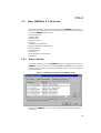
New AMESim 4.2 features . . . . . . . . . . . . . . . . . . . . . . . . . . . . . . . . . . . . . 9
1.6.1
Export facility . . . . . . . . . . . . . . . . . . . . . . . . . . . . . . . . . . . . . . . . . . . . . 9
1.6.2
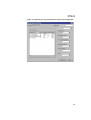
Design Exploration . . . . . . . . . . . . . . . . . . . . . . . . . . . . . . . . . . . . . . . . . 9
1.6.3
Compiler flags . . . . . . . . . . . . . . . . . . . . . . . . . . . . . . . . . . . . . . . . . . . . 11
1.6.4
Stabilizing runs . . . . . . . . . . . . . . . . . . . . . . . . . . . . . . . . . . . . . . . . . . . 11
1.6.5
Display of vectors . . . . . . . . . . . . . . . . . . . . . . . . . . . . . . . . . . . . . . . . . 11
1.6.6
Interfaces . . . . . . . . . . . . . . . . . . . . . . . . . . . . . . . . . . . . . . . . . . . . . . . . 13
1.6.7
Submodel call modifications . . . . . . . . . . . . . . . . . . . . . . . . . . . . . . . . . 14
1.6.8
Model simplification and Real time. . . . . . . . . . . . . . . . . . . . . . . . . . . . 14
1.6.9
Compare Systems. . . . . . . . . . . . . . . . . . . . . . . . . . . . . . . . . . . . . . . . . . 15
1.6.10 Pack and Unpack . . . . . . . . . . . . . . . . . . . . . . . . . . . . . . . . . . . . . . . . . . 16
1.6.11 Enumeration. . . . . . . . . . . . . . . . . . . . . . . . . . . . . . . . . . . . . . . . . . . . . . 18
1.6.12 Watch Parameters and Variables . . . . . . . . . . . . . . . . . . . . . . . . . . . . . . 19
1.6.13 Online help. . . . . . . . . . . . . . . . . . . . . . . . . . . . . . . . . . . . . . . . . . . . . . . 20
Chapter 2: The AMESim Workspace . . . . . . . . . . . . . . . . . . . . . . . . . . 23
2.1
2.1.1
The AMESim User Interface. . . . . . . . . . . . . . . . . . . . . . . . . . . . . . . . . . . 23
The Main Window . . . . . . . . . . . . . . . . . . . . . . . . . . . . . . . . . . . . . . . . . 23
Starting AMESim. . . . . . . . . . . . . . . . . . . . . . . . . . . . . . . . . . . . . . . . . . 23
Closing the Main Window . . . . . . . . . . . . . . . . . . . . . . . . . . . . . . . . . . . 24
i
Table of contents
2.1.2
The Menu Bar . . . . . . . . . . . . . . . . . . . . . . . . . . . . . . . . . . . . . . . . . . . . 24
File Menu . . . . . . . . . . . . . . . . . . . . . . . . . . . . . . . . . . . . . . . . . . . . . . .
Edit Menu . . . . . . . . . . . . . . . . . . . . . . . . . . . . . . . . . . . . . . . . . . . . . . .
Options Menu . . . . . . . . . . . . . . . . . . . . . . . . . . . . . . . . . . . . . . . . . . . .
View Menu . . . . . . . . . . . . . . . . . . . . . . . . . . . . . . . . . . . . . . . . . . . . . .
Parameters Menu. . . . . . . . . . . . . . . . . . . . . . . . . . . . . . . . . . . . . . . . . .
Interface Menu . . . . . . . . . . . . . . . . . . . . . . . . . . . . . . . . . . . . . . . . . . .
Graphs Menu . . . . . . . . . . . . . . . . . . . . . . . . . . . . . . . . . . . . . . . . . . . . .
Icons Menu . . . . . . . . . . . . . . . . . . . . . . . . . . . . . . . . . . . . . . . . . . . . . .
Tools Menu . . . . . . . . . . . . . . . . . . . . . . . . . . . . . . . . . . . . . . . . . . . . . .
Windows Menu . . . . . . . . . . . . . . . . . . . . . . . . . . . . . . . . . . . . . . . . . . .
Help Menu. . . . . . . . . . . . . . . . . . . . . . . . . . . . . . . . . . . . . . . . . . . . . . .
2.1.3
25
27
28
29
29
29
30
31
31
33
33
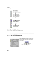
The Toolbars . . . . . . . . . . . . . . . . . . . . . . . . . . . . . . . . . . . . . . . . . . . . . 33
The File Operations Toolbar . . . . . . . . . . . . . . . . . . . . . . . . . . . . . . . . .
The Mode Operations Toolbar . . . . . . . . . . . . . . . . . . . . . . . . . . . . . . .
The Annotation Tools Toolbar . . . . . . . . . . . . . . . . . . . . . . . . . . . . . . .
The Edit Operations Toolbar. . . . . . . . . . . . . . . . . . . . . . . . . . . . . . . . .
The Temporal Analysis Toolbar . . . . . . . . . . . . . . . . . . . . . . . . . . . . . .
The Post Processing Tools Toolbar. . . . . . . . . . . . . . . . . . . . . . . . . . . .
The Linear Analysis Toolbar. . . . . . . . . . . . . . . . . . . . . . . . . . . . . . . . .
34
34
35
36
37
37
38
2.1.4
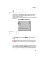
The mouse right-button menu . . . . . . . . . . . . . . . . . . . . . . . . . . . . . . . . 38
2.1.5
The libraries. . . . . . . . . . . . . . . . . . . . . . . . . . . . . . . . . . . . . . . . . . . . . . 39
The standard library . . . . . . . . . . . . . . . . . . . . . . . . . . . . . . . . . . . . . . . 39
The extra libraries . . . . . . . . . . . . . . . . . . . . . . . . . . . . . . . . . . . . . . . . . 39
2.2
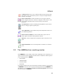
The AMESim four working modes . . . . . . . . . . . . . . . . . . . . . . . . . . . . . 41
2.2.1
Sketch Mode . . . . . . . . . . . . . . . . . . . . . . . . . . . . . . . . . . . . . . . . . . . . . 41
2.2.2
Submodel Mode . . . . . . . . . . . . . . . . . . . . . . . . . . . . . . . . . . . . . . . . . . 41
2.2.3
Parameter Mode . . . . . . . . . . . . . . . . . . . . . . . . . . . . . . . . . . . . . . . . . . 42
2.2.4
Run Mode . . . . . . . . . . . . . . . . . . . . . . . . . . . . . . . . . . . . . . . . . . . . . . . 42
2.3
Tricks and Tips . . . . . . . . . . . . . . . . . . . . . . . . . . . . . . . . . . . . . . . . . . . . . 43
2.3.1
The Lock Button . . . . . . . . . . . . . . . . . . . . . . . . . . . . . . . . . . . . . . . . . . 43
2.3.2
Rotating and mirroring an icon . . . . . . . . . . . . . . . . . . . . . . . . . . . . . . . 43
2.3.3
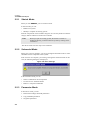
The Status Bar . . . . . . . . . . . . . . . . . . . . . . . . . . . . . . . . . . . . . . . . . . . . 43
2.3.4
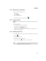
Removing a component. . . . . . . . . . . . . . . . . . . . . . . . . . . . . . . . . . . . . 44
2.3.5
Drag and Drop. . . . . . . . . . . . . . . . . . . . . . . . . . . . . . . . . . . . . . . . . . . . 44
2.3.6
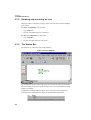
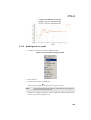
Adding some Text . . . . . . . . . . . . . . . . . . . . . . . . . . . . . . . . . . . . . . . . . 45
2.3.7
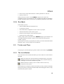
The Ports . . . . . . . . . . . . . . . . . . . . . . . . . . . . . . . . . . . . . . . . . . . . . . . . 45
2.3.8
Displaying/Hiding component labels . . . . . . . . . . . . . . . . . . . . . . . . . . 46
2.3.9
Online help . . . . . . . . . . . . . . . . . . . . . . . . . . . . . . . . . . . . . . . . . . . . . . 46
2.3.10 Keyboard Shortcuts . . . . . . . . . . . . . . . . . . . . . . . . . . . . . . . . . . . . . . . . 47
ii
AMESim 4.2
User Manual
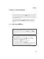
Chapter 3: Getting Started . . . . . . . . . . . . . . . . . . . . . . . . . . . . . . . . . . . 49
3.1
Introduction . . . . . . . . . . . . . . . . . . . . . . . . . . . . . . . . . . . . . . . . . . . . . . . . 49
3.2
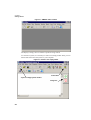
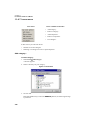
Starting AMESim . . . . . . . . . . . . . . . . . . . . . . . . . . . . . . . . . . . . . . . . . . . 49
3.3
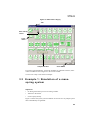
Creating a new sketch . . . . . . . . . . . . . . . . . . . . . . . . . . . . . . . . . . . . . . . . 51
3.3.1
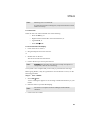
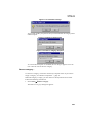
Opening an empty system . . . . . . . . . . . . . . . . . . . . . . . . . . . . . . . . . . . 51
3.3.2
Lock button . . . . . . . . . . . . . . . . . . . . . . . . . . . . . . . . . . . . . . . . . . . . . . 52
3.3.3
Libraries / Categories. . . . . . . . . . . . . . . . . . . . . . . . . . . . . . . . . . . . . . . 52
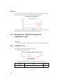
3.4
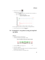
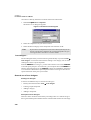
Example 1: Simulation of a mass-spring system . . . . . . . . . . . . . . . . . . . 53
3.4.1
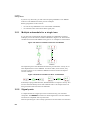
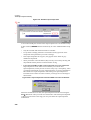
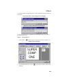
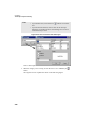
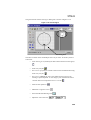
Building the mass spring model. . . . . . . . . . . . . . . . . . . . . . . . . . . . . . . 54
3.4.2
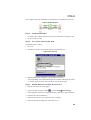
Assigning submodels to components. . . . . . . . . . . . . . . . . . . . . . . . . . . 58
3.4.3
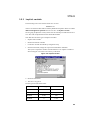
Setting parameters . . . . . . . . . . . . . . . . . . . . . . . . . . . . . . . . . . . . . . . . . 60
3.4.4
Running a simulation . . . . . . . . . . . . . . . . . . . . . . . . . . . . . . . . . . . . . . . 63
3.4.5
Plotting graphs . . . . . . . . . . . . . . . . . . . . . . . . . . . . . . . . . . . . . . . . . . . . 65
3.4.6
Replay facility . . . . . . . . . . . . . . . . . . . . . . . . . . . . . . . . . . . . . . . . . . . . 69
3.4.7
Save and quit AMESim . . . . . . . . . . . . . . . . . . . . . . . . . . . . . . . . . . . . . 72
3.5
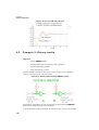
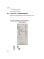
Example 2: A simple mechanical system . . . . . . . . . . . . . . . . . . . . . . . . . 72
3.5.2
Displaying labels on the sketch . . . . . . . . . . . . . . . . . . . . . . . . . . . . . . . 76
3.5.3
Setting parameters . . . . . . . . . . . . . . . . . . . . . . . . . . . . . . . . . . . . . . . . . 79
3.5.4
Changing the values. . . . . . . . . . . . . . . . . . . . . . . . . . . . . . . . . . . . . . . . 80
3.5.5
Aliases for a parameter title, a submodel and a variable title . . . . . . . . 81
Aliasing submodel titles. . . . . . . . . . . . . . . . . . . . . . . . . . . . . . . . . . . . . 81
Aliasing parameter titles . . . . . . . . . . . . . . . . . . . . . . . . . . . . . . . . . . . . 82
Aliasing variable titles . . . . . . . . . . . . . . . . . . . . . . . . . . . . . . . . . . . . . . 83
3.5.6
Setting parameters and running a simulation. . . . . . . . . . . . . . . . . . . . . 83
3.5.7
Using the "External Variables" facility . . . . . . . . . . . . . . . . . . . . . . . . . 85
Plotting curves . . . . . . . . . . . . . . . . . . . . . . . . . . . . . . . . . . . . . . . . . . . . 86
3.5.8
Using old final values . . . . . . . . . . . . . . . . . . . . . . . . . . . . . . . . . . . . . . 88
3.5.9
Zoom a plot . . . . . . . . . . . . . . . . . . . . . . . . . . . . . . . . . . . . . . . . . . . . . . 89
3.5.10 Continuation run . . . . . . . . . . . . . . . . . . . . . . . . . . . . . . . . . . . . . . . . . . 90
3.6
Example 3: A system using an implicit variable. . . . . . . . . . . . . . . . . . . . 91
3.6.2
Signal ports . . . . . . . . . . . . . . . . . . . . . . . . . . . . . . . . . . . . . . . . . . . . . . 92
3.6.3
Implicit variable . . . . . . . . . . . . . . . . . . . . . . . . . . . . . . . . . . . . . . . . . . . 95
3.7
Example 4: System having an algebraic loop . . . . . . . . . . . . . . . . . . . . . . 96
Changing parameters . . . . . . . . . . . . . . . . . . . . . . . . . . . . . . . . . . . . . . . 97
A short explanation . . . . . . . . . . . . . . . . . . . . . . . . . . . . . . . . . . . . . . . . 97
Chapter 4: Advanced Examples . . . . . . . . . . . . . . . . . . . . . . . . . . . . . . . 99
iii
Table of contents
4.1
Introduction . . . . . . . . . . . . . . . . . . . . . . . . . . . . . . . . . . . . . . . . . . . . . . . 99
4.2
Example 1: Quarter car continued . . . . . . . . . . . . . . . . . . . . . . . . . . . . . . 99
4.2.1
State count facility. . . . . . . . . . . . . . . . . . . . . . . . . . . . . . . . . . . . . . . . . 99
4.2.2
Dynamic runs and Stabilizing runs . . . . . . . . . . . . . . . . . . . . . . . . . . . 102
State variable . . . . . . . . . . . . . . . . . . . . . . . . . . . . . . . . . . . . . . . . . . . .
Uniqueness of an equilibrium position . . . . . . . . . . . . . . . . . . . . . . . .
CPU times . . . . . . . . . . . . . . . . . . . . . . . . . . . . . . . . . . . . . . . . . . . . . .
Solver type: Regular/Cautious . . . . . . . . . . . . . . . . . . . . . . . . . . . . . .
Stabilizing run diagnostics . . . . . . . . . . . . . . . . . . . . . . . . . . . . . . . . .
Recommended strategy for obtaining an equilibrium position . . . . . .
104
106
106
106
107
107
4.2.3
Save data/Load data . . . . . . . . . . . . . . . . . . . . . . . . . . . . . . . . . . . . . . 108
4.2.4
Adding text to a plot . . . . . . . . . . . . . . . . . . . . . . . . . . . . . . . . . . . . . . 109
4.3
Example 2: Rotary Inertia. . . . . . . . . . . . . . . . . . . . . . . . . . . . . . . . . . . . 110
4.3.1
Getting AMESim demonstration examples. . . . . . . . . . . . . . . . . . . . . 111
4.3.2
Sign convention for rotary speeds and torques . . . . . . . . . . . . . . . . . . 111
4.3.3
Aliasing with data sampling . . . . . . . . . . . . . . . . . . . . . . . . . . . . . . . . 113
4.3.4
Discontinuities and discontinuity printout . . . . . . . . . . . . . . . . . . . . . 114
4.4
Example 3: Car suspension. . . . . . . . . . . . . . . . . . . . . . . . . . . . . . . . . . . 115
4.4.1
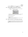
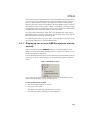
Displaying two or more AMESim systems simultaneously . . . . . . . . 117
4.4.2
Selecting components, line runs and text . . . . . . . . . . . . . . . . . . . . . . 118
4.4.3
Copy, Delete, Cut and Paste Actions . . . . . . . . . . . . . . . . . . . . . . . . . 120
4.4.4
Dynamic blocks. . . . . . . . . . . . . . . . . . . . . . . . . . . . . . . . . . . . . . . . . . 123
4.4.5
Comparing the body displacement with different suspensions. . . . . . 126
4.4.6
Editing the characteristics of existing text . . . . . . . . . . . . . . . . . . . . . 127
4.5
Example 4: Cam operated valve . . . . . . . . . . . . . . . . . . . . . . . . . . . . . . . 128
4.5.1
Description . . . . . . . . . . . . . . . . . . . . . . . . . . . . . . . . . . . . . . . . . . . . . 129
4.5.2
Simulating the system . . . . . . . . . . . . . . . . . . . . . . . . . . . . . . . . . . . . . 130
4.5.3
Creating an XY plot . . . . . . . . . . . . . . . . . . . . . . . . . . . . . . . . . . . . . . 133
4.5.4
Using the plot manager . . . . . . . . . . . . . . . . . . . . . . . . . . . . . . . . . . . . 134
4.5.5
Altering the characteristics of a plotted curve. . . . . . . . . . . . . . . . . . . 136
4.6
Example 5: Vehicle Driveline . . . . . . . . . . . . . . . . . . . . . . . . . . . . . . . . 138
4.6.1
Creating a 1D table data file using the Table editor . . . . . . . . . . . . . . 139
4.6.2
Building the system and setting parameters . . . . . . . . . . . . . . . . . . . . 141
4.6.3
Running the simulation . . . . . . . . . . . . . . . . . . . . . . . . . . . . . . . . . . . . 143
Chapter 5: Batch Runs and Linear Analysis . . . . . . . . . . . . . . . . . . . .145
iv
5.1
Introduction . . . . . . . . . . . . . . . . . . . . . . . . . . . . . . . . . . . . . . . . . . . . . . 145
5.2
Example 1: The quarter car model . . . . . . . . . . . . . . . . . . . . . . . . . . . . . 145
AMESim 4.2
User Manual
5.2.1
Selective save. . . . . . . . . . . . . . . . . . . . . . . . . . . . . . . . . . . . . . . . . . . . 146
5.2.2
Batch runs . . . . . . . . . . . . . . . . . . . . . . . . . . . . . . . . . . . . . . . . . . . . . . 148
Defining batch parameters . . . . . . . . . . . . . . . . . . . . . . . . . . . . . . . . . . 149
Initiating a batch run . . . . . . . . . . . . . . . . . . . . . . . . . . . . . . . . . . . . . . 151
Plotting curves for a batch run . . . . . . . . . . . . . . . . . . . . . . . . . . . . . . . 152
5.3
Example 2: A catapult to demonstrate locked states. . . . . . . . . . . . . . . . 155
5.3.1
Introduction to locked states . . . . . . . . . . . . . . . . . . . . . . . . . . . . . . . . 155
5.3.2
Demonstration . . . . . . . . . . . . . . . . . . . . . . . . . . . . . . . . . . . . . . . . . . . 156
5.3.3
Locked states . . . . . . . . . . . . . . . . . . . . . . . . . . . . . . . . . . . . . . . . . . . . 158
5.3.4
Error type . . . . . . . . . . . . . . . . . . . . . . . . . . . . . . . . . . . . . . . . . . . . . . . 161
5.4
Example 3: Linear analysis with a simple mass spring system. . . . . . . . 162
5.4.1
Linear analysis . . . . . . . . . . . . . . . . . . . . . . . . . . . . . . . . . . . . . . . . . . . 163
5.4.2
Eigenvalue Analysis . . . . . . . . . . . . . . . . . . . . . . . . . . . . . . . . . . . . . . 166
Non-linearities . . . . . . . . . . . . . . . . . . . . . . . . . . . . . . . . . . . . . . . . . . . 168
5.4.3
5.5
Equilibrium position . . . . . . . . . . . . . . . . . . . . . . . . . . . . . . . . . . . . . . 171
Example 4: Frequency response analysis with a mass-spring damper system
. . . . . . . . . . . . . . . . . . . . . . . . . . . . . . . . . . . . . . . . . . . . . . . . . . . . . . . . . 172
5.5.1
Bode, Nichols and Nyquist plots . . . . . . . . . . . . . . . . . . . . . . . . . . . . . 172
5.5.2
Root locus analysis . . . . . . . . . . . . . . . . . . . . . . . . . . . . . . . . . . . . . . . 175
5.6
Example 5: Modal shape analysis with a mechanical system . . . . . . . . . 178
5.6.1
Modal shapes . . . . . . . . . . . . . . . . . . . . . . . . . . . . . . . . . . . . . . . . . . . . 178
5.6.2
Relate the modal shape analysis to the time domain . . . . . . . . . . . . . . 184
5.7
Reference. . . . . . . . . . . . . . . . . . . . . . . . . . . . . . . . . . . . . . . . . . . . . . . . . 185
Chapter 6: The Supercomponent Facility . . . . . . . . . . . . . . . . . . . . . . 187
6.1
Introduction . . . . . . . . . . . . . . . . . . . . . . . . . . . . . . . . . . . . . . . . . . . . . . . 187
6.2
187
Constructing a supercomponent of a P.I.D. controller using a standard icon
6.2.1
Comparing a flat system with a system containing a supercomponent 188
6.2.2
Creating a supercomponent . . . . . . . . . . . . . . . . . . . . . . . . . . . . . . . . . 190
6.3
Supercomponent facility . . . . . . . . . . . . . . . . . . . . . . . . . . . . . . . . . . . . . 194
6.3.2
Exploring a supercomponent . . . . . . . . . . . . . . . . . . . . . . . . . . . . . . . . 195
6.3.3
Changing parameters of a supercomponent. . . . . . . . . . . . . . . . . . . . . 196
6.3.4
Plotting variables of a supercomponent. . . . . . . . . . . . . . . . . . . . . . . . 197
6.4
6.4.1
Managing Supercomponents . . . . . . . . . . . . . . . . . . . . . . . . . . . . . . . . . . 198
Different types of supercomponent . . . . . . . . . . . . . . . . . . . . . . . . . . . 198
Generic supercomponents . . . . . . . . . . . . . . . . . . . . . . . . . . . . . . . . . . 198
v
Table of contents
Customized supercomponents. . . . . . . . . . . . . . . . . . . . . . . . . . . . . . . 198
6.4.2
Multi-level supercomponents . . . . . . . . . . . . . . . . . . . . . . . . . . . . . . . 199
6.4.3
Displaying the available supercomponents and their categories. . . . . 199
6.4.4
Removing a supercomponent or a category . . . . . . . . . . . . . . . . . . . . 200
6.4.5
Modifying a supercomponent . . . . . . . . . . . . . . . . . . . . . . . . . . . . . . . 201
6.5
203
Constructing a supercomponent of a P.I.D. controller using your own icon
6.5.1
Creating a supercomponent category . . . . . . . . . . . . . . . . . . . . . . . . . 203
6.5.2
Creating a supercomponent icon . . . . . . . . . . . . . . . . . . . . . . . . . . . . . 207
6.6
Creating a generic supercomponent containing global parameters . . . . 213
Chapter 7: The AMESim-MATLAB Interface . . . . . . . . . . . . . . . . . .221
7.1
Introduction . . . . . . . . . . . . . . . . . . . . . . . . . . . . . . . . . . . . . . . . . . . . . . 221
7.2
Tutorial examples . . . . . . . . . . . . . . . . . . . . . . . . . . . . . . . . . . . . . . . . . . 221
7.2.1
Setting the MATLAB path list . . . . . . . . . . . . . . . . . . . . . . . . . . . . . . 222
7.2.2
Setting the MATLAB working area . . . . . . . . . . . . . . . . . . . . . . . . . . 223
7.2.3
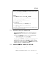
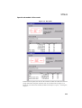
Importing AMESim results into MATLAB . . . . . . . . . . . . . . . . . . . . 223
7.2.4
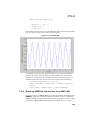
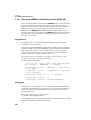
Running AMESim simulations from MATLAB. . . . . . . . . . . . . . . . . 225
Running a simulation from AMESim . . . . . . . . . . . . . . . . . . . . . . . . . 226
Running a simulation from MATLAB . . . . . . . . . . . . . . . . . . . . . . . . 226
Running a batch simulation from MATLAB . . . . . . . . . . . . . . . . . . . 229
7.2.5
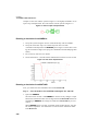
Importing linear analysis results from AMESim into MATLAB . . . . 230
Case of an explicit system. . . . . . . . . . . . . . . . . . . . . . . . . . . . . . . . . . 231
Case of an implicit system . . . . . . . . . . . . . . . . . . . . . . . . . . . . . . . . . 234
7.3
Reference . . . . . . . . . . . . . . . . . . . . . . . . . . . . . . . . . . . . . . . . . . . . . . . . 234
7.3.1
Special .m files available. . . . . . . . . . . . . . . . . . . . . . . . . . . . . . . . . . . 234
7.3.2
Importing temporal (time history) results from AMESim . . . . . . . . . 236
ame2data . . . . . . . . . . . . . . . . . . . . . . . . . . . . . . . . . . . . . . . . . . . . . . . 236
ameloadt . . . . . . . . . . . . . . . . . . . . . . . . . . . . . . . . . . . . . . . . . . . . . . . 236
amegetvar . . . . . . . . . . . . . . . . . . . . . . . . . . . . . . . . . . . . . . . . . . . . . . 237
7.3.3
Importing linear systems from MATLAB into AMESim . . . . . . . . . . 238
Case of a transfer function . . . . . . . . . . . . . . . . . . . . . . . . . . . . . . . . .
Case of a state space . . . . . . . . . . . . . . . . . . . . . . . . . . . . . . . . . . . . . .
Importing .ssp and .jac files to AMESim . . . . . . . . . . . . . . . . . . . . . .
Special submodels in Parameter mode . . . . . . . . . . . . . . . . . . . . . . . .
Special submodels in Run mode . . . . . . . . . . . . . . . . . . . . . . . . . . . . .
7.3.4
238
238
239
242
243
Running AMESim simulations from MATLAB. . . . . . . . . . . . . . . . . 244
amegetcuspar . . . . . . . . . . . . . . . . . . . . . . . . . . . . . . . . . . . . . . . . . . . . 244
amegetgpar . . . . . . . . . . . . . . . . . . . . . . . . . . . . . . . . . . . . . . . . . . . . . 244
vi
AMESim 4.2
User Manual
amegetp . . . . . . . . . . . . . . . . . . . . . . . . . . . . . . . . . . . . . . . . . . . . . . . . 245
ameputcuspar . . . . . . . . . . . . . . . . . . . . . . . . . . . . . . . . . . . . . . . . . . . . 245
ameputgpar. . . . . . . . . . . . . . . . . . . . . . . . . . . . . . . . . . . . . . . . . . . . . . 245
ameputp . . . . . . . . . . . . . . . . . . . . . . . . . . . . . . . . . . . . . . . . . . . . . . . . 246
amela . . . . . . . . . . . . . . . . . . . . . . . . . . . . . . . . . . . . . . . . . . . . . . . . . . 246
amerun . . . . . . . . . . . . . . . . . . . . . . . . . . . . . . . . . . . . . . . . . . . . . . . . . 246
Chapter 8: Activity index . . . . . . . . . . . . . . . . . . . . . . . . . . . . . . . . . . . 247
8.1
Introduction . . . . . . . . . . . . . . . . . . . . . . . . . . . . . . . . . . . . . . . . . . . . . . . 247
8.2
Mathematical definitions. . . . . . . . . . . . . . . . . . . . . . . . . . . . . . . . . . . . . 248
8.3
Using the AMESim Activity index facility. . . . . . . . . . . . . . . . . . . . . . . 249
8.3.1
Example 1: the vehicle driveline . . . . . . . . . . . . . . . . . . . . . . . . . . . . . 249
8.3.2
Example 2: the 3 piston pump (case study) . . . . . . . . . . . . . . . . . . . . . 254
Functional description of the pump . . . . . . . . . . . . . . . . . . . . . . . . . . . 254
Initial modeling . . . . . . . . . . . . . . . . . . . . . . . . . . . . . . . . . . . . . . . . . . 254
Validation of the final reduced model . . . . . . . . . . . . . . . . . . . . . . . . . 262
Comparison and numerical performances . . . . . . . . . . . . . . . . . . . . . . 263
Domain of validity . . . . . . . . . . . . . . . . . . . . . . . . . . . . . . . . . . . . . . . . 264
Summary . . . . . . . . . . . . . . . . . . . . . . . . . . . . . . . . . . . . . . . . . . . . . . . 265
References . . . . . . . . . . . . . . . . . . . . . . . . . . . . . . . . . . . . . . . . . . . . . . 266
Chapter 9: Getting Started with AMEPilot and the Export module 267
9.1
Introduction . . . . . . . . . . . . . . . . . . . . . . . . . . . . . . . . . . . . . . . . . . . . . . . 267
9.2
Polynomial integrator . . . . . . . . . . . . . . . . . . . . . . . . . . . . . . . . . . . . . . . 267
9.2.1
Setting up the export . . . . . . . . . . . . . . . . . . . . . . . . . . . . . . . . . . . . . . 268
9.2.2
Running the simulation . . . . . . . . . . . . . . . . . . . . . . . . . . . . . . . . . . . . 271
9.2.3
Using compound output parameters . . . . . . . . . . . . . . . . . . . . . . . . . . 273
Chapter 10:Getting started with AMESim design exploration features.
277
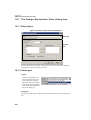
10.1 Introduction . . . . . . . . . . . . . . . . . . . . . . . . . . . . . . . . . . . . . . . . . . . . . . . 277
10.2 Active suspension example . . . . . . . . . . . . . . . . . . . . . . . . . . . . . . . . . . . 277
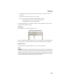
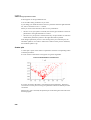
10.3 Design Of Experiments . . . . . . . . . . . . . . . . . . . . . . . . . . . . . . . . . . . . . . 281
10.4 Optimization . . . . . . . . . . . . . . . . . . . . . . . . . . . . . . . . . . . . . . . . . . . . . . 288
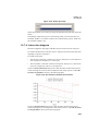
10.5 Monte Carlo. . . . . . . . . . . . . . . . . . . . . . . . . . . . . . . . . . . . . . . . . . . . . . . 294
Chapter 11:Facilities Available in all Modes . . . . . . . . . . . . . . . . . . . . 299
11.1 Selecting objects . . . . . . . . . . . . . . . . . . . . . . . . . . . . . . . . . . . . . . . . . . . 299
Shift + Left-click . . . . . . . . . . . . . . . . . . . . . . . . . . . . . . . . . . . . . . . . . 299
Rubber-banding method. . . . . . . . . . . . . . . . . . . . . . . . . . . . . . . . . . . . 299
vii
Table of contents
11.2 Facilities accessible from permanent toolbar buttons. . . . . . . . . . . . . . . 300
11.2.1 Changing mode . . . . . . . . . . . . . . . . . . . . . . . . . . . . . . . . . . . . . . . . . . 300
11.2.2 Copy selected items to the auxiliary system . . . . . . . . . . . . . . . . . . . . 301
11.2.3 Sketch annotation tools . . . . . . . . . . . . . . . . . . . . . . . . . . . . . . . . . . . . 301
Adding text to the sketch. . . . . . . . . . . . . . . . . . . . . . . . . . . . . . . . . . .
Changing the annotation object. . . . . . . . . . . . . . . . . . . . . . . . . . . . . .
Adding an object to the sketch . . . . . . . . . . . . . . . . . . . . . . . . . . . . . .
Adding stored images to the sketch. . . . . . . . . . . . . . . . . . . . . . . . . . .
301
302
302
303
11.2.4 Blank plots. . . . . . . . . . . . . . . . . . . . . . . . . . . . . . . . . . . . . . . . . . . . . . 303
11.2.5 Table editor . . . . . . . . . . . . . . . . . . . . . . . . . . . . . . . . . . . . . . . . . . . . . 303
11.3 Facilities available through sketch area menus . . . . . . . . . . . . . . . . . . . 305
Copy . . . . . . . . . . . . . . . . . . . . . . . . . . . . . . . . . . . . . . . . . . . . . . . . . .
Set color. . . . . . . . . . . . . . . . . . . . . . . . . . . . . . . . . . . . . . . . . . . . . . . .
Reset color. . . . . . . . . . . . . . . . . . . . . . . . . . . . . . . . . . . . . . . . . . . . . .
Alias . . . . . . . . . . . . . . . . . . . . . . . . . . . . . . . . . . . . . . . . . . . . . . . . . .
Lock States . . . . . . . . . . . . . . . . . . . . . . . . . . . . . . . . . . . . . . . . . . . . .
Text actions . . . . . . . . . . . . . . . . . . . . . . . . . . . . . . . . . . . . . . . . . . . . .
Labels . . . . . . . . . . . . . . . . . . . . . . . . . . . . . . . . . . . . . . . . . . . . . . . . .
Edit properties . . . . . . . . . . . . . . . . . . . . . . . . . . . . . . . . . . . . . . . . . . .
Order . . . . . . . . . . . . . . . . . . . . . . . . . . . . . . . . . . . . . . . . . . . . . . . . . .
Set attributes as default . . . . . . . . . . . . . . . . . . . . . . . . . . . . . . . . . . . .
Bird’s eye view . . . . . . . . . . . . . . . . . . . . . . . . . . . . . . . . . . . . . . . . . .
Help . . . . . . . . . . . . . . . . . . . . . . . . . . . . . . . . . . . . . . . . . . . . . . . . . . .
305
305
307
307
308
309
311
311
311
312
312
313
11.4 Facilities available through the menu bar. . . . . . . . . . . . . . . . . . . . . . . . 314
11.4.1 File menu. . . . . . . . . . . . . . . . . . . . . . . . . . . . . . . . . . . . . . . . . . . . . . . 314
Opening a new system. . . . . . . . . . . . . . . . . . . . . . . . . . . . . . . . . . . . .
Opening an existing system. . . . . . . . . . . . . . . . . . . . . . . . . . . . . . . . .
Saving a system. . . . . . . . . . . . . . . . . . . . . . . . . . . . . . . . . . . . . . . . . .
Save as starter . . . . . . . . . . . . . . . . . . . . . . . . . . . . . . . . . . . . . . . . . . .
Reload saved version. . . . . . . . . . . . . . . . . . . . . . . . . . . . . . . . . . . . . .
Touch. . . . . . . . . . . . . . . . . . . . . . . . . . . . . . . . . . . . . . . . . . . . . . . . . .
HTML report . . . . . . . . . . . . . . . . . . . . . . . . . . . . . . . . . . . . . . . . . . . .
Print, Print selection and Print display . . . . . . . . . . . . . . . . . . . . . . . .
Last opened files list . . . . . . . . . . . . . . . . . . . . . . . . . . . . . . . . . . . . . .
Close . . . . . . . . . . . . . . . . . . . . . . . . . . . . . . . . . . . . . . . . . . . . . . . . . .
Quit . . . . . . . . . . . . . . . . . . . . . . . . . . . . . . . . . . . . . . . . . . . . . . . . . . .
314
316
317
318
319
319
319
322
324
324
325
11.4.2 Edit menu . . . . . . . . . . . . . . . . . . . . . . . . . . . . . . . . . . . . . . . . . . . . . . 326
Copy . . . . . . . . . . . . . . . . . . . . . . . . . . . . . . . . . . . . . . . . . . . . . . . . . .
Display auxiliary . . . . . . . . . . . . . . . . . . . . . . . . . . . . . . . . . . . . . . . . .
Select all . . . . . . . . . . . . . . . . . . . . . . . . . . . . . . . . . . . . . . . . . . . . . . .
External variables . . . . . . . . . . . . . . . . . . . . . . . . . . . . . . . . . . . . . . . .
Find submodel . . . . . . . . . . . . . . . . . . . . . . . . . . . . . . . . . . . . . . . . . . .
Update categories . . . . . . . . . . . . . . . . . . . . . . . . . . . . . . . . . . . . . . . .
Available supercomponents . . . . . . . . . . . . . . . . . . . . . . . . . . . . . . . .
viii
326
326
326
327
327
328
328
AMESim 4.2
User Manual
Available customized. . . . . . . . . . . . . . . . . . . . . . . . . . . . . . . . . . . . . . 334
Available user submodels . . . . . . . . . . . . . . . . . . . . . . . . . . . . . . . . . . 334
Copy to supercomponent . . . . . . . . . . . . . . . . . . . . . . . . . . . . . . . . . . . 335
11.4.3 Options menu . . . . . . . . . . . . . . . . . . . . . . . . . . . . . . . . . . . . . . . . . . . . 336
Path List . . . . . . . . . . . . . . . . . . . . . . . . . . . . . . . . . . . . . . . . . . . . . . . . 336
Submodel alias list . . . . . . . . . . . . . . . . . . . . . . . . . . . . . . . . . . . . . . . . 339
Preferred units . . . . . . . . . . . . . . . . . . . . . . . . . . . . . . . . . . . . . . . . . . . 339
Current drawing settings . . . . . . . . . . . . . . . . . . . . . . . . . . . . . . . . . . . 340
Color preferences . . . . . . . . . . . . . . . . . . . . . . . . . . . . . . . . . . . . . . . . . 341
AMESim preferences. . . . . . . . . . . . . . . . . . . . . . . . . . . . . . . . . . . . . . 342
11.4.4 View menu . . . . . . . . . . . . . . . . . . . . . . . . . . . . . . . . . . . . . . . . . . . . . . 347
Bird’s eye view . . . . . . . . . . . . . . . . . . . . . . . . . . . . . . . . . . . . . . . . . . 347
11.4.5 Interface menu . . . . . . . . . . . . . . . . . . . . . . . . . . . . . . . . . . . . . . . . . . . 347
Display interface status . . . . . . . . . . . . . . . . . . . . . . . . . . . . . . . . . . . . 348
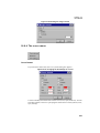
11.4.6 Graphs menu . . . . . . . . . . . . . . . . . . . . . . . . . . . . . . . . . . . . . . . . . . . . 349
11.4.7 Icons menu . . . . . . . . . . . . . . . . . . . . . . . . . . . . . . . . . . . . . . . . . . . . . . 350
Add category.... . . . . . . . . . . . . . . . . . . . . . . . . . . . . . . . . . . . . . . . . . . 350
Remove category... . . . . . . . . . . . . . . . . . . . . . . . . . . . . . . . . . . . . . . . 351
Add component.... . . . . . . . . . . . . . . . . . . . . . . . . . . . . . . . . . . . . . . . . 352
Remove component... . . . . . . . . . . . . . . . . . . . . . . . . . . . . . . . . . . . . . 353
Icon designer.... . . . . . . . . . . . . . . . . . . . . . . . . . . . . . . . . . . . . . . . . . . 354
General use of Icon designer . . . . . . . . . . . . . . . . . . . . . . . . . . . . . . . . 355
Selecting or creating an icon for a supercomponent . . . . . . . . . . . . . . 357
11.4.8 Tools menu. . . . . . . . . . . . . . . . . . . . . . . . . . . . . . . . . . . . . . . . . . . . . . 358
Check submodels . . . . . . . . . . . . . . . . . . . . . . . . . . . . . . . . . . . . . . . . . 358
Expression Editor... . . . . . . . . . . . . . . . . . . . . . . . . . . . . . . . . . . . . . . . 365
Purge... . . . . . . . . . . . . . . . . . . . . . . . . . . . . . . . . . . . . . . . . . . . . . . . . . 367
Pack/Unpack facility . . . . . . . . . . . . . . . . . . . . . . . . . . . . . . . . . . . . . . 369
Table editor... . . . . . . . . . . . . . . . . . . . . . . . . . . . . . . . . . . . . . . . . . . . . 378
Start AMECustom / AMESet / AMEAnimation / Matlab . . . . . . . . . . 378
License viewer... . . . . . . . . . . . . . . . . . . . . . . . . . . . . . . . . . . . . . . . . . 378
11.4.9 Windows menu . . . . . . . . . . . . . . . . . . . . . . . . . . . . . . . . . . . . . . . . . . 379
11.4.10 Help menu . . . . . . . . . . . . . . . . . . . . . . . . . . . . . . . . . . . . . . . . . . . . . . 379
Online. . . . . . . . . . . . . . . . . . . . . . . . . . . . . . . . . . . . . . . . . . . . . . . . . . 379
AMESim demo help . . . . . . . . . . . . . . . . . . . . . . . . . . . . . . . . . . . . . . 380
Get AMESim demo . . . . . . . . . . . . . . . . . . . . . . . . . . . . . . . . . . . . . . . 380
About . . . . . . . . . . . . . . . . . . . . . . . . . . . . . . . . . . . . . . . . . . . . . . . . . . 381
Chapter 12:Facilities Available In Sketch Mode . . . . . . . . . . . . . . . . . 383
12.1 Introduction . . . . . . . . . . . . . . . . . . . . . . . . . . . . . . . . . . . . . . . . . . . . . . . 383
12.2 Adding objects to the sketch . . . . . . . . . . . . . . . . . . . . . . . . . . . . . . . . . . 383
12.2.1 AMESim overlap rule . . . . . . . . . . . . . . . . . . . . . . . . . . . . . . . . . . . . . 383
ix
Table of contents
12.2.2 Adding components to the sketch . . . . . . . . . . . . . . . . . . . . . . . . . . . . 383
Cursor method . . . . . . . . . . . . . . . . . . . . . . . . . . . . . . . . . . . . . . . . . . .
Drag and drop method. . . . . . . . . . . . . . . . . . . . . . . . . . . . . . . . . . . . .
Actions when a component is added to the sketch . . . . . . . . . . . . . . .
Compatible ports . . . . . . . . . . . . . . . . . . . . . . . . . . . . . . . . . . . . . . . . .
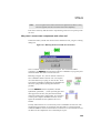
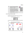
Connections between components . . . . . . . . . . . . . . . . . . . . . . . . . . .
Why can’t I connect two components? . . . . . . . . . . . . . . . . . . . . . . . .
384
384
384
384
385
385
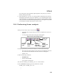
12.2.3 Adding a new line run to the sketch . . . . . . . . . . . . . . . . . . . . . . . . . . 388
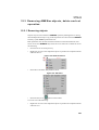
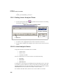
12.3 Removing AMESim objects, delete and cut operation. . . . . . . . . . . . . . 390
12.3.1 Removing objects . . . . . . . . . . . . . . . . . . . . . . . . . . . . . . . . . . . . . . . . 390
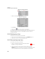
12.3.2 Deleting loose lines . . . . . . . . . . . . . . . . . . . . . . . . . . . . . . . . . . . . . . . 391
12.3.3 Reconnecting loose lines. . . . . . . . . . . . . . . . . . . . . . . . . . . . . . . . . . . 391
12.4 AMESim auxiliary system . . . . . . . . . . . . . . . . . . . . . . . . . . . . . . . . . . . 392
12.5 Moving components . . . . . . . . . . . . . . . . . . . . . . . . . . . . . . . . . . . . . . . . 393
12.6 AMESim ports . . . . . . . . . . . . . . . . . . . . . . . . . . . . . . . . . . . . . . . . . . . . 393
12.7 Removing submodels . . . . . . . . . . . . . . . . . . . . . . . . . . . . . . . . . . . . . . . 396
12.7.1 Why remove a submodel? . . . . . . . . . . . . . . . . . . . . . . . . . . . . . . . . . . 396
12.7.2 Procedure to remove one or more submodels . . . . . . . . . . . . . . . . . . . 397
12.8 Interface menu . . . . . . . . . . . . . . . . . . . . . . . . . . . . . . . . . . . . . . . . . . . . 398
Chapter 13:Facilities available in Submodel mode . . . . . . . . . . . . . . . .399
13.1 Submodel mode - selecting submodels . . . . . . . . . . . . . . . . . . . . . . . . . 399
13.2 The Premier submodel button. . . . . . . . . . . . . . . . . . . . . . . . . . . . . . . . . 400
13.3 Selecting a submodel for a component. . . . . . . . . . . . . . . . . . . . . . . . . . 400
Description of the Submodel List dialog box . . . . . . . . . . . . . . . . . . . 401
13.4 Removing a component submodel . . . . . . . . . . . . . . . . . . . . . . . . . . . . . 404
13.5 Assigning a supercomponent to a component . . . . . . . . . . . . . . . . . . . . 404
13.6 Removing a supercomponent from a component . . . . . . . . . . . . . . . . . . 406
13.7 Shadow subsystem . . . . . . . . . . . . . . . . . . . . . . . . . . . . . . . . . . . . . . . . . 406
Definition . . . . . . . . . . . . . . . . . . . . . . . . . . . . . . . . . . . . . . . . . . . . . . 406
Example. . . . . . . . . . . . . . . . . . . . . . . . . . . . . . . . . . . . . . . . . . . . . . . . 407
Chapter 14:Facilities available in Parameter mode . . . . . . . . . . . . . . .411
14.1 Introduction . . . . . . . . . . . . . . . . . . . . . . . . . . . . . . . . . . . . . . . . . . . . . . 411
14.2 Changing submodel and supercomponent parameter values directly . . 411
14.2.1 Changing parameters for a generic submodel and customized
supercomponent . . . . . . . . . . . . . . . . . . . . . . . . . . . . . . . . . . . . . . . . . 411
State variables . . . . . . . . . . . . . . . . . . . . . . . . . . . . . . . . . . . . . . . . . . . 412
x
AMESim 4.2
User Manual
Constraint variables . . . . . . . . . . . . . . . . . . . . . . . . . . . . . . . . . . . . . . . 413
Fixed variables . . . . . . . . . . . . . . . . . . . . . . . . . . . . . . . . . . . . . . . . . . . 413
Vector variables . . . . . . . . . . . . . . . . . . . . . . . . . . . . . . . . . . . . . . . . . . 414
Real parameters . . . . . . . . . . . . . . . . . . . . . . . . . . . . . . . . . . . . . . . . . . 415
Integer parameters . . . . . . . . . . . . . . . . . . . . . . . . . . . . . . . . . . . . . . . . 416
Text parameters . . . . . . . . . . . . . . . . . . . . . . . . . . . . . . . . . . . . . . . . . . 417
Changing the title of a parameter. . . . . . . . . . . . . . . . . . . . . . . . . . . . . 417
14.2.2 Changing parameters for a generic supercomponent without global
parameters . . . . . . . . . . . . . . . . . . . . . . . . . . . . . . . . . . . . . . . . . . . . . . 418
14.2.3 Changing parameters for a generic supercomponent with global parameters
. . . . . . . . . . . . . . . . . . . . . . . . . . . . . . . . . . . . . . . . . . . . . . . . . . . . . . . 418
14.2.4 Changing parameters for customized submodels . . . . . . . . . . . . . . . . 419
14.2.5 Load/Save of parameter values . . . . . . . . . . . . . . . . . . . . . . . . . . . . . . 420
14.2.6 Editing names and values. . . . . . . . . . . . . . . . . . . . . . . . . . . . . . . . . . . 421
14.3 Facilities provided by the Parameters menu in the menu bar . . . . . . . . . 421
14.3.1 Load/Save of system parameter set . . . . . . . . . . . . . . . . . . . . . . . . . . . 422
Saving a system parameter set . . . . . . . . . . . . . . . . . . . . . . . . . . . . . . . 422
Loading a system parameter set. . . . . . . . . . . . . . . . . . . . . . . . . . . . . . 423
14.3.2
Set final values . . . . . . . . . . . . . . . . . . . . . . . . . . . . . . . . . . . . . . . . . . 424
Introduction . . . . . . . . . . . . . . . . . . . . . . . . . . . . . . . . . . . . . . . . . . . . . 424
Procedure . . . . . . . . . . . . . . . . . . . . . . . . . . . . . . . . . . . . . . . . . . . . . . . 424
14.3.3 Global parameters . . . . . . . . . . . . . . . . . . . . . . . . . . . . . . . . . . . . . . . . 425
Creating a global parameter . . . . . . . . . . . . . . . . . . . . . . . . . . . . . . . . . 425
Assigning a global parameter. . . . . . . . . . . . . . . . . . . . . . . . . . . . . . . . 426
Modifying/Deleting a global parameter. . . . . . . . . . . . . . . . . . . . . . . . 427
Defining a global parameter in terms of other global parameters . . . . 427
14.3.4 Batch parameters . . . . . . . . . . . . . . . . . . . . . . . . . . . . . . . . . . . . . . . . . 427
14.3.5 Common parameters . . . . . . . . . . . . . . . . . . . . . . . . . . . . . . . . . . . . . . 429
14.3.6 Export setup . . . . . . . . . . . . . . . . . . . . . . . . . . . . . . . . . . . . . . . . . . . . . 430
14.4 Facilities provided by the other menus in the menu bar . . . . . . . . . . . . . 431
14.4.1 Parameters item of the View menu . . . . . . . . . . . . . . . . . . . . . . . . . . . 431
Using the Parameters window . . . . . . . . . . . . . . . . . . . . . . . . . . . . . . . 431
Create your own sets of parameters . . . . . . . . . . . . . . . . . . . . . . . . . . . 432
Facilities available in the Parameters window. . . . . . . . . . . . . . . . . . . 434
14.4.2 Compare systems item of the Tools menu. . . . . . . . . . . . . . . . . . . . . . 435
Using the Compare systems facility . . . . . . . . . . . . . . . . . . . . . . . . . . 435
Description of the colours used in the Compare systems facility . . . . 437
Facilities available from the Compare systems dialog box . . . . . . . . . 438
Tricks and tips . . . . . . . . . . . . . . . . . . . . . . . . . . . . . . . . . . . . . . . . . . . 440
xi
Table of contents
14.4.3 Write auxiliary files. . . . . . . . . . . . . . . . . . . . . . . . . . . . . . . . . . . . . . . 440
14.5 Right-button operations . . . . . . . . . . . . . . . . . . . . . . . . . . . . . . . . . . . . . 441
14.5.1 Copy/Paste parameters . . . . . . . . . . . . . . . . . . . . . . . . . . . . . . . . . . . . 441
Copying parameters. . . . . . . . . . . . . . . . . . . . . . . . . . . . . . . . . . . . . . . 441
Pasting parameters. . . . . . . . . . . . . . . . . . . . . . . . . . . . . . . . . . . . . . . . 441
14.5.2 Load/Save parameters . . . . . . . . . . . . . . . . . . . . . . . . . . . . . . . . . . . . . 442
Saving a submodel set of parameters . . . . . . . . . . . . . . . . . . . . . . . . . 442
Loading a submodel set of parameters . . . . . . . . . . . . . . . . . . . . . . . . 443
Chapter 15:Facilities Available in Run Mode . . . . . . . . . . . . . . . . . . . .445
15.1 Introduction . . . . . . . . . . . . . . . . . . . . . . . . . . . . . . . . . . . . . . . . . . . . . . 445
15.2 Time domain and linear analysis modes. . . . . . . . . . . . . . . . . . . . . . . . . 446
15.3 Running a simulation . . . . . . . . . . . . . . . . . . . . . . . . . . . . . . . . . . . . . . . 446
15.3.1 Save status and Save next status of variables . . . . . . . . . . . . . . . . . . . 446
Global change of Save next status. . . . . . . . . . . . . . . . . . . . . . . . . . . . 447
Submodel change of Save next status . . . . . . . . . . . . . . . . . . . . . . . . . 448
Individual variable change of Save next status . . . . . . . . . . . . . . . . . . 448
15.3.2 Locked status of state variables. . . . . . . . . . . . . . . . . . . . . . . . . . . . . . 449
Global change of Locked status . . . . . . . . . . . . . . . . . . . . . . . . . . . . .
Submodel change of Locked status . . . . . . . . . . . . . . . . . . . . . . . . . . .
Change of Locked status for individual state variables. . . . . . . . . . . .
Global view of locked/unlocked status for all the state variables of a
complete model . . . . . . . . . . . . . . . . . . . . . . . . . . . . . . . . . . . . . . . . . .
449
450
451
452
15.3.3 Setting run parameters. . . . . . . . . . . . . . . . . . . . . . . . . . . . . . . . . . . . . 452
General tab . . . . . . . . . . . . . . . . . . . . . . . . . . . . . . . . . . . . . . . . . . . . . 453
Standard options tab . . . . . . . . . . . . . . . . . . . . . . . . . . . . . . . . . . . . . . 456
Fixed step options tab . . . . . . . . . . . . . . . . . . . . . . . . . . . . . . . . . . . . . 462
15.3.4 Integration methods used . . . . . . . . . . . . . . . . . . . . . . . . . . . . . . . . . . 463
Fixed step integrators . . . . . . . . . . . . . . . . . . . . . . . . . . . . . . . . . . . . . 463
The standard integrator . . . . . . . . . . . . . . . . . . . . . . . . . . . . . . . . . . . . 464
15.3.5 The Simulation run dialog box . . . . . . . . . . . . . . . . . . . . . . . . . . . . . . 465
Log report . . . . . . . . . . . . . . . . . . . . . . . . . . . . . . . . . . . . . . . . . . . . . . 466
Warnings/Errors report . . . . . . . . . . . . . . . . . . . . . . . . . . . . . . . . . . . . 466
Progress bar . . . . . . . . . . . . . . . . . . . . . . . . . . . . . . . . . . . . . . . . . . . . . 468
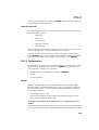
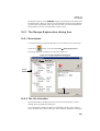
15.4 Load/save plot configuration . . . . . . . . . . . . . . . . . . . . . . . . . . . . . . . . . 468
Load plot configuration . . . . . . . . . . . . . . . . . . . . . . . . . . . . . . . . . . . . 468
Save plot configuration . . . . . . . . . . . . . . . . . . . . . . . . . . . . . . . . . . . . 469
15.5 State count facility . . . . . . . . . . . . . . . . . . . . . . . . . . . . . . . . . . . . . . . . . 469
15.6 Replay facilities . . . . . . . . . . . . . . . . . . . . . . . . . . . . . . . . . . . . . . . . . . . 470
15.6.1 Basic controls of Replay . . . . . . . . . . . . . . . . . . . . . . . . . . . . . . . . . . . 472
xii
AMESim 4.2
User Manual
15.6.2 Advanced options for Replay. . . . . . . . . . . . . . . . . . . . . . . . . . . . . . . . 472
15.6.3 Symbol Options for Replay . . . . . . . . . . . . . . . . . . . . . . . . . . . . . . . . . 474
15.6.4 Using saturation values . . . . . . . . . . . . . . . . . . . . . . . . . . . . . . . . . . . . 478
15.6.5 Some ideas . . . . . . . . . . . . . . . . . . . . . . . . . . . . . . . . . . . . . . . . . . . . . . 479
15.7 Why do linear analysis? . . . . . . . . . . . . . . . . . . . . . . . . . . . . . . . . . . . . . 479
15.8 Performing linear analysis. . . . . . . . . . . . . . . . . . . . . . . . . . . . . . . . . . . . 480
15.8.1 Setting Linear Analysis Times. . . . . . . . . . . . . . . . . . . . . . . . . . . . . . . 481
15.8.2 Linear Analysis Status . . . . . . . . . . . . . . . . . . . . . . . . . . . . . . . . . . . . . 482
15.8.3 Changing the LA status of a variable. . . . . . . . . . . . . . . . . . . . . . . . . . 483
Global changes of LA status . . . . . . . . . . . . . . . . . . . . . . . . . . . . . . . . 483
Changing the status of an individual variable . . . . . . . . . . . . . . . . . . . 484
15.8.4 Eigenvalue Analysis. . . . . . . . . . . . . . . . . . . . . . . . . . . . . . . . . . . . . . . 485
15.8.5 Modal shapes . . . . . . . . . . . . . . . . . . . . . . . . . . . . . . . . . . . . . . . . . . . . 487
How do I select the observer variables to use? . . . . . . . . . . . . . . . . . . 487
Plotting Magnitudes . . . . . . . . . . . . . . . . . . . . . . . . . . . . . . . . . . . . . . . 488
Plotting Energies . . . . . . . . . . . . . . . . . . . . . . . . . . . . . . . . . . . . . . . . . 491
15.8.6 Bode, Nichols and Nyquist plots . . . . . . . . . . . . . . . . . . . . . . . . . . . . . 491
15.8.7 Root locus plots . . . . . . . . . . . . . . . . . . . . . . . . . . . . . . . . . . . . . . . . . . 495
15.9 Speeding up a slow simulation . . . . . . . . . . . . . . . . . . . . . . . . . . . . . . . . 496
15.10 Variables window . . . . . . . . . . . . . . . . . . . . . . . . . . . . . . . . . . . . . . . . . . 497
15.10.1 Use of the Variables window. . . . . . . . . . . . . . . . . . . . . . . . . . . . . . . . 498
The main functions of the Variables window . . . . . . . . . . . . . . . . . . . 498
The right-button menu . . . . . . . . . . . . . . . . . . . . . . . . . . . . . . . . . . . . . 498
15.10.2 Creating your own sets of variables. . . . . . . . . . . . . . . . . . . . . . . . . . . 499
15.10.3 The facilities available in the Variables window. . . . . . . . . . . . . . . . . 501
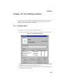
Chapter 16:The Plotting facilities . . . . . . . . . . . . . . . . . . . . . . . . . . . . . 503
16.1 Simple plots. . . . . . . . . . . . . . . . . . . . . . . . . . . . . . . . . . . . . . . . . . . . . . . 503
16.2 Batch plots. . . . . . . . . . . . . . . . . . . . . . . . . . . . . . . . . . . . . . . . . . . . . . . . 504
16.3 Structure of AMEPlot . . . . . . . . . . . . . . . . . . . . . . . . . . . . . . . . . . . . . . . 505
16.4 The AMEPlot Toolbars . . . . . . . . . . . . . . . . . . . . . . . . . . . . . . . . . . . . . . 507
16.5 The AMEPlot Menu bar . . . . . . . . . . . . . . . . . . . . . . . . . . . . . . . . . . . . . 508
16.5.1 The File pulldown menu . . . . . . . . . . . . . . . . . . . . . . . . . . . . . . . . . . . 509
Open. . . . . . . . . . . . . . . . . . . . . . . . . . . . . . . . . . . . . . . . . . . . . . . . . . . 509
Save configuration . . . . . . . . . . . . . . . . . . . . . . . . . . . . . . . . . . . . . . . . 510
Save data . . . . . . . . . . . . . . . . . . . . . . . . . . . . . . . . . . . . . . . . . . . . . . . 510
Export values . . . . . . . . . . . . . . . . . . . . . . . . . . . . . . . . . . . . . . . . . . . . 511
Export plot picture . . . . . . . . . . . . . . . . . . . . . . . . . . . . . . . . . . . . . . . . 511
Print . . . . . . . . . . . . . . . . . . . . . . . . . . . . . . . . . . . . . . . . . . . . . . . . . . . 512
xiii
Table of contents
Quit . . . . . . . . . . . . . . . . . . . . . . . . . . . . . . . . . . . . . . . . . . . . . . . . . . . 512
16.5.2 The Edit pulldown menu . . . . . . . . . . . . . . . . . . . . . . . . . . . . . . . . . . . 512
Copy area. . . . . . . . . . . . . . . . . . . . . . . . . . . . . . . . . . . . . . . . . . . . . . .
Rotate text . . . . . . . . . . . . . . . . . . . . . . . . . . . . . . . . . . . . . . . . . . . . . .
Clear area. . . . . . . . . . . . . . . . . . . . . . . . . . . . . . . . . . . . . . . . . . . . . . .
Select all text . . . . . . . . . . . . . . . . . . . . . . . . . . . . . . . . . . . . . . . . . . . .
512
513
513
513
16.5.3 The View pulldown menu . . . . . . . . . . . . . . . . . . . . . . . . . . . . . . . . . . 513
Zoom . . . . . . . . . . . . . . . . . . . . . . . . . . . . . . . . . . . . . . . . . . . . . . . . . .
Zoom +/- . . . . . . . . . . . . . . . . . . . . . . . . . . . . . . . . . . . . . . . . . . . . . . .
Zoom Previous . . . . . . . . . . . . . . . . . . . . . . . . . . . . . . . . . . . . . . . . . .
AutoScale . . . . . . . . . . . . . . . . . . . . . . . . . . . . . . . . . . . . . . . . . . . . . .
AutoScale All . . . . . . . . . . . . . . . . . . . . . . . . . . . . . . . . . . . . . . . . . . .
Coordinates . . . . . . . . . . . . . . . . . . . . . . . . . . . . . . . . . . . . . . . . . . . . .
3D Rotation . . . . . . . . . . . . . . . . . . . . . . . . . . . . . . . . . . . . . . . . . . . . .
513
514
514
514
514
515
515
16.5.4 The Tools pulldown menu. . . . . . . . . . . . . . . . . . . . . . . . . . . . . . . . . . 515
Plot manager . . . . . . . . . . . . . . . . . . . . . . . . . . . . . . . . . . . . . . . . . . . .
Add text . . . . . . . . . . . . . . . . . . . . . . . . . . . . . . . . . . . . . . . . . . . . . . . .
Update . . . . . . . . . . . . . . . . . . . . . . . . . . . . . . . . . . . . . . . . . . . . . . . . .
Automatic update . . . . . . . . . . . . . . . . . . . . . . . . . . . . . . . . . . . . . . . .
Add titles . . . . . . . . . . . . . . . . . . . . . . . . . . . . . . . . . . . . . . . . . . . . . . .
FFT . . . . . . . . . . . . . . . . . . . . . . . . . . . . . . . . . . . . . . . . . . . . . . . . . . .
Spectral map . . . . . . . . . . . . . . . . . . . . . . . . . . . . . . . . . . . . . . . . . . . .
Batch plot . . . . . . . . . . . . . . . . . . . . . . . . . . . . . . . . . . . . . . . . . . . . . .
XY Plot . . . . . . . . . . . . . . . . . . . . . . . . . . . . . . . . . . . . . . . . . . . . . . . .
XYZ Plot . . . . . . . . . . . . . . . . . . . . . . . . . . . . . . . . . . . . . . . . . . . . . . .
515
516
516
516
516
517
517
517
517
518
16.5.5 The Windows pulldown menu . . . . . . . . . . . . . . . . . . . . . . . . . . . . . . 519
16.5.6 The Help pulldown menu . . . . . . . . . . . . . . . . . . . . . . . . . . . . . . . . . . 519
16.6 The AMEPlot main window. . . . . . . . . . . . . . . . . . . . . . . . . . . . . . . . . . 520
16.6.1 The axis menu . . . . . . . . . . . . . . . . . . . . . . . . . . . . . . . . . . . . . . . . . . . 520
Axis Format. . . . . . . . . . . . . . . . . . . . . . . . . . . . . . . . . . . . . . . . . . . . . 520
Title . . . . . . . . . . . . . . . . . . . . . . . . . . . . . . . . . . . . . . . . . . . . . . . . . . . 521
16.6.2 The plot menu . . . . . . . . . . . . . . . . . . . . . . . . . . . . . . . . . . . . . . . . . . . 522
Format . . . . . . . . . . . . . . . . . . . . . . . . . . . . . . . . . . . . . . . . . . . . . . . . .
Options . . . . . . . . . . . . . . . . . . . . . . . . . . . . . . . . . . . . . . . . . . . . . . . .
Surface plots . . . . . . . . . . . . . . . . . . . . . . . . . . . . . . . . . . . . . . . . . . . .
Add . . . . . . . . . . . . . . . . . . . . . . . . . . . . . . . . . . . . . . . . . . . . . . . . . . .
Remove . . . . . . . . . . . . . . . . . . . . . . . . . . . . . . . . . . . . . . . . . . . . . . . .
Interchange axis. . . . . . . . . . . . . . . . . . . . . . . . . . . . . . . . . . . . . . . . . .
Font . . . . . . . . . . . . . . . . . . . . . . . . . . . . . . . . . . . . . . . . . . . . . . . . . . .
Order tracking . . . . . . . . . . . . . . . . . . . . . . . . . . . . . . . . . . . . . . . . . . .
522
522
524
525
527
527
527
527
16.6.3 The margin menu . . . . . . . . . . . . . . . . . . . . . . . . . . . . . . . . . . . . . . . . 527
16.6.4 The curve menu . . . . . . . . . . . . . . . . . . . . . . . . . . . . . . . . . . . . . . . . . . 528
Curve format . . . . . . . . . . . . . . . . . . . . . . . . . . . . . . . . . . . . . . . . . . . . 528
xiv
AMESim 4.2
User Manual
Remove . . . . . . . . . . . . . . . . . . . . . . . . . . . . . . . . . . . . . . . . . . . . . . . . 529
FFT. . . . . . . . . . . . . . . . . . . . . . . . . . . . . . . . . . . . . . . . . . . . . . . . . . . . 529
16.6.5 The text menu . . . . . . . . . . . . . . . . . . . . . . . . . . . . . . . . . . . . . . . . . . . 530
Edit. . . . . . . . . . . . . . . . . . . . . . . . . . . . . . . . . . . . . . . . . . . . . . . . . . . . 530
Delete . . . . . . . . . . . . . . . . . . . . . . . . . . . . . . . . . . . . . . . . . . . . . . . . . . 530
Font . . . . . . . . . . . . . . . . . . . . . . . . . . . . . . . . . . . . . . . . . . . . . . . . . . . 530
Color . . . . . . . . . . . . . . . . . . . . . . . . . . . . . . . . . . . . . . . . . . . . . . . . . . 531
Rotate . . . . . . . . . . . . . . . . . . . . . . . . . . . . . . . . . . . . . . . . . . . . . . . . . . 531
16.7 The Plot manager . . . . . . . . . . . . . . . . . . . . . . . . . . . . . . . . . . . . . . . . . . 531
16.7.1 Plotting functions of existing items . . . . . . . . . . . . . . . . . . . . . . . . . . . 532
16.8 Useful shortcuts for AMEPlot. . . . . . . . . . . . . . . . . . . . . . . . . . . . . . . . . 536
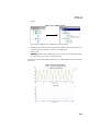
Chapter 17:3D plots and order analysis facilities . . . . . . . . . . . . . . . . 537
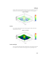
17.1 Surface plots . . . . . . . . . . . . . . . . . . . . . . . . . . . . . . . . . . . . . . . . . . . . . . 537
17.1.1 Types of surface plots . . . . . . . . . . . . . . . . . . . . . . . . . . . . . . . . . . . . . 538
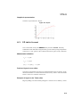
2D plot . . . . . . . . . . . . . . . . . . . . . . . . . . . . . . . . . . . . . . . . . . . . . . . . . 538
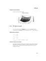
Waterfall . . . . . . . . . . . . . . . . . . . . . . . . . . . . . . . . . . . . . . . . . . . . . . . 538
Mesh. . . . . . . . . . . . . . . . . . . . . . . . . . . . . . . . . . . . . . . . . . . . . . . . . . . 538
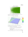
Surface . . . . . . . . . . . . . . . . . . . . . . . . . . . . . . . . . . . . . . . . . . . . . . . . . 539
Surface with light. . . . . . . . . . . . . . . . . . . . . . . . . . . . . . . . . . . . . . . . . 539
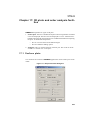
17.1.2 How to create a surface plot. . . . . . . . . . . . . . . . . . . . . . . . . . . . . . . . . 540
17.1.3 Surface plot options . . . . . . . . . . . . . . . . . . . . . . . . . . . . . . . . . . . . . . . 542
17.2 XYZ plots . . . . . . . . . . . . . . . . . . . . . . . . . . . . . . . . . . . . . . . . . . . . . . . . 543
17.3 Order analysis facility . . . . . . . . . . . . . . . . . . . . . . . . . . . . . . . . . . . . . . . 545
Spectral map. . . . . . . . . . . . . . . . . . . . . . . . . . . . . . . . . . . . . . . . . . . . . 545
Order tracking . . . . . . . . . . . . . . . . . . . . . . . . . . . . . . . . . . . . . . . . . . . 546
Fixed sampling. . . . . . . . . . . . . . . . . . . . . . . . . . . . . . . . . . . . . . . . . . . 546
Spectral map. . . . . . . . . . . . . . . . . . . . . . . . . . . . . . . . . . . . . . . . . . . . . 548
Zoom constraints . . . . . . . . . . . . . . . . . . . . . . . . . . . . . . . . . . . . . . . . . 549
Creating a spectral map . . . . . . . . . . . . . . . . . . . . . . . . . . . . . . . . . . . . 549
17.3.1 The Order Amplitude. . . . . . . . . . . . . . . . . . . . . . . . . . . . . . . . . . . . . . 552
Definition . . . . . . . . . . . . . . . . . . . . . . . . . . . . . . . . . . . . . . . . . . . . . . . 552
Order tracking technique . . . . . . . . . . . . . . . . . . . . . . . . . . . . . . . . . . . 552
Reference velocity . . . . . . . . . . . . . . . . . . . . . . . . . . . . . . . . . . . . . . . . 553
Creating an order amplitude plot . . . . . . . . . . . . . . . . . . . . . . . . . . . . . 553
Chapter 18:AMESim export module . . . . . . . . . . . . . . . . . . . . . . . . . . 555
18.1 Introduction . . . . . . . . . . . . . . . . . . . . . . . . . . . . . . . . . . . . . . . . . . . . . . . 555
18.2 Terminology . . . . . . . . . . . . . . . . . . . . . . . . . . . . . . . . . . . . . . . . . . . . . . 555
18.3 Main principles . . . . . . . . . . . . . . . . . . . . . . . . . . . . . . . . . . . . . . . . . . . . 556
18.4 The Export Parameters Setup dialog box . . . . . . . . . . . . . . . . . . . . . . . . 556
xv
Table of contents
18.5 Exporting inputs . . . . . . . . . . . . . . . . . . . . . . . . . . . . . . . . . . . . . . . . . . . 557
18.5.1 Adding inputs to the export setup . . . . . . . . . . . . . . . . . . . . . . . . . . . . 557
Submodel parameters as inputs . . . . . . . . . . . . . . . . . . . . . . . . . . . . . . 557
Global parameters as inputs . . . . . . . . . . . . . . . . . . . . . . . . . . . . . . . . 558
User defined inputs . . . . . . . . . . . . . . . . . . . . . . . . . . . . . . . . . . . . . . . 558
18.5.2 Removing inputs from the export setup . . . . . . . . . . . . . . . . . . . . . . . 558
18.5.3 Input Parameter properties . . . . . . . . . . . . . . . . . . . . . . . . . . . . . . . . . 558
Export Name . . . . . . . . . . . . . . . . . . . . . . . . . . . . . . . . . . . . . . . . . . . . 558
Type of parameters . . . . . . . . . . . . . . . . . . . . . . . . . . . . . . . . . . . . . . . 559
Read-only fields . . . . . . . . . . . . . . . . . . . . . . . . . . . . . . . . . . . . . . . . . 561
18.5.4 Vectors as Input Parameters . . . . . . . . . . . . . . . . . . . . . . . . . . . . . . . . 561
18.5.5 Formatted string Input Parameters . . . . . . . . . . . . . . . . . . . . . . . . . . . 562
18.6 Exporting simple outputs . . . . . . . . . . . . . . . . . . . . . . . . . . . . . . . . . . . . 563
18.6.1 Adding simple outputs to the export setup . . . . . . . . . . . . . . . . . . . . . 563
18.6.2 Removing simple outputs from the export setup . . . . . . . . . . . . . . . . 564
18.6.3 Simple output properties . . . . . . . . . . . . . . . . . . . . . . . . . . . . . . . . . . . 564
Export name . . . . . . . . . . . . . . . . . . . . . . . . . . . . . . . . . . . . . . . . . . . . 564
Read-only fields . . . . . . . . . . . . . . . . . . . . . . . . . . . . . . . . . . . . . . . . . 564
18.7 Compound Output Parameters . . . . . . . . . . . . . . . . . . . . . . . . . . . . . . . . 564
18.7.1 Adding compound outputs to the export setup . . . . . . . . . . . . . . . . . . 565
18.7.2 Removing simple outputs from the export setup . . . . . . . . . . . . . . . . 565
18.7.3 Compound output properties. . . . . . . . . . . . . . . . . . . . . . . . . . . . . . . . 565
Export name . . . . . . . . . . . . . . . . . . . . . . . . . . . . . . . . . . . . . . . . . . . . 566
Expression . . . . . . . . . . . . . . . . . . . . . . . . . . . . . . . . . . . . . . . . . . . . . . 566
18.7.4 Expression evaluation rules. . . . . . . . . . . . . . . . . . . . . . . . . . . . . . . . . 566
18.8 Piloting simulations from outside. . . . . . . . . . . . . . . . . . . . . . . . . . . . . . 567
18.8.1 Setting Input Parameters . . . . . . . . . . . . . . . . . . . . . . . . . . . . . . . . . . . 567
File naming rules. . . . . . . . . . . . . . . . . . . . . . . . . . . . . . . . . . . . . . . . .
Common format rules . . . . . . . . . . . . . . . . . . . . . . . . . . . . . . . . . . . . .
Real Input Parameters . . . . . . . . . . . . . . . . . . . . . . . . . . . . . . . . . . . . .
Integer Input Parameters . . . . . . . . . . . . . . . . . . . . . . . . . . . . . . . . . . .
String list . . . . . . . . . . . . . . . . . . . . . . . . . . . . . . . . . . . . . . . . . . . . . . .
Formatted string . . . . . . . . . . . . . . . . . . . . . . . . . . . . . . . . . . . . . . . . .
567
568
568
568
569
569
18.8.2 Running the simulation . . . . . . . . . . . . . . . . . . . . . . . . . . . . . . . . . . . . 569
18.8.3 Getting the results . . . . . . . . . . . . . . . . . . . . . . . . . . . . . . . . . . . . . . . . 569
File name rules . . . . . . . . . . . . . . . . . . . . . . . . . . . . . . . . . . . . . . . . . . 569
Results format . . . . . . . . . . . . . . . . . . . . . . . . . . . . . . . . . . . . . . . . . . . 570
Output template file. . . . . . . . . . . . . . . . . . . . . . . . . . . . . . . . . . . . . . . 570
18.9 Direct interfaces . . . . . . . . . . . . . . . . . . . . . . . . . . . . . . . . . . . . . . . . . . . 570
xvi
AMESim 4.2
User Manual
18.9.1 Interfaces with iSIGHT and Optimus . . . . . . . . . . . . . . . . . . . . . . . . . 570
iSIGHT. . . . . . . . . . . . . . . . . . . . . . . . . . . . . . . . . . . . . . . . . . . . . . . . . 571
Optimus . . . . . . . . . . . . . . . . . . . . . . . . . . . . . . . . . . . . . . . . . . . . . . . . 571
18.9.2 AMESim/Visual Basic Applications interface . . . . . . . . . . . . . . . . . . 571
Installation . . . . . . . . . . . . . . . . . . . . . . . . . . . . . . . . . . . . . . . . . . . . . . 572
Using the AMEVbaInterface.bas VBA module. . . . . . . . . . . . . . . . . . 572
Subroutines available in AMEVbaInterface.bas . . . . . . . . . . . . . . . . . 573
Chapter 19:AMESim Design exploration module . . . . . . . . . . . . . . . . 577
19.1 Introduction . . . . . . . . . . . . . . . . . . . . . . . . . . . . . . . . . . . . . . . . . . . . . . . 577
19.2 Nomenclature . . . . . . . . . . . . . . . . . . . . . . . . . . . . . . . . . . . . . . . . . . . . . 577
19.3 Key features. . . . . . . . . . . . . . . . . . . . . . . . . . . . . . . . . . . . . . . . . . . . . . . 577
19.3.1 DOE . . . . . . . . . . . . . . . . . . . . . . . . . . . . . . . . . . . . . . . . . . . . . . . . . . . 578
Parameter study . . . . . . . . . . . . . . . . . . . . . . . . . . . . . . . . . . . . . . . . . . 578
Full factorial. . . . . . . . . . . . . . . . . . . . . . . . . . . . . . . . . . . . . . . . . . . . . 578
Central composite . . . . . . . . . . . . . . . . . . . . . . . . . . . . . . . . . . . . . . . . 579
19.3.2 Optimization . . . . . . . . . . . . . . . . . . . . . . . . . . . . . . . . . . . . . . . . . . . . 579
NLPQL. . . . . . . . . . . . . . . . . . . . . . . . . . . . . . . . . . . . . . . . . . . . . . . . . 579
Genetic algorithm. . . . . . . . . . . . . . . . . . . . . . . . . . . . . . . . . . . . . . . . . 580
19.3.3 Monte Carlo . . . . . . . . . . . . . . . . . . . . . . . . . . . . . . . . . . . . . . . . . . . . . 580
19.4 Main principles . . . . . . . . . . . . . . . . . . . . . . . . . . . . . . . . . . . . . . . . . . . . 580
19.5 The Design Exploration dialog box . . . . . . . . . . . . . . . . . . . . . . . . . . . . 581
19.5.1 Description. . . . . . . . . . . . . . . . . . . . . . . . . . . . . . . . . . . . . . . . . . . . . . 581
19.5.2 The list of studies . . . . . . . . . . . . . . . . . . . . . . . . . . . . . . . . . . . . . . . . . 581
19.5.3 The execution panel . . . . . . . . . . . . . . . . . . . . . . . . . . . . . . . . . . . . . . . 582
Log . . . . . . . . . . . . . . . . . . . . . . . . . . . . . . . . . . . . . . . . . . . . . . . . . . . . 582
Warning . . . . . . . . . . . . . . . . . . . . . . . . . . . . . . . . . . . . . . . . . . . . . . . . 582
19.5.4 Actions that Control your DOE . . . . . . . . . . . . . . . . . . . . . . . . . . . . . . 582
Study management. . . . . . . . . . . . . . . . . . . . . . . . . . . . . . . . . . . . . . . . 582
Post processing. . . . . . . . . . . . . . . . . . . . . . . . . . . . . . . . . . . . . . . . . . . 584
Execution . . . . . . . . . . . . . . . . . . . . . . . . . . . . . . . . . . . . . . . . . . . . . . . 590
19.6 The Design Exploration Definition dialog box . . . . . . . . . . . . . . . . . . . . 591
19.6.1 Description. . . . . . . . . . . . . . . . . . . . . . . . . . . . . . . . . . . . . . . . . . . . . . 591
19.6.2 DOE . . . . . . . . . . . . . . . . . . . . . . . . . . . . . . . . . . . . . . . . . . . . . . . . . . . 591
Common part . . . . . . . . . . . . . . . . . . . . . . . . . . . . . . . . . . . . . . . . . . . . 592
Parameter study . . . . . . . . . . . . . . . . . . . . . . . . . . . . . . . . . . . . . . . . . . 593
Full Factorial . . . . . . . . . . . . . . . . . . . . . . . . . . . . . . . . . . . . . . . . . . . . 594
Central Composite . . . . . . . . . . . . . . . . . . . . . . . . . . . . . . . . . . . . . . . . 595
19.6.3 Optimization . . . . . . . . . . . . . . . . . . . . . . . . . . . . . . . . . . . . . . . . . . . . 596
xvii
Table of contents
Common part: problem definition. . . . . . . . . . . . . . . . . . . . . . . . . . . . 597
NLPQL . . . . . . . . . . . . . . . . . . . . . . . . . . . . . . . . . . . . . . . . . . . . . . . . 599
Genetic algorithm . . . . . . . . . . . . . . . . . . . . . . . . . . . . . . . . . . . . . . . . 600
19.6.4 Monte Carlo. . . . . . . . . . . . . . . . . . . . . . . . . . . . . . . . . . . . . . . . . . . . . 602
19.7 The Design Exploration Plots dialog box. . . . . . . . . . . . . . . . . . . . . . . . 604
19.7.1 Description . . . . . . . . . . . . . . . . . . . . . . . . . . . . . . . . . . . . . . . . . . . . . 604
19.7.2 Static part. . . . . . . . . . . . . . . . . . . . . . . . . . . . . . . . . . . . . . . . . . . . . . . 604
19.7.3 Dynamic part . . . . . . . . . . . . . . . . . . . . . . . . . . . . . . . . . . . . . . . . . . . . 605
History plot . . . . . . . . . . . . . . . . . . . . . . . . . . . . . . . . . . . . . . . . . . . . .
Scatter plot. . . . . . . . . . . . . . . . . . . . . . . . . . . . . . . . . . . . . . . . . . . . . .
Main effect diagram . . . . . . . . . . . . . . . . . . . . . . . . . . . . . . . . . . . . . .
Pareto diagram. . . . . . . . . . . . . . . . . . . . . . . . . . . . . . . . . . . . . . . . . . .
Histogram . . . . . . . . . . . . . . . . . . . . . . . . . . . . . . . . . . . . . . . . . . . . . .
605
606
608
609
610
19.7.5 Array of possible plots according the study type . . . . . . . . . . . . . . . . 611
Appendix A:Formats supported by the AMESim Table Editor 613
A.1. Introduction . . . . . . . . . . . . . . . . . . . . . . . . . . . . . . . . . . . . . . . . . . . . . . 613
A.2. 1D table format . . . . . . . . . . . . . . . . . . . . . . . . . . . . . . . . . . . . . . . . . . . . 614
Mathematical definition . . . . . . . . . . . . . . . . . . . . . . . . . . . . . . . . . . .
Preferred layout in text editor . . . . . . . . . . . . . . . . . . . . . . . . . . . . . . .
Example of layout in the Table editor . . . . . . . . . . . . . . . . . . . . . . . . .
Restrictions . . . . . . . . . . . . . . . . . . . . . . . . . . . . . . . . . . . . . . . . . . . . .
Graphical representation . . . . . . . . . . . . . . . . . . . . . . . . . . . . . . . . . . .
614
614
614
614
615
A.3. 2D table format . . . . . . . . . . . . . . . . . . . . . . . . . . . . . . . . . . . . . . . . . . . . 615
Mathematical definition . . . . . . . . . . . . . . . . . . . . . . . . . . . . . . . . . . .
Preferred layout in text editor . . . . . . . . . . . . . . . . . . . . . . . . . . . . . . .
Example of layout in the Table editor . . . . . . . . . . . . . . . . . . . . . . . . .
Restrictions . . . . . . . . . . . . . . . . . . . . . . . . . . . . . . . . . . . . . . . . . . . . .
Graphical representation . . . . . . . . . . . . . . . . . . . . . . . . . . . . . . . . . . .
615
615
615
616
617
A.4. 3D table format . . . . . . . . . . . . . . . . . . . . . . . . . . . . . . . . . . . . . . . . . . . . 617
Mathematical definition . . . . . . . . . . . . . . . . . . . . . . . . . . . . . . . . . . .
Preferred layout in text editor . . . . . . . . . . . . . . . . . . . . . . . . . . . . . . .
Example of layout in the Table editor . . . . . . . . . . . . . . . . . . . . . . . . .
Restrictions . . . . . . . . . . . . . . . . . . . . . . . . . . . . . . . . . . . . . . . . . . . . .
Graphical representation . . . . . . . . . . . . . . . . . . . . . . . . . . . . . . . . . . .
617
617
618
618
618
A.5. Table of 1D tables format . . . . . . . . . . . . . . . . . . . . . . . . . . . . . . . . . . . . 619
Mathematical definition . . . . . . . . . . . . . . . . . . . . . . . . . . . . . . . . . . .
Preferred layout in text editor . . . . . . . . . . . . . . . . . . . . . . . . . . . . . . .
Example of layout in the Table editor . . . . . . . . . . . . . . . . . . . . . . . . .
Restrictions . . . . . . . . . . . . . . . . . . . . . . . . . . . . . . . . . . . . . . . . . . . . .
Graphical representation . . . . . . . . . . . . . . . . . . . . . . . . . . . . . . . . . . .
619
619
620
620
620
A.6. XYs table format . . . . . . . . . . . . . . . . . . . . . . . . . . . . . . . . . . . . . . . . . . 621
xviii
AMESim 4.2
User Manual
Mathematical definition . . . . . . . . . . . . . . . . . . . . . . . . . . . . . . . . . . . . 621
Preferred layout in text editor . . . . . . . . . . . . . . . . . . . . . . . . . . . . . . . 621
Example of layout in table editor. . . . . . . . . . . . . . . . . . . . . . . . . . . . . 622
Graphical representation . . . . . . . . . . . . . . . . . . . . . . . . . . . . . . . . . . . 622
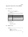
Appendix B:Special files used by AMESim 623
B.1. Introduction . . . . . . . . . . . . . . . . . . . . . . . . . . . . . . . . . . . . . . . . . . . . . . . 623
B.2. AMESim nodes . . . . . . . . . . . . . . . . . . . . . . . . . . . . . . . . . . . . . . . . . . . . 623
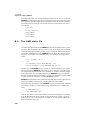
B.3. The AMEIcons file . . . . . . . . . . . . . . . . . . . . . . . . . . . . . . . . . . . . . . . . . 625
B.4. The submodels.index file . . . . . . . . . . . . . . . . . . . . . . . . . . . . . . . . . . . . 625
B.5. The AME.make file. . . . . . . . . . . . . . . . . . . . . . . . . . . . . . . . . . . . . . . . . 626
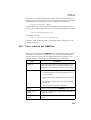
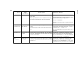
B.6. Files created for AMESim. . . . . . . . . . . . . . . . . . . . . . . . . . . . . . . . . . . . 627
B.7. Purge tool for system files. . . . . . . . . . . . . . . . . . . . . . . . . . . . . . . . . . . . 629
B.8. Pack/Unpack facility . . . . . . . . . . . . . . . . . . . . . . . . . . . . . . . . . . . . . . . . 629
Appendix C:Description of EXPORT functions 631
Index 637
xix
Table of contents
xx
AMESim 4.2
User Manual
Chapter 1: Introduction
1.1
What is AMESim?
AMESim stands for Advanced Modeling Environment for performing
Simulations of engineering systems. It is based on an intuitive graphical interface
in which the system is displayed throughout the simulation process.
AMESim uses symbols to represent individual components within the system
which are either:
•
based on the standard symbols used in the engineering field such as ISO
symbols for hydraulic components or block diagram symbols for control
systems;
or when no such standard symbols exist
•
symbols which give an easily recognizable pictorial representation of the
system.
Figure 1.1: Symbols used in AMESim
Figure 1.1 shows an engineering system using standard hydraulic, mechanical and
1
Chapter 1
Introduction
control symbols.
Figure 1.2 shows an automobile braking system in which some pictorial symbols
are used.
Figure 1.2: Symbols of an automobile braking system
1.2
How is AMESim used?
Using AMESim you build sketches of engineering systems by adding symbols or
icons to a drawing area. When the sketch is complete, a simulation of the system
proceeds in the following stages:
•
Mathematical descriptions of components are associated with the icons.
•
The features of the components are set.
•
A simulation run is initiated.
•
Graphs are plotted to interpret the system behavior.
Figure 1.3 shows a detailed model of a three cylinder piston pump built from HCD
symbols. The arrows are used to give animation for the hydraulic flow rates.
2
AMESim 4.2
User Manual
Figure 1.3: A three cylinder piston pump built from HCD symbols
As much automation as possible has been carried out on these steps and at every
stage you will see the sketch of the system.
Interfaces
Current practice is to provide interfaces between software to enable them to work
together so that you can obtain the best features of each. The standard AMESim
package provides an interface with MATLAB. This gives you access to controller
design features, optimization facilities, power spectral analysis etc.
Other interfaces are also available. For the latest information on AMESim
interfaces, please refer to section 1.6.6 Interfaces.
Equations
AMESim refers to the set of equations defining the dynamic behavior of the
engineering system and its implementation as computer code as the model of the
system. The model is built up from equations and corresponding code for each
3
Chapter 1
Introduction
component within the system. These are referred to as submodels. AMESim
contains large libraries of icons and submodels of components.
The standard library
The standard library provides control and mechanical icons and submodels
allowing you to perform dynamic simulation of a wide variety of engineering
systems. In addition, there are optional libraries such as the Hydraulic Component
Design, the hydraulic resistance, pneumatic, thermal, thermal-hydraulic, cooling
system, powertrain, filling...
1.3
How to use the documentation set
The documentation set is made up of:
•
Printed and PDF manuals for each software of the AMESim platform.
•
Printed and PDF manuals for each library.
•
HTML specification sheets for all submodels.
Printed formats are delivered with the CD ROM containing your applications.
To access the online documentation:
1. Select Help u Online.
An HTML browser is displayed.
Figure 1.4: Online help
2. Select the documentation you want to consult in the content folders, or use the
index, or the search facility.
4
AMESim 4.2
User Manual
1.4
Organization of this manual
This manual describes AMESim used on Unix workstations and on PCs with a
Windows (NT or 2000) or a Linux operating system. Most of the time the
description is exactly the same for both environments. However when it is
necessary to have separate text for each environment, the Unix/Linux description
is given first and the Windows description follows as shown below:
Using Unix:
Description for Unix/Linux environments.
Using Windows:
Description for Windows environments.
Chapter 2 is a presentation of the AMESim workspace.
Chapters 3 to 10 are tutorial chapters with lots of exercises to try. Chapter 3 is
a ‘get you started’ guide in the use of AMESim with standard components and
submodels. It is absolutely essential that new users read this chapter and do the
exercises. The time necessary is from 1 to 2 hours. After this you should be able to
do basic simulation work using AMESim. Soon after this, read Chapter 4 and do
the extra examples.
Chapter 5 covers some more advanced features. Ideally read this after using
AMESim for about 3 weeks. Chapter 6 introduces you to the supercomponent and
Chapter 7 describes the facilities available using the interface with Matlab. With
Chapter 8 you will see how to use the activity index facility which is a powerful
analysis tool based on energy transfer in the submodels of a system. Chapters 9 and
10 introduce the Export and Design Explorations facilities respectively.
Chapters 11 to 19 are arranged for reference. They cover features not covered
fully in the tutorial chapters. Chapter 9 covers facilities available in all AMESim
modes, Chapter 10 covers facilities available in Sketch mode, Chapter 11 covers
facilities available in Submodel mode, Chapter 12 covers facilities available in
Parameter mode, Chapter 13 covers facilities available in Run mode, Chapter 14
deals with plotting facilities and with Chapter 15 you will learn how to deal with
3D plots and order tracking. Chapter 18 and 19 cover the Export and Design
Explorations facilities respectively.
5
Chapter 1
Introduction
1.5
The AMESim 4 software suite
1.5.1
AMESim
AMESim is the main product of the AMESim software suite.
AMESim is an Advanced Modeling Environment for performing Simulations of
engineering systems.
With AMESim, you can:
1.5.2
•
Create new systems.
•
Modify the Sketch of an existing system.
•
Change the submodel behind a component.
•
Load AMESim systems.
•
Change parameters and set up batch runs.
•
Perform standard or batch runs.
•
Plot result graphs.
•
Perform linear analysis.
•
Perform activity index analysis.
•
Export models for running outside of AMESim.
•
Perform Design Exploration studies.
AMECustom
AMECustom is delivered with AMESim.
With AMECustom, you can customize submodels and supercomponents. A
customized object is based on a generic object on which a mask is placed. The only
parameters to be tested are kept visible.
You are able to encode the components of a complex system before distributing it.
1.5.3
AMESet
Advanced AMESim users can use AMESet to create new icons and submodels.
AMESet provides a comprehensive user interface.
With AMESet, you can:
•
Integrate new icons and submodels.
•
Customize component categories and submodels.
Using AMESet, you can create your own component (or line) submodels to
extend the capability of AMESim into your own applications.
6
AMESim 4.2
User Manual
1.5.4
AMERun
AMERun is AMESim without Sketch and Submodel modes.
With AMERun, you can:
•
Load AMESim systems.
•
Change parameters and set up batch runs.
•
Perform standard or batch runs.
•
Plot result graphs.
•
Perform linear analysis.
You cannot:
•
Create new systems.
•
Modify the Sketch of an existing system.
•
Change the submodel behind a component.
AMESim systems are created and tested by experienced AMESim users.
AMERun users can open systems in order to perform studies.
AMERun can be used by:
•
Technicians doing many parameter studies using a system built in by an
experienced engineer;
•
Clients who receive pre-built systems from you;
•
Sale staff who use pre-built systems to demonstrate system behavior to
customers.
7
Chapter 1
Introduction
1.5.5
The whole family of AMESim products
Figure 1.5: AMESim Libraries
Figure 1.6Interfaces with AMESim
8
AMESim 4.2
User Manual
1.6
New AMESim 4.2 features
There have been many improvements implemented in AMESim 4.2. Here are
some of the most important ones. Unless otherwise stated the features are included
in standard AMESim.Export facility
Design Exploration
Compiler flags
Stabilizing runs
Display of vectors
Interfaces
Submodel call modifications
Model simplification and Real time
Compare Systems
Pack and Unpack
Enumeration
Watch Parameters and Variables
Online help
1.6.1
Export facility
This facility enables you to pilot AMESim simulation executables from outside
AMESim. You set up the export by defining inputs and outputs of the model and
postprocessing operations you want applied to these outputs. A specific dialog box
is provided for this.
Figure 1.7: Setting up an Export of an AMESim model
From outside AMESim you can use a new utility called AMEPilot to drive the
simulations.
9
Chapter 1
Introduction
The Export facility can be used by advanced users to set up their own interfaces
between AMESim and other software. All users have access to a new standard
AMESim facility that uses Export and AMEPilot to provide a Design Exploration
environment.
1.6.2
Design Exploration
Design Exploration is actually three facilities:
•
Design Of Experiments
Determine which parameters influence some
performance criterion.
•
Optimization
You want to experiment with a collection of
parameters in order to optimize some
criterion.
•
Robustness analysis
using Monte Carlo
methods
You want to find out how variations in a
parameter due to
•
production tolerances,
•
different operating conditions or,
•
wear,
effect performance.
10
AMESim 4.2
User Manual
Figure 1.8: Optimizing an Active Suspension using a Genetic Algorithm
11
Chapter 1
Introduction
Figure 1.9Varying a tire stiffness in a Monte Carlo study
1.6.3
Compiler flags
The AMESim development team has experimented with compiler flag options for
the simulation executable. This results in faster simulation runs particularly on
Unix platforms.
1.6.4
Stabilizing runs
There have been improvements to the stabilizing run algorithm and this
improvement is particularly noticable with lubrication systems.
1.6.5
Display of vectors
A popular request of displaying vectors in compact or expanded form is
implemented.
12
AMESim 4.2
User Manual
Figure 1.10: Compact and expanded form of vectors
13
Chapter 1
Introduction
1.6.6
Interfaces
iSIGHT and Optimus
Interfaces with the design exploration software iSIGHT and Optimus are provided
as an option. These use the Export setup and AMEPilot facilities.
Figure 1.11: Export to external tools
MSC.ADAMS
Another optional interface is provided with the multibody software
MSC.ADAMS. This allows the following possibilities:
1. Integration of the multibody system
using the AMESim integrator.
2. Integration of the AMESim system
using the ADAMS integrator.
3. A cosimulation using both
integrators.
14
•
For 1, you initiate simulations from the AMESim environment.
•
For 2, you initiate simulations from the MSC.ADAMS environment.
AMESim 4.2
User Manual
•
1.6.7
For 3, simulations can be initiated from either software.
Submodel call modifications
With the provision of the optional Real time facility, it becomes critical to avoid
unnecessary computational effort. In AMESim 4.1 calls to the calculation
function were always made, even if nothing useful was done. Modifications to
AMESet 4.2 mean there is an option of not calling the calculation function. In
AMESim 4.2 this means good speedups for CPU critical applications.
1.6.8
Model simplification and Real time
AMESim provides a collection of tools for model simplification. In AMESim 4.1
you could use the following:
•
state count
•
activity index
•
eigenvalue analysis
•
modal shapes.
The Optimization facility in AMESim 4.2 provides further capability. You can
replace a complex valve by a simple one and use optimization to set the simple
valve model parameters.
When you have removed extreme eigenvalues, you
can use the AMESim 4.2 fixed step integrator option
to check that it runs and produces results compatible
with the original high fidelity model.
Figure 1.12: Using fixed step integrators
15
Chapter 1
Introduction
The AMESim Simulink interface has been
updated to be compatible with Real-Time
Workshop. Together with additional features that
have been added in AMESim an option exists to
export an AMESim model to a real-time target
such as dSPACE or xPC Target. With the right
amount of model simplification the simulation
model of your physical system can then run in realtime which opens the way for many interesting
applications, such as hardware-in-the-loop
simulation.
1.6.9
Compare Systems
It is common to develop a complex model and then to evolve it into several
different versions. The problem then is to determine the differences between the
versions. Doing this manually is definitely not easy!
In AMESim 4.2 you load the models and in Parameter
mode use Tools u Compare systems. This initiates a
process which analyzes the two systems and reports
on the differences.
16
AMESim 4.2
User Manual
Figure 1.13: Compare Systems
Labels are added to the sketch and the changes are summarized in a tree structure.
The expanded tree structure can be printed.
1.6.10 Pack and Unpack
Our users are increasingly employing AMESim as a model exchange
environment. When these models contain special data files and user created
submodels or supercomponents, this process was not easy using AMESim 4.1.
Normally several iterations were needed!
To make this exchange process easier, a special Pack utility has been developed
for AMESim 4.2. This uses a GUI Wizard to assist the user in creating a single
package containing all the components to make the models run. Features are:
•
The models you package are analyzed searching for data files and user
icons, submodels and supercomponents.
•
Any important submodels.index files are analyzed.
•
You have the option of purging the models.
•
AME.make files are analyzed looking for special libraries.
•
You specify the target system the models will run on which can be different to the one you are using.
•
You have the option of not sending source, .spe and .sub files.
17
Chapter 1
Introduction
Figure 1.14: The AMEPack Wizard
Figure 1.15: The auxiliary files have been identified
When the package is received, the corresponding Unpack facility is started. This
allows the models and auxiliary files to be positioned within the destination file
system. If appropriate AMEUnpack will attempt to compile submodel and library
source.
18
AMESim 4.2
User Manual
Figure 1.16: Unpacking the models and auxiliary files
1.6.11 Enumeration
In a submodel with different options defined by an integer parameter, particularly
multiple options, the Change Parameters dialog box was rather ugly. Here is the
submodel UDA1 from AMESim 4.1.
Figure 1.17: Change Parameters dialog box for 4.1 UDA1
With AMESim 4.2 a different approach is used. Here are the default parameters
for UDA01 which is functional equivalent to UDA1.
Figure 1.18: Functional equivalent UDA01 in AMESim 4.2
19
Chapter 1
Introduction
This is achieved using an object orientated approach to show only information that
is strictly needed.The first three parameters displayed in Figure 1.18 are integer
parameters of a special type known as enumeration. The enumeration parameters
can be changed after which new parameters become relevant.
Figure 1.19Changing enumeration parameters
Enumeration makes the parameter lists much clearer and easier to understand.
1.6.12 Watch Parameters and Variables
Often for a model there are a number of parameters and variables of special
significance. These are the parameters that you most frequently change and
variables you most often plot.
In Parameter mode you drag and drop your favorite parameters into a special pane
and they are known as Watch Parameters. The characterisics are saved into the
.ame file and hence AMESim 4.2 can always remember your favorite parameters.
Figure 1.20: Watch Parameters
You can change parameter values in the Watch Parameters pane. On a big model
this provides very rapid access to important model parameters.
20
AMESim 4.2
User Manual
In Run mode a similar technique gives rapid access to important variables. An
automatic update is applied to the values displayed and you can plot direct from
the Watch Variables pane.
Figure 1.21: Watch Variables
1.6.13 Online help
In AMESim 4.1 online help concentrated on
submodels and utilities called by submodels.
AMESim 4.2 provides a search facility for core
AMESim features as they appear in the manual.
To use this, select the Search tab, type one or
more keywords and then click on Search button.
Under Found Documents will be a list of manual
sections that contain the keyword(s). AMEHelp
will try to sort this list so that the most important
entries are at the top. Click on items in this list to
see the corresponding manual entries.
21
Chapter 1
Introduction
Figure 1.22: External variables entry
22
AMESim 4.2
User Manual
23
Chapter 1
Introduction
24
AMESim 4.2
User Manual
Chapter 2: The AMESim Workspace
This section describes:
2.1
•
The AMESim User Interface
•
The AMESim four working modes
•
Some Tricks and Tips
The AMESim User Interface
The AMESim user interface is the basic working area. Depending on which mode
you are working in, you have tools at your disposal:
2.1.1
•
The Main Window
•
The Menu Bar
•
The Toolbars
•
The mouse right-button menu
•
The libraries
The Main Window
Starting AMESim
When you start AMESim, the main window is empty.
23
Chapter 2
The AMESim Workspace
Figure 2.23: AMESim main window
Minimize, restore, close buttons
Title bar
Menu bar
Toolbars
Empty screen
24
AMESim 4.2
User Manual
You can either:
•
Open an empty system:
•
Load an existing system:
When you load an existing system, a browser appears so that you can indicate the
path of the system to open.
Figure 2.24: Browser
1. Select the system you want to open and click on Open or,
2. Double-click on the system you want to open.
Closing AMESim
When you close the main window, you automatically exit from AMESim.
To close the main window, do one of the following:
•
Click on the close
button,
•
Press Ctrl+Q,
•
Select File } Quit in the Menu bar
We will now describe the components of the main interface of AMESim. (Refer
again to Figure 2.23)
2.1.2
The Menu Bar
The Menu bar gives you access to the main features of AMESim.
25
Chapter 2
The AMESim Workspace
Figure 2.25: Menu bar
Note:
2.1.3
Some features are also available through keyboard shortcuts
which are given in the menus. See the list of Keyboard Shortcuts.
The Toolbars
The toolbars display buttons corresponding to AMESim main features. You have
several toolbars at your disposal:
•
•
In all modes:
•
The File Operations Toolbar
•
The Mode Operations Toolbar
•
The Annotation Tools Toolbar
•
The Temporal Analysis Toolbar
In run mode only:
•
The Post Processing Tools Toolbar
•
The Linear Analysis Toolbar
To know more about the AMESim working modes, see “The AMESim four
working modes”, page 34.
The File Operations Toolbar
Start a new system in order to build a sketch.
Open an existing system in order to modify or to complete it.
Save your system.
26
AMESim 4.2
User Manual
The Mode Operations Toolbar
Figure 2.26: Sketch mode
Figure 2.27: Submodel mode
Figure 2.28: Parameter mode
Figure 2.29: Run mode
The Mode Operations Toolbar changes depending on the mode you are working
on. The available features of each mode are different (see Figure 2.26 to Figure
2.29).
In Sketch mode, you can build your sketch using the components that are
available in the categories. The categories are displayed in a vertical toolbar on the left of the main window of AMESim.
In Submodel mode, you can choose the submodels you want to attach to
each component.
In Parameter mode, you can set the parameters of the submodels. You
can save the parameters from one submodel to use them for another submodel. In this case, AMESim will load only the common parameters.
The Run mode enables you to run a simulation and to analyze the results
of the simulation.
The Lock button locks or unlocks the sketch. When you open an existing
system, it is locked. If you need to add or remove components or line
runs, click on the lock button to unlock it.
Premier submodel automatically sets the simplest submodel to each component or line run having no submodel associated with it. It is necessary
to associate a submodel to all components and line runs on the sketch in
order to have access to the Parameter mode.
27
Chapter 2
The AMESim Workspace
Run Parameters displays a dialog box on which you can set the parameters of the simulation.
Click on this button starts the simulation run. At the end of the simulation,
a window displays the details on the run. This is important to know why
a simulation has failed.
The Stop button stops a running simulation.
The Annotation Tools Toolbar
Figure 2.30: Annotation tools toolbar
The Insert text facility can be used to add titles or comments on
your sketch.
You can also insert shapes in the sketch like arrows, lines,
rectangles or ellipses. Choose the shape you want by clicking on
the small arrow next to the shape button. Then, click on the shape
corresponding to your needs.
Finally you can insert images on the sketch. If you click on the
Insert image button, AMESim opens a browser allowing you to
look for the file of the image you want to insert.
The Edit Operations Toolbar
Figure 2.31: Edit operations toolbar
28
AMESim 4.2
User Manual
The Cut button allows you to cut the selected objects and to copy them on
the current system, another one or in an auxiliary system.
The Copy button allows you to copy the selected objects to paste them in
the current system or in another one.
The Paste button allows you to paste the objects you cut or copied in the
current system or in another one.
The Delete button allows you to delete the selected objects. Be careful, if
you use this option, you cannot copy the objects back.
Note:
The copy operation in AMESim does not copy the selected
objects in the Windows clipboard. This means that you can copy
objects and paste them in the same AMESim but not from one
AMESim to another.
The Temporal Analysis Toolbar
The tools available on the Temporal Analysis toolbar are used for the simulation
results analysis.
Figure 2.32: Temporal analysis toolbar
The Blank Plot button displays an empty plot in which you can drag and
drop the variables you wish to plot. From the plot window, you can open
the Plot manager.
The Table Editor button starts the Table editor utility.
The AMEAnimation button starts the viewer for the Planar Mechanical
models.
29
Chapter 2
The AMESim Workspace
The Post Processing Tools Toolbar
Figure 2.33: Post processing tools toolbar
The Temporal Analysis button is selected by default.
The Linear Analysis button opens a new toolbar to set up the linear analysis process.
The Design Exploration button opens a dialog box to initiate design exploration.
The Replay button opens a dialog box to set up the replay.
The State Count button displays the summary of which state variables
controlled the integration step size.
The Linear Analysis Toolbar
Figure 2.34: Linear Analysis Toolbar
The LA Times button opens the Linearization Times dialog box which
allows you to set times for linearization.
The LA Status button opens the LA Status Fields dialog box which
displays the current status of variables.
The Eigenvalues Modal shapes button opens the Linear Analysis Eigenvalues dialog box which displays the eigenvalues for the jacobian
files.
The Frequency Response button displays the Frequency Response dialog
box which allows you to create Bode, Nichols and Nyquist plots.
30
AMESim 4.2
User Manual
The Root Locus button produces the Root Locus dialog box which allows
you to create Root Locus plots.
2.1.4
The mouse right-button menu
You can access many commands with the mouse right-button which displays a
contextual menu. The contextual menu is different depending on the current
working mode and what you click on.
We advise you to use the contextual menu because it is a very quick way to access
the commands.
Figure 2.35: Mouse right-button menu
2.1.5
The libraries
The standard library
AMESim 4.2 is delivered with a standard library consisting of two categories:
Mechanical: complements other AMESim libraries. The Mechanical
category is often used in isolation to simulate complete mechanical systems. Linear and rotary motion elements are included.
Control: contains all the components necessary to control, measure and
observe your system. The Control category may be used to create blockdiagram models of systems.
The extra libraries
You can complete the basic application with the following categories. The categories are available in the menu Options } Path List. When the Path list dialog box
opens, you can select the categories you want to add to the path list from the available category list. Then the category bar is updated and displays the available cat31
Chapter 2
The AMESim Workspace
egories. You can display the category bar on the right, on the left or on the top of
the AMESim interface at your convenience.
You will find further details in the user manual of each category.
Hydraulic: contains many general hydraulic components suitable for
simulating ideal dynamic behavior based on component performance
parameters.
Hydraulic Component Design: contains the basic building blocks of
any hydro-mechanical system. The interpretation of the model layout is
very easy and intuitive.
Hydraulic Resistance: creates large hydraulic networks, evaluate the
pressure drops through the elements and modify the design of the system.
Pneumatic: Contains component level models to model large networks,
and basic elements to design complex pneumatic components.
Pneumatic Component Design: contains the basic building blocks of
any pneumatic-mechanical system. The interpretation of the model layout is very easy and intuitive.
Thermal: used to model traditional heat transfer modes between solid
materials and to study the thermal evolution in these solids when submitted to different kinds of heat sources.
Thermal Hydraulic: used to model thermal phenomena in liquids and
to study the thermal evolution in these liquids when submitted to different kinds of heat sources and power sources.
Thermal Pneumatic: used to model thermal phenomena in gases and
to study the thermal evolution in these gases when submitted to different
kinds of heat sources.
Thermal Hydraulic Component Design: used to study the pressure
levels, the flow rates distribution, the temperatures and the flow rates
evolution in the system.
Powertrain: used to model systems such as driveline or complete manual, automatic or specialized gearboxes, including vibration and loss effects.
Filling: specialized for determination of the time taken to fill the lubrication circuits of an engine with oil during startup.
32
AMESim 4.2
User Manual
Cooling System: allows you to combine models for the cooling system,
lubrication system, and exhaust system to study the complete thermal
behavior of an engine.
Electro-Mechanical: contains elements such as air gaps, metal elements, magnets and coils to construct a magnetic circuit such as a solenoid. Contains dynamic effects such as histeresys and electric
properties.
Two-Phase Flow: used for modelling thermohydraulic systems where
there is a change of phase (liquid-vapor).
Air Conditioning: used to model steady state and dynamic behavior of
air conditioning systems.
Electric Motors and Drive: used to model electric parts of the car
which replace mechanical and hydraulic actuation.
IFP Drive: used to compute fuel consumption and raw emissions of engines.
Planar Mechanical: used to model dynamics of bodies in two dimensions.
2.2
The AMESim four working modes
With AMESim, you can build a sketch, affect submodels to the components, set
up the parameters of the submodels and then launch a simulation. Each step fits in
with a working mode of AMESim:
•
Sketch Mode
•
Submodel Mode
•
Parameter Mode
•
Run Mode
This chapter introduces the very basic features available in the four working modes
of AMESim for the new users. If you are already experienced with AMESim, see
the chapters 11 to 15 Features Available in each Working Mode to discover the
advanced features of AMESim.
33
Chapter 2
The AMESim Workspace
2.2.1
Sketch Mode
When you start AMESim, you are in Sketch mode.
In Sketch mode, you can:
•
Build a new system.
•
Modify or complete an existing system.
With the components of the available categories. It is the only mode in which the
category buttons and the Lock button are available.
Note:
When you open an existing system, the sketch is locked. To
modify the sketch, you must unlock the system by clicking on the
Lock button.
The Sketch mode is the first step to the simulation.
2.2.2
Submodel Mode
When your system is complete, you can go through the Submodel mode to select
submodels for the components of the system.
If the circuit is not complete, you cannot go through the Submodel mode. In this
case, the following dialog box is displayed:
Figure 2.36: Error message
In the Submodel mode, you can:
2.2.3
•
Select a submodel for each component
•
Use the Premier Submodel button
•
Remove a component submodel
Parameter Mode
In Parameter mode, you can:
1. Examine and change submodel parameters
2. Copy submodel parameters
3. Set global parameters
34
AMESim 4.2
User Manual
4. Select an area of the sketch and show common parameters in this area
5. Specify a batch run
When you enter Parameter mode, AMESim compiles the system. The
compilation creates an executable file. This executable file makes the simulation
possible. Normally before you do this run you adjust the parameters of the model.
2.2.4
Run Mode
In Run mode, you can:
•
Initiate standard and batch simulation runs
•
Create plots of results
•
Store and load the configuration of all or some of your plots
•
Initiate linearizations of the current system
•
Perform various analyses on the linearized systems
•
Perform Activity Index analysis
In order to help you to execute these tasks, AMESim displays special toolbars. See
“The Mode Operations Toolbar”, page 27 and “The Post Processing Tools
Toolbar”, page 30.
With the previous modes, you prepared your sketch, you set the submodels and the
parameters. Now, you are ready to run a simulation!
2.3
Tricks and Tips
This part gives you tricks and tips to go faster and save time while using AMESim.
2.3.1
The Lock Button
The Lock button can be found in the Mode Operation toolbar. It can be locked or
unlocked.
When you create a new system, the button is unlocked. Then, you can start
building your sketch. If you open an existing system, unlock the button by
clicking on it to be able to modify the system.
When the button is locked, you are not able to add or remove any
component to the system.
The lock button is a safety device that can be used to prevent you from accidentally
altering the system. If you find yourself blocked from modifying the sketch, it may
be because the system is locked.
35
Chapter 2
The AMESim Workspace
2.3.2
Rotating and mirroring an icon
When you select a component, you may need to rotate or mirror it before adding it
to the sketch.
To rotate a component, you can either:
•
Type Ctrl+R or,
•
Click on the middle button of your mouse.
To mirror a component, you can either:
2.3.3
•
Type Ctrl+M or,
•
Click on the right-button of your mouse.
The Status Bar
The status bar is in the lower part of the interface:
Figure 2.37: The status bar
If your actions do not have the results you expect, look at the status bar which may
present information on what is going wrong. In this case, you should hear a beep
and have a message.
In addition to warnings and description of errors the status bar also displays
(without beeps) confirmation messages and general useful information:
36
AMESim 4.2
User Manual
2.3.4
Removing a component
To delete an icon in the sketch, you can:
2.3.5
•
Type Ctrl+X.
•
Select Edit } Cut.
•
Press Del and Enter keys.
•
Select the object and click on the trash icon
.
Drag and Drop
AMESim offers a drag and drop option. This is much easier and quicker for many
actions.
You can drag and drop:
•
A component from a category to the sketch.
•
A text from a text editor to the sketch.
The text will have the AMESim text format.
•
2.3.6
A parameter from the Change Parameters dialog box to the Batch Control
Parameter Setup dialog box.
Adding some Text
You can easily add some text on your sketch. To add some text, do the following:
1. Click on
.
The pointer becomes an A.
2. Click where you want to add the text.
Then, you see a square
Note:
in which you can type your text.
You are allowed to type your text on several lines by pressing the
Enter key each time you want a new line.
37
Chapter 2
The AMESim Workspace
2.3.7
The Ports
The points at which components are connected together are called
ports. This mass has one port whereas the spring has two. A green
square appears on each port of the components when they are ready to
be connected.
Occasionally components have no ports in which case they cannot be
connected to any other component. An example is the Hydraulic
Properties component:
Note:
2.3.8
With AMESim it is not necessary to have ports connected by
'wires' but you can add wires if you like. This is done frequently
with hydraulic systems where the 'wires' are pipes, it is then
necessary to use them. In most other cases, it gives a much better
sketch if wires are not used when they are not necessary:
Displaying/Hiding component labels
3. Press the mouse right-button on the sketch.
A contextual menu appears.
4. Select the Labels submenu.
The Labels menu appears.
5. Select the Show component labels submenu.
The submodels that have been selected for each
component are displayed as labels.
6. Select the Hide component labels submenu.
The labels disappear.
7. You can do the same for the lines.
2.3.9
Online help
If you need some help on the components, you can refer to the online help:
38
AMESim 4.2
User Manual
8. Click on the menu Help.
9. Click on Online.
The online help is displayed and you can select the document you need with
the directory structure in the left part of the window.
Figure 2.38: Help menu
Figure 2.39: Online help browser
Directory structure
Display of the documents
The Online Help contains information about:
•
The Categories
•
The Tutorial Examples
•
The Utilities
in HTML format. You will also find:
•
The Manuals
•
The Technical Bulletins
in PDF format.
2.3.10 Keyboard Shortcuts
You may prefer to use the keyboard instead of the mouse. Here are the available
39
Chapter 2
The AMESim Workspace
keyboard shortcuts in AMESim:
If you want to...
40
Press...
Start a new system
Ctrl + N
Open an existing system
Ctrl + O
Save
Ctrl + S
Print
Ctrl + P
Quit
Ctrl + Q
Cut
Ctrl + X
Copy
Ctrl + C
Paste
Ctrl + V
Display the current auxiliary system
Ctrl + D
Select All
Ctrl + A
Mirror
Ctrl + M
Rotate
Ctrl + R
Find a Submodel
Ctrl + F
Copy the current selection to a
supercomponent
Ctrl + W
Raise all graphs
Ctrl + T
Lower all graphs
Ctrl + B
Get into Sketch mode
F5
Get into Submodel mode
F6
Get into Parameter mode
F7
Get into Run mode
F8
AMESim 4.2
User Manual
41
Chapter 2
The AMESim Workspace
42
AMESim 4.2
User Manual
43
Chapter 2
The AMESim Workspace
44
AMESim 4.2
User Manual
45
Chapter 2
The AMESim Workspace
46
AMESim 4.2
User Manual
47
Chapter 2
The AMESim Workspace
48
AMESim 4.2
User Manual
49
Chapter 2
The AMESim Workspace
50
AMESim 4.2
User Manual
Chapter 3: Getting Started
In this you will do three exercises constructing engineering systems and analyzing
their dynamic performance using the main AMESim utilities. The time you will
require varies enormously but from 3 to 4 hours is typical. However, the exercises
are open-ended in the sense that there are optional suggestions for further studies
at the end of each exercise.
After completion of these exercises, you should be able to perform simple
simulation studies using standard AMESim components and submodels. We
recommend that you also do the exercises in immediately or soon after you
complete .
3.1
Starting AMESim
Using Unix:
Talk to your system administrator who will show you how to set up your
working environment so that you get access to AMESim.To start AMESim, in
a suitable window change to the directory where you wish to work and type:
AMESim
Using Windows:
Do one of the following:
•
Select AMESim from the menu Program u Imagine AMESim u
AMESim produced by the Start button, or
•
Double click on the AMESim icon on your desktop, or
•
Type AMESim in a MS DOS Command window.
You can configure Windows so that AMESim starts automatically by double-clicking on a system file (.ame file) from the Windows Explorer. To do
so, please refer to the set up procedure in the installation note.
The display shown in Figure 3.1 appears. This is the main display of AMESim.
49
Chapter 3
Getting Started
Figure 3.1: AMESim main interface
The display is empty since no model is opened or being created.
To construct a system, it is necessary to create a new empty model. Then, you can
build a sketch and store the system on your computer.
Figure 3.2: Create a new empty model
Lock button
“Open an empty system” button
Categories
50
AMESim 4.2
User Manual
3.2
Creating a new sketch
3.2.1
Opening an empty system
To create a new sketch, do one of the following:
•
Click on the Open an empty system icon
:
The window shown in Figure 3.2 appears.
•
Press Ctrl+N, or
•
Select File u New in the pulldown menu:
The window shown below appears:
Figure 3.3: You can select the type of the new system
You then have to click on the OK button to get the window shown in Figure 3.2.
The first stage in performing a simulation is to build the system you wish to study.
The system will be built by selecting and positioning individual components.
Before going further, we are going to describe some of the buttons of the AMESim
toolbars. To know more about the AMESim toolbars, please refer to the section
“The Toolbars”, page 26.
51
Chapter 3
Getting Started
3.2.2
Lock button
The lock button is in the Mode Operations toolbar. It is locked or unlocked.
When you open an empty system, the button is unlocked. Then, you can
start building your sketch. If you open an existing system, unlock the
button by clicking on it to be able to modify the system.
The Lock button is a safety device that can be used to prevent you from
accidentally altering the system. If you can’t modify the system, it may be
because the system is locked.
When the button is locked, you are not able to modify the sketch.
3.2.3
Libraries / Categories
Categories belong to libraries. They are represented by a collection of buttons
down the left side of the display which is the vertical toolbar.
If you move the mouse over these buttons, a label will be displayed and give you
the title of each category.
A category is a collection of special icons of components and mathematical models
of these components (referred to as component submodels). Each library consists
of one or more categories.
The standard AMESim library provides 2 categories:
Mechanical
Signal, Control and Observers
lick on the Mechanical category button.
A new window is created as in Figure 3.4:
52
AMESim 4.2
User Manual
Figure 3.4: Mechanical category
Title
Zero velocity
source
2-port
mass
Component label
Close button
If you have optional libraries, such as the hydraulic or pneumatic libraries, these
will be included as other categories in the vertical toolbar.
You are now ready to start the first example.
3.3
Example 1: Simulation of a massspring system
Objectives
•
Go through the whole process of creating a model.
•
Add text to the sketch.
•
Use the replay facility.
Figure 3.5 shows the system you will simulate. It is chosen as a very simple system
that is immediately recognizable.
53
Chapter 3
Getting Started
All the components you need are in the green Mechanical category:
Figure 3.5: Mass spring model
3.3.1
Building the mass spring model
Step 1: Select, rotate and mirror an icon
1. Click on the Mechanical category button to open it.
Normally components in this category are green.
2. Click on the component described as a 1-port mass
Note:
.
When you move the pointer across the display, the pointer takes
the appearance of the mass you selected. You can move a selected
component in different orientations.
3. Try clicking the mouse middle-button and the mouse right-button.
The middle-button rotates the icon and the right-button mirrors (or flips) it
about a vertical axis. This gives eight distinct orientations of the component.
You can also type:
•
Ctrl+R to rotate the component.
•
Ctrl+M to mirror the component.
4. Put the mass to the orientation shown in 2.
5. Put the pointer in the middle of the central display and click the mouse left-button.
The mass will appear in the display with reversed colors.
Note:
AMESim also permits the use of the drag-and-drop principle for
adding components to the sketch. However, this technique is not
as convenient and makes mirror and rotate operations more
difficult. We recommend you use the click method rather than the
drag and drop.
Now, you are going to learn how to remove a component from the sketch.
Step 2: Remove a component from the sketch
1. Select the mass again by clicking on it.
The mass is selected.
2. Press the Del key to delete the selected component.
54
AMESim 4.2
User Manual
3. Click on the Yes button.
Step 3: Build the sketch
1. Add the mass to the display again.
2. Click on the linear spring
.
3. Rotate the spring by typing Ctrl+R.
4. Position it so that its end is close to the mass.
5. Click the mouse left-button.
The spring should connect to the mass. If this does not happen, then the spring
was badly positioned relative to the mass. To resolve this:
1. Select the spring.
2. Move it so that it is well positioned.
3. Click the mouse left-button again.
If you selected by mistake a wrong component, you can press one of the following
keys:
•
Del,
•
Back space or
•
Escape.
The component is removed and the category is displayed again.
The points at which components are connected together are called ports. The mass
has one port whereas the spring has two ports.
A green square appears on the two ports ready to be connected.
Figure 3.6: Ports to be connected
At the moment the 1-port mass is in its normal colors, whereas the spring is in
reverse colors.
Figure 3.7: Appearance of the components
The reason is that 1-port of the spring is unconnected. AMESim is emphasizing
this to remind you that the sketch is incomplete.
6. Add a 2-port mass, another spring and a zero velocity source to complete your
sketch (see Figure 3.5).
55
Chapter 3
Getting Started
Note:
•
The zero velocity source fixes the position of the spring port to
which it is attached.
•
The 1-port and 2-port masses each have an arrow and the
components are added to the sketch so these point in the same
direction. The reason for doing this will be explained later.
Your sketch is complete. Now you are going to add some text to the display.
Step 4: Add, rotate and remove text
To add text:
1. Click on the Text button from the horizontal toolbar
.
Your cursor becomes an A letter.
2. Click on the sketch at the place where you want to add text.
The A letter will be transformed into a blank field.
3. Type Mass-Spring System.
The following field appears on the sketch:
4. Click outside of the field to quit the editing mode.
To rotate text:
Select the text, then click the mouse middle button or use the Ctrl+R keys.
Alternatively you can right click on the text and select the Rotate selection menu.
You have two possible orientations for the text you put on the sketch.
Figure 3.8: Rotate text
56
AMESim 4.2
User Manual
Note:
Mirroring text is not allowed!
If you do not succeed in rotating text, it may be because this would
lead to an overlap.
To remove text:
Select the text to be removed and do one of the following:
•
Press the Del key, or
•
Right-click and select Cut in the contextual menu, or
•
Type Ctrl+X, or
•
Select Edit u Cut.
To move text within the display:
1. Click on the text to select it.
2. Drag and drop the text to the new area.
or
1. Double-click on the text.
The cursor becomes the selected text.
2. Click in the area you want to place the text.
Note:
AMESim does not allow any objects to overlap. An object is a
component, a line run or a text string.
Your system is now complete and you are ready to proceed to the next stage.
Before going further, it may be a good idea to save the sketch. To do so, see the
following procedure:
Step 1: Save a model
1. Select File u Save.
A Save as dialog box appears. You can assign a name and a directory to your
model.
2. Enter the name of your file: MassSpring.
Note:
The name is a sequence of letters and digits without blank
character.
3. Click on the Save button.
57
Chapter 3
Getting Started
Figure 3.9: Save as browser
3.3.2
Assigning submodels to components
Every component in the system must be associated with a mathematical model.
This is a collection of mathematical equations and their implementation as a piece
of computer code.
The AMESim nomenclature is to describe the mathematical model of a
component of a system as a submodel. The term model is reserved for the
mathematical model of the complete system. AMESim contains a large collection
of submodels. As far as it is appropriate, the process of associating submodels with
components is automated.
Step 1: Enter Submodel mode
1. Click on the Submodel mode button from the horizontal toolbar
.
The display will alter its appearance to that shown in Figure 3.10.
Notice that the 1-port mass is of normal appearance but the two springs, the 2port mass and the zero velocity source have their colors reversed. This is because only the 1-port mass has a submodel associated with it. The other components must be assigned a submodel.
Figure 3.10: Components which have no submodel associated
With AMESim a single component may have more than one submodel that can be
associated with it. For the 1-port mass there is only one submodel available so this
is set automatically. For the others, there is a choice of submodels and they can be
set manually. Alternatively, we can let AMESim select the simplest submodel for
58
AMESim 4.2
User Manual
each component which requires one. This is purpose of the Premier submodel
facility which we are going to use in this example.
Step 2: Use Premier submodel facility
1. Click on the Premier Submodel button from the horizontal toolbar
.
Now, all components will have normal appearance indicating they have submodels. For each component, the first submodel is selected in the list.
In order to check the submodel names that have been assigned to the components,
we are going to display them on the sketch.
Step 3: Display/Hide component labels
1. Press the mouse right-button on the sketch.
A Labels menu appears:
Figure 3.11: Labels menu
2. Select the Show component labels submenu.
The submodels that have been selected for each component are displayed as labels.
3. Select the Hide component labels submenu.
The labels disappear.
Using this facility in the current example leads to what is shown in Figure 3.12.
Submodels have short names such as MAS001 which is the submodel associated
with the 1-port mass.
At this stage the names will mean very little to you but as you become more
experienced, the information can be important.
Figure 3.12: Labels of the components
There are three stages remaining:
•
AMESim must generate an executable code for your system.
59
Chapter 3
Getting Started
3.3.3
•
Various parameters must be set.
•
A run must be performed.
Setting parameters
Step 1: Enter Parameter mode
1. Click on the Parameter mode button in the horizontal toolbar
.
AMESim performs various checks and creates an executable code for your
system. The System compilation window appears giving you some technical information about the equations it must solve to perform a simulation. See Figure
3.13.
In this case there are:
•
four variables defined by differential equations, which are referred to as state
variables and
•
there are no variables defined by implicit algebraic equations.
Figure 3.13: System compilation window.
2. Click on the Close button.
The window disappears and the display is as shown in Figure 3.14. The labels are
modified: the numbers appended after the submodel names are called the instance
numbers. This simply serves to distinguish different occurrences of the same
submodel.
60
AMESim 4.2
User Manual
Figure 3.14: Instance numbers appear in the model
Most AMESim submodels have a set of parameters associated with them. Thus
the 1-port mass submodel must have the mass in kg defined, the springs must have
their stiffness rates defined. When AMESim associates a submodel with a
component, these parameters are set to reasonable default values. You must now
set these to the true values.
Now, you will examine the current parameter settings and change some of them.
Step 2: Change the parameters
1. Select the 1-port mass.
The Change Parameters dialog box is produced as shown in Figure 3.15. The
submodel for the 1-port mass is called MAS001 and is a simple one. It contains
two state variables which are velocity at port 1 and displacement at port 1. The
main part of the display is a list of titles describing the parameters, their units
and current values.
If you want to change the value of a parameter:
1. Double-click on this value.
2. Enter a new value.
3. Press the Enter key.
4. Close the dialog box by clicking on OK.
61
Chapter 3
Getting Started
Figure 3.15: Change parameters dialog box
Step 3: Define the state variables
State variables are defined by differential equations. Within the submodel the
derivatives of these state variables will be defined. The code will implement
equations of the form:
dv
= ...
dt
dx
= ...
dt
Each state variable must be given initial value or starting value.
In our case, we must have the value of the velocity, v, and displacement, x, when
the time, t, is zero.
In this model each mass has two state variables. Recall that the complete model
has 4 state variables (see Figure 3.13).
1. Click on each component in turn and look at its parameters.
Note:
The zero velocity source has no parameters to change. Hence an
empty dialog box is produced.
2. Return to the 1-port mass MAS001.
In order to get more interesting results we will reset the velocity initial value to
1 m/s.
Note there are two editable columns in the dialog box. The one on the left is for
changing the titles and the one on the right is for changing the values.
62
AMESim 4.2
User Manual
3. Make sure the value of velocity at port 1 is highlighted (i.e. it is predominantly
black).
4. Enter 1.
5. Press the Enter key.
You could enter new values for other parameters but if necessary.
6. Click on the OK button.
The result is shown in Figure 3.16.
Figure 3.16 : Change the velocity value
Note:
3.3.4
You can load a minimum, default or maximum value by pressing
the appropriate button. The minimum and maximum values are for
guidance only and you can set values outside this range.
Running a simulation
Step 1: Enter Run mode
1. Click on the Run mode button
.
The display changes as follows:
63
Chapter 3
Getting Started
Figure 3.17: Run mode
Step 2: Examine/Set Run parameters
1. Click on the Run Parameters button
.
The Run Parameters dialog box appears as in Figure 3.18.
This allows you to change the characteristics of a run. The display comprises
various numerical values you can change plus a collection of tabs. The options
are set by default to the most commonly used values.
Figure 3.18: Run parameters dialog box
You are going to change the Final time to 1.0 s and the Communication interval
to 0.01 s:
2. Double-click on the final time value.
3. Type 1.0.
64
AMESim 4.2
User Manual
4. Double-click on the communication interval value.
5. Type 0.01.
6. Press the Enter key.
7. Validate your changes by clicking on the OK button.
Now, the run parameters are set. We can start the simulation using the following procedure.
Step 3: Start simulation
Click on the Start Run
button to initiate a run.
In the present example, the run will be over very quickly. We can plot results
immediately.
3.3.5
Plotting graphs
Step 1: Plot variable from a component
1. Click on the 1-port mass.
The Variable List dialog box shown in Figure 3.19 appears:
Figure 3.19: Variable list dialog box
The main part of the display is a list of titles describing the variables, their units
and final values.
2. Select velocity at port 1.
65
Chapter 3
Getting Started
3. Drag and drop it on the sketch or click on the Plot button.
The window below appears:
Figure 3.20: Curve of the velocity at port 1
4. Click on the 2-port mass.
5. Click on velocity at port 1.
6. Drag and drop in the window containing the first plot (AMEPlot - 1).
The graph is updated as follows:
Figure 3.21: Graph updated with the two curves
Note the menus of the graph window: File, Edit, View, Tools, Windows, Help.
Most of these menu items are self-explanatory. The less obvious ones will be
introduced in later examples.
Note:
66
The Graphs pulldown menu in the AMESim menu bar applyies
to all graphs.
AMESim 4.2
User Manual
Figure 3.22 : Graphs menu
7. Go back to the graph window.
8. Select the Tools pulldown menu:
Figure 3.23: Tools menu
9. Select Add Titles.
This places the variable titles on the plot.
Step 2: Change the characteristics of text
1. Click on one of the titles with the mouse right-button.
2. Use the menu to change the font type, the size and the color.
You can also pick up the title with the left button and reposition it.
Step 3: Change the title text
1. Click on the title.
2. Click a second time on the selected text.
3. Type the new text in the field.
Step 4: Print the plot
67
Chapter 3
Getting Started
1. Select File u Print.
Figure 3.24: File menu
Using Windows:
The following dialog box or a similar one is displayed:
Figure 3.25: Print dialog box
Click on OK.
68
AMESim 4.2
User Manual
Using Unix:
The following dialog box is displayed:
Figure 3.26: Setup printer dialog box
Click on OK.
Your printer should produce hard copy of the display. If this does not happen,
contact your local system administrator. There may be a problem with the printer
or network.
Alternatively you can create a plot file for inclusion in documents.
Another way of viewing results is to use the Replay facility.
3.3.6
Using the Replay facility
The Replay facility allows you to display the variable evolution on the sketch.
Then, you can visualize what happens during the simulation.
1. Click on the Replay button
.
The Replay dialog box appears. There is a collection of buttons, which resemble those on a tape deck.:
69
Chapter 3
Getting Started
Figure 3.27: Replay
2. Change the unit from N to m/s.
3. Click on the the Options button: the dialog box is expanded with the extra options shown below:
Figure 3.28: Display of the options
4. Click on the the Symbols button: the dialog box is expanded again and you can
change the symbol used from Numerical to Arrow, as shown below:
70
AMESim 4.2
User Manual
Figure 3.29: Display of the symbol settings
5. Click on the Options button to reduce the size of the Replay dialog box and
click on the Rebuild selection button to take the changes into account.
6. Click on the Play button
.
7. Observe the effects.
Figure 3.30: Variable evolution is displayed on the sketch
8. Click on the other buttons to see what happens.
Note:
The replay facility is sometimes extremely useful as an aid to
understanding.
9. Close the Replay dialog box.
71
Chapter 3
Getting Started
3.3.7
Save and quit AMESim
Step 1: Save and close the system
1. Select File u Save to save your system.
2. Select File u Close to close your file.
If you select Close before saving the system, AMESim displays a Save
system? dialog box. Click on Yes.
To save the system at any stage, you can either:
•
Select Save, or
•
Type Ctrl+S.
Step 2: Reopen your system
1. Select File u Open.
A browser is displayed.
2. Double-click on the name of your system.
When the system is opened:
3. Remove the two springs and replace them by two spring dampers.
4. Right-click on the text.
5. Select Edit in the pulldown menu.
6. Change the title to: Mass Spring-Damper System.
Figure 3.31: Mass Spring-Damper system
Step 3: Leave AMESim
1. Select File u Quit in the pulldown menu.
If you want to start the next exercise, click on the
3.4
button.
Example 2: A simple mechanical
system
Objectives
72
•
Constructing a more complex system using a line connection.
•
Moving a component connected to a line without disconnecting the line.
AMESim 4.2
User Manual
•
Putting labels on the sketch.
•
Aliasing parameters, variables and submodels.
•
Using the External Variables facility.
•
Using the Plot manager (Zoom).
•
Using a Continuation run.
Figure 3.32: Quarter car system
In this exercise you will construct the system shown in Figure 3.32. It is built partly
from components from the signal category (red) and partly from the mechanical
category (green).
This is a model of car suspension. We want to simulate the displacement of the
wheel and the body when the car goes over a step.
Another important point is that a line run is used. It is composed of line segments
which run parallel to the edges of the screen. Note that we could have connected
the ‘Road profile’ icon directly to the mechanical one but maybe it looks better
with the line.
Start a new system
and construct the system with the components shown in
Figure 3.33. At any time you can save your model, you will just be asked for a
name the first time you do this operation.
73
Chapter 3
Getting Started
Figure 3.33: Use the Mechanical and Signal categories to build this system
Note this system contains two components of the following families:
•
Signal duty cycle.
•
Signal to physical unit.
These components are in reverse video in the figure above because they are not
connected yet.
Connecting the signal submodel to the mechanical one requires a little care. Follow
the procedure explained in the first section:
3.4.1
Constructing a line run
Step 1: Construct a line run
A line run joins one component (the source) to another (the destination): it
consists of one or more line segments.
1. Put the mouse cursor close to the port but not inside the source icon.
Note:
If you click directly on the source component, the component
becomes selected.
2. Click the left button.
The pointer takes on the appearance of a cross. As you move the pointer, line
segments follow the pointer. Segments are either horizontal or vertical.
3. To change the direction of the line, click the left button.
4. To connect the line to the port of the destination component, position the point74
AMESim 4.2
User Manual
er close to this port.
5. Click the left button.
If you apply this to the current model, the circuit should now look like Figure 3.34.
Figure 3.34: Construct a line to connect these two components
Note:
•
A small green square appears at the component port.
•
Clicking the mouse right-button removes the last line segment.
•
Clicking the left-button tries to connect to nearby port if
possible.
Having successfully added a line run, we may as well see how it can be removed!
Step 2: Remove a line run
1. Select the line by clicking on it.
2. Press the Del key.
Now put it back again to give the complete system shown in Figure 3.35.
Step 3: Move a connected component
Sometimes things get connected up wrong or they just look aesthetically wrong.
Then, it is desirable to partially reconstruct the system:
1. Select the step icon and move it to the left a small distance as shown in Figure
3.35.
Notice how the line keeps connected. It just follows the step icon:
75
Chapter 3
Getting Started
Figure 3.35: If you move the components, the line keeps connected
You are now ready to proceed to the next stage.
3.4.2
Displaying labels on the sketch
You can display the submodel labels in any mode. In Sketch mode and Submodel
mode, labels will display the submodel title. In Parameter mode and Run mode,
instance numbers are also displayed.
Step 1: Set submodels
1. Click on the Submodel mode button from the horizontal toolbar
.
The display will alter the model appearance to that shown in Figure 3.36.
Notice that the null force and the step icons are of normal appearance. This indicates they are associated with submodels. However, the other components
are not of normal appearance because they do not have submodels associated
with them.
76
AMESim 4.2
User Manual
Figure 3.36: Submodels are not set
2. Click on the Premier submodel button
.
Submodels are set for the remaining components and also for the line.
Step 2: Show/Hide component submodel labels and line submodel
labels
1. Press the mouse right-button.
A menu Labels appears.
2. Select Show component labels and Show line labels.
3. To have a better display, you can rotate labels with the right-click menu.
4. See the results shown in Figure 3.37.
At this stage, the submodel names will mean very little to you. But as you become
more experienced, the information can be important.
In our example, the submodels were selected using the Premier submodel button.
The combination of submodels is the simplest one.
DIRECT submodel
DIRECT submodel is short for direct connection. This is a very general submodel
which actually does nothing at all. It is only used for design convenience: it has no
parameters and no variables. It is as if the two entities it joins where connected
directly together. The DIRECT submodel is always used when a line connects two
components of the Mechanical and Signal, Control and Observers libraries.
77
Chapter 3
Getting Started
Figure 3.37: DIRECT submodel
With other categories such as Hydraulic or Pneumatic, some other line submodels
(different from DIRECT) can be used. These pipe submodels are more complex
since they have parameters and variables. Their goal is to calculate flow rate from
pressure and /or pressure from flow rate depending on which components they are
connected to. See the following example:
Figure 3.38: Example of a line submodel
1. Select the menus Hide component labels and Hide line labels to hide the labels.
Finally look at Figure 3.39. The top and bottom sub-systems are functionally
identical but the upper one has far fewer lines. Generally speaking only use lines
when they are really necessary. This leads to a much neater sketch and there is less
scope for bad connections.
There are two situations were lines are necessary:
78
•
A line submodel is neeeded as in Figure 3.38.
•
It is physically impossible to connect all the ports you want to connect
without leaving a gap. You bridge this gap with a line and then use DIRECT.
AMESim 4.2
User Manual
Figure 3.39: Avoid unnecessary use of lines
is better than
3.4.3
Setting parameters
1. Click on the Parameter mode button
.
2. Save the system as QuarterCar.
3. See Figure 3.41: there are five explicit state variables and no implicit variables.
Figure 3.40: Information about your system
4. Close the window when the label Terminated appears.
5. Click on each component to examine their current parameters.
79
Chapter 3
Getting Started
Figure 3.41: Display of the current parameters
6. Then focus your attention on the upper mass (Figure 3.41).
3.4.4
Changing the values
Step 1: Minimum, maximum and default values
1. Click on one of the parameters.
2. Try using the Min. value, Default value and Max. value buttons.
The value assigned to this parameter changes accordingly.
Step 2: The Options button in Parameter mode
80
AMESim 4.2
User Manual
Figure 3.42: Options button
The Options button gives more details on each parameter.
1. Click on this button in the Change Parameters dialog box.
New columns are displayed: minimum, maximum and default values appear as
well as the parameter type.
2. Click again on the Options button.
The dialog box recovers its original shape.
The purpose of the button labeled External variables is explained in “Using the
"External Variables" facility”, page 86.
The Load and Save buttons are used to store and retrieve the parameters of a
submodel. For the current submodel, there are only four parameters to set. For
some other submodels, there are thirty or more parameters. In such cases it is
useful to store a standard set of parameters for recall on later occasions.
3.4.5
Aliases for a parameter title, a submodel and a
variable title
Aliasing submodel titles
To alias the masses:
1. Select the mass at the top of the model.
2. Right-click on it.
81
Chapter 3
Getting Started
3. Select the Alias submenu.
A dialog box as shown in Figure 3.43 appears.
4. Enter "Body Mass" in the input box of the dialog box.
5. Click on OK.
Figure 3.43: Submodel alias dialog box
6. Alias the other mass as "Wheel Mass".
The List button is now available.
7. Click on it to get the list of the existing aliases.
Figure 3.44: Alias list
Note:
You can also use the menu Options u Submodel alias list.
To unalias any of the two masses:
Click on the Reset button from the Submodel Alias dialog box.
Aliasing parameter titles
To alias a parameter title:
1. Select the mass at the top of the model.
2. Double-click on “displacement port 1”.
3. Type “body displacement”.
4. Click on OK.
82
AMESim 4.2
User Manual
5. Select the other mass.
6. Double-click on “displacement port 1”.
7. Type “wheel displacement”.
8. Click on OK.
Aliasing variable titles
To alias a variable title:
1. Go to Run mode.
2. Select the mass at the top of the model.
3. Double-click on “velocity at port 1”.
4. Type “body velocity”.
5. Click on OK.
6. Select the other mass.
7. Double-click on “velocity at port 1”.
8. Type “wheel velocity”.
9. Click on OK.
Before studying the "external variables" facility, you have to set parameters and
run a simulation.
3.4.6
Setting parameters and running a simulation
You are in Parameter mode.
1. Set the following parameters according to the component numbers on Figure
3.45.
Submodel
Number
on sketch
if any
MAS002
1
SPR000A
2
MAS002
3
SPR000A
4
Title
Value
mass [kg]
400
inclination [degree]
-90
spring rate [N/m]
15000
mass [kg]
50
inclination [degree]
-90
spring rate [N/m]
200000
83
Chapter 3
Getting Started
Submodel
STEP0
Number
on sketch
if any
Title
value after step [null]
step time [s]
The other components keep their default values.
Figure 3.45: Numbers of components
2. Click on the Run mode button
.
3. In the Run Parameters dialog box, set the Final time to 5 s and the
Communication interval to 0.002s.
Figure 3.46: Set the Final time and Communication interval
84
Value
0.1
1
AMESim 4.2
User Manual
4. Click on the Start run button
.
5. Click on the mass component to produce the dialog box shown in Figure 3.47
Figure 3.47: Variable list dialog box.
Port
numbers
This gives a list of variables that are associated with the mass submodel and
may be plotted.
Next to each variable name is the latest value for that variable. Near the bottom,
the run time is given.
You can select items to plot but you can also select items to alias their titles.
3.4.7
Using the "External Variables" facility
1. Click on the External variables button from the Variable List dialog box.
The dialog box shown in Figure 3.48 appears.
This component has 2 ports and is associated with a submodel named MAS002.
The submodel MAS002 and other AMESim submodels compute certain quantities, which AMESim refers to as external variables. In order to do this,
MAS002 needs the values of other external variables, which will be computed
by other submodels. The external variables computed by MAS002 are its
85
Chapter 3
Getting Started
outputs. External variables that MAS002 requires from other submodels are its
inputs. Thus for the port 1, there are three outputs with units m, m/s and m/s/s
and one input with unit N.
Figure 3.48: External variable window
2. Move the cursor over each arrow and see how corresponding title is displayed.
3. Close the External Variables dialog box.
Plotting curves
1. From the body mass Variable List, click on the body displacement variable.
2. Drag and drop it on the sketch.
A window called AMEPlot-1 appears: it contains the plot of the variable
against time.
3. Click on the wheel mass.
4. Select the wheel displacement variable in the Variable List dialog box.
5. Drag and drop it in AMEPlot-1.
6. Do the same for the step submodel and its output variable.
86
AMESim 4.2
User Manual
Figure 3.49: Plotting curves
Interpreting these curves leads to the conclusion that the model did not start
from an equilibrium position.
What follows is a method of finding an equilibrium position. First we must
consider the inputs to the system. In the system sketch, Figure 3.45, we have
the component and associated submodel, STEP0. This provides a disturbance
to the system. In common engineering terms this is an input to the system.
Without this input we would get the free response of the system. With it we
get a forced response.
What we are going to do is run a simulation to produce the free response. If this
settles to an equilibrium position, this is the position we want. We could do this
by going to Parameter mode and removing the step (either by setting value
after the step to zero or by setting the step time to a very large value). However,
AMESim provides an easier way of doing this.
7. In the Run Parameters dialog box, select the Standard options tab.
Figure 3.50: Standard options tab
8. Check the Hold inputs constant box.
9. Click on OK and restart a simulation.
87
Chapter 3
Getting Started
10. Update
the curves.
Figure 3.51: Curves are updated
If you compare Figure 3.51 with Figure 3.49, you can see that in Figure 3.51 the
second phase of the transient motion is absent. The values are very close to an
equilibrium position for the ‘before the step’ phase. If we had specified a final time
of 10 seconds, the values would have been even more accurate.
11. Save the system.
3.4.8
Using old final values
After 5 seconds the system has almost reached an equilibrium state since its
variables remain constant.
Then, you will try the Use old final values facility. This facility
•
extracts the values which were obtained at the end of the last previous
run, and
•
uses them as starting values for the next run.
In this case, the state variable initial values (especially the spring-damper and the
elastic contact) will receive the values for which the system is in equilibrium.
Note:
Before continuing the exercise, save the system as
QuarterCar_FinalValues using File u Save as.
In Chapter 4: Advanced Examples, you will need to use the
original Quarter Car system as saved in 3.4.7 Using the "External
Variables" facility.
Use old final values facility:
1. Open the Run Parameters dialog box.
2. Tick the Use old final values check box.
88
AMESim 4.2
User Manual
Figure 3.52: Set the simulation options
3. Switch to the Standard options tab and untick the Hold inputs constant check
box to restore the input.
This leads to the final results:
Figure 3.53: Update the curves
We have removed the first transient phase by starting in an equilibrium position
but we have kept the second phase.
This is a safe and reliable way of getting an equilibrium position. However, for
a big system the extra run necessary could be very long. An alternative way of
getting an equilibrium position using a stabilizing run is described in the next
chapter.
3.4.9
Zoom a plot
Using the zoom plot facility, you can get more accurate values as in Figure 3.54.
1. Click on the Zoom icon
of the Plot manager or select View u Zoom.
2. Click on the plot to define the first corner of the zooming zone.
89
Chapter 3
Getting Started
3. Keep the mouse left-button held, move the pointer to the opposite corner of the
zooming zone and release the button: the zoom is done automatically.
Figure 3.54: Zoom of a curve
To display the original curve:
1. Click on the AutoScale icon
or select the menu View u AutoScale.
2. Then click on the plot.
3.4.10 Continuation run
1. Click on the Run Parameters button and extend the final time to 10 seconds.
Figure 3.55: General options tab
2. Tick the Continuation run box.
The run will start from where it left off, 5 seconds and continue until 10 seconds.
This is useful for very long simulations you want to continue without starting
again from the beginning.
3. Click on OK.
90
AMESim 4.2
User Manual
4. Click on Start run button
:
To update the curves, do either:
•
Select Tools u Update curves in the pulldown menu of AMEPlot, or
•
Click on the Update curves button.
Figure 3.56: Update the curves
Plot other graphs and note how the system achieves an equilibrium state.
5. Close the system now by selecting File u Close.
3.5
Example 3: A system using an implicit
variable
Objectives
•
Using the properties of the signal ports.
•
Constructing a model using an implicit variable.
Figure 3.57: Model containing an implicit variable
1. Create the system shown in Figure 3.57.
2. Use Premier Submodel.
3. In Parameter mode, save the model as SignalPort and change the frequency of
the left sine wave source to 0.5 Hz.
4. Leave the other parameters at their default values.
91
Chapter 3
Getting Started
If you are very observant, you will notice the spring submodel is now SPR000
whereas it was SPR000A in all the previous examples.
Before going further in this exercise:
3.5.1
•
we will see why SPR000 has to be used instead of SPR000A;
•
we will make a few observations about signal ports.
Multiple submodels for a single icon
In you saw how to examine the external variables of a submodel. Using this
technique you see the external variable of MAS002 in Figure 3.48. The external
variables for XVLC01 and SPR000 in the Quarter car example are shown below.
Figure 3.58: External variables for XVLC01 and SPR000
XVLC01
SPR000
The important point is that MAS002 and XVLC01 provide both a velocity in m/s
and a displacement in m for SPR000A. In contrast VELC, shown below, only
provides a velocity in m/s and hence SPR000A cannot be used in the Implicit
variable example.
Figure 3.59: External variables for VELC and SPR000A
Fortunately a spring submodel exists, SPR000 that does not require a velocity. The
Premier Submodel facility selects this submodel. This is an example of an icon
being associated with more than one submodel.
3.5.2
Signal ports
A component that has a signal port can be connected to any port of another
component. The AMESim convention is that all signals have null units and that
null units are compatible with any other units.
Thus the system Figure 3.60 is totally equivalent to the one below since the units
92
AMESim 4.2
User Manual
of the output of the SIN0 submodels is automatically converted from null to m/s.
Figure 3.60: Signal ports
Step 1: Construct the model
1. Go back to Sketch mode and remove the VELC submodels as in Figure 3.60.
2. Go to Parameter mode.
Step 2: Use various values for the mass
The default mass is 100 kg.
1. Do a run.
2. Record the CPU time given in the Simulation Run dialog box:
Figure 3.61: CPU tim
3. Repeat with the mass changed to 1 kg and then to 0.001 kg.
You will probably notice how much longer the run takes as the mass gets smaller. Another point of interest is the two forces that act on the mass.
Step 3: Plot the difference between the two forces
1. Plot the two forces on a same graph.
2. Click on the Plot manager button
, or select Tools u Plot manager.
3. In the right part of the Plot manager dialog box, click on the Add item button.
4. Enter the title "Force difference".
5. Enter the formula "A2-A1" in the Data source column.
6. In the left part of the dialog box, select the Curve 2.
93
Chapter 3
Getting Started
7. Click on the Remove curve button.
8. Expand Curve 1.
9. Drag and drop the A3 Force difference on the A1 force at port 1:
Figure 3.62: Plot manager
10. Click on OK.
The new plot is the difference between the two forces.
Note:
The forces are about 1000 N and the difference between them with
a mass of 0.001 kg is about 0.01 N.
Figure 3.63: Difference between the two forces
Within the submodel MAS002 is some implementation of an equation like
dv force
=
dt mass
We say that the equation is an ordinary differential equation and the velocity v
is a state variable.
As the mass tends to zero, the net force must also tend to zero. This is why the
difference between the forces acting on the mass is so small for a mass of 0.001 kg.
94
AMESim 4.2
User Manual
3.5.3
Implicit variable
In the limiting case as the mass becomes zero we have:
net force = 0
which is a constraint rather than an ordinary differential equation. These are called
differential algebraic equations and we can call v an implicit variable.
We are going to adjust the velocity of the mass in an attempt to make the net force
zero. This idea is implemented in the submodel MAS000.
Note that there are three types of implicit variables:
•
Implicit state variable.
•
Declared constraint variable.
•
Constraint variable introduced by an algebraic loop.
1. In Submodel mode, change the 2-port mass submodel to MAS000.
The System compilation window records that there is an implicit variable as
shown in Figure 3.64. This is the velocity of the mass.
Figure 3.64: Implicit variable
2. Rerun the simulation.
3. The run is very quick.
See the typical results table below:
Submodel
Mass (kg)
CPU time
MAS002
100
0.131
MAS002
1
0.391
MAS002
0.001
4.87
MAS000
0
0.141
95
Chapter 3
Getting Started
If everything worked correctly, the difference between the forces acting on the
mass would be zero. Figure 3.65 shows what actually happened.
Figure 3.65: Force difference
In this example, which is actually linear, it has worked very well. It works well in
many domains but it is far less reliable in the hydraulic domain.
3.6
Example 4: System having an
algebraic loop
Objectives
•
3.6.1
Constructing a model having an Algebraic loop (also called an implicit loop).
Algebraic loop
What follows is an example of an algebraic loop.
1. Create the system shown below:
Figure 3.66: System having an algebraic loop
2. Set the following parameters and leave the others at their default values:
Submodel
FX00
Title
expression in terms of the input x
Since
2
y = x and x = y + 1
96
Value
x*x
AMESim 4.2
User Manual
AMESim is attempting to solve
y = ( y + 1)
2
2
or y + y + 1 = 0
which has no real solution. If you do a run, the following error message is supplied
by AMESim:
Figure 3.67: Error message
Changing parameters
Returning to the current example, change the following parameters in Parameter
mode:
1. In FX00, set the expression to 2*x+4 which means 2 × x + 4
The system has a unique solution and this is found with no problem.
2. Finally, set the expression to (x-1)**2 which means ( x ∠ 1 )
2
The equation being solved now is y2-y=0 which of course has two solutions.
AMESim will find one of these.
A short explanation
At this point we must pause to explain what is happening. The submodels used are
extremely simple. The whole model consists of nothing more than a single addition
and a single multiplication! There are no derivatives and hence no state variables.
When you changed to Parameter mode, if you were very observant, you will have
noticed that there was one implicit variable. What does this mean?
Figure 3.68: One implicit variable
If you have big experience in the field of simulation, you will have already worked
97
Chapter 3
Getting Started
out that this is a classic example of an algebraic loop also known as an implicit
loop. If you are relatively new to simulation, a brief description is needed.
Algebraic loops
The model you construct consists of a collection of submodels. These submodels
ultimately are pieces of computer code. Each submodel has a function (or
subroutine) which is called when the model runs. In practice, the integrator calls
all the constituent submodels in a particular order to determine the state of the
model at a particular time.
In simple terms:
The submodel function takes its inputs and from them computes its outputs.
Naturally it is a good idea to know the inputs before attempting to compute the
outputs! A consequence of this is that AMESim and other similar software must
sort the submodels into an order such that when a particular submodel is called all
its inputs are known.
Usually this can be done. AMESim libraries are constructed so as to make this
happy state as likely as possible!
However, occasionally it is not possible. What happens normally is that a subset
of the submodels can be sorted successfully but others remain that cannot. No
matter which one is called, at least one of its input is not known.
The resulting submodels are said to form an algebraic loop or alternatively an
implicit loop. Often the components corresponding to the unsorted submodels are
seen to form a loop in the sketch. This is true in the current example.
The solution is that AMESim introduces extra constraint equation(s). For each of
these, an implicit variable is required. You have seen implicit variables in Example
3 of this chapter. These were deliberate implicit variables declared in the
submodels. In the case of implicit variables introduced by algebraic loops, they are
accidental. We would rather they were not there, but we have no alternative.
As a final statement on algebraic loops:
!
Algebraic loops are best avoided but it is not possible to avoid them
totally. Please note:
•
If a solution cannot be obtained, is it a failure of the integrator or is
there genuinely no solution to the equations?
It is usually very difficult to answer this question.
•
If a solution is obtained, is it unique? If there is more than one solution,
have we obtained the right one?
Often a solution can be obtained without any numerical problems. You must rely
on physical analysis to see if the solution is reasonable. This is of course always
true for simulation.
98
AMESim 4.2
User Manual
99
Chapter 3
Getting Started
100
AMESim 4.2
User Manual
Chapter 4: Advanced Examples
In this you will:
4.1
•
Construct more complex examples
•
Do stabilizing runs
•
See aliasing with data sampling
•
Use a dynamic block
•
Use rotary mechanical components
Example 1: Quarter car continued
Objectives
4.1.1
•
Display the state variables of a system
•
Find starting values using Stabilizing run
•
Use of Save data and Load data for comparing graphs
•
Add text to a plot
State count facility
The state count facility allows you to see which state variables (explicit or implicit
or constraint) are slowing down the simulation. The facility is also useful as a
quick way of seeing titles of state variables.
The integration process proceeds in a series of time steps until the final time is
reached. At each of these steps an iterative process is used to determine the state
variable values at the new time. This iterative process must converge for the step
to be successful. In addition, after each step, an error test is applied based on the
tolerance specified in the Run Parameters dialog box. At a particular step, some
variables may easily satisfy the convergence and error tests. Others may only just
pass the tests.
AMESim at each step records the variable that had the greatest difficulty in
satisfying the tests. The State count dialog box is produced in Run mode by
clicking on the State count button
. It summarizes the information which can
be very useful in determining the cause of a slow simulation.
To follow our example, reload the QuarterCar.ame file you created in Chapter
3:Getting Started.
99
Chapter 4
Advanced Examples
Figure 4.1: Quarter car system
To ensure that the procedures described in this examples make sense for your
system, make sure in Parameter mode the following values are set:
Submodel
Number on
sketch if any
Body_Mass/MAS002
1
SPR000A
2
Wheel_Mass/MAS002
3
SPR000A
4
Title
Value
body velocity
0.0
body displacement
0.0
spring force with both
displacements zero
0.0
wheel velocity
0.0
wheel displacement
0.0
spring force with both
displacements zero
0.0
Go to Run mode and run a simulation. There are 5 state variables. To produce the
dialog box shown in Figure 4.2, click on the State count button.
100
AMESim 4.2
User Manual
Figure 4.2: State count dialog box
Note:
The numbers will vary slightly according to the platform on which
you are running.
In this example it is mostly the state variable wheel velocity in submodel
MAS002 (Wheel Mass) which slows down the simulation.
If the simulation is slow, you can click on Update or check the Automatic
update box.
You can rearrange the list by clicking on the Controlled tab.
If you double click on an item in the list, AMESim will identify the corresponding
component as in Figure 4.3.
Figure 4.3: Search facility
With a simple dynamic run for 5 s, the velocity and displacement of the car body
101
Chapter 4
Advanced Examples
is shown in Figure 4.4.
Figure 4.4: Curves of the velocity and displacement of the car
There are two distinct phases to the motion:
1. The car attempts to find an equilibrium position before the step is reached. The
situation is as if the car body was lifted up on its suspension so that the springs
and tires were relaxed with the tires just touching the road and then the body
was suddenly released giving a transient period before the step is encountered.
2. The step is reached and the car attempts to find a new equilibrium position.
In Chapter 3:Getting Started, you saw how to remove this transient behavior by
doing two dynamic runs. In the first run the input(s) are held constant at their initial
values to obtain the free response. In the second run the end results of the first run
are used as starting values. This is by far the safest and most reliable way of
getting an equilibrium position. However, for a big system the initial run may be
very long. An alternative is available which is less reliable but often much faster.
This involves using a stabilizing run.
4.1.2
Dynamic runs and Stabilizing runs
Sometimes we have a very big system and a dynamic run takes a long time. Ideally
we would like to start the simulation with the system in an equilibrium state but do
not want to wait for a long dynamic run to finish.
1. In Parameter mode set the Value after step to 1.
2. In Run mode, click on the Run parameters button
The Run parameters dialog box appears.
3. Click on the Standard options tab.
102
.
AMESim 4.2
User Manual
4. Look at the Run mode area.
By default the Dynamic mode is selected and Stabilizing mode is not. You can
select one or both of these modes.
5. Click on the Stabilizing radio button.
6. Do a run and examine the results for the Body_Mass.
Figure 4.5: Variables of the mass
You will find that the velocity and acceleration have negligible values and the
body is in its equilibrium position.The car body has dropped a distance of
400 × 9.81 450 × 9.81
------------------------- + ------------------------- = 0.283672 m. Note that it is not possible to produce a
15000
200000
meaningful plot because there is not enough data.
Note that there are a confusing collection of terms which mean (almost) the same
thing:
•
stabilizing run,
•
steady-state run,
•
free response run,
•
equilibrium position run.
Stabilizing run is the AMESim preferred term. It is useful at this stage to define
more precisely what we mean by a state variable.
103
Chapter 4
Advanced Examples
State variable
Uniqueness of an equilibrium position
CPU times
Solver type: Regular/Cautious
Stabilizing run diagnostics
Recommended strategy for obtaining an equilibrium position
State variable
AMESim uses a very broad definition of a state variable so that, if the states are
yi , i = 1,.., N , then a state may be:
Type
Description
An explicit state
The state is defined by a
starting or initial value and
an explicit expression for
dy
the derivative -------i
dt
An implicit state
A constraint
The state is defined by a
starting or initial value and
an implicit expression for
dy i
the derivative ------dt
The state is defined by an
algebraic expression not
dy
involving -------i
dt
Example
F1 + F 2
dv
------ = ----------------M
dt
dx
dx
F + C ------ + K dx
------ ------ = 0
dt
dt dt
find v such that
F1 + F2 = 0
In a dynamic run the integrator attempts to estimate the evolution of these state
variables with time.
A successful stabilizing run leads to a equilibrium position. In an equilibrium
position, if all inputs are held constant the state variables will also be constant with
time or their derivatives will be constant.
We now continue with the current example.
1.
2.
Open the Run Parameters dialog box, select the Standard options tab and
select the Stabilizing + Dynamic radio button in the Run mode area.
Start a run.
3. Plot the body displacement and the body velocity.
104
AMESim 4.2
User Manual
Figure 4.6: Body displacement and body velocity
The run correctly produces an equilibrium position at the start of the run then gives
the dynamics of the motion induced by the step. Thus we have two approaches for
starting in an equilibrium position:
•
Use of Hold inputs constant.
•
Use of a stabilizing run.
Both these techniques are useful. The first technique approaches equilibrium using
the natural dynamics of the system. In other words it uses the free response of the
system. The stabilizing run uses a much more aggressive method. The table below
summarizes the relative merits of the techniques.
Hold inputs constant
Reliability
Uniqueness of
solution
CPU time
Parameters
available to
aid
convergence
Stabilizing run
If the system is stable, the
method is normally reliable.
The method does not always work
and when it does work, it may give
an equilibrium position which is not
accessible from the starting value.
Normally if a solution is
obtained, it does not vary
significantly with parameters
such as integrator tolerance.
If there are multiple equilibrium
positions, it is difficult to tell in
advance which one will be found.
Can be significantly higher.
If the method works, CPU times are
normally lower.
We can vary all the dynamic run
parameters: tolerance, error
type, maximum step size,
standard/cautious, final time.
The following parameters will
influence the success of the run and
the CPU time: tolerance, error type,
standard/cautious.
105
Chapter 4
Advanced Examples
We now give a brief note on some of these points.
Uniqueness of an equilibrium position
To illustrate the non-existence of a unique equilibrium position, we present two
examples.
Figure 4.7: No equilibrium state
Here there is no equilibrium state. The stabilizing run must and does fail.
Figure 4.8: Infinite number of equilibrium positions
Here there are a whole range of positions which are equilibrium states. In other
words there are an infinite number of equilibrium positions. The stabilizing run
finds one of these. The Hold inputs constant methods finds the equilibrium
position accessible from the starting position.
Do not think it is always easier to find directly a steady state solution than do
a dynamic solution. Often the opposite is true.
CPU times
It is interesting to compare the two techniques on the current example. Remember
that an estimate for the CPU time is displayed in the Simulation Run dialog box
when the run is complete. When this manual example was prepared, the following
times were recorded.
dynamic run with Hold inputs
constant
CPU times
0.141
Stabilizing run without
dynamic run
0.015
On this example the stabilizing run was much more efficient but on other examples
the opposite would be true.
Solver type: Regular/Cautious
These options are available in the Run Parameters dialog box in the Standard
options tab.
106
AMESim 4.2
User Manual
With numerical algorithms there is often a compromise to be made between speed
and reliability. When the Regular solver type is selected, the AMESim solver is
fairly aggressive trying to get a fast solution. With Cautious selected slower more
reliable strategies are used which often lead to higher CPU times. The options
apply to both stabilizing runs and dynamic runs but the effect is greater for
stabilizing runs.
Perversely with some systems the Regular option is more reliable than Cautious.
Stabilizing run diagnostics
In the current example the stabilizing run works
very well. However, sometimes it fails.In this case
AMESim can be persuaded to display some
diagnostics. To enable these select the Standard
options tab in the Run Parameters dialog box and
tick the Diagnostics check box in the Stabilizing
run options area.
As the stabilizing run starts, an analysis made of the structure of the Jacobian
corresponding to the equations being solved.The Jacobian is a matrix of size
corresponding to number of state variables N in the system. The rank of this
Jacobian is calculated and if it is less than N, messages are displayed. The
following are displayed using a modified version of the current system.
Figure 4.9: Rank of Jacobian less than N
Note that there are references to locked variables. These are described in the next
chapter.
Recommended strategy for obtaining an equilibrium position
Normally experienced AMESim users try using a stabilizing run. If this fails, they
use the Hold inputs constant technique. If this fails, the system possibly does not
have an equilibrium position (see “Uniqueness of an equilibrium position”,
page 107).
107
Chapter 4
Advanced Examples
4.1.3
Save data/Load data
We are going to compare the curves of the body displacement using a simple
dynamic run with the results using a stabilizing run followed by a dynamic run.
1. In the Run parameters
dialog box, select the Standard options tab and
click on the Dynamic radio button.
2. Run a simulation
.
3. Plot the body displacement and save this curve using the File pulldown menu
of the plot selecting Save data.
Figure 4.10: Save data to save the curve
A dialog box is produced which asks for the name of the file.
4. Enter a suitable name e.g. disp.
5. Go back to the Run parameters dialog box and enable the Stabilizing +
Dynamic run mode.
6. Restart the simulation and update the curve of the body displacement.
The old curve is replaced by the new one.
7. To reload the old curve, select Open in the File pulldown menu.
Figure 4.11: Select Open to reload the old curve
8. Select the file named disp with the browser:
You can now see the old and the new curve on the same plot.
9. To add titles, select Tools u Add titles and you will get the Figure 4.12.
108
AMESim 4.2
User Manual
Figure 4.12: Add titles on the plot
4.1.4
Adding text to a plot
1. To add text to a plot, use the Tools pulldown menu.
Figure 4.13: Tools menu in the plot window
2. Select Add text.
3. Click where you want to add the text.
Then, you see a square
Note:
in which you can type your text.
You are allowed to type your text on several lines by pressing Enter
each time you want a new line.
4. Add two text strings to the plot in order to explain the difference between the
two curves, as shown in Figure 4.14:
109
Chapter 4
Advanced Examples
Figure 4.14: You can add text to the plot
4.2
Example 2: Rotary Inertia
Objectives
•
Getting AMESim demos
•
Introducing the sign convention for rotary quantities
•
Introducing aliasing problems
•
Using Discontinuity printout
For this example, you will use the system shown in Figure 4.15. Note that it
consists of two very nearly identical systems.
Figure 4.15: Get this system from the AMESim demos
This model is called RotaryInertia.ame and can be copied from the AMESim
demo area as explained in the previous chapter.
You can build this system yourself but, to save a little time, you can copy a similar
110
AMESim 4.2
User Manual
system from the AMESim demo area. This is a collection of pre-built AMESim
systems which are useful to illustrate certain AMESim features.
4.2.1
Getting AMESim demonstration examples
1. Use Help u Get AMESim demo to produce the Choose demo dialog box.
Figure 4.16: Help menu
The demonstration examples are arranged in folders or directories according to
the domain that they cover. You require the ManualTutorials domain.
2. Open the ManualTutorials folder.
3. Highlight RotaryInertia.ame.
4. Click on Copy and open.
5. AMESim allows you to get as many demo systems as you want so you must
get rid of Choose demo by clicking on Close.
4.2.2
Sign convention for rotary speeds and torques
An arrow appears on the rotary load icon. As with linear loads, when you have a
chain of these, the arrows should all point in the same direction. If you break this
rule, AMESim will compensate and the results will still be correct but much more
difficult to understand. Basically the well known right-hand corkscrew rule is
used.
111
Chapter 4
Advanced Examples
Figure 4.17: External variables of the rotary load
If you look at the system in Figure 4.15 and also Figure 4.17, you can see the
external variables of the rotary load submodel RL01. Only the port 2 velocity is
displayed in the variable list.
1. Look at port 2 in the External Variables dialog box, imagine looking in the direction of f rev/min and operating a right-hand corkscrew.
This gives the direction of rotation.
2. Now look at the port 2 torque denoted by g Nm.
The right-hand corkscrew rule indicates this torque opposes the velocity. Initially the rotary speed is zero.
•
In the A part of the system, the 600Nm torque opposes the velocity and
will make the velocity negative.
•
In the B part of the system, the 600Nm is applied at port 1 and assists
the velocity and will make the velocity positive.
Note: Sign conventions for rotary quantities are much more difficult to
understand than for linear quantities. For this reason, we strongly
recommend you use the replay facility with arrows and numerical
values as an aid to understanding.
112
AMESim 4.2
User Manual
In our example, see Figure 4.15: the modulo blocks between the angle sensor and
the general stopper will convert the angle produced by the sensor to the range 0 to
360 degrees.
3. Run a simulation and plot the output from the sensor of schema A.
You see how it decreases steadily.
4. Look at the output from the modulo block of schema A.
5. You will see an angle in degrees always in the range 0 to 360° as it should be.
However, the graph is not very satisfactory as in Figure 4.18.
Figure 4.18: Output of the modulo block of schema A
Many readers will immediately recognize this phenomenon as aliasing.
4.2.3
Aliasing with data sampling
This is very familiar to control engineers. Put in very simple language we have a
particular communication interval and this means we are sampling the results of
the system at a particular frequency. If there is a phenomenon occurring in the
results with another frequency, in order to see this phenomenon we must have a
sampling frequency which is significantly higher.
In our example, the results are sampled every 0.1s or at 10 Hz.
1. Plot the rotary speed of schema B.
Figure 4.19: Rotary speed of schema B
You see that the shaft is turning at 600 rev/min at the end of the simulation.
This corresponds to 600/60 = 10 Hz.
The data has been rather artificially created so that the communication interval
frequency coincides with the frequency of rotation.
113
Chapter 4
Advanced Examples
2. Try altering the constant torque to 610 Nm and to 590 Nm.
We cannot properly see the phenomenon we are looking for.
To get a meaningful graph, we should sample at a significantly higher frequency than is contained in the data you are plotting.
3. Try changing the communication interval to 0.01s (corresponding to 100Hz)
and to 0.001s (1000Hz).
An alternative is to select Discontinuity printout in the Run parameters dialog box.
4.2.4
Discontinuities and discontinuity printout
You can cure aliasing by reducing the communication interval but alternatively
you can sometimes cure it by enabling Discontinuity printout:
1. Display the Run parameters dialog box.
2. Select the Standard options tab.
3. Tick the Discontinuities printout box in the Dynamic run options area.
Figure 4.20: Standard options
In very simple language a discontinuity is an event that is physically and/or
numerically rather violent. In the current system, the discontinuity occurs many
times when the angle reaches 360° and then immediately drops back to 0°.
The option Discontinuities printout gives extra data in the results file. At the
expense of a bigger results file you get a sharper graph. See Figure 4.21.
When your simulation runs, a results file is created. For the present system, this is
called RotaryInertia_.results. By extra printout, we really mean extra data is added
to this file just before and just after each discontinuity. In some examples, this is
price well worth paying but for some systems that have large numbers of
discontinuities, the results file would be too big.
114
AMESim 4.2
User Manual
Figure 4.21: New output of the modulo block of schema A
Use the replay facility with arrows and numerical values for the rotary quantities.
Figure 4.22 shows the torques.
Figure 4.22: Replay facility
Finally do a run with Stabilizing mode and a Dynamic mode enabled. Note how the
initial transient is successfully removed
4.3
Example 3: Car suspension
Objectives
•
Display two AMESim systems
•
Select a region of the sketch
•
Use the copy/cut/paste
•
Use of dynamic blocks
•
Use a simple control system
115
Chapter 4
Advanced Examples
Figure 4.23: Car suspension
The system you will use is shown in Figure 4.23 and is made up of three subsystems:
•
On the left: the system used on the quarter car example
•
In the center: the theoretical modification known as the sky-hook suspension
•
On the right: the active damper system that approximates to the sky-hook
The idea of the sky-hook is to have an additional damper fixed to the body of the
car and to a point in the sky vertically above the car. Naturally this arrangement is
difficult to arrange! Note that the main damper experiences the velocity of the
wheel and the velocity of the car body. In contrast the sky-hook damper only
experiences the velocity of the car body.
116
AMESim 4.2
User Manual
In the active suspension approximation an important feature is the inclusion of two
velocity sensors to provide the velocity of the wheel and the velocity of the car
body. To replicate the main damper these signals are differenced and passed
through a gain with a value corresponding to the main damper rating. For the skyhook damper only the velocity of the car body is used and this is attached to a gain
corresponding to the sky-hook damper rating. The two signals are combined and
transmitted as forces to the mass of the car and of the wheel.
The road profile is defined in a single duty cycle submodel. The output is then
duplicated and sent to the three sub-systems. This makes it 100% certain that the
three subsystems are receiving the same signal!
To build the system you will copy the quarter car system into a new system. To do
this we need to display two systems simultaneously.
4.3.1
Displaying two or more AMESim systems simultaneously
When you select an existing AMESim system it is loaded and appears in the
sketch area. You can load other existing systems or request new systems. As you
do this, they appear in sketch area.
You can think of them as being in a stack with the last one selected being at the top
of the stack. You can control how they are stacked using the Windows pulldown
menu:
Figure 4.24: Windows menu
You can select one of the systems and bring it to the top of the stack. You can
display them all using the Cascade and Tile options.
For the current tutorial example:
1. Start by loading the quarter car system.
2. Next open a new system.
The quarter car system will go behind the new system.
3. Select the Tile option so that they are both displayed.
117
Chapter 4
Advanced Examples
Figure 4.25: Display of two systems
Note:
•
Only one of the windows is ‘active’. To make a particular window/
system active click in it.
•
Different systems can be in different AMESim modes. One system
can be in Sketch mode and the other in Parameter mode.
The next stage in our example is to select the complete quarter car system, copy
and paste it to the other system. Make sure both systems are in Sketch mode.
4.3.2
Selecting components, line runs and text
If AMESim objects are selected:
118
•
They can be deleted, copied or pasted into the same or another AMESim
system.
•
They can be made into a supercomponent.
•
The shadow subsystem can be used in Submodel mode.
•
The Common parameters facility can be used in Parameter mode.
•
They can be pasted into documents in many word processing software.
AMESim 4.2
User Manual
To select several objects:
The shift key allows you to select several objects which are not connected together:
1. Hold down the Shift key and click on a component, line or text object.
It becomes selected and it is circled with black dotted lines.
2. You can select other objects in the same way but, if the object is already selected, it becomes unselected.
Figure 4.26: Select several objects
In Figure 4.26, one component, one line run and one text object are selected.
To select a larger group of objects:
1. Put the mouse pointer in the sketch area.
2. Hold the mouse left button down and move the pointer.
This defines a rectangle which you see in the sketch area.
3. Release the mouse button.
Objects inside this rectangle become selected.
To select a whole AMESim system:
You can either:
•
Select Edit u Select all in the Edit pulldown menu.
119
Chapter 4
Advanced Examples
•
Type Ctrl+A in the sketch area.
For the current tutorial example, select the whole system. The next stage is to paste
the system into the other window.
4.3.3
Copy, Delete, Cut and Paste Actions
Before doing any of these operations, it is necessary to select the objects you wish
to operate on. Normally, you do these actions in Sketch mode but selecting and
copying can be done in any mode. Note that Cut creates a copy of the items
removed whereas Delete does not. You can always recover an item removed by
Cut by using Paste but Delete is irreversible.
To Cut, Copy, Paste and Delete, you have three alternatives:
•
Select the appropriate item in the Edit pulldown menu.
Figure 4.27: Edit menu
•
120
Use the following buttons:
•
to cut,
•
to copy and
to delete,
to paste.
AMESim 4.2
User Manual
•
Use the following shortcuts:
•
Ctrl+X to cut.
•
Ctrl+C to copy.
•
Ctrl+V to paste.
•
Delete to delete.
For the tutorial example:
Step 1: Paste the system to a different window/system.
1. Select the complete quarter car system.
2. Copy the selected objects e.g. Ctrl+C.
3. Click in the new system to make it active.
The mouse pointer takes on the appearance of the objects copied in the active
window/system. Mirror and Rotate actions can be performed if necessary by
clicking the mouse left button.
4. Paste the objects in the new system e.g. Ctrl+V.
Note:
The usual no overlap rule applies for the copy, cut, paste operations.
Figure 4.28: Paste on the new system
5. Left click to add the objects to the sketch.
121
Chapter 4
Advanced Examples
6. Close the quarter car model in order to work only on the new model.
7. Save the new system as “skyhook” for example.
Step 2: Complete the sketch as in Figure 4.29
1. Remove the line from the road profile.
2. Select all the mechanical components.
3. Paste them twice as in Figure 4.29.
Fortunately, the submodel parameters are preserved in the pasting process.
Figure 4.29: Paste twice the system
Recall we are using a single duty cycle component to define the road profile. Three
copies of this signal must be produced to be fed into the three sub-systems.
There are two ways of doing this:
•
122
Using simple signal duplication blocks
AMESim 4.2
User Manual
Figure 4.30: Signal duplication blocks
•
Using a general dynamic duplicator block
Figure 4.31: dynamic duplicator block
4.3.4
Dynamic blocks
The majority of AMESim components have fixed numbers of ports, fixed
numbers of variables on each port, etc. It is very convenient to have a small
collection of components which allow these quantities to be vary. These are called
dynamic blocks.
AMESim arranges that when a dynamic block is selected from a category dialog
box, the quantities must be defined. When the component is added to the sketch, it
behaves just like any other AMESim component.
The quantities to be defined might be:
•
number of ports
•
number of variables
•
number of inputs
•
number of outputs
•
number of parameters
•
number of real parameters
123
Chapter 4
Advanced Examples
•
number of integer parameters
•
number of states
•
degree of numerator (for a transfer function)
•
degree of denominator (for a transfer function)
Figure 4.32: Define the quantities
The AMESim dynamic blocks in the mechanical and control library are given
below.
Icon
Submodel
DYNGAIN0
dynamic gain
DYNMUX0
dynamic multiplexer block
DYNDMUX0
dynamic demultiplexer block
DYNDUP0
dynamic duplicator block
DYNINT0
dynamic integrator block
DYNDIF1
dynamic differentiator block
DYNFUNC0
124
Label
dynamic function
AMESim 4.2
User Manual
DYNEXE0
dynamic block icon for
interface with internal
executable
DYNSWITCH
dynamic switch block
DYNSUMJUN0
DYNSUBJUN0
dynamic block icon with
variable number of ports on
left and one port on right
dynamic block icon with
variable number of ports on
left and one port on right
DYNSTATESPACE
dynamic block icon with
variable number of ports on
right and variable number of
ports on left
DYNTRANSF
dynamic block icon with one
port on left and one port on
right
LMECHN0
dynamic linear mechanical
node transferring velocity
LMECHN1
dynamic linear mechanical
node with velocity and
displacement transfer
RMECHN0
dynamic rotary node
When one of these blocks is added to the sketch, one or more quantity has to be
defined. This is done by means of a dialog box typified in Figure 4.33.
125
Chapter 4
Advanced Examples
Figure 4.33: Dynamic block
In the current example:
1. Add a dynamic duplicator block to the system specifying 3 ports on the right.
2. Then complete the system as in Figure 4.23.
3. Construct the lines to connect the components.
4. Edit some parts of the system.
4.3.5
Comparing the body displacement with different
suspensions
1. Set the following parameters for the completed system:
Submodel
name
Description
Title
DAM000
Sky-hook damper
damper rating
GA00
Gain representing the main
damper
value of gain
GA00
Gain representing the
skyhook damper
value of gain
STEP0
Step function
Value after step
Step time
Value
2500 N/(m/s)
1000
2500
0.1
1
2. Enable both Stabilizing mode and Dynamic mode.
3. Run a simulation.
4. Compare the car body displacement with the passive, ideal and active suspension.
5. See Figure 4.34.
126
AMESim 4.2
User Manual
Figure 4.34: Body displacement with the different suspensions
4.3.6
Editing the characteristics of existing text
We are going to replace the current title "Quarter car" with the new title "An active
suspension":
Figure 4.35: Right-button menu
1. Put the pointer on the text and hold down the mouse right-button.
This creates a pulldown menu.
Note:
Copy
This option changes the pointer to a copy of the existing text so that
you can paste it to the sketch.
The function of the remaining items is obvious.
2. Click on Text Actions u Edit.
3. Press the Delete, Del or Back Space key to delete the current title, then you
can write the new title.
Note:
Edit
This option makes the text editable. Put the pointer inside the box and
use the keyboard to modify the text.
127
Chapter 4
Advanced Examples
Alig
nme
nt
This option is only useful for multi-line text. The options are Left,
Center and Right justified.
Note also you can edit text in a plot in the same way. The right-button menu in this
case is as follows:
Figure 4.36: Right-button menu on a plot
The function of the options is obvious from their titles.
4.4
Example 4: Cam operated valve
Objectives
128
•
Use a submodel that reads a data file
•
Show how to select simulation parameters
•
Use the Table Editor to preview an existing data file
•
Show how to alter some characteristics of a curve
•
Introduce the plot manager
•
Create an x-y plot
AMESim 4.2
User Manual
4.4.1
Description
Figure 4.37: Valve and valve spring operated by cam
This system represents an automobile engine valve and valve spring assembly
operated by an overhead cam. The overhead cam rotates at constant speed defined
by the signal source CONS0.
The signal is converted to an angular speed in rev/min by OMEGC0 and supplied
to the cam submodel CAM00. This submodel relies on a data file to convert the
rotary angular position in degree to a linear cam displacement in m. In other words,
the data file defines the cam profile.
The cam linear displacement and velocity are passed into a submodel LSPT00A.
This submodel represents the clearance between the cam follower and the top of
the valve. When this clearance becomes zero there is a strong spring force and
damping force modeling the contact.
LCON12 is an example of a mechanical node and is used to exchange velocities,
displacements and forces between the spring submodel SPR000A and the mass
submodel MAS005. Note that this mass has limitations on its movement. We say
it has end-stops.
129
Chapter 4
Advanced Examples
4.4.2
Simulating the system
1. Create the system and use Premier submodel to get the simplest compatible
submodels.
2. Change to Parameter mode and set the following non-default values:
Submodel
Title
file of cam position of angular position
CAM00
Value
Using Unix:
$AME/tutorial/data/
cam.data
Using Windows:
%AME%/tutorial/
data/cam.data
1 for linear splines 2 for cubic splines
2
SPR000A
spring force with both displacements zero
[N]
500
CONS0
constant value
1000
mass [kg]
0.01
MAS005
lower displacement limit [m]
0
upper displacement limit [m]
0.02
gap or clearance with both displacements
zero [mm]
LSTP00A
1
contact stiffness [N/m]
1.0e9
contact damping [N/(m/s)]
1000
It is possible to preview the data in the file defining the cam profile by using the
AMESim Table editor facility. This can be started in two ways.
•
•
In the main menu bar Tools u Table editor.
Click on the Table editor button in the main toolbar.
You can do this in any mode.
3. Start the Table editor using one of the ways described above.
130
AMESim 4.2
User Manual
Figure 4.38: Table editor
4. Click on the Open
or Ctrl+O.
button in the Table editor toolbar or use File u Open
5. Select the data file in the file browser.
The new display in the Table Editor is shown below.
Figure 4.39: cam.data file
131
Chapter 4
Advanced Examples
Note:
The data is displayed on the left as a collection of X-Y pairs.
These data values can be modified, removed and new points can be
added but for the purposes of this exercise do not alter any of the
data.
This format is referred to in AMESim nomenclature as a 1D table.
The 1D table can be represented as a 2D plot which is shown in the
central part of the dialog box.
The layout of this central part is similar to a normal plot and there
is a toolbar for initiating zooms etc.
If you do not see this:
do View u Plot Graph.
In the right of the display are a number of check boxes for altering
the characteristics of the plot.
The X-values go from 0 to 360 degree. You will go outside of this
range in your simulation and you want the profile to repeat every
360 degrees which is the cyclic option.
6. Set the follow options and look at the corresponding plot:
•
linear splines
•
out of range mode: cyclic
7. Click on the Close button.
We now make a few general comments on the data.
The cam shaft is rotating at a constant speed of 1000 rev/min. The initial value of
the angular displacement of the cam is 0 degree (default value) and at the same
time the relative displacement, gap or clearance in LSTP00A is 1 mm. This means
the valve will be initially fully closed with a preload on the spring of 500 N.
8. Set run parameters as follows: at 1000 rev/min we have 1000/60 or about 17
revs/s. Hence 0.2 seconds seems right with a communication interval of 0.001
seconds. Set these simulation parameters and do a run.
The objective is to plot the cam lift profile at various angle.
9. Plot displacement of the cam follower and angular displacement of the cam
modulo(360) on a single plot.
132
AMESim 4.2
User Manual
Figure 4.40: Cam lift profile (360°)
We note the angle is in the range 0 to 360 degree. The displacement is so low on
this scale that we do not see it. Both quantities are plotted against time. To get the
cam profile we want the displacement plotted against the angle. This is described
as an X-Y plot in contrast to the normal Time-Y plot.
4.4.3
Creating an XY plot
AMESim provides two ways of doing this. The first way is very specific and the
second very general. With the plot shown in Figure 4.40 do the following:
1.
Click on the X-Y plot button of the plot toolbar.
Note that the cursor changes its appearance.
2. The next stage is to click in the graph area you want changed to an X-Y plot.
In this case there is only one graph area in the plot so click on this. Figure 4.41
shows the new plot.
Figure 4.41: X-Y plot
The problem here is that the angle is the vertical axis and we would prefer it to
be the horizontal axis. This is easily remedied.
3. Put your pointer in the graph area and select Interchange axes from the rightbutton menu.
133
Chapter 4
Advanced Examples
Figure 4.42: Interchange axes option from the right-button menu
We now have the plot we want.
Figure 4.43: Axes have been changed
Compare Figure 4.43 with Figure 4.39.
We can achieve the same result using a more powerful and flexible method.This
requires use of the plot manager.
4.4.4
Using the plot manager
1. Select Plot manager in the plot toolbar
.
The Plot manager dialog box appears as in Figure 4.44:
134
AMESim 4.2
User Manual
Figure 4.44: Plot manager
In the current example there is a single plotting area in which 2 curves appear as
shown on the left of the dialog box. Underneath are buttons labeled Add curve (it
will be added at the end) and Remove curve (it applies to the curve currently
selected).
On the right we see the items which make up the plot. They are:
•
A0 Time
•
A1CAM00-1 displacement of cam follower
•
A2CAM00-1 angular displacement of the cam modulo (360)
Note that underneath this are two buttons labeled Add item (it will be added at the
end of the list) and Remove item (it operates on the item currently selected).
Note also we can expand each curve to see it constituents.
2. In the left part of the dialog box, select Curve 1 to produce the display shown
in Figure 4.45:
Figure 4.45: Display the axes of the Curve 1
In Curve 1 the x-axis is Time and the y-axis is CAM00-1 displacement of the
cam follower.
135
Chapter 4
Advanced Examples
We want the x-axis to be CAM00-1 angular displacement of the cam
modulo(360).
3. Drag and drop A2 from the right hand list onto X in the left hand list:
Figure 4.46: Drag and drop an item from the list to the curve
4. All we must do is select Curve 2 and then click on Remove Curve.
Figure 4.47: Remove curve 2
5. Finally we click on OK and we have our cam profile:
Figure 4.48: Plot of the cam profile
We will finish the example by altering the characteristics of the curve.
4.4.5
Altering the characteristics of a plotted curve
1. Select the curve caption or legend on the right of the plot with the mouse rightbutton.
136
AMESim 4.2
User Manual
A pulldown menu appears. The Remove function is obvious.
Figure 4.49: Right-button menu
2. Select Curve format:
You get a Curve format dialog box:
Figure 4.50: You can modify the format of the curve
3. Try the various options and see how the plot changes.
Below the curve format is modified so there is no line but blue triangular symbols
with 100% density:
Figure 4.51: New format of the curve
4. At this point, display the File pulldown menu:
137
Chapter 4
Advanced Examples
Figure 4.52: File menu
•
Save will save the circuit file in its current state
•
Save as will produce a dialog box inviting you to give a new name to
your system
•
The last 4 systems opened are displayed and can be reselected.
•
Close will clear the present system and
•
Quit will start a procedure for quitting AMESim
Most of other items on the menu are used far less frequently and are described in
Chapter 9.
It is rarely necessary to select Save because AMESim tries to save the system at
strategic points including when you quit AMESim.
4.5
Example 5: Vehicle Driveline
Objectives
•
Construct a system comprising both linear and rotary mechanical components
•
Use a duty cycle defined by the contents of an ASCII file
The system sketch for this exercise is shown in Figure 4.53.
138
AMESim 4.2
User Manual
Figure 4.53: Sketch of the system
It is a very simple model of a complete car driveline and is set to model a hill start.
Note that:
•
A manual clutch is modelled using FR2R00.
•
The submodel WTX02 is a transformer between rotary and linear motion and
models the differential, drive shafts and wheels.
•
The inertia of the engine and gearbox are model using RL01.
•
The system is built such that the arrows in linear components and rotary
components all point in the same direction. Try always to obey this rule. If you
break the rule, you may have to use negative gear ratios to get things working
well.
•
There are three duty cycle submodels used:
CON0 which gives a constant value and is used to define the axle ratio.
UD00 which allows you to define piecewise a linear profile which is used to
define the engine torque.
UDA1 which takes a profile from an ASCII file and is used to define the operation of the clutch.
The UDA1 submodel could have been replace by another instance of UD00 but
with UDA1 you see how to use the Table editor to create a data file.
•
It would be easy to develop this model to be more accurate and realistic but it
is a good principle in simulation to start with a simple situation and introduce
addition complexity only if necessary to obtain realistic results.
Open this system after copying it from the AMERun demo area: it is called
DriveLine.ame
4.5.1
Creating a 1D table data file using the Table editor
1. Start the Table editor e.g. Tools u Table editor.
You can start the Table editor in any mode and even when no system is displayed.
2. Operate the Format pulldown menu to view the different data file formats
available.
139
Chapter 4
Advanced Examples
Appendix A gives a full description of these.
3. Select the 1D Table format.
Figure 4.54: 1D Table format
4. Click on Help to get details about the 1D Table format.
5. Fill in the values of the table as in Figure 4.55.
The left column is time in seconds and the right column is fraction of full clutch
grip. Hence 0 is no grip and 1 is maximum grip.
Figure 4.55: Fill in the values
Note you have access to a right-button menu. You will need to use this to add
extra rows.
Figure 4.56: Right-button menu
140
AMESim 4.2
User Manual
6. Select the options linear splines and data out of range option extrapolation.
This is the modes we will use in the simulation.
7. Save the file as clutch.data in your working area using File u Save as.
8. Close the Table editor using File u Quit.
4.5.2
Building the system and setting parameters
1. Construct the system as shown in Figure 4.52.
2. Click on the Premier submodel button to select the simplest possible submodels.
Set parameters for the submodels, as suggested in the following table:
Submodel
RL01
Number on
sketch if
any
3
Comment
Defines inertia of
engine and computes
response of engine to
applied torques.
Title
Value
shaft speed port 2
[rev/min]
2500
moment of inertia
[kgm**2]
0.2
Coefficient of
viscous friction
[Nm/(rev/min)]
moment of inertia
[kgm**2]
RL01
RN001
4
Ditto gearbox.
Defines ratio of
gearbox and adjusts
speed and torque
accordingly.
Coefficient of
viscous friction
[NM/(rev/min)]
0
0.001
0
gear ratio
3.0
141
Chapter 4
Advanced Examples
Submodel
Number on
sketch if
any
Comment
Title
output at start of
stage 1
0
output at end of
stage 1
0
duration of stage 1
[s]
UD00
1
Defines engine torque
in Nm
FR2R00
RSD00
CONS0
142
2
0.1
output at start of
stage 2
0
output at end of
stage 2
200
duration of stage 2
[s]
UDA1
Value
2
output at start of
stage 3
200
output at end of
stage 3
200
Defines the operation
of the clutch. 1=fully
engaged, 0=fully
disengaged.
name of data file
defining function
Use the
browser
button and
locate your
clutch.data
file.
The clutch.
maximum
Coulomb
(dynamic) friction
torque for option 1
[Nm]
400
stiffness [Nm/
degree]
200
damper rating
[Nm/(rev/min)]
1
Constant value
0.1
Compliance of
driveline.
Define the overall
transformer ratio
between the drive
shaft and the body.
AMESim 4.2
User Manual
Submodel
Number on
sketch if
any
Comment
Title
mass [kg]
Defines the linear
inertia characteristics
of the complete car.
MAS002
inclination (+90
port 1 lowest, -90
port 1 highest)
[degree]
Value
1000
-10
These parameters imply that:
4.5.3
•
The car is initial at rest but on a 10 degree slope.
•
The engine speed is initially 2500 rev/min and there is a constant torque of 200
Nm.
•
The clutch is disengaged for 0.1s and then is ramped to fully engaged in a
further 0.25s
Running the simulation
1. Run the simulation with a final time of 4 seconds.
2. Plot the (linear) velocity of the car.
Figure 4.57: Linear velocity of the car
Note that initially the car runs backwards down the hill before the clutch begins to
grip and it moves forwards. Perhaps you have failed your driving test?
3. Change the angle in MAS002 to –20degrees.
4. Rerun the simulation.
5. Plot a graph of the linear velocity of the car and the rotary velocity of the engine.
What is happening?
143
Chapter 4
Advanced Examples
Figure 4.58: New curve of the velocity
6. See if the situation can be cured by letting the clutch pedal up more slowly or
by using more throttle (increase the engine torque).
144
AMESim 4.2
User Manual
145
Chapter 4
Advanced Examples
146
AMESim 4.2
User Manual
Chapter 5: Batch Runs and Linear Analysis
5.1
Introduction
In this chapter you will be introduced to some features of AMESim, which were
not covered in Chapters 3 and 4. These are:
•
Selective Save
•
Locked/Unlocked States
•
Batch Runs
•
Linear Analysis facilities including:
•
Bode Plots
•
Nichols Plots
•
Nyquist Plots
•
Root Locus
•
Modal Shapes
These will be introduced using very simple mechanical systems.
5.2
Example 1: The quarter car model
Objectives
•
Introduce the Selective save.
•
Perform Batch runs.
Load your quarter car model shown in Figure 5.1. You will use this model with the
selective save facility.
145
Chapter 5
Batch Runs and Linear Analysis
Figure 5.1: Quater car model
5.2.1
Selective save
Figure 5.2: Tools menu
Many simulations produce result files, which are relatively small, even though you
have stored all the results. As the systems you study get bigger, you will reach a
stage when the size of the result files you create becomes embarrassingly large! At
this stage you need to save a subset of the results. We call this facility selective
save.
By default all variables are saved in the result file. You can specify precisely which
variables you want to be saved. This can be done:
1. Globally for a collection of selected components and line runs or for the whole
system.
2. For a particular submodel.
3. For an individual variable.
146
AMESim 4.2
User Manual
All changes to the save status of variables are made in Run mode.
To change the save status globally:
1. Select a component, several components or the whole system (Ctrl+A).
2. Operate the Tools pulldown menu produced in Run mode.
3. Select Save all variables to ensure ALL variables of the selected items are
saved,
or
4. Select Save no variables to ensure NO variables of the selected items are saved.
To change the save status of all variables of a particular submodel:
1. Click on the appropriate component or line run to produce the Variable list dialog box.
2. Click on Save all to save all the variables of that submodel,
or
3. Click on Save none to save none of the variables of that submodel.
To change the save status of a particular variable:
1. Click on the component or line which contains this variable to display the
Variable list dialog box.
2. Tick off the Save next box of the variable you want to save,
and/or
3. Remove the tick mark in the Save next box of the variable you do not want to
save.
In the current example:
1. In Run mode use Ctrl+A.
2. From the Tools pulldown menu select Save no variables and do a dynamic run.
3. Next try to plot some graphs.
You will find it impossible. This is an extreme situation and the only point of
doing a simulation with no variables saved is for linearizing the system. This
is the subject of another section in this chapter.
4. Select the Body mass component and note all the Saved check boxes are disabled.
5. Click on Save all and do a run.
6. Verify that you can now plot any variable for this component.
7. Finally select Save none for this component.
8. Tick off the body displacement Save next box (see Figure 5.3).
147
Chapter 5
Batch Runs and Linear Analysis
Figure 5.3: Save next and Saved columns
9. Do a run and verify that you can plot body displacement but no other Body mass
variable.
Saved column
When a run is performed and some variables are not saved, the Variable list dialog
box (Figure 5.4) will show the column Saved of these variables as unticked. Note
that Saved is a status that applies to the previous run. Note also that the final value
of the variables that are not saved are displayed in the Value column.
Figure 5.4: Saved column applies to the previous run
Experiment by changing the Save next status of variables at the submodel and
individual variable level.
The big advantage of the selected save is for batch runs. If you want, you can do
50 consecutive runs varying one or more parameters. It would be undesirable to
produce 50 full size results files for a very big system!
5.2.2
Batch runs
With a batch run a number of runs are initiated with different sets of parameters.
These runs are performed sequentially. This creates a series of results files (and
Jacobian files if linear analysis is performed). A batch run is initiated in the
following stages:
•
The characteristics of the parameter values are defined in Parameter mode by
selecting Batch parameters from the Parameters pulldown menu.
•
The batch run is specified in Run mode by producing a Run parameters dialog
box with the Batch radio button selected.
•
Plots of batch runs are done by creating a standard plot and converting it to a
batch plot.
In the current example do a batch run varying the damper rating in N/(m/s) as
follows:
148
AMESim 4.2
User Manual
Run 1
Run 2
Run 3
Run 4
Run 5
Run 6
Run 7
400
600
800
1000
1200
1400
1600
The first step is to define the batch parameter.
Defining batch parameters
Step 1: Set control parameters
1. Go to Parameter mode.
2. Select Batch parameters in the Parameters pulldown menu.
This produces the Batch control parameter setup dialog box.
3. Select the damper submodel.
The Change Parameters dialog box appears.
4. Drag and drop the damper rating onto the Batch control parameters setup dialog box.
Note:
You can also create the Global Parameter Setup dialog box and drag and
drop a global parameter from there to the Batch control parameters
setup dialog box.
Step 2: Set values for control parameters
There are two methods of setting the values for each control parameter:
•
varying between 2 limits,
•
user defined data sets.
If you want a text parameter to be a batch control parameter, you must use the
option user defined data sets.
In the current example:
1. Create the Batch control parameters setup dialog box.
2. Drag and drop damper rating as shown in Figure 5.5.
149
Chapter 5
Batch Runs and Linear Analysis
Figure 5.5: Drag and drop a parameter
3. Close the Change Parameters dialog box.
4. In the Setup method radio buttons enable varying between 2 limits to define the
values of the damper rating.
Batch setup method: varying between 2 limits
This method can be used if the batch parameters are real or integer. With this
method for each control parameter you must specify:
Note:
•
a base value
•
a step size
•
the number of runs to be performed below the base value
•
the number of runs to be performed above the base value
If you have N control parameters and you specify M1,M2,…,MN
different values for the control parameters, there will be M1xM2x…xMN
runs.
By default the value field is the same as the value currently set and displayed in the
corresponding Change Parameters dialog box.
To get the sequence of parameter values we want:
1. Set the Step size to 200, specify Num below to be 3 and Num above to be 3.
150
AMESim 4.2
User Manual
Figure 5.6: Batch parameters varying between two limits
2. Click on OK.
You could equally well have used the Setup method with user defined data sets
enabled.
Batch setup method: user defined data sets
This method can be used if the batch parameters
are real, integer or text. You must specify how
many data sets you require. Do this by clicking on
New set and Remove set as required. For each
control parameter you must specify the value.
If you have N data sets, there will be N runs.
In the current example, if you use this method, you would create 7 data sets with
the values shown in the following figure.
Figure 5.7: User defined data sets
Initiating a batch run
In Run mode perform the following steps:
1. Click on the Run parameters button to produce the Run parameters dialog box,
2. Enable the Batch radio button in the Run type area,
3. Start the run in the normal way.
Note:
Each run creates its own results file and, if there is any linear analysis,
its own jac files.
151
Chapter 5
Batch Runs and Linear Analysis
Figure 5.8 : Results files
Note the message in the Simulation run dialog box in Figure 5.8.
For the current example, when your batch run is complete, you need to plot some
curves. Plotting curves for batch runs is slightly different from plotting curves for
standard runs.
Plotting curves for a batch run
For a given system there are two possible types of results files created by
AMESim:
Figure 5.9: Results files
•
.results created by a standard run,
•
.results.1, .results.2,... created by a batch run.
When you create a Variable list dialog box, the default result file is normally the
.results one. However, you can change this default by selecting from a pulldown
menu in the Variable list dialog box. Whatever file you select, this becomes the
152
AMESim 4.2
User Manual
default one until a new file is selected.
There are two ways of creating a plot results from all or some of the batch runs.
•
Do it manually by changing the results file. This is fine if you want the
result for a single batch run.
•
Specify what you want in a standard plot and convert it to a batch plot
as follows:
Step 1: Create a plot
1. Create a normal plot from a single run using whatever facilities you want (XY plot, plot manager etc.).
Step 2:
Convert the standard plot to a batch plot.
There are two ways of doing this:
1. Use the right button menu in the central plot area and select Options.
This produces a Graph area format dialog box (Figure 5.10).
Figure 5.10: Graph area format
2. In the Options tab enable Batch plot.
As a further refinement, before clicking on OK, you can click on Select batch
runs to produce the Batch run selection dialog box (Figure 5.11).
3. To specify which runs you want, tick the corresponding boxes.
153
Chapter 5
Batch Runs and Linear Analysis
Figure 5.11: You can select some runs
or
4. Use Tools } Batch plot in the AMEPlot menubar. Note the cursor changes.
5. Select the plot area by left clicking. The Batch Run Selection dialog box appears.
6. Make any adjustments you want and click on OK.
Whichever method you choose, your normal plot is now converted to a batch plot.
154
AMESim 4.2
User Manual
Figure 5.12: Batch plot
5.3
Example 2: A catapult to demonstrate
locked states
Objective
•
5.3.1
Obtain a partial equilibrium for a system using locked states.
Introduction to locked states
The locked states facility applies only to stabilizing runs and can be very useful for
the more advanced users but at first reading you may prefer to omit this example.
During a normal stabilizing run state variables are free to evolve, hopefully to
some equilibrium position. A locked state is not allowed to evolve during a
stabilizing run, it is held at its initial value. AMESim provides a facility to give
you control over which states are locked.
155
Chapter 5
Batch Runs and Linear Analysis
Sometimes it is useful to lock a sub-set of state variables and do the stabilizing runs
on the rest of the state variables. The idea is that you lock the values of certain state
variables, but you want the rest to evolve to be consistent with the ones you fix.
Then the system is divided into two parts. Often these parts are in different
domains. Thus we might have a hydraulic power system driving a mechanical load
through an actuator. It might be useful to start the simulation with the hydraulic
sub-system in equilibrium but with the mechanical system in some prescribed nonequilibrium state.
We describe the resulting system as being in a partial equilibrium state.
5.3.2
Demonstration
The system shown in Figure 5.13 represents a catapult loosely based on the type
used in medieval warfare (trébuchet). On the left-hand side we have a large mass
2 m above a lever. On the right-hand side is a much smaller mass. When the large
mass falls onto the lever, the small mass is projected into the air.
Figure 5.13: Catapult model
1. Build the system shown in Figure 5.13.
2. In Submodel mode, use Premier Submodel.
3. Set non-default parameters as follows:
Submodel
Number on
sketch if
any
Title
mass [kg]
MAS002
LML001
156
1
Value
1000
inclination (+90 port 1 lowest, -90 port 1
highest) [degree]
90
distance port 1 to pivot [m]
5
AMESim 4.2
User Manual
Submodel
Number on
sketch if
any
LSTP00A
2
Title
Value
relative displacement, gap or clearance
[mm]
2000
contact damping [N/(m/s)]
1.0e6
mass [kg]
MAS005
LSTP00A
lower displacement limit [m]
-0.15
higher displacement limit [m]
0.15
inclination (+90 port 1 lowest, -90 port 1
highest) [degree]
-90
contact damping [N/(m/s)]
MAS002
4
Note:
2
1.0e6
mass [kg]
20
inclination (+90 port 1 lowest, -90 port 1
highest) [degree]
-90
•
The lever submodel is only valid for small angles about the
horizontal.
•
There is a 5 to 1 velocity ratio provided by the lever.
•
We restrict the movement of the lever using the submodel MAS005.
This submodel is also used to take into account the fact that the
center of mass of the lever is to the right of the pivot.
•
The two instances of submodel LSTP0A parameters have their
contact damping values adjusted to ensure there is no bounce when
they hit the lever.
4. Set final time to 0.5 s and communication interval to 0.001 s.
5. Do a dynamic run.
6. Plot the displacement of the projectile.
It falls down a distance of just over 0.15m. The 0.15m is due to the limit in the
movement imposed by MAS005 and there is an extra 2.0e-6m due to deformation of contact between the projectile and the lever. The large mass also falls
down but does not hit the lever in the 0.5s.
157
Chapter 5
Batch Runs and Linear Analysis
Figure 5.14: Fall of the mass
The objective now is to start with the projectile and lever in equilibrium but with
the large mass still 2m above the lever.
5.3.3
Locked states
If an explicit state or implicit state variable is locked, it is held at a fixed value
during a stabilizing run. Constraint state variables cannot be locked. This can be
used to obtain partial equilibrium states. By default all state variables are unlocked
and are allowed to evolve in a stabilizing run in an attempt to find an equilibrium
state.
To Lock/Unlock individual state variables:
1. Click on a component icon with the mouse right button.
2. Select View lock states in the menu.
The Locked states status dialog box appears as in Figure 5.15. It shows the explicit
or implicit state variables, if any, of the submodel. The locked/unlocked status is
shown in a check box.
To change the status of each variable you can either:
158
•
Use the Unlock All and Lock All buttons, or
•
Click on an individual check box.
AMESim 4.2
User Manual
Figure 5.15: Lock and unlock options
To change globally the locked states status of all state variables of selected
components:
1. Use the Tools pulldown menu,
2. Select Unlock all states or Lock all states:
Figure 5.16: Tools menu
To view the locked/unlocked status of all the state variables of a complete
model:
1. Use the Tools pulldown menu,
2. Select Lock states status: a dialog as shown below is produced.
3. Note that if you click on a submodel name in this list, the associated submodel
is shown with a green label in the sketch.
159
Chapter 5
Batch Runs and Linear Analysis
Figure 5.17: Locked States Summary
In the present example:
We must lock 2 state variables (displacement and velocity) in the heavy mass (both
of which are set to 0.0).
Figure 5.18: Lock the velocity and displacement state variables of the mass
All the other states we wish to evolve into a partial equilibrium so that the lever
will be at rest with the right-hand side down in the extreme position.
1. Check Stabilizing mode in the Run parameters dialog box and start a run.
2. Look in the Variable list dialog box of the heavy mass and note that it still has
a displacement and velocity of 0.0.
3. Check in the Variable list dialog boxes of the other components and note that
many variables have changed. For instance in the left LSPT00A the gap, which
was originally 2000 mm, is now 1970 mm which is due to the movement of the
lever. In the right LSPT00A the gap is about -1.962e-3 mm which is the deformation due to the weight of the projectile.
This example turns out to be extremely easy for the solver. However, this is not
always the case. On some occasions it is necessary to ‘tune’ parameters in order to
get a successful run. AMESim integrators are designed to give a good compromise
between speed and reliability. Normally the default settings lead to a successful
run. Figure 5.19 shows the results on the current example with an earlier version
160
AMESim 4.2
User Manual
of AMESim when the run failed.
Figure 5.19: Warning message
There are 3 options you can try to assist the numerical algorithm in these
circumstances. In the Run Parameters dialog box you should try the following
options:
4. Specify a tighter (smaller) integrator tolerance.
5. Adjust the error type, often Relative can make a lot of difference.
6. Select the Cautious option.
Figure 5.20: Simulation options
Simulation values
5.3.4
Simulation options
Solver options
Error type
After each computation step the AMESim integrator does checks for convergence
and checks to estimate error. In both cases, for each state variable xi, there is a
quantity di estimated and this quantity must be ‘sufficiently small’ for the step to
be accepted. Given a tolerance tol, the three error tests are:
Mixed
di<tol(1+|xi|)
Relative
di<tol(1.0E-20+|xi|)
Absolute
di<tol
The relative error type takes into account the size of the state variable whereas the
absolute error type does not. The mixed error type is the default and is equivalent
to the absolute error when |xi| is small and equivalent to an relative error type when
|xi| is large.
Normally the relative error type is the most demanding and this can be very useful
161
Chapter 5
Batch Runs and Linear Analysis
for a difficult stabilizing run.
5.4
Example 3: Linear analysis with a simple
mass spring system
Figure 5.21: Mass spring system
Objectives:
•
Performing Linear analysis,
•
Introducing Eigenvalue Analysis,
•
Getting an Equilibrium position.
To demonstrate linearization we will start with the mass-spring system shown in
Figure 5.21. This example has the advantage of being simple enough to check
many of the results analytically.
1. Construct the system.
2. Name it SimpleMassSpring.
3. Leave the parameters at default values.
4. Run a simulation.
Next you will use AMESim to linearize the system about some operating point
producing the standard A, B, C and D matrices for the state space equations with:
x· = Ax + Bu
y = Cx + Du
where x, u and y are the state, control and observer variables respectively. Strictly
speaking this is true only for classical ordinary differential equations (O.D.E.s).
AMESim can also solve differential algebraic equations (D.A.E.s). The following
indented paragraph is intended for the more mathematically inclined and can be
skipped if you prefer.
For D.A.E.s, AMESim will linearize the system to produce
Ex· = Ax + Bu
y = Cx + Fx· + Du
where E is in general a singular matrix. AMESim then processes these equations to give
162
AMESim 4.2
User Manual
p
*
i
x· = A x + å B i s u
i=0
*
p
i
y = C x + å Di s u
i=0
where s = d/dt and p is called the index of nil-potency of the D.A.E.s. We stress
that you do not have to do the processing of the equations. This index is a measure of how difficult the system is to solve. If p=0, the system of equations is
actually an ODE. Normally p=1 and p=2 systems can be solved without trouble but p=3 is very difficult and p=4 is almost guaranteed to fail. The problem
is that the equations become progressively more badly conditioned as the index
increases.
5.4.1
Linear analysis
On entry to Run mode, the button labeled Temporal analysis
whereas the Linear analysis button
is selected
is not.
1. Click on the Linear analysis button to enter the Linear analysis mode.
The Linear Analysis toolbar appears.
Figure 5.22: Linear analysis toolbar
Root locus
LA Times
LA Status
Eigenvalues
Modal shapes
Frequency response
2. Select components in the system.
The Variable list dialog box appears with a
new field appended in the third column which
name is Status. For a state variable, this field
indicates free state. If you select the field, you
get a menu with the following items:
•
free state
•
fixed state
•
state observer
163
Chapter 5
Batch Runs and Linear Analysis
Note:
Fixed states are eliminated from the linear analysis. A state observer
is a free state that happens also to be an observer variable.
For any other sort of variable, the original field
value is clear and the cycle sequence is:
•
clear
•
control
•
observer
3. Try to change the status of various variables.
4. Then, click on the LA Status button
status.
to display the current linear analysis
The Summary of linear analysis fields dialog box is displayed as in Figure 5.23.
Figure 5.23: Linear analysis field
5. Ensure that there are no fixed states, no control variables and no observer variables.
If you look at the free state variables, you will find there are often two titles for
the same state variable. Thus the state variable known as MAS002-1 velocity at
port 1 in the 2-port mass is the same as SPR000A-1 velocity at port 1 as far as
the spring submodel is concerned.
We begin by doing a simple linearization with no control, observer or fixed
states. Hence we will get only the A matrix and as the equations of the system
are linear, we will always get the same A matrix.
164
AMESim 4.2
User Manual
Simple linearization
1. Click on the LA times button
5.24.
to produce the dialog box shown in Figure
Figure 5.24: Linearization times dialog box
2. Click on the Add button and set a value in the input box to indicate the time at
which the linearization should be done.
3. Enter linearization times of 0, 1, 2, 3, 4, 5, 6, 7, 8 and 9 seconds.
You can enter as many linearization times as you like using the input box. To
remove a linearization time, select it in the list of linearization times and click
on the Remove button.
4. Run the simulation.
During the run, files named SimpleMassSpring_.jac0,
SimpleMassSpring_.jac1, etc. will be created. Each will contain the results of
the linearization i.e. the A, B, C and D matrices at a single linearization time.
However, in this case B, C and D matrices are null.
Note:
5.4.2
To make full use of these matrices, AMESim provides tools which
are described in the rest of this chapter: Eigenvalue analysis, Bode,
Nichols and Nyquist plots, Modal Shape analysis and root locus.
Eigenvalue Analysis
Much information about the intrinsic behavior of the system is available by
computing the eigenvalues of the Jacobian matrix (matrix A). Note that for this,
you need not have any control or observer variables, but you must have some free
states.
1. Click on the Eigenvalue analysis button
complete.
to see the result, after the run is
165
Chapter 5
Batch Runs and Linear Analysis
Figure 5.25: Eigenvalues analysis dialog box
It is not difficult to work out analytically the eigenvalues of this system as
± j 1000 which is consistent with these results.
2. In the Jacobian file field, select SimpleMassSpring_.jac0, 1, 2, etc. in turn.
The eigenvalues table is then updated in the previous dialog box to show the
eigenvalues of the associated A matrix. You will find that the eigenvalues are
always the same for each .jac file.
You can sort the eigenvalues according to their real part, imaginary part, frequency or their damping ratio by clicking on the title of the appropriate column.
By default, they are sorted in ascending order of frequency in Hz.
3. To store the current list of eigenvalues in a file, select Save.
You obtain the file browser shown in Figure 5.26.
Figure 5.26: File browser
The .jac files are ASCII text files and can be examined in an editor and printed to
166
AMESim 4.2
User Manual
see the elements of the A matrix.
Non-linearities
As soon as some non-linearities are introduced, the A matrix and its eigenvalues
will not be constant. To experiment with this:
1. Change the system to that shown in Figure 5.27.
You have changed the 2-port mass icon. The new mass has the submodel
MAS004 and differs from MAS002 in that there is an option to have friction.
With the default parameter values there is no friction and hence, if you do a series of linearizations with the defaults you will get exactly the same results as
with MAS002.
Figure 5.27: New submodel MAS004
2. To make life more interesting, change the Coulomb (dynamic) and stiction
(static) friction levels to 50 N,
3. Increase the amplitude in the sine wave source to 1000, and
4. Change the frequency to 0.3 Hz.
The new parameters give a force between –1000 N and +1000 N and the mass
will be alternating between being in motion and being stationary held in friction.
At some linearizations you get precisely the same eigenvalues as previous with
MAS002. These correspond to the system being in motion. However, when it
is held in stiction, the eigenvalues are very different as in Figure 5.28.
Figure 5.28: Eigenvalues with a stiction
Technically this is a non-linear system or more accurately a non-linear model. We
could also describe it as a model with precisely two distinct linear modes. The two
modes naturally are separated by a discontinuity.
5. Try changing the viscous friction and/or windage in MAS004 (currently both
zero) to non-zero values.
You will now have the linear (constant A matrix and eigenvalues) results when
167
Chapter 5
Batch Runs and Linear Analysis
in stiction and you will also have varying A matrix and varying eigenvalues
when in motion.
So far we have linearized at times at which the system is not necessarily in
equilibrium and looked at the A matrix and its eigenvalues at these times. This can
be useful in analyzing why a simulation run is fast or slow. One obvious factor is
the size of the system. Big systems tend to have a large number of state variables,
which can make the system very slow. However, there are other factors involved
and the eigenvalues give information on these. In general eigenvalues are complex
numbers. Roughly speaking the solution is made of components, one component
corresponding to each eigenvalue. The real part gives an indication of the damping
of the component of the solution. The imaginary part, if it is non-zero, indicates
oscillations and gives an estimate of the frequency.
Both the real and imaginary parts have units 1/s. Normally the real part is negative
or zero. If it is negative then
∠1
------------------real part
is a time constant in seconds. Very small time constants correspond to very large
negative eigenvalues and very rapid transient behavior. This in turn leads to very
small integration steps. If this rapidly dies out, there are no problems and the
integration step increases.
We can illustrate this with the first order lag system shown below.
Figure 5.29: First order lag system
Note that this system contains a run stats component and its submodel RSTAT. This
component is in the Signal, Control and Observers category and enables you to
monitor information about the integration processed such as steps size, method
used, number of discontinuities processed, etc.
Set the following parameters:
LAG1
time constant [s]
1.0e-8
LAG1
output from the first order lag
0
CONS0
constant value
1
The run will be accomplished very rapidly so that the step size starts at about
10-2.5 (about 0.003) and rises to 10+2.5 (about 300). This is shown in Figure 5.27.
168
AMESim 4.2
User Manual
Figure 5.30: Step size evolution
However, if some input(s) to the system never allows this component of the
solution to die out, then you have a slow simulation. To summarize:
An eigenvalue with a negative real part, which has a very large value,
corresponds to a very small time constant. When the corresponding
component of the solution is excited. The run will be slow. If this
component is continually excited, the whole simulation will be slow.
If the imaginary part of an eigenvalue is non-zero, the corresponding component
of the solution will be oscillatory. When this component of the solution is excited,
the integrator step size is unlikely to get any bigger than a tenth of the
corresponding period (or time for a complete oscillation).
Perhaps the worst situation is a very high frequency component which is
undamped or very lightly damped.
This can be illustrated with a very simple system
comprising a second order lag with a natural
frequency of 1000 Hz and a damping ratio of 1.0e3. The corresponding period is 10-3 seconds and
so the step size cannot exceed 10-4. This is seen
in Figure 5.31. However, if the damping ratio is 1,
the component is damped out and hence the step
size rises.
169
Chapter 5
Batch Runs and Linear Analysis
Figure 5.31: Step size
5.4.3
Equilibrium position
It is not possible in this manual to give a course on frequency analysis. There are
many textbooks giving a good introduction to these interesting and valuable
techniques. (See for example reference [1] in section 5.7 Reference). If you have
little background in this subject, we suggest you get a suitable textbook and do
these examples after or as you read it.
Frequency analysis standard techniques are based on the assumption that the
linearization is done at an equilibrium position. Sometimes it is possible to set
starting values manually which you know give an equilibrium position and this is
true in the simple example we have looked at so far. In general, however, this will
not be possible.
To ensure it is an equilibrium point:
1. Do a very long dynamic run with the Hold inputs constant option. Do the linearization at the end and check carefully by plotting graphs that equilibrium has
been achieved.
2. Do a Stabilizing run with a linearization at the start time.
3. Do a Stabilizing run and Dynamic run with a linearization at the end.
Note:
5.5
If you are doing analysis of this type and there is any Coulomb and
static friction in the model, it is essential to set the values to 0.
Example 4: Frequency response analysis
with a mass-spring damper system
Objectives:
170
•
Produce Bode, Nichols and Nyquist plots.
•
Introduce Root locus analysis.
AMESim 4.2
User Manual
5.5.1
Bode, Nichols and Nyquist plots
Bode, Nichols and Nyquist plots are the most commonly used tools for frequency
response. You need at least one control variable and at least one observer variable.
You must of course do a linearization and it should be at an equilibrium point.
We will use the system shown in Figure 5.32.
Figure 5.32: Build this system
1. Build the system shown.
2. To ensure an equilibrium position set the value of the two duty cycle submodels so that they are constant and zero. Leave all values at their defaults.
3. Do a trial run to ensure the system is in equilibrium.
4. Plot strategic quantities like velocity and displacement against time.
5. If a steady state is not achieved, either check parameters or do a stabilizing run.
6. Set the two output signals from the duty cycle submodels to control variables
and the velocity and displacement in the mass to state observers.
7. Then set a single linearization time at the end of the run.
8. Start a new run.
9. Select the button labeled Frequency response
.
The dialog box shown in Figure 5.33 appears. This allows you to select which
control variable and which observer variable will be used and the type of plot.
The value of the start and final frequency are also displayed.
171
Chapter 5
Batch Runs and Linear Analysis
Figure 5.33: Frequency response dialog box
Note you can choose the unit of frequency in Hz or rad/s.
10. Try the Bode plot first and click on OK. Sometimes, the calculation process can
be long (depending on the number of state variables). You obtain the Bode plot
directly as a semi-logarithmic strip plot as shown in Figure 5.34.
172
AMESim 4.2
User Manual
Figure 5.34: Bode plot
11. Select Nichols to get a plot as shown in Figure 5.35,
Figure 5.35: Nichols plot
12. Select Nyquist to get a plot as shown in Figure 5.36.
173
Chapter 5
Batch Runs and Linear Analysis
Figure 5.36: Nyquist plot
5.5.2
Root locus analysis
For this we consider the same example as shown in Figure 5.32. For a root locus
the roots are those of the characteristic equation, in other words the eigenvalues of
the A matrix. The B, C and D matrices are of no interest in this analysis. It follows
that it is not necessary to have any control or observer variables. If you have any
defined, it will not cause any problems, they will simply be ignored.
The analysis is based on a batch run with only one varying parameter. For
each batch run a linearization is done. To be meaningful this must be done at an
equilibrium point.
1. Leave the parameters at their default values except the damper rating.
2. Set up a batch run with the damper rating varying from 0 with a step size of 250
N/(m/s) with 40 points above as in Figure 5.37.
3. Ensure the system is in equilibrium as before.
Figure 5.37: Set up the batch run parameters
174
AMESim 4.2
User Manual
4. Start the batch run to generate the .jac files for each value of damper rating.
5. When the run process is finished, select the Root Locus button
Linear analysis toolbar to access the root locus data.
in the
You obtain a dialog box shown in Figure 5.38 which allows you to select the
first .jac file of the set generated by the batch process.
Figure 5.38: Select the first .jac file
6. Select the .jac file to obtain the graph shown in Figure 5.39.
Figure 5.39: Nichols plot
Note there are 3 types of symbols:
: first value for each eigenvalue (corresponding to 0 damping here)
: last value for each eigenvalue (corresponding to 10000 N/(m/s))
+: all other eigenvalues.
The grid contains 2 types of curve:
•
circles display the iso-frequency (constant frequency)
•
line correspond to the iso-damping rate (constant damping)
Normally, as in this example, all eigenvalues have zero or negative real parts. It is
possible to have eigenvalues with positive real parts but this indicates a serious
175
Chapter 5
Batch Runs and Linear Analysis
stability problem.
To remind you of the interpretation of a root locus plot, look at Figure 5.40. Note
that on the real axis there are no oscillations. The frequency of oscillation increases
as the imaginary part increases. There is no damping for eigenvalues on the
imaginary axis. Damping increases as the eigenvalue moves to the left of the
imaginary axis. The amplitude grows to the right of the imaginary axis.
Figure 5.40: Root locus plot
IMAGINARY
REAL
176
AMESim 4.2
User Manual
5.6
Example 5: Modal shape analysis with a mechanical system
Objectives:
•
Determine Modal shapes of a simple mechanical system,
•
Relate the modal shape analysis to the time domain.
For more information on this subject see references [2] and [3].
This exercise is based on the example shown in Figure 5.41. There are six state
variables: 3 velocities and 3 displacements.
Figure 5.41: Three mass model
5.6.1
Modal shapes
Step 1: Construct and run the system
1. Construct the system and use Premier submodel.
2. Set the amplitude of the sine wave to 0.
Note:
With these parameters and initial values, the system is in equilibrium.
3. Set the velocity of the left mass to 0.001 m/s (no longer in equilibrium).
4. In the Run parameters dialog box, set the final time to 1 second, the communication interval to 0.01 second and the tolerance to 1.0e-7: since we are dealing
with very small velocities, we want a little extra accuracy.
5. Run a simulation.
6. Plot the velocities of the three masses.
177
Chapter 5
Batch Runs and Linear Analysis
Figure 5.42: Velocities of the masses
We have small perturbations about an equilibrium position. There are 6
eigenvalues and since the perturbations are very small the equations can be
considered as linear and each observer variable have the following form:
6
yi =
å k i, j e
λj t
j=1
We can say each observer variable is a weighted sum of the modes of the system.
Each mode corresponds to an eigenvalue.
Step 2: Linearize at an equilibrium point
1. Set the velocity of the left mass back to zero so that it is in equilibrium.
For modal shapes, there must be free state variables and observer variables.
2. Set the three velocity state variables as state observers so that the linear analysis status is the same as in Figure 5.43.
178
AMESim 4.2
User Manual
Figure 5.43: Linear analysis status
3. Click on
to set the linearization time at 0.5 second.
4. Do a run.
In this case the system should be in an equilibrium state with the starting values.
5. Select Eigenvalue - Modal Shapes
in the Linear analysis toolbar.
6. Select the .jac file created to get the eigenvalues dialog box Figure 5.44.
Figure 5.44: Eigenvalues
179
Chapter 5
Batch Runs and Linear Analysis
There are two 0 eigenvalues, a pair with frequency about 5 Hz and another pair
with a frequency about 8.7 Hz. Normally 0 eigenvalues are little interest.
Step 3: Create animated plots
1. Select either of the two eigenvalues associated with the 5 Hz mode.
2. Click on the Modal Shapes button so that the dialog box in Figure 5.45 appears:
Figure 5.45: Modal shapes analysis
What we have now is a single mode of the system corresponding to a complex
conjugate pair of eigenvalues:
•
There is a list containing the 3 observer variables.
•
The sum of the absolute values in the magnitude column adds up to
100%.
What this table means is that, although this mode is important for the system,
the central mass is not being influenced by these eigenvalues at all.
The left mass velocity and the right mass velocity are influenced by these
eigenvalues but they are completely out of phase.
It is very convenient to have observer variables ordered so that the left mass
velocity is first and the right mass velocity last. This is not necessarily what you
get. Hence you can select individual observer variables and move them using Move
up and Move down to get your preferred order.
Note:
You can scale the magnitudes but the use of this is deferred until
Chapter 12.
3. Click on the Plot Magnitudes button to get a graphical representation of these
values:
180
AMESim 4.2
User Manual
Figure 5.46: Modal shapes at 5 Hz
4. Repeat the sequence of operations with one of the eigenvalues associated with
the 8.7 Hz mode.
You have two bar charts as in Figure 5.46 and Figure 5.47.
Figure 5.47: Modal shape at 8.7 Hz
The middle mass is influenced by this mode.
On each chart there is a bar graph representing the response of each observer to the
mode selected. On each graph, a ModalShapes pulldown menu and a ModalShapes
toolbar are available.
181
Chapter 5
Batch Runs and Linear Analysis
In the ModalShapes menu, we have the following items to operate on the chart:
With....
You can....
Start/Stop
animation
Animate the modal shape through time. Click the special
cursor on the graph region you are interested in. If the
eigenvalue is complex, you see oscillations and
damping. For real eigenvalues you see damping. For a
zero eigenvalue the shape is constant and does not evolve
with time. For an eigenvalue with a positive real part the
shape grows exponentially with time and so a warning
message is displayed and no animation is shown.
Start/Stop all
animations
Animate all the modal shapes if you have several on the
same plots.
Reset animation
Stop the animation and reinitialize the display. Click the
special cursor on the graph region you are interested in.
Animation
options
Specify the number of increments per cycle and the total
number of animation increments used for the animation.
For this option a dialog box appears as shown in Figure
5.48.
Add observer
titles
Display the titles of the observer variables, the frequency
and the damping values of the selected mode.
Temporal view
Create a temporal curve of the magnitude for each
observer.
Figure 5.48: Animation parameters
5. Run animations for your two bar charts.
5.6.2
Relate the modal shape analysis to the time domain
1. Next set the following sine wave parameters:
182
sine wave frequency
5.032921 Hz
sine wave amplitude
0.001
AMESim 4.2
User Manual
This gives a very small (0.001N) disturbance at a frequency corresponding to an
eigenvalue. This will result in very small magnitude velocities and displacements.
To capture these well a Relative Error type is best.
2. Change the Error type to Relative in the Run Parameters dialog box to get even
more accuracy for the small velocities.
3. Run a simulation.
4. Plot the velocities of the three masses as in Figure 5.49:
Figure 5.49: Velocities of the three masses
Note:
•
This is completely consistent with the modal shape analysis:
•
The center mass is barely influenced by a disturbance of this
frequency,
The other two masses are influenced by an equal amount but with
opposite phase.
5. Do a similar test on the 8.717275 Hz frequency and verify the time domain results are consistent with the modal shapes analysis (Figure 5.47).
Often in engineering systems there are undesirable vibrations. Using simulation
with modal shapes it is possible to study and understand these. An engineer can
then predict how to modify the system to damp the frequency or even eliminate it.
5.7
Reference
[1]. Palm W.J., Modeling, Analysis and Control of Dynamic Systems, 2nd Edition, 1999, John Wiley & Sons, Inc.
183
Chapter 5
Batch Runs and Linear Analysis
[2]. Karnopp D.C., D.L. Margolis & R.C. Rosenberg, Systems Dynamics: Modeling and Simulation of Mechatronics Systems, 3rd Edition, 2000, John
Wiley &Sons, Inc.
[3]. Meirovitch L, Elements of Vibration Analysis, 1975, McGraw-Hill.
184
AMESim 4.2
User Manual
185
Chapter 5
Batch Runs and Linear Analysis
186
AMESim 4.2
User Manual
Chapter 6: The Supercomponent Facility
6.1
Introduction
As a model gets bigger it becomes more and more difficult to find a particular
constituent component in it and a single snapshot of the whole system cannot be
taken easily.
The supercomponent facility overcomes these problems. The principle is to select
a group of components and 'shrink-wrap' them onto a single icon. For all libraries
there are strong advantages in using the supercomponent approach.
To create a supercomponent the basic stages are the following:
1. Create a circuit from AMESim standard components and/or specific library
components. We could call this a single level or flat system.
2. Test it thoroughly.
3. Select the area of the model that is to become the supercomponent.
4. Declare it to be supercomponent.
5. Associate it with either a standard or an user constructed icon.
6. Define the ports of this icon.
7. Give the supercomponent a name, a brief description and a full description.
8. Use it in the same way as a normal AMESim component.
We now give a simple example to get you started using the supercomponent
facility. We recommend you to reproduce this example yourself.
6.2
Constructing a supercomponent of a P.I.D.
controller using a standard icon
Objectives
•
Describing the whole process of creating a supercomponent.
•
Using an existing icon from an existing category to store the supercomponent.
The following system uses a PID controller from the Control category. It shows a
position control of a mass. The second order lag is used to model the actuator
mechanism (electrical, hydraulic, pneumatic,...) of the force applied to the mass.
187
Chapter 6
The Supercomponent Facility
6.2.1
Comparing a flat system with a system containing
a supercomponent
Step 1: Create a control loop
Construct the following model.
Figure 6.1: Control loop model
1. Click the Premier submodel button in Submodel mode.
2. In Parameter mode, set the following parameters:
Submodel
UD00
PID000
LAG2
MAS004
188
Number
on sketch
(if any)
1
Title
Value
output at start of stage 1 [null]
1
output at end of stage 1 [null]
1
duration of stage 1 [s]
20
output at start of stage 2 [null]
0.4
output at end of stage 2 [null]
0.4
proportional gain [null]
30
integral gain [null]
10
damping ratio [null]
0.7
displacement port 1 [m]
0.6
mass [kg]
10
coefficient of viscous friction [N/(m/s)]
10
inclination (+90 port 1 lowest, -90 port
1 highest) [degree]
0
AMESim 4.2
User Manual
UD00
2
duration of stage 1 [s]
50
output at start of stage 2 [null]
5
output at end of stage 2 [null]
5
3. You can then run a simulation with a final time of 80 seconds and plot the mass
displacement together with the system input (which is UD00-1 output).
Figure 6.2: Plot of the mass displacement
Notice how the mass position tries to follow the duty cycle.
Step 2: Create the flat system below
The model you have been using is totally equivalent to the system shown in Figure
6.3 which can be built in the same window from a copy/paste of the original one.
Figure 6.3: Complete the previous system with the new PID components
189
Chapter 6
The Supercomponent Facility
1. Construct this system, use Premier submodel and set the following parameters:
Submodel
Number
on sketch
(if any)
GA00
1
INT0
GA00
2
Title
Value
value of gain [null]
30
value of gain [null]
10
value of gain [null]
0
In both cases, the simulation gives the results shown in Figure 6.2.
6.2.2
Creating a supercomponent
From the system shown in Figure 6.3 you are going to create your own
supercomponent and associate it with the PID icon of the signal library which is
used in Figure 6.1. This supercomponent will contain the subsystem below:
Figure 6.4: Components of the future supercomponent
and it will be represented by the following icon:
Figure 6.5: PID icon
This process can be split up into 3 stages:
1. Getting an auxilliary system from selected components.
2. Creating a supercomponent from the auxilliary system.
3. Assigning the supercomponent to a standard component.
More precisely this produces a generic supercomponent. See the AMECustom
manual to customize supercomponents.
Step 1: Getting an auxilliary system from selected components
1. Select the icons to be stored in the supercomponent.
2. Select Edit u Copy to supercomponent, or type the shortcut Ctrl+W.
190
AMESim 4.2
User Manual
Figure 6.6: Auxiliary system dialog box
In both cases the Auxiliary System dialog box is produced. Check that the auxiliary system displayed is correct. If it is not, click on Close immediately and
repeat the process.
Step 2: Creating a supercomponent from the auxilliary system
Using the icons of the Auxilary system dialog box shown in Figure 6.6:
•
A suitable icon can be selected.
•
The supercomponent ports can be set.
•
The supercomponent name can be set.
•
The brief and full description can be set.
1. Click on the button Select an icon in order to get the Icon selection dialog box.
AMESim looks through all the categories it has access to and compiles a list
of icons which all have two signal ports and are compatible with the supercomponent we are trying to make. Notice that the Signal, Control and Observers
category can be opened to display suitable icons.
Figure 6.7: Icon selection dialog box
Note the New Comp icon and New Category buttons. These are used when you
191
Chapter 6
The Supercomponent Facility
build your own icon (as in section 6.5 Constructing a supercomponent of a P.I.D.
controller using your own icon).
2. Find and select the PID icon used in the first example of this chapter (Figure
6.1).
Figure 6.8: PID icon
The icon will be added to the dialog box with ports numbered.
3. Complete the supercomponent as follows:
1. Fill in the supercomponent name.
The name SCPID5 is suggested.
Figure 6.9: Supercomponent name
Rules for supercomponent names:
•
The number of characters must be between 4 and 24.
•
All characters must be letters or digits.
•
The first character must be a letter.
•
AMESim will change all lowercase letter to uppercase.
•
The name must be unique.
•
If you set a name containing at least one digit and the first digit is 5 or
above, there will never be any name clashes with submodels supplied
with AMESim.
Step 3: Assigning the supercomponent to a standard component
1. Define the supercomponent ports.
There must be a correspondence between the auxiliary system and icon ports
of the icon with which the supercomponent is to be associated.
Figure 6.10: Define the ports
Ports are shown in grey and they display a ‘?’ if they are undefined.
192
AMESim 4.2
User Manual
2. Click on each undefined port and select a number from the pulldown menu produced.
3. Fill in the supercomponent brief description.
Figure 6.11: Brief description of the supercomponent
This operation is optional but recommended if you are creating a supercomponent which may be used in several systems.
4. Click on Full Description and fill in the supercomponent full description template.
This is optional but recommended.
Figure 6.12: Full description of the supercomponent
Note:
After having created a supercomponent, it is very easy to modify
the icon, brief description or full description using the Edit basics
facility.
5. Click on the Save button.
A file browser is displayed.
6. Indicate a node directory where a submodels.index file resides.
This will produce a file browser from which you can indicate the directory
where the supercomponent will be stored:
193
Chapter 6
The Supercomponent Facility
Figure 6.13: File browser
7. Select this directory and click on the OK button.
Your supercomponent is created and ready to use.
What follows is an explanation of how this supercomponent can be used.
6.3
Supercomponent facility
6.3.1
Replacing a submodel with a supercomponent
When a supercomponent is associated with an icon, you can use it by clicking on
this icon in Submodel mode: you will find that the supercomponent name is now
part of the submodel list. This is what is shown in Figure 6.14 where a click on the
PID icon of the original system produces a new list of submodels that contains the
supercomponent we have just created.
194
AMESim 4.2
User Manual
Figure 6.14: Submodel list
You can select your new supercomponent so that it replaces the original PID
submodel:
Figure 6.15: Replace the PID submodel by your new supercomponent
6.3.2
Exploring a supercomponent
When a supercomponent is selected in a Submodel List dialog box, the button
Explore, which was greyed for the submodel in Figure 6.14, becomes available and
if you click on it, the content of the supercomponent is displayed:
195
Chapter 6
The Supercomponent Facility
Figure 6.16: Explore supercomponent
The Explore Supercomponent dialog box which shows the components from
which the supercomponent is built, it is referred to as an exploded
supercomponent.
6.3.3
Changing parameters of a supercomponent
If you switch to Parameter mode you get the Explore Supercomponent dialog box
by clicking on the PID supercomponent.
Figure 6.17: How to change parameters in a supercomponent.
196
AMESim 4.2
User Manual
If you select one of the components in the exploded supercomponent, you can
examine and change the value of its parameter.
6.3.4
Plotting variables of a supercomponent
In Run mode the same principle as above is used: when the supercomponent is
exploded, you can click on one of its constituent components and the related
Variable List appears. Variables can then be selected for plotting in the normal
way.
Figure 6.18: Plotting variables of a supercomponent
Running a simulation side by side with the original model is a good test to check
that you get the same result!
197
Chapter 6
The Supercomponent Facility
6.4
Managing Supercomponents
6.4.1
Different types of supercomponent
There are three types of supercomponent:
1. normal Generic supercomponents;
2. generic supercomponent that contain global parameters;
3. Customized supercomponents.
Generic supercomponents
These are always created in AMESim. You can always explore the constituents of
a generic supercomponents. The only opportunity to hide things is to introduce
global parameters. If you do this, the behavior when you click on a generic
supercomponent in Parameter mode is changed:
•
If there are no global parameters, the contents of the generic supercomponent
are displayed immediately.
•
If there are global parameters, these are displayed in a Change Parameters
dialog box. These can be changed in the normal way. You can also explore the
contents of the generic supercomponent by clicking on an Explore button.
When you click on one of the constituents you get a new Change Parameters
dialog box but any parameters defined in terms of a supercomponent global parameter is hidden.
Customized supercomponents
These are created using AMECustom. When used in AMESim they behave just
like submodel components.
To explore the constituents of a customized supercomponent you must use
AMECustom. Even then you may have to supply a password. The whole idea of
the customized supercomponent is that the designer decides what is visible and
what is hidden. The designers hide things for two reasons:
1. there is commercially confidential information in the detailed structure and in
the values of some parameters;
2. detail is hidden to make the supercomponent much easier to use.
You may have already used customized supercomponents without knowing it.
There are customized supercomponents in some AMESim libraries.
See the AMECustom manual to find out more about customized
supercomponents.
198
AMESim 4.2
User Manual
6.4.2
Multi-level supercomponents
As explained in this chapter, supercomponents can be built from various standard
components connected together. It is also possible to build a supercomponent
from other supercomponents. In this case it is called a multi-level
supercomponent and it can contain both standard submodels and other
supercomponents of any type connected together. An example of a multi-level
supercomponent is shown in the figure below.
Figure 6.19: Explore supercomponent dialog box
This multi-level supercomponent is named SCPOS5 and it contains the
supercomponent SCPID5 which we have built in the previous section. The
procedure for creating a multi-level supercomponent is exactly the same as with
standard components.
However, note that a supercomponent cannot contain itself! Multi-level
supercomponents are allowed but recursive supercomponents are not.
6.4.3
Displaying the available supercomponents and
their categories
1. Select Edit u Available supercomponents:
199
Chapter 6
The Supercomponent Facility
Figure 6.20: Available supercomponents dialog box
The Available supercomponent dialog box shows a list of all the existing
supercomponents to which you have access. The supercomponents are stored in
their categories. The PID controller you created should be in the list.
Using this dialog box you can:
6.4.4
•
Remove a supercomponent.
•
Remove a category.
•
Edit a supercomponent.
Removing a supercomponent or a category
To remove a category, it must be empty. If you want to empty a category, use the
Available supercomponents, Available customized and Available user submodels
dialog boxes in the Edit menu.
From the Available supercomponents dialog box
1. Select the supercomponent you want to remove.
2. Click on the Remove button.
The same procedure can be used for a supercomponent category provided it is
empty.
From the Icons menu
1. In the main menubar use Icons u Remove category.
The Remove Category dialog box appears.
200
AMESim 4.2
User Manual
Figure 6.21: Remove a category
2. Select the category you want to remove.
Figure 6.22: Select a category
3. Check the box Remove icons files if you want to remove also the files of the
icon (.ico, .xbm)
6.4.5
Modifying a supercomponent
From the Available supercomponents dialog box, the Edit basics button can be
used to modify the external features of a supercomponent such as its name,
descriptions, icon and ports.
Figure 6.23: Modify a supercomponent
Alternatively, the Edit constituents button can be used to edit a supercomponent in
a new AMESim sketch.
201
Chapter 6
The Supercomponent Facility
Figure 6.24: Available supercomponents
You can then modify the contents of this supercomponent or even rebuild it totally.
In this situation, AMESim must be used exactly as with a standard model except
that:
•
Only Sketch mode and Submodel mode are available.
•
It is possible to change parameters in Submodel mode (right-click on the
component which parameters you want to change).
•
If the supercomponent has any ports, they appear on the sketch as grey
numbered components.
•
These port blocks cannot be deleted, they can only be moved by the drag and
drop method and they must be connected before saving.
•
It is strictly forbidden to add a supercomponent to its own constituents.
Supercomponents can be multi-level in that they can contain other
supercomponents, but they are not recursive in any way. Consequently, when
you edit the constituents of a given supercomponent, it is strictly forbidden to
add a multi-level supercomponent in which this given supercomponent is
included. If one of these two rules is broken you will get an error message as
shown below.
Figure 6.25: A supercomponent cannot be added to its own constituents
When the modifications are done, the supercomponent must be saved using the
File u Save menu. Then you must close the sketch in which the supercomponent
is edited. You are back to the stage you were just before the supercomponent
modification.
202
AMESim 4.2
User Manual
6.5
Constructing a supercomponent of a P.I.D.
controller using your own icon
Objectives
•
Creating and using a new category icon: description of the AMESim icon
designer.
•
Removing a supercomponent from a category, removing a category, editing a
supercomponent.
Using Edit u Available supercomponents create the Available supercomponent
dialog box. Find and select your PID controller and click on Edit basics.
Figure 6.26: You can modify the icon of the supercomponent
The supercomponent currently has an icon (Figure 6.26) and this is shown in the
Auxiliary System dialog box. You are going to replace this with your own icon.
6.5.1
Creating a supercomponent category
The categories you see in the Icon selection dialog box are likely to be all supplied
with the AMESim package. The categories are normally strongly write protected
so AMESim does not allow you to add or remove an icon there. For this reason
you must create your own new category.
First you are going to create a new category to store the new supercomponent icon.
Step 1: Create a new category
1. In the Auxiliary System dialog box (Figure 6.26), click on the Select an icon
button.
This will produce the following dialog box:
203
Chapter 6
The Supercomponent Facility
Figure 6.27: Select a new icon
2. Click on the New category button to display a browser.
3. Select a directory for your supercomponent category.
Figure 6.28: Select a directory in the browser
4. Click on OK.
If the selected directory is not in the AMESim path list, the following dialog
box is produced:
Figure 6.29: You can add the directory in the path list
204
AMESim 4.2
User Manual
You can then update your path list and you will be asked for the category name and
description:
Figure 6.30: Enter a name category for the category
Figure 6.31: Enter a description for the category
As soon as the description is validated, the Icon Designer utility starts. This is
shown in Figure 6.32.
Step 2: Create an icon
1. Use the Add text
button to create a simple icon as shown in Figure 6.32:
Figure 6.32: Icon designer
2. Type and add SUPER, then click on
add ONE.
again and type and add COMP. Finally
205
Chapter 6
The Supercomponent Facility
Note:
•
If you make a mess, select the eraser
text.
and use it to clear the
•
If you do not like the font, click on Font in the Text Input
dialog box to produce the Select Font dialog box. Use this to
select the font you want.
Figure 6.33: You can select a font and a style
Size 8 is about right.
3. When the category icon is ready, click on the Save icon in AMESim files
button.
The original icon list is updated as shown in the following figure:
206
AMESim 4.2
User Manual
Figure 6.34: The icon list is updated
4. Do not close the Icon Selection dialog box.
6.5.2
Creating a supercomponent icon
After creating a supercomponent category you are ready to create the
supercomponent icon.
1. From the Icon selection dialog box (shown in Figure 6.34), select the “SUPER
COMP ONE” category.
Figure 6.35: Select the category
2. Click on the New Comp Icon button.
3. The AMESim icon designer is automatically started to construct the supercomponent icon:
207
Chapter 6
The Supercomponent Facility
Figure 6.36: Icon designer
Figure 6.36 shows the final stage of creation. First a few general points:
•
You can modify the size of the icon using the Width and Height boxes but
the default size is about right.
•
If you create a mess, you can use the eraser
area by clicking on the New icon button
completely clear the existing icon.
or even clear the drawing
. Be careful! This does
We suggest you create the icon in the following steps:
Step 1: Adding ports to the icon
The 2 port styles shown in Figure 6.36 must be added to the icon. There are two
signal ports: one is an input and the other an output.
Figure 6.37 Select a port
208
AMESim 4.2
User Manual
1. To select a port use the pulldown menu.
2. Click on the Add port icons button showing the port style you have just chosen.
3. Move the pointer over the drawing area.
The cursor takes on the appearance of this port style.
4. Click on the drawing area to add in a central position.
5. Select the other port style and put it on the opposite side of the new icon as in
Figure 6.38:
Figure 6.38: Select the ports
Step 2: Adding text on the icon
1. Click on the Add text button
and type in the H(s) text.
2. Add the text string to the center of the drawing area.
Figure 6.39: Add text
Remember that you can always select the Undo button
if things look bad.
Step 3: Using drawing tools
1. Click on the Draw rectangles button
.
Figure 6.40: Add a rectangle
209
Chapter 6
The Supercomponent Facility
2. Add the rectangle to the sketch.
Step 4: Resizing the icon
1. Adjust the icon using the blue arrow buttons so as to move it up in the icon
square.
2. Now, there is a lot of unnecessary white space at the bottom of the icon.
3. Remove this by reducing the icon height at the top of the window:
Figure 6.41: Resize the icon
Note that although the port styles have been added to the icon, the ports are not yet
defined. Ports have the following restrictions:
•
They must be on the perimeter of the icon.
•
They cannot be in a corner.
•
They must be positioned at a black cell.
There are two features that can help you to do this:
Figure 6.42: Zoom
•
Increase the zoom to, say, 800.
•
Use a grid
All you have to do is click on the grid button.
Step 5: Define a port type
Figure 6.43: Menu of the port type
1. Click on the Define ports and port types button.
210
AMESim 4.2
User Manual
2. Select a suitable square in the drawing area.
A port menu appears. In this case there is only one port type which is signal, so
select it.
Step 6: Naming the icon
1. Fill in the box defining the icon name.
This is a compulsory field.
2. Fill in a brief description.
This is optional.
Figure 6.44: Name and brief description of the icon
3. Click on the Save icon in AMESim files button
:
Figure 6.45: Save the icon
Step 7: Saving the icon
1. Find and select the new icon and then click on the OK button.
The new icon will appear in the right of the Auxiliary system dialog box:
Figure 6.46: The new icon is set
2. Click on the Save button to produce a directory browser.
211
Chapter 6
The Supercomponent Facility
3. Select the node directory to store the new supercomponent.
4. Click on OK.
The AMESim categories are now updated.
Your supercomponent is now ready to use.
Figure 6.47: The supercomponent appears in the new category
5. Return to sketch mode if necessary and click on the “SUPER COMP ONE”
category.
6. Pick up the new icon adding to the old system.
7. Run a simulation with this supercomponent:
Figure 6.48: Run a simulation
Comparing the different versions each model gives, of course, the same results:
212
AMESim 4.2
User Manual
Figure 6.49: Results of the simulation
6.6
Creating a generic supercomponent containing global parameters
A global parameter is useful when a given parameter is used many times in a model
and must have the same value. To learn more about global parameters, see 14.3.3
Global parameters.
To describe this process we use an example stored in the demo area.
Step 1: Get the system from the AMESim demos.
1. Help u Get AMESim demo to produce the Choose Demo dialog box.
2. Open the ManualTutorials folder and select FlatTwin.ame.
3. Click on Copy and open.
The system is shown below.
213
Chapter 6
The Supercomponent Facility
Figure 6.50: Flat twin system
It is a simple representation of a twin cylinder engine.
4. Go to Parameter mode and look at the six global parameters.
Figure 6.51: Global parameters
Each one of these is used in one or more submodels.
5. Click on one of the crank icons to see how these are used in a component.
Figure 6.52: Crank parameters
214
AMESim 4.2
User Manual
Step 2: Create a supercomponent containing components using
global parameters.
1. Select all objects in the sketch using Ctrl+A.
2. Holding the Shift down, click on the rotary mass.
You should now have all components selected except the rotary mass.
Figure 6.53: Selection of the components
3. Start making supercomponent using Edit u Copy to supercomponent to get
the Auxiliary System dialog box.
Figure 6.54: Auxiliary system dialog box
4. Specify the supercomponent name as TWINCYLINDER and the brief description as twin cylinder engine.
Step 3: Specify an icon for the supercomponent.
1. It is now necessary to specify an icon for the supercomponent. Click on Select
an icon to produce the Icon Selection dialog box.
215
Chapter 6
The Supercomponent Facility
Figure 6.55: Select an icon
You will find that there are just a few existing icons that are compatible (i.e.
having a single rotary shaft port).
2. Either select one of the existing icons or do the following to produce a more
interesting icon:
216
•
Select your supercomponent category (SUPER COMP ONE).
•
Click on the New Comp Icon button.
•
Load the file named flattwin.xbm from the Icons subdirectory of the
AMESim tutorial directory.
•
Add a rotary shaft port at position (47,49).
•
Click on the the Save icon in AMESim file button.
•
Select this new icon from the Icon Selection dialog box and click on the
OK button.
AMESim 4.2
User Manual
Figure 6.56: Twin cylinder icon
Step 4: Save the supercomponent.
1. Click on Save and select the directory where you want your supercomponent
to be stored.
The following dialog box appears.
Figure 6.57: Global parameters
AMESim has spotted that there are global parameters and if you want to con-
tinue with the save you have two choices:
•
If you click on Replace, the global parameters in the auxiliary system
will be replaced by their current value defined in Figure 6.51. Thus referring to Figure 6.52, ANG is replaced by 0.0, R by 30 and L by 20.
•
If you click on Keep, a copy of the global parameters is made and these
have a scope which is restricted to the generic component being created.
2. Click on Keep to save the supercomponents complete with global parameters.
Step 5: Use your new supercomponent in the system shown and see
how it behaves in Parameter and Run mode.
217
Chapter 6
The Supercomponent Facility
Figure 6.58: Use
the new supercomponent in the system
1. In Parameter mode, click on the supercomponent.
You get a Change Parameters dialog box which contains the global parameters
with scope limited to the supercomponent.
Figure 6.59: Change parameters dialog box
2. Now click on Explore.
You can see the constituents of the supercomponent.
218
AMESim 4.2
User Manual
Figure 6.60: Constituents of the supercomponent
3. Click on one of these constituents.
You get a Change Parameters dialog box for that constituent but with any parameter defined in terms of a supercomponent global parameter hidden. Thus
in this example the mass is hidden.
Figure 6.61: The mass is hidden
In Run mode the constituents are shown immediately and if you click on one
of the constituents you will get its associated variables.
219
Chapter 6
The Supercomponent Facility
Figure 6.62: Constituents of the supercomponent
220
AMESim 4.2
User Manual
221
Chapter 6
The Supercomponent Facility
222
AMESim 4.2
User Manual
Chapter 7: The AMESim-MATLAB Interface
7.1
Introduction
This chapter is relevant only if you have access to the MATLAB package and have
some experience of using it.
Some simple exercises are presented to get you started. Finally there is a reference
section.
7.2
Tutorial examples
Figure 7.1: Mass-spring-damper system
In order to demonstrate the interface, the mass-spring-damper system shown in
Figure 7.1 will be used.
1. Construct this system and save it as MSD.ame.
2. Run a simulation of 8 seconds leaving all the parameters at their default values.
3. Plot the mass displacement against time as shown in Figure 7.2:
Figure 7.2: Mass displacement against time
In the first part of this exercise you will load the AMESim results and display them
using the graph plotting facilities of MATLAB. The files MSD_.results and
MSD_.var are needed for this. These files will be read and processed by a
collection of utilities in the form of MATLAB.m files stored in a subdirectory of
the AMESim system area.
221
Chapter 7
The AMESim-MATLAB Interface
7.2.1
Setting the MATLAB path list
Using Unix:
The easiest way to ensure MATLAB has access to these is to check that the
environment variable MATLABPATH contains a reference to $AME/matlab/
amesim, where $AME is the AMESim installation directory. The
MATLABPATH environment variable might have been set up by your system
administrator.
Try the command:
echo $MATLABPATH
•
If this prints something containing the string matlab/amesim, it is likely that
the environment variable has been set up properly.
•
If it prints something that does not contain this string, we need to add the
AMESim path to it.
In a C-shell this is done by the following command:
setenv MATLABPATH ${MATLABPATH}:${AME}/matlab/amesim
If you are using Korn shell (ksh) or Bourne shell (sh), try the following:
MATLABPATH=$MATLABPATH:$AME/matlab/amesim;
export MATLABPATH
•
If
echo $MATLABPATH
produced an empty string or an error message, set the environment variable
MATLABPATH as follows (for C-shell):
setenv MATLABPATH ${AME}/matlab/amesim
and for ksh or sh
MATLABPATH=$AME/matlab/amesim;
export MATLABPATH
The setting of the environment variables can be performed automatically on
login if you add the commands used above to your .cshrc (for csh) or to your
.profile (ksh or sh).
Note: The commands should be put in your start-up file (.cshrc or .profile)
after the AME environment variable is set.
222
AMESim 4.2
User Manual
Using Windows:
First, you must check that the MATLAB path list contains a directory such as:
%AME%\matlab\amesim
where %AME% is the directory where AMESim is installed.
To do so:
1. Start MATLAB and select the menu File u Set Path….
This produces a dialog box from which you can click on the Add Folder…
button. A directory browser appears.
2. Move to your %AME%\matlab\amesim directory.
3. Click on the buttons OK.
4. Save and Close.
This will add this directory to the MATLAB path list.
5. Start MATLAB application if it is not done and type:
help amesim
to get a table of contents of the available commands. It also enables you to run
the commands described in this manual.
7.2.2
Setting the MATLAB working area
•
When starting MATLAB, make sure you are in the directory where your
AMESim models are stored. A file browser is available in MATLAB to
change to this directory.
•
If you have closed AMESim, it is necessary to run the AMELoad utility:
•
from a terminal window if you are using Unix, or
•
from a DOS window if you are using Windows.
This utility unpacks the AMESim .ame file it receives in argument provided it
is called from the directory where this file is stored. In our case, this is
MSD.ame which we want to use with MATLAB. For using any command
mentioned in this section, it is necessary that an AMESim model, for which a
simulation has been run, is available and unpacked.
7.2.3
Importing AMESim results into MATLAB
When your AMESim model MSD.ame is unpacked and you have MATLAB
running, try to reproduce the following run session:
>> help ameloadt
AMELOADT Load AMESim .RESULTS format temporal files.
223
Chapter 7
The AMESim-MATLAB Interface
[R,S] = AMELOADT('NAME') extracts temporal results and
variables name
for the system NAME and sort it in alphabetic order.
The data in .RESULTS file is placed in matrix R. This
matrix is of
size the number of variables in the .VAR file by the
number of points
logged. R(1,:) is the time vector
A list of variables on the .VAR list is stored in a text
matrix S
The global variables ResultsFromAMESim VarNamesFromAMESim are set,
AMEPLOT relies on this.
[R,S] = AMELOADT ask for user the name of the system.
See also AMELOADJ, AMEPLOT, AMERUN.
>> [R,S]=ameloadt('MSD');
There are 10 variables
There are 81 points per variable
>> S
S =
time [s]
MAS001_1 acceleration at port 1 [m/s/s]
MAS001_1 displacement port 1 [m]
MAS001_1 velocity at port 1 [m/s]
SD0000_1 duplicate of force at port 1 [N]
SD0000_1 force at port 1 [N]
SD0000_1 spring compression [m]
SD0000_1 spring force [N]
SIN0_1 sine wave output
224
AMESim 4.2
User Manual
VELC_1 velocity output [m/s]
>> plot(R(1,:), R(3,:))
>> xlabel(S(1,:))
>> ylabel(S(3,:))
Note that the results are stored in a matrix R and the names (titles) of the variables
in S. You will get a plot similar to the the following one:
Figure 7.3: Plot in MATLAB
An alternative to use the index into the R and S arrays is to use the amegetvar
function that extracts values and titles from the R and S arrays. This makes it
unnecessary to know where the variables are stored in the R and S arrays, it is
sufficient to know the titles. The plot above has actually been created using:
[t,tlabel]=amegetvar(R,S,’time [s]’);
[disp, displabel] = amegetvar(R,S,’MAS001_1 displacement*’);
plot(t,disp); xlabel(tlabel); ylabel(displabel);
7.2.4
Running AMESim simulations from MATLAB
It is also possible to use MATLAB for the control of simulation experiments of an
AMESim model. The commands available are listed in section 7.3.4 Running
AMESim simulations from MATLAB. This makes it possible to use the scripting
possibilities in MATLAB for doing batches of simulation runs. As a simple
225
Chapter 7
The AMESim-MATLAB Interface
example we can start with the system in Figure 7.1 but slightly modified to let us
input a step in displacement. This can be done with the system in Figure 7.4.
Figure 7.4: Stet as input in displacement
Running a simulation from AMESim
1. Set up this system using the Premier submodel facility and call it MSD2.
2. Set up the value after step at 0.1 and the step time at 0.2 seconds.
A simulation should produce the AMESim plot in Figure 7.5 if the mass is 100
kg, the inclination 0 degree, the spring rate 100000 N/m and the damping 1000
N(m/s).
3. Do not use any selective save feature.
4. Set the final time to 1 second and the communication interval to 0.01 second.
Figure 7.5: Plot of the displacement
Running a simulation from MATLAB
Now, you will do the same simulation from within MATLAB.
Step 1: Save the model, close AMESim and unpack the .ame file
1. Quit from AMESim.
The main reason for this is that AMESim is unaware of any changes to input
files for the simulation model. If we change them from MATLAB and then do
something in AMESim, the changes we made from MATLAB may be overwritten.
When AMESim closes a system, it normally packs all files into the .ame file.
We need to unpack the .ame file before we can access the simulation model
from MATLAB.
226
AMESim 4.2
User Manual
2. It is now necessary to change to the working directory for running the
AMELoad program which unpacks the .ame file. After changing to the directory where MSD2 is stored, type:
Using Unix:
AMELoad MSD2
from a terminal window.
or
Using Windows:
AMELoad MSD2
from a DOS window.
3. After the command has completed, do an:
Using Unix:
ls
or
Using Windows:
dir
This command allows you to make sure you have a number of files in the current directory, all beginning with MSD2_.
The file called:
MSD2_ (using Unix) or
MSD2_.exe (using Windows)
is the actual simulation model. If this file is missing, you need to start AMESim
again and make sure that you do a simulation before saving and quitting from
AMESim.
Step 2: Listing parameters from MATLAB
Now you will try something very simple like listing all the parameters in the
model.
1. If necessary start MATLAB and use its browser to move to the directory where
you saved your MSD2 model.
2. Type:
amegetp('MSD2')
or for a more selective parameter listing type:
227
Chapter 7
The AMESim-MATLAB Interface
amegetp('MSD2','MAS001-1*')
This last command gives you a list of the parameters for the mass.
3. Verify that the mass is set to 100 [kg].
Step 3: Running a standard simulation from MATLAB
To run a simulation from MATLAB, do the following:
1. Use the command:
[R,S]=amerun('MSD2',0,1,0.001);
This will run a simulation starting at time 0 ending at 1 second with a communication interval of 0.001 second. After the simulation is complete, the result
file is automatically loaded and the results are saved in R and S.
In S you have a list with the variable titles. By looking at S you can find out
which row in R belongs to what variable.
2. Type:
S
MATLAB will answer with:
S =
time [s]
HIDDEN
MAS001_1 acceleration at port 1 [m/s/s]
MAS001_1 displacement port 1 [m]
MAS001_1 velocity at port 1 [m/s]
SD0000_1 duplicate of force at port 1 [N]
SD0000_1 force at port 1 [N]
SD0000_1 spring compression [m]
SD0000_1 spring force [N]
STEP0_1 step output
XVLC01_1 displacement output [m]
XVLC01_1 velocity output [m/s]
This is the full set of variables because you have not used any selective save. If you
had, you would have a subset of variables in S. If no variables had been saved,
amerun would have produced an error message.
You can see that the displacement is on the fourth line. It is thus in the fourth row
of the R matrix. Time is in the first row.
3. To plot the displacement against time type:
plot(R(1,:),R(4,:))
The resulting plot should look like that in Figure 7.6.
228
AMESim 4.2
User Manual
Figure 7.6: Plot in MATLAB
Running a batch simulation from MATLAB
Now, you are going to do a series of simulations varying the mass between 1 and
200 kg in steps of 20 and produce a plot of these.
1. Create a file named:
sweepmass.m
using your favorite text-editor, in the same directory as the AMESim model.
The content of this file is shown below. You don't need to input the % signs or
the text following these, since they are comments.
% Set up a vector with the masses we want to test
sweeppars=1:20:201;
% We'll save the time and velocity in these two variables
% so we start by deleting any old results
clear time displacement;
% Loop through all elements in sweeppars
for i=1:length(sweeppars),
% Set the mass
ameputp('MSD2','MAS001-1 mass [kg]',sweeppars(i))
229
Chapter 7
The AMESim-MATLAB Interface
[R,S]=amerun('MSD2',0,1,0.01);
time(i,:)=R(1,:);
% run a simulation
% save the time
displacement(i,:)=R(4,:); % save the displacement
end
plot(time’, displacement’)% Plot all
2. Save the file in the directory where the MSD2.ame file lives.
3. Add this directory to the MATLAB path list.
4. Run this MATLAB program by typing:
sweepmass
at the MATLAB prompt. This will start a batch of 11 simulations. In the end
it will plot a graph with all 11 step responses. This should look like Figure 7.7.
Figure 7.7: Batch of 11 simulations
This was a simple example of what is possible to do with the commands for
controlling an AMESim simulation from within MATLAB. A simple extension
to the present example would be to set up a linearization at some time (using
AMESim or amela) and import the linear model into MATLAB at each iteration.
Other possible usage includes more advanced sensitivity analysis, optimization of
parameters in the simulation model, etc. Only the users imagination (and ability to
write MATLAB programs) limits the use.
7.2.5
230
Importing linear analysis results from AMESim
AMESim 4.2
User Manual
into MATLAB
Next you will use AMESim to linearize the system at some operating point
producing the standard A, B, C and D matrices for the state space equations:
x· = Ax + Bu
y = Cx + Du
where x, u and y are the state variables, control and observer variables.
The process of linearizing a system in AMESim is described in Chapter 5: Batch
Runs and Linear Analysis. We must mention again that, if there are any differential
algebraic equations in the system (not so in this case), the equations become
x· = Ax +
p
i
Σ Bis u
i = 0
y = Cx +
p
i
Σ Di s u
i = 0
where p is the index of nil-potency. This number roughly speaking is a measure of
how implicit the system is. If the index is 0, it is ordinary differential equation and
it is explicit.
If you construct a system containing a zero mass submodel MAS000, an infinitely
stiff spring SPR1 or a differentiator DIF00 you will certainly get an index greater
than 1.
Case of an explicit system
Load the MSD example into AMESim. Perform the following:
1. Set a linearization time at t = 1 seconds.
2. Change the status of the variables as follows:
•
SIN0: sine wave output -> control.
•
SD0000: velocity at port 2 -> state observer.
3. Restart a run.
This will ensure that at least one file named MSD_.jac0 has been created. If there
had been more linearization times, a series of files: MSD_.jac0, MSD_.jac1, etc.
would have been created. MSD_.jac0 contains the results of the linearization i.e.
the A, B, C and D matrices at the single linearization time. These results can be
read using the utility ameloadj.m. Here is part of a typical session reading the state
space matrices and performing some simple analysis:
>> help ameloadj
AMELOADJ Load AMESim .JAC format jacobian files.
231
Chapter 7
The AMESim-MATLAB Interface
[A,B,C,D,x,u,y,t,xvals] = AMELOADJ('system_.jac0')extracts continuous statespace matrix (A,B,C,D) about the current point at time(t)
computed by AMESim using numerical perturbations. In
X,U,Y it returns the titles of states, input, output
variables. xvals contains the values of the free state
variables at the point of linearization, available for
models created with AMESim 4.2 or later.
In matrix or state-space form, the equations can be written as:
x· = Ax + Bu
y = Cx + Du
where u is a vector of control inputs, x is a state vector, y is a
vector of observer outputs.
[A,B,C,D,x,u,y,t,xvals] = AMELOADJ asks for the name of
the system
[A,B,C,D,x,u,y,t,xvals] = AMELOADJ('system',N) loads the
Nth jacobian
[A,B,C,D,x,u,y,t,xvals] = AMELOADJ('system',N,M) loads
the Nth jacobian from the Mth batch run.
See also EIG, CONTROL system toolbox, AMELOADT
>> [A,B,C,D]=ameloadj;
Name of the system? MSD
* Linearization time = 1 [s]
* There are 3 free state variables
MAS001 instance 1 velocity at port 1 [m/s]
MAS001 instance 1 displacement port 1 [m]
SD0000 instance 1 spring force [N]
232
AMESim 4.2
User Manual
* There are 1 control inputs:
SIN0 instance 1 sine wave output
* There are 1 observer outputs:
MAS001 instance 1 velocity at port 1 [m/s]
>> format short e
>> eig(A)
ans =
0
-5.0000e+00 + 3.1225e+01i
-5.0000e+00 - 3.1225e+01i
>> damp(A)
Eigenvalue
Damping
Freq. (rad/s)
-1.00e+00
0.00e+00
-5.00e+00 + 3.12e+01i
1.58e-01
3.16e+01
-5.00e+00 - 3.12e+01i
1.58e-01
3.16e+01
0.00e+00
>> step(A,B,C,D,1)
>> bode(A,B,C,D)
>> amebode('MSD')
Note:
The data used in the above simulation comprised a mass
of 100 kg, a spring rate of 100000 N/m and a damping
rate of 1000 N/(m/s). Working analytically using this data
the equations can be reduced to a second order system
with the two eigenvalues:.
∠ 5 ± 5 39 i
These values are reproduced in the numerical results but there is an extra
eigenvalue of 0. This is because there is a connection between the two state
variables displacement of mass and spring displacement. Analytically one of these
state variables can be eliminated to form a minimal system with only two state
variables. Numerically this redundancy shows up as the zero eigenvalue. The rank
233
Chapter 7
The AMESim-MATLAB Interface
of the 3x3 Jacobian A is 2.
Case of an implicit system
amebode.m is a special utility that operates directly on AMESim files. In this case
it produces the same result as bode.m but it is capable of working with implicit
systems. To illustrate this Figure 7.8 shows the 100 kg mass divided into two 50
kg masses with an infinitely stiff spring interposed between. This is a trick to force
the system to be implicit (with index of nil-potency 2) but essentially identical.
Figure 7.8: Implicit system
1. Modify your system as above and save it as MSD3.ame.
2. Change the masses of both MAS002 and MAS001 to 50 kg and ensure the inclinations are 0 degrees.
3. Do a linearization at suitable time and type in the following command from
MATLAB:
amebode('MSD3')
4. Verify you get the same bode plot as with MSD.
If you also compute the eigenvalues, notice that they are the same as before except for additional 0 eigenvalues due to further redundancy.
The examples we have used are linear and it does not really matter at what time we
linearize. With a genuine non-linear system, unless the system is in equilibrium,
you will get different state space matrices, eigenvalues, etc. at different times.
Normally you perform your linearization at some carefully chosen operating point
and it is valid only in the neighborhood of this point.
These simple tutorial examples do not pretend to explore all the possibilities of the
interface. It only tries to get you started.
7.3
Reference
7.3.1
Special .m files available
This section describes the special .m files stored in the AMESim system area
and there are examples of the more commonly used .m files. Some of the files
are called from others and you would not normally use them directly. The ones
you might use directly are as follows:
•
234
amebode.m operates on a .jac file created by AMESim and produces a
AMESim 4.2
User Manual
bode plot. The system may be explicit or implicit.
•
ame2data.m can be used for reading data created with the Export values
facility from an AMESim plot, within MATLAB.
•
ameloadj.m loads the results of an AMESim linearization into
MATLAB. For an example of this, see section 7.2.5 Importing linear
analysis results from AMESim into MATLAB
•
ameloadt.m loads a complete AMESim results file into MATLAB. For
an example see 7.2.3 Importing AMESim results into MATLAB.
•
data2ame.m creates an ASCII data file in a format that can be read by
an AMESim plot, using the Open pulldown menu.
•
fx2ame.m saves data for one-dimensional interpolation in a form
suitable for use with AMESim submodel associated with the icon.
•
fxy2ame.m saves data for two-dimensional interpolation in a form
suitable for use with AMESim submodel associated with the icon.
•
ss2ame.m takes matrices A, B, C, D defining a state space system and
creates an ASCII file in a format that can be read by AMESim. This is
described in section 7.3.3 Importing linear systems from MATLAB into
AMESim.
•
tf2ame.m takes a continuous transfer function and creates an ASCII file
in a format that can be read by AMESim. This is described in section
7.3.3 Importing linear systems from MATLAB into AMESim.
•
amegetp.m gets parameters from a named AMESim system. An
example on usage is given in section 7.2 Tutorial examples The syntax
is described in section 7.3.4 Running AMESim simulations from
MATLAB.
•
ameputp.m sets parameters for the named AMESim system. The syntax
is described in section 7.3.4 Running AMESim simulations from
MATLAB.
•
amegetcuspar.m gets a parameter for a customized supercomponent/
submodel. This is described in 7.3.4 Running AMESim simulations
from MATLAB.
•
ameputcuspar.m sets a parameter for a customized supercomponent/
submodel. This is described in 7.3.4 Running AMESim simulations
from MATLAB.
•
amegetgpar.m gets a global parameter. This is described in 7.3.4
Running AMESim simulations from MATLAB.
•
ameputgpar.m sets a global parameter. This is described in 7.3.4
Running AMESim simulations from MATLAB.
•
amegetvar.m extracts the named variables from previously loaded R
and S vectors. This is especially convenient for post-processing. This is
described in 7.3.4 Running AMESim simulations from MATLAB.
235
Chapter 7
The AMESim-MATLAB Interface
•
amela.m sets linearization times for an AMESim system. The syntax is
described in section 7.3.4 Running AMESim simulations from
MATLAB.
•
amerun.m runs an AMESim model, with possibility to set run
parameters. An example on usage is given in section 7.2 Tutorial
examples The syntax is described in section 7.3.4 Running AMESim
simulations from MATLAB.
You can use the MATLAB help facility to gain information on the syntax of each
of these commands.
7.3.2
Importing temporal (time history) results from
AMESim
After a simulation, it is possible to import the results into MATLAB for further
analysis. There are two commands that can be used for this: ame2data and
ameloadt. The first assumes that you have saved data from an AMESim plot
window while the latter imports a .results file into MATLAB. Another command
that may be useful in this concept is the ameplot command, which simplifies
plotting AMESim data with MATLAB.
ame2data
The ame2data command loads an AMESim plot file, saved with the command
Export values in an AMEPlot window. It can be used in three different ways:
•
ame2data('filename') produces the plot of the loaded data in
filename, reproducing more or less the same plot as in AMESim. It
does not create any variables in MATLAB.
•
[XY] = ame2data('filename') returns the matrix XY which is of
size the number of points by the number of quantities. The first columns
of XY contain the x-axis values and the following contain the y-axes
quantities.
•
[X,Y] = ame2data('filename') returns a vector of x-axis values
(X) and a matrix of y-axis values (Y). X and Y has the same length,
decided by the number of points saved. Y has as many columns as
variables plotted.
When invoked with no filename argument, ame2data ask for filename.
ameloadt
The ameloadt command loads a complete AMESim result file into MATLAB. It
is used as:
•
236
[R,S] = ameloadt('name') which extracts temporal results and
variables name for the system name and sorts it in alphabetic order. The
data in the name.results file is placed in matrix R. This matrix is of size
AMESim 4.2
User Manual
Nvar x Npoints, where Nvar is the number of variables stored,
(normally the same as in the .var file plus 1 for the time) and Npoints is
the number of points logged. R(1,:) is the time vector. A list of variables
(obtained from the name.var file) is stored in the text matrix S. Due to
the way AMESim stores variables there might be some duplicate
names. This typically occurs when using submodels that use the
variable type duplicate variables. It should be noted that the
corresponding data could be sign reversed. If no system name is given,
MATLAB displays a file selection dialog box for selecting the .results
file.
amegetvar
The amegetvar command is a utility function for extracting variables from the
AMESim time results arrays. It requires that the result file is loaded using
ameloadt. The amegetvar command then gives easy access to the variables using
their titles. This is convenient since the order the variables are stored in the R and
S arrays may change if the system is rebuilt. The titles can contain simple wild card
expressions such as ‘*[bar]*’ to select several variables. The return value is a
another pair of string and values vectors. Example of usage:
[R,S] = ameloadt('testsystem');
time
= amegetvar(R,S,'time [s]');
xp
= amegetvar(R,S,'HJ000_1 rod displacement [m]');
plot(time,xp);
It is not necessary to create the intermediate variables for a simple plot. The
example below will create a plot with all variables having the unit [bar].
[R,S] = ameloadt('testsystem');
plot(amegetvar(R, S,'time [s]'), amegetvar(R, S,
'*[bar]*'));
One can also do the selection in several steps to create more complex selections.
The command below will first select all variables from the’HJ000_1’ submodel
and then select the pressures. The pressure values are used for a plot, the titles are
used to create labels.
[R,S] = ameloadt('testsystem');
[R_HJ000, S_HJ000]=amegetvar(R,S,’HJ000_1*’);
[pressures, presslabel]=amegetvar(R_HJ000, S_HJ000,
'*[bar]*')
plot(amegetvar(R, S,'time [s]'), pressures);
xlabel(‘time’); ylabel(presslabel);
7.3.3
Importing linear systems from MATLAB into
237
Chapter 7
The AMESim-MATLAB Interface
AMESim
By using linear models in the form of either transfer functions or state space, it is
possible to export models from MATLAB to be used within AMESim. Here is an
example of a procedure that is quite common:
•
Create a non-linear model of a physical system in AMESim.
•
Linearize the non-linear model at some operating point.
•
Import the linearized model into MATLAB.
•
Design a linear controller in MATLAB using the linearized AMESim
model.
•
Export the linear controller.
•
Import the linear controller into AMESim and test it on the full nonlinear model.
The functions in MATLAB you will use to export the controller are ss2ame and
tf2ame. These two functions can be used to export any linear system from
MATLAB to AMESim. This might be a:
•
single input, single output state space or transfer function controller,
•
multiple input, multiple output state space controller,
•
special filter,
•
any linear model of a Simulink system.
In all cases, an ASCII file is created.
Case of a transfer function
If you have a transfer function of the form:
num ( s )
-----------------den ( s )
within MATLAB you first define num and den.
num=[0 0 3947.84]
den=[1 125.664 3947.84]
then type:
tf2ame(num, den, ’filename1.ssp’)
Case of a state space
Similarly if you have a state space system of the form:
x· = Ax + Bu
y = Cx + Du
238
AMESim 4.2
User Manual
in which A, B, C and D are defined within MATLAB type:
ss2ame(A,B,C,D, ’filename2.ssp’)
In both cases, .ssp is the preferred AMESim extension of the file created.
Importing .ssp and .jac files to AMESim
Figure 7.9: Interface menu in AMESim
To import these files into AMESim:
1. In Sketch mode, with the lock in the open position, operate the Interface pulldown menu shown in Figure 7.9 and select Import linear model.
This produces a dialog box similar to that shown in Figure 7.10.
Figure 7.10: Open browser
When you select the appropriate file a new dialog box is created with the
appropriate number of input and output ports. Figure 7.11 shows a single input single output transfer function block obtained from the two vectors num and den
which were previously defined.
239
Chapter 7
The AMESim-MATLAB Interface
Figure 7.11: Linear model import dialog box
Figure 7.12: Multiple inputs and outputs
Figure 7.12 shows a multiple input - multiple output state space system block.
Note:
240
•
There is a special dynamic block for transfer functions
(DYNTRANSF) and another for state space systems
(DYNSTATESPACE). AMESim uses these blocks once the
MATLAB .ssp file is imported.
•
You are not allowed to adjust the number of inputs and outputs
because this is fixed by the values specified in the file as saved
from MATLAB.
•
The ports are denoted by > symbols and each port has a single
external variable associated with it having null units.
•
There is no restriction on the number of state space and
transfer function blocks you can import.
AMESim 4.2
User Manual
Note:
•
You can label each port with text and put a short general title
with up to three lines of text.
•
The order of the outputs from the block is reversed compared
with their MATLAB counterpart, this is because AMESim
numbers the ports beginning on the left side and continuing
counterclockwise.
2. Click on OK and add the block to the system.
Figure 7.13 shows an example.
Figure 7.13: Example of a block with simple input and output
An AMESim .jac file can be imported into any AMESim model by the menu
Interface u Import linear model. In this case, you must select the .jac extension
when you get the file browser:
Figure 7.14: Open browser
241
Chapter 7
The AMESim-MATLAB Interface
Special submodels in Parameter mode
Figure 7.15: Parameter mode
In Parameter mode, the parameters of the state space or transfer function blocks
can be examined and modified (See Figure 7.15). The parameters of the state space
block are the elements of the A, B, C and D matrices. The parameters of the transfer
function block are the coefficients in the numerator and denominator of the
transfer function block. Any state variables are regarded as internal variables. For
the import of state space models from .ssp or .jac files their start values are read
from the file, or set to zero if the start values are not present in the file. For the
transfer function blocks the initial values are always set to zero.
242
AMESim 4.2
User Manual
Special submodels in Run mode
Figure 7.16: Run mode
In the Simulation phase, the titles for the external variables are taken from the text
strings entered for the ports when the icon was constructed as in Figure 7.13.
However, if no titles were entered, the titles will be input1, input2,... and output1,
output2...
243
Chapter 7
The AMESim-MATLAB Interface
7.3.4
Running AMESim simulations from MATLAB
When a simulation model has been created in AMESim, there exists an executable
program that reads data from files and saves the result in files. By using any
programs that can modify the input files and analyze the output it is possible to
automate, for instance, a sensitivity analysis. Earlier in the chapter some
commands in the AMESim MATLAB toolbox for loading result files were
presented. There are also commands in the AMESim toolbox that can be used for
examining and setting parameters and for running simulations. These will be
presented in this section.
amegetcuspar
The amegetcuspar retrieves the parameter info from the customized objects
(submodels or supercomponents).
amegetcuspar ('SYS','SUBMODEL',INSTANCE, 'NAME') gets the value of the
parameter NAME in submodel SUBMODEL for the system SYS. The NAME is
either the parameter name or its title. An INSTANCE value of -1 means all
instances. The function returns: the number of parameters found, submodel,
instance, param title, value and parameter name as in:
[out_found_number, out_submodel, out_instance, out_par_title, out_value,
out_unit, out_parname] = amegetcuspar(sysname).
All return values are cell arrays.
[num, sub, inst, titles, values, units, name]=amegetcuspar ('circuit1', 'SUBSYSTEM', 1, 'pipediam')
amegetcuspar ('circuit1', 'SUBSYSTEM', 1, 'pipe diameter
for all pipes')
amegetcuspar ('circuit1', 'SUBSYSTEM', -1, 'pipe diameter for all pipes')
amegetcuspar ('circuit1', '*', -1, 'pipediam')
amegetcuspar ('circuit1', '*')
amegetcuspar ('circuit1', 'pipediam_SUBSYSTEM_1')
amegetgpar
amegetgpar ('SYS','NAME') gets the value of the global parameter NAME in the
system SYS. The NAME is either the name or its title. The function returns the
number of parameters found, submodel, instance, parameter title, value and
parameter name as in:
[out_found_number, out_par_title, out_value,
out_parname]=amegetgpar(sysname);
This command returns as cell arrays all the parameters that match. With no output
arguments it displays the parameters that match.
244
AMESim 4.2
User Manual
[num, titles, values, names]= amegetgpar ('circuit1',
'pipediam');
amegetgpar ('circuit1')
amegetp
The amegetp command examines parameters for a system. It can be used in several
ways:
•
[par, val] = amegetp(‘SYS’) gets all parameters and puts their
titles in the par vector and their values in the val vector. Used without
an assignment it displays the parameter titles and values.
•
[par, val] = amegetp(‘SYS’, ’parameter title’) gets one
or several parameters depending on the parameter title written.
•
amegetp(‘MSD2’, 'MAS001 instance 1 mass [kg]') gets the
mass of MAS001-1.
•
amegetp('MSD2', 'MAS001-1 mass [kg]') same as above.
•
amegetp('MSD2', 'MAS*') all MAS* submodels.
•
amegetp('MSD2', '*', 1) all instance 1.
•
amegetp('MSD2', 'spring*') parameters containing the word
spring.
•
amegetp('MSD2', '[m]*') parameters with unit [m].
ameputcuspar
The ameputcuspar command sets the parameters on the mask for customized
objects (submodels or supercomponents).
ameputcuspar ('SYS','SUBMODEL',INSTANCE, 'NAME', VAL) sets the value
(VAL) of the parameter NAME in submodel SUBMODEL for the system SYS.
The NAME is either the name or its title. An INSTANCE value of -1 means all
instances. The function returns the number of parameters set.
ameputcuspar ('circuit1', 'SUBSYSTEM', 1, 'pipediam',
12)
ameputcuspar ('circuit1', 'SUBSYSTEM', 1, 'pipe diameter
for all pipes', 12)
ameputcuspar ('circuit1', 'SUBSYSTEM', -1, 'pipe diameter for all pipes', 12)
ameputcuspar ('circuit1', '*', -1, 'pipediam', 12)
ameputgpar
ameputgpar ('SYS','NAME',VAL) sets the value (VAL) of the global parameter
NAME in the system SYS. The NAME is either the global parameter name or its
245
Chapter 7
The AMESim-MATLAB Interface
title. The function returns the number of parameters set.
ameputgpar ('circuit1', 'pipediam', 12)
ameputgpar ('circuit1', 'pipe diameter for all pipes',
12)
ameputp
The ameputp command sets parameters for a system. The syntax for this command
is similar to that of amegetp with the difference that it is not possible to change
more than one parameter at once. Some examples, which all set the mass in
MAS001-1 to 10 [kg]:
• ameputp('MSD', 'MAS001 instance 1 total mass [kg]',
10)
• ameputp('MSD', 'MAS001-1 mass [kg]', 10)
• ameputp('MSD', 'MAS001-1 mass*', 10)
amela
The amela command sets linearization times for the linear analysis tool.
•
amela('MSD2')displays the linearization times for the system MSD2.
•
amela('MSD2',0.1)sets a linearization time to 0.1.
•
amela('MSD2',[0.1 0.5])sets the linearization times to 0.1 and
0.5.
•
amela('MSD2',[])removes the linearization times.
amerun
The amerun command runs an AMESim model.
•
amerun('MSD2')runs the simulation of the model MSD2.
•
[R,S] = amerun('MSD2')runs a simulation and loads the results into
R and the variable titles into S.
•
[R,S, SYSNAME, RETVAL, TEXT_OUT] = amerun('MSD2') runs
a simulation and loads the results into R, variable titles into S,
systemname into SYSNAME, RETVAL is set to zero for a successful run
and not zero for a failed run, TEXT_OUT is filled with any text output
from the model. This is probably the preferred way to use this script in
automated runs since it is possible to inspect the value of RETVAL and
stop the run if the value is different from zero.
246
AMESim 4.2
User Manual
247
Chapter 7
The AMESim-MATLAB Interface
248
AMESim 4.2
User Manual
249
Chapter 7
The AMESim-MATLAB Interface
250
AMESim 4.2
User Manual
Chapter 8: Activity index
8.1
Introduction
The activity index facility is a powerful analysis tool based on energy transfer in
the submodels of a system. The energy is split up into physical types:
•
R: dissipation.
•
C: capacitance.
•
I: inertia.
and into the following physical domains:
•
hydraulic,
•
mechanical,
•
electrical,
•
thermal,
•
magnetic,
•
electric.
Taking the mechanical domain as an example, the different physical types can be
found in the following submodels:
MAS001: mechanical inertia,
SPR000A: mechanical capacitance,
DAM000: mechanical dissipation.
For a given domain, one submodel can have more than one
physical type:
SD0000A: mechanical capacitance and mechanical dissipation.
Activity index can identify the most energy-active components of a system and the
most energy-passive components. It can also be used to simplify complex models.
This is done by eliminating, where possible, the most energy-passive components.
The study of the activity indexes in each submodel of a system can sometimes
permits you to reduce the model complexity down to a level which remains
247
Chapter 8
Activity index
accurate enough to simulate the phenomena being studied. The following
definition found in reference 2 expresses this perfectly.
Proper model
A proper model is one that:
8.2
•
has physically meaningful parameters;
•
has physically meaningful state variables;
•
has the minimum complexity required to address the modeling objective (Frequency Range of Interest).
Mathematical definitions
The activity of an element i in a submodel is defined as a temporal integration of
the power absolute value.
τ
A(τ) =
ò P(t)
⋅ dt
0
where P is the power in the element. The units are J.
The activity represents a quantity of energy that crosses the studied element. This
is a different definition from energy because it takes into account the absolute
value of power.
The activity index of an element i in a submodel is the ratio between the activity
of the considered element and the total activity of the system.
AI i =
Ai
åA
i
system
The procedure of simplification consists in removing the “least active” elements
which are the elements having the lowest activity index. Sometimes submodels
can be replaced by more simple versions, or they can be totally removed, this leads
to the simplification of the whole model. However, the simplifications made by
this method apply to the system under a particular duty cycle. The simplification
is not necessary valid for another duty cycle.
The definition of activity suggests that it should be a state variable. However, the
values of activity vary over a huge range and great accuracy is completely
unnecessary. For this reason a simple trapezoidal integrator is employed for
activity variables. This updates activities only at print points. This enables activity
calculations to be done with very small overheads. Naturally with this approach,
activities do not appear in linear analysis.
The first step is to calculate the activity index of all elements in each submodel of
the system. Next, activity indexes are sorted to identify the elements with high and
248
AMESim 4.2
User Manual
low activity (most and least active). With the activity indexes sorted, we can
specify a threshold of the total activity that we want to include in the model. This
threshold defines a target limit between retained and eliminated elements of the
system.
The activity index is used as a tool for simplification but it can also help in giving
a general understanding of the dynamic behavior of models. Activity index is
especially useful for large multi-domain systems. Activity index calculations have
been added to the following categories/libraries:
•
Mechanical
•
Powertrain
•
Hydraulic
•
Hydraulic component design
•
Hydraulic resistance
Two examples are presented in this chapter. The first is very simple and we
recommend you follow this example with AMESim. The second is a case study
involving a complex multi-domain system.
8.3
Using the AMESim Activity index facility
8.3.1
Example 1: the vehicle driveline
In order to illustrate how to use the activity index facility in AMESim, follow the
procedure below:
1. Open the model named VehicleDriveline.ame which you already used in
Chapter 5:Batch Runs and Linear Analysis (or retrieve it from the demo area
in the ManualTutorials directory).
Figure 8.1: Vehicle driveline demo
2. Run a simulation and click on the mass.
The dialog box below appears:
249
Chapter 8
Activity index
Figure 8.2: Variable list of the mass
During this simulation the activity computation in submodels was turned off. We
must now enable these calculations.
3. Open the Run Parameters dialog box and select the Standard options tab. In
the Dynamic run options area, put a tick mark in the Activity index calculations
check box.
Figure 8.3: Dynamic run options
4. Click on OK and restart the simulation.
5. Click on the mass again, the dialog box below appears:
250
AMESim 4.2
User Manual
Figure 8.4: New values with activity index calculations
As you can see, a new variable is displayed at the end of the list. You will find
similar activity variables if you click on most other mechanical submodels.
Some submodels have no energy exchange and hence do not have activity
variables. Examples of these are the ideal sensors.
You can plot these variables but you can also get a list of them in a single dialog
box as explained below.
6. Use Tools u Activity index.
This produces the following dialog box:
Figure 8.5: Activity Index List dialog box
You will see the list of all the activity variables defined in the model. Each one
251
Chapter 8
Activity index
is associated with a given submodel and is either a dissipation, an inertia or a
capacitance. In this dialog box, note the following:
•
Time: indicating the simulation time for the values displayed.
•
Update and Automatic update: for a long simulation, you can use
these to refresh the current time and the values of the activity variables,
either manually or automatically.
•
Sum: if you select one or several lines in the list, the sum of the selected
Activity indexes will be displayed as in the example below
Figure 8.6: Sum of the activity indexes
•
Format: the value of the activity variables can be displayed either in
fixed or in floating format. The sum of the indexes, if displayed also responds to this format.
Figure 8.7: Two formats for activity indexes
•
252
You can do various sorts of processes. If you click on a tab at the top of
any column, the list will be sorted according to the selected column.
This means, for example that you can sort the activities by physical,
type (R,C,I) but the most useful sort is by index so that we can see the
energy active and energy passive items.
AMESim 4.2
User Manual
Figure 8.8: List sorted by type
•
You can do special plots. If you select one or several items in the list,
the Plot button becomes available. If you click on it, you will get a
graphical representation of the selected activity indexes.
7. Sort the list by clicking on the Index tab and plot the two most active items.
Note that these are the linear inertia of the car and the rotary inertia of the
engine. This seems very reasonable. Note that their sum is over 90%.
Figure 8.9: Plot of the two most active items
8. Next select the three smallest activities and plot them. Together they account
for about 0.02% of activity.
Figure 8.10: Plot of the three smallest activities
Looking at these values, we can see that dissipation in both RL01 submodels
is so small that we could use RL02 instead.
253
Chapter 8
Activity index
8.3.2
Example 2: the 3 piston pump (case study)
The aim of this example is to describe how Activity Index Analysis was applied to
a complex multi-domain model of a real industrial system. It consisted of a 3 piston
radial pump. The starting point was a very complex model which showed very fine
details but ran very slowly. The methodology was applied in order to produce a
simpler model which ran much faster but which still included essential properties
and dynamic behavior. Results and numerical performances of the original and
simplified models were compared.
Functional description of the pump
This section is not essential for the description of the methodology. For nonhydraulic readers it is safe to skip to the next section.
The radial pump consisted of housing, camshaft and three pistons elements with
suction plate and high-pressure check valves associated with each piston.
Pistons were arranged radially around the camshaft and held upon it by preloaded
springs.
When the piston extended, volume in its chamber increases. The resulting negative
pressure permited the suction plate to open and the filling to begin.
While the piston traveled to the top of the cam lobe, the pressure increases in the
chamber closing the inlet valve. Then the high-pressure check is opened and the
fluid was pushed to the system outside the pump. Each piston provided a flow in
the same way.
The pump was filled by the fluid delivered by a feeding pump (2 bar), which also
insures the lubrication of the system.
Initial modeling
The complex model of pump produced is presented in the following figure. An
expert engineer, wanting fine details to be represented in the sketch at the expense
of the simulation time, built this model. This model contains:
•
Moving parts: pistons, inlet valves and outlet valves with their inertias, friction
phenomena were taken into account.
•
Elastic end stops of the valves.
•
Elastic contact between piston and camshaft.
•
Hydraulic volumes.
•
Pressure drops due to restrictions.
•
Leakage flows in pistons.
This model contained 35 state variables: pressure in volumes, velocity and
displacement of inertias and relative displacement in the piston/camshaft contacts.
254
AMESim 4.2
User Manual
Figure 8.11: A complex model of pump
255
Chapter 8
Activity index
These state variables had to be correctly initialised, and a simulation for 10
revolutions of pump were carried out in order to reach an equilibrium state. At
1000 rpm the range needed for the simulation was [0, 0.6] sec, the tolerance was
10-7 and the computation time was 2 h 26 min with a PC working at 800 MHz.
State variables were initialized with the final values obtained at the end of this
simulation. Eigenvalue analysis performed at intervals of 0.01 seconds revealed a
large range of frequencies. You can see below the highest and lowest (non-zero)
frequencies at a time of 0.01 seconds.
Figure 8.12: Highest and lowest frequencies at 0.01 seconds
Relating this to the concept of a proper model, clearly the highest frequencies are
outside the range of interest. (A frequency of 1.6e8 Hz is at the high end of radio
waves.)
As expected the Activity indexes also show a great variation. The highest activity
is due to the load and the pipe system supplying the load. Three hydraulic
chambers next to the pistons are also identified as being critical.
Figure 8.13: Great variation between the activity indexes
Of equal significance are the low activity items.
256
AMESim 4.2
User Manual
Figure 8.14: Low activity items
The methodology was to make a copy of the system (Edit u Save as) and
progressively simplify it. At each stage strategic graphs were plotted and
compared with the originals.
The first candidates for removal were the three SPR000A springs. (Remember you
can double click on items in the Activity index list to identify a component in the
sketch). Between them they account for about 9e-6 %. Why was their activity
index so low? Plotting a few graphs revealed that the mass (i.e.the ball in the valve)
moves very little and it is only permitted a maximum movement of 1mm. This
means the spring force is almost constant at the preload value. The simplest
solution is to replace the springs by a constant force. This created a marginal
improvement. Note that there are no states in the springs so that we do not expect
a great gain.
Figure 8.15: Replace the spring by a constant force
The next candidates for removal are the hydraulic chambers BHC11 instances 4, 5
and 6. These are difficult to remove because they supply a state variable pressure
to the orifices BHO11 instances 1, 2 and 3.
Figure 8.16: Hydraulic chambers
However, these orifices also have very low activity index. In addition we can see
that:
257
Chapter 8
Activity index
•
the pressure at each cylinder input is virtually the same as tank pressure
and
•
the orifices are big (3mm diameter) for the flow that they carry and
hence the pressure drop across each orifice is very small.
Figure 8.17: Activity index of the orifices
It is very simple to remove these chambers and orifices in one step connecting the
tank directly to the pump inlet.
At this point it is worth introducing three very important points:
•
The activity index facility suggests components or phenomena within components that perhaps could be removed but it does not tell you how to do it.
•
It is usually not possible to simply start at the lowest activity and work upwards. As we will see there are sometimes very low activity elements which
we cannot remove. This is usually because the adjacent components cannot be connected.
•
Often a threshhold such as 0.1% or even 1% can be used. We try to remove components from the bottom of the list upwards until the sum is just
below the threshold. In the current example the sum of the activity index
of all the components removed was below the 0.1%.
•
Sometimes it is possible to remove groups of components simultaneously.
The methodology was applied again respecting the points above. We do not give
instance number because these change as components are removed. The main
steps are:
1. BAI22 submodels in the outlet valve: we replace the elastic end stops by
inelastic endstops by using BAI21.
2. The three BHO11 orifice submodels between the outlet valves and the pump
pistons are low on the lists. We can easily remove them provided we combine
the BHC11 chambers. We must correct the dead volume in the single chamber
to be the sum of the dead volume in the two chambers.
Figure 8.18: Remove the BHO11 orifices
This removes three more state variables and the simulation now runs
significantly faster. At this point we consider the new activity index values.
258
AMESim 4.2
User Manual
Figure 8.19: New activity index values
Clearly there are components or elements within components that we would
like to remove but it is not always easy. The easiest low activity elements to
remove were three BHO11 submodels. However, to do this it was necessary to
do something about the gaps created.
Each of these orifices received a pressure at one port from the single HL000
line submodel and at the other ports from three hydraulic chamber BHC11
submodels. Plotting the pressures (which were state variables) in these
chambers they were virtually identical. Indeed the pressure in HL000 was also
virtually the same. Plotting the volume in each hydraulic chamber it varied
from 0.3986 to 0.4 cc. Since HL000 has no friction or inertia calculations, it is
effectively also a hydraulic chamber. Hence it seemed reasonable to remove
orifices but also hydraulic chambers. Taking their total volume to be 1.2 cc,
we increase the volume in HL000 to compensate.
259
Chapter 8
Activity index
Figure 8.20: Remove hydraulic chambers
260
AMESim 4.2
User Manual
Figure 8.21: Reduced model
261
Chapter 8
Activity index
The model then contained 26 state variables instead of 35. The simulation time for
one revolution of the pump, for the reduced model was 49 seconds compared with
13 minutes for the complex model. The gain in performance was dramatic; the
removal of less active elements lead to the removal of the highest dynamics of the
system which previously slowed down the simulation.
As the system was reduced, it was validated against the original model which had
been itself validated by experimental measurements.
Validation of the final reduced model
Models were compared with the observation of displacements of moving parts, the
shape of flow-rate delivered at the outlet of the pump, and pressure in one piston
chamber.
Figure 8.22: Results of the complex model
Figure 8.23: Results of the reduced model
262
AMESim 4.2
User Manual
Figure 8.24: Comparison of the pressure in piston chamber
Figure 8.25: Comparison of the output flow rate
An excellent agreement of the results was observed. Actually only the average
value of the flow-rate was not preserved because the dissipative elements were
eliminated during the reduction of the model. However, the difference was
acceptable: 0.0025 L/min or 0.2% compared to the original model. On the other
hand shapes of curves were similar, all frequential components were preserved.
Comparison and numerical performances
Using the run stats submodel the behavior of the integrator during a simulation
could be observed. Figure 8.26 and Figure 8.27 show the evolution of the
integration step and CPU time for both models:
263
Chapter 8
Activity index
Figure 8.26: Evolution of the integration step
Figure 8.27: Evolution of the CPU time
Domain of validity
All model reduction carried out with the Activity Index Analysis is limited to the
coditions under which it was tested and the parameters used. Thus the reduced
model was validated for a pump speed of 1000 rev/min and for the other set
parameters, such as feeding pressure, fluid type, diameters, etc. This model was
tested at another pump speeds to check if the domain of validity could be extended.
Pump speed is now 1500 rpm for the models, results are compared in Figure 8.28.
264
AMESim 4.2
User Manual
Figure 8.28: Evolution of the pump speed
Figure 8.29: Evolution of the pressure in piston chamber
As you can see, the differences were more significant. At 1000 rpm the difference
between the flow-rates was about 0.2% but for 1500 rpm it was 0.6 %: this was
still considered acceptable.
The extension of the domain of validity is never guaranteed and a comparison
with the initial model is always necessary. If significantly different results are
observed, a new Activity Index Analysis must be carried out in order to see if
some elements cannot be removed under the new conditions.
Summary
The Activity Index Analysis proved to be an efficient method for the reduction of
the complex and slow-running model: the results were very similar between the
two models and the gain in numerical performance was impressive.
However, the removal of less active elements is not an automatic task and requires
a lot of thought and judgement. The functionality of the elements is fundamental
and sometimes it is necessary to merge different elements rather than removing
265
Chapter 8
Activity index
one of them.
This tool also makes it possible for the engineer to evaluate the relative importance
of each part of a system, and it allows him/her to generate “proper models”
containing only necessary information to represent the essential behavior.
References
[1]. Rosenberg R.C., T. Zou, “Power-Based Model Insight”, Proceedings of the
1988 ASME Winter Annual Meeting, Symposium on Automated Modeling
for Design, pp 61-67, Published by ASME, 1988.
[2]. Louca L.S., J.L. Stein, G.M. Hulbert, J. Spague, “Proper Model Generation:
An Energy-Based Methodology”, Proceedings of ICBGM 1997, 3rd International Conference on Bond Graph Modeling and Simulation, Phoenix, 1997.
[3]. Louca L.S., J.L. Stein, G.M. Hulbert, “A Physical-Based Model Reduction
Metric with an Application to Vehicle Dynamics”, Proceeding of the 4th
IFAC Non-Linear Control SystemsSymposium, 1998.
266
AMESim 4.2
User Manual
Chapter 9: Getting Started with AMEPilot and
the Export module
9.1
Introduction
We recommend you read this chapter and do the tutorial exercise if you intend to:
•
use the AMESim design exploration/optimization facilities,
•
use the interface between AMESim and other commercial design exploration/optimization software,
•
use VBA (Visual Basic for Applications) to pilot AMESim simulations
(e.g. using Excel),
•
design an interface between AMESim and your in-house code.
AMEPilot provides AMESim users with an easy way to initiate AMESim model
runs from outside AMESim. Using this tool, it is easy to change parameters of the
model and get post-treated results of the simulation. The Export facility sets up
parameters in a format suitable for AMEPilot.
Using the AMESim and other commercial design exploration/optimization
software the Export facility is used first. Then AMEPilot is used by the design
exploration/optimization facility to trigger simulations.
More advanced users can also use Export and AMEPilot to interface AMESim
with other software.
In this chapter you will:
9.2
•
Setup an export.
•
Define the export inputs.
•
Use a formatted string parameter.
•
Define simple and compound outputs.
•
Pilot simulation runs with AMEPilot.
Polynomial integrator
Objectives:
•
Use the export facility for a very simple AMESim model.
•
Use formatted strings.
267
Chapter 9
Getting Started with AMEPilot and the Export module
•
Change export parameters from outside AMESim.
•
Launch the AMESim model from outside AMESim.
The system you will use is shown in Figure 9.1.
Figure 9.1: Example for Export
The submodel FX00 has a text parameter which defines a function of the input.
This input is time and is provided by the submodel CLOC. The output is integrated
by the submodel INT0.
9.2.1
Setting up the export
Step 1: Create the system shown in Figure 9.1.
Name it polynomialIntegrator.ame.
Step 2: Go to Parameter mode and use Parameter u Export setup.
Figure 9.2: Export setup menu
This will create a Export Parameters Setup dialog box.
268
AMESim 4.2
User Manual
Figure 9.3: The Export Parameters Setup dialog box
Note the three tabs. Input Parameters is currently selected.
Step 3: Set the parameters needed for the export
Click on Add three time to create three new export parameters.
Figure 9.4: Three new export parameters
By default these are Real and this is what we
want. These export parameters will be
accessible outside of AMESim. Edit the Export
Name and Default value fields as shown:
Next click on FX00 and drag and drop the text parameter onto the Export setup
dialog box.
Note that because it is a text parameter, it is classified as Formatted string not Real.
Set the Export Name field to polynomial and the Default value field to
${a}*x^2+${b}*x+${c}
269
Chapter 9
Getting Started with AMEPilot and the Export module
respectively.
Note
•
${a} means the value of a.
•
The formatted string is really ax + bx + c where x is the input
from CLOC i.e. time.
•
The parameters polynomial, a, b and c are accessible from
outside AMESim using the Export facility. If you run a
normal simulation within AMESim the text parameter of
FX00 is still x.
•
Using the Export facility, the text parameter is defined by
polynomial.
2
The Input parameters are now complete.
Step 4: Define the output
1. Keep the Export Parameters Setup dialog box open.
Figure 9.5: Simple Output Parameters tab
2. Click on the INT0 icon.
3. The Variable List dialog box appears.
4. Select the output from integrator
5. Drag and drop it to the Export Parameters Setup dialog box.
270
AMESim 4.2
User Manual
6. A new line appear in the list of simple output parameters.
7. Change the name of the added
parameter to integralValue.
8. Save the export setup by clicking on the Save button.
This is a minimum save. If the check box Export to external tool is checked, a
Export format menu becomes active which allows you to select a commercial
software which uses the Export facility to interface with AMESim. Extra files
are then created specific for this software
Figure 9.6: Export format
The export setup is now complete.
Note:
The files
polynomialIntegrator_.in.tpl,
polynomialIntegrator_.out.tpl and
polynomialIntegrator_.xpt
have been created. When you save the model, the files will be
included in the .ame file.The file with the extension .xpt is needed
by AMEPilot and for this reason the model will be loaded into
AMESim when you use AMEPilot.
9.2.2
Running the simulation
Before you run a simulation outside AMESim using AMEPilot, run a normal
simulation inside AMESim. Plot a graph of the output from the integrator.
Figure 9.7: Output from integrator with normal run
271
Chapter 9
Getting Started with AMEPilot and the Export module
Clearly the function being integrated is x which is the default value in FX00. Keep
AMESim and polynomialIntegrator.ame open and keep your graph displayed.
You are ready to run AMEPilot.
Step 1: Set the parameters you want for the run using an ASCII file
1. In the directory where you saved polynomialIntegrator.ame, make a copy of
the file polynomialIntegrator_.in.tpl named polynomialIntegrator_.in.
2. Edit polynomialIntegrator_.in using your preferred text editor.
The file contains the following lines:
a 1
b 1
c 1
3. Change it to
a 3
b 2
c 1
4. Save it.
This means the polynomial being integrated with respect to time is:
P(t ) = 3 × t 2 + 2 × t + 1
Applying simple integration the result we should get is
10
integralValue =
ò ( 3t
2
+ 2t + 1 ) dt = 1110
0
Step 2: Run the simulation
1. Open a command line window of your operating system.
2. Go into the directory where polynomialIntegrator.ame is stored.
3. Ensure that a environment variable AME is set and points to the directory where AMESim is installed.
4. Ensure that your PATH environment variable is setup so that
AMEPilot is visible.
5. Launch the following command:
AMEPilot ./polynomialIntegrator
Step 3: Read the results
When the command is completed, the results are available in the file
named polynomialIntegrator_.out.
272
AMESim 4.2
User Manual
1. Open the file with your preferred editor.
2. The contents of the file is:
integralValue
1.11000000000004e+003
3. Update your plot in AMESimRun and compare it with Figure 9.7.
Figure 9.8: Output from integrator using AMEPilot.
Clearly the parameters defined in the Export facility are being used.
You can try other sets of coefficients for the polynomial by changing the values associated with a, b and c.
9.2.3
Using compound output parameters
Let us imagine we are not only interested in computing the integration on the
whole interval [0,10]. We also want to be able to compute this integration on any
interval [startTime,stopTime] included in [0,10]
An easy way of doing this is to use compound output parameters.
Step 1: Setting compound parameters
1. Open the Export Parameters Setup dialog box with the menu
Parameters u Export Setup… .
2. Add two new inputs with the Add button named startTime and
stopTime with default values respectively 0 and 10.
Figure 9.9: New inputs
273
Chapter 9
Getting Started with AMEPilot and the Export module
3. Go to Run mode.
4. Add the output of FX00 to the list of simple output parameters and
rename it P.
5. Click on the Compound Output Parameters tab to raise it.
6. Click on the Add button.
A new line appears.
7. Change the name to restrictedInteg. Click twice on the expression
cell. Enter the following expression:
integ(restrict(P, startTime, stopTime))
(You can use the expression editor as explained in chapter 9.)
8. Click on the Save button.
Figure 9.10: Compound Output Parameters
Step 2: Set the communication interval and run the simulation
1. As the compound output parameter accuracy depends on the communication interval, set a smaller communication interval: for instance 0.01 (see 15.3.3Setting run parameters for details about
setting this).
2. Change the contents of the file polynomialIntegrator_.in to:
a 3
b 2
c 1
startTime 0
stopTime 10
3. To do that you can either:
add the two last lines to the one used previously
or
remove this file and make a copy of the
274
AMESim 4.2
User Manual
polynomialIntegrator_.in.tpl file named polynomialIntegrator_.in.
4. Run the simulation using AMEPilot and load the
polynomialIntegrator_.out file into an editor.
The results are:
integralValue
P
1.11000000000004e+003
3.21000000000000e+002
restrictedInteg
1.11000050000000e+003
5. Now change the startTime to 2 and the stopTime to 8. Note that
8
ò2 ( 3t
2
+ 2t + 1 ) dt = 570
6. Run the simulation with AMEPilot. The contents of
polynomialIntegrator_.out is then conform to our expectation:
integralValue
P
3.21000000000000e+002
restrictedInteg
Note:
1.11000000000004e+003
5.70000299999993e+002
Simple output parameters are values obtained directly from the
results file.
Compound outputs parameters are obtained by post processing a
valid expression involving Simple output parameters, Input
parameters and other Compound output parameters.
275
Chapter 9
Getting Started with AMEPilot and the Export module
276
AMESim 4.2
User Manual
Chapter 10: Getting started with AMESim
design exploration features
10.1 Introduction
The design exploration module in AMESim provides you with a set of techniques
which will allow you to explore your design space. We assume you have a mature
model but you still have freedom to experiment with some of the parameters:
1. You want to determine which parameters influence some performance
criterion.
2. You want to experiment with a collection parameters in order to optimize some
criterion.
3. You want to find out how variation on a parameter due to
•
production tolerances,
•
different operating conditions or
•
wear
affect performance.
The design exploration facility allows you to do all of these under the headings
•
Design Of Experiments (DOE)
•
Optimization
•
Robustness analysis using Monte Carlo runs
respectively.
The first step toward Design Exploration consists in selecting the inputs (the
AMESim model parameters) and the outputs (the AMESim model variables) that
you want to investigate. This is done in AMESim using the Export module. In this
chapter, we assume you have some knowledge about the AMESim Export
module. If this is not true, read the Chapter 9:Getting Started with AMEPilot and
the Export module first and do the tutorial example.
10.2 Active suspension example
Objectives
In this example you will:
277
Chapter 10
Getting started with AMESim design exploration features
•
Define DOE, Optimization and Monte Carlo studies.
•
Run these studies.
•
Plot graph dedicated to design exploration.
•
Do post-treatments specific to design exploration.
The example deals with a very much simplified car suspension. It is not intended
to be a serious design exercise on suspension design. However, it does illustrate
the principles involved, is easy to understand and can be completed fairly quickly.
We recommend you do this exercise yourself. The system is shown below.
Figure 10.1: An active suspension
Step 1: Get the system from the AMESim demos
278
AMESim 4.2
User Manual
1. Help u Get AMESim demo to produce the Choose Demo dialog box.
2. Open the ManualTutorials folder and select ActiveSuspension.ame.
3. Click on Copy and open.
Note that it is made of two models of a car suspension:
•
A passive suspension.
•
An active suspension.
A similar example has already been used in Chapter 4:Advanced Examples.
We will use the notation PS to stand for Passive Suspension and AS to stand for
Active Suspension. Remember the car drives over a ‘step’ in the road of height 10
cm.
Consider two output quantities of each suspension model:
•
The vertical acceleration of the car body.
•
The compression of the spring which models the tire.
A high vertical acceleration of the car body is very uncomfortable for the vehicle
passengers. It is desirable to have the acceleration less than 1 g = 9.81 m/s/s. The
second quantity models the compression of the tire. A negative compression
means that the tire is no longer in contact with the road.
This motivates two criteria:
1. make the tire compression positive if possible and
2. minimize the acceleration of the body.
We also consider that all the parameters are fixed excepted the damper rates
which we are allowed to vary.
Step 2: Plot the original curves
The original settings give the following results.
Figure 10.2: PS Body acceleration
Max. acceleration
279
Chapter 10
Getting started with AMESim design exploration features
Figure 10.3: PS Spring compression
Min. compression
The active suspension has initial values which make it identical to the passive
suspension.
Step 3: Do the export setup
Use the export setup as described in Chapter 9:Getting Started with AMEPilot and
the Export module in order to get the export setup shown in Figure 10.4:Inputs,
Figure 10.5:Simple Outputs, Figure 10.6:Compound Outputs.
Figure 10.4: Inputs
Here, the rate of the three dampers are declared as being inputs available for design
exploration. This constitutes the design space.
Figure 10.5: Simple Outputs
The four simple outputs declared will not be use directly. Remember we are not
interested in the final values of these variables but rather in the maximum values
of some of them and the minimum values of others. To do this we must define
some Compound Output Parameters.
280
AMESim 4.2
User Manual
Figure 10.6: Compound Outputs
For both suspension model, we define:
•
A compound output as being the maximum value of the acceleration.
•
A compound output as being the lowest local minimum of the compression.
These compound outputs correspond to the values marked in Figure 10.2: to Figure
10.6:.
Our purpose in this chapter is to find a way to decrease the maximum of body
accelerations and to control the minimum tire compression.
10.3 Design Of Experiments
The first step is to have a look at inputs that are under our control. For this the tool
is DOE.
We consider first the passive suspension. We want to estimate the effect of the
damper rate on both outputs.
Step 1: Define a Full Factorial DOE for the passive suspension.
1. Click on the Design Exploration button
Exploration dialog box.
to produce the Design
281
Chapter 10
Getting started with AMESim design exploration features
Figure 10.7: Design Exploration dialog box
2. Study u New… to produce the Design
Exploration Definition dialog box.
Figure 10.8: Design Exploration Definition dialog box.
3. Change the study name to PS_DOE.
4. Note the Study type is by default DOE. Keep it
as this and select Full factorial for the
technique. With this technique, if there are N
controls each with a high and low value, every
combination of parameters is run. This gives 2N
runs. Here N=1 giving two runs.
282
AMESim 4.2
User Manual
5. Click on the check box near PS_DamperRate
so that the box is ticked. This declares it as used
as a control in the study. The other two
parameters will not be used as a control in this
study.
6. Click twice on the Low level cell to edit it and change the value to 500.
7. Click twice on the High level cell to edit it and change the value to 1500.
Figure 10.9: Definition a Full Factorial DOE
8. Click on the Responses tab.
9. Click on the check boxes near
PS_max_BodyAcceleration and
PS_min_TireCompression to declare them as
used as responses.
10. Click on the OK button.
Figure 10.10: The Full Factorial appears in the DOE studies
283
Chapter 10
Getting started with AMESim design exploration features
Step 2: Run PS_DOE and display the main effects
1. Click on the Start button. The button
becomes disable (gray) and the stop
button is enabled until the end of the
process.
2. Wait until the end of the process (2 runs
are done corresponding to the two
extreme values of the control parameter).
3. Right-click on the PS_DOE item in the
list and then select Add Plot in the menu.
The Design Exploration Plots dialog box
appears.
Figure 10.11: The Design Exploration Plots dialog box.
284
AMESim 4.2
User Manual
4. Select Main Effect Diagram in the Plot type
drop down list.
5. Select PS_DamperRate in the Factor drop
down list. In this case there is only one item in
the list.
6. Select PS_max_BodyAcceleration in the
Response drop down list.
7. Click on the OK button.
A plot window appears with the selected main effect plot. (See Figure 10.12:)
8. Do the same for PS_min_TireCompression (Figure 10.13:).
Figure 10.12: Main effect plot of the PS body acceleration
285
Chapter 10
Getting started with AMESim design exploration features
Figure 10.13: Main effect plot of the PS tire compression
Figure 10.12: shows that when the damper rate increases, the maximum value of
the body acceleration increases too. So we have to decrease the damper rates. To
get the maximum acceleration below 9.81 m/s/s we need a damper rate less than
about 1050 N/(m/s). On the other hand, Figure 10.13: shows that when the damper
rate increase, the minimum value of the tire compression increases too. With the
lowest damper rate value the acceleration is significantly low but the spring
compression is negative and the wheel has left the ground. To ensure the wheel
does not leave the road, we require a damper rate of at least 770 N/(m/s).
In conclusion we can say that we can achieve our objectives with the passive
suspension with a damper rate between 770 and 1100 N/(m/s). Since there is only
one control parameter, it would be very easy to experiment with values between
these extremes.
We will now try with the active suspension.
Step 3: Define a Full Factorial DOE for the active suspension.
Use Study u New... and in the same way as in the previous steps, create a DOE
named AS_DOE.
There are two factors involved:
•
AS_MainDamperRate (low level = 500, high level = 1500)
•
AS_SkyHookDamperRate (low level = 500, high level = 1500)
The other factor is not involved. The responses involved are:
•
AS_max_BodyAcceleration
•
AS_min_TireCompression
Step 4: Examine the design matrix.
286
AMESim 4.2
User Manual
1. Select the Controls tab again and click on Show design matrix.
2. Check the Show values box to display the values that will be used for the four
runs. (With N=2, 2N=4.)
Figure 10.14: The Design Matrix dialog box.
3. Click on Close and then OK to return to the Design Exploration dialog box.
Step 5: Run AS_DOE and display the effect table.
1. Right-click on the AS_DOE item in the list and
select Set active in the menu. AS_DOE appears
in bold.
2. Click on the Start button.
3. The button becomes disable (gray) until the end of the process.
4. Wait the end of the process. Four runs are done.
5. Right-click on the AS_DOE item in the list and select Effect Table in the menu.
Figure 10.15: Effect table
The tables shows linear regression coefficients. The positive value 2.02757
indicates that body acceleration increases as the main damper rate increases
287
Chapter 10
Getting started with AMESim design exploration features
whereas the value of -0.191442 indicates the acceleration reduces as the sky hook
damper rate increases. We hope to control acceleration with a high sky hook
damping rate.
The value -0.001401 indicates that the sky hook damper rate has very little
influence on tire compression whereas 0.0124051 indicates the main damper rate
rate is more important for the tire compression. We can ignore the sky hook
damper rate and seek to set the keep the tire compression positive by a sufficiently
large main damper rate.
With two parameters it is not easy to manually optimize the values but we have an
automatic way of doing it.
10.4 Optimization
We are now going to try to set the damper rates so that the performance is in some
sense optimal. To do this we have to:
•
Define one or more quantities which the optimization process will try to
minimize. These are objectives.
•
Set restriction on quantities which we want to impose. These are called
constraints.
If you have experience with optimization, you will know that setting objectives is
not easy and several attempts are often necessary before reasonable objectives are
defined. When this exercise was developed, the first objectives resulted in very
soft damper settings. These gave impressively low acceleration and the wheel
stayed on the road. The problem was the car was still bouncing with a signification
amplitude at the end of the run (2 seconds). It is necessary to prevent this.
Step 1: Redefine the Export setup.
It is necessary to review the outputs.
1. Set the Simple Output Parameters as in Figure 10.16:.
Figure 10.16: Simple Output Parameters for AS Optimization.
We have added the body displacement in order to control the amplitude of any
oscillations at the end to the two second period.
2. Set the Compound Output Parameters as in Figure 10.17:.
288
AMESim 4.2
User Manual
Figure 10.17: Compound Output Parameters for AS Optimization.
The quantity AS_max_TireJump will be either zero or a positive quantity. In
the latter case it indicates the tire has left the road.
The quantity restrict(AS_BodyDisplacement,1.5,2.0) is the body displacement
over the range 1.5 ≤ t ≤ 2 seconds. The body displacement equilibrium position after the step is 0.1 m. Hence AS_max_FinalDisplacement is the maximum amount by which the body differs from the equilibrium position over the
last half second.
Step 2: Define an optimization process
1. Study u New… to produce the Design
Exploration Definition dialog box.
2. Change the study name to AS_Optimization.
3. Select Optimization for the Study type and keep
NLPQL selected.
4. Click on the check boxes near
AS_SkyHookDamperRate and
AS_max_BodyAcceleration to declare them as
inputs the algorithm will use. The check boxes
should be ticked.
5. Set the values of upper and lower bound as well as the default value as shown
in Figure 10.18:. Note that the default for AS_SkyHookDamperRate. has been
changed from 0 to 1500. The NLPQL algorithm is sensitive to starting values.
289
Chapter 10
Getting started with AMESim design exploration features
Figure 10.18: The inputs for the optimization process are now complete.
6. Click on the Outputs tab.
7. Click on the check box near AS_max_BodyAcceleration to declare it as an
objective. This means that we want to make the absolute value of this output as
small as possible.
8. Click twice on the Upper bound cell of max_TireJump line to edit it.
9. Enter the value 0.0. This way, you add a constraints on this output: you want it
to be not to exceed 0.0.
10. In a similar way make the Upper bound for AS_max_FinalDisplacement 0.02.
This means that during the last half second we constrain the body displacement
to be within 2 mm of the equilibrium position.
Figure 10.19: Outputs for the optimization process
11. Click on the OK button.
Step 3: Run and observe the optimization process.
1. Start AS_Optimization. The run is fast and the algorithm gives the following
solution after 51 runs.
290
AMESim 4.2
User Manual
Figure 10.20: The Active Suspension with NLPQL.
Note: The most common error that you may experience using NLPQL, is the error
number 4: 'The line search could not be terminated successfully'. This is
often a problem of accuracy which can be cured by adjusting the relative
gradient step and the desired final accuracy. However, even with this error,
the results obtained are often good enough to be used as they are.
With a main damper setting of about 820 and a skyhook damper setting of
about 1349 N/(m/s) the maximum acceleration is very reasonable at 8.6 m/s/s.
The constraints are respected: the tire stays in contact with the road and the car
body is within 2 mm of the equilibrium position for the last 0.5 seconds of the
run.
2. When the run is complete or even while it is running, it is instructive to plot
some quantities. You can do normal plots and set an automatic update.
3. Alternatively right-click on the AS_Optimization
item in the list and select Add plot... in the menu.
The Design Exploration Plots dialog box appears.
4. Keep History plot in the plot type drop down list.
5. Select AS_max_BodyAcceleration on the left hand side list and click on the >>
button.
6. AS_max_BodyAcceleration appears on the right hand side list.
7. Click on OK.
291
Chapter 10
Getting started with AMESim design exploration features
Figure 10.21: Evolution of Body Acceleration
Note:
During one run the acceleration was much lower. This was not
selected as best because of the constraints.
If you do this plot setup before the end of the process, the auto update
is on. Otherwise it is off.
8. When the run is complete plot from the sketch the body acceleration and the
tire compression.
Figure 10.22: Optimized body acceleration
292
AMESim 4.2
User Manual
Figure 10.23: Optimized tire compression
9. The best results are given in the Log tab.
Note that if you run a standard simulation now, you will get the initial results
again. You can apply to the system the parameter values obtained by the optimization process. To do that, right-click on AS_Optimization item in the study
list and select the Apply best results item. After that, if you run a standard simulation you will get the results shown in Figure 10.22: and Figure 10.23:.
Step 4: If you have time, repeat the optimization with the genetic
algorithm. This run will be much longer.
1. Click on AS_Optimization and select Edit....
2. Change NLPQL to Genetic algorithm. This
algorithm is normally much slower but is often
more robust.
3. If you are short of time, change the Max.
number of generations to 10 (which will result
in about 800 runs) but if you can leave it running
for a few hours, leave the value at 100 (requiring
about 8000 runs).
293
Chapter 10
Getting started with AMESim design exploration features
Note there is no stopping criterion in the genetic algorithm so you get the full
number of runs. However, if you interrupt the algorithm using the stop button,
you normally get the best results so far.
4. The best results are given in the Log tab.
Figure 10.24: The genetic algorithm results
The result is very similar to that obtained with NLPQL with a main damper rate of
820 N/(m/s) and a sky hook damper rate of 1319 N/(m/s) the minimum
acceleration is 8.6 m/s/s and the tire stays in contact with the road. The oscillations
are damped out to an amplitude of just over 2 mm after 1.5 seconds.
In this case the NLPQL algorithm is preferable.
10.5 Monte Carlo
Now, imagine there is an uncertainty in the value of the tire spring rate. What is
the effect of such an uncertainty on the tire compression? In this section we try to
answer this question.
We consider that the uncertainty can be modeled by a Gaussian distribution with
a mean value of 100000N/m (the nominal value) and a standard deviation of 1000
(1% of the nominal value).
Step 1: Define the Monte Carlo study
1. Close the Design Exploration dialog box.
2. Add the spring rate parameter of the AS_Tire submodel as an input to the
export setup and name it AS_TireSpringRate.
Figure 10.25: Extra Input for Monte Carlo Study.
3. Close the Export Setup dialog box and open the Design Exploration one.
294
AMESim 4.2
User Manual
4. Use Study u New… to produce the Design Exploration Definition dialog box.
5. Set the Study type to Monte Carlo.
6. Name the study AS_MonteCarlo.
7. Setup the controls as shown in Figure 10.26:
Figure 10.26: Setup the controls
8. Setup the responses as shown in Figure 10.27:
Figure 10.27: Setup the responses
9. Set the number of runs to perform to 200.
10. Click on the OK button.
This setup means that during execution:
•
AS_SkyHookDamperRate and AS_MainDamperRate will remain constant (at
the value obtained by the optimization process).
•
AS_TireSpringRate will vary so that it will have a mean value very near to
100000 and a standard deviation very near to 1000.
•
The only output saved as a results will be AS_min_TireCompression.
295
Chapter 10
Getting started with AMESim design exploration features
Step 2: Run and analyze the Monte Carlo study
1. Start SH_MonteCarlo and wait for the 200 runs
to complete.
2. Right-click on the AS_Optimization item in the
list and select Add plot in the menu.
The Design Exploration Plots appears
3. Select Histogram in the plot type drop down list.
4. Select AS_min_TireCompression in the item to
plot drop down list.
5. Click on the OK button. You get the plot shown on Figure 10.28:.
Figure 10.28: Histogram of the frequency distribution
As you can see, for some cases, the tire compression is negative. The wheel would
lose contact with the road!
296
AMESim 4.2
User Manual
To correct this, you can re-do an
optimization process, almost the same as
done previously, but putting a constraint on
AS_min_TireCompression with a lower
bound of 0.005 m (= 5 mm) in order to have
a safety factor.
The results are as shown.
If you then re-do the same Monte Carlo simulation, using the parameters found by
the last optimization process, the histogram you obtain is the one shown in Figure
10.29:.
Figure 10.29: New histogram the tire in contact with the road
In this case, even with the uncertainty the tire remains in contact with the road.
297
Chapter 10
Getting started with AMESim design exploration features
298
AMESim 4.2
User Manual
Chapter 11: Facilities Available in all Modes
The facilities available in all modes are accessible through:
•
Buttons which are permanently displayed in the tool bar.
•
Items on the menu bar pulldown menus.
•
Right button menus that can be created in the sketch area or on selected
objects.
Some AMESim facilities apply only if one or more objects are selected. You can
select objects in any mode.
11.1 Selecting objects
Shift + Left-click method
This method of selection allows you to select several objects which are not in the
same region of the sketch. To select two objects:
1. Click on the first object.
2. Press the shift key.
3. Click on the second object.
Note:
If you have selected several objects and want to unselect one of
these objects, press the shift key and click on the object to
unselect.
Rubber-banding method
Rubber-banding is a quick way of selecting objects by dragging the cursor over the
region you want to select:
1. Click on left top corner of the region to select.
299
Chapter 11
Facilities Available in all Modes
Figure 11.1: Rubber-banding method
X
The cursor becomes a hand.
2. Keep pressing the left button of the mouse.
3. Drag the cursor to the right bottom corner of the region.
A rectangle shows the region which is selected.
4. Stop pressing the left button of the mouse.
The selected components are surrounded with dotted rectangles with black squares
in the corner.
Figure 11.2: Selected components
Note:
If an object is not totally covered with the selection rectangle, it is
not selected.
11.2 Facilities accessible from permanent
toolbar buttons
11.2.1 Changing mode
These four buttons allow you to change between the basic AMESim modes:
300
AMESim 4.2
User Manual
Figure 11.3: Mode operations toolbar
Run Mode
Sketch Mode
Submodel Mode
Parameter Mode
There are a few restrictions:
•
You cannot enter Submodel mode from Sketch mode until the sketch is
complete with all ports connected.
•
You cannot enter Parameter mode or Run mode from Submodel mode
until all components and line runs have submodels.
In addition you may be blocked from leaving a mode because a dialog box is
displayed which must be closed first.
11.2.2 Copy selected items to the auxiliary system
Figure 11.4: Copy button
This button is sensitive only if one or more objects in the sketch are selected. When
you click on this button, a copy is taken and stored and is known as the auxiliary
system. The current auxiliary system can be seen by doing Edit u Display
auxiliary.
11.2.3 Sketch annotation tools
Figure 11.5: Annotation tools toolbar
add an
image
add text
add an object
of the selected type
select an
object type
Adding text to the sketch
When you click on the Text
button, as you move your pointer across the
sketch area the pointer has the following appearance
.
301
Chapter 11
Facilities Available in all Modes
Click in sketch area and enter text in the input box:
.
Changing the annotation object
This is done from the pulldown menu.
Figure 11.6: Object pulldown menu
Arrows, lines, rectangles and ellipses are available. The default object is a line.
When you change the object, the appearance of the currently selected object button
changes.
Adding an object to the sketch
Figure 11.7: Insert object button
1. Click on the Insert button.
In the sketch area the pointer changes its appearance.
2. Proceed according to the type of object.
Adding arrows and lines
1. Click on the sketch at the start point and for any intermediate point.
2. Double click for the end point.
Adding rectangles and ellipses
1. Click on the sketch holding the left button down.
This position will define one corner of a box containing the rectangle or ellipse.
2. Move the pointer and release the button to define the opposite corner of the
box.
302
AMESim 4.2
User Manual
Adding stored images to the sketch
1. Click on the Insert image
button.
A Select an Image browser appears.
Figure 11.8: Browser
2. Browse for the image you require and click on OK.
11.2.4 Blank plots
Normally you use this button in Run mode but it is active in both
modes. Refer to Chapter 14: Facilities available in Parameter mode for
further details.
11.2.5 Table editor
To start the Table editor you can either:
•
Click on the Table editor
•
Use Tools u Table editor.
button or
The Table editor allows you to create, modify and preview data stored in the
following formats:
•
1D table
•
2D table
•
3D table
•
Table of 1D tables
303
Chapter 11
Facilities Available in all Modes
•
XYs table
These are described in detail in Appendix A: Formats supported by the AMESim
Table Editor. A particular format can be selected from a pulldown menu.
Figure 11.9: Table formats
The display is divided into three areas as shown below:
Figure 11.10: Table Editor
Data entry
Graphical display
Graphical options
The graphical display and graphical options areas can be suppressed or redisplayed
using View u Plot graph in the menu bar but note that for 3D tables no graphical
representation is available.
The default form of graphical display area varies according to the table option
displayed. It has its own toolbar to make it very similar to an AMESim plot.
The graphical options area is useful for investigating different interpolation types
and data out of range options.
As many Table editors as you like can be displayed simultaneously. Close a Table
editor using File u Quit in the menu bar.
304
AMESim 4.2
User Manual
11.3 Facilities available through sketch area
menus
In the sketch area a right button click produces a menu. The nature of this menu
depends upon where the pointer was and what objects, if any, where selected when
the mouse button was clicked. Here an object can be a component, line run, text or
any other sort of object. We list the possible items that are on the menu in all
modes.
Copy
At least one object should be selected. The selected objects are copied to the
auxiliary system or to the clipboard. You can see the auxiliary system by doing
Edit u Display auxiliary.
You might do this to:
•
Paste to the same or a different AMESim system.
•
Paste into certain word processing documents.
•
Make a supercomponent.
Set color
Changing the color of components and line runs
This process can be applied to a collection of selected objects or to all objects of a
particular type.
1. Select the components or line runs.
2. Create the right button menu.
3. Select Set color.
The Select color dialog box is produced.
305
Chapter 11
Facilities Available in all Modes
Figure 11.11: Select color dialog box
4. Define the color you want and click on OK.
To revert selected components and line runs to their default colors:
1. Select the components and line runs.
2. Create the right button menu.
3. Select Reset color.
Changing the color of categories and line runs
This process applies to all objects in the currently active sketch and to any objects
subsequently added to any sketch.
1. Select Options u Color preferences.
This produces the Color preferences dialog box.
306
AMESim 4.2
User Manual
Figure 11.12: Color preferences dialog box
In the Categories and Lines option groups:
2. Select a category or a line in the pulldown menus.
3. Click on the color box to display the Select color dialog box.
4. Select one of the basic colors or move the cross cursor on the color palette to
create your customized colors.
Figure 11.13: Color selection
Reset color
At least one component or line run should be selected. The selected components
and lines are returned to their default color.
Alias
A dialog box as shown in Figure 11.14 appears, and you can assign an alias to the
selected component.
307
Chapter 11
Facilities Available in all Modes
Figure 11.14: Submodel alias dialog box
If some aliases already exist, the List button is available. You can get the list of all
the existing aliases as shown below:
Figure 11.15: Alias list
Note:
You can also use the menu Options u Submodel alias list for the
same purpose.
You can click on the Reset button from the Submodel Alias popup if you want to
remove an alias from a selected component:
Figure 11.16: Reset button
Lock States
The following variables:
•
explicit states
•
implicit states
but not constraint variables have a Locked status which is true or false. This locked
308
AMESim 4.2
User Manual
status only influences the results if there is any sort of stabilizing run. If one of
these variables is locked, its value is not allowed to vary during a stabilizing run.
Selecting this menu item will produce a dialog box similar to the one shown in
Figure 11.17. From there you can lock or unlock the state variables of the selected
component.
The locked states facility is useful for advanced users who wish to obtain a partial
equilibrium for their system.
Figure 11.17: Lock states status
Text actions
At least one text object should be selected. A submenu is produced giving 4
options. However the Edit option is available only if the pointer was over a text
object. You cannot edit several text strings simultaneously!
Figure 11.18: Sketch area menu for text actions
309
Chapter 11
Facilities Available in all Modes
Edit
If you click on the Edit item, the text changes into a form where
it can be edited.
Font
This produces a Select Font dialog box. Changes you make will be applied to all
the selected text objects.
Figure 11.19: Select font dialog box
Color
This produces a Set Color dialog box exactly the same as in Figure 11.11. Any
changes you make will be applied to all the selected text objects.
Alignment
This gives you access to the following submenu.
Figure 11.20: Alignment submenu
Any changes you make will be applied to all the selected text objects. The
operation is only useful if you have at least two lines of text. Examples of the 3
options are shown below.
310
AMESim 4.2
User Manual
Figure 11.21: Text alignment
Labels
Figure 11.22: Submenu for labels
This applies only to components or line runs. A submenu is produced. The
operation applies to the selected objects but if no objects are selected, the operation
applies to all objects of this type.
Edit properties
This applies only when annotation objects other than text are selected. If the
transparency check box is not selected a filled rectangle or ellipse can be created.
Figure 11.23: Properties of annotation objects
Order
A submenu is produced. This can be used when filled objects overlap.
311
Chapter 11
Facilities Available in all Modes
Figure 11.24: Order submenu
Figure 11.25: Square sent backward
Set attributes as default
This applies when an annotation object is selected. Any new object added
subsequently to the sketch will have the attributes set as default.
Bird’s eye view
This produces a reduced size sketch which enables you to view the whole of an
extremely large system. If you click on an object in the reduced sketch, AMESim
tries to centralize the main sketch on this object. The rectangle shown in the
reduced sketch represents the visible part in the main sketch. You can move this
rectangle and the main sketch will respond to this.
Figure 11.26: Bird’s eye view window
You can also start the facility using View u Bird’s eye view.
If you right-click on the Bird’s eye view window, the popup menu below will
appear:
312
AMESim 4.2
User Manual
Figure 11.27: Right-click menu for Bird’s eye view
You can now:
•
Modify the view scale.
•
Refresh the view.
•
Close the Bird’s eye view window.
You can also resize the window to modify the view scale.
You must select the Refresh menu item to refresh the picture of the sketch.
Help
You must have the pointer over a component or line to get this item in the menu.
This initiates the process of displaying HTML documentation appropriate for the
object you clicked on.
313
Chapter 11
Facilities Available in all Modes
11.4 Facilities available through the menu bar
11.4.1 File menu
File menu
Items available in all modes
•
Opening a new system
•
Opening an existing system
•
Saving a system
•
Save as starter
•
Reload saved version
•
Touch
•
HTML report
•
Print, Print selection and Print display
•
Last opened files list
•
Close
•
Quit
Opening a new system
There are three ways to open a new system:
•
Click on the New button in the tool bar.
•
Use File u New in the menu bar.
•
Use Ctrl+N.
In the first case, a blank sketch area appears.
In the two last cases a New dialog box appears. This dialog box shows a list of
available starters:
314
AMESim 4.2
User Manual
Figure 11.28: List of the available starters
A starter is a piece of model containing icons and submodels that are commonly
used for building models using a particular library Instead of starting from zero
each time a new model of the same type must be built, you can use the
corresponding starter.
Basic starters are supplied with all the AMESim categories requiring property
icons. Use these starters to be sure that the compulsory icons are included in your
systems if they require components of these categories.
It is also possible to:
•
Create your own starters by clicking on the Starter radio button in the
New dialog box, or
•
Save an existing system as a starter by using the Save as starter item of
the File menu.
In these cases, the starters contain the circuit with the submodels and their
parameters but also the global parameters, if some exist, and the run parameters.
The list shown above is built from:
•
The path list, for the standard starters, and
•
A Starter directory for the user starter systems. This Starter directory is
set in the AMESim preferences:
315
Chapter 11
Facilities Available in all Modes
Figure 11.29: Starter directory in AMESim preferences
After selecting the starter you need (a preview is available to help you), just click
on OK so that a new model, based on this starter, is created.
Note:
•
An Empty system starter can be chosen. This is equivalent to
click on the New button in the tool bar.
•
Several starters can be selected. In this case they are
concatenated to create the resulting new system.
Opening an existing system
There are three ways to open an existing system:
•
Use File u Open in the menu bar.
•
Click on the Open button in the tool bar.
•
Use Ctrl+O.
In all of these cases a file browser appears. This enables you to change directories and select a .ame file in the directory.
316
AMESim 4.2
User Manual
Figure 11.30: Browser
If the system you want to open is in the list
of last opened files, click directly on it.
Note:
See in “AMESim preferences”, page 343 how to remove the
preview of the system in the Open dialog box. You can also
change the number of recently opened files.
Saving a system
You can use the Save facility or Save as. A new system does not have a name and
before you enter Parameter mode, AMESim will initiate a Save as. If you try to
Save a new system with no name before this, AMESim will divert the request to
Save as.
Save as is useful for saving the current system under a new name. It may be
convenient to do Save before doing the Save as so that you have a copy of the
original system with its original name in its latest form.
There are three ways to initiate Save:
•
Use File u Save in the menu bar.
•
Click on the Save button in the menu bar.
•
Use Crtl+S.
There is only one way to initiate Save as:
317
Chapter 11
Facilities Available in all Modes
•
Use File u Save as.
Save as produces a file browser in which you can change directory:
Figure 11.31: Browser
You can create a new folder or directory.
•
Finally you must enter a file name. You should enter a name with no
spaces. You can enter the full name including the .ame extension but, if
you omit this, AMESim will add the extension for you. If the name you
enter is the same as an existing system in the same folder, a warning
dialog box is produced.
Figure 11.32: Warning dialog box
Save as starter
In addition to special starters supplied with AMESim, you can create your own
starters. These are models which can be loaded when you create a new model. Here
is a list of things that you might want to put in a starter:
318
•
Components associated with submodels or supercomponents that you
use very frequently.
•
The image of your company logo.
•
Text relevant to a particular project.
•
Your preferred simulation parameters.
•
Your favorite global parameters
AMESim 4.2
User Manual
When the model is in the state you want, do File u Save as starter. You will get
a dialog box in which you must enter the name.
Figure 11.33: Defining a starter name
Starters are stored in a special folder or directory. To see which folder is used for
starters or to change this folder see “AMESim preferences”, page 343.
Reload saved version
If you make changes to a system and then wish you had not, File u Reload saved
version enables you to recover the system in the state when it was last saved.
Touch
The term is probably familiar to Unix users but it is less well-known to Windows
users.
When you change from Sketch or Submodel mode into Parameter mode AMESim
sometimes compiles and links code to create a new executable and sometimes it
does not. The decision is made on the basis of two criteria:
1. If no executable exists, the compilation and link must take place.
2. If an executable does exist, the compilation and link is done only if it is strictly
necessary. It is strictly necessary if there has been a change to the system which
makes the executable out-of-date.
The Touch facility enables you to over-rule AMESim and force the creation of a
new executable next time you enter Parameter mode with this system.
The majority of AMESim users never need use Touch. However, more advanced
users who create their own submodels will find it extremely useful.
HTML report
You can produce an HTML documentation of your system very easily and rapidly.
The HTML report will contain the circuit schematics, a description of the
components and line submodels, the contents of supercomponents, graphs and
eigenvalues. AMESim provides a standard report but you can create custom
templates if you know HTML and if you want to complete your reports.
Create an HTML report
319
Chapter 11
Facilities Available in all Modes
To create an HTML report, do the following:
1. Select File u HTML report.
The HTML Report dialog box appears.
Figure 11.34: HTML Report dialog box
2. In the Save HTML report as area use the Browse button to indicate the path
where you want to save the report.
3. Select the options following your needs.
4. Click on OK.
The HTML report is saved in the folder you indicated in the Save HTML report
as area.
320
AMESim 4.2
User Manual
Save HTML report as:
Indicate the name of the HTML report and use the browser to indicate the place
where to save it.
Select the type of report:
If you want to use your own template, tick the HTML report with template
button.
Select a HTML template to use:
If you have selected the HTML report with template you can now use the
browser to select which template you want to use.
How much parameter details:
Non-default option indicates that the non-default parameters only will be
detailed in the HTML report.
What is included in report:
Indicate here what element you want to include in the report.
Create a custom template
If you know HTML and if you want to customize your HTML reports, you can
create your own templates.
To create a template:
Using Unix:
Copy ‘$AME/misc/custom_report_template.html’ file to your working
directory (assuming that ‘$AME’ is the AMESim installation directory).
Using Windows:
Copy ‘%AME%/misc/custom_report_template.html’ file to your working
directory (assuming that ‘%AME%’ is the AMESim installation directory).
1. Modify the HTML template copy as you like.
!
You must not modify or delete the following paragraph entries which
are used by AMESim to generate HTML reports:
<p><!-- AME sketch --></p>
<p><!-- AME components --></p>
321
Chapter 11
Facilities Available in all Modes
<p><!-- AME lines --></p>
<p><!-- AME graphs --></p>
<p><!-- AME supercomponents --></p>
<p><!-- AME eigenvalues --></p>
<p><!-- AME globalparams --></p>
Any kind of HTML code can be included in all other parts of the HTML file (fonts,
pictures, colors...)
Print, Print selection and Print display
In all cases you will get a Print dialog box.
Using Windows:
The following dialog box or a similar one is displayed:
Figure 11.35: Windows Print dialog box
322
AMESim 4.2
User Manual
Using Unix the form is:
The following dialog box is displayed:
Figure 11.36: Unix Setup Printer dialog box
These are general dialog boxes for printing. The important features allow you to:
•
Select a printer.
•
Print using this printer or store the print in a file.
•
Select a page size.
•
Select Portrait or Landscape.
•
Specify color or grey-scale.
•
Request multiple copies.
If you wish to print an exploded supercomponent, you can do this from an Explore
Supercomponent dialog box by clicking on the Print button.
323
Chapter 11
Facilities Available in all Modes
Figure 11.37: Explore supercomponent dialog box
In the File menu, there are three types of print:
Print
This option prints the whole system even if part or all of it is currently off-screen.
You can use Ctrl + P as a shortcut.
Print selection
This option is sensitive only if at least one object in the system is selected. Only
the objects currently selected will be printed.
Print display
This prints only the part of the system that is currently visible.
Last opened files list
The File menu displays the last opened files list. You can use the AMESim
preferences to indicate the number of last opened files you want to display.
Close
To close the current active system use:
•
File u Close.
To close all the systems open in your current AMESim use:
324
AMESim 4.2
User Manual
•
Windows u Close all.
If a system has been modified, AMESim will ask if you want to save it.
If a simulation is running, a dialog box asks you if you want to stop the simulation.
Figure 11.38: Warning message before quitting AMESim
If you answer No, AMESim closes the system but the simulation keeps running.
You can open the system later in the normal way. A dialog box asks you if you
want to use unsaved files. Answer Yes to find the simulation results.
Figure 11.39: AMESim asks you if you want to use unsaved files
Quit
To exit AMESim use either:
•
File u Quit.
•
Ctrl + Q.
If any system has been modified, AMESim will ask if you want to save it.
If a simulation is running, a dialog box asks you if you want to stop the simulation.
If this is the case, refer to the previous section on Close.
325
Chapter 11
Facilities Available in all Modes
11.4.2 Edit menu
Edit menu
Items available in all modes
•
Select all
•
Find submodel...
•
Update categories
•
Available supercomponents...
•
Available customized...
•
Available user submodels...
If any objects are selected:
•
Copy
•
Copy to supercomponent...
•
External variables
If any object has been copied:
•
Paste from clipboard
•
Display auxiliary...
Copy
Edit u Copy or Ctrl+C puts a copy of components into the auxiliary system or
annotation elements into a clipboard.
Display auxiliary
Edit u Display auxiliary or Ctrl+D displays a dialog box containing the auxiliary
system. From the Auxiliary system dialog box, you can create a supercomponent.
See Chapter 6: The Supercomponent Facility.
Select all
Edit u Select all or Ctrl+A selects all the objects in the system.
326
AMESim 4.2
User Manual
External variables
If there is one component selected and it is associated with a submodel you will
get an External Variables dialog box.
Figure 11.40: External variables dialog box
If no submodel is associated to the component, a list of submodels is opened.
Find submodel
With this facility you can search for one or more submodels in your sketch.
Edit u Find submodel or Ctrl+F displays the Find submodel dialog box.
Figure 11.41: Find submodel dialog box
1. Type the name of the submodel in Submoldel Name.
2. If you know more details you can:
•
Type the submodel alias in the Submodel Alias field or,
•
Check the Search instance number box and key the instance number.
327
Chapter 11
Facilities Available in all Modes
The Search instance number box is only available in Parameter mode
and in Run mode.
3. If you know fewer details, you can use wild cards.
Figure 11.42: Wild cards
You can replace whole or part of the submodel name or alias with a ‘*’. The *
allows you to replace the part of the submodel name you do not know or to enlarge the search. You can replace a single character by a ‘?’.
Examples:
•
If you search on SPR*, you will find all the submondels beginning with
SPR.
•
If you search on *01, you will find all the submodels ending with 01.
•
If you know only the instance number, type it in the Instance Number
box and type a * in the Submodel Name field. You will find all the
submodels which have this instance number.
4. Click on Find button.
Update categories
Edit u Update categories starts a reinitialization of the category icons, the
contents of the categories and associated data structures based on the current path
list. If you are in Sketch mode, you will see the category icons disappear and be
reconstructed.
Use this facility if you are creating new icons in AMESim or AMESet and want
to be sure that AMESim displays the absolutely latest icons and absolutely latest
submodels.
Available supercomponents
Edit u Available supercomponents initiates a supercomponent management
facility. The first stage is a search of the current pathlist looking for
supercomponents. If the path list is long and involves using a slow computer
network, this search can be slow. Eventually an Available supercomponent dialog
328
AMESim 4.2
User Manual
box is created which initially shows the location of supercomponents.
Figure 11.43: Available supercomponents dialog box
You can expand items on the list in two stages. Firstly the icons are displayed:
Figure 11.44: Icons are displayed
and secondly the supercomponent names are displayed:
Figure 11.45: Supercomponent names are displayed
This gives you access to what is available. In addition, if you highlight an
individual supercomponent, three buttons become sensitive.
329
Chapter 11
Facilities Available in all Modes
Figure 11.46: Available supercomponents
Remove
If you click on the Remove button, provided you have the necessary write
permission to do so, you can delete the supercomponent. A Remove
supercomponent dialog box is created giving two levels of deletion:
•
Submodel entry − the entry for the supercomponent is deleted from the
submodel.index file.
•
All files − this entry is deleted and in addition the files associated with the
supercomponent (.des, .spe and .sub) are deleted.
Figure 11.47: Remove supercomponent
If you or one of your colleagues are using this supercomponent in a system:
•
The system will continue to work.
•
Check submodels will remark on the absence of a .spe file if it was deleted.
•
You can copy/paste it within the system or to another one but
•
You cannot select it in Submodel mode.
Edit Basics
If you create supercomponents, sooner or later you will get one of them wrong and
you will have to correct it. If you click on Edit Basics you return to the final stages
of supercomponent creation. You can then do many modifications except that you
cannot edit the constituent objects. Use Edit constituents for this.
330
AMESim 4.2
User Manual
Figure 11.48: Auxiliary system dialog box
Note:
•
If you have a model which uses the supercomponent in its old
form, it will continue to work. However, it is a good idea to run
the model through Check Submodels in the Tools menu to
update to the new supercomponent.
•
If you want to keep the original, you can save the modified
version under a new name.
Recovering the auxiliary system of a supercomponent
Normally you will want to paste this system into the active window. Perform the
following steps:
1. Adjust the pathlist if necessary to ensure you have access to the supercomponent.
2. Put the active system in Sketch mode and ensure it is unlocked.
3. Edit u Available supercomponents u Edit basics.
4. In the Auxiliary system dialog box (Figure 11.48), click on the Paste button.
5. Close the Auxiliary system dialog box.
Edit constituents
If you get the constituents of a supercomponent wrong, you can modify them using
the following steps:
1. If necessary, adjust the pathlist.
2. Edit u Available supercomponents.
3. Select the supercomponent of interest.
331
Chapter 11
Facilities Available in all Modes
4. Click on Edit constituents.
Figure 11.49: Edit constituents
Figure 11.49 shows an example of a supercomponent in process of being edited.
In many ways AMESim behaves as if a full AMESim model was loaded but there
are important differences:
•
Only Sketch mode and Submodel mode are available.
•
It is possible to change parameters in Submodel mode.
•
If the supercomponent has any ports, they appear on the sketch as grey
numbered components.
•
These port blocks cannot be deleted, they can only be moved by the drag and
drop method and they must be connected before saving.
•
It is strictly forbidden to add a supercomponent to its own constituents.
Supercomponents can be multi-level but they are not recursive in any way.
Consequently, when you edit the constituents of a given supercomponent, it is
strictly forbidden to add a multi-level supercomponent in which this given
supercomponent is included. If one of these two rules is broken you will get an
error message as follows:
Figure 11.50: Recursive supercomponents are not allowed
To change the parameters of a submodel constituent of a supercomponent:
332
AMESim 4.2
User Manual
1. Go to Submodel mode.
2. Right-click on the component to produce a pulldown menu.
3. Select Change parameters.
Figure 11.51: Right-click menu
4. Make the changes you require in the normal way.
5. When you have the changes you want, you must save and close the supercomponent.
•
File u Save
•
File u Close
However, AMESim will not allow you to save an incomplete supercomponent.
Figure 11.52: The supercomponent must be complete
Available customized
Figure 11.53: Available customized dialog box
333
Chapter 11
Facilities Available in all Modes
The process of creating and maintaining customized objects is primarily the
domain of AMECustom. However, you can check if customized objects are
available, remove a customized object and start AMECustom from AMESim.
Initiate the process as follows:
1. Edit u Available customized.
If you highlight a particular customized object, you can:
•
Remove it by clicking on Remove.
•
Start AMECustom to edit it by clicking on Load.
Available user submodels
Figure 11.54: Available User Submodels dialog box
You can create and maintain your own submodels using AMESet. Within
AMESim, you can check if user submodels are available. The Available user
submodels dialog box allows you to display the list of user submodels, to remove
one or start AMESet from AMESim. Initiate the process as follows:
1. Edit u Available user submodels.
If you highlight a user submodel, you can:
•
Remove it by clicking on Remove.
•
Start AMESet to edit it by clicking on Load.
Copy to supercomponent
To use this facility:
1. You must select at least one object.
If the object is a component it must have a submodel. You cannot copy to a supercomponent a single line run. It must be linked at least to one component.
2. Edit u Copy to supercomponent.
This creates the Auxiliary System dialog box in the form used for creating a su334
AMESim 4.2
User Manual
percomponent.
Figure 11.55: Auxiliary system dialog box
The function of the Mirror, Rotate, Paste and Print buttons is obvious. If you click
on Supercomponent, the dialog box ‘toggles’ to its smaller size without the special
buttons and boxes needed for creating a supercomponent.
The minimum you must do to create a supercomponent is:
1. Select an existing or create a new icon suitable for the supercomponent.
2. If the supercomponent has ports, specify them completely by right-clicking on
it.
3. Specify a suitable supercomponent name.
4. Click on Save.
The following are optional but it is a good idea to do them:
1. Specify a one line brief description.
2. Complete a full description of the supercomponent. If the supercomponent has
ports, specify them completely.
335
Chapter 11
Facilities Available in all Modes
11.4.3 Options menu
This menu contains the following submenus:
Options menu
Items available in all modes
•
Path List
•
Submodel alias list
•
Preferred units
•
Current drawing settings
•
Color preferences
•
AMESim preferences
Path List
The path list controls:
•
The component categories that are displayed in AMESim.
•
The accessible submodels.
•
The way the executable files generated by AMESim are created.
•
The priority for Premier submodel facility.
When you select the Path list menu item, the following dialog box appears:
336
AMESim 4.2
User Manual
Figure 11.56: Select the path list dialog box
Available categories
In the Available categories list, you have the AMESim libraries for which you
have a license. The full set currently is described in 2.1.5 The libraries. Your list
may be shorter depending on the licenses you have .
You can remove a library from the Current path list. Normally the only reason to
do this is a shortage of library licenses compared to the number of people using
AMESim. Suppose you have 5 AMESim licenses but only one pneumatic library
license. You may wish to give up the pneumatic license so that a colleague can
have it. To do this select the item in the Current path list so that it is highlighted
and then click on the Remove button.
Note:
It is not normally necessary or desirable to remove the Standard
AMESim library.
To reinstate an available category you can:
•
Double click on it in the Available categories table, or
•
Select it in the Available categories table and click on the Add to path list
button.
It will then appear in the current Path list.
337
Chapter 11
Facilities Available in all Modes
Additional directories
You can install additional directories to the current path list. If you have libraries
not provided with but compatible with AMESim, you can also install the
directories of the corresponding submodels.index (and possible AMEIcons) file(s).
In addition more advanced users may wish to modify the way in which the
AMESim executable is created by putting a special AME.make file in a directory.
This file will be accessed if this directory is added to the path list.
The key feature is to add a directory in which at least one of the following files is
situated:
•
submodels.index
•
AMEIcons
•
AME.make
To add a directory:
1. Enter the directory full name the data field.
2. Click on the Add button, or select the Browse button.
The latter creates a directory browser similar to Figure 11.57.
3. Search for the directory you want.
4. Click on OK.
The directory will be added to the Current path list:
Figure 11.57: Browser
Note:
338
•
You can select an item in the Current path list and move it up
or down using the arrow buttons.
•
The changes you make are finally installed when you click on
the OK button. If you select the Cancel button, the changes
will be ignored.
AMESim 4.2
User Manual
Submodel alias list
This item is sensitive only if the active system has at least one submodel or
supercomponent with an alias installed. In this case when you click on it, you will
get an Alias list dialog box. This is for information only. All you can do is read it
and click on Close.
Figure 11.58: Alias list
•
If you click on a submodel in the Alias list, the alias label is displayed in the
sketch.
•
If you click on an alias name in the Alias list, you can modify the name.
Preferred units
AMESim allows you to modify the units of parameters and variables. Thus it is
possible to display a pressure in psi instead of bar or a mass in g instead of kg. If
you select this menu item a dialog box similar to the one below appears:
Figure 11.59: Preferred Units
In the first column you can see a list of domains. In the second column a check box
indicates if a translation is installed for one of the units associated with this
domain. This list of units can be seen by clicking on the cross to the left of the
339
Chapter 11
Facilities Available in all Modes
selected domain.
A Find button associated with a field is there to help you to access directly to a
given unit if you don’t know in which domain it lives.
Figure 11.59 shows what happens if we wish to have frequencies currently given
in Hz to be displayed in kHz. Parameters and variables that were in Hz are now
displayed in kHz as in Figure 11.60.
Figure 11.60: Change Parameters dialog box
The units configuration is saved in the current directory (folder) in a file named
AME.units so all the systems that will be opened in this area will use this
translation file.
Current drawing settings
This produces the Current Drawing Settings dialog box shown below.
340
AMESim 4.2
User Manual
Figure 11.61: Current Drawing Settings
Use this to change the characteristics of annotation objects. Any changes you make
will apply to new annotation objects you add to the sketch.
Color preferences
Use this facility if you want to change the category colors and their associated
components and lines. If you select this menu item the following dialog box
appears. You can use three pulldown lists to modify:
•
A category color.
•
A line run color.
•
A line run style.
Figure 11.62: Color preferences
341
Chapter 11
Facilities Available in all Modes
AMESim preferences
To set your preferences for the use of AMESim, select AMESim preferences in the
menu:
Figure 11.63: AMESim preferences
2
The content of dialog box is controlled by the currently set tab. In general:
•
Set the options according to your needs and click on OK.
•
The values are recorded.
•
If you click on Cancel, the values will be ignored.
•
To return to the AMESim default values, click on Restore defaults button.
For each tab the options are now described.
General
Refer to Figure 11.63.
•
342
Preview in file browser:
AMESim 4.2
User Manual
Figure 11.64: Preview of the system in the browser
This checkbox controls whether a preview of the system is shown in the
file browser when selecting .ame files. You might wish to disable the
preview if you find your machine slows when saving systems.
•
Acknowledgement before deleting: Select this checkbox if you want
AMESim to ask for confirmation before any object is deleted from the
sketch.
•
Disable beep: Select this checkbox to prevent AMESim from beeping
on detecting an error.
•
Automatic lock sketch: Select this checkbox to ensure the lock icon is in
the locked position when Sketch mode is entered.
•
The Application Font button gives access to a Select Font dialog box.
Figure 11.65: Select font dialog box
343
Chapter 11
Facilities Available in all Modes
If you make any changes, they will be applied to AMESim. On some
machines when AMESim is installed, the default font is unsuitable.
Use this facility to correct.
Figure 11.66: You can modify the default font if necessary
•
Background: this enables you to personalize the background (normally
grey) when no system is displayed.
•
Number of files in ‘Last Open Files’ list: this is 4 by default.
Drawing Settings
Selecting this tab gives a collection of options for changing the default
characteristics of annotation objects.
Figure 11.67: Settings of annotation objects
Changes you make will apply to future objects you add to the sketch.
Compilation / Parameters
344
AMESim 4.2
User Manual
Using Windows:
Figure 11.68: Two compilers are available
GCC compiler for Windows
AMESim needs a compiler to produce the executable file of your system.
The compiler allows you to go to the Parameter mode. At this stage, AMESim
produces a .exe file to run the system.
Two compilers may be used with AMESim: Microsoft Visual C++ and the
GCC compiler. GCC is under the GNU general public license. Naturally your
choice depends on which of these is installed. You must at least have one these
installed.
You should ask your administrator which compilers are installed for AMESim.
Then, you can set in the AMESim preferences your current compiler.
If you want to use the GCC compiler instead of Visual C++, you must check
if any of your previous systems used ″home-made″ submodels or libraries. If
this is the case, you must recompile submodels by using AMESet with GCC
and libraries with batch command files.
345
Chapter 11
Facilities Available in all Modes
Using Unix:
Figure 11.69: Unix Compilation and Parameters Options.
Automatic windows close on successful compilation: The status of this check box
determines the behavior of the System Compilation dialog bock which appears
when the executable for the model is being created. If the box is enabled (ticked),
the dialog box disappears when the executable is successfully created. If it is
disabled, you must click on the Close button.
Debug by default: For most people this check box should stay disabled (unticked).
For some people who know how to use a source code debugger they need to check
this bock to ensure the executable is created in debug mode.
Copy parameters option: This option allows you to select the condition for which
parameters are copied (either when set titles or original tiles or both match).
Simulation Post processing
Figure 11.70: Options for simulation post processing
This tab gives access to two items.
346
•
Delay for slow network: Increase this value when your model is stored
on a remote machine and you get an error message related to the model
.data file.
•
Delay for automatic update (in ms): This controls how often a plot (or
a Variable List dialog box) is updated when the Automatic update
option is selected. The default option of 2000 ms is about the smallest
value that is acceptable.
•
Plot windows stay on top: this option determines if plots tend to stay on
top of the AMESim or tend to go behind.
AMESim 4.2
User Manual
11.4.4 View menu
View menu
Items available in all modes
•
Bird’s eye view
Bird’s eye view is available in all modes.
Parameters and Variables are available in their respective modes: Parameter
mode and Run mode. See Chapter 14: “Facilities available in Parameter mode”,
page 411 and Chapter 15: “Facilities Available in Run Mode”, page 445.
Bird’s eye view
To start the Bird’s eye view, you can either:
•
Right-click on the sketch and select the Bird’s eye
view item in the popup menu, or
•
Select View u Bird’s eye view.
Please refer to the end of section 11.3 Facilities available through sketch area
menus for more details.
11.4.5 Interface menu
Interface menu
Items available in all modes
•
Display interface status
Generate files for Real-Time is available in Run mode. The other items are
available in Sketch mode.
347
Chapter 11
Facilities Available in all Modes
If the active system uses an interface, its name appears as the last item in the menu.
If you do not work with an interface, the item is replaced with a grey No interface
blocks in system item.
Display interface status
This facility displays the characteristics of the interface block currently used in the
model. The number of input and output is displayed as well as the interface type
and port titles.
In Sketch and Submodel modes (if the sketch is unlocked), it is also possible to
change the type of interface using the Type of interface pulldown list. This allows
for simple switching between, for instance, a Simulink interface and the Simulink
cosimulation interface.
In Sketch mode, unlock the sketch before displaying the Interface status dialog box
to enable the type of interface pulldown menu.
Figure 11.71: Interface status dialog box
348
AMESim 4.2
User Manual
11.4.6 Graphs menu
Graphs menu
Items available in all modes
•
Raise all graphs
•
Lower all graphs
•
Iconify all graphs
•
Deiconify all graphs
•
Title all graphs
•
Cascade all graphs
•
Close all graphs
Raise all graphs
Select this menu item when you want to display all the AMEPlot windows in the
foreground.
Lower all graphs
Select this menu item when you want to display all the AMEPlot windows in the
background.
Iconify all graphs
Select this menu item when you want to iconify all the AMEPlot windows.
Deiconify all graphs
Select this menu item when you want to deiconify all the AMEPlot windows.
Tile all graphs
If there are at least two AMEPlot windows, this facility will tile them.
Cascade all graphs
If there are at least two AMEPlot windows, this facility will display them in
cascade.
Close all graphs
This facility will close all the AMEPlot windows.
349
Chapter 11
Facilities Available in all Modes
11.4.7 Icons menu
Icons menu
Items available in all modes
•
Add category...
•
Remove category...
•
Add component...
•
Remove component...
•
Icon designer...
In this section you will learn about:
•
General use of Icon designer
•
Selecting or creating an icon for a supercomponent
Add category...
To add a category:
1. Select Icons u Add category.
A browser appears.
2. Select a directory for your category.
Figure 11.72: Browser
3. Click on OK.
If the selected directory is not in the AMESim path list, the following message
is produced:
350
AMESim 4.2
User Manual
Figure 11.73: Information message
You can then update your path list and you will be asked for the category name
and description:
Figure 11.74: Enter a category name
Figure 11.75: Enter a category description
As soon as the description is validated, the Icon Designer appears. You can
now create an icon for the new category.
Remove category...
To remove a category, it must not contain any component icons. If you want to
empty a category, see “Remove component...”, page 354.
When the category is empty, you can remove it directly from the Icons menu.
Follow the following instructions:
1. Select Icons u Remove category.
The Remove Category dialog box appears:
351
Chapter 11
Facilities Available in all Modes
Figure 11.76: Remove category dialog box
2. Select the category you want to remove.
3. Check the box Remove icons files if you want to remove also the files of the
icon (.ico, .xbm).
Add component...
To add a component:
1. Select Icons u Add component.
The Design Component Icon dialog box appears.
Figure 11.77: Design component icon
2. Assign an icon to the new component:
You can create a new icon, load an icon you already created for an other system
or select an icon from a category used in the current system:
•
To create a new icon:
1. Click on the Draw icon button.
The Icon Designer appears.
2. See section 6.5.2 Creating a supercomponent icon (step 1 to step 6)
to learn how to create an icon and add ports to it.
•
352
To load an icon from another system:
AMESim 4.2
User Manual
1. Click on the Load icon button.
A browser appears.
2. Select the Bitmap file you want to assign to the new component.
3. Click on Open.
•
To select an icon from current system categories:
1. Click on the Select icon button.
The Icon Selection dialog box appears.
2. Select the icon you want.
3. Click on OK.
3. Complete the new component:
•
Enter the name of the component in the Name field.
•
Enter a description for the new component.
•
Select the parent category you want to assign to the new component in
the Parent category pulldown menu.
The component you have created is only an icon. You must now assign to this icon
either:
•
a submodel: please refer to the AMESet manual, or
•
a supercomponent: please refer to section 6.2.2 Creating a
supercomponent
Remove component...
There are two types of component icon:
1. Standard AMESim component icons.
2. User component icons. These are the ones you create yourself.
You can only remove user component icons. The following condition must also be
satisfied:
•
It must have no submodels or supercomponents associated with it.
If you want to remove a user component submodel,
you must use the Edit u Available user submodels
(see “Available user submodels”, page 335). For
supercomponents use Edit u Available user
supercomponents (see “Available
supercomponents”, page 329). However, if the
submodel or supercomponent is customized use Edit
u Available user customized (see “Available
customized”, page 334).
When the component has no submodel or supercomponent associated with it, you
353
Chapter 11
Facilities Available in all Modes
can remove it directly from the Icons menu. Follow the instructions:
1. Select Icons u Remove component.
The Remove Icon dialog box appears.
Figure 11.78: Remove icon dialog box
2. Select the component icon you want to remove.
3. Select the Parent category of the component icon and click on OK.
Note:
If you remove a component icon, the icon is destroyed and you can
not use it for an other component. If you want to keep the icon, you
can copy the files .xbm and .ico in a new folder.
Icon designer...
The Icon designer facility can be started as a general facility if you select Icons u
Icon designer. It can also be started when creating a new category icon or when
creating an icon for a supercomponent.
With the AMESim Icon Designer, you can create and save one or more AMESim
icons and specify the ports. At a later time, you can import them into AMESim to
attach to supercomponents (or into AMESet to import for submodels). Since there
is no notion of a submodel or supercomponent in the Icon Designer there are no
special restriction on the ports you can add.
General use of Icon designer
Starting Icon designer
You have two different ways to start the Icon designer:
•
Directly from the menu bar: Icons u Icon designer.
•
Creating a supercomponent.
•
Adding a category.
•
Adding a component.
Description of Icon designer
There are minor variations in the facility according to how it is started. We give
here a general description and describe the variation under entries for each usage.
354
AMESim 4.2
User Manual
The general form of the Icon designer dialog box is shown in Figure 11.79.
Figure 11.79: Icon designer
Drawing area
The idea is to draw on the left hand part the icon you want. To do this you have
some tools:
•
Clear drawing area (useful if you make a mess and want to start again):
•
Load icon from file:
•
Save icon to specified file normal so that it can be read back later using
Load icon from file:
•
Save icon to AMESim file: this is the natural choice when you are
creating a supercomponent. A new category icon would be saved to a
.xbm file and a new component icon to a .ico file:
•
Undo the last operation:
•
Add/remove a grid on a icon:
•
Zoom the left hand drawing area:
•
Adjust the size of the icon:
355
Chapter 11
Facilities Available in all Modes
•
Freehand drawing:
•
Drawing lines:
•
Drawing rectangles and ellipses or, when used with the shift key,
squares and circles:
•
Adding text:
•
Erasing:
•
Moving your drawing up, down, left, right:
•
Checking the cursor position:
Adding ports to the icon
An icon port is where the component will connect to other components or to a line
run. A port must be located:
•
On a black square,
•
On the perimeter of the icon but,
•
Not in a corner.
AMESim ports come in different types and each has its own special style.
To add a port to the icon, see the following steps:
Figure 11.80: Tools for adding a port
Set a
port
position
Add a
and type
port
style
Select a
port type
Step 1: Select a port type using the pulldown menu
You may have unrestricted choice or a very limited choice. The
Add a port style button will take on the appearance of the port
type you select.
Step 2: Click on the port style icon and move the pointer over the
drawing area
The port style appears at the edge of the drawing area. When you are in the position
you want, left-click. Note the port style has been added to the icon but no port has
356
AMESim 4.2
User Manual
yet been set.
Step 3: Click on the Set port position button and note the change in
the cursor
This option is only available if you are creating an icon for a
supercomponent.
Use the center of this cursor to select the port position. You will
find that it is easier to set a port by using the grid and the zoom
facility. Note that a list of current port positions is updated under
the Icon preview.
Selecting or creating an icon for a supercomponent
These procedures are described in sections 6.2.2 Creating a supercomponent and
6.5.2 Creating a supercomponent icon.
357
Chapter 11
Facilities Available in all Modes
11.4.8 Tools menu
Tool menu
Items are available in all modes
•
Check submodels...
•
Expression Editor...
•
Purge...
•
Pack/Unpack facility
•
Table editor...
•
Start AMECustom / AMESet / AMEAnimation /
Matlab
•
License viewer...
Check submodels
Introduction
When you open an existing AMESim system, there are two situations in which it
is necessary to verify that the submodels and supercomponents in the system are
valid and up-to-date:
•
358
There is a major new release of AMESim involving changes to
submodels and/or supercomponents. Your existing AMESim systems
have submodels and/or supercomponents which are now out-of-date.
AMESim 4.2
User Manual
•
You create your own submodels and/or supercomponents and
sometimes have to change them. The AMESim system you open
contains submodels and/or supercomponents which are now out-ofdate.
Procedure
The check submodels facility is designed to detect such problems and attempt to
correct them. The facility is available in all mode. However, regardless of the
mode you start the facility, you will find that you will be moved to Sketch mode.
1. Select Tools u Check submodels.
Note:
If you open an AMESim system that was created with a older
version than AMESim 4.2, the Check submodels facility will start
automatically. If this check is performed without problems, it is
done in the background and you will never know that in happened.
If a problem does occur, it will revert to foreground mode and you
will see the special dialog box.
The Check submodels dialog box is shown in Figure 11.81.
Figure 11.81: Check submodels dialog box
You can click on Start with the dialog box in this state or expand it by clicking
on Details. (If it was started automatically and a problem was detected, you
will not need to click on Start or Details.) The dialog box then takes on the form
shown in Figure 11.82.
359
Chapter 11
Facilities Available in all Modes
Figure 11.82: Expanded Check Submodels dialog box
Note the Use path from circuit check box. By default this is enabled. System
details are stored in a .cir file and this contains details of the path of any submodel or supercomponent set. Normally we expect these objects not to have
moved and so you do not need to change the default. However, if you move a
.ame file from one computer system to another, the path in the .cir file becomes
irrelevant and hence you should disable this check box.
Note also the tabs labeled Submodels (selected by default) and Report. The
first show the tree structure of the circuit as the check proceeds and the second
is more detailed and contains no graphics. It is of a form that can be printed.
2. Click on the Start button.
Each submodel/supercomponent of the model is checked against the specification of this submodel/supercomponent. When the submodel or supercomponent is set, AMESim records the directory or folder in which submodel/
supercomponent specification is stored. If the specification is not there or the
directory does not exist, AMESim then uses the current path list to search for
it.
If all is well, you get a display like Figure 11.83 indicating that no inconsisten360
AMESim 4.2
User Manual
cies were found.
Figure 11.83: No inconsistencies have been found
Inconsistencies
Note that if you click an entry in the submodel list, a label will
occur in the corresponding component in the sketch.
However, inconsistencies may be found. There are two possible situations:
•
The characteristics of the submodel/supercomponent in the model is
different from that in the specification. The number of parameters is
different, the number of internal or external variables is different, or the
type of a variable is different etc.
•
The submodel/supercomponent specification cannot be found in the
place recorded in the model nor can it be found in any of the places
specified in the path list. This may be because it has been moved to
another place or it has been deleted.
If either of these problems occurs, the checking process stops with an indication of
the problem.
Check submodels: characteristics of a submodel have changed
Whenever possible, the check submodels facility tries to fix this problem but this
is not always possible. Figure 11.84 shows a situation where no fix is possible. In
the absolute worst possible situation is that AMESim decides to close the system.
361
Chapter 11
Facilities Available in all Modes
Figure 11.84: Submodels incompatible
The submodels in AMESim libraries as distributed are constructed so that this
does not happen. However, if you create your own submodels, during the process
of development, this problem can occur. If it does, the best thing to do is to remove
the submodel is to click on Remove. You can then attempt to fix the problem
manually.
The only other alternative is only applicable if you have more than one submodel
of the same name. This is of course extremely bad practice. However, if you can
find another submodel of the same name that you think will be compatible, specify
the location. Either edit the path of use the browse button.
Figure 11.85: Locating a submodel
Figure 11.86 shows a less severe problem in which the specification is found but
there is inconsistency. AMESim is offering to fix the problem. Normally the best
response is to click on Update or Update all. Update will alter the current
submodel within the model so that it is totally consistent with the specification.
Figure 11.86: Inconsistency can be fixed
362
AMESim 4.2
User Manual
If you click on Update all:
•
The current submodel is updated.
•
If any other inconsistencies are detected and AMESim can fix them, an
update is done without any further effort from you.
Check submodels: specification of a submodel is not found
Figure 11.87 shows an example of a specification not being found. In the example
shown the file BAP511.spe cannot be found.
Figure 11.87: A .spe file is not found
You must either:
•
Type in the directory or folder where this file resides or
•
Click on the Browse button to find it.
Then click on the Update button.
There are two other options:
1. Click on Close to abandon Check submodels. If the model is older
than 4.2, AMESim will close it and you will not be allowed to work
on it with AMESim 4.2.
2. Click on Ignore so that Check submodels continues with the current
submodel not updated.
If you use the second option, it is important to know the consequences.
!
•
For a generic or customized supercomponent it is not
necessary that the .spe file and .sub files be accessible.
Provided the constituents are checked successfully all should
be well.
•
For a customized submodel it is not necessary that the .spe
file be accessible.
•
For a generic submodel AMESim prefers that submodel is
accessible. It really is better if it is. However, if you insist,
you can click on Ignore and AMESim will reluctantly. A
warning typified by Figure 11.88 is then displayed.
363
Chapter 11
Facilities Available in all Modes
Figure 11.88: Warning for missing .spe file
The reason for this is that AMESim is often used for model exchange
between companies. The models may contain user submodels/supercomponents. However, the sender wishes that as much as possible be
hidden from the recipient. The absolute minimum that must be sent to
the recipient is the object code of the user generic submodels.
!
If there are no changes to the sender’s user generic submodel .spe files,
everything should be OK. However, if there are changes, there could be
a lot of trouble!
Terminating Check Submodels
Check Submodels is terminated by clicking on Close. If the check was stopped
before it was complete, you get the following message.
Figure 11.89: Check not completed
If the check was completed but a generic submodel .spe file was not located, a
further warning about the missing .spe file(s) is given.
Figure 11.90: Last warning about missing .spe file
If there were no problems at all, you may get the following dialog box. This allows
you to create a backup of the system before the update that can be read by an old
version of AMESim.
364
AMESim 4.2
User Manual
Figure 11.91: System changed dialog box
If you do not like this facility, check the box No never.
Expression Editor...
Starting the Expression Editor
Normally the Expression Editor is used for entering values in the form of
expressions in a Change Parameters dialog box. However, in any mode it can be
started using Tools u Expression Editor...
Figure 11.92: Expression Editor
Input box
Use of the Expression Editor
You can use the Expression Editor for:
•
general calculations,
•
entering mathematical functions and expressions as a parameter value.
Procedure
365
Chapter 11
Facilities Available in all Modes
1. To enter a mathematical function in the input box, select a function in the
Mathematical functions list.
2. Double-click on the mathematical function.
The mathematical function is placed in the input box.
3. Enter one or several values in the brackets.
You can select values in the Fundamental constants and Global parameters
lists by double-clicking on the values.
4. If necessary complete the expression by selecting operators and functions in
the two lists.
5. When your expression is complete, click on the equal button.
The result is displayed in the grey box next to the equal button.
Expressions
The expressions that you can enter in the input box can be made up of:
•
global parameters;
•
real and integer constants;
•
the label PI which is taken to be an approximation to
•
the arithmetic operations +, -, *, / and for raising to a power ^ or **;
•
the boolean operations: !, !=, &&, ||, >, <, >=, <=,= =;
•
parentheses ‘(‘ and ‘)’ with their usual mathematical significance;
•
coma ‘,’ for separating variables;
•
the following functions of one variable:
π;
sin
cos
tan
acos
asin
atan
log
log10
sinh
cosh
tanh
acosh
asinh
atanh
exp
abs
sqrt
integ
differ
lsqrta
fabs
•
the following functions of two variables:
atan2
•
sign
and the following functions of two or more variables:
min
max
AMESim will first check your expression. If it finds it is acceptable, it will enter
the expression as a value of a parameter if you started the Expression Editor from
a Change Parameters dialog box.
Note:
366
The maximum size for an expression is 255 characters.
AMESim 4.2
User Manual
Purge...
This facility must be used when you want to remove some files which are not
compulsory for a .ame file associated with an AMESim system. They are files that
can easily be recreated. This is very useful for example when you want to send a
big system to an other user by email In addition it can be useful if you are about to
package the files using Tools u Pack.
Procedure
We recommend you do the purge on a system that is closed because AMESim will
generate again all the files if you save the system.
1. To purge a .ame file, select the menu item Tools u Purge.
A dialog box as in Figure 11.93 appears.
Figure 11.93: Selective purge dialog box
2. Click on the Select file button.
A file browser as shown below appears:
367
Chapter 11
Facilities Available in all Modes
Figure 11.94: Browser
3. Select the .ame file you want to purge and click on Open.
The list of all the files currently associated with your model is displayed as in
Figure 11.95.
Figure 11.95: List of the files associated to your model
The column To be removed? provides check boxes to select the files you want
to remove.
4. Select the files you want to remove or not by clicking on the check boxes and/
or the two buttons Check all and Check none.
5. A special check box labeled Default for AMERun prevents you from removing
files that are compulsory for AMERun (although they could be removed for
AMESim). Put a tickmark on it if necessary.
6. Click on the Purge button if you want to remove the selected files or click on
368
AMESim 4.2
User Manual
Close if you want to abort this operation.
Note:
If the .ame file you selected contains only compulsory files then
you get the dialog box below:
Pack/Unpack facility
The aim of the Pack/Unpack facility is to provide an easy mechanism to exchange
models (.ame files) between users. Another use is to provide a convenient archive
mechanism for models.
It is necessary to have some special nomenclature for Pack and Unpack. Five terms
are now introduced.
1. Auxiliary files: It is possible to directly send (for instance by email) the .ame
files. However, this often lead to failure because certain files are missing. We
will refer to these files as auxiliary files. Here are some examples of auxiliary
files:
•
tables (i.e. data files) read by submodels;
•
images stored in files;
•
user (as distinct from AMESim) submodels and associated .spe, .c, .f,
.html, .obj (or .o);
•
user supercomponents and associated .spe, .sub and .html files;
•
user customized objects and associated .spe, .sub and .html files;
•
submodels.index, AME.make files;
•
files defining user categories and icons contained in those categories;
•
libraries (.lib or .a) and associated source and makefiles.
2. AMESim nodes: These are the parent folders or directories where submodels
and supercomponents are stored. If a submodel is stored in the folder
/home/user/simulation/valves/submodels
then /home/user/simulation/valves is an AMESim node. All AMESim nodes
must contain a submodels.index file. See Appendix B: “Special files used by
AMESim”, page 623 for further details.
3. AMESim node labels: If submodels/supercomponents are stored in the
AMESim node
H:\simulation\injection
369
Chapter 11
Facilities Available in all Modes
then the AMESim node label is injection. Ideally all AMESim node labels
should be unique.
4. Homogeneous transfer: This is a transfer of a .pck file where the sender platform and the recipient platform are the same
5. Heterogeneous transfer: This is a transfer of a .pck file where the sender platform and the recipient platform are different.
With the Pack facility you can quickly assemble all the models with the auxiliary
files.
With the Unpack facility the recipient user can open the .pck file and install the
models and auxiliary files.
Note:
The Pack/Unpack facility is very useful when you send a system
by email because many firewalls do not accept to transfer the .exe
files.
How to pack a system
The Pack facility is guided by the AMEPack Wizard so that it is very easy to use.
During the process, you can go back to previous step with the Back button.
To pack a system, follow these instructions:
Step 1: Preparation
!
This is the most important step. If you try to economize here, you may
waste a lot of time in the future.
Decide on the models (.ame files) you are going to pack. Check that they
are in good working order. To maximize chances of success do the
following:
•
Do a Check Submodels. Correct any problems detected.
•
Use File u Touch to force a recompilation. Can it find the all the
files properly for a good compilation? If not, correct the problem.
•
Run the model and examine the results. Do any operations you think
are critical for the recipient.
If appropriate, purge the models.
Determine which softaware(s) the recipient will use. Will the recipient
use AMESim or AMERun or both?
Decide the level of security you wish to impose. Do you want to exclude
source files? Do you want to exclude .spe and .sub files?
370
AMESim 4.2
User Manual
!
When you use the Pack facility, you may be informed that there is a
major problem with the model. One example is a that a submodel is
completely missing. If this happens it probably means you did not
complete Step 1 properly. Pack will allow you to continue despite
problems. However, if you do this, the recipient may have a lot of
problems!
Step 2: Define package properties
1. The models you want to pack should be closed.
2. Select the menu item Tools u Pack to open the AMEPack Wizard.
Figure 11.96: AMEPack Wizard
The Package Name field must be specified.It allows you to select the directory
in which you want to save the new .pck file as explained below.
3. To select a directory, click on the browser button
.
A Save as browser appears.
4. Select the directory in which you want to save your .pck file.
5. Enter a file name.
6. Click on the Save button.
7. In the Target Platforms area, select the platform(s) on which you expect the recipient to run the models you send.
By default, the platform you are using is selected.
371
Chapter 11
Facilities Available in all Modes
8. In the Target Software area, select the software (AMESim or AMERun) on
which your system will be used. If you want both AMESim and AMERun, select AMESim. By default the selected platform is the one you are using.
When you select a target software, the AMEPack Wizard helps you to select the
necessary auxiliary files. For example, if the system will be run only with
AMERun, you do not have to add libraries or customized objects.
9. In the Exclude Files area, select the files you do not want to add to the package
file. This facility is very useful for confidentiality because it allows you to restrict access to vital information.
For a heterogeneous transfer you can exclude object files but the source must
be included. For a homogeneous transfer include the object files but you can
exclude the source and specification files.
10. Click on Next to continue.
You must enter at least a package name and a platform to be able to click on
Next.
Step 3: Select models and files to exchange
The next dialog box contains an empty list and invites you to select models and
files to exchange.
1. To enter the names and directory of the files that you want to exchange, use the
buttons Add Models and Add Files.
Figure 11.97: Add Models and Add Files buttons
372
AMESim 4.2
User Manual
2. When all necessary files are entered, click on Next.
Note:
You must have at least one file in the list.
If you want to remove a file, you can easily delete the file by
pressing the Del key.
3. If you have forgotten to purge a model, you select a model and click on Purge.
To know more about the Purge facility, see “Purge...”, page 368.
Step 4: Adding auxiliary files
The AMEPack Wizard will search the model .ame files looking for auxiliary files.
The new dialog box displays the list of files that will be contained in the package.
Figure 11.98: List of files necessary to run the system
The list of files is displayed with a code of colors:
Color
Meaning
Black
The file is included in the pack.
Grey
The file is excluded of the pack because it is part of the
%AME% (or $AME) directory. This means that the
target user will have the file and it is not necessary to
add it to the .pck.
Red
The AMEPack Wizard has not found the file. You
must include these missing files before completing the
pack.
You can deselect some files if you think they are not useful. To deselect a file,
untick the check box in the Add column. If you want to remove all source files you
373
Chapter 11
Facilities Available in all Modes
can go back to the first step and tick the Exclude source files box.
If you think that a critical file is missing, click on Back and then on Add File to
include it.
In our example, the last file is grey and cannot be deselected. You cannot delete it
from the list. Actually this file is used is specified in a text parameter and must be
read by a submodel to allow AMESim to run the system.
This step requires some knowledge of the files that are necessary to run a system.
If you want to know more about the files produced by AMESim to run a system,
see Appendix B: “Special files used by AMESim”, page 623.
Click on Next.
Step 5: Create package file
The new dialog box informs you on the result of the process and summarizes the
basic information on the package file.
Figure 11.99: Result of the process
Result of the process
Summary of the package
file properties
List of the files contained
in the package, report
on errors and warnings that
occurred
Note that in this example the advice in Step 1 was not followed!
Click on Finish.
374
AMESim 4.2
User Manual
The process of packing files is now finished. You can send the .pck file to an other
user who will then unpack the file to be able to use the system.
Unpacking a .pck file
If you receive a package file .pck containing system(s) and auxiliary files, you will
have to unpack the file to be able to use the models it contains. In addition to
models the .pck file may contain auxiliary files such as user submodels and
supercomponents (see “Pack/Unpack facility”, page 370).
!
A potential problem is that you have already got some of these auxiliary
files. If you regularly receive models from the same source, this is very
likely to happen. You do not want multiple copies of these files.
AMEUnpack will try to avoid this happening but needs some help from
you. The best thing to do when you use AMEUnpack is as follows:
Ideally you should adjust your path list so that it contains all the user
AMESim nodes that are on your disk system. At least it should contain
all the important ones.
When AMEPack looks at important auxiliary files such as those
associated with submodels and supercomponents, it has the AMESim
node label for the senders directory system. If the same node label is
found on the recipient path list, AMEPack will try to install the files at
this node.
To unpack a .pck file, follow these steps:
1. Save the .pck file in your local area.
2. You must store the models contained in the .pck in a specific directory. We recommend you create a new directory. The directory will then be empty. We will
refer to it as the extract directory.
3. Start AMESim and then you can either:
4. Select the menu item Tools u
Unpack.
4. Click on the Open
The Open dialog box appears.
5. Select the package file you want
to unpack.
button.
The Open dialog box appears.
or
5. In the File type pulldown menu,
select the .pck type.
6. Select the package file you want
to unpack.
7. Examine your path list. Ensure that it contains all the user AMESim nodes that
are on your disk system.
8. Click on Open.
375
Chapter 11
Facilities Available in all Modes
The AMEUnpack dialog box appears:
Figure 11.100: AMEUnpack dialog box
You must fill the Extract to common directory field. This is the extract directory and will be where the models (.ame files) will be stored. The data files that
these models require will be in subdirectories of this directory.
Customize target directories: Remember that AMEPack will try to locate many
auxiliary files in existing AMESim nodes that have the same node label as on
the senders directory system. What happens to any files that are not located in
this way? By default new AMESim nodes will be created as subdirectories of
the extract folder. However, if you check Customize target directories, you can
choose the AMESim nodes in which you want to save the files.
You can check Overwrite existing files if some files already exist in the directory and you can Ask to open models after unpacking.
Information: In this area, you have the list of files contained in the .pck and you
can have also useful information to help you unpack this package like compilation of submodels or libraries.
9. Click on the browser button
to select the directory you created.
A message informs you that the package has been successfully unpacked.
Figure 11.101: Information message
10. Click on OK.
376
AMESim 4.2
User Manual
11. Click on Finish button to end the operation.
12. Load the models transferred and check they run OK. For a heterogeneous transfer:
AMEUnpack will create the submodel object files by compiling the source
code;
AMEUnpack will also attempt to create any utility libraries (.lib or .a files) by
compiling the source and building the libraries. This is normally successful if
the library is arranged in a standard way.
For a homogeneous transfer normally the object files and any .lib or .a files will
have been included.
Table editor...
The table editor can be started using Tools u Table editor or by clicking on the
toolbar button. Please refer to “Table editor”, page 304 for details.
Start AMECustom / AMESet / AMEAnimation / Matlab
You can start AMECustom, AMESet and Matlab from AMESim if you have
the corresponding license.
License viewer...
This utility indicates who is using AMESim licences:
Figure 11.102: License viewer
•
who is using which software (AMESim, AMESet, AMERun,...);
•
who is using which library;
•
who is running a simulation
at the current time. The token number as well as the total number of tokens per
feature is also given.
377
Chapter 11
Facilities Available in all Modes
11.4.9 Windows menu
The Windows menu contains the display facilities. You can choose one of the
following:
Cascade display:
Tile display:
Display one of the opened files:
Close all the files:
11.4.10Help menu
Help menu
Items available in all modes
•
Online
•
AMESim demo help
•
Get AMESim demo
•
About
Online
This menu item gives you access to an HTML file browser from which you can get
documentation on the topic of your choice. At the left side of the screen you can
find the three following tabs:
378
•
Contents, which shows the list of the documentation topics.
•
Index, from which you can type in a keyword and get the related entries.
•
Search, from which you can get the list of all the documents containing
at least one occurrence of a given keyword.
AMESim 4.2
User Manual
Figure 11.103: Help browser
AMESim demo help
If you select this menu item, a HTML file browser is produced. From there, you
can get a description on each AMESim model supplied in the demo area.
Get AMESim demo
From the dialog box shown in Figure 11.104 you can expand the tree structure and
select and copy any model from the demo area to a directory of your choice.
Figure 11.104: Choose demo dialog box
If you use this menu item, the dialog box above appears and you can click on a
379
Chapter 11
Facilities Available in all Modes
cross associated with a demo directory you are interested in. Each directory
contains a list of AMESim models. If you select one of these and you click on the
Copy or Copy and open button, a directory browser as shown in Figure 11.105 is
produced. From there, you can choose the place where the demo model you
selected will be copied.
Figure 11.105: Browser
About
This utility provides various information on:
•
your version of AMESim
•
the libraries you are allowed to use
•
how to reach us
When you select this menu item, the dialog box below appears:
380
AMESim 4.2
User Manual
Figure 11.106: About AMESim information
This information is important if you need to use the hotline facility.
381
Chapter 11
Facilities Available in all Modes
382
AMESim 4.2
User Manual
383
Chapter 11
Facilities Available in all Modes
384
AMESim 4.2
User Manual
385
Chapter 11
Facilities Available in all Modes
386
AMESim 4.2
User Manual
387
Chapter 11
Facilities Available in all Modes
388
AMESim 4.2
User Manual
389
Chapter 11
Facilities Available in all Modes
390
AMESim 4.2
User Manual
Chapter 12: Facilities Available In Sketch
Mode
12.1 Introduction
This chapter describes the facilities that can only be used in Sketch mode, it is
organized for easy reference using the main index. The main activity in Sketch
mode is adding objects to the sketch.
12.2 Adding objects to the sketch
Text and annotation objects can be added in any mode. See Chapter 11: Facilities
Available in all Modes.
Line run and component objects can only be added to a system in Sketch mode.
The overlap rule is rigorously applied to certain AMESim objects.
12.2.1 AMESim overlap rule
The following AMESim objects:
•
components
•
line runs
•
text strings
are basically rectangular in shape (piecewise rectangular in the case of line runs).
There must be no overlap between these objects with the single exception that line
runs can cross text objects.
Annotation objects other than text do not have to obey the overlap rule.
12.2.2 Adding components to the sketch
There are two ways of adding components to the sketch:
•
The component Cursor method, and
•
The Drag and drop method.
In either case:
•
The category dialog box of the component must be displayed;
383
Chapter 12
Facilities Available In Sketch Mode
•
The lock button must be in the unlocked state.
Cursor method
1. Click on the category button to open the dialog box.
2. Click on the component you require.
3. The category dialog box will disappear and the cursor will take on the appearance of the component but with reversed colors.
4. Use the mouse right button or Ctrl+M to mirror the component (mirror about
a vertical axis).
5. Use the mouse middle button or Ctrl+R to rotate the component as required.
6. To abandon the operation, press Del, the backspace key or Escape.
Alternatively click on the Trash can button. The cursor should return to its normal appearance.
7. Put the component into the required position and click the mouse left button.
This is the most flexible method of adding a
component to the sketch because the category dialog
box is hidden during the operation and you can
easily rotate and mirror the component.
Drag and drop method
To drag and drop do the following:
1. Move the category dialog box so that the destination position of the component
is exposed.
2. Drag and drop the component to the required position.
Actions when a component is added to the sketch
Which ever method of adding the component is used:
•
An attempt is made to connect the component to other components
already added to the sketch.
•
If only one submodel is available, it is assigned to the component. If no
submodel is available from the path list, the component cannot be added
to the sketch.
Compatible ports
Two ports are compatible if they are of the same type or at least one of them is a
signal port.
384
AMESim 4.2
User Manual
Connections between components
AMESim allows components to be connected together at their ports without line
runs. Two components can be connected at their ports if:
•
The ports are compatible types.
•
The ports are within a threshold distance (actually 12 pixels).
•
At least one compatible combination of submodels exists (see next
section).
If the ports are of compatible types, green squares
appear when the components are close to each other.
Green squares
If you left-click, provided there are no overlap
problems, the components will ‘snap’ together. In
other words they get connected.
Why can’t I connect two components?
When you try to connect two components, you can get the following error message
even if the ports have compatible types:
Figure 12.1: Example of components that cannot be connected
This happens when no compatible combination of submodels exists between these
two components. Components and line runs are associated with submodels which
produce and require quantities that are exchanged with other submodels. These
quantities are called external variables:
•
External variables produced by a submodel are called outputs.
•
External variables required by a submodel are called inputs.
•
The main function of a submodel is to calculate its outputs from its
inputs.
Two submodels are compatible when each one receives the inputs it requires
from the other.
In order to display the external variables of a submodel associated with a
component or line run, right-click on this object and select the External variables
item of the menu.
385
Chapter 12
Facilities Available In Sketch Mode
Figure 12.2: Use of right-button click to get External variables
•
If a submodel is already attached to the object, you will directly get the
External Variables dialog box:
Figure 12.3: External Variables dialog box
•
386
If no submodel is attached to the object, you will get a Submodel List dialog
box. You can then select the submodel for which you want to check the
external variables:
AMESim 4.2
User Manual
Figure 12.4: Submodel List dialog box
When the submodel is selected, click on the External variables button:
Figure 12.5: The External Variables dialog box appears
Having a look at the external variables of two components is very useful to
understand why you cannot connect them together. You will always find that at
least one input of at least one component is not supplied by the other:
387
Chapter 12
Facilities Available In Sketch Mode
Figure 12.6: Mass will connect to spring but not to other mass
Incompatible
submodels
Compatible
submodels
12.2.3 Adding a new line run to the sketch
Definition
Drawing a line run
Why can’t I connect two components with a line run?
Definition
AMESim line runs go from one component port to another. The ports must be
compatible. Line runs consist of one or more line segments.
Line segments are horizontal or vertical but never oblique.
Drawing a line run
Make sure the lock button is in the unlocked state. Next perform the
following steps:
1. left-click near one of the unconnected component ports to start a line run,
2. left-click elsewhere to draw an angle and start a new line segment if necessary,
3. left-click near a compatible port to end a line run.
If the ports are compatible, a green square will appear.
388
AMESim 4.2
User Manual
Note:
You can right-click to remove the last line segment but, if there is only
one line segment, the line run will be removed completely.
Press the Control key and left-click to stop drawing a line run or to pick up a line
run end.
Why can’t I connect two components with a line run?
Some times when you left click to left click to end the line run, you get a warning
dialog box.
Figure 12.7: Warning about an invalid line connection
This is a similar situation to that shown in Figure 12.1 but with an added
complexity. In AMESim all components will have submodels if you get beyond
Submodel mode.The same is true for line runs.
Referring to Figure 12.7, the two masses will have to
have submodels and also the line run. if we replace
one of the masses by a spring we can see this. To be
successful a compatible combination of submodels for
the mass, spring and line joining them must be
possible.
In some AMESim libraries (hydraulic, thermal
hydraululic, pnuematic, ...) lines represent pipes and
these pipes have friction, they have fluid in them
which has inertia and is compressible. It is necessary
to have quite complex submodels for these. In the
figure the submodel for the hydraulic line run is
HL000.
In many other libraries in is not necessary to have submodels for line runs. The
mechanical (green) library is an example. For these there is a general pseudo
submodel DIRECT which is short for direct connection. It is as if the line run was
not there are the components were connected port to port.
389
Chapter 12
Facilities Available In Sketch Mode
At this point it is worth repeating some general advice:
•
Do not use unnecessary line runs in your sketch.
See Figure 3.39 page 80 for an example of good and bad practice.
390
AMESim 4.2
User Manual
12.3 Removing AMESim objects, delete and cut
operation
12.3.1 Removing objects
Objects may be removed from an AMESim system by deleting them or cutting
them. Cut operations keep a copy of the objects that are removed in the AMESim
auxiliary system. Delete operations do not.
Both operations must be done with the lock button in the unlocked state. First
select one or more AMESim objects that are to be removed. To delete do one of
the following:
•
Press the Del or the backspace key.
•
Right-click on one of the component objects to produce the component menu
and select Delete.
Figure 12.8: Right-click menu
•
Select Delete from the Edit pulldown menu,
Figure 12.9: Edit menu
•
Select the Trash can
button in the toolbar.
To cut do one of the following:
•
Right-click on one of the component objects to produce the component menu
and select Cut.
391
Chapter 12
Facilities Available In Sketch Mode
Figure 12.10: Right-click menu
•
Select Cut in the Edit pulldown menu.
Figure 12.11: Edit menu
•
Press Ctrl+X.
•
Select the Cut
button in the toolbar to cut the objects.
If a component was one of the selected objects and a connected line run was not,
then the line remains and is known as a loose line. Normally you delete or
reconnect loose lines.
12.3.2 Deleting loose lines
To delete one or more loose lines, you can either:
1. Select the loose lines and delete them like any other AMESim object, or
2. Select Delete loose lines in the Edit pulldown menu.
12.3.3 Reconnecting loose lines
To reconnect a loose line, you can either:
1. Offer up a compatible component (note the green squares)
and allow it to ‘snap’ to the line run.
2. Near the end of the loose line left-click with the control key pressed.
AMESim then behaves as if the line run was in process of being drawn. If possible any submodel for the line run and its parameters will be retained.
392
AMESim 4.2
User Manual
12.4 AMESim auxiliary system
Copying objects into the AMESim auxiliary system
Cut operations for removing objects place the objects in a special AMESim
auxiliary system. Selected objects can also be placed in this auxiliary system
without removing them by:
•
Selecting Copy in the Edit pulldown menu, or
•
Right-clicking on the component to produce a popup menu, or
•
Typing the short cut Ctrl+C or
•
Clicking on the Copy button in the toolbar.
Copy operations can be done in any mode. The objects in the auxiliary system can
be pasted into the current active system or another that is made active. They can
also be converted to a supercomponent.
A line run connected to an unselected component is not copied.
Using Windows:
The copy process described above also puts a copy of the objects into the
system clipboard. You can then paste them into your favorite word processor.
You can also copy objects from another software into AMESim using the
system clipboard. To do this in the AMESim menubar use Edit u Paste from
clipboard.
Pasting the contents of the AMESim auxiliary system
First check the following:
•
Change the active window if you want to copy from one system to another.
•
Ensure the system is in the Sketch mode.
•
Ensure the lock button is in the unlocked state.
Next you can:
•
Select Paste from the Edit pulldown menu, or
•
Use the equivalent short cut Ctrl+V or
•
Click on the Paste button in toolbar.
The cursor takes on the appearance of the contents of the auxiliary system. You
can rotate and/or mirror it as necessary. Then, you can add it to the system by
left clicking.
393
Chapter 12
Facilities Available In Sketch Mode
12.5 Moving components
There are three methods of moving components which are already added to the
sketch:
•
The component cursor method.
•
The drag and drop method, and
•
The arrow key method.
In all cases the lock button must be in the unlocked state.
Component cursor method
This method can only be used to move a single component:
1. Double click on the component.
The component is removed from the sketch and reappears as the cursor.
Any line runs that were attached to the component will be left as loose lines.
Drag and drop method
This method can be used to move one or more components:
1. Select the component(s) you wish to move.
2. Keep pressing the mouse left button.
3. Then move the pointer and the component(s) to the new position.
4. Stop pressing the mouse left button.
This operation is called drag and drop. AMESim will attempt to move the
components as a unit with the line runs still connected. However, the AMESim
overlap rule will be observed.
Arrow keys method
This method can be used to move one or more components:
1. First select the component(s) you wish to move.
2. Use the arrow keys to move the component(s).
The system moves 16 pixels for each key stroke. If you use the arrow keys, in
combination with the Ctrl key, the system will move 1 pixel for each key
stroke.
12.6 AMESim ports
There are currently ten standard AMESim port types and each has a special
394
AMESim 4.2
User Manual
appearance. AMESim uses this special classification of ports in order to prevent
you from joining ports of different types. Thus you cannot connect a spring to the
hydraulic pump outlet. All ports except signal ports are normally transmitting
power. We now review the ten port types and display the port appearance for each.
Linear ports correspond to shafts, which exhibit one-dimensional
linear motion and are typified by the ends of a spring. Typical
external variables with their units on linear ports are shown below.
Rotary ports represent rotating shafts such as pump and motor
shafts. Typical rotary ports with their external variables are as
follows:
Rope ports are similar to linear ports and the external variables
have similar units. However, the quantity in m is a uncoiling
displacement which is quite different from the displacement on a
linear port.
Signal ports do not transmit power. They simply convey a
quantity, the signal, to the next component. Often the signal is
modified in some way by the component. They are very common
in control systems. A signal is received by a component at a signal
input port and transmitted to another component at a signal output
port. The input and output signal ports are shown differently to
emphasize the direction of the signal.
395
Chapter 12
Facilities Available In Sketch Mode
For the remaining ports we describe the appearance of the ports. Refer to library
manuals to see typical external variables.
Flow ports may be hydraulic, thermal hydraulic, pneumatic or thermal
pneumatic. They represent flow inlets or outlets such as in the inlet and
outlet ports of a hydraulic pump. The plain appearance of the port is
due conventions in the fluid power industries.
Electrical ports transmit electrical power with associated quantities
voltages and currents.
Thermal ports are used when there is heat flow between solids or
between a solid and a fluid.
Magnetic ports are used to transmit magnetic power.
Meca2D ports are used to transmit two dimension displacements,
velocities and accelerations as well as torque and force.
Geocom ports are used to transmit geometric data of evaporators and
condensors.
In early versions of AMESim, a port could only be connected to another port of
precisely the same type. This rule was rigidly enforced and prevented impossible
connections.
The rule was relaxed slightly so that signal ports could be attached to any other port
but it is still impossible to connect a hydraulic pump outlet to a mechanical spring.
However, any signal port can be connected to a mechanical spring or to a hydraulic
pump outlet. If a signal source were connected to a hydraulic pump outlet it would
be regarded as a pressure source. If it were connected to a mass, it would be
regarded as a force source.
This gives enormous flexibility but must be used sparingly and with care. The must
common signal port connection is between a signal input port and a signal output
port.
12.7 Removing submodels
12.7.1 Why remove a submodel?
To answer this question, see the following example:
396
AMESim 4.2
User Manual
Figure 12.12: Rotary load
Suppose you want to modify this to the form in Figure 12.13:
Figure 12.13: Displacement of the rotary load
If you try to do this without removing any submodels, Figure 12.14 is the nearest
you will get.
Figure 12.14: Some submodels are removed
The problem is that neither the torque conversion block nor the rotary inertia are
connected to angle sensor. The reason is the submodels attached to these
components, TORQC, RL01 and ADT00, are not compatible. This is clear from
Figure 12.15.
397
Chapter 12
Facilities Available In Sketch Mode
Figure 12.15: External variables of the original submodels
ADT00
TORQC
RL01
When you remove the submodel (ADT00) from the angle sensor and go to Sketch
mode a different submodel is selected for this component which is compatible with
TORQC and RL01. This is shown in Figure 12.16.
Figure 12.16: External variables of the new submodel of the sensor
ADT01
12.7.2 Procedure to remove one or more submodels
In Sketch mode, components may or may not have submodels. In some libraries
line runs may have submodels. If they have, then the submodel can be removed.
To remove a submodel, do the following:
1. Select the components and/or line runs the submodels of which you wish to remove.
2. Right-click on one of them:
398
AMESim 4.2
User Manual
Figure 12.17: Right-click menu
3. Select Remove component submodels.
All the selected component and/or line run submodels are removed.
12.8 Interface menu
This menu contains three items that are only vailable in Sketch mode:
Figure 12.18: Interface menu
These items are used to import models to AMESim or to export AMESim models.
•
For more information on Create export icon, please refer to the MATLAB/
Simulink interface manual or the Adams interface manual.
•
For more information on Import linear model, please refer to the section
Importing .ssp and .jac files to AMESim in Chapter 7: The AMESimMATLAB Interface.
•
For more information on Import Adams model, please refer to the Adams
interface manual.
399
Chapter 12
Facilities Available In Sketch Mode
400
AMESim 4.2
User Manual
Chapter 13: Facilities available in Submodel
mode
13.1 Submodel mode - selecting submodels
•
Before Submodel mode can be entered from Sketch mode, all components and
lines must be completely connected. It is not possible to enter Submodel mode
if this condition is not met.
•
When a new system is built and Submodel mode is entered for the first time,
some submodels are set automatically for some components and line runs. A
submodel is automatically assigned to a given component or line if:
•
there is only one submodel available for it, and this submodel is compatible with its adjoining component or line submodels, or
•
there is more than one submodel available for it, but only one is compatible with its neighbour submodels.
In the case of a line run, the submodel associated with it will probably be the
DIRECT submodel. The DIRECT submodel is the simplest possible line submodel: the two ports connected by the line behave as if they were directly connected together.
•
No submodel is automatically assigned to a given component or line run if
there is more than one submodel available and compatible with its neighbour
submodels.
In this situation, the user must select manually a submodel for this component
or line run from a list of suitable submodels.
Components and line runs which do not have submodels associated with them
have reverse video appearance: the foreground and background colors are interchanged.
•
All components and line runs must be associated with submodels before
entering Parameter mode.
Note:
•
There is one special button labeled Premier submodel in
Submodel mode.
•
The Categories buttons disappear when entering Submodel
mode since they cannot be used anymore.
399
Chapter 13
Facilities available in Submodel mode
13.2 The Premier submodel button
The Premier submodel button is used to assign in one click the
simplest possible submodels to all the components and line runs
which are not currently associated with a submodel.
The submodels selected are the first that appear at the top of the list of suitable
submodels when the process is performed manually (see next section). For a given
component or line run, standard AMESim submodels are actually arranged in an
order so that the simplest one appears at the top and the most complex at the
bottom.
Hence it is the first submodel of the list that is automatically selected and assigned
when the Premier submodel button is clicked. This process is applied to all
components and line runs which do not have submodels yet.
This facility is very useful in the early stages of development of a model when it
is appropriate to use the simplest possible submodels. As the model is developed,
more complex submodels can be selected manually if you feel this is necessary.
13.3 Selecting a submodel for a component
1. Click on the component you are interested in.
A dialog box is produced, as shown in Figure 13.1, comprising:
400
•
a list of suitable submodels,
•
a check box labeled Copy common parameters when submodel
changes,
•
four buttons labeled OK, Cancel, External variables, and Help.
AMESim 4.2
User Manual
Figure 13.1: The Submodel List dialog box
Initially the first submodel in the list is highlighted. You can select any other
submodel in the list. The highlighted submodel will be the ‘active’ one when
the OK, External variables, or Help button is selected.
Compatibility checks are made with adjoining component submodels. This
means that the submodels which are not compatible are not included in the list.
2. Tick or untick the check box labeled Copy common parameters when submodel
changes according to your needs. It must normally be ticked so that the value
of the parameters that are common to:
•
the submodel currently assigned, and to
•
the new submodel (the active one when the OK button is clicked)
are kept.
If you do not want these parameters to keep their current value, you just have
to untick this check box. In this case the parameters of the new submodel will
be assigned their default value.
3. Click on OK.
The highlighted submodel is now associated with the component.
Description of the Submodel List dialog box
External Variables
The External variables button produces a dialog box showing the external
variables of the highlighted submodel. External variables are quantities produced
by a submodel that are exchanged with other submodels associated with connected
components or lines.
401
Chapter 13
Facilities available in Submodel mode
•
External variables produced by a submodel are called outputs.
•
External variables required by a submodel are called inputs.
•
The main function of a submodel is to calculate its outputs from its inputs.
Figure 13.2: The External Variables dialog box
Submodel
Name
Component
Icon
Output
Inputs
Ports
Figure 13.2 shows a typical example. The information about outputs and inputs is
useful in discovering why submodels can or cannot be connected together.
Also useful is the information displayed by the message in italics:
For variables which have a direction associated with them, a positive
sign is in the direction of the arrow.
This information describes the sign convention used by AMESim for external
variables.
The Close button can be selected to remove the External Variables dialog box.
Help
The Help button displays a description of the highlighted submodel. This
description is in HTML format and it appears in a separate window as shown
below:
402
AMESim 4.2
User Manual
Figure 13.3: Displaying information on a submodel
Remove
Figure 13.4: Removing a submodel
If the component is already associated with a submodel when it is selected, the
dialog box produced is slightly different as shown in Figure 13.4. The header
indicates the name of the submodel currently assigned to the component and the
Remove button becomes available.
If you click on the Remove button, the current submodel is removed from the
component. You will very rarely use this button. Normally you simply select
another submodel and the removal of the current one is automatic. If you do this,
AMESim will attempt to copy the parameters of the old submodel to the new
403
Chapter 13
Facilities available in Submodel mode
provided the check box labeled Copy parameters when submodel changes is
ticked.
There is one circumstance in which you do need to explicitly remove a component
submodel. This is described in the next section.
Cancel
The Cancel button can be used to close the Submodel List dialog box without
setting any submodel.
13.4 Removing a component submodel
•
Sometimes you need to select a particular submodel for a given component.
But this submodel does not appear in the list of suitable submodels for this
component.
•
The reason for this may be that the submodel you need is not compatible with
the submodels currently associated with adjoining components.
•
In these circumstances you must select the adjoining components and click on
the Remove button in order to remove their associated submodels. Then it may
be possible to select the submodel you need for your component since there is
no more compatibility constraints with adjoining components.
13.5 Assigning a supercomponent to a component
If the icon you click on has been used to create a supercomponent, the submodel
list will contain the name of this supercomponent (see Figure 13.5). A
supercomponent can be assigned to a component exactly the same way as a
standard submodel.
404
AMESim 4.2
User Manual
Figure 13.5: Submodel List dialog box for a supercomponet
Note that if you select the supercomponent in the list, the Explore button becomes
available and you can get a view of its content by clicking on this button as shown
in Figure 13.6.
Figure 13.6: Exploring a supercomponent
If you then click on one of the supercomponent constituents, another Submodel
List dialog box appears.
405
Chapter 13
Facilities available in Submodel mode
Figure 13.7: Submodel list
This new Submodel List contains only one item which is the submodel assigned to
the component in the supercomponent. You are not allowed to remove or replace
the submodel associated with the constituent of a supercomponent from this dialog
box. If you want to do so, you must edit the supercomponent constituents as
explained in Chapter 6, section 6.4 Managing Supercomponents (Modifying a
supercomponent).
13.6 Removing a supercomponent from a component
•
If a supercomponent is assigned to a component, you can click on it to get a
dialog box similar to the one shown in Figure 13.5.
•
To remove the supercomponent, click on the Remove button.
•
However, you can simply select another submodel or supercomponent in the
list when this is possible.
13.7 Shadow subsystem
Definition
The Shadow subsystem facility allows you to make a copy of the currently marked
system including the submodel parameters. At the same time all submodels are
removed from the marked components in the sketch. The sketch can be modified
in some way and then the submodel parameters are automatically copied back.
406
AMESim 4.2
User Manual
This is very useful in two situations:
•
You are using the Hydraulic Component Design library and at some
stage you have to do a major reconstruction involving switching from
one causality to another and consequently using other submodels.
•
You are using one of the libraries: Hydraulic Resistance, Thermal
Hydraulic or Filling. You then want to switch to another of these libraries without loosing any parameter.
Example
We now illustrate the principle using a very simple example constructed from the
standard AMESim library rather than from an optional library. Figure 13.8 shows
a mechanical system with the submodels displayed:
Figure 13.8: Rotary load
Suppose you have carefully set parameters for the submodels and you do not want
to loose them. Now suppose you wish to change the position of the sensor (ADT00)
so as to put it between the torque source (TORQC) and the load (RL02). This
operation is not possible since the external variables of ADT00 are not compatible
with those of TORQC and RL02: the units are convenient but the directions are not.
A solution to this problem is to remove the submodels assigned to these
components and to replace them by compatible ones after the system
reconstruction.
To proceed without loosing the parameters, do the following:
1. Select all the components of the system.
2. Select Edit u Copy to shadow from the menu bar.
The dialog box shown in Figure 13.9 appears.
3. Click on Yes to save the model.
407
Chapter 13
Facilities available in Submodel mode
Figure 13.9: It is recommended to save the shadow system
4. The submodels are all removed as shown in Figure 13.10.
Figure 13.10: Submodels are removed
Note:
If you immediately select Edit u Copy from shadow, the
submodels are recovered in their previous state. This is like an
‘Undo’ facility.
5. Go back to Sketch mode and modify the system as in Figure 13.11.
Figure 13.11: Put the rotary load next to the rotary spring
The modification would not have been possible with the submodel ADT00 still
assigned to the sensor component because of compatibility constraints with adjoining components.
6. Switch to Submodel mode and click on the Premier submodel button.
You get a different submodel for the sensor (ADT01) but all the parameters of
the previous system (shown in Figure 13.8) have been preserved.
408
AMESim 4.2
User Manual
Figure 13.12: Submodels are changed if necessary but parameters are preserved
409
Chapter 13
Facilities available in Submodel mode
410
AMESim 4.2
User Manual
Chapter 14: Facilities available in Parameter
mode
14.1 Introduction
The main purpose of Parameter mode is to allow you to change the parameters of
submodels and supercomponents. There are three basic possibilities:
•
Accessing the parameters directly by clicking on the component or line
run.
•
Saving and loading parameter sets from files.
•
Copying parameter sets and pasting them to another component or line
run.
The items in the Parameters pulldown menu are sensitive only in the Parameter
mode, except the last one. They initiate more complex processes involving
parameters.
14.2 Changing submodel and supercomponent
parameter values directly
To do this click on the component or line run concerned. If some parameters can
be changed, a dialog box is produced. The form of the dialog box depends on the
type of submodel/supercomponent that is associated with the component or line
run. There are 5 possibilities for a component:
•
Generic submodel
•
Customized submodel
•
Generic supercomponents without global parameters
•
Generic supercomponents with global parameters
•
Customized supercomponent
For a line run the only possibility is a generic submodel.
14.2.1 Changing parameters for a generic submodel and
customized supercomponent
You can think of customized supercomponents as ‘honorary’ submodels. They
411
Chapter 14
Facilities available in Parameter mode
behave just like generic submodels. It is not possible to explode or explore them.
The designer of the customized supercomponent decides the parameters and
variables you have access to and these are what you see.
An example of the dialog box for these cases, produced by clicking on the
component or line run, is shown in Figure 14.1.
Figure 14.1: Accessible parameters
A list of all the parameters and certain variables that can be changed is displayed.
There is a Title, a Value and a Unit column. The first two of these are editable.
To be precise the list may contain the following:
•
The initial values of State variables (preceded by #)
•
The starting values to be used for Constraint variables (preceded by #)
•
The values of Fixed variables (preceded by #)
•
Vector variables
•
Real parameters
•
Integer parameters
•
Text parameters
A short note on each of these is appropriate.
You will learn also about Changing the title of a parameter.
412
AMESim 4.2
User Manual
State variables
Most but not all AMESim models contain some state variables. These are
variables defined by an ordinary differential equation. Thus we might have a
velocity defined as in:
dv
force
------ = net
--------------------mass
dt
In order to follow the evolution of v with time, it is necessary to have the starting
value or initial value of v. This value is set in the Change Parameters dialog box.
As with real parameters, you have access to an Expression Editor (Figure 14.7).
Constraint variables
Constraint variables contain an expression called a residual. We must adjust the
constraint variable to make the residual (as near as possible) zero. An example is
a zero mass in which we have to adjust the velocity v such that when two forces F1
and F2 are applied the following residual is zero.
ε = F 1 + F2
At the start of the simulation run the value of the variable is determined by an
iterative process. You can set the starting value to be used in this iterative process
with the Change Parameters dialog box. If the iterative process is slow to
converge, a better starting value may speed things up.
As with real parameters, you have access to an Expression Editor (Figure 14.7).
Fixed variables
This is something of a contradiction! They are fixed in the sense that during a
simulation they do not change their value. They are variables in the sense that they
are exchanged at ports like any other variables. An example is the hydraulic tank
or reservoir submodel TK000 which has a fixed variable representing the pressure
in the tank.
As with real parameters, you have access to an Expression Editor (see Figure
14.7).
Note:
You can have information on the nature of the items in the list by
clicking on the Options button (Figure 14.2).
413
Chapter 14
Facilities available in Parameter mode
Figure 14.2: Extended options
Vector variables
The common feature of state, fixed and constraint variables is that they all can be
vectors, which means they can all have a dimension greater than one. In this case,
each component of the vector can have either:
•
the same initial values, or
•
different initial values.
These vectors can be displayed two ways according to the state of the Expand
vectors item of the Options menu:
Figure 14.3: Options menu
If it is checked then each component of the vector can be set individually:
414
AMESim 4.2
User Manual
Figure 14.4: Values are set individually
If it is not checked then all the components of the vector are set to the same value
at once:
Figure 14.5: Same value for all the components
Note:
If all the components have the same value for a given vector, then the
common value is displayed, otherwise the Value field is set to ???:
Figure 14.6: Values are not common
Real parameters
Real parameters get into the simulation run as real constants but they are actually
stored as text strings. This gives added flexibility because you can type an
expression like 1/60 which can be more convenient than typing
0.01666666666667. You can also use expressions involving global real
parameters, global integer parameters, pi (p) and certain mathematical functions.
In the Value input box you have access to an Expression Editor as shown in
Figure 14.7.
415
Chapter 14
Facilities available in Parameter mode
Figure 14.7: Expression editor
Enter an
expression
then
click on the
‘=’ button
The Expression Editor enables you to enter an expression, check its validity and
its value (click on the ‘=’ button). When you are happy with the expression click
on the OK button. Note that for real parameters the minimum and maximum values
are advisory only.
Integer parameters
There are two types of integer parameters:
•
Standard: these are similar to real parameters but the minimum and
maximum values are rigorously enforced.
Figure 14.8: Standard
•
416
Enumeration: these are associated with a list of text strings. If the first
string in the list is selected, the parameter is assigned a value of one; if
AMESim 4.2
User Manual
the second string is selected, the parameter is assigned a value of two
and so on:
Figure 14.9: Enumeration
Text parameters
These are text strings. There are two common uses for text parameters:
•
To specify the name of files that are to be read by the submodel.
In this case, you get access to a file browser as in Figure 14.10.
Figure 14.10: Specify the name of the file with the browser
•
To give an expression that is to be evaluated by the submodel.
In this case you get acces to the Expression Editor as in Figure 14.7.
Changing the title of a parameter
Each item in the list has a title and this field is editable. Select the field and make
the changes you want (Figure 14.11).
417
Chapter 14
Facilities available in Parameter mode
Figure 14.11: Titles are editable
To restore the original title, select the item in the list and click on the Reset title
button.
14.2.2 Changing parameters for a generic supercomponent without global parameters
If you click on a component associated with a generic supercomponent without
any global parameter, you get an Explore Supercomponent dialog box. An
example is shown in Figure 14.12.
Figure 14.12: You can modify the parameters of a supercomponent
To continue treat the contents as a system and click on components and line runs
to examine and modify their parameters.
14.2.3 Changing parameters for a generic supercomponent with global parameters
This is intermediate between a generic supercomponent without global parameters
and a customized supercomponent. The global parameters in question have a scope
limited to the supercomponent.
When you click on it you will get a Change Parameters dialog box. This will
display the global parameters. However, unlike a customized supercomponent,
there is an Explore button. When you click on this you will see the constituents of
418
AMESim 4.2
User Manual
the supercomponent. Note that parameters in the constituents that depend on the
global parameters are hidden. See “Creating a generic supercomponent containing
global parameters”, page 213 for an example.
14.2.4 Changing parameters for customized submodels
If you click on a component which is associated either with:
•
a customized submodel, or
•
a generic submodel for which customized versions are available,
the Change Parameters dialog box will have an extra pulldown menu and an extra
check box as shown in Figure 14.13.
The pulldown menu enables you to change between the generic ‘parent’ and the
available customized versions of it.
The check box is labeled Copy common parameters when submodel changes and
it must normally be ticked so that the value of the parameters that are common to
the old and the new submodel are kept.
If you don’t want the parameters to keep their previous value, you just have to
untick this check box. In this case the parameters of the new submodel will be
assigned their default value.
Figure 14.13: Available customized submodels pulldown menu
419
Chapter 14
Facilities available in Parameter mode
14.2.5 Loading/Saving parameter values
See Load and Save buttons in Figure 14.13. These buttons are used to store special
submodel or supercomponent parameters (from the source) so that they can be read
back and applied to another submodel or supercomponent (the destination). The
source and destination do not need to be the same. If the source is a
supercomponent, the destination must be an instance of the same supercomponent.
Figure 14.14: You can save parameters
To save the parameters:
1. Click on the component or line run to produce the Change Parameters dialog
box.
2. Click on the Save button.
3. Select an existing file or enter a new filename (Figure 14.14). The preferred
extension is .par.
To load back the parameter set:
1. Select the appropriate component or line run to produce the Change
Parameters dialog box.
2. Click on the Load button.
3. Select the file containing the parameters required (Figure 14.15).
Figure 14.15: Load parameters
420
AMESim 4.2
User Manual
14.2.6 Editing names and values
You can edit the names, titles and values of submodels, parameters, variables,
global parameters, units, icons, categories.
In AMESim there is a limit size for titles and expressions. See the following table:
Object
Limit size in number of characters
Submodel name
23
Submodel description
127
Submodel alias
23
Submodel password
31
Variable/parameter values
255
Text parameter values
Text parameter values are machine
dependant:
Win32: 512
Variable/parameter title
127
Activity variable title suffix
127
Variable/parameter name
32
One line macro/multi lines macro
expressions
255
File Path
File paths are machine dependant:
Win32: 512
14.3 Parameters menu
The items of the Parameters menu are only accessible in Parameter mode except
the last one, Export setup, which is also available in Run mode.
421
Chapter 14
Facilities available in Parameter mode
Figure 14.16: Parameters menu
14.3.1 Load/Save of system parameter set
This facility is used when you want to keep a particular set of parameters of a given
model. It applies to the parameters of all the components and lines of the model. If
you modify these parameters for different simulations, it is then very easy to
recover the original parameters by loading the set previously saved. As you can
save several sets, it is also easy and fast to compare results of simulations using
different sets of parameters. However, if you make any modification to the
system so that the executable is recreated, all system parameter set will be
removed.
Saving a system parameter set
1. Select the menu Parameters u Save system parameter set, the dialog box
below is produced:
Figure 14.17: Save a set of parameters
422
AMESim 4.2
User Manual
2. Type in a description for this set of parameters in the New set field.
Note:
•
The text you type in is a description not a filename.
AMESim organizes the filenames and these are packed into
the .ame file when you save the system.
•
If a set of parameters already exists, its description will appear
on the list and you will then have the possibility to select it. In
this case its content will be overwritten by the new set of
parameters.
3. Click on the Save button.
Note:
You can manually delete a set of system parameters by selecting
its description in the Save Set of Parameters dialog box and by
pressing the Del key.
Loading a system parameter set
1. Select the menu Parameters u Load system parameter set, the dialog box
below is produced:
Figure 14.18: Load a set of parameters
2. Select the system parameter set you want to load in the Configuration title
column. Alternatively, you can type in the name of this set of system
parameters in the Set title field.
3. Click on the Load button.
Note:
You can manually delete a set of system parameters by selecting
its description in the Load Set of Parameters dialog box and by
pressing the Del key.
423
Chapter 14
Facilities available in Parameter mode
14.3.2 Set final values
Introduction
One of the common problems of simulation is finding suitable values for the initial
values of state variables. If the values set are unsuitable, there will be fast transient
behavior at the start of the simulation. This will mean a slow start to the simulation.
In addition the transient behavior may show up on plots which would be
undesirable.
There are a number of solutions to this problem:
•
It may be appropriate to select the option of a stabilizing run followed
by a dynamic run. This may also result in a slow start to the run and
would have to be repeated for every run.
•
Use the run parameters option Use old final values.
•
Use the Set final values utility. AMESim will read the corresponding
.results file, extract the final values of the state variables and use them
to overwrite their initial values. The Set final values utility is similar to
the run option Use old final values. However, it is permanent since the
old initial values are overwritten. But you have always the possibility to
save the original parameter set of the system.
Procedure
1. Select Parameters u Set final values, the dialog box below appears:
Figure 14.19: Set final values
2. If you click on:
424
•
Yes, the state variable initial values are overwritten by the final values
of the previous simulation which are extracted from the .results file. In
this case, the original initial values are lost.
•
No, the procedure is canceled.
•
Save, the dialog box below appears and you have the opportunity to
save the current system set of parameters before the state variable initial
values are overwritten. In this case, the original initial values can be restored.
AMESim 4.2
User Manual
Figure 14.20: Save a set of parameters
For more details on saving and loading a system parameter set, please refer to
section 14.3.1 Load/Save of system parameter set.
3. If the .results file does not exist, cannot be read or AMESim thinks the system
has been changed so the values in this file are no longer appropriate, a suitable
warning message is displayed.
14.3.3 Global parameters
This facility is useful when a given parameter is used many times in a model and
must have the same value. If you want to observe the effect of this particular
parameter on the system, you must change it in all the components in which it is
used before starting each simulation. Alternatively you can declare a global
parameter and assign it in all the components where it is needed. Then you just
have to change the global parameter (only one value) before each simulation.
Creating a global parameter
1. Select Parameters u Global parameters.
The Global Parameters Setup dialog box is produced:
Figure 14.21: Create a global parameter
425
Chapter 14
Facilities available in Parameter mode
2. Click on the tab related to the type of your global parameter (Real, Integer or
Text).
3. Click on the Add new button.
A new line is created in the table with dummy values for each column.
4. Double click on each dummy value and type in the proper value as shown in
Figure 14.22.
Figure 14.22: Enter new values
5. Click on OK.
Assigning a global parameter
1. Click on the component or line which requires the global parameter.
2. Instead of assigning a value to the concerned parameter, type in the name of the
global parameter as shown in Figure 14.23.
Figure 14.23: Enter the name of the global parameter
426
AMESim 4.2
User Manual
During the simulation the global parameter is replaced by its value.
Modifying/Deleting a global parameter
1. Select Parameters u Global parameters.
The Global parameters dialog box appears.
2. If you want to modify the value of a parameter, double click on the value you
want to modify and type in the new value.
This new value will be taken into account in all the components where the global parameter is used.
3. If you want to delete a global parameter, select it and click on the Remove
button.
4. Click on OK for validation.
Defining a global parameter in terms of other global parameters
This is possible provided this global parameter is defined after
(lower in the list) the ones it depends on. If this is not the case, you
can use the two arrows to reorder the global parameters properly.
14.3.4 Batch parameters
This menu must be used to set up parameters for a batch run. An example of this
type of run is given in Chapter 5.
To set a parameter for a batch run, do as follows:
1. Select the menu Parameters u Batch parameters.
The Batch control parameter setup dialog box appears:
Figure 14.24: Set parameters for a batch run
427
Chapter 14
Facilities available in Parameter mode
2. Click on the component of the model which contains the parameter you are
interested in.
3. Drag and drop this parameter in the Batch Control Parameter Setup dialog box.
You have also the possibility to select a global parameter, the description of
which is given in section 14.3.3 Global parameters You could add other parameters but we will stick to one only. Notice the two options:
•
varying between 2 limits
•
user defined data sets
4. Assign values to the parameter:
•
With the option varying between 2 limits selected, you must set a base value, a
step size and a number of values below and above the base value, as shown in
Figure 14.25.
Figure 14.25: Varying between two limits
The resulting minimum and maximum values are given as well as the number
of simulations.
•
428
With the option user defined data sets selected, you must click on the New set
button each time you want to assign a new value to the parameter. You can also
remove a set by selecting it from the pulldown menu and clicking on the
Remove set button.
AMESim 4.2
User Manual
Figure 14.26: User defined data sets
5. When it is ready, click on OK to validate your setup.
14.3.5 Common parameters
This facility is used to assign identical parameters to selected components. It can
also be used to check that a given parameter has the same value in all the selected
components and lines. In some AMESim library, this facility is essential. An
example is the hydraulic library where most submodels have the title of an integer
parameter index of hydraulic fluid. By using common parameters all or a subset of
these can be changed in one operation.
Assigning common parameters:
1. Select a group of components and lines (at least two).
2. Select Parameters u Common parameters.
You get a list of parameters. Each title in the list occurs in at least two submodels. These are the common parameters. The values of all the common parameters are also displayed. Note that three question marks appear (???) when
different values are set to a given common parameter in different components.
See the Common parameters dialog box below:
429
Chapter 14
Facilities available in Parameter mode
Figure 14.27: Values of common parameters
Remember that common means it appears in at least two submodels.
Note:
•
If you set a new value in the Common parameters dialog box,
all the selected components which contain the modified
parameter will be updated accordingly after clicking on the OK
button.
•
You can reset the title of a common parameter and if you do,
the title will be copied to all the original submodels which have
the old title.
•
Min. Value and Max. value are constructed with the most
restrictive range. Hence if one submodel has an integer
parameter with minimum 0 and maximum 10 and another with
minimum 1 and maximum 20, the Common parameters dialog
box will show a minimum of 1 and a maximum of 10.
14.3.6 Export setup
This facility is fully described in Chapter 9.
430
AMESim 4.2
User Manual
14.4 Facilities provided by the other menus in
the menu bar
14.4.1 Parameters item of the View menu
Figure 14.28: View menu
When you study the behavior of a system, you are particularly interested in the
value of certain parameters. You apply different values to the same parameters and
start several runs to compare the results.
The Parameters window gives a permanent and direct access to the most
commonly used parameters.
This facility is very easy to use and very helpful for repetitive tasks. If you want to
test different values for the same parameters, you just have to create a set of these
parameters and save it with your system. Consequently, when you test different
values for the same parameters, you do not have to look for these parameters in the
model and click on various components or lines to change their value. You just use
the Parameters window to get a direct access to all of them.
Using the Parameters window
The main Functions of the Parameters window
With the Parameters window you can create from one to fifteen sets of parameters.
Each set has its own tab and you can:
•
create or remove a tab,
•
create or delete a parameter in each tab.
The following table shows the possible actions in the Parameters window:
Action
Add a parameter
Process
Drag and drop the parameter from the Change Parameters
dialog box to the Parameters window.
Select the Parameter you want to delete and:
Delete a parameter
•
Right-click on the Parameters window and select the
Delete item in the menu, or
•
Press the Del key.
431
Chapter 14
Facilities available in Parameter mode
Action
Process
Add a tab
Right-click on the Parameters window and select Add tab
in the menu.
Remove a tab
Right-click on the Parameters window and select Remove
tab in the menu.
The right-button menu
You can get a quick access to the main functions of the Parameters window with
the right-button menu:
Figure 14.29: Right-button menu
The first two functionalities are related to the tabs of the window: you can add or
remove tabs.
The Delete item applies to the parameters.
Create your own sets of parameters
A very simple drag and drop will help you to create a set of parameters. See the
following instructions:
Step 1: Create the first set of parameters
1. Select View u Parameters.
The Parameters window appears at the bottom of the AMESim interface with
an empty parameters set.
Figure 14.30: Parameters window
Now you can create a set of parameters.
2. In the sketch select a component from which you want to study a parameter.
The Change Parameters dialog box displays the parameters of the selected
component.
3. Drag and drop a parameter to the Parameters window as in Figure 14.31.
432
AMESim 4.2
User Manual
Figure 14.31: Drag and drop of the parameters
4. If you want to remove a parameter from the Parameters window, right-click on
the parameter and select Delete in the right-button menu (see Figure 14.29).
Step 2: Add a new set of parameters
If you want to organize your parameters in different sets you can add a new tab in
the Parameters window.
1. Right-click on the Parameters window and select Add tab in the right-button
menu (see Figure 14.29).
A new tab is created.
2. Add the parameters you want to put in the new set of parameters.
You can create up to 15 tabs.
433
Chapter 14
Facilities available in Parameter mode
Figure 14.32: Several sets of parameters
Note:
The last tab may be created by the Check submodels utility if the
process has failed for some submodels. See “Facilities available
in the Parameters window”, page 434.
Facilities available in the Parameters window
The Check submodels tab
The Check submodels facility creates automatically a Parameters to check tab
when it fails to update a parameter or when there is a doubt about the value of a
parameter.
In this case when you close the Check submodels dialog box the following message
appears:
Figure 14.33: Warning message
AMESim informs you that a tab has been added to the Parameters window that is
available in Parameter mode.
Figure 14.34: “Parameters to check” tab
This tab gives a list of the parameters you have to check.
Find utility
The Parameters window provides a find utility: if you click on a parameter in the
window, the label of the component or line using this parameter is displayed in the
sketch.
434
AMESim 4.2
User Manual
Parameters window is editable
You can edit the values of the parameters directly in the Parameters window. This
is very useful because you do not have to open the Change Parameters dialog box
each time you want to compare the behavior of your system with different values
of some parameters.
Save of the Parameters window
The place of the Parameters window in the interface of AMESim is saved when
you change the mode and when you close AMESim.
14.4.2 Compare systems item of the Tools menu
Figure 14.35: Tools menu
You can compare two systems in order to highlight the differences between them.
It is possible to compare systems which are completely different but in most cases,
it is more interesting to compare two similar systems which have different
submodels and parameters or even a few different components.
Using the Compare systems facility
You can compare only two systems even if several systems are opened in
AMESim. If more than two systems are opened, you will have to select the
reference system and the system to analyze.
1. Check that both systems you want to analyze are in Parameter mode.
2. Open the Compare systems dialog box by selecting Tools u Compare
systems...
435
Chapter 14
Facilities available in Parameter mode
Figure 14.36: Compare systems dialog box
Pulldown
lists
By default, the Reference system is the first system you have opened with
AMESim. You can reverse the Reference and Analyzed systems by using the
pulldown lists.
3. Click on
to start the comparison.
The data which are compared appear in the window:
Figure 14.37: Compared data
To analyze the differences you need know the code of colours used in the Compare
systems facility.
436
AMESim 4.2
User Manual
Description of the colours used in the Compare systems facility
The code of colours used by AMESim for the comparison between two systems
will help you to quickly identify the results of the comparison.
This colour...
Means that...
Blue
This is the same submodel but the parameters or the titles
are different.
Orange
This is the same component but the submodels are
different or one of them is customized.
Green
This component only appears in the Analyzed circuit.
Red
This component does not appear in the Analyzed circuit.
Yellow
This parameter value has been copied from one circuit to
the other. An arrow appears next to the value which will be
set when clicking on the OK button.
This submodel has been modified with AMESet.
Purple
Note:
Most of the time, you will be informed of the
inconsistencies by the Check submodels facility when you
open the system.
When you visualize the results of the comparison and the labels on
the sketch you must keep in mind that the information is always
based on the Analyzed circuit. See Figure 14.38.
437
Chapter 14
Facilities available in Parameter mode
Figure 14.38: Labels appear in the sketch
Facilities available from the Compare systems dialog box
Copy parameters
You can modify parameters by copying the Reference parameter to the Analyzed
parameter or you can do the opposite. The copy facility is only possible when the
parameters are presented in blue.
To copy a parameter, do the following:
1. Select the parameter you want to copy.
438
AMESim 4.2
User Manual
Two buttons become active in the Compare systems dialog box:
Figure 14.39: Arrow buttons
2. Click on the right arrow
parameter.
to copy the Reference parameter to the Analyzed
The Analyzed parameter value appears in yellow and an arrow indicates that
the Reference parameter will be copied to the Analyzed parameter when you
click on the OK button. See Figure 14.40:
Figure 14.40: Arrow indicating the parameter which will be copied
3. To cancel the copy operation, use the two buttons Undo and Redo that appear
in a red square in Figure 14.40.
439
Chapter 14
Facilities available in Parameter mode
Note:
If you copy the value of a parameter and valid this operation by
clicking on OK, the parameter will not appear any more in the list
of differences if you reopen the Compare systems dialog box.
4. To validate your modifications, click on OK.
When you click on OK this closes the Compare systems dialog box. If you reopen it, the parameters you have copied before will not appear in the list because they are not different anymore! If you want to go back to the previous
situation, the only possibility is to close the system without saving it.
Center a component in the sketch
When you compare big systems, it is not easy to visualize one of the components
in the sketch. You can use the Center element button
in the sketch.
to center the component
Tricks and tips
•
Parameter mode
To compare two systems, they must be both in Parameter mode.
•
Blue color
You can copy parameters only if they appear in blue.
•
Check submodels facility
To correct an inconsistence in a supercomponent, use the Check submodels facility.
•
Cancel the last modifications
If you wish you had not applied the last modifications, the only possibility to
go back to the original configuration is to close the current system without saving and reopen it.
14.4.3 Write auxiliary files
Use this facility when you need to create or update the files that are used when a
simulation of the model is started.
This is extremely useful when you have an interface with another application (such
as Matlab or Simulink) which uses your model files. In this case, select File u
Write aux. files so that your model files are available and up to date.
440
AMESim 4.2
User Manual
14.5 Right-button operations
Some parameter facilities are available through the mouse right-button menu
which appears by right-clicking on a component or a line:
Figure 14.41: Right-button menu
14.5.1 Copy/Paste parameters
On occasions, there will be several instances of the same submodel and the
parameters of each instance will be the same. Typing in exactly the same values
for a second or third time is very tedious. To cover this situation a copy submodel
parameters facility is provided. You can also copy component parameters to paste
them on a line and vice versa.
Copying parameters
1. First decide which is the source submodel.
2. Next right-click on it.
3. Select the Copy parameters submenu as shown in Figure 14.41.
Pasting parameters
1. Right-click on the destination submodel.
2. Select the Paste parameters submenu.
441
Chapter 14
Facilities available in Parameter mode
A dialog box appears indicating how many parameters have been copied:
Figure 14.42: Information message for pasted parameters
You can copy:
•
from a submodel to another.
•
from a submodel within a supercomponent to another within a supercomponent.
•
from a submodel within a supercomponent to a normal submodel.
•
from a normal submodel to another within a supercomponent.
You are allowed to copy parameters:
•
from a submodel to another instance of the same submodel.
•
from a submodel to a different submodel.
In the latter case, if the submodels have parameters in common i.e. the same titles
and same units, a copy will be made. You can also copy from a supercomponent
to another supercomponent provided they have the same name.
Finally, note that all the above conditions also apply to any customized object
since it is seen as a submodel.
14.5.2 Load/Save parameters
This facility is used to save the current set of parameters of a selected submodel to
a file and to load it back when necessary. This is useful when you need to keep a
record of the parameters used for a submodel before changing them. It is then easy
to recover the original values.
Alternatively this can be used when you have a series of systems which use some
common components. Rather than setting the submodel parameters in every
system, the values are saved from one system and loaded to the others.
If the source submodel and the destination submodels are not the same, an attempt
is made to match parameter title and units, and copy for each match that is found.
Saving a submodel set of parameters
1. Right-click on the submodel the parameters of which you want to save.
2. Select the Save parameters submenu.
The Save parameters dialog box is produced:
442
AMESim 4.2
User Manual
Figure 14.43: Save the submodel set of parameters
3. Type in the name of a file.
4. Click on the Save button.
Loading a submodel set of parameters
1. Right-click on the submodel the parameters of which you want to set.
2. Select the Load parameters submenu.
A file browser appears.
3. Select the file containing the parameters previously saved:
Figure 14.44: Load a submodel set of parameters
When this is validated the Change parameters dialog box associated with the
submodel is displayed so that you can check the new values:
443
Chapter 14
Facilities available in Parameter mode
Figure 14.45: Check the new values
444
AMESim 4.2
User Manual
Chapter 15: Facilities Available in Run Mode
15.1 Introduction
In run mode you can:
•
Specify the characteristics of simulation runs.
•
Initiate these simulation runs.
•
Plot graphs of the results.
•
Specify linear analysis to be performed at various times.
•
Post-process the linear analysis results.
•
Post-process activity index results.
•
Start the design exploration control panel and perform design export
studies.
•
Start the export parameters control panel and create export files.
There are a large number of special icons in run mode as shown in Figure 15.1.
Figure 15.1: Icons available in Run mode
State count
Set run
parameters
Start run
Replay
Stop run
Design exploration
Time domain
mode
Linear analysis
mode
1
Set LA times
Blank plot
Table editor
LA status
Eigenvalues Frequency
response
Root
locus
Since the construction of plots is such a major activity, the description of time
domain plots is described in the following chapter.
445
Chapter 15
Facilities Available in Run Mode
15.2 Time domain and linear analysis modes
When you click on a component or line run,
AMESim behaves differently if Time domain
mode or Linear analysis mode is currently
selected (see Figure 15.1). If Linear analysis
mode is selected a group of special icons are
displayed.
In Time domain mode you can plot graphs. This activity involves AMESim
reading the .results files from either a standard run or a batch run.
In Linear analysis mode you can:
•
Set the characteristics for linear analyses to be done during next run.
•
Look at eigenvalues.
•
Do Bode, Nyquist and Nichols plots.
•
Examine modal shapes.
•
Do a root locus plot.
This involves AMESim reading .jac (Jacobian) files.
In both modes run parameters can be set and runs initiated.
15.3 Running a simulation
To run a simulation:
1. If necessary, change the Save status and Locked status of variables.
2. If necessary, change the linear analysis status of variables.
3.
4.
Set the run parameters to define the characteristics of the run. To do this
click on the Run parameters button to produce the Run Parameters dialog box.
Initiate the run by clicking on the Start run button.
When the run starts, a Simulation run dialog box appears.
15.3.1 Save status and Save next status of variables
If the Save next status of a variable is true, during the next run its value will be
added to the .results file. The Save next status of variables does not in any way
influence linear analysis results.
446
AMESim 4.2
User Manual
The Save next status of variables can be changed:
•
Globally for the currently selected sub-system.
•
For all variables in a submodel.
•
For individual variables.
In the .results file a variable is saved or not according to its saved status when the
run was initiated. This may be different from its current status.
If you want to change the status of a variable tick the corresponding box within the
Save next column before the run. The saved variables are in the .results file and you
can plot them.
The column Saved shows if a variable has been saved or not and consequently if it
is plottable.
Figure 15.2: Save next column is editable
Note:
The column Saved is not editable. It is for information only.
Global change of Save next status
1. Select the part of the system of interest or select the whole system using
•
Ctrl+A or
•
Edit u Select all.
Figure 15.3: Tools menu
2. Create the right button menu or use the Tools pulldown menu. In either case
select:
•
Save all variables or
•
Save no variables.
If all you want to do is a series of linear analyses with a big system, it may be
appropriate to do a run with the Save next status of all variables false.
447
Chapter 15
Facilities Available in Run Mode
Submodel change of Save next status
1. Make sure you are in Time domain mode
.
2. Click on a component or line run to produce the Variable list dialog box.
3. Click on Save all to ensure that all variables in that submodel will be saved during next run.
Figure 15.4: Save next status
4. Click on Save none to ensure that no variables in that submodel will be saved
during the next run.
Individual variable change of Save next status
1. Make sure you are in Time domain mode
448
.
AMESim 4.2
User Manual
Figure 15.5: Individual change of save next status
2. Click on a component or line run to produce the Variable list dialog box.
3. Alter the check box status in the Save next column.
A tick means the variable will be saved during the next run.
15.3.2 Locked status of state variables
The following variables:
•
Explicit state
•
Implicit state
but not constraint variables have a Locked status which is true or false. This locked
status only influences the results if there is any sort of stabilizing run. If one of
these variables is locked, its value is not allowed to vary during a stabilizing run.
The locked states facility is useful for advanced users who wish to obtain a partial
equilibrium for their system.
The Locked status of state variables can be changed:
•
Globally for the currently selected sub-system.
•
For all state variables in a submodel.
•
For individual state variables.
It is also possible to get a view of all the state variables of the current model sorted
by their Locked/Unlocked status.
Global change of Locked status
1. Select the part of the system of interest or select the whole system using
•
Ctrl+A or
•
Edit u Select all.
2. Create the right-button menu or use the Tools menu. In either case select:
•
Unlock all states or
•
Lock all states.
449
Chapter 15
Facilities Available in Run Mode
Figure 15.6: Tools menu
Note:
•
The default is that all states are unlocked. This means all states
are free to evolve during the stabilizing run.
•
If all states are locked, then the stabilizing run does nothing.
All state variables will have their values set in Parameter
mode.
Submodel change of Locked status
1. Make sure you are in Time domain mode
.
2. Right-click on a component or line run to produce the pulldown menu.
Figure 15.7: Right-click menu
3. Select Lock states to produce the Locked states status dialog box (Figure 15.8).
4. Click on Unlock All or Lock All as appropriate.
450
AMESim 4.2
User Manual
Figure 15.8: Lock states status dialog box
Change of Locked status for individual state variables
1. Make sure you are in Time domain mode
.
Figure 15.9: Right-click menu
2. Right-click on a component or line run to produce the pulldown menu.
3. Select Lock states to produce the Locked states status dialog box.
Figure 15.10: Locked states
4. Alter the state of the check buttons in the Locked column to change the Locked
status of individual state variables.
451
Chapter 15
Facilities Available in Run Mode
Global view of locked/unlocked status for all the state variables of a
complete model
1. Use the Tools pulldown menu.
2. Select Lock states status: a dialog box appears containing all the state variables
of the system.
These are sorted in two tables: locked states or unlocked states.
Figure 15.11: Locked states summary
15.3.3 Setting run parameters
If you click on the Run parameters button, you get the Run Parameters
dialog box. This is used to change characteristics of next run. You can
change numerical values and enable or disable various check and radio
buttons.
At the top of the dialog box 3 tabs give you access to groups of parameters and
options you can change:
Figure 15.12: Tabs of the Run parameters dialog box
When you have made the changes you want, click on the OK button to save them.
If you click on Cancel, your changes will be ignored.
We now look at the parameters and options available under the three tabs
452
AMESim 4.2
User Manual
General tab
Figure 15.13: Run Parameters dialog box General tab
With the General tab selected you have access to values and options which apply
to both the standard integrator and fixed step integrators as in the example shown
in Figure 15.13. The Value column is editable.
To change a value:
1. Double-click on it.
2. Type the new value in the edited box.
The meaning of the first two items in the list is obvious. A short note on the third
item and on the various option buttons is appropriate.
Communication interval
During the run data is added to the results file. The communication interval
specifies how often this is done. The smaller the communication interval is, the
larger the .results file is. Most AMESim users like about 1000 points in their result
files.
Hence the formula:
Communication interval
Final time - Start time
= --------------------------------------1000
is good in most situations.
The communication interval and the step size used by the AMESim integrator are
completely independent. If you enable the Discontinuity printout button, extra
values are added to .results file at these discontinuity points.
453
Chapter 15
Facilities Available in Run Mode
Integrator type
This gives access to radio buttons to select either
the standard or a fixed step integrator. Normally
you require the standard integrator. If you have any
sort of implicit variables in your system, you will
not be able to select Fixed step integrator.
Run type
here are two radio buttons:
•
Single run.
•
Batch.
If Batch is selected, the Batch options button is sensitive. Click on this if you want
to specify a subset of batch runs to occur. Define which runs to suppress in the
Batch Run Selection dialog box.
Figure 15.14: Batch run selection
Single run examples are explained in Chapter 3 and Batch runs are described in
Chapter 5.
454
AMESim 4.2
User Manual
Miscellaneous
This is a collection of four check boxes that determine the
characteristics of the run. These check buttons can be
enabled or disabled in any combination.
With the Statistics button enabled, when the run is
complete, a brief summary of what happened in the run is
displayed in the Simulation run dialog box:
Figure 15.15: Summary of the run characteristics
Note that the accuracy of the CPU time depends on the platform you are using. On
at least one platform CPU times are extremely inaccurate.
Monitor time is enabled by default and a progress bar appears at the bottom of the
Simulation run dialog box.
Figure 15.16: Progress bar
On some platforms creating this bar slows the simulation down significantly on
simple runs.
•
Experiment with your local AMESim running with the button enabled and
disabled. If there is a significant difference you may prefer to keep it disabled.
•
If you want to do bench mark tests, it is a good idea to disable it.
Continuation run is disabled by default. Sometimes you do a simulation run and
you subsequently wish you had set a greater final time. You can reset it and execute
the whole run again but this is not attractive if the run was long. The alternative is:
•
increase the final time,
•
enable the Continuation run check button.
The .results file will be read and state variable values will be used as starting values
for next run. In this run the Start time will be the final time in the .results file and
the Final time will be the value defined in Simulation values.
If the Use old final values button is enabled, AMESim tries to extract the final
values from the current .results file and use them as starting values for next run.
This is not the same as a continuation run.
455
Chapter 15
Facilities Available in Run Mode
Standard options tab
Figure 15.17: Run Parameters dialog box Standard options tab
The Standard options tab can only be selected if the Integrator type radio button
Standard integrator is enabled (Figure 15.13 : Run Parameters dialog box General
tab). There are two values and a number of groups of radio buttons and check
buttons that can be set. These are now described.
Tolerance
The AMESim standard integrator performs integration in a series of discrete steps.
At each step an iterative process is employed and this process must converge. Thus
after each integration step a convergence test is employed. When the iterations do
converge, an error test is employed to determine if the results are accurate
enough. If either of these tests fails, the step must be repeated with a smaller step
size.
These two tests use the tolerance value defined in Simulation values list.
A number of important statements must be made:
456
•
There is no precise connection between the tolerance and actual maximum
error in the results. The most general thing we can say is that the smaller the
tolerance is, the more accurate are the results.
•
Normally you should not use values less than 1.0e-10 but occasional tolerances
down to 1.0e-14 work.
•
Normally you should not use values greater than 1.0e-3.
•
If you are going to trust the results, it is very good practice to perform a
series of runs with a sequence of tolerances. Look for consistency between
the results. The default value for the tolerance is 1.0e-5. Normally if you
AMESim 4.2
User Manual
perform further runs with 1.0e-6, 1.0e-7, 1.0e-8, 1.0e-9, you will not notice any
significant difference. If you do, believe the results produced with the
smaller tolerance.
An extremely useful submodel is SIMP1 which is associated with the
icon shown. The icon contains a ‘!’ and this means use with caution.
This caution is necessary because parameters set in SIMP1 take
precedence over the values in the Run Parameters dialog box. The
parameter of interest is highlighted below.
Figure 15.18: Parameters of STMP1
If your sketch contains this icon, you drag and drop this parameter into a Batch
Control Parameters Setup dialog box, you can organize a batch run with the
tolerance varying. The parameters below give a batch run with tolerances 1.0e5, 1.0e-6, 1.0e-7, 1.0e-8 and 1.0e-9.
Figure 15.19: Batch run
Maximum time step
This value specifies a limit on the step size that can be used by the AMESim
integrator. The default value is 1.0e30 which is very large and means that this step
size is unlimited. This value is good on the vast majority of runs but occasionally
AMESim takes too big steps producing strange results. In such circumstances it is
useful to reduce the maximum step size. If you enable the Cautious option as the
Solver type, the integrator step will never exceed the Communication interval.
457
Chapter 15
Facilities Available in Run Mode
Run mode
There are three radio buttons and precisely one is
enabled. When Dynamic is enabled the run will advance
the solution through time. When Stabilizing is enabled
the run will attempt to find an equilibrium state for the
model. When Stabilizing + Dynamic is enabled there will
be a Stabilizing run which will be followed immediately
by a Dynamic run.
Dynamic run options
There are three check buttons. They are sensitive only
if either Dynamic or Stabilizing + Dynamic is enabled.
If you enable Discontinuity printout, extra values are
added to .results file at discontinuity points.
By default the Activity index calculation check box is disabled and no activity
index calculations are done and no activities will be displayed in the Variable List
dialog box. When it is enabled the calculations will be done and CPU times will
be slightly higher. Activity index calculations are the subject of Chapter 8: Activity
index.
If the Hold inputs constant check box is enabled, the integrator always calls the
model with the time at its starting value. This means the inputs to the model are
held constant. You can use this option to obtain an equilibrium position.
Stabilizing run options
There are two check buttons. They are sensitive only if
either the Stabilizing or Stabilizing + Dynamic is
enabled.
Lock non-propagating states by default is disabled. If
it is enabled, during a stabilizing run any state variable
tend to ‘run away’ reaching very large values are held
at their initial values.
This value does not influence any other state variable and for this reason is
described as non-propagating. A very simple example where this facility is useful
is shown. The angular position of this rotary system is computed as a state variable
and is an output at the signal port. However, nothing is done with this signal and it
is a non-propagating state. In addition there is nothing to restrict the value. During
a stabilizing run the angle will run away and reach a very large values. If Lock nonpropagating states is enabled, this will not happen. The angle state variable will
stay at its initial value.
458
AMESim 4.2
User Manual
If on the other hand we do something with this state
variable by introducing some feedback, the state
variable is no longer non-propagating and in the
second system shown it is not necessary to enable
the check box.
Diagnostics can be enabled to give advice when a stabilizing run fails. The
problem with stabilizing runs is that it is very easy to set up problems that do not
have solutions. This is particularly easy if you are manually locking states. To
illustrate this, consider the quarter car example.
Figure 15.20: Quarter car example
Suppose we decide to do a stabilizing run with the velocity in the body mass
locked. Recall that we do this by right-clicking on this component and enabling the
appropriate state in the Locked states dialog box.
Figure 15.21: Lock the body mass velocity
459
Chapter 15
Facilities Available in Run Mode
If the Stabilizing run diagnostics check box is disabled, AMESim reports in the
Simulation run dialog box that the run was not successful. However, if the check
box is enabled, AMESim does a little analysis and offers suggestions as shown in
Figure 15.22.
Figure 15.22: Suggestions of AMESim after the run
Error type
There are three radio buttons:
•
Mixed.
•
Relative.
•
Absolute.
One of these must always be enabled. Most of the time the default Mixed button is
the most suitable. There are two circumstances when Relative performs better:
•
When there is a stabilizing run and it fails to produce an answer with the
Mixed error test, it is always worth trying the Relative error test.
•
When there is one or more state variable that is badly scaled in that it is
always extremely small, the Relative option may be better.
If we call the tolerance tol, for each state variable yi for the convergence and the
error test some measure ε i is computed. Thus, the three tests are:
Type
Mixed
Test
εi < tol(1+yi)
Relative
εi < tol(1.0e-10+yi)
Absolute
εi < tol
The Absolute error test is there for completeness but is rarely used.
460
AMESim 4.2
User Manual
Solver type
This is either Regular by default or Cautious. Normally the
Standard option results in a faster run but there are exceptions. If
you find that a run fails with Standard, try Cautious.
Miscellaneous
By default Minimal discontinuity handling is
disabled and most of the time you should leave it in
this state.
If you enable the button, AMESim will ignore all but the most violent
discontinuities. If you find runs are very slow and are prepared to take a risk in
order to get faster results, try enabling this button. Sometimes runs are
spectacularly faster but they may be slower and the simulation may fail
completely.
Fixed step options tab
Figure 15.23: Run parameters Fixed step options dialog box
Figure 15.23 shows the Run Parameters dialog box with the Fixed step options tab
selected. The values and options that can be set are now described.
Integration method
There are three options: Euler, Adams-Bashforth and Runge-Kutta. All these
methods are explicit and implemented with fixed step.
Euler’s method is too well known to require further description.
Adams-Bashforth methods of orders 2 to 4 are provided. These are linear
multistep methods. They have the advantage that only one call to the model is
required per step. Their disadvantages is that they are less stable for higher orders.
Runge-Kutta methods of orders 2 to 1 are provided. Their stability improves as
461
Chapter 15
Facilities Available in Run Mode
the order increases but the number of calls to the model per step also increases with
order.
Step to use
This is the fixed step that will be used.
Order
This item is only visible if Adams-Bashforth or
Runge-Kutta is selected. (Euler’s method is order 1.)
You can set the order to 2, 3 or 4.
15.3.4 Integration methods used
This section is appropriate reading for those who are interested in the numerical
algorithms employed by AMESim.
Some simulation software gives you a menu of integration algorithms from which
you are invited to make a choice. Even for a specialist numerical analyst, given a
newly constructed system, it is difficult to make an informed selection. The
problem is made much more difficult because the characteristics of the equations
governing the system may change in the course of the simulation. This often
happens at discontinuity points. Just before the discontinuity algorithm A might be
very suitable. After the discontinuity it is very unsuitable and algorithm B is much
better. It is unreasonable to expect the user to recognize this fact, stop the
simulation at this point and restart with a different integration algorithm. In
practice what often happens is that an integration algorithm is used which is
unsuitable for at least part of the simulation. This may lead to very long run times.
The AMESim integrators provided can be divided into two types:
•
variable step, variable order methods with control of errors
•
fixed step, fixed order methods with no error control.
The standard AMESim integrator uses a collection of 17 variable step variable
order methods. These are very robust and flexible. They are capable of adapting to
a wide variety of problems. Most of the time you will be using these methods.
Fixed step integrators
Fixed step fixed order methods are much less robust and flexible that the variable
step variable order methods. However, they are extensively used in real time
simulation. Note that facilities are available to export an AMESim model to a real
time environment. However, there are limitation on the models that will run in this
environment:
The equations governing the model normally must be explicit. In other words
there must be no constraints or implicit state variables.
There will be some limit on the size of the model. This limit will depends on
462
AMESim 4.2
User Manual
the capability of the real time platform.
The dynamics of the model must be sufficiently slow. Study of this often involves determining the eigenvalues of the system.
Experienced users often developed very complex high fidelity models in
AMESim. To run these models in a real time environment normally involves work
to reduce the complexity. This process is often called model reduction. After a
while the modeler begins to think that the model is sufficiently reduced to run in
the target real time environment. At this stage the reduced model can be run in
AMESim with the fixed step fixed order integration methods provided.
Remember that the reference results are the high fidelity results. If this is
successful, the export to the real time environment can go ahead.
!
There is nothing to stop you trying to run all your models with fixed step
fixed order integrators. For general simulation this is not recommended.
Remember these are explicit methods with very limited stability and
there is no error control.
For the rest of this section we will assume that we are doing general simulation
with variable step variable order methods.
The standard integrator
One very common problem that arises in simulation of engineering systems is that
of numerical stiffness. A stiff problem is one in which there is a time constant
which is extremely small compared to the simulation range i.e. Final time - Start
time. The famous Gear’s method was specifically developed to solve such
problems. Most other integration algorithms are impossibly slow when applied to
such problems.
Another common problem is discontinuities. These are points at which there is a
switch from a set of one or more governing equation(s) to another completely
different set. One extreme example occurs in the modeling of an mass where there
are physical limitations on movement. These are often referred to as
endstops.AMESimRun uses two techniques to model endstops:
1. they are modeled as elastic with a spring force and a damping force or
2. they are modeled as inelastic so that the mass collides with the endstop coming
instantaneously to rest.
The second alternative is often described as an ideal endstop. With an ideal
endstop the mass reaches an extreme position and it is modeled as coming
instantaneously to rest – a true discontinuity. The mass is then fixed in the extreme
position until there is a force of the correct sign and of sufficient magnitude to
overcome static friction moves it away from the extreme position. A more detailed
description of problems arising from discontinuities is given in the AMESet
manual to which the interested reader is referred.
Gear’s method is very intolerant of discontinuities unless special code is inserted
to deal with them. Unfortunately the equations defining the model of many
engineering systems are stiff and contain discontinuities. If discontinuity-handling
463
Chapter 15
Facilities Available in Run Mode
code is not provided or is provided but not used, Gear’s method may fail on these
problems.
Simple Runge-Kutta algorithms are relatively tolerant of discontinuities and can
perform well on some problems but they are very unsuitable for stiff problems.
However, many simulations are performed on stiff problems rich in discontinuities
using these methods. Often a solution can be obtained, but the run times can be
hours or days. The answer here is to use a Gear integrator with good discontinuity
handling. The saving in computing times can be spectacular.
The standard AMESim integrator does not give the user a choice of integration
algorithm. Instead the characteristics of the equations governing the model are
used to select automatically the most appropriate algorithm. If the model contains
any implicit variables the differential algebraic equation integration algorithm
DASSL is used otherwise the ordinary differential equation integration algorithm
LSODA is used.
DASSL is probably the best differential algebraic equation integration algorithm
currently available and is certainly the only one that is widely used. It uses a
collection of integrators of the same type as those employed in Gear’s method.
Differential algebraic equations often behave like ordinary differential equations
with a time constant that tends to zero so this is hardly surprising. Non-stiff
integrators do not work well with differential algebraic equations.
LSODA uses a collection of non-stiff integration (Adams-Moulton multistep)
methods and the same collection of stiff integration (backward differentiation
formulae multistep) methods as are employed in Gear’s method. LSODA monitors
the characteristics of the governing equations and switches between the non-stiff
and stiff integrators as is necessary. By this means LSODA is generally a very
efficient solver irrespective of the characteristics of the model ordinary differential
equations.
DASSL and LSODA as implemented in AMESim are substantially different from
the original algorithms.
15.3.5 The Simulation run dialog box
When you initiate a run, the Simulation run dialog box is created. The name of the
system is also displayed in the title. There are two buttons available:
•
Stop run and
•
Close.
In addition there are the progress bar and two run reports. The two run reports are
accessed by selecting one of the following tabs:
Figure 15.24: Tabs of the run report
Use the scroll bar to view the whole report.
464
AMESim 4.2
User Manual
Log report
Routine messages are put in this report. The final CPU time is always displayed
and the end of the run.
Note:
With modern computers and small systems, CPU times are very
small and very inaccurate. They can be considered meaningless.
For larger systems CPU times are more meaningful.
Record of discontinuities
If Discontinuity output is enabled, extra data are put into the .results file and in
addition a record of the discontinuity is put into the run log. Remember you can
use scroll bars to examine the complete log. Remember also you can double click
on a line to identify the submodel in the sketch.
Figure 15.25: Run log
Stabilizing run diagnostics
See “Stabilizing run options”, page 459.
Warnings/Errors report
This report contains description of incidents in the run where there may have been
a problem.
Submodel warning and error messages
Submodels in AMESim libraries check the parameters they are given. If they find
some questionable data they will stop the simulation run or issue a warning
message according to the level of severity.
465
Chapter 15
Facilities Available in Run Mode
Figure 15.26: Warning message
Panic step reductions error messages
Figure 15.27: Click on the message to find the submodel in the sketch
Double click here to find
the submodel in the sketch
In some AMESim submodels a check is made to ensure that certain physical
quantities do not achieve unrealistic values. Common examples are absolute
pressures and absolute temperatures that become negative. Usually the integrator
can fix the problem itself without you knowing any problem occurred. However,
it some cases it cannot and the problem persists (repeated requested for step
reductions) to the extent that the run has to be stopped.
The cause may be:
466
•
The integrator is going too fast and needs to be restricted. Follow the advice by
setting a much lower maximum step size, enabling the Cautious option or
reducing the tolerance.
•
There is some bad parameter data in a submodel.
•
The model is physically impossible and must be totally revised. Below is a very
simple example which was used to create the message shown in Figure 15.27.
The component on the left is removing 1 L of fluid every minute from the pipe.
The other end of the pipe is blocked. The simulation runs until all fluid is
removed from the pipe and then it has to fail.
AMESim 4.2
User Manual
Figure 15.28: Physically impossible example
The report indicates the submodel where the problem occurs. If you have persistent
problems:
1. Investigate the parameters of the submodel indicated.
2. Plot graphs of variables in this submodel.
3. Do a continuation run specifying a much smaller communication run and a final time just before the time the report indicates the problem occurred and then
repeat 2 above.
Progress bar
The progress bar shows how far the simulation has gone but it only works if you
enable the Monitor time check button in the Run Parameters dialog box
(Simulation options tab).
Figure 15.29: Progress bar
15.4 Load/save plot configuration
Load plot configuration
1. Use Graphs u Load plot configuration to reload a configuration file previously saved.
This opens a file browser.
A configuration file (.plt) contains information on the settings of one or more
plots such as the colors, text, fonts, scale axis, number of rows and/or columns
if there are several plots.
Note:
The data points of the curve(s) are not loaded from the .plt file,
they come from the current simulation.
2. Select the file giving the configuration you require.
467
Chapter 15
Facilities Available in Run Mode
An attempt will be made to reconstruct the plot(s) using the current results file.
Even if the system has been partially reconstructed, there is a reasonable
chance that some or all the figures can be regenerated.
A similar menu item is available from the AMEplot window (see 16.5.1 The
File pulldown menu). The difference here is that you load the plot configuration of one or more plots that were previously saved.
Save plot configuration
1. Use Graphs u Save plot configuration.
The dialog box shown in Figure 15.30 appears.
2. Select a directory where you want to save your configuration file.
3. Type in a name for the file.
4. Click on the Save button.
The preferred extension for saving a graph configuration is .plt.
Note:
If your system is NAME.ame, it is useful to give the plt file a name
starting with ‘NAME_.’ Thus, if you name the file NAME_.1.plt,
it will be saved in the NAME.ame file when closing your system.
Figure 15.30 : Save As dialog box
A similar menu item is available from the AMEPlot window (see 16.5.1 The
File pulldown menu). The difference here is that you save the plot configuration of all the plots currently opened.
15.5 State count facility
The main purpose of this is to try to identify the reason for a slow run. A secondary
use of the State count facility is to give ready access to a list of the state variables
in the correct order.
Convergence tests and error tests are made on each state variable at every step. For
468
AMESim 4.2
User Manual
a particular step one variable will be the slowest to converge or will hold the
biggest error. The state count facility is initiated by clicking on the State count
button producing the State count dialog box. This is shown in Figure 15.31.
Figure 15.31: State count dialog box
In unsorted form the list is ideal for viewing the complete list of states in order.
Sort the list by double clicking on the Controlled tab. In sorted form you can see
which state variable is slowing the simulation down. Remember you can double
click on an item in the list to identify the submodel in the sketch.
15.6 Replay facilities
This facility is an important aid to understanding and is great for adding diagrams
to reports. Before you use this facility, explode any supercomponents you will
need.
The facility is initiated by selecting the Replay button. If any
components are selected, replay will apply to the selection otherwise it
applies to the complete system.
An example of the Replay dialog box shown in Figure 15.32. This gives you access
to the most basic features of replay.
469
Chapter 15
Facilities Available in Run Mode
Figure 15.32: Replay Setup
AMESim will analyze the system and determine which
units are used for external variables in the current system. You can then select the unit you are interested in.
Obviously some sort of results file must be available.
This may be created with a single run or a batch run.
Normally it will have created with a Dynamic run but a
very limit replay can be done after a Stabilizing run.
Normally each variable is calculated in a particular
submodel where it is an output and is used in
another submodel where it is an input. The sketch
will show the numerical values of all external
output variables with the unit selected. (Duplicate
variables and hidden variables are excluded.) The
value is displayed using a label and these labels can
be selected and moved in order that they can be
read more easily. By selecting and using a right
button click the label can be deleted.
Note you can also enable or disable other options.
470
•
Line. This is that grey line joining the label to
the component.
•
Title. If enabled this will display the external
variable title. This is useful only if there are a
small number of labels.
•
Float format. When this is enabled, numbers
are displayed like 4.25708e-001 as opposed to
0.42571 when it is disabled.
AMESim 4.2
User Manual
15.6.1 Basic controls of Replay
The most widely used controls are shown below.
Figure 15.33: Basic controls of replay
Fine adjustment of current time
Go to end time
Go to start time
Stop Play
You can also use the slider to select a time.
Alternatively you can edit the time in the input box. If you
wanted the forces in N at time 5 seconds, ensure the unit N is
selected and edit the value in the input box to 5. If you then
do File u Print, you will get a paper copy of the system
including the replay details. Alternatively you can CopyPaste to a word processor.
You can select part or all of the sketch when the Replay dialog box is displayed.
Click on Rebuilt selection to update the labels displayed based on this new
selection. This is slow on a big system. Do not use this button for changes which
do not involve changing the selection.
Click on Close to terminate the replay session.
Click on Options to gain access to more advanced replay options.
15.6.2 Advanced options for Replay
When you click on Options, the Replay display changes as shown in Figure 15.34
: Advanced options for Replay. The extra commands are grouped under various
headings.
471
Chapter 15
Facilities Available in Run Mode
Figure 15.34: Advanced options for Replay
Time settings
Normally the start time and end
time are defined in the results
file.
You can make reasonable changes to these using the input boxes and sliders. The
changes you make will change the way the animation behaves.
472
AMESim 4.2
User Manual
Animation settings
Use Play Mode to specify the characteristics of the
animation.The meaning of the three options is obvious.
Use the Animation Speed slider to adjust the speed of the
animation.
Scale settings
With a particular unit selected, AMESim will read the results file and hence it will
know the maximum and minimum values.
Figure 15.35: Maximum and minimum values for a unit
These max. and
min. values apply
to...
this
unit
The Max. and Min. fields are editable.
Normally using the default symbols (numerical
values) the labels are yellow. If you edit the
Max. and Min. values to give a smaller range,
values outside this new range will be displayed
in red. The values are then described as
saturated.
Numerical labels or symbols are very useful but other symbols are available. To
access these click on the Symbols>> button.
15.6.3 Symbol Options for Replay
The fully expanded is shown in Figure 15.36.
473
Chapter 15
Facilities Available in Run Mode
Figure 15.36: Fully expanded Replay dialog box
Using the controls in the Symbol Settings are, you can:
•
Select one or more units you want. AMESim will analyze the system and
determine which units are used for variables in the current system. They will
all appear in the Available Units list.
•
Select result files created from standard or batch runs.
•
Select a symbol to use.
•
Define the characteristics of the symbol.
In Figure 15.37 are the main features in Symbol Setting area.
474
AMESim 4.2
User Manual
Figure 15.37: Symbol Settings
Select a
results file
Select a
symbol
Set symbol
characteristics
Select a unit
Install selected
unit
Remove selected
unit
The normal sequence sequence of steps is as follows:
1. If necessary, select another results file.
This is appropriate if you have done batch runs.
2. Select a symbol to use.
The Arrow symbol is good if you what to show a direction associated with the value (e.g. velocities, forces, flow rates etc.). Gauge and Scrollbar are better for
variables with no sense of direction (e.g. pressures,
volumes, etc.).
475
Chapter 15
Facilities Available in Run Mode
3. Select characteristics for the symbol using the check boxes.
If you tick Title, you will get the variable title.
If you tick Min/Max you will get the minimum
and maximum saturation values for the unit
you will select. This is only available for
Gauge and Scrollbar.
If you tick Value then for Arrow, Gauge and
Scrollbar you will get the numerical value in
addition to the symbol. Normally you need
this.
If you tick Float Format you will get values in
the form 1.234e01 otherwise you will get the
form 12.34.
4. Now select the unit you want in the Available Units list.
5. Install the unit by clicking on >>.
6. Click on Update sketch.
476
AMESim 4.2
User Manual
Note: • What has been described so far sets global
properties. It is also possible to set these
properties local to a single symbol. To do
this right click on a symbol.
•
Alternative select a collection of symbols or
select using the rubberbanding method.
Normal components will have black squares
in the corners and symbols will have green
squares. Right click on one of the symbols.
Any changes you make will be applied to all
of the selected symbols.
•
If a symbol is of no interest, select Delete.
15.6.4 Using saturation values
The symbols are by default scaled to suit data in the results file. You may be
interested in showing some values which do not display well on this scale. To
remedy this set the Min. and Max. values.
Figure 15.38: Set the Min and Max values
Any symbols corresponding to values outside this range will then be displayed in
a distinctive way such as a different color or a patterned color instead of a solid
color.
Figure 15.39: Patterned color and solid color
477
Chapter 15
Facilities Available in Run Mode
15.6.5 Some ideas
Experience suggests the following work well:
•
If there is a direction associated with the value such as linear or rotary
speed, hydraulic flow rate, etc., use the Arrows option with values
displayed.
•
With the Arrows symbol you can only set a maximum saturation level.
If you set this very low e.g. 1.0e-6, almost all values will be saturated
and so the symbols will be full size. Use this with values displayed to
give a value and a direction.
•
It is more difficult to understand the sign convention for rotary
quantities than linear ones. Make life easier for yourself and make
extensive use replay with Arrows.
•
For quantities with no direction such as hydraulic pressure, Numerical
or Scrollbar symbols are best. Use a saturation level to indicate
pressures exceeding an extreme value e.g. pressure exceeding 200bar.
•
If you are interested in air-release or cavitation in a hydraulic system,
use a high saturation level of 1bar and a low saturation level of -1bar.
15.7 Why do linear analysis?
It can be extremely difficult analyzing time domain results even for a very skilled
simulation expert. Such experts make extensive use of the frequency domain. In
other words they use linear analysis.
Important tools are:
•
Bode plots.
•
Nichols plots.
•
Nyquist plots.
•
Modal shapes.
•
Root locus plots.
It is extremely important to realize that use of these tools is meaningless unless
the linearization is carried out at an equilibrium position. In addition it is
necessary to switch off stick-slip friction (also called dry friction).
How do I ensure my system is in equilibrium? Do a Stabilizing run or do a long
Dynamic run with Hold inputs constant.
However, simple eigenvalue analysis can be useful with the system not in
equilibrium:
1. Some simulation people at a very early stage in development of a model perform a series of eigenvalue analysis just to get an idea of the system frequen478
AMESim 4.2
User Manual
cies. If they have some extremely high frequencies, they may try to remove
them by altering the model.
2. If the simulation is very slow, it is often possible to determine the reason by
studying the eigenvalues. The worst situation is a very high frequency eigenvalue which has very small damping. This guaranties a slow simulation. Again
it may be possible to eliminate this high frequency by altering the model without loosing the essential characteristics of the system.
15.8 Performing linear analysis
When you click on the Linear analysis button
:
•
The dialog box you get when you click on a component or line run is
different.
•
A new group of icons shown in Figure 15.40 appears.
Figure 15.40: Linear analysis icons
Initiate root
locus plot
Set linear
analysis
times
View the
current
linear analysis
status
Initiate
eigenvalue
and modal
shape analysis
Initiate
Bode,
Nichols and
Nyquist
plots
In order to perform any sort of linear analysis you must do the following:
•
Set at least one linear analysis time in the interval defined by the Start
time and Final time defined in the Run Parameters dialog box.
•
Initiate a run.
Under the following conditions:
•
Standard run.
•
System called NAME.
•
N LA times in the interval.
then, the files NAME_.jac0, NAME_.jac1, etc. will be created.
If it is a batch run comprising M runs, NM files are created
NAME_.jac0.1, NAME_.jac1.1, etc.
•
•
479
Chapter 15
Facilities Available in Run Mode
•
NAME_.jac0.M, NAME_.jac1.M, etc.
15.8.1 Setting Linear Analysis Times
1. Click on the LA Times button
box shown in Figure 15.41.
to produce the Linearization times dialog
Figure 15.41: Enter linearization times
2. Edit as necessary
1. Click here
2. You can enter as many times as you like,
3. To remove a time, highlight the item in the list and click on Remove,
4. Click on OK to validate your changes, If you click on Cancel, they are not accepted.
15.8.2 Linear Analysis Status
Using state variable in its broadest sense to include:
•
Explicit states.
•
Implicit states.
•
Constraint variables.
All state variables have an LA status which is one of the following:
•
Free state.
•
Fixed state.
•
State observer.
A fixed state is a state which is excluded from the linearization process. If a state
is not fixed, it is free. If there are N states, M of which are fixed, the order of the
Jacobian produced is N-M. A free state that is also an observer variable is called a
state observer. No state variable can be made a control variable.
All variables other than states, also have an LA status which is one of the
480
AMESim 4.2
User Manual
following:
•
Clear.
•
Control.
•
Observer.
To get current status of variables, click on the LA Status button to produce the
Summary of LA Status fields dialog box.
Figure 15.42: LA Status Fields dialog box
Note: • The information is stored in 4 lists under the headings Free states,
Fixed states, Control variables and Observer variables.
•
If a state variable is also an observer variable it will appear in both
the Free states and the Observer variables lists. This is the only
occasion when a variable can appear on more than one list.
•
Under each item is an output variable. If a corresponding input
variable exists, this is also added prefixed by a ‘~’.
•
You cannot change anything in the dialog box. After reading and
admiring it, all you can do is click on Close.
15.8.3 Changing the LA status of a variable
Global changes of LA status
One of the most common changes is between free state and state observer. For this
reason there is a quick way of doing a group of them.
481
Chapter 15
Facilities Available in Run Mode
1. Select the part of the system of interest or select the whole system using:
•
Ctrl+A or
•
Edit u Select all.
2. In the menubar use Tools u No state observer or Tools u All state observer.
Changing the status of an individual variable
1. In LA mode click on the component or line run in question to produce the
Variable List dialog box.
Figure 15.43: Status of variables
2. Click on the item in the Status column to produce the pulldown menu.
3. Select the required status.
4. Click on OK to accept any changes you make or Cancel to abandon them.
Note with this version of the Variable List dialog box you can also:
•
Change a variable title.
•
Plot graphs.
Note also that the status of vectors of state, constraint and fixed variables can be
displayed two ways according to the state of the Expand vectors item of the
Options menu:
482
AMESim 4.2
User Manual
Figure 15.44: Expand vector in the Options menu
If it is checked then each component of the vector can be set individually:
Figure 15.45: Components of the vectors can be set individually
If it is not checked then all the components of the vector are assigned the same
status at once. In this case, when all the components have the same status for a
given vector, then the common status is displayed, otherwise the Status field is set
to ???.
Figure 15.46: Different status for elements of same vector displayed as ???
15.8.4 Eigenvalue Analysis
In LA mode click on the Eigenvalues Modal shapes button to produce the
Linear Analysis: eigenvalues dialog box.
483
Chapter 15
Facilities Available in Run Mode
Figure 15.47: Eigenvalues dialog box
•
If there is a choice of jac files for the active system, you select the one
you want using the Jacobian file pulldown menu.
•
If the simulation is still running (standard or batch) creating more jac
files, you can get access to the latest ones by clicking on Update.
Note:
484
•
You can switch between Fixed (1234.56) and Floating
(1.23456e+03) format using radio buttons.
•
You can switch between a frequency in Hz and Rad/s using
radio buttons.
•
By clicking on a column header tab (Frequency, Damping
ratio, etc.), you can sort the list so that the values in the column
are in ascending or descending order.
•
You can plot the position of the eigenvalues by clicking on the
Plot button.
•
You can save the eigenvalue details to a file by clicking on the
Save button.
AMESim 4.2
User Manual
Figure 15.48: Plot of the position of the eigenvalues
15.8.5 Modal shapes
To plot Modal shapes, you must:
•
Have at least one observer variable,
•
Have at least one free state (state observers count as free states) so that
you have at least one eigenvalue,
•
Do the linearization in an equilibium position.
If you break the first two rules, AMESim will stop you. The third rule is your
entire responsibility.
You proceed by selecting a particular eigenvalue. Note that:
•
This implies a particular frequency that is a characteristic frequency of the
system.
•
The plot will show how each observer variable responds to a small disturbances
of this frequency.
How do I select the observer variables to use?
If there is more than one observer variable, in order to make a valid comparison it
is better to have them all with the same unit e.g. all linear velocities in m/s. This is
the best solution for a magnitude modal shape.
Some variables such as linear and rotary velocity, hydraulic or pneumatic flow rate
and electrical flow rate have special significance in that an energy is proportional
to the square of these variables. (In bond graph terms these variables are called
flows.) It is necessary to introduce a different constant of proportionality for each
observer to get an expression for the energy. In this case the units need not be the
same. This is the solution for energy modal shapes.
The general procedure is as follows:
485
Chapter 15
Facilities Available in Run Mode
1. Click on the Eigenvalues Modal shapes button
to produce the Linear
Analysis: eigenvalues dialog box. Referring to Figure 15.49 note that eigenvalues are either real or occur in conjugate pairs.
2. Create the Modal Shapes analysis dialog box as follows:
•
Highlight the eigenvalue of interest. Note that, if it is part of a conjugate
pair, you get precisely the same result from an eigenvalue and its
conjugate.
•
Click on the Modal shapes button to produce the Modal Shapes analysis
dialog box (Figure 15.49).
Figure 15.49: Modal Shapes analysis
3. You can reorder the observer variables by highlighting items in the list and
clicking on Move up or Move down.
Now see:
•
Plotting Magnitudes
•
Plotting Energies
Plotting Magnitudes
This is the simplest form of modal shapes analysis:
1. Adjust some scale factor if necessary, so that all observers have consistent values. This is useful if different units are used, in this case a conversion factor
must be applied.
2. Click on the Plot Magnitudes button to produce the plot typified by Figure
15.50:
486
AMESim 4.2
User Manual
Figure 15.50: Plot of magnitudes
Reset
animation
Start/Stop
animation
AMESim produces animation to see how each observer responds.
To start the animation:
1. Click on the Start/Stop animation button
ModalShapes pulldown menu.
or select the item in the
Figure 15.51: ModalShapes menu
A small flag cursor appears.
2. Click on the graph area where you want the animation to occur.
Note that the response of the observer:
•
will normally be oscillatory if the eigenvalue is complex,
•
will normally be a simple decay in magnitude for a real negative eigenvalue,
•
will be nothing at all if that observer is not influenced by that frequency.
487
Chapter 15
Facilities Available in Run Mode
To adjust the animation:
1. Select Animation parameters in the ModalShapes pulldown menu.
This produces the Animation parameters dialog box.
Figure 15.52: Animation parameters
•
By increasing the Total number of increments, the animation will last longer.
•
By increasing the Number of increments per cycle, the animation will appear
to run slower and be more detailed.
To add titles for the x- and y-axes:
1. Select Tools u Add titles just like on any plot but this does not give the observer variable titles,
2. To get the observer variable titles, select ModalShapes u Add Observer
Titles.
To animate a collection of modal shape plots
If you have more that one modal shape plot displayed
you can animate them all by using ModalShapes u
Start/Stop.
Temporal view of modal shapes
As an aid to understanding of modal shapes a temporal view is provided. Starting
from a model shape plot do the following steps.
1. Select ModalShapes u Temporal view.
2. The pointer will take a special form. Select the modal shape plot of interest.
488
AMESim 4.2
User Manual
Figure 15.53: Temporal view of modal shapes
Plotting Energies
In the Modal Shapes analysis dialog box:
1. Ensure all observer variables are such that an energy is proportional to the
square of their value.
2. Adjust the scale factor values, if necessary, in order to get energies when these
scale factors are multiplied by the square of the observer values.
3. Click on the Plot Energies button.
4. Add titles, or adjust and start the animation as for the magnitudes.
15.8.6 Bode, Nichols and Nyquist plots
To plot these, you must:
•
Have at least one observer variable.
•
Have at least one free state.
•
Do the linearization at an equilibium position.
If you break the first two rules, AMESim will stop you. The third rule is your
entire responsibility.
The procedure is as follows:
1. Set the LA status of variables as required.
489
Chapter 15
Facilities Available in Run Mode
2. Set the LA times as required.
3. Perform the simulation run.
4. Click on the Frequency response button to produce the Frequency response dialog box:
Figure 15.54: Frequency response
5. If necessary, select the required Jacobian file using the pulldown menu.
Figure 15.55: Jacobian file pulldown menu
6. Select one control variable and one observer variable.
7. Adjust parameters as necessary. The Value field is editable (Default values are
very reasonable).
Figure 15.56: Set parameters
8. Ensure that the Frequency radio button you want is enabled.
490
AMESim 4.2
User Manual
Figure 15.57: Select a frequency
9. Select the type of plot and then click on OK.
Figure 15.58: Select a type of plot
It is not possible to select more than one observer variable and combine the plots
directly. However, you can produce separate plots and drag and drop them together
but please be reasonable by ensuring they are of the same type!
Figure 15.59 shows two Bode plots combined.
Figure 15.59: Combination of the two Bode plots
491
Chapter 15
Facilities Available in Run Mode
Figure 15.60: Nichols plot
For Nichols and Nyquist plots, the curve is annotated with a frequency in Hz or
rad/s (which ever you selected). Powers of 10 (e.g. 100, 101, etc.) are annotated and
indicated by open circles. Between these, with a logarithmic scale, nine
intermediate values are indicated by filled circles (e.g. 2x100, 3x100,..., 9x100).
Figure 15.61: Nyquist plot
15.8.7 Root locus plots
To display a root locus plot you must:
492
•
Perform a batch run normally with one varying parameter.
•
Have at least one free state.
•
Do a linearization at an equilibrium point.
AMESim 4.2
User Manual
It is not necessary to have any control or observer variables since they play no part
in the root locus plot.
Perform the following steps:
1. With a standard run verify that you are producing an equilibrium state.
2. Set the linearization time so as to be in the equilibrium state.
3. Set up batch run parameters.
4. Perform the batch run.
5. Click on the Root locus button to produce the Root locus dialog box.
Figure 15.62: Root locus
6. Normally there is only one linearization done in each batch run. There is only
one Jacobian file to select.
7. Click on OK.
The plot appears with individual eigenvalues denoted by a symbol. The default
symbol is ‘+’ but for the first in the sequence an open circle is used and for the
last a closed circle.
Note that often, due to the extreme values of some eigenvalues, some zooming
or resetting of axes is required to clarify what is happening (see Figure 15.63).
Figure 15.63: Example of extreme valuesin Root Locus plot
493
Chapter 15
Facilities Available in Run Mode
Figure 15.64: Zoom on Root Locus plot
15.9 Speeding up a slow simulation
The three main tools to do this are:
•
State count
This identifies a state variable that as far as the integrator is concerned is the
most difficult. The problem may be in the corresponding submodel but may
also be in an adjoining one.
•
Log report
Check this for an excessive number of
discontinuities. If this is happening, look at
parameters that might be causing this. An
example is a mass with limited movement and
elastic end-stops. If the stiffness and damping
are badly set, there may a lot of bounces.
Improving the parameters may solve the
problem. Alternatively, if you are using
MAS21, you could change to a ideal numerical
end-stop.
•
Activity index
This is described in Chapter 8. This facility focuses on submodels and elements
within submodels. You can try to simplify the model by eliminating the least
active elements.
Other possibilities are:
494
•
Live with the existing situation. Be reasonable. If you have very big systems
and you want to keep very high frequency eigenvalues, you will probably have
a slow simulation.
•
Cheat on the data. Decrease the stiffness of a strong spring. Increase the
volume of a small hydraulic chamber. Increase the mass/moment of inertia of
AMESim 4.2
User Manual
a very small inertia. This is not as bad as might appear. Often you can adjust
parameters to change extreme eigenvalues without significantly altering the
overall system behavior. For running a system in a real time environment this
is often necessary.
15.10 Variables window
When you study a system, you usually want to launch several runs in order to
compare the results. As you do this you create a series of plots to compare the
results. However, you plot only a small subset of the variables available. These are
the variables of special interest to you.
To speed up access to these variables, you can create and display sets of variables
using a special area known as the Variables window.
To display the Variables window you must be in Run mode
Then:
1. Use View u Variables.
The Variables window will then appear.
Figure 15.65: Variables window
To remove the Variables window:
2. Use View u Variables.
15.10.1Use of the Variables window
The main functions of the Variables window
With the Variables window you can create from one to fifteen sets of variables.
Each set is represented by a tab. So, you can:
•
create or remove a tab and
•
create or delete a variable in each tab.
495
Chapter 15
Facilities Available in Run Mode
The following table gives the possible actions in the Variables window:
Action
Add a variable
Process
Drag and drop the variable from the Change Variables
dialog box to the Variables window.
Select the variable you want to delete and:
Delete a variable
•
Right-click on the Variables window and select the
Delete item in the menu, or
•
Press the Del key.
Add a tab
Right-click on the Variables window and select Add tab in
the menu.
Remove a tab
Right-click on the Variables window and select Remove
tab in the menu.
The right-button menu
You can rapidly access the main functions of the Variables window by a rightclick menu on the Variables window.
Figure 15.66: Right-button menu of the Variables window
The first two functionalities relate to the tabs of the window: you can add a tab or
remove the current tab. Note there will always be one set defined. You cannot
remove the last variable set.
The Delete functionality relates to the variables
in the set. Select one or more variables and put
the pointer on one of them before using the right
button.
15.10.2Creating your own sets of variables
If you have already created some sets of parameters in Parameter mode using the
Parameters window, there may be state, implicit and fixed variables in the set.
When you enter the Run mode these variables will also be in the corresponding sets
in the Variables window.
If you want to create your own sets of variables, follow the following instructions.
496
AMESim 4.2
User Manual
Step 1: Create the first set of variables
1. Select View u variables.
•
The Variables window is opened with an empty set of variables.Now
you can create a set with the variables you want to study.
2. Select in the sketch one of the components from which you want to study a
variable.
The Variable list dialog box displays the variables of the selected component.
3. Select the variable you want to add to the Variables set.
4. Drag and drop the variable to the Variables window as in Figure 15.67.
Figure 15.67: Drag and drop of the variables
5. If you want to delete a variable from the Variables window, right-click on the
variable and select Delete in the menu.
Step 2: Adding a new set of variables
If you want to organize your variables in different sets you can add new sets of
variables as follows:
1. Right-click on the Variables window and select Add tab in the menu.
A new tab is created.
497
Chapter 15
Facilities Available in Run Mode
2. Add the variables that you want to put in the new set.
You can create up to 15 tabs.
Figure 15.68: Several sets of variables
15.10.3The facilities available in the Variables window
Automatic update of the variables
•
The variables are automatically updated during the run.
•
If you modify a submodel and run a new simulation, the list of variables is
updated.
•
If a variable of the list is no longer part of the submodel, this variable is
removed from the list.
Plots
You can plot the variables directly from the Variables window by a drag and drop
of the variable to the sketch.
Search facility
The Variables window provides a search facility:
•
if you click on a variable in the window, the label is displayed in the sketch so
that you can see the corresponding component (see Figure 15.67).
•
if you double-click on a variable inside a supercomponent, the Explore
Supercomponent dialog box appears and displays the label of the
corresponding submodel.
Save of the Variables window position
The position of the Variables window in the interface of AMESim is saved when
you change the mode and when you close AMESim.
498
AMESim 4.2
User Manual
Chapter 16: The Plotting facilities
This chapter is a reference guide to graph plotting facilities in the time domain. For
plotting facilities in the frequency domain, such as Bode plots, please refer to
Chapter 15: Facilities Available in Run Mode.
16.1 Simple plots
You can plot a curve in Run mode using three methods:
1. Select a variable in the Variable List dialog box and click on the Plot button.
Figure 16.1: Variable List dialog box
Note that more than one variable can be plotted at the same time using the Shift
and Ctrl keys for standard multi-selection in the list.
2. Select a variable in the Variable List dialog box or in the Variables window and
drag and drop it on the sketch.
503
Chapter 16
The Plotting facilities
3. Open a blank plot by clicking on the Blank Plot button
of the Temporal
analysis toolbar, then select a variable in the Variable List dialog box or the
Variables window and drag and drop it on the blank plot. You can also drag
and drop a variable in any plot already containing other curves, in this case you
do not need to open a new blank plot.
Note that if there is more than one relevant results file, you can select the one you
want from a menu accessible from the Variable List dialog box.
Figure 16.2: Selecting a results file
16.2 Batch plots
A batch plot is possible only if a batch run has been done. Assuming this is the
case, use the following steps:
Step 1: Work with a standard plot
1. Create a standard plot.
2. Do any manipulation on the standard plot that you want performed on the batch
plot (interchange axes, plot manager etc.).
Step 2: Convert the standard plot to a batch plot
This can be done from the Tools menu of the toolbar or using
the right click menu in an individual plot area.
Either
1. Use Tools u Batch plot. Note the cursor change.
2. Click on the plot relevant plot area to produce the Batch
Run Selection dialog box (Figure 16.3).
3. Make any adjustments to the batch runs you want (by default it is all of them) and click on OK.
504
AMESim 4.2
User Manual
Figure 16.3: Selecting batch plots
or
4. Click in the plot area and select Options to produce the
Graph Area Format dialog box.
5. Check the Batch plot check box. If necessary specify a
subset of batch runs by clicking on Select batch runs to
produce the dialog box shown in Figure 16.3.
6. Click on OK and the standard plot is converted to a batch plot.
Note that all the operations you applied to the curves of the standard plot are
applied separately to curves of the batch plot. Note also you can return the batch
plot to a standard plot. Do this by repeating either of the methods.
16.3 Structure of AMEPlot
Once an AMEPlot is open you can see that it contains:
•
A menubar.
•
A toolbar.
•
A Main Window.
•
A status bar.
505
Chapter 16
The Plotting facilities
This is shown in Figure 16.4.
Figure 16.4: The regions of AMEPlot
Menu
bar
Tool bars
Main
window
Status
bar
Some facilities in the menu bar and the tool bar apply to the whole main window.
Others apply to a single plot area.
In the main window you can add several plot
areas.
1. To add other plot areas in the same window,
right-click on the first plot.
2. Select Add u Row or Add u Column.
If there is more than one plot, they are labeled as
in Figure 16.5 : The labels for plots
506
AMESim 4.2
User Manual
Figure 16.5: The labels for plots
Plot (1,1)
Plot (2,1)
Plot (1,2)
Plot (2,2)
16.4 The AMEPlot Toolbars
AMEPlot has three toolbars containing buttons which are all equivalent to a menu
item of the menu bar:
Each button is equivalent to:
File u Open and Ctrl+O
File u Save configuration and Ctrl+S
File u Print and Ctrl+P
507
Chapter 16
The Plotting facilities
View u Zoom
View u Zoom+/View u Zoom Previous
View u AutoScale
View u Coordinates
View u 3D rotation
Tools u Plot manager
Tools u Add text
Tools u Update curves
Tools u FFT
Tools u Batch plot
Tools u XY Plot
16.5 The AMEPlot Menu bar
The menus contain the main facilities available in the AMEPlot. See the details in
the following paragraphs.
16.5.1 The File pulldown menu
Some of the facilities are also accessible in the
Standard toolbar. They apply to the complete
main window.
Open
508
Print
Save configuration
AMESim 4.2
User Manual
Open
If you select this menu item or click on the button, a file browser appears.
You can select three kinds of files:
•
A configuration file (.plt). This is a file created previously by selecting
Save configuration. It contains information on the variables selected
and the settings of a plot(s) such as the colors, text, fonts, number of
rows and/or columns if there are several curves. Note that the datapoints of the curve(s) are not loaded from that file, they come from the
current simulation.
•
A data file created previously by selecting Save data. It contains datapoints of curve(s) previously displayed. These data may have nothing to
do with the current simulation. This facility is extremely useful for
comparing different results.
•
A result file (.results). A List of variables dialog box is displayed. Use
this dialog box to select the variables to plot.
Figure 16.6: Selecting a file to plot
Save configuration
When you save configuration you record the complete specification of the
plot. This option does not save the data points of the curve(s). The
preferred extension is .plt. When you open the file .plt, AMESim tries to
implement this specification using the current results file.
1. Select File u Save configuration.
A file browser appears (as in Figure 16.7 : Saving a Plot Configuration).
2. Select the directory where you want to save your data file.
3. Type in a name for this file and click on the Save button.
509
Chapter 16
The Plotting facilities
Figure 16.7: Saving a Plot Configuration
Save data
When you save data, the file contains:
the datapoints of the curve(s),
the titles and units of the variables concerned.
It does not contain information on colors, additional text, fonts, number of rows
and/or columns.
1. Select File u Save data.
A file browser appears (similar to Figure 16.7 : Saving a Plot Configuration).
2. Select the directory where you want to save your data file.
3. Type in a name for this file and click on the Save button.
Your file is saved with no particular extension.
Export values
This is the lowest level save. When you export values, the file contains
only the datapoints, of the curve(s) in an ASCII format. This file is
useful if you want to use the curve datapoints in another application
like a spreadsheet or Matlab, or even if you want to produce a table for
a submodel such as the one shown.
Note:
All the curves you want to save with the Export values facility
must have the same variable as abscissa.
The Table editor can read this format.
1. Select File u Export values.
510
AMESim 4.2
User Manual
A file browser appears (similar to Figure 16.7 : Saving a Plot Configuration).
2. Select the directory where you want to save your data file.
3. Type in a name for this file and click on the Save button.
Export plot picture
This facility stores the image of the graph in a number of popular formats. The
resulting file can be read into many word processors. The image can also be
imported into to AMESim and added to the sketch.
1. Select File u Export plot picture.
A file browser appears (similar to Figure 16.7 : Saving a Plot Configuration).
2. Select the format you want to use.
3. Select the directory where you want to
save your data file.
4. Type in a name for this file and click
on the Save button.
Print
Select this menu item or click on the button if you want to print the content
of the AMEPlot main window. A dialog box appears where you can select
the printer you wish to use then click on the OK button.
Figure 16.8: Print setup
511
Chapter 16
The Plotting facilities
Quit
Select this menu item if you want to close the AMEPlot window.
16.5.2 The Edit pulldown menu
The operations apply to the whole main window.
Copy area
If you select this menu item the contents of the AMEPlot main window is copied
in the clipboard. Using Windows, you can paste into some other software such as
most word processors.
Rotate text
This rotates selected text which can be either the title of an axis or a piece of text
added manually. Use also Ctrl + R.
Clear area
This removes all the content of the AMEPlot main Window (curve(s) and text). A
dialog box appears to ask for confirmation.
Select all text
This selects all the text displayed on the AMEPlot main window. You can then
press the Del key to delete all the text or use Edit u Rotate text to rotate all the
text.
Use also Ctrl+A to select all text.
512
AMESim 4.2
User Manual
16.5.3 The View pulldown menu
Most of the facilities are also accessible through the view
toolbar.
All except AutoScale All apply to a single plot.
3D
Rotation
Zoom
Coordinates
Zoom +/Zoom Previous
Autoscale
Zoom
If you select this menu item, your cursor takes on the appearance of the
Zoom icon. You can then define a rectangle around a particular part of a
curve by clicking on the mouse left button, to define the first corner. Then
move to the place of the opposite corner with the mouse button remained
clicked. When this is done the selected area gets zoomed and it replaces the
original curve.
Zoom +/-
If you select this menu item, your cursor takes on the appearance of a Zoom
+/- icon. You can then click on the plot you want to zoom-in on with the
mouse left button. If instead of this you want to zoom-out, click on the
mouse right button. In order to disable this facility select the menu item
again: your cursor recovers its original appearance. Use also the mouse
wheel.
Zoom Previous
Select this menu item or tool bar button when you want to undo the last
zoom. Your cursor takes on the appearance of the Zoom Previous icon.
Click on the curve to undo the last zoom. This facility can be used several
times on a same plot if several zoom have been applied to it. When you
select this menu item, your cursor gets a different appearance and you can
then select the plot you want to ‘unzoom’. AMEPlot memorizes five zoom
levels.
513
Chapter 16
The Plotting facilities
AutoScale
Select this menu item or click on this button when you want to fix the axis
range to have the original curve point number in the curve area. Your cursor
takes on the appearance of the Autoscale icon. Then select the plot you want
to recover.
AutoScale All
This utility is identical to the previous one (AutoScale) but it applies to all the plots
displayed in the main window. (See Figure 16.5.)
Coordinates
Use this menu item or tool bar button when you want to know the
coordinates of a given point on a curve. A cross cursor is produced that
you can move to the interesting position. As you move the mouse cursor,
you will see its current coordinates at the bottom of the AMEPlot
window. For more accuracy, this facility can be used after zooming a
region. In separate axis mode, if you want to see the coordinates of a
curve, you must click on the legend before moving the cursor.
3D Rotation
Use this menu item when you which to adjust the view point of a surface
plot or a XYZ plot.
16.5.4 The Tools pulldown menu
}
}
514
This menu contains ten items. The
more common facilities also appear in
the toolbar.
Applies to main
window
Plot
manager
Applies to a plot
Add text
Update
curves
Batch
plot
XY plot
FFT
plot
AMESim 4.2
User Manual
Plot manager
From this menu item or tool bar button you get a dialog box showing the
current curves and variables (items). You can then add new curves and /or
new items built from the existing items.
A complete description of this facility is given in section 16.7 The Plot manager
Figure 16.9: The Plot Manager dialog box
Add text
Select this menu item or click on the button when you want to add text
strings or comments to the plots. Click in the plot area where you want
to add text. A blank field with a cursor inside appears. Type in the text
you want to add. Press Enter to start a new line. Click outside the text
area to complete the process.
Update
If your .results file has changed since you created a plot, you may want to
update the curves to take these changes into account. This is the purpose of
this menu item and toolbar button. The facility can be used after starting a
new simulation or if the simulation is still in progress.
Automatic update
If you run a long simulation you may want to plot variable(s) even if the simulation
is not over. Then you can manually update the curve along the simulation (using
the Update curves menu item) or you can ask AMESim to do it for you. When this
is done a small clock appears in the bottom right of the plot.
515
Chapter 16
The Plotting facilities
Add titles
Select this menu item in order to display the titles of the variables assigned to each
axis of the curve(s).
FFT
This facility applies a Fast Fourier Transform to the curve(s) of the selected
plot. This is used to analyze the frequency contents of the data. When you
select this menu item, the mouse pointer takes on the appearance of the FFT
icon. Then you must click on the plot on which you want to apply the FFT.
If you re-apply this operation on the same plot you get back the original
curve(s).
Figure 16.10: FFT
Spectral map
The starting point is normally at XY plot in which the X axis item is a rotary
velocity. When Spectral map is selected there is a cursor change. Select the
relevant plot with the pointer. See Chapter 15 for a full description.
Batch plot
This facility is used to convert a standard plot to a batch plot. When you select this
menu item, the cursor changes. Then you must click on the plot on which you want
to convert to a batch plot. If you re-apply this operation on the same plot you get
back the original curve(s).
516
AMESim 4.2
User Manual
XY Plot
This menu item is used to eliminate the current X-axis variable and replace
it by the last Y-axis variable. This implies there must be at least two Y-axis
variables. The cursor changes its appearance and you select the plot that you
wish to operate on.
Figure 16.11: A typical XY-plot
XYZ Plot
This menu item is used to eliminate the current X-axis variable and replace it by
the first Y-axis variable. The second Y-axis variable becomes a new Y-axis and
the remaining Y-axis items become Z-axis items. This implies there must be at
least three Y-axis variables. The cursor changes its appearance and you select the
plot that you wish to operate on. If there were originally N Y-axis items, the result
will be N-2 ‘twisted wire’ curves in 3D space.
517
Chapter 16
The Plotting facilities
Figure 16.12: A typical XYZ-plot
16.5.5 The Windows pulldown menu
The items apply to all graphs. The function of each
item is obvious from its name.
16.5.6 The Help pulldown menu
This menu contains only an About menu item which provides
the AMESim current version. Its associated shortcut is F1.
518
AMESim 4.2
User Manual
16.6 The AMEPlot main window
This is the place where the curves are plotted. By using the mouse right button you
can get different menus depending on the position of the mouse pointer:
•
If you right-click on or close to an axis, you will get the axis menu.
•
If you right-click in a plot area, you will get the plot menu.
•
If you right-click on a number associated with a curve, you will get the curve
menu.
•
If you right-click on a text string you will get the text menu.
•
If you right-click anywhere else (outside the plot areas, to the right of, or above
it) you will get the margin menu
Figure 16.13: AMEPlot
Text
menu
Y axis
menu
Curve menu
Margin menu
Plot menu
X axis menu
16.6.1 The axis menu
Axis Format
If you select the Axis Format item, you get access to a dialog box from which you
can modify either the format or the scale of the selected axis.
519
Chapter 16
The Plotting facilities
See Figure 16.14 : Format and scale tabs the Format and Scale tabs.
Figure 16.14: Format and scale tabs
The Format tab:
You can choose a new color for the selected axis as well as different style and
thickness. From the same tab you can also choose a new color for the margins.
The Scale tab:
•
Here you can modify the minimum and maximum values of the selected axis:
this is done by checking the Custom check box and by setting the new value in
place of the current one.
•
The Logarithmic check box switches between a logarithmic scale and a linear
scale.
•
The Separate axis check box switches between the mode of a single vertical
axis for all plotted variables, and a separate Y-axis for each plotted variables.
Title
If you select the Title menu item, the title as well as the unit of the variable(s)
associated with the selected axis are displayed.
520
AMESim 4.2
User Manual
Figure 16.15: Set titles
16.6.2 The plot menu
Format
If you select this menu item, the Graph area format dialog box shown in Figure
16.16 appears with the Format tab selected.
Figure 16.16: The Format tab
521
Chapter 16
The Plotting facilities
You can modify the characteristics of the grid (color, style, thickness) and the color
of the background.
Options
This gives you access to the Graph Area Format dialog box with the Options tab
selected.
Figure 16.17: Options tab
In the second tab, shown in Figure 16.17, you can deal with the following options:
Batch setup
The Batch setup option allows you
to convert a standard plot to a
batch plot if there are batch run
results files.
Tick the Batch plot check box and click on OK.
You can also click on the Select batch runs button to get access to the list of the
runs. Then select the runs you want to include in the plot.
FFT setup
The FFT plot check box can be
used to apply an FFT to plot area
(ticked) or to cancel an FFT in the
plot area (not ticked).
The same operation can be done with the FFT button in the tool bar
. If the
check box is ticked, you can select different window and detrend types for the FFT
522
AMESim 4.2
User Manual
by clicking on the FFT options button. Note that:
Note:
•
The Boxcar option is suitable for the majority of data.
However, if the horizontal axis range does not contain an
integer number of periods, the other window options may be
used.
•
The Detrend type can be used to remove an aperiodic part of
the signal.
Figure 16.18: FFT options
Special grids
In addition to the standard grid, special grids
are used for Nichols and Root Locus plots. For
these plots, special grids are present by
default. But you can remove them by ensuring
the appropriate check box is not ticked.
Surface plots
This item gives you access to the Graph Area Format dialog box with the Surface
plots tab selected.
This is covered in Chapter 17: 3D plots and order analysis facilities.
523
Chapter 16
The Plotting facilities
Figure 16.19:Surface plot tab
Add
From this menu item you get an additional menu
which allows you to add a row or a column to
your plot(s) or add some text.
Row
If you select Row, an empty area appears at the
bottom of the AMEPlot main window. Then you can drag and drop any curve from
an existing plot (by selecting its associated number). A new plot containing the
selected curve is created. If you do this operation with Ctrl key pressed, it is a
copy giving two identical versions of the same curve. If you do it without the
Ctrl key pressed, it is a move.
Alternatively you can drag and drop from a Variable List dialog box.
524
AMESim 4.2
User Manual
Figure 16.20: Adding a row
Column
If you select Column, an empty area appears at the right of the AMEPlot main
window. Then you can drag and drop any curve from an existing plot (by selecting
its associated number). A new plot containing the selected curve is created.
Alternatively you can drag and drop from a Variable List dialog box.
Figure 16.21: Adding a column
Text
Select Add u Text and click in the plot area where you want to add text. A
blank field with a cursor inside appears. Type in the text you want to add. Press
Enter to start a new line. Click in another part of the plot to terminate.
525
Chapter 16
The Plotting facilities
Remove
From this menu item you get an additional
menu which allows you to:
•
Remove the last row from the
main window by selecting Row.
•
Remove the last column from the
main window by selecting
Column.
•
Remove all the curves for the
selected plot by selecting All
graph(s).
Interchange axis
This may be used to interchange the axis of the selected plot. Be careful, texts and
titles already displayed are not interchanged.
Font
This option allows you to change the size, the style, the script and the font of the
numbers which annotate a curve or a special grid. If you select this item in the plot
menu, a Select Font dialog box appears so that you can make the changes you
want. The font menu item is only available if there is annotation on the curve or
chart in linear analysis plots.
Order tracking
This menu item is available only if a spectral map is displayed. It is described in
Chapter 15.
16.6.3 The margin menu
This contains only the Margin format item which allows you
to select a new color for the margin. This facility is also
available from the Axis format item (see section 16.6.1 The
axis menu).
526
AMESim 4.2
User Manual
Figure 16.22: Setting the margin format
16.6.4 The curve menu
Curve format
If you select this menu item, the Curve format dialog box appears.
Figure 16.23: Changing the format/style of a curve
Use this to modify the characteristics of the curve (color, style, thickness). You can
also add a symbol to the curve specifying the characteristics of the symbols (color,
style, density).
527
Chapter 16
The Plotting facilities
Bar chart options
If the curve is a bar chart (e.g. modal shapes), there is a
special tab called Options. In this tab, you can set two
options which are:
•
Y values: displays bar chart values in %. This useful for Activity Index
plots.
•
Phases: this option is only available for Modal Shapes analysis. This
option allows you to display the phase angle of the studied linearization
time.
Remove
Use this to remove the selected curve.
FFT
This menu item is active only if you have applied a FFT to the plot area. In this
case you can select various window and detrend types for the FFT. You can also
adjust the time constraints. In Figure 16.24 the FFT was constructed from a run
with start time 0 s and end time 10 seconds. Sometimes you might want to adjust
this. Starting with the time plot you could restrict the time axis to 2 seconds to 7
seconds. Then do the FFT. Using the Time constraints facility you can adjust the
start time and end time directly.
Figure 16.24: The FFT options
528
AMESim 4.2
User Manual
16.6.5 The text menu
The text menu options apply to the selected text. The text can be
either the title of an axis or text added manually.
Edit
Select this menu item when you want to modify the
selected text. The text appears in an editing area. Use the
arrow keys to adjust the text cursor position and then
modify the text.
Delete
Select this menu item when you want to delete the selected text.
Font
Select this menu item when you want to change the font of the selected text. The
dialog box shown below appears and you can select the font characteristics you
want.
Figure 16.25: Changing the font of text on a plot
529
Chapter 16
The Plotting facilities
Color
Select this menu item when you want to change the color of the selected text. The
Select color dialog box shown below appears. You can select the color you want.
Figure 16.26: Selecting a color for text
You can select one of the basic colors or move the cross cursor on the color palette
to create your customized colors.
Rotate
Select this menu item to rotate the selected text.
16.7 The Plot manager
This tool is important when you need to do complex plots that are not simple plots
against time or simple XY-plots. You can introduce new variables which are
functions of one or more existing variables, containing common mathematical
functions such as sin, cos, exp, etc. You can then use these new variables on plots.
It can be accessed either by selecting the menu Tools u Plot manager or by
clicking on the Plot manager button.
530
AMESim 4.2
User Manual
Figure 16.27: Use of the Plot manager
Click on this button
16.7.1 Plotting functions of existing items
Suppose we use the very simple system shown with
submodels defined by Premier submodels and default
parameters.
The output from the sine source is sin ( 2πt ) and the analytical solution to the
derivative is 2π cos ( 2πt ) . The objective is to plot the output from the derivative
block, compare it with the analytical derivative and also plot the error.
1. Produce a plot with all variables you need for the task. In this case the output
from the derivative block and time are all that is necessary so plot the derivative
against time (Figure 16.28).
Figure 16.28: A simple plot
Note that there is a clearly a large error in the derivative at the start. This is due
to simple submodel used which relies on history.
2. Start the plot manager by click on the toolbar button
manager dialog box (Figure 16.27).
to produce the Plot
531
Chapter 16
The Plotting facilities
3. Concentrate your attention on the right hand window.
This shows that there are variables defined in the plot:
•
A0 which is time
•
A1 which is the output from the differentiator
2. Click twice on the Add item button to produce two new variables.
The new variables are called A2 and A3.
Figure 16.29: Adding new items in the Plot manager
4. Fill the fields for A2 and A3 as shown in Figure 16.30 : Specifying the new
items:
Figure 16.30: Specifying the new items
Note:
•
The names of the variables are case insensitive. Thus A0 or a0
can be used for the time.
•
You can use the expression
editor by a clicking on the
button.
•
If you terminate your expression
with the Enter or tab key or the
input focus changes in some
other way, AMESim will check
your expression. If it does not
like it, the expression is removed
and an error message will
appear.
We now have all the variables we need.
Focus your attention on the left window.
5. Click twice to Add curve and expand the curves as shown in Figure 16.31 left
532
AMESim 4.2
User Manual
figure.
Figure 16.31: Adding curves
The X and Y variables are not defined for curves 2 and 3.
6. Drag and drop variables from the right hand window to the left window to get
the contents of the window as shown in the right figure.
7. Click on OK.
AMESim produces the modified plot. If some error occurs in evaluation such
as a division by zero, an error message appears.
In Figure 16.32 are plots of the result with a row added and the error moved to the
lower row.
Figure 16.32: The final plots
533
Chapter 16
The Plotting facilities
Note:
•
There are also Remove curve and Remove item buttons not
used in the above example (Figure 16.27). To use these buttons
first highlight the curve or variable you want to remove. It is
better not to remove variables until you are absolutely sure
they will not be needed.
•
You do not have to get it right first time! Remember you can
always have another go.
Valid expressions for the Plot manager
The following are valid:
•
References to existing variables such as A0, A1, A2, (or a0, a1, a2) etc.
•
Real and integer constants such as 12.5, 0.1234e-3, -24.
•
The label pi which is taken to be an approximation to π .
•
The arithmetic operations +, -, *, / and for raising to a power ^ or **.
•
Parentheses ‘(’ and ‘)’ with their usual mathematical significance.
•
The following functions of one variable:
sin
cos
tan
asin
acos
atan
log
log10
sinh
cosh
tanh
asinh
acosh
atanh
exp
abs
sqrt
integ
differ
•
The following functions of two variables:
atan2
•
sign
The following functions of two or more variables:
min
max
The function atan2(a,b) means atan(a/b) unless b=0 in which case it means
atan( ∞ ) = π/2 if a ≠ 0 and is an error otherwise. The function sign(a,b) means the
absolute value of a with the sign of b. The function differ differentiates the
argument with respect to time whereas integ integrates it. Note these two functions
operate on the data stored in the results file. There is no control on error for these
two functions and they should be regarded as rough estimates. The meaning of the
other functions is obvious.
If A1, A2 and A3 appear in the items to plot, the following are valid calculated
items:
A1+A2
a1-a2
12.3
534
AMESim 4.2
User Manual
(A1+A2)/A3
sin(A1)
a1*pi
a1**2
a2^2
max(a1,a2/a3,abs(a1))
16.8 Useful shortcuts for AMEPlot
Facility
Shortcut
Open a file
Ctrl+O
Save configuration
Ctrl+S
Print
Ctrl+P
Quit
Ctrl+Q
Copy
Ctrl+C
Rotate labels
Ctrl+R
Select all text
Ctrl+A
Raise all graphs
Ctrl+T
Lower all graphs
Ctrl+B
Help
F1
535
Chapter 16
The Plotting facilities
536
AMESim 4.2
User Manual
Chapter 17: 3D plots and order analysis facilities
AMESim distinguishes two types of 3D plots:
1. Surface plots. These are created from 2D plots where a large number of related
curves are displayed. The 2D curves are displayed as ‘slices’ stacked one behind the other.This 3D representation gives an additional method of comparing
the plots. To further aid comparisons:
•
We can view the surface from different angles
•
We have different shading options
2. XYZ plots. This is a natural extension of the XY plot. The result can be described as a ‘twisted wire’ in 3D space.
17.1 Surface plots
Two situations are common in AMESim applications where surface plots can be
useful:
Figure 17.1: Graph area format dialog box
537
Chapter 17
3D plots and order analysis facilities
•
We do a batch run and create 2D plots of the results. The large number of
curves makes comparisons difficult and so we convert to a surface plot.
•
We have an array of values which we plot as a 2D plot. An example is the
arrays of pressure and flow rate variables in some of the hydraulic line
submodels. It is possible to convert to surface plots and visualize water
hammer effects.
To get a good results there should be at least five 2D plots.
We introduce the topic by illustrating the different types of surface plot available.
To initiate the process, use the right button menu in the 2D plot and select Surface
plot. This produces the Graph Area Format dialog box shown in Figure 17.1, with
the Surface plot tab selected. The 2D radio button will be selected. The different
types of surface plot are created by selecting another radio button and clicking on
OK.
17.1.1 Types of surface plots
2D plot
This is always the starting point. However, if a true surface plot has already been
created, you can return to the starting 2D plot by selecting this button.
Waterfall
This is the simplest surface plot. It is a simple stack of slices. Slices can hide each
other if hide line option is selected (the default). The Y axis represents the slice
number. The color varies with the Z-value.
Figure 17.2: Waterfall
Mesh
With this option a mesh is drawn by adding lines to the waterfall plot curves on the
538
AMESim 4.2
User Manual
surface. If the X-values are identical for each slice, these are parallel to the Y axis
and the mesh viewed from above is rectanglar otherwise it can be polygonal.
Figure 17.3: Mesh
Surface
This is like the mesh plot but with the surface polygons colored. The mesh is
optionally drawn in black.
Figure 17.4: Surface
Surface with light
This is a variation of the surface plot in which the color is not a function of Z value
but a function of the orientation of each polygon with a specified light vector.
539
Chapter 17
3D plots and order analysis facilities
Figure 17.5: Surface with light
17.1.2 How to create a surface plot
We will illustrate the creation of a 3D plot from a batch run. If you do not
remember how to create batch plots, please refer to chapter 5. We will use a
mathematical example which creates the effect of a drop falling down on water.
Build the following system:
Figure 17.6: Build this system
and carry out the following steps.
Step 1: set parameters.
1. Enter the value for the signal function of inputs x and y:
cos(sqrt(x*x+y*y))/max(1,sqrt(x*x+y*y))
2. Then go to Parameters u Batch parameters.
3. Drag and drop the CONS0-1 parameter to the Batch Control Parameter Setup
dialog box and set the batch parameters as follows:
540
AMESim 4.2
User Manual
Figure 17.7: Set the batch parameters
Step 2: Run the system.
1. Go to Run mode.
2. Set the run parameters in the Run parameters dialog box:
Quantity
Value
Start time
-5 s
Final time
5s
Communication interval
0.25 s
3. Select Batch run.
4. Start the run.
Step 3: Plot the f(x,y) output. This will produce a simple 2D plot.
Figure 17.8: 2D plot
Step 4: Convert to a batch plot.
541
Chapter 17
3D plots and order analysis facilities
Click on the Convert standard plot to batch button in the plot toolbar. Note
the cursor change.
or
1. Use Tools u Batch plot. Note the cursor change.
2. In either case, click on the plot area.
3. Click on OK in the Batch Run Selection dialog box.
Figure 17.9: Batch plot
Step 5: Convert to a surface plot.
1. Right-click on the plot.
2. Select the Surface plot menu item.
3. Try the different types of surface plots to display them like in 17.1.1 Types of
surface plots.
Step 6: View the surface plot from different angles.
1. Click on the 3D rotation button in the plot toolbar. Note the cursor changes to
.
2. Put the cursor on the surface plot, hold the left button and move the cursor. The
surface will redraw when you release the left button.
17.1.3 Surface plot options
To learn about the options you can apply to surface plots, the best approach is to
experiment with the different combinations of options available in the Graph Area
Format dialog box when the Surface plot tab is selected.
542
AMESim 4.2
User Manual
Type
The different types of surface plots are described in 17.1.1 Types of surface plots.
View orientation
Sets the azimuth and elevation view angles. The elevation is restricted in the range of
-90° to 90°.
Light orientation
For a surface with light plots, you can specify the position of the light. Set the azimuth
and elevation angles of the light.
Colormap
You can modify the colors of the surface using the pulldown menu.
If the Interpolate colors option is not set, the colormap uses a restricted number of
colors.
Misc
Show cube box: you can show or hide the cube which materialize the borders of the 3D
plot.
Hide lines: within waterfall and mesh plots you can show or hide lines which are not
obscured by the suface.
Show mesh: you can show or hide the mesh corresponding to the points used to draw
the surface.
17.2 XYZ plots
Recall that for an XY plot you first produce at least 2 curves plotted against time.
When this is converted to an XY plot, the first quantity becomes X (horizontal
axis) and the other quantities become the Y values.
The rules for XYZ plots are an extension to this. You need at least 3 curves plotted
against time. When these are converted to an XYZ plot:
•
the first quantity becomes X,
•
the second quantity becomes Y,
•
the other quantities become Z.
If you convert a 2D plot to an XYZ plot, you cannot return to a 2D plot.
We will illustrate the creation of an XYZ plot from a mathematical example which
creates a spiral. The mathematical formula we will use is:
x = cos ( θ )
543
Chapter 17
3D plots and order analysis facilities
y = sin ( θ )
z = 0.01 θ
Figure 17.10: Build the following system
Step 1: Set parameters.
Figure 17.11: Plot of X,Y and Z against time
The parameters are obvious from the equations shown in Figure 17.10, but
obviously you must use x instead of theta. Leave the ramp at the default settings.
Step 2: Run the simulation and plot X, Y and Z against time.
1. Set the final time to 50 and perform the run.
Plot X, Y and Z against time, respecting this order.
Step 3: Convert to a XYZ plot.
1. Use Tools u XYZ plot. Note the cursor change.
2. Click on the plot area to produce your spiral.
544
AMESim 4.2
User Manual
Figure 17.12: XYZ plot
Step 4: View the XYZ plot from different angles.
1. Click on the 3D rotation button in the plot toolbar. Note the cursor changes to
.
2. Put the cursor on the XYZ plot, hold the left button and move the cursor. The
surface will redraw when you release the left button.
17.3 Order analysis facility
Order analysis is a post-processing tool used extensively in automotive industry.
Order analysis allows engineers to analyze and diagnose vibrations and noise in
variable-speed systems, usually car engines.
We start by defining the more general term spectral map.
17.3.1 Spectral map
A spectral map consists in a series of FFT applied to a same variable. Each
FFT is processed over a restricted time range. The time windows are
contiguous and can overlap:
545
Chapter 17
3D plots and order analysis facilities
Figure 17.13: FFT series
By this means the FFTs are taken over a range of conditions.
Note that although we refer to the time range, the variable is usually some other
quantity: it is rev/min in the example to be shown.
There are 2 common methods of generating spectral maps:
1. Order tracking,
2. Fixed sampling order analysis.
Order tracking
In this case, the sampling of data varies with time. It usually is proportional to a
variable of the system like a rotation speed. The data samples are produced at
constant angle increments.
The maximum observable frequency depends on the system reference velocity.
Therefore, in the frequency domain, the definition and the number of observable
orders are constant. This is not used in AMESim.
Fixed sampling
This method manipulates time data with a constant time sampling frequency. This
means the sampling of data is done at constant time increments. The increments
correspond to the communication interval in AMESim. The communication
interval determines the Nyquist critical frequency i.e. the maximum observable
frequency. The smaller the communication interval, the larger will be the
observable frequency.
This means that with a variable speed, the number of data samples per revolution
is not constant: it goes down when the system speed increases. At high speeds,
only a few orders can be viewed. The definition at low speed is much better.
AMESim uses the fixed sampling order analysis method because the results
returned by the generated executable have constant time increments (normally
extra discontinuity printouts are not used in the process).
The starting point of a spectral map is normally some variable plotted against
rotary velocity as shown below:
546
AMESim 4.2
User Manual
Figure 17.14: First plot
The final plot is a spectral map based on this data with a series of FFT curves
displayed as a waterfall plot.
Figure 17.15: Spectral map
The complete set of FFTs shows the evolution over the speed range.
In order to produce this, it is necessary to define:
•
any restrictions on rotary speed range called zoom constraints;
•
the characteristics of the time windows and their overlap;
•
the normal FFT options;
•
whether the plot produced is in the same window as the original plot or
in a new window.
The basic step in converting an XY plot to a set of FFTs is to select the Tools u
547
Chapter 17
3D plots and order analysis facilities
Spectral map menu item. This produces the Spectral Map Creation dialog box in
which you define these settings.
Figure 17.16: Setting of the spectral map
Below are brief notes on setting of the Spectral map and Zoom constraints
quantities.
Spectral map
•
Number of FFTs
This is the number of time intervals and will also be
the number of slices in the waterfall plot. If the
number you set is large in relation to the number of
data points in the results file, you may get a
warning dialog box like the one below. If this is so,
either reduce the number of FFTs or rerun with a
reduced communication interval in order to get a
greater number of data points.
Figure 17.17: Warning message
•
Overlap
The overlap is a percentage of the time range of each FFT time window that is
common with a neighbor FFT time windows (see Figure 17.13). Remember the
time range is identical for all FFTs.
548
AMESim 4.2
User Manual
Figure 17.18: Overlap
0% overlap
•
100% overlap
FFT range
The time range of each FFT is determined by the zoom constraints, number of
FFTs and overlap. However, remember that the variable is normally not time and
the actual unit on the X axis of the original plot will be displayed (rev/min).
Zoom constraints
Often it is desirable to restrict the computations to a
limited range of the rotary speed. These are called
zoom constraints. This can be done by two methods:
1. zoom the original curve before the selection of the order tracking
2. zoom in the Spectral Map Creation dialog box, using the zoom constraints sliders.
17.3.2 Creating a spectral map
A realistic example to use would be a complex model of an engine. However, the
very simple example below illustrates all the main features.
Figure 17.19: A very simple engine
We shall refer to this as our ‘engine’. The submodel RAMP0 is set up to make our
engine ramp from 1000 rev/min to 7000 rev/min. This is often described as engine
run-up. Construct the system leaving all parameters at their default value except
the following values in the submodel RAMP0:
549
Chapter 17
3D plots and order analysis facilities
value before ramp
1000
slope
600
and set the initial rotary speed of the of RL02 to -1000 rev/min to agree with the
rotary input. Next do the following:
1. Set the communication interval to 0.001 seconds and do a run.
This ensures there are 10000 data points for each variable. Normally you need
a lot of a data points for a good spectral map. This means in a complex system
you may have to use the selective save facility.
Do not use extra discontinuity output. This is not helpful.
2. Plot the rotary speed output of the OMEGCO.
3. Add on the same plot the torque port 1 of CRANK0.
4. Convert the plot in a 2D standard plot using either the
Tools u XY plots.
button or the menu
Figure 17.20: 2D plot
5. Now go to Tools u Spectral Map and click on the graph.
The Spectral Map Creation dialog box appears.
6. Increase the number of FFTs to 50 and select the maximum detrend
(Quadratic).
550
AMESim 4.2
User Manual
Figure 17.21: Set up the FFT
7. Click on OK.
The spectral map corresponding to the variable appears in a waterfall plot:
Figure 17.22: Waterfall plot
551
Chapter 17
3D plots and order analysis facilities
Note:
•
The X axis is a frequency in Hz.
•
The Y axis is a rotary speed in rev/min.
•
The spectral map shows clearly 4 periodic responses of
the torque to the periodic forcing function (engine
speed). These are called the orders and they correspond
to the frequency of the engine speed and 2, 3 and 4
times this frequency. The first order (engine speed) is
very strong, order 2 is significant and the other two
(orders 3 and 4) are weak.
•
You can alter the scale of any of the axes.
•
You can rotate the view point. Try viewing the plot
from above.
17.4 The Order Amplitude
17.4.1 Definition
The order amplitude is the curve displaying the amplitude of the different orders
against the reference speed of the system. It corresponds to the integration of a
vertical slice through the spectral map.
Such a curve can show some possible resonances in the system.
17.4.2 Order tracking technique
As the sampling method used in AMESim is fixed time interval, the orders in the
spectral map do not correspond to spectral lines. It is therefore necessary to
integrate over a certain bandwidth to obtain a valuable order amplitude. The
bandwidth and order are selected in the Order Analysis dialog box:
Figure 17.23: Order analysis dialog box
The Figure 17.22 shows that the orders are close to each other at low speed. A
552
AMESim 4.2
User Manual
constant integration bandwidth can integrate more than 1 order amplitude at very
low speed. Therefore it is possible to specify a variable bandwidth proportional to
the reference velocity by selecting its unit in % instead of Hz.
17.4.3 Reference velocity
In order to process the order tracking, the spectral map must be linked to the
reference velocity of the system during a run-up or run-down. This is done by
setting this velocity as X item of the source curve of the spectral map. This is what
you have done in the current example. In this case, the reference velocity appears
on the Y axis of the waterfall spectral map.
The reference velocity must be a rotary velocity so that its unit is compatible with
Hz.
Note that the velocity does not need to be monotonic. In case of run-up followed
by a run-down, the velocity of the system on the spectral map Y axis will simply
be replaced by the time, and a warning is displayed:
Figure 17.24: Warning message
17.4.4 Creating an order amplitude plot
1. Use the spectral map you created in Figure 17.22.
2. Click on the spectral map with the mouse right button and select the Order
tracking item in the pulldown menu:
Figure 17.25: Right-click menu
3. Set the order and bandwidth values as follows:
553
Chapter 17
3D plots and order analysis facilities
Figure 17.26: Set up the order analysis
4. Specify that you want a new plot.
The unit of the bandwidth (Hz or %) indicates whether the bandwidth is constant or proportional to the reference velocity.
Note that order 1 corresponds to engine speed. The order is normally a positive
integer but you can type any positive real number. This is useful when you have
vibrations with frequencies that are simple rational multiples of engine frequency such as 1/2=0.5 and 3/2=1.5. These do not occur in the current example
but are very possible with complex multi-cylinder engines.
5. Click on OK.
6. Repeat for orders 2, 3 and 4 and transfer the curves onto a single plot.
Figure 17.27: Single plot
The plot shows the strong order 1, moderate order 2 and weak orders 3 and 4. The
magnitudes are relatively constant with none of the engine speeds used creating
any resonances. A more realistic model of an engine would probably have
exhibited more interesting resonances!
554
AMESim 4.2
User Manual
Chapter 18: AMESim export module
18.1 Introduction
The export module provides AMESim users with an easy way to initiate
AMESim model runs from outside AMESim. Using this tool, it is easy to set
parameters of the model and get post-treated results of the simulation.
This module is useful if you want to trigger simulations either manually from
command line or from any in-house or commercial piece of software. In other
words, this module is an easy interface to many software.
If you are a user of the optimization tools iSIGHT or Optimus, this module
provides you also with a direct interface to these tools.
This chapter is a reference guide for
•
the concepts used in the export module,
•
the way parameters and variables are exported and
•
the way an AMESim simulation is piloted from outside AMESim.
If you have not done so already, we recommend you read Chapter 9: Getting
Started with AMEPilot and the Export module first and do the tutorial exercise.
18.2 Terminology
In AMESim we talk about submodel parameters, global parameters and submodel
variables. For the export module we talk about input and output parameters.
Input Parameters are values associated with a name that are directly or indirectly
needed by the simulation to run. Every submodel parameter visible in Parameter
mode and every global parameter of a model could be used as an export input
parameter.
Output parameters are values associated with a name that are produced by the
simulation or that are computed from other output parameters. Every submodel
variable could be used as an export output parameter. Such outputs are called
Simple Output Parameters.
Compound Output Parameters are post-treated outputs: they are computed from
user defined expressions which involve any export Input Parameters, Simple
Output Parameters or other Compound Output Parameters. Certain functions may
also be used.
555
Chapter 18
AMESim export module
18.3 Main principles
Use of the export module involves two stages:
1. Parameterization in AMESim.
2. Execution of the model from outside AMESim.
The parameterization step basically consists in defining the inputs and outputs that
will be exported. In other words, in this step, you will select the parameters and
variables you want to make visible outside of AMESim. You also have to define
the post-treatment you want to perform in order to get post treated results. This step
is done fully in AMESim using a dedicated graphical user interface.
The execution step may be done from any software. During this step you (or the
software you use) will have to create an ASCII file to set parameters, start the
executable AMEPilot and read the result from an ASCII file.
The processes involved in this two main steps are now described.
18.4 The Export Parameters Setup dialog box
The Export Parameters Setup dialog box can be started in Parameter and Run
modes through the menu path Parameters u Export Setup. Figure 18.1 shows
this dialog box.
Figure 18.1: Export Setup dialog box
As you can see, Input Parameters, Simple Output Parameters and Compound
Output Parameters are organized each with its own tab.
The Export to an external tool check box and Export format pulldown list are
useful only if you intend to interface AMESim with iSIGHT or Optimus (this is
556
AMESim 4.2
User Manual
described later). At any stage you can save your setup using the Save button. Note
that it will not close the dialog box. To do this use the Close button. If some
unsaved changes remain, AMESim will ask you whether or not you want to save
these changes.
18.5 Exporting inputs
Here we focus on Input Parameters. They are displayed in a list giving all the
properties that define the Input Parameters, as show on Figure 18.2.
Figure 18.2: Empty list of Input Parameters
18.5.1 Adding inputs to the export setup
Adding an Input Parameter to the export setup means that you will be able to
specify its value using an ASCII file at run time.
Input Parameters may be of different origins:
•
submodel parameters,
•
global parameters,
•
user defined (meaning they have no link at all with the AMESim model).
The way of adding an input depends on its origin. In all cases do the following first.
1. Ensure you are in Parameter mode.
2. Use Parameters u Export setup to create the Export Parameters Setup dialog
box and ensure the Input Parameters tab is selected.
Submodel parameters as inputs
In order to add submodel parameters to the selection of inputs:
1. Click on the component that holds the parameter you are interested in:
The Change Parameters dialog box appears.
2. Select the parameter you are interested in, drag it and drop it on the Export
Parameters Setup dialog box:
557
Chapter 18
AMESim export module
A new line appears in the input list.
3. Modify export names and parameter properties as explained in 18.5.3 Input
Parameter properties.
Global parameters as inputs
In order to add global parameters to the selection of inputs:
1. Open the Global Parameters Setup dialog box: Parameters u Global
parameters.
2. Select the global parameter you are interested in, drag it and drop it to the
Export Parameters Setup dialog box:
A new line appears in the input list.
3. Modify export names and parameter properties as explained in 18.5.3 Input
Parameter properties.
User defined inputs
In order to add your own parameters to the selection of inputs:
1. Click on the Add button:
A new line appears in the input list.
2. Modify export names and parameter properties as explained in 18.5.3 Input
Parameter properties.
This user defined input is mainly used for formatted string. The concept of
formatted string is explained in 18.5.5 Formatted string Input Parameters.
18.5.2 Removing inputs from the export setup
To remove a parameter from the Input Parameters tab, select it in the list and click
on the Remove button or press the Del key.
18.5.3 Input Parameter properties
Once the Input Parameters have been added, their properties have to be set. The
following paragraphs details the properties that define an Input Parameter.
Export Name
The export name is the identifier of the parameter. Thus, it has to be unique in the
export setup (an export name used for an input cannot be used for another input or
output). In the whole export module, this name is used to refer to that Input
Parameter. In the rest of the chapter we will talk about the input name to mean
the export name of the input.
558
AMESim 4.2
User Manual
This name has to start with an alphabetical character and must contain only
alphanumerical character and underscores.
For convenience, a default name is automatically set by AMESim. It is strongly
advised that you set it to a name which is meaningful to you.
Type of parameters
Input Parameters may be of 6 types. For a user defined
input, when created, it will be of type Real but it can be set
to any of the 6 types. For other input variables, only a
subset of the types is available.
For submodel real parameters or global real parameters the
type when created is Real but it can be set to Real or Real
discrete.
For submodel integer parameters or global integer
parameters the type when created is Integer but it can be set
to Integer or Integer discrete.
For submodel text parameters or global text parameters the
type must be Formatted string or String list.
For all types the Export Name field and the Default value must be set. In addition
for each of the 6 types other fields must be set as follows.
Possible values
Upper bound
Lower bound
Real
No
Yes
Yes
Real discrete
Yes
No
No
Integer
No
Yes
Yes
Integer
discrete
Yes
No
No
559
Chapter 18
AMESim export module
Possible values
Upper bound
Lower bound
Formatted
string
No
No
No
String list
Yes
No
No
Possible values are lists of one or more elements separated by semicolons i.e. ‘;’.
A semicolon after the last member of the list is optional. Here is an example of a
real list:
12;24.5;1.23e-1
An example of Possible values for type String list is a list of file names:
FluidProps1.data;FluidProps2.data;FluidProps7.data
•
Real and Integer
The parameter can take any value between an Upper bound and Lower bound.
•
Real discrete and Integer discrete
The value of the parameter can take any of the values that are declared as being
Possible values. The Default value must be a possible values.
•
String list
The value of the parameter can only be chosen among the values that are declared as being Possible values. During the execution stage, you will not directly set its value but assign to it the index of the desired string in the possible
string list.
•
Formatted string
This is a string in which AMEPilot will replace some formatted elements with
current values of other parameters. Thus, at the execution stage, you do not set
its value directly but AMEPilot does it using other parameter values. The
Formatted string is more complex than the other types and hence there is a special section devoted to it: 18.5.5 Formatted string Input Parameters.
Checks are preformed when you try to save. If an error is detected, a suitable
message is displayed.
Figure 18.3: Examples of errors in the Input Parameters
560
AMESim 4.2
User Manual
Note:
Discrete parameters are only useful if you intend to use direct
interfaces provided in AMESim or AMESim design exploration
build-in features. In other cases, it is not used by the export
module and may be filled in by the user just for information
purposes.
Read-only fields
When an Input Parameter is a submodel parameter or a global parameter, certain
information is inherited which becomes read-only fields of the Input Parameter. If
the source is a submodel parameter the Submodel field is constructed from the
submodel name and instance number. The parameter title is used for the AMESim
Title field. If it is a real parameter the unit is copied to the Units field.
Figure 18.4: Input Parameter for a submodel parameter
For global parameters the treatment is similar.
Figure 18.5: Input for a global parameter
For user defined Input Parameters, the Submodel, AMESim Title and Units fields
are empty.
Figure 18.6: Input for a user defined parameter
18.5.4 Vectors as Input Parameters
Some submodel parameters are vectors. In this case, some of the behavior depends
on the expand option you have selected (See “Vector variables”, page 414). With
the Input Parameters tab selected, if you drag and drop a vector quantity:
if the Expand vectors option is
enabled, the individual
elements of the vector are
displayed;
561
Chapter 18
AMESim export module
if the Expand vectors option is
disabled, the vector is
displayed as a single quantity.
It is important to note you cannot have a single element of the vector only. It is all
or nothing! Other important points to note for vectors are that regardless of the
Expand vectors state:
•
Change the Export Name field in the normal way but do not add any sort of
bracket (this will be done automatically when you validate). All element names
will be updated.
•
Remove the vector in the normal way (press the Remove button or press the
Delete key). All vector elements will be removed.
For other fields the behavior is consistent with the Change Parameters dialog box.
With Expand vectors
enabled, you can change
individual elements.
If the individual elements
are set to different values,
a ??? will be displayed
when Expand vectors is
disabled.
If you set a value with
Expand vectors displayed,
the value will be set for
every value of the array.
18.5.5 Formatted string Input Parameters
The Input Parameter type Formatted string is more complex that the other types
and deserve a special section. A simple example is given first after which there is
a general description.
562
AMESim 4.2
User Manual
Figure 18.7: Simple use of a Formatted string.
The Formatted string is used to define a submodel text parameter. In this case it is
actually the name of a data file.The part of the string specified by ${FluidIndex} is
an instruction to AMEPilot to insert into the string the current value of the Input
Parameter named FluidIndex. If FluidIndex has the value 8, you will get the string
fluid8.data. Since FluidIndex can take any values between 0 and 12 inclusive there
are 13 distinct strings that can be defined. See 9.2.1 Setting up the export for
another simple example.
Now for the general description.
The Formatted string is a way for you to make a text parameter evolve according
to the value of other parameters. It uses formatted elements which will be replaced
at run time. These formatted elements are made of the export name of an integer
or real Input Parameter associated with '${}' characters. They look like
${parameter_name}.
At run time, every occurrence of ${parameter_name} will be replaced by the
current value of the parameter named parameter_name.
18.6 Exporting simple outputs
Here we focus on Simple Output Parameters. They are displayed in a list giving
all the properties that define the simple output parameters, as shown on Figure
18.8.
Figure 18.8: Empty list of Export Simple Output Parameters
18.6.1 Adding simple outputs to the export setup
Simple Output Parameters are parameters that correspond to submodel variables.
Adding a simple output to the export setup means that you will get the final value
(value at the end of the simulation) of the corresponding variable.
563
Chapter 18
AMESim export module
Even if you are not interested in that final value, you may have to add a variable in
the simple output list in order to build the Compound Output Parameter you want
(see 18.7 Compound Output Parameters).
In order to add a Simple Output Parameter, go through the following steps:
1. Ensure you are in Run mode.
2. If necessary select Parameter u Export Setup… to create the Export
Parameter Setup dialog box.
3. Click on the component that holds the variable you are interested in:
the Variable List box appears.
4. Select the variable you are interested in, drag and drop it on the Export
Parameter Setup dialog box
A new line appears in the simple output list.
18.6.2 Removing simple outputs from the export setup
To remove a parameter from the Simple Output Parameter setup, select it in the
list and click on the Remove button or press the Delete key.
18.6.3 Simple output properties
Once you have added Simple Output Parameters to the list, you have to set some
properties.
Export name
This is the same as for Input Parameters: see “Export Name”, page 559.
Read-only fields
In the list of simple outputs displayed in the Export Parameter Setup dialog box,
the fields Submodel, AMESim Title and Units are read-only. They concern the
origin of the Simple Output Parameter.
18.7 Compound Output Parameters
With the Compound Output Parameters tab selected these are displayed in a list
with two fields, as show on Figure 18.9.
564
AMESim 4.2
User Manual
Figure 18.9: Empty list of Compound Output Parameters
18.7.1 Adding compound outputs to the export setup
Compound Output Parameters are computed by AMEPilot, using an expression
that you supply. The expression can be any valid combination of:
Simple Output Parameters,
Input Parameters,
other Compound Output Parameter,
simple mathematical functions,
special export functions.
Simple mathematical functions are things like sin, exp, abs etc. These are
described in “Expression Editor...”, page 366. Some special export functions
(globMin, globMax, and restrict) have been introduced in the example in Chapter
10: Getting started with AMESim design exploration features
The full list of special export functions and a description of each is given in
Appendix C: Description of EXPORT functions.
In order to add a new Compound Output Parameter, go through the following
steps:
1. If necessary select Parameter u Export Setup… to create the Export
Parameter Setup dialog box.
2. Ensure the Compound Output Parameters is the active tab.
3. Click on the Add button.
A new line appears in the input list.
18.7.2 Removing simple outputs from the export setup
To remove a parameter from the Compound Output Parameter list, select it in the
list and click on the Remove button or press the Delete key.
18.7.3 Compound output properties
Once the Compound Output Parameters have been added, their properties have to
be set. The following paragraph details the properties that define a Compound
565
Chapter 18
AMESim export module
Output Parameters.
Export name
This is the same as for Input Parameters: see “Export Name”, page 559.
Expression
This property is needed by AMEPilot in order to compute that output.
To change the expression, click twice on corresponding cell: you enter then the
editing mode. You have two possibilities to set the new expression:
•
If it is simple, you can just type in the new expression and validate it by
pressing the Enter key.
•
Click on the
button on the right side of the edited cell. Then an expression
editor appears and allows you to build the expression. To learn about creating
expression please refer to “Expression Editor...”, page 366. However, note that
the expression editor you get have some inhancements for export setup as
shown in Figure 18.10.
Figure 18.10: Special Expression Editor for Export Setup.
Mathematical
functions
include
special
Export
functions
Global
Parameters
are replaced
by Simple
Output
Parameters
and other
Compound
Output
Parameters
18.7.4 Expression evaluation rules
At run time, the following rules are applied to evaluate the expression:
566
•
For Input Parameters, the value used is the one used to perform the simulation
(e.g. the one you set or the default one).
•
For Simple Output Parameters: unless you specify something else (using the
AMESim 4.2
User Manual
valueAt function for instance) the value used is the value of the corresponding
variable at the end of the simulation.
•
For Compound Output Parameters, the value used is the result of evaluating
the corresponding expression.
•
Some specific functions consider all the values taken by a variable during the
simulation period. If such function is applied to a Compound Output
Parameter, this Compound Output Parameter will have to be evaluated for
each simulation communication time.
Under some circumstances, it is impossible to compute a Compound Output
Parameter. In this case, the result is said to be undefined and then all Compound
Output Parameters which use it are also undefined.
Finally, note that even an integer Input Parameter is considered as real when
used in an expression.
18.8 Piloting simulations from outside
Once you have exported inputs and outputs to the external world, you will be able
to pilot the simulation from outside. In this section it is assumed you are running
AMEPilot manually. If you are using the AMESim design exploration facility or
one of the interfaces that uses AMEPilot, similar processes occur but they are
automatic.
If you really want to do things manually or you are designing an interface and need
to know how AMEPilot works, read this section. Otherwise go to 18.9 Direct
interfaces.
To pilot the simulation do that in three steps detailed below:
1. Setting Input Parameters value using an ASCII file.
2. Running the simulation using AMEPilot.
3. Getting the results in an ASCII file.
18.8.1 Setting Input Parameters
You are able to set the Input Parameters (parameter that will be used to perform
the simulation) using an ASCII file. This file name and format must obey basic
rules which are exposed in that paragraph.
File naming rules
The name of the file you must use to set the Input Parameter values is based on
the name of the target model. If your model is named myModel then the input file
name has to be myModel_.in. You can create this entirely yourself but there is an
easier way of doing it. A file named myModel_.in.tpl is created. This contains the
567
Chapter 18
AMESim export module
Input Parameters with their default values. Make a copy of this as myModel_.in
and edit this.
Common format rules
Not all the Input Parameters have to be in the file, in other words, you may omit
some parameters. The default value will be used for the missing Input Parameters.
There are no constraints regarding the order the Input Parameters appear in the
file.
Real Input Parameters
In the input file, there must be one line per real Input Parameter for which you
want to set a value. Each line must start with the Export Name of the Input
Parameter, followed by one or more spaces and the value you want to set to your
value. You can use the format you want for the value.
Thus if one of the Input Parameter you want to set is named 'mainDampingRating'
and the value you want to set is 12000, one line of the input file has to be:
mainDampingRating
12000
or
mainDampingRating
12 000.000
or
mainDampingRating
1.2e4
In the case of a vector, add one line per component of the vector. If the export
name of the vector is internalNodePressure, then each line has to start with
internalNodePressure[i] where i is the index of the vector component. So, for
instance if internalNodePressure has a dimension of 3, you add the following 3
lines to the input file:
internalNodePressure[1]
1.0
internalNodePressure[2]
1.2
internalNodePressure[3]
1.4
Integer Input Parameters
In the same way, in the .in file, there must be one line per integer Input Parameter
for which you want to set a value. Each line must start with the export name of the
Input Parameter, followed by one or more spaces and the value you want to set to
your value. You can use the format you want for the value.
Thus if one of the Input Parameter you want to set is named indexOfFluid and the
568
AMESim 4.2
User Manual
value you want to set is 2, one line of the input file has to be:
indexOfFluid
2
or
indexOfFluid
0.2e1
String list
String list Input Parameters are special in that you do not set directly the parameter
value. Instead of that, you assign the index of the wanted string in the list of
possible strings.
For instance, let us imagine you have defined an export Input Parameter of type
String list. The name of that parameter is fluidPropsFile. This corresponds to a
submodel parameter which indicates the file which contains the fluid properties to
use. You have set the following list of possible values (which is obviously a list of
available files):
waterProps.data; dieselProps.data; 15W40.data.
If you want to perform a run using the fluid properties of diesel, add the following
line to the input file:
fluidPropsFile
2
Formatted string
Formatted strings should not appears in the input file. The value used for these
parameters are built up using values of other Input Parameters.
18.8.2 Running the simulation
To perform the simulation, you will need an executable provided with AMESim
which is named AMEPilot.
You call this executable, giving an argument the which is the name of your model,
not including the .ame extension but including the full access path.
For instance, you will call from a command line:
AMEPilot ../myArea/myModel.
18.8.3 Getting the results
File name rules
The name of the file AMEPilot uses to store output parameter values is based on
the name of the target model. If your model is named myModel then the input file
569
Chapter 18
AMESim export module
name is myModel_.out.
Results format
As for the input file, in the output file there is one line per output. Each line starts
with the export name of the output parameter, followed by the corresponding
value.
Output template file
!
As an input template file is created when saving the export setup, a template of
the output file is also created. This file has the same name as the output file
excepted that the extension of that file is .out.tpl. It may be useful when you are
using an external tool (like Optimization tools) which needs such a template.
The value stored in that file are meaningless for the user but is meaningful for some
AMESim add-on like the MS Excel interface.
18.9 Direct interfaces
Based on the export module, AMESim provides direct interfaces to some
commercial tools. Using these interfaces, these tools will be able to pilot
simulation and get results from it. In this section each subsection describes a direct
interface to a given tool.
In all cases, the first step consists in setting up the export as described earlier in
this chapter.
18.9.1 Interfaces with iSIGHT and Optimus
Figure 18.11: Export format
1. Once your export setup is done, in the Export Parameters Setup tick the Export
parameter setup check box.
Then, Export format pulldown list is made available.
2. Click on it and select the name of the tool you want to use.
3. Save the export setup.
570
AMESim 4.2
User Manual
iSIGHT
When you have saved the export setup, AMESim creates a file directly readable
by iSIGHT using the MDOL format (see iSIGHT manual for more details). If your
model is named myModel then the name of the created file is myModel_.desc.
To use this file, just load it into iSIGHT and use iSIGHT as normal. In iSIGHT you
recover all the inputs with default values, bounds and outputs.
Be aware that every time you do this manipulation, the myModel_.desc is
overwritten. In this case you may loose your changes. Thus, it is strongly advised
you save your description file in iSIGHT before changing anything.
Optimus
When you have saved the export setup, AMESim calls an executable provided
with Optimus (ensure that this executable is reachable from your working
environment). An OPTIMUS document is generated that knows how to pilot the
AMESim model, and can read the results. This document can be loaded into
Optimus. For more details about that process, please refer to the Optimus user
manual.
18.9.2 AMESim/Visual Basic Applications interface
This paragraph is only intended for Windows users who know how to include
some subroutines in Visual Basic code, and having some skills in Visual Basic for
Applications coding.
To have a good idea of what the interface can do, please refer to the Excel example
that is available from the following AMESim menu:
Help u Get AMESim demo... u Interfaces u AMESimVba
Open the ExcelInterface.ame system and follow the instructions.
The Visual Basic for Applications (VBA) is a macro language that can be used to
customize and extend MS Office applications. The AMESim/VBA interface is a
set of VBA subroutines gathered in a VBA module. This module can be included
in any application that can deal with VBA. Then you can use this set of subroutines
to pilot AMESim simulations from such an application.
The name of this module is AMEVbaInterface.bas. It is stored in the
%AME%\misc directory where %AME% is the AMESim installation directory.
The principle is fairly simple: the AMEVbaInterface.bas module includes several
VBA subroutines that can be used to:
•
Get parameters from an AMESim systems (AMEVbaGetPar subroutine)
•
Modify parameters (AMEVbaPutPar subroutine)
•
Run a simulation within a VB application (AMEVbaRun subroutine)
•
Get final results after the simulation (AMEVbaGetFinalRes subroutine)
571
Chapter 18
AMESim export module
•
Get simulation results (AMEVbaGetRes subroutine)
A typical use of these subroutines is from the code of an Excel application, in order
to display parameters and results in an Excel worksheet and also to use the data
for any post-treatment.
Installation
Requirements
•
At least AMESim 4.2.
•
A license file including the AMEPilot runtime feature.
•
An application that is able to deal with VBA modules (Excel, Word, Visual
Basic, …).
•
An opened and compiled AMESim system.
Step 1: Include the AMEVbaInterface.bas VBA module into a VB
application linked to an AMESim system
1. Create a new VB application
2. Import the AMEVbaInterface.bas module into the application project
The AMEVbaInterface.bas module is now imported in the current VB application and it can be used with an AMESim system to perform simulations.
Step 2: Create the main code of the VB application, using the
AMEVbaInterface.bas module
Using the AMEVbaInterface.bas VBA module
The AMEVbaInterface.bas VBA module includes 5 subroutines, that can be called
in the main code of a VB application.
Many combinations of calls to these subroutines can be performed by skilled VBA
developers. However, the most common use of the AMEVbaInterface.bas VBA
module is divided into 10 steps. Please refer to the ExcelInterface.ame system
from the demo area in order to get a complete illustration of this procedure.
1. Call the AMEVbaGetPar subroutine.
It reads parameter titles, parameter values and variable titles from an AMESim
system and puts them into 3 tables. Parameters and variables are imported from
AMESim to the VBA code.
2. Add in the main code a process that reads parameter and variable tables and
displays these elements in the project interface (worksheet cells for example).
This is the responsibility of the VBA developer. Parameters and variables are
imported from the VBA code to the project interface (Excel for example).
3. Let the final user modify parameter values by hand, in the project interface,
where these parameters have been written in step 2.
572
AMESim 4.2
User Manual
4. Read parameters that may have been modified by the final user, and put them
into 2 temporary tables (these tables can be the same as defined in step 1). This
is the responsibility of the VBA developer. Parameters are exported from the
project interface to the VBA code.
5. Call the AMEVbaPutPar subroutine.
It reads contents of the 2 temporary tables (new parameter titles and values)
filled in step 4 and puts them into an AMESim data file linked to the current
AMESim system. Parameters are exported from the VBA code to AMESim.
6. Call the AMEVbaRun subroutine.
It reads parameters defined by the final user, it then runs the simulation, finally
it writes simulation results in an AMESim result file.
7. Call the AMEVbaGetFinalRes subroutine.
It reads simulation final results (titles and values) and puts them into 2 final result tables. Final results are imported from AMESim to the VBA code.
8. Add in the main code a process that reads final result tables and displays final
results in the project interface. This is the responsibility of the VBA developer.
Final results are imported from the VBA code to the project interface.
9. Call the AMEVbaGetRes subroutine.
It reads simulation results (titles and values) and puts them into 2 result tables.
Results are imported from AMESim to the VBA code.
10. Add in the main code a process that reads result tables and displays results in
the project interface. This is the responsibility of the VBA developer. Results
are imported from the VBA code to the project interface.
Subroutines available in AMEVbaInterface.bas
The AMEVbaGetPar subroutine
Definition
•
It reads parameter titles, parameter values and variable titles from an AMESim
system and stores them into three tables.
•
To use this subroutine, it is necessary that study parameters and variables have
already been exported using the Export setup functionality of AMESim.
Syntax
•
Call AMEVbaGetPar(system, inTitles, inValues, outTitles, subErr)
Or
•
AMEVbaGetPar system, inTitles, inValues, outTitles, subErr
Arguments
•
system: String expression whose value is the complete path and name of an
AMESim system without extension. If the system argument is a wrong system
573
Chapter 18
AMESim export module
name or path, an error message is displayed.
•
inTitles: Array of type String. It stores parameter titles imported from the
AMESim system specified by the system argument. It has to be declared in the
main VBA code before calling AMEVbaGetPar.
•
inValues: Array of type Double. It stores parameter values imported from the
AMESim system specified by the system argument. It has to be declared in the
main VBA code before calling AMEVbaGetPar.
•
outTitles: Array of type String. It stores variable titles imported from the
AMESim system specified by the system argument. It has to be declared in the
main VBA code before calling AMEVbaGetPar.
•
subErr (optional, 0 by default): Integer. It stores a flag corresponding to the
final status of the call to AMEVbaGetPar. If subErr = 0, AMEVbaGetPar has
succeeded. If subErr = 1, AMEVbaGetPar has failed.
The AMEVbaPutPar subroutine
Definition
•
It reads parameter titles and values in two corresponding tables, and writes
them into the AMESim system.
Syntax
•
Call AMEVbaPutPar(system, inTitles, inValues, subErr)
Or
•
AMEVbaPutPar system, inTitles, inValues, subErr
Arguments
•
system: String expression whose value is the complete path and name of an
AMESim system without extension. If the system argument is a wrong system
name or path, an error message is displayed.
•
inTitles: Array of type String. It writes parameter titles into the AMESim
system specified by the system argument. It has to be declared in the main
VBA code before calling AMEVbaPutPar.
•
inValues: Array of type Double. It writes parameter values into the AMESim
system specified by the system argument. It has to be declared in the main
VBA code before calling AMEVbaPutPar.
•
subErr (optional, 0 by default): Integer. It stores a flag corresponding to the
final status of the call to AMEVbaPutPar. If subErr = 0, AMEVbaPutPar has
succeeded. If subErr = 1, AMEVbaPutPar has failed.
The AMEVbaRun subroutine
Definition
•
574
It reads parameters stored in the AMESim system, it runs the simulation, and
it generates simulation results.
AMESim 4.2
User Manual
Syntax
•
Call AMEVbaRun(system, subErr)
Or
•
AMEVbaRun system, subErr
Arguments
•
system: String expression whose value is the complete path and name of an
AMESim system without extension. If the system argument is a wrong system
name or path, an error message is displayed.
•
subErr (optional, 0 by default): Integer. It stores a flag corresponding to the
final status of the call to AMEVbaRun. If subErr = 0, AMEVbaRun has
succeeded. If subErr = 1, AMEVbaRun has failed.
The AMEVbaGetFinalRes subroutine
Definition
•
It reads titles and values of final results in the AMESim system and stores them
into final result tables.
Syntax
•
Call AMEVbaGetFinalRes(system, outTitles, outValues, subErr)
Or
•
AMEVbaGetFinalRes system, outTitles, outValues, subErr
Arguments
•
system: String expression whose value is the complete path and name of an
AMESim system without extension. If the system argument is a wrong system
name or path, an error message is displayed.
•
•
outTitles: Array of type String. It stores final result titles imported from the
AMESim system specified by the system argument. It has to be declared in the
main VBA code before calling AMEVbaGetFinalRes.
outValues: Array of type Double. It stores final result values imported from the
AMESim system specified by the system argument. It has to be declared in the
main VBA code before calling AMEVbaGetFinalRes.
•
subErr (optional, 0 by default): Integer. It stores a flag corresponding to the
final status of the call to AMEVbaGetFinalRes. If subErr = 0,
AMEVbaGetFinalRes has succeeded. If subErr = 1, AMEVbaGetFinalRes has
failed.
TheAMEVbaGetRes subroutine
Definition
•
It reads titles and results in the AMESim system and stores them into result
tables.
575
Chapter 18
AMESim export module
Syntax
•
Call AMEVbaGetRes(system, outTitles, outValues, subErr)
Or
•
AMEVbaGetRes system, outTitles, outValues, subErr
Arguments
•
system: String expression whose value is the complete path and name of an
AMESim system without extension. If the system argument is a wrong system
name or path, an error message is displayed.
576
•
outTitles: Array of type String. It stores result titles imported from the
AMESim system specified by the system argument. It has to be declared in the
main VBA code before calling AMEVbaGetRes.
•
outValues: Array of type Double. It stores result values imported from the
AMESim system specified by the system argument. It has to be declared in the
main VBA code before calling AMEVbaGetRes.
•
subErr (optional, 0 by default): Integer. It stores a flag corresponding to the
final status of the call to AMEVbaGetRes. If subErr = 0, AMEVbaGetRes has
succeeded. If subErr = 1, AMEVbaGetRes has failed.
AMESim 4.2
User Manual
577
Chapter 18
AMESim export module
578
AMESim 4.2
User Manual
Chapter 19: AMESim Design exploration
module
19.1 Introduction
The design exploration module in AMESim provides a set of techniques which
will allow you to explore your design space.
The first step towards design exploration consists in selecting the inputs (the
AMESim model parameters) and the outputs (the AMESim model variables) that
you want to investigate. This is done in AMESim using the export module. This
is described in Chapter 18: AMESim export module.
The techniques provided in AMESim are the most commonly used in this domain.
In this chapter you will find the necessary information to use these techniques
within AMESim. It is not possible to give here a fully detailed presentation of the
techniques used for design exploration. There are many excellent text books on
this subject.
19.2 Nomenclature
In the Export facility we consistently use the terms input and output and these are
useful general terms. It is unfortunate that in different domains of design
exploration different terms are used. The following table summarizes the situation.
Inputs
Design of experiments
•
Controls
Outputs
Responses
or sometimes
•
Factors
Optimization
Inputs
Outputs
Monte Carlo
Controls
Responses
19.3 Key features
The key features are divided into three families which will be described in this
577
Chapter 19
AMESim Design exploration module
paragraph:
•
DOE
•
Optimization
•
Monte Carlo
For each family, one or more techniques are provided.
19.3.1 DOE
DOE stands for Design Of Experiments. These are structured methods which
allow you to determine the relationship between:
•
factors (input of a process, e.g. AMESim model parameter) and
•
responses (outputs of a process, e.g. AMESim model variable, post treated or
not).
•
In this section the following notation is used:
•
The number of parameters is N.
•
The levels of a parameter are the set of the values that are used for the
parameter.
The levels are defined by the user at the beginning of the process.
Three DOE methods are provided with AMESim.
Parameter study
This is the simplest method of DOE. You set as many levels as you want for each
parameter. The first run performed by AMESim will use the first level for each
parameter: this is the nominal parameter set. Then AMESim will perform runs in
which only one parameter value is different from the nominal parameter set. As
many runs as necessary will be performed in order to test each parameter level.
No specific post-treatments are associated with this technique.
Full factorial
The full factorial DOE provided with AMESim is limited to 2 levels for each
parameters. The idea here is to perform a run for each combination of parameters.
This means that 2N runs are necessary.
Full factorial technique allows AMESim to compute the main effect of each factor
or group of factors. Some specific plots are associated with this technique:
578
•
Pareto plots,
•
main effect diagram,
•
interaction diagram.
AMESim 4.2
User Manual
All these post-treatments are available in AMESim and are described in 19.7 The
Design Exploration Plots dialog box.
Central composite
The central composite can be seen as a full factorial to which some extra runs are
added. You define 5 levels:
•
a high level,
•
a low level,
•
a central level,
•
a high star level and
•
a low star level.
The low and high levels are used to perform the same sequence of runs as for full
factorial. The other ones are used to perform 2×N+1 extra runs.
The main objective of that technique is to obtain a quadratic response surface
model. AMESim allows you to perform such a technique but the post-treatment
that leads to the response surface model is not provided yet with AMESim.
19.3.2 Optimization
By optimization we mean a process of finding the best set of parameters to reach
a goal while not violating some constraints. In AMESim the goal is always to
make a quantity as close to zero as possible.
To do optimization, two algorithms are available in AMESim:
•
NLPQL
•
Genetic algorithm
NLPQL
NLPQL is an implementation of a sequential quadratic programming (SQP)
algorithm. SQP is a standard method, based on the use of gradient of objective
function and constraints, to solve nonlinear optimization problem. This method
works fine provided that:
•
The problem is not too large.
•
Functions and gradients can be evaluated with sufficiently high precision.
•
The problem is smooth and well scaled.
As NLPQL uses gradients, discrete parameters are excluded from such a
method.
A characteristic of the method is that it stops as soon as it finds a local minimum.
Thus, the result you obtain may be highly dependent on the starting point you give
579
Chapter 19
AMESim Design exploration module
to the algorithm.
Genetic algorithm
A genetic algorithm (GA) is a computer based metaphor of Darwin’s theory of
natural selection.
In such algorithms, an individual represents a set of parameter values.
Description of AMESim GA:
•
The first step of the GA is to randomly generate a population of individuals.
•
Then the best individuals are kept whereas the other ones are removed from the
population and replace by ‘children’ of the others. Children are obtained by
randomly choosing two parents among the best individuals and choosing
parameters close to the parent ones.
•
In addition to this, individuals mutate: their characteristics (parameter values)
are changed by adding perturbations to their values.
•
After several generations, individuals converge to one or several best solutions.
19.3.3 Monte Carlo
In Monte Carlo techniques you assign a statistical distribution associated with a
standard deviation (or amplitude) to each parameter. AMESim will randomly
choose a set of parameter values for each run: AMESim makes this choice
respecting the statistical settings of parameters.
AMESim provides tools to do the statistical analysis of the responses (statistic
moments and histograms).
19.4 Main principles
In AMESim design exploration tool, we introduce the concept of a study. Here a
study is a set of inputs and outputs, associated with a name and a design
exploration technique and its properties.
A study name has to be unique inside a family.
It is possible to define and store several studies at the same time. You can run
whichever you want, but two studies cannot run simultaneously.
All the studies can involve a subset or the whole set of input and output parameters
that has been selected with the export setup.
During the execution stage, AMESim does a sequence of runs, changing for each
run the model parameters and reading and post-processing the results. For each run
(or just for a subset), the values of model inputs and outputs are stored in a log file.
The format of this file is described in “Log file viewer”, page 589.
580
AMESim 4.2
User Manual
During this sequence of runs, AMESim changes only temporarily the values of the
model parameters. Hence you do not loose the parameter setting of your model that
you have done in parameter mode: after this execution, if you do a standard run,
the parameters you have set in parameter mode are used.
19.5 The Design Exploration dialog box
19.5.1 Description
To create the Design Exploration dialog box you can either click on the Design
Exploration
button or use the menu Tools u Design Exploration.
The Design Exploration dialog box is shown in Figure 19.1.
Figure 19.1: Design Exploration dialog box
Menu bar
List of
studies
Execution panel
19.5.2 The list of studies
The left hand side of the dialog box shows the list of all the studies you have
defined. They are gathered by study type.
You can expand or collapse the items corresponding to study types in order to
show or hide the list of items of that type. If you expand a study item (clicking on
581
Chapter 19
AMESim Design exploration module
the cross near the study names), a list of inputs and outputs involved in that study
is displayed. This list is hidden if you collapse the study item.
19.5.3 The execution panel
From the execution panel, you can
start studies,
examine study executions using the Log and Warning tabs.
stop studies and
Log
The Log tab displays general information regarding the study execution.
Warning
The Warning tab displays:
•
The number of the runs that have been done.
•
Warnings concerning model simulation or study processing.
•
Errors concerning model simulation or study processing.
19.5.4 Actions that Control your DOE
Study management
Creating a study
To create a new study, you can:
•
Select the menu item Study u New…
or
•
Right-click on the DOE or
Optimization or Monte Carlo item in
the study list and select New study… in
the menu.
The Design Exploration Definition dialog box appears. Depending on the item you
selected, the default study type will be DOE, Optimization or Monte Carlo.
This is described in 19.6 The Design Exploration Definition dialog box.
582
AMESim 4.2
User Manual
Editing an existing study
To edit an existing study, you can:
•
Select the study you want to edit and then do
Study u Edit…
or
•
Locate the study you want to edit in the
study list and right-click on it. Select New
study… in the menu.
Use this action when you want to change the settings of a study. This action makes
the Design Exploration Definition dialog box appear. You can change everything
except the study type. If the study you edit is currently running, the Design
Exploration Definition dialog box is open in read only mode. For further
information about that window, please refer to 19.6 The Design Exploration
Definition dialog box.
Remove studies
To remove a study you can:
•
Select the study you want to remove
from the study list and the do Study u
Remove…
or
•
Locate the study you want to remove in
the study list and right-click on it.
Select Remove study… in the menu.
583
Chapter 19
AMESim Design exploration module
Setting the active study
The active study is the one in bold font.
There are two ways to change the active study:
•
You can use Study u Set Active Study to change the active study.
When you select this item, a submenu appears in which there is one item per
study. The current active study is marked up with a tick mark as shown in Figure 19.2.
Figure 19.2: Right-click menu on the active study
DOE studies
Optimization studies
Monte Carlo studies
If you select another study name it becomes the new active one.
Alternatively
•
You can also right click on the study
you want and select Set as active
study from the menu.
Note that it is not possible to change the active study if a study is running.
Post processing
Effect table
The Effect table applies to DOE Full factorial and Central composite. It is
available only when the study execution is completed.
584
AMESim 4.2
User Manual
To display the effect table you can:
•
Select the DOE Full factorial or Central
composite study item in the study list and then
use Data u Effect table… or
•
Right-click on the DOE Full factorial or Central
composite study item in the study list and select
Effect table… in the menu.
The following dialog box appears:
Figure 19.3: Interaction table
It displays the mean effect of the variation of each input or couple of input on each
output. Using the Save to file button you can save the contents of this window to
an ASCII file. In the case diplayed in Figure 19.3, the contents of the file is:
Effects\Responses ;out1
;out2
;
in1
;-2.61695548255900e-002 ;-1.29917017839812e-001
;
in2
;-2.30228495004801e-002 ;-1.18964124698163e-001
;
in1/in2
;6.52131038554993e-004
;
;1.60774631889675e-002
585
Chapter 19
AMESim Design exploration module
Statistics
To display the statistic table you can:
•
Select the study item in the study list and click
on the menu item Data u Statistics… or
•
Right-click on the study item in the study list
and select Statistics… in the menu.
The following dialog box appears:
Figure 19.4: Statistics table
It gives for each inputs and outputs, the mean value, the standard deviation, the
skewness and the Kurtosis. For a random variable X, the formulae applied to get
these results are:
Mean value =
1
N
N
åX
=µ
i
i =1
N
å (X
Kurtosis =
586
1
Nσ 3
1
Nσ 4
− µ)2
i =1
S tan dard deviation =
Skewness =
i
N
N
å(X
i
− µ )3
i =1
N
å (X
i =1
i
− µ)4 − 3
=σ
AMESim 4.2
User Manual
Using the Save to file button you can save the contents of that window to an ASCII
file. In the case diplayed in Figure 19.4, the contents of the file is:
Figure 19.5: Contents of the file
Plot
You can create normal AMESim plots when a study is in progress. This is very
useful particularly with an automatic update applied to the plot because you can
then watch the evolution of the study.
In addition you can create special plots specific for Design Exploration. The plots
available depends on the type of study and are described in 19.7.5 Array of
possible plots according the study type.
To add a plot you can:
•
Select the study item in the study list and click
on the menu item Data u Add plot… or
•
Right-click on the study item in the study list
and select Add plot… in the menu.
The Design Exploration Plots appears. See 19.7 The Design Exploration Plots
dialog box for more information.
Best results
The aim of optimization studies is to determine best parameters which make a
model reach a given goal. As mentioned in 19.4 Main principles, the parameter
setting used in the study are not automatically applied to the AMESim model. If
you return to Parameter mode you will find the parameters are unchanged.
587
Chapter 19
AMESim Design exploration module
However, in the case of an Optimization study you may want to apply the ‘best’
parameters found in that study to your model. There is the two ways you can do
this:
•
Select the study item in the study list and click
on the menu item Data u Apply best results or
•
Right-click on the Optimization study item in
the study list and select Apply best results in the
menu.
Remember this is only available with Optimization studies. A study must have
been completed successfully before using this action.
Log file viewer
During the execution of a study, AMESim does a sequence of runs, changing for
each run the model parameters and reading and post-processing the results. For
each run, the values of model inputs and outputs are stored in a log file.
To display this file you can either:
•
Select the study item in the study list and click on the menu item Data u Log
file…
or
•
Right-click on the DOE Full factorial study item in the study list and select Log
file… in the menu.
The Log File Viewer appears:
588
AMESim 4.2
User Manual
Figure 19.6: Log file viewer
}
}
}
File header
Run sequences
File footer
The contents of that file depend on the technique used. But it keeps the same
structure:
•
The file header gives the list of inputs and outputs used in the corresponding
study. It also reminds you of the type of study and gives the starting date of the
study.
•
The run sequences: each line contains inputs used for runs and the
corresponding outputs. At the beginning of lines, a character indicates the
status of the run. The characters are :
•
•
0 if the run fails
•
1 if the run succeeds
•
b if the run succeeds and is the best of all the runs (used only with genetic algorithm).
The file footer gives general information concerning study execution. Some
error messages can appear here if the study cannot be completed. If the study
is an optimization one and has been processed successfully, the file footer also
contains the best results obtained as shown in Figure 19.7.
589
Chapter 19
AMESim Design exploration module
Figure 19.7: Best result
For NLPQL optimization studies, not all the runs are stored in that file. In this case,
one line corresponds to one iteration. The definition of iterations is given in
“NLPQL”, page 580.
Execution
Start
You can start a study execution using the Start
study which is the one in bold font.
button. It starts the active
You can only start one study execution at a time, so that the Start button is disabled
when a study is being processed.
Stop
To stop a study execution, use the Stop
button. It will stop immediately
all the processes attached to the study execution. It is enabled only when a
simulation is running.
Close
Use the Close button when you have finished to use the design exploration module.
You are not allowed to close the Design exploration dialog box while a study is
executed. If you try to do so, you are asked if you want to end the execution. If you
answer Yes, it is as if you clicked on the Stop button. Then, nothing is done.
590
AMESim 4.2
User Manual
19.6 The Design Exploration Definition dialog
box
19.6.1 Description
You will use the Design Exploration Definition dialog box to create or to edit a
new study (see “Creating a study”, page 583 and “Editing an existing study”,
page 583). Figure 19.8 shows the dialog box. It is dynamically adapted to the study
type selected in the drop down list on the top left corner. This drop down list is
disabled when you edit an existing study because it is not possible to change the
type of an existing study.
Figure 19.8: Definition of the Design Exploration
This part
is common
to all studies
This part
is different
according
to the type
of study
Only the very top part of the dialog box is common to all study type. It is made of
the Study type pulldown list and the Study name field:
Figure 19.9: Common part to all studies
19.6.2 DOE
If you select the DOE Study type, you get the dialog box shown in Figure 19.9.
Whatever techniques you choose, the part which is study type dependent consists
of:
591
Chapter 19
AMESim Design exploration module
•
A pulldown list to set the technique.
•
A Show design matrix button to display the planned sequence of runs according
to the current setting.
•
Two tabbed pages:
•
One, named Controls, lists inputs that can be declared as controls.
•
One, named Responses, lists outputs that can be declared as responses.
Only the list of the Controls page depends on the technique you set.
In this paragraph we explain the common and specific parts of DOE setting area.
Common part
The Technique pulldown list allows you to set the technique of design exploration.
You can choose from:
•
Parameter study,
•
Full factorial,
•
Central composite.
When you change the technique, the list of controls is adapted to your choice.
When you click the Show design matrix button, a dialog box appears to show you
the sequence of runs which is planned according to the current setting. The Figure
19.10 shows this dialog box which displays the runs planned for a Full factorial
study.
Figure 19.10: Design matrix
You can either display the actual values that will be assigned to inputs for each run
or display instead of the values, a code that represent the level. This code depends
on the chosen technique and is explained in paragraphs dedicated to each
technique.
To switch between the two displays, tick or un-tick the Show values check box.
The Responses tab displays a list of all the outputs available from the export setup
(Figure 19.11). It could be Simple or Compound Output Parameters.
592
AMESim 4.2
User Manual
Figure 19.11: Responses tab
The list consists of two columns:
•
The first one contains the name you gave to the parameter in the export setup
(read only).
•
The second one contains a check box. Only parameters for which the check box
is ticked are considered as responses: they will be saved in the log file and will
be available for post-treatments.
Click on a check box to tick or un-tick it.
Even if the tab contents depend on the technique, some elements are common to
all techniques. For all techniques, this tab is made of a list in which:
•
The first column contains the name you gave to the parameter in the export
setup.
•
The second one contains check boxes. A ticked check box means that the
corresponding input parameters is considered as a factor.
•
The value contained in the Default values column is used to assign the value of
an input if it is not used as a factor (if the corresponding check box is not
checked).
Parameter study
The principle of Parameter study is described in “Parameter study”, page 578.
The input list displayed for the parameter study techniques is shown in Figure
19.12.
Figure 19.12: List of inputs
The values defined in the Levels column will be used as levels for factors.
1. Enter the possible levels here, separated with a ';'.
The first level is considered as the nominal one.
2. To change this list, click twice on the corresponding cell and type in the new
list.
593
Chapter 19
AMESim Design exploration module
The list must be made of values compatible with the export parameter setting.
For instance, numerical values only for real inputs, values from the possible
value lists for discrete inputs, …
An example of a design matrix corresponding to a parameter study is given in
Figure 19.13. On that figure you can see the two possible displays.
Figure 19.13: Two possible displays of the design matrix
Display of the
code
Display of the
value
For the design matrix of a parameter study:
•
0 means the nominal level (the first one in the possible value list),
•
1, 2, 3, …means the other levels numbered from left to right.
Full Factorial
The principle of Full factorial study is explained in “Full factorial”, page 579.
The input list displayed for the Full factorial study techniques is shown in Figure
19.14.
Figure 19.14: List of inputs
There are two more columns compared with the standard ones:
•
The first one is the low level.
•
The second one is the high level.
The way to change these values depends on the type of parameter attached to it:
594
AMESim 4.2
User Manual
•
If it is a discrete one:
1. Click twice on the corresponding cell:.
2. An arrow appears.
3. Click on the arrow.
4. A dropdown list gives you the main possible values.
5. Select the value you want to set.
otherwise you edit it in the normal way.
An example of a design matrix corresponding to a Full factorial is given in Figure
19.15. On that figure you can see the two possible displays.
Figure 19.15: Design matrix for a full factorial
For the design matrix of a full factorial DOE, -1 means the low level whereas +1
means high level..
Central Composite
For Central composite DOE, there are three more columns than for Full factorial
DOE. They display the high star level, low star level and central level (see “Central
composite”, page 579 for more details).
Figure 19.16: Central composite
You edit these values in the same as for the Full factorial DOE.
In the design matrix, the correspondence between levels and codes are the
following:
•
-2 means low star level
•
-1 means low level
595
Chapter 19
AMESim Design exploration module
•
0 means central level
•
1 means high level
•
2 means high star level
An example of such a design matrix with two inputs is given in Figure 19.17.
Figure 19.17: Design matrix
19.6.3 Optimization
Figure 19.18 shows the Design Exploration Definition dialog box when
Optimization is selected as study type.
596
AMESim 4.2
User Manual
Figure 19.18: DesignExploration Definition for Optimization
As shown in Figure 19.18, the definition of the optimization is divided into two
parts:
•
The first part is common to all optimization studies and concerns the definition
of the optimization problem.
•
The second part concerns the technique to use in order to solve the optimization
problem.
These parts are described in the following paragraphs.Common part: problem defi-
nition
To definite the optimization problem you must:
•
Specify the input parameters.
•
Set an acceptable range for these parameters.
•
Specify the objective to reach.
•
Specify the constraints to be respected.
597
Chapter 19
AMESim Design exploration module
This is done using the common part of the optimization setup area. It is made of
two tabs containing a list of inputs and a list of outputs.
Figure 19.19: List of inputs
Figure 19.20: List of outputs
For both lists, the first column contains the name you gave to each parameter in the
export setup.
Inputs
You can tick the check boxes of the column Used for the input parameters you
want to involve in the optimization process (the input parameters you want
AMESim to make them vary). When NLPQL technique is selected, it is not
possible to tick the lines corresponding to discrete parameters. Remember you
must use the Genetic algorithm if you want to use discrete parameters.
When the check box is not ticked, the value of the input remains constant during
the optimization process. The value is specified in the Default value column.
Lower bound and Upper bound columns are ignored for these parameters.
For the other inputs, AMESim makes their values vary within the range specified
by Lower bound and Upper bound columns.
For the NLPQL algorithm you must specify a starting value for all used inputs. In
that case, the default values are used as starting values.
Outputs
Tick the check boxes of the column Objective to set the corresponding output as
an objective. The optimization algorithm will make the sum of the absolute value
of all the objective outputs and will try to make it as small as possible.
Using the Lower bound and Upper bound columns, you can set constraints on
several outputs.
For instance in Figure 19.20, we want to minimize the absolute value of out1 while
keeping out2 greater than 15.
An output is saved in the log file if it is an objective or if it is under constraints.
598
AMESim 4.2
User Manual
Once the common part is filled, you have the choice between two algorithm in
order to solve the problem. The specific attributes you have to set for these
algorithms is described in the following paragraphs.
NLPQL
When NLPQL algorithm is selected the properties shown in Figure 19.21 are
displayed.
Figure 19.21: NLPQL properties
Relative gradient step
NLPQL algorithm needs AMESim to compute the gradients of the objective
function and constraints in all directions available in the design space. Each input
involved in the optimization process is a direction.
These gradients are computed using the finite difference method. To explain that
let us take an example.
Imagine that the objective function is
input parameters.
z = f ( x, y ) where x and y are the two
The gradient is
æ ∂f
ö æ f ( x0 , y 0 ) − f ( x0 + δ x0 , y 0 ) ö÷
ç ( x0 , y 0 ) ÷ ç
δ x0
÷
÷≈ç
grad ( f )( x0 , y 0 ) = ç ∂∂fx
−
f
(
x
,
y
)
f ( x0 , y 0 + δ y 0 ) ÷
ç
ç (x , y )÷
0
0
ç ∂y 0 0 ÷ ç
÷
δ y0
è
ø è
ø
The previous approximation is used to compute the gradients. The relative
gradient step is the d quantity.
A run is performed with x = x0 and y = y0 to determine f(x0, y0). Then two other
runs are needed to compute f(x0+δx0, y0) and f(x0, y0+δy0). This is called an
iteration. Only the central run is stored in the log file.
For other points, the computation of the gradient are not needed. In these cases, the
599
Chapter 19
AMESim Design exploration module
iteration is made of only one run.
Most of the problems you may encounter regarding algorithm convergence will be
related to the gradient computation accuracy.
Desired final accuracy
This is termination accuracy.
It should not be much smaller than the accuracy by which gradients are computed.
Print mode
This properties determine the level of output information displayed during
execution. Three levels are available:
No print,
Diagnostic,
Verbose.
Note that the messages that are added with Diagnostic and Verbose mode can only
be useful if you have some knowledge about Sequential Quadratic programming
(SQP).
Genetic algorithm
Figure 19.22 shows the area dedicated to genetic algorithm settings.
Figure 19.22: Genetic algorithm properties
Basics of genetic algorithm are described in “Genetic algorithm”, page 580.
600
AMESim 4.2
User Manual
The meaning of the properties you can set are explained here.
Population size
This the number of individuals in the population.
Reproduction ratio
This is the percentage of the population which is replaced by new individuals
(children) at each iteration.
Max. number of generations
This is the number of reproduction cycle to perform.
Mutation probability
The mutation probability is only used for discrete parameters. It represents the
probability for each element of the population to have its discrete parameters
mutated.
Mutation amplitude
This is a real number which must be between 0 an 1.
Mutation consists in adding a noise to parameters of some individual. The mean
value of this noise is 0. This real value is used to compute the standard deviation
of this noise. If α is this value, the noise standard deviation for a parameter is
std dev = α × (upper bound − lower bound )
In practice, if you set a value near 0, the speed of convergence has a chance to
increase. On the other hand if you set a value near 1, there is more design
exploration and thus there are less chances that the algorithm converge toward a
local optimum.
Seed
Genetic algorithms are based on the use of random number generation. AMESim
implementation of this algorithm use a pseudo-random number generator. This
means that if you execute twice the algorithm without changing the settings, you
will get exactly the same results.
If you change only the seed values, then the starting points will be completely
different as well as the randomly generated numbers.
Here are some rules to keep in mind when setting up a genetic algorithms:
•
The number of runs that will be perform regarding your setting can be
computed by applying the following formula:
Nr ( G ∠ 1 )
number of runs ≈ N + -------------------------100
where N is the population size, r is the reproduction ratio and G is the number
of generations.
601
Chapter 19
AMESim Design exploration module
•
the population size should be chosen in function of the number of parameters.
Experiments shows that population size ≥ 4.5 × number of parameters often gives
good results.
•
A high reproduction ratio often leads to fast convergence but it is also likely to
lead to a local convergence. A reproduction ratio between 50% and 85% often
gives good results.
•
The number of generations to set depends on the number of runs you are ready
to accept in term of calculation time but it must be greater than 10 to get
relevant results
19.6.4 Monte Carlo
Figure 19.23: Monte Carlo definition
The most important feature is the two tabs:
•
The Controls tab containing the list of inputs that can be declared as controls.
•
The Responses tab containing the list of outputs that can be declared as
responses.
For both lists, the first column contains the names you gave to each parameter in
the export setup.
Controls
Figure 19.24: Controls tab
The Used column contains check boxes. If it ticked, AMESim will make the
parameter value vary respecting:
602
AMESim 4.2
User Manual
•
The distribution type set in the Distribution column. It could be Uniform or
Gaussian.
•
The mean value set in the Mean value column.
•
The value stored in the "Std deviation/Amplitude" which is
•
the standard deviation for a Gaussian distribution
•
the amplitude for a uniform distribution.
If an input parameter is not ticked as used, the value specified in the Mean value
column will be used for all runs.
Responses
The responses list is shown in Figure 19.25.
Figure 19.25: Responses tab
The Used column contains check boxes. If it is ticked, then the value obtained for
each run will be stored in the log file and will be available for post-treatments.
Number of runs
Use this field to specify the number of runs you want to perform.
Seed
AMESim uses a pseudo-random number generator to choose the input parameters
values. In such a generator, the initial seed value determines all the values that will
be generated. If you do a Monte Carlo execution twice with the same seed value,
you exactly the same results. In order to perform different Monte Carlo execution
with the same parameter settings, change the seed value.
603
Chapter 19
AMESim Design exploration module
19.7 The Design Exploration Plots dialog box
19.7.1 Description
Figure 19.26: Design Exploration Plots dialog box
Static part
Dynamic
part
It can be divided into two parts. The first part is static, the other one is dynamic
and depends on the type of plot you select.
19.7.2 Static part
Log file
Select in the dropdown list
the log file from which you
want to plot data. The first
part of the name corresponds
to the model, the second part
to the study name and the last
part to the study type.
Study type
This gives you the type of study and the technique that was used to create the log
file.
604
AMESim 4.2
User Manual
Plot type
Use this dropdown list to select the type of plot you want. The types of plots
available in this list depend on the study type of the selected log file. See 19.7.5
Array of possible plots according the study type for the possible plots for each
study type.
Selecting a plot type makes the dynamic part change as described in the following
paragraphs.
19.7.3 Dynamic part
History plot
A history plot is used to follow the evolution of one or more parameters during the
design exploration process. It plots the parameter(s) (on y axis) against the run or
iteration number (on x axis).
Figure 19.27: Example of a history plot
When History plot is selected, the dynamic part of the dialog box is as shown in
the following figure.
Figure 19.28: History plot setup
To plot a parameter, select it in the left hand side list and click on the ">>" button.
605
Chapter 19
AMESim Design exploration module
It then appears on the right hand side list.
You can add as many parameters as you want.
If you change your mind and want to remove a parameter from the right hand side
list, select it and click on the "<<" button.
When you click on the OK button, there are two possibilities:
•
The One in one plot option is selected, then as many plot windows as there are
parameters in the right hand side are created.
•
The All in one plot option is selected, then only one plot window is created in
which all the parameters present in the right hand side are plotted.
If the design exploration process is still running when you create this plot, the
automatic update is on in order to follow the evolution of the process. Otherwise,
the automatic update is off.
Scatter plot
A scatter plot is a plot of the values of a parameter versus the corresponding values
of another parameter.
It can be used to visualize the convergence of a genetic algorithm.
Figure 19.29: Example of a scatter plot
It can also be used to determine a correlation between parameters. The Figure
19.29 shows a scatter plot involving two parameters which are linked by a linear
correlation.
When Scatter plot is selected, the dynamic part of the dialog box looks like in the
following figure:
606
AMESim 4.2
User Manual
Figure 19.30: Scatter plot setup
Select the parameter you want to plot using the dropdown lists and click on the OK
button.
If the design exploration process is still running when you create this plot, the
automatic update is on in order to follow the evolution of the process. Otherwise,
the automatic update is off.
19.7.4 Interaction diagram
Interaction diagrams only apply on DOE Full factorial and Central composite.
It is used to determine if two factors (factor1 and factor2) interact with each other
regarding a response (response1).
It is made of two lines:
•
The first line is the mean variation of response1 when factor1 varies from low
level to high level and factor2 is at low level.
•
The second line is the mean variation of response1 when factor1 varies from
low level to high level if factor2 is at high level.
If factor2 has no interaction with factor1 then the mean variation when factor1
varies from high to low level does not depend on the value of factor2. Then the
two lines are parallel as shown in the following figure.
Figure 19.31: No interaction between the two factors
If factor2 has interaction with factor1 then the mean variation when factor1
varies from high to low level depends on the value of factor2. Then the two lines
are not parallel as shown in the following figure.
607
Chapter 19
AMESim Design exploration module
Figure 19.32: Interaction between the two factors
When Interaction diagram is selected, the dynamic part of the dialog box is as
shown in the following figure.
Figure 19.33: Setup of an interaction diagram
Select the factors and the response you want to consider using the dropdown lists
and click on the OK button.
You must wait the end of the design exploration process to create such a plot.
This type of plot cannot be updated.
Main effect diagram
Main effect diagrams only apply on DOE Full factorial and Central composite.
It is used to visualize the main effect of a factor on a response.
It represents the mean variation of a response when a factor varies from low level
to high level. The slope of the line gives the main effect.
608
AMESim 4.2
User Manual
Figure 19.34: Example of a Main effect diagram
When Main effect diagram is selected, the dynamic part of the dialog box is as
shown in the following figure:
Figure 19.35: Setup of an Main effect diagram
Select the factor and the response you want to consider using the dropdown lists
and click on the OK button.
You must wait the end of the design exploration process to create such a plot.
This type of plot cannot be updated.
Pareto diagram
Pareto diagrams only apply on DOE Full factorial and Central composite.
It is used to determine which factor or group of factors are the most influential
regarding a response.
It is a bar chart. Each bar represent, the contribution in percentage of a factor or
group of factors on the variation of a given response.
A blue bar means that the contribution is positive while a red bar means that the
contribution is negative. A factor has a positive contribution if the value of the
response increase when the factor goes from low to high level.
609
Chapter 19
AMESim Design exploration module
Figure 19.36: Example of a Pareto diagram
When Pareto diagram is selected, the dynamic part of the dialog box is as shown
in the following figure.
Figure 19.37: Setup of a Pareto diagram
Select the response you want to consider using the dropdown list and click on the
OK button.
If you do not want to display meaningless factors, set a threshold which is not 0:
the factors or group of factors with a contribution smaller than the threshold value
will not be displayed.
You must wait the end of the design exploration process to create such a plot.
This type of plot cannot be updated.
Histogram
Histograms are bar charts which represent the statistical distribution of a
parameters.
610
AMESim 4.2
User Manual
Figure 19.38: Example of a histogram
Each bar represents the number of runs for which the value of the parameter is in
a given interval. You can adjust the size of the intervals by choosing the number
of bars you want at plot creation.
When such a plot is created, a piece of text is added to the graph area which gives
statistics about the considered response.
When Histogram is selected, the dynamic part of the dialog box is as shown in the
following figure.
Figure 19.39: Setup of a histogram
Select the parameter you want to consider using the dropdown list and click on the
OK button.
You can setup the number of bars you want in your histogram.
This type of plot cannot be updated.
19.7.5 Array of possible plots according the study type
DOE
History
Optimization
Parameter
Study
Full
Factorial
Central
composite
NLPQL
Genetic
Algorithm
X
X
X
X
X
Monte
Carlo
X
611
Chapter 19
AMESim Design exploration module
DOE
Optimization
Monte
Carlo
Parameter
Study
Full
Factorial
Central
composite
NLPQL
Genetic
Algorithm
X
X
X
X
X
X
Interaction
diagram
X
X
Main effect
diagram
X
X
Pareto
diagram
X
X
Scatter
Histogram
X
X
X
X
X
X
History
X
X
X
X
X
X
Scatter
X
X
X
X
X
X
612
AMESim 4.2
User Manual
613
Chapter 19
AMESim Design exploration module
614
AMESim 4.2
User Manual
Appendix A: Formats supported by the
AMESim Table Editor
A.1. Introduction
It is often necessary to define data in an ASCI file in a special format that can be
read by an AMESim submodel. The data is needed for a large variety of purposes
and consequently there are a large number of different formats. However, there are
five special formats which are very widely used:
•
1D table
•
2D table
•
3D table
•
Table of 1D tables
•
XYs table
In addition there is another format, currently not used by any AMESim
submodels, but used by AMESim using File u Export values in a plot. This
format is called XYs table.
Files can always be created in a normal text editor but for these 4 special formats
an AMESim utility called the Table editor is available to assist you. The utility
allows you to:
•
Create a new data file.
•
Load an existing data file.
•
Preview graphically the data.
•
Modify the data points.
•
Add new data.
In this appendix we use the following notation:
A sequence of x-values x1 ,x 2 ,… ,xN is strictly monotonic if it satisfies one of
the following conditions:
x1 < x2 < … < xN or( x1 > x2 > …) > x N
If N=1, the sequence is taken to be strictly monotonic.
The five special formats will now be described.
613
Appendix A
Formats supported by the AMESim Table Editor
A.2. 1D table format
This is the format read by the AMESim utility function rtable1d. Tables read
using this utility are normally processed using linear splines or cubic splines
functions.
Mathematical definition
( x i, y i ), i = 1 ( 1 )N
Preferred layout in text editor
There should be two real numbers per line separated by a white space. This gives
two columns the first column being the x-values and the second column the yvalues.
Example of layout in the Table editor
Figure A.1: Layout for a 1D table
Restrictions
614
•
If the table is processed using linear splines, the number of data pairs must be
greater than or equal to 1. If there is only one data point, y is assumed to be
constant for all x.
•
If the table is processed using cubic splines, the number of data pairs must be
greater or equal to 2.
•
If the values are to be processed by any sort of linear or cubic splines, x-values
must be strictly monotonic
AMESim 4.2
User Manual
Graphical representation
The data is represented as a 2D plot.
Figure A.2: 2D plot
A.3. 2D table format
This is the format read by the AMESim utility function rtable2d. Normally
submodels which read tables using this utility process them by using interpolation
with linear or cubic splines in the x-direction and linear splines in the y-direction.
Mathematical definition
x i, i = 1 ( 1 )N
x , j = 1 ( 1 )M
j
( z i, j, i = 1 ( 1 )N ), j = 1 ( 1 )M
Preferred layout in text editor
The integer N should be in the first row and M should be in the second row. In the
third row should be N x-values and in the fourth row M y-values. After this should
be the z-values in N columns with M rows.
Example of layout in the Table editor
Begin by adding rows and columns putting the x-values in 1st row and the y-values
615
Appendix A
Formats supported by the AMESim Table Editor
in the first column but leaving the top left position clear.
Figure 1.3: Layout for a 2D table
x-values
y-values
Next fill in the corresponding z-values.
Figure A.4: Z values
z-values
Restrictions
616
•
The number of x-values must always be greater than or equal to 1.
•
If there is only 1 x-value, z- values are assumed to be independent of x.
•
If interpolation using cubic splines is to be used in the x-direction, there must
be at least 2 x-values.
•
The number of y-values must be greater than or equal to 1.
•
If there is only 1 y-value, z-values are assumed to be independent of y.
•
If any sort of interpolation is to be used in the x-direction, the x-values must be
strictly monotonic.
•
If any sort of interpolation is to be used in the y-direction, the y-values must be
strictly monotonic.
AMESim 4.2
User Manual
Graphical representation
The data is represented as a 3D plot.
Figure A.5: 3D plot
A.4. 3D table format
This is the format read by the AMESim utility function rtable3d. Normally
submodels that use rtable3d use linear interpolation in the x-, y- and z-directions.
Mathematical definition
x i, i = 1 ( 1 )N
x j, j = 1 ( 1 )M
z k, k = 1 ( 1 )P
( ( u i, j, k, i = 1 ( 1 )N ), j = 1 ( 1 )M ), k = 1 ( 1 )P
Preferred layout in text editor
The integer N should be in the first row, M should be in the second row and P in
the third row. In the forth row should be N x-values, in the fifth row M y-values
and in the sixth P z-values. After this should be P blocks of the u-values in N
columns with M rows.
617
Appendix A
Formats supported by the AMESim Table Editor
Example of layout in the Table editor
Figure A.6: Layout for a 3D table
Restrictions
•
The number of x-values must always be greater than or equal to 1.
•
If there is only 1 x-value, u-values are assumed to be independent of x.
•
The number of y-values must be greater than or equal to 1.
•
If there is only 1 y-value, u-values are assumed to be independent of y.
•
The number of z-values must be greater than or equal to 1.
•
If there is only 1 z-value, u-values are assumed to be independent of z.
•
If any sort of interpolation is to be used in the x-direction, the x-values must be
strictly monotonic.
•
If any sort of interpolation is to be used in the y-direction, the y-values must be
strictly monotonic.
•
If any sort of interpolation is to be used in the z-direction, the z-values must be
strictly monotonic.
Graphical representation
There is no graphical representation for 3D tables.
618
AMESim 4.2
User Manual
A.5. Table of 1D tables format
This is similar to a 2D table but in the X-Y plane the grid is not necessarily
rectangular.It is read by the function rtablemd.
Mathematical definition
y ,N
1 1
( x 1, i, z 1, i ), i = 1 ( 1 )N 1
y 2, N 2
(x
, z ), i = 1 ( 1 )N
2, i 2, i
2
…
y M, N M
(x
,z
), i = 1 ( 1 )N
1, M 1, M
M
Preferred layout in text editor
The value of y 1 and the integer N 1 should be in the first row. In the next rows
should be a 1D table of N 1 data pairs. After this on the next row should be the
value of y 2 and the integer N 2 . This is followed by a 1D table of N 2 data pairs.
The pattern is then repeated until the table is complete.
619
Appendix A
Formats supported by the AMESim Table Editor
Example of layout in the Table editor
Figure A.7: Table of 1D tables
Restrictions
•
The number of y-values (and number of 1D data sets) must always be greater
than or equal to 1.
•
If there is only 1 y-value, z-values are assumed to be independent of y.
•
If there are more than 1 y-values, they must form a strictly monotonic
sequence.
•
Within each 1D data set the number of x-values must be greater than or equal
to 1.
•
Within each 1D data set, if the number of x-values is greater than 1, z is
assumed to be independent of x for the corresponding y-values.
Graphical representation
The data is represented as a 3D plot. However, the waterfall option is the most
useful.
620
AMESim 4.2
User Manual
Figure A.8: 3D plot
A.6. XYs table format
This format is currently not used by any AMESim submodels but it is used by
Export values in AMESim plots. It is a natural extension of a 1D plot.
Mathematical definition
( x , y , …, y
), i = 1 ( 1 )N
i 1, i
M, i
Preferred layout in text editor
Enter the table as a matrix with M+1 columns and N rows.
621
Appendix A
Formats supported by the AMESim Table Editor
Example of layout in table editor
Figure A.9: Layout for a XYs table
Graphical representation
The data is presented as a 2D plot.
Figure A.10: 2D plot
622
AMESim 4.2
User Manual
Appendix B: Special files used by AMESim
B.1. Introduction
AMESim uses many special files. These are stored:
•
directly in the root of the AMESim directory, or
•
in AMESim nodes.
We describe below the most important scripts that are stored in the installation directory: These scripts must be called from a terminal window with the name of an
AMESim model as argument.
File
Description
AMEload.sh
Open a .ame file into its constituents.
AMEsave.sh
Save the constituent files into their .ame file.
AMEclean.sh
Delete constituent files so that only the .ame file
remains.
AMEcompile.sh
Create an executable for the model using its source
code.
All the constituent files that are stored in a .ame file are described in section Files
created for AMESim.
In the next sections, we describe:
•
AMESim nodes
•
the Files created for AMESim
•
the Purge tool for system files.
B.2. AMESim nodes
An AMESim node is any folder or directory which is used as the root of a storage
area by:
•
AMESet for generic submodels,
•
AMESim for generic supercomponents,
•
AMECustom for customized submodels and supercomponents.
623
Appendix B
Special files used by AMESim
Below is shown a typical structure of an AMESim node.
Figure B.1: AMESim node
The last field of the pathname of an AMESim node is label of the AMESim node.
In the above example libcs is the label of the AMESim node. Ideally all AMESim
node labels should be unique.
The folders are used as follows:
Folder
Exists...
Purpose
submodels
always.
Used to store details of submodels and
supercomponents associated with the
node.
Icons
only if a category
has been created.
Used to store category icons and icons of
components stored in the category.
lib
only if a user creates it manually.
The preferred place to store an archive library (.a or .lib).
data
only if a user creates it manually.
The preferred place for any data files.
doc
always.
The preferred place to store any documentation files such as HTML.
The files in the AMESim node are as follows:
File
Exists...
Purpose
submodels.index
always.
Used to associate submodels and supercomponents with icons.
AMEIcons
only if a category is created.
Used to specify the files of the category
associated with the node.
AME.make
only if created
manually.
Used to modify the behaviour of the facility that creates or ‘makes’ the executable of an AMESim model.
Files in the Icons folder
The .xbm files define the icons for categories. The .ico files define the icons for the
624
AMESim 4.2
User Manual
components in the category, the icon description and the position and type of their
ports.
Files and folders in the submodels folder
•
.spe files which specifies the characteristics of the submodel. These
files are read by AMESim and specify how the call is to be made to the
submodel.
•
.sub files which specify the contents of a supercomponent.
•
.c or .f files which are the source code of the submodels.
•
.o or .obj files which are the object code of the submodels created when
the source is compiled. On some platforms these are stored in a special
sub-directory of submodels and in others directly in submodels.
Files in the doc folder
This folder has a complex structure which is as follows:
Figure B.2: The structure of a doc folder
The important point is that the html folder contains .html files for the submodels
and supercomponents associated with the AMESim node.
B.3. The AMEIcons file
The AMEIcons file contains a specification of the categories that you can use
(.xbm file), the specific components in each category (.ico file) and a description
of each category. The directories on the AMESim path list are searched in the
specified order looking for AMEIcons files. The final result is a merge of the
contents of the files successfully read. An example of AMEIcons file is given
below:
./Icons/ac.xbm
./Icons/ac.ico
%Air-Conditioning
B.4. The submodels.index file
The file submodels.index is used by AMESim to know which submodel is
625
Appendix B
Special files used by AMESim
associated with which icon. When a submodel must be set for an icon of a sketch,
AMESim goes through the directories of the path list looking for submodels.index
files which are opened and read. At the end of the process, the suitable submodels
are listed for the selected icon. An example of a piece of submodels.index file is
given below:
submodels
ac_vd_compressor
&ACVDCOMP00
&ACVDCOMP01
&ACVDCOMP02
B.5. The AME.make file
The AME.make file specifies how AMESim creates the executable for the systems
you build. This executable is the one you run in Simulation mode. The executable
is created using rules formed by reading and processing the AME.make files that
are found in the directories of the AMESim path list. These files usually contain
four lines. An example of an AME.make file is given from the Cooling System
library:
$(CC) -I$(AME)/lib -c
$(CC)
-L$(THISNODE)/lib/$(MACHINETYPE) -lAC
win32:$(THISNODE)\lib\$(MACHINETYPE)\AC.lib
The first line tells AMESim how to compile the code generated for your system.
The second line tells AMESim what utility to use to create the executable after it
has compiled the generated code. This is normally a C compiler, a Fortran compiler or a link-loader. The third and fourth lines tell AMESim of any extra libraries
that must be linked when the executable is formed. The third line is used by Unix
systems whereas the fourth one is used by Windows systems.
AMESim will take the first two lines of the first AME.make it finds on the path list
and merge the third or fourth lines of all the AME.make files it finds.
Initially the only AME.make is in the AMESim system area (specified by the AME
environment variable). It can be useful to copy this file into your working area
using
cp $AME/AME.make .
copy %AME%\AME.make .
You can then edit it so that the executables are created in a different way. Equally
well, an AME.make file can be placed in a special directory to allow a group of
users to access it. If you develop your own libraries, you can specify a library you
have created and wish to use.
626
AMESim 4.2
User Manual
Using Unix, the recommended name for a library starts with lib and ends with
extension a, for instance libMyLib.a. You must specify the extra library/libraries
and the pathname to where they are stored. An example of a third line is
-L/home/cwr/mylibs -lMyLib
Using the Microsoft Compiler, the recommended name for a library ends with
extension lib, for instance MyLib.lib. The way of specifying the path to the library
is
C:\home\cwr\mylibs\MyLib.lib
A fourth line looks like:
win32:C:\home\cwr\mylibs\MyLib.lib
If a third or fourth line already exists, it is probably better to add this text at the
beginning of the line.
B.6. Files created for AMESim
When you create a system using AMESim, run a simulation and perhaps perform
a linearization, some files are created. Below is a list of the files that might be
present if the name of the system was NAME. The purpose of each file is also
indicated. Note that unless otherwise indicated, all files are ASCII files.
File
Description
NAME.ame
contains the whole collection of files necessary for the
system concatenated into a single file and optionally
compressed to save disk space. It is not an ASCII file.
NAME_.cir
is a description of the complete system including:
•
the form and position of each component, the position of each line,
•
a description of each submodel and values currently
set,
•
the description and position of any text annotating
the system,
•
details of any linear analysis requested.
NAME_.c
the source code generated by AMESim for the system.
NAME_.obj or
NAME.o
a binary file containing the compiled form of the source
code for the system.
NAME_.exe or
NAME_
a binary file containing the executable created for the
system.
627
Appendix B
Special files used by AMESim
File
628
Description
NAME_.make
the instructions required to compile the source code and
produce the executable.
NAME_.data
the parameters set for the system which will be read
when the executable runs.
NAME_.data.n
the parameters set for the system which will be read
when the executable runs for batch run n.
NAME_.sim
the parameters specifying the run as set in the Run
parameters popup.
NAME_.param
the file created when you select the List parameters item
in the Tools pulldown menu in Parameters mode. It
contains a list of all the submodels used and the
parameters set at the time the file was created.
NAME_.var
a list of all the external and internal variables used for
the current system. Each item in the list consists of the
submodel name and instance number, variable title and
units. The information in this file is useful in
interpreting the Full output option for a simulation run.
It is also used when AMESim results are read into
Matlab.
NAME_.results
a binary file containing the results of a simulation run.
NAME_.results.n
binary file containing the results of a batch simulation
run n.
NAME_.state
a list of the state and implicit variables. The latter
include both implicit variables declared in submodels
and those generated by AMESim to resolve implicit
loops.
NAME_.err
a count of how many times each state and implicit
variable limited the integration step size. The
information in this file and in NAME_.state is used to
create the State count popup.
NAME_.la
the details of any linear analysis requested.
NAME_.lock
details of the locked/unlocked status of state variables.
This file is only used in a stabilizing run.
NAME_.sad
used to define characteristics of a batch run.
NAME_.sai
used to define characteristics of a batch run.
AMESim 4.2
User Manual
File
Description
NAME_.ssf
used to define which variables are to be saved in the
results file.
NAME.BAK.LOG
information on backups of the system.
NAME.BAK*
a binary file which is a backup of the system. The
characters * are a coded form of the time and date at
which the backup was created.
NAME_.jacn
where n=0,1,2,... are the results of linearization. If a
series of linearizations at various times are requested,
the results of the linearization at the first time are stored
in NAME_.jac0, at the second time in NAME_.jac1 etc.
NAME_.jacn.m
the result of linearization n for batch run m.
When you create a new system, a collection of files is created for your system.
When you save the system, copies of the files in their current state are collected
into one single .ame file and optionally compressed. When you clear the system or
quit from AMESim, all the files of the form NAME_.* are removed. This leaves a
NAME.ame file and possibly files NAME.BAK.LOG and NAME.BAK*.
When you load an old system, the files stored in NAME.ame are recovered as
NAME_.* files but NAME.ame remains unchanged until the system is saved
again.
B.7. Purge tool for system files
If you want to send big systems to a colleague you need to reduce the size of your
.ame files. The Purge tool is very easy to use and will help you to purge in a few
clicks the files which are not compulsory.
1. To purge a .ame file, use the menu item Tools u Purge.
2. Click on the Select file button to select the .ame file to purge.
The following operations are obvious but if you want more information about this
facility, see “Purge...”, page 368.
B.8. Pack/Unpack facility
Some systems use external information like images, customized objects, supercomponents or other objects. If you want to send a complete system to a colleague,
629
Appendix B
Special files used by AMESim
you may have problems to send seperate files joined to the system. AMESim provides the Pack/Unpack facility to help you gathering all necessary information so
that your colleagues can efficiently run the system.
AMESim creates a .pck file containing all the elements of the system. Then, it is
very easy to send one file instead of a large quantity of objects.
When your colleague receives the .pck file, he just has to unpack the file to be able
to use the system.
To pack a .ame file and all connected objects, use the menu item Tools u Pack.
AMESim provides a wizard to help you during the process. However if you want
more information about the Pack/Unpack facility see “Pack/Unpack facility”,
page 370.
To unpack, use the same menu Tools u Unpack. To know more about the unpack
facility see “Pack/Unpack facility”, page 370.
630
AMESim 4.2
User Manual
Appendix C: Description of EXPORT functions
In this appendix we define the functions which are specific to the export module
and we give a description of each.
Each function can be combined to any other.
In this whole appendix, we consider AMESim variables as functions of time.
The value assigned to a simple output parameter is the value held by the corresponding variable at the end of the simulation.
In the following array, A and B can be input parameters, output parameters or expressions.
T, T1 and T2 can be numerical values, input parameters, output parameters or expressions.
619
valueAt(A,T)
Brief
description
Value at time t
Full description
Returns the value of a variable or expression at a
given time.
If the specified time is not a communication time,
the nearest communication time is considered.
Domain of definition
The result value is said to be undefined if :
the specified time is outside the domain of definition of the variable or expression.
A or T are undefined.
T is lower than Start Time or greater than Final
Time
restrict(A,T1,T2)
Restriction to a
time interval
Allows the user to only consider part of a simulation
result.
If used alone, the result value is the value at time t=
T2.
The domain of definition is limited to [T1, T2].
This means that valueAt(restrict(A, T1, T2),t) is
undefined for t < T1 and t > T2.
It is also undefined on every point where A is undefined.
leftTrunc(A,T)
Left truncation of
a signal
Allows the user to ignore the left part of a simulation result. If used alone, the result value is the value
at time t= Final Time.
The domain of definition is limited to [T,Final
time]. This means that valueAt(leftTrunc(A,
T),t) is undefined for t < T. It is also undefined
on every point where A is undefined.
rightTrunc(A,T)
Right truncation
of a signal
Allows the user to ignore the right part of a simulation result. If used alone, the result value is the value
at time t= T.
The domain of definition is limited to [Start
Time, T]. This means that valueAt(rightTrunc(A, T),t) is undefined for t > T. It is also
undefined on every point where A is undefined.
Appendix C
620
Syntax
Syntax
Brief
description
Full description
Domain of definition
Global Maximum
Computes the maximum value reached by a variable
or expression on the domain of definition of A.
The domain of definition is [Start Time, Final
time]. This means that valueAt(globMax(A,
T),t) is undefined for t > Final time and t < Start
Time but is defined and constant anywhere else
(using valueAt with globMax is not useful at all).
It is also defined even on point where A is undefined. But it is always undefined if A is never defined on [Start Time, Final time].
globMin(A)
Global Minimum
This function is defined as globMin(A) = -globMax(-A).
cf globMax(A)
locMax(A)
Local Maximum
Computes all the local maxima (points where the
slope changes from positive to negative) of a variable or expression on the domain of definition of A,
and keep the highest one.
If at least one local maximum is found, the domain of definition is [Start Time, Final time].
Otherwise, the domain of definition is empty.
This means that valueAt(locMax(A, T),t) is either never defined or defined and constant only
for t in [Start time, Final Time] (using valueAt
with locMax is not useful at all). It may also be
defined even on point where A is undefined. But
it is always undefined if A is never defined for 3
consecutive communication times on [Start
Time, Final time].
locMin(A)
Local Minimum
defined as locMin(A) = -locMax(-A).
cf locMax(A).
globMaxTime(A)
Global Maximum Time
Computes the time for which globMax(A) is
reached.
The domain of definition is the same as for globMax function.
AMESim 4.2
User Manual
621
globMax(A)
Full description
globMinTime(A)
Global Minimum
Time
This function is defined as globMinTime(A) = globMaxTime(-A)
cf globMaxTime(A).
locMaxTime(A)
Local Maximum
Time
Computes the time for which the highest local maximum is found.
The domain of definition is the same as for locMax function
locMinTime(A)
Local Minimum
Time
This function is defined as locMinTime(A) = locMaxTime(-A).
cf locMaxTime(A).
reachTime(A,B)
Reach Time
Tries to find the first communication time ti for
If no such time is found, the function is never defined. Otherwise, valueAt(reachTime(A, B), t) is
defined and constant only for t in [Start Time, Final Time] and is not defined for any other t. It
may also be defined even on point where A or B
are undefined.
which:
- A(ti) and B(ti) are defined and are such as:
A(ti) = B(ti)
OR
- A(ti-1), B(ti-1), A(ti) and B(ti) are defined and
are such as:
A(ti-1) < B(ti-1) AND
A( ti ) ≥ B( ti )
OR
A(ti-1) > B(ti-1) AND
A( ti ) ≤ B( ti )
Domain of definition
Appendix C
622
Brief
description
Syntax
Syntax
differ(A)
Brief
description
Derivation
Full description
Computes the derivative of a variable A.
The result value is defined as:
A(Ti + k ) − A(Ti )
dA
(Ti ) =
dt
Ti + k − Ti
Excepted for TN=EndTime where the formula used
s:
Domain of definition
differ(A) is defined for every Ti where A(Ti) and
A(Ti+k) are defined where k is the first integer
for which Ti≠Ti+k.
It is also defined for TN=EndTime if A(TN-k) is
defined where k is the first integer for which
TN≠TN-k.
A (T N ) − A (T N − k )
dA
(T N ) =
dt
T N − TN −k
integ(A)
Integration
Returns the value of the integration of A on the
whole domain of definition of A.
It is defined as soon as A(t) is defined for at least
one t.
To compute the integral we are using the following
approximation (trapezoidal method):
valueAt(integ(A), T) is defined if and only if T
belongs to the domain of definition of A and is
T
ò
T2
T1
A( t ) dt ≈
N2
å(t
i = N 1+ 1
i
− t i −1
A( t i ) + A( t i − 1 )
)×
2
ò
StartTime
A(t )dt
.
Thus, if A is defined on [T1, T2], integ(reT2
strict(A, T1, T2)) is ò
T1
A(t )dt
.
valueAt(integ(restrict(A, T1, T2)), T) is defined
T
ò
T1
A(t )dt
.
623
AMESim 4.2
User Manual
only if T belongs to [T1, T2] and is
mean(A)
Brief
description
Mean Value
Full description
The mean value definition of a signal used here is
the classic one:
mean( A) =
1
∆T
Domain of definition
The domain of definition is the same as for the
integ function.
ò A(t )dt
∆T
and
mean ( A) = 0 if ∆T = 0
dist(A,B)
Distance between two curves
The definition of the distance between two signals is
the classic one:
dist ( A, B ) = ò
FinalTime
StartTime
A(t ) − B (t ) dt
dist(A,B) is then computed as integ(fabs(A-B)).
It is defined as soon as A and B are defined at a
given time T.
Appendix C
624
Syntax
AMESim 4.2
User Manual
Index
Numerics
1D table . . . . . . . . . . . . . . . . . . . . . . . . . . . . . . . . . . . . . . . . . . . . . . . . . . . . . . . . . . . . . . . 139
1D table format . . . . . . . . . . . . . . . . . . . . . . . . . . . . . . . . . . . . . . . . . . . . . . . . . . . . . . . . . 614
2D table format . . . . . . . . . . . . . . . . . . . . . . . . . . . . . . . . . . . . . . . . . . . . . . . . . . . . . . . . . 615
3D plots facility . . . . . . . . . . . . . . . . . . . . . . . . . . . . . . . . . . . . . . . . . . . . . . . . . . . . . . . . . 537
3D rotation of plot . . . . . . . . . . . . . . . . . . . . . . . . . . . . . . . . . . . . . . . . . . . . . . . . . . . . . . . 515
3D table format . . . . . . . . . . . . . . . . . . . . . . . . . . . . . . . . . . . . . . . . . . . . . . . . . . . . . . . . . 617
A
About . . . . . . . . . . . . . . . . . . . . . . . . . . . . . . . . . . . . . . . . . . . . . . . . . . . . . . . . . . . . . . 33, 381
Acknowledgement before deleting . . . . . . . . . . . . . . . . . . . . . . . . . . . . . . . . . . . . . . . . . . 343
Active study . . . . . . . . . . . . . . . . . . . . . . . . . . . . . . . . . . . . . . . . . . . . . . . . . . . . . . . . . . . . 584
Active window . . . . . . . . . . . . . . . . . . . . . . . . . . . . . . . . . . . . . . . . . . . . . . . . . . . . . . . . . 392
Activity index . . . . . . . . . . . . . . . . . . . . . . . . . . . . . . . . . . . . . . . . . . . . . . . . . . . .32, 42, 247
Mathematical definitions . . . . . . . . . . . . . . . . . . . . . . . . . . . . . . . . . . . . . . . . . . . . . . 248
Using the AMERun Activity index facility . . . . . . . . . . . . . . . . . . . . . . . . . . . . . . . . 249
Using the AMESim Activity index facility . . . . . . . . . . . . . . . . . . . . . . . . . . . . . . . . 249
Adams interface . . . . . . . . . . . . . . . . . . . . . . . . . . . . . . . . . . . . . . . . . . . . . . . . . . . . . . . . . 398
Add component to sketch . . . . . . . . . . . . . . . . . . . . . . . . . . . . . . . . . . . . . . . . . . . . . . . . . . 31
Add Row/Column to plot . . . . . . . . . . . . . . . . . . . . . . . . . . . . . . . . . . . . . . . . . . . . . . . . . 525
Add text to plot . . . . . . . . . . . . . . . . . . . . . . . . . . . . . . . . . . . . . . . . . . . . . . . . . . . . . . . . . 516
Add text to sketch . . . . . . . . . . . . . . . . . . . . . . . . . . . . . . . . . . . . . . . . . . . . . . . . . . . . . . . . 56
Add titles to plot . . . . . . . . . . . . . . . . . . . . . . . . . . . . . . . . . . . . . . . . . . . . . . . . . . . . . . . . 516
Air Conditioning library . . . . . . . . . . . . . . . . . . . . . . . . . . . . . . . . . . . . . . . . . . . . . . . . . . . 40
Algebraic loop . . . . . . . . . . . . . . . . . . . . . . . . . . . . . . . . . . . . . . . . . . . . . . . . . . . . . . . . . . . 96
Algorithms for optimization . . . . . . . . . . . . . . . . . . . . . . . . . . . . . . . . . . . . . . . . . . . . . . . 579
Aliases . . . . . . . . . . . . . . . . . . . . . . . . . . . . . . . . . . . . . . . . . . . . . . . . . . . . . . . . . . . . . . . . . 81
Submodel Alias List . . . . . . . . . . . . . . . . . . . . . . . . . . . . . . . . . . . . . . . . . . . . . . . . . . 339
Aliasing
Parameter titles . . . . . . . . . . . . . . . . . . . . . . . . . . . . . . . . . . . . . . . . . . . . . . . . . . . . . . . 82
Submodel titles . . . . . . . . . . . . . . . . . . . . . . . . . . . . . . . . . . . . . . . . . . . . . . . . . . . . . . . 81
Unaliasing . . . . . . . . . . . . . . . . . . . . . . . . . . . . . . . . . . . . . . . . . . . . . . . . . . . . . . . . . . 82
Variable titles . . . . . . . . . . . . . . . . . . . . . . . . . . . . . . . . . . . . . . . . . . . . . . . . . . . . . . . . 83
Aliasing with data sampling . . . . . . . . . . . . . . . . . . . . . . . . . . . . . . . . . . . . . . . . . . . . . . . 113
AME.make file . . . . . . . . . . . . . . . . . . . . . . . . . . . . . . . . . . . . . . . . . . . . . . . . . . . . . . . . . 626
AME.units . . . . . . . . . . . . . . . . . . . . . . . . . . . . . . . . . . . . . . . . . . . . . . . . . . . . . . . . . . . . . 340
ame2data . . . . . . . . . . . . . . . . . . . . . . . . . . . . . . . . . . . . . . . . . . . . . . . . . . . . . . . . . . . . . . 236
ame2data.m . . . . . . . . . . . . . . . . . . . . . . . . . . . . . . . . . . . . . . . . . . . . . . . . . . . . . . . . . . . . 235
amebode.m . . . . . . . . . . . . . . . . . . . . . . . . . . . . . . . . . . . . . . . . . . . . . . . . . . . . . . . . . . . . 235
AMECustom . . . . . . . . . . . . . . . . . . . . . . . . . . . . . . . . . . . . . . . . . . . . . . . . . . . . . . . . . . . . . 6
amegetcuspar.m . . . . . . . . . . . . . . . . . . . . . . . . . . . . . . . . . . . . . . . . . . . . . . . . . . . . . . . . . 235
amegetcuspar . . . . . . . . . . . . . . . . . . . . . . . . . . . . . . . . . . . . . . . . . . . . . . . . . . . . . . . . . . . 244
amegetgpar . . . . . . . . . . . . . . . . . . . . . . . . . . . . . . . . . . . . . . . . . . . . . . . . . . . . . . . . . . . . 244
amegetgpar.m . . . . . . . . . . . . . . . . . . . . . . . . . . . . . . . . . . . . . . . . . . . . . . . . . . . . . . . . . . 235
637
Index
amegetp . . . . . . . . . . . . . . . . . . . . . . . . . . . . . . . . . . . . . . . . . . . . . . . . . . . . . . . . . . . . . . . 245
amegetp.m . . . . . . . . . . . . . . . . . . . . . . . . . . . . . . . . . . . . . . . . . . . . . . . . . . . . . . . . . . . . . 235
amegetvar . . . . . . . . . . . . . . . . . . . . . . . . . . . . . . . . . . . . . . . . . . . . . . . . . . . . . . . . . . . . . 237
amegetvar.m . . . . . . . . . . . . . . . . . . . . . . . . . . . . . . . . . . . . . . . . . . . . . . . . . . . . . . . . . . . 235
AMEIcons file . . . . . . . . . . . . . . . . . . . . . . . . . . . . . . . . . . . . . . . . . . . . . . . . . . . . . . . . . 625
amela . . . . . . . . . . . . . . . . . . . . . . . . . . . . . . . . . . . . . . . . . . . . . . . . . . . . . . . . . . . . . . . . . 246
amela.m . . . . . . . . . . . . . . . . . . . . . . . . . . . . . . . . . . . . . . . . . . . . . . . . . . . . . . . . . . . . . . . 236
AMEload utility . . . . . . . . . . . . . . . . . . . . . . . . . . . . . . . . . . . . . . . . . . . . . . . . . . . . . . . . 223
ameloadj.m . . . . . . . . . . . . . . . . . . . . . . . . . . . . . . . . . . . . . . . . . . . . . . . . . . . . . . . . . . . . 235
ameloadt . . . . . . . . . . . . . . . . . . . . . . . . . . . . . . . . . . . . . . . . . . . . . . . . . . . . . . . . . . . . . . 236
ameloadt.m . . . . . . . . . . . . . . . . . . . . . . . . . . . . . . . . . . . . . . . . . . . . . . . . . . . . . . . . . . . . 235
AMEPilot
launching . . . . . . . . . . . . . . . . . . . . . . . . . . . . . . . . . . . . . . . . . . . . . . . . . . . . . . . . . . 569
Running a simulation . . . . . . . . . . . . . . . . . . . . . . . . . . . . . . . . . . . . . . . . . . . . . . . . . 271
AMEPlot
Adding rows and columns . . . . . . . . . . . . . . . . . . . . . . . . . . . . . . . . . . . . . . . . . . . . . 506
Edit menu . . . . . . . . . . . . . . . . . . . . . . . . . . . . . . . . . . . . . . . . . . . . . . . . . . . . . . . . . . 512
File menu . . . . . . . . . . . . . . . . . . . . . . . . . . . . . . . . . . . . . . . . . . . . . . . . . . . . . . . . . . 509
Main window . . . . . . . . . . . . . . . . . . . . . . . . . . . . . . . . . . . . . . . . . . . . . . . . . . . . . . . 520
Menu bar . . . . . . . . . . . . . . . . . . . . . . . . . . . . . . . . . . . . . . . . . . . . . . . . . . . . . . . . . . 508
Plot menu . . . . . . . . . . . . . . . . . . . . . . . . . . . . . . . . . . . . . . . . . . . . . . . . . . . . . . . . . . 522
Short cuts for . . . . . . . . . . . . . . . . . . . . . . . . . . . . . . . . . . . . . . . . . . . . . . . . . . . . . . . 536
Structure of . . . . . . . . . . . . . . . . . . . . . . . . . . . . . . . . . . . . . . . . . . . . . . . . . . . . . . . . 505
Toolbars . . . . . . . . . . . . . . . . . . . . . . . . . . . . . . . . . . . . . . . . . . . . . . . . . . . . . . . . . . . 507
Tools menu . . . . . . . . . . . . . . . . . . . . . . . . . . . . . . . . . . . . . . . . . . . . . . . . . . . . . . . . 515
View menu . . . . . . . . . . . . . . . . . . . . . . . . . . . . . . . . . . . . . . . . . . . . . . . . . . . . . . . . . 513
Windows menu . . . . . . . . . . . . . . . . . . . . . . . . . . . . . . . . . . . . . . . . . . . . . . . . . . . . . 519
ameputcuspar . . . . . . . . . . . . . . . . . . . . . . . . . . . . . . . . . . . . . . . . . . . . . . . . . . . . . . . . . . 245
ameputcuspar.m . . . . . . . . . . . . . . . . . . . . . . . . . . . . . . . . . . . . . . . . . . . . . . . . . . . . . . . . 235
ameputgpar . . . . . . . . . . . . . . . . . . . . . . . . . . . . . . . . . . . . . . . . . . . . . . . . . . . . . . . . . . . . 245
ameputgpar.m . . . . . . . . . . . . . . . . . . . . . . . . . . . . . . . . . . . . . . . . . . . . . . . . . . . . . . . . . . 235
ameputp . . . . . . . . . . . . . . . . . . . . . . . . . . . . . . . . . . . . . . . . . . . . . . . . . . . . . . . . . . . . . . . 246
ameputp.m . . . . . . . . . . . . . . . . . . . . . . . . . . . . . . . . . . . . . . . . . . . . . . . . . . . . . . . . . . . . 235
AMERun . . . . . . . . . . . . . . . . . . . . . . . . . . . . . . . . . . . . . . . . . . . . . . . . . . . . . . . . . . . . 7, 246
amerun.m . . . . . . . . . . . . . . . . . . . . . . . . . . . . . . . . . . . . . . . . . . . . . . . . . . . . . . . . . . . . . 236
AMESet . . . . . . . . . . . . . . . . . . . . . . . . . . . . . . . . . . . . . . . . . . . . . . . . . . . . . . . . . . . . . . . . 6
AMESim
Quitting . . . . . . . . . . . . . . . . . . . . . . . . . . . . . . . . . . . . . . . . . . . . . . . . . . . . . . . . . . . 325
Starting . . . . . . . . . . . . . . . . . . . . . . . . . . . . . . . . . . . . . . . . . . . . . . . . . . . . . . . . . . . . 49
system files . . . . . . . . . . . . . . . . . . . . . . . . . . . . . . . . . . . . . . . . . . . . . . . . . . . . . . . . 627
AMESim auxiliary system
Copying to . . . . . . . . . . . . . . . . . . . . . . . . . . . . . . . . . . . . . . . . . . . . . . . . . . . . . . . . . 392
AMESim demonstration examples . . . . . . . . . . . . . . . . . . . . . . . . . . . . . . . . . . . . . . 111, 213
AMESim icon designer . . . . . . . . . . . . . . . . . . . . . . . . . . . . . . . . . . . . . . . . . . . . . . . . . . . 207
AMESim linear analysis results
Importing into MATLAB . . . . . . . . . . . . . . . . . . . . . . . . . . . . . . . . . . . . . . . . . . . . . 230
AMESim preferences . . . . . . . . . . . . . . . . . . . . . . . . . . . . . . . . . . . . . . . . . . . . . . . . . . . . 342
AMESim User Interface . . . . . . . . . . . . . . . . . . . . . . . . . . . . . . . . . . . . . . . . . . . . . . . . . . . 23
638
AMESim 4.2
User Manual
AMESim Workspace . . . . . . . . . . . . . . . . . . . . . . . . . . . . . . . . . . . . . . . . . . . . . . . . . . . . . . 23
Animation for modal shapes . . . . . . . . . . . . . . . . . . . . . . . . . . . . . . . . . . . . . . . . . . . . . . . 489
Annotation object . . . . . . . . . . . . . . . . . . . . . . . . . . . . . . . . . . . . . . . . . . . . . . . . . . . . . . . 383
Annotation tools . . . . . . . . . . . . . . . . . . . . . . . . . . . . . . . . . . . . . . . . . . . . . . . . . . . . . . . . 301
Add an instance of an object . . . . . . . . . . . . . . . . . . . . . . . . . . . . . . . . . . . . . . . . . . . 302
Adding arrows and lines . . . . . . . . . . . . . . . . . . . . . . . . . . . . . . . . . . . . . . . . . . . . . . . 302
Adding rectangles and ellipses . . . . . . . . . . . . . . . . . . . . . . . . . . . . . . . . . . . . . . . . . . 302
Adding stored images . . . . . . . . . . . . . . . . . . . . . . . . . . . . . . . . . . . . . . . . . . . . . . . . . 303
Adding text . . . . . . . . . . . . . . . . . . . . . . . . . . . . . . . . . . . . . . . . . . . . . . . . . . . . . . . . . 301
Changing object . . . . . . . . . . . . . . . . . . . . . . . . . . . . . . . . . . . . . . . . . . . . . . . . . . . . . 302
Annotation Tools Toolbar . . . . . . . . . . . . . . . . . . . . . . . . . . . . . . . . . . . . . . . . . . . . . . . . . . 35
Apply best results . . . . . . . . . . . . . . . . . . . . . . . . . . . . . . . . . . . . . . . . . . . . . . . . . . . . . . . 293
Arrow key method . . . . . . . . . . . . . . . . . . . . . . . . . . . . . . . . . . . . . . . . . . . . . . . . . . . . . . . 393
Arrow keys method of moving components . . . . . . . . . . . . . . . . . . . . . . . . . . . . . . . . . . . 393
Auto Update of plot . . . . . . . . . . . . . . . . . . . . . . . . . . . . . . . . . . . . . . . . . . . . . . . . . . . . . . 516
Automatic lock sketch . . . . . . . . . . . . . . . . . . . . . . . . . . . . . . . . . . . . . . . . . . . . . . . . . . . . 343
AutoScale . . . . . . . . . . . . . . . . . . . . . . . . . . . . . . . . . . . . . . . . . . . . . . . . . . . . . . . . . .90, 514
Auxiliary system . . . . . . . . . . . . . . . . . . . . . . . . . . . . . . . . . . . . . . . . . . . . . . . . . . . . 190, 392
Recovering from supercomponent . . . . . . . . . . . . . . . . . . . . . . . . . . . . . . . . . . . . . . . 331
Available customized . . . . . . . . . . . . . . . . . . . . . . . . . . . . . . . . . . . . . . . . . . . . . . . . . . . . . 28
Available supercomponents . . . . . . . . . . . . . . . . . . . . . . . . . . . . . . . . . . . . . . . . . . . .28, 328
Axis menu of plot . . . . . . . . . . . . . . . . . . . . . . . . . . . . . . . . . . . . . . . . . . . . . . . . . . . . . . . 520
B
Backspace . . . . . . . . . . . . . . . . . . . . . . . . . . . . . . . . . . . . . . . . . . . . . . . . . . . . . . . . . . . . . 390
Batch options . . . . . . . . . . . . . . . . . . . . . . . . . . . . . . . . . . . . . . . . . . . . . . . . . . . . . . . . . . . 454
Batch parameters . . . . . . . . . . . . . . . . . . . . . . . . . . . . . . . . . . . . . . . . . . . . . . . . . . . . .29, 427
Defining batch parameters . . . . . . . . . . . . . . . . . . . . . . . . . . . . . . . . . . . . . . . . . . . . . 149
Batch run . . . . . . . . . . . . . . . . . . . . . . . . . . . . . . . . . . . . . . . . . . . . . . . . . . . . . . . . . . . . . . 148
Initiating . . . . . . . . . . . . . . . . . . . . . . . . . . . . . . . . . . . . . . . . . . . . . . . . . . . . . . . . . . . 151
Plotting curves . . . . . . . . . . . . . . . . . . . . . . . . . . . . . . . . . . . . . . . . . . . . . . . . . . . . . . 152
Selection . . . . . . . . . . . . . . . . . . . . . . . . . . . . . . . . . . . . . . . . . . . . . . . . . . . . . . . 153, 504
Batch set up method
User defined data sets . . . . . . . . . . . . . . . . . . . . . . . . . . . . . . . . . . . . . . . . . . . . . . . . . 151
Vary between 2 limits . . . . . . . . . . . . . . . . . . . . . . . . . . . . . . . . . . . . . . . . . . . . . . . . 150
Batch setup of plot . . . . . . . . . . . . . . . . . . . . . . . . . . . . . . . . . . . . . . . . . . . . . . . . . . . . . . . 523
Batch simulation
from MATLAB . . . . . . . . . . . . . . . . . . . . . . . . . . . . . . . . . . . . . . . . . . . . . . . . . . . . . 229
Bird’s eye view . . . . . . . . . . . . . . . . . . . . . . . . . . . . . . . . . . . . . . . . . . . . . . . . . . . . . . . . . . 29
Blank plot button . . . . . . . . . . . . . . . . . . . . . . . . . . . . . . . . . . . . . . . . . . . . . . . . . . . . .37, 303
Bode plot . . . . . . . . . . . . . . . . . . . . . . . . . . . . . . . . . . . . . . . . . . . . . . . . . 172, 233, 234, 491
C
Cascade all graphs . . . . . . . . . . . . . . . . . . . . . . . . . . . . . . . . . . . . . . . . . . . . . . . . . . . . 31, 349
Categories . . . . . . . . . . . . . . . . . . . . . . . . . . . . . . . . . . . . . . . . . . . . . . . . . . . . . . . . . . . . . . 52
Category . . . . . . . . . . . . . . . . . . . . . . . . . . . . . . . . . . . . . . . . . . . . . . . . . . . . . . . . . . 383, 399
Removing . . . . . . . . . . . . . . . . . . . . . . . . . . . . . . . . . . . . . . . . . . . . . . . . . . . . . . . . . . 200
Central composite . . . . . . . . . . . . . . . . . . . . . . . . . . . . . . . . . . . . . . . . . . . . . . . . . . . 579, 595
Changing mode . . . . . . . . . . . . . . . . . . . . . . . . . . . . . . . . . . . . . . . . . . . . . . . . . . . . . . . . . 300
639
Index
Check submodels . . . . . . . . . . . . . . . . . . . . . . . . . . . . . . . . . . . . . . . . . . . . . . . . . . . . . . . . 31
Characteristics of a submodel have changed . . . . . . . . . . . . . . . . . . . . . . . . . . . . . . . 361
Customized . . . . . . . . . . . . . . . . . . . . . . . . . . . . . . . . . . . . . . . . . . . . . . . . . . . . . . . . 365
Inconsistency problems . . . . . . . . . . . . . . . . . . . . . . . . . . . . . . . . . . . . . . . . . . . . . . . 361
Specification of a submodel is not found . . . . . . . . . . . . . . . . . . . . . . . . . . . . . . . . . 363
Clear variable . . . . . . . . . . . . . . . . . . . . . . . . . . . . . . . . . . . . . . . . . . . . . . . . . . . . . . . . . . 482
Clipboard . . . . . . . . . . . . . . . . . . . . . . . . . . . . . . . . . . . . . . . . . . . . . . . . . . . . . . . . . . . . . 392
Close all . . . . . . . . . . . . . . . . . . . . . . . . . . . . . . . . . . . . . . . . . . . . . . . . . . . . . . . . . . . . . . . 33
Close all graphs . . . . . . . . . . . . . . . . . . . . . . . . . . . . . . . . . . . . . . . . . . . . . . . . . . . . . . . . . . 31
Closing the Main Window . . . . . . . . . . . . . . . . . . . . . . . . . . . . . . . . . . . . . . . . . . . . . . . . . 25
Color preferences . . . . . . . . . . . . . . . . . . . . . . . . . . . . . . . . . . . . . . . . . . . . . . . . . . . . 28, 306
Common parameters . . . . . . . . . . . . . . . . . . . . . . . . . . . . . . . . . . . . . . . . . . . . . . . . . . 29, 429
Communication interval . . . . . . . . . . . . . . . . . . . . . . . . . . . . . . . . . . . . . . . . . . . . . . . . . . 453
Compare systems . . . . . . . . . . . . . . . . . . . . . . . . . . . . . . . . . . . . . . . . . . . . . . . . . . . . 31, 435
Description of the colours used in the Compare systems facility . . . . . . . . . . . . . . . 437
Using the Compare systems facility . . . . . . . . . . . . . . . . . . . . . . . . . . . . . . . . . . . . . 435
Compatible types . . . . . . . . . . . . . . . . . . . . . . . . . . . . . . . . . . . . . . . . . . . . . . . . . . . . . . . 385
Compilers . . . . . . . . . . . . . . . . . . . . . . . . . . . . . . . . . . . . . . . . . . . . . . . . . . . . . . . . . . . . . 345
GCC compiler . . . . . . . . . . . . . . . . . . . . . . . . . . . . . . . . . . . . . . . . . . . . . . . . . . . . . . 345
Component . . . . . . . . . . . . . . . . . . . . . . . . . . . . . . . . . . . . . . . . . . . . . . . . . . . . . . . . . . . . 383
Adding to sketch . . . . . . . . . . . . . . . . . . . . . . . . . . . . . . . . . . . . . . . . . . . . . . . . . . . . 383
Assigning a supercomponent . . . . . . . . . . . . . . . . . . . . . . . . . . . . . . . . . . . . . . . . . . . 404
Changing color . . . . . . . . . . . . . . . . . . . . . . . . . . . . . . . . . . . . . . . . . . . . . . . . . . . . . 305
Connections between . . . . . . . . . . . . . . . . . . . . . . . . . . . . . . . . . . . . . . . . . . . . . . . . . 385
Moving . . . . . . . . . . . . . . . . . . . . . . . . . . . . . . . . . . . . . . . . . . . . . . . . . . . . . . . . 75, 393
Removing a supercomponent . . . . . . . . . . . . . . . . . . . . . . . . . . . . . . . . . . . . . . . . . . 406
Removing from sketch . . . . . . . . . . . . . . . . . . . . . . . . . . . . . . . . . . . . . . . . . . . . . . . . 54
Selecting a submodel for . . . . . . . . . . . . . . . . . . . . . . . . . . . . . . . . . . . . . . . . . . . . . . 400
Component icon
Rotating . . . . . . . . . . . . . . . . . . . . . . . . . . . . . . . . . . . . . . . . . . . . . . . . . . . . . . . . . . . . 54
Selecting . . . . . . . . . . . . . . . . . . . . . . . . . . . . . . . . . . . . . . . . . . . . . . . . . . . . . . . . . . . 54
Component labels . . . . . . . . . . . . . . . . . . . . . . . . . . . . . . . . . . . . . . . . . . . . . . . . . . . . . . . . 59
Display . . . . . . . . . . . . . . . . . . . . . . . . . . . . . . . . . . . . . . . . . . . . . . . . . . . . . . . . . . . . . 59
Hide . . . . . . . . . . . . . . . . . . . . . . . . . . . . . . . . . . . . . . . . . . . . . . . . . . . . . . . . . . . . . . . 59
Compound Output Parameter
removing . . . . . . . . . . . . . . . . . . . . . . . . . . . . . . . . . . . . . . . . . . . . . . . . . . . . . . . . . . 565
Compound Output Parameters . . . . . . . . . . . . . . . . . . . . . . . . . . . . . . . . . . . . . . . . . 555, 564
adding . . . . . . . . . . . . . . . . . . . . . . . . . . . . . . . . . . . . . . . . . . . . . . . . . . . . . . . . . . . . 565
expression evaluation rules . . . . . . . . . . . . . . . . . . . . . . . . . . . . . . . . . . . . . . . . . . . . 566
Compound output parameters . . . . . . . . . . . . . . . . . . . . . . . . . . . . . . . . . . . . . . . . . . . . . . 273
Compount Output Parameters
expression . . . . . . . . . . . . . . . . . . . . . . . . . . . . . . . . . . . . . . . . . . . . . . . . . . . . . . . . . 566
Connect . . . . . . . . . . . . . . . . . . . . . . . . . . . . . . . . . . . . . . . . . . . . . . . . . . . . . . . . . . . . . . . 384
Constraint variables . . . . . . . . . . . . . . . . . . . . . . . . . . . . . . . . . . . . . . . . . . . . . . . . . 104, 413
constraints . . . . . . . . . . . . . . . . . . . . . . . . . . . . . . . . . . . . . . . . . . . . . . . . . . . . . . . . . . . . . 288
Continuation run . . . . . . . . . . . . . . . . . . . . . . . . . . . . . . . . . . . . . . . . . . . . . . . . . . . . . 90, 455
Control library . . . . . . . . . . . . . . . . . . . . . . . . . . . . . . . . . . . . . . . . . . . . . . . . . . . . . . . . . . 39
Control variable . . . . . . . . . . . . . . . . . . . . . . . . . . . . . . . . . . . . . . . . . . . . . . . . . . . . . . . . 482
640
AMESim 4.2
User Manual
Controls for design exploration . . . . . . . . . . . . . . . . . . . . . . . . . . . . . . . . . . . . . . . . . . . . . 577
Cooling System . . . . . . . . . . . . . . . . . . . . . . . . . . . . . . . . . . . . . . . . . . . . . . . . . . . . . . . . . . 40
Cooling System library . . . . . . . . . . . . . . . . . . . . . . . . . . . . . . . . . . . . . . . . . . . . . . . . . . . . 40
Coordinates of a plot . . . . . . . . . . . . . . . . . . . . . . . . . . . . . . . . . . . . . . . . . . . . . . . . . . . . . 515
Copy common parameters . . . . . . . . . . . . . . . . . . . . . . . . . . . . . . . . . . . . . . . . . . . . . . . . . 400
Copy from shadow . . . . . . . . . . . . . . . . . . . . . . . . . . . . . . . . . . . . . . . . . . . . . . . . . . . . . . . 28
Copy of selected objects . . . . . . . . . . . . . . . . . . . . . . . . . . . . . . . . . . . . . . . . . . . . . . . . . . 326
Copy of selected system . . . . . . . . . . . . . . . . . . . . . . . . . . . . . . . . . . . . . . . . . . . . . . . . . . 120
Copy to shadow . . . . . . . . . . . . . . . . . . . . . . . . . . . . . . . . . . . . . . . . . . . . . . . . . . . . . . . . . . 27
Copy to supercomponent . . . . . . . . . . . . . . . . . . . . . . . . . . . . . . . . . . . . . . . . . . . . . . .27, 335
Copy, Cut and Paste actions . . . . . . . . . . . . . . . . . . . . . . . . . . . . . . . . . . . . . . . . . . . . . . . 120
Create a template . . . . . . . . . . . . . . . . . . . . . . . . . . . . . . . . . . . . . . . . . . . . . . . . . . . . . . . . 321
Create an HTML report . . . . . . . . . . . . . . . . . . . . . . . . . . . . . . . . . . . . . . . . . . . . . . . . . . . 320
Create export icon . . . . . . . . . . . . . . . . . . . . . . . . . . . . . . . . . . . . . . . . . . . . . . . . . . . . . . . 398
Current drawing settings . . . . . . . . . . . . . . . . . . . . . . . . . . . . . . . . . . . . . . . . . . . . . . .28, 340
Cursor method of adding components . . . . . . . . . . . . . . . . . . . . . . . . . . . . . . . . . . . . . . . 384
Cursor method of moving components . . . . . . . . . . . . . . . . . . . . . . . . . . . . . . . . . . . . . . . 393
Curve
Altering characteristics of . . . . . . . . . . . . . . . . . . . . . . . . . . . . . . . . . . . . . . . . . . . . . 136
Curve menu of plot . . . . . . . . . . . . . . . . . . . . . . . . . . . . . . . . . . . . . . . . . . . . . . . . . . . . . . 528
Customized submodel
Changing parameters . . . . . . . . . . . . . . . . . . . . . . . . . . . . . . . . . . . . . . . . . . . . . . . . . 419
Customized supercomponent
Changing parameters . . . . . . . . . . . . . . . . . . . . . . . . . . . . . . . . . . . . . . . . . . . . . . . . . 411
Cut . . . . . . . . . . . . . . . . . . . . . . . . . . . . . . . . . . . . . . . . . . . . . . . . . . . . . . . . . . . . . . . . . . . 390
Cut of selected system . . . . . . . . . . . . . . . . . . . . . . . . . . . . . . . . . . . . . . . . . . . . . . . . . . . . 120
D
DASSL . . . . . . . . . . . . . . . . . . . . . . . . . . . . . . . . . . . . . . . . . . . . . . . . . . . . . . . . . . . . . . . 465
data2ame.m . . . . . . . . . . . . . . . . . . . . . . . . . . . . . . . . . . . . . . . . . . . . . . . . . . . . . . . . . . . . 235
Debug compilation . . . . . . . . . . . . . . . . . . . . . . . . . . . . . . . . . . . . . . . . . . . . . . . . . . . . . . . 28
Deiconify all graphs . . . . . . . . . . . . . . . . . . . . . . . . . . . . . . . . . . . . . . . . . . . . . . . . . . 31, 349
Delay for slow network . . . . . . . . . . . . . . . . . . . . . . . . . . . . . . . . . . . . . . . . . . . . . . . . . . . 346
Delete . . . . . . . . . . . . . . . . . . . . . . . . . . . . . . . . . . . . . . . . . . . . . . . . . . . . . . . . . . . . . . . . 390
Design exploration . . . . . . . . . . . . . . . . . . . . . . . . . . . . . . . . . . . . . . . . . . . . . . . . . . . 32, 277
Controls . . . . . . . . . . . . . . . . . . . . . . . . . . . . . . . . . . . . . . . . . . . . . . . . . . . . . . . . . . . 577
Factors . . . . . . . . . . . . . . . . . . . . . . . . . . . . . . . . . . . . . . . . . . . . . . . . . . . . . . . . . . . . 577
Responses . . . . . . . . . . . . . . . . . . . . . . . . . . . . . . . . . . . . . . . . . . . . . . . . . . . . . . . . . . 577
Design Exploration Definition dialog box . . . . . . . . . . . . . . . . . . . . . . . . . . . . . . . . . . . . 591
Design Exploration dialog box . . . . . . . . . . . . . . . . . . . . . . . . . . . . . . . . . . . . . . . . . . . . . 581
Design Exploration Plot
History plot . . . . . . . . . . . . . . . . . . . . . . . . . . . . . . . . . . . . . . . . . . . . . . . . . . . . . . . . . 605
Interaction diagram . . . . . . . . . . . . . . . . . . . . . . . . . . . . . . . . . . . . . . . . . . . . . . . . . . 607
Main effect diagram . . . . . . . . . . . . . . . . . . . . . . . . . . . . . . . . . . . . . . . . . . . . . . . . . . 608
Pareto diagram . . . . . . . . . . . . . . . . . . . . . . . . . . . . . . . . . . . . . . . . . . . . . . . . . . . . . . 609
Plot type . . . . . . . . . . . . . . . . . . . . . . . . . . . . . . . . . . . . . . . . . . . . . . . . . . . . . . . . . . . 605
Possible plots . . . . . . . . . . . . . . . . . . . . . . . . . . . . . . . . . . . . . . . . . . . . . . . . . . . . . . . 611
Scatter plot . . . . . . . . . . . . . . . . . . . . . . . . . . . . . . . . . . . . . . . . . . . . . . . . . . . . . . . . . 606
Design matrix . . . . . . . . . . . . . . . . . . . . . . . . . . . . . . . . . . . . . . . . . . . . . . . . . . . . . . . . . . 596
641
Index
Design of experiments . . . . . . . . . . . . . . . . . . . . . . . . . . . . . . . . . . . . . . . . . . . . . . . 277, 578
Central composite . . . . . . . . . . . . . . . . . . . . . . . . . . . . . . . . . . . . . . . . . . . . . . . . . . . 579
Full factorial . . . . . . . . . . . . . . . . . . . . . . . . . . . . . . . . . . . . . . . . . . . . . . . . . . . . . . . 578
parameter study . . . . . . . . . . . . . . . . . . . . . . . . . . . . . . . . . . . . . . . . . . . . . . . . . . . . . 578
Destroy all graphs . . . . . . . . . . . . . . . . . . . . . . . . . . . . . . . . . . . . . . . . . . . . . . . . . . . . . . . 349
Differential algebraic equations . . . . . . . . . . . . . . . . . . . . . . . . . . . . . . . . . . . . . 95, 162, 231
Direct connection . . . . . . . . . . . . . . . . . . . . . . . . . . . . . . . . . . . . . . . . . . . . . . . . . . . . . . . 389
DIRECT submodel . . . . . . . . . . . . . . . . . . . . . . . . . . . . . . . . . . . . . . . . . . . . . . . 77, 389, 399
Disable beep . . . . . . . . . . . . . . . . . . . . . . . . . . . . . . . . . . . . . . . . . . . . . . . . . . . . . . . . . . . 343
Discontinuities . . . . . . . . . . . . . . . . . . . . . . . . . . . . . . . . . . . . . . . . . . . . . . . . . . . . . . . . . 114
Record of . . . . . . . . . . . . . . . . . . . . . . . . . . . . . . . . . . . . . . . . . . . . . . . . . . . . . . . . . . 466
Discontinuity printout . . . . . . . . . . . . . . . . . . . . . . . . . . . . . . . . . . . . . . . . . . . . . . . . . . . . 114
Display auxiliary . . . . . . . . . . . . . . . . . . . . . . . . . . . . . . . . . . . . . . . . . . . . . . . . . . . . . 27, 326
Display component labels . . . . . . . . . . . . . . . . . . . . . . . . . . . . . . . . . . . . . . . . . . . . . . . . . . 46
Display interface status . . . . . . . . . . . . . . . . . . . . . . . . . . . . . . . . . . . . . . . . . . . . . . . . . . . 348
Displaying labels on the sketch . . . . . . . . . . . . . . . . . . . . . . . . . . . . . . . . . . . . . . . . . . . . . 76
Documentation set . . . . . . . . . . . . . . . . . . . . . . . . . . . . . . . . . . . . . . . . . . . . . . . . . . . . . . . . 4
Drag and Drop . . . . . . . . . . . . . . . . . . . . . . . . . . . . . . . . . . . . . . . . . . . . . . . . . . . . . . . . . . 44
Drag and drop method . . . . . . . . . . . . . . . . . . . . . . . . . . . . . . . . . . . . . . . . . . . . . . . 383, 393
Drag and drop method of adding components . . . . . . . . . . . . . . . . . . . . . . . . . . . . . . . . . 384
Drag and drop method of moving components . . . . . . . . . . . . . . . . . . . . . . . . . . . . . . . . 393
Drawing tools . . . . . . . . . . . . . . . . . . . . . . . . . . . . . . . . . . . . . . . . . . . . . . . . . . . . . . . . . . 209
Dynamic blocks . . . . . . . . . . . . . . . . . . . . . . . . . . . . . . . . . . . . . . . . . . . . . . . . . . . . . . . . 123
Dynamic run . . . . . . . . . . . . . . . . . . . . . . . . . . . . . . . . . . . . . . . . . . . . . . . . . . . . . . . . . . . 458
Dynamic run options . . . . . . . . . . . . . . . . . . . . . . . . . . . . . . . . . . . . . . . . . . . . . . . . . . . . . 458
E
Edit basics . . . . . . . . . . . . . . . . . . . . . . . . . . . . . . . . . . . . . . . . . . . . 193, 201, 203, 330, 331
Edit constituents . . . . . . . . . . . . . . . . . . . . . . . . . . . . . . . . . . . . . . . . . . . . . . . . . . . . 201, 330
Edit menu . . . . . . . . . . . . . . . . . . . . . . . . . . . . . . . . . . . . . . . . . . . . . . . . . . . . . . . . . . 27, 326
Copy . . . . . . . . . . . . . . . . . . . . . . . . . . . . . . . . . . . . . . . . . . . . . . . . . . . . . . . . . . . . . . 27
Cut . . . . . . . . . . . . . . . . . . . . . . . . . . . . . . . . . . . . . . . . . . . . . . . . . . . . . . . . . . . . . . . . 27
Delete . . . . . . . . . . . . . . . . . . . . . . . . . . . . . . . . . . . . . . . . . . . . . . . . . . . . . . . . . . . . . . 27
Paste . . . . . . . . . . . . . . . . . . . . . . . . . . . . . . . . . . . . . . . . . . . . . . . . . . . . . . . . . . . . . . . 27
Rotate . . . . . . . . . . . . . . . . . . . . . . . . . . . . . . . . . . . . . . . . . . . . . . . . . . . . . . . . . . . . . . 27
Effect Table . . . . . . . . . . . . . . . . . . . . . . . . . . . . . . . . . . . . . . . . . . . . . . . . . . . . . . . . . . . 288
Effect table . . . . . . . . . . . . . . . . . . . . . . . . . . . . . . . . . . . . . . . . . . . . . . . . . . . . . . . . . . . . 584
Eigenvalue Analysis . . . . . . . . . . . . . . . . . . . . . . . . . . . . . . . . . . . . . . . . . . . . . . . . . 166, 485
Electrical ports . . . . . . . . . . . . . . . . . . . . . . . . . . . . . . . . . . . . . . . . . . . . . . . . . . . . . . . . . 395
Electro-Mechanical library . . . . . . . . . . . . . . . . . . . . . . . . . . . . . . . . . . . . . . . . . . . . . . . . . 40
Equilibrium position . . . . . . . . . . . . . . . . . . . . . . . . . . . . . . . . . . . . . . . . . . . . . . . . . 171, 480
Error messages in a run . . . . . . . . . . . . . . . . . . . . . . . . . . . . . . . . . . . . . . . . . . . . . . . . . . . 466
Error type . . . . . . . . . . . . . . . . . . . . . . . . . . . . . . . . . . . . . . . . . . . . . . . . . . . . . . . . . 161, 460
Execution panel for design exploration . . . . . . . . . . . . . . . . . . . . . . . . . . . . . . . . . . . . . . 582
Expand vectors . . . . . . . . . . . . . . . . . . . . . . . . . . . . . . . . . . . . . . . . . . . . . . . . . . . . . . . . . . 28
Explicit system . . . . . . . . . . . . . . . . . . . . . . . . . . . . . . . . . . . . . . . . . . . . . . . . . . . . . . . . . 231
Exploded supercomponent . . . . . . . . . . . . . . . . . . . . . . . . . . . . . . . . . . . . . . . . . . . . . . . . 196
Export facility . . . . . . . . . . . . . . . . . . . . . . . . . . . . . . . . . . . . . . . . . . . . . . . . . . . . . . . . . . 267
Export format . . . . . . . . . . . . . . . . . . . . . . . . . . . . . . . . . . . . . . . . . . . . . . . . . . . . . . . . . . 556
642
AMESim 4.2
User Manual
Export Name . . . . . . . . . . . . . . . . . . . . . . . . . . . . . . . . . . . . . . . . . . . . . . . . . . . . . . . . . . . 558
Export plot picture . . . . . . . . . . . . . . . . . . . . . . . . . . . . . . . . . . . . . . . . . . . . . . . . . . . . . . . 511
Export setup . . . . . . . . . . . . . . . . . . . . . . . . . . . . . . . . . . . . . . . . . . . . . . . . . . . . . . . . . 29, 268
Compound output parameters . . . . . . . . . . . . . . . . . . . . . . . . . . . . . . . . . . . . . . . . . . 273
Formatted string . . . . . . . . . . . . . . . . . . . . . . . . . . . . . . . . . . . . . . . . . . . . . . . . . . . . . 269
Input Parameters . . . . . . . . . . . . . . . . . . . . . . . . . . . . . . . . . . . . . . . . . . . . . . . . . . . . . 269
Template files . . . . . . . . . . . . . . . . . . . . . . . . . . . . . . . . . . . . . . . . . . . . . . . . . . . . . . . 272
Terminology . . . . . . . . . . . . . . . . . . . . . . . . . . . . . . . . . . . . . . . . . . . . . . . . . . . . . . . . 555
Export to an external tool . . . . . . . . . . . . . . . . . . . . . . . . . . . . . . . . . . . . . . . . . . . . . . . . . 556
Export values of plot . . . . . . . . . . . . . . . . . . . . . . . . . . . . . . . . . . . . . . . . . . . . . . . . . . . . . 511
Expression editor . . . . . . . . . . . . . . . . . . . . . . . . . . . . . . . . . . . . . . . . . . . . . . . . .32, 365, 415
Expressions . . . . . . . . . . . . . . . . . . . . . . . . . . . . . . . . . . . . . . . . . . . . . . . . . . . . . . . . 366
For Export setup . . . . . . . . . . . . . . . . . . . . . . . . . . . . . . . . . . . . . . . . . . . . . . . . . . . . . 566
External variables . . . . . . . . . . . . . . . . . . . . . . . . . . . . . . . . . . . . . . . . . . . . . . . . .27, 85, 385
Displaying . . . . . . . . . . . . . . . . . . . . . . . . . . . . . . . . . . . . . . . . . . . . . . . . . . . . . . . . . 401
Extra libraries . . . . . . . . . . . . . . . . . . . . . . . . . . . . . . . . . . . . . . . . . . . . . . . . . . . . . . . . . . . 39
F
Facilities available in Parameter mode . . . . . . . . . . . . . . . . . . . . . . . . . . . . . . . . . . . . . . . 411
Factors for design exploration . . . . . . . . . . . . . . . . . . . . . . . . . . . . . . . . . . . . . . . . . . . . . . 577
FFT . . . . . . . . . . . . . . . . . . . . . . . . . . . . . . . . . . . . . . . . . . . . . . . . . . . . . . . . . . . . . . . . . . 529
Setup . . . . . . . . . . . . . . . . . . . . . . . . . . . . . . . . . . . . . . . . . . . . . . . . . . . . . . . . . . . . . . 523
FFT plot . . . . . . . . . . . . . . . . . . . . . . . . . . . . . . . . . . . . . . . . . . . . . . . . . . . . . . . . . . . . . . . 517
File menu . . . . . . . . . . . . . . . . . . . . . . . . . . . . . . . . . . . . . . . . . . . . . . . . . . . . . . . . . . . 25, 314
Close . . . . . . . . . . . . . . . . . . . . . . . . . . . . . . . . . . . . . . . . . . . . . . . . . . . . . . . . . . . . . . . 26
HTML Report . . . . . . . . . . . . . . . . . . . . . . . . . . . . . . . . . . . . . . . . . . . . . . . . . . . . . . . . 26
New . . . . . . . . . . . . . . . . . . . . . . . . . . . . . . . . . . . . . . . . . . . . . . . . . . . . . . . . . . . . . . . 25
Open . . . . . . . . . . . . . . . . . . . . . . . . . . . . . . . . . . . . . . . . . . . . . . . . . . . . . . . . . . . . . . . 25
Quit . . . . . . . . . . . . . . . . . . . . . . . . . . . . . . . . . . . . . . . . . . . . . . . . . . . . . . . . . . . . . . . . 26
Save . . . . . . . . . . . . . . . . . . . . . . . . . . . . . . . . . . . . . . . . . . . . . . . . . . . . . . . . . . . . . . . 25
Save as . . . . . . . . . . . . . . . . . . . . . . . . . . . . . . . . . . . . . . . . . . . . . . . . . . . . . . . . . . . . . 25
Touch . . . . . . . . . . . . . . . . . . . . . . . . . . . . . . . . . . . . . . . . . . . . . . . . . . . . . . . . . . . . . . 26
File Operations Toolbar . . . . . . . . . . . . . . . . . . . . . . . . . . . . . . . . . . . . . . . . . . . . . . . . . . . 34
Filling library . . . . . . . . . . . . . . . . . . . . . . . . . . . . . . . . . . . . . . . . . . . . . . . . . . . . . . . . . . . . 40
Find submodel . . . . . . . . . . . . . . . . . . . . . . . . . . . . . . . . . . . . . . . . . . . . . . . . . . . . . . . 27, 327
Fixed state . . . . . . . . . . . . . . . . . . . . . . . . . . . . . . . . . . . . . . . . . . . . . . . . . . . . . . . . . . . . . 482
Fixed variables . . . . . . . . . . . . . . . . . . . . . . . . . . . . . . . . . . . . . . . . . . . . . . . . . . . . . . . . . 413
Flat system . . . . . . . . . . . . . . . . . . . . . . . . . . . . . . . . . . . . . . . . . . . . . . . . . . . . . . . . . . . . . 187
Flow ports . . . . . . . . . . . . . . . . . . . . . . . . . . . . . . . . . . . . . . . . . . . . . . . . . . . . . . . . . . . . . 395
Formatted string . . . . . . . . . . . . . . . . . . . . . . . . . . . . . . . . . . . . . . . . . . . . . . . . . . . . . . . . 269
not in input file . . . . . . . . . . . . . . . . . . . . . . . . . . . . . . . . . . . . . . . . . . . . . . . . . . . . . . 569
Formatted string Input Parameters . . . . . . . . . . . . . . . . . . . . . . . . . . . . . . . . . . . . . . 560, 562
Free state . . . . . . . . . . . . . . . . . . . . . . . . . . . . . . . . . . . . . . . . . . . . . . . . . . . . . . . . . . . . . . 482
Frequency response . . . . . . . . . . . . . . . . . . . . . . . . . . . . . . . . . . . . . . . . . . . . . . . . . . . . . . 492
Full factorial . . . . . . . . . . . . . . . . . . . . . . . . . . . . . . . . . . . . . . . . . . . . . . . . . . .282, 578, 594
fx2ame.m . . . . . . . . . . . . . . . . . . . . . . . . . . . . . . . . . . . . . . . . . . . . . . . . . . . . . . . . . . . . . . 235
fxy2ame.m . . . . . . . . . . . . . . . . . . . . . . . . . . . . . . . . . . . . . . . . . . . . . . . . . . . . . . . . . . . . . 235
643
Index
G
Gear’s method . . . . . . . . . . . . . . . . . . . . . . . . . . . . . . . . . . . . . . . . . . . . . . . . . . . . . . . . . . 464
Generic submodel
Changing parameters . . . . . . . . . . . . . . . . . . . . . . . . . . . . . . . . . . . . . . . . . . . . . . . . . 411
Generic supercomponent
Changing parameters . . . . . . . . . . . . . . . . . . . . . . . . . . . . . . . . . . . . . . . . . . . . . . . . . 418
Genetic algorithm . . . . . . . . . . . . . . . . . . . . . . . . . . . . . . . . . . . . . . . . . . . . . . . . . . . 580, 600
Mutation probability . . . . . . . . . . . . . . . . . . . . . . . . . . . . . . . . . . . . . . . . . . . . . . . . . 601
Population size . . . . . . . . . . . . . . . . . . . . . . . . . . . . . . . . . . . . . . . . . . . . . . . . . . . . . . 601
Reproduction ratio . . . . . . . . . . . . . . . . . . . . . . . . . . . . . . . . . . . . . . . . . . . . . . . . . . . 601
Seed . . . . . . . . . . . . . . . . . . . . . . . . . . . . . . . . . . . . . . . . . . . . . . . . . . . . . . . . . . . . . . 601
Geocom ports . . . . . . . . . . . . . . . . . . . . . . . . . . . . . . . . . . . . . . . . . . . . . . . . . . . . . . . . . . 395
Get AMESim demo . . . . . . . . . . . . . . . . . . . . . . . . . . . . . . . . . . . . . . . . . . . . . . . . . . 33, 380
Global parameters . . . . . . . . . . . . . . . . . . . . . . . . . . . . . . . . . . . . . . . . . . . . . . . . . . . . 29, 425
Assigning . . . . . . . . . . . . . . . . . . . . . . . . . . . . . . . . . . . . . . . . . . . . . . . . . . . . . . . . . . 426
Components using . . . . . . . . . . . . . . . . . . . . . . . . . . . . . . . . . . . . . . . . . . . . . . . . . . . 215
Create a generic supercomponent containing . . . . . . . . . . . . . . . . . . . . . . . . . . . . . . 213
Defining in terms of other global parameters . . . . . . . . . . . . . . . . . . . . . . . . . . . . . . 427
Modifying/deleting . . . . . . . . . . . . . . . . . . . . . . . . . . . . . . . . . . . . . . . . . . . . . . . . . . 427
Graph
Plotting . . . . . . . . . . . . . . . . . . . . . . . . . . . . . . . . . . . . . . . . . . . . . . . . . . . . . . . . . . . . 65
Graphs menu . . . . . . . . . . . . . . . . . . . . . . . . . . . . . . . . . . . . . . . . . . . . . . . . . . . . . . . . 30, 349
Grid of plot . . . . . . . . . . . . . . . . . . . . . . . . . . . . . . . . . . . . . . . . . . . . . . . . . . . . . . . . . . . . 524
H
Help menu . . . . . . . . . . . . . . . . . . . . . . . . . . . . . . . . . . . . . . . . . . . . . . . . . . . . . . 33, 379, 402
Hide all replay sysmbols . . . . . . . . . . . . . . . . . . . . . . . . . . . . . . . . . . . . . . . . . . . . . . . . . . . 32
Hide component labels . . . . . . . . . . . . . . . . . . . . . . . . . . . . . . . . . . . . . . . . . . . . . . . . . . . . 46
Hold inputs constant . . . . . . . . . . . . . . . . . . . . . . . . . . . . . . . . . . . . . . . . . . . . . . . . . 105, 463
HTML report . . . . . . . . . . . . . . . . . . . . . . . . . . . . . . . . . . . . . . . . . . . . . . . . . . . . . . . 26, 319
Create a template . . . . . . . . . . . . . . . . . . . . . . . . . . . . . . . . . . . . . . . . . . . . . . . . . . . . 321
Create an HTML report . . . . . . . . . . . . . . . . . . . . . . . . . . . . . . . . . . . . . . . . . . . . . . . 320
Hydraulic Component Design library . . . . . . . . . . . . . . . . . . . . . . . . . . . . . . . . . . . . . . . . . 39
Hydraulic library . . . . . . . . . . . . . . . . . . . . . . . . . . . . . . . . . . . . . . . . . . . . . . . . . . . . . . . . . 39
Hydraulic Resistance library . . . . . . . . . . . . . . . . . . . . . . . . . . . . . . . . . . . . . . . . . . . . . . . . 39
I
Icon
Add category . . . . . . . . . . . . . . . . . . . . . . . . . . . . . . . . . . . . . . . . . . . . . . . . . . . . . . . 350
Adding ports . . . . . . . . . . . . . . . . . . . . . . . . . . . . . . . . . . . . . . . . . . . . . . . . . . . . . . . 208
Adding text . . . . . . . . . . . . . . . . . . . . . . . . . . . . . . . . . . . . . . . . . . . . . . . . . . . . . . . . 209
Creating . . . . . . . . . . . . . . . . . . . . . . . . . . . . . . . . . . . . . . . . . . . . . . . . . . . . . . . . . . . 205
Define a port type . . . . . . . . . . . . . . . . . . . . . . . . . . . . . . . . . . . . . . . . . . . . . . . . . . . 210
Icon designer . . . . . . . . . . . . . . . . . . . . . . . . . . . . . . . . . . . . . . . . . . . . . . . . . . . . . . . 354
Icons menu . . . . . . . . . . . . . . . . . . . . . . . . . . . . . . . . . . . . . . . . . . . . . . . . . . . . . . . . . 350
Multiple submodels for a single icon . . . . . . . . . . . . . . . . . . . . . . . . . . . . . . . . . . . . . 92
Naming the icon . . . . . . . . . . . . . . . . . . . . . . . . . . . . . . . . . . . . . . . . . . . . . . . . . . . . 211
Remove category . . . . . . . . . . . . . . . . . . . . . . . . . . . . . . . . . . . . . . . . . . . . . . . . . . . . 351
Resizing . . . . . . . . . . . . . . . . . . . . . . . . . . . . . . . . . . . . . . . . . . . . . . . . . . . . . . . . . . . 210
644
AMESim 4.2
User Manual
Saving the icon . . . . . . . . . . . . . . . . . . . . . . . . . . . . . . . . . . . . . . . . . . . . . . . . . . . . . . 211
Icon designer
Adding ports . . . . . . . . . . . . . . . . . . . . . . . . . . . . . . . . . . . . . . . . . . . . . . . . . . . . . . . . 356
Structure of dialog box . . . . . . . . . . . . . . . . . . . . . . . . . . . . . . . . . . . . . . . . . . . . . . . . 355
Iconify all graphs . . . . . . . . . . . . . . . . . . . . . . . . . . . . . . . . . . . . . . . . . . . . . . . . . . . . .31, 349
Icons folder of AMESim node
Files in . . . . . . . . . . . . . . . . . . . . . . . . . . . . . . . . . . . . . . . . . . . . . . . . . . . . . . . . . . . . 624
IFP C3D . . . . . . . . . . . . . . . . . . . . . . . . . . . . . . . . . . . . . . . . . . . . . . . . . . . . . . . . . . . . . . . . 32
IFP Drive . . . . . . . . . . . . . . . . . . . . . . . . . . . . . . . . . . . . . . . . . . . . . . . . . . . . . . . . . . . . . . . 41
Implicit loop . . . . . . . . . . . . . . . . . . . . . . . . . . . . . . . . . . . . . . . . . . . . . . . . . . . . . . . . . . . . 96
Implicit system . . . . . . . . . . . . . . . . . . . . . . . . . . . . . . . . . . . . . . . . . . . . . . . . . . . . . . . . . 234
Implicit variable . . . . . . . . . . . . . . . . . . . . . . . . . . . . . . . . . . . . . . . . . . . . . . . . . . . . . . . . . 95
Import Adams model . . . . . . . . . . . . . . . . . . . . . . . . . . . . . . . . . . . . . . . . . . . . . . . . . . . . . 398
Import linear model . . . . . . . . . . . . . . . . . . . . . . . . . . . . . . . . . . . . . . . . . . . . . . . . . . . . . . 398
Index of nil-potency . . . . . . . . . . . . . . . . . . . . . . . . . . . . . . . . . . . . . . . . . . . . . . . . . 163, 231
Input . . . . . . . . . . . . . . . . . . . . . . . . . . . . . . . . . . . . . . . . . . . . . . . . . . . . . . . . . . . . . . 86, 385
Input Parameter . . . . . . . . . . . . . . . . . . . . . . . . . . . . . . . . . . . . . . . . . . . . . . . . . . . . . . . . . 555
Input file . . . . . . . . . . . . . . . . . . . . . . . . . . . . . . . . . . . . . . . . . . . . . . . . . . . . . . . . . . . 567
User defined . . . . . . . . . . . . . . . . . . . . . . . . . . . . . . . . . . . . . . . . . . . . . . . . . . . . . . . . 557
Input Parameters
From global parameter . . . . . . . . . . . . . . . . . . . . . . . . . . . . . . . . . . . . . . . . . . . . . . . . 557
from submodel . . . . . . . . . . . . . . . . . . . . . . . . . . . . . . . . . . . . . . . . . . . . . . . . . . . . . . 557
Removing . . . . . . . . . . . . . . . . . . . . . . . . . . . . . . . . . . . . . . . . . . . . . . . . . . . . . . . . . . 558
Types . . . . . . . . . . . . . . . . . . . . . . . . . . . . . . . . . . . . . . . . . . . . . . . . . . . . . . . . . . . . . 559
With vectors . . . . . . . . . . . . . . . . . . . . . . . . . . . . . . . . . . . . . . . . . . . . . . . . . . . . . . . . 561
Integer discrete Input Parameters . . . . . . . . . . . . . . . . . . . . . . . . . . . . . . . . . . . . . . . . . . . 560
Integer Input Parameters . . . . . . . . . . . . . . . . . . . . . . . . . . . . . . . . . . . . . . . . . . . . . . . . . . 560
Integration methods . . . . . . . . . . . . . . . . . . . . . . . . . . . . . . . . . . . . . . . . . . . . . . . . . . . . . . 463
Integrator
Error type . . . . . . . . . . . . . . . . . . . . . . . . . . . . . . . . . . . . . . . . . . . . . . . . . . . . . . . . . . 460
Maximum time step . . . . . . . . . . . . . . . . . . . . . . . . . . . . . . . . . . . . . . . . . . . . . . . . . . 457
Tolerance . . . . . . . . . . . . . . . . . . . . . . . . . . . . . . . . . . . . . . . . . . . . . . . . . . . . . . . . . . 456
Integrator type . . . . . . . . . . . . . . . . . . . . . . . . . . . . . . . . . . . . . . . . . . . . . . . . . . . . . . . . . . 454
Interchange axis of plot . . . . . . . . . . . . . . . . . . . . . . . . . . . . . . . . . . . . . . . . . . . . . . . . . . . 527
Interface menu . . . . . . . . . . . . . . . . . . . . . . . . . . . . . . . . . . . . . . . . . . . . . . . . . . . . . . . . . . 347
Create interface icon . . . . . . . . . . . . . . . . . . . . . . . . . . . . . . . . . . . . . . . . . . . . . . . . . . 30
Display interface status . . . . . . . . . . . . . . . . . . . . . . . . . . . . . . . . . . . . . . . . . . . . . . . . 30
Import linear model . . . . . . . . . . . . . . . . . . . . . . . . . . . . . . . . . . . . . . . . . . . . . . . . . . . 30
Interfaces
AMESim interfaces . . . . . . . . . . . . . . . . . . . . . . . . . . . . . . . . . . . . . . . . . . . . . . . . . . . 29
Interface Menu . . . . . . . . . . . . . . . . . . . . . . . . . . . . . . . . . . . . . . . . . . . . . . . . . . . . . . . 29
iSIGHT
interface with . . . . . . . . . . . . . . . . . . . . . . . . . . . . . . . . . . . . . . . . . . . . . . . . . . . . . . . 570
J
jac file . . . . . . . . . . . . . . . . . . . . . . . . . . . . . . . . . . . . . . . . . . . . . . . . . . . . . . . . . . . . . . . . 239
Jacobian files . . . . . . . . . . . . . . . . . . . . . . . . . . . . . . . . . . . . . . . . . . . . . . . . . . . . . . . . . . . 485
645
Index
K
Keyboard shortcuts . . . . . . . . . . . . . . . . . . . . . . . . . . . . . . . . . . . . . . . . . . . . . . . . . . . . 25, 47
L
LA status
Changing . . . . . . . . . . . . . . . . . . . . . . . . . . . . . . . . . . . . . . . . . . . . . . . . . . . . . . . . . . 483
Labels
Show . . . . . . . . . . . . . . . . . . . . . . . . . . . . . . . . . . . . . . . . . . . . . . . . . . . . . . . . . . . . . . 77
Last systems opened list . . . . . . . . . . . . . . . . . . . . . . . . . . . . . . . . . . . . . . . . . . . . . . . . . . . 26
Libraries . . . . . . . . . . . . . . . . . . . . . . . . . . . . . . . . . . . . . . . . . . . . . . . . . . . . . . . . . . . . 39, 52
Licence viewer . . . . . . . . . . . . . . . . . . . . . . . . . . . . . . . . . . . . . . . . . . . . . . . . . . . . . . 33, 378
Line run . . . . . . . . . . . . . . . . . . . . . . . . . . . . . . . . . . . . . . . . . . . . . . . . . . . . .73, 74, 383, 388
Adding to sketch . . . . . . . . . . . . . . . . . . . . . . . . . . . . . . . . . . . . . . . . . . . . . . . . . . . . 388
Changing color . . . . . . . . . . . . . . . . . . . . . . . . . . . . . . . . . . . . . . . . . . . . . . . . . . . . . 305
Constructing . . . . . . . . . . . . . . . . . . . . . . . . . . . . . . . . . . . . . . . . . . . . . . . . . . . . . . . . 74
Removing . . . . . . . . . . . . . . . . . . . . . . . . . . . . . . . . . . . . . . . . . . . . . . . . . . . . . . . . . . 75
Line segment . . . . . . . . . . . . . . . . . . . . . . . . . . . . . . . . . . . . . . . . . . . . . . . . . . . . . 73, 74, 388
Linear analysis . . . . . . . . . . . . . . . . . . . . . . . . . . . . . . . . . . . . . . . . . . . . . . . . . . . . . . . . . 163
Performing . . . . . . . . . . . . . . . . . . . . . . . . . . . . . . . . . . . . . . . . . . . . . . . . . . . . . . . . . 480
Why do it? . . . . . . . . . . . . . . . . . . . . . . . . . . . . . . . . . . . . . . . . . . . . . . . . . . . . . . . . . 479
Linear Analysis mode . . . . . . . . . . . . . . . . . . . . . . . . . . . . . . . . . . . . . . . . . . . . . . . . . . . . 446
Linear Analysis Status . . . . . . . . . . . . . . . . . . . . . . . . . . . . . . . . . . . . . . . . . . . . . . . . . . . 482
Linear analysis status
with vectors . . . . . . . . . . . . . . . . . . . . . . . . . . . . . . . . . . . . . . . . . . . . . . . . . . . . . . . . 485
Linear Analysis Times
Setting . . . . . . . . . . . . . . . . . . . . . . . . . . . . . . . . . . . . . . . . . . . . . . . . . . . . . . . . . . . . 481
Linear ports . . . . . . . . . . . . . . . . . . . . . . . . . . . . . . . . . . . . . . . . . . . . . . . . . . . . . . . . . . . . 394
linear regression coefficients . . . . . . . . . . . . . . . . . . . . . . . . . . . . . . . . . . . . . . . . . . . . . . 288
Linear system . . . . . . . . . . . . . . . . . . . . . . . . . . . . . . . . . . . . . . . . . . . . . . . . . . . . . . . . . . 237
List of opened files . . . . . . . . . . . . . . . . . . . . . . . . . . . . . . . . . . . . . . . . . . . . . . . . . . . . . . . 33
List of studies . . . . . . . . . . . . . . . . . . . . . . . . . . . . . . . . . . . . . . . . . . . . . . . . . . . . . . . . . . 581
Listing AMESim parameters
From MATLAB . . . . . . . . . . . . . . . . . . . . . . . . . . . . . . . . . . . . . . . . . . . . . . . . . . . . . 227
Load an existing system . . . . . . . . . . . . . . . . . . . . . . . . . . . . . . . . . . . . . . . . . . . . . . . . . . . 24
Load plot configuration . . . . . . . . . . . . . . . . . . . . . . . . . . . . . . . . . . . . . . . . . . . . . . . 30, 468
Load system parameter set . . . . . . . . . . . . . . . . . . . . . . . . . . . . . . . . . . . . . . . . . . . . . . . . . 29
Lock all states . . . . . . . . . . . . . . . . . . . . . . . . . . . . . . . . . . . . . . . . . . . . . . . . . . . . . . . . . . . 32
Lock button . . . . . . . . . . . . . . . . . . . . . . . . . . . . . . . . . . . . . . . . . . . . . . 35, 43, 52, 384, 388
Locked states status . . . . . . . . . . . . . . . . . . . . . . . . . . . . . . . . . . . . . . . . . . . . . . 32, 155, 449
Global change . . . . . . . . . . . . . . . . . . . . . . . . . . . . . . . . . . . . . . . . . . . . . . . . . . . . . . 449
Individual state variables . . . . . . . . . . . . . . . . . . . . . . . . . . . . . . . . . . . . . . . . . . 158, 451
Submodel change . . . . . . . . . . . . . . . . . . . . . . . . . . . . . . . . . . . . . . . . . . . . . . . . . . . . 450
Log file . . . . . . . . . . . . . . . . . . . . . . . . . . . . . . . . . . . . . . . . . . . . . . . . . . . . . . . . . . . . . . . 604
Log file viewer . . . . . . . . . . . . . . . . . . . . . . . . . . . . . . . . . . . . . . . . . . . . . . . . . . . . . . . . . 588
Log report . . . . . . . . . . . . . . . . . . . . . . . . . . . . . . . . . . . . . . . . . . . . . . . . . . . . . . . . . . . . . 466
Loose line
Deleting . . . . . . . . . . . . . . . . . . . . . . . . . . . . . . . . . . . . . . . . . . . . . . . . . . . . . . . . . . . 391
Loose lines . . . . . . . . . . . . . . . . . . . . . . . . . . . . . . . . . . . . . . . . . . . . . . . . . . . . . . . . . . . . 391
Reconnecting . . . . . . . . . . . . . . . . . . . . . . . . . . . . . . . . . . . . . . . . . . . . . . . . . . . . . . . 391
646
AMESim 4.2
User Manual
Lower all graphs . . . . . . . . . . . . . . . . . . . . . . . . . . . . . . . . . . . . . . . . . . . . . . . . . . . . . 30, 349
LSODA . . . . . . . . . . . . . . . . . . . . . . . . . . . . . . . . . . . . . . . . . . . . . . . . . . . . . . . . . . . . . . . 465
M
Magnetic ports . . . . . . . . . . . . . . . . . . . . . . . . . . . . . . . . . . . . . . . . . . . . . . . . . . . . . . . . . . 395
Margin menu of plot . . . . . . . . . . . . . . . . . . . . . . . . . . . . . . . . . . . . . . . . . . . . . . . . . . . . . 527
Marking components, line runs and text . . . . . . . . . . . . . . . . . . . . . . . . . . . . . . . . . . . . . . 118
MATLAB . . . . . . . . . . . . . . . . . . . . . . . . . . . . . . . . . . . . . . . . . . . . . . . . . . . . . . . . . . . . . 221
Path list . . . . . . . . . . . . . . . . . . . . . . . . . . . . . . . . . . . . . . . . . . . . . . . . . . . . . . . . . . . . 222
MATLAB linear systems
Importing into AMESim . . . . . . . . . . . . . . . . . . . . . . . . . . . . . . . . . . . . . . . . . . . . . . 237
MATLAB/Simulink interface . . . . . . . . . . . . . . . . . . . . . . . . . . . . . . . . . . . . . . . . . . . . . . 398
MATLABPATH . . . . . . . . . . . . . . . . . . . . . . . . . . . . . . . . . . . . . . . . . . . . . . . . . . . . . . . . 222
Maximum time step . . . . . . . . . . . . . . . . . . . . . . . . . . . . . . . . . . . . . . . . . . . . . . . . . . 456, 457
Mechanical library . . . . . . . . . . . . . . . . . . . . . . . . . . . . . . . . . . . . . . . . . . . . . . . . . . . . . . . . 39
Menu Bar . . . . . . . . . . . . . . . . . . . . . . . . . . . . . . . . . . . . . . . . . . . . . . . . . . . . . . . . . . . . . . . 25
Minimal discontinuity handling . . . . . . . . . . . . . . . . . . . . . . . . . . . . . . . . . . . . . . . . 461, 463
Mirror an icon . . . . . . . . . . . . . . . . . . . . . . . . . . . . . . . . . . . . . . . . . . . . . . . . . . . . . . . .43, 54
Modal shapes . . . . . . . . . . . . . . . . . . . . . . . . . . . . . . . . . . . . . . . . . . . . . . . . . . . . . . . 178, 487
Plotting Energies . . . . . . . . . . . . . . . . . . . . . . . . . . . . . . . . . . . . . . . . . . . . . . . . . . . . 491
Plotting Magnitudes . . . . . . . . . . . . . . . . . . . . . . . . . . . . . . . . . . . . . . . . . . . . . . . . . . 488
Relation to time domain . . . . . . . . . . . . . . . . . . . . . . . . . . . . . . . . . . . . . . . . . . . . . . . 184
Mode Operations Toolbar . . . . . . . . . . . . . . . . . . . . . . . . . . . . . . . . . . . . . . . . . . . . . . . . . . 34
Model . . . . . . . . . . . . . . . . . . . . . . . . . . . . . . . . . . . . . . . . . . . . . . . . . . . . . . . . . . . . . . . . . 58
Monitor time . . . . . . . . . . . . . . . . . . . . . . . . . . . . . . . . . . . . . . . . . . . . . . . . . . . . . . . 455, 463
Monte Carlo . . . . . . . . . . . . . . . . . . . . . . . . . . . . . . . . . . . . . . . . . . . . . . . 277, 294, 580, 602
Controls tab . . . . . . . . . . . . . . . . . . . . . . . . . . . . . . . . . . . . . . . . . . . . . . . . . . . . . . . . 602
Mouse right-button menu . . . . . . . . . . . . . . . . . . . . . . . . . . . . . . . . . . . . . . . . . . . . . . . . . . 38
Move a connected component . . . . . . . . . . . . . . . . . . . . . . . . . . . . . . . . . . . . . . . . . . . . . . . 75
Move text . . . . . . . . . . . . . . . . . . . . . . . . . . . . . . . . . . . . . . . . . . . . . . . . . . . . . . . . . . . . . . . 57
N
New features . . . . . . . . . . . . . . . . . . . . . . . . . . . . . . . . . . . . . . . . . . . . . . . . . . . . . . . . . . . . . 9
Nichols plot . . . . . . . . . . . . . . . . . . . . . . . . . . . . . . . . . . . . . . . . . . . . . . . . . . . . . . . . 172, 491
NLPQL algorithm . . . . . . . . . . . . . . . . . . . . . . . . . . . . . . . . . . . . . . . . . . . . . . . . . . . . . . . 579
Desired final accuracy . . . . . . . . . . . . . . . . . . . . . . . . . . . . . . . . . . . . . . . . . . . . . . . . 600
Iteration . . . . . . . . . . . . . . . . . . . . . . . . . . . . . . . . . . . . . . . . . . . . . . . . . . . . . . . . . . . 599
Print mode . . . . . . . . . . . . . . . . . . . . . . . . . . . . . . . . . . . . . . . . . . . . . . . . . . . . . . . . . 600
Relative gradient step . . . . . . . . . . . . . . . . . . . . . . . . . . . . . . . . . . . . . . . . . . . . . . . . . 599
NLPQL algorithm for optimization . . . . . . . . . . . . . . . . . . . . . . . . . . . . . . . . . . . . . . . . . . 599
Non-linear system . . . . . . . . . . . . . . . . . . . . . . . . . . . . . . . . . . . . . . . . . . . . . . . . . . . . . . . 234
Numerical stiffness . . . . . . . . . . . . . . . . . . . . . . . . . . . . . . . . . . . . . . . . . . . . . . . . . . . . . . 464
Nyquist plot . . . . . . . . . . . . . . . . . . . . . . . . . . . . . . . . . . . . . . . . . . . . . . . . . . . . . . . . 172, 491
O
objectives . . . . . . . . . . . . . . . . . . . . . . . . . . . . . . . . . . . . . . . . . . . . . . . . . . . . . . . . . . . . . . 288
Objects
Adding to sketch . . . . . . . . . . . . . . . . . . . . . . . . . . . . . . . . . . . . . . . . . . . . . . . . . . . . 383
Removing from sketch . . . . . . . . . . . . . . . . . . . . . . . . . . . . . . . . . . . . . . . . . . . . . . . . 390
Observer variable . . . . . . . . . . . . . . . . . . . . . . . . . . . . . . . . . . . . . . . . . . . . . . . . . . . . . . . 482
647
Index
OnLine . . . . . . . . . . . . . . . . . . . . . . . . . . . . . . . . . . . . . . . . . . . . . . . . . . . . . . . . . . . . . . . 379
Online help . . . . . . . . . . . . . . . . . . . . . . . . . . . . . . . . . . . . . . . . . . . . . . . . . . . . . . . . . . 33, 46
Open an empty system . . . . . . . . . . . . . . . . . . . . . . . . . . . . . . . . . . . . . . . . . . . . . . . . . . . . 24
Optimization . . . . . . . . . . . . . . . . . . . . . . . . . . . . . . . . . . . . . . . . . . . . . . . . . . . 277, 288, 579
Apply best results . . . . . . . . . . . . . . . . . . . . . . . . . . . . . . . . . . . . . . . . . . . . . . . . . . . 293
Best results . . . . . . . . . . . . . . . . . . . . . . . . . . . . . . . . . . . . . . . . . . . . . . . . . . . . . . . . . 587
Optimus
Interface with . . . . . . . . . . . . . . . . . . . . . . . . . . . . . . . . . . . . . . . . . . . . . . . . . . . . . . . 570
Options button . . . . . . . . . . . . . . . . . . . . . . . . . . . . . . . . . . . . . . . . . . . . . . . . . . . . . . . . . . 80
Options menu . . . . . . . . . . . . . . . . . . . . . . . . . . . . . . . . . . . . . . . . . . . . . . . . . . . . . . . 28, 336
Order analysis facility . . . . . . . . . . . . . . . . . . . . . . . . . . . . . . . . . . . . . . . . . . . . . . . . . . . . 537
Ordinary differential equation . . . . . . . . . . . . . . . . . . . . . . . . . . . . . . . . . . . . . . . . . . . . . . 94
Output . . . . . . . . . . . . . . . . . . . . . . . . . . . . . . . . . . . . . . . . . . . . . . . . . . . . . . . . . . . . . 85, 385
Overlap rule . . . . . . . . . . . . . . . . . . . . . . . . . . . . . . . . . . . . . . . . . . . . . . . . . . . . . . . . . . . 383
P
Pack . . . . . . . . . . . . . . . . . . . . . . . . . . . . . . . . . . . . . . . . . . . . . . . . . . . . . . . . . . . . . . . . . . 369
Unpack . . . . . . . . . . . . . . . . . . . . . . . . . . . . . . . . . . . . . . . . . . . . . . . . . . . . . . . . . . . . 369
Pack/Unpack . . . . . . . . . . . . . . . . . . . . . . . . . . . . . . . . . . . . . . . . . . . . . . . . . . . . . . . . . . . 369
.pck file . . . . . . . . . . . . . . . . . . . . . . . . . . . . . . . . . . . . . . . . . . . . . . . . . . . . . . . . . . . 372
AMEPack Wizard . . . . . . . . . . . . . . . . . . . . . . . . . . . . . . . . . . . . . . . . . . . . . . . . . . . 370
Panic step reductions . . . . . . . . . . . . . . . . . . . . . . . . . . . . . . . . . . . . . . . . . . . . . . . . . . . . 467
Parameter
Changing title of . . . . . . . . . . . . . . . . . . . . . . . . . . . . . . . . . . . . . . . . . . . . . . . . . . . . 417
Parameter mode . . . . . . . . . . . . . . . . . . . . . . . . . . . . . . . . . . . . . . . . . . . . . . . . . . 35, 42, 399
Change submodel parameters . . . . . . . . . . . . . . . . . . . . . . . . . . . . . . . . . . . . . . . . . . . 42
Common parameters . . . . . . . . . . . . . . . . . . . . . . . . . . . . . . . . . . . . . . . . . . . . . . . . . . 42
Compilation before entering . . . . . . . . . . . . . . . . . . . . . . . . . . . . . . . . . . . . . . . . . . . . 42
Copy submodel parameters . . . . . . . . . . . . . . . . . . . . . . . . . . . . . . . . . . . . . . . . . . . . . 42
Enter . . . . . . . . . . . . . . . . . . . . . . . . . . . . . . . . . . . . . . . . . . . . . . . . . . . . . . . . . . . . . . 60
Set global parameters . . . . . . . . . . . . . . . . . . . . . . . . . . . . . . . . . . . . . . . . . . . . . . . . . 42
Specify a batch run . . . . . . . . . . . . . . . . . . . . . . . . . . . . . . . . . . . . . . . . . . . . . . . . . . . 42
Parameter study . . . . . . . . . . . . . . . . . . . . . . . . . . . . . . . . . . . . . . . . . . . . . . . . . . . . 578, 593
Parameterization of model for export . . . . . . . . . . . . . . . . . . . . . . . . . . . . . . . . . . . . . . . . 556
Parameters . . . . . . . . . . . . . . . . . . . . . . . . . . . . . . . . . . . . . . . . . . . . . . . . . . . . . . . . . . . . . . 29
Batch run . . . . . . . . . . . . . . . . . . . . . . . . . . . . . . . . . . . . . . . . . . . . . . . . . . . . . . . . . . 427
Change . . . . . . . . . . . . . . . . . . . . . . . . . . . . . . . . . . . . . . . . . . . . . . . . . . . . . . . . . . 61, 80
Copy/Paste . . . . . . . . . . . . . . . . . . . . . . . . . . . . . . . . . . . . . . . . . . . . . . . . . . . . . . . . . 441
Integer . . . . . . . . . . . . . . . . . . . . . . . . . . . . . . . . . . . . . . . . . . . . . . . . . . . . . . . . . . . . 416
Load/Save . . . . . . . . . . . . . . . . . . . . . . . . . . . . . . . . . . . . . . . . . . . . . . . . . . . . . 420, 442
Real . . . . . . . . . . . . . . . . . . . . . . . . . . . . . . . . . . . . . . . . . . . . . . . . . . . . . . . . . . . . . . 415
Setting . . . . . . . . . . . . . . . . . . . . . . . . . . . . . . . . . . . . . . . . . . . . . . . . . . . . . . . . . . . . . 79
Text . . . . . . . . . . . . . . . . . . . . . . . . . . . . . . . . . . . . . . . . . . . . . . . . . . . . . . . . . . . . . . 417
Parameters menu . . . . . . . . . . . . . . . . . . . . . . . . . . . . . . . . . . . . . . . . . . . . . . . . . . . . . 29, 421
Paste from clipboard . . . . . . . . . . . . . . . . . . . . . . . . . . . . . . . . . . . . . . . . . . . . . . . . . . . . . . 27
Paste of copied system . . . . . . . . . . . . . . . . . . . . . . . . . . . . . . . . . . . . . . . . . . . . . . . . . . . 120
Path List . . . . . . . . . . . . . . . . . . . . . . . . . . . . . . . . . . . . . . . . . . . . . . . . . . . . . . . . . . . 28, 336
Additional directories . . . . . . . . . . . . . . . . . . . . . . . . . . . . . . . . . . . . . . . . . . . . . . . . 337
Piloting simulations using AMEPilot . . . . . . . . . . . . . . . . . . . . . . . . . . . . . . . . . . . . . . . . 567
648
AMESim 4.2
User Manual
Planar Mechanical library . . . . . . . . . . . . . . . . . . . . . . . . . . . . . . . . . . . . . . . . . . . . . . . . . . 41
Plot
Adding text . . . . . . . . . . . . . . . . . . . . . . . . . . . . . . . . . . . . . . . . . . . . . . . . . . . . . . . . . 109
Adding titles . . . . . . . . . . . . . . . . . . . . . . . . . . . . . . . . . . . . . . . . . . . . . . . . . . . . . . . . 108
Batch . . . . . . . . . . . . . . . . . . . . . . . . . . . . . . . . . . . . . . . . . . . . . . . . . . . . . . . . . . . . . 504
Blank . . . . . . . . . . . . . . . . . . . . . . . . . . . . . . . . . . . . . . . . . . . . . . . . . . . . . . . . . . . . . 303
Drag and drop method . . . . . . . . . . . . . . . . . . . . . . . . . . . . . . . . . . . . . . . . . . . . . . . . 503
Plot button method . . . . . . . . . . . . . . . . . . . . . . . . . . . . . . . . . . . . . . . . . . . . . . . . . . . 503
Plotting graphs . . . . . . . . . . . . . . . . . . . . . . . . . . . . . . . . . . . . . . . . . . . . . . . . . . . . . . . 65
Save data/Load data . . . . . . . . . . . . . . . . . . . . . . . . . . . . . . . . . . . . . . . . . . . . . . . . . . 108
Simple . . . . . . . . . . . . . . . . . . . . . . . . . . . . . . . . . . . . . . . . . . . . . . . . . . . . . . . . . . . . 503
Plot image
Exporting to word processor . . . . . . . . . . . . . . . . . . . . . . . . . . . . . . . . . . . . . . . . . . . 511
Plot manager . . . . . . . . . . . . . . . . . . . . . . . . . . . . . . . . . . . . . . . . . . . . . . . . . . .134, 515, 531
Valid expressions for . . . . . . . . . . . . . . . . . . . . . . . . . . . . . . . . . . . . . . . . . . . . . . . . . 535
Plots
Special for design exploration . . . . . . . . . . . . . . . . . . . . . . . . . . . . . . . . . . . . . . . . . . 587
Plotting curves . . . . . . . . . . . . . . . . . . . . . . . . . . . . . . . . . . . . . . . . . . . . . . . . . . . . . . . . . . . 86
Pneumatic library . . . . . . . . . . . . . . . . . . . . . . . . . . . . . . . . . . . . . . . . . . . . . . . . . . . . . . . . 39
Ports . . . . . . . . . . . . . . . . . . . . . . . . . . . . . . . . . . . . . . . . . . . . . . . . . . . . . . . . . . . . . . . . . . . 55
Adding ports to the icon . . . . . . . . . . . . . . . . . . . . . . . . . . . . . . . . . . . . . . . . . . . . . . . 356
AMESim . . . . . . . . . . . . . . . . . . . . . . . . . . . . . . . . . . . . . . . . . . . . . . . . . . . . . . . . . . 393
Compatible ports . . . . . . . . . . . . . . . . . . . . . . . . . . . . . . . . . . . . . . . . . . . . . . . . . . . . 384
Post Processing Tools Toolbar . . . . . . . . . . . . . . . . . . . . . . . . . . . . . . . . . . . . . . . . . . . . . . 37
Powertrain library . . . . . . . . . . . . . . . . . . . . . . . . . . . . . . . . . . . . . . . . . . . . . . . . . . . . . . . . 40
Preferences . . . . . . . . . . . . . . . . . . . . . . . . . . . . . . . . . . . . . . . . . . . . . . . . . . . . . . . . . . . . 342
Preferred units . . . . . . . . . . . . . . . . . . . . . . . . . . . . . . . . . . . . . . . . . . . . . . . . . . . . . . . 28, 339
Premier submodel . . . . . . . . . . . . . . . . . . . . . . . . . . . . . . . . . . . . . . . . . . . . 35, 59, 399, 400
Preview of the system . . . . . . . . . . . . . . . . . . . . . . . . . . . . . . . . . . . . . . . . . . . . . . . . . . . . 342
Print . . . . . . . . . . . . . . . . . . . . . . . . . . . . . . . . . . . . . . . . . . . . . . . . . . . . . . . . . . . . . . . 26, 322
Print display . . . . . . . . . . . . . . . . . . . . . . . . . . . . . . . . . . . . . . . . . . . . . . . . . . . . . . . . . 26, 322
Print of plot . . . . . . . . . . . . . . . . . . . . . . . . . . . . . . . . . . . . . . . . . . . . . . . . . . . . . . . . . . . . 512
Print selection . . . . . . . . . . . . . . . . . . . . . . . . . . . . . . . . . . . . . . . . . . . . . . . . . . . . . . .26, 322
Progress bar . . . . . . . . . . . . . . . . . . . . . . . . . . . . . . . . . . . . . . . . . . . . . . . . . . . . . . . . . . . . 468
Purge
For AMERun . . . . . . . . . . . . . . . . . . . . . . . . . . . . . . . . . . . . . . . . . . . . . . . . . . . . . . . 369
Purge tool . . . . . . . . . . . . . . . . . . . . . . . . . . . . . . . . . . . . . . . . . . . . . . . . . . . . . . . . . .32, 367
R
Raise all graphs . . . . . . . . . . . . . . . . . . . . . . . . . . . . . . . . . . . . . . . . . . . . . . . . . . . . . . 30, 349
Real discrete Input Parameters . . . . . . . . . . . . . . . . . . . . . . . . . . . . . . . . . . . . . . . . . . . . . 560
Real Input Parameters . . . . . . . . . . . . . . . . . . . . . . . . . . . . . . . . . . . . . . . . . . . . . . . . . . . . 560
Real parameters . . . . . . . . . . . . . . . . . . . . . . . . . . . . . . . . . . . . . . . . . . . . . . . . . . . . . 414, 485
Relay
Using Float Format . . . . . . . . . . . . . . . . . . . . . . . . . . . . . . . . . . . . . . . . . . . . . . . . . . 477
Reload saved version . . . . . . . . . . . . . . . . . . . . . . . . . . . . . . . . . . . . . . . . . . . . . . . . . . . . . . 26
Remove a component . . . . . . . . . . . . . . . . . . . . . . . . . . . . . . . . . . . . . . . . . . . . . . . . . .31, 54
Remove a component submodel . . . . . . . . . . . . . . . . . . . . . . . . . . . . . . . . . . . . .42, 397, 404
Remove a line run . . . . . . . . . . . . . . . . . . . . . . . . . . . . . . . . . . . . . . . . . . . . . . . . . . . . . . . . 75
649
Index
Remove text . . . . . . . . . . . . . . . . . . . . . . . . . . . . . . . . . . . . . . . . . . . . . . . . . . . . . . . . . . . . 57
Removing a component . . . . . . . . . . . . . . . . . . . . . . . . . . . . . . . . . . . . . . . . . . . . . . . . . . . 44
Replay . . . . . . . . . . . . . . . . . . . . . . . . . . . . . . . . . . . . . . . . . . . . . . . . . . . . . . . . . 69, 112, 470
Adding Min/Max . . . . . . . . . . . . . . . . . . . . . . . . . . . . . . . . . . . . . . . . . . . . . . . . . . . . 477
Adding titles . . . . . . . . . . . . . . . . . . . . . . . . . . . . . . . . . . . . . . . . . . . . . . . . . . . . . . . 477
Adding Value . . . . . . . . . . . . . . . . . . . . . . . . . . . . . . . . . . . . . . . . . . . . . . . . . . . . . . . 477
Available Units . . . . . . . . . . . . . . . . . . . . . . . . . . . . . . . . . . . . . . . . . . . . . . . . . . . . . 477
Fully expanded . . . . . . . . . . . . . . . . . . . . . . . . . . . . . . . . . . . . . . . . . . . . . . . . . . . . . 474
Selecting a symbol . . . . . . . . . . . . . . . . . . . . . . . . . . . . . . . . . . . . . . . . . . . . . . . . . . . 476
Responses for design exploration . . . . . . . . . . . . . . . . . . . . . . . . . . . . . . . . . . . . . . . . . . . 577
Right button operations
Parameter mode . . . . . . . . . . . . . . . . . . . . . . . . . . . . . . . . . . . . . . . . . . . . . . . . . . . . . 441
Robustness analysis . . . . . . . . . . . . . . . . . . . . . . . . . . . . . . . . . . . . . . . . . . . . . . . . . . . . . 277
Root locus plot . . . . . . . . . . . . . . . . . . . . . . . . . . . . . . . . . . . . . . . . . . . . . . . . . . . . . 175, 495
Rope ports . . . . . . . . . . . . . . . . . . . . . . . . . . . . . . . . . . . . . . . . . . . . . . . . . . . . . . . . . . . . . 394
Rotary ports . . . . . . . . . . . . . . . . . . . . . . . . . . . . . . . . . . . . . . . . . . . . . . . . . . . . . . . . . . . 394
Rotate an icon . . . . . . . . . . . . . . . . . . . . . . . . . . . . . . . . . . . . . . . . . . . . . . . . . . . . . . . . 43, 54
Rotate text . . . . . . . . . . . . . . . . . . . . . . . . . . . . . . . . . . . . . . . . . . . . . . . . . . . . . . . . . . . . . . 56
Run
Dynamic . . . . . . . . . . . . . . . . . . . . . . . . . . . . . . . . . . . . . . . . . . . . . . . . . . . . . . . . . . 102
Stabilizing . . . . . . . . . . . . . . . . . . . . . . . . . . . . . . . . . . . . . . . . . . . . . . . . . . . . . . . . . 102
Run mode . . . . . . . . . . . . . . . . . . . . . . . . . . . . . . . . . . . . . . . . . . . . . . . . . . . . . . . . . . . 35, 42
Analyses of the linearized systems . . . . . . . . . . . . . . . . . . . . . . . . . . . . . . . . . . . . . . . 42
Create plots of results . . . . . . . . . . . . . . . . . . . . . . . . . . . . . . . . . . . . . . . . . . . . . . . . . 42
Initiate linearizations . . . . . . . . . . . . . . . . . . . . . . . . . . . . . . . . . . . . . . . . . . . . . . . . . . 42
Initiate standard and batch simulation runs . . . . . . . . . . . . . . . . . . . . . . . . . . . . . . . . . 42
Store and load the configuration . . . . . . . . . . . . . . . . . . . . . . . . . . . . . . . . . . . . . . . . . 42
Run Parameters
Fixed step options tab . . . . . . . . . . . . . . . . . . . . . . . . . . . . . . . . . . . . . . . . . . . . . . . . 462
General tab . . . . . . . . . . . . . . . . . . . . . . . . . . . . . . . . . . . . . . . . . . . . . . . . . . . . . . . . . 453
Integrator type . . . . . . . . . . . . . . . . . . . . . . . . . . . . . . . . . . . . . . . . . . . . . . . . . . . . . . 454
Run type . . . . . . . . . . . . . . . . . . . . . . . . . . . . . . . . . . . . . . . . . . . . . . . . . . . . . . . . . . . 454
Standard options tab . . . . . . . . . . . . . . . . . . . . . . . . . . . . . . . . . . . . . . . . . . . . . . . . . 456
Run parameters . . . . . . . . . . . . . . . . . . . . . . . . . . . . . . . . . . . . . . . . . . . . . . . . . . . . . . . . . . 35
Examine . . . . . . . . . . . . . . . . . . . . . . . . . . . . . . . . . . . . . . . . . . . . . . . . . . . . . . . . . . . . 64
Set run parameters . . . . . . . . . . . . . . . . . . . . . . . . . . . . . . . . . . . . . . . . . . . . . . . . 64, 452
Run type . . . . . . . . . . . . . . . . . . . . . . . . . . . . . . . . . . . . . . . . . . . . . . . . . . . . . . . . . . . . . . 454
Running a simulation . . . . . . . . . . . . . . . . . . . . . . . . . . . . . . . . . . . . . . . . . . . . . . . . . 63, 446
S
Saturation values
Use in replay . . . . . . . . . . . . . . . . . . . . . . . . . . . . . . . . . . . . . . . . . . . . . . . . . . . . . . . 478
Save a model . . . . . . . . . . . . . . . . . . . . . . . . . . . . . . . . . . . . . . . . . . . . . . . . . . . . . . . . . . . . 57
Save all variables . . . . . . . . . . . . . . . . . . . . . . . . . . . . . . . . . . . . . . . . . . . . . . . . . . . . . . . . 31
Save configuration of plot . . . . . . . . . . . . . . . . . . . . . . . . . . . . . . . . . . . . . . . . . . . . . . . . 510
Save data of plot . . . . . . . . . . . . . . . . . . . . . . . . . . . . . . . . . . . . . . . . . . . . . . . . . . . . . . . . 510
Save next status . . . . . . . . . . . . . . . . . . . . . . . . . . . . . . . . . . . . . . . . . . . . . . . . . . . . . . . . . 446
Global change . . . . . . . . . . . . . . . . . . . . . . . . . . . . . . . . . . . . . . . . . . . . . . . . . . 147, 447
Individual variable change . . . . . . . . . . . . . . . . . . . . . . . . . . . . . . . . . . . . . . . . 147, 448
650
AMESim 4.2
User Manual
Submodel change . . . . . . . . . . . . . . . . . . . . . . . . . . . . . . . . . . . . . . . . . . . . . . . . 147, 448
Save no variables . . . . . . . . . . . . . . . . . . . . . . . . . . . . . . . . . . . . . . . . . . . . . . . . . . . . . . . . . 31
Save plot configuration . . . . . . . . . . . . . . . . . . . . . . . . . . . . . . . . . . . . . . . . . . . . . . . . 30, 469
Save status . . . . . . . . . . . . . . . . . . . . . . . . . . . . . . . . . . . . . . . . . . . . . . . . . . . . . . . . . . . . . 446
Save system parameter set . . . . . . . . . . . . . . . . . . . . . . . . . . . . . . . . . . . . . . . . . . . . . . . . . . 29
Saved column . . . . . . . . . . . . . . . . . . . . . . . . . . . . . . . . . . . . . . . . . . . . . . . . . . . . . . . . . . 148
Search facility
Variables window . . . . . . . . . . . . . . . . . . . . . . . . . . . . . . . . . . . . . . . . . . . . . . . . . . . . 501
Select a submodel for each component . . . . . . . . . . . . . . . . . . . . . . . . . . . . . . . . . . . . . . . . 42
Select all . . . . . . . . . . . . . . . . . . . . . . . . . . . . . . . . . . . . . . . . . . . . . . . . . . . . . . .27, 119, 326
Selecting objects
Rubber-banding method . . . . . . . . . . . . . . . . . . . . . . . . . . . . . . . . . . . . . . . . . . . . . . . 299
Shift + Right-click method . . . . . . . . . . . . . . . . . . . . . . . . . . . . . . . . . . . . . . . . . . . . . 299
Selective save . . . . . . . . . . . . . . . . . . . . . . . . . . . . . . . . . . . . . . . . . . . . . . . . . . . . . . . . . . 146
Set final values . . . . . . . . . . . . . . . . . . . . . . . . . . . . . . . . . . . . . . . . . . . . . . . . . . . . . . 29, 424
Shadow subsystem . . . . . . . . . . . . . . . . . . . . . . . . . . . . . . . . . . . . . . . . . . . . . . . . . . . . . . 406
Show all replay symbols . . . . . . . . . . . . . . . . . . . . . . . . . . . . . . . . . . . . . . . . . . . . . . . . . . . 32
Sign convention . . . . . . . . . . . . . . . . . . . . . . . . . . . . . . . . . . . . . . . . . . . . . . . . . . . . . . . . . 111
Signal ports . . . . . . . . . . . . . . . . . . . . . . . . . . . . . . . . . . . . . . . . . . . . . . . . . . . . . . . . . . . . 394
Compatability with other ports . . . . . . . . . . . . . . . . . . . . . . . . . . . . . . . . . . . . . . . . . . . 92
SIMP1
Use in batch runs . . . . . . . . . . . . . . . . . . . . . . . . . . . . . . . . . . . . . . . . . . . . . . . . . . . . 457
Simple Output Parameter
removing . . . . . . . . . . . . . . . . . . . . . . . . . . . . . . . . . . . . . . . . . . . . . . . . . . . . . . . . . . 564
Simple Output Parameters . . . . . . . . . . . . . . . . . . . . . . . . . . . . . . . . . . . . . . . . . . . . . 555, 563
adding . . . . . . . . . . . . . . . . . . . . . . . . . . . . . . . . . . . . . . . . . . . . . . . . . . . . . . . . . . . . . 563
Simulation
Starting . . . . . . . . . . . . . . . . . . . . . . . . . . . . . . . . . . . . . . . . . . . . . . . . . . . . . . . . . . . . . 65
Simulation Post processing . . . . . . . . . . . . . . . . . . . . . . . . . . . . . . . . . . . . . . . . . . . . . . . . 346
Sketch
Creating a new . . . . . . . . . . . . . . . . . . . . . . . . . . . . . . . . . . . . . . . . . . . . . . . . . . . . . . . 51
Sketch area menus . . . . . . . . . . . . . . . . . . . . . . . . . . . . . . . . . . . . . . . . . . . . . . . . . . . . . . . 305
Copy . . . . . . . . . . . . . . . . . . . . . . . . . . . . . . . . . . . . . . . . . . . . . . . . . . . . . . . . . . . . . . 305
Reset color . . . . . . . . . . . . . . . . . . . . . . . . . . . . . . . . . . . . . . . . . . . . . . . . . . . . . . . . . 307
Set color . . . . . . . . . . . . . . . . . . . . . . . . . . . . . . . . . . . . . . . . . . . . . . . . . . . . . . . . . . . 305
Sketch mode . . . . . . . . . . . . . . . . . . . . . . . . . . . . . . . . . . . . . . . . . . . . . . . . 35, 41, 383, 399
Slow simulation
Speeding up . . . . . . . . . . . . . . . . . . . . . . . . . . . . . . . . . . . . . . . . . . . . . . . . . . . . . . . . 496
Snap . . . . . . . . . . . . . . . . . . . . . . . . . . . . . . . . . . . . . . . . . . . . . . . . . . . . . . . . . . . . . . . . . . 385
Solution
Uniqueness . . . . . . . . . . . . . . . . . . . . . . . . . . . . . . . . . . . . . . . . . . . . . . . . . . . . . . . . . . 98
Solver type
Cautious . . . . . . . . . . . . . . . . . . . . . . . . . . . . . . . . . . . . . . . . . . . . . . . . . . . . . . . . . . . 461
Special .m files . . . . . . . . . . . . . . . . . . . . . . . . . . . . . . . . . . . . . . . . . . . . . . . . . . . . . . . . . 234
Special AMESim files . . . . . . . . . . . . . . . . . . . . . . . . . . . . . . . . . . . . . . . . . . . . . . . . . . . . 623
Spectral map . . . . . . . . . . . . . . . . . . . . . . . . . . . . . . . . . . . . . . . . . . . . . . . . . . . . . . . . . . . 517
ss2ame.m . . . . . . . . . . . . . . . . . . . . . . . . . . . . . . . . . . . . . . . . . . . . . . . . . . . . . . . . . . . . . . 235
ssp file . . . . . . . . . . . . . . . . . . . . . . . . . . . . . . . . . . . . . . . . . . . . . . . . . . . . . . . . . . . . . . . . 239
651
Index
Stabilizing + Dynamic run . . . . . . . . . . . . . . . . . . . . . . . . . . . . . . . . . . . . . . . . . . . . . . . . 458
Stabilizing run . . . . . . . . . . . . . . . . . . . . . . . . . . . . . . . . . . . . . . . . . . . . . . . . . . . . . . . . . . 458
Stabilizing run diagnostics . . . . . . . . . . . . . . . . . . . . . . . . . . . . . . . . . . . . . . . . . . . . 107, 466
Stabilizing run options . . . . . . . . . . . . . . . . . . . . . . . . . . . . . . . . . . . . . . . . . . . . . . . . . . . 458
Standard library . . . . . . . . . . . . . . . . . . . . . . . . . . . . . . . . . . . . . . . . . . . . . . . . . . . . . . . . . 39
Start AMECustom / AMESet / Matlab . . . . . . . . . . . . . . . . . . . . . . . . . . . . . . . . . . . . . . . 378
Start run . . . . . . . . . . . . . . . . . . . . . . . . . . . . . . . . . . . . . . . . . . . . . . . . . . . . . . . . . . . . . . . 35
State count . . . . . . . . . . . . . . . . . . . . . . . . . . . . . . . . . . . . . . . . . . . . . . . . . . . . . . . . . 99, 469
Finding the submodel . . . . . . . . . . . . . . . . . . . . . . . . . . . . . . . . . . . . . . . . . . . . . . . . 101
State observer . . . . . . . . . . . . . . . . . . . . . . . . . . . . . . . . . . . . . . . . . . . . . . . . . . . . . . . . . . 482
All state observers . . . . . . . . . . . . . . . . . . . . . . . . . . . . . . . . . . . . . . . . . . . . . . . . 32, 483
No state observers . . . . . . . . . . . . . . . . . . . . . . . . . . . . . . . . . . . . . . . . . . . . . . . . 32, 483
State space . . . . . . . . . . . . . . . . . . . . . . . . . . . . . . . . . . . . . . . . . . . . . . . . . . . . 230, 231, 238
State variable . . . . . . . . . . . . . . . . . . . . . . . . . . . . . . . . . . . . . . . . . . . . . . . . . . . 62, 104, 412
Constraint . . . . . . . . . . . . . . . . . . . . . . . . . . . . . . . . . . . . . . . . . . . . . . . . . . . . . . . . . 104
Explicit . . . . . . . . . . . . . . . . . . . . . . . . . . . . . . . . . . . . . . . . . . . . . . . . . . . . . . . . . . . 104
Implicit . . . . . . . . . . . . . . . . . . . . . . . . . . . . . . . . . . . . . . . . . . . . . . . . . . . . . . . . . . . 104
Initial value . . . . . . . . . . . . . . . . . . . . . . . . . . . . . . . . . . . . . . . . . . . . . . . . . . . . . . . . . 62
Statistics
Kurtosis . . . . . . . . . . . . . . . . . . . . . . . . . . . . . . . . . . . . . . . . . . . . . . . . . . . . . . . . . . . 586
Mean value . . . . . . . . . . . . . . . . . . . . . . . . . . . . . . . . . . . . . . . . . . . . . . . . . . . . . . . . 586
Standard deviation . . . . . . . . . . . . . . . . . . . . . . . . . . . . . . . . . . . . . . . . . . . . . . . . . . . 586
Statistics for design exploration . . . . . . . . . . . . . . . . . . . . . . . . . . . . . . . . . . . . . . . . . . . . 586
Statistics of simulation run . . . . . . . . . . . . . . . . . . . . . . . . . . . . . . . . . . . . . . . . . . . . . . . . 455
Statistics table . . . . . . . . . . . . . . . . . . . . . . . . . . . . . . . . . . . . . . . . . . . . . . . . . . . . . . . . . . 586
Status Bar . . . . . . . . . . . . . . . . . . . . . . . . . . . . . . . . . . . . . . . . . . . . . . . . . . . . . . . . . . . . . . 43
Stiff problem . . . . . . . . . . . . . . . . . . . . . . . . . . . . . . . . . . . . . . . . . . . . . . . . . . . . . . . . . . . 464
Stop button . . . . . . . . . . . . . . . . . . . . . . . . . . . . . . . . . . . . . . . . . . . . . . . . . . . . . . . . . . . . . 35
String list Input Parameters . . . . . . . . . . . . . . . . . . . . . . . . . . . . . . . . . . . . . . . . . . . . . . . 560
Study
Creating . . . . . . . . . . . . . . . . . . . . . . . . . . . . . . . . . . . . . . . . . . . . . . . . . . . . . . . . . . . 582
Editing existing . . . . . . . . . . . . . . . . . . . . . . . . . . . . . . . . . . . . . . . . . . . . . . . . . . . . . 583
Making it active . . . . . . . . . . . . . . . . . . . . . . . . . . . . . . . . . . . . . . . . . . . . . . . . . . . . . 584
Removing . . . . . . . . . . . . . . . . . . . . . . . . . . . . . . . . . . . . . . . . . . . . . . . . . . . . . . . . . 583
Study for design exploration . . . . . . . . . . . . . . . . . . . . . . . . . . . . . . . . . . . . . . . . . . . . . . . 580
Submodel . . . . . . . . . . . . . . . . . . . . . . . . . . . . . . . . . . . . . . . . . . . . . . . . . . . . . . 58, 384, 385
Aliasing . . . . . . . . . . . . . . . . . . . . . . . . . . . . . . . . . . . . . . . . . . . . . . . . . . . . . . . . . . . . 81
Assigning submodels to components . . . . . . . . . . . . . . . . . . . . . . . . . . . . . . . . . . . . . 58
Changing parameters . . . . . . . . . . . . . . . . . . . . . . . . . . . . . . . . . . . . . . . . . . . . . . . . . 411
Procedure to remove a submodel . . . . . . . . . . . . . . . . . . . . . . . . . . . . . . . . . . . . . . . 397
Removing in Sketch mode . . . . . . . . . . . . . . . . . . . . . . . . . . . . . . . . . . . . . . . . . . . . . 396
Removing in Submodel mode . . . . . . . . . . . . . . . . . . . . . . . . . . . . . . . . . . . . . . . . . . 403
Selecting . . . . . . . . . . . . . . . . . . . . . . . . . . . . . . . . . . . . . . . . . . . . . . . . . . . . . . 399, 400
Submodel Alias List . . . . . . . . . . . . . . . . . . . . . . . . . . . . . . . . . . . . . . . . . . . . . . . . . . 28, 339
Submodel mode . . . . . . . . . . . . . . . . . . . . . . . . . . . . . . . . . . . . . . . . . . . . . . . . . . 35, 41, 399
Enter Submodel mode . . . . . . . . . . . . . . . . . . . . . . . . . . . . . . . . . . . . . . . . . . . . . . . . . 58
Premier Submodel . . . . . . . . . . . . . . . . . . . . . . . . . . . . . . . . . . . . . . . . . . . . . . . . . . . . 42
Remove a component submodel . . . . . . . . . . . . . . . . . . . . . . . . . . . . . . . . . . . . . . . . . 42
652
AMESim 4.2
User Manual
Submodels folder of AMESim node
Files in . . . . . . . . . . . . . . . . . . . . . . . . . . . . . . . . . . . . . . . . . . . . . . . . . . . . . . . . . . . . 625
submodels.index file . . . . . . . . . . . . . . . . . . . . . . . . . . . . . . . . . . . . . . . . . . . . . . . . . . . . . 625
Supercomponent . . . . . . . . . . . . . . . . . . . . . . . . . . . . . . . . . . . . . . . . . . . . . . . .187, 194, 404
Behavior in Submodel mode . . . . . . . . . . . . . . . . . . . . . . . . . . . . . . . . . . . . . . . . . . . 194
Brief description . . . . . . . . . . . . . . . . . . . . . . . . . . . . . . . . . . . . . . . . . . . . . . . . . . . . . 193
Changing parameters . . . . . . . . . . . . . . . . . . . . . . . . . . . . . . . . . . . . . . . . .196, 333, 411
Creating . . . . . . . . . . . . . . . . . . . . . . . . . . . . . . . . . . . . . . . . . . . . . . . . . . . . . . . 190, 355
Creating category for . . . . . . . . . . . . . . . . . . . . . . . . . . . . . . . . . . . . . . . . . . . . . . . . . 203
Creating icon for . . . . . . . . . . . . . . . . . . . . . . . . . . . . . . . . . . . . . . . . . . . . . . . . . . . . 203
Customized . . . . . . . . . . . . . . . . . . . . . . . . . . . . . . . . . . . . . . . . . . . . . . . . . . . . . 190, 198
Displaying the available supercomponents and their categories . . . . . . . . . . . . . . . . 199
Edit basics . . . . . . . . . . . . . . . . . . . . . . . . . . . . . . . . . . . . . . . . . . . . . . . . . . . . . 201, 330
Edit constituents . . . . . . . . . . . . . . . . . . . . . . . . . . . . . . . . . . . . . . . . . . . . . . . . . 201, 331
Exploring . . . . . . . . . . . . . . . . . . . . . . . . . . . . . . . . . . . . . . . . . . . . . . . . . . . . . . . . . . 195
External variables . . . . . . . . . . . . . . . . . . . . . . . . . . . . . . . . . . . . . . . . . . . . . . . . . . . . 196
Full description . . . . . . . . . . . . . . . . . . . . . . . . . . . . . . . . . . . . . . . . . . . . . . . . . . . . . . 193
Generic . . . . . . . . . . . . . . . . . . . . . . . . . . . . . . . . . . . . . . . . . . . . . . . . . . . . . . . . 190, 198
List of available . . . . . . . . . . . . . . . . . . . . . . . . . . . . . . . . . . . . . . . . . . . . . . . . . . . . . 199
Managing supercomponents . . . . . . . . . . . . . . . . . . . . . . . . . . . . . . . . . . . . . . . . . . . . 198
Modifying . . . . . . . . . . . . . . . . . . . . . . . . . . . . . . . . . . . . . . . . . . . . . . . . . . . . . . . . . . 201
Multilevel . . . . . . . . . . . . . . . . . . . . . . . . . . . . . . . . . . . . . . . . . . . . . . . . . . . . . . . . . . 199
Plotting variables . . . . . . . . . . . . . . . . . . . . . . . . . . . . . . . . . . . . . . . . . . . . . . . . . . . . 197
Ports . . . . . . . . . . . . . . . . . . . . . . . . . . . . . . . . . . . . . . . . . . . . . . . . . . . . . . . . . . . . . . 192
Recursive not allowed . . . . . . . . . . . . . . . . . . . . . . . . . . . . . . . . . . . . . . . .199, 202, 332
Removing . . . . . . . . . . . . . . . . . . . . . . . . . . . . . . . . . . . . . . . . . . . . . . . . . . . . . . 200, 330
Rules for names . . . . . . . . . . . . . . . . . . . . . . . . . . . . . . . . . . . . . . . . . . . . . . . . . . . . . 192
Save . . . . . . . . . . . . . . . . . . . . . . . . . . . . . . . . . . . . . . . . . . . . . . . . . . . . . . . . . . . . . . 217
Surface plots . . . . . . . . . . . . . . . . . . . . . . . . . . . . . . . . . . . . . . . . . . . . . . . . . . . . . . . . . . . 537
Symbol
Arrow . . . . . . . . . . . . . . . . . . . . . . . . . . . . . . . . . . . . . . . . . . . . . . . . . . . . . . . . . . . . . 476
Gauge . . . . . . . . . . . . . . . . . . . . . . . . . . . . . . . . . . . . . . . . . . . . . . . . . . . . . . . . . . . . . 476
Scrollbar . . . . . . . . . . . . . . . . . . . . . . . . . . . . . . . . . . . . . . . . . . . . . . . . . . . . . . . . . . . 476
Symbol Settings . . . . . . . . . . . . . . . . . . . . . . . . . . . . . . . . . . . . . . . . . . . . . . . . . . . . . . . . . 475
System
Closing . . . . . . . . . . . . . . . . . . . . . . . . . . . . . . . . . . . . . . . . . . . . . . . . . . . . . . . . . . . . 324
Displaying more than one . . . . . . . . . . . . . . . . . . . . . . . . . . . . . . . . . . . . . . . . . . . . . 117
Opening an empty . . . . . . . . . . . . . . . . . . . . . . . . . . . . . . . . . . . . . . . . . . . . . . . . . . . . 51
Opening an existing . . . . . . . . . . . . . . . . . . . . . . . . . . . . . . . . . . . . . . . . . . . . . . . . . . 316
Physically impossible . . . . . . . . . . . . . . . . . . . . . . . . . . . . . . . . . . . . . . . . . . . . . . . . . 467
Saving . . . . . . . . . . . . . . . . . . . . . . . . . . . . . . . . . . . . . . . . . . . . . . . . . . . . . . . . . . . . . 317
System parameter set
Load/Save . . . . . . . . . . . . . . . . . . . . . . . . . . . . . . . . . . . . . . . . . . . . . . . . . . . . . . . . . . 422
T
Table editor . . . . . . . . . . . . . . . . . . . . . . . . . . . . . . . . . . . . . . . . . . . . . . . . . 32, 37, 139, 378
1D table . . . . . . . . . . . . . . . . . . . . . . . . . . . . . . . . . . . . . . . . . . . . . . . . . . . . . . . . . . . 614
2D format . . . . . . . . . . . . . . . . . . . . . . . . . . . . . . . . . . . . . . . . . . . . . . . . . . . . . . . . . . 615
3D table . . . . . . . . . . . . . . . . . . . . . . . . . . . . . . . . . . . . . . . . . . . . . . . . . . . . . . . . . . . 617
653
Index
Special formats . . . . . . . . . . . . . . . . . . . . . . . . . . . . . . . . . . . . . . . . . . . . . . . . . . . . . 613
Table of 1D tables . . . . . . . . . . . . . . . . . . . . . . . . . . . . . . . . . . . . . . . . . . . . . . . . . . . 619
XYs table . . . . . . . . . . . . . . . . . . . . . . . . . . . . . . . . . . . . . . . . . . . . . . . . . . . . . . . . . . 621
Table of 1D tables format . . . . . . . . . . . . . . . . . . . . . . . . . . . . . . . . . . . . . . . . . . . . . . . . . 619
Technique
Design of experiment . . . . . . . . . . . . . . . . . . . . . . . . . . . . . . . . . . . . . . . . . . . . . . . . 592
Temporal Analysis Toolbar . . . . . . . . . . . . . . . . . . . . . . . . . . . . . . . . . . . . . . . . . . . . . . . . 37
Text . . . . . . . . . . . . . . . . . . . . . . . . . . . . . . . . . . . . . . . . . . . . . . . . . . . . . . . . . . . . . . . . . . 383
Adding to sketch . . . . . . . . . . . . . . . . . . . . . . . . . . . . . . . . . . . . . . . . . . . . . . . . . . . . . 36
Editing characteristics . . . . . . . . . . . . . . . . . . . . . . . . . . . . . . . . . . . . . . . . . . . . . . . . 127
Moving . . . . . . . . . . . . . . . . . . . . . . . . . . . . . . . . . . . . . . . . . . . . . . . . . . . . . . . . . . . . 57
Removing . . . . . . . . . . . . . . . . . . . . . . . . . . . . . . . . . . . . . . . . . . . . . . . . . . . . . . . . . . 57
Rotating . . . . . . . . . . . . . . . . . . . . . . . . . . . . . . . . . . . . . . . . . . . . . . . . . . . . . . . . . . . . 56
Text menu of plot . . . . . . . . . . . . . . . . . . . . . . . . . . . . . . . . . . . . . . . . . . . . . . . . . . . . . . . 530
Text parameters . . . . . . . . . . . . . . . . . . . . . . . . . . . . . . . . . . . . . . . . . . . . . . . . . . . . . . . . 417
tf2ame.m . . . . . . . . . . . . . . . . . . . . . . . . . . . . . . . . . . . . . . . . . . . . . . . . . . . . . . . . . . . . . . 235
Thermal Hydraulic Component Design library . . . . . . . . . . . . . . . . . . . . . . . . . . . . . . . . . 40
Thermal Hydraulic library . . . . . . . . . . . . . . . . . . . . . . . . . . . . . . . . . . . . . . . . . . . . . . . . . 40
Thermal library . . . . . . . . . . . . . . . . . . . . . . . . . . . . . . . . . . . . . . . . . . . . . . . . . . . . . . . . . . 40
Thermal Pneumatic library . . . . . . . . . . . . . . . . . . . . . . . . . . . . . . . . . . . . . . . . . . . . . . . . . 40
Thermal ports . . . . . . . . . . . . . . . . . . . . . . . . . . . . . . . . . . . . . . . . . . . . . . . . . . . . . . . . . . 395
Tile . . . . . . . . . . . . . . . . . . . . . . . . . . . . . . . . . . . . . . . . . . . . . . . . . . . . . . . . . . . . . . . . . . . 33
Tile all graphs . . . . . . . . . . . . . . . . . . . . . . . . . . . . . . . . . . . . . . . . . . . . . . . . . . . . . . . 31, 349
Time domain mode . . . . . . . . . . . . . . . . . . . . . . . . . . . . . . . . . . . . . . . . . . . . . . . . . . . . . . 446
Tolerance
Integrator . . . . . . . . . . . . . . . . . . . . . . . . . . . . . . . . . . . . . . . . . . . . . . . . . . . . . . . . . . 456
Toolbars . . . . . . . . . . . . . . . . . . . . . . . . . . . . . . . . . . . . . . . . . . . . . . . . . . . . . . . . . . . . . . . 33
Tools menu . . . . . . . . . . . . . . . . . . . . . . . . . . . . . . . . . . . . . . . . . . . . . . . . . . . . . . . . . 31, 358
Touch . . . . . . . . . . . . . . . . . . . . . . . . . . . . . . . . . . . . . . . . . . . . . . . . . . . . . . . . . . . . . . . . 319
Transfer function . . . . . . . . . . . . . . . . . . . . . . . . . . . . . . . . . . . . . . . . . . . . . . . 235, 238, 240
Trash can button . . . . . . . . . . . . . . . . . . . . . . . . . . . . . . . . . . . . . . . . . . . . . . . . . . . . . . . . 390
Tricks and Tips . . . . . . . . . . . . . . . . . . . . . . . . . . . . . . . . . . . . . . . . . . . . . . . . . . . . . . . . . . 43
Adding some Text . . . . . . . . . . . . . . . . . . . . . . . . . . . . . . . . . . . . . . . . . . . . . . . . . . . . 45
Displaying/Hiding component labels . . . . . . . . . . . . . . . . . . . . . . . . . . . . . . . . . . . . . 46
Drag and Drop . . . . . . . . . . . . . . . . . . . . . . . . . . . . . . . . . . . . . . . . . . . . . . . . . . . . . . . 44
Keyboard shortcuts . . . . . . . . . . . . . . . . . . . . . . . . . . . . . . . . . . . . . . . . . . . . . . . . . . . 47
Online help . . . . . . . . . . . . . . . . . . . . . . . . . . . . . . . . . . . . . . . . . . . . . . . . . . . . . . . . . 46
Ports . . . . . . . . . . . . . . . . . . . . . . . . . . . . . . . . . . . . . . . . . . . . . . . . . . . . . . . . . . . . . . . 45
Removing a component . . . . . . . . . . . . . . . . . . . . . . . . . . . . . . . . . . . . . . . . . . . . . . . . 44
Rotating and mirroring an icon . . . . . . . . . . . . . . . . . . . . . . . . . . . . . . . . . . . . . . . . . . 43
Status Bar . . . . . . . . . . . . . . . . . . . . . . . . . . . . . . . . . . . . . . . . . . . . . . . . . . . . . . . . . . . 43
Two-Phase Flow . . . . . . . . . . . . . . . . . . . . . . . . . . . . . . . . . . . . . . . . . . . . . . . . . . . . . . . . . 40
U
Uncertainty . . . . . . . . . . . . . . . . . . . . . . . . . . . . . . . . . . . . . . . . . . . . . . . . . . . . . . . . . . . . 294
Units
Preferred . . . . . . . . . . . . . . . . . . . . . . . . . . . . . . . . . . . . . . . . . . . . . . . . . . . . . . . . . . 339
Unlock all states . . . . . . . . . . . . . . . . . . . . . . . . . . . . . . . . . . . . . . . . . . . . . . . . . . . . . . . . . 32
Update categories . . . . . . . . . . . . . . . . . . . . . . . . . . . . . . . . . . . . . . . . . . . . . . . . . . . . 27, 328
654
AMESim 4.2
User Manual
Update curves of plot . . . . . . . . . . . . . . . . . . . . . . . . . . . . . . . . . . . . . . . . . . . . . . . . . . . . 516
Use old final values . . . . . . . . . . . . . . . . . . . . . . . . . . . . . . . . . . . . . . . . . . . . . . . . . . . 88, 455
V
Values
Minimum, maximum and default . . . . . . . . . . . . . . . . . . . . . . . . . . . . . . . . . . . . . . . . . 80
Variables . . . . . . . . . . . . . . . . . . . . . . . . . . . . . . . . . . . . . . . . . . . . . . . . . . . . . . . . . . . . . . . 29
Variables window . . . . . . . . . . . . . . . . . . . . . . . . . . . . . . . . . . . . . . . . . . . . . . .497, 498, 501
Creating Plots . . . . . . . . . . . . . . . . . . . . . . . . . . . . . . . . . . . . . . . . . . . . . . . . . . . . . . . 501
vectors
as Input Parameters . . . . . . . . . . . . . . . . . . . . . . . . . . . . . . . . . . . . . . . . . . . . . . . . . . 561
View menu . . . . . . . . . . . . . . . . . . . . . . . . . . . . . . . . . . . . . . . . . . . . . . . . . . . . . . . . . . . . 347
Workspace . . . . . . . . . . . . . . . . . . . . . . . . . . . . . . . . . . . . . . . . . . . . . . . . . . . . . . . . . 347
View pulldown menu
Parameters . . . . . . . . . . . . . . . . . . . . . . . . . . . . . . . . . . . . . . . . . . . . . . . . . . . . . . . . . 431
W
Warning messages in a run . . . . . . . . . . . . . . . . . . . . . . . . . . . . . . . . . . . . . . . . . . . . . . . . 466
Warnings/Errors report . . . . . . . . . . . . . . . . . . . . . . . . . . . . . . . . . . . . . . . . . . . . . . . . . . . 466
Windows menu . . . . . . . . . . . . . . . . . . . . . . . . . . . . . . . . . . . . . . . . . . . . . . . . . .33, 117, 379
Cascade . . . . . . . . . . . . . . . . . . . . . . . . . . . . . . . . . . . . . . . . . . . . . . . . . . . . . . . . . . . . 33
Write aux. files . . . . . . . . . . . . . . . . . . . . . . . . . . . . . . . . . . . . . . . . . . . . . . . . . . . . . . . . . . 26
X
XY plot . . . . . . . . . . . . . . . . . . . . . . . . . . . . . . . . . . . . . . . . . . . . . . . . . . . . . . . . . . . 133, 517
XYs table format . . . . . . . . . . . . . . . . . . . . . . . . . . . . . . . . . . . . . . . . . . . . . . . . . . . . . . . . 621
Z
Zoom of plot . . . . . . . . . . . . . . . . . . . . . . . . . . . . . . . . . . . . . . . . . . . . . . . . . . . . . . . . 89, 514
Zoom Previous of plot . . . . . . . . . . . . . . . . . . . . . . . . . . . . . . . . . . . . . . . . . . . . . . . . . . . . 514
655
Index
656
AMESim 4.2
User Manual
Reporting Bugs and using the Hotline Service
AMESim is a large piece of software containing many hundreds of thousands of lines
of code. With software of this size it is inevitable that it contains some bugs. Naturally
we hope you do not encounter any of these but if you use AMESim extensively at
some stage, sooner or later, you may find a problem.
Bugs may occur in the pre- and post-processing facilities of AMESim, AMERun,
AMESet, AMECustom or in one of the interfaces with other software. Usually it is
quite clear when you have encountered a bug of this type.
Bugs can also occur when running a simulation of a model. Unfortunately it is not possible to say that, for any model, it is always possible to run a simulation. The integrators used in AMESim are robust but no integrator can claim to be perfectly reliable.
From the view point of an integrator, models vary enormously in their difficulty. Usually when there is a problem it is because the equations being solved are badly conditioned. This means that the solution is ill-defined. It is possible to write down sets of
equations that have no solution. In such circumstances it is not surprising that the integrator is unsuccessful. Other sets of equations have very clearly defined solutions.
Between these extremes there is a whole spectrum of problems. Some of these will be
the marginal problems for the integrator.
If computers were able to do exact arithmetic with real numbers, these marginal problems would not create any difficulties. Unfortunately computers do real arithmetic to
a limited accuracy and hence there will be times when the integrator will be forced to
give up. Simulation is a skill which has to be learnt slowly. An experienced person will
be aware that certain situations can create difficulties. Thus very small hydraulic volumes and very small masses subject to large forces can cause problems. The State
count facility can be useful in identifying the cause of a slow simulation. An eigenvalue analysis can also be useful.
The author remembers spending many hours trying to understand why a simulation
failed. Eventually he discovered that he had mistyped a parameter. A hydraulic motor
size had been entered making the unit about as big as an ocean liner! When this parameter was corrected, the simulation ran fine.
It follows that you must spend some time investigating why a simulation runs slowly
or fails completely. However, it is possible that you have discovered a bug in an
AMESim submodel or utility. If this is the case, we would like to know about it. By
reporting problems you can help us make the product better.
On the next page is a form. When you wish to report a bug please photocopy this form
and fill the copy. You telephone us, having the filled form in front of you means you
have the information we need. Similarly include the information in an email.
To report the bug you have three options:
•
reproduce the same information as an email
•
telephone the details
•
fax the form
Use the fax number, telephone number or email address of your local distributor.
AMESim 4.2
User Manual
HOTLINE REPORT
Creation date:
Created by:
Company:
Contact:
Keywords (at least one):
£ Bug
Problem type:
£ Improvement
£ Other
Summary:
Description:
Involved operating system(s):
£ All
£ Unix (all)
£ PC (all)
£ HP
£ Windows 2000
£ IBM
£ Windows NT
£ SGI
£ Windows XP
£ SUN
£ Linux
£ Other:
£ Other:
Involved software version(s):
£ All
£ AMESim (all)
£ AMERun (all)
£ AMESet (all)
£ AMECustom (all)
£ AMESim 4.0
£ AMERun 4.0
£ AMESet 4.0
£ AMECustom 4.0
£ AMESim 4.0.1
£ AMERun 4.0.1
£ AMESet 4.0.1
£ AMECustom 4.0.1
£ AMESim 4.0.2
£ AMERun 4.0.2
£ AMESet 4.0.2
£ AMECustom 4.0.2
£ AMESim 4.0.3
£ AMERun 4.0.3
£ AMESet 4.0.3
£ AMECustom 4.0.3
£ AMESim 4.1
£ AMERun 4.1
£ AMESet 4.1
£ AMECustom 4.1
£ AMESim 4.1.1
£ AMERun 4.1.1
£ AMESet 4.1.1
£ AMECustom 4.1.1
£ AMESim 4.1.2
£ AMERun 4.1.2
£ AMESet 4.1.2
£ AMECustom 4.1.2
£ AMESim 4.1.3
£ AMERun 4.1.3
£ AMESet 4.1.3
£ AMECustom 4.1.3
£ AMESim 4.2
£ AMERun 4.2
£ AMESet 4.2
£ AMECustom 4.2
AMESim 4.2
User Manual
4.1
Support and contact information
Support
The support webpage is at http://www.amesim.com/support.aspx. This area is
securized and provides:
•
upgrades,
•
frequently asked questions,
•
user contribution and
•
a bug reporting form.
All requests can be sent through this form or directly to [email protected].
For problems with specific systems, please provide a test case and test procedure, if
possible, and please purge (using the AMESim Purge tool) the affected system if result
data is not needed, then compress the files.
Contact information
Below we present the contact information for all our offices:
•
World zone
•
Telephone numbers
•
E-mails
Below you will find contact information on our worldwide offices. For more
information (mail addresses for example), please refer to our contact webpage.
Web Site
http://www.amesim.com
Headquarter & Development
Center
NORTH AMERICA
Software, Inc.
S.A. Roanne
Tel: +33 4-77-23-60-30
Fax: +33 4-77-23-60-31
E-mail: [email protected]
FRANCE - SWITZERLAND SPAIN - PORTUGAL BENELUX
S.A. Paris
Tel: +33 1-39-43-08-12
Fax: +33 1-39-43-52-19
E-mail: [email protected]
ITALY - SWITZERLAND
S.A. Lyon
Tel: +33 4-37-69-72-30
Fax: +33 4-78-54-39-61
E-mail: [email protected]
Tel: (1) 734-207-5557
Fax: (1) 734-207-0117
E-Mail: [email protected]
SOUTH AMERICA
KEOHPS Ltd
Tel: (55) 48 239 – 2281
Fax: (55) 48 239 – 2282
E-Mail: [email protected]
JAPAN
Japan K.K.
Tel : +81 (0) 3 3351 9691
Fax : +81 (0) 3 3351 9692
E-mail: [email protected]
CHINA
China
Tel: + 86 21 34 12 34 58
E-mail: [email protected]
UK
U.K.
Tel: +44 (0) 1869 351 994
Fax: +44 (0) 1869 351 302
E-mail: [email protected]
GERMANY - AUSTRIA FINLAND - DENMARK NETHERLANDS - NORWAY SWEDEN - SWITZERLAND EASTERN EUROPE
Software GmbH
Tel: +49 (0) 89 / 548495-35
Fax: +49 (0) 89 / 548495-11
E-Mail: [email protected]
HUNGARY
Budapest University of Technology
& Economics
Tel: (36) 1 463 4072 / 463 2464
Fax: (36) 1 463 3464
E-Mail: [email protected]
United Right Technology
Tel: (86) 10-67082450(52)(53)(54)
Fax: (86) 10-67082449
E-Mail: [email protected]
SOUTH KOREA
SHINHO Systems Co., Lt
Tel: +82 31 608 0434
Fax: +82 31 608 0439
E.Mail: [email protected]
ISRAEL
Tel : +972 3534 4432
Fax : +972 3535 5514
E-mail: [email protected]
AMESim 4.2
User Manual