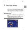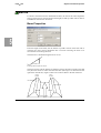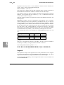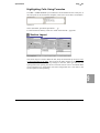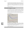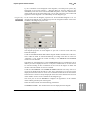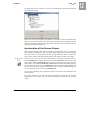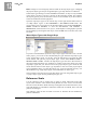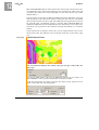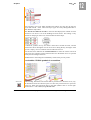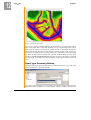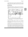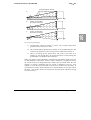
1
SoundPLAN User's Manual October 2005 Braunstein + Berndt GmbH / SoundPLAN LLC Page • i Contents Contents 1 2 Installation and Service 1 Hardware Requirements The Installation New installation of SoundPLAN Notification of new Updates Upgrading SoundPLAN SoundPLAN Service Modules 1 1 2 3 3 4 Tutorial 5 Tutorial with the Project "Starter" Part 1 - Road Traffic Noise Part 2 - First steps in the Graphics Part 3 - Industry Noise Part 4 - Industry Noise - Detailed Investigation of the Supermarket Part 5 - Indoor Factory Noise - calculation of the indoor level and the calculation from indoor to outdoor 3 SoundPLAN-Manager Data organization Functions of the SoundPLAN Manager Change display options Project-Info Create a new project or select an existing one Create new project Select an existing project Copy, delete, insert and pack projects Copy and paste projects Pack and extract projects Options -> Settings Program Settings Settings for Distributed Computing System Settings Project Settings: Global and Current Project Object Numbering Input and display of the object number Examples for format string and sort order Additional Graphics Formats SoundPLAN Manual 5 5 23 28 33 39 47 47 47 48 48 48 48 49 50 50 51 52 52 52 53 54 55 55 57 58 Page • ii Contents Settings for the Export of Graphics Branching into SoundPLAN modules Hotline Support with e-Mail 4 Geo-Database 59 59 61 63 Working with the Geo-Database Overview Geo-Database Structure of the Geo-Database The data structures in the background The graphical user interface The Coordinate Table Top View, Side Projection and 3D-Wire Model Rotate Enter Objects Elevation data entry 63 64 65 66 67 68 68 70 71 72 Enter objects with right angles The Coordinate System Object dots and object properties Settings for Geo-files and Object types Measure distances Generate and edit Situations and Geo-Files 73 73 74 76 78 78 Add an existing/new Geo-File New Situation / Edit Situations Data entry 78 80 81 Digitizing mode Digitizing from scanned maps Digitizing with a digitizing tablet DXF Import DXF-Export Import of SoundPLAN DOS (V4.2) data ArcView-Import ArcView Export LIMA BNA-interface ASCII- interface CARD/1 and Stratis Interface Use elevations from a Digital Ground Model Assignment of terrain elevations to Objects Filter Grid Elevations 81 82 85 87 90 90 91 91 92 92 94 94 96 96 Zoom-Mode and View port administration Object zoom Storing view ports Rename or delete a view port Editing the data 98 98 98 99 99 The edit mode Properties and coordinates editing dialog 99 100 SoundPLAN Manual Page • iii Contents Moving Through a List of Coordinates 102 Undo 102 Define Properties for Attribute Operations, Object Info and Shape File Export 103 Activate objects 104 Select points or objects 104 Delete points or objects 107 Insert a point 107 Move point 107 Move, duplicate and rotate marked objects 107 Graphics-Object type 108 Split objects 108 Invert entry direction 108 Change Geo-File Assignment 109 Convert object type 109 Coordinate operations 110 Attribute operations 110 Search for an object known by it's ID number 112 Copy object 112 GeoTools for selected (marked) line objects 112 Create a buffer 114 Create intersections and split 115 Intersections with the terrain 115 Generate a parallel object 116 Connect lines and generate areas 116 Coordinate Transformation 117 Calculating object height from a DGM 118 Evaluate points for mean building heights 118 Assign texts to buildings 119 Reassign receivers to buildings 119 Prepare buildings 120 Distribute population 121 Regenerate new object numbers 121 5 SoundPLAN Manual Objects and their Properties 123 Road Alignments Road Properties Cross Sections / Road Profiles Road bridges Emission Level Calculation Multiple Reflection Documentation of the Emission Level 123 124 125 126 127 133 134 Signal - Intersection Addition 134 Parking Lots Calculation of the Emission Level of Parking Lots 135 135 Railways 138 Page • iv Contents Railway Properties Railway bridges Emission Level Calculation Lmax-railway (pass-by level) Documentation of the Emission Levels of Railways 138 139 140 143 145 Industrial Noise Sources Source Properties Lmax Industry Assigning Sources to Buildings Additional Information Index Card 145 146 147 147 148 Industrial Building Properties Industrial Building Indoor Noise 151 151 153 Buildings Building Properties 155 155 Elevation Lines and Profile Lines Supply of Elevation Information 160 160 Break Lines (Terrain edges) 162 Spot Heights (Terrain Points) 162 Noise Protection Walls Wall Properties 163 163 Berms Berm Properties 166 166 Volume Type Absorption (Mitigation Areas) Volume Type Absorption Properties 167 168 Ground Areas (Ground Effect) 169 Floating Screens Calculation of the insertion loss 170 170 Area usage 171 Single Point Receivers Receiver Properties 172 172 Cross section 175 Calculation Area 175 Geometry Texts Text Properties 176 176 Point, Polyline, Area • Photo Point Photo Documentation Value grid 177 177 178 179 SoundPLAN Manual Page • v Contents 6 Libraries Overview Available Libraries and their File Names Data organization of the libraries Importing Libraries Libraries from SoundPLAN DOS Working with the Libraries Backup copy of libraries Emission, Absorption, Transmission and Attenuation Libraries Emission Library Transmission library Directivity Library 2D-Directivity 3D directivity Day Histogram Library Assessment Library The Road Day Histogram Library Print libraries Export Libraries 7 Calculations Run file and calculations Generate calculations runs and edit the properties Calculation run properties Selection and assignment of Situations and Geo-Files File number of the results Logbook, Error messages and Default settings Default Standards and Run Commands Start or terminate a calculation run Graphical presentation of geometry in calculations Calculation settings for noise calculations Assessment Calculation Types Using a DGM for the calculation Single point receivers sound (SPS) Grid Noise Map Calculations Cross-sectional Noise Map Facade Noise Map Calculations Calculation of the City Noise Map 8 Result Tables (Documentation) Overview Getting started with the Result Tables Table Types Special Actions for Different Table Types Column Setup SoundPLAN Manual 181 181 181 181 182 184 184 188 188 190 191 191 191 193 194 195 197 198 199 201 201 202 202 206 207 208 210 210 213 215 217 218 218 218 219 223 224 227 231 231 232 232 234 235 Page • vi Contents Column format Column settings Legend Column Setup for Diagrams Detail header setup Table Settings Delete and store result files Sort order Calculation Run Info 236 236 238 239 239 239 240 241 241 Page Layout Page Format Page Layout Headers and Footers 243 243 243 244 The Preview 245 Print Result table 246 Export of the Result table 246 Store and Load a Result table (QRP) 9 Spreadsheet 246 247 Overview Spreadsheet Getting started with the Spreadsheet Components of the Spreadsheets Generate a new Spreadsheet, amend or edit it Generate new Spreadsheets Filter for new tables in the Spreadsheet Amend an existing Spreadsheet Update Spreadsheet Content Update results Insert results and additional information Add reference road or railway Add columns with additional information 247 247 248 249 250 251 253 253 254 255 256 256 Table Settings The Formula Editor Usage of structure fields in formulas Export formulas Designing Spreadsheet tables Column layout Highlighting cells using the cell layout Highlighting Cells Using Formulas Section Layout Structured Tables Table statistics 257 258 263 263 264 264 266 267 267 268 270 Print Spreadsheet 271 SoundPLAN Manual Page • vii Contents Print legend Export spreadsheets 10 Wall Design Overview Wall Design's Internal Organization Wall Design Performance Using Wall Design Optimization in Wall Design Starting the optimization Receiver locations Wall segments Optimization History Minimizing Costs Print wall table Storing the Wall back in the Geo-Database Using Wall Design for areas Model restrictions of Wall Design 11 Expert System Industrial Noise Overview Expert System for Industrial Noise Concept of Expert System for Industry Noise Sort criteria Detail window Graphics window Day histogram Spectrum Contribution Level Sum Diagram properties Preparation of a noise control concept Assign noise mitigations The Optimization Print and reuse the noise control concept Using the noise control concept in additional calculations Store the noise control concept into existing result tables for documentation and graphics 12 Graphics Overview Graphics Quick Overview of the Graphics Sheet Elements in the Graphics Create New Elements Activate Elements Move and Zoom Elements Cut, Paste and Copy Elements Store and Insert Elements Central Editing Tools SoundPLAN Manual 271 272 273 273 274 277 278 280 282 284 284 285 286 287 287 288 289 291 291 294 295 295 296 296 297 297 298 300 301 302 305 305 306 307 307 308 309 311 312 313 314 314 314 Page • viii Contents Zoom Sheet Components Acceleration of the Screen Output Sheet Templates Element Properties Layout Name, Size and Position Edge Specialties for Sheet Properties Specialties of the Map Properties The Map Graphics-File-Selection-Manager File Selection Edit the Content of a Map Object Type File Reference Scale Site Map / Geometry Data Point Type Object Types Line Type Object Types Area Object Types Object Type Geomety Text Composite Object Types Presentation of Area-type Results Requesting results for area type data types Object Types for Area-type Objects Contour Line and Grid Value Export Presentation of the Facade Noise Map Result Requests in the Facade Noise Map Object Type Facade Noise Map Display as level chart tables, RLS-90 Symbols, Planning Guideline Austria File selection of level tables / RLS-90 symbols Object type level table/RLS-90 symbols Presentation as Level Chart Parameters for the Level Chart Object type Level Charts Presentation of Geometry bitmaps Object type Geometry-bitmap Troubleshooting for printing geometry bitmaps Building and Area Evaluation and Statistics (EU Environmental Noise Regulation) Building Evaluation Object type EU buildings (Annex VI) Area Type Evaluation File-Operations Procedure for the file operations Color scale and color palette Color palette Color scale Legend 314 314 315 316 316 317 318 320 320 321 322 323 323 326 331 332 333 335 337 340 343 344 345 346 347 352 353 353 354 357 357 359 364 364 365 365 366 367 367 367 369 369 371 371 375 375 377 381 SoundPLAN Manual Page • ix Contents Edit legend Text boxes North arrow Scale bar Emphasise Graphically Using Symbols SoundPLAN Symbols Adminstration of symbols The symbol editor Requesting new symbols Spreadsheets in the graphics Draw attribute labels 3D Graphics Basic principles Display options, views and movements Geometry parameters of the scene 3D-settings 3D-Graphics model data check 3D tab in the object type setup 3D-Graphics Animation The Animation Printing Export 13 Noise Mapping Projects and Strategic Noise Maps Tiling projects Preparing the project for tiling The tiling manager Tiling navigator Tiling projects in the Geo-database Calculate tiled projects Tiling projects in the graphics Conflict map / Summed-up conflict map Confict map How to generate conflict maps Procedure for summed-up conflict maps Annoyance Analysis Supplementary Necessary Information Working on an Annoyance Analysis in SoundPLAN Implementation of the EU Directive on Environmental Noise The Interim Calculation methods EU noise mapping - data to be estimated Definition of Time Ranges and Standards Environmental Noise Guideline (Annex VI) 14 SoundPLAN Manual 381 383 384 384 385 386 386 387 388 390 391 393 393 394 395 396 397 398 401 403 404 405 407 407 407 408 410 411 411 413 413 413 414 416 417 417 417 420 420 421 421 422 Aircraft Noise 425 General Procedures 425 425 Page • x Contents Aircraft Noise – Data Entry Airport Runways for Start- and Landing Approach- and Departure Flight Paths Aircraft Classes Library Aircraft Traffic Data Aircraft Noise in the Geo-Database Aircraft Noise in the Calculation Aircraft Noise in the Result Tables Aircraft Noise in the Graphics New features for Aircraft Noise in SoundPLAN 6 15 Air Pollution MISKAM Introduction The MISKAM – calculation core MISKAM Background Material Motivation Physics of the Model Wind Tunnel Simulations Measurements of Traffic Induced Imissions Model Results Model Numerics MISKAM and MISKAM-SCREENING under SoundPLAN Assessment of the Emission Wind roses, weather statistics, processing results Theory and Praxis The calculation model: What MISKAM can do What MISKAM cannot do... MISKAM project flow under SoundPLAN Step 1: Module Geo-database Object type: Calculation area MISKAM Object type: Road Object type Buildings Data type MISKAM-Source: MISKAM in the Calculation Core Calculation definition for MISKAM-SCREENING Calculation definition in MISKAM Run File TAB Graphics: MISKAM in the Graphics 16 Technical Acoustics in SoundPLAN Overview Physical Descriptors of Noise From Levels to Rating Noise Modeling the Real World Physics Versus Standards Calculating Principles Screening 426 426 427 428 430 432 437 437 438 439 439 441 441 441 442 442 444 446 446 447 448 448 448 449 449 450 451 453 453 453 456 457 458 459 459 460 463 463 465 465 465 466 466 466 467 471 SoundPLAN Manual Page • xi Contents Ground Effect, Komega, Directivity Reflection Volume Type Absorption The Search Angle Method 17 Principles and Standards Overview Road Noise Philosophy of Modeling RLS 90 / DIN 18005 The Source Level LME The Propagation Calculation of Road Traffic Noise (CoRTN) The Reference and Basic Noise Levels The Propagation Concepts of Screening, Ground Attenuation and Reflection Deviations from CoRTN Statens Planverk 48 The Equations of Statens Planverk 48 Ground Effect and Screening Deviations from Statens Planverk 48 Federal Highway Model (FHWA) The Equations of FHWA Traps and Solutions Deviations from FHWA Railway Noise Principles of Emission Schall 03 / DIN 18005 / Transrapid The Emission Noise Level Schall 03 The Propagation from a Railway line according to Schall 03 Traps and Solutions ÖAL 30 The Equations of the Standard Deviations from the Standard Calculation of Railway Traffic Noise (CoRN) The Reference Noise Level CoRN The Propagation of CoRN Traps and Solutions Deviations from the English Railway Traffic Calculation Nordic Rail Prediction Method The Reference Noise Level - Nordic Rail Prediction The Propagation - Nordic Rail Prediction Method Deviations from Nordic Rail Prediction Method Industry Noise Acoustical Schools (ISO / Nordic / CONCAWE) Spreading / Komega / Ground Effect From Area and Line to Point Sources Cross References between Sources and Buildings SoundPLAN Manual 476 477 479 481 485 485 485 485 487 487 489 492 493 495 497 499 499 499 500 503 503 503 506 507 507 508 508 508 510 512 512 512 513 513 514 515 517 517 517 517 518 520 520 521 521 522 525 Page • xii Contents VDI 2714, VDI 2720 or ISO 9613 The Equations of VDI 2714/2720, ISO 9613 The Meteorological Correction Cmet – ISO 9613 General Prediction Method Concepts and Equations (Gen. Pred. Method, ÖAL 28) Deviations from General Prediction Method , ÖAL 28 CONCAWE The Equations of the Standard (CONCAWE) Traps and Solutions Calculations Inside Buildings VDI 3760E The Indoor Factory Noise Module Calculation Method Interpretation of the SPC Special Noise Calculation Cases Buildings as Sources Tunnel Bridges Gallery Implemented Calculation Standards V.6.3 18 Index 527 527 529 531 531 536 536 537 540 540 540 545 546 546 546 547 549 550 553 555 SoundPLAN Manual Page • 1 Installation and Service 1 Installation and Service Hardware Requirements The hardware listings below are not a minimum configuration, but a configuration enabling professional work. SoundPLAN can be run on a Pentium 200 but the processing speed would be dissatisfying. Towards the high end there are no limits except economics and availability. PC Pentium 2 GigaHertz or higher Operating system Windows NT 4.0, Windows 2000 or WindowsXP Graphics card with a resolution of minimum 1024 x 768, 256 colors, 32 MB memory or higher, for 3D-Graphics you need a graphics card with OpenGL drivers and at least 32 MB memory RAM memory >= 512 MB Hard disk 60 GigaByte 17" Monitor WinTab compatible Digitizer (WinTab drivers are available for nearly all current digitizers) All windows compatible printers and plotters can be used. The Installation The first installation of SoundPLAN is done with a CD and a floppy disk containing the license information, user name and address. The CD has an autorun function, automatically opening the CD browser. Within the browser, you can install the software and demo or test projects, read the manual on screen or print it and view other information on SoundPLAN. If the autorun function is disabled on your PC, please call "browser.exe" (depending on the CD) from the Windows Explorer. SoundPLAN Manual Hardware Requirements 1 1 Page • 2 Installation and Service New installation of SoundPLAN From SoundPLAN 6.3 versions with the same main version number can be installed parallel to older versions. The older version (6.2) does not have to be uninstalled. In the Windows Registry a new key is generated for the SoundPLAN version 6.3. Before starting with the SoundPLAN installation log in as the Administrator. The installations-CD contains a self starting browser. Select the browser language and then navigate to the program installation. SoundPLAN can be installed as a regular program or as a demo version (e.g. for Distributed Computing), the programs are identical except for the demo version has all modules activated but also has the write mechanism deactivated. To install SoundPLAN as a regular or as a demo version, click on the appropriate menu topic and follow the install-shield script. If the program is installed as a regular version, the program needs the license file and thus will ask you at the end of the installation for this license file. If you received a new license file (BABGxxxx.006), please direct the program to the location where this file is stored. You can also point the program towards the location of the V6.2 installation; SoundPLAN can take this license file for the new installation. Steps: • Insert the CD and place the installation disk in the floppy drive. Autorun opens the CD Browser. • Attach the SoundPLAN hardlock to the parallel or USB port before you start the installation. • Call the installation in the browser. • The installation program will prepare the installation and guides you through it. The installation program suggests C:\Program files\SoundPLAN 6.3\ as the path for the program files. For any other location, enter the new path. Click the button "continue". SoundPLAN copies the files from the CD to your hard disk. The installation program will request the license disk. Make sure that the disk is in the floppy drive (or in a folder on your harddisk) and click "OK". Important: If you are asked to restart the PC after the installation is finished, please leave the CD in the drive and log on with the same name as the last time so that the installation can get finished with the same user rights etc. Hint: Please ensure that the hardlock (dongle) is attached to the parallel or USB port. The hardlock drivers do not recognize hardlocks on the serial port automatically. If for any reason you cannot use the parallel port for the hardlock, please contact Braunstein + Berndt for help. SoundPLAN is now successfully installed on your PC. Run SoundPLAN from the Start menu under the label SoundPLAN 6.3 in the program group of SoundPLAN 6.3. The Installation SoundPLAN Manual Installation and Service Page • 3 After the installation is finished you may want to copy the demo projects that have been adapted to the capabilities of the new version. To install the projects click on the topic INSTALL DEMO-PROJECTS. With the first start of the version 6.3 you will be asked if you want to copy your existing GlobData folder to a new location. If you want to use older projects with the older version and prepare new projects with the new 6.3, the global settings such as the object setup should be kept separate. Projects that you intend to open in the version 6.3 should be copied to a new location as well, once you open the project in the version 6.3 it will be converted to 6.3 and will no longer open correctly in 6.2. In SoundPLAN 6.3 all older projects will be displayed with a gray SoundPLAN project folder. Upon opening it you will be asked if you want to convert it into a 6.3 project. Notification of new Updates With the version 6.1 SoundPLAN started to offer updates directly in the web. With the new version the program can trigger the search for new versions directly from the program. The first time you open SP 6.3 you will be asked if the program shall search in the web if there is a new version of the program available. YES activates the service and the program asks whether you want to search for a new update at once, with NO the service will be deactivated (for example if you PC has no internet connection). In the program settings (OPTIONS -> SETTINGS) you can modify this setting any time. If the field CONFIRM INTERNET CONNECTION contains a "Yes", the program will notify you every time it is looking for a new version of the program, with the setting "No" it contacts the internet without notifying you. Upgrading SoundPLAN After you have installed the latest CD version, updates of SoundPLAN are available for download from the Internet. Via HELP -> UPDATES & DOWNLOADS you get access to the latest update. If you already have the latest revision working on your PC a message will indicate that there is no further update available at this point of time. A program update is an EXE file. Download the file to your computer, close SoundPLAN, open the EXE file with a double click in the Windows Explorer, select the language and the update is executed. A license update updates the license information of your version, e.g. if you purchase additional modules. Copy the license file (BABGxxxx.006) to your PC and execute HELP -> UPDATE LICENSE in the SoundPLAN Manager. SoundPLAN Manual The Installation 1 1 Page • 4 Installation and Service SoundPLAN Service Modules The SoundPLAN Handbook is available in printed form and as an electronic Acrobat Reader pdf document. The Acrobat Reader is enclosed in the CD and can be installed from \CD_50\acrobat. The SoundPLAN On-Line Help in the program provides information to current problems and is updated with every SoundPLAN version. The SoundPLAN Hotline is available from your local distributor or SoundPLAN LLC (mailto:[email protected]). Find information on your local distributor in the SoundPLAN Manager via HELP -> INFO. SoundPLAN Service Modules SoundPLAN Manual Page • 5 Tutorial 2 2 Tutorial Tutorial with the Project "Starter" This is a simple example for SoundPLAN beginners to get an overview on how to work with SoundPLAN. During the installation of the demo projects, the project Starter is installed in the sub-folder Demos. The project only includes a bitmap as data background, it is your job to work it out. Because of the modular structure of SoundPLAN, it is possible that this project deals with modules not covered by your license. In this case, please skip this part of the description and go on with the next part. As this example has been defined for the handling of SoundPLAN and for all SoundPLAN users all over the world, the calculation standard and the assessment cannot be customized for every country. Part 1 - Road Traffic Noise Two terraced houses, each with three flats (an old part and a newer part) are affected by noise from a road and a business district. For these two houses first the noise levels must be calculated (separately for road noise and industrial noise) and then a noise protection wall has to be optimized, so that the limits for traffic noise are kept in the first floor. The results are shown either in tables or in grid noise maps. Open SoundPLAN with START -> PROGRAM FILES -> SOUNDPLAN 6.3. General Project Settings Select project Select the project "Starter" via PROJECT -> NEW/ SELECT -> activate the project in the tree view and click SELECT. The preset calculation guidelines are displayed on the screen. To change the settings or to check the enhanced settings, click on the STANDARDS. SoundPLAN Manual Tutorial with the Project "Starter" Page • 6 Tutorial 2 We use the German RLS-90 for the calculation of road traffic noise and the ISO 9613-2 for parking lot noise and industrial noise. For the assessment, we selected the DIN 18005 Traffic. Enhanced settings Click on the symbol with the two small dots to open the enhanced settings of the standard. Creation and calculation of the ground model As the first step, the elevation lines have to be digitized to calculate a digital ground model (DGM). All subsequent elevation information for the objects comes from the DGM. Open the GEO-DATABASE. With a new project the graphical user interface of the Geo-Database is opened directly. Load the prepared bitmap: FUNDAMENTALS -> BITMAP -> LOAD. Select the bitmap "site map". Bitmaps have to be assigned to real world coordinates by entering the actual coordinates at reference points: The bitmap in this project already shows four reference points; choose at least two but preferably three of them as reference points. 1300/550 bottom left 1550/550 bottom right 1550/850 top right 1300/850 top left Enter the given coordinates of one reference point into the white cells in the first row and place the cursor roughly on the corresponding reference point in the bitmap. Click once, and then a zoom window for exact positioning is opened. Click again at the intersection of the axes - the first point has now been assigned. Tutorial with the Project "Starter" SoundPLAN Manual Page • 7 Tutorial Enter the coordinates of the second reference point into the second row of the table and click on the corresponding reference point in the bitmap, and so on. After you have assigned the third reference point, the standard deviation is shown at the bottom of the bitmap assignment window, which should be much less than 10 in this porject. If it is too high, please check the reference points. Click OK. Next, all the elevation lines in the plan will be digitized. Select OPTIONS -> HEIGHT DIALOG ONLY AT 1. POINT and select the object type "elevation line" in the index card "Environment": New object (F2) Start digitizing for example in the upper left corner with the elevation line 231 m: Click roughly on the first point and then the exact position with another left click in the zoom window and enter 231 in the elevation dialog. Digitize one coordinate after the other in the same way. After you have entered the last coordinate of the elevation line finish the entry of this object with F2 or the symbol button NEW. Digitize all elevation lines in the project in the same way and check the model via VIEW -> FRONT ELEVATION or F8. If a coordinate is not entered at the correct position, select the elevation line with the right mouse button -> select object (or pull a frame with the right mouse button around at least one point of the elevation line) and move the coordinate with the left mouse button to the correct position. Should you have entered the wrong elevation for an elevation line, you can correct this selecting the elevation line, call Edit -> Coordinate operation and set h1 to the correct elevation. Save the situation via FILE -> SAVE SITUATION. As this is the first situation in the project, overwrite "New Situation" with "Basics" and "New Geofile" with "Elevation". Call the CALCULATION CORE (activate the SoundPLAN Manager in the Windows task bar and click on the icon Calculation). You will automatically access the properties of the calculation run: SoundPLAN Manual Tutorial with the Project "Starter" 2 Page • 8 Tutorial 2 Assign geometry data for the triangulation Enter the RUN NAME "Calculate DGM" and select the CALCULATION TYPE "Digital Ground Model" from the selection list in "Geometry". Select the GEOMETRY DATA with the double arrow. Currently, only one situation is available. Double click on the situation "Basics" or push it with drag & drop to the right hand side to use it in the calculation. In every calculation, SoundPLAN needs a number for the result files. We choose NUMBER 9999 in order to make it easier to sort the true calculations. Click OK and start the calculation with seconds. . The triangulation only takes a few Save the calculation table under the name "all calculations" and switch to the GeoDatabase via the Windows task bar. Entry and calculation of road traffic noise The first step is the calculation of the road traffic noise. Save the open situation "basics" via FILE -> SAVE AS under a new name. The name of the situation is: "road noise without noise protection" and click OK. New Geofile, load Geofile Create a new Geofile for the geometry of the residential area: Click on the icon NEW and then the icon . Overwrite the name "new geofile" with "residential area" and load this Geofile with OK into the situation. GEOFILE Additionally load the DGM: FUNDAMENTALS -> DGM -> LOAD. Double click on file RDGM9999.dgm. You can view the triangles and the elevation of the cursor position via the menu VIEW. Now digitize the first building (2, Jefferson road). Symbol building Select the Geofile "residential area" from the Geofile selection list. Click on the building symbol building in the index card "environment". (If you want to see the icons for all objects, switch to options object selection: all objects.) Click on the read digitizing cross. Entry modes: The entry modes: There is the following difference between the black cross and the red cross: The first time the black cross digitizes the coordinates. Afterwards, the left mouse button is used to open the properties of the appropriate object, the right Tutorial with the Project "Starter" SoundPLAN Manual Page • 9 Tutorial mouse button hosts edit functions. If points are close together, it might be impossible to set new coordinates, as the program automatically enters the properties of an existing point. In this case the red cursor helps. Here the left mouse button is only used to enter new coordinates, the right mouse button captures a coordinate, to connect a new object to an existing object. Put the cursor on the first building coordinate (upper left corner) and click on the left mouse button. The vicinity of the cursor position is enlarged in the zoom window. Now click on the exact position. The elevations in the elevation dialog are filled in from the values in the DGM and click OK. Enter the building properties in the property dialog box: ROAD NAME: Jefferson Street, NO. 2, double click on the field NAME to overtake the settings. REFLECTION LOSS: 1 (non absorbant) HEIGHT OF BUILDING: 6m RECEIVER HEIGHT ABV. GROUND FLOOR: HEIGHT OF FLOORS: 2,8 m NUMBER OF FLOORS: DECISIVE FLOOR: AREA USAGE: 2,4 m 2 1 GR (general residential) The building has two floors, as the noise protection wall shall be dimensioned for the ground floor, the ground floor is determined the decisive floor. Leave the dialogue with OK and enter the other coordinates of the building. New object After you have entered the last coordinate (upper right corner) finish the entry of this object. The building is closed and hatched in light green. The facade at the Whitefield Drive should be divided at the property borders of the terrace houses (especially for the calculation of a Facade Noise Map), the back of the building need not be divided. Select the magnifying glass on the tool bar and enlarge the view, clicking several times with the left mouse button on the viewport. View object dots Select the black cross and activate the object dots with the icon Object dots on the left of the object selection list. Click on the first point of the building with the right mouse button and select INSERT AFTER from the popup menu. SoundPLAN Manual Tutorial with the Project "Starter" 2 Page • 10 Tutorial 2 The inserted coordinate is placed in the middle of the two edge points and marked with a small black square. Drag the marked point (with the left mouse button pressed) to the first property border. Insert another point after the point just inserted and move it to the second property border. Normally, the input accuracy is not that exact, so that the building won't be right angled. You can correct this with a GeoTool. Place the cursor near the upper left corner of the building, keep the right mouse button pressed and pull a frame. At least one coordinate of the building must be within the frame. You can also click on one coordinate of the building with the right mouse button and select SELECT OBJECT from the popup menu. Select GEOTOOL -> POLYLINE -> CALCULATE RIGHT ANGLED. Deactivate the marks by dragging the mouse with the right mouse button pressed from bottom to top (or with the right mouse button CLEAR SELECTION). Digitize the second building - 4, Jefferson Street. Click on the bottom left edge coordinate of the first building with the right mouse button (black cross from the Tutorial with the Project "Starter" SoundPLAN Manual Page • 11 Tutorial tool bar) and select CAPTURE COORDINATE from the popup menu. The properties of the new building are automatically carried over from the other building. Change the house number to "4" and double click on the field NAME. The lower building has 3 floors. Enter BUILDING HEIGHT 8,5 m and NUMBER OF FLOORS 3. Enter the other edge coordinates of the second building and close the building (F2). Divide the Whitefield Drive facade at the property borders of the terrace houses, by inserting additional points. The buildings should look like the sketch below if you switch on the object dots (icon left to the object selection list). Location of the receivers: Icon receiver: Three receivers are assigned to the buildings. Because of the task to build a noise protection wall, one receiver should be located in the northernmost part of the first building and two further receivers at the northernmost and the southernmost terrace house of the second building. Click on the icon receiver from the icon bar (tab index card "receivers"). Place one point near the desired building facade. Confirm the elevation dialog box with OK. No elevation information is needed because the receiver will be assigned to the building together with the elevation information. Elevations coming from the DGM will be ignored, too. Set the check mark in the field CENTERED in the receiver properties and click on the upper third of the facade in the picture. As you can see, all the relevant building information is transferred to the receiver. Add an "a" to the house number in the receiver name and click OK. SoundPLAN Manual Tutorial with the Project "Starter" 2 Page • 12 2 Tutorial Repeat the actions with the two other receivers. Add an "a" to the first and a "d" to the second receiver to the receiver name "4, Jefferson Street" after the house number. New Geofile, load Geofile Now create a new Geofile for the supermarket and the metal sheet factory on the left hand side of the road. The name of the Geofile is "industrial buildings". Select the building icon from the icon bar. Ground floor elevation and terrain elevation are taken from the DGM. The wall height of the supermarket is 4,5 m, the wall height of the metal sheet factory and the residential building next door is 6 m (the residential building is the small part of the building). All buildings are within an industrial area. Assign a receiver to the residential building of the metal sheet factory. Use the preset values for the other fields. Icon Road For the first calculation, only the road is still missing. Create another Geofile, named "Road". Select the icon for the road from the icon bar. Place the first road coordinate at the upper edge of the bitmap in the middle of the road. The emission lines are created automatically from the definition of the profile in the road properties. Object elevation (upper edge of the road) and terrain elevation are the same and are taken from the DGM. Regarding the ROAD PROPERTIES the following properties have to be entered: NAME: Whitefield Drive Select the calculated mode with the CALCULATED field check box for the emission level (LmE) and click on the POCKET CALCULATOR: INPUT TYPE: City roads ADT (AVERAGE DAILY TRAFFIC) SPEED: 12300 vehicles/24h vCar/vTruck= 50 km/h For all other fields, use the preset values. Click OK to close the emission calculation. As a situation can contain more than one road, the road for the reference kilometer for receivers and noise protection walls must be determined in the road properties. The check box "reference axis" can only be set at the first road coordinate. Set the check box for the REFERENCE AXIS. Tutorial with the Project "Starter" SoundPLAN Manual Page • 13 Tutorial PROFILE: 3,25/3,25 (RQ 3,25) (Tab index card "profile") Digitize the course of the road and enter coordinates at the positions of the small squares on the bitmap. The road properties change at these small squares. Now select the black cross to edit the properties of some of the road coordinates. At the junction with the Jefferson Street, the TRAFFIC VOLUME increases to 12700 vehicles/24h. Left click on the road point to open the properties and then on the pocket calculator to change the traffic volume. (Is the road point not exactly in the intersection with the axis of the Jefferson Road? Select the road by pulling a small frame around one of the road points with the right mouse button and move the coordinate with the left mouse button). At the next junction, the traffic volume increases to 13100 vehicles/24 h, then in the south of the terrace buildings, the SPEED increases to 70 km/h for cars and trucks. At the motorway access, the traffic volume decreases to 8500 vehicles/24h. Use Ctrl+ R or call VIEW -> REFRESH to display the created emission lines and activate the Object dots of the road (icon object dots on/off on the left to the object selection list): The double circles indicate the coordinates where at least one property changes. In the road properties and in "edit object properties" you can jump with and from one coordinate where the properties change to the next one. (The other arrows go to the first or last coordinate and to the next or previous coordinate.) If you only want to see the road, as in the picture on the left hand side, select VIEW > CURRENT OBJECT TYPE and click on the road icon from the icon bar. The work in the Geodatabase is done. Save the situation via FILE -> SAVE SITUATION. Call the CALCULATION and load the existing run file "all calculations". Click on "+" to create a new calculation run. Place the cursor in the empty line in the fields "name" or "calculation type" and double click or select EDIT -> RUN PROPERTIES. "Road noise without noise protection". This text fills the place holder "calculation title" in the results tables. RUN NAME: CALCULATION TYPE: Select from the left selection list "Outdoor noise" and on the right side "Single point sound". Assign geometry data DATA: Click on the double arrow, you will see a window which shows the available situations on the left side and the situations selected for the calculation on the right side. The file type "situations" is selected in the selection list for the file type. Drag the situation "road noise without noise protection" to the right side or double click on the situation. SoundPLAN Manual Tutorial with the Project "Starter" 2 Page • 14 Tutorial 2 This number may only be assigned once! For big projects in might be useful to create several run files for different areas. For small projects it is better to use only one run file. The numbers can have 4 digits. Enter the number "1" for this calculation. NUMBER OF RESULT FILES: Tab index card SETTINGS: Set angle increment, number of reflections and reflection depth to "1". Tab index card STANDARDS: Calculation according to RLS-90 Assessment according to DIN 18005 Traffic, the limits are 55/45 dB(A) (day/night) for the residential area and 65/55 dB(A) for the business district. Tab index cardSPS (Single points sound) PLAIN RESULT TABLES AND LEVEL CHARTS should be selected, then click OK. Go to the tab index card GRAPHICS in the calculation kernel, you will see the data you entered. If an error message occurs, saying that something is wrong with the data, look at the tab index card LOG BOOK, go back to the Geodatabase and correct the error. Start the calculation with . Controlling the calculation: Cancel, pause, distributed computing, calculate all runs marked with "yes", single run The level chart and the results for the currently calculated receiver are displayed in the tab index card Graphics. You can check the results later again in the calculation kernel with a right click on the receiver. This method is extremely useful if you want to verify a result, as geometry, level chart and result are displayed together. Tutorial with the Project "Starter" SoundPLAN Manual Page • 15 Tutorial Check the results in the Result Tables (Documentation) Open the RESULT TABLES and open the file RSPS0001.res.The file name is a combination of "R" for results, The calculation type, here "SPS" ("Single Point Sound") and the number of the calculation. You will see four tab index cards. RUN INFO, containing the information on the run settings and data in the calculation. SINGLE RECEIVERS, containing the results of the single point calculation for every receiver and the difference from the target values. DETAILS + GRAPHICS, containing the detailed information for every receiver (in this case only the day histogram of the road, because "detailed result tables" has not been set in the calculation run.) ROADS, containing detailed information on the emission level of the road. Look at the tab index card SINGLE RECEIVERS first: The results exceed the given limits - it might be possible to reach the limits for the ground floor with a noise protection wall. Before printing the table, look at the column settings and the page layout. Choose the COLUMN SETUP from the right mouse menu and check the visible columns, column width, texts and legends for the column header. Go to the tab index card TABLE SETTINGS. Here the title of the table and if necessary two further texts can be defined for example "Annexe 1". Page layout Click on the icon PAGE LAYOUT (or the right click in the single point table), check page format, layout (with company logo) and header and footer texts. In the header + footer text tab index card, the variables for the project name (from the SoundPLAN Manager), the run name (from the calculation run) and the table title (from the column setup) are included. Own texts can be added to the table header and footer - centre justified, for the fields in the middle, and left and right for the fields on the left or right side. ASCII or Excel export of the table Click on preview to check the table format. Here you can print the table or export it to Excel or ASCII, if you click on the SAVE button and select the desired format (in both cases without the table headers). The format of the table with column headers and legend texts is stored with every table under the name "file name.fmt" in the project. Input of a noise protection wall or dimensioning of the wall with Wall Design It the module Wall Design is not covered by your license, enter the wall with a defined height to calculate the level reduction of the noise protection wall. (Look at HELP -> PROGRAM MODULES in the SoundPLAN Manager to see the licensed modules.) Wall Design needs the following steps: • Determing the base line of the noise protection wall in a separate Geofile. SoundPLAN Manual Tutorial with the Project "Starter" 2 Page • 16 Tutorial • Precalculation with the calculation type Wall Design. 2 • Calling Wall design and creation of the noise protection wall. • Saving the result in a new Situation (with noise protection). Call the Geodatabase again, the situation "without noise protection" should still be open. Select FILE -> SAVE SITUATION AS and type in the file name "Wall dimensioning" (users without Wall Design type in "Road noise with noise protection"). Remove selected Geofile from the situation The receiver in the business district is not relevant when dimensioning the noise protection wall, so select the Geofile "industrial buildings" (only if you dimension the wall) in the Geofile selection list and click the remove icon. You can switch off the bitmap via the selection list on the right hand side (NO or just fade it out (clear check box). The DGM is stored with the situation and used for the calculation, unless you close it via FUNDAMENTALS -> DGM -> CLOSE. BITMAP SELECTED) Create a new Geofile for the wall base line or the noise protection wall. Icon noise protection wall The name of the Geofile should be "Wall base line" or "Noise protection wall" as appropriate. Choose the icon "noise protection wall" from the icon bar. For the dimensioning of the wall, the wall base line must anyway be stored in a separate Geofile. The base line passes along with the property border of the terraced houses. The noise protection wall starts at the property border in the Jefferson Street and ends approximately at the y coordinate 650. The object elevation is taken from the DGM. Properties: Those, who are working with Wall Design, should set the the wall height for the base line is 0 m. OPTIMIZATION property, If you do not have Wall Design set the wall height to 3 m and leave optimization unset. For the other properties the default settings are retained. Tutorial with the Project "Starter" SoundPLAN Manual Page • 17 Tutorial Digitize the coordinates of the wall. Then select the wall (click on one coordinate with the right mouse button, select SELECT OBJECT from the popup menu) and split the wall in constant segments of 5 meters: GEOTOOLS -> POLY LINE -> INTERPOLATION -> CREATE SEGMENTS WITH CONSTANT DISTANCE IN [M] and enter 5. Save the situation and open the CALCULATION. Load the run file "all calculations". Place the cursor in the line "calculation without noise protection", right click and select COPY and then with another right click PASTE IN NEW ROW. Go to the new calculation run and open the calculation properties via double click on the cell "Name" or the right mouse menu. Those who don't have Wall Design, can skip the next section. NAME OF THE CALCULATION RUN: CALCULATION TYPE: Wall design precalculation Outdoor Noise - Wall Design - Single points DATA: Click on the double arrow and assign the situation "Wall dimensioning" instead of "road noise without noise protection" with drag & drop and click OK. NUMBER FOR RESULT FILES: 2 There are no changes in the tab index cards "Settings" and "Standards". Settings in the tab index card "Wall Design": WALL ELEMENT HEIGHT: MAXIMUM WALL HEIGHT: 0,25 m 20 elements The property IGNORE WALL HEIGHT … is deactivated in this case. Start selected single run Leave the properties with OK, switch to the graphics tab index card and run the calculation (start selected single run). Leave the calculation core after the calculation has been successfully executed (please save the run file) open WALL DESIGN from the SoundPLAN Manager. Open the file RWDN0002.res. On the left hand side of the screen, you will see in four tab index cards information concerning the calculation run, receivers and wall elements, on the right the site map and a front view of the geometry data. Site map and front elevation can be rotated via the right mouse button, you can also change the draw type (3D-map). Click on the RECEIVER LOCATIONS tab index card, the levels of all receivers is colored red, which means that the level exceeds the limit. The decisive receivers are selected for the optimization. The other floors are displayed, but they won't be taken into account for the optimization. SoundPLAN Manual Tutorial with the Project "Starter" 2 Page • 18 2 Run the optimization Tutorial Without changing the settings, just let Wall Design optimize the wall for the minimum surface. Click on the green start arrow. With the icon the wall is built up until either all limit levels are reached or all available wall elements are used. The icon is used to build up the wall elements step by step. With every mouse click, a new element is put on the wall. Before the start of the optimization, you will be asked to confirm the omptimization criteria. The first criterion is "level reduction" and the wall shall be built according to the smallest wall surface for the time slice day. As target level the defined limit level shall be used. After the optimization the wall looks could look more or less like this: fter the first optimization, the tab index cards receiver locations, wall segments and history show different perspectives of the wall which can be used to analyse the automatic optimization. The visual appearance of the result looks more or less OK. Click on the history tab index to see a graph showing the effectiveness of the elements. Should the wall look uneven, adjust the wall height (number of elements) in the "wall segments" tab index card. Store wall Store the optimized wall back to the Geodatabase. SoundPLAN automatically creates a new Situation and replaces the Geofile which contains the base line with the optimized noise protection wall. Please enter new names for the Situation and the Geofile: The name of the Situation is "Road noise with noise protection" and the name of the Geofile is "noise protection wall" (please overwrite the default ""). Go back to the GEODATABASE, call FILE -> OPEN SITUATION, click on the + in front of the situation "Road noise with noise protection" and assign the Geofile "industrial buildings" with drag & drop. Open the situation with a double click. Look at the wall in the front view VIEW -> FRONT ELEVATION (). Not all of the wall segments have been used for the optimization of the wall. Please delete the coordinates without a wall height (even wall elements with zero height have a screening effect in the propagation calculation!).). Tutorial with the Project "Starter" SoundPLAN Manual Page • 19 Tutorial Click on the first point with the wall height 0 in the site map with the right mouse button and select SELECT POINT from the popup menu. Press the shift key and click on the last point (right mouse button) and select SELECT POINT again. Delete the coordinates with CTRL+ DEL. Repeat this procedure and delete the coordinates with wall height 0 at the end of the wall. Save the situation and switch over to the CALCULATION. Those, who do not work with Wall Design should continue from here. Open the file "all calculations" and insert another calculation with the + button. Open the run properties. RUN NAME: "Road noise with noise protection". CALCULATION TYPE: DATA: Outdoor Noise - Single point sound Situation "Road noise with noise protection" NUMBER OF THE RESULT FILES: 3 Tab index card SETTINGS: Set angle increment, number of reflections and reflection depth to "1". Pease set the "plain result tables" property in the tab index card SPS. Leave the run properties and calculate this calculation with (start selected single calculation). Save the run file and leave the calculation core. Combination of results with the Spreadsheet Now the results with and without noise protection will be compared with the limit values. Call the SPREADSHEET from the SoundPLAN Manager. Select a template from the template selection list. Select the sample template "B14", click on NEW and opten the file RSPS0001.res. SoundPLAN Manual Tutorial with the Project "Starter" 2 Page • 20 Tutorial 2 The filter settings are correct for this example project, leave the dialogue with OK. The results are automatically read into the level columns 19 and 20, together with further properties, such as the name of the receiver location or the limit levels. The reference axis of the road is loaded from the result file so that the columns13, 14 and 15are correctly filled in. Please note that the column numbers refer to the column headers. Add the levels with noise protection to the columns 25 and 26: FILE -> LOAD RESULTS AND FURTHER INFORMATION -> ADD RESULT COLUMNS, SELECT and open it. In the window "assign level columns" the cursor is already placed on the cell level coumn day; select the column 25 in the selection list on the right hand side and click OK. The limits are the same, therefore the limit columns don't have to be imported again. Recalculate all columns Now most of the columns are now filled in. Only the values for columns which contain formulas must be updated. Click on the pocket calculator to update the calculation and confirm the message that you really want to calculate all columns. If you want to have a look at a formula, click on the column header of column 29 with the right mouse button and select FORMULA from the menu. The table is in principle ready, if you want to, you can change the layout - font size, hide columns, or ad a text column with comments. The dotted red line shows page breaks and the page width, defined in the page layout. Please change the layout of the table to your needs using the menu items or the icons: Tutorial with the Project "Starter" SoundPLAN Manual Page • 21 Tutorial Some hints: • Spreadsheets are divided into the two parts title and data, which are formatted independently in the column setup. • The right mouse menu is accessed from the column header. • The column layout can be adapted for more than one column at a time, if at least one cell of the desired columns is highlighted. • The cell layout can be used in combination with calculate and highlight from the right mouse menu. The cells are highlighted with a formula (e.g. x19>55; (the semicolon stands for the end of the formula)). • If you change the text size in the icon bar, it changes the text size for data and title, whereby the displayed size is the text size of the data; the title size is two points bigger. Call the page layout (FILE format etc. -> PAGE LAYOUT) to set header and footer texts, table If you are ready, the table can be printed. When you are used working with the Spreadsheet, you will find out the flexibility of the Spreadsheet defining the contents and the appearance of your tables. The formulae help to get any needed statement or statistics and for the appearance you can highlight limit violations in another color or structure the table to make it easier to read. Example table structure Calculation of a Grid Noise Map For the graphical documentation of the calculation results, grid noise maps have to be created 2 m above ground for the situations with and without noise protection and the differences. The length scale is 1:1000 and the page format is letter or A4. First define a calculation area in the CALCULATION. SoundPLAN Manual GEODATABASE, then execute the Tutorial with the Project "Starter" 2 Page • 22 2 Icon calculation area Tutorial The Geodatabase is still open. Select the icon calculation area from the icon bar. Activate the bitmap and digitize the calculation area roughly on the basis of the coordinates 1300/900, 1500/900, 1500/500, 1300/500 (use the red cross). The calculation area has to be surrounded by elevation information, so that the receiver elevation can be calculated for all grid points. The calculation area should be in a separate Geofile, so the Geofile assignment has to be changed now. Create a new Geofile named "calculation area". Select the calculation area (Alt+ left mouse button anywhere within the area - the object type calculation area must be active), call EDIT -> CHANGE GEOFILE ASSIGNMENT and select the Geofile "calculation area" from the selection list. Remove current Geofile The Geofile "calculation area" shall not be part of a situation, but is added to the Grid noise map calculations separately. Make sure, that the Geofile "calculation area" is still the current Geofile in the selection list and click "remove current Geofile". Confirm, that you want to save the changes in the Geofile calculation area. Call the CALCULATION CORE. Open the run file "all calculations" and copy the calculation run " road noise without noise protection" (right mouse button -> COPY, right mouse button -> PASTE IN NEW ROW). Double click in the run name to edit the properties: NAME OF THE CALCULATION RUN: CALCULATION TYPE: GNM without noise protection Outdoor noise - Grid noise map DATA: Load the Geofile "calculation area" in addition to the Situation "road noise without noise protection". Click on the double arrow, select "Geofiles" from the selection list and add the Geofile "calculation area" to the already assigned data. NUMBER FOR RESULT FILES: 11 The settings in the tab index cards "settings" and "standards" do not change. Set the specifications in the new tab index card GRID MAP, the GRID meters, and select CALCULATE DGM, all other settings are not changed. SPACE is 5 Switch to the GRAPHICS tab index card and start the calculation. First the digital ground model is calculated, then the ground elevation is displayed with a coloured scale (important tool for checking the elevation model), after that the real calculation is started. Use the same procedure for the situation with noise protection: Copy the "grid noise map without noise protection" calculation run, modify the name of the calculation, double click on the cell data and change the situation "road noise without noise protection" to "road noise with noise protection". NUMBER FOR RESULT FILES: Tutorial with the Project "Starter" 13 SoundPLAN Manual Page • 23 Tutorial Start all calculations marked with "yes" Double click on the cell CALC to remove the "Yes" for the three calculation runs we have already done. The both GNM calculation runs should be marked with a "yes" in the first cell. Click on the green arrow, to calculate all calculation runs marked with "yes". The calculation kernel calculates both calculation runs in a batch mode. Part 2 - First steps in the Graphics SoundPLAN has the possibility to use templates in the Graphics, so that completely formatted maps are created in no time. You can save each of your own maps as tamplate, so that you can use them for further maps also in other projects. The delivered templates are examples, how maps could be organized. In this tutorial, we will generate a map with one of the delivered templates and derive two further maps from the first one. Please read in the manual how to create own templates and how to position the elements on the sheet using the alignment of elements. Open the Graphics via the SoundPLAN Manager and select the template "A4 portrait" from the template selection list. You will see a preview on the left hand side. Click NEW tofill the template with data in the File selection manager. Select the Situation "road noise without noise protection", put it with Drag & Drop or the right arrow into the files in the map and confirm the legend selection. SoundPLAN offers the legend from the template. Select from the selection list the FILE TYPE "Grid Noise Map", select the calculation without noise protection (RRLK0011.res). Select in the following dialog the time slice you want to show, here: time slice day, and the colored scale you want to use, the colored scale from the template is offered. Confirm the parameter settings and click OK, the map is already nearly formatted. Go to ELEMENT -> SHEET COMPONENTS to look at the elements in this template and the hierarchie in which the elements are arranged. SoundPLAN Manual Tutorial with the Project "Starter" 2 Page • 24 Tutorial 2 lle elements are arranged on the sheet within a group box. Click through the elements with the arrow keys, the active element is displayed with marks. Geometry parameters The next step is to adapt the length scale. Double click on the map (or right mouse button -> EDIT CONTENTS) to get to the map contents. Call GEOMETRY VIEWPORT -> GEOMETRY PARAMETERS and enter the 1:1000 (respectively 80 feet). Click OK. The geometry viewport has to be moved a little bit to the left. Call GEOMETRY Change geometry VIEWPORT -> CHANGE GEOMETRY VIEWPORT and then from the right mouse menu MOVE. Move the frame, so that the grid map is within the viewport. viewport Close "edit map contents" with OK. Double click on the Description text box (or right mouse button -< EDIT CONTENTS and change the preset text: First row: Tutorial SoundPLAN Second row: Grid Noise Map without noise protection Third row: Time range day, Calculation 2 m above ground Section layout The text has already been divided in the two text layouts "Title" and "Standard text". First column [Return] Second row [Ctrl+ Return] Third row With Ctrl+ Return, the text was divided into two sections, so that the upper two rows are assigned to the section layout "Title" and the last row is assigned to the section layout "Standard text". The section layout can be adapted to your needs with the icon ABSATZLAYOUT. Make sure that ADAPT BOX TO CONTENTS is set and click OK. The colored scale shall display 3dB intervalls and contain 12 intervalls. Click right on the colored scale and select EDIT CONTENTS. Automatic scaling Select the symbol for the AUTOMATIC SCALING. Change the number of intervalls to 12 and the step size to 3. Click OK, the modified colored scale is displayed. Try Tutorial with the Project "Starter" SoundPLAN Manual Page • 25 Tutorial different scale types and intervals until it fits to your needs. In order to highlight the limit value, you could change the color of the interval 54 - 57 manually, click on the color field and select another color. Scale layout Click on the icon SCALE LAYOUT and change the row height to 4, so that the color fields have a distance. Additionally, you can set the edge lines around each of the color fields. Leave the scale layout and the scale editing. If you want to change the colors in general or if you want to add further colors, close scale editing and select PARAMETERS -> SHEET COLORS or PARAMETERS -> PROJECT COLORS. The OBJECT Situation. TYPE receivers will not be displayed on the map, but is part of the Activate the map and call the MAP OBJECT TYPES from the right mouse menu. Deselect the "show" and "use in legend" check boxes. Click OK. Delete row As the legend has been created while loading the data, the entry receiver has to be deleted manually. Double click on the legend box to EDIT THE CONTENTS, highlight the row receiver and delete it with the icon DELETE ROW. For the Grid Map, the output parameters will be changed. Call the MAP OBJECT TYPES again and select the grid noise map in the branch results. Deselect USE SCALE COLOR in the sub object type main interval in the section contour line; the contour lines are now displayed in black. Leave the masks with OK. Exchange the bitmap for the company logo and enter project engineer and date in the appropriate text box, then the first map is complete. Save the sheet (file name: Road noise without noise protection) and print it. The adapted layout of the tamplate shall be used as the basis for further graphics (thus you don't have to change company name and company logo) and will be be saved as a new template. Please select FILE -> SAVE AS TEMPLATE and enter the file name and description (file name: GNM A4, description: basic template A4 (letter) with colored scale). Own templates are always stored in the folder "…\My files\SoundPLAN\Globdata" and can be used for all projects. New sheet Now we need to create the sheet with noise protection. Call a new sheet and select the just created template from the selection list. Click new to enter the file selection manager - load the Situation "Road noise with noise protection" and the grid noise SoundPLAN Manual Tutorial with the Project "Starter" 2 Page • 26 2 Tutorial map "with noise protection". Click OK to close the file selection manager. Change the contents of the text box containing the description of the plan. Now you only have to save the sheet and print it out. For the difference map save the sheet with noise protection unter the name "Difference" (FILE -> SAVE SHEET AS). Activate the map and open the file selection manager via the right mouse button. The Situation "with noise protection" is correct for this sheet, but remove the grid noise map via the arrow to the left arrow from the map data. Select the file type "grid operations" and click on the double arrow. ssign the grid noise map without noise protection to the base file and the grid noise map with noise protection to the operation file (time slice day for both maps). Click CONTINUE and then OK. Select the colored scale 1 while loading the data, however, the value range must be adapted to the difference values. The colored scale for the difference map should be a fluid color gradient from white to blue. Call PARAMETERS -> SHEET COLORS, to create a new colored scale. Click on the color field white and then . Place the cursor to the first field of a completely black row and click . Select a color field with a dark blue and click again . . Now click on the pocket Place the cursor on the last field of this row and click calculator: The RGB values of the colors are interpolated between white and dark blue. Tutorial with the Project "Starter" SoundPLAN Manual Page • 27 Tutorial 2 Close the color definition with OK. Automatic scaling Now edit the colored scale with a double click or EDIT CONTENTS via the right mouse button. Open the automatic scaling and enter the following settings: Lowest value: 0 Step size: 1 Number of Intervals: 12 Color selection: Clic on the color field and select the white field from the fluid blue to white scale. Deactivate the check mark ASCENDING, so that the scale colors are used from the right to the left. Close the dialog and change the header of the colored scale to "noise reduction". Close the scale editing - the third map is ready. With extended modules, there are many methods for displaying the calculation results in the graphics. Here are three examples. The steps for creating these plans are always the same. The data are loaded in the file selection manager and afterwards designed in the map object types. For some of the display types, special calculations are needed, others just use the results we have already created. This graphical output shows the differences between the two situations without and with noise protection, together with the level tables at the facades (single point calculation) and the geo referenced bitmap we used in the Geodatabase (both module Cartography). SoundPLAN Manual Tutorial with the Project "Starter" Page • 28 2 Tutorial The cross section map (module Cross Section Map) shows the effect of the noise protection wall. The cross section is entered in the Geodatabase and calculated with a grid cross section calculation. This is a 3D view on the grid noise map (module 3D Model). Some of the object types have special 3D properties. It is also possible to display facade points (Facade Noise Map) or cross section maps in 3D. Part 3 - Industry Noise Now it will be investigated, whether a small supermarket can be built in the business district. The metal sheet factory already exists. The business district emits with 65 dB(A)/m2. Both companies on the other road side are in a business district. In the first place, it must be defined, what area level is allowable to keep a limit level of 55 dB(A) for the day and 40 dB(A) for the night at the border of the residential area. Please create a new Situation in the Geodatabase. This Situation only contains the residential buildings but not the buildings in the business district. The business district contains the two company properties. Bot properties should be defined as Tutorial with the Project "Starter" SoundPLAN Manual Page • 29 Tutorial separate noise sources, so that it is possible to determine different limits for each of the properties. Working with the Geo-Database The first steps should be known now: New situation Call OPEN SITUATION (when you open the Geodatabase, you will automatically see the Situation Manager), click on NEW SITUATION; name it "industry noise", assign the Geofile "residential area" with drag & drop and open the Situation. Select the bitmap again from the selection list. Icon area source Create a new Geofile named "industrial sources", double click to load it to the situation and select the icon area source from the icon bar. Digitize the property of the supermarket according to the following sketch. The object elevation of the area source is 235 m, the terrain elevation is 0, so that ground effects are disabled. Properties: NAME: Property supermarket Group: Right click on the field, select INSERT, type in "supermarket" and press enter on the keyboard. DAY HISTOGRAM: The source emits during the day with 65 dB(A)/m2, in the night with 50 dB(A)/m2. As there is only one entry possible for the level, we have to use the day histogram and assign 65 dB(A) for the day and 50 dB(A) for the night. There is another possibility: You could define two sources with the same geometry, one for day and one for night. SoundPLAN Manual Tutorial with the Project "Starter" 2 Page • 30 2 Tutorial Access the day histogram library with , SoundPLAN opens the day histogram library of this project. Enter the element name "industrial area", switch over to the values tab index card and select "dB" from the selection list. Assign the value 50 to the hours 01-06 am and 10-12 pm, and 65 to the daytime hours (highlight the cells with Shift+ arrow key). Click ACCEPT to assign the library entry to the Geodatabase. Use the preset values for all other properties. The calculation will be done with a center frequency of 500 Hz and the level entered in the day histogram library is per m2. Enter the other coordinates, then ( or F2). Capture the two edge coordinates of the first property for the input of the second industrial property with right mouse button -> CAPTURE COORDINATE. The elevation is stored, the property dialog is opened directly. Enter the SOURCE NAME "Property metal sheet factory" and insert a new GROUP "metal sheet factory". All other properties are equal. Capture the second edge coordinate and digitize the other coordinates of this area. Ready: Save the situation and open the Calculation. Working in the Calculation core: Open the run file "All calculations" and create a new calculation run. Please enter the calculation properties: NAME OF THE CALCULATION RUN: CALCULATION TYPE: DATA: noise contingent investigations Outdoor noise - Single points sound "Industry noise.sit" NUMBER FOR RESULT FILES: 101 Use the preset values in the SETTINGS tab index card. Tab index card SPS: Set "plain result tables" and "detailed result tables". Close the run properties with OK, switch to the graphics of the calculation and calculate this single run. As the sources are entered with a center frequency, SoundPLAN states during the calculation that the ground absorption for these sources is calculated according to the alternative method of the ISO 9613-2. Tutorial with the Project "Starter" SoundPLAN Manual Page • 31 Tutorial Working in the Result tables Open the file RSPS0101.res and look at the results in the tab index card single receivers. The assessment levels exceed the limits by about 5 dB(A). The first aim is to create a source contribution table. Receiver names, limit levels and assessment levels are displayed in a header row, the sources and their contribution at the receivers in the data rows. This display type consists of two tables, fit into each other. Go to the DETAILS + GRAPHICS tab index SOURCE CONTRIBUTION tab index card. card and then in the lower table to the The assessment level at the receiver is displayed in the upper table, the contribution level of the sources in the lower table. For projects with more data, it might be useful to sort the single receiver table, e.g. according to the highest assessment level. The sort order is also used for the upper table in the "details and graphics" tab index card. Click the right mouse button in one of the tables and select SOURCE CONTRIBUTION REPORT -> ALL RECEIVERS. If you look at the header rows, you will see, that the receiver location is without a text in front of it, the other values are described by a text. This can be handled with the DETAIL HEADER SETUP in the upper table, accessible with the right mouse button (close the preview): SoundPLAN Manual Tutorial with the Project "Starter" 2 Page • 32 Tutorial 2 The receiver name is in the second row. It is set but without a column header (look at the legend text below, to identify the contents of the column). This is the same for the floor in the second row. Close the detail header setup again and open the table. COLUMN SETUP from the lower For the column "LrD" enter "Contribution level" in the first title row and "day" in the second title row and click "centered" for title and column alignment. Proceed the same way for column "LrN". Switch to the table settings tab index card an set "title 2" so that it will be displayed in the column header. You can also allow page breaks in the detail list for larger tables. Open the contribution report (preview) again, and check the layout. Limitation of the maximum emission level by use of the attenuation column: As the assessment levels day and night exceeded the given limits by about 5 dB(A), we have to restrict the sources to a maximum emission level. An attenuation for the sources can be defined in the last column of the source contribution table. Tutorial with the Project "Starter" SoundPLAN Manual Page • 33 Tutorial Enter the value by which the source should be attenuated, SoundPLAN calculates immediately the assessment levels at the receivers. The attenuations are entered as positive values. Try out and enter different values, until the limit levels are kept. One of the sources has to be reduced by 6 dB(A), the other by 5 dB(A). Prepare the table for the printout: Select PAGE LAYOUT from the right mouse menu, or the icon bar, check the settings and texts, call the PREVIEW and print the table. Part 4 - Industry Noise - Detailed Investigation of the Supermarket The limits for residential areas 55 dB(A) during the day and 40 dB(A) in the loudest hour of the night have to be kept in the neighbourhood of the supermarket. The contribution levels between 6 and 7 am and 20 and 22 pm will get an addition of 6 dB(A) for the rest period. At night the maximum level must not exceed the limit by 20 dB(A), during the day by 30 dB(A). The task of the investigation is, whether the limits are kept and to propose noise reduction measures if needed. Please take into account, that the limit levels have to be divided between the metal sheet factory and the new supermarket. As the metal sheet factory does not work at night time, the supermarket can use the whole noise limitation. During the daytime, the level must be split up. The level for residential areas has to be reduced by 3 dB(A), approximately according to the proportion of the contribution levels in the above example. These examples have been created to show how to use SoundPLAN. Not all of the assumptions are checked in detail. Please do not use these assumptions in real life! The delivery with heavy trucks begins before 6 o'clock in the morning. The opening hours of the supermarket are from 8 am to 20 pm. The following sources are relevant: Delivery with heavy trucks: Between 5 and 6 am 2 trucks Between 6 and 7 am 2 trucks Between 7 am and 8 pm 8 trucks A loading procedure with fork lifters which lasts 8 minutes is assigned to each of the trucks. The sound power level of the truck is 65 dB(A)/m, the sound power level of the fork lifter is 90 dB(A). SoundPLAN Manual Tutorial with the Project "Starter" 2 Page • 34 Tutorial There are two parking lots with 100 (east parking lot) and 40 (west parking lot) places. There are 2 car movements per parking place during the opening hours. Later, the parking lots will be completely empty. 2 A heating system with the opening of the air condition is at the southern facade of the building, with a sound power level of 65 dB(A) all day and night. Only the sound sources on the property of the supermarket are taken into account. The ISO 9613 part 2 is used for the propagation calculation. The Bavarian parking lot study 1994 is used for the emission calculation of the parking lots. Working with the Geo-Database Create a new Situation in the Situation Manager duplicating the situation "road noise without noise protection" and assign the name "supermarket". Open the new Situation. Remove selected Geofile from the situation All contained Geofiles are now part of the new situation. Please remove the Geofile "Road" (select Geofile "road" in the selection list and press ). Activate the bitmap "site map" in the selection list and check whether the DGM is still loaded. There is a building in the north of the supermarket that has to be absolutely part of the investigation. Create a new Geofile, digitize the new building and assign a receiver at the southern facade. The name of the Geofile is "mixed area". The building name is "4 Pine tree lane" and has two floors, the area usage is a mixed area. Create another Geofile named "sources supermarket" for all sources of the supermarket. Icon line source Let's start with the trucks. The trucks access the property on the west side of the supermarket, and then reverse towards the unload place. So two truck movements have to be assigned per truck. Enter the line source according to the above graphics and change the object elevation in the dialog to 233 m. The following properties are assigned: NAME: Approach truck GROUP: Select "supermarket" from the selection list. COMMENT (not Tutorial with the Project "Starter" absolutely necessary): Level: 1 movement per hour and meter SoundPLAN Manual Page • 35 Tutorial New library element DAY HISTOGRAM: Create a new day histogram. Click on the double arrow to access the library, create a new element with the plus and enter the name "truck approach". Go to the "values" tab index card and select "U/h" (units per hour) from the selection list. Enter the operating hours: 4 movements between 5 and 6 am and 4 movements between 6 and 7 am. The 8 trucks during the day can be split up to the operation hours or assigned to any hour between 7 am and 20 pm. Click ACCEPT. The new element is updated in the source properties dialog. The CALCULATION MODE is a center frequency of 500 Hz. Enter a level of 75 dB(A) per meter (this level is derived from the sound power level of the truck considering the time needed for the distance of 1 meter). Next, enter the uploading with fork lifters. As sometimes two trucks can be uploaded at the same time, the uploading zone is defined as an area source. An uploading period of 8 minutes is assigned to every truck. The sound power level for the uploading duration of one hour is set to 90 dB(A) for the total uploading zone. The source is 1 meter above ground. Digitize the uploading zone according to the above graphics, using the following properties: DAY HISTOGRAM: Copy the element "truck COPY TO -> .\starter\time.db (project library), SoundPLAN Manual approach" with right mouse click -> select NEW ELEMENT from the dialog Tutorial with the Project "Starter" 2 Page • 36 Tutorial and enter the name "uploading zone". Go to the values tab index card, select min/h (minutes per hour) from the selection list and assign 8 minutes to each truck. 2 The CALCULATION MODE is a center frequency of 500 Hz. SOUND POWER LEVEL: 90 dB(A) per unit Close to the area source is a small annex to the supermarket, which we have not yet digitized. Select the Geofile "industrial buildings" and digitize the building. The building is 4 m high. Go back to the Geofile "sources supermarket". Next we will define the west parking lot. As with the other noise sources, we will define a day histogram out of the movement in units/h.). The number of places is only used to calculate the addition for the lanes. The fields "number of movements" can be omitted. Icon parking lot Select the icon "parking lot" from the icon bar and digitize the first parking lot with the following properties: NAME: "West parking lot" NUMBER OF PARKING LOTS N: 40 DAY HISTOGRAM TOTAL PARKING LOT: Create a new element named "west parking lot". It has 40 places, which is 80 movements/h. After the opening hours of the supermarket (between 8 and 9 pm) there are still 40 movements until the parking lot is empty. Activate the check boxes for "addition 'Taxtmaximalpegel'" (addition for the impulse) and "addition for lanes". Tutorial with the Project "Starter" SoundPLAN Manual Page • 37 Tutorial Finish the entry of the west parking lot. Digitize the second parking lot (Name East parking lot, 100 places, the other properties are the same). Create a new element in the day histogram library. Copy the Element "west parking lot" as described above and assign 200 units instead of 80 units (and 100 units instead of 40 units). The above graphics shows the two parking lots. The last source is the opening of the air condition at the southern facade of the supermarket. It is placed at a distance of 10 m from the southwest corner of the building, 4 m above ground (or 30 m from the southeast corner - this depends on the input direction of the building). Activate the object dots and the start marking of the building: Right mouse click on the object selection list -> SETTINGS AND and check mark "with points" for the object type building. The opening is a point source and is assigned to the building. Select the icon point source from the icon bar, place the point source near the southern facade of the supermarket and confirm the elevation dialog with OK. Enter the point source properties: NAME: Air condition GROUP: Supermarket DAY HISTOGRAM: 100 % each hour (new element in the day histogram library) SOUND POWER LEVEL: 65 dB(A) Go to the Geometry/Building ref tab index card. Now assign the point source to the building, entering the distance to corner (10 m) and the height above ground floor (4 m) and clicking on the southern facade of the supermarket. If you entered the building clockwise (you can see this from the small arrow at the first building facade), enter 30 m, as now the distance refers to the southeast corner. SoundPLAN Manual Tutorial with the Project "Starter" 2 Page • 38 Tutorial 2 The definition in the Geodatabase is complete, save the situation. Working in the run file Call the calculation and load the existing run file "all calculations". Create a new calculation run and enter the following calculation properties: NAME OF THE CALCULATION RUN: CALCULATION TYPE: DATA: Supermarket without noise protection Outdoor noise - Single points sound Supermarket.sit NUMBER FOR RESULT FILES: 102 Check the SETTINGS in the tab index card, number of reflections 3, reflexion depth 1 and set enable side diffraction. For sources without spectra the ground absorption of the ISO 9613-2 is automatically calculated according to the alternative method. As the limit value during the day time has to be split up between the metal sheet factory and the supermarket, we have to define a new assessment, derived from the library element "TA Lärm". Click >>, select the element "TA Lärm", click the right mouse button and copy it to the project library and enter the name "TA Lärm limit day reduced". Reduce the limit level for the residential area to 52 (day). Go to the SPS tab index card and set "plain result tables" and "detailed result tables". Start the calculation. As the sources are entered with a center frequency, SoundPLAN states during the calculation that the ground absorption for these sources is calculated according to the alternative method of the ISO 9613-2. Results The limit level day is slightly exceeded for the receivers in the residential area. During the night the levels in the mixed area are exceeded. Tutorial with the Project "Starter" SoundPLAN Manual Page • 39 Tutorial 2 The next task is to design attenuation measures in the Geodatabase for the calculation of different variants. The original sound sources will not be changed. Open the Situation Manager with duplicate the Situation "supermarket" (new name "supermarket with noise protection") and the Geofile "sources supermarket" (new name "supermarket sources with attenuation"). FILE -> OPEN SITUATION, Replace the Geofile "sources supermarket" with "supermarket sources with attenuation". What could be attenuation measures? Here are some proposals: Limitation of the number of trucks before 6 am (change of the day histogram) or use of noise reduced trucks (change of the sound power level). Change of the track of the trucks, with separate access for both directions. Better screening between the truck access and the building in the mixed area. Noise protection wall at the east parking lot. Other ideas? You see how important it is to have the possibility of building different scenarios in the Situation Manager! But one condition must be taken into account: Please do not copy buildings to another Geofile, if receivers or sources are assigned to the buildings. The receivers and sources would have to be reassigned afterwards. A better way is to store receivers or sources in own Geofiles. If you copy these Geofiles, the assignments will be kept. Part 5 - Indoor Factory Noise - calculation of the indoor level and the calculation from indoor to outdoor A metal sheet factory is established in the south of the supermarket. The factory works in two shifts, from 6:00 am to 10:00 pm. We know the indoor noise sources, the absorption areas and the attenuation of the components of the building. The inner level is calculated according to VDI 3670, afterwards the outdoor propagation calculation is executed according to ISO 9613-2. SoundPLAN Manual Tutorial with the Project "Starter" Page • 40 2 Tutorial The calculation of the indoor level is executed in the middle of the inner facades. Steps: 1. Preparatory work in the library: Copy of transmission spectra, absorption spectra and the emission spectra form the system library to the project library. 2. Definition of the industrial building 3. Transformation of the facades in noise sources and assignment of the transmission spectra 4. Definition of the general properties for the indoor noise calculation 5. Assignment of the absorption spectra to the facades and definition of embedded components 6. Definition of the noise sources within the industrial building 7. Calculation indoor to outdoor (Hallout) 8. Outdoor calculation Preparatory work and entry of the industrial building Copy the desired emission spectra, transmission spectra and absorption spectra from the system library to the project library: Open the library from the SoundPLAN Manager and call the system transmission library and the project transmission library via LIBRARIES -> SYSTEM -> TRANSMISSION and LIBRARIES -> PROJECT -> TRANSMISSION. (The local empty transmission library is created). Select the desired element in the system library (keep the Ctrl key pressed to select several elements), click the right mouse button and copy the element "1mm sheet steel trapezium profile d=45 mm" to the project library: Proceed the same way for the transmission spectrum "Double glazing 4/8/4 mm". The system transmission library includes many elements; therefore it is advisable to reduce the number of displayed elements with the text filter: Do the same procedure for the following elements of the emission and absorption libraries (the project absorption library is just created, too): Tutorial with the Project "Starter" SoundPLAN Manual Page • 41 Tutorial 2 Next open the Geodatabase and create a new Situation. Select the Situation "supermarket", duplicate it and name it as "metal sheet factory". Remove the Geofile "supermarket sources" from the Situation (right mouse button -> remove or drag & drop). Create a new Geofile named "metal sheet factory" and open the Situation. The metal sheet factory (factory building and residential building) has been digitized as one building. Now we need to split it into the factory building (object type industrial building) and the residential building (object type building). The building of the supermarket has to be copied to the Geofile "metal sheet factory". Select the object type "building", click on the red cross cursor and make sure that the Geofile "metal sheet factory" is selected. Capture the edges of the residential building with the right mouse button and change the name of the building to "residential building of metal sheet factory". Select the object type "industrial Symbol industrial building" and capture the edges of the factory building. Ignore the properties of the building industrial building at the moment (close the properties with OK). Symbol building Remove the Geofile "Industrial buildings" from the Situation "metal sheet factory". Transformation of the facades to noise sources Click on one coordinate of the factory building with the left mouse button and assign the base properties name = metal sheet factory, height = 6 m and refection loss = 1 dB. Go to the sources tab index card. Apart from of the joint facade with the residential building, all facades of the factory building have the same properties. As already defined properties are adopted to further objects (here facades), we define one facade in detail first, so that we only have to change the joint facade afterwards. Right click on the first facade in the right hand window and select DEFINE AS SOURCE. In the new Level definition tab index card, select Li(Calc)-6-R from the selection list in the field LW (Calc means that the indoor level is entered after the SoundPLAN indoor calculation). SoundPLAN Manual Tutorial with the Project "Starter" Page • 42 2 Tutorial The table below shows the values for the indoor level, the transmission and the sound pressure level of the area that is emitting to outdoor. We have to assign only the transmission spectra, as the indoor level is calculated and the sound pressure level results from Lw=Li-6-R following the equation 7a of the VDI 2571. Click on the double arrow in the row "R" and assign the element "1 mm sheet steel trapezium profile". As the library element was defined in octaves, also the table in the factory building is in octaves. Further properties, group name and day histogram are entered in the general tab index card (lower part of the properties dialog). Create a new element in the day histogram library. Click on the double arrow and create the element "metal sheet". The factory works 100 % from 6 am to 10 pm. Assign the group "metal sheet factory" from the selection list, which was created during the calculation of the noise limitation. All properties of the first facade are defined. Right click on any of the facades in the right hand window and select DEFINE ALL FACADES. The roof has to be converted separately to a source (right click on the roof and define it as source) and put back the properties of the joint facade with the residential building, as nothing is emitting to outdoor at this facade. Click on this facade in the right hand window and unset the property DEFINE AS SOURCE. You can name the facades in the GENERAL tab index card. The northern and the southern facade have embedded sources, at the southern facade an open door and a window, and a light band at the northern facade. Click left on the southern facade (facade 3) in the tree window. An embedded component can either be entered with the mouse in the graphical window or with its coordinates (right mouse button). The coordinates refer to the lower left corner of the facade. You have got to be aware that all coordinates of an embedded component are within the facade. The below pictures shows the position of the components and the coordinates of the door … Tutorial with the Project "Starter" SoundPLAN Manual Page • 43 Tutorial 2 the coordinates for the window at the southern facade … and the coordinates of the light band on the northern facade (facade 5). Assign the properties and transmission spectra to the new sound sources. For the open door, we have to create a new library element. Select the LEVEL DEFINITION tab index card, click on the double arrow in the row R and create a new element called "open door" with +, select octaves and enter 0 to all frequencies. The window and the light band have the transmission spectrum "double glazing". Assign the group (metal sheet factory) and the day histogram (also metal sheet factory) to the embedded soures in the tab index card GENERAL. Indoor calculation We need to define the base properties and the absorption characteristics of the components for the indoor calculation. Base properties: SoundPLAN Manual Tutorial with the Project "Starter" Page • 44 Tutorial 2 It is necessary that values are assigned to all components of the building including floor and ceiling. Assign the default spectrum to all components with ALL FACADES ABSORPTIVE. The default spectrum is assigned to all components. Embedded components with different absorption spectra can be defined either by the percentage of the area or with length and width. In our case, the components embedded in the facades for the transmission can also be used for the absorption inside the building. Select COPY SOURCES AS ABSORPTION AREAS in the tree window (right mouse button) for the facades containing embedded components. The embedded components are displayed, if you click on the + in the tree structure. Assign the absorption spectra to the embedded components - the absorption spectrum for the open door has not yet been created (the values are 1 for every frequency) and close the property box of the industrial building.. Definition of the noise sources within the industrial building The sound sources in the factory building are separate object types, without ground elevation. The elevation of the sources is the elevation above sea level. To make the handling of the indoor sound sources easier, a local coordinate system has been created together with the industrial building. The reference elevation of the indoor sound sources is the floor of the industrial building. Switch to the local coordinate system with FUNDAMENTALS -> LOCAL SYSTEM -> METAL SHEET FACTORY. The x and y coordinates refer to the first building side of the factory building. The sound sources (two point sources and one area source) have the following position: Select the object types from the indoor Noise tab index card: Tutorial with the Project "Starter" SoundPLAN Manual Page • 45 Tutorial Geometry: According to the above sketch, the relative height above floor is 2 m. Saw, grind, hammer: Spectrum Sheet metal shop (sanding and hammering), unset USE LIBRARY DEFINITION and enter a sound power level of 105 dB(A) / unit. Punching presses: Spectrum Metal sheet (punching sheet metal), unset USE LIBRARY DEFINITION and enter a sound power level of 110 dB(A) each. The noise sources within the factory building won't get a day histogram and a group. The last step in the Geodatabase is the definition of indoor receivers and/or a line for the sound propagation curve (SPC). For a grid noise map calculation, no calculation area is needed, as the industrial building is automatically used, therefore the calculation area must only be defined if the calculation area is smaller than the industrial building (object type calculation area). Save the situation and open the CALCULATION. Load the run file "all calculations" and create new calculation runs for the indoor calculation, the calculation indoor to outdoor (calculates the noise emitting from the components) and a single point calculation outdoor. For the indoor to outdoor calculation the receivers are automatically created in the middle of the components, 0,2 cm shifted to the inner side. NAME: Indoor to outdoor (for the calculation of the emitting areas) and Indoor calculation (for the calculation inside the industrial building) CALCULATION TYPE: Hallout (In -> Out) for the first calculation run and Indoor SPS for the second one. DATA: metal sheet.sit for both calculation runs Make sure that PLAIN RESULT TABLES is set in the SPS tab index card. Use the preset values in the "indoor" tab index card. NUMBER FOR RESULT FILES: 103 and 104 When the situation in the Geodatabase has been saved, SoundPLAN adds entries in the emission library for Li, which are filled in during the indoor to outdoor calculation. The indoor level is entered into the properties of the industrial building in the Geodatabase. For the result tables, the results are stored under the name RHOTxxxx.res. You will find the reverberation time here. As the relevant receivers (2 and 4 a/d Jefferson Street and 4 Pine tree lane) have already been defined and are part of this situation, so we can execute the outdoor calculation right now. NAME: Metal sheet - calculation outdoor CALCULATION TYPE: DATA: Blechbearbeitung.sit RESULT: SoundPLAN Manual Single points sound 105 Tutorial with the Project "Starter" 2 Page • 46 Tutorial Settings in the SETTINGS tab index card: 2 SEARCH ANGLE: 1 degree NUMBER OF REFLECTIONS: REFLEXION DEPTH: SIDE DIFFRACTION 5 1 enabled Set the PLAIN RESULT TABLES in the SPS tab index card. The assessment levels are not critical as long as the metal sheet factory doesn't enlarge the production to the night time range. The two pictures below show the result of a grid noise map calculation with the industrial building: You can see a substantial difference between the façade with the door and the others. Tutorial with the Project "Starter" SoundPLAN Manual SoundPLAN-Manager Page • 47 3 SoundPLAN-Manager 3 SoundPLAN consists of multiple programs that jointly assure the functionality of the suite of SoundPLAN. Each of the programs is specially geared to fulfill special functions where you can concentrate on the task and not have all menus of the entire program cluttering the screen. As the program is split into individual program modules it is possible to edit data for one variation while another is prepared for the plotter and another is being calculated. Multitasking with SoundPLAN not only works within the same project but can also be applied for different projects. Data organization In SoundPLAN a project folder (subdirectory) is generated for each project. This way it is guaranteed that all data belonging to the project are stored together. This procedure helps you and your colleagues to efficiently manage projects big and small. In the SoundPLAN-Manager you can generate new general subdirectories and new project folders. This way it is possible further organize the project to keep for example bitmaps and imported files separate from the rest of the project. Functions of the SoundPLAN Manager SoundPLAN Manual Data organization Page • 48 SoundPLAN-Manager The SoundPLAN Manager coordinates the entire program suite and defines the global settings and enables sending hotline e-mails and the access to the closed SoundPLAN user forum. Change display options Each program module of the suite contains a short description which may be displayed when the mouse is on the symbol. Under OPTIONEN -> DISPLAY OPTIONS you can activate and deactivate the display of the module name and the descriptive text. In the section FONT you can customize the fonts, size and color of the description: 3 Change display options Project-Info Edit project-info On the right hand of the SoundPLAN Manager screen the project information and the selected standards are displayed. The project info is generated with the creation of a new project. If you want to modify the description, either click on the project description or on the icon or open the menu PROJECT -> PROJECT-INFO. Create a new project or select an existing one Project new / select When you start SoundPLAN for the very first time the project selection is opened directly to let you create a new project or open a project which has already been installed on your PC. Later on SoundPLAN will always open the last project you worked on. If you want to select a different project or create a new one open PROJECT -> NEW / SELECT . Create new project Create new project First navigate to the place where you want the new project to be located and the “new project”. click on the symbol SoundPLAN projects are presented in the pick list as blue folders with the stylized "SoundPLAN - snail". This way SoundPLAN projects can be recognized and distinguished from normal folders. It may be necessary to convert normal Windows folders into SoundPLAN projects, for example when you generated the folder and already stored the bitmaps or other external data in it. To convert the folder right click on the folder and select the Create a new project or select an existing one SoundPLAN Manual Page • 49 SoundPLAN-Manager option -> CONVERT TO VERSION 6 PROJECT. Or mark the folder and select the option EDIT -> CONVERT TO VERSION 6 PROJECT. When creating a new project first enter the name of the project. The usual restriction of Windows concerning the length and the use of special characters applies. Over length project names will be truncated. To describe the project or the course of action in the entire project, use the project info freely, there is enough space for an in depth description although only a limited text will be displayed on the screen of the SoundPLAN Manager. Enter the project title, the project engineer and the client. The field DESCRIPTION enables you to write a long description of the project. The project info can be read and edited any time by selecting PROJECT -> PROJECT-INFO. Click on OK and the project folder is created, with a click on the SELECT button the project is opened. Select an existing project Project new/select In SoundPLAN the project that was active when the program was terminated last is loaded as the default project. Select a different one with PROJECT -> NEW/SELECT. SoundPLAN Manual Create a new project or select an existing one 3 Page • 50 Higher folder 3 SoundPLAN-Manager If the project is in a different folder on the same drive use the symbol "Higher Folder" and select the appropriate path. If the project resides on a different drive first and then navigate to the correct path as described select the correct drive with above. Hint: Drives on the network must be first connected with get a drive letter then proceed as above. EXTRAS -> NET CONNECTION to In the info field on the right side the SoundPLAN project description you entered is displayed. Hint: Projects on a CD-ROM cannot be opened directly as the Windows operating system marks files on the CD as read only. Therefore the project must be first copied to the harddisk. With the Windows explorer copy the project and then right click on the folder to remove the read only mark on the subdir. The dialog is under “properties”. Click OK and confirm the attribute change to be „applied changes to this folder, subfolder and files.“ SoundPLAN projects can be selected by double clicking or with the button SELECT. Copy, delete, insert and pack projects All functions described here can either be called through the menu „Edit“ or by right clicking on a project. This description only describes the way via the menu. Some of the functions are not accessible all of the time, for example the option „Paste“ can only be used after a project has been copied before. Copy and paste projects Click on the project you want to copy – it changing to a blue background. Select on the right mouse button as well). SoundPLAN in addition shows the project name so that you can be certain to always open and process the right project. Copying projects is very quick as SoundPLAN only stores the project info in the clipboard, the physical copying is done when you paste the project. Select the target path and select EDIT -> PASTE. Now SoundPLAN copies the project. If a project folder of the same name already exists, the project is copied into a folder with the name „Copy of project name.” EDIT -> COPY (available Delete or rename projects Click on a project and select the option EDIT -> DELETE or press the DELETE key. SoundPLAN will ask for a confirmation of this procedure. In case you still answered this wrong, you will find your project in the Recycle bin from where you can restore the project if needed. To rename a project click on the project to activate it and select EDIT -> RENAME (or the project name is highlighted in blue and you can edit the name. F2), Copy, delete, insert and pack projects SoundPLAN Manual SoundPLAN-Manager Page • 51 Pack and extract projects To save space when archiving projects or when you want to send the project to someone, SoundPLAN has the capability to compress entire projects into packed archives. To pack your project open EDIT -> PACK. In the following definition box set additional parameters for the zipped archive. The first entry is the path of the project to be packed, the next entry field defines the path where the packed archive shall be stored. When data are sent to an overseeing agency or to the hotline, some of the data may not be necessary but would inflate the packed file. Therefore SoundPLAN has a menu to customize what will be stored in the archive and what is not. The files to be stored are filtered via the file extension, select which file types shall be stored and which not. The setting EXCLUDE TEMPORARY AND NON SOUNDPLAN FILES should be clicked in most cases. The full list of the files to be included and excluded can be viewed in detail and edited after it is opened with EDIT LIST. After packing the files with PACK, the size of the archive is displayed on the bottom of the entry box. To extract a project, click on the project and click on EDIT -> EXTRACT and enter the path where the archive is to be extracted to. SoundPLAN Manual Copy, delete, insert and pack projects 3 Page • 52 SoundPLAN-Manager Options -> Settings 3 The options provide various pre-settings that are stored globally and edited to meet the requirements of each project. Program Settings The SHARED PATH FOR GLOBAL SETTINGS determines a folder, for example on the server, where the color palette, the global object types, as well as templates for general plots, results tables, spreadsheets and graphics sheets are stored. The files are not automatically stored to this folder, but for organizing reasons the user himself must copy them. In order to solve questions such as "How should SoundPLAN react if the network is not available?" or "Who has priority, when two people want to access files in this directory?" Therefore, SoundPLAN still uses a fix folder for the global settings (..\My Documents\SoundPLAN\Globdata). To adjust the data, right click in the tree view on the left side on program -> COPY THE CONTENTS OF THE GLOBAL FOLDER TO GLOBDATA, or COPY THE CONTENTS OF GLOBDATA TO THE GLOBAL FOLDER. The PATH FOR GLOBAL LIBRARIES defines where the global libraries are stored. If the global path is not accessible, you will not be able to open the global libraries. The NUMBER OF RECENTLY OPENED FILES defines for all parts of SoundPLAN the number of files displayed in the history list of the menu file. Settings for Distributed Computing Distributed computing (DC) uses other PC's in a network, not currently in use, for calculations. One PC, called the workstation PC or client PC controls the allocation Options -> Settings SoundPLAN Manual SoundPLAN-Manager Page • 53 of calculation jobs to the server PC's. In order to make a PC a server PC, at least a demo version of SoundPLAN and a control program, DC control, must be installed. The network port for the workstation PC, the server PC and DC control can be changed here if necessary. The ports must be identical for all PC's used for distributed computing. For server PCs, data is stored during the calculation, which is deleted after the distributed calculation is finished. SoundPLAN creates a new folder for this data under "..\My Documents\SoundPLAN\Distrib" on the server PC. Because the server PC cannot calculate if there is not enough hard disk space available, it is possible to change the PATH FOR DATA FOR DISTRIBUTED COMPUTING. System Settings Some computers have hardware components that do not fully support the 3DGraphics and the bitmap processing. In order to run these modules satisfactorily, you can change some of the system settings. Most of the graphics cards have a double buffer for the intermediate storage of complex graphics data. This second storage is used when moving a scene in the 3DGraphics so that moves smoothly. If you cannot open 3D-Graphics perhaps your graphics card does not support the second storage. In this case, switch USE DOUBLE BUFFER FOR 3D-GRAPHICS to NO. Hint: It might also be that the graphics card generally supports the second storage, but that it is switched off in the graphics card settings. Please contact your hardware specialist first. If geometry bitmaps are not printed or are printed incorrectly, the printer driver might not support the more effective standard routine for bitmap output. In this case, switch USE ALTERNATIVE PRINT ROUTINE FOR BITMAPS to YES. The NEAREST CLIP PLANE is also relevant for 3D-Graphics. Even good graphics cards often have difficulties displaying the nearest clip plane, which is 0,1m for the 3D-Graphics. This leads to incorrect display of areas. Set the nearest clip plane to 5 m for example and check the result in the 3DGraphics. Examples: Clipping plane 0.1 m (left picture) and 5 m (right picture). You can change the nearest clip plane in the 3D-Graphics for each scene (p. 395). STANDARD PRINTER FOR THE GRAPHICS: Often a different printer than the Windows standard printer is used for the graphical printouts. Therefore, you can select another printer installed on your system. The Windows standard printer is still used for the table printouts. SoundPLAN Manual Options -> Settings 3 Page • 54 SoundPLAN-Manager Project Settings: Global and Current Project Define project settings as needed in most of your projects. When creating new projects, SoundPLAN automatically uses global pre-settings for the new project. You can change these settings for the current project. 3 To transfer settings from one project to another or to the global settings, right click on the tree view to the left, select LOAD SETTINGS, select the project6.sp from the desired project and press OK. Hint: The settings of the current project are also accessible form the Geo-Database, the Calculation and the Graphics via OPTIONS -> PRESETTINGS. Each of the programs leads you to the settings in the branch which is relevant for this part of SoundPLAN. But you can also open every other branch in the settings, for example to create a new graphics object tye in the Geo-Database. The changes take immediately effect. The format for the object numbers of receivers / buildings, industrial sources and photo locations is defined in the branch DEFINITION OF OBJECT NUMBER. See "Object Numbering" on page 55 for details. Define the time slices for calculations with the assessment levels DEN day, evening, night in the branch DEN TIME SLICES. For example Day 6 am to 7 pm Evening 7 pm to 10 pm Night 10 pm to 6 am (6-19) (19-22) (22-6) If you want to use the Lden emission calculation but only get the assessemnt levels for day and night, set the time slice evening to 0-0. The time slices must not overlap and must include the 24 hours of a day. The GRAPHICS-SETTINGS provide the color palette and the object types. You can now edit the global object types directly. For the length scale you can also select 'feet'. The USAGES descriptions are defined in the settings. If you have changed the description in the settings and want to use them in the graphics of an existing project, select EDIT -> INSERT USAGE DESCRIPTIONS FROM THE PRESETTINGS in the project object types. It is possible to change the standard properties of some objects in the GEODATABASE in the settings (e.g. the height of the first floor above the ground floor, which determines the position of the first receiver, the height of the floors, the distance of a receiver from the facade and the alignment of road and house number. The STANDARDS are set globally and for the current project but you can change them in the calculation kernel for each calculation run. Use CALCULATION TYPE to predefine standard settings that the calculation kernel will use when this calculation type is used. Set the definitions for each calculation type in the tab index card "settings" in the run properties and set the parameters for the calculation type itself, such as the grid size or the calculation height above ground for a grid noise map calculation. Options -> Settings SoundPLAN Manual Page • 55 SoundPLAN-Manager Please check the run properties in the calculation kernel if you copy calculation runs and change the calculation type afterwards. SoundPLAN automatically uses the presettings. Object Numbering Glossary definition: Because of the new object numbering, it is important to define very clearly the words used in SoundPLAN for different numbers. Object ID - is a unique key, automatically assigned to the objects during the input or import in the Geo-Database. It appears in the status bar. The ID is displayed in the calculation log book if error messages occur (e.g. road attributes of road #2333 are missing) and it can be used to find an object in the Geo-Database. Serial number - is automatically assigned to each receiver during the calculation according to the sequence of the data. Since the serial number is assigned automatically, it might change after a recalculation. Object number - the user assigns the object number to receivers, buildings and noise sources in the Geo-Database. The object number doesn't change - unless you consciously change the number. The object number is not a value but a text. This has the advantage that the object number is not sorted alpha-numerically but via a freely definable sort sequence. The object number is incremented automatically, so the sort order for receivers or sources in the tables is 1, 2, … 10 instead of 1, 10, 2, … without any changes of the pre-settings. Changing the format string and sort order allows you to accomplish many tasks. For example: • Mark free field receivers separately, but sort continuously. • Add additional receivers or sources later, without changing the original sort order. • Insert receivers or sources at a defined location in the table. • Use specified object numbers, e.g. for different parts of a project. Input and display of the object number Definitions for the format string and an additional sort order are located in the settings in the SoundPLAN Manager. During data entry in the Geo-Database, enter the number as you want it to appear in the output. Define new basic number Use DEFINE OBJECT NUMBER to define the number just entered as the new basic number, from which the number for additional objects is automatically incremented. SoundPLAN Manual Object Numbering 3 Page • 56 SoundPLAN-Manager If the defined format string contains letters and/or separation signs, the object number might be A100 or 11.1, for example. The entry of the format string uses placeholders for letters and numbers in the SoundPLAN Manager in OPTIONS -> SETTINGS: 3 0,(9) as a place holder for numbers (9 fills the numbers from the left to the right) A,a as place holder for characters . ,; as separation marks Definition of the numbering in the settings Hint: If you want to change the format for the object number while you are working on a project, call OPTIONS -> PRE-SETTINGS in the Geo-Database and change the format string or the sort order for the current project. The changes take effect as soon as you close the settings and return to the Geo-Database. The object number is written to the result file during the calculation and is added afterwards to the table output in the results tables and the spreadsheets. For the graphical output, you can use the object number as a reference in the file type "level tables". Object number and stored sort string in the tables and as a reference in the graphical output The sort order according to the defined object number uses the column with the format for the sort order (formatted object number or format string) and not the column object number. The column does not have to be set to visible. Object Numbering SoundPLAN Manual Page • 57 SoundPLAN-Manager Examples for format string and sort order Add additional receivers or sources to a later stage of a project, without changing the original sort order. Format string 0 0 0 . 0 Sort order 1 2 3 4 5 Entry in the Geo-Database = Display in tables /graphics stored format for the sort order 1 1.1 1.2 2 2.1 001.0 001.1 001.2 002.0 002.1 The original format string in a project was 00 … Entry in the Geo-Database = Display in tables /graphics stored format for the sort order 1 11 01 11 … now you want to add more receivers and you need to use three-digit numbers. Supplement the format string to 000.0. The display for existing receivers will not change, only the stored format changes: Entry in the Geo-Database = Display in tables /graphics stored format for the sort order 1 1.1 2 11 001.0 001.1 002.0 011.0 In addition, you can use characters to identify receivers and sources, (for example for free field receivers). Because the objects should be sorted according to the actual number, the sort order becomes important. Format string A A 0 0 0 0 A Sort order 5 6 1 2 3 4 7 Entry in the Geo-Database = Display in tables /graphics T1 2 G3 5 5a T-5 SoundPLAN Manual stored format for the sort order 0001T 0002 0003G 0005 0005 a 005TObject Numbering 3 Page • 58 SoundPLAN-Manager The sort order defines the order in which the characters should be considered. Assign a number to each component of the format string: 1 for the first sort order, 2 for the second sort order and so on. Use separation marks to separate character blocks and number blocks. Valid separation marks are , . and ; 3 In character blocks, any characters, spaces and special characters are allowed, but no separation marks and numbers. A format string may contain several character blocks. Small characters in the format string are displayed the way the user entered them (small or capital letters). Capital letters in the format string are always displayed in capital letters. Additional Graphics Formats A tool of SoundPLAN allows additional formats to bit organized picture files. In addition to BMP SoundPLAN now allows the use of JPG, TIF and PNG, GIF and LZW-compressed TIF. Because of the now expired royality of GIF files, the alternative PNG format has become much more popular. PNG depending on the number of colors can have a significant compression with almost no loss in quality. In contrast to GIF PNG can handle graphics of higher resolution than 256 colors. As SoundPLAN graphics and the 3D-graphics use relatively few colors, the PNG format is very well suited for exporting these graphics to: Size as a 24 bit - bitmap: 8,1 MB (uncompressed TIF is similar in size) Size as a 24 bit - PNG: 98 kB Additional Graphics Formats SoundPLAN Manual Page • 59 SoundPLAN-Manager Settings for the Export of Graphics For the export of graphics and diagrams from the Result Table, the Expert System for Industrial Noise the Graphics you can define additional options for the graphics formats. For BMP, PNG and TIF you can define the resolution in [dpi] and the color resolution when selecting the topic OPTIONS. If graphics are to be exported in the JPG-format, you can choose between 3 JPEGCOMPRRESSION TYPES: YUV 4:1:1 (low resolution), YUV 4:2:2 (mean resolution) and YUV 4:4:4 (high resolution). For the compression type 4:1:1 the program stores the data as 4x1x1 bytes instead the shown 4x4x4 bytes. With the switch compression quality select the magnitude of the file compression. The higher the compression, the smaller the file and the bigger the quality loss of the picture. Branching into SoundPLAN modules Via the SoundPLAN-Manager you have access to all modules of the program. Select the icon of the program module and click on it to get into: • Library: Access to the emission-, absorption-, transmissions- and mitigation library, the definitions of 2D- and 3D-directivity as well as day histograms, wind statistics, pollution component library(MISKAM) and the assessment library. The library comes with limited data and is ready to host your project and global data. • Geo-Database Entry of data via digitizer and on screen on top of a scanned bitmap, import of data from older SoundPLAN versions, DXF, AutoCAD and GIS systems. SoundPLAN Manual Branching into SoundPLAN modules 3 Page • 60 SoundPLAN-Manager Data are assembled to Geo-Files that can be freely combined to form Situations. • 3 Calculation Core Calculation on the basis of the data entered in the Geo-Database. Extensive log book functions with error and warning log, graphics control of the calculation, spreadsheet type definition of the calculation to calculate multiple calculations in a row. • Documentation Table type preparation of the result data from single point calculation and Façade Noise Maps. Master/detail organization of the data, scalable detail for receivers, sources and the transmission path. Table type presentation on the printer. • Spreadsheet Spreadsheet type presentation of results from SoundPLAN single point receivers and Facade Noise Maps. Extra columns can be generated for text and values, additional calculation results can be read into the extra columns, result columns can be added and formulas to do numerics with results from multiple calculations. The window dimensioning feeds off this spreadsheet. • Expert Industry Detailed analysis of the interaction of sources and receivers, sorted lists of sources, receivers and source contributions. Generation of noise control concepts with cost optimization. 3D solid graphics modeling to see where the sources and receivers are located. Additional detail windows for diagrams. • Wall Design Dimensioning of noise protection walls and berms for multiple receivers, minimization of cost of the walls, interactive dimensioning with corrections to the wall form and instant results, 3D solid view of wall and surrounding, Wall performance diagram. • Graphics Graphics presentation of calculation results if various formats. Flexible arrangement of different map types with multiple maps per sheet. Templates to define an office standard. • Long Straight Road Rough screening type calculations according to German RLS 90 for road noise to determine the necessary height of noise protection walls and berms. • City Noise Screening Rough screening type calculations according to the German RLS 90 for road noise. Works for long straight roads and buildings left and right. Branching into SoundPLAN modules SoundPLAN Manual Page • 61 SoundPLAN-Manager • Aircraft noise definition Define the airport, the runways and flight paths and add flight schedules to create the entry data for aircraft noise calculations according to AZB and ECAC. • Socket Server Start the communication interface for the Distributed Computing (DC). Selecting the menu item EXECUTE ->SOCKET SERVER will trigger the socket server to be loaded. This little communication program needs to be running on all PCs that are supposed to take part in Distributed Computing calculations. To use the computer for DC the box ENABLE REMOTE COMPUTING ON THIS COMPUTER needs to be clicked. LAUNCH DC SERVER ON WINDOWS STARTUP enables the DC socket server to be launched every time Windows is started. Hotline Support with e-Mail Open the menu entry HELP -> SEND EMAIL to send an e-mail to the SoundPLAN hotline. The e-mail form should already have the mail address of your SoundPLAN service partner, if not, the e-mail address can be found in the file support.ini in your SoundPLAN folder. If you submit a hotline problem, please describe in detail what the nature of the problem is, for example the calculation run, the situation, the graphics sheet that is causing questions. Questions to the functionality of the license, hardlock etc should always be accompanied with the file UPDATE.LOG and the BABG file for your license. Having the answers makes the turn around time of the help line much faster. SoundPLAN Manual Hotline Support with e-Mail 3 Page • 63 Geo-Database 4 Geo-Database Working with the Geo-Database The Geo-Database contains all data required for the processing of your project. Aside from geometrical data the descriptive information for acoustical and air pollution calculations is stored here. The Geo-Database with the built in access to the library where emission spectra, reflective properties, day histograms and other descriptive data are managed, offers a very efficient and consistent toolbox for noise and air pollution projects, regardless if a small area or big agglomerations are noise mapped. In the following paragraph you can read a short synopsis of the tools and processes of the Geo-Database. Data entry: Depending on the data type and format please select the data entry (often you will combine different entry modes): Basis Functionality Paper plan Digitizer: DIGITIZER -> INITIALIZE, enter the reference coordinates, check the scale and in case you have more than 2 reference coordinates the standard deviation. After this request a Geo-File, select the object type and digitize. Scanned map Digital map in the formats *.bmp, *.tif, *.png, *.jpg or *.gif. FUNDAMENTALS -> BITMAP -> LOAD, enter reference coordinates, check the scale and in case you have more than 2 reference coordinates the standard deviation. Then request a Geo-File, select the object type and digitize on screen. DXF data FILE -> IMPORT -> DXF. Load the DXF file and select the layer and additional import properties. The data are imported in the SoundPLAN format as general points, lines, areas and texts. After import screen the data and convert the object type and the Geo-File-assignment. CARD/1, Stratis FILE -> IMPORT -> CARD/1, STRATIS, open file, read the data. The data are converted into the corresponding SoundPLAN object types. ASCII DATEI -> IMPORT -> ASCII FORMAT, load file, define format, select SoundPLAN Geo-File and object type, select the column in the ASCII file and possibly define standard object properties. ESRI Shape file FILE -> IMPORT -> ESRI SHAPE FILE, load file, select SoundPLAN Geo-File and object type, assign SoundPLAN properties to ESRI SoundPLAN Manual Working with the Geo-Database 4 Page • 64 Geo-Database properties and possibly define standard properties. Elevation model creation: If your data did not contain a complete and consistent elevation model it is wise to create a situation for the sole purpose of generating and managing such a 3D elevation model. With this situation you generate a DGM (Digital Ground Model) calculation run. Afterwards the finished DGM is loaded into the Geo-Database (FUNDAMENTALS -> DGM -> LOAD) in the background and is supplying the elevation basis for many steps of generating and refining your model. Digitizing with mouse or digitizer (absolute The object and the terrain elevations are coordinates) extracted from the loaded DGM 4 Digitizing with mouse or digitizer (relative The terrain elevation is extracted from the coordinates) DGM the object elevation is entered relative to the DGM Objects without elevation information Mark objects, call EDIT -> COORDINATE FUNCTIONS, select h1 respectively h2 and execute the function =DGM. Elevation of the bottom of the roof or top of Mark objects, GEO TOOLS -> CALC. walls known OBJECT HEIGHT FROM DGM places the objects relative on the terrain and stores the difference between the top of the object and the terrain as the wall height. Enter objects: Select the object type from the list, select the correct Geo-File, enter the first coordinate, check elevations and if needed enter them. Enter the object properties and if required additional coordinates. Line and area type objects are finished by requesting a new object with NEW or F2. Editing the data: Generally objects need to be selected (marked) before they can be edited, except of some operations valid for the entire object with the access through the right mouse button. Overview Geo-Database In the Geo-Database you enter the geometry of all objects relevant for your investigation and add attributes for it. Aside from the coordinates, the object elevations above sea level and if needed the terrain elevation, additional descriptive attributes are assigned to the objects. Depending on the object type the type and amount of descriptive information varies from object to object. A road for example amongst other attributes has the cross section and the emission calculations as attributes, a noise protection wall needs the height of the wall and the reflective properties. The entry of the data is accomplished either with the digitizer or by digitizing on screen on top of a scanned map or by importing digital data from outside sources. The entry with the digitizer (for the external digitizer or for digitizing on screen) is the same for all objects. You enter the first coordinate of the object and then define the elevation with the elevation dialogue or set it to the elevations suggested by the digital ground model. In the next step fill out the input mask for the object attributes. Lastly you digitize additional coordinates until the object is defined completely. As Overview Geo-Database SoundPLAN Manual Page • 65 Geo-Database the object properties of neighboring objects are often the same, the properties of the next objects are preset with the attributes of the one entered last, therefore it is advisable to digitize similar objects together. It is important that the data are managed in logical blocks. The Geo-Database allows structuring the data in Geo-Files and Situations. Geo-Files are the smallest blocks of data that can be arranged in the Situation Manager to form Situations. A Geo-File can be part of multiple Situations so that the geometry can be freely arranged for different planning variations and purposes without creating redundant data. All data entered into the Geo-Database can be edited further. This is particularly important for data imported from other software programs. For example, filtering data to a manageable size or connecting lines to polygons are important data processing tools. Attribute operations, generating parallel objects and other functions are forming the tool box that make the Geo-Database an efficient tool edit and customize your data. Structure of the Geo-Database In the Geo-Database you work in Situations that consist of a single or multiple GeoFiles. The Geo-File is the smallest storage unit and can contain a single object (for example a road), multiple objects of the same type (example all elevation lines in the investigation area) or multiple objects of different types (for example the entire geometry of the noise analysis). Geo-Files are assembled in the Situation Manager to form larger units the Situations. Example of the different content of the Geo-Files and their assembly to Situations Situations and Geo-Files are used by the calculation core for the computation of the noise propagation and in the graphics for the presentation of the geometry. A GeoFile can be part of multiple Situations, so that the geometry is assembled depending on the planning variation or type of calculation that is to be performed, without the need to copy data into redundant data structures. Geo-Files do not have to be assigned to Situations. In some cases, for example with the objects calculation area, cross section line or receivers, it may be sensible to SoundPLAN Manual Structure of the Geo-Database 4 Page • 66 Geo-Database keep them in Geo-Files of their own and adding them to the calculation in the form of Geo-Files rather than Situations. In the picture above the base data are assigned to Geo-Files (1..7) according to object type. In the Situation Manager these Geo-Files are assembled to form the Situations A, B, C. As data supply for the calculation of the „prognosis with noise control“ a Grid-Noise calculation needs Situation C and Geo-File 6 as data supply. For the calculation of selected single stand alone receivers the Situation C and GeoFile 7 would be required. For the graphical display you probably will not want to present the calculation area as an object, so the file selection here should only contain the Situation C and the result data. 4 How you want to manage the geometrical data depends on the size of the project and your preferences. The Geo-Database is very flexible and accommodate small, medium and huge projects very efficiently. The data structures in the background Geo-Files (*.geo) contain the coordinates and elevation information and all attributes of the objects. Situations (*.sit) are a list of all Geo-Files included in the Situation. The Geo-Files are not stored physically in the situation, only references are stored here. This has the big advantage that as no redundant data is generated, it is not necessary to edit the same data in each Situation where they occur. If a Geo-File in a Situation is renamed, the name will automatically be updated in all other situations where this Geo-File is referenced. When a Situation is opened, a database copy of the properties of the included objects (TmpWorks.*) is generated. During the editing of data you actually work with the copy of the data, until you save the Situation. When the data are stored, the temporary copy is replaced and all attributes are stored again in the Geo-Files. The last version of the Geo-Files or the Situation is always saved as a backup copy under the normal names with the extensions *.~si or *.~ge. Aside from the „undo" function this feature of backup copies of the data is increasing the data security. Structure of the Geo-Database SoundPLAN Manual Page • 67 Geo-Database The graphical user interface Regardless if your data are available in paper form or are from an imported file or a scanned bitmap, the data entry is fast and well organized. 4 Geo-Database - graphics screen This picture gives you a first overview of the elements found on screen: The top part of the screen shows the current Geo-File, all new data will be stored in this file unless a new one is made the current file. Next to it you see the Geo-Fileadministration and the currently selected object type. Below you see the grouped object selection icons (you can also opt to see all object types at the same time with OPTIONS -> OBJECT SELECTION 2). Below follow the controls for the selection of the view port and next to it the functions for the scaling and rotation of the map (in 90°-steps or continuous). The definition of view port windows and rotations are not possible when bitmaps are loaded into the background. When a bitmap is loaded, the view control area contains 4 more control arrows to fine tune the fit between the bitmap and the other data. On the left side of the map area you can see icons for different modes of input. With each mode the functions assigned to the mouse buttons may vary. In the status line on the bottom of the screen you see on the left side the world coordinate of the position of the cursor on the map. From the second coordinate the distance between the last coordinate and the new cursor position is displayed. Keep the left mouse button pressed to determine the distance between any two coordinates on the screen. When you move the cursor to an already digitized coordinate, the middle of the status line will present the coordinate and height (object and terrain) and on the right the name of the object and the object ID. SoundPLAN Manual The graphical user interface Page • 68 Geo-Database The Coordinate Table 4 The COORDINATE TABLE aids you with checking your coordinates. The table is not shown by default, it needs to be activated either through the VIEW menu or with the key strokes <Ctrl-T>. It is advisable to place the windows for the table and the map view as side by side windows with the commands for WINDOW -> TILE. Either the map view or the table is active. To find a certain object in the table, select the object from the object list. In the graphics window the coordinates of the object are shown with little circles. Increase the size of the object dots with VIEW -> POINT SIZE to better see the object in the map view. When the graphics map view is active and you move the cursor to a coordinate of an object, the cursor in the coordinate table moves to this coordinate as well. Red coordinate lines are indicating that there are attributes assigned to this coordinate. Top View, Side Projection and 3D-Wire Model As an important tool for the elevation control of your data you can toggle in the Geo-Database between top view, projections and a 3D wire frame presentation. Select VIEW -> FRONT ELEVATION (F8), SIDE ELEVATION (F9) or 3D WIREFRAME (F10). The graphical user interface SoundPLAN Manual Page • 69 Geo-Database 4 Front elevation projection in the Geo-Database You see all objects contained in the current situation in the top view (site map) and as a projection. The following information is displayed (some information only when the object dots and the object properties are activated VIEW -> OBJECT OPTIONS, select "with properties" and "with points"): • The building reference plane of buildings is marked with a thick blue line. • Coordinates that contain attributes are depicted with a bigger dot than regular coordinates. • When the object elevation is different from the terrain elevation, the difference is drawn with a grey hatch pattern. • For receivers that are assigned to buildings the base elevation is drawn as a double circle, the receivers relevant for the calculation are displayed as circles. • The lowest elevations found in the set of data are shown on screen as a dashed line. • Objects with "zero elevation" are depicted below the dashed line and have no influence on the height scale. There are some objects that do not contain elevation information, for example calculation areas or the cross section line. In case other objects do not contain elevations, please check your data. • Hint: Use the GeoTool SELECT OBJECTS objects that do not have correct elevations. WITH ELEVATION <= [M] to find • Errors in the model can be identified by looking for object lines crossing the dotted line. In this case some coordinates still must have the elevation set to zero. With the mouse you can move to the objects in the projection and see the elevation of the cursor position in the status line on the bottom. In addition you can invoke the property dialogue (left mouse click) and the elevation dialogue (right mouse button) in projections and 3D model. SoundPLAN Manual The graphical user interface Page • 70 Geo-Database The elevation stretch factor can be zoomed by pulling up the frame of the lower window. Click on the upper edge of this window and keep the left mouse button pressed. When the cursor shape changes to , move the mouse upwards. An additional aid in checking your model is the 3D wire frame model. Open it with VIEW -> 3D WIREFRAME F10. 4 3D-wire frame model in the Geo-Database TILTING the model is accomplished with the selection box on the right side of the bar on top of the graphics window. Hint: In the wire frame model you zoom by choosing the magnifying glass cursor and clicking on the screen. Click with the left mouse button to zoom in and zoom out using the right mouse button. Rotate The data can be rotated in steps of 90 degrees by clicking on the arrow buttons or any increment with the slider. The controls are as follows: Tip: With the arrow left/right arrow keys of the keyboard the view is rotated in increments of 2 degrees for each click. It is not possible to rotate the geometry when a bitmap is loaded. The graphical user interface SoundPLAN Manual Page • 71 Geo-Database Enter Objects The coordinates x and y are entered either with the pointing device of the digitizer or by left clicking with the mouse on a bitmap on screen. The elevations (object elevation and terrain elevation) and additional object properties are entered in the appropriate dialogue boxes. If you want to connect (reuse location and elevation) to an already existing coordinate, you can do so by right clicking and selecting the option CAPTURE COORDINATE. For entering the data first click on the object type icon on the object type bar or select the object type from the object list. 4 Object bar of all objects grouped according to function Object bar with all object types ungrouped Object list Select the data entry cursor: As the Geo-Database handles the entry of data as well as the editing of already existing data, some of the cursors in addition to the normal mode have specialized data entry functions. Data entry mode Data entry mode: This mode is only for entering data. With the left mouse button you digitize the data with the right mouse button you capture coordinates that are in the background as base data. Properties of existing data objects cannot be accessed in this mode. Data editing mode Data editing mode: As long as no other objects are within the capture circle, you can still digitize new objects in the editing mode. When another object is in close proximity, the shape of the cursor changes from a cross into an arrow and with left clicking you can enter into the objects property dialogue. The right mouse buttons have additional functions assigned to them. When the object needs elevation information and the settings of the elevations dialog in the options menu have the option activated, the elevation entry box is opened. After this the box for the definition of the object properties is opened. As each object has its own set of properties and its own entry screens see the chapter "Objects and their properties" (p. 123) for details. SoundPLAN Manual Enter Objects Page • 72 Geo-Database Starting with the second coordinate of a line object, the distance between the new coordinate and the last coordinate entered is presented in the status line on the bottom of the screen. Elevation data entry As elevations are a major factor in noise simulations, the elevation dialog is opened directly after the entry of the coordinate. Depending on the object type there will be an entry field for the objects elevation and often for the terrain at the object also. For some objects the elevations has a special meaning, the description can be found with the description of the object. In the menu OPTIONS you can select if the elevation dialog is suppressed or only opened at the first coordinate of a string or always. ELEVATION DIALOG ALWAYS is the default setting. To enter elevation lines, buildings etc it is sufficient to enter the elevation only with the first coordinate, to define a ridge of a mountain or a master alignment of a road, the dialog needs to be invoked for each coordinate. When you have loaded a digital ground model in the background, ELEVATION DIALOG ALWAYS is the standard setting. 4 Entry of elevations When object and terrain elevations are the same, enter the object elevation, the terrain elevation is set to the same elevation by double clicking in the data entry field for terrain elevation. When a Digital Ground Model is loaded the object and terrain elevation is derived from the DGM but can be overwritten any time. Hint: The elevation dialog is only opened for objects that need elevation information (texts, calculation areas and cross section lines do not need elevations). The properties dialogs are only opened for objects that have attributes (elevation lines and spot heights do not need descriptive attributes). Working with relative elevations Tool relative elevation Enter Objects To work with relative elevations click on the icon in the symbol bar on the left side of the screen. If a DGM is loaded in the situation the terrain elevation is extracted from the DGM, the object elevation needs to be defined relative to the terrain. When the relative elevations are defined using the DGM, the elevation will remain correct even when DGM is corrected at a later stage. If no DGM is loaded, the relative elevations are always referenced to a ground elevation of 0 meters. SoundPLAN Manual Page • 73 Geo-Database Via the GEOTOOLS RELATIVE -> ABSOLUTE ELEVATION RELATIVE ELEVATION coordinates can be changed from and ABSOLUTE -> relative to absolute elevations and vise versa. To make the elevations absolute, the elevation of the DGM is entered in the terrain elevation and the relative height of the object is added to generate the object elevation. Changing absolute elevations into relative ones, the will place the difference between the DGM and the absolute elevation into the terrain elevation spot, the object elevation then takes the difference between the terrain and the object elevation. Objects that only have the object elevation but no terrain elevation (walls, berms and elevation lines) receive an additional slot for the terrain elevation when the elevation is switched from absolute to relative elevations. Caution: Do not confuse the object elevation with the wall height! When relative elevations are selected, the elevation dialog will show in brackets that the object elevations are in relative heights. When passing with the cursor over an object, the status line will show [R] in front of the coordinates to show that the elevations in the coordinate are defined relative. Enter objects with right angles in the symbol bar on the left side of the screen to enter the Click on the icon objects with right angles. From the third coordinate of a string the entry cursor can only be moved in a right angle to the last coordinate. When closing the object, the last coordinate is moved so that all angles of the object are right angles. As coordinates can be only entered in an imaginary line perpendicular to the last line segment, it may be difficult to move the cursor to the new object icon. In this case either use F2 or move the cursor to the gray frame around the data entry. Hint: The right angle mode automatically calculates the last coordinate of an area object, so that you do not need to enter it. Marked area objects can be converted into right angle objects with the menu item GEOTOOLS -> POLYLINE -> CALCULATE RIGHT ANGLES. If the angle is out of the correctable range, a warning message is dispatched. The Coordinate System SoundPLAN uses a Cartesian coordinate system. The x axis equals 0° and the y axis is rotated 90° in the mathematically positive direction: N 90° W 0° 180 ° 360° E 270° S SoundPLAN Manual Enter Objects 4 Page • 74 Geo-Database Object dots and object properties The object dots mark the location of the coordinates, double rings indicate that the object has the definition of descriptive attributes. With VIEW -> ENHANCED OBJECT VIEW or with function key <F4> the object dots can be toggled. In the menu VIEW -> OBJECT OPTIONS -> OBJECT DOT SIZE the size of the dots can be in customized. It is much easier to find the coordinates when the object dots are activated, on the other hand the editing speed is much slower. You can therefore change the settings to meet your needs, see "Settings for Geo-files and Object types" on page 76. 4 Object dots do not change with the zoom factor of the normal map view. When you are displaying large amounts of data with a big magnification, the object dots may become so big that it may be necessary to resize the object dot size or deactivate the object dots all together. In this case it might be necessary to change the object dot size or zoom in the data. Object dots and the start of string/entry direction marker When digitizing new objects, the object dots of the new object are always visible. Coordinates with attached attribute definitions are displayed with a double circle, the data entry direction is marked with an arrow. All other coordinates are drawn with a single circle. Hint: The start arrow of an object helps you in determining if data loaded from external sources are present as poly line or were imported as single stand alone line segments. See the GeoTool „Connect lines and generate areas" on page 116. The object properties are always defined at a coordinate. For some line type objects (roads, railways, noise protection walls..) it is also possible to modify the object definitions at any coordinate of the string. The object properties are valid until they are replaced by a new definition. To open the object definitions close in on the coordinate until the mouse cursor changes into an arrow and left clicks. When you are still entering a new object or have activated an existing object, the last coordinate is displayed with a red circle, this helps finding the object to continue with the data entry. When SoundPLAN finds multiple coordinates within the search range of the arrow curser, a pick list is displayed where you can pick the correct object for editing. Select the object of choice and continue. If there are too many objects found within the search radius you can either resize the SEARCH RADIUS in the menu OPTIONS or zoom into the area. See the paragraph "Editing the data" on page 99. Object dots and object properties SoundPLAN Manual Page • 75 Geo-Database 4 Object dots and additional information in object dot view The screen section above shows which additional attributes are offered in the object dot presentation: • The arrow marks the first coordinate of a string and defines the direction of data entry. • Coordinates with an object definition are highlighted with a double circle. • For roads the emission level is drawn next to coordinates where the level definition changes. • For roads and railways the kilometer post is displayed. • For noise protection walls the height of the wall is printed next to each coordinate where the height of the wall changes. • Facades of buildings enabled for Façade-Noise Calculations are marked with a bold blue line, facades not marked for the calculation are drawn with a thin blue line. • For receivers, industrial sources and photo points the object number is displayed. • If a 2d-directivity is assigned to the frequency spectrum of an industrial source, the direction is shown. • For photo points, the view direction and the view angle are printed. • Receivers assigned to a building are displayed in green color, receivers not assigned to buildings are drawn in yellow. Receivers that were originally assigned to a building where the reference has been lost (by deleting the SoundPLAN Manual Object dots and object properties Page • 76 Geo-Database building or copying them for example) are marked in red. In addition the sweeping angle from where the noise can be received is drawn with a blue arc. Full circles indicate that the incoming noise is not restricted, a half circle a sweep angle of 180 degrees. • The rate of incline on roads can be visualized. >5 - 10 % "<" or ">" >10-15 % "<<" or ">>" >15% "<!!!>" 4 Settings for Geo-files and Object types For structured editing of complicated data it is often beneficial that Geo-files and Object types have their own controls of display states. This way all files except for the one to be amended can be protected against overwriting and all data except the active one can be grayed out while a reference object (for example a road) can be highlighted while another object (for example a noise barrier) is edited. Objects Settings For the object options right click on the selection list and select VIEW -> OBJECT OPTIONS. SETTINGS or open Reset all settings: Mark object types with the Shift or Ctrl-key and set the options: All object types contained in the open situation are displayed. Activate the setting for the object type of choice by clicking in the appropriate box. HIDDEN – the object type is invisible, but when the file is stored will be included in the file. WITH POINTS - for this object type the entry coordinates are made visible with little circles. Object dots and object properties SoundPLAN Manual Page • 77 Geo-Database WITH ATTRIBUTES – if the object has attributes they are shown (for example the kilometers on a road or the facades activated for a facade noise map) BACKGROUND – the object-type cannot be edited and is displayed in gray color. When you mark objects, the background objects are not included. However, background data are still snapped to when capturing coordinates with the right mouse button in the digitizing mode with the red cross. HIGHLIGHTED – the object type is drawn with double thick lines in the normal object color. This setting is very helpful when working with background bitmaps. Hint: When an object vanishes after it has just been digitized, the currently used object type is probably set to the „hidden” state. Geo-file Settings For the Geo-file-options right click on selection list for the Geo-files and select PROPERTIES or open VIEW -> GEO-FILE-OPTIONS. All Geo-files contained in the situation are listed. Reset all settings: Mark Geo-Files with the shift or Ctrl key and set the options: Geo-files can assume one of the following states: READ ONLY – the Geo-file is drawn normally and can also be edited but any modifications will be discarded unless the status of read only is modified before storing the situation. Caution: If you are generating new data and the current Geo-file is „read only“ the data you created will be discarded when you close the situation or leave the Geo-database! HIDDEN – the Geo-file is not visible. BACKGROUND – the content of the Geo-file can not be edited and is drawn in gray color. F4 or VIEW -> EXTENDED OBJECT VIEW toggles the display between the status of „selected object properties” and without “object properties”. Caution: The selected settings are still active even if the extended object view is not activated. SoundPLAN Manual Object dots and object properties 4 Page • 78 Geo-Database Measure distances If no DGM is loaded, you can see the difference between the last entered coordinate and the cursor position in the left part of the status bar (with a DGM in the background, open OPTIONS -> SHOW OBJECT INFO): You can also measure the distance between any position on the screen: Keep the left mouse button pressed and move the mouse from one position to the next. Go to the digitizing mode, to measure the distance between two points. 4 Generate and edit Situations and Geo-Files With the first opening of the Geo-Database in a new project, the program automatically generates a new situation (New Situation.sit) with a Geo-File (New GeoFile.geo) so that you can start with entering or importing data right away. When you leave the Geo-Database, you are asked to rename the situation and after this to rename the Geo-File. Add an existing/new Geo-File Click on the symbol next to the Geo-File pick list to request a new Geo-File or to activate an existing Geo-File and open it for editing in the current Situation. Geo-File Selection Tip: Only Geo-Files not already open in the existing Situation are presented. When all Geo-Files of your project are activated in the open Situation, the pick list will be empty. In the Geo-File selection you can add Geo-Files to the situation, generate new GeoFiles, delete or duplicate them. In the window on the left side you see the file name and if details are enabled the information with date and time when the file was edited last. Generate and edit Situations and Geo-Files SoundPLAN Manual Page • 79 Geo-Database On the right side the description and a preview picture of the Geo-File are presented. With VIEW -> DETAILS you can monitor the Geo-File history instead of the preview picture. The history contains all information about the Geo-File, from which project it originates, if it was imported or has been renamed etc.. The following functions are available either with the menu mouse button or the symbol icons. FILE or via the right You can select multiple adjacent Geo-Files by using the shift + left click or can select single files with Ctrl = left click. In addition you can activate all Geo-Files (EDIT -> SELECT ALL) or can invert the selection (EDIT -> INVERT SELECTION). With OK or a double click on the Geo-File you get back into the data editing mode. View filters for Geo-Files Especially in huge projects containing a multitude of Geo-Files, the Geo-File list may become so overcrowded that it is cumbersome to navigate. For this case the program allows to filter all file names, descriptions and contained view ports contained in a project. As a filter you can either show all files that contain the filter keyword in the file name or you use the file description to host the searchable keywords. If you filter via the file name the filter text "building" would find all Geo-Files, where a part of the file name is "building". If you filter via the description , using e.g. variant 1as a key word finds all Geo-Files relevant for variant 1 Click SoundPLAN Manual to terminate the filter definition and to view all Geo-Files again. Generate and edit Situations and Geo-Files 4 Page • 80 Geo-Database New Situation / Edit Situations Call the menu topic box: FILE -> OPEN SITUATION. On the screen you see the following 4 On the left side you see all situations of the project, on the right side the description and graphics preview of the highlighted situation. Situations like Geo-Files can be duplicated, renamed or deleted. Execute the functions via the symbol icons the menu SITUATION or the right mouse button. NEW generates a new empty situation which you need to name first and then assign Geo-Files (existing ones or new ones). As soon as you click on the + the display changes. Instead of the situation information you now see the Geo-Files contained in the Situation. In the middle section of the box all Geo-Files of the project are displayed, on the right side is a description and the preview graphics, respective the file history. Geo-Files contained in the Situation are printed in gray, once they are assigned to the situation, they cannot be assigned a second time to the same situation. In case Generate and edit Situations and Geo-Files SoundPLAN Manual Page • 81 Geo-Database you still want to assign the file again, you need to duplicate the file first and then assign it and modify it. You can jointly move the assignment of Geo-Files to a Situation. To mark adjoining Geo-Files press the shift key and left click on the first and last Geo-File. Single GeoFiles are selected with Ctrl and left click. With a double click on the Situation or the OK icon open the selected Situation. In the Geo-Database user interface you not only can generate and activate additional Geo-Files but also can unassign the Geo-Files from the situation. Please observe that when you unassign a Geo-File it is always the Geo-File shown in the Geo-File selection picklist. In case you had made changes to the Geo-File you are unassigning, you will be asked if you want to store the data. Opens the Geo-File selection (new Geo-File/assign existing file). Unassigns the Geo-File "noise protection wall" from the Situation. Stores the Geo-File "noise protection wall". Stores the Geo-File "noise protection wall" under a new name. Data entry SoundPLAN allows data entry in many different forms and ways depending on the format of your data. If you have physical plans you can either use a digitizing tablet or scan them and digitize on screen with the mouse. If your data are already in electronic form you can import them with the interfaces to external data (ArcView, DXF) or via the free programmable ASCII interface. In addition you can use a Digital Ground Model as the basis of the elevation model and can extract the elevations from it for each coordinate or place coordinates that were generated without elevation information on top of the DGM. Differences to the DGM can also be used to define the height of objects (tops of buildings from a special DGM can be use to set the building height Digitizing mode When coordinates are close together it often happens that the cursor homes in on an existing coordinate and changes into an arrow. As this is most of the time is not desirable when digitizing new objects, the Geo-Database offers an additional entry mode that does not home into other objects. Click on the red cross icon on the left side of the data entry area. The cursor changes into a crosshair cursor. It is not possible to edit the properties here. In this mode it is not possible however to edit the object attributes of already digitized coordinates, to do so you need to activate the default editing mode by clicking on the black cross icon. SoundPLAN Manual Data entry 4 Page • 82 Geo-Database Capture coordinates You can capture coordinates that are already present in your situation. Capturing copies the location and elevation information, thus the coordinates are twice in your data set. The data are handled separate from one another so if one gets moved to a new location, the other one will not automatically move. To capture a single coordinate right click on the coordinate and select -> CAPTURE (data entry mode - black cross). For multiple coordinates it is advisable to activate the digitizing mode and to right click on each of the coordinates. When a coordinate has been captured and the X, Y and Z component has been taken over there is a confirmation gong. COORDINATE 4 Hint: Identical coordinates are visible when you pull a „rubber band“ frame around it by moving the mouse with the right button pressed over it. The marking for double coordinates are canceling each other out so that the movement cursor becomes visible when you home in on the coordinate but the coordinate appears to be unmarked. Digitizing from scanned maps Nowadays copy shops and blueprint printing facilities offer the service to scale even big A0 size plans. So it is becoming more and more popular to digitize the data off bitmaps rather than with a digitizing tablet as long as they are not available in digital form. Please keep in mind that the color depth of the bitmap should not too high and think about possibly reducing a color bit map to a gray scale one. The larger the bitmap the more memory is consumed by it and the slower the processing speed. To work with scanned plans in SoundPLAN they need to be in the formats *.bmp, *.tif, *.jpg, *.png or *.gif. Load Bitmap and enter the reference points Bitmaps, scanned plans, must be loaded into memory and then adapted to the world coordinate scale. Call FUNDAMENTALS -> BITMAP -> LOAD and open the scanned map. SoundPLAN loads the map and presents it in the reference coordinate entry screen. If the reference coordinates of a TIF file are stored in a TFW file, the reference cooridiantes have already been filled in. Click OK to continue. Data entry SoundPLAN Manual Page • 83 Geo-Database 4 Load bitmap With the magnifying glass you can enlarge/decrease the scale factor of the view port. Click on the symbol . Left click as long as the scale is still too big. With the right mouse button, you increase the scale factor of the map. When the scanned plan is larger than window move the plan with the scroll bars within the window. For the entry of the reference coordinates click on the digitizing cross. The scale in a plane is fixed with 2 reference coordinates however it is advisable to use 3 reference coordinates. When more than 2 reference coordinates are used, the program will use a Helmert transformation to minimize the error that might be in the data from scanning the plan. The reference coordinates should be as far apart as possible and should encompass the study area as much as possible. Enter the numerical value of the reference coordinates with the keyboard in the white fields and then click with the mouse on the coordinate in the graphics. To accurately enter the data even with a relative big scale, the first mouse click opens a zoom window with the coordinate in its center. Home in on the reference coordinate as accurately as possible and click again. Repeat this procedure with the other reference coordinates. The standard deviation is computed if at least 3 reference coordinate pairs are entered. The standard deviation is the mean square deviation between the scales of all reference coordinate combinations. The magnitude of the standard deviation decreases with the number of coordinate pairs and increases with the scale of the plan. The standard deviation should not exceed: Scale 1:500 Scale 1:5000 Scale 1:10000 SoundPLAN Manual 5 20 30 Data entry Page • 84 Geo-Database When the standard deviation is too high the reason could be: • Entry not precise enough (activate the reference coordinates in the table and click on the coordinates on screen again). • X and Y swapped (Correct the values in the table) Press OK to leave the reference coordinate entry and start digitizing on screen. The reference coordinates are stored with the bitmap so the calibration of the map needs to be done only once for this project. Data entry with bitmap basis 4 Select which object you want to digitize. When you click with the digitizing cross on a coordinate, a zoom window is opened where you now can more precisely enter the coordinate. Confirm the entry with another left click on the coordinate. With the zoom window you can leave the view with a relative big scale. This has the advantage that you do not have to move the view port with the scroll bar. With zooming in more closely to the area, you can position the cursor first roughly and then pinpoint the coordinate in the zoom window. This saves time and the eyes. Zoom window for digitizing on bitmaps The zoom window at data entry shows the original scale factor of the bitmap. Working with multiple bitmaps Projects may have multiple bitmaps however in the Geo-Database only a single bitmap can be open at a time. To make loading different already calibrated bitmaps easier there is a new control on the screen next to the rotation control to select a bitmap and a click box to hide the bitmap. Additional controls allow the bitmap to be moved in small increments. Multi bitmap selection and move controls Data entry SoundPLAN Manual Page • 85 Geo-Database Restrictions when working with bitmaps Certain restrictions are imposed when a bitmap is loaded on screen. Neither the 3D wire frame model nor the projections can be used while the bitmap is loaded. Rotating the screen was disabled because it would take too much calculation time to rectify rotated bitmaps on screen. While the bitmap is in memory the customary viewports are disabled. Digitizing with a digitizing tablet When you have the data on a paper plan and do not want to work with bitmaps, you can still enter the data via a digitizing tablet. Installing the digitizer tablet driver SoundPLAN can interface with almost all digitizers. Prerequisite for the communication between the digitizer and SoundPLAN is the WinTab-driver. WinTab is a standard that is respected by the hardware suppliers and the software developers. With new digitizers the WinTab-driver should be delivered with the hardware. On the SoundPLAN installation-CD you can find the WinTab-drivers for many common digitizers. If you cannot find the proper driver, please contact the dealer where you bought your digitizer. Before SoundPLAN can interface with the digitizer, the driver must be installed under Windows. Please follow the digitizer installation guide that came with the hardware. The digitizer is always active in SoundPLAN when the WinTab-driver was loaded at Windows start time. Therefore it is important that you power up the digitizer before you boot the computer. In order for the driver to recognize the entire digitizing area the digitizing pointer should be in the upper right hand corner of the tablet at start time. When the digitizer is active, the menu DIGITIZER is active. The coordinate system SoundPLAN assumes a Cartesian coordinate system. The y-axis points north and the x-axis east (if this is not the case the north arrow in the plotter graphics will not point to and the direction abbreviation of a receiver in the documentation will not be correct either. In any case the x-axis is always 90° to the right of the y-axis. Initialize (calibrate) the digitizer scale with reference coordinates Before you can work with the digitizer, a coordinate transformation must be established that transforms the digitizers own coordinate system into the world coordinate system. With DIGITIZER -> INITIALIZE you open a entry screen for the entry of the reference coordinates. Internal points where the x and y coordinates are known, are compared to the coordinates the digitizer sends. As 2 coordinates are defining a horizontal plane and the scale of it, at least 2 reference coordinates are necessary (we recommend 3 reference coordinates). When more than 2 coordinate pairs are present, SoundPLAN calculates the transformation using the Helmert transformation. This enables the program to correct un even stretch in X and in Y direction of the plan. SoundPLAN Manual Data entry 4 Page • 86 4 Geo-Database Reference coordinates in the coordinate system The reference coordinates should be as far apart as possible and should encompass the study area as much as possible. Initialize the digitizer For the coordinate transformation type the needed reference coordinates in the white fields in the data entry box and then click with the digitizer pointing device on the coordinate on the plot. The reception of the coordinate from the digitizer is confirmed with a tone. When at least 2 coordinates have been entered, the scale factor of the map and the digitizer resolution are shown on the right side. When at least 3 coordinates are present, the standard deviation of scales between all coordinate pairs is presented. The standard deviation is the squared difference between all possible scales and is an indication of the magnitude of error that will be in newly digitized data. The magnitude of the standard deviation decreases with the number of reference coordinates and increases with the. The maximal tolerable error with 3 reference coordinates should not exceed: Scale 1:500 Scale 1:5000 Scale 1:10000 Data entry 5 20 30 SoundPLAN Manual Page • 87 Geo-Database When the location error becomes too big to be tolerated, the reason may be: • Inaccurate data entry (activate the reference coordinates in the table and click on the coordinates on the plan.) • X and Y swapped (Correct the values in the table) • Scale factor is wrong (some digitizers have the zero/zero coordinate in the upper left hand corner instead of the lower left side. In this case it helps to swap X and Y in the coordinate assignment. Press OK to leave the reference coordinate entry and start digitizing on screen. The reference coordinates are stored so that this map calibration needs to be done only once. Move the plan on the digitizer or get a new plan The reference coordinates are stored with the plan so that you only have to resend the coordinates from the digitizer when you move the plan on the digitizer. Just send the new reference points from the digitizer. Tip: If the plans do not contain an inert coordinate system with reference crosses is fixed distances, you need to mark at least 2 reference coordinate pairs in the overlapping area of both plans. Use the digitizer as a mouse While digitizing the digitizer is in an absolute mode, whereas the mouse is working in a relative mode. This means that with successive moves you can access any part of the screen with the mouse. The digitizer is restricted to the dimensions of the digitizing tablet. The mode of the digitizer pointing device changes from the absolute into the relative mode when the coordinate entry is done and the elevation dialog is started and you are asked to enter the object properties. In general you can use the digitizer as a mouse when you deactivate the absolute mode of the digitizer with DIGITIZER -> DIGITIZER MODE (F12). When the absolute mode of the digitizer is active, a mark is in front of the menu entry. As the digitizer in general is not very responsive, it is still advisable to use mouse and digitizer parallel. DXF Import The geometry (X, Y, Z coordinate) from the DXF file is imported as general point, line and area information. The actual object type is not known. To efficiently work with DXF data it is paramount that you know the organization of the data in the DXF file. In AutoCAD layers are generated and attributes are assigned to the data. Knowledge of the layers in the file, the naming convention and eventually a description of the layers (layer list) is important for the distribution of the incoming data to SoundPLAN object types. In AutoCAD there is no fixed naming convention for the layers, so it is advisable to get information about the layer names from the data supplier. The least amount of work you have with importing the data if the supplier SoundPLAN Manual Data entry 4 Page • 88 Geo-Database of the data only exported the data you need, however in praxis this will be seldom the case. Call FILE -> IMPORT -> DXF and load the DXF-file. The layer list is generated from the content of the file and is shown on screen. 4 DXF-Import layer list By default all layers marked with a green hook are imported and are written into permanent DXF Geo-Files. You can now click OK to load the data and display them on screen. Layers you do not want to import you deactivate with a double click on the green mark. With the menu SELECT ALL or INVERT SELECTION customize your selection. The layer can be imported either into temporary or permanent Geo-Files depending on the selection LOAD AS TEMPORARY GEO-FILES or LOAD AS PERMANENT GEOFILES. Temporary Geo-Files (TMP_LAYERNAME) are only stored after they have been assigned to user defined Geo-Files, SoundPLAN ignores the temporary data when saving the Situation. Permanently imported layers (DXF_LAYERNAME) are always stored in the Situation. When importing DXF data without knowing the content and structure of the file, it is advisable to import all data into temporary Geo-Files and then to select the view to look at the data Geo-File by Geo-File (VIEW -> CURRENT GEO-FILE). By scrolling through the list of Geo-Files you see the content of each file as a graphics on screen. If you discover that you only need the data from a few Geo-Files, you can scroll to the temporary Geo-File, mark the data and then move the data to a different GeoFile with EDIT -> CHANGE ASSIGNED GEO-FILE. You do not need to delete the other temporary Geo-Files, when you close the situation, the temporary Geo-Files are discarded. If you need most of the data from the DXF file in multiple layers it may be faster to import the data again, this time into PERMANENT GEO-FILES. You see how important the data preparation is! The following objects are imported, some of them with additional attributes and functions: Data entry SoundPLAN Manual Page • 89 Geo-Database DXF Objects • Coordinates with the elevation equal to zero can be ignored when importing. • Individual line elements are connected to polylines when CONNECT LINES is activated. Several lines are connected to polylines if the end coordinate of one line is identical to the begin coordinate of the following line. The lines must be adjacent in the data file to one another for this function to work. • Circles and arcs are transformed into polylines. For the conversion you can set the density of coordinates in the polyline to low, middle and high. • Texts are imported as Geometry texts which you can assign sizes at import time. • Furthermore there is the possibility to directly convert texts into spot heights. Often the DXF file is not 3 dimensional but the heights are written on the plan as a text. With the setting Import as spot height you convert the text into the Z part of a coordinate. When activating this setting make sure that you only import the layers where the elevation information is hosted, the data would become unusable if the property numbers or the address of a building would be converted into the elevation information. • With the coordinate transformation reference coordinates from a local DXFscale can be transformed into the world coordinate system SoundPLAN uses. You need to read the coordinate twice, once to locate the local coordinates of the reference coordinates and the second time to assign the coordinates to the reference points. Select 3 or 4 reference points that you can identify in the local coordinate system and in the world coordinate system. The reference coordinates should be apart as far as possible to minimize potential coordinate errors. SoundPLAN uses the Helmert transformation to convert coordinates from the local into the world coordinate system. SoundPLAN stores the coordinates, so that you must execute the coordinate transformation only once per project. With pressing the OK button, the DXF-data are imported and converted into SoundPLAN unspecified objects of the type point, line, area and texts. Edit the data with the functions "Convert object type" page 109 and "Change Geo-File Assignment" page 109. SoundPLAN Manual Data entry 4 Page • 90 Geo-Database DXF-Export Situations from the Geo-Database can be exported into DXF files. Select the menu SoundPLAN exports the geometry data contained in the situation with the name of the Situation as the file name for example a Situation „Analysis“ would be exported into the DXF file ANALYSIS.DXF. The layers in the file are named after the object types used in SoundPLAN. The file is written into the project subdirectory. FILE -> EXPORT -> DXF. Import of SoundPLAN DOS (V4.2) data Old data generated from the SoundPLAN DOS version 4.0 and newer can be imported directly into the Geo-Database. Select FILE -> IMPORT -> SOUNDPLAN DOS. 4 In the entry screen first select the path to your DOS data in the right field and then select from the pick list the data type you want to import. The available files are in the right field. When you mark a file, the first comment lines of the DOS files are printed in the info box. Mark the files you want to import by left clicking, multiple successive files are marked with Shift+ left click and multiple single files with Ctrl+ left click. Press OK to import the data. The following object types are converted from the DOS format to the Windows version, some of the object properties have changed and many properties are new, others do not have an equivalent under Windows: Road alignments - The emission level is calculated and the width of the traffic lanes are assigned t the new object. Railway lines - Only the geometry is imported, the emission level needs to be recomputed. Industrial noise sources - Only the geometry is imported, all other object properties need to be redefined. Buildings - are imported with the geometry and properties, however the area usage needs to be defined. Receivers - are imported with geometry and property but without the assignment of the area usage. When receivers are located at buildings, the assignment of the receiver to a specific building must be redone. Elevation lines, spot heights, calculation area - are imported completely, no attributes needed. Mitigation areas - are imported with geometry and attributes Noise screens - are interpreted as noise protection walls and the properties are assigned. Ground effect - is imported with geometry and properties. Data entry SoundPLAN Manual Page • 91 Geo-Database ArcView-Import Via the ArcView interface Shapefiles from GIS software can be imported into SoundPLAN, the file can only contain data from a single object type but hosts coordinates and descriptive attributes. Rather than creating temporary Geo-Files, the interface is loading the data directly into a Geo-File of your choice with the correct data type and the correctly set attributes. Invoke the import via FILE -> IMPORT -> ESRI SHAPEFILE: Define, to where (object type and Geo-File) and how (assignment of columns from the source file to the imported to the SoundPLAN objects. OBJECT TYPE AND GEO-FILE: Select the object type and select the Geo-File into which the data are to be imported. It is also possible to create a new Geo-File. With the switch DEFINE STANDARD PROPERTIES you can define the default properties for all attributes that are not explicitly defined in the Shapefile. The assignment of the standard object properties are activated when all data are in the entry menu are defined and you are starting the import by pressing on the CONTINUE button. FILTER DEFINITION AND OBJECT TYPE PROPERTIES: The SOURCE FIELD shows column headers from the shape file. In the column TARGET FIELD all fields of the the respective SoundPLAN object type are listed. You can assign the connection from source to target field with a double click or the arrow key. Click on the CONTINUE button to import the file and, if clicked, invoke the standard property dialog. Example: You have imported buildings without information on the building height. Afterwards you receive data with building heights. Assign the column identifying the objects (e.g. name or object ID) and the new properties. Double clicking the identifier defines the search key and displays it in red. Proceeding the import will change the building height, all other properties remain unchanged. ArcView Export Define for the Export to ESRI shape files which properties shall be exported in addition to the coordinates. Enter the name of the folder, in which the exported shape files shall be written, the default setting is the name of the situation. In a tree structure all object types contained in the situation are listed, for each object type all in SoundPLAN entered attributes are listed as the next level. By double clicking on the object or clicking on the object „+" sign the tree structure is opened up and displays all details. SoundPLAN Manual Data entry 4 Page • 92 4 Geo-Database Double clicking on an attribute assures that this parameter will be exported. The objects and attributes defined for the export are displayed in the window on the right hand side. Field names in the Shape files can only be 10 characters long. As SoundPLAN truncates the names the identifiers can become unreadable. Press F2 to enter a meaningful label but observe that neither spaces nor special characters may be part of the label. You can define own field names, see "Define Properties for Attribute Operations, Object Info and Shape File Export", page 103. The selections and settings are stored either for the project or in the global context. LIMA BNA-interface The LIMA BNA interface automatically imports the data and assigns the appropriate object properties. With the standard Geo-File menu select the Geo-File where you want the data to be imported and set the object type to the type you want to import and then call the import menu with FILE -> IMPORT -> LIMA BNA. The attributes are imported as much as possible, however with some objects like roads the emission level is imported but not the parameters that are used in the computation of the emission level. ASCII- interface With the ASCII interface you can import ASCII data (*.ASC, *.CSV, *.TXT,) and ASCII exported SoundPLAN DOS data (coordinates + attributes) into SoundPLAN. As soon as attributes are contained in the same file the import file must be restricted to a single object type. As soon as attributes are contained in the same file the import file must be restricted to a single object type. Rather than creating temporary Geo-Files, the interface is loading the data directly into a Geo-File of your choice with the correct data type and the correctly set attributes. Call the import with FILE -> IMPORT -> ASCII TABLE and answer the entry fields. Data entry SoundPLAN Manual Page • 93 Geo-Database FILE: Enter the path to your file here. FIXED COLUMN WIDTH / FIELD SEPARATOR: Data can be imported from files where the they have been written either with a fixed format or the program can separate the format into columns with the help of field separators contained in the text (either semicolon, TAB, blanc or a user selected sign). If you are unsure of the file format import it and see what is in the file. The first lines of the file are shown in the file preview window. With fixed column width you need to define what is in which column by moving the slider to the left or right for each column. For files stored with field separators select one of the predefined choices or enter the appropriate field separator. determines how many lines of file header are not interpreted as regular data. It is important to keep in mind: IMPORT STARTING FROM LINE: FIRST LINE CONTAINS THE COLUMN HEADERS: sets the operation to expect the first line of the file to contain the column descriptions. The table header is important for the correct assignment of the data. Here you select how different objects are separated. It can be done either with an EMPTY LINE or a single other character or a sequence of characters (LINE BEGINS WITH SUBSTRING). When the procedure with the substring is selected, enter the string in the box next to the selection. OBJECT SEPARATOR: Defines how comment and text lines are marked so that they are filtered out (for example '*' for SoundPLAN DOS Import) COMMENT LINES BEGIN WITH: With NEXT the box for the FILTER DEFINITION opens. Define, to where (object type and Geo-File) and how (assignment of columns from the source file to the imported to the SoundPLAN objects. Select the object type and select the Geo-File into which the data are to be imported. It is also possible to create a new Geo-File. With the switch DEFINE STANDARD PROPERTIES you assign the default settings to the data that are not defined by the object on file itself. The assignment of the standard object properties are activated when all data are in the entry menu are defined and you are starting the import by pressing on the CONTINUE button. OBJECT TYPE AND GEO-FILE: FILTER DEFINITION AND OBJECT TYPE-PROPERTIES: If all settings in the format menu are correct, the column headers from the imported file are presented in the SOURCE FIELD. In the column TARGET FIELD all fields of the respective SoundPLAN object type are listed. You can assign the connection from source to target field with a double click or the small arrows. SoundPLAN Manual Data entry 4 Page • 94 Geo-Database Click on the CONTINUE button to import the file and, if clicked, invoke the standard property dialog. Add properties via the search key You can import further properties or update already imported properties for existing objects via a SEARCH KEY. 4 Example: You have imported buildings without information on the building height. Afterwards you receive data with building heights. Assign the column identifying the objects (e.g. name or object ID) and the new properties. Double clicking the identifier defines the search key and displays it in red. Proceeding the import will change the building height, all other properties remain unchanged. CARD/1 and Stratis Interface Select FILE -> IMPORT -> CARD/STRATIS (German road planning software.) As the exporting programs have a dedicated SoundPLAN export interface, the data are already assembled to import an entire project in the correct format for SoundPLAN. The object types are assigned automatically but you still must define some of the object properties in the edit object properties menu. Use elevations from a Digital Ground Model If you import terrain information or have already digitized elevation lines and spot heights, start a calculation run to generate a digital ground model (DGM). This DGM then will be the basis of the elevation generation when digitizing new objects. In case a DGM was generated using the tops of buildings or noise screens, the attributes of the building height and the height of noise protection walls can be derived from the DGM. This way you for example can first digitize the elevation lines and spot heights in your project and then set all elevations later on as relative elevations, relative to the DGM. Digitize first all elevation relevant data or import the elevation data from file. Open the calculation core now and generate a new calculation run (if the project does not already have a run file a new run file is first automatically created). Double click on the cell "name" to open the calculation run properties. Use elevations from a Digital Ground Model SoundPLAN Manual Page • 95 Geo-Database 4 Define calculation run Select the calculation run type for DIGITAL GROUND MODEL and via a click on the double arrow in the field „data" open the file selection and define which file contains your elevation information which you want to triangulate. In the field for the result data file enter the number for the result file and store the calculation definition by clicking on the OK button. Start the calculation by clicking on the green arrow above the calculation table header. Switch to the Geo-Database and open the DGM with the menu entry BASIC DATA -> In the menu View customize the appearance of the DGM on screen. DGM -> LOAD. DGM ELEVATIONS shows the elevation of the current cursor position is presented in the status line of the Geo-Database screen. The (+) and (-) sign indicates if the elevations in the path or the cursor movement is increasing or decreasing. When you activate the DGM TRIANGLES all triangles are presented in light gray on screen. DGM border shows the outer edge of the DGM. For the entry of the geometry the best way is to activate the DGM BORDER and deactivate the DGM TRIANGLES, this gives you the best overview of the screen. You can place both the DGM and a bitmap into the background of the Geo-Database screen. SoundPLAN Manual Use elevations from a Digital Ground Model Page • 96 Geo-Database Assignment of terrain elevations to Objects Data that are only available in 2 dimensions can be easily set to the terrain elevations with the coordinate function. 4 Coordinate operation: Referencing object elevations to the DGM Mark the objects you want to define and then select EDIT -> COORDINATE FUNCTION and set the parameter for h1 =DGM. Click on EXECUTE. The screen remains active so that you can set the elevation of the object (h2) without starting from the beginning. Enter the parameter h2 and set it =DGM. With OK execute and leave this function. For buildings the elevation h1 is defined as the building reference elevation (most of the time the elevation of the ground floor). The ground floor elevation is the same for the entire building, the values of all coordinates of the building are averaged and assigned to all coordinates of the building. Hint: The coordinate function only allows a single operation at a time. In order to set the building reference plane to half a meter above the ground, first the elevation h1 must be set to the terrain elevation h1=DGM and then in a second step the elevation is increased by half a meter with h1+0,5. Filter Grid Elevations The algorithm expects that the entered elevation points are actually formating a grid, if this is not the case, an error message will be dispatched. In contrast to the grid noise interpolation the algorithm of the grid elevation filter is starting with small cell sizes and checking the elevation differences in the directions of x-axis, y-axis and diagonally. Intermediate coordinates that are located in the plane are filtered out. In the Geo-Database open the ASCII import from the menu FILE -> IMPORT -> ASCII and select the appropriate file and file format. Use the object type spot heights and activate the field FILTER GRID ELEVATIONS. Assign the columns to be imported to the source of the file. TABLE After the pre-import enter the allowed tolerance for elevation data. Filter Grid Elevations SoundPLAN Manual Page • 97 Geo-Database 4 For your information the number of original grid points, the physical extension of the grid field and the grid spacing is shown. Enter the MAXIMAL ELEVATION DIFFERENCES, within this tolerance elevations are filtered out. The bigger the filter value, the smaller the resulting file and the less accurate the data. When you click on the button FILTER, SoundPLAN assesses the number of remaining points and the percentage of the original points that will be filtered. At this time the data are not imported, therefore you can still alter the filter settings if you think that the accuracy is insufficient or the filter leaves too many coordinates. By hitting the OK button, the data are imported. Below the example shows the same 3D view and cross-section, on the left hand side as the original and on the right side as the filtered data with an elevation tolerance of 50 cm: The number of coordinates in the original for the grid of 300 x 150 meters with a resolution of 1x1 meters was 40326 points. The filtered elevations consist of 2027 points, almost 95% of the points were filtered out and still the railway line berme is sufficient. See also "Evaluate points for building height" (page 118) and "Computing the object height from a DGM" (page Fehler! Textmarke nicht definiert.). SoundPLAN Manual Filter Grid Elevations Page • 98 Geo-Database Zoom-Mode and View port administration Using the coordinate range of the input data, SoundPLAN generates a view port called TOTAL VIEW. At any time you can generate and store additional view ports. When the overview is active you see all available view ports as black frames with a little black square in the top left hand corner. In zoom-mode you define views, store the view ports or enlarge or zoom in to them. 4 Select the magnifying glass icon on the left border of the screen, position the cursor in the upper left hand corner of the window you want to generate, press the left mouse button and pull a “rubber band” around the are you want to enlarge. Reset view port to When opening the Geo-Database, the size in the field ZOOM is set to 100%. In the "total view": field INC select the factor by which you want to scale the view port up and down. The default setting is 50 meaning that the view is zoomed in/out by 50%. You can change the view port step by step by clicking on the arrows or by left clicking (enlarge) or right click (shrink). Other controls are the arrow keys on the keyboard with enlargement up and shrinking down. By clicking on the switch the view is switched to the total view. At present the screen only can handle a maximum zoom factor depending on the screen resolution. If you want to zoom in further, please store this view as a view port and select it, this procedure will regenerate the screen with a zoom factor of 100%. Object zoom Zoom mode + ALT key When you want to zoom a specific object to the maximal size, the object zoom is the suitable tool. Select the magnifying glass cursor and hold the ALT key pressed. The magnifying glass cursor has an additional mark with the letters OBJ as soon as the cursor is within the reach of an object. Clicking the left mouse button will enlarge the object to maximal size with the scale factor set to 100% so that you can zoom in further. If multiple objects are found in the search radius a selection list is displayed from which you can pick the correct object. Storing view ports Storing view ports When you want to store a view as a repeatable view port, zoom and move to the desired settings and store the view port with SAVE CURRENT VIEWPORT and enter a name for the view. When you want to recall a view port to screen, either click in the overview window on the little square in the top left hand corner or select the view port by name from the view port list. Zoom-Mode and View port administration SoundPLAN Manual Page • 99 Geo-Database Selection list of stored viewports Rename or delete a view port Select the view port you want to delete, move the mouse to the selected view port and right click. Select from the options DELETE VIEWPORT or RENAME VIEWPORT. Editing the data After initially entering or importing the data the objects need to be further defined and corrected. SoundPLAN offers many different editing tools. The editing tools are located in the menus EDIT and GEOTOOLS. Some of the functions have a redundant access through the right mouse button. In all cases where the editing function is not triggered through the right mouse button, the object needs to be marked before the editing can take place. The edit mode In the edit mode existing coordinates or their properties are opened for editing by moving the cursor to the coordinate dot. When the cursor is within the catch radius of the coordinate, the appearance changes from the original crosshair cursor into an arrow. For editing your data it is a good advice to activate the object dots. Selection arrow The arrow cursor is important for editing the data. When the cursor comes close to a coordinate, the shape of the cursor changes from the edit cross to the selection arrow. Define the distance to the coordinate, in which the cursor changes to the selection arrow in OPTIONS -> SEARCH RADIUS=X. The default setting of the search radius is 5 pixels. Often more than one object is found within the search radius. In this case a list is presented with all objects found to select the appropriate object. When you select an object in the list, the current object is highlighted, which makes it easier to find the desired object. SoundPLAN Manual Editing the data 4 Page • 100 Geo-Database Selection list of objects found The object selection list shows object type, object name and object ID. During the entry or the import in the GeoDatabase the object ID is generated automatically in ascending order. If you copy objects, the objects will lie on top of each other. The higher object ID identifies the copied object. 4 As soon as the selection arrow appears, the status line will present the coordinates and elevations of the coordinate. By left clicking you open the property dialog of the object (as long as the object type has properties), with right clicking you open a properties and options editing dialog. Properties and coordinates editing dialog (Right mouse button) This menu option shows the object type, object number, the coordinates and elevations in the status line. With this function you can edit the x, y coordinates and both (terrain and object) elevations. The second elevation is only present when the object type requires separate terrain and object elevations. Use the selection arrows to step through the list of coordinates and check the elevations. Caution, by clicking on the icon dialog. Navigation arrows Editing the data the coordinate is deleted without further confirm With the arrow icons you move in the object properties edit function from one object to the next/last object of the same object type. SoundPLAN Manual Geo-Database Page • 101 Open property mask You can open the propery mask directly from EDIT OBJECT PROPERTIES to make changes at a special coordinate. Click OK to get back to the object properties. You can activate additional object information in the VIEW menu: 4 VIEW -> GEO-FILE: Shows the Geo-File that the object is assigned to. The assignment can be modified via a pick list of Geo-Files. VIEW -> GRAPHICS-OBJECT TYPE: Each object has a graphics object type to display it in the graphics section of SoundPLAN. If your license contains the module for Cartography, you can define your own graphics object types and thus influence how the object appears in the graphics modules. At present only the number of the graphics object type is shown here but in the future this will be extended to edit the graphics object type here. VIEW -> PROPERTIES: Coordinates that contain properties will show a summary or all parameters in the property information field. The properties are grouped in blocks that are organized in a tree structure. With the black cross you can delete individual blocks of properties, with the red cross you delete all properties on an object. Some properties, for example "calculate emissions" for roads and railway lines are switches that can be activated and deactivated. Here "0" means deactivated and "1" means activated. Properties of existing data objects cannot be accessed in this mode. SoundPLAN Manual Editing the data Page • 102 Geo-Database Moving Through a List of Coordinates In the entry boxes for defining the properties of line type objects (roads, railways, noise protection walls..) that may have variances in the properties within the same object, you will find the following symbols: 4 Industrial sources, building geometry, texts and receivers do not allow a change in the object properties within the string of coordinates of the same object. In this case you will find the following symbols: Previous and next object refer to the entry order. Point, line and area sources are handled as the same object type. Undo Use EDIT -> UNDO (Ctrl+ Z) to cancel changes for coordinates and property definition until you stored the situation. The action for "undo" is included in the menu. Editing the data SoundPLAN Manual Page • 103 Geo-Database Define Properties for Attribute Operations, Object Info and Shape File Export Use OPTIONS -> OBJECT PROPERY SETTINGS or right click on the symbol of the object type for which you want to define the attribute function settings or set the object information to be displayed. 4 The object properties are stored in multiple records. Each node represents a record; the attributes contained in the record are expanded by clicking on the + sign in front of the record header (the same as in the Windows explorer). As soon as you click on an attribute itself the attribute names and the descriptive comments are displayed on the right side. The field name is shown in the attribute functions and presented in the object information. For the Shape-file export you can store individual fields under a new name. In order to keep the list of attributes for which attribute functions are available simple, you can define for which attribute to enable attribute functions, this is done with the click box “ALLOW ATTRIBUTE OPERATION” on the right side. For roads and railways there are several standard dependant attributes that are always presented for one standard at a time, the standard selected in the SoundPLAN Manager for the current project. With the click box SHOW PROPERTY AS OBJECT INFO you select which one of the object properties shall be presented on screen when the mouse is moving over the object. SoundPLAN Manual Editing the data Page • 104 Geo-Database 4 According to the settings in the property definitions you select which parameter is presented when the mouse is moved over a coordinate of an object of the particular type. To activate the object info, activate the setting for it under OPTIONS -> SHOW OBJECT INFO Activate objects If you want to amend an object by adding or inserting coordinates, you must first activate the object. With the right mouse button select -> ACTIVATE OBJECT. You see that the coordinates already entered, the start arrow and the last coordinate now appear in red. You only can continue digitizing at the last coordinate of a string. If you want to add coordinates at the beginning of the string, you first need to change the data entry direction. Select points or objects Already existing objects and object coordinates often need to be marked in order to edit them. Some of the GeoTools refer to all objects visible on the screen if no objects are selected (marked). If you only want to edit a particular object, many editing steps can be also directly invoked by right clicking on the object and selecting the editing option from the menu. Under VIEW -> SELECTED OBJECTS (F3) you can show only objects that are selected. Marking objects always is in reference to the data shown on screen. To limit the selection use the filter options in the VIEW menu. To mark objects there are several options that can be used alone or in combination: Editing the data SoundPLAN Manual Page • 105 Geo-Database Select objects with the right mouse button Click the right mouse button on an object and select the menu entry SELECT POINT or SELECT OBJECT. Multiple coordinates in a row (for example of a noise protection wall with zero wall height after dimensioning the wall) you activate by holding the Alt-key pressed, with the Ctrl-key pressed you can activate multiple not adjacent coordinates. When multiple objects are within the search radius, first select the appropriate object from the pick list. To mark multiple objects or all objects in an area, click with the mouse on the top left hand corner of the area and hold the left mouse button down while moving over the area where you want to mark the coordinates. All objects touching the activation rectangle are marked. If you hold down the Ctrl-key, you can repeatedly activate areas with all objects of subsequent swipes marked. Mark objects with the Alt + left mouse button Objects can also be activated with the Alt+ left mouse button by clicking on the object of choice. To activate additional objects hold the Ctrl-key pressed. For area type objects the correct object type must be selected. With an additional click (with the Alt and Ctrl-keys still pressed) you unmark the object. Mark all objects EDIT -> SELECT ALL OBJECTS CTRL+ A, selects all objects loaded. If you want to mark all objects fitting a filter first filter out the objects with VIEW -> CURRENT OBJECT TYPE or VIEW -> CURRENT GEO-FILE and then select all objects. Mark objects via a line or an area Mark a line or area and invoke the menu EDIT -> SELECT OBJECTS VIA AREA OR LINE to mark all objects that are intersected by the line or are inside the area. You can either use an existing object or generate an auxiliary line or polygon. The line or area object if it is marked in the process will remain marked and thus can be deleted later on. If you do not want to delete the object used to mark the others undo the marking with Alt+Ctrl+left click on the object before you delete all marked objects. This function too is applied to all visible data, so use the filter possibilities in VIEW > CURRENT OBJECT TYPE or VIEW -> CURRENT GEO-FILE to show only certain objects. Invert the selection The function EDIT -> INVERT SELECTION to unmark all previously marked objects and mark all previously unmarked objects. his is an easy option to crop data that were imported and are exceeding the scope of the study. Generate a polygon around the area you want to keep, mark the coordinates in the area with SELECT OBJECTS VIA AREA OR LINE and then invert the marking to select all data outside the polygon. Selecting objects via the attributes If you want to mark all objects of the same object type and common properties, open menu EDIT -> SELECT WITH ATTRIBUTES. SoundPLAN Manual Editing the data 4 Page • 106 Geo-Database To define the criteria the relationship operators <, >, =, <>, <=, >= and * (part) can be used. Select the object type and the attribute for the selection. . Use the criterion * to find all objects of one object type with a common part in one of the properties 4 When the attribute has the addition named index or ID, you cannot directly use the name but first find the reference number for the name and then use the index number or the number of a library element. Internally often there are references in the database rather than the full object attributes. Example: The index No. of the area usage in buildings, receivers and usage area definitions is in reference to the sequence in the area definition list of the object type (0 = not defined, 2 = general area, 4 = mixed residential and small business, 7 = general residential etc.) Properties that are assigned from the library (source spectra, absorption spectra, day histograms etc.) reference the library via the number of the element in the project library. The element number is always presented in the library when you move the mouse over the element name. Select objects with elevation <= [m] The GeoTool SELECT OBJECTS WITH ELEVATION <= [M] is a tool to find and select objects that were imported without elevation information. Delete the selected objects or use a DGM to provide the elevation information. Tip: If you import DXF data, you can ignore coordinates without elevation information during the import. Select objects with length <= [m] SELECT OBJECTS WITH LENGTH <= [M] marks all line objects that have a length smaller than a threshold value. Select objects with an area <= [m²] With this GeoTool SELECT OBJECTS WITH AN AREA <= [M²] auxiliary buildings like garages can be identified and selected. This tool is useful to make sure that FacadeNoise-Maps do not include buildings where no residents will live. The auxiliary buildings once marked can be transferred into a Geo-File of their own. Editing the data SoundPLAN Manual Page • 107 Geo-Database Clear selection Unmark selected objects with EDIT -> CLEAR SELECTION, the menu on the right mouse button or by moving the mouse cursor to the lower right hand of the entry screen, and moving the mouse with the right button pressed to the top left position. Delete points or objects Move the cursor to the point you want to delete until the cursor changes from the crosshair into the arrow. Right click and select DELETE POINT or DELETE OBJECT. To delete points and objects with the right mouse button, the coordinates do not need to be selected. Selected objects are deleted with EDIT -> DELETE (CTRL+ DEL). Insert a point If you want to insert a coordinate into an already existing object, select the coordinate in front (in data entry direction), press the right mouse button and select the menu entry INSERT POINT AFTER. The new coordinate is generated in the middle between the selected coordinate and the next one. The elevation is interpolated between the 2 bordering coordinates and the point is marked so that you can move it to the correct position. Move point Movement cursor When a point or an object is selected, the cursor changes into the movement cursor when you are getting in range or the search radius around the point.. The point now can be freely moved to a new position. Even if the entire object is marked, only the single point is moved where the cursor is positioned. If you keep the right mouse button pressed, you can move a point to identical coordinates of an existing point. When you release the right mouse button and the cursor is close enough to the new position, the new coordinate is assumed with x, y and elevations, if you were not close enough, the point reverts to the original position. Move, duplicate and rotate marked objects As soon as one or multiple objects are marked, the Geo-Database places a magenta square in the center of gravity of the group. Clicking on this square and keeping the left mouse button pressed will move the groupt to a new location. The contour of the new location is indicated as an outline. SoundPLAN Manual Editing the data 4 Page • 108 Geo-Database If you hold the Ctrl-key pressed while attempting to move the objects with the left mouse button, will rotate the object around the center of gravity. 4 Keep the Alt-key pressed and move the objects with the left mouse button to duplicate the marked objects. Graphics-Object type If you have access to the module Cartography, you can assign object types that you created through the options menu of the SoundPLAN Manager to Geo-Database objects. The freely defined objects must reside in the projects object setup. The presentation of the object according to the object design is only done in the Graphics, not in the Geo-Database. Select the objects you want to process and execute EDIT -> GRAPHIC-OBJECT TYPE. In the list you find all possible variations for the selected graphics object type. Select the Graphics object type, store the situation and then view it in the Graphics. A single object can be assigned a Graphics Object Type by right clicking and then executing GRAPHICS -OBJECT TYPE. Split objects Use this function to split an object into 2 separate objects. Right click on the point where the new object should start and invoke the function -> ENHANCED FUNCTIONS -> SPLIT OBJECT. If the object dots are activated, you will see that the attribute definition mark is repeated at the beginning of the new object and that the new object has between the first and second coordinate a new direction arrow. Split objects Invert entry direction Sometimes it is necessary to change the entry direction of a line object (for example when you want to add coordinates at the beginning of the line). Another use of this facility is to uniform the entry of buildings so that the documentation provides a better overview. Trigger the function with right clicking and ENHANCED FUNCTIONS -> CHANGE INPUT DIRECTION. Some properties cannot be assigned correctly when Editing the data SoundPLAN Manual Page • 109 Geo-Database changing the entry direction. If this is the case, SoundPLAN will issue a warning message. For industrial buildings the entry direction is automatically adjusted to have the entry of the coordinates in a counter clockwise direction. Change Geo-File Assignment Select the objects you want to move into another Geo-File, invoke the menu EDIT -> (or click the right mouse button in an area where you do not home in on another existing coordinate). All Geo-Files present in the situation are listed in the selection box. When storing your data next, all objects that were selected are removed from the old Geo-File and are moved to the newly assigned one. CHANGE ASSIGNED GEO-FILE Change assigned Geo-File With right clicking on a single object and selecting the function ENHANCED FUNCTIONS -> CHANGE ASSIGNED GEO-FILE you can move this object to the GeoFile currently displayed in the box of the active Geo-File. No further file selection is triggered here. Or open right mouse menu -> EDIT OBJECT PROPERTIES and select another Geo-File included in the Situation. Convert object type Select the objects you want to convert and trigger the function EDIT -> CONVERT (or right click at a place where you do not home in to another coordinate) and select the new object type from the pick list. OBJECT TYPE Convert object type If the object in the existing object type has defined attributes they will be lost when converting to the new object type. If this is the case SoundPLAN will give you a warning. The convert function can also be triggered with a right click and the selection ENHANCED FUNCTIONS -> CONVERT OBJECT TYPE. In this case the object type will automatically change to the object type that is currently active in the object type selection bar, no further selection pick list is shown. No further file selection is triggered here. SoundPLAN Manual Editing the data 4 Page • 110 Geo-Database Coordinate operations With the coordinate operations you can modify the x and y coordinates and, which is more likely, the object and terrain elevations for one or multiple objects at the same time. Select the objects and trigger the function EDIT -> COORDINATE OPERATIONS (or right click in an area where you do not activate another coordinate). In the selection box select the parameter that should be modified x, y, h1 or h2 (h1 is the default setting), in the field below enter the function you want to use for example +0,5 or =125. In rare cases your data may be stored with y, x instead of x, y coordinates. In this case you must swap the x and y coordinates via the “Coordinate Transformation” see page 117. 4 Coordinate functions The following operations are possible: • Set equal to (=) • Add (+) • Subtract (-) • Multiply (*) • Divide by (/) • For h1 the function =h2 is also possible • For h1 and h2 the function =DGM will set the coordinates to a digital ground model if one is loaded in memory and the coordinate is within the area of the DGM. See "Use elevations from a Digital Ground Model" on page 94. Attribute operations Attribute operations are used to modify the properties of attributes associated with a single object type for one or many objects at the same time. In order not to make the selection list too long, you can define the attributes you want to be listed for attribute operations, see "Define Properties for Attribute Operations, Object Info and Shape File Export", page 103. Select the object type from the symbol bar or via the pick list. Now SoundPLAN knows which attributes you will be able to choose from for the selected object type. Mark the objects you want to modify and trigger the function EDIT -> ATTRIBUTE (or right click on an area where the cursor will not snap to a OPERATIONS Editing the data SoundPLAN Manual Page • 111 Geo-Database coordinate). Select the attribute from the pick list and enter the desired operation in the field below. For example +3, =102.5 or =Mainstreet. Attribute operations 4 The following functions are possible: • Set equal to (=) • Add (+) • Subtract (-) • Multiply (*) • Divide by (/) For texts only the set equal to is possible (=). Hint for attributes organized in a selection list: Use the sequence number in the selection list (0 first item, 1 second item...). For example the area usage in the building properties or receiver properties is referenced to the index number in the table rather than to the identifier (so that you can customize the identifier to your needs). Use the sequence number in the list (0 = not defined, , 4 = mixed area, 7 = general residential etc.). For library elements use the element number of the library element. Hint: Main buildings are converted into auxiliary buildings with the function EDIT -> GRAPHICS OBJECT TYPE. In the attribute operations you can reference to fields in the same attribute block. The operand must be enclosed in square brackets "[]". This way for example you can copy the noise level in the road emission from one time slice to another one. This function is necessary for guidelines, that are only delivered with 3 time slices (e.g. StL 97 Switzerland), and entered (not calculated) emissions day / night have been updated to the time slices day / evening instead of day / night. SoundPLAN Manual Editing the data Page • 112 Geo-Database Search for an object known by it's ID number In the logbook of the SoundPLAN calculation core the warning and error messages are sometimes indicating that a particular object in a situation/Geo-File has a problem. (For example "Road attributes of road #1793 are missing"). The search function helps to find the object with the ID that is listed in the error message. Select EDIT -> SEASRCH OBJECT and enter the object ID number (or right click on an area where the cursor will not snap to a coordinate). The data on screen are redrawn in a way that shows the maximum size of the searched object, the last coordinate of the object is marked with a red circle. To continue digitizing the existing object, it must be activated. In this case it is probably easier to right click on the object and then select the ACTIVATE OBJECT function. 4 Copy object Select the object you want to copy into another Geo-File and invoke the function EDIT -> COPY OBJECT. In contrast to the function "Change Geo-File assignment" a new object is generated here. GeoTools for selected (marked) line objects Some GeoTools are explicitly working only on line type objects when they are selected. The menu options are only shown when the object has been selected (marked). Filter coordinates When you have imported external data, that were created for the most part for different purposes than for a noise calculation, the data often are too detailed to be used as they are. The amount of data included in a calculation has great influence on the calculation time. To optimize the calculation time it is wise to thin the data where they are excessively detailed. Editing the data SoundPLAN Manual Page • 113 Geo-Database Select the objects and invoke the function GEOTOOLS -> POLYLINE -> FILTER. Enter the filter width and click the OK button. The coordinates selected, for the filter width of 2 meters as in the above example, are all within a zone of 2 meters left and 2 meters right between existing, unselected coordinated. Elevation differences are not considered in the selection. Delete the selected coordinates with CTRL+ DEL or EDIT -> DELETE. Interpolation -> n points per segments The line must at least contain 3 coordinates. SoundPLAN inserts the number of coordinates you requested in a 3 dimensional spline, the already existing coordinates will not be modified. Trigger the function GEOTOOLS -> LINIE -> INTERPOLATION -> CREATE N POINTS EACH SEGMENT and enter the desired number of intermediate coordinates. The interpolated coordinates are selected and the terrain elevation is set to zero. The picture above shows the result in the projection. Interpolation -> constant segment size The line must at least contain 3 coordinates. SoundPLAN inserts coordinates on a 3 dimensional spline in the spacing you requested. The existing coordinates remain unchanged. Invoke the function with GEOTOOLS -> LINE -> INTERPOLATION -> CREATE SEGMENTS WITH CONST. DISTANCE IN [M] and enter the desired spacing or coordinates along the line in [m]. The spacing may not be smaller than the closest distance of coordinates of the line. The interpolated coordinates are selected and the terrain elevation is set to zero. The picture above shows the result in the projection. Interpolation -> Create a point in a defined distance Coordinates are connected with straight lines, which will re result in a light error of road length in curved roads and railway lines. This tool inserts a coordinate in a selected distance from the start of the line. The distance is calculated using a 3 dimensional spline rather than the straight line connections so the distance from the start coordinate is very accurate. The line must at least contain 3 coordinates. Trigger the function with GEOTOOLS -> LINE -> INTERPOLATION -> CREATE POINT WITH DEFINED DISTANCE TO THE FIRST POINT The interpolated coordinate is selected and the terrain elevation of the new coordinate is set to 0. SoundPLAN Manual Editing the data 4 Page • 114 Geo-Database Smooth elevations When the digital ground model was inaccurate it will happen that some of the road sections show jumps in elevations that will exceed the allowable limits for roads and will cause excessive road incline additions in the emission calculations. The elevations of the existing coordinates are moved in and iterative way so that it does not result in a systematic error. 4 Open GEOTOOLS -> LINE -> SMOOTH ELEVATIONS and enter the number of iterations. The terrain elevations will remain unchanged. As the coordinates remain marked, you can view the results afterwards and if needed run additional iterations. This function is also very useful to smooth a road that shall be used as an animation track for the 3D-Graphics. Divide sections Lines and areas can be divided into smaller sections so that noise protection walls or facades of buildings can be structured more. Trigger GEOTOOLS -> LINE -> DIVIDE SECTIONS and enter the new distance between points in [m]. The elevation of the new coordinates is interpolated. The existing points are remaining, if the requested distance is smaller than the minimum distance, no further coordinate is inserted. Clean multiple points GEOTOOLS -> POLY LINE -> CLEAN MULTIPLE POINTS filters coordinates that are less than 1 cm apart. This geo-tool can also be used to clear up double coordinates at the beginning and the end of buildings, e.g. to avoid error messages in the calculation. Create a buffer For line type objects you can generate buffers that are made by drawing a parallel to the existing line to the left and another one tot he right and generating an area out of the new lines. This way you generate an area around your line type object for Editing the data SoundPLAN Manual Page • 115 Geo-Database example to select and eliminate elevation lines in this area later with the GeoTool CREATE INTERSECTIONS AND SPLIT. Invoke GEOTOOLS -> CREATE A BUFFER and enter the distance between the line around which you want to create a buffer and the outer edge of the buffer (for example enter 4.5m if you want to create a buffer with a width of 9 meters). Create intersections and split If you want to split the lines and cut them so that the buffer remains free of the line, use this GeoTool. It generates points along the marked intersection line and splits the objects. The area itself and the objects within are marked so that both are deleted when you hit the Ctrl + Del. When inserting cutting points along a line, the cutting line will remain selected. Procedure with the example of an area, the functions are the same as with the line. You can either use an existing area or digitize an auxiliary polygon. Select the area and trigger GEOTOOLS -> CREATE INTERSECTIONS AND SPLIT. The start arrows indicate that the elevation lines within the area now are objects of their own and are also selected. With Ctrl + Del the elevation lines in the area are delete. If the original area (that was used to mark and split the elevation lines) shall not be deleted, eliminate the mark with a Alt + Ctrl left click on the area. Be aware that the object type for the area must be the currently selected type!. Another option to generate the cutting polygon is via the GeoTool CREATE A BUFFER. The pictures below present the results (on the right side the cutting polygon was retained, on the left the cutting polygon was deleted as well): Intersections with the terrain A line can be fit into the terrain in such a way that all intersections with objects containing elevation information will be defined in their elevations. If the object and the terrain elevation differ, the terrain elevation will be used. The terrain elevation of the cutting line will remain untouched. Trigger GEOTOOLS -> INTERSECTIONS WITH TERRAIN. In the projection you can see that the inserted points are placed on to the terrain. The original line remains marked so that you can delete it with Ctrl+ Del or EDIT -> DELETE. SoundPLAN Manual Editing the data 4 Page • 116 Geo-Database Generate a parallel object The function GENERATE PARALLEL OBJECT often is used to generate a parallel line to a road alignment and define this line as the base of a noise protection wall. Another useful option is the generation of parallel source lines for example of a 2 track railway line. Select the object and trigger the function GEOTOOLS -> GENERATE PARALLEL OBJECT. 4 Generate a parallel object Select the object type from the pick list (the object type selected in the object selection bar is the default setting for this operation) and enter the distance in [m] between the existing line and the new one. A positive value will generate the new line to the right (in entry direction of the existing line) and a negative value will generate the parallel to the left of the existing line. Connect lines and generate areas Data imported from external sources sometimes are not present as complete lines and areas but rather as fragments. With F4 activate the OBJECT DOTS to check the data. To process the objects in SoundPLAN, the line fragments should be combined to polylines and completed area. This function is done with GEOTOOS -> CONNECT OBJECTS and GEOTOOLS -> GENERATE AREAS. The prerequisite for CONNECT LINES: The last coordinate of a line must be identical to the first coordinate of the following line. The algorithm GENERATE AREAS still is able to generate the areas if the coordinates defining line elements are within 10 cm of each other. The algorithm recognizes the area and connects the polyline and converts it into areas. Select all lines you want to connect and then trigger the function CONNECT LINES or GENERATE AREAS from the menu GEOTOOLS. Activate the object dots to check if all object coordinates now share a single start arrow. Hint: If not all line fragments are connected into a polyline the most likely reason is that the first and last coordinate of subsequent line elements are not identical or for areas the distance is bigger than 10 cm. On selected objects that share the same coordinates the object mark is not visible. The second drawing of the mark "undraws" the first drawing. The example below shows how the lines should look before and after connecting the lines: Editing the data SoundPLAN Manual Page • 117 Geo-Database Lines converted to polylines and lines converted to areas When the two sets of coordinates are not identical a bit of extra work is needed: Either mark the lines and pull the last coordinate of a line segment with the right mouse button depressed on to the first coordinate of the next line (when the marking vanishes, the point is available twice). The other option, specially suitable if the gap between the objects is bigger, is to select the first line with the right mouse button and the option SELECT OBJECT, and then capture the first coordinate of the following line with the CAPTURE COORDINATE command of the right mouse button. When both lines have different entry directions, the direction of the selected object will set the direction for the new object. Hint: You should carry out operations like concatenating lines before you define the objects attributes. When the lines come with different sets of attributes, they may get lost in the concatenation of the lines because the entry direction of some line elements must be changed in the process and then the attributes will have a wrong range of validity. Coordinate Transformation The GeoTool Coordinate Transformation offers two alternate transformation methods. The first method requires a fixed point for the rotation and a rotation angle, the second one uses the same transformation procedures as is used to transform the coordinate systems of bitmaps, digitizers and DXF data. The transformation is a very useful tool to rotate entire groups of objects for example to reorient a planned industrial plant with sources and buildings. Select one or multiple objects and use the GEOTOOLS -> COORDINATE TRANSFORMATION. To rotate selected objects enter the rotation angle and the coordinate around which the rotation shall be carried out (for example the corner of the plant). SoundPLAN Manual Editing the data 4 Page • 118 Geo-Database Coordinate transformation with rotation 4 To move the data to their new location via the full transformation, open the tab General and enter at least 2 pairs of reference coordinates. Coordinate transformation via reference coordinates If you enter more than 2 pairs you can also stretch the objects and correct them further. Calculating object height from a DGM In the processing of aerial photography data the files can contain the tops of buildings and the tops of noise protection walls. A SoundPLAN GeoTool calculates the wall height by evaluating the tops of the object with the elevation found in the DGM. A SoundPLAN GeoTool calculates the heights of the objects by overlaying the DGM over the terrain elevations and storing the difference as the objects height. If multiple coordinates are available SoundPLAN averages the heights and writes the results into the field “wall height” for walls and respectively “building height” for buildings. Mark the objects and select GEOTOOLS -> CALC. OBJECT HEIGHT FORM DGM. View the results in the 3D view or side projection. Evaluate points for mean building heights SoundPLAN can estimate the mean building height from aerial photography (laser scan data). A geo-tool polls all spot height points located in a building, averages the elevations and calculates the difference between the foot of the building and the Editing the data SoundPLAN Manual Page • 119 Geo-Database averaged height and places this parameter into the building attribute for the building height. To make use of this tool the following steps are needed: Import and filter the spot elevations and then use GEO-TOOLS -> EVALUATE POINTS FOR BUILDING HEIGHT. The buildings need to be marked. Compared to the method described in "Calculate object heights from a DGM", this method has distinct advantages. The program does not need to store all elevation information on file, this will take time and calculation time; loading of the “eves” DGM is not needed; the accuracy of the new method is higher because steep flanks on the building sides as in the DGM can not pull down the elevation of the eves. Assign texts to buildings Texts that have the position marker (black plus sign) inside the building can be automatically assigned to the building properties. Buildings and texts do not have to reside in the same Geo-File. The buildings must be visible on screen. Select (mark) the texts and with GEOTOOLS -> ASSIGN TEXT TO BUILDING the text will be stored in one of the fields object name, house number, building height or road name. Reassign receivers to buildings You can reassign receivers to buildings, if the Geodatabase lost the assignment. As every object in the Geodatabase has a unique object ID and the ID is used as the building reference for the receiver, assignment can be lost, e.g. because the buildings have been copied. Hint: You can see lost assignments, if receivers assigned to buildings are displayed in red instead of green. See "Object dots " on page 74. Objects do not have to be selected. Call GEOTOOLS -> REASSIGN RECEIVERS TO and check the result. In case the receiver was not assigned, the distance of the receiver to the facade was exceeding the possible maximum distance. The façade can be found if it is within twice the distance as set in the field of the receiver setting the “Dist. Façade”. BUILDINGS SoundPLAN Manual Editing the data 4 Page • 120 Geo-Database Prepare buildings GEOTOOLS -> PREPARE BUILDINGS is very useful to jointly prepare many buildings in an imported set of data and set the needed parameters for the Façade Noise Map. The automatic definitions are entered into the properties of the buildings. 4 Entry screen "Prepare buildings" Select the buildings you want to process. DEFINE BUILDING NAME fills in the field building name with road name and house number. You can create a ROAD NAME as well as a continuous HOUSE NUMBER. The number can be automatically converted into a GeoText. Most often the road names and house numbers are present and so that these can be assigned to the buildings properties. SELECT ALL FACADES FOR THE FACADE NOISE MAP means all facades of all marked buildings that are longer than the MINIMAL LENGTH (min. length in [m]) are marked. Use the minimum length to exclude garages and very small areas of the main buildings. When you activate VIEW -> ENHANCED OBJECT VIEW you can see which facades are selected for the Façade Noise Map as thick blue lines. You can also use this function to deactivate facades for selected buildings. Enter a value which is bigger than the longest facade (e.g. 1000) in the field MINIMAL LENGTH. With the height of the building in place, SoundPLAN can CALCULATE THE NUMBER OF FLOORS of the building and define the positions of the receivers. The calculation assumes the height of each floor as 2.80 m. If in addition to the box ADAPT HEIGHT OF 1. FLOOR is activated, the first receiver is placed in 2.40 m above the ground floor and every subsequent receiver is increased by the value of the floor height (2.80 m). Hint: Data imported from other programs often do not place main buildings and auxiliary buildings (garages etc.) into separate layers. For auxiliary buildings no Façade Noise Map needs to be produced. Use the GeoTool SELECT OBJECTS WITH AREA <= [M²] to select auxiliary buildings and place them into a separate Geo-File. Before using the GeoTool PREPARE BUILDINGS you should switch VIEW to CURRENT GEO-FILE and select the Geo-File with the main buildings only. Editing the data SoundPLAN Manual Page • 121 Geo-Database HOUSE NUMBER AS GEOTEXT creates a GeoText within the building from value in the field house number. OBJECT NUMBER AS GEOTEXT creates a GeoText within the building from value in the field object number. calculates the number of inhabitants per building from the parameters ground area, number of floors and a user defined area per inhabitant. DEFINE INHABITANTS Distribute population If you have the population numbers for the entire town or district by district, you can assign the population figures to the SoundPLAN usage areas and distribute them to all residential buildings in accordance to the number of square meters of living space (for each building area times number of floors). As the population numbers are rounded to integer values the tally of the population will generate a rounding off error, which is documented after the distribution of the population numbers. To distribute the population, mark the usage areas and call the GEOTOOLS -> DISTRIBUTE POPULATION. This tool distributes the population only to buildings assigned the attribute main "building." Regenerate new object numbers Object numbers can be regenerated for a special area (select objects) or for all objects included in the situation in accordance with the format string. Select TOOLS -> OBJECT NUMBER and select whether you want to generate new object numbers for receivers, buildings or sources. SoundPLAN knows the last used object number for this object type and offers the next free number. Enter any number, in accordance to the format string. If the number does not correspond to the format string SoundPLAN shows a message with the current format string. SoundPLAN Manual Editing the data 4 Page • 123 Objects and their Properties 5 Objects and their Properties Some of the objects, especially the noise sources, noise barrier and ground effect have special standard dependent properties. Please read the standard or ask your local distributor for details. Road Alignments The object type road represents the object type for roads. The object is used in the acoustics and air pollution modeling as a line element. The road master alignment is entered with X and Y coordinates, the elevation of the object and the terrain elevation. The width of the road and the distance of the emission bands are defined in the tab index card PROFILE. The elevation of the emission band is computed automatically from the elevation of the object. (For example 0.5 meters above the road surface for RLS-90.) For noise simulations, the height of the source above the terrain usually has a dominant influence on the calculation of ground attenuation. Therefore the terrain elevation is directly linked to the object instead of calculating it from other data. The terrain elevation is also used as a fix point for digital terrain models. If a digital ground model (DGM) is loaded in the background, the terrain elevation will be set equal to the road elevation by default. For roads level with the surrounding terrain or in a cutting, this information is sufficient, but for roads on a fill situation, the adjustments need to be made individually. Model the upper and the lower edge of the berm with elevation lines, because elevation lines influence not only the ground attenuation but also the sound shielding. Roads are no obstacles for the noise propagation. For rough calculations or for receivers far away from a road on a fill situation, you can possibly leave out the elevation lines and adjust the terrain elevation. Embankments must always be modelled with elevation lines at the upper edge of the embankment. SoundPLAN Manual Road Alignments 5 Page • 124 Objects and their Properties Road Properties 5 The properties menu for roads is divided into separate tab index cards for the noise emission, the kilometer post, the road profile and the bridge definition. The kilometer post and reference line definition are the same for all the calculation methods. The emission properties depend on the calculation standard and are different for each of the calculation standards in SoundPLAN. Name and section The NAME describes the object, the SECTION is used to further describe parts of a road. Both, name and section are displayed in the road emission documentation in the result tables. Kilometer posts and Reference axis The km post is used in the SoundPLAN Spreadsheet, in the emission table of roads and in Wall Design and can be displayed in the Graphics, if desired, together with the reference kilometer of a noise protection wall (Cartography). A kilometer post is assigned to each road coordinate together with the direction (ascending or descending). You can enter the kilometer post manually or let SoundPLAN calculate the distances. Activate the check box CALCULATED for the automatic calculation. As line objects are entered as straight lines in SoundPLAN, Road Alignments SoundPLAN Manual Objects and their Properties Page • 125 there might be differences between the calculation and the real world. Deactivate the automatic calculation in the course of the road entry, if needed, and enter a correct value. The automatic calculation is continued with the manually entered value. Object option View the kilometer in the Geo-Database with VIEW -> OBJECT OPTIONS or click the "with properties" symbol "with properties" (road as active object type). In order to use the kilometer in the Spreadsheet and in the Graphics, one road axis must be defined as REFERENCE AXIS. Activate the checkbox at the first coordinate of the road. If a reference axis is defined, it is automatically loaded in the Spreadsheet from the situation used in the calculation. You can change the situation used with a right mouse click on the column header -> CHANGE CONTENTS. Cross Sections / Road Profiles Entry of the road profile Roads are digitized as line objects. The line depicts the road master alignment. For the acoustics calculations, the place of emission is not always the middle of the road. For the exact definitions of your standard, please consult the SoundPLAN reference manual and read the standard. In the RLS 90 for example, the emission is placed in the middle of both outer lanes. Enter the lane width, the distances of the emission bands for both lanes, and the dimensions of the central reservation. The values entered here will apply for both the acoustical simulation and the graphics for the band type noise map and the gray road band depicting the road. SoundPLAN Manual Road Alignments 5 Page • 126 Objects and their Properties Direction of the Master Alignment Definition middle divide Right lane width Left lane width Distance of emission bands Definition of road profile For single lanes, activate the check box coordinate of the road axis. SINGLE EMISSION BAND road at the first The predefined road profiles cover a wide range of symmetrical profiles as well as some asymmetrical profiles needed to define turning lanes. Here are some samples: 5 Road with 2 lanes Master Alignment Distance of Emission Bands Road with 6 lanes Master Alignment Distance of Emission Bands Road with 3 lanes Master Alignment Distance of Emission Bands Examples for variations in the road profiles and the distances of the lanes Road bridges The bridge definition uses its own tab index card. Activate the check box bridge at the first coordinate of the bridge and enter the distance between the axis and the bridge edge (left and right from the axis) and if necessary the height of a screen on the bridge above the gradient. Deactivate the bridge check box at the end of the bridge again. Please observe the following characteristics: 1. Bridge surface and bottom and the screens on a bridge are not reflective. 2. Define the bridge only once, even if a road is divided into several single emission lanes. 3. Enter the bottom of the valley for all roads in the terrain elevation field. Full functionality of the bridge properties can only be offered for calculation guidelines, which use a closed handling of the sound diffraction on the basis of the total sound path. Road Alignments SoundPLAN Manual Page • 127 Objects and their Properties Emission Level Calculation The entries for the emission calculation of roads differ according to the used standard. For example different vehicle types, different emission heights, different definition of the emission level and so on. We here exemplary described the German standards and the EU interim standards. Please read chapter "Principles and Standards" for further information. Please observe: A road section can only be evaluated in a noise simulation if the first coordinate of the section is associated with acoustical properties defining the source strength of the emission line. For roads with 2 separate emission bands, SoundPLAN assumes equal conditions in both lanes, so the emission level for both lanes will be equal. If this is not the case and you want to enter both lanes with different properties, you must define 2 separate emission bands. If you already know the emission level, you may enter the figure in the road properties. Pocket calculator If you need to calculate the emission level from the number of vehicles, speeds etc., activate the check box calculator. CALCULATED and click on the button for the pocket Depending on the set calculation standard, additional entry fields are displayed with the parameters needed in the standard. Gradient Addition Object option The gradient addition might lead to very high additions, therefore it is visualized in "with properties" the Geo-Database. Please activate "with properties" for roads in the object options. 5-10 % >5 - 10 % >10-15 % >15% "<" or ">" "<" or ">" "<<" or ">>" "<!!!>" The calculation kernel returns an error message if the gradient is higher than 30%. SoundPLAN Manual Road Alignments 5 Page • 128 Objects and their Properties General Entry of the Traffic Volume in the "Lden" Emission Definition 5 Many of the emission calculations available in SoundPLAN use the same input mask to enter the traffic data. Depending on the entry type you will see the following parameters: Time slices: Define the time slices in the project options (SoundPLAN Manager, OPTIONS -> SETTINGS) in the branch "DEN time slices". If you do not need all three time slices enter "0-0" in the time slice. All time slices together must include the 24 hours of the day. One-way traffic: Some standards need the information whether the traffic flows uphill or downhill. If the check box one-way traffic is clicked, the total traffic volume is in entry direction or versus entry direction, otherwise the traffic volume is divided symmetrically in both directions. The gradient in % is calculated from the coordinates and displayed in the lower left corner in blue letters. Driving on the right side / left side: The driving condition might be important for two lane roads with gradient to decide which level is assigned to which lane. The driving condition is entered in the SoundPLAN Manager under OPTIONS -> SETTINGS, branch program. For your information the selection is displayed in the lower left corner in blue letters. ADT [vehicles/24h]: Average daily traffic volume Vehicles/h: Traffic volume per hour for each of the time slices in total or separatly for different vehicle types. k: Factors for the calculation of the hourly traffic volume from the ADT: k*ADT=vehicles/h for each of the time slices p[%]: Portion of the selected vehicle type at the total traffic volume per time slice. Road Alignments SoundPLAN Manual Page • 129 Objects and their Properties Tab index card "level": The displayed levels for the time ranges day, evening and night are the average levels over the hours of the time range. For the entry types where the road day histogram library is used, the emission stored per hour, so that you can select assessments with any assessment time range definition, e.g. the loudest 8 hours or the assessment time ranges day and night. Define the entry type with the selection list: ROAD DAY HISTOGRAM LIBRARY + ADT The distribution of the traffic volume over time originates from the road day histogram library, the average daily traffic (ADT) is entered manually. You can use this input type with data assigned from a road network. In this case the ADT comes from the network element, assigned in the tab index card "traffic". The percentage of the vehicle types are exactly the same as in the road day histogram library. ROAD DAY HISTOGRAM LIBRARY + ADT + HT The distribution of the traffic volume over time originates from the road day histogram library, the average daily traffic (ADT) and the percentage of heavy traffic is entered manually. This input type can also be used together with data assigned from a road network. In this case the ADT and the portions of the vehicle types are taken from the network element, assigned in the tab index card traffic. The vehicle types of the road day histogram library are converted to the number of vehicles assigned in the network element, whereas the temporal distribution according to the road day histogram library is taken into account. PORTION OF THE ADT MANUALLY The portions of the ADT are entered as factors and the heavy traffic portion is entered in per cent. If a road type of the road day histogram library has been selected, the hourly distribution averaged to the time ranges and converted into factors. VEHICLE/H FROM THE INDUSTRY DAY HISTOGRAM LIBRARY For industry and leisure noise investigations you can enter the traffic lanes of a parking lot, which has to be calculated according to the exact procedure of the Bavarian parking lot study. A day histogram from the industry day histogram library is assigned to each vehicle type. If you want to add elements to the industry day histogram library, click on the double arrow next to OPEN DAY HISTOGRAM LIBRARY. VEHICLE/H MANUALLY Enter the vehicles per hour for each vehicle type and each time range. There are two additional entry types for CRTN (UK): 12, 4, 8, 18 HOUR DATA and 18 HOUR DATA. Enter the additional parameters for the calculation of the emission level in the fields of the tab index card SPEED, SURFACE, ETC. SoundPLAN Manual Road Alignments 5 Page • 130 Objects and their Properties Emission calculation according to RLS-90and RLS-90 (Lden) The RLS-90 assumes the source for normal roads to be 0.5 meters above the middle of the two outer lanes. Each of the lanes receives half the traffic volume. A single source line in the middle of the road receives all of the traffic for one way streets. The emission level referred to as LME Level Mean Emission is the noise level to be measured 25 meters from the center of the road, 4 meters above the ground. 5 Data entry screen for the RLS 90 Entry Type You can enter the data in different ways depending on the type of traffic volume information available. The values can be entered with the average daily traffic (ADT) and adjustment factors or as hourly values for maximum or average hour. In table 3 of the RLS 90 there are set values given for the conversion of the ADT for different road types. In this table the conversion factor for night time was not defined as an exact factor. The RLS attempts to be on the safe side, therefore the traffic numbers add to more than 100% of the ADT. If you have the correct number of vehicles, you may correct the figures by hand. Traffic Speed First enter the posted speed for cars and trucks in [km/h]. (The RLS uses the posted maximum speed versus measured speed. This extra safety margin is already included in the correction function.) For cars, the speed of 30 [km/h] is internally applied when the speed entered is less then 30, analog the speed of 130 is used for any speed entered >130 [km/h]. For trucks, the analog range is 30 .. 80 [km/h]. SoundPLAN allows a number of different choices for traffic data entry. After long time traffic observation, the German Road Research Department (Bundesanstalt für Straßenwesen) derived certain traffic types where only the number of vehicles is entered, and the percentage of heavy vehicles and a factor to calculate the traffic load at night are calculated from a table. ADT will be used as the abbreviation for Average Daily Traffic. Road Alignments SoundPLAN Manual Page • 131 Objects and their Properties Street class Federal freeway Federal roads Undivided highways Secondary road system out of town Roads within the city Day Night 06:00 - 22:00 22:00 - 06:00 M P M P Vehicle / hour % Vehicle / hour % 0,06*ADT 25 0,014*ADT 45 0,06*ADT 20 0,014*ADT 20 0,06*ADT 20 0,014*ADT 10 0,06*ADT 10 0,014*ADT 3 Aside from the predefined table, you can define the numbers for the average daily traffic or enter the number of vehicles directly. For the ADT extra parameters, you need to define the percent of heavy vehicles and the ADT multiplication factor to calculate the hourly traffic at night. The calculation can be performed for the RLS 90 and the DIN 18005, which is identical to older versions of the RLS 81. As small differences exist, the LME calculation needs to be version specific. The speed is the permitted speed in km / h. Note that trucks are only permitted to drive 80 km/h. The validity of an extrapolation of the formulas will be questionable. Level Additions The free field noise level at 25 meters distance was measured for certain standardized conditions. If the conditions vary, additions to the basic LME are applied. The definition box contains additions for roads climbing up hills, road surface and multiple reflections in street canyons. Definition of additions and compilation of the LME Select the ROAD SURFACE ADDITIONS from the selection list. The right field shows the magnitude of the addition. As not all road surfaces are standardized, and you may have evidence for another road surface addition, the „own road type“ entry can be used to enter your measured value. Some road surface additions are valid only for a certain speed range. These factors are considered automatically. For a prognosis SoundPLAN Manual Road Alignments 5 Page • 132 Objects and their Properties calculation, very often the assumed value is „Asphalt Concrete“ with a deduction of 2 [dB(A)] for all speeds above 60 [km/h]. The following table details the different entries. Note that the components are speed dependent. Maximum permitted speed in km/h Road surface 30 km/h 40 km/h >=50 km/h >= 60 km/h Non grooved asphalts, asphalt concrete 0 0 0 0 Concrete or grooved asphalts 1 1,5 2 2 Collbestone with smooth texture 2 2,5 3 3 Cobblestone with rough texture 3 4,5 6 6 Concrete with metal broom treatment 1 1 1 1 Concrete with burlap cloth (smooth) 0 0 0 -2 Asphalt concrete without grit 0 0 0 -2 Porous asphalt with more than 15% pores 0/11 type 0 0 0 -4 Porous asphalt with more than 15% pores 0/8 type 0 0 0 -5 The RLS 90 states that roads in a retained cut can be calculated with an increased emission level. The increase of the emission level follows the formula: 5 Drefl = 4 * Height of walls / Distance of retaining walls =< 3.2 dB If the walls have been built with absorbent material the formula changes to: Drefl = 2 * Height of walls / Distance of retaining walls =< 1.6 dB THE GRADIENT (RATE OF CLIMB/DECENT) of the road is entered in %. The value can be entered by hand or SoundPLAN will evaluate it between each set of coordinates. Please mark your choice. The noise is the same for both incline and decline! The increase of noise for inclines follows the formula: Dincline = 0.6 * gradient -3 (for gradient > 5%) RLS-90 (Lden) You can define up to 3 time slices. The definition of the traffic volume is described in "General Entry of the Traffic Volume in the "Lden" Emission Definition" on page 128, the definition of speed and additions correspond to the original "RLS-90" entries. Road Alignments SoundPLAN Manual Objects and their Properties Page • 133 Emission calculation according to „Guide du Bruit“ and „Guide du Bruit (Lden)“ Define the traffic flow, the vehicles per hour and the speed for light and heavy vehicules during day time (6-22 h) and night time (22-6 h) in the tab index card TRAFFIC. The TRAFFIC FLOW is defined as steady (motorway), unsteady (city traffic), accelerating (after crossings) and decelerating (before crossings). The road gradient (ascending g > 2%, horizontal -2% <= g <=2%, descending g < 2%) is calculated from the elevation of the coordinates and is displayed on the lower left side of this tab index card. The tab index card "ADDITIONS" defines the road surface and the correction for "Multiple Reflection" see page 133. The correction for the ROAD SURFACE is not part of the standard, but is taken from ISO 11819-1. Select "own entry" to enter a user defined correction. Speed dependent corrections refer to the speed of light vehicles. According to Guide du Bruit the emission level is the Leq (sound power per meter) for the time slices day (6-22 h) and night (22-6 h). Guide du Bruit (Lden) You can define up to 3 time slices. The definition of the traffic volume is described in "General Entry of the Traffic Volume in the "Lden" Emission Definition" on page 128, the definition of speed and additions correspond to the original "Guide du Bruit" entries. Multiple Reflection The multiple reflection assessment included in the emission dialogs is part of the RLS 90. For other emission calculations, it is a deviation from the standard. However, it may be good practice. Multiple reflections in street canyons are added as a correction on value to the LME. In this case the propagation calculation shall only evaluate the first reflection as otherwise the multiple reflections are overcompensated. The multiple reflection depends on the average building height of SoundPLAN Manual Road Alignments 5 Page • 134 Objects and their Properties the lower side of the street (hBeb[m]) and width (w[m]) of the street canyon, as well as the average reflection loss. The reflection loss only distinguishes between reflective and absorbent of the reflecting walls. Documentation of the Emission Level During the calculation of a calculation run which includes road noise, SoundPLAN creates a table for the documentation of the emission levels of the included roads. Access this table in the Result Tables in the tab index card "Roads". Signal - Intersection Addition 5 The signal addition accounts for the increased annoyance of traffic noise close to a traffic signal. As the physical effect is hardly measurable, the addition is very questionable. However, as it is part of the RLS 90, it is part of SoundPLAN. The signal addition is calculated for receivers at certain distances from the traffic light. The intersection of the crossing road axis is marked with a signal mark. The best way to enter the coordinate is to use the function „Capture Coordinate“ if there is a coordinate in the intersection. The signal mark must be at the same elevation as the road. In the next box the signal mark is assigned to the road. The traffic light can be active all day (0:00 to 24:00), during day time (6:00 to 22:00) or during night time (22:00 to 6:00). Depending on the distance between the receiver and the traffic signal, the addition is between 1 and 3 dB(A). For the signal addition, the 3 dimensional distance between the axis intersection and the receiver is evaluated: 0m to 40 m => + 3.0 dB(A) from 40 m to 70 m => + 2.0 dB(A) from 70 m to 100 m => + 1.0 dB(A) Definition of the signal and position marks Signal - Intersection Addition SoundPLAN Manual Objects and their Properties Page • 135 Enter the intersection points in the preview box to the right. The cursor is shown as a small cross. When SoundPLAN gets close to one of the intersection points, the signal position is marked with an asterisk. The menu „assigned roads“ lets you check the automatic assignment of the signal addition to the road axis. If a road has been assigned an addition, but does not have a traffic signal, click on the road and delete it from the list using the delete button on the keyboard. Parking Lots Parking lots are area sources with a uniform sound power. The source modeling is performed in accordance to calculation standards (RLS 90, DIN 18005, Bavarian Parking Lot Study). The propagation either uses the German RLS 90 or the ISO 9613 industrial model. The complete parking lot is assigned a uniform sound power (sound pressure in 25 meters distance) depending on the type of parking lot, turn over, and calculation standard. The DIN 18005 and RLS 90 consider the parking lot a uniform area source, the Bavarian Study divides the parking lot into an area source and the driving paths between the parking bays. The area source in this case is calculated with the industrial model and the road part with the RLS 90. The parking lot is entered with the outside border and SoundPLAN triangulates it at calculation time. To enter the parking lot, enter the outside border. The terrain and source elevations are identical. SoundPLAN adds 0.5 meters for the source height above the terrain. For special elevated park decks, the ground elevation needs to be defined with extra elevation lines. If sections of the parking lot are used by different vehicle types or the usage of the parking lot is not uniform, subdivide the parking lot into homogenous units. Calculation of the Emission Level of Parking Lots SoundPLAN offers 3 calculation methods for parking lot emissions: Definition of the emission level according to DIN 18005, RLS 90 and Bavarian parking lot study SoundPLAN Manual Parking Lots 5 Page • 136 Objects and their Properties Calculation in Accordance to DIN 18005 The rough assessment of the DIN 18005 can be viewed as outdated. It was used for the preplanning. The total traffic load of the parking lot is divided into the time slots day and night. For the vehicle classes, cars, trucks and motorcycles and the number of turnovers per hour for all parking bays is entered. One time parking converts into two moves coming and going. From the source data, the DIN 18005 calculates the total noise emission which is then distributed evenly over the parking lot. Calculation in Accordance with RLS 90 The calculation is performed in accordance with the 16th Federal German Immission Law. The emission is assessed in accordance to the number of parking lots, the turnover per hour at day and night time, and the parking lot type. 5 The RLS 90 offers additions for different parking lot types: Car parking: 0 dB Motorcycle parking: 5 dB Truck and bus parking: 10 dB The emission of the parking lot is calculated from the vehicle turnover number with the addition from the parking lot type automatically added to the emission level. If you have evidence that the additions do not fit your situation, the field „own entry“ allows you to enter and document your own values. Calculation in Accordance to the Bavarian Parking Lot Study The SoundPLAN adaptation is based on the 3rd and 4th revision of „Parkplatzlärmstudie des Bayerischen Landesamts für Umweltschutz“. The study contains two methods. The estimate method assesses the driving lanes as part of the overall noise emission level per square meter. The „in depth method“ discounts the driving lanes from the parking lot and requests they be modeled separately. The traffic volume of the parking lot is entered with the number of vehicle moves per parking bay and the day and night time hour separately. The number is multiplied by the number of bays available. The „in depth“ method separates the calculation into the road part to be calculated according to the RLS 90 and the parking specific noise (opening doors and trunks, reverse driving out of the bay, etc...) to be calculated with the ISO 9613. Different parking lot types are assessed with type specific additions. The value of the additions is added to the emission level calculated. The field „own values“ allows for a value and description of parking lot types of your own or differences in the values from the parking lot study. Caution: If the „in depth“ method is used, remember to model the driving lanes within the parking lot. Parking Lots SoundPLAN Manual Objects and their Properties Page • 137 Additions for the driving lanes within the parking lot The „estimate method“ is used when the traffic volume in the driving lanes cannot be estimated sufficiently. In this case, the per unit sound power is increased with a driving lane addition. Mark the appropriate button in the dialog box when entering the number of parking bays. Calculation of the Tact Maximum Noise Level Aside from the Leq for the parking lot, the maximum noise level according to the „tact Maximum Noise Level“ can be assessed according to the „TA Lärm“ or „VDI 2058.“ If this is required, mark the button „TA Lärm Maximum.“ Maximum level parking lot Enter the maximum level to calculate the Lmax of a parking lot. Make sure that the the Lmax is defined in the used library element and check mark Lmax industry in the tab index card "assessment" in the calculation kernel. Spectral calculation Check mark USE TYPICAL SPECTRUM to calculate parking lots according to the Bavarian parking lot study in a spectral way. The typical spectrum is "Starting of cars". The Bavarian parking lot guideline has been revised completely in 2003 and is available in the guideline selection for parking lots as emission calculation in addition to the parking lot guideline 1994. The major changes are: • Adaptation to the requirements of the German TA-Lärm • Complete revision of the emission data • Additional parking lot types • Additional figures such as net sales areas, hotel beds ... • The combined method (in the old version estimate method) is now the standard method. The separate method (in the old version "in depth" method) should only be used in special cases. • More information on noise peak • Calculation methods for multi-storey car parks and underground car parks. SoundPLAN Manual Parking Lots 5 Page • 138 Objects and their Properties Railways The object type „Railways“ is used to mark the emission line of a railway for noise simulations and for maps. The track master alignment is entered with the coordinates, the object elevation and the terrain elevation. The terrain elevation is used in the DGM calculation. For noise simulations, the height of the source above the terrain usually has a dominant influence on the calculation of ground attenuation. 5 The object elevation is the elevation of the rail head, the terrain elevation the elevation of the ballast bed. The emission elevation is calculated from the object elevation according to the terms in the standard. Model the upper and the lower edge of a berm or an embankment with elevation lines or terrain edges. Multiple tracks are defined as a set of single track railway lines. The geometry can be generated by using the functions to create parallel objects. Railway Properties Railways SoundPLAN Manual Objects and their Properties Page • 139 The definition cards for the railway properties are divided into the „description“ of the railway line, the emission level calculation, the definition of correction factors and the entry for the mile posts. Kilometer posts and Reference axis The km post is used in the SoundPLAN Spreadsheet, in the railway emission documentation in the Geo-Database (DOCUMENTATION -> RAILWAY) emission table of roads and in Wall Design and can be displayed in the Graphics, if desired, together with the reference kilometer of a noise protection wall (Cartography). 5 A kilometer post is assigned to each road coordinate together with the direction (ascending or descending). You can enter the kilometer post manually or let SoundPLAN calculate the distances. Activate the check box CALCULATED for the automatic calculation. As line objects are entered as straight lines in SoundPLAN, there might be differences between the calculation and the real world. Deactivate the automatic calculation in the course of the road entry, if needed, and enter a correct value. The automatic calculation is continued with the manually entered value. View the kilometer in the Geo-Database with VIEW (activate the PROPERTIES in the OBJECT OPTIONS). -> EXTENDED OBJECT VIEW In order to use the kilometer in the Spreadsheet and in the Graphics, one railway axis must be defined as REFERENCE AXIS. Activate the checkbox at the first coordinate of the railway. If a reference axis is defined, it is automatically loaded in the Spreadsheet from the situation used in the calculation. You can change the situation used with a right mouse click on the column header -> CHANGE CONTENTS. Railway bridges The bridge definition uses its own tab index card. Activate the check box bridge at the first coordinate of the bridge and enter the distance between the axis and the bridge edge (left and right from the axis) and if necessary the height of a screen on SoundPLAN Manual Railways Page • 140 Objects and their Properties the bridge above the gradient. Deactivate the bridge check box at the end of the bridge again. Please observe the following characteristics: • Bridge surface and bottom and the screens on a bridge are not reflective. • Define the bridge only once, even if a railway has several axis. • Enter the bottom of the valley for all railways in the terrain elevation field. Full functionality of the bridge properties can only be offered for calculation guidelines, which use a closed handling of the sound diffraction on the basis of the total sound path. Emission Level Calculation The entries for the emission calculation of railways differ according to the used standard. For example different vehicle types, different emission heights, different definition of the emission level and so on. We here exemplary described the German standards and the EU interim standards. Please read chapter "Principles and Standards" for further information. 5 Definition of the LME According to Schall03 Please observe: A section of the railway line can only be evaluated for noise calculation purposes when the first coordinate of the section contains information about the noise emitted. The emission level LME (Level Mean Emission) can be calculated in SoundPLAN or it can be set directly if the values are known. The values are valid from the coordinate to where they are attached to the end of the coordinate string or the definition is replaced. Every time the conditions, the speed, or the rail ballast bed or bridges change, a new coordinate with a new definition of the LME is needed. First define the description of the rail line, the track number, direction, the status and state the purpose of the calculation as analytical or as a prognosis for a prognosis year. Then open the emission calculation for Schall03. The list of trains traveling on the line is opened. Emission calculation LME according to Schall03 Railways SoundPLAN Manual Objects and their Properties Page • 141 In SoundPLAN, the train types and properties are taken directly from the tables of Schall03. These figures are recommendations and not fixed law. Please check the validity of the settings for your special case. (Train types match, the % of disk breaks is correct...) Predefined Train Types Click on the first field of the table to open the selection list of predefined train types. When selecting the predefined trains, the settings are copied from the setup and must be checked. The speed entered is the maximum speed the train can travel, therefore you must define the actual train speed and the number of trains on the line. Hint: The train type ICE has been given an addition of 1 dB(A) when traveling faster then 250 km/h. Therefore there are two types of ICE in the setup - one for lower speeds and one for high speeds. User Defined Train Types Select the selector „Own Entries“ from the list and enter the values for your set of trains. The emission is normally calculated separately for each track for the time slots day and night. The noise levels for each train type on the line are evaluated and the sum is drawn and displayed as the LME for the track. Parameters Used in the LME-Calculation According to Schall03 In order to calculate the LME according to the Schall03 the following parameters are needed: • • • • Number of trains day/night for each type of train Train type addition and break type percentage (disk versus wheel) Train speed Train length Track Specific Corrections for the LME The track dependent additions are defined in the tab index card "Correction." Definition of the track dependent corrections SoundPLAN Manual Railways 5 Page • 142 Objects and their Properties For assessing the radius and curve addition, the selection tables according to Schall03 are supplied. To account for level crossings, increase the LME 5 dB(A) for a section twice the road width. The correction (firm track) may not be applied for the same section. . The correction for Multiple reflections can be evaluated as follows: Calculation of the multiple reflection addition Multiple reflections are accounted as an addition to the emission level LME. Please observe that when the multiple reflection addition is applied, the propagation calculation needs to be limited to the first order reflection. The height of the walls of the railway canyon (the lower side height), the width of the canyon and the average reflection losses (reflective, absorbent) are necessary parameters in the multiple reflection calculation. SoundPLAN calculates the addition and automatically applies it to the LME. 5 The increased noise from bridges is accounted for with a 3 dB(A) addition. If the bridge already exists, it is advisable to measure the increased noise level and enter the increase. Emission calculation according to „RMR2002(Lden)“ The dialog has the two tab index cards "emission" (railway traffic data) and "correction" (track specific corrections). Click on TRAIN SETUP and enter all necessary country specific train types in the train library. Railways SoundPLAN Manual Objects and their Properties Page • 143 Open a new line with (+) and enter a name for the new train type. Select a train catergory, suitable for the train type from the selection list and enter the mean speed non-braking trains vc [km/h]. Please look at the RMR for further information on the train categories. (http://forum.europa.eu.int/public/irc/env/noisedir/library -> Directive 2002/49 -> Noise Mapping -> Recommended interim computation methods -> Report of the interim methods project ->Rail traffic noise -> RMR English translation). Go back to the train emission dialog and select the required trains from the selection list in the column train type. Enter the percentage of braking trains in train stations (pr [%]) and the mean spead of the braking trains vr,c[km/h]. To finish the emission entries enter the number of train units, i.e. carriages or engines for the time slices day, evening and night. Track data Definitions for the TRACK TYPE (bed, sleepers) 5 and TRACK DISCONNECTIONS (switches, crossings) are necessary. The emission table shows the emission leve (mean sound power per meter) for all frequencies, emission heights and time slices. The RMR distinguishes between five emission heights above rail head. 0 m (bs), 0.5m (as), 2m, 4m, 5m Depending on the train category, the emission is not defined for all emission heights. Lmax-railway (pass-by level) The calculation of the Lmax-rail is possible with any of the following standards: „Schall 03 (Lden)“, „ÖNorm S5011 (Lden)“, „Kilde Rep. 130“, „NMT96“, „Japan Narrow-Gauge Railways“. In the emission calculation for railway select a single train for the maximum noise level, add if necessary the time slice Lmax Railway in the assessment library element and check mark the noise LEVEL CHARTS in the calculation properties (tab index card SPS). For the calculation of the level-time-chart the railway is virtually divided into many small sections each representing a time window of 125 ms of the train passing by. The time window of 125 ms was selected to coincide with the „fast“ setting SoundPLAN Manual Railways Page • 144 Objects and their Properties commonly found in noise level meters. For each of the virtual sections and for each possible noise transmission path (direct and all reflections) the transmission losses and the travel time of the wave (speed of sound= 330 m/s) is calculated and recorded. Starting at the begin of the line the noise emitted by the entire train is calculated by taking the sound power (or equivalent) for the train traveling at the current speed is taken and added to the transmission loss to form the sound pressure for each section. All sections from the starting position on are integrated until the length of the train is reached. For the “start location” the sound pressure is recorded and then the start point of the train is moved the equivalent of 125 ms down the rail line. The noise of the train is not simply integrated but the added with the delay it takes the wave to travel from the train to the receiver. This way reflected noise will be arriving at the receiver later than the direct wave. After recording the noise for one position of the train and moving the train ahead on the line, a new speed is established for this position and the sound pressure is calculated. This procedure assures that the noise level from the entire train is recorded over time and the maximum noise level etc can be calculated. 5 The level time chart is available in the Result Tables Documentation. Open the level-time-chart in the calculation results under the tab Details + Graphics. By right clicking -> DIAGRAM PROPERTIES you can switch the scaling of the level axis from the auto setting to a fixed scale and can disable the curve depicting the speed of the noise increase. You can store the diagram in various graphics formats by right clicking and selecting the option -> SAVE DIAGRAM. Railways SoundPLAN Manual Objects and their Properties Page • 145 Documentation of the Emission Levels of Railways ASCII Export: Copy to clipboard: View the documentation of the emission calculation of railways in the Geo-Database via DOCUMENTATION -> RAILWAY. You can view and print the emission table (table of trains and the resulting emission level), the emission succession table (changes in the emission table according to track depending corrections) or the complete table including all information. Moreover you can export it to an ASCII file or copy it to the clipboard. Define the PAGE LAYOUT before you print the table. The definition of the page layout is described in the chapter Result Tables (page 243). Industrial Noise Sources The noise sources for industrial applications (and sports and leisure facilities) can be point, line and area sources. Sources are described geometrically with coordinate x, y, h and the terrain height: For point sources, the coordinate marks the source. Line sources can be approximated using a polygon. Whenever the sound power per meter of a source changes, generate a new line source. Area sources are defined by the border coordinates. Area sources can be placed in any shape or orientation, but they must always form a plane. Small deviations are automatically adjusted. If the source does not form a plane, subdivide the source into smaller units that are planes. Inserted areas of a different sound power are possible. The ground effect is greatly influenced by the height of the source above the terrain. As SoundPLAN automatically triangulates the source, the terrain height can be evaluated for every possible source position. The terrain height of the source is not used for generating the digital terrain model the Grid Noise Maps are based upon. SoundPLAN Manual Industrial Noise Sources 5 Page • 146 Objects and their Properties Source Properties The properties for a source are identical for point, line and area sources 5 Properties of industrial sources Enter the SOURCE NAME for the documentation of your project data. The OBJECT NUMBER is used for the description of the sources in the Result Tables and can be displayed as a text attribute in the Graphics. The organization unit GROUP gathers the results of multiple sources under a single label for the result tables. The selection list shows already existing groups (or "not defined" in a new project). Select one of the entries or click the right mouse button and select INSERT from the popup menu to generate a new group. COMMENT is used to describe the source. This comment can be placed in the Result Tables. Assignment of DAY HISTOGRAMS Most industrial sources do not operate 24 hours a day at a constant sound power output. In order to assess the noise for day and night, and possibly evaluate special quiet times, the sound power output must be known for 24 hours. SoundPLAN averages the values for day and night time. The calculation type allows you to choose between mean frequency or entire spectral calculations. If you want to calculate only the noise in the mean frequency, enter the value of the mean frequency in the MEAN FREQUENCY box. If spectral data are unknown, Industrial Noise Sources SoundPLAN Manual Objects and their Properties Page • 147 industrial applications in the project phase most often are calculated using the mean frequency of 500 Hz. For spectral calculations, select FREQUENCY SPECTRUM from the SoundPLAN library or generate a new entry in the library and assign it. The sound power can be assigned to line and area noise sources either as a noise level for the complete unit or as a level per meter (square meter). If the sound power is defined per unit, the total emission of the entire source is entered and will be distributed evenly over the entire source line / area. The setting per meter will interpret the entered sound power as a sound power per meter of length of a line source and as a level per square meter for an area source. The total sound power of the source is the value entered plus 10 * log (size of source). Spectra are referenced in the library as a sound power per unit or as the value of the entire unit. When the data is assigned a source, the reference is automatically transferred. You can select whether the library element is used with all its properties (including the spound power level) or as a reference spectrum with a different sound power level. Deactivate the check box USE LIBRARY DEFINITION to enter a sound power level. Please check the settings FILTER and REFERENCE. If calculating with the option mean frequency, set the correct sound power level and possibly adjust the figure to accommodate the source size. Lmax Industry Here the peak noise level is calculated that is caused by one or by multiple sources. Enter the value for the Lw''_max in the entry field in the bottom of the source definition screen. The emission spectrum and the directivity are considered to be the same as for the Leq calculation. The day histogram is only evaluated to make sure that the particular source is active in the hour. For point sources the maximum is a temporary maximum, for line and area sources the maximum may also depend on the location within the source. This method is applied to calculate the maximum noise level of a point source moving along a line or within an area. If the check box TOTAL SOUND POWER LOCATED IN ONE POINT is clicked, the program is checking which location would cause the maximal contribution of the point source moving along the line. When this control is activated, the program assumes that the entered noise level is a level per unit. Assigning Sources to Buildings SoundPLAN allows individual point, line and area sources to be assigned directly to buildings so the kΩ. Wall can be evaluated directly and the 3 dB(A) can be added to the source. The first reflection on this facade is suppressed in the calculation. Area sources can be defined with different object elevations so windows and doors of an industrial building can be simulated. SoundPLAN Manual Industrial Noise Sources 5 Page • 148 5 Objects and their Properties Source assignment of buildings Define the source and open the index card Geometry/Building Ref. A zoomed view of the site map appears in the preview window. Use the left mouse button to click the side of the building where you want to assign the source. In the field „Building Ref.“ you will see the building ID. When the ID equals „0“ no reference to a building has been established. Sources can be referenced to a building if they are no more than 20 cm away from the facade. KΩ. Wall is automatically set to 3 dB(A) and the first reflection on this facade is suppressed for this source. You can anchor the source at a set distance from the beginning of a wall. The data entry direction of the building is marked with a small arrow. The building’s elevation above ground floor is the elevation of the source. Therefore the elevation does not need to be defined in the dialog box. An exception would be if you want to position a vertical area source on a building. In this case the elevation dialog should be set to request an elevation with each coordinate entered. Additional Information Index Card In the tab index card „additional“, the values for correction factors kΩwall and kΩground, the addition for impulse type noise, and the tonality addition are defined. You must also define the main direction of the source when using 2-dimensional directivity. Correction Factors kΩ Wall and Ground, kT and kI Industrial Noise Sources SoundPLAN Manual Page • 149 Objects and their Properties Sources with a non spherical radiation pattern need to be associated with a directivity. There are multiple reasons why noise radiates this way and there are multiple ways to adjust the propagation calculation for it. The most simple example is a source close to the ground. The radiation is in a half sphere, so the noise distributed in the rest should be increased 3 dB. Different standards describe this fact in different ways. The VDI standard 2714 issues a kΩ ground correction of 3 dB for this situation, but the Nordic General Prediction Method (and ÖAL 28) calculates the effect as part of the Ground Effect. For details, see the SoundPLAN Reference Handbook. If the source is located on a building, radiation is also restricted and can be adjusted by associating it with a directivity or by assigning kΩ wall as a correction. See the table below for details. The kΩ Wall additions can be omitted when the source is associated with a directivity already accounting for the uneven radiation. In this case set the factor kΩ to „0.“ kΩ in kΩ VDI 2714, ISO9613 in SoundPLAN Nordic, Concawe 0 dB For spherical radiation (example: from a smoke stack) Set the factor kΩ,ground = 0 +3 dB For a radiation into the half sphere (example: from a fork lifter on the stock yard) Set KΩ,ground = 3 in the VDI/ISO 9613 and set KΩ,ground = 0 in the Nordic/ÖAL/Concawe +6 dB For Sources on vertical walls (quarter spherical propagation), kΩ,ground=3 and kΩ,Wall=3 are set. The source is positioned directly on the wall, the wall reflections are ignored. If the connection from source to wall is not desired, SoundPLAN will attempt to calculate the reflection (depending on the geometry). In this case the kΩ,Wall should be set to zero. +9 dB For sources propagating into an eighth of a sphere (source in a building corner) kΩ,ground is set to 3 and kΩ,Wall is set to 6 dB. For this case the reflections from both adjacent walls will be disabled. For all other cases set kΩ,ground to 3 dB and kΩ,wall to 3 dB and assign the source to a single wall. The second wall will automatically assess the reflections. The corrections kT and kI take account of the increased annoyance of sources with an impulse characteristic and sources with a strong tonal component. Physically, both adjustments should be assigned as add-ons to the noise level at the receiver because a tonal or impulse adjustment may be justified for some receivers but not for those with different propagation geometry. When one source is dominant, the corrections may be needed. When the ambient noise level masks the previously dominant source, the additions should be removed. SoundPLAN Manual Industrial Noise Sources 5 Page • 150 Objects and their Properties 2-Dimensional Directivity The 2-dimensional directivity of a source is assigned to the source in the library, but the orientation must be established under the additional information index card in the field ROTATION ANGLE. The source is depicted with an additional direction arrow for the mean direction of the source. Look at the preview window in the tab index card "Geometry / Building Ref.". The directivity of sources which have been to buildings is automatically adjusted. For the directivity of area sources, choose whether SoundPLAN should determine the directivity on the basis of the center of gravity of the entire area or on the basis of each sub-area generated by dissection. For the calculation of the horizontal directivity only the first and the forth quadrant are taken into account. The x-axis (0-direction) is horizontal. The vertical directivity is rotation-symmetric. 5 3D Directivity When a source in the library is associated with a 3D directivity, the index card for additional information requires values for the orientation of the source in the 3D space (X, Y, Z). For example, a loudspeaker can be directed north, east, south or west and pointed up or down to some degree. Assigning a 3D directivity The directivity can be rotated around the basic axis or around an already rotated axis. For the directivity of area sources, choose whether SoundPLAN should determine the directivity on the basis of the center of gravity of the entire area or on the basis of each sub-area generated by dissection. Industrial Noise Sources SoundPLAN Manual Objects and their Properties Page • 151 Industrial Building With the industrial building calculate the area dependent sound power level which emits to outdoors from the inner level in the industrial building, taking into account the attenuation of the embedded components of the facade. The inner level may come from measurement, from literature or from a Indoor calculation. Select the object type industrial building and enter the name, the building height and the reflection loss. Finish the entry of the geometry before you start defining the sources. Industrial sources need to be entered counter clockwise. If you entered it clockwise, the input direction is automatically changed. Important: Later changes in the geometry (e.g. insert points, calculate right angled, change the building height) may lead to errors. For example if a source does no longer correspond to a facade. Therefore define the geometry before you start to define the sources! Open the properties of the industrial building again and define the embedded sources. Properties Industrial Building Properties of industrial buildings Click on the tab index card SOURCES. In the graphics window on the left hand side you see the facades of the building and the roof together with already embedded sources. In the tree view on the right you see the facades and the embedded sources. You can convert the facades into sources. Right click on the facade in the tree view and select DEFINE AS SOURCE. SoundPLAN converted the facade and displays the level definition dialog. SoundPLAN Manual Industrial Building 5 Page • 152 Objects and their Properties As SoundPLAN uses the properties of the last entered source for the next one, it is advisable to enter similar sources one after the other. Embedded sources can be entered with the mouse or via known coordinates. Highlight the facade or source in which the new source is to be embedded. Select the . desired source type with the icons Each facade has a local coordinate system. 0/0 is in the lower left corner. When you want to enter the source with the mouse, click on the facade to create a point source or pull the mouse for a line or area source. To enter the source via known coordinates, right click on the facade and select INSERT from the popup menu. 5 Define source with known values The dialog depends on the source type. For area sources enter P_t (distance from the left edge), P_h (distance from the bottom), the width and the height. The areas of the embedded sources are subtracted from the facades. Then assign the source properties. For Lw select from the following list: CENTER FREQUENCY: Enter the frequency and the emitting sound power level in the lowest row of the entry lines. In most cases select "meter" in the field reference, the emitting sound power level refers to one square meter. FROM LIBRARY: Click on the double arrow in the lowest entry line and select the library element. If you want to change the summed up sound power level, deselect the check box USE LIBRARY DEFINITION. LI - 6 – R: This method corresponds to the equation 7a of the German VDI 2571. Assign the inner level and the transmission in octaves or third octaves from the library. SoundPLAN calculates the emitting L''w. If Li and R do not have the same value range, only the intersection is taken into account. If necessary, complete the value range in the library. The row Li can also be filled in with the calculated inner level from a Indoor Noise calculation (LI(CALC)-6-R). LI - 4 – R'W: This method corresponds to the equation 7b of the German VDI 2571. Enter inner level and transmission as single values. Industrial Building SoundPLAN Manual Page • 153 Objects and their Properties According to EN DIN 12354 the diffusion term Cd is dependent on the room properties and on the surface properties of the inner side of the building. Situation Cd in dB Relatively small, uniform rooms (diffuse field) in front of reflective surface -6 Relatively small uniform rooms (diffuse field) in front of absorptive surface -3 Big flat or long halls, many sound sources (average industrial building) in front of reflective surface -5 Industrial building, few dominant and directed emitting sources in front of reflective surface -3 Industrial building, few dominant and directed emitting sources in front of absorptive surface 0 Indoor Noise The module Indoor Noise is used to calculate the sound pressure level in industrial buildings according to the German VDI 3760. Any ground plan of the building is possible, but floor and ceiling are always parallel to each other. Inner walls are possible but only from floor to ceiling. For the calculation of indoor factory noise only one industrial building is allowed in the data. Define the average room height (the height of the inner room height may differ from the outside), the scattering object density and the absorption of floor, ceiling, scattering objects and facades. Absorption of heterogeneous facades is automatically calculated according to the area parts of the different surfaces or by entering the dimensions of embedded sources. If you have already defined component emitting to outdoors, you can transfer these components for the entry of the absorption spectra. Use the Indoor Noise module to execute the following calculations: • Single point sound (use the locale coordinate system (Geo-Database -> fundamentals -> locale System) to define receivers and sound sources inside the industrial building). Day histograms and assessments are taken into account. Select the object types in the tab index card "indoor noise" for the definition of receivers, sources and indoor walls. SoundPLAN Manual Industrial Building 5 Page • 154 Objects and their Properties • SPC calculation (sound propagation curve). Enter a sound propagation curve with 2 points. • Indoor Noise + Grid Noise Map: If no calculation area is part of the Situation (smaller than the industrial building), the Grid Noise Map is calculated for the area of the industrial building. • Calculation from inside the industrial building to the outside. All components, defined as sound sources must have the setting „Li(Calc)-6-R“. Day histograms of the indoor sound sources are not taken into account! Entry of the Industrial Building for Indoor Noise Calculations Click on the tab index card Indoor Noise in the industrial building. Enter the average room height, the scattering object density and the absorption of the scattering objects. In addition define the absorption spectrum you will need most in this industrial building as DEFAULT ABSORPTION SPECTRUM. Click the button all FACADES ABSORPTIVE to transfer the spectrum to all facades and to convert them into absorptive areas. 5 Click on the facades with a different absorption spectrum in the tree view and select another element from the library with the double arrow. You can also add additional embedded absorptive areas in the graphic window or via right mouse click -> INSERT. Transform already existing embedded components with right mouse click > COPY SOURCE AS ABSORPTIVE AREA. Close the industrial building after you have defined all facades, components, celing and floor. Assign the local coordinate system (FUNDAMENTALS -> LOCAL SYSTEM). A local coordinate system is automatically created for every industrial building. 0/0 is the ground floor elevation of the first coordinate of the industrial building, the x axis goes along the first side. You can also load a bitmap via FUNDAMENTALS -> LOAD -> BITMAP. Indoor Noise objects Enter the indoor noise objects, sources, walls, receivers and sound propagation curves relative to the ground of the industrial building. You do not need to enter a calculation area for a Grid Noise Map calculation, the industrial building is automatically used. If you select the global coordinate system instead of the local, the relative entered elevations are transformed to absolute elevations. Calculation and Evaluation Calculate indoor noise single points, indoor noise grid maps, sound propagation curves and indoor to outdoor separately. We recommend a search angle of 1 degree and an accuracy of 0,5 dB. SoundPLAN automatically creates result tables for indoor to outdoor calculations and for sound propagation curves. For indoor noise single points, define the stored results in the tab index card SPS. We recommend a color printer for the printout of sound propagation curves. Industrial Building SoundPLAN Manual Page • 155 Objects and their Properties Buildings Buildings are an important factor in both the outdoor noise propagation assessment and the MISKAM air pollution dispersion model. For TA Luft (Gaussian air pollution model) and aircraft noise calculations, buildings are used for display purposes only. The object is referenced to the ground floor elevation (z1). All heights (building height, receivers, etc...) are measured from this position. The terrain elevation assigned to the building is the mean elevation in the middle of the building. This elevation is used in the digital ground model. Receivers at additional floors Receiver at ground floor Ground floor elevation Building base 5 The ground floor is located at a fixed height above the terrain. Definition of buildings Building Properties A building is defined with the elevations of the corners (terrain elevations) and the elevation of the ground floor reference (z1). Each building has only a single set of property information. Variations in the building height can be assigned via the terrain elevation. If necessary, additional buildings may be needed to complete the building. Pressing F2 or the icon closes the building. SoundPLAN Manual Buildings Page • 156 Objects and their Properties When you assign receivers to a building, the BUILDING NAME is proposed as receiver name. For Façade Noise Map calculations, the building name is automatically used as receiver name. We recommend not to fill in the building name manually but to define the entry fields ROAD NAME and NO. and then assign both entries with a double click on the field BUILDING NAME. Use the Geotool "Prepare buildings" (page 120) to define several building names at the same time. The order of road name and house number is selected via OPTIONS -> PRESETTINGS, branch Geo-Datababase. Use the object number (page 55) for individual numbering of the Façade Noise Map receivers, if the automatically assigned serial number (alpha-numerical numbering according to the receiver name) is not sufficient. Select whether the building is a main building (residential building) or an auxiliary building (garage, industrial building). Main and auxiliary buildings are displayed in the graphics as two different object types. The Geotool "Distribute population" (page 121) assigns the number of inhabitants only to main buildings. 5 You can add further display types if the module Cartography is licensed. Open the project object types via OPTIONS -> PRESETTINGS, branch graphics. Duplicate the object type main building, enter a new name and change the layout. Close the project object types, go back to the Geo-Database and assign the new object type via EDIT -> GRAPHICS OBJECT TYPE. The new layout is only visible in the Graphics. For City Noise Map calculations receivers at auxiliary buildings are not added to the receiver table, so that only receivers at main buildings are documented in the tables and in the graphcis. The REFLECTION LOSS describes the loss of energy occurring at each reflection of sound waves off an object. The magnitude of the loss depends on the material of the wall, the impact angel, the frequency, and the size of the wall. For normal noise assessments, the reflection losses are estimated with the following table. For traffic noise, the following ranges can be applied (RLS-90): Facade type Reflection loss in dB(A) smooth facade of a building 1 facade with balconies and uneven fronts 2 The absorption of sound at a reflection is a frequency dependent phenomenon. In general, higher frequencies are absorbed more than lower frequencies. This means the higher frequencies are lost first while the lower ones remain. With the spectrum Buildings SoundPLAN Manual Objects and their Properties Page • 157 change, the reflection losses are diminished. To compensate for this, the reflection loss is discounted 10 % for higher orders of reflections. The BUILDING HEIGHT is relevant for screening and reflecion during the propagation calculation. It is entered relative to the ground floor elevation. If gutter elevations are available from laser scan data (ASCII grid), the building height can be calculated with the Geotool "Evaluate points for building height" (page 118). The form of the roof is usually not relevant for the propagation calculation. In most calculations it is sufficient to set the building height in the middle between gutter and ridge. Only for special problems or to show the roof in cross sections and in the 3D-Grapics it might be useful to enter the ridge as a noise protection wall. The base line is entered at the position of the ridge in m above see level with a wall height of 0. Assign the graphics-object type "ridge" for the display in cross sections and 3DGraphics. Settings for Receivers in the Building Properties If receivers are assigned to a building (single point receivers or Façade Noise Map receivers), all relevant data is entered with the building. During referencing the receiver, the parameters are reused for the receivers. In this way the number of floors, height of the floors, area usage, building names and other parameters are defined only once. The field RECEIVER HEIGHT ABOVE GROUND FLOOR defines the calculation height of the first receiver. Depending on the standard, this might be in the center of a floor (1.5 m), at the ceiling of a floor (2.4 m) or in a height of 4 meters. The HEIGHT OF FLOORS defines the position of additional receivers above the first receiver. The NUMBER OF FLOORS defines the number of calculated receivers per façade. The DECISIVE FLOOR is used for the display if the settings refer only to one floor: • Presentation of the level chart during the calculation • Preset floor for the dimensioning of noise protection walls (Wall Design) • Upon request, tabular results can be presented for the decisive floor only (Result Tables and Spreadsheet) The AREA USAGE is used to compare the resulting noise levels (assessment levels) with the noise limits and to map the noise excess as a conflict in the tabular documentation (Result Tables and Spreadsheet), for dimensioning noise protection walls (Wall Design) and in the Graphics (Façade Noise Map and level tables). The calculation additions according to TA Lärm are area usage dependent. The area usage definition entered in a building is is transferred to the receivers assigned to the building. When optimizing a noise protection wall the the target level is proposed according to the area usage. Use the "Attribute operations" (page 110) to change the area usage of several buildings. SoundPLAN Manual Buildings 5 Page • 158 Objects and their Properties Facade Noise Map - Activate Facades 5 Activate all facades to be calculated for the Facade Noise Map The module Facade Noise Map allows calculating automized single points without the need to enter single receivers. All facades where the receivers should be placed need to be marked. The position of the receivers (in the center of the façade, distance in meters, …) is later defined in the calculation properties. In the preview window in the tab index card "Façade Noise Map" you see the building and its surroundings. The cursor marking the facades is a small cross. Click on all sides of the buildings you want included in the calculation. SELECT ALL activates all facades of the building, the previously activated facades and vice verse. INVERT SELECTION deactivates Use the GeoTool "Prepare buildings" (page 120) to prepare the façade receivers for several buildings. You can define a minimum length so that small facades such as balconies are exluded. Object option "properties" Activate the object properties of the buildings, to see the activated facades with a thick blue line. If two buildings have a common façade, the receivers within this façade will not be calculated. Property number, Owner, Inhabitants Each building can be assigned a PROPERTY NUMBER, the OWNER and the number of INHABITANTS per building. The number of inhabitans is needed to show the affected people in a noise interval for annoyance analyses, strategic noise maps and action plans according to the European directive on environmental noise. Without exact knowledge on the number of inhabitants, you can roughly estimate the inhabitants with the option "m² per inhabitant" in the Geotool "Prepare buildings" (page 120). Buildings SoundPLAN Manual Objects and their Properties Page • 159 If information on inhabitants is available in an area or in a grid, you can use the Geotool "Distribute population" (page 121) or convert them with the Value grid (page 179). Building information as well as settings resulting from the building geometry (e.g. area * number of floors) can be inserted in the Spreadsheet for the evaluation of annoyance analyses. 5 Adjust Right Angles Area polygons (buildings and others) can be entered with right angles. Enter all polygons or buildings and mark the buildings to be rectified: Make sure „Buildings“ in the object list is activated. Select VIEW -> CURRENT type. Now the buildings are the only objects visible on screen. Press the right mouse button in the top left corner of the screen and pull the frame around all the objects. They will be marked when you release the button. (Ctrl+ A for all buildings). OBJECT Next, select GEOTOOLS -> POLY LINE -> CALCULATE RIGHT ANGLED. All buildings with angles in an acceptable range will be rectified. If you see the warning message „identical coordinates found“ a side of a building has a line segment less than 1 cm. Please check your data and try again. If the message „angles not in acceptable range“ is shown, the program cannot decide if an angle is 90 or 180 degrees. In both cases SoundPLAN leaves the original version of the data unchanged. Tool right angle Use the right angle mode from the tool box to enter buildings right angled. SoundPLAN automatically calculates the last coordinate of an area object, so that you do not need to enter it. SoundPLAN Manual Buildings Page • 160 Objects and their Properties Elevation Lines and Profile Lines The object type „elevation lines“ applies to ISO elevation lines in the cartographic sense and to lines following a terrain. The first type represents lines of the same elevation, whereas the second type models elevation profiles and cutting edges. In SoundPLAN the same object type represents both functions. 5 In noise calculations, elevation lines are evaluated to calculate the ground effect and the screening (if applicable). The particular functions of the elevation lines depend on the calculation standard. Some standards tie the ground effect to the average height of the line of sight above the terrain, whereas others calculate the ground reflection position in great detail. Please read the chapters detailing the ground effect in the SoundPLAN reference handbook. Although the screening does depend on the standard, please remember an effect which may not seem so obvious. Most calculation standards require the screening to be evaluated not only in the shadow zone but also in the illuminated zone. Only regular screens and break lines provide screening in the shadow. The elevation coordinates and break lines are used in generating the digital terrain model. Elevation lines consist of the coordinate information x and y and the elevation. For normal elevation lines, the elevation remains the same for multiple coordinates. Therefore the default configuration of the Geo-Database requests new elevation information for only the first coordinate of a sting. For break lines, the elevation dialog can be configured to request elevation information for each coordinate. Change the setting in the OPTIONS menu. Hint: If you want to know the elevation of a coordinate, move the mouse cursor close enough to change its appearance to an arrow. The x and y coordinates and the elevation are shown in the screen’s status bar. Supply of Elevation Information Only the following data types are used to generate the digital ground model for the Grid Noise Map: • Elevation lines • Elevation information in road and railroad file. The elevation of the master alignment string is ignored, and only terrain information is used. If the value is zero, use the elevation of the master alignment string. • For buildings, all coordinates are averaged and the mean value is used as an elevation reference. If the building is not closed, every wall section generates an elevation point. • Elevation points The coordinates from all these data types are used for the digital ground model. All data is automatically loaded and triangulated. Elevation Lines and Profile Lines SoundPLAN Manual Objects and their Properties Page • 161 Triangulation Lines from all line type data (elevation lines, roads and railroad) are used in the triangulation as line information. This ensures that no triangle generated during triangulation connects coordinates across the lines. Cross connecting the left and right cutting edge across the road would have devastating results. In spite of all possible checking, the model generation can and should influence how the triangulation is accomplished. One problem is the tendency for plates to form. This often happens when the data is loaded from other programs and has many coordinates along elevation lines and uses a rough spacing in the elevation. Eliminating some coordinates or inserting extra lines in an elevation line file prevents plates forming. "Plate tendency" With extra elevation line Improving a triangulation SoundPLAN Manual Elevation Lines and Profile Lines 5 Page • 162 Objects and their Properties Break Lines (Terrain edges) In addition to the normal elevation lines, SoundPLAN supplies the data type „Terrain edge“. The major difference is that break lines are evaluated for screening in shadow and illuminated zones. Even when the line of site is not interrupted, the program will calculate the screening! (This, of course, also depends on the requirements of the particular standard.) Break line 5 Definition break line Break lines can be assigned two different elevations - one for the left and right side as seen from the data entry direction. In this way vertical walls filled on the back can be simulated. Break lines are always incorporated into the digital ground model. Hint: During the calculation of the DGM, terain edges are split up in two elevation lines. The elevation line representing the right elevation is moved 5 cm to the right in entry direction. Spot Heights (Terrain Points) Singular elevation information (spot heights) can be used to supply details for the digital terrain model. Via the terrain model, they influence the location of receivers. The noise propagation calculation is not influenced by spot heights. Often external data include a grid of spot heights. You can use spot heights in a calculation if you calculate a DGM and use this DGM for the calculation. In this case it is not necessary to create elevation lines from a spot height grid (see use elevations from a DGM (Digital Ground Model). Terrain points which are available in a DXF file as a text can be converted to spot heights, see DXF Import. Hint: Use the option IGNORE elevation lines or spot heights. COORDINATES WITH Z=0 during the DXF import of ASCII elevation grids (laser scan data) can be filtered out before you import them, see filter grid elevation. Break Lines (Terrain edges) SoundPLAN Manual Objects and their Properties Page • 163 Noise Protection Walls Walls are used to describe noise control walls and retaining walls for the noise calculation. Sometimes they are also used to define the ridge of a roof. The wall height refers to the base line (example: with a wall height of 4 m the screening edge is 4 m above the base line). A wall with the wall height "0" is taken into account for the screening effect. The elevation of the screening edge is the elevation of the base line. Wall Properties 5 Wall properties Activate the check box OPTIMIZATION to use a wall for the precalculation for Wall Design, see chapter Wall Design. The optimization walls must be stored in a separate Geo-File. Wall Height In the noise calculation, always the top of the wall is evaluated. The wall top depends on the elevation of the foot and the wall height. When a search ray intercepts a line element, the elevation is calculated from the elevations of the last and next points, and the distances to these coordinates. For a noise control wall, the interpolated position is the base of the wall. An interpolation of the wall height for the intersection position is used to calculate the top of the wall. Noise control walls often have sudden changes of height. For example, there may be a 5 meter noise control wall which at one point changes to 3 meters. In this case the wall height should not be interpolated. To prevent interpolation, activate the checkbox CONSTANT ELEMENT HEIGHT. SoundPLAN Manual Noise Protection Walls Page • 164 Objects and their Properties Site plan Wall element with constant height cross section Definition of wall elements with constant height for sudden changes in the wall height 5 For constant wall height, the wall is parallel to the ground and the height remains constant within a wall section. If the checkbox is not marked, the wall top is adjusted to the height of the next point. In this case the height of the wall elements changes when the terrain elevation is changing. Check the data with F8 or VIEW -> FRONT ELEVATION. Reflection Losses The dialog box which allows you to enter the wall height has a definition box to select the reflective properties of the wall. The type of reflection can be „No reflections,“ „both sides same reflective properties,“ „only left side,“ „only right side reflective“ and „different reflective properties on both sides.“ Left and right sides are always referenced from the data entry direction. The first coordinate of a string is marked. In accordance to the type of reflective properties chosen, the data entry boxes for the reflection losses appear. Walls can be associated with a single value reflection loss like the buildings or they can be associated with a spectral absorption coefficient from the SoundPLAN library. The reflection loss depends on the material used. Reflective walls in general have a reflection loss of 1 dB (A). For traffic noise calculations or other simulations where the spectral calculations of the reflection losses are not required, you can set the losses according to the following table: Wall type Reflection loss in dB(A) Reflective surfaces 1 Absorbent noise control walls 4 Highly absorbent noise control walls *) 8 *) Entry type: no reflection Please enter reflection losses as a single value in the left field. Spectral entries are to open the library. Look at the SoundPLAN noise taken from the library. Press libraries for details. Noise Protection Walls SoundPLAN Manual Page • 165 Objects and their Properties Hints for Model Generation with Walls Reflective bridge bases are connected to the terrain as follows: Elevation line Reflective wall Reflective surfaces as obstacles Tilted reflective objects cannot be automatically calculated in SoundPLAN at this time. You need to estimate the energy reflected in a direction and adjust the reflection loss to accommodate for the reduced influx of noise at a receiver. If this does not help, think about constructing a mirror image source minus the sound power of the reflection. Ridges You can enter a ridge as a noise protection wall. The base line is entered at the position of the ridge in m above see level with a wall height of 0. Assign the graphics-object type "ridge" for the display in cross sections and 3D-Graphics. Useful GeoTools for Walls Generate a wall which is parallel to a road with 116). GEOTOOLS -> CREATE PARALLEL OBJECTS (page Use GEOTOOLS -> POLY LINE -> DIVIDE SECTIONS (page 114) to create a wall with konstant wall segments for Wall Design. SoundPLAN Manual Noise Protection Walls 5 Page • 166 Objects and their Properties Berms For berms constructed as noise abatement facilities, the foot of the wall is digitized. The top of the berm is constructed from the height, tilt and top width. This is done in SoundPLAN without user interaction Berm Properties 5 Enter the height of the berm, the tilt and the top width. The tilt of the back side is irrelevant for noise control calculations but is used for assessing the mass to be moved when constructing the berm. 1 The berm tilt is calculated using the factor of 1:m: m Principle sketch of the berm tilt The factor for the wall tilt and the top width are always entered in regards to the data entry direction. Positive values will cause the berm (and top) to be constructed to the right of the entered line, negative values will construct them to the left of the line. negative top width positive top width Berm tilt backside Berm tilt backside negative tilt - positive tilt + Data entry direction Berms SoundPLAN Manual Page • 167 Objects and their Properties Use VIEW -> REFRESH (Ctrl+ R) to show the calculated berm lines. You can click on the berm lines, calculated from slope, height and top width with the right mouse button (CAPTURE COORDINATE) or in the digitizing mode to place a wall on top of the berm. Volume Type Absorption (Mitigation Areas) Volume type absorption can be used in SoundPLAN to simulate forests and congested areas. Volume type absorption areas are considered only for noise calculations and to depict forests and closed residential sections in 3D-Graphics. For big scale noise maps it may be impossible to digitize every building. Therefore it may be wise to gather uniform residential areas into a Volume Type Absorption area. For forests, this object type is a sufficient description of the absorptive properties. Enter the polygon enclosing the area. The direction of entry is irrelevant. To close the polygon, click NEW or press <F2>. The areas must be entered so the bottom of the area forms a plane. If the area does not form a large plane, please make several smaller absorption areas. The first line of buildings, as viewed from the receiver, should be modeled as buildings to correctly establish the reflective properties. The buildings behind the first row can be modeled as a volume type absorption area. Volume type areas can be inserted in each other if the top height of the area or the absorption coefficient differs. To avoid confusing SoundPLAN about which area is valid, a clear hierarchy of areas must be established. Areas can be included in other areas, but a polygon of volume absorption should not touch the enclosing polygon. The absorption D is processed as follows: SG Absorbing distance [m] f Absorption factor [dB/m] The absorbing distance SG is the length of a 5 km arc positioned between source and receiver. If between screens, buildings and other impermeable objects are found between source and receiver, all distances between the tops of the objects are connected with 5 Km arcs. If a search ray passes through multiple volume type absorption areas, the total absorption is calculated as follows: SoundPLAN Manual Volume Type Absorption (Mitigation Areas) 5 Page • 168 Objects and their Properties DG Total absorption fi x SGi Absorption area i Caution! Avoid buildings within absorption areas. Sources can be located within the absorption areas. Volume Type Absorption Properties 5 Properties of volume type absorption areas Select the absorption area type "building", "forest" or "industrial site." The effective height is the height of the absorbing area above the ground. The absorption factor is entered in dB(A) per meter. Values between 0.05 and 0.1 dB/m are found in the literature. ISO 9613 ignors the value for attenuation per meter and uses an absorption type dependend attenuation spectrum instead. Mitigation areas are referenced to the DGM or to elevation lines respectively. When a DGM was selected for the calculation of the ground absorption in the Calculation core the mitigation area is placed on this DGM. Volume Type Absorption (Mitigation Areas) SoundPLAN Manual Page • 169 Objects and their Properties In the Geo-Database no elevations information is needed any longer, only the height of the mitigation area above the ground, however the elevation is not displayed in the projection of the Geo-Database. Check the location of the mitigation area if needed with a cross section line in the Graphics. Ground Areas (Ground Effect) Most standards use the ground absorption factor to evaluate the ground effect. Unless the ground type is defined, the whole area is soft. When defining areas, only areas with hard ground need defining. The ground type is evaluated in almost all non German calculation standards. The German standards make the ground effect dependent only on the average height of the line of sight and the distance between source and receiver. The VDI 2714 uses kΩ,ground to adjust for the propagation into the half sphere. Most other calculation methods calculate the effects directly. With regards to the ground effect, the path from source to receiver can be divided into three parts: 1. 2. 3. Area around the source Area between source and receiver Area around the receiver The ground effect depends on phase effects of the waves. Depending on the „softness of the ground,“ some frequencies can be suppressed while others are unattenuated. The ground absorption coefficient defines the softness. Hard ground is nonabsorbent and soft ground is fully absorbent. The area is defined by the polygon surrounding it. The direction of data entry is irrelevant. Ground Effect Properties Ground absorption is defined as follows: G=0 hard ground such as asphalt and water G=1 soft ground such as fields and grass (default setting) G = p/100 Set G to any value representing an average of soft and hard ground. Calculations according to RVS 3.02 and NMPB 96 determine the hard groud of the road automatically from the lane width entered in the road properties and uses it in the propagation calcuation. For two lane roads with a central reservation, the central reservation is not included and the second lane is taken into account as hard ground. SoundPLAN Manual Ground Areas (Ground Effect) 5 Page • 170 Objects and their Properties Nord 2000 and ASJ (Japan) define the ground absorption according to the effective flow resitivicy. The ground factor is not relevant for these standars. Floating Screens Floating screens can be used define a horizontal screen with a defined object elevation above ground, for example the roof of a petrol station. The floating screen is not reflective. You can define a wall height for the floating screen which may change within the object, e.g. if you want to define a wall only at one edge of the floating screen. The wall height can be negative. 5 Floating screen properties Calculation of the insertion loss An additional insertion loss is calculated and added to the normal insertion loss caused by normal screens (may include side screening). The normal insertion loss takes in most cases the ground effect into account. Calculation of the insertion loss: A "rubber band path" is determined. The partial insertion losses for each of the "rubber band path" segments are determined and summed up. The total insertion loss is limited to the value of the maximum screening loss for multiple screening. Calculation of the partial insertion loss: If the line of sight is not blocked a negative extra path length is determined, otherwise the smallest extra path length (over the top or below) is computed. The insertion loss is calculated from the extra path length and is limited to the maximum value for single screening loss. The formula is taken from the VDI 2720 with C3=1 and C2=20 (single screen). Floating Screens SoundPLAN Manual Objects and their Properties Page • 171 Area usage Use the object type area usage to derive noise limit exceedance for conflict maps and to take penalties for the rest hours for the assessment according to TA Lärm for Grid Noise Maps and City Noise Maps into account. Please enter usage areas for the assessment according to TA Lärm, as the calculation area is automatically assigned the area usage "resediential area". Therefore the assessment levels in industrial areas or mixed areas will be too high because of the penelties for the rest hours. Up to 32 different usages can be defined in SoundPLAN. The predefined names and abbreviations come from the German DIN 18005. To change usage names go to the SoundPLAN Manager OPTIONS -> SETTINGS, branch usages. The time slices, noise limits and penelties are defined in the assessment library. The abbreviations are displayed in the Result Tables, the Spreadsheet, in Wall Design and in the level tables in the Graphics. The following steps are necessary to transfer the area usage from the area to the buildings: Open EDIT -> SELECT WITH ATTRIBUTES and select the attribute "area usage". The criterion is = the index of the usage in the usage table. E.g. Index 2 for business district, index 4 for mixed area or index 7 forgeneral residential. Then use EDIT -> SELECT WITH AREA OR LINE to select / mark the builidings inside the selected areas. Make sure that "building" is the current object type and select EDIT -> ATTRIBUTE OPERATIONS. The attribute is "area usage" and the operation "=index number" (see above). In addition you can use the area usage to enter or import the number of inhabitants per area or block for evaluation and annoyance analyses. The number of inhabitants is inserted in an area table (Spreadsheet) and can be used as an evaluation criterion. For the evaluation and statistics according to the European directive, the number of inhabitants needs to be transferred to the buildings: Mark the buildings and invoke the GeoTool "Distribute Population" (page 121). SoundPLAN Manual Area usage 5 Page • 172 Objects and their Properties Single Point Receivers Single point receivers are locations where a noise or air pollution single point calculation is to be performed and for the Wall Design precalculation with single points. Receivers can be assigned directly to buildings. Therefore, you can skip the elevation dialogue for receivers connected to a building. Receiver Properties 5 Properties of receivers Connecting Receivers to Buildings When receivers are attached directly to buildings, SoundPLAN can make sure the receivers are not accidentally located inside the building. By placing the receiver directly on the facade, the section where the noise can be received is corrected and reflections on the „own“ facade are suppressed. If you are using the CoRTN standard, the receiver will be placed 1 m in front of the facade. Digitize a receiver near the building where you want it attached. In the properties dialog a zoomed window of the area around the receiver is displayed. To attach the receiver to a building, click the side of the building you want used as a base for the receiver. SoundPLAN now references the receiver to the building and shows the road name and number derived from connecting the building to the road. The property number and area usage identifier are transferred. The section where the receiver can receive the noise is also adjusted to coincide with the direction of the facade. As the buildings are always referenced with their elevation to the ground floor, the receivers can be set relative to this position. By default SoundPLAN will position the receivers at the relative height defined in the SETTINGS in the SoundPLAN Manager for the current project. For additional floors, the receiver position is derived adding the floor height defined in the SETTINGS to the height of the first Single Point Receivers SoundPLAN Manual Page • 173 Objects and their Properties receiver. To change the settings, go to Database. OPTIONS -> PRESETTINGS in the Geo- Floor Height Terrain elevation Height of ceiling Ground floor Ground floor elevation Terrain elevation Definition of receivers Check the settings in the tab index card "floors." The settings are derived from the building properties for receivers attached to buildings. 5 Geometry definition in the receiver properties In the geometry definition, the x, y and z receiver coordinates are mapped. You can also enter the angles of the segment from which the receiver will receive the noise. Most often the noise is assessed for 360° to include the noise from the other side of the building. However, some standards or assessments require a limited segment for noise intake. For many noise evaluations, especially for traffic noise, it is sufficient to calculate only the noise from the exposed side. To do this, right click on the facade. Receivers in Front of the Building and in the free Field When calculating single receivers not attached to a building, the receivers must be given the exact elevation of the receiver and the elevation of the terrain. Set the number of floors to 1 and the relative height to the ground floor to 0. If the receiver is placed on a balcony in front of the main facade, the influx of noise should be set to 360 degrees and the reflection on the „own“ facade enabled. For this case you can reference the receiver to the building to set the elevations and delete the „building reference“ later. The height of the floors, decisive floor and SoundPLAN Manual Single Point Receivers Page • 174 Objects and their Properties number of floors will be processed. Adjust the object elevation to the position where the first receiver shall be calculated. Hints for Calculating the Ground Effect When receivers are attached to buildings, the reference to the terrain height of the receiver is established automatically via the terrain height of the building. The height of the receiver above the terrain is used in all standards for calculating the ground effect. Normal assignement of the terrain elevation at the receiver Receiver Source hI Terrain elevation assigned to the building 5 Elevation lines Terrain elevation of source The calculation of hI, for receivers not attached to buildings is slightly different. Receiver without a connection to a building Source Receiver Terrain elevation receiver Elevation line Terrain elevation source Receiver representation in the Geo-Database The color of assigned and not assigned receivers differs. A yellow circle displays a not attached receiver, a green circle shows, that a receiver is assigned to a building and a red circle shows, that the receiver was originally assigned to a building but the assignment got lost. The assignment of a receiver to a building might get lost if the buildings were copied. The calculation kernel then displays the warning message ""receiver name" assigned building not found." Go back to the Geo-Database and assign the receivers again, either with a click on the façade of the receiver or with the Geotool REASSIGN RECEIVERS TO BUILDINGS. Single Point Receivers SoundPLAN Manual Objects and their Properties Page • 175 Display the receiver properties (VIEW -> OBJECT OPTIONS) to see the entered angle range: Receiver with 360° (on the right), 180° (in the middle) and 5° (on the left) Cross section Cross sections are used to define the cross section for cross sectional grid noise map calculations. Enter the two coordinates for the cross section. Elevation lines, spot heights, roads, railways and berms are used to define the terrain. The ground relief is automatically calculated out of the highest and the lowest point of the relief. A cross section of the input data can also be defined in the graphics. Display of Objects in the Cross Section Point objects are displayed and used for the calculation if the distance between the point and the cross section is smaller than a defined maximum distance. The maximum distance for the calculation is defined in the run kernel. For the display of point objects, the distance can be entered in the graphics. There are two types of line objects. The one has a wall height, such as walls, the other is only available as a line, such as line sources, emission bands and so on. Walls are displayed as a vertical line, the others as horizontal lines with a length of 10 cm. Also with areas there is a difference in the definition. Areas with height (buildings, volume absorption areas) are displayed as a cross section through the area, areas without height (road and railway bands) are displayed with a thickness of 10 cm. Calculation Area Calculation areas are used to define the area for grid type calculations for noise and air pollution calculations. As the calculation area for MISKAM-calculations has special requirements, the generation of these calculation areas has its own start symbol. The calculation area limits the area for City Noise Maps in which succeeding triangulations define the receivers. Use the calculation area for Façade Noise Maps and single point calculations to limit the area in which the receivers are calculated. Receivers outside the calculation area are displayed in gray in the graphics tab index card of the calculation kernel. SoundPLAN Manual Cross section 5 Page • 176 Objects and their Properties A grid of receivers is generated within the calculation area, with all receivers at a user defined height above the ground. The noise or air pollution values are either calculated or interpolated for each of the grid points. The calculation area can be any form or shape, convex or concave. The calculation area polygon itself does not require elevation information. As all grid points within the calculation area are positioned at a specific height, the elevation information comes from other sources (spot heights, elevation lines, receivers....). Use CONSTANT GROUND ELEVATION (0 M) for a calculation where no elevations are necessary. Geometry Texts Geometry texts, as the name indicates, describe the geometry. Road names, house numbers and other describing texts are positioned at a location fixed in world coordinates. Texts describing particular elements of a plot should be entered in the Graphics as Plotter texts. 5 Location and size of geometry texts are managed in the world coordinate system. The geometry texts are bound to coordinates and are zoomed up and down with the drawing. Text Properties Text properties Enter the text in the appropriated field and look at the text in the graphics window. The cross marks the text coordinates. The text size is shown in [m]. For control, purposed the conversion into points is given as well. Define the text font, character size, color and attributes (normal, bold, cursive, underlined). Click the appropriate field. Clicking the color selection field opens the color palette. The TEXT ANGLE can be entered in degrees manually or by dragging it with the mouse. Move the mouse with the right button depressed until the text is suitably aligned. Geometry Texts SoundPLAN Manual Page • 177 Objects and their Properties The TEXT DIRECTION determines the text direction from the text anchor: Vertical alignment top centered bottom Exampletext Horizontal alignment Exampletext left centered right The position of the little cross at the text is the anchor for rotating text. The angle of rotation is entered in degrees. For all fields in text properties aside from the rotation angle, you can reposition the text with the little cross cursor. Move the cross to a new location and the text is anchored at the new location. Point, Polyline, Area Points, polylines and areas are generell objects without properties but they can have elevations. The layers from DXF files are always imported as points, lines and areas and afterwards transformed to SoundPLAN objects with the relevant acoustical properties. You can use these general objects to display additional objects in the graphics if you assign a graphics object type such as the boundery of the investigation area, a river or trees for the 3D-view. Photo Point Photo points describe the location of the photos you took for example during a site inspection. Aside from the link to the picture file you can enter a description, a name, an object number and the direction. Photo point definition in the Geo-Database and photo location in the Graphics The photo documentation in the Geo-Database enables you to document the situation with photos taken with a digital camera. The dataflow is complete from the SoundPLAN Manual Point, Polyline, Area 5 Page • 178 Objects and their Properties entry in the Geo Data-Base over the display of the photo locations in the Graphics to the printout of the photos. As you can use the page layout you can easily create the photo documentation for the annex of you report. Photo Documentation The pictures (*.bmp or *.jpg) you have defined as photo locations in the GeoDatabase are automatically transferred into the folder "Photo" in you current project. In the properties of the photo define the view direction and angle and under the tab INFO write your description of the photo. Enter an object number for the photos to ensure that you can identify the photo locations in the Graphics sheet in the printout. Open the photo documentation in the Geo-Database with PHOTO auf. DOCUMENTATION -> Customize the layout of the printout. The place holder shows the placement of portrait and landscape pictures within the frame and adjusts with modifying the number of pictures on the page. The actual layout on the page is visible in the preview section. 5 On top of the photo you can enter the photo number and the title (name) from the photo point definition as well as the file name. Below the picture the description from the photo definition can be placed. Customize content and layout under SHOW/FONT. Photo Point SoundPLAN Manual Page • 179 Objects and their Properties Define which information with which layout shall be included in the photo documentation. View the changes in the layout in the layout preview. Under the tab PICTURE AREA define the spacing of texts and pictures and the size of frames and lines. Define the PAGE LAYOUT (see page 243) with the customary header and footer sections. The line width determines the line width of the outer frame line. Value grid A new object type "value grid" is introduced for the layout. In some countries the population numbers are available in a grid of 100 by 100 meters. The ASCII file containing this information has the fixed format: municipality code 157 157 157 157 gridID 7197 61835 7197 61836 7197 61837 7197 61838 households 12 10 8 8 persons 31 23 26 22 The GridID is the yx Coordinate of the lower left hand side divided by 100. In SoundPLAN the fixed format was extended to allow values from a general value grid to be entered. For the adaptation of the specialized table a convert program is available, which resolves the GridID into x and y coordinate components (jklconvert.exe). After converting the data, they can be imported via the ASCII data import. SoundPLAN Manual Value grid 5 Page • 180 Objects and their Properties In the standard properties of the value grid you can enter the grid spacing, the reference for the value grid (lower left hand side or middle of the grid) and a description of the value. 5 The population figures are distributed to individual buildings with the GeoTool "Distribute population" (page 121). Buildings that are located in multiple grid cells are assigned to belong to the grid cell where the center of gravity of the building is located. Value grid SoundPLAN Manual Page • 181 Libraries 6 Libraries Overview In SoundPLAN, data that might be applied in different projects are managed in global libraries. To deliver a consistent approach and maintain a greater flexibility, the libraries consist of three parts - a system library, delivered with SoundPLAN (not changable because it will be overwritten with SoundPLAN updates) a global library to host the reusable information, and a project dependent library to store the data that applies only to the local project. Available Libraries and their File Names 6 Within the libraries you can both copy and start new, empty libraries. Data organization of the libraries The system libraries are installed in the SoundPLAN program sub directory under the path "language"\System\libs. "en\.. " is the default for the English libraries, but there are some amended libraries available for different countries (especially for the assessment library). SoundPLAN Manual Overview Page • 182 Libraries Select the library path during the installation or later in the SoundPLAN Manager, OPTIONS -> SELECT LANGUAGE. The following localized libraries are available: • English default (US) • English (UK) • Danish • German • Japanese The system libraries are overwritten with each new installation of SoundPLAN In order to saveguard your changes against overwriting, the system libraries cannot be changed, but copied to a global or project library. If the user amends and customizes the libraries, they must be first copied to a global library folder. By default the path for the global libraries is "..\My Documents\SoundPLAN\Globdata\libs". You can change this path in the library: Open the library and select LIBRARY -> The global path may also be on a network drive to enable the access to the same system library to all SoundPLAN users. GLOBAL PATH. 6 As a common approach means that data on the server may be changed, it is mandatory that a local copy of the data is available that cannot be changed by someone else. Therefore, when the library is opened for the first time in a project, SoundPLAN creates a local empty copy of the library in the project folder. You can then copy the needed library elements to the project library. If no library data is accessed in your project, no local libraries are cluttering your harddisk. Importing Libraries Select the path, where you want to import the data. For the global emission library for example LIBRARIES -> GLOBAL -> EMISSION. Open the import via FILE -> IMPORT and select the desired file format (Excel, ASCII or SoundPLAN DOS library. Import definition for an Excel or ASCII file Importing Libraries SoundPLAN Manual Page • 183 Libraries The columns of the Excel or ASCII file have to be assigned to the fields in the library. SoundPLAN offers an AUTOMATIC LINK to compare the column headers with the library fields. The automatic link only works properly, if the column headers correspond to the library field names. The list of assigned columns is displayed in the field on the left side of the import dialog. Import templates for Excel files are included in the SoundPLAN installation. Access them with the Windows Explorer SoundPLAN 6 -> System -> Libs. If you arrange your Excel libraries in the format of the templates, you must only select AUTOMATIC LINK, check the result and then START IMPORT in the Excel import dialog. Column assignment via the automatic link Check the links. If not all columns are assigned correctly, you can define further assignments manually. Click DEFINE LINK to define a new assignment or double click on an automatic link to change it. Define the assignment of single columns with the library fields or a text which is automatically added to all imported library elements in a defined field. Manual column assignment Select the desired column and assign a library field from the lower selection list. You can add a text or a value to a defined column. This is useful, if you want to add an "A" to the library field filter, because the imported spectra are A-weighted. Activate the field FIX and enter the text or value. APPLY adds the link to the list of links without leaving the dialog. If you want to define several links, it is faster to use apply instead of OK. Remove existing links with DELETE LINK. Enter the data range for the new library elements WITH START IMPORT FROM LINE NO. The column definition (field names from the library) is displayed in the first header row, the data from the Excel or ASCII file in the following rows. SoundPLAN Manual Importing Libraries 6 Page • 184 Libraries If necessary, activate the check box STOP IMPORT IN LINE NO., e.g. if additional information is part of the file or if you only want to import some of the elements in the file. After all assignments are correct, import the library elements with START IMPORT. Libraries from SoundPLAN DOS If you created and used the SoundPLAN libraries in the DOS version, you can import the libraries selecting FILE -> IMPORT. The program requires the path to the SoundPLAN DOS program and will show you the available libraries. Click Open to import the DOS library. Working with the Libraries The libraries are automatically opened when data from the libraries is required in the properties of an object. This is the case for day histograms and spectral data describing sources and the absorptive characteristics of reflective walls. 6 According the needs of the respective library, the number and content of the index cards may vary. The next section describes the general features of the library and the special requirements of the libraries. The libraries with the example of the emission library The libraries consist of two parts. A list of all elements is shown in the left window. New entries are inserted in this list. The right window is fitted with several index cards that are specific to the library type. The index cards contain spectra, numerical values, group definitions, noise limits, diagrams, etc... Edit Library Elements The library elements are managed in a database. Each element is a record which can be edited, generated and deleted. The symbol bar is used to control the records: Working with the Libraries SoundPLAN Manual Page • 185 Libraries Hint: When you are editing a library element and want to move to the next element, SoundPLAN asks if you want to store the changes in the library or continue editing. If you do not want to permanently store the data in the library, press undo the changes, otherwise you will not be able to leave the edit mode. Copy Library Elements Records can be copied from the global to the project library and vise versa and from the system library to the global or project library. To copy the records, open both libraries, select the record to be copied (Ctrl+ left mouse click for single elements and Shift+ arrow keys for an element block) and click the right mouse button or select EDIT ->COPY TO. If two libraries are open, both paths are listed. Mark the library where you want to copy the elements. If one of the element already exists in the target library, there are several options how to handle it: Record already exists Enter Comments and Numeric Values For each record, you can enter a comment of any length and descriptive parameters. It is often useful to document the origin of the data, the literature where information was found, the reliability of the data and any special knowledge about the component. SoundPLAN Manual Working with the Libraries 6 Page • 186 Libraries Comment Field in the "General" tab index card Up to 4 characteristic values can be made in individual fields for size, weight, speed etc. can be set in the tab index card "Characteristics." Group Reference A library element can be assigned up to four groups. The groups function as search criteria and will appear in the source documentation. 6 Index Cards Groups To assign a record to a group, open the index card for groups. The four empty fields can now be assigned a group by opening the selection arrow. If none of the present groups fit your needs, a new group can be created using the navigation keys. If several people in your office use SoundPLAN, coordinate the nomenclature so the group will not loose its usefulness quickly. Delete (the minus in the navigation bar) removes a group definition. Caution!! All records belonging to this group will loose the member state to the group!!! Please think first and delete later! Scale of the Y Axis For the graphical presentation of spectra (source, absorption, transmission and attenuation) the Y axis default is set to the auto scale mode and is filling the entire available area optimally. If you want to browse and compare spectra quickly, it may Working with the Libraries SoundPLAN Manual Page • 187 Libraries be advisable to disable the auto scale function and assign a value range. To do this, open „View“ and disable the „Auto Scale“ mode in the „Y-Scale“ entry. The fields Min and Max indicate the range you will see from the spectral data in the graphical form. Scaling the Y Axis Color definition Colors can be customized for the printout of the libraries and graphics within the documentation. Select VIEW -> COLORS. If selection positions are not available, then they do not apply to the library currently open (assessment library). Clicking on the „Edit“ bar modifies the colors. Customize Colors in the Library Click any of the existing colors or define your own colors using „Define Colors.“ The user defined colors use RGB values (0..255) or the color number, brightness and saturation (0..240). „ADD Color“ accepts the color in the palette and you can then select it for your color scheme. Hide Element Box If you need more room on screen for data entry or for graphics, you can hide the list of all available records by opening VIEW -> HIDE ELEMENT BOX. By clicking the same selection again, the element box reappears. SoundPLAN Manual Working with the Libraries 6 Page • 188 Libraries Backup copy of libraries The libraries now offer the possibility to save the library as a backup (FILE -> BACKUP). The numbers of the library elements are kept intact so that the references between the library elements and the sources etc will not get corrupted. The backup of the library is hosted in the folder "Backup". This backup copy can also be used to convert a project library by copying the project library (with all necessary files!) from the backup folder into the project. Emission, Absorption, Transmission and Attenuation Libraries The data entry in the libraries for emission (source spectra), absorption, transmission and attenuation (noise control measures) is so similar they are described together. The emission library has some additional functions. 6 On the first tab you now see the graphics with the diagram and the average value, a picture of the element (if one exists) and the description. Aside from this change you now have filter functions at your disposal to filter the elements according to the membership in groups (in addition you can use AND or OR to filter according to 2 groups), within a certain value range, or according to a text which is included in the element name or the description. Hint: In existing projects the new OLE connections and graphics are not available, this is reserved to new projects. You can use the "Backup copy of libraries" see page 188. If your global library does not contain elements created by you, you should delete the global library and use the system library in order to get access to the new features. Insert pictures In the picture area you can assign your own pictures or sketches for each element. As the pictures are stored directly in the library, the size of the image files should be as small as possible. Without resizing the picture area graphics of 250 x 250 pixel Emission, Absorption, Transmission and Attenuation Libraries SoundPLAN Manual Page • 189 Libraries are displayed in total, this for practical means should be the max size for the pictures. The frames can be resized by grabbing and moving the frame. Press the right mouse button and select LOAD to select a picture file or select INSERT to enter a picture from the clipboard. If you want to remove the picture select CLEAR. Insert OLE links In addition to the direct storage the program offers 2 OLE connections to connect library elements with any information such as a recording of the sound of the source or a measurement protocol in a word file or an Excel spreadsheet. The files you are connecting via OLE will be copied into the project respective the GlobData area. This assures that the data will be copied with the project. The library only contains the reference and this way does not get too bloated With a double click or via the right mouse button start the program behind the OLE connection. If you copy the library element to a different project, the background files are copied along with it. Enter values 6 Index Card Values The value field offers either octave or third octave spectra according to your needs and select the lower and upper boundery of the FREQUENCY RANGE. After customizing the record, enter the values in the table. Depending on the library type, either the total noise level (sources) or the total rated transmission loss is shown in the gray field in the left corner. Hint: Use copy & paste if values are available in another software, e.g. an EXCEL sheet. SoundPLAN Manual Emission, Absorption, Transmission and Attenuation Libraries Page • 190 Libraries Emission Library Check your data to see if it is linear, or weighted with an A..D filter, and select the filter type accordingly. If your data is available in [dB], but you want to keep it in the library as an A weighted spectrum, enter the data as a linear spectrum and after the data is typed in, change the weighting to [dB(A)]. SoundPLAN understands this as a command to change the weighting and converts it to dB(A). In the field REFERENCE, please enter the values as sound pressure level (for transmission purposes), as power spectrum per meter (or square meter for area sources), or as the total spectrum of the entire source. You can assign 2D or 3D directivity adjustments to the source. To enter the data, double click on the text fields for one of the options. Select 2D or 3D and open the directivity library with the double arrow. 6 With the possibility to assign a 2D directivity horizontally and vertically, you can also define a source with a rotational symmetry around the Z Axis much more easily than with the full 3D directivity. This is often sufficient especially if no real 3D directivity data are available. The simplified simulation of a 3D directivity rotates only around the z axis and radiates symmetrically in all directions. It is possible to assign different directivities for each frequency of the spectrum (check box FREQUENCY DEPENDENT) or one directivity for all frequencies. If you assign one directivity for all frequencies, this directivity will be assigned also to later added frequencies. Emission, Absorption, Transmission and Attenuation Libraries SoundPLAN Manual Page • 191 Libraries Transmission library The noise transmission library has been amended with single values for the German 24. BImSchV and the correction factors C and Ctr. These values are used for a planned extension of the program. Directivity Library 2-dimensional and 3-dimensional directivities are defined in the directivity library and assigned directly to the source. When the source spectrum is taken from the library to the source properties, the directivity is assigned implicitly and with the definition of the mean direction all parameters needed for the directivity are included. 2D-Directivity Data entry is accomplished numerically in a table or by pointing and clicking with the mouse on the diagram. Directivities are entered in the table as pairs of values with the direction in degrees and the value of the level change in dB(A). Directivity Diagram of a Fighter Jet 0° is the axis of the source. When assigning a source to a building, this axis should be the normal vector of the facade. Create a new element, enter the new element’s name and enter the value pairs consisting of direction and dB(A) change under the index chard values. In the index SoundPLAN Manual Directivity Library 6 Page • 192 Libraries card diagram, select the interpolation of the values. SoundPLAN interpolates the directivity in such a way that every 10 degrees a value is available. The interpolation can be carried out either as a 3rd order polynomial or as an exponential spline with tension factors ranging from 1 to 20. The tension factor is a parameter for the smoothness of the resulting curves with a factor of 1 being equivalent to the 3rd order polynomial. The interpolation line is shown as a green line. When the values created by the interpolation are accurate enough, accept the values into the table as the final set of data. The values now are present every 10 degrees. SoundPLAN recognizes certain symmetries (mirrored at the x or the y axis), so if values are entered only between 0° and <90° they are extrapolated for all quadrants, and when the values are entered between 0° and <180° the data is extrapolated for the second half. Data Entry for Single Symmetry: 6 Angle Delta [dB] 30 5 60 5 90 4 120 3 150 2 179 1 CAUTION: DO NOT ENTER A VALUE OF 180 DEGREES! Data Entry for Double Symmetry: Angle Delta [dB] 10 5 20 5 30 4 40 3 50 2 60 1 70 -1 80 -2 89 -3 CAUTION: DO NOT ENTER A VALUE OF 90 DEGREES! Select the index card for Diagram and select the interpolation. SoundPLAN shows the interpolation for all quadrants. When the values seem right, accept them. SoundPLAN now fills the table every 10 degrees with the interpolated values, and the missing values generated by the symmetries are extrapolated. The directivity diagram can be zeroed so the addition of the directivity diagram to a source does not change the overall sound power. The values of the diagram are increased or decreased so that the sum of the values in the diagram becomes zero dB. Directivity Library SoundPLAN Manual Page • 193 Libraries As the directivity can be made for the horizontal plane or for the rotational symmetry around the Z-axis, numerous cases where a 3D directivity is called for but no values are available can be simulated. 3D directivity The full 3D directivity requires much more data entry than the 2D version. For every 10 degrees of latitude a directivity diagram is needed. 6 Example of the 3D Directivity with the Value Table An example demonstrates the complex matter of the 3D directivity. The directivity is shown in the X-Y plane. The angle between the Z axis and 0° is drawn in the diagram in the bottom right corner as a red line. z z-angle 20° z-angle 90° SoundPLAN Manual 0° Directivity Library Page • 194 Libraries Display of the Z axis Values for the 3D directivity usually are available from the manufacturer of the component. The 3D directivities delivered in the library represent zeroed directivities for loudspeakers. The mean direction of the speaker is the Z axis, so the speakers directivity need to be positioned. x y 0 dB z Transmission in Z Direction 6 Day Histogram Library The day histogram or times of operation are needed for sources not transmitting a constant sound power over 24 hours. Often the noise assessments prescribe a quiet time during the day where a penalty is added to the noise level of quiet hours. Single descriptors similar to SEL, LDN and others can be created and customized only if the sound power is known for the entire day. For each hour of the day the information on the status of the source is needed. The source can be active 100% or a fraction of it. The definitions of the fraction can be either the number of noise events during the hour or the fraction of time during which the source is active (either so many minutes or seconds per hour or as a percentage). If the selected base data is events per hour, the sound power needs to represent a single event. Day Histogram Library in the Graphical Form Day Histogram Library SoundPLAN Manual Page • 195 Libraries Example: A fork lifter drives 20 times an hour between the store and the production hall. In this case the sound power of the source should be set to cover a single event and the day histogram should be for 20 events per hour. Use the + to request a new element and click on the index card for values. Enter the duration of the event. You can define the hours of operation in one of the following modes: • minutes / hour • seconds / hour • units / hour • % • dB Assessment Library The assessment library contains noise limits for defined usage areas and procedures for evaluating the level. SoundPLAN is delivered with a number of assessment standards, but the library can be amended with your procedures and noise limits. The noise limits vary depending on the type of noise, the assessment procedure and the characteristic of the area for which the assessment is targeted (area usage). SoundPLAN uses the abbreviated area identifiers as keys so they cannot yet be modified. Only the name of the object can be overwritten the SETTINGS of the SoundPLAN Manager, branch AREA USAGE. When entering a new project in the SoundPLAN Manager, check the assessment in the SETTINGS, branch STANDARDS. In the calculation core you can change the assignment locally for a single calculation run. Creating a New Assessment Record Create a new element. In the index card DEFINE set the time slots for which the assessed noise levels shall be calculated from the 24 hours of the day. A single time slot is the minimum requirement. SoundPLAN Manual Assessment Library 6 Page • 196 Libraries Assessment library with the definition of time slots 6 Enter the name of time slot and identifier in the appropriate fields and define the hours assigned to a specific time slot. If no further definitions are given, the identifier is used to characterize the time slot in the documentation. Ta is the number of hours for averaging the time slot in the assessment level. No entry in the field “Ta” has to be made if the time slot is the same as Ta. Some standards the hours in the time slot and the hours for averaging the time slot are not the same. In this case, please enter the averaging time into the field “Ta”. SoundPLAN calculates n 1 10 log • ∑ 10 0,1• Li Ta i =1 the evaluation level using the formula: The assignment of hours to a time slot can overlap. For example, the overall Leq and the loudest hour at night time can form individual time slots. Some assessment procedures demand only the noisier hours within a time period. In this case enter the number of hours in the field N LOUDEST. For the single loudest hour at night, enter the value „1.“ The loudest hour will be used from the hours assigned to the time slot night time. ADD is used to define new time slots. The number of time slots is not limited. If you want to delete a time slot, make sure the index card you want to delete is active before you click DELETE. Enter the noise limit for each time slot in the index card LIMITS. The values are preset with „0“ and only the time slots associated with a limiting value need to be set. The index card ADDITIONS (penalties) is used to define penalty times for certain area usages and hours. In the table you can assign the same value to multiple fields by clicking on a field and moving the mouse with the left button pressed. All marked fields will be set to the value of the base cell. Select whether the defined additions shall be used in each of the time slots with the check box TAKE PENALTIES INTO ACCOUNT. For the Lden assessment the additions are only taken into account for the Lden but not for Lday, Levening and Lnight. Assessment Library SoundPLAN Manual Page • 197 Libraries Time slots for maximum noise levels The noise limits for the maximum noise levels are administered the same way as the other noise limits. For this the selection of the time slots was amended by the choice „assessment type“. The following assessment types are available: LEQ: This is the assessment type like it was prior to version 6.2, it represents an average noise level during a defined period of time. Even when the loudest hour is selected, the value still represents the loudest of the 24 hourly average noise levels computed from the noise level history. When Leq values are entered, only Leq results can be calculated from them! LMAX-ROAD: This represents a maximum noise level of a single vehicle pass by (in general a truck). Depending on the receiver location the maximum noise level can be caused by different roads. At the moment the Lmax-road is only used in the standards „Statens planverk report no. 48; 1980“ and „Road Traffic Noise – Nordic Pred. Method; 1996“. LMAX-RAILWAY: SoundPLAN first calculates a time history of a passing by train and then calculates the maximum noise level and the SEL from the data. The calculation of the Lmax-rail is possible with any of the following standards: „Schall 03 (Lden)“, „ÖNorm S5011 (Lden)“, „Kilde Rep. 130“, „NMT96“, „Japan Narrow-Gauge Railways“. The level-time chart can be opened in the Documentation under the tab graphics. LMAX-INDUSTRY: Here the peak noise level is calculated that is caused by one or by multiple sources. The Road Day Histogram Library For different road types, the number of vehicles or factors for each hour is entered in the road day histogram library. The library manages the vehicle types defined in the appropriate standard. Therefore, SoundPLAN divides the vehicle types into cars / trucks or cars, noise reduced / normal heavy and light trucks. If the calculation has to be executed according to different standards with different vehicle type classifications, the library element has to be defined for the different standards. Assign the road types in the road properties of the Geo-Database, according to the entry type of the emission calculation. You can either enter the number of vehicles of an actual traffic count or the factors of a characteristic time distribution for a specific road type. SoundPLAN Manual The Road Day Histogram Library 6 Page • 198 Libraries Use the DISPLAY FORMAT to select if decimal places should be displayed and how many to display. You can also choose to display "-" for values equal 0, to get better clarity. The definition of the display format is fixed, so you have to define negative values (in the middle range), too, even if it doesn't make sense in this case. +;-;0 Definition of the value range 0.00;-;- Shows positive values with two decimal places and 0 as "-". 0 Shows all values without decimal places. A semicolon separates the ranges; a point separates a decimal. Select the appropriate standard from the selection list summarizes standards with the same vehicle types. STANDARD. SoundPLAN Activate DO NOT NORM, if the sum of all 24 values is not 100%, as for the table 3 of the RLS-90. Copy hourly values You can use the clipboard to paste hourly values from an external software (e.g. an Excel spreadsheet), or copy one element to another within the library. Make sure the cursor is placed in the table and not in the section of the element name (the element name may not be highlighted) and press CTRL+ C. 6 Select the items on the list that you want to copy . The item COMPLETE GRID WITH can only be used to copy data to an external program. HEADER Then select the element where you want the values copied, (make sure the table is active) and press CTRL+ V. You can copy the definition of a complete element if you click right on the element name, copy it to the same library and give it a new name. Print libraries You can print the element list of the selected library, as well as the detail data of the elements. Open FILE -> PRINT and select whether you want to print the LIST OF ELEMENTS or the ELEMENT DATA. Print libraries SoundPLAN Manual Page • 199 Libraries The element lists are a tabular output of all elements with the assigned values of the selected library. If you select element data, the selected element is printed with all details (charts, values, comments ...). Print options Adjust font, text size and background color for the title row. Click on PAGE LAYOUT to define page size, margins and header and footer texts. The page layout is a central function in SoundPLAN, used for all printouts. Please read section page layout in the chapter Result tables (page 243). The preview shows the content of the data but not the page layout. Export Libraries You can export the element lists to a text file (ASCII). Click ELEMENTS and click the "save as" button. PRINT -> LIST OF If you want to copy the element list to the clipboard, click the "copy to clipboard" button. These functions are not available for the element data printout. Emission, absorption, transmission and attenuation libraries have a special Excel export. Click FILE -> EXCEL EXPORT and enter a file name. SoundPLAN Manual Print libraries 6 Page • 201 Calculations 7 Calculations Run file and calculations Open the CALCULATION from the project manager. The user interface of the calculation core is a table where each of the calculations in a project should have their own line. This way you always have an overview of all calculations in the project and you can always re-run the data in case the model data changed. Each project must have one but can also have multiple run files. For very big projects it may be useful to structure the calculations in multiple run files, for small and medium sized projects it is advisable to host all calculations in the same file. Each line in the run file is defining a calculation of its own, each calculation will have multiple receivers to be calculated. In the calculation definition you select the basic data to be calculated, select the function that should be run, define additional parameters for the calculation and request the type, amount and location of the results from the calculation. Calculation settings that were defined globally or for the project through the SoundPLAN Manager can be modified here to suite the need of a particular calculation run. Run file You see in one glimpse what type of calculations, what result file number and which geometry information was sent to the calculations and when the data was last edited and when the calculation was run last. An additional benefit of the table type arrangement is that multiple calculations can be chained easily to be processed one after the other. This is especially helpful if you want to have multiple jobs done over night or on the weekend. An in depth log book informs you of warnings and error messages that happened during the calculation and also logs events that might have an influence on the calculation results. Security SoundPLAN Manual Run file and calculations 7 Page • 202 Calculations settings that define when the calculation will be aborted are user defined. This way you are always in charge of the calculation and the overseer of the quality assurance. Generate calculations runs and edit the properties When you open the calculation core for the first time, a run file with the name "noname.run" is opened and the table with the calculation definitions is opened. In the course of project work you will generate multiple more calculations, to request a new one click on the icon + on the navigation bar. To enable a calculation, the first column must contain the marker YES which you get by double clicking in the first column. Enter the name of the calculation in the table or open the calculation property dialog by double clicking on the column NAME or the column CALC TYPE or via right clicking on the line and selecting PROPERTIES. An empty line without definitions is deleted as soon as you move away from it. Another handy possibility to create new calculations is to right click on an existing calculation to u COPY the line and afterwards again with right clicking PASTE or PASTE IT IN A NEW ROW. The cursor jumps to the column RESULT, enter a result number here that has not been used by another calculation. The result number is used in identifying results from the calculation in Documentation, Graphics etc. When you leave the run file, you are asked for the file name of the run file. For small and medium project it is sufficient to store all calculation runs in the same file, so you could conveniently name the file "all.run." 7 Calculation run properties All calculations need certain parameters and settings. When you generate a new calculation run all parameters are set to the default conditions. These conditions are defined in the SoundPLAN Manager OPTIONS -> SETTINGS, branch run commands for the global settings or the project settings. For every type of calculation you can customize the default settings at this location. As long as the project does not have a run file stored, the definition table for all calculations is opened directly to set the properties of the first calculation. When you open the Calculation core the next time the run file dialog is opened where you need to confirm the name of the run file. Select the calculation run by double click on the fields NAME or CALC TYPE or open the properties via the menu EDIT -> RUN PROPERTIES. Generate calculations runs and edit the properties SoundPLAN Manual Page • 203 Calculations Calculation properties Under the tab GENERAL you enter the name of the calculation run, select the calculation type and the data to be processed and enter the number that will identify the results afterwards. CALCULATION ENABLED: In the batch processing only calculation runs that have this box checked are processed. The checkmark corresponds with the „YES“ in the first column in the table. Batch calculations are triggered clicking on the field . determines that an interrupted calculation is not overwritten but continued at the calculation point where it was interrupted. CONTINUE IF POSSIBLE To trigger a single calculation (the highlighted one) click on the button. The calculation does not need to be enabled and only the active calculation will be executed. Please select a calculation type from the list of calc. types. Depending on the selected type of calculation the definition box will have a number of extra tabs to host the calculation type specific information: A: single point receivers sound (SPS) -> page 218 The Situations and Geo-File hosting the geometry must contain single point receivers. Click on the tab with the label “SPS” to open the definition box for single point receivers. Define which level of results you want to generate, PLAIN RESULT TABLES only create a list of receivers with the noise levels, LEVEL CHARTS will store the directional diagrams indicating from which direction the noise reaches the receiver, DETAILED RESULT TABLES stores much more data detailing the sources, average conditions and the transmission path. PROTOCOL TABLES will write a complete account for each partial calculation but will create a huge file and should be used only in cases where you want to see every detail. If the graphics are activated during the calculations, you can see the level charts in the size selected in the field RADIUS for the time of the day selected in TIME SLICE. If a calculation area is contained in the geometry only receivers inside the calculation area are calculated. SoundPLAN Manual Generate calculations runs and edit the properties 7 Page • 204 Calculations B: Grid Noise Map -> page 219 The geometry must contain a calculation area and must have sufficient elevation information so that every spot in the calculation area has a defined elevation. If a rubber band is strung around all coordinates containing elevation information, the calculation are must completely fit inside. In the tab for the Grid Noise Map define the parameters for grid spacing, receiver height above the terrain and interpolation criteria for the acceleration of the calculation. C: Façade Noise Map -> page 224 In principle the Façade Noise Map is an automated single receiver calculation. The façades of the building that shall host receivers need to be specially marked in the Geo-Database. In the Façade Noise Map tab set the spacing of receivers for each façade is set. Receivers are calculated for all floors (up to 255.) For the Façade map most of the times only simple result tables are generated. If a calculation area is included in the geometry, only receivers inside the calculation area are calculated. D: City Noise Map -> page 227 7 The geometry must contain a calculation area and it must be have sufficient elevation information so that the elevation of every receiver can be interpolated between existing elevation points. The City Noise Map combines DGM (Digital Ground Model) calculations with single point receiver calculations. Especially in the cores of older cities where the roads are very narrow, this calculation procedure has distinct advantages over the Grid Noise Map. In this case the City Noise Map will use only use a fraction of the receivers the Grid Noise Map would use for the same quality of contours. Reflections on façades close to the receivers can be enabled or suppressed. E: Wall Design precalculation -> page 279 The calculation for Wall Dimensioning is a pre calculation for the read on line dimensioning of the wall or berm. Amongst the normal geometry there must be a Geo-File containing the wall which has been marked in the properties for the wall dimensioning. The settings for the calculations pertain to the wall element height and the maximum number of elements for the wall to be dimensioned. If the button IGNORE WALL OR BERM HEIGHTS IN DESIGN FILE is clicked, the heights of the wall in the wall design Geo-File will be ignored, otherwise the height iteration process starts with the wall of the already set height. F: Cross-sectional Noise Map -> page 223 The Cross-sectional Noise Map is a vertical Grid Noise Map. The Cross-section line is entered through the Geo-Database as a line receiver and must be present in one of the Geo-Files of the calculation. Around the Cross-section line enough elevation information must be present to assure that the program can define the terrain elevations along the cutting line. In the tab for the Cross-sectional Noise Map the maximal height to which the map shall be calculated and the grid spacing must be defined. Interpolations criteria must be set for the acceleration of the calculation. Generate calculations runs and edit the properties SoundPLAN Manual Page • 205 Calculations G: Elevation lines With this calculation type the elevation information from the geometry is triangulated and elevation lines are generated and stored as a Geo-File to be used in the Geo-Database or with any other module. The elevation difference between the elevation lines and the file number for the result need to be defined. H: Digital Ground Model DGM This calculation type triangulates all elevation coordinates contained int he GeoFiles and puts the result at the disposal of the Geo-Database and the Graphics. The main purpose of this calculation is to generate the triangulation for digitizing data form bitmaps in the Geo-Database. I: Indoor Single Point Receivers, Grid Noise Map, Sound Propagation Curve For the calculation of noise in industrial buildings several different calculation types are needed. The settings for the calculations are the same as for the noise propagation outside with the exception that the industrial hall has a flat bottom and therefore no DGM is needed for the calculation of the Grid Noise Map, neither is a calculation area needed. In addition there are some additional parameters for the indoor calculation to set the accuracy of the calculation. J: Hallout (In -> Out) From the simulated or set noise level inside the industrial hall and the transmission loss of walls and roof, this calculation determines the sound power of the building for the calculation of the environmental noise. Receivers for this indoor calculation are automatically generated one meter from the inside walls in the middle of all wall sections. K: Miskam and Miskam Screening -> page 459 In the Geo-Database the Miskam calculation area is entered and already contains the sequence of grid spacing and height sequencing of the stacked grids. In the calculation run definition the pollutants are selected and calculations grids and meteorology are defined. L: TA-Luft (Gaussian air pollution model) single receivers and Grid Pollution Maps The settings required here are for the selection of the pollutant and the 3D-wheather statistics. M: Aircraft noise single receivers, contour lines and Grid Maps -> page 437 In addition to the settings in the airport and operations definition the standard and some special parameters need to be defined here. Under the tab DESCRIPTION you find an empty sheet where you can note your comments and information describing the calculation run. Filling out this description is especially helpful when the duration of the project is long and multiple people are working on the project. When the cursor is positioned on a calculation run and the line is highlighted, the comments are displayed at the bottom of the screen. This SoundPLAN Manual Generate calculations runs and edit the properties 7 Page • 206 Calculations description will be stored with all result data so it helps very much to understand the meaning of the result files. Hint: The settings in the run properties can not be edited as soon as results are available. Changes in the properties require that the result files are deleted first. This guarantees, that calculation info and calculation result have the same parameter settings. Copy a calculation run To generate a new calculation run with the same settings as an existing run, the calculation runs can be copied. Right click on a calculation run to COPY it, then select a new calculation run by clicking on the + sign, move to the new empty line and PASTE the calculation run by right clicking and selecting the appropriate action. If you right click and select the option PASTE IN A NEW ROW, SoundPLAN will generate the new row for you and paste the copied content into it. Hint: After copying calculation runs it is necessary to check all calculation parameter, they were not generated from the default settings but came from the calculation where they were copied from. If you select a different calculation type, the settings will be inserted with the default conditions. Selection and assignment of Situations and GeoFiles 7 Via the tab DATA assign the geometry data that shall be used in the calculations. In general this will be done with the situations created and stored in the Geo-Database. It is also possible to connect Geo-Files directly or even files from the DOS version or SoundPLAN. By clicking the double arrow in the box for the calculation data, you open the window for the file selection where the data are selected and assigned tot he calculation run. Selection of the geometry The left and side shows the available files, the right side the files selected for the calculation run. The big selection window presents all files available for the file type that is selected above. If situations are selected, the box shoes all situations of the Generate calculations runs and edit the properties SoundPLAN Manual Page • 207 Calculations project, if Geo-Files are selected then all Geo-Files are presented. The files hooked into a calculation run can have different types, situations and single Geo-Files can be included and in addition to this mitigation files generated by the Expert System for Industrial Noise and GausBeam Script files that are the result of a calculation of complex meteorology (wind and temperature inversions) for industry noise. When the Situations are the file type of choice, the contained Geo-Files and a pictogram of the Situation are displayed below the Situation listing. To include one or multiple Situations, mark them (for a single just click on it, for multiple ones use the Shift and Ctrl keys and click) and click on the icon or pull them across to the right with “Drag & Drop”. In some cases it might be sensible to include singular Geo-Files in the calculation (for example Wall Dimensioning Geo-Files or to include a Geo-File with a calculation area in calculation run that was used for single point sound calculation and now is used to calculate a Grid Noise Map) Before selecting the files switch the file type to the „GeoFiles (*.geo)“. In the same way files from the DOS version 4 can be activated in the calculation. To get the proper list of file types and check what files are available, check the click box “V4”. If you want to exclude a Situation or Geo-File from the calculations, mark the files and either by clicking on the icon or with “Drag & Drop” transfer the files from the right side back into the left side. File number of the results All results of a calculation run contain the same unique number as part of the file name. This number was entered in the general tab of the calculation run definitions under the label NUMBER OF RESULT FILES. The result file number can have up to 4 digits and can only be used once to give the result files a unique identifier. In case you are assigning a number to the calculation run that is already in use in another calculation run, SoundPLAN will warn you. The result files have a fixed format and follow the naming convention as listed below. as part of their file name.: RSPSxxxx.res RGLKxxxx.res RRLKxxxx.res RSLKxxxx.res RWNDxxxx.res RHOTxxxx.res RHRKxxxx.res RHSPxxxx.res RSAKxxxx.res RDGMxxx.res RIHYxxxx.res SoundPLAN Manual Results of single receiver calculations Façade Noise Maps Grid Noise Maps City Noise Maps Wall Dimensioning files used by Wall Design Results from the Hallout Calculation Grid Noise Map inside a factory building Single point sound inside a factory Results of the sound decay curve in the factory building Digital Ground model Elevation lines to be included as a Geo-File Generate calculations runs and edit the properties 7 Page • 208 Calculations Depending on the degree of detail you request for the storage of results, result tables, level charts and detail tables are stored using the same unique number as part of the file name (for example RPGDxxxx.* for level charts and RROAxxxx.* for the road emission table for roads.) The Documentation, Spreadsheets and the Graphics all can read the result database when the result files are opened. When you delete a calculation run entry from the table, result files are not deleted. If the same number as used by the existing files is reused, a warning messages is dispatched indicating that results with the number already exist. Reconstruct the calculation run from the result file In case by accident you have deleted a calculation run entry and already have stored the run file, you can reconstruct the entry in the run file from the result files. Right click and select the menu IMPORT RESULT FILE. From the list of results select the one you want to reconstruct and click on the OK button. Logbook, Error messages and Default settings The logbook keeps track of all actions that occur during a calculation run. For example which files are loaded, what is calculated and if there are warnings and error messages. The logbook is stored in each project under the name "Lastlog.rtf", if the file grows to a bigger size than 300 kB, the display in the logbook is emptied and the data stored under the name Logbk0.rtf. You do not have to wait for this to happen, you can manually empty the logbook or store it or print its content. 7 Calculations can produce errors! Most errors are caused by faulty data or missing parameters and attributes, some occur at special conditions for a particular geometry and some occur because SoundPLAN simply has made a mistake (unfortunately no program is completely free of bugs). In general SoundPLAN distinguishes between warnings, exceptions and fatal errors. Warnings are logged with red italic writing, exceptions are printed in magenta and fatal errors are in bold red writing. In addition blue text is used to indicate that the user has aborted the calculation. When WARNINGS are given, the calculations are continued as normal and for the most part the results are reliable. For example the warning message "Grid elevations could not be calculated for all receivers, x receivers were not calculated" means that the elevation data did not make it possible to securely interpolate the elevations for all receivers of a Grid Noise Map. A warning message "KΩ-Wall >=0.1, but no wall found in the vicinity of the source" – is hinting that a data entry error is present, either KΩ-Wall is set to the wrong value or a wall should be present but is not because it was deleted or is in a Geo-File that is no longer part of the situation that is assigned to the calculation. The examples show that you should always look into the logbook after a calculation, there might be warnings that something in the data was not correct and if this is the case corrections should be made in the Geo-Database. EXCEPTIONS do not necessarily lead to an exit from the calculations. SoundPLAN can handle certain exceptions and still continue with the calculations. The number of possible exceptions is set in the calculation parameters. For example exceptions can occur resulting in one receiver not having been calculation but the rest of the Grid Noise Map would be calculated correctly. If exceptions occur, something Generate calculations runs and edit the properties SoundPLAN Manual Page • 209 Calculations unexpected happened in the calculation core and you should pack the project and send us the data along with the description so that we can research what happened and fix the problem. "Division by zero" for example is indicating that a value was zero but the program did not expect it to be, "Illegal access to memory" shows that the program tried to access a memory location that was never assigned. Problems like these need to be fixed and the program authors do this, but in order to reproduce the error they need the data. ERROR will immediately terminate the calculation. Errors can be have various roots but very often are caused by the geometry data. For example "Roads assigned to traffic light xxx could not be found" or "Building xxx, No. yyy has no attributes". Next to the error description you will find the object ID of the data object that is causing the problem. With this ID number you can search for the object in the GeoDatabase. (EDIT ->SEARCH OBJECT opens the dialog for the object ID with OK the object will be zoomed to fill the screen.) Run Settings 7 In OPTIONS/RUN calculation runs. SETTINGS define general pre-settings for all projects and all Calculations can be finished even if problems have occurred. The number of such exceptions can be set for single point receivers and for Grid Noise Maps. By default up to 10 exceptions are allowed. Please always look in the logbook if an exception has caused a receiver not to be calculated. With Grid Noise Maps exceptions will mark the receiver that has not been calculated properly, the receivers with the exceptions can be processed later. Define how many grid points can be skipped until the program terminates. CANCLE BATCH RUN ON SINGLE RUN TERMINATION: Determines if the entire batch run of multiple calculations shall be terminated if one of the runs is reporting unrecoverable errors. Hint: As data entry errors often become visible and get noted when the geometry data are loaded into memory, it is good practice to load the data of all calculations before the entire batch is started. To do so position the cursor on the calculation run SoundPLAN Manual Generate calculations runs and edit the properties Page • 210 Calculations to be checked and click on the tab GRAPHICS and then look for errors under the tab LOG-BOOK. Warnings and errors from loading the data are noted now and can be rectified in the Geo-Database if necessary. DURATION OF WAITING LOOPS sets the time available to select between different options. In the batch run the calculation always goes to the next step, so if you need to intervene or have the data presented a different way, there is only a limited time until the automatic process continues. Default Standards and Run Commands The default settings (OPTIONS ->DEFAULT STANDARDS) define the standards to be used in a calculation and all the parameters for all run commands (OPTIONS ->RUN COMMANDS). The same settings can be edited as global settings and as settings valid only for the project that is currently open. If global settings are edited they will be effective only when a new project is generated, it has no influence on the projects that already exist. Start or terminate a calculation run With the symbols below the calculations are controlled: 7 These functions are also accessible via the menu keys listed in the menu. CALCULATION or via the function With F7 a calculation run can be processed STEP BY STEP in a way that the program calculates a receiver and then pauses until you hit F7 to calculate the next receiver. All calculations can be stopped and resumed at a later time. When you call the calculation the next time the following screen is displayed: Generate calculations runs and edit the properties SoundPLAN Manual Page • 211 Calculations Select the option RESTART -> OVERWRITE to start the calculation from the beginning, CONTINUE to resume a calculation that had been interrupted and CANCEL to exit from the calculation. With the continue option the program resumes exactly where it was terminated, therefore this is a very handy way to quit a pause the calculation, do some other work and then continue without having lost the calculation. Make the choice while the pause progression bar on the bottom of the box is active. The time for this bar is set in OPTIONS -> RUN SETTINGS -> DURATION OF WAITING LOOPS. Distributed Computing Through the menu CALCULATION/START DISTRIBUTED COMPUTING SoundPLAN starts a calculation mode where the time consuming process of calculating many receivers is distributed in a network of PCs. In order for this option to work, the calculation core of SoundPLAN must be installed on other PCs in a network with the TPC/IP protocol active. In order for SoundPLAN to find the other computers and see that the users have given the permission to use the resource, a communications kernel must be running on all participating PCs. This program is called the socket server and is started through the SoundPLAN Manager through the menu EXECUTE > SOCKET SERVER. When the socket server is running the SoundPLAN icon is visible in the task bar. After activating the Distributed Computing option, a box with all possible servers on the left will appear. PCs that shall participate in the SoundPLAN calculation need to be activated and then with the arrow to the right transferred to the list of PCs that are participating in the calculations. The DC client immediately is trying to establish communication with the servers that are in the field of the PCs participating in the calculation. The communication between the server and the client is visible in the Status column where the C+R is showing communication and response has been established. To start the calculation click on the field START CALCULATION OF ALL RUNS SoundPLAN will now pack the project and send it to all servers. After receiving the data the client will distribute the calculation tasks. For single receivers, Façade Noise Maps and City Noise Maps each server will receive one receiver at a time, calculate the noise levels and send the results back to the MARKED WITH “YES”. SoundPLAN Manual Generate calculations runs and edit the properties 7 Page • 212 Calculations client. For Grid Noise Maps the client will send the server a filed of 9 x 9 receivers to do the calculations. If the communication breaks down, a client is shut down or a server does not respond with result data, the client will eventually reassign the missing receivers to another server to make sure none of the receivers is left without calculations. Statistics After you started a calculation run, SoundPLAN displays status information about the calculation that is running. 7 The statistics shows the coordinate of the receiver currently calculated, the number of total receivers and how many are already done. The calculation times are only estimates based on the time of the first receivers. The times can vary during the calculation, often with Grid Noise Maps SoundPLAN is under predicting at first, then over predicting slightly in the middle of a big area. Often the edges of the Grid Noise Map contain more interpolated coordinates than the average, thus the program thinks at first that the calculation is faster than it actually is. For Grid Noise Maps the timer is updated after each cell of 9 x 9 values, for all other calculations it is updated after each receiver. Calculation run-info The calculation run-info writes a protocol of all parameters relevant to the calculation, the files that were activated for the calculation and the version of the calculation program. This assures a complete documentation of the entire calculation run. The calculation run-info is copied into each result table and can be printed from there as well. Generate calculations runs and edit the properties SoundPLAN Manual Page • 213 Calculations Graphical presentation of geometry in calculations To graphically check the calculation results you can click on the tab GRAPHICS while the calculation is running. For single receivers, Façade Noise Maps and City Noise Maps the level chart is presented along with a table of the calculation results for each floor. For Grid Noise Map and Cross-sectional Noise Maps the results are presented as squares painted in accordance to a color scale. If you want to know which of the receivers was interpolated, right click on the map and select the option GRID POINT TYPE. Bright red squares are calculated receivers, dark red squares indicate interpolations and gray squares are indicating the square is completely inside a building. A print function is not planned for the graphics in the calculations; this is the domain of the Graphics modules themselves. Hint: The graphical display increases the calculation time by as much as 20%! Display of level chart and the results from single point receivers, Façade Noise Maps and City Noise Map SoundPLAN Manual Generate calculations runs and edit the properties 7 Page • 214 Calculations Display of a Grid Noise Map with the color scale and the presentation of calculated/interpolated receivers. Even when the calculation is finished, the results are available in the calculation core. Click on the calculation run, activate the graphics by clicking on the Graphics tab. If the noise map has been calculated you can right click on the map area and select LOAD GRID MAP. Right click on a point on the map and get the information: 7 To present the entire map for a different time slot or to present the terrain elevations instead of the noise levels, activate the correct selection. If you want to change to display the terrain elevations, you probably need to correct the color scale. To change the colors, click on the EDIT button on the color scale. For single point receivers and Facade Noise Maps the level charts can be called back on screen if the option STORE LEVEL CHART has been activated in the run parameters, if this option was not clicked only the noise levels are shown in tabular form. Generate calculations runs and edit the properties SoundPLAN Manual Page • 215 Calculations Calculation settings for noise calculations Calculation settings for noise calculations The default settings to all calculation parameters are done in the SoundPLAN Manager under OPTIONS- > SETTINGS -> RUN COMMANDS. For the ANGULAR INCREMENT 1° for the most part is a good compromise between calculation time and accuracy. For rough pre calculations and Grid Noise Maps it is possible to increase the search angle see the paragraph "Possibilities for the acceleration of Grid Noise Map calculations" on page 17. For calculations "Strictly according to RLS-90" and "Strictly according to Schall 03" the angular increment is fixed to 1° and cannot be modified. The definition of NUMBER OF REFLECTIONS and REFLECTION DEPTH can be found in the chapter "Technical Acoustics in SoundPLAN" page 478. For calculations "Strictly according to RLS-90" only the first order reflection is evaluated, "Strictly according to Schall 03" calculates without reflections. When the NUMBER OF REFLECTIONS is set to a higher value, still only a single reflection will be calculated for road noise and no reflection for railway noise. All other objects (industrial, parking lots) present in the calculation will be calculated using the defined number of reflections. During the calculation SoundPLAN searches for sources in a set distance around the receiver. The MAXIMAL SEARCH RADIUS (default setting is 5000 m) sets how far a source can be from the receiver and still contribute to the noise level at the receiver. This restriction is mostly effective for big noise mapping projects. In general noise mapping and evaluations are based on the dB(A) filter. Any filter from linear to B, C and D can be set. SoundPLAN Manual Generate calculations runs and edit the properties 7 Page • 216 Calculations For standards that have provisions for SIDE DIFFRACTION, this feature can be activated or deactivated. Standards that do not “know” side diffraction will always work without it, regardless if the feature is activated or not. For further information about the side about the side diffraction see chapter "References", page xxx. As the calculation of the side diffraction is very computation intensive, this feature should be deactivated in a draft type calculation. Caution: Do not forget to re-enable this feature later on for the final calculation. Railway noise has been assessed as being less annoying so there is a railway bonus that subtracts 5 dB to compensate for this difference. CALCULATION TOLERANCE: When calculating big noise maps the calculation time is a critical element. The SoundPLAN calculation core is very fast but it still would be desirable to have even higher calculation speed. Unfortunately with optimizing the code we have reached a limit, further speed increases can only be reached by selecting the important sources and omitting sources that have no influence on the results. A freeway (motorway, autobahn, autostrada …) needs to be taken into account even if the distance to the receiver is multiple kilometers, however a residential road next to a city arterial can probably be neglected when the distance is a couple hundred meters. 7 Part of the new strategy is a user definable tolerance. All sources are ranked in accordance to their free field contribution at the receiver. When the sum of all sources is calculated and the user defined tolerance is subtracted the position in the contribution list can be established from which on the rest of all sources would increase the total noise level less than the given tolerance. SoundPLAN in the next step calculates the details (ground effect, screening, reflections…) of all sources that according to the tolerance evaluation need to be calculated. The calculation internally is done on a hour by hour basis in order to make sure that the loudest hour can be calculated. As the noise sources seldom are in the free field, the final noise levels are less than the first free field assessment. This however means that contributions that the program initially did not require may be out of the tolerance zone and thus need to be calculated. Therefore SoundPLAN cyclically reevaluates which sources need to be taken into account until no new sources are included in the list. This procedure guarantees that the error is actually much less than entered tolerance. REFLECTION DEPTH: In past versions the program after a reflection again searched for all possible reflections until the reflection depth was reached. This procedure is producing an extreme increase of the number of paths that the program needs to follow. Now the program is setting the reflection depth to 0 after each reflection. This means that a reflection is considered after the search passed over an obstacle but in the continued path the program is no longer searching on the opposite side of further obstacles. Taken into account that reflections are only on vertical walls, this model is more physically correct than the previous procedure. Reflections by reflecting obstacles that can neither be seen directly nor with help of the reflection depth, can still be accounted for in version 6.2. To do so the reflectors in the vicinity (at the moment 100 meters) of the source are marked and included in the search for possible reflections. SOURCE SIDE REFLECTIONS: Generate calculations runs and edit the properties SoundPLAN Manual Page • 217 Calculations DYNAMICAL SUBDIVISION OF LINE AND AREA SOURCES: Prior to version 6.1 all sources for all standards (except: RLS90, Schall 03, TransRapid, Kilde67, EMPA, SEMIBEL, CRN, FHWA) were calculated by locating the substitute source in the in the center of gravity of the source. A dynamic subdivision then evaluated ground effect and screening for each coordinate of the source and if the differences within the source were bigger than the defined tolerance, the source was subdivided along a line perpendicular to the minimum and maximum of the ground and screening values. Now the intersection is only recalculated if no intersection between the middle of the search triangle and the source exists. Assessment Select the assessment from the Library. As a default the assessment selected at project setup is entered. Below the assessment list there is a new selection for the assessment type. There you can select certain assessment types. An assessment type can only be calculated if it’s also included in the time slices defined in the assessment library. If a time slice is not defined, it is crossed out. The possibility to deselect certain assessment types was introduced to reduce calculation time and to make the results more compact. Especially the calculation of Lmax is more time consuming than pure Leqcalculation. The noise limits for the maximum noise levels are administered the same way as the other noise limits. For this the selection of the time slots was amended by the choice „assessment type“. The following assessment types are available: LEQ: This is the assessment type like it was prior to version 6.2, it represents an average noise level during a defined period of time. Even when the loudest hour is selected, the value still represents the loudest of the 24 hourly average noise levels computed from the noise level history. When Leq values are entered, only Leq results can be calculated from them! LMAX-ROAD: This represents a maximum noise level of a single vehicle pass by (in general a truck). Depending on the receiver location the maximum noise level can be caused by different roads. At the moment the Lmax-road is only used in the standards „Statens planverk report no. 48; 1980“ and „Road Traffic Noise – Nordic Pred. Method; 1996“. LMAX-RAILWAY: SoundPLAN first calculates a time history of a passing by train and then calculates the maximum noise level and the SEL from the data. The calculation of the Lmax-rail is possible with any of the following standards: SoundPLAN Manual Generate calculations runs and edit the properties 7 Page • 218 Calculations „Schall 03 (Lden)“, „ÖNorm S5011 (Lden)“, „Kilde Rep. 130“, „NMT96“, „Japan Narrow-Gauge Railways“. The level-time chart can be opened in the Documentation under the tab graphics. LMAX-INDUSTRY: Here the peak noise level is calculated that is caused by one or by multiple sources. Calculation Types Using a DGM for the calculation The DGM can be utilized in noise calculations alternatively instead of elevation lines. If a Situation contains elevation lines they won't be loaded for the calculation. Break lines must still be part of the data. If a situation contains a DGM it will be automatically entered in the data selection list as a separate data type. If a DGM contained in the Situation shall not be used, it must be manually taken out of the file list. Important: Be aware that all elevation lines in the situation are not loaded for the calculation. Make sure that all additional elevation information you defined (e.g. a cutting) is included in the data for the DGM calculation. Single point receivers sound (SPS) The receivers for the single point sound calculations are entered in the Geo-Database and if the reflection on the „own“ facade shall be ignored, they are assigned to the building. Click on the tab “SPS” Single Point Sound to set additional parameters: 7 Settings for a single point sound calculation Select the grade of detail for the calculation results. Different parts of the results can be opened in the Result Tables, the Spreadsheet and the Graphics. See also the paragraph “File number of the results“ on page 207, the file name of the individual tables are listed there. Simple result tables: Calculation Types • Receiver list • Road emission table (if roads are contained in the data) • Railway emission table (if railways are in the data) SoundPLAN Manual Page • 219 Calculations • Source table (if industrial sources are in the data) • Day histogram of the noise level at the receiver • Emission frequency tale (if industrial sources are in the data) • Emission day histograms (if industrial sources are in the data) • Result table with frequencies (if industrial sources are in the data) Level Charts: • Level charts including pass-by level for railways (for presentation in the calculation core and to include in the Graphics in a map) Detail-Result Tables: • Result tables of groups of sources • Result table for mean propagation and partial noise levels. • Result table of assessed noise level contributions (if industrial sources are in the data) • Result tables for the Industry Expert Spreadsheet Protocol Tables • Protocol tables detailing the intermediate values for each standard. The protocol tables generate huge files and will slow down any calculation, therefore this option should be used only for selected receivers where every detail of the calculation needs to e checked. For answers that look implausible the protocol can be even used on a limited angular range to check the details in the section where the user has doubts. Grid Noise Map Calculations Grid Maps and the derived contour maps are the tools to visualize the noise at street level outside buildings and in nature. As the Grid Noise Map calculates reflections from all buildings, the levels can be up to 3 dB higher than Single Point Receivers Sound at the buildings. SPS receivers suppress reflections at the “own façade” (exception is CoRTN). Comparing SPS receivers and Grid Noise Map receivers is only possible if the SPS receiver is located in front of the building and is not attached to the building. The angular area must be set to contain all 360 degrees. The Grid Noise Map generates a grid of receivers over the calculation area defined in the Geo-Database. The seed address for the grid depends on the grid spacing and is always set in a manner that adjacent grids would have the same pattern of grid points. For the middle of each grid cell the noise level is either calculated or interpolated from the receivers around it. One of the situations must contain a calculation area, often it may be a good choice to store the calculation area in a GeoFile of its own and directly select this GeoFile for the calculation. If the geometry has been generated on the basis of a DGM, it is wise to use this DGM also for the calculation (click on USE DGM). The setting CALCULATE DGM first generates a DGM and then does the calculations. In contrast to the DGM SoundPLAN Manual Calculation Types 7 Page • 220 Calculations calculation type the elevations contained in roads, railways and buildings are also used in the DGM calculation If you activate the graphics display during the calculations the result of the DGM calculation can be inspected, the terrain elevations are mapped according to a color scale for all grid points in the calculation area. Display of the terrain elevations before the noise calculation As a correct elevation model is paramount for the noise propagation calculation, the colored elevation plot helps pinpoint problems in the model before the calculation actually starts. Errors can only be fixed in the Geo-Database. 7 For the Grid Noise Map define the parameters for the grid generation and the interpolation under the Tab GRID NOISE MAP. is used to calculate a Grid Noise Map for the entire calculation area, continue a Grid Noise Map that is already partially calculated or recalculate the Grid Noise Map after the geometry was altered. RECALCULATE GRID NOISE MAP (See “Correct or recalculate a Grid Noise Map” on page 222) is CALCULATE NEW GRID NOISE MAP Calculation Types SoundPLAN Manual Page • 221 Calculations used to recalculate a part of the noise map after a local correction to the date model has been made. The choice of GRID SPACING depends on considerations of accuracy, calculation time and memory/file size. In un-congested landscape a grid spacing of 20 to 50 meters is sufficient whereas in a city environment the spacing should be between 5 and 15 meters. The RECEIVER HEIGHT ABOVE TERRAIN sets the elevation of the receivers as the elevation interpolated from the DGM + the height entered. The default height above the terrain is defined through the options in the SoundPLAN Manager. The parameter MAX. NUMBER OF SUBSTITUTE RECEIVERS defines how many receivers shall be used if the original grid middle is within a building. If multiple substitute receivers are used, the level is averaged between all results. Normally a single substitute receiver is sufficient. Grid Noise Maps with higher numbers of substitute receivers will consume much more calculation time in urban environment. As the calculation of the DGM for big noise maps with megabytes of raw data may consume multiple hours, it is advisable to reuse the DGM for correction calculations or in case the DGM already has been established from another calculation. Check the click box REUSE DGM NO. to activate an already existing DGM. If CALCULATE DGM is checked and the Grid Noise Map is calculated, the DGM is stored with the same file number as the Grid Noise Map. Interpolation during the Grid Noise Map Calculation The calculation of the Grid Noise Map is organized in blocks of 9 by 9 receivers. From the entire map a sub-grid of 81 receivers is read into memory, calculated and then stored. The Distributed Computing distributes those sub-grids to the participating servers. The 4 corners of the blocks and the middle receiver are always calculated. Other receivers of the block are interpolated if the following conditions are meet: • The corners of the block and the middle are within the calculation area, • the level of the middle of the block is between the minimum and maximum found in the block, • all corners and the middle do not exceed the maximum spread allowed for the block defined in the field MIN/MAX, • the deviation for the interpolation of the block middle does not exceed the maximal DIFFERENCE. If all criteria are satisfied, all receivers in the block not already calculated will be interpolated. If not, the block is subdivided into 4 blocks and the same procedure starts again until all receivers of the block are either calculated or interpolated. There are 3 interpolation criteria: MIN/MAX sets the maximal permissible level difference between the corners of a block. SoundPLAN averages the values of opposite corners and compares the result to the calculated value. For the middle of the block there are 3 values to compare, one calculated one and 2 interpolated ones. If the difference between the calculated and the interpolated one is smaller than the value entered in the field DIFFERENCE the SoundPLAN Manual Calculation Types 7 Page • 222 Calculations rest of the block is interpolated. The default setting of 0,15 dB is conservative. Higher values will accelerate the calculations as the interpolation is less likely to be suppressed, however the accuracy will be reduced with higher settings. The FIELD SIZE defines the maximal size of blocks for the interpolation. Field size 1x1 entirely suppresses the interpolation of receivers. The following settings are possible: 1x1 3x3 5x5 9x9 no interpolation interpolation block maximal with 9 receivers interpolation block maximal with 25 receivers interpolation block maximal with 81 receivers Possibilities for the acceleration of Grid Noise Map calculations Depending on the area, the topographical conditions and accuracy requirements, the calculation of the Grid Noise Map can be accelerated by the following means: • Increase the angular increment of the search procedure (caution if RLS 90 strict is set as the standard, the angular increment is always 1 degree) • Check and maximize the interpolation criteria for the accuracy desired • Decrease the number of reflections • Reduce the reflection depth • Decrease the maximal search radius • Set the number of substitute receivers to 1 Correct or recalculate a Grid Noise Map 7 If you only want to recalculate part of the calculation area because in a section of the map the base data have changed but the change will not effect the entire map, activate the option GRID NOISE MAP RECALCULATION. The partial calculation area (which needs to be entered as a calculation area and should be stored in a Geo-File of its own) needs to be completely within the original calculation area. The settings of grid spacing and height of the receivers above the ground are disabled for the correction calculations, these parameters are taken from the existing grid file. The calculation area in which all receivers are to be recalculated, needs to be defined in the Geo-Database and needs to be included in the calculation. Caution: Please make sure that only one calculation area is activated for the calculation it should be the area for the recalculations and should be a Geo-File of its own. The results of Grid Noise Maps are only documented in graphical form, not in the format of single receivers. However to check the calculation tables detailing the emission of the different noise types are generated: Calculation Types • Road emission table (if roads are in the data) • Railway emission table (if railways are in the data) • Source table (if industrial sources are in the data) • Emission day histograms (if industrial sources are in the data) SoundPLAN Manual Page • 223 Calculations In the graphics the grid values and the contour lines can be exported in various file formats. See „File number of the results“ on page 207, if you want to see the filenames for result files. Cross-sectional Noise Map For the Cross-sectional Noise Map a vertical noise map is generated along the Cross-section line entered in the Geo-Database as the line type receiver. The elevation supply along this line must be assured. It is impossible to extrapolate elevations in areas without sufficient elevation data. Settings for the Cross-sectional Noise Map With the GRID SPACING the spacing of the receivers is defined, the spacing is the same in height and along the Cross-sectional line. The spacing has big influence on the calculation time and the accuracy of the results. The CALCULATION HEIGHT determines the number if receivers in vertical direction relative to the receiver with the lowest elevation. Receivers are placed and calculated in an equidistant grid between the lowest terrain coordinate along the cross-sectional line to the top of the calculation area. The interpolation works analog to the interpolation in the normal horizontal Grid Noise Map. Cross-sectional Noise Map – graphical display during the calculation The MAXIMALE DISTANCE OF SPOT HEIGHTS is the distance at which spot heights can be used to set the elevation along the Cross-section line. Elevation lines intersecting the Cross-section line do not need this parameter, it only influences the distance of spot heights to the Cross-sectional lines. SoundPLAN Manual Calculation Types 7 Page • 224 Calculations For Cross-sectional Noise Maps the same interpolation criteria apply as for the Grid Noise Map. Please read the paragraph "Interpolation during the Grid Noise Map Calculation" on page 15. Grid Noise Maps and Cross-sectional Noise Maps are stored with the same file name. Check the result file number so that you are not by accident overwriting a Grid Noise Map or Cross-sectional Noise Map with he same file number. The results of Cross-sectional Noise Maps are only documented in graphical form, not in the format of single receivers. However to check the calculation tables detailing the emission of the different noise types are generated: • Road emission table (if roads are in the data) • Railway emission table (if railways are in the data) • Source table (if industrial sources are in the data) • Emission day histograms (if industrial sources are in the data) In the graphics the grid values and the contour lines can be exported in various file formats. See „File number of the results“ on page 207, if you want to see the filenames for result files. Facade Noise Map Calculations The Façade Noise Map is featuring the graphical representation of an automated single point receiver calculation where the receivers are generated by the program for all facades enabled for the calculation. As the receivers are generated automatically this mapping module can be used for big calculation areas where detailed result documentations and spreadsheets are required. 7 In the Geo-Database the parameters of the elevation of the receiver and the usage of the receiver is directly defined with the building. For each building it is also possible to define which facade of the building shall be assessed and which one not. Use the Geotool PREPARE BUILDINGS in the Geo-Database to define the facades to be calculated for several buildings. If a calculation area is included in the data, receivers for the Façade Noise Maps are only calculated in the area inside the calculation area, receivers on the outside are suppressed. Facades of buildings connected to each other are recognized and skipped in the calculation. If one of the facades is higher than the other, the higher one will have receivers calculated only in the section that is above the adjacent building. In the calculation core there are additional definitions for the Facade Noise Map available clicking on the tab for the Facade Noise Map: Calculation Types SoundPLAN Manual Page • 225 Calculations Parameter settings for the Facade Noise Map For the automatic generation of receivers the following settings can be made: With checking the click-box ONE RECEIVER INT HE MIDDLE OF EACH FACADE each facade will have one receiver in the middle. In addition you can request TWO RECEIVERS AT THE END OF EACH FACADE with a defined spacing from the corner. This might be a sensible addition when the building is very close to a congested road where a single receiver would not represent the noise levels on the façade correctly. With the third option you can request receivers to be spaced with an even spacing along the facade (RECEIVER WITH SPACING OF). If you want to have a 3D presentation of the Façade Noise Map, a close spacing (1 meter spacing) of the receivers is producing a nice presentation, however the calculation time will be by magnitudes longer than with only a single receiver per facade: Select the setting ONE RECEIVER IN THE CENTER OF THE FAÇADE + ONE POINT 2M IN FRONT OF THE FAÇADE to calculate the "quiet façade" according to the EU Directive (double the calculation time). The DISTANCE TO THE FACADE defines how far in front of the facade the receivers shall be located. Some standards have specific requirements for this (CoRTN locates the receiver 1 meter in front). The default setting of this parameter should be SoundPLAN Manual Calculation Types 7 Page • 226 Calculations declared in the Options of the SoundPLAN Manager, locally the parameter can always be adjusted to the requirement of the particular calculation run. If you want to limit the reception direction of noise for the façade so that the noise from behind the building will not be evaluated for the receivers check the click box LIMIT SEARCH ANGLE BY OWN FACADE (180°). The reflection on the “own” façade in any case is suppressed. Instead of calculating the receivers for each floor you can select to calculate in a defined height above ground. This method can be used to calculate according to the EU Directive. In the second section define what RESULT TYPES for table type and graphical presentation you want to generate. Normally the SIMPLE RESULT TABLE is sufficient for the Facade Noise Map. See „File number of the results“ on page 207, if you want to see the filenames for result files. The simple result tables generate the following documentation tables: 7 • Receiver table • Road emission table (if roads are in the data) • Railway emission table (if railways are in the data) • Source table (if industrial sources are in the data) • Receiver day history • Emission day histograms (if industrial sources are in the data) • Emission frequency table (if industrial sources are in the data) • Receiver frequency table (if industrial sources are in the data) Level Charts: • Level charts (for the display in the calculation core, the Documentation detail table under "Details + Graphics" and in the Graphics) For Facade Noise Maps the level charts should be used only on smaller maps as this option will create vast amounts of data and extend the calculation time! Detail-Result tables: Calculation Types • Result table of groups • Result table of the mean propagation conditions and partial noise levels • Result tables of assessed partial noise levels (if industrial sources are in the data) • Result tables for the module Expert System for Industry Noise SoundPLAN Manual Page • 227 Calculations Calculation of the City Noise Map The City Noise Map is a series of single point receiver calculations where the location of the receivers is determined by an iterative triangulation analog to the DGM. In contrast to the SPS calculation the City Noise Map only calculates receivers in one elevation that is calculated from the terrain elevation of the elevation DGM and the relative height of the wire-mesh above ground. City Noise Map offers the same accuracy as the Grid Noise Map but accomplishes this with less calculated receivers. The City Noise Map is not a module of its own, it is active when the license contains the modules for Grid Noise Map and Facade Noise Map. For the graphical results the wire mesh of the triangulation is used to interpolate the location of the noise contour lines. Contour lines then are drawn using color scales. The City Noise Map achieves the better mapping quality by using more receivers where the noise levels are changing and having a coarser wire-mesh where the noise levels are only changing gradually. Furthermore receivers are located in fixed distances to source lines, barriers and buildings and thus the map avoids the singularities that occur in the Grid Noise Map by having some receivers extremely close to the source line, which in the Grid Noise Map creates “spots” along barriers and source lines. 7 Triangulation in the City Noise Map The graphics above shows the different density of receivers in the free field and around buildings, barriers and the source lines. Receivers are generated along the following objects: SoundPLAN Manual • Road edges, railway lines, industrial line sources • Facades • Noise protection walls and berms • Back side of the plateau of berms • Area usages • Elevation break lines Calculation Types Page • 228 Calculations Settings for the City Noise Map In the first step the City Noise Map is setting receivers along the mandatory line elements of the table above. The position of the receivers is determined by following the line elements and placing receivers in the set RECEIVER SPACING, the elevation of the receiver is calculated from an interpolation of the DGM and the HEIGHT ABOVE GROUND parameter. After this initial placement the receivers are iteratively triangulated and if the triangles proved bigger than the receiver spacing around the original line elements and bigger than the receiver spacing * FREE FIELD FACTOR, receivers are inserted in the middle of the triangles and the procedure starts anew until all placement criteria are met. The SEARCH RANGE from which the receivers close to facade are receiving noise contributions can be set to DETERMINED BY THE FAÇADE so that the calculation excludes the noise passing over the building. The switch SUPPRESS REFLECTION ON OWN FAÇADE excludes reflections on buildings very close by and this delivers answers that then can directly be compared with the single point receiver sound calculations. 7 Select the setting ADDITIONAL POINTS 2M IN FRONT OF THE FACADE to calculate the "quiet façade" according to the EU Directive (double the calculation time). Hint: If you want to display the City Noise Map in the Graphics as a Facade Noise Map, please checkmark SUPPRESS REFLECTION ON OWN FACADE. Facade receivers are only stored for main buildings. If the geometry data in the Geo-Database were generated on the basis of a DGM it is advisable to use the same elevation model for the City Noise Map (setting USE DGM). The setting CALCULATE DGM will generate the DGM firs before starting the receiver triangulation. In contrast to the direct DGM calculations the DGM invoked by City Noise Map will also use the elevations contained in roads, railway lines and buildings. Calculation Types SoundPLAN Manual Page • 229 Calculations Receivers are generated as a table, furthermore additional tables are generated to check the emissions of the noise types contained in the calculation: • Receiver table • Road emission table (if roads are contained in the data) • Railway emission table (if railways are in the data) • Source table (if industrial sources are in the data) • Emission day histogram table (if industrial sources are in the data) Level Charts: • Level charts for the display during the calculation, the detail table of the Documentation and the Graphics (to be used with caution, this option creates huge data files and extend the calculation time) Detail tables: • Partial noise levels See as well the paragraph „File number of the results“ on page 207, if you want to familiarize yourself with the file names of results. 7 SoundPLAN Manual Calculation Types Result Tables (Documentation) Page • 231 8 Result Tables (Documentation) Overview Single receiver calculations can be presented with extensive user formatted documentation. The settings in the run file table determine if SoundPLAN writes more or less extensive result files for the documentation module. The documentation can be styled individually and the templates can be stored and reused in other calculations. A preview mode lets you view the table before printing it. Simple stand alone tables and more complicated master/detail tables with more in depth results presentation in two interdependent tables can be generated. The calculation log is attached to the documentation so all parameters and data files leading to the results can be traced. This is vital for quality control purposes. Page layout, footers, headers, table layout and logo boxes can be defined as desired. 8 Result table on screen SoundPLAN Manual Overview Page • 232 Result Tables (Documentation) Getting started with the Result Tables The calculation run parameters (before you start the calculation) define how detailed a documentation will be. Open the RUN PROPERTIES with a double click on the run name column and set the hard disk settings in the „SPS“ index card. Choose from: • only plain results • intermediate and final results • calculation protocol with all calculation steps • graphical presentation of results (level chart, spectrum, day histogram, railway pass-by level) Hint: Level charts generate huge files on the hard disk and prolong the calculation time. It is therefore advisable, especially for Façade Noise Maps, to activate the check box "level charts" only if needed. After the calculation is done, call the documentation module from the SoundPLAN manager and select the file number of the result file. All results are stored in the same file. Via a selection menu, define which table columns you want printed and assign a table format to each column. Check if the table layout fits your requirements, if the printing is landscape or portrait and how the headers and footers are formatted. Select the information to be included in the table by calling the table index card. 8 After formatting the table, use the preview to see how the finished table looks when printed. If you are satisfied, print the table from the preview mode. If not, return to the formatting stage and make changes. Table Types Depending on the selected documentation depth in the calculation properties, the calculation type and the sources included in the caluclation, different table types and tab index cards are available in the Result Tables. Getting started with the Result Tables SoundPLAN Manual Result Tables (Documentation) Page • 233 The tab index cards "Run info", "Single receivers" and "Details + Graphics" (at least with the tab index cards "Day histogram" and "Charts") are always available. The source input data or emission levels for road, railway, industrial sources and parking lots are documented in additional tab index cards. Further tables are available for indoor noise calculations and aircraft noise. The tab index card "Details + Graphics" would provide further detail tables if "detail result tables" was check marked in the calculation properties. The documentation presents two tables on screen. The bottom table presents the details from the selection made in the top list. The bottom table can contain spectra, day histograms, level charts, partial level log, source day histogram and a record on the mean propagation parameters for each source. The detail results in the lower table refer to the receiver table. The above screen shows the source contribution at each of the receivers. Hint: The sort order of the receiver table cannot be changed in the upper table. Please go to the single receiver tab index card and click the right mouse button to change the sort order. The columns of the receiver table look so squeezed, because the column width refers to the distances in the column header. For the printout, both tables are combined to one table, thus delivering a structured, readable document. The content of the upper table is displayed in a header column. SoundPLAN Manual Table Types 8 Page • 234 Result Tables (Documentation) Special Actions for Different Table Types Depending on the table different actions and settings are available clicking the right mouse button in the table. Single Receiver Table Select whether you want to display all calculated floors or only the decisive floor. The setting comes from the building / receiver property in the Geo-Database. Road Emission Table Select the settings for the road inclination. shows the road coordinates with changes in the emission level but without taking the road inclination into account. WITHOUT GRADIENT ADDITION additionally shows road coordinates with changes in the emission level because of the gradient addition. WITH GRADIANT ADDITION ALL GRADIENTS additionally shows road coordinates with changes in the road inclination even if the emission level does not change. Source Table The table of the noise sources contains in the upper the source spectra, sound power, size and correction factors, and in the lower table the source day histograms. You can toggle between Lw spectrum / L'w spectrum and octaves / third octaves in the upper table and between Lw 24h distribution and L'w 24h distribution in the lower table. Spectrum and Contribution Spectrum Table You can toggle between octaves / third octaves and change or switch off the dB filter weighting. The selected setting is stored in the table format. 8 Select for the contribution spectra the time slices to be displayed. Source Contribution Table The source contribution table allows adding attenuations for individual sources. The attenuations are deducted from the source contribution and the assessment level is corrected accordingly. Sort the receivers in the single receiver table descending according to the noise limit violation and the source contributions descending according to the contribution level for the desired time slice. Table Types SoundPLAN Manual Page • 235 Result Tables (Documentation) Store the attenuations to assign them again after a new calculation. Attenuations are stored under the file name RMNDxxxx.mnd (xxxx is the number of the result file). If you load the attenuations again, you will see the attenuations stored in the file. To reset the attenuations for all sources, select mouse menu. RESET ATTENUATION from the right Charts / Diagrams The charts can be stored in different graphics formats (see page 58) to a file on the hard disk or copied to the clipboard. Column Setup The column setup is defined for each table type. Depending on the table, the following setup may vary, but in principle it remains the same for all table types and formats. 8 Open the column setup via the right mouse button -> COLUMN SETUP or in the upper detail tables with -> DETAIL HEADER SETUP. SoundPLAN Manual Column Setup Page • 236 Result Tables (Documentation) Column format The column headers, legend texts and column properties (alignment, width, visible/not visible) are stored in a format file with the extension *.fmt. Most of the chararacteristics will be dilivered with the file RSPSGLOB.FMT, which is installed in the language dependent system path during the installation. The column headers for the assessment levels and the limit levels come from the assessment library. As soon as you open a result file in the Result Tables, SoundPLAN creates a format file for this result (result file name.fmt). Changes in the column headers or column properties will only be stored in the format file for this result unless you store them with SAVE GLOBALLY in the RSPSGLOB.FMT in your GlobData folder. You can globally store individual columns or all columns of this table. If desired, you can overwrite the page layout and the table settings, too. Use reset titles to overwrite the settings in the current table with the global settings and the assessment library. Please select, whether you want to overwrite all columns or the selected columns. 8 The assessment used during the calculation is also stored in the format file (*.fmt). If the assessment columns in the format file and the assessment used during the calculation do not correspond (for example after a recalculation with another assessment); you will get a warning message. Please use reset titles to initialize the column headers from the assessment library. Column settings The left field shows all the available columns. Use the arrow keys to move within the table. The column settings for the highlighted column can be viewed to the right. The column layout can be defined individually for each column. Headlines and column headers can be justified left, right or centered. The [X] indicates that a column should be printed. You can remove the x with a double click or with the VISIBLE click box in the properties. The TITLE fields (title 1, title 2 and units) define the column title and indicate if it should be printed. For Column Setup SoundPLAN Manual Page • 237 Result Tables (Documentation) combination tables it may be advisable to disable a header „Floor“ when the line already has „ground floor“ as a content. Especially for combination tables, the units can be suppressed or be placed adjacent to the value itself. (See below). The fields for DISPLAY FORMAT and and rounding of decimals. ROUNDING ADDITION set the column format The COLUMN WIDTH is set in [mm]. The field next to the column width shows the remaining print width for the chosen layout and paper size. The numbers automatically adjust to changes from landscape to portrait and to the margin size. Positive numbers on the right side indicate the table still has some room. If the number is negative, part of the table is outside the area that will be printed. Extra space in the table is printed as a free column. Use the mouse to change the column width. Caution: On screen the table is not shown with the assigned text sizes. The ruler above the text helps with the formatting. A PRINT PREVIEW shows the exact layout before the table is printed. Rearranging Columns The sequence of columns can be changed. Click on the gray column header to move and drag it with the left mouse button depressed to the new location. A black vertical line will show the new location. In column layout keep the left mouse button pressed on the line to be moved and drag it to its new location. Presentation of Numerical Values in the Columns The fields DISPLAY and ROUNDING define the layout of the column and how the numerical values are rounded. The DISPLAY FORMAT of a table column can be configured individually. Along with setting the number of digits after the decimal, you can place a text into the column. SoundPLAN Manual 0 acts as a place holder for digits. If string to be placed in this column contains a digit in the place of the place holder, the digit will be output, otherwise the „0“ will be used instead. # acts as a placeholder for digits. If string to be placed in this column contains a digit in the place of the place holder, the digit will be output, otherwise a blanc will be used instead. . Decimal. Which character is used in your table depends on the Windows country code set in your PC. , Separator for thousand. When the field „Presentation“ contains one or multiple„,“, the thousand separator will be inserted in all groups of 3 digits left of the decimal. Which character is used depends on the country settings of Windows. „Text“ Hyphenated characters are output as they are, they do not influence the formatting of the numerical string. Column Setup 8 Page • 238 Result Tables (Documentation) Expample: Show only values > 0 in the difference columns with two decimals, for values = 0 and < 0 only a minus shall be displayed. DISPLAY FORMAT: #,##0.00;"-";"-" The position of the farthest left digit and the farthest right is setting the numerical format and thus determines the number of columns reserved in the output. The numerical values are always rounded to the number of digits after the decimal delimiter. If your format does not contain any „0“ or „#“ behind the decimal the values will be rounded to integers. When the number contains more digits then reserved, the additional characters will still be printed. the numbers can be accomplished in many different ways. Coordinates will be rounded but noise levels should not be rounded the same way. As the noise scale is logarithmical, values beyond a set threshold should be rounded up. With the rounding addition you can influence the threshold. The rounding addition is added to the last digit shown after the decimal and the value is truncated after the last digit then. The value for the „rounding addition“ can between 0 and 9.999. This means that a value of „0“ will just truncate the value, a value of „5“ will cause the program to round the normal way and the „9.999“ will always round up to the next value. ROUNDING The following table shows some examples for rounding additions between 0, 5 and 9.5. Rounding additions 0 5 9,5 integer value 0 0,5 0,95 one digit behind decimal 0 0,05 0,095 two digits behind decimal 0 0,005 0,0095 Example: 8 The level 49.04 shall be truncated to 49 dB(A), but the level 49.05 should be rounded up to 50 dB(A). No digits behind the decimal are desired. The rounding addition (RA) required is 9.5: 49.04 (+ RA 9.5 on first digit behind the decimal) = 49,99 => truncated to 49 49.05 (+ RA 9.5 on first digit behind the decimal) = 50,00 => truncated to 50 Legend The legend text output in the legend section of the printed sheet can be assigned freely. Enter the legend text in the field LEGEND in the COLUMN SETUP. The legend is printed with the table according to the definition in the table settings. To print the legend individually, click the right mouse button in any of the tables and select LEGEND REPORT. Column Setup SoundPLAN Manual Result Tables (Documentation) Page • 239 Column Setup for Diagrams For diagrams additional or modified parameters are needed: Column layout for diagrams The headlines will always be printed with the diagrams, the second headline in the diagram section is used as the label to the diagram axis if activated in the index card table settings. The field COLUMN sets the width of the column. The size of the diagram is automatically adjusted to keep the ratio of height and width constant. For the diagrams too you see the remaining printable width. The field DIAGRAM HEIGHT sets the height for all diagrams placed in the same line. The proportions of the diagrams are maintained. Detail header setup The definition of the column width in the setup for the column headers in detail tables differs from other tables. The column width is the length of the field in the column header. Title 1 is printed before the content, the unit after the content. Title 2 is not displayed. Table Settings The document layout is organized via format settings stored in a separate file with the extension *.fms. Each table has a format file assigned. Format files can be stored globally in the GLOBDATA folder so that you only have to create a documentation layout once and can always use it with new projects. One format file for page size A4 portrait and one for A4 landscape are delivered. When creating a new documentation, a format file has to be assigned to that table. This file is copied to the project. SoundPLAN Manual Table Settings 8 Page • 240 Result Tables (Documentation) Table Settings Select the display in the column headers with the check boxes title1, title2 and unit. The print options define the position and printout of the legend and whether you want to display the receiver name for all floors or only for the first floor. With the selection RECEIVER NAME ONLY FOR FIRST FLOOR, object number and serial number are only printed for the first floor, too. Define for the printout of detail tables whether a page break is allowed within a block. Otherwise the complete block with the column header will be printed on the next page. 8 In the table settings, the report title and two additional texts can be entered to be placed in the headers or footers of the table. Access the page layout and the print preview directly from the table settings with the icon PAGE LAYOUT. Delete and store result files Many different tables are stored during the calculation depending on the calculation type and result documentation depth. MISKAM calculations include the tables for every pollutant and the wind fields. FILE -> OPEN, click on the result file (*.res) DELETE key. For security reasons, the database Go to you want to delete and press the tables that will be deleted are displayed in a message. Please confirm the action. Delete and store result files SoundPLAN Manual Result Tables (Documentation) Page • 241 As a backup copy, you can store all database tables related to a result file under a new name. Go to FILE -> SAVE AS and change the number or enter a text instead of the number. The file name must begin with RSPS. Sort order Sort single receiver tables, source tables and detail tables according to the columns in the table. Select SORT from the right mouse menu. Click on the sort column on the left hand side and click on the arrow. If necessary select a second sort column that shall be used as a secondary sort criterion. The sort order can be ascending or descending for all selected columns. Calculation Run Info The run info is extremely helpful for the consistancy of long-lasting projects. Even after years you can exactly ascertain the parameters used in the calculation: SoundPLAN version, kernel version, calculation parameters and geometry data. The project description is also part of the run info. SoundPLAN Manual Sort order 8 Page • 242 Result Tables (Documentation) Depending on the settings in the table format for the run info (right mouse button -> TABLE FORMAT) the different parts of the run info can be printed for your records. 8 Calculation Run Info SoundPLAN Manual Result Tables (Documentation) Page • 243 Page Layout Page Format In the page layout you define the print sheet size, print mode (landscape / portrait) and the border width. The page number of the first page of the print job can be set to generate a continuous document. Several print sheet sizes are available. Additionally a custom size can be created if you need another size. Page Layout 8 In the page layout you define the character size for the column content, the color of the headers and the layout of page header and footer. Size and content of the header and footer are defined in the index card Header and Footer. In the section LIST HEADER COLORS select the colors for the master and the detail table separately. SoundPLAN Manual Page Layout Page • 244 Result Tables (Documentation) available as a bitmap can be inserted in the header as well as the footer. Click on the gray field to select the logo. The switch VISIBLE toggles the printing of the logo. When you check the Logo justification button ("stretch"), the logo is fitted into the allocated space. The print preview however will decrease its speed because of it and therefore it is advisable to select a logo of proper size. COMPANY LOGOS The header and footer can be partitioned with vertical lines. Click on the selection box and define the distance of the box from the left and right border. Headers and Footers Headers and footers can be processed individually. Both parts have three partitions: Left, centered, right alignment. Even if the variables are shown as left aligned in the partition, you will see in the print preview that the texts in the left aligned partition are left aligned, in the centered partition centered and in the right aligned partition the texts are right aligned. For each entry you can set the font, character type and character size. 8 You can enter a text of your own which will be printed on every page. For the entry the following options are prepared for you and will automatically be updated in case the information changes. Click the cursor to the partition where the text should be displayed and select the report variable to be displayed: Variable name Origin Company name License file Consultants name Project info Project name Project info Project path calculation run title (only Result Table) Calculation kernel / calulation run Table tittle (only Result Table) text defined in the table settings Page number Date + Time Text 1 + 2 (only Result Table) Page Layout text defined in the table settings SoundPLAN Manual Page • 245 Result Tables (Documentation) USE RICHTEXT FORMAT: Enables the use of different fonts in one header or footer section. The Windows versions Windows 2000 and later do no longer show the richtext scopes transparent. It is therefore advisable to check mark TEXT BOXES SIDE BY SIDE (WINDOWS 2000 + XP) when using richtexts. Check the page layout in the preview and adjust the footer section if necessary. BOX HEIGHT of the header and The Preview Preview The preview shows you the documentation on screen the way it will look printed later on. The preview can be accessed from the documentation main menu via . or in the table layout with the button The functions of the icons are as follows: SoundPLAN Manual The Preview 8 Page • 246 Result Tables (Documentation) Print Result table With the icon PRINT send the print job to the printer. Select all pages or only a part of the result documentation. Depending on the print options in COLUMN SETUP -> TABLE SETTINGS, the legend is printed before the table, after the table or not. If needed, change the start number for the printout in PAGE LAYOUT -> PAGE FORMAT. Export of the Result table You can export the result table of your project as an ASCII or EXCEL file to be processed further in another program. Moreover you can export it as a WMF file. Every page of the result documentation is stored in a separate wmf file. The name of The files are named as "filenamxxx.wmf". xxx is a consecutive number. Open the preview click on the SAVE icon and select the desired format. Store and Load a Result table (QRP) A result table can be stored as a "Quick Report File (QRP)" and be reloaded later on. Please beware that this file will not automatically adjust to new calculation results if the calculation has been rerun with different data or parameters. The storage mechanism is meant mainly as a safeguard if you want to adjust the layout of the result table later without starting from the beginning again. 8 The Preview SoundPLAN Manual Page • 247 Spreadsheet 9 Spreadsheet Overview Spreadsheet The difference between the result table and the Spreadsheet is that the result table provides detailed information on the results of one calculation run (e.g. frequency spectra, mean propagation ...) whereas the Spreadsheet can compare and compose results from several calculation runs. The Spreadsheet is a tool for enhanced documentation. One of the main advantages of the Spreadsheet is possibility of creating formulas for specified columns which can be as complex as in a program such as Excel. The features "table structure" and "table statistics" allow the user to summarize columns with the same contents in header rows to obtain a higher readability. The delivered templates help you to create meaningful tables in a short time. Thus the concept is very flexible, many documentation tasks can be accomplished. For example the comparison of different variants of an investigation, the creation of complex formulas, definition of header blocks and so on. You can create your own templates which contain the information needed for special tasks or special demands. The Spreadsheet is not only used for tabulated documentation of the calculation results but is also the background of the conflict table in the graphics. Getting started with the Spreadsheet The results of a Single Point Clculation, a Facade Noise Map calculation or a City Noise Map can be loaded in the Spreadsheet. SoundPLAN Manual Overview Spreadsheet 9 Page • 248 Spreadsheet The process to create and print a Spreadsheet is: • Open the Spreadsheet from the SoundPLAN Manager. • Choose a new template or select a template from the selection list in the Spreadsheet file manager. • Select the result file you want to process clicking the NEW button. • Adjust the layout such as column width, text font and style • Import results from other calculations in the existing table via the File menu and define the columns in which the results shall be imported • Create new value or text columns and enter a formula for example to show the level reduction or the levels exceeding the limits • Use the layout possibilities for example to display the values exceeding the limits in bold. Enter in the item calculate and mark of the right mouse button menu x13>0; (mark all entries in this column >0) and click on the icon CELL LAYOUT • Insert and format text rows to separate different sections in a table. • Adjust the page layout • Print the table Components of the Spreadsheets Wincity Expert Documentation Table Table header Page layout 9 Table contents Braunstein + Berndt GmbH 08/08/99 Page 1 Sketch: composites of a Spreadsheet The Spreadsheets consists of these sections, which are defined in different menus: The page layout is defined in FILE -> PAGE LAYOUT. The page layout is only visible in the preview of the page layout. While processing the Spreadsheet the page layout is not visible. The maximum width of the table to fit in the page and the page break are displayed as red dotted lines. Getting started with the Spreadsheet SoundPLAN Manual Page • 249 Spreadsheet The column header shows the physical order of the columns. Some columns are nearly never displayed in the table (e.g. x, y, z), other columns might have been added later or you changed the position of a column in the table. Therefore the physical order is not a consecutive number. The formulae use the physical column number. The table header contains the titles of the columns. In the table header cells can be combined to create easy to read headings. The header attributes can be edited when clicking on the COLUMN LAYOUT while the cursor is positioned in the header. The table content is created out of the data loaded to the table. The attributes can be edited when clicking on the COLUMN LAYOUT while the cursor is positioned in the table contents. Change text size The text size and font for the table contents and the header can be changed in the for the whole TABLE LAYOUT of the TABLE SETUP. Once the settings have been made the text size table can be shrunk or enlarged in the field text size. All texts are modified proportionally. In addition to table contents and header, TEXT ROWS can be inserted. The text size and font of the text rows is defined in the section layout for standard text and title on the right hand side of the tool bar. Generate a new Spreadsheet, amend or edit it Upon opening the spreadsheet the first program part is now the spreadsheet file manager. 9 If you want to generate a new spreadsheet, first select the spreadsheet type. If you want to open one of the spreadsheets you worked on last, go to the bottom of the Window dialogue and open an existing file. Select the template for the table from the selection list in the Spreadsheet file manager. SoundPLAN Manual Generate a new Spreadsheet, amend or edit it Page • 250 Spreadsheet Depending on the languages to be installed during the installation, additional localized templates are offered. The default templates (subfolder en) are always installed and displayed. generates a table with predefined columns: receiver name, floor, direction, limit levels and level columns. NEW TEMPLATE uses the columns and the layout of the currently opened table. When you start the Spreadsheet, the current template is the same as the new template. CURRENT TEMPLATE You can store your own templates for further use. User defined templates are stored in the folder GLOBDATA and are available for every new table and all projects. Click FILE -> NEW and load the desired result file. When you load the results of a facade noise map calculation the facade key is added to the receiver name. If you do not want to display the facade key, activate FILTER FACADE KEY in OPTIONS -> DOCUMENT SETTINGS. The document setting dialog is automatically displayed for new Spreadsheets. If you want to a file that is not on the list, please use the OPEN command on the bottom of the file manager. Generate new Spreadsheets Generate new table from a template 9 After selecting the spreadsheet type, you are presented with all templates fitting the selected file type. The current template is shown in the preview window. Select the desired template and continue with NEW. In the next step the file open dialogue is shown, here you select the result file you want to take as the base of the spreadsheet. If you have selected the switch SHOW DOCUMENT SETTINGS BEFORE LOADING the spreadsheet settings are opened. Generate new table without a Template After selecting a spreadsheet type you see the columns that by default are included in the spreadsheet. Result columns are not shown because the number of desired time slots is not known at this point. With the button „COLUMNS“ you get to the column selection where you can activate all possible columns fit for the file type of the current spreadsheet. Generate a new Spreadsheet, amend or edit it SoundPLAN Manual Page • 251 Spreadsheet Next to the hook you see the table header used in the spreadsheet, in the top one of the lower fields you see the legend text and in the last field a description of the column explains the content. Next select the result columns, the noise level columns and the time slots for which you want them presented. After the column selection, continue as always with the spreadsheet. Filter for new tables in the Spreadsheet 9 Normally the Spreadsheet performs all calculations without truncating. Because of rounding the numbers if you display a column with only one or without decimal places it may be that differences have unexpected results depending on where in the process the results are rounded. Activate the setting CALCULATE WITH DISPLAYED DECIMAL VALUES to get results consistent with the values displayed in the table. SoundPLAN Manual Filter for new tables in the Spreadsheet Page • 252 Spreadsheet Example with one digit after the decimal: 51, 5 (51,541) - 51, 5 (51,450) results in setting is activated: 0,0 setting is not activated: 0,1 DISPLAY ONLY THE SELECTED FLOOR hides all lines from the result file except of the floor marked as decisive (in Geo-Database) in the definition of the receiver. If you want to display all floors, select TABLE -> SHOW HIDDEN ROWS. When receivers differ between two result files the option UPDATE AND ADD DATA IN NEW COLUMNS ONLY FOR EXISTING RECEIVERS assures that the program is not generating extra receiver lines for the second result file but rather amends only the ones already present. If you have customized the names of the time slices in the table header, the program will reset the names to the settings in the assessment library when you store and subsequently reload the file, unless you deactivate the setting SET NAME OF TIME SLICE IN TITLE. The facade marker is created automatically during the calculations and normally has no relevance for the user. In case you want to include this marker in the table, deactivate the setting FILTER FACADE NOISE MAP MARKER. DO NOT DISPLAY POINTS ON THE FACADE SMALLER THAN... [M], loads all receivers but only displays the receivers fitting the filter definition. Receivers blanked out are still included in the table statistics. This filter is used to prepare a Spreadsheet for the Graphics: Receivers at non-relevant facades (balconies, oriels..) shall not be part of the Spreadsheet but shall be loaded and displayed in the Graphics if the limit at the facade is violated. In contrast to this the option LOAD ONLY RECEIVERS ON FACADES BIGGER THAN ... [M] loads only the receivers on facades exceeding the criteria and thus the statistics will be only on the basis of these receivers. When you load a Spreadsheet into the Graphics and want to mark facades where the limit was violated, the first option will load and display all facades whereas the second will not, here only facades loaded into the spreadsheet will be displayed. The first two filters are mutually exclusive. 9 The last four options are used for special noise assessment procedures as are used in RAS-W (Germany), KNI (Switzerland) or the European Environmental Noise Ordinance (EU) where only certain receivers are processed. Only desired receivers are loaded the others are not included in the spreadsheet. LOAD ONLY BUILDINGS WITH CONFLICTS loads all receivers at a building as soon as at least one receiver at this building exceeds limit. LOAD ONLY FLOORS WITH CONFLICTS only loads the receivers on floors where the noise limit was violated. LOAD ONLY THE RECEIVER WITH THE HIGHEST LEVEL ON EACH FACADE loads only one receiver per façade and LOAD ONLY THE RECEIVER WITH THE HIGHEST LEVEL PER BUILDING loads all floors of the receiver with the highest level per building. When you create a new table, the DOCUMENT SETTINGS are automatically displayed for checking and modification. Filter for new tables in the Spreadsheet SoundPLAN Manual Page • 253 Spreadsheet Amend an existing Spreadsheet Under the menu topic INFORMATION. FILE you find the entry LOAD RESULTS AND ADDITIONAL If you want to load calculation results in additional or existing columns, select ADD After selecting the result file a dialogue opens where you can choose the columns into which the results shall be read or where new columns with the new content shall be generated. RESULTS. If you want to generate new information columns, the same column selection is opened as in creating a new Spreadsheet, the only difference is that the columns already present are grayed out. Information columns in the receiver spreadsheet From the source of the data the spreadsheet classes the information into 2 types: 1. into information contained in the result file generated by a calculation run, and 2. into information directly read from a situation created in the Geo-Database. If you select columns of the first type, the spreadsheet searches for the first noise level column and retrieves the information from the result file. If you selected the second type of information, the program needs to know the situation or geo-file where the information is stored. Please observe that the columns referencing information to a particular road (mile (km) post, distance to the road, height above road..) require that the road in question must be marked in the stationing dialogue as the reference road. Update Spreadsheet Content Under the menu point FILE select UPDATE RESULTS. A dialogue opens where you can select groups of columns to be updated to new information generated in a more recent calculation. This route was chosen because it is seldom needed to update the geometry columns, which for large tables would consume a lot of on –line time. 9 Groups are always updated completely. If you are amending a group, the complete group will be updated. Check column content By right clicking on a column header the selection CONTENT is showing the origin of the data. For columns tied to time slots, the time slot is presented as additional SoundPLAN Manual Filter for new tables in the Spreadsheet Page • 254 Spreadsheet information. For result columns the time when the results were calculated is presented; with this date you can make the decision if this particular column needs to be updated. Change the content of geometry containing columns When you generate a new spreadsheet using existing templates, the current result file is always marked as the data source. For the geometry dependant columns the situation used in the calculation run is used as the data source. If you have a spreadsheet with 2 variants and do not want to reference the data to the situation contained in the first result file, open the column header and select CHANGE CONTENT. Read results into existing result columns In the column header select CHANGE CONTENT to select a different result file. Update results The Spreadsheet recognizes changes in the results (i.e. that the date of the results file is newer), if you executed a calculation again. When you start the Spreadsheet, you are asked whether you want to update the results. During working in the Spreadsheet, you can update the results via the menu FILE -> and FILE -> REBUILD RESULTS. UPDATE RESULTS REBUILD RESULTS completely builds the table, executes the filters in OPTIONS -> DOCUMENT SETTINGS, adds new receivers and removes receivers no longer in the data. Cell layout, text rows and manual changes are lost. The Spreadsheet will inform you about the number of added and removed receivers. UPDATE RESULTS updates only the results already included in the table. No receivers are added or removed, but cell layout, table structure and text rows are kept. You can define the cell layout via a formula, to keep the formatting when you rebuild the results. See „Highlighting Cells Using Formulas“ on page 267. 9 After result columns have been added or the results have been updated, you will get the information, how many receivers are additionally or how many receivers have not been found. Filter for new tables in the Spreadsheet SoundPLAN Manual Page • 255 Spreadsheet Insert results and additional information Insert results and additional information For the documentation of the results of several calculation runs e.g. different noise sources or different states of investigation (analysis, forecast) you need to add columns to the existing table. Select FILE -> INSERT RESULTS AND ADDITIONAL INFORMATION and then ADD RESULT TABLE or ADD RESULT COLUMNS. Add result columns Additional results from another investigation state or another noise source can be inserted in new or existing columns in a table. If the coordinates of the receiver locations are the same as in the previous result file, the results are added in additional columns for the same receiver. Otherwise new receivers would be added at the end of the table. Column selection for additional results In the dialog box, all values that can be imported are shown. The additional results may either be inserted in an existing and formatted column or in a new one. The column numbers of the existing value columns are selected in the selection list SELECT LEVEL COL. Insert in new column means, that SoundPLAN adds new value columns and inserts the values. SoundPLAN Manual Insert results and additional information 9 Page • 256 Spreadsheet Add result table An additional results table can be added if the calculation has been done in several calculation runs. The rows are added at the end of the existing table. Select the result file desired from the open dialog box. Add reference road or railway A reference road or railroad can be selected from a Situation in the Geo-Database to show the kilometer post in the table. It is necessary that the field reference line in the road or railroad properties is hooked. Reference line is check marked in the properties The reference axis is automatically assigned from the geometry data used in the calculation. If you want to use the reference axis from another situation, click right on the column header of the column station and select change contents. Add columns with additional information You can enter additional information for the documentation and evaluation of the data using ADD ADDITIONAL INFORMATION COLUMNS. 9 When moving the mouse over the column name, the origin of the information is displayed. Insert results and additional information SoundPLAN Manual Page • 257 Spreadsheet Table Settings The table setup is accessed via TABLE -> TABLE SETTINGS or via the icon from the tool bar. The table setup displays the existing columns with its description, column width, visibility in the current table, the table layout including the text font and size and information on the table width. Additionally the legend text is entered or changed here and formulas can be entered. The formula editor is one of the main advantages of the Spreadsheet which makes it as flexible as it is. The functions of the formula editor and a list of the commands are described in "The Formula Editor" (page 258). Table Setup All available columns are displayed in the list. The X in the first column shows whether a column is visible in the current table or not. Double click with the left mouse button on the field in the appropriate row to change the mark. The column number is the physical number of the column which is used by the formula interpreter. This field cannot be edited. The column width can either be changed in the table itself when the cursor shape , or in the TABLE SETUP or the COLUMN LAYOUT if you want to changes to a enter the accurate number. The column title is taken from the header entered in the table. This field cannot be edited. The three record cards on the right hand side of the dialog box handle table header, table contents and table width definitions. SoundPLAN Manual Table Settings 9 Page • 258 Spreadsheet The font definition is the same for table header and table contents. Once the fonts and text sizes have been modified, the texts can be proportionally enlarged or shrunk via the text size field on the right hand of the tool bar . The text size displayed is the table contents text size. The ROW DISTANCE is the height of each row in table contents or table header. TEXT DISTANCE FROM CELL TOP defines the position of the text in the row and is automatically adjusted to the row distance. A background COLOR can only be defined for the table header. The table width includes the options fit last column in page width which means that the last column of the table is enlarged or shrunk. See ”Column width optimization tools” on page 258. The edge lines of the table can be activated and defined here, too. In the info box TABLE WIDTH, information on the maximum size which fits in the page width and the width of the selected columns is provided. If the table doesn't fit in the page width, either choose landscape in the page layout or shrink the column sizes. The maximum width of the table and the page length is also displayed in the table itself with a dotted red line. Column width optimization tools SoundPLAN offers tools to optimize the column width: To adjust the column width to the longest entry in the column, select the button in the COLUMN LAYOUT. To optimize the column widths for the whole table, i.e. to enlarge or shrink all columns so that they fit in the page width, choose OPTIMIZE COLUMN WIDTHS from the TOOLS menu. To adjust the last column of the table to fit in the page width, choose FIT COLUMN IN PAGE WIDTH from the WIDTH record card in the TABLE SETUP. LAST Hint: Be careful with combined cells in the header. The optimization tool cannot optimize combined cells. In this case SoundPLAN will optimize the cells in the table content. 9 The Formula Editor In the Spreadsheets values and attributes can be calculated via formulas. The formulas are interpreted column wise. The result of a formula is written into a before created value or text column. The commands are more or less the same as in table calculation programs such as Excel or 123. Before a column can be calculated, a formula has to be assigned. Create a value or text column, open the table setup and enter the formula in the appropriate field. Table Settings SoundPLAN Manual Page • 259 Spreadsheet When entering a formula, the little hook marking RECALCULATE ALL becomes visible. With complex tables it is often better to deactivate the automatic calculation and to start the calculation afterwards in the table from the right mouse button menu on the column header via CALCULATE for the current column. inserts a value column or select item INSERT VALUE COLUMN from the TABLE menu inserts a text column or select item INSERT TEXT COLUMN from the TABLE menu Then go to the table setup and enter the formula in the appropriate field according to the instructions above. Example: In a new text column "yes" is to be entered if the acceptable noise level day or night is exceeded. (The limit is in column x7 (day) or x8 (night) and the level day / night is column x11/x12.) IF x11 - x7 >0 OR x12 – x8 >0 THEN "yes" ELSE "-"; Formula Syntax Important: The end of a formula has to be signed with a semicolon ; . The structure of the formulas is described using syntax charts. Please read these charts always from left to right. If branchings are used in the syntax chart, select the branch needed. If a branch leads back, it is marked with an arrow. When returned to the main branch, read further to the right. Such a construction is called a loop. The instruction is such a loop (see chart below): Enter a value in the main branch, e.g. 5, in the backwards branch an operator has to be entered, e.g. +. Back in the main branch a value is needed again, e.g. 4. The instruction therefore is: 5 + 4; The terms operator and value are place holders for additional syntax charts, which can be further encapsulated by other place holders. In the description the key words are written in capital letters. Instruction: Operator ; Value ( ) Conditional Instruction: IF Instruction THEN Instruction conditional instruction SoundPLAN Manual ELSE Instruction ; conditional instruction Table Settings 9 Page • 260 Spreadsheet Table of the formula commands A column is defined by XNo (Column Number) in a formula. Multiple columns are divided by a comma, if two dots (..) are entered between the columns, all columns in this range are interpreted. X1, X3: The columns x1 and x3 are interpreted X1..X3: The columns x1, x2, x3 are interpreted Operators Arithmetic operators +, -, *, / (division), ^ (xy power) Relational operators <, <=, =, >=, >, <> Boolean operators AND, OR Instructors IF, THEN, ELSE Case Branching Case result IS value : formula ; value : formula ; … [ELSE: formula ;] END; The result can be An integer value or a text Therefore the value can be an integer value or a text. The ELSE branch is optional. In case no case is true and no else branch was defined, the formula interpreter will terminate with an error condition. Example: X9 is the column with the area usage. The formula column is the noise limit column. CASE X9 IS „GR“: 59; „MI“: 64; „BD“: 69; ELSE: 0; END; 9 Statistic functions COUNT ( Column Relation Value ) MIN ( Column ) MAX ( Column ) Arithmetic functions Function ( instruction ) ROUND ROUND (instruction[,decimal places]) Result is the rounded value (e.g. round(x10,1) RLS90 rounded value according to RLS 90 SCHALL03 rounded value according to Schall 03 Table Settings SoundPLAN Manual Page • 261 Spreadsheet TRUNC TRUNC (instruction[,decimals]) result is the truncated value SQR result is x² SQRT result is square root of x EXP result is xy LN result is the natural logarithm LOG result is the logarithm to the base 10 LogLEV result is the logarithmic level ELEV result is the energetical level ABS Example: LogLEV(ELEV(x2)+ELEV (x3)); result is the summed up level You can also use LEVEL SUM (columns) or LEVEL DIFF (columns) result is the absolute of an value Text functions RIGHT, LEFT, MID Function if only a part of a text shall be displayed RIGHT (text, number of characters) LEFT (text, number of characters) MID (text, start position, number of characters) Example: RIGHT ("SoundPLAN 5.0",5) result Sound MID ("SoundPLAN 5.0",6,4) result PLAN TEXT With relations and instructions, VALUE can also be a text. The text has to be marked by "". Text relations do not differ between normal letters and capital letters. TEXT converts a value in a text, additionally the number of decimal places can be entered TEXT (instruction[, decimal places]) Example: TEXT (x11-x9,1) VALUE converts a text in a value SoundPLAN specific functions SoundPLAN Manual KM converts the km post calculated in the Geo-Database into km+meter (in GeoDB; 0,665 -> 0+665) CONFLICT VALUE (instruction) If the result of the instruction is <0, the result is 0 else the difference between level value and limit level. If the instruction includes a limit level column, the spreadsheet checks, if the limit level is 0 (not available). In this case, the result of the instruction is also 0. Example: Level column X19 Limit column X17 Conflict value (x19-x17) 60,3 59 1,3 58,7 59 0 60,3 0 0 Table Settings 9 Page • 262 Spreadsheet CONFLICT (instruction) If the result of the instruction is <0, the result is 0 else 1 (Boolean value). If the instruction includes a limit level column, the spreadsheet checks, whether the limit level is 0. In this case, the result of the instruction is also 0. Assessment table GV Grid value: instead of x if the grid value shall be used (Assessment table) CV Conflict value: instead of x if the conflict value shall be used (Assessment table) GRIDCOUNT Counts the number of grid values (Assessment table) CONFLICTCOUNT Counts the number of conflict values (Assessment table) Instructions for cell layout formulas CELL CELL (Parameter, [Parameter,[Parameter …]]) Defines text color, text style and the cell background color. It is defined using special key words or RGB values. However, SoundPLAN doesn't save the RGB values, but the color numbers from the SoundPLAN color palette. The command TF replaces the entered RGB values with the closest color from the color palette. TC Text color: TC is only needed if you use RGB values instead of key words. CELL(red,bold) is sufficient to determine the text color as red and bold. CELL(TC(r,g,b),bold) The instruction TC is needed if you use RGB values CC Cell color: To set the cell color, it is always necessary to add the instruction CC. CELL(CC=keyword) Example: Cell color should be lightgray and the cell text red and bold. CELL(CC=lightgray, red, bold) Keywords are: BOLD, ITALIC, UNDERLINE 9 RED, GREEN, BLUE, BLACK, WHITE, YELLOW MAGENTA, CYAN, GRAY LIGHT and DARK can accompany the color names (except black and white). e.g. LIGHTRED The color name must be written in one word. Except for gray, full colors use the RGB values 255 and 0, light colors use 255 and 200, the dark colors use 200 and 0. If CONFLICT (X19-X17) then CELL (ZF=lightred, bold) else CELL (gray); If a conflict occurs, the cell background is light red and the text Table Settings SoundPLAN Manual Page • 263 Spreadsheet is bold. Because the text color doesn't change, the definition of the text color is taken from the column layout. Without a conflict, the text color is gray. As often only the cells with conflict should be changed, the ELSE branch can be omitted. Instead of If CONFLICT (X19-X17) then CELL (ZF=lightred, bold) else CELL (); If CONFLICT (X19-X17) then CELL (ZF=lightred, bold); Usage of structure fields in formulas You can use formulas in regular data lines and in the fields of structure lines. XKnumber Block begin- or Header line XFnumber Block end- or Footer line The following example can only be solved with the usage of structured fields in formulas: As soon as a single receiver at a building is exceeding the noise limit, all receivers shall indicate that they are eligible for noise control subsidies. This is how this problem now can be solved: You define a Boolean column as the preliminary column containing the yes/no answer to noise control subsidies. You assess the conflict for each receiver separately In the structure line (header) you include this Boolean column and sum the results for the Boolean columns for all receivers. If this sum field is residing in column 4 of the structure line, the final noise control column then can be set using the formula: XK4 > 0; Export formulas In order to get an overview on the used formulas, especially for big tables, use FILE > EXPORT FORMULAS. All Spreadsheet columns with content, legend text and formula are written into an ASCII file. SoundPLAN Manual Table Settings 9 Page • 264 Spreadsheet Designing Spreadsheet tables There are a lot of possibilities to design the Spreadsheet tables. • Format single cells, for example to highlight level exceeding • Combine cells in the table header • Make tables easier to read using the table structure • Use the 3 section layouts for the formatting of text Column layout The column layout can be accessed either via the right mouse button menu from the column header or via TABLE -> LAYOUT -> TITLE COLUMN or DATA COLUMN. The column layout is always valid for all column marked or the current column in which the cursor is positioned. If the cursor is positioned in the table header, the column layout enters the header layout; if it is positioned in the table contents, the layout for the table contents is opened. 9 The background color of the columns can only be set in the table header. In the table contents this field is disabled. The column width can be set numerically. Via the button the column width is assigned to the longest entry in each column. Enter the number of decimal places and the round mode. The round mode has several rounding options: The round mode MATHEMATICAL rounds according to the mathematics standards on the specified decimal places: 1 decimal place: 2 decimal places: Designing Spreadsheet tables 0,3499 -> 0,3 0,3499 -> 0,35 0,3500 -> 0,4 0,3500 -> 0,35 SoundPLAN Manual Page • 265 Spreadsheet The round result depends on the numbers of decimal places defined in the field DECIMAL PLACES. The round mode places: 1 decimal place: DOWN (TRUNCATE) cuts down the value to the specified decimal 0,3499 -> 0,3 0,3500 -> 0,3 The round mode UP (TRUNCATE+1) cuts down the value to the specified decimal places and adds 1 on the last decimal place: 1 decimal place: 0,3499 -> (0,3 + 0,1) = 0,4 0,3500-> (0,3 + 0,1) = 0,4 Define text style settings bold, italic and underlined, text color and the alignment of the text in a column for the complete column. In addition to text settings for complete columns, the text style can be changed for marked cells to bold and/or italic without entering the column layout if the option MARK COMPLETE ROWS from the OPTIONS menu is disabled (no hook in front of the option). Apart from the text style settings the alignment and the text color an output mode to display texts only if they are different to the previous text can be set: Only texts different to the previous text are displayed. To get a clear output, SoundPLAN can eliminate texts that are the same as in the row before. This can be defined for each column you want. In this example all repeated texts are only displayed once. Enable this function with a click in the field DO NOT SHOW TEXT IF SAME AS PREVIOUS TEXT. If more then the text in one column should not be shown, it is necessary to define a reference column to which the column text refers. Click on the field USE REFERENCE COLUMN and enter the column number from the column header. E.g. the area usage is always the same but it should be displayed with every receiver location. Click in the column area usage on the field DO NOT SHOW TEXT IF SAME AS PREVIOUS TEXT, activate USE REFERENCE COLUMN and enter the column number of the receiver name (in the example column No. 7). Moreover the blocks can be separated by lines. Click on the field BETWEEN DIFFERENT TEXTS and define the line width and the color. SHOW LINE Another possibility to make big tables easy to read is to use "Structured Tables" (see page 268). SoundPLAN Manual Designing Spreadsheet tables 9 Page • 266 Spreadsheet The TEXT DISTANCE defines the distance from the left and right edge of the cell. This can be used if for example the level values shall be displayed right aligned but with a specified distance from the right edge of the cell. The EDGE LINES define for each edge line separately whether the edge lines should be displayed, and if yes in which line width and color. Calculate and mark Single cells can be marked by either clicking Ctrl+ left mouse button or by using the function CALCULATE AND MARK in the right mouse button menu from the column header. With this function for example all cells in which the acceptable noise limit has been exceeded can be marked automatically to be displayed in bold. The item MARK marks the current column to modify the layout. Sort Structured sorting is now possible. Open the TABLE -> SORT and select the column that is used for sorting. A second list allows a second sort criterion for cases where multiple entries are the same. 9 Highlighting cells using the cell layout Cell layout Use the cell layout to change the layout for highlighted cells, e.g. to highlight receivers with limit violations. You can either highlight cells using the Ctrl-key and left mouse click on the cells or using the function "Calculate and mark" (see page 266). Designing Spreadsheet tables SoundPLAN Manual Page • 267 Spreadsheet Highlighting Cells Using Formulas In TABLE -> TABLE SETTINGS you can define a second formula for the cell layout, so the cell layout can be stored in the templates, and is still correct after a recalculation. The key is: CELL (Parameter, [Parameter,[Parameter …]]) For the instructions and key words see "Table of the formula ", page 260. Section Layout Section layout The section layout is used to define the title, body text and block layout of text rows or structured tables in the table. The layout of the table columns is modified in the column layout or in the table setup. Changes in the font, letter type and size, line spacing and section spacing can also be reviewed. The text rows or structured tables can be assigned a top and bottom line and a background color. The items in the section layout are self-explaining. 9 SoundPLAN Manual Designing Spreadsheet tables Page • 268 Spreadsheet Structured Tables The structured table shows selected columns as a header row and exclude them from the table. Thereby the table becomes easy to read and smaller. As an example, the receiver name, the area usage and the limits should be displayed in the header line. Example of block definitions in the Spreadsheet Mark the columns in the table that should be displayed in the header row by selecting them via the mouse. Select TABLE -> STRUCTURED might look like that: TABLE -> DEFINE BLOCK HEADER, the dialog box 9 Block definition – not modified The first column is the COLUMN number in the table. X and Y position show the position of the text and / or value in the header row. It is automatically taken from the column width. TEXT BEFORE and TEXT AFTER are taken from the column header in the table. FONT describes the selected section layout. Now the block definition can be modified: Structured Tables SoundPLAN Manual Page • 269 Spreadsheet E.g. in the header row it is not necessary to show the text "receiver name", and the noise limits which are unmodified displayed as Limit day 64 dB(A) Limit night 54 dB(A) perhaps shall be displayed as Limit day / night 64 / 54 dB(A) Furthermore the receiver shall be displayed in a bigger text size and bold. It is a little bit tricky to adjust the x position. The default width in the header row is column width of this column in the table. Click OK to return to the table and change the x position until it fits in the header row. The x position of the following items in the header row is adjusted automatically if the appropriate field in the dialog box is hooked. The y position has only to be modified if different text sizes are used in the header row or if the header is displayed in more than one row. The modified dialog box might look as follows: Block definition - modified The result of the modification can be seen in the example above. There are three section layouts that are modified in the table itself and assigned to the column in the structured table dialog. If more then the text in one column should not be shown, it is necessary to define a reference column to which the column text refers to. Select the column number from the column header in the field REFERENCE COLUMN. If the field ALLOW PAGE BREAK IN BLOCK is disabled, only whole blocks are printed on one page. With long blocks it might be suitable to allow the page break in the block. To delete a defined structured table definition, select TABLE -> STRUCTURED TABLE -> DELETE BLOCK HEADER. The columns that had been displayed in the header row have to be made visible manually in the TABLE SETUP. You can define a block footer with statistical information per block, see "Table statistics" (page 270) Hint: Once a structured table has been defined, this definition can be stored as a template so that the definition is available for other projects and tables. SoundPLAN Manual Structured Tables 9 Page • 270 Spreadsheet Table statistics The table statistics contains statistical information for the whole table. A block footer is also a statistics, but it contains statistcal information per block (e.g. per building). These functions are available: Add new value columns and enter a formula in the table settings. If these columns are only used to calculate the statistics you can hide the columns in the table settings. The table statistics can be placed at the beginning or at the end (default) of the table. Activate the box INSERT STATISTICS ON TOP at the bottom of the definition mask table statistics. Definition of a statistics in TABLE -> TABLE STATISTICS -> DEFINE 9 Effect in the Spreadsheet Table statistics SoundPLAN Manual Page • 271 Spreadsheet Print Spreadsheet Define the page layout for the final printout of a Spreadsheet. The page layout is a central function in SoundPLAN used for all printouts. It is described on page 243. Open the page layout via FILE -> PAGE LAYOUT and the printer via FILE -> PRINT. If the printout of the legend is active, it is automatically printed before or after the table. The preview of the page layout within the Spreadsheet is only visible if you click on Preview in the page layout. The table itself is printed in the way you see it on the screen. Print legend The legend of the column headers is automatically created using the legend texts you entered in the TABLE SETTINGS. The legend contains only visible columns with assigned legend texts. All other columns are ignored. If you combined columns in the column title, the legend text is only inserted from the first of the combined columns. The legend is drawn in the section layout standard text. Select FILE -> LEGEND. Select the order of column number and column header (text). If you don’t want to show one of them deselect the check box. Click preview to look at the printout: SoundPLAN Manual Print Spreadsheet 9 Page • 272 Spreadsheet Select the print options for the legend in the lower part of the legend definition (before table, after table or no printout). The page number of the legend is automatically adapted. Export spreadsheets You can export the spreadsheet table in ASCIIformat using FILE -> EXPORT. If you want to export only a part of the Spreadsheet you can also use Copy & paste to use the table in another application. 9 Print Spreadsheet SoundPLAN Manual Page • 273 Wall Design 10 Wall Design Overview Calculating and optimizing the dimensions of noise protection walls is a time consuming task. Designing the wall for one receiver is manageable if the source is just one line. Usually the permitted height is selected and the barrier length needed to shield the receiver to the proper noise level must be determined. Otherwise, you can specify the length of a noise screen and calculate the screen height needed to reach the proper noise level. Noise Screen Projection ReceiverBuilding Road Road Noise Screen Building Receiver Dimensioning a noise screen for a single receiver The task of optimizing becomes complicated when more than one receiver must be protected. In most cases you would begin dimensioning the noise screen for each one of the receivers, superimpose the screens, and check how much the noise control target was exceeded. You would then modify the screen by hand to optimize it at certain locations. Real optimization by hand (even with the help of a computer) is impossible! SoundPLAN Manual Overview 10 Page • 274 Projection Wall Design Road Road Noise Screen Receiver Optimizing a noise screen by hand for multiple receivers Optimizing a noise screen means finding the screen with the smallest surface area shielding the receivers to the desired level. A second optimization is a minimization of costs. SoundPLAN provides these options plus even more. The optimal noise screen might be the least expensive solution, but it may also be the least aesthetic. The structure of noise protection walls should fit into the landscape. Beginning with the minimal solution, you can modify the noise screen design while keeping the noise control objective. SoundPLAN can optimize complicated areas with multiple sources (road, rail, industry) and receivers in areas having different requirements (residential or industrial). Wall Design's Internal Organization In order to better understand Wall Design's capabilities, examine the completed calculations. The following picture shows an example of a road with a parallel noise barrier which is to be dimensioned for one receiver. SoundPLAN's search rays (triangles sent with a constant angular spacing) intersect the barrier and the roads when scanning. The geometry for every cut is organized according to distance from the receiver as seen in the flow chart following. Wall Design's goal is to calculate the screening influence for every intersection with the noise barrier and record the differences. 10 Overview SoundPLAN Manual Page • 275 Wall Design Single search ray Noise screen parallel to the road Road with 2 lanes Height above ground Intersection with the noise screen Receiver Cutting through the geometry The iteration of the noise screen is shown for one lane Distance from the receiver Calculations for Wall Design After the search ray intersects the screen element, the influence of a 0.0 screen is calculated. A defined increment is used to increase the height of the noise barrier a specified number of iterative steps. The element height and the number of elements are defined in the calculation properties. 10 Flow chart of optimizing calculations SoundPLAN Manual Overview Page • 276 Wall Design Completely calculation the noise in one ray allows the influence of ground attenuation and screening to be evaluated and used later to optimize the noise barrier. As more than on search ray may pass over an element of the noise barrier, the values stored in the matrix must have different energies than the zero height barrier. When all contributions that passed over a single barrier section have been evaluated, the "noise footprint" of this barrier element for the receiver being calculated has been recorded. SoundPLAN stores all energetic reductions in a matrix that is up to 20 elements high for every receiver and as wide as the total wall elements. Wall design loads this matrix and searches for the barrier elements yielding the highest reduction of sound energy per surface (or per cost). The barrier selection uses an iterative process. Start of Iteration Search for receivers not shielded properly all elements lower than desired noise levels? yes done no Search for the best screen element Calculation of the noise level with new level Selecting the barrier elements As documented in the flow chart, receivers are included in the barrier selection process only if their noise level exceeds the set limit. For all improperly shielded receivers, SoundPLAN searches for the element resulting in the highest reduction of noise energy (stored in the matrix) for all receivers. During this search SoundPLAN examines the next element to be added and evaluates the usage of the next 2 3+ elements. 10 If the base of the noise screen was not intersected with the search ray, the first element has no protecting value. Only elements high enough to intercept the line of sight provide a positive reduction of noise per area. In this case the highest attenuation per square meter requires many more elements than just those breaking the line of sight. Overview SoundPLAN Manual Page • 277 Wall Design The noise reduction per square meter of wall surface (or wall surface * specific cost) is the main goal for selecting barrier elements. The element's efficiency can be seen in the diagram. [dB (A)] 74 72 70 68 66 64 62 60 58 56 54 1 2 surface area in 1000 * [m ²] Noise level reduction and increase of wall size As seen in the diagram, increasing the wall size beyond 2000 m² dos not decrease the noise levels at a justifiable rate. Even if SoundPLAN manages to reach the set noise levels, the cost to performance ratio becomes increasingly worse. The decision maker must decide how much sound the noise screen shall shield and at which point passive measures (improved windows) are the more cost effective solution. For clarity, the cost-performance diagram was shown only for one receiver. In a real situation, the diagram would contain many more lines, and for each receiver a characteristic cost to performance line. Wall Design Performance Wall Design can perform accurately only if all the parts are present. Before the optimization can be run, several steps need to be completed. 1. Define the wall's position as a regular screen in the Geo-Database. Copying and moving the coordinates sideways defines the position of the major road or rail, or the screen can be digitized. The wall height can be ignored because Wall Design will determine this. It is advisable to extend the potential wall beyond both sides of the perpendicular position of the receivers. It the walls are not needed, Wall Design will ignore them, and if they are necessary, the will be included in the pre calculation. The wall elements should not be SoundPLAN Manual Wall Design Performance 10 Page • 278 Wall Design longer than 10% of the distance between the source line and the receiver. The wall has to be entered in separate Geo-File, otherwise the wall cannot be pre calculated. 2. Wall Design can optimize a noise control wall for minimum surface area or for minimum cost. Minimizing the cost requires price information for the noise control wall. SoundPLAN offers a cost matrix which you must configure to local conditions. Costs can be defined for walls and berms and can consist of land acquisition, foundation and building costs for different wall heights. Planting costs for berms are a separate factor. When digitizing the wall base line, different wall elements may have different cost. One part could be concrete, another part could have translucent material and yet another part could be constructed of lumber. 3. A calculation run is necessary for Wall Design to obtain all information about the efficiency of wall sections. SoundPLAN dimensions only one wall per calculation although other berms and walls may be present in the calculation. Sources can be from road, railway and industry. The wall base line is marked with a little hook in the field Optimization in the properties of the walls and berms in the Geo-Database. It has to be stored in a separate Geo-File. 4. Use Wall Design for on line dimensioning and optimization of the noise screen. The noise screen element heights are dimensioned using the calculated data. The following tools are available: • Automatic calculation of the shortest wall height or the least cost. The selection can be all at once or step by step. • Definition of the minimum and maximum element heights so the all can aesthetically fit into the landscape. It might be advisable to complete a second automatic dimensioning for the wall elements that don't have defined heights. • View the dimensional noise screen as a graphic in the top view and as a 2D projection or 3D view. • Generation of a cost performance diagram. This is part of the procedure for deciding when to stop dimensioning the wall if it does not meet the objective. The selected wall can be transferred to the selection matrix for further studies. • Transfer of the wall to the Geo-Database as a normal screen for later use (calculation of noise maps, etc.). Please recalculate the result in any case. 10 Using Wall Design Wall Design requires work in different SoundPLAN modules: Additional Properties in the Geo-Database objects Define the position of the wall base line(s) in a separate Geo-File in the GeoDatabase. Activate the field OPTIMIZATION in the properties of the wall. Using Wall Design SoundPLAN Manual Page • 279 Wall Design The property reflection loss in the wall properties is not taken into account for the Wall Design precalculation. Please set this property after you stored the designed wall back to the Geo-Database. Define the slope and the top width for noise protection, in order to correctly calculate the screening edge in the precalculation. You don't have to enter a wall height because it is optimized in Wall Design. But existing heights e.g. from a retraining wall can be taken into account in the Wall optimization. The sections of the wall base line should not be too wide. Depending on the geometry situation and the distance of the receivers from the source, the size of the sections can be different. The following table shows empirical values: Inner cities Outside cities Highways 5 to 10 meters 20 to 40 meters up to 100 meters Use the GeoTool DIVIDE SECTIONS to divide the wall base line into several sections. The elevation information will be interpolated. Precalculation in the Calculation Kernel In the next step the wall base line has to be pre calculated in the Calculation Kernel to obtain all information about the efficiency of wall sections. Add a calculation run to the already existing or create a new run file. For details see also Chapter "Calculations". You can use Wall Design for single receivers as well as for Facade Noise Maps. Enter a run name, select the run type Wall Design from the selection list and select the data needed. 10 SoundPLAN Manual Using Wall Design Page • 280 Wall Design Do not forget the number for the result file. Check the pre settings in the dialogues SETTINGS and STANDARDS and look at the Wall Design properties: The default setting for the height of each element is 0.5 meters and for the maximum number of elements used for the iteration it is 20 elements. These default settings can be modified according to your needs. Activate the field IGNORE WALL/BERM HEIGHTS IN DESIGN GEO-FILE if the wall that should be optimized has been assigned an object height in the Geo-File. On the other hand the object height of a finished noise barrier can be taken into account if a cost estimation should be done. Make sure that the calculation is enabled (yes in the first column of the run file) and start the calculation via . Optimization in Wall Design After the calculation run has been finished successfully, open Wall Design from the SoundPLAN Manager. Load the result of a designed (pre-calculated) screen file in the OPEN window. The Wall Design window will be displayed on the screen: 10 Using Wall Design SoundPLAN Manual Page • 281 Wall Design On the left hand side information on the calculation run, the receivers, the wall segments and on the history of iteration are displayed in four sections. On top of the window, information on the surface, length and costs are shown, additionally the user can select whether the optimization of the wall should be done on the surface optimum or on the cost minimum and what time slice should be taken into account. The lower part of the graphic displays the site map, and the upper part the front elevation. Right click to change the DISPLAY TYPE (site map, front elevation, 3D) as well as the DRAW TYPE (wire frame, hidden lines or areas). Depending on the display type, further functions are available via the right mouse button. Right mouse button menu for site map (left), front view (middle) and 3D map (right) Additional options: • OPTIONS -> SHOW ONLY BUILDINGS WITH RECEIVERS removes buildings without assigned receivers from the graphics. • It is possible to enter a stretch factor for the front elevation. • To speed up the optimization, the building process of the wall is no longer displayed (OPTIONS -> DISPLAY WALL BUILDING PROCESS). In the Wall Design graphics the screen can be zoomed to the current receiver location or the current wall element, depending on the current table on the left hand side. Set CENTER AUTOMATICALLY to refresh the screen section while going through the receiver or wall element list. SoundPLAN Manual Using Wall Design 10 Page • 282 Wall Design Wall design uses the SoundPLAN Graphics. The object types OPTIONS -> OBJECT control the objects representation and particularly the representation whether or not receivers exceed the limits. TYPES You can select the representation (color, size) for all receivers, for the highlighted receiver and for the wall base line, all wall elements and the highlighted wall segment. The graphics window in Wall Design contains all object types stored in the Situation. You can also select the objects you want to see. Open the object types and deselect show for the object types you don't need to see. Starting the optimization All floors are shown, however only the decisive floor is by default activated for dimensioning. Via the selection list SET USED RECEIVERS under the tab receivers select other floors, the highest level found at the receiver or all receivers. As all floors are contained in the receiver table, the current level and how much the receiver exceeds the limit is always visible for all receivers, even the receivers that are not activated for the optimization. 10 In case the big number of receivers becomes too crowded, you can hide receivers not activated for the optimization with RECEIVERS -> SHOW ONLY SELECTED RECEIVERS. The optimization is started by clicking on or via the OPTIMIZATION -> RUN <F9>. The criteria for the optimization, the time slice and possible corrections to the noise target level are requested before the start of the optimization. Using Wall Design SoundPLAN Manual Page • 283 Wall Design The first criterion is • Level reduction • Level reduction per meter façade length • Level reduction per inhabitant As a second criterion select between "minimum wall surface" and "minimum cost" and select the time slice for the optimization. The target level is the level that should be reached after the optimization. You have the possibility to use the limit defined in the assessment during in the precalculation, add /subtract a correction to the defined limit, add/subtract a correction to the calucated level, set a target level for all receivers or edit the target level. The wall is gradually built until all used receivers keep the limits or the number of wall elements is not sufficient to keep the target levels. In this case the following message is displayed and still some of the used receivers are displayed in red. The level reduction is also calculated for the receivers not used for the optimization, these receivers are often still displayed in red. This message will normally show up for wall optimizations with Façade Noise Maps. A step by step iteration with constant observation of the selection of the wall elements can be done by clicking or via item SINGLE STEP <F7> from the OPTIMIZATION menu. If you choose the step by step approach, you can interrupt the building of the wall at any time with . SoundPLAN Manual Using Wall Design 10 Page • 284 Wall Design Receiver locations This section gives detailed information on the receivers. If a reference axis of a road or railway has been defined in the road or railway properties of the Geo-Database, the kilometer post is shown for the exact location of a receiver. The next columns display the receiver height above ground, the number of floors, the decisive floor and the area usage. The TARGET LEVEL is the level that should be kept after the optimization. If the area usage has been defined for the receivers in the Geo-Database and an assessment library has been selected in the calculation run the target level is taken from the limits in the assessment library. If not, a target level can be set in Wall Design for all receivers by either using <F4> or selecting the item RECEIVERS -> SET TARGET VALUES otherwise the target level is 0, and can never be kept. When starting Wall Design, a YES is placed in the first column for the decisive for of all the receivers, which means that all the receivers are included in the optimization. Use <F2> or the item SELECT FOR OPTIMIZATION from the RECEIVER menu. Sometimes it is suitable to exclude a receivers from the optimization after the first calculation, e.g. if the limit cannot be kept and therefore passive measures (improved windows) have to be designed. Wall segments Section Wall segments For information this section shows the assigned km post and the base elevation of the wall. Wall height, length and costs can only be added after the first optimization. When optimizing a wall, often a minimum or maximum height is pre defined by the planning authorities. Those default heights can be entered via the items SET MINIMUM HEIGHTS or SET MAXIMUM HEIGHTS from the WALL menu. 10 Hint: The maximum number of wall elements cannot be higher than defined in the Wall Design properties in the calculation run. After the first calculation the wall might look like that: Using Wall Design SoundPLAN Manual Page • 285 Wall Design Wall with gaps after the first optimization Some segments of the wall do not need to be built to keep the limits. Therefore minimum and maximum heights (number of elements) can be set in the table itself. Modify the number of elements in the columns MIN and MAX but not in the column ELEMENTS, this column should be calculated. Please do not forget to optimize again after modifying minimum or maximum heights! Optimization History Optimization histogram If the objective of dimensioning the noise screen to the set noise limits can not be met, or if Wall Design requires an excessive amount of wall surface, the situation can be analyzed using the cost to performance diagram. The diagram shape is a representation of the Fresnel diagrams with attenuation and extra path length. If the noise screen is lengthened, the benefits per surface area decrease. This is also visible in the wall size to noise level diagrams. Wall Design, however, uses elements in the perpendicular position and elements along a stretch of receivers, the height is increased and the elements chosen shield the noise from the sides. The diagram can be plotted in different modes: The x-axis can map the surface area or the total cost, while the y-axis can map the absolute noise levels over the area of the noise screen (actual level), the noise SoundPLAN Manual Using Wall Design 10 Page • 286 Wall Design reduction (level difference to the start level) or the levels exceeding the limits (level difference to the target level). For the optimization according to characteristics (façade length avobe target level, inhabitants above target level) further diagrams hep with the analysis of the best cost / benefit ratio. are used to move in the diagram to view every state of the wall – the wall elements built are displayed in the graphics, costs, length, surface area and so on are displayed in the table. Each move to the right begins the next iterative selection. iterative step, goes to the previous step to the next step and goes to the first to the last step. Minimizing Costs If the objective in Wall Design is to minimize the cost, SoundPLAN needs the cost definitions. Cost table in Wall Design The cost table is divided into costs applying to berms and costs applying to walls. The costs for berms are rough estimates because the volume and area are calculated with a simple model rather than with a digital ground model. --- Surface area (planting cost) ---Volume (Fill material) --- Area (land aquisition) The acutal landscape is ignored in the calculations 10 Calculations of berm parameters Using Wall Design Foot print Defines the cost per area that the wall or berm developer needs to acquire Volume Defines the cost per volume for berms. The material must be transported, compacted, etc. Sometimes there is a demand to deposit excavation material and the charges to dump that location allow the entry of a negative cost. SoundPLAN Manual Page • 287 Wall Design Surface area Defines planting costs for the berm Base Start up costs and foundation costs Height < 1 m Cost of the wall if the wall height is less than 1 meter Height 1- 3 m Cost of the wall if the wall height is between 1 and 3 meters Height 3- 5 m Cost of the wall if the wall height is between 3 and 5 meters Height > 5 m Cost of the wall if the wall is higher than 5 meters Print wall table After the optimization has been finished, you can print the wall table with headers and footers from the SoundPLAN page layout. Select WALL -> PRINT TABLE. Go to the PREVIEW to show the wall table on screen. Click on change the headers and footers, see page 243. PAGE LAYOUT to Storing the Wall back in the Geo-Database Save wall After the optimization of the wall or berm has been finished, it can be stored in the Geo-Database for further calculations and for the display in the Graphics. Select FILE -> SAVE WALL or click the symbol button SAVE WALL. 10 Dialog box for storing the designed wall in the Geo-Database SoundPLAN Manual Using Wall Design Page • 288 Wall Design The optimized wall and the original geometry situation will be stored in a new planning variant. The new Situation includes all Geofiles from the original Situation used for the precalculation for Wall Design. The Geofile with the wall base line is exchanged with a Geofile with the optimized wall. Enter a name for the new Situation and for the Geofile with the optimized wall. You can also select an existing Situation or an existing Geofile but make sure not to overwrite the original data. When saving back a berm with different wall heights to the Geo-Database the berm heights will be smoothened. Using Wall Design for areas For a wall optimization of Facade Noise Maps the program optimizes not just single receivers but entire sections of towns. Very likely you will receive a message that not all receivers with all the floors as calculated in the Facade Noise Map can be shielded and thus pressed below the target level. After processing of the cost parameters it is possible to select the position in the noise protection histogram where the total cost, the sum of active and passive measures has a minimum. The curves in the diagram below show which iteration step has the best cost benefit ratio. The passive noise control was made more expensive with a weighting factor of 10:1 in the cost table. 10 The weighting of receivers can be set either to be for the number of inhabitants above the limit (level reduction per inhabitants) or to the total length of the facade that is not properly shielded (level reduction per facade length). Receivers at facades that are already in the iteration below the limit are disregarded in the iteration. All inhabitants of a building are assigned to the loudest facade. An additional criterion assessing the performance of a noise control wall is the diagram "average attenuation". Using Wall Design for areas SoundPLAN Manual Page • 289 Wall Design Model restrictions of Wall Design Wall Design is set up to iterate the height of a noise protection wall. Every model has certain restrictions, and Wall Design is no exception. • If a search ray finds more than one wall section to be optimized, only the wall element closest to the receiver is iterated, and the second intersection of the wall will be set to a height of zero. • Wall Design calculates only the screening effect and the influence on the ground effect. It does not calculate the influence of the reflection on the other side of the road. If this is important, calculate and optimize the wall for the side where the screening is important and then transfer the coordinates to another wall object type on the other side. • The optimization is exact for vertical walls. A post calculation will deviate from the Wall Design results only if there were multiple intersections between the search ray and the screen. (This may happen when reflections are on the other side of the road.) • The optimization is not exact for berms. During the calculation, SoundPLAN intersects a wall element. Inside the calculation, the wall element increases in height. For a vertical wall, the coordinates of the top remain the same. For berms, the top moves away from the road. Eventually the cut of slanting intersections will get out of scope from the element originally intersected. If all wall elements have the same height, the reduction will be accounted for the wrong element, which leads to a systematic error. After optimizing a berm, it is mandatory to check the results with an extra calculation run! 10 SoundPLAN Manual Using Wall Design for areas Page • 290 Wall Design One element of the barrier Search ray Multi lane road Noise barrier (berm) Movement of the barrier location with increasing the height of the barrier Intersections of search ray with moved top of the barrier Optimizing problem with berms After optimizing a berm, it is mandatory to check the results with an extra calculation run! In the picture, the first 5 iterations of the berms generate an intersection within the element credited for the final reductions. The next 8 iterative steps extrapolate where the wrong element is credited. The last iterations move the screen beyond the position of the building and no extra screening is found. In normal cases, the barrier is not as flat as in the example, but optimizing the barrier over the building does not make sense either. The problem of crediting the wrong element with a reduction is still serious and needs to be observed. 10 Using Wall Design for areas SoundPLAN Manual Expert System Industrial Noise Page • 291 11 Expert System Industrial Noise Overview Expert System for Industrial Noise The Expert System for Industrial Noise is an analysis tool to develop noise control concepts for industrial complexes that often have very many individual sources and for each source may have different spectra, time histograms and solutions. As this program module has multiple windows it is possible to view different aspects of the same facility at the same time from different angles. With sort functions it is possible to very quickly figure out which are the problem receivers and to locate the main sources causing the problems and to simulate noise control options to see which combination of noise control measures has the best ratio of cost to performance. In the following chapter read a short synopsis about the generation of noise control with the module Expert System for Industrial Noise. The functions used are described in detail in the next section: • In the Calculation Core a noise calculation must be already carried out with detailed results stored before the Expert System for Industrial Noise is of any use. • Open the module for the Expert System from the SoundPLAN Manager • With file -> new read all result files from the single receiver calculation (with detailed results enabled at the calculation) into the Expert System. (file -> opens an already prepared and stored noise control concept.) • Initially the screen contains 3 windows: The top two windows, the receiver list and the source contribution list are always visible. In the third window you can select different views to your data by clicking on different tabs. For the receiver list you can select different time slots (edit -> time slots, in brackets the assessment standard used in the calculation is visible) and change the sort criteria. (edit -> sort receivers according to). For the source contribution select if individual sources, groups or both shall be displayed (right click -> view sources). • With the right mouse button additional detail windows can be generated or closed. • In the additional detail windows select the content via the tabs on top of each window: SoundPLAN Manual Overview Expert System for Industrial Noise 11 Page • 292 Expert System Industrial Noise • Top view or 3D- view show all sources and receivers highlighting the receiver marked in the receiver list (active receiver) in the top left window and highlighting the source marked in the source list (active source) in the top right hand window. • Day histogram of the noise level at the receiver Day histogram of the sources Day histogram of source contributions to the receiver • Sound pressure spectrum at the receiver Spectrum of the source Spectrum of the source contribution • Sorted source contribution diagram (lowest contributions on the right edge of the diagram with each contribution sorted so the magnitude is rising to the left) • List of noise control measures • Ranking of the noise control measures Noise control cost/performance diagram • The layout of the diagrams (diagram type, colors, title of the axis) can be customized via Options -> Diagram settings or via a right click on the diagram. • To generate a noise control concept, noise control options are assigned to the sources in the noise control measures list: left click on a source in the source list (top right hand window) to put the focus on a particular source and right click in the noise control measure list (or enter it via measures -> add measures for "Name of source") to add a new noise control measure for the highlighted source. It is possible to define multiple measures for each source. The noise control measure is either inserted from the noise control measures library when the measure is defined as a level difference over frequency or directly if the measure is a single figure reduction of noise levels. By right clicking on the noise control measure list and selecting the option generate new library elementment you open the library to generate a new frequency dependant noise control measure (difference and cost). • Generate noise control measures in the noise control measure library: Enter the element name and under the tab values difference spectrum and under the tab Characteristics assign the costs to the measure. • Single figure broad band reductions in noise levels can be directly assigned tot he measure list in the Expert System without using the library. From the entry selection use the own values (single value) and enter the values in the fields Mitigation and cost. Overwrite the text in the selection list. 11 • Each source can be assigned multiple noise control measures. The measures are either alternative or additive (see index). • Multiple sources in the source list can be jointly activated and assigned a joint noise control measure from the library or single value mitigation. Overview Expert System for Industrial Noise SoundPLAN Manual Expert System Industrial Noise Page • 293 • By right clicking on the source list and selecting the option View -> sources and groups you can assign a group of sources the same noise control measure. • Optimizing: In the noise control measure list each measure needs to be set to one of the following options in the column “Active“: Yes, No or Opti. yes means that the mitigation will be used in any case and the influence of noise control measure will be accounted for the particular source and all receivers. no likewise means that the measure will not be used for noise control of the source and opti allows the program to evaluate if it has a beneficial ratio of price to performance and will use it if this is the case and not if there are no sufficient benefits or the measure is not needed to attain the goal. With the setting for Opti the influence of the noise control measure is not accounted right away, this is done by triggering the menu option Measures -> Optimization. The program then polls all combinations and ranks the source modification measures according to the ration of price to performance and uses all measures until the noise control goal is met. If you want all new measures to have the default setting to optimize it, click on the menu option Options -> add mesures as „opti“. By activating multiple measures at the same time (shift click) the status for multiple measures can be changes simultaneously. • With the column Index you can define how multiple measures for the same source are handled. For example there are the options of silencer A or silencer B for the same source. Both options are used as alternatives to each other, therefore the index for one measure needs to be different from the index of the other option. If the index number would be the same both measures could be used at the same time. • After running the optimization you can manually fine tune the noise control concept. The measures recommended by the program are printed in the noise control measure list on a white background; measures not needed are printed on a gray background. Under the tab labeled „Attenuation“ select the left side tab „Attenuation/cost plot“ to see from which source modification on the relationship of cost/benefit becomes unproductive. On the diagram click on the source modification position from where on all further modifications should not be used any more. In the table under the tab “Measure range” you can check the results of this limitation but can also change the status of individual entries into “Yes” or “No”. After this setting you can redo the optimization under the constraints given. • The noise attenuation concept now needs to be stored and is available to be included in any calculation run involving industrial noise sources. To include the attenuation concept in a calculation open the calculation run and select the mitigation file in the section with the label Data as the file type Expert industry attenuation files (*.atn). If the purpose of the calculation is to generate feed data for the documentation, the results can be directly stored back into the result database by using the Expert’s menu with the option file > Save to result No. xxx. SoundPLAN Manual Overview Expert System for Industrial Noise 11 Page • 294 Expert System Industrial Noise • With file -> printDrucken you can print a table of the measures used, the receiver list or the details of the current receiver. The header and footers of the pages are customized in the section page layout of the print menu. Concept of Expert System for Industry Noise Before the Expert System can be opened, the data first must be generated in the Calculation Core. Start a SINGLE POINT SOUND calculation with the DETAIL RESULT TABLES in the tab SPS enabled. This setting will store the intermediate and final results needed by the Expert System. Relationship of the individual graphics and tables amongst each other. The graphics show that the result data can be assembled in various forms and formats. Depending of project size, scope and advancement of the study it may be advisable to rearrange the detail windows depicting different content. The typical steps in the Expert System are: • Check input data (sources, receivers, geometry) • Gain an overview over which sources have a prominent influence upon the receivers. • Generate the concept of noise control measures • Post process the optimized noise control measures The tables of the receiver list and the source list are always visible. Under PREVIEW alignment of source and receiver list can be toggled from side by side to sequential. Detail windows, which you can request by right clicking on a table or diagram (but not on graphics), you can place in the same row or in separate rows below each other. -> SWITCH ALIGNMENT the 11 Concept of Expert System for Industry Noise SoundPLAN Manual Page • 295 Expert System Industrial Noise Receivers by default are sorted by the magnitude of the excess of noise (E w/a A). With EDIT –> SORT RECEIVERS BY the sort criteria can be changed. Sort criteria Point number (number of the receiver) Name Lr w/o A (Assessed noise level without noise control measures) E w/o A (Excess of the noise limit without noise control) Lr w A (Assessed noise level with noise control measures) E w A (Excess with noise control measures) Attenuation (Magnitude of the noise control measure) Source contributions are always ranked in accordance to their contribution at the receiver highlighted in the receiver list. If groups have been assigned tot he sources it is possible not only to assign attenuations to individual sources but also to the group itself. Switch the display in the source contribution list in PREVIEW (or via right clicking): Sources Groups and sources Groups In additional detail windows select different views to the data for a selected receiver or source. Detail window You can add multiple detail windows side by side or below each other. On any window (except the 3D or top view graphics, where you need to click on the tabs ) right click on the window and then -> ADD DETAIL WINDOW. In the following dialog select where the new window shall be inserted. When no longer needed close the additional windows again by right clicking and selecting -> REMOVE DETAIL WINDOW. "Splitter" You can modify the width of the detail windows and the height of the rows by positioning the cursor on the border between the windows and as soon as the cursor changes the shape to move the border to its new position. SoundPLAN Manual Concept of Expert System for Industry Noise 11 Page • 296 Expert System Industrial Noise Graphics window You can display the geometry data in a top view as a frontal projection or as a 3D projection. To switch between the display modes right click on the graphics picture and in the select the VIEW TYPE. If the view type is “front view” or “3D map” there is an additional choice to define the DRAW TYPE with the choices “Wire frame”, “Hidden line” and “Hidden surface”. The graphics settings and selection of the movements (move, zoom, rotate, move height) are also controlled via right clicking on the picture and selecting the menu choices, the movements are invoked by moving the mouse while holding down the left mouse button. In the graphics the selected receiver and the selected source are highlighted. Colors, sizes and line thicknesses are controlled from the menu point OPTIONS-> OBJECT TYPES. Day histogram In the diagram type for the day histogram there are 3 tabs on the left side of the diagram allowing the display to switch between the day histogram at the receiver (receiver) or to view the day histogram of the sound power (source) or the contributions at the receiver. 11 Concept of Expert System for Industry Noise SoundPLAN Manual Expert System Industrial Noise Page • 297 Spectrum With the 3 tabs on the left side of the spectrum diagram you can select the view to represent the spectral information at the receiver caused by all sources (receiver) or the sound power spectrum of the highlighted source (source) or the contribution of the highlighted sources at the receiver. Contribution Level Sum For a quick overview of potential noise control measures the diagram with the progressive addition of the sources is very helpful. The vertical blue line depicts the noise limit for the selected time slot. The diagram is generated by ranking the source contributions and from the right hand side of the diagram starting with the lowest contribution to the source. As the source contributions are ranked each additional source is added to the left of all smaller contributions the new data point in the diagram is always representing all contributions from the new source contribution on. The diagram shows how much SoundPLAN Manual Concept of Expert System for Industry Noise 11 Page • 298 Expert System Industrial Noise the level is raising if the new source is being considered. In this display it is quickly visible that noise control must start with controlling the sources above the noise limit and sources that are very close to it. If the diagram is very flat the noise at the receiver is caused by many independent sources, if the rise is steep, only a few sources are responsible. The red line represents the situation without and the green with noise control measures in place. For measures and attenuations see "Preparation of a noise control concept", page 300. On any of the charts you can right click and select the option COPY CHART CLIPBOARD to copy the diagram into other software packages such as WORD. TO Diagram properties The properties of the diagrams can be set individually for each of the diagram types, the program can display different content in different formats and configurations. It makes sense to display multiple sources in the source contributions but in the attenuation diagram it is wise to only view it for a receiver at the time for the selected receiver only. The diagram properties are opened by right clicking on the diagram to be edited and selecting the option CHART PROPERTIES. Another access is via the options menu and the selection of chart properties there. Diagram properties with general settings 11 All settings under the tab GENERAL are valid for all diagram types. Here the text fonts for the diagram header, legends, axis title and axis labels are set. To set the parameters click on the button boxes and configure them. In addition you can set the colors for the background of the normal diagrams and the background, bottom and sides for the 3D diagrams. Concept of Expert System for Industry Noise SoundPLAN Manual Page • 299 Expert System Industrial Noise Up to 10 elements can be displayed in the diagrams (10 sound power spectra, day histograms at 10 receiver locations ...) therefore there are 10 boxes where you can individually select the colors from the SoundPLAN palette. The color and thickness of the border line for the selected time slot is set on this control box. The content and appearance of the diagrams is set individually for each diagram type. Navigation keys In the second tab the diagram properties for each individual diagram is set. To navigate from diagram type to diagram type use the navigation buttons in the lower left hand of the diagram properties box. Diagram properties for individual diagrams The diagram-properties for each diagram is split into 3 sections: Title and scale, Elements and Style. Under the tab TITELE AND SCALE find the diagram headers and the titles of the axis. The Y-AXIS can either be scaled automatically according to the data or if the box „automatic“ is not clicked be scaled according to the MINIMUM and MAXIMUM values to be user defined. Specialties for some diagrams: For the CONTRIUTION PLOT you can define for the XAXIS if you want to display all sources or only the N loudest sources. As the sources are sorted according to their contribution at the receiver the degree of detail will increase when the number of sources is limited. Under the tab ELEMENTS: The NUMBER OF SERIES indicates how many sources or receivers are displayed in the chart as a line, bar or 3D graph. Up to 10 series can be displayed at the same time. For noise level contribution charts the level sum without and with noise control are always displayed on the same chart therefore the selection of the number of series is not available for this diagram type. The lower part of the tab ELEMENTS configures the appearance of the element names and the general layout of the legend. Select the element name from the following possibilities: NO ELEMENT NAMES SoundPLAN Manual – The element names are not displayed in the diagram Concept of Expert System for Industry Noise 11 Page • 300 Expert System Industrial Noise ELEMENT NAME IN TITLE AS LIST – The element names are printed on the diagram as a table ELEMENT NAME IN ONE TITLE ROW – All element names are all placed in the title row ELEMENT NAMES IN LEGEND – Places the element names into the legend. To recognize the elements color coding is used. For this option additional settings are for the placement of the legend, background color, frames and shadows. For the STYLE of the diagrams the following chart styles are to your disposal: Bar diagram Line diagram Line diagram with steps Area diagram Area diagram with steps All diagram types can be drawn as regular 2D diagrams or as 3D-diagrams. The LINE THICKNESS is only valid for line diagrams relevant: For 2D-diagrams the parameter LINEN THICKNESS sets the thickness of the element line, for 3D-diagrams this parameter controls the thickness of the border line. In addition you can specially highlight the data points with the SHOW POINTS option (not available for bar graphs). Preparation of a noise control concept First all data is analyzed using the tables and diagrams and the noise control potential of prominent sources at critical receivers is evaluated. Before you start with the noise control concept in the Expert System, define the noise mitigation potential inside the factory buildings by evaluating absorptive material at the ceilings, design needed noise control walls and evaluate the timing of the sources and check if sources can be shifted from the costly night time into daytime. After all these factors are exploited rerun the calculation. In the Expert System the first step is to assign noise control measures and costs to the sources with sufficient control potential. The optimization itself can only rank the noise control measures to find which combination will control the noise for the lowest price possible. Optionally you can set the program in OPTIONS -> DO OPTIMIZATION WITHOUT to only evaluate the noise control potential without taking the cost into account. COSTS 11 Noise control measures can be set to a status as YES-> use this measure or NO -> do not use this measure or OPTI -> to leave it up to the optimization to choose if the noise control benefits are greater than the costs. Often the exact costs connected to a noise control measure are not known at this stage. If this is the case it is possible to substitute the cost with a point system where Preparation of a noise control concept SoundPLAN Manual Expert System Industrial Noise Page • 301 low costs are set to 1, middle costs are associated with 5 and high costs are represented by the figure 20. A noise control calculation with these figures will not yield the total costs but nonetheless will show the tendency in the optimization. Assign noise mitigations In the detail window select the tab measures. In the level contribution table select a group or source that shall be assigned a noise control measure (the source will be highlighted with a white background) and add a noise control measure in the table of measures by right clicking or by invoking the process through the menu MEASURES. The sub menu allows to ADD A MEASURE TO SOURCE “XXX”. Add a measure for a single source or group The field with the header „name“ shows „Own entry (single value)“. If you want to work with broad band values without using the noise attenuation library, you can type the name of the measure here and enter the magnitude of the attenuation in the next field and the cost of the measure in the last one. Attenuations from the library Open the library from the menu with EDIT -> LIBRARY or in the detail window „measures“ by right clicking and selecting -> NEW LIBRARY ELEMENT. You can find the details of how to work with the library in the chapter Library. Check the system library if there are elements that fit your needs; if there are elements already in the system library, copy them to the project lib. The attenuations are given in octaves, the costs are added under the tab characteristics in the top most left position: Entry of the cost in the attenuation library Pick the measure in the Expert system in the window measure from the lib list. Assign multiple sources to the same noise control measure Mark multiple sources or groups with the mouse or by using the shift + arrow keys. The selected sources or groups are showing on a white background when marked. By right clicking in the detail window “Measures” select the option ADD MEASURE TO SOURCES: NR. – NR.. In the following window the measures are predefined. SoundPLAN Manual Preparation of a noise control concept 11 Page • 302 Expert System Industrial Noise Predefine measures assigned to multiple sources Enter the dialog if you want to have the same measures for multiple sources or skip this phase by clicking on the OK button. If you skip the definitions here you still can assign the measure manually or select the library elements. The Optimization With the optimization routines the noise control concept can be optimized even if the measures are not beneficial for all the receivers. The program will select the most suitable combination of noise control measures. The Optimization Algorithm: In the first step the program looks for the receiver with the highest violation of the noise limit. In the next step the program evaluates for all sources modifications the ratio of cost to benefit (if the option -> opti is active for the measure) to find the best ratio of cost to performance (or just the attenuation if the optimization was run disregarding the cost). After the noise control measure was selected the noise level of the source is subtracted from the noise level of all receivers. If the noise levels at one or multiple receivers is still above the limit, the optimization procedure is carried out again. The optimization only stops if all receivers are below the limit or no further unused noise control measure is available. When you want to carry out the optimization the measures need to have the status "OPTI". Select OPTIONS -> ADD MEASURES AS „OPTI“ so that you do not need to modify the status manually. 11 In this case the measures and costs are not accounted for immediately but only in the process of the optimization. The difference due to noise control measures is accounted for in the noise level at the receiver and at the contribution table. If there are measures that have been determined to be undertaken in any case, it may be beneficial to switch the status from „OPTI“ to „YES“. Preparation of a noise control concept SoundPLAN Manual Page • 303 Expert System Industrial Noise Meaning of the status of "Active" In the noise control Measure list the source modifications assigned to sources can have any of 3 states in the column „Active“: Yes, Opti and No. YES means that the measure will be used in any case, the measure is instantly accounted for in the contribution list etc.. If OPTI is selected, the differences are not accounted for until the OPTIMIZATION has determined that the measure has a beneficial ratio of cost to performance. With NO the measure will not be used at all (this only becomes relevant when the optimization has been run and certain measures that the program might select shall be blocked from being used). If measures have been entered with the status "Yes" and shall be modified later on into "Opti", mark the column with the shift and arrow keys and change the status of the last entry by clicking on the field and selecting the option for „opti“. Change the status of multiple measures simultaneously Limitation of the optimization algorithm: The algorithm used in the optimization is non recursive. When the most suitable measure was found (example: Measure A, 5 dB attenuation, $1000 cost), it is added to the measure list. If the noise limit is violated at one or multiple receivers, the next measure (example: Measure B, 15 dB attenuation, $4000 cost) is requested and entered in the measure list. The ratio of cost to benefit for the measure 2 is worse than for measure 1. If measure 2 alone would have been sufficient, the program would not realize, the optimization is not recursive and does not reevaluate that measure 1 is obsolete. If multiple receivers and multiple sources with multiple modifications are in the optimization, it is not very likely that the outcome would be different from a recursive procedure. Mutually exclusive measures Each noise source can be assigned multiple noise control measures that can be either in addition to each other of exclude each other. The „Index“ column is defining the status of noise control measures for the same source. Meaning of „Index“: For a source only measures having the same index can be used simultaneously, measures with different index numbers are mutually exclusive. Exception: Index 0 can be combined with and other index. Alternative measures: If you have multiple different fan types to choose from you ultimately want to have only one selected, so the measures are mutually exclusive. Fan a can have the index 1, fan B the index 2... If the optimization finds fan B to have the best ratio of cost to performance all other fans are discarded. If a silencer is SoundPLAN Manual Preparation of a noise control concept 11 Page • 304 Expert System Industrial Noise considered for any of the fans the index should be set to 0 to be compatible with any of the measures. Additive Measures: Noise control measures that can be used in addition to each other share the same index number. Example: The noise control for a piece of equipment can comprised of multiple independent measures (swap bearings, reduce RPM, building an enclosure around the machine). Measures that are connected must be defined as one measure. A silencer that only fit one of the new fans must be defined as a combination package, if it fits multiple source modifications it could be split and the index should be 0 then.. In order to have the measure used in the optimization the status must be set to Opti. Select MEASURES -> OPTIMIZATION to start the optimization run. After the Opti calculation click on the tab index card attenuation (if needed add a new detail window). Attenuation-/cost diagram and ranking of the measures Under the tab Attenuation click on the left side tab “Attenuation plot” to view the attenuation / cost diagram. The vertical line shows to which noise control measure the noise control options need to be considered. Under the tab “Measure range” the list of measures are ranked according to the effectiveness of the source modification and the cost of it. Measures with a gray background are not needed. After the optimization measures not used because of index number conflicts are displayed with cursive text. 11 Preparation of a noise control concept SoundPLAN Manual Page • 305 Expert System Industrial Noise The optimization is a tool, the decision which measure to use however is yours. Therefore the optimization status is not switched after the optimization. You can change the status of individual source modifications by hand from opti to “Yes” or “No“. Sometimes you run the optimization for one time slot, determine what source modifications are required there, set these to “Yes” and then run the optimization for another time slot with some measures already predetermined and others open for further optimization. Print and reuse the noise control concept For the documentation of the noise control concept you can print the following tables: • Receiver list • List of used noise control measures • Contribution of the sources at selected receivers Select the table of your choice after invoking the menu FILE -> PRINT. In the preview review the layout of the table. The normal SoundPLAN page format is used, with PAGE LAYOUT in the print menu customize the layout of your printout. Details about the page layout can be found in the chapter about the result tables. By right clicking on one of the detail windows you also can select the option COPY to move your data into other programs and format the printout there USED MEASURES TO CLIPBOARD Hint: Only measures containing the „yes“ status are printed and moved to the clipboard, measures containing „opti“ or „no“ are ignored. Using the noise control concept in additional calculations Save the noise control concept via FILE -> SAVE or SAVE AS as a attenuation file (xxx.atn). By including this file in the list of files of a calculation run, the attenuations of the noise control concept are included in the calculation. Enter the attenuation file in the calculation run properties in addition to the situations and geo files. To include the attenuation file click on the >> in the „data“ entry field and select the attenuation file from the list of attenuation files. With the > key you include the attenuation file (*.atn) in the list of files assigned to the current calculation run. SoundPLAN Manual Print and reuse the noise control concept 11 Page • 306 Expert System Industrial Noise The results can be processed as usual, the Documentation, Spreadsheet and Graphics always will show the noise levels as defined in the Geo-Database reduced by the attenuations defined in the noise control concept of the Expert System for Industrial Noise. Store the noise control concept into existing result tables for documentation and graphics With the menu FILE -> SAVE TO RESULTX NO. XXX the noise control concept is directly stored back into the result files. When the result files are opened in the documentation the selected source modifications are accounted for. Caution: A new calculation run will overwrite the results in the result files, so if the noise control concept shall be accounted for it must be added to the calculation as a *.atn file! 11 Print and reuse the noise control concept SoundPLAN Manual Page • 307 Graphics 12 Graphics Overview Graphics SoundPLAN Graphics combines the geometry data and calculation results with supplemental elements such as north arrows, scale bars, legends, color scales and textboxes to form dynamic maps and drawings to be printed on printers and plotters, or saved on disk for use in other forms of documentation. The individual elements are stored as SoundPLAN sheets so you can activate and edit them on screen anytime. A sheet represents a complete drawing with all data and settings shown as they will appear when printed. Use templates to develop highly refined graphics and store them for future use in the same or other projects. If you develop your own templates for each of your standard paper/drawing formats and store them as templates, everything is stored except the files. In the future, you only need to select the template and activate the data files to efficiently create drawings of your company standard. The templates used in the SoundPLAN projects on the installation CD can be used as a basis for creating your own styles and templates. The following sketch shows the interdependencies of the elements of a SoundPLAN graphic: SoundPLAN Manual Overview Graphics 12 12 Page • 308 Graphics • SoundPLAN is delivered with a global color pallet which is copied into every project and every sheet. Changes made to the global color pallet do not modify the appearance in current projects or existing sheets. This pallet is only the template for future projects. • Every object has an entry in the global object type library that contains predefined drawing settings. When a new project is started, the global object type library is copied into the project. A local copy of the object type library is included with every map. Customizing the global object type library will only affect future projects. Customizing the projects object library will only affect new plans. Changes in the global or project object type libraries do not affect existing saved plans. • The objects in the geometry data and the result types in the map define the object types of a map. They influence both the legend and scale of the map. • The geometry view (position, zoom factor and rotation) controls the generation of the north arrow and scale bar. You can position these anywhere on the map. • Select situations and calculation results via the file selection manager. They appear in the map as file lists. Quick Overview of the Graphics The following section is a short overview of the procedures used to create new graphics. The functions themselves will be described later in more detail. • Open the graphics from the SoundPLAN Manager. Choose the format most suitable for your drawing from the list of templates. • The File Selection Manager will appear. Select the files to be included in the map, choosing from the pick lists of available geometry and result files. Click on a situation (or geo-files) and move the file(s) using drag and drop, by double clicking, or clicking the arrow symbol from the left box to the right Quick Overview of the Graphics SoundPLAN Manual Page • 309 Graphics box representing the map. Select the proper legend and decide if descriptive text attributes shall be generated automatically from the geo-data (kilometer, wall height…). The legend selection only becomes important when additional data are added or when using templates. From the list of result types, select the type of results you want to display and move the result file to the right side the same way as you did the situations. Many result files have data for many different time slots. You must select the time slot and confirm it with OK. After selecting all result files desired in the map, click the OK button to leave the file selection. • Open the menu ELEMENT of the sheet elements. -> SHEET COMPONENTS to view the relationships • In EDIT MAP (double-click on the marked map or press the right mouse button and select EDIT CONTENT), adjust the scale and the rotation with the menu GEOMETRY VIEWPORT and the menu selections GEOMETRY PARAMETER (numerical entry of scale and rotation) and change geometry viewport (right mouse button zoom, rotate or move). Click change geometry viewport to finalize the modifications. Click the OK button on the bottom right side of the screen to close the edit map mode. • Edit the content of the space holders in the form by double clicking on it or by right clicking on the space holder and selecting the edit content option. In order to activate an element, the element must be active. • The MAP OBJECT TYPES library controls the appearance of individual objects in the map. It also includes the settings of the calculation results. Activate the map and select the right mouse option MAP OBJECT TYPES. Move to the appropriate branch of the Object Setup. Here is where you determine if the object is to be drawn, set the drawing sequence, and control the pen colors, pen width, hatch patterns, etc. Additional controls linked to the Cartography module are available under the Cartography tab. There are also additional settings under 3D-Graphics for users licensed with this module. • Store the graphics and print it via the FILE menu. Sheet Elements in the Graphics SoundPLAN is designed so you work on a Sheet which is independent of printer capabilities and settings. You arrange and insert all the required elements on this sheet. The elements are layered hierarchically, meaning that every element has a parent element associated with it. The sheet is the highest layer; all other elements are associated with the sheet. The following example is a drawing you can view on screen and print on a printer. Below the drawing is the arrangement of the individual elements as seen on screen. SoundPLAN Manual Sheet Elements in the Graphics 12 12 Page • 310 Graphics On the same layer in the sheet, you see a group box containing a map and a group box for the map’s descriptive field. The north arrow is inserted directly on the map. Within the descriptive box, you find a text box with the map header, color scale, legend and scale, and another group box for the company name. Within this group box, you see a bitmap and a text box for the company address. The elements of the sheet can be arranged in any order; whatever element is activated when a new element is requested will automatically become the parent element for the new element. The sheet is always the top of the hierarchy and can be present only once on the drawing. Parallel sheets or a sheet within a sheet are not possible. The following elements can be part of a sheet: • Map • Text box • Color scale Sheet Elements in the Graphics SoundPLAN Manual Page • 311 Graphics • Legend • Scale bar • Graphics box (for jpegs...) • Text • Symbol • Spreadsheet box Each element has properties (background color, borderline color, etc.) and content (the text in a text box or the scale bar, etc.). If a new element is requested, this new element becomes the child element and inherits certain settings from the parent. When the parent element is moved, all its children move with it. Child elements can only be moved within the space of the parent element. Symbol text box Arrow symbol Experience the procedures yourself. On the menu bar, click the text symbol and use the left mouse button to pull open a text box. Request another text box and pull it open inside the first text box. Now click on the frame of the first box to activate it and drag it to a new location. As you can see, the text box contained in the parent moves with it. Click the arrow on the top right side of the menu bar to deactivate the parent box. Now activate the child box and move it. As you can see, the child box only moves within the parent box. Now activate the outside box and zoom it by dragging the corner marks. The child box enlarges proportionally when the parent box is zoomed. You can undo the relationship of parent and child element by copying the element from the parent to the next ancestor. Here is the process. Cut the element from the parent box by activating the child box and then typing Ctrl+ X. Now click on the background and insert the element with Ctrl+ V. The parent/child relationship has ended. The elements are now siblings and can be moved independently. You can even move the former child box over the former parent. Additional elements can be oriented and anchored as parent elements. The child element is now fixed in its position in relationship with the parent. Further details are part of "Alignment", page 318. Create New Elements Some elements are automatically generated when the data for the map are loaded. For example, when geometry data are loaded, a legend is automatically generated SoundPLAN Manual Sheet Elements in the Graphics 12 12 Page • 312 Graphics from the object types contained in the situations and geo-files. Likewise, a color scale is generated for file types that require color scales. The value range of the result files is queried to find a sensible color progression for the scale. All other elements (and, if needed, a new legend or color scale) are user generated via the symbol buttons or via the menu ELEMENT -> CREATE. Hint: Except with the Cartography module, only one map and one graphics box can be on a sheet. Cartography has no limitation. The elements for symbol and spreadsheet are only available with the Cartography module. Cursor fore Elements, that must be pulled open The cursor changes to a rectangle with a crosshair for “pulling open” a new element (text box, graphics box, color scale or legend). Position the cursor in the upper left corner. Press the left mouse button and pull the element to the approximate desired size. You can resize the box any time. Use ADAPT BOX TO CONTENT to adjust the box size to the content size. Cursor for scale For all other elements (scale bar, north arrow and symbol), click the appropriate bar, north arrow symbol button and then click on the sheet where you want the element to appear. The cursor adapts to the element type. and symbol For more information about editing the properties and contents of the elements, go to the section, "Element Properties" on page 9, and read the sections pertaining to the specific elements. Activate Elements Cursor within an Only one element can be the active element at any given time. This active element active element can be edited. It is highlighted by “grab” points outlining it. When an element is active, only a parent or sibling element on the same hierarchy can be activated. Sheet Elements in the Graphics SoundPLAN Manual Page • 313 Graphics Arrow symbol In order to activate inserted elements, the cursor must have the arrow format. To get the arrow format, click the arrow on the right frame of the screen, press <ESC>, or click on the gray frame around the drawing. For sheets with complex nested elements, it is best to activate an element directly. Do this via the sheet components box (see page 314), or via the keyboard by pressing the space bar until the desired element is activated. You will see the name of the element in the status line. Shift+ space bar activates the parent of the active element. Delete Element To delete an element, activate it and press <delete>. Move and Zoom Elements When an element is activate, the corners and middle of each frame show “grab” points. Resize the element box by clicking the “grab” points while pressing the left mouse button. If the cursor is inside the element, this procedure will move the element. You can also move the element using the arrow keys. Press <Return> to confirm the new position. Under PARAMETERS -> OPTIONS in the EDIT tab, you can set the movement to millimeters or pixel. When the cursor is close to one of the “grab” points, it changes to a small double arrow. The element box can now be enlarged or reduced (zoomed). Press the left mouse button if you want to zoom the box and its content proportionally. If you want to keep the ratio of the sides of the box but do not want to zoom the content, press the <Ctrl>-key while pressing the left mouse button. If you want to change the widths and heights non-proportionally, press the <Shift> key with the left mouse button. The following table is valid for all rectangular elements. Left mouse button Content is zoomed proportionally with box <Ctrl>+ left mouse button Only the box (not the content) is zoomed <Shift>+ left mouse button Height and width are zoomed independently; the content is not zoomed Use PARAMETER -> OPTIONS tab EDIT VISUALLY, to define if the frame and the distance between the inner frame and the outer line shall be zoomed proportionally with the box. Special Considerations for Text, North Arrow and Symbol Press <Ctrl>+ left mouse button to rotate texts continuously. The north arrow zooms with any of the “grab” points. If you want to rotate the north arrow, do this in the symbol properties, but be aware that the direction of the north arrow will coincide with the Y-axis of the loaded data. A symbol is zoomed using the “grab” points on the lines and is rotated with the “grab” points in the corners. Shift and Ctrl have no meaning for symbols. SoundPLAN Manual Sheet Elements in the Graphics 12 12 Page • 314 Graphics Cut, Paste and Copy Elements When an element is active, you can cut and copy it via the keyboard, menu or symbol buttons. When cutting an element and inserting it into an element of a different hierarchy, you are moving the element to a different place in the hierarchy tree. The displacement of the inserted element is defined under PARAMETER -> OPTIONS, tab EDIT VISUALLY. Do not panic when you cut a color scale included in a map to paste it into a map descriptive box and the map is redrawn without the noise map. The noise map requires the intervals and colors definitions, and will reappear when the scale is reinserted into the map in a different hierarchy. Store and Insert Elements Single elements of a graphics sheet (for example, a formatted color scale) can be stored globally to be available for any project. To store the element, select the menu FILE -> STORE ELEMENT and navigate to the global folder. Elements stored this way can be inserted into any sheet via the menu FILE -> INSERT ELEMENT. If an element is active at the time of insertion, the new element will be inserted into the active element. If nothing is activated, the new element will be inserted into the sheet. Central Editing Tools Zoom Use the zoom function to enlarge the map on screen. The geometry view port is not modified. It is set independently in Edit Map. Zoom modes , Zoom element Entire sheet Click on the magnifying glass to activate the zoom mode. You can pull open an area (press the left mouse button while pulling open the frame) or click on the left mouse button until the step by step zoom reaches the desired magnification. The area to be zoomed is always the area around the cursor. To zoom out, click the right mouse button. Use PARAMETER -> OPTIONS, tab ADDITIONAL, to set the size of the zoom step in [%]. Click on the magnifying glass again or click on the arrow in the top right corner to leave the zoom mode. It is also possible to zoom an element to maximum size on screen. Click on ELEMENT and then click with the left mouse button on the element. ZOOM Use ENTIRE SHEET to set the zoom factor to view the entire sheet on screen. Sheet Components You can open an overview of all elements contained in the sheet (text boxes, plans, legends...) by requesting the menu ELEMENT -> SHEET COMPONENTS. All elements Central Editing Tools SoundPLAN Manual Page • 315 Graphics are displayed in a tree structure so you can see the hierarchy and edit the properties and content as desired. When you click on an element, the element is activated in the sheet. Besides this feature, you can also see the tree structure of the elements and can understand why the element inherits properties from the parent. Elements can be opened directly for editing via the Sheet Components. Acceleration of the Screen Output When editing elements, dialog boxes and entry screens appear that you must close after setting the parameters. The area under these dialog boxes must be redrawn every time a box is closed. When you have a large amount of data in a grid noise map or many objects that contain hatch patterns, the redraw can take a lot of time. Redraw (paint brush) In order to save time, you can choose what needs to be redrawn every time a box is closed. REFRESH ALL redraws the entire map. ONLY GEOMETRY will omit the noise maps. ONLY SIMPLE GEOMETRY draws only the simple geometry but omits the hatch patterns, etc. SIMPLE GEOMETRY WITH RESULTS will also omit hatch patterns, but will show the noise maps. NO REFRESH takes the least time redrawing because the area where boxes are closed remains white. After you have finished editing, it is wise to redraw the entire screen using REFRESH ALL. To save time redrawing, the symbol hints appear on the status line rather than next to the symbols. If you have extensive noise maps and are not interested in viewing the colored areas between the contour lines, you can prevent drawing the contour fills by pressing <ESC>. SoundPLAN Manual Central Editing Tools 12 12 Page • 316 Graphics Sheet Templates To save time when you begin a new sheet, SoundPLAN generates templates to store all the sheet settings without the files. These templates can be stored in the global folder so every project can access them. Several templates in different formats (A4, A3, portrait, landscape) are present in SoundPLAN. These templates are examples how the various elements of the map can be placed on the sheet. As the printable area is different for each printer, you may need to customize these templates to fit the requirements of your printer. We assume you have a standard layout for your office’s plans, with the unique logo, colors, etc. of your company. Use our templates to help create your own company templates for the three standard formats, with predefined map description boxes, company logo, etc. Map folding schemes are regarded the same as color sequencing for noise maps. If you use different printers, it is wise to customize the templates for each printer so the printable size is observed and the color sequence looks good on each particular printer. Generate templates from existing graphics sheets for various sheet sizes and purposes and store them via FILE -> SAVE AS TEMPLATE in the GLOBDATA folder. When making the next map, select the appropriate template in the graphics file manager and select the desired graphics and result files to fill the template. The box RECALCULATE FORMAT in the file selection must be checked. The only remaining task is to select the geometry view port, fill in the text boxes and customize the legend. Hint: If you want to compile the legend, scale, north arrow and a text box to form one block, leave some space in the box in case the object type description of the legend has more entries than the template and requires more room. Likewise, the north arrow might consume more room if the view port is rotated differently than in the template. Element Properties The element properties (background color, borderline color, frame width, etc.) define the appearance of the element boxes. There are multiple ways to open the element properties: Click on the element and select PROPERTIES from the menu to the right. Use the menu ELEMENTS -> SHEET COMPONENTS. Press the space bar on the keyboard and use <Ctrl+ Return>. The sheet and map contain specific properties discussed below. The other element type properties vary only slightly, so they can be described together. There is a box labeled SHOW to the lower left that must be marked in order to show (print) this element. Normally the box is checked. However, there are some situations where you don’t want to show an element but still want it included in the Element Properties SoundPLAN Manual Page • 317 Graphics map. For example, a scale in a 3D Grid noise map or a legend that does not fit into the 3D-map. When you want the element to reappear, open ELEMENTS -> SHEET COMPONENTS, click on the properties and check the box to show the item. Layout Box properties - layout The BACKGROUND COLOR can be inherited from the parent element. This is especially useful if you want to place multiple elements in the parent element and want the background to be the same color. If you decide to change the background color, you only need to set the background on the parent element and the children will automatically change. You also have the option to set the background as transparent or assign a color from the color palette. The frame can be adjusted jointly or line by line. There are controls to activate/disable a line, and to define line width and color. Cartography The Cartography module allows shadows behind the boxes. The shadow is halftransparent. Base Settings for Boxes Use PARAMETER -> BASE SETTINGS to define the general layout for all new boxes in all projects. Each new box, legend and scale will use these default settings until the definitions are changed. SoundPLAN Manual Element Properties 12 12 Page • 318 Graphics Base settings for all boxes Select base settings that will require the least amount of editing. You can always adjust the properties for each of the elements locally to suit your map. Name, Size and Position Each element can be assigned a NAME. The name created automatically for new elements is the element type and a number. The number is automatically incremented for new elements so the name is unique. The element name is presented in the sheet components and when moving between element with the space bar. The name appears in the status line at the bottom of the screen. The POSITION of an element describes the relative position in [mm] of an element in relation to the parent. You can also see the size of the element. Use these fields to place the elements accurately. KEEP PROPORTIONS forces the box to zoom up and down proportionately, keeping the ratio of the sides constant. The text box and bitmap box can be rotated in increments of 90°. Select ROTATION from the selection list. Texts can be rotated any degree by pressing the <Ctrl> and the left mouse button. Moving the mouse will rotate the text. If you want to rotate multiple texts the same number of degrees, it is useful to enter the ANGLE in the element properties. Alignment In the following example, the address field is grouped within the combined text boxes. Element Properties SoundPLAN Manual Page • 319 Graphics A specific box to combine multiple texts and other boxes is not necessary because a regular text box with no text does this. In the example above, the group combine box contains a graphics box that is anchored on the left side. The additional text box is fitted into the group box and adjusts to the size of the text box. When the bitmap is enlarged, the texts will zoom with it. Cursor if the element cannot be moved because it is anchored and therefore fixed When a text box is anchored to the top as a legend box, its height can only be modified by moving the bottom of the text box. All other measurements are determined by the size of the parent box. The text box size is fixed and cannot be moved. If the width of the legend box is changed, the width of the text box will automatically change. The following possibilities exist to anchor a child element within the parent box: • Top • Bottom • Right side • Left side • Fitted Fitted elements use the entire remaining space of a parent box. They are completely dependant in their location and size. As nothing remains of the parent box, it only functions as a container used to move the entire group of boxes. To activate the group box, navigate to the correct box using the space bar or select ELEMENTS -> SHEET COMPONENTS. Please remember when the parent box is activated, the other elements can no longer be activated automatically. Only the parent box can be moved or edited. Click the arrow symbol on the right side of the screen or press Esc to activate the correct element, or use the space bar to move through the list of elements. The sequence of anchoring and fitting boxes inside the parent box is crucial. The first box will use the remaining width of the parent box. The sizes of the next boxes will use the remaining space. Please observe the following samples. SoundPLAN Manual Element Properties 12 12 Page • 320 Graphics Caution: If you mix boxes that are anchored top/bottom and left/right in the parent box and then delete a box, the entire arrangement may no longer work. For complex boxes, it might be sensible to sub-group items and place another group box rather than place each individual element separately. Use CUT and PASTE to move existing boxes (legends and color scales that were created automatically on the sheet) into a group box. To do this, activate the box to be moved, click the symbol CUT (scissors), activate the parent box where you want to insert the element and click the symbol to INSERT. Edge Use the EDGE tab index card to state the distance between the frame and the content of the box. The edge can be set for all sides or for individual sides. You can also set the increments of the edge distance to 0.1, 0.5 or 1 [mm]. If increasing the edge of the box causes the text to no longer fit the box, the text is truncated. It is the user’s job to resize the text to fit the box. Specialties for Sheet Properties When a sheet is stored, the file name is stored as the description and as the name of the element (sheet). Select the sheet size from the A-row of sizes (A0-square meter, A1-half square meter...) and define if the sheet is portrait or landscape. The sheet you are creating must conform to your printer’s printable area. This printable area may be different from the actual A-sizes, in which case you must adjust the size. SoundPLAN can poll the printer driver to determine the maximum Element Properties SoundPLAN Manual Page • 321 Graphics print size of the respective printer. Click the symbol PRINT, select the printer driver and the desired paper format and click OK. SoundPLAN requests the active drawing area from the printer driver for the selected paper size and shows the data in the info box. Copy the values for the maximum sheet size into the fields for the sheet height and width. Be aware that this will probably change the proportions of the sheet because the unprintable area on the sides is usually different from the space on the sides. If you want to retain the previous proportions, click EXECUTE and the program will maximize the area while maintaining the proportions. These parameters can then be entered in the properties for the sheet. Click OK and finish the last dialog with ABBORT. You can enter the default sheet size for new sheets in the graphics file manager. In the menu SHEET PROPERTIES, use BRIGHTEN COLORS to brighten the printer colors if they appear darker than the colors on screen. There are separate controls for color and for black/gray. Specialties of the Map Properties Use NAME, POSITION AND SIZE to designate if child boxes inside the map shall be attached to the inner frame of the map. This is especially useful if your map has a double frame with the coordinate crosses in it. Frame Properties The map can have specialized frame properties instead of edge properties. SoundPLAN Manual Element Properties 12 12 Page • 322 Graphics Frame properties of the map A map can be enclosed with a double frame which may contain coordinate cross marks. The map content moves inwards due to the size of the frame. The default frame setting is 10 mm wide with a transparent background. If you only want to see the outer frame, set the frame width to 0 mm and deactivate the inner frame lines. If you want to fill the frame with color, deactivate the transparent settings and choose a color from the color selection field. Color and width of the outer frame lines are changed under the tab LAYOUT. Choose if you want the inner frame lines and pick the color and thickness. SoundPLAN pre-selects the spacing of the coordinate grid inside the frame according to the scale selected for the map. Use the field COORDINATE AXIS - GRID SIZE IN [M] to change the settings. Aside from the grid in the frame, this value also controls the coordinate raster reference. RASTER REFERENCE MARKS on the map can be activated or COMBINE REFERENCE MARKS connects the marks creating a regular suppressed. grid pattern over the entire map. When this is active, the size settings for the marks are ignored. Other controls are for line thickness and color. The If you have activated the raster reference marks but do not see them on screen, the spacing of the marks is probably too big. The coordinate text in the frame in the double frame can be enabled or suppressed. Other controls are for text size and color. The Map There are several steps in creating a map. The first step is selecting the data in the file manager. Use EDIT MAP to select the geometry view port. Customize the appearance of the objects in the Map-Object-types (right mouse button) and customize how each object type is drawn. Set the properties for the map and other elements, and customize the graphics objects in the object type setup. You can edit this information anytime during a project. The Map SoundPLAN Manual Page • 323 Graphics Graphics-File-Selection-Manager When you open the graphics, the Graphics-File-Selection-Manager opens so you can select a template for a new sheet, select files from the current project or open any of the recently processed sheets. The TEMPLATE-SELECTION contains the model plots delivered with SoundPLAN. The SoundPLAN system folders contain multi-lingual templates. The GLOBDATA folder (which is located under ..\My Documents\SoundPLAN\) hosts user generated templates. The OPEN FILE SELECTION is the default setting for templates with a single map on the sheet, and opens the File Selection Manager for situations and result files when you click the NEW button. If multiple maps are on the sheet, SoundPLAN cannot determine which map is to be used, so the OPEN FILE SELECTION is deactivated. You must open the sheet, mark the map and then activate the File Selection Manager via the right mouse button menu. If you click the button SAVE AS DEFAULT, the next time you open the graphics this template will be suggested as the standard. The SHEET PROPERTIES and the box INSERT MAP are only active when you open an empty sheet. Open the new sheet, open the SHEET PROPERTIES and define the sheet size and orientation. If the box INSERT MAP is active, the new map will be maximized to use the entire space on the sheet. To leave the graphics file selection manager, click NEW, which opens the file selection or moves to the main graphics level, or OPEN, which loads an existing sheet of the current project, or select one of the graphics sheets processed recently. File Selection The File Selection determines which data will be used in the map. When generating a new map, you will usually use the File Selection after choosing the templates or forms. SoundPLAN Manual The Map 12 12 Page • 324 Insert Map Graphics From the graphics main level, activate the map, right click and select FILE SELECTION. If the sheet does not contain a map, the box in the Graphics-FileSelection-Manager for generating a map was deactivated. Request a new map with the symbol INSERT MAP. The FILE TYPE “situation” is the default setting. Other types must be requested. All existing situations are listed on the left side. The top box contains the file name and description. The bottom has a bitmap depicting the data in the situation and the geofiles that make up the situation. Activate situations with the mouse (use the shift and Ctrl keys to mark multiple situations) and move the files to the right side, creating a list of files that will be included in the map. To move the files, double click the file, mark a file and use the arrow symbol between the file boxes or “Drag & Drop.” For the geometry data, SoundPLAN creates a legend of all object types contained in the situations and geo-files. Confirm the request to generate the legend. If you used a template for the sheet, the legend was taken from the template and may need editing. Use RECALCULATE FORMAT to define if the geometry view port that was the basis of the template shall be used or if the scale and view shall be recalculated from the geometry in the situation. The field RECALCULATE FORMAT is shown at the bottom of the main screen when you open a template. This enables you to view the geometry even if the template was based on a different part of the coordinate system. After selecting all situations, proceed with other file types. Use the arrow symbol to move a file into the map. The program only copies the file name and removes it from the list of available files on the left. The Map SoundPLAN Manual Page • 325 Graphics In the selection list, you can choose to view all geometry and result files licensed or show only the file types that are already present in your project. Click the check box SHOW DATA TYPES ONLY IF RESULTS AVAILABLE in PARAMETER -> OPTIONS, under the tab additional. Some of the file types require additional parameters. These are requested when the data are loaded. The parameter description is included in the description of the file types. For grid noise maps, for example, you are asked which time slot shall be presented and which scale shall be used. Scales already contained in the sheet can be activated here. SoundPLAN Manual The Map 12 12 Page • 326 Graphics Use the double arrow to edit the scale, or accept the automatic settings. To edit the scale later, right click on it and select the option EDIT CONTENT. More information about scales is described in "Color scale and color palette" page 375. Leave the parameter entry with OK and click OK again to return to the main graphics screen. Edit the Content of a Map Double-clicking the map (or using the right mouse button -> EDIT CONTENTS) opens the Edit Map facility. The black line framing the loaded data indicates the section of data to be printed. The view port depends on the measurements of the map (width and height) and thus cannot be modified here. You can modify the part of the geometry that shall be visible in the printed map. The currently selected scale factor is seen in the status line at the bottom of the screen. Functions in Edit Map: • Define the view port (world coordinates of the geometry at the center of the map, rotation around the center and scale factor) via numerical definition (geometry parameter) or with the mouse (change geometry view port). • Show cross-section display and 3D-view. Even without a license for the Cross-Sectional Map and 3D modules, the cross-section through the terrain and the 3D-wire frame models can be started. • Store the map view as a geo-file. • Generate your own geo-referenced bitmap from the loaded data (i.e. as a reference map for the tiling). • Customize the map-object types via PARAMETER -> MAP-OBJECT TYPES Functions dependant on the data and the license for certain operations: • Edit grid values. • Export contour lines. • Position level tables and RLS-90 symbols. • Move contour line texts. • Store the map view of one or multiple (loaded) bitmaps in a new file. For example, to crop a large geometry bitmap or to compile one bitmap from multiple, single bitmaps. When the situations and results are loaded, SoundPLAN automatically calculates the world coordinates of the center of the view port and defines the scale factor. The scale is calculated to maximize the view of the geometry with north being the y-axis of the coordinate system. The Map SoundPLAN Manual Page • 327 Graphics Elements positioned in the map are not displayed in "Edit map content". For your information activate the elements with PARAMETERS -> SHOW CHILD BOXES. Geometry parameter Geometry parameter The most common practice is to print the map with a fixed rounded scale factor rather than maximizing the scale. Open the geometry parameter with the symbol GEOMETRY PARAMETER or via GEOMETRY VIEWPORT -> Use GEOMETRY PARAMETER to enter the numerical values for the scale factor. If desired, also enter the rotation around the middle. If you know the world coordinates of the center of the view port (this is the best way to make sure the view is the same as in another map), you can enter them here. Change Viewport Overview The view port can be entered numerically or generated graphically. First, Use the symbol button OVERVIEW to zoom to maximum size. This presents the entire data on screen with a black line framing the printed part of the view port. Change geometry To graphically edit the view port, click the symbol button CHANGE GEOMETRY viewport VIEWPORT or select CHANGE GEOMETRY VIEPORT from the GEOMETRY VIEWPORT menu. Now you can move, zoom and rotate the black frame representing the view port. Use the right mouse button to request a menu to change the functionality of the mouse. Aside from these options, secondary options use the shift and Ctrl keys. The following options are available: move – keep left mouse button pressed and move. SoundPLAN Manual The Map 12 12 Page • 328 Graphics zoom - <Shift>- keep left mouse button pressed. Move up=zoom out, move down=zoom in. rotate - <Ctrl>- keep left mouse button pressed and move. Selection via the right mouse button: The symbol button remains pressed until the changes to the view port are made permanent by clicking it a second time. Site View, Cross Section or 3D-View Use Edit Map to edit the top view, geometry cross section and wire frame 3D model regardless of the license situation with 3D and Cross Sectional Map. Site View Content When data is loaded into a map, the default view is the top view (except for Crosssectional Noise Map). For the site view, you can also generate the following standard settings. To edit the settings, open PARAMETER -> SITE MAP SETTINGS, or open it via the object type settings. The MINIMUM LINE WIDTH defines the pen thicknesses. Line widths, which for a selected scale factor would be smaller than the set minimum size, will be drawn with the minimum line width. The MINIMUM TEXT SIZE ensures texts will be suppressed when their size falls below the minimum text size when the scale factor is increased causing the geo-texts to scale down. For displaying texts, choose if texts that are clipped at the border of the map shall be totally suppressed, or if clipped texts shall be printed. If you only want complete texts to be printed, click the box. Text backgrounds can be completely clipped as in the left picture so the background is white, or the clipping can be confined to lines and symbols as in the right picture. The Map SoundPLAN Manual Page • 329 Graphics Hint: clipping just the lines and symbols consumes a lot of CPU power. If you have many texts and a lot of other data, activate this option only in the final version of the map. Deactivate it for editing the map. adjusts the spacing of the line width and distance of the hatch lines when the scale of the map is increased or decreased (see "Reference Scale" on page 332). If you deactivate this setting, the objects are always drawn with the same hatch regardless of the ratio of the map scale and hatch reference scale. USE REFERENCE SCALE AS FACTOR FOR LINE WIDTH, HATCH DISTANCES... Geometry Cross Section A predefined cross section can be presented on screen and can be printed. Choose VIEW -> CROSS SECTION -> NEW and mark the cut line with the cursor. For the cross section, you can adjust the following settings under PARAMETER -> CROSS SECTION SETTINGS: The RELIEF HEIGHT [M] is the vertical height of the ground. It is derived from the geometry data. Sometimes flat situations look better if the relief height is artificially increased. For grid noise maps, it is possible that the ground doesn’t cover the lowest row of grid points. Increasing the relief height helps in this situation. If point objects are contained in the cross section cutting line, the parameter MAXIMUM POINT DISTANCE FROM CROSS SECTION defines the distance in [m] from the cutting line where the point object is displayed (as a projection). SoundPLAN Manual The Map 12 12 Page • 330 Graphics The OUTSIZE FACTOR controls the ratio of the vertical to the horizontal scales (stretch of the height). When processing a vertical grid noise map, you cannot generate a new cross section. You can, however, toggle between the cross-section display and the site view and you can modify the cross-section parameters. 3D-Wire Frame Model Even without a license for 3D Graphics, you can create a rudimentary view of your data as a 3D wire frame model. Double click on the map, or press the right mouse button -> EDIT CONTENT, and VIEW -> WIRE FRAME MODEL. You can move feely in the entire study area. Use the right mouse button to open a menu with the following movement options: “Move” is active by default. The modes used the most, such as “change distance” and “rotate + tilt,” are also available using the left mouse button + the Shift key and Ctrl key. The mouse cursor shows the active mode. See also "3D Graphics" on page 393. The red, blue and green lines indicate the x, y, and z axis and their intersection with the scene. The scene rotates around the green line (z-axis). The intersection of the coordinate lines is the center for changes in the distance. Choose the borderline color and whether to draw an object as a 3D-wire frame model under the tab 3D in the map object types. Show Child Boxes You can show the child boxes related to the map (text boxes, scales…) wihtin EDIT Activate PARAMETERS -> SHOW CHILD BOXES to accurately move and zoom the view port to fit on the map with the child boxes. The child boxes cannot be modified here. To modify them, you must return to the graphics main menu. MAP. The Map SoundPLAN Manual Page • 331 Graphics Object Type File The object type file contains the entire layout information for all objects to be drawn (geometry-object types such as buildings and roads, result types such as grid noise map and façade noise map, and external data such as geometry bitmaps). Layouts for all object types are included in SoundPLAN, but you can customize and store them as your own company layouts. The object types defined in the projects object type file are not only used in the graphics but also control the on-screen appearance of the data in the modules Wall Design and Expert System for Industrial Noise. The layout possibilities for the various object types are described in the following sections. Administration and Access of the Object Types When you install SoundPLAN, a global object type file is automatically installed with the file name: objects.got. This file is duplicated as the project-object types for each new project, and is stored in the project. For each map you create, the project object types of all objects in the map are included as the map-object types. If you include additional data later on, the object map-types are supplemented to contain layout information for all object types. All object type files can be edited individually. The advantages of this structure are as follows: • Modifications delivered with new versions of SoundPLAN do not influence the layout of existing projects and maps. • If a client wishes to have a special layout for their particular project, the settings made for this client do not automatically become the default setting for all projects. • Layout changes and options you want to make permanent can be moved to the global object types using Drag & Drop. • As the map-object types only contain the objects found in the map, the map object types are probably smaller than the global or project variant. SoundPLAN Manual The Map 12 12 Page • 332 Graphics Hint: Changes in an existing map must be made in the map-object types. Changing the project-object type setup or the global-object type setup here has no influence. Some object types belong to certain SoundPLAN modules, so they are only included in the object type file if you have a license for the particular module. For example, the object types for point, line and area sources are not available if you do not have a license for Industrial Noise Propagation. Open the map-object types in the current map via the right mouse button menu or via "Map Object Types" in the PARAMETER -> MAP OBJECT TYPES menu. The project-object types you can process in the main graphics level under PARAMETER -> OBJECT TYPES IN PROJECT, or from the Geo-database with OPTIONS -> PRESETTINGS, in the branch current project, node Graphics. In the graphics open the file for editing by selecting the main topic, in the GeoDB click on the box next to the file name. Move Object Types with Drag & Drop If you have customized the layout of a map’s object types and want to use it for the entire project, you can move the customized object types from the map-object types to the project-object types. To do this, open the map-object types with the right mouse button and open the project-object types via the menu OBJECT TYPES -> PROJECT-OBJECT TYPES. Activate the map-object types and move the window to the right so that both object type windows are visible. Click on the object type in the map-object types that you want moved to the project-object types. Press the left mouse button and move the object type anywhere in the tree of the project-object types. Regardless where you drag the object type, it will be inserted correctly. Use this method to copy single object types or entire branches of object types. The procedure is the same for moving map-object types into the global-object types or project-object types into the global-object types, etc. Reference Scale Use the reference scale to assign sizes in [mm] to items referenced in the map layout. This reference scale ensures hatch patterns have the correct size and lines have the correct thickness. When the map is enlarged to the world-scale factor, lines, texts and patterns are scaled down. When the world-scale is reduced, lines, texts and patterns are enlarged. The reference scale can also be used to increase or decrease all line thicknesses, patterns and hatches. The Map SoundPLAN Manual Page • 333 Graphics If you want the entries in [mm] maintained even when they are scaled up or down, simply deactivate the reference scale. In the object types under SETTINGS -> SITE MAP remove the check from the box USE REFERENCE SCALE AS FACTOR FOR LINE WIDTH, HATCH DISTANCE… Generate Own Object Types Duplicating object types allows you to generate multiple layouts for the same object type. For example, it may be useful to draw different types of roads with different layouts to show one road is under federal jurisdiction, another is the responsibility of the state and another is under local jurisdiction. Another application would be to classify buildings as residential, industrial, school and hospital buildings. Duplicate Object Open the project-object types via OPTIONS -> PRESETTINGS in the Geo-database Types and activate the object type you want duplicated. Press the symbol button DUPLICATE. Enter a new name for the new object type and customize the legend text. Then modify the layout for the new sub-object as described in "Site Map / Geometry Data" page 333. Assign the new layout to the marked objects in the Geodatabase using EDIT -> GRAPHICS-OBJECT TYPE. The following example assumes roads and buildings have been duplicated for different layouts: Site Map / Geometry DataAfter moving a situation or a geo-file to the right side of the file selection box, you must decide if the new geometry object types should be hosted in a new legend or if the existing map legend should be used and amended. An existing legend will only be present if you are developing the current map from a template or if you are reloading data. The options are only relevant for these two situations. If this is not the case, do not change the default settings. The option ONLY AMEND OBJECT TYPES THAT ARE NOT ALREADY CONTAINED IN THE MAP causes only object types to be included that are now in the map but were not in the map prior to reloading (in other words, the newly created ones). AMEND LEGEND WITH ALL OBJECT TYPES FOUND IN THE MAP causes the graphics to poll SoundPLAN Manual Site Map / Geometry Data 12 12 Page • 334 Graphics the entire geometry for object types not already contained in the legend. Old and new object types will be included. Cartography Users with a license for the Cartography module can load text attributes or scale attributes into the map. If you want to display text style attributes (for example, stationing a reference kilometer of a noise protection wall) or scale attribute (for example the emission level of a road), load these by double clicking, using Drag & Drop or by clicking the arrow between the file windows. The attributes are formatted via the object types. See "Draw attribute labels" page 391. The loaded geometry data can be customized with the map-object types. SoundPLAN delivers a basic layout for all standard objects. You can use these or adapt them to your company drawing style. All object types you enter in the GeoDatabase have a corresponding entry in the object type file. The map object types are only a subset of the project-object types. As the settings in this class of object types are very similar, we will describe only the difference between a point, line and area type object type, the geometry-text and a composite object. Settings made with the Cartography module have their own tabs. The tab 3D graphics is always present as it is possible to control the object layout for the wire frame model. The base settings of each object type determine if the object shall be drawn in the site map and the cross-sectional map, and what name the object type will have in the legend. Defining the drawing sequence determines the “stacking order” of objects in the map. The larger the number in the DRAWING SEQUENCE field, the later the object will be drawn. The larger number will never be overwritten. Site Map / Geometry Data SoundPLAN Manual Page • 335 Graphics Point Type Object Types . You control the layout of point type objects via the base settings. If you have the Cartography module, the screen looks a little bit different; the selection of the point symbol is under the Tab Cartography. Enter the object size in [mm] or [m]. If the size is [mm], the symbol is drawn in [mm] regardless of the scale of the drawing. If [m] is chosen, the symbol will always have the same ratio with other objects, but it will zoom up and down. To determine the size, an imaginary rectangle is drawn around the symbol. The longest side of this rectangle defines the symbol size. Click SYMBOL to select a different symbol. Customize it further by selecting the color for the entire symbol. Cartography With Cartography you can customize point type objects even more by combining multiple point type objects and including texts and bitmaps. Depending on the drawing element (symbol, text, bitmap), additional layout controls are available. SoundPLAN Manual Site Map / Geometry Data 12 12 Page • 336 Graphics In this example, two signs and a text were combined to form the parking lot symbol. In the preview under "site map" you will see the part of the symbol highlighted in the tree, and to the right you see the entire symbol. Symbol definition Insert Symbol Click the asterisk to insert a symbol. Use SYMBOL SELECTION to select a symbol. In the selection list, choose if you want to see all the symbols or only the symbols of a selection list. SoundPLAN provides a symbol library which you can amend with your own symbols created in the symbol editor. See "SoundPLAN Symbols," page 386, for details. Symbols can be comprised of lines and/or areas. FILL COLOR, BORDER COLOR, LINE COLOR and LINE WIDTH are the tools used to create symbols. A check box defines what is to be drawn and what is not to be drawn. Use the double arrow behind the line color fields to correct line connections and line ends. For each symbol, enter the SIZE, the DISPLACEMENT in x- and y- direction and the RATIO between width and height. Symbols can have different appearances without creating separate symbols. Unsymmetrical symbols can be rotated by defining the ANGLE. If the symbol should have a fixed orientation in the world-coordinate system (i.e., a north arrow), the Site Map / Geometry Data SoundPLAN Manual Page • 337 Graphics symbol must be rotated when the entire map is rotated. To ensure this happens, click the box ADJUST TO ROTATION. Insert Text Texts can also be used to create composite symbols such as the parking lot symbol or a symbol depicting the area usage. Assign the size in [mm] or in [m] to the text and select a font. The box ADJUST TO ROTATION forces a symbol to be drawn with a fixed direction referenced to the axis’s of the world coordinate system. When the map is rotated, the symbol moves with it. This is useful for the north arrow. Insert Graphics Symbols available as graphics (as files of the type *.bmp, *.jpg, *.gif, *.tif, *.png, *.wmf , *.emf…) can be integrated into symbols for point type objects. Select if the graphics is available in bitmap format or as a Windows metafile, and then choose the file. If the file you selected is not present in the current project, SoundPLAN asks if it should copy the file, move it to the project or only generate a link to the file. Enter the SIZE and click the background shown. Delete symbol components TRANSPARENT box if you do not want to have the To delete individual symbol components of composite symbols, highlight them and click the X-button. Line Type Object Types Enter the line thickness and color. Line definition Cartography In the Cartography module under the tab base settings, you can request the appearance of line type objects. They can be drawn by simply connecting the coordinates or smoothed using an exact or smooth Bezier line. The exact Bezier line will pass through the entered coordinates whereas the coordinates in the smooth Bezier line are subject to an interpolation. SoundPLAN Manual Site Map / Geometry Data 12 12 Page • 338 Graphics Left shows "no Bezier," the middle, "exact Bezier," and the right, "smooth Bezier." Under the Cartography tab, you can further customize lines by sandwiching multiple lines or generating chains of lines and symbols. When Cartography settings are present, line thickness and color are not part of the base settings. Customize the layout of lines, selecting from different line types (solid, dashed, pointed or dash point…). Enter the line thickness and color, and for non-solid lines, the PATTERN SIZE (pattern length includes the space between the line elements) and the PATTERN RATIO. For dash point lines, the points are always placed in the middle of the space between the patterns. For LINE CONNECTIONS and the END OF THE LINE, select from the options shown. Insert Line A line object can be comprised of multiple lines. To show a railway, for example, use a thick black line and place a thinner, dashed white line on top. Site Map / Geometry Data SoundPLAN Manual Page • 339 Graphics Hint: Lines are drawn in the sequence listed in the “components of the objects” box. If you need to change the sequence, simply Drag & Drop the components where you need them. Insert Symbol Chains Use symbol chains to display an unlimited number and type of symbols along the line. The line itself does not have to be displayed. The symbol chains must contain at least one symbol. In the symbol chain shown above, for example, two symbols represent the line; one is the arrow depicting the migration and the other is a toad depicting the subject of the migration. See “Symbol definition,” page 336, and “Line definition,” page 337. Select the symbol spacing in the symbol chain of the object component chain. For the POINT SIZE, the size from the symbol definition is entered initially. If you are using a symbol chain with multiple symbols, you many need to adjust this setting because it will have the cumulative size of the symbols. When the LINE POINTS checkbox is activated, the points comprising the line are marked. Spacing and displacement are ignored. Use ADJUST SYMBOL TO LINE to select if the symbols are rotated to conform to the direction of the line or if the symbols are always oriented in a fixed direction. SoundPLAN Manual Site Map / Geometry Data 12 12 Page • 340 Graphics draws a symbol to mark the end of the line, even if the line spacing cannot be maintained. SHOW LAST POINT The spacing is entered as the FACTOR OF THE POINT SIZE. For example, for a point size of 5 mm, the spacing with a factor of “1" will result in a spacing of 5 mm and with a factor of "5" will result in a spacing of 25 mm. Only enter the offset as a factor of the point size if you want to move the first symbol of a chain. You need this if you intend to make symbol chains comprised of multiple symbols. If the symbols have different sizes, calculate the factor as a factor of the smallest joint multiplier and divide by the number of chains to be used. The preview picture helps one understand this procedure. Insert a 3D Wall For all line types, you can insert a 3D wall that is only visible in the 3D-graphics Delete Object components (including the wire frame variant), so that a line can be placed at a user selected height. Ensure that this object type is also marked for printing under the tab 3Dgraphics. Delete individual object components of added object definitions using the X in the symbol bar. Area Object Types Site Map / Geometry Data SoundPLAN Manual Page • 341 Graphics For area type objects, define fill color, borderline and hatch separately from each other. Hatch Patterns To select a hatch pattern, click on the double arrow and select one from the pattern list. Click OK to confirm the selection. When the box FIT TO FIRST EDGE is marked, the pattern will be oriented on a line going through these first two coordinates. Cartography Area Definition Cartography allows you to define your own hatch patterns and fill areas using customized symbol fills. Standard hatches with fill color and border color are best defined in the base settings. When you define more complex definitions under the tab Cartography, the controls in the base settings are deactivated for this object. Insert Hatches In addition to the standard hatches, you can also generate composite hatches. This can be a useful tool if you want to display hatches with different colors. Define the line type (see "Line definition," page 337), the parameters for angle, spacing, displacement (sideways offset) and the displacement (offset of the beginning of the line). SoundPLAN Manual Site Map / Geometry Data 12 12 Page • 342 Graphics Use DISPLACE to generate a pattern of dashed and other non-solid lines: Displace = 0,0 Insert Pattern Displace = 0,5 Use the pattern definition to assign any shape and any number of symbols to fill the shape. The shape can also have a background fill color. The pattern must contain at least one symbol. In the example above, the fill of the area used symbols for conifer and deciduous trees. You define the fill pattern. See “Symbol definition,” page 336. To define the symbol spacing, click on the pattern in the component list. For the POINT SIZE, first enter the size from the symbol definition. This field may have to be customized if you have chains comprised of multiple symbols. For multiple symbols, the point size is actually the pattern size (i.e. the size of all symbols together). DISTANCE and DISPLACEMENT of the symbols are defined in [mm]. Use DISPLACE to offset individual symbol chains. Delete Object Components Use the X in the symbol bar to delete individual object components of object definitions. Site Map / Geometry Data SoundPLAN Manual Page • 343 Graphics Object Type Geomety Text The layout of geometry texts was defined in the Geo-Database. All settings from the Geo-Database (color, text type and font) are used in the texts of the graphics. Only the size can change. Enter the size as a FACTOR OF GEODB SIZE. Cartography Cartography has the option to control the size of the text in [m] (of the drawing) or in [mm] (of world coordinates). Text backgrounds can be completely clipped as in the left picture so the background is white, or the clipping can be confined to lines and symbols as in the right picture. SELECT THE OPTIONS IN SETTINGS -> SITE MAP. Hint: If texts included in the geometry data are not displayed, check the site map settings in the object types under SETTINGS -> SITE MAP. Texts smaller than the minimum text size are suppressed, so check the minimum text size and make changes as needed. SoundPLAN Manual Site Map / Geometry Data 12 12 Page • 344 Cartography Graphics If you do not have Cartography, the general layout for the object type text is derived from the Geo-database. With Cartography, however, you can generate your own text object types and format them in the graphics. After defining your own text object type, assign it to the object in the Geo-database. You can also highlight texts and assign a background color. Use TEXT CLIPPING to clip the text background from the geometry. One of the text clipping options in SETTINGS -> SITE MAP must be activated. The box DISPLAY FRAME creates a frame around the text with the frame color and width of your choice. The frame width can be defined for all four individual sides as a factor of the text size or in [mm]. Composite Object Types Some object types consist of multiple sub-object types (i.e. roads, railways or noise protection walls). The layouts of all sub-object types are defined independently of each other. The user also determines which sub-object type will be displayed in the map and included in the legend. Each object type (with all sub-object types) is printed in the same output sequence; the only distinction is the order the object is read from the file. Files read first will be printed first, which allows you to control the drawing sequence of objects within the same object type. For example, you can use the sequence of loading and drawing to influence how the intersection is drawn and which road is drawn last. If you want to print a bridge with the noise protection walls attached to the sides as in the picture below to the right, store both objects in separate Geo-files and load them in the correct sequence. Site Map / Geometry Data SoundPLAN Manual Page • 345 Graphics In the picture to the left, road 1 was loaded first, with the result that the road intersects the bridge, but the road is actually underneath the bridge. In the picture to the right, road 2 was loaded first and the output is correct. Presentation of Area-type Results Area-type data types are: • Grid Noise Map • City Noise Map • Cross-sectional Grid Noise Map • DGM (Digital Ground (or terrain) Model) • Measurement Map • Grid Operations (for example: Difference map) • Triangle Operations (for example: Difference map) • Area Maps (Conflict Map) • TA-Luft (Air Pollution Gauss) Grid Map • MISKAM Grid Map • Contour Map Aircraft Noise Select the needed FILE TYPE in the file selection. Depending on the type of results selected, additional information may be requested at loading time. Cartography Import Measurement Values Measurement values present as an ASCII text file (file extension *.txt) must be imported before they can be used. Cartesian coordinates as well as polar data can be processed. Select the file type MEASUREMENT MAP and activate the ASCII file. SoundPLAN reads part of the file and shows the structure of the file in a screen so you can define the import filter and declare which column shall have which meaning: SoundPLAN Manual Presentation of Area-type Results 12 12 Page • 346 Graphics Enter the number of header lines. If there aren’t any, set the value to 0. The individual columns are listed one below the other. Activate the column and use the double arrow to connect it to one of the data slots in the SoundPLAN measurement array. You could also enter the column number in the measurement array as an alternative. Column number 0 means that this value is not present. For point data, assign at least the fields X POSITION, FIRST VALUE and LAST VALUE. SoundPLAN needs different values for data present in the polar system. For this, assign at least the fields ANGLE POSITION, DISTANCE POSITION and FIRST VALUE and LAST VALUE. Additionally, you can enter the coordinates of the center. In order to decipher the coordinate transformation, SoundPLAN needs to know the direction of the zero angle and if the angles are rotating around the center in a mathematically correct (counter clockwise) direction. For SoundPLAN, the direction of 0° is equivalent with the positive X-axis, or east. In case the definition of 0° in your data differs from this definition, enter the angular difference. For example, enter 90° if the coordinate system is mathematically positive and 0° points north. For the negative Y-axis, enter the offset as –90°. Target File SoundPLAN automatically creates a *.PLI and a *.TRX file with the file name taken from the import file. The *.PLI file contains the point list and the assigned values. The *.TRX file contains the triangulation of the measurement data. If you want to re-open the measurement file or need to do mathematical operations with the measurement data, open the *.PLI file. Requesting results for area type data types The calculation results are calculated simultaneously for all time slots and all air pollution components and are hosted in the same file. Therefore the program requires information concerning which time slot or pollution component you want to depict in the map and which scale to use. Scales stored in a sheet or template can be activated from a pick list. In a new sheet, only a single scale is available. As an alternative, you can present the terrain elevations of the model that was the basis of Presentation of Area-type Results SoundPLAN Manual Page • 347 Graphics the noise simulation via a color scale. In this case, select a new color scale in order to represent the value range correctly. The general data entry for scale related parameters is similar, but details vary. Parameters for loading area type results – Grid Noise Map shown Click the double arrow to process the scale at this location, or accept the values of the automatically generated scale and customize it later using "Edit content" via the right mouse button. Editing scales is described in “Color scale and color ,” page 375. Press OK to confirm the selection. Click OK again to leave the file selection. If you want to modify loaded data (time slot, pollutant or scale), open the file selection again and right click the result file selection. The time slot, pollutant and scale selection will open. For City Noise Maps calculated frequency by frequency, the result selection, time slots, and frequency need to be chosen. The results that will be found in the file are only those that have been requested previously and stored in the calculation settings. Object Types for Area-type Objects The layout of area type results can be customized using the settings found in the object type file. Each file type has a primary object type. SoundPLAN Manual Presentation of Area-type Results 12 12 Page • 348 Graphics SHOW CONTOUR LINES should always be active unless you want to display the grid or the triangles. If it is deactivated, neither the main interval, the middle interval nor additional intervals will produce contour lines or fills. Use FILTER VALUE to define the bandwidth for grid based contour lines where the contour points are interpolated, resulting in a smoothing of the contour lines. The bandwidth is determined by the ratio of the grid spacing to the filter value. As the filter value is the divisor of the grid spacing, the maximum bandwidth is the grid spacing itself. Enter the filter value. SoundPLAN calculates the bandwidth. For a grid spacing of 5m and a filter value of 100, all base points for the contour lines within a bandwidth of 5cm will be deleted. In order to not skew the results, the base points should be thinned at the most to a bandwidth of 2m (which coincides with a filter value of 10 for 5m grid spacing). The comparison above shows that a filter bandwidth of 5 meters is not correct, while the result with a filter bandwidth of 2 meters is almost the same as the unfiltered contours. For all triangulation based results (City Noise map), the filter value is entered in [m]. determines the display quality of the contour lines. The difference between the exact and the smooth Bezier curve is that the contour lines move through the base points for the exact Bezier and the base points for the smooth Bezier curves are interpolated. BEZIER TYPE Although the exact Bezier curve moves through the base points, the curve may be subject to big fluctuations causing the smoothed Bezier curve to describe the nature of the contour line more correctly. If the quality is insufficient, reduce the grid spacing! The OUTPUT SEQUENCE for contour lines can be set independently from the main object type. Additionally, the optional contour line texts (Cartography) can be set so they are always printed on top of all other objects. Forcing the contour line labels to be printed over the other objects means you do not have to reset the output sequence. Presentation of Area-type Results SoundPLAN Manual Page • 349 Graphics The EDGE LINE (border of the calculation area) is not a contour line, so you can choose if you want to display it and choose which line color and width it should have. If you want to display the grid (only grid noise maps and grid based air pollution maps), activate SHOW GRIDS and deactivate the SHOW CONTOUR LINES. You can have the color of the grid cells interpolated between the scale colors by checking the box with the label FLUID SCALE. The values of the base grid/triangulation can be presented by marking VALUES AS TEXT. This is not a sensible presentation option, but it can be very helpful to check the model results. Edit Map includes an option to edit the grid values. Select RRLKXXX.GM -> EDIT GRID VALUES. EDIT -> DATA -> The entered corrections will be lost with a new calculation or if the grid file is not stored. Definition of Intervals SoundPLAN Manual Presentation of Area-type Results 12 12 Page • 350 Graphics fills the areas between the contour lines with the scale color. You determine if the contour lines themselves are printed and in which color and with which line width. Users with Cartography can also select the line type (solid, dashed, dotted ...). FILL CONTOUR AREAS The sub-objects for the main, middle and additional intervals determine if only the intervals present in the scale will be shown or these plus other intervals. The middle interval splits the base intervals in half. The additional interval generates an interval for each dB value, but different spacing is possible. FILL CONTOUR AREAS for middle and additional intervals interpolates the color between the colors of the scale. This allows you to generate a color sequence showing each dB step in a consistent fashion. If the contour lines are output in scale color, you can request that the colors are not the fill scale colors, but rather the colors of discrete values. See "Color Scale," page 375. Cartography Label Contour Lines You can activate the labels for the contour values for area type results in the subobject types. Activate the SHOW button and select TEXT CLIPPING to remove patterns and the DISTANCE between the text labels. Use hatches around the text label. Under the Cartography tab, further customize the objects of the contour line text labels (contour line, text, text background). Presentation of Area-type Results SoundPLAN Manual Page • 351 Graphics Generate a main and secondary text to the contour line labels. Use ALWAYS ALLIGN TO TOP to select how the text should be position on the contour lines. When it is marked, the graphic will look like the picture to the left. If the check box on the right side of the decimal-values is active, decimals are only printed if needed. For example, using a color scale with intervals of 2.5 dB, the 47.5 dB contour will have the digit after the decimal, the 50 dB contour will not. The contour label texts themselves can be processed further in "Edit map content." Select EDIT -> DATA -> "RESULT FILE".RES -> MOVE CONTOUR LINE TEXTS. When the cursor nears a contour line text, its shape changes from + to an arrow. Use the arrow to move the text with the left mouse button or delete it. Use the right mouse button to generate additional contour line labels at different locations. The texts are inserted horizontally and maintain the existing angle when moved. Use Ctrl + left mouse button to rotate the texts to a different angle. Hint: SoundPLAN remembers the position of contour line texts edited manually. Therefore, the program asks if you want to retain the text position when you modify the contour line spacing. Limit Contour Lines For the area type presentation, it is possible to draw the noise limit contour line independent of the scale. Simply activate the result-object-type in the sub-object LIMIT LINE and define the color, width and value of the limit line. For air pollution maps the value is in reference to the displayed unit. Cartography The Cartography module allows you to duplicate object types and sub-object-types creating multiple noise limit lines in the same map. Just as with the scale dependant contour lines, the noise limits can be assigned text labels indicating the dB value. SoundPLAN Manual Presentation of Area-type Results 12 12 Page • 352 Graphics Contour Line and Grid Value Export Grid values and/or contour lines in the area type presentation can be exported to various file formats: • ASCII (grid values and contours) • DXF (grid values and contours) • ESRI ArcView Shapefile (grid values and contours) • CARD/1 (contours) • SoundPLAN Geofile – elevation lines / poly-lines (contours) Some of the export options are only present if that particular export type is licensed. Open Edit Map (double click on the map or right click -> EDIT CONTENTS) and then open the export menu via EDIT -> EXPORT OF GRID VALUES or EDIT -> EXPORT OF CONTOUR LINES. Enter the path, the export type and the file name. Depending on the export and file type, it may occur that no export settings are displayed and requested. Example: Export settings in ASCII-export When exporting grids to DXF-files, the exported values always represent the time slot selected for the map display. For ASCII and SHP export, you can choose to export the display values or all time slots. When you select EXPORT ALL VALUES OF THE GRID FILE, you can also export the elevation of the receivers (EXPORT GROUND ELEVATION). For the ASCII export, also enter the column separator character. For contour line export, the filter value and Bezier type is requested. This setting will greatly influence the size of the export file. The smooth Bezier type will greatly inflate the number of exported points. Additionally, the parameter STEP WIDTH in [m] will further influence the number of exported points. Contour lines can be exported as areas or individual lines. Exporting to SoundPLAN elevation lines or poly lines using the setting "area" is not sensible. Presentation of Area-type Results SoundPLAN Manual Page • 353 Graphics Presentation of the Facade Noise Map The following results can be presented as a Facade Noise Map with the Facade Noise Map license: • Calculation type Facade Noise Map • Calculation type Single Receivers • City Noise Map (only available if Grid Noise Map and Facade Noise Map are licensed) calculated with request of single receivers at buildings (switch “own reflections” set in the calculation settings) • Spreadsheet (receiver tables) Result Requests in the Facade Noise Map After selecting one of the results, additional parameters are requested for display and layout: Facade Noise Map Selection Select the time slot to be displayed (day, night ...) and choose for which floors the Façade Noise Map shall be drawn. You can select a particular floor, the loudest receiver or the top floor. These settings are valid in the site map; in the 3D-view all floors are presented. The noise assessment used in the calculation is needed in order to display receivers with conflicts (depending on the setting in the object-type Facade Noise Map) and for the conflict map of receivers with limits violations. In the field CONFLICT FROM, select the threshold noise level from which all receivers are to be counted as conflict receivers. For example, a value of -5 dB will count receivers as having a conflict even if the noise level is 5 dB below the noise limit. SoundPLAN Manual Presentation of the Facade Noise Map 12 12 Page • 354 Graphics In “load options,” select if receivers representing a section of the facade smaller than xx meters shall be loaded. Suppressing very small facade sections will increase the readability of the map. If the calculation settings enabled multiple receivers per façade, it is possible to suppress all but the receiver with the highest noise level per facade (LOAD ONLY THE POINT WITH THE HIGHEST LEVEL PER FAÇADE). Use the double arrow to process the scale at this time, or accept the default settings and customize the scale later by requesting “edit content” via the right mouse menu. Customizing scales is described on page 375. Click OK to return to the graphics display. Load Spreadsheet as Facade Noise Map When a Spreadsheet is loaded as a Facade Noise Map, two additional parameters can be entered. A column with Boolean values can be loaded as REFERENCE. This column will be used instead of the noise level to determine if a receiver has a conflict. The conflict can also be made dependant on a column of the spreadsheet containing the information of “significant increase” of noise levels. Use the POINT REFERENCE COLUMN to insert your own text for the facade points. All text columns present in the Spreadsheet are offered as an option. In the object type Facade Noise Map, select the text "selected column from spreadsheet". The load options are omitted because potential filters (receivers on facades smaller than x meters) are already executed in the Spreadsheet. Object Type Facade Noise Map Presentation of the Facade Noise Map SoundPLAN Manual Page • 355 Graphics Various options are available for the Facade Noise Map layout. The default setting displays all receivers as hexagons filled with a color from the color scale. Receivers exceeding the noise limit have a black border. You can customize these setting to suit your needs. In order to use the same values in the table type printout as in the graphics, the noise values can be rounded the same way: mathematically round up truncate RLS-90 The rounding is always done for the decimal position requested. In addition to, or instead of the color coding, the values can be presented as a text for example to get a reference between spreadsheet and graphics: • Level value • Conflict value • Scale interval number (for example, for noise level zones) • Serial number (automatically generated at run time) • Object number (defined in the Geo-database) • Facade identifier (only for calculation type Facade Noise Map) • Selected column from the Spreadsheet (point reference column) The following options are also available: USE SCALE COLORS defines if symbols on the facade are to be drawn in scale color as shown in the left example, or in a color of a Facade Sub Object (Facade Receiver, Conflict-Facade Receiver, Free Field Receiver and Conflict-Free Field Receiver) as shown in the middle example. The last example shows Façade Receivers in the 3DGraphics. If you selected a “closed” scale type (the lowest interval is not used), you can prevent the receiver symbols below the lower end of the scale from being drawn. fills buildings with the color representing the highest noise level found on the facade of this building. This display variant is especially helpful for zoom factors where the individual façade points are no longer visible. In 3D-Graphics the buildings are also filled in the scale color instead of the color assigned to the object type buildings. FILL BUILDINGS IN SCALE COLOR SoundPLAN Manual Presentation of the Facade Noise Map 12 12 Page • 356 Graphics It can also be useful to have FACADES FILLED IN SCALE COLOR if you want to show individual facades of floors exceeding the noise limits. The layout of the color bars (width and distance from the facade) is determined by the sub-type "Facade with noise level exceeded." As there is a display conflict between the modes "Show facades with scale color" and "Show only facades with conflict," only one of the settings can be active at a time. Deactivate one before selecting the other. The receivers are separated into FACADE POINTS, CONFLICT-FACADE POINTS, FREE and CONFLICT-FREE FIELD POINTS so you can give the different receivers a different layout. In the sub object types for the facade and free field points you define: FIELD POINTS • Show yes/no • Symbol and symbol size • Fill color, if not determined by the scale color • Show border line and border color If you select FACADE WITH CONFLICT, all facades and floors with a conflict in the assigned time slot will be highlighted by a bar using your choice of color, line thickness and spacing. Under the Cartography tab, customize line joints and line endings. You can also extend the conflict facade to cover all floors and all time slots. Presentation of the Facade Noise Map SoundPLAN Manual Page • 357 Graphics The sub-object type START MARKER (via a small arrow) shows the entry direction of the corners of the building and marks the first corner. This reference makes it easier to understand the tabular form of the grid noise map. The receiver names are generated sequentially in the data entry direction starting with the first receiver, “A.” Create difference maps and other arithmetic operations using the file type "Façade Noise Map Operations", see "File-Operations" on page 371. Display as level chart tables, RLS-90 Symbols, Planning Guideline Austria Cartography The following calculation results can be displayed as level tables, RLS-90 symbols or Austrian planning guideline: • Single point receivers • Facade Noise Map • City Noise Maps calculated with receivers attached to buildings (mark suppress reflections on “own” facade in the calculation settings) • Spreadsheet tables (receiver tables) File selection of level tables / RLS-90 symbols After selecting the calculation results, additional parameters are requested for layout and display details. SoundPLAN Manual Display as level chart tables, RLS-90 Symbols, Planning Guideline Austria 12 12 Page • 358 Graphics Select the layout from the layout list. The layout can be customized later in the object type level tables/RLS-90 symbols. Level tables RLS-90 symbols Noise control measures Austria In the map, you can attach the level tables and the RLS-90 symbols directly to the facades, or they can be located in a RESULT BOX where a reference point is placed at the facade or in a defined space in front of it. The result box is then detached from the facade. To make the map more readable, use LOAD OPTIONS to reduce the number of result points presented so the information won’t overlap. This is especially useful for Façade Noise Maps in order to have readable texts without manually adjusting them in "Edit Map Contents". Refer to page 362. The symbols of the result presentation are included in the symbol explanation. A new legend can be used to house the explanations, but it is also possible to include them in the existing legend. Display as level chart tables, RLS-90 Symbols, Planning Guideline Austria SoundPLAN Manual Page • 359 Graphics Load spreadsheet as a level table/RLS-90 symbols When you load a SoundPLAN spreadsheet as a level table/RLS-90 symbol, additional parameters are required. Enter the first level column and the first noise limit column. The spreadsheet can contain multiple sets of answers, so carefully choose the variant you want displayed. For example, if a façade shall be colored to show the noise limit exceeded or possible subsidies for noise control windows, you can substitute the columns of the noise limit with Boolean columns from the spreadsheet (true = color marking). Click the box REFERENCE COLUMN to value. There must be as many successive level columns as time slots used in the calculation. If there are not as many, only the time slots with a corresponding reference column can be presented. Use the REFERENCE COLUMN to amend the reference points with a user defined text. All text columns are presented. In the object type level tables/RLS-90 symbols, select the key for the reference point with “Identification with the selected column of the spreadsheet". The load operations are obsolete here because the filter (receivers on facades smaller than x…) has already been defined in the spreadsheet. Object type level table/RLS-90 symbols SoundPLAN Manual Display as level chart tables, RLS-90 Symbols, Planning Guideline Austria 12 12 Page • 360 Graphics Because there are so many options available, the layout can have so many different variations that it is not practical to discuss all the options and combinations. Modifications in the definition of the object type can always be seen in the preview picture. Use trial and error to determine what best fits your needs. The REFERENCE POINTS are the link between the graphics and the table, respectively the result box of the graphics. The layout of the reference points is divided into the sub-types facade point, free field point, conflict faced point, and conflict free field point. You can display all reference points or only those showing the noise level violations. The reference is identified via a KEY entered as a text for each reference point. • continuous number (generated automatically during calculations) • object number (defined in the geo-database) • house number and facade marking • selected text columns of the spreadsheet (receiver reference column) If the results shall be presented directly in the map or the line between results and result box is desired, the line between FACADE AND RECEIVER determines the line between the reference point and the results. Under the tab “results,” select if you want to display all results or only those with conflicts (noise limit violations). In order to maintain compatibility between the documentation and the graphics, it is possible to round the results the same way: mathematically rounded truncated RLS-90 up Rounding is always done to the number of decimal slots selected. The reference points are divided into FACADE NOISE LEVELS, CONFLICT-FACADE POINTS, FREE FIELD POINTS and CONFLICT-FREE FIELD POINTS so you can customize the layout for different points and treat them individually. In the sub object types for the facade and the free field points, you select: • draw yes/no • drawing symbol and symbol size • fill color • border lines draw/suppress and if selected the border color Use the sub-type FACADES WITH CONFLICT to highlight the facades with a special color when the noise level of the receiver exceeds the noise limit defined for that type receiver. Use the file typ "façade noise map" to limit the façade marker to display only a single time slot and a single selected floor. Define the bar color and width, and if needed, the displacement between the bar and the façade. Under the Cartography tab, line connections and endings can be further configured. Display as level chart tables, RLS-90 Symbols, Planning Guideline Austria SoundPLAN Manual Page • 361 Graphics The sub-object types level tables and RLS-90 symbols are split into the tabs for layout and content + fonts. These sub-object types are easily distinguished due to their different components. The MINIMUM NUMBER OF FLOORS in the level table displays the number of floors selected in “set floors” even if the building has fewer floors. This setting is only sensible for keeping an entire row of result tables the same shape. For RLS-90 symbols, the top unit shows which floor exceeds the limit, and the bottom units show the highest level at the receiver during the day and night. If the top unit is empty, no level violations were found at the receiver. Activate the boxes under the tab content and fonts to select the content. The level with noise level violation cannot be deactivated. Use the double arrow to open the text layout and configure the fonts. Modifications in the settings are immediately visible in the preview picture. Level tables / RLS-90 symbols in a result box Delete line When loading, determine if the results shall be presented in a result box. If so, only the facade will show the reference point. To show only selected receiver positions in the box, delete the appropriate lines in the table (double click or use the right mouse button -> edit content) using DELETE LINE. SoundPLAN Manual Display as level chart tables, RLS-90 Symbols, Planning Guideline Austria 12 12 Page • 362 Graphics Reference point and results are referenced with the key you selected in the main object type. Choosing "Identification via house number and facade marker" amends the reference point with the facade identifier and the result box with the house number and facade identifier. The switch side by side determines if house number and facade identification shall be drawn side by side or below each other in the reference point. Depending on the selection, you may have to customize the symbol for the reference point (change height ratio to width or select a different symbol) under the cartography tab. Layout result box Layout result box Use LAYOUT RESULT BOX to define the spacing and relative positioning, and to determine if the header shall be generated from the street name or the receiver name. If the reference point or the results in the box are too large or too small, correct the box with a factor the size selected in the object types. Headers generated from street or receiver names are always inserted in front of the first receiver for which the reference fits. The header lines structure the result box. Select STORE AS STANDARD if you always want this layout. Move results Use “Edit map content,” to move the results to a new location. Select EDIT -> DATA > "RESULT FILE".RES. When the cursor nears one of the results, it changes from a + to an arrow. Use the arrow cursor with the left mouse button pressed to move the table or symbol. SoundPLAN remembers the new position. If you load another result file in the same map, you can decide if you want to keep the result positioning from file xxx. Display as level chart tables, RLS-90 Symbols, Planning Guideline Austria SoundPLAN Manual Page • 363 Graphics Planning guideline Austria Load the status quo of the current situation (either as single receivers or as a Facade Noise Map) for the time slot LrN and have the program display only the facades currently exceeding the noise limit (map-object types -> Façade Noise Map -> activate facades with noise limit violation and select the appropriate time slot.) For the border contour line to show, the appropriate grid noise map must be loaded. In the map-object types /object type Grid Noise Map, deactivate the main interval and activate the border contour line. To present the noise immission map for the prognosis, load the single receivers or the Facade Noise Map via the file type LEVEL TABLES / RLS 90 SYMBOLS. Select NOISE CONTROL MEASURES (AUSTRIA) from the options. Customize the presentation layout as usual in the object types. For the two bars, the color, width and spacing to the facade is defined in sub-object types "Beam 50-55 dB" and "Beam >55 dB". According to the “Planungsleitfaden” (planning guideline) for noise control, the excessive noise limit must be mapped for the time slot night. For the display, the assessment standard expects two time slots of which SoundPLAN automatically selects the second one. For the prognosis noise map, the object type Grid Noise Map must have the border contour line activated and the value and color must be set. SoundPLAN Manual Display as level chart tables, RLS-90 Symbols, Planning Guideline Austria 12 12 Page • 364 Graphics Presentation as Level Chart Level charts can be presented in the graphics when the calculation run is set for the generation of level charts. Otherwise the data for the level charts are not stored. It is possible to store level charts for: • Single receivers • Façade Noise Maps • City Noise Maps Because SoundPLAN stores all of the level charts of an entire calculation run, the files can become very large, especially for city and façade noise maps. It is therefore wise to only activate the storage when you intend to use the data later in the graphics. Parameters for the Level Chart Select the time slot and the floor for which you want to present the level chart. queries all receivers and shows the floor with the highest noise level for each receiver location. HIGHEST LEVEL Level charts can be presented as a ray diagram or as a circumference line. You can even load the same level chart diagram file twice, perhaps to present the nighttime levels as a ray diagram and the daytime levels as a circumference line. Presentation as Level Chart SoundPLAN Manual Page • 365 Graphics Object type Level Charts The level values can be drawn in the middle of the diagram. To do this, activate the text and format it. The value can be the activate time slot or all time slots in a column. The size of the level charts is defined by the parameter SIZE IN [MM] FOR 10 DB. In the sub-object types total noise level, reflected noise and circumference are customized with line colors and pen width. Additionally, in the sub-object typ "Measure" you can activate the scale rings and the dB scale. Presentation of Geometry bitmaps Cartography Background graphics that were calibrated in the Geo-Database to be used as digitizing background can be sandwiched with other data in the SoundPLAN graphics. In the file selection, only files geo-referenced by the Geo-Database are shown (*.grf). For this purpose you can find geo-reference files in the project folder that contain the transformation information. The filename is the same as the graphics itself. SoundPLAN Manual Presentation of Geometry bitmaps 12 12 Page • 366 Graphics Geometry bitmaps in the Graphics The view of a single or multiple bitmaps can be stored in a geo-referenced fashion under a new name. This is especially advisable for very large bitmaps where only a small section is required in the map, for rotated bitmaps, or if multiple bitmaps are contained in the map. Because the new bitmap is already present in the correct size and rotation, the loading time is greatly reduced. It is advisable to store the bitmap only when the final map section has been selected. In EDIT MAP, open the menu item FILE -> STORE GEOMETRY BITMAP and enter the picture file format, resolution and color depth. In the map itself, the old bitmap will be replaced with the one just stored. Object type Geometry-bitmap The format options for geometry bitmaps are located in the object type setup in the branch external data -> geometry-bitmap. In the object type definitions you can select if the bitmap shall be drawn solid or transparent (normal or additive). Use the additive setting to combine bitmaps with Presentation of Geometry bitmaps SoundPLAN Manual Page • 367 Graphics other area bound output. In this case the color values from the bitmap and the existing background colors are added. The "normal" output only shows the bitmap as a solid area. In the solid display, colors brighter than a user defined threshold value will default to white and be output 100% transparent. In these places the background is visible. Troubleshooting for printing geometry bitmaps Depending on the printer and the size of the background graphics, there can be some problems printing the bitmaps. If the sheet looks correct on screen but does not print correctly, the problem usually is not SoundPLAN but the printer driver. Here are some hints to rectify the problem. • Try the ALTERNATIVE PRINTER ROUTINE SETTINGS, branch program -> system for Bitmaps (PARAMETERS -> • Reduce the color depth of your bitmap in a program such as Paintshop Pro or Adobe Photoshop. • Depending on the printer driver (for example, HPDesignJet) you can activate the option "print generation in the computer." This will slow down the printing, but it can help if the printer does not have sufficient memory. • Use “print to file” to enter the file name with the extension „.prn“ and send the print file with 'copy/b "print file name.prn" "printer name " ' in the MS-DOS mode to the printer. • For some office printers the results are better if the PCL printer driver is used instead of the postscript driver. Building and Area Evaluation and Statistics (EU Environmental Noise Regulation) Building and/or area assessment can be presented in graphical form for the following calculation types: • Facade Noise Map (Assessment of complete facades and buildings) • City Noise Map (Assessment of buildings and areas) • Grid Noise Map (Area assessment) The definition for both assessment types comes from annex VI of the European Environmental Noise Directive (END), however, the implementation in SoundPLAN is more flexible so that it can be used with user defined intervals as well as for other purposes than stated in the END. Building Evaluation In order to do the evaluation building by building, select ONE RECEIVER IN THE CENTER OF THE FAÇADE AND ONE POINT 2 M IN FRONT OF THE FAÇADE in the calculation run properties for Façade Noise Maps and click for the City Noise Map SoundPLAN Manual Building and Area Evaluation and Statistics (EU Environmental Noise Regulation) 12 12 Page • 368 Graphics run properties ADDITIONAL POINTS 2 M IN FRONT OF THE FAÇADE to calculate the quiet façade. For the City Noise Map, the setting SUPRESS REFLECTIONS ON THE OWN FACADE must also be set in order to store the building receivers. For the facade assessment, the results must be loaded in the file manager for the data type EU Buildings (Annex VI). If you select a new color scale, the new scale will automatically be created in the colors and according to the scale of the annex VI with the preset intervals and with the extra columns for the display of inhabitants affected in the various intervals. But you can change the colored scale to any number of intervals and scale type. For the assessment of the quiet facade with the building assessment, additional receivers are inserted 2 meters in front of the facade. The results are then compared to the results of the noisiest facade and if the difference is greater than 20 dB the facade is marked as being an especially quiet facade and the number of inhabitants assigned to the facade are then added to the number of residents living with an especially quiet facade. The attribute "with noise control" is processed if the building has been marked as having noise control windows and other noise control measures (ADDITIONAL tab in the building properties). You can activate/deactivate the additional columns of the building assessment in the scale layout. The columns are only presented when the assessment has been completed. Scale layout in the colored scale contents Building and Area Evaluation and Statistics (EU Environmental Noise Regulation) SoundPLAN Manual Page • 369 Graphics File selection for the building assessment Select the time slot and the floor for which you want to present the level chart. queries all receivers and shows the floor with the highest noise level for each receiver location. MAXIMUM LEVEL Select whether the all inhabitants shall be assigned to the loudest value at the building or the inhabitants shall be split up to the levels at each façade. Hint: Reload the results (open the file selection manager and right click on the result file) after you changed the intervals in the colored scale, in order to update the additional columns. Object type EU buildings (Annex VI) In the sub-object types for the loudest facade and quietest facade define the width and color of the bar and the distance to the facade. If buildings with special noise control measures are present, the outside of the building will be colored according to your color and line width selection made in the sub-object type Noise Control Measures. Area Type Evaluation For the area type assessment of grid noise maps and city noise maps the area sizes per scale interval is plotted out by the program to find how many square meters are in each scale interval. It is also possible to find the number of square meters above a threshold noise level and to document the number of residential buildings and inhabitants in a scale interval or above the threshold value. SoundPLAN Manual Building and Area Evaluation and Statistics (EU Environmental Noise Regulation) 12 12 Page • 370 Graphics Activate the area assessment in the file selection by checking the box AREA EVALUATION for grid noise maps and city noise maps. CREATE EU By default the area assessment will deliver statistical answers for the threshold values over 55 dB(A), over 65 dB(A) and over 75 dB(A). In additional columns the total area, the total number of buildings and the total number of residents above the thresholds are listed. This means too that the interval above 65 dB(A) contains the values for the interval 75 dB(A) etc.. The clickbox CALCULATE THE ISO AREAS WITH STEP SIZE [M] is deactivated after the first calculation. Only activate this box if results or the scale intervals have changed. Via the step size you control the size of the grid that is the basis of the plotting of the areas. The default setting for grid noise maps is the grid size used in the calculation and for city noise maps 1 m. The smaller the number, the more accurate the results but the higher the calculation time for the plotting. Out of the contour lines of the scale intervals SoundPLAN creates a grid structure in the defined step size. Next each grid point is checked for its value and the grid area is added to the appropriate interval, except the grid point is within a building. Afterwards the building area is added to the interval of the highest level at the building and the building as well as the residents is entered into the appropriate scale interval. Caution: The levels include all reflections. The area evaluation is only created if you select a NEW COLOR SCALE. The new scale will be generated for the intervals over 55, 65 and 75 dB(A) by default. Edit the scale with the double arrow button if you want to generate the evaluation for more or other intervals or another scale type. If you change the intervals in colored scale editing in the Graphics, it is necessary to update the evaluation in the file selection manager. Activate the clickbox CALCULATE THE ISO AREAS. The area evaluation is coupled to the scale type. With the first four scale types (which represent intervals) area size, residential buildings and inhabitants are Building and Area Evaluation and Statistics (EU Environmental Noise Regulation) SoundPLAN Manual Page • 371 Graphics calculated for the set intervals. With the next four scale types (which represent thresholds) area size, residential buildings and inhabitants are calculated above these thresholds. The additional columns of the area assessment you can activate/deactivate in the scale layout. The selection is not shown until the assessment has been carried out. Scale layout in the colored scale contents File-Operations Some of the calculation results can be used for calculation operations on a file basis. Depending on the file type, there are 3 different file operation types that can be defined as an object type or in the file selection: • Facade Noise Map operations • Triangulated Map operations (City Noise Map, Measurement values point lists) • Grid Map based operations For the building-, triangle and grid based maps, select from the following options: • add • subtract (difference map) • add as level • subtract as level • select smallest value from receivers of 2 maps • select the highest value from receivers of 2 maps In addition, you can add a constant or a base noise level to a map. For GRID AIR POLLUTION MAP, select from the following options: • add • subtract (difference map) • add using a nomogram • subtract using a nomogram In addition, constants can be added by value or via a nomogram. Procedure for the file operations In the file selection, select the operations type with the double arrow normally used to select files. SoundPLAN Manual File-Operations 12 12 Page • 372 Graphics The basic procedure is the same for all file operations: Select the base file, then the operation to be performed and then the operand file. For grid operations it is possible to list multiple files both as base and as operand files. To add a constant to a noise level, a second operand file is not required. Internally, SoundPLAN generates a formula similar to the ones used in the SoundPLAN spreadsheet. The formula is stored with the drawing and will reexecute when you decide to load different files into the same sheet or if you store the drawing as a template. The parameters or the operation itself can be modified later. Right click on the file “formula” in the file selection to open the entry screen for file operations. To change the time slot, for example, right click on the base file and the operations file. Extended formula entry Activate EXTENDED to open the extended formula entry. Enter your formulas (for example, for weighing different noise source types). You don’t need to open the Spreadsheet from the SoundPLAN Manager to change the formulas there. This File-Operations SoundPLAN Manual Page • 373 Graphics formula interpreter is the same as in the Spreadsheet. Please read the section, The Formula editor, in the Spreadsheet chapter. Mark a file on the left side. Use the arrow symbol or double click on the file to open a specific parameter window. Click OK to insert the file with the selected parameters and correct syntax at the cursor position into the formula. The OPERATORS are in the upper block. Aside from the basic arithmetic symbols, use (^) to raise a value to the power of or use (++) to add energetically and (--) to subtract energetically. These 2 operators replace the function "lpeg (epeg() +/epeg())". The comma as separator is used for additional parameters. The number block contains the decimal separator and the semicolon to mark the end of the formula. Click on the button in order to move the content into the formula. In the selection list FUNCTIONS, select the function of choice. With the arrow to the right hand side of the pick list, add the function to the formula. Brackets are added and the cursor is positioned between them to enter required parameters. Specialty of grid-operations Grid operations can be carried out with grid files of different grid spacing. In the base file, the finest grid is polled and the total area covered by the grid is established. The less detailed grid map is interpolated at loading time to yield the finer grid. For grid points in the overlapping areas, select how the grid values shall be processed: • use the last value loaded • generate an average value of all values • use the lease favorite value (highest level) • use the most favorite value (lowest level) • add the values as levels The grid generated from the base grid files will become the basis for additional grid operations, which means the grid will not be made finer even if one of the operands has a finer grid. The result map will also only contain receiver points contained in the base map. Receivers that would enlarge the base area are discarded. Arithmetic with City Noise Maps and measurement data It is also possible to use the triangulated data from city noise maps and measurements as an operand file. Here again the base files determine the grid of the result files. The value at the grid point is interpolated within the triangles of the operand file. In order to best represent a city noise map, the grid spacing for the base file should be much finer than the triangulation distance. To facilitate this, a grid spacing of the base file is displayed to allow the user to manually select a finer spacing for the conversion of the triangulated file. SoundPLAN Manual File-Operations 12 12 Page • 374 Graphics Specialty of the Facade Noise Map operations In order to avoid time intensive searches for receivers, the receivers in both files should be the same. To achieve this, both calculations should contain the same buildings and the resolution of the Facade Noise Map defined in the calculation settings should be the same. Select the time slot so the results for different propagation conditions or different assessments can be compared with each other. After leaving the file selection, select the floor to be presented. SoundPLAN carries out the operations for all floors and presents the selected floor. If you selected the operation „subtract“ and the view option „highest value,“ the results are obtained by subtracting the values floor by floor and then finding the highest value. Specialty of operations on triangulated results Triangulated operations can be carried out with the City Noise Map or with measurement point lists. If the City Noise Map constitutes the base map, the operand map can be a City Noise Map or a measurement point list (in order to calibrate a noise map for a background noise level). In case the base map is a measurement point list, the operand can only be a measurement point list. If a City Noise Map is the base map, the calculation area of the base map is also the calculation area for the result file. This means that the calculation areas do not need to be identical, but also means the calculation area is not expanded beyond the area of the base file. As the calculation area is not truncated, this means difference maps for City Noise Maps only make sense for identical calculation areas. As measurement point lists are not associated with calculation areas, you must define if the operation shall be carried out for the entire area or for the area defined by the points contained in both files. The structure of base and operation files should be identical. Both maps should contain the same time slots. Measurement point lists need to have the same information in the same columns of the file. SoundPLAN does not check if the content of the columns fit together; this is the responsibility of the user. SoundPLAN only checks that the columns are compatible with each other. Operations with files containing different points in them If base and operation files are the same file type, either City Maps or measurement point lists, SoundPLAN proceeds as follows: • First the points are synchronized. This means points contained on the base file that are not in the operations file are inserted in the operations file. In the process, the triangle where the point is located is searched and values of all columns are derived by linear interpolation. • Next, a copy of the base file is generated. The operation is carried out for all points and all value or level columns. If a column in one file is a value column but the other file contains a different type in this place, no operation is invoked for this column. File-Operations SoundPLAN Manual Page • 375 Graphics • After carrying out the operation, a new triangulation is made. For City Noise Maps, the calculation area is regarded. For measurement point lists, a new hull around all points is generated. If the base file is a City Noise Map and the operations file is a measurement point list, steps 1 and 3 are omitted. The program will locate the receiver positions of the City Noise Map in the measurement point list, interpolate the value with a linear interpolation and then process the result. Color scale and color palette Color scales are used for all area type displays and the Facade Noise Map. If you work without a template, the color scale is usually generated when loading the data. It is created by searching for the lowest and highest values and suggesting a scale with steps between the values as integer numbers (steps of 1, 2, 3... dB). The basis for the color scale is the color palette in which the colors are defined and grouped together to color scales. The color scale uses a palette of up to 16 consecutive colors. Color palette The color palette is used to define the colors for all object types in the object setup and to define the colors for the scales. SoundPLAN is delivered with a default color palette the user can amend or customize via the SoundPLAN Manager - OPTIONS -> SETTINGS in the branch global -> graphics. The color palette can contain up to 240 colors organized in 15 lines of 16 colors. The colors are defined as RGB values. RGB = Red-Green-Blue components of a color, each ranging 0 - 255. The global palette is copied into each project as a project palette. Each sheet generated in the project will contain a copy of the palette so that modifications done locally will remain intact. When you load a template, the template’s color palette is used. Open the color palette via PARAMETER -> SHEET COLORS. The color definition for the entire project is opened via PARAMETER -> PROJECT COLORS. The color palette SoundPLAN Manual Color scale and color palette 12 12 Page • 376 Graphics Modifications in a project’s colors palette is effective only if the color palettes of the sheets are opened and the project colors are assigned to them. Define new colors /compile scale colors To define a new color or edit an existing one, left click on the color field you want to modify and then right click (or double arrow on the color field) to move the color field into the processing area. The color is shown along with the RGB contributions. Enter a numerical value for one of the components or modify the component step by step with the up/down arrows. The result is immediately visible on screen. Unfortunately, the representation of the colors in the final printed map depends on many other factors, such as printer driver, printer type and paper, so the color might not be exactly the same. Once the desired color has been established, click on the arrow to the left to move the color back into the palette. The color is always inserted in the position highlighted in the palette. With the left/right arrow, colors can be defined and modified, and they can be moved to different positions to make a different scale at another spot in the palette: Click on the palette -> arrow right (or double click on the color field) -> click on a new color field in the palette -> arrow left. Interpolate colors Pocket calculator To generate color sequences for scales or to detail color settings for objects, to interpolate SoundPLAN interpolates colors between 2 given color values to find the right color values sequence. Select the first color and place it into an empty black field. Select the second color and place it to the right of the first color, leaving as many black spaces as you want to have interpolated in between. To fill the gap with interpolated colors, click on the pocket calculator icon. Color sequences can also be defined stretching across lines. Hint: For a gray scale, the first value can not be black (0,0,0). The program would ignore this. Set a very dark gray for the first color, for example, 5,5,5. Delete color values Delete color values To delete single colors, activate the color field, click the button „0“ and click the color filed again. To delete a row of colors, click the first color, click the button „0“, and click the last color. Print and calibrate color values Use the PRINT button to send the color scale to the printer. Colors are printed with the RGB values. Depending on screen and printer resolutions and the printer drivers, the colors can appear very different on paper than on screen. As the printed version is usually more important, it is wise to calibrate the colors for the printer. A second possibility is to calibrate the entire color sequence by making the entire palette brighter or darker for a selected sheet. This is done in the sheet properties. Color scale and color palette SoundPLAN Manual Page • 377 Graphics Hint: Some printers allow the calibration of colors to the screen; please refer to the printer handbook. Color scale When results are presented with a color scale, the scale is normally generated automatically from the values found in the map. The colors are taken from the project-color palette, with the start color defined under PARAMETER -> BASE SETTINGS used as the beginning of the color sequence. Section layout A scale can contain 2 text sizes (title and standard text) which you can customize under the symbol button SECTION LAYOUT. When entering a title, <return> starts a new line and <Ctrl + return> starts a new paragraph. The scale intervals are generated as a table. You can enlarge columns by left clicking the column header after the cursor is displayed as the splitter cursor. Use the splitter cursor with the left mouse button pressed to change the column width to the desired size. Insert text lines, You can also insert data and text lines in the scale to mark additional intervals and delete lines, enter include comments in the scale. This could be done to indicate from which level the data lines noise limit has been exceeded. Use the symbol ‘delete line’ to delete both text and data lines. , , When the number of columns in a scale or the width of the scale is increased, use ADAPT BOX TO CONTENT to resize the box around the scale. With nested elements, however, this may force you to rearrange some of the elements or to resize the scale again. If you do not click „adapt,” the box will remain its original size. If the content is bigger than the box, the remaining part is truncated. Use ZOOMFAKTOR (Zf) to enlarge the scale for editing. SoundPLAN Manual Color scale and color palette 12 12 Page • 378 Graphics Base settings for the color scale A color scale is created using 16 consecutive colors of the palette. Scale colors are defined in PARAMETER -> BASE SETTINGS as well as the selection if the values shall be ascending or descending. Both settings can be edited any time. Automatic scaling Automatic scaling Automatic scaling creates a new scale of up to 16 intervals. Click on AUTOMATIC SCALING. For automatic scaling, select the INCREMENT and the NUMBER OF INTERVALS. ASCENDING sets the first value of the scale as the highest or lowest value. The automatic scaling procedure calculates the highest value of the scale according to the size of the increment and the number of intervals. When entering the smallest value and the size of the increment, normally 3 digits are used after the decimal. When closing the entry screen, the required number of decimals is calculated from the numbers found and entered. In addition, define the MEASUREMENT and UNIT (the scale is used for all grid based maps) and the NUMBER OF DECIMALS. If you select a decimal number as the increment size, the number of decimals is automatically adjusted. The color palette is used for the COLOR SELECTION. A line in the palette has 16 color fields so you can administer color scales with ease. SoundPLAN is delivered with a line of palette entries. At any given time you can define your own scales with PARAMETER -> SHEET COLORS (or project colors). If SoundPLAN defines the colors, the scale is generated using consecutive colors beginning with a user entered start color. If you deactivate SET, your modified colors Color scale and color palette SoundPLAN Manual Page • 379 Graphics are not overwritten and additional intervals remain blank. ASCENDING means colors are inserted to the right or to the left of the clicked color field. In AUTOSCALING, the highest scale value is computed from the number of intervals and the increment size. For the smallest value and the increment size, 3 digits after the decimal are presented. When leaving the screen, this is automatically adjusted to the requirements. If it is smaller than the number entered, the defined number of digits is used. Scale layout It is possible to have a scale generated automatically and customize it later You are not bound to restrictive interval sizes. You can assign the left value field any value and the right side value will adjust to it. This allows you to create "speaking" scales. For example, use green colors up to the target value, yellow colors to the noise limit, and red and purple colors to highlight the problems. Single scale colors can be changed by clicking the color field and selecting a new color from the palette. For different display possibilities, the graphics offer the following scale types for your selection. The Grid Noise Map is a nice example. If you designate the space between contour lines be filled with color, the color will indicate, for example, that the noise level is between 55 und 60 dB(A). Or you can omit the color fill and color the noise contours themselves. The color is the indication of the value (55 or of 60 dB(A) in our example). SoundPLAN Manual Color scale and color palette 12 12 Page • 380 Graphics SCALE TYPE defines if the color shall represent an interval (the first 8 scale types) or if the color shall represent a discrete value. Other parameters define if the interval boundaries shall be part of the interval itself and which column shall be presented in what sequence. If you are still not satisfied with the scale labeling, you can use the suggested scale description and customize it. In this mode, however, you can no longer use the auto scaling nor can you insert or delete lines in the scale, so this option should be set only when scale type and intervals are already satisfactory. If you have to modify these parameters later, simply deactivate the click box COMMENT COLUMN. The description can be any length and can cover multiple lines. (Virtue of this modification, sheets created with version 6.3 can only be opened from an earlier version if the sheet has been stored using the filter option to store the sheet in the format of version 6.0). The lowest interval can be truncated if, for example, you do not want to show areas smaller than 50 dB(A). For area type maps, the contour areas of the lowest value will be left blank. For Facade Noise Maps, you can select if the building point shall be drawn in the color selected in the object setup or if it shall be omitted. If you use the lowest interval, you can convert the interval from an open interval of the type >= into a closed one of the type =. This may be useful for conflict maps that always would show, for example, <= 3. A closed interval would show 0 < color <= 3. Please be advised that the scale type is only the display setting for the scale and has no influence on the presentation of the results. The switch „use lowest interval” modifies the drawing of the map itself. Scale layout To add to the flexibility of the display of the scale, you can further customize the scale in the SCALE LAYOUT: Color scale and color palette SoundPLAN Manual Page • 381 Graphics • line height not smaller then the indicated letter size • height (or thickness, for contour lines) of the color rectangle • left and right margine. • a line shall be drawn around the color rectangle and line width and color • the scale interval numbers in Arabic or Roman numerals Legend SoundPLAN creates the legend from the object types present in the data and the drawing settings from the object type setup. Only object types and section headers in the object type setup that have the explicit OK to be included in the legend as shown in USE IN LEGEND. The automatically generated legend consists of all activated section headers and all loaded and activated object types. The sequence in the legend is the same as in the object type setup. The legend contains the object type and the legend text. How an object type is presented in the legend depends on the current layout setting of the object type setup. If you change the color of an object type, the color in the legend is automatically adjusted. Edit legend SoundPLAN Manual Legend 12 12 Page • 382 Graphics Insert line, delete Use the text and data symbol button to insert and delete text and data and to insert line more text lines to segment the legend further. , When entering headers, <return> starts a new line and <Ctrl+ return> starts a new paragraph. The layout of the section must remain the same within a paragraph. Data lines are organized as a table. The width of the columns can be adjusted by left clicking the column separator and moving the slider to the desired position. For line and area type objects, the width of the legend can be adjusted by modifying the first column. resized the box around the legend to accommodate the legend. With nested box constructions, this means that other elements may have to be moved. If you do not activate this switch, the legend box will remain the same size, which may cause the content of the legend to be truncated. ADAPT BOX TO CONTENT Use the ZOOM FACTOR (Zf) to increase the size of the legend for editing. Paragraph layout In the paragraph (section) layout you can define two formats for two layouts; one for the STANDARDTEXT layout and one for the TITLE. You can see how the font, size, spacing and justification influence the result. Change the positioning of the layout entries The legend entries sequence is determined by the sequence of loading of the geofiles. Result types are sequenced according to the sequence of the files loaded. Use the symbol buttons for cut, copy and insert or use the shortcuts (Ctrl+ X, Ctrl+ C, Ctrl+ V) to change the sequencing. The legend entries are always inserted above the cursor position. Insert additional legend entries If data are loaded with no entry in the legend, for example because the box "use in legend" was not clicked, you can still insert this in the legend. New legend box 1. Make sure the desired object type in the object type settings is active and checked for insertion in the legend. Open a new legend box. The content is initially empty and is filled when you double click the legend box or select EDIT CONTENT from the right click mouse menu. Mark the object type you want to insert, press Ctrl+ C or the symbol button COPY. Double click the existing legend and position the cursor below where you want to insert the entry and paste in the line with Ctrl + V or use the symbol button INSERT. This possibility is especially useful to insert a single object type into a legend. Legend SoundPLAN Manual Page • 383 Graphics 2. Open the file selection and click on the situation with the right mouse button to show the parameter selection of the geometry data. Activate the menu entry COMPLETE LEGEND WITH ALL DATA FOUND IN MAP and click OK. If needed, you can always delete undesired entries from the legend. The second way of amending the legend is more useful if many object types were missing in the legend. Text boxes Text boxes are available for entering descriptions on the map. They function as containers for nested boxes with legends, etc.. Edit text box New text box After requesting and sizing a text box, double click on it or choose EDIT CONTENT from the right mouse menu. An entry screen with a text editor opens. You can write and format your text in this editor. Insert line, Delete line Use these symbol buttons to insert lines or delete lines. The text editor does not offer the comfort of flow text, so you must request new lines with <return> and start new paragraphs with <Ctrl+Enter>. Within a paragraph (or section) the layout must be the same. , Use ADAPT BOX TO CONTENT to adjust the size of the text box to the size of its content. With nested elements, any adjustment may mean you need to refit boxes within the parent box. If the option to adjust the box to the content is not used and the content has increased, the excess content will be truncated. Use the ZOOM FACTOR (Zf) to increase the size of the legend for editing. SoundPLAN Manual Text boxes 12 12 Page • 384 Section layout Graphics In the layout you can define two formats for two layouts; one for the layout of the STANDARDTEXT and for the TITEL. You can see how changes of font, size, spacing and justification influence the result. Start a new paragraph with <Ctrl+ Enter>. Hint: If you want to use multiple text layouts, simply use multiple frameless text boxes, each with the customized layout. North arrow When a north arrow is inserted, it is positioned with a predefined size. Grab the north arrow by the positioning marks to resize it. Normally the north arrow is automatically rotated to point north. You only have to manually rotate the north arrow to point it north if the bitmap used for digitizing was not oriented towards true north. If the need arises, open the PROPERTIES via the right mouse menu. Define color and line parameters in the layout settings. Use SYMBOL to select a symbol for the north arrow and to select colors for borders and fills. Scale bar The scale is generated automatically from the min/max coordinates and the sizes of the sheet. Changes in the viewport or manually resetting the view, changes the scale factor. You can choose if you want to present the scale as the scale factor or as the scale bar or both. North arrow SoundPLAN Manual Page • 385 Graphics Use FONT to select the text attribute for the distance scale text and for labeling the scale bar. Delete the text SCALE 1: if you do not want the text. Use WITH SCALE VALUE to insert the scale bar. The SPACE TEXT - BAR between the scale text and the scale bar is used to separate the components from each other. For the SCALE BAR, select the unit ([m] or [km]), the NUMBER OF SECTIONS and the SECTION LENGTH in the set unit size. The first section is presented in two colors if the switch DIVIDE FIRST SECTION IN TWO PARTS is clicked. To further customize the scale bar, select the WIDTH OF THE BAR and the color of the segments. Additionally, request an EDGE around the bar to frame the white. Check draw the edge; as usual, color and line width is your choice. SHOW to Use ADAPT BOX TO CONTENT to adjust the size of the text box to the size of its content. With nested elements, any adjustment may mean you need to refit boxes within the parent box. If the option to adjust the box to the content is not used and the content has increased, the excess content will be truncated. Emphasise Graphically Using Symbols Cartography Element "Symbol" Use the element "Symbol" to draw arrows or other symbols on a map. Click the SYMBOL button and then click on the map about where you want to insert the symbol. A symbol will be displayed. Double click on the symbol SoundPLAN Manual Emphasise Graphically Using Symbols 12 12 Page • 386 Graphics to edit attributes and select a different symbol. Aside from the default symbols, you can also create your own library of user defined symbols. Move symbol, rotate and zoom In the symbol settings, define the size, position, angle, line width and the ratio of height to width. Grab the middle of the symbol box to move it to a new location. Click of the grab points of the symbol frame with the mouse to stretch the symbol. To rotate the symbol, click on one of the corners, and to zoom, click on one of the middle markers. Move the symbol with the left mouse button pressed while moving the mouse on the canvas. The old position of the symbol remains valid until you release the mouse button. Symbols are rotated and zoomed around the middle marker of the symbol: SoundPLAN Symbols Cartography Adminstration of symbols SoundPLAN is delivered with a small symbol library named „Symbols.sym“. The file is installed in the system folder and will remain there for future extension of the symbol library. You can create your own symbols in the symbol editor. All symbols are accessible, both the SoundPLAN default symbols and the user created ones, so you can use both sets jointly. User generated symbols are stored in the project under the name „User.sym“. To store the symbols so that they become accessible in other projects, store the file SoundPLAN Symbols SoundPLAN Manual Page • 387 Graphics "User.sym" via the menu FILE -> SAVE in the globdata-folder. If you change to another project that does not already contain a User.sym file, the file from the globdata folder will be copied into the project. If the file already exists, it will not be overwritten but amended with the new symbols. Otherwise projects received from outside bureaus would have the symbol file overwritten or if your global symbol file was shorter, the graphics would attempt to load a symbol from an empty place. Compatibility to older versions The version 6.3 symbol library basically contains the same symbols as older versions. Converting older symbol libraries to newer ones is possible because the id remains the same, but if the same symbol was possibly present multiple times, SoundPLAN would only leave a single instance of the symbol and delete the rest. If you have used a symbol that was redundant and thus deleted, the drawing will not show this symbol any longer and you will have to reinsert the symbol. In case you have generated your own symbols in the DOS version, they have a totally different resolution and format and will not be automatically included in the new symbol library. It is also not possible to store the new symbols in a backwards compatible format. The symbol editor Open the symbol editor from the OBJECT TYPES via EXTRA -> SYMBOL EDITOR. The symbol editor is a tree structure containing all symbols (the SoundPLAN symbols and the user created ones) in the GlobData folder. By default, the SoundPLAN symbols are named „SP-Symbol” with the symbol-ID trailing. SP-symbols cannot be altered, but they can be used as the basis of your own creations. The symbols you generate are called „Own Symbol“. These symbols depict the symbol ID as well. You can alter the symbol name, however, the name has little meaning for the drawing. The drawing references the symbol by the symbol ID. The symbols are organized according to function groups. In each group you can amend the symbols and generate new ones and even generate new function groups. You can delete you own symbols and user created branches of the symbol tree. SoundPLAN Manual SoundPLAN Symbols 12 12 Page • 388 Graphics To the right of the symbol tree is the symbol editor. Between the symbol tree and the symbol editor you see two buttons. The upper button moves the symbol from the symbol tree to the symbol editor. The lower button moves the symbol editor to the currently active location of the symbol tree. If the symbol is a SoundPLAN symbol, a copy of the symbol is created as a user generated symbol. If the symbol was user created and is already present, the program asks permission to overwrite the symbol. If permission is denied, the symbol is inserted as a new user created symbol. To include it, first generate a new symbol in the branch of the symbol library you want to place the symbol, then move the symbol from the drawing canvas to the symbol tree. Requesting new symbols A symbol can be generated from multiple symbol elements: • Lines • Area • Circles Click on the particular symbol to open it for drawing. For lines and areas, mark the first point with the mouse, then move to the next point with the mouse and enter it. Do this until you close the symbol with a double click. Areas are automatically closed. Ellypses, rectangles and regular polygons are entered by pulling the box around it open. For regular polygons, also enter the number of points in the polygon. Symbol layout The symbol components can be assigned attributes such as line colors, line width and for area type symbols the border and fill colors. This flexibility allows the generation of very complex multicolored symbols. As a color of its own, you can assign „no color“ to area type objects for the border or fill. SoundPLAN Symbols SoundPLAN Manual Page • 389 Graphics You can assign symbols to be drawn in the colors defined in the symbol generator or you can assign the color via the object setup for the object type. In order to distinguish both color definitions, the switch LAYOUT FIX in the symbol definition must be set appropriately for each element. If the box is checked, the symbol is drawn with the settings of the symbol lib. If not, the color setting of the object setup is used. Please look at the symbol for the traffic light: The symbol consists of a rectangle with 3 circles of different colors. The circles are assigned the colors red, yellow and green. The frame is disabled. Both are marked with the setting „Layout fix“. For the rectangle, the default settings were left intact, i. e. the border is dark gray and the fill is light gray. You can modify the fill and border colors and leave the lights untouched. If the lights were not set „Layout fix“, they too would be drawn in the new fill color. Entry grid In the editor you see a green frame which indicates the normal size of the symbol. The lower left coordinate is (-500/-500), the upper right one is (500/500). The middle coordinate (0/0) is the pivot point around which all rotating and stretching actions revolve. For a point type object type consisting only of a symbol, the (0/0) coordinate is located at the exact location of the world coordinate assigned to the object in the Geo-database. The editor contains a visible and an invisible coordinate grid. The grid size functions as an orientation and the pixel size constitutes an entry aid as points can only be placed in the fixed grid of the pixel grid. Both grid spacing can be adjusted in the options menu. SoundPLAN Manual SoundPLAN Symbols 12 12 Page • 390 Graphics Spreadsheets in the graphics Spreadsheets and parts of spreadsheets can be presented in a table box. New table box Pull open a table box and double click to edit content (or use the menu item EDIT CONTENT). Select the desired table in the "file open" dialog and set the file filter to show the desired type of table (level-, measurement value or area table). The next part of the file open dialog shows the selected file along with two buttons. Use SELECT to choose a different table. Use EDIT to open the spreadsheet from the graphics so you can customize the table, select different columns, and so on. Near the bottom you can choose if the entire table shall be shown in the box or only the part of the table that fits the definition of the filter. Any integer number column can function as the filter. In a level table, the definition, for example, fits for the object number (i.e. to present the spreadsheet only for a single building) and the building number. It is also possible to generate an integer column of your own (TABLE -> ADD COLUMN -> VALUE AS INTEGER VALUE). The filter column can be deactivated from showing in the box, for example, if the content is also part of a structured table. Likewise, a filter column of the spreadsheet can be temporarily activated. Spreadsheets in the graphics SoundPLAN Manual Page • 391 Graphics The lines selected by the filter to be presented in the box do not have to be located in adjacent positions. If a start of structure line is in front of the filtered line or an end of structure line is found after the filtered line, they are included in the box. Draw attribute labels Cartography The types of available attribute labels to be included as text and scale labels are shown when the files are loaded. Double clicking the attribute or using the arrows causes the labels to be included in the map. The following attributes can be printed on the map: Text lables • Receiver names and numbers • Source number and name (also embedded sources of an industrial building and indoor noise sources) • Road alignment and railway kilometer marks if the road or railway line is defined as the reference axis • Wall height for noise control walls and berms where the height of the wall changes • Reference kilometer of the reference axis of a noise control walls and berms for the beginning and end of the wall or berm and where the wall height changes. • Indoor factory noise receivers and names • Photo location Scale lables • Emission level • Inclination The LmE in the picture above is presented for both time slices, the outside is the day time, the inner band is the night time, separately for each direction. The display definition is set in the object type setup under the cartography tab. Select the map-object type for the sub-object. SoundPLAN Manual Draw attribute labels 12 12 Page • 392 Graphics Sub object types are always inserted; the attribute labels, however, are only displayed when you have selected them in the file selection. The preview picture shows how modifications on the definition will change the appearance of the attribute labels. For duplicate object types, for example to distinguish between existing and planned noise control walls, the text attributes are defined and administered separately. If you want to draw text labels describing the height of the wall, etc., you must load the text attribute labels for both attribute types in the load procedure of the graphics file manager. The text attributes receiver name, source name and photo position can now be moved and rotated (this is not yet possible for the attributes along other objects such as the stationing and the height of walls). Open "Edit Map" and call EDIT -> DATA -> "*.SIT" or *.GEO. As soon as you move the cursor over a text, the cursor changes into a small arrow with which you can Draw attribute labels SoundPLAN Manual Page • 393 Graphics grab the text and move it to a new position. Rotate the text with the Control key and mouse movement. Texts moved manually can no longer be placed with the object type placement settings. If you modify the object type, the position calculation no longer functions correctly and some of the texts will be miss-placed. As a consequence it is recommended to manually move the texts only after the layout placement is finished. Hint: Movements of texts can not be transferred to other situations even if they contain the same geo-files (and thus the same texts). 3D Graphics 3D-Graphics is organized in two modules. With the 3D-Graphics module you can view your project in 3D and move inside the data set using the mouse and cursor movements. The 3D Animations module allows you to use a given path (at the moment every road and railway line can be a path). It is also possible to move the viewpoint along a given path in a user defined speed. The scenes can be stored as an AVI file so can play it back on any PC. Together with Cartography, it is possible to enhance the scene with trees, roofs and other 3D objects. Load the data as usual and call Edit Map by double clicking on the map or using the menu. Select VIEW -> 3D-MODEL. Depending on the graphics card and the amount of data, the 3D picture can appear almost instantly or it can take a short time to process the data and display the picture. Basic principles 3D-Graphics uses the graphics 3D-standard OpenGL. As soon as the graphics is triggered, the objects are converted into OpenGL objects. Unfortunately, OpenGL only draws on screen and does not have its own printer driver. Because of this, when you click the OK button to leave 3D graphics, a bitmap is generated for the selected viewport. The bitmap generated here can have a different resolution than the screen resolution. Higher resolutions are desired if the bitmap is to be printed in bigger format. Bitmap here stands for a map delivered in individual pixels. The scene can be stored as *.bmp, *.jpg, *.png, *.gif and *.tif. The bitmap is stored in the sheet rather than as a separate file. Depending on the graphics format, this storage principle can make the files for the 3D-graphics very big. Modifications invoked by changes in the object type settings are not instantly effective in the bitmap bound into the drawing. They only become effective when the user regenerates the bitmap by opening it in Edit Content. The speed of redrawing and manipulating 3D-Graphics depends very much on the speed of the graphics card. The graphics card must support OpenGL and have at least 32 MB RAM. Some graphics cards use graphics processors and process the graphics operations in a dedicated processor while others have the main processor emulate the operation. So it is wise to pay attention to the graphics processor. Please contact SoundPLAN if you would like a recommendation. SoundPLAN Manual 3D Graphics 12 12 Page • 394 Graphics Display options, views and movements The 3D-view can show the model as a solid model or as a wire frame with or without hidden line removal. Select the display type from the list. Normally the solid model is sufficient. However, for very big models, the faster display may prove helpful to format the drawing in the 3D wire frame model and activate the solid model after the formatting is finished. View parameters are the same in all display types. In the list next to the display, select what you want to manipulate with cursor movements. lets you move within the 3D-model. LIGHT lets you tilt and rotate the light source. VIEW is only active in conjunction with the module 3D-Graphics Animation (see below). SCENE Movements in 3D-Graphics The various movement modes are selected via the right mouse button, the cursor keys and the mouse. All movements are relative to the 0/0/0 location of the coordinate system. The coordinate axis is displayed by default, but it can be deactivated in the menu PARAMETER -> 3D SETTINGS. The coordinate axis and the frame around the drawing are not displayed in the final bitmap. The step size of the movement is controlled using the slider to the right of the frame. Step sizes are dependant on the size of the data model, the types of objects present in the map (facade points of the Facade Noise Map, for example, will slow the graphics considerably) and the type of graphics card installed in the PC. The cursor changes appearance depending on the movement type. The most common movements are available via mouse and arrow keys. A right click on the canvas opens a menu with all available movements. Left mouse button + movement (or via the arrow keys): Move the world (move in all directions in the model) 3D Graphics SoundPLAN Manual Page • 395 Graphics Left mouse button + shift or page up/down: Change distance to the middle of the world (change distance) Left mouse button + Ctrl or Ctrl + arrow keys: Rotate and tilt the world or light Left mouse button + Alt or shift + arrow keys: Move height You can also use the right mouse button to rotate and tilt the model and change the distance. Left and right movements combine the movements. Use the zoom command to change the focus length of the view. Caution! This will change the perspective of the model. Redraw Some modifications are not instantly visible; they require a redraw triggered by the REDRAW button to the right of the screen. The redraw not only refreshes the screen but forces Open-GL to re-render the model. As the rendering requires considerable calculation time, this command is not directly triggered but must be started by the user. If the changes you made to the model are not visible immediately, it is advisable to click REDRAW. Geometry parameters of the scene Use GEOMETRY VIEWPORT -> GEOMETRY PARAMETER to open a dialog that depicts all view parameters of the scene. The NEAREST CLIPPING PLANE is defined in the system settings of the SoundPLAN Manager (options -> settings, under program -> system). As different viewports might correct display problems, it is also possible to override the system settings locally by hand. Even good graphics cards sometimes have difficulties displaying the nearest clipping plane if this clipping plane is only 0.1 meters away from the object. This inaccuracy leads to display problems at the edges of objects. SoundPLAN Manual 3D Graphics 12 12 Page • 396 Graphics Try setting the minimum distance for the nearest clipping plane to 5 meters and to 0.1 meters and check the results in the 3D-Graphics. Example: Clipping plane 0.1 m Example: Clipping plane 5 m 3D-settings Additional settings are found under PARAMETER -> 3D-SETTINGS: • Perspective or orthogonal projection • Rotate and tilt the light along with the world • For display type "hidden lines": Draw lines in black or in object color, line width and fill color • Background color for scene • Produce a map frame: The view selected in 3D-model is shown on screen allowing a more exact positioning of the view • Display coordinate axis: Helps with navigation in 3D-graphics as the 0/0/0 position is the pivot point for rotation 3D Graphics SoundPLAN Manual Page • 397 Graphics 3D-Graphics model data check The 3D-data model check allows you to see errors in the model. The elevation errors in the example above were extreme. However, for the noise propagation, the 3rd dimension is crucial and the model data should always be reviewed with a critical eye in the 3D model check. A verification of the 3D model quality is a corner stone of quality assessment. The following data types are displayed: • Road and railway bands with emission lines and signal addition • Point, line and area sources • Buidlings without roofs • Walls and berms • Mitigation areas • Elevation lines, elevation points and break lines • Receivers with all floors • General points, lines and areas • Digital Ground Model • Grid Noise and Grid Air Pollution maps • Facade Noise Maps • City Noise Maps • Crossectional Noise Maps • File operations Hint: Model data are displayed the way the calculation core uses them (i.e. buildings and mitigation areas are not specially intersected with the terrain)! SoundPLAN Manual 3D Graphics 12 12 Page • 398 Graphics 3D tab in the object type setup For the geometry and result object types, you may configure the appearance of the 3D-objects independent of the top view graphics settings. Point object types Point objects in 3D-graphics are presented in the x, y and z plane. For object positions on the terrain, you can choose between the bottom and the middle of the symbol. Cartography Cartography includes additional options and possibilities. Under the Cartography tab, switch to the 3D-symbols. You can display the points as planes, rotation symmetric solids or as cylinders: From left to right: 2 xz planes, 10 xz planes, rotation symmetric body with 18 steps of rotation, cylinder. For 3D-graphics, rotation symmetrical objects are best suited. Line object types For line type object types in 3D-graphics, the line width is interpreted as the height of the object. For noise control walls, the height defined in the Geo-database is used to set the height of the wall. For changes in the wall height, the attribute "constant wall element" is evaluated. 3D Graphics SoundPLAN Manual Page • 399 Graphics Cartography With Cartography, a 3D-wall is inserted to simulate the appearance of the noise control wall. (The 3D wall can be inserted in all line type objects, not only in the noise protection wall.) When the posts are activated, a round post is generated at the location of every coordinate. If the posts are generated a little bit wider and higher than the wall, the construction is more vivid. Area object types For areas in the 3D-graphics, it is possible to assign different color schemes than in the top view. By assigning the “transparent” color to the object, the border line of the area is drawn with the set line width and color. Buildings are drawn with the flat roof defined in the field COLOR with walls defined in the field BORDER COLOR. SoundPLAN Manual 3D Graphics 12 12 Page • 400 Graphics Bridges can be made more vivid by assigning an additional (negative) height. The bridge edges are defined via the noise control wall built into the bridge object. Digital Ground Model (3D) The Digital Ground Model (3D view requires the Cartography module) can be loaded with or without a color elevation scale. Without a color scale the triangles are drawn in a single color. When SHADED is activated, the 3D character is much more vivid. Grid Noise Map (3D) When Grid Noise Maps are drawn in 3D, the settings in the main object type of the Grid Noise and Grid Air Pollution Map are relevant. The map is drawn in the elevation where the receivers of the grid maps are calculated. In the 3D-tab, the button USE GROUND ELEVATIONS can be activated to project the noise map onto the ground. If the ground is displayed with the noise map, the program has difficulties in the drawing sequence with 2 objects of the same location. Therefore it is advisable to add a negative value to the ground elevation. Changes become active only when the paintbrush button is clicked, which renders the scene again. Façade Noise Map (3D) Facade Noise Maps are especially suited for displaying in 3D because the noise levels of all floors are shown. Variations of the layout and general configuration are described in the section "Object Type Facade Noise Map" (page 354). Drawing the Facade Noise Map on screen is very demanding of the processor, so please be patient with the speed of movements in the 3D-Graphics. A faster option is to color the entire façade according to the level rather than drawing single receiver locations. The 3D-settings for facade points are the same as for the 3D- Point object types. Cross Sectional Noise Map (3D) Cross sectional noise maps are very well suited to present the functionality of a noise map. 3D Graphics SoundPLAN Manual Page • 401 Graphics 3D-Graphics Animation The 3D-Graphics Animation contains the following extra features: • Trees: 3 types of trees are delivered with the standard object setup -deciduous trees, conifer trees and shrubs. Cartography allows you to generate any shape of tree • Presentation of slanted roof forms in 3D • Movement mode "View" with the view from any one of the receivers contained in the situation • Animation along a given animation track (road or railway axis) and generation of an AVI movie file of a simulated pass along the animation track. View display When you activate the view-mode, the center of the loaded scene becomes the camera position. The movement STROLING AROUND is active in this display mode. Mouse movements back and forward with the left mouse button pressed move you backward and forward. With mouse movements left and right you rotate left and right. An additional movement mode is GLANCE AROUND. By moving the mouse left/right your view rotates left/right. (Ctrl+ arrow keys right/left) or mouse movement back and forward will move your view up and down relative to the horizon (Ctrl+ arrow keys up/down). SoundPLAN Manual 3D Graphics 12 12 Page • 402 Graphics View settings For the view settings, you can find an extra configuration sheet under PARAMETER > 3D-SETTINGS: Define if the Grid Noise Map and the triangulation of measurement locations shall be used for the automatic elevation modeling and if SoundPLAN should assess the camera position relative to the terrain. Activate the ground slope if you do not always want to look strictly horizontal in the movement mode STROLE AROUND and GLANCE AROUND. If the box is checked, the view will follow the terrain. Define the distance between the camera position and the second point used in the slope calculation. As it is very confusing for the viewer to move through solid walls and find himself inside a building, you can set a switch to disable the movement through solid walls. If the switch is set, it is impossible to move into buildings. If it is not set, there are no restrictions. Both the automatic tilting of the view while on the move and making sure you are not vanishing inside buildings take a lot of computation power and will limit the speed of movement in the model. 3D View direction In this mode, all receivers contained in the situations and geo-files are polled and the views from each „window” are recreated. By jumping from receiver to receiver, the 3D view direction is set to be perpendicular to the façade direction away from the building. With selecting a particular building, the view mode is set to LOOK AROUND. Roofs Define the ridges on the roofs as a noise control wall and assign the graphics object type "roof" to the object. This way the roof can function in the calculation as a barrier and the program can generate 3D roof structures from it. The third dimension of the top of the roof ridge needs to be set to absolute elevation above sea level. If you can import the geometry of the ridges with a different definition, the graphics has an adjustment of the definition available for this case under PARAMETER -> OPTIONS. This definition is valid not only locally but as a general setup for all projects. The roof ridge lines must be stored in the same situation as the buildings themselves. How does the 3D graphics work? First, all ridges belonging to a building are polled (all ridges whose mid-point is inside a building). These lines are shortened and 3D Graphics SoundPLAN Manual Page • 403 Graphics lengthened to end directly at the side of the building (if they are more than 0.1 meters from the edge they are not extended). Afterwards the ridges are triangulated and presented in 3D. If the roof does not look as planned, additional ridge lines may be needed to define the surfaces. The new lines must also be given the graphics object type of the ridge lines. The Animation The animation can be carried out on line in edit map or can generate an AVI file to be displayed by any multimedia player. In Edit Map, select the animation track under PARAMETER can be any road or railway alignment. -> 3D-SETTINGS / ANIMATION TRACK. Tracks The parameters at the top of the form define the position of the „driver.” The is the vertical offset (if set to 0 the driver drives in the middle of the road) and uses positive values to move to the right and negative values to move to the left. (Drivers in the UK use negative values, the rest of Europe and the US use positive values). DISTANCE FROM TRACK AXIS The lower half of the entry window defines the parameters of the film generation, such as the number of frames per second. The speed is regulated by entering the driving speed on the road or by defining the spacing between the pictures. If the spacing between pictures is small, the film gets smoother but the size of the AVI file increases. In order to have the film as smooth as possible, it is necessary to smooth the animation track in the geo-database. For this purpose the geo-tools “Smooth height" and "Create segments of constant length" are available. The animation is controlled using the recorder keys. The green arrow is used to start the on-line animation. When the animation is running, use the red block as the pause key and the red dot as the stop key. When the pause key has been pressed, it is possible to look around or move around at the SoundPLAN Manual 3D Graphics 12 12 Page • 404 Graphics location where the animation stopped. When the stop key is pressed, the viewpoint returns to the overview. Use the blue arrows to move along the animation path between start and stop. Recorder key Press the recorder key to generate an AVI file from the animation. The AVI file is stored in the project folder. For your information the expected size of the AVI file is shown. If the file exceeds your space, reduce the number of frames or the size of the movie. When the AVI file is generated, the file is uncompressed, so the files can easily become multiple gigabytes. The internet is a good source for you to choose compression programs. Please also be aware to use a common CODEC because this driver must not only be present on the PC generating the compressed AVI but also on the PC playing it back. Printing For printing and plotting your sheets, SoundPLAN uses the infra-structure Windows supplies. When editing the sheet, the preparations are totally independent of the printer. After you invoke FILE -> PRINT or press the print symbol button, select which printer shall be used. The printer selected in the settings of the SoundPLAN Manager under Program/Printer for graphics is the default. SoundPLAN asks to enter the active drawing area because the active area most often is smaller than the paper size. If your sheet exceeds the maximum printable size, the program dispatches a message: Printing SoundPLAN Manual Page • 405 Graphics Message if the maximum printable area is exceeded by the sheet If this message appears, you do not have to re-edit the entire sheet. Use FIT SHEET IN to modify the sheet and map sizes to the maximum printable size. The scale factor is not changed, just the geometry view is modified. If you want to have the same content and do not care that the scale is different, check the box ADAPT LENGTH SCALE. Click EXECUTE to resize the map. Another option is to conventionally resize the plot in the SoundPLAN graphics or to select a different paper size. PAPER SIZE The options "print," "back" and "abort" can be selected without having to “resize the print area" or "adapt the length scale." Maybe the print is only a draft print and it is not important if the frame is missing on part of the print. To print the sheet, click PRINT. A possible reason to return to the print menu is to select the proper paper size if you had forgotten to select properly earlier. Setting the sheet size for HP DesignJet with roll media The plotter driver for the HP DesignJet has a small bug. When you set an A0-roll media as the paper size and set the sheet size to A4, the sheet size plotted is still a bit smaller than A4, with the result that only part of the sheet is plotted. If you set the size to „Oversized A4“ you can enter the size in mm and force the plotter to plot the sheet totally. Maximum sizes on some printer drivers are often not what the printer is actually capable of. In this case it is wise to print via a PDF file, although the Adobe Acrobat has certain limitations as well. Export The sheet or individual elements of the sheet can be copied to a file or the clipboard and can be entered in other applications such as a word document. Invoke FILE -> EXPORT TO FILE. If an element (not the entire sheet) is active, select if you want to export only the active element or the entire sheet. SoundPLAN Manual Export 12 12 Page • 406 Graphics Enter a file name and select the graphics format; Metafile (*.wmf, *.emf) or bitmap (*.bmp, *.tif, *.jpg, *.png) via the filter selection list. By default the graphics is stored in the project, but you can customize the path. Metafiles are scalable vector graphics, so the quality of the graphics is better if you use a different resolution in the target application. For bitmaps, there is an extra switch, OPTIONS, for further controls. See Settings for the export of graphics. The clipboard was used as an extra in order to be able to further control the graphics format (metafile or bitmap) with color depth and resolution. Call FILE -> ERPORT TO CLIPBOARD and select the type of bitmap or metafile. For bitmaps, select the color depth and resolution. With Edit -> Insert or Ctrl+ V, the graphics is inserted in the target application. Export SoundPLAN Manual Page • 407 Noise Mapping Projects and Strategic Noise Maps 13 Noise Mapping Projects and Strategic Noise Maps Tiling projects In order to process big noise studies without loosing the overview and keeping the loading times, calculation and graphics preparations times as short as possible, the entire project can be sectioned into equally sized tiles. The basis of the tiles is a georeferenced background graphics. The x- and y-size of the tiles can be different from each other. Preparing the project for tiling The tiling is started with a visual reference on a bitmap. In order for the bitmap to perform this task, it must be a geo-referenced bitmap. If you cannot find a bitmap like this that already contain the coordinate references with it, you can generate your own geo-referenced bitmaps in the SoundPLAN graphics from the project data you already have. At the beginning of the new project, import data into the Geo-Database that cover all of the geographical scope of the project (for example the roads and the calculation area). Store the situation and load it in the graphics. Invoke EDIT MAP and store the data via EDIT -> CREATE GEOREFERENCED BITMAP in one of the available data formats. The background graphics generated this way is used in Geo-database, Calculation core and the graphics to graphically select the area for which data need to be loaded. The background graphics is always presented by the tiling manager in gray tones to allow other content which is in color to be superimposed on it. It may even be useful to take a digital into the Geo-database, georeference it there, add the border of the calculation area and store it for the Graphics where you then can turn it into a geo- referenced bitmap to be used in the tiling. Important hint: Please keep in mind that the graphics for the background of the tiling needs to be opened each time the tiling manager or the navigator is opened. Depending on the size of the used geo-referenced bitmap and the throughput of the PC this can amount to considerable time. SoundPLAN Manual Tiling projects 13 Page • 408 Noise Mapping Projects and Strategic Noise Maps In any case it is wise to reduce the color depth of digital maps. In the example below the background graphics is stored as a PNG with a color depth of 16 colors and a resolution of 100 dpi. The quality for the use of digitizing and tiling is sufficient. The background graphics for the tiling can be exchanged any time. 13 Open FILE tiling. Symbol button tiling manager -> OPEN BITMAP, if you want to select a new background graphics for First define the size of the tiles in [meters]. Open the Geo-database and open the situation manager with VIEW TOOLS -> TILES, or with the symbol button TILING MANAGER and select the background graphics. Only geo-reference files with the extension *.grf are presented. You can enter the size for the tiles in x-direction and y-direction individually in a value scope of 500 meters to 10 km. As soon as the tile size is selected, the grid of tiles is superimposed on the bitmap. Click on EDIT -> DEFINE, if you want to change the tile size. Store the definition with SAVE DEFINITION or when you leave the tiling manager. As soon as the tile size is defined, it can not be changed or deleted any more. The tiling manager Mark tiles Tiling projects When loading data, the tile manager opens up to let you select for which geographical region you need the data. The default only entire tiles are loaded. If you want to activate an area free of the constraints of the tile borders, deactivate the button ‚tile“. In the calculation core it is only possible to select complete tiles. SoundPLAN Manual Page • 409 Noise Mapping Projects and Strategic Noise Maps 13 Cancel selection Click on the button in red. CANCEL SELECTION to cancel the selection of the area marked Document the project status tile by tile For each tile you can document the status of the project: SoundPLAN Manual Tiling projects Page • 410 13 Symbol button edit Noise Mapping Projects and Strategic Noise Maps Open the tiling manager (either in the situation manager or via the tiling navigator) and press the symbol button EDIT. In this mode you can enter the status for the activated tiles. Aside from the status you can also enter the name of the operator and write comments pertaining the status of the project or what needs to be done or where problems were found with the data. The project status to be assigned tile by tile are: • undefined (no color) • currently edited (yellow) • calculating (blue) • contains errors (red) • done (green) By right clicking (on a tile or activating an area), the tiling log book is opened. It contains all entries for each of the tiles. This information is stored in the situation file. If the calculations or graphics are using only a single situation, the log book is presented here as well. You can then define the project status for example to mark the area as having errors. This way you can find it in the tiling manager right away. Tiling navigator In the Geo-database and in the Graphics under VIEW -> NAVIGATOR the tiling navigator is opened where you can easily change the geographical area for which the data are loaded. Aside from the navigator buttons with which you can quickly change the area, a little overview window is presented. You can move the navigator any place on the screen even move it outside of the drawing area. Tiling projects SoundPLAN Manual Noise Mapping Projects and Strategic Noise Maps Page • 411 13 When you move with the navigator arrow into an area from which no data have been loaded, the geo-files for the area are loaded instantly which may result in a little delay. Via the symbol tiling navigator in the middle of the arrows you open the full tile manager to choose a different area or to enter the project status for the tiles. You can move the overview window out of the navigator and zoom it at will. Left click on the double line on top of the overview picture and move the graphics window. If you want to recombine the windows, move it with the left mouse button to the navigation window until you see a gray double line on the right side of the arrow keys. Tiling projects in the Geo-database When a situation is loaded in the situation manager where a geo-file contained in the situation is completely outside of the area selected in the tiling manager, the geo-file is not loaded. As the program need to load entire geo-files when the file is opened for editing, it is advisable to structure the geo-files in such a manor that the data are stored borough by borough with each section of town represented by a different geo-file. It is also advisable to contain the data of variants and noise types in separate situations, this way the tiling manager can keep track of the project status. For the calculation and the graphics it is also possible to load individual geo-files in addition to situations. The tile manager opens up to let you select the region of your project you want to process as soon as a project has been organized with tiles. The region is selected before the situation manager starts. Keep the left mouse button pressed to select the region or directly select the tiles you want to load for processing. By clicking the OK button the data are loaded. Caution: If you hit OK without selecting a region, the entire situation will be loaded. Calculate tiled projects Tiles help in the structured processing of a project but they are not meant to be a replacement for calculation area. Even with the tiled environment, results are only generated within the calculation area. If the project is set up for tiles, the tab GENERAL in the calculation properties box allows the project to be calculated tile by tile- even tiled and distributed to multiple PCs in a network. Distributed Computing processes each tile the same as a non tiled environment, thus the speed advantage remains even if there is only a single tile. SoundPLAN Manual Tiling projects Page • 412 Noise Mapping Projects and Strategic Noise Maps Activate CALCULATE TILES and click the button TILES to select the tiles to be processed. The status of the tiles as defined in the Geo-database, are presented in color, so you can see which tile needs to be calculated and which is not done with data entry. Unfortunately this service is only available is you use a single situation to manage your data. With the left mouse button pressed move over the tiles to be activated for calculation. If the area is not continuous, press the Ctrl-key in addition to activate multiple areas of tiles. 13 Tiles selected are presented with a blue frame around them. Blue tiles indicate that the tiles do not contain any results or that not all receivers in the tiles are finished. When tiles are selected for calculation that are already finished, the program will ask for permission to overwrite the results. YES overwrites the existing result files and marks the tile with a red frame, with NO the tile will be ignored if it is already fully calculated or it will be framed in blue if it was not finished by the previous calculation. The status "calculating" is reset if an already marked tile is clicked again with the Ctrl-key pressed. The calculation core needs information beyond the tiles where it is requested to produce results. For this reason data within the maximal search radius around the selected tiles will be loaded. For example will the program for a tile size of 1 km and a search radius of 2000 m load data from -2000 to + 3000 m if the lower left hand corner of the tile is at the coordinate 0/0. Under VIEW -> TILES you can see which one of the tiles are already calculated (crosshatched). The tile that is currently calculated is framed in green. Tiling projects SoundPLAN Manual Page • 413 Noise Mapping Projects and Strategic Noise Maps DGMs used in the tiling projects to calculate the elevation of the receivers, need to be calculated prior to calculating the noise map. In the appropriate place you only USE DGM is possible, other entries are blocked. Tiling projects in the graphics In the graphics use the tiling manager to select the region for which you want to load the data. After the selection of the region proceed to the selection of the files. Caution: If you click OK without selecting a region, all data will be loaded. The selected region is automatically fitted into the scope of the visible frame with the maximum zoom factor. Use the navigator arrows (VIEW -> NAVIGATOR)Verwenden Sie die Navigationspfeilchen (ANSICHT -> NAVIGATOR) um in den nächsten Bereich zu wechseln und den Kachelmanager (Symbol in der Mitte der Navigatorpfeilchen oder PLANBEREICH BEARBEITEN in der Dateiauswahl) um einen anderen Bereich auszuwählen. Conflict map / Summed-up conflict map Confict map Conflict maps show limit violations for each of the area usages of one noise type. The limit violations sharply change at the area usage bounderies. The basis of the graphical representation is an automatically created Spreadsheet of the file type area table. SoundPLAN Manual Conflict map / Summed-up conflict map 13 Page • 414 Noise Mapping Projects and Strategic Noise Maps 13 How to generate conflict maps Go to the file selection manager in the Graphis. Load the geometry and select the file type "Area table (Conflict map)". Click on the double arrow to define the content of the conflict map. Select first a Situation or a Geofile which includes the noise zones / area usages and assign it with a double click or the arrow. The file is automatically assigned to the upper part of the dialog. Then select the file type Grid Noise Map or City Noise Map from the file type selection list. Choose the result file and the time slice you want to display. The default assessment is the assessment used in the calculation run. If necessary you can select another assessment from the selection list. Click OK. Now you are asked for the column of the automatically created area table you want to display in the Graphics. Conflict map / Summed-up conflict map SoundPLAN Manual Page • 415 Noise Mapping Projects and Strategic Noise Maps 13 The presettings are suitable for the graphical representation of the conflict map: The value you loaded in the conflict map definition (column of the area table), the display kind (calculated value (conflict)) and "show values above 0" or with a correction. Click OK to view the conflict map on the screen. What is happening in the background? Look at the area table: Right mouse menu -> CONFLICT /AREA MAP. Automatically create area map The area table is another type of the Spreadsheet. Instead of the receiver points, the area table is built up according to the usage areas defined in the Geo-Database. You see the names of the noise zones in the first column, the area usage type in the second, the zone size, the number of inhabitants if defined in the forth column, the limit level per zone in the fifth column and the average noise level day minus the limit level in the last column (formula GV0-x5;). How to interprete this formula? SoundPLAN creates a copy of the grid map for each area covering just the bounderies of the grid map. This copy is filled with the values according to the the formula: Use Grid Value from the the grid map which is assigned to this column (0) and subtract the value in column 5 (limit value). Please read chapter Spreadsheet for details, see page 258. You can add further time slices or calculations for other noise types to prepare summed-up conflict maps. SoundPLAN Manual Conflict map / Summed-up conflict map Page • 416 Noise Mapping Projects and Strategic Noise Maps 13 Add another Time Slice from the same Grid Noise Map To add another time slice, go to FILE -> INSERT RESULTS AND ADDITIONAL INFORMATION -> ADD RESULTS. Select the same result file as you used in the definition for the conflict map, select the time slice LrN and import it into a new grid column. Change the assessment if necessary, otherwise you can use the same column. Click OK. Now you need to enter a formula for the column LrN: GV0 - x5; GV0 is the gid value of the own column X5 is the column with the limit value. Click on the pocket calculator to recalculate all columns. Procedure for summed-up conflict maps To add grid values of another Grid Noise Map for a summed-up conflict map, go to FILE -> INSERT RESULTS AND ADDITIONAL INFORMATION -> ADD RESULTS. Load another calculation result file, select in the next dialog the time slice and if necessary another assessment (e.g. if you used another assessment for industry noise) and import the data into new columns. Click OK. Now you can sum up and weigh the results in a new grid column. Insert grid column Enter a new grid column (TABLE conflicts. -> INSERT GRID COLUMN) for the summed-up Go to TABLE -> TABLE SETTINGS and enter the formula for the summed-up conflict. The following example adds the single conflicts of both grid maps: LLEV (ELEV(GV6) + ELEV(GV8)); Please read Chapter Spreadsheet "Formula Editor" (page 258) for details. Leave the table settings and click yes to recalculate all columns. The area table shows the average value of all grid columns. Therefore a conflict may occur in a part of the grid cells even if the average is < 0. Hint: This formula for summed-up conflict adds all grid points. I.e. there might be grid point, that do not have a single conflicts but a summed-up conflict. If only grid points with a single conflict should be taken into account, us CV (conflict value) instead if GV: Conflict map / Summed-up conflict map SoundPLAN Manual Noise Mapping Projects and Strategic Noise Maps Page • 417 LLEV (ELEV(CV6) + ELEV(CV8)); Example: Conflict value of the grid point in column 6: -0,1 Conflict value of the grid point in column 6: +0,5 The formula "LLEV(ELEV(GV6) + ELEV(GV));" adds both levels. The formula "LLEV (ELEV(CV6) + ELEV(CV8));" ignors the "-0,1" and returns the result of column 8. Go back to the Graphics with under a new name. FILE -> RETURN TO GRAPHICS and save the table To change the displayed values (time slice, noise type, summed up conflicts) in the conflict map, go to the file selection manager, right click on the file *.bfl and select column 7 from the selection list. Annoyance Analysis Facade Noise Map or City Noise Map is necessary for creating annoyance analyses and other implementation of the EU Directive on Environmental Noise. Both modules store additional building information and exclude the reflection of the own facade of the buildings. The Facade Noise Map automatically excludes the facade reflection. You can set the City Noise Map to exclude the facade reflection, by selecting the appropriate property in the tab index card CITY NOISE MAP in the run properties. Supplementary Necessary Information For an annoyance analysis, add additional information to the building properties (e.g. number of occupants, employees or pupils per building, or the zone type) and import them to the SoundPLAN spreadsheet for analysis. In most cases, you won't know the occupants per building, but you can also use the number of occupants per area, or calculate them in the SoundPLAN spreadsheet using the floor area. Define the usage areas in building blocks, in order to prepare the graphical display of affected people per hectare. It would be useful to select the buildings where no one lives or works, store them in separate Geo-Files and assign 'auxiliary buildings' in the building properties. In this way, these buildings won't be taken into account in a Facade Noise Map calculation, the SoundPLAN spreadsheet filters out the results at auxiliary buildings of a City Noise Map calculation. Working on an Annoyance Analysis in SoundPLAN Check the document settings of the SoundPLAN spreadsheet at OPTIONS -> DOCUMENT SETTINGS -> NEW DOCUMENTS. For the exact realization of the EU SoundPLAN Manual Annoyance Analysis 13 Page • 418 13 Noise Mapping Projects and Strategic Noise Maps Directive on Environmental Noise, load only the receiver with the highest level per building. Load the results file and exclude unnecessary columns in the TABLE SETTINGS. Call FILE -> LOAD RESULTS AND ADDITIONAL INFORMATION -> ADD COLUMNS WITH BUILDING INFORMATION, select a situation that includes the buildings and choose the information that shall be added. Then create a new value column and interpret the information using formulas. Example: "Building area x number of floors" has been loaded in column 25. Assuming that all buildings are residential buildings and there is one inhabitant per 40 m² floor area, create a value column and enter the formula "x25/40;" to obtain the number of occupants per building. If you want to determine the number of affected people over a Lden of 65 dB(A), add another value column and calculate the affected inhabitants per building with the formula IF "Column Lden" > 65 THEN "column number of occupants per building" ELSE 0; to calculate the number of occupants per building. Use TABLE -> TABLE STATISTICS to show the affected people for the whole area. For the graphical result check and presentation the magnitude of the conflict should be mapped in the Graphics using a colored scale. Within the SoundPLAN spreadsheet create a new area table (FILE -> FILE TYPE -> AREA TABLE) with the building blocks that were previously prepared in the Geo-Database. Select FILE -> NEW and load the Situation or Geo-File containing the building blocks as area usages. Then load the column with the affected occupants per building from the original SoundPLAN spreadsheet (which is a table referenced to a point list): FILE -> LOAD RESULTS AND ADDITIONAL INFORMATION -> ADD POINT TABLE COLUMN and select the Spreadsheet and appropriate column. Use the column operation to select how to insert the contents of the column in the area table: Annoyance Analysis SoundPLAN Manual Page • 419 Noise Mapping Projects and Strategic Noise Maps Select if only values > 0 should be loaded. In order to obtain a convincing statement of the annoyance, the affected people per building block must be standardized to a specific reference size ( e.g., to affected people per km²). Create another value column and enter the appropriate formula: "Column affected people" / "Column size of the building block in m²" * 1000000; Call the Graphics, load the situation and select the file type in the file selection manager. AREA MAP (CONFLICT MAP) Select the column you want displayed. Additional selections are possible. The result "affected people per km²" might appear as: SoundPLAN Manual Annoyance Analysis 13 Page • 420 13 Noise Mapping Projects and Strategic Noise Maps Implementation of the EU Directive on Environmental Noise The EU Directive on the Assessment and Management of Environmental Noise passed in June 2002. However, the work on this directive is not yet completely finished. For example, the EU Directive indicated which calculation standards should be preferentially used. But statements for the emission and meteorology for all member countries for road noise, railway noise and aircraft noise are still missing. The Dutch railway noise standard is not even available in English. There are plans, to solve these issues by June 2003. National standards, as far as they already exist, can be put on a equivalent state thereafter. Limit levels and time ranges must be defined by June 2004. There are relatively clear definitions for evaluating health aspects and for the demands on strategic noise mapping and action plans, so they can be implemented for the most part. The dose-effect relation in comparison with the different noise types is still not clear. SoundPLAN can only provide the implementation of the present state of affairs. We implemented some of the criteria very flexible, so you are able to adjust the settings, for example the definition of the time ranges, additional noise indices or the entry of the expected limit levels. The Interim Calculation methods With the implementation of the Dutch railway model RMR 2002 the Interimcalculation standards required for the EU Noise Mapping for road noise, railway noise and industry noise are implemented in SoundPLAN. The methods described in the final report for road (NMPB 96) and for industry (ISO9613) were already implemented in past versions but slightly revised to align them with the final report. EMISSION CALCULATION "GUIDE DU BRUIT": constants and calculations for the parameter E were changed. The additions for the road surface type are now selected from the list defined in ISO 11819-1. PROPAGATION CALCULATION NMPB96: Calculation of the air absorption according to standards conform parameters rather than fixed values. The percentage value p for the homogenate case can now be entered separately for each of the Lden time slices. ISO 9613-2: The factor C0 was extended for the 3 time slices day, evening and night. This modification will cause changes in the documentation of the parameter Cmet in the mean propagation table. Additional information concerning the Interim Calculation Methods can be downloaded from the website : http://forum.europa.eu.int/Public/irc/env/noisedir/library Implementation of the EU Directive on Environmental Noise SoundPLAN Manual Noise Mapping Projects and Strategic Noise Maps Page • 421 EU noise mapping - data to be estimated • Lden and Lnight (yearly averaged!) • Free field levels (open window) • Receiver height 4 m (± 0,2 m) at most exposed façade • (Noise control measures) • (Buildings with a quiet facade) QF: Lden,min < Lden,max – 20 dB and Lden,min calculated 2 m in front of facade • Number of people exposed to Lden = 55 – 59 dB, 60 – 64 dB, 65 – 69 dB, 70 – 74 dB, > 75 dB • Number of people exposed to Lnight = 50 – 54 dB, 55 – 59 dB, 60 – 64 dB, 65 – 69 dB, > 70 dB • The total area in km2 exposed to Lden > 55, 65, 75 dB and the total number of dwellings (buildings) and the total number of people within these areas Definition of Time Ranges and Standards Call OPTIONS -> SETTINGS in the SoundPLAN Manager You can define the time ranges and standards globally and for the current project. Check the pre-settings of the TIME RANGES. They may not overlap and must include all 24 hours. Entry of the time ranges day, evening, night If you only want to utilize the time ranges day and night, enter e.g. 6-22 in the time range day, 0-0 in the time range evening and 22-6 in the time range night. Go to STANDARDS in the tree view and select whether the emission calculation should be executed as before or according to the EU environmental noise standard. Selection of the emission calculation according to Lden The SoundPLAN home screen shows the selection of the emission calculation: SoundPLAN Manual Implementation of the EU Directive on Environmental Noise 13 Page • 422 Noise Mapping Projects and Strategic Noise Maps 13 Changes in the Assessment Library The assessment library has a new field, TAKE PENALTIES INTO ACCOUNT in the definition of the time ranges. Remove the mark in this field so the penalties in the library element Lden are not taken into account for the time ranges evening and night. Environmental Noise Guideline (Annex VI) Bulding Statistics For buildings with special noise control (for example noise control windows) the ADDITIONAL tab of buildings now has an additional click box to state this fact. The Geo-tool PREPARE BUILDINGS now allows to estimate the number of residents of a building from the floor size and the height of the building. Mark the buildings, start the function PREPARE BUILDINGS and activate the box DEFINE INHABITANTS and enter the number of square meters per resident. For the calculation of the quiet facade of a building, the receiver is to be positioned 4 meters above the ground and 2 meters away from the facade. The noise level at this position must be compared with the loudest level of the building. If the difference between the loudest and the quietest facade is exceeding 20 dB the building is marked to contain a quiet facade. In order to post-process the quiet facade the run parameter of City Noise Map or Facade Noise Map must have the box EU-DIRECTIVE activated, otherwise the receiver 2 meters away from the facade will not be calculated. In the Spreadsheet you can activate the Spreadsheet type "EU Statistics" to receive a complete statistics for all level intervals and time slots. If your example does not contain any buildings with a quiet facade, deactivate this column in the TABLE SETTINGS. When loading the data of the type "EU-Directive (Annex VI)" in the Graphics, activate the following selection as the level columns for Lden or Lnight. Implementation of the EU Directive on Environmental Noise SoundPLAN Manual Noise Mapping Projects and Strategic Noise Maps Page • 423 13 The buildings are colored in the scale colors of the noise level of the loudest receiver found at the building. The loudest facade is marked with a red bar. If requested the quiet facade is marked with a green bar. For buildings with special noise control a special border color can be selected in the object types for buildings with special noise control. Area Statistics According to Annex VI the area assessment will deliver statistical answers for the threshold values over 55 dB(A), over 65 dB(A) and over 75 dB(A). In additional columns the total area, the total number of buildings and the total number of residents above the thresholds are listed. This means too that the interval above 65 dB(A) contains the values for the interval 75 dB(A) etc.. The statistics is created clicking the check box EU area evaluation in the Graphics file selection manager selecting Grid Noise Maps or City Noise Maps. See Chapter Graphics "Area Type Assessment for details. SoundPLAN Manual Implementation of the EU Directive on Environmental Noise Page • 425 Aircraft Noise 14 Aircraft Noise 14 General The SoundPLAN module Aircraft Noise enables the calculation of noise levels in the vicinity of airports. The setup and calculations are based upon the German standards „Anleitung zur Berechnung von Lärmschutzbereichen nach dem Gesetz zum Schutz gegen Fluglärm“ (AzB) from 1975 and 1984 as well as the „Datenerfassungssystem“ (DES). The standards are were developed under the guidance of the German Federal Ministry of Interior (Bundesminister des Inneren). The ÖAL 24 calculates according to the AzB, however in curve sections an adjustment according to "ECAC Doc 29" is considered. "ECAC Doc 29" is in principle, built on the calculation algorithms of the AzB, but ground attenuation and emission characteristics are calculated according to „ICAO CIRCULAR 205AN/1/25:1988". As before, only "calm wind conditions" are considered. With the specification of the operations data for the various assessment time slots (day/night), the energy equivalent noise level Leq according to AzB, the assessed noise level LrFl according to DIN 45 643 or the „Noise and Number Index“ NNI (Great Britain) can be computed (NNI is still in the implementation phase). Hint: Elevation lines, buildings and other obstacles are ignored in the propagation model of the AzB. Topographical information is only used for the Digital Ground Model (DGM) in order to establish the elevation of the receivers in the Grid Noise Map. For the calculations the airport elevation is always the reference. Procedures At present the access to the data entry to the aircraft noise module is through the SoundPLAN Manager ADDITIONAL TOOLS -> AIRCRAFT NOISE DEFINITION. Here you can enter the airport with all related data (runways, aircraft classes, routes and operations data). These data can be combined at will with other SoundPLAN data types and Geo-files (receivers, calculation areas ...) to be used in the Calculation Core and the Graphics. Table type results you will find like normal in the Documentation. In order to ease the start up with this module the “official” example project supplied by German Umwelt Bundesamt (German EPD) is included on the CD. SoundPLAN Manual General Page • 426 Aircraft Noise Aircraft Noise – Data Entry 14 In the main start-up screen you can define the airport geometry and the available runways for start and landing. Via the buttons on the right hand side you have access to the definition sheets for routes, aircraft classes and operations data. All sheets are designed to resemble the data entry of the DES, all identifiers, abbreviations and indices are used strictly as defined in the AzB and DES. Aircraft Noise – data entry Airport The top part of the main data entry screen is used to define the airport. Each airport has one airport reference point (PFP). All local references (runways..) are in relationship to this reference point. The locations name and placement is user definable, the coordinates are at the moment confined to the coordinates R=>X and H=>Y. The global referencing with degrees, minutes, seconds of longitude and latitude is planned but not finished. Airport Definitions Aircraft Noise – Data Entry SoundPLAN Manual Page • 427 Aircraft Noise The airport elevation is only used for the Documentation and the presentation in the Graphics. The AzB in general defines the receiver elevation as the elevation of the airport itself. The last section of the flight path ends with leaving the airport radius. According to AzB and the Airfield Noise Regulations the airport radius is set to 20.000 meters. In the Graphics this radius is displayed but so far it is not applied in the Calculations. 14 Runways for Start- and Landing Data Entry Screen for Runways Each airport can contain any number (greater than zero) of runways. Each runway has 2 approach and departure directions. The runway reference point (PB) is defined by the distance (X,Y) to the airport reference point PFP. For each of the directions of start and landing the orientation is defined by taking the magnetic heading of the runway and dividing the number by ten. Additional entries such as the overall length of the runway (no influence to the calculations) and the distance of the starting point and the threshold from the runway reference PB can be taken from the DES or are measured on the runway chart. In case the start point –as seen in start direction- is behind the runway reference point, the distances need to be entered as a negative number. Density-1-and Line-up area according to AzB SoundPLAN Manual Aircraft Noise – Data Entry Page • 428 Aircraft Noise The density-1-area (linear digression of the aircraft from 100% to 0%) according to the AzB is defined as a length of 1500 meters. For short runways this could exceed the length of the runway, therefore it needs to shortened to suit the situation. The value to be entered here represents the distance of the threshold from the runway reference point. Hint: If you at a later stage delete runways, the references to the flight path will be unreferenced, therefore in order to make the data consistent again, a new runway needs to be assigned to the path. 14 Approach- and Departure Flight Paths Flight Paths For the entry of the flight path first select the path type, the tables will adapt according to the selected path type. A switch at a later stage may result in the loss of data (operations). The following path types are available: Selection of Flight Path Type After the selection of the path type you can define the track. The name is free definable but “speaking” names are sensible. In the next field you can select one of the available runways. Starting and landing always is lined up with the runway direction, a runway direction of 180° (from North to South) will cause approaches and departures to be from north to south. In general the definition of the flight path is done section by section. The first section starts with the reference point for the runway PB. For the departure the description is following the flight path, for the landing the description is in reverse order. Additional sections of the flight path are always starting at the end of the previous section. Each section is either described in column 1 was a straight section or in the columns 2..4 as an arc. Changes in direction are entered with the columns 2 left/right, 3 Change in heading in degrees and 4 radius of the curve. The columns 5 and 6 define a corridor width distributing the flight tracks evenly over an area. 5 is the corridor width at the beginning of the section, 6 represents the end of the section. For military flights the height at each of the sections can be defined in column 7. This entry will override the elevation data as they normally are defined via the aircraft class. Aircraft Noise – Data Entry SoundPLAN Manual Page • 429 Aircraft Noise Path Description for Fixed Wing For approaches and pattern flights the glide path must be defined. In case this is not known, the path can be assumed (according to AzB) to a L/D of 1:20. In addition to the glide path the begin and end of the line up area needs to be defined. The DES references the begin and end of the line up area to the runway reference point. From these data the linear increase of the aircraft from 0% to 100% are calculated. For pattern flights and departures this line up area is omitted. Data Entry for Departure and Approach Flight Paths The Entry of the flight altitude the airport for departure and approach is only relevant for certain aircraft classes. For pattern flights the altitude is limited to the maximal elevation in the pattern (pattern altitude). Flight Track for Helicopters SoundPLAN Manual Aircraft Noise – Data Entry 14 Page • 430 Aircraft Noise The track description for rotary wing aircraft is the same as for fixed wing. The helicopter landing point PH according to DES is defined as follows: The nearest runway is superimposed with a new coordinate system. The X coordinate is in the path direction, the Y coordinate of the system is rotated by 90 ° to the left. x-distance 14 y-distance Run way 9 (90 °) Run way 27 (270 °) PB y-distance PB x-distance Coordinate Entry for Helicopters The definition of the helicopter touch down area is defined in the DES. For future versions of this program a free definitions directly in world coordinates in reference to the airport coordinate system is planned. Aside from this the data fields should be self explanatory. In doubt look into the AzB for reference. Aircraft Classes Library Aircraft classes library Data entry Screen for Aircraft Classes The aircraft classes library has the same structure as all the other libraries (system, global, project). The library contains the tabs "properties", "AzB-Profiles" and "comments". If you open an older project, where the classes were not yet handled in the library, the old classes are automatically written in the project library as soon as you open the Aircraft Noise Definition the first time. Old classes can also imported from another project to the library. The common aircraft classes published in AzB are installed in SoundPLAN already and can therefore be used in each project without re-configuring this definition. In order to keep your project manageable all unused classes should be deleted. When Aircraft Noise – Data Entry SoundPLAN Manual Page • 431 Aircraft Noise entering new classes please keep in mind that the change of aircraft classes may result in changes in the data fields. In case data are already are present, it is possible that these will get lost when the class is changed. Z,V,H - Table 14 Z,V,H-Table With the Z,V,H-table the flight altitude of the aircraft class is described. Analog to AzB not only numerical values but also certain characters are allowed as input („X“, „-“, „h“ and „tgw“). When the elevation column has the character „h“ entered, the altitude of the flight path (over airport elevation) will be computed from the path. With the entry. „X“ the altitude will be computed according to a formula (see entry of the aircraft class). For the entry „tgw“ the tangent of the glide path w is calculated, the parameter itself is to be entered in the cell „dH/ds´“. On, Rn - Table On,Rn-Table The On,Rn table contains the emission spectrum (octave band) of an aircraft class for a set reference distance s0 and the direction factor Rn, which in a simplified fashion simulates the directivity of the aircraft. From these octave bands the tables of the AzB are derived that are the basis of the propagation calculations. To generate . the tables press SoundPLAN Manual Aircraft Noise – Data Entry Page • 432 Aircraft Noise Generate Table Sheets according to AzB 14 Generating one of the table sheets Intermediate values for other distances will be derived by linear interpolation using the logarithmic distance lg(s). With the parameter “Limit Row No” you set the maximal distance for which the aircraft noise is considered relevant. For greater distances the emissions of the aircraft class is set to zero. Aircraft Traffic Data The aircraft traffic data tables describe the various modes of operations (variants). Aircraft traffic data Data Entry Table Aircraft Traffic Aircraft Noise – Data Entry SoundPLAN Manual Page • 433 Aircraft Noise The system always opens the traffic data for the selected table. For each path all possible aircraft type groups are displayed. The data entry calls for the number of aircraft flying in the 6 most active months of the year for this particular group on this path (variant). There are two columns for the time slices day and night. In order to assign the quiet time penalties for night time according to DIN 45 643, the number of aircraft must be entered separately for day and night. The first column (day takes the number of flights between 07 and 19 hours. In the column „day/rest period“ the sum of flights in the quiet time from 06 to 07 hours and 19 to 22 hours is to be entered. The night column takes the number of flights between 22 and 06 hours for the night time. The last column (only used for DIN 45 643) the number of flights in the loudest hour of the night can be entered. For the calculation according to DIN the assessment level for the night time (from column3) will be set to the loudest hour at night time if this level exceeds the average of the night by more than 4 dB. For calculations according to the AzB or AzB-L the number of flights for day is the sum of columns 1 and 2. Therefore it is sufficient to enter the data into either one of the columns. The column 4 with the max at night is ignored for the AzB. For the current table you can view the paths of your aircraft classes by pressing on . the button Used Flight Paths (here all paths) Used Flight Paths (here departure 8Ab) Import of Aircraft Traffic Data You can define the import parameters, so that an automatic link is possible. SoundPLAN Manual Aircraft Noise – Data Entry 14 Page • 434 14 Aircraft Noise Select the time range of the import data in the field TIME FACTOR. Write the name of the column header in the import file into the text field TRACK HEADER . You can combine the track name with the track description via the field TRACK ENCODING. The setting "track+text+runway" creates e.g. a track description "ALS2G-33" instead of "ALS2G", if only "track" is selected. Write the name of the runway header in the import file into the text field RUNWAY HEADER. The aircraft traffic data can only be imported, if the created track description corresponds to a track name in the DES. Tracks that couldn't be assigned during the import are displayed in a separate window. IMPORTANT: When you import traffic data the existing traffic data in the current table are deleted and exchanged with the imported data. If track descriptions are identical they are summed up for the respective track. The automatic allocation of the column header for aircraft groups and time slices is defined by GROUP TIME ENCODING. The spelling of time slices have to match with the column headers in the mask "2.3. Flight Traffic Data". IMPORTANT: The identification follows the group names and not the name of the class! For groups with more than one take-off class all traffic will be summed up to one class. For the automatic assignment you have to define a unique group for each take-off payload. You can check and change the assignment groups/time slices in the import dialogue. If data for one track is not in rows rather in columns, then you can transform your whole data e.g. in EXCEL with "insert content" according to "transponate". Push IMPORT to start the Excel import definition. Please see the description for the import in chapter libraries-> Import. When using AUTOMATIC LINK, the program tries to create all necessary connections according to your import settings. The spelling has to match with the column header of the import data (big or small caps are ignored). If it doesn't work, you can define manual links. Aircraft Noise – Data Entry SoundPLAN Manual Page • 435 Aircraft Noise 14 The pick list shows all (group) x (time slice) combinations not yet linked to a column. The creation of the pick list is defined in the import settings. HINT: Within „Define link" you can see how the column header has to be spelled for an automatic link. Air Traffic Calculator The air traffic calculator is for exchange of traffic between tracks, exchange between time slices (evening <> night) or for roughly estimations (table "today" * 1.5 = table "2010"). In a text box at the bottom of the calculator all used operations are listed. The calculator is capable of the 4 basic operations of arithmetic, selected cleaning (NULL) of traffic and exchanging traffic EX. The operations are possible for selected tables, tracks, groups and time slices. All operations can be undone. On big screens it's possible to view at the calculator and the traffic data at once, to recognize the impact of an operation. Examples: On the whole table all traffic for night period was typed to the evening column. If only on one track, then select just this track for exchange. Replace values on a track with values from other tables: SoundPLAN Manual Aircraft Noise – Data Entry Page • 436 Aircraft Noise a) 14 Clear all traffic on track: With that settings you would produce nonsense. You only delete the cleared the evening column. For a correct procedure you have to set the box for the time slice to ALL TIMES. For the actual viewed track the clearing operation is performed by the button CLEAR TRACKS. b) Add track: In the lower part of the above picture you can see, that the operation was already performed. The listed operations can be undone. The data will be set to the condition before the operation. Manual entries after the operation will also be reset. c) Add multiple tracks: Open the selection list for multiple tracks (tables, groups or time slices) with a double click on the appropriate list box. The selected tracks of the second operand will be summed up and added to the first operand. In this example the result is stored on the track of the first operand. It can also be another track. The selection of every other track is possible. Aircraft Noise – Data Entry SoundPLAN Manual Page • 437 Aircraft Noise Aircraft Noise in the Geo-Database The flight paths and the various reference points for the airport, runways thresholds and start points are all contained in the Geo-File. The file name (for example $FL$0000.GEO) and the description should not be modified as otherwise the references to the operations data will get lost. Otherwise the Geo-file is treated the same way as all the other Geo-Files, it is to be included in the Situation along with the calculation area and other data. Situation Manager of the Geo Database After loading the geometry of the airport and the reference points are displayed as general line and point objects. At the moment the objects can be still be moved in the Geo-Database, this however will not have any influence upon the calculations. In the future these objects will be treated as fixed place objects and will not be open for editing. Aircraft Noise in the Calculation In the Calculation you can select between the “Aircraft Noise Grid Map” and the “Aircraft Noise Single Point Sound”. After selecting one of these options the index card for Aircraft Noise is included. Selection Calculation Standard Here you can select the calculation parameters and the type of documentation (simple or detail). At present you can choose between 4 calculation standards: Strict accordance with AzB, AzB (free), AzB-L (revision from 1997) and DIN 45643 strict SoundPLAN Manual Aircraft Noise – Data Entry 14 Page • 438 Aircraft Noise or according to DIN 45643 (free). With open the extended parameter set. For some of the standards these are fixed and cannot be. 14 Calculation Parameters Aircraft Noise The parameters are the decay parameter (halving parameter q) to be set to 3 or 4 , the factor for the signal duration t10 (1 or 0,5), the limit level (user discretion) and the table limit in accordance to (AzB, AzB-L, free or none). The table limits themselves are contained in the definition of the aircraft classes and will be executed accordingly. Aircraft Noise in the Result Tables Depending on the setting in the calculation core you will generate different results for the Documentation. Settings relevant for the Documentation The Calculation Run Information is generated for each run regardless of the other settings. For “Plain Result Tables” the program generates a list of the receivers and the assed noise levels as well as a list of the flight paths with the aircraft numbers (this has no print function at present). If the “Detail Result Tables” are requested, detailed results of paths and their sections will be generated for the Aijk-Table. Example, Aijk-Table Aircraft Noise – Data Entry SoundPLAN Manual Page • 439 Aircraft Noise Aircraft Noise in the Graphics In the Graphics as usual you can display the results along with the line graphics of the flight paths. Demobeispiel "Fluglärm - AzB" - Alle Flugstrecken - Plan 00 Pegelwerte nach AzB in dB(A) 45 < 48 < 51 < 54 < 57 < 60 < 63 < 66 < 69 < 72 < 75 < 78 < 81 < 84 < <=45 <=48 <=51 <=54 <=57 <=60 <=63 <=66 <=69 <=72 <=75 <=78 <=81 <=84 Legende Immissionsort Höhenpunkt Start- und Landebahn Abflug Startpunkt Rundflug Landung Landeschwelle Flugkorridor Flugplatzbezugspunkt Bahnbezugspunkt Maßstab 1:45000 0 0.2 0.4 0.8 1.2 Einflussradius 1.6 km Rechengebiet Used Flight Paths (here for all paths) Demobeispiel "Fluglärm - AzB" - Nur Abflugstrecke 8Ab Abflugstrecke 4/2 - Plan Pegelwerte nach AzB in dB(A) 30 < 33 < 36 < 39 < 42 < 45 < 48 < 51 < 54 < 57 < 60 < 63 < 66 < 69 < <=30 <=33 <=36 <=39 <=42 <=45 <=48 <=51 <=54 <=57 <=60 <=63 <=66 <=69 Legende Immissionsort Höhenpunkt Start- und Landebahn Abflug Startpunkt Rundflug Landung Landeschwelle Flugkorridor Flugplatzbezugspunkt Bahnbezugspunkt Maßstab 1:85000 0 0.4 0.8 1.6 2.4 Einflussradius 3.2 km Rechengebiet Used Flight Paths (here Departure 8Ab) New features for Aircraft Noise in SoundPLAN 6 • Use settings (in earlier versions graphics settings) to hide the display of the influence radius in Geo-Database and Graphics. • Definition of the flight traffic data: It is possible to change the size of the window to show as many flight classes as possible without scrolling. The name of the Geo-File is now written in front of the name of the tables, for SoundPLAN Manual New features for Aircraft Noise in SoundPLAN 6 14 Page • 440 Aircraft Noise example, „$FL$0003-semicircle". It is only possible to change the description, not the number of the Geo-File. • The elements of the Austrian standard are now available in the flight classes library. 14 • For the documentation of the input data, two new switches are available in the data sheet 'traffic data'. only tab. creates a text file with the traffic data of the current table. Total provides a complete documentation of all input data of the airport (airport, runways, tracks, classes and traffic data). The text files are stored in the project folder under the name „Docu_FT$FL$0003.txt" (only tab.) and „Documentation$FL$0003.txt" (total), for example to import them to Excel. • There are two new calculation standards in the calculation kernel "ÖAL 24" and "ECAC Doc 29". The "ÖAL 24" calculates according to the AzB, however in curve sections an adjustment according to "ECAC Doc 29" is considered. "ECAC Doc 29" is in principle, built on the calculation algorithms of the AzB, but ground attenuation and emission characteristics are calculated according to „ICAO CIRCULAR 205-AN/1/25:1988". For calculations according to ECAC you can choose between the wind situations "moderate wind" and "calm downwind" Up to now the wind situation was always "moderate wind". • Nine results (10 for DIN 45643) are now stored for grid map calculations. These include the assessed level for the whole day as well as the un-assessed level and the maximum level for each of the four time ranges. The maximum level is the mean value over the maximum levels of the part corridors. The part corridors are assessed using the normal spreading function. The next version will also show the absolute peak level of a part corridor. Hint: if the number above threshold (NAT) is calculated instead of the levels, always the maximum levels of the part corridors are taken into account. • For single point calculations, the levels for the different time ranges are calculated un-assessed as well as assessed according to the selected standard. • For single point aircraft noise calculations a protocol file containing all airport data is created. It is displayed in the Results tables. • Contour map aircraft noise is now available as a new entry in the Graphics file selection manager. New features for Aircraft Noise in SoundPLAN 6 SoundPLAN Manual Air Pollution MISKAM Page • 441 15 Air Pollution MISKAM Introduction The prediction of the expected pollution loads due to traffic sources is becoming more and more vital in congested city environment as the threshold for the permitted pollution load is becoming lower and lower. There is virtually no planning measure in city and regional planning where the questions of air pollution (peak and average values) could be ignored. Measurements play a vital roll in the assessment of the air pollution situation, however because of the tremendous costs involved the scope of the measurements is limited both in the time and regional scope. Secondly the measurements can only cover existing conditions, variants of the plan cannot be evaluated. For some time improvements in the numerical methods are adding prognostic capabilities to the standard measurement approach. In the past sophisticated numerical models could only be run on big mainframes but with the recent improvement of PC performance they now can be run on standard PC. In light of this it is not understandable that at large the government bodies are still only demanding answers from inferior Gauss models (TA-Luft) that ignore the influence of terrain and buildings. The MISKAM – calculation core The model MISKAM (Mikroskaliges Klima- und Ausbreitungsmodell/ micro scale climate and propagation model) by the virtue of the mathematical description of the atmospheric physics is probably the most advanced model of its type. It was developed at the Institut für Physik der Atmosphäre der Universität Mainz (Institute for the Physics of the atmosphere of the University of Mainz) (previously called Institut for Meteorology). This institute for more than 10 years has worked on research concerning regional and local climate and propagation models. Aside from the generation and further development of MISKAM the focus at the moment is on the regional climate model KLIMM (Climate-Model Mainz). KLIMM is conceived for modeling questions of regional climate and air hygiene with area sizes measuring 5 to 50 km. The tasks MISKAM was designed for are micro scale solving propagation models of few 100 meters in size. As MISKAM is modeling the physical processes it is perfectly suited to model small scale tasks in road construction and city planning. SoundPLAN Manual Introduction 15 Page • 442 Air Pollution MISKAM Here the direct influence of the terrain and buildings is of big influence to the dispersion and transport of the pollutants. 15 MISKAM is a three dimensional non-hydrostatic flow and dispersion model for local prognosis of wind distribution and pollutant concentration in areas ranging from roads to city districts. Originally the model was generated for micro climate questions (Eichhorn, 1989), due to user requests it was later extended to cover the dispersion of car traffic pollutants on standard PC. MISKAM permits the explicit treatment of buildings in the form of rectangle cubes (3-D-Raster), so that the flow around buildings can be modeled realistically. In addition the authors attempted to create a model which straightforward applied the physics thus was able to model the dispersion with minimal use of empirical-diagnostics relationships. MISKAM is built on the complete 3 dimensional motion equations for the simulation of the wind field and the advection-diffusion-equations for the dispersion of density neutral substances. MISKAM Background Material The microscale climate and pollutant dispersion model MISKAM is a complex physical model for small scale simulation of air pollutants. The model was developed at the Institute for the Physics of the Atmosphere of the German University of Mainz. The model was chosen by the German engineering association VDI as the only model fulfilling the VDI 3782 /8 "Ausbreitungsberechnung für Kfz-Emissionen" ( Dispersion simulation for car exhaust). Additional information are included in a translation of the description of the program author Dr. J. Eichhorn. As the physics and executable code for MISKAM was developed by Dr. J. Eichhorn, it is advisable to directly contact Dr. Eichhorn at the University of Mainz for questions regarding the scientific content and support of the model. For questions regarding the data preparation and the graphics please contact your local SoundPLAN dealer or Braunstein + Berndt directly. The following brochure introduces the numerical hydraulic- and dispersion model MISKAM. This advanced prognosis model can become an important tool in an ecologically oriented city planning, because it can simulate the air hygienical consequences of city planning measures before they are realized and be used in the selection of the optimal solution. Because of it's physically advanced modeling, the program can be used in a big variety of problems. Motivation The prognosis of traffic induced immissions is gaining importance. Today hardly any planning measure in city or traffic infrastructure planning can be undertaken without studying it's effect on the pollution load imposed upon the citizen (mean or peak concentrations). The assessment of air pollutants plays an important role and the tremendous costs of measuring programs force the planners to use simulations. For some years the development of numerical simulation programs has been fostered as an accompanying measure to measurement programs. The tremendous developments in the computer hardware sector now allow the use of numerical MISKAM Background Material SoundPLAN Manual Air Pollution MISKAM Page • 443 simulation models on a PC platform, that a few years ago were confined to the big university mainframes. In this light it is astonishing that government requirements are still only demanding the use of Gauss models (TA-Luft, MLuS) although their weaknesses are known. The VDI 3782 will change this trend and will lead to the use of complex models that simulate the conditions of complex terrain and in congested environment. The model MISKAM from the included physical description offers the most advanced procedures amongst a number of similar calculation models. It was developed by the Institute of the Physics of the Atmosphere (sometimes known by it's old name Institute for Meteorology) of the University of Mainz. This Institute has been developing regional and local climate and dispersion models. Aside the continued development for this model the current focus is the regional climate model "KLIMM" (Climate Model Mainz). KLIMM will be focused for the simulation of regional climate conditions and air hygienically questions for a scope ranging from 5 to 50 km. The scope of MISKAM is limited to small pollutant simulations where the size of the study measures in the range of a couple hundred meters. This qualifies MISKAM specially for simulations of small scale effects of city traffic infra structure planning. MISKAM is a 3 dimensional non-hydrostatic wind flow and dispersion model for the small scale prognosis of wind conditions and the concentrations of air pollutants in the vicinity of buildings and along roads. Originally it was developed for the assessment of micro climate problems, it's range was extended to enable the prognosis of air pollution concentrations along roads. Additionally, sedimentation and dry deposition of pollutants may be taken into account. Simulated air flow around a building SoundPLAN Manual MISKAM Background Material 15 Page • 444 Air Pollution MISKAM Flow around a u-shaped building, horizontal wind field at a height on 2m. Inflow velocity is 5 m/s at a height of 10m. The building height is 28 m. The thick line corresponds to the circulation zone from wind tunnel experiment. 15 Air flow in the 3rd dimension Pollutant concentrations of above example Distribution of a polluting gas from a point source at the center of the backyard. Normalized mass concentration (10-3m-2), the thick line indicates the 10-3m-2 contour line as obtained from the wind tunnel experiment. MISKAM allows the explicit processing of buildings in the form of rectangular block structures so that the effects of the air flow around buildings can be modeled realistically. MISKAM makes the attempt to simulate all effects from the physical causes on without the use of empirical corrections. MISKAM is based on the 3 dimensional kinematical equations for the solution of the hydraulic model and on the advection-diffusion-equation of density neutral substances. The flow model is the first step in solving the pollution questions, the dispersion constitutes the second part of it. In the following overview an insight of the physical and numerical concepts of MISKAM is given. Physics of the Model To obtain realistic concentration distributions within complex building structures, care must be given to properly simulate the three-dimensional wind field. Therefore, the complete Eulerian equations of motion are adopted. Buoyancy effects, however, are neglected as well as the Coriolis force, which for the limited model sizes is of less importance. The set of dynamic equations reads MISKAM Background Material SoundPLAN Manual Page • 445 Air Pollution MISKAM Pollutant transport is modeled by solving a transport equation for arbitrary mass concentrations where Qc denotes the sum of sinks, i.e. deposition at the ground, and sources of the mass concentration c. The turbulent exchange coefficients are computed from a k-e model. Once the prognosis equations for the turbulent kinetic energy k and for the dissipation rate e are solved, Km is computed from For simplicity, Kh=1.35 Km is assumed. Values for the empirical constants cm, c1, c2 and s are taken from Paterson and Apelt (1989). At the surface, exchange coefficients are calculated from the external Monin-Obukhov laws as specified by Clarke (1970). The solution of the velocity field is carried out by using the well-known procedure described by Patrinos and Kistler (1977) who introduce an auxiliary velocity field which is free from dynamic pressure disturbance. The final velocity field is obtained by iteratively solving a Poisson equation for the pressure disturbance and substituting the results into the preliminary wind field. Special care has been taken to simulate flow separation at building edges which has been a minor defect of earlier model versions. The method adopted in the present study is due to Paterson and Apelt and uses a zero longitudinal velocity at the upper front of the buildings. All other grid points near solid surfaces are treated as usual. The prognostic equations are solved on an arbitrary scalable Cartesian grid. Upstream discretisation is used for the advection terms. In order to reduce numerical diffusion, however, the advection scheme proposed by Smolarkiewicz and Grabowski (1989) may be applied. The diffusion equations are solved by use of a standard ADI procedure. Finally, a SOR method is used to solve the Poisson equation. This method is known to be reliable but slow in comparison to newer techniques. Nevertheless, SOR has been selected because of its remarkably lower memory requirements thus enabling MISKAM to run on standard personal computers. SoundPLAN Manual MISKAM Background Material 15 Page • 446 Air Pollution MISKAM Wind Tunnel Simulations A variety of wind tunnel experiments have been carried out by Klein et al. (1994) to obtain a data base for the validation of microscale models. A comparison of five different models, including MISKAM, as applied to the wind tunnel data was subject to a study by Röckle and Richter (1995). 15 Since MISKAM has been improved in various parts, several of these simulations have been repeated by the author. The following figures show results for the flow and pollutant transport around a U-shaped building. In Picture 8-6, the horizontal wind field in the lowest grid level is shown. A well-pronounced pair of lee-eddies is noticed as well as the reattachment of the flow about 50 m downstream of the building. This gives a recirculation zone extending roughly two times the building height. The wind tunnel measurements by Klein et al. imply a slightly larger recirculation zone. Pollutant dispersal has been simulated for an arbitrary gas released from a point source located at ground level outside the backyard, at the centre of the backyard and above the building’s roof. Picture 8-8 shows a vertical cross-section of the normalized mass concentration cU/Q where U is the inflow velocity at height 10 m, Q is the emission rate and c the mass concentration with the source located at the centre of the yard. The simulation corresponds to the wind field shown in Figure 87. The dotted line represents the 10' m’ contour line as obtained from the wind tunnel experiments showing an almost exact agreement of model result and measurement. Measurements of Traffic Induced Imissions Wind tunnel and model studies of pollutant dispersal have also been carried out for more complex building configurations representing parts of a large chemical plant at Ludwigshafen (F.R.G.). Details are given in the report by Röckle and Richter (1995). The present study will give an impression of MISKAM’s performance for a highly structured build-up by applying the model to an inner city roadway at Frankfurt. Model results will be compared to immission data that have been collected during a one-week measuring program carried out by the Centre of Environmental Research at the University of Frankfurt in conjunction with Lahmeyer International, Frankfurt. A vertical profile of four equally spaced measuring points was taken as well as two additional ground level measurements, one near the entrance of a building facing the roadway, the other at the rear side of the building row, representing the undisturbed background conditions. The measuring site was located at the west side of the road. Since westerly winds were prevailing throughout the measuring period, highest immission concentrations had to be expected at the ground level data points. Therefore, the lowest point of the vertical profile was used as reference point. During peak hours (6.30 to 9.30 a.m., 3.30 to 7.30 p.m.), each of the measuring points was attached every 5 minutes. For the remaining time, an alternating scheme of 30 minutes measurements of the vertical profile and measurements at the reference point was used. MISKAM Background Material SoundPLAN Manual Air Pollution MISKAM Page • 447 To obtain realistic emission rates as input for the numerical simulations, emission factors for different types of vehicles have been taken from a recent study (PROGNOS, 1993). Traffic data (number of vehicles per hour, fraction of different car types etc.) have been estimated from a traffic census carried out for one day of the measuring period. Model Results Preliminary results of MISKAM - computations of the immission distributions as compared to the measured data will be presented below. The simulations were carried out for Dec 8, 1994, covering the peak hours from 6 a.m. to 10 a.m. Picture 8-9 shows the time averaged mass concentrations for NO” at the lowest grid level (1.5 m). Pic 8-9: NO2 concentrations Computed NO2 concentrations (mg/m3) at a height of 1.5 m at Eschenheimer Landstraße, Frankfurt Germany. Averaged values for Dec 8, 1994, 6 a.m. Open dots denote locations of ground measuring points, the solid dot denotes the location of the vertical profile. As expected, maximum values are found at the lee-side of the roadway. A more homogeneous structure of the immission distribution results in those parts of the model domain where the flow field is less influenced by the building structure. Since the model runs for the complete measuring period are not yet finished, only preliminary findings can be drawn concerning the quality of the model simulations. A first examination of simulated and observed concentrations for the period evaluated in Picture 8-9 shows a moderate overestimation of the observed mean values at ground level by roughly 15 %, while model results for the upper points of the vertical profile are lower than the corresponding observations. This discrepancy SoundPLAN Manual MISKAM Background Material 15 Page • 448 Air Pollution MISKAM may be removed by properly specifying the thermal stratification as input for the numerical simulations. 15 To obtain a comprehensive impression of MISKAM’s quality, an evaluation of the complete experimental data set is required. Furthermore, model sensitivity to external parameters (thermal stratification, roughness of underlying surfaces etc.) must be examined comprehensively. Present results, however, indicate that MISKAM is a well-designed tool for practical planning purposes. This has also been concluded from validation experiments which have been carried out by other authors. For example, Bächlin et al. (1995), has tested various microscale models, including MISKAM, by simulating annual average concentrations of exhaust gases near an inner city road in Hannover / Germany. There has been a one-year series of measurements for the corresponding site which has been carried out by the German control organization TÜV. A comparison of observed and simulated mean values gives deviations of approximately 10 % for the MISKAM simulations which agrees well with the results of the present study. Model Numerics The equations are discontinuous in their location, they are solved exactly for grid points of a Cartesian coordinate system. The grid mesh can be generated with different grid spacings in X and Y, and the Z-axis can be either equally spaced or the layers of the system can be individually placed. MISKAM and MISKAM-SCREENING under SoundPLAN MISKAM and MISKAM screening are both the same piece of software, MISKAM represents the full version and MISKAM Screening a “simplified” version that has several options disabled. The differences are not rooted in the calculation procedures but rather in the declaration of the meteorology (wind statistics) and a reduced result processing for the MISKAM Screening. Assessment of the Emission The MISKAM program kernel implemented in SoundPLAN can only calculate the dispersion of emissions. The emission rates of vehicles and stationary sources must be defined by the user in [kg/hour]. In the past SoundPLAN offered an interface to the handbook for emission factors published by the German EPD. The EPD made it clear that it would violate their copyright to embed the emission factors directly into SoundPLAN. At the moment we are looking for an alternative source for the emission. However the emission factors very much depend on the local fleet, the engine size and the proportion of vehicles equipped with catalytic converters. Because of the local nature of the emission values the calculation of the emission rates needs to be established locally. MISKAM and MISKAM-SCREENING under SoundPLAN SoundPLAN Manual Air Pollution MISKAM Page • 449 Wind roses, weather statistics, processing results In MISKAM SCREENING the meteorology is defined and classified in 6 main wind directions (0°, 60°, 120°...) and their occurrence in percent of the time. The results are limited to the mean and the maximal concentrations (approximation of the 98%-percentile). The full version (MISKAM Complete) in addition to the capabilities of limited version MISKAM SCREENING can calculate with any number of user definable meteorological situations and can deliver more detailed analysis of the results of individual meteorological situations (pollution concentration, surface deposition and wind fields). These results can be presented in cartographically enhanced maps. To ease the compilation of the wind statistics, the developers are working on tools to classify the 3D weather statistics. Theory and Praxis The 23 amendment to the German environmental law (23. Bausch) and the latest European guidelines in accordance with common measurement praxis define the 98th percentile as threshold values. They define for each reference time slots the percentage of cases permitted to exceed the pollution concentration threshold. For a calculation in accordance to the German TA Luft (Technische Anleitung Luft = Technical Guidelines for Air pollution modeling) this procedure seems suitable as it can handle a big number of meteorological cases.. In regards to the emissions which can show distinctive day histograms, the TA-Luft itself can be sufficient. Even for the more exact procedures of MISKAM the percentile assessment is only feasible with diminished accuracy. First of all the wind statistics that can be handled with acceptable simulation time on a PC requires the class size to be rough enough so that the size of individual classes are exceeding the 2% probability (>> 98 %value). Secondly as a general praxis the prognosticated pollutant emission is generated from the average daily traffic, which like TA-Luft and MISKAM does not detail the fluctuations over the day in a day histogram. In rush hour the traffic flow is about 2.4 times the daily average. In order to offer some help in this situation, the program supplies the answers of the mean value and the max value reflecting the ratio of the average and peak flow. The max value covers the permissible 2 % excess of the 98 percentile well enough so that the results are always on the safe side. Obviously given enough calculation time and input data, the program can simulate the exceeding frequency of thresholds or can pinpoint the threshold of smell. For a fine enough resolution of the weather statistics (24 to 36 situations) a super fast computer system is mandatory as well as some patience. Often it is more sensible to simulate critical single situations and correlate their time resolution. SoundPLAN Manual MISKAM and MISKAM-SCREENING under SoundPLAN 15 Page • 450 Air Pollution MISKAM The calculation model: What MISKAM can do From the point of view of the consultant the possibility of using a validated numerical model to obtain safe estimates of the expected pollution concentrations is promising. For once expensive measuring campaigns can be reduced and on the other hand the consistent coverage of an area is preferable to the point type results of measurements while exceeding the accuracy and scope demanded by law. As long as the numerical model has a suitable user interface and facilities, a PC based model seems to offer a fast replacement of the complex procedures involving measurements, calculations and meteorological know how. 15 As is already apparent from the wording of the last paragraph, such a view contains many dangers. If a computer model is taking over too much of the work of a consultant, the effect can be that the consultant looses the critical eye for the results and accepts the results of the simulation without the necessary scrutiny. Because of this it is of great importance to be aware of the limitations of the model. This is reason for the next section. MISKAM is suited for: • Calculation of quasi-stationary wind fields in the vicinity of isolated buildings or in the range of structured settlements. Here it is noted that the structure of the settlement is only simulated with the finite resolution of the grid representing the buildings. The terrain is assumed as a plane, the elevations of all objects on this plans is adjusted automatically in accordance. By permitting 3D input data the same data as for a noise simulation can be reused. • Simulation of the dispersion of the plume of density neutral non reactive substances in pre-calculated wind and turbulence fields from given source distribution. • Assessment of the temporary mean values and percentiles from a collective for given wind fields. • Comparison of mean and maximum values with text and threshold values. For the calculation of the wind fields the effects of terrain and roughness length can be taken into consideration. The assignment of the roughness length to individual grid cells at the moment is only possible as a constant for the entire model. In the future areas of equal roughness length will be permitted (specially for big scale simulation). Wind direction and speed statistics are obtained by superimposing singular results. The weighting in part can be changed at a later stage. A further parameter relevant for the flow is the thermal layering. For the entire model the laps rate is constant and is entered as the vertical gradient of the potential temperature. The influence of the layering is given in a reduction of the turbulent exchange for stable layering as well as an intensification for labile conditions. Aside from the source distribution the effect of sedimentation and deposition are used to simulation of the pollutant dispersion, so that an estimate of non density The calculation model: What MISKAM can do SoundPLAN Manual Page • 451 Air Pollution MISKAM neutral substances is possible. Both processes are controlled by assigning characteristic constant vertical velocities to substances. The speed of sedimentation is superimposed to the vertical wind velocity in the advection calculation. In addition the deposition speed determines which proportion of the transported substances are deposited on ground and buildings and thus are removed from the atmospheric transport mechanism. Both speeds shall be understood as pollutant specific constants and need to be entered by the user in an appropriate manner. What MISKAM cannot do... ... but how SoundPLAN can support you in your effort. The processing capabilities listed in the last paragraph make MISKAM a versatile tool in city planning and road and infrastructure developments. With all tools built into MISKAM it needs to be understood that it cannot be regarded as a black box but rather a tool that requires considerable amount of thought and work. Uncritical acceptance of the results shall be avoided. The following tasks of the numerical simulation are not carried out by MISKAM automatically but are supported by SoundPLAN: • Generation of a discrete grid optimally fitted to the calculation are (3-D-grid). The definitions and specially the fitting of the grid to the topographical and building situation is a task demanding the understanding of the consultant. Specially in the cases where the exact representation of the buildings is not possible. In SoundPLAN only the grid spacing is required, the buildings and sources are fitted to this raster structure. Checking the results visually is supported by the program. • Terrain elevations are not supported, where the terrain is mandatory (at a steep slope of a hill) the terrain can be approximated by buildings. Local wind components in reality triggered by the thermal effects of the slopes cannot be simulated on the PC successfully. The wind effects near slopes however can be incorporated into the model by including them into the wind statistics that drive the wind field generation. This way the pollution concentration near slopes can be approximated. • The positioning of sources and the definition of the source is a task for the user. Here it needs to be observed that the sources need to be incorporated into the 3D-grid and that they not necessarily are placed at the elevations defined in the SoundPLAN Geo-Database. The placement of SoundPLAN-Objects in the 3-D-grid is automated by SoundPLAN. • MISKAM does not supply any emission rates. The emission rates are part of the modeling expertise of the model user who needs to explicitly define the define all grid cells containing sources. SoundPLAN Manual What MISKAM cannot do... 15 Page • 452 Air Pollution MISKAM Here as well SoundPLAN automates the transfer of the sources to the grid representation. For road traffic the emission is taken from the properties of the road object. The selection of pollutants is confined to the pollutants mentioned in the German MLUS. Additional pollutants for industrial sources can be defined via the pollution library. The research of the pollutant characteristics like depositions speed and sedimentation speed lays in the hands of the user. 15 Hints to the calculation of the emissions from traffic sources: The program HBEFA ican be obtained from Infras, Mühlemattstraße 45, CH-3007 Bern. For the simplified calculation of the emission the TÜV Automotive GmbH, Kaiserstraße 100, 52134 Herzogenrath, is offering an alternative Access-Datenbase Mobilev (cost around. 1000 DM). Here as well the copyright resides with the UBA (German Environmental Protection Agency) • The superposition of wind statistics used in multiple MISKAM runs needs to be accomplished by superimposing the weighted results of the individual calculation runs. Here SoundPLAN is helping by evaluating the different SoundPLAN Meteorology files created by you. • Finally it remains the responsibility of the user to define sensible fields of receivers and interpret the results in a correct manner. • Aside the requirements mentioned in the last paragraph, MISKAM users need to accept additional imposed by limitations of the model itself. Following is a list of modeling aspects that so far must be left to future: • Thermodynamic processes (energy transfer between different media) involving the heat exchange between the earth surface, walls and roofs of buildings and the air as well as thermal expansion and evaporation with its cooling cannot be handled by the model as the memory requirements and the calculation time would surpass the capabilities of the PC. • MISKAM does not regard any of the chemical processes happening in the atmosphere. Of special regards for traffic induced pollutants would be the conversion of NOx to NO2, for which the empirical relations are known. The model did not incorporate the equations because the accuracy would be questionable and it is possible to deduce the concentration from the concentrations of the base components. SoundPLAN is using the Romberg-Function for the NO2-conversion rate from NOx. Modeling the plume dispersion without regarding the thermodynamic is certainly reducing the usability and accuracy of the model because for certain situations these effects can have a big influence (for example street canyons with asymmetric exposure to the sun). In the average concentrations for an entire year these effects will hardly be identifiable so that one of the most pronounced usages of the model is not restricted by it. For the calculations of rows of meteorological scenarios the thermal effects can be ignored as well as the studies most likely are undertaken for critical air hygiene What MISKAM cannot do... SoundPLAN Manual Page • 453 Air Pollution MISKAM situations (worst case scenarios). For the near ground concentrations the most prominent thermal influence, the layering is incorporated in the calculation of the turbulent diffusion coefficients. This listing insinuates that the scope of MISKAM is very narrow. In praxis the spectrum however covers almost all air hygienic aspects needed such as the annual average, percentiles and peak. To accomplish these tasks MISKAM requires the competent and careful cooperation of the consultant. If all considerations are met, MISKAM delivers results that are reliable and trustworthy. Additional information regarding the MISKAM model can be found in the VDI – guideline 3782 sheet 8 (green print). In this VDI paper MISKAM is recommended for air hygienic assessments. MISKAM project flow under SoundPLAN Working MISKAM within SoundPLAN for the most part is self explanatory once you have mastered the first steps with help of these short instructions. Step 1: Module Geo-database As a SoundPLAN new user please familiarize yourself first with the basic functions and procedures of the Geo-Database. After having understood the structures and gained the first experience with the Geo-Database, please proceed here. MISKAM and MISKAM-SCREENING make use of three different object types: calculation area (grid/raster definition), roads (emission) and buildings (flow obstacles). The full version MISKAM in addition to these objects can handle the type MISKAM point pollution source (emission of pollutants) for the definition of point type emissions of any pollutant. In the future MISKAM will be retrofit with line and area emitters. In addition both MISKAM and MISKAM Screening will receive an object for the local definition of terrain roughness (vegetation, undifferentiated buildings etc.). Object type: Calculation area MISKAM (MISKAM and MISKAM-SCREENING) The MISKAM calculation area defines how the simulation area is split into three dimensional grid cells. The entire simulation are is comprised of the inner equidistant grid for which results are generated and the outside area which is automatically added by SoundPLAN to cope with the transient effects at the edges of the calculation area (in the Geo-database displayed as a frame). The calculation grid always is rectangular and therefore can be hinged to a single coordinate (on screen the lower left corner of the area). Properties automatically requested after entering the calculation area finish the definition. SoundPLAN Manual MISKAM project flow under SoundPLAN 15 Page • 454 Air Pollution MISKAM 15 Explanations of the property screen: tab GRID: Definition of the grid spacing for the inner are for which results shall be generated No: Dist: Length: number of grid cells in x or y-direction size of grid cells, (passive, cannot be edited) size of calculation area derived dist from No and dist in x/y-direction Definition of grid cell size for the expanded area which is needed for the calculation but does not yield visible results. (transient area size) No: number of additional grid cell rows / columns (recommended: 5-10) Factor: the width/height of the additional cells can be scaled with increasing distance from the central area without compromising the accuracy of the calculations. This way the transient area can be enlarged without consuming too much memory. The parameter can be varied between 1.0 and 1.99 with the data entry only geared for the digits after the decimal. Rotation of the calculation area Rotation: angle measured against the clock (mathematically positive) 0° is to the right = positive x axis. Explanations for the property screen: tab Layer: Definition of the vertical component of the grid (layers) Layers: number of layers in the grid (= number in the 3rd dimension) Height: can be selected equidistant for all layers and then be corrected once the checkbox “equidistant” is deactivated. This is wise so that the top of the calculation grid is in the undisturbed flow. The entry is always representing the top of each layer relative to the terrain. MISKAM project flow under SoundPLAN SoundPLAN Manual Page • 455 Air Pollution MISKAM 15 What needs to be considered when building the model? For the building configuration the following specifications need to be met:: 1. The height of the highest building after converting it into the raster shall not exceed 30 % of the total height of the model (set the numbers of layers and the succession of heights accordingly). 2. Inside the expanded calculation area the outermost 3 rows and columns need to have an identical setting of the obstacles. The horizontal grid resolution in this are must be constant as well. In doubts an obstacle free border is preferable to a border where buildings are cut. In order to automate the transition of SoundPLAN noise data, this procedure is incorporated automatically. 3. To make sure that sensitive single point receivers are out of the transient area, they should be located at least 10 rows/columns away from the border (here again the expanded area counts). 4. Grid cells containing sources are not suited for as reference receivers for the comparison to the pollution limit. If possible the grid spacing should be reduced. 5. For the calculation pollutant concentrations in prominent street canyons, the street canyon should at least contain 6 grid cells across, preferably even more. Assessing entire residential areas often cannot be performed with such a resolution, it would exceed the memory of the PC. In this case it is sensible to first calculate a rough screening calculation and then pick the critical areas to perform a calculation with increased resolution. For certain evaluations of traffic scenarios the rough resolution might even be sufficient to pinpoint the differences of planning variations. If only a single street canyon is in the simulation, it is preferable to rotate the grid so that the street is parallel to the rows or cells of the grid. SoundPLAN Manual MISKAM project flow under SoundPLAN Page • 456 Air Pollution MISKAM In the area that is used to map the emissions the grid size shall be small in comparison to the size of the buildings, in the expanded area the relationship does not matter this much as this area is only added in order to keep the transient area out of the visible range. Buildings can be modeled with a resolution as low as ±1 m, complex buildings and roof structures can be simulated by generating complex interwoven buildings. As the buildings are only used to “fill” 3D grid cells, multiple buildings at the same location is not a problem as it can be in the acoustics calculations. 15 In the non displaying expanded area the buildings need to be digitized with an accuracy of ±20 %. In this area it is not needed either to simulate the different forms of roofs, buildings can be digitized as blocks where the height is a compromise between the drain and the ridge. For a rough screening calculation as is the domain of MISKAM Screening, the grid cell size can be much bigger, thus a much larger area can be simulated. If critical pollution loads are discovered in some part of the screened are, a closer look with higher resolution can pinpoint this area in a second stage. Object type: Road (MISKAM and MISKAM-SCREENING) You can use the same roads that you may have already generated for the acoustical calculation. The property declaration for the roads contains a tab for the definitions of the road exhaust components. Here you can define the pollutants per km of road per day in kg. The pollutants for the calculation are CO, HC, C6H6, NOx, Pb, SO2, PM. Aside from the pollutants the dimensions of the road must be defined in the tab „Profiles“. The emissions are dispersed by MISKAM over the entire road width. MISKAM project flow under SoundPLAN SoundPLAN Manual Air Pollution MISKAM Page • 457 15 (General information about the properties of this object can be found in the handbook ) Object type Buildings (MISKAM and MISKAM-SCREENING) In general you can reuse the same buildings here as were used for the noise calculations. For the refinement of the geometry it may be wise to open the situation manager and generate a copy of the geo-file from the noise calculations so that specific roof forms can be generated by stacking multiple buildings on the same spot. The data entry of this object type is described in the handbook. Of all object properties only the height of the building is used. SoundPLAN Manual MISKAM project flow under SoundPLAN Page • 458 Air Pollution MISKAM Data type MISKAM-Source: The MISKAM-source is only available in the complete version of MISKAM. At the moment this object is only supplying point pollution sources, future extensions to cover line and area sources are planned. 15 Height of the source above the ground Emission rate of the pollutant Pollutant selection from the list supplied in the library Library access to enter the pollutants and their properties The library has facilities to enter pollutants or pollutant cocktails that might be used in this or future projects. For the definition of the pollutants the name, abbreviated name and the parameters for the sedimentation speed and deposition speed (for particles and aerosols) need to be entered here. In the left part of the property tab select the component from the library and enter the amount pot pollutants in mg/second. Evaluation criteria such as concentration limits and the threshold for odor will be incorporated into the library in the future. At present the assessment parameters get incorporated into the selection of scales colors when the data are selected for plotting. Green colors for example can be chosen to depict uncritical concentrations and yellow and red for critical areas. Pollutants not found in the library can be entered after opening the library with the double arrow on the bottom of the screen. For each source the height of the emission above the plane needs to be defined in the box Chimney extra height. The thermodynamic extra rise of the plume must be included in this figure. MISKAM project flow under SoundPLAN SoundPLAN Manual Air Pollution MISKAM Page • 459 MISKAM in the Calculation Core After you have familiarized yourself with the principles of the run file, you can generate a new run file and start with the definitions for the calculation. Please observe that the result file numbers shall be unique numbers used only once in a project. A MISKAM calculation No. 1 otherwise would destroy the databases of the acoustical calculation No.1. Calculation definition for MISKAM-SCREENING In the Run File open the properties and click on the tab General. Here Select the Calculation type MISKAM Screening. In the tab MISKAM Screening select the pollutants that shall be evaluated in the calculation all pollutants that were assigned to the roads are available. Now enter the parameter for the stability of the atmosphere with the vertical temperature gradient in degrees Kelvin per 100 meters. The vertical temperature gradient often called the laps rate shows the cooling in the layered atmosphere caused at large by the changes in pressure with increased altitude. (gas law p1*T1=p2*T2) As the screening version always attempts to be on the safe side, the setting for the laps rate of 0 degrees will be a stable layering which is associated with high pollution concentrations. In the next section the wind statistics need to be defined. In MISKAM Screening 6 different wind directions can be weighted with their contributions. The columns for velocity and the wind measurement height are automatically applied to all wind directions. When the worst case situation is evaluated for the wind speed, this will produce results of sufficient accuracy for the screening procedure. SoundPLAN Manual MISKAM in the Calculation Core 15 Page • 460 Air Pollution MISKAM Finally the tab Description should be used to describe the calculation intention and the parameters that were assigned. Calculation definition in MISKAM In the run file open the properties and select the MISKAM option in the General tab. 15 Library access to generate the meteorology data Selection of the meteorology file The tab settings contains 3 groups. The first one is for pollutant selection. Here you select the pollutants that should be simulated. Only pollutants that are used in the project can be activated, however it may happen that an error message appears indicating that a certain (or more than one) pollutant is not present in the calculation. This may be caused by the pollution source laying outside the scope of the calculation grid. Only pollution sources inside the frame of the expanded area will deliver input into the calculation. After the pollutant selection 3 Emission parameters are requested. The portion of particle emission and the forecast year at the moment are deactivated as they are in reference to the Handbook for emission factors for road traffic, which is not implemented at this point of time (there are licenses questions with the German EPA) The factor for the hour with the heaviest traffic is an adjustment factor between the average hourly traffic based on the 24 hours of the day to the peak traffic at rush hour. This factor in general is 2.4 of the average. The peak hour has 10% of the daily traffic. If no more detailed data are available, please use this value. The peak hour adjustment is used in the calculation of the 98 percentile. In the box Met-File select a wind statistic. This statistics must be user generated from the data obtained from the nearest weather station. The double arrow leads to the library where multiple weather statistics can be generated and stored. MISKAM in the Calculation Core SoundPLAN Manual Air Pollution MISKAM Page • 461 Atmospheric class for TA-Luft not used in MISKAM. 15 Frequency of events (does not have to yield 1) For each weather situation please enter the measurement height of the reference station, wind direction, wind speed and the vertical temperature gradient in °K In the next step the MISKAM specific parameters must be defined in the tab MISKAM. Here 3 boxes are awaiting your input, defining the terrain roughness used in the simulation, a propagation iteration parameter and what data shall be stored for each calculation. The box for the roughness at the moment is passive, so far MISKAM can only handle a homogenous roughness. The roughness in general is used to approximate the turbulent influence of obstacles on the terrain that is not incorporated explicitly in the calculation. Vehicles, shrubs and trees are all contributing to the roughness. The preset 10 cm is the average value found in an urban street canyon. SoundPLAN Manual MISKAM in the Calculation Core Page • 462 Air Pollution MISKAM For each entry set in the wind statistics MISKAM is going to perform a simulation of its own with a wind field and concentration grid maps. If only the final results are desired, the check boxes for wind fields and immission are not needed, they would invoke the program to store all intermediate results which can be used in a more detailed analysis later on. The influence on the amount of data can be tremendous as is shown in the attached table for the following parameters: 20 calculation layers, a meteorology file with 36 cases and 6 pollutants: 15 Displayable wind fields Wind field results: [off] Immission results pollutants : [off] - Displayable maps for the pollutant concentrations Possible mean value maps generated for pollutant concentration - Possible maximum value maps generated for pollutant concentration Total: 6 pollutants x 20 layers = 120 scenarios for maximum concentrations Wind field results: [on] Immission results pollutants: [off] Wind field results: [off] Immission results pollutants: [on] 20 layer x 36 cases = 720 scenarios ‚wind field‘ - - 6 pollutants x 720 wind fields = 4320 scenarios of concentrations - 4320 scenarios of concentrations - - 120 scenarios for maximum concentrations 720 + 240 = 960 possible maps Æfori 100 x 100 grid cells 9.600.000 single results stored 4320 + 240 = 4560 possible maps Æfor 100 x 100 grid cells 45.600.000 single results stored 4320 + 720 + 240 = 5280 possible maps Æfor 100 x 100 grid cells 52.800.000 single results stored 6 pollutants x 20 layers = 120 scenarios mean concentration 240 possible maps Æfor 100 x 100 grid cells: 2.400.000 values stored Wind field results: [on] Immission results pollutants: [on] 720 scenarios ‚wind field‘ 120 scenarios mean concentration This example shows that you should activate single detail results only for selected calculations as the project otherwise would grow to a size that is not manageable any more. Last not least there is a comment tab for the description of what was simulated. Next it would be wise to store the calculation settings and open the Graphics Tab of the complete calculation run. Hint: If you want to delete all files of a MISKAM calculation at a time, go to the module Result Tables, select the desired result in FILE -> OPEN and press the key DEL. MISKAM in the Calculation Core SoundPLAN Manual Air Pollution MISKAM Page • 463 Run File TAB Graphics: The graphics tab shows the model data as they will be used in the MISKAM calculation. As soon as the calculation starts the grid mesh generated by MISKAM is displayed. Source representation and the buildings can at least be controlled in the plane. When you start the calculation the cursor is displayed as the hour glass indicating that the system is busy. Nonetheless you still can move between the run file, log book and graphics. MISKAM in the Graphics Please familiarize yourself first with the general procedures of the Graphics. The handbook explains the details. MISKAM-results can only be displayed graphically. Here each of the calculation layers can be displayed in al variants as a Grid map, as number, color grid or contour line map. For the display of each wind field for each meteorological situation a wind vector can be displayed for each cell. In the graphics module you can select at data loading time to display the 2wind field map MISKAM“ or the „Concentration map MISKAM“. To display a wind field you need to select the meteorological scenario and the layer. Additional data for presentation can be loaded at users discretion. Hint: In MISKAM-SCREENING wind fields cannot be displayed as the single scenarios are not stored. If the check box “Wind fields” is not marked no wind fields can be presented. For the pollution concentration presentation the selection if more plentiful: Select the pollutant and select either mean value, maximum value, meteorology case or odor. Hint: In MISKAM-SCREENING the selections “meteorology case” and “odor” are not available. When no single situation for the pollution concentration was stored, meteorological case and odor are void. Under the keyword „odor“ the presentation of the excess frequency of a threshold value is prepared. The threshold value is requested in the same box. According to this procedure for each of the grid cells the program checks how many of the calculated scenarios lead to an excess to the threshold value. Instead of the odor threshold you can enter the percentile threshold and receive the results of how often this threshold has been violated. The generation of a suitable color scale (for example for the P98: values > 2% Æ red color otherwise green) depicts the excess of the threshold very clearly. SoundPLAN Manual MISKAM in the Graphics 15 Technical Acoustics in SoundPLAN Page • 465 16 Technical Acoustics in SoundPLAN Overview An acoustics or noise consultation project includes modeling, calculations, concepts for improving the noise situation, documentation and assessments, the investigation report and the graphical presentation. The modeling, calculations and assessments are based on norms and standards defined in ISO and other standards reports. In the normal text you will find many references to calculation methods, most of which are derived from use of the German standards for road, rail and industry. Notes are included if a standard deviates from general practice. How a particular standard defines a specific detail is written in specialized chapters. In the modeling section, you will convert a real life situation into an abstract model which SoundPLAN will use to automatically process the data and calculate noise levels. The type of calculation depends on the specific consulting task you want to perform. Physical Descriptors of Noise The units for noise measurement are dB(A). The descriptor in brackets (A) indicates the noise level is corrected to suit the human ear which is not linear like a sound level meter but is frequency dependent. Most of the time dB(A) refers to the Leq, the energy equivalent noise level. In some cases (UK road noise), the descriptor is the L10 which is the noise level exceeded 10% of the time. In the literature for the assessment of noise events, the statistical descriptors L5 and L95 are also known. The maximum noise level, Lmax, is also a descriptor used in some standards (Rail noise Scandinavia). Noise levels like the Lmax and the L10 are difficult to obtain from a calculation if no special provisions are made for them. The Lmax for train noise, for example, describes the maximum noise level from the loudest train. It is obvious that on a 2 track rail line there is a chance that two trains meet somewhere. In this case, 2 trains would cause an increase of 3 dB. As these levels are statistical descriptors, the nature of two trains in practice is not relevant. SoundPLAN Manual Overview 16 Page • 466 Technical Acoustics in SoundPLAN From Levels to Rating Noise Often the pure noise level a piece of machinery creates in a factory is not as important as the rated noise. The first part of the assessment is the adjustment of the machine's operating time per hour or events per hour (i.e. a press). The Leq is adjusted to the operating time. Along with the calculation of noise levels for 24 hours, different time penalties need to be considered. In most places, the noise limits at night are 10 dB less than during the day. Some places have penalty factors for morning and evening hours. SoundPLAN processes the hourly Leq and then rates them in accordance to the required descriptors. 16 Descriptors for noise rating (or noise assessment) can be the Leq for day and night, or the loudest hour at night, the SEL, the NEF or others. SoundPLAN is delivered with several noise assessment standards. The definitions can include multiple time slots and penalty times. The noise assessment standard of choice needs to be selected. Modeling the Real World Noise measurements have been performed for many years and still need to be used to assess the sound power of machines. For anything to be measured, the object must be present. For a simulation, a physical phenomena has been abstracted to a mathematical model which can be applied to imaginary situations. If the simulation shows the noise levels are unacceptably high, the proposed solutions can be tested by changing the model and studying the results. Models are usually not a complete description of the reality as only the main aspects are described. This is true of acoustic simulations as well. The atmospheric aspects are included only in a very rudimentary form. As models are not a complete description of the real world, the models need to be constructed as carefully as possible and calibrated with measurements. Physics Versus Standards One would assume that the principles of physics are the same world wide. The principles might be the same, but the interpretation of acoustical phenomena is not the same! The physical laws of acoustics were studied at different times in different countries. The equations derived from these studies were written into standards which everyone should follow. The initial developments began at a time when the engineer's tools consisted of slide rules and nomograms rather than computers. This demanded some acoustic aspects to be simplified as much as possible. SoundPLAN is a standards based application guaranteed to fulfill standards to within 0.2 dB or less. SoundPLAN's representation of the physics will be as good as the standard selected. Modeling the Real World SoundPLAN Manual Page • 467 Technical Acoustics in SoundPLAN Calculating Principles This section in the handbook is written for the SoundPLAN user who is not completely familiar with acoustics. Some explanations will seem obvious to the expert, but there are some hints concerning how SoundPLAN interprets propagation details. As noise maps are created from single point calculations, it is very important to describe the noise level calculation process for single receivers. All sources are independent and can be calculated separately. Results of all source contributions can be added to the immission level using the formula: Li,sum = 10 * Log ( Σ (10 Lii / 10 )) The single source contribution can be described by Li = Lw - C1 - C2 ... Cn with Li = immission level at the receiver Lw = sound power (or equivalent) C1..Cn = coefficients describing different propagation aspects The sound level at a receiver is derived from the sound power and the propagation. The propagation coefficients are spreading, air absorption, screening, ground effect and reflection. Source Emission Noise can be emitted from various sources, most of which you can calculate with SoundPLAN. Sources include roads, railroads, airports, point, line and area sources inside and outside buildings. All sources have their own definition for emission data and other descriptions. For road, railroad and aircraft noise, SoundPLAN contains a source model calculating the sound power or a derived value from the traffic data. Industry noise requires use of measured data. The emission data defines the next section of geometric data. The source type determines the source geometry entry. A point source needs only one coordinate. A line source is defined with at least 2 points. If more than 2 points are chained together, SoundPLAN assumes there is a continuous poly line. An area source requires at least 3 coordinates. As long as the area is defined as one plain, SoundPLAN can accept any number of coordinates for the area source. If the source is not on one plain, you need to divide it into smaller source polygons with each polygon on a plain. If area sources contain more than 3 coordinates, SoundPLAN separates them into a series of triangles at loading time. The second limitation for line and area sources is that the condition within the source needs to be uniform. If there is a change in traffic volume or speed, there is also a change in noise emission and thus a new source definition is necessary. Roads, railroads and industry sources are only definitions of noise emission. If the road is on an embankment, the embankment may act as a shield for other sources. SoundPLAN Manual Modeling the Real World 16 Page • 468 Technical Acoustics in SoundPLAN Spreading The sound power definition is based on the energy distributed over a sphere with a surface area of one square meter. As the distance from the source increases, the surface of the area of the sphere also increases. With the rule Area = 4 * π * R² the spreading of a sphere at any distance from the source is set to: 10 * log ( R0 / ( 4 * π ∗ R² ). In most cases, the distance R0 and 4 * π are substituted with 11 dB and the square of the distance is taken in front of the equation. The division in the log is replaced with a multiplication by -1 so the resulting formula is -11 -20 * log ( R). W2 Spreading of a point source W 1 16 I2 I W 1 Spreading ∆LDistance = -11 - 20 * log (distance) only applies for point sources and only if the propagation is uniform over the whole sphere. The law of spreading is different for line sources and area sources. Geometrical spreading 6 dB / doubling distance Lx dB dL= 6 dB m R1 Distance R2 Spreading for a point source When the line of a line source is much longer than the distance from the receiver to the line source, the spreading is calculated from the line and increases only in 2 dimensions. With increasing the distance the characteristics of the propagation gets closer to a point source. Modeling the Real World SoundPLAN Manual Page • 469 Technical Acoustics in SoundPLAN Line source R2 = 2 x R1 R2 R1 Geometrical spreading 3 dB / doubling distance Lx dL= 3 dB dB R1 R2 m Distance Spreading for a line source A receiver inside the area source will receive a constant noise level. Outside the area source, increased distance slowly changes the characteristics to be more like that of a point source. Area sound source Geometrical spreading 0/3/6 dB / doubling distance Lx dL= 0 dB dL= 3 dB dB dL= 6 dB Distance m Spreading of an area source All industry noise standards evaluate spreading with 20*log(distance) + 11 dB. The calculation methods for railroad and road tend to calculate the spreading with a SoundPLAN Manual Modeling the Real World 16 Page • 470 Technical Acoustics in SoundPLAN formula derived from experimental data. As air absorption usually is not included, the term spreading accounts for it. Details concerning spreading for the different standards can be seen in the sections on standards formulas. Air Absorption Air, like any other medium, does not permit sound waves to propagate without loss. The losses depend on the frequency, temperature, relative humidity and air pressure. As far as the calculation standards are concerned, when air absorption is not implicitly calculated in the spreading, there are three different methods used to evaluate air absorption: Standard for air absorption ANSI 126 16 Date the standard Calculation method preferring the air was issued absorption method 1978 Nordic General Prediction Method for Industrial Plants ISO 3891 VDI 2714 / 2720 ÖAL 28 ISO 9613 Part 1 ISO 9613 Part 2 ISO 9613 is the most recent and most flexible standard. The values are calculated from formulas derived from the relaxation curves of nitrogen and oxygen. Temperature, moisture, frequency and pressure are input parameters for the calculation. ISO 3891 is partly from tables and partly interpolated with a formula. ANSI 126 is only available in table form. The accuracy of one method compared to another is unknown. However, as ISO 9613 has the latest publishing date, it is probably the most accurate method. SoundPLAN allows you to choose the method you want for the standards with air absorption by selecting the appropriate setting. If no other conditions are defined, SoundPLAN will use the following default conditions: Acoustical Standard General Prediction Method for Industrial Plants VDI 2714 / 2720 ÖAL 28 / 30 Temperature Relative Humidity 15 degrees Celsius 70 percent 10 degrees Celsius 70 percent ISO 9613 Concawe When sources are associated with an octave band, all frequencies higher than 1999 Hz result in the lowest third octave value of the band used for the frequency. As the ANSI 126 is only given in table form prepared for octave bands, the values are inserted directly. Modeling the Real World SoundPLAN Manual Page • 471 Technical Acoustics in SoundPLAN Absorption losses in dB(A) Air absorption for different temperatures and frequencies 70 * 60 50 * 40 * * 30 O X 20 * 10 X* O 125 * X O 250 * X O 500 ** O X 1000 ** * O X 2000 4000 Octave middle frequencies in Hz Air absorption Screening Screening occurs when a sound wave is diffracted around an edge. Screening can be around horizontal and vertical edges, but the default assessment in SoundPLAN is only over an obstacle. In the industry standards, the horizontal screening can be activated by activating the appropriate field. The function evaluating the screening is given the parameters of frequency and extra path length. The principle of the extra path length Noise Control Wall Dist. screen-receiver Dist.source-screen Direct dist source-receiver Normalized zero extra path length point Screening over a single obstacle SoundPLAN Manual Modeling the Real World 16 Page • 472 Technical Acoustics in SoundPLAN The extra path length is the extra distance the sound has to travel over the obstacle. (distance source to screen ) + (distance screen to receiver) - (distance source to receiver). For bigger distances, the extra path length leads to an overestimation of the screening effect. This is due to the atmosphere. As the air pressure decreases with increasing altitude, the atmosphere itself is bending the sound waves back to the ground. This means that the sound is traveling on a curved path and not in a straight line. For bigger distances, the extra path length for the curved path is much smaller than linear connections from source to receiver via the screen would allow. How a standard interprets the physics determines how the effect is managed. Details are listed with the standards. The screening effect itself is best described with the Fresnel number theory. However, many standards use formulas derived from measurements that do not allow direct comparison to the theory. In SoundPLAN, diffracting effects can be found from screens, elevation files and reflecting objects. 16 In normal operations, SoundPLAN evaluates the diffraction over a screen. Diffraction around obstacles is only processed if the calculation standard has made provisions for it and if you have told SoundPLAN to calculate the side diffraction. (For big noise maps, this option would greatly increase calculation time and produce minimal changes in the results.) Screens are active even when the height of a screen is set to zero. Elevation lines have a very similar function, but there are some changes. Elevation lines act as screens only when they produce a positive extra path length, whereas screens for most standards cause a screening loss even if the line of sight is not interrupted. Screens, in contrast, have no direct influence on the ground effect. (In the Nordic Methods there is an indirect influence). Most standards regard the average height of the line of sight above the terrain as the measure for their ground effect. In the next section this is also the case. Modeling the Real World SoundPLAN Manual Page • 473 Technical Acoustics in SoundPLAN Average height for 4th floor Average height for ground floor a) Bottom bldg. b) 4th floor: ground effect ground floor: screening Noise Screen Bottom bldg. 4th floor: ground effect ground floor: screening c) Elevation Line Bottom bldg. Screening and ground effect a) Ground effect without screening is present. The average height above ground increases from floor to floor. b) The screen shields the ground floor, and the rest is ground attenuation. The screen for the 4th floor is irrelevant. The result is identical to situation 'a'. c) There is screening for the ground floor. The result is the same as in situation 'b'. For the 4th floor, the average elevation is raised causing the ground effect to be different than situation 'a'. When you prepare a noise calculation, remember that the models calculate the sum of many different contributions. When a single contribution is slightly inaccurate, the overall result won't change drastically. Today's survey methods allow the civil engineer to manage coordinates that are minute in difference and very close together. You do not need to feed data with very fine resolution into the model . If you abstract the model, which eliminates a lot of small details, the average remains the same. The models need to be abstracted to increase speed without sacrificing too much accuracy. SoundPLAN Manual Modeling the Real World 16 Page • 474 Technical Acoustics in SoundPLAN Elevation lines in given model Elevation lines as used by SoundPLAN 16 Thinning and abstracting elevation lines Use Elevation lines for describing terrain features, small mounds and hills modeling the landscape Defining cut and fill situations for road and railway Use Screens for Walls and screens that do not raise the average contours. Tops of Buildings Recommendation: As elevation lines are evaluated for screening and ground effect, it is recommended to generate the basic model of the terrain with elevation lines. If you intend to design and optimize noise screens afterwards, you can always copy the coordinates from the elevation line file into the screen file. Horizontal Screening / Side Diffraction As mentioned above, a sound wave is not only traveling over an obstacle but also around it. SoundPLAN only processes the side diffraction for standards that have explicit provisions for the side diffraction. As the calculation time with side diffraction is often twice the time without it, you must tell SoundPLAN to calculate the side diffraction. Horizontal Diffraction Source Pl P Receiver Pr Principle of side diffraction Modeling the Real World SoundPLAN Manual Page • 475 Technical Acoustics in SoundPLAN SoundPLAN calculates the path around buildings and screens for the side diffraction. Only objects directly connected from source to receiver are evaluated. The side diffraction is evaluated by placing a rubber band around the obstacles that are found between source and receiver. The following sketches show the range of operation of the algorithms used. Buildings are only evaluated if they are dissected by the direct connection source to receiver. Side diffraction with 2 buildings Side diffraction Receiver Receiver Path left Path left Search rayl Search ray Path right Path right Source Building not found by search ray. Side diffraction with a screen in between Receiver Source Situation with one building Receiver Path left Path left Search ray Search ray Path right Noise screen Path right Source Situation as above but the 2 buildings entered as one building Source Side diffraction for buildings Receiver Receiver Side diffraction path left Search ray Elevation line Search ray Side diffraction left Screen Side diffraction right Side diffration path right Source Source Side diffraction differences elevation line versus screen (a) SoundPLAN Manual Only the building with the receiver attached is evaluated for the side diffraction. When the "rubber band" stretches over the second building, it is not found. Modeling the Real World 16 Page • 476 Technical Acoustics in SoundPLAN (b) If you want the annexed building to be part of the path evaluation, you must connect the two buildings. (c) The screen between the buildings is processed and the "rubber band" placed around it. (d) The line between the buildings was defined as an elevation line which causes SoundPLAN to ignore it. Only screens and reflecting objects (buildings) are evaluated for the side diffraction. SoundPLAN only regards the side diffraction for the direct interaction of source and receiver. For reflected noise, only the direct, vertical diffraction is evaluated. Ground Effect, Komega, Directivity 16 A sound wave traveling across the ground interacts with the ground. The wave is reflected and absorbed and interferences between the direct wave and the reflected wave can occur. The diversity of answers concerning the ground effect is greater than any other aspect. Some standards (all German standards) disregard the ground absorption coefficient and handle propagation over a field the same way as over a lake. The ground effect only depends on the distance from source to receiver and the average height of the line of sight above the ground. The other extreme is found in the Nordic General Prediction Method for Industrial Plants, where the ground effect is split into source, middle and receiver dependent effects for the ground reflection and absorption. The interaction of screening and ground absorption is another area where big differences are found in the standards. Another controversial issue between the industrial standards is an effect that the Nordic standards associate with the ground effect, and VDI 2714 / 2720 and ISO 9613 declare as an addition of constants to the spreading. The “Spreading” for a point source was defined on page 468. If the source is close above a reflective surface, the propagation is not spherical, but a half sphere. The VDI school states that all energy is reflected on the hard ground thus doubling the sound levels for the rest (addition of 3 dB). If the source is located on a wall, the propagation is a quarter sphere, doubling the noise level for the rest of the propagation again by adding 3 dB(A). The addition, which can be 0 dB for a point source high in the air or 3 dB closer to the ground, increases by another 3 dB if the source is located close to a wall. The addition is labeled KΩ in the VDI standards. The Nordic standards have implicitly included the KΩ with an adjustment for the ground absorption in the formulas for the ground effect. Therefore, the addition of KΩ,Ground in the Nordic industrial standards would be incorrect! The KΩ,Wall is correct if one assumes that the wall itself is the source or that the absorption of the wall can be neglected. If the KΩ method for the walls is not used, the directivity needs to take its place. Modeling the Real World SoundPLAN Manual Page • 477 Technical Acoustics in SoundPLAN Komega In the written standards, the corrections KΩ are listed with the settings 0,3,6,9 dB(A) for the different cases intermediate values must be based on the assessment of the engineer. Engineering judgment is required to assess if these cases really apply. KΩ = 0 is set for the smoke stack high in the air, but how high it needs to be before the value becomes 3 dB(A) is not defined. K Ω in VDI 2714 0 dB(A) +3 dB(A) +6 dB(A) +9 dB(A) KΩ in Applicable for the case Nordic Method Spheric Propagation 0 dB(A) Example: Smoke stack Propagation into a half sphere 0 dB(A) Example: Forklifter drivin on hard surface Propagation into a quarter sphere +3 dB(A) Example: The outside walls of a factory building Proppagation into an eighth of a sphere +6 dB(A) Example: A fan in a corner As there are differences between the VDI and the Nordic methods in the application of K in relationship to the ground, SoundPLAN has split the entry into one value for KΩ Ground for the ground and another one for KΩ,Wall for the walls. Upon loading sources and buildings, SoundPLAN checks if the settings for KΩ are feasible. If KΩ,Ground is zero and no directivity was used and the source is found at the outside walls of a building, a warning message is issued. Reflection Most objects reflect sound. The main principle of reflection is : Angle of Incident = Angle of Reflection Sound a a B u ild ing Reflection on a wall SoundPLAN Manual Modeling the Real World 16 Page • 478 Technical Acoustics in SoundPLAN For the reflection, the angles of incident and reflection must be observed both in the floor plan and in the third dimension. The angles are not the only criterion to qualify a wall for a reflection. The size of an object must be at least as big as half the wave length, otherwise the sound wave is absorbed. This restriction applies also for two dimensions. A sound wave hitting the wall with an angle Α > 85 degrees will also not be reflected. If a wall qualifies for the reflection, remember that there is a loss associated with the reflection. The wall is absorbing part of the sound energy. The absorption is a material characteristic, so the user must enter it in SoundPLAN. The absorption of a surface is usually highly frequency dependent. Therefore industry noise calculations can perform the reflection calculation with an absorption spectrum. All calculation standards offer different interpretations for the conditions needed for a reflection to occur. Explanations are included in the descriptions of the particular standard. 16 Normal traffic noise which is only calculated for a center frequency, does not require the absorption to be specified in frequency spectra. In this case SoundPLAN requires the entry of the reflection losses in dB. Absorption Coe fficie nt 0 Re fle ction losse s in dB(A) 0 0,1 -0,5 0,2 -1 0,3 -1,6 0,4 -2,2 0,5 -3 0,6 -4 0,7 -5,2 0,8 -7 0,9 -10 1,0 -100 Number of reflections and reflection depth Two parameters are relevant for the reflection calculation. One is the number of reflections, the other is the reflection depth. The number of reflections depicts how many reflections of a search ray are permitted until the operation is stopped. The reflection depth defines the number of potential reflecting surfaces that the search ray may pass over so that reflections ray can still be found. Please look at the two examples to clarify these two parameters: Modeling the Real World SoundPLAN Manual Page • 479 Technical Acoustics in SoundPLAN Settings Legend Number of Reflections 1 Search ray Reflection found Reflection not found Reflection depth 2 Receiver 16 Legend Settings Number of Reflections 3 Reflection depth 2 Search ray Reflection found Reflection not found Receiver Reflections found and not found in dependence of „number of reflections“ and „reflection depth“ Volume Type Absorption A sound wave passing through a group of obstacles will be partly absorbed. It is not important if the obstacles are forests, residential buildings or the pipes of a refinery. The bigger the distance the sound travels in the "volume" type absorption, the higher the losses. As the sound over longer distances is not transmitted in the line of sight but in a curved path, only the stretches of the propagation leading through the area can attenuate the sound. SoundPLAN assumes the arc connecting source and receiver to have a radius of 5500 meters. It uses a polygon with the maximum distance between coordinates as 50 meters to approximate the arc. SoundPLAN Manual Modeling the Real World Page • 480 Technical Acoustics in SoundPLAN If a hard obstacle is found in the propagation path, the arc connects the top most points of the obstacle so the lines don't cut through it. Only the part of the path cutting into the defined absorption area will be accounted for in the attenuation. The attenuation equals: Losses = Distance through area * attenuation per meter The attenuation per meter is entered in the Geo-Database. Most standards put a ceiling on the maximum value of attenuation. Details are listed in the individual module descriptions. Sound ray passing over a building Sound ray radius 5000 m S 16 G Building attenuation Source Receiver Volume absorption with ray passing over a building Sound ray through a congested area Sound ray radius 5000 m S G Building attenuation Source Receiver Volume absorption with congested area Sound ray through a forest S S D D Sound ray radius 5000 m Attenuation through vegetation (forest) Source Receiver Volume absorption with forest area Modeling the Real World SoundPLAN Manual Page • 481 Technical Acoustics in SoundPLAN The Search Angle Method SoundPLAN uses a sector method. Starting from the receiver, search "rays" scan the geometry for sources, reflections, screens and geometry modifying the ground attenuation. The scanning rays use a constant increment angle of 1 degree (default setting), but you may choose any increment. The finer the increments, the more accurate and slower the calculations. The engineer must consider the trade-off of speed versus accuracy for the particular calculation. Studying the definition more closely shows a search triangle is a more accurate description than a search ray. As one search triangle adjoins another, the search triangles cover the entire ground around the receiver, whereas a set of rays would miss the components between rays. When SoundPLAN finds a source in the search direction, it automatically calculates the part of the source contained in the search triangle and processes that partial source. Area sources and industrial line sources remain areas and lines for all calculations. Line sources from road and rail are abstracted to point sources and treated like point sources in the calculation. Details of the source search for the industrial models are contained in the chapter for industry noise. 2 3 5 4 1 Substitute point source Principle of search triangle method The sketch explains the following principles: a) The noise contributions hitting the receiver from different directions are drawn to scale with the receiver at the center. From the length of the arrows, you can measure the noise contributed from the direction the ray is pointing. During a calculation, this can be made visible on screen with scaling rings incrementally 10 dB each. b) Point sources are automatically accounted for in the sector where they are found. The calculation was performed with the geometry exactly between the SoundPLAN Manual The Search Angle Method 16 Page • 482 Technical Acoustics in SoundPLAN source and the receiver, unlike line sources where the line is in the middle of the triangle. c) Line sources are automatically divided into segments fitting inside the search triangles. d) Line sources leading away from the receiver are divided so that the condition L< 0.5*distance is fulfilled. with L=Length of source segment S=Distance source to receiver e) Area sources are clipped with the search triangle before performing the noise calculations. The corners of the clipped area sources are further checked for propagation differences. If the corners deviate more than a definable limit, the resulting area source is partitioned further until the differences are negligible. 16 In calculating the noise for a single receiver, SoundPLAN treats every search ray the same way. Therefore all components can be explained with one sample ray. The following drawing shows road and industrial sources. The receiver is shielded with a noise screen. An elevation line is also part of the model. Top View for one search Ray Reflection loss Array of point sources Receiver Building Source found in search triangle Noise screen Sources outside the scope Elevation line Section of road in search triangle Road outside the scope Floor plan of model The search found and marked the section of road and all industry sources which are within the search triangle. The noise screen is only found in the intersection of the middle of the search triangle with the object. After the direct input of noise is calculated, SoundPLAN calculations mirrors the position of the receiver and looks from there for reflected noise. The intersection through the model generated a 2 dimensional cross-section. The Search Angle Method SoundPLAN Manual Page • 483 Technical Acoustics in SoundPLAN Section through the model Ventilation on roof Receiver in ground floor Area sources Road sources Point sources from the air conditioner Section through the mode The cross-section through the model is represented in the calculation core as a list of objects found. The list is organized according to the distance from the receiver. Height Industry sources Receiver Road Distance Screen Section model inside the SoundPLAN calculation core The calculation inside SoundPLAN is split into a search and an acoustics calculation part. First, all objects loaded in the calculation are cut and the intersections are entered in the object list. The second step processes the acoustics starting at the receiver and searching for the next source in the list. When a source is found, the noise contribution for the receiver is calculated. These calculations evaluate spreading, air absorption, screening, ground effect, reflection and volume type absorption. The contributions of the sources found in the search triangle are added for the cumulative noise level. SoundPLAN Manual The Search Angle Method 16 Principles and Standards Page • 485 17 Principles and Standards Overview SoundPLAN is a multi purpose and multi standard application. SoundPLAN offers solutions for most countries that require calculations be performed in accordance with a set standard. Calculations can be performed with different types of sources. Road, railroad and industry sources can be calculated in one run. The exception to the rule is a road calculated in accordance to the UK standards CoRTN. The results for this standard are the L10 for 1 and 18 hours and cannot be calculated together with the Leq from other sources. SoundPLAN will issue a warning message if it found an illegal combination in the RUN File. The time slots day, night and 'special' are computed for all calculations. If the railroad method from Scandinavia is activated, SoundPLAN needs the third time slot to calculate the maximum noise level from the train. Therefore the third time slot for any other source is disabled. For calculation reasons concerning finding the maximum noise level, the scanning angle increment is then fixed to one degree. Road Noise Standards for road noise are implemented for many countries. If your country is not listed in our materials or web site, it does not mean that you cannot use SoundPLAN. It is likely there is no national standard, in which case the standard used needs to be decided with the agency issuing the order for the noise study. If a standard is modified,. SoundPLAN will be revised as soon as the modified standard's text is published. All these standards calculate noise emitted from road traffic as a broad band noise. No differentiation is made to accommodate for the different spectra of tire noise versus engine, transmission and exhaust noise. Trucks and passenger cars use the same frequency which is also not modified by speed. Philosophy of Modeling All standards share the basic setup. All models are split into a source and a propagation model which are separate from one another. SoundPLAN Manual Overview 17 Page • 486 Principles and Standards The emission noise level (also called basic noise level) is calculated from the traffic parameters for a certain reference distance. The sound power is not used as a noise description. The reference distance, however, varies from standard to standard. 10, 12.5, 15 and 25 meters are used in the standards. This means that the emission level cannot be compared between different standards! The propagation also has differences in almost all components. The biggest difference is the philosophy concerning how a section of road is managed. One school from the measurement practice stated that the noise level from a road decays with distance. The distance effect from a road is used to describe the entire road. If only a section of the road is to be calculated, the level from the section is described by deducting 10*log(segment angle / 180) from the level the whole road would cause. Road section Road Distance D Difference between road to 17 starting angle and receiver ending angle of the section of road Receiver Angle method for road section Another school states that a section of road is to be treated as a point source. All energy emitted from a section is concentrated in one point and propagated from there to the receiver. Certain conditions of uniformity and length of the section must be observed. The propagation does not require the perpendicular distance from source to receiver. The influence of a section depends on 10 * log ( length of road section ) and a formula describing the spreading from the point source. Road Road section Distance receiver to middle of the road section Length of the road section Receiver Point source method for road sections Philosophy of Modeling SoundPLAN Manual Principles and Standards Page • 487 The angular method may seem obvious as a method derived from hand measurements and calculations. It has a number of negative impacts. The biggest problem is if the receiver is positioned in the extended source line. In this case, the perpendicular distance and the angular difference between beginning and end angle become zero, leading to a mathematical disaster. SoundPLAN solves the problem by rotating the road section around its middle until the intersecting angle is at least 5 degrees. Another problem is the requirement of calculating the perpendicular distance. This process adds an extra step to the calculations, increasing the calculation time and possibly causing accuracy problems. If the receiver is positioned on the same elevation as the road section, one would expect the perpendicular distance to depend only on the coordinates x and y. This is true only if the road section is flat. If not, the third dimension will increase the perpendicular distance, adding an error to the calculations. RLS 90 / DIN 18005 The German government issued the RLS 90 as the successor for the RLS 81. The DIN 18005 for road noise is almost identical to the RLS 81. As RLS 90 has replaced RLS 81, this description will ignore the DIN 18005. The RLS 90 guideline establishes specific technical standards and measurement procedures for the prediction and abatement of road and parking lot noise. The RLS 90 specifications rate (rating level) the sound level at the receiver location for the day (6:00 AM to 10:00 PM) and night (10:00 PM to 6:00 AM) time ranges for the evaluation of the resulting sound impact. The RLS 90 uses the point source method with spreading, ground attenuation, screening and reflection. The standard consists of two separate models. The source model uses the traffic data and results in the reference noise level at 25 meters distance from the road at 4 meters above the ground. This noise level is called LME Level Mean Emission in SoundPLAN, but is referred to as the L25 ( for reference distance 25 meters). The propagation model has the mean emission for day and night as an input and the noise levels at the receiver for day and night as the result. The Source Level LME The following data is required for calculating the source level: Vehicle data (number of vehicles per hour, % of heavy vehicles) Speed for cars and trucks Road surface adjustments Road gradients Multiple reflection addition The source level Lm,E is calculated by: SoundPLAN Manual RLS 90 / DIN 18005 17 Page • 488 Principles and Standards Lm,E = Lm(25,basic) + CSpeed + CRoadSurface + CGradient + CRef The Lm(25,basic) is the standardized level for the following conditions: Speed 100 km/h for cars and 80 km/h for trucks Road surface non-grooved asphalt Gradient < 5% Free field propagation Lm(25,basic) = 37.3 + 10 * log { M * ( 1 + 0.082 * P ) with M = Mean hourly traffic volume (vehicles per hour). Average daily traffic (ADT) P = Percentages of trucks exceeding 2.8 tons Speed correction CSpeed = Lcar - 37.3 + 10 * log [ ( 100 + ( 100.1*C ) * P ) / ( 100 + 8.23 * P ) Lcar = 27.8 + 10 * log [ 1 + ( 0.02 * Vcar ) 3 ] 17 Ltruck = 23.1 + 12.5 * log ( Vcar ) C = Ltruck - Lcar Vcar = Speed of cars (min. 30 km/h max. 130 km/h) Vtruck = Speed of trucks (min. 30 km/h max. 80 km/h) Road surface addition CRoadSurface = additions and subtractions according to the table 4 of RLS Road gradient addition CGradient = addition for road gradients 0 dB(A) for gradients less than 5% 0.6 * |g| - 3 for gradients > 5% with g=gradient of road Multiple reflection addition CRef = Correction for multiple reflections between retaining walls CRef = 4 * (wall height ) / ( distance between retaining walls ) CRef < 3.2 dB for hard surfaces RLS 90 / DIN 18005 SoundPLAN Manual Page • 489 Principles and Standards CRef = 2 * (wall height) / ( distance between retaining walls) CRef < 1.6 dB for absorbent walls The Propagation The sound level at the receiver location is derived from the sound levels of all road sources. All contributions of sectional calculations greater than 0 dB are added energetically for the noise level. In addition to the calculated noise levels, an addition of 1, 2 or 3 dB may be added to the contributions of a road if the receiver was found 100, 70 or 40 meters from a traffic light. The closer the distance, the bigger the addition to compensate for breaking and accelerating. In the search triangle method, a section of road within the search triangle is calculated as a separate source. The source is ocated 0.5 meters above the road surface. The level contribution is calculated with the formulas: Lm = LMean Emission + CSection length + CSpreading + CGround absorption + Cscreening Road sections included Search ray 17 for this search ray ROAD Receiver Section of road in one search ray Correction of section length CSection length = 10 * log ( length of section within the search triangle ) Spreading and Air absorption Spreading and air absorption combine to one formula depending on the distance: CSpreading = 11.2 - 20 * log ( distance ) - distance / 200 Distance = distance from middle of the section to the receiver SoundPLAN Manual RLS 90 / DIN 18005 Page • 490 Principles and Standards Ground attenuation and meteorological absorption CGround absorption = ( av. height ) / distance * (34 + 600 / distance ) - 4.8 < 0 av height is the average height of the line of sight above the terrain When there is screening, the ground absorption is not evaluated. The RLS 90 ignores the ground impedance ( absorption coefficient )! The shaded area between the line of sight and the ground is averaged for the ground attenuation. Road Receiver average height 17 Average height of the propagation above the ground Screening CScreening = 10 * log ( 3 + 80 * Extra path length * Cmet ) Extra path length = A + B + D – (direct distance) Screening is only evaluated in the shadow zone. Obstacles not interfering with the line of sight are disregarded. Direct distance D B Receiver Road A Extra path length RLS 90 / DIN 18005 SoundPLAN Manual Page • 491 Principles and Standards Height in meters Model with 7 potential screens Receiver Road Distance in meters potential screens Selection of the screens used to determine the extra path length First iterative step finding the biggest extra path length Receiver eight in meters 17 Road Distance in meters First iteration Second iterative step finding the biggest extra path length Receiver Height in meters Road Distance in meters Second iterative step Third iterative step finding the biggest extra path length Receiver Height in meters Road Distance in meters Last iterative step SoundPLAN Manual RLS 90 / DIN 18005 Page • 492 Principles and Standards The selection of screens included in the calculation of the extra path length follows an iterative procedure. In the first order between source and receiver the screen resulting in the extra path length is found. Then the process is repeated with each half until the 'rubber bands' stretched over the screens do not find any more screens increasing the extra path length. Meteorological Correction Cmet = exp [ -1 / 2000 * Sqrt { ( A * B * direct distance ) / (2 * extra path length) }] If there is multiple screening, the distance between the outer screens for the Cmet calculations is added to the bigger distance of A and B. The meteorological correction factor assumes that noise is traveling on a curved path from source to receiver. As the atmosphere density decreases with increasing altitude, noise is bent back to the ground. Inversions and downwind situations increase this effect. The VDI 2714 sets the radius of the arc to 5500 meters. Reflections SoundPLAN calculates single and multiple reflections by finding the mirror receiver and looking for sources from the mirror receiver through the point where the last wall was intercepted. 17 Segmentation Constraints Road sections require special attention if the extended source line would lead through the receiver. When the length of a segment to be calculated is longer than the distance from the middle of the segment to the receiver, the source line needs to be divided in the middle. SoundPLAN does this in an iterative process. Deviations from RLS-90 No deviations were necessary in the implementation of the standard. A calculation in strict accordance to RLS-90 When the „strict accordance“ box is checked, settings preferred by the German Road Administration are activated: Only single reflections are computed and the search angle is set to 1 degree. Calculation of Road Traffic Noise (CoRTN) Calculation of Road Traffic Noise (CoRTN) was issued as a means to standardize the assessment of entitlements under the "Noise Insulation Regulations." SoundPLAN is based upon the 1988 version. The noise levels to be calculated are the statistical descriptors L10 for the loudest hour and an average L10 for an 18 hour period. The following description of the standard does not attempt to be a complete description. We recommend you obtain a copy from HMSO if you use CoRTN. Calculation of Road Traffic Noise (CoRTN) SoundPLAN Manual Page • 493 Principles and Standards The Reference and Basic Noise Levels CoRTN requires noise levels to be calculated one meter in front of the facade. Reflections of the own facade are not calculated. A facade correction of 2.5 dB is added to the final result of the calculation. The calculation consists of a source model and a propagation calculation. The reference distance of the source model is 10 meters from the nearest edge of the carriage way. Unless the carriage ways are separated by more than 5 meters and when the outer edges of the carriage ways are differing by less than one meter, the road is assessed as one source line 3.5 meters from the nearest curb. The source is 0.5 meters above the road surface. reference level = basic noise level + speed correction + heavy vehicle adjustments + corrections for gradients The influence of different types of pavement are not part of the official method. The basic noise level for the hourly L10 is calculated: L10 = 42.2 + 10 Log10 q dB(A) For the 18 hour L10 it is: L10 (18 - hour) = 29.1 + 10 Log10 Q dB(A) with q the number of passenger cars for the hourly and Q the number of cars for the 18 hour period. The assumed speed is 75 km/h and no trucks. Speed correction: "Corrections are made for the speed of vehicles, the percent of heavy vehicles and gradients." Correction = 33 * Log10 ( V + 40 + 500 / V ) + 10 * Log10 ( 1 + 5*p / V) - 68.8 dB(A) Speed correction and ∆ V The traffic speed V is already adjusted for the situation by the "Change in mean traffic speed ∆ V in terms of the percentage of heavy vehicles p and the gradient G (percent)." ∆V = [ 0.73 + ( 2.3 + 1.15 * p / 100 ) * p / 100] * G km/h Correction for mean traffic speed V and percentage of heavy vehicles p: with the definition p = 100*f / q or 100*F/Q "Correction for gradient G" is set as Correction = 0.3 G dB(A) SoundPLAN Manual Calculation of Road Traffic Noise (CoRTN) 17 Page • 494 Principles and Standards For low traffic volume and short distances to the source line there is a correction of the basic noise level. K = -16.6 log(D) * sqr(log(C)) with D= 30 / d’ d’=shortest slant distance C=traffic volume(1h) / 200 or traffic volume(18h) / 4000 17 Data entry screen for the CoRTN Speed The speed entered is the permitted speed. For trucks (heavy vehicles) driving up an incline, CoRTN reduces the speed. The reduced speed is not directly visible. Number of Vehicles and gradient The number of vehicles is to be entered for the following slots: • Hourly vehicle count for the calculation of the L10 (q) • % of heavy vehicles for the hourly L10 • Vehicle count for the 18 hour L10 (Q) • % of heavy vehicles for the 18 hour L10 The gradient of a road changes the traffic speed and increases the noise with the correction: * G in dB(A) G = Gradient in % The value in dB(A) caused by the gradient of a road is shown in the table as DG. Calculation of Road Traffic Noise (CoRTN) SoundPLAN Manual Page • 495 Principles and Standards Road surface The road surface is classified for the following additions: Road surface type Valid for speed 1 own additions Surface Correction own addition own addition 2 Concrete >=75 km/h 10*log(90*TD+30)-20dB(A) 3 Asphalt >=75 km/h 10*log(90*TD+60)-20dB(A) 4 Impervious road surface <75 km/h -1 5 Pervious road surface all speeds -3.5 The correction is calculated with the texture depth (TD) of the road which can be measured with the sand-patch test. (How this is accomplished is unknown to this author!) The Propagation Noise levels are calculated as additions to the reference noise level (corrected basic noise level) L10 = reference level - distance correction Cd - ground attenuation 17 Cg - view angle correction Cv - screening Cs + reflection correction Cr Distance Correction Cd = -10*log(d’/13.5) where d’=shortest slant distance from effective source position. (taken in the perpendicular position) valid for d>4.0 meters Ground Attenuation For 0.75 < H < (d+5)/6 Cg=5.2*I*log((6*H-1.5)/(d+3.5)) For H < 0.75 Cg=5.2*I*log(3/(d+3.5)) For H > (d+5)/6 Cg=0 % of absorbent ground < 10 -29 SoundPLAN Manual value for I 0 0.25 -19 0.5 -29 0.75 > 90 1 Calculation of Road Traffic Noise (CoRTN) Page • 496 Principles and Standards View angle Correction Cv = 10*log(View angle / 180) Correction for Screening The screening is split into illuminated and shadow zones. The insertion loss is evaluated with a polynomial, Cs =A0 + A1* x + A2 * X * X + ... + An * X * X .. * X with the coefficients: X = log10 (δ), with δ being the extra path length. Coefficients Shadow zone A0 17 Illuminated zone -15.4 0 A1 -8.26 0.109 A2 -2.787 -0.815 A3 -0.831 0.479 A4 -0.198 0.3284 A5 0.1539 0.04385 A6 0.12248 A7 0.02175 -3<=X <=12 -4 <= x < = 0 The range of validity for the potential barrier correction is defined as follows: Shadow zone Illuminated zone For x < -3 Cs = -5.0 For x < -4 Cs = -5.0 For x < 1.2 Cs = -30.0 For x > 0 Cs = 0 Multiple Screening Multiple screening is evaluated for the most and the second most effective screen. Cs,combined = -10*log(Anitlog(-Cs1/10)+Anitlog(-Cs2*J/10)-1) J = sqrt ( sqrt (M / (d+3.5) ) with M the distance of the screens Reflection Correction Cr = 1.5 (sum of reflected angles / sum of total angle) Only the first reflection is evaluated! Calculation of Road Traffic Noise (CoRTN) SoundPLAN Manual Page • 497 Principles and Standards Concepts of Screening, Ground Attenuation and Reflection All calculations for spreading, ground effect and screening are based on the perpendicular distances from receiver to the road. This means that the ground effect of a road leading away from the receiver is zero. The formulas state the validity of the formulas for distances >= 4 meters. The screening is also evaluated during the projection of data in the perpendicular position. This leads to greater than expected screening losses for shallow angles between the road and the search ray. Projection of screen geometry to the perpendicular position Intersection with the source Perpendicular position Intersection with the screen Projection of geometry Example: Calculation in the Screen intersection 5 meters Extra Path length = 0.079 meters 1000 200 Screen Calculation in the projection 5 meters Extra Path length = 2.686 meters 25 5 Effect of projecting the screening geometry onto the perpendicular position Assuming the distance to a section of road is 1000 meters and the distance from source to screen equals 200 meters for a screen 5 meters above the road, the extra path length would equal 0.079 meters. If the perpendicular distance to the road is only 25 meters, the projection yields an extra path length of 2.686 meters. This leads to systematic errors. In the normal mode, SoundPLAN leaves this problem untouched. SoundPLAN Manual Calculation of Road Traffic Noise (CoRTN) 17 Page • 498 Principles and Standards The reflection is another chapter in need for special explanations. CoRTN does not calculate the reflected images to evaluate the reflections, but adds a constant to the results. The drawing in the CoRTN handbook best explains the situation: Buildings Noise barrier A2 A3 A1 Road A4 Noise barrier Reflection correction = + 1.5 (Aï/A*) in dB(A) where Aï = A1 + A2 + A3 + A4 and A* = Total segment angle 17 Reflections in CoRTN If the opposite side of the road is completely reflective, the maximum correction due to reflections can be 1.5 dB. The absorption coefficient of the reflecting object is not evaluated. CoRTN states that reflections can only occur from the opposite facades. It is difficult for SoundPLAN to evaluate the term 'opposite facade.' SoundPLAN accounts only reflected noise passing over the road where it was emitted. Building Angle for reflected noise Road Receiver Building No reflections in CoRTN ! Reflections at the own building Reflections that did not pass over the road once are not accounted. The same applies for reflections into side roads. Calculation of Road Traffic Noise (CoRTN) SoundPLAN Manual Page • 499 Principles and Standards Deviations from CoRTN CoRTN requires every step to be rounded to the next 0.1 dB(A). SoundPLAN does not do this. The whole calculations are performed with double precision numbers with no rounding except for final results. Ground attenuation => calculation with the actual distances Screening => calculation without a projection for the perpendicular position Reflection => ray tracing with a selection of number of reflections shall evaluate SoundPLAN Statens Planverk 48 Statens Planverk 48 is the joint Nordic Prediction Method for Road Traffic Noise. It was revised in 1989, and the 1992 English translation was used for the implementation of the rules. The Equations of Statens Planverk 48 The standard separates the emission model from the propagation using a basic noise level with a distance of 10 meters as the interface. The method calls for a sectional calculation method with the spreading calculated in the perpendicular positions and segments adjusted in accordance to their angular size. The following section is taken directly from the paper: "The contribution to the LAeq from each section is calculated and all contributions are added. Each contribution is calculated according to Equation (4). LAeq = LAeq(10m) + ∆LV + ∆LN + ∆LL + ∆LAV + ∆LMS + ∆LÖ + ∆LF (4) Indices in Equation (4) means corrections for V = speed N = number of vehicles TF = fraction of heavy vehicles AV = distance (spreading) MS = ground and screening Ö = other factors (view angle, road gradient, reflections, etc....) F = facade sound insulation Basic Situation LAeq ( 10 m) = 68 dB when SoundPLAN Manual Statens Planverk 48 17 Page • 500 Principles and Standards N = 24000 vehicles per 34 hours and V = 50 km/h a = 10 m (distance from centre of vehicle path) hm = 1.5 m (receiver height) straight, horizontal, infinite road with normal asphalt, freely flowing traffic (but also applicable in city traffic). Speed If V >= 50 km/h ∆LV = 30 lg (V/50) If V < 50 km/h ∆LV = 0 Traffic Intensity ∆LN = 10 lg (N/24000) Heavy Vehicles ∆LTF = 10 lg[(100-p+500*p/v)/100] for 50 >= v >= 90 km/h LTF = 10 [(100-p +50/9* (90/v)3*p)/100] for v>90 km/h p=% heavy vehicles 17 v=speed [km/h] Road Gradient ∆ΛΣτ = 2∗Γ/100 + 3∗Γ/100 ∗ λγ(1+π) G = road gradient [0/00] p = percentage heavy vehicles [%] Distance (Geometrical Spreading) ∆LAV = -10 * lg ( Sqrt ( ( a² + ( hm + hb - 0.5 ) ² ) / 10 ) a = distance to road centre line hm = receiver height hb = road surface height" Ground Effect and Screening The concepts of ground effect and screening are difficult to understand from the formulas, so these concepts will be explained in words and shown with drawings. The vehicle noise on the road passes across the ground. Depending on the geometry, the sound is reflected and absorbed. The ground impedance and screening further influence these effects. The reflection plane is the central concept for noise propagating from a road. A limited number of planes which reflect the noise are used to approximate the ground Statens Planverk 48 SoundPLAN Manual Page • 501 Principles and Standards between source and receiver. From these, the major reflection plane is to be used for the remaining calculations. D1 D2 He Hv Line of sight Reflection plane Linearizing the terrain for a reflection plane The picture shows the linearized reflection plane. The noise control wall has an effective height He above the reflection plane. For the noise reflected on the ground, the height Hv of the noise control wall above the reflection plane is the main characteristic. D1 Hb 17 D2 He(<0) Hv Line of sight Reflection plane Reflection plane with road on a fill When the road is on an embankment higher than 1.5 meters above the reflection plane, the edge of the road functions as the diffraction edge. When SoundPLAN discovers this, it automatically places an elevation line at the road edge and handles the case as a screened case. SoundPLAN Manual Statens Planverk 48 Page • 502 Principles and Standards D1 D2 He Reflection plane of Line t sigh Hb Reflection plane with road in a cutting When the road is in a cutting, the road actually may be underneath the reflection plane. The effective height of the screen is the perpendicular distance from the line of sight to the edge of the cutting. As the cutting is dependent on the site geometry, the user must enter the edge. 17 The sketches show that screening and ground effect are related. The standard says the following concerning screening and ground effect: Case A: No screening occurs and the road surface is less than 1.5 m above ground Case B: Other cases are treated as screened cases. This includes roads on embankments of more than 1.5 m and roads in cuttings. The non screened case locates the reflection plane and calculates the ground reflection according to the site geometry and the absorption coefficient on the ground. Only two states are differentiated - acoustically hard and porous. SoundPLAN averages the ground absorption coefficient between source and receiver and then determines if the case is soft or hard (hard < 0.5; soft > 0.5). For the screened case, soft versus hard is determined for both sides of the screen, leading to 4 possible routes. The formulas for ground effect are highly complex and require a number of cases to be treated separately. As the formulas do not directly assist understanding a model situation, they are omitted in this text. The Reflection Plane The major problem in the ground effect is defining the linearized reflection plane. An engineer would automatically decide correctly for a manual calculation . Algorithms must be used for an automatic calculation. All coordinates marking ground elevation points (elevation lines, roads, buildings) are separated into a maximum of 5 sections from source to receiver. If more coordinates are found within a section, a substitute line will be calculated with the methods of linear regression. A second step evaluates which of these is the major reflection plane. Statens Planverk 48 SoundPLAN Manual Page • 503 Principles and Standards Other corrections View angle correction for a road section of the angular size α. ∆Lα = 10 lg ( α / 180 ) Small distances ∆LΚΑ= formula for very small distances from road to receiver Reflections are calculated with the normal SoundPLAN method of calculating the mirror receiver and searching for new roads from that position.. Multiple screening is considered for two screens or for thick screens. The steepest tangent from source and receiver to the screens is selected for the first order of barrier calculations. From the highest point, a line is drawn parallel to the ground until it intersects with the other tangent. The distance of the two tangent points is used for the screen thickness. The formulas evaluate the multiple screen addition with formulas using the distances and the tangent angles. Deviations from Statens Planverk 48 The standard was implemented in its entirety. Adjustments to the formulas were made for the selection of the reflection plane, as the standard assumes the plane is known. The facade insulation chapter was omitted in the calculations. Similar assessments are possible in the Documentation. Federal Highway Model (FHWA) The FHWA model is one of the oldest models for calculating noise impact from road sources. The December 1978 version was used as the reference for the SoundPLAN implementation. The model calculates the contributions from cars, medium and heavy trucks separately. The Equations of FHWA The method is best described with a direct quote from the model: "The FHWA Highway Traffic Noise Prediction Model (hereafter referred to as the FHWA model), like several other prediction models, arrives at a predicted noise level through a series of adjustments to a reference sound level. In the FHWA model, the reference level is the energy mean emission level. Adjustments are then made to the reference mean emission level to account for traffic flows, for varying distances from the roadway, for finite length roadways, and for shielding. All of those variables are related by the following equation:" Leq(h)i = (L0)Ei reference energy mean emission level + 10 * log [ (Ni*π*D0) / ( Si*T ) traffic flow adjustment SoundPLAN Manual Federal Highway Model (FHWA) 17 Page • 504 Principles and Standards + 10 * log ( D0 / D ) 1+ α distance adjustment + 10 * log (Ψα(Φ1,Φ2) / π finite roadway adjustment +∆S shielding adjustment where Leq(h)i is the hourly equivalent sound level of the ith class of vehicles (L0)Ei is the reference energy mean emission level of the ith class of vehicles Ni is the number of vehicles in the ith class passing a specified point during some specified time period (1 hour) D is the perpendicular distance, in meters, from the center line of the traffic lane to the observer. D0 is the reference distance at which the emission levels are measured. In the FHWA model, D0 is 15 meters. D0 is a special case of D. Si is the average speed to the ith class of vehicles and is measured 17 in kilometers per hour (km/h) T is the time period over which the equivalent sound level is computed (1 hour). α is a site parameter whose values depend upon site conditions Ψ is a symbol representing a function used for segment adjustments, i.e., an adjustment for finite length roadways. ∆S is the attenuation, in dB, provided by some type of shielding such as barriers, rows of houses, densely wooded areas, etc." Noise levels are to be calculated separately for 3 classes of vehicles - cars, medium trucks and heavy trucks. The calculations are kept separate in SoundPLAN because the height of the source lines above the road surface is different for each vehicle class (medium trucks have only 2 axles and the weight is between 4,500 kg an d 12,000 kg). Vehicle type Passenger cars Formula for the refe rence mean emission 38.1 * log(S) - 2.4 Height of the source above the road surface 0m Medium trucks 33.9 * log(S) + 16.4 0.7 m Heavy trucks 24.6 * log(S) + 38.5 2.44 m Federal Highway Model (FHWA) SoundPLAN Manual Page • 505 Principles and Standards Distance Adjustment to the Reference Levels The distance adjustment connects the ground effect with the spreading. This connection of two effects is based on measurements showing different drop off rates for hard versus soft sites. 10 * log ( D0 / D ) 1+ α The major concern is the assessment of the site (absorption) factor α . When the ground is hard, all of the energy is reflected. When the ground is soft, the FHWA model assumes 50% absorption. When SoundPLAN detects a road source and evaluates the ground absorption coefficient between road and receiver, it averages all intermediate sections and then limits the absorption coefficient to a maximum of 0.5. Setting criteria for aection of drop-off rate per doubling of distance: Situation Drop-Off-Rate All situations in which the source or the receiver are located 3 meters above the ground or whenever the line-of- 3 dB(A) (Alpha = 0) sight averages mor than 3 meters above the ground All situations involving propagation over the top of a barrier 3 meters or more in height 3 dB(A) (Alpha = 0) Where the height of the line-of-sight is less thän 3 meters an there is a clear (unobstructed) view of the highway, the ground is hard and there are no intervening structures 3 dB(A) (Alpha = 0) Where the height of the line-of-sight is less than 3 meters and the view of the roadway is interrupted by isolated buildings, clumps of bushes, scattered trees, or the intervening ground is soft or covered with vegetation. 4.5 dB(A) (Alpha = 0,5) Finite Length Roadway Adjustments to the Reference Levels The finite length of a roadway is defined via a difference in angles from one side to the other -> see "Philosophy of Modeling" on page 485. The equations for hard sites are the same as described above, 10 * log (Ψα(Φ1,Φ2) / π ) = 10 * log (∆Φο / 180ο) For soft sites or any Alpha between 0 and 0.5 the procedures are far more complicated! The FHWA standard text uses nomograms for the evaluation, which is not a solution for a computer. They are not even useful for checking the accuracy of the calculations as the angles SoundPLAN uses are beyond the scope of the diagrams. SoundPLAN Manual Federal Highway Model (FHWA) 17 Page • 506 Principles and Standards For calculations of the soft site, the FHWA model specifies an integral to be solved with the Simpson's approximation: Ψα(Φ1,Φ2) = (10 * log ( Integral (sqrt(cos (Φ) dΦ)) - 10 * log (π ) The integration is to be performed from the angular beginning to the end. Implied in the angle method is the increasing distance with shallow angles. A Roadway segment Angle 1 B Angle 2 Receiver Angles from receiver to roadway 17 The perpendicular position is defined as the zero angle. The integration for Ψα(Φ1,Φ2) is performed from the beginning angle to the ending angle. The beginning angle in this case is a negative number and the ending angle a positive one. The Shielding Adjustments to the Reference Levels The screening is based on the extra path length see "Screening" on page 471. Note that the extra path length for all classes of vehicles is different. (The sources are set for cars 0 meters, medium trucks 0.7 meters and heavy trucks 2.44 meters above the road surface). It is based upon the Fresnel number theory stating: N0 = 2(δ0 / λ) With δ0 as the extra path length and λ as the wave length for 550 Hz. The step from the Fresnel number to the reduction in noise levels requires the solution of integrals, one for the illuminated area and one if the receiver is in the shadow zone. Traps and Solutions Warning: This selection table which sets criteria for the drop-off rate has created some confusion. If the propagation from a road is passing over a soft site with a height of the line of sight less than 3 meters, the coefficient Alpha is 0.5. If a berm is 200 meters distance from the road and the berm is high enough for the average height to exceed the 3 meter mark, suddenly there is a drastic increase of noise levels. In some cases the increase can be seen even in the shielded part on the back side of the berm! This is an expression of a modeling inconsistency included in the FHWA model. As SoundPLAN follows the standards text, this problem is also included. Federal Highway Model (FHWA) SoundPLAN Manual Principles and Standards Page • 507 Deviations from FHWA For screening, the FHWA model sets a ceiling for the screening loss to 20 dB for walls and 23 dB for berms. As in SoundPLAN, diffracting edges can be from elevation line files, buildings and screens, this differentiation is too close. SoundPLAN evaluates the screening and if more than one screening edge is active, SoundPLAN treats it like a berm in the FHWA model. Railway Noise Railroad noise is a very common noise source. As train stations are historically built in city centers, or cities grew around the stations, trains travel through very congested areas. SoundPLAN has implemented different train noise models: • Schall 03 from Germany • Ö-Norm S 5011 from Austria • Nordic train from Scandinavia • CoRN from the UK • RMR 2002 from the Netherlands (recommended for the EU • SEMIBEL from Switzerland • Nordic Prediction Method for Train Noise NMT 98 from Scandinavia • Nordic Rail Prediction Method Kilde Report 130 from Scandinavia • Japan Narrow Gauge Railways from Japan All models attempt to calculate the Leq from trains. The Nordic model calculates the maximum noise level Lmax in addition to the Leq. The Austrian model uses the same procedures for the train noise as for the industry noise model, with calculations performed on an octave band sound power. Input for the four models is also different. The Nordic standard states that all trains are basically the same in their emission, length, and speed. The German model connects the emission to the percentage of disk brakes of the train and a train type specific addition to the emission level. The British model uses a list of engines and cars to compile a train. The addition to a basic noise level in the first order depends on the number of wheels. The Austrian model is radically different. It has provisions for entering the Lw in speed dependent octave bands. The Lw for a particular train is interpolated according to the train speed. The train results are as different as the input and the calculation procedures. All models calculate the Leq at a receiver location. The Nordic method also yields the Lmax. All standards except the German Schall 03 result in the measurable noise level. The Schall 03 results in a rated noise level. A German train company survey led to a 5 dB train bonus. The train bonus assumes a train produces the same annoyance as a road if the train has a 5 dB higher noise level than the road. SoundPLAN Manual Railway Noise 17 Page • 508 Principles and Standards Principles of Emission All train models calculate the emission noise level (basic noise level or reference noise level) from the train speed, length and number. As there is usually more than one train to be evaluated, the emission noise level requires its own data entry and calculation spreadsheet. The emission calculation is handled separately in the GeoDatabase. After entering a train track, a reference to the emission level file is evaluated in a control line. Schall 03 / DIN 18005 / Transrapid The German Federal Railroad (Deutsche Bundesbahn) developed the Schall 03. The SoundPLAN implementation is based on the 1990 edition. The calculated sound levels are Leq for the day (6:00 to 22:00) and night (22:00 to 6:00). A bonus of 5 dB(A) is subtracted from the final result of the calculation. The Emission Noise Level Schall 03 17 The procedure for calculating the noise level at a receiver is divided into two sections. The emission level is calculated from the traffic data for a reference distance of 25 meters. The propagation assesses the noise level at the receiver under the influence of the site geometry and the reference noise level. Trains of a similar type, speed and disk brake percentages are added to determine the emission level of this particular class of trains. The emission levels of all groups of trains are added energetically to form the comprehensive emission level for day and night. The Emission Level Lm,E is calculated with the formula: Lm,E = 10 * log [ Σ 10 ( 0.1 * ( 51 + D Fz + DD + DL + DV ) + DTt + DBr + DLC + Dra] 51 dB is the basic noise level of one train. DFz, DD, DL and DS are additions applying to the particular train. DFz Adjustment to the type of train /car DD Adjustment for % of disk brakes DL Adjustment for train length DS Adjustment for train speed DTt, DBr, DLC and DRa are additions applying to the train track. DTt Adjustment for track type DBr Adjustment for bridges DLC Adjustment for level crossings DRA Adjustments for small radius Schall 03 / DIN 18005 / Transrapid SoundPLAN Manual Page • 509 Principles and Standards DFz is declared as an addition to the basic noise level of 51 dB and is stated by the German Railway for all type of rolling stock. The general definition of the railway company is setting the values to: Type of vehicle D fz Vehicles with permissible speeds v > 100 km/h using wheel absorbers -4 Vehicles with wheel disk brakes (series 403, 420, 472) -2 Vehicles with wheel disk brakes (Bx caars, taking the locomotive into account) -1 Subway 2 Street cars 2 All remaining types of railway 0 This figure needs calibration for trains you enter in the list. The easiest method is to measure the train at a not too complex site with a low ambient noise level and then make a calculation model for the situation. The difference between the measured value and the simulated one is the value to be added as a calibration. DD adjusts the noise level in accordance of the percentages disk brakes. DD = 10 * log ( 5 - 0.04 * P ) with P=% of disk brakes. 17 DL accounts for the length of the train with DL = 10 * log ( 0.01 * Length of train) DS adjusts the noise levels to the speed of the train with DS = 20 * log ( 0.01 * V ) with V = speed in [km/h] There are categories of adjustments DTt for the different track types. Type of track D Tt Track body with grassplot - (street car) -2 Ballast bed with concrete ties under special surveilance 0 Ballast bed with wooden ties 0 Ballast bed with concrete ties normal maintenance 2 Slab track and tracks for street cars set in roads 5 DBr adjusts the emission for noisy bridges. The effect should be measured for existing bridges. For predictive purposes, an addition of DBr = 3 dB(A) should be applied. DLC can be used to adjust the emission for a higher noise level at level crossings. The standard recommends DLC = 5 dB(A). DRA The effect of the squeaking noises found at tight turns can be assessed with the table: SoundPLAN Manual Schall 03 / DIN 18005 / Transrapid Page • 510 Principles and Standards Radius of curve D Ra < 300 meters 8 From 300 meters to 500 meters 3 > 500 meters 0 The Propagation from a Railway line according to Schall 03 The calculation of the noise impact requires the track to be divided into sections. The noise emission is positioned in the middle of each section at the height of the railhead The formulas used in the propagation are: Lr,k = Lm,E,k + 19.2 + 10 * log lk + DI,k + Ds,k + DBM,k + DKorr,k + Bonus Lr,k Is the noise level at the receiver caused by a single section of rail k. Lm,E,k The emission level assigned to the rail section 17 Lk Length of a section of rail found within the search triangle DI,k Directivity of the source (see drawing following next paragraph) DI,k = 10 * log ( 0.22 + 1.27 * sin2 δk) with δ as the angle of the ray and the railroad track Ds,k Spreading with Ds,k = 10 * log ( 1 / ( 2 * π * (distance source to receiver)²k ) Dl,k Air absorption Dl = -( distance source to receiver ) / 200 DBM,k Influence of ground and meteorological attenuation DBM = (a_h_l_s) / Dist S * ( 34 + 600 / Dist S ) - 4.8 < 0 Dist S is the distance source to receiver a_h_l_s is the average height of the line of sight in the integration of the distance between the line of sight and the ground divided by the distance source to receiver. DKorr,k Influence of screens and reflective surfaces Schall 03 / DIN 18005 / Transrapid SoundPLAN Manual Page • 511 Principles and Standards angle for the directivity Angle for directivity Screening Screening is evaluated for an extra path length > zero and for screens in the illuminated area with an extra path length > -0.033 meters. The positive extra path length is evaluated from the input files reflection, screening and elevation line, the illuminated area is only derived from screens and reflection files (buildings). The selection method for the screen is identical with the description for the road noise according to the RLS 90. The insertion loss of a noise screen is calculated with : De,k = - ( 10 + log ( 3 + 60 * extra path length * Kw,k ) + DBM,k ) < 0 The meteorological correction Kw equals Kw = 10 X with X = (-1 / 2.3 * 2000) * sqrt ( (A * B * direct distance) / (2 * extra path length)) A = distance from source to screen B = distance from screen to receiver For the illuminated area the factor Kw is set to 1. If there is screening from more than one screen, the distance between the screens is added to the smaller of the distances A or B for calculating Kw. Please note that ground effect is added in the formula and that the result of the whole procedure shall be a negative number. This means that the screening effect is zero if it is smaller than the ground effect! SoundPLAN Manual Schall 03 / DIN 18005 / Transrapid 17 Page • 512 Principles and Standards Calculation in strict accordance to Schall 03“ When the „strict accordance“ box is checked, settings preferred by the German Railway Administration are activated: No reflections are computed and the search angle is set to 1 degree and the railway bonus of 5 dB(A) is set. Traps and Solutions The Schall 03 normally does not regard reflections. If buildings are included in the calculation run, the diffraction over the building is evaluated but not the reflections. As reflections do occur, the standards should not be interpreted literally. ÖAL 30 The ÖAL 30 is unique in three ways. First, it is the only standard for railroad noise that uses octave bands to describe noise emission and propagation. Second, it allows the user a method to calibrate the model for any rail bound vehicles. Third, it uses an established standard for the propagation. The ÖAL 30 is based on the ÖAL 28 which is identical to the Nordic "General Prediction Method for Industrial Plants." As it is identical, please use the description of the Nordic Industry standard for the propagation of railways in accordance to ÖAL 30. 17 The Equations of the Standard Railway noise calculations based on the ÖAL 30 require two separate steps. The first is a calculation of the source level Lw based on the measured noise data from several passes of trains. The Austrian standard ÖNORM S 5024 specifies rules for measuring the Lw from trains. As the measurement from trains is not part of SoundPLAN, the content is not further detailed. The sound power per meter of train track is the energetic addition of the sound powers of all trains adjusted by the duration of the noise event. As the sound power of trains is speed dependent, many measurements at different speeds are needed to be able to interpolate the sound power for a particular speed. The emission calculation for trains performs this task from a list of preset and user adjustable sound powers for different speeds. The sound pressure Li at the receiver is the energetic sum of the contributions of all angles SoundPLAN scanned. The propagation is calculated according to the rules of the ÖAL 28 or the Nordic General Prediction Method for Industrial Plants. The propagation is described in the chapter “General Prediction Method” on page 531. An addition to the ÖAL 28 is the directivity associated with the train. Li = Lw - 11 sound power of a section of train track interface sound power to 1 meter dist + 10*log(section length) adjustment to finite section length + 20*log(1/distance) spreading ÖAL 30 SoundPLAN Manual Page • 513 Principles and Standards + 10*log(0.15+0.85*sqr(S)/sqr(R)) directivity of train (see below) + air absorption + ground absorption + screening 3 The directivity of a train depends on the two-dimensional perpendicular distance S and the three-dimensional distance R. Receiver Track Point source representing a section of Perpendicular 2 dimensional distance from source to receiver the track L 17 L Directivity of train NOTE: For the purpose of calculating spreading and screening, the source is located on the railhead closest to the receiver. For the evaluation of the ground effect, the location is 0.3 meters above this point. Deviations from the Standard The critical part of this standard is the evaluation of the ground effect. The source height above the reflection plane is of major importance. SoundPLAN uses the elevation of the terrain next to the train track labeled "elev. terrain" as a first order adjustment. The elevation SoundPLAN uses might be completely different. The ground between source and receiver must be approximated by a limited number of reflecting planes. From these, the major planes are chosen as the reflection planes for the remaining calculations. Calculation of Railway Traffic Noise (CoRN) The paper describing noise propagation from railroads was published in 1993 and became a standard in 1995. The 1995 version is the basis for the SoundPLAN implementation. In contrast to the Calculation of Road Traffic Noise, the railway model describes the noise levels at the receiver as Leq rather than L10. As Leq and L10 SoundPLAN Manual Calculation of Railway Traffic Noise (CoRN) Page • 514 Principles and Standards cannot be used in one calculation, this is a major problem for comprehensive noise studies involving road and rail. Noise levels are to be assessed 1 meter in front of the facade. SoundPLAN positions the receiver in that location if the receiver was found to be within the reflex tolerance and if the beginning and ending angles correspond with the orientation of the facade. The calculation separates the equations describing the emission of the train in terms of the SEL and the propagation. The emission "Reference Noise Level" is assessed from a table of basic configurations and equations adjusting for train length and speed. The distance the basic noise level is calculated is set to 25 meters, which also differs from the distance used in CoRwTN. At the end of the calculation, the SEL is converted to the Leq by subtracting 43.3 dB for the 6 hour and 48.1 dB for the 18 hour Leq. The Reference Noise Level CoRN 17 The emission reference level for a single vehicle is the sum of the BASELINE SEL + vehicle type adjustments + track type adjustments. The energetic sum of all single vehicle SELs is used as the reference level in the calculations. (correction 10*log(N) with N=total number of vehicles). The BASELINE SEL for the rolling railway vehicles is calculated with: SEL = 31.2 + 20 * log ( V) V = speed in km/h For Diesel engines under full power the formula is: SEL = 112.6 - 10 * log ( V ) V = speed in km/h A table of additions and subtractions to the Baseline SEL is provided in the standard. As the values are visible in the emission calculation of Calculation of Railway Traffic Noise, they are not repeated here. The adjustments to different track conditions and types are listed in the following table. Type / Description Correction Factor dB(A) Continiously W elded Rail (CW R) Concrete Sleepers + Ballast Beds 0 Continiously W elded Rail (CW R) Timber Sleepers + Ballast Beds 0 Jointed Track (60' lengths) 2.5 Slab Tracks 2 Concrete Bridges and Viaducts with Parapets 1 Steel Bridges: with Parapets 4 Steel Bridges: Box Girder with Rails fitted directly to Girder + orthotropic Slab. Rail earer + Cross Girder + Lattice Girder 9 Calculation of Railway Traffic Noise (CoRN) SoundPLAN Manual Page • 515 Principles and Standards As the propagation is different for engines under full power than for normal vehicles, SoundPLAN calculates a separate reference level for the engines and for the rest of the vehicles. The location for the emission from engines is 4 meters above the nearest rail. For all others it is the position of the nearest rail. The Propagation of CoRN SoundPLAN calculates the Leq and adds the levels Log10 for each segment of the rail line . For each section the level results from: Leq = Reference Level See above - 10*log(d/25) distance correction with d=perpendicular distance + 10 * log ( π* θ/180 - cos(2*α)*sin(θ) -5 correction for view angle for all trains except diesel locomotives under full power with the angle θ degrees. The angle α is the angle between the segment bisector and a line through the receiver parallel to the railway. - 0.008*d + 0.2 air absorption with d=perpendicular distance (Only for trains. Engines under full power are ignored) - 0.6*I*(6-H)*log(d/25) For 1.0<H<0.6 - 3*I*log10(d/25) For H>1.0 +0 For H>6.0 Ground absorption as a function of the perpendicular horizontal distance and the average height between source and receiver. I is the absorption coefficient of the ground between source and receiver. - screening Screening The extra path length is calculated in the geometry projection onto the perpendicular position. The extra path length in the shadow zone is calculated from the data types screens, elevation lines and reflecting objects. Only reflecting objects and screens are used in the illuminated zone . In the shadow zone, barriers distinguish between absorptive and reflective barriers (reflections between the train and the barrier). There are three sets of formulas with the extra path length (delta) as entry data: ILLUMINATED ZONE: screening = 0 for delta < -0.5 screening=0.55 -1.85*log(10exp-3-delta) for -0.5m < delta < 0 m SoundPLAN Manual Calculation of Railway Traffic Noise (CoRN) 17 Page • 516 Principles and Standards SHADOW ZONE: Reflective Barrier screening = -15.4 for delta > 2.5 m screening = -5*log(10+470*delta) for 0m < delta < 2.5 m Absorptive Barrier screening = -19.8 for delta > 2.5m screening =-2.17+0.868*delta -9.4*log(2+50*delta) for 0 < delta < 2.5 Reflections are evaluated the same way as in CoRTN (see " 17 Calculation of Railway Traffic Noise (CoRN) SoundPLAN Manual Page • 517 Principles and Standards Concepts of Screening, Ground Attenuation and Reflection" on page 497). Traps and Solutions Deviations from the physically correct way will occur with the projection of the geometry to the perpendicular position. See chapter "Calculation of Road Traffic Noise (CoRTN" on page 492 for details. Deviations from the English Railway Traffic Calculation When the angle between the rail and the search ray becomes smaller than 5 degrees, the section of rail is "rotated" so that this minimum angle remains. The formulas set the minimum perpendicular distance between the track and the receiver to 10 meters. Even if SoundPLAN discovers a receiver less than that distance from the track after rotating the section, the formulas are applied with the distance of 10 meters. Nordic Rail Prediction Method The Nordic Rail Traffic Noise Prediction Method was prepared in 1984 for the Nordic Council of Ministers Noise Group, NBG. It applies for all countries in Scandinavia. There are small changes in some formulas. The SoundPLAN implementation is based on extra definitions of the developers of the standard, DELTA of Lyngby, Denmark. The Nordic Method is the only method known to require the Leq and the Lmax from trains. SoundPLAN follows the rules of the Lmax calculations but does not assume the Lmax occurs in the perpendicular position. SoundPLAN calculates the Lmax in complex terrain and with assessment of reflections. The Reference Noise Level - Nordic Rail Prediction The reference noise level describes the emission from all trains during a 24 hour period. The reference level is valid for a train on infinitely long, straight track with continuously welded rails. The reference noise level for the Leq calculations is: L = 50 + 10 * log( l24 /1000 ) - 10 * log ( a / 100 ) + 23.5 * log ( V / 80 ) L Reference noise level of the 24 hour Leq level in dB(A) (= 50 dB(A) at 100m with 1000 m of cumulative train length within 24 hours). a perpendicular distance from the track center line to the prediction position in meters. SoundPLAN Manual Nordic Rail Prediction Method 17 Page • 518 Principles and Standards l24 total train length of all passing trains in a typical 24 hour period, in meters. V speed of the train in kilometers The emission for the Lmax noise level is described as: L = 10 * log ( 10 ∆L1/10 + 10 ∆L2/10 ) L1 maximum noise level caused by the railroad cars L2 maximum noise level caused by the engine L1 = 92 - 10 * log ( a / 10 ) + 10 * log(atan ( lt / ( 2 * a ) ) / 1.37) + 30.5 * log ( V / 80 ) L2 = 50 - 20 * log ( a / 10 ) + ( 44 - 100 / sqrt( lt )) * ( 3 / sqrt ( a ) ) + 30.5 * log ( V / 80 ) lt length of the train causing the Lmax V speed of the train (if train is slower than 80 km/h, the speed correction is zero. 17 The Propagation - Nordic Rail Prediction Method The noise level at the receiver for a single segment of rail is composed of the reference noise level and a distance adjustment, angular size, ground absorption and screening. Li = L reference reference noise level as described above +10 * log ( α / 180 ) view angle adjustment - 12 * log ( d / ( 1 + d / 10 )) + 3 * log ( h ) + 7.76 ground absorption for the Leq calculation d = distance from source to receiver h = average height of the line of sight above the ground - 12 * log ( a / ( 1 + a / 10 )) + 3 * log ( h ) + 7.76 ground absorption for the Lmax calculation a = perpendicular distance from track to receiver (SoundPLAN deviates and uses the formulas for the Leq) - 10 * log ( as ) - 10 * log ( ( e + 1 / ( 4 * ( as +1 ) ) ) * ( 1 / ( 1 + e / 3 ) ) ) - 7.5 Nordic Rail Prediction Method SoundPLAN Manual Page • 519 Principles and Standards screening with e = extra path length as = the perpendicular distance from the screen to the track center. If the screen has high absorption paneling on the rail side the value as = 15 should be used. If the perpendicular distance between the rail and the screen is exceeding 15 meters, the value is set to 15 meters. Calculations for the Maximum Noise Level – Nordic Rail Prediction Method SoundPLAN calculates the noise levels for the Lmax the same way as for the Leq. For every degree of angle (the Nordic rail method angular increment is fixed to 1 degree), a search ray is sent from the receiver scanning for track and terrain geometry. The calculation for the Leq is performed the same way as for all other standards. The Lmax results are written in a special matrix for later evaluation. Search for the maximum noise level search ray perpendicular position zero direction train track Engine Maximum level matrix buildings 1 A B C D railroad cars search ray displayed 360 Calculations for the maximum noise level In the drawing, it is apparent that the maximum noise level cannot be expected in a position symmetrical to the perpendicular position to the track. The calculation sends ray after ray to scan the entire track. For every angle (one sample is displayed in the drawing), SoundPLAN writes the following values into the matrix: • A contains the length of the track segment found in the search ray. • B contains the maximum noise level for a hypothetical engine in the middle of the segment. SoundPLAN Manual Nordic Rail Prediction Method 17 Page • 520 Principles and Standards • C contains the maximum noise level caused by the railroad cars of this search triangle. • D contains the reflected components of the noise this section generated. After the initial calculation, SoundPLAN searches the matrix for the maximum noise level. As there are 360 search rays, there are 360 potential locations for the engine. The cars can be either in front or behind the engine. As the railroad track is not wound around the receiver, the possible 720 cases in practice are reduced by half. SoundPLAN finds the maximum noise level by adding the values from C and D beginning at the engine position and continuing until the integration of the train length in section A is bigger than the total length of the train. The last element is then interpolated. The maximum noise level calculated for all potential engine locations is the maximum noise level for a single track. If there is more than one track, the same procedure is repeated for all tracks. The maximum from all track files is the maximum noise level found at the receiver location. This procedure is very calculation intensive, yet is the only possible way to find the maximum noise level in complex geometry. Deviations from Nordic Rail Prediction Method 17 The limitation of the formulas to distances from the track of less than 300 meters is not included in the model. In some copies of the standard text there is a limitation of the extra path length (e) to 2 meters. As this is not part of the Danish version, it was omitted in the implementation. The cross-reference between the screen and the ground effect shows differences. The SoundPLAN implementation : ∆ Ls is not rounded to integer numbers. There are three groups for ∆Lground for ∆Ls >= -4 full ground effect -10 <= ∆Ls <= -4 half the ground effect -10 > ∆Ls no ground effect SoundPLAN offers more detailed calculations than the Leq for a 24 hour period. All calculations are created for the time periods day (06:00-22:00) and night (22:0006:00). Industry Noise The SoundPLAN parameter menu offers six different choices for calculations of frequency dependent industry noise. Three of the choices do not require much explanation. The ÖAL 28 is identical with the Nordic General Prediction Method for Industrial Plants, the ISO 9613 is identical with the VDI 2714 / VDI 2720 and the Industry Noise SoundPLAN Manual Page • 521 Principles and Standards Hong Kong Construction Noise regulation is identical to the ISO 9613, but ignores the air absorption and ground attenuation. The remaining three choices have similar definitions for the physical parameters of the sound power and the spreading. There are differences in concepts and formula for all other steps defining the propagation. There are even differences in scope. The Nordic and the ISO methods are set for any distances from source to receiver. The CONCAWE method was designed for the oil Industry and was meant for the propagation over long distances across flat terrain (water or land). This method cannot be used for distances less than 100 meters as the formulas for ground effect and meteorological effect are not valid. Acoustical Schools (ISO / Nordic / CONCAWE) The Nordic method and the CONCAWE method assume all calculations are based on octave bands. For major components, SoundPLAN must branch into one of the eight octaves to perform calculations. The ISO method does not supply different formulas for different frequency and can therefore be used for any frequency. The CONCAWE method is especially suited for assessments where prevailing winds and meteorological conditions do not fit normal conditions as in the other standards. CONCAWE is the only standard that allows the meteorological influence to be assessed. The Nordic method has a strong point in the explicit interaction of the ground effect. As the Nordic method is the only one available for accurate frequency dependent calculations of the ground effect, it is included in the appendix of the VDI 2714 and ISO 9613. The ISO and VDI methods have their particular merits in calculation speed. They are magnitudes faster than the Nordic or the CONCAWE calculations, making their use for noise maps of a whole city advantageous. Spreading / Komega / Ground Effect In the ISO 9613, the spatial directivity of the source is unique. It belongs to the characteristic of the source regardless if it transmits the sound energy into the full, half or quarter sphere. This separates the ground effect from the ground reflection and it is only described as a ground absorption. The formula for ground absorption depends on the average height of the line of sight above the ground, and the ground impedance is completely ignored. In the Nordic method, the spatial directivity is not included in the method. The interaction with the ground is included in the ground effect. SoundPLAN has separated the spatial directivity Komega from the ISO standard into a directivity for the ground which must be observed in the ISO and set to zero in the Nordic method. The Nordic method uses directivity to manage the second part of the spatial directivity (sources attached to buildings). Possible conflicts and resulting error messages are explained later. SoundPLAN Manual Acoustical Schools (ISO / Nordic / CONCAWE) 17 Page • 522 Principles and Standards From Area and Line to Point Sources Noise sources can have many different shapes. For modeling, they are abstracted to three different types - point, line and area sources. All calculations manage point sources, and all description use the distance from source to receiver as a main parameter. Part of the abstraction process in the calculation converts area and line sources into one or multiple point sources. During this process, the following questions need answers: What size of source can a single point source represent? How can larger sources be divided into smaller pieces? Where is the substitute point source located? How is the height of the point source above the ground defined for the ground effect? For a line source, the same rules apply as documented for road sources. For line vertical sources, the law of length versus distance applies as well. Line sources will be separated into segments when the length of the source is longer than the distance from receiver to the middle of the source. 17 Area sources are administered very differently. When an area source consisting of more than 3 coordinates is loaded for calculations, it is divided into triangles. This enables SoundPLAN to adapt the source to any shape. Even areas placed on top of other areas (i.e. windows and doors on a building) can be properly managed this way. The algorithms used to separate a source into a set of triangles are documented in the next pictures: Desintegrating an area source into a set of triangles 3 4 2 8 9 5 10 11 1 6 7 14 12 13 Complex area source A list of coordinates defines the area source, the ground elevation at every coordinate, information on sound power and operations data. Regardless of how the Acoustical Schools (ISO / Nordic / CONCAWE) SoundPLAN Manual Principles and Standards Page • 523 sound power was entered, the loading procedure recalculates it for the sound power per square meter. Desintegrating an area into a set of triangles Triangulating an area source The area source is divided into 12 separate triangles sharing the same source definitions. The list of triangles describes only 12 sets of references to the polygon points of the original source. No extra coordinates are necessary. If one of the new triangles is completely within the search triangle, the area size is multiplied by the sound power per square meter and assigned to the center of gravity of the triangle for the calculation of the propagation. If the source triangle does not completely fit into the search triangle, the part of the source triangle inside the search triangle is cut and managed as a source polygon of its own. For all points belonging to the new source polygon, the height of the terrain is calculated from the original triangle's ground elevation. The new polygon usually is not a triangle any more, as more coordinates are inserted due to the cutting . All values are computed for these new coordinates (X, Y, Z, ground elevation). SoundPLAN Manual Acoustical Schools (ISO / Nordic / CONCAWE) 17 Page • 524 Principles and Standards Intersection of the search triangle with a source triangle Coordinate of source triangle with X,Y,Z, triangle size and the ground elevation Source triangle Coordinate of the center of gravity of the source triangle with X,Y,Z, ground elevation and source administration references Search Ray Coordinate of the source polygon derived from the intersection with Search triangle the search triangle with X,Y,Z and ground elevation Coordinate of the center of gravity of the source polygon with X,Y,Z, area size, ground elevation and references to the source administration 17 Cutting a source triangle The distance from the middle of the polygon to the receiver was smaller than the biggest distance found within the triangle. The triangle had to be cut into two separate source polygons. The polygons are managed separately for the remainder of the calculations. The remaining question is if one point source can represent the new polygon. The last constraint is the requirement for the source to find uniform propagation conditions. A point source can only represent a line or area source if the ground attenuation and the screening of the point source is representative for the whole source. The criteria for uniformity is user definable in SoundPLAN. For all coordinates of the source polygon, the ground attenuation and screening are assessed and compared to the value which was set in the parameters to the maximum permitted difference between the values. If there are differences between the coordinates exceeding the maximum, the source is divided in the middle between the minimum and maximum value. This procedure is recursively repeated until the differences within the source are below the set maximum value or the maximum number of iterations is reached. The maximum number is also user definable. Acoustical Schools (ISO / Nordic / CONCAWE) SoundPLAN Manual Page • 525 Principles and Standards Building as the Source Source triangles Noise screen Receiver Search triangle Successive division of the source Division of a source In the above picture, the building radiates the noise. Upon loading, the original source rectangle was separated into two triangles. During the calculation process part of the source was within the search triangle (ray). As there are two original triangles, after the cutting there are two source polygons. Further investigation indicated that the noise screen did not shield the top of the triangle which is above the line of sight. As the bottom of the polygon is shielded, the maximum difference within the source is exceeded, resulting in further recursive disintegration. Aside from the direct shielding, the influence of side diffraction and ground effect can cause the source polygon to have a tension too big to be evaluated as one point source. Cross References between Sources and Buildings If a source is attached to a building or if the building itself is the source, several points need to be observed in order to avoid possible problems. The source coordinates of a building can be transferred directly from a building (not yet implemented). In this case, the coordinates of the source are exactly in the plane loaded for the buildings. For point sources marking an opening in the wall, the coordinates will be either slightly inside or outside the building. For all cases, the treatment is the same. A receiver with clear sight to the source needs to evaluate the direct input and oppress any possible reflection or screening effects from the building. SoundPLAN Manual Acoustical Schools (ISO / Nordic / CONCAWE) 17 Page • 526 Principles and Standards Possible reflections if the source is in front of the building Direct input from the source Receiver Source The reflection on the "own" facade is suppressed Source in front of a building Possible screening over the top of the building if the source is inside the building Source 17 Receiver Possible screening from a source inside a building For the above situation, the search procedure must find and evaluate two screens. For the look from the back side of the building at least 2 screens must be found. Source Receiver Sources on the other side of the building Acoustical Schools (ISO / Nordic / CONCAWE) SoundPLAN Manual Page • 527 Principles and Standards In order to satisfy the rules mentioned in the last three pictures, it is apparent that a direct link must be established between the source and the building . All sources are checked at loading time to see if they are within a certain distance from a building. If a source is found within the defined and is not higher than the top of the reflection wall, a reference between the source and the reflector is established. The source is then moved to a location 10 mm in front of the reflecting facade. This enables the search procedure to correctly evaluate the screening from the back side while ensuring there is no screening on the visible side. The own facade reflection is directly disabled. However, noise bouncing off the opposite facade can be reflected again on the own facade. The direct link is also used to check the correctness of KOMEGA and directivity. If a source is attached to a building and there is no directivity associated with the source and there is no KOMEGA defined, a warning message is written to the LOG File. VDI 2714, VDI 2720 or ISO 9613 The ISO 9613 Part 2 and the German VDI 2714 / VDI 2720 are identical. The concept of the standards dates as far back as 1976. The current version of the VDI 2714 is dated 1988 and is still called a draft. It includes all aspects of the propagation of a frequency dependent industrial source except for screening, which has its own standard, the VDI 2720 which is dated 1991. The ISO 9613 includes both parts and was approved in 1992. In the following materials, the standard is abbreviated as ISO 9613. ISO 9613 is a general purpose standard for outdoor noise propagation. The main emphasis was to create an easy to use, reliable standard where all formulas produced results with smooth curves. (Remember that nobody had a PC in 1976). The Equations of VDI 2714/2720, ISO 9613 The sound pressure at the receiver Leq is the sum of all contributing frequencies. The sound pressure for a single frequency is calculated by: LS = [ LW + DI +K0 ] - [DS + Σ D] with LS sound pressure for a single frequency LW sound power DI directivity of the source K0 spherical model DS spreading Σ D different contributing factors • air absorption • ground absorption and meteorological effects • volume type absorption • screening SoundPLAN Manual VDI 2714, VDI 2720 or ISO 9613 17 Page • 528 Principles and Standards K0 is defined by the spatial angle Ω with K0 = 10 * lg ( 4 * π / Ω ) dB(A) The spreading "Spreading" on page 468 of a point source is set to : DS = 20 * log ( dist. source, receiver ) + 11 dB(A) See "Spreading" on page 468. The air absorption is evaluated in accordance to the ISO 9613 or ISO 1913 part 1 or ANSI 126. See "Air Absorption" on page 470. The ground and meteorological attenuation (DBM) depends on the average height of the line of sight above the terrain (Hm) and the distance from source to receiver (Sm). The ground impedance is ignored. DBM = [ 4.8 - 2 * Hm / Sm * ( 17 + 300 / Sm ) ] dB > 0 dB Komega, Directivity" on page 476. See "Ground Effect, distance source to receiver The average height of the line of sight between source and receiver is the Integral between line of 17 sight and the ground divided by the distance from source to receiver Ground Calculating the average height of the line of sight above the ground The “Volume Type Absorption” is detailed on page 479. The principle of screening is explained in "Screening" on page 471. The formulas define an insertion loss which is the combination of screening, volume absorption (foliage, buildings) and the ground attenuation. If the ground attenuation is bigger than the screening, the effect of the screening is zero dB. If the screening effect is bigger than the ground absorption, the ground absorption is ignored. The screening is calculated with the formulas: Dz = 10 * log (C1 + C2 / λ * C3 * Z * Kw ) dB λ wavelength of the sound Z extra path length C1 constant 3 C2 factor 20 for normal calculations 40 for calculations using the ground reflection explicitly C3 factor = 1 for single screen factor = (1 + (5*λ/e)²) / ( 1/3 + (5*λ/e)²) VDI 2714, VDI 2720 or ISO 9613 SoundPLAN Manual Page • 529 Principles and Standards for multiple screens with e=distance between the screens Kw correction factor for meteorological influences Kw = exp ( -sqrt ( Aq * Aa * Sm ) / 2*Z ) ) ) Aq distance source to screen Aa distance screen to receiver Sm distance source to receiver All other corrections such as inversions and wind are listed in the standard, but no quantifying formulas are provided. For the calculations in accordance with the VDI 2714 / 2720 / ISO 9613 the following settings can be selected: Calculation of the air absorption accordance with ISO 3891 or ISO 9613 or ANSI 126 or calculate without air absorption. When the air absorption is set to ISO 3891 or ANSI 126 only the values of the standard in regards to pressure, temperature and relative moisture are available. If the ISO 9613 is selected, all intermediate values are calculated from the relaxation curves for these elements. Area sources at loading time are triangulated, at calculation time SoundPLAN subdivides the triangles if the dimensions of the source are too big (compared to the distance of the equivalent point source). The resulting polygons are intersected with the search triangle and ground effect and screening are assessed to see if the source is homogenous. If not, the source will be subdivided further. In the field diameter of source to distance the automatic subdivision can be controlled. If the relationship diameter to distance would be evaluated strictly, a receiver located within the source would subdivide the source forever. To handle this case you can control the minimum distance at which the subdivision should be undertaken. All sources located closer will be processed without further disintegration. The number of iterative steps taken and the maximum tolerable spread of ground effect can be controlled to customize the calculation core to your application. The Meteorological Correction Cmet – ISO 9613 The ISO 9613 calculates the sound propagation for outdoor noise sources for downwind situations. The result is the so called LAT(DW). In order to obtain a long term value LAT(LT) a meteorological correction Cmet must be applied. L AT ( LT ) =L AT ( DW ) − C met Cmet is calculated according to clause 8 of the ISO 9613. C met = 0 if [ C met = C 0 1 − 10(hs + hr ) / d p ] if d p ≤ 10(hs + hr ) d p > 10(hs + hr ) With: Hs SoundPLAN Manual source height (m) VDI 2714, VDI 2720 or ISO 9613 17 Page • 530 Principles and Standards hr receiver height (m) dp distance (m) between the source and receiver projected to the horizontal ground plane C0 factor (in dB) which depends on local meteorological statistics for wind speed and direction and temperature gradients For practical use the C0 may be estimated from elementary analysis of the local meteorological statistics, or local authorities may establish methods to evaluate C0. The use of wind statistics to calculate C0 In Germany basically two methods were introduced to calculate C0 on the basis of an annual wind statistic. The first one, from the Bavarian EPA is based on the following formula: Kq Kg K T − m − − T T C0 = −10 lg m 10 10 + q 10 10 + g 10 10 100 100 100 Where: 17 Tm calm annual mean percentage of meteorological conditions for downwind and Km deviation of sound level according to downwind conditions in dB (a value of 0 dB is proposed to use) Tq annual mean percentage of crosswind conditions deviation of sound level with crosswind relative to downwind conditions in Kq dB (a value of 1,5 dB is proposed to use) Tg annual mean percentage of upwind conditions deviation of sound level with headwind relative to downwind conditions in Kg dB (a value of 10 dB is proposed to use) Tm, Tq and Tg are defined by the annual frequency distribution of the wind direction, which is stated in 13 classes. 12 classes correspond to 30 degree angel sectors and one class is for calm. The three groups for the wind directions are defined as: Downwind: ±45° in direction towards to the receiver (=90° sector) and calm Crosswind: 45° to 135° and 225° to 315° in direction of the propagation Upwind: ±45° opposite to the direction of propagation The second method is very similar. The only difference is, the fixed values for km, kq and kg are replaced by a function ∆L(ε ) , depending on the angle. ∆L(ε ) = 5 − 5 * cos(ε − 45 * sin(ε )) VDI 2714, VDI 2720 or ISO 9613 SoundPLAN Manual Page • 531 Principles and Standards Where: ε = 0 deg corresponds to downwind ε = ±90 deg corresponds to crosswind ε = ±180 deg corresponds to upwind Co is calculated over the 11 sectors (each 30 degrees) of the wind statistic. ∆L (ε ), i − 11 Ti 10 10 C0 = −10 lg ∑ i =1 100 Where: Ti annual part in % of meteorological conditions for the sector i General Prediction Method / ÖAL 28Report 32 from the Lydteknisk Laboratorium (now DELTA ACOUSTIC and VIBRATION) is titled "Environmental Noise from Industrial Plants. General Prediction Method." It is referred to as General Prediction Method in SoundPLAN. All Scandinavian countries involved in the Nordforsk project are working in accordance to this document. The Austrian Acoustical Society (Österreichischer Arbeitsring für Lärmbekämpfung) translated the report into German under the report number ÖAL 28. It is binding in all of Scandinavia and Austria. The calculations can be performed on the basis of 1/1 or 1/3 octaves. However, as the equations are given only in 1/1 octaves, the recommendation is to use 1/1 octaves. For calculations with single frequencies, the equations will revert to one of the 8 octaves for the ground effect. Concepts and Equations (Gen. Pred. Method, ÖAL 28) The noise level at the receiver for a single frequency is calculated with the equation: L(f) = Lw sound power + directivity directional influence of the source radiating the noise unevenly (horizontal and vertical) divergence spreading with 20 * log(distance) + 11 dB air absorption The General Prediction Method prefers ANSI 126, the ÖAL 28 prefers the ISO 3891. Calculations according to ISO 9613 are also possible. See section "Air Absorption" on page 470. - screening single and multiple obstacle with horizontal and vertical screening SoundPLAN Manual General Prediction Method 17 Page • 532 Principles and Standards + ground effect ground absorption and reflection - volume type absorption (in plant scattering, attenuation due to foliage, buildings etc.) Directivity Source directivity is described in chapter Libraries „Directivity library" and chapter Objects „industrial sources“ concerning input of the directivity. Divergence DLd = -10 * log ( 4 * π * R² ) R = distance source to receiver = -20 * log ( R ) - 11 The reflection on the ground, which in some standards is added to the source ( +3 dB (A) ), is calculated as part of the ground effect and may not be used in conjunction with the General Prediction Method. Screening 17 Industry noise is implemented with single screening and procedures concerning when and how to calculate double screening. There is no limitation concerning double screening in the standards text. In a note from the developers of the standard, this limitation is temporarily defined as: The distance between the two screens needs to be larger than 0.25*dist (source to receiver). To qualify as a screen, the horizontal dimensions perpendicular to the line between source and receiver should be greater than one wavelength. Screening is evaluated for both the illuminated and the shadow zone (positive and negative extra path length). The extra path length is calculated with regard to the curve of the transmission path due to the refraction in the atmosphere. The effect of the refraction is ∆h = (D1 * D2) / (16 * ( D1 + D2 ) ). Screen Geometry T = top edge of screen source Q = intersection point K + delta H K = intersection of the line of sight Hs receiver D1 D2 Hi Geometry of screen with changes in ground effect In the picture, the refraction raised the intersection between the screen and the line of sight by ∆h from position K to position Q. The extra path length is calculated (source - T) + ( T - receiver ) - ( source - Q ) - ( Q - receiver ). The effective screen General Prediction Method SoundPLAN Manual Page • 533 Principles and Standards height he is the distance between Q and T . As the screening reduces the ground effect, the source and receiver height Hi and Hs are measured from the increased height position rather than the ground. The screening evaluates the Fresnel Numbers over and around the obstacle. The calculation of the extra path length for the side diffraction is completed as explained in Chapter 6.2.2.4. ∆LS = 10 * Ch * Log [ 1 / (20*Nv +3) + 1 / (20*Nl +3) + 1 / (20*Nr +3) ] Ch screen size correction Nv Fresnel number for the bending over the screen N = 0.0047 * extra path length * frequency Nl Fresnel number for the screening around the object to the left Nr Fresnel number for the screening around the object to the right Ground effect The ground effect assumes there is a source, middle and receiver component for which frequency dependent procedures calculate the ground effect. The main parameters are the source height (HS) and the receiver height (HI) above the reflection plane and the ground absorption coefficient. d ds di Hs Hi Source zone ds = 30*Hs Middle zone Receiver zone di = 30*Hi d > 30*Hs + 30*Hi d = 30*Hs + 30*Hi d < 30*Hs + 30* Hi ds=di=d Definition of reflection plane SoundPLAN Manual General Prediction Method 17 Page • 534 Principles and Standards Calculation of Hs and Hi, the heights above the reflection plane In the first order, Hs and Hi are fixed at the data entry level. For the receiver, the program assumes a 2 meter default value for single receivers, or 2.8 meters for the lowest of a multi story receiver calculation. When the receiver is attached to a building, the ground is fixed at the bottom of the reflecting wall. If the user wants to deviate from the default conditions or the automatic calculation, a control line establishes the height of the receiver above the reflection plane. The user must implement ground elevation for the source. These are the first order measures to establish the values for Hi and Hs. Unfortunately, this is not a solution for all cases. When a source is close to the edge of a roof, the values for Hs may be different in all directions! Additional problems occur if we assume the ground is not flat. For these cases, SoundPLAN calculates the source and receiver heights using statistics. A regression analysis beginning at the source evaluates the best fit for an assumed reflection plane. The same procedure also occurs at the receiver. The calculation proceeds as follows: In the propagation direction from source to receiver, spot heights are calculated assuming the ground is flat between the points. Data is derived from elevation lines, screens and other objects containing elevation information. 17 Using theses spot heights, the program searches for “nearly” flat sections within the given profile. Using a regression analysis, the program reduces the number of flat sections to a maximum of 5. SoundPLAN calculates Hi, Hs and the possible extension 30*Hi, Hs for all possible sections. Selecting the section with the best fit for Hi,Hs and distances Di,Ds produces the correct Hi and Hs. With this procedure, SoundPLAN automatically reproduces calculations 1..f in Appendix E of the General Prediction Method. The formulas for the ground effect are: Frequency in Hz 63 125 250 500 1000 2000 4000 8000 Ground effect for source and receiver part in dB 1,5 1,5 - G * a(h) 1,5 - G * b(h) 1,5 - G * c(h) 1,5 - G * d(h) 1,5 * (1 - G) 1,5 * (1 - G) 1,5 * (1 - G) Ground effect for the middle part in dB 3*m 3 * m (1 - G) a(h) = 1.5 + 3.0 * exp -0.12 * (h-5)² * (1-exp -d / 50 ) + 5.7*exp -0.09 * h² * (1-exp -2.8 * 10e-6 * d² ) b(h) = 1.5 + 8.6 * exp -0.09 * h² * ( 1 - exp -d / 50 ) c(h) = 1.5 + 14 * exp -0.46 * h² * ( 1 - exp -d / 50 ) d(h) = 1.5 + 5.0 * exp -0.9 * h² * ( 1- exp -d / 50 ) General Prediction Method SoundPLAN Manual Page • 535 Principles and Standards m=0 for d <= 30 * ( hi + hs) 30 * ( hs + hi) m = 1 - ---------------------- for d > 30 * ( hs + hi) d Influence of Screening upon the Ground Effect Calculation of the ground effect is dependent upon the parameters Hs and Hi for source and receiver components of the propagation. When screening occurs, the ground effect needs to be decreased. Raising the source / receiver height above the reflection plane using the formula Hs = Hs + He * ( 1- dss/d) accomplishes this. Only evaluate this when Hs is less then 5 meters, causing a break in the model (SoundPLAN has omitted this limitation). The length of Ds and Di is calculated with the “physical” source height. The values Ds and Di are used for calculating the values of G for the source and receiver and for the assessment if a middle section is present. All objects found in the direct propagation path are evaluated, and objects below the plain from source to receiver are excluded from the side diffraction. As the General Prediction Method confines screening to the two most effective screens, there is a deviation from the recommended procedures. In the General Prediction Method, the effective screen height is calculated for every pair of normal and side diffractions. Here, the side diffraction is evaluated in the conventional way for the most and second most effective screens. Influence of the Side Diffraction upon Ground Effect A grid noise map calculated for a large power plant indicated problems created within the standard. Section 4.7 states that hs,i is to be lifted when hs,i < 5m and significant screening occurs. For consistency reasons and with consent from standards developer, this condition <5 was removed. The "significant screening" can also create problems. In the evaluated case, the obstacle was the machine house of a big power plant and the source was not attached to the building. As it turned out, the noise behind the building was greater than in the free field. The analysis showed the reason to be that the He was very high and the extra path length around the building was very small on one side. SoundPLAN calculates the free field conditions and compares them to the screened case with the shift in the ground effect. It then verifies there is no increase due to the lifting of source and receiver. Multiple Screening A single screen is limited in the screening to a 20 dB reduction. For multiple screening, SoundPLAN assumes the top of screen one as an imaginary source and if the limitations of the distance from screen to screen is observed, it calculates the value for the second screen. The overall screening can then amount to 40 dB. It is important to switch the screen positions and calculate first for one position and then reverse and calculate the second combination of screens. Choose the combination with the highest attenuation. SoundPLAN deviates from the given procedures in Step b of Appendix C. The side diffraction of a single screen is not evaluated. For SoundPLAN Manual General Prediction Method 17 Page • 536 Principles and Standards long screens, the result is identical with the test questions, but for short screens there is a deviation in results. Reflections For Reflections, the restrictions concerning the angle of incident and the sizes are implemented. The restriction stating the reflection should be taking place a wavelength from the edge of the reflector was not implemented. Cylindrical objects are not part of the model as they need to be simulated in segments. Deviations from General Prediction Method , ÖAL 28 With the permission of the organization developing the standard, the following positions were modified: When significant screening occurs, the ground attenuation is changed. The source and receiver height used in the ground attenuation are to be changed when Hsource or Hreceiver are less than 5 meters. As a receiver 4.99 meters above the ground would be lifted to a higher position than a receiver set at 5.01, the limitation was omitted. If there is a high value for screening over an obstacle (effective height of screen many meters) but source and receiver are in a position where the horizontal diffraction is carrying the noise around the building, the increase of source and receiver height will cause an increase of noise levels behind the building. SoundPLAN compares the two effects and makes sure that no increase of noise levels will occur. 17 The selection process for the Hsource and Hreceiver in complex terrain is not detailed in the standard. With the statistical formulas (linear regression), SoundPLAN partitions the distance from source to receiver into 5 sections and then selects which has the best fit. (There are no procedures for this in the standard). For double screening, there must be a certain distance between two screens to count as two individual screens. (This distance is not specified in the standard.) The developers of the standard set the distance between the screens to 0.2 * distance from source to receiver. SoundPLAN has implemented this. CONCAWE The CONCAWE method is a research paper especially designed for the requirements of large facilities. It was published in 1981 under the title, "The propagation of noise from petroleum and petrochemical complexes to neighboring communities." This method is the only one dealing explicitly with the influence of wind and the stability of the atmosphere. CONCAWE SoundPLAN Manual Page • 537 Principles and Standards The Equations of the Standard (CONCAWE) The sound pressure at the receiver is described with : Lp = Lw + D - Σ K Lw sound power D directivity of the source Σ K correction factors K1..K7 K1 = 10 * log (4 * π * d² ) K2 = air absorption See chapter 6.2.2.2 for details. See chapter 6.2.2.3 for details. The air absorption is evaluated in accordance to ISO 9613 or ISO 1913 part 1 or ANSI 126 or the ISO3891. K3 = ground attenuation set to -3 dB for hard surfaces The following equations apply for propagation over soft surfaces: K3,63 Hz = 33.4 -35.04 (log d) +9.159 (log d)² - 0.3508 (log d)³ 17 K3,125 Hz = 8.96 - 35.8 (log d) + 20.4 (log d)² - 2.85 (log d)³ K3,250 Hz = -64.2 + 48.6 (log d) - 9.53 (log d)² + 0.634 (log d)³ K3,500 Hz = -74.9 + 82.23 (log d) - 26.921 (log d)² + 2.9258 (log d)³ K3,1k Hz = -100.1 + 104.68 (log d) - 34.693 (log d)³ + 3.8068 (log d)³ K3,2k Hz = -7.0 + 3.5 (log d) K3,4k Hz = -16.9 + 6.7 (log d) d = distance from source to receiver If the propagation is over both hard and soft ground, only the soft ground is used for distance d. K4 = correction due to refractions by wind and temperature gradients. The basis of this correction is the meteorological category of the atmosphere which is assessed in accordance with Pasquill and Turner: Meteorological Category SoundPLAN Manual Pasquil Stability Category A, B C, D, E 1 V < -3.0 - F, G - 2 -3<V <-0.5 V < -3.0 - 3 -0.5<V <+0.5 -3<V <-0.5 V < -3.0 4 0.5<V <+3 -0.5<V <+0.5 -3<V <-0.5 5 V > +3.0 0.5<V <+3 -0.5<V <+0.5 6 - V > +3.0 0.5<V <+3 CONCAWE Page • 538 Principles and Standards All values are set to zero for category 4. The other categories have additional formulas for the meteorological correction in the different categories: 63 Hz K4,category 1 = -38.9 + 26.4 (log d) - 2.84 (log d)² - 0.234 (log d)³ K4,category 2 = 16.1 - 28.43 (log d) + 14.4 (log d)² - 2.1 (log d)³ K4,category 3 = -4 + 2 (log d) K4,category 5 = 3.35 - 2.26 (log d) + 0.407 (log d)² - 0.0572 (log d)³ K4,category 6 = 69.3 - 73.2 (log d) + 24.688 (log d)² - 2.7531 (log d)³ 125 Hz 17 K4,category 1 = -137 + 142 (log d) -46.8 (log d)² + 5.14 (log d)³ K4,category 2 = -23.2 + 19.53 (log d) - 4.646 (log d)² + 0.3358 (log d)³ K4,category 3 = -3 + 1.5 (log d) K4,category 5 = 6.8 -3.4 (log d) K4,category 6 = 29.5 -25.62 (log d) + 6.286 (log d)² -0.4904(log d)³ 250 Hz K4,category 1 = -104 - 100 (log d) -30.3 (log d)² - 3.03 (log d)³ K4,category 2 = -84.9 + 91.93 (log d) -30.873 (log d)² - 3.4295 (log d)³ K4,category 3 = -100.6 + 101.23 (log d) -32.352 (log d)² + 3.4306 (log d)³ K4,category 5 = 7.4 - 4.2 (log d) K4,category 6 = 31.7 -23.81 (log d) + 4.055 (log d)² -0.1043 (log d)³ 500 Hz K4,category 1 = -20.9 + 3.86 (log d) + 6.39 (log d)² -1.43 (log d)³ K4,category 2 = -133.7 + 142.63 (log d) - 47.851 (log d)² + 5.3118 (log d)³ K4,category 3 = -96.8 + 102.98 (log d) -34.868 (log d)² + 3.9016 (log d)³ K4,category 5 = 7.4 - 4.2 (log d) K4,category 6 = 19.8 - 8.8 (log d) - 2.035 (log d)² + 0.6747 (log d)³ 1000 Hz CONCAWE K4,category 1 = -54.3 + 39 (log d) - 4.92 (log d)² - 0.239 (log d)³ K4,category 2 = -148.2 + 164.99 (log d) - 56.287 (log d)² + 6.3422 (log d)³ SoundPLAN Manual Page • 539 Principles and Standards K4,category 3 = -150 + 160.95 (log d) -54.786 (log d)² + 6.1604 (log d)³ K4,category 5 = 104.6 -108.03 (log d) + 35.295 (log d)² - 3.8227 (log d)³ K4,category 6 = 123.4 -127.6 (log d) + 42.017 (log d)² -4.584 (log d)³ 2000 Hz K4,category 1 = -69.9 + 63.6 (log d) -16.9 (log d)² + 1.43 (log d)³ K4,category 2 = -143 + 142.18 (log d) -44.509 (log d)² + 4.6195 (log d)³ K4,category 3 = -116.3 + 120.85 (log d) - 39.944 (log d)² + 4.378 (log d)³ K4,category 5 = 60.3 - 64.07 (log d) + 21.458 (log d)² - 2.3784 (log d)³ K4,category 6 = 82.3 - 90.98 (log d) + 31.444 (log d)² - 3.584 (log d)³ 4000 Hz K4,category 1 = -126 + 128 (log d) -40.4 (log d)² + 4.24 (log d)³ K4,category 2 = -125.4 + 124.75 (log d) -38.807 (log d)² + 4.017 (log d)³ K4,category 3 = -127.5 + 135.12 (log d) - 45.709 (log d)² + 5.1113 (log d)³ K4,category 5 = 28.7 - 20.1 (log d) + 2.68 (log d)² + 0.0957 (log d)³ K4,category 6 = 66.4 - 60.77 (log d) + 16.409 (log d)² - 1.4457 (log d)³ 17 The wind direction is always defined as the component in the direction to or from the source. Crosswind components are ignored. If the wind speed was entered without the wind direction, the program uses the worst case scenario for all directions. K5 = source and receiver height correction if the propagation line of more than 2 meters above the ground sight is For (K3 + K4 ) > -3 dB K5 = ( K3 + K4 + 3 ) * ( γ -1 ) dB γ = arctan [ ( Hs + Hr ) / d ] Hs = height of the source above the ground Hr = height of the receiver above the ground K6= screening based on the Fresnel number N derived from the diffraction theory. As the equations from the Nordic General prediction method were used here, see details in "General Prediction Method" on page 531. K7= in plant scattering. As no details are given in the standard, details from volume attenuation apply (see "Volume Type Absorption" on page 479). SoundPLAN Manual CONCAWE Page • 540 Principles and Standards Traps and Solutions As the formulas use third order polygons with large constants, their border value for the distance 0 meters would be the constant. Therefore the formulas are only valid for distances greater than 100 meters. As there is no guarantee that the formulas are not used at smaller distances, SoundPLAN extrapolates the formulas for the area between zero and 100 meters. The value at the distance is set to zero and the value at 100 meters is calculated using the formulas. Values between 0 and 100 meters are calculated with linear interpolation. Screening, double screening and the change of ground attenuation in the screened case are not explicitly detailed in the CONCAWE standard, which only provides references to other papers. SoundPLAN uses the Nordic procedures for the screening. Calculations Inside Buildings 17 Calculations inside buildings are used for many different reasons. The acoustics in a concert hall is calculated before the hall is built, and the acoustical quality can be fine-tuned for music or for speech. Noise calculations, on the other hand, are used to protect workers exposed to a noisy environment. There are many different applications for different purposes and each one has special requirements. Models in the category of tuning concert halls require large amounts of data for modeling every surface larger than a certain size. The model in SoundPLAN is not suited for these calculations. The Indoor Factory Noise model calculates noise in the workplace for noise control purposes. The noise model must be built quickly and deliver results for receivers inside, as well as information for modeling the noise outside the factory. The VDI 3760 E was chosen as a model because it does not require detailed data on all surfaces inside the building, yet is flexible enough to solve the questions for noise in the workplace. The geometry of the room is not significant, the only limitation is that the floor must be flat and the floor and ceiling parallel to each other. Different sections of the walls can have different absorptive properties. The interaction with outside geometry uses a ray tracing model, with the scattering of smaller objects following the Sabine principles. Both the inside and outside calculations use the same ray tracing technique for 2 dimensions. The floor and ceiling need to be parallel because the third dimension of reflections is taken care of by mirroring the sources at floor and ceiling. VDI 3760E The following chapter provides a brief summary of the mathematical concepts SoundPLAN uses in the Indoor Noise Module. Basic Assumptions VDI 3760E Simplifications are required for calculating indoor sound pressure levels. As proposed in the VDI 3760E, this model assumes the following: Calculations Inside Buildings SoundPLAN Manual Page • 541 Principles and Standards The laws of geometrical acoustics are used. Therefore wave type phenomena are absent. Surfaces, which are all planes, reflect the sound energy spectrally as if from an infinite plane. Any surface absorbs sound energy according to an energy absorption coefficient, which is independent from the angle of incidence. Sound is treated as an energy function, not as a pressure function. Therefore energies may be summed directly and phase effects are absent. General Equations VDI 3760E Scattering of sound from obstacles in the room (tables, machines, etc.) is accounted for statistically. Thus, a characteristic is the scattering object density: q= S 4∗ V (1) or the mean free path lm of the sound rays between succeeding scatterings Im = 1 4∗ V = q S (2) S is the total surface of everything in the room volume V with objects bigger than the wavelength. The sound energy in the room consists of direct and scattered sound. Direct sound is that part of the sound energy which hasn't been scattered on its way to the receiver. For a point sound source in an homogeneous, infinitely large room filled with scattering objects, this part of the energy density is: Ed (r ) = P ∗ e −( q+m)∗r 4∗ π∗ c∗ r 2 (3) P = Sound power of the source [W] q = Scattering object density [1/m] defined in (1) c = Speed of sound [m/s] r = Distance between sound source and receiver [m] m = damping constant of air The energy density of the direct sound in a closed room is the sum of the energy densities from the original and all mirror sources. For the mirror sources, the reflection losses must be taken into account. This sum is: inf Ed = inf inf ∑ ∑ ∑ i =− inf j =− inf k =− inf (1 − α ) i ∗ (1 − α ) j ∗ (1 − α ) k ∗E d (rijk ) (4) αx,αy,αz are the mean absorption coefficients of the room boundary planes (mirror planes). ri,j,k is the distance between the mirror source of order i,j,k and the receiver. SoundPLAN Manual Calculations Inside Buildings 17 Page • 542 Principles and Standards In SoundPLAN, a ray tracing algorithm in the x,y plane finds the position of the mirror sources and the direction of the sound to the receiver. The z direction assumes the plane has a horizontal floor and ceiling. This allows the user to calculate buildings with arbitrary floor plans, having parallel floor and ceiling. Calculation of the Scattering Energy Density The method used is a 1986 development of S. Jovicic, based on his 1979 (‘2’) paper . According to (‘2’), the energy density of the scattered sound in an infinitely wide flat room is: Es (r) = 3∗ q∗ p ∗ e( − r ∗sqrt( 3∗q∗a)) 4∗ π∗ c∗ r (5) with a = b + αs‘q + m (6) The αs‘ is the mean absorption exponent of the scattering objects αs‘ = - ln ( 1 - as) 17 (7) The exponent b describes the sound energy losses due to absorption of floor and ceiling. It is calculated as follows: for qh<1 b(α i ) = − q∗In{qh∗ (1 − αi α 2 α' 1 ) + (1 − i )∗ [1 − exp( − ∗ ( − 1))]} (8) 4 2 α' 2 qh and for qh>=1 b(α ) = − q∗In(1 − αi ∗ qh) 4 b = b(α floor) + b(α ceiling) h= (9) (10) mean height of the room α floor, α ceiling= mean absorption coefficient of floor and ceiling The energy density in an infinite closed room is analogue to Eq. (4) inf Ed = inf inf ∑ ∑ ∑ i =− inf j =− inf ki=− inf (1 − α x ) i ∗ (1 − α y ) j ∗E S (rijk ) (11) The reflection coefficients for floor and ceiling are omitted because they are already included in the derivation of equations (8) or (9). A ray tracing method is again used in the summation. Calculations Inside Buildings SoundPLAN Manual Page • 543 Principles and Standards Sound Propagation Curves (SPC) The SPC measurements or calculations are an indication of the acoustical quality of the room, just as is the reverberation time. Except for rooms where Sabine's Theory applies, the reverberation time depends on the positions of the source and microphone and therefore can not serve as a 'merit figure' of the room. In contrast, if proper SPC paths are selected, the SPC provide an overview on the acoustical quality of the entire room. In the SPC measurement procedure, a point source with a uniform distribution of sound energy (e.g. a Dodekeader Loudspeaker System) and a known power level per octave is used. The sound pressure level along a certain measurement path is measured with the source at the beginning. If the sound power level per octave of the source in the octave band n equals and if you measure the sound pressure level at the distance r from the source in the same octave band L p,f (r) , then the Sound Propagation Curve is the row of numbers D f (r) = L p,f (r) - L w,f These values (numeric differences between measured sound pressure levels and the sound power level of the sources) correspond to the real sound pressure level calculated from a source with 0 dB sound power level in each octave band. In practice, as SPC should refer to a given spectrum of the source, an over all SPCvalue is: ∑ 10 ∑ 10 (D f +L w ,f )/10 dB D = 10∗ log L w ,f /10 dB 17 dB The following spectrum normalizes the frequency (A-weighted) Sound Propagation Curve SPCo. Frequency [Hz] Lw ,f,0 63 -26,5 125 -22,1 250 -12 500 -6,4 1000 -5,1 2000 -5,7 4000 -10,1 The path of the Sound Propagation Curves is not critical if the room has a simple structure. The measurement can be used to estimate the sound pressure level for a group of sources at a receiver . Assessment of the SPC provides two characteristics. The first is the excess level above free field, and the second is the decay per doubling of distance. Both characteristics are calculated for three different distance regions. near 1m =< r =< 5m In this region, the SPC is dependent on the direct sound field of the source. The relative position of the source to the reflecting surface has a major influence on the sound propagation (i.e. a source in a corner of the room). middle SoundPLAN Manual 5m =< r =< 16m Calculations Inside Buildings 8000 -15,1 Page • 544 Principles and Standards This is the most important region for the acoustical assessment of a room. According to VDI3760, this region should be used to evaluate the acoustical quality. far 16m =< r =< 64m The SPC usually depends on the facilities in the room (scattering objects). Excess Level Above Free Field DLf The free field value for the distance ri is defined: D i,B = 20 * log ( r0 / ri ) dB - 11 dB with r0 = 1m The higher the SPC is above the free field curve, the greater the influence of the room and its reflecting objects, and the more negative the acoustical quality. The difference level between free field curve and SPC of sample i is: DLfi = D i - D i,B The mean excess level above free field between rn and rm with the samples i = n..m is: 17 ∑ (Dlf i Dlf (rn , rm , f ) = + Dlfi−1 )∗ log( ri ) ri−1 rm 2∗ log( ) rn with Σ from i=n+1 to m Decay per Doubling of Distance DL2 This is another value used to evaluate the influence of the room. The DL2 from the samples i = n..m of the SPC-values Di in the frequency-band f is calculated using a regression analyses: ri ri Z∗ ∑ D i ∗ log( ) − ∑ D i ∗ ∑ log( ) ro ro DL2(rn , rm , f ) = ri ri Z∗ ∑ (log( )) 2 − ( ∑ log( ))² ro r0 with z=m-n+1. ; with Σ from i=n+1 to m Calculations Inside Buildings SoundPLAN Manual Page • 545 Principles and Standards The Indoor Factory Noise Module Calculation Method D +D +D +D +D +D I S L BM D E Rw Le L R SOURCE L a w i Integration of indoor and outdoor noise SoundPLAN has implemented the calculation inside buildings as a two dimensional ray tracing method with a calculation of the diffuse scattered noise from a statistical assessment. The principles are explained in Chapter 6.5. There are several restrictions that must be observed when using the Indoor Factory Noise Module: • Floor and ceiling need to be parallel to one another. • All reflecting walls need to have the same height • The ceiling can only have an average absorption coefficient. • Walls can be segmented but the absorptive properties are uniform for the whole wall segment. • Diffractions cannot be handled inside the factory building. Indoor Factory Noise calculates the model in octaves, so it is wise to enter the data in octave bands. The calculations inside the building continue until the margin of error is less than 0.5 dB. This creates long calculation times for rooms with low interior absorption. Calculations for different types of receivers are as follows: • Single receiver calculation with all post processing options as the calculation outdoors. • Grid Noise Map to create noise contour maps inside the building. Here the calculation area shall not be bigger than the building. • Calculation of the Sound Propagation Curve (SPC). This calculation provides a more in-depth characteristic of the room's acoustical quality than the reverberation time. SoundPLAN places receivers along a defined measurement path and then calculates the noise. A source with a test SoundPLAN Manual The Indoor Factory Noise Module Calculation Method 17 Page • 546 Principles and Standards spectrum is placed at the beginning of the path. The receivers are spaced along the path beginning with very short distances with distances increasing with greater distance from the receiver. The SPC results are written in a file which can graphically display the SPC curve. The curve compares the noise decay to free field conditions. • Noise calculation needed for calculating the noise from the building. After defining the noise transmission for all walls, SoundPLAN calculates receivers for the middle of each section of the room. Interpretation of the SPC The acoustical quality of a room depends on the two parameters DLf and DL2, the higher DL2 and the smaller DLf, the better the quality of the room. If the middle part of an industrial hall (distance 5 to 16 meters) shows DL2 greater than or equal to 4 dB and DLf is smaller than 8 dB, the room can be evaluated as a good room in the view of the industrial noise control. (Quote from VDI 3760) Special Noise Calculation Cases 17 All calculation standards use situations with normal free field conditions, spreading, screening and ground effect. In practice, there are always cases for which the models are not prepared. Often the easiest way to deal with the problem is to measure the effect and make the assessments. As there is nothing to be measured in the planning stage, a model estimate must be used. The next sub chapters outline cases with special inlaid sources for noise radiating buildings, effects of tunnels, noise galleries and bridges. Buildings as Sources The sound power radiated from a building is usually derived from the noise levels inside the building and the transmission losses at the outer walls and the roof. The noise level inside the building can be measured or simulated and sometimes a typical setup is found in the literature. Regardless how the noise levels on the inside are acquired, the procedures for calculating the noise on the outside are the same: Special Noise Calculation Cases SoundPLAN Manual Page • 547 Principles and Standards 1. DATA TRANSFER Building -> Sources 4 5 1 3 2 2. Desintegration Insertion of windows and openings 3. Assignment of source data to surfaces Noise level inside for every component from the library added up or directly derived from an inside calculation Transmission losses from the library Caclulation of the emitted sound power in the "New Source Entry Sheet" 4. Calculation Run for the outside noise Calculation procedures from noise inside a building to outside SoundPLAN can transfer a building into a source. A new source can automatically be generated for the walls and for the ceiling. If the roof is not flat, there is no automatic procedure available. Defining inlaid areas of windows and doors reduces the size of the different faces of the building. At loading time, SoundPLAN transfers every source into a list of triangles and cuts inlaid sources out of the outer shell. This guarantees that the combined area size of the wall and the window yields the total facade area. No surface is counted twice. If the noises levels on the inside of the building were calculated from an Indoor Factory Noise calculation, they can be used for the calculation on the outside. Detailed descriptions of procedures are in the chapter describing file entry and manipulations of the Geo-Database. Tunnel The mouth of the tunnel has the characteristic of an area source. It is very important not to assume the noise originates 0.5 meters above the ground - especially when noise screens are connected to the tunnel. The shape of the tunnel and the acoustic treatment inside the tunnel influences the directivity associated with the tunnel. As there is no traffic model managing directivity, this chapter assumes a uniform directivity of the noise emitted from tunnels. The procedures and formulas are describing a simplified model, more complex models would uses directivities to describe the source. The calculation can be completed using the traffic or industry model. The German RLS 90 and VDI 2714 were used as examples. SoundPLAN Manual Special Noise Calculation Cases 17 Page • 548 Principles and Standards Calculation of a Tunnel with the road model The area source of the mouth of the tunnel is replaced with line sources for every meter of the tunnel portal. The emission for the road sections is as follows: Lm25 = LmFBR + DTunnel - 19.2 + 3 - 4 dB(A) Lm25 Emission of the line sources per meter of tunnel portal LmFBR Noise level calculated for the curb position from an infinitely long line source DTunnel Adjustment factor for the tunnel derived from noise level measurements from Dr. S. Ullrich, 1974 Correction depending on the tunnel design: 17 Short tunnel (up to 100 m) non absorbent 10.2 dB(A) Short tunnel (up to 100 m) absorbent 4.2 dB(A) Long tunnel non absorbent 13.8 dB(A) Long tunnel absorbent 6.4 dB(A) Long tunnel partly absorbent 8.7 dB(A) Absortion material inside the tunnel at least as far as 3 times the diameter of the tunnel. Additions: + 3 dB correction for transmission of the noise into the quarter sphere (VDI 2714) - 4 dB correction for the transmission from the inside to the outside (equation 7b of the VDI 2571) - 19.2 dB conversion from the sound power level per meter [Lw'] to the emission level according to the RLS-90. Note that the above listed emission needs to cover the tunnel from one side to the other, stacking source lines every meter. Tunnel portal Tunel portal Tunnel wall Line sources 1m Substitute noise source Reference reciever for LmFBR Tunnel geometry Special Noise Calculation Cases SoundPLAN Manual Page • 549 Principles and Standards Calculation of a Tunnel with the Industry Model The tunnel portal is defined as an area source with the sound power Lw as: Lw'' = LmFBR + DTunnel + 3 - 4 dB(A) Lw'' Sound power per square meter of tunnel portal LmFBR Noise level calculated for the curb position from an infinitely long line source DTunnel Adjustment factor for the tunnel derived from noise level measurements from Dr. S. Ullrich, 1974 Correction depending on the tunnel design: Short tunnel (up to 100 m) non absorbent 10.2 dB(A) Short tunnel (up to 100 m) absorbent 4.2 dB(A) Long tunnel non absorbent 13.8 dB(A) Long tunnel absorbent 6.4 dB(A) Long tunnel partly absorbent 8.7 dB(A) Absortion material inside the tunnel at least as far as 3 times the diameter of the tunnel. Additions: + 3 dB correction for transmission of the noise into the quarter sphere (VDI 2714) - 4 dB correction for the transmission from the inside to the outside (equation 7b of the VDI 2571) Bridges Noise emitted from bridges can sometimes pose a big modeling problem. The side of the bridge provides some shielding effect from the noise of vehicles passing over the bridge. For most other sources, the bridge does not generate additional shielding as the noise must be able to pass underneath. Bridges themselves can shield noise or they may have a noise screen mounted on the side. For road and railroad, SoundPLAN defines screening edges as those that are "visible" for the assigned source line. Activate the bridge in the tab index card BRIDGE and define the width between the road axis and the bridge edge and, if necessary the screening edges on the bridge. SoundPLAN Manual Special Noise Calculation Cases 17 Page • 550 Principles and Standards Bridge definition local in the road file definition of the distances from the middle to the left and from the middle to the right with heights above the road Noise shielded by the side of the bridge Road middle coordinates Bridge Direct intake of noise without shielding Road Bridge definition 17 SoundPLAN's ray tracing procedure finds all geometry in the search direction. For screening and ground absorption, only objects located between the source and the receiver are evaluated. This means that a noise screen with an angled top like in the following picture will not be evaluated for the nearest road because the distance from the screen to the receiver is bigger than from the source to the receiver. dis L s Noise screen with angled top The solution for this situation is in to define a bridge. The command can even be used if the noise wall completely covers the road like a gallery. For a gallery, the screening will be under estimated but the reverberation chamber increases the noise so that the two effects compensate each other for a first order estimate. Gallery As noted above, the conditional bridge commands simulate galleries for a rough estimate. This approach accounts for the direct influence of the sources upon the receiver. Due to reflections between the ceiling and the road, there is a diffuse sound field inside the gallery. The noise from this diffuse scattering must be added to the direct impact. Special Noise Calculation Cases SoundPLAN Manual Page • 551 Principles and Standards One possibility is to calculate the direct impact using conditional screens and defining a set of sources at the opening of the gallery similar to the tunnel procedure. Noise screen on top of a berm Direct noise source Noise galery Diffuse noise source Cross-section through a noise gallery with an extra screen Calculation of the diffuse component in a gallery as industry noise The opening of the gallery is defined as an area source. The sound power is derived from the diffuse sound field inside the gallery. The numbers in the examples are prepared for the German RLS 90 and VDI 2714. Lw,diffuse = LmE + 10 * log ( Sb0 ) - 10 * log ( am ) - 10 * log ( hopen ) - 10 * log( n ) - 14.6 [dB(A)] Lw,diffuse sound power per square meter. [db(A) / m²] covering the opening of the noise gallery to account for the diffuse multiple reflections inside. LmE sound pressure from the road inside the gallery calculated for the reference distance of 25 meters. [dB(A)] β0 angle of coverage of the road inside the gallery (see next picture) αm average absorption coefficient inside the gallery (for frequencies 500-800 Hz) Σ (αx * Ax ) am = --------------------- αx abso. coefficient of surface x Σ Ax sum of all surfaces in m² in Σ Ax gallery (road, ceiling, back) hopen height of the opening in front of the gallery. [m] n number of lanes inside the gallery. Calculation of the diffuse component in a gallery as a road source LmE,diffuse = LmE + 10 * log ( Sb0 ) - 10 * log ( am ) - 10 * log ( hopen ) - 10 * log( n ) - 33.8 SoundPLAN Manual [dB(A)] Special Noise Calculation Cases 17 Page • 552 Principles and Standards LmE,diffuse sound pressure in 25 meters from the road. For every meter of height of the gallery opening, a separate emission band needs to simulate the diffuse noise component. The rest of the components are analog to the industry model. b = 130 b = 150 Definition of β 17 Some data entry details need to be observed for calculations at the closed side of the gallery. Regardless if roads or an industry area source simulate the opening of the gallery, the top of the gallery represents a screen for that noise component. If a road source simulates the opening, the top can be simulated with conditional screens, otherwise the top must be a regular elevation line or screen. If a regular elevation line or screen is used, remember that only geometry between the source position and the receiver is evaluated. In this case the extra screening element is between the area source and the receiver. Direct noise source Noise galery Diffuse noise source Noise on the closed side of the gallery Special Noise Calculation Cases SoundPLAN Manual Page • 553 Principles and Standards Implemented Calculation Standards V.6.3 Unfortunately not all standards have issued test procedures and examples. We regard a standard tested if it fulfills the official test examples or has been recalculated in a systematic way delivering the same answers as hand or spreadsheet calculations. Each standard if not explicitly required is tested with a tolerance of 0.2 dB. As it is a considerable workload to generate test examples and verifying them, not all standards have been tested in the same depth. Before an update is released, all standards are tested by rerunning all test examples and comparing them in an Excel spreadsheet to a master spreadsheet. Road • RLS-90 (Germany), the test examples are fulfilled and are contained on CD, additional tests are done. • RVS 3.02 (Austria), the test examples are fulfilled and are contained on CD, additional tests are done. • NMPB 96 (France/EU) tested against the examples in the standard • EMPA StL 86, StL 95, StL 97 (Switzerland), tested • CoRTN (UK), tested • FHWA (USA) tested against the examples in the standard • Statens planverk report no. 48 (Denmark), 1980 tested • ASJ RTN Model B 1998 (Japan) Quality assurance done by trading partner Ono Sokki • ASJ RTN Model B 2003 (Japan) Quality assurance done by trading partner Ono Sokki • DIN 18005 (Germany) road tested • Nordic Traffic Noise Prediction 1996 tested • Nord2000 Straße, tests not finished • Emission calculation Hungarian road Railway • SCHALL-03 (Germany), the test examples are fulfilled and are contained on CD, additional tests are done. • Transrapid (Germany), test examples solved • DIN 18005 (Germany) tested with emissions for railways • Calculation of Rail Noise CRN 99 (UK) tested • ONR 305011(Austria), tested • RMR 2002 (Nederlande/EU), no official test questions available, comparison with other software products show differences. SoundPLAN Manual Implemented Calculation Standards V.6.3 17 Page • 554 Principles and Standards • SEMIBEL (Switzerland) tested • Nordic Prediction Method for Train Noise NMT 98 (Scandinavia) tested • Nordic Rail Prediction Method Kilde Report 130 (Scandinavia) tested • Nord2000 railway, tests not finished • Japan Narrow Gauge Railways (Japan), Quality assurance done by trading partner Ono Sokki • Emission calculation Hungarian rail tested internally Industry • ISO 9613-2 tested • DIN 18005 Gewerbe (Germany) tested • VDI 2714/2720 tested • TA Lärm einfaches Verfahren tested 17 • ÖAL-28 (Austria) and the General Prediction Method for Industrial Plants (Denmark) were tested on the basis of the quality assurance done by Delta. The multiple screening for the ÖAL 28 was retrofit for the „rubber band method“, the test questions were adapted. • Nord2000 Gewerbe (Scandinavia), tests not finished • Construction Noise (Hong Kong) tested • BS5228 (GB) untested • ASJ CN Model 2002 (Japan), Quality assurance done by trading partner Ono Sokki • Concawe (NL): tested against hand calculations • VDI 3760 (Germany), tested Aircraft Noise • The aircraft noise module according to AzB was checked and certified by the German Environmental Protection Agency (Umweltbundesamt). The calculation algorithms are fulfilling the accuracy (4/10000 dB) required by the German EPA for single receivers, grid calculations and contour calculations. Air pollution • TA-Luft (Gauss-Modell) tested • MISKAM und MISKAM Screening; tested Implemented Calculation Standards V.6.3 SoundPLAN Manual Page • 555 Index 18 Index 2 2D-Directivity Library 191 3 3D directivity library 193 3D wire model 68 3D-Graphics 393 graphics card 1 A Absorption Library 188 Acceleration of Grid Noise Map calculations: 222 Activate object 104 Add result columns Spreadsheet 255 Add result table Spreadsheet 256 Air Absorption 470 Air Pollution 441, see MISKAM Aircraft Noise 425 Calculation Core 437 Documentation 438 GeoDatabase 437 Graphics 439 Aircraft Traffic Data 432 Airport Definition 426 Alignment Elements 318 Animation 3D-Graphics 401 Annoyance analyses 417 ArcView Grid/Contour line export 352 ArcView export 91 ArcView-Interface 91 Area evaluation 367 SoundPLAN Manual Area usage 171 Area Usage 171 Assign to Buildings 157 ASCII Grid/Contour line export 352 ASCII-Interface 92 Assessment Maximum noise levels 197 Assessment library 195 Assessment Library 195 Create 195 Assign texts to buildings 119 Assigning Sources to Buildings 147 Assignment of Situations and Geo-Files in the run file 206 Attenuation Library 188 Attribute labels (Graphics 391 Attribute operations 110 Automatic Scaling 378 B Backup copy Library 188 Base settings Boxes 317 Colored scale 378 Batch calculation 202, 203 Berms 166 Bitmap load 82 Bitmaps in the Graphics 365 Box properties 316 Break Lines 162 Bridges 549 Building evaluation 367 Building Properties additional settings for MISKAM 457 Buildings 155 Connecting Receivers 172 Decisive Floor 157 Buildings as Sources 546 C Calculate and mark Spreadsheet 266 Calculate elevation for objects without elevation 96 Calculating Principles 467 Calculation 201 assignment of Situations and Geo-Files 206 Distributed computing 211 Index • 555 18 Page • 556 18 error message object (GeoDB) 112 Calculation area MISKAM 453 Calculation Area 175 Calculation enabled 202, 203 Calculation logbook 208 Calculation of Railway Traffic Noise 513 Calculation of Road Traffic Noise (CoRTN) 492 Calculation run properties 202 Calculation run settings 209 Calculation settings MISKAM 459 Calculation settings for noise calculations 215 Calculation statistics 212 Calculation types City Noise Map 227 Cross-sectional Noise Map 223 Façade Noise Map 224 Grid Noise Map 219 Single receivers 218 Capture coordinates 82 CARD/1 Contour line Export 352 Card/1-Interface 94 Change Input direction 108 Change assigned GeoFile 109 Change view port (Graphics 327 City Noise Map calculation parameters 227, 228 City Noise Map calculation 227 Clear selection 107 Cmet ISO 9613 529 Color definition Library 187 Color palette 375 Colored scale Layout 379 Column layout Spreadsheet 264 Column Layout Diagrams 239 Spreadsheet 264 Column setup (ResTab) 235 Comments and Numeric Values Library 185 CONCAWE 536 Conflict map 413 Connect lines 116 Connecting Receivers to Buildings 172 Contour line Export 352 Contour line texts Rotate 350 Contour lines Implemented Calculation Standards V.6.3 Index label 350 Convert object type 109 Coordinate capture 82 Coordinate operations 110 Coordinate table 68 Coordinate transformation 117 Copy Library records 185 Project 50 Copy object 112 Copy objects 108 Correction Factors kΩ 148 Correction Factors k( 148 CoRTN Emission Calculation 493, 494 Create New Assessment Record 195 Create map File selection 323 Cross section Entry 175 Cross Sections Road Profile 125 Cross-sectional Noise Map calculation 223 D Data entry Aircraft Noise 426 with bitmap basis 84 Data Entry Aircraft Noise 426 Data organisation 47 Day Histogram Library 194 Decisive Floor Buildings 157 Definition of scale intervals 350 Delete point or object 107 project 50 Viewport (GeoDB) 99 Designing Spreadsheet tables 264 DGM Calculate object height 118 Digitize 94 DGM in the calculation 218 Digitalizing Digitizing tablet 85 Digitizer use as mouse 87 Digitizing from scanned maps 82 SoundPLAN Manual Page • 557 Index Digitizing mode 81 DIN 18005 487 Directivity 476 Directivity Library 191 Distance measure 78 Distributed computing 211 Documentation 231 Presentation of numerical values 237 Drahtmodell Geodatenbank 68, 70 Drawing sequence 334 DXF Grid/Contour line Export 352 DXF Export Geometry data 90 E Edge Boxes / Elements 320 Edit Legend 381 library Records 184 Library Records 184 Map contents 326 North arrow 384 object properties 100 Scale bar 384 Situation 80 Text boxes 383 Edit data 99 Edit map 326 Edit mode 99 Element Activate (Graphics) 312 create (Graphics) 311 Delete (Graphics) 313 Edge properties 320 Layout 317 Move, zoom (Graphics) 313 Name, Größe, Position 318 Name, Size, Position 318 Element properties 316 Elevation dialog 72 Elevation entry 72 Elevation from DGM 96 Elevation Lines 160 Elevation stretch factor Projections GeoDB 68, 70 Emission calculation Guide du Bruit 133 Guide du Bruit (Lden) 132, 133 SoundPLAN Manual NMPB 133 RMR 2002 (Lden) 142 Emission Calculation CoRTN 493, 494 Guide du Bruit 133 Guide du Bruit (Lden) 133 NMPB 133 Parking Lots 135 RLS 90 130 RMR 2002 (Lden) 142 Emission documentation Road 134 Emission Library 188 Additional Parameters 190 Error message object (Calc) Search object (GeoDB) 112 ESRI Shape file 91 ESRI Shapefile Grid/Contour line export 352 EU Interim calculation methods 420 EU Directive on environmental Noise 420 EU Environmental noise regulation 367 Export Grid values / Contour lines 352 Export ArcView 91 Geometry data as DXF 90 Library elements ASCII 199 Library elements EXCEL 199 Result table 246 Spreadsheet 272 Export Graphics 405 Extract project 51 F Facade Noise Map Object type 354 Prepare buildings 120 Façade Noise Map calculation parameters 224 Façade Noise Map calculation 224 Facade Noise Maps Active Facades 158 Federal Highway Model (FHWA 503 File operations (Graphics) 371 File selection 323 Filter Geodatenbank 112, 113 Filter definition Index • 557 18 Page • 558 ASCII-Interface 92, 93 Filter settings Spreadsheet 251 Fixed Wing Flight Path Description 429 Formula editor 258 Table of the commands 260 Front elevation 68 G 18 Gallery 550 Gebäudelärmkarte Dateiauswahl 353 General Prediction Method 531 Generate areas 116 Generate parallel object 116 Geo-Database 64 Structure 65 GeoFile assignment Change 109 Geo-Files and Situations Structure 65 Geometry bitmaps (Graphics 365 Geometry parameters 327 Geometry Texts 176 GeoTools Assign texts to buildings 119 Calculate object height from DGM 118 connect lines 116 coordinate transformation 117 Filter/Koordinatenliste ausdünnen 112 generate areas 116 Generate parallel object 116 Prepare buildings 120 Graphical presentation in calculations 213 Graphics Export 405 Graphics 307 Load data 323 Graphics file selection manager 323 Grid Noise Map acceleration of calculation 222 calculation parameters 219, 220 Interpolation during the calculation 221 Load (Graphics) 346 recalculation 222 Grid Noise Map calculation 219 Grid values Export 352 Ground absorption 169 Ground areas 169 Ground effect 169, 476 Implemented Calculation Standards V.6.3 Index Ground Effect 476 Group Reference Libraries 186 Grundeinstellungen Boxen 317 Guide du Bruit 133 H Hardware requirements 1 Hatch patterns 341 Headers and Footers Result tables 244 Helicopters Flight Path Description 429, 430 Helmerttransformation Bitmap initialisieren 82, 83 Highlighting singles cells Spreadsheet 266, 267 Horizontal Screening 474 I Identical points create 107 Import ArcView 91 SoundPLAN DOS (GeoDB) 90 Import Libraries ASCII 182 Excel 182 SoundPLAN DOS 182 Import measurement values Graphics 345 Indoor Factory Noise Module Calculation Method 545 Indoor Noise 153 Industrial building 151 Properties 151 Industrial Noise Sources Definition in the Geo-Database 145 Industry Noise 520 Initialize Digitizer 85 Insert point 107 Installation Update 3 InstallationSoundPLAN 1 Interim calculation methods END 420 Interpolate colors (Graphic 376 Interpolation SoundPLAN Manual Page • 559 Index Grid Maps 221 Invert Input direction 108 ISO 9613 527 Cmet 529 K km posts Railway 139 Road 124 Komega 477 Koordinatenliste ausdünnen 112 Koordinatenvergleich 85 L Label contour lines 350 Layout Element 317 Legend 381 Legend definition Spreadsheet 271 Length scale bar 384 Library Assessment 195 Day histogram 194 Road day histogram 197 Library 181 3D directivity 191, 193 Absorption 188 ASCII import 182 Attenuation 188 Backup copy 188 Copy records 185 Edit records 184 Emission 188 Excel import 182 Transmission 188 Library Print 198 Library Print 198 License update 3 LIMA BNA-Interface 92 Load Bitmap 82 Load data Graphics 323 SoundPLAN Manual M Map 322 Maximum noise levels Library definition 197 Measure distances 78 Minimizing costs Wall Design 286 Minimum text size 328 MISKAM Air Pollution 441 Background Material 442 Calculation Core 441 Calculation settings 459 under SoundPLAN 448 MISKAM Screening 448, see MISKAM Mitigation Areas 167 Move objects 108 Move point 107 create identical points 107 N New Situation 80 NMPB 133 Noise Mapping 407 Noise zones 171 Nordic Rail Prediction Method 517 North arrow 384 number of reflections 478 18 O ÖAL 28 531 ÖAL 30 512 Object activate 104 copy 112 delete 107 generate parallel object 116 search (GeoDB) 112 select 104 Object dots 74 Object height from DGM 118 Object properties edit 100 Object setup 331 Object types 331 Objects Move, copy, rotate 108 Index • 559 Page • 560 rotate 117 Objekt trennen 108 Optimization Wall design 289, Siehe Pack projekt 51 Page Format Documentation 243 Page Layout Documentation 243 Paragraph layout 382 Parking Lots 135 Philosophy of Modeling 485 Plot 404 Point delete 107 select 104 Polardaten Messwerte 346 Prepare buildings 120 Presentation of numerical Values in the Columns 237 Principles and Standards 485 Print Library elements 198 Print (Graphics) Sheet too large 404 Print Graphics 404 Print Spreadsheet 271 Profile Lines 160 Project copy and paste 50 delete 50 rename 50 Punktdaten Messwerte 346 Digitizer 85 Reference road or railway Spreadsheet 256 Reference scale 332 Reflection 477 Reflection depth 478 Reflection Loss Buildings 155, 156 Walls 164 Reflections Number of 478 Relative elevations 72 Rename Project 50 Result table Export 246 Result Tables 231 Right Angle Calculation Buildings 159 Right angle mode 73 RLS 90 487 Emission Calculation 130 RMR 2002 (Lden) Emission calculation 142 Road Alignments Definition in the Geo-Database 123 Road day histogram library 197 Road Noise 485 Road Properties 124 Additional settings for MISKAM 456 Rotate Contour line texts 350 Geodatabase 70 Rotate objects 117 Rotate objects 108 Rounding Spreadsheet 264 Run file 201 assignment of Situations and Geo-Files 206 Runways for Start and Landing 427 R S Railway emission documentation 145 Railway Noise 507 Railway Properties 138, 139 Railways Definition 138 Rearranging Columns (ResTab 237 Reference axis Road properties 124, 125, 139 Reference points Bitmap 82 Scale bar 384 Scale intervals define 350 Scale of y-axis Library 186 Schall 03 / DIN 18005 / Transrapid 508 Screening 471 Search Angle Method 481 Search object (GeoDB) 112 Section layout P 18 Index Implemented Calculation Standards V.6.3 SoundPLAN Manual Page • 561 Index Spreadsheet 267 Select points or objects 104 Selection clear 107 Sheet components 314 Sheet templates 316 Side Diffraction 474 Side projection 68 Signal-Intersection Addition 134 Signs and symbols 381 Single calculation 202, 203 Single point calculations 218 Single Point Receivers 172 Situation edit 80 new 80 Situation ´Manager 78 Size Sheet 320 Sort Spreadsheet 266 SoundPLAN-Manager 47, 48 Sources Industrial Noise Sources 145 Railways 138 Road Alignments 123 Special Noise Calculation Cases 546 Split objects 108 Spot Heights 162 Spreading 468 Spreading / Komega / Ground Effect Industry Noise 521 Spreadsheet Add additional columns 256 Add building information 256 Add result columns 255 Amend existing table 253 Calculate and mark 266 Column layout 264 Export 272 Export formulas 263 Filter settings 251 Getting started 247 New 249 Print 271 Reference road or railway 256 Structured tables 268 Table settings 257 Table statistics 270 Update results 253 Spreadsheet file manager 249 Spreadsheets in the Graphics 390 Standardabweichung Bitmap initialisieren 82, 83 SoundPLAN Manual Start or terminate a calculation run 210 Starting the optimization Wall Design 279, 282 Statens Planverk 48 499 Stationing Railway 139 Road 124 Store Viewport (GeoDB) 98 Strategic noise maps 407 Stratis-Interface 94 Structured tables Spreadsheet 268 Summed-up conflict maps 416 Symbol editor 386 Syntax of a formula 259 T Table Settings Result tables 239 Spreadsheet 257 Table statistics Spreadsheet 270 Templates Graphics 316 Termiante or start a calculation run 210 Terrain edges 162 Terrain Points 162 Text boxes 383 Texts Geometry Texts 176 Texts are not displayed (Graphics) 328 Tile projects 407 Transmission Library 188 Troubleshooting for printing geometry bitmaps 367 Tunnel 547 U Undo GeoDB 102 Update Installation 3 Update Spreadsheet results 253 V VDI 2714 / 2720 527 VDI 3760E 540 Index • 561 18 Page • 562 Index Viewport (GeoDB) delete 99 rename 99 store 98 Volume Type Absorption 167, 479 W Wall Design Internal organization 274 Model restrictions 289 Performance 277 Tasks in the Calculation 279 Tasks in the Geo-Database 278 Walls 163 Weather statistics MISKAM 449 Wind roses MISKAM 449 Z Zones 171 Zoom Graphics general 314 Zoom mode 98 18 Implemented Calculation Standards V.6.3 SoundPLAN Manual