1
Spatial intensity distribution analysis
Matlab user guide
August 2011
Guide on how to use the SpIDA graphical user interface.
This little tutorial provides a step by step tutorial explaining how to get started using the
GUI_SpIDA. This software is provided “as is,” without any warranty whatsoever. For any
comments, feedbacks or question, do not hesitate to contact [email protected] . This GUI
should work on most operating systems; it was tested on Windows 32 and 64 bits, MAC OS X
and UNIX as long as you have a recent version of MaTLAB. This GUI was created on MaTLAB
Version 7.10.0.499 (R2010a) 64-bit (win64) but should work on most of older versions.
Standalone compiled versions are also available for users that do not have MaTLAB licenses or
have a license that does not include needed toolboxes. The appropriate MCRInstaller.exe first
has to be installed before being able to use the GUI. For now, only the Windows 32bit and
64bits versions are available.
1. Launch GUI_SpIDA to start using the program. It is important to set the Current Folder to
the directory that contains the GUI files.
2. Load an image.
a.After the initial launch, an explorer window will open and offer you to load some image
file. The images can be single image, time series or Z-stack. If the loaded file contains
more than one image, a scroll bar will appear to permit navigation through images.
The chosen folder will be saved for subsequent image loading. To load another image
just click in the “load image” textbox on top of the GUI.
Load image
textbox
3. Set the correct parameters for the image file.
a.The GUI will attempt to obtain the information from the file itself. If it cannot, a dialog
box will appear and the correct image information can be manually set. The pixel size
and the beam waist radius in micron are needed. The pixel size depends on the
microscope settings (objective, zoom, size of image) and the beam size, which is
defined as the point spread function (PSF) mostly depend of the laser used and the
PSF for each laser line can be characterized using small fluorescent micropheres.
4. Understand the histogram parameters.
a.The White Noise (WN) corresponds to the intensity value when the laser is off. Usually,
it can be estimated by taking the mean intensity of a region in an image where no
cells/fluorophores are present.
b. The histogram intensity bin can be changed by varying the number in the box “Bin”. It
will change the number of points in the histogram. It can be modified to change the
analyzing time but should not affect the results on a wide value range.
c. The resolution (Res) is defined here as the number of pixels included in the beam waist
radius (i.e. wxy / pixel size).
d. An intensity threshold can be included in the fit of the histogram and can be modified
by changing the value in the boxes “Th”. The analysis will consider only the pixels
between Thmin and Thmax.
5. Chose a region of interest (ROI) to analyze
a.The button “Chose Region” will enable the selection of a region to analyze. Clicking
twice on the image after pressing on the button “Chose Region” will delimitate a
rectangle region. The two chosen pixel positions are shown to the left of the two
buttons “Chose Region” and “Draw Region”.
b. The button “Draw Region” refreshes the image with the new coordinates, if changed,
and the intensity histogram with the histogram parameters. A zoom of the chosen
region with enhanced contrast is also presented in the lower part of the GUI.
c. The check box “Normalize” in the on position will change the contrast and make only
the pixels of the image in the threshold range visible. This only affects the visualization
of the image and does not change the analysis.
6. Run the analysis
a. After the selection of the region to be analyzed and by setting the histogram
parameters. Clicking on the “GO!” button will run the SpIDA analysis on the selected
subregion. The number of populations in the SpIDA fit can be set to 2 by changing the
“# Pop”. “Monomer_Dimer” means that there are a mixture of monomers and dimers
in the image. The monomeric quantal brightness can also be fixed in the fit. The
monomeric quantal brightness can be estimated using samples expressing monomeric
fluorescent proteins (e.g. mGFP) or by measuring the quantal brightness of fluorescent
secondary antibodies depending on the systems and probes used. A dimer will then be
twice as bright as a monomer. If the monomeric quantal brightness is set to 0, the
monomeric quantal brightness will also be fit. The results of the fits are shown in the
box “Results SpIDA”.
i. The “Area” is the area of the chosen region in beam areas (pi*wxy2).
ii. The amplitude of the fit is the height of the histogram in pixels.
iii. The density of the each of the population is also given. The density has
units of particles per effective illumination volume. This effective volume
can be a surface if the region chosen is on the cell membrane (pi*wxy2) or
a volume if the ROI is completely included in a cell (e.g. cytoplasm or
nucleus), then the volume can be approximated as the effective volume
of a three dimensional Gaussian (pi3/2* wxy2 wz).
iv. The quantal brightness is the average brightness of a fluorescent entity in
the effective volume and has units of intensity.
b. To do an analysis with noise correction. The “Slope Variance” textbox will appear by
clicking on the “PMT Noise” check box. After adequate detector calibration (see
Detector calibration section lower) and setting the appropriate value for the slope of
the variance as a function of the mean (“Slope Variance”). Again, clicking on the
button “GO!” will run the SpIDA analysis and the results will appear in the box “Results
SpIDA”. For each set of imaging parameters, this should be done for obtaining
accurate results.
7. Save the results
To save the results of an analysis just press the button “Save all!” and the GUI will save a
“.dat” file with the name of the image with all the fit values and set parameters. If the
button “Save with Go!” is activated, the results will be saved automatically in the chosen
folder when the analysis is done, whereas when the button “Save with Choose Region!”
is set to true, the analysis will be launched and the results will be saved automatically.
Those two options exist ultimately to save on the number of clicks.
Detector calibration
SpIDA studies the fluctuations of the signal in the image to give information on the number
of particles and their quantal brightness, for this reason it is important to consider only the
fluctuations that originate from the signal and not the detector. To calibrate the detector, it is
important to empirically determine the inherent noise over the entire output range of the PMT
for our system. Because, SpIDA is based on the assumption that the measured intensity is
linearly proportional to the photon counts, it is important to confirm that the response of the
PMT is linear over the range of intensity used in the experiment.
To do this one can look at the back reflection of the laser from a mirror or using an
extremely dense fluorescent slide and measure as a function of time the intensity from a pointscan measurement. Using this technique a graph of the variance of the signal vs. the mean
intensity can be graphed. An example the variance of the back reflection vs. the mean intensity
of each measurement is presented lower. Using this, the SpIDA histograms incorporating this
detector noise for one or two populations can be obtained assuming a Gaussian noise function
at all intensities. It is important to note that the slope can depend on many parameters (dwell
time, PMT voltage, scan speed, temperature etc.) and that for each set of parameters the
calibration should be made. Similar calibration can be done for a CCD camera by generating
movies of constant stable light source and generating a graph of the variance of each pixel as a
function of the mean intensity.