1
1
INSTITUTE FOR AEROSPACE STUDIES
UNIVERSITY OF TORONTO
AER525
ROBOTICS
ROBOTSIM and MARS IDSE
User's Manual
Professor: M. Reza Emami
Course homepage: http://aer525.aerospace.utoronto.ca/
2
TABLE OF CONTENTS
0.0. Introduction
4
1: ROBOTSIM
5
1.1. Getting Started with ROBOTSIM
6
1.1.1.System Requirements and Main Window
6
1.1.2. The Robots Menu: Defining the Robot Manipulator
8
1.2. Conducting simulations in ROBOTSIM
9
1.2.1. Introduction to Simulations
9
1.2.2. Types of Simulations Available
10
1.2.3. Entering Information into the Simulation Dialog
12
1.3. Analyzing results of ROBOTSIM simulations
14
1.3.1. 3-D Animation of Simulation Results
14
1.3.2. Graphs of Simulation Results
16
1.3.3. Matrices of Simulation Results
16
1.3.4. Exporting Simulation Results
17
2: The MARS IDSE
18
2.1. About the MARS Manipulator
19
2.2. Setting up the MARS IDSE
20
2.2.1 MARS Manipulator Interface
20
2.2.2 Configuring the initial position of the MARS manipulator
21
2.3. Conducting experiments with the MARS IDSE
22
2.3.1 D-H parameters and Transform Matrices
22
2.3.2 Simulations using the MARS Manipulator
22
2.4. Analyzing results of MARS IDSE simulations
2.4.1 3-D animations of simulations
25
25
3
2.4.2 Simulation graphs
28
3: Appendix
30
3.1 Technical specifications of ROBOTSIM manipulators
30
3.1.1 PUMA
31
3.1.2 Scorbot
32
3.1.3 Stanford
33
3.1.4 RoboTwin
34
4
0. Introduction
The laboratory component of the AER525S Robotics course is designed to allow students to gain handson experience with working on and using robotics manipulators. This is done by allowing students to
apply knowledge and skills taught in lectures and homework assignments to actual robotic
manipulators, and observe firsthand the science that governs robotic manipulator devices.
In order to facilitate the demonstration of robotic arm mechanics, the laboratory component of this
course will make use of the ROBOTSIM simulation software. This software comprises two parts that will
be discussed separately in this manual. The first part, referred to as ROBOTSIM, is a purely MATLABbased simulation that can be customized in order to simulate the mechanics of a wide range of robotic
manipulators, ranging from the well-known SCORBOT, Stanford and PUMA manipulators to custom
designs inputted by the user with arbitrary numbers of joints and custom physical characteristics. This
software allows students to experiment with the basic mechanics of robotic manipulators in a virtual
environment.
The second half of the simulation software, known as MARS IDSE, is a much more detailed and realistic
simulation that focuses around the MARS robotic manipulator designed specifically for this course. This
MATLAB- and SIMULINK-based simulation allows students to control virtually every aspect of a realistic
virtual MARS manipulator, designed to be as accurate as possible to the original, physical MARS
manipulator. As with ROBOTSIM, the MARS IDSE allows students to perform simulations on the
manipulator and observe how the mechanics of robotic manipulators affect the movement of a robotic
arm - the main difference lies in the fidelity of the simulation to the original, real-world manipulators
that they represent. Due to the increased detail, the system requirements of MARS are much higher
than those of ROBOTSIM.
The purpose of this manual is to provide a concise yet comprehensive guide to the often unintuitive user
interface of the MARS IDSE and ROBOTSIM software. It is expected that the student will possess some
understanding of mathematical and physical concepts taught in this course (e.g. Denavit-Hartenberg
parameters, transformation matrices, forward and inverse kinematics/dynamics calculations, common
feedback control systems).
5
ROBOTSIM
6
1.1. Getting Started with ROBOTSIM
1.1.1: System Requirements and Main Window
The ROBOTSIM robotics simulation laboratory is a robot arm simulator that allows students to
experiment with the basic mechanics of robot manipulators in a virtual environment. In addition to a
variety of built-in industry-standard manipulators, the ROBOTSIM software can be used to simulate
custom-defined manipulator arms. Note that unlike MARS IDSE, which is a specialized high-fidelity
simulation of a robotic arm with heavy emphasis on realism, ROBOTSIM is a general-purpose simulator
with a greater emphasis on versatility than realism. For this reason, ROBOTSIM's physics model is much
simpler than that of the MARS IDSE. The implications of ROBOTSIM's simplified physics model will be
discussed in Section 1.2.1.
Please note that there exists two versions of the standalone executable: a 64-bit and a 32-bit
executable, for 64-bit and 32-bit computer processors respectively. Please choose the correct version
for your computer. Note that the software is only designed to run on the Windows operating system.
Compatibility with Macintosh or Linux-based Windows emulators (such as Wine) has not been tested;
usage with such software may result in crashes or undesired operation, and is strongly discouraged.
The Matlab code will run on any computer that has the proper installation of MATLAB, including nonWindows machines should a proper version of MATLAB be installed. Note that while in theory the
Matlab code should run properly on non-Windows machines, it has not been tested on operating
systems other than Windows, and certain parts of the software that depend on third-party software
such as the 3D animations/visualizations will not function properly on non-Windows machines.
For all versions, it is necessary to install the Matlab Compiler Runtime (MCR) version 8.1 on the
computer - the 64-bit version for the 64-bit P-code and executable, and the 32-bit version for the 32-bit
P-code and executable, downloadable here. The 32-bit version is capable of running on a 64-bit
computer, but not vice-versa. Note that later versions of the MCR are not back-compatible - the
software will fail to run with 8.2 or any other version of the MCR that is not 8.1. Running the P-code
version of MARS will require a version of Matlab with the full version of the "Simulink 3D Animation"
toolbox. The ECF computers are equipped with the 32-bit MCR, but lack the toolbox, and so cannot run
the P-code version of MARS. ROBOTSIM does not require any additional toolboxes to run properly.
In order to open the VRML animations generated by MARS and ROBOTSIM, a VRML viewer is required.
The ECF laboratories use the Cortona3D viewer, which can be found at the URL:
http://www.cortona3d.com/cortona3dviewer. Note that only the Internet Explorer version of the
Cortona3D viewer has been fully tested to work with the software, and other versions of Cortona3D
(such as Chrome and Firefox versions) may not function properly.
7
Figure 1: The main panel.
The drop down menus are as follows:
Robots: This menu allows the user to select the type of robot that will be simulated by the ROBOTSIM
software. A number of preset robot manipulator types (MARS, Scorbot, PUMA, Stanford, RoboTwin)
may be selected, or the user may define their own robot specifications with custom joint counts and
physical characteristics. Note that all experiments involving the MARS manipulator are handled in the
second part of the software (MARS IDSE), which will be discussed in detail in the second half of the
manual.
Simulations: This menu allows the user to perform a number of simulations on the chosen robot type,
ranging from inverse/forward kinematics/dynamics simulations in ideal conditions to non-ideal
controller-driven (e.g. PID) simulations.
Results: This menu provides a variety of means of analyzing the results of a simulation, such as graphs, a
3D animation of the manipulator's movements, and transformation matrices.
Reset: This option will reset the settings to their initial state at start-up. This includes erasing the results
of the latest simulation, as well as all simulation settings and robot manipulator definitions.
Progress Meter: This option is available only in the standalone version of the ROBOTSIM software. It
displays a window that shows the status of the current simulation in progress. In the Matlab version, this
information is instead outputted to the workspace, and so this option is not necessary.
Exit: This option will close the program.
8
Note that the Robot, Simulations and Results operations must be selected in that order: for obvious
reasons, simulations on robots cannot be conducted without a robot selected, and results of simulations
cannot be examined without a simulation conducted.
1.1.2: The Robots menu: Defining the Robot Manipulator
This menu provides a list of pre-defined robot manipulator types, as well as allowing the student to
define a custom robot manipulator with a user-defined number of joints and physical characteristics.
The "PUMA", "Scorbot", "Stanford" and
"RoboTwin" 1 options will load predefined robot manipulators into the
program for the purposes of
simulation. The "MARS Manipulator"
option will allow a student to
experiment with the MARS
manipulator, which will be dealt with in
the second half of the manual as
mentioned earlier.
The "User Defined" option will allow
the student to create a custom-defined
robot for simulation in the ROBOTSIM
software. Upon selecting this option,
the following control panel appears.
Figure 2: User-defined robot input panel.
List index: This indicates the current link's location in the robot (1 being the base), out of the total
number of links in the robot.
Kinematic Parameters: This allows the user to define the kinematic parameters of the selected link. The
four fields define the Denavit-Hartenberg parameters as follows:
Length: the length of the common normal, defined as "r" or "a" in lecture
Offset: The offset along the previous z to the common normal, often shown in lecture as "d"
Theta: The angle about previous z from the old x to the new x in degrees, shown as "θ" in lecture
Twist: The angle about the common normal, from old z axis to new z axis in degrees, shown as "α" in
lecture
1
This option has been disabled, as the RoboTwin manipulator is an obsolete manipulator no longer in use.
9
Joint type (Sigma): Whether the joint is a prismatic (sliding) joint or a revolute (rotating) joint. Using
standard D-H conventions, this information is stored as the "sigma" value, where sigma = 1 for a
prismatic joint and 0 for a revolute one.
Dynamic Parameters: This allows the user to define the dimensions, mass and moments of inertia of the
selected link segment. The R fields allow the user to input the location of the center of mass with
respect to the link coordinate frame, while the I fields define the moments of inertia about the axes of
the link.
Delete Link: This removes the current link from the manipulator, while preserving the order of the other
links.
Next Link/Previous Link: This goes to the next/previous link in the manipulator. If at the last link, "Next
Link" will add an additional link to the manipulator.
Save/Load Robot: This allows the user to save the current robot manipulator configuration into a MAT
file for future use, and load configurations saved this way into the manipulator.
1.2. Conducting simulations in ROBOTSIM
1.2.1: Introduction to Simulations
After selecting a robot in the Robot menu, the user can now carry out a simulation of said robot using
the ROBOTSIM software and analyze the data resulting from the simulation. This is done using the
Simulation menu in the ROBOTSIM main window. To carry out a simulation, the menu item matching
the desired type of simulation is selected, and the desired parameters are inputted, along with the
simulation length and time step. The time step is the amount of (in-simulation) time that passes
between position and force updates - note that a large time step value could, depending on the
frequency, make a joint appear to be immobile or the response of a manipulator to a PID controller lag
somewhat.
It is important to note that the ROBOTSIM simulation, while for most intents and purposes an accurate
representation of actual, physical robotic arms, is still a computerized simulation, and therefore
operates under different laws of physics than the real world. Most importantly, friction, air resistance,
and manipulator collisions (parts of the manipulator colliding with other parts of the manipulator) are
ignored completely - manipulators will clip through themselves freely. All manipulators are simulated as
perfectly rigid constructs. Physical effects and forces that are fully replicated in the simulations include
centrifugal and centripetal forces ("G-forces"), gravity (9.81 m/s2 downwards for this simulation), inertial
effects, and most other mechanical interactions excluding the aforementioned friction, air resistance,
and manipulator collisions. Joints do not have any limits in ROBOTSIM: revolute joints will be fully
capable of rotating a full 360 degrees, and prismatic joints can extend to infinity (or move backwards).
Joint "locking", which allows for the immobilization of specified joints, is not supported in ROBOTSIM as
this feature is not universal in robotic manipulators - the majority of manipulators, including all
10
biological manipulators (e.g. human arm) and most of the manipulators in use in this course (excluding
the MARS manipulator), use feedback control systems in order to maintain a given position and cannot
"lock" their positions against external force.
For all data entry fields, the following units are used:
Force: Newtons
Torque: Newton metres
Position: Degrees for revolute joints, metres for prismatic joints and end effector
1.2.2: Types of Simulations Available
Forward kinematics: This simulation takes in the initial position of the manipulator, and given a set of
new position values simulates the position of the end effector given the new positions for each joint.
(Constant values indicate that the element does not move). Note that in kinematics simulations the
mass of the manipulator is ignored, and the position is under the complete and direct control of the user
- no forces are simulated.
Inverse kinematics: This simulation takes in the initial position of the manipulator and a set of values
describing the position vector, the orientation vector (projection of the Y-axis of the end effector's
frame of reference on the base frame), and the approach vector (projection of the Z-axis of the end
effector's frame of reference on the base frame) of the end effector. Using these values, it calculates
position values for all other joints that are necessary in order for the end effector to assume its given
position and orientation. Ensure that the entered variables are valid before simulating, e.g. do not try
to simulate the end effector too far away from the robot base, etc.
For the inverse kinematics simulation, the normal, orientation, and approach vectors are the first,
second and third columns respectively of the following matrix:
𝑥�𝑛 ∙ 𝑥
�0
�0
Rn = �𝑥�𝑛 ∙ 𝑦
𝑥�𝑛 ∙ 𝑧�0
0
𝑦
�
�0
𝑛∙𝑥
𝑦
�
�0
𝑛∙𝑦
𝑦
�
∙
𝑛 𝑧�0
𝑧�
�0
𝑛∙𝑥
𝑧�
�0 �
𝑛∙𝑦
𝑧�
∙
𝑛 𝑧�0
where the n subscript indicates a vector in the n frame (end effector tip), the 0 subscript indicates a
vector in the 0 frame, and ∙ denotes the vector dot product. As with the forward kinematics simulation
mass of manipulator is ignored.
Note that the inverse kinematics simulation in the ROBOTSIM software (and software-based IK
simulations in general) is inherently inaccurate, and improperly entered variables can cause the
simulation to fail. Assignments in this course will not involve use of inverse kinematics simulations for
this reason.
11
Differential kinematics: This simulation takes in the initial position of the manipulator along with the
velocity of the manipulator's joints, and uses this data to calculate the velocity and position of the endeffector of the robot. As in all kinematics simulations, forces are not simulated. If all joint positions are
constant, then data is recorded in the graphs. If joint positions are all constant, however, information
will be recorded in matrices, which can be accessed by going to the Results menu and selecting
"Matrices".
Statics: This simulation takes in the joint position, and the torque and force on the end effector. Using
these values, the simulation calculates the amount of force needed on all joints in order to keep the
system stationary. This is equivalent to an inverse dynamics simulation with all joints not moving.
Forward dynamics: Using the initial position and velocity of the manipulator as well as forces acting on
the end effector, torques on the joints, and the end effector moment, the forward dynamics simulation
presents a realistic simulation of the movement and positions of the joints in the manipulator. Note that
gravity is simulated in all forward dynamics simulations, as well as centrifugal and centripetal forces.
Only manipulator self-collision (the manipulator colliding with parts of itself) and friction are ignored.
WARNING: As the ROBOTSIM software does not support "joint locking" features unlike MARS IDSE, be
very careful in assigning forces to the joints. All joints should be carefully checked to prevent
unintended behaviour during simulations. Also, this simulation is very CPU-intensive and can take
several minutes or more to complete.
Inverse dynamics: Using the initial position in conjunction with position changes (e.g. ramp or sinusoidal
varying position) in the joints, the inverse dynamics simulation calculates the torque/force that each
unlocked joint must exert in order to carry out these position changes (or maintain the current position,
should a joint be set to "constant"). The position is under the direct and absolute control of the user in
this case, as with forward kinematics simulations; the main difference is that the forces required for all
position changes are calculated in this simulation. This includes the force that must be exerted in order
to resist forces exerted by gravity, as well as centrifugal and centripetal forces ("G-forces"). As with
forward dynamics, manipulator self-collision and friction are ignored.
PID Controls: This simulation is a combination of the Forward Dynamics and Inverse Dynamics
simulations. Like the inverse dynamics simulation, an initial position is inputted along with position
changes. In addition to this data, though, the P, I and D coefficients for a PID (proportion-integralderivative) feedback controller are inputted; this information is then used to simulate the forces needed
to cause the joints to best match the inputted positions. The PID controller coefficients are inputted on a
per-joint basis in the form of arrays: the first element in the array corresponds to the first joint, the
second element to the second joint, and so on.
This is, in effect, a simulation of inverse dynamics under non-ideal conditions. Expect the simulated
movement of the joints to differ from the inputted parameters due to the fact that the joint positions
are manipulated by PID-controlled actuators. As with forward and inverse dynamics simulations, this
simulation will take into account gravitational, centrifugal, and centripetal forces. WARNING: This
simulation is extremely CPU-intensive.
12
User Controls: This simulation, similarly to the PID controls, is a simulation of inverse dynamics under
non-ideal conditions. Using a custom, user-defined feedback control system, along with initial position
and position change variables, the User Controls simulation uses the user-defined feedback control
algorithm to simulate the forces needed to move the manipulator into the positions that were defined
in the position variables. It is the responsibility of the user to ensure that the controller file contains a
functional control script. Note that it is necessary to modify this controller for each different robot
configuration due to the varying number of joints in varying robots.
1.2.3: Entering Data into the Simulation Dialog
Upon selecting a simulation from
the Simulations menu, the
simulation dialog appears. The
user then inputs the desired
parameters into the simulation,
and clicks "Solve" to run the
simulation. If so desired, the
simulation information can be
saved to a MAT file by clicking on
the "Save Simulation" button
after inputting parameters. Later
simulations can then be run with
the same parameters by using
the "Load Simulation" button to
load previously saved input
parameters into a simulation.
The parameter types are
Figure 3: A simulation input dialog (in this case, for the forward dynamics simulation).
selected from the buttons on
the left-hand side of the
dialog, which will allow the desired data to be inputted on a per-joint basis (or per-axis basis in the case
of parameters relating to the end-effector ("hand") of the manipulator) via the drop-down menus and
text fields on the right. Note that as each simulation only accepts some of the inputs on the left of the
dialog, some of the input variables will be disabled as they are not used as inputs by the selected
simulation. Following is a description of the parameter types:
End Time: The length of the simulation output, in seconds. The software will simulate the operation of
the manipulator for this length of time.
Time Step: The amount of in-simulation time between each update.
Initial Joint Position: The position of the joints at t = 0. This is given in degrees for revolute joints, and
metres for prismatic joints. All variables for position use the Denavit-Hartenberg parameters as the
reference point (e.g. at a position value of zero). Positions are entered on a per-joint basis.
13
Initial Joint Velocity: The velocity of the joints at t = 0. This is given in degrees per second for revolute
joints, and metres per second for prismatic joints. Velocities are entered on a per-joint basis.
Joint Position: For kinematics and inverse dynamics simulations, this variable, assigned on a per-joint
basis defines the position of the joints with respect to time. For controls simulations, this defines the
desired position of the joints with respect to time (which the controller will try to meet as closely as
possible). The user-set variable may either be constant, or expressed in the form of a ramp, sinusoidal or
user-defined function.
Joint Velocity: This variable, assigned on a per-joint basis, defines the velocity of the joints with respect
to time. The user-set variable may either be constant, or expressed in the form of a ramp, sinusoidal or
user-defined function.
Hand Position: This variable, assigned on a per-axis basis, defines the end effector's position in the X, Y
and Z axes (where the origin, (0, 0, 0), is the base of the robot). The user-set variable may either be
constant, or expressed in the form of a ramp, sinusoidal or user-defined function.
Hand Rotation: This variable, assigned on a per-axis basis, defines the rotation of the end effector. The
end effector rotation in 3-D space is defined using the rotation matrix:
𝑥�𝑛 ∙ 𝑥
�0
�0
Rn = �𝑥�𝑛 ∙ 𝑦
𝑥�𝑛 ∙ 𝑧�0
0
𝑦
�
�0
𝑛∙𝑥
𝑦
�
∙
𝑦
𝑛 �
0
𝑦
�
𝑛 ∙ 𝑧�0
𝑧�
�0
𝑛∙𝑥
𝑧�
∙
𝑦
�
𝑛
0�
𝑧�
∙
𝑧
�
𝑛
0
where the n subscript indicates a vector in the n frame (end effector tip), the 0 subscript indicates a
vector in the 0 frame, and ∙ denotes the vector dot product. Each column therefore contains the
projection of one axis of the end effector frame onto the robot base frame. ROBOTSIM determines the
hand rotation using the orientation and approach vectors, which are the second and third columns of
the rotation matrix respectively. By inputting these vectors into the matrix, ROBOTSIM automatically
calculates the first column (the "normal" vector) thereby determining the rotation of the end effector.
The user-set variable may either be constant, or expressed in the form of a ramp, sinusoidal or userdefined function.
Hand Torque: This variable, assigned on a per-axis basis, defines the torque on the end effector about
each axis of its frame, in newton metres. The user-set variable may either be constant, or expressed in
the form of a ramp, sinusoidal or user-defined function.
Hand Force: This variable, assigned on a per-axis basis, defines the force on the end effector in the
direction of each axis of its frame, in newtons. The user-set variable may either be constant, or
expressed in the form of a ramp, sinusoidal or user-defined function.
Controller: This button opens a dialog box where the user can configure the parameters of a PID
controller used in the simulation. These parameters include the Kp, Ki and Kd coefficents (P, I and D
coefficients respectively) and the offset of the PID controller. Each variable consists of a list of numbers
separated by spaces; each number corresponds to a joint.
14
For a user-defined controls simulation, the user will be asked to select a file containing the controller
code (written in Matlab script). It is recommended that users consult controller_user.m for details, and
modify it in order to satisfy their requirements. Note that it will be necessary to specially tune
controller_user.m to the robotic manipulator being simulated.
1.3. Analyzing results of ROBOTSIM simulations
1.3.1: 3D Animations of Simulation Results
Once a simulation has been carried out, the Results menu of the ROBOTSIM window offers a number of
tools to allow users to observe the results of ROBOTSIM simulations. Among these tools are a 3D
animation that allows users to observe a visualization of the simulation results in real time, a set of
graphs that display the various values of the variables of each joint (e.g. velocity, position, force) and the
manipulator's end-effector (hand), in addition to the Jacobian matrices of the manipulator. The 3D
animation is available for all simulation types except differential kinematics.
The 3D animation will generate an animated 3D model illustrating the simulation results, showing the
movement of the manipulator during the simulation. For viewing the 3D model, the IDSE uses the
Cortona3D image viewer, which will be loaded in a web browser window. Following is a brief guide to
using the Cortona3D image viewer. An in-depth guide can be found at
http://www.parallelgraphics.com/l2/bin/cortona3d_guide.pdf (see pages 1 through 6).
The Cortona3D viewer's camera movement controls are governed through two movement modes: the
navigation modes (walk, fly, study/examine) and the option (plan, pan, turn, roll). The camera
movement can be controlled through the keyboard or the mouse - the latter involves clicking and
dragging the mouse pointer on the screen. The controls are as shown in Figure (4).
The WALK mode restricts the
camera to movement on the
absolute horizontal plane relative
to the base of the robot, thereby
allowing the camera to "walk" on
said horizontal plane. In this
mode, plan moves the camera
forwards and backwards from the
manipulator (by dragging mouse
towards top and bottom of screen
respectively), and pan allows
movement forwards and
backwards like plan with the
addition of moving sideways by
dragging mouse towards sides of
the screen. Turn allows rotating the view angle of the camera. Note that in walk mode, plan and pan
Figure 4: The Cortona3D viewer used by the MARS IDSE. The view used in
ROBOTSIM is very similar, barring the additional ability to display joint frame axes.
15
move in the same directions regardless of camera orientation, turning away from the manipulator and
using plan mode to move "forwards" will still move the camera towards the manipulator even though it
is looking away. Roll is disabled in walk mode.
The FLY mode allows the camera to move in all three axes. Note that unlike walk mode, movement in fly
mode is relative to the camera orientation and is not governed by an absolute reference frame. In this
mode, plan moves the camera forwards and backwards along its longitudal axis when the mouse is
pointed towards the top and bottom of the screen, and rotates the camera viewpoint left or right when
placed towards left and right sides of screen respectively. Pan moves the camera on its vertical plane,
perpendicular to its longitudal axis. Turn rotates the camera in place, similar to turn in walk mode. Roll
rotates the camera along its longitudal axis when the mouse is dragged to the left or right sides ("rolling"
the camera like an aircraft), and pitches the camera up and down when mouse is dragged to top or
bottom of screen.
The STUDY/EXAMINE mode is similar to the fly mode, but all commands that rotate the camera in place
in fly mode instead makes it orbit around a central point (the centre of the bounding box containing the
manipulator model). Plan works identically to plan in fly mode, but orbits the camera around the robot
instead of rotating its viewpoint left and right - the forward/reverse translation is unchanged from fly
mode. Pan works identically to pan in fly mode. Turn orbits the camera around the robot, and roll rolls
the camera around its longitudal axis when the mouse is dragged to the left or right, but orbits it around
the robot when it is dragged vertically.
The Straighten button orients the camera such that it is facing the manipulator perpendicular to its
vertical axis. The Restore button restores the viewpoint to the initial viewpoint (which the camera is in
when the visualization is first started), and the Fit button fits the manipulator on the screen.
A button labeled Show/hide frames shows/hides the lines drawn on each joint and on the robot base
illustrating the axes of their frames.
Note that this application may be blocked by your internet browser; make sure to configure your
browser so as to allow the Cortona3D applet to load.
Those who run the ROBOTSIM software on their own computers will need to download software
capable of opening and viewing WRL and VRML files. The Cortona3D software used by the laboratory
computer is free for personal, non-commercial and academic use, and may be downloaded from the
Cortona3D website at the URL: http://www.cortona3d.com/cortona3dviewer. Note that the MARS IDSE
and ROBOTSIM 3D views are compatible only with Internet Explorer, and will not work properly on
Firefox or Google Chrome. This software has been tested and confirmed compatible only with the
Windows OS; users of Internet Explorer on non-Windows machines may experience visualization failures
or crashes.
16
1.3.2: Graphs of Simulation Results
Selecting the "Graphs" option from the
Results menu launches a window that allows
for the viewing of graphs depicting the
changes of certain variables of the
manipulator with respect to time.
Information about the outputted parameters
may be found in Section 1.2.3: Entering
Information into the Simulation Dialog. Note
that in certain simulation types (such as
controls simulations), an inputted parameter
may differ from the actual parameter (e.g.
input position being different from actual
position in controls simulations): in these
cases, the respective parameter (e.g.
Position) represents the inputted data, while
a separate variable (shown as e.g. "Position (actual)") represents the actual position of the manipulator
taking into account the non-ideal factors of a simulation. In all cases, the horizontal axis represents time,
and the vertical axis the parameter in question.
Figure 5: Graphs window used in ROBOTSIM.
The Options menu in the Graph window allows the user to configure the view of the data shown in the
graph window. "Display Grid Lines" shows or hides the grid lines on the graph window, while "Enable
mouse zooming" enables or disables zooming of the window using the mouse. When mouse zoom is
activated, clicking once on a plot will zoom in on the clicked location, while double-clicking will reset the
graph to default zoom level. Right-clicking on the plot will display a menu that allows the user to further
control mouse zooming, such as by disabling vertical or horizontal zooming.
1.3.3: Matrices of Simulation Results
For a number of select simulation types with constant values, one of the results outputted by the
simulation involves a set of matrices describing the position of the manipulator resulting from the
inputted position variables. In the case of a forward kinematics simulation, these matrices are the D-H
transformation matrices of the joints, and in the case of an inverse kinematics or differential kinematics
simulation they are the Jacobian transform matrices (J0 being used to find the 0 frame (lowest joint of
robot) with respect to the R frame (base of robot), and Jn giving the N frame (end of the robot, after the
end-effector and any attachments) with respect to the 0 frame). Q is a vector that shows the position of
N frame relative to the T frame (the tip of the end effector, before any attachments). The statics
simulation creates, in addition to a J0 and Q matrix similar to that in inverse or differential kinematics,
force and torque vectors showing the force or torque present on the joints.
17
Note that matrix angles, if present, are all in radians. This is because many mathematical operations that
make use of simulation matrices, especially calculus operations (e.g. integration) are much simpler when
conducted using radians as opposed to degrees, and simulation matrices are provided primarily for this
purpose.
1.3.4: Exporting Simulation Results
Selecting the "Export" option from the simulation menu will export the results of the simulation into a
text format, with each variable being a row. The variables exported into the file are the same as those
that are displayed in the graphs viewable from the graph option of the simulation menu. This text
format is a fixed-width machine-readable format. This data may then be imported into software such as
Microsoft Excel for later analysis.
In addition to exporting the simulation data into human-readable text form, it is also possible to export
simulation data into Matlab MAT file format.
The MAT file format saves all variables (except for time) in a struct. The "expanded" element of this
struct contains an array that describes the change of this variable with respect to time. Variables that
exist on a per-joint basis, such as position, velocity, torque and force, are listed in arrays: the nth
element of this array corresponds to the nth joint. Time is saved in a single array.
18
THE MARS IDSE
19
2.1. The MARS Manipulator
2.1.1: About the MARS Manipulator
The Modular, Autonomously Reconfigurable Serial (MARS) Manipulator is an 18-degree of freedom
(DOF) serial link manipulator. It is designed to be physically capable of emulating both new and past
robotic manipulators, and achieves this through its capability of locking specific joints, which
immobilizes those joints thereby reducing the manipulator's number of degrees of freedom. This allows
the MARS to emulate lesser DOF robots such as the SCORBOT and Stanford manipulator without any
modifications to its hardware configuration.
The MARS manipulator is an 18 degree-of-freedom manipulator that consists of
six "modules". These six modules, from the one closest to the base to the one
furthest from it, are labeled as "C1", "C2", "B1", "B2", "A1", and "A2". These
modules differ only in size and actuator power, and similar-lettered modules
(e.g. "C1" and "C2") are more or less identical. Each module consists of a
prismatic joint linked to the base (or to the roll joint of the previous module), to
which a pitch joint is linked, which itself is linked to a roll joint which connects to
the next module. A diagram depicting the kinematic configuration of a single
MARS module is shown in Figure (6). All prismatic actuators can extend up to
Figure 6: Layout of a
single module in the
0.05 metres from their base (fully-retracted) configuration, and all pitch joints
MARS manipulator.
can rotate up to 90 degrees in either direction from their default location (giving
a 180 degree field of motion). It is important to note that, as in the real MARS manipulator, roll joints
are limited to rotating 180 degrees clockwise or counterclockwise from the initial location, similarly to
the human neck. This is due to the fact that the real MARS manipulator uses wires to connect its
modules, and therefore revolutions beyond 180 degrees run the risk of damaging these wires.
The MARS IDSE (Integrated Development and Simulation Environment) is a high-fidelity simulation of a
MARS manipulator in a virtual environment. The IDSE is designed to simulate the MARS manipulator as
closely as possible, down to the exact weight distribution of each segment on the manipulator. The
initial position of the MARS manipulator can be adjusted, and this position tracked in real time through
the use of a 3d visualization in the MARS IDSE. The MARS manipulator's joints can be locked in userdefined positions, preventing any movement of the joint; this allows the MARS to simulate manipulators
featuring fewer degrees of freedom.
20
2.2. Setting up the MARS IDSE
2.2.1: MARS Manipulator Interface
Below (Figure (7)) is the graphical user interface (GUI) that is used when working with the MARS
simulator.
Figure 7: GUI of the MARS IDSE.
Note the images at the top center of the GUI: this is the definition of the hardware frame of reference of
the robot, or the "0 frame". Due to the complexity of the GUI, the features of the MARS manipulator will
be broken down into sections. These will include: configuring the initial position of the MARS
manipulator using the panel on the top right, performing simulations using the panels on the left of the
GUI, obtaining reference frame transform matrices and D-H parameters in the center panes, and
analyzing the motion of the manipulator using the buttons on the lower right.
21
2.2.2: Configuring the Initial Position of the MARS Manipulator
The position configuration panel (Figure (8))
allows the student to configure the initial
position of the MARS manipulator, as well as
lock joints in order to prevent them from
moving. In order to visualize the appearance of
the manipulator in the initial position, click the
"Activate visualization" button beneath this
panel in order to show a real-time 3D model of
the manipulator.
Each of the joints attached to the modules can
be controlled via their respective slider (or by
entering a value directly into the field). Note
the limits at the ends of the sliders - the joints
are unable to move beyond these limits,
whether it be during the simulation or during
the configuration of the MARS manipulator's
initial position. The joints can be locked in a
certain position by checking the checkbox to
the right of the joint angle/distance field with a
padlock icon beside it. This will lock the joint in
the position determined by the slider to the
left of the checkbox.
Configurations for the MARS manipulator can
be saved and loaded in the form of either a
.mat configuration file or a text representation
of a 1x18 vector [q]. The 1x18 vector (which
can be entered in the text field at the top)
describes the positions of each joint, in
degrees or metres based on whether the joint
Figure 8: Position configuration panel on upper left of GUI.
is a roll/pitch or prismatic joint. In this vector,
the values from left to right correspond with the listed joints from top to bottom. Vectors can be loaded
from the field into the settings by pressing the "SET" button, and a vector can be generated from the
settings by pressing the "Read" button. Likewise, configurations can be loaded from and saved to
configuration files through the "Load" and "Save" buttons respectively. While both vectors and
configuration files store the positions of all of the joints in the robot, configuration files, unlike the
vectors, will record which of the joints have been locked.
22
2.3. Conducting experiments with the MARS IDSE
2.3.1: D-H Parameters and Transform Matrices
By clicking the "Calculate DH Parameters" button, the MARS simulator will, using the initial position of
the manipulator, generate the Devanit-Hartenberg parameters in addition to a number of transform
matrices that describe the locations of the R frame, 0 frame, the N frame and NT frame with respect to
each other.
In this simulation, the 0 frame is defined as the base of the robot (based on the location of the lowest
unlocked joint), and R as the hardware frame (which never changes, and is on the table). The N frame is
the frame at the end of the robot (defined as being at the very end of the robot - after the end effector
and any attachments mounted on it), and the T frame is the frame of the joint to which the end effector
is attached. This is usually zero, unless the A2 roll joint is locked.
The RT0 transformation matrix is used to find the 0 frame with respect to the R frame, whereas the 0TN
matrix gives the N frame with respect to the 0 frame. The nPnt vector shows the position of N relative to
T.
2.3.2: Simulations using the MARS Manipulator
Figure (9) illustrates the control panel for
performing MARS manipulator simulations.
Forward/inverse dynamics/kinematics
simulations and controls simulations with PID
and custom controllers are available. To use
the simulations, the user sets values in the
panel for the desired simulation type. This is
done by selecting the parameter via the dropdown menus, and then setting the values of
the parameters by clicking on one of the radio
buttons to the left and entering a value into
the text field. Variables may be set as constant
values, as ramp values (linear relation of time),
or as sinusoidal values. User-defined values
may also be used; this option takes in a time
and a value vector, both of which must be of
same length. In this mode, times are mapped
to values, and the resulting function involves
the software moving linearly between the
values, "connecting the dots". Note that each
element in the time vector must be greater
Figure 9: Simulation control panel on right side of GUI.
23
than the previous one, and that time elements exceeding the simulation length will not have their
corresponding value elements taken into account by the simulation.
When all values are inputted, click on the "Run Simulation" button, and wait for the "Simulation
Complete" dialog box to appear. Generating graphs or 3D animations should not be performed when
the simulation software is busy (indicated by red text reading "BUSY" appearing on the panel of the
simulation currently being run). Only one simulation can be run at a time. After the successful
completion of a simulation, the data may be analyzed via the Scopes (accessible by clicking the button
marked "Scopes" on the bottom right of the GUI) or exported into a MAT or CSV file by clicking the
respective buttons. A failed simulation, indicated by a "Simulation Failed" dialog box, will not generate
data. In the event that a simulation has failed, it is recommended that one checks the inputted variables
to ensure that they are within the MARS manipulator's operational limits.
Note that the MAT and CSV files containing exported data store them in the form of parallel lists. Each
list represents one variable (e.g. the position of joint A1 Roll), and there is one for each variable that is
accessible via the Scopes graphs (in addition to one list for the time variable). These files enable users to
analyze simulation data outside of the MARS IDSE using MATLAB or Excel/Libreoffice Calc. It should be
noted, however, that for long simulations, the CSV export method can be very slow due to the fact that
long simulations may contain several hundred thousand individual data points that need to be written to
a CSV file by the software.
Simulation parameters can be saved into MAT-files by clicking the "Save Sim" button on the respective
simulation's control area. These simulations can then be loaded at a later time by clicking on the "Load
Sim" button. While the MARS IDSE software will indicate if there are any discrepancies between the
saved simulation and the one loaded into memory (e.g. caused by locked joints, which by definition are
incapable of motion), it is advised that the software end user verify that the simulation parameters
loaded match those that are desired. It is the responsibility of the user to properly identify saved
simulation parameters so that they will not be confused with saved joint initial position parameters
(although the MARS IDSE software will be able to identify the type of simulation that is loaded, and act
accordingly if an attempt to load an incorrect simulation type is made).
WARNING: Due to the higher fidelity of the MARS IDSE simulations compared with ROBOTSIM,
complex simulations involving forward dynamics or controls that may be possible in ROBOTSIM can
and will crash in MARS. For this reason, it is strongly recommended that forward dynamics
simulations in MARS be made as simple as possible to avoid simulation failures.
Following is a brief description of the simulation types available:
Forward kinematics: This simulation takes in the initial position of the manipulator, and given a set of
new position values simulates the position of the end effector given the new positions for each joint.
(Constant values indicate that the element does not move). Note that in kinematics simulations the
mass of the manipulator is ignored.
24
Inverse kinematics: This simulation takes in the initial position of the manipulator and a set of values
describing the position vector, the orientation vector (projection of the Y-axis of the end effector's
frame of reference on the base frame), and the approach vector (projection of the Z-axis of the end
effector's frame of reference on the base frame) of the end effector. Using these values, it calculates
position values for all other joints that are necessary in order for the end effector to assume its given
position and orientation. Ensure that the entered variables are valid before simulating, e.g. do not try
to simulate the end effector too far away from the robot base, etc.
For the inverse kinematics simulation, the normal, orientation, and approach vectors are the first,
second and third columns respectively of the following matrix:
𝑥�𝑛 ∙ 𝑥
�0
𝑥
�
∙
𝑦
Rn = � 𝑛 �0
𝑥�𝑛 ∙ 𝑧�0
0
𝑦
�
�0
𝑛∙𝑥
𝑦
�
∙
𝑦
𝑛 �
0
𝑦
�
𝑛 ∙ 𝑧�0
𝑧�
�0
𝑛∙𝑥
𝑧�
∙
𝑦
�
𝑛
0�
𝑧�
𝑛 ∙ 𝑧�0
where the n subscript indicates a vector in the n frame (end effector tip), the 0 subscript indicates a
vector in the 0 frame, and ∙ denotes the vector dot product. As with the forward kinematics simulation
mass of manipulator is ignored.
Note that the inverse kinematics simulation in the ROBOTSIM software is inherently inaccurate.
Assignments in this course will not involve use of inverse kinematics simulations for this reason.
Forward dynamics: Using the initial position of the manipulator as well as forces acting on the end
effector, torques on the joints, and the end effector moment, the forward dynamics simulation presents
a realistic simulation of the movement and positions of the joints in the manipulator. Note that gravity is
simulated in all forward dynamics simulations, as well as centrifugal and centripetal forces. Only
manipulator self-collision (the manipulator colliding with parts of itself) and friction are ignored.
Inverse dynamics: Using the initial position in conjunction with position changes (e.g. ramp or sinusoidal
varying position) in the joints, the inverse dynamics simulation calculates the torque/force that each
unlocked joint must exert in order to carry out these position changes (or maintain the current position,
should a joint be set to "constant"). This includes the force that must be exerted in order to resist forces
exerted by gravity, as well as centrifugal and centripetal forces ("G-forces"). As with forward dynamics,
manipulator self-collision and friction are ignored.
Controls: This simulation is a combination of the Forward Dynamics and Inverse Dynamics simulations.
Like the inverse dynamics simulation, an initial position is inputted along with position changes. In
addition to this data, though, the P, I and D coefficients for a PID (proportion-integral-derivative)
feedback controller are inputted; this information is then used to simulate the forces needed to cause
the joints to best match the inputted positions. This is, in effect, a simulation of inverse dynamics under
non-ideal conditions. Expect the simulated movement of the joints to differ from the inputted
parameters due to the fact that the joint positions are manipulated by PID-controlled actuators. As with
forward and inverse dynamics simulations, this simulation will take into account gravitational,
centrifugal, and centripetal forces. WARNING: This simulation is extremely CPU-intensive. While a
25
coarse simulation resolution is available that is faster, expect simulations even using the coarse
simulation resolution to take several minutes.
It is important to note that the dynamics and controls simulations are highly realistic simulations of the
MARS manipulator that take into account the exact (and asymmetrical) mass distribution of the real
MARS manipulator in addition to other physical effects such as gravity; e.g. the modules of the MARS
manipulator are not idealized as cubic masses of homogeneous density. For this reason, these
simulations (especially the controls simulation) are extremely CPU-intensive and will take some time to
complete. In light of this, the controls simulation has 2 resolution settings: a coarse setting at one
thousand (1000) position calculations per second of simulation runtime, and a fine setting at one million
(1000000) position calculations per second of simulation runtime. A controls simulation at fine
resolution can take hours to days to complete in real time, and thus it is strongly advised that the fine
resolution controls simulation be used with discretion and only when all calculations are certain to be
correct. In addition, it is strongly advised to lock any unused joints during a controls or dynamics
simulation due to the added complexity of simulating added joints, as well as gravitational effects on the
manipulator. Most experiments will leave only one or two joints unlocked for the purposes of
experimentation. Note that an excessively complex simulation could cause the simulation to crash due
to the sheer number of calculations involved.
It is also important to note that manipulator self-contact (e.g. one part of the manipulator coming into
physical contact with another) is NOT simulated in kinematics simulations due to the complexity
involved.
2.4. Analyzing results of MARS IDSE simulations
As with other components of the ROBOTSIM software, the IDSE software features multiple means of
obtaining data generated by simulations. These means include 3D animations that depict the result of
the simulations, as well as graphs that record the state of various variables (including but not limited to
force, velocity, position and acceleration) with the passage of time in the simulation. Both can be
accessed via their respective buttons on the lower right corner of the IDSE GUI, and will generate figures
based on the last completed simulation.
2.4.1: 3-D animation of simulations
The 3D animation will generate an animated 3D model illustrating the simulation results, showing the
movement of the manipulator during the simulation. For viewing the 3D model, the IDSE uses the
Cortona3D image viewer, which will be loaded in a web browser window. Following is a brief guide to
using the Cortona3D image viewer. An in-depth guide can be found at
http://www.parallelgraphics.com/l2/bin/cortona3d_guide.pdf (see pages 1 through 6). Note that in
general the 3D animation interfaces used by MARS IDSE and ROBOTSIM (see Section 1.3.1) are identical
barring minor differences.
26
Figure 10: Cortona3D viewer GUI as seen in "3D Animation" mode.
The Cortona3D viewer's camera movement controls are governed through two movement modes: the
navigation modes (walk, fly, study/examine) and the option (plan, pan, turn, roll). The camera
movement can be controlled through the keyboard or the mouse - the latter involves clicking and
dragging the mouse pointer on the screen. The controls are as shown in Figure (10).
The WALK mode restricts the camera to movement on the absolute horizontal plane relative to the base
of the robot, thereby allowing the camera to "walk" on said horizontal plane. In this mode, plan mode
moves the camera forwards and backwards from the MARS manipulator (by dragging mouse towards
top and bottom of screen respectively), and pan allows movement forwards and backwards like plan
with the addition of moving sideways by dragging mouse towards sides of the screen. Turn allows
rotating the view angle of the camera. Note that in walk mode, plan and pan move in the same
directions regardless of camera orientation, turning away from the MARS manipulator and using plan
mode to move "forwards" will still move the camera towards the manipulator even though it is looking
away. Roll is disabled in walk mode.
The FLY mode allows the camera to move in all three axes. Note that unlike walk mode, movement in fly
mode is relative to the camera orientation and is not governed by an absolute reference frame. In this
mode, plan moves the camera forwards and backwards along its longitudal axis when the mouse is
pointed towards the top and bottom of the screen, and rotates the camera viewpoint left or right when
placed towards left and right sides of screen respectively. Pan moves the camera on its vertical plane,
perpendicular to its longitudal axis. Turn rotates the camera in place, similar to turn in walk mode. Roll
rotates the camera along its longitudal axis when the mouse is dragged to the left or right sides ("rolling"
27
the camera like an aircraft), and pitches the camera up and down when mouse is dragged to top or
bottom of screen.
The STUDY/EXAMINE mode is similar to the fly mode, but all commands that rotate the camera in place
in fly mode instead makes it orbit around a central point (the centre of the bounding box containing the
MARS manipulator model). Plan works identically to plan in fly mode, but orbits the camera around the
robot instead of rotating its viewpoint left and right - the forward/reverse translation is unchanged from
fly mode. Pan works identically to pan in fly mode. Turn orbits the camera around the robot, and roll
rolls the camera around its longitudal axis when the mouse is dragged to the left or right, but orbits it
around the robot when it is dragged vertically.
The Straighten button orients the camera such that it is facing the MARS manipulator perpendicular to
its vertical axis. The Restore button restores the viewpoint to the initial viewpoint (which the camera is
in when the visualization is first started), and the Fit button fits the manipulator on the screen.
Figure 11: Simulink 3D viewer GUI, used for MARS visualizations (not
animations).
The visualization window (Figure (11))
uses a control interface that is similar in
function if not in appearance. In this
window, the arrow buttons function
similar to the plan option of each mode,
while dragging the mouse functions
similarly to the turn option of each
mode (except walk mode, in which
dragging the mouse works similarly to
the plan option). This window allows
the user to view changes to the initial
configuration of the MARS manipulator
in real time. The visualization window
utilises the Simulink 3D viewer built into
Matlab to display the visualization, and
therefore does not require the
installation of any third-party software
unlike the 3D animation.
Note that the Cortona application may be blocked by your internet browser; make sure to configure
your browser so as to allow the Cortona3D applet to load.
Those who run the MARS IDSE software on their own computers will need to download software
capable of opening and viewing WRL and VRML files. The Cortona3D software used by the remote
computer is free for personal, non-commercial and academic use, and may be downloaded from the
Cortona3D website at the URL: http://www.cortona3d.com/cortona3dviewer. Note that the MARS IDSE
and ROBOTSIM 3D views are compatible only with Internet Explorer, and will not work properly on
Firefox or Google Chrome.
28
2.4.2: Simulation graphs
Figure 12: Graphs window.
The graphs are displayed via a window (Figure (12)) that shows four graphs simultaneously. Each graph
can be used to show the change in one dependent variable over time for a single joint. The fields below
each graph window allow the adjustment of the bounds of the graph by typing in the desired value and
then pressing the Return key. Mouse zoom options as well as graph grid lines can be toggled via the
"Options" menu at the top menu bar. When mouse zoom is activated, clicking once on a plot will zoom
in on the clicked location, while double-clicking will reset the graph to default zoom level. Right-clicking
on the plot will display a menu that allows the user to further control mouse zooming, such as by
disabling vertical or horizontal zooming.
In inverse and forward kinematics simulations, torque/force graphs will show a massive, short spike
before showing the results. This is due to a quirk of the software, and is to be ignored - it is suggested to
set the left bound (x-min) slightly ahead of this spike in order to exclude it from the data.
The following types of graphs are available, and may be accessed on a per-joint basis by selecting them
from the drop-down menus above each plot area:
29
Position/velocity/acceleration: These three graph types show the position, velocity and acceleration of
joints. For pitch and roll joints, this is given in degrees, degrees/s, or degrees/s2, respectively, and for
prismatic joints this is given in m, m/s, or m/s2, respectively.
Computed force: This graph type shows the computed amount of force exerted by the joint in order to
assume the position that was inputted. Note that this is the force that is actually exerted by the joint,
not the force that the simulator was instructed to exert. For prismatic joints, the force is given in
newtons (N), and for pitch and roll joints the force is given in newton meters (Nm).
Signal force: This graph type shows the amount of force that the joint was instructed by the simulator to
exert. Note that this differs from the computed force in that it is the amount of force the simulator was
instructed to exert and not the force that was actually exerted by the joint. For prismatic joints, the
force is given in newtons (N), and for pitch and roll joints the force is given in newton meters (Nm).
End effector position: This graph shows the relationship between the position of the end effector in the
x, y, and z axes versus time. The x, y and z coordinate values are all plotted on the same graph, and are
all given in metres.
Roll/pitch/yaw angles of end effector: These graphs show the relationship between the yaw, pitch and
roll angles (which represent the angles between the x, y, and z axes of the end effector frame and the x,
y and z axes of the base frame, respectively) and time. The angles are given in degrees.
30
APPENDIX
3.1. Technical specifications of ROBOTSIM manipulators
The following convention is used for all specifications:
-Standard D-H parameters are used, with α = angle about common normal from old z to new z, A =
length of common normal, D = offset along previous z to common normal, θ = angle about previous z
from old x to new x, sigma = 1 for prismatic and 0 for revolute joints
-Angles are in degrees
-Lengths are in metres
-R in the dynamics matrix denotes location of the centre of mass with respect to, Iaa denotes the
moment of inertia about the a axis (e.g. Ixx =∫(𝑦 2 + 𝑧 2 )𝑑𝑚, and Iab denotes the product of inertia on the
ab-plane (e.g. 𝐼𝑥𝑦 = ∫ 𝑥 ∗ 𝑦 𝑑𝑚.
Note that while attempts have been made to match these specifications as closely to the real, physical
manipulators as possible, these technical specifications are only accurate with respect to the virtual
manipulators used in the ROBOTSIM simulation and should not be treated as a perfectly accurate
description of their real-world counterparts.
31
3.1.1: PUMA
6 degree of freedom manipulator with 6 revolute joints and 0 prismatic joints
D-H
Joint 1
Joint 2
Joint 3
Joint 4
Joint 5
Joint 6
DYNAMICS
Joint 1
Joint 2
Joint 3
Joint 4
Joint 5
Joint 6
α
-90
0
-90
90
-90
0
Mass
0
17.4
4.80
0.82
0.34
0.09
Rx
0
-0.3638
0
0
0
0
A
0
0.4318
0.0203
0
0
0
Ry
0
0.0006
-0.014
0.019
0
0
Rz
0
0.0774
0.07
0
0
0.032
θ
0
0
0
0
0
0
Ixx
0
0.13
0.066
0.0018
0.0003
0.00015
D
0
0.1254
0
0.4318
0
0
Iyy
0.35
0.5240
0.0860
0.0013
0.0004
0.00015
Izz
0
0.5390
0.0125
0.0018
0.0003
0.00004
sigma
0
0
0
0
0
0
Ixy
0
0
0
0
0
0
Iyz
0
0
0
0
0
0
Ixz
0
0
0
0
0
0
32
3.1.2: Scorbot
5 degree-of-freedom manipulator with 5 revolute joints and 0 prismatic joints
D-H
Joint 1
Joint 2
Joint 3
Joint 4
Joint 5
DYNAMICS
Joint 1
Joint 2
Joint 3
Joint 4
Joint 5
α
90
0
0
90
0
Mass
2
1
0.8
0.3
0.2
A
0
0.2
0.2
0
0
Rx
0
0.1
0.11
0
0
Ry
0
0
0
0.04
0
θ
0
0
0
0
0
Rz
-0.1
0
0
0
-0.05
Ixx
1.6*10-2
3*10-3
2.4*10-3
1.6*10-4
1.5*10-4
D
0.35
0
0
0
0.12
Iyy
1.6*10-2
2.6*10-3
2.1*10-3
0.6*10-4
1.5*10-4
Izz
1.5*10-2
2.5*10-3
2.0*10-3
1.6*10-4
1.0*10-4
sigma
0
0
0
0
0
Ixy
0
0
0
0
0
Iyz
0
0
0
0
0
Ixz
0
0
0
0
0
33
3.1.3: Stanford
6 degree of freedom manipulator with 5 revolute joints and 1 prismatic joint
D-H
Joint 1
Joint 2
Joint 3
Joint 4
Joint 5
Joint 6
DYNAMICS
Joint 1
Joint 2
Joint 3
Joint 4
Joint 5
Joint 6
α
-90
90
0
-90
90
0
Mass
9.29
5.01
4.25
1.08
0.63
0.51
Rx
0
0
0
0
0
0
A
0
0
0
0
0
0
Ry
0.0175
-1.054
0
0.092
0
0
Θ
0
0
-90
0
0
0
Rz
-.1105
0
-6.447
-0.054
0.566
1.554
Ixx
0.2760
0.1080
2.5100
0.0020
0.0030
0.0130
D
0.412
0.154
0
0
0
0.263
Iyy
0.2550
0.0180
2.5100
0.0010
0.0030
0.0130
Izz
0.0710
0.1000
0.0060
0.0010
0.0004
0.0003
sigma
0
0
1
0
0
0
Ixy
0
0
0
0
0
0
Iyz
0
0
0
0
0
0
Ixz
0
0
0
0
0
0
34
3.1.4: RoboTwin
4 degree of freedom manipulator with 4 revolute joints and 0 prismatic joints
D-H
Joint 1
Joint 2
Joint 3
Joint 4
α
90
90
90
0
A
0
0
0.51
0
Θ
0
0
0
0
D
0.28
0.32
0
0
sigma
0
0
0
0
DYNAMICS Mass Rx
Ry
Rz
Ixx
Iyy
Izz
Ixy
Iyz
Joint 1
4.023 0
-0.009 -0.13
0.0420 0.0400 0.0075 0
-0.0035
Joint 2
2.191 0
0.026
-0.063 0.0208 0.0160 0.0070 0
0.0035
Joint 3
2.810 0.142 -0.020 0
0.0076 0.0340 0.0388 -0.0059
-0.0059
Joint 4
1.385 -.191 0
0
0.0014 0.0063 0.0065 0
0
Note that the RoboTwin manipulator has been disabled in ROBOTSIM - technical specifications are
provided for reference purposes only.
Ixz
0
0
0
0