1
FSAIPACK: User’s guide
July, 2013
1
Contents
1 Introduction
3
2 Theoretical background
2.1 Static FSAI . . . . . . . . . . . .
2.2 Static pattern generation . . . .
2.3 Dynamic FSAI computation with
2.4 Fully iterative FSAI construction
2.5 FSAI post-filtration . . . . . . .
2.6 Recurrent FSAI computation . .
3 Package decription
. . . . . . . . . . . . . . . .
. . . . . . . . . . . . . . . .
adaptive pattern generation
. . . . . . . . . . . . . . . .
. . . . . . . . . . . . . . . .
. . . . . . . . . . . . . . . .
.
.
.
.
.
.
.
.
.
.
.
.
3
5
6
7
9
11
12
13
4 FSAIPACK Command Language
14
4.1 Syntax rules . . . . . . . . . . . . . . . . . . . . . . . . . . . . . . 16
4.2 Examples . . . . . . . . . . . . . . . . . . . . . . . . . . . . . . . 17
2
1
Introduction
The parallel solution to large sparse linear systems of equations:
Ax = b
(1)
where A ∈ Rn×n , x, b ∈ Rn , is a central task in computational science and
engineering. While iterative methods based on Krylov subspaces are well-suited
for an effective implementation on High Performance Computing (HPC) platforms, most preconditioning techniques are not. For a recent thorough review,
see e.g. [6].
A well-known preconditioner for Symmetric Positive Definite (SPD) linear
systems is the Factorized Sparse Approximate Inverse (FSAI). The native FSAI
algorithm was originally introduced by [15] about 20 years ago with the aim at
computing an explicit sparse approximation of the inverse of the exact lower
Cholesky factor of A by means of a Frobenius norm minimization procedure.
FSAI is a robust tool endowed with attractive theoretical properties, such as its
optimality for a given sparsity pattern with respect to the Kaporin conditioning
number of the preconditioned matrix [14]. The aspect that mainly impacts on
the FSAI quality and efficiency is the selection of its sparsity pattern. Originally,
the algorithm was conceived assuming that a pattern S for the non-zero entries
of the preconditioner is statically set by the user. A typical choice based on
the Neumann series expansion of A−1 is to use for S the pattern of a small
power of A, i.e., A2 or A3 . However, even small powers of A can be very dense,
thus slowing down the overall algorithm. Possible remedies to such a drawback
can be either using the power of a sparsified A [5] or post-filtering the FSAI
preconditioner by dropping its smallest entries [16] or both. More recently, also
a dynamic pattern computation has been advanced [12] using an algorithm that
chooses adaptively the most significant terms to be retained for each row of the
preconditioner. Another possibility is to build the preconditioner recursively, so
as to compute a dense and high quality FSAI as the product of a few sparse
factors [3]. The choice of the most efficient technique for generating the FSAI
non-zero pattern is strongly problem-dependent. In most cases, a combination
of existing strategies would probably provide the best outcome.
The software package FSAIPACK collects all existing ways for computing
a FSAI preconditioner. FSAIPACK allows for combining different strategies
to build S, in both a static and dynamic way, thus thoroughly exploiting the
preconditioner full potential. The combination of different strategies can be
managed by direct library calls or by the FSAIPACK Command Language, that
provide the user with a great flexibility and easiness of use. The strategy can
be defined by a sequence of commands in ASCII format that can be interpreted
by the driver. The commands follow a number of syntax rules that must be
complied with for a successful run. FSAIPACK is programmed in Fortran90
using the OpenMP directives for shared memory parallel computations.
2
Theoretical background
The FSAI preconditioner M −1 for SPD matrices is defined as the product:
M −1 = GT G
3
(2)
where G is an approximation of the inverse of the exact lower Cholesky factor
L of A. Theoretically, FSAI is computed by minimizing the Frobenius norm:
kI − GLkF
(3)
over all G ∈ WS , where WS is the set of matrices with the lower triangular nonzero pattern S. In contrast to other inverse ILU techniques [2], the computation
of G can be performed without knowing L explicitly. Differentiating (3) with
respect to the G entries gij and setting to zero yields:
[GA]ij = [LT ]ij
∀ (i, j) ∈ S
(4)
Since LT is upper triangular while S is a lower triangular pattern, the matrix
equation (4) can be rewritten as:
0
i 6= j, (i, j) ∈ S
(5)
[GA]ij =
lii
i=j
e such
Since L is unknown, G is not available from (5). Instead, we compute G
that:
e ij = δij
(6)
[GA]
∀ (i, j) ∈ S
e
where δij is the Kronecker delta. The FSAI factor G is finally found scaling G:
e
G = DG
(7)
where D is a diagonal matrix. The choice of D is not unique. In principle, the
best choice would be using the inverse of the diagonal entries of L. However,
it can be shown that if the diagonal entries of GAGT are unitary, the Kaporin
number of the preconditioned matrix:
κ=
1
T
n tr(GAG )
T
det(GAG )1/n
(8)
is minimum over all matrices belonging to WS [13, 14]. Such a condition can
be enforced by setting:
e −1/2
D = [diag(G)]
(9)
The FSAI preconditioner is very robust, as it exists for any non-zero pattern
S that includes the main diagonal and the preconditioned matrix is SPD by
construction. Moreover, the computation of each row of G can be performed
independently on the others, thus the resulting setup process exhibits a high
inherent parallelism. However, the actual FSAI performance is intimately connected to the selection of S. Quite obviously, the denser the pattern, the more
accurate and expensive the preconditioner. In particular, equation (6) shows
e is computed by solving a dense mi × mi system, with
that the i-th row of G
mi denoting the number of non-zeroes retained in the i-th row. As a consequence, the setup cost turns to be proportional to m3i , thus growing up very
quickly as mi increases. The optimal a priori choice of an appropriate non-zero
pattern is a difficult task that can be addressed either statically or dynamically,
e.g. [9, 5, 10, 12]. The most effective techniques currently available for defining
S are described in the sequel.
4
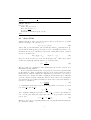
ALGORITHM 1: STATIC FSAI - FSAI computation from a given static non-zero
pattern.
Input: Matrix A, the non-zero pattern S
Output: Matrix G
for i = 1, n do
Gather A[Pi , Pi ] from A ;
e i = e mi ;
Solve A[Pi , Pi ] g
p
ei / gei,mi ;
gi = g
Scatter the coefficients in g i into G[i, Pi ]
end
2.1
Static FSAI
Assume that the non-zero pattern S is given. Denote by Pi the set of column
indices belonging to the i-th row of S:
Pi = {j : (i, j) ∈ S}
(10)
and by A[Pi , Pi ] the submatrix of A collecting the entries akl such that k, l ∈ Pi .
ei and g i the dense vectors containing the non-zero coefLet us indicate with g
e and G, respectively. Using this notation, equation
ficients in the i-th row of G
(6) can be re-written as:
i ∈ {1, 2, . . . , n}
A[Pi , Pi ]e
g i = emi ,
(11)
where emi is the mi -th vector of the canonical basis of Rmi . The row g i of G is
ei with the square root of its last entry:
obtained by scaling g
gi = p
ei
g
gei,mi
(12)
The procedure for computing a static FSAI given the non-zero pattern S is
summarized in Algorithm 1.
From a computational viewpoint, for a generic row i the most expensive tasks
in Algorithm 1 consist of gathering A[Pi , Pi ] from A and solving the related
linear system, with the numerical complexities proportional to m2i and m3i ,
ei and scattering the coefficients
respectively. In contrast, the tasks of scaling g
of g i into G have a linear complexity with mi , hence their cost is negligible.
Let us define the preconditioner density µG as the ratio between the number of
non-zeroes of G and A:
nnz(G)
(13)
µG =
nnz(A)
or, equivalently, as the ratio between the average number of non-zeroes of each
row of G, mG , and A, mA :
mG
µG =
(14)
mA
For a regularly distributed problem, i.e., mi ≃ mG for any i, the asymptotic
cost c for the preconditioner setup turns out to be proportional to the third
power of µG :
(15)
c ∝ n · m3G = n · m3A µ3G
Therefore, the cost for computing FSAI grows very rapidly with increasing the
preconditioner density.
5
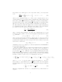
ALGORITHM 2: MK PATTERN - Generation of a static non-zero pattern.
Input: Matrix A, parameters τ , µmin , k, µmax
Output: Non-zero pattern S
repeat
e ← Drop(A, τ );
A
if µAe < µmin then τ ← τ (µAe /µmin )
until µAe ≥ µmin ;
B0 = I ;
for i = 1, k do
Bi ← Low(Bi−1 A) ;
if µBi ≥ µmax then exit the loop
end
Store the pattern of Bk as S ;
2.2
Static pattern generation
The problem of generating static non-zero patterns for the FSAI preconditioner
has been already discussed by several authors. Traditionally, for approximate
inverses based on a Frobenius norm minimization [1, 7] the non-zero pattern of
small powers of A is suggested. However, the number of entries in S grows so
quickly with the power of A that only the second or third power can be used in
real applications.
With FSAI only a lower triangular pattern is needed, with the upper part of
Ak actually useless. In [9, 10] it is shown that better patterns can be obtained
with k steps of the recurrence:
Bi ← Low(Bi−1 A)
i = 1, 2, . . . , k
(16)
starting from B0 = I. In equation (16) Low(·) denotes the lower triangular part
of a matrix. The non-zero pattern computed according equation (16) can become quite dense also for relatively small values of k. Hence, a safety parameter
µmax is introduced that provides an upper limit to the preconditioner density.
Whenever µmax is reached, the procedure (16) is stopped. On the other hand,
in order to include in S also entries belonging to high powers of A pre-filtration
of A may be recommended [5]. In the FSAIPACK implementation, a sparsified
e is computed by dropping all the entries aij of A such that:
matrix A
aij < τ |aii ajj |
(17)
with τ a user-specified real parameter. Setting the optimal value for τ is strongly
problem-dependent and may be a difficult task if the coefficients of A lie in a
narrow interval. In particular, a large τ value may cause the loss of too many
entries. For this reason the parameter µmin that enforces a minimal density for
e is also introduced.
A
The pre-filtration process desribed above has a linear complexity, hence repeating the procedure a few times does not impact signficantly on the overall setup cost. Algorithm 2 describes the procedure used to generate S in FSAIPACK
where the function Drop summarizes the pre-filtration process of equation (17).
6
2.3
Dynamic FSAI computation with adaptive pattern
generation
Adaptive procedures have been developed to generate dynamically S during the
FSAI computation with the aim at selecting for each row the “best” positions
[8, 10, 12]. In FSAIPACK we use an approach similar to the one proposed in
[12] for Block FSAI preconditioning. The use of this algorithm in the context
of FSAI is new.
Suppose that an initial guess G0 for G has already been computed and call
1
S′ its non-zero pattern. The default initial guess is G0 = diag(A)− 2 with S′ the
diagonal pattern, however any other choice is acceptable. Then, write G0 as:
e 0G
e0
G0 = D
(18)
e 0 = diag(G0 ), i.e., the diagonal entries of G
e 0 are unitary. It can be
where D
e
proved [12] that the entries of G0 can be directly computed by solving the dense
linear systems:
0
0
0
g 0,i = −A[P i , i],
A[P i , P i ]e
i ∈ {1, 2, . . . , n}
(19)
0
e0,i is the vector collecting
where P i = Pi0 \ i, Pi0 = {j : (i, j) ∈ S′ }, and g
e 0 . Consider the Kaporin
the non-zero off-diagonal terms in the i-th row of G
conditioning number of the preconditoned matrix G0 AGT0 :
1
1
e 0G
e 0 AG
eT D
e 0)
tr(G0 AGT0 )
tr(D
0
n
n
κ=
=
1
e0G
e 0 AG
e T0 D
e 0 ) n1
det(G0 AGT0 ) n
det(D
(20)
e 0 ) = det(G
e T ) = 1,
Recalling that G0 AGT0 has unitary diagonal entries and det(G
0
it follows that:
h
i1
e 0 AG
e T0 ) n
det diag(G
1
1
κ=
=
(21)
1
1
e 0 ) n2
det(A) n det(D
det(A) n
e 0 [i, :] the i-th row of G
e 0 , the numerator of equation (21) reads:
Denoting by G
n
n
h
i Y
Y
e0 A
eG
e T0 ) =
e 0 [i, :]AG
e0 [i, :]T =
det diag(G
ψ0,i
G
i=1
(22)
i=1
e 0 [i, :]AG
e0 [i, :]T . Hence, the Kaporin conditioning number of the
with ψ0,i = G
preconditioned matrix is:
1
κ = det(A)− n
n
Y
ψ0,i
(23)
i=1
The objective is to find an augmented pattern S∞ allowing for a reduction of
e0
κ in equation (23). The idea is to compute the gradient of κ with respect to G
and add in S∞ the positions corresponding to its largest components. Notice
e 0 only, so the adaptive
that each ψ0,i in (23) depends on the i-th row of G
pattern generation can be efficiently carried out in parallel. Denote by ∇ψ0,i ,
7
e 0 [i, :]. Its components
the gradient of ψ0,i with respect to the components of G
read:
!
n
X
∂ψ0,i
∀j = 1, . . . , i − 1
(24)
=2
ajr g0,ir + aji
∂g0,ij
r=1
e 0 [i, :], i.e., ∇ψ0,i can be computed at the cost of
with g0,ij the coefficients of G
a sparse matrix by vector product. After computing ∇ψ0,i using equation (24)
0
the non-zero pattern P i is enlarged by adding the s positions corresponding to
1
e1,i from equation (19).
the largest entries of ∇ψ0,i , thus obtaining P i and then g
e2 , G
e 3 , . . .,
The above procedure can be repeated k times to find all the rows of G
e
Gk . The current preconditioner quality can be monitored quite inexpensively
by computing the value of ψk,i . Therefore it is possible to stop the adaptive
procedure for every row whenever a relative exit tolerance is met:
e k [i, :]AG
ek [i, :]T
ψk,i
G
=
≤ε
e 0 [i, :]AG
e0 [i, :]T
ψ0,i
G
(25)
with ε a user-specified parameter. To reduce the computational cost of each
iteration it is also possible to enforce some dropping by neglecting those entries
gk,ij such that:
|gk,ij | ≤ τ ke
g k,i k2
j = 1, . . . , i − 1
(26)
with τ another user-specified parameter. When either ψk,i has been reduced
below the prescribed tolerance ε or a maximum number of iterations kiter are
e k [i, :] is properly
performed, the adaptive procedure is stopped and each row G
scaled back to ensure that:
Gk [i, :]AGk [i, :]T = 1
(27)
A summary of the above adaptive procedure as implemented in FSAIPACK is
provided in the Algorithm 3.
As to the computational cost, each iteration requires the same operations as
Algorithm 1 plus the computation of ∇ψk,i . If we denote by mk,i the number of
e k , the cost for computing ∇ψk,i is on the average
non-zeroes of the i-th row of G
proportional to mA · mk,i , while the cost for gathering and solving the dense
linear subsystem are proportional to m2k,i and m3k,i , respectively, as already
pointed out previously. After kiter iterations of the above procedure starting
e 0 = I with τ = 0, the cost ci for computing the i-th row is:
from G
ci ∝
kX
iter
k=1
h
i
2
3
2
3
4
mA · sk + (sk) + (sk) = (α0 mA + α1 ) kiter +(α0 mA + α2 ) kiter
+α3 kiter
+α4 kiter
(28)
where αi , i = 0, . . . , 4, are five scalar coefficients
depending
on
s.
For
k
iter
√
large enough, i.e., approximately kiter ≥ mA , the overall cost of the adaptive
procedure turns out to be proportional to the fourth power of the preconditioner
density:
n
X
4
ci ∝ n · kiter
= n · m4A µ4G
c=
(29)
i=1
The large computational cost has to be compensated for by a faster PCG convergence.
8
ALGORITHM 3: ADAPT FSAI - Dynamic FSAI with adaptive pattern generation.
Input: Matrix A, Matrix G0 (optional), Parameters kiter , s, τ , ε
Output: Matrix G
if G0 is present then
e 0 ← diag(G0 )−1 G0 ;
G
else
e 0 = I;
G
end
for i = 1, n do
for k = 0, kiter − 1 do
Compute ∇ψk,i ;
k+1
Compute P i
∇ψk,i ;
k
by adding to P i the indices of the s largest components of
k+1
k+1
k+1
, P i ] and A[P i , i] from
k+1
k+1
k+1
A[P i , P i ]e
g k+1,i = −A[P i , i];
Gather A[P i
A;
Solve
if ψk+1,i ≤ ε ψ0,i then exit the loop over k;
ek+1,i such that gek+1,ij ≤ τ ke
Drop the entries of g
g k+1,i k2 ;
end
1
k+1
deii = (−e
g Tk+1,i A[P i , i])− 2 ;
e
e
g
← deii g
;
k+1,i
k+1,i
ek+1 into Gk+1 [i, Pik+1 ]
Scatter the coefficients of g
end
2.4
Fully iterative FSAI construction
The adaptive pattern generation can be computationally expensive, with the
most expensive task being the repeated solution to dense linear subsystems with
size mk,i . The objective is to minimize ψk,i for each row i, i.e., the quadratic
form (22). To do this a steepest descent algorithm can be implemented. Let us
define α such that:
e k [i, :] + α∇ψk,i → min
(30)
ψk,i G
with α reading:
α=−
T
∇ψk,i
∇ψk,i
T A∇ψ
∇ψk,i
k,i
e k is updated as:
Then, the current i-th row of G
e k+1 [i, :] = G
e k [i, :] + α∇ψ T
G
k,i
(31)
(32)
e k [i, :] may be full, so that some dropping
Actually, after only a few iterations G
is mandatory. In the FSAIPACK implementation a dual dropping strategy is
enforced by means of the user-specified parameters τ and mmax representing,
as usual, the relative threshold tolerance and the maximum number of entries
to be retained, respectively [18]. As in Algorithm 3, the iterative procedure
for building FSAI is controlled by two user-specified parameters, kiter and ε,
defining the maximum number of iterations and the exit tolerance of the steepest
descent algorithm, respectively. Because of the dropping, this procedure is
actually an incomplete steepest descent algorithm.
9
ALGORITHM 4: PROJ FSAI - Fully iterative FSAI computation.
Input: Matrix A, kiter , mmax , τ , ε, Matrix G0 (optional), Matrix M −1 (optional)
Output: Matrix G
if G0 is present then
e 0 ← diag(G0 )−1 G0 ;
G
else
e 0 ← I;
G
end
if M −1 is not present then M −1 ← I;
for i = 1, n do
for k = 0, kiter − 1 do
Compute ∇ψk,i ;
p = M −1 ∇ψk,i ;
T
α = −∇ψk,i
p/pT Ap;
e k+1 [i, :] = G
e k [i, :] + α∇ψk,i ;
G
e k+1 [i, :] larger than τ kG
e k+1 [i, :]k2 ;
Select the mmax largest entries of G
if ψk+1,i ≤ ε ψ0,i then exit the loop over k;
end
e k [i, :]AG
e k [i, :]T )− 12 ;
deii = (G
e k [i, :];
Gk [i, :] = deii G
end
The steepest descent convergence can be accelerated by using an inner preconditioner M −1 , e.g., a previously computed FSAI, at the expense of an additional computational cost. The fully iterative FSAI computation procedure is
provided in Algorithm 4, that is reminiscent of the idea proposed in [4] where
a self-preconditioned descent-type method is used to compute a non-factored
approximate inverse.
All iterations in Algorithm 4 have approximately the same computational
cost because a fixed number of entries are retained for each row. The more
expensive operations are the computation of ∇ψk,i and α, both requiring a
sparse matrix by a sparse vector multiplication. At most, the computational
complexity of these tasks is proportional to mA · mmax and mM −1 · mA · mmax ,
where mM −1 is the average number of non-zeroes per row of M −1 . The overall
cost for the fully iterative construction of the i-th row is therefore:
ci ∝ kiter · (1 + mM −1 ) · mA · mmax
(33)
with the total cost estimated as:
c ∝ n · kiter · (1 + mM −1 ) · mA · mmax = n · kiter · (1 + mM −1 ) · m2A · µG (34)
Hence, the cost for computing G with Algorithm 4 is approximately linear with
the density µG , with the proportionality constant depending linearly on kiter
and mM −1 . For such a reason, the use of a preconditioned iteration may have a
strong impact on the overall cost, and should be used only when a quite sparse
and effective M −1 is available.
10
ALGORITHM 5: POST FILT - FSAI post-filtration.
Input: Matrix A, Matrix G, Parameters τ , mmax
Output: Matrix G
for i = 1, n do
Select the mmax largest entries of g i such that |gij | ≥ τ kg i k2 ;
ei and the discarded entries in εi ;
Store the selected entries in g
Create the set of discarded column indices Ei ;
Gather A[Ei , Ei ] from A;
−1/2
deii = 1 + εTi A[Ei , Ei ]εi
;
ei ← deii g
ei ;
g
ei into G[i, Pi \ Ei ];
Scatter the coefficients of g
end
2.5
FSAI post-filtration
Experience suggests that FSAI may have several small entries, independently
of the strategy used to generate S. In order to make the FSAI application
cheaper with no important detrimental effects on the PCG convergence rate an
a posteriori sparsification of G can be performed. This technique, introduced in
[16], is called post-filtration and proceeds as follows. Assume that G has already
been computed. The off-diagonal non-zero entries of the i-th row, stored in the
dense vector g i , are processed using a dual threshold strategy similar to the
one suggested in [18] in the context of ILU factorizations. Two user-specified
parameters mmax and τ are needed, such that only the largest mmax off-diagonal
entries of g i are retained with an absolute value larger than τ kg i k2 . Each vector
g i is therefore decomposed as:
e i + εi
gi = g
i = 1, . . . , n
(35)
ei and εi collect the sparsified row and the discarded entries, respectively.
where g
e which however no longer satisei , i = 1, . . . , n, form the matrix G
All vectors g
e G
e T has unitary diagonal
fies the condition that the preconditioned matrix GA
entries. This condition helps accelerate the PCG convergence [21], hence to
e with the
restore it the actual post-filtered FSAI factor G is defined by scaling G
e
aid of the diagonal matrix D:
eG
e
G=D
(36)
Let us define the set Ei collecting the column indices of the discarded entries εi :
Ei = | : }i| ∈ εi
(37)
e can be computed as:
Then the coefficients of D
deii = 1 + εTi A[Ei , Ei ]εi
−1/2
(38)
The post-filtration procedure is summarized in Algorithm 5.
As to the computational cost, filtering a row with mi non-zeroes and selecting
the largest entries have a linear and superlinear complexity, respectively, while
the cost for the computation of deii is proportional to m2i as it requires the
11
ALGORITHM 6: REC FSAI - Recurrent FSAI computation.
Input: Matrix A, nℓ
Output: Matrices G1 , G2 , . . ., Gnℓ
A0 = A;
G0 = I;
for k = 0, nℓ − 1 do
Ak+1 = Gk Ak GTk ;
Compute Gk+1 as the FSAI factor of Ak+1 ;
end
gathering of a submatrix from A. Hence, the average post-filtration cost c can
be estimated as:
c ∝ n · m2G = n · m2A · µ2G
(39)
and is therefore usually negligible relative to the cost of computing G. The postfiltration procedure generally produce sparse FSAI factors with no significant
loss in the convergence rate.
2.6
Recurrent FSAI computation
Another way to reduce the FSAI cost though retaining a large number of nonzero entries is to compute G as the product:
G=
nℓ
Y
Gk
(40)
k=1
where Gk , k = 1, . . . , nℓ , is the k-th level FSAI. The final G implicitly inherits
a large number of non-zeroes even though each Gk is rather sparse. This idea,
first introduced in [16] and later developed by [22, 3], looks similar to multilevel
preconditioners, e.g., [20, 11].
The k-th term Gk is computed as the FSAI factor of Ak :
Ak = Gk−1 Ak−1 GTk−1
(41)
by any of the previous techniques. The procedure starts with G0 = I and
A0 = A, and proceeds through nℓ levels. A summary is provided in Algorithm
6.
Quite obviously, the matrix G in (40) is never formed explicitly and its
density is generally much larger than the sum of the Gk densities. Hence, the
sum of the costs for computing each factor Gk is generally smaller than the cost
for computing the final G in just one step. The overall cost of the recurrent
FSAI computation depends on both the strategy used for Gk at each level and
the sparse matrix-matrix product Ak+1 = Gk Ak GTk . The full computation of
Ak+1 is not feasible, hence a dropping is implemented using again the dual
strategy defined by mmax and τ , and preserving the symmetry of Ak+1 .
A sketch of the procedure used to compute B = GAGT is provided in Algorithm 7. The cost ci for computing the i-th row of B with Algorithm 7 is
proportional to:
ci ∝ mG,i · mA + mmax · mG,i
(42)
12
ALGORITHM 7: PREC MAT - Computation of a FSAI preconditioned matrix.
Input: Matrix A, Matrix G, mmax , τ
Output: Matrix B = GAGT
for i = 1, n do
v = AG[i, :]T ;
Select the mmax largest entries of v such that |vj | ≥ τ kvk2 , j = 1, 2, . . . , n;
w = Gv;
Select the mmax largest entries of w such that |wj | ≥ τ kwk2 , j = i, i + 1, . . . , n;
Scatter w into B[i, :];
end
Transpose the strict upper part of B into its strict lower part;
with the overall average cost:
c ∝ n · mG · (mA + mmax ) = n · mA · (mA + mmax ) · µG
3
(43)
Package decription
The FSAIPACK software package is a collection of functions and subroutines
that implement the Algorithm 1 through 7 for shared memory parallel computers
with the Fortran90 programming language and OpenMP directives for multithread execution [17]. As all the algorithms exhibit a high degree of parallelism,
an MPI implementation for distributed memory computers is not theoretically
difficult and is currently under development.
A number of derived data types and classes are defined and can be accessed
at the user level with the aim at making the FSAIPACK use easier (Table 1):
• Pattern: a data structure used to store the pattern of a matrix in the
compressed sparse row storage mode [19]. Pattern includes two member
integer variables, nrows and nterm, with the size and the number of
non-zeroes of the matrix, respectively, and two member integer arrays,
iat and ja, storing the pointer to the beginning of each row and the
column indices of the non-zeroes of the matrix, respectively;
• CSRMAT: a derived data type that extends the Pattern type so as to
include also the coefficients of the matrix. CSRMAT includes as members
a Pattern variable patt and a double precision array coef collecting the
matrix coefficients in row-major order;
• FSAIP Prec: a derived data type containing two lists of pointers to
CSRMAT type variables, LEFT and RIGHT. The definition of this data
type has been selected to store a FSAI preconditioner in the most general
form (40). LEFT and RIGHT are the list in ascending and descending
order of the Gk and GTk factors, respectively. The FSAIP Prec type
variable is accessed by a function that includes new factors in the LEFT
and RIGHT lists, and by a routine that applies the preconditioner to a
vector.
The derived data types are supplemented with the respective constructors and
destructors along with other specific functions.
13
Derived Data Type
Member Variables
Member Functions
Pattern
nrows, nterm, iat, ja
new Pattern, dlt Pattern
CSRMAT
patt, coef
new CSRMAT, dlt CSRMAT,
new CSRCOEF, dlt CSRCOEF,
copy CSRMAT
FSAIP Prec
LEFT, RIGHT
append LEFT, append RIGHT,
delete LEFT, delete RIGHT,
apply FSAIP Prec, dlt FSAIP Prec
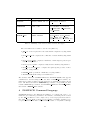
Table 1: Summary of the user-accessible derived data types
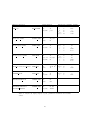
The other functions accessible to the user are (Table 2):
• MK patt: creates a pattern for the static FSAI computation by Algorithm
2;
• CPT static FSAI: computes the coefficients of a static FSAI by Algorithm
1;
• CPT adaptive FSAI: computes a FSAI factor with adaptive pattern generation of Algorithm 3;
• CPT projection FSAI: computes a fully iterative FSAI by Algorithm 4;
• CPT preconditioned Matix: computes the sparse-sparse product of three
matrices of Algorithm 7;
• FILTER FSAI: post-filters a FSAI factor by Algorithm 5;
• TRANSPOSE FSAI: transposes a FSAI factor.
The member functions APPEND LEFT and APPEND RIGHT, that append
a FSAI factor and its transposed to the lists of a FSAI Prec variable, are
indirectly accessible by using a specific interpreted command, as it will be shown
later. All functions return a CSRMAT-type variable, except MK patt, that
returns a Pattern type variable, and APPEND LEFT and APPEND RIGHT,
that return a FSAIP Prec variable.
4
FSAIPACK Command Language
FSAIPACK allows for the different algorithms to be combined in order to optimize the preconditioner performance. For instance, an initial pattern created
by the MK patt function can be improved by a few steps performed with either CPT adaptive FSAI or CPT projection FSAI, potentially obtaining a better preconditioner than that computed using a static or a dynamic technique
14
Function
Input parameters
Output parameters
MK patt
CSRMAT:
integer:
double:
Pattern:
A
k
τ , µmin , µmax
pattin (optional)
Pattern:
pattout
CPT static FSAI
CSRMAT:
Pattern:
A
pattin
CSRMAT:
G
CPT adaptive FSAI
CSRMAT:
integer:
double:
CSRMAT:
A
kiter , s
τ, ε
G0 (optional)
CSRMAT:
G
CPT projection FSAI
CSRMAT:
integer:
double:
CSRMAT:
CSRMAT:
A
kiter , mmax
τ, ε
G
Gp , GTp (optional)
CSRMAT:
G
CPT preconditioned Matrix
CSRMAT:
integer:
double:
CSRMAT:
A
mmax
τ
G
CSRMAT:
B
FILTER FSAI
CSRMAT:
integer:
double:
CSRMAT:
A
mmax
τ
G
CSRMAT:
G
TRANSPOSE FSAI
CSRMAT:
G
CSRMAT:
GT
APPEND LEFT
CSRMAT:
G
FSAI Prec:
F SAI
APPEND RIGHT
CSRMAT:
GT
FSAI Prec:
F SAI
Table 2: Summary of the functions directly accessible at the user level with the
Input and Output parameters
15
Type
Comment
Command
Data
Character
#
>
Any number
Table 3: First non-blank character of each line type.
only. To improve the easiness of use of FSAIPACK, a command language is defined that allows for the implementation of a user-specified strategy to compute
FSAI. The commands are stored as an array of character variables of maximal
length 100. Each element of such array represents a single line of the strategy
and must comply with a set of syntax rules. The strategy array is used as input
for the FSAIPACK driver with the Command Language interpreter provided as
an open source code.
4.1
Syntax rules
Strategy lines belong to three types:
1. comment type,
2. command type,
3. data type.
The type of each line is identified by the first non-blank character, according to
Table 3.
The objects handled by the strategy are CSRMAT type variables identified
by a user-specified string of characters, except the final preconditioner that is
a FSAIP Prec type variable. The CSRMAT objects are managed in a fully
dynamic way by the command language, allocating and deallocating automatically the user-specified data structures whenever needed. Mandatory object
identifiers are:
1. A: system matrix identifier,
2. PREC: final preconditioner identifier.
A and PREC must be used at least once in each strategy. The maximum length
of the string identifying each object is 11 characters.
A comment line can be introduced at any point of a strategy. FSAIPACK
Command Language discards any character located after the comment type
identifier #. A comment can be also introduced at the end of a command or a
data type line.
A command line is a string with at most 100 characters with the syntax:
> keyword [ input , input : output ] -character -character -...
The keyword is the identifier of a function implemented in the FSAIPACK library. The symbols [ and ] include the identifiers of the CSRMAT objects
used as input and output of the function identified by the keyword. A function
can have more than one input objects separated by the symbol ,. All functions
16
have only one output object. The symbol : is the separator between input
and output objects. All functions depend on a set of user-specified parameters.
If the user does not specifies a parameter value, a default is automatically assumed. The parameters set by the user are identified by the symbol - followed
by a character associated to the parameter. Each command type line must be
followed by a number of data type lines equal to the number of parameters set
by the user. Each data type line contains a numerical value that is assigned to
a parameter according to the order of the parameters declared in the command
type line. Blank characters can be inserted wherever in a command or data
type line and are discarded by the interpreter.
The available keywords, required input and output objects, user-specified
parameters and default values are summarized in Table 4. The symbols A and B
denote CSRMAT type variables, patt a non-zero pattern included in a CSRMAT
type variable, G a CSRMAT type variables containing a FSAI preconditioner
factor, and F SAI the FSAIP Prec type variable with the final preconditioner,
which is always denoted by PREC in our syntax.
4.2
Examples
This is an example strategy:
# This is an example strategy
> MK PATTERN [A:patt] -k -t # Two out of four parameters are set
2 # Number of steps of power recurrence
0.05 # Pre-filtration tolerance
> STATIC FSAI [A,patt:G]
# The static FSAI is improved dynamically
> ADAPT FSAI [A:G] -n -e # G is an Input/Output object
10 # Number of adaptive steps
1.e-3 # Exit tolerance
# Post-filtering a FSAI factor is generally recommended
> POST FILT [A:G] # Default parameters are used
# It is necessary to transpose G and append the left and right factors
> TRANSP FSAI [G:Gt]
> APPEND FSAI [G,Gt:PREC] # PREC is a mandatory identifier
The strategy above performs the following operations:
• the system matrix is used to build the static pattern patt by k=2 steps
of the power recurrence and t=0.05 as pre-filtration tolerance
• the system matrix and the pattern patt are used to compute statically
the FSAI factor G
• the factor G is improved dynamically by n=10 steps of the adaptive procedure with exit criterion e=10−3
• the factor G is post-filtered according to the entries of the system matrix
• the factor G is transposed into Gt
• the factors G and Gt are appended in the final preconditioner
17
Function, Keyword
MK Patt
Input/Output
MK PATTERN
In:
In/Out:
A
patt
Parameters, identifier, default
µmin
µmax
t
k
m
M
0.05
3
0.20
5.00
τ
k
CPT static FSAI
STATIC FSAI
In:
Out:
A, patt
G
CPT adaptive FSAI
ADAPT FSAI
In:
In/Out:
A
G
kiter
s
τ
ε
n
s
t
e
30
1
0.00
1e-3
CPT projection FSAI
PROJ FSAI
In:
Opt. in:
In/Out:
A
Gp , GTp
G
kiter
mmax
τ
ε
n
s
t
e
10
10
0.00
1e-8
CPT preconditioned Matrix
PREC MAT
In:
Out:
A, G, GT
B
mmax
τ
n
t
n
0.00
FILTER FSAI
POST FILT
In:
In/Out:
A
G
mmax
τ
n
t
n
0.05
TRANSPOSE FSAI
TRANSP FSAI
In:
Out:
G
GT
APPEND LEFT and
APPEND RIGHT
APPEND FSAI
In:
In/Out:
G, GT
F SAI
Table 4: Keywords, input/output objects, parameter identifiers and defualt
values.
18
Recall that the APPEND FSAI keyword is mandatory at the end of any strategy.
References
[1] Benson, M. W. 1973. Iterative solution of large scale linear systems. M.Sc.
Thesis, Lakehead University, Thunder Bay (ON), 1973.
[2] Benzi, M. and T˚
uma, M. 1999. A comparative study of sparse approximate
inverse preconditioners. Applied Numerical Mathematics 30, 305-340.
[3] Bergamaschi, L. and Martinez, A. 2012. Banded target matrices and
recursive FSAI for parallel preconditioning. Numerical Algorithms 61, 223–
241.
[4] Chow, E.i and Saad, Y. 1998. Approximate inverse preconditioners via
sparse-sparse iterations. SIAM J. Sci. Comput. 19, 995–1023.
[5] Chow, E. 2000. A priori sparsity patterns for parallel sparse approximate
inverse preconditioners. SIAM J. Sci. Comput. 21, 1804–1822.
[6] Ferronato, M. 2012. Preconditioning for sparse linear systems at
the dawn of the 21st century: history, current developments, and future
perspectives. ISRN Applied Mathematics 2012, Article ID 127647, doi:
10.5402/2012/127647
[7] Frederickson, P. O. 1975. Fast approximate inversion of large sparse
linear systems. Mathematical Report 7, Lakehead University, Thunder Bay
(ON), 1975.
[8] Grote, M. and Huckle, T. 1997. Parallel preconditioning with sparse
approximate inverses. SIAM J. Sci. Comput. 18, 838–853.
[9] Huckle, T. 1999. Approximate sparsity patterns for the inverse of a matrix
and preconditioning. Appl. Num. Math. 30, 291–303.
[10] Huckle, T. 2003. Factorized sparse approximate inverses for preconditioning. J. Supercomput. 25, 109–117.
[11] Janna, C., Ferronato, M., and Gambolati, G. 2009. Multilevel incomplete factorizations for the iterative solution of non-linear FE problems.
Int. J. Num. Meth. Eng. 80, 651–670.
[12] Janna, C. and Ferronato, M. 2011. Adaptive pattern research for
Block FSAI preconditioning. SIAM J. Sci. Comput. 33, 3357–3380.
[13] Kaporin, I. E. 1990. A preconditioned conjugate gradient method for
solving discrete analogs of differential problems Diff. Equat. 26, 897–906.
[14] Kaporin, I. E. 1994. New convergence results and preconditioning strategies for the conjugate gradient method. Num. Lin. Alg. Appl. 1, 179–210.
[15] Kolotilina, L. Yu. and Yeremin, A. Yu. 1993. Factorized sparse
approximate inverse preconditioning. I. Theory. SIAM J. Mat. Anal. Appl. 14,
45–58.
19
[16] Kolotilina, L. Yu. and Yeremin, A. Yu. 1999. Factorized sparse approximate inverse preconditioning. IV. Simple approaches to rising efficiency.
Numerical Linear Algebra with Applications 6, 515–531.
[17] OpenMP website. http://www.openmp.org.
[18] Saad, Y. 1994. ILUT: a dual threshold incomplete ILU factorization.
Num. Lin. Alg. Appl. 1, 387–402.
[19] Saad, Y. 2003. Iterative Methods for Sparse Linear Systems (2nd edn.).
SIAM, Philadelphia (PA).
[20] Saad, Y. and Suchomel, B. 2002. ARMS: an algebraic recursive multilevel solver for general sparse linear systems. Num. Lin. Alg. Appl. 9, 359–378.
[21] Van Der Sluis, A. 1969. Condition numbers and equilibration of matrices. Numer. Math. 14, 14–23.
[22] Wang, K. and Zhang, J. 2003. MSP: a class of parallel multistep successive sparse approximate inverse preconditioning strategies. SIAM J. Sci.
Comput. 24, 1141–1156.
20