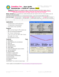
1
Beam Beam Beam Beam Beam Beam Beam Beam Beam Beam Profilers Profilers Profilers Profilers Profilers Profilers Profilers Profilers Profilers Profilers BeamMap / Beam’R / ColliMate BeamScopeBeamScope-P7 SlitSlit- scan Beam Profilers User Manual This page left blank Very IMPORTANT This information is here so that you cannot miss it. BeamScope-P7. In conjunction with a specific supplement, this manual covers the initial release of BeamScope-P7 instruments. A full combined manual will be released in the future. Do not ‘hot’ plug or unplug the head while the software is on. You may damage the unit. If you do this, turn off your PC, disconnect the power cord, count up to ten, reconnect the head, and reconnect the power cord to the PC. Restart your PC. Do not accidentally plug the monitor cable into the DataRay PCI card or the head. You will damage the PCI card. Since January 2001, many BeamMaps have been 4XY and 3XYKE units rather than the ‘Classic’ five-plane configuration. These will appear as BeamMap Collimates when the software reads the EEPROM, since wide plane spacing BeamMap ColliMate heads were the first to use this slit arrangement. 4XY heads have no knife-edge mode. To avoid slit damage, observe the maximum irradiance limits, section 1.8.2. A cool head may take five to ten minutes to get going. The software keeps repeating the start sequence until it detects normal operation. See section 3.6.2 d). If the software is behaving strangely, try File, Load Defaults in the Pull-down menu. The beam should be centered on the instrument for accurate measurements. See pp. 3-6 & 3-7 If you get a result or inconsistency you do not understand, before you call, proceed as follows: Via the Pull-down menu go: File, Save, Save current data … to save the single profile set. or: Save all data in data buffer … to save a sequence of data, particularly if you are seeing instability. The saved file (*.bmf, *.bcf, *.brf, *.bsf or *.wcf format) includes calibration data for your instrument. DataRay technical support can then view the data exactly as you see it. Email the result to [email protected] and/or your distributor with your comments. Then call. If User Manual authors had their way ... “If you read this manual first, you are entitled to free product support by phone, fax or email. For those who decide not to bother to read this manual before calling for support, a Help line charged at a ‘per minute’ rate is available.” … … seriously though, do read this manual to enjoy the full benefit of your investment. BeamMap, Beam’R, ColliMate, BeamScope-P7 DataRay Beam Profilers User Manual Serial Number: _____________________ Purchased by: _____________________ Date: ___________ Rev. 0207A ©2002 July 2002 DataRay Inc. All rights reserved. 605 Stapp Road, Boulder Creek, California 95006, USA Corporate Office: (831) 338-9055 • Fax: (831) 338-9098 [email protected] • www.dataray.com Product Support: (303) 543-8235 • [email protected] Table of Contents 1 INTRODUCTION ...............................................................................................................1-1 1.1 WELCOME ......................................................................................................................1-1 1.2 ABOUT BEAMMAP AND BEAM’R....................................................................................1-2 1.3 BEAM’R VERSUS BEAMMAP...........................................................................................1-5 1.4 SYSTEM CONFIGURATION ...............................................................................................1-5 1.5 MODEL YOUR BEAM .......................................................................................................1-5 1.6 FUNCTIONAL DESCRIPTION.............................................................................................1-6 1.6.1 BeamMap Principle of Operation..........................................................................1-6 1.6.2 BeamMap ColliMate Principle of Operation.........................................................1-9 1.6.3 Beam’R Principle of Operation. ..........................................................................1-10 1.7 CALIBRATION ...............................................................................................................1-11 1.8 PRODUCT SPECIFICATIONS............................................................................................1-12 1.9 BEAM LIMITS ................................................................................................................1-17 1.9.1 Beam Acquisition and Measurement Region .......................................................1-17 1.9.2 Beam Power Limits ..............................................................................................1-18 1.9.3 Beam Waist Diameters.........................................................................................1-22 1.9.4 Slit Dimension and Beam Waist...........................................................................1-22 1.9.5 Beam Numerical Aperture and f/# .......................................................................1-25 1.9.6 Beam M2 limits.....................................................................................................1-25 1.10 MANUAL CONVENTIONS ...............................................................................................1-28 1.11 MANUAL AND COPYRIGHT NOTICE ..............................................................................1-28 2 INSTALLATION.................................................................................................................2-1 2.1 UNPACK THE HARDWARE ...............................................................................................2-1 2.2 PART NUMBERS ..............................................................................................................2-1 2.3 COMPUTER MINIMUM REQUIREMENTS...........................................................................2-2 2.4 INSTALLATION ................................................................................................................2-3 2.5 SOFTWARE INSTALLATION INSTRUCTIONS......................................................................2-4 2.6 LABVIEW™, LABWINDOWS, VISUAL BASIC, DLL’S. ....................................................2-5 2.7 PC CARD INSTALLATION. ...............................................................................................2-5 2.8 MOUNTING THE HEAD ....................................................................................................2-7 2.8.1 Connecting the Head..............................................................................................2-7 3 QUICK-START TUTORIALS...........................................................................................3-1 3.1 SOFTWARE QUICK-START TUTORIAL .............................................................................3-2 3.1.1 Start the Software...................................................................................................3-2 3.1.2 Examine Previously Saved Data ............................................................................3-3 3.2 MANIPULATE THE IMAGE AND THE PROFILE ANALYSIS ...............................................3-9 3.2.1 2D & 3D Display & Manipulation ........................................................................3-9 3.2.2 Choose a Beam Width Definition.........................................................................3-10 Table of Contents 3.2.3 Set Diameter Display Mode .................................................................................3-12 3.2.4 Set Pass-Fail ........................................................................................................3-12 3.2.5 Change Profile Display........................................................................................3-14 3.3 PULL-DOWN MENUS .....................................................................................................3-16 3.3.1 File.......................................................................................................................3-16 3.3.2 Device ..................................................................................................................3-17 3.3.3 Hardware .............................................................................................................3-18 3.3.4 Palettes.................................................................................................................3-19 3.3.5 View .....................................................................................................................3-19 3.3.6 Setup ....................................................................................................................3-23 3.3.7 Options.................................................................................................................3-24 3.3.8 Average ................................................................................................................3-25 3.3.9 Filter ....................................................................................................................3-25 3.3.10 Help......................................................................................................................3-26 3.3.11 Log Data ..............................................................................................................3-26 3.4 BUTTON BAR BUTTONS ................................................................................................3-27 3.5 SHORT CUTS .................................................................................................................3-30 3.6 HARDWARE QUICK-START TUTORIAL ..........................................................................3-31 3.6.1 Precautions and Safety Warnings ........................................................................3-31 3.6.2 Starting Up...........................................................................................................3-31 3.6.3 Beam’R Knife Edge or Slit Mode.........................................................................3-33 APPENDIX A: FUNCTION REQUEST FORM .................................................................................2 APPENDIX B: M-SQUARED AND ITS MEASUREMENT .....................................................3 APPENDIX C: TECHNICAL SUPPORT, SALES, RETURNS, DISTRIBUTORS AND REPRESENTATIVES............................................................................................................................13 APPENDIX D: BEAMMAP/BEAM’R CALIBRATION .............................................................14 INDEX............................................................................................................................................................................18 CHAPTER ONE 1 INTRODUCTION 1.1 1.1 WELCOME ......................................................................................................................1-1 1.2 ABOUT BEAMMAP AND BEAM’R....................................................................................1-2 1.3 BEAM’R VERSUS BEAMMAP...........................................................................................1-5 1.4 SYSTEM CONFIGURATION ...............................................................................................1-5 1.5 MODEL YOUR BEAM .......................................................................................................1-5 1.6 FUNCTIONAL DESCRIPTION.............................................................................................1-6 1.6.1 BeamMap Principle of Operation..........................................................................1-6 1.6.2 BeamMap ColliMate Principle of Operation.........................................................1-9 1.6.3 Beam’R Principle of Operation. ..........................................................................1-10 1.7 CALIBRATION ...............................................................................................................1-11 1.8 PRODUCT SPECIFICATIONS............................................................................................1-12 1.9 BEAM LIMITS ................................................................................................................1-17 1.9.1 Beam Acquisition and Measurement Region .......................................................1-17 1.9.2 Beam Power Limits ..............................................................................................1-18 1.9.3 Beam Waist Diameters.........................................................................................1-22 1.9.4 Slit Dimension and Beam Waist...........................................................................1-22 1.9.5 Beam Numerical Aperture and f/# .......................................................................1-25 1.9.6 Beam M2 limits.....................................................................................................1-25 1.10 MANUAL CONVENTIONS ...............................................................................................1-28 1.11 MANUAL AND COPYRIGHT NOTICE ..............................................................................1-28 1.1 WELCOME Welcome to DataRay Beam Profiling. These innovative products define state-of-the-art, featurerich, real-time, dual-mode slit/knife-edge beam profiling in accordance with the ISO 11146 Standard*. They are designed as research, development, QA and manufacturing test tools that can be easily customized to your application. The program combines easy-to-use intuitive software and proven beam profiling algorithms. With a little time and patience, we think you will be pleasantly surprised with how easy to use we have made it. [* International Organization for Standardization. ISO 111146: Test methods for laser beam parameters: Beam widths, divergence angle and beam propagation factor. http://webstore.ansi.org/ansidocstore/default.asp ] This manual covers the BeamMap, Beam’R and BeamMap ColliMate product ranges. Beam’R capabilities are a subset of BeamMap capabilities. In conjunction with a specific supplement, this manual covers the initial release of BeamScope-P7 instruments. In order to save time for Beam’R users, sections which only apply to BeamMap are indicated by a thick gray line down the left hand side of the page, see left. BeamMap, Beam’R, ColliMate, BeamScope-P7 1-1 Introduction In order to save time for BeamMap users, sections which only apply to Beam’R are indicated by a double gray line down the left hand side of the page, see left. DataRay is committed to providing the ultimate in beam profiling performance, and welcomes constructive criticism of these products and of this manual. Please contact us. www.dataray.com is always the source for the most current versions of software, manuals, application notes, specifications, parts lists, etc. At any time, you may download the latest version of the software and/or manual updates and application notes for free. Visit the website in order to determine whether an update is available. If you need a function that is not included in the current version, please fill out and fax a Function Request form found as Appendix A of this manual. Many requested software functions can be added with relative ease, and may be done for free, and possibly added to future releases. However, if the requested embellishment is considered extensive and/or obscure, DataRay reserves the right to quote a fee for the requested change. The BeamMap and ColliMate product lines originated in response to OEM requests for production line instruments to measure focal position. We welcome requests for custom hardware configurations. 1.2 ABOUT BEAMMAP AND BEAM’R BeamMap represents a radical new approach to real-time beam profiling. It couples a novel, patented, multi-plane real-time slit scanning system to improved slit technology, and to the dramatic increases in processing power represented by continuously evolving PC technology. [A 500 MHz Pentium III is required to fully real-time process the 5 Mega-Samples per second resulting from eight apertures, with 0.09 µm sample resolution and a 5 Hz update rate.] Initially designed as a custom product for an OEM customer’s production line, it is now available as a standard product If you have every used a single plane beam profiler to measure a tightly focused beam, you will appreciate the problems that DataRay set out to solve. Problem 1 - Measuring tightly focused beams. A focused, aligned in-spec. beam should have the classic hyperbolic W(z) (diameter) versus z profile shown right. Prior to alignment and focusing, the beam: May not be focused at z = 0 May be misaligned in position and angle May meet neither the beamwaist diameter nor the irradiance specifications. May have M2 (Beam Quality) greater than specification Beam prior to alignment Aligned in-spec. beam An instrument with a single plane of measurement gives just one plane of information. With only a single plane of measurement, finding the focus can be a truly frustrating exercise. Setting multiple assemblies to the identical focus in a production environment can be costly. If the assembly will not adjust correctly, you have no real-time indication of what the problem might be. 1-2 BeamMap, Beam’R, ColliMate, BeamScope-P7 Introduction Solution BeamMap enables you to measure and correct these beam focus and alignment errors. It measures the beam in multiple planes. If these planes are around the focus position, even when not at the focus, BeamMap can: Measure the axial misalignment (pointing) Indicate the current focus direction Estimate the beamwaist diameter at the focus Estimate the off-axis distance of the focus Estimate M2 and/or beam divergence. Do all this in real-time When the central measurement plane is positioned in the focal plane, these estimates become measurements of: Focus position in z X-Y position and θxz angle Beam-waist diameter and irradiance M2 Beam Quality and/or beam divergence … with sub-micron repeatability, … at a 4 Hz update rate for real-time adjustment … with respect to BeamMap axes or a user-defined reference. * (The standard head has 250 µm plane spacing; 50, and 100 µm spacing is available for very tightly focused beams, 500 µm for diverging beams, 3 or 4 planes at several mm spacing for collimated beams.) The BeamMap measurement head is the only commercially available multi-plane head for tightly focused laser beams. It saves setup time and ensures accurate, repeatable results. If the BeamMap head is moved in z, it can give unambiguous indication of when the beamwaist position is at the central measurement plane. If all assemblies are to be set to the same focus, place the central measurement plane at the design focus [or at the focus of a ‘golden’ (reference) unit] and adjust all assemblies to the same focus quickly and easily. Problem 2 – ‘Tunnel’ slits The Rayleigh Range of a tightly focused laser beam can be as low as 2.0 µm. [400 nm, f/1 optics, M2 =1, focused beam diameter 1 µm.] (The Rayleigh Range is the distance from the focus at which the beam increases its diameter by √2) BeamMap, Beam’R, ColliMate, BeamScope-P7 1-3 1.2 Introduction The actual slits in standard slit scanners can actually have a large depth in the z direction, they are three-dimensional slits with partially reflective sidewalls. This reduces the accuracy of the focus determination. The ‘air’ slits conventionally employed are 12.5 or 25 µm thick in the z direction, or 6 µm thick for the best available air slits. To a tightly focused beam, they look like a reflective tunnel rather than a two-dimensional slit. Solution Custom-developed, True2D™ slits allow accurate profiling of very tightly focused beams. 25 µm deep conventional True2D™ Slit rough wall ‘tunnel’ slit These new metallic film slits, defined using high resolution optical lithography, comprise multiple opaque layers deposited on a sapphire substrate. The total slit thickness is ~2 microns, nearly an order of magnitude thinner than the best air slits. The thermally conductive sapphire substrate allows high power performance. Problem 3 – ‘Jitter’ Historically, it has been very difficult to drive a stepping motor (or other motor) smoothly enough, with the necessary constant rotational velocity and positional repeatability, to work with multiple apertures at high resolution. Solution A custom motor with micro-step drive plus damping, produces an ultra-smooth motion which all but eliminates motor ‘cogging’ and can hence achieve the required precision. Place a finger on the head. Feel how low the residual vibration is. Individual rotation-to-rotation position error is better than 1 part in 105. This error is reflected in the ‘≤ ± 1µm rms’ specification for centroid position. The displayed centroid position is normally the running average of four samples. However, if the centroid position on a profile to profile basis changes by more than 2 µm, then the display immediately updates to the new position and restarts the running average. In Jitter suppression mode, the displayed profiles are position stabilized on the screen for sample to sample centroid variations ≤ ± 5% of the x1 range. This feature removes centroid jitter in the displayed profile but retains the actual centroid position in the displayed Xc position. If profile zoom is selected, then the stabilization range is a higher percentage of the displayed width: ± 10% for the x2 range, ± 20% for the x4 range, etc. Problem 4 – Beam Collimation/Divergence/Pointing If you have ever used a single plane profiler to measure and adjust a collimated beam, then you know the time consuming procedure. Measure once, move the profiler along the z axis, measure in the second plane, calculate beam divergence, readjust, start again …. Who has time for all this? 1-4 BeamMap, Beam’R, ColliMate, BeamScope-P7 Introduction Solution BeamMap ColliMate heads (BeamMapC in the software) use widely spaced planes to extend multi-plane BeamMap profiler technology to beam divergence and pointing measurement, achieving an accuracy of better than 1 mrad. They dramatically simplify the measurement of collimation and alignment & the adjustment of multiple assemblies to the same axes. 1.3 Beam’R versus BeamMap The Beam’R head measures in a single plane, and is an economical derivative designed for the measurement of beams that are not highly divergent or convergent. Beam’R uses two pairs of x-y slits, one pair with 2.5 µm slit width and one pair with 25 µm slit width. (5 & 50 µm for InGaAs). There is one slit every 90o on the puck. Each pair of slits is at ±45o to the puck radius, to give effective slit widths of 3.5 and 35 µm respectively. (7 & 70 µm for InGaAs heads). 1.4 SYSTEM CONFIGURATION The BeamMap, Beam’R profiling systems consists of the (interchangeable) scan head, a PCI card (ISA prior to October 2000), a 3-meter long cable, and the latest version of the software. The system is shipped ready to install on any 500 MHz or higher Pentium II PC; a Pentium III or higher is preferred, with an available PCI card slot. 1.5 MODEL YOUR BEAM Download Fit_BeamMaps.xls from the website to model your beam with respect to your head. BeamMap, Beam’R, ColliMate, BeamScope-P7 1-5 1.3 1.4 Introduction 1.6 FUNCTIONAL DESCRIPTION The following is a brief description of the BeamMap and Beam’R working principles. The actual plane spacing and slit sizes for any given head are held in the EEPROM and may be accessed from the Hardware menu. 1.6.1 BeamMap Principle of Operation A disk [‘puck’] carrying multiple slits rotates about an axis parallel to the z-axis, This satisfies the orthogonal linear scan requirements of the ISO 11146 standard. The slits are precisely located in multiple planes separated in z in the focal region. Slits are placed at particular angles to the local radial direction. Slits at + & – 45o to the radial direction scan the beam to determine beam centroid for orthogonal profiles; effective slit width is √2 greater than actual slit width. P4, z = 0 Rotating ‘puck’ carrying apertures at different planes in z P5, z = +d P3,z = -d P6, z = +2d P2, z = -2d P1, z = 0, @ -45o Face-on view of rotating ‘puck’ P8, z = 0 P7, z = 0, @ +45o Schematic 2W(z) versus z beam profile Photosensitive detector connected to processing electronics z -axis Direction of Laser Beam Propagation -2d -d 0 +d +2d Planes in z Reference z = 0 plane BeamMap ‘Classic’ puck configuration 1-6 BeamMap, Beam’R, ColliMate, BeamScope-P7 Introduction BeamMap ‘Classic’ Puck: Slit Scan Sequence Schematic & Detail 1.5 Position: Slit Width (µm): Orientation: z-plane: P1 2.5 o -45 0 Displayed Profiles: 5 Profile display: 3 Profile display: 1 1 Profile display: P2 10 P3 5 P4 2.5 P5 5 P6 10 -2d -d 0 +d +2d 1 2 3 2 1 4 5 P7 2.5 o +45 0 3 P8 25 0 3* 2* 1* * When Enable knife edge mode is selected, this slit replaces the z=0, 2.5 µm slit. For alignment with the beam axes, the puck is inside a rotatable head, with on-screen electronic angle readout. On the first scan, the software detects the 13.5% outer limits of the profile and then sets an overscan of the profile width by a factor of approximately four times the profile width. The scanned width is digitized as 2048 equally spaced samples. The intensity is digitized by a 12-bit (4096 level) ADC (Analog-to-Digital Converter). The software determines the zero level in the digitized profile and then processes it to give the data required for display and data logging. It feeds back intensity information to the AGC. (Automatic Gain Control) which adjusts the gain in 2 dB steps from 0 to 34 dB. The user configures screen functions to implement the measurements as desired. User set Pass/Fail criteria, plus real-time results facilitate its use as a development and production alignment tool. BeamMap is uniquely suited to the active alignment focusing and verification of tightly focused laser beams. Results may be analyzed for assembly optimization, Statistical Process Control and QA. BeamMap, Beam’R, ColliMate, BeamScope-P7 1-7 Introduction BeamMap Standard Puck ‘4XY’ Schematic: Position: Orientation: P1 o -45 P2 o +45 4XY BeamMap Standard head Si Slit Width* (µm): 5 5 IGA Slit Width* (µm): 10 10 z-plane mm: -s -s P3 o -45 P4 o +45 P5 o -45 P6 o +45 P7 -45 P8 o +45 2.5 5 0 2.5 5 0 5 10 s 5 10 s 25 50 4s 25 50 4s 3XYKE BeamMap head for small beams Si Slit Width* (µm): 5 5 2.5 IGA Slit Width* (µm): 10 10 5 z-plane mm: -50 -50 0 2.5 5 0 5 10 50 5 10 50 25 50 0 25 50 0 10 25 2s 10 25 2s 10 25 4s 10 25 4s 4XYD BeamMap Divergence measurement head Si Slit Width* (µm): 10 10 10 10 IGA Slit Width* (µm): 25 25 25 25 z-plane mm: -s -s 0 0 Where s is the plane spacing in µm: 50, 100, 250 or 500 µm 1-8 BeamMap, Beam’R, ColliMate, BeamScope-P7 Introduction 1.6.2 BeamMap ColliMate Principle of Operation For beams <100 mrad divergence only. By measuring the beam diameter and centroid as a function of z, both the beam divergence and beam pointing may be determined. 3-plane heads also achieve high X,Y profile resolution from the additional 5 µm XY slit pair in the final plane. Far Field Mode: In far field mode, it calculates simple beam divergence and pointing as a least squares linear fit to the measured beam diameters and centroid positions. 3 measurement planes, 10 mm spacing Detector 4 measurement planes at 0, 5, 10 & 25 mm Detector Near Field Mode: In near field mode, close to the beamwaist, it calculates beamwaist position & diameter, far-field divergence and M2, as a hyperbolic fit in the beamwaist region. Accuracy is improved by placing a measurement plane close to the beam waist. BeamMap Collimation Puck Schematic: Position: P1 P2 P3 P4 P5 P6 P7 P8 o o o o o o o Orientation: -45 +45 +45 -45 -45 +45 +45 -45 3-plane BMSCM3 BeamMap ColliMate head (50 µm slits for IGA heads) Slit Width* (µm): 25 25 25 25 25 2.5 25 2.5 z-plane mm: 0 5 0 5 10 25 10 25 4-plane BMSCM4 BeamMap ColliMate head (50 µm slits for IGA heads Slit Width* (µm): 25 25 25 25 25 25 25 25 z-plane mm: 0 10 0 10 20 20 20 20 BeamMap, Beam’R, ColliMate, BeamScope-P7 1-9 1.5 Introduction 1.6.3 Beam’R Principle of Operation. A rotating disk or ‘puck’ carries four slits, one 2.5 µm pair, and one 25 µm pair. (5 & 50 µm pairs with InGaAs heads). The slits are precisely located in a single plane. Slits at +45o and 45o to the radial direction scan through the beam in order to determine beam centroid and to give orthogonal ‘x-y’ profiles. Due to the 45o inclination, the effective slit widths for such scans are √2 greater than the actual slit width, i.e. 3.5 and 35 µm respectively (7 & 70 µm pairs with InGaAs heads). Face-on view of rotating ‘puck’ 2.5 µm slit at +45o to radius 25 µm slit at -45o to radius 2.5 µm slit at 45o to radius 25 µm slit at +45o to radius Rotating ‘puck’ carrying apertures in single plane, shown dashed. Photosensitive detector connected to processing electronics. z -axis Direction of Laser Beam Propagation Beam’R Slit Scan Sequence Schematic & Detail Position : P1 o Orientation: -45 Si Slit Width (µm): 2.5 IGA Slit Width (µm): 5 Si Effective Width (µm): 3.5 IGA Effective Width (µm): 7 z-plane: 0 Displayed Profiles: Normal Slit mode: U Wide Slit Knife-edge mode: 1-10 P2 o +45 2.5 5 3.5 7 0 P3 o -45 25 50 35 70 0 P4 o +45 25 50 35 70 0 U V V BeamMap, Beam’R, ColliMate, BeamScope-P7 Introduction When the beam diameter goes below 10 µm, the user may choose knife-edge mode using the 35 µm effective width slits. (20 and 70 µm for InGaAs) Rotating about an axis parallel to the zaxis, satisfies the orthogonal linear scan requirements of the ISO 11146 beam profiling standard. For alignment with the beam axes, the puck is inside a rotatable head. 1.5 1.6 1.7 CALIBRATION Calibration of the actual slit positions and angles on the individual pucks is essential to correct operation. For this reason pucks are not interchangeable in the field. Heads are interchangeable, because head calibration data is held by the EEPROM in the head and read when the software is started. Calibration does not assume that the slits are perfectly positioned on the puck, nor does it consider the puck to be square on the motor shaft. Instead the individual slits are assumed to lie in skew planes. The planes of each individual slit are accurately measured. See Appendix D for more detailed information on the calibration. Calibration does assume that the master clock on the card is accurate to its specification. I.e. better than 0.1% over time and over the specified operating temperature range of 15 to 60 oC. [Equivalent to better than 1 minute per day] Calibration does not assume that the beam is always at its nominal radius. As the beam moves away from the instrument center, measurement of the centroid position with the ± 45o slits allows determination of the actual centroid position Xc, Yc. This value is used to correct the actual radial distance ‘R’ of the beam centroid from the rotation axis, and hence the calibration of the measured beam diameters. BeamMap, Beam’R, ColliMate, BeamScope-P7 1-11 Introduction 1.8 PRODUCT SPECIFICATIONS Parameter Specifications Collimate heads as standard BeamMap heads unless otherwise noted, Specifications are subject to change without notice. Items in Italics do not apply to Beam’R Wavelengths 190 to 1150 nm Silicon detector <800 to 1750 nm InGaAs detector 1 to 4 µm InAs detector All heads are CW only Dimensions of capture region (x, y) 4.7 x 6.5 mm for Silicon heads 4.0 mm diameter for InGaAs heads 3.0 mm diameter for InAs heads Dimensions of sampled region (x, y) 6.5 x 6.5 mm for Silicon heads 4.0 mm diameter for InGaAs heads (3 mm for ColliMates) 3.0 mm diameter for InAs heads Waist diameters (2W 0), Numerical Aperture, f/# 0.5 to ~1500 µm, [At all plane spacings] NA(max) >0.9, f/#(min) <0.55 for 50 µm plane spacing Waist diameter resolution Waist diameter resolution Resolution: 0.2% of beam diameter 0.1 µm best resolution Accuracy: ±<0.5µm ± ≤2% of diameter Waist diameter measurements (x) & (x,y) - ‘Second moment’ 4σ diameter to ISO 11146 2 - 1/e (13.5%) Gaussian width - Knife-Edge algorithm for beams <50% of slit diameter - User selectable % of peak - Simultaneous display of four beamwidths per profile Waist centroid position error [Can be worse for noisy beams.] (x,y) ± ≤2 µm rms. Centroid averaging option after one hour warm-up Position stability with respect to a mechanical reference: [x value after one hour warm-up] ± ≤ 2 µm in x, ± ≤ 1 µm in y, Uniformity across measurement region ± ≤2% relative error for uniform beams Not definable for extremely non-uniform beams Z-axis waist distance from given datum ± ≤ 2 µm best for BeamMap heads (Beam quality and NA dependent) ± ≤ 100 µm typical for ColliMate heads. Beam divergence Beam pointing: ± 1 mrad accuracy over ± 100 mrad range ± 1 mrad accuracy over ± 100 mrad range 2 Beam M (See graphs at website) Maximum Beam Power/Irradiance ± <5%, M2 = 1.0 to >20 [ 2W0 ≤ 2.[1000.M2.λ/π]0.5 ] λ >400 nm λ <400 nm (or add external sampling/attenuation) Max. Total: ~1 W Max. Irradiance: ~1 mW/µm2 Displayed Profiles All profiles from all slits may be displayed 2-D plot (10,16 or 256 colors, gray scale) 3-D plot (10,16 or 256 colors, gray scale) Display graphics Xc,Yc Centroid position Zoom profiles x1 to x16 2 M ; Focus; Axial misalignment; Divergence/Collimation 1-12 Lower. See Sec. 1.8.2 Lower. See Sec. 1.8.2 BeamMap, Beam’R, ColliMate, BeamScope-P7 Introduction Relative Power measurement Unlimited relative to a reference measurement input by the user. User may enter units such as mW, %, etc. Rolling bar histogram of last 10 measurements Auto Gain Range 45 dB optical (30,000:1) Update rate, all measurements 3 Hz. See minimum PC requirements, below. Source to first plane distance (Marked on head calibration sticker) 2 to 3 mm for standard BeamMap heads. 12, 7 mm for ColliMate CM3, CM4 heads. Measurement Analysis: Pass / Fail: Averaging: Statistics: On-screen, on values & graphics, in selectable colors User selectable running average (5 - ∞ samples) Min., Max., Mean, Standard Error in the Mean Head Dimensions, see drawing below Across axis width x Height x Along axis depth 51 x 100 x 90 mm (2.0 x 3.9 x 3.5 inches) ColliMate 3-plane head: 120 mm (4.7 inches) deep ColliMate 4-plane head: 125 mm (4.9 inches) deep Mounting ¼-20 threaded mounting holes + dowel pin locations. See drawing on next page. Weight, Head 550 gm (1.4 lb) for standard heads. 600 gm (1.5 lb) for ColliMate heads. Temperature: Operating ambient for head Storage 18 to 30o C. 5 to 55o C. Non-condensing atmosphere Cable 3 m (10 ft.) standard length: 15 pin D connectors Minimum PC requirements (Mac version not available) 500 MHz Pentium III running Windows 98, NT4, 2000 or XP; 128 MB RAM; PCI Slot; 10 MB HD space; SVGA (600 x 800) display. BeamMap, Beam’R, ColliMate, BeamScope-P7 1.7 [Earlier models 34 dB optical (2500:1)] 1-13 Introduction PC Card edge connections. 15-pin female D connector Do not insert the video monitor cable into this socket. You will damage the PCI card. Lens Plate Concept This plate is factory attached to the front of the Beam’R or BeamMap. BeamMap ‘Head Plane’ side. User accessible ‘Measurement Plane’ side. 1.0” (25.4 mm) See the www.dataray.com website for the current BMLensPlateDS.pdf data sheet. It employs diffraction limited Geltech aspheric lenses coated for the wavelengths of interest. These lens are designed for use with the small beams typical of fiber optics. The magnification M of the actual unit is determined during calibration and marked on the unit. The software can be set to correct for M. 1-14 BeamMap, Beam’R, ColliMate, BeamScope-P7 Introduction DB-HD-15 connector 1.7 89.5 mm (3.52”) Rotation Clamp ~1.8 mm to face of puck ~2.3 mm to Beam’R measurement plane ~2.1 mm to BeamMap zero plane, 100 µm plane spacing ~2.3 mm to BeamMap zero plane, 250 µm plane spacing Optical Axis 9.5 mm diameter, 1.8 mm deep recess 26.0 mm (1.02”) 94 mm (3.725”) 0.825 C 0.500 C A 0.250 0.000 B A C C B C 0.250 0.500 A C -0.050 0 0.5 1.0 2.0 (-1.25 mm) BeamMap/Beam’R Mounting Detail 0.825 2.5 2.925 3.1 3.5 [Dimensions in inches. Specified accuracy ± 0.003” [± 0.1 mm] 1” = 25.4 mm] Holes ‘A’ Tapped ¼-20 x 0.30” deep on a pedestal 0.75” diameter, 0.020” high. Holes ‘B’ Tapped ¼-20 x 0.30” deep. Holes ‘C’ 0.128” diameter x 0.30 inches deep, dowel pin location hole. Overall Head Dimensions: 94.0 x 89.5 x50.8 mm (3.725” x 3.52” x 2.00”) BeamMap, Beam’R, ColliMate, BeamScope-P7 1-15 Introduction DB-HD-15 connector 89.5 mm (3.52”) Rotation Clamp 1.8 mm to first plane of puck Optical Axis 9.5 mm diameter, 1.8 mm deep recess 26.0 mm (1.02”) 4.5” (114 mm) * 0.825 C 0.500 C A 0.250 0.000 B A C B C C 0.250 0.500 A C 0.825 -0.050 0 0.5 1.0 2.8 3.3 3.7 3.8 4.3 (-1.25 mm) [Dimensions in inches. Specified accuracy ± 0.01” [± 0.25 mm] 1” = 25.4 mm] Holes ‘A’ Tapped ¼-20 x 0.30” deep on a pedestal 0.75” diameter, 0.020” high. Holes ‘B’ Tapped ¼-20 x 0.30” deep. Holes ‘C’ 0.128” diameter x 0.30 inches deep, dowel pin location hole. Overall ColliMate CM3 Head Dimensions: 114.0 x 89.5 x 50.8 mm (4.5” x 3.52” x 2.00”) Overall ColliMate CM4 Head Dimensions: 119.0 x 89.5 x 50.8 mm (4.7” x 3.52” x 2.00”) 1-16 BeamMap, Beam’R, ColliMate, BeamScope-P7 Introduction 1.9 BEAM LIMITS Regions are shown actual size. Important: For infrared detectors, note the smaller sizes given in italics. Items 1.8.1 through 1.8.3 also apply to Beam’R. Items 1.8.4 and 1.8.5 do not. 1.9.1 Beam Acquisition and Measurement Region 6.5(x) x 4.7(y) mm for Silicon for accurate measurement. [6.5(x) x 6.5(y) mm for Silicon for less accurate measurement.] 4.0 mm diameter for InGaAs detectors, shown in red or darker gray. 3.0 mm diameter for InAs detectors, shown in white. For accurate profile measurement, the beam to be measured must lie totally within the Acquisition & Measurement region. [If the beam lies outside the region, the centroid position reading will be absent or invalid.] For the most accurate measurements, center the beam at [x,y] = [0,0]. Errors will increase towards the edges of the region. An easy way to determine if measurement errors are likely is if the Peak = xx.x % (see Section 3.1.2, Default Profile detail) has decreased by more than 5% from it’s value on-axis at [0,0]. For accurate measurement of beams at the 13.5% clip level (1/e2) the beam diameter should ≤ 50% of the beam measurement region dimension. For true 4σ (Variance) measurement to the ISO 11146 standard, the beam diameter at the 13.5% clip level, should be a maximum of half the measurement regions shown. The ISO standard also requires that five-sample averaging should be performed. The 4σ measurement integral is truncated by the software at 99% of the energy in the beam. This approach is less sensitive to amplitude noise than the alternative approach of truncating the integral at a certain low clip level. See Section 3.2.2. BeamMap, Beam’R, ColliMate, BeamScope-P7 1-17 1.8 Introduction 1.9.2 Beam Power Limits Measure your beam with a calibrated power meter before letting power fall on the head. Note that the current version of these products will not operate with pulsed beams. It will work with pseudo-CW beams with very high pulse rates >100 kHz. If you need a higher saturation power (but not damage limit) version, ask for a /ND2 version with an ND2 filter in front of the detector. Under any circumstances the following maxima apply. The following slit and head damage limits always apply: Total power on the head must not exceed 1 W, or head/slit damage may occur. Total irradiance (power density) at any λ >500 nm must not exceed 0.5 mW/µm2 (mm of beam diameter), or slit damage may occur. Total irradiance (power density) at any λ <500 nm must not exceed 0.25 mW/µm2 times the relative value given on the graph below, or slit damage may occur. Beware of back reflections from the slits. Always employ appropriate eye protection. Power limits versus beam diameter The graphs on the second and third pages that follow show the upper and lower power limits for reference wavelengths of 633 nm for the Silicon heads and 1350 nm for the InGaAs and InAs heads. For other wavelengths multiply the values indicated by the factor indicated on the graph immediately below this text. The damage limits given above still apply. Relative allowable beam power compared with reference λ versus λ 10 InAs 1 Si InGaAs 0.1 0.1 1 10 Wavelength in µm 1-18 BeamMap, Beam’R, ColliMate, BeamScope-P7 Introduction The graphs which follow show as a range enclosed by a line, the approximate range of powers versus beam diameter that the BeamMap/Beam’R and ColliMate products can measure without additional external attenuation. For BeamMap/Beam’R, the lines are not straight for the following reasons: 1.8 Upper Limit The one Watt total forms a horizontal upper bound. Down to around 10 µm, preamplifier saturation is the upper bound on allowed power through slit. It is proportional to beam width. However as the beam size decreases to a few µm, one hits the slit damage threshold limit and the upper limit then decreases, proportional to (beam diameter)2. Right Hand Limit This limit depends upon the detector size and, for ColliMate heads, the distance from the front plane to the detector and the wavelength. Higher Maximum Power Limits: Lower sensitivity heads /ND heads can be made to special order at no or small extra charge. The dashed lines show /ND2 for silicon heads and /ND1.5 for InGaAs, showing the higher maximum limits. This can be as a fixed internal filter or a magnetically attached removable external filter. At the lower beam diameters due to slit irradiance limits, the higher irradiances can only be achieved with the external filter. BeamMap, Beam’R, ColliMate, BeamScope-P7 1-19 Introduction Approx. Silicon BeamMap/Beam'R Limits @ 633 nm Max. Limit is ~80% low er @ <350 nm & ~50% higher @ 1064 nm 1000 With ND2 filter Total Beam Power in mW 100 10 1 0.1 0.01 0.001 1 10 100 Be am diam e te r in µ m 1000 10000 Approx. InGaAs BeamMap/Beam'R Limits @ 1300 nm Max. limit is ~10% low er @ 1550 nm; ~50% higher @ 830 nm 1000 With ND1.5 filter Total Beam Power in mW 100 10 1 0.1 0.01 0.001 0.0001 1 1-20 10 100 1000 Be am diam e te r in µ m 10000 BeamMap, Beam’R, ColliMate, BeamScope-P7 Introduction Approx. Silicon ColliMate Limits @ 633 nm 50% lower @ <350 nm & @ 10 64 nm 1000 With ND2 filter 1.8 Total Beam Power in mW 100 10 1 0.1 0.01 0.001 0.0001 10 100 1000 Be am diam e te r in µ m 10000 Approx. InGaAs ColliMate Limits @ 1300 nm 10% lo wer @ 1550 nm; 50% higher @ 830 nm 1000 With ND1.5 filter Total Beam Power in mW 100 10 1 0.1 0.01 0.001 0.0001 100 BeamMap, Beam’R, ColliMate, BeamScope-P7 1000 Be am diam e te r in µ m 10000 1-21 Introduction 1.9.3 Beam Waist Diameters A standard formula for the minimum beamwaist for a focused laser beam with M2 = 1 is: 2w ≈ 1.3 x f/# x λ ≈ 8.7 µm @ 670 nm, f/10 For a beam of minimum possible divergence but higher M2, this would become: 2w ≈ 1.3 x f/# x λ x M2 From this you may estimate the lowest possible beam waist diameter for your beam. You may measure beam diameters up to the beam measurement limits in 1.8.1 above. 1.9.4 Slit Dimension and Beam Waist For ‘Slit mode’ measurements, the de facto industry standard is that the 13.5% Clip Level beam diameter should be at least a factor of three greater than the slit width, and preferably a factor of five. To strictly meet the ISO 11146 Standard requires a factor of twenty. [Paragraph A.3.3 of the Standard.] In addition, the slit length should be twice the beam diameter [per the ISO Standard]. In ‘Knife-edge mode’, the beam diameter should be at least a factor of three less than the slit width. In this mode the effective slit width is the sample spacing of 0.087 µm. When the slit width approaches the beam diameter, software correction should be made for the slit width. DataRay automatically compensates the diameter readings for slit diameter. If this is not done, the error is nearly 5% for Gaussian beams when the slit width to beam diameter (s/2w) is 25% of the 1/e2 beam diameter. A simple correction (difference of squares) for slit width reduces this error to 1.35%. DataRay’s algorithm reduces the error to <0.1%, and to ~1% at (s/2w) ratios as high as 0.70. This compensation has been modeled as the movement of a slit across two-dimensional Gaussian beams and ‘top-hat’ distributions. The three graphs show the compensation error as a function of [beam diameter/slit width] for a simple compensation algorithm (square root of the difference of the squares, clip level independent), and for the more complex, clip-level dependent, algorithm employed by DataRay. The first two graphs are for Gaussians. 1-22 BeamMap, Beam’R, ColliMate, BeamScope-P7 Introduction % Error versus Slitwidth/Beamwidth Ratio 2.0% Difference of Squares Corrrection, 13.5% Clip. 1.5% 1.8 Formula, 50% Clip 1.0% Formula, 13.5% Clip % Error 0.5% 0.0% -0.5% -1.0% Difference of Squares Corrrection, 50% Clip. -1.5% -2.0% 0 0.1 0.2 0.3 0.4 0.5 0.6 0.7 0.8 0.9 1 Slitwidth 's' / Beamwidth '2w' % Error versus Slitw idth/Beam w idth Ratio: Gaussian Beam s 20% Uncorrected Error 13.5% 50% Difference of Squares Correction 13.5% 50% % Error 15% 10% Formula 13.5% 50% 5% 0% -5% 0 0.1 0.2 0.3 0.4 0.5 0.6 0.7 0.8 0.9 1 Slitw idth 's' / Beam w idth '2w ' BeamMap, Beam’R, ColliMate, BeamScope-P7 1-23 Introduction % Error versus Slitwidth/Beamwidth Ratio: Circular Top Hat Beams 15% 10% Difference of Squares Corrrection, 13.5% 5% Formula, 13.5% Clip % Error 0% -5% Difference of Squares Corrrection, 50% Clip. Formula, 50% Clip -10% -15% -20% -25% 0 0.1 0.2 0.3 0.4 0.5 Slitwidth 's' / Beamwidth '2w' 1-24 BeamMap, Beam’R, ColliMate, BeamScope-P7 Introduction 1.9.5 Beam Numerical Aperture and f/# Based upon a maximum measured beam diameter of ~3 mm and a minimum inner slit pair separation of 0.2 mm, the absolute maximum measurable NA is >0.9. This corresponds to an f/# of < f/0.55. [NA = 1/(2 x f/#)] 1.9.6 Beam M2 limits M2 is calculated as a weighted least squares fit of beamwaist diameter 2W(z) at five z positions. π.W 20 . M = λ.z 2 2 2W ( z) 2W 0 −1 In order to accurately measure M2 it is preferable to measure the beam divergence at z/zR ≥1. zR = 2W 0 π.W02 = 2 Θ M .λ With available slit plane separations of S = 100, 250, 500 µm and 10 mm, the z/zR =1 criterion for the 100 µm plane separation (outer planes at ± 2 times the plane separation) is met for: z = 200µm ≥ zR zR ≤ 200 µm i.e. i.e. or: 2 π.W 0 / 2 M .λ ≤ 200 µm 2 0.5 2W 0 ≤ [800.M .λ/π] for 100 µm plane spacing 2 0.5 for 250 µm plane spacing 2 0.5 for 500 µm plane spacing 2W 0 ≤ [2000.M .λ/π] 2W 0 ≤ [4000.M .λ/π] 2 0.5 2W 0 ≤ [80000.M .λ/π] for 10 mm plane spacing The three graphs show the sets of curves for the 100, 250 and 500 µm plane spacing pucks. For the 10 mm puck, the values are ten times greater than the 100 µm puck. Always choose the largest puck spacing that will handle your beam. See section 1.5. BeamMap, Beam’R, ColliMate, BeamScope-P7 1-25 1.8 Introduction BeamWaist Maximum Values, 100 µm spacing puck 250 M2 = 50 Beamwaist Daimeter 2W0 200 150 25 10 100 5 50 2 1 0 0 500 1000 1500 2000 2500 3000 3500 4000 λ nm BeamWaist Maximum Values, 250 µm spacing puck 50 250 M2 = 25 Beamwaist Daimeter 2W0 200 10 150 5 100 2 1 50 0 0 500 1000 1500 2000 2500 3000 3500 4000 λ nm 1-26 BeamMap, Beam’R, ColliMate, BeamScope-P7 Introduction BeamWaist Maximum Values, 500 µm spacing puck 50 400 1.8 M2 = 350 Beamwaist Daimeter 2W0 25 300 250 10 200 5 150 2 100 1 50 0 0 500 1000 1500 2000 2500 3000 3500 4000 λ nm BeamMap, Beam’R, ColliMate, BeamScope-P7 1-27 Introduction 1.10 MANUAL CONVENTIONS ‘click’ always means ‘left-click the mouse button’. ‘double-click’ always means ‘double-click with the left button’. ‘click and drag’ means ‘left-click on the object indicated, hold down the button, drag the object across the screen to the desired position, and then release the button’. If a right-click is required this is clearly indicated as ‘right-click’. ‘select’ or ‘check’ means ‘left-click with the mouse button’. ‘press’ always means ‘press the keyboard key’ ‘enter’ means enter using the keyboard. e.g. Enter ‘Alt F, S‘ means ‘Press the F key while holding down the Alt key, then release the Alt key and press the key marked S’. Sometimes it is necessary to finish with the Enter key to complete the process. 10 pt. Arial Bold indicates keyboard entry items or words etc. found on the screen. 1.11 MANUAL AND COPYRIGHT NOTICE This manual describes the operation of the BeamMap and Beam’R Beam Profilers. DataRay Inc. reserves the right to make changes to this manual and to the equipment described herein without notice. DataRay has made considerable efforts to ensure that the information in this manual is accurate and complete. However, DataRay will not be liable for any technical or editorial errors or omissions or for any incidental, special or consequential damages of any nature resulting from the furnishing of this manual, or for the operation and performance of equipment in connection with this manual. DataRay retains copyright to the contents of this manual. Purchasers of the DataRay product(s) described herein may make up to two photocopies of this manual for use in conjunction with the equipment. No other copying for any other purpose is allowed without the express written permission of DataRay Inc., Boulder Creek, California. BeamScope, BeamScope10-6, BeamMap, Beam’R, ColliMate, DataRay, WinCam-PCI and WinCamD are trademarks of DataRay Inc. All rights reserved. Windows 95, 98, Me, NT, 2000 & XP are trademarks of MicroSoft Corporation. Pentium is a trademark of Intel Corporation. LabVIEW™ and LabWindows are trademarks of National Instruments. 1-28 BeamMap, Beam’R, ColliMate, BeamScope-P7 Installation CHAPTER TWO 2 INSTALLATION 2.1 UNPACK THE HARDWARE ...............................................................................................2-1 2.2 PART NUMBERS ..............................................................................................................2-1 2.3 COMPUTER MINIMUM REQUIREMENTS...........................................................................2-2 2.4 INSTALLATION ................................................................................................................2-3 2.5 SOFTWARE INSTALLATION INSTRUCTIONS......................................................................2-4 2.6 LABVIEW™, LABWINDOWS, VISUAL BASIC, DLL’S. ....................................................2-5 2.7 PC CARD INSTALLATION. ...............................................................................................2-5 2.8 MOUNTING THE HEAD ....................................................................................................2-7 2.8.1 Connecting the Head..............................................................................................2-7 2.1 UNPACK THE HARDWARE Please check your purchase. Locate and identify all items. If any items appear damaged or missing or you have any other questions, please contact us. Do not unpack the PC card until you are ready to install it in the computer. 2.2 PART NUMBERS Part Numbers BeamMap * Description BMS4XY250/Si BMS4XY250/IGA BMS4XY250/IA PC-BM BMH4XY250/Si BMH4XY250/IGA BMH4XY250/IA Complete system, PC-BM plus BMH250/Si Complete system, PC-BM plus BMH250/InGaAs Complete system, PC-BM plus BMH250/InAs PC-BM: ISA card for PC + Software + Cable + User Manual Silicon detector head, 2.5 µm slits, 250 micron plane separation InGaAs detector head, 5 µm slits, 250 micron plane separation Indium Arsenide detector head, 10 µm slits, 250 micron plane separation * 250 µm plane separation is standard. To order 50, 100, 250 or 500 µm plane separation, replace the 250 in the part number by 50, 100, 250 or 500. For BeamMap ColliMate systems, replace 250 by CM3 or CM4 for the 3 or 4-plane head. To add an ND2 filter over the detector add /ND2 to the part number. To add a LensPlate, ask for a BMLP/1:3.4/0.55 Lens Plate, data sheet at website. Beam'R BR/Si BR/IGA BR/IA Silicon detector; 2.5 µm & 25 µm XY dual axis Slits InGaAs detector; 5 µm & 50 µm XY dual axis Slits Indium Arsenide detector; 10 µm & 100 µm XY dual axis Slits Visit www.dataray.com for the latest update and details for this list. BeamMap, Beam’R, ColliMate, BeamScope-P7 2-1 2.1 2.2 Installation 2.3 COMPUTER MINIMUM REQUIREMENTS WARNING: PC’s with an unusual BIOS may be difficult to configure to work with the software. BeamMap, Beam’R & ColliMate are not available in a Mac-compatible version. 500 MHz Pentium II PC or faster required. 500 MHz Pentium III or higher prefered. SVGA or better video system: 800 x 600 with 256 colors or better. A free ½-PCI slot. A Microsoft compatible mouse. Windows 95, 98, NT4.0 (Service Pack 5 or higher), 2000 or XP. A hard drive with 10 MB or more available space. A CD drive. Since capture and manipulation is processor intensive, conflicts may (or may not) occur with networked computers; the normal solution is not to log on to the network when using the Beam Profiler. Although these products do not use Interrupts, sometimes problems arise due to Interrupt (IRQ) or I/O conflicts. The problem may be solved by moving the board to a different slot, [all card slots are not created equal by all manufacturers] or by looking at IRQ status by following the trail: Desktop, My computer, right-click and select Properties, Device Manager, Properties, View Resources, and look at Interrupt request [IRQ] or Input/output [I/O]. Rarely, but never yet in our experience, you may need to enter the BIOS and attempt to allocate the IRQ’s. Due to the individual PC configuration issues involved and the non-standard implementations of the ‘Standards’ that do exist, DataRay can give no guarantees in solving such problems. Contact technical support. 2-2 BeamMap, Beam’R, ColliMate, BeamScope-P7 Installation 2.4 INSTALLATION Most installation problems are caused by not carefully following the instructions. Hardware installation is never as simple as software only installation. If you want to save time, read and follow the instructions. Install the software before the PC card. The software can be used to view data whether or not the PC card is installed. For BeamScope-P7, see the supplement accompanying the shipment. Then follow this section. The absolutely latest software is not necessarily the version shipped with the hardware. Always visit the Support, Software Upgrades section of www.dataray.com in order to determine whether a more recent version is available for download and installation. Check the version and the date. If you do not already have it, download the latest version of iDataRay.exe from the website and place it in a temporary directory named, e.g. c:\Temp. In case you need to return to an older version of the software, rename any old Dataray directory, as c:\datarayx-xxy, where x-xxy is the version number found on the top line of the opened program. If this is a completely new DataRay software installation you may skip the section immediately below on previously installed versions. Important: Previously Installed Versions prior to 2.01A? If you have a version older than 2.01A in the PC, due to the change in driver, unless you take the following precautions, your computer could freeze on start-up after you have installed the card. This would be due to a conflict between the new driver and DriverX, installedthe earlier version of the software. [The last version which used DriverX was 2.00E.] Before installing the PCI card, restart the PC, and delete driverx.sys & driverx.vxd from: NT & 2000 95 and 98 c:\winnt\system & c:\winnt\system32\drivers c:\windows\system & c:\windows\system32\drivers. All versions: Start, Run …, type in regedit, and press Enter. Then go Edit, Find, type driverx in the Find what: box and click Find Next. This may take some minutes. Wherever it finds a subdirectory with driverx references, delete it/them, and then press Find Next to find the next of the possibly multiple locations. BeamMap, Beam’R, ColliMate, BeamScope-P7 2-3 2.4 Installation Windows NT, 2000, XP: You must install the software as ‘Administrator’. ‘User with Administrator Rights’ is not enough. [If you cannot even install the software, it may be that your Administrator (i.e. the real live person) has restricted your software installation rights, and must therefore be called in to install the software.] To install this software under Windows NT, you must be running NT 4.0 with Service Pack 5 or higher. If you are at all unsure, do not waste your time but get someone who knows NT or 2000 to help you. 2.5 SOFTWARE INSTALLATION INSTRUCTIONS These instructions assume that you are running Windows 95, 98, NT, 2000 or XP and using a PC that meets the minimum requirements listed in Section 1.7 of this manual, ‘Specifications’. These instructions also assume that you are reasonably familiar with Windows. 1) The software is installed from within Windows. If your computer is not running Windows at this time, please run it now. Avoid potential installation problems, by turning off programs running in the background e.g. anti-virus software, network connections, ICQ, Instant Messenger, automatic fax reception, etc. Having said that, to date such programs have given us no problems in lab tests. 2) In Windows Explorer, from c:\Temp, or whichever temporary directory you put it in, double-click iDataRay.exe to install the software. You can install over an existing version of the software. The install program will allow you the option of changing the drive and directory location of the software. The default is c:\Program Files\DataRay . Important. Currently, to put the icon on the desktop, in the Choose Shortcut Location you must select the On the Desktop option, or it will default to the In an existing program group option. To be amended at some future date. 3) Double-click the icon to start the program. The first time the program is run, or if a newer version has been installed, Board not found and …Loading defaults messages may appear. This is normal. Other problems? Contact us. 4) Install the software driver for the PCI card as follows: In c:\Program Files/DataRay, locate DataRayWin2K.inf, for Windows NT, 2000 and XP and DataRay.inf for Windows 98 and Me. Right-click the appropriate file and click Install. This makes the driver available for the PCI card installation. 5) There are no other drivers or components to be installed at this stage. Congratulations. You have successfully completed software installation. 2-4 BeamMap, Beam’R, ColliMate, BeamScope-P7 Installation 2.6 LABVIEW™, LABWINDOWS, VISUAL BASIC, DLL’S. See Dlls Application Note, Rev. YYMMX, downloadable from the website. Contact DataRay Technical Support for additional information. 2.7 PC CARD INSTALLATION. The PC card has been designed to be easy to use and easy to install. There are no switches or jumpers to set. Follow the simple steps below. If using the Magma notebook PC interface, first read the MagmaCB1H.pdf application note at the website. It is recommended that you work at a static safe workstation and wear a wrist strap grounded to the computer casework. 1) Shut down all programs, turn off the power to your computer & disconnect all power cords. Remove the PC cover. 2) Select an expansion slot for the PCI card. It is good practice to allow the card a maximum amount of ‘breathing-room’ for heat dissipation. 3) Remove the rear slot cover bracket, if present. Save the screw for future use. 4) If you are not working at a static safe work station and wearing a wrist strap grounded to the computer, then before removing the card from the bag, contact the pink or metallic looking static safe bubble-wrap bag to the computer metalwork. Then immediately place the card in the computer. 5) Carefully hold the card by its top edges and guide it into its expansion slot. Ensure that the card sits firmly in the slot. 6) Secure the card in place by with the screw and replace the computer cover. 7) Connect the supplied 15-pin D connector cable first to the card and then to the head. [Ignore the RJ45 (Ethernet standard) socket. This will be used with the BeamScope 2D or M2 attachment drive which the PCI card will support in the future with an alternate PLA (programmable logic array).] 8) Reconnect the previously disconnected PC power cords. Power up the computer. 9) Except for the first time, or when the head is cold or unused for some time, the puck will start spinning and may spin slowly whenever your computer is powered up, irrespective of whether or not the software is installed or opened. This ensures that the head is always warmed up and that thermal creep is small during use. The exceptional rotational stability of the puck is due to the use of viscous damping on the microstepped stepper motor. If the unit has not been used for some time, or if the head is cold, the puck may not start/run for several minutes. Do not worry, the software detects the problem and continuously restarts the rotation until it is Running. BeamMap, Beam’R, ColliMate, BeamScope-P7 2-5 2.6 Installation 10) When you restart the computer with the card installed, follow the screen dialog. In Windows 95, 98, & 2000, but not NT, it will look something like: New Hardware Found PCI bridge Windows has found new hardware and is locating the software for it Which quickly changes to: Update Device Driver Wizard You want to allow Windows to search for the driver. Click: Next for Yes (Recommended), but first let the computer complete its start up for all the little icons at the bottom of the screen. I.e. wait until the hourglass has changes back to the normal cursor and stays that way, and the hard drive has stopped clicking. You will get the message: Windows was unable to locate a driver for this device. Select: Other Locations … and Browse … to c:\programs\dataray, and click OK, then OK again, and then Finish. In case your installation is slightly different, the file that you are trying to install as a driver is dataray.inf for Windows ’95 or ’98, or dataraywin2k.inf for Windows 2000, both found in c:\programs\dataray and separately on the CD. [Note that Windows NT, 2000, XP may copy these files to the c:\WINNT\inf directory and rename them as oem_.inf.] Then mount and connect the head (Sections 2.7 below) and start the software. If it does not change from *** Starting *** to Running in a short period, then it has not found the driver, in which case, see 11) below. In NT, which does not install in the same sense, this Wizard process does not happen. If when you start the software it comes up with No boards found., then, as the screen advises, Try one reboot. If the same message reappears when you restart the software after the reboot, reboot it once more. If you still have no success, contact DataRay Technical support. 11) If the card did not link properly in the first place, then at the desktop, right click on My Computer, select Properties, Device Manager, click on the + sign next to Other Devices, and double-click BeamMap and Beam’R and BeamScope PCI based Profilers. Select Drivers and then click on Update Drivers … to get to the Update Device Driver Wizard in 9) above. If the system is still not working, it can be useful to ‘refind’ the PCI card. In Device Manager, Remove, DataRay BeamMap series and then Refresh to allow the system to refind the card. This will take you to 10) above. 2-6 BeamMap, Beam’R, ColliMate, BeamScope-P7 Installation “I’ve done this and it still does not work.” Although heads and cards are interchangeable, all systems are checked as a head plus card combination prior to shipping. The probability that one of the components is not working is extremely low. If it still does not work, the most likely explanation is that you accidentally skipped one or more instructions. Proceed as follows: Go Start, Settings, Control Panel, Add/Remove programs, DataRay and uninstall the software. Delete the card in Device Manager, and then power down the computer and take out the card. Reboot the computer and then shut it down again. Reread the instructions carefully, and start again from scratch. If you are still unsuccessful, contact Technical Support. 2.8 MOUNTING THE HEAD 1. See the mounting detail on pp. 1-15 and 1-16. It is recommended that you mount the head before you connect it. As with any software driven hardware, you must close the software before connecting the hardware. 2. Since the sensitive area is only a few mm in diameter, ensure that either the head or the source assembly can be adjust in x, y and preferably z. 3. If you are using a ColliMate head, allow for some θx-z and θy-z adjustment. 4. Mount the head off the ¼”-20 thread holes in the base. Dowel locations are also available. If you wish to rotate the head about the z-axis to align with the beam axes of an elliptical beam, then mount it off the rotating boss at the rear of the head. 2.8.1 Connecting the Head. 1. As with any software driven hardware, you must close the software before connecting the hardware. If you ‘hot’ plug or unplug the head and damage it, then serious damage may not be covered by the three year warranty. More importantly you will waste a week sending the head out for repair and getting it back. 2. Connect the 3m (10 ft.) 15-pin D connector cable between the head and the PC card. The safest way to do this is to line up the top (short) edge of the D connector and ‘fold’ it down from above. Do tighten the screw connectors at least ‘finger-tight’. 3. Start the PC if it not already started. In order to achieve high precision from a stepper motor, damping is employed. If the unit has not been used for some time, or if the head is cold, the puck may not start for some minutes. 4. Start the software. To start taking data press F1, click on the Go button or the Ready button, or press g on the keyboard. The puck will rotate at ~5 Hz BeamMap, Beam’R, ColliMate, BeamScope-P7 2-7 2.6 2.7 Installation and the system should take data. Allow up to 15 minutes if the head is cold and has sat unused for weeks. Do not worry; the software goes into auto restart mode and once the head has warmed up the puck will start rotating. If you put your finger on the head you should feel the stepper motor trying to restart. Be patient. If after 15 minutes it has still not started … at which stage it will change from Motor Stalled to Running … contact Technical Support. 5. If the head feels hot to the touch but has still not started close the software, let it cool down to ambient then reconnect and retry. 6. If you try to start taking data with no head connected, you will get the message shown. Click OK to close this window. 7. If you try to start two copies of the program, the message shown will appear. Click OK and then find the copy that you have already opened on the task bar at the bottom of the screen. Congratulations. You have successfully completed installation. “I’ve done this and it still does not work.” Although heads and cards are interchangeable, all systems are checked as a head plus card combination prior to shipping. The probability that one of the components is not working is extremely low. If it still does not work, the most likely explanation is that you accidentally skipped one or more instructions. Proceed as follows: Go Start, Settings, Control Panel, Add/Remove programs, Dataray and uninstall the software. Delete the card in Device Manager, and then power down the computer and take out the card. Reboot the computer and then shut it down again. Reread the instructions carefully, and start again from scratch. If you are still unsuccessful, contact Technical Support. 2-8 BeamMap, Beam’R, ColliMate, BeamScope-P7 Quick-Start Tutorial CHAPTER THREE 3 QUICK-START TUTORIALS Okay, so you want to start quickly without reading all the manual, but do not want to damage the hardware, or just want to evaluate the software. This chapter is for you. Follow the step-by-step instructions, refer to other sections where noted, and you will learn all you need measure beam profiles. Unfamiliar with the hardware, or just evaluating the software? Start at Section 3.1. Acquainted with the software but never used the hardware? Go to Section 3.6. 3.1 SOFTWARE QUICK-START TUTORIAL .............................................................................3-2 3.1.1 Start the Software...................................................................................................3-2 3.1.2 Examine Previously Saved Data ............................................................................3-3 3.2 MANIPULATE THE IMAGE AND THE PROFILE ANALYSIS ...............................................3-9 3.2.1 2D & 3D Display & Manipulation ........................................................................3-9 3.2.2 Choose a Beam Width Definition.........................................................................3-10 3.2.3 Set Diameter Display Mode .................................................................................3-12 3.2.4 Set Pass-Fail ........................................................................................................3-12 3.2.5 Change Profile Display........................................................................................3-14 3.3 PULL-DOWN MENUS .....................................................................................................3-16 3.3.1 File.......................................................................................................................3-16 3.3.2 Device ..................................................................................................................3-17 3.3.3 Hardware .............................................................................................................3-18 3.3.4 Palettes.................................................................................................................3-19 3.3.5 View .....................................................................................................................3-19 3.3.6 Setup ....................................................................................................................3-23 3.3.7 Options.................................................................................................................3-24 3.3.8 Average ................................................................................................................3-25 3.3.9 Filter ....................................................................................................................3-25 3.3.10 Help......................................................................................................................3-26 3.3.11 Log Data ..............................................................................................................3-26 3.4 BUTTON BAR BUTTONS ................................................................................................3-27 3.5 SHORT CUTS .................................................................................................................3-30 3.6 HARDWARE QUICK-START TUTORIAL ..........................................................................3-31 3.6.1 Precautions and Safety Warnings ........................................................................3-31 3.6.2 Starting Up...........................................................................................................3-31 3.6.3 Beam’R Knife Edge or Slit Mode.........................................................................3-33 BeamMap, Beam’R, ColliMate, BeamScope-P7 3-1 3 Quick Start Tutorial 3.1 SOFTWARE QUICK-START TUTORIAL Do not just read this User Manual. Do sit at the computer and try out the software. Unless otherwise stated, this software tutorial is applicable whether you are using BeamMap, ColliMate or Beam’R. 3.1.1 Start the Software [See Chapter 2 if the software is not yet installed.] Double-click the icon to start the software. If you have a PC card installed and a head connected, the default screen appropriate to the product will appear. The BeamMap screen is shown. The other screens are similar. If the PC card and/or a head is not present, a warning will appear. Click OK. The BeamMap main screen default display should appear: To see the Beam’R or ColliMate (BeamMapC) start-up screen, click Device in the pull-down menu bar and select appropriate product. The main screen display should appear: 3-2 BeamMap, Beam’R, ColliMate, BeamScope-P7 Quick-Start Tutorial 3.1.2 Examine Previously Saved Data Click on this button, or enter Alt F, O , to open the Open dialog box. Select Sample.bmf file, and click OK to see a screen similar to that below. As software upgrades occur, the detailed appearance and/or the initial settings may change. To see ColliMate (*.bcf) or Beam’R (*.brf) sample files select from Files of type: . 3.1 When you simply capture open an image it does not change the current settings of the various display and measurement options. It is possible to do this by saving an acquired image with specific display settings as a *.job file and then opening this file which contains display and analysis settings. See Sec. 3.3.1. To see other device screens, under Device select BeamMapC or Beam’R. Open a *.bcf or *.brf file. Have a look and then return to via Device to BeamMap and the *.bmf file. BeamMap, Beam’R, ColliMate, BeamScope-P7 3-3 Quick Start Tutorial Note the Main screen areas for the default settings, starting at top left: The Caption bar displays: - DataRay version 1.06C, The software version on your PC. - Recall [pre-1.05E]. The current software operating mode and the Rev. of the software employed to save the recalled file - BeamMap[C:\DATARAY\SAMPLE.BMF]. The file currently displayed. - Profile 1 of 5. The profile number ‘i of n’. - Filter = 0.2%. The current profile filter setting. Pull-down Menus – have a quick look. Note the existence of keyboard short-cuts. Section 3.2 describes the pull-down menus in more detail. Toolbar: Accesses frequently used functions. Sec. 3.3 contains detailed descriptions. The top version is what appears if you have no PC card installed and are simply evaluating the software. A number of buttons are grayed out. The lower version is what appears if the PC card is installed and a head is present. Hover the mouse over any button to see a description of its function. If additional buttons appear in later software revs, hover the mouse to determine their function. 3-4 Clip levels User set profile clip levels that determine 2Wa and 2Wb, see below and Sec. 3.2.3. BeamMap, Beam’R, ColliMate, BeamScope-P7 Quick-Start Tutorial Head Status and Results. 3 The first line is the current head status. 2 M , Xc, Yc, & Zc are the beam M2 and centroid. 2 [In Beam’R mode, M & Zc are absent.] Note that Xc[abs.] & Yc[abs.] or [rel.] are the running average of four rotations as long as the individual readings are within 2 µm of the running average. If the rotation to rotation change is >2 µm, then a new running average is immediately started. 3.1 Ellipticity[u/v] is the ratio of the beamdiameters measured on the u and v axes. Default Profile detail. Zero level. Note first that the zero level is a three pixel wide line, the center of which is the actual zero as set by the software after subtraction of the baseline. This zero level line is set five pixels above the base of the graph area so that negative noise remains visible. 2Wxa and 2Wxb: Profile widths at the Clip[a] and Clip[b] levels, expressed as a % of peak. Zoom = 2X. Indicates horizontal zoom on this profile. (Blank if not selected) Scale = xx.x µm/div for the current Zoom setting. Zplane = xxx µm The plane on the BeamMap puck at which the profile was taken. A negative number indicates a plane closer to the input end of the head. Beam’R takes all measurements in the same plane, therefore invariably zplane = 0 µm o Φ = xx.x and the arrow indicate the angle from zero (about the z- axis) at which the data was taken. With the head viewed face-on, positive angles are measured clockwise from 12 o’clock, negative angles anti-clockwise. The rear mount contains an angle transducer. If you mount the head off the rear mount and rotated it about the z –axis, then the indicated angle changes. To view a less cluttered screen, under Options you may deselect Show Rotation Angles. Peak = xx.x%. Indicates the peak value of the (unnormalized) profile as a percentage the display height, which is also the percentage of the 12-bit (4096 levels) ADC range. G = xx dB. The amplifier gain on this channel. The gain changes from 0 to 34 dB in steps of 2 dB. A factor of 10 dB corresponds to a change of x10 in the peak intensity. BeamMap, Beam’R, ColliMate, BeamScope-P7 3-5 Quick Start Tutorial Status Bar Help Hints. VERY USEFUL but much ignored. Almost every area of the screen is a ‘Button’ which you may left-click or right-click to cause something to happen. Watch the Help Hints change on the Status Bar at the bottom of the screen as you move the cursor across the screen. Instructions for using the current function appear here. E.g. for the profile area: If at any time you are not sure how to do something, move to the relevant area of the screen, look at the Help Hints bar, and you will often find your answer. Centroid position in X, Y, Z. The large gray target has a user-chosen diameter and shows the region around the Relative centroid (user defined) or the Absolute centroid (head defined), based upon the Xc, Yc values. X & Y are the conventional axes, where X is horizontal and Y is vertical. The U, V axes are the axes measured by the 45o slit pair(s). Standard BeamMap measures profiles along the X, U and V axes for the central plane, and along the X axis only for the outer planes. Beam’R and ColliMate heads measure profiles along the U, V axes. The 30 pixel diameter circle shows the beam centroid in relation to the Absolute head centroid reference established at the time the instrument was calibrated. The 15 pixel diameter circle shows the beam centroid in relation to the last selected Relative centroid. The ellipse on the bottom line shows the calculated distance of the actual focus from the zero plane of the instrument. The scale is the same as that of the centroid display. The circles and the ellipse are always the inverse color to the part of the target on which they sit. 3-6 BeamMap, Beam’R, ColliMate, BeamScope-P7 Quick-Start Tutorial Right-click on the target area to open the box shown right. The defaults are as shown. Select a specific Wander display radius = XX microns to lock the centroid display to a particular radius. This is particularly useful if you are using relative centroid and fine adjusting the centroid position. When the beam is outside the selected radius the indicator will appear to be stuck on the appropriate edge or corner. For accurate measurement the beam centroid should normally lie within the 500 µm radius screen. 3.1 Choose the Reverse X axis sign or Reverse Y axis sign to do precisely that. If you mount the head from its rear rotation mount, then deselect Scan head is fixed (non-rotating). Selecting Set fixed head mounting angle. (default=0) opens a Parameter input box which allows you to do precisely that. This is useful if (e.g.) you employ a 45o block to set the u,v, axes square to an optical table. Zero: XY: ‘Z’ or ‘A’bs. is a button that toggles between Absolute centroid and Relative centroid. [Pressing Z or A on the keyboard gives the same result.] If you select Z, it resets the relative centroid to the current centroid position, whatever that might be. 2D Profile Display This area is used to display a derived 2D plan view interpretation of the beam profiles. It is a visualization tool. The 2D display algorithm assumes the only reasonable reconstruction of the information contained in two orthogonal scans. I.e. that: The measured X profile is the same for all values of Y. The measured Y profile is the same for all values of X − A Gaussian beam will appear like a true Gaussian. − An elliptical beam with orthogonal Gaussian profiles will appear like an elliptical beam. − A beam with a tail on one profile will appear to have a tail in that direction. − A beam with extended tails on both profiles will appear like a four point star. BeamMap, Beam’R, ColliMate, BeamScope-P7 3-7 Quick Start Tutorial − A square beam will appear square. − A circular ‘Top Hat’ beam will appear close to square. − A beam with complex structure in one or both directions will show the same structure in the 2D image. Right-click on the 2D area to open the box shown right. This allows you to change the palette selection and to zoom the 2D profile area. If a rectangular selection region [yellow box] for the 3D display has been selected, then the 2D zoom also zooms the 3D area. 3-8 BeamMap, Beam’R, ColliMate, BeamScope-P7 Quick-Start Tutorial 3.2 MANIPULATE THE IMAGE AND THE PROFILE ANALYSIS This takes you beyond the defaults described in Section 3.1. 3.2.1 2D & 3D Display & Manipulation In the menu bar, go to View and Show 3D, a 3D version of the 2D reconstruction. 3.1 Right-click on the 2D image area to bring up the Zoom and color palette options. Choose a higher Zoom setting to zoom the 3D image. The sample file is shown above at Zoom = 8. Click and drag in the 3D box to change the view of the 3D image. Side-to-side motion rotates the image. Up-down motion changes the tilt angle. Right-click the 3D image and a floating menu appears. Experiment. 96 wires is normally overkill. 64 wires are normally enough. Click and drag on the 2D display to create a square Inclusion Region around the beam (or a section of a beam) to be viewed in 3D. To move the square, place the cursor in the 2D area and hold down the shift key while moving the cursor. Note that the 3D image is always the region defined by the yellow rectangle. To deselect the region, left-click on the 2D image area. BeamMap, Beam’R, ColliMate, BeamScope-P7 3-9 Quick Start Tutorial 3.2.2 Choose a Beam Width Definition. Click on the Clip[a] or Clip[b] ‘button’ to open a Clip level entry dialog box that allows you to choose a Beam Width definition. Clip Level set at 13.5% (1/e2) is the commonly employed ‘de facto’ standard. (Actually 13.53%). ‘Standard’ clip levels of 1/e2 (13.5%), FWHM (Full Width Half Maximum, 50%), or 86.5% can be selected from the menu. Any user set percentage can be entered in the Clip level input box. Baseline Zero. The software automatically determines the peak level and the outer crossings of the raw 13.5% width. It then scans a width approximately four times greater than this raw 13.5% width. The actual baseline is then calculated as the average of the values at either end of the scan (5% of the scan length at each end). This baseline is then subtracted to create the zero level displayed. If ISO 11146 compliant Sigma X4 (variance) method (Second Moment) is selected, the clip level is ignored. With a beam profile that is a pure Gaussian, the Variance definition is exactly the same as selecting a 13.5% Clip Level, but if your beam is non-Gaussian, and most beams are, the Variance method is more consistent. An exception to this general rule is that the presence of a significant background level or background noise will skew the Variance reading to larger values. In accordance with Section 6.2 of the ISO 11146 Standard, the software calculates the Second Moment by integrating over 99% of the total energy in the profile. In order to allow for any baseline tilt, the zero levels on either side of the center are treated separately and integration from the centroid is separately performed for 99% of the energy on each side of the centroid. See Section 3.5 of Appendix B for Beam Diameter definitions. For a broader discussion on Variance, see Appendix B, Sec. 4. 3-10 BeamMap, Beam’R, ColliMate, BeamScope-P7 Quick-Start Tutorial Ctrl Alt S pulls up the Parameter Input box shown. This allows you to set a different integral energy calculation percent. If you change this, the calculation is no longer ISO 11146 compliant. You may use this facility to exclude energy in the wings or in structure distant from the main beam. Once you get away from the 99% default value, it is your call what is appropriate - we cannot provide advice on the appropriateness or not of alternative percentage settings. Enable Knife Edge (KE) mode. If you check this option, the software automatically assesses whether or not the mode is appropriate for the zero plane slit and uses it accordingly. When the beam’s FWHM (Full Width Half Maximum) is smaller than 25% of the alternate slit width, the software will automatically decide to use the alternate zero plane slit (normally 25 µm wide) in Knife-Edge (KE) mode. (The software hysteresis range is set at 115% to 125%) The displayed results and the curve are based upon a KE analysis of the data. The screen shows the processed profile in the standard profile color, and fits the Gaussian to it. Knife Edge Processing. The slit acts like two opposed knife-edges. As it scans the profile, this gives first the integral of the actual beam profile, then a flat top while the beam energy is totally within the slit width, and then the inverse integral of the profile. In order to determine the actual beam profile, the software differentiates the raw profile from the left and right hand edges of the slit to produce the original profile and its inverse. These are then added to give the original profile, displayed with its centroid at the slit center position. IMPORTANT: The raw data from the slit is shown as a line normalized to just below 50% and as an inverse color to the graph background. This line should look like a top hat with sloppy edges and the edges should be the mirror image of one another. If the raw data does not have a flat top, then the beam is too wide to perform accurate analysis in KE mode. Noise in Knife Edge mode. Note that KE profiles will always be noisier than slit mode profiles, because they are a differential of the raw signal. Worst case, this can lead to 4σ widths which are wider than they would be for a perfect profile. Select an appropriate level of Average or Filter from the pull-down menu to reduce the noise at the expense of resolution. See Sec. 3.3.9. Note that due to centroid jitter Average may increase the effective diameter. BeamMap, Beam’R, ColliMate, BeamScope-P7 3-11 3.1 Quick Start Tutorial 3.2.3 Set Diameter Display Mode Under Setup choose Display modes. 1-microns NNN.M um is a common choice. If you decide to choose 2-microns NN.MM um *, then heed the * =“not recommended” warning. The second decimal place is 10% of the smallest sample spacing and is essentially meaningless … but a customer wanted the option, so … 3.2.4 Set Pass-Fail Left-click on any result area of the screen to open a Pass/Fail parameters dialog box. You may set an Upper Limit and a Lower Limit for the particular parameter. Check the Enable Test box to enable the test. When the test is enabled, the numbers will be displayed on-screen in the chosen Pass/Fail colors. The default colors are Green for Pass and Red for Fail. Right click on a result to change these colors. See 3.2.5, below. 3-12 BeamMap, Beam’R, ColliMate, BeamScope-P7 Quick-Start Tutorial Check the Lock w/ Password box to lock the criteria. The box below appears. Remember the Password. It you change it, it cannot be retrieved. If you put in the wrong password, the box shown right will appear. At the time of writing, the master password is ‘ peanuts ’, all lower case. If at some later time this does not work, contact DataRay. 3.1 Right-click on any result area of the screen to open Pass/Fail parameters dialog box. Unless you have good reason, or good color sense, it is suggested that you stay with the default values. Note particularly that: If the software determines or ‘suspects’ a result to be invalid for whatever reason, the numbers will appear in white. An example of ‘suspects’ is when the profile peak is >100% (saturated) or <10%; in either case, the results will appear white as a warning. If you wish to highlight a particular set of numbers, change the background color. Ensure that it is not a color that is too close to the text colors, or the visual contrast will ‘wash out’. BeamMap, Beam’R, ColliMate, BeamScope-P7 3-13 Quick Start Tutorial 3.2.5 Change Profile Display Right-click on any 1D profile area to open the display selection box shown here. Defaults settings are as shown. Checking Global selections applies the selected items to all the profiles. Choose Linear or Logarithmic profile display modes. Both linear modes set the baseline to zero to compensate for ambient lighting and preamplifier offset on a dynamic basis. Linear normalized normalizes the profile to 100%, and is the default display mode. Log modes are useful for assessing structure and ghosts in the wings. Choose Thin or Thick Line and Fill mode to choose how the profile is displayed. The latter modes are particularly useful when adjusting a laser assembly and observing the display monitor from across the test bench, or when saving the screen data for a presentation. Enter intensity multiplier opens a dialog box that allows you to multiply the display profile in order to see detail in the wings. It only changes the display, not the amplifier gain. To change the gain, see Gain Lock and Change in Section 3.4. Show clip levels, Show Gaussian fit and Show scale grids, allow you to control how ‘busy’ the display appears. Uncheck what you do not need. Show clip levels displays the variable clip levels in blue on the profile Clip[c], Clip[d]. the widths set by these levels are shown as 2Wc = and 2Wd =, immediately below the xx.x µm/div scale indication. You may drag and click the levels shown on the screen. If Clip[a] or Clip[b] is 4σ, c or d is locked. Show Gaussian fit. A Gfit results line appears over the 2w results and a red line Gaussian appears superimposed over the profile. The Gaussian fit is based upon: 3-14 − Based upon an iterated linear fit about the 13.5% diameter. − With a centroid the same as that of the beam. − With the area under the curve is the same that of the beam − Over a width that includes 99% (default) of the power in the profile. As with the 4σ diameter, Ctrl Alt S allows you to set a different percentage for the included power. BeamMap, Beam’R, ColliMate, BeamScope-P7 Quick-Start Tutorial − The automatic fit is achieved by iteratively adjusting the height and width of the Gaussian until the Least Squares difference between the actual profile and the Gaussian profile is minimized. The %fit is currently calculated as: [1 - [(Sum of absolute differences)/(Gaussian profile area)]] expressed in %. □ □ Show Top-Hat fit The Top Hat fit: − Determines and subtracts the baseline. (True for all modes of operation). − Determines the ‘50% of peak’ edges of the profile. Defines the center (as opposed to centroid) of the beam as the midpoint between these two points. − Determines the Least Squares level of the central 80% of this region. It plots a straight line at this mean level, and defines it as 100% for the purpose of subsequent TopHat fit calculations. − Shows the Top-Hat fit in % as: 100[1- (Total area of |deviations|/Area under line)]. Show std. dev. For both the Gaussian and Top Hat fits, a vertical red line appears on the graph at the point of maximum deviation, and the Max Deviation and Std. Deviation are overwritten in red on the graph. See Sec. 3.3.7 for a choosing fit options up to TEM3,0 . TIP: On slower PCs, to speed up the processing, do not show these options. Show scale grids is a self-explanatory option. Set profile colors allows precisely that. You can waste infinite amounts of time on this! The Zoom 1X to 16X allows you to zoom the profile area on which the cursor is currently sitting. If Global selections is checked, then all profiles will change, TIP: Pressing ‘i’ and ‘o’ on the keyboard zooms the profile ‘in’ or ‘out’ respectively, and is much faster than accessing the menu. □ Profile to Clipboard sends the profile on which the cursor is sitting to the Clipboard Center profile. In order to center the profile in the profile area in which the cursor lies, press ‘c’ for ‘Center’ on the keyboard Pan profile. In order to pan the profile in the profile area in which the cursor lies, press ‘P’ for ‘Pan’ on the keyboard and the current cursor position in the profile box will be centered in the BeamMap, Beam’R, ColliMate, BeamScope-P7 3-15 3.2 Quick Start Tutorial window. E.g. place the cursor to the left of the profile and when you press ‘p’ the profile will move right. Measure any distance on a profile. Click and drag a line between two features in the profile, in order to determine the (horizontal) distance between these features. This is shown as Dist. = xx.x µm on the bottom left of the table below the profile. Left click in the profile area to delete the line and the measurement.. 3.3 PULL-DOWN MENUS The majority of the pull-down menus are only applicable to live sessions, but it is important to take a look at them and read the brief description to understand the versatility and intuitive nature of the software. 3.3.1 File Where there is a corresponding button on the button bar, it is illustrated below. Open… Ctrl+O Opens the Open dialog box for files. Save Ctrl+S Opens the Save As dialog box for files. Save current data saves the current on-screen profile. 3-16 BeamMap, Beam’R, ColliMate, BeamScope-P7 Quick-Start Tutorial Select data from data buffer opens a Beam Select Dialog box that allows you to select which profiles to save. Select all data from data buffer saves all the profiles in the buffer. If you select the Attach notes function, a dialog will open that you can fill in. When you save the file the Notes will be saved with it, and will Print with notes when you select that function. Load Job and Save Job… A Job file allows saving and opening particular software setups. It is especially useful when testing a variety of laser assemblies on a regular basis. Saving a complex setup with specific Pass/Fail criteria is a very effective way of saving time and establishing parameters for repeatable results. Multiple *.job files can be saved, each with a different set of settings. Load Defaults does precisely that, useful if things seem screwed up. Holding the Shift key down while starting the software has the same effect. Screen to Clipboard sends the screen area between the Toolbar and the Status bar to the clipboard, allowing import into reports generated in other software. Saving Images as *.jpg or *.gif files. To save images as *.jpg (JPEG) or *.gif (Graphics Interchange Format) files, the simplest way is to use the Screen to clipboard, 2D to clipboard, 3D to clipboard or Graph to clipboard features in the DataRay software, and then paste them (Ctrl V) into Microsoft Paint, found under Start, Programs, Accessories, Paint. Within Paint, use the Save As… then Save as type: features to save as JPEG or GIF formats. (For some reason, not all versions of Paint support this - sorry.) Print… Ctrl P, Print Preview and Print Setup… are self-explanatory. The software will print the current screen, the date & a BeamMap screen plot title. Print with Notes allows the addition of notes to the printout. The next block shows the six most recent files that have been saved and/or opened. Exit does precisely that. 3.3.2 Device Select the hardware that you are working with. If you have multiple heads connected to multiple cards, Select different head. BeamMap, Beam’R, ColliMate, BeamScope-P7 3-17 3.3 Quick Start Tutorial 3.3.3 Hardware [In a future release, these functions will be found under Device and Options respectively.] □ Program head eeprom NEVER ATTEMPT TO PROGRAM THE EEPROM without first speaking to DataRay. This calibration file is an accessible diagnostic that you can read out to DataRay if things go wrong. Before you do anything with it, click on Save as file to save the original as a text file. If you screw it up, you cannot reset to any defaults. In extremis DataRay can send you the Serial#.txt file for your head and you can reload it. Jitter Suppression. This function allows you to view profiles ‘jitter free’ during active capture, by keeping the centroid of the profile at a constant position on the display when the jitter is less than ± 10% of the plot width on the (default) x2 zoom scale. [± 5% on the x1 scale, ± 20% on the x4 scale etc.]. This is particularly useful for looking at narrow profiles. Jitter suppression does not change the x,y centroid readout which remains correct. You may toggle between enabled & disabled Jitter suppression. □ 3-18 Shut off motor on close. Does precisely that, if you choose this option. BeamMap, Beam’R, ColliMate, BeamScope-P7 Quick-Start Tutorial 3.3.4 Palettes Select the palette that you require. High color palette is 128 color. Monochrome palette is 128 level gray scale. 16 color palette is precisely that 10 color palette is precisely that Ink Saver mode, changes the black and blue-black background (the lowest 2% of the levels after background subtraction) to a white background. This does what it says. It saves ink when you print, and minimizes that soggy floppy paper feeling. 3.3.5 View Allows you to select what is occupying the screen. Some options may be grayed out if they are not available for the head that you are using. Useful if you have set up for production test and do not want to offer access to certain functions or to confuse people with the 2D/3D displays. Set the screen up as you wish and then save it as a *.job file with a password. Also useful in the unlikely event that you are working with a 600 x 800 or lower resolution monitor, and you wish to reduce what you are trying to display. Divergence The Divergence function performs a least squares best fit to the beam diameter and centroid versus measurement plane values, in order to determine the angular divergence Φ[u], & v and the Pointing[x] & d y of the beam. This unweighted fit assumes a straight-line divergence, generally applicable in the far field more than two Rayleigh Ranges from any focus. BeamMap. The Clip[a] and Clip[b] results are displayed in terms of Numerical Aperture NA o [=sin(Φ/2)], full angle divergence, Φ in (degrees) and mr (milliradians), and the calculated distance Zc (in the centroid values display area) from the zero plane of the puck to the source. BeamMap, Beam’R, ColliMate, BeamScope-P7 3-19 3.3 Quick Start Tutorial BeamMapC. The u-axis and v-axis results are displayed in terms of Numerical Aperture NA o [=sin(Φ/2)], full angle divergence, Φ in (degrees) and mr (milliradians), and the calculated distance Zc from the zero plane of the puck to the source. Note that NA for optical fibers is frequently defined at the 1% level, so set one of the Clip[x] levels appropriately. Check in log mode profile display that the noise level is sufficiently low to give reasonable results with a 1% clip level. The noise should be at least –30 dB, or use profile averaging in order to reduce the noise to this level. If you are working with a focused beam rather than a divergent or collimated beam, then the Divergence results are calculated correctly but are nonsense. They are nonsense because the algorithm performs a straight line fit to the results, but the actual results for a focused beam are a fit to a hyperbola. See M2 below for a correct calculation of the far field divergence. [At the time of writing, the divergence function addresses measurement of TEMxx laser beams diverging from a point source. It does not currently offer (cosθ)-1 compensation for Lambertian sources. This may be added in later versions.] 3-20 BeamMap, Beam’R, ColliMate, BeamScope-P7 Quick-Start Tutorial Msquared The software calculates and tabulates the values of M2, 2W0, z0, zR, Φ, NA and f/# for beams in the near field within two Rayleigh ranges of the beamwaist. The hyperbolic curve fit uses the unweighted 2W values. 3.3 4XY and ColliMate display. To be in keeping with the ISO 11146 definition of M2, it is the 4σ diameters should used to 2 calculate M and 2Wo. If 4σ beam diameter definition is not chosen, then a warning Not using 4xSigma will appear on the graph. Φ is the Full Angle divergence. NA is Numerical Aperture. NA =sin(Φ /2) =1/2(f/#) The calculated Zo/Zr is displayed in a bar which changes color from green to orange to red. For accurate M2 estimates the bar should be green, indicating Zo/Zr <0.20. 2 The tabulated M and 2Wo values are used to calculate the displayed curve. The data from the five planes is displayed on a graph as white circles, together with a purple line which is the weighted least squares fit to the best hyperbolic curve. The horizontal scale is dependent on the plane separation of the head being used. The vertical scale is normalized to show the highest measured diameter at 100%. The vertical scale therefore varies as each result is taken. Always check that you have entered the correct wavelength, or the M2 value will be in error. Focusing: The Zo ( =Zc) value is the calculated distance of the zero plane from the focus. When the focus is not in the zero plane, the bottom of the curve will be off-center. When optimizing focus position, this is the value which should be observed. BeamMap, Beam’R, ColliMate, BeamScope-P7 3-21 Quick Start Tutorial BeamMap ‘Classic’ Puck 5-Plane display. Power Bar The auto-scaling Power bar function gives an indication of relative power as a scrolling tensample histogram. Click on the bar to open the dialog box shown. Enter the power as measured by a calibrated power meter, and the unit of measurement. The power bar will then display relative to the measurement entered. 3-22 BeamMap, Beam’R, ColliMate, BeamScope-P7 Quick-Start Tutorial Show Function keys does precisely that. Function keys are user definable on-screen shortcuts. These on-screen keys parallel the F5 to F12 keys on your keyboard. Left click on a key to bring up the Function define dialog box shown here. Scroll through the options. They allow you to view particular profiles, particular beams, and/or particular heads, manipulate files, etc. [The available selection may change as the software evolves.] 3.3 Select a function and a label. To change the allocation of a function key, hold down the shift key and click on the function key to be changed. Show 2D Update live 2D, slows update Show 3D Update live 3D, slows update This set of options allows you to choose what is being updated on-screen. Selecting these functions may slow the screen update rate on slower PCs. If you select Show 2D but not Update live 2D, slows update, then the 2D graphic only updates when you stop data collection. 3.3.6 Setup Allows you to: Set Password. Entering the current Password allows you to reset the global password to a new Password. Password protected functions are locked when this option is selected. (See 3.2.4) INCREDIBLY IMPORTANT!!! You must record/remember the new Password that you set. DataRay cannot retrieve this for you. Display Modes was handled in Section 3.2.3. BeamMap, Beam’R, ColliMate, BeamScope-P7 3-23 Quick Start Tutorial Set Wavelength must be set in nm if you wish the M2 value to be correct. You cannot change wavelength in a saved file, so set it first. If you forgot to set the wavelength and need to interpret some saved files, remember that the M2 value is proportional to (1/λ). □ Enter M factor for LensPlate. Compensates displayed values for the LensPlate magnification, object to image. 3.3.7 Options Show rotation angles. Selects readout on-screen of the rotation angle of the slits. TEM[0,0] only Normally you should keep this unchecked. In this case, if the software detects that the profile contains more than two crossings of the 13.5% level, the fit will be the appropriate TEMX,0 fit (up to TEM3,0 View of front face of rather than a simple Gaussian TEM0,0 fit. If it detects Beam’R/BeamMap ‘n’ crossings of the 13.5% level, it will fit a TEM(n-2),,0 curve to the profile. Select this (default) option to force a simple TEM0,0 Gaussian fit. Auto name files If you select this option, when you save a file a name will be suggested in the format: In the format: BX_YY_MM_DD_HH_MM_SS … which is a device abbreviation (BM, BC or BR) followed by the date and time (24 hour clock) read off your computer’s clock. Slit orientation o 0 -φ +φ [In the future this may change to a shorter version: BXYYMMDD_HHMMSS ] 3-24 BeamMap, Beam’R, ColliMate, BeamScope-P7 Quick-Start Tutorial 3.3.8 Average Opens the Profile Averaging menu. Choose either a running average based upon a specific number, Average 5 to 100, of profiles, or choose Continuous (accumulation) averaging of the profiles. An averaging mode indication will appear in blue on the profile graphic. Reset on drift resets the averaging in the centroid position when the drift is (currently) >5 µm. 3.3 The displayed results are derived from the averaged profile. Reset average [ESC]. Press the Esc button to restart the averaging. Enable Average or [CTRL A]. If this is checked (the default), CTRL A toggles averaging on and off. 3.3.9 Filter Filter selects a triangular weighting smoothing function performed as a running smooth of the profile. Select Filter = 0.X% Full Scale. The actual FWHM of the triangular filter may be calculated as: FWHM = [% of full scale x Scale µm/div x Zoom factor]/10 E.g., for: % of full scale = 0.2 Scale µm/div = 50 Zoom factor =4 FWHM = 4 µm Since smoothing causes an increase in the width of the smoothed profile, the displayed value for the beamwidth is corrected using the same algorithm as is used for slit width correction. See Sec. 1.8.3. FWHM Samples BeamMap, Beam’R, ColliMate, BeamScope-P7 3-25 Quick Start Tutorial 3.3.10 Help Contains no useful information at the time of writing. Will be added in later releases. 3.3.11 Log Data Click on this button to open the Data log dialog. Click on Enter sample rate to enter a rate between 1 and 3600 sph (samples per hour). The rest of the buttons in the dialog are selfexplanatory. The logged data is saved as a text file which may be exported to a text compatible file or to programs such as Excel. In the near future a new software version will offer display of the logged data. This may also become a button on the button bar. 3-26 BeamMap, Beam’R, ColliMate, BeamScope-P7 Quick-Start Tutorial 3.4 BUTTON BAR BUTTONS Some button bar buttons have already been addressed; this section covers the remainder. BeamMap BeamMapC ColliMate Heads 3.4 Beam’R These three buttons, in order, Clear the data from the screen, and Open and Save files. Selects the BeamMap profile display. The grayed out button is the current selection. The full contrast buttons are the alternative selections. 1 shows the central Z = 0 profile. 3 shows the central Z = 0 profile, plus the beam centroid determining profiles from the ± 45o slits. 5 shows the central Z = 0 profile, plus the profiles from the Z = -2, Z = -1, Z = +1 and Z = +2 slits. Selects the BeamMapC ColliMate heads profile display. The grayed out button is the current selection. The full contrast buttons are the alternative selections. Important: F M L H will change to 1 2 3 4 in Q4 2000. The U or the V button selects the set of four u or v profiles in the sequential planes. 3-plane ColliMate heads. The F, M, L, H buttons select the First, Middle Last and High resolution last, pairs of u,v slits seen by the beam. Will change to 1, 2, 3, 4 in Q4 2000. 4-plane ColliMate heads. The 1, 2, 3, and 4 buttons will select the first, second, third and fourth pairs of u,v slits seen by the beam. For Beam’R these buttons are X, Y and B for Both. BeamMap, Beam’R, ColliMate, BeamScope-P7 3-27 Quick Start Tutorial The G button starts the capture of profiles by the head, or press F1 on the keyboard. The F button initiates the profile search process, or press F4 on the keyboard. The S button stops the capture of profiles by the head, or press F2 on the keyboard. The matrix like button opens the Select Beam Set Dialog which allows you to select a beam from the stored data. Move the cursor over the array and click the beam that you wish to view. The left-right arrows allow you to scroll through the beams without first opening the dialog. The caption line at the top tells you which beam you are looking at. Page Up, Page Down has the same effect. These buttons allow you to toggle between live mode and saved data. This button restarts the averaging. 3-28 BeamMap, Beam’R, ColliMate, BeamScope-P7 Quick-Start Tutorial Gain lock and change. This set of buttons allows you to lock the gain and then change it as desired. This is useful if you want to: View unnormalized profiles and then watch the profile vary as you adjust the laser or the laser assembly. View structure low down on the wings of the profile by deliberately setting the center of the beam in saturation. Etc. From left to right, the buttons enable you to: - Lock the gain at the current settings. - Increase the gain by +2 dB. - Set the gain to Maximum - Reset the gain to the original gains - Decrease the gain by -2 dB. - Unlock the gain 3.4 Range lock. This pair of buttons allows you to Lock and Unlock the profile scale range in µm/div. When locked both the range and the lateral position of the range is locked. This is useful if you want to watch the profile width vary as you adjust the laser or the laser assembly, but do not want the width auto-ranging function to change the display. Log Data. See section 3.3.12 Print & Print with Notes. This pair of buttons allows you to print just the screen or the screen with additional notes. In either case the header includes the software version number, and the day and date of printing. The file name will be added to this default header in the near future. BeamMap, Beam’R, ColliMate, BeamScope-P7 3-29 Quick Start Tutorial 3.5 SHORT CUTS Keyboard Shortcut keys are tabulated below. Some require hardware to be present. F1 Starts active profile acquisition Page Up Access the previous image F2 Stops active image acquisition Access the next image F4 Searches for the profile Page Down F5 to F12 Open the Function define dialog Alt F4 Exits the program C Centers the profile, when the cursor is within the profile. 1 Selects single BeamMap profile a Selects absolute position display b Selects both profiles for Beam’R c Centers the profile in the grid g Go (Start); starts data collection i Zooms in o Zooms out p Pan the profile r Resets Profile scale Zoom to 1X s Stop; stops data collection u Selects the u-axis profiles v middle plane Selects first slit pair for ColliMate head 2 Selects second ColliMate head 3 Selects three middle BeamMap profiles slit pair for plane Selects third slit pair for ColliMate head 4 Selects fourth ColliMate head 5 Selects five BeamMap X profiles Selects the v-axis profiles Ctrl Alt C Repaints screen x Selects x profile for Beam’R Ctrl Alt F Forces Beam’R Knife-edge mode y Selects y profile for Beam’R Ctrl Alt M Ctrl D Opens an M Debug diagnostic. Factory use only. Opens the calibration Factory use only. Ctrl Alt P Increments reference Factory use only. Ctrl L Locks the gain and search. Press again to re-enable. Ctrl Alt S Ctrl O Opens input box for the Sigma power inclusion percent Open a file Ctrl P Prints the results Ctrl Alt W Opens WinCamD debug. Factory use only. Ctrl S Opens Save dialog Ctrl V Opens match points diagnostic. Factory use only. 3-30 dialog. slit pair for 2 phase. BeamMap, Beam’R, ColliMate, BeamScope-P7 Quick-Start Tutorial 3.6 HARDWARE QUICK-START TUTORIAL 3.6.1 Precautions and Safety Warnings Do not skip this. If you do not take these precautions, you may damage the equipment or your eyes. When installing hardware internally, always remove power from the computer. Failure to do so can damage you, the computer and/or the system. Be aware of electrical hazards. When installing PC cards, check to make sure that the boards are properly seated in their sockets. Keep the operational environment clean and dry. Use only low pressure, clean dry air for cleaning. Always measure the beam power and try to estimate the beam diameter before analyzing a laser beam for the first time. Ensure that it meets the maximum irradiance and maximum power limits in the specifications. Be aware of the laser beam path and its reflections. Always use beam blocks and Wear Proper Eye Protection for the wavelength being analyzed. Always close the program properly. Never turn off the computer while the program is active. Failure to shut down first can result in the accumulation of fragmented files. Since image capture and manipulation is processor intensive, conflicts may occur with networked computers. DataRay can give no assistance in solving such problems; the normal solution is not to log on to the network when using the program. 3.6.2 a) Starting Up If you have not already done so install the PC Card and software - Sections 2.2 and 2.3. With the software off, connect the head to the PC card using the cable provided. b) Eye Safety: Put on your laser safety goggles before you turn on the laser. Use a viewer or phosphor card for beams invisible to the naked eye. c) Mount the head in a rigid manner such that the head will intercept the laser beam in a plane perpendicular to the beam axis. Note that the Head Capture region diameter is 4.7 x 6.5 mm for BeamMap & Beam’R. [3 mm for InGaAs or InAs detectors.] If you don’t aim the beam properly, it will not be captured. In many cases, it helps to install the head or the assembly to be measured on an X-Y-Z stage with one micron resolution, and preferably with motor drives if you are measuring small beams. IMPORTANT: The U,V measurement axes are at ± 45o to the fixed mounting holes on the base of the head. If you seek to measure profiles on elliptical beams, ensure that you orient the head to the beam by using the rear rotation mount, or the beam to head. See Sections 1.5.1 and 5.1.2 BeamMap, Beam’R, ColliMate, BeamScope-P7 3-31 3.6 Quick Start Tutorial d) Start the software. Press ‘g’ on the keyboard or click on the Go or the Ready button to start taking data. The motor will ramp up to the assigned motor speed. The software incorporates an auto-start routine based upon the assign motor speed. If the motor does not attain this speed within a defined few seconds, the software will continuously attempt to restart the motor and a Motor stalled message will appear until the software detects rotation at the set speed. If the head is cold this may take up to a few minutes. (E.g. you just received the unit from the courier’s truck and the package and head is cool or cold, or your lab is not temperature stabilized at a temperature above 20o C.) In order to ensure that the head temperature stays fairly constant, the motor runs when the PC is powered up, whether or not the software itself is on. If the head stays stalled and becomes significantly warm, close the software, allow the head to cool back to ambient, reconnect the head and restart the software. If the problem persists, call. e) As with any experiment with sub-micron resolution, it is recommended that for the most accurate results the equipment is left permanently on. If this is not possible, always allow a suitable period of warm-up before attempting to take the most accurate results. IMPORTANT: Due to motor damping, the x absolute position is temperature dependent to a small extent. For this reason, never compare x position results taken in a situation where the head temperature is varying by more than ± 5o C. f) If you are reasonably well aligned, the beam centroid will be indicated within the centroid target. If not you will need to adjust the beam in x and y by reading the Xc and Yc positions, viewing the centroid screen, and adjusting the head or the assembly. IMPORTANT: For accurate results, center the beam to within +250 µm or better. If you are not well centered, then in extreme cases, not all the energy going through the slits will fall on the detector and this shading will result in error. Xc, Yc Position Running Average. The displayed centroid position is the running average of four readings, except that any rotation-to-rotation centroid change of >2.0 µm is instantly displayed and the running average is restarted. This ensures that the displayed centroid position is both low-noise and lag-free. Once within the target area, the readings will be accurate and the profiles may be analyzed as discussed earlier in the chapter. g) For BeamMap only, click the Setup menu and select Set Wavelength in order to ensure a correct M2 reading. 3-32 BeamMap, Beam’R, ColliMate, BeamScope-P7 Quick-Start Tutorial 3.6.3 Beam’R Knife Edge or Slit Mode Beam’R has 2.5 µm and 25 µm slit pairs. You may switch between them as appropriate if Knife Edge (KE) mode is enabled. See Section 3.2.3. If KE is not enabled, Beam’R will work in slit mode only using the 2.5 µm slits. 3.6 BeamMap, Beam’R, ColliMate, BeamScope-P7 3-33 Quick Start Tutorial 3-34 BeamMap, Beam’R, ColliMate, BeamScope-P7 Appendices Appendices Appendix A: BeamMap/Beam’R Function Request Form Appendix B: M-Squared and its Measurement Appendix C: Technical Support, Sales, Returns, Distributors & Reps Appendix D: BeamMap/Beam’R Calibration App. Index BeamMap, Beam’R, ColliMate, BeamScope-P7 A-1 Appendices APPENDIX A: FUNCTION REQUEST FORM To DataRay Inc. Fax #: (303) 494-1431 Please answer the questions on this form to request/suggest a software and/or hardware upgrade. Fax the completed form to DataRay. We will normally give an initial response within five working days. Your Name: __________________ Organization: __________________ Phone#: ____________ Fax #: ____________ Email: ________________ 1) What is the request/suggestion? What exactly would this do? 2) What equations and/or parameters does this function use? 3) How do you want the results displayed and/or printed? 4) Please briefly describe the beam that you are trying to measure: Wavelength ______________ [ Must be CW for BeamMap/Beam’R/ColliMate ] Mean Power ________________ Beam 1/e2 diameter ________mm Other ____________________________________________________________ A-2 BeamMap, Beam’R, ColliMate, BeamScope-P7 Appendices APPENDIX B: M-SQUARED AND ITS MEASUREMENT 1. Why Care about M-Squared? There are several possible reasons for understanding M-squared (M2) and wanting to measure its value for a laser system: It is the QA delivery or acceptance criterion on a laser or laser system. You are attempting to understand why your ‘focused’ laser spot diameter is larger than calculation predicted. You are tasked with measuring M2, and/or somebody gave you a copy of the ISO 11146 standard Ref.1. Because M2 is an invariant property of a laser beam propagating through an optical system. M2 may therefore be used to describe the beam at any point in that optical system. (The optical system must neither aberrate nor truncate the beam.) App. Whichever reasons apply, if you are to ensure that your measurements are valid, it is useful, even necessary, to understand what you are measuring and the limitations of the technique. This Note attempts to comprehensively yet concisely address: B1 B2 The concept of M2 M2 formulae and how it is measured Useful ‘Rules of Thumb’ and ‘Sanity Checks’ 2 2. M2 Definition & Formulations M is a dimensionless parameter that characterizes the degree of imperfection of a real-world laser beam. The lower the value of M2, (i.e. the closer the beam is to diffraction-limited TEM00 perfection), the more tightly the beam can be focused to a small spot. No laser beams are ‘perfect’. Due to limitations of the optical cavity, the lasing medium, and/or the output/ancillary optics, most beams are not the ‘perfect’, diffraction-limited, Gaussian profile, pure TEM00 mode described in textbooks. Complex beams can contain multiple TEMxy mode contributions leading to high values of M2. Even a good laboratory HeNe laser has an M2 of around 1.1 to 1.2, rather than the 1.0 of a ‘perfect’ TEM00 beam. At its simplest M2 may defined as: The ratio of the divergence of the actual beam, to that of a theoretical, diffraction-limited beam with the same waist diameter. BeamMap, Beam’R, ColliMate, BeamScope-P7 A-3 Appendices A prerequisite of M-Squared measurement is the availability or creation of an accessible beamwaist. Referring to Figure 1: 2 Figure 1. M : The 'Embedded Gaussian' Concept Normalized Beam Diameter (2W(z) / 2W 0) 2.0 Actual Beam, M2>1 1.0 θ 0.0 -1.0 Θ 2W 0 Embedded Gaussian, M2=1 -2.0 -4.0 -2.0 0.0 2.0 4.0 Normalized Distance (z/zR) from Beam-Waist M2 = Where: And Θ ….1) θ measured, far-field, full-angle divergence of the actual beam Θ = The θ = The theoretical far-field divergence of a ‘perfect’ TEM00 Gaussian beam which has the same waist diameter as the measured beam. since: θ= 2λ πW0 ….2) Where: 2W0 = The beam waist diameter. (The measured beam waist diameter must be the second moment definition of beam diameter – see Section 3.5.3) Substituting 2) into 1) gives: π M2 = .Θ.2W0 4λ ….3) The shape of the M2 curve may be shown to be hyperbolic of the form: z 2W ( z) = 2W 0 1 + zR 2 ….4) Where zR is the Rayleigh Range, which is defined as the distance at which the beam diameter is √2 greater than the diameter at the waist. zR may be shown to be: zR = A-4 2W 0 π.W02 = 2 Θ M .λ ….5) BeamMap, Beam’R, ColliMate, BeamScope-P7 Appendices 2 Rearrangement of equations 3) to 5) gives a redefinition of M in terms of a measured diameter at distance z from the beam waist: π.W 20 . M = λ.z 2 2 2W ( z) 2W 0 −1 ….6) Therefore any system that claims to measure M2 must adequately measure the waist diameter 2W(z) versus z over an appropriate range of z. (See Section 3) It is important to understand that, at any given wavelength, a given value of M2 does not define a single curve. From equation 3) it is apparent that a single value of M2 defines a family of curves with a constant Θ.2W0 product. To better illustrate this point, Figure 2 shows the curves for five different 1064 nm beams with the same M2 value of 3, but with waist widths 2W0 of 5, 10, 15, 20 & 25 µm, and therefore different values of Θ. 2 Figure 2. Curves with Constant M but with Differing Waist Widths & Divergence 40 2W(z) microns 35 30 25 20 15 10 5 0 -100 -75 -50 -25 0 25 50 75 100 z microns To reiterate this point: Curves with identical divergence Θ, or with identical beamwaist 2W0, do not necessarily have identical M2 values. Curves with identical M2 do not necessarily have identical divergence or identical beamwaist diameter. Figure 2 emphasizes the necessity of measuring both Θ (i.e. 2W(z) versus z) and 2W0 in order to determine M2. If either side of the beam waist region is inaccessible - for example, within or at the end of the laser housing, or within a closed optical chain - then an ancillary optic must be used to form a waist region. See Sections 3.3 and 3.4. BeamMap, Beam’R, ColliMate, BeamScope-P7 A-5 App. B2 Appendices 2.1 Asymmetric & Astigmatic Beams So far this note has assumed circularly symmetric beams; the shapes are identical in X and Y. Real beams are frequently asymmetric and astigmatic. That is: a) The beams may be purely asymmetric, having the same waist positions z0X = z0Y, but different waist diameters, 2W0X ≠ 2W0Y or b) The beams may be purely astigmatic, having different waist positions, z0X ≠ z0Y, but with 2W0X = 2W0Y or c) The beams may be asymmetric and astigmatic having different waist positions, z0X ≠ z0Y, and different widths, 2W0X ≠ 2W0Y or d) The beams may exhibit neither astigmatism nor asymmetry at the beamwaist, but may have asymmetric divergence, Θ0X ≠ Θ0Y Condition a), b), c) or d), or any combination thereof, leads to MX2 ≠ MY2. Any attempt to measure M2 must realistically assume c) until the measurements prove otherwise. Although the rest of this note assumes circular symmetry and a single dimension, the reader should always bear in mind that both X and Y measurements should be taken in order to characterize the beam accurately and adequately. 2.2 The ISO 11146 Standard The ISO 11146 standard (See Section 4 of this Application Note and Ref. 1), discusses both beamwidth and M2 measurement in more detail. Importantly it defines that: Second Moment rather than Gaussian equivalent diameter must be used when establishing 2W(z) versus z. (See section 3.5.3 for the second moment formulation). The second moment diameter is specified because only the product (M2) of divergence and waist diameter measured in this manner is conserved for a generalized non-Gaussian beam. (A mixture of TEMxy modes). (And this product is only conserved in an optical system which does not truncate the beam.) The Gaussian equivalent beam diameter is only appropriate for a TEM00 laser beam. Five separate measurements of diameter must be averaged. Any slit, pinhole or knife-edge scanner must scan the beam in a plane at right angles to the zaxis. Rotating drum scanners with slits or knife-edges in tangential planes around the circumference scan in a circular trajectory rather than a plane. Not an issue for CCD camera based systems. A-6 BeamMap, Beam’R, ColliMate, BeamScope-P7 Appendices 3. M2 Measurement Rules-of-Thumb and Sanity Checks M2 is not a quantity that can be measured to the last fraction of a percent. An M2 value accuracy of ±10 % is often acceptable; ±5 % is good, and better than ±5 % is exceptional. What accuracies need to be achieved in the raw measurements in order to measure M2 accurately? 3.1 Accurately Measuring the Waist From equation 4), and figure 1), it is apparent that in order to measure 2W0 accurately, a measurement must be made within a certain fractional distance (z/zR) of the waist. For the fractional error in 2W0 to be less than ‘g’, the measurement must be made within a normalized distance from the waist given by (Ref.2): z = 2g zR ….7) App. E.g. For g < ±0.01 (1%), (z/zR) ≤ ±0.14 (14%). Therefore any measurement within 1/7th of a Rayleigh range of the z = 0 beamwaist position can in principle measure 2W0 to within ±1%. A small table can be constructed: 2W0 Accuracy Sought Allowable (z/zR) error ± 1% ± 14% ± 2% ± 20% ± 5% ± 32% ± 10% ± 45% 3.2 Accurately Measuring Divergence and/or 2w(z) versus z. Divergence Θ may be measured directly at large values of (z/zR). Referring to figure 1, at large z the diagonals defining Θ are asymptotic to the hyperbolic curve of 2W(z) versus z, and Θ could be calculated from 2W(z) as: Θ = 2.arctan(W(z)/z) ….8) [= (2W(z)/z) for small Θ] BeamMap, Beam’R, ColliMate, BeamScope-P7 A-7 B3.1 Appendices The error in this assumption may be calculated from equations 4) and 8) to be: Θ Error from 2W(z) Error (z/zR) value <+1% ≥5.7 <+2% ≥4.4 <+5% ≥3.0 <+10% ≥2.2 Since some of these (z/zR) values may be inconveniently large, Θ is not normally measured directly. Instead, M2 is calculated by fitting the measurements of 2W(z) versus z to the hyperbolic curve of equation 6). Ref.2 shows that for maximum sensitivity to the fractional change versus z in the shape of the hyperbolic curve, it is preferable to work within the region: 0.5< z/zR <2.0 ….9) Working at values of z/zR<0.5 compromises the accuracy of the measurements. Working at values of z/zR>2.0 is not as big a problem, but leads to lower accuracy as the ratio increases. But unless M2 is already known, how can you know zR and work within the (z/zR) regions indicated by the discussions above? In practice: An approximate value of M2 may be known and zR can then be estimated before setting up and starting the measurements. zR can be calculated from the M2 measurements. After the first run, the set-up can be assessed in order to verify that the (z/zR) region is in accord with condition 9). 3.3 Inaccessible Beam Waists If no accessible beam waist exists, then an ancillary lens must be used to form the waist. This is normally the case when the laser itself is being measured, since the beam waist is in the vicinity of the output mirror. Diverging beam from inaccessible waist Lens New waist The ancillary lens used to form the waist should be in the far-field of the laser, preferably >zR (i.e. zR for the laser source) from the limiting aperture or laser waist. (‘Away from diffractive overlay from the mode selecting aperture of the laser’, Ref. 2). For a ‘typical’ HeNe, 2W0 ≈ 0.8 mm, divergence Θ ≈ 1 mrad, zR = 2W0/Θ ≈ 0.8 m. A-8 BeamMap, Beam’R, ColliMate, BeamScope-P7 Appendices 3.4 Correct Waist formation using a Lens. In order not to increase the M2 of the original beam, this lens must be used within its aberrationfree, diffraction-limited region of operation. For a plano-convex singlet, typically employed in these applications, spherical aberration is the dominant on-axis aberration. In order to keep this contribution well below (a factor of five below) the diffraction limit, it may be shown (Ref.3) that: f-number ≥ (137.f/λ)0.25 ….10) Where: f mm is the focal length of the lens λ µm is the laser wavelength f-number is defined as f divided by the 1/e2 diameter of the beam at the lens For a 25 mm diameter, 75 mm focal length, plano-convex lens, this leads to: λ nm 400 633 830 1064 f/# Max. Beamwidth at Lens > f/12.7 2.0 mm > f/11.3 2.2 mm > f/10.6 2.4 mm > f/9.9 2.5 mm App. B3.3 B3.4 (Due to the 0.25 power dependence in equation 10), even a wider tolerance, such as allowing the aberration contributions to be equal, only decreases the f/number to >f/7.6 at 633 nm for a maximum beamwidth of 3.3 mm. Ref. 2 conservatively recommends >f/20 in all circumstances.) It is therefore important to perform such a calculation for the lens employed, and if necessary use a lens with either with lower aberrations or a longer focal length. Typically, the choice to reduce spherical aberration would be either an achromat, which normally has significantly reduced spherical aberration, or a laser focusing singlet. A longer focal length plano-convex singlet may be a solution. [But only if the Rayleigh range can be kept low enough for the scan range if a scanning M2 stage is employed. See, e.g., DataRay’s BeamScope™-P5 with its M2 Accessory scan stage.] BeamMap, Beam’R, ColliMate, BeamScope-P7 A-9 Appendices 4. Beamwidth Definition 4.1 Gaussian Beams True Gaussian beams have no ‘edges’; that is, the intensity of a perfect Gaussian never actually falls to zero at large distances from the center. This arises from the nature of the (circularly symmetric) Gaussian intensity profile: I(r ) = I0 .e− 2r 2 / w2 = 2P πw 2 .e−2r 2 / w2 Normalized Gaussian Intensity Profile 1 0.8 0.6 ….11) Where: r is the radius w is the radius at the point at which the intensity has fallen to 13.5% (1/e2) of the peak value. P is the total power in the beam 0.4 0.2 (1/e2) 0.135 0 -2.0 -1.0 0.0 r/w 1.0 2.0 Replace r2 by (x2 + y2) and consider the profile at constant x and varying y. It is apparent that the shape of the profile is Gaussian wherever a cut is taken across the profile. It is this principle which allows slits and knife-edges to be employed in the measurement of beams which are close to Gaussian. 4.2 Beam Irradiance In order to assess whether the irradiance (W/mm2) from a given laser might overload a beam profiler, it is useful to be able to calculate the peak irradiance. From equation 11), the on-axis irradiance at r = 0 is given by: I(0) = (2P/πw2) = 2.6P/(2w)2 W/mm2 for diameter 2w in mm. For example: • The peak irradiance from a 1 mm diameter, 10 mW HeNe is 26 mW/mm2. • The peak irradiance from a 5 mm diameter, 5 W NdYag is 520mW/mm2. A-10 BeamMap, Beam’R, ColliMate, BeamScope-P7 Appendices 4.3 Second Moment Beam Diameter Conventionally beam diameters have been measured at the 1/e2 intensity point; i.e. at 13.5% of the maximum intensity. For the reason outlined in section 2.2a), ISO 11146 mandates the use of a ‘Second Moment’ definition of beam diameter: ….12) 2Wσ ( z ) = 2 2 .σ( z ) where the variance, σ2(z), is calculated as: σ2 (z ) = ∫∫ r .I(r, φ, z).r.dr.dφ ∫∫ I(r, φ, z).r.dr.dφ 2 ….13) Where I(r,φ,z) is the radial intensity distribution versus angular position φ, along propagation axis z. In more useful x and y terms, (since these are what actually get measured): σx 2 App. ( x − x ) .I( x, y, z ).dx.dy (z ) = ∫∫ ∫∫ I( x, y, z)..dx.dy σ y 2 (z ) = 2 B 4.3 ∫∫ ( y − y ) .I( x, y, z).dx.dy ∫∫ I( x, y, z)..dx.dy 2 2Wσx ( z ) = 4.σ x ( z ) 2 Wσy ( z ) = 4.σ y ( z ) x,y ….14) denotes the centroid of the I(x,y,z) intensity distribution (The ISO 11146 standard actually terms the quantities E(x,y,z) rather than I(x,y,z) , and dσx(z) & dσy(z) rather than 2W σx(z) & 2W σy(z). Here we have used the more familiar terminology rather than the less common terminology used in the ISO standard.) For a pure Gaussian intensity distribution, the second moment width is identical to the more familiar 1/e2 (13.5% of peak intensity) width. There are a number of potential disadvantages to the use of second moment as a beam diameter definition, none of which are insurmountable in a well-designed system. a) Unless the results are gathered and processed automatically, the second moment diameter is non-trivial to calculate. It is not possible to simply ‘measure’ it directly from a graphical plot of the data. b) Any unsubtracted background in the wings, either purely analog noise or quantization noise due to inadequate dynamic range in the sensor or the ADC (analog to digital converter) leads BeamMap, Beam’R, ColliMate, BeamScope-P7 A-11 Appendices to errors in the second moment. In general it leads to an over-estimation of the second moment width. c) 2 2 If the I(x,y,z) intensity profile has wings which fall at a rate slower than 1/x or 1/y , then the double integral actually increases as x and y increase. For reasons b) and c) most commercial second moment beam diameter software first automatically determines and subtracts the background, and then truncates I(x,y,z) to the zeroed background level at a predetermined distance from the 1/e2 diameter. Some software allows the user to override this distance. 5. Acknowledgements. In parts, this Application Note draws on Reference 2, and we have used the same notation wherever possible. 6. References 1. ISO 11146. “Optics and optical instruments. Lasers and laser related equipment. Test methods for Beam widths, divergence angle and beam propagation factor.” Published by the International Organization for Standardization. 2. T. F. Johnston Jr., “Beam propagation (M2) measurement made as easy as it gets: the four-cuts method”, Applied Optics, Vol. 37, No. 21, 20 July 1998, pp. 4840-4850. 3. Anonymous; ‘Fundamental Optics, Lens Selection:’; Melles Griot Catalog Appendices. Equation 4 assumes equal contributions from diffraction and spherical aberration. This application note modifies that assumption to five times greater diffraction than spherical aberration. A-12 BeamMap, Beam’R, ColliMate, BeamScope-P7 Appendices APPENDIX C: TECHNICAL SUPPORT, SALES, RETURNS, DISTRIBUTORS AND REPRESENTATIVES DataRay maintains a network of knowledgeable, non-exclusive, Distributors and Representatives, and also offers direct product support. As with all companies, contact names and telephone numbers vary with time, and therefore have not been included here. Visit www.dataray.com for a complete listing. The current procedure for returning product is also posted at the website, in the On-line Support area. App. C BeamMap, Beam’R, ColliMate, BeamScope-P7 A-13 Appendices APPENDIX D: BEAMMAP/BEAM’R CALIBRATION 1. Static Calibration The electronics takes 2048 samples per slit position at 14.20 mm nominal radius which is a minimum sample pitch of 0.087 µm. [The nominal circumferential interval between the slit centers is 11.15 mm.] The primary zero reference for the samples is with respect to the P4, z = 0 slit, and the cardinal motor step timing at which it crosses the axis. This is x = 0. Secondary zero references occur at 128,000 sample intervals. Static Calibration does assume that the master clock on the PC card is accurate to its short-term stability per revolution of better than ± 0.0001% (better than one part in 106). Actual slit position Nominal slit position +y XIn XOut Static Calibration does not assume that the slits were positioned accurately on the puck, nor does it consider the puck to be square on the motor shaft. Instead the individual slits are assumed to lie in skew planes. Using a finely focused laser beam assembly mounted on an X-Y-Z positioning stage with 1µm readout accuracy, the planes of each individual slit are accurately measured, with care being taken to eliminate the effects of backlash. From these measurements the absolute plane of the slit is defined. This information is loaded into an EEPROM in the head (allowing interchangeable heads) and is used to determine the absolute position of beams measured during actual use. A-14 BeamMap, Beam’R, ColliMate, BeamScope-P7 Appendices 2. Dynamic Calibration Dynamic Calibration does assume that the master clock on the PC card is accurate to its longterm specification drift of < ± 0.01%, over the specified operating temperature range of 15o to 60o C, and to its short-term stability per revolution of better than ± 0.0001% (better than one part in 106). Dynamic Calibration does not assume that the beam is always at its nominal radius. The linear beam diameter 2w is the product of the actual radius ‘R’ (beam centroid to the center of rotation), the number of samples ‘N’ between the specified clip levels, and the angle ‘θstep’ turned by the puck [(2π/1,024,000) radians per sample]. i.e. 2w = R.N.θstep. As the beam moves in the y direction, measurement of the centroid position with the ± 45o slits allows determination of the actual centroid position in y. This value is used to correct the actual radial distance ‘R’ of the beam centroid from the rotation axis, and hence the calibration of the measured beam diameters in x. 3. Correction for Angular Scan versus Linear Scan The BeamMap slit does not perform a strict linear scan, but rather it performs a rotational scan which sets the slit at an angle to the beam. The question therefore becomes, how far from a linear motion is the actual motion in a real BeamMap, and what corrections need to be applied. Consider the [extreme] case shown in the diagram below, with a Gaussian beam centered at [0,0]. O App. D θ A Gaussian profile is Gaussian whatever the cut that you take across it. Let: • R = OD, the distance of the beam centroid from the rotation axis. • 2r = 2.AD = 2.CD = 2Rsinθ, the actual radius of the beam at the measured clip level. • 2w = 2Rθ, the measured diameter of the beam at the clip level. A B C D Where: θ is known from the measured angle of rotation of the puck, and equals half the number of samples represented by the diameter measurement x. The issue therefore becomes whether or not 2r = 2w to sufficient accuracy. i.e. whether or not, 2Rsinθ = 2Rθ i.e. whether or not, sinθ = θ For sin θ to equal θ to better than 0.1%, θ must be ≤ 4.5o, a beam diameter ≤ 2.24 mm. For better than 0.2%, θ must be ≤ 4.5o, a beam diameter ≤ 3.14 mm. For better than 0.5%, θ must be ≤ 9.9o, a beam diameter of ≤ 4.96 mm. BeamMap, Beam’R, ColliMate, BeamScope-P7 A-15 Appendices For off-axis beams, the equations become more complex. For accurate measurements use onaxis alignment in x. Next consider a uniform top hat energy distribution: O The slit is treated as two chords which cut off different areas of the circle. The intercepted energy is the difference between these two areas. The same equations and limits apply. θ Note that it is necessary to accurately correct for the off-axis position of the centroid and from this to accurately calculate the effective radius at which the measurement is being taken. A B C D A-16 BeamMap, Beam’R, ColliMate, BeamScope-P7 Appendices This page intentionally left blank. BeamMap, Beam’R, ColliMate, BeamScope-P7 A-17 Appendices INDEX Note: ‘A-_’ refers to pages in the Appendices A Angle, rotation, 3-7, 3-24 Angular Divergence, 3-19 Averaging Centroid, 3-32 Profiles, 3-25 Results, 3-25 B BeamMap vs. Beam’R, 1-5, 1-6, 1-10, 1-12 Beam Acquisition/Measurement area, 1-17 Divergence, 3-19, 3-20 NA & f/#, 1-25, 3-19, 3-20 Power Limits, 1-19 Select from stored data, 3-25 M2, 1-19 Waist diameter, 1-22 Width Definition, 3-10 Button Areas, 3-9 Button Bar, 3-27 Computer Minimum Requirements, 2-2 Configuration, system, 1-5 Connection to PC card, 2-6 D Data Examine Previously Saved, 3-3 Save to File, 3-16 Defaults, Load, 3-17 Deviations, Std, and Max., 3-15 Device Selection, 3-3, 3-17 Diameter Display mode, 3-12 Dimensions, 1-13, 1-15, 1-16 Display Modes, 3-12 Distance, 3-16 Distributors, A-13 Divergence, 3-19 Dll’s, 2-4 E Eye Safety, 3-31 C Calibration, 1-11, A-14 Caption Bar, 3-4 Center profile, 3-15 Centroid Averaging, 3-32 Beam, 3-6 Clip Level, 3-5, 3-10 Stability, 3-18 Clear, 3-27 Clipboard Screen to, 3-17 Profile to, 3-17 2D to, 3-17 3D to, 3-17 Clip Level, 3-5, 3-10 ColliMate, 1-9, 3-3, 3-20, 3-22 Colors, 3-13, 3-19 A-18 F File, Open, Save, 3-16, 3-27 Filter, profile smoothing, 3-25 Functional Description BeamMap, 1-6 Beam’R, 1-10 ColliMate, 1-9 Function Keys, 3-23 Function Request Form, A-1 G G, Go, 3-32 Gain Amplifier, 3-6 Lock and Change, 3-29 Gaussian BeamMap, Beam’R, ColliMate, BeamScope-P7 Appendices Beam Definition, A-10 Fit, 3-14 *.gif, save as, 3-17 Global Selection, 3-14 Grids, 3-15 H Hardware Pull-down Menu, 3-18 Quick-Start Tutorial, 3-31 Head Status and Results, 3-5 Help, 3-26 M M2, 3-21 M2 and Its Measurement, App. Note, A-3 Main Screen, 3-4 Manual Conventions, 1-28 Menus, Pull-down, 3-16 Mounting, 1-15, 2-6 N NA, Numerical Aperture, 1-25, 3-7, 3-19, 3-20, 3-21 Normalize Profile, 3-14 I Included power, 3-11 Inclusion Region, 3-9 Installation, 2-1 Head, 2-6 PC Card, 2-3 Software, 2-4 Irradiance, Beam, A-10 ISO 11146, 3-10, A-6 J Jitter, 1-4 Jitter Suppression, 1-5, 3-18 *.job files, 3-3, 3-17 *.jpg, save as, 3-17 K Knife-Edge Mode, 3-11, 3-33 L LabVIEW, 2-4 LabWindows, 2-4 LensPlate, 1-14 Line Type, 3-14 Linear, 3-14 Live Update Mode, 3-23 Log data, 3-26 Logarithmic, 3-14 BeamMap, Beam’R, ColliMate, BeamScope-P7 O Open, 3-16 Options, 3-24 P Palette, 3-19 Pan profile, 3-16 Pass/Fail Criteria Colors, 3-13 Setup, 3-12 Password, 3-13, 3-23 Part Numbers, 2-1 PC Card installation, 2-3 PC Card connections, 1-14, 2-6 PC minimum requirements, 2-2 Peak Response, 3-5 Percentage Fit, 3-14 Power, Relative, 3-22 Precautions, 3-31 Principle of Operation BeamMap, 1-6 Beam’R, 1-10 ColliMate, 1-9 Print, 3-16 Print Setup, 3-17 Profile Averaging, 3-25 Colors, 3-13 Filter, 3-25 Gain, 3-6 Index A-19 Appendices Gaussian fit, 3-14 Grids, 3-14 Linear, 3-14 Normalized, linear, 3-14 Logarithmic, 3-14 Pan, 3-16 Select, 3-27 Smoothing, 3.25 Widths, 3-10 Zoom, 3-15 ‘Puck’, 1-6 Puck Astigmatism, Divergence, 1-8 BeamMap, 1-6 Beam’R, 1-10 Calibration, 1-11, A-14 ColliMate, 1-9 Pull-down Menu Bar, 3-4 Pull-down Menus, 3-16 Slit Mode Widths, 1-22 Slit Width, correction for, 1-17 Software Installation, 2-4 Quick-Start Tutorial, 3-1 Specifications, 1-12 Starting Up Hardware, 3-28 Software, 3-2 Status Bar, 3-6 Support, A-13 T Technical Support, A-13 TEM mode, 3-24 Toolbar, 3-5 Top-hat fit, 3-15 Theta XZ, 3-19 True2D™ slits, 1-4 Q Quick-Start Tutorials, 3-1 Hardware, 3-28 Software, 3-2 R Range lock, 3-9 Rayleigh Range, A-5 Representatives, A-13 Results averaging, 3-25 Returns, A-13 Rotation angle, 3-7, 3-24 S S, Stop, 3-28 Safety, 3-31 Sample Data, 3-3 Save As, 3-16 Scale, 3-5 Screen Dump to Clipboard, 3-16 Second Moment Beam Width, 3-10, A-6, A10 Setup, 3-23 Short Cut Keys, 3-30 Slits, 1-4 A-20 U V Variance (Second Moment), 3-10, A-6, A-10 View, 3-19 W Wavelength Set, 3-24 Working Principle BeamMap, 1-6 Beam’R, 1-10 ColliMate, 1-9 X Y Z Zero Centroid, 3-6 Zoom Image, 3-8 BeamMap, Beam’R, ColliMate, BeamScope-P7 Appendices Profile, 3-5, 3-14 Numeric 2D Image, 3-7 To clipboard, 3-17 3D Inclusion Region, 3-9 To clipboard, 3-17 View, 3-9 4σ ‘Second Moment’ Beam Diameter, 3-10, A-6, A-10 Index BeamMap, Beam’R, ColliMate, BeamScope-P7 A-21