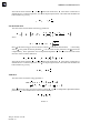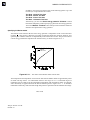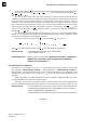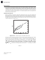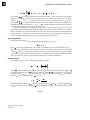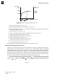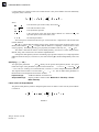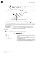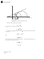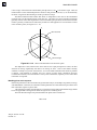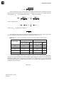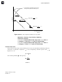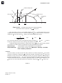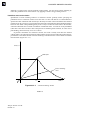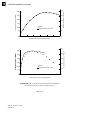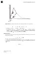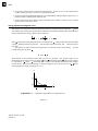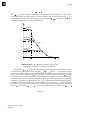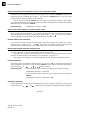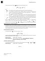
1
Abaqus Analysis User’s Manual Abaqus 6.12 Analysis User’s Manual Volume III: Materials Abaqus Version 6.6 ID: Printed on: Abaqus Analysis User’s Manual Volume III Abaqus Version 6.6 ID: Printed on: Legal Notices CAUTION: This documentation is intended for qualified users who will exercise sound engineering judgment and expertise in the use of the Abaqus Software. The Abaqus Software is inherently complex, and the examples and procedures in this documentation are not intended to be exhaustive or to apply to any particular situation. Users are cautioned to satisfy themselves as to the accuracy and results of their analyses. Dassault Systèmes and its subsidiaries, including Dassault Systèmes Simulia Corp., shall not be responsible for the accuracy or usefulness of any analysis performed using the Abaqus Software or the procedures, examples, or explanations in this documentation. Dassault Systèmes and its subsidiaries shall not be responsible for the consequences of any errors or omissions that may appear in this documentation. The Abaqus Software is available only under license from Dassault Systèmes or its subsidiary and may be used or reproduced only in accordance with the terms of such license. This documentation is subject to the terms and conditions of either the software license agreement signed by the parties, or, absent such an agreement, the then current software license agreement to which the documentation relates. This documentation and the software described in this documentation are subject to change without prior notice. No part of this documentation may be reproduced or distributed in any form without prior written permission of Dassault Systèmes or its subsidiary. The Abaqus Software is a product of Dassault Systèmes Simulia Corp., Providence, RI, USA. © Dassault Systèmes, 2012 Abaqus, the 3DS logo, SIMULIA, CATIA, and Unified FEA are trademarks or registered trademarks of Dassault Systèmes or its subsidiaries in the United States and/or other countries. Other company, product, and service names may be trademarks or service marks of their respective owners. For additional information concerning trademarks, copyrights, and licenses, see the Legal Notices in the Abaqus 6.12 Installation and Licensing Guide. Abaqus Version 6.6 ID: Printed on: Locations SIMULIA Worldwide Headquarters SIMULIA European Headquarters Rising Sun Mills, 166 Valley Street, Providence, RI 02909–2499, Tel: +1 401 276 4400, Fax: +1 401 276 4408, [email protected], http://www.simulia.com Stationsplein 8-K, 6221 BT Maastricht, The Netherlands, Tel: +31 43 7999 084, Fax: +31 43 7999 306, [email protected] Dassault Systèmes’ Centers of Simulation Excellence United States Australia Austria Benelux Canada China Finland France Germany India Italy Japan Korea Latin America Scandinavia United Kingdom Fremont, CA, Tel: +1 510 794 5891, [email protected] West Lafayette, IN, Tel: +1 765 497 1373, [email protected] Northville, MI, Tel: +1 248 349 4669, [email protected] Woodbury, MN, Tel: +1 612 424 9044, [email protected] Mayfield Heights, OH, Tel: +1 216 378 1070, [email protected] Mason, OH, Tel: +1 513 275 1430, [email protected] Warwick, RI, Tel: +1 401 739 3637, [email protected] Lewisville, TX, Tel: +1 972 221 6500, [email protected] Richmond VIC, Tel: +61 3 9421 2900, [email protected] Vienna, Tel: +43 1 22 707 200, [email protected] Maarssen, The Netherlands, Tel: +31 346 585 710, [email protected] Toronto, ON, Tel: +1 416 402 2219, [email protected] Beijing, P. R. China, Tel: +8610 6536 2288, [email protected] Shanghai, P. R. China, Tel: +8621 3856 8000, [email protected] Espoo, Tel: +358 40 902 2973, [email protected] Velizy Villacoublay Cedex, Tel: +33 1 61 62 72 72, [email protected] Aachen, Tel: +49 241 474 01 0, [email protected] Munich, Tel: +49 89 543 48 77 0, [email protected] Chennai, Tamil Nadu, Tel: +91 44 43443000, [email protected] Lainate MI, Tel: +39 02 3343061, [email protected] Tokyo, Tel: +81 3 5442 6302, [email protected] Osaka, Tel: +81 6 7730 2703, [email protected] Mapo-Gu, Seoul, Tel: +82 2 785 6707/8, [email protected] Puerto Madero, Buenos Aires, Tel: +54 11 4312 8700, [email protected] Stockholm, Sweden, Tel: +46 8 68430450, [email protected] Warrington, Tel: +44 1925 830900, [email protected] Authorized Support Centers Argentina Brazil Czech & Slovak Republics Greece Israel Malaysia Mexico New Zealand Poland Russia, Belarus & Ukraine Singapore South Africa Spain & Portugal Abaqus Version 6.6 ID: Printed on: SMARTtech Sudamerica SRL, Buenos Aires, Tel: +54 11 4717 2717 KB Engineering, Buenos Aires, Tel: +54 11 4326 7542 Solaer Ingeniería, Buenos Aires, Tel: +54 221 489 1738 SMARTtech Mecânica, Sao Paulo-SP, Tel: +55 11 3168 3388 Synerma s. r. o., Psáry, Prague-West, Tel: +420 603 145 769, [email protected] 3 Dimensional Data Systems, Crete, Tel: +30 2821040012, [email protected] ADCOM, Givataim, Tel: +972 3 7325311, [email protected] WorleyParsons Services Sdn. Bhd., Kuala Lumpur, Tel: +603 2039 9000, [email protected] Kimeca.NET SA de CV, Mexico, Tel: +52 55 2459 2635 Matrix Applied Computing Ltd., Auckland, Tel: +64 9 623 1223, [email protected] BudSoft Sp. z o.o., Poznań, Tel: +48 61 8508 466, [email protected] TESIS Ltd., Moscow, Tel: +7 495 612 44 22, [email protected] WorleyParsons Pte Ltd., Singapore, Tel: +65 6735 8444, [email protected] Finite Element Analysis Services (Pty) Ltd., Parklands, Tel: +27 21 556 6462, [email protected] Principia Ingenieros Consultores, S.A., Madrid, Tel: +34 91 209 1482, [email protected] Taiwan Thailand Turkey Simutech Solution Corporation, Taipei, R.O.C., Tel: +886 2 2507 9550, [email protected] WorleyParsons Pte Ltd., Singapore, Tel: +65 6735 8444, [email protected] A-Ztech Ltd., Istanbul, Tel: +90 216 361 8850, [email protected] Complete contact information is available at http://www.simulia.com/locations/locations.html. Abaqus Version 6.6 ID: Printed on: Preface This section lists various resources that are available for help with using Abaqus Unified FEA software. Support Both technical engineering support (for problems with creating a model or performing an analysis) and systems support (for installation, licensing, and hardware-related problems) for Abaqus are offered through a network of local support offices. Regional contact information is listed in the front of each Abaqus manual and is accessible from the Locations page at www.simulia.com. Support for SIMULIA products SIMULIA provides a knowledge database of answers and solutions to questions that we have answered, as well as guidelines on how to use Abaqus, SIMULIA Scenario Definition, Isight, and other SIMULIA products. You can also submit new requests for support. All support incidents are tracked. If you contact us by means outside the system to discuss an existing support problem and you know the incident or support request number, please mention it so that we can query the database to see what the latest action has been. Many questions about Abaqus can also be answered by visiting the Products page and the Support page at www.simulia.com. Anonymous ftp site To facilitate data transfer with SIMULIA, an anonymous ftp account is available at ftp.simulia.com. Login as user anonymous, and type your e-mail address as your password. Contact support before placing files on the site. Training All offices and representatives offer regularly scheduled public training classes. The courses are offered in a traditional classroom form and via the Web. We also provide training seminars at customer sites. All training classes and seminars include workshops to provide as much practical experience with Abaqus as possible. For a schedule and descriptions of available classes, see www.simulia.com or call your local office or representative. Feedback We welcome any suggestions for improvements to Abaqus software, the support program, or documentation. We will ensure that any enhancement requests you make are considered for future releases. If you wish to make a suggestion about the service or products, refer to www.simulia.com. Complaints should be made by contacting your local office or through www.simulia.com by visiting the Quality Assurance section of the Support page. Abaqus Version 6.6 ID: Printed on: CONTENTS Contents Volume I PART I 1. INTRODUCTION, SPATIAL MODELING, AND EXECUTION Introduction Introduction: general 1.1.1 Abaqus syntax and conventions Input syntax rules Conventions 1.2.1 1.2.2 Abaqus model definition Defining a model in Abaqus 1.3.1 Parametric modeling Parametric input 2. 1.4.1 Spatial Modeling Node definition Node definition Parametric shape variation Nodal thicknesses Normal definitions at nodes Transformed coordinate systems Adjusting nodal coordinates 2.1.1 2.1.2 2.1.3 2.1.4 2.1.5 2.1.6 Element definition Element definition Element foundations Defining reinforcement Defining rebar as an element property Orientations 2.2.1 2.2.2 2.2.3 2.2.4 2.2.5 Surface definition Surfaces: overview Element-based surface definition Node-based surface definition Analytical rigid surface definition 2.3.1 2.3.2 2.3.3 2.3.4 i Abaqus ID:usb-toc Printed on: Fri February 3 -- 18:01:12 2012 CONTENTS Eulerian surface definition Operating on surfaces 2.3.5 2.3.6 Rigid body definition Rigid body definition 2.4.1 Integrated output section definition Integrated output section definition 2.5.1 Mass adjustment Adjust and/or redistribute mass of an element set 2.6.1 Nonstructural mass definition Nonstructural mass definition 2.7.1 Distribution definition Distribution definition 2.8.1 Display body definition Display body definition 2.9.1 Assembly definition Defining an assembly 2.10.1 Matrix definition Defining matrices 3. 2.11.1 Job Execution Execution procedures: overview Execution procedure for Abaqus: overview 3.1.1 Execution procedures Obtaining information Abaqus/Standard, Abaqus/Explicit, and Abaqus/CFD execution SIMULIA Co-Simulation Engine controller execution Abaqus/Standard, Abaqus/Explicit, and Abaqus/CFD co-simulation execution Abaqus/CAE execution Abaqus/Viewer execution Python execution Parametric studies Abaqus documentation Licensing utilities ASCII translation of results (.fil) files Joining results (.fil) files Querying the keyword/problem database ii Abaqus ID:usb-toc Printed on: Fri February 3 -- 18:01:12 2012 3.2.1 3.2.2 3.2.3 3.2.4 3.2.5 3.2.6 3.2.7 3.2.8 3.2.9 3.2.10 3.2.11 3.2.12 3.2.13 CONTENTS Fetching sample input files Making user-defined executables and subroutines Input file and output database upgrade utility Generating output database reports Joining output database (.odb) files from restarted analyses Combining output from substructures Combining data from multiple output databases Network output database file connector Mapping thermal and magnetic loads Fixed format conversion utility Translating Nastran bulk data files to Abaqus input files Translating Abaqus files to Nastran bulk data files Translating ANSYS input files to Abaqus input files Translating PAM-CRASH input files to partial Abaqus input files Translating RADIOSS input files to partial Abaqus input files Translating Abaqus output database files to Nastran Output2 results files Translating LS-DYNA data files to Abaqus input files Exchanging Abaqus data with ZAERO Encrypting and decrypting Abaqus input data Job execution control 3.2.14 3.2.15 3.2.16 3.2.17 3.2.18 3.2.19 3.2.20 3.2.21 3.2.22 3.2.23 3.2.24 3.2.25 3.2.26 3.2.27 3.2.28 3.2.29 3.2.30 3.2.31 3.2.32 3.2.33 Environment file settings Using the Abaqus environment settings 3.3.1 Managing memory and disk resources Managing memory and disk use in Abaqus 3.4.1 Parallel execution Parallel execution: overview Parallel execution in Abaqus/Standard Parallel execution in Abaqus/Explicit Parallel execution in Abaqus/CFD 3.5.1 3.5.2 3.5.3 3.5.4 File extension definitions File extensions used by Abaqus 3.6.1 FORTRAN unit numbers FORTRAN unit numbers used by Abaqus 3.7.1 iii Abaqus ID:usb-toc Printed on: Fri February 3 -- 18:01:12 2012 CONTENTS PART II 4. OUTPUT Output Output Output to the data and results files Output to the output database Error indicator output 4.1.1 4.1.2 4.1.3 4.1.4 Output variables Abaqus/Standard output variable identifiers Abaqus/Explicit output variable identifiers Abaqus/CFD output variable identifiers 4.2.1 4.2.2 4.2.3 The postprocessing calculator The postprocessing calculator 5. 4.3.1 File Output Format Accessing the results file Accessing the results file: overview Results file output format Accessing the results file information Utility routines for accessing the results file OI.1 Abaqus/Standard Output Variable Index OI.2 Abaqus/Explicit Output Variable Index OI.3 Abaqus/CFD Output Variable Index 5.1.1 5.1.2 5.1.3 5.1.4 iv Abaqus ID:usb-toc Printed on: Fri February 3 -- 18:01:12 2012 CONTENTS Volume II PART III 6. ANALYSIS PROCEDURES, SOLUTION, AND CONTROL Analysis Procedures Introduction Solving analysis problems: overview Defining an analysis General and linear perturbation procedures Multiple load case analysis Direct linear equation solver Iterative linear equation solver 6.1.1 6.1.2 6.1.3 6.1.4 6.1.5 6.1.6 Static stress/displacement analysis Static stress analysis procedures: overview Static stress analysis Eigenvalue buckling prediction Unstable collapse and postbuckling analysis Quasi-static analysis Direct cyclic analysis Low-cycle fatigue analysis using the direct cyclic approach 6.2.1 6.2.2 6.2.3 6.2.4 6.2.5 6.2.6 6.2.7 Dynamic stress/displacement analysis Dynamic analysis procedures: overview Implicit dynamic analysis using direct integration Explicit dynamic analysis Direct-solution steady-state dynamic analysis Natural frequency extraction Complex eigenvalue extraction Transient modal dynamic analysis Mode-based steady-state dynamic analysis Subspace-based steady-state dynamic analysis Response spectrum analysis Random response analysis 6.3.1 6.3.2 6.3.3 6.3.4 6.3.5 6.3.6 6.3.7 6.3.8 6.3.9 6.3.10 6.3.11 Steady-state transport analysis Steady-state transport analysis 6.4.1 Heat transfer and thermal-stress analysis Heat transfer analysis procedures: overview Uncoupled heat transfer analysis 6.5.1 6.5.2 v Abaqus ID:usb-toc Printed on: Fri February 3 -- 18:01:12 2012 CONTENTS Fully coupled thermal-stress analysis Adiabatic analysis 6.5.3 6.5.4 Fluid dynamic analysis Fluid dynamic analysis procedures: overview Incompressible fluid dynamic analysis 6.6.1 6.6.2 Electromagnetic analysis Electromagnetic analysis procedures Piezoelectric analysis Coupled thermal-electrical analysis Fully coupled thermal-electrical-structural analysis Eddy current analysis Magnetostatic analysis 6.7.1 6.7.2 6.7.3 6.7.4 6.7.5 6.7.6 Coupled pore fluid flow and stress analysis Coupled pore fluid diffusion and stress analysis Geostatic stress state 6.8.1 6.8.2 Mass diffusion analysis Mass diffusion analysis 6.9.1 Acoustic and shock analysis Acoustic, shock, and coupled acoustic-structural analysis 6.10.1 Abaqus/Aqua analysis Abaqus/Aqua analysis 6.11.1 Annealing Annealing procedure 7. 6.12.1 Analysis Solution and Control Solving nonlinear problems Solving nonlinear problems 7.1.1 Analysis convergence controls Convergence and time integration criteria: overview Commonly used control parameters Convergence criteria for nonlinear problems Time integration accuracy in transient problems vi Abaqus ID:usb-toc Printed on: Fri February 3 -- 18:01:12 2012 7.2.1 7.2.2 7.2.3 7.2.4 CONTENTS PART IV 8. ANALYSIS TECHNIQUES Analysis Techniques: Introduction Analysis techniques: overview 9. 8.1.1 Analysis Continuation Techniques Restarting an analysis Restarting an analysis 9.1.1 Importing and transferring results Transferring results between Abaqus analyses: overview Transferring results between Abaqus/Explicit and Abaqus/Standard Transferring results from one Abaqus/Standard analysis to another Transferring results from one Abaqus/Explicit analysis to another 10. 9.2.1 9.2.2 9.2.3 9.2.4 Modeling Abstractions Substructuring Using substructures Defining substructures 10.1.1 10.1.2 Submodeling Submodeling: overview Node-based submodeling Surface-based submodeling 10.2.1 10.2.2 10.2.3 Generating global matrices Generating matrices 10.3.1 Symmetric model generation, results transfer, and analysis of cyclic symmetry models Symmetric model generation Transferring results from a symmetric mesh or a partial three-dimensional mesh to a full three-dimensional mesh Analysis of models that exhibit cyclic symmetry 10.4.1 10.4.2 10.4.3 Periodic media analysis Periodic media analysis 10.5.1 Meshed beam cross-sections Meshed beam cross-sections 10.6.1 vii Abaqus ID:usb-toc Printed on: Fri February 3 -- 18:01:12 2012 CONTENTS Modeling discontinuities as an enriched feature using the extended finite element method Modeling discontinuities as an enriched feature using the extended finite element method 11. 10.7.1 Special-Purpose Techniques Inertia relief Inertia relief 11.1.1 Mesh modification or replacement Element and contact pair removal and reactivation 11.2.1 Geometric imperfections Introducing a geometric imperfection into a model 11.3.1 Fracture mechanics Fracture mechanics: overview Contour integral evaluation Crack propagation analysis 11.4.1 11.4.2 11.4.3 Surface-based fluid modeling Surface-based fluid cavities: overview Fluid cavity definition Fluid exchange definition Inflator definition 11.5.1 11.5.2 11.5.3 11.5.4 Mass scaling Mass scaling 11.6.1 Selective subcycling Selective subcycling 11.7.1 Steady-state detection Steady-state detection 12. 11.8.1 Adaptivity Techniques Adaptivity techniques: overview Adaptivity techniques 12.1.1 ALE adaptive meshing ALE adaptive meshing: overview Defining ALE adaptive mesh domains in Abaqus/Explicit ALE adaptive meshing and remapping in Abaqus/Explicit Modeling techniques for Eulerian adaptive mesh domains in Abaqus/Explicit viii Abaqus ID:usb-toc Printed on: Fri February 3 -- 18:01:12 2012 12.2.1 12.2.2 12.2.3 12.2.4 CONTENTS Output and diagnostics for ALE adaptive meshing in Abaqus/Explicit Defining ALE adaptive mesh domains in Abaqus/Standard ALE adaptive meshing and remapping in Abaqus/Standard 12.2.5 12.2.6 12.2.7 Adaptive remeshing Adaptive remeshing: overview Selection of error indicators influencing adaptive remeshing Solution-based mesh sizing 12.3.1 12.3.2 12.3.3 Analysis continuation after mesh replacement Mesh-to-mesh solution mapping 13. 12.4.1 Optimization Techniques Structural optimization: overview Structural optimization: overview 13.1.1 Optimization models Design responses Objectives and constraints Creating Abaqus optimization models 14. 13.2.1 13.2.2 13.2.3 Eulerian Analysis Eulerian analysis Defining Eulerian boundaries Eulerian mesh motion Defining adaptive mesh refinement in the Eulerian domain 15. 14.1.1 14.1.2 14.1.3 14.1.4 Particle Methods Smoothed particle hydrodynamic analyses Smoothed particle hydrodynamic analysis Finite element conversion to SPH particles 16. 15.1.1 15.1.2 Sequentially Coupled Multiphysics Analyses Predefined fields for sequential coupling Sequentially coupled thermal-stress analysis Predefined loads for sequential coupling 17. 16.1.1 16.1.2 16.1.3 Co-simulation Co-simulation: overview 17.1.1 Preparing an Abaqus analysis for co-simulation Preparing an Abaqus analysis for co-simulation ix Abaqus ID:usb-toc Printed on: Fri February 3 -- 18:01:12 2012 17.2.1 CONTENTS Co-simulation between Abaqus solvers Abaqus/Standard to Abaqus/Explicit co-simulation Abaqus/CFD to Abaqus/Standard or to Abaqus/Explicit co-simulation 18. 17.3.1 17.3.2 Extending Abaqus Analysis Functionality User subroutines and utilities User subroutines: overview Available user subroutines Available utility routines 19. 18.1.1 18.1.2 18.1.3 Design Sensitivity Analysis Design sensitivity analysis 20. 19.1.1 Parametric Studies Scripting parametric studies Scripting parametric studies 20.1.1 Parametric studies: commands aStudy.combine(): Combine parameter samples for parametric studies. aStudy.constrain(): Constrain parameter value combinations in parametric studies. aStudy.define(): Define parameters for parametric studies. aStudy.execute(): Execute the analysis of parametric study designs. aStudy.gather(): Gather the results of a parametric study. aStudy.generate(): Generate the analysis job data for a parametric study. aStudy.output(): Specify the source of parametric study results. aStudy=ParStudy(): Create a parametric study. aStudy.report(): Report parametric study results. aStudy.sample(): Sample parameters for parametric studies. x Abaqus ID:usb-toc Printed on: Fri February 3 -- 18:01:12 2012 20.2.1 20.2.2 20.2.3 20.2.4 20.2.5 20.2.6 20.2.7 20.2.8 20.2.9 20.2.10 CONTENTS Volume III PART V 21. MATERIALS Materials: Introduction Introduction Material library: overview Material data definition Combining material behaviors 21.1.1 21.1.2 21.1.3 General properties Density 22. 21.2.1 Elastic Mechanical Properties Overview Elastic behavior: overview 22.1.1 Linear elasticity Linear elastic behavior No compression or no tension Plane stress orthotropic failure measures 22.2.1 22.2.2 22.2.3 Porous elasticity Elastic behavior of porous materials 22.3.1 Hypoelasticity Hypoelastic behavior 22.4.1 Hyperelasticity Hyperelastic behavior of rubberlike materials Hyperelastic behavior in elastomeric foams Anisotropic hyperelastic behavior 22.5.1 22.5.2 22.5.3 Stress softening in elastomers Mullins effect Energy dissipation in elastomeric foams 22.6.1 22.6.2 Viscoelasticity Time domain viscoelasticity Frequency domain viscoelasticity 22.7.1 22.7.2 xi Abaqus ID:usb-toc Printed on: Fri February 3 -- 18:01:12 2012 CONTENTS Nonlinear viscoelasticity Hysteresis in elastomers Parallel network viscoelastic model 22.8.1 22.8.2 Rate sensitive elastomeric foams Low-density foams 23. 22.9.1 Inelastic Mechanical Properties Overview Inelastic behavior 23.1.1 Metal plasticity Classical metal plasticity Models for metals subjected to cyclic loading Rate-dependent yield Rate-dependent plasticity: creep and swelling Annealing or melting Anisotropic yield/creep Johnson-Cook plasticity Dynamic failure models Porous metal plasticity Cast iron plasticity Two-layer viscoplasticity ORNL – Oak Ridge National Laboratory constitutive model Deformation plasticity 23.2.1 23.2.2 23.2.3 23.2.4 23.2.5 23.2.6 23.2.7 23.2.8 23.2.9 23.2.10 23.2.11 23.2.12 23.2.13 Other plasticity models Extended Drucker-Prager models Modified Drucker-Prager/Cap model Mohr-Coulomb plasticity Critical state (clay) plasticity model Crushable foam plasticity models 23.3.1 23.3.2 23.3.3 23.3.4 23.3.5 Fabric materials Fabric material behavior 23.4.1 Jointed materials Jointed material model 23.5.1 Concrete Concrete smeared cracking Cracking model for concrete Concrete damaged plasticity 23.6.1 23.6.2 23.6.3 xii Abaqus ID:usb-toc Printed on: Fri February 3 -- 18:01:12 2012 CONTENTS Permanent set in rubberlike materials Permanent set in rubberlike materials 24. 23.7.1 Progressive Damage and Failure Progressive damage and failure: overview Progressive damage and failure 24.1.1 Damage and failure for ductile metals Damage and failure for ductile metals: overview Damage initiation for ductile metals Damage evolution and element removal for ductile metals 24.2.1 24.2.2 24.2.3 Damage and failure for fiber-reinforced composites Damage and failure for fiber-reinforced composites: overview Damage initiation for fiber-reinforced composites Damage evolution and element removal for fiber-reinforced composites 24.3.1 24.3.2 24.3.3 Damage and failure for ductile materials in low-cycle fatigue analysis Damage and failure for ductile materials in low-cycle fatigue analysis: overview Damage initiation for ductile materials in low-cycle fatigue Damage evolution for ductile materials in low-cycle fatigue 25. 24.4.1 24.4.2 24.4.3 Hydrodynamic Properties Overview Hydrodynamic behavior: overview 25.1.1 Equations of state Equation of state 26. 25.2.1 Other Material Properties Mechanical properties Material damping Thermal expansion Field expansion Viscosity 26.1.1 26.1.2 26.1.3 26.1.4 Heat transfer properties Thermal properties: overview Conductivity Specific heat Latent heat 26.2.1 26.2.2 26.2.3 26.2.4 xiii Abaqus ID:usb-toc Printed on: Fri February 3 -- 18:01:12 2012 CONTENTS Acoustic properties Acoustic medium 26.3.1 Mass diffusion properties Diffusivity Solubility 26.4.1 26.4.2 Electromagnetic properties Electrical conductivity Piezoelectric behavior Magnetic permeability 26.5.1 26.5.2 26.5.3 Pore fluid flow properties Pore fluid flow properties Permeability Porous bulk moduli Sorption Swelling gel Moisture swelling 26.6.1 26.6.2 26.6.3 26.6.4 26.6.5 26.6.6 User materials User-defined mechanical material behavior User-defined thermal material behavior 26.7.1 26.7.2 xiv Abaqus ID:usb-toc Printed on: Fri February 3 -- 18:01:12 2012 CONTENTS Volume IV PART VI 27. ELEMENTS Elements: Introduction Element library: overview Choosing the element’s dimensionality Choosing the appropriate element for an analysis type Section controls 28. 27.1.1 27.1.2 27.1.3 27.1.4 Continuum Elements General-purpose continuum elements Solid (continuum) elements One-dimensional solid (link) element library Two-dimensional solid element library Three-dimensional solid element library Cylindrical solid element library Axisymmetric solid element library Axisymmetric solid elements with nonlinear, asymmetric deformation 28.1.1 28.1.2 28.1.3 28.1.4 28.1.5 28.1.6 28.1.7 Fluid continuum elements Fluid (continuum) elements Fluid element library 28.2.1 28.2.2 Infinite elements Infinite elements Infinite element library 28.3.1 28.3.2 Warping elements Warping elements Warping element library 28.4.1 28.4.2 Particle elements Particle elements Particle element library 29. 28.5.1 28.5.2 Structural Elements Membrane elements Membrane elements General membrane element library Cylindrical membrane element library 29.1.1 29.1.2 29.1.3 xv Abaqus ID:usb-toc Printed on: Fri February 3 -- 18:01:12 2012 CONTENTS Axisymmetric membrane element library 29.1.4 Truss elements Truss elements Truss element library 29.2.1 29.2.2 Beam elements Beam modeling: overview Choosing a beam cross-section Choosing a beam element Beam element cross-section orientation Beam section behavior Using a beam section integrated during the analysis to define the section behavior Using a general beam section to define the section behavior Beam element library Beam cross-section library 29.3.1 29.3.2 29.3.3 29.3.4 29.3.5 29.3.6 29.3.7 29.3.8 29.3.9 Frame elements Frame elements Frame section behavior Frame element library 29.4.1 29.4.2 29.4.3 Elbow elements Pipes and pipebends with deforming cross-sections: elbow elements Elbow element library 29.5.1 29.5.2 Shell elements Shell elements: overview Choosing a shell element Defining the initial geometry of conventional shell elements Shell section behavior Using a shell section integrated during the analysis to define the section behavior Using a general shell section to define the section behavior Three-dimensional conventional shell element library Continuum shell element library Axisymmetric shell element library Axisymmetric shell elements with nonlinear, asymmetric deformation xvi Abaqus ID:usb-toc Printed on: Fri February 3 -- 18:01:12 2012 29.6.1 29.6.2 29.6.3 29.6.4 29.6.5 29.6.6 29.6.7 29.6.8 29.6.9 29.6.10 CONTENTS 30. Inertial, Rigid, and Capacitance Elements Point mass elements Point masses Mass element library 30.1.1 30.1.2 Rotary inertia elements Rotary inertia Rotary inertia element library 30.2.1 30.2.2 Rigid elements Rigid elements Rigid element library 30.3.1 30.3.2 Capacitance elements Point capacitance Capacitance element library 31. 30.4.1 30.4.2 Connector Elements Connector elements Connectors: overview Connector elements Connector actuation Connector element library Connection-type library 31.1.1 31.1.2 31.1.3 31.1.4 31.1.5 Connector element behavior Connector behavior Connector elastic behavior Connector damping behavior Connector functions for coupled behavior Connector friction behavior Connector plastic behavior Connector damage behavior Connector stops and locks Connector failure behavior Connector uniaxial behavior 32. 31.2.1 31.2.2 31.2.3 31.2.4 31.2.5 31.2.6 31.2.7 31.2.8 31.2.9 31.2.10 Special-Purpose Elements Spring elements Springs Spring element library 32.1.1 32.1.2 xvii Abaqus ID:usb-toc Printed on: Fri February 3 -- 18:01:12 2012 CONTENTS Dashpot elements Dashpots Dashpot element library 32.2.1 32.2.2 Flexible joint elements Flexible joint element Flexible joint element library 32.3.1 32.3.2 Distributing coupling elements Distributing coupling elements Distributing coupling element library 32.4.1 32.4.2 Cohesive elements Cohesive elements: overview Choosing a cohesive element Modeling with cohesive elements Defining the cohesive element’s initial geometry Defining the constitutive response of cohesive elements using a continuum approach Defining the constitutive response of cohesive elements using a traction-separation description Defining the constitutive response of fluid within the cohesive element gap Two-dimensional cohesive element library Three-dimensional cohesive element library Axisymmetric cohesive element library 32.5.1 32.5.2 32.5.3 32.5.4 32.5.5 32.5.6 32.5.7 32.5.8 32.5.9 32.5.10 Gasket elements Gasket elements: overview Choosing a gasket element Including gasket elements in a model Defining the gasket element’s initial geometry Defining the gasket behavior using a material model Defining the gasket behavior directly using a gasket behavior model Two-dimensional gasket element library Three-dimensional gasket element library Axisymmetric gasket element library 32.6.1 32.6.2 32.6.3 32.6.4 32.6.5 32.6.6 32.6.7 32.6.8 32.6.9 Surface elements Surface elements General surface element library Cylindrical surface element library Axisymmetric surface element library 32.7.1 32.7.2 32.7.3 32.7.4 xviii Abaqus ID:usb-toc Printed on: Fri February 3 -- 18:01:12 2012 CONTENTS Tube support elements Tube support elements Tube support element library 32.8.1 32.8.2 Line spring elements Line spring elements for modeling part-through cracks in shells Line spring element library 32.9.1 32.9.2 Elastic-plastic joints Elastic-plastic joints Elastic-plastic joint element library 32.10.1 32.10.2 Drag chain elements Drag chains Drag chain element library 32.11.1 32.11.2 Pipe-soil elements Pipe-soil interaction elements Pipe-soil interaction element library 32.12.1 32.12.2 Acoustic interface elements Acoustic interface elements Acoustic interface element library 32.13.1 32.13.2 Eulerian elements Eulerian elements Eulerian element library 32.14.1 32.14.2 User-defined elements User-defined elements User-defined element library EI.1 Abaqus/Standard Element Index EI.2 Abaqus/Explicit Element Index EI.3 Abaqus/CFD Element Index 32.15.1 32.15.2 xix Abaqus ID:usb-toc Printed on: Fri February 3 -- 18:01:12 2012 CONTENTS Volume V PART VII 33. PRESCRIBED CONDITIONS Prescribed Conditions Overview Prescribed conditions: overview Amplitude curves 33.1.1 33.1.2 Initial conditions Initial conditions in Abaqus/Standard and Abaqus/Explicit Initial conditions in Abaqus/CFD 33.2.1 33.2.2 Boundary conditions Boundary conditions in Abaqus/Standard and Abaqus/Explicit Boundary conditions in Abaqus/CFD 33.3.1 33.3.2 Loads Applying loads: overview Concentrated loads Distributed loads Thermal loads Electromagnetic loads Acoustic and shock loads Pore fluid flow 33.4.1 33.4.2 33.4.3 33.4.4 33.4.5 33.4.6 33.4.7 Prescribed assembly loads Prescribed assembly loads 33.5.1 Predefined fields Predefined fields 33.6.1 PART VIII 34. CONSTRAINTS Constraints Overview Kinematic constraints: overview 34.1.1 Multi-point constraints Linear constraint equations 34.2.1 xx Abaqus ID:usb-toc Printed on: Fri February 3 -- 18:01:12 2012 CONTENTS General multi-point constraints Kinematic coupling constraints 34.2.2 34.2.3 Surface-based constraints Mesh tie constraints Coupling constraints Shell-to-solid coupling Mesh-independent fasteners 34.3.1 34.3.2 34.3.3 34.3.4 Embedded elements Embedded elements 34.4.1 Element end release Element end release 34.5.1 Overconstraint checks Overconstraint checks 34.6.1 PART IX 35. INTERACTIONS Defining Contact Interactions Overview Contact interaction analysis: overview 35.1.1 Defining general contact in Abaqus/Standard Defining general contact interactions in Abaqus/Standard Surface properties for general contact in Abaqus/Standard Contact properties for general contact in Abaqus/Standard Controlling initial contact status in Abaqus/Standard Stabilization for general contact in Abaqus/Standard Numerical controls for general contact in Abaqus/Standard 35.2.1 35.2.2 35.2.3 35.2.4 35.2.5 35.2.6 Defining contact pairs in Abaqus/Standard Defining contact pairs in Abaqus/Standard Assigning surface properties for contact pairs in Abaqus/Standard Assigning contact properties for contact pairs in Abaqus/Standard Modeling contact interference fits in Abaqus/Standard Adjusting initial surface positions and specifying initial clearances in Abaqus/Standard contact pairs Adjusting contact controls in Abaqus/Standard Defining tied contact in Abaqus/Standard Extending master surfaces and slide lines xxi Abaqus ID:usb-toc Printed on: Fri February 3 -- 18:01:12 2012 35.3.1 35.3.2 35.3.3 35.3.4 35.3.5 35.3.6 35.3.7 35.3.8 CONTENTS Contact modeling if substructures are present Contact modeling if asymmetric-axisymmetric elements are present 35.3.9 35.3.10 Defining general contact in Abaqus/Explicit Defining general contact interactions in Abaqus/Explicit Assigning surface properties for general contact in Abaqus/Explicit Assigning contact properties for general contact in Abaqus/Explicit Controlling initial contact status for general contact in Abaqus/Explicit Contact controls for general contact in Abaqus/Explicit 35.4.1 35.4.2 35.4.3 35.4.4 35.4.5 Defining contact pairs in Abaqus/Explicit Defining contact pairs in Abaqus/Explicit Assigning surface properties for contact pairs in Abaqus/Explicit Assigning contact properties for contact pairs in Abaqus/Explicit Adjusting initial surface positions and specifying initial clearances for contact pairs in Abaqus/Explicit Contact controls for contact pairs in Abaqus/Explicit 36. 35.5.1 35.5.2 35.5.3 35.5.4 35.5.5 Contact Property Models Mechanical contact properties Mechanical contact properties: overview Contact pressure-overclosure relationships Contact damping Contact blockage Frictional behavior User-defined interfacial constitutive behavior Pressure penetration loading Interaction of debonded surfaces Breakable bonds Surface-based cohesive behavior 36.1.1 36.1.2 36.1.3 36.1.4 36.1.5 36.1.6 36.1.7 36.1.8 36.1.9 36.1.10 Thermal contact properties Thermal contact properties 36.2.1 Electrical contact properties Electrical contact properties 36.3.1 Pore fluid contact properties Pore fluid contact properties 37. 36.4.1 Contact Formulations and Numerical Methods Contact formulations and numerical methods in Abaqus/Standard Contact formulations in Abaqus/Standard 37.1.1 xxii Abaqus ID:usb-toc Printed on: Fri February 3 -- 18:01:12 2012 CONTENTS Contact constraint enforcement methods in Abaqus/Standard Smoothing contact surfaces in Abaqus/Standard 37.1.2 37.1.3 Contact formulations and numerical methods in Abaqus/Explicit Contact formulation for general contact in Abaqus/Explicit Contact formulations for contact pairs in Abaqus/Explicit Contact constraint enforcement methods in Abaqus/Explicit 38. 37.2.1 37.2.2 37.2.3 Contact Difficulties and Diagnostics Resolving contact difficulties in Abaqus/Standard Contact diagnostics in an Abaqus/Standard analysis Common difficulties associated with contact modeling in Abaqus/Standard 38.1.1 38.1.2 Resolving contact difficulties in Abaqus/Explicit Contact diagnostics in an Abaqus/Explicit analysis Common difficulties associated with contact modeling using contact pairs in Abaqus/Explicit 39. 38.2.1 38.2.2 Contact Elements in Abaqus/Standard Contact modeling with elements Contact modeling with elements 39.1.1 Gap contact elements Gap contact elements Gap element library 39.2.1 39.2.2 Tube-to-tube contact elements Tube-to-tube contact elements Tube-to-tube contact element library 39.3.1 39.3.2 Slide line contact elements Slide line contact elements Axisymmetric slide line element library 39.4.1 39.4.2 Rigid surface contact elements Rigid surface contact elements Axisymmetric rigid surface contact element library 40. 39.5.1 39.5.2 Defining Cavity Radiation in Abaqus/Standard Cavity radiation 40.1.1 xxiii Abaqus ID:usb-toc Printed on: Fri February 3 -- 18:01:12 2012 Abaqus Version 6.6 ID: Printed on: Part V: Materials • • • • • • Chapter 21, “Materials: Introduction” Chapter 22, “Elastic Mechanical Properties” Chapter 23, “Inelastic Mechanical Properties” Chapter 24, “Progressive Damage and Failure” Chapter 25, “Hydrodynamic Properties” Chapter 26, “Other Material Properties” Abaqus Version 6.6 ID: Printed on: MATERIALS: INTRODUCTION 21. Materials: Introduction Introduction 21.1 General properties 21.2 Abaqus Version 6.6 ID: Printed on: INTRODUCTION 21.1 Introduction • • • “Material library: overview,” Section 21.1.1 “Material data definition,” Section 21.1.2 “Combining material behaviors,” Section 21.1.3 21.1–1 Abaqus Version 6.6 ID: Printed on: MATERIAL LIBRARY 21.1.1 MATERIAL LIBRARY: OVERVIEW This chapter describes how to define materials in Abaqus and contains brief descriptions of each of the material behaviors provided. Further details of the more advanced behaviors are provided in the Abaqus Theory Manual. Defining materials Materials are defined by: • • selecting material behaviors and defining them (“Material data definition,” Section 21.1.2); and combining complementary material behaviors such as elasticity and plasticity (“Combining material behaviors,” Section 21.1.3). A local coordinate system can be used for material calculations (“Orientations,” Section 2.2.5). Any anisotropic properties must be given in this local system. Available material behaviors The material library in Abaqus is intended to provide comprehensive coverage of both linear and nonlinear, isotropic and anisotropic material behaviors. The use of numerical integration in the elements, including numerical integration across the cross-sections of shells and beams, provides the flexibility to analyze the most complex composite structures. Material behaviors fall into the following general categories: • • • • • • • • • • general properties (material damping, density, thermal expansion); elastic mechanical properties; inelastic mechanical properties; thermal properties; acoustic properties; hydrostatic fluid properties; equations of state; mass diffusion properties; electrical properties; and pore fluid flow properties. Some of the mechanical behaviors offered are mutually exclusive: such behaviors cannot appear together in a single material definition. Some behaviors require the presence of other behaviors; for example, plasticity requires linear elasticity. Such requirements are discussed at the end of each material behavior description, as well as in “Combining material behaviors,” Section 21.1.3. 21.1.1–1 Abaqus Version 6.6 ID: Printed on: MATERIAL LIBRARY Using material behaviors with various element types There are no general restrictions on the use of particular material behaviors with solid, shell, beam, and pipe elements. Any combination that makes sense is acceptable. The few restrictions that do exist are mentioned when that particular behavior is described in the pages that follow. A section on the elements available for use with a material behavior appears at the end of each material behavior description. Using complete material definitions A material definition can include behaviors that are not meaningful for the elements or analysis in which the material is being used. Such behaviors will be ignored. For example, a material definition can include heat transfer properties (conductivity, specific heat) as well as stress-strain properties (elastic moduli, yield stress, etc). When this material definition is used with uncoupled stress/displacement elements, the heat transfer properties are ignored by Abaqus; when it is used with heat transfer elements, the mechanical strength properties are ignored. This capability allows you to develop complete material definitions and use them in any analysis. Defining spatially varying material behavior for homogenous solid continuum elements using distributions in Abaqus/Standard In Abaqus/Standard spatially varying mass density (“Density,” Section 21.2.1), linear elastic behavior (“Linear elastic behavior,” Section 22.2.1), and thermal expansion (“Thermal expansion,” Section 26.1.2) can be defined for homogeneous solid continuum elements using distributions (“Distribution definition,” Section 2.8.1). Using distributions in a model with significant variation in material behavior can greatly simplify pre- and postprocessing and improve performance during the analysis by allowing a single material definition to define the spatially varying material behavior. Without distributions such a model may require many material definitions and associated section assignments. 21.1.1–2 Abaqus Version 6.6 ID: Printed on: MATERIAL DEFINITION 21.1.2 MATERIAL DATA DEFINITION Products: Abaqus/Standard Abaqus/Explicit Abaqus/CFD Abaqus/CAE References • • • • “Material library: overview,” Section 21.1.1 “Combining material behaviors,” Section 21.1.3 *MATERIAL “Creating materials,” Section 12.4.1 of the Abaqus/CAE User’s Manual Overview A material definition in Abaqus: • • • • • • specifies the behavior of a material and supplies all the relevant property data; can contain multiple material behaviors; is assigned a name, which is used to refer to those parts of the model that are made of that material; can have temperature and/or field variable dependence; can have solution variable dependence in Abaqus/Standard; and can be specified in a local coordinate system (“Orientations,” Section 2.2.5), which is required if the material is not isotropic. Material definitions Any number of materials can be defined in an analysis. Each material definition can contain any number of material behaviors, as required, to specify the complete material behavior. For example, in a linear static stress analysis only elastic material behavior may be needed, while in a more complicated analysis several material behaviors may be required. A name must be assigned to each material definition. This name allows the material to be referenced from the section definitions used to assign this material to regions in the model. Input File Usage: *MATERIAL, NAME=name Each material definition is specified in a data block, which is initiated by a *MATERIAL option. The material definition continues until an option that does not define a material behavior (such as another *MATERIAL option) is introduced, at which point the material definition is assumed to be complete. The order of the material behavior options is not important. All material behavior options within the data block are assumed to define the same material. Abaqus/CAE Usage: Property module: material editor: Name Use the menu bar under the Material Options list to add behaviors to a material. 21.1.2–1 Abaqus Version 6.6 ID: Printed on: MATERIAL DEFINITION Large-strain considerations When giving material properties for finite-strain calculations, “stress” means “true” (Cauchy) stress (force per current area) and “strain” means logarithmic strain. For example, unless otherwise indicated, for uniaxial behavior Specifying material data as functions of temperature and independent field variables Material data are often specified as functions of independent variables such as temperature. Material properties are made temperature dependent by specifying them at several different temperatures. In some cases a material property can be defined as a function of variables calculated by Abaqus; for example, to define a work-hardening curve, stress must be given as a function of equivalent plastic strain. Material properties can also be dependent on “field variables” (user-defined variables that can represent any independent quantity and are defined at the nodes, as functions of time). For example, material moduli can be functions of weave density in a composite or of phase fraction in an alloy. See “Specifying field variable dependence” for details. The initial values of field variables are given as initial conditions (see “Initial conditions in Abaqus/Standard and Abaqus/Explicit,” Section 33.2.1) and can be modified as functions of time during an analysis (see “Predefined fields,” Section 33.6.1). This capability is useful if, for example, material properties change with time because of irradiation or some other precalculated environmental effect. Any material behaviors defined using a distribution in Abaqus/Standard (mass density, linear elastic behavior, and/or thermal expansion) cannot be defined with temperature and/or field dependence. However, material behaviors defined with distributions can be included in a material definition with other material behaviors that have temperature and/or field dependence. See “Density,” Section 21.2.1; “Linear elastic behavior,” Section 22.2.1; and “Thermal expansion,” Section 26.1.2. Interpolation of material data In the simplest case of a constant property, only the constant value is entered. When the material data are functions of only one variable, the data must be given in order of increasing values of the independent variable. Abaqus then interpolates linearly for values between those given. The property is assumed to be constant outside the range of independent variables given (except for fabric materials, where it is extrapolated linearly outside the specified range using the slope at the last specified data point). Thus, you can give as many or as few input values as are necessary for the material model. If the material data depend on the independent variable in a strongly nonlinear manner, you must specify enough data points so that a linear interpolation captures the nonlinear behavior accurately. When material properties depend on several variables, the variation of the properties with respect to the first variable must be given at fixed values of the other variables, in ascending values of the second variable, then of the third variable, and so on. The data must always be ordered so that the independent 21.1.2–2 Abaqus Version 6.6 ID: Printed on: MATERIAL DEFINITION variables are given increasing values. This process ensures that the value of the material property is completely and uniquely defined at any values of the independent variables upon which the property depends. See “Input syntax rules,” Section 1.2.1, for further explanation and an example. Example: Temperature-dependent linear isotropic elasticity Figure 21.1.2–1 shows a simple, isotropic, linear elastic material, giving the Young’s modulus and the Poisson’s ratio as functions of temperature. Young s modulus, E ν Poisson s ratio, ν E 1 2 3 4 5 6 Temperature, θ Figure 21.1.2–1 Example of material definition. In this case six sets of values are used to specify the material description, as shown in the following table: Elastic Modulus Poisson’s Ratio Temperature For temperatures that are outside the range defined by and , Abaqus assumes constant values for E and . The dotted lines on the graph represent the straight-line approximations that will be used for this model. In this example only one value of the thermal expansion coefficient is given, , and it is independent of temperature. 21.1.2–3 Abaqus Version 6.6 ID: Printed on: MATERIAL DEFINITION Example: Elastic-plastic material Figure 21.1.2–2 shows an elastic-plastic material for which the yield stress is dependent on the equivalent plastic strain and temperature. σ Elastic data: E1, ν1 (ε21, σ21 ) (ε11, σ11 ) (ε31 , σ31 ) θ = θ1 θ = θ2 (ε01 , σ01 ) (ε02 , σ02 ) (ε22 , σ22 ) (ε32 , σ32 ) (ε12 , σ12 ) εpl Figure 21.1.2–2 Example of material definition with two independent variables. In this case the second independent variable (temperature) must be held constant, while the yield stress is described as a function of the first independent variable (equivalent plastic strain). Then, a higher value of temperature is chosen and the dependence on equivalent plastic strain is given at this temperature. This process, as shown in the following table, is repeated as often as necessary to describe the property variations in as much detail as required: Yield Stress Equivalent Plastic Strain Temperature Specifying field variable dependence You can specify the number of user-defined field variable dependencies required for many material behaviors (see “Predefined fields,” Section 33.6.1). If you do not specify a number of field variable 21.1.2–4 Abaqus Version 6.6 ID: Printed on: MATERIAL DEFINITION dependencies for a material behavior with which field variable dependence is available, the material data are assumed not to depend on field variables. Input File Usage: *MATERIAL BEHAVIOR OPTION, DEPENDENCIES=n *MATERIAL BEHAVIOR OPTION refers to any material behavior option for which field dependence can be specified. Each data line can hold up to eight data items. If more field variable dependencies are required than fit on a single data line, more data lines can be added. For example, a linear, isotropic elastic material can be defined as a function of temperature and seven field variables ( ) as follows: *ELASTIC, TYPE=ISOTROPIC, DEPENDENCIES=7 , , , , E, , , , This pair of data lines would be repeated as often as necessary to define the material as a function of the temperature and field variables. Abaqus/CAE Usage: Property module: material editor: material behavior: Number of field variables: n material behavior refers to any material behavior for which field dependence can be specified. Specifying material data as functions of solution-dependent variables In Abaqus you can introduce dependence on solution variables with a user subroutine. User subroutines USDFLD in Abaqus/Standard and VUSDFLD in Abaqus/Explicit allow you to define field variables at a material point as functions of time, of material directions, and of any of the available material point quantities: those listed in “Abaqus/Standard output variable identifiers,” Section 4.2.1, for the case of USDFLD, and those listed in “Available output variable keys” in “Obtaining material point information in an Abaqus/Explicit analysis,” Section 2.1.7 of the Abaqus User Subroutines Reference Manual, for the case of VUSDFLD. Material properties defined as functions of these field variables may, thus, be dependent on the solution. User subroutines USDFLD and VUSDFLD are called at each material point for which the material definition includes a reference to the user subroutine. For general analysis steps the values of variables provided in user subroutines USDFLD and VUSDFLD are those corresponding to the start of the increment. Hence, the solution dependence introduced in this way is explicit: the material properties for a given increment are not influenced by the results obtained during the increment. Consequently, the accuracy of the results will generally depend on the time increment size. This is usually not a concern in Abaqus/Explicit because the stable time increment is usually sufficiently small to ensure good accuracy. In Abaqus/Standard you can control the time increment from inside subroutine USDFLD. For linear perturbation steps the solution variables in the base state are available. (See “General and linear perturbation procedures,” Section 6.1.3, for a discussion of general and linear perturbation steps.) Input File Usage: Abaqus/CAE Usage: *USER DEFINED FIELD User subroutines USDFLD and VUSDFLD are not supported in Abaqus/CAE. 21.1.2–5 Abaqus Version 6.6 ID: Printed on: MATERIAL DEFINITION Regularizing user-defined data in Abaqus/Explicit and Abaqus/CFD Interpolating material data as functions of independent variables requires table lookups of the material data values during the analysis. The table lookups occur frequently in Abaqus/Explicit and Abaqus/CFD, and are most economical if the interpolation is from regular intervals of the independent variables. For example, the data shown in Figure 21.1.2–1 are not regular because the intervals in temperature (the independent variable) between adjacent data points vary. You are not required to specify regular material data. Abaqus/Explicit and Abaqus/CFD will automatically regularize user-defined data. For example, the temperature values in Figure 21.1.2–1 may be defined at 10°, 20°, 25°, 28°, 30°, and 35° C. In this case Abaqus/Explicit and Abaqus/CFD can regularize the data by defining the data over 25 increments of 1° C and your piecewise linear data will be reproduced exactly. This regularization requires the expansion of your data from values at 6 temperature points to values at 26 temperature points. This example is a case where a simple regularization can reproduce your data exactly. If there are multiple independent variables, the concept of regular data also requires that the minimum and maximum values (the range) be constant for each independent variable while specifying the other independent variables. The material definition in Figure 21.1.2–2 illustrates a case where the material data are not regular since , , and . Abaqus/Explicit will also regularize data involving multiple independent variables, although the data provided must satisfy the rules specified in “Input syntax rules,” Section 1.2.1. Error tolerance used in regularizing user-defined data It is not always desirable to regularize the input data so that they are reproduced exactly in a piecewise linear manner. Suppose the yield stress is defined as a function of plastic strain in Abaqus/Explicit as follows: Yield Stress Plastic Strain 50000 .0 75000 .001 80000 .003 85000 .010 86000 1.0 It is possible to regularize the data exactly but it is not very economical, since it requires the subdivision of the data into 1000 regular intervals. Regularization is more difficult if the smallest interval you defined is small compared to the range of the independent variable. Abaqus/Explicit and Abaqus/CFD use an error tolerance to regularize the input data. The number of intervals in the range of each independent variable is chosen such that the error between the piecewise linear regularized data and each of your defined points is less than the tolerance times the range of the dependent variable. In some cases the number of intervals becomes excessive and Abaqus/Explicit or 21.1.2–6 Abaqus Version 6.6 ID: Printed on: MATERIAL DEFINITION Abaqus/CFD cannot regularize the data using a reasonable number of intervals. The number of intervals considered reasonable depends on the number of intervals you define. If you defined 50 or less intervals, the maximum number of intervals used by Abaqus/Explicit and Abaqus/CFD for regularization is equal to 100 times the number of user-defined intervals. If you defined more than 50 intervals, the maximum number of intervals used for regularization is equal to 5000 plus 10 times the number of user-defined intervals above 50. If the number of intervals becomes excessive, the program stops during the data checking phase and issues an error message. You can either redefine the material data or change the tolerance value. The default tolerance is 0.03. The yield stress data in the example above are a typical case where such an error message may be issued. In this case you can simply remove the last data point since it produces only a small difference in the ultimate yield value. Input File Usage: Abaqus/CAE Usage: *MATERIAL, RTOL=tolerance Property module: material editor: General→Regularization: Rtol: tolerance Regularization of strain-rate-dependent data in Abaqus/Explicit Since strain rate dependence of data is usually measured at logarithmic intervals, Abaqus/Explicit regularizes strain rate data using logarithmic intervals rather than uniformly spaced intervals by default. This will generally provide a better match to typical strain-rate-dependent curves. You can specify linear strain rate regularization to use uniform intervals for regularization of strain rate data. The use of linear strain rate regularization affects only the regularization of strain rate as an independent variable and is relevant only if one of the following behaviors is used to define the material data: • • • • • • • low-density foams (“Low-density foams,” Section 22.9.1) rate-dependent metal plasticity (“Classical metal plasticity,” Section 23.2.1) rate-dependent viscoplasticity defined by yield stress ratios (“Rate-dependent yield,” Section 23.2.3) shear failure defined using direct tabular data (“Dynamic failure models,” Section 23.2.8) rate-dependent Drucker-Prager hardening (“Extended Drucker-Prager models,” Section 23.3.1) rate-dependent concrete damaged plasticity (“Concrete damaged plasticity,” Section 23.6.3) rate-dependent damage initiation criterion (“Damage initiation for ductile metals,” Section 24.2.2) Input File Usage: Use the following option to specify logarithmic regularization (default): *MATERIAL, STRAIN RATE REGULARIZATION=LOGARITHMIC Use the following option to specify linear regularization: Abaqus/CAE Usage: *MATERIAL, STRAIN RATE REGULARIZATION=LINEAR Property module: material editor: General→Regularization: Strain rate regularization: Logarithmic or Linear 21.1.2–7 Abaqus Version 6.6 ID: Printed on: MATERIAL DEFINITION Evaluation of strain-rate-dependent data in Abaqus/Explicit Rate-sensitive material constitutive behavior may introduce nonphysical high-frequency oscillations in an explicit dynamic analysis. To overcome this problem, Abaqus/Explicit computes the equivalent plastic strain rate used for the evaluation of strain-rate-dependent data as Here is the incremental change in equivalent plastic strain during the time increment , and and are the strain rates at the beginning and end of the increment, respectively. The factor ( ) facilitates filtering high-frequency oscillations associated with strain-rate-dependent material behavior. You can specify the value of the strain rate factor, , directly. The default value is 0.9. A value of does not provide the desired filtering effect and should be avoided. Input File Usage: Abaqus/CAE Usage: *MATERIAL, SRATE FACTOR= You cannot specify the value of the strain rate factor in Abaqus/CAE. 21.1.2–8 Abaqus Version 6.6 ID: Printed on: MATERIAL BEHAVIORS 21.1.3 COMBINING MATERIAL BEHAVIORS Products: Abaqus/Standard Abaqus/Explicit Abaqus/CAE References • • • “Material library: overview,” Section 21.1.1 “Material data definition,” Section 21.1.2 “Creating materials,” Section 12.4.1 of the Abaqus/CAE User’s Manual Overview Abaqus provides a broad range of possible material behaviors. A material is defined by choosing the appropriate behaviors for the purpose of an analysis. This section describes the general rules for combining material behaviors. Specific information for each material behavior is also summarized at the end of each material behavior description section in this chapter. Some of the material behaviors in Abaqus are completely unrestricted: they can be used alone or together with other behaviors. For example, thermal properties such as conductivity can be used in any material definition. They will be used in an analysis if the material is associated with elements that can solve heat transfer problems and if the analysis procedure allows for the thermal equilibrium equation to be solved. Some material behaviors in Abaqus require the presence of other material behaviors, and some exclude the use of other material behaviors. For example, metal plasticity requires the definition of elastic material behavior or an equation of state and excludes all other rate-independent plasticity behaviors. Complete material definitions Abaqus requires that the material be sufficiently defined to provide suitable properties for those elements with which the material is associated and for all of the analysis procedures through which the model will be run. Thus, a material associated with displacement or structural elements must include either a “Complete mechanical” category behavior or an “Elasticity” category behavior, as discussed below. In Abaqus/Explicit density (“Density,” Section 21.2.1) is required for all materials except hydrostatic fluids. It is not possible to modify or add to material definitions once an analysis is started. However, material definitions can be modified in an import analysis. For example, a static analysis can be run in Abaqus/Standard using a material definition that does not include a density specification. Density can be added to the material definition when the analysis is imported into Abaqus/Explicit. All aspects of a material’s behavior need not be fully defined; any behavior that is omitted is assumed not to exist in that part of the model. For example, if elastic material behavior is defined for a metal but metal plasticity is not defined, the material is assumed not to have a yield stress. You must ensure that the material is adequately defined for the purpose of the analysis. The material can include behaviors that are not relevant for the analysis, as described in “Material library: overview,” Section 21.1.1. Thus, 21.1.3–1 Abaqus Version 6.6 ID: Printed on: MATERIAL BEHAVIORS you can include general material behavior libraries, without having to delete those behaviors that are not needed for a particular application. This generality offers great flexibility in material modeling. In Abaqus/Standard any material behaviors defined using a distribution (“Distribution definition,” Section 2.8.1) can be combined with almost all material behaviors in a manner identical to how they are combined when no distributions are used. For example, if the linear elastic material behavior is defined using a distribution, it can be combined with metal plasticity or any other material behavior that can normally be combined with linear elastic behavior. In addition, more than one material behavior defined with a distribution (linear elastic behavior and thermal expansion, for example) can be included in the same material definition. The only exception is that a material defined with concrete damaged plasticity (“Concrete damaged plasticity,” Section 23.6.3) cannot have any material behaviors defined with a distribution. Material behavior combination tables The material behavior combination tables that follow explain which behaviors must be used together. The tables also show the material behaviors that cannot be combined. Behaviors designated with an (S) are available only in Abaqus/Standard; behaviors designated with an (E) are available only in Abaqus/Explicit. The behaviors are assigned to categories because exclusions are best described in terms of those categories. Some of the categories require explanation: • “Complete mechanical behaviors” are those behaviors in Abaqus that, individually, completely define a material’s mechanical (stress-strain) behavior. A behavior in this category, therefore, excludes any other such behavior and also excludes any behavior that defines part of a material’s mechanical behavior: those behaviors that belong to the elasticity and plasticity categories. • “Elasticity, fabric, and equation of state behaviors” contains all of the basic elasticity behaviors in Abaqus. If a behavior from the “Complete mechanical behaviors” category is not used and mechanical behavior is required, a behavior must be selected from this category. This selection then excludes any other elasticity behavior. • “Enhancements for elasticity behaviors” contains behaviors that extend the modeling provided by the elasticity behaviors in Abaqus. • “Rate-independent plasticity behaviors” contains all of the basic plasticity behaviors in Abaqus except deformation plasticity, which is in the “Complete mechanical behaviors” category because it completely defines the material’s mechanical behavior. • “Rate-dependent plasticity behaviors” contains behaviors that extend the modeling provided by the rate-independent plasticity behaviors and by the linear elastic material behavior. If elastic-plastic behavior must be modeled, you should select an appropriate plasticity behavior from one of the plasticity behaviors categories and an elasticity behavior from one of the elasticity behaviors categories. 21.1.3–2 Abaqus Version 6.6 ID: Printed on: MATERIAL BEHAVIORS General behaviors: These behaviors are unrestricted. Behavior Keyword Requires Material damping *DAMPING Elasticity, fabric, hyperelasticity, hyperfoam, low-density foam, or anisotropic hyperelasticity (except when used with beam or shell general sections or substructures) Density *DENSITY Required in Abaqus/Explicit, except for hydrostatic fluid elements Solution-dependent state variables *DEPVAR Thermal expansion *EXPANSION Complete mechanical behaviors: These behaviors are mutually exclusive and exclude all behaviors listed for elasticity, plasticity, and hydrostatic fluid behaviors, including all related enhancements. Behavior Acoustic medium Deformation plasticity (S) Mechanical user material Keyword Requires *ACOUSTIC MEDIUM Density *DEFORMATION PLASTICITY *USER MATERIAL (, TYPE=MECHANICAL in Abaqus/Standard) Elasticity, fabric, and equation of state behaviors: These behaviors are mutually exclusive. Behavior Keyword Elasticity *ELASTIC Equation of state Fabric (E) (E) *EOS *FABRIC Hyperelasticity *HYPERELASTIC Hyperfoam *HYPERFOAM Anisotropic hyperelasticity (S) Hypoelasticity *ANISOTROPIC HYPERELASTIC *HYPOELASTIC 21.1.3–3 Abaqus Version 6.6 ID: Printed on: Requires MATERIAL BEHAVIORS Behavior Keyword Porous elasticity (S) Low-density foam (E) Requires *POROUS ELASTIC *LOW DENSITY FOAM Enhancements for elasticity behaviors: Behavior Keyword Requires Elastic shear behavior for an equation of state(E) *ELASTIC, TYPE=SHEAR Equation of state Strain-based failure measures *FAIL STRAIN Elasticity Stress-based failure measures *FAIL STRESS Elasticity Hysteresis(S) *HYSTERESIS Hyperelasticity (excludes all plasticity behaviors and Mullins effect) Mullins effect *MULLINS EFFECT Hyperelasticity (excludes hysteresis), hyperfoam or anisotropic hyperelasticity Compressive failure theory(S) *NO COMPRESSION Elasticity Tension failure theory(S) *NO TENSION Elasticity Viscoelasticity *VISCOELASTIC Elasticity, hyperelasticity, or hyperfoam (excludes all plasticity behaviors and all associated plasticity enhancements); or anisotropic hyperelasticity Shear viscosity for an equation of state(E) *VISCOSITY Equation of state Rate-independent plasticity behaviors: These behaviors are mutually exclusive. Behavior Keyword Requires *BRITTLE CRACKING Isotropic elasticity and brittle shear Modified DruckerPrager/Cap plasticity *CAP PLASTICITY Drucker-Prager/Cap plasticity hardening and isotropic elasticity or porous elasticity Cast iron plasticity *CAST IRON PLASTICITY Cast iron compression hardening, cast iron tension hardening, and isotropic elasticity Brittle cracking (E) 21.1.3–4 Abaqus Version 6.6 ID: Printed on: MATERIAL BEHAVIORS Behavior Keyword Requires Cam-clay plasticity *CLAY PLASTICITY Elasticity or porous elasticity (in Abaqus/Standard) Isotropic elasticity (in Abaqus/Explicit) Concrete (S) *CONCRETE Isotropic elasticity Concrete damaged plasticity *CONCRETE DAMAGED PLASTICITY Concrete compression hardening, concrete tension stiffening, and isotropic elasticity Crushable foam plasticity *CRUSHABLE FOAM Crushable foam hardening and isotropic elasticity Drucker-Prager plasticity *DRUCKER PRAGER Drucker-Prager hardening and isotropic elasticity or porous elasticity (in Abaqus/Standard) Drucker-Prager hardening and isotropic elasticity or the combination of an equation of state and isotropic linear elastic shear behavior for an equation of state (in Abaqus/Explicit) Plastic compaction behavior for an equation of state(E) *EOS COMPACTION Linear equation of state Jointed material(S) *JOINTED MATERIAL Isotropic elasticity and a local orientation Mohr-Coulomb plasticity *MOHR COULOMB Mohr-Coulomb hardening and isotropic elasticity Metal plasticity *PLASTIC Elasticity or hyperelasticity (in Abaqus/Standard) Isotropic elasticity, orthotropic elasticity (requires anisotropic yield), hyperelasticity, or the combination of an equation of state and isotropic linear elastic shear behavior for an equation of state (in Abaqus/Explicit) 21.1.3–5 Abaqus Version 6.6 ID: Printed on: MATERIAL BEHAVIORS Rate-dependent plasticity behaviors: These behaviors are mutually exclusive, except metal creep and time-dependent volumetric swelling. Behavior Keyword Requires *CAP CREEP Elasticity, modified Drucker-Prager/Cap plasticity, and Drucker-Prager/Cap plasticity hardening Metal creep(S) *CREEP Elasticity (except when used to define rate-dependent gasket behavior; excludes all rate-independent plasticity behaviors except metal plasticity) Drucker-Prager creep(S) *DRUCKER PRAGER CREEP Elasticity, Drucker-Prager plasticity, and Drucker-Prager hardening Metal plasticity *PLASTIC, RATE Elasticity or hyperelasticity (in Abaqus/Standard) Cap creep (S) Isotropic elasticity, orthotropic elasticity (requires anisotropic yield), hyperelasticity, or the combination of an equation of state and isotropic linear elastic shear behavior for an equation of state (in Abaqus/Explicit) Nonlinear viscoelasticity(S) *VISCOELASTIC, NONLINEAR Hyperelasticity Rate-dependent viscoplasticity *RATE DEPENDENT Drucker-Prager plasticity, crushable foam plasticity, or metal plasticity Time-dependent volumetric swelling(S) *SWELLING Elasticity (excludes all rate-independent plasticity behaviors except metal plasticity) Two-layer viscoplasticity(S) *VISCOUS Elasticity and metal plasticity Enhancements for plasticity behaviors: Behavior Annealing temperature Brittle failure (E) Keyword Requires *ANNEAL TEMPERATURE Metal plasticity *BRITTLE FAILURE Brittle cracking and brittle shear 21.1.3–6 Abaqus Version 6.6 ID: Printed on: MATERIAL BEHAVIORS Behavior Keyword Requires Cyclic hardening *CYCLIC HARDENING Metal plasticity with nonlinear isotropic/kinematic hardening Inelastic heat fraction *INELASTIC HEAT FRACTION Metal plasticity and specific heat Oak Ridge National Laboratory constitutive model(S) *ORNL Metal plasticity, cycled yield stress data, and, usually, metal creep Porous material failure criteria(E) *POROUS FAILURE CRITERIA Porous metal plasticity Porous metal plasticity *POROUS METAL PLASTICITY Metal plasticity Anisotropic yield/creep *POTENTIAL Metal plasticity, metal creep, or two-layer viscoplasticity Shear failure(E) *SHEAR FAILURE Metal plasticity Tension cutoff *TENSION CUTOFF Mohr-Coulomb plasticity Enhancement for elasticity or plasticity behaviors: Behavior Keyword Requires *TENSILE FAILURE Metal plasticity or equation of state Damage initiation *DAMAGE INITIATION For elasticity behaviors: elasticity based on a traction-separation description for cohesive elements or elasticity model for fiber-reinforced composites For plasticity behaviors: elasticity and metal plasticity or Drucker-Prager plasticity Damage evolution *DAMAGE EVOLUTION Damage initiation Damage stabilization *DAMAGE STABILIZATION Damage evolution Tensile failure (E) 21.1.3–7 Abaqus Version 6.6 ID: Printed on: MATERIAL BEHAVIORS Thermal behaviors: These behaviors are unrestricted but exclude thermal user materials. Behavior Keyword Requires Thermal conductivity *CONDUCTIVITY Volumetric heat generation(S) *HEAT GENERATION Latent heat *LATENT HEAT Density Specific heat *SPECIFIC HEAT Density Complete thermal behavior: This behavior is unrestricted but excludes the thermal behaviors in the previous table. Behavior (S) Thermal user material Keyword Requires *USER MATERIAL, TYPE=THERMAL Density Pore fluid flow behaviors: These behaviors are unrestricted. Behavior Keyword Requires *GEL Permeability, porous bulk moduli, and absorption/exsorption behavior Moisture-driven swelling(S) *MOISTURE SWELLING Permeability and absorption/exsorption behavior Permeability(S) *PERMEABILITY Swelling gel (S) Porous bulk moduli (S) Absorption/exsorption behavior(S) *POROUS BULK MODULI Permeability and either elasticity or porous elasticity *SORPTION Permeability 21.1.3–8 Abaqus Version 6.6 ID: Printed on: MATERIAL BEHAVIORS Electrical behaviors: These behaviors are unrestricted. Behavior Dielectricity Keyword (S) Requires *DIELECTRIC Electrical conductivity(S) *ELECTRICAL CONDUCTIVITY Fraction of electric energy released as heat(S) *JOULE HEAT FRACTION Piezoelectricity(S) *PIEZOELECTRIC Mass diffusion behaviors: These behaviors exclude all other behaviors. Behavior Mass diffusivity Solubility (S) (S) Keyword Requires *DIFFUSIVITY Solubility *SOLUBILITY Mass diffusivity Hydrostatic fluid behaviors: Behavior Fluid bulk modulus (S) Keyword Requires *FLUID BULK MODULUS Hydraulic fluid Hydrostatic fluid density *FLUID DENSITY Fluid thermal expansion coefficient(S) *FLUID EXPANSION 21.1.3–9 Abaqus Version 6.6 ID: Printed on: Hydraulic fluid GENERAL PROPERTIES 21.2 General properties • “Density,” Section 21.2.1 21.2–1 Abaqus Version 6.6 ID: Printed on: DENSITY 21.2.1 DENSITY Products: Abaqus/Standard Abaqus/Explicit Abaqus/CFD Abaqus/CAE References • • • “Material library: overview,” Section 21.1.1 *DENSITY “Specifying material mass density,” Section 12.8.1 of the Abaqus/CAE User’s Manual, in the online HTML version of this manual Overview A material’s mass density: • must be defined in Abaqus/Standard for eigenfrequency and transient dynamic analysis, transient heat transfer analysis, adiabatic stress analysis, and acoustic analysis; • • • • • must be defined in Abaqus/Standard for gravity, centrifugal, and rotary acceleration loading; • can be defined with a distribution for solid continuum elements in Abaqus/Standard. must be defined in Abaqus/Explicit for all materials except hydrostatic fluids; must be defined in Abaqus/CFD for all fluids; can be specified as a function of temperature and predefined variables; can be distributed from nonstructural features (such as paint on sheet metal panels in a car) to the underlying elements using a nonstructural mass definition; and Defining density Density can be defined as a function of temperature and field variables. However, for all elements in Abaqus/Standard with the exception of acoustic, heat transfer, coupled temperature-displacement, and coupled thermal-electrical elements , the density is a function of the initial values of temperature and field variables and changes in volume only. It will not be updated if temperatures and field variables change during the analysis. For Abaqus/Explicit the exception includes acoustic elements only. For Abaqus/CFD the density is considered constant for incompressible flows. For acoustic, heat transfer, coupled temperature-displacement, and coupled thermal-electrical elements in Abaqus/Standard and acoustic elements in Abaqus/Explicit, the density will be continually updated to the value corresponding to the current temperature and field variables. In an Abaqus/Standard analysis a spatially varying mass density can be defined for homogeneous solid continuum elements by using a distribution (“Distribution definition,” Section 2.8.1). The distribution must include a default value for the density. If a distribution is used, no dependencies on temperature and/or field variables for the density can be defined. 21.2.1–1 Abaqus Version 6.6 ID: Printed on: DENSITY Input File Usage: Use either of the following options: Abaqus/CAE Usage: *DENSITY *DENSITY, DEPENDENCIES=n Property module: material editor: General→Density You can toggle on Use temperature-dependent data to define the density as a function of temperature and/or select the Number of field variables to define the density as a function of field variables. Units Since Abaqus has no built-in dimensions, you must ensure that the density is given in consistent units. The use of consistent units, and density in particular, is discussed in “Conventions,” Section 1.2.2. If American or English units are used, you must be particularly careful that the density used is in units of ML , where mass is defined in units of FT L . Elements The density behavior described in this section is used to specify mass density for all elements, except rigid elements. Mass density for rigid elements is specified as part of the rigid body definition (see “Rigid elements,” Section 30.3.1). In Abaqus/Explicit a nonzero mass density must be defined for all elements that are not part of a rigid body. In Abaqus/Standard density must be defined for heat transfer elements and acoustic elements; mass density can be defined for stress/displacement elements, coupled temperature-displacement elements, and elements including pore pressure. For elements that include pore pressure as a degree of freedom, the density of the dry material should be given for the porous medium in a coupled pore fluid flow/stress analysis. If you have a complex density for an acoustic medium, you should enter its real part here and convert the imaginary part into a volumetric drag, as discussed in “Acoustic medium,” Section 26.3.1. The mass contribution from features that have negligible structural stiffness can be added to the model by smearing the mass over an element set that is typically adjacent to the nonstructural feature. The nonstructural mass can be specified in the form of a total mass value, a mass per unit volume, a mass per unit area, or a mass per unit length (see “Nonstructural mass definition,” Section 2.7.1). A nonstructural mass definition contributes additional mass to the specified element set and does not alter the underlying material density. 21.2.1–2 Abaqus Version 6.6 ID: Printed on: ELASTIC MECHANICAL PROPERTIES 22. Elastic Mechanical Properties Overview 22.1 Linear elasticity 22.2 Porous elasticity 22.3 Hypoelasticity 22.4 Hyperelasticity 22.5 Stress softening in elastomers 22.6 Viscoelasticity 22.7 Nonlinear Viscoelasticity 22.8 Rate sensitive elastomeric foams 22.9 Abaqus Version 6.6 ID: Printed on: OVERVIEW 22.1 Overview • “Elastic behavior: overview,” Section 22.1.1 22.1–1 Abaqus Version 6.6 ID: Printed on: ELASTIC BEHAVIOR 22.1.1 ELASTIC BEHAVIOR: OVERVIEW The material library in Abaqus includes several models of elastic behavior: • Linear elasticity: • Plane stress orthotropic failure: • Porous elasticity: • Hypoelasticity: • Rubberlike hyperelasticity: • Foam hyperelasticity: • • Linear elasticity (“Linear elastic behavior,” Section 22.2.1) is the simplest form of elasticity available in Abaqus. The linear elastic model can define isotropic, orthotropic, or anisotropic material behavior and is valid for small elastic strains. Failure theories are provided (“Plane stress orthotropic failure measures,” Section 22.2.3) for use with linear elasticity. They can be used to obtain postprocessed output requests. The porous elastic model in Abaqus/Standard (“Elastic behavior of porous materials,” Section 22.3.1) is used for porous materials in which the volumetric part of the elastic strain varies with the logarithm of the equivalent pressure stress. This form of nonlinear elasticity is valid for small elastic strains. The hypoelastic model in Abaqus/Standard (“Hypoelastic behavior,” Section 22.4.1) is used for materials in which the rate of change of stress is defined by an elasticity matrix multiplying the rate of change of elastic strain, where the elasticity matrix is a function of the total elastic strain. This general, nonlinear elasticity is valid for small elastic strains. For rubberlike material at finite strain the hyperelastic model (“Hyperelastic behavior of rubberlike materials,” Section 22.5.1) provides a general strain energy potential to describe the material behavior for nearly incompressible elastomers. This nonlinear elasticity model is valid for large elastic strains. The hyperfoam model (“Hyperelastic behavior in elastomeric foams,” Section 22.5.2) provides a general capability for elastomeric compressible foams at finite strains. This nonlinear elasticity model is valid for large strains (especially large volumetric changes). The low-density foam model in Abaqus/Explicit (“Low-density foams,” Section 22.9.1) is a nonlinear viscoelastic model suitable for specifying strain-rate sensitive behavior of low-density elastomeric foams such as used in crash and impact applications. The foam plasticity model (“Crushable foam plasticity models,” Section 23.3.5) should be used for foam materials that undergo permanent deformation. Anisotropic hyperelasticity: The anisotropic hyperelastic model (“Anisotropic hyperelastic behavior,” Section 22.5.3) provides a general capability for modeling materials that exhibit highly anisotropic and nonlinear elastic behavior (such as biomedical soft tissues, fiber-reinforced elastomers, etc.). The model is valid for large elastic strains and captures the changes in the preferred material directions (or fiber directions) with deformation. The fabric model in Abaqus/Explicit (“Fabric material behavior,” Section 23.4.1) for woven fabrics captures the directional nature of the stiffness along the fill and the warp yarn directions. It also captures the shear response as the yarn directions rotate relative to each other. The model takes into account finite strains including large shear rotations. It captures the highly nonlinear elastic response of fabrics through the use of test data or a user subroutine, VFABRIC (see “VFABRIC,” Section 1.2.3 of the Abaqus User Subroutines Reference Manual) for the material characterization. The test data based Fabric materials: 22.1.1–1 Abaqus Version 6.6 ID: Printed on: ELASTIC BEHAVIOR fabric behavior can include nonlinear elasticity, permanent deformation, rate-dependent response, and damage accumulation. • Viscoelasticity: The viscoelastic model is used to specify time-dependent material behavior (“Time domain viscoelasticity,” Section 22.7.1). In Abaqus/Standard it is also used to specify frequency-dependent material behavior (“Frequency domain viscoelasticity,” Section 22.7.2). It must be combined with linear elasticity, rubberlike hyperelasticity, or foam hyperelasticity. • Parallel network viscoelastic model: The parallel network viscoelastic model in Abaqus/Standard (“Parallel network viscoelastic model,” Section 22.8.2) is intended for modeling nonlinear viscous behavior for materials subjected to large strains, such as polymers. The model consists of multiple parallel elastic and viscoelastic networks. The elastic response is defined using the hyperelastic material model, and the viscous response is specified using the flow rule derived from a creep potential. • Hysteresis: • Mullins effect: • No compression or no tension elasticity: The hysteresis model in Abaqus/Standard (“Hysteresis in elastomers,” Section 22.8.1) is used to specify rate-dependent behavior of elastomers. It is used in conjunction with hyperelasticity. The Mullins effect model (“Mullins effect,” Section 22.6.1) is used to specify stress softening of filled rubber elastomers due to damage, a phenomenon referred to as Mullins effect. The model can also be used to include permanent energy dissipation and stress softening effects in elastomeric foams (“Energy dissipation in elastomeric foams,” Section 22.6.2). It is used in conjunction with rubberlike hyperelasticity or foam hyperelasticity. The no compression or no tension models in Abaqus/Standard (“No compression or no tension,” Section 22.2.2) can be used when compressive or tensile principal stresses should not be generated. These options can be used only with linear elasticity. Thermal strain Thermal expansion can be introduced for any of the elasticity or fabric models (“Thermal expansion,” Section 26.1.2). Elastic strain magnitude Except in the hyperelasticity and fabric material models, the stresses are always assumed to be small compared to the tangent modulus of the elasticity relationship; that is, the elastic strain must be small (less than 5%). The total strain can be arbitrarily large if inelastic response such as metal plasticity is included in the material definition. For finite-strain calculations where the large strains are purely elastic, the fabric model (for woven fabrics), the hyperelastic model (for rubberlike behavior), or the foam hyperelasticity model (for elastomeric foams) should be used. The hyperelasticity and fabric models are the only models that give realistic predictions of actual material behavior at large elastic strains. The linear or, in Abaqus/Standard, porous elasticity models are appropriate in other cases where the large strains are inelastic. In Abaqus/Standard the linear elastic, porous elastic, and hypoelastic models will exhibit poor convergence characteristics if the stresses reach levels of 50% or more of the elastic moduli; this 22.1.1–2 Abaqus Version 6.6 ID: Printed on: ELASTIC BEHAVIOR limitation is not serious in practical cases because these material models are not valid for the resulting large strains. 22.1.1–3 Abaqus Version 6.6 ID: Printed on: LINEAR ELASTICITY 22.2 Linear elasticity • • • “Linear elastic behavior,” Section 22.2.1 “No compression or no tension,” Section 22.2.2 “Plane stress orthotropic failure measures,” Section 22.2.3 22.2–1 Abaqus Version 6.6 ID: Printed on: LINEAR ELASTICITY 22.2.1 LINEAR ELASTIC BEHAVIOR Products: Abaqus/Standard Abaqus/Explicit Abaqus/CAE References • • • • “Material library: overview,” Section 21.1.1 “Elastic behavior: overview,” Section 22.1.1 *ELASTIC “Creating a linear elastic material model” in “Defining elasticity,” Section 12.9.1 of the Abaqus/CAE User’s Manual, in the online HTML version of this manual Overview A linear elastic material model: • • • • is valid for small elastic strains (normally less than 5%); can be isotropic, orthotropic, or fully anisotropic; can have properties that depend on temperature and/or other field variables; and can be defined with a distribution for solid continuum elements in Abaqus/Standard. Defining linear elastic material behavior The total stress is defined from the total elastic strain as where is the total stress (“true,” or Cauchy stress in finite-strain problems), is the fourth-order elasticity tensor, and is the total elastic strain (log strain in finite-strain problems). Do not use the linear elastic material definition when the elastic strains may become large; use a hyperelastic model instead. Even in finite-strain problems the elastic strains should still be small (less than 5%). Defining linear elastic response for viscoelastic materials The elastic response of a viscoelastic material (“Time domain viscoelasticity,” Section 22.7.1) can be specified by defining either the instantaneous response or the long-term response of the material. To define the instantaneous response, experiments to determine the elastic constants have to be performed within time spans much shorter than the characteristic relaxation time of the material. Input File Usage: Abaqus/CAE Usage: *ELASTIC, MODULI=INSTANTANEOUS Property module: material editor: Mechanical→Elasticity→Elastic: Moduli time scale (for viscoelasticity): Instantaneous 22.2.1–1 Abaqus Version 6.6 ID: Printed on: LINEAR ELASTICITY If, on the other hand, the long-term elastic response is used, data from experiments have to be collected after time spans much longer than the characteristic relaxation time of the viscoelastic material. Long-term elastic response is the default elastic material behavior. Input File Usage: Abaqus/CAE Usage: *ELASTIC, MODULI=LONG TERM Property module: material editor: Mechanical→Elasticity→Elastic: Moduli time scale (for viscoelasticity): Long-term Directional dependence of linear elasticity Depending on the number of symmetry planes for the elastic properties, a material can be classified as either isotropic (an infinite number of symmetry planes passing through every point) or anisotropic (no symmetry planes). Some materials have a restricted number of symmetry planes passing through every point; for example, orthotropic materials have two orthogonal symmetry planes for the elastic properties. The number of independent components of the elasticity tensor depends on such symmetry properties. You define the level of anisotropy and method of defining the elastic properties, as described below. If the material is anisotropic, a local orientation (“Orientations,” Section 2.2.5) must be used to define the direction of anisotropy. Stability of a linear elastic material Linear elastic materials must satisfy the conditions of material or Drucker stability (see the discussion on material stability in “Hyperelastic behavior of rubberlike materials,” Section 22.5.1). Stability requires that the tensor be positive definite, which leads to certain restrictions on the values of the elastic constants. The stress-strain relations for several different classes of material symmetries are given below. The appropriate restrictions on the elastic constants stemming from the stability criterion are also given. Defining isotropic elasticity The simplest form of linear elasticity is the isotropic case, and the stress-strain relationship is given by The elastic properties are completely defined by giving the Young’s modulus, E, and the Poisson’s ratio, . The shear modulus, G, can be expressed in terms of E and as . These parameters can be given as functions of temperature and of other predefined fields, if necessary. In Abaqus/Standard spatially varying isotropic elastic behavior can be defined for homogeneous solid continuum elements by using a distribution (“Distribution definition,” Section 2.8.1). The distribution must include default values for E and . If a distribution is used, no dependencies on temperature and/or field variables for the elastic constants can be defined. 22.2.1–2 Abaqus Version 6.6 ID: Printed on: LINEAR ELASTICITY Input File Usage: Abaqus/CAE Usage: *ELASTIC, TYPE=ISOTROPIC Property module: material editor: Mechanical→Elasticity→Elastic: Type: Isotropic Stability The stability criterion requires that , , and . Values of Poisson’s ratio approaching 0.5 result in nearly incompressible behavior. With the exception of plane stress cases (including membranes and shells) or beams and trusses, such values generally require the use of “hybrid” elements in Abaqus/Standard and generate high frequency noise and result in excessively small stable time increments in Abaqus/Explicit. Defining orthotropic elasticity by specifying the engineering constants Linear elasticity in an orthotropic material is most easily defined by giving the “engineering constants”: the three moduli , , ; Poisson’s ratios , , ; and the shear moduli , , and associated with the material’s principal directions. These moduli define the elastic compliance according to The quantity has the physical interpretation of the Poisson’s ratio that characterizes the transverse strain in the j-direction, when the material is stressed in the i-direction. In general, is not equal to : they are related by = . The engineering constants can also be given as functions of temperature and other predefined fields, if necessary. In Abaqus/Standard spatially varying orthotropic elastic behavior can be defined for homogeneous solid continuum elements by using a distribution (“Distribution definition,” Section 2.8.1). The distribution must include default values for the elastic moduli and Poisson’s ratios. If a distribution is used, no dependencies on temperature and/or field variables for the elastic constants can be defined. Input File Usage: Abaqus/CAE Usage: *ELASTIC, TYPE=ENGINEERING CONSTANTS Property module: material editor: Mechanical→Elasticity→Elastic: Type: Engineering Constants Stability Material stability requires 22.2.1–3 Abaqus Version 6.6 ID: Printed on: LINEAR ELASTICITY When the left-hand side of the inequality approaches zero, the material exhibits incompressible behavior. Using the relations = , the second, third, and fourth restrictions in the above set can also be expressed as Defining transversely isotropic elasticity A special subclass of orthotropy is transverse isotropy, which is characterized by a plane of isotropy at every point in the material. Assuming the 1–2 plane to be the plane of isotropy at every point, transverse isotropy requires that = = , = = , = = , and = = , where p and t stand for “in-plane” and “transverse,” respectively. Thus, while has the physical interpretation of the Poisson’s ratio that characterizes the strain in the plane of isotropy resulting from stress normal to it, characterizes the transverse strain in the direction normal to the plane of isotropy resulting from stress in the plane of isotropy. In general, the quantities and are not equal and are related by = . The stress-strain laws reduce to where = and the total number of independent constants is only five. In Abaqus/Standard spatially varying transverse isotropic elastic behavior can be defined for homogeneous solid continuum elements by using a distribution (“Distribution definition,” Section 2.8.1). The distribution must include default values for the elastic moduli and Poisson’s ratio. If a distribution is used, no dependencies on temperature and/or field variables for the elastic constants can be defined. Input File Usage: Abaqus/CAE Usage: *ELASTIC, TYPE=ENGINEERING CONSTANTS Property module: material editor: Mechanical→Elasticity→Elastic: Type: Engineering Constants 22.2.1–4 Abaqus Version 6.6 ID: Printed on: LINEAR ELASTICITY Stability In the transversely isotropic case the stability relations for orthotropic elasticity simplify to Defining orthotropic elasticity in plane stress Under plane stress conditions, such as in a shell element, only the values of , , , , , and are required to define an orthotropic material. (In all of the plane stress elements in Abaqus the surface is the surface of plane stress, so that the plane stress condition is .) The shear moduli and are included because they may be required for modeling transverse shear deformation in a shell. The Poisson’s ratio is implicitly given as . In this case the stress-strain relations for the in-plane components of the stress and strain are of the form In Abaqus/Standard spatially varying plane stress orthotropic elastic behavior can be defined for homogeneous solid continuum elements by using a distribution (“Distribution definition,” Section 2.8.1). The distribution must include default values for the elastic moduli and Poisson’s ratio. If a distribution is used, no dependencies on temperature and/or field variables for the elastic constants can be defined. Input File Usage: Abaqus/CAE Usage: *ELASTIC, TYPE=LAMINA Property module: material editor: Mechanical→Elasticity→Elastic: Type: Lamina Stability Material stability for plane stress requires 22.2.1–5 Abaqus Version 6.6 ID: Printed on: LINEAR ELASTICITY Defining orthotropic elasticity by specifying the terms in the elastic stiffness matrix Linear elasticity in an orthotropic material can also be defined by giving the nine independent elastic stiffness parameters, as functions of temperature and other predefined fields, if necessary. In this case the stress-strain relations are of the form For an orthotropic material the engineering constants define the matrix as where When the material stiffness parameters (the ) are given directly, Abaqus imposes the constraint for the plane stress case to reduce the material’s stiffness matrix as required. In Abaqus/Standard spatially varying orthotropic elastic behavior can be defined for homogeneous solid continuum elements by using a distribution (“Distribution definition,” Section 2.8.1). The distribution must include default values for the elastic moduli. If a distribution is used, no dependencies on temperature and/or field variables for the elastic constants can be defined. Input File Usage: Abaqus/CAE Usage: *ELASTIC, TYPE=ORTHOTROPIC Property module: material editor: Mechanical→Elasticity→Elastic: Type: Orthotropic 22.2.1–6 Abaqus Version 6.6 ID: Printed on: LINEAR ELASTICITY Stability The restrictions on the elastic constants due to material stability are The last relation leads to These restrictions in terms of the elastic stiffness parameters are equivalent to the restrictions in terms of the “engineering constants.” Incompressible behavior results when the left-hand side of the inequality approaches zero. Defining fully anisotropic elasticity For fully anisotropic elasticity 21 independent elastic stiffness parameters are needed. The stress-strain relations are as follows: When the material stiffness parameters (the ) are given directly, Abaqus imposes the constraint for the plane stress case to reduce the material’s stiffness matrix as required. In Abaqus/Standard spatially varying anisotropic elastic behavior can be defined for homogeneous solid continuum elements by using a distribution (“Distribution definition,” Section 2.8.1). The distribution must include default values for the elastic moduli. If a distribution is used, no dependencies on temperature and/or field variables for the elastic constants can be defined. Input File Usage: Abaqus/CAE Usage: *ELASTIC, TYPE=ANISOTROPIC Property module: material editor: Mechanical→Elasticity→Elastic: Type: Anisotropic 22.2.1–7 Abaqus Version 6.6 ID: Printed on: LINEAR ELASTICITY Stability The restrictions imposed upon the elastic constants by stability requirements are too complex to express in terms of simple equations. However, the requirement that is positive definite requires that all of the eigenvalues of the elasticity matrix be positive. Defining orthotropic elasticity for warping elements For two-dimensional meshed models of solid cross-section Timoshenko beam elements modeled with warping elements (see “Meshed beam cross-sections,” Section 10.6.1), Abaqus offers a linear elastic material definition that can have two different shear moduli in the user-specified material directions. In the user-specified directions the stress-strain relations are as follows: A local orientation is used to define the angle between the global directions and the user-specified material directions. In the cross-section directions the stress-strain relations are as follows: where represents the beam’s axial stress and and represent two shear stresses. Input File Usage: *ELASTIC, TYPE=TRACTION Abaqus/CAE Usage: Property module: material editor: Mechanical→Elasticity→Elastic: Type: Traction Stability The stability criterion requires that , , and . Defining elasticity in terms of tractions and separations for cohesive elements For cohesive elements used to model bonded interfaces (see “Defining the constitutive response of cohesive elements using a traction-separation description,” Section 32.5.6) Abaqus offers an elasticity definition that can be written directly in terms of the nominal tractions and the nominal strains. Both uncoupled and coupled behaviors are supported. For uncoupled behavior each traction component depends only on its conjugate nominal strain, while for coupled behavior the response is more general (as shown below). In the local element directions the stress-strain relations for uncoupled behavior are as follows: 22.2.1–8 Abaqus Version 6.6 ID: Printed on: LINEAR ELASTICITY The quantities , , and represent the nominal tractions in the normal and the two local shear directions, respectively; while the quantities , , and represent the corresponding nominal strains. For coupled traction separation behavior the stress-strain relations are as follows: Input File Usage: Use the following option to define uncoupled elastic behavior for cohesive elements: *ELASTIC, TYPE=TRACTION Use the following option to define coupled elastic behavior for cohesive elements: Abaqus/CAE Usage: *ELASTIC, TYPE=COUPLED TRACTION Use the following option to define uncoupled elastic behavior for cohesive elements: Property module: material editor: Mechanical→Elasticity→Elastic: Type: Traction Use the following option to define coupled elastic behavior for cohesive elements: Property module: material editor: Mechanical→Elasticity→Elastic: Type: Coupled Traction Stability The stability criterion for uncoupled behavior requires that coupled behavior the stability criterion requires that: 22.2.1–9 Abaqus Version 6.6 ID: Printed on: , , and . For LINEAR ELASTICITY Defining isotropic shear elasticity for equations of state in Abaqus/Explicit Abaqus/Explicit allows you to define isotropic shear elasticity to describe the deviatoric response of materials whose volumetric response is governed by an equation of state (“Elastic shear behavior” in “Equation of state,” Section 25.2.1). In this case the deviatoric stress-strain relationship is given by where is the deviatoric stress and is the deviatoric elastic strain. You must provide the elastic shear modulus, , when you define the elastic deviatoric behavior. Input File Usage: Abaqus/CAE Usage: *ELASTIC, TYPE=SHEAR Property module: material editor: Mechanical→Elasticity→Elastic: Type: Shear Elements Linear elasticity can be used with any stress/displacement element or coupled temperature-displacement element in Abaqus. The exceptions are traction elasticity, which can be used only with warping elements and cohesive elements; coupled traction elasticity, which can be used only with cohesive elements; shear elasticity, which can be used only with solid (continuum) elements except plane stress elements; and, in Abaqus/Explicit, anisotropic elasticity, which is not supported for truss, rebar, pipe, and beam elements. If the material is (almost) incompressible (Poisson’s ratio for isotropic elasticity), hybrid elements should be used in Abaqus/Standard. Compressible anisotropic elasticity should not be used with second-order hybrid continuum elements: inaccurate results and/or convergence problems may occur. 22.2.1–10 Abaqus Version 6.6 ID: Printed on: NO COMPRESSION OR NO TENSION ELASTICITY 22.2.2 NO COMPRESSION OR NO TENSION Products: Abaqus/Standard Abaqus/CAE WARNING: Except when used with truss or beam elements, Abaqus/Standard does not form an exact material stiffness for this option. Therefore, the convergence can sometimes be slow. References • • • • • • “Material library: overview,” Section 21.1.1 “Elastic behavior: overview,” Section 22.1.1 “Linear elastic behavior,” Section 22.2.1 *NO COMPRESSION *NO TENSION “Specifying elastic material properties” in “Defining elasticity,” Section 12.9.1 of the Abaqus/CAE User’s Manual, in the online HTML version of this manual Overview The no compression and no tension elasticity models: • are used to modify the linear elasticity of the material so that compressive stress or tensile stress cannot be generated; and • can be used only in conjunction with an elasticity definition. Defining the modified elastic behavior The modified elastic behavior is obtained by first solving for the principal stresses assuming linear elasticity and then setting the appropriate principal stress values to zero. The associated stiffness matrix components will also be set to zero. These models are not history dependent: the directions in which the principal stresses are set to zero are recalculated at every iteration. The no compression effect for a one-dimensional stress case such as a truss or a layer of a beam in a plane is illustrated in Figure 22.2.2–1. No compression and no tension definitions modify only the elastic response of the material. 22.2.2–1 Abaqus Version 6.6 ID: Printed on: NO COMPRESSION OR NO TENSION ELASTICITY Strain A B C D Time C D Time Stress A B Stress A C Figure 22.2.2–1 Input File Usage: B D Strain A no compression elastic case with an imposed strain cycle. Use one of the following options: *NO COMPRESSION *NO TENSION 22.2.2–2 Abaqus Version 6.6 ID: Printed on: NO COMPRESSION OR NO TENSION ELASTICITY Abaqus/CAE Usage: Property module: material editor: Mechanical→Elasticity→Elastic: No compression or No tension Stability Using no compression or no tension elasticity can make a model unstable: convergence difficulties may occur. Sometimes these difficulties can be overcome by overlaying each element that uses the no compression (or no tension) model with another element that uses a small value of Young’s modulus (small in comparison with the Young’s modulus of the element using modified elasticity). This technique creates a small “artificial” stiffness, which can stabilize the model. Use with other material models No compression and no tension definitions can be used only in conjunction with an elasticity definition. These definitions cannot be used with any other material option. Elements The no compression and no tension elasticity models can be used with any stress/displacement element in Abaqus/Standard. However, they cannot be used with shell elements or beam elements if section properties are pre-integrated using a general section definition. 22.2.2–3 Abaqus Version 6.6 ID: Printed on: FAILURE MEASURES 22.2.3 PLANE STRESS ORTHOTROPIC FAILURE MEASURES Products: Abaqus/Standard Abaqus/Explicit Abaqus/CAE References • • • • • • • • “Material library: overview,” Section 21.1.1 “Elastic behavior: overview,” Section 22.1.1 “Linear elastic behavior,” Section 22.2.1 *FAIL STRAIN *FAIL STRESS *ELASTIC “Defining stress-based failure measures for an elastic model” in “Defining elasticity,” Section 12.9.1 of the Abaqus/CAE User’s Manual, in the online HTML version of this manual “Defining strain-based failure measures for an elastic model” in “Defining elasticity,” Section 12.9.1 of the Abaqus/CAE User’s Manual, in the online HTML version of this manual Overview The orthotropic plane stress failure measures: • • • • • are indications of material failure (normally used for fiber-reinforced composite materials; for alternative damage and failure models for fiber-reinforced composite materials, see “Damage and failure for fiber-reinforced composites: overview,” Section 24.3.1); can be used only in conjunction with a linear elastic material model (with or without local material orientations); can be used for any element that uses a plane stress formulation; that is, for plane stress continuum elements, shell elements, and membrane elements; are postprocessed output requests and do not cause any material degradation; and take values that are greater than or equal to 0.0, with values that are greater than or equal to 1.0 implying failure. Failure theories Five different failure theories are provided: four stress-based theories and one strain-based theory. We denote orthotropic material directions by 1 and 2, with the 1-material direction aligned with the fibers and the 2-material direction transverse to the fibers. For the failure theories to work correctly, the 1and 2-directions of the user-defined elastic material constants must align with the fiber and the transverseto-fiber directions, respectively. For applications other than fiber-reinforced composites, the 1- and 2material directions should represent the strong and weak orthotropic-material directions, respectively. In all cases tensile values must be positive and compressive values must be negative. 22.2.3–1 Abaqus Version 6.6 ID: Printed on: FAILURE MEASURES Stress-based failure theories The input data for the stress-based failure theories are tensile and compressive stress limits, and , in the 1-direction; tensile and compressive stress limits, and , in the 2-direction; and shear strength (maximum shear stress), S, in the X–Y plane. All four stress-based theories are defined and available with a single definition in Abaqus; the desired output is chosen by the output variables described at the end of this section. Input File Usage: Abaqus/CAE Usage: *FAIL STRESS Property module: material editor: Mechanical→Elasticity→Elastic: Suboptions→Fail Stress Maximum stress theory If , ; otherwise, stress failure criterion requires that . If , ; otherwise, . The maximum max Tsai-Hill theory If , ; otherwise, criterion requires that . If , Tsai-Wu theory The Tsai-Wu failure criterion requires that The Tsai-Wu coefficients are defined as follows: is the equibiaxial stress at failure. If it is known, then otherwise, 22.2.3–2 Abaqus Version 6.6 ID: Printed on: ; otherwise, . The Tsai-Hill failure FAILURE MEASURES where . The default value of is zero. For the Tsai-Wu failure criterion either must be given as input data. The coefficient is ignored if is given. or Azzi-Tsai-Hill theory The Azzi-Tsai-Hill failure theory is the same as the Tsai-Hill theory, except that the absolute value of the cross product term is taken: This difference between the two failure criteria shows up only when and have opposite signs. Stress-based failure measures—failure envelopes To illustrate the four stress-based failure measures, Figure 22.2.3–1, Figure 22.2.3–2, and Figure 22.2.3–3 show each failure envelope (i.e., ) in ( – ) stress space compared to the Tsai-Hill envelope for a given value of in-plane shear stress. In each case the Tsai-Hill surface is the piecewise continuous elliptical surface with each quadrant of the surface defined by an ellipse centered at the origin. The parallelogram in Figure 22.2.3–1 defines the maximum stress surface. In Figure 22.2.3–2 the Tsai-Wu surface appears as the ellipse. In Figure 22.2.3–3 the Azzi-Tsai-Hill surface differs from the Tsai-Hill surface only in the second and fourth quadrants, where it is the outside bounding surface (i.e., further from the origin). Since all of the failure theories are calibrated by tensile and compressive failure under uniaxial stress, they all give the same values on the stress axes. σ22 σ11 Figure 22.2.3–1 Tsai-Hill versus maximum stress failure envelope ( 22.2.3–3 Abaqus Version 6.6 ID: Printed on: ). FAILURE MEASURES σ22 σ11 Tsai-Hill Tsai-Wu Figure 22.2.3–2 Tsai-Hill versus Tsai-Wu failure envelope ( , ). σ22 σ11 Tsai-Hill Azzi-Tsai-Hill Figure 22.2.3–3 Tsai-Hill versus Azzi-Tsai-Hill failure envelope ( ). Strain-based failure theory The input data for the strain-based theory are tensile and compressive strain limits, and , in the 1-direction; tensile and compressive strain limits, and , in the 2-direction; and shear strain limit, , in the X–Y plane. Input File Usage: Abaqus/CAE Usage: *FAIL STRAIN Property module: material editor: Mechanical→Elasticity→Elastic: Suboptions→Fail Strain Maximum strain theory If , ; otherwise, strain failure criterion requires that . If max 22.2.3–4 Abaqus Version 6.6 ID: Printed on: , ; otherwise, . The maximum FAILURE MEASURES Elements The plane stress orthotropic failure measures can be used with any plane stress, shell, or membrane element in Abaqus. Output Abaqus provides output of the failure index, R, if failure measures are defined with the material description. The definition of the failure index and the different output variables are described below. Output failure indices Each of the stress-based failure theories defines a failure surface surrounding the origin in the threedimensional space . Failure occurs any time a state of stress is either on or outside this surface. The failure index, R, is used to measure the proximity to the failure surface. R is defined as the scaling factor such that, for the given stress state , that is, is the scaling factor with which we need to multiply all of the stress components simultaneously to lie on the failure surface. Values indicate that the state of stress is within the failure surface, while values indicate failure. For the maximum stress theory . The failure index R is defined similarly for the maximum strain failure theory. R is the scaling factor such that, for the given strain state , For the maximum strain theory . Output variables Output variable CFAILURE will provide output for all of the stress- and strain-based failure theories (see “Abaqus/Standard output variable identifiers,” Section 4.2.1, and “Abaqus/Explicit output variable identifiers,” Section 4.2.2). In Abaqus/Standard history output can also be requested for the individual stress theories with output variables MSTRS, TSAIH, TSAIW, and AZZIT and for the strain theory with output variable MSTRN. Output variables for the stress- and strain-based failure theories are always calculated at the material points of the element. In Abaqus/Standard element output can be requested at a location other than the material points (see “Output to the data and results files,” Section 4.1.2); in this case the output variables are first calculated at the material points, then interpolated to the element centroid or extrapolated to the nodes. 22.2.3–5 Abaqus Version 6.6 ID: Printed on: POROUS ELASTICITY 22.3 Porous elasticity • “Elastic behavior of porous materials,” Section 22.3.1 22.3–1 Abaqus Version 6.6 ID: Printed on: POROUS ELASTICITY 22.3.1 ELASTIC BEHAVIOR OF POROUS MATERIALS Products: Abaqus/Standard Abaqus/CAE References • • • • • “Material library: overview,” Section 21.1.1 “Elastic behavior: overview,” Section 22.1.1 *POROUS ELASTIC *INITIAL CONDITIONS “Creating a porous elastic material model” in “Defining elasticity,” Section 12.9.1 of the Abaqus/CAE User’s Manual, in the online HTML version of this manual Overview A porous elastic material model: • • • • is valid for small elastic strains (normally less than 5%); is a nonlinear, isotropic elasticity model in which the pressure stress varies as an exponential function of volumetric strain; allows a zero or nonzero elastic tensile stress limit; and can have properties that depend on temperature and other field variables. Defining the volumetric behavior Often, the elastic part of the volumetric behavior of porous materials is modeled accurately by assuming that the elastic part of the change in volume of the material is proportional to the logarithm of the pressure stress (Figure 22.3.1–1): where is the “logarithmic bulk modulus”; defined by is the initial void ratio; p is the equivalent pressure stress, is the initial value of the equivalent pressure stress; is the elastic part of the volume ratio between the current and reference configurations; and is the “elastic tensile strength” of the material (in the sense that as ). Input File Usage: Use all three of the following options to define a porous elastic material: *POROUS ELASTIC, SHEAR=G or POISSON to define 22.3.1–1 Abaqus Version 6.6 ID: Printed on: and POROUS ELASTICITY p p0 p0 εevoll p elt -p elt Figure 22.3.1–1 Abaqus/CAE Usage: Porous elastic volumetric behavior. *INITIAL CONDITIONS, TYPE=STRESS to define *INITIAL CONDITIONS, TYPE=RATIO to define Use all three of the following options to define a porous elastic material: Property module: material editor: Mechanical→Elasticity→Porous Elastic Load module: Create Predefined Field: Step: Initial: choose Mechanical for the Category and Stress for the Types for Selected Step Load module: Create Predefined Field: Step: Initial: choose Other for the Category and Void ratio for the Types for Selected Step Defining the shear behavior The deviatoric elastic behavior of a porous material can be defined in either of two ways. By defining the shear modulus Give the shear modulus, G. The deviatoric stress, , is then related to the deviatoric part of the total elastic strain, , by In this case the shear behavior is not affected by compaction of the material. Input File Usage: *POROUS ELASTIC, SHEAR=G 22.3.1–2 Abaqus Version 6.6 ID: Printed on: POROUS ELASTICITY Abaqus/CAE Usage: Property module: material editor: Mechanical→Elasticity→Porous Elastic: Shear: G By defining Poisson’s ratio Define Poisson’s ratio, . The instantaneous shear modulus is then defined from the instantaneous bulk modulus and Poisson’s ratio as where is the logarithmic measure of the elastic volume change. In this case Thus, the elastic shear stiffness increases as the material is compacted. This equation is integrated to give the total stress–total elastic strain relationship. Input File Usage: Abaqus/CAE Usage: *POROUS ELASTIC, SHEAR=POISSON Property module: material editor: Mechanical→Elasticity→Porous Elastic: Shear: Poisson Use with other material models The porous elasticity model can be used by itself, or it can be combined with: • • • • the “Extended Drucker-Prager models,” Section 23.3.1; the “Modified Drucker-Prager/Cap model,” Section 23.3.2; the “Critical state (clay) plasticity model,” Section 23.3.4; or isotropic expansion to introduce thermal volume changes (“Thermal expansion,” Section 26.1.2). It is not possible to use porous elasticity with rate-dependent plasticity or viscoelasticity. Porous elasticity cannot be used with the porous metal plasticity model (“Porous metal plasticity,” Section 23.2.9). See “Combining material behaviors,” Section 21.1.3, for more details. Elements Porous elasticity cannot be used with hybrid elements or plane stress elements (including shells and membranes), but it can be used with any other pure stress/displacement element in Abaqus/Standard. If used with reduced-integration elements with total-stiffness hourglass control, Abaqus/Standard cannot calculate a default value for the hourglass stiffness of the element if the shear behavior is defined through Poisson’s ratio. Hence, you must specify the hourglass stiffness. See “Section controls,” Section 27.1.4, for details. If fluid pore pressure is important (such as in undrained soils), stress/displacement elements that include pore pressure can be used. 22.3.1–3 Abaqus Version 6.6 ID: Printed on: HYPOELASTICITY 22.4 Hypoelasticity • “Hypoelastic behavior,” Section 22.4.1 22.4–1 Abaqus Version 6.6 ID: Printed on: HYPOELASTICITY 22.4.1 HYPOELASTIC BEHAVIOR Products: Abaqus/Standard Abaqus/CAE References • • • • “Material library: overview,” Section 21.1.1 “Elastic behavior: overview,” Section 22.1.1 *HYPOELASTIC “Creating a hypoelastic material model” in “Defining elasticity,” Section 12.9.1 of the Abaqus/CAE User’s Manual, in the online HTML version of this manual Overview The hypoelastic material model: • • • is valid for small elastic strains—the stresses should not be large compared to the elastic modulus of the material; is used when the load path is monotonic; and must be defined by user subroutine UHYPEL if temperature dependence is to be included. Defining hypoelastic material behavior In a hypoelastic material the rate of change of stress is defined as a tangent modulus matrix multiplying the rate of change of the elastic strain: where is the rate of change of the stress (the “true,” Cauchy, stress in finite-strain problems), is the tangent elasticity matrix, and is the rate of change of the elastic strain (the log strain in finite-strain problems). Determining the hypoelastic material parameters The entries in are provided by giving Young’s modulus, E, and Poisson’s ratio, , as functions of strain invariants. The strain invariants are defined for this purpose as You can define the material parameters directly or by using a user subroutine. 22.4.1–1 Abaqus Version 6.6 ID: Printed on: HYPOELASTICITY Direct specification You can define the variation of Young’s modulus and Poisson’s ratio directly by specifying E, , and . Input File Usage: Abaqus/CAE Usage: , , *HYPOELASTIC Property module: material editor: Mechanical→Elasticity→Hypoelastic User subroutine If specifying E and as functions of the strain invariants directly does not allow sufficient flexibility, you can define the hypoelastic material by user subroutine UHYPEL. Input File Usage: Abaqus/CAE Usage: *HYPOELASTIC, USER Property module: material editor: Mechanical→Elasticity→Hypoelastic: Use user subroutine UHYPEL Plane or uniaxial stress For plane stress and uniaxial stress states Abaqus/Standard does not compute the out-of-plane strain components. For the purpose of defining the above invariants, it is assumed that ; that is, the material is assumed to be incompressible. For example, in a uniaxial stress case (such as a truss element) this assumption implies that Large-displacement analysis For large-displacement analysis the strain measure in Abaqus is the integration of the rate of deformation. This strain measure corresponds to log strain if the principal directions do not rotate relative to the material. The strain invariant definitions should be interpreted in this way. Use with other material models The hypoelastic material model can be used only by itself in the material definition. It cannot be combined with viscoelasticity or with any inelastic response model. See “Combining material behaviors,” Section 21.1.3, for more details. Elements The hypoelastic material model can be used with any of the stress/displacement elements in Abaqus/Standard. 22.4.1–2 Abaqus Version 6.6 ID: Printed on: HYPERELASTICITY 22.5 Hyperelasticity • • • “Hyperelastic behavior of rubberlike materials,” Section 22.5.1 “Hyperelastic behavior in elastomeric foams,” Section 22.5.2 “Anisotropic hyperelastic behavior,” Section 22.5.3 22.5–1 Abaqus Version 6.6 ID: Printed on: RUBBER HYPERELASTICITY 22.5.1 HYPERELASTIC BEHAVIOR OF RUBBERLIKE MATERIALS Products: Abaqus/Standard Abaqus/Explicit Abaqus/CAE References • • • • • • • • • • • “Material library: overview,” Section 21.1.1 “Elastic behavior: overview,” Section 22.1.1 “Mullins effect,” Section 22.6.1 “Permanent set in rubberlike materials,” Section 23.7.1 *HYPERELASTIC *UNIAXIAL TEST DATA *BIAXIAL TEST DATA *PLANAR TEST DATA *VOLUMETRIC TEST DATA *MULLINS EFFECT “Creating an isotropic hyperelastic material model” in “Defining elasticity,” Section 12.9.1 of the Abaqus/CAE User’s Manual, in the online HTML version of this manual Overview The hyperelastic material model: • • • is isotropic and nonlinear; is valid for materials that exhibit instantaneous elastic response up to large strains (such as rubber, solid propellant, or other elastomeric materials); and requires that geometric nonlinearity be accounted for during the analysis step (“General and linear perturbation procedures,” Section 6.1.3), since it is intended for finite-strain applications. Compressibility Most elastomers (solid, rubberlike materials) have very little compressibility compared to their shear flexibility. This behavior does not warrant special attention for plane stress, shell, membrane, beam, truss, or rebar elements, but the numerical solution can be quite sensitive to the degree of compressibility for three-dimensional solid, plane strain, and axisymmetric analysis elements. In cases where the material is highly confined (such as an O-ring used as a seal), the compressibility must be modeled correctly to obtain accurate results. In applications where the material is not highly confined, the degree of compressibility is typically not crucial; for example, it would be quite satisfactory in Abaqus/Standard to assume that the material is fully incompressible: the volume of the material cannot change except for thermal expansion. Another class of rubberlike materials is elastomeric foam, which is elastic but very compressible. Elastomeric foams are discussed in “Hyperelastic behavior in elastomeric foams,” Section 22.5.2. 22.5.1–1 Abaqus Version 6.6 ID: Printed on: RUBBER HYPERELASTICITY We can assess the relative compressibility of a material by the ratio of its initial bulk modulus, to its initial shear modulus, . This ratio can also be expressed in terms of Poisson’s ratio, , since , The table below provides some representative values. Poisson’s ratio 10 0.452 20 0.475 50 0.490 100 0.495 1000 0.4995 10,000 0.49995 Compressibility in Abaqus/Standard In Abaqus/Standard the use of “hybrid” (mixed formulation) elements is recommended in both incompressible and almost incompressible cases. In plane stress, shell, and membrane elements the material is free to deform in the thickness direction. Similarly, in one-dimensional elements (such as beams, trusses, and rebars) the material is free to deform in the lateral directions. In these cases special treatment of the volumetric behavior is not necessary; the use of regular stress/displacement elements is satisfactory. Compressibility in Abaqus/Explicit Except for plane stress and uniaxial cases, it is not possible to assume that the material is fully incompressible in Abaqus/Explicit because the program has no mechanism for imposing such a constraint at each material calculation point. Instead, we must provide some compressibility. The difficulty is that, in many cases, the actual material behavior provides too little compressibility for the algorithms to work efficiently. Thus, except for plane stress and uniaxial cases, you must provide enough compressibility for the code to work, knowing that this makes the bulk behavior of the model softer than that of the actual material. Some judgment is, therefore, required to decide whether or not the solution is sufficiently accurate, or whether the problem can be modeled at all with Abaqus/Explicit because of this numerical limitation. If no value is given for the material compressibility in the hyperelastic model, by default Abaqus/Explicit assumes 20, corresponding to Poisson’s ratio of 0.475. Since typical unfilled elastomers have ratios in the range of 1,000 to 10,000 ( 0.4995 to 0.49995) and filled elastomers have ratios in the range of 50 to 200 ( 0.490 to 0.497), this default provides much more compressibility than is available in most elastomers. However, if the elastomer is relatively unconfined, this softer modeling of the material’s bulk behavior usually provides quite accurate results. 22.5.1–2 Abaqus Version 6.6 ID: Printed on: RUBBER HYPERELASTICITY Unfortunately, in cases where the material is highly confined—such as when it is in contact with stiff, metal parts and has a very small amount of free surface, especially when the loading is highly compressive—it may not be feasible to obtain accurate results with Abaqus/Explicit. If you are defining the compressibility rather than accepting the default value, an upper limit of 100 is suggested for the ratio of . Larger ratios introduce high frequency noise into the dynamic solution and require the use of excessively small time increments. Isotropy assumption In Abaqus all hyperelastic models are based on the assumption of isotropic behavior throughout the deformation history. Hence, the strain energy potential can be formulated as a function of the strain invariants. Strain energy potentials Hyperelastic materials are described in terms of a “strain energy potential,” , which defines the strain energy stored in the material per unit of reference volume (volume in the initial configuration) as a function of the strain at that point in the material. There are several forms of strain energy potentials available in Abaqus to model approximately incompressible isotropic elastomers: the Arruda-Boyce form, the Marlow form, the Mooney-Rivlin form, the neo-Hookean form, the Ogden form, the polynomial form, the reduced polynomial form, the Yeoh form, and the Van der Waals form. As will be pointed out below, the reduced polynomial and Mooney-Rivlin models can be viewed as particular cases of the polynomial model; the Yeoh and neo-Hookean potentials, in turn, can be viewed as special cases of the reduced polynomial model. Thus, we will occasionally refer collectively to these models as “polynomial models.” Generally, when data from multiple experimental tests are available (typically, this requires at least uniaxial and equibiaxial test data), the Ogden and Van der Waals forms are more accurate in fitting experimental results. If limited test data are available for calibration, the Arruda-Boyce, Van der Waals, Yeoh, or reduced polynomial forms provide reasonable behavior. When only one set of test data (uniaxial, equibiaxial, or planar test data) is available, the Marlow form is recommended. In this case a strain energy potential is constructed that will reproduce the test data exactly and that will have reasonable behavior in other deformation modes. Evaluating hyperelastic materials Abaqus/CAE allows you to evaluate hyperelastic material behavior by automatically creating response curves using selected strain energy potentials. In addition, you can provide experimental test data for a material without specifying a particular strain energy potential and have Abaqus/CAE evaluate the material to determine the optimal strain energy potential. See “Evaluating hyperelastic and viscoelastic material behavior,” Section 12.4.7 of the Abaqus/CAE User’s Manual, for details. Alternatively, you can use single-element test cases to evaluate the strain energy potential. You can use single-element test cases to evaluate the strain energy potential. 22.5.1–3 Abaqus Version 6.6 ID: Printed on: RUBBER HYPERELASTICITY Arruda-Boyce form The form of the Arruda-Boyce strain energy potential is where U is the strain energy per unit of reference volume; , , and D are temperature-dependent material parameters; is the first deviatoric strain invariant defined as where the deviatoric stretches ; J is the total volume ratio; is the elastic volume ratio as defined below in “Thermal expansion”; and are the principal stretches. The initial shear modulus, , is related to with the expression A typical value of is 7, for which . Both the initial shear modulus, , and the parameter are printed in the data (.dat) file if you request a printout of the model data from the analysis input file processor. The initial bulk modulus is related to D with the expression Marlow form The form of the Marlow strain energy potential is where U is the strain energy per unit of reference volume, with as its deviatoric part and volumetric part; is the first deviatoric strain invariant defined as as its where the deviatoric stretches ; J is the total volume ratio; is the elastic volume ratio as defined below in “Thermal expansion”; and are the principal stretches. The deviatoric part of the potential is defined by providing either uniaxial, equibiaxial, or planar test data; while the volumetric part is defined by providing the volumetric test data, defining the Poisson’s ratio, or specifying the lateral strains together with the uniaxial, equibiaxial, or planar test data. 22.5.1–4 Abaqus Version 6.6 ID: Printed on: RUBBER HYPERELASTICITY Mooney-Rivlin form The form of the Mooney-Rivlin strain energy potential is where U is the strain energy per unit of reference volume; , , and are temperature-dependent material parameters; and are the first and second deviatoric strain invariants defined as where the deviatoric stretches ; J is the total volume ratio; is the elastic volume ratio as defined below in “Thermal expansion”; and are the principal stretches. The initial shear modulus and bulk modulus are given by Neo-Hookean form The form of the neo-Hookean strain energy potential is where U is the strain energy per unit of reference volume; and parameters; is the first deviatoric strain invariant defined as are temperature-dependent material where the deviatoric stretches ; J is the total volume ratio; is the elastic volume ratio as defined below in “Thermal expansion”; and are the principal stretches. The initial shear modulus and bulk modulus are given by Ogden form The form of the Ogden strain energy potential is 22.5.1–5 Abaqus Version 6.6 ID: Printed on: RUBBER HYPERELASTICITY where are the deviatoric principal stretches ; are the principal stretches; N is a material parameter; and , , and are temperature-dependent material parameters. The initial shear modulus and bulk modulus for the Ogden form are given by The particular material models described above—the Mooney-Rivlin and neo-Hookean forms—can also be obtained from the general Ogden strain energy potential for special choices of and . Polynomial form The form of the polynomial strain energy potential is where U is the strain energy per unit of reference volume; N is a material parameter; and are temperature-dependent material parameters; and are the first and second deviatoric strain invariants defined as where the deviatoric stretches ; J is the total volume ratio; is the elastic volume ratio as defined below in “Thermal expansion”; and are the principal stretches. The initial shear modulus and bulk modulus are given by For cases where the nominal strains are small or only moderately large (< 100%), the first terms in the polynomial series usually provide a sufficiently accurate model. Some particular material models—the Mooney-Rivlin, neo-Hookean, and Yeoh forms—are obtained for special choices of . Reduced polynomial form The form of the reduced polynomial strain energy potential is where U is the strain energy per unit of reference volume; N is a material parameter; and temperature-dependent material parameters; is the first deviatoric strain invariant defined as 22.5.1–6 Abaqus Version 6.6 ID: Printed on: are RUBBER HYPERELASTICITY where the deviatoric stretches ; J is the total volume ratio; is the elastic volume ratio as defined below in “Thermal expansion”; and are the principal stretches. The initial shear modulus and bulk modulus are given by Van der Waals form The form of the Van der Waals strain energy potential is where and Here, U is the strain energy per unit of reference volume; is the initial shear modulus; is the locking stretch; a is the global interaction parameter; is an invariant mixture parameter; and D governs the compressibility. These parameters can be temperature-dependent. and are the first and second deviatoric strain invariants defined as where the deviatoric stretches ; J is the total volume ratio; is the elastic volume ratio as defined below in “Thermal expansion”; and are the principal stretches. The initial shear modulus and bulk modulus are given by Yeoh form The form of the Yeoh strain energy potential is where U is the strain energy per unit of reference volume; and parameters; is the first deviatoric strain invariant defined as 22.5.1–7 Abaqus Version 6.6 ID: Printed on: are temperature-dependent material RUBBER HYPERELASTICITY where the deviatoric stretches ; J is the total volume ratio; is the elastic volume ratio as defined below in “Thermal expansion”; and are the principal stretches. The initial shear modulus and bulk modulus are given by Thermal expansion Only isotropic thermal expansion is permitted with the hyperelastic material model. The elastic volume ratio, , relates the total volume ratio, J, and the thermal volume ratio, : is given by where is the linear thermal expansion strain that is obtained from the temperature and the isotropic thermal expansion coefficient (“Thermal expansion,” Section 26.1.2). Defining the hyperelastic material response The mechanical response of a material is defined by choosing a strain energy potential to fit the particular material. The strain energy potential forms in Abaqus are written as separable functions of a deviatoric component and a volumetric component; i.e., . Alternatively, in Abaqus/Standard you can define the strain energy potential with user subroutine UHYPER, in which case the strain energy potential need not be separable. Generally for the hyperelastic material models available in Abaqus, you can either directly specify material coefficients or provide experimental test data and have Abaqus automatically determine appropriate values of the coefficients. An exception is the Marlow form: in this case the deviatoric part of the strain energy potential must be defined with test data. The different methods for defining the strain energy potential are described in detail below. The properties of rubberlike materials can vary significantly from one batch to another; therefore, if data are used from several experiments, all of the experiments should be performed on specimens taken from the same batch of material, regardless of whether you or Abaqus compute the coefficients. Viscoelastic and hysteretic materials The elastic response of viscoelastic materials (“Time domain viscoelasticity,” Section 22.7.1, and “Parallel network viscoelastic model,” Section 22.8.2) and hysteretic materials (“Hysteresis in elastomers,” Section 22.8.1) can be specified by defining either the instantaneous response or the long-term response of such materials. To define the instantaneous response, the experiments outlined in 22.5.1–8 Abaqus Version 6.6 ID: Printed on: RUBBER HYPERELASTICITY the “Experimental tests” section that follows have to be performed within time spans much shorter than the characteristic relaxation times of these materials. Input File Usage: Abaqus/CAE Usage: *HYPERELASTIC, MODULI=INSTANTANEOUS Property module: material editor: Mechanical→Elasticity→Hyperelastic: Material type: Isotropic; any Strain energy potential except Unknown: Moduli time scale (for viscoelasticity): Instantaneous If, on the other hand, the long-term elastic response is used, data from experiments have to be collected after time spans much longer than the characteristic relaxation times of these materials. Longterm elastic response is the default elastic material behavior. Input File Usage: Abaqus/CAE Usage: *HYPERELASTIC, MODULI=LONG TERM Property module: material editor: Mechanical→Elasticity→Hyperelastic: Material type: Isotropic; any Strain energy potential except Unknown: Moduli time scale (for viscoelasticity): Long-term Accounting for compressibility Compressibility can be defined by specifying nonzero values for (except for the Marlow model), by setting the Poisson’s ratio to a value less than 0.5, or by providing test data that characterize the compressibility. The test data method is described later in this section. If you specify the Poisson’s ratio for hyperelasticity other than the Marlow model, Abaqus computes the initial bulk modulus from the initial shear modulus For the Marlow model the specified Poisson’s ratio represents a constant value, which determines the volumetric response throughout the deformation process. If is equal to zero, all of the must be equal to zero. In such a case the material is assumed to be fully incompressible in Abaqus/Standard, while Abaqus/Explicit will assume compressible behavior with (Poisson’s ratio of 0.475). Input File Usage: Abaqus/CAE Usage: *HYPERELASTIC, POISSON= Property module: material editor: Mechanical→Elasticity→Hyperelastic: Material type: Isotropic; any Strain energy potential except Unknown or User-defined: Input source: Test data: Poisson's ratio: Specifying material coefficients directly The parameters of the hyperelastic strain energy potentials can be given directly as functions of temperature for all forms of the strain energy potential except the Marlow form. Input File Usage: Use one of the following options: *HYPERELASTIC, ARRUDA-BOYCE *HYPERELASTIC, MOONEY-RIVLIN *HYPERELASTIC, NEO HOOKE 22.5.1–9 Abaqus Version 6.6 ID: Printed on: RUBBER HYPERELASTICITY ) *HYPERELASTIC, OGDEN, N=n ( ) *HYPERELASTIC, POLYNOMIAL, N=n ( *HYPERELASTIC, REDUCED POLYNOMIAL, N=n ( *HYPERELASTIC, VAN DER WAALS *HYPERELASTIC, YEOH Abaqus/CAE Usage: ) Property module: material editor: Mechanical→Elasticity→Hyperelastic: Material type: Isotropic; Input source: Coefficients and Strain energy potential: Arruda-Boyce, Mooney-Rivlin, Neo Hooke, Ogden, Polynomial, Reduced Polynomial, Van der Waals, or Yeoh Using test data to calibrate material coefficients The material coefficients of the hyperelastic models can be calibrated by Abaqus from experimental stress-strain data. In the case of the Marlow model, the test data directly characterize the strain energy potential (there are no material coefficients for this model); the Marlow model is described in detail below. The value of N and experimental stress-strain data can be specified for up to four simple tests: uniaxial, equibiaxial, planar, and, if the material is compressible, a volumetric compression test. Abaqus will then compute the material parameters. The material constants are determined through a least-squares-fit procedure, which minimizes the relative error in stress. For the n nominal-stress–nominal-strain data pairs, the relative error measure E is minimized, where is a stress value from the test data, and comes from one of the nominal stress expressions derived below (see “Experimental tests”). Abaqus minimizes the relative error rather than an absolute error measure since this provides a better fit at lower strains. This method is available for all strain energy potentials and any order of N except for the polynomial form, where a maximum of is allowed. The polynomial models are linear in terms of the constants ; therefore, a linear leastsquares procedure can be used. The Arruda-Boyce, Ogden, and Van der Waals potentials are nonlinear in some of their coefficients, thus necessitating the use of a nonlinear least-squares procedure. “Fitting of hyperelastic and hyperfoam constants,” Section 4.6.2 of the Abaqus Theory Manual, contains a detailed derivation of the related equations. It is generally best to obtain data from several experiments involving different kinds of deformation over the range of strains of interest in the actual application and to use all of these data to determine the parameters. This is particularly true for the phenomenological models; i.e., the Ogden and the polynomial models. It has been observed that to achieve good accuracy and stability, it is necessary to fit these models using test data from more than one deformation state. In some cases, especially at large strains, removing the dependence on the second invariant may alleviate this limitation. The Arruda-Boyce, neo-Hookean, and Van der Waals models with = 0 offer a physical interpretation and provide a better prediction of general deformation modes when the parameters are based on only one test. An extensive discussion of this topic can be found in “Hyperelastic material behavior,” Section 4.6.1 of the Abaqus Theory Manual. 22.5.1–10 Abaqus Version 6.6 ID: Printed on: RUBBER HYPERELASTICITY This method does not allow the hyperelastic properties to be temperature dependent. However, if temperature-dependent test data are available, several curve fits can be conducted by performing a data check analysis on a simple input file. The temperature-dependent coefficients determined by Abaqus can then be entered directly in the actual analysis run. Optionally, the parameter in the Van der Waals model can be set to a fixed value while the other parameters are found using a least-squares curve fit. As many data points as required can be entered from each test. It is recommended that data from all four tests (on samples taken from the same piece of material) be included and that the data points cover the range of nominal strains expected to arise in the actual loading. For the (general) polynomial and Ogden models and for the coefficient in the Van der Waals model, the planar test data must be accompanied by the uniaxial test data, the biaxial test data, or both of these types of test data; otherwise, the solution to the least-squares fit will not be unique. The strain data should be given as nominal strain values (change in length per unit of original length). For the uniaxial, equibiaxial, and planar tests stress data are given as nominal stress values (force per unit of original cross-sectional area). These tests allow for entering both compression and tension data. Compressive stresses and strains are entered as negative values. If compressibility is to be specified, the or D can be computed from volumetric compression test data. Alternatively, compressibility can be defined by specifying a Poisson’s ratio, in which case Abaqus computes the bulk modulus from the initial shear modulus. If no such data are given, Abaqus/Standard assumes that D or all of the are zero, whereas Abaqus/Explicit assumes compressibility corresponding to a Poisson’s ratio of 0.475 (see “Compressibility in Abaqus/Explicit” above). For these compression tests the stress data are given as pressure values. Input File Usage: Use one of the following options to select the strain energy potential: *HYPERELASTIC, TEST DATA INPUT, ARRUDA-BOYCE *HYPERELASTIC, TEST DATA INPUT, MOONEY-RIVLIN *HYPERELASTIC, TEST DATA INPUT, NEO HOOKE ) *HYPERELASTIC, TEST DATA INPUT, OGDEN, N=n ( ) *HYPERELASTIC, TEST DATA INPUT, POLYNOMIAL, N=n ( *HYPERELASTIC, TEST DATA INPUT, REDUCED POLYNOMIAL, N=n ( ) *HYPERELASTIC, TEST DATA INPUT, VAN DER WAALS *HYPERELASTIC, TEST DATA INPUT, VAN DER WAALS, BETA= ( ) *HYPERELASTIC, TEST DATA INPUT, YEOH In addition, use at least one and up to four of the following options to give the test data (see “Experimental tests” below): *UNIAXIAL TEST DATA *BIAXIAL TEST DATA *PLANAR TEST DATA *VOLUMETRIC TEST DATA Abaqus/CAE Usage: Property module: material editor: Mechanical→Elasticity→Hyperelastic: 22.5.1–11 Abaqus Version 6.6 ID: Printed on: RUBBER HYPERELASTICITY Material type: Isotropic; Input source: Test data and Strain energy potential: Arruda-Boyce, Mooney-Rivlin, Neo Hooke, Ogden, Polynomial, Reduced Polynomial, Van der Waals (Beta: Fitted value or Specify), or Yeoh 22.5.1–12 Abaqus Version 6.6 ID: Printed on: RUBBER HYPERELASTICITY In addition, use at least one and up to four of the following options to give the test data (see “Experimental tests” below): Test Test Test Test Data→Uniaxial Test Data Data→Biaxial Test Data Data→Planar Test Data Data→Volumetric Test Data Alternatively, you can select Strain energy potential: Unknown to define the material temporarily without specifying a particular strain energy potential. Then select Material→Evaluate to have Abaqus/CAE evaluate the material to determine the optimal strain energy potential. Specifying the Marlow model The Marlow model assumes that the strain energy potential is independent of the second deviatoric invariant . This model is defined by providing test data that define the deviatoric behavior, and, optionally, the volumetric behavior if compressibility must be taken into account. Abaqus will construct a strain energy potential that reproduces the test data exactly, as shown in Figure 22.5.1–1. MARLOW TEST DATA Figure 22.5.1–1 The results of the Marlow model with test data. The interpolation and extrapolation of stress-strain data with the Marlow model is approximately linear for small and large strains. For intermediate strains in the range 0.1 to 1.0 a noticeable degree of nonlinearity may be observed in the interpolation/extrapolation with the Marlow model; for example, some nonlinearity is apparent between the 4th and 5th data points in Figure 22.5.1–1. To minimize undesirable nonlinearity, make sure that enough data points are specified in the intermediate strain range. 22.5.1–13 Abaqus Version 6.6 ID: Printed on: RUBBER HYPERELASTICITY The deviatoric behavior is defined by specifying uniaxial, biaxial, or planar test data. Generally, you can specify either the data from tension tests or the data from compression tests because the tests are equivalent (see “Equivalent experimental tests). However, for beams, trusses, and rebars, the data from tension and compression tests can be specified together. Volumetric behavior is defined by using one of the following three methods: • Specify nominal lateral strains, in addition to nominal stresses and nominal strains, as part of the uniaxial, biaxial, or planar test data. • • Specify Poisson’s ratio for the hyperelastic material. Specify volumetric test data directly. Both hydrostatic tension and hydrostatic compression data can be specified. If only hydrostatic compression data are available, as is usually the case, Abaqus will assume that the hydrostatic pressure is an antisymmetric function of the nominal volumetric strain, . If you do not define volumetric behavior, Abaqus/Standard assumes fully incompressible behavior, while Abaqus/Explicit assumes compressibility corresponding to a Poisson’s ratio of 0.475. Material test data in which the stress does not vary smoothly with increasing strain may lead to convergence difficulty during the simulation. It is highly recommended that smooth test data be used to define the Marlow form. Abaqus provides a smoothing algorithm, which is described in detail later in this section. The test data for the Marlow model can also be given as a function of temperature and field variables. You must specify the number of user-defined field variable dependencies required. Uniaxial, biaxial, and planar test data must be given in ascending order of the nominal strains; volumetric test data must be given in descending order of the volume ratio. Input File Usage: To define the Marlow test data as a function of temperature and/or field variables, use the following option: *HYPERELASTIC, MARLOW with one of the following first three options and, optionally, the fourth option: *UNIAXIAL TEST DATA, DEPENDENCIES=n *BIAXIAL TEST DATA, DEPENDENCIES=n *PLANAR TEST DATA, DEPENDENCIES=n *VOLUMETRIC TEST DATA, DEPENDENCIES=n Abaqus/CAE Usage: Property module: material editor: Mechanical→Elasticity→Hyperelastic: Material type: Isotropic; Input source: Test data and Strain energy potential: Marlow In addition, select one of the following first three options and, optionally, the fourth option to give the test data (see “Experimental tests” below): Test Test Test Test Data→Uniaxial Test Data Data→Biaxial Test Data Data→Planar Test Data Data→Volumetric Test Data 22.5.1–14 Abaqus Version 6.6 ID: Printed on: RUBBER HYPERELASTICITY In each of the Test Data Editor dialog boxes, you can toggle on Use temperature-dependent data to define the test data as a function of temperature and/or select the Number of field variables to define the test data as a function of field variables. Alternatively, you can select Material→Evaluate to have Abaqus/CAE evaluate the material. If you included temperature dependencies, field variable dependencies, or lateral nominal strain in the test data—which can only be defined in the Marlow hyperelastic definition—Marlow will be the only strain energy potential available for evaluation. User subroutine specification in Abaqus/Standard An alternative method provided in Abaqus/Standard for defining the hyperelastic material parameters allows the strain energy potential to be defined in user subroutine UHYPER. Either compressible or incompressible behavior can be specified. Optionally, you can specify the number of property values needed as data in the user subroutine. The derivatives of the strain energy potential with respect to the strain invariants must be provided directly through user subroutine UHYPER. If needed, you can specify the number of solution-dependent variables (see “User subroutines: overview,” Section 18.1.1). Input File Usage: Use one of the following two options: Abaqus/CAE Usage: *HYPERELASTIC, USER, TYPE=COMPRESSIBLE, PROPERTIES=n *HYPERELASTIC, USER, TYPE=INCOMPRESSIBLE, PROPERTIES=n Property module: material editor: Mechanical→Elasticity→Hyperelastic: Material type: Isotropic; Input source: Coefficients and Strain energy potential: User-defined: optionally, toggle on Include compressibility and/or specify the Number of property values Experimental tests For a homogeneous material, homogeneous deformation modes suffice to characterize the material constants. Abaqus accepts test data from the following deformation modes: • • • • Uniaxial tension and compression Equibiaxial tension and compression Planar tension and compression (also known as pure shear) Volumetric tension and compression These modes are illustrated schematically in Figure 22.5.1–2 and are described below. The most commonly performed experiments are uniaxial tension, uniaxial compression, and planar tension. 22.5.1–15 Abaqus Version 6.6 ID: Printed on: RUBBER HYPERELASTICITY TENSION COMPRESSION UNIAXIAL TEST DATA TU, U ∋ 3 2 λ1=λU= 1 + ∋ 1 , λ2=λ3= 1/÷ λU U BIAXIAL TEST DATA T B, B ∋ 1 3 2 ∋ λ1=λ2=λB= 1 + B 2 , λ3= 1/ λB PLANAR TEST DATA TS, S 3 ∋ 2 λ1=λS= 1+ ∋ 1 S , λ2= 1, λ3= 1/ λS VOLUMETRIC TEST DATA p, V V0 1 3 2 λ1=λ2=λ3= λv , V = λv V0 3 Figure 22.5.1–2 Schematic illustrations of deformation modes. 22.5.1–16 Abaqus Version 6.6 ID: Printed on: RUBBER HYPERELASTICITY Combine data from these three test types to get a good characterization of the hyperelastic material behavior. For the incompressible version of the material model, the stress-strain relationships for the different tests are developed using derivatives of the strain energy function with respect to the strain invariants. We define these relations in terms of the nominal stress (the force divided by the original, undeformed area) and the nominal, or engineering, strain defined below. The deformation gradient, expressed in the principal directions of stretch, is where , , and are the principal stretches: the ratios of current length to length in the original configuration in the principal directions of a material fiber. The principal stretches, , are related to the principal nominal strains, , by Because we assume incompressibility and isothermal response, The deviatoric strain invariants in terms of the principal stretches are then and, hence, and Uniaxial tests The uniaxial deformation mode is characterized in terms of the principal stretches, , as where is the stretch in the loading direction. The nominal strain is defined by To derive the uniaxial nominal stress , we invoke the principle of virtual work: so that 22.5.1–17 Abaqus Version 6.6 ID: Printed on: = 1. RUBBER HYPERELASTICITY The uniaxial tension test is the most common of all the tests and is usually performed by pulling a “dog-bone” specimen. The uniaxial compression test is performed by loading a compression button between lubricated surfaces. The loading surfaces are lubricated to minimize any barreling effect in the button that would cause deviations from a homogeneous uniaxial compression stress-strain state. Input File Usage: Abaqus/CAE Usage: *UNIAXIAL TEST DATA Property module: material editor: Mechanical→Elasticity→Hyperelastic: Material type: Isotropic; Input source: Test data and Test Data→Uniaxial Test Data Equibiaxial tests The equibiaxial deformation mode is characterized in terms of the principal stretches, where , as is the stretch in the two perpendicular loading directions. The nominal strain is defined by To develop the expression for the equibiaxial nominal stress, , we again use the principle of virtual work (assuming that the stress perpendicular to the loading direction is zero), so that In practice, the equibiaxial compression test is rarely performed because of experimental setup difficulties. In addition, this deformation mode is equivalent to a uniaxial tension test, which is straightforward to conduct. A more common test is the equibiaxial tension test, in which a stress state with two equal tensile stresses and zero shear stress is created. This state is usually achieved by stretching a square sheet in a biaxial testing machine. It can also be obtained by inflating a circular membrane into a spheroidal shape (like blowing up a balloon). The stress field in the middle of the membrane then closely approximates equibiaxial tension, provided that the thickness of the membrane is very much smaller than the radius of curvature at this point. However, the strain distribution will not be quite uniform, and local strain measurements will be required. Once the strain and radius of curvature are known, the nominal stress can be derived from the inflation pressure. Input File Usage: Abaqus/CAE Usage: *BIAXIAL TEST DATA Property module: material editor: Mechanical→Elasticity→Hyperelastic: Material type: Isotropic; Input source: Test data and Test Data→Biaxial Test Data 22.5.1–18 Abaqus Version 6.6 ID: Printed on: RUBBER HYPERELASTICITY Planar tests The planar deformation mode is characterized in terms of the principal stretches, where , as is the stretch in the loading direction. Then, the nominal strain in the loading direction is This test is also called a “pure shear” test since, in terms of logarithmic strains, which corresponds to a state of pure shear at an angle of 45° to the loading direction. The principle of virtual work gives where is the nominal planar stress, so that For the (general) polynomial and Ogden models and for the coefficient in the Van der Waals model this equation alone will not determine the constants uniquely. The planar test data must be augmented by uniaxial test data and/or biaxial test data to determine the material parameters. Planar tests are usually done with a thin, short, and wide rectangular strip of material fixed on its wide edges to rigid loading clamps that are moved apart. If the separation direction is the 1-direction and the thickness direction is the 3-direction, the comparatively long size of the specimen in the 2-direction and the rigid clamps allow us to use the approximation ; that is, there is no deformation in the wide direction of the specimen. This deformation mode could also be called planar compression if the 3-direction is considered to be the primary direction. All forms of incompressible plane strain behavior are characterized by this deformation mode. Consequently, if plane strain analysis is performed, planar test data represent the relevant form of straining of the material. Input File Usage: Abaqus/CAE Usage: *PLANAR TEST DATA Property module: material editor: Mechanical→Elasticity→Hyperelastic: Material type: Isotropic; Input source: Test data and Test Data→Planar Test Data Volumetric tests The following discussion describes procedures for obtaining values (or D, for the Arruda-Boyce and Van der Waals models) corresponding to the actual material behavior. With these values you can compare the material’s initial bulk modulus, , to its initial shear modulus ( for the polynomial model, for Ogden’s model) and then judge whether values that will 22.5.1–19 Abaqus Version 6.6 ID: Printed on: RUBBER HYPERELASTICITY provide results are sufficiently realistic. For Abaqus/Explicit caution should be used; should be less than 100. Otherwise, noisy solutions will be obtained and time increments will be excessively small (see “Compressibility in Abaqus/Explicit” above). The and D can be calculated from data obtained in pure volumetric compression of a specimen (volumetric tension tests are much more difficult to perform). In a pure volumetric test ; therefore, and (the volume ratio). Using the polynomial form of the strain energy potential, the total pressure stress on the specimen is obtained as This equation can be used to determine the . If we are using a second-order polynomial series for U, we have , and so two are needed. Therefore, a minimum of two points on the pressure-volume ratio curve are required to give two equations for the . For the Ogden and reduced polynomial potentials can be determined for up to . A linear least-squares fit is performed when more than N data points are provided. An approximate way of conducting a volumetric test consists of using a cylindrical rubber specimen that fits snugly inside a rigid container and whose top surface is compressed by a rigid piston. Although both volumetric and deviatoric deformation are present, the deviatoric stresses will be several orders of magnitude smaller than the hydrostatic stresses (because the bulk modulus is much higher than the shear modulus) and can be neglected. The compressive stress imposed by the rigid piston is effectively the pressure, and the volumetric strain in the rubber cylinder is computed from the piston displacement. Nonzero values of affect the uniaxial, equibiaxial, and planar stress results. However, since the material is assumed to be only slightly compressible, the techniques described for obtaining the deviatoric coefficients should give sufficiently accurate values even though they assume that the material is fully incompressible. Input File Usage: Abaqus/CAE Usage: *VOLUMETRIC TEST DATA Property module: material editor: Mechanical→Elasticity→Hyperelastic: Material type: Isotropic; Input source: Test data and Test Data→Volumetric Test Data Equivalent experimental tests The superposition of a tensile or compressive hydrostatic stress on a loaded, fully incompressible elastic body results in different stresses but does not change the deformation. Thus, Figure 22.5.1–3 shows that some apparently different loading conditions are actually equivalent in their deformations and, therefore, are equivalent tests: • • • Uniaxial tension Equibiaxial compression Uniaxial compression Equibiaxial tension Planar tension Planar compression On the other hand, the tensile and compressive cases of the uniaxial and equibiaxial modes are independent from each other: uniaxial tension and uniaxial compression provide independent data. 22.5.1–20 Abaqus Version 6.6 ID: Printed on: RUBBER HYPERELASTICITY σn σB = -σn p = -σn + Uniaxial tension = Hydrostatic compression σn Equibiaxial compression σB = -σn p = -σn = + Uniaxial compression Hydrostatic tension Equibiaxial tension The stresses, σi, shown here are true (Cauchy) stresses and not nominal stresses. Figure 22.5.1–3 Equivalent deformation modes through superposition of hydrostatic stress. Smoothing the test data Experimental test data often contain noise in the sense that the test variable is both slowly varying and also corrupted by random noise. This noise can affect the quality of the strain energy potential that Abaqus derives. This noise is particularly a problem with the Marlow form, where a strain energy potential that exactly describes the test data that are used to calibrate the model is computed. It is less of a concern with the other forms, since smooth functions are fitted through the test data. Abaqus provides a smoothing technique to remove the noise from the test data based on the Savitzky-Golay method. The idea is to replace each data point by a local average of its surrounding data points, so that the level of noise can be reduced without biasing the dominant trend of the test data. In the implementation a cubic polynomial is fitted through each data point i and n data points to the immediate left and right of that point. A least-squares method is used to fit the polynomial through these 22.5.1–21 Abaqus Version 6.6 ID: Printed on: RUBBER HYPERELASTICITY points. The value of data point i is then replaced by the value of the polynomial at the same position. Each polynomial is used to adjust one data point except near the ends of the curve, where a polynomial is used to adjust multiple points, because the first and last few points cannot be the center of the fitting set of data points. This process is applied repeatedly to all data points until two consecutive passes through the data produce nearly the same results. By default, the test data are not smoothed. If smoothing is specified, the default value is n=3. Alternatively, you can specify the number of data points to the left and right of a data point in the moving window within which a least-squares polynomial is fit. Input File Usage: For the Marlow form, use one of the first three options and, optionally, the fourth option; for the other potential forms, use one and up to four of the following options: *UNIAXIAL TEST DATA, SMOOTH=n ( ) *BIAXIAL TEST DATA, SMOOTH=n ( ) *PLANAR TEST DATA, SMOOTH=n ( *VOLUMETRIC TEST DATA, SMOOTH=n ( Abaqus/CAE Usage: ) ) Property module: material editor: Mechanical→Elasticity→Hyperelastic: Material type: Isotropic; Input source: Test data and Test Data→Uniaxial Test Data, Biaxial Test Data, Planar Test Data, or Volumetric Test Data In each of the Test Data Editor dialog boxes, toggle on Apply smoothing, and select a value for n ( ). Model prediction of material behavior versus experimental data Once the strain energy potential is determined, the behavior of the hyperelastic model in Abaqus is established. However, the quality of this behavior must be assessed: the prediction of material behavior under different deformation modes must be compared against the experimental data. You must judge whether the strain energy potentials determined by Abaqus are acceptable, based on the correlation between the Abaqus predictions and the experimental data. You can evaluate the hyperelastic behavior automatically in Abaqus/CAE. Alternatively, single-element test cases can be used to derive the nominal stress–nominal strain response of the material model.Single-element test cases can be used to derive the nominal stress–nominal strain response of the material model. See “Fitting of rubber test data,” Section 3.1.4 of the Abaqus Benchmarks Manual, which illustrates the entire process of fitting hyperelastic constants to a set of test data. Hyperelastic material stability An important consideration in judging the quality of the fit to experimental data is the concept of material or Drucker stability. Abaqus checks the Drucker stability of the material for the first three deformation modes described above. The Drucker stability condition for an incompressible material requires that the change in the stress, , following from any infinitesimal change in the logarithmic strain, , satisfies the inequality 22.5.1–22 Abaqus Version 6.6 ID: Printed on: RUBBER HYPERELASTICITY Using , where is the tangent material stiffness, the inequality becomes thus requiring the tangential material stiffness to be positive-definite. For an isotropic elastic formulation the inequality can be represented in terms of the principal stresses and strains, As before, since the material is assumed to be incompressible, we can choose any value for the hydrostatic pressure without affecting the strains. A convenient choice for the stability calculation is , which allows us to ignore the third term in the above equation. The relation between the changes in stress and in strain can then be obtained in the form of the matrix where that . For material stability must be positive-definite; thus, it is necessary This stability check is performed for the polynomial models, the Ogden potential, the Van der Waals form, and the Marlow form. The Arruda-Boyce form is always stable for positive values of ( , ); hence, it suffices to check the material coefficients to ensure stability. You should be careful when defining the or for the polynomial models or the Ogden form: especially when , the behavior at higher strains is strongly sensitive to the values of the or , and unstable material behavior may result if these values are not defined correctly. When some of the coefficients are strongly negative, instability at higher strain levels is likely to occur. Abaqus performs a check on the stability of the material for six different forms of loading—uniaxial tension and compression, equibiaxial tension and compression, and planar tension and compression—for (nominal strain range of ) at intervals . If an instability is found, Abaqus issues a warning message and prints the lowest absolute value of for which the instability is observed. Ideally, no instability occurs. If instabilities are observed at strain levels that are likely to occur in the analysis, it is strongly recommended that you either change the material model or 22.5.1–23 Abaqus Version 6.6 ID: Printed on: RUBBER HYPERELASTICITY carefully examine and revise the material input data. If user subroutine UHYPER is used to define the hyperelastic material, you are responsible for ensuring stability. Improving the accuracy and stability of the test data fit Unfortunately, the initial fit of the models to experimental data may not come out as well as expected. This is particularly true for the most general models, such as the (general) polynomial model and the Ogden model. For some of the simpler models, stability is assured by following some simple rules. • For positive values of the initial shear modulus, , and the locking stretch, form is always stable. • • For positive values of the coefficient • For the Yeoh model stability is assured if all . Typically, however, will be negative, since this helps capture the S-shape feature of the stress-strain curve. Thus, reducing the absolute value of or magnifying the absolute value of will help make the Yeoh model more stable. , the Arruda-Boyce the neo-Hookean form is always stable. Given positive values of the initial shear modulus, , and the locking stretch, the Van der Waals model depends on the global interaction parameter, a. , the stability of In all cases the following suggestions may improve the quality of the fit: • Both tension and compression data are allowed; compressive stresses and strains are entered as negative values. Use compression or tension data depending on the application: it is difficult to fit a single material model accurately to both tensile and compressive data. • • Always use many more experimental data points than unknown coefficients. If is used, experimental data should be available to at least 100% tensile strain or 50% compressive strain. • Perform different types of tests (e.g., compression and simple shear tests). Proper material behavior for a deformation mode requires test data to characterize that mode. • Check for warning messages about material instability or error messages about lack of convergence in fitting the test data. This check is especially important with new test data; a simple finite element model with the new test data can be run through the analysis input file processor to check the material stability. • Use the material evaluation capability in Abaqus/CAE to compare the response curves for different strain energy potentials to the experimental data. Alternatively, you can perform one-element simulations for simple deformation modes and compare the Abaqus results against the experimental data. The X–Y plotting options in the Visualization module of Abaqus/CAE can be used for this comparison. You can perform one-element simulations for simple deformation modes and compare the Abaqus results against the experimental data. • Delete some data points at very low strains if large strains are anticipated. A disproportionate number of low strain points may unnecessarily bias the accuracy of the fit toward the low strain range and cause greater errors in the large strain range. 22.5.1–24 Abaqus Version 6.6 ID: Printed on: RUBBER HYPERELASTICITY • • • • Delete some data points at the highest strains if small to moderate strains are expected. The high strain points may force the fitting to lose accuracy and/or stability in the low strain range. Pick data points at evenly spaced strain intervals over the expected range of strains, which will result in similar accuracy throughout the entire strain range. The higher the order of N, the more oscillations are likely to occur, leading to instabilities in the stress-strain curves. If the (general) polynomial model is used, lower the order of N from 2 to 1 (3 to 2 for Ogden), especially if the maximum strain level is low (say, less than 100% strain). If multiple types of test data are used and the fit still comes out poorly, some of the test data probably contain experimental errors. New tests may be needed. One way of determining which test data are erroneous is to first calibrate the initial shear modulus of the material. Then fit each type of test data separately in Abaqus and compute the shear modulus, , from the material constants using the relations Alternatively, the initial Young’s modulus, The values of data. or , can be calibrated and compared with that are most different from or indicate the erroneous test Elements The hyperelastic material model can be used with solid (continuum) elements, finite-strain shells (except S4), continuum shells, membranes, and one-dimensional elements (trusses and rebars). In Abaqus/Standard the hyperelastic material model can be also used with Timoshenko beams (B21, B22, B31, B31OS, B32, B32OS, PIPE21, PIPE22, PIPE31, PIPE32, and their “hybrid” equivalents). It cannot be used with Euler-Bernoulli beams (B23, B23H, B33, and B33H) and small-strain shells (STRI3, STRI65, S4R5, S8R, S8R5, S9R5). Pure displacement formulation versus hybrid formulation in Abaqus/Standard For continuum elements in Abaqus/Standard hyperelasticity can be used with the pure displacement formulation elements or with the “hybrid” (mixed formulation) elements. Because elastomeric materials are usually almost incompressible, fully integrated pure displacement method elements are not recommended for use with this material, except for plane stress cases. If fully or selectively reduced-integration displacement method elements are used with the almost incompressible form of this material model, a penalty method is used to impose the incompressibility constraint in anything except plane stress analysis. The penalty method can sometimes lead to numerical difficulties; therefore, the 22.5.1–25 Abaqus Version 6.6 ID: Printed on: RUBBER HYPERELASTICITY fully or selectively reduced-integrated “hybrid” formulation elements are recommended for use with hyperelastic materials. In general, an analysis using a single hybrid element will be only slightly more computationally expensive than an analysis using a regular displacement-based element. However, when the wavefront is optimized, the Lagrange multipliers may not be ordered independently of the regular degrees of freedom associated with the element. Thus, the wavefront of a very large mesh of second-order hybrid tetrahedra may be noticeably larger than that of an equivalent mesh using regular second-order tetrahedra. This may lead to significantly higher CPU costs, disk space, and memory requirements. Incompatible mode elements in Abaqus/Standard Incompatible mode elements should be used with caution in applications involving large strains. Convergence may be slow, and in hyperelastic applications inaccuracies may accumulate. Erroneous stresses may sometimes appear in incompatible mode hyperelastic elements that are unloaded after having been subjected to a complex deformation history. Procedures Hyperelasticity must always be used with geometrically nonlinear analyses (“General and linear perturbation procedures,” Section 6.1.3). 22.5.1–26 Abaqus Version 6.6 ID: Printed on: ELASTOMERIC FOAM BEHAVIOR 22.5.2 HYPERELASTIC BEHAVIOR IN ELASTOMERIC FOAMS Products: Abaqus/Standard Abaqus/Explicit Abaqus/CAE References • • • • • • • • • • • “Material library: overview,” Section 21.1.1 “Elastic behavior: overview,” Section 22.1.1 “Energy dissipation in elastomeric foams,” Section 22.6.2 *HYPERFOAM *UNIAXIAL TEST DATA *BIAXIAL TEST DATA *PLANAR TEST DATA *VOLUMETRIC TEST DATA *SIMPLE SHEAR TEST DATA *MULLINS EFFECT “Creating a hyperfoam material model” in “Defining elasticity,” Section 12.9.1 of the Abaqus/CAE User’s Manual, in the online HTML version of this manual Overview The elastomeric foam material model: • • • • • is isotropic and nonlinear; is valid for cellular solids whose porosity permits very large volumetric changes; optionally allows the specification of energy dissipation and stress softening effects (see “Energy dissipation in elastomeric foams,” Section 22.6.2); can deform elastically to large strains, up to 90% strain in compression; and requires that geometric nonlinearity be accounted for during the analysis step (see “Defining an analysis,” Section 6.1.2, and “General and linear perturbation procedures,” Section 6.1.3), since it is intended for finite-strain applications. Abaqus/Explicit also provides a separate foam material model intended to capture the strain-rate sensitive behavior of low-density elastomeric foams such as used in crash and impact applications (see “Low-density foams,” Section 22.9.1). Mechanical behavior of elastomeric foams Cellular solids are made up of interconnected networks of solid struts or plates that form the edges and faces of cells. Foams are made up of polyhedral cells that pack in three dimensions. The foam cells can be either open (e.g., sponge) or closed (e.g., flotation foam). Common examples of elastomeric 22.5.2–1 Abaqus Version 6.6 ID: Printed on: ELASTOMERIC FOAM BEHAVIOR foam materials are cellular polymers such as cushions, padding, and packaging materials that utilize the excellent energy absorption properties of foams: the energy absorbed by foams is substantially greater than that absorbed by ordinary stiff elastic materials for a certain stress level. Another class of foam materials is crushable foams, which undergo permanent (plastic) deformation. Crushable foams are discussed in “Crushable foam plasticity models,” Section 23.3.5. Foams are commonly loaded in compression. Figure 22.5.2–1 shows a typical compressive stressstrain curve. STRESS Densification Plateau: Elastic buckling of cell walls Cell wall bending STRAIN Figure 22.5.2–1 Typical compressive stress-strain curve. Three stages can be distinguished during compression: 1. At small strains ( 5%) the foam deforms in a linear elastic manner due to cell wall bending. 2. The next stage is a plateau of deformation at almost constant stress, caused by the elastic buckling of the columns or plates that make up the cell edges or walls. In closed cells the enclosed gas pressure and membrane stretching increase the level and slope of the plateau. 3. Finally, a region of densification occurs, where the cell walls crush together, resulting in a rapid increase of compressive stress. Ultimate compressive nominal strains of 0.7 to 0.9 are typical. The tensile deformation mechanisms for small strains are similar to the compression mechanisms, but they differ for large strains. Figure 22.5.2–2 shows a typical tensile stress-strain curve. There are two stages during tension: 1. At small strains the foam deforms in a linear, elastic manner as a result of cell wall bending, similar to that in compression. 2. The cell walls rotate and align, resulting in rising stiffness. The walls are substantially aligned at a tensile strain of about . Further stretching results in increased axial strains in the walls. 22.5.2–2 Abaqus Version 6.6 ID: Printed on: STRESS ELASTOMERIC FOAM BEHAVIOR Cell wall alignment Cell wall bending STRAIN Figure 22.5.2–2 Typical tensile stress-strain curve. At small strains for both compression and tension, the average experimentally observed Poisson’s ratio, , of foams is 1/3. At larger strains it is commonly observed that Poisson’s ratio is effectively zero during compression: the buckling of the cell walls does not result in any significant lateral deformation. However, is nonzero during tension, which is a result of the alignment and stretching of the cell walls. The manufacture of foams often results in cells with different principal dimensions. This shape anisotropy results in different loading responses in different directions. However, the hyperfoam model does not take this kind of initial anisotropy into account. Strain energy potential In the elastomeric foam material model the elastic behavior of the foams is based on the strain energy function where N is a material parameter; and , , and are temperature-dependent material parameters; are the principal stretches. The elastic and thermal volume ratios, The coefficients are related to the initial shear modulus, , by 22.5.2–3 Abaqus Version 6.6 ID: Printed on: and , are defined below. ELASTOMERIC FOAM BEHAVIOR while the initial bulk modulus, , follows from For each term in the energy function, the coefficient is related to the Poisson’s ratio, , by the expressions determines the degree of compressibility. Thus, if is the same for all terms, we have a single effective Poisson’s ratio, . This effective Poisson’s ratio is valid for finite values of the logarithmic principal strains ; in uniaxial tension . Thermal expansion Only isotropic thermal expansion is permitted with the hyperfoam material model. The elastic volume ratio, , relates the total volume ratio (current volume/reference volume), J, and the thermal volume ratio, : is given by where is the linear thermal expansion strain that is obtained from the temperature and the isotropic thermal expansion coefficient (“Thermal expansion,” Section 26.1.2). Determining the hyperfoam material parameters The response of the material is defined by the parameters in the strain energy function, U; these parameters must be determined to use the hyperfoam model. Two methods are provided for defining the material parameters: you can specify the hyperfoam material parameters directly or specify test data and allow Abaqus to calculate the material parameters. The elastic response of a viscoelastic material (“Time domain viscoelasticity,” Section 22.7.1) can be specified by defining either the instantaneous response or the long-term response of such a material. To define the instantaneous response, the experiments outlined in the “Experimental tests” section that 22.5.2–4 Abaqus Version 6.6 ID: Printed on: ELASTOMERIC FOAM BEHAVIOR follows have to be performed within time spans much shorter than the characteristic relaxation time of the material. Input File Usage: Abaqus/CAE Usage: *HYPERFOAM, MODULI=INSTANTANEOUS Property module: material editor: Mechanical→Elasticity→Hyperfoam: Moduli time scale (for viscoelasticity): Instantaneous If, on the other hand, the long-term elastic response is used, data from experiments have to be collected after time spans much longer than the characteristic relaxation time of the viscoelastic material. Long-term elastic response is the default elastic material behavior. Input File Usage: Abaqus/CAE Usage: *HYPERFOAM, MODULI=LONG TERM Property module: material editor: Mechanical→Elasticity→Hyperfoam: Moduli time scale (for viscoelasticity): Long-term Direct specification When the parameters N, , , and are specified directly, they can be functions of temperature. The default value of is zero, which corresponds to an effective Poisson’s ratio of zero. The incompressible limit corresponds to all . However, this material model should not be used for approximately incompressible materials: use of the hyperelastic model (“Hyperelastic behavior of rubberlike materials,” Section 22.5.1) is recommended if the effective Poisson’s ratio . Input File Usage: Abaqus/CAE Usage: ) *HYPERFOAM, N=n ( Property module: material editor: Mechanical→Elasticity→Hyperfoam: Strain energy potential order: n ( ); optionally, toggle on Use temperature-dependent data Test data specification The value of N and the experimental stress-strain data can be specified for up to five simple tests: uniaxial, equibiaxial, simple shear, planar, and volumetric. Abaqus contains a capability for obtaining the , , and for the hyperfoam model with up to six terms (N=6) directly from test data. Poisson effects can be included either by means of a constant Poisson’s ratio or through specification of volumetric test data and/or lateral strains in the other test data. It is important to recognize that the properties of foam materials can vary significantly from one batch to another. Therefore, all of the experiments should be performed on specimens taken from the same batch of material. This method does not allow the properties to be temperature dependent. As many data points as required can be entered from each test. Abaqus will then compute , , and, if necessary, . The technique uses a least squares fit to the experimental data so that the relative error in the nominal stress is minimized. It is recommended that data from the uniaxial, biaxial, and simple shear tests (on samples taken from the same piece of material) be included and that the data points cover the range of nominal strains expected to arise in the actual loading. The planar and volumetric tests are optional. 22.5.2–5 Abaqus Version 6.6 ID: Printed on: ELASTOMERIC FOAM BEHAVIOR For all tests the strain data, including the lateral strain data, should be given as nominal strain values (change in length per unit of original length). For the uniaxial, equibiaxial, simple shear, and planar tests, stress data are given as nominal stress values (force per unit of original cross-sectional area). The tests allow for both compression and tension data; compressive stresses and strains should be entered as negative values. For the volumetric tests the stress data are given as pressure values. Input File Usage: Use the first option to define an effective Poisson’s ratio ( for all i), or use the second option to define the lateral strains as part of the test data input: *HYPERFOAM, N=n, POISSON= , TEST DATA INPUT ( ). *HYPERFOAM, N=n, TEST DATA INPUT ( ) In addition, use at least one and up to five of these additional options to give the experimental stress-strain data (see “Experimental tests” below): *UNIAXIAL TEST DATA *BIAXIAL TEST DATA *PLANAR TEST DATA *SIMPLE SHEAR TEST DATA *VOLUMETRIC TEST DATA Abaqus/CAE Usage: Property module: material editor: Mechanical→Elasticity→Hyperfoam: toggle on Use test data; Strain energy potential order: n ( ); optionally, toggle on Use constant Poisson's ratio: and enter a value for the effective Poisson's ratio ( for all i) In addition, use at least one and up to five of the suboptions to give the experimental stress-strain data (see “Experimental tests” below): Suboptions→Uniaxial Test Data Suboptions→Biaxial Test Data Suboptions→Planar Test Data Suboptions→Simple Shear Test Data Suboptions→Volumetric Test Data Experimental tests For a homogeneous material, homogeneous deformation modes suffice to characterize the material parameters. Abaqus accepts test data from the following deformation modes: • • • • • Uniaxial tension and compression Equibiaxial tension and compression Planar tension and compression (pure shear) Simple shear Volumetric tension and compression 22.5.2–6 Abaqus Version 6.6 ID: Printed on: ELASTOMERIC FOAM BEHAVIOR The stress-strain relations are defined in terms of the nominal stress (the force divided by the original, undeformed area) and the nominal, or engineering, strains, . The principal stretches, , are related to the principal nominal strains, , by Uniaxial, equibiaxial, and planar tests The deformation gradient, expressed in the principal directions of stretch, is where , , and are the principal stretches: the ratios of current length to length in the original configuration in the principal directions of a material fiber. The deformation modes are characterized in terms of the principal stretches, , and the volume ratio, . The elastomeric foams are not incompressible, so that . The transverse stretches, and/or , are independently specified in the test data either as individual values from the measured lateral deformations or through the definition of an effective Poisson’s ratio. The three deformation modes use a single form of the nominal stress-stretch relation, where is the nominal stress and is the stretch in the loading direction. Because of the compressible behavior, the planar mode does not result in a state of pure shear. In fact, if the effective Poisson’s ratio is zero, planar deformation is identical to uniaxial deformation. Uniaxial mode In uniaxial mode Input File Usage: Abaqus/CAE Usage: , , and . *UNIAXIAL TEST DATA Property module: material editor: Mechanical→Elasticity→Hyperfoam: toggle on Use test data, Suboptions→Uniaxial Test Data Equibiaxial mode In equibiaxial mode Input File Usage: Abaqus/CAE Usage: and . *BIAXIAL TEST DATA Property module: material editor: Mechanical→Elasticity→Hyperfoam: toggle on Use test data, Suboptions→Biaxial Test Data 22.5.2–7 Abaqus Version 6.6 ID: Printed on: ELASTOMERIC FOAM BEHAVIOR Planar mode In planar mode or biaxial test data. Input File Usage: Abaqus/CAE Usage: , , and . Planar test data must be augmented by either uniaxial *PLANAR TEST DATA Property module: material editor: Mechanical→Elasticity→Hyperfoam: toggle on Use test data, Suboptions→Planar Test Data Simple shear tests Simple shear is described by the deformation gradient where is the shear strain. For this deformation shear deformation is shown in Figure 22.5.2–3. . A schematic illustration of simple F Δx σ22=TT τ =TS shear strain γ = Δx h σ11 fixed distance h l Figure 22.5.2–3 The nominal shear stress, where Simple shear test. , is are the principal stretches in the plane of shearing, related to the shear strain 22.5.2–8 Abaqus Version 6.6 ID: Printed on: by ELASTOMERIC FOAM BEHAVIOR The stretch in the direction perpendicular to the shear plane is The transverse (tensile) stress, , developed during simple shear deformation due to the Poynting effect, is Input File Usage: Abaqus/CAE Usage: *SIMPLE SHEAR TEST DATA Property module: material editor: Mechanical→Elasticity→Hyperfoam: toggle on Use test data, Suboptions→Simple Shear Test Data Volumetric tests The deformation gradient, , is the same for volumetric tests as for uniaxial tests. The volumetric deformation mode consists of all principal stretches being equal; The pressure-volumetric ratio relation is A volumetric compression test is illustrated in Figure 22.5.2–4. The pressure exerted on the foam specimen is the hydrostatic pressure of the fluid, and the decrease in the specimen volume is equal to the additional fluid entering the pressure chamber. The specimen is sealed against fluid penetration. Input File Usage: Abaqus/CAE Usage: *VOLUMETRIC TEST DATA Property module: material editor: Mechanical→Elasticity→Hyperfoam: toggle on Use test data, Suboptions→Volumetric Test Data Difference between compression and tension deformation For small strains ( 5%) foams behave similarly for both compression and tension. However, at large strains the deformation mechanisms differ for compression (buckling and crushing) and tension (alignment and stretching). Therefore, accurate hyperfoam modeling requires that the experimental data used to define the material parameters correspond to the dominant deformation modes of the problem being analyzed. If compression dominates, the pertinent tests are: • • • Uniaxial compression Simple shear Planar compression (if Poisson’s ratio ) 22.5.2–9 Abaqus Version 6.6 ID: Printed on: ELASTOMERIC FOAM BEHAVIOR volumetric gauge pressure gauge pump valve fluid foam rigid pressure chamber Volumetric compression test. Figure 22.5.2–4 • Volumetric compression (if Poisson’s ratio ) If tension dominates, the pertinent tests are: • • • • Uniaxial tension Simple shear Biaxial tension (if Poisson’s ratio Planar tension (if Poisson’s ratio ) ) Lateral strain data can also be used to define the compressibility of the foam. Measurement of the lateral strains may make other tests redundant; for example, providing lateral strains for a uniaxial test eliminates the need for a volumetric test. However, if volumetric test data are provided in addition to the lateral strain data for other tests, both the volumetric test data and the lateral strain data will be used in determining the compressibility of the foam. The hyperfoam model may not accurately fit Poisson’s ratio if it varies significantly between compression and tension. 22.5.2–10 Abaqus Version 6.6 ID: Printed on: ELASTOMERIC FOAM BEHAVIOR Model prediction of material behavior versus experimental data Once the elastomeric foam constants are determined, the behavior of the hyperfoam model in Abaqus is established. However, the quality of this behavior must be assessed: the prediction of material behavior under different deformation modes must be compared against the experimental data. You must judge whether the elastomeric foam constants determined by Abaqus are acceptable, based on the correlation between the Abaqus predictions and the experimental data. Single-element test cases can be used to calculate the nominal stress–nominal strain response of the material model. See “Fitting of elastomeric foam test data,” Section 3.1.5 of the Abaqus Benchmarks Manual, which illustrates the entire process of fitting elastomeric foam constants to a set of test data. Elastomeric foam material stability As with incompressible hyperelasticity, Abaqus checks the Drucker stability of the material for the deformation modes described above. The Drucker stability condition for a compressible material requires that the change in the Kirchhoff stress, , following from an infinitesimal change in the logarithmic strain, , satisfies the inequality where the Kirchhoff stress . Using , the inequality becomes This restriction requires that the tangential material stiffness be positive definite. For an isotropic elastic formulation the inequality can be represented in terms of the principal stresses and strains Thus, the relation between changes in the stress and changes in the strain can be obtained in the form of the matrix equation where Since must be positive definite, it is necessary that 22.5.2–11 Abaqus Version 6.6 ID: Printed on: ELASTOMERIC FOAM BEHAVIOR You should be careful about defining the parameters , , and : especially when , the behavior at higher strains is strongly sensitive to the values of these parameters, and unstable material behavior may result if these values are not defined correctly. When some of the coefficients are strongly negative, instability at higher strain levels is likely to occur. Abaqus performs a check on the stability of the material for nine different forms of loading—uniaxial tension and compression, equibiaxial tension and compression, simple shear, planar tension and compression, and volumetric tension and compression—for (nominal strain range of ), at intervals . If an instability is found, Abaqus issues a warning message and prints the lowest absolute value of for which the instability is observed. Ideally, no instability occurs. If instabilities are observed at strain levels that are likely to occur in the analysis, it is strongly recommended that you carefully examine and revise the material input data. Improving the accuracy and stability of the test data fit “Hyperelastic behavior of rubberlike materials,” Section 22.5.1, contains suggestions for improving the accuracy and stability of elastomeric modeling. “Fitting of elastomeric foam test data,” Section 3.1.5 of the Abaqus Benchmarks Manual, illustrates the process of fitting elastomeric foam test data. Elements The hyperfoam model can be used with solid (continuum) elements, finite-strain shells (except S4), and membranes. However, it cannot be used with one-dimensional solid elements (trusses and beams), small-strain shells (STRI3, STRI65, S4R5, S8R, S8R5, S9R5), or the Eulerian elements (EC3D8R and EC3D8RT). For continuum elements elastomeric foam hyperelasticity can be used with pure displacement formulation elements or, in Abaqus/Standard, with the “hybrid” (mixed formulation) elements. Since elastomeric foams are assumed to be very compressible, the use of hybrid elements will generally not yield any advantage over the use of purely displacement-based elements. Procedures The hyperfoam model must always be used with geometrically nonlinear analyses (“General and linear perturbation procedures,” Section 6.1.3). 22.5.2–12 Abaqus Version 6.6 ID: Printed on: ANISOTROPIC HYPERELASTIC BEHAVIOR 22.5.3 ANISOTROPIC HYPERELASTIC BEHAVIOR Products: Abaqus/Standard Abaqus/Explicit Abaqus/CAE References • • • • • • • “Material library: overview,” Section 21.1.1 “Elastic behavior: overview,” Section 22.1.1 “Mullins effect,” Section 22.6.1 *ANISOTROPIC HYPERELASTIC *VISCOELASTIC *MULLINS EFFECT “Creating an anisotropic hyperelastic material model” in “Defining elasticity,” Section 12.9.1 of the Abaqus/CAE User’s Manual, in the online HTML version of this manual Overview The anisotropic hyperelastic material model: • • • • provides a general capability for modeling materials that exhibit highly anisotropic and nonlinear elastic behavior (such as biomedical soft tissues, fiber-reinforced elastomers, etc.); can be used in combination with large-strain time-domain viscoelasticity (“Time domain viscoelasticity,” Section 22.7.1); however, viscoelasticity is isotropic; optionally allows the specification of energy dissipation and stress softening effects (see “Mullins effect,” Section 22.6.1); and requires that geometric nonlinearity be accounted for during the analysis step (“General and linear perturbation procedures,” Section 6.1.3) since it is intended for finite-strain applications. Anisotropic hyperelasticity formulations Many materials of industrial and technological interest exhibit anisotropic elastic behavior due to the presence of preferred directions in their microstructure. Examples of such materials include common engineering materials (such as fiber-reinforced composites, reinforced rubber, wood, etc.) as well as soft biological tissues (arterial walls, heart tissue, etc.). When these materials are subjected to small deformations (less than 2–5%), their mechanical behavior can generally be modeled adequately using conventional anisotropic linear elasticity ( see “Defining fully anisotropic elasticity” in “Linear elastic behavior,” Section 22.2.1). Under large deformations, however, these materials exhibit highly anisotropic and nonlinear elastic behavior due to rearrangements in the microstructure, such as reorientation of the fiber directions with deformation. The simulation of these nonlinear large-strain effects calls for more advanced constitutive models formulated within the framework of anisotropic hyperelasticity. Hyperelastic materials are described in terms of a “strain energy potential,” , which 22.5.3–1 Abaqus Version 6.6 ID: Printed on: ANISOTROPIC HYPERELASTIC BEHAVIOR defines the strain energy stored in the material per unit of reference volume (volume in the initial configuration) as a function of the deformation at that point in the material. Two distinct formulations are used for the representation of the strain energy potential of anisotropic hyperelastic materials: strain-based and invariant-based. Strain-based formulation In this case the strain energy function is expressed directly in terms of the components of a suitable strain tensor, such as the Green strain tensor (see “Strain measures,” Section 1.4.2 of the Abaqus Theory Manual): where is Green’s strain; is the right Cauchy-Green strain tensor; is the deformation gradient; and is the identity matrix. Without loss of generality, the strain energy function can be written in the form where is the modified Green strain tensor; is the distortional part of the right Cauchy-Green strain; is the total volume change; and is the elastic volume ratio as defined below in “Thermal expansion.” The underlying assumption in models based on the strain-based formulation is that the preferred material directions are initially aligned with an orthogonal coordinate system in the reference (stress-free) configuration. These directions may become non-orthogonal only after deformation. Examples of this form of strain energy function include the generalized Fung-type form described below. Invariant-based formulation Using the continuum theory of fiber-reinforced composites (Spencer, 1984) the strain energy function can be expressed directly in terms of the invariants of the deformation tensor and fiber directions. For example, consider a composite material that consists of an isotropic hyperelastic matrix reinforced with families of fibers. The directions of the fibers in the reference configuration are characterized by a set of unit vectors ,( ). Assuming that the strain energy depends not only on deformation, but also on the fiber directions, the following form is postulated The strain energy of the material must remain unchanged if both matrix and fibers in the reference configuration undergo a rigid body rotation. Then, following Spencer (1984), the strain energy can be expressed in terms of an irreducible set of scalar invariants that form the integrity basis of the tensor and the vectors : 22.5.3–2 Abaqus Version 6.6 ID: Printed on: ANISOTROPIC HYPERELASTIC BEHAVIOR where and are the first and second deviatoric strain invariants; third strain invariant); and are the pseudo-invariants of , is the elastic volume ratio (or ; and , defined as: The terms are geometrical constants (independent of deformation) equal to the cosine of the angle between the directions of any two families of fibers in the reference configuration: Unlike for the case of the strain-based formulation, in the invariant-based formulation the fiber directions need not be orthogonal in the initial configuration. An example of an invariant-based energy function is the form proposed by Holzapfel, Gasser, and Ogden (2000) for arterial walls (see “HolzapfelGasser-Ogden form,” below). Anisotropic strain energy potentials There are two forms of strain energy potentials available in Abaqus to model approximately incompressible anisotropic materials: the generalized Fung form (including fully anisotropic and orthotropic cases) and the form proposed by Holzapfel, Gasser, and Ogden for arterial walls. Both forms are adequate for modeling soft biological tissue. However, whereas Fung’s form is purely phenomenological, the Holzapfel-Gasser-Ogden form is micromechanically based. In addition, Abaqus provides a general capability to support user-defined forms of the strain energy potential via two sets of user subroutines: one for strain-based and one for invariant-based formulations. Generalized Fung form The generalized Fung strain energy potential has the following form: where U is the strain energy per unit of reference volume; and D are temperature-dependent material parameters; is the elastic volume ratio as defined below in “Thermal expansion”; and is defined as where is a dimensionless symmetric fourth-order tensor of anisotropic material constants that can be temperature dependent and are the components of the modified Green strain tensor. The initial deviatoric elasticity tensor, , and bulk modulus, , are given by 22.5.3–3 Abaqus Version 6.6 ID: Printed on: ANISOTROPIC HYPERELASTIC BEHAVIOR Abaqus supports two forms of the generalized Fung model: fully anisotropic and orthotropic. The number of independent components that must be specified depends on the level of anisotropy of the material: 21 for the fully anisotropic case and 9 for the orthotropic case. Input File Usage: Use one of the following options: *ANISOTROPIC HYPERELASTIC, FUNG-ANISOTROPIC *ANISOTROPIC HYPERELASTIC, FUNG-ORTHOTROPIC Abaqus/CAE Usage: Property module: material editor: Mechanical→Elasticity→Hyperelastic; Material type: Anisotropic; Strain energy potential: FungAnisotropic or Fung-Orthotropic Holzapfel-Gasser-Ogden form The form of the strain energy potential is based on that proposed by Holzapfel, Gasser, and Ogden (2000) and Gasser, Ogden, and Holzapfel (2006) for modeling arterial layers with distributed collagen fiber orientations: with where U is the strain energy per unit of reference volume; , D, , , and are temperaturedependent material parameters; is the number of families of fibers ( ); is the first deviatoric strain invariant; is the elastic volume ratio as defined below in “Thermal expansion” and are pseudo-invariants of and . The model assumes that the directions of the collagen fibers within each family are dispersed (with ) describes the rotational symmetry) about a mean preferred direction. The parameter ( level of dispersion in the fiber directions. If is the orientation density function that characterizes the distribution (it represents the normalized number of fibers with orientations in the range with respect to the mean direction), the parameter is defined as It is also assumed that all families of fibers have the same mechanical properties and the same dispersion. When the fibers are perfectly aligned (no dispersion). When the fibers are randomly distributed and the material becomes isotropic; this corresponds to a spherical orientation density function. 22.5.3–4 Abaqus Version 6.6 ID: Printed on: ANISOTROPIC HYPERELASTIC BEHAVIOR The strain-like quantity characterizes the deformation of the family of fibers with mean direction . For perfectly aligned fibers ( ), ; and for randomly distributed fibers ( ), . The first two terms in the expression of the strain energy function represent the distortional and volumetric contributions of the non-collagenous isotropic ground material, and the third term represents the contributions from the different families of collagen fibers, taking into account the effects of dispersion. A basic assumption of the model is that collagen fibers can support tension only, because they would buckle under compressive loading. Thus, the anisotropic contribution in the strain energy function appears only when the strain of the fibers is positive or, equivalently, when . This condition is enforced by the term , where the operator stands for the Macauley bracket and is defined as . See “Anisotropic hyperelastic modeling of arterial layers,” Section 3.1.7 of the Abaqus Benchmarks Manual, for an example of an application of the Holzapfel-Gasser-Ogden energy potential to model arterial layers with distributed collagen fiber orientation. The initial deviatoric elasticity tensor, , and bulk modulus, , are given by where is the fourth-order unit tensor, and is the Heaviside unit step function. Input File Usage: *ANISOTROPIC HYPERELASTIC, HOLZAPFEL, LOCAL DIRECTIONS=N Abaqus/CAE Usage: Property module: material editor: Mechanical→Elasticity→Hyperelastic; Material type: Anisotropic; Strain energy potential: Holzapfel, Number of local directions: N User-defined form: strain-based Alternatively, you can define the form of a strain-based strain energy potential directly with user subroutine UANISOHYPER_STRAIN in Abaqus/Standard or VUANISOHYPER_STRAIN in Abaqus/Explicit. The derivatives of the strain energy potential with respect to the components of the modified Green strain and the elastic volume ratio, , must be provided directly through these user subroutines. Either compressible or incompressible behavior can be specified in Abaqus/Standard; only nearly incompressible behavior is allowed in Abaqus/Explicit. Optionally, you can specify the number of property values needed as data in the user subroutine as well as the number of solution-dependent variables (see “User subroutines: overview,” Section 18.1.1). Input File Usage: In Abaqus/Standard use the following option to define compressible behavior: *ANISOTROPIC HYPERELASTIC, USER, FORMULATION=STRAIN, TYPE=COMPRESSIBLE, PROPERTIES=n In Abaqus/Standard use the following option to define incompressible behavior: 22.5.3–5 Abaqus Version 6.6 ID: Printed on: ANISOTROPIC HYPERELASTIC BEHAVIOR *ANISOTROPIC HYPERELASTIC, USER, FORMULATION=STRAIN, TYPE=INCOMPRESSIBLE, PROPERTIES=n In Abaqus/Explicit use the following option to define nearly incompressible behavior: *ANISOTROPIC HYPERELASTIC, USER, FORMULATION=STRAIN, PROPERTIES=n Abaqus/CAE Usage: Property module: material editor: Mechanical→Elasticity→Hyperelastic; Material type: Anisotropic, Strain energy potential: User, Formulation: Strain, Type: Incompressible or Compressible, Number of property values: n User-defined form: invariant-based Alternatively, you can define the form of an invariant-based strain energy potential directly with user subroutine UANISOHYPER_INV in Abaqus/Standard or VUANISOHYPER_INV in Abaqus/Explicit. Either compressible or incompressible behavior can be specified in Abaqus/Standard; only nearly incompressible behavior is allowed in Abaqus/Explicit. Optionally, you can specify the number of property values needed as data in the user subroutine and the number of solution-dependent variables (see “User subroutines: overview,” Section 18.1.1). The derivatives of the strain energy potential with respect to the strain invariants must be provided directly through user subroutine UANISOHYPER_INV in Abaqus/Standard and VUANISOHYPER_INV in Abaqus/Explicit. Input File Usage: In Abaqus/Standard use the following option to define compressible behavior: *ANISOTROPIC HYPERELASTIC, USER, FORMULATION=INVARIANT, LOCAL DIRECTIONS=N, TYPE=COMPRESSIBLE, PROPERTIES=n In Abaqus/Standard use the following option to define incompressible behavior: *ANISOTROPIC HYPERELASTIC, USER, FORMULATION=INVARIANT, LOCAL DIRECTIONS=N, TYPE=INCOMPRESSIBLE, PROPERTIES=n In Abaqus/Explicit use the following option to define nearly incompressible behavior: *ANISOTROPIC HYPERELASTIC, USER, FORMULATION=INVARIANT, PROPERTIES=n Abaqus/CAE Usage: Property module: material editor: Mechanical→Elasticity→Hyperelastic; Material type: Anisotropic, Strain energy potential: User, Formulation: Invariant, Type: Incompressible or Compressible, Number of local directions: N, Number of property values: n 22.5.3–6 Abaqus Version 6.6 ID: Printed on: ANISOTROPIC HYPERELASTIC BEHAVIOR Definition of preferred material directions You must define the preferred material directions (or fiber directions) of the anisotropic hyperelastic material. For strain-based forms (such as the Fung form and user-defined forms using user subroutines UANISOHYPER_STRAIN or VUANISOHYPER_STRAIN), you must specify a local orientation system (“Orientations,” Section 2.2.5) to define the directions of anisotropy. Components of the modified Green strain tensor are calculated with respect to this system. For invariant-based forms of the strain energy function (such as the Holzapfel form and user-defined forms using user subroutines UANISOHYPER_INV or VUANISOHYPER_INV), you must specify the local direction vectors, , that characterize each family of fibers. These vectors need not be orthogonal in the initial configuration. Up to three local directions can be specified as part of the definition of a local orientation system (“Defining a local coordinate system directly” in “Orientations,” Section 2.2.5); the local directions are referred to this system. In Abaqus/CAE, the local direction vectors of the material are orthogonal and align with the axes of the assigned material orientation. The best practice is to assign the orientation using discrete orientations in Abaqus/CAE. Material directions can be output to the output database as described in “Output,” below. Compressibility Most soft tissues and fiber-reinforced elastomers have very little compressibility compared to their shear flexibility. This behavior does not warrant special attention for plane stress, shell, or membrane elements, but the numerical solution can be quite sensitive to the degree of compressibility for three-dimensional solid, plane strain, and axisymmetric elements. In cases where the material is highly confined (such as an O-ring used as a seal), the compressibility must be modeled correctly to obtain accurate results. In applications where the material is not highly confined, the degree of compressibility is typically not crucial; for example, it would be quite satisfactory in Abaqus/Standard to assume that the material is fully incompressible: the volume of the material cannot change except for thermal expansion. Compressibility in Abaqus/Standard In Abaqus/Standard the use of “hybrid” (mixed formulation) elements is required for incompressible materials. In plane stress, shell, and membrane elements the material is free to deform in the thickness direction. In this case special treatment of the volumetric behavior is not necessary; the use of regular stress/displacement elements is satisfactory. Compressibility in Abaqus/Explicit With the exception of the plane stress case, it is not possible to assume that the material is fully incompressible in Abaqus/Explicit because the program has no mechanism for imposing such a constraint at each material calculation point. Instead, some compressibility must be modeled. The difficulty is that, in many cases, the actual material behavior provides too little compressibility for the algorithms to work efficiently. Thus, except for the plane stress case, you must provide enough 22.5.3–7 Abaqus Version 6.6 ID: Printed on: ANISOTROPIC HYPERELASTIC BEHAVIOR compressibility for the code to work, knowing that this makes the bulk behavior of the model softer than that of the actual material. Failing to provide enough compressibility may introduce high frequency noise into the dynamic solution and require the use of excessively small time increments. Some judgment is, therefore, required to decide whether or not the solution is sufficiently accurate or whether the problem can be modeled at all with Abaqus/Explicit because of this numerical limitation. If no value is given for the material compressibility of the anisotropic hyperelastic model, by default Abaqus/Explicit assumes the value , where is the largest value of the initial shear modulus (among the different material directions). The exception is for the case of user-defined forms, where some compressibility must be defined directly within user subroutine UANISOHYPER_INV or VUANISOHYPER_INV. Thermal expansion Both isotropic and orthotropic thermal expansion is permitted with the anisotropic hyperelastic material model. , relates the total volume ratio, J, and the thermal volume ratio, : The elastic volume ratio, is given by where are the principal thermal expansion strains that are obtained from the temperature and the thermal expansion coefficients (“Thermal expansion,” Section 26.1.2). Viscoelasticity Anisotropic hyperelastic models can be used in combination with isotropic viscoelasticity to model ratedependent material behavior (“Time domain viscoelasticity,” Section 22.7.1). Because of the isotropy of viscoelasticity, the relaxation function is independent of the loading direction. This assumption may not be acceptable for modeling materials that exhibit strong anisotropy in their rate-dependent behavior; therefore, this option should be used with caution. The anisotropic hyperelastic response of rate-dependent materials (“Time domain viscoelasticity,” Section 22.7.1) can be specified by defining either the instantaneous response or the long-term response of such materials. Input File Usage: Abaqus/CAE Usage: Use either of the following options: *ANISOTROPIC HYPERELASTIC, MODULI=INSTANTANEOUS *ANISOTROPIC HYPERELASTIC, MODULI=LONG TERM Property module: material editor: Mechanical→Elasticity→Hyperelastic; Material type: Anisotropic; Moduli: Long term or Instantaneous 22.5.3–8 Abaqus Version 6.6 ID: Printed on: ANISOTROPIC HYPERELASTIC BEHAVIOR Stress softening The response of typical anisotropic hyperelastic materials, such as reinforced rubbers and biological tissues, under cyclic loading and unloading usually displays stress softening effects during the first few cycles. After a few cycles the response of the material tends to stabilize and the material is said to be preconditioned. Stress softening effects, often referred to in the elastomers literature as Mullins effect, can be accounted for by using the anisotropic hyperelastic model in combination with the pseudo-elasticity model for Mullins effect in Abaqus (see “Mullins effect,” Section 22.6.1). The stress softening effects provided by this model are isotropic. Elements The anisotropic hyperelastic material model can be used with solid (continuum) elements, finite-strain shells (except S4), continuum shells, and membranes. When used in combination with elements with plane stress formulations, Abaqus assumes fully incompressible behavior and ignores any amount of compressibility specified for the material. Pure displacement formulation versus hybrid formulation in Abaqus/Standard For continuum elements in Abaqus/Standard anisotropic hyperelasticity can be used with the pure displacement formulation elements or with the “hybrid” (mixed formulation) elements. Pure displacement formulation elements must be used with compressible materials, and “hybrid” (mixed formulation) elements must be used with incompressible materials. In general, an analysis using a single hybrid element will be only slightly more computationally expensive than an analysis using a regular displacement-based element. However, when the wavefront is optimized, the Lagrange multipliers may not be ordered independently of the regular degrees of freedom associated with the element. Thus, the wavefront of a very large mesh of second-order hybrid tetrahedra may be noticeably larger than that of an equivalent mesh using regular second-order tetrahedra. This may lead to significantly higher CPU costs, disk space, and memory requirements. Incompatible mode elements in Abaqus/Standard Incompatible mode elements should be used with caution in applications involving large strains. Convergence may be slow, and in hyperelastic applications inaccuracies may accumulate. Erroneous stresses may sometimes appear in incompatible mode anisotropic hyperelastic elements that are unloaded after having been subjected to a complex deformation history. Procedures Anisotropic hyperelasticity must always be used with geometrically nonlinear analyses (“General and linear perturbation procedures,” Section 6.1.3). 22.5.3–9 Abaqus Version 6.6 ID: Printed on: ANISOTROPIC HYPERELASTIC BEHAVIOR Output In addition to the standard output identifiers available in Abaqus (“Abaqus/Standard output variable identifiers,” Section 4.2.1, and “Abaqus/Explicit output variable identifiers,” Section 4.2.2), local material directions will be output whenever element field output is requested to the output database. The local directions are output as field variables (LOCALDIR1, LOCALDIR2, LOCALDIR3) representing the direction cosines; these variables can be visualized as vector plots in the Visualization module of Abaqus/CAE (Abaqus/Viewer). Output of local material directions is suppressed if no element field output is requested or if you specify not to have element material directions written to the output database (see “Specifying the directions for element output in Abaqus/Standard and Abaqus/Explicit” in “Output to the output database,” Section 4.1.3). Additional references • Gasser, T. C., R. W. Ogden, and G. A. Holzapfel, “Hyperelastic Modelling of Arterial Layers with Distributed Collagen Fibre Orientations,” Journal of the Royal Society Interface, vol. 3, pp. 15–35, 2006. • Holzapfel, G. A., T. C. Gasser, and R. W. Ogden, “A New Constitutive Framework for Arterial Wall Mechanics and a Comparative Study of Material Models,” Journal of Elasticity, vol. 61, pp. 1–48, 2000. • Spencer, A. J. M., “Constitutive Theory for Strongly Anisotropic Solids,” A. J. M. Spencer (ed.), Continuum Theory of the Mechanics of Fibre-Reinforced Composites, CISM Courses and Lectures No. 282, International Centre for Mechanical Sciences, Springer-Verlag, Wien, pp. 1–32, 1984. 22.5.3–10 Abaqus Version 6.6 ID: Printed on: STRESS SOFTENING IN ELASTOMERS 22.6 Stress softening in elastomers • • “Mullins effect,” Section 22.6.1 “Energy dissipation in elastomeric foams,” Section 22.6.2 22.6–1 Abaqus Version 6.6 ID: Printed on: MULLINS EFFECT 22.6.1 MULLINS EFFECT Products: Abaqus/Standard Abaqus/Explicit Abaqus/CAE References • • • • • • • • • • • • • • “Material library: overview,” Section 21.1.1 “Combining material behaviors,” Section 21.1.3 “Elastic behavior: overview,” Section 22.1.1 “Hyperelastic behavior of rubberlike materials,” Section 22.5.1 “Anisotropic hyperelastic behavior,” Section 22.5.3 “Permanent set in rubberlike materials,” Section 23.7.1 “Energy dissipation in elastomeric foams,” Section 22.6.2 *HYPERELASTIC *MULLINS EFFECT *PLASTIC *UNIAXIAL TEST DATA *BIAXIAL TEST DATA *PLANAR TEST DATA “Mullins effect” in “Defining damage,” Section 12.9.3 of the Abaqus/CAE User’s Manual, in the online HTML version of this manual Overview The Mullins effect model: • • • • • • • is intended for modeling stress softening of filled rubber elastomers under quasi-static cyclic loading, a phenomenon referred to in the literature as Mullins effect; provides an extension to the well-known isotropic hyperelastic models; is based on the theory of incompressible isotropic elasticity modified by the addition of a single variable, referred to as the damage variable; assumes that only the deviatoric part of the material response is associated with damage; is intended for modeling material response in situations where different parts of the model undergo different levels of damage resulting in a different material response; is applied to the long-term modulus when combined with viscoelasticity; and cannot be used with hysteresis. Abaqus provides a similar capability that can be applied to elastomeric foams (see “Energy dissipation in elastomeric foams,” Section 22.6.2). 22.6.1–1 Abaqus Version 6.6 ID: Printed on: MULLINS EFFECT Material behavior The real behavior of filled rubber elastomers under cyclic loading conditions is quite complex. Certain idealizations have been made for modeling purposes. In essence, these idealizations result in two main components to the material behavior: the first component describes the response of a material point (from an undeformed state) under monotonic straining, and the second component is associated with damage and describes the unloading-reloading behavior. The idealized response and the two components are described in the following sections. Idealized material behavior When an elastomeric test specimen is subjected to simple tension from its virgin state, unloaded, and then reloaded, the stress required on reloading is less than that on the initial loading for stretches up to the maximum stretch achieved during the initial loading. This stress softening phenomenon is known as the Mullins effect and reflects damage incurred during previous loading. This type of material response is depicted qualitatively in Figure 22.6.1–1. d c' stress c b' b B C a stretch Figure 22.6.1–1 Idealized response of the Mullins effect model. This figure and the accompanying description is based on work by Ogden and Roxburgh (1999), which forms the basis of the model implemented in Abaqus. Consider the primary loading path of a previously unstressed material, with loading to an arbitrary point . On unloading from , the path is followed. When the material is loaded again, the softened path is retraced as . If further loading is then applied, the path is followed, where is a continuation of the primary loading path (which is the path that would be followed if there was no unloading). If loading is now stopped at , the path is followed on unloading and then retraced back to on reloading. If no further 22.6.1–2 Abaqus Version 6.6 ID: Printed on: MULLINS EFFECT loading beyond is applied, the curve represents the subsequent material response, which is then elastic. For loading beyond , the primary path is again followed and the pattern described is repeated. This is an ideal representation of Mullins effect since in practice there is some permanent set upon unloading and/or viscoelastic effects such as hysteresis. Points such as and may not exist in reality in the sense that unloading from the primary curve followed by reloading to the maximum strain level attained earlier usually results in a stress that is somewhat lower than the stress corresponding to the primary curve. In addition, the cyclic response for some filled elastomers shows evidence of progressive damage during unloading from and subsequent reloading to a certain maximum strain level. Such progressive damage usually occurs during the first few cycles, and the material behavior soon stabilizes to a loading/unloading cycle that is followed beyond the first few cycles. More details regarding the actual behavior and how test data that display such behavior can be used to calibrate the Abaqus model for Mullins effect are discussed later and in “Analysis of a solid disc with Mullins effect and permanent set,” Section 3.1.7 of the Abaqus Example Problems Manual. The loading path will henceforth be referred to as the “primary hyperelastic behavior.” The primary hyperelastic behavior is defined by using a hyperelastic material model. Stress softening is interpreted as being due to damage at the microscopic level. As the material is loaded, the damage occurs by the severing of bonds between filler particles and the rubber molecular chains. Different chain links break at different deformation levels, thereby leading to continuous damage with macroscopic deformation. An equivalent interpretation is that the energy required to cause the damage is not recoverable. Primary hyperelastic behavior Hyperelastic materials are described in terms of a “strain energy potential” function that defines the strain energy stored in the material per unit reference volume (volume in the initial configuration). The quantity is the deformation gradient tensor. To account for Mullins effect, Ogden and Roxburgh propose a material description that is based on an energy function of the form , where the additional scalar variable, , represents damage in the material. The damage variable controls the material properties in the sense that it enables the material response to be governed by an energy function on unloading and subsequent submaximal reloading different from that on the primary (initial) loading path from a virgin state. Because of the above interpretation of , it is no longer appropriate to think of U as the stored elastic energy potential. Part of the energy is stored as strain energy, while the rest is dissipated due to damage. The shaded area in Figure 22.6.1–1 represents the energy dissipated by damage as a result of deformation until the point , while the unshaded part represents the recoverable strain energy. The following paragraphs provide a summary of the Mullins effect model in Abaqus. For further details, see “Mullins effect,” Section 4.7.1 of the Abaqus Theory Manual. In preparation for writing the constitutive equations for Mullins effect, it is useful to separate the deviatoric and the volumetric parts of the total strain energy density as 22.6.1–3 Abaqus Version 6.6 ID: Printed on: MULLINS EFFECT In the above equation U, , and are the total, deviatoric, and volumetric parts of the strain energy density, respectively. All the hyperelasticity models in Abaqus use strain energy potential functions that are already separated into deviatoric and volumetric parts. For example, the polynomial models use a strain energy potential of the form where the symbols have the usual interpretations. The first term on the right represents the deviatoric part of the elastic strain energy density function, and the second term represents the volumetric part. Modified strain energy density function The Mullins effect is accounted for by using an augmented energy function of the form where is the deviatoric part of the strain energy density of the primary hyperelastic behavior, defined, for example, by the first term on the right-hand-side of the polynomial strain energy function given above; is the volumetric part of the strain energy density, defined, for example, by the second term on the right-hand-side of the polynomial strain energy function given above; represent the deviatoric principal stretches; and represents the elastic volume ratio. The function is a continuous function of the damage variable and is referred to as the “damage function.” When the deformation state of the material is on a point on the curve that represents the primary hyperelastic behavior, , , , and the augmented energy function reduces to the strain energy density function of the primary hyperelastic behavior. The damage variable varies continuously during the course of the deformation and always satisfies . The above form of the energy function is an extension of the form proposed by Ogden and Roxburgh to account for material compressibility. Stress computation With the above modification to the energy function, the stresses are given by where is the deviatoric stress corresponding to the primary hyperelastic behavior at the current deviatoric deformation level and is the hydrostatic pressure of the primary hyperelastic behavior at the current volumetric deformation level . Thus, the deviatoric stress as a result of Mullins effect is obtained by simply scaling the deviatoric stress of the primary hyperelastic behavior with the damage variable . The pressure stress is the same as that of the primary behavior. The model predicts loading/unloading along a single curve (that is different, in general, from the primary hyperelastic behavior) from any given strain level that passes through the origin of the stress-strain plot. It cannot 22.6.1–4 Abaqus Version 6.6 ID: Printed on: MULLINS EFFECT capture permanent strains upon removal of load. The model also predicts that a purely volumetric deformation will not have any damage or Mullins effect associated with it. Damage variable The damage variable, , varies with the deformation according to where is the maximum value of at a material point during its deformation history; r, , and m are material parameters; and is the error function defined as When , corresponding to a point on the primary curve, its minimum value, , given by . On the other hand, attains upon removal of deformation, when . For all intermediate values of , varies monotonically between and . While the parameters r and are dimensionless, the parameter m has the dimensions of energy. The equation for reduces to that proposed by Ogden and Roxburgh when . The material parameters may be specified directly or may be computed by Abaqus based on curve-fitting of unloading-reloading test data. These parameters are subject to the restrictions , , and (the parameters and m cannot both be zero). Alternatively, the damage variable can be defined through user subroutine UMULLINS in Abaqus/Standard and VUMULLINS in Abaqus/Explicit. If the parameter and the parameter m has a value that is small compared to , the slope of the stress-strain curve at the initiation of unloading from relatively large strain levels may become very high. As a result, the response may become discontinuous, as illustrated in Figure 22.6.1–2. This kind of behavior may lead to convergence problems in Abaqus/Standard. In Abaqus/Explicit the high stiffness will lead to very small stable time increments, thereby leading to a degradation in performance. This problem can be avoided by choosing a small value for . The choice can be used to define the original Ogden-Roxburgh model. In Abaqus/Standard the default value of is 0. In Abaqus/Explicit, however, the default value of is 0.1. Thus, if you do not specify a value for , it is assumed to be 0 in Abaqus/Standard and 0.1 in Abaqus/Explicit. The parameters r, , and m do not have direct physical interpretations in general. The parameter m controls whether damage occurs at low strain levels. If , there is a significant amount of damage at low strain levels. On the other hand, a nonzero m leads to little or no damage at low strain levels. For further discussion regarding the implications of this model to the energy dissipation, see “Mullins 22.6.1–5 Abaqus Version 6.6 ID: Printed on: MULLINS EFFECT d c' stress c b' b B C a stretch Figure 22.6.1–2 Overly stiff response at the initiation of unloading. effect,” Section 4.7.1 of the Abaqus Theory Manual. The qualitative effects of varying the parameters r and individually, while holding the other parameters fixed, are shown in Figure 22.6.1–3. ~ σ stress stress ~ η m (β2 ) σ ~ ηm (β 1 ) σ increasing r increasing β stretch stretch Figure 22.6.1–3 Qualitative dependence of damage on material properties. The left figure shows the unloading-reloading curve from a certain maximum strain level for increasing values of r. It suggests that the parameter r controls the amount of damage, with decreasing damage for increasing r. This behavior follows from the fact that the larger the value of r, the less the damage variable can deviate from unity. The figure on the right shows the unloading-reloading curve from a certain maximum strain level for increasing values of . The figure suggests that increasing also leads to lower amounts of damage. It also shows that the unloading-reloading response approaches the asymptotic response given by , where is the minimum value of , faster for lower values of . 22.6.1–6 Abaqus Version 6.6 ID: Printed on: MULLINS EFFECT The dashed curves represent the asymptotic response at two different values of values of r and m, is a function of . In particular, if , The above relation is approximately true if ( and ). For fixed is much greater than m. Specifying the Mullins effect material model in Abaqus The primary hyperelastic behavior is defined by using the hyperelastic material model (see “Hyperelastic behavior of rubberlike materials,” Section 22.5.1). The Mullins effect model can be defined by specifying the Mullins effect parameters directly or by using test data to calibrate the parameters. Alternatively, you can define the Mullins effect model with user subroutine UMULLINS in Abaqus/Standard and VUMULLINS in Abaqus/Explicit. Specifying the parameters directly The parameters r, m, and field variables. Input File Usage: Abaqus/CAE Usage: of the Mullins effect can be given directly as functions of temperature and/or *MULLINS EFFECT Property module: material editor: Mechanical→Damage for Elastomers→Mullins Effect: Definition: Constants Using test data to calibrate the parameters Experimental unloading-reloading data from different strain levels can be specified for up to three simple tests: uniaxial, biaxial, and planar. Abaqus will then compute the material parameters using a nonlinear least-squares curve fitting algorithm. It is generally best to obtain data from several experiments involving different kinds of deformation over the range of strains of interest in the actual application and to use all these data to determine the parameters. It is also important to obtain a good curve-fit for the primary hyperelastic behavior if the primary behavior is defined using test data. By default, Abaqus attempts to fit all three parameters to the given data. This is possible in general, except in the situation when the test data correspond to unloading-reloading from only a single value of . In this case the parameters m and cannot be determined independently; one of them must be specified. If you specify neither m nor , Abaqus needs to assume a default value for one of these parameters. In light of the potential problems discussed earlier with , Abaqus assumes that in the above situation. The curve-fitting may also be carried out by specifying any one or two of the material parameters to be fixed, predetermined values. As many data points as required can be entered from each test. It is recommended that data from all three tests (on samples taken from the same piece of material) be included and that the data points cover unloading/reloading from/to the range of nominal strain expected to arise in the actual loading. The strain data should be given as nominal strain values (change in length per unit of original length). The stress data should be given as nominal stress values (force per unit of original cross-sectional area). 22.6.1–7 Abaqus Version 6.6 ID: Printed on: MULLINS EFFECT Nominal Stress These tests allow for entering both compression and tension data. Compressive stresses and strains are entered as negative values. For each set of test input, the data point with the maximum nominal strain identifies the point of unloading. This point is used by the curve-fitting algorithm to compute for that curve. Figure 22.6.1–4 shows some typical unloading-reloading data from three different strain levels. Nominal Strain Figure 22.6.1–4 Typical available test data for Mullins effect. The data include multiple loading and unloading cycles from each strain level. As Figure 22.6.1–4 indicates, the loading/unloading cycles from any given strain level do not occur along a single curve, and there is some amount of hysteresis. There is also some amount of permanent set upon removal of the applied load. The data also show evidence of progressive damage with repeated cycling at any given maximum strain level. The response appears to stabilize after a number of cycles. When such data are used to calibrate the Mullins effect model, the resulting response will capture the overall stiffness characteristics, while ignoring effects such as hysteresis, permanent set, or progressive damage. The above data can be provided to Abaqus in the following manner: • • The primary curve can be made up of the data points indicated by the dashed curve in Figure 22.6.1–4. Essentially, this consists of an envelope of the first loading curves to the different strain levels. The unloading-reloading curves from the three different strain levels can be specified by providing the data points as is; i.e., as the repeated unloading-reloading cycles shown in Figure 22.6.1–4. As discussed earlier, the data from the different strain levels need to be distinguished by providing them as different tables. For example, assuming that the test data correspond to the uniaxial tension state, three tables of uniaxial test data would have to be defined for the three different strain levels shown in Figure 22.6.1–4. In this case Abaqus will provide a best fit using all the data points (from all strain levels). The resulting fit would result in a response that is an average of all the test data 22.6.1–8 Abaqus Version 6.6 ID: Printed on: MULLINS EFFECT at any given strain level. While permanent set may be modeled (see “Permanent set in rubberlike materials,” Section 23.7.1), hysteresis will be lost in the process. • Alternatively, you may provide any one unloading-reloading cycle from each different strain level. If the component is expected to undergo repeated cyclic loading, the latter may be, for example, the stabilized cycle at each strain level. On the other hand, if the component is expected to undergo predominantly monotonic loading with perhaps small amounts of unloading, the very first unloading curve at each strain level may be the appropriate input data for calibrating the Mullins coefficients. Once the Mullins effect constants are determined, the behavior of the Mullins effect model in Abaqus is established. However, the quality of this behavior must be assessed: the prediction of material behavior under different deformation modes must be compared against the experimental data. You must judge whether the Mullins effect constants determined by Abaqus are acceptable, based on the correlation between the Abaqus predictions and the experimental data. Single-element test cases can be used to derive the nominal stress–nominal strain response of the material model. The steps that can be taken for improving the quality of the fit for the Mullins effect parameters are similar in essence to the guidelines provided for curve fitting the primary hyperelastic behavior (see “Hyperelastic behavior of rubberlike materials,” Section 22.5.1, for details). In addition, the quality of the fit for the Mullins effect parameters depends on a good fit for the primary hyperelastic behavior, if the primary behavior is defined using test data. The quality of the fit can be evaluated by carrying out a numerical experiment with a single element that is loaded in the same mode for which test data has been provided. Alternatively, the numerical response for both the primary and the softening behavior can be obtained by requesting model definition data output (see “Output,” Section 4.1.1) and carrying out a data check analysis. The response computed by Abaqus is printed in the data (.dat) file along with the experimental data. This tabular data can be plotted in Abaqus/CAE for comparison and evaluation purposes. The primary hyperelastic behavior can also be evaluated with the automated material evaluation tools in Abaqus/CAE. Input File Usage: *MULLINS EFFECT, TEST DATA INPUT, BETA and/or M and/or R In addition, use at least one and up to three of the following options to give the unloading-reloading test data (see “Experimental tests” in the section describing hyperelastic test data input, “Hyperelastic behavior of rubberlike materials,” Section 22.5.1): *UNIAXIAL TEST DATA *BIAXIAL TEST DATA *PLANAR TEST DATA Multiple unloading-reloading curves from different strain levels for any given test type can be entered by repeated specification of the appropriate test data option. Abaqus/CAE Usage: Property module: material editor: Mechanical→Damage for Elastomers→Mullins Effect: Definition: Test Data Input: enter the values for up to two of the values r, m, and 22.6.1–9 Abaqus Version 6.6 ID: Printed on: MULLINS EFFECT beta. In addition, select and enter data for at least one of the following: Add Test→Biaxial Test, Planar Test, or Uniaxial Test User subroutine specification An alternative method for defining the Mullins effect involves defining the damage variable in user subroutine UMULLINS in Abaqus/Standard and VUMULLINS in Abaqus/Explicit. Optionally, you can specify the number of property values needed as data in the user subroutine. You must provide the damage variable, , and its derivative, . The latter contributes to the Jacobian of the overall system of equations and is necessary to ensure good convergence characteristics in Abaqus/Standard. If needed, you can specify the number of solution-dependent variables (“User subroutines: overview,” Section 18.1.1). These solution-dependent variables can be updated in the user subroutine. The damage dissipation energy and the recoverable part of the energy may also be defined for output purposes. User subroutines UMULLINS and VUMULLINS can be used in combination with all hyperelastic potentials in Abaqus, including user-defined potentials (via user subroutines UHYPER, UANISOHYPER_INV, and UANISOHYPER_STRAIN Abaqus/Standard, and VUANISOHYPER_INV and VUANISOHYPER_STRAIN in Abaqus/Explicit). Input File Usage: Abaqus/CAE Usage: *MULLINS EFFECT, USER, PROPERTIES=constants Property module: material editor: Mechanical→Damage for Elastomers→Mullins Effect: Definition: User Defined Viscoelasticity When viscoelasticity is used in combination with Mullins effect, stress softening is applied to the longterm behavior. In this case specification of the parameter (which has units of energy) should be done carefully. If the underlying hyperelastic behavior is defined with an instantaneous modulus, will be interpreted to be instantaneous. Otherwise, is considered to be long term. Elements The Mullins effect material model can be used with all element types that support the use of the hyperelastic material model. Procedures The Mullins effect material model can be used in all procedure types that support the use of the hyperelastic material model. In linear perturbation steps in Abaqus/Standard the current material tangent stiffness is used to determine the response. Specifically, when a linear perturbation is carried out about a base state that is on the primary curve, the unloading tangent stiffness will be used. In Abaqus/Explicit the unloading tangent stiffness is always used to compute the stable time increment. As a result, the inclusion of Mullins effect leads to more increments in the analysis, even when no unloading actually takes place. 22.6.1–10 Abaqus Version 6.6 ID: Printed on: MULLINS EFFECT The Mullins effect material model can also be used in a steady-state transport analysis in Abaqus/Standard to obtain steady-state rolling solutions. Issues related to the use of the Mullins effect in a steady-state transport analysis can be found in “Steady-state transport analysis,” Section 6.4.1, and “Analysis of a solid disc with Mullins effect and permanent set,” Section 3.1.7 of the Abaqus Example Problems Manual. Output In addition to the standard output identifiers available in Abaqus (“Abaqus/Standard output variable identifiers,” Section 4.2.1, and “Abaqus/Explicit output variable identifiers,” Section 4.2.2), the following variables have special meaning for the Mullins effect material model: DMENER Energy dissipated per unit volume by damage. ELDMD Total energy dissipated in element by damage. ALLDMD Energy dissipated in whole (or partial) model by damage. The contribution from ALLDMD is included in the total strain energy ALLIE. EDMDDEN Energy dissipated per unit volume in the element by damage. SENER The recoverable part of the energy per unit volume. ELSE The recoverable part of the energy in the element. ALLSE The recoverable part of the energy in the whole (partial) model. ESEDEN The recoverable part of the energy per unit volume in the element. The damage energy dissipation, represented by the shaded area in Figure 22.6.1–1 for deformation until , is computed as follows. When the damaged material is in a fully unloaded state, the augmented energy function has the residual value . The residual value of the energy function upon complete unloading represents the energy dissipated due to damage in the material. The recoverable part of the energy is obtained by subtracting the dissipated energy from the augmented energy as . The damage energy accumulates with progressive deformation along the primary curve and remains constant during unloading. During unloading, the recoverable part of the strain energy is released. The latter becomes zero when the material point is completely unloaded. Upon further reloading from a completely unloaded state, the recoverable part of the strain energy increases from zero. When the maximum strain that was attained earlier is exceeded upon reloading, further accumulation of damage energy occurs. Additional reference • Ogden, R. W., and D. G. Roxburgh, “A Pseudo-Elastic Model for the Mullins Effect in Filled Rubber,” Proceedings of the Royal Society of London, Series A, vol. 455, p. 2861–2877, 1999. 22.6.1–11 Abaqus Version 6.6 ID: Printed on: DISSIPATION IN ELASTOMERIC FOAMS 22.6.2 ENERGY DISSIPATION IN ELASTOMERIC FOAMS Products: Abaqus/Standard Abaqus/Explicit References • • • • • • • • • • “Material library: overview,” Section 21.1.1 “Combining material behaviors,” Section 21.1.3 “Elastic behavior: overview,” Section 22.1.1 “Hyperelastic behavior in elastomeric foams,” Section 22.5.2 “Mullins effect,” Section 22.6.1 *HYPERFOAM *MULLINS EFFECT *UNIAXIAL TEST DATA *BIAXIAL TEST DATA *PLANAR TEST DATA Overview Energy dissipation in elastomeric foams in Abaqus: • • • • • allows the modeling of permanent energy dissipation and stress softening effects in elastomeric foams; uses an approach based on the Mullins effect for elastomeric rubbers (“Mullins effect,” Section 22.6.1); provides an extension to the isotropic elastomeric foam model (“Hyperelastic behavior in elastomeric foams,” Section 22.5.2); is intended for modeling energy absorption in foam components subjected to dynamic loading under deformation rates that are high compared to the characteristic relaxation time of the foam; and cannot be used with viscoelasticity. Energy dissipation in elastomeric foams Abaqus provides a mechanism to include permanent energy dissipation and stress softening effects in elastomeric foams. The approach is similar to that used to model the Mullins effect in elastomeric rubbers, described in “Mullins effect,” Section 22.6.1. The functionality is primarily intended for modeling energy absorption in foam components subjected to dynamic loading under deformation rates that are high compared to the characteristic relaxation time of the foam; in such cases it is acceptable to assume that the foam material is damaged permanently. The material response is depicted qualitatively in Figure 22.6.2–1. 22.6.2–1 Abaqus Version 6.6 ID: Printed on: DISSIPATION IN ELASTOMERIC FOAMS d c' stress c b' b B C a stretch Figure 22.6.2–1 Typical stress-stretch response of an elastomeric foam material with energy dissipation. of a previously unstressed foam, with loading to an arbitrary Consider the primary loading path point . On unloading from , the path is followed. When the material is loaded again, the softened path is retraced as . If further loading is then applied, the path is followed, where is a continuation of the primary loading path (which is the path that would be followed if there were no unloading). If loading is now stopped at , the path is followed on unloading and then retraced back to on reloading. If no further loading beyond is applied, the curve represents the subsequent material response, which is then elastic. For loading beyond , the primary path is again followed and the pattern described is repeated. The shaded area in Figure 22.6.2–1 represents the energy dissipated by damage in the material for deformation until . Modified strain energy density function Energy dissipation effects are accounted for by introducing an augmented strain energy density function of the form where represent the principal mechanical stretches and is the strain energy potential for the primary foam behavior described in “Hyperelastic behavior in elastomeric foams,” Section 22.5.2, defined by the polynomial strain energy function 22.6.2–2 Abaqus Version 6.6 ID: Printed on: DISSIPATION IN ELASTOMERIC FOAMS The function is a continuous function of the damage variable, , and is referred to as the “damage function.” The damage variable varies continuously during the course of the deformation and always satisfies , with on the points of the primary curve. The damage function satisfies the condition ; thus, when the deformation state of the material is on a point on the curve that and the augmented energy function reduces to represents the primary foam behavior, the strain energy potential for the primary foam behavior. The above expression of the augmented strain energy density function is similar to the form proposed by Ogden and Roxburgh to model the Mullins effect in filled rubber elastomers (see “Mullins effect,” Section 22.6.1), with the difference that in the case of elastomeric foams an augmentation of the total strain energy (including the volumetric part) is considered. This modification is required for the model to predict energy absorption under pure hydrostatic loading of the foam. Stress computation With the above modification to the energy function, the stresses are given by where is the stress corresponding to the primary foam behavior at the current deformation level . Thus, the stress is obtained by simply scaling the stress of the primary foam behavior by the damage variable, . From any given strain level the model predicts unloading/reloading along a single curve (that is different, in general, from the primary foam behavior) that passes through the origin of the stress-strain plot. The model also predicts energy dissipation under purely volumetric deformation. Damage variable The damage variable, , varies with the deformation according to where is the maximum value of at a material point during its deformation history; r, , and m are material parameters; and is the error function. When , corresponding to a point on the primary curve, . On the other hand, upon removal of deformation, when , the damage variable, , attains its minimum value, , given by For all intermediate values of , varies monotonically between and . While the parameters r and are dimensionless, the parameter m has the dimensions of energy. The material parameters can 22.6.2–3 Abaqus Version 6.6 ID: Printed on: DISSIPATION IN ELASTOMERIC FOAMS be specified directly or can be computed by Abaqus based on curve fitting of unloading-reloading test data. These parameters are subject to the restrictions , , and (the parameters and m cannot both be zero). Alternatively, the damage variable can be defined through user subroutine UMULLINS in Abaqus/Standard and VUMULLINS in Abaqus/Explicit. If the parameter and the parameter m has a value that is small compared to , the slope of the stress-strain curve at the initiation of unloading from relatively large strain levels may become very high. As a result, the response may become discontinuous. This kind of behavior may lead to convergence problems in Abaqus/Standard. In Abaqus/Explicit the high stiffness will lead to very small stable time increments, thereby leading to a degradation in performance. This problem can be avoided by choosing a small value for . In Abaqus/Standard the default value of is 0. In Abaqus/Explicit, however, the default value of is 0.1. Thus, if you do not specify a value for , it is assumed to be 0 in Abaqus/Standard and 0.1 in Abaqus/Explicit. The parameters r, , and m do not have direct physical interpretations in general. The parameter m controls whether damage occurs at low strain levels. If , there is a significant amount of damage at low strain levels. On the other hand, a nonzero m leads to little or no damage at low strain levels. For further discussion regarding the implications of this model on the energy dissipation, see “Mullins effect,” Section 4.7.1 of the Abaqus Theory Manual. Specifying properties for energy dissipation in elastomeric foams The primary elastomeric foam behavior is defined by using the hyperfoam material model. Energy dissipation can be defined by specifying the parameters in the expression of the damage variable directly or by using test data to calibrate the parameters. Alternatively, you can define the Mullins effect model with user subroutine UMULLINS in Abaqus/Standard and VUMULLINS in Abaqus/Explicit. Specifying the parameters directly The parameters r, m, and in the expression of the damage variable can be given directly as functions of temperature and/or field variables. Input File Usage: Abaqus/CAE Usage: *MULLINS EFFECT Property module: material editor: Mechanical→Damage for Elastomers→Mullins Effect: Definition: Constants Using test data to calibrate the parameters Experimental unloading-reloading data from different strain levels can be specified for up to three simple tests: uniaxial, biaxial, and planar. Abaqus will then compute the material parameters using a nonlinear least-squares curve fitting algorithm. See “Mullins effect,” Section 22.6.1, for a detailed discussion of this approach. Input File Usage: *MULLINS EFFECT, TEST DATA INPUT, BETA and/or M and/or R In addition, use at least one and up to three of the following options to give the unloading-reloading test data: *UNIAXIAL TEST DATA 22.6.2–4 Abaqus Version 6.6 ID: Printed on: DISSIPATION IN ELASTOMERIC FOAMS *BIAXIAL TEST DATA *PLANAR TEST DATA Multiple unloading-reloading curves from different strain levels for any given test type can be entered by repeated specification of the appropriate test data option. Abaqus/CAE Usage: Property module: material editor: Mechanical→Damage for Elastomers→Mullins Effect: Definition: Test Data Input: enter the values for up to two of the values r, m, and beta. In addition, enter data for at least one of the following Suboptions→Biaxial Test, Planar Test, or Uniaxial Test User subroutine specification An alternative method for specifying energy dissipation involves defining the damage variable in user subroutine UMULLINS in Abaqus/Standard and VUMULLINS in Abaqus/Explicit. Optionally, you can specify the number of property values needed as data in the user subroutine. You must provide the damage variable, , and its derivative, . The latter contributes to the Jacobian of the overall system of equations and is necessary to ensure good convergence characteristics in Abaqus/Standard. If needed, you can specify the number of solution-dependent variables (“User subroutines: overview,” Section 18.1.1). These solution-dependent variables can be updated in the user subroutine. The damage dissipation energy and the recoverable part of the energy can also be defined for output purposes. Input File Usage: Abaqus/CAE Usage: *MULLINS EFFECT, USER, PROPERTIES=constants Property module: material editor: Mechanical→Damage for Elastomers→Mullins Effect: Definition: User Defined Elements The model can be used with all element types that support the use of the elastomeric foam material model. Procedures The model can be used in all procedure types that support the use of the elastomeric foam material model. In linear perturbation steps in Abaqus/Standard the current material tangent stiffness is used to determine the response. Specifically, when a linear perturbation is carried out about a base state that is on the primary curve, the unloading tangent stiffness will be used. In Abaqus/Explicit the unloading tangent stiffness is always used to compute the stable time increment. As a result, the inclusion of stress-softening effects may lead to more increments in the analysis, even when no unloading actually takes place. 22.6.2–5 Abaqus Version 6.6 ID: Printed on: DISSIPATION IN ELASTOMERIC FOAMS Output In addition to the standard output identifiers available in Abaqus (“Abaqus/Standard output variable identifiers,” Section 4.2.1, and “Abaqus/Explicit output variable identifiers,” Section 4.2.2), the following variables have special meaning when energy dissipation is present in the model: DMENER Energy dissipated per unit volume by damage. ELDMD Total energy dissipated in element by damage. ALLDMD Energy dissipated in whole (or partial) model by damage. The contribution from ALLDMD is included in the total strain energy ALLIE. EDMDDEN Energy dissipated per unit volume in the element by damage. SENER The recoverable part of the energy per unit volume. ELSE The recoverable part of the energy in the element. ALLSE The recoverable part of the energy in the whole (partial) model. ESEDEN The recoverable part of the energy per unit volume in the element. The damage energy dissipation, represented by the shaded area in Figure 22.6.2–1 for deformation until , is computed as follows. When the damaged material is in a fully unloaded state, the augmented energy function has the residual value . The residual value of the energy function upon complete unloading represents the energy dissipated due to damage in the material. The recoverable part of the energy is obtained by subtracting the dissipated energy from the augmented energy as . The damage energy accumulates with progressive deformation along the primary curve and remains constant during unloading. During unloading, the recoverable part of the strain energy is released. The latter becomes zero when the material point is unloaded completely. Upon further reloading from a completely unloaded state, the recoverable part of the strain energy increases from zero. When the maximum strain that was attained earlier is exceeded upon reloading, further accumulation of damage energy occurs. 22.6.2–6 Abaqus Version 6.6 ID: Printed on: VISCOELASTICITY 22.7 Viscoelasticity • • “Time domain viscoelasticity,” Section 22.7.1 “Frequency domain viscoelasticity,” Section 22.7.2 22.7–1 Abaqus Version 6.6 ID: Printed on: TIME DOMAIN VISCOELASTICITY 22.7.1 TIME DOMAIN VISCOELASTICITY Products: Abaqus/Standard Abaqus/Explicit Abaqus/CAE References • • • • • • • • • “Material library: overview,” Section 21.1.1 “Elastic behavior: overview,” Section 22.1.1 “Frequency domain viscoelasticity,” Section 22.7.2 *VISCOELASTIC *SHEAR TEST DATA *VOLUMETRIC TEST DATA *COMBINED TEST DATA *TRS “Defining time domain viscoelasticity” in “Defining elasticity,” Section 12.9.1 of the Abaqus/CAE User’s Manual, in the online HTML version of this manual Overview The time domain viscoelastic material model: • describes isotropic rate-dependent material behavior for materials in which dissipative losses primarily caused by “viscous” (internal damping) effects must be modeled in the time domain; • assumes that the shear (deviatoric) and volumetric behaviors are independent in multiaxial stress states (except when used for an elastomeric foam); • can be used only in conjunction with “Linear elastic behavior,” Section 22.2.1; “Hyperelastic behavior of rubberlike materials,” Section 22.5.1; or “Hyperelastic behavior in elastomeric foams,” Section 22.5.2, to define the continuum elastic material properties; • can be used in Abaqus/Explicit with “Linear elastic traction-separation behavior” in “Defining the constitutive response of cohesive elements using a traction-separation description,” Section 32.5.6; • is active only during a transient static analysis (“Quasi-static analysis,” Section 6.2.5), a transient implicit dynamic analysis (“Implicit dynamic analysis using direct integration,” Section 6.3.2), an explicit dynamic analysis (“Explicit dynamic analysis,” Section 6.3.3), a steady-state transport analysis (“Steady-state transport analysis,” Section 6.4.1), a fully coupled temperature-displacement analysis (“Fully coupled thermal-stress analysis,” Section 6.5.3), a fully coupled thermal-electrical-structural analysis (“Fully coupled thermal-electrical-structural analysis,” Section 6.7.4), or a transient (consolidation) coupled pore fluid diffusion and stress analysis (“Coupled pore fluid diffusion and stress analysis,” Section 6.8.1); • can be used in large-strain problems; 22.7.1–1 Abaqus Version 6.6 ID: Printed on: TIME DOMAIN VISCOELASTICITY • • can be calibrated using time-dependent creep test data, time-dependent relaxation test data, or frequency-dependent cyclic test data; and can be used to couple viscous dissipation with the temperature field in a fully coupled temperature-displacement analysis (“Fully coupled thermal-stress analysis,” Section 6.5.3) or a fully coupled thermal-electrical-structural analysis (“Fully coupled thermal-electrical-structural analysis,” Section 6.7.4). Defining the shear behavior Time domain viscoelasticity is available in Abaqus for small-strain applications where the rate-independent elastic response can be defined with a linear elastic material model and for large-strain applications where the rate-independent elastic response must be defined with a hyperelastic or hyperfoam material model. Small strain Consider a shear test at small strain in which a time varying shear strain, , is applied to the material. The response is the shear stress . The viscoelastic material model defines as where is the time-dependent “shear relaxation modulus” that characterizes the material’s response. This constitutive behavior can be illustrated by considering a relaxation test in which a strain is suddenly applied to a specimen and then held constant for a long time. The beginning of the experiment, when the strain is suddenly applied, is taken as zero time, so that (since for ), where is the fixed strain. The viscoelastic material model is “long-term elastic” in the sense that, after having been subjected to a constant strain for a very long time, the response settles down to a constant stress; i.e., as . The shear relaxation modulus can be written in dimensionless form: where form is the instantaneous shear modulus, so that the expression for the stress takes the The dimensionless relaxation function has the limiting values 22.7.1–2 Abaqus Version 6.6 ID: Printed on: and . TIME DOMAIN VISCOELASTICITY Anisotropic elasticity in Abaqus/Explicit The equation for the shear stress can be transformed by using integration by parts: It is convenient to write this equation in the form where is the instantaneous shear stress at time t. This can be generalized to multi-dimensions as where is the deviatoric part of the stress tensor and is the deviatoric part of the instantaneous stress tensor. Here the viscoelasticity is assumed to be isotropic; i.e., the relaxation function is independent of the loading direction. This form allows a straightforward generalization to anisotropic elastic deformations, where the deviatoric part of instantaneous stress tensor is computed as . Here is the instantaneous deviatoric elasticity tensor, and is the deviatoric part of the strain tensor. Large strain The above form also allows a straightforward generalization to nonlinear elastic deformations, where the deviatoric part of the instantaneous stress is computed using a hyperelastic strain enery potential. This generalization yields a linear viscoelasticity model, in the sense that the dimensionless stress relaxation function is independent of the magnitude of the deformation. In the above equation the instantaneous stress, , applied at time influences the stress, , at time t. Therefore, to create a proper finite-strain formulation, it is necessary to map the stress that existed in the configuration at time into the configuration at time t. In Abaqus this is done by means of the “standard-push-forward” transformation with the relative deformation gradient : which results in the following hereditary integral: where is the deviatoric part of the Kirchhoff stress. The finite-strain theory is described in more detail in “Finite-strain viscoelasticity,” Section 4.8.2 of the Abaqus Theory Manual. 22.7.1–3 Abaqus Version 6.6 ID: Printed on: TIME DOMAIN VISCOELASTICITY Defining the volumetric behavior The volumetric behavior can be written in a form that is similar to the shear behavior: where p is the hydrostatic pressure, is the instantaneous elastic bulk modulus, is the dimensionless bulk relaxation modulus, and is the volume strain. The above expansion applies to small as well as finite strain since the volume strains are generally small and there is no need to map the pressure from time to time t. Defining viscoelastic behavior for traction-separation elasticity in Abaqus/Explicit Time domain viscoelasticity can be used in Abaqus/Explicit to model rate-dependent behavior of cohesive elements with traction-separation elasticity (“Defining elasticity in terms of tractions and separations for cohesive elements” in “Linear elastic behavior,” Section 22.2.1). In this case the evolution equation for the normal and two shear nominal tractions take the form: where , , and are the instantaneous nominal tractions at time t in the normal and the two local shear directions, respectively. The functions and now represent the dimensionless shear and normal relaxation moduli, respectively. Note the close similarity between the viscoelastic formulation for the continuum elastic response discussed in the previous sections and the formulation for cohesive behavior with traction-separation elasticity after reinterpreting shear and bulk relaxation as shear and normal relaxation. For the case of uncoupled traction elasticity, the viscoelastic normal and shear behaviors are assumed to be independent. The normal relaxation modulus is defined as where is the instantaneous normal moduli. The shear relaxation modulus is assumed to be isotropic and, therefore, independent of the local shear directions: 22.7.1–4 Abaqus Version 6.6 ID: Printed on: TIME DOMAIN VISCOELASTICITY where and are the instantaneous shear moduli. For the case of coupled traction-separation elasticity the normal and shear relaxation moduli must be the same, , and you must use the same relaxation data for both behaviors. Temperature effects The effect of temperature, , on the material behavior is introduced through the dependence of the instantaneous stress, , on temperature and through a reduced time concept. The expression for the linear-elastic shear stress is rewritten as where the instantaneous shear modulus by is temperature dependent and is the reduced time, defined where is a shift function at time t. This reduced time concept for temperature dependence is usually referred to as thermo-rheologically simple (TRS) temperature dependence. Often the shift function is approximated by the Williams-Landel-Ferry (WLF) form. See “Thermo-rheologically simple temperature effects” below, for a description of the WLF and other forms of the shift function available in Abaqus. The reduced time concept is also used for the volumetric behavior, the large-strain formulation, and the traction-separation formulation. Numerical implementation Abaqus assumes that the viscoelastic material is defined by a Prony series expansion of the dimensionless relaxation modulus: where N, , and , , are material constants. For linear isotropic elasticity, substitution in the small-strain expression for the shear stress yields where 22.7.1–5 Abaqus Version 6.6 ID: Printed on: TIME DOMAIN VISCOELASTICITY The are interpreted as state variables that control the stress relaxation, and is the “creep” strain: the difference between the total mechanical strain and the instantaneous elastic strain (the stress divided by the instantaneous elastic modulus). In Abaqus/Standard is available as the creep strain output variable CE (“Abaqus/Standard output variable identifiers,” Section 4.2.1). A similar Prony series expansion is used for the volumetric response, which is valid for both smalland finite-strain applications: where Abaqus assumes that . For linear anisotropic elasticity, the Prony series expansion, in combination with the generalized small-strain expression for the deviatoric stress, yields where The are interpreted as state variables that control the stress relaxation. For finite strains, the Prony series expansion, in combination with the finite-strain expression for the shear stress, produces the following expression for the deviatoric stress: where 22.7.1–6 Abaqus Version 6.6 ID: Printed on: TIME DOMAIN VISCOELASTICITY The are interpreted as state variables that control the stress relaxation. For traction-separation elasticity, the Prony series expansion yields where The are interpreted as state variables that control the relaxation of the traction stresses. If the instantaneous material behavior is defined by linear elasticity or hyperelasticity, the bulk and shear behavior can be defined independently. However, if the instantaneous behavior is defined by the hyperfoam model, the deviatoric and volumetric constitutive behavior are coupled and it is mandatory to use the same relaxation data for both behaviors. For linear anisotropic elasticity, the same relaxation data should be used for both behaviors when the elasticity definition is such that the deviatoric and volumetric response is coupled. Similarly, for coupled traction-separation elasticity you must use the same relaxation data for the normal and shear behaviors. In all of the above expressions temperature dependence is readily introduced by replacing by and by . Determination of viscoelastic material parameters The above equations are used to model the time-dependent shear and volumetric behavior of a viscoelastic material. The relaxation parameters can be defined in one of four ways: direct specification of the Prony series parameters, inclusion of creep test data, inclusion of relaxation test data, or inclusion of frequency-dependent data obtained from sinusoidal oscillation experiments. Temperature effects are included in the same manner regardless of the method used to define the viscoelastic material. Abaqus/CAE allows you to evaluate the behavior of viscoelastic materials by automatically creating response curves based on experimental test data or coefficients. A viscoelastic material can be evaluated only if it is defined in the time domain and includes hyperelastic and/or elastic material data. 22.7.1–7 Abaqus Version 6.6 ID: Printed on: TIME DOMAIN VISCOELASTICITY See “Evaluating hyperelastic and viscoelastic material behavior,” Section 12.4.7 of the Abaqus/CAE User’s Manual. Direct specification The Prony series parameters , , and can be defined directly for each term in the Prony series. There is no restriction on the number of terms that can be used. If a relaxation time is associated with only one of the two moduli, leave the other one blank or enter a zero. The data should be given in ascending order of the relaxation time. The number of lines of data given defines the number of terms in the Prony series, N. If this model is used in conjunction with the hyperfoam material model, the two modulus ratios have to be the same ( ). Input File Usage: *VISCOELASTIC, TIME=PRONY The data line is repeated as often as needed to define the first, second, third, etc. terms in the Prony series. Abaqus/CAE Usage: Property module: material editor: Mechanical→Elasticity→Viscoelastic: Domain: Time and Time: Prony Enter as many rows of data in the table as needed to define the first, second, third, etc. terms in the Prony series. Creep test data If creep test data are specified, Abaqus will calculate the terms in the Prony series automatically. The normalized shear and bulk compliances are defined as where is the shear compliance, is the total shear strain, and is the constant shear stress in a shear creep test; is the volumetric compliance, is the total volumetric strain, and is the constant pressure in a volumetric creep test. At time , . The creep data are converted to relaxation data through the convolution integrals Abaqus then uses the normalized shear modulus and normalized bulk modulus least-squares fit to determine the Prony series parameters. in a nonlinear Using the shear and volumetric test data consecutively The shear test data and volumetric test data can be used consecutively to define the normalized shear and bulk compliances as functions of time. A separate least-squares fit is performed on each data set; and the two derived sets of Prony series parameters, and , are merged into one set of parameters, . 22.7.1–8 Abaqus Version 6.6 ID: Printed on: TIME DOMAIN VISCOELASTICITY Input File Usage: Use the following three options. The first option is required. Only one of the second and third options is required. *VISCOELASTIC, TIME=CREEP TEST DATA *SHEAR TEST DATA *VOLUMETRIC TEST DATA Abaqus/CAE Usage: Property module: material editor: Mechanical→Elasticity→Viscoelastic: Domain: Time and Time: Creep test data In addition, select one or both of the following: Test Data→Shear Test Data Test Data→Volumetric Test Data Using the combined test data Alternatively, the combined test data can be used to specify the normalized shear and bulk compliances simultaneously as functions of time. A single least-squares fit is performed on the combined set of test data to determine one set of Prony series parameters, . Input File Usage: Use both of the following options: Abaqus/CAE Usage: *VISCOELASTIC, TIME=CREEP TEST DATA *COMBINED TEST DATA Property module: material editor: Mechanical→Elasticity→Viscoelastic: Domain: Time, Time: Creep test data, and Test Data→Combined Test Data Relaxation test data As with creep test data, Abaqus will calculate the Prony series parameters automatically from relaxation test data. Using the shear and volumetric test data consecutively Again, the shear test data and volumetric test data can be used consecutively to define the relaxation moduli as functions of time. A separate nonlinear least-squares fit is performed on each data set; and the two derived sets of Prony series parameters, and , are merged into one set of parameters, . Input File Usage: Use the following three options. The first option is required. Only one of the second and third options is required. *VISCOELASTIC, TIME=RELAXATION TEST DATA *SHEAR TEST DATA *VOLUMETRIC TEST DATA Abaqus/CAE Usage: Property module: material editor: Mechanical→Elasticity→Viscoelastic: Domain: Time and Time: Relaxation test data In addition, select one or both of the following: 22.7.1–9 Abaqus Version 6.6 ID: Printed on: TIME DOMAIN VISCOELASTICITY Test Data→Shear Test Data Test Data→Volumetric Test Data Using the combined test data Alternatively, the combined test data can be used to specify the relaxation moduli simultaneously as functions of time. A single least-squares fit is performed on the combined set of test data to determine one set of Prony series parameters, . Input File Usage: Use both of the following options: Abaqus/CAE Usage: *VISCOELASTIC, TIME=RELAXATION TEST DATA *COMBINED TEST DATA Property module: material editor: Mechanical→Elasticity→Viscoelastic: Domain: Time, Time: Relaxation test data, and Test Data→Combined Test Data Frequency-dependent test data The Prony series terms can also be calibrated using frequency-dependent test data. In this case Abaqus uses analytical expressions that relate the Prony series relaxation functions to the storage and loss moduli. The expressions for the shear moduli, obtained by converting the Prony series terms from the time domain to the frequency domain by making use of Fourier transforms, can be written as follows: where is the storage modulus, is the loss modulus, is the angular frequency, and N is the number of terms in the Prony series. These expressions are used in a nonlinear least-squares fit to determine the Prony series parameters from the storage and loss moduli cyclic test data obtained at M frequencies by minimizing the error function : where and are the test data and and , respectively, are the instantaneous and long-term shear moduli. The expressions for the bulk moduli, and , are written analogously. The frequency domain data are defined in tabular form by giving the real and imaginary parts of and —where is the circular frequency—as functions of frequency in cycles per time. is the Fourier transform of the nondimensional shear relaxation function . Given the frequency-dependent storage and loss moduli , , , and , the real and imaginary parts of and are then given as 22.7.1–10 Abaqus Version 6.6 ID: Printed on: TIME DOMAIN VISCOELASTICITY where and properties. are the long-term shear and bulk moduli determined from the elastic or hyperelastic Input File Usage: Abaqus/CAE Usage: *VISCOELASTIC, TIME=FREQUENCY DATA Property module: material editor: Mechanical→Elasticity→Viscoelastic: Domain: Time and Time: Frequency data Calibrating the Prony series parameters You can specify two optional parameters related to the calibration of Prony series parameters for viscoelastic materials: the error tolerance and . The error tolerance is the allowable average root-mean-square error of data points in the least-squares fit, and its default value is 0.01. is the maximum number of terms N in the Prony series, and its default (and maximum) value is 13. Abaqus will perform the least-squares fit from to until convergence is achieved for the lowest N with respect to the error tolerance. The following are some guidelines for determining the number of terms in the Prony series from test data. Based on these guidelines, you can choose . • • There should be enough data pairs for determining all the parameters in the Prony series terms. Thus, assuming that N is the number of Prony series terms, there should be a total of at least data points in shear test data, data points in volumetric test data, data points in combined test data, and data points in the frequency domain. The number of terms in the Prony series should be typically not more than the number of logarithmic “decades” spanned by the test data. The number of logarithmic “decades” is defined as , where and are the maximum and minimum time in the test data, respectively. Input File Usage: Abaqus/CAE Usage: *VISCOELASTIC, ERRTOL=error_tolerance, NMAX= Property module: material editor: Mechanical→Elasticity→Viscoelastic: Domain: Time; Time: Creep test data, Relaxation test data, or Frequency data; Maximum number of terms in the Prony series: ; and Allowable average root-mean-square error: error_tolerance Thermo-rheologically simple temperature effects Regardless of the method used to define the viscoelastic behavior, thermo-rheologically simple temperature effects can be included by specifying the method used to define the shift function. Abaqus supports the following forms of the shift function: the Williams-Landel-Ferry (WLF) form, the Arrhenius form, and user-defined forms. Thermo-rheologically simple temperature effects can also be included in the definition of equation of state models with viscous shear behavior (see “Viscous shear behavior” in “Equation of state,” Section 25.2.1). 22.7.1–11 Abaqus Version 6.6 ID: Printed on: TIME DOMAIN VISCOELASTICITY Williams-Landel-Ferry (WLF) form The shift function can be defined by the Williams-Landel-Ferry (WLF) approximation, which takes the form: where is the reference temperature at which the relaxation data are given; is the temperature of interest; and , are calibration constants obtained at this temperature. If , deformation changes will be elastic, based on the instantaneous moduli. For additional information on the WLF equation, see “Viscoelasticity,” Section 4.8.1 of the Abaqus Theory Manual. Input File Usage: Abaqus/CAE Usage: *TRS, DEFINITION=WLF Property module: material editor: Mechanical→Elasticity→Viscoelastic: Domain: Time, Time: any method, and Suboptions→Trs: Shift function: WLF Arrhenius form The Arrhenius shift function is commonly used for semi-crystalline polymers. It takes the form where is the activation energy, is the universal gas constant, is the absolute zero in the temperature scale being used, is the reference temperature at which the relaxation data are given, and is the temperature of interest. Input File Usage: Use the following option to define the Arrhenius shift function: *TRS, DEFINITION=ARRHENIUS In addition, use the *PHYSICAL CONSTANTS option to specify the universal gas constant and absolute zero. Abaqus/CAE Usage: The Arrhenius shift function is not supported in Abaqus/CAE. User-defined form The shift function can be specified alternatively in user subroutines UTRS in Abaqus/Standard and VUTRS in Abaqus/Explicit. Input File Usage: Abaqus/CAE Usage: *TRS, DEFINITION=USER Property module: material editor: Mechanical→Elasticity→Viscoelastic: Domain: Time, Time: any method, and Suboptions→Trs: Shift function: User subroutine UTRS 22.7.1–12 Abaqus Version 6.6 ID: Printed on: TIME DOMAIN VISCOELASTICITY Defining the rate-independent part of the material response In all cases elastic moduli must be specified to define the rate-independent part of the material behavior. Small-strain linear elastic behavior is defined by an elastic material model (“Linear elastic behavior,” Section 22.2.1), and large-deformation behavior is defined by a hyperelastic (“Hyperelastic behavior of rubberlike materials,” Section 22.5.1) or hyperfoam (“Hyperelastic behavior in elastomeric foams,” Section 22.5.2) material model. The rate-independent elasticity for any of these models can be defined in terms of either instantaneous elastic moduli or long-term elastic moduli. The choice of defining the elasticity in terms of instantaneous or long-term moduli is a matter of convenience only; it does not have an effect on the solution. The effective relaxation moduli are obtained by multiplying the instantaneous elastic moduli with the dimensionless relaxation functions as described below. Linear elastic isotropic materials For linear elastic isotropic material behavior and where and are the instantaneous shear and bulk moduli determined from the values of the userdefined instantaneous elastic moduli and : and . If long-term elastic moduli are defined, the instantaneous moduli are determined from Linear elastic anisotropic materials For linear elastic anisotropic material behavior the relaxation coefficients are applied to the elastic moduli as and 22.7.1–13 Abaqus Version 6.6 ID: Printed on: TIME DOMAIN VISCOELASTICITY where and are the instantaneous deviatoric elasticity tensor and bulk moduli determined from the values of the user-defined instantaneous elastic moduli . If both shear and bulk relaxation coefficients are specified and they are unequal, Abaqus issues an error message if the elastic moduli is such that the deviatoric and volumetric response is coupled. If long-term elastic moduli are defined, the instantaneous moduli are determined from Hyperelastic materials For hyperelastic material behavior the relaxation coefficients are applied either to the constants that define the energy function or directly to the energy function. For the polynomial function and its particular cases (reduced polynomial, Mooney-Rivlin, neo-Hookean, and Yeoh) for the Ogden function for the Arruda-Boyce and Van der Waals functions and for the Marlow function For the coefficients governing the compressible behavior of the polynomial models and the Ogden model 22.7.1–14 Abaqus Version 6.6 ID: Printed on: TIME DOMAIN VISCOELASTICITY for the Arruda-Boyce and Van der Waals functions and for the Marlow function If long-term elastic moduli are defined, the instantaneous moduli are determined from while the instantaneous bulk compliance moduli are obtained from for the Marlow functions we have Mullins effect If long-term moduli are defined for the underlying hyperelastic behavior, the instantaneous value of the parameter in Mullins effect is determined from Elastomeric foams For elastomeric foam material behavior the instantaneous shear and bulk relaxation coefficients are assumed to be equal and are applied to the material constants in the energy function: 22.7.1–15 Abaqus Version 6.6 ID: Printed on: TIME DOMAIN VISCOELASTICITY If only the shear relaxation coefficients are specified, the bulk relaxation coefficients are set equal to the shear relaxation coefficients and vice versa. If both shear and bulk relaxation coefficients are specified and they are unequal, Abaqus issues an error message. If long-term elastic moduli are defined, the instantaneous moduli are determined from Traction-separation elasticity For cohesive elements with uncoupled traction-separation elastic behavior: and where is the instantaneous normal modulus and and are the instantaneous shear moduli. If long-term elastic moduli are defined, the instantaneous moduli are determined from For cohesive elements with coupled traction-separation elastic behavior the shear and bulk relaxation coefficients must be equal: where is the user-defined instantaneous elasticity matrix. If long-term elastic moduli are defined, the instantaneous moduli are determined from 22.7.1–16 Abaqus Version 6.6 ID: Printed on: TIME DOMAIN VISCOELASTICITY Material response in different analysis procedures The time-domain viscoelastic material model is active during the following procedures: • • transient static analysis (“Quasi-static analysis,” Section 6.2.5), • • • explicit dynamic analysis (“Explicit dynamic analysis,” Section 6.3.3), • fully coupled thermal-electrical-structural analysis (“Fully coupled thermal-electrical-structural analysis,” Section 6.7.4), and • transient (consolidation) coupled pore fluid diffusion and stress analysis (“Coupled pore fluid diffusion and stress analysis,” Section 6.8.1). transient implicit dynamic analysis (“Implicit dynamic analysis using direct integration,” Section 6.3.2), steady-state transport analysis (“Steady-state transport analysis,” Section 6.4.1), fully coupled temperature-displacement analysis (“Fully coupled thermal-stress analysis,” Section 6.5.3), Viscoelastic material response is always ignored in a static analysis. It can also be ignored in a coupled temperature-displacement analysis, a coupled thermal-electrical-structural analysis, or a soils consolidation analysis by specifying that no creep or viscoelastic response is occurring during the step even if creep or viscoelastic material properties are defined (see “Fully coupled thermal-stress analysis,” Section 6.5.3, or “Coupled pore fluid diffusion and stress analysis,” Section 6.8.1). In these cases it is assumed that the loading is applied instantaneously, so that the resulting response corresponds to an elastic solution based on instantaneous elastic moduli. Abaqus/Standard also provides the option to obtain the fully relaxed long-term elastic solution directly in a static or steady-state transport analysis without having to perform a transient analysis. The long-term value is used for this purpose. The viscous damping stresses (the internal stresses associated with each of the Prony-series terms) are increased gradually from their values at the beginning of the step to their long-term values at the end of the step if the long-term value is specified. Use with other material models The viscoelastic material model must be combined with an elastic material model. It is used with the isotropic linear elasticity model (“Linear elastic behavior,” Section 22.2.1) to define classical, linear, small-strain, viscoelastic behavior or with the hyperelastic (“Hyperelastic behavior of rubberlike materials,” Section 22.5.1) or hyperfoam (“Hyperelastic behavior in elastomeric foams,” Section 22.5.2) models to define large-deformation, nonlinear, viscoelastic behavior. It can also be used with anisotropic linear elasticity and with traction-separation elastic behavior in Abaqus/Explicit. The elastic properties defined for these models can be temperature dependent. Viscoelasticity cannot be combined with any of the plasticity models. See “Combining material behaviors,” Section 21.1.3, for more details. 22.7.1–17 Abaqus Version 6.6 ID: Printed on: TIME DOMAIN VISCOELASTICITY Elements The time domain viscoelastic material model can be used with any stress/displacement, coupled temperature-displacement, or thermal-electrical-structural element in Abaqus. Output In addition to the standard output identifiers available in Abaqus (“Abaqus/Standard output variable identifiers,” Section 4.2.1, and “Abaqus/Explicit output variable identifiers,” Section 4.2.2), the following variables have special meaning in Abaqus/Standard if viscoelasticity is defined: EE Elastic strain corresponding to the stress state at time t and the instantaneous elastic material properties. CE Equivalent creep strain defined as the difference between the total strain and the elastic strain. Considerations for steady-state transport analysis When a steady-state transport analysis (“Steady-state transport analysis,” Section 6.4.1) is combined with large-strain viscoelasticity, the viscous dissipation, CENER, is computed as the energy dissipated per revolution as a material point is transported around its streamline; that is, Consequently, all the material points in a given streamline report the same value for CENER, and other derived quantities such as ELCD and ALLCD also have the meaning of dissipation per revolution. The recoverable elastic strain energy density, SENER, is approximated as where is the incremental energy input and is the time at the beginning of the current increment. Since two different units are used in the quantities appearing in the above equation, a proper meaning cannot be assigned to quantities such as SENER, ELSE, ALLSE, and ALLIE. Considerations for large-strain viscoelasticity in Abaqus/Explicit For the case of large-strain viscoelasticity, Abaqus/Explicit does not compute the viscous dissipation for performance reasons. Instead, the contribution of viscous dissipation is included in the strain energy output, SENER; and CENER is output as zero. Consequently, special care must be exercised when interpreting strain energy results of large-strain viscoelastic materials in Abaqus/Explicit since they include viscous dissipation effects. 22.7.1–18 Abaqus Version 6.6 ID: Printed on: FREQUENCY DOMAIN VISCOELASTICITY 22.7.2 FREQUENCY DOMAIN VISCOELASTICITY Products: Abaqus/Standard Abaqus/CAE References • • • • • “Material library: overview,” Section 21.1.1 “Elastic behavior: overview,” Section 22.1.1 “Time domain viscoelasticity,” Section 22.7.1 *VISCOELASTIC “Defining frequency domain viscoelasticity” in “Defining elasticity,” Section 12.9.1 of the Abaqus/CAE User’s Manual, in the online HTML version of this manual Overview The frequency domain viscoelastic material model: • • • • • • describes frequency-dependent material behavior in small steady-state harmonic oscillations for those materials in which dissipative losses caused by “viscous” (internal damping) effects must be modeled in the frequency domain; assumes that the shear (deviatoric) and volumetric behaviors are independent in multiaxial stress states; can be used in large-strain problems; can be used only in conjunction with “Linear elastic behavior,” Section 22.2.1; “Hyperelastic behavior of rubberlike materials,” Section 22.5.1; and “Hyperelastic behavior in elastomeric foams,” Section 22.5.2, to define the long-term elastic material properties; can be used in conjunction with the elastic-damage gasket behavior (“Defining a nonlinear elastic model with damage” in “Defining the gasket behavior directly using a gasket behavior model,” Section 32.6.6 ) to define the effective thickness-direction storage and loss moduli for gasket elements; and is active only during the direct-solution steady-state dynamic (“Direct-solution steady-state dynamic analysis,” Section 6.3.4), the subspace-based steady-state dynamic (“Subspace-based steady-state dynamic analysis,” Section 6.3.9), the natural frequency extraction (“Natural frequency extraction,” Section 6.3.5), and the complex eigenvalue extraction (“Complex eigenvalue extraction,” Section 6.3.6) procedures. Defining the shear behavior Consider a shear test at small strain, in which a harmonically varying shear strain 22.7.2–1 Abaqus Version 6.6 ID: Printed on: is applied: FREQUENCY DOMAIN VISCOELASTICITY where is the amplitude, , is the circular frequency, and t is time. We assume that the specimen has been oscillating for a very long time so that a steady-state solution is obtained. The solution for the shear stress then has the form where and are the shear storage and loss moduli. These moduli can be expressed in terms of the (complex) Fourier transform of the nondimensional shear relaxation function : where is the time-dependent shear relaxation modulus, and are the real and imaginary parts of , and is the long-term shear modulus. See “Frequency domain viscoelasticity,” Section 4.8.3 of the Abaqus Theory Manual, for details. The above equation states that the material responds to steady-state harmonic strain with a stress of magnitude that is in phase with the strain and a stress of magnitude that lags the excitation by . Hence, we can regard the factor as the complex, frequency-dependent shear modulus of the steadily vibrating material. The absolute magnitude of the stress response is and the phase lag of the stress response is Measurements of and as functions of frequency in an experiment can, thus, be used to define and and, thus, and as functions of frequency. Unless stated otherwise explicitly, all modulus measurements are assumed to be “true” quantities. Defining the volumetric behavior In multiaxial stress states Abaqus/Standard assumes that the frequency dependence of the shear (deviatoric) and volumetric behaviors are independent. The volumetric behavior is defined by the bulk storage and loss moduli and . Similar to the shear moduli, these moduli can also be expressed in terms of the (complex) Fourier transform of the nondimensional bulk relaxation function : where is the long-term elastic bulk modulus. 22.7.2–2 Abaqus Version 6.6 ID: Printed on: FREQUENCY DOMAIN VISCOELASTICITY Large-strain viscoelasticity The linearized vibrations can also be associated with an elastomeric material whose long-term (elastic) response is nonlinear and involves finite strains (a hyperelastic material). We can retain the simplicity of the steady-state small-amplitude vibration response analysis in this case by assuming that the linear expression for the shear stress still governs the system, except that now the long-term shear modulus can vary with the amount of static prestrain : The essential simplification implied by this assumption is that the frequency-dependent part of the material’s response, defined by the Fourier transform of the relaxation function, is not affected by the magnitude of the prestrain. Thus, strain and frequency effects are separated, which is a reasonable approximation for many materials. Another implication of the above assumption is that the anisotropy of the viscoelastic moduli has the same strain dependence as the anisotropy of the long-term elastic moduli. Hence, the viscoelastic behavior in all deformed states can be characterized by measuring the (isotropic) viscoelastic moduli in the undeformed state. In situations where the above assumptions are not reasonable, the data can be specified based on measurements at the prestrain level about which the steady-state dynamic response is desired. In this case you must measure , , and (likewise , , and ) at the prestrain level of interest. Alternatively, the viscoelastic data can be given directly in terms of uniaxial and volumetric storage and loss moduli that may be specified as functions of frequency and prestrain (see “Direct specification of storage and loss moduli for large-strain viscoelasticity” below.) The generalization of these concepts to arbitrary three-dimensional deformations is provided in Abaqus/Standard by assuming that the frequency-dependent material behavior has two independent components: one associated with shear (deviatoric) straining and the other associated with volumetric straining. In the general case of a compressible material, the model is, therefore, defined for kinematically small perturbations about a predeformed state as and where p is the deviatoric stress, ; is the equivalent pressure stress, ; is the part of the stress increment caused by incremental straining (as distinct from the part of the stress increment caused by incremental rotation of the preexisting stress with respect to the coordinate system); 22.7.2–3 Abaqus Version 6.6 ID: Printed on: FREQUENCY DOMAIN VISCOELASTICITY is the ratio of current to original volume; is the (small) incremental deviatoric strain, ; is the deviatoric strain rate, ; is the (small) incremental volumetric strain, ; is the rate of volumetric strain, ; is the deviatoric tangent elasticity matrix of the material in its predeformed state (for example, is the tangent shear modulus of the prestrained material); is the volumetric strain-rate/deviatoric stress-rate tangent elasticity matrix of the material in its predeformed state; and is the tangent bulk modulus of the predeformed material. J For a fully incompressible material only the deviatoric terms in the first constitutive equation above remain and the viscoelastic behavior is completely defined by . Determination of viscoelastic material parameters The dissipative part of the material behavior is defined by giving the real and imaginary parts of and (for compressible materials) as functions of frequency. The moduli can be defined as functions of the frequency in one of three ways: by a power law, by tabular input, or by a Prony series expression for the shear and bulk relaxation moduli. Power law frequency dependence The frequency dependence can be defined by the power law formulæ and where a and b are real constants, cycles per time. Input File Usage: Abaqus/CAE Usage: and are complex constants, and is the frequency in *VISCOELASTIC, FREQUENCY=FORMULA Property module: material editor: Mechanical→Elasticity→Viscoelastic: Domain: Frequency and Frequency: Formula Tabular frequency dependence The frequency domain response can alternatively be defined in tabular form by giving the real and imaginary parts of and —where is the circular frequency—as functions of frequency in cycles per time. Given the frequency-dependent storage and loss moduli , , , and , the real and imaginary parts of and are then given as where and properties. are the long-term shear and bulk moduli determined from the elastic or hyperelastic 22.7.2–4 Abaqus Version 6.6 ID: Printed on: FREQUENCY DOMAIN VISCOELASTICITY Input File Usage: Abaqus/CAE Usage: *VISCOELASTIC, FREQUENCY=TABULAR Property module: material editor: Mechanical→Elasticity→Viscoelastic: Domain: Frequency and Frequency: Tabular Abaqus provides an alternative approach for specifying the viscoelastic properties of hyperelastic and hyperfoam materials. This approach involves the direct (tabular) specification of storage and loss moduli from uniaxial and volumetric tests, as functions of excitation frequency and a measure of the level of pre-strain. The level of pre-strain refers to the level of elastic deformation at the base state about which the steady-state harmonic response is desired. This approach is discussed in “Direct specification of storage and loss moduli for large-strain viscoelasticity” below. Prony series parameters The frequency dependence can also be obtained from a time domain Prony series description of the dimensionless shear and bulk relaxation moduli: where N, , , and , , are material constants. Using Fourier transforms, the expression for the time-dependent shear modulus can be written in the frequency domain as follows: where is the storage modulus, is the loss modulus, is the angular frequency, and N is the number of terms in the Prony series. The expressions for the bulk moduli, and , are written analogously. Abaqus/Standard will automatically perform the conversion from the time domain to the frequency domain. The Prony series parameters can be defined in one of three ways: direct specification of the Prony series parameters, inclusion of creep test data, or inclusion of relaxation test data. If creep test data or relaxation test data are specified, Abaqus/Standard will determine the Prony series parameters in a nonlinear least-squares fit. A detailed description of the calibration of Prony series terms is provided in “Time domain viscoelasticity,” Section 22.7.1. For the test data you can specify the normalized shear and bulk data separately as functions of time or specify the normalized shear and bulk data simultaneously. A nonlinear least-squares fit is performed to determine the Prony series parameters, . 22.7.2–5 Abaqus Version 6.6 ID: Printed on: FREQUENCY DOMAIN VISCOELASTICITY Input File Usage: Use one of the following options to specify Prony data, creep test data, or relaxation test data: *VISCOELASTIC, FREQUENCY=PRONY *VISCOELASTIC, FREQUENCY=CREEP TEST DATA *VISCOELASTIC, FREQUENCY=RELAXATION TEST DATA Use one or both of the following options to specify the normalized shear and bulk data separately as functions of time: *SHEAR TEST DATA *VOLUMETRIC TEST DATA Use the following option to specify the normalized shear and bulk data simultaneously: Abaqus/CAE Usage: *COMBINED TEST DATA Property module: material editor: Mechanical→Elasticity→Viscoelastic: Domain: Frequency and Frequency: Prony, Creep test data, or Relaxation test data Use one or both of the following options to specify the normalized shear and bulk data separately as functions of time: Test Data→Shear Test Data Test Data→Volumetric Test Data Use the following option to specify the normalized shear and bulk data simultaneously: Test Data→Combined Test Data Conversion of frequency-dependent elastic moduli For some cases of small straining of isotropic viscoelastic materials, the material data are provided as frequency-dependent uniaxial storage and loss moduli, and , and bulk moduli, and . In that case the data must be converted to obtain the frequency-dependent shear storage and loss moduli and . The complex shear modulus is obtained as a function of the complex uniaxial and bulk moduli with the expression Replacing the complex moduli by the appropriate storage and loss moduli, this expression transforms into After some algebra one obtains 22.7.2–6 Abaqus Version 6.6 ID: Printed on: FREQUENCY DOMAIN VISCOELASTICITY Shear strain only In many cases the viscous behavior is associated only with deviatoric straining, so that the bulk modulus is real and constant: and . For this case the expressions for the shear moduli simplify to Incompressible materials If the bulk modulus is very large compared to the shear modulus, the material can be considered to be incompressible and the expressions simplify further to Direct specification of storage and loss moduli for large-strain viscoelasticity For large-strain viscoelasticity Abaqus allows direct specification of storage and loss moduli from uniaxial and volumetric tests. This approach can be used when the assumption of the independence of viscoelastic properties on the pre-strain level is too restrictive. You specify the storage and loss moduli directly as tabular functions of frequency, and you specify the level of pre-strain at the base state about which the steady-state dynamic response is desired. For uniaxial test data the measure of pre-strain is the uniaxial nominal strain; for volumetric test data the measure of pre-strain is the volume ratio. Abaqus internally converts the data that you specify to ratios of shear/bulk storage and loss moduli to the corresponding long-term elastic moduli. Subsequently, the basic formulation described in “Large-strain viscoelasticity” above is used. For a general three-dimensional stress state it is assumed that the deviatoric part of the viscoelastic response depends on the level of pre-strain through the first invariant of the deviatoric left Cauchy-Green strain tensor (see “Hyperelastic material behavior,” Section 4.6.1 of the Abaqus Theory Manual, for a definition of this quantity), while the volumetric part depends on the pre-strain through the volume ratio. A consequence of these assumptions is that for the uniaxial case, data can be specified from a uniaxial-tension preload state or from a uniaxial-compression preload state but not both. The storage and loss moduli that you specify are assumed to be nominal quantities. Input File Usage: Use the following option to specify only the uniaxial storage and loss moduli: *VISCOELASTIC, PRELOAD=UNIAXIAL You can also use the following option to specify the volumetric (bulk) storage and loss moduli: *VISCOELASTIC, PRELOAD=VOLUMETRIC 22.7.2–7 Abaqus Version 6.6 ID: Printed on: FREQUENCY DOMAIN VISCOELASTICITY Abaqus/CAE Usage: Property module: material editor: Mechanical→Elasticity→Viscoelastic: Domain: Frequency and Frequency: Tabular Use the following option to specify only the uniaxial storage and loss moduli: Type: Isotropic or Traction: Preload: Uniaxial Use the following option to specify only the volumetric storage and loss moduli: Type: Isotropic: Preload: Volumetric Use the following option to specify both uniaxial and volumetric moduli: Type: Isotropic: Preload: Uniaxial and Volumetric Defining the rate-independent part of the material behavior In all cases elastic moduli must be specified to define the rate-independent part of the material behavior. The elastic behavior is defined by an elastic, hyperelastic, or hyperfoam material model. Since the frequency domain viscoelastic material model is developed around the long-term elastic moduli, the rate-independent elasticity must be defined in terms of long-term elastic moduli. This implies that the response in any analysis procedure other than a direct-solution steady-state dynamic analysis (such as a static preloading analysis) corresponds to the fully relaxed long-term elastic solution. Use with other material models The viscoelastic material model must be combined with the isotropic linear elasticity model to define classical, linear, small-strain, viscoelastic behavior. It is combined with the hyperelastic or hyperfoam model to define large-deformation, nonlinear, viscoelastic behavior. The long-term elastic properties defined for these models can be temperature dependent. Viscoelasticity cannot be combined with any of the plasticity models. See “Combining material behaviors,” Section 21.1.3, for more details. Elements The frequency domain viscoelastic material model can be used with any stress/displacement element in Abaqus/Standard. 22.7.2–8 Abaqus Version 6.6 ID: Printed on: NONLINEAR VISCOELASTICITY 22.8 Nonlinear viscoelasticity • • “Hysteresis in elastomers,” Section 22.8.1 “Parallel network viscoelastic model,” Section 22.8.2 22.8–1 Abaqus Version 6.6 ID: Printed on: HYSTERESIS 22.8.1 HYSTERESIS IN ELASTOMERS Products: Abaqus/Standard Abaqus/CAE References • • • “Elastic behavior: overview,” Section 22.1.1 *HYSTERESIS “Defining hysteretic behavior for an isotropic hyperelastic material model” in “Defining elasticity,” Section 12.9.1 of the Abaqus/CAE User’s Manual, in the online HTML version of this manual Overview The hysteresis material model: • • • • • • defines strain-rate-dependent, hysteretic behavior of materials that undergo comparable elastic and inelastic strains; provides inelastic response only for shear distortional behavior—the response to volumetric deformations is purely elastic; can be used only in conjunction with “Hyperelastic behavior of rubberlike materials,” Section 22.5.1, to define the elastic response of the material—the elasticity can be defined either in terms of the instantaneous moduli or the long-term moduli; is active during a static analysis (“Static stress analysis,” Section 6.2.2), a quasi-static analysis (“Quasi-static analysis,” Section 6.2.5), or a transient dynamic analysis using direct integration (“Implicit dynamic analysis using direct integration,” Section 6.3.2)—it cannot be used in fully coupled temperature-displacement analysis (“Fully coupled thermal-stress analysis,” Section 6.5.3), fully coupled thermal-electrical-structural analysis (“Fully coupled thermal-electrical-structural analysis,” Section 6.7.4), or steady-state transport analysis (“Steady-state transport analysis,” Section 6.4.1); cannot be used to model temperature-dependent creep material properties—however, the elastic material properties can be temperature dependent; and uses unsymmetric matrix storage and solution by default. Strain-rate-dependent material behavior for elastomers Nonlinear strain-rate dependence of elastomers is modeled by decomposing the mechanical response into that of an equilibrium network (A) corresponding to the state that is approached in long-time stress relaxation tests and that of a time-dependent network (B) that captures the nonlinear rate-dependent deviation from the equilibrium state. The total stress is assumed to be the sum of the stresses in the two networks. The deformation gradient, , is assumed to act on both networks and is decomposed into elastic and inelastic parts in network B according to the multiplicative decomposition The nonlinear rate-dependent material model is capable of reproducing the hysteretic behavior of elastomers 22.8.1–1 Abaqus Version 6.6 ID: Printed on: HYSTERESIS subjected to repeated cyclic loading. It does not model “Mullins effect”—the initial softening of an elastomer when it is first subjected to a load. The material model is defined completely by: • • a hyperelastic material model that characterizes the elastic response of the model; a stress scaling factor, S, that defines the ratio of the stress carried by network B to the stress carried by network A under instantaneous loading; i.e., identical elastic stretching in both networks; • a positive exponent, m, generally greater than 1, characterizing the effective stress dependence of the effective creep strain rate in network B; • an exponent, C, restricted to lie in creep strain rate in network B; • a nonnegative constant, A, in the expression for the effective creep strain rate—this constant also maintains dimensional consistency in the equation; and • a constant, E, in the expression for the effective creep strain rate—this constant regularizes the creep strain rate near the undeformed state. , characterizing the creep strain dependence of the effective The effective creep strain rate in network B is given by the expression where B, and is the effective creep strain rate in network B, is the nominal creep strain in network is the effective stress in network B. The chain stretch in network B, , is defined as where . The effective stress in network B is defined as is the deviatoric Cauchy stress tensor. , where Defining strain-rate-dependent material behavior for elastomers The elasticity of the model is defined by a hyperelastic material model. You input the stress scaling factor and the creep parameters for network B directly when you define the hysteresis material model. Typical values of the material parameters for a common elastomer are , (sec)−1 (MPa)−m , , , and (Bergstrom and Boyce, 1998; 2001). Input File Usage: Abaqus/CAE Usage: Use both of the following options within the same material data block: *HYSTERESIS *HYPERELASTIC Property module: material editor: Mechanical→Elasticity→Hyperelastic: Suboptions→Hysteresis The input of the parameter 22.8.1–2 Abaqus Version 6.6 ID: Printed on: is not supported in Abaqus/CAE. HYSTERESIS Elements The use of the hysteresis material model is restricted to elements that can be used with hyperelastic materials (“Hyperelastic behavior of rubberlike materials,” Section 22.5.1). In addition, this model cannot be used with elements based on the plane stress assumption (shell, membrane, and continuum plane stress elements). Hybrid elements can be used with this model only when the accompanying hyperelasticity definition is completely incompressible. When this model is used with reduced-integration elements, the instantaneous elastic moduli are used to calculate the default hourglass stiffness. Output In addition to the standard output identifiers available in Abaqus/Standard (“Abaqus/Standard output variable identifiers,” Section 4.2.1), the following variables have special meaning if hysteretic behavior is defined: EE Elastic strain corresponding to the stress state at time t and the instantaneous elastic material properties. CE Equivalent creep strain defined as the difference between the total strain and the elastic strain. These strain measures are used to approximate the strain energy, SENER, and the viscous dissipation, CENER. These approximations may lead to underestimation of the strain energy and overestimation of the viscous dissipation since the effects of internal stresses on these energy quantities are neglected. This inaccuracies may be particularly noticeable in the case of nonmonotonic loading. Additional references • Bergstrom, J. S., and M. C. Boyce, “Constitutive Modeling of the Large Strain Time-Dependent Behavior of Elastomers,” Journal of the Mechanics and Physics of Solids, vol. 46, no. 5, pp. 931–954, May 1998. • Bergstrom, J. S., and M. C. Boyce, “Constitutive Modeling of the Time-Dependent and Cyclic Loading of Elastomers and Application to Soft Biological Tissues,” Mechanics of Materials, vol. 33, no. 9, pp. 523–530, 2001. 22.8.1–3 Abaqus Version 6.6 ID: Printed on: NONLINEAR VISCOELASTICITY 22.8.2 PARALLEL NETWORK VISCOELASTIC MODEL Product: Abaqus/Standard References • • • • • “Material library: overview,” Section 21.1.1 “Combining material behaviors,” Section 21.1.3 “Inelastic behavior,” Section 23.1.1 *HYPERELASTIC *VISCOELASTIC Overview The parallel network nonlinear viscoelastic model: • • • • is intended for modeling materials that exhibit nonlinear viscous behavior and undergo large deformations; consists of multiple elastic and viscoelastic networks in parallel; uses a hyperelastic material model to specify the elastic response; and uses multiplicative split of the deformation gradient and a flow rule derived from a creep potential to specify the viscous behavior. Material behavior The parallel network nonlinear viscoelastic model consists of multiple elastic and viscoelastic networks connected in parallel, as shown in Figure 22.8.2–1. The number of viscoelastic networks, N, can be arbitrary; however, at most one purely elastic equilibrium network (network 0 in Figure 22.8.2–1) is allowed in the model. If the elastic network is not defined, the stress in the material will relax completely over time. The model can be used to predict complex behavior of viscous materials subjected to finite strains, which cannot be modeled accurately using the linear viscoelastic model available in Abaqus (see “Time domain viscoelasticity,” Section 22.7.1). An example of such complex behavior is depicted in Figure 22.8.2–2, which shows normalized stress relaxation curves for three different strain levels. This behavior can be modeled accurately using the nonlinear viscoelastic model, but it cannot be captured with the linear model. In the latter case, the three curves would coincide. Elastic behavior The elastic part of the response for all the networks is specified using the hyperelastic material model. Any of the hyperelastic models available in Abaqus can be used (see “Hyperelastic behavior of rubberlike materials,” Section 22.5.1). The same hyperelastic material definition is used for all the networks, scaled 22.8.2–1 Abaqus Version 6.6 ID: Printed on: NONLINEAR VISCOELASTICITY . . . . . . 0 1 2 N . . . . . . Figure 22.8.2–1 Nonlinear viscoelastic model with multiple parallel networks. 1.00 Stress 0.95 sigma1 sigma2 sigma3 0.90 0.85 0.80 1.0 1.5 2.0 2.5 3.0 3.5 4.0 Time Figure 22.8.2–2 Normalized stress relaxation curves for three different strain levels. by a stiffness ratio specific to each network. Consequently, only one hyperelastic material definition is required by the model along with the stiffness ratio for each network. The elastic response can be specified by defining either the instantaneous response or the long-term response. Viscous behavior Viscous behavior must be defined for each viscoelastic network. It is modeled by assuming the multiplicative split of the deformation gradient and the existence of the creep potential, , from which the flow rule is derived. In the multiplicative split the deformation gradient is expressed as 22.8.2–2 Abaqus Version 6.6 ID: Printed on: NONLINEAR VISCOELASTICITY where is the elastic part of the deformation gradient (representing the hyperelastic behavior) and is the creep part of the deformation gradient (representing the stress-free intermediate configuration). The creep potential is assumed to have the general form where is the Cauchy stress. If the potential is specified, the flow rule can be obtained from where is the symmetric part of the velocity gradient, , expressed in the current configuration and is the proportionality factor. In this model the creep potential is given by and the proportionality factor is taken as , where is the equivalent deviatoric Cauchy stress and is the equivalent creep stain rate. In this case the flow rule has the form or, equivalently where is the Kirchhoff stress, is the determinant of , is the deviatoric Cauchy stress, is the deviatoric Kirchhoff stress, and . To complete the derivation, the evolution law for must be provided. In this model can be determined from either a power-law strain hardening model or a hyperborlic-sine model. Power-law strain hardening model The power-law strain hardening model is available in the form A, m, and n is the equivalent creep strain rate, is the equivalent creep strain, is the equivalent deviatoric Kirchhoff stress, and are material parameters. 22.8.2–3 Abaqus Version 6.6 ID: Printed on: NONLINEAR VISCOELASTICITY Hyperbolic-sine law model The hyperbolic-sine law is available in the form where and are defined above, and A, B, and n are material parameters. Thermal expansion Only the isotropic thermal expansion is permitted with the nonlinear viscoelastic material (“Thermal expansion,” Section 26.1.2). Defining viscoelastic response The nonlinear viscoelastic response is defined by specifying the identifier, stiffness ratio, and creep law for each viscoelastic network. Specifying network identifier Each viscoelastic network in the material model must be assigned a unique network identifier or network id. The network identifiers must be consecutive integers starting with 1. The order in which they are specified is not important. Input File Usage: Use the following option to specify the network identifier: *VISCOELASTIC, NONLINEAR, NETWORKID=networkId Defining the stiffness ratio The contribution of each network to the overall response of the material is determined by the value of the stiffness ratio, , which is used to scale the elastic response of the network material. The sum of the stiffness ratios of the viscoelastic networks must be smaller than or equal to 1. If the sum of the ratios is equal to 1, the purely elastic equilibrium network is not created. If the sum of the ratios is smaller than 1, the equilibrium network is created with a stiffness ratio, , equal to where denotes the number of viscoelastic networks and Input File Usage: is the stiffness ratio of network . Use the following option to specify the network’s stiffness ratio: *VISCOELASTIC, NONLINEAR, SRATIO=ratio 22.8.2–4 Abaqus Version 6.6 ID: Printed on: NONLINEAR VISCOELASTICITY Specifying the creep law The definition of creep behavior in Abaqus/Standard is completed by specifying the creep law. Strain hardening power law creep model The strain hardening law is defined by specifying three material parameters: A, n, and m. For physically reasonable behavior A and n must be positive and −1 < m ≤ 0. *VISCOELASTIC, NONLINEAR, LAW=STRAIN Input File Usage: Hyperbolic sine creep model The hyperbolic sine creep law is specified by providing three nonnegative parameters: A, B, and n. Input File Usage: *VISCOELASTIC, NONLINEAR, LAW=HYPERB Material response in different analysis steps The material is active during all stress/displacement procedure types. However, the creep effects are taken into account only in a quasi-static analysis (see “Quasi-static analysis,” Section 6.2.5). In other stress/displacement procedures the evolution of the state variables is suppressed and the creep strain remains unchanged. Elements The nonlinear viscoelastic model is available with continuum elements that include mechanical behavior (elements that have displacement degrees of freedom), except for one-dimensional and plane stress elements. Output In addition to the standard output identifiers available in Abaqus/Standard (“Abaqus/Standard output variable identifiers,” Section 4.2.1), the following variables have special meaning for the nonlinear viscoelastic material model: CEEQ The overall equivalent creep strain, defined as CE The overall creep strain, defined as CENER The overall viscous dissipated energy per unit volume, defined as SENER The overall elastic strain energy density per unit volume, defined as . . . . In the above definitions denotes the stiffness ratio for network , denotes the number of viscoelastic networks, the subscript or superscript is used to denote network quantities, and the network is assumed to be the purely elastic network. 22.8.2–5 Abaqus Version 6.6 ID: Printed on: RATE SENSITIVE ELASTOMERIC FOAMS 22.9 Rate sensitive elastomeric foams • “Low-density foams,” Section 22.9.1 22.9–1 Abaqus Version 6.6 ID: Printed on: LOW-DENSITY FOAMS 22.9.1 LOW-DENSITY FOAMS Products: Abaqus/Explicit Abaqus/CAE References • • • • • “Material library: overview,” Section 21.1.1 “Elastic behavior: overview,” Section 22.1.1 *LOW DENSITY FOAM *UNIAXIAL TEST DATA “Creating a low-density foam material model” in “Defining elasticity,” Section 12.9.1 of the Abaqus/CAE User’s Manual, in the online HTML version of this manual Overview The low-density foam material model: • • • • • is intended for low-density, highly compressible elastomeric foams with significant rate sensitive behavior (such as polyurethane foam); requires the direct specification of uniaxial stress-strain curves at different strain rates for both tension and compression; optionally allows the specification of lateral strain data to include Poisson effects; allows for the specification of optional unloading stress-strain curves for better representation of the hysteretic behavior and energy absorption during cyclic loading; and requires that geometric nonlinearity be accounted for during the analysis step (see “Defining an analysis,” Section 6.1.2, and “General and linear perturbation procedures,” Section 6.1.3), since it is intended for finite-strain applications. Mechanical response Low-density, highly compressible elastomeric foams are widely used in the automotive industry as energy absorbing materials. Foam padding is used in many passive safety systems, such as behind headliners for head impact protection, in door trims for pelvis and thorax protection, etc. Energy absorbing foams are also commonly used in packaging of hand-held and other electronic devices. The low-density foam material model in Abaqus/Explicit is intended to capture the highly strain-rate sensitive behavior of these materials. The model uses a pseudo visco-hyperelastic formulation whereby the strain energy potential is constructed numerically as a function of principal stretches and a set of internal variables associated with strain rate. By default the Poisson’s ratio of the material is assumed to be zero. With this assumption, the evaluation of the stress-strain response becomes uncoupled along the principal deformation directions. Optionally, nonzero Poisson effects can be specified to include coupling along the principal directions. 22.9.1–1 Abaqus Version 6.6 ID: Printed on: LOW-DENSITY FOAMS The model requires as input the stress-strain response of the material for both uniaxial tension and uniaxial compression tests. Poisson effects can be included by also specifying lateral strain data for each of these tests. The tests can be performed at different strain rates. For each test the strain data should be given in nominal strain values (change in length per unit of original length), and the stress data should be given in nominal stress values (force per unit of original cross-sectional area). Uniaxial tension and compression curves are specified separately. The uniaxial stress and strain data are given in absolute values (positive in both tension and compression). On the other hand, when specified, the lateral strain data must be negative in tension and positive in compression, corresponding to a positive Poisson’s effect. The model does not support negative Poisson’s effect. Rate-dependent behavior is specified by providing the uniaxial stress-strain curves for different values of nominal strain rates. Both loading and unloading rate-dependent curves can be specified to better characterize the hysteretic behavior and energy absorption properties of the material during cyclic loading. Use positive values of nominal strain rates for loading curves and negative values for the unloading curves. Currently this option is available only with linear strain rate regularization (see “Regularization of strain-rate-dependent data in Abaqus/Explicit” in “Material data definition,” Section 21.1.2). When the unloading behavior is not specified directly, the model assumes that unloading occurs along the loading curve associated with the smallest deformation rate. A representative schematic of typical rate-dependent uniaxial compression data is shown in Figure 22.9.1–1 with both loading and unloading curves. It is important that the specified rate-dependent stress-strain curves do not intersect. Otherwise, the material is unstable, and Abaqus issues an error message if an intersection between curves is found. 3 2 1 u 1 u 2 u 3 Figure 22.9.1–1 Rate-dependent loading/unloading stress-strain curves. During the analysis, the stress along each principal deformation direction is evaluated by interpolating the specified loading/unloading stress-strain curves using the corresponding values of principal nominal strain and strain rate. The stress is then corrected by a coupling term if non-zero 22.9.1–2 Abaqus Version 6.6 ID: Printed on: LOW-DENSITY FOAMS Poisson effects are included. The representative response of the model for a uniaxial compression cycle is shown in Figure 22.9.1–1. Input File Usage: Input File Usage: Use the following options to specify a low-density foam material: *LOW DENSITY FOAM *UNIAXIAL TEST DATA, DIRECTION=TENSION *UNIAXIAL TEST DATA, DIRECTION=COMPRESSION Use the first option to specify a low-density foam material with zero Poisson’s ratio (default), or use the second option to include Poisson effects by defining lateral strains as part of the test data input: *LOW DENSITY FOAM,LATERAL STRAIN DATA=NO (default) *LOW DENSITY FOAM, LATERAL STRAIN DATA=YES In addition, use these two options to give the experimental stress-strain data Abaqus/CAE Usage: *UNIAXIAL TEST DATA, DIRECTION=TENSION *UNIAXIAL TEST DATA, DIRECTION=COMPRESSION Property module: material editor: Mechanical→Elasticity→Low Density Foam: Uniaxial Test Data→Uniaxial Tension Test Data, Uniaxial Test Data→Uniaxial Compression Test Data Relaxation coefficients Unphysical jumps in stress due to sudden changes in the deformation rate are prevented using a technique based on viscous regularization. This technique also models stress relaxation effects in a very simplistic manner. In the case of a uniaxial test, for example, the relaxation time is given as , where , , and are material parameters and is the stretch. is a linear viscosity parameter that controls the relaxation time when , and typically small values of this parameter should be used. is a nonlinear viscosity parameter that controls the relaxation time at higher values of deformation. The smaller this value, the shorter the relaxation time. controls the sensitivity of the relaxation speed to the stretch. The default values of these parameters are (time units), (time units), and . Input File Usage: Use the following option to specify relaxation coefficients: *LOW DENSITY FOAM , , Abaqus/CAE Usage: Property module: material editor: Mechanical→Elasticity→Low Density Foam: Relaxation coefficients: mu0, mu1, alpha Strain rate When Poisson’s ratio is zero, three different strain rate measures can be used for the evaluation of the stress-strain response along each principal deformation direction for general three-dimensional deformation states: the nominal volumetric strain rate, the nominal strain rate along each principal 22.9.1–3 Abaqus Version 6.6 ID: Printed on: LOW-DENSITY FOAMS deformation direction, or the maximum of the nominal strain rates along the principal deformation directions. By default, the nominal volumetric strain rate is used; this approach does not produce rate-sensitive behavior under volume-preserving deformation modes (e.g., simple shear). Alternatively, each principal stress can be evaluated based either on the nominal strain rate along the corresponding principal direction or the maximum of the nominal strain rates; both these approaches can provide rate-sensitive behavior for volume-preserving deformation modes. All three strain rate measures produce identical rate-dependent behavior for uniaxial loading conditions when the Poisson’s ratio is zero. When non-zero Poisson effects are defined, the model uses the maximum nominal strain rate along the principal deformation directions for the evaluation of the stress-strain response. This is the default and only strain rate measure available for this case. Input File Usage: Use the following option to use the volumetric strain rate (default when Poisson’s ratio is zero): *LOW DENSITY FOAM, STRAIN RATE=VOLUMETRIC Use the following option to use the nominal strain rate evaluated along each principal direction: *LOW DENSITY FOAM, STRAIN RATE=PRINCIPAL Use the following option to use the maximum of the nominal strain rates along the principal directions (default and only option available when Poisson’s ratio is not zero): Abaqus/CAE Usage: *LOW DENSITY FOAM, STRAIN RATE=MAX PRINCIPAL Use the following option to use the volumetric strain rate (default): Property module: material editor: Mechanical→Elasticity→Low Density Foam: Strain rate measure: Volumetric Use the following option to use the strain rate evaluated along each principal direction: Property module: material editor: Mechanical→Elasticity→Low Density Foam: Strain rate measure: Principal Extrapolation of stress-strain curves By default, for this material model and for strain values beyond the range of specified strains, Abaqus/Explicit extrapolates the stress-strain curves using the slope at the last data point. When the strain rate value exceeds the maximum specified strain rate, Abaqus/Explicit uses the stress-strain curve corresponding to the maximum specified strain rate by default. You can override this default and activate strain rate extrapolation based on the slope (with respect to strain rate). Input File Usage: Use the following option to activate strain rate extrapolation of loading curves: *LOW DENSITY FOAM, RATE EXTRAPOLATION=YES 22.9.1–4 Abaqus Version 6.6 ID: Printed on: LOW-DENSITY FOAMS Abaqus/CAE Usage: Property module: material editor: Mechanical→Elasticity→Low Density Foam: toggle on Extrapolate stress-strain curve beyond maximum strain rate Tension cutoff and failure Low-density foams have limited strength in tension and can easily rupture under excessive tensile loading. The model in Abaqus/Explicit provides the option to specify a cutoff value for the maximum principal tensile stress that the material can sustain. The maximum principal stresses computed by the program will stay at or below this value. You can also activate deletion (removal) of the element from the simulation when the tension cutoff value is reached, which provides a simple method for modeling rupture. Input File Usage: Use the following option to define a tension cutoff value without element deletion: *LOW DENSITY FOAM, TENSION CUTOFF=value Use the following option to allow element deletion when the tension cutoff value is met: Abaqus/CAE Usage: *LOW DENSITY FOAM, TENSION CUTOFF=value, FAIL=YES Use the following option to define a tension cutoff value: Property module: material editor: Mechanical→Elasticity→Low Density Foam: toggle on Maximum allowable principal tensile stress: value Use the following option to allow element deletion when the tension cutoff value is met: Property module: material editor: Mechanical→Elasticity→Low Density Foam: toggle on Remove elements exceeding maximum Thermal expansion Only isotropic thermal expansion is permitted with the low-density foam material model. The elastic volume ratio, , relates the total volume ratio (current volume/reference volume), J, and the thermal volume ratio, , via the simple relationship: is given by where is the linear thermal expansion strain that is obtained from the temperature and the isotropic thermal expansion coefficient (“Thermal expansion,” Section 26.1.2). 22.9.1–5 Abaqus Version 6.6 ID: Printed on: LOW-DENSITY FOAMS Material stability The Drucker stability condition for a compressible material requires that the change in the Kirchhoff stress, , following from an infinitesimal change in the logarithmic strain, , satisfies the inequality where the Kirchhoff stress . Using , the inequality becomes This restriction requires that the tangential material stiffness be positive definite. For an isotropic elastic formulation the inequality can be represented in terms of the principal stresses and strains Thus, the relation between changes in the stress and changes in the strain can be obtained in the form of the matrix equation where . Since must be positive definite, it is necessary that When Poisson’s ratio is zero, the off diagonal terms of become zero. In that case the necessary conditions for a positive definite matrix reduce to ; that is, the slope of the specified uniaxial stress-strain curves in the space of Kirchhoff stress versus logarithmic strain must be positive. You should be careful defining the input data for the low-density foam model to ensure stable material response for all strain rates. If an instability is found, Abaqus issues a warning message and prints the lowest value of strain for which the instability is observed. Ideally, no instability should occur. If instabilities are observed at strain levels that are likely to occur in the analysis, it is strongly recommended that you carefully examine and revise the material input data. When nonzero Poisson effects are defined, it is highly recommended that you provide uniaxial test data in tension and compression for the same range of strain rates. 22.9.1–6 Abaqus Version 6.6 ID: Printed on: LOW-DENSITY FOAMS Elements The low-density foam model can be used with solid (continuum) elements and generalized plane strain elements. One-dimensional solid elements (truss and rebar) are also available for the case when no lateral strains are specified (Poisson’s ratio is zero). The model cannot be used with shells, membranes, or the Eulerian elements (EC3D8R and EC3D8RT). Procedures The low-density foam model must always be used with geometrically nonlinear analyses (“General and linear perturbation procedures,” Section 6.1.3). 22.9.1–7 Abaqus Version 6.6 ID: Printed on: INELASTIC MECHANICAL PROPERTIES 23. Inelastic Mechanical Properties Overview 23.1 Metal plasticity 23.2 Other plasticity models 23.3 Fabric materials 23.4 Jointed materials 23.5 Concrete 23.6 Permanent set in rubberlike materials 23.7 Abaqus Version 6.6 ID: Printed on: OVERVIEW 23.1 Overview • “Inelastic behavior,” Section 23.1.1 23.1–1 Abaqus Version 6.6 ID: Printed on: INELASTIC BEHAVIOR 23.1.1 INELASTIC BEHAVIOR The material library in Abaqus includes several models of inelastic behavior: • • • • • Classical metal plasticity: The yield and inelastic flow of a metal at relatively low temperatures, where loading is relatively monotonic and creep effects are not important, can typically be described with the classical metal plasticity models (“Classical metal plasticity,” Section 23.2.1). In Abaqus these models use standard Mises or Hill yield surfaces with associated plastic flow. Perfect plasticity and isotropic hardening definitions are both available in the classical metal plasticity models. Common applications include crash analyses, metal forming, and general collapse studies; the models are simple and adequate for such cases. Models for metals subjected to cyclic loading: A linear kinematic hardening model or a nonlinear isotropic/kinematic hardening model (“Models for metals subjected to cyclic loading,” Section 23.2.2) can be used in Abaqus to simulate the behavior of materials that are subjected to cyclic loading. The evolution law in these models consists of a kinematic hardening component (which describes the translation of the yield surface in stress space) and, for the nonlinear isotropic/kinematic hardening model, of an isotropic component (which describes the change of the elastic range). The Bauschinger effect and plastic shakedown can be modeled with both models, but the nonlinear isotropic/kinematic hardening model provides more accurate predictions. Ratchetting and relaxation of the mean stress are accounted for only by the nonlinear isotropic/kinematic model. In addition to these two models, the ORNL model in Abaqus/Standard can be used when simple life estimation is desired for the design of stainless steels subjected to low-cycle fatigue and creep fatigue (see below). Rate-dependent yield: As strain rates increase, many materials show an increase in their yield strength. Rate dependence (“Rate-dependent yield,” Section 23.2.3) can be defined in Abaqus for a number of plasticity models. Rate dependence can be used in both static and dynamic procedures. Applicable models include classical metal plasticity, extended Drucker-Prager plasticity, and crushable foam plasticity. Creep and swelling: Abaqus/Standard provides a material model for classical metal creep behavior and time-dependent volumetric swelling behavior (“Rate-dependent plasticity: creep and swelling,” Section 23.2.4). This model is intended for relatively slow (quasi-static) inelastic deformation of a model such as the high-temperature creeping flow of a metal or a piece of glass. The creep strain rate is assumed to be purely deviatoric, meaning that there is no volume change associated with this part of the inelastic straining. Creep can be used with the classical metal plasticity model, with the ORNL model, and to define rate-dependent gasket behavior (“Defining the gasket behavior directly using a gasket behavior model,” Section 32.6.6). Swelling can be used with the classical metal plasticity model. (Usage with the Drucker-Prager models is explained below.) Annealing or melting: Abaqus provides a modeling capability for situations in which a loss of memory related to hardening occurs above a certain user-defined temperature, known as the annealing temperature (“Annealing or melting,” Section 23.2.5). It is intended for use with metals subjected to high-temperature deformation processes, in which the material may undergo melting and possibly resolidification or some other form of annealing. In Abaqus annealing or melting can be modeled 23.1.1–1 Abaqus Version 6.6 ID: Printed on: INELASTIC BEHAVIOR with classical metal plasticity (Mises and Hill); in Abaqus/Explicit annealing or melting can also be modeled with Johnson-Cook plasticity. The annealing temperature is assumed to be a material property. See “Annealing procedure,” Section 6.12.1, for information on an alternative method for simulating annealing in Abaqus/Explicit. • Anisotropic yield and creep: Abaqus provides an anisotropic yield model (“Anisotropic yield/creep,” Section 23.2.6), which is available for use with materials modeled with classical metal plasticity (“Classical metal plasticity,” Section 23.2.1), kinematic hardening (“Models for metals subjected to cyclic loading,” Section 23.2.2), and/or creep (“Rate-dependent plasticity: creep and swelling,” Section 23.2.4) that exhibit different yield stresses in different directions. The Abaqus/Standard model includes creep; creep behavior is not available in Abaqus/Explicit. The model allows for the specification of different stress ratios for each stress component to define the initial anisotropy. The model is not adequate for cases in which the anisotropy changes significantly as the material deforms as a result of loading. • Johnson-Cook plasticity: The Johnson-Cook plasticity model in Abaqus/Explicit (“Johnson-Cook plasticity,” Section 23.2.7) is particularly suited to model high-strain-rate deformation of metals. This model is a particular type of Mises plasticity that includes analytical forms of the hardening law and rate dependence. It is generally used in adiabatic transient dynamic analysis. • Dynamic failure models: • Porous metal plasticity: • Cast iron plasticity: Two types of dynamic failure models are offered in Abaqus/Explicit for the Mises and Johnson-Cook plasticity models (“Dynamic failure models,” Section 23.2.8). One is the shear failure model, where the failure criterion is based on the accumulated equivalent plastic strain. Another is the tensile failure model, which uses the hydrostatic pressure stress as a failure measure to model dynamic spall or a pressure cutoff. Both models offer a number of failure choices including element removal and are applicable mainly in truly dynamic situations. In contrast, the progressive failure and damage models (Chapter 24, “Progressive Damage and Failure”) are suitable for both quasi-static and dynamic situations and have other significant advantages. The porous metal plasticity model (“Porous metal plasticity,” Section 23.2.9) is used to model materials that exhibit damage in the form of void initiation and growth, and it can also be used for some powder metal process simulations at high relative densities (relative density is defined as the ratio of the volume of solid material to the total volume of the material). The model is based on Gurson’s porous metal plasticity theory with void nucleation and is intended for use with materials that have a relative density that is greater than 0.9. The model is adequate for relatively monotonic loading. The cast iron plasticity model (“Cast iron plasticity,” Section 23.2.10) is used to model gray cast iron, which exhibits markedly different inelastic behavior in tension and compression. The microstructure of gray cast iron consists of a distribution of graphite flakes in a steel matrix. In tension the graphite flakes act as stress concentrators, while in compression the flakes serve to transmit stresses. The resulting material is brittle in tension, but in compression it is similar in behavior to steel. The differences in tensile and compressive plastic response include: (i) a yield stress in tension that is three to five times lower than the yield stress in compression; (ii) permanent volume increase in tension, but negligible inelastic volume change in compression; (iii) different hardening behavior in tension and compression. The model is adequate for relatively monotonic loading. 23.1.1–2 Abaqus Version 6.6 ID: Printed on: INELASTIC BEHAVIOR • Two-layer viscoplasticity: The two-layer viscoplasticity model in Abaqus/Standard (“Two-layer viscoplasticity,” Section 23.2.11) is useful for modeling materials in which significant time-dependent behavior as well as plasticity is observed. For metals this typically occurs at elevated temperatures. The model has been shown to provide good results for thermomechanical loading. • ORNL constitutive model: The ORNL plasticity model in Abaqus/Standard (“ORNL – Oak Ridge National Laboratory constitutive model,” Section 23.2.12) is intended for cyclic loading and high-temperature creep of type 304 and 316 stainless steel. Plasticity and creep calculations are provided according to the specification in Nuclear Standard NEF 9-5T, “Guidelines and Procedures for Design of Class I Elevated Temperature Nuclear System Components.” This model is an extension of the linear kinematic hardening model (discussed above), which attempts to provide for simple life estimation for design purposes when low-cycle fatigue and creep fatigue are critical issues. • Abaqus/Standard provides a deformation theory Ramberg-Osgood plasticity model (“Deformation plasticity,” Section 23.2.13) for use in developing fully plastic solutions for fracture mechanics applications in ductile metals. The model is most commonly applied in static loading with small-displacement analysis for which the fully plastic solution must be developed in a part of the model. Deformation plasticity: • Extended Drucker-Prager plasticity and creep: The extended Drucker-Prager family of plasticity models (“Extended Drucker-Prager models,” Section 23.3.1) describes the behavior of granular materials or polymers in which the yield behavior depends on the equivalent pressure stress. The inelastic deformation may sometimes be associated with frictional mechanisms such as sliding of particles across each other. This class of models provides a choice of three different yield criteria. The differences in criteria are based on the shape of the yield surface in the meridional plane, which can be a linear form, a hyperbolic form, or a general exponent form. Inelastic time-dependent (creep) behavior coupled with the plastic behavior is also available in Abaqus/Standard for the linear form of the model. Creep behavior is not available in Abaqus/Explicit. • Modified Drucker-Prager/Cap plasticity and creep: The modified Drucker-Prager/Cap plasticity model (“Modified Drucker-Prager/Cap model,” Section 23.3.2) can be used to simulate geological materials that exhibit pressure-dependent yield. The addition of a cap yield surface helps control volume dilatancy when the material yields in shear and provides an inelastic hardening mechanism to represent plastic compaction. In Abaqus/Standard inelastic time-dependent (creep) behavior coupled with the plastic behavior is also available for this model; two creep mechanisms are possible: a cohesion, Drucker-Prager-like mechanism and a consolidation, cap-like mechanism. • Mohr-Coulomb plasticity: The Mohr-Coulomb plasticity model (“Mohr-Coulomb plasticity,” Section 23.3.3) can be used for design applications in the geotechnical engineering area. The model uses the classical Mohr-Coloumb yield criterion: a straight line in the meridional plane and an irregular hexagonal section in the deviatoric plane. However, the Abaqus Mohr-Coulomb model has a completely smooth flow potential instead of the classical hexagonal pyramid: the flow potential is a hyperbola in the meridional plane, and it uses the smooth deviatoric section proposed by Menétrey and Willam. • The clay plasticity model (“Critical state (clay) plasticity model,” Section 23.3.4) describes the inelastic response of cohesionless soils. The model provides a reasonable match to the experimentally observed behavior of saturated clays. This model defines the inelastic Critical state (clay) plasticity: 23.1.1–3 Abaqus Version 6.6 ID: Printed on: INELASTIC BEHAVIOR behavior of a material by a yield function that depends on the three stress invariants, an associated flow assumption to define the plastic strain rate, and a strain hardening theory that changes the size of the yield surface according to the inelastic volumetric strain. • • • • The foam plasticity model (“Crushable foam plasticity models,” Section 23.3.5) is intended for modeling crushable foams that are typically used as energy absorption structures; however, other crushable materials such as balsa wood can also be simulated with this model. This model is most appropriate for relatively monotonic loading. The crushable foam model with isotropic hardening is applicable to polymeric foams as well as metallic foams. Jointed material: The jointed material model in Abaqus/Standard (“Jointed material model,” Section 23.5.1) is intended to provide a simple, continuum model for a material that contains a high density of parallel joint surfaces in different orientations, such as sedimentary rock. This model is intended for applications where stresses are mainly compressive, and it provides a joint opening capability when the stress normal to the joint tries to become tensile. Concrete: Three different constitutive models are offered in Abaqus for the analysis of concrete at low confining pressures: the smeared crack concrete model in Abaqus/Standard (“Concrete smeared cracking,” Section 23.6.1); the brittle cracking model in Abaqus/Explicit (“Cracking model for concrete,” Section 23.6.2); and the concrete damaged plasticity model in both Abaqus/Standard and Abaqus/Explicit (“Concrete damaged plasticity,” Section 23.6.3). Each model is designed to provide a general capability for modeling plain and reinforced concrete (as well as other similar quasi-brittle materials) in all types of structures: beams, trusses, shells, and solids. The smeared crack concrete model in Abaqus/Standard is intended for applications in which the concrete is subjected to essentially monotonic straining and a material point exhibits either tensile cracking or compressive crushing. Plastic straining in compression is controlled by a “compression” yield surface. Cracking is assumed to be the most important aspect of the behavior, and the representation of cracking and postcracking anisotropic behavior dominates the modeling. The brittle cracking model in Abaqus/Explicit is intended for applications in which the concrete behavior is dominated by tensile cracking and compressive failure is not important. The model includes consideration of the anisotropy induced by cracking. In compression, the model assumes elastic behavior. A simple brittle failure criterion is available to allow the removal of elements from a mesh. The concrete damaged plasticity model in Abaqus/Standard and Abaqus/Explicit is based on the assumption of scalar (isotropic) damage and is designed for applications in which the concrete is subjected to arbitrary loading conditions, including cyclic loading. The model takes into consideration the degradation of the elastic stiffness induced by plastic straining both in tension and compression. It also accounts for stiffness recovery effects under cyclic loading. Crushable foam plasticity: Abaqus/Explicit offers a general capability for modeling progressive damage and failure in ductile metals and fiber-reinforced composites (Chapter 24, “Progressive Damage and Failure”). Progressive damage and failure: Plasticity theories Most materials of engineering interest initially respond elastically. Elastic behavior means that the deformation is fully recoverable: when the load is removed, the specimen returns to its original shape. 23.1.1–4 Abaqus Version 6.6 ID: Printed on: INELASTIC BEHAVIOR If the load exceeds some limit (the “yield load”), the deformation is no longer fully recoverable. Some part of the deformation will remain when the load is removed, as, for example, when a paperclip is bent too much or when a billet of metal is rolled or forged in a manufacturing process. Plasticity theories model the material’s mechanical response as it undergoes such nonrecoverable deformation in a ductile fashion. The theories have been developed most intensively for metals, but they are also applied to soils, concrete, rock, ice, crushable foam, and so on. These materials behave in very different ways. For example, large values of pure hydrostatic pressure cause very little inelastic deformation in metals, but quite small hydrostatic pressure values may cause a significant, nonrecoverable volume change in a soil sample. Nonetheless, the fundamental concepts of plasticity theories are sufficiently general that models based on these concepts have been developed successfully for a wide range of materials. Most of the plasticity models in Abaqus are “incremental” theories in which the mechanical strain rate is decomposed into an elastic part and a plastic (inelastic) part. Incremental plasticity models are usually formulated in terms of • • • a yield surface, which generalizes the concept of “yield load” into a test function that can be used to determine if the material responds purely elastically at a particular state of stress, temperature, etc; a flow rule, which defines the inelastic deformation that occurs if the material point is no longer responding purely elastically; and evolution laws that define the hardening—the way in which the yield and/or flow definitions change as inelastic deformation occurs. Abaqus/Standard also has a “deformation” plasticity model, in which the stress is defined from the total mechanical strain. This is a Ramberg-Osgood model (“Deformation plasticity,” Section 23.2.13) and is intended primarily for ductile fracture mechanics applications, where fully plastic solutions are often required. Elastic response The Abaqus plasticity models also need an elasticity definition to deal with the recoverable part of the strain. In Abaqus the elasticity is defined by including linear elastic behavior or, if relevant for some plasticity models, porous elastic behavior in the same material definition (see “Material data definition,” Section 21.1.2). In the case of the Mises and Johnson-Cook plasticity models in Abaqus/Explicit the elasticity can alternatively be defined using an equation of state with associated deviatoric behavior (see “Equation of state,” Section 25.2.1). When performing an elastic-plastic analysis at finite strains, Abaqus assumes that the plastic strains dominate the deformation and that the elastic strains are small. This restriction is imposed by the elasticity models that Abaqus uses. It is justified because most materials have a well-defined yield point that is a very small percentage of their Young’s modulus; for example, the yield stress of metals is typically less than 1% of the Young’s modulus of the material. Therefore, the elastic strains will also be less than this percentage, and the elastic response of the material can be modeled quite accurately as being linear. In Abaqus/Explicit the elastic strain energy reported is updated incrementally. The incremental change in elastic strain energy ( ) is computed as , where is the incremental change in total strain energy and is the incremental change in plastic energy dissipation. is much smaller than and for increments in which the deformation is almost all plastic. 23.1.1–5 Abaqus Version 6.6 ID: Printed on: INELASTIC BEHAVIOR Approximations in the calculations of and result in deviations from the true solutions that are insignificant compared to and but can be significant relative to . Typically, the elastic strain energy solution is quite accurate, but in some rare cases the approximations in the calculations of and can lead to a negative value reported for the elastic strain energy. These negative values are most likely to occur in an analysis that uses rate-dependent plasticity. As long as the absolute value of the elastic strain energy is very small compared to the total strain energy, a negative value for the elastic strain energy should not be considered an indication of a serious solution problem. Stress and strain measures Most materials that exhibit ductile behavior (large inelastic strains) yield at stress levels that are orders of magnitude less than the elastic modulus of the material, which implies that the relevant stress and strain measures are “true” stress (Cauchy stress) and logarithmic strain. Material data for all of these models should, therefore, be given in these measures. If you have nominal stress-strain data for a uniaxial test and the material is isotropic, a simple conversion to true stress and logarithmic plastic strain is where E is the Young’s modulus. Example of stress-strain data input The example below illustrates the input of material data for the classical metal plasticity model with isotropic hardening (“Classical metal plasticity,” Section 23.2.1). Stress-strain data representing the material hardening behavior are necessary to define the model. An experimental hardening curve might appear as that shown in Figure 23.1.1–1. First yield occurs at 200 MPa (29000 lb/in2 ). The material then hardens to 300 MPa (43511 lb/in2 ) at one percent strain, after which it is perfectly plastic. Assuming that the Young’s modulus is 200000 MPa (29 × 106 lb/in2 ), the plastic strain at the one percent strain point is .01 − 300/200000=.0085. When the units are newtons and millimeters, the input is Yield Stress Plastic Strain 200. 0. 300. .0085 Plastic strain values, not total strain values, are used in defining the hardening behavior. Furthermore, the first data pair must correspond with the onset of plasticity (the plastic strain value must be zero in the first pair). These concepts are applicable when hardening data are defined in a tabular form for any of the following plasticity models: 23.1.1–6 Abaqus Version 6.6 ID: Printed on: INELASTIC BEHAVIOR True stress, MPa True stress, lb/in2 300 40000 200 30000 0.85 Figure 23.1.1–1 • • • • • • • • • • • 1.0 Log strain, percent Experimental hardening curve. “Classical metal plasticity,” Section 23.2.1 “Models for metals subjected to cyclic loading,” Section 23.2.2 “Porous metal plasticity,” Section 23.2.9 (isotropic hardening classical metal plasticity must be defined for use with this model) “Cast iron plasticity,” Section 23.2.10 “ORNL – Oak Ridge National Laboratory constitutive model,” Section 23.2.12 “Extended Drucker-Prager models,” Section 23.3.1 “Modified Drucker-Prager/Cap model,” Section 23.3.2 “Mohr-Coulomb plasticity,” Section 23.3.3 “Critical state (clay) plasticity model,” Section 23.3.4 “Crushable foam plasticity models,” Section 23.3.5 “Concrete smeared cracking,” Section 23.6.1 The input required to define hardening is discussed in the referenced sections. Specifying initial equivalent plastic strains Initial values of equivalent plastic strain can be specified in Abaqus for elements that use classical metal plasticity (“Classical metal plasticity,” Section 23.2.1) or Drucker-Prager plasticity (“Extended Drucker-Prager models,” Section 23.3.1) by defining initial hardening conditions (“Initial conditions in Abaqus/Standard and Abaqus/Explicit,” Section 33.2.1). The equivalent plastic strain (output variable PEEQ) then contains the initial value of equivalent plastic strain plus any additional equivalent plastic strain due to plastic straining during the analysis. However, the plastic strain tensor (output variable PE) contains only the amount of straining due to deformation during the analysis. The simple one-dimensional example shown in Figure 23.1.1–2 illustrates the concept. The material is in an annealed configuration at point A; its yield stress is . It is then hardened by loading it along the path ; the new yield stress is . A new analysis that employs the same hardening curve 23.1.1–7 Abaqus Version 6.6 ID: Printed on: INELASTIC BEHAVIOR σ 2 σE0 C, E 1 σB0 F B 1 2 1 A D ε pl 1 ε εpl2 ε2 Figure 23.1.1–2 Initial equivalent plastic strain example. , starting from point D, by specifying a as the first analysis takes this material along the path total strain, . Plastic strain will result and can be output (for instance) using output variable PE11. To obtain the correct yield stress, , the equivalent plastic strain at point E, , should be provided as an initial condition. Likewise, the correct yield stress at point F is obtained from an equivalent plastic strain PEEQ . 23.1.1–8 Abaqus Version 6.6 ID: Printed on: METAL PLASTICITY 23.2 Metal plasticity • • • • • • • • • • • • • “Classical metal plasticity,” Section 23.2.1 “Models for metals subjected to cyclic loading,” Section 23.2.2 “Rate-dependent yield,” Section 23.2.3 “Rate-dependent plasticity: creep and swelling,” Section 23.2.4 “Annealing or melting,” Section 23.2.5 “Anisotropic yield/creep,” Section 23.2.6 “Johnson-Cook plasticity,” Section 23.2.7 “Dynamic failure models,” Section 23.2.8 “Porous metal plasticity,” Section 23.2.9 “Cast iron plasticity,” Section 23.2.10 “Two-layer viscoplasticity,” Section 23.2.11 “ORNL – Oak Ridge National Laboratory constitutive model,” Section 23.2.12 “Deformation plasticity,” Section 23.2.13 23.2–1 Abaqus Version 6.6 ID: Printed on: CLASSICAL METAL PLASTICITY 23.2.1 CLASSICAL METAL PLASTICITY Products: Abaqus/Standard Abaqus/Explicit Abaqus/CAE References • • • • • • • • • • • • “Rate-dependent yield,” Section 23.2.3 “Anisotropic yield/creep,” Section 23.2.6 “Johnson-Cook plasticity,” Section 23.2.7 Chapter 24, “Progressive Damage and Failure” “Dynamic failure models,” Section 23.2.8 “Material library: overview,” Section 21.1.1 “Inelastic behavior,” Section 23.1.1 “UHARD,” Section 1.1.35 of the Abaqus User Subroutines Reference Manual *PLASTIC *RATE DEPENDENT *POTENTIAL “Defining classical metal plasticity” in “Defining plasticity,” Section 12.9.2 of the Abaqus/CAE User’s Manual, in the online HTML version of this manual Overview The classical metal plasticity models: • • • • • • • use Mises or Hill yield surfaces with associated plastic flow, which allow for isotropic and anisotropic yield, respectively; use perfect plasticity or isotropic hardening behavior; can be used when rate-dependent effects are important; are intended for applications such as crash analyses, metal forming, and general collapse studies (Plasticity models that include kinematic hardening and are, therefore, more suitable for cases involving cyclic loading are also available in Abaqus: see “Models for metals subjected to cyclic loading,” Section 23.2.2.); can be used in any procedure that uses elements with displacement degrees of freedom; can be used in a fully coupled temperature-displacement analysis (“Fully coupled thermal-stress analysis,” Section 6.5.3), a fully coupled thermal-electrical-structural analysis (“Fully coupled thermal-electrical-structural analysis,” Section 6.7.4), or an adiabatic thermal-stress analysis (“Adiabatic analysis,” Section 6.5.4) such that plastic dissipation results in the heating of a material; can be used in conjunction with the models of progressive damage and failure in Abaqus (“Damage and failure for ductile metals: overview,” Section 24.2.1) to specify different damage initiation 23.2.1–1 Abaqus Version 6.6 ID: Printed on: CLASSICAL METAL PLASTICITY criteria and damage evolution laws that allow for the progressive degradation of the material stiffness and the removal of elements from the mesh; • can be used in conjunction with the shear failure model in Abaqus/Explicit to provide a simple ductile dynamic failure criterion that allows for the removal of elements from the mesh, although the progressive damage and failure methods discussed above are generally recommended instead; • can be used in conjunction with the tensile failure model in Abaqus/Explicit to provide a tensile spall criterion offering a number of failure choices and removal of elements from the mesh; and • must be used in conjunction with either the linear elastic material model (“Linear elastic behavior,” Section 22.2.1) or the equation of state material model (“Equation of state,” Section 25.2.1). Yield surfaces The Mises and Hill yield surfaces assume that yielding of the metal is independent of the equivalent pressure stress: this observation is confirmed experimentally for most metals (except voided metals) under positive pressure stress but may be inaccurate for metals under conditions of high triaxial tension when voids may nucleate and grow in the material. Such conditions can arise in stress fields near crack tips and in some extreme thermal loading cases such as those that might occur during welding processes. A porous metal plasticity model is provided in Abaqus for such situations. This model is described in “Porous metal plasticity,” Section 23.2.9. Mises yield surface The Mises yield surface is used to define isotropic yielding. It is defined by giving the value of the uniaxial yield stress as a function of uniaxial equivalent plastic strain, temperature, and/or field variables. In Abaqus/Standard the yield stress can alternatively be defined in user subroutine UHARD. Input File Usage: Abaqus/CAE Usage: *PLASTIC Property module: material editor: Mechanical→Plasticity→Plastic Hill yield surface The Hill yield surface allows anisotropic yielding to be modeled. You must specify a reference yield stress, , for the metal plasticity model and define a set of yield ratios, , separately. These data define the yield stress corresponding to each stress component as . Hill’s potential function is discussed in detail in “Anisotropic yield/creep,” Section 23.2.6. Yield ratios can be used to define three common forms of anisotropy associated with sheet metal forming: transverse anisotropy, planar anisotropy, and general anisotropy. Input File Usage: Abaqus/CAE Usage: Use both of the following options: *PLASTIC (to specify the reference yield stress ) ) *POTENTIAL (to specify the yield ratios Property module: material editor: Mechanical→Plasticity→Plastic: Suboptions→Potential 23.2.1–2 Abaqus Version 6.6 ID: Printed on: CLASSICAL METAL PLASTICITY Hardening In Abaqus a perfectly plastic material (with no hardening) can be defined, or work hardening can be specified. Isotropic hardening, including Johnson-Cook hardening, is available in both Abaqus/Standard and Abaqus/Explicit. In addition, Abaqus provides kinematic hardening for materials subjected to cyclic loading. Perfect plasticity Perfect plasticity means that the yield stress does not change with plastic strain. It can be defined in tabular form for a range of temperatures and/or field variables; a single yield stress value per temperature and/or field variable specifies the onset of yield. Input File Usage: Abaqus/CAE Usage: *PLASTIC Property module: material editor: Mechanical→Plasticity→Plastic Isotropic hardening Isotropic hardening means that the yield surface changes size uniformly in all directions such that the yield stress increases (or decreases) in all stress directions as plastic straining occurs. Abaqus provides an isotropic hardening model, which is useful for cases involving gross plastic straining or in cases where the straining at each point is essentially in the same direction in strain space throughout the analysis. Although the model is referred to as a “hardening” model, strain softening or hardening followed by softening can be defined. Isotropic hardening plasticity is discussed in more detail in “Isotropic elastoplasticity,” Section 4.3.2 of the Abaqus Theory Manual. If isotropic hardening is defined, the yield stress, , can be given as a tabular function of plastic strain and, if required, of temperature and/or other predefined field variables. The yield stress at a given state is simply interpolated from this table of data, and it remains constant for plastic strains exceeding the last value given as tabular data. Abaqus/Explicit will regularize the data into tables that are defined in terms of even intervals of the independent variables. In some cases where the yield stress is defined at uneven intervals of the independent variable (plastic strain) and the range of the independent variable is large compared to the smallest interval, Abaqus/Explicit may fail to obtain an accurate regularization of your data in a reasonable number of intervals. In this case the program will stop after all data are processed with an error message that you must redefine the material data. See “Material data definition,” Section 21.1.2, for a more detailed discussion of data regularization. Input File Usage: Abaqus/CAE Usage: *PLASTIC, HARDENING=ISOTROPIC (default if parameter is omitted) Property module: material editor: Mechanical→Plasticity→Plastic: Hardening: Isotropic Johnson-Cook isotropic hardening Johnson-Cook hardening is a particular type of isotropic hardening where the yield stress is given as an analytical function of equivalent plastic strain, strain rate, and temperature. This hardening law is suited 23.2.1–3 Abaqus Version 6.6 ID: Printed on: CLASSICAL METAL PLASTICITY for modeling high-rate deformation of many materials including most metals. Hill’s potential function (see “Anisotropic yield/creep,” Section 23.2.6) cannot be used with Johnson-Cook hardening. For more details, see “Johnson-Cook plasticity,” Section 23.2.7. Input File Usage: Abaqus/CAE Usage: *PLASTIC, HARDENING=JOHNSON COOK Property module: material editor: Mechanical→Plasticity→Plastic: Hardening: Johnson-Cook User subroutine In Abaqus/Standard the yield stress for isotropic hardening, user subroutine UHARD. Input File Usage: Abaqus/CAE Usage: , can alternatively be described through *PLASTIC, HARDENING=USER Property module: material editor: Mechanical→Plasticity→Plastic: Hardening: User Kinematic hardening Two kinematic hardening models are provided in Abaqus to model the cyclic loading of metals. The linear kinematic model approximates the hardening behavior with a constant rate of hardening. The more general nonlinear isotropic/kinematic model will give better predictions but requires more detailed calibration. For more details, see “Models for metals subjected to cyclic loading,” Section 23.2.2. Input File Usage: Use the following option to specify the linear kinematic model: *PLASTIC, HARDENING=KINEMATIC Use the following option to specify the nonlinear combined isotropic/kinematic model: Abaqus/CAE Usage: *PLASTIC, HARDENING=COMBINED Property module: material editor: Mechanical→Plasticity→Plastic: Hardening: Kinematic or Combined Flow rule Abaqus uses associated plastic flow. Therefore, as the material yields, the inelastic deformation rate is in the direction of the normal to the yield surface (the plastic deformation is volume invariant). This assumption is generally acceptable for most calculations with metals; the most obvious case where it is not appropriate is the detailed study of the localization of plastic flow in sheets of metal as the sheet develops texture and eventually tears apart. So long as the details of such effects are not of interest (or can be inferred from less detailed criteria, such as reaching a forming limit that is defined in terms of strain), the associated flow models in Abaqus used with the smooth Mises or Hill yield surfaces generally predict the behavior accurately. 23.2.1–4 Abaqus Version 6.6 ID: Printed on: CLASSICAL METAL PLASTICITY Rate dependence As strain rates increase, many materials show an increase in their yield strength. This effect becomes important in many metals when the strain rates range between 0.1 and 1 per second; and it can be very important for strain rates ranging between 10 and 100 per second, which are characteristic of high-energy dynamic events or manufacturing processes. There are multiple ways to introduce a strain-rate-dependent yield stress. Direct tabular data Test data can be provided as tables of yield stress values versus equivalent plastic strain at different equivalent plastic strain rates ( ); one table per strain rate. Direct tabular data cannot be used with Johnson-Cook hardening. The guidelines that govern the entry of this data are provided in “Rate-dependent yield,” Section 23.2.3. Input File Usage: Abaqus/CAE Usage: *PLASTIC, RATE= Property module: material editor: Mechanical→Plasticity→Plastic: Use strain-rate-dependent data Yield stress ratios Alternatively, you can specify the strain rate dependence by means of a scaling function. In this case you enter only one hardening curve, the static hardening curve, and then express the rate-dependent hardening curves in terms of the static relation; that is, we assume that where is the static yield stress, rate, and R is a ratio, defined as dependent yield,” Section 23.2.3. Input File Usage: Abaqus/CAE Usage: is the equivalent plastic strain, is the equivalent plastic strain at . This method is described further in “Rate- Use both of the following options: ) *PLASTIC (to specify the static yield stress ) *RATE DEPENDENT (to specify the ratio Property module: material editor: Mechanical→Plasticity→Plastic: Suboptions→Rate Dependent User subroutine In Abaqus/Standard user subroutine UHARD can be used to define a rate-dependent yield stress. You are provided the current equivalent plastic strain and equivalent plastic strain rate and are responsible for returning the yield stress and derivatives. Input File Usage: Abaqus/CAE Usage: *PLASTIC, HARDENING=USER Property module: material editor: Mechanical→Plasticity→Plastic: Hardening: User 23.2.1–5 Abaqus Version 6.6 ID: Printed on: CLASSICAL METAL PLASTICITY Progressive damage and failure In Abaqus the metal plasticity material models can be used in conjunction with the progressive damage and failure models discussed in “Damage and failure for ductile metals: overview,” Section 24.2.1. The capability allows for the specification of one or more damage initiation criteria, including ductile, shear, forming limit diagram (FLD), forming limit stress diagram (FLSD), Müschenborn-Sonne forming limit diagram (MSFLD), and, in Abaqus/Explicit, Marciniak-Kuczynski (M-K) criteria. After damage initiation, the material stiffness is degraded progressively according to the specified damage evolution response. The model offers two failure choices, including the removal of elements from the mesh as a result of tearing or ripping of the structure. The progressive damage models allow for a smooth degradation of the material stiffness, making them suitable for both quasi-static and dynamic situations. This is a great advantage over the dynamic failure models discussed next. Input File Usage: Use the following options: *PLASTIC *DAMAGE INITIATION *DAMAGE EVOLUTION Abaqus/CAE Usage: Property module: material editor: Mechanical→Damage for Ductile Metals→criterion: Suboptions→Damage Evolution Shear and tensile dynamic failure in Abaqus/Explicit In Abaqus/Explicit the metal plasticity material models can be used in conjunction with the shear and tensile failure models (“Dynamic failure models,” Section 23.2.8) that are applicable in truly dynamic situations; however, the progressive damage and failure models discussed above are generally preferred. Shear failure The shear failure model provides a simple failure criterion that is suitable for high-strain-rate deformation of many materials including most metals. It offers two failure choices, including the removal of elements from the mesh as a result of tearing or ripping of the structure. The shear failure criterion is based on the value of the equivalent plastic strain and is applicable mainly to high-strain-rate, truly dynamic problems. For more details, see “Dynamic failure models,” Section 23.2.8. Input File Usage: Use both of the following options: Abaqus/CAE Usage: *PLASTIC *SHEAR FAILURE The shear failure model is not supported in Abaqus/CAE. Tensile failure The tensile failure model uses the hydrostatic pressure stress as a failure measure to model dynamic spall or a pressure cutoff. It offers a number of failure choices including element removal. Similarly to the 23.2.1–6 Abaqus Version 6.6 ID: Printed on: CLASSICAL METAL PLASTICITY shear failure model, the tensile failure model is suitable for high-strain-rate deformation of metals and is applicable to truly dynamic problems. For more details, see “Dynamic failure models,” Section 23.2.8. Input File Usage: Use both of the following options: Abaqus/CAE Usage: *PLASTIC *TENSILE FAILURE The tensile failure model is not supported in Abaqus/CAE. Heat generation by plastic work Abaqus optionally allows for plastic dissipation to result in the heating of a material. Heat generation is typically used in the simulation of bulk metal forming or high-speed manufacturing processes involving large amounts of inelastic strain where the heating of the material caused by its deformation is an important effect because of temperature dependence of the material properties. It is applicable only to adiabatic thermal-stress analysis (“Adiabatic analysis,” Section 6.5.4), fully coupled temperature-displacement analysis (“Fully coupled thermal-stress analysis,” Section 6.5.3), or fully coupled thermal-electrical-structural analysis (“Fully coupled thermal-electrical-structural analysis,” Section 6.7.4). This effect is introduced by defining the fraction of the rate of inelastic dissipation that appears as a heat flux per volume. Input File Usage: Use all of the following options in the same material data block: *PLASTIC *SPECIFIC HEAT *DENSITY *INELASTIC HEAT FRACTION Abaqus/CAE Usage: Use all of the following options for the same material: Property module: material editor: Mechanical→Plasticity→Plastic Thermal→Specific Heat General→Density Thermal→Inelastic Heat Fraction Initial conditions When we need to study the behavior of a material that has already been subjected to some work hardening, initial equivalent plastic strain values can be provided to specify the yield stress corresponding to the work hardened state (see “Initial conditions in Abaqus/Standard and Abaqus/Explicit,” Section 33.2.1). Input File Usage: Abaqus/CAE Usage: *INITIAL CONDITIONS, TYPE=HARDENING Load module: Create Predefined Field: Step: Initial, choose Mechanical for the Category and Hardening for the Types for Selected Step 23.2.1–7 Abaqus Version 6.6 ID: Printed on: CLASSICAL METAL PLASTICITY User subroutine specification in Abaqus/Standard For more complicated cases, initial conditions can be defined in Abaqus/Standard through user subroutine HARDINI. Input File Usage: Abaqus/CAE Usage: *INITIAL CONDITIONS, TYPE=HARDENING, USER Load module: Create Predefined Field: Step: Initial, choose Mechanical for the Category and Hardening for the Types for Selected Step; Definition: User-defined Elements Classical metal plasticity can be used with any elements that include mechanical behavior (elements that have displacement degrees of freedom). Output In addition to the standard output identifiers available in Abaqus (“Abaqus/Standard output variable identifiers,” Section 4.2.1, and “Abaqus/Explicit output variable identifiers,” Section 4.2.2), the following variable has special meaning for the classical metal plasticity models: PEEQ where is the initial Equivalent plastic strain, equivalent plastic strain (zero or user-specified; see “Initial conditions”). 23.2.1–8 Abaqus Version 6.6 ID: Printed on: CYCLIC LOADING OF METALS 23.2.2 MODELS FOR METALS SUBJECTED TO CYCLIC LOADING Products: Abaqus/Standard Abaqus/Explicit Abaqus/CAE References • • • • • • • • “Material library: overview,” Section 21.1.1 “Inelastic behavior,” Section 23.1.1 “Anisotropic yield/creep,” Section 23.2.6 “UHARD,” Section 1.1.35 of the Abaqus User Subroutines Reference Manual *CYCLIC HARDENING *PLASTIC *POTENTIAL “Defining classical metal plasticity” in “Defining plasticity,” Section 12.9.2 of the Abaqus/CAE User’s Manual, in the online HTML version of this manual Overview The kinematic hardening models: • • • • • are used to simulate the inelastic behavior of materials that are subjected to cyclic loading; • • • can be used to model rate-dependent yield; include a linear kinematic hardening model and a nonlinear isotropic/kinematic hardening model; include a nonlinear isotropic/kinematic hardening model with multiple backstresses; can be used in any procedure that uses elements with displacement degrees of freedom; in Abaqus/Standard cannot be used in adiabatic analyses, and the nonlinear isotropic/kinematic hardening model cannot be used in coupled temperature-displacement analyses; can be used with creep and swelling in Abaqus/Standard; and require the use of the linear elasticity material model to define the elastic part of the response. Yield surfaces The kinematic hardening models used to model the behavior of metals subjected to cyclic loading are pressure-independent plasticity models; in other words, yielding of the metals is independent of the equivalent pressure stress. These models are suited for most metals subjected to cyclic loading conditions, except voided metals. The linear kinematic hardening model can be used with the Mises or Hill yield surface. The nonlinear isotropic/kinematic model can be used only with the Mises yield surface in Abaqus/Standard and with the Mises or Hill yield surface in Abaqus/Explicit. The pressure-independent yield surface is defined by the function 23.2.2–1 Abaqus Version 6.6 ID: Printed on: CYCLIC LOADING OF METALS where is the yield stress and is the equivalent Mises stress or Hill’s potential with respect to the backstress . For example, the equivalent Mises stress is defined as where is the deviatoric stress tensor (defined as equivalent pressure stress, and is the identity tensor) and tensor. , where is the stress tensor, p is the is the deviatoric part of the backstress Flow rule The kinematic hardening models assume associated plastic flow: where is the rate of plastic flow and is the equivalent plastic strain rate. The evolution of the equivalent plastic strain is obtained from the following equivalent plastic work expression: which yields for isotropic Mises plasticity. The assumption of associated plastic flow is acceptable for metals subjected to cyclic loading as long as microscopic details, such as localization of plastic flow occurring as a metal component ruptures due to cyclic fatigue loads, are not of interest. Hardening The linear kinematic hardening model has a constant hardening modulus, and the nonlinear isotropic/kinematic hardening model has both nonlinear kinematic and nonlinear isotropic hardening components. Linear kinematic hardening model The evolution law of this model consists of a linear kinematic hardening component that describes the translation of the yield surface in stress space through the backstress, . When temperature dependence is omitted, this evolution law is the linear Ziegler hardening law 23.2.2–2 Abaqus Version 6.6 ID: Printed on: CYCLIC LOADING OF METALS where is the equivalent plastic strain rate and C is the kinematic hardening modulus. In this model the equivalent stress defining the size of the yield surface, , remains constant, , where is the equivalent stress defining the size of the yield surface at zero plastic strain. Nonlinear isotropic/kinematic hardening model The evolution law of this model consists of two components: a nonlinear kinematic hardening component, which describes the translation of the yield surface in stress space through the backstress, ; and an isotropic hardening component, which describes the change of the equivalent stress defining the size of the yield surface, , as a function of plastic deformation. The kinematic hardening component is defined to be an additive combination of a purely kinematic term (linear Ziegler hardening law) and a relaxation term (the recall term), which introduces the nonlinearity. In addition, several kinematic hardening components (backstresses) can be superposed, which may considerably improve results in some cases. When temperature and field variable dependencies are omitted, the hardening laws for each backstress are and the overall backstress is computed from the relation where is the number of backstresses, and and are material parameters that must be calibrated from cyclic test data. are the initial kinematic hardening moduli, and determine the rate at which the kinematic hardening moduli decrease with increasing plastic deformation. The kinematic hardening law can be separated into a deviatoric part and a hydrostatic part; only the deviatoric part has an effect on the material behavior. When and are zero, the model reduces to an isotropic hardening model. When all equal zero, the linear Ziegler hardening law is recovered. Calibration of the material parameters is discussed in “Usage and calibration of the kinematic hardening models,” below. Figure 23.2.2–1 shows an example of nonlinear kinematic hardening with three backstresses. Each of the backstresses covers a different range of strains, and the linear hardening law is retained for large strains. The isotropic hardening behavior of the model defines the evolution of the yield surface size, , as a function of the equivalent plastic strain, . This evolution can be introduced by specifying directly as a function of in tabular form, by specifying in user subroutine UHARD (in Abaqus/Standard only), or by using the simple exponential law where is the yield stress at zero plastic strain and and b are material parameters. is the maximum change in the size of the yield surface, and b defines the rate at which the size of the yield 23.2.2–3 Abaqus Version 6.6 ID: Printed on: CYCLIC LOADING OF METALS [x1.E3] 70. = 60. 50. [psi] 1 2 + 2 ( 4.0 ×10⁴ 1.0 e 40. 30. 1 ( 2.0 ×10⁴ 1.0 e + 3 20 pl 500 pl ) ) 20. 3 10. 0. 0.00 0.05 0.10 0.15 0.20 4.0 ×10⁴ pl 0.25 0.30 equivalent plastic strain Figure 23.2.2–1 Kinematic hardening model with three backstresses. surface changes as plastic straining develops. When the equivalent stress defining the size of the yield surface remains constant ( ), the model reduces to a nonlinear kinematic hardening model. The evolution of the kinematic and the isotropic hardening components is illustrated in Figure 23.2.2–2 for unidirectional loading and in Figure 23.2.2–3 for multiaxial loading. The evolution law for the kinematic hardening component implies that the backstress is contained within a cylinder of radius , where is the magnitude of at saturation (large plastic strains). It also implies that any stress point must lie within a cylinder of radius (using the notation of Figure 23.2.2–2) since the yield surface remains bounded. At large plastic strain any stress point is contained within a cylinder of radius , where is the equivalent stress defining the size of the yield surface at large plastic strain. If tabular data are provided for the isotropic component, is the last value given to define the size of the yield surface. If user subroutine UHARD is used, this value will depend on your implementation; otherwise, . Predicted material behavior In the kinematic hardening models the center of the yield surface moves in stress space due to the kinematic hardening component. In addition, when the nonlinear isotropic/kinematic hardening model is used, the yield surface range may expand or contract due to the isotropic component. These features allow modeling of inelastic deformation in metals that are subjected to cycles of load or temperature, resulting in significant inelastic deformation and, possibly, low-cycle fatigue failure. These models account for the following phenomena: 23.2.2–4 Abaqus Version 6.6 ID: Printed on: CYCLIC LOADING OF METALS max 0 0 0 s + 0 0 N s = k =1 Ck k 0 pl Figure 23.2.2–2 One-dimensional representation of the hardening in the nonlinear isotropic/kinematic model. s3 2 3 limit surface ∂F 2 N Ck ∑ 3 k =1 γ k s 0 2 3 s2 s1 yield surface Figure 23.2.2–3 Three-dimensional representation of the hardening in the nonlinear isotropic/kinematic model. 23.2.2–5 Abaqus Version 6.6 ID: Printed on: CYCLIC LOADING OF METALS • • This effect is characterized by a reduced yield stress upon load reversal after plastic deformation has occurred during the initial loading. This phenomenon decreases with continued cycling. The linear kinematic hardening component takes this effect into consideration, but a nonlinear component improves the shape of the cycles. Further improvement of the shape of the cycle can be obtained by using a nonlinear model with multiple backstresses. Cyclic hardening with plastic shakedown: This phenomenon is characteristic of symmetric stress- or strain-controlled experiments. Soft or annealed metals tend to harden toward a stable limit, and initially hardened metals tend to soften. Figure 23.2.2–4 illustrates the behavior of a metal that hardens under prescribed symmetric strain cycles. Bauschinger effect: Δε = constant σ σ 3 2 1 ε time 1 2 stabilized plastic shakedown Figure 23.2.2–4 • Δε = constant Plastic shakedown. The kinematic hardening component of the models used alone predicts plastic shakedown after one stress cycle. The combination of the isotropic component together with the nonlinear kinematic component predicts shakedown after several cycles. Ratchetting: Unsymmetric cycles of stress between prescribed limits will cause progressive “creep” or “ratchetting” in the direction of the mean stress (Figure 23.2.2–5). Typically, transient ratchetting is followed by stabilization (zero ratchet strain) for low mean stresses, while a constant increase in the accumulated ratchet strain is observed at high mean stresses. The nonlinear kinematic hardening component, used without the isotropic hardening component, predicts constant ratchet strain. The prediction of ratchetting is improved by adding isotropic hardening, in which case the ratchet strain may decrease until it becomes constant. However, in general the nonlinear hardening model with a single backstress predicts a too significant ratchetting effect. A considerable improvement in modeling ratchetting can be achieved by superposing several kinematic hardening models (backstresses) and choosing one of the models to be linear or nearly linear ( ), which results in a less pronounced ratchetting effect. 23.2.2–6 Abaqus Version 6.6 ID: Printed on: CYCLIC LOADING OF METALS σ 1 2 δε 5 mean stress ε 1 2 δε ratchet strain Figure 23.2.2–5 • Ratchetting. Relaxation of the mean stress: This phenomenon is characteristic of an unsymmetric strain experiment, as shown in Figure 23.2.2–6. σ ε Figure 23.2.2–6 Relaxation of the mean stress. As the number of cycles increases, the mean stress tends to zero. The nonlinear kinematic hardening component of the nonlinear isotropic/kinematic hardening model accounts for this behavior. Limitations The linear kinematic model is a simple model that gives only a first approximation of the behavior of metals subjected to cyclic loading, as explained above. The nonlinear isotropic/kinematic hardening model can provide more accurate results in many cases involving cyclic loading, but it still has the following limitations: 23.2.2–7 Abaqus Version 6.6 ID: Printed on: CYCLIC LOADING OF METALS • The isotropic hardening is the same at all strain ranges. Physical observations, however, indicate that the amount of isotropic hardening depends on the magnitude of the strain range. Furthermore, if the specimen is cycled at two different strain ranges, one followed by the other, the deformation in the first cycle affects the isotropic hardening in the second cycle. Thus, the model is only a coarse approximation of actual cyclic behavior. It should be calibrated to the expected size of the strain cycles of importance in the application. • The same cyclic hardening behavior is predicted for proportional and nonproportional load cycles. Physical observations indicate that the cyclic hardening behavior of materials subjected to nonproportional loading may be very different from uniaxial behavior at a similar strain amplitude. The example problems “Simple proportional and nonproportional cyclic tests,” Section 3.2.8 of the Abaqus Benchmarks Manual, “Notched beam under cyclic loading,” Section 1.1.7 of the Abaqus Example Problems Manual and “Uniaxial ratchetting under tension and compression,” Section 1.1.8 of the Abaqus Example Problems Manual, illustrate the phenomena of cyclic hardening with plastic shakedown, ratchetting, and relaxation of the mean stress for the nonlinear isotropic/kinematic hardening model, as well as its limitations. Usage and calibration of the kinematic hardening models The linear kinematic model approximates the hardening behavior with a constant rate of hardening. This hardening rate should be matched to the average hardening rate measured in stabilized cycles over a strain range corresponding to that expected in the application. A stabilized cycle is obtained by cycling over a fixed strain range until a steady-state condition is reached; that is, until the stress-strain curve no longer changes shape from one cycle to the next. The more general nonlinear model will give better predictions but requires more detailed calibration. Linear kinematic hardening model The test data obtained from a half cycle of a unidirectional tension or compression experiment must be linearized, since this simple model can predict only linear hardening. The data are usually based on measurements of the stabilized behavior in strain cycles covering a strain range corresponding to the strain range that is anticipated to occur in the application. Abaqus expects you to provide only two data pairs to define this linear behavior: the yield stress, , at zero plastic strain and a yield stress, , at a finite plastic strain value, . The linear kinematic hardening modulus, C, is determined from the relation You can provide several sets of two data pairs as a function of temperature to define the variation of the linear kinematic hardening modulus with respect to temperature. If the Hill yield surface is desired for this model, you must specify a set of yield ratios, , independently (see “Anisotropic yield/creep,” Section 23.2.6, for information on how to specify the yield ratios). This model gives physically reasonable results for only relatively small strains (less than 5%). 23.2.2–8 Abaqus Version 6.6 ID: Printed on: CYCLIC LOADING OF METALS Input File Usage: Abaqus/CAE Usage: *PLASTIC, HARDENING=KINEMATIC Property module: material editor: Mechanical→Plasticity→Plastic: Hardening: Kinematic Nonlinear isotropic/kinematic hardening model The evolution of the equivalent stress defining the size of the yield surface, , as a function of the equivalent plastic strain, , defines the isotropic hardening component of the model. You can define this isotropic hardening component through an exponential law or directly in tabular form. It need not be defined if the yield surface remains fixed throughout the loading. In Abaqus/Explicit if the Hill yield surface is desired for this model, you must specify a set of yield ratios, , independently (see “Anisotropic yield/creep,” Section 23.2.6, for information on how to specify the yield ratios). The Hill yield surface cannot be used with this model in Abaqus/Standard. The material parameters and determine the kinematic hardening component of the model. Abaqus offers three different ways of providing data for the kinematic hardening component of the model: the parameters and can be specified directly, half-cycle test data can be given, or test data obtained from a stabilized cycle can be given. The experiments required to calibrate the model are described below. Defining the isotropic hardening component by the exponential law Specify the material parameters of the exponential law , , and b directly if they are already calibrated from test data. These parameters can be specified as functions of temperature and/or field variables. Input File Usage: Abaqus/CAE Usage: *CYCLIC HARDENING, PARAMETERS Property module: material editor: Mechanical→Plasticity→Plastic: Suboptions→Cyclic Hardening: toggle on Use parameters. Defining the isotropic hardening component by tabular data Isotropic hardening can be introduced by specifying the equivalent stress defining the size of the yield surface, , as a tabular function of the equivalent plastic strain, . The simplest way to obtain these data is to conduct a symmetric strain-controlled cyclic experiment with strain range . Since the material’s elastic modulus is large compared to its hardening modulus, this experiment can be interpreted approximately as repeated cycles over the same plastic strain range (using the notation of Figure 23.2.2–7, where E is the Young’s modulus of the material). The equivalent stress defining the size of the yield surface is at zero equivalent plastic strain; for the peak tensile stress points it is obtained by isolating the kinematic component from the yield stress (see Figure 23.2.2–2) as for each cycle i, where . Since the model predicts approximately the same backstress value in each cycle at a particular strain level, . The equivalent plastic strain corresponding to is 23.2.2–9 Abaqus Version 6.6 ID: Printed on: CYCLIC LOADING OF METALS σnt σ2t σ1t σ σ εplc 0 εplt σ1c σ2c σnc Figure 23.2.2–7 Δεpl = εplt − εplc εpl Symmetric strain cycle experiment. Data pairs ( , ), including the value at zero equivalent plastic strain, are specified in tabulated form. The tabulated values defining the size of the yield surface should be provided for the entire equivalent plastic strain range to which the material may be subjected. The data can be provided as functions of temperature and/or field variables. To obtain accurate cyclic hardening data, such as would be needed for low-cycle fatigue calculations, the calibration experiment should be performed at a strain range, , that corresponds to the strain range anticipated in the analysis because the material model does not predict different isotropic hardening behavior at different strain ranges. This limitation also implies that, even though a component is made from the same material, it may have to be divided into several regions with different hardening properties corresponding to different anticipated strain ranges. Field variables and field variable dependence of these properties can also be used for this purpose. Abaqus allows the specification of strain rate effects in the isotropic component of the nonlinear isotropic/kinematic hardening model. The rate-dependent isotropic hardening data can be defined by specifying the equivalent stress defining the size of the yield surface, , as a tabular function of the equivalent plastic strain, , at different values of the equivalent plastic strain rate, . Input File Usage: Use the following option to define isotropic hardening with tabular data: *CYCLIC HARDENING Use the following option to define rate-dependent isotropic hardening with tabular data: Abaqus/CAE Usage: *CYCLIC HARDENING, RATE= Property module: material editor: Mechanical→Plasticity→Plastic: Hardening: Combined: Suboptions→Cyclic Hardening 23.2.2–10 Abaqus Version 6.6 ID: Printed on: CYCLIC LOADING OF METALS Defining the isotropic hardening component in a user subroutine in Abaqus/Standard Specify directly in user subroutine UHARD. may be dependent on equivalent plastic strain and temperature. This method cannot be used if the kinematic hardening component is specified by using half-cycle test data. Input File Usage: Abaqus/CAE Usage: *CYCLIC HARDENING, USER You cannot define the isotropic hardening component in user subroutine UHARD in Abaqus/CAE. Defining the kinematic hardening component by specifying the material parameters directly The parameters and can be specified directly as a function of temperature and/or field variables if they are already calibrated from test data. When depend on temperature and/or field variables, the response of the model under thermomechanical loading will generally depend on the history of temperature and/or field variables experienced at a material point. This dependency on temperaturehistory is small and fades away with increasing plastic deformation. However, if this effect is not desired, constant values for should be specified to make the material response completely independent of the history of temperature and field variables. The algorithm currently used to integrate the nonlinear isotropic/kinematic hardening model provides accurate solutions if the values of change moderately in an increment due to temperature and/or field variable dependence; however, this algorithm may not yield a solution with sufficient accuracy if the values of change abruptly in an increment. Input File Usage: *PLASTIC, HARDENING=COMBINED, DATA TYPE=PARAMETERS, NUMBER BACKSTRESSES=n Abaqus/CAE Usage: Property module: material editor: Mechanical→Plasticity→Plastic: Hardening: Combined, Data type: Parameters, Number of backstresses: n Defining the kinematic hardening component by specifying half-cycle test data If limited test data are available, and can be based on the stress-strain data obtained from the first half cycle of a unidirectional tension or compression experiment. An example of such test data is shown in Figure 23.2.2–8. This approach is usually adequate when the simulation will involve only a few cycles of loading. For each data point ( ) a value of ( is the overall backstress obtained by summing all the backstresses at this data point) is obtained from the test data as where is the user-defined size of the yield surface at the corresponding plastic strain for the isotropic hardening component or the initial yield stress if the isotropic hardening component is not defined. Integration of the backstress evolution laws over a half cycle yields the expressions 23.2.2–11 Abaqus Version 6.6 ID: Printed on: CYCLIC LOADING OF METALS σ σ1, ε1pl σ3, ε3pl σ2, ε2pl σ0 εpl Figure 23.2.2–8 Half cycle of stress-strain data. which are used for calibrating and . When test data are given as functions of temperature and/or field variables, Abaqus determines several sets of material parameters ( , ,..., , ), each corresponding to a given combination of temperature and/or field variables. Generally, this results in temperature-history (and/or field variablehistory) dependent material behavior because the values of vary with changes in temperature and/or field variables. This dependency on temperature-history is small and fades away with increasing plastic deformation. However, you can make the response of the material completely independent of the history of temperature and field variables by using constant values for the parameters . This can be achieved by running a data check analysis first; an appropriate constant values of can be determined from the information provided in the data file during the data check. The values for the parameters and the constant parameters can then be entered directly as described above. If the model with multiple backstresses is used, Abaqus obtains hardening parameters for different values of initial guesses and chooses the ones that give the best correlation with the experimental data provided. However, you should carefully examine the obtained parameters. In some cases it might be advantageous to obtain hardening parameters for different numbers of backstresses before choosing the set of parameters. Input File Usage: *PLASTIC, HARDENING=COMBINED, DATA TYPE=HALF CYCLE, NUMBER BACKSTRESSES=n Abaqus/CAE Usage: Property module: material editor: Mechanical→Plasticity→Plastic: Hardening: Combined, Data type: Half Cycle, Number of backstresses: n Defining the kinematic hardening component by specifying test data from a stabilized cycle Stress-strain data can be obtained from the stabilized cycle of a specimen that is subjected to symmetric strain cycles. A stabilized cycle is obtained by cycling the specimen over a fixed strain range until a 23.2.2–12 Abaqus Version 6.6 ID: Printed on: CYCLIC LOADING OF METALS steady-state condition is reached; that is, until the stress-strain curve no longer changes shape from one cycle to the next. Such a stabilized cycle is shown in Figure 23.2.2–9. Each data pair ( ) must be specified with the strain axis shifted to , so that and, thus, . σ σ1 σ2 σi σn εipl = εi − σi − εp0 E Δε εp0 Figure 23.2.2–9 εi ε Stress-strain data for a stabilized cycle. ) values of ( is the overall backstress obtained by summing all the For each pair ( backstresses at this data point) are obtained from the test data as where is the stabilized size of the yield surface. Integration of the backstress evolution laws over this uniaxial strain cycle, with an exact match for the first data pair ( ), provides the expressions where denotes the backstress at the first data point (initial value of the backstress). The above equations enable calibration of the parameters and . If the shapes of the stress-strain curves are significantly different for different strain ranges, you may want to obtain several calibrated values of and . The tabular data of the stress-strain curves obtained at different strain ranges can be entered directly in Abaqus. Calibrated values corresponding to each strain range are reported in the data file, together with an averaged set of parameters, if model definition data are requested (see “Controlling the amount of analysis input file processor information written to the 23.2.2–13 Abaqus Version 6.6 ID: Printed on: CYCLIC LOADING OF METALS data file” in “Output,” Section 4.1.1). Abaqus will use the averaged set in the analysis. These parameters may have to be adjusted to improve the match to the test data at the strain range anticipated in the analysis. When test data are given as functions of temperature and/or field variables, Abaqus determines several sets of material parameters ( , ,..., , ), each corresponding to a given combination of temperature and/or field variables. Generally, this results in temperature-history (and/or field variablehistory) dependent material behavior because the values of vary with changes in temperature and/or field variables. This dependency on temperature-history is small and fades away with increasing plastic deformation. However, you can make the response of the material completely independent of the history of temperature and field variables by using constant values for the parameters . This can be achieved by running a data check analysis first; an appropriate constant values of can be determined from the information provided in the data file during the data check. The values for the parameters and the constant parameters can then be entered directly as described above. If the model with multiple backstresses is used, Abaqus obtains hardening parameters for different values of initial guesses and chooses the ones that give the best correlation with the experimental data provided. However, you should carefully examine the obtained parameters. In some cases it might be advantageous to obtain hardening parameters for different numbers of backstresses before choosing the set of parameters. The isotropic hardening component should be defined by specifying the equivalent stress defining the size of the yield surface at zero plastic strain, as well as the evolution of the equivalent stress as a function of equivalent plastic strain. If this component is not defined, Abaqus will assume that no cyclic hardening occurs so that the equivalent stress defining the size of the yield surface is constant and equal to (or the average of these quantities over several strain ranges when more than one strain range is provided). Since this size corresponds to the size of a saturated cycle, this is unlikely to provide accurate predictions of actual behavior, particularly in the initial cycles. Input File Usage: *PLASTIC, HARDENING=COMBINED, DATA TYPE=STABILIZED, NUMBER BACKSTRESSES=n Abaqus/CAE Usage: Property module: material editor: Mechanical→Plasticity→Plastic: Hardening: Combined, Data type: Stabilized, Number of backstresses: n Initial conditions When we need to study the behavior of a material that has already been subjected to some hardening, Abaqus allows you to prescribe initial conditions for the equivalent plastic strain, , and for the backstresses, . When the nonlinear isotropic/kinematic hardening model is used, the initial conditions for each backstress, , must satisfy the condition for the model to produce a kinematic hardening response. Abaqus allows the specification of initial backstresses that violate these conditions. However, in this case the response corresponding to the backstress for which the condition is violated produces kinematic softening response: the magnitude 23.2.2–14 Abaqus Version 6.6 ID: Printed on: CYCLIC LOADING OF METALS of the backstress decreases with plastic straining from its initial value to the saturation value. If the condition is violated for any of the backstresses, the overall response of the material is not guaranteed to produce kinematic hardening response. The initial condition for the backstress has no limitations when the linear kinematic hardening model is used. You can specify the initial values of and directly as initial conditions (see “Initial conditions in Abaqus/Standard and Abaqus/Explicit,” Section 33.2.1). Input File Usage: *INITIAL CONDITIONS, TYPE=HARDENING, NUMBER BACKSTRESSES=n Abaqus/CAE Usage: Load module: Create Predefined Field: Step: Initial, choose Mechanical for the Category and Hardening for the Types for Selected Step; Number of backstresses: n User subroutine specification in Abaqus/Standard For more complicated cases in Abaqus/Standard initial conditions can be defined through user subroutine HARDINI. Input File Usage: *INITIAL CONDITIONS, TYPE=HARDENING, USER, NUMBER BACKSTRESSES=n Abaqus/CAE Usage: Load module: Create Predefined Field: Step: Initial, choose Mechanical for the Category and Hardening for the Types for Selected Step; Definition: User-defined, Number of backstresses: n Elements These models can be used with elements in Abaqus/Standard that include mechanical behavior (elements that have displacement degrees of freedom), except some beam elements in space. Beam elements in space that include shear stress caused by torsion (i.e., not thin-walled, open sections) and do not include hoop stress (i.e., not PIPE elements) cannot be used. In Abaqus/Explicit the kinematic hardening models can be used with any elements that include mechanical behavior, with the exception of one-dimensional elements (beams, pipes, and trusses) when the models are used with the Hill yield surface. Output In addition to the standard output identifiers available in Abaqus (“Abaqus/Standard output variable identifiers,” Section 4.2.1, and “Abaqus/Explicit output variable identifiers,” Section 4.2.2), the following variables have special meaning for the kinematic hardening models: ALPHA ALPHAk ALPHAN PEEQ Total kinematic hardening shift tensor components, . kinematic hardening shift tensor components ( ). All tensor components of all the kinematic hardening shift tensors, except the total shift tensor. where is the initial Equivalent plastic strain, equivalent plastic strain (zero or user-specified; see “Initial conditions”). 23.2.2–15 Abaqus Version 6.6 ID: Printed on: CYCLIC LOADING OF METALS PENER Plastic work, defined as: . This quantity is not guaranteed to be monotonically increasing for kinematic hardening models. To get a quantity that is monotonically increasing, the plastic dissipation needs to be computed as: . In Abaqus/Standard this quantity can be computed as a user-defined output variable in user subroutine UVARM. 23.2.2–16 Abaqus Version 6.6 ID: Printed on: RATE-DEPENDENT YIELD 23.2.3 RATE-DEPENDENT YIELD Products: Abaqus/Standard Abaqus/Explicit Abaqus/CAE References • • • • • • • • • “Classical metal plasticity,” Section 23.2.1 “Models for metals subjected to cyclic loading,” Section 23.2.2 “Johnson-Cook plasticity,” Section 23.2.7 “Extended Drucker-Prager models,” Section 23.3.1 “Crushable foam plasticity models,” Section 23.3.5 “Material library: overview,” Section 21.1.1 “Inelastic behavior,” Section 23.1.1 *RATE DEPENDENT “Defining rate-dependent yield with yield stress ratios” in “Defining plasticity,” Section 12.9.2 of the Abaqus/CAE User’s Manual, in the online HTML version of this manual Overview Rate-dependent yield: • is needed to define a material’s yield behavior accurately when the yield strength depends on the rate of straining and the anticipated strain rates are significant; • is available only for the isotropic hardening metal plasticity models (Mises and Johnson-Cook), the isotropic component of the nonlinear isotropic/kinematic plasticity models, the extended DruckerPrager plasticity model, and the crushable foam plasticity model; • can be conveniently defined on the basis of work hardening parameters and field variables by providing tabular data for the isotropic hardening metal plasticity models, the isotropic component of the nonlinear isotropic/kinematic plasticity models, and the extended Drucker-Prager plasticity model; • can be defined through specification of user-defined overstress power law parameters, yield stress ratios, or Johnson-Cook rate dependence parameters (this last option is not available for the crushable foam plasticity model and is the only option available for the Johnson-Cook plasticity model); • cannot be used with any of the Abaqus/Standard creep models (metal creep, time-dependent volumetric swelling, Drucker-Prager creep, or cap creep) since creep behavior is already a rate-dependent mechanism; and • in dynamic analysis should be specified such that the yield stress increases with increasing strain rate. 23.2.3–1 Abaqus Version 6.6 ID: Printed on: RATE-DEPENDENT YIELD Work hardening dependencies Generally, a material’s yield stress, (or for the crushable foam model), is dependent on work hardening, which for isotropic hardening models is usually represented by a suitable measure of equivalent plastic strain, ; the inelastic strain rate, ; temperature, ; and predefined field variables, : Many materials show an increase in their yield strength as strain rates increase; this effect becomes important in many metals and polymers when the strain rates range between 0.1 and 1 per second, and it can be very important for strain rates ranging between 10 and 100 per second, which are characteristic of high-energy dynamic events or manufacturing processes. Defining hardening dependencies for various material models Strain rate dependence can be defined by entering hardening curves at different strain rates directly or by defining yield stress ratios to specify the rate dependence independently. Direct entry of test data Work hardening dependencies can be given quite generally as tabular data for the isotropic hardening Mises plasticity model, the isotropic component of the nonlinear isotropic/kinematic hardening model, and the extended Drucker-Prager plasticity model. The test data are entered as tables of yield stress values versus equivalent plastic strain at different equivalent plastic strain rates. The yield stress must be given as a function of the equivalent plastic strain and, if required, of temperature and of other predefined field variables. In defining this dependence at finite strains, “true” (Cauchy) stress and log strain values should be used. The hardening curve at each temperature must always start at zero plastic strain. For perfect plasticity only one yield stress, with zero plastic strain, should be defined at each temperature. It is possible to define the material to be strain softening as well as strain hardening. The work hardening data are repeated as often as needed to define stress-strain curves at different strain rates. The yield stress at a given strain and strain rate is interpolated directly from these tables. Input File Usage: Use one of the following options: Abaqus/CAE Usage: *PLASTIC, HARDENING=ISOTROPIC, RATE= *CYCLIC HARDENING, RATE= *DRUCKER PRAGER HARDENING, RATE= Use one of the following models: Property module: material editor: Mechanical→Plasticity→Plastic: Hardening: Isotropic, Use strain-rate-dependent data Mechanical→Plasticity→Drucker Prager: Suboptions→Drucker Prager Hardening: Use strain-rate-dependent data Cyclic hardening is not supported in Abaqus/CAE. 23.2.3–2 Abaqus Version 6.6 ID: Printed on: RATE-DEPENDENT YIELD Using yield stress ratios Alternatively, and as the only means of defining rate-dependent yield stress for the Johnson-Cook and the crushable foam plasticity models, the strain rate behavior can be assumed to be separable, so that the stress-strain dependence is similar at all strain rate levels: where (or in the foam model) is the static stress-strain behavior and is the ratio of the yield stress at nonzero strain rate to the static yield stress (so that ). Three methods are offered to define R in Abaqus: specifying an overstress power law, defining R directly as a tabular function, or specifying an analytical Johnson-Cook form to define R. Overstress power law The Cowper-Symonds overstress power law has the form where and are material parameters that can be functions of temperature and, possibly, of other predefined field variables. Input File Usage: Abaqus/CAE Usage: *RATE DEPENDENT, TYPE=POWER LAW Property module: material editor: Suboptions→Rate Dependent: Hardening: Power Law (available for valid plasticity models) Tabular function Alternatively, R can be entered directly as a tabular function of the equivalent plastic strain rate (or the axial plastic strain rate in a uniaxial compression test for the crushable foam model), ; temperature, ; and field variables, . Input File Usage: Abaqus/CAE Usage: *RATE DEPENDENT, TYPE=YIELD RATIO Property module: material editor: Suboptions→Rate Dependent: Hardening: Yield Ratio (available for valid plasticity models) Johnson-Cook rate dependence Johnson-Cook rate dependence has the form where and C are material constants that do not depend on temperature and are assumed not to depend on predefined field variables. Johnson-Cook rate dependence can be used in conjunction with the Johnson-Cook plasticity model, the isotropic hardening metal plasticity models, and the extended 23.2.3–3 Abaqus Version 6.6 ID: Printed on: RATE-DEPENDENT YIELD Drucker-Prager plasticity model (it cannot be used in conjunction with the crushable foam plasticity model). This is the only form of rate dependence available for the Johnson-Cook plasticity model. For more details, see “Johnson-Cook plasticity,” Section 23.2.7. Input File Usage: Abaqus/CAE Usage: *RATE DEPENDENT, TYPE=JOHNSON COOK Property module: material editor: Suboptions→Rate Dependent: Hardening: Johnson-Cook (available for valid plasticity models) Elements Rate-dependent yield can be used with all elements that include mechanical behavior (elements that have displacement degrees of freedom). 23.2.3–4 Abaqus Version 6.6 ID: Printed on: CREEP AND SWELLING 23.2.4 RATE-DEPENDENT PLASTICITY: CREEP AND SWELLING Products: Abaqus/Standard Abaqus/CAE References • • • • • • • • • • “Material library: overview,” Section 21.1.1 “Inelastic behavior,” Section 23.1.1 “Defining the gasket behavior directly using a gasket behavior model,” Section 32.6.6 *CREEP *CREEP STRAIN RATE CONTROL *POTENTIAL *SWELLING *RATIOS “Defining a creep law” in “Defining plasticity,” Section 12.9.2 of the Abaqus/CAE User’s Manual, in the online HTML version of this manual “Defining swelling” in “Defining plasticity,” Section 12.9.2 of the Abaqus/CAE User’s Manual, in the online HTML version of this manual Overview The classical deviatoric metal creep behavior in Abaqus/Standard: • • • • • • • can be defined using user subroutine CREEP or by providing parameters as input for some simple creep laws; can model either isotropic creep (using Mises stress potential) or anisotropic creep (using Hill’s anisotropic stress potential); is active only during steps using the coupled temperature-displacement procedure, the transient soils consolidation procedure, and the quasi-static procedure; requires that the material’s elasticity be defined as linear elastic behavior; can be modified to implement the auxiliary creep hardening rules specified in Nuclear Standard NEF 9-5T, “Guidelines and Procedures for Design of Class 1 Elevated Temperature Nuclear System Components”; these rules are exercised by means of a constitutive model developed by Oak Ridge National Laboratory (“ORNL – Oak Ridge National Laboratory constitutive model,” Section 23.2.12); can be used in combination with creep strain rate control in analyses in which the creep strain rate must be kept within a certain range; and can potentially result in errors in calculated creep strains if anisotropic creep and plasticity occur simultaneously (discussed below). 23.2.4–1 Abaqus Version 6.6 ID: Printed on: CREEP AND SWELLING Rate-dependent gasket behavior in Abaqus/Standard: • • uses unidirectional creep as part of the model of the gasket’s thickness-direction behavior; • • is active only during steps using the quasi-static procedure; and can be defined using user subroutine CREEP or by providing parameters as input for some simple creep laws; requires that an elastic-plastic model be used to define the rate-independent part of the thicknessdirection behavior of the gasket. Volumetric swelling behavior in Abaqus/Standard: • • • can be defined using user subroutine CREEP or by providing tabular input; • requires that the material’s elasticity be defined as linear elastic behavior. can be either isotropic or anisotropic; is active only during steps using the coupled temperature-displacement procedure, the transient soils consolidation procedure, and the quasi-static procedure; and Creep behavior Creep behavior is specified by the equivalent uniaxial behavior—the creep “law.” In practical cases creep laws are typically of very complex form to fit experimental data; therefore, the laws are defined with user subroutine CREEP, as discussed below. Alternatively, two common creep laws are provided in Abaqus/Standard: the power law and the hyperbolic-sine law models. These standard creep laws are used for modeling secondary or steady-state creep. Creep is defined by including creep behavior in the material model definition (“Material data definition,” Section 21.1.2). Alternatively, creep can be defined in conjunction with gasket behavior to define the rate-dependent behavior of a gasket. Input File Usage: Use the following options to include creep behavior in the material model definition: *MATERIAL *CREEP Use the following options to define creep in conjunction with gasket behavior: Abaqus/CAE Usage: *GASKET BEHAVIOR *CREEP Property module: material editor: Mechanical→Plasticity→Creep Choosing a creep model The power-law creep model is attractive for its simplicity. However, it is limited in its range of application. The time-hardening version of the power-law creep model is typically recommended only in cases when the stress state remains essentially constant. The strain-hardening version of power-law creep should be used when the stress state varies during an analysis. In the case where the stress is constant and there are no temperature and/or field dependencies, the time-hardening and 23.2.4–2 Abaqus Version 6.6 ID: Printed on: CREEP AND SWELLING strain-hardening versions of the power-creep law are equivalent. For either version of the power law, the stresses should be relatively low. In regions of high stress, such as around a crack tip, the creep strain rates frequently show an exponential dependence of stress. The hyperbolic-sine creep law shows exponential dependence on the stress, , at high stress levels ( , where is the yield stress) and reduces to the power-law at low stress levels (with no explicit time dependence). None of the above models is suitable for modeling creep under cyclic loading. The ORNL model (“ORNL – Oak Ridge National Laboratory constitutive model,” Section 23.2.12) is an empirical model for stainless steel that gives approximate results for cyclic loading without having to perform the cyclic loading numerically. Generally, creep models for cyclic loading are complicated and must be added to a model with user subroutine CREEP or with user subroutine UMAT. Modeling simultaneous creep and plasticity If creep and plasticity occur simultaneously and implicit creep integration is in effect, both behaviors may interact and a coupled system of constitutive equations needs to be solved. If creep and plasticity are isotropic, Abaqus/Standard properly takes into account such coupled behavior, even if the elasticity is anisotropic. However, if creep and plasticity are anisotropic, Abaqus/Standard integrates the creep equations without taking plasticity into account, which may lead to substantial errors in the creep strains. This situation develops only if plasticity and creep are active at the same time, such as would occur during a long-term load increase; one would not expect to have a problem if there is a short-term preloading phase in which plasticity dominates, followed by a creeping phase in which no further yielding occurs. Integration of the creep laws and rate-dependent plasticity are discussed in “Rate-dependent metal plasticity (creep),” Section 4.3.4 of the Abaqus Theory Manual. Power-law model The power-law model can be used in its “time hardening” form or in the corresponding “strain hardening” form. Time hardening form The “time hardening” form is the simpler of the two forms of the power-law model: where is the uniaxial equivalent creep strain rate, t A, n, and m is the uniaxial equivalent deviatoric stress, is the total time, and are defined by you as functions of temperature. is Mises equivalent stress or Hill’s anisotropic equivalent deviatoric stress according to whether isotropic or anisotropic creep behavior is defined (discussed below). For physically reasonable behavior A and n must be positive and . Since total time is used in the expression, such reasonable 23.2.4–3 Abaqus Version 6.6 ID: Printed on: CREEP AND SWELLING behavior also typically requires that small step times compared to the creep time be used for any steps for which creep is not active in an analysis; this is necessary to avoid changes in hardening behavior in subsequent steps. *CREEP, LAW=TIME Property module: material editor: Mechanical→Plasticity→Creep: Law: Time-Hardening Input File Usage: Abaqus/CAE Usage: Strain hardening form The “strain hardening” form of the power law is where and are defined above and is the equivalent creep strain. Input File Usage: *CREEP, LAW=STRAIN Abaqus/CAE Usage: Property module: material editor: Mechanical→Plasticity→Creep: Law: Strain-Hardening Numerical difficulties Depending on the choice of units for either form of the power law, the value of A may be very small for typical creep strain rates. If A is less than 10−27 , numerical difficulties can cause errors in the material calculations; therefore, use another system of units to avoid such difficulties in the calculation of creep strain increments. Hyperbolic-sine law model The hyperbolic-sine law is available in the form where and R A, B, and n are defined above, is the temperature, is the user-defined value of absolute zero on the temperature scale used, is the activation energy, is the universal gas constant, and are other material parameters. This model includes temperature dependence, which is apparent in the above expression; however, the parameters A, B, n, , and R cannot be defined as functions of temperature. 23.2.4–4 Abaqus Version 6.6 ID: Printed on: CREEP AND SWELLING Input File Usage: Use both of the following options: Abaqus/CAE Usage: *CREEP, LAW=HYPERB *PHYSICAL CONSTANTS, ABSOLUTE ZERO= Define both of the following: Property module: material editor: Mechanical→Plasticity→Creep: Law: Hyperbolic-Sine Any module: Model→Edit Attributes→model_name: Absolute zero temperature Numerical difficulties As with the power law, A may be very small for typical creep strain rates. If A is very small (such as less than 10−27 ), use another system of units to avoid numerical difficulties in the calculation of creep strain increments. Anisotropic creep Anisotropic creep can be defined to specify the stress ratios that appear in Hill’s function. You must define the ratios in each direction that will be used to scale the stress value when the creep strain rate is calculated. The ratios can be defined as constant or dependent on temperature and other predefined field variables. The ratios are defined with respect to the user-defined local material directions or the default directions (see “Orientations,” Section 2.2.5). Further details are provided in “Anisotropic yield/creep,” Section 23.2.6. Anisotropic creep is not available when creep is used to define a rate-dependent gasket behavior since only the gasket thickness-direction behavior can have rate-dependent behavior. Input File Usage: Abaqus/CAE Usage: *POTENTIAL Property module: material editor: Mechanical→Plasticity→Creep: Suboptions→Potential Volumetric swelling behavior As with the creep laws, volumetric swelling laws are usually complex and are most conveniently specified in user subroutine CREEP as discussed below. However, a means of tabular input is also provided for the form where is the volumetric strain rate caused by swelling and , , are predefined fields such as irradiation fluxes in cases involving nuclear radiation effects. Up to six predefined fields can be specified. Volumetric swelling cannot be used to define a rate-dependent gasket behavior. Input File Usage: Abaqus/CAE Usage: *SWELLING Property module: material editor: Mechanical→Plasticity→Swelling 23.2.4–5 Abaqus Version 6.6 ID: Printed on: CREEP AND SWELLING Anisotropic swelling Anisotropy can easily be included in the swelling behavior. If anisotropic swelling behavior is defined, the anisotropic swelling strain rate is expressed as where is the volumetric swelling strain rate that you define either directly (discussed above) or in user subroutine CREEP. The ratios , , and are also user-defined. The directions of the components of the swelling strain rate are defined by the local material directions, which can be either user-defined or the default directions (see “Orientations,” Section 2.2.5). Input File Usage: Abaqus/CAE Usage: Use both of the following options: *SWELLING *RATIOS Property module: material editor: Mechanical→Plasticity→Swelling: Suboptions→Ratios User subroutine CREEP User subroutine CREEP provides a very general capability for implementing viscoplastic models such as creep and swelling models in which the strain rate potential can be written as a function of equivalent pressure stress, p; the Mises or Hill’s equivalent deviatoric stress, ; and any number of solution-dependent state variables. Solution-dependent state variables are used in conjunction with the constitutive definition; their values evolve with the solution and can be defined in this subroutine. Examples are hardening variables associated with the model. The user subroutine can also be used to define very general rate- and time-dependent thicknessdirection gasket behavior. When an even more general form is required for the strain rate potential, user subroutine UMAT (“User-defined mechanical material behavior,” Section 26.7.1) can be used. Input File Usage: Abaqus/CAE Usage: Use one or both of the following options. Only the first option can be used to define gasket behavior. *CREEP, LAW=USER *SWELLING, LAW=USER Use one or both of the following models. Only the first model can be used to define gasket behavior. Property module: material editor: Mechanical→Plasticity→Creep: Law: User defined Mechanical→Plasticity→Swelling: Law: User subroutine CREEP 23.2.4–6 Abaqus Version 6.6 ID: Printed on: CREEP AND SWELLING Removing creep effects in an analysis step You can specify that no creep (or viscoelastic) response can occur during certain analysis steps, even if creep (or viscoelastic) material properties have been defined. Input File Usage: Use one of the following options: Abaqus/CAE Usage: *COUPLED TEMPERATURE-DISPLACEMENT, CREEP=NONE *SOILS, CONSOLIDATION, CREEP=NONE Use one of the following options: Step module: Create Step: Coupled temp-displacement: toggle off Include creep/swelling/ viscoelastic behavior Soils: Pore fluid response: Transient consolidation: toggle off Include creep/swelling/viscoelastic behavior Integration Explicit integration, implicit integration, or both integration schemes can be used in a creep analysis, depending on the procedure used, the parameters specified for the procedure, the presence of plasticity, and whether or not geometric nonlinearity is requested. Application of explicit and implicit schemes Nonlinear creep problems are often solved efficiently by forward-difference integration of the inelastic strains (the “initial strain” method). This explicit method is computationally efficient because, unlike implicit methods, iteration is not required. Although this method is only conditionally stable, the numerical stability limit of the explicit operator is usually sufficiently large to allow the solution to be developed in a small number of time increments. Abaqus/Standard uses either an explicit or an implicit integration scheme or switches from explicit to implicit in the same step. These schemes are outlined first, followed by a description of which procedures use these integration schemes. 1. Integration scheme 1: Starts with explicit integration and switches to implicit integration based on either stability or if plasticity is active. The stability limit used in explicit integration is discussed in the next section. 2. Integration scheme 2: Starts with explicit integration and switches to implicit integration when plasticity is active. The stability criterion does not play a role here. 3. Integration scheme 3: Always uses implicit integration. The use of the above integration schemes is determined by the procedure type, your choice of the integration type to be used, as well as whether or not geometric nonlinearity is requested. For quasi-static and coupled temperature-displacement procedures, if you do not choose an integration type, integration scheme 1 is used for a geometrically linear analysis and integration scheme 3 is used for a geometrically nonlinear analysis. You can force Abaqus/Standard to use explicit integration for creep and 23.2.4–7 Abaqus Version 6.6 ID: Printed on: CREEP AND SWELLING swelling effects in coupled temperature-displacement or quasi-static procedures, when plasticity is not active throughout the step (integration scheme 2). Explicit integration can be used regardless of whether or not geometric nonlinearity has been requested (see “General and linear perturbation procedures,” Section 6.1.3). For a transient soils consolidation procedure, the implicit integration scheme (integration scheme 3) is always used, irrespective of whether a geometrically linear or nonlinear analysis is performed. Input File Usage: Abaqus/CAE Usage: Use one of the following options to restrict Abaqus/Standard to using explicit integration: *VISCO, CREEP=EXPLICIT *COUPLED TEMPERATURE-DISPLACEMENT, CREEP=EXPLICIT Use one of the following options to restrict Abaqus/Standard to using explicit integration: Step module: Create Step: Visco: Incrementation: Creep/swelling/viscoelastic integration: Explicit Coupled temp-displacement: toggle on Include creep/swelling/ viscoelastic behavior: Incrementation: Creep/swelling/viscoelastic integration: Explicit Automatic monitoring of stability limit during explicit integration Abaqus/Standard monitors the stability limit automatically during explicit integration. If, at any point in the model, the creep strain increment is larger than the total elastic strain, the problem will become unstable. Therefore, a stable time step, , is calculated every increment by where is the equivalent total elastic strain at time t, the beginning of the increment, and equivalent creep strain rate at time t. Furthermore, where is the is the Mises stress at time t, and where is the gradient of the deviatoric stress potential, is the elasticity matrix, and is an effective elastic modulus—for isotropic elasticity by Young’s modulus. 23.2.4–8 Abaqus Version 6.6 ID: Printed on: can be approximated CREEP AND SWELLING At every increment for which explicit integration is performed, the stable time increment, compared to the critical time increment, , which is calculated as follows: , is The quantity errtol is an error tolerance that you define as discussed below. If is less than , is used as the time increment, which would mean that the stability criterion was limiting the size of the time step further than required by accuracy considerations. Abaqus/Standard will automatically switch to the backward difference operator (the implicit method, which is unconditionally stable) if is less than for nine consecutive increments, you have not restricted Abaqus/Standard to explicit integration as discussed above, and there is sufficient time left in the analysis (time left ). The stiffness matrix will be reformed at every iteration if the implicit algorithm is used. Specifying the tolerance for automatic incrementation The integration tolerance must be chosen so that increments in stress, Consider a one-dimensional example. The stress increment, , is , are calculated accurately. where , , and are the uniaxial elastic, total, and creep strain increments, respectively, and E is the elastic modulus. For to be calculated accurately, the error in the creep strain increment, , must be small compared to ; that is, Measuring the error in as leads to You define errtol for the applicable procedure by choosing an acceptable stress error tolerance and dividing this by a typical elastic modulus; therefore, it should be a small fraction of the ratio of the typical stress and the effective elastic modulus in a problem. It is important to recognize that this approach for selecting a value for errtol is often very conservative, and acceptable solutions can usually be obtained with higher values. 23.2.4–9 Abaqus Version 6.6 ID: Printed on: CREEP AND SWELLING Input File Usage: Use one of the following options: *VISCO, CETOL=errtol *COUPLED TEMPERATURE-DISPLACEMENT, CETOL=errtol *SOILS, CONSOLIDATION, CETOL=errtol Abaqus/CAE Usage: Use one of the following options: Step module: Create Step: Visco: Incrementation: toggle on Creep/swelling/viscoelastic strain error tolerance, and enter a value Coupled temp-displacement: toggle on Include creep/swelling/ viscoelastic behavior: Incrementation: toggle on Creep/swelling/ viscoelastic strain error tolerance, and enter a value Soils: Pore fluid response: Transient consolidation: toggle on Include creep/swelling/viscoelastic behavior: Incrementation: toggle on Creep/swelling/viscoelastic strain error tolerance, and enter a value Loading control using creep strain rate In superplastic forming a controllable pressure is applied to deform a body. Superplastic materials can deform to very large strains, provided that the strain rates of the deformation are maintained within very tight tolerances. The objective of the superplastic analysis is to predict how the pressure must be controlled to form the component as fast as possible without exceeding a superplastic strain rate anywhere in the material. To achieve this using Abaqus/Standard, the controlling algorithm is as follows. During an increment Abaqus/Standard calculates , the maximum value of the ratio of the equivalent creep strain rate to the target creep strain rate for any integration point in a specified element set. If is less than 0.2 or greater than 3.0 in a given increment, the increment is abandoned and restarted with the following load modifications: or where p is the new load magnitude and is the old load magnitude. If , the increment is accepted; and at the beginning of the following time increment, the load magnitudes are modified as follows: or When you activate the above algorithm, the loading in a creep and/or swelling problem can be controlled on the basis of the maximum equivalent creep strain rate found in a defined element set. As 23.2.4–10 Abaqus Version 6.6 ID: Printed on: CREEP AND SWELLING a minimum requirement, this method is used to define a target equivalent creep strain rate; however, if required, it can also be used to define the target creep strain rate as a function of equivalent creep strain (measured as log strain), temperature, and other predefined field variables. The creep strain dependency curve at each temperature must always start at zero equivalent creep strain. A solution-dependent amplitude is used to define the minimum and maximum limits of the loading (see “Defining a solution-dependent amplitude for superplastic forming analysis” in “Amplitude curves,” Section 33.1.2). Any number or combination of loads can be used. The current value of is available for output as discussed below. Use all of the following options: Input File Usage: *AMPLITUDE, NAME=name, DEFINITION=SOLUTION DEPENDENT *CLOAD, *DLOAD, *DSLOAD, and/or *BOUNDARY with AMPLITUDE=name *CREEP STRAIN RATE CONTROL, AMPLITUDE=name, ELSET=elset The *AMPLITUDE option must appear in the model definition portion of an input file, while the loading options (*CLOAD, *DLOAD, *DSLOAD, and *BOUNDARY) and the *CREEP STRAIN RATE CONTROL option should appear in each relevant step definition. Abaqus/CAE Usage: Creep strain rate control is not supported in Abaqus/CAE. Elements Rate-dependent plasticity (creep and swelling behavior) can be used with any continuum, shell, membrane, gasket, and beam element in Abaqus/Standard that has displacement degrees of freedom. Creep (but not swelling) can also be defined in the thickness direction of any gasket element in conjunction with the gasket behavior definition. Output In addition to the standard output identifiers available in Abaqus/Standard (“Abaqus/Standard output variable identifiers,” Section 4.2.1), the following variables relate directly to creep and swelling models: CEEQ Equivalent creep strain, CESW Magnitude of swelling strain. . The following output, which is relevant only for an analysis with creep strain rate loading control as discussed above, is printed at the beginning of an increment and is written automatically to the results file and output database file when any output to these files is requested: RATIO Maximum value of the ratio of the equivalent creep strain rate to the target creep strain rate, . AMPCU Current value of the solution-dependent amplitude. 23.2.4–11 Abaqus Version 6.6 ID: Printed on: ANNEALING OR MELTING 23.2.5 ANNEALING OR MELTING Products: Abaqus/Standard Abaqus/Explicit Abaqus/CAE References • • • “Material library: overview,” Section 21.1.1 *ANNEAL TEMPERATURE “Specifying the annealing temperature of an elastic-plastic material” in “Defining plasticity,” Section 12.9.2 of the Abaqus/CAE User’s Manual, in the online HTML version of this manual Overview This capability: • • • • is intended to model the effects of melting and resolidification in metals subjected to high-temperature processes or the effects of annealing at a material point when its temperature rises above a certain level; is available for only the Mises, Johnson-Cook, and Hill plasticity models; is intended to be used in conjunction with appropriate temperature-dependent material properties (in particular, the model assumes perfectly plastic behavior at or above the annealing or melting temperature); and can be modeled simply by defining an annealing or melting temperature. Effects of annealing or melting When the temperature of a material point exceeds a user-specified value called the annealing temperature, Abaqus assumes that the material point loses its hardening memory. The effect of prior work hardening is removed by setting the equivalent plastic strain to zero. For kinematic and combined hardening models the backstress tensor is also reset to zero. If the temperature of the material point falls below the annealing temperature at a subsequent point in time, the material point can work harden again. Depending on the temperature history a material point may lose and accumulate memory several times, which in the context of modeling melting would correspond to repeated melting and resolidification. Any accumulated material damage is not healed when the annealing temperature is reached. Damage will continue to accumulate after annealing according to any damage model in effect (see “Damage and failure for ductile metals: overview,” Section 24.2.1). In Abaqus/Explicit an annealing step can be defined to simulate the annealing process for the entire model, independent of temperature; see “Annealing procedure,” Section 6.12.1, for details. Material properties The annealing temperature is a material property that can optionally be defined as a function of field variables. This material property must be used in conjunction with an appropriate definition of material 23.2.5–1 Abaqus Version 6.6 ID: Printed on: ANNEALING OR MELTING properties as functions of temperature for the Mises plasticity model. In particular, the hardening behavior must be defined as a function of temperature and zero hardening must be specified at or above the annealing temperature. In general, hardening receives contributions from two sources. The first source of hardening can be classified broadly as static, and its effect is measured by the rate of change of the yield stress with respect to the plastic strain at a fixed strain rate. The second source of hardening can be classified broadly as rate dependent, and its effect is measured by the rate of change of the yield stress with respect to the strain rate at a fixed plastic strain. For the Mises plasticity model, if the material data that describe hardening (both static and ratedependent contributions) are completely specified through tabular input of yield stress versus plastic strain at different values of the strain rate (see “Rate-dependent yield,” Section 23.2.3), the (temperaturedependent) static part of the hardening at each strain rate is specified by defining several yield stress versus plastic strain curves (each at a different temperature). For metals the yield stress at a fixed strain rate typically decreases with increasing temperature. Abaqus expects the hardening at each strain rate to vanish at or above the annealing temperature and issues an error message if you specify otherwise in the material definition. Zero (static) hardening can be specified by simply specifying a single data point (at zero plastic strain) in the yield stress versus plastic strain curve at or above the annealing temperature. In addition, you must also ensure that at or above the annealing temperature, the yield stress does not vary with the strain rate. This can be accomplished by specifying the same value of yield stress at all values of strain rate in the single data point approach discussed above. Alternatively, the static part of the hardening can be defined at zero strain rate, and the rate-dependent part can be defined utilizing the overstress power law (see “Rate-dependent yield,” Section 23.2.3). In that case, zero static hardening at or above the annealing temperature can be specified by specifying a single data point (at zero plastic strain) in the yield stress versus plastic strain curve at or above the annealing temperature. The overstress power law parameters can also be appropriately selected to ensure that at or above the annealing temperature the yield stress does not vary with strain rate. This can be accomplished by selecting a large value for the parameter (relative to the static yield stress) and setting the parameter . For hardening defined in Abaqus/Standard with user subroutine UHARD, Abaqus/Standard checks the hardening slope at or above the annealing temperature during the actual computations and issues an error message if appropriate. The Johnson-Cook plasticity model in Abaqus/Explicit requires a separate melting temperature to define the hardening behavior. If the annealing temperature is defined to be less than the melting temperature specified for the metal plasticity model, the hardening memory is removed at the annealing temperature and the melting temperature is used strictly to define the hardening function. Otherwise, the hardening memory is removed automatically at the melting temperature. Input File Usage: Abaqus/CAE Usa