1
Baumer SXG
User's Guide for Dual Gigabit Ethernet Cameras
with Kodak Sensors
2
Table of Contents
1. General Information������������������������������������������������������������������������������������������������� 6
2. General safety instructions������������������������������������������������������������������������������������� 7
3. Intended Use������������������������������������������������������������������������������������������������������������� 7
4. General Description������������������������������������������������������������������������������������������������� 7
5. Camera Models��������������������������������������������������������������������������������������������������������� 8
5.1 SXG – Cameras with C-Mount�������������������������������������������������������������������������������� 8
5.2 SXG-F – Cameras with F-Mount����������������������������������������������������������������������������� 9
6. Product Specifications������������������������������������������������������������������������������������������ 10
6.1 Sensor Specifications������������������������������������������������������������������������������������������� 10
6.1.1 Quantum Efficiency for Baumer SXG Cameras��������������������������������������������� 10
6.1.2 Progressive Scan������������������������������������������������������������������������������������������� 10
6.1.3 Readout Modes�����������������������������������������������������������������������������������������������11
6.2 Timings������������������������������������������������������������������������������������������������������������������ 13
6.2.1 Free Running Mode���������������������������������������������������������������������������������������� 13
6.2.2 Trigger Mode�������������������������������������������������������������������������������������������������� 14
6.3 Field of View Position�������������������������������������������������������������������������������������������� 18
6.4 Process- and Data Interface��������������������������������������������������������������������������������� 19
6.4.1 Pin-Assignment Interface������������������������������������������������������������������������������� 19
6.4.2 Pin-Assignment Power Supply and Digital IOs���������������������������������������������� 19
6.4.3 LED Signaling������������������������������������������������������������������������������������������������� 19
6.5 Environmental Requirements�������������������������������������������������������������������������������� 20
6.5.1 Temperature and Humidity Range for Storage and Operation����������������������� 20
6.5.2 Heat Transmission������������������������������������������������������������������������������������������ 20
6.5.3 Mechanical Tests�������������������������������������������������������������������������������������������� 21
7. Software������������������������������������������������������������������������������������������������������������������ 22
7.1 Baumer-GAPI�������������������������������������������������������������������������������������������������������� 22
7.2 3rd Party Software�������������������������������������������������������������������������������������������������� 22
8. Camera Functionalities������������������������������������������������������������������������������������������ 23
8.1 Image Acquisition�������������������������������������������������������������������������������������������������� 23
8.1.1 Image Format������������������������������������������������������������������������������������������������� 23
8.1.2 Pixel Format��������������������������������������������������������������������������������������������������� 24
8.1.3 Exposure Time����������������������������������������������������������������������������������������������� 26
8.1.4 Look-Up-Table������������������������������������������������������������������������������������������������ 26
8.1.5 Gamma Correction����������������������������������������������������������������������������������������� 27
8.1.6 Region of Interest (ROI)��������������������������������������������������������������������������������� 27
8.1.7 ROI Readout�������������������������������������������������������������������������������������������������� 27
8.1.8 Binning����������������������������������������������������������������������������������������������������������� 29
8.1.9 Brightness Correction (Binning Correction)���������������������������������������������������� 30
3
8.2 Color Adjustment – White Balance����������������������������������������������������������������������� 30
8.2.1 User-specific Color Adjustment���������������������������������������������������������������������� 30
8.2.2 One Push White Balance������������������������������������������������������������������������������� 30
8.3 Auto Tap Balance�������������������������������������������������������������������������������������������������� 31
8.4 Analog Controls����������������������������������������������������������������������������������������������������� 31
8.4.1 Brightness (Offset / Black Level)�������������������������������������������������������������������� 31
8.4.2 Gain���������������������������������������������������������������������������������������������������������������� 31
8.5 Pixel Correction����������������������������������������������������������������������������������������������������� 32
8.5.1 General information���������������������������������������������������������������������������������������� 32
8.5.2 Correction Algorithm��������������������������������������������������������������������������������������� 32
8.5.3 Defectpixellist������������������������������������������������������������������������������������������������� 32
8.6 Sequencer������������������������������������������������������������������������������������������������������������� 33
8.6.1 General Information���������������������������������������������������������������������������������������� 33
8.6.2 Examples�������������������������������������������������������������������������������������������������������� 34
8.6.3 Capability Characteristics of Baumer-GAPI Sequencer Module�������������������� 34
8.6.4 Double Shutter����������������������������������������������������������������������������������������������� 35
8.7 Process Interface�������������������������������������������������������������������������������������������������� 36
8.7.1 Digital IOs������������������������������������������������������������������������������������������������������� 36
8.8 Trigger Input / Trigger Delay��������������������������������������������������������������������������������� 38
8.8.1 Trigger Source������������������������������������������������������������������������������������������������ 39
8.8.2 Debouncer������������������������������������������������������������������������������������������������������ 40
8.8.3 Flash Signal���������������������������������������������������������������������������������������������������� 40
8.8.4 Timer�������������������������������������������������������������������������������������������������������������� 41
8.8.5 Counter ���������������������������������������������������������������������������������������������������������� 42
8.9 User Sets�������������������������������������������������������������������������������������������������������������� 42
8.10 Factory Settings�������������������������������������������������������������������������������������������������� 42
9. Interface Functionalities���������������������������������������������������������������������������������������� 43
9.1 Link Aggregation Group Configuration������������������������������������������������������������������ 43
9.1.1 Camera Control���������������������������������������������������������������������������������������������� 43
9.1.2 Image data stream����������������������������������������������������������������������������������������� 43
9.2 Device Information������������������������������������������������������������������������������������������������ 44
9.3 Baumer Image Info Header ���������������������������������������������������������������������������������� 45
9.4 Packet Size and Maximum Transmission Unit (MTU)������������������������������������������� 45
9.5 "Packet Delay" (PD) ��������������������������������������������������������������������������������������������� 46
9.5.1 Example 1: Multi Camera Operation – Minimal IPG��������������������������������������� 46
9.5.2 Example 2: Multi Camera Operation – Optimal IPG��������������������������������������� 47
9.6 Frame Delay��������������������������������������������������������������������������������������������������������� 48
9.6.1 Time Saving in Multi-Camera Operation�������������������������������������������������������� 48
9.6.2 Configuration Example����������������������������������������������������������������������������������� 49
9.7 Multicast���������������������������������������������������������������������������������������������������������������� 51
9.8 IP Configuration���������������������������������������������������������������������������������������������������� 52
9.8.1 Persistent IP��������������������������������������������������������������������������������������������������� 52
9.8.2 DHCP (Dynamic Host Configuration Protocol)����������������������������������������������� 52
9.8.3 LLA����������������������������������������������������������������������������������������������������������������� 53
9.8.4 Force IP���������������������������������������������������������������������������������������������������������� 53
9.9 Packet Resend������������������������������������������������������������������������������������������������������ 54
9.9.1 Normal Case�������������������������������������������������������������������������������������������������� 54
9.9.2 Fault 1: Lost Packet within Data Stream�������������������������������������������������������� 54
9.9.3 Fault 2: Lost Packet at the End of the Data Stream��������������������������������������� 55
4
9.9.4 Termination Conditions ���������������������������������������������������������������������������������� 55
9.10 Message Channel����������������������������������������������������������������������������������������������� 56
9.11 Action Commands����������������������������������������������������������������������������������������������� 57
9.11.1 Action Command Trigger������������������������������������������������������������������������������ 57
9.11.2 Action Command Timestamp������������������������������������������������������������������������ 58
10.Start-Stop-Behaviour��������������������������������������������������������������������������������������������� 59
10.1 Start / Stop Acquisition (Camera)������������������������������������������������������������������������ 59
10.2 Start / Stop Interface������������������������������������������������������������������������������������������� 59
10.3 Pause / Resume Interface���������������������������������������������������������������������������������� 59
10.4 Acquisition Modes����������������������������������������������������������������������������������������������� 59
10.4.1 Free Running������������������������������������������������������������������������������������������������ 59
10.4.2 Trigger���������������������������������������������������������������������������������������������������������� 59
10.4.3 Sequencer���������������������������������������������������������������������������������������������������� 59
11.Lens install�������������������������������������������������������������������������������������������������������������� 60
12.Cleaning������������������������������������������������������������������������������������������������������������������ 61
13.Transport / Storage������������������������������������������������������������������������������������������������ 61
14.Disposal������������������������������������������������������������������������������������������������������������������ 61
15.Warranty Information��������������������������������������������������������������������������������������������� 62
16.Support�������������������������������������������������������������������������������������������������������������������� 62
17.Conformity�������������������������������������������������������������������������������������������������������������� 63
17.1 CE����������������������������������������������������������������������������������������������������������������������� 63
17.2 FCC – Class B Device���������������������������������������������������������������������������������������� 63
5
1. General Information
Thanks for purchasing a camera of the Baumer family. This User´s Guide describes how
to connect, set up and use the camera.
Read this manual carefully and observe the notes and safety instructions!
Target group for this User´s Guide
This User's Guide is aimed at experienced users, which want to integrate camera(s) into
a vision system.
Copyright
Any duplication or reprinting of this documentation, in whole or in part, and the reproduction of the illustrations even in modified form is permitted only with the written approval of
Baumer. This document is subject to change without notice.
Classification of the safety instructions
In the User´s Guide, the safety instructions are classified as follows:
Notice
Gives helpful notes on operation or other general recommendations.
Caution
Pictogram
6
Indicates a possibly dangerous situation. If the situation is not avoided, slight
or minor injury could result or the device may be damaged.
2. General safety instructions
Observe the following safety instruction when using the camera to avoid any damage or
injuries.
Caution
Provide adequate dissipation of heat, to ensure that the temperature does
not exceed +60°C (+140°F).
The surface of the camera may be hot during operation and immediately
after use. Be careful when handling the camera and avoid contact over a
longer period.
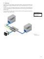
3. Intended Use
The camera is used to capture images that can be transferred over two GigE interfaces
to a PC.
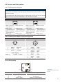
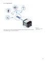
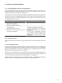
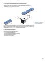
4. General Description
1
3
2
4
6
Nr.
Description
Nr.
5
Description
1
(respective) lens mount
4
Digial-IO supply
2
Power supply
5
GigE Port 1
3
GigE Port 0
6
Signaling-LED
7
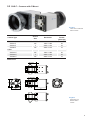
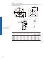
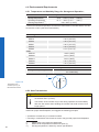
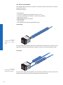
5. Camera Models
5.1 SXG – Cameras with C-Mount
Figure 1 ►
Front view of a Baumer
SXG C-Mount camera.
Sensor
Size
Resolution
Full
Frames
[max. fps]
SXG10
1/2"
1024 x 1024
120
SXG20
2/3"
1600 x 1200
68
SXG21
2/3"
1920 x 1080
64
SXG40
1"
2336 x 1752
32
SXG80
4/3"
3296 x 2472
16
SXG10c
1/2"
1024 x 1024
120
SXG20c
2/3"
1600 x 1200
68
SXG21c
2/3"
1920 x 1080
64
SXG40c
1"
2336 x 1752
32
SXG80c
4/3"
3296 x 2472
16
Camera Type
Monochrome
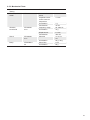
Color
Dimensions
36
26
UNC 1/4 20
36
26
52
16 x M3 depth 6
72
Figure 2 ►
Dimensions of a
Baumer SXG camera.
8
36
26
52
5.2 SXG-F – Cameras with F-Mount
◄ Figure 3
Front view of a Baumer
SXG-F camera.
Sensor
Size
Resolution
Full
Frames
[max. fps]
SXG21-F
2/3"
1920 x 1080
64
SXG40-F
1"
2336 x 1752
32
SXG80-F
4/3"
3296 x 2472
16
SXG21c-F
2/3"
1920 x 1080
64
SXG40c-F
1"
2336 x 1752
32
SXG80c-F
4/3"
3296 x 2472
16
Camera Type
Monochrome
Color
Dimensions
36
26
UNC 1/4 20
36
26
52
16 x M3 depth 6
72
36
26
52
◄ Figure 4
Dimensions of a
Baumer SXG-F
camera.
9
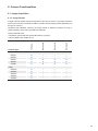
6. Product Specifications
6.1 Sensor Specifications
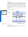
6.1.1 Quantum Efficiency for Baumer SXG Cameras
The quantum efficiency characteristics of monochrome and color matrix sensors for
Baumer SXG cameras are displayed in the following graphs. The characteristic curves for
the sensors do not take the characteristics of lenses and light sources without filters into
consideration, but are measured with an AR coated cover glass.
Figure 5 ►
Quantum efficiency for
Baumer SXG cameras.
Quantum Efficiency [%]
Quantum Efficiency [%]
Values relating to the respective technical data sheets of the sensors manufacturer.
350
450
550
650
750
SXG (monochrome)
850
950
1050
Wave Length [nm]
350
450
550
650
SXG (color)
750
850
950
1050
Wave Length [nm]
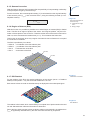
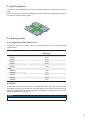
6.1.2 Progressive Scan
All cameras of the SXG series are equipped with Progressive Scan.
Microlens
Figure 6 ►
Structure of an imaging
sensor with global shutter (interline).
Pixel
Active Area (Photodiode)
Storage Area
Progressive Scan means that all pixels of the sensor are reset and afterwards exposed
for a specified interval (texposure).
For each pixel an adjacent storage area exists. Once the exposure time elapsed, the
information of a pixel is transferred immediately to its storage area and read out from
there.
Due to the fact that photosensitive surface gets "lost" by the implementation of the storage
area, the pixels are mostly equipped with microlenses, which focus the light to the pixels
active area.
10
6.1.3 Readout Modes
The Kodak sensors, used in Baumer SXG cameras, are subdivided into four Taps.
◄ Figure 7
Taps of the sensor.
Due to Baumer's integrated calibration technique, these taps are invisible within the recorded images, but affect the operation and the rate of the readout process and therewith
the readout time (treadout).
6.1.3.1 Quad Mode
On quad readout mode all four taps are read out simultaneously as displayed in the subsequent figure.
◄ Figure 8
Quad Tap Readout
Mode.
The data of all pixels of one tap are moved to the output register and afterwards transfered to the memory.
Once the information have left the output register, the readout is done.
This mode provides the full potential of the sensor and leads to the maximum frame
rate.
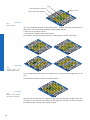
6.1.3.2 Dual Mode
On dual readout mode two taps (Tap 1 + Tap 2 and Tap 3 + Tap 4) are combined.
◄ Figure 9
Dual Tap Readout
Mode.
The data of all pixels of one tap are moved to the output register and afterwards transfered to the memory.
Once the information have left the output register, the readout is finished.
Due to the fact, that more data needs to be read out, the treadout is increased compared to
the quad readout mode.
It is considered:
treadout(Dual Mode) ≈ 2 × treadout(Quad Mode)
11
6.1.3.3 Single Mode
In single readout mode all taps are combined as displayed in the subsequent figure.
Figure 10 ►
Single Tap Readout
Mode.
The data of all pixels of the sensor are moved to the output register and afterwards transfered to the memory.
Once the information have left the output register, the readout is done.
Due to the fact, that the complete sensor needs to be read out, the readout time treadout is
increased compared to quad and dual readout mode.
It is considered:
12
treadout(Single Mode) ≈ 4 × treadout(Quad Mode)
6.2 Timings
The image acquisition consists of two seperate, successively processed components.
Exposing the pixels on the photosensitive surface of the sensor is only the first part of the
image acquisition. After completion of the first step, the pixels are read out.
Thereby the exposure time (texposure) can be adjusted by the user, however, the time needed for the readout (treadout) is given by the particular sensor and image format.
Baumer cameras can be operated with two modes, the Free Running Mode and the
Trigger Mode.
The cameras can be operated non-overlapped*) or overlapped. Depending on the mode
used, and the combination of exposure and readout time:
Non-overlapped Operation
Overlapped Operation
Here the time intervals are long enough
to process exposure and readout successively.
In this operation the exposure of a frame
(n+1) takes place during the readout of
frame (n).
Exposure
Exposure
Readout
Readout
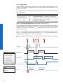
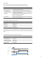
6.2.1 Free Running Mode
In the "Free Running" mode the camera records images permanently and sends them to
the PC. In order to achieve an optimal (with regard to the adjusted exposure time texposure
and image format) the camera is operated overlapped.
In case of exposure times equal to / less than the readout time (texposure ≤ treadout), the maximum frame rate is provided for the image format used. For longer exposure times the
frame rate of the camera is reduced.
Exposure
texposure(n)
treadout(n)
Readout
tflash(n)
Flash
texposure(n+1)
tflash(n+1)
tflashdelay
treadout(n+1)
Timings:
A - exposure time
frame (n) effective
B - image parameters frame (n) effective
C - exposure time
frame (n+1) effective
D - image parameters frame (n+1) effective
Image parameters:
Offset
Gain
Mode
Partial Scan
tflash = texposure
*)
Non-overlapped means the same as sequential.
13
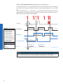
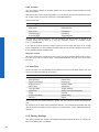
6.2.2 Trigger Mode
After a specified external event (trigger) has occurred, image acquisition is started. Depending on the interval of triggers used, the camera operates non-overlapped or overlapped in this mode.
With regard to timings in the trigger mode, the following basic formulas need to be taken
into consideration:
Case
texposure < treadout
texposure > treadout
Formula
(1)
(2)
(3)
(4)
tearliestpossibletrigger(n+1) = treadout(n) - texposure(n+1)
tnotready(n+1) = texposure(n) + treadout(n) - texposure(n+1)
tearliestpossibletrigger(n+1) = texposure(n)
tnotready(n+1) = texposure(n)
6.2.2.1 Overlapped Operation: texposure(n+2) = texposure(n+1)
In overlapped operation attention should be paid to the time interval where the camera is
unable to process occuring trigger signals (tnotready). This interval is situated between two
exposures. When this process time tnotready has elapsed, the camera is able to react to
external events again.
After tnotready has elapsed, the timing of (E) depends on the readout time of the current image (treadout(n)) and exposure time of the next image (texposure(n+1)). It can be determined by the
formulas mentioned above (no. 1 or 3, as is the case).
In case of identical exposure times, tnotready remains the same from acquisition to acquisition.
Trigger
tmin
ttriggerdelay
Timings:
A - exposure time
frame (n) effective
B - image parameters frame (n) effective
C - exposure time
frame (n+1) effective
D - image parameters frame (n+1) effective
E - earliest possible trigger
Image parameters:
Offset
Gain
Mode
Partial Scan
14
Exposure
texposure(n)
treadout(n)
Readout
TriggerReady
Flash
texposure(n+1)
treadout(n+1)
tnotready
tflash(n)
tflashdelay
tflash(n+1)
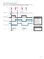
6.2.2.2 Overlapped Operation: texposure(n+2) > texposure(n+1)
If the exposure time (texposure) is increased form the current acquisition to the next acquisition, the time the camera is unable to process occuring trigger signals (tnotready) is scaled
down.
This can be simulated with the formulas mentioned above (no. 2 or 4, as is the case).
Trigger
tmin
ttriggerdelay
Exposure
texposure(n)
treadout(n)
Readout
TriggerReady
Flash
texposure(n+1)
treadout(n+1)
tnotready
tflash(n)
tflashdelay
texposure(n+2)
tflash(n+1)
Timings:
A - exposure time
frame (n) effective
B - image parameters frame (n) effective
C - exposure time
frame (n+1) effective
D - image parameters frame (n+1) effective
E - earliest possible trigger
Image parameters:
Offset
Gain
Mode
Partial Scan
15
6.2.2.3 Overlapped Operation: texposure(n+2) < texposure(n+1)
If the exposure time (texposure) is decreased from the current acquisition to the next acquisition, the time the camera is unable to process occuring trigger signals (tnotready) is scaled
up.
When decreasing the texposure such, that tnotready exceeds the pause between two incoming
trigger signals, the camera is unable to process this trigger and the acquisition of the image will not start (the trigger will be skipped).
Trigger
tmin
ttriggerdelay
Timings:
A - exposure time
frame (n) effective
B - image parameters frame (n) effective
C - exposure time
frame (n+1) effective
D - image parameters frame (n+1) effective
E - earliest possible trigger
F - frame not started /
trigger skipped
Image parameters:
Offset
Gain
Mode
Partial Scan
Exposure
texposure(n)
treadout(n)
Readout
TriggerReady
Flash
texposure(n+1)
texposure(n+2
treadout(n+1)
tnotready
tflash(n)
tflash(n+1)
tflashdelay
Notice
From a certain frequency of the trigger signal, skipping triggers is unavoidable. In general, this frequency depends on the combination of exposure and readout times.
16
6.2.2.4 Non-overlapped Operation
If the frequency of the trigger signal is selected for long enough, so that the image acquisitions (texposure + treadout) run successively, the camera operates non-overlapped.
Trigger
tmin
ttriggerdelay
Exposure
texposure(n)
treadout(n)
Readout
TriggerReady
Flash
texposure(n+1)
treadout(n+1)
tnotready
tflash(n)
tflashdelay
tflash(n+1)
Timings:
A - exposure time
frame (n) effective
B - image parameters frame (n) effective
C - exposure time
frame (n+1) effective
D - image parameters frame (n+1) effective
E - earliest possible trigger
Image parameters:
Offset
Gain
Mode
Partial Scan
17
6.3 Field of View Position
The typical accuracy by assumption of the root mean square value is displayed in the
figures and the table below:
±ß
±YR
±YM
±X M
±X R
Photosensitive
surface of the
sensor
Figure 11 ►
Sensor accuracy of
Baumer SXG cameras.
18
±Z
Camera
Type
± xM,typ
[mm]
± yM,typ
[mm]
± xR,typ
[mm]
± yR,typ
[mm]
± βtyp
[°]
SXG10
0,11
0,11
0,11
0,11
SXG20
0,11
0,11
0,11
SXG21
0,11
0,11
0,11
SXG40
0,11
0,11
SXG80
0,11
0,11
± ztyp
[mm]
± ztyp
[mm]
0,51
0,025
-
0,11
0,51
0,025
-
0,11
0,51
0,025
0,05
0,11
0,11
0,55
0,025
0,05
0,11
0,11
0,47
0,025
0,05
(C-Mount) (F-Mount)
6.4 Process- and Data Interface
6.4.1 Pin-Assignment Interface
Notice
Both data ports supports Power over Ethernet (38 VDC .. 57 VDC). Both ports can be
connected to a PoE power sourcing equipment however only one port will be used to
power the camera.
For the data transfer, the ports are equal. For Single GigE connect one Port and for Dual
GigE connect the second Port additionally. The order does not matter.
Data / Control 1000 Base-T (Port 0)
LED2
LED2
LED1
8
1
LED1
8
1 MX1+ (green/white) 5 MX3- (blue/white)
(negative/positive Vport)
2 MX1- (green)
Data / Control 1000 Base-T (Port 1)
1
1 MX1+ (green/white)
5 MX3- (blue/white)
(negative/positive Vport)
6 MX2- (orange)
(negative/positive Vport)
(positive/negative Vport)
2 MX1- (green)
6 MX2- (orange)
(negative/positive Vport)
(positive/negative Vport)
3 MX2+ (orange/white) 7 MX4+ (brown/white) 3 MX2+ (orange/white)
(positive/negative Vport)
4 MX3+ (blue)
7 MX4+ (brown/white)
(positive/negative Vport)
8 MX4- (brown)
4 MX3+ (blue)
8 MX4- (brown)
6.4.2 Pin-Assignment Power Supply and Digital IOs
M8 / 3 pins
M8 / 8 pins
3
4
3
1
5
(brown)
3
(blue)
4
(black)
7
1
Power VCC
1
(white)
Line 5
GND
2
(brown)
Line 1
not used
3
(green)
Line 0
4
(yellow)
GND
5
(grey)
6
(pink)
Uext
Line 3
7
(blue)
Line 4
8
(red)
Line 2
Power Supply
Power VCC
8
6
4
1
2
20 VDC ... 30 VDC
6.4.3 LED Signaling
3
◄ Figure 12
LED positions on Baumer SXG
camera.
1
2
LED
Signal
Meaning
1
green / green flash
Link active / Receiving
2
yellow
Transmitting
3
green / yellow
Power on / Readout active
19
6.5 Environmental Requirements
6.5.1 Temperature and Humidity Range for Storage and Operation*)
Temperature
Storage temperature
-10°C ... +70°C ( +14°F ... +158°F)
Operating temperature*
Housing temperature
+5 °C ... +60°C (+41°F ... +140°F)
max. +60°C (+140°F)
**)***)
* If the environmental temperature exceeds the values listed in the table below, the camera must be cooled. (see Heat Transmission)
Camera Type
Environmental Temperature
Monochrome
SXG10
+19°C (+66.2°F)
SXG20
+18°C (+64.4°F)
SXG21
+18°C (+64.4°F)
SXG40
+16°C (+60.8°F)
SXG80
+14°C (+57.2°F)
Color
SXG10c
+20°C (+68°F)
SXG20c
+20°C (+68°F)
SXG21c
+20°C (+68°F)
SXG40c
+19°C (+66.2°F)
SXG80c
+19°C (+66.2°F)
Humidity
Storage and Operating Humidity
10% ... 90%
non condensing
T
Figure 13 ►
Temperature measurement point (T) of
Baumer SXG cameras.
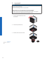
6.5.2 Heat Transmission
Caution
Provide adequate dissipation of heat, to ensure that the temperature does
not exceed +60°C (+140°F).
The surface of the camera may be hot during operation and immediately
after use. Be careful when handling the camera and avoid contact over a
longer period.
As there are numerous possibilities for installation, Baumer does not specifiy a specific
method for proper heat dissipation, but suggest the following principles:
▪▪ operate the cameras only in mounted condition
▪▪ mounting in combination with forced convection may provide proper heat dissipation
20
*)
**)
***)
Please refer to the respective data sheet.
Measured at temperature measurement point (T).
Housing temperature is limited by sensor specifications.
6.5.3 Mechanical Tests
Environmental
Testing
Standard
Parameter
Vibration, sinusodial
IEC 60068-2-6
Search for Resonance
10-2000 Hz
Amplitude underneath crossover
frequencies
1.5 mm
Acceleration
1g
Test duration
15 min
Frequency range
20-1000 Hz
Acceleration
10 g
Displacement
5.7 mm
Test duration
300 min
Puls time
11 ms / 6
ms
Acceleration
50 g / 80 g
Pulse Time
2 ms
Acceleration
80 g
Vibration,
broad band
Shock
Bump
IEC 600682-64
IEC 600682-27
IEC60068-229
21
7. Software
7.1 Baumer-GAPI
Baumer-GAPI stands for Baumer “Generic Application Programming Interface”. With this
API Baumer provides an interface for optimal integration and control of Baumer Gigabit
Ethernet (GigE) , Baumer CameraLink® and Baumer FireWire™ (IEEE1394) cameras.
This software interface allows changing to other camera models or interfaces. It also allows the simultaneous operation of Baumer cameras with Gigabit Ethernet, CameraLink®
and FireWire™ interfaces.
This GAPI supports Windows® (XP, Vista and Win 7) and Linux® (from Kernel 2.6.x) operating systems in 32 bit, as well as in 64 bit. It provides interfaces to several programming
languages, such as C, C++ and the .NET™ Framework on Windows®, as well as Mono
on Linux® operating systems, which offers the use of other languages, such as e.g. C# or
VB.NET.
The SXG camera features are supported from BGAPI V 1.7.0
7.2 3rd Party Software
Strict compliance with the Gen<I>Cam™ standard allows Baumer to offer the use of 3rd
Party Software for operation with cameras of the SX series.
You can find a current listing of 3rd Party Software, which was tested successfully in combination with Baumer cameras, at http://www.baumer.com.
22
8. Camera Functionalities
8.1 Image Acquisition
8.1.1 Image Format
A digital camera usually delivers image data in at least one format - the native resolution
of the sensor. Baumer cameras are able to provide several image formats (depending on
the type of camera).
Compared with standard cameras, the image format on Baumer cameras not only includes resolution, but a set of predefined parameter.
Full frame
Binning 2x2
Binning 1x2
Binning 2x1
These parameters are:
▪▪ Resolution (horizontal and vertical dimensions in pixels)
▪▪ Binning Mode (see chapter 8.1.8)
SXG10
■
□
□
□
SXG20
■
□
□
□
SXG21
■
■
■
■
SXG40
■
■
■
■
SXG80
■
■
■
■
SXG10c
■
□
□
□
SXG20c
■
□
□
□
SXG21c
■
□
□
□
SXG40c
■
□
□
□
SXG80c
■
□
□
□
Camera Type
Monochrome
Color
23
8.1.2 Pixel Format
On Baumer digital cameras the pixel format depends on the selected image format.
Mono 8
Mono 10
Mono 12
Bayer RG 8
Bayer RG 10
Bayer RG 12
8.1.2.1 Pixel Formats on Baumer SXG Cameras
SXG10
■
■
■
□
□
□
SXG20
■
■
■
□
□
□
SXG21
■
■
■
□
□
□
SXG40
■
■
■
□
□
□
SXG80
■
■
■
□
□
□
SXG10c
□
□
□
■
■
■
SXG20c
□
□
□
■
■
■
SXG21c
□
□
□
■
■
■
SXG40c
□
□
□
■
■
■
SXG80c
□
□
□
■
■
■
Camera Type
Monochrome
Color
8.1.2.2 Definitions
Notice
Below is a general description of pixel formats. The table above shows, which camera
support which formats.
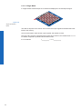
Bayer:
Raw data format of color sensors.
Color filters are placed on these sensors in a checkerboard pattern, generally
in a 50% green, 25% red and 25% blue array.
Mono:
Monochrome. The color range of mono images consists of shades of a single
color. In general, shades of gray or black-and-white are synonyms for monochrome.
Figure 14 ►
Sensor with Bayer
Pattern.
24
RGB:
Color model, in which all detectable colors are defined by three coordinates,
Red, Green and Blue.
Red
White
Black
◄ Figure 15
RBG color space displayed as color tube.
Green
Blue
The three coordinates are displayed within the buffer in the order R, G, B.
BGR:
Here the color alignment mirrors RGB.
YUV:
Color model, which is used in the PAL TV standard and in image compression.
In YUV, a high bandwidth luminance signal (Y: luma information) is transmitted
together with two color difference signals with low bandwidth (U and V: chroma
information). Thereby U represents the difference between blue and luminance
(U = B - Y), V is the difference between red and luminance (V = R - Y). The third
color, green, does not need to be transmitted, its value can be calculated from
the other three values.
YUV 4:4:4
Here each of the three components has the same sample rate.
Therefore there is no subsampling here.
YUV 4:2:2
The chroma components are sampled at half the sample rate.
This reduces the necessary bandwidth to two-thirds (in relation to
4:4:4) and causes no, or low visual differences.
YUV 4:1:1
Here the chroma components are sampled at a quater of the
sample rate.This decreases the necessary bandwith by half (in
relation to 4:4:4).
Pixel depth: In general, pixel depth defines the number of possible different values for
each color channel. Mostly this will be 8 bit, which means 28 different "colors".
For RGB or BGR these 8 bits per channel equal 24 bits overall.
8 bit:
Byte 1
10 bit:
Byte 2
Byte 3
◄ Figure 16
Bit string of Mono 8 bit
and RGB 8 bit.
unused bits
Byte 1
12 bit:
Byte 2
unused bits
Byte 1
◄ Figure 17
Spreading of Mono 10
bit over 2 bytes.
◄ Figure 18
Spreading of Mono 12
bit over two bytes.
Byte 2
25
8.1.3 Exposure Time
On exposure of the sensor, the inclination of photons produces a charge separation on
the semiconductors of the pixels. This results in a voltage difference, which is used for
signal extraction.
Light
Photon
Charge Carrier
Pixel
Figure 19 ►
Incidence of light causes
charge separation on
the semiconductors of
the sensor.
The signal strength is influenced by the incoming amount of photons. It can be increased
by increasing the exposure time (texposure).
On Baumer SXG cameras, the exposure time can be set within the following ranges (step
size 1μsec):
Camera Type
texposure min
texposure max
SXG10
10 μsec
1 sec
SXG20
10 μsec
1 sec
SXG21
10 μsec
1 sec
SXG40
10 μsec
1 sec
SXG80
10 μsec
1 sec
SXG10c
10 μsec
1 sec
SXG20c
10 μsec
1 sec
SXG21c
10 μsec
1 sec
SXG40c
10 μsec
1 sec
SXG80c
10 μsec
1 sec
Monochrome
Color
8.1.4 Look-Up-Table
The Look-Up-Table (LUT) is employed on Baumer monochrome cameras. It contains 212
(4096) values for the available levels of gray. These values can be adjusted by the user.
26
8.1.5 Gamma Correction
H
With this feature, Baumer SXG cameras offer the possibility of compensating nonlinearity
in the perception of light by the human eye.
For this correction, the corrected pixel intensity (Y') is calculated from the original intensity
of the sensor's pixel (Yoriginal) and correction factor γ using the following formula (in oversimplified version):
γ
Y' = Yoriginal
8.1.6 Region of Interest (ROI)
0
E
▲ Figure 20
Non-linear perception of
the human eye.
H -Perception of bright-
ness
E - Energy of light
With this function it is possible to predefine a so-called Region of Interest (ROI) or Partial
Scan. This ROI is an region of pixels of the sensor. On image acquisition, only the information of these pixels is sent to the PC. Therefore all the lines of the sensor need not be
read out, which decreases the readout time (treadout). This increases the frame rate.
This function is employed, when only a region of the field of view is of interest. It is coupled
to a reduction in resolution.
The ROI is specified by four values:
▪▪ Offset X - x-coordinate of the first relevant pixel
▪▪ Offset Y - y-coordinate of the first relevant pixel
▪▪ Size X - horizontal size of the ROI
▪▪ Size Y - vertical size of the ROI
Start ROI
End ROI
8.1.7 ROI Readout
◄ Figure 21
Parameters of the ROI.
For the readout of the ROI, the vertical subdivision of the sensor (see 6.1.3. Readout
Modes) is unimportant – only the horizontal subdivision is of note.
Both sensor halves are read out simultaneously as displayed in the subsequent figure.
◄ Figure 22
ROI: Readout.
The readout is line based, which means always a complete line of pixels needs to be read
out and afterwards the irrelevant information is discarded.
Due to the fact, that the sensor halves are always read out symmetrically, the readout time
treadout is significantly affected both by the size of the ROI and also by its position.
27
ROI
Pixel Information of Interrest
Read out Lines
Discarded Pixel Information
Figure 23 ►
ROI:
Read out Lines.
The most significant reduction of the readout time – compared to a full frame readout in
dual mode – can be achieved if the ROI is positioned as follows:
▪▪ within one of the sensor halves
▪▪ symmetrically spread to both sensor halves
For example, the readout time of the ROI's in the figures 21 and 22 is the same.
Figure 24 ►
ROI:
Example ROI's with
identical readout times.
On asymmetrically spread ROI's, the readout time is affected by the bigger part of the
ROI.
An example for this fact is shown in the figure below:
Figure 25 ►
ROI:
Read out time linked
with position of the ROI.
The ROI has the same size as in figure 21, but is not symmetrically spread to both sensor halves. In this special case the time for the readout of the same number of pixels is
increased by 50%, caused only by ROI's position.
28
8.1.8 Binning
On digital cameras, you can find several operations for progressing sensitivity. One of
them is the so-called "Binning". Here, the charge carriers of neighboring pixels are aggregated. Thus, the progression is greatly increased by the amount of binned pixels. By using
this operation, the progression in sensitivity is coupled to a reduction in resolution.
Baumer cameras support three types of Binning - vertical, horizontal and bidirectional.
In unidirectional binning, vertically or horizontally neighboring pixels are aggregated and
reported to the software as one single "superpixel".
In bidirectional binning, a square of neighboring pixels is aggregated.
Binning
Illustration
Example
without
◄ Figure 26
Full frame image, no
binning of pixels.
1x2
◄ Figure 27
Vertical binning causes
a vertically compressed
image with doubled
brightness.
2x1
◄ Figure 28
Horizontal
binning
causes a horizontally
compressed image with
doubled brightness.
2x2
◄ Figure 29
Bidirectional
binning
causes both a horizontally and vertically
compressed image with
quadruple brightness.
29
8.1.9 Brightness Correction (Binning Correction)
The aggregation of charge carriers may cause an overload. To prevent this, binning correction was introduced. Here, three binning modes need to be considered separately:
Binninig
Realization
1x2
1x2 binning is performed within the sensor, binning correction also takes
place here. A possible overload is prevented by halving the exposure time.
2x1
2x1 binning takes place within the FPGA of the camera. The binning correction is realized by aggregating the charge quantities, and then halving
this sum.
2x2
2x2 binning is a combination of the above versions.
Total charge
quantity of the
4 aggregated
pixels
Binning 2x2
Figure 30 ►
Aggregation of charge
carriers from four pixels
in bidirectional binning.
Charge quantity
Super pixel
8.2 Color Adjustment – White Balance
This feature is available on all color cameras of the Baumer SXG series and takes
place within the Bayer processor.
White balance means independent adjustment of the three color channels, red,
green and blue by employing of a correction factor for each channel.
8.2.1 User-specific Color Adjustment
The user-specific color adjustment in Baumer color cameras facilitates adjustment of the
correction factors for each color gain. This way, the user is able to adjust the amplification of each color channel exactly to his needs. The correction factors for the color gains range from 1 to 4.
non-adjusted
histogramm
histogramm after
user-specific
color adjustment
Figure 31 ►
Examples of histogramms for a nonadjusted image and for
an image after userspecific white balance..
8.2.2 One Push White Balance
Here, the three color spectrums are balanced to a single white point. The correction factors of the color gains are determined by the camera (one time).
non-adjusted
histogramm
Figure 32 ►
Examples of histogramms for a non-adjusted image and for an
image after "one push"
white balance.
30
histogramm after
„one push“ white
balance
8.3 Auto Tap Balance
The feature "Auto Tap Balance" corrects the possible differences in brightness of the four
Taps.
This is achieved by calculating the average of the brightness of the pixels at the border of
the taps (on the figure below green).
8.4 Analog Controls
8.4.1 Brightness (Offset / Black Level)
On Baumer cameras, the Offset / Black Level is adjustable from 0 to 1023 LSB (least
significant bit).
Camera Type
Step Size 1 LSB
Relating to
Monochrome
SXG10
14 bit
SXG20
14 bit
SXG21
14 bit
SXG40
14 bit
SXG80
14 bit
Color
SXG10c
14 bit
SXG20c
14 bit
SXG21c
14 bit
SXG40c
14 bit
SXG80c
14 bit
8.4.2 Gain
In industrial environments motion blur is unacceptable. Due to this fact exposure times
are limited. However, this causes low output signals from the camera and results in dark
images. To solve this issue, the signals can be amplified by user within the camera. This
gain is adjustable from 0 to 26 db.
Notice
Increasing the gain factor causes an increase of image noise.
31
8.5 Pixel Correction
8.5.1 General information
A certain probability for abnormal pixels - the so-called defect pixels - applies to the sensors of all manufacturers. The charge quantity on these pixels is not linear-dependent on
the exposure time.
The occurrence of these defect pixels is unavoidable and intrinsic to the manufacturing
and aging process of the sensors.
The operation of the camera is not affected by these pixels. They only appear as brighter
(warm pixel) or darker (cold pixel) spot in the recorded image.
Warm Pixel
Figure 33 ►
Distinction of "hot" and
"cold" pixels within the
recorded image.
Cold Pixel
Charge quantity
„Warm Pixel“
Figure 34 ►
Charge quantity of "hot" and
"cold" pixels compared with
"normal" pixels.
Charge quantity
„Normal Pixel“
Charge quantity
„Cold Pixel“
8.5.2 Correction Algorithm
On monochrome cameras of the Baumer SXG series, the problem of defect pixels is
solved as follows:
▪▪ Possible defect pixels are identified during the production process of the camera.
▪▪ The coordinates of these pixels are stored in the factory settings of the camera (see
8.5.3 Defectpixellist).
▪▪ Once the sensor readout is completed, correction takes place:
▪▪ Before any other processing, the values of one neighboring pixels on the left and the
right side of the defect pixel, will be read out
▪▪ Then the average value of these 2 pixels is determined
▪▪ Finally, the value of the defect pixel is substituted by the previously determined
average value
Defect Pixel
Figure 35 ►
Schematic diagram of
the Baumer pixel
correction.
Average Value
Corrected Pixel
8.5.3 Defectpixellist
As stated previously, this list is determined within the production process of Baumer cameras and stored in the factory settings. This list is editable.
32
8.6 Sequencer
8.6.1 General Information
A sequencer is used for the automated control of series of images using different sets of
parameters.
n0
n1
A
m
B
o
n2
C
z
◄ Figure 36
Flow chart of
sequencer.
m - number of sequence repeti-
tions
n - number of set
repetitions
o - number of
sets of parameters
z - number of frames
per trigger
nx-1
The figure above displays the fundamental structure of the sequencer module.
The loop counter (m) represents the number of sequence repetitions.
The repeat counter (n) is used to control the amount of images taken with the respective
sets of parameters. For each set there is a separate n.
The start of the sequencer can be realized directly (free running) or via an external event
(trigger). The source of the external event (trigger source) must be determined before.
The additional frame counter (z) is used to create a half-automated sequencer. It is absolutely independent from the other three counters, and used to determine the number of
frames per external trigger event.
Sequencer Parameter:
The mentioned sets of
parameter include the following:
▪▪ Exposure time
▪▪ Gain factor
▪▪ Repeat counter
▪▪ IO-Value
The following timeline displays the temporal course of a sequence with:
▪▪ n = (A=5), (B=3), (C=2) repetitions per set of parameters
▪▪ o = 3 sets of parameters (A,B and C)
▪▪ m = 1 sequence and
▪▪ z = 2 frames per trigger
A
n=1
n=2
z=2
B
n=3
n=4
z=2
n=5
n=1
z=2
n=2
C
n=3
z=2
n=1
n=2
z=2
t
◄ Figure 37
Timeline for a single
sequence
33
8.6.2 Examples
8.6.2.1 Sequencer without Machine Cycle
C
C
Sequencer
Start
B
B
A
Figure 38 ►
Example for a fully automated sequencer.
A
The figure above shows an example for a fully automated sequencer with three sets of
parameters (A,B and C). Here the repeat counter (n) is set for (A=5), (B=3), (C=2) and the
loop counter (m) has a value of 2.
When the sequencer is started, with or without an external event, the camera will record
the pictures using the sets of parameters A, B and C (which constitutes a sequence).
After that, the sequence is started once again, followed by a stop of the sequencer - in this
case the parameters are maintained.
8.6.2.2 Sequencer Controlled by Machine Steps (trigger)
C
C
Sequencer
Start
B
B
A
Figure 39 ►
Example for a half-automated sequencer.
A
Trigger
The figure above shows an example for a half-automated sequencer with three sets of
parameters (A,B and C) from the previous example. The frame counter (z) is set to 2. This
means the camera records two pictures after an incoming trigger signal.
8.6.3 Capability Characteristics of Baumer-GAPI Sequencer Module
▪▪ up to 128 sets of parameters
▪▪ up to 4 billion loop passes
▪▪ up to 4 billion repetitions of sets of parameters
▪▪ up to 4 billion images per trigger event
▪▪ free running mode without initial trigger
34
8.6.4 Double Shutter
This feature offers the possibility of capturing two images in a very short interval. Depending on the application, this is performed in conjunction with a flash unit. Thereby the first
exposure time (texposure) is arbitrary and accompanied by the first flash. The second exposure time must be equal to, or longer than the readout time (treadout) of the sensor. Thus the
pixels of the sensor are recepitve again shortly after the first exposure. In order to realize
the second short exposure time without an overrun of the sensor, a second short flash
must be employed, and any subsequent extraneous light prevented.
Trigger
Flash
Exposure
Prevent Light
◄ Figure 40
Example of a double
shutter.
Readout
On Baumer SXG cameras this feature is realized within the sequencer.
In order to generate this sequence, the sequencer must be configured as follows:
Parameter
Setting:
Sequencer Run Mode
Once by Trigger
Sets of parameters (o)
2
Loops (m)
1
Repeats (n)
1
Frames Per Trigger (z)
2
35
8.7 Process Interface
8.7.1 Digital IOs
Cameras of the Baumer SXG series are equipped with three input lines and three output
lines.
8.7.1.1 IO Circuits
Notice
Low Active: At this wiring, only one consumer can be connected. When all Output pins
(1, 2, 3) connected to IO_GND, then current flows through the resistor as soon as one
Output is switched. If only one output connected to IO_GND, then this one is only usable.
The other two Outputs are not usable and may not be connected (e.g. IO Power VCC)!
Output high active
Camera
Output low active
Customer Device
Uext Pin
Camera
Customer Device
IO Power VCC
IO Power VCC
DRV
Camera
IN1 Pin
RL
IOUT
Out (n)
Pin
Input
Customer Device
Out
Uext Pin (Out1, 2, 3)
RL
IOUT
IO GND
IO GND
IN GND Pin
IO GND
Out1 or Out2
or Out3
8.7.1.2 User Definable Inputs
The wiring of these input connectors is left to the user.
Sole exception is the compliance with predetermined high and low levels (0 .. 4,5V low,
11 .. 30V high).
The defined signals will have no direct effect, but can be analyzed and processed on the
software side and used for controlling the camera.
The employment of a so called "IO matrix" offers the possibility of selecting the signal and
the state to be processed.
On the software side the input signals are named "Line0", "Line1" and "Line2".
state selection
(software side)
state high
Line0
(Input) Line0
state low
state high
(Input) Line1
Line1
state low
state high
(Input) Line2
Figure 41►
IO matrix of the
Baumer SXG on input
side.
36
Line2
state low
IO Matrix
8.7.1.3 Configurable Outputs
With this feature, Baumer offers the possibility of wiring the output connectors to internal
signals, which are controlled on the software side.
Hereby on cameras of the SXG series, 17 signal sources – subdivided into three categories – can be applied to the output connectors.
The first category of output signals represents a loop through of signals on the input side,
such as:
Signal Name
Explanation
Line0
Signal of input "Line0" is loopthroughed to this ouput
Line1
Signal of input "Line1" is loopthroughed to this ouput
Line2
Signal of input "Line2" iys loopthroughed to this ouput
Within the second category you will find signals that are created on camera side:
Signal Name
Explanation
FrameActive
The camera processes a Frame consisting of exposure
and readout
TriggerReady
Camera is able to process an incoming trigger signal
TriggerOverlapped
The camera operates in overlapped mode
TriggerSkipped
Camera rejected an incoming trigger signal
ExposureActive
Sensor exposure in progress
TransferActive
Image transfer via hardware interface in progress
ExposureEnlarged
This output marks the period of enlarged exposure time
state low
state high
(Output) Line 4
state low
state high
(Output) Line 5
state low
IO Matrix
Off
Line0
Line1
Line2
Loopthroughed
Signals
state high
(Output) Line 3
signal selection
(software side)
FrameActive
TriggerReady
TriggerOverlapped
TriggerSkipped
ExposureActive
TransferActive
ExposureEnlarged
UserOutput0
UserOutput1
UserOutput2
Timer1Active
Timer2Active
Timer3Active
SequencerOutput0
SequencerOutput1
SequencerOutput2
User defined Signals
state selection
(software side)
nternal Signals
Beside the 10 signals mentioned above, each output can be wired to a user-defined
signal ("UserOutput0", "UserOutput1", "UserOutput2", "SequencerOut 0...2" or disabled
("OFF").
◄ Figure 42
IO matrix of the
Baumer SXG on output
side.
37
8.8 Trigger Input / Trigger Delay
U
30V
11V
4 5V
0
Trigger signals are used to synchronize the camera exposure and a machine cycle or, in
case of a software trigger, to take images at predefined time intervals.
high
Different trigger sources can be used here:
low
t
Figure 43 ▲
Trigger signal, valid for
Baumer cameras.
Line0
Actioncommand
Line1
Off
Line2
SW-Trigger
Possible settings of the Trigger Delay
Delay
0-2 sec
Number of tracked Triggers
512
Step
1 µsec
There are three types of trigger modes. The timing diagrams for the three types you can
see below.
Normal Trigger with adjusted Exposure
Trigger (valid)
A
Camera in trigger
mode:
A - Trigger delay
B - Exposure time
C - Readout time
Exposure
B
Readout
C
Time
Pulse Width controlled Exposure
Trigger (valid)
Exposure
B
Readout
C
Time
Edge controlled Exposure
Trigger (valid)
Exposure
B
Readout
C
Time
38
lo
able gic c
others
on
trol er
lectric se
m
pho
t
or
ns
oe
program
8.8.1 Trigger Source
Ha
a
rdw
re trigger
ger signal
trig
s
er
re trigg
twa
of
Each trigger source has to be activated separately. When the trigger mode is activated,
the hardware trigger is activated by default.
◄ Figure 44
Examples of possible
trigger sources.
39
8.8.2 Debouncer
The basic idea behind this feature was to seperate interfering signals (short peaks) from
valid square wave signals, which can be important in industrial environments. Debouncing
means that invalid signals are filtered out, and signals lasting longer than a user-defined
testing time tDebounceHigh will be recognized, and routed to the camera to induce a trigger.
In order to detect the end of a valid signal and filter out possible jitters within the signal, a
second testing time tDebounceLow was introduced. This timing is also adjustable by the user.
If the signal value falls to state low and does not rise within tDebounceLow, this is recognized
as end of the signal.
The debouncing times tDebounceHigh and tDebounceLow are adjustable from 0 to 5 msec in steps
of 1 μsec.
This feature is disabled by default.
Debouncer:
Please note that the edges
of valid trigger signals are
shifted by tDebounceHigh and
tDebounceLow!
Depending on these
two timings, the trigger
signal might be temporally
stretched or compressed.
U
30V
Incoming signals
(valid and invalid)
high
11V
4.5V
0
low
∆t1
∆t2
∆t3
∆t4
∆t5
t
∆t6
Debouncer
tDebounceHigh
U
t
tDebounceLow
30V
Filtered signal
11V
4.5V
high
low
0
t
∆tx
high time of the signal
tDebounceHigh user defined debouncer delay for state high
tDebounceLow user defined debouncer delay for state low
Figure 45 ►
Principle of the Baumer
debouncer.
8.8.3 Flash Signal
On Baumer cameras, this feature is realized by the internal signal "ExposureActive",
which can be wired to one of the digital outputs.
40
8.8.4 Timer
Timers were introduced for advanced control of internal camera signals.
On Baumer SXG cameras the timer configuration includes four components:
Setting
Description
Timeselector
There are three timers. Own settings for each timer can be
made. (Timer1, Timer2, Timer3)
TimerTriggerSource
This feature provides a source selection for each timer.
TimerTriggerActivation
This feature selects that part of the trigger signal (edges or
states) that activates the timer.
TimerDelay
This feature represents the interval between incoming trigger signal and the start of the timer.
(0 μsec .. 2 sec, step: 1 μsec)
TimerDuration
By this feature the activation time of the timer is adjustable.
(10 μsec .. 2 sec, step: 1 μsec)
Different Timer Trigger sources can be used:
Timer Trigger sources
Input Line0
Exposure Start
Input Line1
Exposure End
Input Line2
Frame Start
SW-Trigger
Frame End
ActionCommandTrigger
TriggerSkipped
For example the using of a timer allows you to control the flash signal in that way, that the
illumination does not start synchronized to the sensor exposure but a predefined interval
earlier.
For this example you must set the following conditions:
Setting
Value
TriggerSource
InputLine0
TimerTriggerSource
InputLine0
Outputline7 (Source)
Timer1Active
TimerTriggerActivation
Falling Edge
Trigger Polarity
Falling Edge
InputLine0
Exposure
Timer
ttriggerdelay
texposure
tTimerDelay
tTimerDuration
41
8.8.5 Counter
You can count the Events in the table below. The count values of these Events are readable and writable.
With the function "Event Source/activation" you can specify which event should be counted. These events can also be used as a CounterResetSource.
These events are:
CounterTriggerSources / CounterResetSources
Input Line0
ExposureStart
Input Line1
Input Line2
Softwaretrigger
ActCmdTrigger
ExposureEnd
FrameStart
FrameEnd
TriggerSkipped
You can set a counter duration. You can therefore set the number of events to be
counted. When the set value is 0, then the maximum number of countable events
is 232-1 (4294967295).
If you specify a value, then the counter counts up to that value and stops. Then a GigE
event is triggered ("Counter1/2End") and the status of the counter changes from ACTIVE
to the readable status COMPLETED.
Reset the counter
When the reset event is reached or the counter is reset by software with "reset counter",
then the count value is stored under "CounterValueAtReset" and set the counter value
back to 0.
8.9 User Sets
Three user sets (1-3) are available for the Baumer cameras of the SXG series. The user
sets can contain the following information:
Parameters
Binning Mode
Defectpixellist
Digital I/O Settings
Exposure Time
Gain Factor
Look-Up-Table
Sequencer
Timer
Fixed Frame Rate
Gamma
Mirroring Control
Partial Scan
Pixelformat
Readout Mode
Testpattern
Trigger Settings
Action Command Parameter
Counter
Frame Delay
Offset
These user sets are stored within the camera and and cannot be saved outside the device.
By employing a so-called "user set default selector", one of the three possible user sets
can be selected as default, which means, the camera starts up with these adjusted parameters.
8.10 Factory Settings
The factory settings are stored in an additional parametrization set which is used by default. This settings are not editable.
42
9. Interface Functionalities
9.1 Link Aggregation Group Configuration
Link Aggregation (LAG) allows grouping the two links of the SXG camera to form a “virtual” link, enabling the camera to treat the LAG as if it was a single link. This is done in a
transparent way from the application perspective.
It is important to note that LAG does not define the distribution algorithm to be used at the
transmission end of a link aggregation group. Since LAG shows a single MAC/IP, then
switches cannot figure out how to distribute the image traffic: the traffic might end-up on
one outgoing port of the switch.
Characteristic
Static LAG
Number of network interfaces
2
Number of IP address
1
Number of stream channels
1
Load balancing
Round-robin distribution algorithm
Physical link down recovery
Packets redistributed on remaining
physical link
Grouping configuration
All links are automatically grouped
on the device. Manual grouping must
be performed on the PC (often called
teaming)
9.1.1 Camera Control
The communication for the camera control is always sent on the same physical link of the
LAG.
9.1.2 Image data stream
A round-robin distribution algorithm allows for a uniform distribution of the bandwidth associated to the image data since all image packets have the same size. So it adequately
balances the bandwidth across the two available links. A suitable packet size must be
selected to ensure all physical links can handle it.
Because of this loose definition of conversation and the selected distribution algorithm, it
is necessary for the receiver of the image data to be tolerant to out-of-order packets and
accommodate longer timeouts than seen with Single Link configuration.
Special provision must be taken for the inter-packet delay: it represents the delay between packets of the image data stream travelling on a given physical link.
43
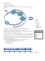
9.2 Device Information
This Gigabit Ethernet-specific information on the device is part of the Discovery-Acknowledge of the camera.
Included information:
▪▪ MAC address
▪▪ Current IP configuration (persistent IP / DHCP / LLA)
▪▪ Current IP parameters (IP address, subnet mask, gateway)
▪▪ Manufacturer's name
▪▪ Manufacturer-specific information
▪▪ Device version
▪▪ Serial number
▪▪ User-defined name (user programmable string)
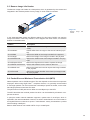
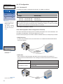
Single GigE
Figure 46 ►
Transmission of data
packets with single
GigE
By using Single GigE all data packets are sequentially transmitted over one cable. At the
beginning of a frame will transmitted a Header and at the end will transmitted a Trailer.
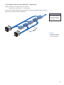
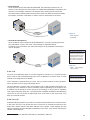
Dual GigE
Figure 47 ►
Transmission of data
packets with Dual GigE
44
By using Dual GigE the data packets are alternately distributed over both cables.The
Header and the Trailer are always transmitted over the same cable.
9.3 Baumer Image Info Header
The Baumer Image Info Header is a data packet, which is generated by the camera and
integrated in the first data packet of every image, if chunk mode is activated.
◄ Figure 48
Baumer Image
Header
Info
In this integrated data packet are different settings for this image. BGAPI can read the
Image Info Header. Third Party Software, which supports the chunk mode, can read the
features in the table below.
Feature
Description
ChunkOffsetX
Horizontal offset from the origin to the area of interest (in
pixels).
ChunkOffsetY
Vertical offset from the origin to the area of interest (in pixels).
ChunkWidth
Returns the Width of the image included in the payload.
ChunkHeight
Returns the Height of the image included in the payload.
ChunkPixelFormat
Returns the PixelFormat of the image included in the payload.
ChunkExposureTime
Returns the exposure time used to capture the image.
ChunkBlackLevelSelector
Selects which Black Level to retrieve data from.
ChunkBlackLevel
Returns the black level used to capture the image included
in the payload.
ChunkFrameID
Returns the unique Identifier of the frame (or image) included in the payload.
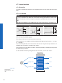
9.4 Packet Size and Maximum Transmission Unit (MTU)
Network packets can be of different sizes. The size depends on the network components
employed. When using GigE Vision®- compliant devices, it is generally recommended
to use larger packets. On the one hand the overhead per packet is smaller, on the other
hand larger packets cause less CPU load.
The packet size of UDP packets can differ from 576 Bytes up to the MTU.
The MTU describes the maximal packet size which can be handled by all network components involved.
In principle modern network hardware supports a packet size of 1518 Byte, which is
specified in the network standard. However, so-called "Jumboframes" are on the advance
as Gigabit Ethernet continues to spread. "Jumboframes" merely characterizes a packet
size exceeding 1500 Bytes.
Baumer SXG cameras can handle a MTU of up to 16384 Bytes.
45
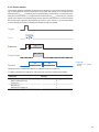
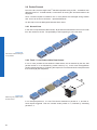
9.5 "Packet Delay" (PD)
To achieve optimal results in image transfer, several Ethernet-specific factors need to be
considered when using Baumer SXG cameras.
Upon starting the image transfer of a camera, the data packets are transferred at maximum transfer speed (1 Gbit/sec). In accordance with the network standard, Baumer employs a minimal separation of 12 Bytes between two packets. This separation is called
"Packet Delay" (PD). In addition to the minimal PD, the GigE Vision® standard stipulates
that the PD be scalable (user-defined).
Figure 49 ►
Principle of Packet Delay
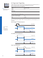
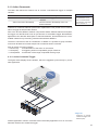
9.5.1 Example 1: Multi Camera Operation – Minimal IPG
Setting the IPG to minimum means every image is transfered at maximum speed. Even
by using a frame rate of 1 fps this results in full load on the network. Such "bursts" can
lead to an overload of several network components and a loss of packets. This can occur,
especially when using several cameras.
▲ Figure 50
Operation of two cameras employing a Gigabit
Ethernet switch.
Data processing within
the switch is displayed
in the next two figures.
Figure 51 ►
Operation of two cameras employing a
minimal inter packet
gap (IPG).
46
In the case of two cameras sending images at the same time, this would theoretically occur at a transfer rate of 2 Gbits/sec. The switch has to buffer this data and transfer it at a
speed of 1 Gbit/sec afterwards. Depending on the internal buffer of the switch, this operates without any problems up to n cameras (n ≥ 1). More cameras would lead to a loss of
packets. These lost packets can however be saved by employing an appropriate resend
mechanism, but this leads to additional load on the network components.
9.5.2 Example 2: Multi Camera Operation – Optimal IPG
A better method is to increase the IPG to a size of
optimal IPG = packet size + 2 × minimal IPG
In this way both data packets can be transferred successively (zipper principle), and the
switch does not need to buffer the packets.
Max. IPG:
On the Gigabit Ethernet
the max. IPG and the data
packet must not exceed 1
Gbit. Otherwise data packets can be lost.
◄ Figure 52
Operation of two cameras employing an optimal
inter packet gap (IPG).
47
9.6 Frame Delay
Another approach for packet sorting in multi-camera operation is the so-called Frame Delay, which was introduced to Baumer Gigabit Ethernet cameras in hardware release 2.1.
Due to the fact, that the currently recorded image is stored within the camera and its
transmission starts with a predefined delay, complete images can be transmitted to the PC at once.
The following figure should serve as an example:
Figure 53 ►
Principle of the Frame
delay.
Due to process-related circumstances, the image acquisitions of all cameras end at the
same time. Now the cameras are not trying to transmit their images simultaniously, but –
according to the specified transmission delays – subsequently. Thereby the first camera
starts the transmission immediately – with a transmission delay "0".
9.6.1 Time Saving in Multi-Camera Operation
As previously stated, the Frame delay feature was especially designed for multi-camera
operation with employment of different camera models. Just here an significant acceleration of the image transmission can be achieved:
Figure 54 ►
Comparison of frame
delay and inter packet
gap, employed for a
multi-camera
system
with different camera
models.
For the above mentioned example, the employment of the transmission delay feature results in a time saving – compared to the approach of using the inter paket gap – of approx.
45% (applied to the transmission of all three images).
48
9.6.2 Configuration Example
For the three used cameras the following data are known:
Camera
Sensor
Pixel Format
Model Resolution (Pixel Depth)
[Pixel]
Data
Volume
Readout Exposure Transfer Time
Time
Time
(DualGigE)
[bit]
[bit]
[msec]
[msec]
[msec]
SXG10 1024 x 1024
8
8388608
8
6
≈ 3,91
SXG20 1600 x 1200
8
15360000
15
6
≈ 7.15
SXG80 3296 x 2472
8
65181696
56
6
≈ 30.35
▪▪ The sensor resolution and the readout time (treadout) can be found in the respective
Technical Data Sheet (TDS). For the example a full frame resolution is used.
▪▪ The exposure time (texposure) is manually set to 6 msec.
▪▪ The resulting data volume is calculated as follows:
Resulting Data Volume = horizontal Pixels × vertical Pixels × Pixel Depth
▪▪ The transfer time (ttransferGigE) for full Dual-GigE transfer rate is calculated as follows:
Transfer Time (Dual-GigE) = Resulting Data Volume / 10243 × 500 [msec]
All the cameras are triggered simultaniously.
The transmission delay is realized as a counter, that is started immediately after the sensor readout is started.
Trigger
Camera 1
texposure(Camera 1)
(HXG20)
Timings:
A - exposure start for all
cameras
B - all cameras ready for transmission
C - transmission start
camera 2
D - transmission start
camera 3
treadout(Camera 1)
ttransfer(Camera 1)*
Camera 2
texposure(Camera 2)
(HXG40)
treadout(Camera 2)
* Due to technical issues
the data transfer of
camera 1 does not take
place with full Dual-GigE
speed.
ttransferGigE(Camera 2)
Camera 3
texposure(Camera 3)
(SXG80)
treadout(Camera 3)
ttransferG gE(Camera 3)
TransmissionDelay
Camera 2
◄ Figure 55
Timing diagram for the transmission delay of the three employed
cameras, using even exposure
times.
TransmissionDelay
Camera 3
49
In general, the transmission delay is calculated as:
n
t TransmissionDelay( Camera n ) = t exp osure( Camera 1) + t readout ( Camera 1) − t exp osure( Camera n ) + ∑ t transferGigE( Camera n
1)
n≥3
Therewith for the example, the transmission delays of camera 2 and 3 are calculated as
follows:
tTransmissionDelay(Camera 2) = texposure(Camera 1) + treadout(Camera 1) - texposure(Camera 2)
tTransmissionDelay(Camera 3) = texposure(Camera 1) + treadout(Camera 1) - texposure(Camera 3) + ttransferGige(Camera 2)
Solving this equations leads to:
tTransmissionDelay(Camera 2) = 6 msec + 8 msec - 6 msec
= 8 msec
= 8000000 ticks
tTransmissionDelay(Camera 3) = 6 msec + 8 msec - 6 msec + 7.15 msec
= 15.15 msec
= 15150000 ticks
Notice
In BGAPI the delay is specified in ticks. How do convert microseconds into ticks?
1 tick = 1 ns
1 msec = 1000000 ns
1 tick = 0,000001 msec
ticks= tTransmissionDelay [msec] / 0,000001 = tTransmissionDelay[ticks]
50
9.7 Multicast
Multicasting offers the possibility to send data packets to more than one destination address – without multiplying bandwidth between camera and Multicast device (e.g. Router
or Switch).
The data is sent out to an intelligent network node, an IGMP (Internet Group Management
Protocol) capable Switch or Router and distributed to the receiver group with the specific
address range.
In the example on the figure below, multicast is used to process image and message data
separately on two differents PC's.
Multicast Addresses:
For multicasting Baumer
suggests an adress
range from 232.0.1.0 to
232.255.255.255.
◄ Figure 56
Multicast Data Flow
51
Internet Protocol:
9.8 IP Configuration
On Baumer cameras IP v4
is employed.
9.8.1 Persistent IP
A persistent IP adress is assigned permanently. Its validity is unlimited.
Notice
Please ensure a valid combination of IP address and subnet mask.
IP range:
Subnet mask:
0.0.0.0 – 127.255.255.255
Figure 57 ▲
Connection pathway for
Baumer Gigabit Ethernet cameras:
The device connects
step by step via the
three descr bed mechanisms.
255.0.0.0
128.0.0.0 – 191.255.255.255
255.255.0.0
192.0.0.0 – 223.255.255.255
255.255.255.0
These combinations are not checked by Baumer-GAPI, Baumer-GAPI Viewer or camera on the fly. This check is performed when restarting the camera, in case of an invalid
IP - subnet combination the camera will start in LLA mode.
* This feature is disabled by default.
9.8.2 DHCP (Dynamic Host Configuration Protocol)
The DHCP automates the assignment of network parameters such as IP addresses, subnet masks and gateways. This process takes up to 12 sec.
Once the device (client) is connected to a DHCP-enabled network, four steps are processed:
▪▪ DHCP Discovery
In order to find a DHCP server, the client sends a so called DHCPDISCOVER broadcast to the network.
DHCP:
Please pay attention to the
DHCP Lease Time.
Figure 58 ►
DHCP Discovery
(broadcast)
▪▪ DHCP Offer
After reception of this broadcast, the DHCP server will answer the request by a
unicast, known as DHCPOFFER. This message contains several items of information,
such as:
Information for the client
MAC address
offered IP address
IP adress
Information on server
subnet mask
duration of the lease
Figure 59 ►
DHCP offer (unicast)
52
▪▪ DHCP Request
Once the client has received this DHCPOFFER, the transaction needs to be confirmed. For this purpose the client sends a so called DHCPREQUEST broadcast to the
network. This message contains the IP address of the offering DHCP server and
informs all other possible DHCPservers that the client has obtained all the necessary
information, and there is therefore no need to issue IP information to the client.
◄ Figue 60
DHCP Request
(broadcast)
▪▪ DHCP Acknowledgement
Once the DHCP server obtains the DHCPREQUEST, a unicast containing all necessary information is sent to the client. This message is called DHCPACK.
According to this information, the client will configure its IP parameters and the process is complete.
DHCP Lease Time:
The validity of DHCP IP
addresses is limited by the
lease time. When this time
is elapsed, the IP configuration needs to be redone.
This causes a connection
abort.
◄ Figure 61
DHCP
Acknowledgement (unicast)
9.8.3 LLA
LLA (Link-Local Address) refers to a local IP range from 169.254.0.1 to 169.254.254.254
and is used for the automated assignment of an IP address to a device when no other
method for IP assignment is available.
The IP address is determined by the host, using a pseudo-random number generator,
which operates in the IP range mentioned above.
LLA:
Please ensure operation
of the PC within the same
subnet as the camera.
Once an address is chosen, this is sent together with an ARP (Address Resolution Protocol) query to the network to check if it already exists. Depending on the response, the
IP address will be assigned to the device (if not existing) or the process is repeated.
This method may take some time - the GigE Vision® standard stipulates that establishing
connection in the LLA should not take longer than 40 seconds, in the worst case it can
take up to several minutes.
9.8.4 Force IP*)
Inadvertent faulty operation may result in connection errors between the PC and the camera.
In this case "Force IP" may be the last resort. The Force IP mechanism sends an IP address and a subnet mask to the MAC address of the camera. These settings are sent
without verification and are adapted immediately by the client. They remain valid until the
camera is de-energized.
*) In the GigE Vision® standard, this feature is defined as "Static IP".
53
9.9 Packet Resend
Due to the fact, that the GigE Vision® standard stipulates using a UDP - a stateless user
datagram protocol - for data transfer, a mechanism for saving the "lost" data needs to be
employed.
Here, a resend request is initiated if one or more packets are damaged during transfer
and - due to an incorrect checksum - rejected afterwards.
On this topic one must distinguish between three cases:
9.9.1 Normal Case
In the case of unproblematic data transfer, all packets are transferred in their correct order
from the camera to the PC. The probability of this happening is more then 99%.
Figure 62 ►
Data stream without damaged
or lost packets.
9.9.2 Fault 1: Lost Packet within Data Stream
If one or more packets are lost within the data stream, this is detected by the fact, that
packet number n is not followed by packet number (n+1). In this case the application
sends a resend request (A). Following this request, the camera sends the next packet and
then resends (B) the lost packet.
Figure 63 ►
Resending lost packets within
the data stream.
In our example packet no. 3 is lost. This fault is detected on packet no. 4, and the resend request triggered. Then the camera sends packet no. 5, followed by resending
packet no. 3.
54
9.9.3 Fault 2: Lost Packet at the End of the Data Stream
In case of a fault at the end of the data stream, the application will wait for incoming
packets for a predefined time. When this time has elapsed, the resend request is
triggered and the "lost" packets will be resent.
◄ Figure 64
Resending of lost packets at
the end of the data stream.
In our example, packets from no. 3 to no. 5 are lost. This fault is detected after the predefined time has elapsed and the resend request (A) is triggered. The camera then resends packets no. 3 to no. 5 (B) to complete the image transfer.
9.9.4 Termination Conditions
The resend mechanism will continue until:
▪▪ all packets have reached the pc
▪▪ the maximum of resend repetitions is reached
▪▪ the resend timeout has occured or
▪▪ the camera returns an error.
55
9.10 Message Channel
The asynchronous message channel is described in the GigE Vision® standard and offers the possibility of event signaling. There is a timestamp (64 bits) for each announced
event, which contains the accurate time the event occurred. Each event can be activated
and deactivated separately.
Eventmap SXG:
Bit
Edge
Event-ID
XML-Event-Description
GigE Vision Standard Events
0x0007
PrimaryApplicationSwitch
SXG Hardware-Events
0
rising
0x9000
Line0RisingEdge
1
falling
0x9001
Line0FallingEdge
2
rising
0x9002
Line1RisingEdge
3
falling
0x9003
Line1FallingEdge
4
rising
0x9004
Line2RisingEdge
5
falling
0x9005
Line2FallingEdge
6
rising
0x9006
Line3RisingEdge
7
falling
0x9007
Line3FallingEdge
8
rising
0x9008
Line4RisingEdge
9
falling
0x9009
Line4FallingEdge
10
rising
0x900A
Line5RisingEdge
11
falling
0x900B
Line5FallingEdge
12
rising
0x900C
ExposureStart
13
rising
0x900D
ExposureEnd
14
rising
0x900E
FrameStart
15
rising
0x900F
FrameEnd
16
rising
0x9010
TriggerReady
17
rising
0x9011
TriggerOverlapped
18
rising
0x9012
TriggerSkipped
19
rising
0x9013
Software
20
rising
0x9014
Action1
21
rising
0x9015
Action2
22
rising
0x9016
Link0Up
23
falling
0x9017
Link0Down
24
rising
0x9018
Link1Up
25
falling
0x9019
Link1Down
26
rising
0x901A
Timer1End
27
rising
0x901B
Timer2End
28
rising
0x901C
Timer3End
29
rising
0x901D
Counter1End
30
rising
0x901E
Counter2End
31
rising
0x901F
Gev_Event_Link_Speed_Change
0x9020
GigEVisionError
0x9021
EventLost
0x9022
EventDiscarded
0x9023
GigEVisionHeartbeatTimeOut
SXG-Software-Events
56
9.11 Action Commands
The basic idea behind this feature was to achieve a simultaneous trigger for multiple
cameras.
Action Command
Action Command Trigger
Action Command Timestamp
Description
used to send a trigger to all connected
cameras.
used to reset the Timestamp of the connected cameras
Action Command:
Since hardware release 2.1
the implemetation of the
Action Command follows
the regulations of the GigE
Vision® standard 1.2.
Therefore a broadcast ethernet packet was implemented. This packet can be used to
induce a trigger as well as other actions.
Due to the fact that different network components feature different latencies and jitters,
the trigger over the Ethernet is not as synchronous as a hardware trigger. Nevertheless,
applications can deal with these jitters in switched networks, and therefore this is a comfortable method for synchronizing cameras with software additions.
The action command is sent as a broadcast. In addition it is possible to group cameras,
so that not all attached cameras respond to a broadcast action command.
Such an action command contains:
▪▪ a Device Key - for authorization of the action on this device
▪▪ a Group Key - for triggering actions on separated groups of devices
▪▪ a Group Mask - for extension of the range of separate device groups
9.11.1 Action Command Trigger
The figure below displays three cameras, which are triggered synchronously by a software application.
◄ Figure 65
Triggering of multiple
cameras via trigger over
Ethernet (ToE).
Another application of action command is that a secondary application or PC or one of the
attached cameras can actuate the trigger.
57
9.11.2 Action Command Timestamp
The figure below show a PC with 1-n connected cameras, which are receives the Action
Command "Timestamp" from the PC. Thus, the time signal of all 1-n cameras can simultaneously set to 0.
Figure 66 ►
Timestamping of multiple cameras over Ethernet.
58
10. Start-Stop-Behaviour
10.1 Start / Stop Acquisition (Camera)
Once the image acquisition is started, three steps are processed within the camera:
▪▪ Determination of the current set of image parameters
▪▪ Exposure of the sensor
▪▪ Readout of the sensor.
Afterwards a repetition of this process takes place until the camera is stopped.
Stopping the acquisition means that the process mentioned above is aborted. If the stop
signal occurs within a readout, the current readout will be finished before stopping the
camera. If the stop signal arrives within an exposure, this will be aborted.
Special Case: Asynchronous Reset
The asynchronous reset represents a special case of stopping the current acquisition.
Thereby exposure is aborted immediately. Thus the current image is not read out and the
image is upcasted.
This feature was introduced to accelerate the changing of image parameters.
Asynchronous Reset:
For further information on
the timings of this feature,
please see the respective
data sheets.
10.2 Start / Stop Interface
Without starting the interface, transmission of image data from the camera to the PC
will not proceed. If the image acquisition is started befor the interface is activated, the
recorded images are lost.
If the interface is stopped during a transmission, this is aborted immediately.
10.3 Pause / Resume Interface
Pausing while the interface is operational, results in an interim storage of the recorded
images within the internal buffer of the camera.
After resuming the interface, the buffered image data will be transferred to the PC.
10.4 Acquisition Modes
In general, three acquisition modes are available for the cameras in the Baumer SXG
series.
10.4.1 Free Running
Free running means the camera records images continuously without external events.
10.4.2 Trigger
The basic idea behind the trigger mode is the synchronization of cameras with machine
cycles. Trigger mode means that image recording is not continuous, but triggered by
external events.
10.4.3 Sequencer
A sequencer is used for the automated control of series of images, using different settings
for exposure time and gain.
59
11. Lens install
Notice
Avoid contamination of the sensor and the lens by dust and airborne particles when
mounting a lens to the device!
Therefore the following points are very important:
▪▪ Attach lenses in an environment that is as dust free as possible!
▪▪ Keep the dust covers on camera and lens as long as possible!
▪▪ Hold the camera downwards with unprotected sensor (or filter- /cover glass)!
▪▪ Avoid contact with any optical surface of the camera or lens!
1. Turn the camera with the lens mount
to the bottom.
2. Unscrew the protective cap.
3. Screw the lens on the lens mount.
Figure 67 ►
Procedure of lens install
60
12. Cleaning
Cover glass
Notice
The sensor is mounted dust-proof. Remove of the cover glass for cleaning is not necessary.
Avoid cleaning the cover glass of the CCD sensor if possible. To prevent dust, follow the
instructions under "Install lens".
If you must clean it, use compressed air or a soft, lint free cloth dampened with a small
quantity of pure alcohol.
Housing
Caution!
volatile
solvents
Volatile solvents for cleaning.
Volatile solvents damage the surface of the camera.
Never use volatile solvents (benzine, thinner) for cleaning!
To clean the surface of the camera housing, use a soft, dry cloth. To remove persistent
stains, use a soft cloth dampened with a small quantity of neutral detergent, then wipe
dry.
13. Transport / Storage
Notice
Transport the camera only in the original packaging. When the camera is not installed,
then storage the camera in original packaging.
Storage Environment
Storage temperature
Storage Humidy
-10°C ... +70°C ( +14°F ... +158°F)
10% ... 90% non condensing
14. Disposal
Dispose of outdated products with electrical or electronic circuits, not in the
normal domestic waste, but rather according to your national law and the
directives 2002/96/EC and 2006/66/EC for recycling within the competent
collectors.
Through the proper disposal of obsolete equipment will help to save valuable resources and prevent possible adverse effects on human health and
the environment.
The return of the packaging to the material cycle helps conserve raw materials an reduces the production of waste. When no longer required, dispose
of the packaging materials in accordance with the local regulations in force.
Keep the original packaging during the warranty period in order to be able
to pack the device properly in the event of a warranty claim.
61
15. Warranty Information
Notice
There are no adjustable parts inside the camera!
In order to avoid the loss of warranty do not open the housing!
Notice
If it is obvious that the device is / was dismantled, reworked or repaired by other than
Baumer technicians, Baumer Optronic will not take any responsibility for the subsequent performance and quality of the device!
16. Support
If you have any problems with the camera, then feel free to contact our support.
Worldwide
Baumer Optronic GmbH
Badstrasse 30
DE-01454 Radeberg, Germany
Tel: +49 (0)3528 4386 845
Website: www.baumer.com
62
mail: [email protected]
17. Conformity
Cameras of the Baumer SXG family comply with:
▪▪ CE
▪▪ FCC Part 15 Class B
▪▪ RoHS
17.1 CE
We declare, under our sole responsibility, that the previously described Baumer SXG
cameras conform with the directives of the CE.
17.2 FCC – Class B Device
This equipment has been tested and found to comply with the limits for a Class B digital
device, pursuant to part 15 of the FCC Rules. These limits are designed to provide reasonable protection against harmful interference in a residential environment. This equipment
generates, uses, and can radiate radio frequency energy and, if not installed and used
in accordance with the instructions, may cause harmful interference to radio communications. However, there is no guarantee that interference will not occure in a particular
installation. If this equipment does cause harmful interference to radio or television reception, which can be determined by turning the equipment off an on, the user is encouraged
to try to correct the interference by one or more of the following measures:
▪▪ Reorient or relocate the receiving antenna.
▪▪ Increase the separation between the equipment and the receiver.
▪▪ Connect the equipment into an outlet on a circuit different from that to which the
receiver is connected.
▪▪ Consult the dealer or an experienced radio/TV technician for help.
63
Subject to change without notice. Printed in Germany 07/13. v1.5 11079156
Technical data has been fully checked, but accuracy of printed matter not guaranteed.
Baumer Optronic GmbH
Baumer Optronic GmbH
Badstrasse 30
DE-01454 Radeberg, Germany
Phone +49 (0)3528 4386 0 · Fax +49 (0)3528 4386 86
[email protected] · www.baumer.com
DE-01454 Radeberg, Germany
Phone +49 (0)3528 4386 0 · Fax +49 (0)3528 4386 86
[email protected] · www.baumeroptronic.com