Download CardioViz3D : Cardiac Simulation Data Processing - GForge

INRIA Sophia-Antipolis
Research Project Asclepios
CardioViz3D : Cardiac Simulation Data
Processing and Visualization,
User Manual
Nicolas Toussaint
April 28, 2008
INRIA Sophia Antipolis - Research Project ASCLEPIOS.
2004, route des Lucioles - BP 93. 06902 Sophia Antipolis Cedex France
2
Contents
1 Introduction
1.1 About CardioViz3D . . . . .
1.2 CardioViz3D feature overview
1.3 System Requirements . . . .
1.4 Installing CardioViz3D . . . .
1.4.1 Windows . . . . . . .
1.4.2 Mac OSX . . . . . . .
1.4.3 Linux systems . . . .
1.5 Get started . . . . . . . . . .
.
.
.
.
.
.
.
.
.
.
.
.
.
.
.
.
.
.
.
.
.
.
.
.
.
.
.
.
.
.
.
.
.
.
.
.
.
.
.
.
.
.
.
.
.
.
.
.
.
.
.
.
.
.
.
.
.
.
.
.
.
.
.
.
.
.
.
.
.
.
.
.
.
.
.
.
.
.
.
.
.
.
.
.
.
.
.
.
.
.
.
.
.
.
.
.
.
.
.
.
.
.
.
.
.
.
.
.
.
.
.
.
.
.
.
.
.
.
.
.
5
5
5
6
6
7
7
7
7
2 Data management
2.1 Importing a DICOM exam . . . . . . . . . . . . . . .
2.1.1 Supported (and unsupported) configurations
2.1.2 2D+t and 3D+t configuration . . . . . . . . .
2.2 Importing a sequence . . . . . . . . . . . . . . . . . .
2.3 Playing a sequence . . . . . . . . . . . . . . . . . . .
2.4 Landmark system . . . . . . . . . . . . . . . . . . . .
2.5 Mesh attributes system . . . . . . . . . . . . . . . .
2.5.1 Static mesh attribute . . . . . . . . . . . . .
2.5.2 Mesh sequence attributes . . . . . . . . . . .
2.6 Exporting your data . . . . . . . . . . . . . . . . . .
2.6.1 Exporting a DICOM exam . . . . . . . . . .
.
.
.
.
.
.
.
.
.
.
.
.
.
.
.
.
.
.
.
.
.
.
.
.
.
.
.
.
.
.
.
.
.
.
.
.
.
.
.
.
.
.
.
.
.
.
.
.
.
.
.
.
.
.
.
.
.
.
.
.
.
.
.
.
.
.
.
.
.
.
.
.
.
.
.
.
.
.
.
.
.
.
.
.
.
.
.
.
.
.
.
.
.
.
.
.
.
.
.
.
.
.
.
.
.
.
.
.
.
.
.
.
.
.
.
.
.
.
.
.
.
.
.
.
.
.
.
.
.
.
.
.
.
.
.
.
.
.
.
.
.
.
.
.
.
.
.
.
.
.
.
.
.
.
9
10
11
12
13
14
14
15
15
17
18
19
.
.
.
.
.
.
.
21
21
22
24
25
25
26
27
.
.
.
.
.
29
30
30
30
31
31
.
.
.
.
.
.
.
.
.
.
.
.
.
.
.
.
.
.
.
.
.
.
.
.
.
.
.
.
.
.
.
.
.
.
.
.
.
.
.
.
.
.
.
.
.
.
.
.
.
.
.
.
.
.
.
.
.
.
.
.
.
.
.
.
.
.
.
.
.
.
.
.
3 Generic vizualization tools
3.1 Image visualization . . . . . . . . . . . . . . .
3.2 Mesh vizualization . . . . . . . . . . . . . . .
3.3 Snapshot and movie exports . . . . . . . . . .
3.4 Time tables . . . . . . . . . . . . . . . . . . .
3.4.1 Landmark follow-up . . . . . . . . . .
3.4.2 Global parameter evolution follow-up
3.4.3 Other time table properties . . . . . .
4 Image processing tools
4.1 Arithmetic operations
4.2 Convolution process .
4.3 Clipping planes . . . .
4.4 Crop image . . . . . .
4.5 Surface extraction . .
.
.
.
.
.
.
.
.
.
.
.
.
.
.
.
.
.
.
.
.
.
.
.
.
.
.
.
.
.
.
.
.
.
.
.
.
.
.
.
.
3
.
.
.
.
.
.
.
.
.
.
.
.
.
.
.
.
.
.
.
.
.
.
.
.
.
.
.
.
.
.
.
.
.
.
.
.
.
.
.
.
.
.
.
.
.
.
.
.
.
.
.
.
.
.
.
.
.
.
.
.
.
.
.
.
.
.
.
.
.
.
.
.
.
.
.
.
.
.
.
.
.
.
.
.
.
.
.
.
.
.
.
.
.
.
.
.
.
.
.
.
.
.
.
.
.
.
.
.
.
.
.
.
.
.
.
.
.
.
.
.
.
.
.
.
.
.
.
.
.
.
.
.
.
.
.
.
.
.
.
.
.
.
.
.
.
.
.
.
.
.
.
.
.
.
.
.
.
.
.
.
.
.
.
.
.
.
.
.
.
.
.
.
.
.
.
.
.
.
.
.
.
.
.
.
.
.
.
.
.
.
.
.
.
.
.
.
.
.
.
.
.
.
.
.
.
.
.
.
.
.
.
.
.
.
.
.
.
.
.
.
.
.
.
.
.
.
.
.
.
.
.
.
.
.
.
.
.
.
.
.
.
.
.
.
.
.
.
.
.
.
.
.
.
5 Mesh processing tools
5.1 Mesh projection . . . . .
5.2 Mesh cropping . . . . .
5.3 Interactive mesh moving
5.4 Surface extractor tool .
5.5 Orientation vectors . . .
5.6 Anatomical fibers . . . .
.
.
.
.
.
.
33
33
34
34
35
35
37
6 Segmentation tools
6.1 Surface generator . . . . . . . . . . . . . . . . . . . . . . . . . . . . . . . . . .
39
39
7 Conclusions
41
. . .
. . .
tool
. . .
. . .
. . .
.
.
.
.
.
.
.
.
.
.
.
.
.
.
.
.
.
.
.
.
.
.
.
.
4
.
.
.
.
.
.
.
.
.
.
.
.
.
.
.
.
.
.
.
.
.
.
.
.
.
.
.
.
.
.
.
.
.
.
.
.
.
.
.
.
.
.
.
.
.
.
.
.
.
.
.
.
.
.
.
.
.
.
.
.
.
.
.
.
.
.
.
.
.
.
.
.
.
.
.
.
.
.
.
.
.
.
.
.
.
.
.
.
.
.
.
.
.
.
.
.
.
.
.
.
.
.
.
.
.
.
.
.
.
.
.
.
.
.
.
.
.
.
.
.
.
.
.
.
.
.
.
.
.
.
.
.
Chapter 1
Introduction
1.1
About CardioViz3D
CardioViz3D is a free software, available at http://www-sop.inria.fr/asclepios/software/
CardioViz3D, dedicated to the visualization and processing of 4D medical data, and especially cardiac imaging and simulation data. Besides its capabilities in terms if static image
and mesh visualization, CardioViz3D offers adapted tools for visualizing and processing dynamic data (i.e. that integrate a time dimension). Such time sequences are easy to import,
visualize in real time, and process. DICOM exams import is provided and supports time sequences directly. CardioViz3D uses the Visualization ToolKit VTK [3] as its base framework.
The user interface uses KWWidgets library [2]. Some image processing tools use the Insight
ToolKit ITK [1].
1.2
CardioViz3D feature overview
1. Static and dynamic image support.
2. Static and dynamic surfacic and volumic mesh support.
3. Image visualization: color map changing, window level changing, zoom effect, multi
plave views, user event synchronization, volume rendering, volume cropping box, user
defined plane intersection, shading effect, etc.
4. Mesh visualization: color chaging, light/opacity effects, surface representations, surface
Gouraud interpolation, scalar mapping, plane intersections.
5. DICOM exam import, DICOM flags overviews, dynamic DICOM series support (2D+t
and 3D+t).
6. DICOM exam export, DICOM flags editing, etc.
7. Dynamic sequence creation and export.
8. Dynamic scalar field visualization on meshes.
9. Magnified snapshot export (2D and 3D), movie export (of static or dynamic objects).
10. Dynamic point of interest follow-up on meshes.
11. Mesh projection on 2D slices, mesh cropping.
5
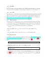
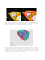
Figure 1.1: This is a screenshot of CardioViz3D, showing the MRI atlas of the heart, and a
volume mesh geometry segmentation of the ventricules.
12. Interactive (dynamic-)mesh manual registration.
13. Vector field visualization on meshes.
14. Interactive surface mesh generation.
15. ...
1.3
System Requirements
CardioViz3D is available for Microsoft Windows XP (x86 and x64), LINUX x86 and x64
(Fedora Core 7) and MAC OS X (Tiger and higher). At least 1GB of memory is required,
as well as a powerful processor (P4 2GHz, AMD FX 3800+ or later). Also, a powerful
graphic card is recommended. You may experience difficulties to visualize images with volume
rendering technique using an ATI card (this is a known issue). CardioViz3D is multi-threaded,
thus optimaly using multi-core technologies.
1.4
Installing CardioViz3D
CardioViz3D software is available from this webpage: http://www-sop.inria.fr/asclepios/
software/CardioViz3D. You will find a lot of useful information, screenshots, tutorials, links,
testing data, online documentation, etc.
6
1.4.1
Windows
From the webpage, download the installer (CardioViz3D-X.X.X-win32-xXX.exe) corresponding to your architecture (x86 for 32 bit processors, x64 for 64 bit ones). Execute it. It will
overwrite any previous installation of CardioViz3D you might have on your computer.
1.4.2
Mac OSX
From the webpage, download the package installer (CardioViz3D-X.X.X-macOSX-Universal.dmg).
These are universal binaries and will suit for all macOS 10 (Tiger and higher) architecture.
Execute it, it will also overwrite any previous installation of CardioViz3D you might have on
your computer. Note that you will need X11 environement installed on your computer (see
http://www.apple.com/support/downloads/x11formacosx.html).
1.4.3
Linux systems
From the webpage, download the dedicated tarball (CardioViz3D-X.X.X-linux-FCX-xXX)
corresponding to your architecture (x86 for 32 bit processors, x64 for 64 bit ones). Untar the
file in a dedicated directory. The binary is included in the output directory, as well as the
needed libraries. You might need to add a line in your bashrc file to be able to execute the
software. Depending on your system, this line should be something like:
in bash :
export LD_LIBRARY_PATH = my_cardioviz3d_directory:${LD_LIBRARY_PATH}
in tclsh :
setenv LD_LIBRARY_PATH my_cardioviz3d_directory:${LD_LIBRARY_PATH}
1.5
Get started
You will find test data, tutorial and screenshots at this webpage: http://www-sop.inria.
fr/asclepios/software/CardioViz3D. First click on the Open file(s) button (Fig. 1.2 left).
You can ask for opening several files at the same time. See Sect. 1.2 for a list of supported
formats.
TIP: Ctrl+O directly opens the import dialog
Each image will induce the creation of a new tab, whose name corresponds to the image
file name, meshes will be incorporated to the currently opened tab.
TIP: Ctrl+T creates a new empty tab. Useful to separate several imported meshes.
After the import, data are listed by name in the Data Manager on the left of the window
(Fig. 1.2 right). Select one of them by clicking on its corresponding line, the system will
automatically switch to the corresponding tab. A checkbox allows you to control its visibility.
7
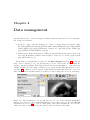
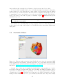
Figure 1.2: This zoom points out the principal structures of CardioViz3D. The main toolbar
on the top of the window gathers the most important functions of the software, such as the
open button to import any data, the DICOM import button, the sequence import button,
etc. You can see on the upper left corner the “Data Manager” that summarizes all imported
data. At the bottom of it, you see a set of buttons. Each button represents a toolobx, the
first and second ones rely to general purposes.
NOTE: Each action you might do in the toolboxes acts on the currently
selected dataset(s) and only on it(them).
In the main toolbar (Fig. 1.2), you will find the most important functionnalities of
CardioViz3D. The first set of buttons rely on data import and export, please refer to Sect.
2 for specific imports such as DICOM or sequences. The second set of buttons are dedicated
to user interactions choices in the 2D views. Assuming you are visualizing an image in
CardioViz3D, this image is represented in 3 perpendicular plane sections (axial, coronal and
sagittal views) and a 3D representation of it. In the 2D views you have several kinds of mouse
interactions that are possible:
1. the arrow allows to navigate between slices in the different views.
2. The orange color map button allows you to change the window and the level of the
image. Note that these parameters are also available from the visualization toolbox
(see Sect. 3.1).
3. The zoom button allows to zoom in and out in the xurrent image slice. Press Shift to
translate the visualization.
TIP: Press Shift when the zoom interaction is ON to translate the current
slice.
8
Chapter 2
Data management
CardioViz3D is able to read several types of image and mesh data, here is a non exhaustive
list of supported formats :
1. Static (i.e. 2D or 3D) and dynamic (i.e. 2D+t or 3D+t) image file support: Analyze (.hdr) NIFTI (.nii .nii.gz), MetaFile (.mhd .mha), DICOM format (.dcm), NRRD
(.nrrd), GIPL (.gipl .gipl.gz) VTK image format (.vti, .vtk), PNG (.png), JPEG (.jpg
.jpeg), TIFF (.tif .tiff), InrImage (.inr.gz)
2. Surfacic and volumic mesh support: VTK polydata and unstructured grid format (.vtp
.vtu .vtk), HomeMade formats (.tr3D .atr3D .tr .trian .noboite .mesh .tet3D .atet3D
.sm), OBJ format (.obj)
Each dataset you might import is added to the Data Manager (see Fig. 1.2 on the left
side). Select a dataset to act on it through the toolboxes. The checkbox aligned with the
dataset controls its visibility. Each dataset has its associated view port, i.e. a tab where the
dataset is drawn. You can change a dataset view port through the Data Information toolbox
(see Fig. 2.1). When you select dataset, CardioViz3D automatically raises the correct tab
where the dataset is currently drawn. Note that you cannot change the view port of an image.
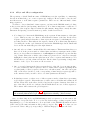
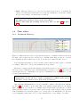
Figure 2.1: The information toolbox (left) allows you to act on the currently highlighted
dataset. You can remove it from the Data Manager, save it into a file, pop up some DICOM
information (see Sect. 2.1), or show a histogram of its scalar information. You can also
change the view port (tab) of a specific dataset. Tabs are shown on the right.
9
You can save a specific dataset into a file, or remove it from the Data Manager (and from
the views), through the information toolbox. Note that removing a dataset from the Data
Manager does NOT actually delete its corresponding file.
TIP: When a dataset is highlighted, Crtl+S to save it into a file
TIP: When a dataset is highlighted, Crtl+D to remove it from the Data
Manager
2.1
Importing a DICOM exam
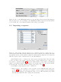
Figure 2.2: The DICOM importer helps you in importing a DICOM exam as easily as possible.
Double click on a volume to show a list of available DICOM flag information, indicate when
you detect 2D+t or 3D+t image sequences, then click OK to import all volumes.
First click on the Import DICOM exam button on the main toolbar (a “cd-like” button).
A dialog pops up (Fig. 2.2). From here you will be able to reconstruct volumes, construct
4D sequences, etc... You have basically two different options :
1. First: you can import the exam from its root directory path. CardioViz3D will scan
recursively this directory and reconstruct all available volumes. The scan process
might take a few minutes for large exams.
2. Second: you can import manually one or several DICOM image files. Each file will be
considered as a volume.
10
Note that importing a DICOM exam from a root directory overwrites the previous set of
volumes.
Each line of the list corresponds to a volume, i.e. a volumic image (a volume can actually
contain only one slice). Select one or several volumes to act on it(them). The preview window
shows the middle slice of this volume. Note that there is no 3D reconstruction yet, to fasten
the process. Press “interactive” to see the entire volume playing.
TIP: double click on a volume to pop up a window listing all visible
DICOM flags for this volume (Fig. 2.3).
Figure 2.3: Double click on a desired volume from the importer to show this information box.
It shows all available DICOM flags from the DICOM series corresponding to the selected
volume, such as pixel type, protocol, patient information, but also heart rate, etc... You will
find a search box to help you find a specific DICOM information.
TIP: At any time of the DICOM import process, you can press reset to go
back to initial configuration (after loading a DICOM root for instance).
2.1.1
Supported (and unsupported) configurations
CardioViz3D supports most of the DICOM exam configurations. The volume images are reconstructed from the slice files using the DICOM series flag. In some cases, a single DICOM
series flag can have several volumes (for example in case of interlaced T2 / proton-density
acquisition). Detect these non coherent volumes by looking at the preview window (“interactive” button has to be pressed). Press split to un-interlace these volumes. CardioViz3D
uses the patient position DICOM flag to distribute slices between instances. This interlace
configuration case also appear in some Diffusion Weighted MRI acquisitions, but splitting
using this button reconstructs the volumes correctly.
TIP: double click on a volume to pop up a window listing all visible
DICOM flags for this volume (Fig. 2.3).
However there are some known configurations that are not handled by CardioViz3D.
DICOM RT format for instance is not yet supported. We also encontered problems reconstructing some 3D and 3D+t UltraSound data.
11
2.1.2
2D+t and 3D+t configuration
The specificity of CardioViz3D in terms of DICOM import is the capability of constructing
directly from this dialog one or more sequence(s) of images. However this tool needs some
user interaction to well define sequence parameters. There are two different kinds of time
image sequences.
You have to detect what kind of time sequence you have in the DICOM exam by looking
at the preview window (and pressing “interactive”). Note that an imperative condition to a
good ending of the sequence import is that the time instance images have exactly the same
dimension and spacing. Several scenari are possible, detailed as followed:
1. N “volumes” (i.e. lines in the DICOM importer) represent N time instances of the same
object. This is an easy one. Remove all additional volumes of the list. In the 3D+t
Sequence panel, indicate that these volume represent a sequence by validating the corresponding checkbox. Then indicate the sequence duration. Note that if any information
concerning the cardiac cycle duration is found in the DICOM flags, CardioViz3D will
detect it and automatically preset the right duration.
2. One and only one volume contains all the 3D+t information. This means that when you
have a look on the preview window of this volume and when you navigate in the volume
slices, you detect that several instances of a 3D object are actually incorporated in this
“big” volume. First remove all the other volumes (or press select to only select currently
highlighted volume), then use the Split button in order to separate time instances. You
should then see several volumes in the list. Each volume representing a single time
instance of the object. You can now follow scenario 1.
3. One or several volumes in the list represent slice(s) of the 3D object moving in time,
i.e. some volumes are 2D+t sequences. If a set of these 2D+t sequences (putting them
together) make a “3D+t” sequence, then refer to the 4th scenario. On other cases, just
click on the 2D+t checkbox of the corresponding volume line(s), sequence(s) will be
well constructed and you will be able to set their parameters afterward.
4. In this last scenario, you have a set of 2D+t sequences in the volume list, representing
a global 3D+t sequence. First make sure you have remove all additional volumes from
the list. Then click on the 3D+t checkbox and set the sequence duration, then click on
any of the 2D+t checkbox to indicate CardioViz3D that it is a set of 2D+t sequences.
The software will construct the global sequence.
TIP: the preview page (Fig. 3.2 helps summarizing the imported data.
To activate/deactivate it go to the Application Setting (View menu).
Once you have imported your DICOM images and/or sequences you can retrieve the
DICOM flags of a specific data. To do so select the desired image or image sequence in the
Data Manager, go to the information toolbox and click on the DICOM information button
(“CD” button), the same information dialog will pop up (see Fig. 2.4). Note that you can
open several of these dialogs (corresponding to different images) to compare the data.
12
Figure 2.4: Recover the DICOM information of a specific image (select it in the data manager)
after the import process by clicking on the DICOM information button in the information
toolbox (Left), the corresonding information dialog will pop up (right).
2.2
Importing a sequence
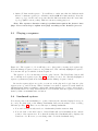
Figure 2.5: The Sequence importer allows you to construct a sequence of data from one or
several dataset files. Import file(s) with the Open button. Import some attribute files with
the attribute button. Set the sequence duration, edit the time step flags if needed, then press
OK. The sequence will be built and added to the Data Manager.
CardioViz3D is able to construct some data sequences and play them. From the main
toolbar you will see the Sequence Importer button, a dialog will show up to help you in
the sequence construction (Fig. 2.5). Load the different files corresponding to the different
frames of your future sequence. Note that the order is important. You can add several files
at the same time. About the attribute loading, please refer to Sect. 2.5.
Several kinds of data sequences can be constructed :
1. Image sequence : If you want to create a sequence from a DICOM exam, please refer
to Sect. 2.1. On the other hand, if you want to create a sequence from several image
files (2D or 3D images), representing the same object at different (time) steps, make
sure that they match in terms of image size and spacing.
13
2. Surface/Volume mesh sequence : You will have to make sure that the different mesh
files are consistent together (i.e. all surface meshes OR all volume meshes). Press the
“same topology” checkbox if you are sure that the different meshes have the exact same
topology (links between points). This is for memory saving purposes.
Note: The sequence duration setting is predominant against the frames’ time
flags. Press return key to update time flags according to the duration just set.
2.3
Playing a sequence
Figure 2.6: The sequence toolbox will help you to play/pause your imported sequence(s).
Press the Manage Sequence button to set parameters of the currently highlighted sequence.
You can tune the speed with the dedicated spinbox.
The sequence toolbox is announced by the “play” button. The Play/Pause button will
act on all imported sequences (see Fig. 2.6). You have access to the currently highlighted
sequence’s parameters (such as its duration) with the Manage Sequence button.
In case the sequence(s) are not cyclic, you can act on the play mode toggle button to play
sequences in a go and back way. When “real-time” is activated, sequences actual durations
will match their duration parameter, with a risk of frame skipping (i.e. a 2.0 seconds sequence
will actually last 2.0 seconds). When this mode is deactivated, then the sequence is rendered
frame by frame at maximum time resolution.
2.4
Landmark system
You can associate some landmakrs (i.e. points of interest) the currently displayed view-port
(i.e. tab). For that click on the Manage Landmarks button in the main toolbar. A dialog
will raise (see Fig. 2.7). There are several ways of defining landmarks :
1. You can load a previously saved set of landmarks (default extension .lms)
2. You can click on the Add button. CardioViz3D will add a landmark in the current
position of the current view. Note that the freshly added landmark will be displayed in
a random color. However you can change this color in the landmark dialog.
14
Figure 2.7: The landmark system allows you to define points of interest. Control each landmark parameters in the landmark dialog (left). After adding landmarks, they are displayed
in all available views (right).
3. On a 2D view : Shift+RightClick will add a landmark to the current mouse position.
4. On a 3D view : Shift+RightClick will add a landmark to the current mouse position,
at the first intersection with the surface of the selected dataset (only available for mesh
data).
TIP-1: To translate a landmark in a 2D view : LeftClick on it and drag
it until desired position.
TIP-2: Double LeftClick on a landmark to make the cross position match
the landmark position.
At any moment you can save the current set of landmarks (default extension is .lms). The
“Remove” button will remove the currently selected landmark while the “Remove All” button
will remove all landmarks from the views. In the landmark dialog you can choose the color
and size of a specific landmark.
Don’t forget to save your landmarks before leaving CardioViz3D.
2.5
2.5.1
Mesh attributes system
Static mesh attribute
You can easily attribute some data to a surface or volume mesh.
This data can be scalars, vectors, or higher order objects (tensors,etc) associated to the points or cells (i.e. triangles/tetrahedra)
of the mesh. Let us take a foo example. Consider a surface mesh
made of 3 triangles, the VTK file woud look like tetrahedron.vtk:
# vtk DataFile Version 3.0
vtk output
15
Figure 2.8: 3D view
of the resulting tetrahedron.
ASCII
DATASET POLYDATA
POINTS 4 float
0 0 0
1 0 0
0 1 0
0 0 1
POLYGONS 4 16
3 0 1 2
3 0 1 3
3 0 2 3
3 1 2 3
Resulting surface mesh is shown Fig. 2.8. Let’s consider we
want to associate scalars to each of the points of this surface mesh.
CardioViz3D has its own attibute file system. The idea is to have
a unique file describing the data associated to a specific geometry.
Several parameters can be set :
1. A single description name (string).
2. A flag describing to what the data will be associated (1 for
points, 2 for cells).
3. The dimension of the data (1 for scalars, 3 for vectors, etc)
4. The number of data (number of points or number of cells).
Now we can build our own file describing a scalar on each point of the tetrahedron
tetrahedroncolors.cvcolor:
Point_Color
1
4 1
1.0 4.0 3.2 2.7
1. 1st line : the description name
2. 2nd line : association flag (1 for points / 2 for cells)
3. 3rd line : number of scalars; Dimension of the data
4. 4th line : actual data (1D scalars)
Resulting tetrahedron is shown Fig. 2.9 where you can see the corresonding color map.
The extension has no influence on the reading process. However the description name is quite
important. Indeed this name will result in the attribute list on the information toolbox (Fig.
2.1). It will also be listed in the visualization toolbox as possible data to be visualized (Sect.
16
Figure 2.9: 2D and 3D views of the tetrahedron example to which scalars have been associated
to each of its points. Access to the scalar visualization in the visualization toolobx (see Fig.
3.4).
3.2). Note in the actual data, scalars are separated by a space.
TIP: If the description name is “Position” and the scalars are actually
vectors associated to the points of a mesh, then CardioViz3D will take the
data as real coordinate positions and overwrite current mesh positions
with it.
TIP: If you save the resulting mesh in a VTK format, scalars will be
incorporated into the outout file
2.5.2
Mesh sequence attributes
Extending the last section, CardioViz3D has a file reading process for sequence attributes. Sequence attributes consist on a list of files describing the evolution in time of any scalar/vector
field associated to the mesh points/cells. This of course includes the point positions. File
header is slightly different, a file is needed for each frame and for each scalar field.
Let us go back to our previous example. We want the color field to change during time.
We need to build some file describing this evolution. At each frame, we need to indicate in
the file an additional parameters : the frame number the scalars will be associated to.
Then our previous tetrahedroncolors.cvcolor will be turned into tetrahedroncolors i.cvcolor:
Point_Color
1
17
4 1 1 i
1.0 4.0 3.2 2.7
3rd line : number of scalars; scalar dimension; cycle number; frame number
By replacing i with the frame number, and replacing the scalars by some that evolve in
time, we will be able to construct a time sequence (Sect. 2.2).
In the sequence importer, just import our base geometry : tetrahedron.vtk. Then associate scalars directly from here with the load attributes button. Load all previously created
tetrahedroncolors i.cvcolor. Set the sequence duration and press OK. This example (files
and output video) is available from CardioViz3D website.
TIP: If you save the mesh sequence in a set of VTK files, scalars will
be incorporated into the outout files
2.6
Exporting your data
Figure 2.10: left: In the information toolbox, you will find the save button allowing you to
save currently highlighted dataset at any time into a specified file. right: From the main
toolbar, you can save the entire data manager with the save button. Note that this action
might take some time for large sets of data.
At any time, you can save the currently imported data in CardioViz3D. As shown in
section 1.5, the imported data is summarized in a dedicated window. Select (highlight) a
specific dataset here. From the information toolbox, you can save this dataset in a desired
file (see Fig. 2.10). Note that the extension given by the user will be determinant for the
writing process. However if no extension is given then the dataset is saved in a default format.
TIP: Ctrl+S when a dataset is highlighted will pop up a save dialog
In case the dataset you want to export is a sequence, process the same way, unless you
will be asked for a export directory in it is a mesh sequence. In this case CardioViz3D will
save a serie of VTK files (or Analyze dor images) corresponding to all frames of the selected
18
sequence. In case of image sequence, CardioViz3D is able to read and write 4D image files.
Note that for that specific case of image sequence, you will need a file format that supports
4D images. We recommend the NIFTI format (.nii). However, no extension information from
the user will directly take this option.
2.6.1
Exporting a DICOM exam
Figure 2.11: left: The DICOM exporter dialog. You can select the images you want to export
in the exam. click on the “CD” button to have access to the highlighted image DICOM flags
information. right: The DICOM flags window. You can edit the flags by double ckicking on
one of them.
The DICOM importer button on the main toolbar can drop down a sub-menu allowing
the user to open the DICOM exporter dialog, see Fig. 2.11. From there you can select a set
of images you want to export. Note that CardioViz3D will also export image sequences (as
a set of volume images).
The process used for writing uses an external library to actually save each volume into a
set of 2D image files. You can set a prefix for the output image files.
Note: Image that have not been imported directly from a DICOM exam
don’t have any DICOM information. However some default DICOM
flags are set during the writing process.
After all parameters are set, press OK. You will be asked for an output directory. Note
that the writing process can take some time in case of large exams.
19
20
Chapter 3
Generic vizualization tools
To each independent dataset (listed in the data manager), you can apply some vizualization
parameters. Tuning some parameters will act on the currently selected (highlighted) object(s)
on the data manager and only on this(these) one(s). As said before, an image (or an image
sequence) has its own tab in the main window. On the other hand, meshes are incorporated
in these tabs. You can create an empty tab by pressing Ctrl+T.
The visualization toolbox is (obviously) dedicated to visualization parameter tuning. Select the desired dataset(s) in the data manager, the corresponding specific parameters will
raise in the toolbox.
3.1
Image visualization
Figure 3.1: This figure shows the image parameters being tuned. You can set a color map
associated to the currently selected image (or image sequence). Access to the 3D rendering
mode, activate the cropping box, control the windowing, etc.
The image vizualization parameters allow you to set the color map of an image (Fig. 3.1.
Volume rendering mode is available. You can also activate the shading effects on the volume
rendering from the visualization toolbox. Note that volume rendering is not supported by all
graphic cards. Note also that the shading effects dramatically slow down the rendering time.
The windowing feature consists on a range that you can control either with the mouse or with
the corresponding minimum and maximum value entries. Note that the range is synchronized
21
with the mouse interaction in the 2D views.
There is an interesting feature that allow you to see all your imported images (and image
sequences) in a same page: the Preview Page (see Fig. 3.2). Activate/Deactivate this
feature with the View Menu→Application Settings→CardioViz3D settings.
Figure 3.2: The preview page summarizes all imported volume images. If sequences have been
imported, they will be played also here. You can activate and deactivate this feature through
the Application Settings panel (View Menu), you will find the corresponding checkbox. Note
that user interactions are all synchronized in this page.
You can also visualize a specific user defined plane from an image. For that in the 3D
view of the desired image press P. A plane will appear in the center of the image. Shrink or
expand the plane thanks to the control points, Change its orientation with the arrow. You
will see a dialog showing up while you manipulate this plane. This dialog displays the exact
intersection between the plane widget and the underlying image (see Fig. 3.3).
TIP: Clicking on the middle of the plane will translate it among the
orientation axis. Clicking on the arrow will rotate the orientation axis.
3.2
Mesh vizualization
Meshes are more versatile to render. That is why the visualization tools are more “complex”
(Fig. 3.4). You can set some light effects associated to the selected mesh. If the mesh is
“projected” in 2D views (see Sect. 5), then all visualization parameters are shared between
the projections and the 3D object.
Another aspect of mesh visualization is related to their attributes. Meshes can have scalar,
vector or tensor attributes associated to each of their vertices/cells (see Sect. 2.5). In the
case of scalar attributes, they can be visualized on the surface (or volume) of the object. In
Fig. 3.4 left, the attribute mapping part has the aim of letting the user choose to visualize
22
Figure 3.3: Press P in the 3D view to activate the plane selection feature. Manipulate the
plane widget with the control points and the arrow (left). The dialog displays the exact
intersection between the image and the user defined plane. Press P again to deactivate it.
Figure 3.4: This figure shows the mesh visualization parameterization being used. You can
set its color, some light effects, surface representations (wireframe, surface), etc. On the right
is shown a mesh rendered in the 3D view.
23
a specific attribute of the currently selected mesh (see Sect. 2.5). Note that you might encounter some known issues : when you try to transfer a mesh from a view port to another,
you loose the attribute visualization properties you might have set befor ethe transfer.
Scalars are mapped in the mesh representation(s). Linear interpolation is done between
values. Note that interpolation is not done in case the scalars are associated to triangles
(or any other cell type). You can choose the color map to associate to the currently visible
scalars and you can display the corresponding scalar bars in the views.
TIP: sometimes the lighting settings can affect the colors. In case scalars
are mapped to the mesh, disable any light by setting the color “value”
down to zero.
3.3
Snapshot and movie exports
Figure 3.5: From the main toolbar you will find the snapshot-movie export button. In case
of movie export choice, this movie exporter will raise to help you exporting 3 types of movies.
The slice type will explore all slices of a 2D view. The camera type will allow you to control
camera movements of a 3D view. Finally the time type will snap through time the current
2D/3D view.
In the main toolbar, the screen-like button annouce the possibility to export a snapshot
of the current full screen view. However you can drop down a menu to choose to export a
movie out of the current view (Fig. 3.5). Different types of movies can be exported:
1. Slice : Considering a 2D view, you can use this export type to snap each available
slices into a movie. Note that the number of output frames can be set.
2. Camera : Use this export type if you want to control a 3D camera for your movie.
Move the sliders according to the desired path.
24
3. Time : This type allows you to export your sequence(s) as a movie. It will take the
current view and snap it while time is evolving. By default the best amount of frame
is set (corresponding to the finest time resolution).
TIP-1: You can choose to let the cross visible or not during export in
the Application Settings Panel of the View Menu.
TIP-2: The scalar bar visibility can be set to ON : see Sect. 3.1 & Sect.
3.2.
3.4
3.4.1
Time tables
Landmark follow-up
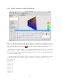
Figure 3.6: This is the time table of a specific mesh sequence. Available scalars are shown on
the right, click on their respective checkboxes to visualize them. Export a movie or a table
file containing all visible values. Act on the zoom buttons to adjust the field of view.
It is sometimes interesting to follow a scalar evolution among a time sequence of meshes
for example. This can be done by the landmark follow-up feature.
First select a sequence in the data manager, then in the sequence toolbox, press the “point
follow-up” button. This will pop up a landmark manager dialog (see Sect. 2.4). You can load
a previously saved set of landmarks. Save the set of landmark before clicking OK to be able
to retrieve this landmark set.
TIP: An easy way to add landmarks can be done by pressing Shift +
Right-Click on the 3D view. Then a landmark is added at the mouse
position, on the surface of the first mesh encontered.
Once all desired landmarks have been set, clcik OK to validate. The time table will raise
(see Fig. 3.6). You will see on the right a list of the available graphs that you can display.
Click on the their “eye” checkbox to visualize them. Each graph represents the evolution
during the time sequence of a specific scalar, at the specific position given by the previously
defined landmark. Note that the graph’s color corresponds to the landmark color. However
you can manually change this color by double-clicking in the corresponding color square.
25
3.4.2
Global parameter evolution follow-up
Figure 3.7: .The global parameters file system allows you to visualize in real-time the evolution
of some global scalar among the time line of dynamic sequence. Here a synthetic sequence
is shown in the 3D view (see Sect. 2.5.2) to which a global parameters file has been loaded
(ecg.par). Click on the “global parameter follow-up” button to raise the time table.
CardioViz3D also has a sequence global parameters file system. The idea is to follow 1D
scalars among the sequences. These scalar values are not associated to any specific point or
cell or position of the dataset. A typical example would be the electro-cardiogram associated
to a cardiac dynamic sequence.
The file system is quite simple. The idea is first to provide a set of strings that explain
the different scalar curves, and then list the data. Here is a simple example file ecg.par:
Time Phase ECG
0.0 1 0.01
0.1 2 0.02
0.2 2 0.03
0.3 2 0.03
0.4 3 0.02
0.5 3 0.01
0.6 3 0.00
0.7 3 0.01
0.8 4 0.01
0.9 5 0.01
26
To load this file, just select the desired sequence in the data manager. Then in the Information toolbox, there is a “load attribute” button (see Fig. 2.1). Click on it and load the
global parameter file. Once this is done, go back to the sequence toolbox. From there you
can click on the “Global Parameters” button (see Fig. 2.6). It will pop up a time table with
all previously loaded global attributes. The result is shown Fig. 3.7.
TIP-1: the number of lines in the global parameter file does not have
to match the number of frames of the sequence. All 1D curves are
“stretched” to match the sequence time size.
TIP-2: The global parameter file extension has no influence on the reading process.
3.4.3
Other time table properties
TIP-1: RightClick in the time table window to zoom in & out through
out the graph.
TIP-2: MiddleClick in the time table window to navigate (translate) in
the graph.
Time table graphs are perfectly synchronized with the sequence toolbox. Hence you can
play the sequence (Fig. 2.6), you will see the scalar evolving according to time. A vertical
bar is also shown to remind the current time.
You might want to export this data, this can be done by several ways:
1. You can export a screenshot of the current field of view, or export a movie, with the
snaphot export button (see also Sect. 3.3).
2. The save data button will write a spreadsheet file (.csv), this file will contain semicolumn separated values for all currently visible graphs.
27
28
Chapter 4
Image processing tools
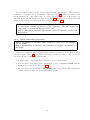
IMPORTANT : Toolboxes contain image/mesh/sequence processing algorithms. These algorithms are beta versions and should not be considered otherwise. At the current stage of developement (v1.4.0), most of
the toolboxes are still work in progress. Some of the provided features
are relatively stable and there is no warranty concerning their efficiency.
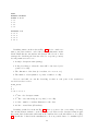
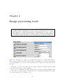
Figure 4.1: The Image processing toolbox (left) allows the user to apply simple filters to
images. On the right, an example is shown where an arithmetic operation is being applied
to two input images (e.g. Image1 + Image2 ). All filters are applied to the currently selected
image(s).
The image toolbox provides some basic processing for images and image sequences. Each
of its buttons provides a specific treatment.
First, select your image(s) (or image sequence(s)) of interest in the Data Manager, then
select the filter you want to apply to it. The next sections explain briefly what are the image
processing features proposed in this toolbox.
29
4.1
Arithmetic operations
As shown in Fig. 4.1, the arithmetic operations allow you to compute the sum, multiplication, etc, of one or two input images. Several operations are available and will act on the
currently selected set of image(s). Some operations need only one input image. This is the
case of the N OT and the IN V operations. However all other arithmetic operations will
take two input images. Note that all operations are 4D compatible. This means that if
the dataset(s) currently selected are image sequence(s), then CardioViz3D will reflect this
by performing the desired operation frame by frmane between the two sequences. Note that
this sequence processing operation is only possible if the two inputs have exactly the same
amount of frames. There is no time interpolation.
4.2
Convolution process
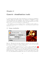
This button just proposes a convolution of the input image (or sequence), using the recursive
gaussian approach proposed by Deriche [4] (with σ of 2.0). See Fig. 4.2. At current stage of
developement there is no parameter available for the gaussian convolution.
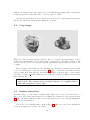
Figure 4.2: On the left the input image (here an anatomical atlas of the heart. On the right
the result of the convolution process.
4.3
Clipping planes
This feature allows the user to to define a plane in the 3D view in order to clear the image
above this plane.
When you click on the dedicated button, a dialog raises to explain you how to control the
plane position and orientation. This is done in the 3D view, moving the plane is synchronized
30
with the other image views. Once this is done, press OK, the input image will be transformed
so that the part above the plane will be “cleared” with zero values.
Careful : the input image is altered by the process, there is no output image derived from
this process, unless the binary mask defining the operation.
4.4
Crop image
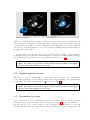
Figure 4.3: The crop image function allows to place a box in the 3D view thanks to control
points, CardioViz3D will create an output image corresponding to the inside of this box. On
the left you can see the box being placed in the input image. On the right the result of the
cropping.
The crop image button will act on the currently selected image (or image sequence). Click
on it, a box will appear on the 3D view (Fig. 4.3). Place it and size it with the dedicated
control points, then click OK. An output image (or image sequence) will be created under
the name of extractor output, taking the size of the user defined box (limited by the input
image dimensions).
TIP: this feature is available in 4D. Simply select your image sequence
and crop it. The output will be an image sequence of “cropped” frames.
All other parameters will be kept.
4.5
Surface extraction
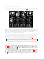
From any image, you can extract a surface mesh. This can be done by the last button of
the toolbox. The dialog raised will help you defining the parameters of the extraction (Fig.
4.4). You can define a threshold value or a iso-value with respect to the currently highlighted
image on the data manager.
You can see the resulting surface mesh in Fig. 4.4. Here are some brief explanations
about the parameters provided by the dialog:
31
1. Name: the name of the output image.
2. Threshold/iso-value: You can define a threshold value α. The algorithm will then
separate the input image in two regions : 6 α and > α. On the other hand you can
define a iso-value β. the algorithm is the same but it interpolates the value between
pixels to have a subpixel resolution mesh.
3. Decimate: You can choose to decimate the output mesh. The decimation algorithm
used is from VTK.
4. Target reduction: This parameter will define the spatial resolution of the output mesh.
It represents a percentage of the input image finest spacing resolution.
5. Smooth: You can also smooth the output mesh (vtk filter), this is actually recommended.
Note: this feature is not available for image sequences.
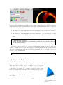
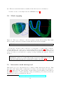
Figure 4.4: Left: The surface extractor provides a quick algorithm to extract a surface mesh
from an input image. A dialog allows to set some extraction parameters. Right: Here is
shown the result of a surface extraction (thresholding at a specific value) of the anatomical
atlas. The image color map chosen here is GE-colors (see section 3.1). The output surface
mesh is shown in bright green.
32
Chapter 5
Mesh processing tools
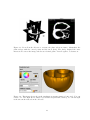
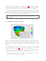
Figure 5.1: Left: The mesh processing toolbox contains a few features to manage surface
and volume mesh objects (or sequence of those). They act on the currently selected mesh
(or mesh sequence). Right: This image shows the result of the projection process of the
“atlasgeometry”. volume mesh.
The mesh processing toolbox proposes some simple algorithm for surface and volume mesh
processing. First select the desired mesh (or mesh sequence) in the data manager, then click
on the desired process. Here are some brief explanations on how to use each of them.
5.1
Mesh projection
When opening a mesh file, the mesh object is directly rendered in the 3D view. One might
want to have an insight in the mesh geometry slice by slice. This can be done here by the
projection tool (see Fig. 5.1). It simply consists on creating a “bounding box” corresponding
to the bounds (in real coordinates“ of the currently selected mesh. The mesh is then projected
in three orientation planes.
The resolution of the synthetic image is 128x128x128, respecting the real coordinates
mesh bounds. This means that the spacing in x, y, and z is adapted to match the mesh real
33
size. This also means that distances visualized in the 2D views are real distances.
You have access to some sample data via vtkINRIA webpage1
5.2
Mesh cropping
Figure 5.2: The crop tool allows to control a cropping box in the 3D view (left). This results
in the cropping of the selected dataset, synchronized in the 2D views (right).
TIP: You can use this tool with some mesh sequence as input.
For the user convenience, this tool allows to crop any surface or volume mesh (or sequence
of those) thanks to the control of a box widget in the 3D view (see Fig. 5.2). This tool does
not affect the structure of the mesh but only its visualized representations on the 2D & the 3D
views. Note that you can disable the cropping box widget visibility throught the dedicated
checkbox.
Known limitation: When cropping a mesh, some of the visualization
parameters (such as a scalar color map) can be lost. However it can be
retrieved easily through the visualization toolbox (see Sect. 3.2).
5.3
Interactive mesh moving tool
This feature proposes to interactively move a surface/volume mesh in the 3D view. Thus
all points of the dataset will be transformed according to the user-defined movement (see
Fig. 5.3). First select the desired mesh (or mesh sequence) in the manager, then click ion
the move mesh button. A dialog will raise to help you in this step. You can now follow the
instructions to move your mesh in the 3D view.
1
downoald sample data : http://www-sop.inria.fr/asclepios/software/vtkINRIA3D
34
Figure 5.3: The interactive moving tool allows the user to drag a selected mesh in the 3D
view and drop it at a specific location. All points coordinates of the dataset will be replaced
by transformed ones. This tool is also avaliable in 4D. In this figure you can see on the left
the 3D view of the input situation, and on the right the resulting situation after interactive
moving has been performed.
At any moment you can cancel the step by pressing ”cancel“ When you have finished
moving the mesh, press OK. The mesh will update according to the affine matrix defined by
the user movement, you can now save your resulting mesh (see Sect. 2.6).
TIP: this process is available in 4D : simply move the currently displayed
frame, the entire set of frames will be transformed according to the affine
matrix. All other parameters are kept.
5.4
Surface extractor tool
The next tool acts on volume meshes to extract the surface geometry of it. Simply click
on the button while the desired volume mesh is selected in the manager, an output mesh is
created under the name of inputmeshname surf ace. See Fig 5.4.
TIP: this process is available in 4D : simply move the currently displayed
frame, the entire set of frames will be transformed according to the affine
matrix. All other parameters are kept.
5.5
Orientation vectors
Vector fields can be loaded as attributes of a mesh (or a mesh sequence). The file system is
exactly the same as the scalar field attribute system (see Sect. 2.5), exept the dimension of
the data is now 3. Vector can be affected to the points (nodes) of the mesh or to the cells
(triangles/tetrahedra) of the mesh. In the mesh processing toolbox, the orientation vectors
35
Figure 5.4: The surface extractor tool just isolates the surface of a volume mesh and creates
another mesh object with it. On the left the input mesh projected in a 2D view, on the right
the result of the surface extraction. The surface mesh is represented in red.
Figure 5.5: This figures shows a snapshot of the CardioViz3D 3D view where an anatomical
geometry atlas of the heart is being displayed. A vector field has been provided to this
geometry through the mesh attribute system. In the mesh toolbox, you can display the
available vector field. Vectors are color-coded with their unsigned orientation. A cropping
box allows to select a area of interest of this vector field.
36
button will scan the currently selected dataset to find some associated vector field.
Vectors are then normalized and color coded with an unsigned orientation lookup table.
X axis oriented vector are shown in red, Y axis oriented vectors are shown in green, while Z
axis oriented vector are shown in blue. The surrounded box displayed around the vectors can
be manipulated by its control spheres to crop the vector field interactively. The Checkbox
next to the button controls the cropping box visibility. Figure 5.5 illustrates this specific
visualization process.
TIP: The orientation vectors button is a toggle. Press it a second time
to hide the vector field.
Note that in case of a mesh (single-topology-) sequence, the vector field being associated
to the points (or the cells) of the sequence, vectors will follow the points in their displacement
during time.
5.6
Anatomical fibers
Figure 5.6: This screenshot shows the CardioViz3D 3D view, where the anatomical MRI
atlas of the heart is being displaed, as well as a setlection of a corresponding fiber field coming
from a DTI sequence (ex-vivo) and a fiber tracking process. All data can be downloaded from
this adress : http://www-sop.inria.fr/asclepios/data/heart).
Another type of data can be visualized in CardioViz3D : “anatomical fibers”. Indeed,
fiber fields coming from a DTI exam (and a fiber-tracking algorithm) for instance can be
represented as continuous lines (e.g. polylines), color-coded once again with their unsigned
orientation (see Sect. 5.5). This data can be imported as a VTK polydata file in the data
manager. Then in the mesh tool box, you can indicate that this data corresponds actually
37
to anatomical fibres, in order to have access to an interactive mode of fiber bundle selection.
When clicking on the anatomical fibers button (with anatomical fibers currently selected),
you will see a cropping box surrounding the fiber field. Manipulate this box with the control
spheres. Only the fibers that pass through the box will be displayed.
38
Chapter 6
Segmentation tools
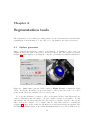
The segmentation toolbox aims at providing advanced tools for the interactive and automatic
segmentation of medical images. So far, only one tool is available, the Surface Generator.
6.1
Surface generator
This tool allows the interactive creation of 3D surfaces. To launch it, select a tab containing an image and click on the Surface Generator button. The dialog window presented
in figure 6.1 is then displayed, providing the controls to personalize the manual segmentation.
Figure 6.1: Left: Surface generator dialog window. Right: Example of interactive delineation. In blue the 3D surface, in green an “inside” control point, in red the “on” control
points and in yellow the currently selected control point.
To create the 3D surface, you have to place on the image (in any of the 2D-views) some
control points that define the “inside”, “on” and “outside” regions of your surface. To this
aim, navigate into the image and place the cursor where you want to add the control point.
Then, click on the “outside”, “on” or “inside” buttons of the dialog window to actually add
it (figure 6.1). As you add points, the 3D surface is created interactively, in real-time. The
underlying algorithm is based on the variational implicit surfaces proposed by Turk et al. [5].
39
To easily create the surface, first place one or two “inside” points, then
draw the surface by placing the “on” points. Use the three 2D views
to help you in the 3D design. To create concave curves, you can use
“outside” points. The closer they are to the actual surface, the more
control you have on the local curvature.
You can select a control point by middle-clicking on it. You can then move it (by dragand-drop) or delete it (by pushing the appropriate button in the dialog window). Then, click
on the “refresh” button to rebuild the 3D surface. If you want to restart from scratch, click
on the “reset” button to destroy all the control points.
The control points can be saved and reloaded through the dialog window. Finally, the
name of the 3D surface as it is showed in the data manager can be edited in the related
textbox.
Several advanced options are available to further tune the delineation process:
1. Model resolution: this slider allows you to define the surface resolution. It is in
percent of the resolution of the underlying image.
2. Add boundary constraints: automatically adds “outside” control points at the image
corners to further constraint the 3D surface. With 0 divisions, one control point at each
corner of the image is placed. With 1 division, control points are placed at the corner
plus the middle of the faces and edges of the image (when seen as a cube), and so on.
3. Save implicit function: the implicit function used to create the 3D surface is saved
when clicking on OK.
4. Save ROI: a binary mask corresponding to the inside of the 3D surface is saved when
clicking on OK.
When you have finished the segmentation, click on OK to save it into the data manager.
40
Chapter 7
Conclusions
CardioViz3D is a software dedicated to dynamic medical data visualization and processing.
Even it is still at an early stage of developement, it already provides potential users with
simple and easy to use features. A large range of data is supported, including DICOM format. An effort has been made to adapt all features to a dynamic data level. This means that
image/mesh sequences are easy to import (or build), and that image and mesh processing
and visualization tools can be applied to sequence of data.
CardioViz3D is freely available. For more information, please visit our website http:
//www-sop.inria.fr/asclepios/software/CardioViz3D.
From this link, you will find :
1. More screenshots & tutorial videos;
2. Some example data, links to the heart anatomical atlas, as well as the DTI heart atlas;
3. Online html documentation;
4. forums and user mailing lists, feel free to let any comments on CardioViz3D forums;
5. News about future feature and recent releases;
6. etc.
41
42
Bibliography
[1] http://www.itk.org.
[2] http://www.kwwidgets.org.
[3] http://www.vtk.org.
[4] R. Deriche. Recursively implementing the gaussian and its derivatives. Technical report,
INRIA, 1993.
[5] G. Turk and J. O’Brien. Variational implicit surfaces. Technical report, Georgia Institute
of Technology, 1999.
43