Download Platinum TSS200 cable network tester

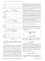
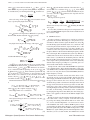
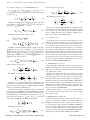
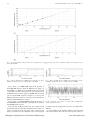
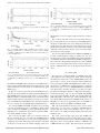
WHITEPAPER:
SSTDR
SPREAD-SPECTRUM
TIME-DOMAIN
REFLECTOMETRY
MADE IN
USA
Whitepaper: Spread Spectrum Time-Domain Reflectometry
www.T3Innovation.com
IEEE SENSORS JOURNAL, VOL. 5, NO. 6, DECEMBER 2005
1469
Analysis of Spread Spectrum Time Domain
Reflectometry for Wire Fault Location
Paul Smith, Member, IEEE, Cynthia Furse, Senior Member, IEEE, and Jacob Gunther, Member, IEEE
Abstract—Spread spectrum time domain reflectometry (SSTDR)
and sequence time domain reflectometry have been demonstrated
to be effective technologies for locating intermittent faults on aircraft wires carrying typical signals in flight. This paper examines
the parameters that control the accuracy, latency, and signal to
noise ratio for these methods. Both test methods are shown to be
effective for wires carrying ACpower signals, and SSTDR is shown
to be particularly effective at testing wires carrying digital signals such as Mil-Std 1553 data. Results are demonstrated for both
controlled and uncontrolled impedance cables. The low test signal
levels and high noise immunity of these test methods make them
well suited to test for intermittent wiring failures such as open circuits, short circuits, and arcs on cables in aircraft in flight.
Index Terms—Aging wire detection, arc detection, sequence time
domain reflectometry (STDR), spread spectrum time domain reflectometry (SSTDR), time domain reflectometry (TDR), wire fault
detection.
I. INTRODUCTION
F
OR MANY years, wiring has been treated as a system that
could be installed and expected to work for the life of an
aircraft [1]. As aircraft age far beyond their original expected
life span, this attitude is rapidly changing. Aircraft wiring problems have recently been identified as the likely cause of several
tragic mishaps [2] and hundreds of thousands of lost mission
hours [3]. Modern commercial aircraft typically have more than
100 km of wire [2]. Much of this wire is routed behind panels or
wrapped in special protective jackets, and is not accessible even
during heavy maintenance when most of the panels are removed.
Among the most difficult wiring problems to resolve are those
that involve intermittent faults [4]. Vibration that causes wires
with breached insulation to touch each other or the airframe,
pins, splices, or corroded connections to pull loose, or “wet
arc faults” where water drips on wires with breached insulation
causing intermittent line loads. Once on the ground these faults
Manuscript received April 10, 2004; revised September 14, 2004. This work
was supported in part by the Utah Center of Excellence for Smart Sensors and in
part by the National Science Foundation under Contract 0097490. The associate
editor coordinating the review of this paper and approving it for publication was
Prof. Michael Pishko.
P. Smith is with VP Technology, LiveWire Test Labs., Inc., Salt Lake City,
UT 84117 USA (e-mail: [email protected]).
C. Furse is with the Department of Electrical and Computer Engineering, University of Utah, Salt Lake City, UT 84112 USA, and also with VP Technology,
LiveWire Test Labs., Inc., Salt Lake City, UT 84117 USA (e-mail: cfurse@
ece.utah.edu).
J. Gunther is with the Department of Electrical and Computer Engineering,
Utah State University, Logan, UT 84322-4120 USA (e-mail: [email protected].
edu).
Digital Object Identifier 10.1109/JSEN.2005.858964
often cannot be replicated or located. During the few milliseconds it is active, the intermittent fault is a significant impedance
mismatch that can be detected, rather than the tiny mismatch
observed when it is inactive. A wire testing method that could
test the wires continually, including while the plane is in flight
would, therefore, have a tremendous advantage over conventional static test methods.
Another important reason to test wires that are live and in
flight is to enable arc fault circuit breaker technology [5] that is
being developed to reduce the danger of fire due to intermittent
short circuits. Unlike traditional thermal circuit breakers, these
new circuit breakers trip on noise caused by arcs rather than requiring large currents. The problem is that locating the tiny fault
after the breaker has tripped is extremely difficult, perhaps impossible. Locating the fault before the breaker trips could enable
maintenance action.
This paper describes and analyzes one such method, based
on spread spectrum communication techniques that can do just
that. This method is accurate to within a few centimeters for
wires carrying 400-Hz aircraft signals as well as MilStd 1553
data bus signals. Results are presented on both controlled and
uncontrolled impedance cables up to 23 m long.
Early research on spread spectrum time domain reflectometry
(SSTDR) [6] has considered fault location tests on high voltage
power wires. Sequence time domain reflectometry (STDR) [7]
has been studied and used to test twisted pairs for use in communications. More recently, it has been demonstrated for location
of intermittent faults such as those on aircraft wiring [18]. These
test methods could be used as part of a smart wiring system
[2], and could provide continuous testing of wires on aircraft
in flight, with automatic reporting of fault locations to facilitate
quick wiring repairs. This could be done by integrating the electronics into either the circuit breaker or into “connector savers”
throughout the system. In order for this to be feasible, the prototype system that has been described here is being redesigned
as a custom ASIC, which should cost on the order of $10–$20
per unit in bulk. This paper focuses on the analysis of SSTDR
and STDR. Parameters required for these methods to function
as potential test methods on wires carrying 400-Hz ACor high
speed digital data such as Mil-Std 1553 are discussed. This analysis is critical to determine the system tradeoffs between speed,
accuracy, code length/system complexity, etc. This ideal analysis provides information on the expected accuracy, which is
verified with tests of near-ideal lossless controlled impedance
coax. The effect of realistic noncontrolled impedance cable is
also evaluated, and sources of error within a realistic system are
discussed.
1530-437X/$20.00 © 2005 IEEE
Whitepaper: Spread Spectrum Time-Domain Reflectometry
www.T3Innovation.com
1470
IEEE SENSORS JOURNAL, VOL. 5, NO. 6, DECEMBER 2005
Fig. 1. S/SSTDR circuit diagram.
II. CURRENT WIRE TEST TECHNOLOGY
There are several test technologies that can be used to pinpoint the location of wiring faults. Some of the most publicized
methods are: time domain reflectometry (TDR) [8], standing
wave reflectometry (SWR) [12], frequency domain reflectometry (FDR) [13], impedance spectroscopy [14], high voltage,
inert gas [15], resistance measurements, and capacitance measurements. At the present time, these test methods cannot reliably distinguish small faults such as intermittent failures on
noncontrolled impedance cables without the use of high voltage.
In addition, the signal levels required to reliably perform these
tests may interfere with aircraft operation if applied while the
aircraft is in use [4]. Another test method is needed that can test
in the noisy environment of aircraft wiring, and that can be used
to pinpoint the location of intermittent faults such as momentary
open circuits, short circuits, and arcs.
III. SPREAD SPECTRUM WIRE TESTING
Spread spectrum signals, both in baseband (STDR) [7] and
modulated (SSTDR) [6], are detectable through cross correlation, even though they may be buried in noise. The ability to
pick out the signal is due to processing gain, which for direct
sequence spread spectrum (DSSS) can be expressed as
(3 dB/100 m) 70- shielded twisted pair cable, and allows for a
SNR of 17.5 dB [17].
The block diagram of the STDR/SSTDR block is shown in
Fig. 1. A sine wave generator (operating at 30–100 MHz) creates
the master system clock. Its output is converted to a square wave
via a shaper, and the resulting square wave drives a pseudo-noise
digital sequence generator (PN Gen). To use SSTDR, the sine
wave is multiplied by the output of the PN generator, generating
a DSSS binary phase shift keyed (BPSK) signal. To use STDR,
the output of the PN generator is not mixed with the sine wave.
The test signal is injected into the cable. The total signal from
the cable (including any digital data or ACsignals on the cable,
and any reflections observable at the receiver) is fed into a correlator circuit along with a reference signal. The received signal
and the reference signal are multiplied, and the result is fed to
an integrator. The output of the integrator is sampled with an
analog-to-digital converter (ADC). A full correlation can be collected by repeatedly adjusting the phase offset between the two
signal branches and sampling the correlator output. The location of the various peaks in the full correlation indicates the location of impedance discontinuities such as open circuits, short
circuits, and arcs (intermittent shorts). Test data indicate that this
test method can resolve faults in a noisy environment to within
1/10th to 1/100th the length of a PN code chip on the cable, depending on the noise level, cable length, and type of cable [4].
IV. STDR/SSTDR ANALYSIS
where
is the bandwidth of the spread-spectrum signal, is
the duration of one entire STDR/SSTDR sequence (considering
the entire sequence equal to one bit in communication-system
terms),
is the duration of a PN code chip,
is the chip rate
in chips per second, and
is the symbol rate, which in this
case is the number of full sequences per second [16].
Because of this processing gain, it is reasonable to assume
that a spread spectrum test system could operate correctly in a
noisy environment with 400-Hz 115-V ACor digital data on the
wires. The test system could be designed such that it would not
be damaged by or interfere with any of the signals already on
the wires. For the analysis that follows, the digital data on the
wires will be assumed to be Mil-Std 1553, a standard aircraft
communication data bus that specifies a 1 Mbit/second data rate,
a 2.25–20 V RMS signal level, normally operates on low-loss
Whitepaper: Spread Spectrum Time-Domain Reflectometry
The operation of STDR/SSTDR depends on the fact that portions of electrical signals are reflected at discontinuities in the
characteristic impedance of the cable. A spread spectrum signal
shown in Fig. 2 is injected onto the wires, and as with TDR,
the reflected signal will be inverted for a short circuit and will
be right-side-up for an open circuit [8]. The observed reflected
signal is correlated with a copy of the injected signal. The shape
of the correlation peaks is shown in Fig. 3. In this figure, the
modulating frequency is the same as the chip rate. Note that the
sidelobes in the correlation peak are sinusoids of the same amplitude as the off-peak autocorrelation of the ML code. This is
due to the selected modulation frequency and synchronization.
Use of a different modulation frequency or different synchronization will yield a different correlation pattern that may have
higher side lobes [4]. Different PN sequences also have different
peak shapes, as shown in Fig. 4 for ML and gold codes.
www.T3Innovation.com
SMITH et al.: ANALYSIS OF SPREAD SPECTRUM TIME DOMAIN REFLECTOMETRY
Fig. 2. STDR and SSTDR signals. The SSTDR signal is modulated with
.
Fig. 3.
Autocorrelations of STDR and SSTDR signals from Fig. 2.
1471
throughout, they definitely do not have even spacing throughout
the bundle. The response is not as smooth as that seen in Fig. 5,
due to the multiple small reflections that occur within the uncontrolled impedance bundle. These multiple reflections as well as
the variations in velocity of propagation that go with them will
reduce the accuracy of the method somewhat for uncontrolled
impedance cables, as we shall see later.
When a peak detection algorithm (to identify the approximate
open circuit location) is coupled with a curve fitting approach
(to determine its precise location), the length of the wires can
be calculated very accurately as shown in Fig. 4(a) and (b) for
the controlled and uncontrolled impedance wires, respectively.
The maximum error observed for controlled impedance cables
is 3 cm, and for the uncontrolled impedance wires is 6 cm. The
minimum measurable length for both systems is approximately
3.5 m, as seen in these figures. This is because the initial and
final peaks overlap. A more advanced curve fitting approach can
be used to distinguish these overlapping peaks.
For the discussion that follows, the ideal case will be assumed
where the cable is lossless. An additional assumption is that
frequency dispersion is negligible in the cable. That is, that all
frequencies travel down the cable at the same rate.
A. Expected Correlator Output With Generalized Noise
The correlator output can be analyzed in terms of the signal
injected onto the cable, various reflections of that signal, and
any unwanted signals (noise) received at the correlator input.
Let
be a recursive linear sequence of period consisting
of 1s and 1 s. Then let
Fig. 4.
Autocorrelations of ML and gold codes.
(1)
where
otherwise
(2)
is a recursive linear signal (RLS) of period
so that
consisting of 1s and 1 s. Here,
is the minimum duration of a 1 or 1, otherwise known as a “chip.” Note that
Fig. 5. Correlator output for STDR and SSTDR tests on 75- coax cable
with an open circuit 23 m down the cable. Note the peak at zero (connection
between the test system and cable), multiple reflections, and definitive shape of
the correlation peaks.
The location of the peaks in the correlator output in conjunction with an estimate of the velocity of propagation indicates
the distance to impedance discontinuities. Fig. 5 shows normalized sample test data collected on 75- coax cable. The correlation peaks after 23 m are due to multiple reflections in the
23-m cable. The response for noncontrolled impedance cable
is not as clean, which is to be expected because of the variation in impedance and subsequent small reflections as well as
minor variation in velocity of propagation down the length of
the cable. Fig. 6(a) and (b) show the STDR and SSTDR correlation responses measured on two 22 AWG wires in a loosely
bundled set of 22 wires that is 9.9 m long. The wires snake in
and out within the bundle, and although they are roughly parallel
Whitepaper: Spread Spectrum Time-Domain Reflectometry
(3)
for any for a RLS of duration .
The test system will send a signal
onto the cable, which
will be reflected by some arbitrary number of impedance discontinuities in the cable. The reflected signals will return to the test
system after some transmission delay. Along with the reflected
signals will be some noise that will depend on the nature of the
cable being tested, anomalies in the signal generation, and extraneous noise. The noise could be white noise, or it could contain
signals such as Mil-Std 1553.
Let
be the received signal, defined as
(4)
where
to
is the amplitude of reflected signal
relative
is the time delay before receiving reflection , and
www.T3Innovation.com
1472
Fig. 6.
IEEE SENSORS JOURNAL, VOL. 5, NO. 6, DECEMBER 2005
(a) STDR and (b) SSTDR correlation response for an open circuit measured on two 22 AWG wires in a loosely bundled set of 22 wires that is 9.9 m long.
is a noise signal of duration
uncorrelated to
.
The correlator output will be
, that is statistically
B. Correlator Output in the Presence of White Noise
The cross correlation of noise terms with
can be discussed in terms of the nature of the noise terms. If
is white
Gaussian noise, the cross-correlation analysis can be described
explicitly [11]. From (6), the cross correlation of
with
has mean
(7)
(5)
As can be seen from (5), the correlator output will depend
on the reflected signals and the noise, and is, therefore, determined by both deterministic and nondeterministic signals. The
expected value
of the correlation
must, therefore, be
considered
and variance
(8)
where
is the noise power received at the input, and
is
the energy in the reference signal
over one period.
Thus, the effect of white noise in the system will be to add
variation to the measurements proportional to the energy of the
signal
, but it will not cause a consistent DC offset.
C. Correlator Output in the Presence of Mil-Std 1553
(6)
In the last step in (6), the fact that
is zero mean and
is asynchronous to
was used.
The output of the correlator in the absence of noise is the
sum of cross correlations of scaled and time-shifted copies of
and the original
. The expected output in the presence
of noise is the same as the output in the absence of noise, with
some additional random noise term that is zero mean.
Whitepaper: Spread Spectrum Time-Domain Reflectometry
As with white noise, the mean output of the correlator with
Mil-Std 1553 as the noise source
is zero as shown in (6).
The variance of the noise is a bit more involved to calculate since
for Mil-Std 1553
not proportional to
(9)
which is not the same as it is for white noise, as shown in (8).
The signal used for correlation
will be integrated over a
single period. It can, therefore, be considered to be an energy
signal [11], and its energy spectral density is given by
(10)
www.T3Innovation.com
SMITH et al.: ANALYSIS OF SPREAD SPECTRUM TIME DOMAIN REFLECTOMETRY
where
is the Fourier transform of
. Since
is of
finite duration, its power spectral density (PSD) is only nonzero
if considered only over the integration time , in which case
(11)
is the Fourier transform of the subsection of
where
used for the cross correlation for
. Note that, in
general,
because the cross correlation may be
over only a few bits of
. However, the expected value for
is
.
The expected noise power is
can be found in several
The total energy in the signal
ways as given by Rayleigh’s theorem [11]
(12)
Let
be the noise signal due to Mil-Std 1553 operating on
the wires. The Fourier transform of
is given by
(13)
Rayleigh’s theorem gives the energy of the signal
as
(14)
and the PSD defined over
as
(15)
is not a periodic function, the cross-correlation funcAs
tions listed below that deal with
will be linear cross correlations. If both
and
or their derivatives are used in a
cross correlation, it will be operating on one cycle of
and
be defined over
, unless otherwise specified. If only
is shown in a cross correlation or autocorrelation, it will
be a circular cross correlation or autocorrelation, and will be
nonzero only for
. Since
,
and will be treated as if
.
The Fourier transform of the cross correlation of
and
is
(16)
where
is the complex conjugate of
The energy in this cross correlation is
.
(17)
The expected energy in the cross correlation over time
is given by
(18)
Whitepaper: Spread Spectrum Time-Domain Reflectometry
1473
(19)
which is true for any noise source
, including the Mil-Std
1553 signal.
It is clear that (19) indicates that spectral overlap between the
noise and STDR/SSTDR signal results in unavoidable noise in
the correlator output.
D. SSTDR Modulation
In order to perform a consistent cross correlation, a reference
signal must be available. This brings us to the question of synchronization. If the reference signals modulation is off by 90
from the driving signals modulation, the cross correlation of the
received signal and the reference signal would be zero, as the
two signals would be orthogonal to each other. Another cross
correlation of the same signal could return a different result, if
the phase difference between the modulating frequency and the
PN code changed. This would make the system very difficult to
calibrate. Because the choice has been made to use PN codes, it
makes sense to synchronize the modulating sinewave with the
PN code [4]. By generating the signals in a consistent way, a reference signal can be generated which can be used consistently
with the injected signal, providing for a system that gives consistent results under similar circumstances.
Sample aircraft cables tested with S/SSTDR have significant
loss at high frequency. Noncontrolled impedance cables (discrete bundled wires) over 60 m long have been tested with STDR
and over 15-m long have been tested with SSTDR (which has
higher frequency content).
Another effect of realistic aircraft cable is the effect of variation in the velocity of propagation (VOP). Typical wires have
VOP ranging from 0.66 to 0.76 times the speed of light [9]. If
the type of wire is known, the correct velocity can be used to
obtain the best possible calculation for the length of the wire. If
the type of wire is not known, and average values are used, additional errors of up to 10% could be observed. Correlation peaks
show higher dispersion if they are due to reflections farther down
the cable, as shown in Fig. 2. This effect can be accounted for
by changing the shape that is matched by the curve fitting algorithm as it is applied to reflections from different lengths down
the cable.
Results for both controlled and uncontrolled impedance aircraft cables with a variety of signals on the line were tested
[4]. Using curve fitting, both methods had errors on the order
of 3 cm for controlled impedance coax and 6 cm for uncontrolled bundled cable with or without 60-Hz signals for both
open and short circuited cables. However, as expected, SSTDR
performs significantly better than STDR in the presence of the
MilStd-1553 signal utilizing the uncontrolled impedance bundled wire (a worse case than normal, since MilStd 1553 would
www.T3Innovation.com
1474
IEEE SENSORS JOURNAL, VOL. 5, NO. 6, DECEMBER 2005
normally be implemented on controlled impedance twisted pair
wire). For an SNR of 24 dB, STDR has an error of about
24 cm, and SSTDR had less than 3 cm of error. SSTDR still
had less than 6 cm of error down to and SNR of 53 dB below
the MilStd 1553 data signal. Both methods could be used effectively, since the required SNR for MilStd 1553 is 17 dB,
however the advantage of SSTDR for a high frequency noisy
environment was clearly demonstrated.
For noise signals that are broad in frequency spectrum, the
integral in (23) is quite involved, and is best handled numerically
on a case-by-case basis.
The effects of changing certain parameters can be studied analytically in such a way as to provide excellent insight into factors other than signal and noise power that affect the SNR. These
analyzes are carried out below.
A. Changing the Length of the STDR/SSTDR Signal
V. SIGNAL-TO-NOISE RATIO
The SNR is defined as the signal power divided by the average noise power. For a digital signal such as Mil-Std 1553,
this would be expressed as
In order to approximate a signal with times the number of
chips as
, let us define a new signal
such that
is proportional to
, and let the duration of
be
. Letting the amplitude of
be the same as
(25)
(20)
In the case of STDR/SSTDR, the STDR and SSTDR signals
are the desired signals, and other signals are noise. Therefore,
considering the signal-to-noise power of the STDR and SSTDR
signals in the presence of another signal (Mil-Std 1553 in this
example), gives
(21)
means “cross-correlated
after correlation, where
power.”
The reflection terms
represent the reflections at various distances down the cable. To detect each of these
signals, the correlator offset is set to time
. All other reflection terms are considered noise terms. The received signal
after cross correlation is
(22)
In the frequency domain
(26)
were
which is what would be expected if the duration of
increased by a factor of by adding more chips to its sequence.
Letting
(27)
gives
(28)
with
which is the noise energy in the cross correlation of
over the time
. The expected value of the noise
power over the interval
is the noise power over the
interval
, given by
From (22) and (19), the SNR is
(29)
(23)
The integral in (23) needs to be carried out for every signal
of interest that could be a noise source. For spectrally narrow
noise, such as the 115 V 400 Hz on aircraft, (23) simplifies to
.
which is valid because
The central peak of the autocorrelation is given by
(30)
The signal power is
(31)
From (31) and (29), the SNR is
(32)
Hz
Hz
(24)
has very little of its
From this, it can be seen that if
energy centered at
Hz, the SNR will be large.
Whitepaper: Spread Spectrum Time-Domain Reflectometry
Equation (32) shows that doubling the length of the PN code
while leaving all other parameters the same will double (increase by 3 dB) the SNR. This is true for any noise type including 400-Hz ac, Mil-Std 1553, and white noise.
www.T3Innovation.com
SMITH et al.: ANALYSIS OF SPREAD SPECTRUM TIME DOMAIN REFLECTOMETRY
1475
and the average noise power is
B. Scaling the Frequency of the STDR/SSTDR Signal
, and
, where is a conLet
stant. Using the scaling property of the Fourier transform and
assuming
(42)
The SNR from (42) and (34) is
(33)
The signal of interest after correlation is the peak value in the
, which is
, and corresponds to
autocorrelation of
the energy in
, given by
(43)
(34)
Equation (43) shows that in SSTDR mode, doubling the chip
rate of the PN code and modulation frequency while leaving all
other parameters the same will increase the SNR for SSTDR
tests by 6 dB if the major noise contributor is Mil-Std 1553.
This is vastly superior to the STDR results.
(35)
C. Self-Induced Noise
Examining correlator noise output, we have
and
(36)
If STDR is considered with the chip rate much greater than
the Mil-Std 1553 data rate of 1 MHz, it can be assumed that
is approximately constant in the region where the majority
of the power of
exists. Then,
will also be
approximately constant in that region if
. With these assumptions, (36) can be written as
(37)
A certain amount of noise comes from the selection of a particular PN code. This is considered noise, because there is a deviation in the cross correlation of all PN codes from the ideal
of a central peak with no side-lobes. Fig. 7 shows the autocorrelations of two identical-power PN sequences, one of which is
using a ML code [10], and the other of which is using a gold code
[10]. Note that the power in the two autocorrelations is not equal,
even though the power in the signals used to generate them is
equal. In fact, the power in the ML code autocorrelation is 56%
the power in the gold code autocorrelation. This extra power in
the gold code autocorrelation is self-induced noise power, and
it reduces the SNR for STDR/SSTDR tests.
D. STDR/SSTDR Code Selection
and the average noise power is
(38)
The SNR from (38) and (34) is
(39)
Equation (39) states that in STDR mode, doubling the chip
rate of the PN code while leaving all other parameters the same
will have no appreciable effect on the SNR for STDR tests if the
major noise contributor is Mil-Std 1553.
Attention is now turned to changing the chip rate and modulation frequency for SSTDR tests. For SSTDR with a chip rate
much greater than the Mil-Std 1553 data rate of 1 MHz, scaling
the SSTDR chip rate and modulation frequency by a factor
will change the slope near
by a factor
. So, in the
region where the Mil-Std 1553 signal is significant
(40)
With this approximation
(41)
Whitepaper: Spread Spectrum Time-Domain Reflectometry
The optimal PN code depends on the nature of the application.
The PN code with the lowest side lobes in its autocorrelation is
a ML code. It is, therefore, optimal for use when only one PN
code will be used at a time.
The PN code with the next best autocorrelation properties
is the Kasami code [11]. It is the best PN code choice when
simultaneous tests on one or more conductors can interfere with
each other. This is due to the high degree of orthogonality of
signals in a Kasami set. If, however, the number of simultaneous
tests exceeds the number of codes in the Kasami set, then codes
with higher autocorrelation side-lobes, such as gold codes, may
be used. One-shot codes, such as those similar to Barker codes,
may also be used for STDR/SSTDR.
Many other PN codes are a poor choice for STDR/SSTDR
due to high autocorrelation side lobes or the lack of a single
autocorrelation peak.
E. STDR/SSTDR Using ML Codes
When the background noise is white noise, the total noise
power after correlation is identical for both the STDR and
SSTDR cases because the noise is spectrally flat. In this case,
it is clear that there is little advantage of STDR over SSTDR or
vice versa. However, when the noise is not spectrally flat, such
as is the case with a Mil-Std 1553 or other digital data signal,
the spectral overlap of the noise with the STDR/SSTDR signal
will change the relative benefits of STDR versus SSTDR.
www.T3Innovation.com
1476
Fig. 7. Actual versus distance estimated with a curve-fit algorithm on (a) a 75tested with S/SSTDR.
Fig. 8. ML code STDR signal at 1-V RMS, with a signal length of 63 chips at
30 MHz, operating in the presence of Mil-Std 1553 at 10-V RMS.
Fig. 8 shows a 1-V RMS STDR signal in the presence of
10-V RMS Mil-Std 1553. Since the Mil-Std 1553 signal is at
10-V RMS, it is 20 dB above the STDR signal level. The PN
code length is 63 bits, which will give a processing gain of
36 dB. The chip rate in this figure is 30 MHz. The processing
gain for longer STDR sequences is higher, so a lower power
STDR signal can be used in an actual test system that will not
interfere with the Mil-Std 1553 signal.
Fig. 9 shows a 1-V RMS SSTDR signal in the presence of
10-V RMS Mil-Std 1553. The PN code length used to generate
this SSTDR signal is 63 bits.
Even after the 36 dB processing gain, the correlation peak
shown in Fig. 10 is not clear due to the high noise level after correlation. Consider, however, the clarity of the correlation peak
in Fig. 11. In both cases, the amplitude of the correlation peak
Whitepaper: Spread Spectrum Time-Domain Reflectometry
IEEE SENSORS JOURNAL, VOL. 5, NO. 6, DECEMBER 2005
cable and (b) a pair of two 22 AWG wires within a loose bundle of 22 wires
Fig. 9. ML code SSTDR signal at 1-V RMS, with a signal length of 63 chips
at 30 MHz, operating in the presence of Mil-Std 1553 at 10-V RMS.
Fig. 10. Normalized cross correlation of a reference ML code STDR signal
with the signal shown in Fig. 8.
is identical, but the background noise levels are significantly
different.
To gain insights into the dramatic difference in background
noise levels shown in Figs. 10 and 11, the spectral content of
www.T3Innovation.com
SMITH et al.: ANALYSIS OF SPREAD SPECTRUM TIME DOMAIN REFLECTOMETRY
Fig. 11. Normalized cross correlation of a reference ML code SSTDR signal
with the signal shown in Fig. 9.
Fig. 12. Normalized PSD of a ML code STDR signal of length 63 chips at
30 MHz (1-V RMS), ML code SSTDR signal of length 63 chips at 30 MHz
(1-V RMS), and Mil-Std 1553 (1-V RMS). Signals are normalized with respect
to the peak STDR power.
1477
Fig. 14. Normalized PSD of the cross-correlator (XCorr) output for a pure ML
code SSTDR (ideal case) signal of length 63 chips at 30 MHz (1-V RMS), and
a 1-V RMS ML code SSTDR signal in the presence of a 10-V RMS Mil-Std
1553 signal.
that naturally occurs in a single sample per iteration correlator
design.
Fig. 14 shows the PSD of the cross correlation shown in
Fig. 11, alongside the cross correlation of an SSTDR signal in
the ideal case where there is no noise. The background noise is
significantly lower than the peak of the desired signal. Again,
the frequency spectrum of the noise is broad due to the random
sampling of the noise that naturally occurs in a single sample
per iteration correlator design.
It is clear from these simulations that STDR and SSTDR can
be used to find impedance changes in wiring. It is also clear
that the spectral content of the SSTDR signal can be adjusted to
avoid mutual interference between the SSTDR and digital signals on the wires. Tests with narrowband noise, such as 400-Hz
115-V ac, show a negligible effect on the correlator output compared to wideband noise such as the digital signals discussed
above.
VI. CONCLUSION
Fig. 13. Normalized PSD of the cross-correlator (XCorr) output for a pure ML
code STDR (ideal case) signal of length 63 chips at 30 MHz (1-V RMS), and a
1-V RMS ML code STDR signal in the presence of a 10-V RMS Mil-Std 1553
signal.
the STDR and SSTDR signals with respect to the Mil-Std 1553
signal can be examined. The PSD of these three signals as used
in the simulations is shown in Fig. 12, normalized to the peak
STDR power.
In Fig. 12, it can be seen that the power in the Mil-Std 1553
signal is centered about 0 Hz, as is the power in the STDR signal.
The SSTDR signal, however, slopes down to a spectral null at
0 Hz (dc). If this is considered in light of (19), it is clear that there
will be significantly more unwanted power in the cross correlation of an STDR signal with Mil-Std 1553 than there will be in
the cross correlation of an SSTDR signal with Mil-Std 1553.
To compare SSTDR with STDR, frequencies above the chip
rate were not trimmed off prior to modulation, which caused
some aliasing in the SSTDR case. Tests performed using bandlimiting prior to modulation did not show a significant difference in the SSTDR correlator output.
Fig. 13 shows the PSD of the cross correlation shown in
Fig. 12, alongside the cross correlation of an STDR signal in
the ideal case where there is no noise. The background noise
completely dwarfs the desired signal. The frequency spectrum
of the noise is broad due to the random sampling of the noise
Whitepaper: Spread Spectrum Time-Domain Reflectometry
This paper has examined STDR and SSTDR using ML
codes. Equations were developed to enable system design by
describing the interactions of the STDR/SSTDR signal and
various types of noise in the correlator output. Simulations
were performed for STDR and SSTDR tests for ML codes in
the presence of a Mil-Std 1553 background signal to study the
effects of this type of noise on STDR/SSTDR tests. Equations
were developed to describe the effects of scaling test system
parameters including the number of chips in the PN sequence
and the PN sequence chip rate used for STDR and SSTDR.
It was shown that doubling the PN code length doubles the
SNR independent of the noise type, and that doubling the chip
rate (and modulation frequency for SSTDR) in the presence of
Mil-Std 1553 can have no appreciable effect on the SNR for
STDR, but can increase the SNR for SSTDR by 6 dB.
ML codes were identified as the best code to use for testing
single wires at a time due to the higher self-induced noise
present with other code choices. Kasami codes are the optimal codes to use when performing multiple interacting tests
simultaneously.
The work covered in this paper shows that SSTDR and
STDR can be effective tools for locating defects on live cables,
and this was demonstrated for both controlled and uncontrolled
impedance cables carrying 60 Hz (similar to 400 Hz) and
1-MHz Mil Std 1553 signals. This discussion has shown that
www.T3Innovation.com
T3 Innovation
808 Calle Plano
Camarillo, CA 93012
Contact Us:
(805) 233-3390
www.T3innovation.com
Whitepaper: Spread Spectrum Time-Domain Reflectometry
www.T3Innovation.com