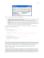
Download Simplicity 1692686 Specifications

The AnyBodyTM Modeling System
Tutorials
Version 3.0.0, September 2007
Copyright © 2007, AnyBodyTM Technology A/S
Home: www.anybodytech.com
1
Tutorials
The AnyBody tutorials are step by step introductions to the use of the AnyBody system and in particular to
construction of models in AnyScript. The tutorials are tightly linked to a collection of demo AnyScript files.
These samples are usually developed as a response to popular requests by our users. The demo comes first,
and a tutorial is subsequently developed around it.
This pdf-document is a collection of the tutorials exported directly from the AnyBody web page. Each of the
following chapter is indeed one tutorial. We apologize for broken links and other parts of the text that is not
well-designed as a text document in this format. This document is primarily aimed at printing the text, in
case you prefer to read a paper version. When working with the tutorials, we recommend that you use an
electronic version, either the online version or a version installed on your computer together with AnyBody.
2
Getting Started.................................................................................................................. 4
Lesson 1: Using the standing model .................................................................................. 6
Lesson 2: Controlling the posture...................................................................................... 9
Lesson 3: Reviewing analysis results ................................................................................12
Getting started with AnyScript ........................................................................................ 16
Lesson 1: Basic concepts ................................................................................................17
Lesson 2: Defining segments and displaying objects ...........................................................22
Lesson 3: Connecting segments by joints ..........................................................................28
Lesson 4: Definition of movement ....................................................................................32
Lesson 5: Definition of muscles and external forces ............................................................35
Lesson 6: Adding real bone geometries.............................................................................42
Interface features ........................................................................................................... 46
Lesson 1: Windows and workspaces .................................................................................47
Lesson 2: The Editor Window ..........................................................................................49
Lesson 3: The Model View Window ...................................................................................54
Lesson 4: The Chart Views ..............................................................................................60
Lesson 5: The Command Line Application..........................................................................70
A study of studies............................................................................................................ 73
Lesson 1: Model Information ...........................................................................................77
Lesson 2: Setting Initial Conditions ..................................................................................82
Lesson 3: Kinematic Analysis...........................................................................................84
Lesson 4: Inverse Dynamic Analysis .................................................................................88
Lesson 5: Calibration Studies ..........................................................................................94
Muscle modeling ........................................................................................................... 102
Lesson 1: The basics of muscle definition ........................................................................ 103
Lesson 2: Controlling muscle drawing ............................................................................. 108
Lesson 3: Via point muscles .......................................................................................... 112
Lesson 4: Wrapping muscles ......................................................................................... 115
Lesson 5: Muscle models .............................................................................................. 121
Lesson 6: General muscles............................................................................................ 142
Lesson 7: Ligaments .................................................................................................... 150
The mechanical elements .............................................................................................. 158
Lesson 1: Segments .................................................................................................... 159
Lesson 2: Joints .......................................................................................................... 161
Lesson 3: Drivers ........................................................................................................ 162
Lesson 4: Kinematic Measures....................................................................................... 162
Lesson 5: Forces ......................................................................................................... 175
Advanced script features............................................................................................... 176
Lesson 1: Using References........................................................................................... 176
Lesson 2: Using Include Files ........................................................................................ 177
Lesson 3: Mathematical Expressions............................................................................... 178
Building block tutorial ................................................................................................... 178
Lesson 1: Modification of an existing application............................................................... 181
Lesson 2: Adding a segment ......................................................................................... 184
Lesson 3: Kinematics ................................................................................................... 188
Lesson 4: Kinetics........................................................................................................ 195
Lesson 5: Starting with a new model .............................................................................. 199
Lesson 6: Importing a Leg Model ................................................................................... 202
Lesson 7: Making Ends Meet ......................................................................................... 208
Lesson 8: Kinetics - Computing Forces............................................................................ 217
Lesson 9: Model Structure ............................................................................................ 222
Validation of models...................................................................................................... 223
Kinematic input ........................................................................................................... 225
Parameter studies and optimization.............................................................................. 227
Defining a parameter study........................................................................................... 228
Optimization studies .................................................................................................... 240
3
Trouble shooting AnyScript models ............................................................................... 253
4
Getting Started
This tutorial is the starting point for new users. Its purpose is to allow users to get the first model up and
running fairly quickly.
The AnyBody Modeling System can be approached on a number of levels depending on the amount of detail
the modeling task requires. Listing the approaches in top-down order may produce the following:
•
•
•
Loading a model defined by somebody else and changing simple parameters like the applied load or
the posture. For instance, the so-called StandingModel from the model repository allows for addition
of loads to certain predefined points on the model, and the system will compute the muscular
reactions.
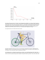
Modifying a model made by somebody else but similar to what you want to obtain. For instance, one
of the bicycle models from the repository could be changed into a recumbent bike.
Building a new model by taking a predefined collection of body parts from the repository and
equipping it with boundary conditions and an environment to interact with. For instance, it is rather
5
•
•
easy to create a model of a gymnastic exercise on the floor this way.
Constructing a model from single predefined body parts in the repository. This allows for detailed
control of which body parts are included in the model and may be useful for, for instance, detailed
investigations of the internal forces in a single limb.
Constructing a body model and its environment bottom-up. This is recommended for users
interested in development models that are not covered by the current model repository. This could
either be detailed models of missing body parts or perhaps single joints, or it could be models of
various animals. The basic steps of such bottom-up model construction are described in the tutorial
Getting Started with AnyScript, which is a good place to start for new users, even if you do not plan
to build models bottom-up.
These various levels of model building complexity are covered in The Building Block Tutorial.
As you can see above, the more detailed approaches are covered by other tutorials. To get you up and
running quickly, we shall take the top-down approach in this tutorial and use the model library to accomplish
the following:
1.
2.
3.
Load the predefined standing model, place it in a given posture, and apply an external force to it.
Modify the predefined standing model to carry a hand bag.
Create a new model and import a predefined collection of body parts from the library to obtain a
model of a simple gymnastics exercise.
This entire tutorial relies heavily on the body model repository. It is a library of predefined models and body
parts developed by scientists as a research undertaking. The models are placed in the public domain and are
therefore totally open to scrutiny and are consequently improved and changed constantly. The effort is
coordinated by the AnyBody Research Project at Aalborg University in Denmark. If you are a new user and
unfamiliar with the structure of the repository, then it is strongly recommended that you pop over to the
scientific homepage for a short interlude to familiarize yourself with the structure an idea behind it. When
you feel familiar with the ideas, come back here and continue the tutorial. The link to the repository on the
scientific homepage is here: www.anybody.aau.dk/Repository/.
Before you continue you must download the entire repository and save it on your hard disk. A selection of
models from the respository are included in the demo collection which is installed with AnyBody. These
demo models should be sufficient for your work with this and other tutorials, but because the repository
keeps geting updated it may be a good idea to download and unpack the newest version from
www.anybody.aau.dk/Repository/ before you start any serious modeling work.
The demo models, including the Standing Model to be used in this tutorial, are available from the Demo tab
of the AnyBody Assistant dialog box.
6
When you open AnyBody for the first time, the Demo tab does not contain any models, but only a short
guide on how to extract the demo models. After having done this, brief descriptions and links to the models
are available in the tab. In addition, it is easy to reinstall the demo models later, which may be useful when
you have been playing around with them for a while; this way you can reset all the changes you have made.
You can also reinstall them to a new location, if you wish to keep your own changes to the first installation.
Now you are all set to go, and you can proceed with the lesson 1: Using the standing model.
Lesson 1: Using the standing model
The model repository contains a number of applications that are generic in nature and can serve dual
purposes: Either they can be used with minor modifications or they can with minor modifications become a
model of something else. The Standing Model is one of these general applications, and we shall use it here
by virtue of its first ability, i.e. pretty much as it is.
The standing model can be found in the repository under ARep/Aalborg. This position indicates that it is an
application as opposed to merely a body part, and that it was developed by the AnyBody Research Group at
Aalborg University. The model comprises most of the available body parts in the library. The main file is
called StandingModel.Main.any, and this is the one you must load.
You can open the file with the file manager in AnyBody or by Windows Explorer, but it can be recommend
that you use the demo files installed together with AnyBody. In this case, you can take the shortcut via the
the Demo tab of the AnyBody Assistant dialog box. The Demo tab will contain links to many interesting
models including the Standing Model.
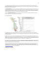
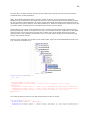
Before you hit the load button, please have a look at the structure of the main file. The first part of it should
look like this:
Main = {
#include "DrawSettings.any"
AnyFolder Model={
AnyFolder HumanModel={
7
//This model is only for kinematic analysis and should be used when playing
//around with the kinematics of the model since leaving the muscles out, makes
//the model run much faster
#include
"..\..\..\BRep\Aalborg\BodyModels\FullBodyModel\BodyModel_NoMuscles.any"
//This model uses the simple constant force muscles
//#include "..\..\..\BRep\Aalborg\BodyModels\FullBodyModel\BodyModel.any"
//This model uses the simple constant force muscles for shoulder-arm and spine
//but the 3 element Hill-type model for the legs
//Remember to calibrate the legs before running the inverse anlysis
//This is done by pressing Main.Bike3D.Model.humanModel.CalibrationSequence in
the
//operationtree(lower left corner of screen)
//#include "..\..\..\BRep\Aalborg\BodyModels\FullBodyModel\BodyModel_Mus3E.any"
AnyFolder StrengthParameters={
AnyVar SpecificMuscleTensionSpine= 90; //N/cm^2
AnyVar StrengthIndexLeg= 1;
AnyVar SpecificMuscleTensionShoulderArm= 90; //N/cm^2
};
//Pick one of the scaling laws
//Do not scale
#include "..\..\..\BRep\Aalborg\Scaling\ScalingStandard.any"
//Scaling unifoRmly in all directions to macth segments lengths
//#include "..\..\..\BRep\Aalborg\Scaling\ScalingUniform.any"
//Scaling taking length and mass of the segments into account
//#include "..\..\..\BRep\Aalborg\Scaling\ScalingLengthMass.any"
//Scaling taking length, mass and fat of the segments into account
//#include "..\..\..\BRep\Aalborg\Scaling\ScalingLengthMassFat.any"
//
//
//
Scaling={
#include "..\..\..\BRep\Aalborg\Scaling\AnyFamilyAnyJack.any"
};
};
Please notice that depending on who touched the file last, the choice of body model and scaling option as
defined by the lines commented in or out may be different for you than shown above. Please make sure that
you have chosen the BodyModel_NoMuscles and the ScalingStandard options, and that the Scaling folder is
commented out.
The standing model has a few things, which are predefined, and some that you can modify. Here is a short
list:
•
•
•
•
The model is supported by having both its feet rigidly connected to ground. This conditon applied no
matter what posture the model is put into.
The posture of the model is controlled via angles for all major joints except the ankles. So the
model has a place where joint angles can be specified directly, and the model will assume the
posture defined by the joint angles. We shall return to this topic shortly.
The model automatically balances its posture by means of the ankle angles such that its collective
center of mass remains vertically above the ankle joints. For instance, if the model extends the
arms in front of it, then the ankles will adjust and move the entire model slightly backwards to
maintain the balance.
The model has a set of predefined points to which can be applied three-dimensional external forces
simply defined as spatial vectors. When doing so, the muscles of the model will be recruited to
8
balance the extrnal forces. Please notice that it is possible to apply an external force large enough
to require tension between the feet and the floor. Because of the rounding condition of the feet such
a tension will be provided by the model but the situation may not be realistic because real feet
rarely stick to the ground.
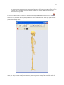
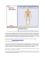
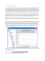
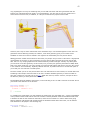
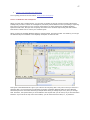
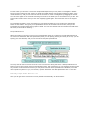
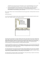
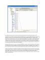
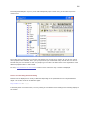
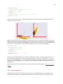
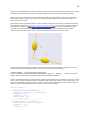
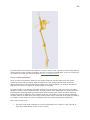
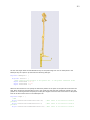
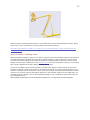
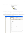
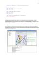
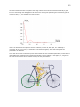
It is time to load the model. You do this by pressing one of the Load Model buttons that look like this
and are located in left hand side of the toolbar of the AnyScript Editor windows and on the main frame
toolbar. F7 is a convenient shortcut when reloading the same model many times. Since the model currently
has no muscles, it should load very quickly. Pressing the menus Window -> Model View (new) should
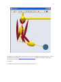
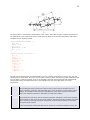
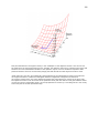
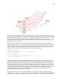
produce the following result:
The icons in the toolbar at the top of the Model View window allows you to modify the image, zoom, pan,
rotate, etc. They should be mostly self explanatory. Now is a good time to play a bit around with them and
9
familiarize yourself with the options.
Having loaded the model it is time to proceed to lesson 2: Controlling the posture.
Lesson 2: Controlling the posture
The Standing Model has been developed to a fairly complex level, automating many of the operations that
are necessary to specify the posture of a full body model. The short story about the kinematics of the model
is that it is based on a specification of angles in all the joints. These specifications can be found in one of the
model files, mannequin.any. You can see where this file is included if you scroll down a bit in the
StandingModel.any file until you come to this point:
//This file contains joint angles which are used at load time for
//setting the initial positions
#include "Mannequin.any"
If you double-click the Mannequin.any file name in the editor window, then the file opens up a new window.
You will see a file with the following structure:
AnyFolder Mannequin = {
AnyFolder Posture = {
AnyFolder Right = {
};
AnyFolder Left = {
};
};
AnyFolder PostureVel={
AnyFolder Right = {
};
AnyFolder Left = {
};
};
AnyFolder Load = {
AnyFolder Right = {
};
AnyFolder Left = {
};
}; // Loads
};
(We have removed all the stuff in between the braces.) This file is typical for the AnyScript language in the
sense that it is organized into so-called folders, which is a hierarchy formed by the braces. Each pair of
braces delimits an independent part of the model with its own variables and other definitions.
Everything in this file is contained in the Mannequin folder. It contains specifications of joint angles,
movements, and externally applied loads on the body. Each of these specifications is again subdivided into
parts for the right and left hand sides of the body respectively.
The first folder, Posture, contains joint angle specifications. You can set any of the joint angles to a
reasonable value (in degrees), and when you reload the model it will change its posture accordingly. Please
make sure that the values are as follows:
10
AnyFolder Right = {
//Arm
AnyVar SternoClavicularProtraction=-23;
//This value is not used for initial
position
AnyVar SternoClavicularElevation=11.5;
//This value is not used for initial
position
AnyVar SternoClavicularAxialRotation=-20; //This value is not used for initial
position
AnyVar GlenohumeralFlexion = 0;
AnyVar GlenohumeralAbduction = 10;
AnyVar GlenohumeralExternalRotation = 0;
AnyVar ElbowFlexion = 0.01;
AnyVar ElbowPronation = 10.0;
AnyVar WristFlexion =0;
AnyVar WristAbduction =0;
AnyVar HipFlexion = 0.0;
AnyVar HipAbduction = 5.0;
AnyVar HipExternalRotation = 0.0;
AnyVar KneeFlexion = 0.0;
AnyVar AnklePlantarFlexion =0.0;
AnyVar AnkleEversion =0.0;
};
When these parameters are set for the right hand side, the left hand side automatically follows along and
creates a symmetric posture. This happens because each of the corresponding settings in the Left folder just
refers back to the setting in the right folder. The ability to do this is an important part of the AnyScript
language: Anywhere a number is expected, you can substitute a variable.
If at any time you want a non-symmetric posture, simply replace some of the variable references in the Left
folder by numbers of your choice.
Further down in the Mannequin.any file you find the folder PostureVel. This is organized exactly like Posture,
but the numbers you specify here are joint angle velocities in degrees per second. For now, please leave all
the values in this folder to zero.
Finally, the last section of the file is named Load. At this place you can apply three-dimensional load vectors
to any of the listed points. These load vectors are in global coordinates, which means that x is forward, y is
vertical, and z is lateral to the right. Let us apply a vertical load to the right hand as if the model was
carrying a bag:
AnyFolder Load = {
AnyVec3 TopVertebra = {0.000, 0.000, 0.000};
AnyFolder
AnyVec3
AnyVec3
AnyVec3
AnyVec3
AnyVec3
AnyVec3
};
AnyFolder
AnyVec3
AnyVec3
Right = {
Shoulder
Elbow
Hand
Hip
Knee
Ankle
=
=
=
=
=
=
Left = {
Shoulder
Elbow
= {0.000, 0.000, 0.000};
= {0.000, 0.000, 0.000};
{0.000,
{0.000,
{0.000,
{0.000,
{0.000,
{0.000,
0.000, 0.000};
0.000, 0.000};
-50.000, 0.000};
0.000, 0.000};
0.000, 0.000};
0.000, 0.000};
11
AnyVec3
AnyVec3
AnyVec3
AnyVec3
Hand
Hip
Knee
Ankle
= {0.000, 0.000, 0.000};
= {0.000, 0.000, 0.000};
= {0.000, 0.000, 0.000};
= {0.000, 0.000, 0.000};
};
}; // Loads
The downward load of -50 N in the right hand roughly corresponds to a weight of 5 kg. To enable the model
to actually carry the load we must equip it with muscles. This is done by selecting a body model with
muscles:
//This model should be used when playing around with the model in the
//initial modelling phase since leaving the normal muscles out, makes the
//model run much faster. The model uses artificial muscles on each dof. in
//the joints which makes it possible also to run the inverse analysis.
//#include "..\..\..\BRep\Aalborg\BodyModels\FullBodyModel\BodyModel_NoMuscles.any"
//This model uses the simple constant force muscles
#include "..\..\..\BRep\Aalborg\BodyModels\FullBodyModel\BodyModel.any"
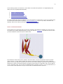
When you reload the model (by pressing F7) it will take more time than before because it is now equipped
with more than 500 muscles. If you have done everything right, you should see the comforting message
'Loaded Successfully' in the message window at the lower left hand side of the AnyBody main frame window.
Now it is time to analyze muscle and joint forces.
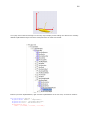
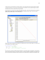
Also at the upper left hand side of the screen you will see a tree containing 'Main' and 'Study'. If you unfold
'Study' you will get the following:
12
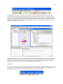
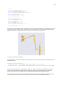
If you click once on InverseDynamicAnalysis and then on the Run button in the bottom of the window then
the system will start analyzing the muscle and joint forces in the model under the influence of gravity and
the load we applied to the hand. This takes a few seconds during which you will see the muscles standing
out from the body and subsequently falling into place. When the analysis is finished you will notice a slight
color change in the muscles and also some bulging, primarily in the right arm. The bulging is proportional to
the force in each muscle, and the degree of red color is proportional to the muscles tone.
You have just completed your first analysis of an AnyBody model. In the next lesson we shall briefly
examine the results. Lesson 3: Reviewing analysis results.
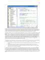
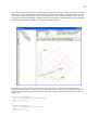
Lesson 3: Reviewing analysis results
The muscle bulging in the Model View window provides an immediate feedback on the overall stres state of
the body, but it does not give much detailed information. For detailed investigation of results, the system
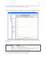
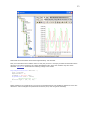
provides several charting facilities. Here we shall just review the basic functionality: The ChartFX View. It
provides the basic ability to make two-dimensional diagrams depicting the results. You can also export the
graphs to the clipboard on several different formats or as text for pasting into a spreadsheet.
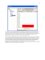
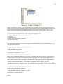
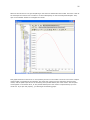
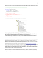
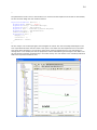
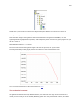
The first step is to click Window -> ChartFX 2D (new). A new window containing a blank field in the middle
and a tree view in the left hand pane appears.
The tree expands to reveal the entire structure of output data generated by AnyBody. Every element in the
model generates some form of output from the analysis, so the tree is very large. One of the first nodes you
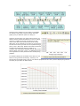
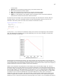
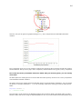
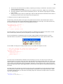
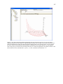
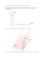
encounter is the MaxMucleActivity variable:
13
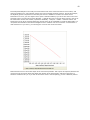
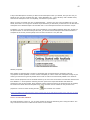
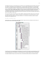
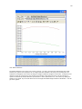
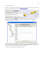
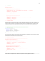
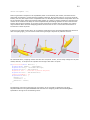
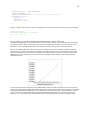
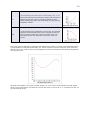
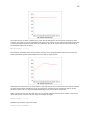
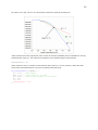
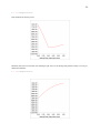
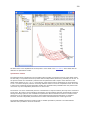
Clicking the node produces an empty cordinate system in the large field. The reason why it is empty is that
the standard setting of the ChartFX View is to display time-varying data for moving models. In this simple
case our model is static, so it does not make much sense to draw curves. Instead we shall switch the setting
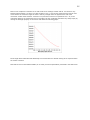
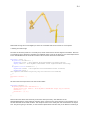
to Bar diagrams in by the Gallery button in the toolbar:
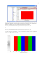
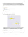
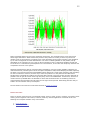
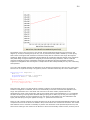
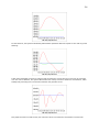
You will obtain the following Image:
14
This tells you that to stand upright and carry the 50 N load in the right hand, the model is using 4.00e-001
= 40% of its maximum voluntary contraction. This means that the relative load of the muscle with the
highest activity in the system is 40% of the muscle's strength. Even though one number is a very simplified
way of regarding a system with hundreds of muscles, there are good mathematical reasons why this
particular number is a good measure of the human effort of a particular task.
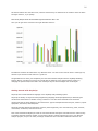
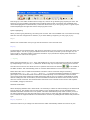
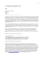
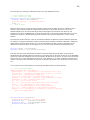
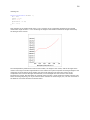
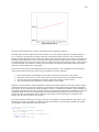
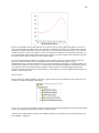
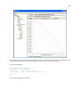
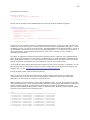
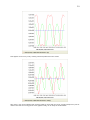
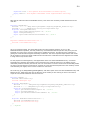
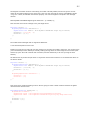
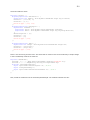
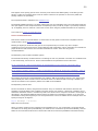
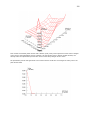
You can obtain more detailed information if you expand the Model branch in the tree view on the left hand
side of the bar diagram. Going down through Model -> HumanModel -> Right -> ShoulderArm -> Mus gives
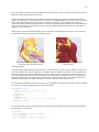
you a long list of all the muscles in the right shoulder and arm. A bit down this list you can find the rotator
cuff muscle supraspinatus, which tends to be one of the sources of rotator cuff pain. Like many of the
muscles in the model, the anatomical muscle supraspinatus is divided into several mechanical branches to
account for fibers going in different directions and attaching to different bones. If you open op
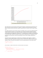
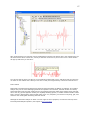
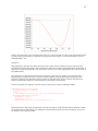
Supraspinatus_3 you can find the property Fm inside. Click it once, and you should see a new bar illustrating
the force in this muscle element similar to the picture below.
15
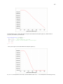
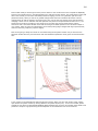
This shows that the force in this muscle branch is roughly 18 N. Notice the specification line above the
graphics pane marked with the red circle above. This is where the specification of the current picture is
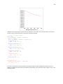
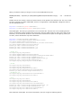
listed. You can use this to plot several muscles at the same time. If you change
Main.Study.Output.Model.HumanModel.Right.ShoulderArm.Mus.supraspinatus_3.Fm
to
Main.Study.Output.Model.HumanModel.Right.ShoulderArm.Mus.supraspinatus_*.Fm
i.e. replace the figure 3 with an asterix, '*', then you should see a bar diagram of all the supraspinatus
muscles in the right hand side of the body.
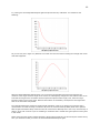
16
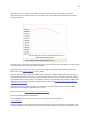
All these branches have the same force, which is because they are assumed in the model to have the same
strength. However, if you specify:
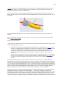
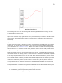
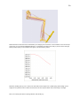
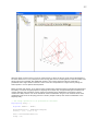
Main.Study.Output.Model.HumanModel.Right.ShoulderArm.Mus.*.Fm
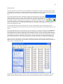
then you will get all the muscles in the right shoulder and arm:
The different muscles do indeed have very different forces. You can see the muscle name in a little pop-up
window if you hold the mouse still over a given bar.
Congratulations! You have just completed your first biomechanical analysis with the AnyBody Modeling
System. Now is a good time to play a bit around with the facilities of the system and the model. Try
changing the posture and/or the load in the mannequin.any file and investigate the results again.
Getting started with AnyScript
AnyScript is the model definition language of the AnyBody body modeling system.
AnyScript is actually an object-oriented programming language developed specifically for describing the
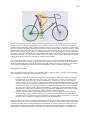
construction and behavior of bodies of living creatures. It can also model the different environment
components that the body happens to be connected to. Typical examples would be bicycles, furniture, sports
equipment, hand tools, and workplaces.
AnyScript contains facilities for definition of bones (called segments), their connections by joints, muscles,
movements, constraints, and exterior forces.
One of the ideas behind AnyScript is that its text-based format and object-oriented structure makes it easy
to transfer elements between models. You can build a library of body segments for use in your different
analysis projects, and you can easily exchange models with other users and collaborate with them on
17
complex modeling tasks.
The syntax of AnyScript is much like a Java, JavaScript, or C++ computer program. If you already know one
of these programming languages, you will quickly feel at home with AnyScript. But don't be alarmed if you
have no programming experience. AnyScript is very logically constructed, and this tutorial is designed to
help new users getting started as gently as possible.
So let us take the bull by the horns and get you introduced to the world of body modeling with AnyScript.
This tutorial comprises six lessons during which you will complete your first AnyScript model, a simplified
model of an arm.
Each lesson (after lesson 1) begins with a link to a file with the AnyScript code. If you have a problem
making your own code work, simply download the file and start from there.
This tutorial consists of the following lessons:
•
•
•
•
•
•
Lesson
Lesson
Lesson
Lesson
Lesson
Lesson
1:
2:
3:
4:
5:
6:
Basic concepts
Defining segments and displaying the model
Connecting segments by joints
Definition of movement
Definition of muscles and external forces
Adding real bone geometries
Let's get started with Lesson 1: Basic concepts
Lesson 1: Basic concepts
The AnyBody system contains an editor designed for authoring AnyScript files. So the first thing to do is to
get AnyBody up and running. Double-click the AnyBody icon, and you should be greeted by the AnyBody
Assistant and behind that an empty workspace.
18
As you can see, the Main Frame window contains a smaller frame at the bottom. This frame provides much
of your interaction with the system once you have a model running. Notice now in particular the empty
rectangular lower portion of the frame. It is the Output Window. The system talks to you through this
window. Notice that this window as well as many other text views in AnyBody can contain active links like in
a HTML browser. These links can help you navigate faster around in the system.
As computer software goes, AnyBody is much like any other Computer-Aided Engineering tool. You can
create data from scratch, you can read in previously defined data, and you can exchange data between
models. Once you have your data in place, you can perform various actions on it. Let us begin by creating a
new AnyScript model. The menu clicks File -> New Main will bring up a new window in which you can
construct your model using the AnyScript language.
19
The new windows is basically a text editor. This main pane of the Editor window will contain the actual
AnyScript text. The system has already created the skeleton of a model for you from a built-in template.
The narrow pane attached to the left side of the Main Frame is a tree view pane, where you find hierarchical
representations of the model defined in the text window. If you are familiar with modern feature-based CAD
systems, this idea will be very familar to you. Almost the same tree views are available on the Editor
windows containing the AnyScript code, but they are closed by default. These additional tree views give you
the possibility to browse large models in several views at a time. The following tree views are available to
you:
•
•
•
The Model Tree View shows all objects in the model. It is current
The Operation Tree (only on the Main Frame) shows a subset of the model objects but in the same
structural ordering. The objects in this subset are so-called operations that are the things you can
do to the model. An operation can be selected in the Operation Tree and thereafter controlled by the
Run, Step, Reset, etc. buttons below (or on the Main Frame toolbar or the Operations menu). More
about operations will follow later.
The File Tree shows all the files in a model. So far we will only be working with one file, the socalled Main file.
On the Editor windows, you will additionally find some tree views that do not show the objects of the model,
but things available to you while modeling.
•
•
The Class Tree shows all the classes in the AnyScript language and it can assist you in inserting the
code to create objects.
The Global and Function Trees show the globally available elements, hereunder functions, in the
lanugauge.
So far the Model, the Operation and the File Trees are empty, because the model is not yet loaded into the
system. In the upper left corner of the editor you see the little icon
. This means "Script to Model".
When you click this icon, the system processes whatever text you have in the editor window and tries to
form a valid AnyBody model. The tree view gets generated and updated this way. A similar button is found
20
in the Main Frame toolbar and the key F7 is a convennient shortcut for this function.
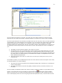
The script to model operation also saves your model files. The first time you save a new file, AnyBody
requires you to give your model a name, so clicking the
dialog.
icon the first time produces a "Save As"
Let's have a look at what the system has generated for you. If we forget about most of the text and
comments, the overall structure of the model looks like this:
Main = {
AnyFolder MyModel = {
}; // MyModel
AnyBodyStudy MyStudy = {
};
}; // Main
What you see is a hierarchy of braces - just like in a C, C++, or Java computer program. The outermost pair
of braces is named "Main". Everything else in the model goes between these braces.
Right now, there are two other sections inside the Main braces: The "AnyFolder MyModel" and the
"AnyBodyStudy MyStudy". These are the two basic elements of most AnyBody models. The term "AnyFolder"
is very general. In fact, any pair of braces in AnyScript is a folder. You can think of a folder as a directory on
your hard disk. A directory can contain other directories and files. It's exactly the same with folders. They
can contain other folders and elements of the model. The "AnyFolder MyModel" is the folder containing the
entire model you are going to build. The name "MyModel" can be changed by you to anything you like. In
fact, let's change it to ArmModel (in the forthcoming AnyScript text we'll highlight each change by red. Just
type the new name into the file, and don't forget to also change other occurrences of MyModel to ArmModel
in the file.
Notice the prefix "Any". All reserved words in AnyScript begin with "Any". This way you can distinguish the
elements that belong to the system from what the user defines. Another way of recognizing reserved words
is by virtue of their color in the editor. Class names are recognized by the editor as soon as you type them
and colored blue.
It must be emphasized that AnyScript is case sensitive.
There is more to an AnyScript file than the model. Once you have a model, you can perform various
operations on it. These operations are often collected in "studies", and the "AnyBodyStudy MyStudy" is
indeed such a study. You can think of a study as the definition of a task or set of tasks to perform. The
study also contains methods to perform the tasks. The Study of Studies tutorial contains much more
information about these subjects. For now, let's just rename "MyStudy" to "ArmModelStudy".
Let's look a little closer at the contents of what is now the ArmModel folder:
// The actual body model goes in this folder
AnyFolder ArmModel = {
// Global Reference Frame
AnyFixedRefFrame GlobalRef = {
// Todo: Add points for grounding
// of the model here
}; // Global reference frame
// Todo. Add the model elements such as
// segments, joints, and muscles here.
}; // ArmModel
Most of what you see above is just comments. It is always useful to add lots of comments to your models.
21
may know it from C++ or the Java language. Notice also that lines are terminated by semicolon ';'. Even the
lines with closing braces must be terminated by a semicolon. If you do no terminate with a semicolon, then
the statement continues on the next line. You can comment and uncomment a block of lines in one click by
means of the buttons at the top of the Editor window.
The only actual model element in the ArmModel is the declaration of the "AnyFixedRefFrame GlobalRef". All
models need a reference frame - a coordinate system - to work in, so the system has created one for you.
An AnyFixedRefFrame is a predefined data type you can use when you need it. What you have here is the
definition of an object of that type. The object gets the name "GlobalRef", and we can subsequently refer to
it anywhere in the ArmModel by that name.
You will notice that there is a "to do" comment inside the braces of this reference frame suggesting that you
add points for grounding the model. Don't do it just yet. We will return to this task later.
But here's an important notice: Everything you define in this tutorial from now on is part of the ArmModel
folder and should go between the its pair of braces. If you define something outside these braces that
should have been inside, then the necessary references between the elements of the model will not work.
What you have here is actually a valid AnyScript model, although it is empty and cannot do much. If you
have typed everything correctly, then you should be able to press the
icon and get the messages
Loading Main : "C:\...\NewModel1.any"
Scanning...
Parsing...
Constructing model tree...
Linking identifiers...
Evaluating constants...
Configuring model...
Evaluating model...
Loaded successfully.
Elapsed Time : 0.063000
in the Output Window. But what happens if you mistype something? If your typo leads to a syntactical error,
then it will be found by the AnyBody system when it parses the file, and instead of the "AnyScript loaded
successfully", you will get an impolite message that something is wrong. A common mistake is to forget a
semicolon somewhere. Try removing the last semicolon in the AnyScript file, and load again. You get a
message saying something like:
ERROR(SCR.PRS11) : C:\...\NewModel1.any(27) : 'EOF' unexpected
Model loading skipped
22
We now assume that you have removed eventual errors and have loaded the model successfully.
If you are up to it, let's continue onward to Lesson 2: Segments.
This is a typical error message. First there is a message ID, then a file location and finally the body of
the message. The former two are written in blue ink and underlined to show the underlying active links. The
file location is the line where the bug was found by the system. If you double-click this link, the cursor in the
Editor Window jumps to the location of the error. Notice that this is where the system found the error, but
the error can sometimes be caused by something you mistyped earlier in the file so that you actually have
to change something elsewhere in your model. If you are in doubt of what the error message means, try
clicking the error number ERROR(SCR.PRS11). This will give you a little pop-up window with a more
complete explanation:
Lesson 2: Defining segments and displaying objects
Here's an AnyScript file to start on if you have not completed the previous lesson:
demo.lesson2.any
There are some elements that must be present in a body model for it to make any sense at all. The first one
is segments. They are the rigid elements of the body that move around when the model does its stuff. When
modeling a human or other higher life form, they usually correspond to the bones of the body. However,
they can also be used to model machines, tools, and other things that might be a part of the model but do
not belong to the human body. Hence the more general term "segment"*.
A segment is really nothing but a frame of reference that can move around in space and change its
orientation. It has an origin where its center of mass is assumed to be located, and it has axes coinciding
with its principal inertia axes.
We shall start by defining a folder for the segments. Please add the following text to your model (new text
marked by red):
// The actual body model goes in this folder
AnyFolder ArmModel = {
// Global Reference Frame
AnyFixedRefFrame GlobalRef = {
23
// Todo: Add points for grounding
// of the model here
}; // Global reference frame
// Segments
AnyFolder Segs = {
}; // Segs folder
}; // ArmModel
Did you notice that the word AnyFolder turned blue as soon as you typed its last letter? If it did not, you
have mistyped something. Try loading the model by clicking the
icon (or pressing F7). If you expand
the ArmModel branch in the tree view, you should see a new, empty branch named Segs. It is the new
folder you just defined. We are now ready to add a segment to the model, and this would probably be a
good time to introduce you to the object inserter.
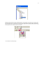
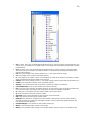
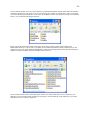
If you look at the left hand side of the tree view in the editor window, you will notice tabs running down the
vertical edge. The tabs give you access to different tree views or let you close the tree view completely if
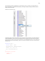
you would rather use the space for something else. One of the tabs is called "Classes" and it produces a tree
that has two branches at its root. Both of these branches contain all the predefined classes in AnyScript. In
the first branch, "ClassTree", the classes are ordered hierarchically. This reflects the object-oriented idea
that classes inherit properties from each other. This might be a way of locating a class with particular
properties if you are not sure of the class name.
The other branch, "Class List", simply contains an alphabetical list of all the classes. This is useful if you
know the name of the class you are looking for. Try opening each of the two trees and look for the class
AnySeg. Then make sure the cursor in the editor window is located inside the newly defined AnyFolder Segs.
Finally, right-click the AnySeg class name in the tree and choose "Insert object". You should get this:
// Segments
AnyFolder Segs = {
AnySeg <ObjectName>
{
//r0 = {0, 0, 0};
24
//rDot0 = {0, 0, 0};
//Axes0 = {{1, 0, 0}, {0, 1, 0}, {0, 0, 1}};
//omega0 = {0, 0, 0};
Mass = 0;
Jii = {0, 0, 0};
//Jij = {0, 0, 0};
//sCoM = {0, 0, 0};
};
}; // Segs folder
The object inserter has created a template of a segment for you. It contains all the properties you can set
for an AnySeg object. Some of them are active while other are commented out by two leading slashes. The
ones that are commented out are optional properties. You can set them if you like, but if you leave them out
they will retain the values already indicated in the inserted lines. If you do not plan on using them, you can
erase them. The object properties without leading slashes are those that must be set. This is the case for
Mass and Jii, for instance, which are respectively the mass of the segment and the diagonal elements of the
inertia tensor. In a system that simulates dynamics, all segments must have mass and inertia. The system
allows you to set them to zero, but it does not make sense not to set them at all.
More formally, object properties are divided into three different groups:
•
•
•
Obligatory. Like Mass and Jii, these must be set by the user when the object is defined
Access denied. These are computed automatically by the system and cannot be specified by the
user.
Optional. These can be set by the user or left to their default values.
You can find a complete description of all possible properties of all objects in the reference manual.
Let us give the new segment the name UpperArm and set its Mass = 2 and also assign reasonable values
for Jii:
AnySeg UpperArm = {
//r0 = {0, 0, 0};
//Axes0 = {{1, 0, 0}, {0, 1, 0}, {0, 0, 1}};
Mass = 2;
Jii = {0.001, 0.01, 0.01};
}; //UpperArm
Click
again (or press F7). Among the messages you get are:
Model Warning: Study 'Main.ArmStudy' contains too few kinematic constraints to be
kinematically determinate.
Don't worry about it just now. It only means that you are not finished with the necessary elements to do an
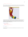
actual analysis yet.
Now that we have a physical object in the model, let's see what it looks like. To make something visible in
AnyBody, you have to add a line that defines visibility:
AnySeg UpperArm = {
//r0 = {0, 0, 0};
//Axes0 = {{1, 0, 0}, {0, 1, 0}, {0, 0, 1}};
Mass = 2;
Jii = {0.001, 0.01, 0.01};
AnyDrawSeg drw = {};
}; // UpperArm
25
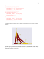
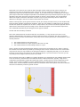
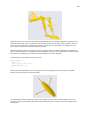
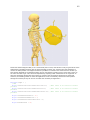
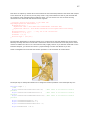
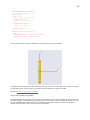
Reload the model, and then choose the menus Window -> Model View (new). This opens a graphics window
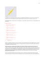
and displays what looks like a long yellow ellipse. On the toolbar at the top of the graphics window, click the
rotation icon
. Then click inside the graphics field and drag the mouse in some direction. This causes
the yellow ellipse to rotate, and you will see that it is actually an ellipsoid with a coordinate system through
it. If you entered the inertia properties in the Jii specification as written above, then your ellipsoid should
be ten times as long as it is wide. Try changing the "0.001" to "0.01" and reload. The ellipsoid becomes
spherical. The dimensions of the ellipsoid are scaled this way to fit the mass properties of the segment you
are defining. It is best to change Jii back to {0.001,0.01,0.01} again.
As you can see, Jii is a vector. If you know your basic mechanics, you may wonder why it is not a 3 x 3
matrix. The reason is that Jii only contains the diagonal members (the moments of inertia), which is all you
need to specify if your segment-fixed reference frame is aligned with the principal axes. If not, the offdiagonal elements (the deviation moments) can be specified in a property called Jij, which by default
contains zeros.
We are eventually going to attach things like muscles, joints, external loads, and visualization objects to our
segments. To this end we need attachment points. They are defined in the local coordinate system of the
segment. For a given body part it may be a laborious and difficult task to sort out the correct points.
Fortunately, good people have done much of the work for you, and, if you construct your model wisely, you
can often grab most of what you need from models defined by other people. For now, let us assume that
you have sorted out the coordinates of all the points you need on UpperArm, and that you are ready to start
adding them. Rather than going through the drill with the object inserter, you can copy and paste the
following lines:
AnySeg UpperArm = {
//r0 = {0, 0, 0};
//Axes0 = {{1, 0, 0}, {0, 1, 0}, {0, 0, 1}};
Mass = 2;
Jii = {0.001, 0.01, 0.01};
AnyDrawSeg drw = {};
AnyRefNode ShoulderNode = {
sRel = {-0.2,0,0};
};
AnyRefNode ElbowNode = {
sRel = {0.2,0,0};
};
AnyRefNode DeltodeusA = {
sRel = {-0.1,0,0.02};
};
AnyRefNode DeltodeusB = {
sRel = {-0.1,0,-0.02};
};
AnyRefNode Brachialis = {
sRel = {0.1,0,0.01};
};
AnyRefNode BicepsShort = {
sRel = {-0.1,0,0.03};
};
AnyRefNode Brachioradialis = {
sRel = {0.05,0,0.02};
};
AnyRefNode TricepsShort = {
sRel = {-0.1,0,-0.01};
};
}; // UpperArm
26
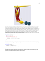
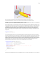
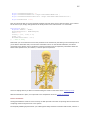
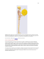
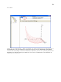
Try loading the model again and have a look at the graphical representation. If you zoom out enough, you
should see your points floating around the ellipsoid connected to its center of gravity by yellow pins.
One segment does not make much of a mechanism, so let's define a forearm as well. In the segs folder, add
these lines:
AnySeg ForeArm = {
Mass = 2.0;
Jii = {0.001,0.01,0.01};
AnyRefNode ElbowNode = {
sRel = {-0.2,0,0};
};
AnyRefNode HandNode = {
sRel = {0.2,0,0};
};
AnyRefNode Brachialis = {
sRel = {-0.1,0,0.02};
};
AnyRefNode Brachioradialis = {
sRel = {0.0,0,0.02};
};
AnyRefNode Biceps = {
sRel = {-0.15,0,0.01};
};
AnyRefNode Triceps = {
sRel = {-0.25,0,-0.05};
};
AnyDrawSeg DrwSeg = {};
}; // ForeArm
}; // Segs folder
When you reload the model you may not be able to see that the forearm has been added. In fact it is there,
but it is placed exactly on top of the upper arm and since the two segments have similar mass properties, it
is impossible to see which is which.
Before we proceed it might be worth thinking a bit about why objects get placed the way they do in the
model and how we can control the placement. The first thing to notice is that we are in the process of
making a model of a living organism which supposedly will move about changing its position all the time. So
there really is no "right" placement of a segment in the model. The second thing to notice is that even if we
are able to exercise some control over the placement of objects, then at least we have not done so yet. So
this is why the system for lack of better information places both segments at the origin of the global
reference frame at load time.
What eventually will happen is that we will define joints to constrain the segments with respect to each
other and also drivers to specify how the mechanism will move. When all that is done, these specifications
27
will determine where everything is at every point in time. But we need to go through several steps of
definitions and subsequently the system must do some equation solving before everything can fall into its
"right" position. So what to do in the meantime? Well, perhaps you noticed that the UpperArm segment we
originally created with the object inserter has two properties named r0 and Axes0. These two properties
determine the location and orientation of the segment at load time. The r0's are easy because they are
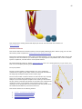
simply three-dimensional coordinates in space. So we can separate the two segments at load time like this:
AnySeg UpperArm = {
r0 = {0, 0.3, 0};
//Axes0 = {{1, 0, 0}, {0, 1, 0}, {0, 0, 1}};
Mass = 2;
Jii = {0.001, 0.01, 0.01};
AnyDrawSeg drw = {};
and
AnySeg ForeArm = {
r0 = {0.3, 0, 0};
Mass = 2.0;
Jii = {0.001,0.01,0.01};
This will clearly separate the segments in your model view:
So far so good. But it might improve the visual impression if the were also oriented a bit like we would
expect an arm to be. This involves the Axes0 property, which is really a rotation matrix. Such matrices are a
bit difficult to cook up on the fly. The predefined version in the UpperArm segment looks like this:
AnySeg UpperArm = {
r0 = {0, 0.3, 0};
Axes0 = {{1, 0, 0}, {0, 1, 0}, {0, 0, 1}};
If your spatial capacity is really good, you can start figuring out unit vectors for the coordinate system
orientation you want and insert them into the Axes0 specification instead of the existing ones. But there is
28
corresponding to a given axis and rotation angle. Therefore, we can specify:
AnySeg UpperArm = {
r0 = {0, 0.3, 0};
Axes0 =RotMat(-90*pi/180, z);
When you reload again you will see that the UpperArm is indeed rotated -90 degrees about the z axis as the
function arguments indicate. Notice the multiplication of the angle by pi/180. AnyBody identifies the word
"pi" as 3.14159... and dividing this with 180 gives the conversion factor between degrees and radians.
Angles in AnyScript are always in radians, but anywhere a number is expected you can substitute it by a
mathematical expression just like in other programming languages.
In the next section we will look at how joints can be used to constrain the movement of segments and allow
them to articulate the way we desire. So if you are up to it, let's continue onward to Lesson 3: Connecting
segments by joints.
-------------------------------*In rigid body dynamics terminology, a "segment" would be called a "rigid body", but to avoid unnecessary
confusion between the rigid bodies and the total body model, we have chosen to use "segments" for the
rigid parts of the model.
Lesson 3: Connecting segments by joints
Here's an AnyScript file to start on if you have not completed the previous lesson:
demo.lesson3.any.
You can think of joints in different ways. We tend to perceive them as providers of freedom, which is correct
compared to a rigid structure. However in dynamics it is often practical to perceive joints to be constraining
movement rather than releasing it. Two segments that are not joined (constrained) in any way have 2 x 6 =
12 degrees of freedom. When you join them, you take some of these degrees of freedom away. The
different joint types distinguish themselves by the degrees of freedom they remove from the connected
segments.
A segment without joints is basically floating free in space. When you connect the segments by joints, you
bind them together in some sense. But the mechanism as a whole can still fly around in space.
Not knowing where stuff is in space can be very impractical so the first thing to do is usually to ground the
mechanism somewhere. Perhaps you remember that the system added these lines somewhere in the top of
the AnyScript model:
AnyFixedRefFrame GlobalRef = {
// Todo: Add points for grounding
// of the model here
}; // Global reference frame
This is actually the definition of a global reference frame of the model. You can think of it as a coordinate
system fixed somewhere in global space. Otherwise, it is just like a segment in the sense that we can add
points to it for attachment of joints and muscles. Lets do just that. Again you can insert the objects with the
object inserter or to save time simply cut and paste the following lines into your model:
AnyFixedRefFrame GlobalRef = {
AnyDrawRefFrame DrwGlobalRef = {};
AnyRefNode Shoulder = {
sRel = {0,0,0};
};
AnyRefNode DeltodeusA = {
29
sRel = {0.05,0,0};
};
AnyRefNode DeltodeusB = {
sRel = {-0.05,0,0};
};
AnyRefNode BicepsLong = {
sRel = {0.1,0,0};
};
AnyRefNode TricepsLong = {
sRel = {-0.1,0,0};
};
}; // Global reference frame
The first line, "AnyDrawRefFrame ..." does nothing else than cause the global reference system to be
displayed in the graphics window. If for some reason you don't want the reference frame to be visible, just
erase this line or make it a comment by prefixing it with "//". It is often nice to have a visualization of the
global reference frame, but the current version may be a bit on the large side for the model. Let us reduce
the size a little bit and change the color to better distinguish it from the yellow segments:
AnyDrawRefFrame DrwGlobalRef = {
ScaleXYZ = {0.1, 0.1, 0.1};
RGB = {0,1,0};
};
The remaining lines are definitions of points in the global reference frame.
Now that we have the necessary points available, we can go ahead and fix the upper arm to the global
reference frame by means of a "shoulder" joint. A real shoulder is a very complex mechanism with several
joints in it, but for this 2-D model, we shall just define a simple hinge. We create a new folder to contain the
joints and define the shoulder:
}; // LowerArm
}; // Segs folder
AnyFolder Jnts = {
//--------------------------------AnyRevoluteJoint Shoulder = {
Axis = z;
AnyRefNode &GroundNode = ..GlobalRef.Shoulder;
AnyRefNode &UpperArmNode = ..Segs.UpperArm.ShoulderNode;
}; // Shoulder joint
}; // Jnts folder
A hinge is technically called a revolute joint, and this is what the type definition "AnyRevoluteJoint" means.
After that, the definition is just a matter of setting the properties of the joint that make it behave the way
we want. Let's have a closer look at each property:
Axis = z;
The AnyBody system is inherently three-dimensional. This applies also when we are creating a model that
will only operate in two dimensions, and it means that a revolute joint must know which axis to rotate
about. The property Axis = z simply specifies that the segment will rotate about the z axis of the node at the
joint. Does that sound complicated?
Well, a segment is really a reference frame. The nodes on segments are also reference frames, and each
reference frame can have its orientation defined by the user. A joint of this type forces the two z axes of the
two joined nodes to be parallel. You can control the mutual orientation of the two joined segments by
rotating the reference frames of the nodes you are connecting. This is relevant if you want one of the joints
to rotate about some skew axis.
30
The joint connects several segments, and it needs to know which point on each segment to attach to. For
this purpose, we have lines like
AnyRefNode &GroundNode = ..GlobalRef.Shoulder;
AnyRefNode &UpperArmNode = ..Segs.UpperArm.ShoulderNode;
The simple explanation is that these lines define nodes on the GlobalRef and UpperArm to which the joint
attaches. Notice the two dots in front of the names. They signify that the GlobalRef and Segs folders are
defined two levels up compared to where we are now in the model. If you neglected the two dots, then
AnyBody would be searching for the two objects in the Shoulder folder, and would not be able to find them.
This "dot" system is quite similar to the system you may know from directory structures in Dos, Windows,
Unix, or just about any other computer operating system.
But there is more to it than that. You can see that the Shoulder point on GlobalRef has been given the local
name of "GroundNode". This means that, within the context of this joint, we can hereafter refer to the point
as "GroundNode". This is practical because it allows us to assign shorter names to long external references.
Another specialty is the '&' in front of the local name. If you have C++ experience, you should be familiar
with this. It means that GroundNode is a reference (a pointer) to GlobalRef.Shoulder rather than a copy of
it. So if GlobalRef.Shoulder moves around, Shoulder.GroundNode follows with it. Hit F7 to load the model
again to make sure that the definition is correct.
We need an elbow joint before we are finished: the elbow. The definition is completely parallel to what you
have just seen, but we shall use one of the handy tools to define the references. The skeleton of the elbow
joint is as follows:
AnyFolder Jnts = {
//--------------------------------AnyRevoluteJoint Shoulder = {
Axis = z;
AnyRefNode &GroundNode = ..GlobalRef.Shoulder;
AnyRefNode &UpperArmNode = ..Segs.UpperArm.ShoulderNode;
}; // Shoulder joint
AnyRevoluteJoint Elbow = {
Axis = z;
AnyRefNode &UpperArmNode = ;
AnyRefNode &ForeArmNode = ;
}; // Elbow joint
}; // Jnts folder
As you can clearly see, the nodes in the Elbow joint are not pointing at anything yet. In this simple model it
is easy to find the relative path of the pertinent nodes on the upper arm and the forearm, but in a complex
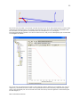
model it can be very difficult to sort these references out. So the system offers a tool to help you. If you
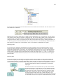
click the model tab in the tree view on the left hand side of the editor window, then the tree of objects in the
loaded model appears. Anything that was defined in the model when it was recently successfully loaded can
be found in this tree including the two nodes we are going to connect in the elbow. Click to place the cursor
just before the semicolon in the &UpperArmNode definition in the Elbow joint. Then expand the tree as
shown below.
31
When you right-click the ElbowNode you can select "Insert object name" from the context menu. This writes
the full path of the node into the Elbow joint definition where you placed the cursor. Notice that this method
inserts the absolute and not the relative path. Repeat the pocess to expand the ForeArm segment and insert
its ElbowNode in the line below to obtain this:
AnyRevoluteJoint Elbow = {
Axis = z;
AnyRefNode &UpperArmNode = Main.ArmModel.Segs.UpperArm.ElbowNode;
AnyRefNode &ForeArmNode = Main.ArmModel.Segs.ForeArm.ElbowNode;
}; // Elbow joint
Seems like everything is connected now. So why do we still get the annoying error message:
Model Warning: Study 'Main.ArmStudy' contains too few kinematic constraints to be
kinematically determinate.
when we reload the model? The explanation is that we have connected the model but we have not specified
its position yet. Each of the two joints can still take any angular position, so there are two degrees of
freedom left to specify before AnyBody can determine the mechanism's position. This is taken care of by
kinematic drivers.
They are one of the subjects of Lesson 4: Definition of movement.
32
Lesson 4: Definition of movement
Here's an AnyScript file to start on if you have not completed the previous lesson: demo.lesson4.any.
If you have completed the three previous lessons, you should have a model with an upper arm grounded at
the shoulder joint and connected to a forearm by the elbow. What we want to do now is to make the arm
move.
How can an arm with no muscles move? Well, in reality it cannot, but in what we are about to do here, the
movement comes first, and the muscle forces afterwards. This technique is known as inverse dynamics. We
shall get to the muscles in the next lesson and stick to the movement in this one.
Our mechanism has two degrees of freedom because it can rotate at the shoulder and at the elbow. This
means that we have to specify two drivers. The natural way is to drive the shoulder and elbow rotations
directly and this is in fact what we shall do. But we could also choose any other two measures as long as
they uniquely determine the position of all the segments in the mechanism. If you were building this model
for some ergonomic investigation, you might want to drive the end point of the forearm where the wrist
should be located in x and y coordinates to simulate the operation of some handles or controls. And this
would be just as valid a model because the end point position uniquely determines the elbow and shoulder
rotations.
For now, let's make a new folder and define two drivers:
}; // Jnts folder
AnyFolder Drivers = {
//--------------------------------AnyKinEqSimpleDriver ShoulderMotion = {
AnyRevoluteJoint &Jnt = ..Jnts.Shoulder;
DriverPos = {-100*pi/180};
DriverVel = {30*pi/180};
}; // Shoulder driver
//--------------------------------AnyKinEqSimpleDriver ElbowMotion = {
AnyRevoluteJoint &Jnt = ..Jnts.Elbow;
DriverPos = {90*pi/180};
DriverVel = {45*pi/180};
}; // Elbow driver
}; // Driver folder
This is much like what we have seen before. The folder contains two objects: ShoulderMotion and
ElbowMotion. Each of these are of type AnyKinEqSimpleDriver. A driver is really nothing but a mathematical
function of time. The AnyKinEqSimpleDriver is a particularly simple type that starts at some position at time
= 0 and increases or decreases at constant velocity from there. These two drivers are attached to joints,
and therefore they drive joint rotations, but the same driver type could be used to drive any other degree of
freedom as well, for instance the Cartesian position of a point.
The lines
33
AnyRevoluteJoint &Jnt = ..Jnts.Shoulder;
and
AnyRevoluteJoint &Jnt = ..Jnts.Elbow;
are the ones that affiliate the two drivers with the shoulder and elbow joints respectively. They are
constructed the same way as the joint definition in Lesson 3 in the sense that a local variable, Jnt, is
declared and can be used instead of the longer global name if we need to reference the joint somewhere
else inside the driver. Notice also the use of the reference operator '&' that causes the local variable to be a
pointer to the global one rather than a copy. It means that if some property of the globally defined joint
changes, then the local version changes with it.
The specifications of DriverPos and DriverVel are the starting value of the driver and the constant velocity,
respectively. Since these drivers drive angles, the units are radians and radians/sec.
Try loading the model again by hitting F7. If you did not mistype anything, you should get the message
"Loaded successfully" and no complaints about lacking kinematic constraints this time.
This is good news, because you are now actually ready to see the model move. If you look closer at the
pane in the bottom of the main frame, you will notice that it now contains the root of a tree in its upper left
cell. This is the place where the AnyBody system places your studies, and from this window you can execute
them, i.e., start analyses and calculations.
34
Try expanding the ArmStudy root. You will get a list of the study types that
the system can perform. "Study" is a common name for operations you can perform on a model. When you
click one of the studies, the buttons on the middle, lower part of the panel come to life. Try clicking the
KinematicAnalysis study. With the buttons, you can now execute various types of analysis. The panel
contains three buttons:
•
•
•
Run. This button starts the highlighted study and runs it until the end, usually producing some sort
of motion in the model. When Run has been pushed, it changes name to Break. If you push it in this
state, it pauses the running operation. F5 is a shortcut to this function to Run and Break.
Step. This button advances the operation one step. What a step is depends on the type of
operation, but it is typically a time step in a dynamic analysis. (F6 is the shortcut key for Stepping)
Reset. This puts the operation back to its initial position. You must reset before you can start a new
analysis, if you have stopped it in the middle. (F4 is the shortcut for resetting operations)
All these functions are also available from the Main Frame toolbar and the menu Operation.
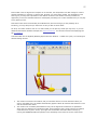
Do you have a Model View window open? This is the one where you can see the model graphically. If not,
open one with Window->New model view from the pull down menus at
the top of the screen. Now, try your luck with the KinematicAnalysis
study and the Run button. What should happen is that the model
starts to move as the system runs through 101 time steps of the
study.
Since we have no muscles so far, kinematic analysis is really all that
makes sense. A kinematic analysis is pure motion. The model moves,
and you can subsequently investigate positions, velocities, and
accelerations. But no force, power, energy or other such things are
computed. These properties are computed by the
InverseDynamicAnalysis, which is actually a superset of the
KinematicAnalysis.
Try the Reset button, and then the Step button. This should allow you
to single-step trough the time steps of the analysis. When you get
tired of that, hit the Run button, and the system completes the
remaining time steps.
The analysis has 101 time steps corresponding to a division of the
total analysis time into 100 equal pieces. The total time span
simulated in the analysis is 1 sec. These are default values because we
did not specify them when we defined the ArmModelStudy in the
AnyScript model. If you want more or less time steps or a longer or
shorter analysis interval, all you have to do is to set the corresponding
property in the ArmModelStudy definition. When you click "Run", all
the time steps are executed in sequence, and the mechanism
animates in the graphics window.
So far, the model is merely a two-bar mechanism moving at constant
joint angular velocities. There is not much biomechanics yet. However,
the system has actually computed information that might be
interesting to investigate. All the analysis results are available in the
ArmModelStudy branch of the tree view. You can expand the tree as
35
shown in the figure to the right.
Directly under the ArmModelStudy branch you find the Output branch where all computed results are stored.
Notice that the Output branch contains the folders we defined in the AnyScript model: GlobalRef, Segs, and
so on. In the Segs folder you find ForeArm, and in that a branch for each of the nodes we defined on the
arm. Try expanding the branch for the HandNode. It contains the field 'r' which is the position vector of the
node. We might want to know the precise position of the HandNode at each time in the analysis, for instance
if we were doing an ergonomic study and wanted to know if the hand had collided with anything on its way.
If you double-click the 'r' node, the position vector of the hand node for each time step is dumped in the
message window at the bottom of the screen. So you get the information you wanted, but perhaps not in a
very attractive way. But we can do much better than that. AnyBody has special windows for investigating
results. You open them from the pull-down menus by choosing Window -> ChartFX 2D (new).
This gives you a new window structured just like the editor window with a tree view to the left, but with an
empty graphics field instead of the large text editor field to the right. The graphics field is for graphing
results.
The tree in this window is much like the tree in the editor window except that some of the data have been
filtered out, so that you mainly see the parts of the tree that are relevant in terms of results or output. You
can expand of the tree in the chart window through ArmStudy and Output until you come to the HandNode.
When you pick the property 'r', you get three curves corresponding to the development of the three
Cartesian coordinates of this node during the analysis. Try holding the mouse pointer over one of the curves
for a moment. A small label with the global name of the data of the curve appears. All data computed in
AnyBody can be visualized this way.
So far, we have only the kinematic data to look at. Before we can start the real biomechanics, we must add
some muscles to the model.
This is the subject of Lesson 5: Definition of muscles and external forces.
Lesson 5: Definition of muscles and external forces
36
Here's an AnyScript file to start on if you have not completed the previous lesson:
demo.lesson5.any.
We have seen that models in AnyBody can move even though they do not have any muscles. This is
because we can ask the system to perform a simple kinematic analysis that does not consider forces.
However, things don't get really interesting until we add muscles to the model.
Skeletal muscles are very complicated mechanical actuators. They produce movement by pulling on our
bones in complicated patterns determined by our central nervous system. One of the main features of
AnyBody is that the system is able to predict realistic activation patterns for the muscles based on the
movement and external load.
The behavior of real muscles depends on their operating conditions, tissue composition, oxygen supply, and
many other properties, and scientists are still debating exactly how they work and what properties are
important for their function. In AnyBody you can use several different models for the muscles' behavior, and
some of them are quite sophisticated. Introducing all the features of muscle modeling is a subject fully
worthy of its own tutorial. Here, we shall just define one very simple muscle model and use it
indiscriminately for all the muscles of the arm we are building.
As always, we start by creating a folder for the muscles:
AnyFolder Muscles = {
}; // Muscles folder
The next step is to create a muscle model that we can use for definition of the properties of all the muscles.
AnyFolder Muscles = {
// Simple muscle model with constant strength = 300 Newton
AnyMuscleModel MusMdl = {
F0 = 300;
};
}; // Muscles folder
Now we can start adding muscles. If you want the model to move, you basically need muscles to actuate
each joint in the system. Remember that muscles cannot push, so to allow a joint to move in both directions
you have to define one muscle on each side of the joint in two dimensions. If you work in three dimensions
and you have, say, a spherical joint, then you may need much more muscles than that. In fact, it can
sometimes be difficult to figure out exactly how many muscles are required to drive a complex body model.
It is very likely that your career in body modeling will involve quite a few frustrations caused by models
refusing to compute due insufficient muscles.
Let's add just one muscle to start with. These lines will do the trick:
AnyFolder Muscles = {
// Simple muscle model with constant strength = 300 Newton
AnyMuscleModel MusMdl = {
F0 = 300;
};
//--------------------------------AnyViaPointMuscle Brachialis = {
AnyMuscleModel &MusMdl = ..Muscles.MusMdl;
AnyRefNode &Org = ..Segs.UpperArm.Brachialis;
AnyRefNode &Ins = ..Segs.ForeArm.Brachialis;
AnyDrawMuscle DrwMus = {};
};
}; // Muscles folder
37
that it goes from its origin to insertion via a number of predefined points. The via-points are the
AnyRefNodes defined in the second and third property lines. If you have a muscle that goes in a straight line
from origin to insertion, then you can just define two points like we have done here. If you have a more
complicated muscle path, then all you need to do is to add the points in between the origin and insertion.
The physiological behavior of the muscle is defined by the first property
AnyMuscleModel &MusMdl = ..Muscles.MusMdl;
You can see that it points right back to the muscle model we started out by creating. Notice the two leading
dots. Finally, the line
AnyDrawMuscle DrwMus = {};
ensures that the muscle is visible in the graphics window. Lets have a look at it. If you have the Model View
window (you know, the one with the rendering of the model in it) open, then just hit F7. If you don't have
the Model View window open, choose Window -> Model View (new) from the pull down menus at the top of
the main frame. You should see a thick, red line connecting the muscle's origin and insertion points. There
are other ways to visualize muscles, but we shall save that for the dedicated the muscle tutorial.
Notice that the muscle's position on the body might be a little strange because we have not yet positioned
the segments relative to each other by a kinematic analysis.
All the other muscles are defined in the same way:
//--------------------------------AnyViaPointMuscle Brachialis = {
AnyMuscleModel &MusMdl = ..Muscles.MusMdl;
AnyRefNode &Org = ..Segs.UpperArm.Brachialis;
AnyRefNode &Ins = ..Segs.ForeArm.Brachialis;
AnyDrawMuscle DrwMus = {};
};
//--------------------------------AnyViaPointMuscle DeltodeusA = {
AnyMuscleModel &MusMdl = ..Muscles.MusMdl;
AnyRefNode &Org = ..GlobalRef.DeltodeusA;
AnyRefNode &Ins = ..Segs.UpperArm.DeltodeusA;
AnyDrawMuscle DrwMus = {};
};
//--------------------------------AnyViaPointMuscle DeltodeusB = {
AnyMuscleModel &MusMdl = ..Muscles.MusMdl;
AnyRefNode &Org = ..GlobalRef.DeltodeusB;
AnyRefNode &Ins = ..Segs.UpperArm.DeltodeusB;
AnyDrawMuscle DrwMus = {};
};
//--------------------------------AnyViaPointMuscle Brachioradialis = {
AnyMuscleModel &MusMdl = ..Muscles.MusMdl;
AnyRefNode &Org = ..Segs.UpperArm.Brachioradialis;
AnyRefNode &Ins = ..Segs.ForeArm.Brachioradialis;
AnyDrawMuscle DrwMus = {};
};
//--------------------------------AnyViaPointMuscle BicepsShort = {
AnyMuscleModel &MusMdl = ..Muscles.MusMdl;
AnyRefNode &Org = ..Segs.UpperArm.BicepsShort;
AnyRefNode &Ins = ..Segs.ForeArm.Biceps;
AnyDrawMuscle DrwMus = {};
38
};
//--------------------------------AnyViaPointMuscle TricepsShort = {
AnyMuscleModel &MusMdl = ..Muscles.MusMdl;
AnyRefNode &Org = ..Segs.UpperArm.TricepsShort;
AnyRefNode &Ins = ..Segs.ForeArm.Triceps;
AnyDrawMuscle DrwMus = {};
};
//--------------------------------AnyViaPointMuscle BicepsLong = {
AnyMuscleModel &MusMdl = ..Muscles.MusMdl;
AnyRefNode &Org = ..GlobalRef.BicepsLong;
AnyRefNode &Ins = ..Segs.ForeArm.Biceps;
AnyDrawMuscle DrwMus = {};
};
//--------------------------------AnyViaPointMuscle TricepsLong = {
AnyMuscleModel &MusMdl = ..Muscles.MusMdl;
AnyRefNode &Org = ..GlobalRef.TricepsLong;
AnyRefNode &Ins = ..Segs.ForeArm.Triceps;
AnyDrawMuscle DrwMus = {};
};
Try adding the data and viewing the result by reloading. You should get a picture more or less as what you
see below:
The model does not seem to be correctly connected at the elbow. The ArmStudy actually contains a default
operation for getting the elements ordered with respect to each other. It is the SetInitialConditions study in
the tree at the upper left corner of the Main Frame. Try clicking it, then hit the Run button, and the
segments fall into position as shown below.
39
We now have enough muscles in the model to start computing the muscle forces that can drive the motion.
But there is one more detail to take care of, and it is both important and slightly intricate. The bottom line
is: There must be something for the muscles to drive - some load to carry. We have not added any exterior
forces to the model yet, but that is not the problem. You remember, perhaps, from Lesson 2 that each
segment has a mass. Additionally, the ArmModelStudy is equipped with a standard gravity of -9.81 units in
the global y direction. This means that gravity actually provides the external force the analysis needs to
make any sense.
What is the problem then? Well, unless you specify otherwise, drivers, like the ones we added to the elbow
and shoulder joints, act like motors. This means that they provide whatever moment or force that might be
necessary to make the motion happen. Although it would be practical, few of us have motors built into our
joints. Instead, we have very efficient muscles so we want to leave the task of providing force in the model
to them. The way to do that is to set a property called Reaction.Type for the driver to zero. This is how it's
done for the shoulder:
AnyKinEqSimpleDriver ShoulderMotion = {
AnyRevoluteJoint &Jnt = ..Jnts.Shoulder;
DriverPos = {-100*pi/180};
DriverVel = {30*pi/180};
Reaction.Type = {Off};
}; // Shoulder driver
This additional line makes sure that the driver provides the motion but not the moment. Why is AnyScript
made that way? Why would anyone ever want to model a joint with a motor in it? The explanation is that
AnyScript models for ergonomic studies often comprise machinery that the body of the model is connected
to. And this machinery can have motors that provide moment or force input to the system. Why is the motor
then switched on by default? Well, models under development often do not have enough muscles to move.
Such models will not work before the last muscle is added unless they have motors in the drivers, and it is
practical to be able to run an analysis now and then during development to check that the model works
correctly.
As you can see, the single Off is encapsulated in braces, {Off}. This is because it is a vector. A driver by
default has several components and hence all the data in the driver is vector quantities. For semantic
reasons this applies even when the driver only controls one degree of freedom as it does here.
Add a similar line to the definition of the elbow driver and we are ready to compute muscle forces. Click the
40
InverseDynamicAnalysis in the study tree at the bottom left of the screen and then the Run button, and
watch the model move. It should look exactly like in the kinematic analysis, however, during this analysis,
the AnyBody system computes all muscle and joint forces in addition to a whole lot of other useful
information. To see it, you once again have to open a ChartFX window (if you don't have the one we used
previously open) by means of the menu Window -> ChartFX 2D (new) in the pull down menus in the top of
the main frame. In this new window, expand the ArmStudy -> Output -> Model -> Muscles branch. You
should see a list of all the muscles appearing. Each of them can be expanded to reveal the data inside. Let
us expand the brachialis muscle and investigate its force variation over the movement. You should see a
node named Fm. If you click it, you should get a curve like the one shown below:
Notice that the force in the muscle drops as the movement proceeds. This is quite as expected, because the
moment arm of the gravity about the elbow gets smaller as the elbow flexes, and less muscle force is
therefore needed to carry it. If you look at the muscle force in the BicepsLong, you see a different pattern:
41
This muscle grows in force during the movement. That is because it is influenced by the movement of two
joints, namely the shoulder and the elbow. In addition, it collaborates both with DeltoidusA on shoulder
flexion, and with the other elbow flexors, and these muscles all have to level their work in relation to each
other.
This might sound like there are heuristic rules built into AnyBody. This is not the case. AnyBody distributes
the work between the muscles in a very systematic way: It solves an optimization problem to actuate
muscles so that the maximum relative load on any muscle is minimized. This corresponds to postponing
muscle fatigue as far as possible, and it causes muscle to collaborate as much as they can. This sometimes
involves development of antagonistic muscle forces, i.e., forces that appear to contradict the movement but
in fact relieve weaker muscles of load. Muscle synergy and the occasional presence of antagonists is well
known from many experiments, and the minimum fatigue criterion used in AnyBody reproduces this
behavior.
Now that we have the analysis going, we might want to investigate the model's behavior in different
situations. A typical example could be to see how it carries an external load in addition to gravity. Let us
imagine that the model is performing a dumbbell curl where it carries some load at the hand. We start by
attaching a node to the forearm at the position of the palm. Add this definition to the ForeArm section:
AnyRefNode PalmNode = {
sRel = {0.27,0,0};
};
The next step is to add an external force. We make a folder for this purpose:
AnyFolder Loads = {
//--------------------------------AnyForce3D Dumbbell = {
AnyRefNode &PalmNode = ..Segs.ForeArm.PalmNode;
F = {0,-100,0}; // Force in Newton
};
}; // Loads folder
42
That's all there is to it. Now you can analyze how the model will react to a downward force of 100 N
(approximately 10 kg dumbbell weight). If you reload, rerun, and investigate the BicepsLong force again,
you should see this:
The muscle force is obviously much larger than before, and the development is also different. It now reaches
a maximum during the movement and drops off again.
Applied forces do not have to be constant. They can change with time and other properties in the model.
Please refer to the tutorial on forces for more details.
There are infinitely many studies that could be made using even a simple model like this one, and you are
encouraged to experiment a little or a lot. To get reliable results, however, would take at the very least an
individual definition of the muscles with a realistic strength for each of them, and a more detailed modeling
of the deltoid's origin-insertion path in the shoulder; it can be a comprehensive job to define a realistic body
model which is exactly why most users would probably start out using the body model available from the
AnyBody Research Project.
This tutorial, being of introductory nature, will instead skip to a new subject: How can we add realistic
geometries of bones and other elements to our model?
Now, let's continue to Lesson 6: Adding real bone geometrics
Lesson 6: Adding real bone geometries
Here's an AnyScript file to start on if you have not completed the previous lesson:
demo.lesson6.any.
So far, the graphics of the model you have developed is what we can call a stick figure representation. This
is a straightforward way of seeing the model and it reflects the mechanics very vividly, but it does not look
43
very physiological. You may be wondering how you can add cool bones and other geometries that will
impress your colleagues and look good in your presentations. You may want to put your model into an
environment such as a room, a treadmill, or a bicycle to illustrate the purpose of the model.
However, there may be other reasons than mere aesthetics why it can be advantageous to work with real
geometries. When attaching muscles, for instance, a real bone geometry gives you an instant visual
feedback on where the muscle is located in the organism as illustrated by the two pictures above.
Adding geometric models such as bones is fortunately very simple. All you need is a file with a 3-D graphical
representation of the bone or other component you may wish to add. The format of the file must be STL
ascii. STL is a very simple graphical file format that basically contains triangles. Virtually any CAD system
you can think of can save geometry on STL format, so if you have your geometry described on IGES, STEP,
DXF or any other usual type, just run it through your favorite CAD system and convert it to STL. STL comes
in two varieties: ascii and binary. AnyBody needs an ascii file, so please make sure to choose that option if
you create your own STL files in a CAD system.
The bone models you see on the pictures above are a bit elaborate for a short tutorial, so we shall start with
something a little simpler. What we want to do now is to add a dumbbell geometry to the arm model we
have just created. You can find a file to use here. Right-click the link, choose "save as", and put the file in
the directory where you have placed the arm model.
The dumbbell should be added to the forearm, so the first thing to do it to add a reference to the STL file we
just saved to the definition of the forearm:
AnyDrawSeg DrwSeg = {};
AnyDrawSTL DrwSTL = {
FileName = "dumbbell.stl";
};
}; // ForeArm
Try reloading the model again. You will probably see nothing but grey the Model view. A closer investigation
of the problem would reveal that the entire arm model is actually situated inside the dumbbell handle. This
is because the STL file was created in millimeters, where the arm model is in meters. Rather than going
back to whatever CAD system was used and scale the dumbbell model down 1000 times, we can add the
scale definition to AnyScript in the following way:
AnyDrawSTL DrwSTL = {
FileName = "dumbbell.stl";
44
ScaleXYZ = {0.001, 0.001, 0.001};
};
When you reload the model, the picture you get should be similar to what you see below. The dumbbell is
visible now and has the right size, but it is sitting at the center of gravity of the lower arm rather than at the
hand, and it is not oriented correctly.
The fact is that, when you attach something to a segment, it is positioned at the segment's origin which is
usually the same as the center of mass. However, you can also attach stuff to points, so moving the
dumbbell to the hand is simply a question of moving the reference to it from the ForeArm segment to the
PalmNode that we defined previously. Block the entire AnyDrawSTL folder with the mouse and cut it out.
Then re-insert it under the PalmNode like this:
AnyRefNode PalmNode = {
sRel = {0.27,0,0};
AnyDrawSTL DrwSTL = {
FileName = "dumbbell.stl";
ScaleXYZ = {0.001, 0.001, 0.001};
};
};
AnyDrawSeg DrwSeg = {};
}; // ForeArm
On reload, this produces a new picture with the dumbbell attached at the right location, but it is still not
oriented correctly.
45
We want to rotate the dumbbell 90 degrees about the y axis. We could do that by going back to the CAD
system and modifying the dumbbell STL file, but an easier option is to rotate it directly inside AnyScript.
A geometrical object that you insert gets the same orientation as the coordinate system it is attached to. In
this case the dumbbell is attached to PalmNode. Nodes are actually reference frames with the ability to be
positioned and oriented relatively to other reference frames, for instance a segment or another node. We
have already positioned nodes by means of the member vector sRel and relative orientation happens
similarly with the member matrix ARel, the relative rotational transformation matrix. We wish to rotate the
dumbbell 90 degrees about the local y axis and hence write:
AnyRefNode PalmNode = {
sRel = {0.27,0,0};
ARel = RotMat(90*pi/180, y);
AnyDrawSTL DrwSTL = {
FileName = "dumbbell.stl";
ScaleXYZ = {0.001, 0.001, 0.001};
};
};
As a final cosmetic touch, you may want to change the color of the dumbbell. This can be done by adding
the property RGB to the STL file reference:
AnyDrawSTL DrwSTL = {
FileName = "dumbbell.stl";
ScaleXYZ = {0.001, 0.001, 0.001};
RGB = {0.2,0.4,0.5};
};
The RGB property specifies the blend of colors Red, Green, and Blue in that order for displaying the STL
geometry. The combination above produces a dull blue shade.
46
This completes the Getting Started with AnyScript tutorial. The final result of the efforts is in
demo.arm2d.any.
Interface features
This tutorial deals with the interface features of the AnyBody Modeling System. Before trying your luck with
this tutorial, please complete the Getting Started with AnyScript tutorial.
Much of the interface works like other types of windows software; you can copy and paste data, and you can
arrange the various windows as you would expect. But AnyBody does computations that no other computer
system is capable of, and this calls for some special features.
We need something to work on. Please download this file, save it in a working directory of your choice, and
load it into the AnyBody Modeling System.
The squat problem
The file you have loaded is a squat example. It is a 2-D model and
contains only a single leg with eight muscles. The strength and mass of
the single leg correspond roughly to two ordinary legs.
The arm of the model is used for balance. It does not have any muscles,
and it has no explicit driver attached, but if you run the kinematic
analysis or the inverse dynamic analysis on the model you will see that
the arm moves to maintain the balance of the model. This is because the
model has a driver on the position of the collective center of mass
requiring it to be directly above the contact point with the ground, which
the model accommodates by movement of the arm.
This tutorial consists of the following lessons:
•
•
•
•
Lesson
Lesson
Lesson
Lesson
1:
2:
3:
4:
Windows and workspaces
Editor Window Facilities
The Model View Window
The Chart View
47
•
Lesson 5: The Command Line Application
Let us quickly proceed to the first lesson: Windows and workspaces.
Lesson 1: Windows and workspaces
When you work with a model like this, you are likely to initially go through a series of model refinements,
subsequently conduct a number of investigations, and finally extract data for further processing or reporting.
This may be a process going on over a longer period where you start and stop the AnyBody Modeling
System several times, and you want to quickly come back to the windows layout fitting the task at hand.
This section is about how to control your windows layout.
When you start the AnyBody Modeling System, load the model, and open a model view window, you will get
the standard layout of windows in the AnyBody workspace. It looks like this:
This layout is standard because it gives you a little bit of everything. But it may not be what you want for a
particular task. You may also find yoursef doing a number of basically different tasks for which different
windows layouts are convenient and being annoyed about having to change layout every time you change
task. Therefore, the system offers you three different user layouts that you can set up as you like and switch
between. If you look at the top of the main window, you will notice that the button, L1, is pressed in.
48
This indicates that you are now working in the first of the three user-defined layouts. Each layout can
contain a different user-defined window setup, and you can switch between them by a single mouse click.
Try running the HeelUpStudy.InverseDynamicAnalysis and open a ChartFX window to investigate the results.
Perhaps you want to simultaneously see the Model View window, the Chart window and the AnyScript code,
while you are not particularly interested in the Operations window at the bottom of the screen. You might
arrange the windows as show below.
Suppose you have very carefully set this window layout up and want to keep it for later use after you have
worked with another layout. How can that be done? Simple, you just press the L2 button. This will give you
a fresh layout to work on, and you can always go back to what you had by pressing L1 again. Whichever
layout you create under one of the L1, L2, and L3 buttons is kept for later use.
Workspaces
So, how do you preserve all the windows layouts when you have invested much time in setting them up and
have to shut your computer down for the night? The answer is to save the workspace. A workspace file is a
description of the state of your user interface. Notice the title of the main window:
49
It says "New Workspace" because you did not load a workspace when you started, and you have not yet
saved the one you have created. Click File-> Save Workspace as..., pick a directory and a suitable name,
and save the workspace. Then exit AnyBody, and start the system again.
When you have re-started, click File->Load Workspace..., browse your way to the workspace file you just
saved, and load it. You will get the windows layout back that you had when you started. You can also find a
workspace file in Windows Explorer and double-click it. The workspace files have the extension .anyws.
In addition, you can convenniently find recent workspaces in the AnyBody Assistant dialog box, please see
the picture below. In the Recent Project files tab, you will find recent workspaces and main files listed. A
complete list of recently uses AnyScript files is found in the Recent *.any files tab.
Window properties
Each window is equipped with a number of properties that are saved with the workspace. This set
of properties is often updated in newer version of AnyBody in order to make the workspace storage of your
working environment as good as possible and in order to match new functionality added to the windows.
Some of these properties can be accessed and set by the user. This can be done from the Main Frame menu
item Windows -> GUI Properties. Selecting this item opens a the Properties Window that show the
properties of the current window. Some windows, where frequent access to the properties may be needed,
for instance the Model View and AnyChart View, have a button on thier toolbar for easy access to the
properties. Look for a button looking like this
on the toolbar of a window.
In the next lesson we shall proceed to have a closer look at the individual window types, and why not start
with the Editor Windows.
Lesson 2: The Editor Window
We need something to work on. Let us create a blank file and type something into it using the editor. The
way to do that is to click the "New Include" button on the toolbar:
50
This brings up a new editor window with an empty file, and we can go ahead typing anything we want. The
first thing you have probably noticed about the AnyScript editor is that it recognizes the predefined class
names and highlights them automatically. It does this all the time as you are typing, and it is a great help to
avoid misspellings that might later lead to annoying syntax errors.
Syntax Highlighting
When you start typing something, the writing color is black. This is the standard color in the editor for things
that have not been recognized. For instance, if you start defining a segment, you may type (try it!):
AnySe
And the text remains black until you type the last character of the reserved word:
AnySeg
at which point the text becomes blue. This can be a great help if you are not quite sure about the name of a
particular object. You can try typing the different forms of the name, and when you hit the right one, the
text turns blue. The editor similarly recognizes comments. If you precede the AnySeg class name with a
double-slash, the entire line turns green:
// AnySeg
Please notice that similar to C, C++, Java, and JavaScript you can turn entire blocks of code into a comment
by encapsulating it into a pair of /* */ delimiters. Another easy way to temporarily remove and re-activate
in the toolbar of
several lines from the file is to block the text in question and use the two buttons
the Editor window. This automatically places or removes double slashes in front of each line in the block.
Please also notice the so-called Documentation Comments. This is comments using the following
syntactical forms: /// ..., /** ... */, ///< ..., and /**< ... */. The Documentation Comments are related to a
given object in the model and these comments are treated specially so the information can be accesses
more convenniently after loading the model and thereby help the user of a model to understand the model
without reading the code. In the editor, the Documentation Comments do however have the same color as
other the normal comments. The Documentation Comments' form is similar to other source code systems
like JavaDoc, Doxygen, and others.
Automatic Indentation
When developing software that is hierarchical it is customary to indent the code according to the hierarchical
level of each line. This greatly improves the legibility. In the AnyScript editor we have decided that the
standard indentation for each level is two spaces. The editor automatically keeps track of where you are in
the code as defined by the start and end braces, and it helps you make the right indentations as you type.
Let us continue the segment definition we started above. Remove any leading double slashes and proceed to
type
AnySeg Segment1 = {
and hit the Return key to change line. Notice that the editor automatically indents the next line by two
51
You are not forced to accept this. You can easily backspace to the beginning of the line and start your typing
there, if you like that better. You might write something like:
AnySeg Segment1 = {
Mass = 1.0;
The editor will discover that you did not like its suggested indentation, so the next line you type will begin at
the same character as Mass, and you may proceed to finish the definition of the segment by typing:
AnySeg Segment1 = {
Mass = 1.0;
Jii = {0.1,0.01,0.1};
};
Auto format
Perhaps you decide at this point that the indentation is better after all. (If you do not decide at this point,
you surely will when you have written a few hundred lines and are trying to balance your start and end
braces.) So, how can you restore the default indentation? Well, the AnyScript editor has a very nice feature
called Auto format. It allows you to block a part of the code or the entire file and indent it in one simple
step.
Try highlighting the block you have written , and press Alt-F8. You should get this result:
AnySeg Segment1 = {
Mass = 1.0;
Jii = {0.1,0.01,0.1};
};
This facility is also available in through the pull-down menu Edit->Format Indentation.
If you are ever in a situation where the model will not load and you suspect that you have forgotten a brace
somewhere, simply block the entire file and apply Auto format to it. You will usually be able to see by a few
glances where the error is located.
You can also manually control the indentation of a block of lines. A highlighted block of text can be indented
or unindented in steps of two spaces by pressing Tab or Shift-Tab.
Tree Views
The structure of an AnyScript model is hierarchical. This means that it is obvious to represent the loaded
model as a tree, and the system makes extensive use of this representation in all its different window types.
If you still have the squat model from the previous lesson open, go to the main file and load it (key F7). You
should see a tree at the left hand side of the editor window as in the figure below.
52
What you see here is the Model Tree, which it the main tree view of AnyBody showing all objects in the
loaded model in the structure they are created in the AnyScript code. The Model Tree is in principle available
in many of AnyBody's windows, but some of the information is filtered out in some window types to make
the tree view practical for specific purposes such as browsing output or operations in the model.
The Editor windows have the complete unfiltered Model Tree, and they can take up a significant space in the
Editor window. Therefore, they are by default collapsed to maximize the space for editing and an unfiltered
Model Tree is also available on the Main Frame, which is sufficient for most purposes. Multiple Model Trees
can, however, be handy when working with large models and browsing for information in different places of
the structure; this is the reasons for having the option of opening a Model Tree in the Editor windows.
Moreover, the Model Trees in the Editor have to options for interaction with the code of the particular Editor
Window, which is not available from the Main Frame Model Tree. You can collapse the tree again after
opening it by clicking the X tab on the left hand side of the tree.
We shall not go into details about the functionality in the Model Tree, but notice that right-clicking an object
in the Model Tree give you access to these functions. There are two categories of these functions:
1.
2.
Interaction with the AnyScript code such as inserting object name into the code at the place of the
cursor
Class Operations that are operations associated with the AnyScript classes. These cannot be
explained in detail here because the follow the classes, but there are a couple of very basic Class
Operation that is available to all objects.
In particular notice the Class Operation called Object Description that comprise much practical information
for the given object, including the Documentation Comments made by the AnyScript programmer making
the model. The Object Description is very useful when browsing the model because it contains active links,
which for instance can bring you to the code with single click. The Object Description is considered to be the
most fundamental operation in the Model Tree so it will be activated when you double-click any node in the
tree.
53
The Model Tree offers you several options to go from the tree to associated places the AnyScript code. There
are, however, also options to go the opposite way, i.e. from the code to the Model Tree. Try right-clicking
the code. You will them get a pop-up menu with several editor options. One of these is "Locate in Model
Tree". It will probably be greyed, i.e. disabled, because you have not selected anything that can be related
to the tree. But if you try highlighting an object name in the code it should become active. Selecting this will
bring you to the specific object in the Model Tree. In some cases, there is not a single clear one-to-one
correspondance between the code location and the Model Tree. This happens if the code, you look at, is in
an include file that have been included several times in the model. In such cases, the Editor will provide you
with a list of options to select from.
As you can see, there are also other tree views available. Clicking the Files tab will give you an overview of
the model's include file structure. Models in AnyScript are often divided over several files where one main
file links to other files, which link on to other files and so on. The links are realized by means of include
statements in the AnyScript code:
#include "includefile.any"
The File Tree is very unimpressive in this model because it does not have any include files, but below you
see a File Tree from a more complicated model:
The leaves in the tree are marked by two different icons. The icon with the little red # sign points to a place
in the model with an include statement. If you double-click such a line you will be taken to the position of
the include statement. If you Click the + to the left of the icon, the branch folds out, and you see another
icon below without the # sign. If you click this icon, the include file itself opens up in an editor window.
54
The third tab in the tree view is named Classes. It gives you access to a tree of the predefined classes in the
system. From this tree you can insert templates of new objects. This eliminates much of the need to
remember the syntax of each object and saves you many lookups in the reference manual. The use of the
Classes Tree is described in the Getting Started with AnyScript tutorial.
There are a couple of more tree views. These contains global objects that are available to your code. Global
AnyScript constants are listed in one tree and global AnyScript function in another.
Find and Replace
No editor is complete without a find and replace function. The function in the AnyScript editor is not much
different from what you find elsewhere. It is accessible through the Edit menu or by the keyboard shortcuts
Ctrl-F for find
Ctrl-H for find and replace.
F3 repeats the previous find operation.
Support for External Editors
Some users have very strong preferences when it comes to editors. The AnyBody Modeling System allows
you to use any text editor you like to author your models as long as it saves the files on an ascii text format.
The Main file must be open in the AnyBody Modeling system initially to allow compilation. Once you have
compiled it, the system remembers the current Main file, and it will re-compile it every time you press F7.
This means that you can edit and save any Main or include file by means of an external editor and compile it
from inside the AnyBody Modeling System.
So what happens if you have a file open in an AnyBody Editor Window, and you are simultaneously editing it
in an external editor? Well, every time you press F7 to compile the model, the system will attempt to save
any changed files to pass them on to the compiler from the disk during the compilation. But before the
system saves the file, it checks if the file has been updated from elsewhere, for instance from an external
editor, and the system will ask you if it is supposed to load the newer file into the AnyBody Editor Window.
•
•
If you answer yes, the new file is loaded and used in the compilation.
If you answer no, the old file is saved and used in the compilation, overwriting whatever you have
saved from the external editor.
Let us venture to have a closer look at the Model View
Lesson 3: The Model View Window
The Model View window is the system's graphical representation of the model. You can open a Model View
window by the Window->Model View (new) command.
The Model View displays a special type of model elements that we usually call "Draw Objects". These are the
objects you can attach to the segments, muscles, nodes, surfaces and such on the model. Most classes in
AnyScript have corresponding draw classes, and the library of draw classes is constantly being extended and
improved.
When active, the Model View updates the model as the computation proceeds. The update can involve the
elements moving on the screen or colors or shapes changing to reflect the state of the model such as, for
instance, muscle forces.
55
If the model is not too big and the computer is not too slow, the computation runs fast enough to create a
dynamic animation in real time or close to that. However, for many larger models, the computation is too
slow to give you a dynamic impression of the model's movement. The model view then provides the
opportunity to save the individual frames for subsequent processing into a video animation that you can play
at any speed you like.
This lesson looks into the functionality of the Model View, and even though you can probably use it
intuitively, you may also pick up a useful trick or two you did not know about.
As usual, we need a model to work on. For this tutorial you can pick any model you may have, or you can
download the familiar dumbbell example here: demo.arm2d.any. You will also need the accompanying STL
file: dumbbell.stl.
Load the model into the AnyBody Modeling System and click Window -> Model View (new). You should get a
window looking like this:
•
•
The model is centered in the window, and you should be able to see all its elements. When you
open a new Model View, the window automatically applies a Zoom All function that shrinks the view
until all elements are visible.
The model is not necessarily assembled correctly. All the segments at load time are positioned
where they are defined in the AnyScript model. These positions rarely comply with the kinematical
constraints such as joints. In fact, you might want to assemble the model above correctly by
running the SetINitialConditions operation in the ArmStudy at the lower left corner of the screen.
56
This resolves the kinematical constraints and puts the model into the position defined by its drivers at time
step 0. It produces the picture shown below.
57
Notice that we are looking at the model directly from the side. The default viewing direction is the xy plane.
This coincides well with the International Society of Biomechanics standard of letting the saggital plane
coincide with the global xy plane.
The Toolbar
The Model View has its own toolbar with following button functions:
58
•
On/Off: This button switches automatic update of the window on and off. When switched off, the
window does not update when the model is moving, and it is not possible to rotate, scale and pan
the view. The advantage of switching the update off is that it makes the analysis run faster,
especially on computers without a separate graphics processor.
•
Properties
: Button that opens the properties window (equivalent to menu item Windows ->
GUI Properties). In the properties, you have options for setting properties more specifically. We
shall not go into details about these options here, see below.
Pan tool: Selecting this tool causes the cursor to change shape to a hand. When you drag the
mouse over the screen with the left button down, the picture moves with it.
Zoom tool: When this tool is active, the cursor resembles a small magnifying glass. When you drag
the mouse over the picture with the left button down, it zooms in or out for upward or downward
movements respectively.
Spin tool: This tool allows you to spin the model dynamically on the screen by dragging the mouse
with the left button down. The function is very intuitive and you will soon get the hang of it. It
works like the model is attached to an imaginative sphere centered on the screen. When you hold
down the left mouse button, you are grabbing the surface of the sphere and spinning it with the
movement of the mouse.
Default views: These three buttons represent predefined viewing directions: the xy plane
(standard), the yz plane, and the xz plane respectively.
Zoom all: This button refits the view to contain all the drawing elements.
Record: This button starts video frame capturing explained in more detail below.
Frame count: This panel displaying the number of captured frames during a recording.
Stop recording: This button stops a video frame capturing session. The function is explained in
detail below.
•
•
•
•
•
•
•
•
Model View Properties
The Model View properties accessible to the user contains three groups:
1.
2.
3.
View point settings that are also set by the typical interaction with Model View. Through Pan, Zoom
and Spin operations. These settings in the Properties be set directly or they can be grapped for use
in a camera implemented into your model. The view point definition in the properties of Model View
is using the AnyScript class AnyCameraModelView. This is done to enable easy exchange of view
point properties between model and Model View. The individual properties is introduced in the
AnyScript Reference Manual.
Viewer properties that control viewer behavior.
Scene properties that control general scene properties, such as back ground color, that are not
given in the model definition.
59
Recording video
You may want to save a video file of you simulation for a presentation or simply to be able to show a large
model running in real time. The model view provides the opportunity to save the individual graphics frames
for subsequent processing into a video animation that you can play at any speed you
like.
The function works much like a video tape recorder in the sense that you can push the
red record button any time you like, and what happens in the window is subsequently
saved for further processing. Let's see how it works. Try clicking the record button. A
file manager will pop up and request you to select a location and a naming of the files
you make. The name you select will be appended with _nnn where nnn if the frame
number of each image. You can also select the image type, and jpeg is usually a good choice to limit the
size of the images on the disk.
You will notice that the frame counter lights up, the "Rec" letters flashes, the record button becomes
inactive indicating that you cannot push it twice, and the stop button becomes active indicating that you can
push it.
Everything that takes place in the window will now be recorded. Try spinning the model around a little with
the mouse and notice how the frame counter adds up. Notice that the system is intelligent enough to not
record anything when nothing is happening. This means that you are in no hurry when you have pushed the
Record button. The system only grabs frames when the picture actually changes. This happens either when
you manipulate the picture manually as you did here, or when an analysis is running and producing new
pictures as it proceeds. If you record an analysis with 100 time steps, then you will get 100 frames saved.
When you have 50-100 frames, push the "Stop recording" button. The system will ask you whether you
really want to save the frames. If you answer no, they will be erased. If you save the frames you will be left
with a bunch of image files like this:
The AnyBody Modeling System does not provide a video editing facility to process these files into an AVI,
MPEG or similar video file format. However, many really good and cheap utilities are available for this
60
purpose. We at AnyBody Technology use a very good and inexpensive tool called VideoMach available from
http://www.gromada.com/.
Size matters
Regardless of how videos are processed, they are rather data intensive, and it is a really good idea to plan
the recording well. Depending a little on the image format, the size of the frames you are saving is
proportional to the area of the Model View. This means that it is more rational (and usually gives a better
result) to resize the shape of the Model View to the animation you want in the end, than it is to change the
size or crop the video afterwards.
The next lesson deals with the two different Chart Views for investigating analysis results.
Lesson 4: The Chart Views
The AnyBody Modeling System has two different window types for graphing results:
The ChartFX View and the AnyChart View. The former gives you a large gallery of different graph types to
choose from and has useful features for interfacing with other windows applications such as the option to
copy data on many different formats. However, this view is restricted to two-dimensional graphs.
The AnyChart View gives you the opportunity to make three-dimensional surface plots. It is based on the
AnyScript drawing object class also called AnyChart and this reuse of functionality allows you to make
identic charts in the AnyChart View and inside the model scene, i.e., in Model View. AnyChart is still a fairly
simple chart option, but its functionlity is being extended in future version of AnyBody.
The ChartFX View
Do you still have the demo.Arm2D.any model loaded? If not, try loading it in and we'll play a little with it
and see how results can be investigated.
Please load the model and run the ArmStudy.InverseDynamicAnalysis. Then open a ChartFX View by clicking
Window -> ChartFX (new). You will get a window like this:
61
Notice that the window like all other windows in the AnyBody Modeling
System is divided into a tree pane on the left and the actual data area
to the right. If you play around a bit with the tree you will soon see that
it resembles the trees from most of the other window types, but that
some stuff is missing. This is because the tree is filtered, and it requires
a further explanation:
The AnyBody Modeling System contains a special type of data called
output data. This is essentially what comes out of a computation.
Output data is organized in series with one item for each time step of
the analysis, so the output data is not available until an analysis has
been performed. The tree in the Chart View has been filtered such that
you only see the output data. This makes browsing a bit less confusing.
However, the tree retains its basic structure, so to get to useful data
you normally have to expand the tree through
Main.ArmStudy.Output.Model. Notice that the other option next to
Output is Abscissa. The standard Abscissa in an
InverseDynamicAnalysis is time, so if you expand the Abscissa branch
and click the 't' variable, you will get a straight line with slope 1
because you are plotting time against time.
Global output data
Directly under output you also find some data pertaining to the "global" properties of the model:
•
•
•
•
Ekin - the total kinetic energy of the system
Epot - the total potential energy of the system
Emech - the total mechanical energy of the system, i.e. the sum of potential and kinetic energies
Pmech - the mechanical power of the system
62
Try clicking Ekin, Epot, and Emech in turn. You will notice that Epot and Emech are very similar. This is
because the movement in this model is relatively slow, so the kinetic energy remains small throughout the
simulation and has little influence.
The KinematicError is not very interesting unless something is wrong with the analysis. It stores the error
in the kinematic analysis as a measure of how far the kinematic constraints of the problem are from being
satisfied. Normally this should be zero or very close to zero. If is it not, information about the development
of the kinematic error may help you determine the cause of the problem.
Finally, the MaxMuscleActivity is the a measure of the overall effort of the body model but it requires
further explanation, so we shall get to it a little later.
Time-dependent data
The predominant way of looking at data is as a function of time or rather time steps. If you expand the
Model branch into the Segs section, you can investigate the movement of the "hand" of the model as shown
in the figure above.
Expand the tree until you get to the HandNode object as shown to the left. Then click the r property. This
displays three curves on the screen corresponding to the x, y, and z coordinates of the handnode as the arm
moves. The z coordinate is zero because it is a 2-D problem. By the way, the color codes of the chart view
are red, green and blue in that order, so red is for x, green is for y, and blue is for z.
Let us look as more complex data. Most users of musculoskeletal analysis are interested in muscle forces. In
this model we can find the muscles in the tree by expanding the nodes Main.Model.Muscles. Take the first
muscle, brachialis, and click the Fm property.
Fm is the muscle force, and as you can see, the brachialis force declines as the arm moves. Not all of the
muscle data items in the tree contain any reasonable results. It depends a bit on the muscle model in
question. But the muscle force, Fm, and the active state, Activity, are always available. Please refer to the
Muscle Modeling tutorial for more information.
Detailed data investigation
63
Having an item graphed you may want to investigate
the results a little closer, and the toolbar above the
graph gives you different options for doing so.
However, the first thing you might notice is that if you
hold the mouse pointer still above the curve for a short
moment, a small box will pop up and give you the
name of the data series and the value of the closest
data point. In the example to the right you can see how
the little box informs you that the curve passes through
point (0.04; 1.46e+002). Please notice that the decimal
commas are because this picture is made on a
computer with a European language setting. Notice also
that the Chart View uses 'x' and 'y' to designate the two
axes regardless of which parameters are actually being
graphed.
To facilitate studying of the details of the data you can
switch on the grid lines horizontally, vertically, or in
both directions simultaneously, and you can edit the properties of the x and y axes to display the grid lines
as closely as you desire as shown below.
64
In some cases you can have curves with complicated shapes that you may want to investigate in details.
The zoom tool is handy for that. When you press the toolbar button with the little magnifying glass, zoom
mode switches on, and you can select an area of the chart for closer investigation by dragging the mouse.
You can zoom again on the zoomed area and go as close to the detail you are interested in as you like. The
zoom mode remains active until you click the magnifying glass again. This resets the view to the original
area.
To investigate the data in even more detail you can switch the data box on by clicking the appropriate
button on the toolbar. This gives you a spreadsheet-like box at the bottom of the screen, and you can
investigate the numbers behind the graphs in detail. You can even double-click the numbers and edit them.
Of course, that would be cheating...
The specification line
Above the toolbar in the chart view you find a specification panel. It is useful for several applications that
are a bit more advanced. With the specification panel you can specify plotting of a family of curves, you can
specify your own abscissa, and you can save and recall plot specifications.
You may want to look at several curves at a time. The secret to doing that is the Y data specification line.
This line can to some extent parse the specification string. This means that you can compose the string with
any number of wild characters such as you may know from file name specifications in Windows, Unix and
other operative systems. If you, for instance, replace "brachialis" the data specification with '*' like this:
ArmStudy.Output.Model.Muscles.*.Fm
then you will get all the muscle force curves plotted simultaneously. as shown below:
65
We have eight muscles in this model, so why do you only see two curves? The explanation is that all the
muscles in this model have the same strength, so they team up in groups where all the muscles pull exactly
the same. This model has three groups. The brown curve at the top, the green curve in the middle, and
another green curve of inactive muscles on the x axis. So several curves are hidden under each of the
curves you can see.
As you can see, the legend box at the bottom of the window only shows one muscle. This is because the
muscle names are rather long, and the box simply does not have room for more. However the box is
dockable, and you can place it anywhere you like, including in its own window outside the Chart View, and
you can resize it until it fits the legends you want to display, for instance as shown below:
66
User-defined abscissa
The default abscissa in the chart view is time. However, you can in principle plot data against any scalar
property the system has computed. Let us imagine that the dumbbell curl study we are looking at is an
ergonomic investigation of the effort of lifting the weight to different heights. In that case, it might be more
relevant to plot the muscle force as a function of the height of the hand. The way to do so is simply to
replace the ArmStudy.Output.Abscissa.t specification in the X specification line. Let us start by finding the
position of the hand. If you browse down the tree through Main.Model.Segs.LowerArm.Handnode.r. You will
get three graphs:
67
The three graphs (of which one is constant zero) is because the hand node position is a vector with three
coordinates. We want to extract the height, which is the y coordinate, and use it as the abscissa. But the
abscissa obviously cannot be a vector, so we must construct a scalar variable containing the y coordinate of
the hand node in the AnyScript model. The way to do so represents a very useful and slightly subtle trick,
and requires a bit of explanation.
At the beginning of this lesson you learned that the system automatically defines a group of variables
containing the output from the analysis. But you can also define your own output variables. The only
difference between an output variable and an ordinary AnyVar is that the values of output variables get
stored for each time step.
So how can we make the system perceive a given variable as an output variable? The answer is that any
variable defined inside an operation in a study is a user-defined output variable. Now we are getting to the
point of the case at hand: We can define the y coordinate of the HandNode as a variable in the
InverseDynamicAnalysis operation in the study and subsequently use it as the abscissa of the Chart View.
Here's what to do:
AnyBodyStudy ArmStudy = {
AnyFolder &Model = .ArmModel;
RecruitmentSolver = MinMaxSimplex;
Gravity = {0.0, -9.81, 0.0};
InverseDynamicAnalysis = {
AnyVar HandHeight = Main.ArmModel.Segs.LowerArm.HandNode.r[1];
};
};
As you can see, the new code is an addition to the existing (implicitly defined) InverseDynamicAnalysis
object. The result is that the model now contains a scalar output variable called HandHeight containing the y
coordinate of the handle. Try adding that piece of code to the model, reload, and run the
InverseDynamicAnalysis. You should now have the following section in the tree in the Chart View:
68
As you can see, the tree has been extended with the new variable we have defined. The next step is to use
this variable as the abscissa.
Notice the first line of the panel above. It holds the time specification, but it is grayed out, and you cannot
write anything in the field. To be able to change this line, first click the "Out" button. "Out" means that this
is where to click if you want to select a new abscissa among the output variables. Clicking the button
changes its name to "Auto" and ungrayes the line. Now you can place the cursor by clicking somewhere on
the formerly gray line and subsequently browse your way in the tree to the HandHeight variable and click it.
This places the variable in the X specification, and it is now used as the abscissa of the graph.
Stacking graphs
As you have seen, getting the specifications of a graph completely right can sometimes require a some
amount of clicking around in the tree and in the specification panel. So some way to save your carefully
selected plot specifications can be handy. The specification panel allows you to put your carefully selected
graphs on a stack and to recall them when you want them back. Whenever you click the "Ins" button the
current graph is inserted into the stack and given a number. By means of the "<<" and ">>" buttons you
can scroll back and forth between the plots you have saved. The "Del" button removes the current graph
from the stack.
Exporting data
You are almost bound to want to save your data in various ways. Perhaps you want to save a graph for
inclusion in a report you are writing. Perhaps you desire to save the chart on a compact format for later
review without having to run the AnyBody analysis again. Perhaps you want to export the data to a text file
for processing by statistical software. Or perhaps you want to paste the data into a spreadsheet to make
customized combinations of data for presentation in customized
graph types.
The Chart View has its own file format that you can save and load.
The files have extension .CHT, and they are very compact and easy
to store and exchange. You Open and Save .CHT files with the first
two buttons on the toolbar. A stored .CHT file can be sent to other
AnyBody users, and they can load it in and investigate the results
you have produced. Please notice that a loaded .CHT file is only
computational data. It has no connection to the model that generated
the output data, and you do not get the model loaded when you load
69
the .CHT file.
.CHT files are a convenient way of storing analysis data because they can subsequently be reformatted and
displayed in other ways than you initially planned, for instance a stacked column diagram or a pie chart
instead of curves.
Data can also be exported from the Chart View via the clipboard. The "Copy to clipboard" icon on the toolbar
gives you the opportunity to copy the present chart on different formats:
•
•
•
•
As a bitmap picture. The picture will have screen resolution, so the quality depends on the size of
the Model View. For maximum quality, maximize the AnyBody Modeling System main frame on your
desktop and maximize the Chart View inside the main frame.
As a vector-based windows meta file. This type of file has infinite resolution, so you can scale it up
and down without loss of quality. However, this requires that the application into which you intend
to import the file supports vector graphics.
As a windows object. This option is currently not active.
As a text. This option copies the graphed numbers to the clipboard on text format, and you can
subsequently paste them into a spreadsheet or a text editor. Pasting into a spreadsheet can be very
useful because it allows you to use the data in subsequent processing such as statistical analysis.
A word of caution regarding the the text option: Different countries have different conventions for decimal
numbers. Some use a point as decimal separator, and some use a comma. The numbers copied to the
clipboard from the Chart View follow the nationality settings for decimal point or comma. When you
subsequently paste the numbers into a spreadsheet it is important that the spreadsheet follows the same
conventions. If the numbers coming out of the Chart View for instance use decimal comma and the
spreadsheet receiving them expects number with decimal points, then the spreadsheet will interpret the
numbers you paste in as text rather than numbers.
The AnyChart View
AnyChart is AnyBody's alternative for making charts. AnyChart is special compared to ChartFX in the way
that AnyChart uses the AnyScript class called AnyChart to make the visualization. The AnyScript class
AnyChart is a draw object that can be used in the AnyScript code to make charts in the Model View of the
model. The AnyChart View wraps the features of the AnyChart class into a window in the AnyBody GUI.
Currently, AnyChart pocesses only simple charting features, and therefore AnyChart and ChartFX still lives
side-by-side in the system.
AnyChart collects all its properties as described for the AnyChart class in the AnyScript Reference Manual. In
contrast to ChartFX, all these properties are saved in workspace files, so AnyChart Views are generally
reestablished better, when introduced into workspaces.
AnyChart is AnyBody's only tool for showing 3-D surfaces. One main difference between AnyChart and
ChartFX is that AnyChart allows you to define two Abscissa axes. AnyChart is mainly used in conjunction
with parameter studies and optimization. Please refer to the Parameter Studies and Optimization tutorial for
a demostration of these features.
AnyChart also introduces multiple series in the same chart. The primary mechanism of selecting values to be
depicted in the chart is the same as for ChartFX, but with multiple series you can add several selections
together in the same chart.
One additional small difference between the charts is AnyChart's selection line also that allows you select
elements of vectors, matrices, and higher order tensors. Like in AnyScript code, [] bracket can be used to
select subelements.
The next interface lesson is concerned with a part of the system that really has a minimum interface: The
command line version.
70
Lesson 5: The Command Line Application
The AnyBody Modeling System comes with a command line version included. It is named AnyBodyCon.exe
("Con" for console application), and you will find it in the directory where you install AnyBody. The command
line version is - as the name indicates - a version of the AnyBody Modeling System with the user interface
stripped off. This means that it is executed from a DOS command prompt or - more importantly - by a batch
file or another software application.
As you may suspect from that introduction, the command line version is mostly designed for technical users
wishing to set up their own data processing application by piecing different types of software together.
The console application can either work interactively and accepts commands that you type in response to its
command prompt, or it can take its input from a file containing macro commands. Let us try the interactive
mode. We need a model to work on, so please download and save Demo.outputfile.any in some working
directory.
Here's a tricky part: AnyBodyCon does currently not have any commands for changing the working directory
after it has been started. Therefore, it must be started in a way so that it can find the model files you intend
to load. You can basically do this in two ways from a DOS prompt:
1.
2.
You change directory to wherever you saved Demo.outputfile.any and from here you run the
console program using its full path, e.g. "C:\Program Files\AnyBody
Technology\AnyBody.3.0\AnyBodyCon.exe".
You open AnyBody with a /d argument that sets the working directory of console. You can either
change the directory to the place of AnyBodyCon.exe first or you can use the full path from
anywhere, e.g. "C:\Program Files\AnyBody Technology\AnyBody.3.0\AnyBodyCon.exe" /d
"c:\...\My Documents"
Naturally, you can add the path of AnyBodyCon.exe to the path of your DOS command prompt environment,
but be aware that this can cause confusion in case of multiple installations of AnyBody. We shall cover this
issue of using DOS PATH in more details in a separate section later in this lesson.
You are now ready to use the console application. The application is rather primitive. It only
71
understands eight different commands. You also always get help by using the 'help' command or by calling
AnyBodyCon with /? argument. The latter approach will give you the full help including descriptions of the
possible program arguments. The table below contain a description of the commands accepted by the
AnyBody console.
Command name
Functionality
Example: load "demo.outputfile.any"
load "filename.any"
This command loads an AnyScript model into the system and compiles it.
Don't forget to put the filename between double quotes.
Example: operation Main.ArmStudyInverseDynamicAnalysis
operation <op.name>
This command sets the active operation. This is what you must do as the
first thing after you load a model. All the remaining commands except
exit require an active operation to work on.
Example: run
run
This command takes no arguments. It simply runs the active operation.
Example: step
step
This command takes no arguments. It performs a single step of the
active operation.
Example: reset
reset
This command takes no arguments. It resets the active operation.
Example: print Main.ArmModel.Jnts.Shoulder.Pos
print <object>
This command prints the value of a single variable. If the variable is a
folder, it just lists the names of the element of the folder.
Example: printdown Main.ArmModel.Jnts
printdown <object>
This command recursively prints the values of all elements in an entire
folder.
Example: Exit
exit
This command exits anybodycon.exe and returns to the dos command
prompt.
Now let us try the console application. Start AnyBodyCon.exe from the command prompt and issue the
command sequence:
load "demo.outputfile.any"
operation Main.ArmStudy.InverseDynamicAnalysis
run
exit
72
nearly as interesting as running the Windows version of the AnyBody Modeling System. So why bother?
Well, the command line version of the AnyBody Modeling System faithfully performs all the computations
you ask it to through the command line. But what good does it do you, and how can you access the results?
You could issue print or printdown commands and have the results listed on the screen. It would give you a
whole lot of probably completely useless numbers to look at.
A more clever way to use the command line version is to insert AnyOutputFile objects into the AnyScript
model. If you load the demo.outputfile.any model you have just worked on into the Windows version of the
AnyBody Modeling System, you will notice that it contains two definitions of AnyOutputFile objects inside the
ArmStudy.
// The study: Operations to be performed on the model
AnyBodyStudy ArmStudy = {
AnyFolder &Model = .ArmModel;
RecruitmentSolver = MinMaxSimplex;
Gravity = {0.0, -9.81, 0.0};
AnyOutputFile OutFile1 = {
FileName = "out1.csv";
AnyVar MaxAct = .MaxMuscleActivity;
AnyFloat TestTensorConst = {
{1, 2, 3},
{1, 2, 3}
};
AnyFloat TestTensor = {
{
{1, 2, 3},
{1, 2, 3}*2,
{1, 2, 3}*3,
{1, 2, 3}*MaxAct
},
{
{1, 2, 3},
{1, 2, 3}*2,
{1, 2, 3}*3,
{1, 2, 3}*MaxAct
}
};
};
AnyOutputFile OutFile2 = {
FileName = "out2.csv";
Search = {"ArmModel.Muscles.*.Act*", "ArmModel.Muscles.*.Ft"};
SepSign = ";";
};
};
Furthermore, if you open a file manager and look at the contents of the directory where you are running the
problem, you will notice that two new files have been generated: out1.csv and out2.csv. They are commaseparated files with a semicolon as separator between numbers as defined in the AnyOutputFile above.
If you have software on your computer that is associated with csv files, such as Microsoft Excel, then you
can double-click any of the two files and open it. You will notice that it contains columns of data dumped
from the analysis. The precise nature of the data is defined in the file's header, and it has been determined
by the variables defined inside the corresponding AnyOutputFile object. Please refer to the reference manual
for further information.
73
As you can see, the command line version can produce output data that can be formatted according to your
desire and processed further by other types of software. But the really great thing about the console
application is that you can execute it from other software such as Matlab or Visual Basic and as such build it
into an integrated system for large-scale biomechanical data processing such as response surface-based
optimization. Instead of typing the commands into the application by hand, you can store them in a macro
file. Such files usually have the extension ".anymcr". The command line application can be given such a file
as its command line argument, and it will perform the commands in it. Don't forget to make "exit" the final
command of the macro file if you want the application to end after processing the macro file.
You are now ready to let the command line application be a part of a system for biomechanical data
processing of your own design.
Path specification
As mentioned earlier, you can add the path of AnyBodyCon.exe to the path enviromental variable for your
DOS prompt to ease the call to AnyBodyCon.exe from anywhere. This you can do from the DOS prompt with
a statement such as
path c:\Program Files\AnyBody Technology\AnyBody.3.0\;
or
path %path%;c:\Program Files\AnyBody Technology\AnyBody.3.0\;
if you want to add the AnyBodyCon.exe's path to the exisitng path definition. Notice that you cannot have
any space between ';' and the following path "c:\..." and that you can see the resulting path by simply
calling the internal path command again without arguments.
These statements will only take effect until the current DOS prompt is closed, but you can also add the path
of AnyBodyCon.exe permanently to the path for all DOS prompts. In Windows XP for instance, you do this
from Control Panel -> System under the Advanced tab. You should however be aware that multiple versions
of AnyBody may be installed on the computer at the same time, and therefore, multiple versions of
AnyBodyCon.exe may exist in different locations. Thus, your path specification not only make it easy to call
AnyBodyCon.exe; it will also specify which version that will be used. This can make unclear which one you
are actually using if you need several of them.
To be in full control with multiple installations of AnyBody, you can define aliases by the following procedure
1.
2.
3.
Make a directory with .bat files or shortcut to the AnyBodyCon.exe version you will need. Name the
bat-files properly, so you can recognize the different version, e.g. AnyBodyCon201.bat and
AnyBodyCon30.bat. The bat files contain a single statement, the call of AnyBodyCon.exe with its full
path.
Add this directory to the permanent path of the DOS prompt.
You can now call the different versions of AnyBodyCon via the bat files, so the bat file names are
working as aliases for the real exe files.
A study of studies
Studies are AnyBody's mechanism for specifying "things to do to the model" in the sense that a study
executes the model and gives you results to investigate afterwards. The study or studies is what you see
organized in a tree in the frame at the bottom of the screen when you have loaded a model.
AnyBody's family of study classes looks like this:
74
where the classes with blue icons are the ones you can actually define. In this tutorial we shall focus on
AnyBodyStudy and AnyBodyCalibrationStudy, while a seperate tutorial is dedicated to AnyParamStudy and
AnyOptStudy.
The AnyBodyStudy and Studies in general
A study is really just a folder. It is a pair of braces between which you can place some specifications.
Whatever you put between the braces becomes part of the study. As every object, a study has some
predefined properties that you either can set, must set, or cannot touch.
When you create a new model by means of the menus File -> New Main, the system automatically inserts
an AnyBodyStudy for you (please do it and save the file under some relevant name). It looks like this:
// The study: Operations to be performed on the model
AnyBodyStudy MyStudy = {
AnyFolder &Model = .MyModel;
RecruitmentSolver = MinMaxSimplex;
Gravity = {0.0, -9.81, 0.0};
};
It contains all the things you formally need. Let's start with the two last lines. They read
RecruitmentSolver = MinMaxSimplex;
Gravity = {0.0, -9.81, 0.0};
As you can see, they are simply assignments of values to variables. The two variables shown here have no
type definitions in front of them. This is because they are predefined properties of the AnyBodyStudy object.
The value of RecruitmentSolver tells the system which solution algorithm to use for muscle recruitment, and
Gravity is a specification of the vector of gravitational acceleration affecting the model. The system assumes
that you want to work with the y axis being vertical in space. If you prefer otherwise, simply change the
direction of Gravity to reflect your choice. Please go ahead and load the model if you have not already done
it by pressing F7 or the
icon.
An AnyBodyStudy has many more predefined properties that you can play with. You can get an overview of
these using the Model Browser. The Model Browser is opened from the menu Windows -> Model Browser,
whereafter you can find the study in the Model Tree. Alternatively, you can, as with all objects in the model,
dump the contents of a study in the message window. This is done simply by finding the study in any Model
Tree view, right-clicking it and selecting Dump. This produces a whole lot of output in the Output Window.
Most of the properties deal with solution methods, tolerances, and other stuff that is necessary or handy for
advanced users. For a description of each property, please refer to the AnyScript Reference manual. A few of
the properties, however, are necessary to know even for casual users:
tStart
This is the time at which the study begins. In almost every case, this would be zero. Using a nonzero value of tStart is sometimes used to restrict the study to a subset of the time is was
originally developed for or if the model is driven by measured data which does not begin at t = 0.
75
tEnd
Ah, you guessed it already. This is the time at which the study ends. Contrary to tStart, this often
has to be set by the user. The standard value is tEnd = 1.0, and if you want your study to span
any more or less time, you have to set tEnd manually. A very common modeling mistake is to
define data-based drivers such as the AnyKinEqInterPolDriver with a time span exceeding the
interval from 0 to 1 and then wondering why only a small part of the movement interval gets
simulated. In this case, the user must manually specify tEnd to correspond with the end of the
driver time span.
nStep
AnyBody analyzes movement in discrete time steps, and nStep specifies how many steps the
system should use to come from tStart to tEnd. The steps are equidistant, and since tStart is
always the first analysis time, and tEnd the last, the interval gets divided into nStep-1 equal
intervals. The default value is nStep=100, which for most purposes is a very fine resolution. If you
have a large and time-consuming model, it might be a good idea to manually set nStep to a
smaller number.
The first line of the study reads
AnyFolder &Model = .MyModel;
Notice that the first word of that line is a type definition: "AnyFolder". The predefined properties we have
just discussed need no type definition because the study already knows them. They are already defined and
merely get new values by the assignments we may specify. So the type definition at the beginning of this
line indicates that this property is an addition to the study; something that was not known already. This is
an important point to understand about studies: You can add almost anything to a study and the study does
not need to know its type in advance.
The significance of adding something to a study is that whatever you add becomes a part of what the study
executes. This particular line defines a variable called "Model" and sets it equal to .MyModel. If you look at
the beginning of the AnyScript file, you will see that MyModel is really the folder containing the entire model
the system has generated for you (we refer to it as .MyModel with a leading dot because it is one brace up
compared to where it is referenced from). This means that the entire model comes under influence of the
study. Instead of this line, we could simply have pasted the entire contents of the braces defining the
MyModel in at this place, and in some sense, this is precisely what we have done. The ampersand '&' in front
of "Model" means that Model does not get replicated inside the study. Instead, the '&' means that the study
merely contains a pointer to MyModel. The concept of pointers should be very familiar to you if you have any
experience in C, C++, or Java programming. If not, simply think of a pointer as a handle to something that's
defined elsewhere. Whenever you access it, you are actually handling what it is pointing to.
Instead of including the entire model, we could have chosen to point to some of the sub folders of MyModel.
This would mean that the study would work on just a subset of the model, and it can be very relevant in
some cases. One of the more important is examples is for calibration of muscles as we shall see in the
forthcoming lesson on Calibration Studies.
The elements of a study
When you define an AnyBodyStudy, regardless of what you include between the braces of the study, the
result is four standard operations that appear in the study tree. They each represent something you can do
to the model elements the study is pointing at:
•
•
•
ModelInformation dumps statistics of the mechanical system and is mainly a model debugging tool.
SetInitialConditions reads the values of whatever drivers you have included in the study and puts
the model in the position of these drivers at time tStart. This is done in a multi-step process: The
model is initialized into the initial positions from load time, and the kinematics is subsequently
solved in a few steps (more details can be found in the reference manual). This is particularly useful
for inspection of the specified initial positions when having problems with the initial configuration of
the mechanism.
KinematicAnalysis. A kinematic analysis is a simulation of the movement of the model without
76
•
calculation of any sort of forces. This means that you can run KinematicAnalysis as soon as you
have the movement defined uniquely. You don't need any muscles in the model for this one.
InverseDynamicAnalysis. This is a simulation of the forces involved in the given movement or
posture and whatever can be derived from them. The InverseDynamicAnalysis uses the
KinematicAnalysis as a subroutine, so this requires a correctly defined movement or posture as well
as the muscles or motors necessary to drive the model.
Each of these studies, when executed, assembles the output they generate in the Output section under the
study's tree.
Running operations
You execute operations through the wide, narrow control pane that's usually located at the bottom of the
screen. This is usually referred to as the Operation Window.
The lower portion of this pane is just the message window where the system writes various messages and
dumps object properties when you double-click them as we did before with the entire study. The left of the
upper fields is a filtered version of the tree you can find on the left side of just about any window in the
AnyBody Modeling System. Rather than presenting all the objects of the model, this tree only comprises the
studies. If you expand a study, you will find its operations, which typically are: SetInitialConditions,
KinematicAnalysis, InverseDynamicAnalysis, and MuscleCalibrationAnalysis.
You pick an operation by clicking it once. This highlights its name, and you can now execute it with the Run
or Step buttons in the right hand field. The "Run" button starts the study and it will run until it comes to its
end or encounters an error. Once you press the run button, it changes its name to "Break", and pressing it
in that state breaks the current analysis process.
The "Step" button takes one step at a time, What a step is exactly depends a little on the type of operation.
For KinematicAnalysis, InverseDynamicAnalysis, and MuscleCalibrationAnalysis, a step is one time step of
the movement. For SetInitialConditions, a step is one of the several distinct operations necessary to put the
model into its initial state. We shall return to that subject in the next lesson.
The "Reset" button returns the model to its initial state after it has gone through a sequence of time steps.
You must press "Reset" before you can rerun the model.
77
In the following lessons we shall look in more detail at the different operations in an AnyBodyStudy and
finally also at the AnyBodyCalibrationStudy.
•
•
•
•
•
Lesson
Lesson
Lesson
Lesson
Lesson
1:
2:
3:
4:
5:
ModelInformation
SetInitialConditions
KinematicAnalysis
InverseDynamicAnalysis
AnyBodyCalibrationStudy
We need a model with a bit more substance than the template we created above. If you do not already have
our trusted arm model stored somewhere, please download it here, save it to your disk, and load it into
AnyBody. We are then ready to proceed to Lesson1: ModelInformation.
Lesson 1: Model Information
In this lesson we are presuming that you have the arm2d.any file loaded into AnyBody. If you do not have
the model on file, please download and save a copy from this link: arm2d.any. It should look like this when
you have loaded the model and opened a Model View:
The mechanics of this model is fairly simple in the sense that it only has two segments and two revolute
joints. However, in more realistic models with dozens of segments connected by many joints of different
types it can be very difficult to maintain the overview of the model. Making a model move requires a balance
between the number of kinematic degrees of freedom and the number of constraints, and it can be difficult
to get it completely right. This is where the ModelInformation operation comes in. Let us go ahead and try it
on the arm2d model. Expand the study tree and locate the ModelInformation operation:
78
When you press the run button you will see a whole lot of text scrolling over the message pane below the
study tree. You can scroll up and down using the vertical slider bar, but it is probably easier to maximize the
window and move the divider bar up a little. At this point, if you scroll up a bit you will come to a line of
asterixes where the output from the ModelInformation operation starts. The first section looks like this:
************************************************************
Model Information: (Operation: Main.ArmStudy.ModelInformation):
------------------------------------------------------------0) Contents:
1) List of segments
2) List of joints and kinematic constraints
3) List of reaction forces
------------------------------------------------------------This is obviously a table of contents and it introduces the different sections you can find further down. The
first of these looks like this:
------------------------------------------------------------1) List of segments:
0: Main.ArmModel.Segs.UpperArm
1: Main.ArmModel.Segs.ForeArm
Total number of rigid-body d.o.f.: 12
------------------------------------------------------------This section is a table of the segments in the model. In a simple model like arm2d where all the segments
are defined next to each other, this might seem a little unnecessary, but larger models typically have the
segment definitions divided over many different folders and files, and it can be helpful to see a compiled list
of all of them. AnyBody models are always in three dimensions and a rigid segment in three dimensional
space has six degrees of freedom, i.e. three spatial movements and three rotations. Thus, the
ModelInformation operation multiplies the number of segments by 6 and reports the total number of rigidbody degrees of freedom, in this case 2 x 6 = 12. To enable the system to figure out where everything is in
space we must provide 12 constraints. This is what the next section helps us do:
------------------------------------------------------------2) List of joints and kinematic constraints:
Joints:
0: Main.ArmModel.Jnts.Shoulder (5constr., 1coords.)
1: Main.ArmModel.Jnts.Elbow (5constr., 1coords.)
Total number of joint coordinates: 2
Drivers:
79
0: Main.ArmModel.Drivers.ShoulderMotion (1constr.)
1: Main.ArmModel.Drivers.ElbowMotion (1constr.)
Other:
- none!
Total number of constraints:
Joints: 10
Drivers: 2
Other: 0
Total: 12
------------------------------------------------------------This section counts the kinematic constraints. The sum of constraints must add up to the number of degrees
of freedom in the model, i.e. 12. You can see in the last line of the section above that this indeed the case.
Further up we can see how the 12 constraints come about. 2 x 5 = 10 of them come from the two revolute
joints in the model for the shoulder and elbow. A revolute joint leaves only one degree of freedom between
the two reference frames it connects, so it has five constraints. With two of these we have two degrees of
freedom left in the model because 12 - 2 x 5 = 2. These remaining degrees of freedom after the joints have
been added are also called the joint coordinates. The remaining part of the section must specify this number
of additional constraints.
The usual way of providing constraints for the joint degrees of freedom is by means of drivers. In our case
we have simply added two drivers directly to the two joints as the list shows. However, it does not have to
be like that. We have to provide as many constraints as we have joint coordinates but the constraints need
no address the joint coordinates directly. For instance, we could also have driven the x and y coordinates of
a point on the forearm.
There is also a section called "Other". This is for constraints that are neither any of the predefined joint
types nor driver functions. Such constraints are very frequent in more complex models because the
AnyScript language allows for user-defined joints and other constraints to mimic complex behaviors
movement patternsbetween different joints. This, however, is an advanced topic that we shall postpone for
now.
The final section of the output has the following form:
------------------------------------------------------------3) List of reaction forces:
0: Main.ArmModel.Jnts.Shoulder.Constraints.Reaction(5 active of 5 reactions)
1: Main.ArmModel.Jnts.Elbow.Constraints.Reaction(5 active of 5 reactions)
2: Main.ArmModel.Drivers.ShoulderMotion.Reaction(0 active of 1 reactions)
3: Main.ArmModel.Drivers.ElbowMotion.Reaction(0 active of 1 reactions)
Total number of active reaction and driver forces: 10
------------------------------------------------------------The fact that the reaction and driver forces add up to the same number as the joints and kinemaic
constraints is no coincidence. In a straightforward model like this one, joints usually provide the same
number of reactions as kinematic constraints. This is also how it is in real life in most cases, because the
mechanical joints we have in our surroundings enforce their kinematic constraints by reaction forces. But it
is not always like that in the body. A knee, for instance, can roughly be approximated as a hinge joint (many
physiologists will disgree here) but the internal load-carrying mechanisms in the knee are not like they are
in a mechanical hinge. Instead knee reactions are provided by a complicated interplay between unilateral
joint surfaces, ligaments, and muscles. So AnyBody allows for the definition of joints that only provide
kinematic constraints but not the associated reaction forces. In fact, the system also allows the opposite:
Reaction forces without kinematic constraints. For an in-depth discussion of some of these issues, please
refer to the tutorial on mechanical elements. For now, the bottom line is that counting reactions can
sometimes be tricky, and the ModelInformation operation is helpful in this respect.
80
A few special cases are:
1.
2.
3.
The number of reaction and driver forces is less than the number of rigid body degrees of freedom
in the model as it is the case here. This leaves some reactions to be provided by other elements,
and these elements are usually the muscles in the model.
If the number of reaction and driver forces is equal to the number of rigid body degrees of freedom,
then the model is (usually) capable of balancing itself, and there is no use for muscles. In fact, if
you add muscles to such a mechanism, the muscles will end up doing nothing.
If the model has more reaction and driver forces than rigid body degrees of freedom then it is
statically indeterminate. This usually means that there is something wrong with the model.
Mechanically it is equivalent to the model having multiple different ay of balancing itself and having
no way of determining which is the correct one. Even though AnyBody is capable of computing the
forces in such a model you will often find the solutions oscillating between the infinitely many
possibilities between time steps. Models like these should in general be avoided.
Let us investigate what happens if we make some changes in the model. Let us initially remove one of the
drivers in the model leaving it kinematically indeterminate:
AnyFolder Drivers = {
//--------------------------------//
AnyKinEqSimpleDriver ShoulderMotion = {
//
AnyRevoluteJoint &Jnt = ..Jnts.Shoulder;
//
DriverPos = {-100*pi/180};
//
DriverVel = {30*pi/180};
//
Reaction.Type = {Off};
//
}; // Shoulder driver
//--------------------------------AnyKinEqSimpleDriver ElbowMotion = {
AnyRevoluteJoint &Jnt = ..Jnts.Elbow;
DriverPos = {90*pi/180};
DriverVel = {45*pi/180};
Reaction.Type = {Off};
}; // Elbow driver
}; // Driver folder
When you load the model again you will see the message:
Model Warning: Study 'Main.ArmStudy' contains too few kinematic constraints to be kinematically
determinate.
When you load the model, the system automatically discovers that there seems to be less kinematic
constraints than required. In this situation it might not be possible to assemble the mechanism and it is
almost certainly not possible to run a kinematic analysis. Running the ModelInformation operation produces
this output:
------------------------------------------------------------1) List of segments:
0: Main.ArmModel.Segs.UpperArm
1: Main.ArmModel.Segs.ForeArm
Total number of rigid-body d.o.f.: 12
------------------------------------------------------------2) List of joints and kinematic constraints:
Joints:
0: Main.ArmModel.Jnts.Shoulder (5constr., 1coords.)
1: Main.ArmModel.Jnts.Elbow (5constr., 1coords.)
Total number of joint coordinates: 2
81
Drivers:
0: Main.ArmModel.Drivers.ElbowMotion (1constr.)
Other:
- none!
Total number of constraints:
Joints: 10
Drivers: 1
Other: 0
Total: 11
------------------------------------------------------------The ModelInformation operation allows you to investigate in detail how many constraints are missing and
which ones they may be. Let us shift the missing driver back in:
//--------------------------------AnyKinEqSimpleDriver ShoulderMotion = {
AnyRevoluteJoint &Jnt = ..Jnts.Shoulder;
DriverPos = {-100*pi/180};
DriverVel = {30*pi/180};
Reaction.Type = {Off};
}; // Shoulder driver
//--------------------------------AnyKinEqSimpleDriver ElbowMotion = {
AnyRevoluteJoint &Jnt = ..Jnts.Elbow;
DriverPos = {90*pi/180};
DriverVel = {45*pi/180};
Reaction.Type = {Off};
}; // Elbow driver
... and try something else:
//--------------------------------AnyKinEqSimpleDriver ShoulderMotion = {
AnyRevoluteJoint &Jnt = ..Jnts.Shoulder;
DriverPos = {-100*pi/180};
DriverVel = {30*pi/180};
Reaction.Type = {On};
}; // Shoulder driver
//--------------------------------AnyKinEqSimpleDriver ElbowMotion = {
AnyRevoluteJoint &Jnt = ..Jnts.Elbow;
DriverPos = {90*pi/180};
DriverVel = {45*pi/180};
Reaction.Type = {On};
}; // Elbow driver
What we have done here is to switch the reaction forces in the two joint drivers on. This is equivalent to
imbedding motors into the joints, and it means that the system will obtain enough reaction forces to cary
the loads without help from any muscles, corresponding to the statically determinate situation 2 listed
above. Loading the model does not bring about any warnings, but if you run the InverseDynamicAnalysis
you will get the following message for each time step:
'ArmStudy': The muscles in the model are not loaded due to kinetically over-constrained mechanical
system.
82
And running the ModelInformation operation will give the following feedback:
------------------------------------------------------------3) List of reaction forces:
0: Main.ArmModel.Jnts.Shoulder.Constraints.Reaction(5 active of 5 reactions)
1: Main.ArmModel.Jnts.Elbow.Constraints.Reaction(5 active of 5 reactions)
2: Main.ArmModel.Drivers.ShoulderMotion.Reaction(1 active of 1 reactions)
3: Main.ArmModel.Drivers.ElbowMotion.Reaction(1 active of 1 reactions)
Total number of active reaction and driver forces: 12
------------------------------------------------------------- indicating that the model is precisely statically determinate with 12 reactions corresponding to the 12 rigid
body degrees of freedom.
Having familiarized ourselves with the ModelInformation study, let us proceed to SetInitialConditions in the
next lesson.
Lesson 2: Setting Initial Conditions
Before we look at the SetInitialConditions study, let us just notice that when the model is loaded, the
segments of the model are positioned in space according to their definition in terms of the r0 and Axes0
properties in each segment's definition. These are called the load-time positions.
In the figure below, the user has tried to position the forearm and the upper arm approximately at the right
positions and angles at load time. This is always a good idea, but it is almost impossible to get them
completely in place, and it is not necessary. Indeed, in more complicated models, you can often find the
segments and muscles in a big mess at load time. Typically, you will want to see what the model looks like
when it has been assembled correctly for time step 1. This is what the SetInitialConditions operation is for.
The load-time positions of segments in a simple arm model. Notice that the forearm and upper arm do not
meet correctly at the elbow joint.
When you run the SetInitialConditions operation, it will attempt to put the model in the position is has at
83
not do it automatically when you load the model. Running the SetInitialConditions operation produces a
correctly assembled arm:
The arm correctly assembled at the elbow by SetInitialConditions.
Here's a more detailed explanation: The system must perform a kinematical analysis to connect the model
correctly at the joints. This requires that the model is kinematically determinate. Another way of expressing
that is that there must be the correct number of - and relationship between joints and drivers in the model.
It usually takes some iterations in the model development to get it right. During these iterations it is useful
to be able to load the model and see a picture of it, and this is why the loading simply positions the
segments where the user placed them.
Instead of simply running the SetInitialConditions operation, you can also single-step through it to see what
it does. This is done by clicking the "Step" button instead of the "Run" button.
84
Picking the step button.
The first step re-establishes the load-time conditions. This means that it positions the modes as it was when
you loaded it. This is useful for identification of kinematic problems. The second step positions the segments
honoring the joints. The third does not seem to do much, but it is used for positioning muscles wrapping
over surfaces. It is just not visible in this simple model.
The SetInitialConditions study can be thought of as the first step of a kinematic analysis, which will be the
subject of the next lesson.
Lesson 3: Kinematic Analysis
The KinematicAnalysis operation has a short and a very long explanation. The short explanation is that it
makes the model perform whichever movement you have imposed on it by the drivers you have defined in
the model. And it only does the movement. There is no calculation of forces involved, and the system does
not even have to be properly balanced to be subjected to KinematicAnalysis. However, it does have to be
kinematically determinate, but that concept is definitely a part of the longer explanation.
So, brace yourself, and let's venture on to...
The long explanation
85
An AnyBody model is really a collection of rigid segments. You can think of them as a bunch of
potatoes floating around in space. Technically, each potato is called a "rigid body", but the term "body" can
be misinterpreted in the context of a body modeling system like AnyBody, so we call them "segments".
When a segment flows around in space, it can move in six different directions. We call them degrees of
freedom and usually think of them as movement along the three coordinate axes and rotation about the
same axes. We call these movement directions "degrees of freedom" and an unconstrained segment in
space has six degrees of freedom. If we have n segments in the model, the model will have a total of 6n
degrees of freedom unless some of them are constrained somehow. The purpose of the kinematic analysis is
to determine the position of all the segments at all times, and this requires 6n pieces of information about
the positions to resolve the 6n degrees of freedom. The pieces of information are mathematically speaking
equations. So kinematic analysis is about solving 6n equations with 6n unknowns.
A usual way of constraining degrees of freedom (or adding equations to the system) is to add joints to the
model. When you join two segments they lose some of their freedom to move independently. They become
constrained to each other. Consider two segments joined at their ends by a ball-and-socket joint. They are
now under the constraints that the x, y and z coordinates of the joined points must be the same. In other
words, a ball-and-socket joint adds three constraints or three equations to the system.
If you add enough joints to the system to provide all 6n constraints, then it might be mathematically
possible to solve the equations and find the position of all the segments. But the result would not be very
exciting because the system would not be able to move. Usually a body model will have enough joints to
keep the segments together but few enough to let the model move. After all, movement is what most higher
organisms do. So where do the remaining constraints or equations come from? They are the drivers. When
the joints have eaten up their part of the degrees-of-freedom, enough drivers must be added to resolve the
remaining unknowns in the system up to the required number of 6n. When the AnyBody Modeling System
performs the KinematicAnalysis operation, these drivers are taken through their sequences of values, and
the positions of all the segments are resolved for each time step by solving the 6n equations.
When the model is set up in such a way that it has 6n equations and these equations can be solved, then it
is said to be kinematically determinate. Usually this is necessary to perform the kinematic analysis. We say
"usually" because there are a few exceptions where the system can be solved even when the number of
equations is different from 6n. There are also some cases where the system cannot be solved even though
there are 6n equations available. Both cases are connected with redundant constraints.
If you define two or more constraints that in some way constrain exactly the same degrees of freedom in
the same way, then they are redundant. For instance, you might by mistake repeat the definition of a joint.
You will then have two joints that work exactly the same, and the equations provided by those two joints
will be redundant. You will see them when you count constraints, but they will not have much effect.
The AnyBody Modeling System can sometimes cope with models that have too many constraints as long as
those constraints are not conflicting, i.e. some of them are redundant. But it is a good rule to make sure
that you have the same number of degrees-of-freedom and constraints.
If you have too many constraints and they are incompatible, then the system is kinematically overdeterminate. If you have too few constraints, or some of the constraints are redundant, then the system
may be kinematically indeterminate. Both cases are likely to prevent the KinematicAnalysis operation to
complete.
Actually, even when you have a kinematically indeterminate system, the KinematicAnalysis can fail. This is
actually very easy to picture. Sometimes the segments of the model may be configured such that they
cannot reach each other, or in such a way that they interlock. The real world is full of that sort of
mechanisms: Car doors that get stuck or refuse to close, locks that will not unlock, or stacked glasses that
wedge inseparably into each other. Computer systems that model the real world will have them too, and
just like the real world it can sometimes be difficult to find out what the problem is.
86
Running kinematic analysis
Now that you know the basics of kinematic analysis, let us look at how it is performed. We need an example
to work on, and this one will serve the purpose: demo.SliderCrank3D.any
When you load it and open a Model View you will see
that this is a very simple mechanism comprising only
three segments. They are not yet connected correctly at
their joints, but they will be if you run the
KinematicAnalysis operation. Go to the Study tree, pick
KinematicAnalysis and click the run button. You will see
the model assemble and start moving.
The KinematicAnalysis is precisely an analysis. It
assembles data when it runs, and you can subsequently
investigate those results in the ChartFX view. Pick Window -> ChartFX (new) to open it. The kind of results
you can get from the KinematicAnalysis study is everything that has to do with positions, velocities, and
accelerations. You may expand the tree until you reach the Slider segment, and you can chart its
acceleration by choosing the rDDot property.
Notice the naming of the positional properties: r is position, rDot is velocity, and rDDot is acceleration. "Dot"
or "DDot" are reflections of the mathematical custom of designating differentiation with respect to time by a
dot over the symbol. So velocity would be 'r' with a dot over, and acceleration would be 'r' with two dots.
Try browsing around the tree and look up the various available data.
You may encounter some strange looking results like this one:
87
Why would anything in a smoothly running model behave like this? The answer lies in the ordinate axis. You
will notice that it has no values on it, and if you hold the mouse over a point on the curve a small window
will pop up and show you the value:
You can see that the value is 4.45e-14. For all practical purposes this is zero, and this is also why there are
no values on the ordinate axis. What you see here is really zero augmented by numerical round-off errors.
Final remarks
Notice that kinematic analysis determines velocities and accelerations in addition to positions. The position
analysis is by far the more challenging because the equations are nonlinear, whereas solution for velocity
and acceleration involves linear equations once the positions have been determined. Please notice also that
due to the very general approach used by the AnyBody Modeling System, it handles closed kinematic chains.
This is crucial in biomechanics where closed chains occur very frequently, for instance in bicycling, gait, and
whenever the model grabs something with both hands.
Although the kinematic analysis is useful in its own right for lots of purposes, it is also the first step of the
InverseDynamicAnalysis operation, the subject of the next lesson.
88
Lesson 4: Inverse Dynamic Analysis
Inverse dynamic analysis is at the heart of what the AnyBody Modeling System does. An
InverseDynamicAnalysis operation is like the KinematicAnalysis, except it is augmented with calculation of
forces in the system.
Computing forces in a rigid body mechanical system is more difficult than it may seem. In principle,
resolving forces is a question of setting up the equilibrium equations and solving them. But in mechanism
analysis in general and biomechanics in particular, there are several complications. The system may very
easily become statically indeterminate, which means that there are not enough equilibrium equations
available to resolve the forces in the system. Another complication is caused by the muscles in the system
because they can only pull. This constrains the space of possible solutions and adds a fair bit of
mathematical complexity to the problem.
So the basic requirement to the InverseDynamicAnalysis solver is that is must be able to cope with
•
•
Statically indeterminate problems
Unilateral forces elements.
The fact that a mechanical system involving multiple muscles usually has too few equilibrium equations is
not just of mathematical interest. The physical interpretation is that infinitely many different sets of forces
can balance the mechanism. Have a look at the example we have been using in many of the tutorials, the
simple arm performing a dumbbell curl:
To simplify a little, let us consider just the elbow joint. The model has six muscles spanning the elbow. Four
of these are flexors and can work against the gravity on the dumbbell. In principle, only one flexor is
necessary provided it is strong enough, so having four flexors available gives all sorts of possibilities for
different force combinations. Technically, infinitely many different muscle force combinations can balance
the exterior load in a system like this. This is the essence of statical indeterminacy.
89
For use in this tutorial, a slightly modified version of the model is provided here:
demo.diffmusarm2D.any. Please download it, save it, and load it into the AnyBody Modeling System.
How does a real human body handle this situation? Actually, not a lot is known about how the human body
distributes force between redundant muscles. Compared to other scientific achievements, such as charting
the human genome, it may seem like a simple matter to figure out how much a given muscle is pulling on a
bone. But it is far from simple.
•
•
•
•
Measuring force in the first place is not easy. It is always based on measurement of a deformation
of something.
Measuring force in the human body is almost impossible because it requires insertion of
measurement devices into the body. This is subject to obvious ethical restrictions, and even if a
harmless measurement device could be inserted, it would be difficult to rule out the possibility that
it would influence the function of the body and thereby the results.
Measuring muscle force is possibly the most difficult of all because it involves very large forces in
soft tissues.
Even if we could measure a muscle force, it could only be done for particular situations, and it may
not reveal the overall strategy behind the body's recruitment of muscle forces.
So what do we know about muscle forces in the human body? Well, the following is generally agreed on:
•
•
•
•
Although infinitely many different muscle activation patterns can produce a given movement and
balance given exterior forces, the recruitment is not random. For repeated movements there seems
to be a consistent pattern of muscle activation. In other words, it seems to be based on some
rational criterion.
When several muscles are spanning a joint, they tend to collaborate. Although it may be enough to
activate one or a few muscles, the body tends to use all the available muscles.
In many movements it can be observed that some muscles seem to work against the movement or
the exterior load. These are called antagonistic muscles.
Large muscles provide more force than small muscles.
With the possible exception of the antagonistic muscles, all of this indicates that the body is trying to make
the best of its resources. In fact, it is also known that idle muscles quickly lose their strength. Similarly,
muscles that are exercised will build up strength. This is really the body's way of making the best of its
resources, and it leads to the suspicion that the recruitment of muscles is also based on some sort of
optimality criterion. The interesting point is that if the insufficient system of equilibrium equations is
augmented with an optimality criterion involving muscle forces, then the problem can have a unique
solution. This is precisely the basis of muscle recruitment in the AnyBody Modeling System.
The basic optimality assumption in the AnyBody Modeling System is that the body attempts to use its
muscles in such a way that fatigue is postponed as far as possible. This leads to the idea of minimizing
maximum muscle activity.
Before we proceed, let us investigate the concept of muscle activity. In the AnyBody Modeling System,
muscle activity is defined as muscle force divided by strength. Simple as that may seem, activity depends on
our definition of muscle strength. You may think of muscle strength either as a constant property of a
muscle or as something that changes with the operational conditions of the muscle. For instance, it is well
known that muscle strength decreases with contraction velocity, so that muscles contracting quickly have
less strength than muscles contracting slowly. This only depends on the kind of muscle model you choose,
and it does not change the fact that the AnyBody Modeling System will recruit muscles according to the
following criterion:
Minimize
(maximum muscle activity)
+ e1*(sum of activities)
+ e2*(sum of squared activities)
90
Subject to
•
•
Equilibrium equations fulfilled
Muscles are not allowed to push
In the standard setup of InverseDynamicAnalysis operations in the AnyBody Modeling System, e1 and e2
are both zero. This means that the system is minimizing the maximum muscle activity in each time step. Let
us have a look at the consequences of that. Have you loaded demo.diffmusarm2D.any into the system yet?
If not, please do it now, and run the InverseDynamicAnalysis. Open a ChartFX View, and browse your way
through the output tree to the muscles. Expand any muscle, click "Activity", and replace the muscle's name
in the specification line with an asterisk like this:
ArmModelStudy.Output.Model.Muscles.*.Activity
You should get the picture shown below:
Although we have eight muscles in the model you see only a few curves. The explanation is that, in the
absence of e1 and e2 in the problem formulation above, the system minimizes the maximum activity of any
muscle and this causes the muscle activity curves to fall on top of each other. So each curve you see is
really several curves covering each other. However, since the muscles have different strengths, the common
activities lead to different muscle forces. If we similarly plot the muscle forces by means of the Specification
line:
ArmModelStudy.Output.Model.Muscles.*.Fm
we will get this result:
91
So the very systematic activation pattern becomes much more complex when viewed as muscle forces. Let
us for a moment return to the activities again. They appear to range between approximately 0.30 and 1.20.
These are direct measures of the load of the muscles. A load of 1.0 corresponds to the muscle working at its
ultimate strength. In this case it appears that the muscles are about 20% overloaded when the dumbbell
approaches the end of its movement. One of the advantages of the min/max criterion we are using here is
that it guarantees that there is no other muscle recruitment that would lead to a smaller maximum activity.
In other words, this criterion exploits the organism to its maximum potential and causes the muscles to
collaborate maximally. This is a reasonable strategy for an organism trying to survive in a competitive
environment.
But let us take a look at the consequence of increasing the value of e1. The name of e1 in AnyScript is
RecruitmentLpPenalty. It is a member of the AnyBodyStudy class, so we can assign a value to it. Add the
red line to the AnyScript model, load it, and run the InverseDynamicAnalysis again:
// The study: Operations to be performed on the model
AnyBodyStudy ArmModelStudy = {
AnyFolder &Model = .ArmModel;
RecruitmentSolver = MinMaxSimplex;
RecruitmentLpPenalty = 1.0e+3;
Gravity = {0.0, -9.81, 0.0};
};
We have assigned the rather large value of 1.0e+3 to RecruitmentLpPenalty. Plotting the activities again
produces the following results:
92
This result is much different from the one we had before. The value of 1.0e+3 completely dominates the
criterion, so here we are actually minimizing the sum of muscle activities. This has the effect of recruiting a
minimum set of muscles and only those that are best suited at each position. This is known not to be correct
because the muscles are not collaborating. So what is RecruitmentLpPenalty good for anyway? Well, the
clean min/max criterion with e1 = 0 sometimes can cause unrealistic fluctuations of submaximal muscles
between time steps. In those cases, small values of RecruitmentLpPenalty, say 1.0e-6 or 1.0e-5 can
regularize the problem numerically. In this simple case, it makes no difference. If you keep increasing
RecruitmentLpPenalty to, say, 1.0e-3, it will begin to make a difference on the submaximal muscles, and
this is a sign that you may have increased it too much.
Quadratic muscle recruitment
As long as the solution algorithm is linear, the value of e2 will make no difference. The algorithm is specified
by the variable RecruitmentSolver, and the linear options are
•
•
RecruitmentSolver = MinMaxSimplex;
RecruitmentSolver = MinMaxOOSolSimplex;
These algorithms are very similar in nature and are really just different implementations of the same
technology. For very large and complex problems one algorithm may outperform the other, and this is why
both are available in the system.
However, there is also a third algorithm available, and it differs radically from the two former:
•
RecruitmentSolver = MinMaxOOSolQP;
As the name indicates, this algorithm is quadratic, and it permits inclusion of quadratic terms and thereby
93
e2 in the criterion. This has two potentials:
1.
2.
Small values of e2 may regularize complex problems numerically much like e1 can do.
Large values of e2 can change the formulation of the problem into something different just like e1
can do, but unlike e1, it makes physiological sense to use large values of e2.
Initially, try setting up the study like this:
// The study: Operations to be performed on the model
AnyBodyStudy ArmModelStudy = {
AnyFolder &Model = .ArmModel;
RecruitmentSolver = MinMaxOOSolQP;
RecruitmentLpPenalty = 0.0;
RecruitmentQpPenalty = 0.0;
Gravity = {0.0, -9.81, 0.0};
};
As you have probably guessed, the AnyScript name of e2 is RecruitmentQpPenalty. Load and rerun the
model again and have a look at the activities. They should be just like before. You have changed the
solution algorithm from linear to quadratic but not the formulation of the problem. Since both algorithms
solve the same problem, the results are identical.
However, try changing the setting of the variable like this:
RecruitmentQpPenalty = 1000.0;
This rather high value of e2 will dominate the criterion and leave you with a quadratic solution to the muscle
recruitment problem. Some scientists prefer this solution to the min/max formulation, and AnyBody gives
you the opportunity to choose min/max, quadratic, or any combination of the two by variation of
RecruitmentQpPenalty. The quadratic solution to the problem is the following:
94
As you can see, the tendencies are much the same as before, but the muscular synergy is less outspoken in
the quadratic case, and the maximum muscle activity is therefore higher. Muscles recruited according to the
quadratic criterion will tire before muscles recruited according to the min/max criterion, but the difference
particularly for the activation envelope is not very dramatic. In any case, the AnyBody Modeling System
gives you the opportunity to pick the criterion you believe is the best.
The final lesson in the study of studies deals with muscle calibration.
Lesson 5: Calibration Studies
One of the challenges in body modeling is that models must be able to change size to reflect individuals of
different statures. Even if you are working on a model of a particular individual, you will almost always want
to change the dimensions of the model as you are building it. And if you are developing a generic model to
represent a range of body proportions, you are likely to want the model to depend on the anthropometrical
parameters you define. For instance, the weight of a segment is often represented as some fraction of the
full body weight. Such a property you could make parametric by simply defining it as a function of the full
body weight by means of a simple formula.
But other dimensions are more subtle and difficult to establish as a direct functional dependency of other
parameters. Tendon lengths are perhaps the most prominent example. If you are in doubt of the importance
of tendon lengths, just try to bend over and touch your toes with your knees stretched. Some of us have
hamstring tendons that are so short that we can hardly reach beyond our knees, so tendon lengths directly
limit our ranges of motion. But they also influence the working conditions of our muscles even when the
muscle-tendon unit is not stretched to its limit, so it is important that we define the muscle tendon unit so
that it fits the body model.
A muscle-tendon unit is attached to at least two segments at its origin and insertion respectively. To make
things worse, some muscles span several joints, and most muscles wrap over bones and other tissues with
complex geometries on their way from origin to insertion. So, the basic idea behind calibration of tendon
95
lengths in AnyBody is the assumption that each muscle-tendon unit has its optimal length at some particular
position of the joints it spans. We simply define one or several studies that put the body model in these
positions and adjust the lengths of the tendons to give the attached muscles their optimal lengths in those
positions. When you subsequently run an analysis, the system uses the calibrated tendon lengths regardless
of how they are defined in the AnyScript file. (This means that you have to run the calibration(s) every time
you have reloaded the model if they are to take effect).
AnyBody has several different types of muscle models. Some are very simple and contain no strength-length
relationship, while others do. It goes almost without saying that the former type is not affected by
calibration. If you use one of the latter - more advanced - models, however, calibration may be crucial. If
the tendon is too long, the muscle will end up working in an unnaturally contracted state where it has very
little strength. If the tendon is too short, the muscle will be stretched, and its passive elasticity will affect
the force balance in the system. Since the passive elastic force in a muscle-tendon unit typically grows very
rapidly with stretching, a too short tendon can cause very large antagonistic muscle actions.
Enough talk! Let's define a muscle and calibrate it. We shall begin with the simple arm model we developed
in the "Getting Started with AnyScript" tutorial. If you have not already saved the model in a file, get it
here: arm2d.any.
In that simple example, all the muscles were assumed to be of a simple type with constant strength. We
shall add another and much more detailed muscle model:
// ----------------------------------------------------// Muscles
// ----------------------------------------------------AnyFolder Muscles = {
//--------------------------------// We define one simple muscle model, which we will use
// for all muscles except biceps long
AnyMuscleModel MusMdl = {
F0 = 300;
};
AnyMuscleModel3E BicepsLongModel = {
AnyVar PCSA = 2.66; // Physiological cross sectional area [cm^2]
F0 = PCSA*30; // Presuming a maximum muscle stress of 30 N/cm^2
Lfbar = 0.123; //Optimum fiber length [m]
Lt0 = 0.26; //First guess of tendon slack length [m]
Gammabar = 0.3*(pi/180); //Pennation angle converted to radians
Epsilonbar = 0.053; //Tendon strain at F0
K1 = 10; //Slow twitch factor
K2 = 0; //Fast twitch factor(zero when no info available)
Fcfast = 0.4; //Percentage of fast to slow factor
Jt = 3.0; //Shape parameter for the tendon stiffness
Jpe = 3.0; //Shape parameter for the parallel stiffness
PEFactor = 5.0; //Parameter for influence of parallel stiffness
}; // End of BicepsLongModel
};
As you can see from the comments, the muscle has many parameters you have to set. The significance of
each of these is explained in detail in the muscle modeling tutorial. For this model to take effect, we must
assign it to the biceps long muscle. It is a little further down in the file, where the red line must be changed:
//--------------------------------AnyViaPointMuscle BicepsLong = {
AnyMuscleModel &MusMdl = .BicepsLongModel;
AnyRefNode &Org = Main.ArmModel.GlobalRef.BicepsLong;
AnyRefNode &Ins = ..Segs.LowerArm.Biceps;
AnyDrawViaPointMuscle DrwMus = {};
};
96
What we have done here is to give BicepsLong a new and more advanced muscle model. Let's have a look at
the consequences. Press the M<-S button or F7 and subsequently run the InverseDynamicAnalysis. Then,
open a new ChartFX window to investigate the results.
This graph shows the muscle force or more precisely the force in the tendon. The force in this more complex
muscle model is composed of two elements: The active part coming from the contractile element of the
muscle, and the passive part due to the stretching of the parallel-elastic part of the muscle. The two parts
come together in the tendon force, Ft. The parallel-elastic part of the muscle is represented by Fp in the
result tree. If you pick this property, you should get the following graph:
97
The parallel-elastic force sets in when the muscle is stretched beyond its optimal fiber length. In the
movement of this example, the elbow starts at 90 degrees flexion, and as the graph shows, this gives rise to
about 10 N of passive force at the beginning of the movement. This indicates that the tendon we have
specified is too short. If the movement was extending the elbow instead of flexing it, the passive force would
rise sharply. This means that the result of the simulation depends a lot on having the correct length of the
tendon. If it is too short, too much of the load will carried by passive muscle forces. In this example where
we have only one muscle with a complex model, it would not be too difficult to adjust the tendon length
manually until we get it right, but in models with many muscles, this can be a very tedious task, particularly
since it has to be repeated every time the dimensions of the model are changed. Instead, the answer is to
let AnyBody calibrate the tendon length automatically.
AnyBody's advanced muscle model, the AnyMuscleModel3E, is basically a phenomenological model based on
the classical works of Hill. It presumes that each muscle has an optimum contraction in which its fibers have
their best force-producing capability. If we knew the set of joint positions corresponding to this optimum
fiber length for each muscle, then those joint positions were the ones we would be calibrating the muscle in.
Finding joint positions corresponding to optimum muscle fiber lengths is an active and rather young area of
research, and the correct values are only known for a few muscles in the body. However, it is not surprising
that we seem to have been built in such a way that our muscles attain their optimum fiber lengths in the
joint positions where they do most of their work, and if you are unable to find the information about
optimum joint positions you need, then your best choice may be to calibrate the muscle in the joint position
where it primarily works.
98
Calibrating the muscle in a particular position requires a calibration study. It's basic definition is very simple:
// =======================================================
// "The body study"
// =======================================================
AnyBodyStudy ArmModelStudy = {
AnyFolder &Model = Main.ArmModel;
RecruitmentSolver = MinMaxSimplex;
Gravity = {0.0, -9.81, 0.0};
};
// A new calibration study
AnyBodyCalibrationStudy CalibrationStudy = {
AnyFolder &Model = Main.ArmModel;
nStep = 1;
}; // End of study
If you load the model in you can study the structure of the new study:
You can see that it has multiple operations. The interesting ones are the two latter:
TendonLengthAdjustment and LigamentLengthAdjustment. As the names indicate they are for tendon and
ligament calibration respectively. Notice that the study only has one time step. The model posture in that
step should be the position in which you wish to calibrate the tendon. If you run the
TendonLengthAdjustment operation you will notice that the model takes the initial posture of the flexion
movement it was doing in the InverseDynamicsAnalysis. This is because of the line
AnyFolder &Model = Main.ArmModel;
The ArmModel contains movement drivers, and when they are included in the study they cause the model to
attain the same posture in the calibration study as it does in the inverse dynamic analysis. To be able to
calibrate in another posture we must perform a small restructuring of the model and perhaps recommend a
organizing things a little differently in general when making models.
We included the movement in the model when we developed it in the "Getting Started with AnyScript"
tutorial because we wanted things to be simple. But think for a moment about how you would typically want
to use models. Let's imagine you have developed a model of a leg. One day you might want to simulate
squat, another day perhaps gait, and yet another day a football kick. You would want to use the same model
but with different sets of drivers. This speaks in favor of having drivers, loads, and other problem-specific
properties outside the folder containing the body model.
Calibration is actually an example of using the same model with two different movements, so we have to
place the drivers outside the ArmModel folder. In the editor, highlight the entire Drivers folder, cut it out,
and paste it in right below the end of the ArmModel folder like this:
99
}; // ArmModel
AnyFolder Drivers = {
//--------------------------------AnyKinEqSimpleDriver ShoulderMotion = {
AnyRevoluteJoint &Jnt = Main.ArmModel.Jnts.Shoulder;
DriverPos = {-100*pi/180};
DriverVel = {30*pi/180};
Reaction.Type = {Off};
}; // Shoulder driver
//--------------------------------AnyKinEqSimpleDriver ElbowMotion = {
AnyRevoluteJoint &Jnt = Main.ArmModel.Jnts.Elbow;
DriverPos = {90*pi/180};
DriverVel = {45*pi/180};
Reaction.Type = {Off};
}; // Elbow driver
}; // Driver folder
// Changed!
// Changed!
Notice that after moving the Drivers folder we have changed the references to the joints. We also have to
change the study a little bit. This is because the study points at the ArmModel folder, and that no longer
contains a movement, so the study would not know how to move the model, unless we add this line:
// =======================================================
// "The body study"
// =======================================================
AnyBodyStudy ArmStudy = {
AnyFolder &Model = .ArmModel;
AnyFolder &Drivers = .Drivers;
RecruitmentSolver = MinMaxSimplex;
Gravity = {0.0, -9.81, 0.0};
};
Now we are ready to define a couple of static drivers specifically for calibration of the muscles. We create a
CalibrationDrivers folder right below the Drivers folder:
// ----------------------------------------------------// Calibration Drivers
// ----------------------------------------------------AnyFolder CalibrationDrivers = {
//--------------------------------AnyKinEqSimpleDriver ShoulderMotion = {
AnyJoint &Jnt = Main.ArmModel.Jnts.Shoulder;
DriverPos = {-90*pi/180}; // Vertical upper arm
DriverVel = {0.0};
Reaction.Type = {Off};
};
//--------------------------------AnyKinEqSimpleDriver ElbowMotion = {
AnyJoint &Jnt = Main.ArmModel.Jnts.Elbow;
DriverPos = {30*pi/180}; // 20 degrees elbow flexion
DriverVel = {0.0};
Reaction.Type = {Off};
};
};
These drivers are static because their velocities are zero. They specify a posture with the upper arm vertical
and the elbow at 30 degrees flexion. Notice the expressions converting degrees to radians.
100
The final step is to modify the calibration study to use the calibration drivers:
// A new calibration study
// A new calibration study
AnyBodyCalibrationStudy CalibrationStudy = {
AnyFolder &Model = Main.ArmModel;
AnyFolder &Drivers = .CalibrationDrivers;
nStep = 1;
}; // End of study
What we have now is a study that uses the model together with two static drivers for calibration of the
muscles, and a study that uses the model with the previous set of dynamic drivers. If you run the
CalibrationStudy first, the system will adjust the tendon lengths and remember the values for the
subsequent run of the AnyBodyStudy. Running this sequence of two studies reveals that there is no more
passive force present in the BicepsLong muscle because it has now been calibrated in a more natural
position.
The final issue of this tutorial is: How can we handle calibration of different muscles in different positions?
For instance, it might be reasonable to believe that the elbow extensors should be calibrated in a different
elbow position than the elbow flexors. How can we accomplish that? Well a closer investigation of the
calibration study listed above can actually give us a clue. The study contains the following two lines:
AnyFolder &Model = Main.ArmModel;
AnyFolder &Drivers = Main.CalibrationDrivers;
This tells us that a study manipulates the objects mentioned inside the study folder, in this case the
ArmModel and the CalibrationDrivers. Perhaps you remember that we took the drivers out of the ArmModel,
so that we could refer separately to them in the study? We did this to be able to not refer to the movement
drivers when we run the calibration study and vice versa. Similarly, if we want to calibrate a subset of the
muscles, we simply make it possible to just refer to precisely this subset in the study and leave the others
out.
Let us create a new muscle model for TricepsLong and calibrate that in another position.
}; // End of BicepsLongModel
AnyMuscleModel3E TricepsLongModel = {
AnyVar PCSA = 15; // Physiological cross sectional area [cm^2]
F0= PCSA*30; // Presuming a maximum muscle stress of 30 N/cm^2
Lfbar= 0.194; //Optimum fiber length [m]
Lt0 = 0.35; //First guess of tendon slack length [m]
Gammabar = 2.0*(pi/180); //Pennation angle converted to radians
Epsilonbar = 0.053; //Tendon strain at F0
K1 = 10.0; //Slow twitch factor
K2 = 0.0; //Fast twitch factor(zero when no info available)
Fcfast = 0.4; //Percentage of fast to slow factor
Jt = 3.0; //Shape parameter for the tendon stiffness
Jpe = 3.0; //Shape parameter for the parallel stiffness
PEFactor = 5.0; //Parameter for influence of parallel stiffness
}; // End of TricepsLongModel
AnyViaPointMuscle TricepsLong = {
AnyMuscleModel &MusMdl = .TricpesLongModel;
AnyRefNode &Org = ..GlobalRef.TricpesLong;
AnyRefNode &Ins = ..Segs.ForeArmArm.Tricpes;
AnyDrawViaPointMuscle DrwMus = {};
};
101
Once again we need two drivers to put the model into the posture for calibration of the TricepsLong muscle:
// ----------------------------------------------------// Triceps Calibration Drivers
// ----------------------------------------------------AnyFolder TricepsCalibrationDrivers = {
//--------------------------------AnyKinEqSimpleDriver ShoulderMotion = {
AnyJoint &Jnt = Main.ArmModel.Jnts.Shoulder;
DriverPos = {-90*pi/180}; // Vertical upper arm
DriverVel = {0.0};
Reaction.Type = {Off};
};
//--------------------------------AnyKinEqSimpleDriver ElbowMotion = {
AnyJoint &Jnt = Main.ArmModel.Jnts.Elbow;
DriverPos = {90*pi/180}; // 30 degrees elbow flexion
DriverVel = {0.0};
Reaction.Type = {Off};
};
};
As you can see, this differs from the drivers for calibration of BicepsLong only by using 90 degrees elbow
flexion rather than 30 degrees.
What we could do now is to take the two advanced muscle models out of the ArmModel folder, so that we
could refer to them individually in the study; just like we did with the drivers. But let's try something else
instead. We'll simply refer directly to the individual elements of the ArmModel in the calibration study rather
than the entire ArmModel. This way we are able to leave out the muscles we do not want to include. So we
simply make a new study that looks like this:
// A calibration study for TricepsLong
AnyBodyCalibrationStudy TricepsCalibrationStudy = {
AnyFixedRefFrame &GlobalRef = Main.ArmModel.GlobalRef;
AnyFolder &Segs = Main.ArmModel.Segs;
AnyFolder &Jnts = Main.ArmModel.Jnts;
AnyViaPointMuscle &TricepsLong = Main.ArmModel.Muscles.TricepsLong;
AnyFolder& Drivers = Main.TricepsCalibrationDrivers;
nStep = 1;
}; // End of study
Notice that this study refers to each folder inside the ArmModel individually. This way, we can restrict our
references only to the TricepsLong muscle and leave all the other muscles out. This means that the other
muscles will not be affected by this calibration. So if you initially calibrate all the muscles by the
CalibrationStudy and subsequently run the TricepsCalibrationStudy, then the latter will not overwrite the
effect of the former, but only for the muscle mentioned in the study, i.e. the TricepsLong.
Here's a link to the finished calibration.any example.
102
Muscle modeling
Muscles are the actuators of living bodies. They are activated by the central nervous system (CNS) by a
complicated electro-chemical process. Determining the activation that realizes a desired movement requires
an extremely intricate control algorithm. The CNS is superior to any computer man has made in this respect.
AnyBody mimics the workings of the CNS by computing backwards from the movement and load specified
by the user to the necessary muscle forces in a process known as inverse dynamics. To do so, the system
must know the properties of the muscles involved, and this is where muscle modeling comes into the
picture.
AnyBody contains three different muscle models ranging from simple to more complicated physiological
behavior. The simplest model just assumes a constant strength of the muscle regardless of its working
conditions. The more complicated models take such conditions as current length, contraction velocity, fiber
103
length, pennation angle, tendon elasticity, and stiffness of passive tissues into account. Please refer to the
reference manual for concise information about the available muscle models:
1.
2.
3.
AnyMuscleModel - assuming constant strength of the muscle
AnyMuscleModel3E - a three element model taking serial and parallel elastic elements into account
along with fiber length and contraction velocity
AnyMuscleModel2ELin - a bilinear model taking length and contraction velocity into account.
The muscle models can be linked to different types of muscles:
1.
2.
3.
AnyViaPointMuscle - a muscle that passes through any number of nodes on segments on its way
from origin to insertion
AnyShortestPathMuscle - a muscle that can wrap over geometries such as cylinders and ellipsoids
and even CAD-defined surfaces. Please beware that this muscle type is very computationally
demanding and requires careful adjustment.
AnyGeneralMuscle - a more standard actuator-type muscle that can be attached to a kinematic
measure.
Please refer to the reference manual for more information, or proceed to the basics of muscle modeling in
Lesson 1.
Lesson 1: The basics of muscle definition
The key to understanding muscles in the AnyBody Modeling System is to realize that they mechanically
consist of two separate computational models:
1.
2.
The kinematic model, which determines the muscle's path from origin to insertion depending on the
posture of the body. This also entails finding the length and contraction velocity of the muscle.
The strength model which determines the muscle's strength and possible its passive elastic force
depending on the kinematic state of the muscle.
This would be a sad excuse for a tutorial if we did not have an example to work on. So lt us quickly
construct a very simple example that will enable us to examine the properties of muscles. Here's an
extremely simple one-degree-of-freedom model (right-click and save to disk):
// This is a very simple model for demonstration of muscle modeling
Main = {
AnyFolder MyModel = {
// Global Reference Frame
AnyFixedRefFrame GlobalRef = {
AnyDrawRefFrame drw = {
RGB = {1,0,0};
};
}; // Global reference frame
// Define one simple segment
AnySeg Arm = {
r0 = {0.500000, 0.000000, 0.000000};
Mass = 1.000000;
Jii = {0.100000, 1.000000, 1.000000}*0.1;
AnyRefNode Jnt = {
sRel = {-0.5, 0.0, 0};
};
AnyDrawSeg drw = {};
};
// Attach the segment to ground by a revolute joint
104
AnyRevoluteJoint Jnt = {
AnyRefFrame &ref1 = .GlobalRef;
AnyRefFrame &ref2 = .Arm.Jnt;
Axis = z;
};
// Drive the revolute joint at constant velocity
AnyKinEqSimpleDriver Drv = {
DriverPos = {-10*pi/180};
DriverVel = {40*pi/180};
AnyRevoluteJoint &Jnt = .Jnt;
Reaction.Type = {0};
};
}; // MyModel
// The study: Operations to be performed on the model
AnyBodyStudy MyStudy = {
AnyFolder &Model = .MyModel;
RecruitmentSolver = MinMaxNRSimplex;
Gravity = {0.0, -9.81, 0.0};
};
}; // Main
When you load the model, open a model view window, and run the SetInitialConditions operation, you
should get the following picture:
The model has a driver, so you can run the kinematic analysis and see the movement. The arm flexes about
the origin of the red reference frame. If you try to run the InverseDynamicAnalysis, you will get an error:
Muscle recruitment analysis failed, simplex solver reports that solution does not
satisfy all constraints.
This is because the model does not have any muscles to balance the arm against the downward pull of
gravity. Let us define the simplest possible muscle to carry the load. As mentioned above, a muscle has two
basic components: a kinematic model, and a strength model. We shall begin with the latter, and for the time
being define the simplest possible version.
If you pick the Classes tab in the tree view on the left hand side of the Editor Window, then you will get
access to the class tree. Expand the tree as shown in the picture until you get to the AnyMuscleModel.
105
Notice that this class has three derived classes. These are more advanced muscle models, and we shall get
to those later. However for the time being, place the cursor in the Editor View on an empty line just after
the end brace of the driver definition, right-click the AnyMuscleModel class in the tree, and select "Insert
Class Template".This causes an instance of the AnyMuscleModel class to be inserted into the model (new
code marked with red):
// Drive the revolute joint at constant velocity
AnyKinEqSimpleDriver Drv = {
DriverPos = {-10*pi/180};
DriverVel = {40*pi/180};
AnyRevoluteJoint &Jnt = .Jnt;
Reaction.Type = {0};
};
AnyMuscleModel <ObjectName> = {
F0 = 0;
};
This is the simplest type of muscle model the system provides, and it is simply a specification of strength
corresponding to the assumed maximum voluntary contraction of the muscle. A muscle with this type of
model does not have any dependency on length or contraction velocity, and it does not take the passive
elasticity of the tissue into account. Despite this simplicity, it is used with considerable success for many
studies where the movements or postures are within the normal range of the involved joints, and where
contraction velocities are small.
Let us perform the necessary modifications to make the model useful to us:
AnyMuscleModel SimpleModel = {
F0 = 100;
};
106
The next step is to define a muscle that can use the model. This is actually the first of the two elements
mentioned above: Muscle kinematics.
Again, the AnyBody Modeling System provides a number of choices, and we shall start by picking the
simplest one. It is instructive to once again use the tree to insert a template of the muscle object, because
the tree reveals the class dependency. A muscle resolves kinematical information in the sense that it has a
certain path from origin to insertion, and it also provides force. These two properties are reflected in the way
the muscle classes are derived from a kinematic measure as well as force classes.
The simplest type of muscle is the AnyViaPoint muscle. It spans the path between origin and insertion by
passing through any number of via points on the way. The via points are fixed to segments or to the global
reference frame. It is a simple and convenient way to define many of the simpler muscles of the body,
primarily those in the extremities and the spine. You can, in fact, make a pretty decent model of the legs
entirely with via point muscles.
Place the cursor right after the end brace of the musle model, right-click the AnyViaPointMuscle class in the
tree, and insert an instance of it:
AnyMuscleModel SimpleModel = {
F0 = 100;
};
AnyViaPointMuscle <ObjectName> = {
AnyMuscleModel &<Insert name0> = <Insert object reference (or full object
definition)>;
AnyRefFrame &<Insert name0> = <Insert object reference (or full object definition)>;
AnyRefFrame &<Insert name1> = <Insert object reference (or full object definition)>;
//AnyRefFrame &<Insert name2> = <Insert object reference (or full object
definition)>;
};
Let us start by filling out what we can and removing what we have no use for:
AnyViaPointMuscle Muscle1 = {
AnyMuscleModel &Model = .SimpleModel;
AnyRefFrame &<Insert name0> = <Insert object reference (or full object definition)>;
AnyRefFrame &<Insert name1> = <Insert object reference (or full object definition)>;
};
107
Notice that we have left only two points in the list of via points. This is obviously the minimal requirement
and will create a muscle in a single line from origin to insertion. But before we proceed with the definition of
the muscle we must define the necessary points on the model to attach the muscle to. We shall define the
origin on the global reference frame and the insertion on the segment:
// Global Reference Frame
AnyFixedRefFrame GlobalRef = {
AnyDrawRefFrame drw = {
RGB = {1,0,0};
};
AnyRefNode M1Origin = {
sRel = {0.0, 0.1, 0};
};
}; // Global reference frame
// Define one simple segment
AnySeg Arm = {
r = {0.500000, 0.000000, 0.000000};
Mass = 1.000000;
Jii = {0.100000, 1.000000, 1.000000}*0.1;
AnyRefNode Jnt = {
sRel = {-0.5, 0.0, 0};
};
AnyRefNode M1Insertion = {
sRel = {0.0, 0.1, 0};
};
AnyDrawSeg drw = {};
};
With these two points, we can complete the definition of the muscle:
AnyViaPointMuscle Muscle1 = {
AnyMuscleModel &Model = .SimpleModel;
AnyRefFrame &Orig = .GlobalRef.M1Origin;
AnyRefFrame &Ins = .Arm.M1Insertion;
AnyDrawMuscle drw = {};
};
Notice that we have added an AnyDrawMuscle object to the definition. Like other classes in AnyScript,
muscles are not drawn in the model view window unless you specifically ask for it. When you load the model
and run the SetInitialConditions study you will get the following picture (if your model does not load, and
you cannot find the error, click here to download a model that works):
Notice that the muscle is now able to balance the gravity, and we are able to run the
108
InverseDynamicAnalysis. If you try it out and subsequently open a chart view, you are able to plot the
muscle force:
The muscle force is the item Fm in the list of properties you can plot for a muscle. As you can see, lots of
other properties are available, but if you try to plot them you will find that many of them are zero. This is
because they are not relevant for this very simple type of muscle. We shall return to the significance of the
different properties later in this tutorial.
For now, let's proceed to the next lesson to learn how to control the way a muscle is displayed.
Lesson 2: Controlling muscle drawing
Muscles can be displayed in a variety of fashions depending on the specifications in the AnyDrawMuscle
object. Let us take a look at its definition again:
AnyDrawMuscle drw = {};
It obviously does not contain much, so every setting is at its default value leading to the following display of
the muscle:
109
Let us play around with the settings a bit. An easy way to display all the settings is to discard our manually
defined AnyDrawMuscle object and insert a template from the class tree instead:
Erase the previous AnyDrawMuscle, right-click the AnyDrawMuscle in the tree view, an insert an instance:
AnyViaPointMuscle Muscle1 = {
AnyMuscleModel &Model = .SimpleModel;
AnyRefFrame &Orig = .GlobalRef.M1Origin;
AnyRefFrame &Ins = .Arm.M1Insertion;
AnyDrawMuscle drw = {
//RGB = {0.554688, 0.101563, 0.117188};
110
//Transparency = 1.000000;
//DrawOnOff = 1.000000;
//Bulging = 0.000000;
//ColorScale = 0.000000;
//RGBColorScale = {0.957031, 0.785156, 0.785156};
//MaxStress = 250000.000000;
};
};
Notice that the <ObjectName> must be manually changed to drw (or any other sensible name). The
commented lines (with // in front) are the optional settings. Un-commenting them will not change much
because the values they have listed are the default settings. So we need to change some of the values.
The first thing we shall try is to make the muscle bulge. We do this by setting the value of the Bulge variable
to 1. What this transates to is to make the muscle bulging proportional to the force in the muscle:
AnyDrawMuscle drw = {
//RGB = {0.554688, 0.101563, 0.117188};
//Transparency = 1.000000;
//DrawOnOff = 1.000000;
Bulging = 1;
//ColorScale = 0.000000;
//RGBColorScale = {0.957031, 0.785156, 0.785156};
//MaxStress = 250000.000000;
};
When you try this, you will find that the muscle has become thinner, but you really cannot see it bulge
much. The problem is that the thickness of the muscle is scaled by another factor in addition to the force.
This enables the system to create nice visualizations for intensive and light exercises alike. The additional
factor is the variable MaxStress. The following will increase the muscle thickness:
AnyDrawMuscle drw = {
//RGB = {0.554688, 0.101563, 0.117188};
//Transparency = 1.000000;
//DrawOnOff = 1.000000;
Bulging = 1;
//ColorScale = 0.000000;
//RGBColorScale = {0.957031, 0.785156, 0.785156};
MaxStress = 2500;
};
Why does a smaller value of MaxStress lead to a thicker muscle? Well, you can think of the force in a muscle
as being the product of a tissue stress and the cross sectional area. So, the smaller the tissue stress, the
larger the cross sectional area for a given force. Thus, reducing the value of MaxStress increases the muscle
thickness. If you reload and run the inverse dynamic analysis you will see that the muscle now has a
significant thickness. Its thickness does not change much over the movement, though. This is because the
muscle force is nearly constant over time for the problem we have defined. If we let the joint flex a bit
more, then the moment arm of the muscle will become progressively smaller, and we will get a larger
muscle force. The easy way to accomplish this is to increase the angular velocity of the joint driver:
// Drive the revolute joint at constant velocity
AnyKinEqSimpleDriver Drv = {
DriverPos = {-10*pi/180};
DriverVel = {80*pi/180};
AnyRevoluteJoint &Jnt = .Jnt;
Reaction.Type = {0};
};
111
up to an almost vertical position. If you plot the muscle force, Fm, again in a chart view, then you can see
how the muscle force goes up drastically with the reduced moment arm:
Consequently the muscle now bulges more towards the end of the movement than it does in the beginning:
The muscle thickness does not have to reflect force. Choosing other values for the Bulging property will give
other results:
Bulging value
0
1
2
3
4
Effect
No bulging
Muscle force
Muscle strength
Muscle activity
Constant volume
Comment
This is the default value
Thickness is proportional to force
Constant in this case (but relevant for more advanced muscle models)
The ratio between muscle force and muscle strength
The muscle gets thicker when it contracts
Muscle state can also be visualized with color. This allows for using bulging to visualize the force, while, for
instance, muscle activity can be visualized with color. Try the following:
112
AnyDrawMuscle drw = {
//RGB = {0.554688, 0.101563, 0.117188};
//Transparency = 1.000000;
//DrawOnOff = 1.000000;
Bulging = 1;
ColorScale = 1;
//RGBColorScale = {0.957031, 0.785156, 0.785156};
MaxStress = 2500;
};
When you reload and run the InverseDynamicAnalysis, you will notice that the red shade of the muscle
changes as its activity grows:
When the activity is zero, the color defaults to a rather pale red. You can control this "initial" value of the
scaled color through the property RGBColorscale. As the activity grows towards 1, the color approaches the
default value of the muscle given in the RGB property. For instance, if you want the color interpolated from
a cold blue to a warm red as the muscle activity increases, you can use the following settings:
AnyDrawMuscle drw = {
RGB = {1, 0, 0}; //Red
//Transparency = 1.000000;
//DrawOnOff = 1.000000;
Bulging = 1;
ColorScale = 1;
RGBColorScale = {0, 0, 1}; //Blue
MaxStress = 2500;
};
Finally, the muscle drawing object has a couple of properties in common with other drawing objects: You
can control the transparency of the object through the property of that name. Transparency = 1 means
oblique, and with Transparency = 0, the object becomes completely invisible. All values in between causes
the object to be semi-transparent. You can also turn of the display of the object entirely off by setting
DrawOnOff = 0;
With the drawing of muscles under control, let us proceed to another important issue. Lesson 3: Via point
muscles.
Lesson 3: Via point muscles
Although the name of the muscle class we have used to far is AnyViaPointMuscle, the example has only
showed the muscle passing in a straight line between two points. Real muscles in the body rarely do so.
113
They are usually constrained by various obstacles on their way from origin to insertion, either by connective
tissues or by the contact with bone surfaces.
In the former case, the muscle tends to pass as a piecewise straight line between the constrained points,
and this is relatively easy to to accomplish by means of an AnyViaPointMuscle. In the latter case, the muscle
may engage and release contact with the bone surfaces it encounters. This wrapping over bones is a
problem of contact mechanics and optimization. It requires a different muscle class and it is computationally
much more demanding. In this lesson we shall look at AnyViaPointMuscles and postpone the discussion of
wrapping to the next lesson.
Anatomically, via point muscles are mostly found in the lower extremities and in the spine, while the arms
and shoulders almost exclusively have wrapping muscles.
Most muscles in the legs can be modeled
reasonably with via point muscles.
The deltoid muscle wraps over the head
of the humerus.
Via Point Muscles
Via point muscles pass through a set of at least two points on their way from origin to insertion. Each of the
via points must be attached to a segment or the global reference frame of the model. The first and the last
of the point sequence are special because the muscle is rigidly fixed to them and hence transfers forces in
its local longitudinal direction to them. Conversely, the muscle passes through the interior via points like a
thread through the eye of a needle. This means that the muscle transfers only forces to interior via points
along a line that bisects the angle formed by the muscle on the two sides of the via point.
Let us modify the model we have been working on to investigate the properties of via point muscles. Initially
we reduce the bulging to facilitate study of the muscle path.
AnyDrawMuscle drw = {
//RGB = {0.554688, 0.101563, 0.117188};
//Transparency = 0.2;
//DrawOnOff = 1;
Bulging = 2;
ColorScale = 1;
//RGBColorScale = {0.957031, 0.785156, 0.785156};
MaxStress = 250000;
};
We then move the insertion point of the muscle a bit further out and closer to the axis of the Arm segment
to make room for a via point:
AnySeg Arm = {
r0 = {0.500000, 0.000000, 0.000000};
Mass = 1.000000;
Jii = {0.100000, 1.000000, 1.000000}*0.1;
114
AnyRefNode Jnt = {
sRel = {-0.5, 0.0, 0};
};
AnyRefNode M1Insertion = {
sRel = {0.3, 0.05, 0};
};
AnyDrawSeg drw = {};
};
The next step is to introduce a new point on the Arm segment to function as the via point:
AnySeg Arm = {
r = {0.500000, 0.000000, 0.000000};
Mass = 1.000000;
Jii = {0.100000, 1.000000, 1.000000}*0.1;
AnyRefNode Jnt = {
sRel = {-0.5, 0.0, 0};
};
AnyRefNode M1Insertion = {
sRel = {0.1, 0.0, 0};
};
AnyRefNode ViaPoint = {
sRel = {0.0, 0.1, 0};
};
AnyDrawSeg drw = {};
};
We can then introduce the new point in the sequence of points defining the muscle:
AnyViaPointMuscle Muscle1 = {
AnyMuscleModel &Model = .SimpleModel;
AnyRefFrame &Orig = .GlobalRef.M1Origin;
AnyRefFrame &Via = .Arm.ViaPoint;
AnyRefFrame &Ins = .Arm.M1Insertion;
AnyDrawMuscle drw = {
//RGB = {0.554688, 0.101563, 0.117188};
//Transparency = 0.2;
//DrawOnOff = 1;
Bulging = 2;
ColorScale = 1;
//RGBColorScale = {0.957031, 0.785156, 0.785156};
MaxStress = 250000;
};
};
The figure below shows the result:
115
A muscle can pass through an unlimited number of via points, and the points can be attached to different
segments. This can be used to create rather complex kinematic behaviors of muscles, but it also requires
care in the definition to avoid unrealistic muscle paths when the via points move about with the different
segments.
From-the-point of view of kinematic robustness, the wrapping muscles are easier to handle than via point
muscles, but the price is a much higher computational expense. Wrapping muscles are the subject of Lesson
4.
Lesson 4: Wrapping muscles
Many muscles in the body are wrapped over bones and slide on the bony surfaces when the body moves.
This means that the contact forces between the bone and the muscle are always perpendicular to the bone
surface, and the muscle may in fact release the contact with the bone and resume the contact later
depending on the movement of the body. Via point muscles are not capable of modeling this type of
situation, so the AnyBody Modeling System has a special muscle object for this purpose.
A wrapping muscle is presumed to have an origin and an insertion just like the via point muscle. However,
instead of interior via points is passes a set of surfaces. If the surfaces are blocking the way then the
muscles finds the shortest geodetic path around the surface. Hence the name of the class:
AnyShortestPathMuscle. The fact that the muscle always uses the shortest path means that it slides
effortlessly on the surfaces, and hence there is no friction between the muscle and the surface.
Enough talk! Let us prepare for addition of a wrapping muscle to our model. If for some reason you do not
have a working model from the previous lessons, you can download one here.
A wrapping muscle needs one or several surfaces to wrap on, so the frst thing to do is to define a surface.
For convenience we shall attach the surface to the global reference frame, but such wrapping surfaces can
be attached to any reference frame in the system, including segments. To be able to play around with the
position of the surface, we initially define a point on GlobalRef for the purpose:
// Global Reference Frame
AnyFixedRefFrame GlobalRef = {
AnyDrawRefFrame drw = {
RGB = {1,0,0};
};
AnyRefNode M1Origin = {
sRel = {0.0, 0.1, 0};
};
116
AnyRefNode CylCenter = {
sRel = {0, 0, -0.2};
};
};
// Global reference frame
Having defined the point, we can proceed to create a surface. The wrapping algorithm in AnyBody will in
principle work with any sort of surface including real bone surfaces, but for the time being only parametric
surfaces are used. The reason is that the bony surfaces are really a lot of small planar triangles, and the
corners and edges of the triangles will cause the muscles to slide discontinuously over the surface, which
disturbs the analysis result. The parametric surfaces currently available are cylinders and ellipsoids. Let us
try our luck with a cylinder. Go to the class tree, locate the class AnySurfCylinder, and insert an instance
into the newly defined node on GlobalRef. Then define the name of the cylinder, add an AnyDrawParamSurf
statement, and change the cylinder parameters as shown below:
AnyRefNode CylCenter = {
sRel = {0, 0, -0.2};
AnySurfCylinder WrapSurf = {
Radius = 0.15;
Length = 0.4;
AnyDrawParamSurf drv = {};
//CapRatio = 0.100000;
};
};
};
// Global reference frame
Most of this should be self explanatory. However, please notice that the insertion point of the cylinder is at
{0, 0, 0.2} corresponding exactly to half of the length of the cylinder of 0.4. This causes the cylinder to be
inserted symmetrically about the xy plane as illustrated below:
The cylinder direction is always z in the coordinate direction of the object that the cylinder is inserted into.
So, if the cylinder does not have the orientation you want, then the key to rotate it correctly is to control the
direction of the AnyRefNode that it is inserted into. In fact, let us rotate it just a little bit to make things a
bit more interesting:
AnyRefNode CylCenter = {
sRel = {0, 0, -0.2};
ARel = RotMat(20*pi/180,y);
AnySurfCylinder WrapSurf = {
117
Radius = 0.15;
Length = 0.4;
AnyDrawParamSurf drv = {};
//CapRatio = 0.100000;
};
};
Which causes the cylinder to rotate 20 degrees about the y axis.
There are a couple of things to notice about the cylinder: First of all the graphics looks like the cylinder is
faceted. This is not really the case. Graphically it is displayed with facets out of consideration of the
efficiency of the graphics display, but from the point-of-view of the muscle it is a perfect cylinder. The
second thing to notice is that the ends are capped in such a way that the edges are rounded. You can
control the curvature of this cap by means of the CapRatio variable that is currently commented out in the
cylinder object definition. If you play a bit around with different values of the cap ratio then you will quickly
get a feel for the effect of the variable. The caps allow you to let the muscle wrap over the edge of the
cylinder if necessary.
The next step is to define a wrapping muscle. We shall create one point on the global reference frame and
one point on the arm, and we can then articulate the joint and study the behavior of the wrapping
algorithm. The point on the global reference frame is added like this:
// Global Reference Frame
AnyFixedRefFrame GlobalRef = {
AnyDrawRefFrame drw = {
RGB = {1,0,0};
};
AnyRefNode M1Origin = {
sRel = {0.0, 0.1, 0};
};
AnyRefNode M2Origin = {
sRel = {0.0, 0.15, -0.05};
};
Similarly we add a point to the arm:
// Define one simple segment
AnySeg Arm = {
r = {0.500000, 0.000000, 0.000000};
Mass = 1.000000;
118
Jii = {0.100000, 1.000000, 1.000000}*0.1;
AnyRefNode Jnt = {
sRel = {-0.5, 0.0, 0};
};
AnyRefNode M1Insertion = {
sRel = {0.3, 0.05, 0};
};
AnyRefNode M2Insertion = {
sRel = {-0.2, 0.05, 0.05};
};
Notice that we have given the origin and insertion points a bit of offset in the z direction to make the
problem a bit more exciting. The offset will cause the muscles to cross the cylinder in a non-perpendicular
path to the cylinder axis such as for instance the pronator muscles of the human forearm do.
It is now possible to define the muscle wrapping over the cylinder. The easiest way to do it is to make a
copy of the via point muscle, Muscle1, and then make the necessary changes:
AnyViaPointMuscle Muscle1 = {
AnyMuscleModel &Model = .SimpleModel;
AnyRefFrame &Orig = .GlobalRef.M1Origin;
AnyRefFrame &Via = .Arm.ViaPoint;
AnyRefFrame &Ins = .Arm.M1Insertion;
AnyDrawMuscle drw = {
//RGB = {0.554688, 0.101563, 0.117188};
//Transparency = 0.2;
//DrawOnOff = 1;
Bulging = 2;
ColorScale = 1;
//RGBColorScale = {0.957031, 0.785156, 0.785156};
MaxStress = 250000;
};
};
AnyShortestPathMuscle Muscle2 = {
AnyMuscleModel &Model = .SimpleModel;
AnyRefFrame &Orig = .GlobalRef.M2Origin;
AnySurface &srf = .GlobalRef.CylCenter.WrapSurf;
AnyRefFrame &Ins = .Arm.M2Insertion;
SPLine.StringMesh = 20;
AnyDrawMuscle drw = {
Bulging = 2;
ColorScale = 1;
MaxStress = 250000;
};
};
The two muscles are very similar in their definitions. They both have an origin and an insertion, and they are
both displayed on the screen by means of the same type of drawing object. Notice that if you have many
muscles in a model and you want to have an easy way of controlling the display of all of them, then you can
define the drawing object in an include file, and include that same file in the definition of all the muscles.
This way, when you change the display definition in the include file, it influences all the muscles
simultaneously.
The difference between the two definitions is that the via point of Muscle1 has been replaced by a wrapping
surface in Muscle2. Shortest path muscles can have any number of wrapping surfaces specified in sequence
just like via point muscles can have any number of via points. In fact, a shortest path muscle can also have
via points as we shall see later.
There is one additional specification necessary for a shortest path muscle. The line:
119
SPLine.StringMesh = 20;
This line generates a sequence of 20 equidistant points on the shortest path muscle, and these are the
points that are actually in contact with the wrapping surface(s). More points will give you a more accurate
solution, but they also require more computation time. For shortest path muscles the computation time can
be an important issue. Solving the shortest path problem is a matter of contact mechanics, and with many
muscles in the model this is easily the more computationally demanding operation of all the stuff that the
system does during an analysis. If you have too few points and a complex case of wrapping, the system
may sometimes fail to solve the wrapping problem and exit with an error. In that case the solution is to
increase the number of points.
It is time to see what we have done. If you load the model and run the InverseDynamicAnalysis (and have
done everything right), you will see the model moving through a sequence of positions like this:
As mentioned above, wrapping muscles can also have via points. In fact, we can easily change the via point
muscle, Muscle1, to wrap over the cylinder even though it also has a via point:
AnyShortestPathMuscle Muscle1 = {
AnyMuscleModel &Model = .SimpleModel;
AnyRefFrame &Orig = .GlobalRef.M1Origin;
AnyRefFrame &Via = .Arm.ViaPoint;
AnySurface &srf = .GlobalRef.CylCenter.WrapSurf;
AnyRefFrame &Ins = .Arm.M1Insertion;
SPLine.StringMesh = 20;
AnyDrawMuscle drw = {
Bulging = 2;
ColorScale = 1;
MaxStress = 250000;
};
};
The definition of the two muscle types is very similar, so we only had to change the type from
AnyViaPointMuscle to AnyShortestPathMuscle and insert the wrapping surface and the StringMesh
specification. This gives us the following result:
120
As you can see, both muscles are now wrapping over the cylinder, and we can run the
InverseDynamicAnalysis. It seems to work, but the system provides the following warning:
WARNING - Via-point 'Main.MyModel.GlobalRef.M1Origin' on 'Main.MyModel.Muscle1.SPLine' is located below
the wrapping surface 'Main.MyModel.GlobalRef.CylCenter.WrapSurf'.
This is a warning that you will see rather frequently when working with complex models with wrapping. The
warning comes when one of the end points or a via point is located below the surface over which the muscle
is supposed to wrap. This means that it is impossible for the muscle to pass through the via point without
penetrating the wrapping surface. In this case the system chooses to let the muscle pass through the via
point and the back to the wrapping surface as soon as possible. In the present case, the origin point of
Muscle1 is only slightly below the cylinder surface, so the problem can be rectified by a small offset on the
origin point:
AnyRefNode M1Origin = {
sRel = {0.0, 0.15, 0};
};
If you are analytically inclined, you may be thinking that the muscles might equally well pass on the other
side of the cylinder. And you are quite right. The reason why both muscle pass over the cylinder rather than
under is that this is the side that is the closest to the muscles' paths before the wrapping is resolved. This
means that we can make a muscle wrap on another side of a wrapping surface by making sure that its initial
position is closer to the side we want it to wrap on. The way to do this is to specify one or more so-called
initial wrapping vectors. These are really points that the muscle initially should pass through. You can
specify as many of these points as you like. In the example below we have used two:
AnyShortestPathMuscle Muscle2 = {
AnyMuscleModel &Model = .SimpleModel;
AnyRefFrame &Orig = .GlobalRef.M2Origin;
AnySurface &srf = .GlobalRef.CylCenter.WrapSurf;
AnyRefFrame &Ins = .Arm.M2Insertion;
SPLine.StringMesh = 20;
SPLine.InitWrapPosVectors = {{-0.2, -0.2, 0}, {-0.05, -0.2, 0}};
AnyDrawMuscle drw = {
Bulging = 2;
ColorScale = 1;
MaxStress = 250000;
};
};
Notice that the InitWrapPosVectors like the StringMesh is part of an object called SPLine. This is an object in
121
measure that is really a string that wraps just like a muscle but does nothing else than measure its own
length. These objects can be used outside the muscle definition for various purposes in the model, for
instance for definition of springs or rubber bands.
After you load the model with the added InitWrapVectors, try using the Step button rather than the run
button. This will show you how the system uses the InitWrapVectors to pull the muscle to the other side of
the cylinder:
If you keep pressing the step button you will see how the muscle now wraps on the other side of the
cylinder.
With the kinematics of muscles well under control, we can proceed to another important and interesting
topic, Lesson 5: Muscle models.
Lesson 5: Muscle models
Muscle model is a description of how a muscle behaves under different operating conditions. There are two
schools of thought within this area.
•
•
The first school pursues phenomenological models based on the classical work by A.V. Hill. These
models are usually based on a description of a muscle as a contractile element in combination with
a number of elastic elements. While these models make no attempt to directly model the
microscopic mechanisms of muscle contraction, they do reproduce many properties of muscle
behavior quite well, and most models of this class can be implemented with great numerical
efficiency.
The second school attempts to directly model the microscopic physical phenomena of cross bridge
activity in muscle contraction. The origin of these models is usually attributed to A.F. Huxley, and
they lead to differential equations and consequently to much more computationally demanding
models.
The AnyBody Modeling System requires muscle models because it must take the strength of different
muscles into account when distributing the load over them. A traditional muscle model is one that takes an
activation signal and a present muscle state as input and produces a force as output. But inverse dynamics,
as it is used in the AnyBody Modeling System, does not work quite like that. Instead of taking an activation
signal as input, AnyBody produces the muscle active state as output. This means that typical muscle models
from the literature must be mathematically reversed before they can be used in the AnyBody Modeling
System. Depending on the complexity of the muscle model, this may be more or less difficult.
AnyBody has three muscle models available differing in complexity and accuracy of their representation of
physiological muscles. All of these are phenomenological, i.e. they make no attempt to capture the
complexity of cross bridge dynamics. You may ask why we would want three different models? Why don't we
just use the better of the three models? The answer is that accurate models are good, but they are never
more accurate than the input data, and it is often difficult to find the detailed physiological data that the
complex models require. Instead of basing a computation on data of unknown accuracy it is often preferable
122
to go with a simpler model where the approximations are clear.
In short, AnyBody has the following muscle models available
AnyMuscleModel
This is the simplest conceivable muscle model, and it is the one we have used in
the preceding lessons of this tutorial. The only input to the model is the muscle's
presumed isometric strength, F0, i.e. the force that the muscle can exert in a static
condition at its optimum length. F0 is often believed to be proportional to the
physiological cross sectional area of the muscle, and it is possible to find that
dimension for most significant muscles in the human body from cadaver studies
reported in the scientific literature.
It is important to stress that the strength of this muscle model is independent of
the muscle's current length and contraction velocity. It is known for a fact that
muscles do not behave that way, but for models with moderate contraction
velocities and small joint angle variations even this simple model will work
reasonably well. Such has been shown to be case for bicycling and gait.
AnyMuscleModel2ELin This model presumes that the muscle strength is proportional to the current length
and to the contraction velocity. This means that the muscle gets weaker when its
length decreases or the contraction velocity increases. In other words, the muscle
strength is bilinear in the length and velocity space. The model also presumes that
the tendon is linearly elastic and as such contains two elements: A contractile
element (the muscle), and a serial-elastic element (the tendon).
The rationale behind this model is that a muscle has a certain passive elasticity
built into it. If the muscle it stretched far enough, the passive elasticity will build
up force and reduce the necessity for active muscle force. This is in some cases
equivalent to an increase of the muscle's strength. Notice, however, that this
model has the significant drawback that the force can be switched off even if the
muscle is stretched very far, while the true passive elasticity will always provide a
force when it is stretched.
AnyMuscleModel3E
This is a full-blown Hill model that takes parallel passive elasticity of the muscle,
serial elasticity of the tendon, pennation angle of the fibers, and many other
properties into account. However, it also requires several physiological parameters
that may be difficult to get or estimate for a particular muscle in a particular
individual.
In the reminder of this lesson we shall experiment with the consequences of the different muscle models.
The AnyScript model from the previous lesson will suffice very nicely. You can download a functional version
of the model here:
MuscleDemo.5.any
AnyMuscleModel2ELin
Right-click and save the file to your local disk, and subsequently open the model in the AnyBody Modeling
System. We have already seen the consequences of using the simple muscle model, so we shall proceed
directly to the two-element muscle, the AnyMuscleModel2ELin. Let us define such a muscle model. If you
click the Classes tab in the tree view left of the edit window, expand the class tree, right-click the
AnyMuscleModel2ELin class, and insert a template, you will obtain the following:
AnyMuscleModel SimpleModel = {
F0 = 100;
};
AnyMuscleModel2ELin <ObjectName> = {
123
F0 = 0;
Lfbar = 0;
Lt0 = 0;
Epsilonbar = 0;
V0 = 0;
};
Let us briefly review the parameters:
Parameter
Function
F0
In the simple muscle model, F0 is simply the strength of the muscle. In this two-parameter
model, F0 is the ideal strength, i.e. the strength of the muscle at neutral fiber length and zero
contraction velocity. F0 is measured in force units, i.e. Newton.
Lfbar
The neutral fiber length, i.e. the length of the contractile element at which the muscle has the
strength of F0. Lfbar is measured in length units, i.e. meters.
Lt0
The muscle's total length from origin to insertion can be divided into two parts: the length of
the muscle's contractile element plus the length of the tendon. The tendon is considered in
this model to be linearly elastic, and Lt0 is the slack length of the tendon, i.e. the length
when it is taut but carrying no force. Lt0 is measured in length units, i.e. meters.
Epsilonbar
This parameter controls the elasticity of the tendon. The physical interpretation is that it is
the tendon's strain when subjected to a force of F0. Prescribing a strain rather than an
ordinary spring stiffness is based on the idea that the tendon thickness must be related to the
strength of the muscle: strong muscles need strong tendons. Hence, Epsilonbar can be
presumed with good accuracy to be the same for a wide variety of very different muscles.
Epsilonbar is measures in fractions and is therefore dimensionless.
V0
This model presumes that the muscle's strength depends linearly on its contraction velocity.
V0 is measured in absolute velocity, i.e. m/s.
We can study the significance of the parameters in more detail, if we formulate the strength mathematically:
You can probably recognize the variable names in the table above from the symbols in the equation. As you
can see, this is really a bilinear model, where the variables are Lm and Lmdot. The strength of the muscle
vanishes is any of the two parentheses becomes zero. This can happen if either Lm, i.e. the current length
of the contractile element, becomes half the length of Lfbar, or if Lmdot becomes equal to V0. Please notice
that Lmdot is negative when a muscle is contracting, so meaningful values of V0 must also be negative. The
system automatically truncates negative values of the strength expression to zero.
In a few moments, when we start playing around with the muscle model in AnyBody, you wll recognize
these properties in the available muscle variables in the Chart View.
Let us assign a name and some reasonable parameters to our two-element muscle model:
AnyMuscleModel2ELin Model2 = {
F0 = 200;
Lfbar = 0.3;
Lt0 = 0.5;
Epsilonbar = 0.05;
V0 = -8.0;
124
};
The parameters here are more or less random. In a moment we shall explain the ones that are less random,
but first we must assign the new model to Muscle1:
AnyShortestPathMuscle Muscle1 = {
AnyMuscleModel &Model = .Model2;
AnyRefFrame &Orig = .GlobalRef.M1Origin;
AnyRefFrame &Via = .Arm.ViaPoint;
AnySurface &srf = .GlobalRef.CylCenter.WrapSurf;
AnyRefFrame &Ins = .Arm.M1Insertion;
SPLine.StringMesh = 20;
AnyDrawMuscle drw = {
Bulging = 0;
ColorScale = 1;
MaxStress = 250000;
};
};
We are ready to run the analysis again and investigate the results. Pick the InverseDynamicAnalysis in the
tree of operations and click the Run button. Then open a new Chart View and expand the tree in the Chart
View as far down as Muscle1. You will see a whole list of muscle properties that you can chart simply by
clicking them. Let us initially see how the properties Lm and Lmdot affecting the strength of the model. You
can plot several properties simultaneously in the Chart View by use of an asterix in the variable specification
field at the top of the window like this:
125
Now we can compare the variation of Lm and Lmdot to our settings of Lfbar and V0. Lm seems to vary
between approximately 0.31 and 0.15. With an Lfbar of 0.3 (= 2x0.15) this means that the muscle must
come close to the minimum length at which is has any strength when we approach the end of the
movement. Lmdot varies between -0.24 and -0.06, and this is far from its speed limit V0 = -8, so the
contraction speed is not expected to have much effect. We can investigate the effect very easily simply by
clicking the Strength property of the muscle and obtain the following graph:
The strength does indeed decrease drastically from around 200 N to almost nothing as we expected when
the muscle contracts.
Now that we have muscle data available, let us briefly review the parameters presented in the Chart View:
126
•
•
•
•
•
•
•
•
•
•
•
•
•
•
•
•
•
•
Fin is a force, but it has not physiological significance for a muscle except for internal purposes. The
reason why it is included in the output is that it is inherited from the AnyScript classes that a muscle
is derived from.
Fout is a force, but it has not physiological significance for a muscle except for internal purposes.
The reason why it is included in the output is that it is inherited from the AnyScript classes that a
muscle is derived from.
Lmt is the total length of the muscle-tendon unit, i.e. the origin-insertion length.
Lm is the length of the muscle's contractile element.
Lt is the length of the tendon. This is not necessarily the same as Lt0 because the tendon is linearly
elastic and therefore stretches slightly with the force.
LmtDot is the rate of change of Lmt, i.e. the length change velocity of the total muscle-tendon unit.
LmDot is the contraction velocity of the contractile element.
Activity is the muscle active state in fractions of maxmum voluntary contraction.
CorrectedActivity for this muscle model is the same as Activity.
Fm is the force in the muscle's contractile element. For this muscle type it is equal to the total force
in the muscle-tendon unit because the muscle does not have any parallel components.
Ft is the force in the tendon. For this muscle model it is the same as Fm.
Fp is not relevant for this type of muscle model.
Strength is the muscle's strength at each moment of the movement.
Ft0 is not relevant for this type of muscle model.
Ft0Grad is the derivative of tendon force with respect to active state. For this muscle model is
amounts to exactly the same as the Strength variable, but for muscles with parallel elasticity the
two properties will be different.
PennationAngle is not relevant for this muscle model type.
EPOTt is the potential elastic energy in the tendon.
EPOTp is the potential elastic energy in the parallel-elastic element, which is not included in this
127
•
•
•
•
•
muscle model.
EPOTmt is the total elastic potential energy in the muscle-tendon unit.
Pt is not relevant for this muscle model.
Pm is the mechanical power exerted by the muscle's contractile element.
Pmt is the mechanical power of the muscle-tendon unit on the skeleton.
Pmet is a crude estimate of the metabolic power consumption of the muscle taking different
efficiencies for concentric and eccentric work into account.
We have seen how the length of the muscle affects its strength, but what about the velocity? Well, the
specified values of -8 m/s is a reasonable estimate for many physiological muscles, but let us try to
decrease it and thereby make the muscle more sensitive to contraction velocity:
AnyMuscleModel2ELin Model2 = {
F0 = 200;
Lfbar = 0.3;
Lt0 = 0.5;
Epsilonbar = 0.05;
V0 = -0.3;
};
A value of V0 = -0.3 is close to the contraction velocity of the muscle in the beginning of the simulation.
This, this decreases the strength of the muscle significantly as we can see by reloading, rerunning and
plotting the Strength variable again:
Instead of being monotonically decreasing, the muscle strength now improves slightly in the initial part of
the simulation, but it is all through the simulation significantly weaker than before. The initial increase is due
to the beneficial effect of the decreasing contraction velocity, so this muscle model in spite of its simplicity is
capable of balancing several of the effects of real muscle physiology.
Another of the important input parameters in this example is the nominal tendon length, Lt0. This is a
parameter that has a very large influence on the muscle's performance. The total origin-insertion length of
the muscle-tendon unit depends on the size and posture of the body. The muscle spans this length with the
sum of muscle length, Lm, and tendon length, Lt, such that Lmt = Lm + Lt. Both Lm and Lt change during
the movement of the body. Lt is given by its initial length, Lt0, and the elastic deformation. Lm has to take
up whatever rest of Lmt that is available after Lt has been subtracted. In some cases, the tendon is
significantly longer than the muscle, and this means that a relatively small variation of the tendon length
results in a large relative variation of the portion of Lmt that the muscle has to fill. Obviously Lt0 plays a
significant role for Lt and hence influences the working length of the muscle. Let us investigate this effect by
128
reducing Lt0:
AnyMuscleModel2ELin Model2 = {
F0 = 200;
Lfbar = 0.3;
Lt0 = 0.3;
Epsilonbar = 0.05;
V0 = -0.3;
};
This reduction of the tendon length from 0.5 to 0.3 meters is very significant compared to the nominal
muscle fiber length of Lfbar = 0.3 m. Reducing the length of the tendon increases the length and thereby
the strength of the muscle:
The interdependency between the stretch of the tendon, the length of the muscle, and the strength of the
muscle is the origin of another approximation in the model: The system computes the changed length of the
muscle due to the stretching of the tendon, but this length change is not taken into account in the
computation of the muscle strength. Nevertheless, let us investigate how the stretch of the tendon
influences the muscle. We shall define an external load on the arm, which causes the tendon to stretch. But
before we change anything, let us just notice that the variation of muscle length, Lm, over the movement in
the absence of an external load is as shown below:
129
Definition of an external force requires two new elements in the model: The force itself and a new node on
the arm, which we shall call hand, to which the load can be applied:
// Define one simple segment
AnySeg Arm = {
r = {0.500000, 0.000000, 0.000000};
Mass = 1.000000;
Jii = {0.100000, 1.000000, 1.000000}*0.1;
AnyRefNode Jnt = {
sRel = {-0.5, 0.0, 0};
};
AnyRefNode M1Insertion = {
sRel = {0.3, 0.05, 0};
};
AnyRefNode M2Insertion = {
sRel = {-0.2, 0.05, 0.05};
};
AnyRefNode ViaPoint = {
sRel = {0.0, 0.1, 0};
};
AnyRefNode Hand = {
sRel = {0.5, 0.0, 0};
};
AnyDrawSeg drw = {};
};
AnyForce3D Load = {
AnyRefNode &Attachment = .Arm.Hand;
F = {-100, -100, 0};
};
The load is pointing down and backward at a 45 degree angle, so that it changes its moment arm from
positive to negative a shortly after the midpoint of the analysis. This causes the muscle length to vary in the
following fashion:
130
The interesting point here is that with the long tendon and the high load, the muscle no longer contracts
uniformly. In fact, the muscle extends for much of the movement due to the decreasing load which causes
the elastic tendon to contract instead.
While the two-parameter muscle model captures many of the properties of real muscles it also fails to reflect
important parts of muscle physiology, so it should be applied with care. In particular it does not model
passive elasticity. The following section presents a full-blown Hill-type model, which does not have these
shortcomings.
AnyMuscleModel3E
So far we have been focusing our attention on Muscle1 in the demo model and left Muscle2 with the simple
muscle model. Let us briefly study what Muscle2 is actually doing (if you need an updated working model,
you can download it here: MuscleDemo.5-2.any). Muscle2 wraps about the cylinder and obviously extends
significantly as the arm turns upward. If you run the analysis and plot the length of Muscle2, you will see
that it increases 0.7 to 1 meter. For a normal muscle (actually a muscle of this size would probably be found
in a giraffe) a stretching of that magnitude would almost certainly lead to some passive force in the muscle.
Passive force is what comes from the structural integrity of the muscle. If we disregard the active properties
of the muscle and think of it as simply a piece of material that we can stretch, then the material will proide a
passive resistance depending on how far we stretch it. This is the passive component of the muscle force.
We can easily find passive muscle force in our own bodies: When we bend forward and try to touch our toes
with the straight legs, then most of us will feel the hamstrings getting very taut. This is passive elasticity.
The two-element muscle model of the preceding section handles the presence of this elasticity by increasing
the strength of the muscle, and this works fine if the muscle is supposed to be active in the sense that the
model in such a state would predict a high force with a low muscle activity. But the passive muscle force
cannot be switched off, so it will still be present even if it is disadvantageous, and the two-element model
will not predict this.
The AnyMuscleModel3E is a full-blown Hill-type muscle model that does not suffer from this deficiency. It is
called a three-element model because it has the following components:
1.
2.
3.
A contractile element (CE) representing the active properties of the muscle fibers.
A serial-elastic (T) element representing the elasticity of the tendon.
A parallel-elastic element (PE) representing the passive stiffness of the muscle fibers.
131
The figure above is a schematic representation of the muscle model. We can get a complete impression of
the parameters of the model if we pick the model from the Class List as we have done before and insert a
template into our AnyScript model:
AnyMuscleModel2ELin Model2 = {
F0 = 200;
Lfbar = 0.3;
Lt0 = 0.3;
Epsilonbar = 0.05;
V0 = -0.3;
};
AnyMuscleModel3E <ObjectName> = {
F0 = 0;
Lfbar = 0;
Gammabar = 0;
Epsilonbar = 0;
Lt0 = 0;
Fcfast = 0;
//Jt = 3;
//Jpe = 3;
//K1 = 2;
//K2 = 8;
//PEFactor = 5;
};
Several of these elements are described already in the two-element model above, but some are new and
described in the table below. No excuse we can make is going to soften the fact that muscle modeling at this
level of detail is a technical matter, and it is not possible to describe the physiological and mathematical
background in detail. Instead please refer to the publications at the end of this lesson for further
information:
Gammabar Gamma is the so-called pennation angle. It reflects that fact that most muscles have the
fibers misaligned with the directions of action of the muscle. Gamma changes when the
muscle extends or contracts, and Gammabar is the value of Gamma in the muscle's neutral
position. It is possible to find values for Gammabar for most major muscles in the human
body in the anatomical literature. Gammabar is measured in radians.
Fcfast
Muscle fibers come in two flavors: fast twitch and slow twitch, and the composition of these
vary between the muscles as well as between individuals. Fast fibers, as the name indicates,
have the ability of fast action at the cost of stamina, and slow fibers have opposite properties.
Sprint runners have a high proportion of fast twitch muscles while marathon runners have
many slow twitch muscles.
Fcfast is the fraction of fast twitch fibers in the muscle. It is a fraction between 0 and 1 and
132
hence dimensionless.
Jt and Jpe
Jt and Jpe are elasticity factors for the tendon (serial-elastic) and parallel-elastic elements
respectively. The background of these parameters is that the model presumes a nonlinear
elasticity of these elements, and the precise shape of the force-deformation characteristics of
the element are determined by Jt and Jpe respectively. In essence, Jt and Jpe are material
constants and should not vary too much between different muscles or individuals.
Recommended values are Jt = Jpe = 3.0. These two parameters are dimensionless.
K1 and K2
These two factors are used only to ensure a reasonable relationship between fiber length,
fiber composition, and Fcfast. As discussed in the preceding section, the strength of a muscle
tapers off when its contraction velocity grows. Rather than working with a given maximum
contraction speed as the two-element model does, K1 and K2 enable us to link the maximum
contraction speed to the physiological properties of the muscle. The idea is that muscles with
longer fibers and a larger fraction of fast twitch muscles should have a higher maximum
contraction velocity.
Preferred values for K1 and K2 differ significantly between authors in the scientific literature,
but a good guess would be K1 = 2 and K2 = 8. K1 and K2 formally have the unit of fractions
per time unit, i.e. s-1.
PEFactor
This factor is related to Jpe. Where Jpe controls the shape of the nonlinearity, PEFactor
controls the steepness of the force in the parallel-elastic element as it is elongated. If we
imagine a completely inactive muscle and load the muscle with a force corresponding to the
active strength of the muscle, i.e. F0, then the length of the elongated muscle fibers will be
PEFactor x Lfbar. In other words PEFactor is a dimensionless measure of the flexibility of the
parallel-elastic element of the muscle.
Plausible values for PEFactor would be between 1.5 and 5 where the lower end of the interval
requires a very careful tuning of the muscle to the skeleton to avoid unreasonably large
passive forces.
Knowing the significance of the different parameters, let us pick reasonable values for Muscle2 and study
their influences:
AnyMuscleModel3E Model3 = {
F0 = 100;
Lfbar = 0.3;
Gammabar = 30*pi/180;
Epsilonbar = 0.05;
Lt0 = 0.5;
Fcfast = 0.4;
Jt = 3.0;
Jpe = 3.0;
K1 = 2;
K2 = 8;
PEFactor = 5;
};
Notice that Lfbar + Lt0 = 0.8, which is in the range of the Lmt variation of Muscle2. This is important
because it gives the muscle a reasonable chance of spanning the origin-insertion length.
We also have to associate Muscle2 with the new muscle model:
AnyShortestPathMuscle Muscle2 = {
AnyMuscleModel &Model = .Model3;
AnyRefFrame &Orig = .GlobalRef.M2Origin;
AnySurface &srf = .GlobalRef.CylCenter.WrapSurf;
133
AnyRefFrame &Ins = .Arm.M2Insertion;
SPLine.StringMesh = 20;
SPLine.InitWrapPosVectors = {{-0.2, -0.2, 0},{-0.05,-0.2, 0}};
AnyDrawMuscle drw = {
Bulging = 0;
ColorScale = 1;
MaxStress = 250000;
};
};
Finally, to have a more clean-cut case, we temporarily remove the external force that we previously added
/*AnyForce3D Load = {
AnyRefNode &Attachment = .Arm.Hand;
F = {-100, -100, 0};
};
*/
We are ready to try running the InverseDynamicAnalysis again. Load the model, pick
InverseDynamicAnalysis in the operations tree, and click the Run button. The arm should move as is did in
the previous section. Now, using a Chart View we can investigate the behavior of the new muscle. In the
Chart View's tree, expand the folders as far as Muscle2, and try charting some of the parameters.
The key to understanding the muscle's behavior is to study the forces in the muscle's different elements.
The chart of Fm, which is the force in the muscle's contractile element, is very uninteresting. This muscle
does not contribute to carrying the load, and hence the system does not activate it. But the muscle is not
without force. The property Fp, which is the force in the parallel-elastic element of the muscle has the
following behavior:
In the initial phase of the movement, the parallel-elastic element is slack and adds no force to the muscle.
But as the muscle gets extended, the passive muscle force sets in, and it continues to rise as the movement
progresses. Notice that this passive force acts against the movement and hence requires Muscle1 to work
that much more. But the passive force has another interesting effect, which we can see if we chart the
property Lt, i.e. the length of the tendon (Notice that we have changed the scale of the ordinate axis):
134
From the time the passive force sets in, the tendon starts to elongate a little bit.
The total origin-insertion length of the muscle-tendon unit is the tendon length plus the muscle length, i.e.
Lm + Lt. When Lt is stretched, the effect is that the muscle fibers stretch that much less, and since the
muscle's strength depends on the momentary length of the contractile element, the strain in the tendon can
influence the strength of the muscle. The figure above shows that the tendon stretch is rather limited and
we might therefore expect that the influence on the muscle strength is also limited. However, some muscles
in the human body (for instance m. soleus) have the property of relatively short fibers and a long tendon,
and in this case the effect can be significant.
The three-element muscle model attempts to take this into account in the computation of muscle activity,
coping with the fact that this is a catch 22 type of problem in inverse dynamics:
•
•
•
•
We cannot compute the elongation of the tendon until we know the force in the muscle.
We do not know the force in the muscle until we have solved the muscle recruitment problem.
To solve the muscle recruitment we need the momentary strength of each muscle.
The momentary strength depends on the elongation of the tendon.
We seem to be faced with a circular dependency between the muscle properties. The three-element model
copes with this through a one-time correction: It recruits the muscle without taking the tendon elongation
into account. Then it computes the tendon elongation. Finally, it computes the influence of the elongation on
the muscle's strength and corrects the muscle activity to the level that provides the necessary force with the
modified strength. This is only an approximative solution because the change of muscle strength may
theoretically alter the distribution of force between the muscles, and this alteration is not done by the
system; the correction is local to each muscle.
So much for passive properties. It is more instructive to investigate a muscle model with active force. The
easiest way to do so is to enable our hand force again and change it to point directly upward. This causes
the previously inactive Muscle2 to become active:
// Define one simple segment
AnySeg Arm = {
r = {0.500000, 0.000000, 0.000000};
Mass = 1.000000;
Jii = {0.100000, 1.000000, 1.000000}*0.1;
AnyRefNode Jnt = {
sRel = {-0.5, 0.0, 0};
135
};
AnyRefNode M1Insertion = {
sRel = {0.3, 0.05, 0};
};
AnyRefNode M2Insertion = {
sRel = {-0.2, 0.05, 0.05};
};
AnyRefNode ViaPoint = {
sRel = {0.0, 0.1, 0};
};
AnyRefNode Hand = {
sRel = {0.5, 0.0, 0};
};
AnyDrawSeg drw = {};
};
AnyForce3D Load = {
AnyRefNode &Attachment = .Arm.Hand;
F = {0, 10, 0};
};
With this we can run the InverseDynamicAnalysis again and get the muscle to do some work. Let us
systematically investigate the output:
Fin
This is a force, but it has not physiological significance for a
muscle except for internal purposes. The reason why it is
included in the output is that it is inherited from the AnyScript
classes that a muscle is derived from.
Fout
This is a force, but it has not physiological significance for a
muscle except for internal purposes. The reason why it is
included in the output is that it is inherited from the AnyScript
classes that a muscle is derived from.
Lmt
The length of the muscle-tendon unit. If you plot this property
you will see that it rises almost linearly as the muscle is
extended. Closer investigation, however, will reveal that it is
offset slightly by the nonlinearity caused by the elongation of the
tendon due to the varying force.
Lm
The length of the contractile element.
136
Lt
The length of the tendon. This appears to be constant, but the
tendon length actually changes slightly over the movement with
the changes of muscle force as described above.
LmtDot
The contraction velocity of the muscle-tendon unit. The value is
positive because the muscle is getting longer.
LmDot
The contraction velocity of the contractile element of the muscle.
The value is positive because the muscle is getting longer.
Activity
This is the muscle activity before correction for the change in
muscle length caused by the elastic elongation of the muscle.
The complicated variation is caused by the interplay between
change of moment arm of the applied force, the passive force in
the muscle and the change of muscle strength with the
contraction.
CorrectedActivity
This is the muscle activity after correction for the tendon
elongation. The difference between this graph and the one above
is that the activity toward the end is higher after correction. This
can be difficult to understand and illustrates the complexity of
muscle modeling. The reason is the following: The force in the
muscle reduces towards the end of the movement. When the
force is reduced, the tendon contracts, and this means that the
muscle must elongate even more. Since the muscle length is
already in the interval where further elongation will cause
decreased strength, the tendon contraction has the effect of
increasing the muscle activity.
137
Fm
The force in the contractile element is decreasing throughout the
movement because the moment arm of the external force is
reducing and also because the passive force in the muscle is
contributing more and more to balancing the load.
Ft
The tendon force shows the reduction of the mucle action by
virtue of the reduced external force's moment arm alone. A
simplified explanation is that Ft = Fm + Fp, but this is not
entirely true because we also have to account for the pennation
angle.
Fp
The passive force in the muscle increases as the muscle is
stretched.
Strength
This is the strength of the muscle. It is not corrected for the
tendon elongation.
Ft0
The hypothetical force that the tendon would have if the activity
of the muscle were zero. The reason why this is slightly different
from Fp is that Ft0 acts directly along the action line of the
muscle while Fp is diverted by the pennation angle. This property
is mostly interesting to scientists involved in detailed modeling of
single muscles.
Ft0Grad
The gradient of Ft0 with respect to the muscle activity. For
mathematical reasons this is equal to the Strength, and the two
graphs are identical. The reason why this property is included
under to different names is that the simple muscle model, from
which this model is derived, does not have Ft0Grad and hence
needs a Strength property.
138
PennationAngle
The pennation angle is the angle between the muscle fiber
direction and the muscle line of action. This angle changes when
the muscle contracts and elongates, and the model takes this
effect into account.
EPOTt
The elastic potential energy stored in the tendon.
EPOTp
The elastic potential energy stored in the parallel-elastic element
of the muscle.
EPOTmt
The elastic potential energy stored in the entire muscle-tendon
unit. This can have some practical significance for investigation
of movement economy and sports activities in general.
Pt
The rate of change of elastic potential energy in the tendon.
Pm
The mechanical power of the contractile element.
139
Pmt
The mechanical power of the entire muscle-tendon unit, i.e. the
rate of work performed on the skeleton. Notice that the power is
negative because the muscle is extending against the force.
Muscles behaving like this in the human body are often termed
antagonistic muscles.
Pmet
A crude estimate of the metabolism in the muscle. The estimate
is based on presumed efficiencies of the contractile element of
25% for concentric work and -120% for eccentric work. The
model does not take the metabolism of isometric force into
account.
Calibration
One of the practical challenges in working with detailed muscle models in complex musculoskeletal systems
is the dependency on defined tendon length, Lt0. A brief experiment with our model can reveal where the
difficulty lies. In the model we have just investigated, the activity of Muscle2 has the following development
over the movement:
But what would happen if our guess of tendon length, Lt0, in the muscle model definition was just slightly
off the correct value? Well if we change the current value from 0.5 m to 0.45 m, i.e. a reduction of 10%, we
get the following activity:
140
Not only is the shape of the graph different; the maximum activity is also significantly higher. An error of
10% in an anthropometric data value is not uncommon considering the accuracy of measurement methods
and variation between individuals, and if the influence on the final result is as strong as this, we would not
be able to trust our results. The problem is even more difficult if we desire to scale models up and down in
size: Muscles pass along complex paths from origin to insertion, and the lengths of these paths do not scale
in a simple fashion with, for instance, overall subject height.
As usual in biomechanical modeling, the solution can be found by relying on nature's ability to make the
best of its resources. Nature has not equipped humans with tendons whose lengths are very
disadvantageous for our normal activities. We can use this knowledge to calibrate the tendon lengths for an
individual of a certain size. Quite simply, we shall presume that the tendon lengths are calibrated by nature
to provide the muscles with optimum fiber lengths at certain postures. The AnyBody Modeling System
provides two ways to do that: One is cheap and dirty, and the other one requires additional information. Let
us take a closer look at them:
Cheap and dirty
Cheap and dirty is readily available. If you take a closer look at the list of operations in the study tree, you
will find one called MuscleCalibrationAnalysis.
If you run it, you will see the model moving as it does in the InverseDynamicAnalysis. But when the analysis
is done, the following message appears in the message window:
<address>The tendon length of muscle Main.MyModel.Muscle2 was calibrated. The muscle properties have
been updated. </address>
141
Try running the InverseDynamicAnalysis again and plot the Activity of Muscle2. You should see the
following:
As you can see, this is again very different from what we have seen before. Plotting the strength will reveal
what has happened:
What the MuscleCalibrationAnalysis does is to run through the specified movement and compute the
variation of the origin-insertion length of the muscle. It subsequently changes the user-defined value of Lt0
such that the length of the contractile element equals the optimum fiber length, Lm0, when the origininsertion length is at its mean value. Notice that this does not necessarily correspond to the length when
50% of the movement has passed.
The rationale behind this method of tendon length calibration is that if you analyze a movement that is
representative for what the body is created to do, then the muscles should probably attain their optimum
fiber lengths somewhere safely within the interval of movement. Naturally this is not a very accurate way of
doing it, and it will not work if you are modeling a movement that is outside the typical posture of the joints
in the model.
Please notice that the tendon lengths specified in the AnyScript model are not altered by this method. Every
time you reload the model you must run the MuscleCalibrationAnalysis again.
142
Detailed calibration
There is a more accurate and detailed way of calibrating tendons, but it requires additional information.
More precisely it calibrates the tendon lengths at user-defined joint postures. So each muscle is associated
with a certain set of joint postures for which the muscle is presumed to be at its neutral position. Please
notice that the set of neutral joint postures is in principle different for each muscle in the system. In practice
the calibration usually takes place on sets of muscles at a time, where all the muscles in a set is calibrated
at the same joint postures. This way, all the muscles in a complicated system can be calibrated with a
reasonable number of operations.
Detailed calibration of tendon lengths is covered in the "Study of studies" tutorial. Calibration of ligaments is
much the same type of process and is described in detail in the Ligament tutorial, Lesson 7.
But before we come to ligaments we must cover one last aspect of muscle modeling, namely General
Muscles. They are the topic of the next lesson, Lesson 6 (coming soon).
References
Hill, A.: The heat of shortening and the dynamics constants of a muscle. Proc. Roy. Soc. B., 126, 136-195,
1938.
Huxley, A.: Muscle structure and theories of contraction, Progr. Biophys. 7, 255-318.
Zajac, F.E.: Muscle and Tendon: Properties, Models, Scling, and Application to Biomechanics and Motor
Control. Critical Reviews in Biomedical Engineering, 17, 359-410, 1989.
Lesson 6: General muscles
Physiological muscles are truly amazing machines, and despite many attempts it has not been possible to
make technical actuators that are as light and efficient as natural muscles. As you may have seen in the
preceding sections, the mathematical modeling of muscles is not an easy task either. But once it has been
done, we can use some of the properties of muscles to our advantage. We would like these "muscles" to be
able to have a slightly more general formulation than physiological muscles, which are confined to acting
along strings.
The solution is the AnyGeneralMuscle class. This type of muscle is capable of acting on Kinematic Measures.
Kinematic measures is an abstract class representing anything you can measure on a model, and there is in
fact an entire tutorial lesson devoted to the subject in the section on The Mechanical Elements. Some
examples are:
•
•
•
A general muscle working on a distance measure between two points becomes simply a linear force
provider, or in fact a reaction provider in the sense that the force is not predetermined but will
become whatever equilibrium requires.
A general muscle working on an angular measure, for instance a joint angle, becomes a torque
provider.
A general muscle working on a Center of Mass measure becomes an abstract force working on all
segments of the body contributing to the center of mass.
This lesson demonstrates how general muscles can be used for a variety of modeling tasks.
Muscles as joint torque providers
143
muscles are disregarded and the body is balanced entirely by joint torques. This type of analysis can provide
important information about the function of limbs and joints, and it is extremely numerically efficient.
Joint torque inverse dynamics can be accomplished by adding general muscles to the joints to replace the
physiological muscles of the body. This way, the "muscle forces" computed in the general muscles will
simply be the joint torques.
The example from the preceding lessons is not well suited to play with joint torques, so please download a
new example to start on by clicking here (right-click and save to disk). This is in fact a simplified version of
the simple arm example from the Getting Started with AnyScript tutorial, where the muscles have been
removed. The model has two segments, an upper arm and a forearm, and is attached to the global
reference frame at the shoulder. It has a 100 N vertical load acting downwards at the hand.
The lack of muscles means that the model cannot currently do an inverse dynamics analysis. If you try to
run the InverseDynamicAnalysis operation, you will get the following error message:
<address>ERROR : C:\Documents and Settings\jr\My
Documents\AnyScripts\demo\MuscleDemo\MuscleDemo.6.any(103) : ArmStudy
analysis failed, simplex solver found that problem was unbounded.</address>
:
Muscle recruitment
which is a mathematical way of stating that the model cannot be balanced in the absence of muscles. In this
case we are not going to add real muscles. Instead we shall add general muscles to the revolute joints. The
best way to introduce a general muscle is to insert it from the class tree. Place the cursor after the Drivers
folder, locate the AnyGeneralMuscle in the class tree, and insert a template:
AnyFolder Drivers = {
//--------------------------------AnyKinEqSimpleDriver ShoulderMotion = {
AnyRevoluteJoint &Jnt = ..Jnts.Shoulder;
DriverPos = {-1.7};
DriverVel = {0.4};
Reaction.Type = {0};
}; // Shoulder driver
//--------------------------------AnyKinEqSimpleDriver ElbowMotion = {
AnyRevoluteJoint &Jnt = ..Jnts.Elbow;
DriverPos = {1.5};
DriverVel = {0.7};
144
Reaction.Type = {0};
}; // Elbow driver
}; // Driver folder
AnyGeneralMuscle <ObjectName> = {
//ForceDirection = -1;
AnyKinMeasure &<Insert name0> = <Insert object reference (or full object
definition)>;
AnyMuscleModel &<Insert name0> = <Insert object reference (or full object
definition)>;
};
Just as normal muscles, general muscles must be associated with a muscle model. Let us insert a simple
one:
AnyMuscleModel <ObjectName> = {
F0 = 0;
};
AnyGeneralMuscle <ObjectName> = {
//ForceDirection = -1.000000;
AnyKinMeasure &<Insert name0> = <Insert object reference (or full object
definition)>;
AnyMuscleModel &<Insert name0> = <Insert object reference (or full object
definition)>;
};
The empty fields in the muscle model must be filled in:
AnyMuscleModel MusModel = {
F0 = 100.0;
};
We shall associate the muscle with the shoulder joint:
AnyMuscleModel MusModel = {
F0 = 100.0;
};
AnyGeneralMuscle ShoulderTorque = {
//ForceDirection = -1;
AnyKinMeasure &Angle = .Jnts.Shoulder;
AnyMuscleModel &Model = .MusModel;
};
Providing a torque for the shoulder is not enough. We also need a torque in the elbow:
AnyGeneralMuscle ShoulderTorque = {
//ForceDirection = -1;
AnyKinMeasure &Angle = .Jnts.Shoulder;
AnyMuscleModel &Model = .MusModel;
};
AnyGeneralMuscle ElbowTorque = {
//ForceDirection = -1;
AnyKinMeasure &Angle = .Jnts.Elbow;
AnyMuscleModel &Model = .MusModel;
};
145
Having provided torques for the shoulder and elbow it should be possible to run the inverse dynamic
analysis. However, attempting to do so will provide the same depressing error message as before. The
reason is that general muscles share the ability to be unilateral with normal muscles. The direction of action
is controlled by the variable ForceDirection. If the muscle acts in the positive direction of the joint angle,
then it direction should be set = 1, and if it is in the negative joint angle direction it should be -1. In the
present case the external load tends to work in the negative angle direction for the shoulder as well as the
elbow, and hence the muscles should counteract in the positive direction:
AnyGeneralMuscle ShoulderTorque = {
ForceDirection = 1;
AnyKinMeasure &Angle = .Jnts.Shoulder;
AnyMuscleModel &Model = .MusModel;
};
AnyGeneralMuscle ElbowTorque = {
ForceDirection = 1;
AnyKinMeasure &Angle = .Jnts.Elbow;
AnyMuscleModel &Model = .MusModel;
};
Now the InverseDynamicAnalysis can be performed. Having done so, we can open a new Chart View and
look up the two joint torques as the Fm property of the general muscles. We can plot both of them
simultaneously using an asterix as shown below:
146
Notice that in this case we have used the same strength (muscle model) for both joints. However, the
maximum joint torque in physiological joints varies a lot. The knee extension strength, for instance is
significantly larger than the elbow extension strength. If you perform this type of modeling you can define
joint torque muscles with strengths comparable to the available joint torque and the system can give you an
estimate of how many percent of each joint's strength is used in a given situation. You can also define
different strengths of extension and flexion muscles in a given joint and thereby take for instance the
difference in strength in the knee in these two directions into account.
Another useful property of the general muscles used at joint torque providers is that you can handle closed
loops and other statically indeterminate situations, which are not treatable by traditional inverse dynamics
because the equilibrium equations do not have a unique solution. The muscle recruitment algorithm will the
distribute the load between joints according to their individual strengths, and it is therefore important to
have reasonable estimates of joint strengths for this type of situation.
Contact and other boundary conditions
One of the characteristics of muscles is that they are unilateral, i.e. they can only exert force in one
direction. Mathematically this behavior creates a significant amount of problems, but many mechanical
phenomena have the same characteristics, namely any kind of contact phenomenon. Biomechanics is full of
contact problems:
•
•
•
The contact between a foot and the floor
The contact between the upper thighs and the seat of a chair
The contact between two articulating surfaces in a joint.
There is another less appreciated similarity between muscle forces and contact forces: neither is without
limit. Muscle forces are obviously limited by the strength of the muscle. Contact forces to the environment
may seem like they are only limited by the strength of whatever is supporting the body, but it can also be
limited by friction and by the pressure on the contacting tissues; if you have a stone in one shoe you will
very likely put less weight on that foot than on the other.
So the muscles of the body in addition to creating equilibrium are constrained by the available contact forces
to the environment, and these often have different limits in different directions, typically a high limit in
compression perpendicularly against the supporting surface, a smaller limit for friction tangentially to the
surface, and no reaction available in tension. Mathematically and mechanically this is very much how
muscles work, and the conditions therefore affect the mechanics of the entire system much like muscles do
and can be mimicked by means of general muscles.
147
We are going to make a couple of changes to the simple arm model to investigate contact in more detail. We
shall imagine that the hand of the model has a vertical wall to support against. We have to change the
kinematics to make the arm slide along the wall. It would be really difficult to figure out which joint angle
variations are needed to make the hand move vertically, so we drive the hand directly instead.
AnyFolder Jnts = {
//--------------------------------AnyRevoluteJoint Shoulder = {
Axis = z;
AnyRefNode &GroundNode = ..GlobalRef.Shoulder;
AnyRefNode &UpperArmNode = ..Segs.UpperArm.ShoulderNode;
}; // Shoulder joint
AnyRevoluteJoint Elbow = {
Axis = z;
AnyRefNode &UpperArmNode = ..Segs.UpperArm.ElbowNode;
AnyRefNode &LowerArmNode = ..Segs.LowerArm.ElbowNode;
}; // Elbow joint
}; // Jnts folder
AnyKinLinear HandPos = {
AnyRefFrame &ref1 = .GlobalRef.Shoulder;
AnyRefFrame &ref2 = .Segs.LowerArm.PalmNode;
};
AnyFolder Drivers = {
AnyKinEqSimpleDriver HandDriver = {
AnyKinLinear &Measure = ..HandPos;
MeasureOrganizer = {0,1};
DriverPos = {0.45, -0.6};
DriverVel = {0, 0.5};
Reaction.Type = {0, 0};
};
/* //--------------------------------AnyKinEqSimpleDriver ShoulderMotion = {
AnyRevoluteJoint &Jnt = ..Jnts.Shoulder;
DriverPos = {-1.7};
DriverVel = {0.4};
Reaction.Type = {0};
}; // Shoulder driver
//--------------------------------AnyKinEqSimpleDriver ElbowMotion = {
AnyRevoluteJoint &Jnt = ..Jnts.Elbow;
DriverPos = {1.5};
DriverVel = {0.7};
Reaction.Type = {0};
}; // Elbow driver
*/}; // Driver folder
Notice that the previous two joint angle drivers have been disabled. Otherwise the system would become
kinematically over-determinate. Notice also that the new driver drives two degrees of freedom
corresponding exactly to the two drivers we have disabled. Finally, please notice the line
Reaction.Type = {0, 0};
This means that the wall presently provides no reaction forces to the arm. Plotting the MaxMuscleActivity
provides the following result:
148
The muscle activity is rather constant which is the natural consequence of the moment arms being rather
constant. The gravity as well as the applied load of 100 N are vertical, so one might be tempted to think that
a horizontal support would not make much of a difference. We can do a quick test by simply switching on
the horizontal support of the driver:
Reaction.Type = {1, 0};
This produces immediate proof that mechanics is usually more complicated than expected; even this very
simple mechanical system behaves differently from what we might expect:
Notice that the muscle activity is much smaller in the beginning of the movement with the reaction switched
on and much the same towards the end of the movement. It seems like the muscles are able to use the
horizontal reaction force to their advantage depending on the posture of the mechanism.
Walls in general do not work like that; they can only provide reaction pressure but no tension. This we can
mimic with general a muscle. We first switch the reaction off again:
Reaction.Type = {0, 0};
Subsequently we define a general muscle:
AnyMuscleModel MusModel = {
149
F0 = 100.0;
};
AnyMuscleModel ReacModel = {
F0 = 10000.0;
};
AnyGeneralMuscle WallReaction = {
ForceDirection = -1;
AnyKinMeasureOrg Org = {
AnyKinMeasure &wall = ..HandPos;
MeasureOrganizer = {0};
};
AnyMuscleModel &Model = .ReacModel;
};
There are two things to notice here
1.
2.
The muscle model for the reaction, ReacModel, is much stronger than the joint muscles. This is
because the wall is presumed to be very strong.
The ForceDirection property equals -1. This means that the force is working in the opposite direction
of the Kinematic measure, i.e. in the negative global x direction, just like a contact force with the
wall would do.
Running the InverseDynamicAnalysis again and plotting the two joint torques provides the following graph
(notice they can be plotted simultaneously with the specification line
Main.ArmStudy.Output.Model.*Torque.Fm):
The red curve is the shoulder joint torque, and the green curve is the elbow torque. Notice that the envelope
of these two curves is in fact identical to the MaxMuscleActivity curve we plotted above for the case of no
support. You would think that the support would be beneficial in the final stages of the movement where the
arm could rest a bit against the wall. Actually, it is beneficial for the elbow, but the reaction force also
increases the torque about the shoulder, and since the shoulder (red curve) has the higher load of the two,
this limits the benefit of the support. Let us see what happens if we turn the reaction force the other way
like if the hand could pull against the far side of the wall:
AnyGeneralMuscle WallReaction = {
ForceDirection = 1;
AnyKinMeasureOrg Org = {
AnyKinMeasure &wall = ..HandPos;
MeasureOrganizer = {0};
};
AnyMuscleModel &Model = .ReacModel;
150
};
If you run the model again and plot the same graphs, you will see this:
The wall is obviously useful in the initial stages of the movement where the torque generated by the
reaction force is in the beneficial direction for both the joints. In the later stages of the movement the
presence of the wall decreases the envelope of the muscle forces slightly, but it has increased the torque in
the elbow. The explanation is that the elbow can increase its action beyond what is necessary to carry the
load and generate and additional pressure against the wall, which then decreases the torque in the shoulder.
This example shows how complicated the mechanics of the body is: Even this very simplified case would
have different solutions if the parameters of the model were different. For instance if the shoulder were
much stronger compared to the elbow, then the elbow would not have been able to help the shoulder in the
latter case because the elbow would have the higher load compared to its strength. On the contrary, the
shoulder would have been able to help the elbow in the former case by generating an additional force
pushing against the wall.
This completes the part of this tutorial dealing with muscles. But we are not completely finished yet. The
next lesson deals with the important topic of ligament modeling.
Lesson 7: Ligaments
Ligaments are passive structures that connect articulating bones and keep joints assembled. Mechanically
they are much like muscles but with no active contractile element. Ligaments only provide forces when they
are stretched by the relative movement of the bones they connect.
This tutorial demonstrates how to define, control, and calibrate ligaments. We need a model to work on.
Please download and save the model Demo.Ligament.any. Once you have stored it on your hard disk, load it
into the AnyBody Modeling System and run the SetInitialConditions operation.
151
As you can see, the model is very simple. The blue structure is an "arm" that extends from the center of the
yellow Ground reference frame. It is hinged at the Ground's origin, and a driver bends it downwards. With
the movement, the red ligament is stretched, and a force builds up in it. Try running the
InverseDynamicAnalysis operation. You will see the arm move, and you can subsequently open a Chart View
to investigate the results:
As you can see, the ligament force builds up from nothing to about -2000 N as it is stretched. The value is
negative by convention because it works in the opposite direction of the stretching. Notice that the graph
has an initial horizontal part. This is because force does not build up until the ligament is stretched beyond
its slack length, L0.
Basic mathematical behavior
152
It looks like the force development is slightly nonlinear. This would make sense because ligament elasticity
is generally nonlinear, but in this case it just shows that the abscissa is not the ligament length but rather
an artificial "time" that is proportional to the joint angle.
In the Chart View you can plot any output data against each other. Let's select instead of time the ligament
length. Click the "Out" button, and the field containing the abscissa becomes white. You can now type
LigStudy.Output.Model.Lig.Pos" in the abscissa field:
That's better. Now the elasticity of the ligament is completely linear over the slack length. Let us take a look
at the definition of the ligament model:
AnyLigamentModelPol LigModel = {
L0 = 1.30; // Slack length
eps1 = 0.2; // Strain where F1 is valid
F1 = 1000; // Force in the ligament at strain eps1
};
As you can see, we have only defined three properties. L0 is the slack length. The ligament is not stretched
until its length goes beyond L0, so its strain is zero at L0. When the ligament is stretched, it also builds up a
force. The rate of force development with stretching can be thought of as the stiffness of the ligament, and
153
work with strain here rather than absolute length change? The reason is that ligaments are rather stiff
structures, so small length changes can cause large forces, and it is therefore necessary that the slack
length fits the model precisely. This length will usually have to be tuned to size changes of the body model.
When we work with strain, the stiffness becomes a more generic property of the ligament and is
independent of the length it gets calibrated to.
The three parameters we have defined leave room for no more than a linearly elastic behavior with a slack
length. Ligament elasticity is generally not linear, so we need something extra to be able to specify
nonlinear behavior. The mathematical background for the AnyLigamentModelPol is that it takes the form:
As you can see, it is a fourth order polynomial with the third order term missing. The 0'th order coefficient
accounts for the slack length, and the first order coefficient accounts for the slope when the model is linear
and the second and fourth order terms are missing. But in the presence of the nonlinear terms it becomes
very difficult to interpret the significance of each term. For this reason, the nonlinearity in the model is
defined by two parameters with an easier interpretation than the above-mentioned C2 and C4.
The two parameters are called a0 and a1 respectively. The first parameter, a0, defines the slope of the
curve at slack length. If you study the curve above, you can see that it has a sharp kink at the slack length.
It changes abruptly from zero slope to the nominal slope given by (eps1,F1). The default value of a0 is 1,
and this corresponds to the slope right after the kink being defined entirely by (eps1,F1). In other words,
the curve is pointing directly at the point (eps1,F1). In fact, the significance of the a0 is that it interpolates
the slope between zero (for a0 = 0) and the linear slope you see in the curve above for a0 = 1. Try inserting
the following:
AnyLigamentModelPol LigModel = {
L0 = 1.30; // Slack length
eps1 = 0.2; // Strain where F1 is valid
F1 = 1000; // Force in the ligament at strain eps1
a0 = 0.0;
};
Subsequently reload the model, run the InverseDynamicAnalysis, and plot the ligament force again. You will
see the following:
154
The specification has created a continuous slope of 0 where the curve previously had a kink. Notice that the
curve converges back to the "nominal" slope given by the two points (L0,0) and (eps1,F1)
If you try the following:
AnyLigamentModelPol LigModel = {
L0 = 1.30; // Slack length
eps1 = 0.2; // Strain where F1 is valid
F1 = 1000; // Force in the ligament at strain eps1
a0 = 0.5;
};
- then you get something in between:
155
The significance of a1 is much the same, except it has its effect at the point (eps1,F1). Rather than at
(L0,0). If, for instance you insert this:
AnyLigamentModelPol LigModel = {
L0 = 1.30; // Slack length
eps1 = 0.2; // Strain where F1 is valid
F1 = 1000; // Force in the ligament at strain eps1
a0 = 0.5;
a1 = 0.0;
};
- then you will get a curve that attains zero slope at (eps1,F1):
So, a1 = 0.0 corresponds to zero slope, and the default value of a1 = 1.0 corresponds to the slope given by
156
the values of L0, eps1, and F1. You can similarly increase the slopes by increasing a1:
Unlike normal fourth order polynomials, these curves will continue predictably with no oscillation for as long
as desired after (eps1,F1). The reason for this behavior is the default setting of the parameter
LinRegionOnOff = On
which causes the curve to continue a linear behavior after (eps1,F1). You can, however, obtain the clean
fourth order polynomial behavior is you like by switching this setting off:
AnyLigamentModelPol LigModel = {
L0 = 1.30; // Slack length
eps1 = 0.2; // Strain where F1 is valid
F1 = 1000; // Force in the ligament at strain eps1
a0 = 0.5;
a1 = 1.0;
LinRegionOnOff = Off;
};
157
Clearly, this causes the curve to diverge after (eps1,F1), which is typical for higher order polynomials Unless
you have some special reason for wanting the pure fourth-order behavior, we recommend that you leave
LinRegionOnOff = On.
Calibration
Most ligaments in the body are rather stiff structures in which the force builds up quickly when they are
stretched beyond the slack length. This means that a small error in slack length specification could lead to a
large error in computed ligament force. It therefore becomes crucial that the ligaments fit the other parts of
the model exactly.
The easiest way to determine ligament slack lengths is by means of joint angles. For most joints where
ligaments play in important role, it is obvious in which position of the joint the ligament becomes taut.
Therefore, ligaments are calibrated just like muscles by positioning the joints in question and letting the
system automatically change L0 of each ligament to the length in that position.
Lets try to calibrate our ligament. The first thing we must do is to create a Calibration Study:
AnyBodyCalibrationStudy LigCali = {
AnyFolder &Model = .LigModel;
nStep = 1;
// This driver puts the joint into the calibration position
AnyKinEqSimpleDriver Position = {
DriverPos = {-pi/4};
DriverVel = {0.0};
AnyRevoluteJoint &Jnt = Main.LigModel.Joint;
};
};
Notice the driver in the study. It positions the joint at the angle of -pi/4. This becomes the position in which
the ligament has its slack length. Try loading the model and then browse your way through the tree to the
L0 property of the ligament model:
158
Double-click it, and its value is shown in the Object Description Window. You should find a value of
Main.LigModel.LigModel.L0 = 1.300000;
This is the slack length of the ligament at load time as defined in the ligament model. Now, run the
LigCali.LigamentLengthAdjustment operation, and subsequently double-click the L0 property again. Now you
will see a value of
Main.LigModel.LigModel.L0 = 1.573132;
The system has extended the ligament length a bit to fit the joint angle of -pi/4. Run the
InverseDynamicAnalysis study again, and see the influence of the increased slack length:
You can find the final version of the ligament demo file here.
The mechanical elements
Musculoskeletal modeling is really just an advanced application of the laws of mechanics described by one of
the greatest scientists of all times, Sir Isaac Newton, more than 300 years ago. So the elements of the
models you are working on in the AnyBody Modeling system are mostly mechanical in nature, and to use
159
them you must have sound understanding of the laws of mechanics in general and of Newton's three laws of
motion in particular.
The mechanical elements of an AnyBody model are
•
•
•
•
•
Segments
used to represent bones and other rigid elements of models
Joints
used to connect segments and allow them to articulate with respect to each other
Drivers
used to specify the movement the model should perform and optionally provide power input as
motors
Kinematic measures
abstraction representation of kinematical constraints
Forces
forces applied to the model
This tutorial also contains a short introduction to inverse dynamics and how it differs from forward
dynamics.
This tutorial consists of the following lessons:
•
•
•
•
•
Lesson
Lesson
Lesson
Lesson
Lesson
1:
2:
3:
4:
5:
Segments
Joints
Drivers
Kinematic Measures
Forces
Let's head for Lesson 1: Segments.
Lesson 1: Segments
Segments are defined by the AnySeg keyword in AnyScript. They are the rigid bodies on which the system
bases its analysis. In a body model, segments are usually bones, but since an AnyBody model often
comprises various equipment and other items, segments are also used to model cranks, pedals, handles,
tools, sports equipment, tables, chairs, and all the other environmental objects a body may be connected to.
In fact, An AnyBody model does not have to entail a living body. You can easily create an AnyBody model of
a machine in which no biological elements take part.
Segments in AnyBody are basically a set of mass properties as you can see below.
160
Segments do not have any particular shape associated with them. By default a segment is originated in its
Center of Mass (CoM), but it is possible to move the CoM away from the origin of the segment's reference
frame. The mass properties are defined by means of a mass and an inertia tensor. The segments in the
picture above visualize their mass properties by ellisoids.
Another important property of a segment is that it can have nodes, so-called AnyRefNodes, assigned to it.
The connections between the segment and the AnyRefNodes are rigid, so the nodes move with the segment.
The nodes are visualized by the heads of the pins sticking out from the ellipsoids.
A basic definition of a segment could go like this:
AnySeg Potato = {
Mass = 1;
Jii = {0.01, 0.001, 0.01};
AnyDrawSeg drw = {};
};
Notice that the AnyDrawSeg is just an empty pair of braces signifying that we are using the standard
settings. This will produce the following image:
The AnyDrawSeg always represents segments as ellipsoids with axis ratios corresponding to the inertia
properties. But the AnyDrawSeg class has multiple settings that can be used to control the appearence of
the segment:
161
Please refer to the reference manual for further explanation. The Getting Started with AnyScript tutorial
provides examples of segment definitions.
Next up is Lesson 2: Joints.
Lesson 2: Joints
You normally think of a joint as something that provides the body with its movement capability. We interpret
joints that way because we would not be able to move if our joints were rigid. But there is also an opposite
perception of a joint: as a constraint. If we did not have joints, then our bodies would disconnect into a heap
of bones.
The latter perception is how joints really work in AnyBody. Imagine you have two segments with no joints at
all. They each have 6 degrees of freedom in space: 3 translations and 3 rotations. So two disjoint segments
give us 12 degrees of freedom. If we connect them by a ball and socket joint, then we eliminate 3 degrees
of freedom because they can no longer translate freely with respect to each other, and we are left with a
mechanism with 12 - 3 = 9 degrees of freedom. AnyBody will keep rack of all this for you, but it makes
things much easier to understand if you get used to thinking of joints as constraints.
As a final word about perceiving joints as constraints, it might be worth mentioning that these constraints
are not taken into account at the moment when you load a model into AnyBody. By that time, the segments
are simply positioned in space where you located them in their definition. In principle, the segments may be
in one big, disorganized heap.
The joint constraints are not imposed until you perform some sort of analysis. Each study has the
SetInitialConditions operation for the particular purpose of resolving the constraints and connecting things.
The mathematics of that is a nonlinear system of equations. Such a system may have multiple solutions or
no solutions at all. Even if it has a unique solution, it may de impossible to find. This means that if the
segments are too disorganized from their final positions when they are defined, then the system might not
be able to resolve the constraints and put them in their correct positions. The remedy is to define the
segments so that their initial positions are not too far away from the configuration they will have when the
constraints are resolved. You can read much more about this subject in the tutorial A study of Studies.
AnyBody provides you with a variety of ways you can connect segments by joints. The class tree reveals the
following joint class structure:
162
The different types are described in detail in the reference manual. For examples on how to use joints,
please download and study the following two examples:
•
•
Slider crank in 2D
Slider crank in 3D
The next chapter is Lesson 3: Drivers.
Lesson 3: Drivers
Drivers create movement in a model. They are really functions of time determining the position of a joint or
the distance between two points or some other kinematic measure at any given time through the simulation
period.
There are various drivers available to create different types of time dependency. For a demonstration of the
different types, please download and study the Driver demo.
Next up is Lesson 4: Kinematic Measures.
Lesson 4: Kinematic Measures
You are not likely to have any sort of idea what a kinematic measure is. Don't worry - you're not supposed
to know about it. The concept was invented by AnyBody Technology as a way of describing dimensions in a
kinematic model that you might want to get information about or control with drivers. A joint angle or a
distance between two points are examples of kinematic measures. The position of the center of gravity of
the entire model or a subset of its segments are other examples.
If you define a kinematic measure in your model, then you can study its development. But more importantly
you can control it. You can add a driver to a kinematic measure, and that way control the movement of the
mechanism. Such a driver can be added even when the measure is a less tangible quantity like the collective
center of gravity that is not attached to a particular segment.
Joints can be understood as kinematic measures equipped with drivers. For instance, a spherical joint is a
distance between two points on two different segments that is driven to be zero. This means that, using
kinematic measures, you can define types of joints that are not available as predefined objects in AnyScript.
Do you remember the simple arm example of the "Getting Started with AnyScript" tutorial? That was a 2-D
model of an arm where we produced the movement by driving the angles of the shoulder and elbow joints
directly.
163
But let us imagine that we wanted the hand to reach out an grab something at a specific position. It would
probably be difficult to figure out precisely how to drive the two joint angles to put the hand in the position
we wanted it to attain. Instead, we would want to be able to put the hand (actually the wrist since this
simple model has no hand) directly at the desired position in space and have the elbow and shoulder joints
follow implicitly. This is where the kinematic measures come into play. Let's start off with the model just
about where we left in the "Getting Started with AnyScript" tutorial. Please click here to download the
necessary file, and save it in some working directory on your own hard disk.
Let us try initially to create a kinematic measure that will allow us to track the movement of the wrist. To
honor the folder structure of the model we shall create a new folder for the kinematic measure. Let's place it
just below the Jnts folder to reflect the kinship between kinematic measures and joints:
}; // Jnts folder
AnyFolder KinematicMeasures = {
AnyKinLinear WristPos = {
// These are the nodes that the measure refers to
AnyFixedRefFrame &Ground = Main.ArmModel.GlobalRef;
AnyRefNode &UpperArmNode = Main.ArmModel.Segs.LowerArm.HandNode;
Ref = 0;
};
}; // KinematicMeasures
An AnyKinLinear is a kinematic measure that gauges the spatial vector between two points. The line Ref = 0
means that the coordinates of this linear distance are measured in the coordinate system first of the
measure's end points which in this case happens to be the global reference frame. For other options, please
refer to the Reference Manual.
So far, we have just added a measure that allows us to track the movement of the hand, but it is still driven
by the joint drivers as before. Let's investigate what we have. Load the model and run a KinematicAnalysis
or an InverseDynamicAnalysis, and subsequently open a ChartFX view.
Expanding the tree though Main.ArmModelStudy.Output.Model.KinematicMeasures.WristPos will give you the
options shown to the below.
164
Click Pos, and you will get three graphs tracking the x, y, and z components of the WristPos kinematic
measure.
The z component (blue curve) of the measure remains zero throughout the movement because the model is
two-dimensional. The top curve (red) is the x component, and the bottom curve (green) is the y component.
Now comes the beauty of kinematic measures: Rather than just observing them, you can actually
drive them!
We shall replace the existing drivers on the shoulder and elbow joints by drivers on the x and y components
of the WristPos kinematic measure.
We need to remove the existing elbow and shoulder drivers to avoid kinematic redundancy. You can enclose
the drivers in comment characters /* */, or you can simply erase them, leaving you with an empty drivers
folder:
AnyFolder Drivers = {
}; // Drivers folder
The next step is to fill drivers for the WristPos measure into the Drivers folder. We initially make an empty
skeleton. Notice that we are using an AnyKinSimpleDriver here. If you had measured the hand position by a
165
interpolation driver instead.
AnyFolder Drivers = {
AnyKinEqSimpleDriver HandMotionXY = {
};
}; // Drivers folder
We can now fill contents into the HandMotionXY driver that will guide the hand through space:
AnyFolder Drivers = {
AnyKinEqSimpleDriver HandMotionXY = {
AnyKinLinear &Jnt = ..KinematicMeasures.WristPos;
MeasureOrganizer = {0,1};
DriverPos = {0.4,-0.5};
DriverVel = {0.2,0.5};
DriverAcc = {0.0,0.0};
Reaction.Type = {Off,Off}; // The muscles must do the work
};
}; // Drivers folder
The first of the red lines above refers to the WristPos kinematic measure. It simply specifies that this is the
measure we want to drive. Notice, however that this measure has three components, namely the x, y and z
coordinates. But we only want to drive two of them. The MeasureOrganizer handles that problem. It lines up
the coordinates of the measure in a row for driving. MeasureOrganizer = {0,1} means that the vectors of
driver specifications, such as DriverPos and DriverVel, refer to the x (number 0) and y (number 1)
coordinates of the measure.
The values we suggest for DriverPos and DriverVel have been found by inspection of the graphs depicted
above showing the development of the measure coordinates when we used the shoulder and elbow drivers.
This is good practice because it is so easy to specify wrist positions that the arm cannot reach and thereby
provoke a kinematic incompatibility that may be difficult to find in more complex cases.
To conclude, the special feature about kinematic measures is that you can drive them. In AnyBody, you can
drive anything that you can measure, and this is really a unique facility. If something went wrong for you
along the way, you can download a commented version of the final result here.
Driving models by motion capture marker trajectories
One very common use of kinematic measures is to impose a measured movement on a model. The
measurement can for instance be in terms of optical marker trajectories or joint angles measured by
goniometers. In this tutorial we shall focus on optical markers.
Marker trajectories are recorded by a motion capture (MOCAP) system. It comprises multiple synchronized
video cameras observing a set of spherical markers attached to a moving body and software to compute the
marker coordinates in space by triangulation of the simultaneous pictures recorded by the cameras.
Different types of MOCAP systems produce output on different formats. AnyBody needs to read the marker
trajectories from text files on the following format:
Time
0.00000000000
0.00100100100
0.00200200200
0.00300300300
0.00400400400
0.00500500500
0.00600600600
0.00700700700
0.00800800800
x
0.84147098599
0.84142823805
0.84129997953
0.84108613608
0.84078658373
0.84040114917
0.83992961007
0.83937169543
0.83872708599
y
-0.54030230550
-0.54036887714
-0.54056856433
-0.54090127577
-0.54136685730
-0.54196509307
-0.54269570542
-0.54355835492
-0.54455264021
z
0.00000000000
0.00000000000
0.00000000000
0.00000000000
0.00000000000
0.00000000000
0.00000000000
0.00000000000
0.00000000000
166
0.00900900900
0.01001001000
0.01101101100
0.01201201200
0.01301301300
0.01401401400
0.01501501500
0.01601601600
0.01701701700
0.01801801800
0.01901901900
0.02002002000
0.83799541478
0.83717626771
0.83626918423
0.83527365810
0.83418913820
0.83301408734
0.83174961018
0.83039421700
0.82894718724
0.82740776078
0.82577513921
0.82404848719
-0.54567809793
-0.54693420265
-0.54832036673
-0.54983594020
-0.55148021065
-0.55325177839
-0.55515095782
-0.55717631355
-0.55932688186
-0.56160163587
-0.56399948535
-0.56651927660
0.00000000000
0.00000000000
0.00000000000
0.00000000000
0.00000000000
0.00000000000
0.00000000000
0.00000000000
0.00000000000
0.00000000000
0.00000000000
0.00000000000
The first column is time, and the subsequent columns are values of a kinematic measure. In general you can
have any number of columns, but in the case of marker trajectories the number of columns will be three,
corresponding to the x, y and z coordinates of the marker through space. The columns are separated by
spaces or tabs. The first line in the file is ignored if it does not contain numbers, so it can be used for a
header as is shown here.
Driving a pendulum
We need a model to work on. Please download and save the file mocap.any in a working directory. Load the
model into AnyBody and open a new model view. You should see a vertical segment with a point in each
end. It is in fact a pendulum model linked to the global reference frame by a revolute joint at its upper end
point. We use this example because it is very simple and has a remote similarity with a human limb.
The pendulum only has one single degree of freedom. Let us presume that we have conducted a MOCAP
experiment that has tracked the movement of the end point of the pendulum and that we have saved the
marker trajectories on the file p1.txt. Please download the file and save it in the same directory as
mocap.any.
The mocap.any model that you have downloaded cannot analyze because it is lacking a movement driver.
We are going to use the MOCAP trajectory saved in p1.txt to drive the model. The straightforward way to do
this would be to define a linear kinematic measure between the laboratory origin and the end point of the
pendulum and subsequently drive this measure by the measured trajectory. Let us do precisely that. Place
the cursor in the mocap.any file just below the Joint definition, click the Classes tab in the tree view on the
left hand side of the editor window, locate the AnyKinLinear class, right-click it, and insert a class template:
AnyRevoluteJoint Joint = {
AnyRefFrame &Ground = .GlobalRef;
AnyRefFrame &Pendulum = .Pendulum.Origin;
};
AnyKinLinear <ObjectName>
{
//Ref = -1;
AnyRefFrame &<Insert name0> = <Insert object reference (or full object definition)>;
//AnyRefFrame &<Insert name1> = <Insert object reference (or full object
definition)>;
};
}; // MyModel
Next we fill in the necessary information to point to the correct elements in the model:
AnyKinLinear P1Lin = {
//Ref = -1;
AnyRefFrame &LabOrigin = .GlobalRef;
AnyRefFrame &P1 = .Pendulum.P1;
};
167
We now have a linear measure that is in fact a three-dimensional vector from the origin of the global
reference frame to the end point of the pendulum. But so far we are only measuring the vector. The next
step is to actually drive it by the measured trajectory. We do so by introducing an interpolation driver. Place
the cursor right below the linear measure, go to the class tree, locate the AnyKinEqInterPolDriver class, and
insert a class template in the model:
AnyKinLinear P1Lin = {
//Ref = -1;
AnyRefFrame &LabOrigin = .GlobalRef;
AnyRefFrame &P1 = .Pendulum.P1;
};
AnyKinEqInterPolDriver <ObjectName>
{
//MeasureOrganizer = ;
Type = ;
//BsplineOrder = 4;
//T = ;
//Data = ;
//FileName = "";
//AnyKinMeasure &<Insert name0> = <Insert object reference
(or full object definition)>; You can make any number of these objects!
};
The interpolation driver allows you to either type the vector of interpolated values directly into the AnyScript
file, or to read the data off an external file. It would be very messy to have all the MOCAP'ed data directly in
the AnyScript model, so we opt for reading them directly from the P1.any file. This is done by the following
changes:
AnyKinEqInterPolDriver P1Driver = {
Type = Bspline;
BsplineOrder = 4;
FileName = "P1.txt";
//AnyKinMeasure &<Insert name0> = <Insert object reference
(or full object definition)>; You can make any number of these objects!
};
Notice that we have selected a Bspline interpolation and that the order is set to 4. A Bspline is a smooth
approximation of the data points, so AnyBody is converting the discrete measured values to a continuous
interpolation function. The advantage of this is that you do not have to perform the analysis precisely at the
sampled times in the MOCAP experiment. You can do more or less time steps exactly as you like.
The final step is to specify what the driver should drive, i.e. point at the linear measure we defined before:
AnyKinEqInterPolDriver P1Driver = {
Type = Bspline;
BsplineOrder = 4;
FileName = "P1.txt";
AnyKinMeasure &Lin = .P1Lin;
};
The model now loads, but it also produces the following warning:
The model may be statically indeterminate. There are 8 reactions and only 6 rigid body degrees of freedom.
The message warns you that there are too many elements in the model that can provide reaction forces. In
general, we MOCAP markers are just registering the positions in space. They do not provide any sort of
168
forces to realize this movement. So we need to switch the reaction forces of the new driver off like this:
AnyKinEqInterPolDriver P1Driver = {
Type = Bspline;
BsplineOrder = 4;
FileName = "P1.txt";
AnyKinMeasure &Lin = .P1Lin;
Reaction.Type = {Off, Off, Off};
};
Try loading the model again and run the Kinematic Analysis (In this tutorial we do not use the inverse
dynamic analysis). Most likely it will not work. You will get the following error message:
Model is kinematically over-constrained :
1 unsolvable constraint(s) found
Position analysis failed :
The reason will be obvious if you instead run the ModelInformation operation. It produces a whole lot of
output in the message window among which you find:
1) List of segments:
0: Main.MyModel.Pendulum
Total number of rigid-body d.o.f.: 6
------------------------------------------------------------2) List of joints and kinematic constraints:
Joints:
0: Main.MyModel.Joint (5constr., 1coords.)
Total number of joint coordinates: 1
Drivers:
0: Main.MyModel.P1Driver (3constr.)
Other:
- none!
Total number of constraints:
Joints: 5
Drivers: 3
Other:
0
Total:
8
The model appears to have six degrees of freedom (one segment in space has six degrees of freedom) but
eight kinematic constraints. Therefore, it is over-determinate. The reason for this problem is that the
pendulum only has one degree of freedom when the constraints of the hinge have been subtracted, but we
have added three drivers to it by means of the three coordinates of the linear measure. To solve this
problem we need to select one of the three coordinates for driving and leave the other two coordinates to
their own devices. This way we avoid driving more degrees of freedom than the model actually has. So,
which one should we choose? Does it matter or is it enough that we have one driver for the one degree of
freedom? Unfortunately it does indeed matter. The coordinate we choose to drive should be as descriptive as
possible for the movement of the mechanism. Let us look at the first few lines of the P1.any file:
Time
0.00000000000
0.00100100100
0.00200200200
x
0.84147098599
0.84142823805
0.84129997953
y
-0.54030230550
-0.54036887714
-0.54056856433
z
0.00000000000
0.00000000000
0.00000000000
The movement is basically in two dimensions, so the z coordinate is constantly zero. This coordinate does
not provide any information about the oscillating movement of the pendulum, so it cannot be used. The x
and y directions will work ? perhaps ? but the x coordinate seems to be the better choice given the
pendulum?s typical oscillating movement.
There are at least to ways to only drive the pendulum by the x coordinate. One is obvious and the other is
smart. We shall begin with the obvious way for instructional purposes and switch to the smart way
169
afterwards. To directly drive just one coordinate we need a driver file with just one column of data in
addition to the time column. Please download this version: p1x.txt and save it in the same directory as the
other files of the model. Then make the following changes:
AnyKinEqInterPolDriver P1Driver = {
Type = Bspline;
BsplineOrder = 4;
FileName = "P1x.txt";
AnyKinMeasure &Lin = .P1Lin;
MeasureOrganizer = {0};
Reaction.Type = {Off};
};
The interpolation driver now uses the new file with just the x coordinates. The MeasureOrganizer is a
property you can use to select the pertinent components of the kinematic measure you are driving. The
measure returns an {x,y,z} vector, and MeasureOrganizer = {0} means that we are picking only the first
component (number 0 because all numbers begin with zero in AnyBody) to drive. Finally, since we are only
driving one coordinate, the Reaction.Type vector should now only have one component.
Load the model again, and run the kinematic analysis. You should now see it moving from side to side as
you would expect a pendulum to do. So far so good!
Let us briefly review what we have learned so far:
•
•
•
Models can be driven by MOCAP data
You need to drive as many degrees of freedom as the model has ? no more and no less.
You must choose the coordinates to drive carefully.
There are in fact more issues to consider and smarter ways to create the drivers, and these are the subjects
of the next section.
Local and global coordinates
Before we begin, here?s a link to a functioning model in case you had trouble with the preceding section:
mocap2.any.
We begin this section with a question: Will this also work if the oscillations are larger? We can try it very
easily. Please download and save this file: p2x.txt. Then make the following change:
AnyKinEqInterPolDriver P1Driver = {
Type = Bspline;
BsplineOrder = 4;
FileName = "P2x.txt";
AnyKinMeasure &Lin = .P1Lin;
MeasureOrganizer = {0};
Reaction.Type = {Off};
};
Run the kinematic analysis again. You will see the pendulum moving in a non-pendulum-like fashion. More
precisely the pendulum makes an additional cycle at each end of its primary movement. This was not the
movement that was motion captured, so the analysis is in fact wrong.
The reason for the problem is that the global x direction does not determine the movement very well when
the pendulum is close to horizontal. Here, driving in the y direction would be much better.
The elegant solution to the problem is to change coordinate system of the driver. If the driver works in the
pendulum coordinate system rather than the global coordinate system, then the x direction will be tangential
170
to the path of the pendulum regardless of which direction the pendulum has. But before we can make that
shift, we shall implement the smart way of picking a degree of freedom to drive that we promised in the
preceding section. The idea is based on definition of a new segment representing the MOCAP marker:
AnyKinEqInterPolDriver P1Driver = {
Type = Bspline;
BsplineOrder = 4;
FileName = "P2x.txt";
AnyKinMeasure &Lin = .P1Lin;
MeasureOrganizer = {0};
Reaction.Type = {Off};
};
AnySeg M1 = {
Mass = 0;
Jii = {0, 0, 0}/10;
};
The new segment has no mass and no rotational inertia. The first thing to do is to lock its rotation, and the
most compact way of doing it is this:
AnySeg M1 = {
Mass = 0;
Jii = {0, 0, 0}/10;
};
AnyKinEq RotLock = {
AnyKinRotational rot = {
Type = RotAxesAngles;
AnyRefFrame &ground = ..GlobalRef;
AnyRefFrame &Marker = ..M1;
};
};
Now the marker can only translate, and we shall drive it in all three translations by means of the original
MOCAP'ed data:
AnyKinLinear M1Lin = {
//Ref = -1;
AnyRefFrame &LabOrigin = .GlobalRef;
AnyRefFrame &M1 = .M1;
};
AnyKinEqInterPolDriver M1Driver = {
Type = Bspline;
BsplineOrder = 4;
FileName = "P1.txt";
AnyKinMeasure &Lin = .M1Lin;
//
MeasureOrganizer = {0};
Reaction.Type = {On, On, On};
};
There are several things to notice here: We have created a new linear measure between the laboratory and
the marker segment, M1. Then we have modified the interpolation driver pretty much back to what it was
when we first defined it with the exception that it now drives M1 instead of the pendulum, and it does so
using all three coordinates. Notice also that the reactions are on. This is because when we start making
kinetic analysis, we cannot have a segment floating freely in the air with nothing to keep it in place.
Now all that is missing is to create a link between M1 and the pendulum:
AnyKinEqInterPolDriver M1Driver = {
171
Type = Bspline;
BsplineOrder = 4;
FileName = "P1.txt";
AnyKinMeasure &Lin = .M1Lin;
//
MeasureOrganizer = {0};
Reaction.Type = {On, On, On};
};
AnyKinEq MarkerBodyConstraint = {
AnyKinLinear lin = {
AnyRefFrame &Marker = ..M1;
AnyRefFrame &Body = ..Pendulum.P1;
};
MeasureOrganizer = {0};
};
This brings us exactly back to where we started. If you have done everything right, you now have a model
that oscillates like it did at the end of the preceding section. So, why did we go to all that trouble for
nothing? Well, the new approach has two advantages:
1.
2.
You do not have to edit columns out of the marker trajectory file if you only want to drive one
degree of freedom. The degrees of freedom to drive are controlled by the link between the marker
and the corresponding point on the body.
It allows you to drive the body using local instead of global coordinates.
The second advantage is what will justify the trouble of setting the system up; it is going to allow us to drive
the pendulum correctly also for larger displacements. As the picture indicates, the pendulum has its own
local reference frame that moves with it. As you can se in the figure, this reference frame has its x axis
perpendicular to the length axis of the pendulum and therefore directed along the movement, no matter
which position the pendulum has. So, even when the pendulum has large oscillations, the local x direction
remains a good direction for driving the pendulum.
Let us try to do precisely that. Please download and save this file in the same directory as the model: P2.txt.
Then make the following change:
AnyKinEqInterPolDriver M1Driver = {
Type = Bspline;
BsplineOrder = 4;
FileName = "P2.txt";
AnyKinMeasure &Lin = .M1Lin;
172
//
MeasureOrganizer = {0};
Reaction.Type = {On, On, On};
};
The model now uses the new P2.txt file containing all three coordinates to drive the movement. If you
reload the model by pressing F7 and re-run the kinematic analysis, then you should see the same erroneous
pendulum movement as before. So, here comes the trick: We are going to switch the constraint between the
marker and the pendulum to work in the pendulum?s local coordinate system:
AnyKinEq MarkerBodyConstraint = {
AnyKinLinear lin = {
AnyRefFrame &Marker = ..M1;
AnyRefFrame &Body = ..Pendulum.P1;
Ref = 1;
};
MeasureOrganizer = {0};
};
This is a very simple little trick. The line Ref = 1 simply states that the linear measure between the marker
and the pendulum point should be measured in the local coordinate system of the pendulum. Every linear
measure has a Ref specification. If you do not set it explicitly, the system initiates Ref to -1, which means
the global reference frame. After the global reference frame, the reference frames of the measure
components are listed in numerical order starting from zero. Since M1 is the first measure component, its
reference frame would be numbered zero. So Ref = 0 would refer the linear measure to the marker
coordinate system. Pendulum.P1 is the second component and is therefore numbered 1. Please load the
model again (F7) and re-run the kinematic analysis (F5). The movement should now be correct. Please
notice that even though we are driving in the local pendulum coordinate system we did not have to make
any manual conversion of the MOCAP marker data. The MOCAP marker is still driven in the global laboratory
coordinate system. It is only the measure between the marker and the body that has been converted to
local coordinates, and this is handled automatically by AnyBody when you make the switch of reference, Ref
= 1, to the local system.
The extremities of living creatures work much like the pendulum we have studied here in the sense that
they twist and turn in the global reference frame making it tricky to drive the segments in global
coordinates. Therefore it is usually a major advantage to drive models with MOCAP data using local
reference frames.
If you have trouble getting the model to work, then you can download a workable copy here: mocap3.any.
The topic of the next lesson is noise and accuracy, which is a major pitfall of driving models by MOCAP data.
Noise and accuracy
Nothing man-made is completely perfect and this also goes for experimental data. Motion capture data is
infested with a range of different errors such as soft tissue artifacts, marker placement inaccuracy and
random noise. The data we have used so far is very accurate because it has been manufactured artificially
and stored with 10 decimals in the marker trajectory files we have used. So if we plot the accelerations of
the pendulum marker point, we get the following nice set of curves:
173
Notice that the accelerations are between approximately -500 and 600.
Now, let us introduce some random noise. An easy way to do so is to simply truncate the decimals off the
columns in the marker trajectory file. Please download this file, where the numbers only have three
decimals: P2trunc.txt. Then make the following change in the model:
AnyKinEqInterPolDriver M1Driver = {
Type = Bspline;
BsplineOrder = 4;
FileName = "P2trunc.txt";
AnyKinMeasure &Lin = .M1Lin;
//
MeasureOrganizer = {0};
Reaction.Type = {On, On, On};
};
Please reload (F7) the model and re-run (F5) the kinematic analysis. The pendulum appears to move as it
did before. If we investigate the positions of the driven point, then we get the following:
174
This appears to work very nicely. Plotting velocities produces this nice result:
Still, there is not much indication that anything might be wrong with the result, except perhaps a tiny hint of
visible noise near the turning points of the graphs. Finally, let us study the accelerations:
175
Oops, something appears to have gone completely wrong here. The accelerations are noisy and several
times larger than before. What could be the problem? The problem is actually, that the tiny amount of
random noise we introduced by truncating some of the decimals from the marker trajectory gets amplified
by an order of magnitude for each differentiation. The noise is indistinguishable on the position, hardly
detectable on the velocities, but very large on the accelerations. This is a significant problem because the
inertia forces in a mechanical system depend on the accelerations, so the noise will completely dominate the
computation of forces in the system.
AnyBody interpolates the data by a smooth spline interpolation, and it is actually possible to dampen the
noise somewhat by increasing the order of the spline interpolation and/or downsampling the data. Especially
the latter is a good choice because most MOCAP systems sample at a much higher frequency than necessary
for most movements. However, the best way to solve the problem is to low pass filter the data before
sending them to AnyBody and making sure that the data is stored in the text file with as many decimals as
possible. This will get rid of most of the high frequency noise in the MOCAP data. Furthermore, whenever a
model is driven by MCOAP data it is advisable to check that accelerations are not oscillating more than
expected and that accelerations of body parts are not higher than expected. Distal body parts are likely to
sustain more acceleration than proximal parts.
The last lesson in the tutorial on mechanical elements is Lesson 5: Forces.
Lesson 5: Forces
There are several types of forces in an AnyBody model; forces in joints, forces in muscles, and gravity forces
working on the segments. This section, however, deals only with the application of external forces. The
following two examples illustrate many of the feature.
1.
2.
Demo.Forces.any
Demo.AnyForce.any
176
The first example is a rather basic application of time-varying forces to the well-known 2-D arm model. The
example shows forces defined directly as a mathematical function of time and forces interpolated between a
set of measured values.
The second example illustrates the difference between locally and globally defined forces and how forces
acting on a segment can be summed up.
Advanced script features
AnyScript is a powerful programming language designed particularly to make life easy for body modelers.
Generality and versatility, however, often come at the cost of complexity, and there are some advanced
topics you must grasp to fully realize the potential of the language. This section presents some of those
topics.
This tutorial consists of the following lessons:
•
•
•
Lesson 1: Using References
Lesson 2: Using Include Files
Lesson 3: Mathematical Expressions
We shall begin with Lesson 1: Using references.
Lesson 1: Using References
AnyScript is really a programming language, and just like any other programming language you can define
variables and assign values to them. For instance, you may write
AnyVar a = 10.0;
AnyVar b = a;
Folders are also variables, and a folder definition can go like this:
AnyFolder MyFolder = {
// A whole lot of stuff inside
};
However, folders cannot be assigned like a and b above, so the following is illegal:
AnyFolder MyFolderCopy = MyFolder;
In general, you can only do direct assignment of value variables, i.e. variables containing numbers or
collection of numbers. This assignment is allowed:
AnyVector aa = {1,2,3};
AnyVector bb = aa;
But folder assignments are not allowed. So how can you refer to large portions of the model in just one
assignment operation? The answer is that you can refer by reference, and just about any assignment
between variables of compatible type will work:
AnyFolder &MyFolderCopy = MyFolder;
177
The ampersand, '&', in front of the variable name specifies that this is a reference. What it means that
MyFolderCopy will just point to MyFolder, so whatever you do to MyFolderCopy will happen to MyFolder. It is
as simple as that. A pointer variable takes up very little space in the computer because it does not copy the
data it is pointing to.
This demo example illustrates some of the important uses of pointer variables:
creatingandreferingtoobjects.any
Now, let's continue to Lesson 2: Using Include Files.
Lesson 2: Using Include Files
If you have any sort of experience with C or C++ programming, then the concept of include files will be very
familiar to you. The idea behind include files is very simple: You divide one long file into several smaller
ones. This is primarily useful, if the division into smaller files is based on some logical principle. Simple as it
may be, it enables some pretty neat model structures that can really help your work.
Usually, the structure of files in a model is such that one file is the main file (containing the Main folder),
and the main file contains statements to include other files. An include file can include other files and so on.
Consider, for instance, the case of one very large AnyScript model. If you have the model in a single .any
file, then it may be difficult to locate a particular muscle or another element that you are looking for.
Instead, you could choose to put all the muscle definitions into a separate file. At the position in the main
file where you removed the muscle information, you simply add a statement to include the new muscle file
called muscles.any. The statement could look like this:
#include "muscles.any"
Notice the leading # symbol. It signifies that this is a macro statement, and it is the only type of statement
in AnyScript that does not require a semicolon in the end. This is because the statement is not formally a
part of the AnyScript language. It is something that is processed before the actual model is parsed.
When the system loads the model and reaches the include statement, it simply reads the include file, and
subsequently continues reading the main file. It is a very simple principle, but it does have some interesting
implications:
•
•
•
You can divide large models into smaller and more manageable chunks
You can create blocks of data that are easy to re-use in your model. Simply put the data in a file
and include that same file several times at different positions in your the main file. For instance, if
you have modeled two arms, you might want to use the same set of muscles for both of them. In
that case, create one file containing the muscles and include it twice.
You can create libraries of files containing elements you often use in your modeling tasks, and when
you build a new model much of the work is accomplished simply by including the files you have
made previously. It is much like constructing models from larger building blocks.
The principle of include files in demonstrated in the following four interconnected files:
•
•
•
•
demo.include.any (the main file)
demo.include2.any
demo.include3.any
demo.include4.any
178
Right-click the files and save them in a directory of your choice. Then start AnyBody and load the main file,
demo.include.any.
Next up is Lesson 3: Mathematical Expressions.
Lesson 3: Mathematical Expressions
One of the definite advantages of a modeling language like AnyScript is that mathematical expressions
become a natural element in model construction. By means of mathematical expressions in models you can
make the model parametric, enable scaling in various ways, and create dependencies between elements.
In AnyScript you can in principle write a mathematical expression involving variables and references to other
objects and to time anywhere in an object definition where you would otherwise use a number.
Furthermore, AnyScript handles scalar numbers, vectors, matrices, and in fact tensors of arbitrary
dimensions.
Unlike most programming languages, definition sequence does not have any significance in an AnyScript
model. This means that variables can refer to other variables that are created further down in the model like
this:
AnyVar b = a;
AnyVar a = 10;
Instead of the sequence of definition, AnyScript variables depend on the sequence of evaluation. Some
expressions are can be evaluated when the model is loaded, while others have to wait for certain operations
to complete. For instance, a muscle force is not known until an InverseDynamicAnalysis operation is
performed. The systems keeps track of when everything is evaluated and will complain if you try to use a
variable prematurely.
For instance, kinematic analysis is the first step of an inverse dynamic analysis, so you can make an
external force or a muscle strength depend on a position. This is because forces and muscles strengths are
not used until after the kinematic analysis when the positions have been evaluated. However, you cannot
make a position depend on a muscle force because muscle forces are always computed after positions.
Much of the capability of the mathematical expressions is demonstrated in the example
Demo.MathExpressions.any.
Building block tutorial
Developing accurate models of the human body is an enormous task, and it is not something each user can
do from scratch. We all have to rely on models other people have made, and if we keep improving and
179
exchanging them, we shall end up with a very good supply of models that fit most purposes. The AnyBody
Model Repository is an attempt to provide such a library.
These are some of the tasks you will want to accomplish with predefined models:
•
•
•
To change the model pieces to fit your own purposes - preferably without tampering with the
interior workings of the parts you are using.
To be able to combine existing body parts to larger models.
To be able to attach the parts you can find to model bits you construct yourself.
All this can be done very elegantly in the AnyScript language provided you keep it in mind when you
construct your models. The AnyBody Model Repository is constructed that way, and it contains numerous
examples of the technique. In short, it uses the following elements of the language to make it happen:
1.
2.
3.
Include files
Parameters
Equipping parts with their own interfaces
While there are many different ways models could be constructed to obtain the modularity we are looking
for, the AnyScript Model Repository represents one very well-structured solution, and AnyBody Technology
strongly recommends following the structure of this library when new models are developed.
The Repository Model Structure
The model repository is really not a part of the AnyBody Modeling System. It is a library of models that
scientists and other advanced users have developed and made available in the public domain. The AnyBody
Modeling System does not require you to structure your models in any particular way. But it is much easier
to manage large models if you divide them into logical parts, and if you follow the structure of the
Repository, then you can use the body parts in the Repository for your own models.
So this tutorial is an introduction to the Model Repository structure as well as a case in point of how models
can be organized and interfaced with each other in general.
The Repository has its files structured into two main groups:
ARep stands for "Application Repository", and it contains the various devices, environments and working
situations you may want to hook the body up to. An application could be a model lifting a box, walking, or
riding a bicycle. This means that the ARep branch is where you can find the main files of models you can
analyze, i.e. the files you actually load into the AnyBody Modeling System. You will know them because they
have "Main" in their names: <application name>.Main.any.
BRep is short for "Body Repository", and it contains AnyScript models of the body with no attachments and
no specification of movement, forces, or supports. The entire body model contains many hundred muscles
180
and it is rather heavy computationally. For this reason the BRep directory is structured to enable the user to
link applications to subsets of the body model such as the lower extremities or the shoulder model.
The idea behind the division into ARep and BRep is that each user wants to model the human body in a
special situation. This can take place in the ARep branch with references to the BRep branch but without
tampering with the more delicate BRep parts at all.
Let us stay with the BRep branch for just a moment. The initial models were created by the AnyBody
Research Group from Aalborg, Denmark, but from a rather early stage in the development, other groups of
model developers chipped in. So the BRep branch is divided into separate parts where each group of
developers can keep their own models:
When you develop an application you can choose to link to whatever body model is your favorite or even
choose to generate your own. You may also copy the models of another group into a separate directory and
introduce the changes you favor into it.
Body modeling is challenging because so much data is involved, so most users will - at least initially - prefer
to link to the body models that are already in the BRep branch. This means that the user will create an
application in the ARep directory that links to a number of model parts in the BRep directory. The ARep
directory is structured pretty much like the BRep branch:
Within each of the subdirectories in ARep you will find the different applications that each group has
developed, for instance:
181
You can find more information on the structuring of the individual body part files in the Structure lesson.
In the rest of this tutorial we shall consider the situation where a new application is to be built using body
parts from the Aalborg branch of the BRep. We shall do so using three different strategies of increasing
complexity:
1.
2.
3.
When an existing application is similar enough to what you want to do to form the basis of the new
application.
When a new application is constructed using a set of conveniently organized body parts called body
collections.
When no existing application is similar to the new application and the new application requires a
non-typical collection of body parts.
This tutorial is based on version 6.1 of the AnyScript model repository. Please notice that the repository
models are subject to frequent updates and that a newer, better, and possibly slightly incompatible version
may be available from the homepage of the AnyBody Research Project. Also the demo models provided in
the AnyBody Modeling System may be updated compared to the version used here. To make sure that you
have a compatible version for this tutorial, please begin by downloading a repository here:
Repository.6.1.BlockTutorial.zip (15 MB). As the name indicates, it is a zip file which must be unpacked
preserving its directory structure to some working directory of your local hard disk.
With that done, please proceed to lesson 1: Modification of an existing application.
Lesson 1: Modification of an existing application
182
The ARep branch of the repository contains a large amount of applications
where different collections of body parts are hooked up to more or less complicated environments. Some of
these environments may be extremely simple, such as a floor to stand on, while others may be mechanisms
in their own right such as wheel chairs or bicycles with complicated crank mechanisms. In the vast majority
of cases, the easiest way to develop a new application is to find a similar existing application, copy it, and
modify it to suit your purpose. This is what we shall do in this initial lesson of the building block tutorial.
The standing model
The Aalborg branch of the ARep part of the repository contains a number of versions of standing models.
These models are useful as starting points for many applications comprising the entire body. In the following
we shall perform two modifications of a static standing model that will transform it to a dynamic model
operating a hand-driven pump.
The first step is to go to ARep/Aalborg and locate the directory called StandingModel. Make a copy of the
directory and rename the copy to HandPump (or HandPumpTutorial. If you are working on the full version of
the repository, there might be a HandPump model already. This model originates from the from this
tutorial). Then go into the new HandPump directory, locate the file named StandingModel.Main.any and
rename it to HandPump.Main.any. Then double-click the HandPump.main.any file to open it in the AnyBody
Modeling System, and we are ready to go.
Before starting to modify the model, time may be invested well in familiarization with its basic structure. The
standing model was originally created as an AnyBody-parallel to so-called digital manikins. It is a model
whose posture is controlled by a set of anatomical joint angles specified in the file mannequin.any. If you
browse down a little bit into the main file you will come to the following section:
183
//This file contains joint angles which are used at load time
// for setting the initial positions
#include "Mannequin.any"
// This file contains the exact same joint variables as the mannequin
// file but their values are obtained from the model
// once the kinematic analysis has been done
#include "MannequinValuesFromModel.any"
AnyFolder ModelEnvironmentConnection = {
#include "JointsAndDrivers.any"
//This file will read values in the "Mannequin.any" file and calculate the Axes
//matrices for the segments in the model
#include "InitialPositions.any"
};
Double-clicking the line with "Mannequin.any" will open up the mannequin file. The first part looks like this:
AnyFolder Mannequin = {
AnyFolder Posture = {
//This controls the position of the pelvi wrt. to the global reference frame
AnyVar PelvisPosX=0.046;
AnyVar PelvisPosY=1.16;
AnyVar PelvisPosZ=0;
//This controls the rotation of the pelvis wrt. to the global reference frame
AnyVar PelvisRotX=0;
AnyVar PelvisRotY=0;
AnyVar PelvisRotZ=0;
// These variables control the rotation of the thorax wrt the
// pelvis
AnyVar PelvisThoraxFlexion=0;
AnyVar PelvisThoraxLateralBending=0;
AnyVar PelvisThoraxRotation=0;
AnyVar NeckExtension=0;
AnyFolder Right = {
//Arm
AnyVar SternoClavicularProtraction=-23;
//This value is not used for initial
position
AnyVar SternoClavicularElevation=11.5;
//This value is not used for initial
position
AnyVar SternoClavicularAxialRotation=-20; //This value is not used for initial
position
AnyVar GlenohumeralFlexion =-0;
AnyVar GlenohumeralAbduction = 30;
AnyVar GlenohumeralExternalRotation = 0;
AnyVar ElbowFlexion = 0.01;
AnyVar ElbowPronation = 10.0;
AnyVar WristFlexion =0;
AnyVar WristAbduction =0;
AnyVar HipFlexion = 0.0;
AnyVar HipAbduction = 5.0;
AnyVar HipExternalRotation = 0.0;
AnyVar KneeFlexion = 0.0;
184
AnyVar AnklePlantarFlexion =0.0;
AnyVar AnkleEversion =0.0;
};
AnyFolder Left = {
This first section of the mannequin file contains the folder Posture of which you can only see a subset in the
code above. The posture folder lets you specify anatomical joint angles in degrees, and when you
subsequently load and run the model it will assume the posture you have specified. The bottom part of the
the mannequin file contains this folder:
AnyFolder Load = {
AnyVec3 TopVertebra = {0.000, 0.000, 0.000};
AnyFolder Right = {
AnyVec3 Shoulder
AnyVec3 Elbow
AnyVec3 Hand
=
AnyVec3 Hip
AnyVec3 Knee
AnyVec3 Ankle
};
AnyFolder Left = {
AnyVec3 Shoulder
AnyVec3 Elbow
AnyVec3 Hand
AnyVec3 Hip
AnyVec3 Knee
AnyVec3 Ankle
};
}; // Loads
= {0.000, 0.000, 0.000};
= {0.000, 0.000, 0.000};
{0.000, 0.000, 0.000};
= {0.000, 0.000, 0.000};
= {0.000, 0.000, 0.000};
= {0.000, 0.000, 0.000};
= {0.000, 0.000, 0.000};
= {0.000, 0.000, 0.000};
= {0.000, 0.000, 0.000};
= {0.000, 0.000, 0.000};
= {0.000, 0.000, 0.000};
= {0.000, 0.000, 0.000};
This is a set of three dimensional vectors that allow you to apply external loads to various predefined points
on the model.
The model has an additional feature concerning its posture control: The ankle angle values in the
mannequin.any file are not used. The reason is that the model contains a balancing condition that requires it
to keep its total center of mass directly above the global z axis on which the ankle points are also placed. To
enable the model to accommodate the balance condition it must have some degree of freedom to adjust the
center of mass, and this is done via the ankle joints.
With these basic properties of the model in mind, let us proceed to Lesson 2 in which we shall give the
model something to hold on to.
Lesson 2: Adding a segment
The first step of building the hand pump model is to add a segment which will eventually become the hand
wheel driving the pump. Start by opening the HandPump.Main.any file in AnyBody. In the main file you can
toggle between different versions of the body model and it can be advantageous to select a light version.
This will allow us to get the model up and running without spending a lot of time on reloads. A bit down in
the main file you will find the following:
AnyFolder HumanModel={
//This model should be used when playing around with the model in the
//initial modelling phase since leaving the normal muscles out, makes the
//model run much faster. The model uses artificial muscles on each dof. in
//the joints which makes it possible also to run the inverse analysis.
185
#include
"../../../BRep/Aalborg/BodyModels/FullBodyModel/BodyModel_NoMuscles.any"
//This model uses the simple constant force muscles
//#include "../../../BRep/Aalborg/BodyModels/FullBodyModel/BodyModel.any"
//This model uses the simple constant force muscles for shoulder-arm and spine
//but the 3 element hill type model for the legs
//Remember to calibratate the legs before running the inversae anlysis
//This is done by pressing Main.Bike3D.Model.humanModel.CalibrationSequence in the
//operationtree(lower left corner of screen)
//#include "../../../BRep/Aalborg/BodyModels/FullBodyModel/BodyModel_Mus3E.any"
Make sure that the first of the three red lines is active and the two latter are inactive, i.e. they have double
slashes in front of them. Then load the model by pressing F7.
Before we add the wheel segment, let us spend just a few moments considering where to place it. The file
structure of the application looks like this:
These files are organized according to the principle that the model is divided into three parts:
1.
2.
3.
The model parts concerned with the human body. These are imported from the BRep part of the
repository.
The model parts concerned with the environment. These are the parts that are modeled bottom-up
for each new application.
A section connecting the body parts to the environment.
The wheel we are about to add is not a part of the human body. It logically belongs to the model's
environment, and these parts are defined in the Environment.any file. Please open Environment.any:
AnyFolder EnvironmentModel = {
/* **********************************************************
This folder contains the definition of the Environment
- GlobalRefFrame
********************************************************** */
AnyFixedRefFrame GlobalRef = {
#include "drawcoorsystem.any"
};//GlobalRef
};
As you can see, it is extremely simple containing only a global reference frame, which in this model plays
the role of a floor to stand on. We shall add a hand wheel to the model, but first we shall define a point on
the global reference frame about which the hand wheel will eventually revolve:
186
AnyFolder EnvironmentModel = {
/* **********************************************************
This folder contains the definition of the Environment
- GlobalRefFrame
********************************************************** */
AnyFixedRefFrame GlobalRef = {
#include "drawcoorsystem.any"
AnyRefNode Hub = {
sRel = {0.4, 1.4, 0.0};
AnyDrawNode drw = {};
};
};//GlobalRef
};
When you reload the model and open a Model View Window you will see that a point has appeared in the
form of a little grey ball in front of the chest. The next step is to define the wheel:
Place the cursor just below the definition of GlobalRef. Go to the Class Tab in the left pane Editor Window;
unfold the class list and find AnySeg. Right-click the class and insert a class template. You will obtain this:
AnyFixedRefFrame GlobalRef = {
#include "drawcoorsystem.any"
AnyRefNode Hub = {
sRel = {0.4, 1.4, 0.0};
AnyDrawNode drw = {};
};
};//GlobalRef
AnySeg <ObjectName>
{
//r0 = {0, 0, 0};
//rDot0 = {0, 0, 0};
//Axes0 = {{0, 0, 0}, {0, 0, 0}, {0, 0, 0}};
//omega0 = {0, 0, 0};
Mass = 0;
Jii = {0, 0, 0};
//Jij = {0, 0, 0};
//sCoM = {0, 0, 0};
};
We fill in the blanks and add a draw segment:
AnySeg Wheel = {
r0 = .GlobalRef.Hub.sRel;
Mass = 5;
Jii = {0.003, 0.003, 0.3};
AnyDrawSeg drw = {};
};
Notice that we have given the wheel mass properties that causes the draw segment to take on a wheel
shape. We shall also add two points to the wheel that can subsequently function as handles:
AnySeg Wheel = {
r0 = .GlobalRef.Hub.sRel;
Mass = 5;
187
Jii = {0.003, 0.003, 0.3};
AnyRefNode rHandle = {
sRel = {0.2, 0, 0.1};
};
AnyRefNode lHandle = {
sRel = {-0.2, 0, -0.1};
};
AnyDrawSeg drw = {};
};
Next we fix the wheel segment to the hub node by means of a revolute joint (notice that every time a new
object is inserted it can be done from the Classes tree):
AnySeg Wheel = {
r0 = .GlobalRef.Hub.sRel;
Mass = 5;
Jii = {0.003, 0.003, 0.3};
AnyRefNode rHandle = {
sRel = {0.2, 0, 0.1};
};
AnyRefNode lHandle = {
sRel = {-0.2, 0, -0.1};
};
AnyDrawSeg drw = {};
};
AnyRevoluteJoint WheelHub = {
AnyRefFrame &Hub = .GlobalRef.Hub;
AnyRefFrame &Wheel = .Wheel;
Axis = z;
};
Finally, let us define a driver to make the wheel rotate:
AnyRevoluteJoint WheelHub = {
AnyRefFrame &Hub = .GlobalRef.Hub;
AnyRefFrame &Wheel = .Wheel;
Axis = z;
};
AnyKinEqSimpleDriver WheelTurn = {
AnyRevoluteJoint &Hub = .WheelHub;
DriverVel = {-pi};
};
The model has now gone from being static to moving and to see it move we must increase the number of
time steps in the model. This happens in the study section of the Main file:
AnyBodyStudy Study = {
AnyFolder &Model = .Model;
RecruitmentSolver = MinMaxSimplex;
tEnd = 1.0;
Gravity = {0.0, -9.81, 0.0};
nStep = 10;
MuscleEliminationTol = 1e-7;
}; // End of study
Please reload the model and run the kinematic analysis. You should see the wheel turning half a round.
188
Here's some emergency help if you are having problems making the model work: HandPump.2.zip contains
the three modified files from this lesson.
The next step is to hook the hands up to the handles and get the arms moving in Lesson 3: Kinematics.
Lesson 3: Kinematics
So far we have added a revolving segment - a hand wheel - to the standing model. In this lesson we shall
deal with the kinematics in the sense that we are hooking the hand up to the handles on the wheel. This will
make the arms move with the wheel as it turns and it is a convenient and simple way of realizing what
would otherwise be a rather complex movement.
Before we begin it is worth noticing that we did a successful kinematic analysis at the end of the preceding
lesson. This shows us that the model is kinematically determinate, so there is a balance between joint
degrees of freedom and constraints in the model. So now that we wish to add constraints by hooking the
hands up to the handles we must remove a similar number of the existing constraints. Otherwise the model
will have redundant and mutually incompatible kinematic constraints and refuse to move or even assemble.
The model's arms are currently driven by:
•
•
•
•
three joint angles in the shoulder (the gleno-humeral joint)
one joint angle in the elbow
one pronation angle of the forearm
two joint angles in the wrist
If we attach a hand to a handle by a spherical joint we will be adding three constraints to the model, and we
must correspondingly remove three of the constraints mentioned above. We cannot just remove three
random constraints. For instance, we know that the model is going to have a variation of the elbow angle, so
189
we cannot leave the model with a specification of constant elbow angle. We also know that shoulder flexion
and extension is going to vary through the movement. That will account for the second degree of freedom.
Finally, when the elbow is flexed and the hand is holding on to the handle, shoulder internal and external
rotation is impossible. So that constraint will also have to be removed.
Let us begin by defining the spherical joint between the right hand and the handle. If you unfold the model
tree in the left-hand side of the editor window, then you can come obtain the following:
At the very bottom of this tree you find a glove segment as well as a hand. The glove is a remedy for the
fact that we have a rigid hand in the model. Rigid segments are infinitely strong, and when you attach
something very strong to the environment you can sometimes get unreasonable results. So we have added
an extra glove segment to the hand. The connection between the hand and the glove has a finite strength
that emulates the grip strength of a normal hand. This means that by attaching stuff to the glove rather
than to the hand we eliminate the potential problem of the model abusing the strong hand.
190
The natural position of this joint would be in the jointsanddrivers.any file, because that is where we put the
elements that connect the body to the environment. If you open this file you will see that it has a folder
called Drivers that implements the joint angles specified in the mannequin file. But there is not a Joints
folder. This is because the standing model does not have any actual joints with the environment. So we go
to the top of the file and create a new folder for joints:
AnyFolder Joints = {
};
AnyFolder EnvironmentModel = {
We are going to make two spherical joints. The easiest way to do it is to create the first one with the object
inserter and then copy it to make the second one. Place the cursor on the empty line between the two
braces of the new Joints folder, pick the Classes tab, and unfold the class tree to locate the
AnySphericalJoint. Right-click and insert a template:
AnyFolder Joints = {
AnySphericalJoint <ObjectName>
{
AnyRefFrame &<Insert name0> = <Insert object reference (or full object
definition)>;
AnyRefFrame &<Insert name1> = <Insert object reference (or full object
definition)>;
};
};
We first define the necessary local names:
AnyFolder Joints = {
AnySphericalJoint rhHandle = {
AnyRefFrame &Glove = <Insert object reference (or full object definition)>;
AnyRefFrame &Handle = <Insert object reference (or full object definition)>;
};
};
The next step is to specify the two reference frames to be joined. In this case the two frames will be the
glove of the right hand and the right handle. Both of these can be located in the object tree provided the
model is loaded. Click the Model tab and expand the tree through the HumanModel, Right, an down to the
Glove segment as shown in the figure above. Erase the <> and its contents on the right hand side of the
equality sign, right-click the Glove segment in the tree, and insert the object name:
AnyFolder Joints = {
AnySphericalJoint rhHandle = {
AnyRefFrame &Glove = Main.Model.HumanModel.Right.ShoulderArm.Seg.Glove;
AnyRefFrame &Handle = <Insert object reference (or full object definition)>;
};
};
Similarly, locate the Handle node in the Wheel segment in the EnvironmentModel part of the tree and insert
the name as the second reference frame:
AnyFolder Joints = {
AnySphericalJoint rhHandle = {
AnyRefFrame &Glove = Main.Model.HumanModel.Right.ShoulderArm.Seg.Glove;
AnyRefFrame &Handle = Main.Model.EnvironmentModel.Wheel.rHandle;
};
};
191
It is advisable when modifying models to make changes in small steps and verify that the model is working
for each step. That way you can avoid agonies over mistakes that were made a long way upstream in the
process. So, before we make the second connection between the left hand and the handle let us remove the
now redundant constraints on the right arm and verify that it can move. We resolved in the introduction to
this lesson to remove the joint drivers for elbow flexion, shoulder rotation, and shoulder flexion. We can find
those drivers further down in the JointsAndDrivers file in this section:
// ************************************
// Drivers for the right arm
// ************************************
//Sterno clavicular joint driver
AnyKinEqSimpleDriver SCDriverRight ={
AnyKinMeasureOrg &ref1
=...HumanModel.Interface.Right.SternoClavicularJointProtraction;
AnyKinMeasureOrg &ref2
=...HumanModel.Interface.Right.SternoClavicularJointElevation;
AnyKinMeasureOrg &ref3
=...HumanModel.Interface.Right.SternoClavicularJointAxialRotation;
DriverPos = pi/180*{
.JntPos.Right.SternoClavicularJointProtraction,
.JntPos.Right.SternoClavicularJointElevation,
.JntPos.Right.SternoClavicularJointAxialRotation
};
DriverVel = {0.0,0.0,0};
Reaction.Type={Off,Off,Off};
};
//Glenohumeral joint
AnyKinEqSimpleDriver GHDriverRight={
AnyKinMeasureOrg &ref1 =...HumanModel.Interface.Right.GlenohumeralAbduction;
AnyKinMeasureOrg &ref2 =...HumanModel.Interface.Right.GlenohumeralFlexion;
AnyKinMeasureOrg &ref3 =...HumanModel.Interface.Right.GlenohumeralExternalRotation;
DriverPos=pi/180*{
.JntPos.Right.GlenohumeralAbduction, //GH joint
.JntPos.Right.GlenohumeralFlexion, //GH joint
.JntPos.Right.GlenohumeralExternalRotation //GH joint
};
DriverVel = pi/180*{
.JntVel.Right.GlenohumeralAbduction, //GH joint
.JntVel.Right.GlenohumeralFlexion, //GH joint
.JntVel.Right.GlenohumeralExternalRotation //GH joint
};
Reaction.Type={Off,Off,Off};
};
//Elbow flexion driver
AnyKinEqSimpleDriver ElbowFEDriverRight={
AnyKinMeasureOrg &Elbow =...HumanModel.Interface.Right.ElbowFlexion;
DriverPos=pi/180*{.JntPos.Right.ElbowFlexion};
DriverVel = pi/180*{.JntVel.Right.ElbowFlexion};
Reaction.Type={Off};
};
The elbow flexion driver is easy to remove simply by commenting it out. The glenohumeral driver has three
separate degrees of freedom of which we can remove the flexion and the joint rotation. When we do so, we
must remember to also remove their entries in the DriversPos, DriverVel and Reaction.Type specifications:
//Glenohumeral joint
AnyKinEqSimpleDriver GHDriverRight={
192
AnyKinMeasureOrg &ref1 =...HumanModel.Interface.Right.GlenohumeralAbduction;
//
AnyKinMeasureOrg &ref2 =...HumanModel.Interface.Right.GlenohumeralFlexion;
//
AnyKinMeasureOrg &ref3
=...HumanModel.Interface.Right.GlenohumeralExternalRotation;
//
DriverPos=pi/180*{
//
.JntPos.Right.GlenohumeralAbduction, //GH joint
//
.JntPos.Right.GlenohumeralFlexion, //GH joint
//
.JntPos.Right.GlenohumeralExternalRotation //GH joint
//
};
//
DriverVel = pi/180*{
//
.JntVel.Right.GlenohumeralAbduction, //GH joint
//
.JntVel.Right.GlenohumeralFlexion, //GH joint
//
.JntVel.Right.GlenohumeralExternalRotation //GH joint
//
};
//
Reaction.Type={Off,Off,Off};
DriverVel={0};
Reaction.Type={Off};
};
//Elbow flexion driver
// AnyKinEqSimpleDriver ElbowFEDriverRight={
//
AnyKinMeasureOrg &Elbow =...HumanModel.Interface.Right.ElbowFlexion;
//
DriverPos=pi/180*{.JntPos.Right.ElbowFlexion};
//
DriverVel = pi/180*{.JntVel.Right.ElbowFlexion};
//
Reaction.Type={Off};
// };
Try reloading the model and run the SetInitialConditions operation. The operation may fail, or you may get a
chocking result like this:
193
Ouch! How did that happen? Well, from a mechanical point-of-view, this solution is fully as good as the more
anatomically compatible solution with the elbow bending the other way. Postures like this and failure to
resolve the initial position can happen because the problem is nonlinear. This means that the solution (or
lack thereof) depends on the starting position. So we must start the solution from a point that is closer to
the result we want to get. This can be accomplished by imposing initial orientations on the segments. In
hard-core AnyScript development this is done by means of the two segment properties r0 and Axes0.
However, the standing model on which this application is built conveniently controls the initial posture
through the mannequin.any file. So we can make the necessary changes there:
AnyFolder Right = {
//Arm
AnyVar SternoClavicularJointProtraction=-23;
//This value is not used for initial
position
AnyVar SternoClavicularJointElevation=11.5;
//This value is not used for initial
position
AnyVar SternoClavicularJointAxialRotation=-20; //This value is not used for initial
position
AnyVar GlenohumeralFlexion = 50;
AnyVar GlenohumeralAbduction = 0;
AnyVar GlenohumeralInternalRotation = 0;
AnyVar ElbowFlexion = 40;
194
is set up to impose the same angles on the right and left hand sides. You can now run the KinematicAnalysis
operation and see the model turning the wheel 180 degrees and the right arm following along. With that
working, we can proceed to do exactly the same for the left arm. The first step is to add a joint, which we
can copy from the one we just did for the right hand:
AnyFolder Joints = {
AnySphericalJoint rhHandle = {
AnyRefFrame &Glove = Main.Model.HumanModel.Right.ShoulderArm.Seg.Glove;
AnyRefFrame &Handle = Main.Model.EnvironmentModel.Wheel.rHandle;
};
AnySphericalJoint lhHandle = {
AnyRefFrame &Glove = Main.Model.HumanModel.Left.ShoulderArm.Seg.Glove;
AnyRefFrame &Handle = Main.Model.EnvironmentModel.Wheel.lHandle;
};
};
Notice the changes of 'Right' to 'Left' in the copy. The second step is to remove the redundant drivers on the
left arm exactly as we did for the right arm:
//Glenohumeral joint driver
AnyKinEqSimpleDriver GHDriverLeft={
AnyKinMeasureOrg &ref1 =...HumanModel.Interface.Left.GlenohumeralAbduction;
//
AnyKinMeasureOrg &ref2 =...HumanModel.Interface.Left.GlenohumeralFlexion;
//
AnyKinMeasureOrg &ref3
=...HumanModel.Interface.Left.GlenohumeralExternalRotation;
//
DriverPos=pi/180*{
//
.JntPos.Left.GlenohumeralAbduction, //GH joint
//
.JntPos.Left.GlenohumeralFlexion, //GH joint
//
.JntPos.Left.GlenohumeralExternalRotation //GH joint
//
};
//
DriverVel = pi/180*{
//
.JntVel.Left.GlenohumeralAbduction, //GH joint
//
.JntVel.Left.GlenohumeralFlexion, //GH joint
//
.JntVel.Left.GlenohumeralExternalRotation //GH joint
//
};
//
Reaction.Type={Off,Off,Off};
DriverVel={0};
Reaction.Type={Off};
};
//Elbow flexion driver
// AnyKinEqSimpleDriver ElbowFEDriverLeft={
//
AnyKinMeasureOrg &Elbow =...HumanModel.Interface.Left.ElbowFlexion;
//
DriverPos=pi/180*{.JntPos.Left.ElbowFlexion};
//
DriverVel = pi/180*{.JntVel.Left.ElbowFlexion};
//
Reaction.Type={Off};
// };
The left arm must also be positioned close to the posture is it going to take. Please make the following
changes in the mannequin.any file:
AnyFolder Left = {
//all values are set to be equal to the right side values
//feel free to change this!
//Arm
AnyVar SternoClavicularProtraction=.Right.SternoClavicularProtraction;
AnyVar SternoClavicularElevation=.Right.SternoClavicularElevation;
AnyVar SternoClavicularAxialRotation=.Right.SternoClavicularAxialRotation;
195
AnyVar GlenohumeralFlexion = 0;
AnyVar GlenohumeralAbduction =.Right.GlenohumeralAbduction ;
AnyVar GlenohumeralExternalRotation =.Right.GlenohumeralExternalRotation ;
AnyVar ElbowFlexion = 100;
Now you should be able to run the kinematic analysis with both arms moving with the wheel. If you want to
see an entire cycle, simply change tEnd in the study section in the main file from 1 to 2 seconds:
AnyBodyStudy Study = {
AnyFolder &Model = .Model;
RecruitmentSolver = MinMaxSimplex;
tEnd = 2.0;
Gravity = {0.0, -9.81, 0.0};
nStep = 10;
MuscleEliminationTol = 1e-7;
}; // End of study
Notice that you can furthermore control the pronation of the forearms by the setting in the mannequin file if
you so desire. Notice also that, since we have retained the driver on the shoulder abduction, the lateral
movement of the elbows may be unnatural. A natural movement can be imposed by information about the
lateral elbow position from, for instance, a motion capture experiment.
Here is a helping hand if you did not succeed making the model in this lesson work: HandPump.3.zip.
With the kinematics in place, let us proceed to the computation of forces: Lesson 4: Kinetics.
Lesson 4: Kinetics
Having persuaded the model to move correctly we shall proceed to the task of imposing external forces and
computing muscle and joint forces in the system.
The AnyBody Modeling System allows you to distinguish clearly between kinematics and kinetics, which is a
196
huge advantage when creating models like this one. In the real world, the muscles would be pulling on the
bones, which causes the arms to exert forces on the handles, which subsequently creates the movement of
the wheel. The distinction between kinematics and kinetics in AnyBody allows you to let the wheel rotation
impose the kinematics of the entire system, i.e. reversely of how it happens in the real world, while the
forces flow the correct way from the muscles to the handles.
To make this happen, we must make a couple of additions to the model. Both concern the definition of the
wheel in the Environment.any file. When you open the file you can find the definition of the driver that
makes the wheel revolve. To this driver we must add the following setting:
AnyKinEqSimpleDriver WheelTurn = {
AnyRevoluteJoint &Hub = .WheelHub;
DriverVel = {-pi};
Reaction.Type = {Off};
// No motor in the driver
};
This setting ensures that the driver does not provide any torque to the wheel, and it is separation of
kinematics and kinetics in a nutshell: The driver provides the wheel rotation, which further down the
kinematic chain causes the arms to move too, but it does not provide any sort of torque, so other elements
in the system must do the work. We have to set everything up so that those "other elements" are the
muscles. Right now the muscles would not have a very difficult time providing the work because there wheel
still has no resistance to work against. This we can provide by means of an applied torque. We shall
presume that the arms are driving the wheel against a constant torque, which we can apply as an AnyForce
to the hub:
AnyKinEqSimpleDriver WheelTurn = {
AnyRevoluteJoint &Hub = .WheelHub;
DriverVel = {-pi};
Reaction.Type = {Off};
// No motor in the driver
};
AnyForce WheelTorque = {
AnyRevoluteJoint &Hub = .WheelHub;
F = {30};
};
AnyForce is a generic force object that imposes an external load on whatever kinematic measure you apply
it to. If the measure is linear in nature, then the load is a force. If the measure is rotational as in the case of
the revolute joint in the wheel, then the load becomes a torque. In the present case we are applying 30
torque units of load to the wheel, and because the wheel driver has no motor, this torque must be balanced
by the muscles in the system.
There are just a couple of things to do to ice the cake. The first thing issue is that the original standing
model has its forward/backward posture driven to maintain balance. This makes sense for a freely standing
model, but probably not for a model holding on to a wheel. A more reasonable way to do it would be to
control the distance between the thorax and the wheel hub. Let us initially remove the Center of Mass driver
that is responsible for the balancing condition. This takes place in the JointAndDrivers.any file:
//Constrain the collective CoM to be right above the GlobalRef
// AnyKinEqSimpleDriver CoMDriver = {
//
AnyKinCoM CoM = {
//
AnyFolder &Body = Main.Model.HumanModel;
//
};
//
MeasureOrganizer = {0,2}; // Only the x and z directions
//
DriverPos = {0,0};
//
DriverVel = {0,0};
//
Reaction.Type = {Off,Off};
// };
197
This driver we replace by another driver that controls the two horizontal positions of the thorax with respect
to the wheel hub. As you can see, this is pretty much a copy of the CoM driver that we just removed with
the exception of the changed measure inside the driver. You can use the tree view to insert the long
references to the wheel hub node and the thorax segment.
//Constrain thorax with respect to the wheel hub
AnyKinEqSimpleDriver WheelThorax = {
AnyKinLinear Lin = {
AnyRefFrame &Hub = Main.Model.EnvironmentModel.GlobalRef.Hub;
AnyRefFrame &Thorax = Main.Model.HumanModel.Trunk.SegmentsThorax.ThoraxSeg;
};
MeasureOrganizer = {0,2}; // Only the x and z directions
DriverPos = {-0.4, 0};
DriverVel = {0,0};
Reaction.Type = {Off,Off};
};
The DriverPos specification in this driver allows you to control how far the body should be from the wheel.
Obvously the body cannot be so close that it touches the wheel and it cannot be so far away that it cannot
reach the handles. The value of -0.4 will make the body roughly vertical. If you load the model and run the
kinematic analysis, you will see the result. Try experimenting a bit with the distance if you like.
Closer investigation will reveal that the forearm pronation is a bit unrealistic for a hand wheel.
The simple way to remedy this situation is to change the forearm pronation in the mannequin.any file:
AnyFolder Right = {
//Arm
AnyVar SternoClavicularProtraction=-23;
//This value is not used for initial
position
AnyVar SternoClavicularElevation=11.5;
//This value is not used for initial
position
AnyVar SternoClavicularAxialRotation=-20; //This value is not used for initial
position
AnyVar GlenohumeralFlexion = 50;
AnyVar GlenohumeralAbduction = 0;
AnyVar GlenohumeralExternalRotation = 0;
AnyVar ElbowFlexion = 40.0;
198
AnyVar ElbowPronation = 50.0;
Finally, to not have too large time steps, let us define a slightly higher resolution in the AnyBodyStudy in the
main file:
AnyBodyStudy Study = {
AnyFolder &Model = .Model;
RecruitmentSolver = MinMaxNRSimplex;
tEnd = 2.0;
Gravity = {0.001, -9.81, 0.001};
nStep = 20;
MuscleEliminationTol = 1e-7;
}; // End of study
With this completed, we are ready to attempt an inverse dynamic analysis. For this we need muscles in the
model, so we switch the muscles back in by changing two lines in the main file:
AnyFolder HumanModel={
//This model should be used when playing around with the model in the
//initial modelling phase since leaving the normal muscles out, makes the
//model run much faster. The model uses artificial muscles on each dof. in
//the joints which makes it possible also to run the inverse analysis.
//#include "../../../BRep/Aalborg/BodyModels/FullBodyModel/BodyModel_NoMuscles.any"
//This model uses the simple constant force muscles
#include "../../../BRep/Aalborg/BodyModels/FullBodyModel/BodyModel.any"
This type of loading of the model causes a torsional moment along the length axis of the body because one
hand is pushing on the pedal while the other is pulling. This turns out to make it difficult for the fully
extended knees as they are in the current model to carry the load, so it is advisable to flex the knees
slightly by the knee flexion setting in the mannequin file:
AnyVar KneeFlexion = 5.0;
With these changes performed, please click the InverseDynamicAnalysis operation in the study tree and hit
the run button. You should see the model turning the wheel against the imposed crank torque. Please
beware that with more than 500 muscles in the model each step takes a considerable time.
That is pretty much all there is to it. You should now be able to load the model and run the
InverseDynamicAnalysis to investigate the muscle actions, joint forces and so on.
Here's a set of files that work in case the model is giving you trouble: HandPump.4.zip.
199
Modifications like these from an existing application to a new one probably accounts for 90% of the model
development of AnyBody users. However, in some cases it is not possible to find a good existing application,
and it can be advantageous to build your own model from the body parts in the repository.
The next lessons, starting with Lesson 5, deal with such a case.
Lesson 5: Starting with a new model
In the previous lessons we have been constructing our model by modification of an existing application,
namely the Standing Model. In some cases it may be difficult to find an existing model that is sufficiently
similar to what you want to obtain. In such a case it can be reasonable to begin the modeling project from a
new model rather than an existing model. This is what we shall explore in the forthcoming lessons. We shall
design a model of a single leg stepping on a pedal. Such a model is much more numerically efficient than
the model of the previous lessons, and therefore it makes no sense to begin the project from the standing
model as we did before.
Let us first review the structure of the repository in slightly more detail. One of the objectives of its structure
is to enable a clear division between the body parts and the applications we hook them up to. This comes
through in the data structure of the model we are going to construct. Here is a brief overview of the
principles behind that structure.
200
The model is primarily divided into three folders (a folder is a container of different objects much like a
directory can contain files) as shown above. In fact, the structure contains a few more parts that we will get
to later, but the elements shown above are the more important.
In the middle you see the "HumanModel". This is where we keep the body parts that we are importing from
the BRep part of the repository. This folder contains objects such as segments (bones), joints, muscles, and
ligaments. We also keep information about the scaling of the model in this folder.
It is just as important to notice what this folder does not contain: movement drivers, forces, and joints
between the model and the environment. The external hardware parts of the models such as chairs,
bicycles, tools, or, in the present case, a pedal are stored in the Environment.
To link the body model together with the environment we create a "ModelEnvironmentConnection" folder
typically containing the joint between the objects of the two former folders.
The "Mannequin" part of the model is used for specification of postures, and we shall return to this issue in
more detail later.
Without further ado, let us start building the foot pedal model. The toolbar button "New Main" will generate
an empty model that looks much like this (we have changed the name of the MyModel folder to MyPedal):
// This model demonstrates the construction of a foot pedal example
Main = {
// The actual body model goes in this folder
AnyFolder MyPedal = {
// Global Reference Frame
AnyFixedRefFrame GlobalRef = {
}; // Global reference frame
}; // MyPedal
// The study: Operations to be performed on the model
AnyBodyStudy MyStudy = {
AnyFolder &Model = .MyPedal;
RecruitmentSolver = MinMaxSimplex;
Gravity = {0.0, -9.81, 0.0};
};
}; // Main
The comments have been adapted to reflect the fact that we are going to construct a pedal example. Please
press the save button (or Ctrl-S) and save the model in a new directory under ARep, for instance using the
file name Pedal.Main.any. Notice that the use of the "Main" suffix is a good way to indicate that this is the
starting point of the pedal application.
201
The model can be compiled, but it does not do much, and in any case we shall restructure it right away. As
indicated above, we wish to separate the parts that deal with the environment into a dedicated file. Press
the "New Include" button.
This gives you an empty window. Now fill the following into the new include file:
AnyFolder EnvironmentModel = {
};
This folder is for keeping stuff that forms the environment. In this case it is the global reference frame, i.e.
ground, and the pedal that the foot is going to step on. In fact, let's move the global reference frame to this
folder right away. Simply cut the GlobalRef definition from the Pedal.Main.any file and insert it into the
include file (notice that new AnyScript code is written in red while existing code has the usual syntax
highlighting):
AnyFolder EnvironmentModel = {
// Global Reference Frame
AnyFixedRefFrame GlobalRef = {
}; // Global reference frame
};
It is time to save the new include file. Click the "Save" button or Ctrl-S and save it under the name of
"Environment.any" in the same directory as the Main file.
The next step is to add an include statement in the Main file that incorporates the environment into the
model:
Main = {
// The actual body model goes into this folder
AnyFolder MyPedal = {
#include "Environment.any"
}; // MyPedal
We now have the framework for adding the pedal to the model. We are presuming a pedal hinged in one
end and the foot pushing in the other. We define the segment and the hinge in the Environment.any file:
AnyFolder EnvironmentModel = {
// Global Reference Frame
202
AnyFixedRefFrame GlobalRef = {
}; // Global reference frame
AnySeg Pedal = {
Mass = 2;
Jii = {0.05, 0.001, 0.05};
AnyRefNode Hinge = {
sRel = {0, -0.15, 0};
};
AnyRefNode FootNode = {
sRel = {0, 0.15, 0};
};
AnyDrawSeg drw = {};
};
AnyRevoluteJoint HingeJoint = {
Axis = z;
AnyFixedRefFrame &Ground = .GlobalRef;
AnyRefNode &Pedal = .Pedal.Hinge;
};
};
If you load the model and open a Model View, then you will see the new segment:
It is hinged to the origin of the global reference frame, but there is not much else to see. In the next lesson
we shall look at how we can import a leg model from the repository to step on the pedal.
Next up is Lesson 6: Importing a Leg Model.
Lesson 6: Importing a Leg Model
Having defined the environment, the next step is to introduce a leg into the model. We are gong to pick one
from the repository. The repository has several layers from which you can pick models. At the low level you
can pick individual body parts but will have to manually provide the necessary interfaces or handles to
connect the body parts to each other and to the environment.
203
A much simpler solution is to use a set of popular, pre-defined assemblies of body parts that come with the
necessary interfaces to hook them up to the environment. This is what we shall do here, and it is not much
more than specifying an include file. If you open up the BRep branch of the repository and go to the Aalborg
section, you will find the following directories:
Some of these directories are specfic body parts, while others contain various useful utilities. The
BodyModels directory is a bit of each. It contains the pre-defined assemblies of body models that you can
easily insert into your model. Opening BodyModels reveals the following (please notice that this collection is
subject to constant updates and hence changes a bit over time):
As the names indicate most of these directories contain one body model that you can include into your
application. For the simple pedal example we are going to use the RightLeg model. Opening it up reveals
that there is more to it than a single file:
204
Each of these body models comes in three different forms:
1.
2.
3.
BodyModel.any is the basic version including simple muscle models, i.e. muscles that have constant
strength regardless of length and contraction velocity.
BodyModel_Mus3E.any is the version with Hill-type, three-element muscles that take the
complexities of contraction dynamics, tendon elasticity, and many other physiological properties into
account.
BodyModel_NoMuscles.any is a version where all the anatomical muscles have been replaced by
simple joint torque muscles. This is useful for development, because the model loads and runs much
faster in this version, and for traditional joint-torque-type inverse dynamics.
To use a body model simply add an include statement for the version you want into the Main file of your
application. In our case it goes like this:
Main = {
// The actual body model goes in this folder
AnyFolder MyPedal = {
#include "Environment.any"
AnyFolder HumanModel={
#include "../../../BRep/Aalborg/BodyModels/RightLeg/BodyModel_NoMuscles.any"
};
}; // MyPedal
// The study: Operations to be performed on the model
AnyBodyStudy MyStudy = {
AnyFolder &Model = .MyPedal;
RecruitmentSolver = MinMaxSimplex;
Gravity = {0.0, -9.81, 0.0};
};
}; // Main
Notice that we have created a new folder named 'HumanModel' and inserted the include statement into it.
We are using the model without muscles during the development because it loads much faster. The separate
folder for the human model allows us to add a few necessary additional items. You will see the necessity of
this if you try to load the model by pressing F7. This should produce the following error message:
ERROR(SCR.PRS9) : Repository.6.3/BRep/Aalborg/BodyModels/Include/SettingsTrunk.any(14) :
'Scaling' : Unresolved object
It appears that an object named 'Scaling' is missing from the model. All the body models in the repository
are set up to expect some sort of scaling to be defined by the user. The repository comes with a number of
different scaling laws, and it is possible for the advanced user to define new scaling laws. This, however, is a
worthy subject of a separate tutorial, so here we shall just chose the simplest solution, which is to use the
standard scaling. This really means that we do not scale at all but simply use the body models in the size
205
they were originally defined, i.e. roughly like a 50th percentile European male:
AnyFolder HumanModel={
#include "../../../BRep/Aalborg/BodyModels/RightLeg/BodyModel_NoMuscles.any"
#include "../../../BRep/Aalborg/Scaling/ScalingStandard.any"
};
Now we are at it, we also need to set the basif strength of muscles in the different body parts:
AnyFolder HumanModel={
#include "../../../BRep/Aalborg/BodyModels/RightLeg/BodyModel_NoMuscles.any"
#include "../../../BRepAalborg/Scaling/ScalingStandard.any"
AnyFolder StrengthParameters={
AnyVar SpecificMuscleTensionSpine= 90; //N/cm^2
AnyVar StrengthIndexLeg= 1;
AnyVar SpecificMuscleTensionShoulderArm= 90; //N/cm^2
};
};
The strengths of the body parts scale differently. For the spine and shoulder complex the model needs a
specific stress of the muscle tissue, while the legs need a strength index. However, in both cases a change
of the numbers will scale the strength of the body part accordingly. This gives easy opportunity to, for
instance, reduce the strength of the body when modeling an elderly individual.
When you load the model again you will get a new error message:
ERROR(SCR.PRS9) : Repository.6.3/BRep/Aalborg/BodyModels/Include/SettingsTrunk.any(36) :
'ColorRef' : Unresolved object
ColorRef is the local name of a folder inside the body models. It expects a folder defined in the model
containing definitions of colors of the various objects in the model. All the applications in the repository use
the same color setup, which is responsible for the graphical similarity between the different applications, i.e.
bones, muscles and such with the same colors. To use the same settings here, click the New Include icon,
and fill the following into the new file:
AnyFolder DrawSettings ={
//This is
AnyFolder
AnyVec3
AnyVec3
AnyVec3
AnyVec3
AnyVec3
yellow
the color definitions of the nodes and segments
Colors = {
AnyBodyRed = {149/256,51/256,55/256};
//AnyBody standard red
AnyBodyGreen = {47/256,131/256,80/256}; //AnyBody standard green
AnyBodyBlue = {82/256,85/256,111/256};
//AnyBody standard blue
AnyBodyYellow= {235/256,197/256,17/256}; //AnyBody standard yellow
AnyBodyPaleYellow = {248/256,204/256,115/256}; //AnyBody standard pale
AnyVec3 Nodes = AnyBodyPaleYellow;
AnyVec3 Segments = AnyBodyPaleYellow;
};
206
AnyFolder Muscle ={
AnyVec3 RGB = .Colors.AnyBodyRed;
AnyVar DrawOnOff = 1.0;
AnyVar Bulging = 1.0;
AnyVar ColorScale =1.0;
AnyVec3 RGBColorScale = {0.957031, 0.785156, 0.785156};
AnyVar MaxStress = 100000.000000; //N/m^2 //This number is for graphics only!
AnyVar Transparency =1.0;
};
AnyFolder
AnyVec3
AnyVec3
};
AnyFolder
AnyVec3
AnyVec3
};
AnyFolder
AnyVec3
AnyVec3
};
AnyFolder
AnyVec3
AnyVec3
};
AnyFolder
AnyVec3
AnyVec3
};
AnyFolder
AnyVec3
};
SegmentAxes ={
RGB ={0,0,1};
ScaleXYZ ={0.0001,0.00001,0.00001};
BML ={
ScaleXYZ ={0.0006,0.0006,0.0006};
RGB = .Colors.AnyBodyBlue;
JointAxesProximal = {
RGB = .Colors.AnyBodyRed;
ScaleXYZ = {0.015,0.015,0.015};
JointAxesDistal = {
RGB = .Colors.AnyBodyGreen;
ScaleXYZ = {0.01,0.01,0.01};
SegmentNodes ={
ScaleXYZ ={0.0005,0.0005,0.0005};
RGB = .Colors.AnyBodyRed;
WrapGeometry ={
RGB ={1,1,1};
AnyFolder
DrawSettingsSupport={
AnyFolder Lin={
AnyVar
ScaleFactor=0.004;
AnyVec3 RGB = {0,0,1};
AnyVar Thickness = 0.004;
AnyVar HeadThickness = 2*Thickness;
AnyVar HeadLength = 3*Thickness;
};
AnyFolder Rot={
AnyVar ScaleFactor=0.08;
AnyVec3 RGB = {1,0,0};
AnyVar Thickness = 0.075;
AnyVar HeadThickness = 2*Thickness;
AnyVar HeadLength = 5*Thickness;
};
};
AnyFolder
DrawSettingsJointReactions={
AnyFolder Lin={
AnyVar
ScaleFactor=0.0005;
AnyVec3 RGB = {0,0,1};
AnyVar Thickness = 0.01;
AnyVar HeadThickness = 2*Thickness;
AnyVar HeadLength = 3*Thickness;
};
AnyFolder Rot={
207
AnyVar
AnyVec3
AnyVar
AnyVar
AnyVar
};
};
ScaleFactor=0.001;
RGB = {1,0,0};
Thickness = 0.01;
HeadThickness = 2*Thickness;
HeadLength = 5*Thickness;
AnyFolder
Names={
AnyVec3 RGB={0,0,1};
AnyVec3 ScaleXYZ={0.01,0.01,0.01};
};
AnyFolder Marker={
AnyVec3 Color={0,0,1};
AnyVar Radius=0.005;
};
}; //DrawSettings
Then save the new file under the name "Drawsettings.any". The beauty of all this is that it allows you to
very easily change many of the graphical settings of the entire model just by changing a few numbers in this
file. For instance, if you want to give all the bones in the model a new color, then simply edit the blend of
red, green and blue for the AnyBodyPaleYellow setting near the top opt the file.
To use these settings, the following must be added to the Pedal.Main.any file:
Main = {
#include "DrawSettings.any"
// The actual body model goes in this folder
AnyFolder MyPedal = {
Try loading the model again. F7 should produce the encouraging message:
Model Warning: Study 'Main.MyStudy' contains too few kinematic constraints to be kinematically
determinate.
Evaluating model...
Loaded successfully.
Elapsed Time : 0.831000
The model view should show you the following picture:
208
The pedal seems to be located in the middle of the pelvis, which is really a symptom of the warning that the
model contains too few kinematic constraints. We have not made any specifications yet of how everything in
the model is connected. This will be the topic of Lesson 7: Making Ends Meet.
Lesson 7: Making Ends Meet
So far we have accomplished to define an environment model with a simple pedal and a body model
containing a pelvis and the right leg. What the application is still missing is specifications of how the
different elements are connected and how the model moves. With kinematics it is usually a good idea to
begin with an inventory of degrees of freedom (DOFs) in the model.
The pedal is simple: It is hinged to the global reference frame and therefore just has just one movement
capability, namely a rotation about the hinge. The body model is more complicated. It is disconnected from
everything and is therefore floating around in space. Furthermore it has a number of internal degrees of
freedom that must be controlled: Three rotations in the hip, one rotation in the knee, and two rotations in
the ankle. With the six DOFs of the entire body model in space and the single DOF of the pedal, this adds up
to 13 DOFs. In other words, we need 13 constraints before the model is kinematically determinate.
This is what we plan to do:
1.
The pelvis will be fixed completely at a point corresponding to the contact to a seat. This will do
away with 6 DOFs leaving us with 7 more to specify.
209
2.
3.
4.
5.
The foot will be connected to the pedal by a spherical joint having 3 constraints. This leaves us with
4 more constraints to specify.
The ankle angle will be presumed fixed by two constraints. This leaves 2 DOFs to be constrained.
The lateral position of the knee will be specified by a driver. This leaves a single degree of freedom
in the system.
Finally, we are going to drive the pedal angle. With the aforementioned constraints this will allow us
to specify the posture of the entire system by this single driver.
1. Fixing the pelvis to the global reference frame
We previously joined the pedal to the origin of the global reference frame. This means that the 'seat' to
which we shall fix the pelvis must be displaced a suitable distance from the origin. In the Environment.any
file, add the following to the definition of the GlobalReferenceFrame:
AnyFixedRefFrame GlobalRef = {
AnyRefNode Hpoint = {
sRel = {-0.7, 0.5, 0};
};
}; // Global reference frame
The name Hpoint is a term used in the seating industry to characterize the position of the pelvis in a seat.
Here we shall simply attach the pelvis to this point by means of a rigid connection.
All such specifications are traditionally put into a folder called ModelEnvironmentConnection, and for
historical reasons it is placed in an include file called JointsAndDrivers.any. Hit the 'New Include' button
on the toolbar. It brings up an empty window where we can define the objects we need.:
// This file contains the connections between the model
// and the environment along with the motion drivers
AnyFolder Joints = {
AnyStdJoint SeatPelvis = {
AnyRefNode &Seat = ;
AnySeg &Pelvis = ;
};
};
The local pointer variables &Seat and &Pelvis need something to point to. The best way of locating the
necessary points is to use the object tree at the left hand side of the editor window. Place your cursor in the
editor window on the &Seat line just before the final semicolon. Then expand the three in the left hand side
of the window through MyPedal, EnvironmentModel, GlobalRef to find the Hpoint that we defined previously.
Right-click Hpoint and choose 'Insert Object Name'. The full name of the Hpoint is inserted at the position of
the cursor.
We must repeat the procedure for the Pelvis. Place the cursor on the &Pelvis line just before the semicolon
and subsequently expand the object tree through MyPedal, HumanModel, Trunk, SegmentsLumbar. Inside
the lumbar segments folder you will find the PelvisSeg. Right-click and insert the object name. You should
now have the following:
AnyFolder Joints = {
AnyStdJoint SeatPelvis = {
210
AnyRefNode &Seat = Main.MyPedal.EnvironmentModel.GlobalRef.Hpoint;
AnySeg &Pelvis = Main.MyPedal.HumanModel.Trunk.SegmentsLumbar.PelvisSeg;
};
};
Save the file under the name JointsAndDrivers.any. Then insert the necessary include statement into the
main file:
AnyFolder HumanModel={
#include "../../../BRep/Aalborg/BodyModels/RightLeg/BodyModel_NoMuscles.any"
#include "../../../BRepAalborg/Scaling/ScalingStandard.any"
AnyFolder StrengthParameters={
AnyVar SpecificMuscleTensionSpine= 90; //N/cm^2
AnyVar StrengthIndexLeg= 1;
AnyVar SpecificMuscleTensionShoulderArm= 90; //N/cm^2
};
};
AnyFolder ModelEnvironmentConnection = {
#include "JointsAndDrivers.any"
};
Hit F7 to reload the model. The model still loads in the same position as before. If you run the
SetInitialConditions operation, the body model may move backward with the pelvis to the point you have
specified (You may have to click the model view to update the picture). This brings up the challenge of
getting the model elements aligned reasonably at load time. This is an important topic because the model
will be unable to resolve the initial conditions when we add more constraints if all the segments are loaded
in a big mess on top of each other.
For the purpose of initial alignment, most applications have a file called InitialPositions.any. It contains
specifications of positions and rotations of all segments in the model at load time. It is possible to type
reasonable positions manually into this file, but it is much easier to use the version from the standing model
we used in the first lessons in this tutorial. It allows us to set the load-time positions of the model by means
of anatomical joint angles, which is more intuitive for most users.
As a first step, go to /ARep/Aalborg/StandingModel, and make copies of the two files InitialPositions.any and
Mannequin.any. Paste these files into the directory of the model you are working on here. Then insert a
couple of new include statements into the main file:
AnyFolder MyPedal = {
#include "Environment.any"
#include "Mannequin.any"
AnyFolder HumanModel={
#include "../../../BRep/Aalborg/BodyModels/RightLeg/BodyModel_NoMuscles.any"
#include "../../../BRepAalborg/Scaling/ScalingStandard.any"
AnyFolder StrengthParameters={
AnyVar SpecificMuscleTensionSpine= 90; //N/cm^2
AnyVar StrengthIndexLeg= 1;
AnyVar SpecificMuscleTensionShoulderArm= 90; //N/cm^2
};
};
AnyFolder ModelEnvironmentConnection = {
#include "JointsAndDrivers.any"
#include "InitialPositions.any"
};
}; // MyPedal
211
When you load the model you will get an error in the InitialPositions.any file:
ERROR(SCR.PRS9) : Repository.6.3/ARep/Aalborg/BBTutorial/InitialPositions.any(5) :
object
'ref' : Unresolved
Double-click the line number, and the file opens with the cursor placed at the infamous line. The error is that
the file is referring to a folder called Model, which in our application is called MyPedal. Change the name in
the two subsequent lines:
AnyFolder &ref=Main.MyPedal.HumanModel;
AnyFolder &JointPos=Main.MyPedal.Mannequin.Posture;
and reload again. This time you get another error in the same file. This time it is in a line dealing with the
thorax. The standing model comprises the entire body, while the pedal model only has a pelvis and one leg.
Therefore, we must erase all sections in the file that do not deal with the pelvis or the right leg. When you
are done, the file should have only these definitions:
AnyFolder &ref=Main.MyPedal.HumanModel;
AnyFolder &JointPos=Main.MyPedal.Mannequin.Posture;
ref.Trunk.SegmentsLumbar.PelvisSeg.r0
{JointPos.PelvisPosX,JointPos.PelvisPosY,JointPos.PelvisPosZ};
ref.Trunk.SegmentsLumbar.PelvisSeg.Axes0=
RotMat((pi/180)*JointPos.PelvisRotZ ,z)*
RotMat((pi/180)*JointPos.PelvisRotY ,y)*
RotMat((pi/180)*JointPos.PelvisRotX ,x);
//Right leg
ref.Right.Leg.Seg.Thigh.Axes0
ref.Trunk.SegmentsLumbar.PelvisSeg.Axes0*
ref.Trunk.SegmentsLumbar.PelvisSeg.HipJointRight.RotNode.ARel*
RotMat((pi/180)*JointPos.Right.HipAbduction,x)*
RotMat((pi/180)*JointPos.Right.HipExternalRotation,y)*
RotMat((pi/180)*JointPos.Right.HipFlexion,z)*
ref.Right.Leg.Seg.Thigh.HipJoint.RotNode.ARel';
//shank
ref.Right.Leg.Seg.Shank.Axes0
ref.Right.Leg.Seg.Thigh.Axes0*
ref.Right.Leg.Seg.Thigh.KneeJoint.ARel*
ref.Right.Leg.Seg.Thigh.KneeJoint.RotNode.ARel*
RotMat((-pi/180)*JointPos.Right.KneeFlexion,z)*
//RotMat(pi,y)*
ref.Right.Leg.Seg.Shank.KneeJoint.RotNode.ARel'*
ref.Right.Leg.Seg.Shank.KneeJoint.ARel';
//Foot
ref.Right.Leg.Seg.Foot.Axes0
ref.Right.Leg.Seg.Shank.Axes0*
ref.Right.Leg.Seg.Shank.AnkleJoint.ARel*
ref.Right.Leg.Seg.Shank.AnkleJoint.RotNode.ARel*
RotMat((pi/180)*JointPos.Right.AnklePlantarFlexion ,z)*
RotMat((pi/180)*JointPos.Right.AnkleEversion ,y)*
ref.Right.Leg.Seg.Foot.AnkleJoint.RotNode.ARel'*
ref.Right.Leg.Seg.Foot.AnkleJoint.ARel';
Now reload the model again. This time it should work, and you will get the following picture:
212
We can now forget about the InitialPositions.any file. All positioning from now on takes place in the
Mannquin.any file. Open it up and make the following changes:
AnyFolder Mannequin = {
AnyFolder Posture = {
//This controls the
AnyVar PelvisPosX =
AnyVar PelvisPosY =
AnyVar PelvisPosZ =
position of the pelvis wrt. to the global reference frame
-0.7;
0.5;
0;
What we have done here is to specify the load-time position of the pelvis to the place where we have the
seat. After reload you should be able to see in the model view that the body model has moved to a new
position. It is also a good idea to specify the initial joint angles so that the foot comes closer to the pedal.
This can be done further down in the Mannequin file:
AnyFolder Right = {
//Arm
AnyVar SternoClavicularProtraction=-23;
//This value is not used for initial
position
AnyVar SternoClavicularElevation=11.5;
//This value is not used for initial
position
AnyVar SternoClavicularAxialRotation=-20; //This value is not used for initial
213
position
AnyVar GlenohumeralFlexion =-0;
AnyVar GlenohumeralAbduction = 10;
AnyVar GlenohumeralExternalRotation = 0;
AnyVar ElbowFlexion = 0.01;
AnyVar ElbowPronation = 10.0;
AnyVar WristFlexion =0;
AnyVar WristAbduction =0;
AnyVar HipFlexion = 110.0;
AnyVar HipAbduction = 5.0;
AnyVar HipExternalRotation = 0.0;
AnyVar KneeFlexion = 100.0;
On reload you will see that the body now loads in pretty much the desired position. Notice that this is only to
bring the body close to where it will eventually be. It is not necessary to align the model exactly with the
pedal. The kinematic constraints will take care of this once they are properly defined.
2. Connecting the foot to the pedal
The foot will be connected to the pedal by a spherical joint. This is defined inside the JointsAndDrivers file in
the following way:
AnySphericalJoint PedalFoot = {
AnyRefNode &Pedal = Main.MyPedal.EnvironmentModel.Pedal.FootNode;
AnyRefNode &Foot = Main.MyPedal.HumanModel.Right.Leg.Seg.Foot.MetatarsalJoint2Node;
};
We have cheated just a little. It is possible to define new nodes on the foot for attachment to a specific
place, but we have taken the cheap-and-dirty solution of picking an existing point close to where we
presume the contact with the pedal will be. The MetatarsalJoint2Node is a good approximation.
You will not see any change when you reload the model, but if you run the SetInitialConditions operation,
you might get this (notice you may have to click the model view window to update the picture):
214
Notice that the leg has moved slightly to honor the constraint that the foot must be on the pedal.
3. Setting the ankle angle
The ankle in this body model is a universal joint, which means that it has two degrees of freedom. We wish
to constrain these to degrees of freedom to predefined values. This can be done by a so-called simple driver.
In the JointsAndDrivers file we shall introduce a driver section below the Joints folder:
AnyFolder Joints = {
AnyStdJoint SeatPelvis = {
AnyRefNode &Seat = Main.MyPedal.EnvironmentModel.GlobalRef.Hpoint;
AnySeg &Pelvis = Main.MyPedal.HumanModel.Trunk.SegmentsLumbar.PelvisSeg;
};
AnySphericalJoint PedalFoot = {
AnyRefNode &Pedal = Main.MyPedal.EnvironmentModel.Pedal.FootNode;
AnyRefNode &Foot =
Main.MyPedal.HumanModel.Right.Leg.Seg.Foot.MetatarsalJoint2Node;
};
};
AnyFolder Drivers = {
};
We then insert the simple driver into the Drivers folder:
AnyFolder Drivers = {
AnyKinEqSimpleDriver AnkleDriver = {
AnyUniversalJoint &Ankle = Main.MyPedal.HumanModel.Right.Leg.Jnt.Ankle;
DriverPos = {};
DriverVel = {0, 0};
};
};
Most of this came about the same way as we have done previously: The definition of the
AnyKinEqSimpleDriver (and indeed its complex name) came from the object inserter in the Classes tree at
the left hand side of the editor window. The complete name of the ankle joint was inserted from the object
tree. The joint is going to be static, so the DriverVel specification was also easy to do. What is remaining is
215
two degrees of freedom is which. Fortunately, the model is already loaded, and we can get the current
values for the ankle angles from the object tree. Click your way through the tree to HumanModel->Right>Leg->Jnt->Ankle, and double-click the Pos property. The current angles are dumped in the message
window:
Main.MyPedal.HumanModel.Right.Leg.Jnt.Ankle.Pos = {1.570796, 0};
Now we know which value to assign to the joint angle driver:
AnyFolder Drivers = {
AnyKinEqSimpleDriver AnkleDriver = {
AnyUniversalJoint &Ankle = Main.MyPedal.HumanModel.Right.Leg.Jnt.Ankle;
DriverPos = {1.570796, 0};
DriverVel = {0, 0};
};
};
The model should load again with no significant difference.
4. Fix the lateral position of the knee
Imagine your pelvis on a seat and your foot resting on a point like the model is right now. You can still move
your knee sideways either medially or laterally rotating the leg about an axis through the foot contact point
and the hip joint. We must constrain this movement, and the easiest way to do it is by fixing the knee
laterally.
We shall do this by another simple driver in conjunction with a linear measure. Let us add another driver to
the Drivers folder:
AnyFolder Drivers = {
AnyKinEqSimpleDriver AnkleDriver = {
AnyUniversalJoint &Ankle = Main.MyPedal.HumanModel.Right.Leg.Jnt.Ankle;
DriverPos = {1.570796, 0};
DriverVel = {0, 0};
};
AnyKinEqSimpleDriver KneeDriver = {
DriverPos = {0};
DriverVel = {0};
};
};
This empty driver needs something to drive. We are going to create a linear measure between the global
reference frame and the knee:
AnyKinEqSimpleDriver KneeDriver = {
AnyKinLinear GlobKnee = {
AnyRefFrame &Glob = Main.MyPedal.EnvironmentModel.GlobalRef;
AnyRefFrame &Knee = Main.MyPedal.HumanModel.Right.Leg.Seg.Thigh.KneeJoint;
};
DriverPos = {0};
DriverVel = {0};
};
};
216
The AnyKinLinear is really a vector between the two points it refers to, i.e. in this case the position of the
knee in the global reference frame. However, we only wish to drive one of the coordinates of this vector,
namely the lateral coordinate. This is the z coordinate, which in an AnyScript model has number two,
because numbering begins at 0. To drive only this one coordinate, we insert a measure organizer:
AnyKinEqSimpleDriver KneeDriver = {
AnyKinLinear GlobKnee = {
AnyRefFrame &Glob = Main.MyPedal.EnvironmentModel.GlobalRef;
AnyRefFrame &Knee = Main.MyPedal.HumanModel.Right.Leg.Seg.Thigh.KneeJoint;
};
MeasureOrganizer = {2};
DriverPos = {0};
DriverVel = {0};
};
};
This has the effect of neglecting the x and y coordinates of the vector returned by the linear measure. You
should be able to load the model again, but there is no visible difference.
5. Drive the pedal
The final step is to drive the movement of the pedal. It is hinged to the origin of the coordinate system, and
we shall add a driver to the joint angle pretty much like we did with the ankle and the knee.
AnyKinEqSimpleDriver KneeDriver = {
AnyKinLinear GlobKnee = {
AnyRefFrame &Glob = Main.MyPedal.EnvironmentModel.GlobalRef;
AnyRefFrame &Knee = Main.MyPedal.HumanModel.Right.Leg.Seg.Thigh.KneeJoint;
};
MeasureOrganizer = {2};
DriverPos = {0};
DriverVel = {0};
};
AnyKinEqSimpleDriver Pedal = {
AnyRevoluteJoint &Hinge = Main.MyPedal.EnvironmentModel.HingeJoint;
DriverPos = {100*pi/180};
DriverVel = {45*pi/180};
};
This puts the pedal in an initial 100 degree angle compared to vertical. It also specifies a movement with an
angular velocity of 45 degrees per second, but let us postpone the investigation of that for later.
For now, hit F7 again to reload the model. Notice that the system no longer complains about the model
being kinematically indeterminate. Run the SetInitialConditions operation to get things connected. With a
little luck you will get this picture:
217
With the model kinematically determinate we can proceed and run the KinematicAnalysis operation. Doing
so will show you the movement of the entire system as the pedal is rotating.
Now that the kinematics is in order, let us move on to the kinetic analysis in Lesson 8 and see what the
model is good for.
Lesson 8: Kinetics - Computing Forces
With the kinematic analysis in place we are ready to compute forces and investigate ergonomic properties of
the pedal arrangement. We shall presume that the pedal is loaded by a spring, the force of which the leg
must overcome when stepping on the pedal. AnyScript has a ligament class, which can be used to create
springs of various types. Please refer to the ligament tutorial for further information. However, here we shall
take a simpler approach and simply define the spring force directly.
A force can be added to any kinematic measure by means of the AnyForce class. Because the concept of
kinematic measures is general, the AnyForce class attains the type given by the kinematic measure. If the
measure is a length, then an AnyForce is a force, and if it is an angle, the AnyForce automatically becomes a
moment. In the present case we shall add the AnyForce to the kinematic measure of the pedal's hinge. Let
us initially study the measure. Run the KinematicAnalysis again, open a ChartFX 2D View, and browse your
way through the tree to
Main.MyStudy.Output.Model.EnvironmentModel.HingeJoint.Pos. You should see the following graph:
218
The analysis runs in time from zero to one second, and the pedal angle develops in this time from 100
degrees (1.74 rad) to 145 degrees (2.53 rad). Let us presume that the pedal is loaded by a linear spring
that is slack at 0 degrees and increases its moment linearly with the rotation of the hinge. We might be
wondering: What would be a comfortable spring stiffness for a pedal like that? Not having much experience
with pedal design it might be difficult to imagine just how stiff the spring should be, and we could find
ourselves developing a series of hardware prototypes with different springs and perhaps conducting
subjective investigations with test subjects. A simple task like this could potentially be very time consuming
and expensive.
Let us do it with AnyBody instead. We shall start out by declaring an AnyForce to play the role of the spring.
Since this is not a part of the body it is logical to place it in the Environment.any file. Here's what to add:
AnyRevoluteJoint HingeJoint = {
Axis = z;
AnyFixedRefFrame &Ground = .GlobalRef;
AnyRefNode &Pedal = .Pedal.Hinge;
};
AnyForce Spring = {
AnyRevoluteJoint &Hinge = .HingeJoint;
F = -0.0*.HingeJoint.Pos;
};
This looks easy, does it not? The AnyForce contains a reference to the HingeJoint. Since the degree of
freedom in HingeJoint is rotational, the force is automatically turned into a moment and applied it to the
hinge. The specification of F is the actual size of the force. We have made it proportional to the
HingeJoint.Pos, which is the hinge angle, and we have initially set the spring stiffness to 0.0, to investigate
the effect of having no spring before we start adding a spring force. Notice, by the way, the minus sign in
front of spring constant. It has no importance now, but when we start adding non-zero stiffnesses it will
signify that the spring force goes against the angle, i.e. pushes back onto the foot.
There are just a couple of things we need to do before we can do the InverseDynamicAnalysis operation and
compute the forces: All the drivers we added in the previous lesson have motors built into them. This means
that whatever force or moment is necessary to perform the movement will be provided by the drivers, and
there will be nothing for the muscles to do. Motors in drivers are technically reaction forces, and they can be
219
turned off inside the driver:
AnyFolder Drivers = {
AnyKinEqSimpleDriver AnkleDriver = {
AnyUniversalJoint &Ankle = Main.MyPedal.HumanModel.Right.Leg.Jnt.Ankle;
DriverPos = {1.570796, 0};
DriverVel = {0, 0};
Reaction.Type = {Off, Off};
};
AnyKinEqSimpleDriver KneeDriver = {
AnyKinLinear GlobKnee = {
AnyRefFrame &Glob = Main.MyPedal.EnvironmentModel.GlobalRef;
AnyRefFrame &Knee = Main.MyPedal.HumanModel.Right.Leg.Seg.Thigh.KneeJoint;
};
MeasureOrganizer = {2};
DriverPos = {0};
DriverVel = {0};
Reaction.Type = {Off};
};
AnyKinEqSimpleDriver Pedal = {
AnyRevoluteJoint &Hinge = Main.MyPedal.EnvironmentModel.HingeJoint;
DriverPos = {100*pi/180};
DriverVel = {45*pi/180};
Reaction.Type = {Off};
};
There is one more thing we have to do: The model has no muscles. This can be rectified by a simple change
in the included body model in the main file:
AnyFolder HumanModel={
#include "../../../BRep/Aalborg/BodyModels/RightLeg/BodyModel.any"
#include "../../../BRepAalborg/Scaling/ScalingStandard.any"
AnyFolder StrengthParameters={
AnyVar SpecificMuscleTensionSpine= 90; //N/cm^2
AnyVar StrengthIndexLeg= 1;
AnyVar SpecificMuscleTensionShoulderArm= 90; //N/cm^2
};
};
Now, reload the model and run the InverseDynamicAnalysis. The model should look like this:
220
Notice that the muscle forces are illustrated by the bulging of the muscles. In the ChartFx view near the top
of the tree you can find the MaxMuscleActivity. It expresses the load on the body in percent of its strength.
Plotting this property in the ChartFx View gives you the following result:
Obviously holding the leg out in the air like that without the support of a pedal spring and holding up the
weight of the pedal as well is rather strenuous and in fact requires about 44% of the body's strength.
Now, let us study the effect of spring stifness. We initially try:
221
F = -10*.HingeJoint.Pos;
This produces the activity curve:
Obviously the level is much lower now starting at just 12%, so the spring really seems to help. Let us try to
double the stiffness:
F = -20*.HingeJoint.Pos;
222
This appears to be equally good in terms of activity level and has the added quality of increasing muscle
activity or effort for increasing angle. This can make it easier for the operator to control the pedal and
thereby enhance the operability.
The completed model is available here: PedalDemo.zip.
The AnyBody Modeling System is all about making this type of investigation easy. The mechanical model we
have put together in four simple lessons has a complexity worthy of a Ph.D. project if you develop it bottom
up. In AnyBody, this is a matter of a few hours of work when using the predefined models of the repository.
Let's continue to Lesson 9: Model Structure.
Lesson 9: Model Structure
This section contains recommendations on construction of body parts to make them compatible with the
model structure of the AnyScript Repository.
Building an AnyScript model of a body part or the complete body is much like any other complex
construction work in the sense that it requires planning and coordination. This is particularly true if different
people divide the task between them and later assemble the model. These are the general
recommendations:
The Repository uses the ISB coordinate system.
The International Society of Biomechanics is endorsing the use of a particular convention for coordinate axes
in the human body, and so are we. These recommendations are published in these references:
Wu G, Cavanagh PR.: ISB recommendations for standardization in the reporting of kinematic data. J
Biomech 1995 Oct;28(10):1257-1261
Wu G, Siegler S, Allard P, Kirtley C, Leardini A, Rosenbaum D, Whittle M, D'Lima DD, Cristofolini L, Witte H,
Schmid O, Stokes I.: ISB recommendation on definitions of joint coordinate system of various joints for the
reporting of human joint motion-part I: ankle, hip, and spine. J Biomech 2002 Apr;35(4):543-548.
Conventions like these are always debatable. For instance, ISB recommends a vertical y axis, where many
users probably feel that a vertical z axis is natural But there is a distinct benefit to having a standard, so
most of the models in the repository adhere to the ISB recommendation.
The Repository uses SI Units
SI units are based on meters, kilograms and seconds. They are consistent and therefore eliminate the
possibility of miscalculations due to hidden conversion factors. For instance, a seemingly consistent use of
millimeters instead of meters in a model may lead to the devious error of square root 1000 in some types of
calculations. The AnyBody Modeling System expects all angles to be specified in radians. If you feel more
comfortable working with degrees you can use expressions to convert to radians like this example where we
specify an angle of 30 degrees:
AnyVar KneeAngle = 30*Pi/180;
Bodies and environments
When you load a model from the repository and investigate its tree, you will find that it is structured with
one folder for the body parts (HumanModel), one folder for the environment (EnnvironmentModel), and one
folder for the connection between the human model and the environment (ModelEnvironmentConnection).
223
The idea behind this system is to make the human model and the environment model as independent of
each other as possible.
Some models also have a folder called Mannequin for control of posture.
Validation of models
Somewhere on the way to the decision of using a biomechanical model you have probably asked yourself
the question: Will I be able to trust the results I get?
This is a very relevant question indeed. Computer models are just that: a model of reality, and there will
always be some amount of approximation involved. The good news is that with careful modeling and the
'right model for the right problem' you can get very close to reality with the AnyBody Modeling System
because it is tailor-made for the complexity of musculoskeletal systems.
Investigation of the accuracy of the model goes under the term 'validation', and this is what we will be
dealing with in this tutorial. More precisely, you can expect to find the following in this tutorial:
1.
2.
Clever ideas for validation methods.
Examples of models that have been validated previously.
What can go wrong?
Well, lots, actually. But it is helpful to try to categorize the matter into a few sources of error.
•
•
•
Errors sources in the model
Errors sources in the basic assumptions
Errors sources in the software
Errors sources in the model
An AnyScript model contains a lot of data, and they are all infested with some degree of inaccuracy:
Geometry and mass properties of segments, assumptions about the kinematics and reactions of joints,
properties and attachment points of muscles, and much more.
It has been said about biomechanics that there is a 'right' model for each case. For instance, there is little
point in using a complex muscle model if you have little information about the muscle properties, for
instance fiber lengths and pennation angles. Another consideration is the level of subject-specific accuracy.
Is the purpose of the model to simulate a particular individual, or should it reflect a cross section of the
population?
224
Model data uncertainties
In general, the models in the AnyScript Model Repository are based on data reported in the literature. They
often come from studies of one or few subjects or cadavers, and the data has little or no statistical
significance. You will find the references of the data listed in the comments in the individual AnyScript files.
However, the fact that a specific fiber length or muscle insertion point has been found in an individual
cadaver does not mean that the value is valid for every individual or even typical.
In conclusion there is no guarantee that the values in models from any library are valid for the case you
may want to analyse, and the best advice is to approach the matter with a critical mind. If results look
suspicious in some part of the model, consider whether this can be due to the model input. Some typical
cases are:
•
•
•
The muscle primarily responsible for carrying the load over a joint does not have sufficient strength.
This can happen even in well-tested models if an unusual loading, posture or support condition that
was never tested before is imposed.
The model has attained a posture in which the moment arm of a primary muscle erroneously
becomes zero or negative. This can happen, for instance, if a wrapping muscle slides off its
wrapping surface. The variation of muscle length with the joint angle reflects the moment arm, so if
the moment arm is too small, then the muscle will have little length variation when the joint is
articulated.
If the model makes use of a muscle model with stength/length variation and passive stiffness, then
a tendon length that is poorly calibrated to the model can cause malfunction of its muscle. A too
long tendon will cause its muscle to have little or no strength in its usual operation interval. A too
short tendon will cause a muscle to excert passive force and likely cause muscles on the other side
of the joint to work more than they are supposed to. Please notice that AnyBody has facilities for
calibrating tendon lengths. The muscle modeling tutorial has in-depth information about these
issues.
Boundary conditions
Input to inverse dynamics is movement and boundary conditions, and these can have more influence on the
result than most inexperienced modelers would expect. In fact, they are the principal source of error in
many models. The human body is remarkable in its ability to make the best of the available supports, and
this often creates the illusion that supports are solid while they really are not.
Consider a hand gripping a handle firmly. Apparently, the hand is rigidly connected to the handle, and you
might be inclined to define a model connection between the two elements reflecting this notion. However,
hands have limited strength to hold on with, and handle surfaces have limited friction to offer. If the model
contrary to reality offers an effortless connection between the hand and the handle, then the model is likely
to exploit this as we shall see later.
Movement data
Recorded movement input such as motion capture data is usually in the form of positions over time. But
inertia forces in the model are derived from accelerations, and to obtain accelerations, the positional data
must be differentiated twice thus increasing noise and inaccuracies by two orders of magnitude. This is the
topic of the first lesson of this tutorial, starting at the bottom of this page.
Errors sources in the basic assumptions
As mentioned a couple of times already, the AnyBody Modeling System is based on inverse dynamics. This
means that - for a given point in time - the system solves the equilibrium equations and resolves the interior
muscle and joint forces. Since these time steps are solved independently of each other, the state can in
principle shift abruptly from one step to the next, whereas, in reality, a change of muscle tone requires a bit
of time. Force development in a muscle is the result of an electric signal from the central nervous system,
225
very quick and the system predicts very rapid changes of muscle activation, then the result may not be
realistic.
Another possible source of error is the distribution of force between the muscles. The body has more
muscles than strictly necessary to carry most loads, so is infinitely many different combinations of muscle
forces will balance the external loads. The way AnyBody picks the right one is by an optimality criterion. The
system presumes that the body wants to make the best of its resources. The user has some amount of
control over this criterion, but in its basic form it is a minimum fatigue criterion that distributes the loads as
evenly as possible between the muscles taking their individual strengths into account. Please refer to A
Study of Studies for more detailed information.
So the system basically presumes that the body has the knowledge and the desire to activate muscles
optimally. This is supported by a lot of research, but the precise criterion employed by the body is a matter
of continuous discussion. Furthermore, the ability to instantly choose the optimal muscle recruitment most
likely requires that the movement is skilled and that the required changes of muscle activation are not faster
than the electro-chemical process of muscle contraction can accommodate.
Errors in the software
All software has bugs, and very probably this is also the case for the AnyBody Modeling System. However, in
terms of muscle recruitment, the validity of the software was validated independently in 2004 in a Ph.D.
thesis by Erik Forster from the University of Ulm, Germany. The thesis is available from the list of
publications in the AnyBody Research Project, www.anybody.aau.dk/publications.htm. The basic idea was to
program an independent special-purpose application for gait simulation and then compare it to an identical
gait model in AnyBody. If the results were identical, it would prove the correctness of the algorithms of both
systems. The result was that the output data of the two systems were identical on all but a tiny fraction of
the data. Closer investigation of this tiny fraction revealed that different algorithms - although
mathematically similar - can produce slightly deviating results due to round-off errors.
When compared to the modeling errors and approximations due to the recruitment assumptions, errors in
the software are much less likely to disturb the result of the computation significantly.
Methods of validation
The expression 'garbage in - garbage out' is very much valid for biomechanical simulation. The quality of the
output can never be better than the input. This means that the first step of any validation is to check the
quality of the input. Input comes in the form of movements and applied forces, where the former is the
more difficult. A rough check of the specified movements can be obtained by running a kinematic analysis
and charting the positions, velocities and above all accelerations of characteristic points and segments in the
model as illustrated for the rowing model above. Notice that proximal body parts tend to be heavier than
distal body parts, so larger accelerations are plausible in the distal parts.
Gravity = 9.81 m/s^2 is a good measure to compare your values to. If the accelerations oscillate or attain
unrealistic values, then the input positional information definitely needs careful reviewing and probably
smoothing with a low-pass filter.
Kinematic input
The picture below shows the thorax position variation over time recorded by digitizing images from a video
capture (model curtesy of the Technical University of Vienna) of ergometer rowing. The red curve is the
horizontal position, and the green curve is the vertical position. The lateral position remains zero and is the
blue curve. It looks very reasonable, and it does not seem to be infested with significant noise.
226
To find velocities, the system automatically differentiates positional data with respect to time and we get the
following:
It still looks reasonable except for a suspicion that the maximum velocity around 12 m/s may be a bit high
over such a short distance. The system dfferentiates the velocity function to obtain the accelerations, which
subsequently according to the second law of Newton will generate forces:
This graph still looks nice and smooth, but notice the values: The maximum acceleration is around 300
227
m/s^2 or 30 g. Notice that this is for the thorax and not a distal segment like a hand or a foot. It is not
realistic, and it is in fact an artifact produced by the amplification of small errors in the positional
signal through the two subsequent differentiations.
If you work with recorded movement data, then it is very important to check that the accelerations are
within reasonable limits. The movement is input in inverse dynamics, and if the accelerations are unrealistic,
then the muscle and joint forces will be too.
Too high acceerations are usually due to lack of smoothness of the recorded motion data. The solution is
often to apply smoothing with a low pass filter to reduce the unrealistic acceleratons.
Parameter studies and optimization
The AnyBody Modeling System has a nice mechanism that allows you to perform investigations of the
model's reaction to its parameters and even to automatically find the set of parameters that causes a given
behavior of the model. Some examples of applications are:
•
•
•
•
•
Systematic investigations of the model's sensitivity to a group of parameters such as a muscle
insertion point, muscle strength, or external support point.
Posture and movement prediction.
Optimization of muscular strength for a particular sports performance.
Optimization of the layout of a bicycle for a particular person.
Answering research questions such as: Could a T. rex jump? With optimization you can find the
movement pattern that maximizes, for instance, the jump height given the body weight and
limitations on muscular strength.
Parameter study: Metabolic efficiency of a bicycle as a function of seat height and seat horizontal position.
This functionality is provided through two complementary studies:
The AnyParamStudy performs an exhaustive search of the variable space computing the model's reaction
to every combination of the variables within a given interval. For instance, a parameter study could
investigate the metabolic efficiency of a bicycle depending on the horizontal and vertical position of the
saddle. The advantage of this study is that it gives you the ultimate overview of the system's behavior. The
228
disadvantage is that the number of computations grows exponentially with the number of parameters. A
two-parameter problem with five values of each parameter leads to 5 x 5 = 25 analyses, which is usually no
problem to do, while a five parameter problem will lead to 5^5 = 3125 analyses, which obviously is a more
time-consuming undertaking, at least for larger models.
The AnyOptStudy performs a systematic search within a parameter space using optimization techniques of
solutions that fulfill certain criteria. For instance, you could ask the study to find the saddle position that
maximizes the metabolic efficiency of the bicycle while keeping the maximum muscle activity below a
certain upper limit. The advantage of this study is that it does not need to compute al combinations of the
parameters and therefore can handle spaces with multiple parameters within a reasonable time. The
disadvantage is that it does not provide the overview of the design space that you get from a parameter
study.
This tutorial devotes one lesson to each of the two study types:
1.
2.
Defining a parameter study
Optimization studies
Without further ado, let us get the parameter study defined in lesson 1.
Defining a parameter study
A parameter study is a systematic way to vary a number of model parameters and have the system
automatically run one or several analyses for each combination of parameters.
For instance, you may want to know how the forces affecting a joint prosthesis depend on the implanted
position. Or you may be interested in finding the standing posture by which you can hold a heavy box as
easily as possible between your hands. Or how the position of a handle influences the muscular effort of
operating it.
Or you may be interested in knowing how the seat height and horizontal position influence the muscle effort
and metabolism of the rider. This is precisely what we shall do in this tutorial. To make life a bit easier for
you, we have prepared a bicycle model you can download and play around with. Please click here to
download a zip file and unpack it to some pertinent place on your hard disk.
The bicycle model is pretty much the 2DBike that you may know from the model repository. In fact, the
structure of the model is as in the repository, so we have maintained the traditional division between the
BRep directory containing the human body model and the ARep directory containing the bicycle. You will find
the main file, OptTutorial.main.any, in OptimBike\ARep\Aalborg\OptTutorial (Notice the file
OptTutorial.final.main.any in the same location; this is a file that contains most of the additions we make in
the lessons of this tutorial). Please open The AnyBody Modeling System and load the main file. Opening a
model view window should give you this picture:
229
As you can see the model is very simple. It has two legs and a pelvis that is rigidly fixed to the seat. The
feet are attached to the crank mechanism, and the crank is loaded by a sinusoidal torque and constant
angular velocity producing a mean mechanical output of 165 W. It has a total of 18 muscles - nine on each
leg. You can control the design parameters of the bicycle and the way the rider propels the pedals by means
of the variables at the top of the main file. It might be a good idea to play a bit around with the variables
and run some analyses. Try, for instance, to raise and lower the seat. Notice that if you raise the seat more
than a few centimeters, the model has trouble reaching the pedals. This is really a kinematical problem, but
it causes momentarily very high muscle activities and, if you raise the seat further, makes the kinematical
analysis break down because the feet lose the contact with the pedals.
The crank torque profile of a bicycle rider changes when the set is moved horizontally because the location
of the cycle's dead center changes. To account for this, a special feature has been set up in this model to
adjust the phase shift of the crank torque profile to the seat position such that the minimum crank torque
occurs when the pedals point towards the hip joint regardless of where the saddle is positioned.
Some general terminology
Before we proceed with the definition of a parameter study it might be useful to introduce the terminology
used by AnyBody for parameter and optimization studies:
•
•
A design variable is an independent parameter controlling some aspect of the model, for instance
the seat height, the pedal length, the pelvic angle, the crank torque variation, the cadence, the
strength of a muscle, and so on. In short, just about any property you can set in the AnyScript
model. A design variable is always a single number and it must be associated with upper and lower
variation limits, but it is allowed to construct the model such that many properties depend on each
variable. For instance, you might want to define a variable controlling the soleus muscle strength
and then let the soleus muscle in both legs depend on it. In this way you can distinguish between
dependent and independent parameters, and only independent parameters can be used as design
variables. The AnyScript class defining a design variable is called AnyDesVar.
A design measure is a dependent parameter that results from an analysis with given values of
design variables. Typical examples would be the maximum muscle activity, the metabolism, the
mechanical work, the mechanical power generated by a specific muscle, or the force in a joint. The
AnyScript class for definition of design measures is the AnyDesMeasure.
These two classes are common to parameter studies and optimization studies, so the two types obviously
share several concepts. Let us proceed with the definition of a parameter study. Actually, both these studies
come from the same family of classes having the AnyDesStudy as common parent; we commonly refer to
these studies as design studies. Within this kinship, they also share the definition of the "analysis" to be
performed when evaluating the design measures for a certain set of design variables. The "analysis" is in
230
fact an AnyScript operation (AnyOperation), called Analysis, which is a member of all design studies. To
state an optimization or a parameter study properly, the design variables, the design measures, and the
analysis must all be defined.
Definition of a parameter study
A parameter study is as the name indicates a study. Therefore its natural position in the model is below the
existing AnyBodyStudy. We can insert a new parameter study by means of the object inserter mechanism
from the class tree. Place the cursor below the definition of the AnyBodyStudy Study, click the Classes tab in
the tree view, locate the AnyParamStudy, right-click, and insert a template of the class. You should get the
following result:
AnyBodyStudy Study = {
AnyFolder &Model = .Model;
RecruitmentSolver = MinMaxOOSolSimplex;
Gravity = {0.0, -9.81, 0.0};
tEnd = Main.BikeParameters.T;
};
AnyParamStudy <ObjectName>
{
//LogFile = "";
/*Analysis =
231
{
//AnyOperation &<Insert name0> = <Insert object reference (or full object
definition)>;
};*/
nStep = ;
AnyDesVar &<Insert name0> = <Insert object reference (or full object definition)>;
//AnyDesVar &<Insert name1> = <Insert object reference (or full object definition)>;
AnyDesMeasure &<Insert name0> = <Insert object reference (or full object
definition)>;
//AnyDesMeasure &<Insert name1> = <Insert object reference (or full object
definition)>;
};
As you can see, this requires a bit of additional specifications and general tidying up:
AnyParamStudy ParamStudy = {
Analysis = {
//AnyOperation &<Insert name0> = <Insert object reference (or full object
definition)>;
};
nStep = ;
AnyDesVar &<Insert name0> = <Insert object reference (or full object definition)>;
//AnyDesVar &<Insert name1> = <Insert object reference (or full object definition)>;
AnyDesMeasure &<Insert name0> = <Insert object reference (or full object
definition)>;
//AnyDesMeasure &<Insert name1> = <Insert object reference (or full object
definition)>;
};
Here's a brief explanation of the different components of a parameter study:
Parameter
Analysis
Function
This is a specification of the operation(s) to perform to provide the data we are studying in
the parameter study. This will typically be an InverseDynamicAnalysis operation, but it
could also be simply an evaluation of some mathematical expression, or it could be a
combination of multiple operations, for instance various calibrations followed by an inverse
dynamic analysis.
nStep
This is a specification of how many steps to evaluate in the parameter study for each
parameter.
AnyDesVar
The study must declare at least one of these. It is the parameter(s) that are varied in the
study and for combinations of which the model is analyzed. You can define as many as you
like, but please beware that the number of analyses in the parameter study is the product
of steps for each AnyDesVar, so the time consumption grows exponentially with the number
of AnyDesVars.
AnyDesMeasure Each of these objects specifies a property that is the result of the analysis and which must
be collected for further inspection as the study proceeds. You can define as many of these
as you like.
Let us insert the necessary specifications to perform a parameter study on the saddle position of the bicycle:
AnyParamStudy ParamStudy = {
Analysis = {
AnyOperation &Operation = ..Study.InverseDynamicAnalysis;
};
As you can see, this is a pointer to the inverse dynamic analysis of the existing AnyBodyStudy in the bicycle
model. This specification simply means that to evaluate the parameters we want to investigate in this
parameter study, we must execute the analysis of the bicycle. This may seem obvious in a simple model like
this one, but many AnyScript models contain multiple studies and each study contains multiple operations.
232
The next specification deals with the parameters to vary:
nStep = ;
AnyDesVar SaddleHeight = {
Val = Main.BikeParameters.SaddleHeight;
Min = Val - 0.05;
Max = Val + 0.03;
};
AnyDesVar SaddlePos = {
Val = Main.BikeParameters.SaddlePos;
Min = Val - 0.07;
Max = Val + 0.10;
};
AnyDesMeasure &<Insert name0> = <Insert object reference (or full object definition)>;
//AnyDesMeasure &<Insert name1> = <Insert object reference (or full object
definition)>;
};
Please notice here that we have removed the '&'s that were inserted in the template in front of the variable
names. Instead of pointing at AnyDesVars defined elsewhere we include the entire definition right here in
the study, and this is actually the usual way to do it. Each AnyDesVar gets three properties set. The first one
is called 'Val' and is simply set equal to an existing parameter in the model. The best way to understand this
statement is to think of Val as a reference variable that is equalized in the first case with the SaddleHeight,
which is a parameter defined at the top of the main file. At any time in the parameter study, Val will be
equal to the saddle height as one should expect from the assignment. But in this special case, the
assignment also goes the other way: It lets the parameter study control the value of what is on the right
hand side of the equality sign, in this case the SaddleHeight parameter. We have similarly defined a second
parameter, SaddlePos, which allows the parameter study to vary the horizontal saddle position. This twoway linkage between Val and another variable in the model implies certain restrictions on what assignments
AnyScript allows for this particular case. The referred variable must be a scalar quantity, i.e. either a scalar
or an element of a larger structure (e.g. vector or matrix). Secondly, it must be an independent scalar
quantity, i.e., it cannot depend (by expressions) on other variables; otherwise there would exist an
ambiguity. Alternatively to linking another independent variable in the model, Val can be initialized with
constants. In this case, Val will be the only instance of the design variable and the model must depend
directly on Val. This latter use is a somewhat restricted exploitation of AnyDesVar and is typically not
practical when studies of existing models are to be carried out.
The next step is to define the properties we wish to study, i.e. the dependent parameters or "design
measures" of the model. As you know, after running an operation from a study the results are available in
the Output branch of the tree view of the operation and they can be plotted, dumped and copied to the
clipboard and so on. Now we are defining a study that will execute operations from other studies and
assemble the results for later investigation. We might even want to make mathematical operations on these
results, combine results from different operations, and so on. To do this we must refer to the result we wish
to store for further processing. There is just one semantic problem: The results do not exist until we have
performed the analysis, but we must refer to them already when we author (and load) the model.
To solve this problem we must go back to the AnyBodyStudy Study, from where we want to lift the results,
and declare an object that will allow us to refer to computational results before they are actually made. The
object is of class AnyOutputFun, and we shall add it to the existing AnyBodyStudy:
// The study: Operations to be performed on the model
AnyBodyStudy Study = {
AnyFolder &Model = .Model;
RecruitmentSolver = MinMaxOOSolSimplex;
Gravity = {0.0, -9.81, 0.0};
tEnd = Main.BikeParameters.T;
nStep = 50;
233
AnyOutputFun MaxAct = {
Val = .MaxMuscleActivity;
};
};
This allows us to refer to Study.Output.MaxMuscleActivity before it actually gets created.
AnyOutputFun is actually a class of mathematical function that returns the output (when existing) associated
with the Val member. So here we have created a function called MaxAct that takes no arguments and
returns the output data for .MaxMuscleActivity. Notice that AnyOutputFun must be declared inside a study in
order to resolve the association with the output data structure of the particular study.
We can now use the output function, MaxAct, in our design measure simply by calling the function in the
assignment of the Val member of the AnyDesMeasure:
AnyDesVar SaddlePos = {
Val = Main.BikeParameters.SaddlePos;
Min = Val - 0.07;
Max = Val + 0.10;
};
AnyDesMeasure MaxAct = {
Val = max(..Study.MaxAct());
};
Notice the definition. The MaxAct function for each InverseDynamicAnalysis operation returns a vector of
maximum muscle activities in the model. The vector has as many components as the study has time steps,
i.e. 50 in the present case. In the definition of the AnyDesMeasure we want to save only the largest value of
each of the vector, so we wrap the call of the MaxAct function in another max function. AnyScript gives you
a number of such data processing functions and we shall study others further down. Please refer to the
reference manual for further details.
One thing is missing before we can try the whole thing out: We must specify how many steps we want the
parameter study to perform for each parameter. As in AnyBodyStudies this is done by the nStep variable,
but where nStep in an AnyBodyStudy is an integer variable, it is a vector with one component for each
AnyDesVar in an AnyParamStudy. We shall be modest at first and choose only five steps in each direction.
And so, the final AnyParamStudy looks like this:
AnyParamStudy ParamStudy = {
Analysis = {
AnyOperation &Operation = ..Study.InverseDynamicAnalysis;
};
nStep = {5,5};
AnyDesVar SaddleHeight = {
Val = Main.BikeParameters.SaddleHeight;
Min = Val - 0.05;
Max = Val + 0.03;
};
AnyDesVar SaddlePos = {
Val = Main.BikeParameters.SaddlePos;
Min = Val - 0.07;
Max = Val + 0.10;
};
AnyDesMeasure MaxAct = {
Val = max(..Study.MaxAct());
};
};
234
It is finally time try it out. If you have typed everything correctly, then you should be able to load the model
and expand the Operations Tree in the left hand side of the Main Frame to this:
Make sure you have a Model View window open. Select ParameterStudy as indicated and hit the "Run"
button. You should see the model starting to cycle, and if you watch the vicinity of the saddle carefully, you
will see that the hip joint is changing its position on a 5 x 5 grid. With a reasonably fast computer it should
take a minute or less to do the 25 analyses after which the computations stop. Congratulations! You have
completed your first parameter study. Let us investigate the result.
The obvious way to visualize the results of a study with two parameters is as a 3-D surface. AnyBody has a
window to make that type of plots. Please click Window -> AnyChart 2D/3D (new). A new window containing
a coordinate system and the usual model tree appears:
235
The toolbar of this window indicates a kinship with the Model View window. Indeed, if you select the rotation
button in the toolbar and drag the mouse with the left button down inside the coordinate system you will
notice that the system rotates just like an ordinary Model View. Now, expand the Bike2D node in the tree
until you can click the ParamStudy->Output->MaxAct->Val property. The coordinate system automatically
attains a second abscissa axis and you can see a nice surface like this:
The surface shows the maximum muscle activity over the cycle for each of the 25 combinations of
parameters and provides a very nice overview of the behavior of the model. The surface reveals that the
highest and most backward position is the best. Why not try higher and more backward, then? It is very
simply to do:
AnyDesVar SaddleHeight = {
Val = Main.BikeParameters.SaddleHeight;
Min = Val - 0.05;
Max = Val + 0.05;
};
AnyDesVar SaddlePos = {
Val = Main.BikeParameters.SaddlePos;
Min = Val - 0.10;
Max = Val + 0.10;
};
236
combinations you may notice muscles beginning to bulge more and momentarily attain the color
of magenta. This is the system's way of demonstrating that the muscles have been loaded above 100% of
their strength. The reason why this happens is that, as the seat rises, the model gets into positions where it
is difficult for the feet to reach the pedals. Just before the feet cannot reach the pedals the knee movements
are accelerated causing large inertia forces in the system. All this happens a bit more drastically in an ideal
rigid body model than it would in real life where joints have a bit of slack, segments are slightly elastic, and
the prescribed kinematics may be compromised. You can see very clearly what happens if you go back to
the AnyChart View and study the new surface:
The surface is now completely dominated by the one combination, which is difficult for the model to do. You
can still see the surface shape if you change the scale of the value axis. This and all other settings are
button in the toolbar. Doing so will produce a window with a tree view in
available if you click the
which you can select ValueAxis->Max. Try setting Max to 0.2 and you should obtain the following:
237
What this study reveals is that in terms of muscle activity to drive the bicycle a high seat is advantageous,
but there seems to be a very sharp limit where the leg gets close to not being able to reach the pedals, and
this should not be exceeded. One additional remark in this context is that this bicycle model has a
predefined ankle angle variation whereas a real human can compensate for a higher seat by letting the
ankle operate in a more plantar-flexed position.
Before we finish this section, let us take a look at a particularly important feature of AnyScript mathematics:
The ability to compute integral properties. AnyBody has a simple way of approximating the metabolism of
muscles based on the simulation of each muscle's mechanical work. Metabolism is technically a power
measured in Watt, and the sum of the individual muscle metabolisms will give us an estimate of the total
metabolism involved in the bicycling process. It is fairly simple to add up the muscle metabolisms in the
AnyBody study:
// The study: Operations to be performed on the model
AnyBodyStudy Study = {
AnyFolder &Model = .Model;
RecruitmentSolver = MinMaxOOSolSimplex;
Gravity = {0.0, -9.81, 0.0};
tEnd = Main.BikeParameters.T;
nStep = 50;
238
// Useful variables for the optimization
AnyFolder &r = Main.Bike2D.Model.Leg2D.Right.Mus;
AnyFolder &l = Main.Bike2D.Model.Leg2D.Left.Mus;
AnyVar Pmet = r.Ham.Pmet+r.BiFemSh.Pmet+r.GlutMax.Pmet+r.RectFem.Pmet+
r.Vasti.Pmet+r.Gas.Pmet+r.Sol.Pmet+r.TibAnt.Pmet+
l.Ham.Pmet+l.BiFemSh.Pmet+l.GlutMax.Pmet+l.RectFem.Pmet+
l.Vasti.Pmet+l.Gas.Pmet+l.Sol.Pmet+l.TibAnt.Pmet;
AnyOutputFun MaxAct = {
Val = .MaxMuscleActivity;
};
};
Notice that we have defined the r and l variables for convenience to limit the size of the expressions. If you
run the InverseDynamicAnalysis (go on and try!) you will find the new variable mentioned in the list of
output, and you can chart it in a ChartFX View:
The area under this curve is the total metabolism combusted over a crank revolution. To compute this we
must introduce two more elements. The first one is an AnyOutputFun as we have seen it before. The
purpose if this function is to make it semantically possible to refer to the output of the Pmet variable before
is has actually been computed:
// Useful variables for the optimization
AnyFolder &r = Main.Bike2D.Model.Leg2D.Right.Mus;
239
AnyFolder &l = Main.Bike2D.Model.Leg2D.Left.Mus;
AnyVar Pmet = r.Ham.Pmet+r.BiFemSh.Pmet+r.GlutMax.Pmet+r.RectFem.Pmet+
r.Vasti.Pmet+r.Gas.Pmet+r.Sol.Pmet+r.TibAnt.Pmet+
l.Ham.Pmet+l.BiFemSh.Pmet+l.GlutMax.Pmet+l.RectFem.Pmet+
l.Vasti.Pmet+l.Gas.Pmet+l.Sol.Pmet+l.TibAnt.Pmet;
AnyOutputFun MaxAct = {
Val = .MaxMuscleActivity;
};
AnyOutputFun Metabolism = {
Val = .Pmet;
};
The second missing element is the actual integration of the function. This we perform in the parameter
study where we define the AnyDesMeasure:
AnyParamStudy ParamStudy = {
Analysis = {
AnyOperation &op = ..Study.InverseDynamicAnalysis;
};
nStep = {10,10};
AnyDesVar SaddleHeight = {
Val = Main.BikeParameters.SaddleHeight;
Min = Val - 0.05;
Max = Val + 0.03;
};
AnyDesVar SaddlePos = {
Val = Main.BikeParameters.SaddlePos;
Min = Val - 0.07;
Max = Val + 0.10;
};
AnyDesMeasure MaxAct = {
Val = max(..Study.MaxAct());
};
AnyDesMeasure Metab = {
Val = secint(..Study.Metabolism(),..Study.tArray);
};
};
The secint function performs a numerical integration of the first argument against the second argument.
Each argument must be an array and the number of components in the two arguments must be the same.
Notice the other two changes: We have changed the variable limits back to what they were before and we
have decided to be a little more adventurous and have specified 10 variable steps in each direction. It is
time to run the parameter study again. The new Metab variable is now available in the list under the
ParamStudy in the AnyChart window and can be plotted:
240
We shall return to the capabilities of the AnyChart in more detail in the next lesson, which deals with the
definition of optimization studies.
Optimization studies
The parameter study introduced in the preceding lesson provides a complete overview of the design space,
but the study is only feasible when the problem has few independent parameters, preferably one or two. In
the previous lesson we considered a problem with two parameters and 5 steps in each direction of the
design space leading to 5^2 = 5 x 5 = 25 analyses. If the problem had 10 parameters we would be facing
5^10 = 9.7 million analyses, which is an entirely different matter in terms of computation times. The truth
is that such so-called full factorial parameter studies are computationally infeasible when the problem has
more than very few independent parameters. So what to do?
The solution is to use a method that picks the combinations to compute carefully and only has to evaluate a
few of them. One class of such methods is optimization. An optimization algorithm systematically searches
through the design space for the combination of parameters that minimizes the value of a function of the
parameters, the so-called objective function. Some algorithms also allow the definition of constraint
functions, which are dependent parameters that must be maintained below a certain upper limit.
The AnyBody Modeling System provides a study to handle optimization problems. The mathematical
definition of the problem it solves is as follows:
241
Minimize
g0(x1..xn)
Subject to
gi(x1..xn) <= 0
Lj <= xj <= Uj
where g0 is called the objective function, xj, j=1..n are the design variables, and gi, i=1..m are the
constraints. The definition of an optimization problem in AnyBody is therefore a question of appointing
independent parameters as design variables and dependent parameters as the objective function and
constraints. Please notice that m could be zero in which case we have a problem that is only constrained by
the simple bounds on the variables.
In an optimization terminology, the parameter study from the preceding lesson could be defined as:
Minimize
Metabolic energy consumption
Subject to
Saddle height within predefined limits
Saddle horizontal position within predefined limits
In fact, this is precisely what we are going to do, but before we proceed, let us briefly look at the properties
of a typical musculoskeletal objective function and how the optimization algorithm solves the problem.
The two pictures above both show the result of a parameter study. The picture on the right is the section
indicated by the magnifying glass on the left amplified by 50 times. As you can see, the seemingly smooth
objective function has a microscopic jump. In other words the function is non-smooth and in fact
discontinuous at certain points. Not all design measures have such discontinuities, but some do. The figure
also indicates that the function is smooth in between these discontinuities. Optimization algorithms are
trying to navigate on multi-dimentional hyper-surfaces with such qualities and must consequently be robust
against a certain amount of non-smoothness. The optimization algorithm in AnyBody is indeed capable of
doing this in most cases. It is a special version of a so-called feasible directions algorithm, which seeks out
the optimum in two-step loops. The two steps are:
242
1.
2.
Decide on a search direction.
Perform a linear search to find the minimum along the chosen direction.
This means that it is only necessary to perform analyses of the function values at the points that the
algorithm actually visits and not all points in a predefined grid as we did in the parameter study. It also
means that the algorithm depends on the smoothness of the surface when it decides on a direction to take
in step 1, but once the direction has been chosen, the line search in step 2 can be done with methods that
do not predispose smoothness.
Now that we know what to expect, we can proceed to the actual definition of the optimization study. The
previous definition of the parameter study will help us a lot because an optimization study has almost
exactly the same structure. So the first step would be to simply copy the parameter study:
AnyParamStudy ParamStudy = {
Analysis = {
AnyOperation &Operation = ..Study.InverseDynamicAnalysis;
};
nStep = {5,5};
AnyDesVar SaddleHeight = {
Val = Main.BikeParameters.SaddleHeight;
Min = Val - 0.05;
Max = Val + 0.03;
};
AnyDesVar SaddlePos = {
Val = Main.BikeParameters.SaddlePos;
Min = Val - 0.07;
Max = Val + 0.10;
};
AnyDesMeasure MaxAct = {
Val = max(..Study.MaxAct());
};
};
AnyParamStudy ParamStudy = {
Analysis = {
AnyOperation &Operation = ..Study.InverseDynamicAnalysis;
};
nStep = {5,5};
AnyDesVar SaddleHeight = {
Val = Main.BikeParameters.SaddleHeight;
Min = Val - 0.05;
Max = Val + 0.03;
};
AnyDesVar SaddlePos = {
Val = Main.BikeParameters.SaddlePos;
Min = Val - 0.07;
Max = Val + 0.10;
};
AnyDesMeasure MaxAct = {
Val = max(..Study.MaxAct());
};
AnyDesMeasure Metab = {
Val = secint(..Study.Metabolism(),..Study.tArray);
};
};
We proceed to change a few parameters:
AnyOptStudy OptStudy = {
Analysis = {
243
AnyOperation &Operation = ..Study.InverseDynamicAnalysis;
};
AnyDesVar SaddleHeight = {
Val = Main.BikeParameters.SaddleHeight;
Min = Val - 0.05;
Max = Val + 0.03;
};
AnyDesVar SaddlePos = {
Val = Main.BikeParameters.SaddlePos;
Min = Val - 0.07;
Max = Val + 0.10;
};
AnyDesMeasure Metab = {
Val = secint(..Study.Metabolism(),..Study.tArray);
Type = ObjectiveFun;
};
};
Please notice that the AnyDesMeasure MaxAct was removed, and so was the entire line with the nStep
specification. The optimization study does not use any particular step size but rather adapts its steps
automatically to find the accurate position of the optimum. This is another advantage of optimization over a
parameter study. Finally, we have added a type specification to the Metab object specifying that this is the
objective function of the problem.
This is the definition of an optimization problem that will vary the saddle height and horizontal position to
minimize the metabolism. Let us run it and see what happens. Load the model in and please make sure that
you have a Model View window open so that you can see the difference in the way the seat position is varied
compared to the parameter study.
244
If the model loads you should get a screen picture similar to the one above this text. Expand the OptStudy
branch in the operations tree, click Optimization once and then the Run button. The model starts cycling and
after a few rounds you will notice the saddle position changing, but not in a systematic grid like in the
parameters study. What you will see is gradual changes back and forth in different directions until the
changes wear off and the position converges. Every time you see the step counter below the Run button
changing number it is an indication that the optimizer has picked a new optimization direction to try. You
should see the number increasing in slow steps up to six before the process stops and the system
announces that it is finished. Please notice that the changes of saddle position in the last several steps is
very minute, which is typical for optimization: the first steps bring large changes and large improvements,
while the last many steps only improve slightly.
Now we are going to study the results in more detail using the AnyChart window. Do you still have the
AnyChart window from the previous lesson with the Metabolism parameter study open? It should look like
this:
If not, please run the ParamStudy again and plot the surface. When you have this surface ready, please
open another AnyChart window by clicking Window->AnyChart 2D/3D (new). In the new window, please
expand the tree down to Main.Bike2D.OptStudy.Output.Metab. Then click the Val variable under Metab. This
produces a simple 2-D graph showing the development of the metabolism over the 5 iterations:
245
The graph confirms that the vast majority of the improvement is obtained in a couple of iterations and the
final iteration contributes only by a minor, almost insignificant adjustment. Such iterations with insignificant
improvements occur due to the convergence criterion, i.e., the criterion that stops the optimization process.
The optimizer does not detect mathemtically that the objective function has an optimum value; it merely
detects that the changes of the found solution are small from one iteration to the next. Therefore, the
optimization process will always end with one (or more) steps with insignificant changes.
The optimal solution in the Model View looks like this:
Just above the Metab variable in the tree you can find the two independent variables, SaddleHeight and
SaddlePos, and they can be graphed the same way revealing that their convergence is less monotone over
the iterations. This is also quite usual for optimization processes.
An interesting way to investigate the convergence is to plot it in the variable/objective space rather than
over the iterations. This is what we need the window with the parameter study surface for. At the top of this
window you will find panels listing series and data to be plotted. Please right-click in the series window and
246
select "New":
This will give you a blank "Series 1". When you highlight it by clicking with the mouse you will see the list of
Selected Objects in the right-hand pane is empty. We are going to fill in the SaddleHeight and SaddlePos
variables from the OptStudy as Abscissa and Abscissa2, respectively. This is done by selecting Abscissa and
Abscissa2 in turn and then expanding the OptStudy branch until the SaddleHeight.Val and SaddlePos.Val,
respectively, can be selected:
247
Finally, in the Value field select OptStudy.Metab.Val and look carefully at the plot. You will see that an
additional polyline has been added. It originates approximately at the middle of the surface and shows the
path the optimization process has taken through the design space to the minimum point. You can change
the color of the line by clicking the leftmost button (Properties) in the toolbar directly over the graphics
pane. This gives you access to all the settings and lets you control the appearance of graphs in detail. In the
picture below we have selected RGB = {0,0,1}, i.e. blue, for Series1 and Thickness = 2:
248
This plot illustrates the convergence history in the "landscape" of the objective function. Here we can see
the reasons for the convergence being as it is. Actually, the optimum value lies in a relatively flat region and
therefore the exact mathematical location of the optimum may be of a more academic importance than
practical relevance since we can find many design point with almost the same objective function value.
"A flat optimum", like this, can occasionally cause problems for the optimization process to provide exact
convergence because it is difficult to distinguish between insignificant changes due to flatness or
convergence. Furthermore, one more obstacle for finding the exact optimum is present in the given case.
The objective function is not as smooth as the parameter study with the relative crude grid indicates. Below
you see the result of a parameter study, we have prepared for a small 2 by 2 mm design area in the vicinity
of the end-point of the fist optimization step.
249
This reveals a somewhat jacket surface and a distinct (local) valley of the objective function. Minor changes
of the input to the optimization process, whether it be the starting point or design variable bounds, can
actually make the optimization process dive into this local valley and get stuck in there.
An optimization process that gets stuck in this local minimum could have a convergence history like in the
plots shown below
250
Notice how the final objective function value is slightly higher than the previous optimization result. Notice
also how only the first iteration out of 7 provides significant improvement of the objective function. This step
brings the design value down into to the valley. The remaining iterations zigzags in the bottom of the valley
without being able to get up and out and without providing any visible improvement. Finally, the
convergence criterion is fulfilled. It can be mentioned that the convergence criterion requires both objective
and design changes to be small.
In the beginning of this lesson, we mentioned that the optimization problem formulation also handles
constraints. They can be used for all sorts of purposes. For instance we notice that the optimal solution is a
rather low saddle position, cf. the picture above. Suppose that for some reason, this position is too low. We,
therefore, want to ensure that the distance between the crank and the seat is not too small, for instance
larger than 0.66 m. This can be formulated very nicely as a constraint like this:
AnyDesMeasure Metab = {
Val = secint(..Study.Metabolism(),..Study.tArray);
Type = ObjectiveFun;
};
AnyDesMeasure SeatDist = {
Val = (.SaddleHeight.Val^2+.SaddlePos.Val^2)^0.5 - 0.66;
Type = GreaterThanZero;
};
Notice that constraints are defined as AnyDesMeasures of type LessThanZero or GreaterThanZero. In the
mathematical formulation of the optimization problem stated in the beginning of this lesson, we have only
less-than-or-equal-to constraints, but there is only a minus sign in difference of making a greater-than-orequal-to into a less-than-or-equal-to constraint. You can put this minus sign manually or you can use Type
= GreaterThanZero, which is equivalent. Notice that equality constraints are in principle also a possibility,
but currently the optimization solvers in AnyBody do not handle this type of constraints. Moreover, it is most
often possible to handle equality constraints by means of inequality constraints, because the objective
function's gradient will put pressure on the constraint from one side; thus, it is merely a matter of
determining the proper type of inequality constraint.
Notice also that the constraint is just an AnyDesMeasure, so anything you could conceivably use as an
objective function can also be a constraint. In this case, the constraint is a simple mathematical combination
of variables, but in general it can also be properties such as muscle forces, joint reactions, point locations,
251
segment velocities, and any other model property that the system can compute.
Enough talk; let's try the optimization with the constraint added. Please load the model again, select the
optimization operation, and click the run button. The optimization process will have the following
convergence picture:
If you alo re-run the parameter study, you can get this picture of the convergence:
We see that the result is indeed a compromise since the objective function value cannot be reduced as much
252
as in the unconstrained case. The path of the design values bounces off the constraint and finally it gets
stuck on the constraint even though the objective function still has a downwards inclination. The constraint
lies like a wall through the design space. We can see the convergence path along the constraint by plot the
constraint value, i.e., the SeatDist.Val. This looks like:
where it is obvious how the optimizer hits the constraint, bounces off, hits again, etc. and finally it
converges. At no point in time, the constraint value becomes negative, which was exactly what we
prescribed in its definition.
A final look at the result could be the picture of the model after this constained optimization, which shows a
visible difference compared to the unconstrained solution: The hip position is now higher, i.e., longer from
the crank and to achieve this it is further forward, see the picture below:
253
This completes the introduction to optimization studies.
Trouble shooting AnyScript models
If you think mechanics is simple, it's probably just because you haven't worked with three-dimensional
space yet. The laws of mechanics are pretty easy to comprehend as long as stuff is moving on a onedimensional line. When you go to two dimensions, complications such as rotational inertia and centrifugal
forces start to play a role, but the equations are still not very difficult. The third dimension is what
complicates things enormously and even to the point that mere kinematics becomes a matter for university
scholars. It is quite literally rocket science.
A system like AnyBody is a tremendous help in this situation because it sets up and handles all the
equations inside the system and relieves you of the task of actually handling the mathematics. But the
system does not prevent you from creating models where the syntax or semantics of the model is invalid,
where segments cannot reach their joints, where the kinematics is undefined, or where there are not
enough muscles to balance the forces in the system. You are likely to run into all these problems.
More precisely, you can get the following types of errors:
•
•
Load-time errors - when the AnyScript model is syntactically erroneous
Run-time errors - when a successfully loaded model refuses to be analyzed.
Load-time errors
A load-time error occurs when you load a model by pressing F7 or the M<-S icon on top of each window.
This causes the system to attempt a compilation of the model you have in the window, and any errors
occurring in this respect are load-time errors.
Load-time errors are problems with the syntax of the AnyScript model you have authored. Such a model
must honor a number of very formal semantic rules to be valid, and if it fails the test of any of those, you
will get a load-time error.
Each possible error that can occur is associated with an error message, and the system will print the
message in the message window at the bottom of the screen, for instance like this:
ERROR : C:\MyDocuments\AnyScripts\Main.any(42) : AnyVar : unexpected
or like this:
ERROR : C:\MyDocuments\AnyScripts\Main.any(45) : cannot open file : DrawSetting.any
or this:
ERROR : C:\MyDocuments\AnyScripts\Main.any(133) : EOF : unexpected
As you can see, error messages adhere to a certain structure. The first part after ERROR is the file in which
the system encountered the error. Notice that this may be a different file from the one you were loading
because the main file may spawn to include files during the loading of the model.
After the file name you find a number in parenthesis. This is the number of the line where the error
occurred. If you double-click the file name or the number, the file opens, and the cursor is placed at the line
in question. Be sure to click the file name or line number and not the error message.
After the line number comes the actual specification of the error. With good descriptive error messages and
easy access to the error location you should have the problem fixed in no time. Unfortunately things are not
254
always that nice. First of all, the error messages are not always very descriptive. This is a problem the
AnyBody Modeling System shares with any other computer language compiler in the market. It is not
because programmers specifically want to bother their users. The problem is simply that error messages are
generated by a very formal semantic analysis. This makes them very different from the natural human
expression of the problem, and they can be difficult for the user to understand. But you can get used to
them and people have been known to even grow fond of their conciseness.
The second and more serious problem is that the error may occur in a totally different location from where it
really is. Let's take an example: Suppose by mistake you have included the wrong file like this:
#include "TheWrongFile.any"
somewhere in the model. When the compiler spawns to the wrong file it is likely to meet statements or
references to objects that do not exist. The compiler will report en error in WrongFile.any, but the real error
is in the file that included WrongFile.any.
Here are some typical errors and their consequences:
Forgotten
semicolon
Every statement in AnyScript must be terminated by a semicolon, and it is easy to
forget. The consequence is that the compiler will proceed to the next line and probably
report that it has encountered something unexpected there. By closer investigation,
the next line may be fully in order, and you get confused. The problem was really on
the former line.
Notice also that end braces must also have a semicolon after them.
Unbalanced
braces
Braces {} are used to group things together in AnyScript. They must be coherent and
balanced, and if you have one too few or one too many it can completely change the
structure of the code, and you can get strange error messages. The best remedy is to
use consistent indentations in the code. This makes it easy to follow the brace level
and spot mistakes.
The AnyScript editor can indent your code automatically. If you select all the text and
press Alt-F8, all lines are indented according to the brace level, and this often makes it
much easier to see where the problem is. Beware that the missing brace can be in an
include file.
Mix-up of
decimal points
and commas
Some nationalities use decimal commas, and some use decimal points. The AnyBody
Modeling System consistently uses decimal points regardless of the nationality settings
in your computer. If you type a comma in place of a decimal point, you will get a
syntax error.
Mix-up of 'O' and
'0'
Beware that there is a difference between the letter 'O' and the digit zero, '0'.
Mix-up of 'l' and
'1'
Beware that there is a difference between the letter 'l' and the digit one, '1'.
AnyScript is case-sensitive, so these two statements refer to different variables:
Inconsistent use
of capitals
MyVariable = 1;
Myvariable = 1;
This also means that predefined class names such as AnyVar or AnyFolder must be
written with correct capitalization.
Missing
reference
operator
If by mistake you assign two folders to each other:
AnyFolder MyFolderCopy = MyFolder;
255
you will get the error message:
Folder assignment expected for this object.
What the message means is that this type of assignment is not allowed. You may
argue that the error message is misleading because '=' is indeed an assignment
operator. However, operators in AnyScript are polymorphic, and they are interpreted
in the context of the variables they operate on, and for two folders no proper
assignment operator exists. So, while rhetorically correct, what the statement really
means is that you are missing an ampersand, '&'. Assignment of folders to each other
must be by reference like this.
AnyFolder &MyFolderCopy = MyFolder;
Some classes in AnyScript have members that must be initialized. For instance, this
declaration
AnySeg arm = {
Mass = 12;
};
Missing expected
members
will produce the error:
Obligatory initialization of member : AnyVec3 Jii is missing.
The reason is that AnySeg has a property called Jii which must be given a value before
the definition is complete. Similarly, some objects have properties that are
untouchable. This declaration:
AnySeg arm = {
t = 12;
};
also causes an error:
t : Initialization denied.
because t is a protected variable. It is set automatically by the system and cannot be
assigned a value by the user.
Run-time errors
Run-time errors occur during analysis of a successfully loaded model. Their nature and remedies are
completely dependent on the nature of the study. Please refer to the tutorial "A study of studies" for further
information.
AnyBody Technology A/S · Niels Jernes Vej 10 · DK-9220 Aalborg Ø · Denmark · Tel. +45 9635 4286 · Fax. +45 9635 4599
Copyright (c) AnyBody Technology A/S · 2006 · All rights reserved · Email [email protected]