Download MATLAB CURVE FITTING TOOLBOX - RELEASE NOTES User`s guide

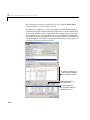
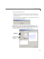
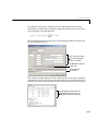
fitoptions
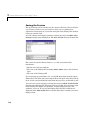
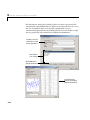
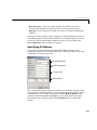
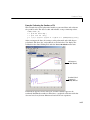
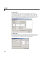
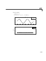
The fit results are shown below.
gfit
gfit =
General model Gauss2:
gfit(x) = a1*exp(-((x-b1)/c1)^2) + a2*exp(-((x-b2)/c2)^2)
Coefficients (with 95% confidence bounds):
a1 =
43.59 (-411.9, 499.1)
b1 =
7.803 (0.7442, 14.86)
c1 =
4.371 (-3.065, 11.81)
a2 =
-10.86 (-373.4, 351.7)
b2 =
11.05 (-190.4, 212.5)
c2 =
6.985 (-124.6, 138.5)
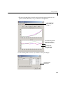
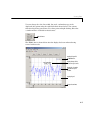
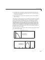
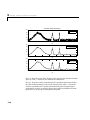
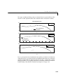
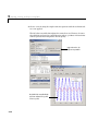
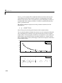
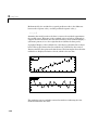
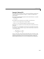
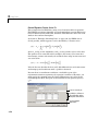
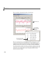
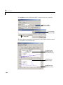
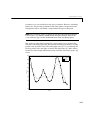
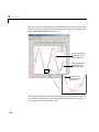
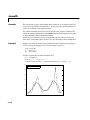
As you can see by examining the fitted coefficients, it is clear that the algorithm
has difficulty fitting the narrow peak, and does a good job fitting the broad
peak. In particular, note that the fitted value of the a2 coefficient is negative.
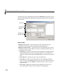
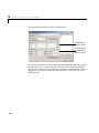
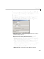
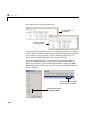
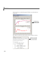
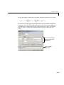
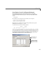
To help the fitting procedure converge, specify that the lower bounds of the
amplitude and width parameters for both peaks must be greater than zero. To
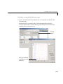
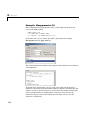
do this, create a fit options object for the gauss2 model and configure the Lower
property to zero for a1, c1, a2, and c2, but leave b1 and b2 unconstrained.
opts = fitoptions('gauss2');
opts.Lower = [0 -Inf 0 0 -Inf 0];
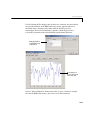
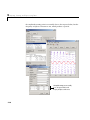
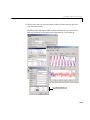
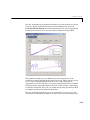
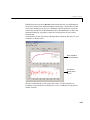
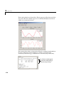
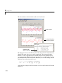
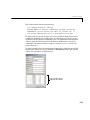
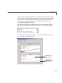
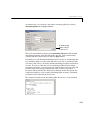
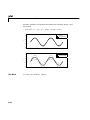
Fit the data using the new constraints.
gfit = fit(x,gdata,ftype,opts)
gfit =
General model Gauss2:
gfit(x) = a1*exp(-((x-b1)/c1)^2) + a2*exp(-((x-b2)/c2)^2)
Coefficients (with 95% confidence bounds):
a1 =
35 (34.82, 35.17)
b1 =
7.48 (7.455, 7.504)
c1 =
3.993 (3.955, 4.03)
a2 =
4.824 (2.964, 6.684)
b2 =
3 (2.99, 3.01)
c2 =
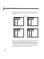
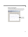
0.03209 (0.01774, 0.04643)
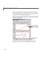
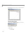
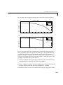
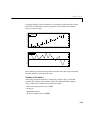
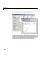
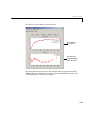
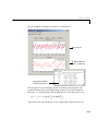
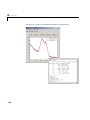
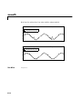
This is a much better fit, although you can still improve the a2 value.
See Also
4-112
cflibhelp, fit, get, set