Download MATLAB CURVE FITTING TOOLBOX - RELEASE NOTES User`s guide

3
Fitting Data
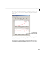
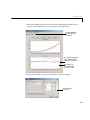
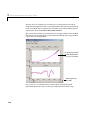
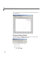
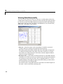
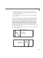
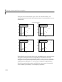
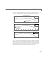
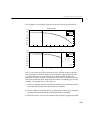
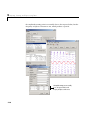
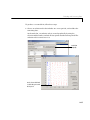
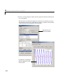
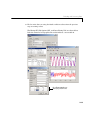
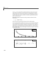
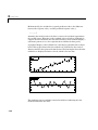
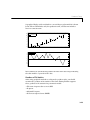
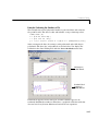
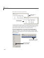
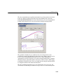
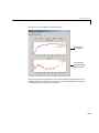
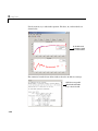
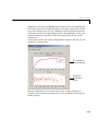
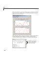
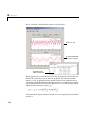
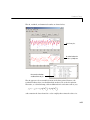
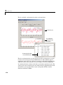
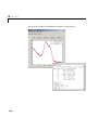
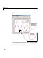
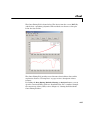
Again, the graphical results show that the linear model is reasonable for the
majority of data points, and the residuals appear to be randomly scattered
around zero. However, three residuals stand out. The largest residual
corresponds to Palm Beach County. The other residuals are at the two largest
predictor values, and correspond to Miami/Dade County and Broward County.
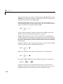
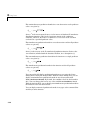
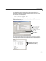
The numerical results are shown below. The inverse slope of the robust fit
indicates that Buchanan should receive one vote for every 189.3 Gore votes.
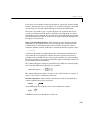
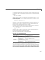
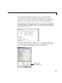
Using the fitted slope value, you can determine the expected number of votes
that Buchanan should have received for each fit. For the Buchanan versus
Bush data, you evaluate the fit at a predictor value of 152,951. For the
Buchanan versus Gore data, you evaluate the fit at a predictor value of
269,732. These results are shown below for both data sets and both fits.
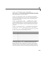
Table 3-5: Expected Buchanan Votes in Palm Beach County
Data Set
Fit
Expected Buchanan Votes
Buchanan vs. Bush
Regular least squares
814
Robust least squares
775
Regular least squares
1246
Robust least squares
1425
Buchanan vs. Gore
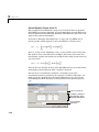
The robust results for the Buchanan versus Bush data suggest that Buchanan
received 3411 – 775 = 2636 excess votes, while robust results for the Buchanan
versus Gore data suggest that Buchanan received 3411 – 1425 = 1986 excess
votes.
3-66