1
ATS-2
ATS-2 User’s Manual
ATS-2
User’s Manual
For ATS Software Version 1.6
Copyright © 2001–2007 Audio Precision, Inc.
All rights reserved.
Document part number 8211.0135 revision 4.
All content in this manual is owned by Audio Precision and is protected by
United States and international copyright laws. Audio Precision allows its
customers to make a limited number of copies of this manual, or portions
thereof, solely for use in connection with the Audio Precision product covered
by this manual. Audio Precision may revoke this permission to make copies at
any time. You may not distribute any copies of the manual, apart from a
transfer of ownership of the Audio Precision product.
Audio Precision®, System One®, System Two™, System Two Cascade™,
System One + DSP™, System Two + DSP™, Dual Domain®, FASTTEST®,
APWIN™, ATS™ and ATS-2™are trademarks of Audio Precision, Inc.
Windows is a trademark of Microsoft Corporation.
Published by:
5750 SW Arctic Drive
Beaverton, Oregon 97005
503-627-0832
1-800-231-7350
fax 503-641-8906
ap.com
Printed in the United States of America
VII0807112021
Contents
Safety Information. . . . . . . . . . . . . . . . . . . . . . . . . . xix
Safety Symbols . . . . . . . . . . . . . . . . . . . . . . . . . . . . xx
Chapter 1
Introduction . . . . . . . . . . . . . . . . . . . . . . . . . . . . . . 1
ATS-2: an Overview . . . . . . . . . . . . . . . . . . . .
APIB . . . . . . . . . . . . . . . . . . . . . . . . . .
GPIB . . . . . . . . . . . . . . . . . . . . . . . . . .
About This Manual . . . . . . . . . . . . . . . . . . . .
ATS-2 Capabilities. . . . . . . . . . . . . . . . . . . . .
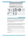
Conceptual Architecture of ATS-2 . . . . . . . . . . .
Other Documentation for ATS-2 . . . . . . . . . . . .
Getting Started with ATS-2 . . . . . . . . . . . . . .
Online Help . . . . . . . . . . . . . . . . . . . . . . .
The AP Basic User’s Guide and Language Reference
The AP Basic Extensions Reference for ATS-2 . . . .
Application Notes and TECHNOTES . . . . . . . . . .
GPIB Documentation for ATS-2 . . . . . . . . . . . . .
.
.
.
.
.
.
.
.
.
.
.
.
.
.
.
.
.
.
.
.
.
.
.
.
.
.
.
.
.
.
.
.
.
.
.
.
.
.
.
.
.
.
.
.
.
.
.
.
.
.
.
.
.
.
.
.
.
.
.
.
.
.
.
.
.
.
.
.
.
.
.
.
.
.
.
.
.
.
.
.
.
.
.
.
.
.
.
.
.
.
.
1
2
2
2
3
4
5
5
6
6
7
7
7
Chapter 2
The ATS Control Software . . . . . . . . . . . . . . . . . . . . . 9
Overview . . . . . . . . . . . . . . . . . . . . . . . . . . . . . . . . 9
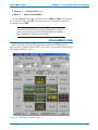
The User Interface . . . . . . . . . . . . . . . . . . . . . . . . . . 9
The Workspace . . . . . . . . . . . . . . . . . . . . . . . . . . . . 10
The ATS Panels . . . . . . . . . . . . . . . . . . . . . . . . . . . . 10
Panel Settings. . . . . . . . . . . . . . . . . . . . . . . . . . . . 11
Panel Readings . . . . . . . . . . . . . . . . . . . . . . . . . . . 12
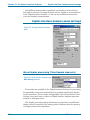
The ATS Menus . . . . . . . . . . . . . . . . . . . . . . . . . . . . 13
The File Menu . . . . . . . . . . . . . . . . . . . . . . . . . . . . 13
The Edit Menu . . . . . . . . . . . . . . . . . . . . . . . . . . . 14
The View Menu . . . . . . . . . . . . . . . . . . . . . . . . . . . 15
The Panels Menu . . . . . . . . . . . . . . . . . . . . . . . . . . 16
ATS-2 User’s Manual
i
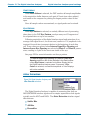
The Help Menu . . . . . . . . . . . . . . .
Access to the Audio Precision Web site
The Status Bar . . . . . . . . . . . . . .
The Toolbars and ATS Icon Buttons . .
The Standard Toolbar . . . . . . . . . .
The Panels Toolbar . . . . . . . . . . . .
The Macro Toolbar . . . . . . . . . . . .
The Learn Mode Toolbar. . . . . . . . .
The Quick Launch Toolbar . . . . . . . .
ATS Add-Ins . . . . . . . . . . . . . . . . . .
Working with Files and ATS . . . . . . . . .
Test Files. . . . . . . . . . . . . . . . . . .
Macro Files . . . . . . . . . . . . . . . . .
Data Files . . . . . . . . . . . . . . . . . .
Waveform Files . . . . . . . . . . . . . . .
Sample Files . . . . . . . . . . . . . . . . .
The Log File . . . . . . . . . . . . . . . . .
Keyboard Shortcuts . . . . . . . . . . . . .
Function Keys . . . . . . . . . . . . . . . .
ATS-2 and GPIB . . . . . . . . . . . . . . . .
.
.
.
.
.
.
.
.
.
.
.
.
.
.
.
.
.
.
.
.
.
.
.
.
.
.
.
.
.
.
.
.
.
.
.
.
.
.
.
.
.
.
.
.
.
.
.
.
.
.
.
.
.
.
.
.
.
.
.
.
.
.
.
.
.
.
.
.
.
.
.
.
.
.
.
.
.
.
.
.
.
.
.
.
.
.
.
.
.
.
.
.
.
.
.
.
.
.
.
.
.
.
.
.
.
.
.
.
.
.
.
.
.
.
.
.
.
.
.
.
.
.
.
.
.
.
.
.
.
.
.
.
.
.
.
.
.
.
.
.
.
.
.
.
.
.
.
.
.
.
.
.
.
.
.
.
.
.
.
.
.
.
.
.
.
.
.
.
.
.
.
.
.
.
.
.
.
.
.
.
.
.
.
.
.
.
.
.
.
.
.
.
.
.
.
.
.
.
.
.
.
.
.
.
.
.
.
.
.
.
.
.
.
.
.
.
.
.
.
.
.
.
.
.
.
.
.
.
.
.
.
.
.
.
.
.
.
.
.
.
18
19
19
19
20
22
23
23
24
24
25
25
25
26
26
27
27
27
27
29
Chapter 3
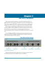
The ATS-2 Hardware . . . . . . . . . . . . . . . . . . . . . . . . 31
The ATS-2 Front Panel . . . . . . . . . . . . . . . . . . . . . . . . 31
The ATS-2 Rear Panel . . . . . . . . . . . . . . . . . . . . . . . . . 32
Power Recycle Time . . . . . . . . . . . . . . . . . . . . . . . . . 34
Chapter 4
Signal Inputs and Outputs . . . . . . . . . . . . . . . . . . . . 35
The Analog Outputs . . . . . . . . . . . . . . . . . .
The Analog Inputs . . . . . . . . . . . . . . . . . . .
The Digital Output . . . . . . . . . . . . . . . . . . .
The Digital Input . . . . . . . . . . . . . . . . . . . .
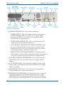
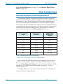
Electrical vs. Data Characteristics Across Formats.
.
.
.
.
.
.
.
.
.
.
.
.
.
.
.
.
.
.
.
.
.
.
.
.
.
.
.
.
.
.
.
.
.
.
.
36
37
38
39
39
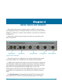
Chapter 5
Signal Analysis with ATS-2 . . . . . . . . . . . . . . . . . . . . 41
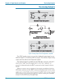
Analog Audio Signals . . . . . . . . . . . . . .
Analog Audio Generation and Output . . .
Analog Audio Input . . . . . . . . . . . . .
Digital Audio Signals . . . . . . . . . . . . . .
The Serial Digital Interface Signal . . . . . .
Digital Audio Generation . . . . . . . . . .
The Analyzer . . . . . . . . . . . . . . . . . .
Real-Time and Batch Mode Measurements
ii
.
.
.
.
.
.
.
.
.
.
.
.
.
.
.
.
.
.
.
.
.
.
.
.
.
.
.
.
.
.
.
.
.
.
.
.
.
.
.
.
.
.
.
.
.
.
.
.
.
.
.
.
.
.
.
.
.
.
.
.
.
.
.
.
.
.
.
.
.
.
.
.
.
.
.
.
.
.
.
.
.
.
.
.
.
.
.
.
41
41
41
42
42
42
42
43
ATS-2 User’s Manual
The Analyzer Instruments . . . . . . . . . . . . . . . . . . . . . 43
Sweeps and Graphs . . . . . . . . . . . . . . . . . . . . . . . . . . 44
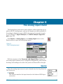
Chapter 6
The Analog Input Panel . . . . . . . . . . . . . . . . . . . . . . 45
Source . . . . . . . . . . . . . . . . . .
Input Termination Option . . . . . .
Peak Monitors . . . . . . . . . . . . . .
Input Ranging . . . . . . . . . . . . . .
Autoranging . . . . . . . . . . . . .
Fixed Range . . . . . . . . . . . . . .
DC Coupling . . . . . . . . . . . . . . .
Converter and Sample Rate Selection
.
.
.
.
.
.
.
.
.
.
.
.
.
.
.
.
.
.
.
.
.
.
.
.
.
.
.
.
.
.
.
.
.
.
.
.
.
.
.
.
.
.
.
.
.
.
.
.
.
.
.
.
.
.
.
.
.
.
.
.
.
.
.
.
.
.
.
.
.
.
.
.
.
.
.
.
.
.
.
.
.
.
.
.
.
.
.
.
.
.
.
.
.
.
.
.
.
.
.
.
.
.
.
.
.
.
.
.
.
.
.
.
.
.
.
.
.
.
.
.
45
46
46
47
47
47
47
48
Chapter 7
The Digital I/O Panel . . . . . . . . . . . . . . . . . . . . . . . . 51
The DIO Output Section . . . . . . . . . . . . . . . . . .
Format. . . . . . . . . . . . . . . . . . . . . . . . . . .
Output Sample Rate-OSR . . . . . . . . . . . . . . . . .
Voltage . . . . . . . . . . . . . . . . . . . . . . . . . .
Output Resolution . . . . . . . . . . . . . . . . . . . .
µ-Law and A-law Compression . . . . . . . . . . . . . .
Preemphasis . . . . . . . . . . . . . . . . . . . . . . .
Scale Freq. by . . . . . . . . . . . . . . . . . . . . . . .
Polarity . . . . . . . . . . . . . . . . . . . . . . . . . .
Send Errors . . . . . . . . . . . . . . . . . . . . . . . .
Changing the Parity bit . . . . . . . . . . . . . . . .
Sending a Validity bit . . . . . . . . . . . . . . . . .
Jitter Generation . . . . . . . . . . . . . . . . . . . . .
Jitter Type . . . . . . . . . . . . . . . . . . . . . . .
Amplitude. . . . . . . . . . . . . . . . . . . . . . . .
Frequency. . . . . . . . . . . . . . . . . . . . . . . .
EQ Curve. . . . . . . . . . . . . . . . . . . . . . . . .
The DIO Input Section . . . . . . . . . . . . . . . . . . .
Format. . . . . . . . . . . . . . . . . . . . . . . . . . .
Input Impedance . . . . . . . . . . . . . . . . . . . . .
Single and Dual Connector Input Bitstream Selection
Single-Connector Mode . . . . . . . . . . . . . . . .
Dual-Connector Mode . . . . . . . . . . . . . . . . .
Input Sample Rate-ISR . . . . . . . . . . . . . . . . . .
Voltage . . . . . . . . . . . . . . . . . . . . . . . . . .
Input Resolution . . . . . . . . . . . . . . . . . . . . .
µ-Law and A-law Expansion . . . . . . . . . . . . . . .
Deemphasis . . . . . . . . . . . . . . . . . . . . . . . .
Scale Freq. by . . . . . . . . . . . . . . . . . . . . . . .
ATS-2 User’s Manual
.
.
.
.
.
.
.
.
.
.
.
.
.
.
.
.
.
.
.
.
.
.
.
.
.
.
.
.
.
.
.
.
.
.
.
.
.
.
.
.
.
.
.
.
.
.
.
.
.
.
.
.
.
.
.
.
.
.
.
.
.
.
.
.
.
.
.
.
.
.
.
.
.
.
.
.
.
.
.
.
.
.
.
.
.
.
.
.
.
.
.
.
.
.
.
.
.
.
.
.
.
.
.
.
.
.
.
.
.
.
.
.
.
.
.
.
.
.
.
.
.
.
.
.
.
.
.
.
.
.
.
.
.
.
.
.
.
.
.
.
.
.
.
.
.
52
53
54
54
55
55
56
57
57
57
58
58
58
59
59
59
60
60
61
62
62
62
62
63
63
64
64
65
65
iii
Rate Ref . . . . . . . . . . . . . . . . . .
Peak Monitors. . . . . . . . . . . . . . .
Data Bit Indicators . . . . . . . . . . . .
Error Indicators . . . . . . . . . . . . . .
The Confidence Indicator . . . . . . .
The Lock Indicator . . . . . . . . . . .
The Coding Indicator . . . . . . . . .
The Parity Bit Indicator . . . . . . . .
The Validity Bit Indicators . . . . . . .
Jitter Measurement . . . . . . . . . . .
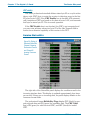
The Status Bits panel . . . . . . . . . . . .
Transmit Status Bits . . . . . . . . . . .
Consumer Format Status Bits . . . . .
Professional Format Status Bits. . . .
Local Address and Time of Day entry
CRC entry . . . . . . . . . . . . . . . .
Receive Status Bits . . . . . . . . . . . .
Hex Control and Display . . . . . . . . .
Dual Connector Mode and Status Bits .
.
.
.
.
.
.
.
.
.
.
.
.
.
.
.
.
.
.
.
.
.
.
.
.
.
.
.
.
.
.
.
.
.
.
.
.
.
.
.
.
.
.
.
.
.
.
.
.
.
.
.
.
.
.
.
.
.
.
.
.
.
.
.
.
.
.
.
.
.
.
.
.
.
.
.
.
.
.
.
.
.
.
.
.
.
.
.
.
.
.
.
.
.
.
.
.
.
.
.
.
.
.
.
.
.
.
.
.
.
.
.
.
.
.
.
.
.
.
.
.
.
.
.
.
.
.
.
.
.
.
.
.
.
.
.
.
.
.
.
.
.
.
.
.
.
.
.
.
.
.
.
.
.
.
.
.
.
.
.
.
.
.
.
.
.
.
.
.
.
.
.
.
.
.
.
.
.
.
.
.
.
.
.
.
.
.
.
.
.
.
.
.
.
.
.
.
.
.
.
.
.
.
.
.
.
.
.
.
.
.
.
.
.
.
.
.
.
.
.
.
.
.
.
.
.
.
.
.
.
.
.
.
.
.
.
.
.
.
.
.
.
.
.
.
.
.
.
66
66
67
67
68
68
68
68
69
69
70
71
72
73
73
74
74
75
75
Chapter 8
The Analog Generator . . . . . . . . . . . . . . . . . . . . . . . 77
Test Signal Generation in ATS-2 . . . . . . .
Two Audio Signal Generators . . . . . . .
Signals for Analog Measurements . . . .
The Analog Generator Panel. . . . . . . . .
Frequency Units . . . . . . . . . . . . . .
Output On/Off and Channel Selection . .
Auto On . . . . . . . . . . . . . . . . . . .
Amplitude Control and Units . . . . . . .
Choosing an Analog Generator Waveform.
Sine waveforms. . . . . . . . . . . . . . .
Wfm: Sine: Normal . . . . . . . . . . . .
Wfm: Sine: Var Phase. . . . . . . . . . .
Wfm: Sine: Stereo . . . . . . . . . . . .
Wfm: Sine: Dual . . . . . . . . . . . . . .
Wfm: Sine: Shaped Burst . . . . . . . .
Wfm: Sine: EQ . . . . . . . . . . . . . . .
Squarewave . . . . . . . . . . . . . . . . .
Wfm: Square . . . . . . . . . . . . . . .
Intermodulation Distortion (IMD) . . . . .
Wfm: IMD: SMPTE/DIN 4:1 . . . . . . . .
Wfm: IMD: SMPTE/DIN 1:1 . . . . . . . .
Noise Waveform . . . . . . . . . . . . . .
iv
.
.
.
.
.
.
.
.
.
.
.
.
.
.
.
.
.
.
.
.
.
.
.
.
.
.
.
.
.
.
.
.
.
.
.
.
.
.
.
.
.
.
.
.
.
.
.
.
.
.
.
.
.
.
.
.
.
.
.
.
.
.
.
.
.
.
.
.
.
.
.
.
.
.
.
.
.
.
.
.
.
.
.
.
.
.
.
.
.
.
.
.
.
.
.
.
.
.
.
.
.
.
.
.
.
.
.
.
.
.
.
.
.
.
.
.
.
.
.
.
.
.
.
.
.
.
.
.
.
.
.
.
.
.
.
.
.
.
.
.
.
.
.
.
.
.
.
.
.
.
.
.
.
.
.
.
.
.
.
.
.
.
.
.
.
.
.
.
.
.
.
.
.
.
.
.
.
.
.
.
.
.
.
.
.
.
.
.
.
.
.
.
.
.
.
.
.
.
.
.
.
.
.
.
.
.
.
.
.
.
.
.
.
.
.
.
.
.
.
.
.
.
.
.
.
.
.
.
.
.
.
.
.
.
.
.
.
.
.
.
.
.
.
.
.
.
.
.
.
.
.
.
.
.
.
.
.
.
.
.
.
.
.
.
77
77
77
78
79
79
79
80
81
81
82
82
83
83
84
87
89
89
89
89
90
90
ATS-2 User’s Manual
Arbitrary Waveforms. . . . . . . . . . . . . . . . . . . . . . . . 91
Setting the DAC Sample Rate . . . . . . . . . . . . . . . . . . . 91
Special Waveforms . . . . . . . . . . . . . . . . . . . . . . . . . 92
Wfm: Special: Polarity . . . . . . . . . . . . . . . . . . . . . . 93
Wfm: Special: Pass Thru . . . . . . . . . . . . . . . . . . . . . 93
Configuring the Analog Outputs . . . . . . . . . . . . . . . . . . 94
Analog Generator References . . . . . . . . . . . . . . . . . . . . 95
“dBr” Amplitude Reference . . . . . . . . . . . . . . . . . . . . 96
Frequency Reference . . . . . . . . . . . . . . . . . . . . . . . 96
Watts Reference . . . . . . . . . . . . . . . . . . . . . . . . . . 96
dBm Reference . . . . . . . . . . . . . . . . . . . . . . . . . . . 96
Chapter 9
The Digital Generator . . . . . . . . . . . . . . . . . . . . . . . 99
Test Signal Generation in ATS-2 . . . . . . . . . . . . . . . . . . . 99
Two Audio Signal Generators . . . . . . . . . . . . . . . . . . . 99
Signals for Digital Measurements . . . . . . . . . . . . . . . . . 99
The Digital Generator Panel . . . . . . . . . . . . . . . . . . . . 100
Frequency Units . . . . . . . . . . . . . . . . . . . . . . . . . . 101
Output On/Off and Channel Selection. . . . . . . . . . . . . . 101
Auto On . . . . . . . . . . . . . . . . . . . . . . . . . . . . . . 101
Channel Invert . . . . . . . . . . . . . . . . . . . . . . . . . . . 102
Amplitude Control and Units . . . . . . . . . . . . . . . . . . 102
Choosing a Digital Generator Waveform . . . . . . . . . . . . . 103
Sine waveforms . . . . . . . . . . . . . . . . . . . . . . . . . . 103
Wfm: Sine: Normal . . . . . . . . . . . . . . . . . . . . . . . 104
Wfm: Sine: Var Phase . . . . . . . . . . . . . . . . . . . . . . 104
Wfm: Sine: Stereo . . . . . . . . . . . . . . . . . . . . . . . . 105
Wfm: Sine: Dual . . . . . . . . . . . . . . . . . . . . . . . . . 105
Wfm: Sine: Shaped Burst . . . . . . . . . . . . . . . . . . . . 106
Wfm: Sine: EQ . . . . . . . . . . . . . . . . . . . . . . . . . . 107
Wfm: Sine: Burst . . . . . . . . . . . . . . . . . . . . . . . . 109
Wfm: Sine+Offset . . . . . . . . . . . . . . . . . . . . . . . 111
Intermodulation Distortion (IMD) . . . . . . . . . . . . . . . . 112
Wfm: IMD: SMPTE/DIN 4:1 . . . . . . . . . . . . . . . . . . . . 112
Wfm: IMD: SMPTE/DIN 1:1 . . . . . . . . . . . . . . . . . . . . 112
Squarewave . . . . . . . . . . . . . . . . . . . . . . . . . . . . 112
Wfm: Square. . . . . . . . . . . . . . . . . . . . . . . . . . . 112
White Noise . . . . . . . . . . . . . . . . . . . . . . . . . . . . 113
Wfm: Noise . . . . . . . . . . . . . . . . . . . . . . . . . . . 113
Arbitrary Waveforms . . . . . . . . . . . . . . . . . . . . . . . 114
Special Waveforms . . . . . . . . . . . . . . . . . . . . . . . . 115
Wfm: Special: Polarity . . . . . . . . . . . . . . . . . . . . . 115
Wfm: Special: Pass Thru . . . . . . . . . . . . . . . . . . . . 116
ATS-2 User’s Manual
v
Wfm: Special: Monotonicity . . . . . . . . . . .
Wfm: Special: J-Test. . . . . . . . . . . . . . . .
Wfm: Special: Walking Ones and Walking Zeros
Wfm: Special: Constant Value . . . . . . . . . .
Wfm: Special: Random . . . . . . . . . . . . . .
Dither . . . . . . . . . . . . . . . . . . . . . . . . . .
Dither Type . . . . . . . . . . . . . . . . . . . . .
Digital Generator References . . . . . . . . . . . .
Volts for Full Scale Reference . . . . . . . . . . .
Frequency Reference. . . . . . . . . . . . . . . .
dBr Reference . . . . . . . . . . . . . . . . . . . .
.
.
.
.
.
.
.
.
.
.
.
.
.
.
.
.
.
.
.
.
.
.
.
.
.
.
.
.
.
.
.
.
.
.
.
.
.
.
.
.
.
.
.
.
.
.
.
.
.
.
.
.
.
.
.
.
.
.
.
.
.
.
.
.
.
.
.
.
.
.
.
.
.
.
.
.
.
117
119
119
120
120
120
121
122
122
122
122
Chapter 10
The Audio Analyzer . . . . . . . . . . . . . . . . . . . . . . . . 123
Overview . . . . . . . . . . . . . . . . . . . . . . .
Loading the Audio Analyzer . . . . . . . . . . . .
Signal Inputs . . . . . . . . . . . . . . . . . . . . .
The Level Meters. . . . . . . . . . . . . . . . . . .
Level Meter Units . . . . . . . . . . . . . . . . .
AC and DC Coupling . . . . . . . . . . . . . . . .
Common-Mode Testing and Coupling Issues.
The Frequency Meters . . . . . . . . . . . . . . .
Meter Ranging. . . . . . . . . . . . . . . . . . .
Autoranging . . . . . . . . . . . . . . . . . . .
Fixed Range . . . . . . . . . . . . . . . . . . .
The Function Meters . . . . . . . . . . . . . . . .
Function Meter Measurement Functions. . . .
Amplitude Function . . . . . . . . . . . . . .
2-Channel Ratio Function . . . . . . . . . . .
Crosstalk Function . . . . . . . . . . . . . . .
THD+N Functions . . . . . . . . . . . . . . . .
THD+N Ratio Function . . . . . . . . . . . . .
THD+N Amplitude Function . . . . . . . . . .
Bandpass Function . . . . . . . . . . . . . . .
SMPTE/DIN IMD Function . . . . . . . . . . . .
Phase Function . . . . . . . . . . . . . . . . .
Function Meter Units . . . . . . . . . . . . . . .
Function Meter Ranging . . . . . . . . . . . . .
Detector Type . . . . . . . . . . . . . . . . . . .
Detector Reading Rate . . . . . . . . . . . . . .
The Bandwidth and Filter Fields. . . . . . . . .
BW: The Highpass Filter. . . . . . . . . . . . . .
BW: The Lowpass Filter . . . . . . . . . . . . . .
The “Fltr” Field . . . . . . . . . . . . . . . . . . .
vi
.
.
.
.
.
.
.
.
.
.
.
.
.
.
.
.
.
.
.
.
.
.
.
.
.
.
.
.
.
.
.
.
.
.
.
.
.
.
.
.
.
.
.
.
.
.
.
.
.
.
.
.
.
.
.
.
.
.
.
.
.
.
.
.
.
.
.
.
.
.
.
.
.
.
.
.
.
.
.
.
.
.
.
.
.
.
.
.
.
.
.
.
.
.
.
.
.
.
.
.
.
.
.
.
.
.
.
.
.
.
.
.
.
.
.
.
.
.
.
.
.
.
.
.
.
.
.
.
.
.
.
.
.
.
.
.
.
.
.
.
.
.
.
.
.
.
.
.
.
.
.
.
.
.
.
.
.
.
.
.
.
.
.
.
.
.
.
.
.
.
.
.
.
.
.
.
.
.
.
.
.
.
.
.
.
.
.
.
.
.
.
.
.
.
.
.
.
.
.
.
.
.
.
.
.
.
.
.
.
.
.
.
.
.
.
.
.
.
.
.
.
.
.
.
.
.
.
.
.
.
.
.
.
.
.
.
.
.
.
.
123
124
125
126
126
127
128
128
129
129
129
130
130
131
132
133
134
135
136
136
137
138
140
140
141
142
143
143
144
145
ATS-2 User’s Manual
Fltr: Weighting Filters. . . . . . . . . .
User Filters . . . . . . . . . . . . . . . .
Bandpass/Bandreject Filter Tuning . .
Fltr: Selecting Harmonics in Bandpass
References . . . . . . . . . . . . . . . . .
Analyzer Analog References . . . . . .
Analyzer Digital References . . . . . .
.
.
.
.
.
.
.
.
.
.
.
.
.
.
.
.
.
.
.
.
.
.
.
.
.
.
.
.
.
.
.
.
.
.
.
.
.
.
.
.
.
.
.
.
.
.
.
.
.
.
.
.
.
.
.
.
.
.
.
.
.
.
.
.
.
.
.
.
.
.
.
.
.
.
.
.
.
.
.
.
.
.
.
.
.
.
.
.
.
.
.
145
147
149
150
151
151
152
Chapter 11
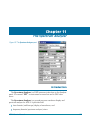
The Spectrum Analyzer . . . . . . . . . . . . . . . . . . . . . 155
Introduction . . . . . . . . . . . . . . . . . . . . . . . . . . .
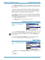
Loading the Spectrum Analyzer . . . . . . . . . . . . . . . .
Signal Inputs . . . . . . . . . . . . . . . . . . . . . . . . . . .
Peak Level Monitors . . . . . . . . . . . . . . . . . . . . . . .
Acquiring, Transforming and Processing . . . . . . . . . . .
The Acquisition Record . . . . . . . . . . . . . . . . . . . . .
Acquisition Length . . . . . . . . . . . . . . . . . . . . . .
Transform Length . . . . . . . . . . . . . . . . . . . . . . . .
Spectrum Analyzer Window Selection . . . . . . . . . . . .
Hann Window . . . . . . . . . . . . . . . . . . . . . . . . .
Blackman-Harris Window . . . . . . . . . . . . . . . . . . .
Flat-Top Window . . . . . . . . . . . . . . . . . . . . . . .
Equiripple Window . . . . . . . . . . . . . . . . . . . . . .
Hamming Window . . . . . . . . . . . . . . . . . . . . . .
Gaussian Window . . . . . . . . . . . . . . . . . . . . . . .
Rife-Vincent Windows . . . . . . . . . . . . . . . . . . . .
None (No Window or Rectangular Window) . . . . . . . .
None, move to bin center . . . . . . . . . . . . . . . . . .
Quasi-AC Coupling . . . . . . . . . . . . . . . . . . . . . . . .
Averaging . . . . . . . . . . . . . . . . . . . . . . . . . . . .
Synchronous Averaging . . . . . . . . . . . . . . . . . . .
Signal Alignment for Synchronous Averaging . . . . . .
Sync (without re-align) . . . . . . . . . . . . . . . . . . .
Sync, re-align . . . . . . . . . . . . . . . . . . . . . . . .
Synchronous Averaging for “Move to bin center”
operations . . . . . . . . . . . . . . . . . . . . . . . . . .
Synchronous Averaging and Frequency Domain Views
Power (Spectrum) Averaging . . . . . . . . . . . . . . . .
Display Processing. . . . . . . . . . . . . . . . . . . . . . . .
Waveform (time domain) Display Processing . . . . . . .
Interpolate . . . . . . . . . . . . . . . . . . . . . . . . .
Display Samples . . . . . . . . . . . . . . . . . . . . . . .
Peak Values . . . . . . . . . . . . . . . . . . . . . . . . .
Absolute Values . . . . . . . . . . . . . . . . . . . . . . .
ATS-2 User’s Manual
.
.
.
.
.
.
.
.
.
.
.
.
.
.
.
.
.
.
.
.
.
.
.
.
.
.
.
.
.
.
.
.
.
.
.
.
.
.
.
.
.
.
.
.
.
.
.
.
155
156
156
157
157
159
160
161
161
163
163
163
164
164
164
164
165
165
166
167
168
169
170
170
.
.
.
.
.
.
.
.
.
.
.
.
.
.
.
.
.
.
170
171
172
173
173
174
174
175
175
vii
Graphic Aliasing . . . . . . . . . . . . . . . . . . . .
Spectrum (frequency domain) Display Processing
FFT Start Time . . . . . . . . . . . . . . . . . . . . . .
Triggering . . . . . . . . . . . . . . . . . . . . . . . .
Free Run . . . . . . . . . . . . . . . . . . . . . . . .
Auto . . . . . . . . . . . . . . . . . . . . . . . . . .
Fixed Sensitivity . . . . . . . . . . . . . . . . . . . .
Trig In (Ext) . . . . . . . . . . . . . . . . . . . . . . .
Digital Gen . . . . . . . . . . . . . . . . . . . . . . .
Analog Gen. . . . . . . . . . . . . . . . . . . . . . .
Line (Mains) . . . . . . . . . . . . . . . . . . . . . .
Jitter Gen . . . . . . . . . . . . . . . . . . . . . . .
Fixed Level . . . . . . . . . . . . . . . . . . . . . . .
Trigger Delay Time . . . . . . . . . . . . . . . . . .
Trigger Slope . . . . . . . . . . . . . . . . . . . . .
Triggering with Synchronous Averaging . . . . . .
Without Re-alignment . . . . . . . . . . . . . . .
With Re-alignment . . . . . . . . . . . . . . . . .
Triggering with Quasi-AC Coupling . . . . . . . . .
References . . . . . . . . . . . . . . . . . . . . . . . .
The Sweep Spectrum/Waveform Button . . . . . . .
Acquired Waveform Files . . . . . . . . . . . . . . . .
Saving Acquired Waveforms . . . . . . . . . . . . .
Opening Acquired Waveforms. . . . . . . . . . . .
Combining Mono to Stereo . . . . . . . . . . . .
Compatibility of Acquired Waveform Files. . . . .
.
.
.
.
.
.
.
.
.
.
.
.
.
.
.
.
.
.
.
.
.
.
.
.
.
.
.
.
.
.
.
.
.
.
.
.
.
.
.
.
.
.
.
.
.
.
.
.
.
.
.
.
.
.
.
.
.
.
.
.
.
.
.
.
.
.
.
.
.
.
.
.
.
.
.
.
.
.
.
.
.
.
.
.
.
.
.
.
.
.
.
.
.
.
.
.
.
.
.
.
.
.
.
.
.
.
.
.
.
.
.
.
.
.
.
.
.
.
.
.
.
.
.
.
.
.
.
.
.
.
.
.
.
.
.
.
.
.
.
.
.
.
.
.
.
.
.
.
.
.
.
.
.
.
.
.
176
176
177
177
178
178
178
179
179
179
179
179
179
180
180
181
181
181
182
182
182
183
184
184
185
185
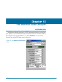
Chapter 12
The Digital Interface Analyzer . . . . . . . . . . . . . . . . 187
Overview . . . . . . . . . . . . . . . . . . . . . . .
ATS-2 Digital Interface Analyzer Analysis Tools .
Digital Interface Analyzer Components . . . . . .
The Digital Interface Analyzer ADC . . . . . . .
Digital Interface Analyzer Capabilities . . . . .
Loading the Digital Interface Analyzer . . . . . .
The Digital Interface Analyzer panel . . . . . . .
Digital Interface Analyzer Waveform Views . . .
Interface Waveform . . . . . . . . . . . . . . .
Eye Pattern . . . . . . . . . . . . . . . . . . . .
Jitter Waveform. . . . . . . . . . . . . . . . . .
Digital Interface Analyzer Spectrum Views . . . .
Interface Spectrum . . . . . . . . . . . . . . . .
Jitter Spectrum . . . . . . . . . . . . . . . . . .
Digital Interface Analyzer Histograms. . . . . . .
viii
.
.
.
.
.
.
.
.
.
.
.
.
.
.
.
.
.
.
.
.
.
.
.
.
.
.
.
.
.
.
.
.
.
.
.
.
.
.
.
.
.
.
.
.
.
.
.
.
.
.
.
.
.
.
.
.
.
.
.
.
.
.
.
.
.
.
.
.
.
.
.
.
.
.
.
.
.
.
.
.
.
.
.
.
.
.
.
.
.
.
.
.
.
.
.
.
.
.
.
.
.
.
.
.
.
.
.
.
.
.
.
.
.
.
.
.
.
.
.
.
187
187
188
188
188
189
189
191
191
192
193
195
195
195
197
ATS-2 User’s Manual
Interface Amplitude Histogram . . . . . . . . . . . . .
Interface Pulse Width Histogram . . . . . . . . . . . .
Interface Bit-Rate Histogram. . . . . . . . . . . . . . .
Jitter Histogram. . . . . . . . . . . . . . . . . . . . . .
InterVuMenu.atsb . . . . . . . . . . . . . . . . . . . . . .
Digital Interface Analyzer panel settings . . . . . . . . .
Wave Display processing (Time Domain view only) . .
Interpolate . . . . . . . . . . . . . . . . . . . . . . .
Display Samples . . . . . . . . . . . . . . . . . . . . .
Peak Values . . . . . . . . . . . . . . . . . . . . . . .
Eye Pattern . . . . . . . . . . . . . . . . . . . . . . .
Jitter Detection . . . . . . . . . . . . . . . . . . . . . .
Squarewave (Converter Clock) Jitter Detection . . .
Averages (spectrum view only) . . . . . . . . . . . . .
FFT Windows for the Digital Interface Analyzer . . . .
Trigger Source. . . . . . . . . . . . . . . . . . . . . . .
Triggering for squarewave acquisitions . . . . . . .
Trigger Slope . . . . . . . . . . . . . . . . . . . . . . .
Data Acquisition . . . . . . . . . . . . . . . . . . . . . .
Receive Error Triggers . . . . . . . . . . . . . . . . .
References . . . . . . . . . . . . . . . . . . . . . . . . .
Saving and Loading Interface Waveforms . . . . . . .
Audible Monitoring in the Digital Interface Analyzer .
.
.
.
.
.
.
.
.
.
.
.
.
.
.
.
.
.
.
.
.
.
.
.
.
.
.
.
.
.
.
.
.
.
.
.
.
.
.
.
.
.
.
.
.
.
.
.
.
.
.
.
.
.
.
.
.
.
.
.
.
.
.
.
.
.
.
.
.
.
.
.
.
.
.
.
.
.
.
.
.
.
.
.
.
.
.
.
.
.
.
.
.
197
198
199
200
201
202
202
203
203
204
204
204
206
207
207
209
210
210
211
211
211
212
212
Chapter 13
The Multitone Audio Analyzer . . . . . . . . . . . . . . . . . 213
Introduction . . . . . . . . . . . . . . . . . . . . . . . . . . . . . 213
Overview: Multitone Testing . . . . . . . . . . . . . . . . . . . . 214
Multitone Waveform requirements. . . . . . . . . . . . . . . 215
Sample multitone waveforms . . . . . . . . . . . . . . . . . 215
Creating custom multitone waveforms . . . . . . . . . . . 216
“Inside Information”: Multitone Generator Settings. . . . . . 216
The Multitone Audio Analyzer panel . . . . . . . . . . . . . . . 217
Signal Inputs . . . . . . . . . . . . . . . . . . . . . . . . . . . . . 217
Peak Level Monitors . . . . . . . . . . . . . . . . . . . . . . . . . 218
Multitone Measurements . . . . . . . . . . . . . . . . . . . . . . 218
Frequency Domain Views by default . . . . . . . . . . . . . 218
Spectrum . . . . . . . . . . . . . . . . . . . . . . . . . . . . . 219
Response . . . . . . . . . . . . . . . . . . . . . . . . . . . . . 220
Distortion . . . . . . . . . . . . . . . . . . . . . . . . . . . . . 221
Noise . . . . . . . . . . . . . . . . . . . . . . . . . . . . . . . . 222
Masking Curve . . . . . . . . . . . . . . . . . . . . . . . . . . . 224
Crosstalk . . . . . . . . . . . . . . . . . . . . . . . . . . . . . . 225
Time Domain View . . . . . . . . . . . . . . . . . . . . . . . . 226
ATS-2 User’s Manual
ix
Frequency Resolution. . . . . . . . . . . . . . . .
Setting Multitone triggering resolution . . . .
Setting frequency resolution for rss summing
FFT Length . . . . . . . . . . . . . . . . . . . . . .
Processing . . . . . . . . . . . . . . . . . . . . . .
Triggering . . . . . . . . . . . . . . . . . . . . . .
Off . . . . . . . . . . . . . . . . . . . . . . . . .
Digital Gen and Analog Gen . . . . . . . . . . .
Tight, Normal and Loose . . . . . . . . . . . . .
Trig In (Ext) . . . . . . . . . . . . . . . . . . . . .
Trigger Delay . . . . . . . . . . . . . . . . . . .
Phase Measurements . . . . . . . . . . . . . . . .
Channel A Phase . . . . . . . . . . . . . . . . . .
Channel B Phase . . . . . . . . . . . . . . . . . .
References . . . . . . . . . . . . . . . . . . . . . .
Other Considerations . . . . . . . . . . . . . . . .
Multitone Minimum Duration Requirements .
Invalid Multitone Readings . . . . . . . . . . . .
Acquired Waveform Files . . . . . . . . . . . . . .
Saving Acquired Waveforms . . . . . . . . . . .
Opening Acquired Waveforms. . . . . . . . . .
Combining Mono to Stereo . . . . . . . . . .
Compatibility of Acquired Waveform Files. . .
Creating Multitone Waveform Files . . . . . . . .
Multitone Creation Utility opening dialog box
Using Existing File Data . . . . . . . . . . . . .
File Options . . . . . . . . . . . . . . . . . . .
Frequencies Menu . . . . . . . . . . . . . . . .
Editing the Frequency List . . . . . . . . . . . .
Sweep Table Definition . . . . . . . . . . . . . .
Creating an MS RIFF (.wav) File . . . . . . . . . .
Final Options. . . . . . . . . . . . . . . . . . . .
.
.
.
.
.
.
.
.
.
.
.
.
.
.
.
.
.
.
.
.
.
.
.
.
.
.
.
.
.
.
.
.
.
.
.
.
.
.
.
.
.
.
.
.
.
.
.
.
.
.
.
.
.
.
.
.
.
.
.
.
.
.
.
.
.
.
.
.
.
.
.
.
.
.
.
.
.
.
.
.
.
.
.
.
.
.
.
.
.
.
.
.
.
.
.
.
.
.
.
.
.
.
.
.
.
.
.
.
.
.
.
.
.
.
.
.
.
.
.
.
.
.
.
.
.
.
.
.
.
.
.
.
.
.
.
.
.
.
.
.
.
.
.
.
.
.
.
.
.
.
.
.
.
.
.
.
.
.
.
.
.
.
.
.
.
.
.
.
.
.
.
.
.
.
.
.
.
.
.
.
.
.
.
.
.
.
.
.
.
.
.
.
.
.
.
.
.
.
.
.
.
.
.
.
.
.
.
.
.
.
.
.
.
.
.
.
.
.
.
.
.
.
.
.
.
.
.
.
.
.
.
.
.
.
.
.
.
.
.
.
.
.
.
.
.
.
.
.
.
.
.
.
.
.
.
.
226
226
227
227
228
229
229
229
229
230
230
230
231
231
231
232
232
233
233
234
234
235
235
236
236
238
239
240
240
241
242
243
Chapter 14
The Harmonic Distortion Analyzer . . . . . . . . . . . . . . 245
Introduction . . . . . . . . . . . . . . . . . . . .
Loading the Harmonic Distortion Analyzer. . .
Signal Inputs . . . . . . . . . . . . . . . . . . . .
The Fundamental Amplitude Meters . . . . . .
The Fundamental Frequency Meters . . . . . .
Harmonic Distortion Product Amplitude . . . .
Harmonic Order Control . . . . . . . . . . .
Distortion Product Bandwidth Limitations
Amplitude Units . . . . . . . . . . . . . . . . .
x
.
.
.
.
.
.
.
.
.
.
.
.
.
.
.
.
.
.
.
.
.
.
.
.
.
.
.
.
.
.
.
.
.
.
.
.
.
.
.
.
.
.
.
.
.
.
.
.
.
.
.
.
.
.
.
.
.
.
.
.
.
.
.
.
.
.
.
.
.
.
.
.
.
.
.
.
.
.
.
.
.
245
247
247
248
248
248
249
249
250
ATS-2 User’s Manual
References . . . . . . . . . . . . . .
Steering Control. . . . . . . . . . .
High Speed/High Accuracy Control
Sweeping and Graphing Results . . .
.
.
.
.
.
.
.
.
.
.
.
.
.
.
.
.
.
.
.
.
.
.
.
.
.
.
.
.
.
.
.
.
.
.
.
.
.
.
.
.
.
.
.
.
.
.
.
.
.
.
.
.
.
.
.
.
.
.
.
.
251
251
252
254
Chapter 15
Sweeps and Sweep Settling . . . . . . . . . . . . . . . . . . 255
Introduction: Sweeps and Graphs .
Batch Mode “Sweeps”. . . . . . .
Plan Your Sweep. . . . . . . . . . .
The Sweep Panel . . . . . . . . . .
Source 1 . . . . . . . . . . . . . . .
Settings or Readings?. . . . . . .
Selecting a Sweep Source . . . .
Start and Stop Values . . . . . . .
Source 1 Log or Lin Scales . . . .
Sweep Resolution . . . . . . . . .
Linear Scale Steps . . . . . . . .
Logarithmic Scale Steps . . . .
X-Axis Divisions . . . . . . . . . .
Data 1 . . . . . . . . . . . . . . . . .
Selecting the Data 1 Reading . .
Top and Bottom Values. . . . . .
Data 1 Log or Lin Scales . . . . . .
Y-Axis Divisions . . . . . . . . . .
Data Limits . . . . . . . . . . . . . .
Data 2 . . . . . . . . . . . . . . . . .
Plotting Data as X-versus-Y . . . .
Data 3 through Data 6. . . . . . . .
Sweep Display Mode . . . . . . . .
Go / Stop / Pause . . . . . . . . . . .
Repeat . . . . . . . . . . . . . . . .
Append . . . . . . . . . . . . . . . .
Appending a File . . . . . . . . . .
Stereo Sweeps . . . . . . . . . . . .
Single Point Sweeps . . . . . . . . .
Nested Sweeps using Source 2 . . .
Pre-Sweep Delay . . . . . . . . . . .
Pre-Sweep Delay and Auto On . .
Table Sweeps . . . . . . . . . . . .
External Sweeps . . . . . . . . . . .
External Sweep Operation . . . .
Start and Stop. . . . . . . . . .
Spacing. . . . . . . . . . . . . .
ATS-2 User’s Manual
.
.
.
.
.
.
.
.
.
.
.
.
.
.
.
.
.
.
.
.
.
.
.
.
.
.
.
.
.
.
.
.
.
.
.
.
.
.
.
.
.
.
.
.
.
.
.
.
.
.
.
.
.
.
.
.
.
.
.
.
.
.
.
.
.
.
.
.
.
.
.
.
.
.
.
.
.
.
.
.
.
.
.
.
.
.
.
.
.
.
.
.
.
.
.
.
.
.
.
.
.
.
.
.
.
.
.
.
.
.
.
.
.
.
.
.
.
.
.
.
.
.
.
.
.
.
.
.
.
.
.
.
.
.
.
.
.
.
.
.
.
.
.
.
.
.
.
.
.
.
.
.
.
.
.
.
.
.
.
.
.
.
.
.
.
.
.
.
.
.
.
.
.
.
.
.
.
.
.
.
.
.
.
.
.
.
.
.
.
.
.
.
.
.
.
.
.
.
.
.
.
.
.
.
.
.
.
.
.
.
.
.
.
.
.
.
.
.
.
.
.
.
.
.
.
.
.
.
.
.
.
.
.
.
.
.
.
.
.
.
.
.
.
.
.
.
.
.
.
.
.
.
.
.
.
.
.
.
.
.
.
.
.
.
.
.
.
.
.
.
.
.
.
.
.
.
.
.
.
.
.
.
.
.
.
.
.
.
.
.
.
.
.
.
.
.
.
.
.
.
.
.
.
.
.
.
.
.
.
.
.
.
.
.
.
.
.
.
.
.
.
.
.
.
.
.
.
.
.
.
.
.
.
.
.
.
.
.
.
.
.
.
.
.
.
.
.
.
.
.
.
.
.
.
.
.
.
.
.
.
.
.
.
.
.
.
.
.
.
.
.
.
.
.
.
.
.
.
.
.
.
.
.
.
.
.
.
.
.
.
.
.
.
.
.
.
.
.
.
.
.
.
.
.
.
.
.
.
.
.
.
.
.
.
.
.
.
.
.
.
.
.
.
.
.
.
.
.
.
.
.
.
.
.
.
.
.
.
.
.
.
.
.
.
.
.
.
.
.
.
.
.
.
.
.
.
.
.
.
.
.
.
.
.
.
.
.
.
.
.
.
.
.
.
.
.
.
.
.
.
.
.
.
.
.
.
.
.
.
.
.
.
.
.
.
.
.
.
.
.
.
.
.
.
.
.
.
.
.
.
.
.
.
.
.
.
.
.
.
.
.
.
.
.
.
.
.
.
.
.
.
.
.
.
.
.
.
.
.
.
.
.
.
.
.
.
.
.
.
.
.
.
.
.
.
.
.
.
.
.
.
.
.
.
.
.
.
.
.
.
.
.
.
.
.
.
.
.
.
.
.
.
.
.
.
.
.
.
.
.
.
.
255
257
257
258
258
259
259
260
260
260
260
261
261
261
261
262
262
263
263
263
263
264
265
266
266
266
266
267
268
269
269
269
270
271
272
273
273
xi
End On . . . . . . . . . . . . . . . . . .
Min Lvl . . . . . . . . . . . . . . . . . .
Start On Rules . . . . . . . . . . . . . .
Some Hints. . . . . . . . . . . . . . . . .
External Stereo Sweep . . . . . . . . . .
External Single Point Sweeps . . . . . .
Time Sweeps . . . . . . . . . . . . . . . . .
Sweep Settling. . . . . . . . . . . . . . . .
The Settling Panel . . . . . . . . . . . . .
Settling Concepts . . . . . . . . . . . . .
Settling Delay Time . . . . . . . . . . . .
Algorithm Selection . . . . . . . . . . .
Exponential Settling Algorithm . . . .
Flat Settling Algorithm . . . . . . . . .
Average Settling Algorithm . . . . . .
Settling Tolerance. . . . . . . . . . . . .
Settling Floor . . . . . . . . . . . . . . .
Settling Issues for Specific Instruments
Timeout . . . . . . . . . . . . . . . . . . .
.
.
.
.
.
.
.
.
.
.
.
.
.
.
.
.
.
.
.
.
.
.
.
.
.
.
.
.
.
.
.
.
.
.
.
.
.
.
.
.
.
.
.
.
.
.
.
.
.
.
.
.
.
.
.
.
.
.
.
.
.
.
.
.
.
.
.
.
.
.
.
.
.
.
.
.
.
.
.
.
.
.
.
.
.
.
.
.
.
.
.
.
.
.
.
.
.
.
.
.
.
.
.
.
.
.
.
.
.
.
.
.
.
.
.
.
.
.
.
.
.
.
.
.
.
.
.
.
.
.
.
.
.
.
.
.
.
.
.
.
.
.
.
.
.
.
.
.
.
.
.
.
.
.
.
.
.
.
.
.
.
.
.
.
.
.
.
.
.
.
.
.
.
.
.
.
.
.
.
.
.
.
.
.
.
.
.
.
.
.
.
.
.
.
.
.
.
.
.
.
.
.
.
.
.
.
.
.
.
.
.
.
.
.
.
.
.
.
.
.
.
.
.
.
.
.
.
.
274
275
275
276
277
277
277
278
279
280
280
280
281
282
282
282
282
283
283
Chapter 16
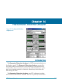
Graphs . . . . . . . . . . . . . . . . . . . . . . . . . . . . . . . . . 285
The Graph Panel . . . . . . . . . . . . . . . . . . . .
Zoom . . . . . . . . . . . . . . . . . . . . . . . . . .
The Graph Options Menu . . . . . . . . . . . . . . .
Zoomout . . . . . . . . . . . . . . . . . . . . . . .
Zoomout to Original . . . . . . . . . . . . . . . .
Optimize . . . . . . . . . . . . . . . . . . . . . . .
Copy to Sweep Panel . . . . . . . . . . . . . . . .
Display Cursors . . . . . . . . . . . . . . . . . . .
Scroll Bars . . . . . . . . . . . . . . . . . . . . . .
Title and Labels . . . . . . . . . . . . . . . . . . .
Comment . . . . . . . . . . . . . . . . . . . . . .
New Data . . . . . . . . . . . . . . . . . . . . . . .
Graph Buffer. . . . . . . . . . . . . . . . . . . . .
Graph Legend . . . . . . . . . . . . . . . . . . . . .
Graph Legend / Data Editor Linkage. . . . . . . .
Graphing invalid or suspect data . . . . . . . . . .
Trace Colors . . . . . . . . . . . . . . . . . . . . . .
Color Assignment for a New Test . . . . . . . . .
Color Assignment for Multiple-Data-Set Sweeps .
Color Cycling in Nested and Appended Sweeps .
Color Cycling with Appended Files . . . . . . . .
xii
.
.
.
.
.
.
.
.
.
.
.
.
.
.
.
.
.
.
.
.
.
.
.
.
.
.
.
.
.
.
.
.
.
.
.
.
.
.
.
.
.
.
.
.
.
.
.
.
.
.
.
.
.
.
.
.
.
.
.
.
.
.
.
.
.
.
.
.
.
.
.
.
.
.
.
.
.
.
.
.
.
.
.
.
.
.
.
.
.
.
.
.
.
.
.
.
.
.
.
.
.
.
.
.
.
.
.
.
.
.
.
.
.
.
.
.
.
.
.
.
.
.
.
.
.
.
.
.
.
.
.
.
.
.
.
.
.
.
.
.
.
.
.
.
.
.
.
285
286
287
287
288
288
289
289
292
293
293
293
294
294
296
298
298
299
299
299
300
ATS-2 User’s Manual
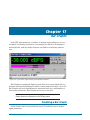
Chapter 17
Bar Graphs . . . . . . . . . . . . . . . . . . . . . . . . . . . . . . 303
Creating a Bar Graph . . . . . .
Bar Graph Setup . . . . . . . . .
Using a Bar Graph for Readings
Using a Bar Graph for Settings .
.
.
.
.
.
.
.
.
.
.
.
.
.
.
.
.
.
.
.
.
.
.
.
.
.
.
.
.
.
.
.
.
.
.
.
.
.
.
.
.
.
.
.
.
.
.
.
.
.
.
.
.
.
.
.
.
.
.
.
.
.
.
.
.
.
.
.
.
.
.
.
.
303
304
305
306
Chapter 18
Editing Data and Setting Limits . . . . . . . . . . . . . . . 307
The Data Editor . . . . . . . . . . . . .
The Data Editor Panel. . . . . . . . .
Columns . . . . . . . . . . . . . . .
Rows . . . . . . . . . . . . . . . . .
Data . . . . . . . . . . . . . . . . .
Editing the Current Data in Memory
Saving ATS Data . . . . . . . . . . . .
Setting Limits . . . . . . . . . . . . . .
Making a Limit File . . . . . . . . . .
Attaching a Limit File . . . . . . . . .
Using the Attached File Editor. . . .
Actions Upon Failure . . . . . . . . .
More About Using AP Data Files . . .
.
.
.
.
.
.
.
.
.
.
.
.
.
.
.
.
.
.
.
.
.
.
.
.
.
.
.
.
.
.
.
.
.
.
.
.
.
.
.
.
.
.
.
.
.
.
.
.
.
.
.
.
.
.
.
.
.
.
.
.
.
.
.
.
.
.
.
.
.
.
.
.
.
.
.
.
.
.
.
.
.
.
.
.
.
.
.
.
.
.
.
.
.
.
.
.
.
.
.
.
.
.
.
.
.
.
.
.
.
.
.
.
.
.
.
.
.
.
.
.
.
.
.
.
.
.
.
.
.
.
.
.
.
.
.
.
.
.
.
.
.
.
.
.
.
.
.
.
.
.
.
.
.
.
.
.
.
.
.
.
.
.
.
.
.
.
.
.
.
.
.
.
.
.
.
.
.
.
.
.
.
.
307
308
308
308
308
309
310
310
311
312
313
314
314
Chapter 19
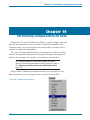
Performing Computations on Data . . . . . . . . . . . . . 317
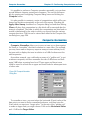
The Compute Dialog Boxes . . . . . . .
Compute: Normalize . . . . . . . . . .
Compute: Invert . . . . . . . . . . . . .
Compute: Smooth. . . . . . . . . . . .
Compute: Linearity . . . . . . . . . . .
Compute: Center . . . . . . . . . . . .
Compute: Delta . . . . . . . . . . . . .
Compute: Average . . . . . . . . . . .
Compute: Minimum . . . . . . . . . . .
Compute: Maximum . . . . . . . . . .
Compute: Equalize . . . . . . . . . . .
Compute Status . . . . . . . . . . . . .
Clear All and Reset. . . . . . . . . . . .
Comparing Results with Original Data.
.
.
.
.
.
.
.
.
.
.
.
.
.
.
.
.
.
.
.
.
.
.
.
.
.
.
.
.
.
.
.
.
.
.
.
.
.
.
.
.
.
.
.
.
.
.
.
.
.
.
.
.
.
.
.
.
.
.
.
.
.
.
.
.
.
.
.
.
.
.
.
.
.
.
.
.
.
.
.
.
.
.
.
.
.
.
.
.
.
.
.
.
.
.
.
.
.
.
.
.
.
.
.
.
.
.
.
.
.
.
.
.
.
.
.
.
.
.
.
.
.
.
.
.
.
.
.
.
.
.
.
.
.
.
.
.
.
.
.
.
.
.
.
.
.
.
.
.
.
.
.
.
.
.
.
.
.
.
.
.
.
.
.
.
.
.
.
.
.
.
.
.
.
.
.
.
.
.
.
.
.
.
.
.
.
.
.
.
.
.
.
.
.
.
.
.
318
319
320
320
321
322
323
324
325
325
326
326
327
327
Chapter 20
Printing and Exporting . . . . . . . . . . . . . . . . . . . . . 329
Printing ATS Graphs . . . . . . . . . . . . . . . . . . . . . . . . . 329
Page Setup . . . . . . . . . . . . . . . . . . . . . . . . . . . . . 330
Print Setup. . . . . . . . . . . . . . . . . . . . . . . . . . . . . 331
ATS-2 User’s Manual
xiii
Printing a Graph. . . . . . . . . . . . . . . . .
Print Preview . . . . . . . . . . . . . . . . . .
Printing ATS Data as a Table . . . . . . . . . . .
Printing to a File. . . . . . . . . . . . . . . . . .
Exporting a Graph . . . . . . . . . . . . . . . . .
Copying a Graph to the Clipboard . . . . . . . .
Copying a Window or Screen to the Clipboard
.
.
.
.
.
.
.
.
.
.
.
.
.
.
.
.
.
.
.
.
.
.
.
.
.
.
.
.
.
.
.
.
.
.
.
.
.
.
.
.
.
.
.
.
.
.
.
.
.
.
.
.
.
.
.
.
.
.
.
.
.
.
.
331
332
332
333
334
334
334
Chapter 21
Monitoring . . . . . . . . . . . . . . . . . . . . . . . . . . . . . . 337
Headphone/Speaker Monitoring.
The Volume Bar . . . . . . . . .
Headphone/Speaker panel . . .
The Monitor Outputs . . . . . . .
The SOURCE Outputs . . . . . .
The FUNCTION Outputs . . . . .
.
.
.
.
.
.
.
.
.
.
.
.
.
.
.
.
.
.
.
.
.
.
.
.
.
.
.
.
.
.
.
.
.
.
.
.
.
.
.
.
.
.
.
.
.
.
.
.
.
.
.
.
.
.
.
.
.
.
.
.
.
.
.
.
.
.
.
.
.
.
.
.
.
.
.
.
.
.
.
.
.
.
.
.
.
.
.
.
.
.
.
.
.
.
.
.
.
.
.
.
.
.
337
337
338
339
340
340
Chapter 22
Sync/Ref, Trigger and Aux . . . . . . . . . . . . . . . . . . . 341
SYNC/REF IN. . . . . . . . . . . . . . .
Sync/Ref Input Panel . . . . . . . .
Reference Input Source . . . . . .
Squarewave frequency ranging.
Frame Lock. . . . . . . . . . . . . .
Input Termination Impedance. . .
Frequency . . . . . . . . . . . . . .
Input Frequency . . . . . . . . . .
Out of Range Indicator . . . . . . .
TRIG IN . . . . . . . . . . . . . . . . .
TRIG OUT and the Main Trigger Panel
Auxiliary Control Output and Input .
.
.
.
.
.
.
.
.
.
.
.
.
.
.
.
.
.
.
.
.
.
.
.
.
.
.
.
.
.
.
.
.
.
.
.
.
.
.
.
.
.
.
.
.
.
.
.
.
.
.
.
.
.
.
.
.
.
.
.
.
.
.
.
.
.
.
.
.
.
.
.
.
.
.
.
.
.
.
.
.
.
.
.
.
.
.
.
.
.
.
.
.
.
.
.
.
.
.
.
.
.
.
.
.
.
.
.
.
.
.
.
.
.
.
.
.
.
.
.
.
.
.
.
.
.
.
.
.
.
.
.
.
.
.
.
.
.
.
.
.
.
.
.
.
.
.
.
.
.
.
.
.
.
.
.
.
.
.
.
.
.
.
.
.
.
.
.
.
.
.
.
.
.
.
.
.
.
.
.
.
341
342
342
343
344
344
344
344
345
345
345
348
Chapter 23
Automating Tests . . . . . . . . . . . . . . . . . . . . . . . . . 351
Introduction . . . . . . .
Learn Mode . . . . . . .
The Macro Editor . . . .
AP Basic Documentation
.
.
.
.
.
.
.
.
.
.
.
.
.
.
.
.
.
.
.
.
.
.
.
.
.
.
.
.
.
.
.
.
.
.
.
.
.
.
.
.
.
.
.
.
.
.
.
.
.
.
.
.
.
.
.
.
.
.
.
.
.
.
.
.
.
.
.
.
.
.
.
.
.
.
.
.
.
.
.
.
.
.
.
.
.
.
.
.
351
351
352
353
Chapter 24
Regulation . . . . . . . . . . . . . . . . . . . . . . . . . . . . . . 355
Examples of Regulated Sweeps . . . . . . . . . . . . . . . . . 359
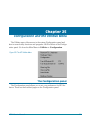
Chapter 25
Configuration and the Utilities Menu . . . . . . . . . . . . 361
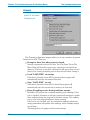
The Configuration panel . . . . . . . . . . . . . . . . . . . . . . 361
xiv
ATS-2 User’s Manual
General . . . . . . . . . . . . .
Log . . . . . . . . . . . . . . .
The Log File . . . . . . . . .
Graph . . . . . . . . . . . . . .
Restoring the ATS-2 Hardware .
Hardware Status . . . . . . . . .
Turn All Outputs OFF / ON . . . .
Clear Log File . . . . . . . . . . .
View Log File . . . . . . . . . . .
Learn Mode . . . . . . . . . . .
Multitone Creation . . . . . . .
.
.
.
.
.
.
.
.
.
.
.
.
.
.
.
.
.
.
.
.
.
.
.
.
.
.
.
.
.
.
.
.
.
.
.
.
.
.
.
.
.
.
.
.
.
.
.
.
.
.
.
.
.
.
.
.
.
.
.
.
.
.
.
.
.
.
.
.
.
.
.
.
.
.
.
.
.
.
.
.
.
.
.
.
.
.
.
.
.
.
.
.
.
.
.
.
.
.
.
.
.
.
.
.
.
.
.
.
.
.
.
.
.
.
.
.
.
.
.
.
.
.
.
.
.
.
.
.
.
.
.
.
.
.
.
.
.
.
.
.
.
.
.
.
.
.
.
.
.
.
.
.
.
.
.
.
.
.
.
.
.
.
.
.
.
.
.
.
.
.
.
.
.
.
.
.
.
.
.
.
.
.
.
.
.
.
.
.
.
.
.
.
.
.
.
.
.
.
362
364
364
366
367
368
368
368
368
369
369
Appendix A
Units of Measurement . . . . . . . . . . . . . . . . . . . . . . 371
Introduction . . . . . . . . . . . . . . . . .
Analog Amplitude Units . . . . . . . . . .
Digital Amplitude Units . . . . . . . . . . .
Digital Data Units . . . . . . . . . . . . . .
Ratio Units . . . . . . . . . . . . . . . . . .
Relative Units . . . . . . . . . . . . . . . .
Frequency Units . . . . . . . . . . . . . . .
Phase Unit . . . . . . . . . . . . . . . . . .
Time Units . . . . . . . . . . . . . . . . . .
DCX-127 Units . . . . . . . . . . . . . . . .
DCX-127 Amplitude Units . . . . . . . . .
DCX-127 Resistance Units . . . . . . . . .
DCX-127 Digital Input and Output Units .
.
.
.
.
.
.
.
.
.
.
.
.
.
.
.
.
.
.
.
.
.
.
.
.
.
.
.
.
.
.
.
.
.
.
.
.
.
.
.
.
.
.
.
.
.
.
.
.
.
.
.
.
.
.
.
.
.
.
.
.
.
.
.
.
.
.
.
.
.
.
.
.
.
.
.
.
.
.
.
.
.
.
.
.
.
.
.
.
.
.
.
.
.
.
.
.
.
.
.
.
.
.
.
.
.
.
.
.
.
.
.
.
.
.
.
.
.
.
.
.
.
.
.
.
.
.
.
.
.
.
.
.
.
.
.
.
.
.
.
.
.
.
.
.
.
.
.
.
.
.
.
.
.
.
.
.
371
372
376
378
378
378
379
380
380
381
381
381
381
Appendix B
The Digital Audio Signal . . . . . . . . . . . . . . . . . . . . . 383
The Serial Digital Interface Signal
Bi-phase Mark Encoding . . . .
The Frame and Subframe . . .
Channel Status. . . . . . . . . .
Serial Interface Measurements. .
.
.
.
.
.
.
.
.
.
.
.
.
.
.
.
.
.
.
.
.
.
.
.
.
.
.
.
.
.
.
.
.
.
.
.
.
.
.
.
.
.
.
.
.
.
.
.
.
.
.
.
.
.
.
.
.
.
.
.
.
.
.
.
.
.
.
.
.
.
.
.
.
.
.
.
.
.
.
.
.
.
.
.
.
.
384
385
385
386
391
Appendix C
FFTs . . . . . . . . . . . . . . . . . . . . . . . . . . . . . . . . . . 393
The Fast Fourier Transform
Real Time vs. Batch Mode. .
Acquiring Data . . . . . . . .
The FFT Record . . . . . . .
FFT Bandwidth. . . . . . . .
FFT Bin Width . . . . . . . .
FFT Record Looping . . . . .
ATS-2 User’s Manual
.
.
.
.
.
.
.
.
.
.
.
.
.
.
.
.
.
.
.
.
.
.
.
.
.
.
.
.
.
.
.
.
.
.
.
.
.
.
.
.
.
.
.
.
.
.
.
.
.
.
.
.
.
.
.
.
.
.
.
.
.
.
.
.
.
.
.
.
.
.
.
.
.
.
.
.
.
.
.
.
.
.
.
.
.
.
.
.
.
.
.
.
.
.
.
.
.
.
.
.
.
.
.
.
.
.
.
.
.
.
.
.
.
.
.
.
.
.
.
.
.
.
.
.
.
.
.
.
.
.
.
.
.
.
.
.
.
.
.
.
393
393
394
394
394
395
396
xv
FFT Windowing . . . . . . . . . . . . . . . . . . . . . . . . . . . 397
Synchronous FFTs . . . . . . . . . . . . . . . . . . . . . . . . . . 399
Graphing FFTs . . . . . . . . . . . . . . . . . . . . . . . . . . . . 400
Appendix D
User Downloadable Filters . . . . . . . . . . . . . . . . . . . 401
Creating User Downloadable Filters . . . . . . . . .
User Downloadable Filter Design Constraints: .
MATLAB Downloadable Filter Support . . . . . . .
ap_write_filter. . . . . . . . . . . . . . . . . . . .
Syntax . . . . . . . . . . . . . . . . . . . . . . .
Description . . . . . . . . . . . . . . . . . . . .
Multiple Sample Rates . . . . . . . . . . . . . .
Filter Restrictions . . . . . . . . . . . . . . . . .
Examples. . . . . . . . . . . . . . . . . . . . . .
ap_read_filter . . . . . . . . . . . . . . . . . . . .
Syntax . . . . . . . . . . . . . . . . . . . . . . .
Description . . . . . . . . . . . . . . . . . . . .
Example . . . . . . . . . . . . . . . . . . . . . .
.
.
.
.
.
.
.
.
.
.
.
.
.
.
.
.
.
.
.
.
.
.
.
.
.
.
.
.
.
.
.
.
.
.
.
.
.
.
.
.
.
.
.
.
.
.
.
.
.
.
.
.
.
.
.
.
.
.
.
.
.
.
.
.
.
.
.
.
.
.
.
.
.
.
.
.
.
.
.
.
.
.
.
.
.
.
.
.
.
.
.
401
401
403
404
404
404
405
405
405
406
406
406
407
Appendix E
AP Waveform File Support . . . . . . . . . . . . . . . . . . . 409
Exporting to .WAV. . .
Operation . . . . . .
Tips and Tricks . . . .
Importing from .WAV .
Operation . . . . . .
MATLAB support . . . .
ap_write_wave . . .
Syntax . . . . . . .
Description . . . .
Example . . . . . .
ap_read_wave . . . .
Syntax . . . . . . .
Description . . . .
Example . . . . . .
.
.
.
.
.
.
.
.
.
.
.
.
.
.
.
.
.
.
.
.
.
.
.
.
.
.
.
.
.
.
.
.
.
.
.
.
.
.
.
.
.
.
.
.
.
.
.
.
.
.
.
.
.
.
.
.
.
.
.
.
.
.
.
.
.
.
.
.
.
.
.
.
.
.
.
.
.
.
.
.
.
.
.
.
.
.
.
.
.
.
.
.
.
.
.
.
.
.
.
.
.
.
.
.
.
.
.
.
.
.
.
.
.
.
.
.
.
.
.
.
.
.
.
.
.
.
.
.
.
.
.
.
.
.
.
.
.
.
.
.
.
.
.
.
.
.
.
.
.
.
.
.
.
.
.
.
.
.
.
.
.
.
.
.
.
.
.
.
.
.
.
.
.
.
.
.
.
.
.
.
.
.
.
.
.
.
.
.
.
.
.
.
.
.
.
.
.
.
.
.
.
.
.
.
.
.
.
.
.
.
.
.
.
.
.
.
.
.
.
.
.
.
.
.
.
.
.
.
.
.
.
.
.
.
.
.
.
.
.
.
.
.
.
.
.
.
.
.
.
.
.
.
.
.
.
.
.
.
.
.
.
.
.
.
.
.
.
.
.
.
.
.
.
.
.
.
.
.
.
.
.
.
.
.
.
.
.
.
.
.
.
.
.
.
.
.
.
.
.
.
.
.
.
.
.
.
.
.
.
.
.
.
.
.
.
.
.
.
.
.
.
.
409
409
410
411
411
412
412
412
412
413
414
414
414
415
Appendix F
Test and Macro Translators . . . . . . . . . . . . . . . . . . 417
Check the Web! . . . . . . . . . . . . . . . . . . . . .
The Test Translator . . . . . . . . . . . . . . . . . . .
Preparing S1.EXE and APWIN tests for translation .
Macros for batch converting APWIN tests . . . .
Using the ATS-2 Test Translator . . . . . . . . . . .
How the Test Translator Makes Decisions. . . . . .
xvi
.
.
.
.
.
.
.
.
.
.
.
.
.
.
.
.
.
.
.
.
.
.
.
.
.
.
.
.
.
.
.
.
.
.
.
.
417
417
419
419
420
421
ATS-2 User’s Manual
Mapping Two Analyzers into One Analyzer. . . . .
Attached file considerations. . . . . . . . . . . . .
Reporting Test Translation Exceptions . . . . . . .
The Macro Translator . . . . . . . . . . . . . . . . . .
Using the Macro Translator . . . . . . . . . . . . .
Identifying the System when Importing Macros
Macro Translator Issues . . . . . . . . . . . . . . . .
Numbers or Constants? . . . . . . . . . . . . . .
Libraries and the “With” Command . . . . . . . .
Referenced Files . . . . . . . . . . . . . . . . . .
Unavailable Features . . . . . . . . . . . . . . . .
Reporting Macro Translation Exceptions . . . . . .
Mapping exceptions and substitutions . . . . . . . .
Analog Generator . . . . . . . . . . . . . . . . . . .
Digital Generator . . . . . . . . . . . . . . . . . . .
Audio Input . . . . . . . . . . . . . . . . . . . . . .
Analyzer Settings . . . . . . . . . . . . . . . . . . .
Digital I/O . . . . . . . . . . . . . . . . . . . . . . . .
Compute Functions . . . . . . . . . . . . . . . . . .
ATS-2 User’s Manual
.
.
.
.
.
.
.
.
.
.
.
.
.
.
.
.
.
.
.
.
.
.
.
.
.
.
.
.
.
.
.
.
.
.
.
.
.
.
.
.
.
.
.
.
.
.
.
.
.
.
.
.
.
.
.
.
.
.
.
.
.
.
.
.
.
.
.
.
.
.
.
.
.
.
.
.
.
.
.
.
.
.
.
.
.
.
.
.
.
.
.
.
.
.
.
.
.
.
.
.
.
.
.
.
.
.
.
.
.
.
.
.
.
.
421
422
422
422
423
424
424
425
425
425
425
425
426
426
427
427
428
430
430
xvii
xviii
ATS-2 User’s Manual
Safety Information
Do NOT service or repair this product unless properly qualified. Servicing should be performed only by a qualified technician or an authorized
Audio Precision distributor.
Do NOT defeat the safety ground connection. This product is designed
to operate only from a 50/60 Hz AC power source (250 V rms maximum)
with an approved three-conductor power cord and safety grounding. Loss
of the protective grounding connection can result in electrical shock hazard
from the accessible conductive surfaces of this product.
For continued fire hazard protection, fuses should be replaced ONLY
with the exact value and type indicated on the rear panel of the instrument
and discussed in the installation manual, Getting Started with ATS-2. The
AC voltage selector also must be set to the same voltage as the nominal
power source voltage (100, 120, 230, or 240 V rms) with the appropriate
fuses. Different fuses are required depending on the line voltage.
The International Electrotechnical Commission (IEC 1010-1) requires
that measuring circuit terminals used for voltage or current measurement
be marked to indicate their Installation Category. The Installation Category
is defined by IEC 664 and is based on the amplitude of transient or impulse voltage that can be expected from the AC power distribution network. This product is classified as INSTALLATION CATEGORY II,
abbreviated “CAT II” on the instrument front panel.
Do NOT substitute parts or make any modifications without the written
approval of Audio Precision. Doing so may create safety hazards.
This product is for indoor use—pollution degree 2.
ATS-2 User’s Manual
xix
Safety Symbols
The following symbols may be marked on the panels or covers of equipment or modules, and are used in this manual:
WARNING!—This symbol alerts you to a potentially hazardous condition, such as the presence of dangerous voltage that could pose a risk of
electrical shock. Refer to the accompanying Warning Label or Tag, and exercise extreme caution.
ATTENTION!—This symbol alerts you to important operating considerations or a potential operating condition that could damage equipment. If
you see this marked on equipment, consult the User’s Manual or Operator’s Manual for precautionary instructions.
FUNCTIONAL EARTH TERMINAL—This symbol marks a terminal that
is electrically connected to a reference point of a measuring circuit or output and is intended to be earthed for any functional purpose other than
safety.
PROTECTIVE EARTH TERMINAL—This symbol marks a terminal that
is bonded to conductive parts of the instrument. Confirm that this terminal
is connected to an external protective earthing system.
xx
ATS-2 User’s Manual
Chapter 1
Introduction
Figure 1. The Audio Precision ATS-2 audio test and measurement system.
ATS-2: an Overview
The Audio Precision ATS-2 is a powerful computer-controlled audio test
and measurement system. The ATS-2 system consists of two key components:
§ The ATS-2 hardware, which provides the connectors and circuitry
necessary for proper signal interface and precise signal generation
and analysis. The hardware is mounted in a compact aluminum and
ATS-2 User’s Manual
1
Chapter 1: Introduction
About This Manual
steel chassis which can be installed in a standard 19 in wide
equipment rack using optional mounting hardware.
§ The ATS measurement software, which runs on a personal computer
(PC) and provides all the control, display, report and automation
functions for the ATS-2 system. The PC is not provided with ATS-2.
With the exception of the mains power switch on the rear panel, there
are no knobs, dials, controls, readouts, meters or switches on the
ATS-2 chassis. All of the measurement settings and adjustments are
made on the PC.
The ATS control software will run under Microsoft Windows XP Professional Service Pack 2 or Microsoft Windows Vista Business Edition (32-bit)
operating systems.
APIB
The control software communicates with the ATS-2 instrument through
the Audio Precision Interface Bus (APIB). Several options have been provided for accessing APIB from your PC, including:
§ The USB-APIB adapter.
§ The APIB PCI card and cable.
§ The APIB PCI Express card and cable.
§ The APIB PCMCIA card and cable.
GPIB
With Option GPIB hardware installed, ATS-2 can also be controlled by
the industry-standard IEEE 488.2 General Purpose Interface Bus (GPIB).
See page 31 for more information about ATS-2 with GPIB.
About This Manual
You’re reading the ATS-2 User’s Manual. This is the primary operation
and reference manual for the Audio Precision ATS-2 audio test and measurement system.
We recommend you begin by reading the separate introductory manual,
Getting Started with ATS-2, which is discussed below.
Look in the ATS-2 User’s Manual for
§ Detailed discussions of every ATS-2 feature and every software
panel, control and display;
2
ATS-2 User’s Manual
ATS-2 Capabilities
Chapter 1: Introduction
§ Reference information on audio test and measurement techniques,
sample and utility file listings and much more.
A copy of the ATS-2 User’s Manual is shipped with every ATS-2 system.
The manual is also published as a PDF on the Audio Precision Resources
Disc and on our Web site at ap.com.
ATS-2 Capabilities
ATS-2 is a comprehensive high-performance audio testing system.
§ ATS-2 can make amplitude, frequency, THD+N, noise, phase,
crosstalk, bandpass, and IMD measurements for analog or digital
audio devices, and can perform a detailed analysis of individual
harmonic distortion products.
§ ATS-2 can perform measurements on audio signals using fast Fourier
transform (FFT) analysis with advanced high-speed FFT analysis
techniques available, including multitone recognition and analysis
capability, frequency adjustment for bin centering, synchronous FFT
processing, and advanced post-FFT analysis. FFT analysis can also
provide time-domain, oscilloscope-type waveform display of signals.
Non-audio signals such as interface signal jitter components can also
be studied with FFT techniques.
§ ATS-2 can use a combination of different measurement instruments
and parameters to perform complex sweeps, and can display and
print the results with a powerful graphing engine. ATS-2 offers control
over instrument regulation and over sweep settling parameters.
Pass/fail limits or equalization data can be attached to a sweep to
constrain a particular measurement. A variety of computations can
be performed on the measured data after acquisition. Sweep tests
can be saved and recalled, and ATS-2 measurements can be
automated by macros written in the AP Basic programming
language.
§ ATS-2 can examine the digital interface signal and perform elemental
analysis of digital communication paths and assure the integrity of
digitally transmitted data. ATS-2 can extract a variety of statistics
from the digital waveform, such as the actual sample rate, the
interface waveform voltage, the active and inactive data bits and flag
bits. ATS-2 can measure the jitter in the interface signal. ATS-2 also
has the capability of transmitting and receiving the full complement
of status bits for both the AES3 (professional) and IEC60958-3
(consumer) digital audio interface signals.
§ ATS-2’s sample rate may be synchronized to an external AES signal,
a squarewave, or an NTSC / PAL video source.
ATS-2 User’s Manual
3
Chapter 1: Introduction
Conceptual Architecture of ATS-2
§ The ATS-2 Performance Upgrade Option adds more power: a pair of
high-bandwidth analog-to-digital converters to extend the analog
analysis bandwidth from 30 kHz up to 120 kHz; and an additional
Analyzer instrument called the Digital Interface Analyzer that can
more closely examine the interface signal, providing eye patterns,
histograms, waveform display and FFT spectrum analysis of the
recovered jitter signal, and triggering from a number of different
interface patterns and bits.
Conceptual Architecture of ATS-2
Figure 2. ATS-2 conceptual block diagram.
The functional components implemented in ATS-2 include two DSP-implemented audio signal generators, a suite of DSP-implemented audio,
data and interface signal analysis capabilities, digital and analog input and
output modules, and modules for synchronization and APIB communication.
All signal generation is performed in the digital domain. One of the two
DSP signal generators is dedicated to the digital output. The signal from
this generator, called the “Digital Generator,” is routed through the digital
audio interface transmitter module and to the balanced, unbalanced and
optical digital outputs. The output of the second DSP signal generator, the
4
ATS-2 User’s Manual
Other Documentation for ATS-2
Chapter 1: Introduction
“Analog Generator,” is converted to an analog signal by a digital-to-analog
converter (DAC). The two-channel output of the DAC is conditioned and
ranged for the balanced and unbalanced analog outputs.
All signal analysis is also performed in the digital domain in DSP. The
digital input is routed through a digital audio interface receiver and applied
to the Analyzer DSP. Analog inputs are first ranged and conditioned for domain conversion, and then are sampled by a high-resolution (or, optionally, a high-bandwidth) analog-to-digital converter (ADC) before being
applied to the Analyzer.
Analog Domain / Digital Domain
Discussions of audio technology often place the signals into one or
another of two realms: the analog domain or the digital domain. These
terms provide a useful conceptual division.
Analog audio signals are analogies of the sound waves that they
represent, varying in frequency and amplitude in a continuous fashion.
In audio electronics, these are voltages and currents that are manipulated by modifying their amplitude or frequency. The term analog domain refers to signals represented and processed in this fashion.
Digital audio signals, on the other hand, are numerical representations of the sound waves. This representation is often carried on an
electrical signal called the interface signal. Digital audio is processed
mathematically in processes gathered together under the name of Digital Signal Processing, or DSP. The term digital domain refers to signals
represented and processed in this fashion.
Other Documentation for ATS-2
Audio Precision publishes a wealth of material on our hardware and software products, about audio theory and on specific test and measurement
techniques. Here are some important documentation resources:
Getting Started with ATS-2
We recommend that you read Getting Started with ATS-2 before reading any other ATS-2 documentation. It is an introductory manual which
will help you correctly set up ATS-2, install the software on your PC and familiarize yourself with the system. Inside Getting Started with ATS-2 manual you’ll find:
§ hardware and software installation instructions;
§ an introduction to the ATS-2 system;
ATS-2 User’s Manual
5
Chapter 1: Introduction
Other Documentation for ATS-2
§ a look at the key features of the ATS control software;
§ a group of Quick Guide tutorials, putting the ATS-2 system to use in
simple tests; and
§ ATS-2 specifications.
A copy of Getting Started with ATS-2 is shipped with every ATS-2 system and is also published in electronic form as a PDF file, available on the
Audio Precision Resources Disc and as a download from the Audio Precision Web site at ap.com.
Online Help
While you are running ATS, you will have much of the information contained in the ATS-2 User’s Manual available to you instantly in the online
Help system included as part of the ATS-2 system.
You can access the Help system while you are using ATS in a couple of
ways:
§ On the Menu bar, click Help. The Help menu offers commands to
search the Help Index, browse through the Help Topics, or select
an alternate Help library, AP Basic Language.
§ ATS also has context-sensitive Help available. Almost every control
and display on each software panel has a help topic associated with
it. To view the topic, simply click on the field or control, then press
the F1 function key.
The AP Basic User’s Guide and Language Reference
You can create simple or complex test and measurement macros to automate ATS-2 using AP Basic, the programming language included with the
system. The same AP Basic language is also used to automate other Audio
Precision PC-controlled systems and to interface with other programming
languages.
The AP Basic User’s Guide and Language Reference is published in electronic form as a PDF file, available on the Audio Precision Resources Disc
and as a download from the Audio Precision Web site at ap.com.
You will also find online Help for AP Basic while running ATS. Click
Help > AP Basic Language Help on the Help menu.
6
ATS-2 User’s Manual
GPIB Documentation for ATS-2
Chapter 1: Introduction
The AP Basic Extensions Reference for ATS-2
The AP Basic Extensions Reference for ATS-2 is a large supplementary library of OLE / ActiveX automation commands for use specifically with
ATS-2.
The AP Basic Extensions Reference for ATS-2 is published in electronic
form as a PDF file, available on the Audio Precision Resources Disc and as
a download from the Audio Precision Web site at ap.com.
You will also find online Help for ATS-2 Basic Extension while running
ATS. Click Help > AP Basic Extension for ATS-2 Help on the Help
menu.
Application Notes and TECHNOTES
From time to time Audio Precision publishes technical papers such as
AP Application Notes and TECH NOTES, which can help in your understanding of the operation of the ATS-2 system. Many of Audio Precision
technical publications are available for download from our Web site at
ap.com. New technical papers and online solutions are added on a regular
basis.
Viewing and Printing PDF files
Audio Precision documentation is provided in Adobe Portable Document Format (PDF) format on the Audio Precision Resources Disc and
on our Web site at ap.com.
You can view the PDF files using Adobe Acrobat Reader, a free program that can be downloaded from Adobe at www.adobe.com. You can
also print PDF files using Acrobat Reader and a Windows compatible
printer.
GPIB Documentation for ATS-2
With Option GPIB hardware installed, ATS-2 can also be controlled by
the industry-standard General Purpose Interface Bus (GPIB).
Basic installation with GPIB is covered in Getting Started with ATS-2.
For GPIB development and programming, order the ATS-2 GPIB Programmer’s Reference Manual.
See page 31 for more information about ATS-2 with GPIB.
ATS-2 User’s Manual
7
Chapter 1: Introduction
8
GPIB Documentation for ATS-2
ATS-2 User’s Manual
Chapter 2
The ATS Control Software
Overview
Most of your interaction with the ATS-2 system will be through the ATS
control software. Once ATS-2 is plugged in, turned on and connected to
your device under test (or DUT), you will be making all your adjustments
and taking all your readings from your computer screen.
The ATS control software is a powerful and complex program, and most
of this book is dedicated to exploring and explaining its many capabilities.
In this chapter, we’ll look at an overview of the software features and learn
the basics of operating the system.
With Option GPIB hardware installed, ATS-2 can also be controlled by
the industry-standard General Purpose Interface Bus (GPIB). See page 31
for more information about ATS-2 with GPIB.
The User Interface
Like many Windows applications, the ATS user interface has a menu
bar, a status bar, toolbars, and a workspace. With these tools you can save
test and data files, export and print measurement results, configure both
the hardware and software to your needs, access online help, design and
launch automated processes and, of course, open and operate the instrument panels where the core test and measurement work is performed.
ATS-2 User’s Manual
9
Chapter 2: The ATS Control Software
The Workspace
The Workspace
Figure 3. The ATS workspace.
The ATS workspace has 5 pages that you can select by menu commands (View > Page #) or by clicking the numbered tabs on the Status
Bar. The workspace is like a multi-layered desktop where you can display
and organize the instrument panels you are using for a particular set of
tests.
Panels can be placed on any workspace page, and duplicated on more
than one page. An instrument panel which appears on more than one
page is simply a redundant display, for your convenience. The settings and
results shown on redundant panels are identical, and a change made on
one page is reflected on the others.
The ATS Panels
The real interaction with ATS-2 is done in control and measurement windows called panels. These can be thought of rather like the physical control panels often found on conventional test and measurement equipment,
with range, function and trigger controls, ON and OFF switches, linear adjustment pots and sliders, numerical meter readouts, bar meters, X-Y waveform displays, graphs and so on.
The ATS panels are available through menu commands, toolbar icons
and keyboard shortcuts.
You can control ATS-2 from just one or two ATS panels, if that’s all your
measurement requires. A more typical test might involve four or five panels; a complicated test, perhaps six or seven.
10
ATS-2 User’s Manual
The ATS Panels
Chapter 2: The ATS Control Software
Figure 4.
An ATS Instrument Panel.
Although the ATS panels can all be placed on one workspace page,
most users prefer to organize their workspace by placing panels on several
different pages.
You can close a panel without canceling its function or effect; for example, you could set a signal’s output voltage and frequency on the Analog
Generator panel, turn the generator ON, then close the panel window.
The signal will continue at the settings you’ve made until you open the
panel again and turn the generator OFF.
Many of the ATS panels come in two sizes, the smaller having fewer
commands and readouts visible, and the larger showing every option. The
most commonly used size for each panel is set as its default size. Double-click on the panel title bar to expand or contract it.
Panel Settings
Settings for tests and measurements are made using several different
types of controls on the panels:
§ Setting fields, which come in several versions:
First is a text box, in which you can directly enter a value from the
keyboard.
Second is a drop-down list box, in which you can make a
selection from a set of choices.
ATS-2 User’s Manual
11
Chapter 2: The ATS Control Software
The ATS Panels
Third is a combination of the first and second, a text box with an
added drop-down list from which you can choose the units to
express your value. See Appendix A, Units of Measurement.
Setting fields display dark (black or blue) text or numbers on a white
field.
§ Check boxes, which allow you to set non-exclusive conditions.
§ Option buttons, which provide for exclusive conditions.
§ Browser buttons, which open dialog boxes called browsers, which
allow you to navigate lists of options, search for a file by browsing
through a hierarchy of folders, and so on. Browser buttons are
identified by the ellipsis mark ( … ).
§ Custom buttons that control special functions, such as GO, ON,
OFF, 1, 0 and so on.
§ Sliders, with which you can continuously adjust a value. Sliders are
found on the Volume toolbar and on Bar Graph panels. Sliders can
be operated by either the mouse pointer or by using the arrow keys.
Panel Readings
Results of tests or measurements are called readings, which ATS can display in several ways, as
§ Reading fields, sometimes called measurement fields or meters.
Reading fields come in two variations, with and without a drop-down
list to select units. See Appendix A, Units of Measurement.
Reading fields always display green text or numbers on a black field.
§ Bar graphs, which display values as a continuous colored bar like a
conventional analog meter.
§ Status indicators, which show the presence or absence of a condition
by a small colored rectangle.
12
ATS-2 User’s Manual
The ATS Menus
Chapter 2: The ATS Control Software
The ATS Menus
The ATS Menu bar extends across the top of the ATS window and is always visible. In this chapter we will take a brief tour of some of the ATS
menus. Details of menu options, controls and submenus will be explored
in the chapters discussing specific ATS functions.
The File Menu
The File menu offers commands for opening, saving, appending, importing, exporting and printing ATS files, and access to the Quick Launch
menu.
Since there are a number of different files types used by ATS, submenus
are available (at the small black arrows } accompanying some menu
choices) to choose, for example, whether to Save As a Test or Data or
Macro file.
The listings at the bottom of the File menu show the last tests opened by
ATS, and provide a convenient way to quickly launch a previously used
test. Simply click on the name of the test you would like to open.
ATS-2 User’s Manual
13
Chapter 2: The ATS Control Software
The ATS Menus
The Edit Menu
The Edit Menu provides several groups of commands:
§ Undo and Cut, Copy, and Paste provide editing functions for ATS
text entries.
§ Copy Panel to Clipboard places a bitmap image of the selected
ATS panel on the Windows clipboard.
§ The Set Analyzer and Set Generator commands provide an easy
way to set reference levels and frequencies for the Analyzer and
Generator panels for relative measurements. These are discussed in
detail in the appropriate chapters.
§ Reset Bar-graph Max/Min clears the gray minimum/maximum
excursion bar from a selected Bar Graph display.
§ The four last commands are only active when the ATS Data Editor is
open and selected, and provide the means to insert, add and delete
data rows.
14
ATS-2 User’s Manual
The ATS Menus
Chapter 2: The ATS Control Software
The View Menu
The View menu allows you to select which workspace page is visible,
and whether or not the Status bar and any combination of Toolbars are displayed. A checkmark next to a View menu listing indicates that the selection is visible.
ATS-2 User’s Manual
15
Chapter 2: The ATS Control Software
The ATS Menus
The Panels Menu
The Panels menu shows all the control panels available in the control
software. Click on a Panel name (or on its corresponding Toolbar button)
to open a panel on the current workspace page. Panels can be duplicated
on more than one page for convenience.
Closing a panel does not stop its activity. If a generator panel
has been set to output a sine wave, or an analyzer panel to
measure a voltage, these activities continue whether or not
the panel is visible on any page.
The panel functions are discussed in detail in these chapters:
§ Analog Generator panel (Ctrl+G). See Chapter 8.
16
ATS-2 User’s Manual
The ATS Menus
Chapter 2: The ATS Control Software
§ Digital Generator panel (Ctrl+D). See Chapter 9.
§ Analog Input panel (Ctrl+A). See Chapter 6.
§ Analyzer panel (Ctrl+Y). See Chapter 10.
§ Sweep panel (Ctrl+S). See Chapter 15.
§ Graph panel. See Chapter 16.
§ Settling panel. See Chapter 15.
§ DCX panel. The DCX-127 is an auxiliary multifunction instrument
controlled by the ATS software. See the user’s manual provided with
the DCX-127.
§ Switcher panel. The SWR-2755 series are auxiliary switching
modules controlled by the ATS software. See the user’s manual
provided with the SWR-2755 switchers.
§ Bar-Graphs panel. See Chapter 17.
§ Data Editor panel. See Chapter 18.
§ Digital I/O (Digital Input/Output or DIO) panel (Ctrl+I). See
Chapter 7.
§ Sync/Ref Input panel. See Chapter 22.
§ Status Bits panel (Ctrl+B). See Chapter 7.
§ Headphone/Speaker panel (Ctrl+H). See Chapter 21.
§ Macro Editor panel. See Chapter 23.
§ Regulation panel. See Chapter 24.
§ Main Trigger panel. See Chapter 22.
§ Auxiliary Control IO panel. See Chapter 22.
ATS-2 User’s Manual
17
Chapter 2: The ATS Control Software
The ATS Menus
The Help Menu
The Help menu gives you direct access to Online help and other information.
§ Tip of the Day…
opens the next Tip, and allows you to enable or disable the Tips on
software launch.
§ ATS Help
links to the Contents tab of the Main Help file for the control
software. Topics in this Main Help file can also be accessed as
context-sensitive help pushing F1 while the cursor is in a control or
reading field.
§ AP Basic Extensions help
is the Help file that lists every AP Basic ActiveX Automation (OLE)
command specific to the ATS-2 instrument. Topics in this Help file
can also be accessed as context-sensitive help pushing F1 while the
cursor is within command string in the AP Basic macro editor.
§ AP Basic Language help
is a listing of the general (non-instrument-specific) commands
available in AP Basic.
§ AP Basic Editor help
provides topics about the use of the AP Basic macro editor.
§ About ATS...
provides information about the specific release of ATS control
software.
§ Release Notes
is a shortcut to the Readme file.
18
ATS-2 User’s Manual
The ATS Menus
Chapter 2: The ATS Control Software
Access to the Audio Precision Web site
The last line on the Help menu,
§ Audio Precision Web...}
opens a submenu that lists the Web links currently provided to ATS. The
list will vary from no links to many, depending upon the ATS installation
and version and whether or not new links have been added or deleted
through visits to the Audio Precision Web site at ap.com or other file maintenance.
You will typically have Web links to
§ Add-Ins: additional software features for ATS, downloadable from the
Audio Precision Web site. See page 24 for more information about
Add-Ins.
§ Home: the Audio Precision home page.
§ Learning Center: the Tech Support Learning Center area at Audio
Precision.
§ Samples: the Tech Support Samples area at Audio Precision.
The Status Bar
The Status bar runs across the bottom of the workspace and shows the
workspace page tabs and various status notes as ATS operates.
The Toolbars and ATS Icon Buttons
ATS has 5 toolbars for quick access to panels and common functions.
The toolbars can “float” at any location you place them on the workspace,
or they can be “docked” or attached to the Menu bar. Whether docked or
floating, the toolbars appear on every workspace page.
The toolbars display icon buttons, which, when clicked with the mouse,
perform the associated functions.
ATS-2 User’s Manual
19
Chapter 2: The ATS Control Software
The ATS Menus
The Standard Toolbar
The Standard toolbar gives you quick access to ATS file, printer and editing operations, as well as Sweep Stop/Start and FFT Time/Frequency domain switching. The buttons on the Standard toolbar are:
New Test resets the ATS control software to its defaults and initiates a
new test.
Open Test presents you with a file browser window to select a previously saved test file (.ats2) for opening.
Save Test saves the current test as .ats2. If the test has not been previously saved, you will be presented with a browser window to choose a file
name and location.
Save All saves not only the current test but any other files which are
currently open, such as data or macro files. If any file has not been previously saved, you will be presented with a browser window to choose a file
name and location.
Print prints the current graph to your default printer with the current settings.
Print Preview provides a preview window of your graph using the current default printer and the current settings.
Undo allows you to “back up” one step in your text editing.
Cut removes the selected text and places it on the Windows clipboard.
Copy places the selected text on the Windows clipboard.
20
ATS-2 User’s Manual
The ATS Menus
Chapter 2: The ATS Control Software
Paste inserts text from the Windows clipboard at the cursor location.
Go starts a sweep.
Stop ends a sweep.
Toggle FFT Time/Frequency Domain switches the graph between a
frequency-domain view (spectrum view) and a time-domain view (waveform view) for the same input signal acquisition. This feature is only available while using the Spectrum Analyzer, the Multitone Audio Analyzer and
the Digital Interface Analyzer.
ATS-2 User’s Manual
21
Chapter 2: The ATS Control Software
The ATS Menus
The Panels Toolbar
The Panels toolbar gives you quick access to 17 often-used ATS panels:
This button opens the Analog Generator panel. See Chapter 8.
This button opens the Analog Input panel. See Chapter 6.
This button opens the Digital Generator panel. See Chapter 9.
This button opens the Analyzer panel. See Chapter 5.
This button opens the Digital Input/Output (DIO) panel. See Chapter 7.
This button opens the Sync/Ref Input panel. See Chapter 22.
This button opens the Status Bits panel. See Chapter 7.
This button opens the Headphone/Speaker panel. See Chapter 21.
This button opens the DCX panel. See Chapter .
This button opens the Switcher panel. See Chapter .
This button opens the Auxiliary Digital I/O panel. See Chapter 22.
This button opens the Trigger panel. See Chapter 22.
22
ATS-2 User’s Manual
The ATS Menus
Chapter 2: The ATS Control Software
This button opens the Sweep panel. See Chapter 15.
This button opens the Settling panel. See Chapter 15.
This button opens the Graph panel. See Chapter 16.
This button opens the Data Editor panel. See Chapter 18.
This button opens a new Bar Graph panel. See Chapter 17.
This button opens the Macro Editor panel. See Chapter 23.
The Macro Toolbar
The Macro toolbar offers 9 one-click operations for running and editing
an AP Basic Macro. See Chapter 23, Automating Tests, for explanations
of functions initiated by Macro toolbar buttons.
The Learn Mode Toolbar
Learn mode logs all your ATS operations as you perform them, building
a script for automation purposes. The Learn Mode toolbar gives you the
ability to turn the script recording function on and off with a click of the
mouse. See Chapter 23, Automating Tests, for explanations of Learn
Mode toolbar button functions.
ATS-2 User’s Manual
23
Chapter 2: The ATS Control Software
ATS Add-Ins
The Quick Launch Toolbar
Quick Launch allows you to create and use custom toolbar buttons to
open ATS tests, run AP Basic macros and even launch other Windows programs.
From the Main menu, choose File > Quick Launch > Customize
Quick Launch to open the Quick Launch Configuration panel, where
you can view or edit the existing Quick Launch commands or to add new
commands of your own.
Figure 5.
The Quick Launch Configuration panel
For each toolbar command, enter (or browse to) a command line with a
complete path in the Command field. Then name the command in the
Menu Text field, and choose toolbar button icon with be browser next to
the Menu Text field. If you would like a macro from the Quick Launch
toolbar to run immediately, check Automatically run when loaded.
To open the test, macro or program, click the button on the Quick
Launch toolbar. In a default installation, the Quick Launch sample files are
installed under …\Program Files\Audio Precision\ATS-2\Quick Launch\.
ATS Add-Ins
An Add-In is a small software package that adds a specific set of features
to ATS. Add-Ins can be downloaded and installed from the Audio Precision Web site.
24
ATS-2 User’s Manual
Working with Files and ATS
Chapter 2: The ATS Control Software
An activated Add-In appears as an additional menu item in the appropriate ATS menu. If you have an Internet connection, you can browse the
available Add-Ins using the Help menu (Help > Audio Precision Web... >
Add-Ins) or go to our Web site at ap.com.
Working with Files and ATS
Part of the power of the ATS control software is its capability to create,
store, load and run files which contain test setup and measurement data information, similar to the way a word processor or spreadsheet application
uses document, template or script files.
Test Files
The key “document” created by the ATS software is the test, although
ATS uses other file types as well. The measurement settings and readings,
control software settings, associated file links and (if you’ve actually used
the test on a DUT) the measurement data are all saved in the test file.
These files can be opened, re-used, modified and re-saved as you wish.
The filename extension for test files is
§ ATS test file—.ats2
When you first launch ATS, a default setup is loaded. You can modify
this initial setup by opening or closing panels, changing configuration, making settings, running a sweep and so on. You can save your custom setup
as a “test” under any name, in any folder you choose. ATS saves the instrument and sweep setup information, the input and output configuration,
the panel sizes and positions, and so on. If you have run the test and produced results, the test data is also saved in the test file.
If you would like to return to a “clean slate” simply click the New Test
button or the New > Test command on the File menu. ATS will discard
your current settings and data and reload the default setup.
Macro Files
Another important ATS file type is the macro file, sometimes called a
procedure file. As in other programs, a macro is a programming script
which can automate program functions. ATS macros are written in the programming language AP Basic, which is included with ATS.
The extension for macro files is
§ AP Basic macro file—.atsb
ATS-2 User’s Manual
25
Chapter 2: The ATS Control Software
Working with Files and ATS
Data Files
ATS stores all data from test results in memory as the test is run. As mentioned before, this information is saved along with panel and sweep setup
information in a test file. The data can also be viewed and edited in a
panel called the Data Editor, and can be saved as a separate file.
ATS can open saved data files in order to attach previous data to a current test. There are four different data file types, each of which has a different use within ATS.
The extensions for data files are
§ AP data file—.atsa
§ AP limit file—.atsl
§ AP sweep file—.atss
§ AP EQ file—.atsq
The four ATS data file types are identical except for their file
name extensions. Data saved as .atsa, .atsl, .atss or .atsq
files can later be used for any data function. The different
extensions serve to help organize data files and to indicate
the intended use of the data.
It is also possible to export ATS data as an ASCII text file for use in a
spreadsheet or text editor program. The extension for an ASCII data file is:
§ AP ASCII data file—.atsx
Waveform Files
For certain analyzer functions performed in DSP, including FFT displays
and some types of interface analysis, ATS acquires a short sample of the
digital waveform. These samples can be saved as waveform files and later
opened by ATS for further use.
The extensions for waveform files are
§ AP stereo waveform file (generator)—.ags
§ AP stereo waveform file (analyzer)—.aas
§ AP mono waveform file (generator)—.agm
§ AP mono waveform file (analyzer)—.aam
§ AP digital interface waveform file—.aai
26
ATS-2 User’s Manual
Keyboard Shortcuts
Chapter 2: The ATS Control Software
Sample Files
Dozens of sample tests and associated files for the ATS-2 are provided
on the Audio Precision Resources Disc and are also available for download
from our Web site at ap.com. You can use the test samples as examples or
as starting points for your own custom tests.
The Log File
ATS can generate a log file, which can contain error messages, file activity, sweep activity, graph information and pass/fail test results. The log file
can be viewed on the screen or printed. The extension for the log file is
§ AP log file—.alg
The log file is enabled and set up on the Configuration panel, and is discussed in detail in Chapter 25.
Keyboard Shortcuts
Many of the ATS Menu and Toolbar commands are also available as
keyboard shortcuts. The Sweep Start command, for example, is F9; the
Analog Generator panel can be brought to the screen with Ctrl+G.
Keyboard shortcuts are identified in the chapters which discuss the functions they command, and are listed as alternative commands in the ATS
menus. They are all listed here as well.
Function Keys
§ F1—Help
Context-sensitive Help—brings the Help topic associated with the
currently selected panel feature to the screen.
§ F2—Resets Min/Max
In a Bar Graph, resets the minimum/maximum value history.
§ F2—Edit
In the Data Editor, enables editing within a data cell.
§ F3—Set Gen Ampl. Ref
Sets the Analog Generator dBr reference value to the current Analog
Generator amplitude setting.
§ Ctrl-F3—Set Gen Freq. Ref
Sets the Analog Generator frequency reference value to the current
Analog Generator frequency setting.
ATS-2 User’s Manual
27
Chapter 2: The ATS Control Software
Keyboard Shortcuts
§ F4—Set Analyzer Ampl. Ref
Sets the Audio Analyzer and the Harmonic Distortion Analyzer dBr
reference value to the current Analyzer amplitude reading.
§ Ctrl-F4—Set Analyzer Freq. Ref
Sets the analyzer frequency reference value to the current value
displayed in the analyzer frequency counter.
§ F6—Re-Transform without Acquire
(for FFT-based, batch mode instruments: Spectrum, Digital Interface
and Multitone Analyzers)
Performs a new transform on the acquired data and graphs the
results.
§ Ctrl-F6—Re-Graph without Transform or Acquire
(for FFT-based, batch mode instruments: Spectrum, Digital Interface
and Multitone Analyzers)
Graphs the transform results currently in DSP memory without
performing a new transform.
§ F7—Graph or Re-Graph
Graphs the data currently in computer memory.
§ Alt-F8—Store in Graph Buffer
Stores the present trace or traces to the Graph Buffer memory.
§ F8—Display Graph Buffer
Displays the trace or traces currently stored in the Graph Buffer
memory.
§ Ctrl-F8—Clear Graph Buffer
Deletes any trace or traces in the Graph Buffer memory.
§ F9—Sweep Start (Go)
Starts a new Sweep; equivalent of Sweep Start or clicking the Go
button.
§ Ctrl-F9—Sweep with Append
Starts a new Sweep while retaining previous data; appending the
new sweep to the old; equivalent of clicking Go when Append box
is checked.
§ Alt-F9—Sweep and Repeat
Starts a new Sweep in repeating mode; equivalent of clicking Go
when Repeat box is checked.
§ F10—Pause Sweep
The “sweep pause button.” Toggles a sweep from running to paused
and back again.
28
ATS-2 User’s Manual
ATS-2 and GPIB
Chapter 2: The ATS Control Software
§ F12—Kill Outputs
The “panic button.” Turns off all generator outputs.
§ Ctrl-F12—Revive Killed Outputs
Turns on any generator outputs previously turned off by the panic
button.
ATS-2 and GPIB
With Option GPIB hardware installed, ATS-2 can also be controlled by
the industry-standard General Purpose Interface Bus (GPIB).
ATS-2 User’s Manual
29
Chapter 2: The ATS Control Software
30
ATS-2 and GPIB
ATS-2 User’s Manual
Chapter 3
The ATS-2 Hardware
There are no controls or displays on the ATS-2 hardware chassis. Instead, the ATS-2 user interface is through the controls and displays of the
ATS control software (ATS.EXE), running on the personal computer connected to the ATS-2 chassis by the Audio Precision Interface Bus (APIB).
The hardware module Option GPIB brings the General Purpose Interface Bus (GPIB) to ATS-2. GPIB is an industry-standard interface that enables ATS-2 to be controlled by a computer running third party or
custom-designed software. Operation with GPIB is not covered in this manual.
For both APIB and GPIB use, all signal generation and analysis is performed in the ATS-2 hardware, including storage of signals acquired for
DSP waveform display or FFT analysis.
The ATS-2 Front Panel
Digital Output
Digital Input
Analog Outputs
Analog Inputs
Power Indicator
Figure 6. ATS-2 Front Panel.
The main digital and analog signal input and output connectors are on
the ATS-2 front panel, with a lighted “power on” indicator.
ATS-2 User’s Manual
31
Chapter 3: The ATS-2 Hardware
The ATS-2 Rear Panel
§ THE DIGITAL OUTPUT
The ATS-2 digital output can be routed to the balanced XLR male “I”
connector, the unbalanced BNC connector or the optical connector
by software selections. When the dual-connector output configuration
is selected, both the “I” and “II” connectors are used together.
§ THE DIGITAL INPUT
The ATS-2 digital input can be routed from the balanced XLR female
“I” connector, the unbalanced BNC connector or the optical
connector by software selections. When the dual-connector input
configuration is selected, both the “I” and “II” connectors are used
together.
§ THE ANALOG OUTPUTS
The ATS-2 analog outputs for both “A” and “B” channels are
available as balanced signals at the XLR male connectors and as
unbalanced signals on the BNC connectors.
§ THE ANALOG INPUTS
The XLR female balanced connectors and the BNC unbalanced
connectors for both “A” and “B” channels are routed to the ATS-2
analog inputs.
See Chapter 4, Signal Inputs and Outputs for more information
about the ATS-2 inputs and outputs and the software panels associated
with them. Refer to the manual Getting Started with ATS-2 for detailed input and output specifications.
The ATS-2 Rear Panel
The only switch on the ATS-2 hardware is the mains power switch. The
power switch is located on the left side of the rear panel in the power entry
module, which also contains the power cord connector, the mains voltage
selector and the power fuse(s).
The ATS-2 monitor and headphone, sync/ref, trigger, auxiliary control
and APIB connections are also mounted on the rear panel.
32
ATS-2 User’s Manual
The ATS-2 Rear Panel
Chapter 3: The ATS-2 Hardware
Fuse Holder /
Power Mains Supply Mains Voltage
Switch Voltage Jumper
Indicator
Power
Fuse
Power
Cord
Replacement Entry
Connector Information Module
Reserved for
GPIB Panel
Sync / Ref In
Monitor
Outputs
Trig In
Trig Out
APIB
S/N, Option
Auxiliary
Headphone
Auxiliary Control In Ground
Label
Connector
Jack
Control Out
Figure 7. ATS-2 Rear Panel.
§ POWER ENTRY MODULE—this module includes the
POWER SWITCH—This switch turns the main power supply to
the ATS-2 hardware ON ( I ) or OFF ( O ). To assure stable
operation after ATS-2 is switched off or loses power, wait 15
seconds before re-applying power.
POWER CORD CONNECTOR—This is a standard grounded
connector for the mains power supply cord.
FUSE HOLDER / MAINS SUPPLY VOLTAGE JUMPER—Open
the cover of the fuse holder (see the separate manual Getting
Started with ATS-2) for access to the mains power fuse and the
mains supply voltage configuration jumper card.
MAINS SUPPLY VOLTAGE INDICATOR—The white tip of the
plastic indicator on the voltage configuration jumper card appears
in one of four small holes to show the mains voltage selection.
§ FUSE REPLACEMENT INFORMATION—This chart lists the fuse
values required for correct operation at the four supply voltage
options.
§ S / N, OPTION LABEL—This label lists the Audio Precision serial
number, date of manufacture and hardware Performance Upgrade
Option, if installed.
§ HEADPHONE JACK—This is a 3.5 mm stereo jack suitable for
driving headphones or other audio monitors.
§ RESERVED FOR GPIB PANEL—This blank panel can be removed
for factory installation of the GPIB configuration option, adding
GPIB (IEEE-488.2 General Purpose Interface Bus) functionality to
ATS-2. Operation under GPIB control is not covered in this manual.
ATS-2 User’s Manual
33
§ APIB INTERFACE—This connector provides the two-way Audio
Precision Interface Bus connection between ATS-2 and the personal
computer running the ATS control software.
§ SYNC / REF IN—This connector provides an additional input for an
external digital audio signal, a squarewave or an NTSC/PAL video
signal for sample rate synchronization (“house sync”). This connector
also serves as the input for the Pass-Thru generator function.
§ MONITOR OUTPUTS—These connectors provide audio signal
monitor outputs. The SOURCE monitor signals are routed from the
input of the ATS-2 Analyzer, at the Level meters; the FUNCTION
monitor signals are routed from the Analyzer Function meter,
monitoring the reading in process.
§ TRIG IN—This connector provides an input to trigger or initiate
certain measurement functions.
§ TRIG OUT—This connector provides an output for the purpose of
triggering an external oscilloscope.
§ AUXILIARY CONTROL OUT—A 9-pin DSUB connector to enable
ATS-2 to control other instruments.
§ AUXILIARY CONTROL IN—A 9-pin DSUB connector for external
control and display input.
§ GROUND CONNECTOR—This is a chassis ground connection
suitable for bare wire or banana plug connection.
Power Recycle Time
To assure stable operation after ATS-2 is switched off or loses power,
wait 15 seconds before re-applying power.
34
ATS-2 User’s Manual
Chapter 4
Signal Inputs and Outputs
This chapter discusses the hardware aspects of ATS-2’s main analog
and digital signal inputs and outputs. Monitor connections are discussed in
Chapter 21, while sync, reference and auxiliary connections are examined
in Chapter 22.
The primary signal input and output connectors are mounted on the
ATS-2 front panel.
Digital Output
Digital Input
Analog Outputs
Analog Inputs
Power Indicator
Figure 8. ATS-2 Front Panel
The analog inputs are configured on the software Analog Input panel;
the analog outputs are controlled from the Analog Generator panel.
A digital audio signal has two aspects: the electrical interface signal and
the information carried in the interface data stream. Selection and electrical configuration of the digital interface signal input and output is accomplished from the Digital Input/Output (DIO) panel, as are many
characteristics of the data stream itself. Additionally, features of the audio
embedded in the data stream are controlled from the Digital Generator
panel.
See Specifications in Getting Started with ATS-2 for detailed hardware specifications for both the analog and digital inputs and outputs.
ATS-2 User’s Manual
35
Chapter 4: Signal Inputs and Outputs
The Analog Outputs
The Analog Outputs
½ ZO
+
½ VG
1
2
N/C
3
–
½ ZO
½ VG
Balanced Output Configuration
ZO
1
VG
2
3
R (typ. 500 W)
Don’t “float”
more than
±0.5 V
0.1 µF
Electronically Floating
Unbalanced Output Configuration
½ ZO
1
VG
½ ZO
2
N/C
3
Common Mode Test Output Configuration
Figure 9. Analog Output Circuit Configurations, simplified.
The ATS-2 analog outputs can provide a balanced output signal, an unbalanced signal or a common-mode-test signal. The software output configuration selection affects both Channels A and B.
The balanced signal is available on the XLR male connector, with pin 2
wired to the “high” leg of the signal, pin 3 to the “low,” and pin 1 to
ground. In balanced mode the BNC connector for that channel is disconnected.
When an output is set to unbalanced, the signal is available at both the
XLR male connector and the BNC connector simultaneously. In this configuration pin 1 of the XLR is wired to ground; the BNC shell and pin 3 of the
XLR are held to the unbalanced signal low; and the center pin of the BNC
and pin 2 of the XLR carry the signal high.
36
ATS-2 User’s Manual
The Analog Inputs
Chapter 4: Signal Inputs and Outputs
Do not “unbalance” the balanced outputs by connecting pin 2
or pin 3 of an XLR output connector to ground, as might be
done with adapter cables. Connecting the ATS-2 balanced
outputs to an unbalanced load will produce distorted
waveforms. Use the unbalanced output connectors for an
unbalanced load.
The common-mode test signal is applied to both pins 2 and 3 of the
XLR connector, while pin 1 is grounded. The BNC connector is disconnected in the common-mode configuration.
Three impedance configurations are available for the ATS-2 at the time
of ordering. Changes in impedance configurations must be performed at
the factory or by an authorized Audio Precision representative.
§ Standard Impedance Configuration
With the standard impedance configuration, output impedances can
be set to 40 W or 150 W in the balanced configuration and to 20 W
or 50 W in the unbalanced.
§ Optional European Impedance Configuration
With the optional European impedance configuration, output
impedances can be set to 40 W or 200 W in the balanced
configuration and to 20 W or 50 W in the unbalanced.
§ Optional 600 W Impedance Configuration
With the optional 600 W impedance configuration, output
impedances can be set to 40 W or 600 W in the balanced
configuration and to 20 W or 50 W in the unbalanced.
Output selection and impedance are set on the Analog Generator panel,
discussed in Chapter 8.
The Analog Inputs
The XLR female balanced connectors and the BNC unbalanced connectors (both A and B channels) are connected to the ATS-2 analog inputs. Input selection is made on the Analog Input panel, discussed in Chapter 6.
In the standard or European impedance configurations, the input load
at each of the analog inputs is fixed at a high impedance, greater than
100 kW.
If you have ordered your ATS-2 with the 600 W impedance option, an
additional field will be shown on the Analog Input panel and you will have
the choice of an input load of either 100 kW or 600 W. This choice affects both balanced and unbalanced inputs. See Chapter 6.
ATS-2 User’s Manual
37
Chapter 4: Signal Inputs and Outputs
The Digital Output
We recommend that you do not use both the balanced and
unbalanced analog inputs of either channel simultaneously.
Circuit conditions external to ATS-2 could degrade the
system performance. However, you may use the balanced
input of one channel and the unbalanced input of the other
channel at the same time.
2
1
ZIN
3
Bal/
Unbal
Ranging
+
–
DC
Couple
Figure 10. Analog Input Circuit Configurations.
The Digital Output
The digital output signal is available as a balanced electrical signal at the
XLR male connectors, in either single or dual-connector configurations.
This output satisfies the electrical requirements of the AES3 professional interface standard. Use the connector labeled “I” for the customary single-connector configuration, and both “I” and “II” for the optional
dual-connector configuration.
The output signal is also available as an unbalanced electrical signal at
the BNC connector. This output satisfies the electrical requirements of both
the AES3id professional standard and the IEC60958-3 standard, which is
compatible with the S/PDIF consumer digital interface format.
The XLR and BNC digital outputs are calibrated with the assumption
that the signal is terminated in the proper impedance (110 W for the balanced output; 75 W for the unbalanced). If the signal isn’t properly terminated the actual output voltage will be different from the voltage specified
in the DIO panel.
The digital output is also provided as an optical signal compatible with
the Toslink® interface.
Digital output selection and interface configuration are set on the DIO
panel, page 51.
38
ATS-2 User’s Manual
The Digital Input
Chapter 4: Signal Inputs and Outputs
We recommend that you do not use the balanced and
unbalanced digital outputs simultaneously. Circuit conditions
external to ATS-2 could degrade the system performance.
However, the optical output can be used simultaneously with
either the balanced or unbalanced digital output.
The Digital Input
The digital input accommodates the same interface formats as the digital output. The XLR female connectors provide a balanced input for satisfying the electrical requirements of an AES3 professional format digital audio
signal in either single or dual-connector configurations. Use the connector
labeled “I” for the customary single-connector configuration, and both “I”
and “II” for the optional dual-connector configuration. Input termination
can be set on the DIO panel to HiZ (approximately 10 kW) or to 110 W,
the AES3 standard.
The BNC input connector is configured for an unbalanced digital signal
satisfying the electrical requirements of both the AES3id professional format and the IEC60958-3 (S/PDIF) consumer interface format. Input termination can be set on the DIO panel to HiZ (approximately 10 kW) or to
75 W.
The optical input is compatible with the Toslink® interface.
Digital input selection and interface configuration are set on the DIO
panel, page 51.
We recommend that you do not maintain connections to the
balanced and unbalanced digital inputs simultaneously.
Circuit conditions external to ATS-2 could degrade the
system performance. However, a connection to the optical
input can be maintained simultaneous to a connection to
either the balanced or unbalanced digital input.
The DIO panel will select only one input at a time.
Electrical vs. Data Characteristics Across Formats
The various standards defining digital audio interface formats cover a
broad number of characteristics, including line impedance, signal voltage,
acceptable rise-time and jitter figures, and also the information carried as
data on the interface.
Although the ATS-2 balanced and unbalanced digital connections do satisfy the electrical requirements for certain standards, as mentioned above,
selecting the balanced or unbalanced digital input or output does not configure the digital data stream. This is done in other fields on the DIO panel
ATS-2 User’s Manual
39
Chapter 4: Signal Inputs and Outputs
The Digital Input
and on the Status Bits panel. See Chapters 7 and Appendix B for a full discussion of the digital data stream and status bits.
It is entirely possible to route digital audio data configured to the professional format standard (AES3) to the unbalanced output with voltage and
impedance characteristics matching the consumer format standard
(IEC60958-3), as it is possible to route consumer-formatted data to the balanced output, at the professional format voltage levels and impedance values.
40
ATS-2 User’s Manual
Chapter 5
Signal Analysis with ATS-2
This chapter gives a brief overview of the tools ATS-2 provides for signal
analysis and serves as an introduction to test and measurement techniques
using ATS-2. ATS-2 can test and measure analog audio signals, the serial
digital interface signal, and the digital audio signal carried on the interface.
For each type of signal, ATS-2 provides the capability to generate a variety of stimulus signals for input to the device under test (DUT), and the capability to analyze the output of the DUT in a number of different ways.
References link the key topics introduced here to later chapters where
they are examined in detail.
Analog Audio Signals
Analog Audio Generation and Output
ATS-2 can produce a wide range of analog audio signals in the Analog
Generator (see Chapter 8) to be applied to the input of an analog DUT as
stimulus signals.
The Analog Generator panel also provides controls to select and configure the analog outputs.
The Analog Generator and the Digital Generator (discussed below) are
similar in appearance and function.
Analog Audio Input
The ATS Analog Input panel provides the means to select and configure
the analog inputs. The signals routed through the Analog Input panel are
then converted to digital audio signals for analysis, using high-performance analog-to-digital converters (ADCs). After conversion, the signals
ATS-2 User’s Manual
41
Chapter 5: Signal Analysis with ATS-2
Digital Audio Signals
are routed to the ATS-2 Analyzer, where a number of different analysis instruments can be applied.
See Chapter 6 for detailed information on the Analog Input panel. The
Analyzer is discussed below.
Digital Audio Signals
The Serial Digital Interface Signal
Digital audio is transmitted and received on the serial digital interface
signal. The interface signal has characteristics which can be measured and
tested, and ATS provides the capability to do this in the Digital Input / Output (DIO) panel, and to a greater extent in the Analyzer instrument called
the Digital Interface Analyzer, which is available as a component of the Performance Upgrade Option.
Since the interface signal carries the digital audio, some characteristics
of the interface signal can be observed by measuring the audio effects on
the embedded signal.
The DIO also configures ATS-2 to receive the data stream from the digital input, and passes the embedded audio on to other ATS-2 functions.
All the input and output configuration of the digital interface signal is accomplished from the DIO panel. See Chapter 7 for detailed information on
the DIO panel.
Digital Audio Generation
ATS-2 can produce a wide range of digital audio signals in the Digital
Generator (see Chapter 9). After generation, the digital audio is embedded
in the serial digital interface signal before being applied to the input of a
digital DUT as a stimulus signal.
As mentioned above, the digital interface signal is configured under the
control of the DIO panel.
The Digital Generator and the Analog Generator (discussed above) are
similar in appearance and function.
The Analyzer
After input conditioning, audio from the analog or the digital inputs can
be routed to the ATS-2 Analyzer. Because the Analyzer uses DSP techniques for measurement and analysis, the audio must be in the digital domain. The audio from the digital input can be applied directly to the
42
ATS-2 User’s Manual
The Analyzer
Chapter 5: Signal Analysis with ATS-2
Analyzer without need of conversion; the analog inputs, as we have seen,
are converted to the digital domain by high-performance ADCs.
Click Panels > Analyzer or the Analyzer button on the Panels
toolbar to open the Analyzer panel.
Real-Time and Batch Mode Measurements
Many of the ATS meters and instruments display their results in real
time; that is, their displays update so quickly that moment-to-moment variations can be observed on a continuous basis. There is some variation in
just how quick real-time measurements actually are; most of the ATS meters have variable detector rates, and the DIO interface monitors update at
approximately 4 times per second. Within certain ranges, however,
real-time measurements provide immediate results.
Other ATS instruments must first acquire a sample of the signal to be analyzed, and then perform DSP calculations on the data before display.
These are called batch mode measurements, since the data is acquired and
processed in discrete “batches.” In batch mode there is always an initial acquisition, after which the data is in memory and different analyses can be
performed.
Analyzer instruments which use FFT techniques, including the Spectrum
Analyzer, the Digital Interface Analyzer and the Multitone Audio Analyzer,
are all batch mode instruments.
The Analyzer Instruments
Figure 11.
ATS Analyzer instrument selection.
The Analyzer panel provides access to several specialized analysis tools
called instruments. Selecting an Analyzer instrument loads a specific measurement program into the Analyzer DSPs. Each Analyzer instrument
changes the appearance of the Analyzer panel, bringing its own set of input, setting, reading and other parameter choices.
The Analyzer instruments are discussed individually in subsequent chapters. They are:
§ The Audio Analyzer, Chapter 10.
ATS-2 User’s Manual
43
Chapter 5: Signal Analysis with ATS-2
Sweeps and Graphs
§ The Spectrum Analyzer, Chapter 11.
§ The Digital Interface Analyzer, Chapter 12.
§ The Multitone Analyzer, Chapter 13.
§ The Harmonic Distortion Analyzer, Chapter 14.
These five chapters discuss every function, control and display available
on each Analyzer instrument panel in detail. If you are new to ATS-2, you
might want to start with the Quick Guides in Getting Started with ATS-2,
which will introduce you to the Analyzer instrument features.
Sweeps and Graphs
The Analog Generator, the Digital Generator, the Analyzer and other
ATS functions can be controlled from the Sweep Panel, which orchestrates
sets of measurements and provides the means to collect, graph, edit, constrain and modify analysis data.
See Chapter 15 for information on using sweeps, Chapter 16 for graphing, Chapter 18 to learn about limits and Chapter 19 for performing computations on test results.
44
ATS-2 User’s Manual
Chapter 6
The Analog Input Panel
The Analog Input panel selects and configures audio signals that are applied to ATS-2’s analog inputs, and sets the sample rate and bandwidth of
the analog-to-digital converters (ADCs) that prepare the signals for analysis. See Chapter 5, Signal Analysis, and Audio Analyzer Signal Inputs, page 125.
Click Panels > Analog Input or the Analog Input button on the
Panels toolbar to open the Analog Input panel.
Figure 12.
The ATS Analog Input panel.
With the exception of the Converter and Sample Rate choices, the
two analog input channels can be configured independently, with Channel
A settings and readings to the left of the panel and Channel B to the right.
Source
Select the analog input source for each channel from the drop-down list.
The choices are:
§ XLR-Bal
This selection attaches the input channel to the balanced XLR input
connection.
ATS-2 User’s Manual
45
Chapter 6: The Analog Input Panel
Peak Monitors
§ BNC-Unbal
This selection attaches the input channel to the unbalanced BNC
input connection.
§ GenMon
This selects the generator monitor path, which bypasses the external
analog inputs and instead attaches the input channel to the Analog
Generator output via an internal connection.
See Chapter 4, Signal Inputs and Outputs, for more details concerning the physical and electrical characteristics of the analog input connections.
Input Termination Option
Figure 13.
The ATS Analog Input panel, shown with
the 600Z impedance option.
In the standard or European impedance configurations, the input load
at each of the analog inputs is fixed at a high impedance, greater than
100 kW.
If you have ordered your ATS-2 with the 600 W impedance option
ATS2-600Z, an additional field will be displayed on the Analog Input panel
as shown in Figure 13.
With this option installed you have the choice terminating the input in a
load of either 100 kW or 600 W. This termination choice affects both the
balanced and unbalanced inputs.
Peak Monitors
Beneath the Source selection fields are two peak-reading monitors, one
for each input channel. These monitors read the peak voltage of the analog inputs, to confirm signal presence and to aid you in setting the input
ranging, if necessary.
46
ATS-2 User’s Manual
Input Ranging
Chapter 6: The Analog Input Panel
Input Ranging
Practical devices have an optimum amplitude operating range in which
they exhibit their best performance. This is true for amplifiers, for measurement instruments and for the ADC circuits used in ATS-2 domain conversion. ATS-2 uses selectable attenuators and gain amplifiers to bring a wide
range of input signals to the optimum amplitude for the measurement detectors.
ATS-2 gives you the choice of automatic ranging (or autoranging) or
manually setting a fixed maximum range.
Analog input ranging is controlled from the Analog Input panel. If you
are using the Audio Analyzer instrument, additional Analyzer ranging
controls are available on that instrument, as explained on page 129.
Autoranging
ATS-2 should normally be operated with automatic ranging, indicated
by a check mark in each the appropriate Auto Range check boxes. This
provides operation with no possibility of clipping due to high-amplitude signals.
Click the Auto Range check box to defeat autoranging. The range setting field for that meter and channel will become active, and you can enter
a fixed maximum range for that input.
Fixed Range
Using a fixed range produces faster measurements, which can be important when speed is at a premium, as within a repetitive routine in an automated testing macro. However, you must know the probable range of the
signal and set a maximum above the highest expected level.
Manual range selection is also preferred when using signals which vary
quickly, such as tone bursts or program material such as voice or music.
Automatic ranging will constantly switch levels when a complex,
wide-range signal is applied. This may make it difficult to adjust a device
for minimum distortion or noise, for example.
DC Coupling
ATS-2’s analyzer circuitry can be DC-coupled from the front-panel connectors to the input of the ADC circuits. With DC coupling enabled, DSP
acquisition of analog signals is extended down to DC.
ATS-2 User’s Manual
47
Chapter 6: The Analog Input Panel
Converter and Sample Rate Selection
DC coupling also provides a superior common-mode rejection ratio
(CMRR) at low frequencies, which is normally limited by the inevitable
small mismatch in the values of the coupling capacitors that serve to block
the DC.
You can choose to pass the DC component of either analog input signal
by checking the DC checkbox for either channel.
§ If the checkbox is checked, DC coupling is enabled for that channel.
§ If the checkbox is unchecked, a capacitor is inserted into the circuit
and the DC component is blocked for that channel.
Converter and Sample Rate Selection
All signal analysis within ATS-2 is performed in the digital domain, and
analog input signals must be converted using analog-to-digital converters
(ADCs). In ATS-2, these are normally 24-bit high-resolution ADCs. You
can choose one of two sampling rate references for the high-resolution
ADCs from the Converter & Sample Rate drop-down list:
§ HiRes@65536 Hz. This is the best choice for most audio testing.
The high-resolution converters offer better noise and distortion
characteristics than the optional high-bandwidth converters, and
when the sampling rate is set to 65,536 Hz the high-frequency
response of the analog inputs extends to 30 kHz.
§ HiRes@OSR. This setting uses the high-resolution ADCs, but the
value of the sampling rate is taken from the Output Sampling
Rate (OSR) setting on the Digital Input/Output (DIO) panel. Some
tests, such as multitone analysis, require that the digital signal applied
to the DSP be synchronous with the OSR, and this selection
provides that synchronization. At the maximum OSR of 108 kHz,
the high-frequency response of the analog inputs extends to 50 kHz.
See Chapter 7, The Digital I/O Panel.
ATS-2 can be ordered with the Performance Upgrade Option installed,
which includes an additional pair of converters, the 16-bit high-bandwidth
ADCs. These converters offer considerably higher sampling rates and available signal bandwidths, at the trade-off of less resolution. The standard
24-bit converters provide 10 dB to 15 dB better residual distortion.
If the high-bandwidth ADCs are installed, three more choices will be
available on the drop-down list:
§ HiBW@131072 Hz. When set at a sampling rate of 131,072 Hz,
the frequency response of the analog inputs extends to 60 kHz.
48
ATS-2 User’s Manual
Converter and Sample Rate Selection
Chapter 6: The Analog Input Panel
§ HiBW@262144 Hz. At this sampling rate setting of 262,144 Hz,
the frequency response of the analog inputs is extended to 120 kHz.
§ HiBW@2xOSR. This setting uses the high-bandwidth ADCs, but
the value of the sampling rate is taken from the Output Sampling
Rate (OSR) setting on the Digital Input/Output (DIO) panel. Some
tests, such as DSP multitone analysis, require that the digital signal
applied to the DSP be synchronous with the OSR, and this selection
provides that synchronization with the high-bandwidth ADCs. See
Chapter 7, The Digital I/O Panel.
ATS-2 User’s Manual
49
Chapter 6: The Analog Input Panel
50
Converter and Sample Rate Selection
ATS-2 User’s Manual
Chapter 7
The Digital I/O Panel
This chapter discusses the Digital I/O panel (also called the Digital Input/Output panel or simply the DIO panel). The DIO panel serves as the
hub for all digital signal input and output configuration. Additionally, a
number of interface signal parameters can be monitored or changed on
the DIO panel and on the linked Status Bits panel.
See Chapter 2 for an explanation of the characteristics of digital audio
signal, including the serial digital interface signal and the embedded digital
audio it carries. The digital input and output hardware connections are discussed in Chapter 4.
Figure 14. The Digital Input/Output (DIO) panel.
ATS-2 User’s Manual
51
Chapter 7: The Digital I/O Panel
The DIO Output Section
On the left of the DIO panel is the Output section, which includes configuration settings and a number of output signal impairment selections.
The rest of the panel is the Input section, which includes input configuration and monitoring. A button near the bottom of the panel accesses the
Status Bits panel.
The DIO Output Section
Figure 15. The DIO
Output Section.
The routing and configuration of the digital interface output signal are
set in the Output section of the DIO panel. Some settings which modify
the embedded audio, such as µ-Law and Pre-emphasis, show up in this
area of the panel as well.
The controls in the bottom half of the panel enable you to impair the digital output in several ways. An impaired digital interface signal can be useful in testing proper operation of interface signal receivers.
52
ATS-2 User’s Manual
The DIO Output Section
Chapter 7: The Digital I/O Panel
Format
Figure 16. The DIO Output Format
Selections.
The first setting field is Format. Select the serial digital interface output
format and connector(s) from the list.
§ XLR
This is the balanced digital output. The signal voltage maximum is
5.10 Vpp, typical of the AES3 professional standard.
§ BNC
This is the unbalanced digital output. The signal voltage maximum is
1.275 Vpp, typical of the AES3id professional standard and twice the
voltage of the IEC60958-3 consumer standard.
§ Optical
This is the Toslink® output.
§ Dual XLR
These balanced digital outputs (I and II) are used in conjunction with
each other, as explained in the Dual Connector Mode sidebar
below. In this mode the Sample rate - OSR field sets the overall
data rate, so the rate per output is 1 2 OSR.
§ Dual XLR 2xOSR
Similar to Dual XLR, with this difference: the Sample rate - OSR
field sets the data rate per connector, so the overall data rate is
2´ OSR.
All the digital outputs are always active. Signal voltage levels at the balanced and unbalance outputs are related by a 4:1 ratio; both will change
when either is adjusted.
Dual Connector Mode
Typically the alternate data subframes in the AES3 signal carry the
left and right audio channels. In the Dual XLR mode, each AES3 interface signal carries a monaural signal whose sub-frame rate is double
the frame rate. Two connections (I and II) are required for 2-channel
audio. Normally, Connector I carries the “A” or left audio channel and
Connector II carries the “B” or right audio channel.
ATS-2 User’s Manual
53
Chapter 7: The Digital I/O Panel
The DIO Output Section
Output Sample Rate-OSR
Figure 17. The DIO Sample rate-OSR and
Voltage selections.
The Sample rate-OSR field (labeled Rate on the small form of the
DIO panel) allows you to set a value for the output sample rate (or OSR).
The default OSR is 48 kHz. Simply click on the field and enter a new rate
from the keyboard. The OSR may be set in the range between 28.8 kHz
to 108 kHz; in Dual XLR mode the range is 57.6 kHz to 216 kHz. A
drop-down list allows you to specify the units of measurement for the
OSR.
The output sample rate set here, the OSR, is available on the Analog Input panel as a sample rate choice for the input ADCs. OSR also shows up
on the Analog Generator panel as a sample rate selection for the DACs
used in arbitrary waveform conversion and as the Pass Thru sample rate.
OSR is also available as an embedded frequency scaling factor selection
in the Scale Freq. by field in both the Output and Input sections of the
DIO panel, where it is called Output Rate.
When using the Dual Connector modes, ADCs or DACs
using OSR as a sample rate selection are clocked by the
connector rate (the cable rate). Frequency scaling is always
by the overall rate.
The output rate may be swept as part of a test by selecting Dio as the instrument and Output Sample Rate at Source 1 or Source 2 on the
Sweep panel. See Chapter 15 for more information about sweeps.
Voltage
See Figure 17 for reference.
The Voltage field displays the output amplitude of the serial digital interface signal. Serial digital interface signal voltage is measured in volts,
peak-to-peak (Vpp).
The signal voltage maximum for the XLR connector setting is 5.10 Vpp,
typical of the AES3 professional standard; voltage maximum for the BNC
connector setting is 1.275 Vpp, typical of the AES3id professional standard
and twice the voltage of the IEC60958-3 consumer standard.
The voltage of the interface signal can be varied to simulate cable attenuation and test the performance of an interface receiver. Type in the Voltage field to enter a new interface voltage.
54
ATS-2 User’s Manual
The DIO Output Section
Chapter 7: The Digital I/O Panel
The XLR and BNC digital outputs are calibrated with the assumption
that the signal is terminated in the proper impedance (110 W for the balanced output; 75 W for the unbalanced). If the signal isn’t properly terminated the actual output voltage will be different from the voltage specified
in the DIO panel.
The output voltage may be swept as part of a test by selecting Dio as
the instrument and Output Voltage at Source 1 or Source 2 on the
Sweep panel.
Output Resolution
Figure 18. The DIO Resolution selections.
The Resolution field shows the output resolution or word width. You
can set the resolution to any integer value from 8 bits to 24 bits by typing
in the value and pressing the Enter key.
Internal to ATS-2, the digital signal is generated at a word length greater
than 24 bits. When a word length is selected in the Resolution field,
dither is added at the appropriate amplitude for that length and the signal
is truncated to the specified value.
The output resolution is independent of the input resolution.
The output resolution may be swept as part of a test by selecting Dio as
the instrument and Output Resolution at Source 1 or Source 2 on the
Sweep panel.
µ-Law and A-law Compression
See Figure 18 for reference.
The field to the right of the Resolution field allows selection of µ-Law
or A-law compression. This selection overrides the normal, uncompressed
word width selected in the left Resolution field, which is grayed out under these conditions.
Choose µ-Law or A-law to enable the compression, or Bits to return to
normal, linear PCM resolutions.
The Digital Generator outputs a 14-bit or 13-bit signal when
the Resolution is set to µ-Law or A-Law. Dither, if enabled,
is properly scaled to these word lengths.
ATS-2 User’s Manual
55
Chapter 7: The Digital I/O Panel
The DIO Output Section
See the sidebar on µ-Law and A-law below for more information on
these companding techniques.
µ-Law and A-Law
The International Telecommunication Union (ITU) specifies in its
standard G.711 two similar approaches for reducing the bit rate in digital voice telephony. Called µ-Law and A-Law, these techniques have
been widely used in digital telecommunications for a number of years.
µ-Law and A-Law are known as companders, converting 14-bit linear PCM samples (µ-Law) or 13-bit linear PCM samples (A-Law) to an
8-bit pseudo floating-point representation via compression at the encoder and expansion at the decoder.
ATS-2 can both transmit and receive µ-Law and A-Law encoded
digital signals through the AES3, IEC60958-3 and optical inputs and
outputs.
Preemphasis
Figure 19. The DIO Preemphasis
selections.
The embedded audio of the digital output signal may be transmitted
without preemphasis, as is normal, or preemphasized according to one of
two different functions. Preemphasis is rarely used.
The consumer format has only one defined preemphasis condition, the
50/15 µs Compact Disc preemphasis. The professional format adds the
CCITT J17 preemphasis.
Either preemphasis function may be selected at normal gain, or with a
headroom allowance of –12 dB (50/15 µs) or –20 dB (J17) if there is a
concern that high-level test signals would exceed clipping (digital full scale)
after preemphasis has been applied.
Matching deemphasis and gain selections are available in the
Deemphasis field of the Input section of the DIO panel to provide overall unity gain and flat response.
56
ATS-2 User’s Manual
The DIO Output Section
Chapter 7: The Digital I/O Panel
Scale Freq. by
Figure 20. The DIO Scale Freq. by
selections
For a digital audio signal of a given sample rate, the embedded audio
will be shifted in frequency when the same data is transmitted at a different
sample rate. The audio frequency will change by the ratio of the two sample rates.
For example, a 1 kHz audio signal generated in DSP at a 48 kHz sample
rate would be converted to a 666.67 Hz signal if transmitted at a 32 kHz
sample rate.
ATS-2 offers the capability to scale the embedded frequency relative to
the interface output or input sample rates.
In the output Scale Freq. by field you can select one of three sample
rate choices as a reference by which to scale the embedded frequency of
the digital output signal. The choices are:
§ Output Rate, which is the rate set in the Sample Rate-OSR field
above.
§ Meas Input Rate, which is the measured input sample rate
displayed on the Input side of the DIO panel.
§ DIO Rate Ref, which is a reference value you can enter on the
Input side of the DIO.
Polarity
Figure 21. The DIO Polarity selection.
The polarity of the serial digital interface bitstream output can be reversed by checking the Invert checkbox. Properly-designed AES3 receivers should function correctly with either polarity of input bitstream.
Send Errors
Four bits are sent at the end of each frame of AES3/IEC60958 data: the
Validity bit, the User bit, the Channel Status bit and the Parity bit. See Ap-
ATS-2 User’s Manual
57
Chapter 7: The Digital I/O Panel
The DIO Output Section
pendix B for more information about Status Bits and the AES3/IEC60958
interface.
ATS displays and sets the Status bits on the Status Bits panel, page 70.
User bits are not displayed or set in ATS.
The states of the output Validity bit and the Parity bit can be changed
on the DIO panel.
Figure 22. The DIO Send Errors selections.
Changing the Parity bit
This bit will normally be high or low to maintain even parity within the
frame. Setting a parity error by checking the Parity checkbox will invert
the state of the Parity bit (bit 31), giving each frame odd parity. AES3 requires that parity be even, and the DUT should respond to odd parity as if
data is corrupt.
Sending a Validity bit
The Validity bit (bit 28) will normally be low, indicating valid linear PCM
audio. Checking the Invalid checkbox will set the Validity bit high, indicating invalid (non-audio or non-linear-PCM) data.
Jitter Generation
In a digital interface data stream, jitter is a variation in time of the pulse
transitions from an ideal clock timing. ATS-2 can add sinusoidal jitter to
the serial interface bitstream.
Figure 23. The DIO Jitter Generation
selections.
58
ATS-2 User’s Manual
The DIO Output Section
Chapter 7: The Digital I/O Panel
Jitter Type
§ Off
Off disables jitter generation.
§ Sine
Sine modulates the interface transition times with sinusoidal jitter.
The amplitude and frequency of the sinewave are set in the fields
below.
§ EQ Sine
EQ Sine adds sinusoidal jitter in the same way as the previous
choice, but attaches an EQ file to the sinewave. This causes the
output jitter amplitude to vary as a function of jitter frequency,
corresponding to the values in the EQ file selected. Use the EQ
Curve browser to attach the file.
Amplitude
Enter the amplitude of the jitter in this field. The units available are UI
(unit intervals), dBUI (decibels referred to 1.00 UI) and s (seconds, typically ns or nanoseconds). Jitter amplitudes are calibrated in terms of the
peak value of a sinewave.
It may seem unusual to measure amplitude in units of time, but jitter is a
variation in time. High levels of jitter produce large time displacements.
The unit interval is defined as the shortest nominal time interval in the
coding scheme. Since an AES3 signal has 64 bits per frame and the
bi-phase coding of the interface nominally doubles this rate, there are
128 UI per AES3 frame.
The UI is useful because it scales with the interface data rate. In the case
of a 48 kHz sample rate and an AES3 frame as described above:
1 UI =
1
(128 ´ 48000 s)
= 163 ns;
or, with a 44.1 kHz sample rate:
1 UI =
1
= 177 ns.
(128 ´ 44100 s)
Jitter amplitude may be swept as part of a test by selecting Dio as the instrument and Jitter Ampl at Source 1 or Source 2 on the Sweep
panel.
Frequency
Enter the frequency of the jitter sinewave in this field.
ATS-2 User’s Manual
59
Chapter 7: The Digital I/O Panel
The DIO Input Section
Jitter frequency may be swept as part of a test by selecting Dio as the instrument and Jitter Freq at Source 1 or Source 2 on the Sweep panel.
EQ Curve
The jitter sinewave generator can be equalized in the same way that the
ATS-2 signal generators can.
Click the EQ Curve... button to select an EQ file to attach to the jitter
generator. See Specifying the EQ Curve on page 88 for general information on using EQ files with generated signals.
The DIO Input Section
Figure 24. The DIO
Input Section.
The routing and configuration of the digital interface input signal are set
in the Input section of the DIO panel.
At the top area of the panel, meters display the measured input sample
rate (ISR) and the interface bitstream voltage level. Some settings which affect the reception of the embedded audio, such as Resolution and
De-emphasis, show up in this area of the panel as well.
The middle area of the panel contains data monitors, embedded audio
peak level meters and interface error flag indicators.
60
ATS-2 User’s Manual
The DIO Input Section
Chapter 7: The Digital I/O Panel
At the bottom of the panel are jitter measurement displays and settings,
and a button to open the Status Bits panel.
Format
Figure 25. The DIO Input Format
Selections.
The first setting field is Format. Select the serial digital interface input
format and connector(s) from the list.
§ XLR (bal)
This is the balanced digital input. When the impedance at Z-In is set
to 110 W, this input satisfies the electrical aspects of the AES3
professional standard.
§ BNC (unbal)
This is the unbalanced digital input. When the impedance at Z-In is
set to 75 W, this input satisfies the electrical aspects of the AES3id
professional standard; with impedance at HiZ, this input satisfies the
IEC60958-3 consumer standard.
§ Optical
This is the Toslink® optical input.
§ GenMon
This selects the generator monitor path, which bypasses the external
digital input connector and instead attaches the digital input to the
Digital Generator output via an internal connection.
§ Dual XLR (bal)
These balanced digital inputs (I and II) are used in conjunction with
each other, as explained in the Dual Connector Mode sidebar on
page 53.
ATS-2 User’s Manual
61
Chapter 7: The Digital I/O Panel
The DIO Input Section
Input Impedance
Figure 26. The DIO Input Impedance / Connector I /
Connector II selections.
To the right of the Format selection field is the Z-In field, which allows
you to choose the input impedance for the digital input. The impedance
choices are different for the balanced and unbalanced inputs.
§ 110 W is the low-impedance selection for the balanced input, which
satisfies electrical aspects of the AES3 professional standard.
§ 75 W is the low-impedance selection for the unbalanced input, which
satisfies the AES3id professional standard.
§ HiZ is the high-impedance selection, which when used with the
unbalanced input satisfies the IEC60958-3 consumer standard. HiZ
can also be used as a bridging input when ATS-2 is connected in
parallel with an external device input, with the external device
providing the termination.
Single and Dual Connector Input Bitstream Selection
See Figure 26.
Single-Connector Mode
When XLR is selected in the Format field, the Connector I / Connector II buttons allow you to choose either of the two balanced digital inputs
for audio and interface measurements.
Dual-Connector Mode
When Dual XLR is selected in the Format field, the Connector I and
Connector II selections allow you to choose either of the two balanced
digital inputs for interface measurements. The DIO panel input sample rate
(ISR) and Voltage displays, the Jitter Measurement reading and all
Digital Interface Analyzer measurements of the digital interface characteristics are of the bitstream selected by the Connector I or Connector II buttons.
With Dual XLR selected, however, the Connector I and Connector
II selections have no effect on the selection of the embedded audio. In
dual-connector mode, the selected Analyzer instrument (Audio Analyzer,
62
ATS-2 User’s Manual
The DIO Input Section
Chapter 7: The Digital I/O Panel
Spectrum Analyzer, Multitone Audio Analyzer, or Harmonic Distortion Analyzer) always analyzes left channel audio from Connector I
and right channel audio from Connector II.
See Chapter 12, The Digital Interface Analyzer.
Input Sample Rate-ISR
Figure 27. The DIO Sample rate-ISR and
Voltage selections.
The Sample rate-ISR field (labeled Rate on the small form of the DIO
panel) displays the measured input sample rate (or ISR) at the Connector I digital input. In dual-connector mode, the ISR displays the sample
rate of either the Connector I or Connector II inputs, as selected. Input
sample rates from 28.8 kHz to 108 kHz are accepted. A drop-down list allows you to specify the units of measurement for the ISR.
The input sample rate displayed here, the ISR, is also available as an
embedded frequency scaling factor selection in the Scale Freq. by field in
both the Output and Input sections of the DIO panel, where it is called
the Meas Input Rate.
The input sample rate may be used to control a sweep as part of a test
by selecting Dio as the instrument and selecting the reading Input Sample Rate at Source 1 or Source 2 on the Sweep panel.
Voltage
See Figure 27 for reference.
The Voltage field displays the input amplitude of the serial digital interface signal. Serial digital interface signal voltage is measured in volts,
peak-to-peak (Vpp). The Voltage field does not display when Optical is selected as the digital input Format.
The serial interface input voltage may be used to control a sweep as
part of a test by selecting Dio as the instrument and selecting the reading
Input Voltage at Source 1 or Source 2 on the Sweep panel.
ATS-2 User’s Manual
63
Chapter 7: The Digital I/O Panel
The DIO Input Section
Input Resolution
Figure 28. The DIO Resolution selections.
The actual resolution or word width of the incoming digital signal is
shown in the Active Bits display below.
The Resolution field shows the resolution or word width to be enforced on the incoming digital signal. You can set the resolution to any integer value from 8 bits to 24 bits by typing in the value and pressing the
Enter key.
If the value entered in the Resolution field matches or exceeds the resolution of the incoming digital signal, the signal is passed on unchanged. If
the value entered is lower than the incoming resolution, the signal is truncated at the LSB.
The value of quantization noise and distortion of the audio of digital input signals measured by the Analyzer instruments will be affected by the Input Resolution setting.
If the input signal being measured is using the Aux bits for another signal, the Input Resolution must be set to 20 bits or fewer to strip off the
Aux signal before measurement by one of the Analyzer instruments. See
Chapter 2 for an explanation of Aux bits in the digital audio word.
The input resolution is independent of the output resolution.
The input resolution may be swept as part of a test by selecting Dio as
the instrument and Input Resolution at Source 1 or Source 2 on the
Sweep panel.
µ-Law and A-law Expansion
See Figure 28 for reference.
The right field of the Resolution section allows selection of µ-Law or
A-law expansion. This selection overrides the word width selected in the
left Resolution field, which is grayed out under these conditions.
Choose µ-Law or A-law to enable the expansion, or Bits to return to
normal, linear PCM resolutions.
See the sidebar on µ-Law and A-law on page 56 for more information
on these companding techniques.
64
ATS-2 User’s Manual
The DIO Input Section
Chapter 7: The Digital I/O Panel
Deemphasis
Figure 29. The DIO Deemphasis
selections
A digital signal transmitted with preemphasis must be deemphasized on
reception. Since preemphasis is rarely used, deemphasis is rarely needed.
See Preemphasis on page 56.
To properly deemphasize a signal you must select deemphasis curves
and gain (50/15 µs Compact Disc at 0 dB or +12 dB; or CCITT J17 at
0 dB or +20 dB) that are complementary to the preemphasis conditions,
to provide overall unity gain and flat response.
The deemphasis (and gain, if any) is implemented after the Channel A
and Channel B Peak Monitors, so the monitor readings will not be affected as deemphasis is turned on and off.
Scale Freq. by
Figure 30. The DIO Scale Freq. by
selections
ATS-2 must normalize the frequency of an incoming digital audio signal
to a local sample rate before display, whether the signal is to be displayed
numerically or as a frequency component on an FFT graph. Depending on
the application, there are several sources of sample rate which may be appropriate for normalization.
ATS offers the capability to select one of four sample rate choices as a
reference by which to scale the embedded frequency of the digital input signal. The choices are:
§ Output Rate, which is the rate set in the Sample Rate - OSR
field.
§ Meas Input Rate, which is the measured input sample rate (ISR).
ATS-2 User’s Manual
65
Chapter 7: The Digital I/O Panel
The DIO Input Section
§ Status Bits A, which is the value of the sample frequency encoded
into the received Channel A status bits.
§ DIO Rate Ref, which is a reference value you can enter on the
Input side of the DIO.
Generally, Meas Input Rate will be used as the scaling source so that
audio signal frequency measurements follow any changes in sample rate
from the source.
If the actual measured value is unstable, you may enter the nominal incoming sample rate in the Rate Ref field and select DIO Rate Ref for stable audio frequency scaling.
The Output Rate selection can be used to measure the frequency- shifting effects of digital processors and sample rate converters.
The Status Bits selection refers frequency measurements to the nominal, standard sample rate (if in fact the sample rate is actually encoded into
the status bits) and will be independent of any moment-to- moment variations in the actual received sample rate.
Rate Ref
Figure 31. The DIO Rate Ref entry field.
Rate Ref is a reference field. A sample rate entered here can be selected as a reference for digital input or output frequency scaling. The acceptable range for Rate Ref is 28.8 kHz to 216.00 kHz.
Peak Monitors
Figure 32. The DIO Peak
Monitors.
The DIO panel provides the capability to view the peak levels of the embedded audio signals. These meters indicate the digital input levels prior to
the application of deemphasis, if used.
The Mode field between the numeric display fields permits selection
among four types of responses:
§ Pos. Peak
displays the greatest positive value during each measurement
66
ATS-2 User’s Manual
The DIO Input Section
Chapter 7: The Digital I/O Panel
interval, which is approximately 1/4 second for all peak monitor
response modes.
§ Neg. Peak
displays the greatest negative value during each measurement
interval.
§ Abs. Peak
displays the absolute value of the greatest positive-going or
negative-going value during each measurement interval. Abs. Peak
is always expressed as a positive number.
§ ½ Pk-Pk
displays the value that is one-half the peak-to-peak range measured
during the measurement interval.
Data Bit Indicators
Figure 33. The DIO
Data Bit Indicators.
The Data Bit indicators show a bit-by-bit view of the embedded data in
the digital signal audio word for each subframe. The two subframes correspond to Channel A and Channel B.
The bits are labeled from the left from the most significant bit (MSB, or
bit 24 of the word) to the least significant bit (LSB, or bit 1 of the word) on
the right. The Data Bit indicators examine the signal in intervals of approximately 1/4 second.
The Data Bit indicators have two modes, selectable by the option buttons to the right of the indicator rows.
When Data Bits is selected, the indicators display green for a bit that is
at data 1 at the moment of measurement, and black for a bit that is at data
0.
When Active Bits is selected, the indicators display green for a bit that
has changed state during the measurement period, and black for a bit that
has not.
Error Indicators
Figure 34. The
DIO
Error Indicators.
ATS-2 User’s Manual
67
Chapter 7: The Digital I/O Panel
The DIO Input Section
The ATS DIO panel contains four error indicators for characteristics of
the serial digital signal. The indicators are labeled Confidence, Lock,
Coding, and Parity. Proper operation is indicated when none of the indicators is lighted. When an indicator lights, it shows that some characteristic
of the digital input signal is marginal or unacceptable.
Both the Digital Interface Analyzer and the Main Trigger panel can select
a Parity, Coding, Lock, or Confidence error flag to act as a trigger.
Two more indicators, labeled Ch A invalid and Ch B invalid, light
when the Validity bit (bit 28, the V bit) of that subframe is asserted.
The Confidence Indicator
The Confidence indicator lights when the ratio between the amplitude
of the 3 UI-long pulse and the following 1 UI-long pulse in a subframe preamble becomes large enough to cause an increasing probability of errors
when “slicing” the input signal into logic high and low values. This large ratio occurs when the transmission bandwidth has been reduced to marginal
or unacceptable values.
The Lock Indicator
The Lock indicator lights when the digital input phase-locked loop is unable to lock to the incoming signal.
The Coding Indicator
The Coding indicator shows a deviation from proper bi-phase coding
in the input serial bitstream. Since the subframe preambles deliberately deviate from the bi-phase coding rules in order to provide a unique synchronization signal, preambles are excluded from the function of the Coding
indicators.
The Parity Bit Indicator
The Parity bit indicator indicates a parity error within a subframe. Correct parity is determined by comparing the parity bit (bit 31, the “P” bit)
with the sum of the remaining 31 bits in each subframe. Any one bit error
or odd number of bit errors introduced in transmission will cause a Parity
error indication.
A deliberate parity bit error (the “P” bit set high) can be transmitted
from the ATS-2 digital output by checking Parity in the DIO Output Send
Errors section.
Unfortunately, even numbers of bit errors within a subframe cannot be
detected by the parity technique.
68
ATS-2 User’s Manual
The DIO Input Section
Chapter 7: The Digital I/O Panel
The Validity Bit Indicators
Two additional indicators show whether the Channel A and B validity
bits (bit 28, the “V” bit) are asserted or not.
A validity bit is associated with each subframe. Exactly how (or if) the
validity bit is set depends upon the design of the particular digital device
being measured. For example, a DAT machine may set its “V” bit to invalid (“V” bit set high) when the tape is not playing and to valid (set low)
when the tape is moving.
The “V” bit transmitted by ATS-2 can be set high (both Channel A and
B are set together) by checking Invalid in the DIO Output Send Errors
section.
Jitter Measurement
Figure 35. DIO
Jitter Measurement.
The jitter of the digital interface signal is shown in the DIO Panel Jitter
Measurement display. This measurement is made from the error signal of
the AES receiver input phase lock loop, and is sensitive to jitter of the total
signal, including transitions in both the preamble and the data sections of
the frames. Jitter measurements may be displayed in units of UI (unit intervals) or s (seconds, typically ns or nanoseconds).
You can choose one of two detector responses, Pk (peak) and Avg (average) for the jitter meter. Both detectors are calibrated in terms of the
peak value of a sinewave.
The averaging detector is typically used for making frequency response
plots of the jitter signal, while the peak detector should be used for characterizing actual interface jitter. Peak jitter measurements will almost always
give a higher number than average, depending upon the crest factor of the
jitter waveform.
Jitter is often dominated by low-frequency noise, so the value of jitter
measured is likely to be a strong function of the bandwidth of the measurement. Four bandwidth selections may be selected for jitter measurements:
§ 50 Hz–100 kHz
§ 120 Hz–100 kHz
§ 700 Hz–100 kHz, and
ATS-2 User’s Manual
69
Chapter 7: The Digital I/O Panel
The Status Bits panel
§ 1200 Hz–100 kHz.
Jitter may be plotted on a graph as a function of some swept parameter
such as time or transmitted jitter amplitude; choose Dio as the Sweep
Data instrument and Interface Jitter as the parameter.
Using the Spectrum Analyzer instrument you can select the Jitter signal and display either the jitter waveform or an FFT spectrum analysis of
the jitter signal. See Spectrum Analyzer Signal Inputs on page 156.
Jitter may also be measured according to an entirely different
technique by the Digital Interface Analyzer instrument,
described in Chapter 12.
The Status Bits panel
Channel status bits are administrative or “housekeeping” data carried in
the AES3 and IEC60958 serial digital interfaces. Each subframe has one
“C” (Channel Status) bit, bit number 30. The bits are gathered and arranged into channel status blocks of 192 bits, marked off by the block start
code which occurs in the interface preamble at intervals of 192 subframes.
Bit 0 in the status block identifies the format as professional or consumer. The information in the status blocks differs, for the most part, between the two formats. See page 386 for more information about Channel
Status.
The ATS Status Bits panel gives you the ability to both view received status bits and to set transmit status bits to any condition. Choose Panels >
Status Bits to open the panel, or click the Status Bits button on the
Toolbar or on the DIO panel.
70
ATS-2 User’s Manual
The Status Bits panel
Chapter 7: The Digital I/O Panel
Figure 36. The Status Bits panel.
Transmit Status Bits
The left side of the status bits panel has a number of fields to select status bit conditions for the transmitted serial interface signal appearing at the
ATS-2 digital output.
The first three option buttons select whether the settings you make operate on Channel A, Channel B or both.
To select the format, click Consumer or Professional. Since the consumer and professional formats vary greatly in the status bit fields available, the choice of format will bring an entirely different set of options to
the panel. We will look at the Consumer format options first.
ATS-2 User’s Manual
71
Chapter 7: The Digital I/O Panel
The Status Bits panel
Consumer Format Status Bits
Figure 37. Transmitting Consumer Format
Status Bits.
With the option buttons and drop-down lists shown here, you can set
any of the consumer format status bit conditions. See page 386 for more
information about Channel Status and for detailed tables of the consumer
format status bit fields and interpretations.
72
ATS-2 User’s Manual
The Status Bits panel
Chapter 7: The Digital I/O Panel
Professional Format Status Bits
Figure 38. Transmitting Professional
Format Status Bits.
With the option buttons and drop-down lists shown here, you can set
any of the professional format status bit conditions. See page 386 for more
information about Channel Status and for detailed tables of the professional format status bit fields and interpretations.
Local Address and Time of Day entry
If the Auto Incr box is checked, ATS automatically enters a continuously increasing count, in audio samples, in both the Local Address and
the Time of Day fields. The count begins at the moment the professional
format is selected, or at the moment the Auto Incr box is checked, whichever occurs later.
If the Auto Incr box is not checked, you may enter a fixed number into
either field.
ATS-2 User’s Manual
73
Chapter 7: The Digital I/O Panel
The Status Bits panel
CRC entry
The AES3 professional standard defines status byte 23 as a cyclic redundancy code (CRC) byte, to assist the receiver in detecting errors in the first
23 bytes (bytes 0–22). If the CRC Enable box is checked, ATS automatically computes a CRC byte based on the data in bytes 0–22, and transmits
that byte as status byte 23. This is normal operation.
If the CRC Enable box is not checked, the CRC is not computed and
you may enter arbitrary values into byte 23 of the Hex Transmit field to
test the error detection capability of the receiver in the DUT.
Receive Status Bits
Figure 39. Display of
Received Status Bits,
Channel A showing
Professional Format
and Channel B
showing Consumer
Format.
The right side of the Status Bits panel displays the conditions read in the
incoming interface data. This display is updated approximately four times
per second. If there are no incoming data, the panel display defaults to the
consumer format fields.
The professional format Reliability Flags display OFF (black) for normal received data and ON (green) for unreliable data. The CRC Valid
flag is ON (green) for valid received CRC, and OFF (black) for invalid
CRC.
74
ATS-2 User’s Manual
The Status Bits panel
Chapter 7: The Digital I/O Panel
Hex Control and Display
Figure 40. Hexadecimal Display and Control of Status Bits.
At the bottom of the Status Bits panel are hexadecimal status bit setting
fields and displays. The hex codes for the channel status conditions are detailed in the AES3 and IEC60958 standards.
The hex fields set (white with black text) and display (black with green
text) the same status conditions as are set and displayed above in the
high-level English display. A setting made in a high-level transmit field will
be echoed in the corresponding hex transmit field; a setting made in a hex
transmit field will be echoed in the corresponding high-level transmit field.
To make an entry in a hex field, click the cursor in the field desired and
move back and forth with the arrow keys. Overtype the hex code or codes
shown with the new value, and press the Enter key to make the change.
Dual Connector Mode and Status Bits
In single-connector mode Channel A and Channel B status bits (corresponding to the A and B subframes in the data stream) can be set and
read.
In dual-connector mode, the Channel A labels on the Status Bits panel
refer to the Connector I signal, and the Channel B labels refer to the Connector II signal.
In this mode the received status bits are read from subframe A on each
of the two signals; subframe B status bits are ignored. Transmitted status
bits, in dual-connector mode, are identical in both subframes.
ATS-2 User’s Manual
75
Chapter 7: The Digital I/O Panel
76
The Status Bits panel
ATS-2 User’s Manual
Chapter 8
The Analog Generator
Test Signal Generation in ATS-2
Most audio testing requires that a stimulus signal be applied to the device under test (DUT). At its simplest, the stimulus may be just a mid-frequency sinewave at a nominal level; a step up would be a sweep of
frequencies, or the combination of tones used for intermodulation distortion (IMD) testing. An example of a very complex stimulus is a multitone
burst, which has many precisely generated frequencies at a range of specific levels.
The signal generation systems in ATS-2 use digital signal processing
(DSP) techniques to create a wide range of stimulus signals.
Two Audio Signal Generators
ATS-2 has two independent audio signal generating systems: the Analog
Generator, which provides signal to the Analog Outputs, and the Digital
Generator, which is the source of the audio embedded in the Digital Output signal.
The Analog and Digital generators both produce their signals in DSP,
and they are similar in operation and in the settings available on their respective instrument panels. The two generators are completely independent and can generate different waveforms simultaneously.
See Chapter 9 for more information on the Digital Generator.
Signals for Analog Measurements
The Analog Generator creates audio signals in DSP that are converted
to the analog domain with two high precision digital-to-analog converters
(DACs). The resulting analog signals are then buffered and conditioned
ATS-2 User’s Manual
77
Chapter 8: The Analog Generator
The Analog Generator Panel
and routed to the analog output circuitry. The outputs are configured by
settings on the Analog Generator panel.
The Analog Generator Panel
Open the Analog Generator panel by choosing Panels > Analog Generator, by clicking the Analog Generator button on the Panel toolbar or
by the keyboard shortcut Ctrl+G. Like most ATS panels, the Analog Generator can be viewed in two sizes. Double-click the panel Title Bar to
change sizes.
Figure 41. The Analog Generator Panel.
The Analog Generator panel is divided into three areas:
§ The upper area, which provides fields for choosing waveforms,
setting amplitude and attaching EQ curves;
§ the center area, which provides controls for bandwidth and output
configuration, and
§ the lower area, which provides fields to set references.
We will first look at general topics of setting frequency and amplitude
and turning the generator ON and OFF; then we will examine the many
waveform selections available in detail; then we will look at configuring the
analog outputs and setting the analog references.
78
ATS-2 User’s Manual
The Analog Generator Panel
Chapter 8: The Analog Generator
Frequency Units
Figure 42. Setting the Analog Generator
Frequency
Frequency may be expressed in absolute units (hertz) and in a variety of
units relative to the value entered in the Reference: Freq field. See Analog Generator References on page 95 and Frequency Units on page
372.
Changing units does not change the frequency of the generator. The existing frequency will simply be re-stated in the new units. Also, the value
displayed after pressing Enter may differ slightly from the value you typed
in, since ATS will step to the nearest frequency increment.
Output On/Off and Channel Selection
Figure 43. Analog Generator On / Off.
The Analog Generator signal outputs are toggled ON and OFF by the
OUTPUTS button. Additionally, each channel output can be switched individually on and off by the CH A and CH B buttons on either side of the
OUTPUTS button. Both the main OUTPUTS button and an individual
channel button must be switched on to route signal to the analog output
circuitry.
Auto On
If the Auto On checkbox is checked, the Analog Generator is automatically switched ON when a sweep starts, and OFF when the sweep stops.
This is useful for power amplifier or loudspeaker testing. With the generator set to OFF and Auto On enabled, signal will only be applied to the
DUT while the sweep is actually running.
ATS-2 User’s Manual
79
Chapter 8: The Analog Generator
The Analog Generator Panel
See Chapter 15 for more information on sweeps. Also see Pre-Sweep
Delay on page 269 for a discussion of avoiding transients in the Auto On
mode.
Amplitude Control and Units
Figure 44. Setting the Analog Generator
Amplitude.
If the Track A checkbox is checked, the amplitudes of both Channel A
and Channel B are set by the Channel A Amplitude setting.
If the Track A checkbox is not checked, the amplitudes of the two Analog Generator channels can be controlled individually. Type a value in the
Amplitude setting field for either Channel A or Channel B and press Enter.
You can choose an amplitude unit of measurement from the units
drop-down list, shown in Figure 44. Changing a unit of measurement will
not change the audio amplitude, only the expression of the value. See Analog Amplitude Units, page 372.
The value displayed after pressing Enter may differ slightly from the
value you typed in, since ATS will step to the nearest amplitude increment.
The Analog Generator will not permit an output amplitude entry greater
than 16 Vrms (22.62 Vp) when configured for a balanced output; or
8 Vrms (11.31 Vp) when configured for an unbalanced output. If you enter a value greater than these maximum values, or a combination of values
(in EQ Sine mode, for example) which results in a greater value, an error
message is displayed.
Waveforms other than a sinewave are calibrated in peak equivalent
sinewave terms; that is, the Amplitude setting field is calibrated to show
the rms value of a sinewave with same peak value as the waveform selected. Selecting a squarewave with an Amplitude value of 1.000 Vrms
on the Analog Generator panel, for example, produces a 1.414 Vp
squarewave signal.
80
ATS-2 User’s Manual
Choosing an Analog Generator Waveform
Chapter 8: The Analog Generator
Choosing an Analog Generator Waveform
The Analog Generator offers a wide choice of test waveforms selectable
from the primary and secondary waveform lists.
Figure 45. Analog Generator Primary
Waveform Selections.
These list selections are, for the most part, sorted by the shape of the
waveform, such as sinewave, squarewave, noise, and so on. Most waveform choices have an associated secondary list, from which you make
your final waveform selection.
This chapter organizes the waveforms by shape. The variations available on the secondary lists are described under each section.
Sine waveforms
This section describes the sine waveforms available to the Analog Generator, which cover the frequency range from 2 Hz to 60 kHz. See page 94
for information on setting the Analog Generator bandwidth. Sinewave frequency can be set in hertz or in a variety of relative units; see Frequency
Units, page 372.
Figure 46. Analog Generator Sine
Waveform Selections.
ATS-2 User’s Manual
81
Chapter 8: The Analog Generator
Choosing an Analog Generator Waveform
Wfm: Sine: Normal
Figure 47. Analog Generator Sine Normal.
The normal sine waveform is the standard waveform for most audio testing, and is the default generator waveform.
Wfm: Sine: Var Phase
Figure 48. Analog Generator
Sine Var Phase.
This choice produces the selected frequency at both Channel A and B
outputs, but the phase of the Channel B output is variable from –180º to
+179.99º with respect to the Channel A output, as controlled by the
Phase B-A field.
A positive value entered in the Phase B-A field will cause the Channel
B output to lead the Channel A output. A negative value entered in the
Phase B-A field will cause the Channel B output to lag the Channel A output. See the illustration below:
82
ATS-2 User’s Manual
Choosing an Analog Generator Waveform
Chapter 8: The Analog Generator
Figure 49. Sine: Var Phase, triggered on Channel A (the larger waveform).
–90.00 deg has been entered in Phase B–A field, causing B (the smaller waveform) to
lag A.
Wfm: Sine: Stereo
Figure 50. Analog Generator Sine Stereo.
This waveform selection produces independent sinewaves on Channel
A and Channel B. The Frequency field sets the frequency of the Channel
A signal, and the Frequency 2 field sets the frequency of the Channel B
signal. Their amplitudes are independently set by the two Amplitude
fields unless the Track A box is checked, in which case the amplitudes are
equal and controlled by the Channel A Amplitude field.
Wfm: Sine: Dual
Figure 51. Analog Generator Sine Dual.
ATS-2 User’s Manual
83
Chapter 8: The Analog Generator
Choosing an Analog Generator Waveform
This selection produces two independent sinewaves which are summed
to create a complex waveform. This complex waveform is sent to both
channel outputs.
The Frequency and Frequency 2 fields permit each component
sinewave frequency to be set independently. The Dual Ampl Ratio field
enables you to set the ratio by which the secondary (Frequency 2)
sinewave component amplitude will be attenuated with respect to the amplitude of the primary (Frequency) sinewave component.
In Sine: Dual, the amplitude setting determines the sum of the amplitudes of the two components. A 1 V amplitude setting with a 25% ratio
produces a waveform which is the sum of a 800 mV sinewave and a
200 mV sinewave.
The Sine: Dual signal is particularly useful as a calibration signal for
harmonic distortion analyzers, where the Frequency signal at reference
amplitude represents the fundamental signal. The secondary (Frequency
2) sinewave can be set to any desired harmonic of the primary (Frequency) “fundamental” sinewave, at an amplitude to represent any desired distortion level. For example, setting the primary (Frequency) at
1 kHz and the secondary (Frequency 2) at 3 kHz with a Dual Amp ratio
of –40.0 dB (1%) produces a 1 kHz signal with third harmonic distortion
of 1.0%.
Wfm: Sine: Shaped Burst
Figure 52. An example of a
shaped burst.
A tone burst is an audio signal (usually a sinewave) that is keyed on and
off. Tone bursts are often used as stimulus signals, and can reveal characteristics of a DUT’s performance which are not observable with continuous
tones.
The Analog Generator Sine: Shaped Burst signal is essentially identical to the Digital Generator Sine: Shaped Burst signal, and both are similar to the Digital Generator Sine: Burst signal.
84
ATS-2 User’s Manual
Choosing an Analog Generator Waveform
Chapter 8: The Analog Generator
For both generators, the Sine: Shaped Burst has a raised-cosine
shaped envelope, creating a relatively narrow energy spectrum around the
sinewave frequency. The Digital Generator Sine: Burst has a rectangular
envelope with fast rise and fall times and consequently a wider spectrum of
energy.
Figure 53. Analog Generator Sine: Shaped
Burst panel.
The frequency of the sinewave is set in the Frequency field. The Amplitude field sets the generator amplitude at the maximum burst ON level.
Figure 54. Tone burst definitions using a shaped burst as an example.
Refer to Figure 54 for definitions of the following settings:
§ Burst
Enter a value in the Burst On field to set the duration of the tone
burst. The maximum Burst On duration is 65,535 cycles of the sine
waveform, if Interval is set to its maximum; the minimum is 1 cycle.
Burst On can be set in units of Cycles or s B (seconds, Burst).
Only Burst On durations which are less than the Interval durations
can be entered.
ATS-2 User’s Manual
85
Chapter 8: The Analog Generator
Choosing an Analog Generator Waveform
§ Interval
Enter a value in the Interval field to set the period between the
onset of the tone burst and the onset of the next burst. The maximum
Interval is 65,536 cycles of the sine waveform; the minimum is
2 cycles. Interval can be set in units of Cycles or s B.
Interval does not describe the time between the end of a
burst and the beginning of the next, but the entire period from
the beginning of one burst until the beginning of the next.
§ Low Level
When a tone burst is ON, the level of the sinewave in the burst is the
same as the current Amplitude setting for the Analog Generator.
When a tone burst is OFF, the low level is the ON level multiplied by
the value set in the Low Level field. The OFF level is a ratio of the
ON level, set here in units of X/Y ratio, dB, % (per cent), or PPM.
See Ratio Units, page 378.
If Low Level is set to equal the burst high-level amplitude, no burst
effect will occur and the output will be a continuous sinewave.
At large amplitude ratios, the amplitude resolution of Low Level
becomes poorer. The display will show the actual available resolution
steps, rather than the value entered.
Zero-Crossing
The beginning and ending of any tone burst are always at the positive-going zero-crossing points of the sinewave, which eliminates transients
from the output.
Because of the zero-crossing nature of the tone bursts, only integer numbers of cycles can be entered as a Burst On or Interval setting; if you are
using s B units, only time durations which represent multiples of the full period of a cycle of the selected sinewave can be entered as a Burst On or
Interval setting.
86
ATS-2 User’s Manual
Choosing an Analog Generator Waveform
Chapter 8: The Analog Generator
Wfm: Sine: EQ
Figure 55. Analog Generator Sine EQ
Generator Equalization
The Sine: EQ setting outputs a normal sinewave, with equalizing amplitude changes made in the generator level according to an attached EQ
data file. This enables you to make a frequency sweep where the generator
amplitude varies as instructed by the data in the attached file.
When you select Sine: EQ and attach an EQ file (see below), a new
field call Post EQ appears on the Analog Generator panel. The Post EQ
field displays the generator amplitude to be applied to the DUT, which is
value entered in the Amplitude field corrected by the value (at that frequency) of the correction factor in the attached EQ file.
When Sine: EQ is selected, the values in the Amplitude field
are displayed in blue rather than black.
To set the output amplitude, you can enter a value in either the Amplitude field or the Post EQ field, and the value in the other field will be
properly adjusted according to the correction factor.
The Analog Generator will not permit an output amplitude entry greater
than 16 Vrms (22.62 Vp) when configured for a balanced output, or
8 Vrms (11.31 Vp) when configured for an unbalanced output. If the value
of the normal (pre-EQ) Amplitude field as modified by the equalization
file would attempt to produce an amplitude greater than these maximum
values, an error message is displayed.
If a frequency value outside the frequency range span of the EQ file is
entered on the generator panel or occurs during a sweep, the Post-EQ amplitude will go to 0 V.
ATS-2 User’s Manual
87
Chapter 8: The Analog Generator
Choosing an Analog Generator Waveform
Specifying the EQ Curve
The EQ curve is specified by an AP data file (usually an EQ file, with
the extension .atsq) which lists frequencies in Column 1 and the corresponding amplitude changes in Column 2 (or another column of your
choice).
Figure 56. EQ file attachment and editing.
Click the EQ Curve button to open the Equalization Curve dialog box,
then click the browser button to open the Equalization Curve file browser.
When you have selected an EQ file, it will be attached to the generator
panel and the file name will appear in the Equalization Curve dialog box.
The default amplitude data column is Column 2; you can choose another
column from the drop-down list in the Equalization Curve dialog box.
To view or edit the EQ file, click the Edit button to open the Attached
File Editor (see page 313).
You can create custom EQ curves by manually creating an ATS EQ file,
or by using the current sweep data in memory and a Compute function to
produce an appropriate EQ file. See Chapters 18 and 19 for more information on saving data files and modifying EQ data from a sweep using Compute functions.
Typical EQ Applications
The most common applications of generator equalization are to produce
a nominally flat output from a device which contains a known equalization
function. Typical examples would be U.S. FM and TV aural broadcast
transmitters using 50 µs and 75 µs preemphasis curves.
88
ATS-2 User’s Manual
Choosing an Analog Generator Waveform
Chapter 8: The Analog Generator
By attaching an equalization curve to the ATS-2 generator that is the inverse of the nominal curve used in the device under test, the resulting measured output should be flat. Small variations from flatness will be a
measurement of the accuracy of equalization in the device, since the .atsq
curves provided are accurate to better than 0.01 dB and the specified generator flatness is of the same order.
Squarewave
Figure 57. Analog Generator Squarewave
Waveform.
Wfm: Square
The frequency range for squarewaves is from 2 Hz to 20 kHz.
The squarewave amplitude is calibrated in peak equivalent sinewave
terms. See Amplitude Control and Units on page 80.
Intermodulation Distortion (IMD)
Intermodulation distortion (IMD) testing requires a stimulus which is a
combination of two waveforms, and a specific analysis technique to evaluate interaction of the waveforms within the DUT. ATS-2 provides two versions of the SMPTE/DIN standard IMD test signals.
IMD signal amplitude is set in the Analog Generator Amplitude field.
The IMD composite waveform amplitude is calibrated in peak equivalent
sinewave terms. See Amplitude Control and Units on page 80.
Figure 58. Analog Generator IMD
Waveform Selections,
Wfm: IMD: SMPTE/DIN 4:1
This selection produces a signal which is the linear combination of two
sinewaves. The first sinewave, set in the IM-Freq field, is a lower-frequency tone that can be assigned any frequency in the range of 40 Hz to
ATS-2 User’s Manual
89
Chapter 8: The Analog Generator
Choosing an Analog Generator Waveform
500 Hz. The frequency of the second sinewave, set in the High Freq field,
can be anywhere in the range from 2 kHz to 60 kHz.
The low-frequency sinewave is linearly combined in 4:1 amplitude ratio
with the high-frequency sinewave.
Wfm: IMD: SMPTE/DIN 1:1
This is the same as the Wfm: IMD: SMPTE/DIN 4:1 selection, except
that the amplitude ratio of the low-frequency sinewave to the high-frequency sinewave is 1:1.
Noise Waveform
Figure 59. Analog Generator Noise
Waveform Selection.
The ATS-2 Analog Generator offers a DSP-generated white noise signal.
The DSP-generated noise is pseudo-random and has a length of 220 or
1,048,576 samples. The DAC sample rate is 131.072 kHz, which means
that the noise pattern repeats about every 8 seconds. The noise has a zero
mean, a crest factor of 1.73 and a rectangular probability distribution function. The spectrum of the noise is flat from just above 0 Hz to 60 kHz.
The noise waveform amplitude is calibrated in peak equivalent
sinewave terms. See Amplitude Control and Units on page 80.
White Noise Characteristics
The spectral distribution of white noise is characterized by equal
noise energy per hertz. This means that the spectral range between
100 Hz and 200 Hz will have the same energy as the range between
10,000 Hz and 10,100 Hz.
If analyzed by a constant-bandwidth spectrum analyzer such as a
superheterodyne or FFT analyzer, white noise will show a flat energy
characteristic versus frequency (up to the bandwidth limitation).
Analysis of white noise with a constant-percentage-bandwidth (constant Q) filter such as in the Audio Analyzer Bandpass mode (or as in
most real-time analyzers) will show a rising characteristic versus frequency, at the rate of 3 dB per octave.
90
ATS-2 User’s Manual
Choosing an Analog Generator Waveform
Chapter 8: The Analog Generator
Arbitrary Waveforms
Figure 60. Loading an arbitrary waveform.
The generator arbitrary waveform function allows you to load a properly formatted digital waveform file into the ATS-2 DSP and route the
waveform to the Analog Generator outputs.
Arbitrary waveform files provided with ATS-2 include single tones, tone
combinations for IMD testing, multitone waveforms and calibration tones,
and other useful waveforms.
Waveform files must be of the Audio Precision .agm (Generator Mono)
or .ags (Generator Stereo) file types. You may also make custom arbitrary
waveform files using a file creation utility provided with ATS-2 or with
third-party applications such as MATLAB. See Multitone Creation on
page 236.
Setting the DAC Sample Rate
To load a waveform file and then output the waveform so that the embedded audio tones are at the intended frequencies, the sample rate of the
Analog Generator DACs must be set to the same sample rate that was
used in creating the file.
If you use a sample rate different from the sample rate at which the file
was created, the frequency of the audio tones embedded in the output signal will be shifted by the ratio of the two sample rates.
When Arb Wfm is selected, a Sample Rate field appears on the lower
portion of the Analog Generator panel.
ATS-2 User’s Manual
91
Chapter 8: The Analog Generator
Choosing an Analog Generator Waveform
Figure 61. Selecting an Arbitrary Waveform
Sample Rate.
You can select from 4 sample rate choices for the DACs:
§ 65536, which is the lower fixed sample rate for the Analog
Generator DACs.
§ 131072, the higher fixed sample rate.
§ OSR, the Output Sample Rate set in the DIO panel. ATS-2 offers
two methods of setting DAC sample rates using the OSR selection.
Go to the first tab of the Configuration panel at Utilities >
Configuration to set the method you prefer, as follows:
If the Set sample rate when loading generator waveforms
checkbox is checked, ATS will automatically set the DIO OSR to
the sample rate of the file being loaded.
If this checkbox is unchecked, you must manually enter the sample
rate you desire in the OSR field on the DIO panel.
§ ISR, the Input Sample Rate read from ATS-2’s digital input and
displayed on the DIO panel.
The Arbitrary Waveform generation memory buffers of the
Analog Generator and Digital Generator are shared. If both
generators have Arb Wfm selected as the waveform, the
same waveform file will be used for both and the same signal
will be produced at both the analog and digital generator
outputs.
Special Waveforms
Figure 62. Analog Generator Special
Waveform Selections
92
ATS-2 User’s Manual
Choosing an Analog Generator Waveform
Chapter 8: The Analog Generator
Wfm: Special: Polarity
Figure 63. Analog Generator Special
Polarity
The polarity waveform is designed to be obviously asymmetrical, so that
it is easily apparent if signal is inverted or not. The waveform is the sum of
the fundamental tone set in the Frequency field and its second harmonic,
in a fixed phase relationship.
When the output of the DUT is viewed using an oscilloscope or the ATS
Spectrum Analyzer in the time-domain view, the signal will reveal whether
or not there has been a polarity inversion in the DUT or in the signal interconnections.
The only setting available for the polarity waveform is Frequency.
Figure 64. Polarity waveform, normal polarity shown.
Wfm: Special: Pass Thru
The Special: Pass Thru selection does not cause a waveform to be
generated; instead, it converts the digital audio signal connected to the
ATS-2 User’s Manual
93
Chapter 8: The Analog Generator
Configuring the Analog Outputs
rear panel SYNC/REF IN BNC connector to an analog signal and passes
it through to the Analog Generator outputs.
This is a convenient way to convert a digital test signal (from a CD, for
example) to an analog test signal. If the REF IN signal is stereo, the output
signal will also be stereo.
In Pass Thru mode, the sample rate of the Analog Generator DACs is
set to the ATS Output Sample Rate (OSR), indicated by the Sample
Rate field on the generator panel which shows OSR in this mode. The
OSR, which is set on the DIO panel, has a range of 28.8 kHz to 108 kHz.
The REF IN signal is sample rate converted to the OSR.
The REF IN signal sample rate must be between 28.8 kHz and
108 kHz. Additionally, the ratio of the REF IN sample rate to the OSR
must fall in the range between 1:3 to 3:1; or, stated another way,
OSR
£ REF IN SR £ OSR ´ 3.
3
The sample rate converter is controlled by ATS to maintain the REF IN
embedded audio at its original frequency. As a result, changing the OSR
setting will not shift the audio frequency of the REF IN signal, but it will affect the signal’s bandwidth. To avoid attenuation and distortion in Special: Pass Thru, the REF IN audio frequency must not exceed
0.47 ´ OSR.
The default setting of the OSR is 48 kHz. To preserve bandwidth, for
most Pass Thru audio testing the OSR should not be set lower than
44.1 kHz.
The amplitude relationship between the REF IN signal and the Analog
Generator output is such that a REF IN signal of 1.00 FS (0 dBFS) will result in a correctly calibrated analog output signal; that is, the signal will
have peaks equal to those of a sinewave of the rms value set in the Analog
Generator amplitude field.
Configuring the Analog Outputs
The analog output configuration is controlled from the Analog Generator panel. Both A and B outputs are configured together. The choices are
§ Bal XLR, a balanced signal on the XLR male connectors (pin 2
high).
§ UnBal BNC/XLR, an unbalanced signal available on both the BNC
and the XLR male connectors (pin 2 high).
§ CMTST XLR, a common-mode test signal on the XLR male
connectors (both pins 2 and 3 high).
94
ATS-2 User’s Manual
Analog Generator References
Chapter 8: The Analog Generator
Figure 66. Analog Output
Configuration, Balanced
You can also choose one of two output impedances using the option buttons. These impedances are available for the balanced and common-mode
configurations:
§ if your ATS-2 was ordered with the standard output impedances, the
choices are 40 W and 150 W;
§ if your ATS-2 was ordered with the Euro impedance option, the
choices are 40 W and 200 W;
§ if your ATS-2 was ordered with the 600 W impedance option, the
choices are 40 W and 600 W.
The impedances available for the unbalanced configuration are always
20 W and 50 W.
Figure 67. Analog Output, European
impedance option.
Figure 68. Analog Output Configuration,
600 W impedance option.
Do not “unbalance” the balanced outputs by connecting pin 2
or pin 3 of an XLR output connector to ground, as might be
done with adapter cables. Connecting the ATS-2 balanced
outputs to an unbalanced load will produce distorted
waveforms. Use the unbalanced output connectors for an
unbalanced load.
See Chapter 4 for more information about the ATS-2 Analog Outputs.
Analog Generator References
With the appropriate choice of units, amplitude and frequency settings
in the Analog Generator can be made relative to reference values. These
references are entered manually in the Analog Generator References
ATS-2 User’s Manual
95
Chapter 8: The Analog Generator
Analog Generator References
area. Freq and dBr references can also be entered “on the fly” from the current generator settings, as explained below.
Figure 69. Analog Generator References
“dBr” Amplitude Reference
The dBr (which is shorthand for “decibels relative to a reference”) reference is an easy way to set a nominal level against which your settings or
readings are made. Enter a reference value in the References: dBr field,
or load it “on the fly” from the current generator amplitude setting using
the menu command Edit > Set Generator dBr Ref or the keyboard
shortcut F3.
You can set an Analog Generator dBr reference in V, dBV or dBu
units.
Frequency Reference
The relative units of frequency for the Analog Generator are F/R, dHz,
%Hz, cent, octs, decs, d%, and dPPM.
In a relative expression, the frequency setting or reading is expressed in
relation to a second reference frequency. For Analog Generator relative frequency settings, this reference frequency is entered in hertz in the Analog
Generator References: Freq field, or it can be entered “on the fly” from
the current generator frequency setting with the menu command Edit >
Set Generator Freq Ref, or with the keyboard shortcut Ctrl+F3.
Watts Reference
Because the watt is a unit of power, a voltage reading in Watts units
will only have meaning if the circuit impedance is known.
To use watts levels, select Watts as the Amplitude unit of measurement, and then set the Watts impedance reference to the correct impedance value for your application. The default value is 8 W.
dBm Reference
Because the dBm is a unit of power (decibels relative to 1 mW), a voltage reading in dBm units will only have meaning if the circuit impedance
is known.
96
ATS-2 User’s Manual
Analog Generator References
Chapter 8: The Analog Generator
To use dBm levels, select dBm as the Amplitude unit of measurement,
and then set the dBm impedance reference to the correct impedance
value for your application. The default value is 600 W.
dBm is rarely the correct choice of units for audio
measurements. dBm units are often mistakenly chosen when
dBu units should be used. See the sidebar dBm versus dBu
on page 375.
ATS-2 User’s Manual
97
Chapter 8: The Analog Generator
98
Analog Generator References
ATS-2 User’s Manual
Chapter 9
The Digital Generator
Test Signal Generation in ATS-2
Most audio testing requires that a stimulus signal be applied to the device under test (DUT). At its simplest, the stimulus may be just a mid-frequency sinewave at a nominal level; a step up would be a sweep of
frequencies, or the combination of tones used for intermodulation distortion (IMD) testing. An example of a very complex stimulus is a multitone
burst, which has many precisely generated frequencies at a range of specific levels.
The signal generation systems in ATS-2 use digital signal processing
(DSP) techniques to create a wide range of stimulus signals.
Two Audio Signal Generators
ATS-2 has two independent audio signal generating systems: the Analog
Generator, which provides signal to the Analog Outputs, and the Digital
Generator, which is the source of the audio embedded in the Digital Output signal.
The Analog and Digital generators both produce their signals in DSP,
and they are similar in operation and in the settings available on their respective instrument panels. The two generators are completely independent and can generate different waveforms simultaneously.
See Chapter 8 for more information on the Analog Generator.
Signals for Digital Measurements
The Digital Generator creates audio signals in DSP that are then embedded in a digital audio interface data stream, such as described in the AES3
or IEC60958 standards. This interface signal is configured for output by setATS-2 User’s Manual
99
Chapter 9: The Digital Generator
The Digital Generator Panel
tings made in the Digital Input/Output (DIO) panel, which is discussed in
detail in Chapter 7. See Appendix B for more information on the digital audio signal.
The Digital Generator Panel
Open the Digital Generator panel by choosing Panels > Digital Generator, by clicking the Digital Generator button on the Panel toolbar or
by the keyboard shortcut Ctrl+D. Like most ATS panels, the Digital Generator can be viewed in two sizes. Double-click the panel Title Bar to
change sizes.
Figure 70. The Digital Generator Panel.
The Digital Generator panel is divided into three areas:
§ The upper area, which provides fields for choosing waveforms,
setting amplitude and attaching EQ curves;
§ the center area, which offers control of dither, and
§ the lower area, which provides fields to set references.
We will first look at general topics of setting frequency and amplitude
and turning the generator ON and OFF; then we will examine the many
waveform selections available in detail; last we will look at choosing the
dither type and setting the digital references.
100
ATS-2 User’s Manual
The Digital Generator Panel
Chapter 9: The Digital Generator
Frequency Units
Figure 71. Setting the Digital Generator
Frequency.
Frequency may be expressed in absolute units (hertz) and in a variety of
units relative to the value entered in the Reference: Freq field. See Digital Generator References on page 122 and Frequency Units on page
372.
Changing units does not change the frequency of the generator. The existing frequency will simply be re-stated in the new units. Also, the value
displayed after pressing Enter may differ slightly from the value you typed
in, since ATS will step to the nearest frequency increment.
Output On/Off and Channel Selection
Figure 72. Digital Generator ON / OFF.
Both channels and the Outputs are shown
The Digital Generator signal outputs are toggled ON and OFF by the
OUTPUTS button. Additionally, each channel output can be switched individually on and off by the CH A and CH B buttons on either side of the
OUTPUTS button. Both the main OUTPUTS button and an individual
channel button must be switched on to route signal to the digital output circuitry.
Auto On
If the Auto On checkbox is checked, the Digital Generator is automatically switched ON when a sweep starts, and OFF when the sweep stops.
This is useful for power amplifier or loudspeaker testing. With the generator set to OFF and Auto On enabled, signal will only be applied to the
DUT while the sweep is actually running.
ATS-2 User’s Manual
101
Chapter 9: The Digital Generator
The Digital Generator Panel
See Chapter 15 for more information on sweeps. Also see Pre-Sweep
Delay on page 269 for a discussion of avoiding transients in the Auto On
mode.
Channel Invert
ATS-2 maintains correct absolute polarity throughout the system. You
can invert the polarity of either audio channel by clicking the Invert
checkbox for that channel. When neither or both Invert boxes are
checked, both channels have the same polarity.
Polarity inversion of one channel with respect to the other can be used
to create the stereo “difference” signal which modulates the subcarrier in
some stereo multiplex systems.
Amplitude Control and Units
Figure 73. Setting the Digital Generator
Amplitude.
If the Track A checkbox is checked, the audio amplitude of both Channel A and Channel B are set by the Channel A Amplitude setting.
If the Track A checkbox is not checked, the audio amplitudes of the
two Digital Generator channels can be controlled individually. Type a
value in the Amplitude setting field for either Channel A or Channel B
and press Enter.
You can choose an amplitude unit of measurement in either the analog
or digital domains from the units drop-down list, shown in Figure 73. The
ability to state a digital audio amplitude in analog terms makes it easy to
work with the analog output values while testing a D-to-A converter, for example, when the full scale analog output of that converter is known. Enter
the DUT voltage which corresponds to digital full scale in the References:
Volts/FS field (see page 122).
102
ATS-2 User’s Manual
Choosing a Digital Generator Waveform
Chapter 9: The Digital Generator
Changing a unit of measurement will not change the audio amplitude,
only the expression of the value. See Digital Amplitude Units, page
376, and Analog Amplitude Units, page 372.
The value displayed after pressing Enter may differ slightly from the
value you typed in, since ATS will step to the nearest amplitude increment.
The Digital Generator will not permit an output amplitude entry greater
than 1.000 FFS (0 dBFS). If you enter a value greater than 1.000 FFS or a
combination of values (in EQ Sine or Sine+Offset modes, for example)
which would result in a value greater than 1.000 FFS, an error message is
displayed.
Waveforms other than a sinewave are calibrated in peak equivalent
sinewave terms; that is, the Amplitude setting field is calibrated to show
the rms value of a sinewave with same peak value as the waveform selected. Selecting a squarewave with an Amplitude value of 100.0 Vrms
on the Digital Generator panel, for example, produces a 141.4 mVp
squarewave signal.
Choosing a Digital Generator Waveform
The Digital Generator offers a wide choice of test waveforms selectable
from the primary and secondary waveform lists.
Figure 74. Digital Generator Primary
Waveform Selections.
These list selections are, for the most part, sorted by the shape of the
waveform, such as sinewave, squarewave, noise, and so on. Most waveform choices have an associated secondary list, from which you make
your final waveform selection.
This chapter organizes the waveforms by shape. The variations available on the secondary lists are described under each section.
Sine waveforms
This section describes the sine waveforms available to the Digital Generator, which cover the frequency range from 2 Hz to just under 50% of the
ATS-2 User’s Manual
103
Chapter 9: The Digital Generator
Choosing a Digital Generator Waveform
sample rate (which is approximately 24 kHz at a 48 kHz sample rate). The
frequency can be set in hertz or in a number of relative units; see Frequency Units, page 372.
Figure 75. Digital Generator Sine Waveform
Selections.
Wfm: Sine: Normal
Figure 76. Digital Generator Sine Normal.
The normal sine waveform is the standard waveform for most audio testing, and is the default generator waveform.
Wfm: Sine: Var Phase
Figure 77. Digital Generator Sine Var
Phase.
This selection produces the selected frequency at both Channel A and B
outputs, but the phase of the Channel B output is variable from –180º to
+179.99º with respect to the Channel A output, as controlled by the
Phase field.
A positive value entered in the Phase B-A field will cause the Channel
B output to lead the Channel A output. A negative value entered in the
104
ATS-2 User’s Manual
Choosing a Digital Generator Waveform
Chapter 9: The Digital Generator
Figure 78. Sine: Var Phase, triggered on Channel A (the larger waveform).
–90.00 deg has been entered in Phase B–A field, causing B (the smaller waveform) to
lag A.
Phase B-A field will cause the Channel B output to lag the Channel A output. See the illustration below:
Wfm: Sine: Stereo
Figure 79. Digital Generator Sine Stereo.
This waveform selection produces independent sinewaves on Channel
A and Channel B. The Frequency field sets the frequency of the Channel
A signal, and the Frequency 2 field sets the frequency of the Channel B
signal. Their amplitudes are independently set by the two Amplitude
fields unless the Track A box is checked, in which case the amplitudes are
equal and controlled by the Channel A Amplitude field.
Wfm: Sine: Dual
This selection produces two independent sinewaves which are summed
to create a complex waveform. This complex waveform is sent to both
channel outputs.
ATS-2 User’s Manual
105
Chapter 9: The Digital Generator
Choosing a Digital Generator Waveform
Figure 81. Digital Generator Sine Dual.
The Frequency and Frequency 2 fields permit each component
sinewave frequency to be set independently. The Dual Ampl Ratio field
enables you to set the ratio by which the secondary (Frequency 2)
sinewave component amplitude will be attenuated with respect to the amplitude of the primary (Frequency) sinewave component.
The Sine: Dual signal is particularly useful as a calibration signal for
harmonic distortion analyzers, where the Frequency signal at reference
amplitude represents the fundamental signal. The secondary (Frequency
2) sinewave can be set to any desired harmonic of the primary (Frequency) “fundamental” sinewave, at an amplitude to represent any desired distortion level. For example, setting the primary (Frequency) at
1 kHz and the secondary (Frequency 2) at 3 kHz with a Dual Amp Ratio of –40.0 dB (1%) produces a 1 kHz signal with third harmonic distortion of 1.0%.
Wfm: Sine: Shaped Burst
Figure 80. Digital Generator Sine Shaped
Burst.
A tone burst is an audio signal (usually a sinewave) that is keyed on and
off. Tone bursts are often used as stimulus signals, and can reveal characteristics of a DUT’s performance which are not observable with continuous
tones.
The Digital Generator Sine: Shaped Burst signal is essentially identical to the Analog Generator Sine: Shaped Burst signal, and both are
similar to the Digital Generator Sine: Burst signal.
106
ATS-2 User’s Manual
Choosing a Digital Generator Waveform
Chapter 9: The Digital Generator
Figure 82. An example of a
shaped burst.
For both generators, the Sine: Shaped Burst has a raised-cosine
shaped envelope, creating a relatively narrow energy spectrum around the
sinewave frequency. The Digital Generator Sine: Burst has a rectangular
envelope with fast rise and fall times and consequently a wider spectrum of
energy.
Refer to Tone Bursts, page 109, for information on making tone burst
settings.
Wfm: Sine: EQ
Figure 83. Digital Generator Sine EQ.
Generator Equalization
The Sine: EQ setting outputs a normal sinewave, with equalizing amplitude changes made in the generator level according to an attached EQ
data file. This enables you to make a frequency sweep where the generator
amplitude varies as instructed by the data in the attached file.
When you select Sine: EQ and attach an EQ file (see below), a new
field named Post EQ appears on the Digital Generator panel. The Post
EQ field displays the generator amplitude to be applied to the DUT, which
ATS-2 User’s Manual
107
Chapter 9: The Digital Generator
Choosing a Digital Generator Waveform
is the value entered in the Amplitude field, corrected by the value (at that
frequency) of the correction factor in the attached EQ file.
When Sine: EQ is selected, the values in the Amplitude field
are displayed in blue rather than black.
To set the output amplitude, you can enter a value in either the Amplitude field or the Post EQ field, and the value in the other field will be
properly adjusted according to the correction factor.
The Digital Generator will not permit an output amplitude entry greater
than 1.000 FFS (0 dBFS). If the value of the normal (pre-EQ) Amplitude
field as modified by the equalization file would produce an amplitude
greater than 1.000 FFS, an error message is displayed.
If a frequency value outside the frequency range span of the EQ file is
entered on the generator panel or occurs during a sweep, the Post-EQ amplitude will go to 0 FFS.
Specifying the EQ Curve
The EQ curve is specified by an ATS data file (usually an EQ file, with
the extension .atsq) which lists frequencies in Column 1 and the corresponding amplitude changes in Column 2 (or another column of your
choice).
Figure 84. EQ file
attachment and editing.
Click the EQ Curve button to open the Equalization Curve dialog box,
then click the browser button to open the Equalization Curve file browser.
When you have selected an EQ file, it will be attached to the generator
panel and the file name will appear in the Equalization Curve dialog box.
108
ATS-2 User’s Manual
Choosing a Digital Generator Waveform
Chapter 9: The Digital Generator
The default amplitude data column is Column 2; you can choose another
column from the drop-down list in the Equalization Curve dialog box.
If you would like to view or edit the EQ file, click the Edit button to
open the Attached File Editor (see page 313).
You can create custom EQ curves by manually creating an ATS EQ file,
or by using the current sweep data in memory and a Compute function to
produce an appropriate EQ file. See Chapters 18 and 19 for more information on saving data files and modifying EQ data from a sweep using Compute functions.
Typical EQ Applications
The most common applications of generator equalization are to produce
a nominally flat output from a device which contains a known equalization
function. Typical examples would be U.S. FM and TV aural broadcast
transmitters using 50 µs and 75 µs preemphasis curves.
By attaching an equalization curve to the ATS-2 generator that is the inverse of the nominal curve used in the device under test, the resulting measured output should be flat. Small variations from flatness will be a
measurement of the accuracy of equalization in the device, since the .atsq
curves provided are accurate to better than 0.01 dB and the specified generator flatness is of the same order.
Wfm: Sine: Burst
Figure 85. Digital Generator Sine Burst.
The frequency of the sinewave is set in the Frequency field. The Amplitude field sets the generator amplitude at the maximum burst ON level.
ATS-2 User’s Manual
109
Chapter 9: The Digital Generator
Figure 86. Tone Burst
Definitions.
Choosing a Digital Generator Waveform
GENERATOR
AMPLITUDE
LOW LEVEL
BURST ON
INTERVAL
Refer to Figure 54 for definitions of the following settings:
§ Burst
Enter a value in the Burst On field to set the duration of the tone
burst. The maximum Burst On duration is 65,535 cycles of the sine
waveform, if Interval is set to its maximum; the minimum is 1 cycle.
Burst On can be set in units of Cycles or s B (seconds, Burst).
Only Burst On durations which are less than the Interval durations
can be entered.
§ Interval
Enter a value in the Interval field to set the period between the
onset of the tone burst and the onset of the next burst. The maximum
Interval is 65,536 cycles of the sine waveform; the minimum is
2 cycles. Interval can be set in units of Cycles or s B.
Interval does not describe the time between the end of a
burst and the beginning of the next, but the entire period from
the beginning of one burst until the beginning of the next.
§ Low Level
When a tone burst is ON, the level of the sinewave in the burst is the
same as the current Amplitude setting for the Digital Generator.
When a tone burst is OFF, the low level is the ON level multiplied by
the value set in the Low Level field. The OFF level is a ratio of the
ON level, set here in units of X/Y ratio, dB, % (per cent), or PPM.
See Ratio Units, page 378.
If Low Level is set to equal the burst high-level amplitude, no burst
effect will occur and the output will be a continuous sinewave.
At large amplitude ratios, the amplitude resolution of Low Level
becomes poorer. The display will show the actual available resolution
steps, rather than the value entered.
110
ATS-2 User’s Manual
Choosing a Digital Generator Waveform
Chapter 9: The Digital Generator
Zero-Crossing
The beginning and ending of any tone burst are always at the positive-going zero-crossing points of the sinewave, which eliminates transients
from the output.
Because of the zero-crossing nature of the tone bursts, only integer numbers of cycles can be entered as a Burst On or Interval setting; if you are
using s B units, only time durations which represent multiples of the full period of a cycle of the selected sinewave can be entered as a Burst On or
Interval setting.
Wfm: Sine+Offset
Figure 87. Digital Generator
Sine + Offset.
This waveform is a combination of a sinewave with a digital DC signal.
Digital DC is essentially the same digital code sent for every sample; see
Wfm: Special: Constant Value on page 120. The frequency of the
sinewave for the Sine+Offset waveform, like the other Digital Generator
sinewaves, can be set in the range of 2 Hz to 50% of the sample rate; the
sinewave level is set in the Amplitude field(s).
The digital DC signal amplitude, which can have a positive or negative
value, is set in the Offset field. The sum of the sinewave and DC amplitudes may not exceed positive or negative full scale (FS). If the sinewave
amplitude is 0 FS the Offset value may be set anywhere in the range between –1.0 FS and +1.0 FS; if the sinewave amplitude is at full scale, the
Offset must be 0 FS.
Although the sinewave amplitude may be set independently for Channel
A and Channel B, the Offset value is common to both channels.
A low-amplitude sinewave with an Offset value that positions the
sinewave at a major bit-switching point of a ladder-type D-to-A converter
is particularly useful for testing linearity at various points in the converter’s
operating range.
ATS-2 User’s Manual
111
Chapter 9: The Digital Generator
Choosing a Digital Generator Waveform
Intermodulation Distortion (IMD)
Intermodulation distortion (IMD) testing requires a stimulus which is a
combination of two waveforms, and a specific analysis technique to evaluate interaction of the waveforms within the DUT.
Figure 88. Digital Generator IMD Waveform
Selection.
ATS provides two versions of the SMPTE/DIN standard IMD test signals.
IMD signal amplitude is set in the Digital Generator Amplitude field.
The IMD composite waveform amplitude is calibrated in peak equivalent
sinewave terms. See Amplitude Control and Units on page 102.
Wfm: IMD: SMPTE/DIN 4:1
This selection produces a signal which is the linear combination of two
sinewaves. The first sinewave, set in the IM-Freq field, is a lower-frequency tone that can be assigned any frequency in the range of 40 Hz to
500 Hz. The frequency of the second sinewave, set in the High Freq field,
can be anywhere in the range from 2 kHz to 50% of the sample rate.
The low-frequency sinewave is linearly combined in 4:1 amplitude ratio
with the high-frequency sinewave.
Wfm: IMD: SMPTE/DIN 1:1
This is the same as the Wfm: IMD: SMPTE/DIN 4:1 selection, except
that the amplitude ratio of the low-frequency sinewave to the high-frequency sinewave is 1:1.
Squarewave
Figure 89. Digital Generator Squarewave
Waveform.
Wfm: Square
The squarewave amplitude is calibrated in peak equivalent sinewave
terms. See Amplitude Control and Units on page 102.
112
ATS-2 User’s Manual
Choosing a Digital Generator Waveform
Chapter 9: The Digital Generator
The frequency range for squarewaves is from approximately 2 Hz to 1/6
of the sample rate (8 kHz at a 48 kHz sample rate; 7.35 kHz at a 44.1 kHz
rate).
In order for the squarewave be synchronous with the sample rate and
have a time-symmetric duty cycle, the available squarewave fundamental
frequencies within that range are limited to even integer submultiples of
the sample rate, with the highest frequency being SR/6 and the lowest being SR/224.
For example, at a 48 kHz sample rate, the highest squarewave frequencies are:
§ 8 kHz (48000/6)
§ 6 kHz (48000/8)
§ 4.8 kHz (48000/10)
§ 4.0 kHz (48000/12)
§ 3.42857 kHz (48000/14), and so on.
White Noise
Figure 90. Digital Generator Noise
Waveform.
Wfm: Noise
The ATS-2 Digital Generator offers a DSP-generated white noise signal.
The DSP-generated noise is pseudo-random and has a length of 220 or
1,048,576 samples, which means that with the DIO OSR set to a sampling rate of 48 kHz the noise pattern repeats about every 22 seconds. The
noise has a zero mean, a crest factor of 1.73 and a rectangular probability
distribution function.
The spectrum of the noise is flat from just above 0 Hz to just below half
the sampling rate, and consists of spikes spaced at SR/220 Hz.
ATS-2 User’s Manual
113
Chapter 9: The Digital Generator
Choosing a Digital Generator Waveform
White Noise Characteristics
The spectral distribution of white noise is characterized by equal
noise energy per hertz. This means that the spectral range between
100 Hz and 200 Hz will have the same energy as the range between
10,000 Hz and 10,100 Hz.
If analyzed by a constant-bandwidth spectrum analyzer such as a
superheterodyne or FFT analyzer, white noise will show a flat energy
characteristic versus frequency (up to the bandwidth limitation).
Analysis of white noise with a constant-percentage-bandwidth (constant Q) filter such as in the Audio Analyzer Bandpass mode (or as in
most real-time analyzers) will show a rising characteristic versus frequency, at the rate of 3 dB per octave.
Arbitrary Waveforms
Figure 91. Loading an
arbitrary waveform.
The generator arbitrary waveform function allows you to load a properly-formatted digital waveform file into the ATS-2 DSP and route the
waveform to the Digital Generator outputs.
Arbitrary waveforms files provided with ATS-2 include single tones, tone
combinations for IMD testing, multitone waveforms and calibration tones,
and other useful waveforms.
Waveform files must be of the Audio Precision .agm (Generator Mono)
or .ags (Generator Stereo) file types. You may also make custom arbitrary
waveform files using a file creation utility provided with ATS-2 or with
third-party applications such as MATLAB. See Multitone Creation on
page 236.
114
ATS-2 User’s Manual
Choosing a Digital Generator Waveform
Chapter 9: The Digital Generator
To load a waveform file and then output the waveform so that the embedded audio tones are at the intended frequencies, the DIO output sample rate (OSR) must be set to the same sample rate that was used in
creating the file. ATS offers two sampling rate options for loading an arbitrary waveform, which are set on the Configuration panel at Utilities >
Configuration.
If the Set sample rate when loading generator waveforms
checkbox on the Configuration panel is checked, ATS will automatically set
the DIO OSR to match the sample rate of the file being loaded. If this
checkbox is unchecked, you must manually enter the sampling rate you desire in the OSR field on the DIO panel.
If you enter a sampling rate different from the sampling rate at which the
file was created, the frequencies of the audio tones embedded in the output signal will be shifted by the ratio of the two sampling rates.
The DSP processes in the multitone audio analyzer require that the
multitone be precisely correct for synchronous operation. If the tones have
been frequency-shifted, the Multitone Analyzer FFTs will not be synchronous, and FFT windows will be necessary. See Chapter 13 for more information on multitone testing.
The Arbitrary Waveform generation memory buffers of the
Analog Generator and Digital Generator are shared. If both
generators have Arb Wfm selected as the waveform, the
same waveform file will be used for both and the same signal
will be produced at both the analog and digital generator
outputs.
Special Waveforms
Figure 92. Digital Generator Special
Waveform Selections.
Wfm: Special: Polarity
The polarity waveform is designed to be obviously asymmetrical, so that
it is easily apparent if signal is inverted or not. The waveform is the sum of
ATS-2 User’s Manual
115
Chapter 9: The Digital Generator
Choosing a Digital Generator Waveform
Figure 93. Digital Generator Special
Polarity.
the fundamental tone set in the Frequency field and its second harmonic,
in a fixed phase relationship.
When the output of the DUT is viewed using an oscilloscope or the ATS
Spectrum Analyzer in the time-domain view, the signal will reveal whether
or not there has been a polarity inversion in the DUT or in the signal interconnections.
Figure 94. Polarity waveform, normal polarity shown.
The only setting available for the polarity waveform is Frequency.
Wfm: Special: Pass Thru
The Special: Pass Thru selection does not cause a waveform to be
generated; instead, it passes the digital audio signal connected to the rear
panel SYNC /REF IN BNC connector through to the Digital Generator
output.
116
ATS-2 User’s Manual
Choosing a Digital Generator Waveform
Chapter 9: The Digital Generator
Since the sample rate at the Digital Generator output is set at the DIO
OSR, this is a convenient way to synchronize an external test signal with
ATS-2. You can also use Pass Thru to convert an external signal from one
sample rate to another, as might be necessary when working at a 48 kHz
sample rate but using a Compact Disc with test signals at a 44.1 kHz sample rate as a source.
The REF IN signal sample rate must be between 28.8 kHz and
108 kHz. The ratio between the OSR and the REF IN signal sample rate
is calculated by ATS and a sample rate converter is used to maintain the
output audio frequency at the REF IN audio frequency value. The Digital
Generator output signal is then synchronized and frame-synced to the converted REF IN signal. Additionally, the ratio of the REF IN sample rate to
the OSR must fall in the range between 1:3 to 3:1; or, stated another way,
OSR
£ REF IN SR £ OSR ´ 3.
3
The range of the OSR is 28.8 kHz–108 kHz. To avoid attenuation and
distortion in Special: Pass Thru, the REF IN audio frequency must not
exceed 0.47 ´ OSR.
If the REF IN signal is stereo, the output signal will also be stereo. Status bytes are not passed through to the output, but are set on the Status
Bytes panel as usual. You can choose whether or not to dither the re-sampled REF IN signal.
The amplitude relationship between the REF IN signal and the Digital
Generator output is controlled by the Digital Generator output amplitude
setting. A setting of 1.00 FS (0 dB FS) will pass the REF IN signal
unattenuated, and lower settings of generator amplitude will attenuate the
audio level.
Wfm: Special: Monotonicity
Figure 95. Digital Generator Special
Monotonicity.
Monotonicity is a low-amplitude “staircase” waveform. It consists of five
complete cycles of squarewave at each of the ten lowest non-zero digital
ATS-2 User’s Manual
117
Chapter 9: The Digital Generator
Choosing a Digital Generator Waveform
amplitude states, plus the same time period at zero. Since this definition is
with reference to the minimum possible amplitude, the absolute amplitude
of the steps depends on the Output: Resolution value (word width, in
bits) on the DIO panel.
The squarewave half-cycle duration is controlled by the Samples/Step
field. For example, with a Samples/Step value of 10 at a 48 kHz sample
rate, the squarewave half-period is 10/48,000 seconds, or 208.3 µs; each
equal-amplitude section is ten half-periods long, or 2.083 ms; and each
eleven-step repetition occurs at a rate of 11 ´ 2.083 ms, or every 22.92 ms.
Figure 96. Monotonicity waveform. 24-bit word width,
10 samples/step, 48 kHz sample rate.
Dither is disabled when the Monotonicity waveform is selected.
The Monotonicity waveform is used principally in testing low-level linearity of D-to-A converters and digital domain devices by viewing their output
in the time domain, using the Spectrum Analyzer instrument.
In the Spectrum Analyzer instrument panel, Select Digital
Gen as the Trigger: Source. The Wave Display field on the
panel should be set to either Display Samples or Absolute
Value, but not Interpolate. See Chapter 11 for more
information about using the Spectrum Analyzer.
Non-linearity is shown by unequal step-to-step amplitudes.
Non-monotonicity is indicated by a reversal in direction of the pattern of
constant decrease from step to step.
118
ATS-2 User’s Manual
Choosing a Digital Generator Waveform
Chapter 9: The Digital Generator
Wfm: Special: J-Test
J-Test is a waveform which produces a maximum amount of data-induced jitter on low-bandwidth digital transmission links. J-Test consists of
a squarewave at one-fourth the sample rate, combined with a second,
low-frequency low-amplitude squarewave that has a digital DC offset.
Dither is disabled for J-Test and no amplitude control is available, since
the signal definition specifies exact data values. The J-Test signal would
normally be transmitted while measuring jitter at the receiving end of a cable or digital transmission system, to estimate the worst-case magnitude of
jitter caused by reduced bandwidth of the transmission link.
Wfm: Special: Walking Ones and Walking Zeros
Figure 97. Digital Generator Special
Walking Ones.
Walking Ones is a signal in which only one bit is at logical “one” at
any moment, with the others all at logical “zero.” The position of the bit
which is at logical “one” is stepped continuously through the word from
LSB to MSB to LSB and back to MSB again, at a rate controlled by the
Samples/Step field.
Figure 98. Digital Generator Special
Walking Zeros.
Walking Zeros is similar except that only one bit is at logical “zero”
and all others are at logical “one.”
Walking Ones and Walking Zeros are typically used in troubleshooting circuitry where the digital word appears in parallel format, in order to
ATS-2 User’s Manual
119
Chapter 9: The Digital Generator
Dither
find “stuck bits.” Dither is disabled for Walking Ones and Walking
Zeros, and the amplitude is fixed.
The walking waveforms can be observed on the DIO panel by viewing
the bit indicators in the Data Bits mode (rather than Active Bits mode).
Set the Samples/Step value to approximately half the sample rate
(24000 for a 48 kHz rate), which results in a 0.5 second per step walking
rate. Slower computers may require a larger Samples/Step value for
proper display on the DIO panel.
Wfm: Special: Constant Value
The Special: Constant Value waveform provides essentially the same
digital code at every sample. This is the digital domain equivalent of an analog DC signal. Digital DC is usually dithered, like most digital waveforms,
so the actual values at each sample will vary slightly by the amount of the
applied dither.
There is no frequency control field for the Constant Value waveform.
The output Amplitude fields set the amplitude of the DC for each channel.
Wfm: Special: Random
Special: Random is a specific, predictable pseudo-random waveform
uniformly distributed across the entire range of code values between plus
and minus full scale. It is intended for error-rate testing of communications
links, AES3 interfaces, and digital recorders.
Random is identical to the Bittest Random waveform of Audio Precision Systems One and Two and the RAND waveform of Portable One
Dual Domain; it may be used with the bit error analysis capability of any
of those instruments.
Dither is disabled for the Random waveform.
Dither
Dither is low-level noise that is combined with the signal to improve linearity, reduce distortion at low amplitudes, and extend the linear operating
range below the theoretical minimum for undithered PCM signals of any
particular resolution.
The dither noise is introduced before quantizing and serves to randomize the quantization distortion and produce an undistorted signal with a
slightly higher noise floor. The elimination of quantization noise results in a
more acceptable audio signal.
120
ATS-2 User’s Manual
Dither
Chapter 9: The Digital Generator
Dither Type
Figure 99. Digital Generator Dither settings.
The Dither Type list on the Digital Generator panel allows you to select
three types of dither for the generator output signal, or none. The dither
type names “rectangular” and “triangular” describe the shape of the
graphs of the probability distribution function (PDF) of the noise signal chosen for dither. The effects of dither on a digital audio signal change with
the level of dither applied and with the PDF of the dither noise signal.
The Output Resolution field on the DIO panel controls the amplitude
of the dither added to the digital generator output. Proper dither amplitude
for a 16-bit system, for example is obtained by entering 16 in the Output
Resolution field.
The Dither Type list choices are:
§ Triangular. Triangular probability distribution function (TPDF) dither
is the default setting in ATS, and is recommended for most
measurement applications. It produces a slightly higher noise floor
than RPDF dither, but it imparts no noise modulation effect to the
audio. Triangular dither can add or subtract up to one LSB peak
amplitude at the selected resolution.
§ Rectangular. Rectangular probability distribution function (RPDF)
dither provides a better signal-to-noise ratio than triangular dither,
but suffers from noise modulation effects. Rectangular dither can add
or subtract up to one-half LSB peak amplitude at the selected
resolution.
§ Shaped. Shaped dither is TPDF dither shaped through a filter,
resulting in a dither signal with a rising 6 dB-per-octave slope, set
with the 0 dB effect point at one-half the sampling rate. This places
most of the dither power at higher frequencies, where much of the
resultant noise falls out-of-band for most devices, and where
audibility is lower.
§ None. No dither is applied.
Certain generator waveforms, such as Monotonicity, J-Test, Walking
Ones or Zeros, and Random waveforms are only usable with no dither.
When one of these waveforms is selected, dither is automatically disabled
and the Dither Type field is not available.
ATS-2 User’s Manual
121
Chapter 9: The Digital Generator
Digital Generator References
Digital Generator References
With the appropriate choice of units, amplitude and frequency settings
in the Digital Generator can be made relative to reference values. These references are entered manually in the Digital Generator References area.
Figure 100. Digital Generator References.
Volts for Full Scale Reference
Digital full scale (FS) is defined as the rms value of a sinewave whose
peaks just touch the maximum values of the coding scheme. When expressed in analog domain units, there must be a reference given to establish the level relationship between the two domains. For Digital Generator
settings, that reference is entered as the rms voltage which is to correspond
to a full scale digital audio signal.
Set the Digital Generator volts for full scale reference in the References: Volts/FS field.
Frequency Reference
The relative units of measurement for the Digital Generator are F/R,
dHz, %Hz, cent, octs, decs, d%, and dPPM.
In a relative expression, the frequency setting or reading is expressed in
relation to a second reference frequency. For Digital Generator relative frequency settings, this reference frequency is entered in hertz in the Digital
Generator References: Freq field.
dBr Reference
The dBr (which is shorthand for “decibels relative to a reference”) reference is an easy way to set a nominal level against which your settings or
readings are made. Enter a reference value in the References: dBr field.
You can set a Digital Generator dBr reference in FFS, %FS, dBFS,
bits, V, Vp, Vpp, dBu, dBV, dec or hex units.
122
ATS-2 User’s Manual
Chapter 10
The Audio Analyzer
Overview
The Audio Analyzer is a DSP instrument selection on the Analyzer
panel. It is one of the key audio analysis tools available in ATS. The Audio Analyzer can measure audio level, frequency, noise, THD+N,
crosstalk, phase and more, with a wide selection of filters and detector characteristics. For many measurements, the Audio Analyzer is the only instrument you will need.
CHANNEL A
----- Vp
CHANNEL B
Digital
AES
Receiver
Input
CHANNEL A
CHANNEL A
CHANNEL A
CHANNEL A
A-to-D
Converters
Peak
Detectors
Ranging
Analog
AC-DC
Coupling
CHANNEL B
CHANNEL B
CHANNEL B
PEAK
METERS
Analog
Inputs
CHANNEL B
Analog Input Panel
DIO
Frequency
References
CHANNEL A
Digital
AC-DC
Coupling
CHANNEL A
----- kHz
CHANNEL B
FREQUENCY
METERS
CHANNEL B
CHANNEL A
CHANNEL A
Ranging
Detectors:
RMS
& Fast RMS
CHANNEL B
CHANNEL A
CHANNEL A
CHANNEL A
CHANNEL A
CHANNEL A
AC
Coupling
Low Pass
Filters
Highpass
Filters
Ranging
Detectors:
RMS, Fast RMS
& Q-Peak
Ranging
Detectors:
RMS, Fast RMS
& Q-Peak
CHANNEL B
CHANNEL B
CHANNEL B
CHANNEL B
----- V
CHANNEL B
LEVEL
METERS
CHANNEL B
Detector
Settings
VariableHighpass
AC
Low Pass
Coupling
Measurement
Function
Filters
Filters
CHANNEL A
Amplitude
References
CHANNEL A
----- V
FUNCTION
METERS
----- V
CHANNEL B
CHANNEL B
Audio Analyzer Panel
Figure 101. Conceptual Block Diagram, Audio Analyzer.
ATS-2 User’s Manual
123
Chapter 10: The Audio Analyzer
Loading the Audio Analyzer
This chapter examines each function, control and display of the Audio
Analyzer in detail. If you are new to ATS-2, you might want to start with
the Quick Guides in Getting Started with ATS-2, which will introduce you
to Audio Analyzer features.
The Audio Analyzer will measure either digital or analog domain audio input signals, as selected by the Input field. It is a two-channel instrument, capable of performing measurements on both channels of a stereo
signal at the same time. For an analog signal, the Audio Analyzer can
measure a frequency range from DC to about 0.45 ´ FS , where FS is the
sample rate of the inputs ADCs set on the Analog Input panel; for digital
signals, the Audio Analyzer can measure a frequency range from DC to
0.5 ´ FS .
There are three pairs of meters on the Audio Analyzer which measure
the input signal simultaneously:
§ the Level meters,
§ the Freq. (frequency) meters, and
§ the Function meters.
As on other ATS panels, you can select the units of measurement you
prefer for each reading display. Other fields on the Audio Analyzer panel
allow you to choose coupling, filter, detector and level reference options.
Some of these options, however, apply only to the Function meters, as
you will see later in this chapter.
Loading the Audio Analyzer
Figure 102. Loading the Audio Analyzer.
To use the Audio Analyzer, first open the Analyzer panel. The Analyzer panel is a command selection on the Panel menu, and is also available by the keyboard shortcut Ctrl+Y, or by clicking the Analyzer button
on the Toolbar.
124
ATS-2 User’s Manual
Signal Inputs
Chapter 10: The Audio Analyzer
Figure 103.
The Audio Analyzer panel.
The Audio Analyzer is loaded in the Analyzer panel as the default instrument. If another Analyzer instrument is loaded, drop down the list and
choose Audio Analyzer.
Signal Inputs
Figure 104.
Audio Analyzer panel inputs.
The Input field of the Audio Analyzer offers two signal input selections: Digital and Analog. These choices access signals from the Digital
Input/Output (DIO) panel or the Analog Input panel, respectively.
Digital signals are sent directly to the Audio Analyzer DSP; analog signals are first digitized by precision ADCs (selected on the Analog Input
panel) before being sent to the Audio Analyzer.
To select digital input connectors, digital input format and configure
other aspects of the serial interface, go to the DIO panel (see Chapter 7).
ATS-2 User’s Manual
125
Chapter 10: The Audio Analyzer
The Level Meters
To select analog input connectors, range, coupling, and ADCs, go to the
Analog Input panel (see Chapter 6).
You will notice that as you select Digital or Analog the appearance of
the Audio Analyzer panel changes as well, displaying a different set of
settings, units and references.
The Level Meters
Figure 105.
The Audio Analyzer Level Meters.
Two Level meters are located near the top of the Audio Analyzer
panel, one for each input channel. The Level meters display the audio amplitude of the input signals. These meters are true rms instruments, using
the normal or the fast rms detector as selected in the Detector (Det) field
lower on the panel.
The meter detectors are discussed in more detail on page 141.
Note: Detector choices affect both the Level meters and the
Function meters. However, the Q-Peak choice is only
effective on the Function meters. If Q-Peak is selected, the
Level meters use the normal rms detector.
Level Meter Units
If you click on the arrow to the right of either Level meter reading field,
a list of measurement unit choices will drop down. The units shown on the
list depend upon whether Analog or Digital is selected in the Input field.
With Digital selected, the units list includes
§ digital domain units: FFS, dBFS, %FS and Bits;
§ relative units: dBr A and dBr B;
§ and units relative to the analog domain: V, dBu, and dBV.
126
ATS-2 User’s Manual
The Level Meters
Chapter 10: The Audio Analyzer
These analog domain units are calculated relative to the value you enter
in the V/FS field in the References area of the panel, and can be helpful in
cross-domain measurements. When measuring an ADC, for example, you
could enter the full-scale analog input voltage of the converter into the
V/FS field and view your results here using one of the analog domain units
available.
With Analog selected, the units list includes
§ analog domain units: V, dBu, dBV, dBm and W (watts);
§ relative units: dBr A, dBr B, dBg A, dBg B;
§ and units relative to the digital domain: FFS, dBFS and %FS.
For an explanation of the units of measurement used in ATS and the references for the relative units, go to Appendix A, Units of Measurement.
AC and DC Coupling
There are a few issues to consider when examining AC and DC signal
coupling in ATS-2.
§ For signals in the analog domain, capacitors can be switched in and
out of the input circuits to block or pass DC. When Analog is
selected as the Audio Analyzer Input, AC or DC coupling is
controlled from the Analog Input panel, as explained in Chapter 4.
§ For signals in the digital domain, blocking or passing DC is
accomplished in DSP. When Digital is selected as the Audio
Analyzer Input, DSP AC or DC coupling is controlled from the
Audio Analyzer panel, as explained below. This selectable coupling
affects the readings shown on the Audio Analyzer Level and
Frequency meters; the Function meters, as you will see below,
always have a high-pass filter implemented, effectively blocking DC
to the various Function readings under all circumstances.
Also refer to the block diagram in Figure 101.
Figure 106.
The Audio Analyzer Level Meters
Coupling Options (Digital Input Only).
With Input set to Digital, the selections on the Audio Analyzer panel
operate as follows:
ATS-2 User’s Manual
127
Chapter 10: The Audio Analyzer
The Frequency Meters
§ When the check box for either channel is unchecked, DC is blocked
in DSP for that channel;
§ When the check box for either channel is checked, DC is passed for
that channel.
Common-Mode Testing and Coupling Issues
When making common-mode tests, small DC offsets from the DUT can
result in significantly different measurements. If your goals do not require
measurements that extend below the audio range to DC, it is usually advisable to use AC coupling to block any DC offset.
For analog inputs, it’s usually best to use the Function meters, which are
always AC-coupled. This is because the use of the Level meters in an
AC-only mode requires that the DC be blocked in the Analog Input circuitry; but even with carefully-chosen, high-tolerance components, any
tiny mismatch in the DC-blocking capacitors can adversely affect common-mode measurements.
For digital inputs, either uncheck the DC checkboxes and use the readings on the Level meters, or use the Function meters, which are always
AC-coupled.
The Frequency Meters
Figure 107.
The Audio Analyzer
Frequency Meters.
The frequency readings of the signals on the two channels are shown in
the Freq meter fields, just below the Level meter readings. In ATS, the frequency meters are sometimes called frequency counters.
The units of measurement include
§ the absolute frequency in Hz, and
§ a variety of relative frequency units: F/R, dHz, %Hz, cent, octs,
decs, d% and dPPM.
128
ATS-2 User’s Manual
The Frequency Meters
Chapter 10: The Audio Analyzer
All the relative frequency units are computed with respect to the Freq
value entered in the References: Freq field lower on the panel. For specific
definitions of these relative frequency units, see the Frequency Units discussion on page 372.
Meter Ranging
Practical devices have an optimum amplitude operating range in which
they exhibit their best performance. ATS-2 gives you the choice of automatic ranging (or autoranging) or manually setting a fixed maximum
range.
Ranging is controlled independently at two different points within the
Audio Analyzer instrument, as shown on Figure 101. The upper set of
Ranging controls acts on the A and B signals applied to the Level meters
and Frequency meter displays. The lower set of Ranging controls acts on
the two channels of the Function meter.
There is an additional set of ranging circuits in the analog
input circuits controlled from the Analog Input panel,
discussed on page 47. If you are using the analog input to
the Audio Analyzer, these ranging controls will also affect
your measurement.
Autoranging
The Audio Analyzer is normally operated with automatic ranging, indicated by a check mark in each of the appropriate Range check boxes.
This provides operation with no possibility of clipping due to high-amplitude signals.
Click the Range check box to defeat autoranging. The range setting
field for that meter and channel will become active, and you can enter a
fixed maximum range for that input.
Fixed Range
Using a fixed range produces faster measurements, which can be important when speed is at a premium as within a repetitive routine in an automated testing macro. However, you must know the probable range of the
signal and set the fixed range maximum above the highest expected level.
Manual range selection is also preferred when listening to program material such as voice or music on the built-in loudspeaker or via the headphone jack. Automatic ranging will constantly switch levels when a
complex, wide-range signal is applied. This may make it difficult to adjust
a device for minimum distortion or noise, for example.
ATS-2 User’s Manual
129
Chapter 10: The Audio Analyzer
The Function Meters
ATS-2 ranges are implemented in discrete steps. When selecting a fixed
range, enter the maximum expected value into the Range field. ATS-2 will
select the next range which accommodates that value.
The Function Meters
Figure 108.
The Audio Analyzer
Function Meters.
The Level meters examined previously display the rms amplitude of the
signal applied to the Audio Analyzer.
The Function meters, which are located in the center of Audio Analyzer, are separate instruments which can measure the input signal in a
number of different ways by applying different measurement functions.
The Function meters also add the option of using signal filtering, as well
as an additional detector selection.
The Function meters are the real power of the Audio Analyzer. Most
of the measurements you will make with the Audio Analyzer will be using the Function meters, with the Level meters as convenient secondary
signal monitors.
Function Meter Measurement Functions
The Function meter measurement function selections are:
§ Amplitude
§ 2-Ch Ratio
130
ATS-2 User’s Manual
The Function Meters
Chapter 10: The Audio Analyzer
§ Crosstalk
§ THD+N Ratio
§ THD+N Ampl
§ Bandpass
§ SMPTE/DIN
§ Phase
Each function is discussed in detail below.
Amplitude Function
Figure 109 shows a conceptual block diagram of the Audio Analyzer
with the Amplitude function selected.
CHANNEL A
1.442 Vp
CHANNEL B
Digital
AES
Receiver
Input
CHANNEL A
CHANNEL A
CHANNEL A
CHANNEL A
A-to-D
Converters
Peak
Detectors
Ranging
Analog
AC-DC
Coupling
CHANNEL B
CHANNEL B
CHANNEL B
PEAK
METERS
Analog
Inputs
CHANNEL B
Analog Input Panel
DIO
Frequency
References
CHANNEL A
Digital
AC-DC
Coupling
CHANNEL A
1.000 kHz
CHANNEL B
FREQUENCY
METERS
CHANNEL B
CHANNEL A
CHANNEL A
Ranging
Detectors:
RMS
& Fast RMS
CHANNEL B
CHANNEL A
LEVEL
METERS
1.005 V
CHANNEL B
CHANNEL B
Detector
Settings
CHANNEL A
CHANNEL A
CHANNEL A
CHANNEL A
CHANNEL A
Low Pass
Filters
Highpass
Filters /
AC Coupling
Weighting
Filters
Ranging
Detectors:
RMS, Fast RMS
& Q-Peak
Low Pass
Filters
Highpass
Filters /
AC Coupling
Weighting
Filters
Ranging
Detectors:
RMS, Fast RMS
& Q-Peak
CHANNEL B
CHANNEL B
CHANNEL B
CHANNEL B
CHANNEL B
Amplitude
References
CHANNEL A
1.005 V
FUNCTION
METERS
1.005 V
CHANNEL B
Measurement Function:
AMPLITUDE
Audio Analyzer Panel
Figure 109. Conceptual Block Diagram, Audio Analyzer, Amplitude Function.
The Amplitude function measurements are similar to the Level meter
measurements. In certain configurations the Amplitude function readings
will be identical to the Level meter readings.
ATS-2 User’s Manual
131
Chapter 10: The Audio Analyzer
The Function Meters
Amplitude measurements can differ from Level meter measurements
for two reasons:
§ Amplitude measurements are affected by the highpass, lowpass,
and weighting filter selections made in the BW and Fltr fields, while
Level meter readings are always unfiltered.
§ In addition to the two rms detectors, Amplitude function
measurements may be made with the quasi-peak detector; the Level
meters always use one of the rms detectors.
Since the Level meters have no equalization or filtering available, you
must use the Amplitude function for weighted or band-limited noise measurements.
2-Channel Ratio Function
CHANNEL A
1.442 Vp
CHANNEL B
Digital
AES
Receiver
Input
CHANNEL A
CHANNEL A
CHANNEL A
CHANNEL A
A-to-D
Converters
Peak
Detectors
Ranging
Analog
AC-DC
Coupling
CHANNEL B
CHANNEL B
CHANNEL B
PEAK
METERS
Analog
Inputs
CHANNEL B
Analog Input Panel
DIO
Frequency
References
CHANNEL A
Digital
AC-DC
Coupling
CHANNEL A
1.000 kHz
CHANNEL B
FREQUENCY
METERS
CHANNEL B
CHANNEL A
CHANNEL A
Ranging
Detectors:
RMS
& Fast RMS
CHANNEL B
A
Highpass
Filters /
AC Coupling
CHANNEL A
Low Pass
Filters
1.005 V
CHANNEL B
LEVEL
METERS
CHANNEL B
Detector
Settings
CHANNEL A
CHANNEL A
Amplitude
References
B
CHANNEL A
CHANNEL A
CHANNEL A
CHANNEL A
Weighting
Filters
Ratio
ChA Function
vs
ChB Level
Ranging
Detectors:
RMS, Fast RMS
& Q-Peak
Ranging
Detectors:
RMS, Fast RMS
& Q-Peak
CHANNEL B
CHANNEL B
Highpass
Filters /
AC Coupling
Low Pass
Filters
Weighting
Filters
Ratio
ChB Function
vs
ChA Level
CHANNEL B
CHANNEL B
CHANNEL B
CHANNEL B
CHANNEL A FUNC.
CHANNEL B LEV.
133.3 %
FUNCTION
METERS
74.053 %
CHANNEL B FUNC.
CHANNEL A LEV.
Measurement Function:
2-CH RATIO
Audio Analyzer Panel
Figure 110. Conceptual Block Diagram, Audio Analyzer, 2-Channel Ratio Function.
Figure 110 shows a conceptual block diagram of the Audio Analyzer
with the 2-Channel Ratio function selected.
132
ATS-2 User’s Manual
The Function Meters
Chapter 10: The Audio Analyzer
The 2-Ch Ratio function displays the ratio of the signal amplitudes in
the two channels, A and B. The Channel A Function meter shows the ratio
A/B, and the Channel B Function meter shows the ratio B/A.
2-Ch Ratio may be expressed in %, dB, or X/Y units. The 2-Ch Ratio function is useful while balancing stereo channels, for example; or for
measuring gain or loss by connecting the Audio Analyzer A channel
across the DUT input and the B channel across the DUT output.
Crosstalk Function
Figure 111 shows a conceptual block diagram of the Audio Analyzer
with the Crosstalk function selected.
CHANNEL A
1.442 Vp
CHANNEL B
Digital
Input
AES
Receiver
CHANNEL A
CHANNEL A
CHANNEL A
CHANNEL A
A-to-D
Converters
Peak
Detectors
Ranging
Analog
AC-DC
Coupling
CHANNEL B
CHANNEL B
CHANNEL B
PEAK
METERS
Analog
Inputs
CHANNEL B
Analog Input Panel
DIO
Frequency
References
CHANNEL A
Digital
AC-DC
Coupling
CHANNEL A
1.000 kHz
CHANNEL B
FREQUENCY
METERS
CHANNEL B
CHANNEL A
CHANNEL A
Ranging
Detectors:
RMS
& Fast RMS
CHANNEL B
Filter Tuning
Steering
Selections
LEVEL
METERS
1.005 V
CHANNEL B
CHANNEL B
Detector
Settings
A
CHANNEL A
Amplitude
References
B
CHANNEL A
CHANNEL A
CHANNEL A
CHANNEL A
Narrow
Bandpass
Filter
Tuned to ChB
Ratio
ChA Function
vs
ChB Level
Ranging
Detectors:
RMS, Fast RMS
& Q-Peak
Narrow
Bandpass
Filter
Tuned to ChA
Ratio
ChB Function
vs
ChA Level
Ranging
Detectors:
RMS, Fast RMS
& Q-Peak
CHANNEL B
CHANNEL B
CHANNEL B
CHANNEL B
CHANNEL B XTALK TO A
CHANNEL B LEV.
0.0025%
FUNCTION
METERS
0.0029%
CHANNEL A XTALK TO B
CHANNEL A LEV.
Measurement Function:
CROSSTALK
Audio Analyzer Panel
Figure 111. Conceptual Block Diagram, Audio Analyzer, Crosstalk Function.
The Crosstalk function measures the leakage, or crosstalk, of a
sinewave from one channel to the other. A typical crosstalk test uses a stereo stimulus, with each channel driven with a sinewave of different frequency.
For each analyzer channel, a bandpass filter is steered to the frequency
in the opposite channel. The amplitude measured at this frequency is the
ATS-2 User’s Manual
133
Chapter 10: The Audio Analyzer
The Function Meters
absolute crosstalk value. The percentage of the opposite channel’s signal
amplitude (as measured by the Level meter) represented by the absolute
crosstalk value of the channel under consideration is displayed in the channel’s function meter.
For example, consider a stimulus with a 1 kHz sinewave on Channel A
and a 2 kHz sinewave on Channel B. In the Audio Analyzer, the Channel
A bandpass filter is steered to 2 kHz, a measurement is made, and the percentage of the Channel B Level meter reading this crosstalk measurement
represents is computed and displayed in the Channel A Function meter display.
Likewise, the Audio Analyzer Channel B bandpass filter is steered to
1 kHz, a measurement is made, and the percentage of the Channel A
Level meter reading this crosstalk measurement represents is computed
and displayed in the Channel B Function meter display.
Crosstalk is a ratio, expressed as:
Crosstalk from B into A =
Level of F1 in A
Level of F1 in B
When only one channel is driven, a Crosstalk percentage reading for
the driven channel will display absurdly high percentages, since the denominator of the fraction (the un-driven channel level) is very close to zero.
Also, since the source of the denominator is a Level meter, which is unfiltered, spurious frequencies may produce erroneous Crosstalk ratios. In
this case, a pre-analyzer filter may be useful.
Crosstalk may be expressed in %, dB, or X/Y units. The Channel A
Function meter shows the percentage of the signal crossed from B into A,
and the Channel B Function meter shows the percentage of the signal
crossed from A into B.
Since the bandpass filter will reject most wide-band noise, the
Crosstalk function provides more accurate measurements of low-amplitude signals in the presence of noise. The filter must be tuned to the frequency of the signal on the opposite channel; see BP/BR Filter Tuning
on page 149.
The BW (high-pass and low-pass) and Fltr (weighting) filter selections
are not available for the Crosstalk function.
THD+N Functions
The two THD+N (total harmonic distortion plus noise) functions use
bandreject (notch) filters to remove the fundamental sinewave signal so
that the detector can measure the remaining harmonic distortion products
and noise.
134
ATS-2 User’s Manual
The Function Meters
Chapter 10: The Audio Analyzer
The bandreject filter center frequencies may be fixed, or may track one
of several parameters. See BP/BR Filter Tuning on page 149.
Figure 112 shows a conceptual block diagram of the Audio Analyzer
with the THD+N functions selected.
CHANNEL A
1.442 Vp
CHANNEL B
Digital
AES
Receiver
Input
CHANNEL A
CHANNEL A
CHANNEL A
CHANNEL A
A-to-D
Converters
Peak
Detectors
Ranging
Analog
AC-DC
Coupling
CHANNEL B
CHANNEL B
CHANNEL B
PEAK
METERS
Analog
Inputs
CHANNEL B
Analog Input Panel
DIO
Frequency
References
CHANNEL A
Digital
AC-DC
Coupling
CHANNEL A
1.000 kHz
CHANNEL B
FREQUENCY
METERS
CHANNEL B
CHANNEL A
CHANNEL A
Ranging
Detectors:
RMS
& Fast RMS
CHANNEL B
Filter Tuning
Steering
Selections
CHANNEL A
1.005 V
CHANNEL B
LEVEL
METERS
CHANNEL B
Detector
Settings
CHANNEL A
CHANNEL A
CHANNEL A
CHANNEL A
CHANNEL A
CHANNEL A
Highpass
Filters /
AC Coupling
Low Pass
Filters
Weighting
Filters
Tunable
Notch
Bandreject
Filter
Ranging
Detectors:
RMS, Fast RMS
& Q-Peak
Highpass
Filters /
AC Coupling
Low Pass
Filters
Weighting
Filters
Tunable
Notch
Bandreject
Filter
Ranging
Detectors:
RMS, Fast RMS
& Q-Peak
CHANNEL B
CHANNEL B
CHANNEL B
CHANNEL B
CHANNEL B
CHANNEL B
Amplitude
References
CHANNEL A
0.0032%
FUNCTION
METERS
0.0036%
CHANNEL B
Measurement Function:
THD+N RATIO or AMPL.
Audio Analyzer Panel
Figure 112. Conceptual Block Diagram, THD+N Functions.
THD+N Ratio Function
The THD+N Ratio function expresses the sum of the distortion products and noise amplitudes relative to the amplitude of the unfiltered signal
(as measured by the Level meter); in other words, the result is a
THD+N-to-signal ratio. Units of % and dB (decibels below the fundamental) are ordinarily used with the THD+N Ratio function.
THD+N Ratio is the common way to express distortion. However, in
an amplitude sweep THD+N Ratio appears to show increasing distortion
and noise with decreasing signal amplitude because the distortion and
noise is stated as a ratio to the decreasing signal. The THD+N Ampl function may be more useful for amplitude sweeps.
ATS-2 User’s Manual
135
Chapter 10: The Audio Analyzer
The Function Meters
Results using the THD+N Ratio function may be expressed in %, dB,
or X/Y units.
THD+N Amplitude Function
The THD+N Ampl (amplitude) function expresses the amplitude of
the distortion products and noise in absolute units, independent of the amplitude of the fundamental signal. Although the previous function,
THD+N Ratio, is used much more commonly, THD+N Ampl is particularly useful when performing amplitude sweeps of audio devices, since it
helps make clear that the noise component is at a constant amplitude and
is unrelated to the signal amplitude.
When using the THD+N Ampl function the list of units and their references for both analog and digital signals are the same as described above
in the Level Meter Units topic on page 126.
Bandpass Function
The Bandpass function is a selective voltmeter (a function sometimes
called a wave analyzer) implemented by DSP techniques. Each channel includes a narrow bandpass filter of approximately 1/13 octave (Q=19,
–3 dB bandwidth approximately 5.2% of center frequency). The bandpass
filter center frequency may be fixed, or may track one of several parameters. See BP/BR Filter Tuning on page 149.
Figure 113 shows a conceptual block diagram of the Audio Analyzer
with the Bandpass function selected.
136
ATS-2 User’s Manual
The Function Meters
Chapter 10: The Audio Analyzer
CHANNEL A
1.442 Vp
CHANNEL B
Digital
Input
AES
Receiver
CHANNEL A
CHANNEL A
CHANNEL A
CHANNEL A
A-to-D
Converters
Peak
Detectors
Ranging
Analog
AC-DC
Coupling
CHANNEL B
CHANNEL B
CHANNEL B
PEAK
METERS
Analog
Inputs
CHANNEL B
Analog Input Panel
DIO
Frequency
References
CHANNEL A
Digital
AC-DC
Coupling
CHANNEL A
1.000 kHz
CHANNEL B
FREQUENCY
METERS
CHANNEL B
CHANNEL A
CHANNEL A
Ranging
Detectors:
RMS
& Fast RMS
CHANNEL B
x1
Filter Tuning x2
Steering
x3
Selections x4
x5
CHANNEL A
1.005 V
CHANNEL B
LEVEL
METERS
CHANNEL B
Detector
Settings
CHANNEL A
CHANNEL A
CHANNEL A
Tunable
Narrow
Bandpass
Filter
Ranging
Detectors:
RMS, Fast RMS
& Q-Peak
Tunable
Narrow
Bandpass
Filter
Ranging
Detectors:
RMS, Fast RMS
& Q-Peak
CHANNEL B
CHANNEL B
CHANNEL B
Amplitude
References
CHANNEL A
0.0032%
FUNCTION
METERS
0.0036%
CHANNEL B
Measurement Function:
BANDPASS
Audio Analyzer Panel
Figure 113. Conceptual Block Diagram, Bandpass Function.
The filter may be tuned to the steering source fundamental frequency or
to its 2nd, 3rd, 4th, or 5th harmonic. This harmonic tracking ability permits swept measurements of individual harmonic distortion products, limited in frequency to a maximum value of 47% of the sample rate.
The BW (high-pass and low-pass) filter selections are not available for
the Bandpass function.
SMPTE/DIN IMD Function
Figure 114 shows a conceptual block diagram of the Audio Analyzer
with the SMPTE IMD function selected.
SMPTE IMD (intermodulation distortion to the SMPTE or DIN standards) measures the amplitude of the IMD residuals created below the
high-frequency component of a two-tone test signal. These are recovered
by first passing the signal through a 2 kHz high-pass filter and then demodulating and filtering the sidebands. Appropriate two-tone test signals can
be generated by the Analog or the Digital Generator. The combined ampli-
ATS-2 User’s Manual
137
Chapter 10: The Audio Analyzer
The Function Meters
tude of the recovered sidebands is stated as a ratio to the amplitude of the
high-frequency tone, with units of % or dB being the most common.
The BW (high-pass and low-pass) filter selections are not available for
the SMPTE/DIN function.
CHANNEL A
1.423 Vp
CHANNEL B
Digital
AES
Receiver
Input
CHANNEL A
CHANNEL A
CHANNEL A
CHANNEL A
A-to-D
Converters
Peak
Detectors
Ranging
Analog
AC-DC
Coupling
CHANNEL B
CHANNEL B
CHANNEL B
PEAK
METERS
Analog
Inputs
CHANNEL B
Analog Input Panel
DIO
Frequency
References
CHANNEL A
Digital
AC-DC
Coupling
CHANNEL A
80.000 Hz
CHANNEL B
FREQUENCY
METERS
CHANNEL B
CHANNEL A
CHANNEL A
Ranging
Detectors:
RMS
& Fast RMS
CHANNEL B
CHANNEL A
830.4 mV
CHANNEL B
LEVEL
METERS
CHANNEL B
Detector
Settings
CHANNEL A
CHANNEL A
CHANNEL A
CHANNEL A
CHANNEL A
CHANNEL A
2 kHz
High Pass
Filter
Sideband
demodulator
750 Hz
Low Pass
Filter
AC
Coupling
Ranging
Detectors:
RMS, Fast RMS
& Q-Peak
2 kHz
High Pass
Filter
Sideband
demodulator
750 Hz
Low Pass
Filter
AC
Coupling
Ranging
Detectors:
RMS, Fast RMS
& Q-Peak
CHANNEL B
CHANNEL B
CHANNEL B
CHANNEL B
CHANNEL B
CHANNEL B
Amplitude
References
CHANNEL A
0.00134%
FUNCTION
METERS
0.00110%
CHANNEL B
Measurement Function:
SMPTE / DIN
Audio Analyzer Panel
Figure 114. Conceptual Block Diagram, SMPTE / DIN Function.
Phase Function
Figure 115 shows a conceptual block diagram of the Audio Analyzer
with the Phase function selected.
The Phase function measures the phase difference between the signals
(which must be the same frequency) on the two input channels. The phase
difference, always expressed in degree units, is shown in the left-hand
Function meter display.
The value displayed is “phase B–A,” the same expression used for the
Sine: Var Phase waveforms of the Digital and Analog Generators. If
Channel B leads Channel A, the display will show a positive reading; if
Channel B lags Channel A, the display will show a negative reading.
138
ATS-2 User’s Manual
The Function Meters
Chapter 10: The Audio Analyzer
CHANNEL A
1.442 Vp
CHANNEL B
Digital
AES
Receiver
Input
CHANNEL A
CHANNEL A
CHANNEL A
CHANNEL A
A-to-D
Converters
Peak
Detectors
Ranging
Analog
AC-DC
Coupling
CHANNEL B
CHANNEL B
CHANNEL B
PEAK
METERS
Analog
Inputs
CHANNEL B
Analog Input Panel
DIO
Frequency
References
CHANNEL A
Digital
AC-DC
Coupling
CHANNEL A
1.000 kHz
CHANNEL B
FREQUENCY
METERS
CHANNEL B
CHANNEL A
CHANNEL A
Ranging
Detectors:
RMS
& Fast RMS
CHANNEL B
CHANNEL A
1.005 V
CHANNEL B
LEVEL
METERS
CHANNEL B
Detector
Settings
Amplitude
References
CHANNEL A
AC
Coupling
–0.8 deg
FUNCTION
METER
Auto
PHASE DISPLAY
SETTING
Phase
Comparator
AC
Coupling
CHANNEL B
Measurement Function:
PHASE
Audio Analyzer Panel
Figure 115. Conceptual Block Diagram, Phase Function.
When using Phase, the right-hand Function meter display becomes a
setting field, with a list of four options: Auto, –180+180 deg, 0+360
deg, and –90+270 deg.
In Auto, ATS reads absolute phase error. Delays in the DUT can cause
signals to lag or lead by many waveform cycles, and for swept measurements Auto will correctly show and plot readings well beyond ±360 degrees. When viewing phase error in Auto without sweeping, the reading is
reset at each waveform cycle and the phase error will always be displayed
as less than ±360 degrees.
The –180+180 deg, 0+360 deg, and –90+270 deg choices express the phase error in “windows” of 360º, with the window for each selection placed along a scale at a different positions in relation to 0º. See
Figure 116.
The BW (high-pass and low-pass) filter selections are not available for
the Phase function.
ATS-2 User’s Manual
139
Chapter 10: The Audio Analyzer
The Function Meters
“–180+180 deg”
“0+360 deg”
“–90+270 deg”
“Auto” reading without sweep
“Auto” when swept and graphed
–540º
–360º
–180º
0º
+180º
+360º
+540º
Figure 116. Audio Analyzer phase display modes.
Function Meter Units
As with the Level meters, the units available for the Function meters depend upon whether the Analyzer Input is set to Digital or Analog. The
measurement function you choose for the Function meters will change
the unit options as well.
§ In the amplitude measurement functions (Amplitude, THD+N
Amplitude, and Bandpass), the analog input and digital input
units and their references are exactly as described above under Level
Meter Units on page 126.
§ In the various ratio-measurement functions (2-Channel Ratio,
Crosstalk, THD+N Ratio, and SMPTE IMD), the available units
are %, dB, and X/Y, independent of whether Analog or Digital
input is selected.
§ In Phase function, the only unit available is degrees.
For an explanation of the units of measurement used in ATS and the references for the relative units, go to Units of Measurement, Chapter 1.
Function Meter Ranging
Like the Level meters, the Function meters have a set of amplitude
ranging controls, which are located lower on the Audio Analyzer panel beneath the Function meter reading fields.
The Function meter ranging controls operate in exactly the same manner as the Level meter ranging controls, which are discussed in detail on
page 129.
140
ATS-2 User’s Manual
The Function Meters
Chapter 10: The Audio Analyzer
Detector Type
Figure 117. The Audio Analyzer
Detector selections.
The right-hand field following the “Det” label permits selection of detector type for the Function meter of the Audio Analyzer. The available selections are RMS, Fast RMS, and Quasi-Peak.
Note: These choices also affect the Level meters. When
either rms detector is selected for the Function meters, the
Level meters use the same type of detection. When
Quasi-Peak is selected for the Function meters, the Level
meters use normal RMS detection.
Detectors and Crest Factor
3.5000 VDC is always 3.5000 VDC. But AC voltages, by definition,
are always changing. We must agree to measure AC (including audio
signals) in a way that is consistent and appropriate for the use at hand.
Historically, AC was simply rectified with a diode (a detector, in radio
terms) for measurement. But what kind of a detector? Half-wave?
Full-wave? How quickly should our detector respond? How long do we
gather signal before we report the voltage?
As time went on, standard AC measurement terms including
“peak,” “peak-to-peak,” “average” and “rms” were agreed upon. For
many purposes, rms (root mean square) AC measurements were often
the most useful, especially for audio work.
The decision to use one or another detector is dependent on what
aspect of an audio signal you are interested in measuring. Different detectors, and signals with different crest factors, will give you different
results.
Crest factor is the ratio of a signal’s peak amplitude to its rms amplitude. Crest factor is a term describing, in simple terms, how “peaky”
or “smooth” a waveform is. A signal with many large, narrow transients
(such as Gaussian white noise) has a high crest factor; a consistent
waveform (such as a flute tone) has a low crest factor.
ATS-2 User’s Manual
141
Chapter 10: The Audio Analyzer
The Function Meters
§ RMS
The RMS choice provides conventional true rms detection with a
measurement time approximately the reciprocal of the selected
reading rate.
§ Fast RMS
The Fast RMS selection provides synchronous rms detection for
periodic signals such as sinewaves and squarewaves, making
accurate measurements in as little as one cycle of signal. Fast RMS
is useful for very rapid frequency response sweeps.
The measurement period is synchronized with zero crossings of the
signal waveform and will always be an integer number of signal
cycles. The actual measurement time is the reciprocal of the detector
reading rate value plus the time necessary for completion of the cycle
of signal in progress when the reading rate period expires. For
example, if the reading rate is set to 64/s (a period of 15.6 ms) and
the signal being measured is a 500 Hz signal (which has a 2 ms
period), the total time of each measurement could vary between 15.6
ms to almost 17.6 ms, depending on the phase of the signal.
§ Quasi-Peak provides a response conforming to the IEC468
specification for noise measurements, and is normally used with the
CCIR (IEC468) weighting filter.
Detector Reading Rate
Figure 118. The Audio Analyzer
Reading Rate selections.
The left-hand field following the “Det” label controls the detector reading rate, the rate at which all the Audio Analyzer meters update. This is
also called integration time. The selections are Auto, 4/s, 8/s, 16/s, 32/s,
64/s, 128/s, and 256/s.
The actual measurement time for a given selection depends on the detector response type selected. For RMS and Quasi-Peak, the measurement time will be approximately the period of the selected rate (for
example, about 125 ms at 8/s). For the Fast RMS detector, the rate selected will set the minimum measurement period. The actual period may
142
ATS-2 User’s Manual
The Function Meters
Chapter 10: The Audio Analyzer
be longer, since with Fast RMS the measurement continues until the next
positive-going zero crossing of the signal cycle.
Normally, Auto will be your best choice, with the most important exception being noise measurements, discussed below. The Auto algorithm
takes into account the signal frequency being measured and whether or
not the bandpass filter is in use, and then selects the fastest reading rate
which will deliver the specified accuracy under these conditions.
For noise measurements, the 4/s selection is recommended to provide
integration of noise over a longer period. You might also choose 4/s when
measuring periodic waveforms for the best accuracy and repeatability at
very low frequencies.
The 8/s, 16/s, 32/s, 64/s, 128/s, and 256/s choices provide progressively faster measurements. If you are watching a bargraph display while
making adjustments to a DUT, for example, the faster rates better approximate real-time readings and will give you better feedback.
However, low-frequency measurement accuracy is reduced at faster
rates. Each step faster in reading rate raises the low-frequency limit to accurate measurement. Faster reading rates are also less tolerant of noise in the
signal.
The Bandwidth and Filter Fields
Beneath the detector fields are three fields which allow selection of various filter options for the Function meters. The first two are labeled “BW”
for bandwidth, and consist of highpass and lowpass filter options. The
third field is labeled “Fltr” and provides weighting filter selections for
some instrument functions and detailed control over the
bandpass/bandreject filters for other functions. Graphs of all the filter
curves are shown in the Specifications chapter in Getting Started with
ATS-2.
BW: The Highpass Filter
Figure 119. The Audio Analyzer
BW: Highpass Filter.
ATS-2 User’s Manual
143
Chapter 10: The Audio Analyzer
The Function Meters
There are two BW (bandwidth) filter control fields. The left field is the
highpass field.
The highpass filter is effective in all Function meter functions except
Crosstalk, Bandpass, SMPTE and Phase. This field allows you to select essentially flat response at low frequencies (the <10 Hz selection), specific highpass filters at 22 Hz, 100 Hz, 400 Hz, or a User HP. A
highpass filter, when selected, is connected in the measurement paths of
both Function meter channels, but does not affect the Level or Frequency meters.
The 22 Hz and 100 Hz high-pass filters are four-pole (24 dB/octave) designs in all functions of the Function meter.
In the two THD+N functions, the 400 Hz filter also is four-pole; however, in the Amplitude or 2-Ch Ratio functions, the 400 Hz filter becomes an extremely sharp, high-rejection ten-pole elliptical high-pass filter.
Selecting the 400 Hz filter in these functions permits quantization noise
and distortion measurements of ADCs and digital systems.
You can also use a custom highpass filter file by selecting User HP. See
User Filters, page 147.
BW: The Lowpass Filter
Figure 120. The Audio Analyzer
BW: Lowpass Filter
The right BW (bandwidth) filter control field is the lowpass field.
The lowpass filter is effective in all Function meter functions except
Crosstalk, Bandpass, SMPTE and Phase. This field allows you to select essentially flat response at high frequencies (the Fs/2 selection), specific lowpass filters at 20 kHz, 15 kHz, or a User LP. Fs refers to the
currently selected sample rate, as determined in the settings in the DIO
panel for digital signals; or in the Analog Input panel for analog signals.
Any lowpass filter, when selected, is connected in the measurement paths
of both Function meter channels, but does not affect the Level or Freq.
meters.
The 20 kHz and 15 kHz lowpass filters are six-pole elliptic designs.
144
ATS-2 User’s Manual
The Function Meters
Chapter 10: The Audio Analyzer
Selection of a 15 kHz or 20 kHz lowpass filter when making THD+N
measurements is particularly important in measuring converters with large
amounts of noise shaping.
Performance of the 15 kHz and 20 kHz lowpass filters is independent of
sample rate at sample rates above approximately 44 kHz. As sample rates
decrease toward twice the corner frequency of the selected filter, it essentially becomes the same as the Fs/2 selection.
You can also use a custom lowpass filter file by selecting User LP. See
User Filters, page 147.
The “Fltr” Field
The field labeled “Fltr,” just beneath the bandwidth filter fields, has different operations in different functions of the Function meter.
§ In the Amplitude, 2-Ch Ratio, and the two THD+N functions, this
field allows selection of weighting filters, as discussed below.
§ In the Bandpass function, the field permits selection of whether the
bandpass filter is tuned to the fundamental frequency of the source
being tracked, or to the 2nd, 3rd, 4th, or 5th harmonics. See BP/BR
Filter Tuning on page 149.
§ In the Crosstalk, SMPTE/DIN and Phase functions, the field
disappears.
Fltr: Weighting Filters
Figure 121. The Audio Analyzer
Fltr selections.
Weighting filters provide response curves which are relevant to the characteristics of human hearing. Weighting filters are frequently required for
meaningful noise measurements and sometimes for THD+N as well. Standards often specify weighting filters for measurements. See the Specifications chapter in Getting Started with ATS-2 for graphs of the filter curves.
Several selections are provided in the weighting filter field—None, “A”
Weighting, CCIR Weighting, “F” Weighting, CCITT Weighting,
ATS-2 User’s Manual
145
Chapter 10: The Audio Analyzer
The Function Meters
C-message Weighting, HI-2 Harmonic Weighting and User
Weighting Filter. When any of these weighting filters is selected, it affects
the Function meter measurement paths of both channels. The Level and
Frequency meters are always unfiltered.
§ None applies no weighting filter.
§ “A” Weighting processes the signal through a psophometric
weighting filter meeting the ANSI A-weighting specification. An
A-weighting filter in combination with the THD+N function is
frequently used for dynamic range measurements of ADCs.
§ CCIR Weighting processes the signal with the weighting filter
described in IEC468. It is normally used in one of two ways:
When used with an rms detector, this filter produces
measurements in accordance with the Dolby Labs CCIR/ARM
method.
When used with the Q-Peak detector at a reading rate of 4/s, this
filter produces measurements satisfying the IEC468 standard.
The IEC468 standard specifies that the unity gain point in the
test intersect the weighting curve at 1 kHz, rather than the
2 kHz intersection specified for the Dolby Labs CCIR/ARM
method. ATS automatically makes the 6 dB level adjustment
to accomplish this when IEC468 Weighting and Q-Peak are
selected together.
§ The “F” Weighting filter is based on psychoacoustic research and
relates to typical human hearing sensitivity at a sound pressure level
of 15 phons.
§ CCITT Weighting and C-message Weighting filters are essentially
voice-band filters sometimes required for telecommunications
applications.
§ The HI-2 Harmonic Weighting filter is available as a selection only
when the Function meters are in THD+N Ratio or THD+N
Amplitude functions. The primary purpose of the HI-2 Harmonic
Weighting filter is for rub and buzz measurements on loudspeakers.
This filter has a rising 12 dB/octave response with the unity gain
frequency four times higher than (two octaves above) the frequency
of the THD+N notch filter, which means it emphasizes the effect of
signals above the fourth harmonic and reduces the effect of signals
below the fourth harmonic. Maximum gain of the HI-2 Harmonic
Weighting filter is limited to 28 dB.
§ User Weighting provides a way to insert a custom weighting filter
into the Function meter paths. See User Filters, below.
146
ATS-2 User’s Manual
The Function Meters
Chapter 10: The Audio Analyzer
The A, IEC468, and F weighting filters are specified to
20 kHz; at sample rates below 44 kHz, their response within
a few kilohertz of Fs/2 will deviate from specification.
Weighting filter responses are perfectly accurate at the following sample
rates:
Sample rates that produce precise filter responses.
32.000 kHz
65.536 kHz
131.072 kHz
44.100 kHz
88.200 kHz
176.400 kHz
48.000 kHz
96.000 kHz
262.144 kHz
At any other sample rate, the filter shape is preserved but the filter
“slides” up or down in frequency by the ratio of the actual sample rate in
use to the nearest sample rate from the list above.
User Filters
User downloadable filters (or user filters), are custom-designed software
filters which can be designed for use in any of the three Audio Analyzer
filter groups.
You can select a user downloadable filter for the Audio Analyzer in the
same way that you choose one of the standard DSP filters.
The low-pass and high-pass filters are selected in the two fields to the
right of the BW (bandwidth) designation. The weighting filters are selected
in the Fltr (filter) field.
DSP filters are not available in every measurement function
of the Audio Analyzer. Set the Function meter function to
Amplitude, 2-Channel Ratio or one of the two THD+N
modes to choose DSP filters.
Click the arrow to drop down the list of filters for any of these fields. The
last filter option on all lists selects the downloadable filter type appropriate
for that setting: User HP, User LP or User Weighting Filter.
Although you can save many different user filter files for use in ATS, you
can only select one user file for each of the three filter positions at any one
time. When ATS is launched, by default no user filter files are selected. To
choose your filters, click the browser button to the right of the Fltr field. A
file browser opens that enables you to select filter files for any of the three
filter types: low-pass, high-pass and weighting. You can also view the filter
Info string for any of the three selected filters.
ATS-2 User’s Manual
147
Chapter 10: The Audio Analyzer
The Function Meters
Figure 122. The Audio Analyzer User Filter file browser.
When you have chosen downloadable filters and closed the browser, notice that the BW and Fltr fields have been automatically set to User to reflect your choices. As long as you do not exit the ATS control software or
load a test file, these downloadable filter files will remain attached to their
filter lists. You still have the option, however, of choosing other ATS-provided filters (or None) from the lists without losing the link to the file you
have selected.
A test saved with an attached user filter will re-attach the filter to the Audio Analyzer when the test is loaded.
If you select User from any of the three filter lists and a user filter file
has not been previously selected for that setting, the user filter file browser
will appear and prompt you to choose a filter file.
User filter files created to a number of specifications are provided on the
Audio Precision Resources Disc, and are also available for download from
our Web site at ap.com.
Audio Precision provides a utility program called FDP as a download
from our Web site at as an aid to creating your own downloadable filters.
Several Matlab functions are also available on the Audio Precision Resources Disc and on the Web site, which will be helpful to Matlab users in
creating properly-formatted downloadable filter files use with ATS. See Appendix D for more information.
148
ATS-2 User’s Manual
The Function Meters
Chapter 10: The Audio Analyzer
Bandpass/Bandreject Filter Tuning
Figure 123. The Audio Analyzer
BP/BR Filter Selections.
The BP/BR Fltr Freq (bandpass/bandreject filter frequency) controls affect only the Function meters, and only in certain functions, as listed below. The filter does not affect the Level meter or Freq. counter readings.
The bandpass filter is a highly selective filter of approximately 1/13 octave bandwidth. Q=19, giving a –3 dB bandwidth of 5.2% of the center
frequency. The filter is tunable across the audio spectrum from 0.04% to
42% of the sample rate (20 Hz to 20 kHz at a 48 kHz sample rate).
The bandpass or peaking form of the filter is used in two Audio Analyzer functions:
§ Crosstalk and
§ Bandpass.
The bandreject or notch form of the filter is used in two other Audio Analyzer functions:
§ THD+N Ratio and
§ THD+N Ampl.
Either the bandpass or bandreject form of the filter may be fixed in frequency, or may be “steered” to automatically track a parameter during a
sweep test. You can select the source of frequency steering information in
the BP/BR Filter Freq field, located in the lower-right area of the Audio
Analyzer panel. The selections are:
§ Counter Tuned
§ Sweep Track
§ AGen Track
§ DGen Track and
ATS-2 User’s Manual
149
Chapter 10: The Audio Analyzer
The Function Meters
§ Fixed.
When the Audio Analyzer is using the Bandpass function, you can
further modify the filter steering source value by changing the setting in the
“Fltr” field, located beneath the BW (bandwidth) setting fields. See Selecting Harmonics in Bandpass on page 150.
§ When Counter Tuned is selected, the frequency value measured by
the Frequency counter becomes the filter steering source. You would
use this when making THD+N or Crosstalk measurements from an
external signal such as playback of a compact disc or reception of a
signal from a distant source.
§ When Sweep Track is selected, the filter tracks the frequency of
whichever generator is selected in the Source 1 or Source 2 fields
of the Sweep panel.
§ When AGen Track is selected, the filter tracks the frequency of the
Analog Generator. This mode is useful for testing ADCs driven from
ATS-2’s analog output.
§ When DGen Track is selected, the filter will automatically track the
frequency of the Digital Generator. This mode is normally used when
sweeping input-to-output through a digital device with the stimulus
tone coming from ATS-2’s Digital Generator.
§ When Fixed is selected, the field immediately below (which is grayed
out in other modes) becomes active. The filter will be set at the
frequency entered in this field.
It is also possible to vary the filter frequency in this mode as part of a
sweep test. Although this is similar to the Sweep Track choice
above, in this case the filter can be swept independent of generator
frequency.
To sweep the filter frequency during a test, first be sure you have
selected Fixed in the BP/BR Filter Freq field here on the Analyzer
panel.
Fltr: Selecting Harmonics in Bandpass
In Bandpass function, the Fltr field offers the selections of Narrow,
Narrow, Freq x2, Narrow, Freq x3, Narrow, Freq x4, and Narrow,
Freq x5.
150
ATS-2 User’s Manual
References
Chapter 10: The Audio Analyzer
Figure 124. The Audio Analyzer
Narrow Fltr harmonic selections.
The default setting, Narrow, sets the filter at the source frequency. The
other choices (Narrow, Freq x2; Narrow, Freq x3 and so on) move the
filter to multiples of the source frequency, allowing you to make individual
harmonic distortion measurements of the 2nd through 5th harmonic.
The filter bandwidth is fixed at the normal 5.2% bandwidth value under
all of these selections, but its center frequency is steered to different integer
multiples of the BP/BR Source steering frequency. See BP/BR Filter
Tuning on page 149.
References
The bottom area of the Audio Analyzer panel includes six fields (with
Input: Analog) or four fields (Input: Digital) in which you can enter reference values. Each reference serves as a basis for its corresponding unit of
measurement on the panel. The Freq. and V/FS references are the same
for both the Analog and Digital inputs; the other reference fields will
change with the input configuration.
Analyzer Analog References
Figure 125. Analyzer
Analog References.
§ dBr A and dBr B
When the Analyzer Input is set to Analog, the dBr A and dBr B
values serve as the analog references for the dBr A and dBr B units
selectable at any meter measuring amplitude.
§ Freq
The frequency (Freq) value serves as the reference for the relative
ATS-2 User’s Manual
151
Chapter 10: The Audio Analyzer
References
frequency units (octs, decs, % Hz, etc.) of Analyzer frequency
meters.
§ V/FS
In some setups when ATS-2 is measuring a signal in one domain
(digital or analog), you may find it more convenient to enter or view
the equivalent of the signal in the other domain. The V/FS (volts for
full scale) value is the analog-to-digital scaling value.
When testing an external ADC, for example, enter the value of
analog input voltage that produces digital full scale output into this
field. Then you can select amplitude meter units as V, Vp, Vpp,
dBu, or dBV to express the measured digital amplitude in terms of
the analog input value to the converter.
In the same way, the dBr A and dBr B reference values may also be
entered as digital or analog domain units, with the V/FS reference
value being used to scale the references.
§ Watts
The watt is a unit of power, not voltage. Since power calculations are
dependent on the circuit impedance, the load impedance
encountered in your test must be entered as a reference for accurate
display of watts (W) measurements. 8 W is the default impedance
for the watts reference.
§ dBm
The dBm, like the watt, is a unit of power (decibels relative to
1 mW). Since power calculations are dependent on the circuit
impedance, the load impedance encountered in your test must be
entered as a reference for accurate display of dBm measurements.
600 W is the default impedance for the dBm reference.
dBm is rarely the correct choice of units for audio
measurements. dBm units are often mistakenly chosen when
dBu units should be used. See the sidebar dBm versus dBu
on page 375.
Analyzer Digital References
Figure 126. Analyzer
Digital References
§ dBr A and dBr B
When the Analyzer Input is set to Digital, the dBr A and dBr B
152
ATS-2 User’s Manual
References
Chapter 10: The Audio Analyzer
values serve as the digital references for the dBr A and dBr B units
selectable at any meter measuring amplitude.
§ Freq
The frequency (Freq) value serves as the reference for the relative
frequency units (octs, decs, % Hz, etc.) of Analyzer frequency
meters.
§ V/FS
In some setups when ATS-2 is measuring a signal in one domain
(digital or analog), you may find it more convenient to enter or view
the equivalent of the signal in the other domain. The V/FS (volts for
full scale) value is the analog-to-digital scaling value.
When testing an external ADC, for example, enter the value of
analog input voltage that produces digital full scale output into this
field. Then you can select amplitude meter units as V, Vp, Vpp,
dBu, or dBV to express the measured digital amplitude in terms of
the analog input value to the converter.
In the same way, the dBr A and dBr B reference values may also be
entered as digital or analog domain units, with the V/FS reference
value being used to scale the references.
ATS-2 User’s Manual
153
Chapter 10: The Audio Analyzer
154
References
ATS-2 User’s Manual
Chapter 11
The Spectrum Analyzer
Figure 127. The Spectrum Analyzer panel.
Introduction
The Spectrum Analyzer is a DSP instrument selection on the Analyzer
panel. It is named “FFT” on instrument browser lists and in OLE references.
The Spectrum Analyzer is a general-purpose waveform display and
spectrum analyzer for ATS-2. It provides both
§ time domain (oscilloscope) display of waveforms, and
§ frequency domain (spectrum analyzer) views.
ATS-2 User’s Manual
155
Chapter 11: The Spectrum Analyzer
Loading the Spectrum Analyzer
The Spectrum Analyzer can analyze and display analog input signals
up to 120 kHz (with the optional high bandwidth ADCs) and digital signals
up to 108 kHz.
Features include large, dedicated memory buffers, flexible triggering, averaging techniques, waveform processing, selectable display methods, a
wide choice of FFT windowing functions, and the capability of shifting a
sinewave signal to a bin center for synchronous analysis.
This chapter examines each function, control and display of the Spectrum Analyzer in detail. If you are new to ATS-2, you might want to start
with the Quick Guides in Getting Started with ATS-2, which will introduce
you to Spectrum Analyzer features.
See Appendix C for a conceptual overview of FFTs.
Loading the Spectrum Analyzer
Figure 128. Loading the Spectrum
Analyzer.
To use the Spectrum Analyzer, first open the Analyzer panel. The Analyzer panel is a command selection on the Panel menu, and is also available by the keyboard shortcut Ctrl+Y, or by clicking the Analyzer icon
on the Toolbar.
Now select FFT Spectrum Analyzer from the list on the Analyzer
panel. This loads the Spectrum Analyzer program into DSP.
Signal Inputs
Figure 129. Spectrum Analyzer panel
inputs.
The Input field of the Spectrum Analyzer offers four signal input selections:
§ Digital.
156
ATS-2 User’s Manual
Peak Level Monitors
Chapter 11: The Spectrum Analyzer
§ Analog.
These two choices access the signals routed from the Digital
Input/Output (DIO) panel or the Analog Input panel, respectively.
§ ChA Analog/ChB Jitter (UI).
§ ChA Analog/ChB Jitter (s).
These two choices apply the Channel A signal from the Analog Input
panel to the Spectrum Analyzer Channel A input, and the jitter
signal from the DIO to the Channel B input. The only difference
between the two choices are the units selected for the jitter
measurements, unit intervals (UI) or seconds.
Digital signals are applied directly to the Spectrum Analyzer DSP; analog signals are first digitized by precision ADCs (selected on the Analog Input panel) before being applied to the Spectrum Analyzer.
To configure analog input connectors, range, coupling, select ADCs,
bandwidth, and so on, go to the Analog Input panel (see Chapter 6). To
configure digital input connectors, digital input format and other aspects of
the interface, go to the DIO panel (see Chapter 7).
Peak Level Monitors
Figure 130. ATS Spectrum Analyzer peak
level meters.
The two Peak Mon meters on the Spectrum Analyzer panel continuously display the peak amplitude of the digital signal as it is presented to
the Spectrum Analyzer. Only digital domain units (FFS, dBFS, %FS,
or bits) are available for these meters.
The primary purpose of the peak monitors is to avoid overload of the input analog-to-digital converters (ADCs). When signal is being acquired
from the analog source and Auto Range is in use on the Analog Input
panel, ADC overload should never be a problem. If any of the Analog Input range controls is fixed, you must verify that the maximum signal amplitude never exceeds digital full scale.
Acquiring, Transforming and Processing
The Spectrum Analyzer instrument acquires, transforms, processes and
displays data in distinct steps. For a frequency domain (spectrum) view,
there are three steps:
ATS-2 User’s Manual
157
Chapter 11: The Spectrum Analyzer
Acquiring, Transforming and Processing
§ acquiring the data,
§ performing the FFT, and
§ processing the results for graphing.
Often all these steps are performed in quick succession for each spectrum display. At other times, only the last step or two are performed on an
acquisition or set of transform results already in memory.
For a time domain (oscilloscope) view, there are only two steps:
§ acquiring the data, and
§ processing the results for graphing.
Three sets of commands control the Spectrum Analyzer processes:
§ Sweep > Start / Go / F9
These commands are all equivalent, and perform all three steps: a
new acquisition is made, the data is transformed, and the results are
processed for display.
§ Sweep > Transform w/o Acquire, / F6
These two commands are equivalent, and perform the two last steps:
the acquired data is transformed, and the results are processed for
display. No new acquisition is made.
§ Sweep > Reprocess Data / Ctrl-F6
These two commands are equivalent, and perform the last step: the
results are processed for display. No new acquisition is made and no
new transform is performed.
For the time domain view, F6 and Ctrl-F6 have the same result.
Making a new acquisition is usually the most time-consuming step in the
process; performing the transform is next and processing the results for display is usually the fastest step. When time becomes an important consideration, as in repeated automated processes, you should take care to include
only necessary FFT steps.
158
ATS-2 User’s Manual
The Acquisition Record
Chapter 11: The Spectrum Analyzer
The Acquisition Record
Figure 131. ATS Spectrum Analyzer
Acquire selections.
See Appendix C for a conceptual overview of FFTs, including a discussion of the acquisition record and FFT length.
In performing an FFT ATS-2 first acquires data, taking a brief sample of
the signal to be analyzed. This acquired data is called the acquisition record, and it is stored in a location in ATS-2’s DSP memory called the acquisition buffer. The two channels of a stereo acquisition are maintained in
two separate acquisition buffers.
Acquiring the data and performing the FFT are two separate steps. You
can choose to acquire new data with each execution of an FFT, or you can
re-transform the same acquired data repeatedly, using different processing
or timing settings with each FFT.
When using the Spectrum Analyzer, the Sweep > Start (F9) command both acquires new data and performs the FFT. Additional menu
commands Sweep > Transform data w/o Acquire (F6) and Sweep >
Reprocess Data (Ctrl+F6) provide you with other options. These commands are discussed in more detail on page 157.
The acquired signal may be viewed in the frequency domain by selecting FFT.Frequency for Source 1 and choosing the desired Start and
Stop values on the Sweep panel.
Any portion of the acquired signal may be viewed in the time domain
by selecting FFT.Time for Source 1 and choosing the desired Start and
Stop values on the Sweep panel.
You can easily set up a new FFT and then toggle between time domain
and frequency domain views using the Sweep Spectrum/Waveform
Button, which is discussed on page 182.
Both channels of the acquired waveform remain in the DSP acquisition
buffer until one of the following events occurs:
ATS-2 User’s Manual
159
Chapter 11: The Spectrum Analyzer
The Acquisition Record
§ a Sweep > Start (or Go or F9) command is issued to acquire new
waveforms;
§ a different Analyzer instrument is loaded;
§ power is turned off to ATS-2; or
§ a different acquisition waveform is loaded from disk as described in
Loading Acquired Waveforms on page 185.
While the waveform is still present in the acquisition buffer, full flexibility
exists to change back and forth between time and frequency domain analysis. You may view different time portions of the record, perform FFTs of different transform lengths, position the transform starting point at different
places in the record, change window functions, change FFT post- processing modes, change time domain processing modes, etc. The results of any
and all of these different modes of analysis may be saved as .ats2 test files.
Saving a test file, however, does not save the acquired waveform, only
the test setup and results. It is possible to also save the acquired waveform,
which can be reloaded at a later time for further analysis. See Saving Acquired Waveforms on page 183.
Acquisition Length
Set the length of the acquisition by selecting a value from the Acquire
list. The acquisition lengths are stated in samples; the duration of the acquisition will depend on the sample rate in use. At a sample rate of 48 kHz, a
256k acquisition will have a duration of 5.46 seconds. Acquisitions can be
equal to or longer than the FFT length you intend to use. A longer acquisition enables you to perform transformations at different points along the
length of the acquired record.
By choosing Track FFT, you can set ATS-2 to acquire only the amount
of data needed for the present transform length, which is set in the FFT
field to the left. This provides faster performance compared to making longer-than-needed acquisitions. See Transform Length, below.
160
ATS-2 User’s Manual
Transform Length
Chapter 11: The Spectrum Analyzer
Transform Length
Figure 132. ATS FFT transform length
selections.
The transform length and sample rate determine the bin width (or frequency resolution) of an FFT. See Appendix C for a conceptual overview
of FFTs, including a discussion of the relationship between transform
length, sample rate and bin width.
Select an FFT length from the FFT list. Your choices are 256, 512,
1024, 2048, 4096, 8192, 16384, and 32768 samples.
When you are performing an FFT on an acquisition record which is longer than the transform length, only the number of samples specified in the
FFT field will be transformed.
Spectrum Analyzer Window Selection
Figure 133. ATS Spectrum Analyzer FFT
Window selections.
See Appendix C for a conceptual overview of FFTs, including basic information on FFT windowing.
The window selections for the Spectrum Analyzer are
§ Blackman-Harris
§ Hann
§ Flat-top
§ Equiripple
§ None
ATS-2 User’s Manual
161
Chapter 11: The Spectrum Analyzer
Spectrum Analyzer Window Selection
§ None, move to bin center
§ Hamming
§ Gaussian
§ Rife-Vincent 4, and
§ Rife-Vincent 5.
Each window function has a different set of trade-offs in effective selectivity and in potential amplitude measurement error.
The Hamming and Hann windows, for example, have the best selectivity near the top of the window but limited rejection of signals more distant
from the center. The Blackman-Harris, Equiripple, and Rife-Vincent windows have much better rejection of more distant signals. The Flat-Top window has the poorest selectivity, but virtually no amplitude error across the
center three bins.
See Figures 134 and 135 for comparison of the close-in selectivity
curves of the Spectrum Analyzer FFT windowing choices.
The window function is applied after signal acquisition and before the
transform, which means that you can change the FFT Window selection
and re-transform the data using the F6 command, without making another
acquisition. You can compare the effects of several different window functions on the same signal acquisition by checking the Append box on the
Sweep panel and using F6 to re-transform the data with new window settings.
FLAT-TOP
WINDOW
HANN
WINDOW
BLACKMAN
HARRIS
WINDOW
EQUIRIPPLE
WINDOW
Figure 134. FFT Window Functions: Flat-Top, Hann, Blackman-Harris and Equiripple.
162
ATS-2 User’s Manual
Spectrum Analyzer Window Selection
Chapter 11: The Spectrum Analyzer
HAMMING
WINDOW
GAUSSIAN
WINDOW
RIFE-VINCENT
4 WINDOW
EQUIRIPPLE
WINDOW
RIFE-VINCENT
5 WINDOW
Figure 135. FFT Window Functions: Hamming, Gaussian, Rife-Vincent 4 and 5.
Equiripple shown for comparison.
Hann Window
The Hann window is a raised cosine window named after its inventor,
Austrian meteorologist Julius von Hann. It provides good selectivity near
the top of the main lobe (about –6 dB one bin away from center and
about –30 dB two bins away), with no sidelobes. Its skirts more than 3
bins off center are not as steep as the Blackman-Harris window. The Hann
window causes approximately –1.5 dB maximum amplitude error due to
window attenuation, if the signal is at the extreme edge of the bin.
Blackman-Harris Window
The Blackman-Harris 4-term minimum sidelobe window was developed
by R. B. Blackman and F. J. Harris. Compared to the Hann window, it is
not quite as selective across the central several bins (about –3 dB in the adjacent bins and about –14 dB two bins off), but has steeper skirts beyond
that point. The Blackman-Harris window has sidelobes below –92 dB (response fall-off is not monotonic). It has a reasonably flat top with a maximum amplitude error of about –0.8 dB if the signal is at the extreme edge
of the bin.
Flat-Top Window
The Flat-Top window is designed for the greatest amplitude measurement accuracy. It provides a maximum amplitude error due to window attenuation of less than –0.02 dB. However, its selectivity is poorer than the
ATS-2 User’s Manual
163
Chapter 11: The Spectrum Analyzer
Spectrum Analyzer Window Selection
other windows. The Flat-Top window is the appropriate window for accurate amplitude measurements (such as when measuring individual harmonics) except when signals are so closely spaced that its selectivity becomes a
problem.
Equiripple Window
The Equiripple window, developed at Audio Precision, is an approximation to the Dolph-Chebyshev window that has the narrowest main lobe
width for a given maximum sidelobe depth. The main lobe is approximately 12 bins wide; that is, the first null is about six bins from the main
lobe center. The first sidelobe, which is also the highest, is –147 dB from
the main lobe. The maximum amplitude error with a signal at the bin
boundary is about 0.5 dB.
Hamming Window
The Hamming window has the sharpest selectivity of all the windows
provided. Adjacent bins average about –7 dB and two bins away the response is about –40 dB. Amplitude error is about –1.7 dB for a signal at
the extreme edge of a bin. The sidelobes of the Hamming start at only
–40 dB to –50 dB below the top of the main lobe, about 4 bins away from
the center bin. The response fall-off is not monotonic.
Gaussian Window
The Gaussian window main lobe width is only slightly wider than the
Blackman-Harris window and the nearby rejection is considerably better
than Blackman-Harris, reaching an average of –100 dB down in the fifth
bin away from center. The sidelobes are down more than –130 dB, compared to about –100 dB for Blackman-Harris. Maximum amplitude error is
about –0.7 dB for a signal at bin edge.
Rife-Vincent Windows
Both Rife-Vincent windows have smooth, monotonically-falling responses with no sidelobes. The Rife-Vincent 4 window has about –0.6 dB
maximum amplitude error, is about –100 dB at 7 bins off center and about
–150 dB at 15 bins off. The Rife-Vincent 5 is slightly wider at the top of the
main lobe, with about –0.5 dB maximum amplitude error. It has sharper
skirts with attenuation reaching about –106 dB at 7 bins off center and
about –150 dB at 12 bins off.
164
ATS-2 User’s Manual
Spectrum Analyzer Window Selection
Chapter 11: The Spectrum Analyzer
None (No Window or Rectangular Window)
The None selection (sometimes called a rectangular window) does not
apply any window function before the FFT. This mode is normally used
only with synchronous signals; it is not generally useful for non- synchronous signals since energy will be spread across the entire spectrum unless
the signal is exactly at bin center. The maximum amplitude error due to
the rectangular window attenuation is about 4 dB. For synchronous signals, there is no amplitude error.
None, move to bin center
This choice also does not apply a window function, but it is not restricted to signals that are synchronous. None, move to bin center may
be used with any signal which consists only of a single sinewave and any
harmonically-related distortion products. For signals that are non-synchronous, this selection modifies the signal so that it becomes synchronous.
None, move to bin center shifts the fundamental frequency of the signal to the center of the nearest bin, which is the same as stretching or compressing the waveform so that an integer number of cycles fits exactly in
the transform length. See Appendix C for a conceptual overview of FFTs,
including basic information on synchronous FFTs.
When used with a single sinewave, this technique results in excellent selectivity, with the signal spreading to the adjacent FFT bin normally
120 dB down or more. Due to the correction, the signal in the DSP buffer
will now be at an exact bin center and NOT at the original frequency.
Here’s an example: assume that you want to test an ADC operating at a
48.00 kHz sample rate, using a test signal frequency of 997 Hz. This frequency is often chosen because it is non-synchronous with the sample rate
and causes the converter under test to be exercised through a large number of its possible states.
With an FFT length of 16,384 samples, the two nearest synchronous frequencies are 996.09375 Hz (exactly 340 cycles in the buffer) and
999.0234375 Hz (exactly 341 cycles). The None, move to bin center
mode of the FFT program will shift the frequency of the acquired 997 Hz
signal in DSP memory down to 996.09375 Hz (the nearest synchronous
frequency) and then perform a windowless FFT.
The result: the ADC under test was exercised at 997 Hz, as desired; and
the frequency correction yielded an unwindowed FFT with high selectivity,
as if the signal had been at the synchronous frequency of 996.09375 Hz.
The frequency correction technique has a maximum correction range of
±4%. At the low end of the frequency range there will be frequencies
which are more than 4% from a bin center. For example, with a
ATS-2 User’s Manual
165
Chapter 11: The Spectrum Analyzer
Quasi-AC Coupling
16,384-sample transform and 48 kHz rate, 37 Hz is approximately the
lower limit above which a sinewave at any arbitrary frequency can be guaranteed to be brought to a synchronous frequency.
The technique will work at still lower frequencies if the signal frequency
is within 4% of a synchronous bin center frequency. Bin center frequencies
may be computed from the equation
Frequency =
( N ´ Sample Rate)
Transform Length
,
where N is the integer number of cycles in the transform.
For example, with N = 7 (exactly seven complete cycles in the FFT
buffer), a transform length of 16,384 and a 48 kHz rate, the synchronous
frequency is 20.5078125 Hz. A ±4% range around that frequency extends
from approximately 19.7 Hz to 21.3 Hz, and a sinewave within that range
will be corrected to the synchronous frequency.
When using Sweep Append and Sweep Repeat with None, move to
bin center as the Window selection, the frequency shift will be performed only once and not with every Append or Repeat operation.
Quasi-AC Coupling
Figure 136. ATS Spectrum Analyzer
coupling selections.
The Spectrum Analyzer can be dc coupled to the input signal, or can operate in one of two modes of quasi-ac coupling. The field at the right of the
Window selection field offers three choices:
§ DC Coupled
§ Subtract Avg
When Subtract Avg is selected, the DSP computes the average
value of all samples in the acquisition buffer and subtracts that
computed value from the value of each sample, before the FFT or
waveform display is performed. For noisy signals, the Subtract Avg
selection generally results in better dc rejection than the Subtract ½
pk-pk selection.
§ Subtract ½ pk-pk.
The Subtract ½ pk-pk selection computes the maximum difference
between positive and negative peak values in the acquisition buffer
and subtracts half that amount from each sample, before the FFT or
waveform display is performed. For symmetric, low-noise signals, the
166
ATS-2 User’s Manual
Averaging
Chapter 11: The Spectrum Analyzer
Subtract ½ pk-pk selection generally results in better dc rejection
than the Subtract Avg selection.
The general effect of either of these selections is similar to having used
ac coupling before acquiring the signal, as long as no signal peaks exceeded digital full scale.
Use of either of the quasi-ac coupling functions may be valuable when
examining low-level signals that have large dc offsets, particularly in time
domain (oscilloscope) presentations where the dc offset might otherwise
cause the signal to be off-screen. Either selection may introduce dc error,
particularly on very low frequency signals.
Also see Triggering with Quasi-AC Coupling on page 182.
Averaging
Figure 137. ATS Spectrum Analyzer
Averaging selections.
The Spectrum Analyzer provides two fundamentally different averaging
techniques for better ability to measure program material and noise, or
low-level and other noisy signals. These are:
§ synchronous averaging, and
§ power (spectrum) averaging.
Both techniques average the signal over a specified number of acquisitions. They do this by summing the signals from all acquisitions and dividing the result by the number of acquisitions.
Synchronous averaging operates on the time-domain signal, which
makes it useful not only for time-domain (oscilloscope) display but also for
frequency-domain (spectrum) analysis, since the source of the signal for
spectrum analysis is the time-domain signal.
ATS-2 User’s Manual
167
Chapter 11: The Spectrum Analyzer
Averaging
Power (spectrum) averaging operates only on the frequency-domain result. After each FFT is performed, the spectra for all passes are summed
and then divided by the number of passes.
During an averaging process, the Status Bar at the lower left of the ATS
workspace counts down through the number of acquisitions as they are
performed.
Averaging factors from 2 to 4096 are available. A selection of 1 disables averaging.
Synchronous Averaging
The primary purpose of synchronous averaging is to reduce noise levels
in order to provide more accurate measurements of signals which would
otherwise be lost in the noise.
Synchronous averaging is performed on the acquired (time domain) signal, so it can be used when viewing noisy signals in the time domain in oscilloscope view.
Figure 138. A time-domain view of –85 dBFS and –100 dBFS 16-bit sinewave signals,
normal dither, no averaging.
Figure 138 shows a time domain display of –85 dBFS and –100 dBFS
16-bit sinewave signals with normal triangular dither and no averaging. All
that can really be seen is that one signal occupies the five lowest-amplitude
digital codes and the other occupies the three lowest codes.
168
ATS-2 User’s Manual
Averaging
Chapter 11: The Spectrum Analyzer
Figure 139. A time-domain view of –85 dBFS and –100 dBFS 16-bit sinewave signals,
normal dither, 256x synchronous averaging, triggered from digital generator.
Figure 139 is the same signal with 256x synchronous averaging, triggered from the digital generator. The sinusoidal waveform is now clearly
visible.
Signal Alignment for Synchronous Averaging
In order for the amplitude of coherent signals to be preserved during synchronous averaging, each new acquisition must be accurately time-aligned
with the previous acquisitions before it is added to the accumulating signal
in DSP memory. For some signals, time alignment may be accomplished
by proper triggering at acquisition. Other signals may require a DSP
re-alignment process. Also see Triggering with Synchronous Averaging on page 181.
Because of the frequency-shifting that occurs using the None, move to
bin center Spectrum Analyzer Window selection, the synchronous averaging choices change with the FFT windowing mode. For all FFT Window selections except None, move to bin center the synchronous choices are:
§ Sync, re-align and
§ Sync.
If None, move to bin center is selected as the FFT Window, there
are four synchronous choices:
§ Sync, re-align, move center first
§ Sync, re-align, average first
§ Sync, move center first, and
§ Sync, average first.
ATS-2 User’s Manual
169
Chapter 11: The Spectrum Analyzer
Averaging
Sync (without re-align)
When you are confident that nature of the signal and the triggering selections on the Spectrum Analyzer panel are sufficient to cause each acquisition to start at the same relative point on the waveform, choose one of the
synchronous selections that do not re-align. The “sync without re-align” options require less digital signal processing and are faster.
Sync, re-align
For some signals, re-alignment may be necessary for synchronous averaging. Choose one of the Sync, re-align options to select this technique.
With re-align, signal is first acquired with any triggering selection (including Free-running, which is untriggered). The DSP then “slides” the signal
forward or backward in time until it is aligned with the sum of already-accumulated signals.
The final averaged result will start at the value set in the Delay field and
continue from that point for the Length value. Any signal before and after
is erased.
For example, if 8192 is selected in the FFT field and 100 ms is entered
in the Delay field (assuming that the Acquire field value is sufficiently
long to contain 100 ms plus 8192 samples), the final averaged result will
start at 100 ms and continue for a bit more than 8192 samples beyond
that point (to approximately 271 ms at a 48 kHz sample rate). A time domain view or an FFT may then be made anywhere within that 8192 samples.
An FFT of a synchronously-sampled signal will be correct only if the signal transformed, as determined by FFT Start Time and Length, lies completely within the occupied portion of the buffer. In the example above,
any FFT Start Time less than 100 ms would produce erroneous data.
Any combination of Start Time and Length extending beyond the
271 ms point would also produce bad data.
Synchronous Averaging for “Move to bin center” operations
With None, move to bin center in the Window field, time aligning is
more complicated because of the frequency shift imposed upon the acquired signal. The two “average first” selections will provide faster operation since the “move to bin center” operation is only done once,
following all acquisitions and averaging. The “move center first” selections perform the bin centering operation at each acquisition, increasing
the measurement time.
However, if the signal frequency changes from acquisition to acquisition
because of flutter or drift, the move center first selections may provide
170
ATS-2 User’s Manual
Averaging
Chapter 11: The Spectrum Analyzer
more accurate measurements. Frequency changes during synchronous averaging will result in amplitude errors since the signals will not be
time-aligned at the end of the buffer even if they are synchronized at their
initial zero crossing.
Figure 140. Low-level signal viewed in the frequency domain, no averaging.
Synchronous Averaging and Frequency Domain Views
As stated before, synchronous averaging is performed on the signal acquisition in the time domain. Since the frequency domain (spectrum) view
uses this time domain acquisition, synchronous averaging is also useful for
frequency domain views.
With synchronous averaging and time alignment via proper triggering or
the Sync, re-align mode, coherent components will be unchanged by the
averaging process. The average value of noise components will be reduced
by 3 dB for each doubling of the averaging factor. Figures 140 and 141
show the same signal conditions, but Figure 141 has been averaged over
128 acquisitions using synchronous averaging. Note that the peak-to-peak
variance of the noise is still approximately as it was with no averaging, but
the average level of the noise is now approximately –180 dBV. This lowered noise floor makes clearly visible a 9 kHz distortion product, another
peak at 12 kHz and the hint of another at 6 kHz.
ATS-2 User’s Manual
171
Chapter 11: The Spectrum Analyzer
Averaging
Figure 141. Low-level signal viewed in the frequency domain, averaged with 128x
synchronous (time domain) averaging. Average noise level is reduced from noise level
shown in Figure 140, with no change in noise variance.
Power (Spectrum) Averaging
Spectrum averaging operates only on the frequency domain (amplitude
vs. frequency) results following an FFT. It will not operate if a time domain
display (FFT.Time at Source 1) has been selected.
The primary purpose of spectrum averaging is to provide a more accurate measurement of the amplitude versus frequency characteristics of varying signals. ATS uses power-law (root-mean-square) averaging to correctly
average noise signals.
Averaging over many seconds or minutes of noise or of program material such as music or voice is very useful in order to determine the
long-term average amplitude vs. frequency distribution.
Coherent (steady or continuous) signals will be unaffected by spectrum
averaging. Variable signals such as noise and program material will converge to their average values at each frequency as the averaging factor is
increased. The result is that the peak-to-peak variance in the displayed
noise floor or program material is reduced while coherent signal amplitudes are unchanged. The average level of the noise floor is not changed.
172
ATS-2 User’s Manual
Display Processing
Chapter 11: The Spectrum Analyzer
Figure 142. Low-level signal viewed in the frequency domain, 128x Power (spectrum
Only) averaging. Noise variance is reduced from noise variance shown in Figure 140,
with no change in average noise level.
Figure 142 shows the same signal illustrated in Figure 140 after 128x
spectrum averaging. Note that the average level of the noise is about
–160 dBV in either case, but the peak-to-peak variance in the noise has
been reduced by the spectrum averaging. The slight rise in noise levels at
high frequency due to noise-shaped dither is visible in the averaged result
but not on any single acquisition and FFT.
Coherent signals very near the noise floor, such as the distortion product
at 9 kHz in Figure 142, may become visible as the noise converges to its
average value.
Spectrum averaging is selectable in the field to the right of the Avgs label as Power (spectrum only).
If a time domain view is selected following a spectrum
averaging process, the Reprocess Data command (Ctrl+F6)
must be used to view the time domain data, rather than the
Transform Data w/o Acquire (F6) command. Only the last
acquisition of the series of averaged acquisitions will be
viewed. See page 157 for more information.
Display Processing
Waveform (time domain) Display Processing
Four modes are available in the Spectrum Analyzer for processing the
amplitude-versus-time relationship of a sampled signal before displaying
the waveform. These modes are applicable only to time domain (oscilloscope) views and have no effect on frequency domain FFT spectrum analysis views.
ATS-2 User’s Manual
173
Chapter 11: The Spectrum Analyzer
Display Processing
The display processing setting determines how the data is modified for
display when the spacing of the sweep points is different from the spacing
of sample points in the acquisition.
The four modes available in the Wave Display field are:
§ Interpolate
§ Display Samples
§ Peak Values, and
§ Absolute Values.
Interpolate
When Interpolate is selected the DSP compares the density of sweep
points requested with the density of sample points available in the acquisition, for the time span of the current sweep and graph.
If the requested points are much less dense than the acquisition points,
the DSP uses a bipolar peak sensing mode to eliminate potential graphic
aliasing problems; otherwise, it interpolates. See Graphic Aliasing on
page 176.
In the bipolar peak sensing mode, the signal waveform is not faithfully
represented but is replaced with an approximation indicating the positive
and negative peak excursions of the signal.
If you use the graph Zoom and Zoomout commands, the time span
represented on the graph changes. When Interpolate is selected, Wave
Display automatically switches between bipolar peak sensing mode and interpolation mode for the best display.
The Interpolate selection produces a much more accurate display of
the signal waveform than the Display Samples mode when the signal frequency is high (such as sample rate/100 or higher).
Display Samples
When Display Samples is selected, for each display point requested
the DSP sends the amplitude of the nearest-in-time acquired sample to the
computer for plotting. Acquisition sample values may be repeated or
dropped, depending upon the relationship of acquisition sample density to
display point density.
This mode is useful when examining the true, quantization-limited waveforms of very low amplitude digital domain signals.
When the signal frequency is low compared to the sample rate, Display
Samples will produce an acceptable representation of the original signal
174
ATS-2 User’s Manual
Display Processing
Chapter 11: The Spectrum Analyzer
waveform. At high signal frequencies, the waveform may be entirely unrecognizable because of graphic aliasing (see page 176); in such a case, the
Interpolation mode should normally be used.
Peak Values
When Peak Values is selected, the DSP searches all sample amplitudes
in the acquisition buffer between each pair of X-axis time values plotted,
and sends to the computer for plotting the largest positive value in that
span.
Since all sample values are examined, no signal peaks can be missed.
Absolute Values
When Absolute Values mode is selected, the DSP searches all sample
amplitudes in each plotted-point-to-plotted-point span as it does in Peak
Values mode, but takes the absolute value of the largest positive or negative value, always sending a positive number to the computer.
Logarithms may be computed when all the numbers involved are positive, so Absolute Values mode brings the advantage that decibel units
may be used on the Y-axis to display the waveform.
Waveform display with Absolute Values mode can create a wide- dynamic-range oscilloscope view that displays the envelope of an audio signal, calibrated in units such as dBV, dBu, and so on.
Absolute Values mode is most effective at representing the
signal envelope when the X-axis span and the Sweep panel
Points values are selected to produce approximately two
plotted points per cycle of the waveform being graphed. For
example, if an envelope display of tone burst waveforms of a
1 kHz signal (1 ms period) is being plotted across a 50 ms
span, the Points value on the Sweep panel should be set to
approximately 100.
ATS-2 User’s Manual
175
Chapter 11: The Spectrum Analyzer
Display Processing
Graphic Aliasing
Figure 143. An example of graphic aliasing, where a large number of samples is
represented by a small number of graph points, resulting in the display of an alias
waveform.
When the density of samples is high compared to the density of graph
points requested by the sweep Steps setting, many samples will be
skipped and not plotted. Depending upon the signal and settings, waveforms very different from the signal waveform may be displayed. This is
called graphic aliasing.
ATS has provided several display processing modes (discussed in detail
previously) that minimize graphic aliasing problems. You can help avoid
graphic aliasing in the following ways, as appropriate to your test:
§ Use a larger number of sweep Steps.
§ Use a shorter sweep span.
§ Use the Interpolate display processing mode. Interpolate
automatically switches from interpolation to bipolar peak sensing to
avoid graphic aliasing.
§ Use the Peak Values or Absolute Values modes, if appropriate.
The Display Samples display mode is most likely to exhibit graphic
aliasing. If you use Display Samples, be sure that the number of graph
points is sufficient to correctly display the number of sample points in the
time span.
Spectrum (frequency domain) Display Processing
If the distance between the Steps in a sweep is greater than the width
of one bin, plotted points are selected by a mechanism called peak picking.
With peak picking, the DSP searches all bins between the previous plotted
point and the current point, and plots the highest bin amplitude within that
range. This ensures that no peaks are missed. Peak picking is used for all
ATS FFT-generated frequency domain displays.
176
ATS-2 User’s Manual
FFT Start Time
Chapter 11: The Spectrum Analyzer
FFT Start Time
You can select any point in the acquired signal record as the beginning
of the portion to be transformed. This is the FFT Start Time.
The FFT is then computed for the contiguous section of samples starting
at the sample at the start time, and continuing for the number of samples
chosen in the Length field. This permits selective spectrum analyses of different sections of complex signals such as program material, or special test
signals such as sinewave bursts.
To change the value of FFT Start Time, click in the field and type in a
new number from the keyboard. The maximum value for FFT Start
Time depends on the sample rate, the acquistion length (in samples) and
the FFT length (in samples), as follows:
Maximum Start Time =
Acquistion Length - FFT Length
.
Sample Rate
If the original signal acquisition was made with a negative value in the
trigger Delay field, negative values up to and including that same value
may be used as FFT Start Time values, permitting spectrum analysis of
the pre-trigger section of the acquired record.
Triggering
Figure 144. Spectrum Analyzer Trigger
Source selections.
The Trigger section of the Spectrum Analyzer consists of the Source
field, a Sens (sensitivity) or Lev (level) field for certain trigger Source selections, and the Slope option buttons to select positive or negative
slopes. Acquisition of signal into the FFT acquisition buffer may start immediately at Sweep Start, or may wait for a trigger event, depending upon
the setting of the Source field.
ATS-2 User’s Manual
177
Chapter 11: The Spectrum Analyzer
Triggering
The selections are:
§ Free Run
§ ChA Auto
§ ChA Fixed Sens
§ ChB Auto
§ ChB Fixed Sens
§ Trig In (Ext)
§ Digital Gen
§ Analog Gen
§ Line (Mains)
§ Jitter Gen
§ ChA Fixed Lev
§ ChB Fixed Lev
Free Run
When Free Run is selected, signal acquisition begins immediately after
Sweep Start (F9 or Go) is initiated, regardless of signal amplitude.
Auto
The ChA Auto and ChB Auto selections will cause triggering at
one-half the peak-to-peak value if the selected channel has a signal amplitude greater than digital infinity zero.
Fixed Sensitivity
ChA Fixed Sens and ChB Fixed Sens use the value set in the Sens
(sensitivity) field as the triggering threshold. The Sens field appears only
when one of these two selections is made.
An FFT acquisition will trigger on the first zero crossing of the selected
slope (positive or negative, set with the adjacent option buttons) that occurs after the signal amplitude is sufficient to swing both through zero and
the Sens value.
If the signal contains a sufficient DC offset such that it does not swing
through zero, no triggering will take place. In this case, use one of the
quasi-AC coupling modes (Subtract Avg or Sub ½ pk-pk) that will
178
ATS-2 User’s Manual
Triggering
Chapter 11: The Spectrum Analyzer
cause the processed signal to pass through zero and permit triggering to
function.
Trig In (Ext)
The Trig In (Ext) selection refers to the TRIG IN BNC connector on
the rear of the ATS-2 chassis. The trigger circuitry is edge-sensitive, and an
FFT acquisition will trigger on a positive-going or negative-going edge on
the signal at this connector, depending upon the setting of the trigger
Slope buttons.
Digital Gen
If the Digital Generator is outputting a Noise waveform, a Digital Gen
trigger occurs once per cycle of the noise sequence.
If the Digital Generator is outputting an Arbitrary Waveform, a Digital
Gen trigger occurs at the first sample of the waveform.
For all other waveforms, a Digital Gen trigger occurs at each cycle of
the waveform.
Analog Gen
If the Analog Generator is outputting a Noise waveform, an Analog
Gen trigger occurs once per cycle of the noise sequence.
If the Analog Generator is outputting an Arbitrary Waveform, an Analog Gen trigger occurs at the first sample of the waveform.
For all other waveforms, an Analog Gen trigger occurs at each cycle of
the waveform.
Line (Mains)
The Line (Mains) provides a trigger at each cycle of the AC waveform
of the mains line powering ATS-2.
Jitter Gen
The Jitter Gen selection provides a trigger at each cycle of the waveform selected in the Jitter Generation section on the DIO panel. This
provides stable viewing of the jitter waveform generated by ATS-2.
Fixed Level
The ChA Fixed Lev and ChB Fixed Lev fields operate identically to
conventional oscilloscope triggering.
ATS-2 User’s Manual
179
Chapter 11: The Spectrum Analyzer
Triggering
When either of these trigger selections is chosen, a level (Lev) setting
field is displayed. Positive or negative values may be entered into this field.
An acquisition will be triggered the first time the signal with the specified
slope (positive or negative) passes through this level.
Trigger Delay Time
Figure 145. ATS Trigger Delay and Slope
selections.
If a negative value was entered in the trigger Delay field
before Sweep Start was pressed, the portion of the record
selected for transform by the FFT Start Time field can extend
back into the pre-trigger portion of the record by entering a
negative value in the FFT Start Time field.
The Spectrum Analyzer instrument has the ability to fill the acquisition buffer with signal samples beginning at the moment of the triggering
event, or starting at a defined time before or after the trigger occurs. This
time is set in the trigger Delay field.
This enables analysis of signal conditions both before and after the triggering event.
A negative value entered in the Delay field determines the length of
time prior to the trigger event signal that samples are retained. The total
length of signal acquired will be as defined in the Length field, with the remainder of the acquisition buffer filled after the trigger.
For example, with the Acquire set to 24k the length of the acquisition
buffer for each channel is 512 ms at a 48 kHz sample rate. If the trigger Delay time value is –50 ms, then 462 additional milliseconds of signal following the trigger will also be acquired to fill the entire 512 ms buffer.
Trigger Slope
See Figure 145.
To the right of the trigger Source field are the trigger Slope buttons. Selecting Pos causes triggering to occur on a positive-going portion of the
trigger source signal, while Neg causes triggering on a negative-going
waveform.
180
ATS-2 User’s Manual
Triggering
Chapter 11: The Spectrum Analyzer
Triggering with Synchronous Averaging
Synchronous averaging, which depends on the precise alignment of
many acquisitions, requires careful consideration of triggering techniques.
See Synchronous Averaging on page 167.
Without Re-alignment
If synchronous averaging without re-align mode is used, proper triggering is absolutely essential. Random, untriggered acquisitions will not be
aligned in time, resulting in cancellation of coherent signals and large amplitude errors.
In stimulus-response testing from ATS-2, either the Analog Gen or Digital Gen (as appropriate) FFT trigger sources should be used. If an external signal is presented from another signal source, one of the ChA or ChB
selections should be used as trigger source.
If signals are being acquired on both channels without re-align, they
must be at the same frequency or must have harmonically-related frequencies. Sync without re-align will properly measure only signals harmonically
related to the trigger source. A signal whose frequency is not related to the
trigger source may have large amplitude errors or may entirely disappear.
With Re-alignment
The re-align mode should be used for accurate amplitude measurements
on all signals above about 10% of the sample rate. Without realignment,
the random time relationship between the signal itself and ATS-2’s sample
clock will cause random misalignment up to ½ clock period, resulting in
partial cancellation that becomes objectionable at high frequencies. Realignment works with interpolated versions of the signal and aligns accurately, producing accurate amplitude measurements even at high
frequencies.
The re-align mode works independently on each channel. If the two
channels carry different frequency signals, re-align mode must be used.
The primary disadvantage of the re-align mode is the additional time
taken by the DSP to do the operation after each acquisition.
The synchronous averaging with re-align
§ acquires signal according to whatever triggering selections are in use,
§ interpolates the acquired signal between the actual sample values,
§ locates the first positive-going zero crossing in the interpolated data,
§ time-aligns that with the first zero crossing in the accumulated record,
and
ATS-2 User’s Manual
181
Chapter 11: The Spectrum Analyzer
References
§ adds the signal from that point onwards into the averaging buffer.
This process is carried out after each of the series of acquisitions to be
averaged, resulting in precise time alignment.
Triggering is not critically important in this mode if the signal is not noisy
and the signal repetition rate is relatively high, since the necessary alignment takes place in the DSP buffer after acquisition.
Noisy signals may not be correctly aligned by this mode, resulting in amplitude error.
Triggering with Quasi-AC Coupling
The Spectrum Analyzer’s quasi-ac coupling (see page 166) occurs before acquisition triggering, so the selection must be considered when attempting to trigger on a low-level portion of a signal.
In the synchronous averaging mode, the DSP must find a zero crossing
in order to time-align waveforms for averaging. If the waveform contains
sufficient dc, there will be no zero crossings. If this dc is removed before averaging there will be zero crossings, permitting alignment.
The Subtract Avg mode may introduce error on low frequency signals
that could be a problem for the DSP in finding zero-crossing locations. For
well-behaved signals the Subtract ½ pk-pk function should produce acceptable results.
References
Analog and digital amplitude and frequency references for the Spectrum
Analyzer are the same as for other Analyzer instruments. See Analyzer
Analog References on page 151 and Analyzer Digital References on
page 152.
The Sweep Spectrum/Waveform Button
ATS provides a dedicated FFT button for simplified Sweep panel setup
and easy switching between frequency domain and time domain viewing.
This button is called the Sweep Spectrum/Waveform button and is located on the Standard Toolbar. It is available when the Spectrum Analyzer,
the Multitone Audio Analyzer or the Digital Interface Analyzer is the Analyzer instrument, and is grayed out under other conditions.
In a new test, first select the Spectrum Analyzer as the Analyzer instrument, then click the Sweep Spectrum/Waveform button. This will automatically enter Sweep panel settings for a two-channel FFT spectrum
182
ATS-2 User’s Manual
Acquired Waveform Files
Chapter 11: The Spectrum Analyzer
display. Click Sweep Start and you will see the FFT plot on the Graph
panel.
Click the Sweep Spectrum/Waveform button again, and the Sweep
panel settings will be re-set for a two-channel waveform display. Click
again and the display will toggle back to a spectrum display.
Clicking the Sweep Spectrum/Waveform button does not acquire or
re-acquire data; it only re-transforms the acquired waveform for time domain or frequency domain display. Click Sweep Start to acquire new
data.
Figure 146. ATS Sweep panel showing
“Waveform” toggle button.
Once an FFT spectrum or waveform view has been set up on the Sweep
panel, a new button appears on the panel. In waveform view, this button is
labeled Spectrum; in spectrum view, it is labeled Waveform. This button
controls the same toggling functions as the Sweep Spectrum/Waveform
button.
Acquired Waveform Files
As with other ATS tests, you can save the setup and results of any Spectrum Analyzer tests as an .ats2 test file. The acquired waveform in the FFT
acquisition buffer, however, is not saved as part of a test. If you want to
keep the acquired data record for further analysis, you must save it as an
.aam (acquisition, mono) or .aas (acquisition, stereo) acquired waveform
file.
Single-channel “mono” waveforms saved at different times can later be
individually loaded into the two channels of the FFT acquisition buffer to
become “stereo” acquisitions for comparison in the time or frequency domains.
ATS-2 User’s Manual
183
Chapter 11: The Spectrum Analyzer
Acquired Waveform Files
Saving Acquired Waveforms
Figure 147. ATS Spectrum Analyzer
Save Stereo Waveform dialog box.
To save an acquisition, select the File > Save As menu command,
choosing either the Stereo Waveforms (.aas) or Mono Waveforms
(.aam) as the file type.
A stereo acquisition waveform file consists of two waveforms joined together into a single file; a mono acquisition waveform file contains a single
waveform. To simultaneously save the waveforms from both acquisition
buffer channels A and B, select the stereo choice. To save only one of the
channels, select mono.
The left half of the dialog box defines what will be saved into the first
section of a waveform file and the right half defines what will go into the
second section of a stereo waveform. If the File > Save As > Mono
Waveform option was selected, the right half of the dialog will be gray.
You can save the entire acquisition record or just the portion currently
designated for transformation from either the channel A or channel B acquisition data. If the transform length is shorter than the acquisition record
length, the waveform file will be correspondingly smaller.
Opening Acquired Waveforms
Figure 148. ATS Spectrum Analyzer
Open Stereo Waveform dialog box.
184
ATS-2 User’s Manual
Acquired Waveform Files
Chapter 11: The Spectrum Analyzer
To open an acquired waveform file, select the File > Open menu command, choosing either the Stereo Waveforms (.aas) or Mono Waveforms (.aam) as the file type.
You can load one waveform or simultaneously load both waveforms
into memory from a stereo file, and you can choose to assign the waveform to either FFT channel and to the acquisition or the transform buffers.
A mono file only contains one waveform, but you have the same flexibility
to load it into either channel or either buffer. When opening a mono waveform file, the right half of the dialog box will be gray.
If acquisition in a file to be opened is greater than the length
of the specified buffer, an error warning will be displayed and
the file will not be opened. If the acquisition length in the file
is shorter than the buffer size, erroneous analysis will result if
the selected FFT length extends beyond the last data sample
in the buffer. You can view the data in the time domain to
determine exactly where the signal ends.
Combining Mono to Stereo
To compare two single-channel acquisitions made at different times or
under different conditions, open the file containing the first acquisition
data. Assign the waveform to FFT channel A or B and load the data. Then
open the second waveform file and do the same, this time loading the data
into the opposite FFT channel.
The resulting two-channel acquisition can be transformed, processed
and viewed, and can be saved as a new stereo waveform file.
Compatibility of Acquired Waveform Files
The waveform files used by both the Spectrum Analyzer and the
Multitone Audio Analyzer have the same format, and with certain restrictions on length, can be used by either instrument.
The Spectrum Analyzer has a larger acquisition buffer, and can open
waveform files up to 256k samples in length. Multitone is limited to opening files with acquisitions of 32k or fewer samples.
Also, although any multitone waveform can be analyzed by the Spectrum Analyzer, only properly-formatted waveform files are useful in
Multitone. See Chapter 13 for more information about the Multitone Audio Analyzer.
ATS-2 User’s Manual
185
Chapter 11: The Spectrum Analyzer
186
Acquired Waveform Files
ATS-2 User’s Manual
Chapter 12
The Digital Interface Analyzer
Overview
The Digital Interface Analyzer is an optional DSP instrument selection on the Analyzer panel. It is named “Intervu” on instrument browser
lists and in AP Basic macro references.
The Digital Interface Analyzer brings to ATS-2 the capability for in-depth
analysis of the serial digital interface signal.
The Digital Interface Analyzer is included with the ATS-2
Performance Upgrade Option package. Check the serial
number / option label on the rear of the ATS-2 chassis to
verify the presence of the Performance Upgrade Option. If
this option is not installed, the Digital Interface Analyzer will
not be available on the Analyzer panel.
ATS-2 Digital Interface Analyzer Analysis Tools
The AES3/IEC60958 serial digital interface signal which carries the embedded audio can be analyzed as a signal in its own right.
The ATS-2 digital input is connected to a receiver circuit that recovers
the timing information, the audio data and the non-audio data from the serial digital interface signal. Basic information about the interface signal is reported to the DIO panel, which displays real-time voltage and jitter
amplitude measurements, and flags up to four defined errors with panel indicators. Also, the jitter signal appears as an input selection to the Spectrum Analyzer for further analysis. For more information, see Chapter 7
regarding interface measurements on the DIO panel, and Chapter 11 for jitter analysis with the Spectrum Analyzer.
ATS-2 User’s Manual
187
Chapter 12: The Digital Interface Analyzer
Digital Interface Analyzer Components
The optional Digital Interface Analyzer provides additional capability,
adding powerful interface signal acquisition and analysis tools that are discussed in this chapter.
See Appendix B for a discussion of digital audio and the serial digital interface signal.
Digital Interface Analyzer Components
The Digital Interface Analyzer includes two key components: a dedicated analog-to-digital converter (ADC) connected to the digital input, and
specialized FFT analysis and display tools.
The Digital Interface Analyzer ADC
The dedicated Digital Interface Analyzer ADC digitizes the interface
waveform as it enters ATS-2, providing a source of acquisitions for the Digital Interface Analyzer FFT analysis. The ADC is an 8-bit converter with an
80.00 MHz sample rate, providing an analysis capability with approximately 30 MHz bandwidth. The Digital Interface Analyzer acquires
1,572,864 samples into its FFT acquisition buffer, resulting in 19.66 ms of
data.
Digital Interface Analyzer Capabilities
The Digital Interface Analyzer provides analysis results in three different
types of displays:
§ time-domain waveform displays, including interface signal
waveforms, interface signal eye patterns and jitter signal waveforms,
§ frequency-domain displays, including interface signal spectrum and
jitter signal spectrum, and
§ statistical displays, including histograms of interface amplitude,
interface rate, interface bit width and jitter amplitude.
The Digital Interface Analyzer uses FFT analysis techniques that have
much in common with the techniques discussed in Chapter 11. Also see
Appendix C for a conceptual overview of FFTs.
188
ATS-2 User’s Manual
Loading the Digital Interface Analyzer
Chapter 12: The Digital Interface Analyzer
Loading the Digital Interface Analyzer
Figure 149. Loading the Digital Interface
Analyzer.
To use the Digital Interface Analyzer, first open the Analyzer panel.
The Analyzer panel is a command selection on the Panel menu, and is also
available by the keyboard shortcut Ctrl+Y, or by clicking the Analyzer
button on the Toolbar.
Now select INTERVU Digital Interface Analyzer from the list on the
Analyzer panel. This loads the Digital Interface Analyzer program into DSP.
The Digital Interface Analyzer panel
Figure 150.
The Digital Interface Analyzer panel.
Unlike the other Analyzer instruments, the Digital Interface Analyzer
panel has no real-time meter displays. Although a number of settings and
preferences are made on the panel, all the results are displayed on the
Graph panel in conjunction with settings on the Sweep panel.
ATS-2 User’s Manual
189
Chapter 12: The Digital Interface Analyzer
Data 1:
Intervu.Jitter(sec)
Intervu.Jitter(UI)
Data 1:
Intervu.
Probability
The Digital Interface Analyzer panel
Data 1:
Intervu.
Amplitude
Data 1:
Intervu.Lower
Eye Opening
Source 1:
Intervu.Jitter(Prob)
Source 1:
Intervu.Time
Source 1:
Intervu.Frequency
Source 1:
Intervu.Amplitude(Prob)
Data 3:
Intervu.Upper
Eye Opening
Interface
Amplitude
Histogram
Jitter
Spectrum
Interface Rate
Histogram
Interface
Spectrum
Jitter
Waveform
Interface
Bit Width
Histogram
Interface
Waveform
Eye
Pattern
Jitter
Histogram
Figure 151. Sweep panel selections for the Digital Interface Analyzer views.
190
ATS-2 User’s Manual
Digital Interface Analyzer Waveform Views
Chapter 12: The Digital Interface Analyzer
Later in this chapter we will look at the Digital Interface Analyzer panel
in detail, but first we will look at the Sweep panel settings necessary to create the nine basic Digital Interface Analyzer views.
The chart in Figure 151 shows the nine views and the Sweep Source 1
and Data 1 (and Data 3, for Eye Pattern) settings which define the views.
Also see InterVuMenu.atsb on page 201. InterVuMenu.atsb is a macro
that makes the Digital Interface Analyzer setup a one-click process, combining a graphical menu interface with automated setup for the nine Digital Interface Analyzer views.
Digital Interface Analyzer Waveform Views
The Digital Interface Analyzer offers two waveform views of the digital
interface signal and one of the interface jitter signal.
Interface Waveform
The interface waveform view shows the bi-phase mark encoded
bitstream which is the serial digital interface signal. The 3 UI-wide preamble cell is clearly visible in this view, shown in Figure 152. See page 380
for an explanation of the unit interval, or UI.
Figure 152. Digital Interface Analyzer interface waveform display. The “Y” preamble
followed by six data cells is shown.
As indicated in Figure 151, this view requires these Sweep settings:
§ Source 1 = Intervu.Time, and
§ Data 1 = Intervu.Amplitude.
ATS-2 User’s Manual
191
Chapter 12: The Digital Interface Analyzer
Digital Interface Analyzer Waveform Views
Source 1 range should be about ±5 V.
Data 1 range will vary according to your requirements, signal conditions, sample rate, triggering choices and so on. A range of 0 s to 4 µs
with a 48 kHz sample rate will show a preamble and a few data cells, as in
Figure 152; shorter spans will show pulse aberrations and rise and fall
times; a range of 0 s to 25 or 35 µs displays an entire frame.
On the Digital Interface Analyzer panel, Wave Display can be set to
any choice except Eye Pattern.
Eye Pattern
The eye pattern is a special view of the interface waveform which gives
a quick estimation of the quality of the signal.
With conventional oscilloscopes, the eye pattern is created by setting the
horizontal sweep to about one UI, triggered at the cell rate (2 UI). The persistence of the screen phosphors (or the storage capabilities of the scope)
display an overlay of hundreds or thousands of data cells.
This produces a one-cell-wide display with a shape like an eye. The inside of the eye is reduced horizontally by jitter (which moves the left and
right sides of the eye in and out); the eye is reduced vertically by noise
(which moves the top and bottom of the eye up and down) or by reduced
signal level; bandwidth reductions tip the leading or trailing sections of the
eye opening.
The Digital Interface Analyzer collects a long series of data cells (about
120,000 at a 48 kHz sample rate) and produces a graphic display equivalent to the inside of an eye pattern on an oscilloscope.
AES3 specifies a minimum eye opening of 200 mV vertically by 0.5 UI
horizontally. The AES3 minimum can be superimposed as a reference on
the eye pattern display by entering these values into a Limit file. The file
48kAES3 Eye-Pattern.atsl is provided as a sample of such a Limit file.
On the Digital Interface Analyzer panel, Wave Display must be set to
Eye Pattern.
192
ATS-2 User’s Manual
Digital Interface Analyzer Waveform Views
Chapter 12: The Digital Interface Analyzer
Figure 153. Digital Interface Analyzer eye pattern (48 kHz rate).
As indicated in Figure 151, this view requires these Sweep settings:
§ Source 1 = Intervu.Time,
§ Data 1 = Intervu.Lower Eye Opening, and
§ Data 3 = Intervu.Upper Eye Opening.
If you set Wave Display to Eye Pattern and then check Stereo Sweep
on the Sweep panel, these selections will be made.
Source 1 range should be 0 ns to about 165 ns, and Data 1 and
Data 3 ranges should be about ±3 V. These will vary according to your
requirements, signal conditions, sample rate, triggering choices and so on.
Jitter Waveform
The jitter modulating the interface waveform can be recovered and
viewed as a signal in its own right. This selection shows the jitter waveform
in the time domain.
ATS-2 User’s Manual
193
Chapter 12: The Digital Interface Analyzer
Digital Interface Analyzer Waveform Views
Figure 154. Digital Interface Analyzer jitter waveform, showing 10 kHz sinewave jitter
from DIO jitter generator.
As indicated in Figure 151, this view requires these Sweep settings:
§ Source 1 = Intervu.Time, and
§ Data 1 = Intervu.Jitter(sec) or Intervu.Jitter(UI)
Jitter is a time modulation, and jitter amplitude is expressed in units of
time, either in seconds or in UI. You choose between the two expressions
when you make your jitter selection in the Data instrument browser.
The Source 1 range will vary with the frequency of the jitter signal. Jitter frequencies can range from almost 0 Hz to several tens of kilohertz. Figure 154 shows a jitter sinewave with a period of about 100 µs, giving a
fundamental frequency of about 10 kHz; Source 1 Stop is set at 200 µs.
The Data 1 range will vary with the jitter amplitude. Typical jitter amplitude ranges from 5 ns to 20 ns or more; Figure 154 shows a range of
±20 ns.
On the Digital Interface Analyzer panel, Wave Display can be set to
any choice except Eye Pattern.
See Jitter Detection on page 204 for more information.
194
ATS-2 User’s Manual
Digital Interface Analyzer Spectrum Views
Chapter 12: The Digital Interface Analyzer
Digital Interface Analyzer Spectrum Views
The Digital Interface Analyzer provides spectrum (frequency domain)
views of the both the digital interface signal and the jitter signal extracted
from the interface signal.
Interface Spectrum
The interface spectrum view shows a spectrum analysis of the serial digital interface signal, covering a frequency range extending from 0 Hz to
over 30 MHz.
Figure 155. Digital Interface Analyzer interface signal spectrum analysis, 48 kHz rate.
As indicated in Figure 151, this view requires these Sweep settings:
§ Source 1 = Intervu.Frequency, and
§ Data 1 = Intervu.Amplitude.
Source 1 range should be 0 Hz to about 35 MHz; Data 1 range
about 0 dBV to –100 dBV. These will vary according to your requirements, signal conditions, triggering choices and so on.
On the Digital Interface Analyzer panel, Wave Display can be set to
any choice except Eye Pattern.
Jitter Spectrum
The jitter spectrum view shows a spectrum analysis of the jitter signal
modulating the interface signal, covering a frequency range extending
from 0 Hz to over 1.5 MHz, depending on the jitter detection employed.
ATS-2 User’s Manual
195
Chapter 12: The Digital Interface Analyzer
Digital Interface Analyzer Spectrum Views
When excessive jitter has been determined to be a problem, spectrum analysis of the jitter signal is a powerful tool in locating the probable source.
Figure 156. Digital Interface Analyzer spectrum analysis of jitter signal.
As indicated in Figure 151, this view requires these Sweep settings:
§ Source 1 = Intervu.Frequency, and
§ Data 1 = Intervu.Jitter(sec) or Intervu.Jitter(UI).
Source 1 range should be 0 Hz to about 1.5 MHz; Data 1 range
about 1 ps to 20 ns on a log scale. These settings will vary according to
your requirements, signal conditions, sample rate, triggering choices and
so on.
When jitter signals below 120 kHz are being studied, use of the Spectrum Analyzer instrument with the Jitter Signal source will provide superior frequency resolution compared to the Digital Interface Analyzer.
Jitter signal analysis using the Spectrum Analyzer is discussed in Chapter
11.
Calibration for Digital Interface Analyzer jitter measurements
is in terms of rms values, contrasting with the peak or
average values selectable for the DIO panel jitter meter. The
DIO panel jitter generator is calibrated in peak values.
196
ATS-2 User’s Manual
Digital Interface Analyzer Histograms
Chapter 12: The Digital Interface Analyzer
Digital Interface Analyzer Histograms
A histogram is a statistical view, showing the probability of occurrence of
a set of events throughout a range of possibilities.
Here’s an example: the interface waveform nominally moves across a
5 Vpp range with very quick transitions. The probability of the instantaneous voltage being either +2.5 V or –2.5 V is high, and all other voltages
have a low probability. The interface amplitude histogram shown in Figure
157 displays these probabilities.
Interface Amplitude Histogram
The interface amplitude histogram view shows a graph of the probability of the interface signal being at particular points across a range of amplitudes. When characterizing the squareness of a digital signal it is often
convenient to view a histogram of the signal amplitude.
With no impairment of the interface signal, the resulting histogram will
consist essentially of two vertical spikes. One is located at approximately
the signal negative peak value and the other at the positive peak value.
If the interface signal pulse top and bottom are clean and level (no tilt or
aberrations), the spikes will be narrow and of high probability values.
Slower rise and fall times cause each spike to broaden in the direction of
zero volts. Normal-mode noise causes broadening of each spike to both
lower and higher amplitude values. If these impairments are severe
enough, the two spikes will merge into a low probability lump spread
across the peak-to-peak voltage range of the signal.
Figure 157. Digital Interface Analyzer interface signal amplitude probability, 5 Vpp signal.
ATS-2 User’s Manual
197
Chapter 12: The Digital Interface Analyzer
Digital Interface Analyzer Histograms
As indicated in Figure 151, this view requires these Sweep settings:
§ Source 1 = Intervu.Amplitude(Prob), and
§ Data 1 = Intervu.Probability.
Source 1 range should be about ±5 V; a Data 1 range of 0% to
about 20% on a linear scale is useful for this view.
Interface Pulse Width Histogram
The interface pulse width histogram view displays the probability of various values of width for interface signal pulses.
With no impairment of the interface signal, the resulting histogram will
consist essentially of three vertical spikes at the 1 UI, 2 UI, and 3 UI points
on the horizontal axis. The height of each UI spike shows the probability of
pulse widths of that value occurring. For typical audio data, the 1 UI and
2 UI spikes will be approximately equal, indicating approximately equal
numbers of one and two UI-wide pulses (logical ones and zeros in the embedded audio data). The 3 UI spike is significantly shorter (lower probability) since pulses of that width occur only in the preamble. Impaired rise
and fall time and/or interfering noise will cause each spike to become
wider, at correspondingly lower probability for any specific pulse width
value.
The displayed time resolution of the pulse width histogram depends
upon the span between the Source 1 Start and Stop values and the
Source 1 Steps value.
Figure 158. Digital Interface Analyzer interface pulse width (interface timing) probability,
48 kHz rate.
198
ATS-2 User’s Manual
Digital Interface Analyzer Histograms
Chapter 12: The Digital Interface Analyzer
As indicated in Figure 151, this view requires these Sweep settings:
§ Source 1 = Intervu.Time, and
§ Data 1 = Intervu.Probability.
Source 1 range should be about 0 to 600 ns; a Data 1 range of
0.01% to about 10% on a logarithmic scale is useful for this view.
On the Digital Interface Analyzer panel, Wave Display can be set to
any choice except Eye Pattern.
Interface Bit-Rate Histogram
The interface bit-rate histogram view displays the probability of occurrence of the various instantaneous frequency values of the interface waveform.
The Digital Interface Analyzer can “invert” the pulse width histogram described above to obtain a bit-rate histogram. The time between each successive pair of zero crossings of the interface signal is measured and these
times are sorted into bins depending upon their value.
Figure 159 shows three spikes, corresponding to the frequency equivalents of the 3 UI, 2 UI, and 1 UI pulses that make up the signal. At a
48 kHz sample rate, the 3 UI pulses are equivalent to a frequency of about
2.07 MHz, the 2 UI pulses correspond to a frequency of about 3.10 MHz,
and the 1 UI pulses are equivalent to a frequency of about 6.16 MHz. Jitter
will spread each spike across the nearby spectrum.
Figure 159. Digital Interface Analyzer interface rate probability, 48 kHz rate.
ATS-2 User’s Manual
199
Chapter 12: The Digital Interface Analyzer
Digital Interface Analyzer Histograms
As indicated in Figure 151, this view requires these Sweep settings:
§ Source 1 = Intervu.Amplitude, and
§ Data 1 = Intervu.Probability.
Source 1 Stop should be set to about 7 MHz; a Data 1 range of 0%
to about 100% on a linear scale is useful for this view.
Jitter Histogram
The jitter histogram view displays the probability distribution of the amplitude of the jitter signal.
The width of the histogram represents the peak-to-peak jitter amplitude.
The breadth of the display near its mid-section is indicative of the average
jitter amplitude.
A jitter signal with low average jitter will be represented by a high probability of near-zero values. Signals with high average jitter are represented
by values falling into bins farther away from zero.
Squarewave jitter will tend to produce a strong pair of peaks at the positive and negative peak jitter amplitudes, with a low amplitude area between them. Sinewave jitter will also produce a graph with two peaks, but
the curve between them will follow a gentle arc. Random jitter histograms
will vary from acquisition to acquisition, while jitter dominated by a coherent signal will tend to be more consistent.
Figure 160. Digital Interface Analyzer jitter probability.
As indicated in Figure 151, this view requires these Sweep settings:
200
ATS-2 User’s Manual
InterVuMenu.atsb
Chapter 12: The Digital Interface Analyzer
§ Source 1 = Intervu.Jitter, and
§ Data 1 = Intervu.Probability.
An initial Source 1 range should be about ±50 ns. Data 1 should be
set on a linear scale, with 0% at the bottom, and a top value between a
few percent up to 50%.
When comparing histograms to the DIO panel jitter meter,
remember that the DIO panel meter calibration is in terms of
peak or average values, while the Digital Interface Analyzer
jitter calibration is in terms of rms values.
InterVuMenu.atsb
Audio Precision Technical Support have written an AP Basic macro
which acts as a simple and powerful “front end” to access the different Digital Interface Analyzer views.
Figure 161. InterVuMenu.atsb menu screen.
ATS-2 User’s Manual
201
Chapter 12: The Digital Interface Analyzer
Digital Interface Analyzer panel settings
InterVuMenu.atsb provides a graphical user interface (shown above)
that loads a selection of sample tests that can be viewed as an introduction
to the Digital Interface Analyzer, or that can be modified and saved for
your own interface measurements.
Digital Interface Analyzer panel settings
Figure 162. The Digital Interface Analyzer
panel.
Wave Display processing (Time Domain view only)
Figure 163. Digital Interface Analyzer panel
Wave Display selections.
Four modes are available in the Digital Interface Analyzer for processing
the amplitude-versus-time relationship of a sampled signal before displaying the waveform. These modes are applicable only to time domain (oscilloscope) views and have no effect on Digital Interface Analyzer spectrum
analysis or histogram views.
The display processing setting determines how the data is modified for
display when the spacing of the sweep points is different from the spacing
of sample points in the acquisition.
202
ATS-2 User’s Manual
Digital Interface Analyzer panel settings
Chapter 12: The Digital Interface Analyzer
The four modes available in the Wave Display field are:
§ Interpolate
§ Display Samples
§ Peak Values
§ Eye Pattern
Interpolate, Display Samples, and Peak Values offer the same
wave display processing as do those choices in the Spectrum Analyzer.
Interpolate
When Interpolate is selected the DSP compares the density of sweep
points requested with the density of sample points available in the acquisition, for the time span of the current sweep and graph.
If the requested points are much fewer than the acquisition points, the
DSP uses a bipolar peak sensing mode to eliminate potential graphic
aliasing problems; otherwise, it interpolates.
In the bipolar peak sensing mode, the signal waveform is not faithfully
represented but is replaced with an approximation indicating the positive
and negative peak excursions of the signal. See Graphic Aliasing on
page 176.
If you use the graph Zoom and Zoomout commands, the time span
represented on the graph changes. When Interpolate is selected, Wave
Display automatically switches between bipolar peak sensing mode and interpolation mode for the best display.
The Interpolate selection produces a much more accurate display of
the signal waveform than the Display Samples mode when the signal frequency is high (such as sample rate/100 or higher).
Display Samples
When Display Samples is selected, for each display point requested
the DSP sends the amplitude of the nearest-in-time acquired sample to the
computer for plotting. Acquisition points may be repeated or dropped, depending upon the relationship of acquisition point density to display point
density.
When the signal frequency is low compared to the sample rate, this may
produce an acceptable representation of the original signal waveform. At
high signal frequencies, the waveform may be entirely unrecognizable in
the Display Samples mode because of graphic aliasing (see page 176).
Interpolation mode should normally be used in this case.
ATS-2 User’s Manual
203
Chapter 12: The Digital Interface Analyzer
Digital Interface Analyzer panel settings
Peak Values
When Peak Values is selected, the DSP searches all sample amplitudes
in the acquisition buffer between each pair of X-axis time values plotted,
and sends to the computer for plotting the largest positive value in that
span.
Since all sample values are examined, no signal peaks can be missed.
Eye Pattern
When Eye Pattern is selected, an entirely different sort of processing
takes place in the DSP. Eye Pattern overlays many one-UI-segments of
the acquired data on top of one another.
Following acquisition of the digital interface signal and extraction of an
average clock signal from it, the worst-case (nearest to 0 V) amplitude is determined for each time increment relative to the beginning of each data
cell. These values are plotted when Intervu.Upper Eye Opening and
Intervu.Lower Eye Opening are selected as Data 1 and Data 3 parameters, resulting in a plot of the worst-case inside of the eye.
See page 192 for more information on the eye pattern.
The Intervu.Upper Eye Opening and Intervu.Lower Eye
Opening selections will not be available in the Data browser
unless Eye Pattern is selected in the Wave Display field on
the Digital Interface Analyzer panel. Conversely, if Eye
Pattern is selected, conventional amplitude vs. time displays
will not be available.
Jitter Detection
Figure 164. Digital Interface Analyzer panel
Jitter Detection selections.
The Digital Interface Analyzer is capable of measuring jitter both on
AES3/IEC60958 interface signals and on simple squarewave clock signals
typically used in ADCs and DACs. The Jitter Detection interface signal
selections are:
§ Stable Bits
§ All Bits
§ Preambles
204
ATS-2 User’s Manual
Digital Interface Analyzer panel settings
Chapter 12: The Digital Interface Analyzer
The Jitter Detection squarewave selections are:
§ Squarewave Rising
§ Squarewave Falling
These modes are described in the following sections.
AES3/IEC60958 Jitter Detection
The AES3/IEC60958 digital interface encodes two channels of digital audio into a single serial data stream. The serial signal consists of 32
cells (bits) per subframe and two subframes (left and right channels) per
frame, for a total of 64 data cells per frame.
The frame rate is equal to the sample rate of the embedded audio.
There are 64 cells (bits) in a complete frame, and the cell rate is
1/64 the audio sample rate. The first four cells of each subframe are the
preamble. The preamble always starts with a 3 UI (1.5 cell) wide pulse
followed by sequences of 1 UI, 2 UI, and 3 UI pulses which are different among the three possible preambles. See Appendix B for more information on the serial digital interface signal.
An ideal pulse train would have regular transitions at exactly equal
intervals corresponding to a master clock frequency. Jitter is the difference in timing of actual transitions of the pulse train from the instants
when the transitions should theoretically have occurred. Therefore, jitter measurements require a stable, ideal clock signal to use as a reference for comparison of the actual transition times.
Part of the Digital Interface Analyzer’s acquisition and processing of
the digital interface signal involves reconstruction of an ideal clock for
use as the reference for jitter measurements. The first three choices in
the Jitter Detection field select the transitions at which the clock timing is compared to the interface signal.
X PRE
DATA
Y PRE
AUX or
LSBs
AUDIO DATA 20 MSBs
VUCP
AUX or
LSBs
AUDIO DATA 20 MSBs
VUCP
PREAMBLE
JITTER
DETECTION
STABLE BITS
JITTER
DETECTION
ALL BITS
JITTER
DETECTION
Figure 165. Digital Interface Analyzer Jitter Detection Selections
ATS-2 User’s Manual
205
Chapter 12: The Digital Interface Analyzer
Digital Interface Analyzer panel settings
Stable Bits
The Stable Bits selection derives the stable reference clock at 1/4 the
actual cell (bit) rate, which is 8 times the audio sample rate. Stable Bits is
synchronized to the beginning transition of the preamble. If Stable Bits is
used, the upper jitter detection frequency limit is reduced by 4:1 compared
to All Bits. This provides an analysis frequency range of approximately
380 kHz at a 48 kHz sample rate.
Stable Bits and Preambles will result in the lowest residual measurement jitter. Stable Bits will be sensitive to all sources of jitter in a typical
system, including jitter induced on an interconnect cable.
All Bits
The All Bits selection derives the stable reference clock at the actual
cell (bit) rate, which is 64 times the audio sample rate. All Bits provides
the maximum jitter detection analysis frequency range of approximately
1.5 MHz at a 48 kHz sample rate.
Preambles
The Preambles selection uses the average rate of the trailing edge of
the first 3-UI-wide pulse in each preamble as the stable clock reference. Signal transitions at the same point are compared to that average reference to
obtain jitter values for display. Since this derived reference clock rate is low
(only twice the audio frame rate), the effective jitter measurement bandwidth equals the audio frame rate (sample rate) when Preambles is selected.
Preambles and Stable Bits will result in the lowest residual measurement jitter. Since the 3-UI pulse in a preamble is the most robust portion of
the digital interface signal and is least affected by reduced bandwidth in
the cable or system, Preambles will be relatively immune to cable effects
and will be dominated by jitter in the source.
The filter algorithm used for the Wave Display: Interpolate
setting requires seven samples of input signal before
displaying an output. This may make the jitter vs. time display
show zeros for the first few microseconds.
Squarewave (Converter Clock) Jitter Detection
In addition to measuring jitter on an AES3 or IEC60958 digital interface
signal, the Digital Interface Analyzer can also measure jitter on any
squarewave connected to the digital input connector, for a range of 5 kHz
to 15 MHz. This feature permits measurement of jitter directly on the clock
signal of ADCs and DACs. The waveform of the jitter may be displayed in
206
ATS-2 User’s Manual
Digital Interface Analyzer panel settings
Chapter 12: The Digital Interface Analyzer
the time domain view, or a spectrum analysis of the jitter may be performed using the frequency domain view.
Select Squarewave Rising to measure jitter on rising edges of the signal and Squarewave Falling to measure on falling edges.
Averages (spectrum view only)
Figure 166. Digital Interface Analyzer panel
Averages selections.
The Digital Interface Analyzer enables you to average the results of multiple acquisitions for frequency domain (spectrum) displays, in order to reduce the variance of noise and to make coherent signals stand out more
clearly. The Averages field selects the number of acquisitions to be averaged, from 2 to 128. A selection of 1 disables averaging.
FFT Windows for the Digital Interface Analyzer
Figure 167. Digital Interface Analyzer panel
Window selections.
The Digital Interface Analyzer has several FFT windowing functions
available for its frequency domain views, listed here:
§ Blackman-Harris
The Blackman-Harris window provides a good trade-off between a
window’s ability to separate closely spaced spectral peaks and its
ability to discriminate between moderately-spaced spectral peaks that
are quite different in amplitude. Depending on whether or not the
tone being measured is centered in the bin, there can be as much as
0.8 dB of error in the amplitude measurement.
§ Hann
The Hann window provides good selectivity near the top of the main
lobe (about –6 dB one bin away from center and about –30 dB two
bins away), with no sidelobes. Its skirts more than 3 bins off center
are not as steep as the Blackman-Harris window. The Hann
ATS-2 User’s Manual
207
Chapter 12: The Digital Interface Analyzer
Digital Interface Analyzer panel settings
window causes approximately –1.5 dB maximum amplitude error
due to window attenuation, if the signal is at the extreme edge of the
bin.
§ Flat-Top
The Flat-Top window provides measurements accurate to a few
hundredths of a decibel for any spectral peak, but sacrifices selectivity
for closely spaced tones.
§ Equiripple
The Equiripple window has the narrowest main lobe width for a
given maximum sidelobe depth. The main lobe is approximately 12
bins wide; that is, the first null is about six bins from the main lobe
center. The first sidelobe, which is also the highest, is –147 dB from
the main lobe. The maximum amplitude error with a signal at the bin
boundary is about 0.5 dB.
§ None
The None selection (sometimes called a rectangular window) does
not apply any window function before the FFT. This mode is
normally used only with synchronous signals; it is not generally useful
for non-synchronous signals since energy will be spread across the
entire spectrum unless the signal is exactly at bin center. The
maximum amplitude error due to the rectangular window attenuation
is about 4 dB.
General purpose spectrum analysis applications, such as displaying the
interface signal spectrum, can use the Blackman-Harris window. When
making FFT-based amplitude measurements of a discrete-frequency jitter
component, the Flat-Top window should be used.
See the discussions of FFT windowing in Chapter 11 and in Appendix
C for more information on the window shapes and their relative advantages and disadvantages.
The amplitude calibration for FFT spectrum analysis of jitter
is in terms of the rms value of the jitter signal, such that a
1 kHz sinewave jitter signal measured at 10 ns peak on the
DIO panel and displayed as a waveform of 20 ns
peak-to-peak in waveform display mode will have an FFT
peak at 1 kHz of about 7 ns (rms = peak ´0.707).
208
ATS-2 User’s Manual
Digital Interface Analyzer panel settings
Chapter 12: The Digital Interface Analyzer
Trigger Source
Figure 168. Digital Interface Analyzer panel
Trigger Source selections.
The Digital Interface Analyzer has an extensive trigger source list with
the additional capability of triggering on up to four error conditions from either the digital input or the SYNC/REF input. These selections are identical
to the choices on the Main Trigger panel; both panels control the same
functions interactively. See Main Trigger panel on page 345 in Chapter
22 for a detailed description of every trigger source.
When Go is pushed, the timing of the beginning of the Digital Interface
Analyzer acquisition is determined by the Trigger Source and Receive
Error selections, the Trigger Slope buttons and the Data Acquisition
buttons. The various Trigger Source choices include several points in the
digital interface from the received digital input, the transmitted digital output or the Sync/Ref received input; from an external clock reference, the
AC mains frequency and internal generators. The trigger from the digital interface signals can be extracted from the X- and Z-preambles (Channel A
subframe), the Y-preambles (Channel B subframe) or the “block” Z-preambles (Block 192 frames).
Most of these alternative triggering sources will not cause any difference
in the display of either spectrum analysis or waveform display of the jitter
signal, or of spectrum analysis of the interface signal waveform. The differences will be seen only when displaying the interface signal waveform
(time domain) with a narrow span (a few microseconds) between the
Source 1 Start and Stop times so that the 3-UI, 2-UI, and 1-UI pulse
widths that make up the preamble can be distinguished.
On the various preamble trigger sources, the trigger operation is such
that the trailing edge of the first 3-UI pulse of the preamble occurs nominally at time zero. The first information displayed after time zero in these
cases will be the remaining 5 UIs of the selected preamble, followed by the
first bit in the data area. Depending on the nature of the interface signal,
ATS-2 User’s Manual
209
Chapter 12: The Digital Interface Analyzer
Digital Interface Analyzer panel settings
that could be the LSB of the audio signal if full 24-bit resolution audio is
transmitted, or the beginning of the 4-bit Auxiliary data area if audio is restricted to 20 bits or fewer.
The transmit preamble selections have the same triggering characteristics. This triggering selection permits measurement of time delay through a
digital device or system under test.
The Transmit and Receive Block selections cause signal to be acquired
at the first Channel Status Block Preamble transmitted or received.
The Receive Block trigger is delayed by two full frames by
the AES receiver.
The Jitter Generator signal triggers at every cycle of the sinewave signal
generated by the DIO jitter generator. This selection provides a stable display of the received jitter waveform when measuring through a digital device.
Triggering for squarewave acquisitions
None of the serial digital interface trigger sources (receive and transmit
block, error and sub-frame sources) is useful when measuring squarewave
jitter.
For stable triggering on a squarewave signal, split the connection with a
BNC “T” adapter and connect the two resultant lines to the ATS-2
DIGITAL INPUT and the TRIG IN rear panel connection. Select Trig In
(Ext) as the Trigger Source.
The Jitter Generator trigger selection works only when AES3 Jitter on
the DIO panel is turned on. This trigger mode can be useful when looking
at jitter on a squarewave clock that is derived from an AES3 signal fed
from ATS-2’s digital generator output.
Trigger Slope
Figure 169. Digital Interface Analyzer
Trigger Slope & Data Acquisition buttons.
The Trigger Slope buttons allow you to select whether the Digital Interface Analyzer acquisition triggers on the positive-going (rising) or negative-going (falling) slope of the trigger waveform selected in the Source
field.
210
ATS-2 User’s Manual
Digital Interface Analyzer panel settings
Chapter 12: The Digital Interface Analyzer
Data Acquisition
The Digital Interface Analyzer data acquisition length is fixed at
1,572,864 samples, which, at the 80 MHz sample rate of the Digital Interface Analyzer ADC, gives an acquisition duration of 19.66 ms. The Data
Acquisition buttons select whether the acquisition is the 19.66 ms before
the trigger event, or the 19.66 ms after the trigger event.
See Figure 169.
Receive Error Triggers
Figure 170. Digital Interface Analyzer panel
Receive Error Trigger selections.
The receive error selections cause data to be acquired when the AES3
receiver of the DIO module detects one or more parity, coding, lock, or
confidence errors. The checkboxes permit the selection of any or all these
types of error to cause triggering.
Sync Error is identical to Receive Error, but pertains to a signal connected to the rear panel SYNC/REF IN connector rather than the front
panel input connector.
Depending upon whether Pre-Trigger or Post-Trigger Data Acquisition was selected, the data in the buffer will precede or follow the first error detection.
References
Figure 171. Digital Interface Analyzer panel
References.
The Freq. value serves as the reference for relative frequency units used
in the Digital Interface Analyzer. Relative frequency units are useful for displaying the spectra relative to the interface sample rate or relative to the jitter frequency.
There are several choices of relative frequency units in ATS, including
F/R, dHz, %Hz, octs, decs, d% and dPPM. These are available any
ATS-2 User’s Manual
211
Chapter 12: The Digital Interface Analyzer
Digital Interface Analyzer panel settings
time that the Sweep Source or Data parameter is set to Intervu.Frequency. For a complete discussion of these units and their definitions see
Appendix A.
Saving and Loading Interface Waveforms
As with other ATS tests, you can save the setup and results of any Digital Interface Analyzer test as an .ats2 test file. The acquired waveform in
the Digital Interface Analyzer acquisition buffer, however, is not saved as
part of a test. If you want to keep the acquired data record for further analysis, you must save it as an .aai (Audio Precision Acquisition Interface) acquired waveform file.
When the Digital Interface Analyzer is selected as the Analyzer instrument, the File > Open > Intervu Waveforms and File > Save As >
Intervu Waveforms menu commands become available.
These commands allow you to save a Digital Interface Analyzer
(Intervu) acquisition waveform to disk as an .aai file, or to open an existing
.aai (Intervu) file and load the waveform into the acquisition buffer.
Audible Monitoring in the Digital Interface Analyzer
It can be useful to listen to the audio on the digital interface signal being
measured, enabling you to make a quick confidence check. It can also
help you determine if the errors being measured correspond to the particular audible defect detected.
When the Digital Interface Analyzer is selected as the Analyzer instrument, the audio embedded in the digital interface signal appears at the
Source A and Source B selections on the Headphone/Speaker panel
and at the SOURCE A and SOURCE B MONITOR OUTPUT BNCs.
212
ATS-2 User’s Manual
Chapter 13
The Multitone Audio Analyzer
Introduction
The Multitone Audio Analyzer is a DSP instrument selection on the Analyzer panel. It is an FFT-based analysis instrument for use with both analog
and digital audio signals. Multitone is called “Fasttest” on instrument
browser lists and in AP Basic macro references.
Figure 172. The Multitone Audio Analyzer
panel.
ATS-2 User’s Manual
213
Chapter 13: The Multitone Audio Analyzer
Overview: Multitone Testing
Overview: Multitone Testing
The Multitone Analyzer uses a synchronous FFT to analyze a special
multitone waveform that is a combination of many sinewaves. Figure 173
shows the spectrum of a signal made up of 36 tones.
For more information about synchronous FFTs and other
concepts used in FFT analysis, see Appendix C.
Figure 173. Spectrum View of Typical Multitone Stimulus Signal.
Although it can be output by either the Analog or the Digital Generators, a multitone waveform is generated in DSP and is designed so that all
the sinewaves will be synchronous.
The multitone signal is applied to the DUT and an acquisition of the device’s output is made for analysis. Since the waveform is synchronous,
each sinewave falls only into its own bin, maximizing frequency resolution.
Any harmonic distortion products created in the DUT will also be synchronous, and each of these products will fall into its own bin as well.
The FFT data can then be interpreted in several ways, extracting amplitude, phase, distortion, noise and crosstalk results. Multitone can provide
detailed, accurate and very fast measurements using a short multitone
“burst.”
The Multitone Analyzer normally provides a frequency domain (spectrum analyzer) view of the signal. A time domain (oscilloscope) view is also
available but is rarely used.
214
ATS-2 User’s Manual
Overview: Multitone Testing
Chapter 13: The Multitone Audio Analyzer
Multitone Waveform requirements
A multitone test signal is a complex waveform, the combination of two
or more sinewaves. There are typically from 3 to 30 or more tones in a
multitone signal; to the ear, it sounds like a dissonant organ chord.
CHANNEL A
Figure 174. Example of multitone
stimulus spectra.
F1
F2
F3
F5
F4
F9
F6
F10
F8
F7
F12
F11
CHANNEL B
F1
F2
F3
F5
F4
F9
F7
F6
F10
F11
F8
F12
We will look at different types of multitone measurements in the next sections; for our example diagrams we will assume the use of the multitone
stimulus signal diagramed in Figure 174. This multitone example has ten
tones on Channel A and ten on Channel B. For crosstalk measurements,
two tones on each channel are unique (F9 and F11 on Channel A, and
F10 and F12 on Channel B).
The number and approximate frequencies of the tones in a multitone
waveform are determined by the type of test you are performing. If you
are making a 1/3-octave spectrum analysis, for example, you would
choose 31 tones, each very near to one of the frequencies specified for the
standard ISO 31 test.
The exact frequencies selected for the 31 tones must each be synchronous for the record length of the FFT. This is accomplished by making
each tone an integer multiple of a base frequency which is synchronous.
Sample multitone waveforms
In ATS-2, multitone waveforms are generated using the Arbitrary Waveform function in either generator, which loads and “plays” a waveform file
ATS-2 User’s Manual
215
Chapter 13: The Multitone Audio Analyzer
Overview: Multitone Testing
from disk. Many multitone waveform files (such as ISO 31) are included
with ATS-2, ready to load and use.
Creating custom multitone waveforms
You can also create your own waveform files using the Multitone Creation Utility. See Creating Multitone Waveform Files on page 236.
Multiple Synchronous Tones in One Waveform
The lowest synchronous frequency for an FFT is the frequency for
which one cycle fits exactly in the transform buffer, calculated by dividing the signal sample rate by the transform length in samples. For example, a sample rate of 48 kHz and a transform length of 8192
samples gives a base frequency of 5.859375 Hz. That frequency and all
integer multiples of that frequency are valid tones to use in a 48 kHz
multitone waveform being measured by an FFT analyzer using an 8192
sample acquisition.
Fortunately, if you decide to create custom waveforms, all these calculations are done for you by the Multitone Creation Utility. See page
236.
“Inside Information”: Multitone Generator Settings
To make multitone analysis fast and consistent, the Multitone Audio Analyzer in ATS-2 requires information about the nature of the multitone file in
use.
The Analyzer must “know” what tones are in the multitone waveform,
the sample rate at which they were generated, etc. In most cases, this information is passed from the ATS-2 generator directly to the Multitone Analyzer with no user input needed.
This is not possible when the multitone waveform is being played from
an audio tape or a CD, or if it is being transmitted from a remote location.
In these cases, you must load a multitone waveform into one of the ATS-2
generators. This waveform must have the same characteristics as the
multitone being used for the test. The audio output of the generator is not
used, but the waveform information is sent to inform the analyzer of the
multitone conditions.
216
ATS-2 User’s Manual
The Multitone Audio Analyzer panel
Chapter 13: The Multitone Audio Analyzer
The Multitone Audio Analyzer panel
Figure 175. Loading the Multitone Audio
Analyzer.
To use the Multitone Audio Analyzer, first open the Analyzer panel.
The Analyzer panel is a command selection on the Panels menu, and is
also available by the keyboard shortcut Ctrl+Y, or by clicking the Analyzer icon on the Toolbar.
Now select FASTTEST Multitone Audio Analyzer from the list on
the Analyzer panel. This loads the Multitone Audio Analyzer program into
DSP.
Signal Inputs
Figure 176. Multitone Audio Analyzer
Signal Inputs.
The Input field of the Multitone Audio Analyzer offers two signal input selections:
§ Digital, and
§ Analog.
These choices access the signals routed from the Digital Input/Output
(DIO) panel or the Analog Input panel, respectively.
Digital signals are applied directly to the Multitone Audio Analyzer
DSP; analog signals are first digitized by precision ADCs (selected on the
Analog Input panel) before being applied to the Multitone Audio Analyzer.
To configure analog input connectors, range, coupling, select ADCs,
bandwidth, etc., go to the Analog Input panel (see Chapter 6). To configure digital input connectors, digital input format and other aspects of interface, go to the DIO panel (see Chapter 7).
ATS-2 User’s Manual
217
Chapter 13: The Multitone Audio Analyzer
Peak Level Monitors
Peak Level Monitors
Figure 177. Multitone Audio Analyzer
Peak Level Monitors.
The two Peak Mon meters on the Multitone panel continuously display
the peak amplitude of the digital signal as it is presented to the Multitone
Audio Analyzer. Only digital domain units (FFS, dBFS, %FS, or bits)
are available for these meters.
The primary purpose of the peak monitors is to avoid overload of the input analog-to-digital converters (ADCs). When signal is being acquired
from the analog source and Auto Range is in use on the Analog Input
panel, ADC over-range should never be a problem. If any of the Analog Input range controls is fixed, you must verify that the maximum signal amplitude never exceeds digital full scale.
Multitone Measurements
Once a multitone signal has been routed through the DUT, an acquisition is made and an FFT is performed. The Measurement field selects the
type of post-processing performed on the FFT results before they are displayed or compared to limits.
Figure 178. Multitone Measurement
selections.
Frequency Domain Views by default
The display for each of these measurement modes is by default a frequency domain view, plotting the results on amplitude vs. frequency
graph. Spectrum and Response measurement results can also displayed
as phase vs. frequency plots by choosing a Fasttest.Phase instrument in
the Sweep Data browser.
218
ATS-2 User’s Manual
Multitone Measurements
Chapter 13: The Multitone Audio Analyzer
Spectrum
Figure 179 shows a diagram representing an FFT spectrum display of
the signal at the DUT output, for our example multitone of Figure 174.
Note that the illustration shows that the DUT has modified the response
and has added noise and distortion to the signal.
CHANNEL A
Figure 179. Example of a
multitone spectrum display.
F1
F2
F3
F5
F4
F9
F6
F7
F8
F11
The ATS Spectrum Multitone Measurement selection provides a normal FFT spectrum display with no processing except for peak picking (see
page 176) when necessary. Since Spectrum mode shows the amplitude
(or phase, if selected) of every bin without discrimination, it is useful for
verification of signal presence but not for analysis.
Figure 180. Typical Multitone Spectrum measurement.
Spectrum normally displays amplitude vs. frequency, but will show
phase vs. frequency if Fasttest.Phase is selected as a Sweep Data instrument.
ATS-2 User’s Manual
219
Chapter 13: The Multitone Audio Analyzer
Multitone Measurements
Response
Response mode displays a response curve drawn through the amplitude (or phase, if selected) measured in each of the bins that correspond to
a stimulus tone in the multitone signal. This gives the gives the frequency
response (or phase response) of the DUT.
CHANNEL A
Figure 181. Example of a
multitone frequency response
graph.
F1
F2
F3
F4
F5
F6
F7
F8
In the multitone frequency response example diagramed in Figure 181,
the amplitude in each of the bins which are known to have tones is shown
as a light gray line. The dark line represents the frequency response curve.
Figure 182. Example of a
multitone phase response graph.
CHANNEL B–A
+ deg
– deg
F1
F2
F3
F4
F5
F6
F7
F8
Response normally displays amplitude vs. frequency, but will show
phase vs. frequency if Fasttest.Phase is selected as a Sweep Data instrument.
In the multitone phase response example diagramed in Figure 182, the
phase in each of the bins which are known to have tones is shown as a
light gray line. The dark line represents the phase response curve.
In ATS, you can measure either the absolute phase relative to the generator, or the phase difference between Channel B and Channel A. See
Phase Measurements, page 230.
The ATS Response Multitone Measurement selection provides a response curve as shown in Figure 183.
220
ATS-2 User’s Manual
Multitone Measurements
Chapter 13: The Multitone Audio Analyzer
Figure 183. Typical Multitone Response measurement, amplitude vs. frequency.
Distortion
CHANNEL A
Figure 184. Example of a
multitone distortion response
graph.
F1
F2
F3
F4
F5
F6
F7
F8
In a conventional distortion test where only a single tone is in the stimulus, only that fundamental frequency needs to be removed. What’s left is
the total harmonic distortion and noise.
For a multitone distortion reading using our example waveform, the bins
containing tones F1 through F10 are rejected from the reading, as shown
by the dotted lines in Figure 184. The residual is the noise and distortion
products, shown as light gray lines. The values in these residual bins are rss
(root sum square) summed between sweep steps, and a distortion response curve (the dark line) is drawn through these results for display.
A typical display of an ATS Multitone Distortion measurement is
shown in Figure 185.
ATS-2 User’s Manual
221
Chapter 13: The Multitone Audio Analyzer
Multitone Measurements
Figure 185. Typical Multitone Distortion measurement.
Noise
CHANNEL A
Figure 186. Example of a
multitone noise response graph.
F1
F2
F3
F4
F5
F6
F7
F8
In many devices, noise is not constant but varies according to the applied signal. Multitone is the only technique that can measure noise in the
presence of signal.
To measure noise without measuring the applied signal, the Multitone
FFT Length must be set to twice the length of the stimulus waveform. In
the ATS Multitone Audio Analyzer, this is accomplished when the FFT
Length is set to Auto.
Under such conditions the analyzer frequency resolution is twice the resolution of the generated signal, with twice the bins of an FFT that matches
the waveform length. The power in these “extra” bins is a measurement of
the noise generated in the DUT in the presence of applied signal, excluding the signal itself. See the sidebar for more detail.
222
ATS-2 User’s Manual
Multitone Measurements
Chapter 13: The Multitone Audio Analyzer
Odd bins only
In multitone tests, the length of the waveform and the length of the
transform buffer are normally set to be the same; in our example, 8192
samples, giving a frequency resolution or bin width of about 5.86 Hz at
a sample rate of 48 kHz.
For a measurement of noise in the presence of signal, the length of
the transform buffer is set to be exactly twice the length of the multitone
waveform. Under these conditions the FFT is still synchronous, but at
16384 samples, the frequency resolution has doubled to 2.93 Hz.
The effect of this is that any tone or product of a tone from the original 8192-sample-long multitone must fall only into alternate bins in the
FFT, the “even” bins that are 5.86 Hz apart. The “in-between” or “odd”
bins (shown in light gray in Figure 186) contain only noise. The result
at each sweep step is twice the rss sum of the noise power in the odd
bins between that sweep step and the step below it. A response curve
(the dark line in Figure 186) is drawn through these results for display.
Why TWICE the rss sum? To take into account the unmeasured
noise power in the skipped “even” bins in each measurement segment.
The ATS Noise Multitone Measurement selection provides a noise vs.
frequency curve as shown in Figure 187.
Figure 187. Typical Multitone Noise measurement.
In a DUT with no distortion, a Multitone Distortion
measurement and a Noise measurement will provide
essentially the same results.
ATS-2 User’s Manual
223
Chapter 13: The Multitone Audio Analyzer
Multitone Measurements
Masking Curve
CHANNEL A
Figure 188. Example of a
multitone masking curve
analysis.
F1
F2
F3
F4
F5
F6
F7
F8
F6
F6
F7
F7
F8
F8
CHANNEL A
F1
F1
F2
F2
F3
F3
F4
F4
F5
F5
In a masking test, ATS determines the correct masking curve (the shapes
of which vary with frequency) for every tone to be evaluated, at the levels
they are received from the DUT. The dark lines in the upper illustration of
Figure 188 are an example of this.
Masking
Masking is a characteristic of human hearing. A loud sound close in
frequency to a quieter sound “masks” the quieter sound; under these
conditions, we perceive only the louder sound. For example, faint noise
or distortion products centered in a range around 7 kHz might be audible in an otherwise quiet signal, but if a louder 7 kHz tone is added to
the signal, the noise will be masked.
The effects of masking vary with frequency and level. Curves have
been determined which quantify masking effects at different frequencies
and levels for the average listener.
It is important to understand and measure masking effects to evaluate under what conditions noise is audible in a dynamic signal. The
Multitone Audio Analyzer tests low-bit-rate perceptual coders with
multitone signals by summing quantization noise and distortion and
comparing it to an embedded psychoacoustic model of the frequency
masking effect.
A composite curve is created which represents the total masking which
would be in effect for the tones selected. You can then append to this
224
ATS-2 User’s Manual
Multitone Measurements
Chapter 13: The Multitone Audio Analyzer
curve the original data in a spectrum or distortion view to produce a graph
like the lower illustration in Figure 188.
You can also save the masking curve data as a limit file and attach it to
other tests.
Crosstalk
CHANNEL A
Figure 189. Example of multitone
crosstalk response graphs.
F1
F2
F3
F5
F4
F9
F6
F10
F8
F7
F11
F12
CHANNEL B
F1
F2
F3
F5
F4
F9
F7
F6
F10
F11
F8
F12
Crosstalk depends on the presence of at least two unique tones in each
channel, tones that are not present in the multitone waveform for the opposite channel.
In our example, F9 and F11 exist only on the A channel, and F10 and
F12 exist only on B. To measure crosstalk from B to A, the Multitone Analyzer rejects all bins but the ones at F10 and F12. In the same way,
crosstalk from A to B is measured by rejecting all bins but the ones at F9
and F11. The only signal in these bins will be crosstalk from the opposite
channel. A response curve (the dark lines) are drawn through these amplitudes on each channel for display.
To characterize crosstalk across a range of frequencies, use multitone
waveforms with a range of unique crosstalk tones.
The ATS Crosstalk Multitone Measurement automatically determines
from the two generator waveform buffers which frequencies are unique to
each channel. Then Crosstalk measures the amplitude on the opposite
(non-driven) channel at each of those unique tones, providing crosstalk response curves as shown in Figure 190.
ATS-2 User’s Manual
225
Chapter 13: The Multitone Audio Analyzer
Frequency Resolution
Figure 190. Typical Multitone Crosstalk measurement.
Time Domain View
A time domain view is also available, showing the multitone waveform
as an oscilloscope-style trace. The time domain view does not change with
measurement mode selection. This view can be useful to observe the peak
levels or crest factor of your multitone signal.
Click the Spectrum/Waveform toggle button or choose
Fasttest.Time in the Sweep Source 1 browser to enable the time domain view. See the table on page 233 for a listing of available and valid
Multitone display modes and their results.
Frequency Resolution
Figure 191. The Multitone Freq
Resolution field.
The Freq Resolution control has two functions:
§ Setting Multitone triggering frequency resolution.
§ Setting root-sum-square (rss) summing frequency resolution in
Response and Distortion measurement modes.
Setting Multitone triggering resolution
The Multitone Audio Analyzer has the ability to recognize a specific
multitone waveform in the received signal by comparing the signal to the
multitone file information passed from the ATS-2 generator. When the frequencies in the received signal match the generator frequencies, the ana-
226
ATS-2 User’s Manual
FFT Length
Chapter 13: The Multitone Audio Analyzer
lyzer recognizes the incoming multitone and issues a trigger to begin the
acquisition and analysis procedure.
If Frequency Resolution has been set to zero and the frequency of the incoming signal has been shifted, Multitone will not recognize the waveform
and will not trigger. A setting greater than zero in the Frequency Resolution
field broadens the range of acceptance, so that Multitone will recognize
and trigger from a frequency-shifted waveform. The maximum value is limited to 13%.
Setting frequency resolution for rss summing
Speed variations such as flutter spread the stimulus tones into close
groupings of modulation products (sidebands). For more accurate measurements the energy in these sidebands must be considered.
The Frequency Resolution control sets the range of frequencies that are:
§ included in an rss sum at each specified tone in Response and
Crosstalk measurement modes; or
§ excluded from the measurement at each specified tone in Distortion
and Noise measurement modes.
A Frequency Resolution setting of 0% returns the amplitude of the bin
at the stimulus tone. Greater Frequency Resolution settings widen the
range to allow inclusion or exclusion of the amplitudes of the close-in modulation products. The maximum widening of resolution is limited to 13%.
FFT Length
Figure 192. Multitone FFT Length
selections.
The Multitone FFT Length field value controls the record length used
when signal is acquired or a re-transformation is initiated. Longer transform lengths produce greater frequency resolution (more bins) in the resulting FFT, but require longer times to acquire and transform the signal.
Auto is the recommended selection. The Auto selection automatically
sets the acquisition buffer and transform length to be exactly twice the
ATS-2 User’s Manual
227
Chapter 13: The Multitone Audio Analyzer
Processing
length of the arbitrary waveform presently loaded into the generator. This
condition is essential for the Noise measurement function of the Multitone
Audio Analyzer, and will also work well with any other Multitone test.
One of the seven fixed FFT lengths can also be selected. For Multitone
to provide useful results, a selected fixed FFT length must be an integral
multiple of the multitone waveform length. See Appendix C for more information on transform length for synchronous FFTs.
Processing
Figure 193. Multitone Processing
selections.
The Processing choices for the Multitone Audio Analyzer are
§ Synchronous
§ Freq Corrected
§ Windowed
Synchronous is the normal selection. Synchronous processing uses
no window function and assumes that the generator tones are synchronous with the FFT length.
Freq Corrected is also a synchronous selection, but, similar to the
None, move to bin center selection in the FFT Analyzer, this choice first
corrects the frequency of the received signal by up to ±4% in an attempt
to make the generator tones and the FFT length synchronous. This process
takes more time than the Synchronous selection, and should be used
only if the received signal has passed through a device that has slightly
shifted its frequency.
Windowed applies a Hann window to the signal before transformation.
This choice offers poorer selectivity than the two synchronous selections,
and should only be used in situations where frequency shifting of the
multitone signal has occurred and the use of the Freq Corrected mode offers insufficient frequency-shifting range or is otherwise undesirable.
228
ATS-2 User’s Manual
Triggering
Chapter 13: The Multitone Audio Analyzer
Triggering
Figure 194. Multitone Triggering
selections.
The Multitone Audio Analyzer has seven triggering modes:
§ Off
§ Digital Gen
§ Analog Gen
§ Tight
§ Normal
§ Loose
§ Trig In (Ext)
Off
Off results in untriggered or free-running operation. Acquisition and processing begin as soon as the Go button pushed.
Digital Gen and Analog Gen
The ATS-2 generators issue a trigger when the first sample of the
Multitone waveform is generated. When Digital Gen or Analog Gen is
selected, the Multitone Analyzer triggers from that source. Digital Gen
and Analog Gen triggers provide consistent, stable operation and are the
recommended triggering modes for locally-generated multitones.
The generator triggering modes are the only triggering modes that will return a correct result in an Independent phase measurement.
Tight, Normal and Loose
Tight, Normal and Loose triggering are for use when receiving a
multitone waveform that is not currently being output from an ATS-2 generator—a waveform from an audio recording or a distant transmitter, for
example. As mentioned before, the same multitone waveform that is being
received must be loaded into the generator. The Multitone Analyzer comATS-2 User’s Manual
229
Chapter 13: The Multitone Audio Analyzer
Phase Measurements
pares the incoming signal with the multitone waveform in memory to decide when to begins its acquisition.
Normal is the recommended setting for receiving an external multitone.
If the signal is degraded and will not trigger properly, Loose relaxes the
triggering criteria and may provide more consistent triggering. Tight enforces the criteria more strictly, and will provide better triggering when the
multitone burst is very short, or when program material on the line might
cause false triggering.
Trig In (Ext)
The Trig In (Ext) triggering selection responds to a trigger event at the
Trig In (Ext) connector on the ATS-2 rear panel.
Trigger Delay
Audio processors (compressors, limiters, etc.) require time to stabilize following any change of level, such as between the multitone burst and the
preceding program material.
If you need to allow processors in an audio chain to stabilize before measurement, a delay can be inserted between recognition and acquisition of
the signal. The Trigger Delay field controls the interval between initial recognition of the incoming multitone signal and capture of the portion of signal which will be analyzed.
If you set a Trigger Delay, be sure that the duration of the multitone
burst transmitted is increased by the same amount over the normal minimum burst duration; see Multitone Minimum Duration Requirements on page 232.
Phase Measurements
Figure 195. Multitone Ch. B Phase
selections.
By default, Multitone results are displayed as amplitude vs. frequency
plots. To measure phase, select Fasttest.ChA Phase or Fasttest.ChB
Phase (or both) as a Sweep Data instrument.
Most multitone waveforms (and all of the multitone samples provided
with ATS-2) have had the phase of each tone shifted randomly to reduce
the crest factor of the waveform. In ATS-2 this process is called “phase randomization.” Waveforms that have had this process applied will not return
230
ATS-2 User’s Manual
References
Chapter 13: The Multitone Audio Analyzer
valid phase results, with one exception mentioned below in Channel B
Phase.
You can create your own multitone waveforms for phase tests without
randomizing the phase by unchecking the “Minimize Crest Factor”
checkbox on the Multitone Creation Utility dialog box. Such waveforms
will have a high crest factor. See Creating Multitone Waveform Files
on page 236.
Channel A Phase
When Fasttest.ChA Phase is selected for Sweep Data in a Multitone
test, the readings are of the absolute phase of the acquired Channel A
multitones relative to the corresponding tones at the ATS-2 generator. The
multitone signal must originate from a local ATS-2 generator, and the
Multitone Analyzer must be set to trigger from that generator. The tones
must not have had their phases randomized.
Channel B Phase
When Fasttest.ChB Phase is selected for Sweep data in a Multitone test,
you can select one of two phase measurements from the Ch. B Phase field:
§ Ch. B
This selection measures the absolute phase of the acquired Channel
B multitones relative to the corresponding tones at the ATS-2
generator. The multitone signal must originate from a local ATS-2
generator, and the Multitone Analyzer must be set to trigger from that
generator. The tones must not have had their phases randomized.
§ Ch. B – Ch. A
This “B minus A” selection measures the phase of the Channel B
multitone signal tones relative to the corresponding tones in the
Channel A signal. For this to be meaningful, the waveform for both
Channel A and Channel B must be identical. Use a mono multitone
waveform, filename extension .agm.
Since a mono waveform has identical tones on each channel,
it is permissible to have used the “Minimize Crest Factor”
feature in the creation of this file. The phase randomization
introduced will be the same on both channels, and the
relative phase measurement will be valid.
References
Analog and digital amplitude and frequency references for the Multitone
Audio Analyzer are the same as for other Analyzer instruments. See AnaATS-2 User’s Manual
231
Chapter 13: The Multitone Audio Analyzer
Other Considerations
lyzer Analog References on page 151 and Analyzer Digital References on page 152.
Other Considerations
Multitone Minimum Duration Requirements
The minimum duration of multitone signal which must be present to
guarantee analyzer triggering depends primarily upon the generator record
length used to create the multitone signal. The required signal duration
also varies inversely with the sample rate at which the signal was generated (and, in the case of digital inputs, will be received). Small variations in
required duration are also a function of whether the signal is acquired from
an analog or the AES3 serial digital source, and whether or not the frequency correction function of the Processing field is in use.
Generator Record
Length
Minimum Burst
Duration
Lowest Freq. &
Minimum Freq.
Spacing
16384
2.1 s
2.92 Hz
8192
1.05 s
5.86 Hz
4096
520 ms
11.7 Hz
2048
260 ms
23.4 Hz
1024
135 ms
46.9 Hz
512
70 ms
93.7 Hz
256
40 ms
187.5 Hz
Table 1. Generator record length versus attributes.
Conditions are 48 kHz sample rate and use of Freq Corrected.
Table 1 shows the minimum multitone signal duration as a function of
generator record length in samples, assuming a 48 kHz sample rate and
the use of Freq Corrected. Multiply the values shown by 0.5 for a 96 kHz
sample rate, by 1.088 for a 44.1 kHz sample rate, and by 1.50 for a
32 kHz sample rate.
If a Trigger Delay is set, the amount of the delay must be added to the
minimum multitone signal duration.
232
ATS-2 User’s Manual
Acquired Waveform Files
Chapter 13: The Multitone Audio Analyzer
Invalid Multitone Readings
When data are not available for graphing or tabular display for the selected combination of Multitone Analyzer display mode and Sweep Source
instrument, the reading will be invalid. The following chart lists the readings available for each combination:
Available Multitone Readings by Measurement and Sweep Type
Normal Sweep
Table Sweep
Amplitude
Phase
Amplitude
Phase
Spectrum
Peak-picked bin
magnitudes
Nearest bin
phase
Nearest bin
magnitude
Same as
Normal Sweep
Response
Interpolated rss
magnitude
Interpolated
phase
Same as
Normal Sweep
Same as
Normal Sweep
Distortion
rss from previous
sweep freq
Invalid
Same as
Normal Sweep
Same as
Normal Sweep
Noise
rss from previous
sweep freq
Invalid
Same as
Normal Sweep
Same as
Normal Sweep
Masking
Curve
Interpolated
masking curve
Invalid
Same as
Normal Sweep
Same as
Normal Sweep
Crosstalk
Interpolated rss
magnitude
Invalid
Nearest rss
magnitude
Same as
Normal Sweep
Table 2. Available Multitone Readings by Measurement, Amplitude and Phase results,
and by Normal Sweep or Table Sweep operation.
Acquired Waveform Files
As with other ATS tests, you can save the setup and results of any
Multitone Audio Analyzer tests as an .ats2 test file. The acquired waveform
in the Multitone acquisition buffer, however, is not saved as part of a test. If
you want to keep the acquired data record for further analysis, you must
save it as an .aam (acquisition, mono) or .aas (acquisition, stereo) acquired waveform file.
Single-channel “mono” waveforms saved at different times can later be
individually loaded into the two channels of the Multitone acquisition
buffer to become “stereo” acquisitions for comparison in the time or frequency domains.
ATS-2 User’s Manual
233
Chapter 13: The Multitone Audio Analyzer
Acquired Waveform Files
Saving Acquired Waveforms
Figure 196. ATS Multitone Audio
Analyzer Save Stereo Waveform dialog
box.
To save an acquisition, select the File > Save As menu command,
choosing either the Stereo Waveforms (.aas) or Mono Waveforms
(.aam) as the file type.
A stereo acquisition waveform file consists of two waveforms joined together into a single file; a mono acquisition waveform file contains a single
waveform. To simultaneously save the waveforms from both acquisition
buffer channels A and B, select the stereo choice. To save only one of the
channels, select mono.
The left half of the dialog box defines what will be saved into the first
section of a waveform file and the right half defines what will go into the
second section of a stereo waveform. If the File > Save As > Mono
Waveform option was selected, the right half of the dialog will be gray.
You can save the entire acquisition record or just the portion currently
designated for transformation from either the channel A or channel B acquisition data. If the transform length is shorter than the acquisition record
length, the waveform file will be correspondingly smaller.
Opening Acquired Waveforms
Figure 197. ATS Multitone Audio
Analyzer Open Stereo Waveform
dialog box.
234
ATS-2 User’s Manual
Acquired Waveform Files
Chapter 13: The Multitone Audio Analyzer
To open an acquired waveform file, select the File > Open menu command, choosing either the Stereo Waveforms (.aas) or Mono Waveforms (.aam) as the file type.
You can load one waveform or simultaneously load both waveforms
into memory from a stereo file, and you can choose to assign the waveform to either channel and to the acquisition or the transform buffers. A
mono file only contains one waveform, but you have the same flexibility to
load it into either channel or either buffer. When opening a mono waveform file, the right half of the dialog box will be gray.
If acquisition in a file to be opened is greater than the length
of the specified buffer, an error warning will be displayed and
the file will not be opened. If the acquisition length in the file
is shorter than the buffer size, erroneous analysis may result.
Combining Mono to Stereo
To compare two single-channel acquisitions made at different times or
under different conditions, open the file containing the first acquisition
data. Assign the waveform to channel A or B and load the data. Then
open the second waveform file and do the same, this time loading the data
into the opposite channel.
The resulting two-channel acquisition can be transformed, processed
and viewed, and can be saved as a new stereo waveform file.
Compatibility of Acquired Waveform Files
The waveform files used by both the Spectrum Analyzer and the
Multitone Audio Analyzer have the same format, and with certain restrictions on length, can be used by either instrument.
The Spectrum Analyzer has a larger acquisition buffer, and can open
waveform files up to 256k samples in length. Multitone is limited to opening files with acquisitions of 32k or fewer samples.
Also, although any multitone waveform can be analyzed by the Spectrum Analyzer, only properly-formatted waveform files are useful in
Multitone. See Chapter 11 for more information about the Spectrum Analyzer.
ATS-2 User’s Manual
235
Chapter 13: The Multitone Audio Analyzer
Creating Multitone Waveform Files
Creating Multitone Waveform Files
Many useful multitone waveforms are provided with ATS and can be
found in the folder \ATS\Waveforms. You can also make your own custom
multitone waveforms using the ATS-2 Multitone Creation utility. On the
Main Menu, choose Utilities > Multitone Creation.
Multitone Creation Utility opening dialog box
Figure 198. ATS-2 Multitone Creation Utility
opening dialog box.
Figure 198 shows the opening dialog box for the Multitone Creation Utility. The key options are:
§ Waveform Name
This is the filename you choose for your multitone waveform and for
all the associated files created by the utility. The filename extension(s)
will be chosen according the file options you choose in other dialogs.
§ Sample Rate
Set the sample rate of your multitone waveform to any rate between
28.8 kHz and 108 kHz, or set it to 131.072 kHz.
§ Margin Headroom
Margin Headroom specifies in decibels the difference between the
highest peak in the multitone waveform and digital full scale.
§ Multitone Waveform Length
Choose from this list the length of one period of your multitone
waveform. 8192 samples is a typical choice. The Multitone
236
ATS-2 User’s Manual
Creating Multitone Waveform Files
Chapter 13: The Multitone Audio Analyzer
Waveform Length cannot be longer than the Record Length,
below.
§ Record Length
Choose from this list the total file length (for one channel, if a stereo
waveform) for your multitone. 8192 is a typical choice. The file may
contain multiple periods of the multitone waveform.
On the left of the panel are four checkboxes:
§ Create Sweep Table File
This option generates a sweep table file, with entries corresponding
to each of the tones in the multitone file.
§ Create MS_RIFF (.wav) File
In addition to any Audio Precision generator waveform files, this
option generates a Microsoft .wav sound file containing the same
multitone waveform as the .agm or .ags source file.
§ Minimize Crest Factor
A complex waveform such as a multitone can have a high crest
factor, making a low rms level necessary to prevent overload.
Different phase relationships among the component tones can reduce
the crest factor. The Minimize Crest Factor command enables an
automatic feature which randomizes the phase relationships of the
component tones repeatedly, then chooses the result with the lowest
crest factor. In the small entry field to the right you can set the
number of times to repeat the phase randomization before selection
of the best candidate.
Since the phases of the tones are randomly changed during
this process, the resulting multitone waveform will provide
meaningful results only in interchannel (Ch.B–Ch.A) phase
measurements.
§ Create Stereo Waveform
By default, the Multitone Creation Utility generates a mono Audio
Precision generator waveform file, with the filename extension .agm.
If this box is checked, a stereo waveform file is generated, with the
filename extension .ags. When Create Stereo Waveform is
checked, two option buttons appear below the checkbox:
Stereo Waveform Amplitude: Make both equal
The A and B channels of a waveform, unless identical, will have
different crest factors. This choice optimizes the level of the
channel with the higher peak amplitude at the selected
Headroom setting, then modifies the amplitude of the opposite
channel by the same factor.
ATS-2 User’s Manual
237
Chapter 13: The Multitone Audio Analyzer
Creating Multitone Waveform Files
Stereo Waveform Amplitude: Optimize individually for
Headroom
This choice optimizes the peak level of each channel individually
with respect to the Headroom setting. Since the channels will likely
have different crest factors, the level of the fundamental tones in
the two channels will likely be different after optimization.
At the bottom of the panel, there are four buttons:
§ Use existing file data
This command begins the file creation process, using the data from a
test or data file for tone frequency, level and phase settings. See Use
existing file data, below.
§ OK
Like Use existing file data, this command begins the file creation
process, but uses the settings you make on the Frequencies Menu for
tone frequency, level and phase settings. See Frequencies Menu,
below.
§ Cancel
This command exits the Multitone Creation Utility, making no
changes in your current test or files on disk.
§ File options
This command opens the Supporting File Creation Options dialog
box. See below.
When you have made the settings you want from this panel, click OK
to create a waveform from the Frequencies Panel, or Use existing file
data to create a waveform from existing data.
As you initiate the file creation process (by clicking OK or Use existing
file data), the Multitone Creation Utility will save your current ATS test as
a temporary file named “Makewave.tmp”. This frees up the ATS
workspace and memory buffers for file creation tasks.
When the Multitone Creation Utility is finished, the file Makewave.tmp is
reloaded into ATS. If you want to do further work with this test, you should
save it under its original filename or under a new filename of your choice.
Using Existing File Data
This command begins the file creation process by using the data in memory or in a data file for tone frequency, level and phase settings. To create
a new list of frequencies in Multitone Creation Utility, click OK instead.
First the current test is saved as “Makewave.tmp”. Then you are presented with the following dialog box:
238
ATS-2 User’s Manual
Creating Multitone Waveform Files
Chapter 13: The Multitone Audio Analyzer
Choose File > Open from the ATS Main menu and select the test or
data file which has the information you want in it, and then click ConFigure 199. ATS Multitone Open File
dialog box.
tinue Macro. Go to Editing the Frequency list, below.
File Options
Figure 200. ATS-2 Multitone Creation Utility
Supporting File Creation Options dialog
box.
The File Options button opens the Supporting File Creation Options dialog box, which offers the following options:
§ Data File(s), containing Frequency, Amplitude and Phase
Information (.atsa)
In addition to the .agm or .ags generator files and sweep table files,
this option specifies the creation of an Audio Precision data file.
§ ASCII Data file(s) containing Frequency, Amplitude and
Phase Information (.atsx)
This is an ASCII text file containing the same information as the data
file in a text table.
ATS-2 User’s Manual
239
Chapter 13: The Multitone Audio Analyzer
Creating Multitone Waveform Files
§ ASCII Waveform statistics file(s) (.wfs)
This is a text listing of statistics concerning the waveform files created.
§ ASCII Sweep Table statistics file(s) (.sts)
This is a text listing of statistics concerning the sweep table file
created.
§ Retain (.agm) files when making Stereo files
When making a stereo generator waveform file, this option enables
you to also generate two mono files, each containing the waveform
information for one channel.
Frequencies Menu
Figure 201. ATS-2 Multitone Creation Utility
Frequencies Menu dialog box.
First, define the range of your multitone signal. Enter the lowest frequency in the Start Frequency field, and the highest in the Stop Frequency field. Select Log or Linear Frequency Spacing, and set the
Number of Frequencies by entering a positive integer in the field.
Editing the Frequency List
Click OK when you have made your settings. The Multitone Creation
Utility will open the Data Editor, displaying the frequencies you have defined, and also the Edit Waveform Definition Menu, as shown in Figure .
The first three buttons on the Edit Definition Menu affect all the frequency selections in the Data Editor.
§ Randomize Phase values
To help minimize the waveform crest factor, this command
randomizes phase values. This is the same as one iteration of the
Minimize Crest Factor function.
240
ATS-2 User’s Manual
Creating Multitone Waveform Files
Chapter 13: The Multitone Audio Analyzer
Figure 202. ATS-2 Multitone Creation Utility Edit Waveform Definition Menu dialog box.
§ Set Phase values to 0.0 deg
This sets all phase values to 0.0 degrees.
§ Set all Magnitude values to 0.0 dBV
This sets all tone amplitudes to 0.0 dBV.
§ Edit Data Values
This command gives you access to the Data Editor, where you can
edit the waveform data, adding or deleting rows, and changing
frequencies, amplitudes and phase values.
If you add new frequencies using Edit Data Values, be sure
that the frequencies you choose are synchronous. See
Appendix C for a discussion of synchronous FFTs.
When you are done editing the data, click OK.
Sweep Table Definition
If you have requested a sweep table, a dialog box will open to enable
you to define the frequencies listed in the sweep table. Your options are as
follows:
§ Fundamental Frequencies
This will list all of the fundamental frequencies in your waveform in
the sweep table.
§ Harmonics
If you select Harmonics, the Multitone Creation Utility will calculate
the harmonics you specify for each of the fundamental tones, and
will list these frequencies in the sweep table. You can specify the
range of harmonics you desire and the utility will generate them up to
ATS-2 User’s Manual
241
Chapter 13: The Multitone Audio Analyzer
Creating Multitone Waveform Files
the Nyquist frequency. You can optionally select to only list the odd
harmonics.
§ IM Products
If you select IM Products, the Multitone Creation Utility will calculate
the intermodulation sum and difference products to the order you
specify for each combination of fundamental tones, and will list these
frequencies in the sweep table. You can specify a listing of IM
Products up to the order you desire, and the utility will generate
them up to the Nyquist frequency.
You must choose at least one of these selections for a valid sweep table
definition. If you want only a subset of these frequencies, you can delete
rows from the sweep table using the Data Editor or the Attached File Editor.
Creating an MS RIFF (.wav) File
If you have requested a .wav file, the following dialog box will open:
You can specify the length of the file, the resolution in bits, and the type
of dither to be used. See page 120 for more information about dither.
Figure 203. ATS-2 Multitone Creation
Utility MS RIFF Creation dialog box.
242
ATS-2 User’s Manual
Creating Multitone Waveform Files
Chapter 13: The Multitone Audio Analyzer
Final Options
A final series of dialog boxes will open, with some examples shown
here.
You may reply Yes or No to any of these boxes. At this point in the process, all the files you have requested have been created and saved, so replying No will not change or abort multitone creation. The Yes options
enable you to continue directly with your testing or to immediately view
the statistics files.
ATS-2 User’s Manual
243
Chapter 13: The Multitone Audio Analyzer
244
Creating Multitone Waveform Files
ATS-2 User’s Manual
Chapter 14
The Harmonic Distortion Analyzer
Figure 204. The Harmonic Distortion
Analyzer panel.
Introduction
The Harmonic Distortion Analyzer is a DSP instrument selection on
the Analyzer panel. The Harmonic Distortion Analyzer permits flexible, highly selective measurement of the amplitude of user-specified harmonic orders. You can choose to measure any individual harmonic or the
sum of any arbitrary selection of harmonic distortion products from the
2nd through the 15th.
The Harmonic Distortion Analyzer uses FFT techniques to isolate
and measure each harmonic. The FFT bins are very narrow, and measureATS-2 User’s Manual
245
Chapter 14: The Harmonic Distortion Analyzer
Introduction
ment of residual noise is almost entirely excluded. This means that the
Harmonic Distortion Analyzer can measure harmonic distortion without noise for any specified set of harmonic products. If all the harmonics
are selected, the Harmonic Sum meters read THD (Total Harmonic Distortion) without noise.
Even though it is internally based on FFT technology, the Harmonic
Distortion Analyzer effectively operates as a real-time program. The
analyzer drives constantly-updating panel meters and its results can be
displayed on bargraphs or plotted as traces on a graph. See Appendix C
for more information on FFTs.
The Harmonic Distortion Analyzer will accept either digital or analog domain audio input signals, as selected by the Input field at the top
of the panel. It is a two-channel instrument, capable of performing measurements on both channels of a stereo signal at the same time. For an
analog signal, the Harmonic Distortion Analyzer can measure a frequency range from dc to half the converter sample rate (FS/2). set on the
Analog Input panel; for digital signals, the Harmonic Distortion Analyzer can measure a frequency range from dc to half the signal sample
rate (FS/2).
There are four pairs of meters on the Harmonic Distortion Analyzer which measure the input signal simultaneously:
§ The Fundamental Amplitude meters.
These meters display the signal amplitude at the selected
fundamental frequency. The frequency that the Harmonic
Distortion Analyzer identifies as the fundamental is determined
by the selection made in the Steering Control field, discussed
below.
§ The Fundamental Frequency meters.
These meters display the frequency of the highest-amplitude
component of the applied signal. These frequency meters (or
counters) are only enabled when Counter Tuned is selected in the
Steering field.
§ The Harmonic Sum 1 meters.
These meters display the sum of the amplitudes of the harmonics
selected in the Harmonic Sum 1 fields, and
§ The Harmonic Sum 2 meters.
These meters display the sum of the amplitudes of the harmonics
selected in the Harmonic Sum 2 fields.
As on other ATS panels, you can select the units of measurement you
prefer for each reading display.
246
ATS-2 User’s Manual
Loading the Harmonic Distortion Analyzer
Chapter 14: The Harmonic Distortion Analyzer
The two Harmonic Sum readings will correctly sum and
display only the distortion products which are within the
bandwidth limitations determined by the sample rate. See
page 249 for more information on bandwidth limitations.
Loading the Harmonic Distortion Analyzer
Figure 205. Loading the Harmonic
Distortion Analyzer
To use the Harmonic Distortion Analyzer, first open the Analyzer
panel by choosing Panels > Analyzer or by the keyboard shortcut
Ctrl+Y, or by clicking the Analyzer button on the Toolbar.
Now select Harmonic Distortion Analyzer from the list on the Analyzer panel. This loads the Harmonic Distortion Analyzer program into
DSP.
Signal Inputs
Figure 206. Harmonic Distortion
Analyzer panel inputs.
The Input field of the Harmonic Distortion Analyzer offers two signal input selections: Digital and Analog. These choices access the signals
routed from the Digital Input/Output (DIO) panel or the Analog Input
panel, respectively.
Digital signals are applied directly to the Harmonic Distortion Analyzer DSP; analog signals are first digitized by precision ADCs (selected on
the Analog Input panel) before being applied to the Harmonic Distortion Analyzer.
To configure analog input connectors, range, coupling, select ADCs,
bandwidth, etc., go to the Analog Input panel (see Chapter 6). To configure digital input connectors, digital input format and other aspects of the interface, go to the DIO panel (see Chapter 7).
ATS-2 User’s Manual
247
Chapter 14: The Harmonic Distortion Analyzer
The Fundamental Amplitude Meters
The Fundamental Amplitude Meters
Figure 207. Harmonic Distortion Analyzer
Fundamental Amplitude Meters.
Two Fundamental Amplitude meters are located near the top of the Harmonic Distortion Analyzer panel, one for each input channel.
The Fundamental Amplitude meters display the rms value of the input signal component at the frequency defined by the Steering control
(described on page 251). This is typically the stimulus signal frequency,
generated by ATS-2’s analog or digital generator. This amplitude value is
used as the reference for all ratio units (%, dB, ppm, X/Y) when the Ratio
box is checked for any Harmonic Sum meter.
The Fundamental Frequency Meters
Immediately below the Fundamental Amplitude meters are the Fundamental Frequency meters (or counters) for the two channels. These
display the frequency of the dominant component of the input signal, normally the fundamental signal. This is the frequency that the Harmonic
Distortion Analyzer’s selective analysis capability will track when Counter Tuned is selected for the Steering mechanism.
The Frequency meters are only enabled when Counter Tuned is selected.
Harmonic Distortion Product Amplitude
Figure 208. Harmonic Distortion Analyzer
Product Amplitude Meters.
Below the Frequency meter displays are panel sections labeled Harmonic Sum 1 and Harmonic Sum 2. Each section contains a meter display and control fields for input channels A and B, for a total of four
Harmonic Sum meters. Each meter consists of the digital display, a Ratio unit checkbox, and controls for selecting the harmonic orders that the
248
ATS-2 User’s Manual
Harmonic Distortion Product Amplitude
Chapter 14: The Harmonic Distortion Analyzer
meter will measure. The meter display has the usual ATS selections of amplitude units. When the Ratio units box is checked, the meter will display
in units of %, dB, X/Y, or ppm, referenced to the fundamental amplitude.
Harmonic Order Control
The rows of numbers below each Harmonic Sum meter provide the
means to select the harmonics the meter reads.
The upper row of numbers selects the even harmonic orders through
the fourteenth—2, 4, 6, 8, 10, 12, and 14. The lower row selects the odd
harmonic orders through the fifteenth—3, 5, 7, 9, 11, 13, and 15. You can
select or deselect any harmonic order by clicking on the number of the order. Clicking the checkbox at the beginning of a row selects or deselects
the entire row of harmonic orders.
When only one harmonic order has been selected for a particular meter,
the display in the meter is the amplitude of the specific harmonic signal selected. For example, clicking 3 in the lower row causes the associated display to continuously measure the amplitude of the third harmonic only.
Clicking the 2, 8, and 10 in the upper row and the 7 and 13 in the
lower row of a meter causes a continuous display of the rms sum of the
2nd, 7th, 8th, 10th, and 13th harmonics of the signal. Checking the boxes
at the left end of both rows causes a THD (total harmonic distortion, without noise) measurement that includes the effects of the 2nd through the
15th harmonics.
Distortion Product Bandwidth Limitations
Note that only those harmonic components within the measurement
bandwidth of the analyzer can be measured, even if all the harmonic orders are selected.
For example, assume that an analog signal is being measured using the
HiRes@65536 converter selected on the Analog Input panel, which establishes a bandwidth to about 30 kHz.
If the fundamental frequency is 9 kHz, only the 2nd (18 kHz) and 3rd
(27 kHz) harmonics fall within the measurement bandwidth. Selecting any
harmonic orders above the 3rd will have no effect on the measurement.
When the fundamental is below about 2 kHz, all harmonics up to and including the 15th will be measured. When the stimulus signal frequency is
swept during a test, higher-order harmonics will be included while the stimulus frequency is low but excluded by the fixed bandwidth when the stimulus frequency is high.
ATS-2 User’s Manual
249
Chapter 14: The Harmonic Distortion Analyzer
Harmonic Distortion Product Amplitude
With analog signals, measurement bandwidth may be increased to as
high as approximately 120 kHz with the HiBW@262144 selection, if the
optional high-bandwidth converter is installed in ATS-2.
With digital signals, bandwidth is intrinsically determined by the sample
rate of the device or system being measured.
Figure 209. Fundamental (top curve), 2nd harmonic, 3rd harmonic, 4th harmonic, and 5th
harmonic amplitudes of a loudspeaker as a function of power.
The four Harmonic Sum meters are completely independent from one
another. On a given channel, one may be set for even harmonics and the
other for odd harmonics; or, one may measure a single individual harmonic while the other measures an arbitrary group of harmonics that may
or may not include the single harmonic selected on the other meter. Each
Harmonic Sum reading for each channel may be simultaneously plotted
as a separate trace on the graph during a single sweep.
Amplitude Units
If you click on the arrow to the right of any amplitude or Harmonic
Sum meter reading field, a list of measurement unit choices will drop
down. The units shown on the list depend upon whether Analog or Digital is selected in the Input field.
With Digital selected, the units list displays:
§ digital domain units: FFS, dBFS, %FS and Bits;
§ relative units: dBr A and dBr B; and
§ units relative to the analog domain: V, dBu, and dBV.
250
ATS-2 User’s Manual
Harmonic Distortion Product Amplitude
Chapter 14: The Harmonic Distortion Analyzer
These analog domain units are calculated using the value you enter in
the V/FS field in the References area of the panel, and can be helpful in
cross-domain measurements.
With Analog selected, the units list displays:
§ analog domain units: V, dBu, dBV, and W (watts).
§ relative units: dBr A, dBr B, dBg A, dBg B;
§ and units relative to the digital domain: FFS, dBFS and %FS.
For an explanation of the units of measurement used in ATS and the references for the relative units, see Appendix A, Units of Measurement.
Click the Ratio checkbox of any of the Harmonic Sum meters to select
the ratio units %,dB, X/Y, and ppm for that meter. The reference of these
ratio units is the Fundamental signal amplitude of that channel.
References
Analog and digital amplitude and frequency references for the Harmonic Distortion Analyzer are the same as for other Analyzer instruments.
See Analyzer Analog References on page 151 and Analyzer Digital
References on page 152.
Steering Control
Figure 210. The Harmonic Distortion
Analyzer Steering
control field.
The Harmonic Distortion Analyzer must identify the fundamental frequency that you have selected for your measurement. The amplitude of
the fundamental component is used as the basis of the Ratio measurements, and the precise frequency of the fundamental must be known to calculate the frequencies of each of the harmonics to be measured.
The Steering control determines how the Harmonic Distortion Analyzer identifies the fundamental signal component. The Steering control
field is centered just above the References section on the Harmonic Distortion Analyzer.
The Steering control enables you to choose a source of frequency “steering” for the identification of the fundamental frequency. The five selections
available in this field are:
ATS-2 User’s Manual
251
Chapter 14: The Harmonic Distortion Analyzer
Harmonic Distortion Product Amplitude
§ Counter Tuned
Counter Tuned uses the measured frequency value displayed in the
Fundamental Frequency field as the steering source for the
fundamental and harmonic selectivity. Choose this mode when
making harmonic distortion measurements from an external signal
such as playback of a Compact Disc or audio tape, or the received
signal from a distant source.
§ Sweep Track
With Sweep Track selected, the fundamental frequency value tracks
the frequency of whichever generator is selected in the Source 1 or
Source 2 fields of the Sweep panel.
§ AGen Track
With AGen Track selected, the fundamental frequency will
automatically track the frequency of the Analog Generator.
§ DGen Track
With DGen Track selected, the fundamental frequency will
automatically track the frequency of the Digital Generator.
§ Fixed
Fixed sets the fundamental frequency to the value you enter in the
field to the right.
High Speed/High Accuracy Control
Figure 211. Harmonic Distortion Analyzer
Distortion High Speed / High Accuracy
selection.
The Harmonic Distortion Analyzer is normally configured to provide accurate results quickly.
When making measurements of distortion products which are lower
than –90 dB or –100 dB (lower than 0.003% to 0.001%) relative to the
fundamental, you can choose to set the instrument to a mode of even
higher accuracy, at the price of some sweep speed.
In the field to the left of the Steering control, choose High Accuracy to
enable this mode. The default mode is High Speed.
252
ATS-2 User’s Manual
Harmonic Distortion Product Amplitude
Chapter 14: The Harmonic Distortion Analyzer
THD vs THD+N
Measurements of THD+N (total harmonic distortion plus noise) vs.
THD (total harmonic distortion, not including the effects of noise) on the
same signal may differ for two reasons—one theoretical, and the other
due to the architecture of typical THD+N analyzers.
The theoretical difference between THD and THD+N lies in the
“+N” term—the noise. If distortion products are much higher in amplitude than the wide-band noise in a signal, the two techniques should
give essentially identical results. In many cases with modern, well-designed audio equipment, actual distortion is very low across most of the
normal operating dynamic range and wide-band noise dominates.
A THD+N analyzer operates by removing the fundamental signal
with a notch (bandreject) filter, then measuring everything left over. The
left-over signal, in this case, is the wide-band noise and distortion
products.
A THD analyzer makes highly selective amplitude measurements
only at each specific harmonic product frequency. The bandwidth of
these selective measurements is so narrow that noise has almost no effect. In such a noise-limited case, a THD analyzer (such as Harmonic
Distortion Analyzer) may produce a much lower value than a THD+N
analyzer (such as the Audio Analyzer in THD+N functions).
Another difference comes about only when Ratio units (%, dB, X/Y,
or ppm) are selected. Practical THD+N instruments make a compromise with the actual definition of distortion ratios in the interest of circuit
economy. The definition of THD and THD+N ratios computes the amplitude of the distortion or distortion and noise products with reference
to the amplitude of the fundamental signal component. However, practical THD+N analyzers use the amplitude of the input signal, including all
distortion products, as the reference instead of the fundamental component alone. At total distortion values of 10.0% and lower (–20 dB and
below), the difference between these two approaches is negligible. At
higher distortion values, the difference may become large.
For example, when the distortion products are at 10.0%, the difference in amplitude between the fundamental component and the complex signal including distortion is less than 0.5%, so distortion values
stated as a percentage of either value are nearly the same. At 45%, typical of a squarewave, there is about a 9.6% difference between stating
distortion ratios relative to the fundamental rather than to the entire,
distorted input signal.
The ATS-2 Harmonic Distortion Analyzer makes a selective amplitude measurement of the fundamental signal and refers all Ratio units to
that value, conforming to definitions. The ATS-2 Audio Analyzer in the
THD+N Ratio function, like all other commercially available THD+N
analyzers, refers the distortion product measurements to the raw input
signal that includes fundamental and harmonics.
ATS-2 User’s Manual
253
Chapter 14: The Harmonic Distortion Analyzer
Sweeping and Graphing Results
Sweeping and Graphing Results
The fundamental and the harmonic products measured by the Harmonic Distortion Analyzer can be swept and graphed in ATS.
The Harmonic Distortion Analyzer must be selected as the Analyzer
instrument. Choose Harmonic as the instrument in the Sweep Data or
Source browser, and the following Parameter selections will be available
for sweeps:
§ ChA Fund Ampl
§ ChA Fund Freq
§ ChA Harm Sum1
§ ChA Harm Sum2
§ ChB Fund Ampl
§ ChB Fund Freq
§ ChB Harm Sum1
§ ChB Harm Sum2
254
ATS-2 User’s Manual
Chapter 15
Sweeps and Sweep Settling
Introduction: Sweeps and Graphs
A “sweep” is a measurement which includes a number of points of data,
the result of varying or “sweeping” one (or more) test parameters across a
certain range and reporting the value of other test parameters at regular
points during the sweep.
You can force ATS to perform a “single-point sweep” for
special purposes, but generally the term sweep indicates that
a number of data points are included in the measurement.
Figure 212. Graphical display of sweep results.
The results of a sweep can be listed in a table and viewed in the Data
Editor; more commonly, the results are plotted on a Graph. As you will
ATS-2 User’s Manual
255
Chapter 15: Sweeps and Sweep Settling
Introduction: Sweeps and Graphs
see, ATS’s Sweep, Data Editor and Graph functions are closely tied. When
the Data Editor and the Graph panel are open next to your Sweep panel,
you can watch the data values and the graph coordinates and traces respond to your Sweep panel settings. See Sweep Display Mode, page
265; Graphs, page 285, and Editing Data and Setting Limits, page
307.
Many times aspects of sweep functions can be described in graphic
terms; for example, the Source divisions are called “X-axis divisions;”
Data results are often called “traces” and so on.
The ATS Sweep function gives you the following capabilities:
§ You can sweep a parameter as an independent variable across a
range you define. This can be an ATS instrument parameter, set in
Source 1, a table of pre-defined values, an external signal tracked as
a sweep source, or a time base to generate chart-recorder type plots.
§ As many as six other parameters (called Data 1 through Data 6)
can be measured during the sweep.
§ You can choose from extensive lists of settings or readings for either
Source or Data selections.
§ You can set the number of sweep steps (or the distance between the
steps) made within your range.
§ You can impose pass / fail limits on your results.
§ You can specify the units and divisions displayed on your graph.
§ You can set sweeps to automatically repeat.
§ You can append successive sweeps on your graph.
§ You can nest sweeps to generate curve families.
Figure 213. Tabular display of sweep results
graphed in Figure 212.
256
ATS-2 User’s Manual
Plan Your Sweep
Chapter 15: Sweeps and Sweep Settling
Batch Mode “Sweeps”
The ATS Sweep panel is also used to initiate and display batch mode
DSP measurements. Although these are unlike real-time sweeps in that
there is not a swept generator signal or discrete channels of resultant data
to be graphed, batch-mode measurements are similar from an operational
point of view and in the graphical requirements for an X-Y type plot with
scaled and calibrated axes.
Batch mode sweeps are selected by choosing the Spectrum Analyzer,
the Digital Interface Analyzer or the Multitone Audio Analzyer in the
Sweep Source and Data instrument browsers.
This chapter focuses on real-time sweeps. For setup and operation of
the Sweep panel in batch mode measurements, see the material in The
Spectrum Analyzer, Chapter 11; The Digital Interface Analyzer,
Chapter 12; and The Multitone Audio Analyzer, Chapter 13.
There are a few Sweep controls (Transform Data w/o
Acquire, Reprocess Data and Spectrum<=>Waveform)
which affect only batch mode measurements. The operation
of these controls is briefly mentioned in this chapter and
explained in more detail in the specific Analyzer chapters.
Plan Your Sweep
When you begin a sweep, a list of questions like these can help you develop an effective test strategy:
§ What parameter will the test sweep? In other words, what is the
independent variable?
§ Over what range?
§ What data results do I want to see? That is, what will the dependent
variables be?
§ What range do I expect the results to cover?
§ How many points of data do I need?
§ How close together must they be?
§ Would my sweep be more useful on a linear or a logarithmic scale?
With this type of information at hand it will be easy to set up the Sweep
panel for your test. We’ll start by looking at the ATS Sweep panel and its
controls and displays.
ATS-2 User’s Manual
257
Chapter 15: Sweeps and Sweep Settling
The Sweep Panel
The Sweep Panel
Figure 214. The ATS-2 Sweep Panel (expanded display).
The ATS Sweep panel is available by selecting Panels > Sweep from
the Menu bar or by clicking the Sweep button on the toolbar; you can
also launch the Sweep panel by selecting Sweep > Show Panel from the
Menu bar or by using the keyboard combination CTRL+S.
Normally, the Sweep panel is used to control a Generator and to collect
readings from the Analyzer to produce sweeps for graphing. It also sets the
parameters for External Sweeps, and sets the parameters to control FFT
graphing for batch-mode instruments.
The compact display of the ATS Sweep panel (which is the left half of
the panel shown in Figure 214) allows you to set up a single-Source
sweep with one or two sets of Data results. If you expand the panel as
shown above, you can use two sweep Sources and up to four more Data
result traces, and you have access to additional controls and settings on
the Sweep panel.
Source 1
Every sweep must have at least one sweep Source and one set of Data
results. The Source 1 area on the Sweep panel is where you will select
and define your primary swept parameter, the independent variable deliberately changed during a sweep test. In a graph of a sweep, Source 1 usu258
ATS-2 User’s Manual
Source 1
Chapter 15: Sweeps and Sweep Settling
ally defines the X-axis (the horizontal graph axis). Source 2 is used for
nested sweeps, which are discussed on page 269.
Settings or Readings?
Source 1 will typically be an internal ATS setting, such as Analog Generator frequency or amplitude. It could just as well be a Digital Generator
setting, or a Digital I/O setting such as Output Sample Rate, for example.
It is also possible to use an external signal as the swept parameter (the independent variable). In this case Source 1 is set to an ATS reading such
as Audio Analyzer frequency or amplitude. A sweep which uses readings
for a source is called an External Sweep. External Sweeps are discussed beginning on page 263.
Selecting a Sweep Source
When ATS is first loaded, the default sweep source in Source 1 is the
Analog Generator frequency. To select a different source, click on the
Source 1 browser button.
Figure 215. The Sweep Source 1 browser dialog box.
A dialog box will open that displays the instruments and parameters
available as sweep sources. Click on a instrument and you will see the settings associated with it in the right browser window.
ATS-2 User’s Manual
259
Chapter 15: Sweeps and Sweep Settling
Source 1
For ordinary sweeps be sure that you have selected your
source from the instrument settings list. Instrument readings
are used for External Sweeps, page 263. The check boxes
on the browser allow you to choose the settings or readings
lists.
Start and Stop Values
The values entered in the Source 1 Start and Stop fields set the
sweep range and direction, and also become values for the graph X-axis
end points.
In a frequency sweep, for example, the default settings are 20 kHz in the
Start field and 20 Hz in the Stop field.
With these settings, the sweep will move downward in frequency from
20 kHz to 20 Hz. If you would like your sweep to move upward from low
to high, enter 20 Hz as the Start value and 20 kHz as the Stop value.
Source 1 Log or Lin Scales
If neither the Start nor the Stop value is zero or negative, you have the
option of calibrating the Source 1 axis with a logarithmic or a linear scale.
Click on the Log or Lin option buttons to change the scale.
If either value is zero or negative, or if decibel units are chosen (these
are available for an amplitude source), the Log and Lin option buttons
will not be available and the scale will be set to linear.
The choice of scale affects the way that step size is calculated for the
sweep and also the distribution of the vertical divisions on the resultant
graph.
Sweep Resolution
The range between the Start and Stop values will be stepped through
as follows:
§ in equal-size increments, in Lin scale mode, or
§ in equal-percentage increments, in Log scale mode.
The number of steps, the size of each step, the Log / Lin selection and
the range between the Start and Stop values are all interrelated.
Linear Scale Steps
When using a linear scale, you can set the step size by entering the number of steps in the Steps field. Only integers between 1 and 65,000 are accepted. After you have made an entry, the value in Stepsize will be
260
ATS-2 User’s Manual
Data 1
Chapter 15: Sweeps and Sweep Settling
recalculated. Alternatively, you can enter a value in the Stepsize field and
ATS will calculate the correct number of steps to produce this step size.
If the value you enter does not result in an integer number of steps, ATS
will round the calculated value of steps to the next lower integer value to
maintain the exact step size you have entered. ATS then takes care of the
remainder by adding a final, smaller step to the Stop value.
Logarithmic Scale Steps
When using a logarithmic scale, the field which had been called
Stepsize in Lin mode is renamed Multiply. You can set the step size by
entering the number of steps in the Steps field just like the Lin setting. Or,
you can enter a value in the Multiply field and ATS will calculate the correct number of steps to produce this step-to-step multiplier.
If the value you enter does not result in an integer number of steps, ATS
will round the calculated value of steps to the next lower integer value to
maintain the exact step-to-step multiplier you have entered, and then takes
care of the remainder by adding a final, smaller step to the Stop value.
X-Axis Divisions
In Lin mode if Auto is checked, the grid lines are selected automatically
based on the Source 1 settings. If Auto is not checked, you can specify a
number of grid lines by entering a value into the Div field.
In Log mode, the placement of grid lines for the graph X-axis divisions
is pre-determined and the Div field and the Auto checkbox are not available.
Data 1
As mentioned before, every sweep must have at least one sweep
Source and one set of Data results. The Data 1 area on the Sweep
panel is where you select and define your primary data result, the dependent variable which changes in response to Source 1. In graphing a sweep,
Data 1 is shown as a trace or curve whose values are always read on the
graph left Y-axis. A discussion of Data 2 begins on page 263, and Data 3
through Data 6 are discussed on page 264.
Selecting the Data 1 Reading
The default reading for Data 1 is the Analyzer Level A amplitude. To
select a different reading, click on the Data 1 browser button.
ATS-2 User’s Manual
261
Chapter 15: Sweeps and Sweep Settling
Data 1
Figure 216. The Sweep Data 1 browser dialog box.
A dialog box will open which displays the instruments and parameters
available as data readings. Click on a instrument and you will see the readings associated with it in the right browser window.
Top and Bottom Values
Enter the graph top and bottom values in the Top and Bottom fields in
the Data 1 section of the Sweep panel. Drop the arrow list to change units
of measurement.
Since Data 1 displays the results of measurements, it is not always possible to predict the range of the values. If you set the Top or Bottom values
too low or high, the data will still be acquired and saved, but the graph
trace will not extend beyond the set values. In this case you can re-enter
the Top or Bottom values and the graph will re-draw itself to correctly
plot your results.
You can also use the Optimize function on the Graph panel
to reset the Y-axis extents to accommodate your results.
You can also have ATS automatically set the Top and Bottom values
on this panel in response to the Data 1 readings. Click the Autoscale
checkbox to enable this function.
Data 1 Log or Lin Scales
If neither the Top nor the Bottom value is zero or negative, you have
the option of calibrating the Data 1 axis on a logarithmic or a linear scale.
262
ATS-2 User’s Manual
Data Limits
Chapter 15: Sweeps and Sweep Settling
If either value is zero or negative, or if decibel units are chosen (these
are available for amplitude data), the Log and Lin option buttons will not
be available and the scale will be set to linear.
Y-Axis Divisions
In Lin mode if Auto is checked, the grid lines are selected automatically
based on the Data 1 settings. If Auto is not checked, you can specify a
number of grid lines by entering a value into the Div field.
In Log mode, the placement of grid lines for the graph Y-axis divisions
is pre-determined and the Div field and the Auto checkbox are not available.
These controls affect scaling for real-time data acquisition. The graph
can be rescaled to accommodate the data in the graph buffer memory using the graph Optimize function, page 288.
Data Limits
The Limits button opens a dialog box enabling you to attach acceptance (pass / fail) limits to a test. See Setting Limits, page 310.
Data 2
Data 2 enables you to plot a second trace of data on your graph
against its own scale and calibration, on the right-hand graph axis.
Data 2 operates in exactly the same way as Data 1, with these exceptions:
§ Data 2 plots against the scale on the graph right Y-axis,
or, if the X-Y Data2 on X option button is selected,
§ Data 2 determines the X-axis calibration to enable you to plot two
measured values, or readings, as an X-versus-Y graph. See below for
an explanation of plotting data X-Y.
When Data 1 and Data 2 are plotted together on a graph, the Data 1
Top and Bottom range settings and intermediate values are displayed on
the graph left Y-axis. The Data 2 Top and Bottom range settings and intermediate values are displayed on the graph right Y-axis.
Plotting Data as X-versus-Y
Sometimes it is useful to plot two measured values against one another
under stimulus from a third signal.
ATS-2 User’s Manual
263
Chapter 15: Sweeps and Sweep Settling
Data 3 through Data 6
In a Data X-versus-Y graph, Data 1 is still plotted on the left Y-axis.
Source 1 is still the independent variable, stepping through the Start /
Stop range and driving the test to create the changes in the Data 1 and
Data 2 dependent variables which will be plotted. However, Source 1
values and calibration will not be displayed on the graph at all; instead,
Data 2 values are used to calibrate the X-axis.
As an example, you can perform an amplitude sweep (Source 1) on a
power amplifier and plot the measured percent distortion (Data 1 on the
Y-axis) against the measured power output (Data 2 on the X-axis). The
amplitude sweep itself is never displayed as such; however, the two sets of
results are graphed to show their dynamic relationship.
You can switch between the conventional X-Y mode and the
X-Y Data2 on X mode at any time using the option buttons on the expanded Sweep panel.
Limits cannot be graphed, and data cannot be compared to
limits when the graph is in X-Y Data2 on X mode.
Data 3 through Data 6
If you are viewing the Sweep panel in its compact mode and
one or more of the Data 3 through Data 6 functions are in
use, these will be listed in the Sweep panel title bar between
sets of arrows, as shown below.
Figure 217. Compact View of the Sweep
Panel with Data 3 and Data 4 active.
Data 3 through Data 6 enable you to plot up to six variables when
used with Data 1 and Data 2. These additional Data functions operate
in exactly the same way as Data 1 and Data 2, with this exception: to be
plotted on the graph, they must share a graph calibration scale (the horizontal scaling lines and the corresponding numerical legend displayed on
the left or right Y-axes) with either Data 1 or Data 2. Consequently, the
Data 3 through Data 6 sections of the Sweep panel have no Top and
Bottom or scaling fields.
264
ATS-2 User’s Manual
Sweep Display Mode
Chapter 15: Sweeps and Sweep Settling
To share a calibration scale with Data 1 or Data 2, the measurements
must be of the same “measurement domain.” For example, dBV, dBM, V
and W are all of the same measurement domain, all being based on voltage measurements. Phase measurements or digital data measurements are
not of this measurement domain and cannot be plotted against the same
calibration scale as voltage.
Of course, all data in a sweep is always available in the Data Editor and
can be viewed in a tabular form, regardless of measurement domain. Data
that cannot be plotted due to measurement domain conflicts will be displayed in the Data Editor in the base unit for that measurement domain.
Here’s an example: if Data 1 is percent distortion and Data 2 is level,
it will not be possible to also plot phase on Data 3. If, however, you
wanted to plot channel A and B level and the phase difference between
them, you could assign channel A level to Data 1, phase to Data 2 and
channel B level to Data 3. The Data 3 measurements would be plotted
against the left-hand Y-axis calibration set in Data 1.
Sweep Display Mode
When ATS makes a sweep, the results can be displayed as a graph, as a
table, or both.
Click the Create Graph and / or Create Table checkboxes on the expanded Sweep panel to choose the sweep display mode. When you run a
sweep you will be able to view the data entering your display in real time.
The tabular display is shown in the ATS Data Editor panel (see page
307). If you have made a sweep without Create Table set, you can still
choose to view the data in the Data Editor, which is opened by clicking the
Data Editor button or by using the Menu command Panel > Data Editor.
When using a graph for display, you are limited to two sets of unit
choices (Volts, dBr, etc.) for your data results, since ATS can use only the
left and right Y-axes to calibrate data values. However, in tabular form this
constraint does not exist, and you can specify different units and measurement domains for each of the Data 1 through Data 6 columns, if you
wish.
If you are running sweeps in an automated or manufacturing
test situation where speed is most important, you can set
both sweep display modes OFF for fastest performance.
ATS-2 User’s Manual
265
Chapter 15: Sweeps and Sweep Settling
Go / Stop / Pause
Go / Stop / Pause
Once you have your Source and Data settings made, all that remains
is to start the sweep. Simply click the Go button on the Sweep panel or the
toolbar; you can also start the sweep by selecting Sweep > Start from
the Menu bar or by pressing function key F9.
To stop the sweep, click the Stop button on the Sweep panel or the
toolbar; you can also stop the sweep by selecting Sweep > Stop from the
Menu bar or by pressing the ESC key.
To pause or unpause a sweep, press function key F10.
Repeat
You can set ATS to repeat your sweep indefinitely. Click the Repeat
check box on the Sweep panel to enter the Repeat mode.
Selecting Sweep > Start with Repeat from the Menu bar or pressing
the key combination ALT+F9 sets the Repeat mode and starts the
sweep.
When you need to interrupt repeated batch-mode processing such as
FFT or multitone tests, do it by unchecking the Repeat box and letting the
sweep completely finish. If you use Stop you will leave invalid data in the
DSP that will result in a meaningless graph.
Append
You can set ATS to append your sweeps to the graph, retaining your previous data and appending the new data to the old. Normally, when not using Append, ATS clears the existing sweep data from the graph and from
memory before beginning a new sweep.
To enter the Append mode, click the checkbox on the Sweep panel.
Click the box a second time to remove the check and exit the Append
mode.
Selecting Sweep > Start with Append from the Menu bar or pressing
the key combination CTRL+F9 sets the Append mode and starts the
sweep.
Appending a File
You can also append previously saved data to a current sweep by using
the File > Append command, which opens a file browser dialog box. Select a test (.ats2) or data (.atsa, .atsq, .atss or .atsl) file to be appended.
266
ATS-2 User’s Manual
Stereo Sweeps
Chapter 15: Sweeps and Sweep Settling
The data currently in memory and the file to be appended must be compatible in these ways:
§ they must have compatible Source 1 selections; for example, both
set to frequency or both to amplitude.
§ they must both have the same structure of Data 1 and Data 2
selections; for example, a data file with data plotted at both Data 1
and Data 2 can not be appended to current data in memory which
has Data 2 set to None.
§ they must both have compatible “measurement domains;” for
example, a measurement of distortion shown in percent units, which
expresses a ratio, may not be appended to a measurement of level in
amplitude units, which does not express a ratio. However, distortion
shown in absolute units, such as volts or dBu, can be appended to
amplitude data.
Data appended from a file will be graphed in the same color used in the
original test or data file. Both the original and the appended data can be
viewed in the Data Editor.
Stereo Sweeps
ATS has the ability to sweep two channels of a device simultaneously
with the Stereo sweep function. Although you could manually set up two
sweep Data functions and get the same results, using the Stereo sweep
function brings some additional advantages.
§ Automatic selection and setup of opposite channel data settings,
including Limit file selection.
If you have entered a channel of only one reading instrument (in
Data 1), ATS will set up the opposite channel in Data 3 to match.
Since both of these readings are of the same measurement domain,
they will both be plotted against the calibration and scaling on the
left-hand Y-axis. This leaves Data 2 and the right-hand Y-axis
available for other use.
If you also set up a channel from a second reading source (in
Data 2) during a stereo sweep, ATS will automatically set up the
opposite channel in Data 4 to match.
§ In stereo sweep crosstalk tests, ATS performs automatic input and
output switching and runs two cross-channel measurements in
succession. The two passes are plotted as separate data in one graph
and saved in one file.
To make a Stereo sweep:
ATS-2 User’s Manual
267
Chapter 15: Sweeps and Sweep Settling
Single Point Sweeps
§ Set up Source 1 and Data 1 (and Data 2, if you want to plot two
different pairs of variables) for your sweep.
§ Click the Stereo checkbox on the Sweep panel.
Some reading parameter selections (such as Phase or DCX-127 DMM
Volts) are not stereo signals. If you select such a parameter for Data 1 or
Data 2, the Stereo sweep function will not be available.
Opposite-channel Limit files which have been automatically attached
to Data 3 or Data 4 in Stereo sweep can be changed or disabled by clicking the Limits button for that Data function.
Single Point Sweeps
A single point sweep is an ATS sweep in which the independent variable, Source 1, is held at only one value. ATS can then acquire the measurement data for any dependent variables you have set in Data 1
through Data 6.
Single point sweeps are often used in AP Basic macros to “grab” a value
or set of values. Single point sweep results differ from meter readings in
several ways:
§ The single point Data result is dependent upon the Source value
specified.
§ The data can be displayed in a tabular format in the Data Editor.
§ The data can be saved as an .atsa file, and recalled or exported.
§ Sweep settling algorithms and delays can be applied.
§ The data results can be compared against Limit files.
To make a single point sweep, click the Single Point checkbox on the
Sweep panel. Then select an instrument setting parameter for Source 1.
Enter the value at which you want to make your measurement in the
Source 1 Start field, and set up whatever Data functions you want.
Since an X-Y graph cannot be drawn for a single point measurement,
the result will only be displayed in a table. Select Create Table on the expanded Sweep panel. Click Go, and data will be acquired and displayed
in the Data Editor table. See Sweep Display Mode on page 265 and
Data Editor on page 307.
268
ATS-2 User’s Manual
Nested Sweeps using Source 2
Chapter 15: Sweeps and Sweep Settling
Nested Sweeps using Source 2
ATS can generate a family of curves using Source 1 and Source 2 together in a nested sweep. An ATS nested sweep controls two different setting parameters in an interrelated manner.
You can use nested sweeps to generate a set of frequency response
curves made at a number of different amplitudes, for example; or you can
graph overlaid response measurements for a multichannel recorder, using
an Audio Precision switcher under ATS-2 control.
The nested sweep feature is enabled by entering settings into Source 2.
In a nested sweep, Source 1 is still used as the primary independent
variable. When the sweep starts, ATS looks first to Source 2 for the initial
Start setting, then begins the first Source 1 sweep. When that is completed, ATS then increments by one Source 2 step. Then the Source 1
sweep is made again. This process is repeated until all the steps defined in
Source 2 have been completed.
The X-axis scaling and calibration are taken from the Source 1 settings.
The Source 2 parameter values are not directly visible on the graph, but
these values are displayed in the Graph Legend (see page 295).
The Source 1 and Source 2 controls and browser operate identically.
Pre-Sweep Delay
The pre-sweep delay setting enables you to specify a time delay between the Go command and the actual beginning of the sweep, to allow
for stabilization of the generator or the device under test, if necessary. This
can help eliminate transient “glitches” at the start of a sweep. The allowable pre-sweep delay range is 0.000 seconds to 4.000 seconds; the default
setting is 200 ms.
The pre-sweep delay is also applied before batch-mode DSP sweeps. Acquisition of signal into any of the Analyzer FFT (batch-mode) programs
will not begin until the pre-sweep delay period (or 200 ms, whichever is
greater) has passed.
In nested sweeps (using Source 2), the pre-sweep delay is applied at
the beginning of each nested sweep.
Pre-Sweep Delay and Auto On
The initial transient created when a generator is turned on requires a delay before measurement to allow the generator, DUT, ranging and analyzer
circuits to stabilize. When Auto On is enabled, the ON command is apATS-2 User’s Manual
269
Chapter 15: Sweeps and Sweep Settling
Table Sweeps
plied to the generator at the moment the sweep starts. To avoid the effects
of the switching transient, set the Pre-Sweep Delay to a sufficient time, in
many cases .5 sec to 1 sec or more.
See pages 79 and 101 for more information about Auto On.
Table Sweeps
The sweeps we’ve looked at so far step through a range of values set in
Source 1, controlling ATS instrument settings as the independent variable.
In a table sweep, the points of measurement are read from a table rather
than taken from Source 1 the Start / Stop settings. You must still use the
Source 1 browser to choose the ATS instrument parameter that is to be
used, but the range, direction, number of steps and the step size are all determined by the values entered in the sweep table.
This allows you to specify exact values and precise step sizes, which do
not need to be regularly spaced. The sweep will move in whatever direction the values dictate, including forward or backward.
A sweep table is assigned to a sweep by “attaching” an appropriate AP
data file. This is usually a file saved as an AP sweep data file, with the extension .atss. Click Table Sweep on the Sweep panel to view the file attachment browser. Find the .atss file you want to attach to your sweep and
select it.
Other AP data file types can also be attached as sweep files.
See More About Using AP Data Files on page 314.
Before you attach the file, you must indicate to ATS which column of
data in the table will be your independent variable, that is, which values
will drive your sweep. Drop the Column field list on the browser and
choose the column. If you are not sure which column you want, click the
Edit button on the browser. This opens the Attached File Editor. You can
view the table in the Attached File Editor and decide which column to
choose. For more information on using the Data Editor and the Attached
File Editor, go to Chapter 18.
The Attached File Editor is similar in appearance to the Data
Editor, but the two have different functions.
When you are ready, click OK. The table will be attached to your
sweep. You will notice that the Steps and Stepsize (or Multiply) fields
have disappeared from Source 1, since they are no longer needed.
270
ATS-2 User’s Manual
External Sweeps
Chapter 15: Sweeps and Sweep Settling
The Start, Stop and scale controls (Log, Lin, Div and Auto) are still
available, but they no longer affect the performance of the sweep; they are
only used to set the graph calibration and divisions. If you set the graph
range in Start and Stop narrower than the range of the values in the
sweep table, there will be points beyond the range which will not be plotted.
If instead of attaching an existing sweep table you would like to create
your own, open the Data Editor panel by clicking the Data Editor button
or using the Menu command Panel > Data Editor. You can enter, edit
and delete values in the Data Editor to create your sweep table. Save the
contents of the Data Editor as a sweep data file (.atss) using the Menu command File > Save As > Sweep Tables.
External Sweeps
All the sweeps we’ve discussed are internal sweeps; that is, the parameters and settings for the Source 1 independent variable come from within
the ATS-2 system, whether they are generator settings or data from a
sweep table.
It is also possible to use an external signal as the independent variable.
For example, a CD alignment disc may have a frequency sweep as a test
track, and to test the playback capabilities of the CD player you may want
to perform a response sweep with the disc as the signal source. This is
called an external sweep.
The Sweep panel settings for an internal sweep not only set and sweep
the generator parameters but also configure the sweep and graph engines
for the display you desire. Start or Stop values and sweep direction, for
example, are clearly defined. An internal sweep is defined by panel settings.
The Source 1 independent variable in an external sweep, however, is
driven by meter measurements, not by generator settings. In the case of
the CD test disc, the measured frequency of the received test signal becomes the Source 1 information, and the measured channel A and B amplitudes become the Data 1 and Data 3 results.
So in an external sweep, ATS must monitor the input signal readings to
extract sweep controls from that signal. ATS has no way to predict the behavior of an external signal, and you must specify considerations such as
the range and direction of the sweep, when to graph a point, or when to
start and end the sweep.
Even with these specifications, extracting usable sweep controls from input signals can be difficult. Noise, flutter, or level changes can all cause an
external sweep to act erratically or graph spurious points.
ATS-2 User’s Manual
271
Chapter 15: Sweeps and Sweep Settling
External Sweeps
ATS provides a number of special controls to set up an external sweep
and produce stable results.
External Sweep Operation
Figure 218. Source 1 Instrument Browser in External Sweep
mode.
To enable the External Sweep mode choose an instrument reading instead of a setting for the independent variable in the Source 1 browser.
When this is done, the controls available in the Source 1 section of the
Sweep panel will change to External Sweep controls. The Steps,
Stepsize / Multiply and Table Sweep controls disappear, and Spacing,
End On, Min Lvl and the Min Lvl I.D. fields appear in their place, as
shown in Figure 219.
For a frequency sweep, the Source 1 instrument reading will be an Analyzer frequency meter; for amplitude-controlled sweeps a level or amplitude reading is normally used.
Before acquisition the reading must also satisfy the
requirements entered in the Settling panel for that instrument.
See Sweep Settling, page 278.
272
ATS-2 User’s Manual
External Sweeps
Chapter 15: Sweeps and Sweep Settling
Figure 219. Source 1 External Sweep
Controls
Start and Stop
In an External Sweep, the extent and direction of the sweep is not under
ATS’s control. You must inform the Sweep panel of the range in which you
expect the signal, and the direction you expect it to move. This allows ATS
to track the signal for proper plotting on the graph.
Enter the expected values in the Start and Stop fields. If the value of
Start is less than Stop, ATS will expect that the sweep will proceed upward, in the direction of lesser to greater. If Start is greater than Stop,
ATS assumes that the sweep will proceed downward.
If the sweep actually moves in the direction opposite to that indicated by
the Start and Stop field values, ATS cannot plot a meaningful graph.
The Start and Stop values and associated units also set the graph
scales and calibration, and the field values provide references for other External Sweep controls such as End On.
Spacing
The Spacing field helps to determine the step size within the sweep.
Spacing is entered as a percentage, and the range for each new data
point is the value of the last point plotted, plus or minus the Spacing percentage. At the beginning of a sweep, the Start On rules (below) determine whether or not Spacing affects the acquisition of the first plotted
point.
ATS-2 User’s Manual
273
Chapter 15: Sweeps and Sweep Settling
External Sweeps
End On
The End On field in the Source 1 section of the Sweep panel allows
you to set the conditions under which an External Sweep test will terminate. An External Sweep test can be manually terminated by pressing the
Esc key or clicking on the Stop button when it is apparent that the sequence of test tones has ended, but End On can terminate the sweep automatically.
End On follows this logic:
§ if the value set in End On equals the Stop value (plus or minus the
Spacing percentage), the sweep will terminate when the End On
value occurs;
§ if the value set in End On does not equal Stop (±Spacing) and is
outside the range set by Start and Stop, the sweep will terminate
when the End On value occurs;
§ if the value set in End On does not equal Stop (±Spacing) and is
within the range set by Start and Stop, the sweep will terminate on
a second occurrence of the End On value.
This produces several different behaviors:
§ The first case, where End On equals Stop (±Spacing), allows you
to set End On at the end of your desired sweep. The last value
acquired (Stop ±Spacing) will be graphed.
§ The second case, where End On does not equal Stop (±Spacing)
and is outside the Start–Stop range, allows you to set End On
beyond your desired sweep. You can, for example, place an
out-of-band cue tone after the swept tones to terminate the sweep.
§ The third case, where End On does not equal Stop (±Spacing)
and is within the Start–Stop range, allows you to set End On to a
value in the mid-range of your desired sweep. This accommodates,
for example, a frequency test which sweeps across the desired
spectrum and then returns to a mid-spectrum tone. If End On is set
to that mid-spectrum tone, it will note the first occurrence of that tone
as the sweep passes through it, and at the return the second
occurrence of the tone will terminate the sweep. Many pre-recorded
test tapes and CDs are made just this way, with, for example, a 20 Hz
to 20 kHz sweep followed by a 1 kHz reference tone. When
performing split-site measurements with ATS-2 or another Audio
Precision System, the remote generator can be set up so that the
generator dwells at its Generator panel setting (which can be a
mid-band reference frequency) before and after a Source 1 frequency
sweep.
274
ATS-2 User’s Manual
External Sweeps
Chapter 15: Sweeps and Sweep Settling
Min Lvl
The value set in the Min Lvl (minimum level) field allows you to exclude any measurements below a preset level, as measured by the meter
specified in the field just to the right of Min Lvl. This acts as a “noise
gate,” preventing noise or low-level signals from interfering with the process. When Min Lvl is set very low, all signals will exceed the setting and
will be plotted; when Min Lvl is set very high, no signals will exceed the
setting and nothing will be plotted. This is useful in directing the sweep to
ignore the silence between tracks on a test CD, for example.
Start On Rules
Additional external sweep controls called the Start On Rules have
been added as OLE commands available to ATS through the AP Basic language. A macro has been created to give you easy access to the Start On
Rules.
On the ATS Menu bar, click File > Open > Macro and select the file
xstart-onrules.atsb. Then, on the Menu bar, click Macro > Run. The following dialog box will appear:
Figure 220. External Sweep “Start-On”
Rules Panel.
Selection of a Start-On Rule remains in effect until a new selection has
been made or until the ATS control software has been closed. The default
Start-On Rule is Within Start ± Spacing settings.
In an external sweep, the Go button enables the acquisition of sweep
measurements; however, no data will be acquired until the externally-generated signal satisfies the conditions set by the Start On rule which is in effect.
There are three Start On rules:
ATS-2 User’s Manual
275
Chapter 15: Sweeps and Sweep Settling
External Sweeps
§ Within Start ± Spacing settings.
The sweep starts on a settled reading that is above the Min Lvl
value, and that is also within the tolerance set by applying the
Spacing percentage to the Start value. For example, if Start is
20 Hz and Spacing is 5%, a reading between 19 Hz and 21 Hz will
start the sweep. Or, if Start is 1 V rms and Spacing is 10%, an
amplitude between 0.9 and 1.1 V rms will start the sweep.
This rule governs the normal behavior of external sweeps. The other
two Start On rules are:
§ Beyond the Start Setting.
The sweep starts on a settled reading that is above the Min Lvl value
and exceeds the Start value in the sweep direction (up or down, as
determined by the relative values of the Start and End settings). No
data is collected until the Source1 meter reading passes (or equals)
the Start value.
§ Any Settled Reading.
The sweep starts on a settled reading that is above the Min Lvl
value, without regard to the value in the Start field. Sweep
measurements are collected in the direction set by the Start and
Stop field values. In a sweep with Start at 20 Hz and Stop at
20 kHz, a 1 kHz measurement will not accept the next value until
1 kHz + Spacing is satisfied. Under this rule, the data collected can
include values above or below the sweep graph limits set in Start
and Stop.
Some Hints
Internal sweeps, and some external sweeps, are called step sweeps because the independent variable is moved across the sweep range in discrete steps. Many external sweeps, however, move across their range in a
continuous change of values. These are called continuous sweeps or glide
sweeps.
Since the signal is gliding continuously from one value to another in a
glide sweep it will never stabilize and settle as it will in a step sweep, which
pauses at each step for some period of time. To acquire these continuously
changing values, ATS’s sweep settling features must be disabled. See
Sweep Settling on page 278.
On the Settling panel, set the Analyzer.Frequency settling Algorithm
to None and Delay to 0.00.
Also, check your Min Lvl settings. The default meter assigned to make
the Min Lvl reading is Analyzer.Level A, but a browser can offer you a
selection of other sources. Be sure the meter that you have selected is the
276
ATS-2 User’s Manual
Time Sweeps
Chapter 15: Sweeps and Sweep Settling
appropriate meter for your test, that you have considered the effect of any
filters you may have attached to the meter, and that the Min Lvl threshold
setting is correct.
External Stereo Sweep
External sweeps can also be configured as stereo sweeps by clicking the
Stereo Sweep checkbox on the Sweep panel. ATS will automatically set
the Data 3 (and Data 4, if necessary) settings to match the Data 1 (and
Data 2) settings for stereo pairs. See Stereo Sweeps on page 267 for a
full discussion.
Since ATS is entirely dependent upon the External signal in an External
sweep, the automatic switching for the Stereo sweep crosstalk feature
(page 267) for ordinary sweeps is not available for external sweeps.
External Single Point Sweeps
External sweeps can also be configured as Single Point sweeps by clicking the Single Point checkbox on the Sweep panel. See Single Point
Sweeps on page 268 for a full discussion.
When set up for an External Single Point Sweep, ATS will wait until the
input signal satisfies all the criteria you have set, including Min Lvl, the operative Start-On Rule, and Settling. When the Source 1 reading fulfills
these requirements, a Data reading will be taken.
An external single point sweep is useful to extract a single reading under
a specific condition, or permit an AP Basic macro to continue only at the
point that a measured parameter reaches a certain value.
An X-Y graph will not be drawn for a single-point measurement. The result can be viewed in the Data Editor table.
Time Sweeps
In addition to generator sweeps and external sweeps, ATS can graph
data against time in a Time Sweep, producing a “chart recorder” style measurement. Time Sweeps are commonly used to measure instability or drift
of audio parameters over time, or to plot moment-to-moment variations
such as wow and flutter or phase jitter.
To run a Time Sweep, open the Source 1 browser and select Time as
your instrument and Sweep Time as the parameter. The Show Readings and Show Settings checkboxes have no effect on your parameter
choices, since you are neither setting a generator nor tracking a measured
reading.
ATS-2 User’s Manual
277
Chapter 15: Sweeps and Sweep Settling
Sweep Settling
The time interval starts when you click the Sweep Go button. You can
view the Time Sweep from the beginning if you have entered 0.000 s as
your Start value. The sweep will continue until your Stop value is
reached.
As with generator sweeps, you can enter the number of Steps (or step
Multiply, in Log mode) or Stepsize as Source 1 settings. For very
closely spaced readings, ATS’s ability to make measurements will be limited by other factors, such as Sweep Settling or meter detector reading
rates. For example, if your selected reading rate is 8 readings per second,
two consecutive readings cannot be closer than 125 ms.
At the very short reading intervals which are necessary to acquire measurements which are close together, the speed of your computer and the
number of panels open in ATS and the windows open in other software
running will have a noticeable effect on the speed of acquisition.
Sweep Settling
Most of the measurements in ATS-2 are taken continuously, often at
rates as high as 32 or 64 readings per second. The real-time numeric meter
displays show this “raw” data, and you will notice that the readings jump
around when the signal contains transients or other momentary disruptions. We mentally “settle” these measurements as we observe them, ignoring the brief extremes and taking the perceived average or trend as the
reading.
If raw readings like this were plotted without some way of excluding the
transients, there would often be meaningless points spread across the
graph.
The process of sweeping can also add spurious results to the measurement. This is because the Sweep panel is stepping through Source 1 parameter changes, and with each change both the system generators and
typical DUTs need a moment to stabilize.
To address these considerations, ATS has a sweep Settling panel to set a
list of criteria which the measured parameter must satisfy before being acquired. These settling values can be adjusted for various measurement conditions and goals, with the result that clear and meaningful graphs (or
tables of data) can be obtained.
ATS normally obtains settled data by discarding early measurements
and plotting only later, repeatable values after both the DUT and the
ATS-2 generator and analyzer have stabilized. ATS has default settling values in place when you launch the software, but you can reset the defaults
on the Settling panel to optimize settling for different measurements. Set-
278
ATS-2 User’s Manual
Sweep Settling
Chapter 15: Sweeps and Sweep Settling
tling values are saved when you save a test file, and are recalled when a
test file is loaded.
The settling values only affect real-time sweep measurements, and, in
AP Basic macros, OLE meter readings. ATS panel meter readings and
batch mode instrument readings are not settled.
The Settling Panel
Figure 221. The sweep Settling panel.
The ATS Settling panel is available by selecting Panels > Settling
from the Menu bar or by clicking the Settling button on the toolbar; you
can also launch the Settling panel by selecting Sweep > Show Settling
Panel from the Menu bar.
The Settling panel allows you to set a number of settling parameters for
each of the meters available in an ATS sweep. The Analyzer meters available on the Settling panel will change with the Analyzer instrument you
have selected.
ATS-2 User’s Manual
279
Chapter 15: Sweeps and Sweep Settling
Sweep Settling
Settling Concepts
Since much of the signal disruption occurs at the beginning of a sweep
step because of instrument and DUT stabilization, the ATS settling function
first ignores early readings, and then calculates when a reading should be
considered stable enough for data to be acquired.
The Settling panel offers two independent controls to accomplish this for
each ATS meter: the Settling Delay time and the Settling Algorithm selection.
Settling Delay Time
The first task in settling is to ignore all early readings. Any measurements
which arrive within the period between the beginning of a sweep step and
the time set in the Delay field are discarded.
Typical default Delay settings are in the 20 ms to 100 ms range, depending on the instrument selected.
The Delay value is independent of the Algorithm choice, and is effective even if the Algorithm selection is None. To disable the sweep settling
delay for a particular instrument, enter 0.00 as the value in the Delay
field.
For Time Sweeps where it is desired to make as many measurements
per second as possible, the Delay value should be set to 0.00 and the Algorithm selection should be None.
All settling functions must be disabled when performing an External
Sweep which has a continuously moving independent variable (a glide
sweep). See Some Hints on page 276.
Algorithm Selection
In addition to setting a Delay time, you can also select one of three (or
None) Settling Algorithms to evaluate the stability of your signal.
The three Settling Algorithms are:
§ Exponential
Exponential usually provides consistent results in the minimum
length of time. Since typical device transients tend to fall off in an
exponential fashion, this can be a very useful settling algorithm,
especially for analog signals.
§ Flat
Flat provides highly repeatable results, but often requires more
settling time than Exponential. Flat is the default algorithm
selection.
280
ATS-2 User’s Manual
Sweep Settling
Chapter 15: Sweeps and Sweep Settling
§ Average
Average is useful for noise measurements and for other random or
aperiodic signals.
The algorithms look to the Settling panel for values to use in making
their evaluation of signal settling. Average uses only the Points value; Exponential and Flat also look to the values set in the Tolerance and
Floor fields.
As mentioned in Settling Delay Time, above, all measurements taken
during the initial Delay period are discarded before ATS begins evaluating
the signal with any of the selected algorithms.
Exponential Settling Algorithm
The Exponential Algorithm reports a data point after a certain number of readings (the value set in the Points field) fall within an exponential
settling criteria envelope, an example of which is shown in Figure 222. The
shape and calibration of this envelope are determined primarily by the
value set in the Tolerance field. The Floor field, which is explained below, keeps the size of the envelope from decreasing to zero as the value being measured becomes very small.
+16%
+8%
+4%
+2%
+1%
–1%
–2%
Envelope Centering
determined
by Latest Point
–4%
–8%
–16%
5th
Preceding
Point
4th
Preceding
Point
3rd
Preceding
Point
2nd
Preceding
Point
Preceding
Point
Latest
Point
Figure 222. Successfully settled reading using Exponential method,
where Tolerance is set to 1 % and Points is set to 5.
To satisfy the Exponential criteria, a measurement N must agree with
the immediately preceding measurement N - 1, within the Tolerance
ATS-2 User’s Manual
281
Chapter 15: Sweeps and Sweep Settling
Sweep Settling
value; and must also agree with measurement N - 2, within twice the Tolerance value; and with measurement N - 3, within four times the Tolerance value, and so on. This relationship must hold for the number of
consecutive measurements set in the Points field. Figure 222 shows a series of points which have fallen within the specified Exponential settling
criteria envelope.
Flat Settling Algorithm
The Flat Algorithm reports a data point when these two conditions
are met:
§ The signal is so stable that the difference between any two
consecutive readings (expressed as a percentage) is less than the
percentage value specified in the Tolerance field.
§ This degree of stability is held through the number of readings
specified in the Points field.
The settling criteria envelope for the Flat algorithm is a pair of horizontal lines at the plus-and-minus tolerance percentage values. The gray lines
on Figure 222 illustrate the Flat envelope for a 1% Tolerance setting.
The Flat algorithm guarantees that the signal transients have been settled to the specified Tolerance for some time. This tends to take longer
than the Exponential algorithm.
Average Settling Algorithm
The Average settling algorithm takes the mathematical average of the
number of consecutive measurements entered in the Points field and reports the result as a data point. The Average algorithm is particularly useful
when the signal is fundamentally noisy and might never settle within a
practical tolerance.
Settling Tolerance
Settling Tolerance represents the amount of variability you are willing to
accept from test to test. A tolerance of 0.1 % (about 0.01 dB) may be appropriate for frequency response tests on a DUT with excellent characteristics; at the other extreme, tolerances of 10 % to 25 % may be necessary to
obtain data under noisy conditions. The default value is 1 %.
Settling Floor
When working near the very bottom of the dynamic range for a particular ATS instrument, the difference between two adjacent values or
quantization levels can be large compared to the criteria in the settling algo-
282
ATS-2 User’s Manual
Timeout
Chapter 15: Sweeps and Sweep Settling
rithm. At levels greater than a few percent of full scale on the instrument,
the value set in the Tolerance field is normally the determining parameter,
but close to the bottom of a measurable range another technique is
needed to keep the settling from slowing down the sweep or even stopping
it entirely.
The Floor setting provides this protection. Whenever the value set in
the Floor field is larger than the product of the measured signal and the
Tolerance percentage, the algorithm uses the Floor value instead of waiting for the signal to satisfy the Tolerance criteria.
For example, with a Tolerance of 1% and a Floor setting of 1 µV, the
Floor takes over when the measured signal drops to 100 µV.
The default values of Floor for each ATS meter are chosen to be approximately the resolution of that meter on its most sensitive range. Since
resolution increases as the reading rate slows, it may be appropriate to
change the default Floor values when the reading rate is fixed at a specific
value.
Settling Issues for Specific Instruments
Settling for each meter in ATS is independently controlled by its own
row of fields on the Settling panel.
Audio Analyzer Reading meter settling values are stored independently
for each Audio Analyzer mode. For example, the settling values for Audio
Analyzer Amplitude A and B are independent of the settling values for
Audio Analyzer THD+N Amplitude A and B.
The Audio Analyzer Phase mode has no Tolerance field. The acceptable variability for this meter should be entered in the Floor field in degrees. An entry of +10.00 deg, for example, sets a 10-degree-wide
window of acceptance for the selected algorithm to use in calculation.
Timeout
It is possible with extremely noisy signals that the instability of the measured parameter is consistently greater than the Tolerance value entered
on the Settling panel, and that it is impossible to satisfy the Settling algorithm and get a settled reading.
The Timeout control exists to keep your sweep from running slowly or
even locking up under these conditions. If a settled reading cannot be
made within the period of time entered in the Timeout field, ATS will calculate the average value of the last 6 measurements, enter that value as a
data point and move on to the next sweep step.
ATS-2 User’s Manual
283
Chapter 15: Sweeps and Sweep Settling
Timeout
The default Timeout value (per step) is 4.000 s.
“Timed-out” points are marked with a white “T” at the top of the graph,
above the plotted point. In the Data table, each timed-out point is indicated with the letter T following the data.
The Log File can also indicate timed-out data with several notices. See
The Log File, page 364.
284
ATS-2 User’s Manual
Chapter 16
Graphs
The graph is a central feature of the ATS-2 test and measurement system. As mentioned in Chapter 15, the functions of the Graph panel and
the Sweep panel are closely related.
To configure and initiate any measurement to be plotted on a graph,
you must go first to the instrument panels and then to the Sweep panel.
Whether real-time Analyzer measurements or batch-mode FFT measurements, the Sweep panel is the control center.
Besides collecting the data for the graph display, the Sweep panel also
sets the graph scaling and calibration; that is, the number and spacing of
the vertical and horizontal graticule lines, and the X-axis and Y-axis numerical calibration and unit domain.
To change these graph parameters you must go to the Sweep panel. To
view the graphed data in a tabular format, go to the Data Editor.
This chapter discusses the display controls available on the Graph
panel.
The Graph Panel
The ATS Graph panel is available by selecting Panels > Graph from
the Menu bar or by clicking the Graph icon on the toolbar.
The Graph panel plots the Source and Data information provided by
the Sweep panel as X-Y relationships and provides a number of controls to
modify the display, examine the traces with cursors, and add labels, comments and descriptive legend information to both the screen display graph
and exported or printed versions of the graph.
ATS-2 User’s Manual
285
Chapter 16: Graphs
Zoom
Figure 223. The ATS Graph panel.
The Graph panel itself can be resized to any practical dimension or aspect ratio you prefer by dragging the borders with the mouse pointer. Similarly, the Legend and Comment areas within the Graph panel can be
adjusted for size.
Zoom
Figure 224. Dragging the mouse pointer across the graph to zoom.
You can “zoom in,” or magnify, any area of the graph by dragging the
mouse pointer diagonally across the area you would like to magnify.
Dragging the mouse pointer will draw a rectangle surrounding the area, as
286
ATS-2 User’s Manual
The Graph Options Menu
Chapter 16: Graphs
shown in Figure 224. When you release the mouse button the graph will
re-size itself to the rectangle you have drawn. You can perform this operation repeatedly to zoom further and further in.
When you are zooming into graphs of batch-mode measurements, the
Sweep Reprocess Data (Ctrl-F6) command is normally sent to the Analyzer, requesting new data at the new sizing, so that the zoomed view will
consist of the maximum possible resolution. This automatic reprocessing
can be disabled on the Configuration panel by unclicking Reprocess FFT
data on zoom.
The Sweep Reprocess Data command is only effective if the
acquired signal is still in the DSP memory. A test file loaded
from disk, for example, will only contain the Graph data of the
FFT being viewed when the test was saved, and increasing
the resolution during a zoom is not possible.
The Graph Options Menu
Click the right mouse button anywhere within the graph itself and the
Graph Options menu will appear at the mouse pointer. This menu provides graph display and control options, as shown in Figure 225.
Figure 225. Graph Options menu.
Zoomout
Choose Zoomout to reverse the last Zoom operation and reduce the
magnification of the graph. If you have Zoomed repeatedly, clicking
Zoomout repeatedly will back you out of your Zoom operations, one at a
time.
ATS-2 User’s Manual
287
Chapter 16: Graphs
The Graph Options Menu
If you are viewing batch-mode data, the Zoomout command will also
send the Sweep Reprocess Data command, following the same behavior as with the Zoom command.
Zoomout to Original
Choose Zoomout to Original to return to the original graph sizing
and coordinates in one step.
If you are viewing batch-mode data, the Zoomout to Original command will also send the Sweep Reprocess Data command, following
the same behavior as with the Zoom and the Zoomout commands.
Optimize
The Optimize graph option is a method of zooming or magnifying the
scale of the graph relative to the signal currently on the graph. An optimized graph will replot with new Y-axis coordinates for a maximum-resolution display of the signal.
Although you can optimize your graph at any time, it is usually most effective to optimize after the conclusion of a sweep. There are four Optimize choices:
§ Optimize Individually.
This option is only available if both Y-axes are in use, displaying data
mapped to the Data 1 or Data 2 coordinates. Optimize
Individually sets the left Y-axis calibration for the best display of the
Data 1 set of values, and sets the right Y-axis calibration for the best
display of the Data 2 set of values.
§ Optimize Together.
This option is only available if both Y-axes are in use, displaying data
mapped to Data 1 or Data 2 and which use the same unit
domains. Optimize Together sets both the left and right Y-axis and
calibration for the best display of the entire range of values. This
feature provides the ability to graphically compare traces (of the same
unit domain) plotted against both left and right Y-axes.
§ Optimize Left Only.
This option is only available if the left Y-axis (displaying Data 1 and
other data plotted against the Data 1 axis) is in use. Optimize Left
Only sets the left Y-axis calibration for the best display of the Data 1
set of values.
§ Optimize Right Only.
This option is only available if the right Y-axis (displaying Data 2
and other data plotted against the Data 2 axis) is in use. Optimize
288
ATS-2 User’s Manual
The Graph Options Menu
Chapter 16: Graphs
Right Only sets the right Y-axis calibration for the best display of the
Data 2 set of values.
Unlike the Zoom features, the Optimize options do not issue a Sweep
Reprocess Data command to the DSP for batch-mode FFT measurements. Optimize only operates on the graph display and does not plot
new data.
There is no need to reprocess batch-mode measurements
after Optimizing. Reprocessing is necessary when the
X-axis scale is changed; Optimize only re-scales the Y-axis.
To return to your original display, click Zoomout or Zoomout to Original.
Copy to Sweep Panel
It is often the case that after zooming or optimizing your graph, you decide that you should re-run your sweep with Start, Stop, Top and Bottom
settings which correspond to the coordinates on your resized graph. A
shortcut to this adjustment is provided with the Copy to Sweep Panel selection. Copy to Sweep Panel takes the modified graph calibrations provided by Zoom or Optimize and writes these as settings in the Sweep
panel. A new sweep will create a new graph with the X and Y-axis calibrations from the zoomed or optimized graph.
Display Cursors
ATS provides two cursors as aids in interpreting your graph. On the
Graph Options menu, click Display Cursors. A green vertical line will appear, with two display boxes at the top and the bottom of the graph, adjacent to the cursor position.
The green line is actually two cursor lines on top of each other. The
value in the bottom display box on the graph is the X-axis position of the
cursors. The value in the top display box is the difference between the
X-axis positions of the two cursors. Since the cursors begin in the same position, the initial difference is 0.00000.
You can move the cursors by placing the mouse pointer on the green
line and dragging sideways. The mouse pointer changes from the standard
arrow to a dragging pointer, which indicates by a number whether you are
dragging cursor 1 or cursor 2. When you have dragged the cursors off one
another, each cursor is assigned its own X-axis display box.
ATS-2 User’s Manual
289
Chapter 16: Graphs
The Graph Options Menu
Figure 226. Graph Cursors on a deselected trace.
The cursors are shown as vertical lines whenever no Data traces are selected. To select a trace, click on the corresponding row shown in the
graph legend; the legend row then appears highlighted to indicate that it is
selected. See Graph Legend later in this chapter on page 295. The selected trace will be displayed as a thicker line, and the cursors will be assigned to that trace, displayed as crossed circles rather than vertical lines.
The crossed circles can be dragged along the trace with the mouse pointer.
To deselect a trace, click the selected row a second time, clicking in the
Data or Axis cell.
When a trace is selected, the Y-axis values at both cursor intersections
are shown in new display boxes at the left side of the graph. A new display
box also appears at the top of the graph, showing the difference between
the two cursor Y-axis values.
You can also move the cursors on the graph using the keyboard. When
the graph window is selected (click anywhere in the graph), the left and
right arrows move a cursor horizontally across the trace. To select the other
cursor, press an arrow key while holding the SHIFT key depressed, then
move the cursor as before.
To move the cursors to another trace, press the up or down arrow keys.
290
ATS-2 User’s Manual
The Graph Options Menu
Chapter 16: Graphs
Figure 227. Graph Cursors on a selected trace with graph legend highlighted.
One or both cursors can be deselected entirely, or the two cursors can
be assigned to different traces. In the Legend box, there are two columns
labeled Cursor 1 and Cursor 2. The data in these columns are the Y values for that particular cursor position. Two of the cells in the Cursor columns also have an asterisk (*) leading the numeric values. This asterisk
indicates the cursor assignment.
To reassign one cursor to a different trace, first click the Cursor 1 or
Cursor 2 column header, which will change to read ***Select***. The
entire column will be highlighted. Then, in that column, click the cursor cell
in the row which corresponds to the trace where you would like to move
the cursor.
To unassign cursors, select a cursor column as in the previous paragraph
and click on the cell displaying the “cursor selected” asterisk. The cursor
for that trace will be unassigned.
Cursors may be assigned to different traces only if the two traces have
compatible parameters or unit domains.
If the graph is a nested sweep, the Source 2 value for the selected trace
is shown in a display box at the top of the graph.
ATS-2 User’s Manual
291
Chapter 16: Graphs
The Graph Options Menu
Figure 228. Graph Cursors 1 and 2 on different traces.
Cursors are restricted to regions of valid data, and cannot be moved to
the blank regions on a trace that represent invalid results. See Data Display Flags, page 309.
Scroll Bars
If you have zoomed to a particular graph region and would like to view
another region, open the Graph Options menu and click Scroll Bars. This
provides an easy way to move around a graph which extends beyond the
Graph panel window.
If you don’t need to scroll, click again on Scroll Bars. The scroll bars
will disappear.
292
ATS-2 User’s Manual
The Graph Options Menu
Chapter 16: Graphs
Title and Labels
Figure 229. Graph Title
and Labels dialog box.
You can modify or add titles and labels to your graph. On the Graph Options menu, click Title and Labels. A dialog box will appear for you to
make your entries. The Company Name setting has its source in the ATS
Configuration panel, where you can enter a company name or other information.
Comment
You can optionally enter comments in the Comment Edit box, which
is displayed on the Graph panel below the Graph Legend. On the Graph
Options menu, click Comment to view the Comment Edit box on
screen.
Your comments will always print at the bottom of a tabular data printout
(File > Print > Data). When printing a graph (File > Print > Graph),
you have the option of printing the comments or not, depending on your
selections on the Page Setup dialog box, discussed on Page 330.
New Data
To clear the graph and the Data Editor, click New Data in the Graph
Options menu. This has the same function as the command File > New
> Data. This command actually removes the data from memory, not just
from the display, and cannot be undone.
ATS-2 User’s Manual
293
Chapter 16: Graphs
Graph Legend
Graph Buffer
Figure 230. Graph Buffer
commands.
The Graph Buffer is a dedicated display memory in which you can store
a trace (or set of traces) as a reference, and then recall the reference for
comparison to a graph of current data. When you click Graph Buffer a
small submenu appears with these choices:
§ Store Trace
Click Store Trace to put the traces currently on the Graph panel into
the Graph Buffer memory. You may also use the keyboard
combination ALT+F8.
§ Recall Trace (Hide Trace)
This choice toggles between Recall Trace and Hide Trace. The
stored reference trace appears in the color gray on the screen, and
can be switched on and off with this command. You may also use the
keyboard shortcut F8 as a toggle.
§ Delete Trace
Click Delete Trace to clear the Graph Buffer memory. You may also
use the keyboard combination CTRL+F8.
This feature allows you to use a measurement of a specific unit or condition as a visual reference for comparison or adjustment of other units.
Reference traces are retained and properly plotted even if you change
graph scaling and calibration, including the use of zooming and optimization. Units of measurement can be changed as long as the unit domain remains the same (volts to watts to dBu, for example).
Reference traces are NOT retained through changes between analog
and digital domain, or when plots are changed from absolute units to ratio
units.
Reference traces are displayed in the color gray.
Graph Legend
Figure 231. The Graph Legend.
294
ATS-2 User’s Manual
Graph Legend
Chapter 16: Graphs
On the Graph panel immediately beneath the graph itself is a display
called the Graph Legend. The Legend displays one row for each graph
trace in memory, showing information about the display of that trace and
providing drop-down lists to modify some of the display parameters. If a
limit file has been loaded, the limit traces appear in the Legend as well.
The Legend columns are:
§ (No Title)
The leftmost column selects which Data rows are plotted as traces on
the graph. Selected rows show an “X” in this column. The title box
for this column is blue when the Graph Legend is selected and gray
otherwise.
§ Sweep
When more than one sweep is in memory (in cases of appended
sweeps or nested sweeps) this column identifies the trace or traces
associated with each sweep. The sweeps are numbered sequentially.
§ Trace
When more than one set of data is associated with a sweep (in cases
where Data 2 through Data 6 are used), each data set will produce
an additional trace. The traces are numbered sequentially for each
sweep. The trace numbers correspond with the sweep data numbers.
§ Color
The Color column shows the color currently assigned to each trace,
and offers a drop-down list so that you can change a trace’s color.
§ Line Style
The Line Style column shows the line style currently assigned to
each trace, and offers a drop-down list so that you can change a
trace’s line style.
§ Thickness
The Thick column shows the line thickness currently assigned to
each trace, and offers a drop-down list so that you can change a
trace’s line thickness. Thicknesses greater than 1 can only be applied
to Solid line style traces.
§ Data
The Data column shows the ATS instrument and parameter
associated with that trace.
§ Axis
The Axis column shows whether the trace is calibrated and scaled
on the left or right Y-axis.
ATS-2 User’s Manual
295
Chapter 16: Graphs
Graph Legend
§ Source 2
If Source 2 is used (a nested sweep), the ATS instrument, parameter
and value associated with that trace are shown in this column.
§ Comment
The trace Comment column provides a cell to enter an optional
comment for each trace row in the Graph Legend.
§ Cursor 1
If cursors are enabled, this column shows the value of the associated
trace at its intersection with Cursor 1. An asterisk in the cell
indicates that the cursor is assigned to that trace.
§ Cursor 2
If cursors are enabled, this column shows the value of the associated
trace at its intersection with Cursor 2. An asterisk in the cell
indicates that the cursor is assigned to that trace.
The Source 2 column and the Cursor 1 and Cursor 2 columns will
only be displayed if these options are in use.
The Graph Legend box can be resized by dragging its top border with
the mouse pointer. If the list of traces in the Legend is too long to display,
scroll bars will appear on the Legend box for navigation. Column widths
can also be resized by dragging the border between column headings with
the mouse pointer.
Figure 232. Graph and
Graph Legend showing
data trace and upper and
lower limit traces.
Graph Legend / Data Editor Linkage
The display of information in the graph Legend is visually linked with
the tabular sweep data display shown in the Data Editor. For appended or
296
ATS-2 User’s Manual
Graph Legend
Chapter 16: Graphs
nested sweeps, this can help in identifying which line shown in the Data
Editor is associated with a particular trace.
Figure 233. Graph Legend and Data Editor, showing the linked relationship of the
typefaces used in the two displays, for a nested sweep.
This linkage in the displays identifies the correspondence between data
and traces in two ways:
§ Normal Type or Bold Type.
Alternate sets of traces in both the graph Legend and the Data Editor
are displayed in alternating bold and normal typefaces. A bold
typeface is used for odd-numbered sets of traces; a normal typeface
is used for even-numbered sets of traces.
§ Data Editor scrolling.
The Data Editor automatically scrolls so that the set of data
corresponding to the trace selected in the Graph Legend is shown at
the top of its window.
ATS-2 User’s Manual
297
Chapter 16: Graphs
Graphing invalid or suspect data
Graphing invalid or suspect data
Not all readings can be displayed on the Graph panel. A single-point
sweep, for example, returns only one data point. This cannot be displayed
on an ATS graph. See Single-Point Sweeps, page 268.
Invalid readings are skipped, leaving a blank region in the graph. Cursors are restricted to regions of valid data. If an entire trace consists only of
invalid readings, the message “No Valid Data in Selected Trace” will be displayed. See Data Display Flags, page 309.
Occasionally Sweep Settling will “time out” before a final, settled reading can be made. In such cases, the unsettled data point is plotted but is
flagged both in the Data Editor and on the Graph panel. Timed out points
are marked with a white “ T ” at the top of the graph, above the plotted
point. See Timeout, page 283.
When regulation is used, occasionally ATS’s attempt to regulate the data
will be unsuccessful. In such cases, the unregulated data point is plotted
but is flagged both in the Data Editor and on the Graph panel. Regulation
failures are marked with a white “ R ” at the top of the graph, above the
plotted point. See Regulation, page 355.
Trace Colors
ATS traces are normally displayed in one of six colors:
§ cyan
§ green
§ yellow
§ red
§ magenta, and
§ blue.
These colors can be automatically assigned by ATS according to the
type of sweep and the settings made on the Configuration panel. The order of these colors is called the “color cycle,” and when ATS automatically
increments colors it always does so following this order. The cycle “wraps
back” from blue to cyan when the end of the cycle is reached.
The color gray is also available and can be manually assigned to any
trace. However, gray is not part of the color cycle and is normally reserved
as the color for reference traces recalled from the Graph Buffer.
298
ATS-2 User’s Manual
Trace Colors
Chapter 16: Graphs
Color Assignment for a New Test
When a single sweep is made in a new test, ATS normally chooses cyan
as the color for the trace. However, if you have assigned a different color
to a trace and subsequently run a new test without closing ATS, the color
you have previously chosen will be the trace color for the new test.
Color Assignment for Multiple-Data-Set Sweeps
In a single sweep with more than one set of Data values being plotted,
by default ATS assigns the Data traces colors according to this pattern:
Data 1
cyan
Data 2
green
Data 3
yellow
Data 4
red
Data 5
magenta
Data 6
blue
If the Reset color cycle checkbox in the Configuration panel is
checked, each new sweep will assign colors to the Data sets in this way,
whether or not you have made manual color changes in the Graph Legend.
If the Reset color cycle checkbox in the Configuration panel is unchecked, ATS will use this assignment of colors initially. If you manually
change any color-to-Data assignment, ATS will maintain your new color
assignments throughout subsequent sweeps.
See Chapter 25, Configuration.
Color Cycling in Nested and Appended Sweeps
When nested or appended sweeps are made, each Data trace in each
sweep follows the color cycle pattern, picking up at the place in the pattern
where the same Data trace of the previous sweep left off. For example, a
Data 1 trace which was green in a particular sweep would be displayed in
yellow in the next appended or nested sweep.
ATS-2 User’s Manual
299
Chapter 16: Graphs
Trace Colors
Figure 234. Traces
automatically sequence
through the color cycle for
appended data and nested
sweeps.
When a test file is opened, the first display will be the traces from the
loaded test using the colors saved in that file. If new sweeps are appended
to this test by sweeping with the Append box checked, the colors assigned
to the appended sweeps traces depend on a Configuration setting:
§ If the Use Test Colors Only checkbox on the Graph tab of the
Configuration panel is unchecked, the trace colors will rotate through
the color cycle, using the test colors as the starting point.
§ If the Use Test Colors Only checkbox is checked, color cycling is
disabled and each appended trace will maintain the trace color
loaded in the test.
See Chapter 25, Configuration.
Color Cycling with Appended Files
When a current sweep is appended with sweep data from disk using the
File > Append command, the colors assigned to the sweep traces from
the appended file depend on a Configuration setting:
§ If the Cycle Trace Colors checkbox on the Graph tab of the
Configuration panel is unchecked, the appended file trace colors will
come in without change.
300
ATS-2 User’s Manual
Trace Colors
Chapter 16: Graphs
§ If the Cycle Trace Colors checkbox is checked, the colors of the
traces appended from disk will move through the color cycle, using
the last set of traces currently in memory as the starting point.
See Chapter 25, Configuration.
ATS-2 User’s Manual
301
Chapter 16: Graphs
302
Trace Colors
ATS-2 User’s Manual
Chapter 17
Bar Graphs
Each ATS instrument has a number of settings and readings on its control panel; the Analog Generator, for example, has fields to set frequency
and amplitude, and the Audio Analyzer has fields to read these parameters.
Figure 235. Typical Bar Graph reading, with optional comment.
Bar Graphs are graphical display panels that can be associated with instrument settings and readings for easier control and observation. Up to 32
Bar Graphs can exist simultaneously, associated with any combination of
instrument parameters. Bar Graphs can be set to any size.
Bar Graphs are not related to the graphs controlled by the
Sweep panel and displayed on the Graph panel.
Creating a Bar Graph
A Bar Graph can be associated with any ATS field that sets or reads a
signal parameter.
ATS-2 User’s Manual
303
Chapter 17: Bar Graphs
Bar Graph Setup
To create a Bar Graph, click on the setting or reading field to be associated with the Bar Graph, then either click on the Bar Graph icon or
choose Panels > Bar Graphs > <new>. A new Bar Graph will be created and associated with the parameter that you highlighted. If no appropriate field was highlighted, the default new Bar Graph association is with
the Audio Analyzer Level Meter, Channel A. You can change the association at any time using the Bar Graph Setup panel, discussed below.
Figure 236. Creating a
Bar Graph by
right-clicking the
mouse.
Another way to make a new Bar Graph is to right-click the setting or
reading field in which you are interested, and click Create Bargraph from
the menu which appears.
Bar Graph Setup
Click the Setup button to access the Bar Graph Setup panel. The
Setup button may not be visible if the Bar Graph panel is sized too small.
Figure 237. Bar Graph Setup
panel.
304
ATS-2 User’s Manual
Using a Bar Graph for Readings
Chapter 17: Bar Graphs
At the top of the Bar Graph Setup panel is a Connection browser, similar to the instrument browsers at Source and Data in the Sweep panel.
You can select the instrument and setting or reading parameter for this Bar
Graph using the Connection browser.
Checkboxes allow you to Display Digits Only or toggle the Comment display.
Target Range displays a dark bar on the Bar Graph to give a visual indication of a range of interest. You can turn the Target Range display on or
off by checking the Range On checkbox. Set the extents of the Target
Range in the Lower and Upper fields in this area.
Target Range is enabled only on a Bar Graph configured for readings.
In the Axis area you can set up the range of the Bar Graph display, or
click Autoscale to let ATS scale the display in response to the signal.
For most parameters you can make the choice between a logarithmic or
linear scale by clicking the Log or Lin option buttons.
The Increment field is only available for settings, and enables you to
specify the minimum increment by which the setting can be changed.
Using a Bar Graph for Readings
To use a Bar Graph for readings, you must create the graph while an instrument reading field is highlighted, or you must select an instrument reading parameter from the Connection browser in the Bar Graph Setup panel.
Figure 238. Typical Bar Graph for readings, with optional comment.
Bar Graph readings are displayed as green digits and also as a horizontal magenta bar. The bar will respond to the signal reading in real time, simulating an analog meter. You can remove the bar display by selecting
Display Digits Only on the Setup panel.
ATS-2 User’s Manual
305
Chapter 17: Bar Graphs
Using a Bar Graph for Settings
When the magenta bar moves to show a changing signal, a narrow gray
horizontal bar will appear on the magenta bar to indicate the history of
minimum and maximum readings. This can be reset by clicking the Reset
button or the Reset Min/Max button on the Setup panel.
You can also add a Target Range display bar to a readings Bar Graph.
Target Range displays a dark bar over the magenta bar to give a visual indication of a range of interest. Refer to the previous Bar Graph Setup
topic for information on setting a Target Range.
Using a Bar Graph for Settings
To use a Bar Graph for settings, you must create the graph while an instrument setting field is highlighted, or you must select an instrument setting parameter from the Connection browser in the Bar Graph Setup
panel.
Figure 239. Typical Bar Graph for settings.
Bar Graph settings are displayed as green digits and also as a horizontal
white bar with a slider control. Moving the slider along the bar will adjust
the signal setting in real time, simulating an analog control. You can remove the slider bar display by selecting Display Digits Only on the
Setup panel.
You can move the slider by dragging it with the mouse pointer, or, if the
slider has been most recently selected, by using the left and right keyboard
arrows.
The minimum setting step can be changed by entering a new value into
the Increment field on the Bar Graph Setup panel.
When the slider has been moved, a blue horizontal bar will appear on
the white bar to indicate the history of minimum and maximum settings.
This can be reset by clicking the Reset button or the Reset Min/Max button on the Setup panel.
306
ATS-2 User’s Manual
Chapter 18
Editing Data and Setting Limits
The Data Editor
Any data collected by the Sweep panel, including stimulus and response
data from real-time sweeps, and bin centers and values in batch-mode
measurements, is temporarily stored in memory during an ATS session.
This data can be replaced, deleted, appended to, stored on disk, and so
on. ATS data which has been stored on disk as an .atsa file or within a test
can be loaded to become the current data in memory.
The Data Editor panel gives you a view of the current data in a table,
much like a spreadsheet page. The Graph panel uses these values to draw
the traces on the X-Y graph display; if you change a value in a Data Editor
cell, the corresponding point on the graph will move.
Certain data will not graph, including a single point sweep, a sweep
which contains changes of direction in Source 1 values, or, in graphs
where two unit domains already occupy the left and right Y-axes, another
data set expressed in a third unit domain.
The Data Editor, however, shows all the data in current memory, even
data which will not graph. If you have accidentally configured a sweep that
will not graph, the Data Editor can verify whether or not the sweep has executed, and allows you to examine the data to find the error.
The Data Editor is closely tied to both the ATS Sweep and Graph functions, which are discussed in Chapter 15 and Chapter 16.
ATS-2 User’s Manual
307
Chapter 18: Editing Data and Setting Limits
The Data Editor
The Data Editor Panel
Figure 240. The Data
Editor panel.
The ATS Data Editor is available by selecting Panels > Data Editor
from the Menu bar or by clicking the Data Editor icon on the toolbar.
Columns
Data Editor columns cannot be edited. You cannot add, delete, move or
rename a Data Editor column. These columns correspond to the Source
and Data settings in the Sweep panel; to add or remove a column you
must reconfigure the sweep.
The column width can be adjusted by dragging the column header delimiters with the mouse pointer.
Rows
Data editor rows correspond to Sweep measurement points. You may
add or remove Data Editor rows. Adding or removing rows changes the
data in memory; the graph and stored data files will reflect your modifications.
Data
The settings and reading values shown in the Data Editor cells can also
be edited. Editing the value in a cell changes the data in memory, and the
graph and stored data files will reflect your modifications.
Data Display Typefaces
The displayed values in the cells can appear in a normal typeface, in a
bold typeface, and, when limits are exceeded, in a red typeface.
308
ATS-2 User’s Manual
The Data Editor
Chapter 18: Editing Data and Setting Limits
The normal and bold typefaces alternate between sweeps (or changes
in sweep direction) for easy identification of data sets when performing appended or nested sweeps. These normal/bold designations correspond to
the normal/bold designations in the Graph Legend display.
The Data Editor will also scroll to the first data point in a trace when the
row for that trace has been selected in the Graph Legend. Graph cursor locations are indicated in the Data Editor by highlighting the cursor cells with
a light gray background.
See Graph Legend / Data Editor Linkage, page 296.
Data Display Flags
Data values may also be flagged with letters to indicate special conditions:
§ B (Bad) indicates invalid data from Analyzer overload, an invalid
Multitone reading, etc. Instead of a measured value, the Data Editor
shows “------”.
§ U (Upper) indicates that the measurement value has exceeded the
Upper limit. This condition is also marked by a red typeface. See
Limits on page 310.
§ L (Lower) indicates that the measurement value has passed below
the Lower limit. This condition is also marked by a red typeface. See
Limits on page 310.
§ T (Timeout) indicates that settling has timed out for this
measurement. See Timeout on page 283.
§ R (Regulation) indicates that the attempt to regulate this data reading
was unsuccessful. See Regulation on page 355.
Editing the Current Data in Memory
In the Data Editor window, you can enter or change data in any cell by
selecting the cell with the mouse pointer and entering or deleting the value.
For other editing options, right click within the Data Editor window. The
Data Editor menu will open and provide the following choices:
§ New Data
New Data erases all the information in memory and cannot be
undone.
§ Insert Row Before inserts a row before the currently selected row.
§ Insert Row After inserts a row after the currently selected row.
ATS-2 User’s Manual
309
Chapter 18: Editing Data and Setting Limits
Setting Limits
§ Add Row to the End will add one row to an empty data table, or
will add one row below the last existing row.
§ Delete Row deletes the currently selected rows.
§ Select all rows
§ Unselect all rows
Saving ATS Data
The information in the Data Editor is saved on disk, along with other information, as part of an (.ats2) ATS test file. When a test is loaded, the test
information becomes the current data and is viewable in the Data Editor.
The current data shown in the Data Editor can also be saved in several
types of data-only files, which ATS uses for different purposes, as follows:
§ Data (.atsa) file. Data files can be reloaded as current data.
§ Limit (.atsl) file. Limit files can be attached to a sweep to provide
upper and lower pass/fail limits against which to compare the current
measurements. Limits are discussed below.
§ Sweep (.atss) file. Sweep files are used to store data for Table
Sweeps, which are sweeps that get their Source data from a table
rather than Sweep panel settings. See Table Sweeps, page 270.
§ EQ (.atsq) file. EQ files are used to modify sweep measurements by
computing the sweep data against the data in an EQ table. See
Compute Equalize, page 326.
Setting Limits
You may want to compare a graph of a DUT’s performance with an
ideal device or with a published standard. It is possible to append one
graph to another and make a visual comparison, but ATS provides a more
powerful technique: setting limits and performing a pass/fail test.
To set limits in ATS, you must attach a limit file to your sweep. See
Chapter 15 for a detailed discussion of sweeps.
When a measured sweep value exceeds a set limit value, the measurement is flagged as having failed the limit. This flag can be viewed in the
Data Editor or reported in more detail in the Log file. If your pass/fail test is
part of an automated AP Basic macro, the flag can be reported, or it can
be used as a trigger for some other command. A limit can also be configured to immediately stop the sweep on failure. See Actions Upon Failure, page 314.
310
ATS-2 User’s Manual
Setting Limits
Chapter 18: Editing Data and Setting Limits
Making a Limit File
Any ATS data which can be viewed in the Data Editor or saved as a
data file can be a Limit File. This enables you to use actual measured data
from a test on one DUT as the limits or standards for a test on a different
DUT.
Instead, you may want to use published standards or arbitrary values as
your limits. In these cases you can enter the data manually into the Data
Editor, or edit an existing Limit File in the Attached File Editor, or create
limit values in a spreadsheet or text editor program and import the file into
ATS.
As an example, we will create a limit file in the Data Editor.
First set up a new sweep with two data traces. The default sweep starts
with only one trace, Data 1; to add a second trace go to the Data 3
browser and set it to DSP Analyzer Level B. Click Single Point and
Go; this will inform the Data Editor that you are using two data columns.
Open the Data Editor. The display will have three column headings and
one row of data, the single point sweep you just performed. Click the right
mouse button to open the Data Editor menu, and add five more rows using the Add Row to the End command, repeated five times.
To enter a value, click the cursor in a cell and type. To make a complete
trace, you must enter all the Source and Data values necessary to describe the limit you want. If the Graph panel is open, you can view the
trace as you create it.
Create a limit trace by entering the values shown in Figure 241.
Figure 241. Creating a
Limit Data in the Data
Editor
This will produce the limit traces shown in Figure 242.
ATS-2 User’s Manual
311
Chapter 18: Editing Data and Setting Limits
Setting Limits
Figure 242. Limit Traces
shown on Graph.
When you are satisfied with the limits you have created, save the data
as an AP limit file using the command File > Save As > Limit Data.
When making a limit file, there are some constraints you must remember:
§ The Source 1 column of the limit data must correspond with the
Source 1 parameter of the sweep the file will be attached to. For
example, a frequency-sweep test may have generator or FFT
frequency as Source 1, and any limit files used with this test must
also have frequency at Source 1.
§ There must be a Data column heading for each limit.
§ The units of measurement for each limit data column must be in the
same unit domain as the corresponding data in the sweep the file will
be attached to.
You can save upper and lower limits in two separate files; or, you can
save upper and lower limits as two different data columns in the same file.
If two measurements are to be compared against exactly the same limits,
as is often done in stereo sweeps, the same data column can be used as a
limit for multiple measurements. If you have checked the Stereo Sweep
checkbox on the Sweep panel, the limit attached to Data 1 will also be attached to Data 3. See Stereo Sweeps, page 267.
Attaching a Limit File
Limits are attached to specific data traces on a sweep. To attach a limit
file, choose the data in your sweep that you would like to compare to a
limit (Data 1, for example) and click the Limit button for that Data.
The Limit File Attachment dialog box will appear. Browse to the data file
that contains the limit data you would like to use. You can select any type
312
ATS-2 User’s Manual
Setting Limits
Chapter 18: Editing Data and Setting Limits
of AP data file, not just an “.atsl” Limit file, as the source of your limit values.
Figure 243. Limit File
Attachment dialog box.
You can attach upper limits, lower limits, or both. Just select a data file
in the appropriate area of the dialog box. Check the box labeled Upper
and Lower Limit are from same file if you are using data from a single
file for both upper and lower limits.
Once you attach a data file, a list of the available data columns in the
file will be displayed in the list box under the file selection field. If there is
more than one data column, you must indicate the column you would like
to use as limit data for your sweep.
Using the Attached File Editor
Once a file is attached, you have the opportunity to edit the data in the
file. Click on the Edit Upper Limit or Edit Lower Limit button to edit
the attached file. The Attached File Editor will open.
Figure 244. The Attached
File editor.
The Attached File Editor is very similar in appearance to the Data Editor
(page 307), but the two windows have different functions. The Data Editor
displays the data in memory, while the Attached File Editor displays the
data in the upper or lower attached file. The Attached File Editor is also
available from the Table Sweep dialog box (see page 270) and the EQ
Curve dialog box (see page 87).
ATS-2 User’s Manual
313
Chapter 18: Editing Data and Setting Limits
Setting Limits
You can view and edit the attached limit data in the Attached File Editor. In the Attached File Editor display, the column corresponding to the
limit data you have selected is marked with two asterisks (**).
Changes you make in the attached file values will not be effective until
you save the file. To save a file from the Attached File Editor, close the editor window. A dialog box will open and prompt you to save the file. The
file is always saved under its current file name, overwriting the previously
saved file.
The commands on the File menu (File > Save > Limit, etc.)
save the data in current memory, not the edited data in an
attached file. Close the Attached File Editor to properly save
this data.
Actions Upon Failure
A pass/fail test fails when the measured data exceeds a limit value during a test. Depending upon the system settings and configuration, ATS will
indicate a limit failure in several ways:
§ Terminate Sweep
Normally, the sweep will continue even if limits are exceeded.
However, if you click the Terminate Sweep on Failure box on the
Limit File Attachment dialog box, the sweep will end if a limit is
exceeded.
§ Tabular Display Flags
Any measurement that exceeds a limit will be marked with a U (for
upper) or an L (for lower) in the Data Editor table. See Data Editor,
page 307.
§ Log File Indicators
If Log Errors is set in the Configuration panel, limit failures will be
shown in detail, displaying Source, Data and Limit values and the
amount and sign (+ or –) of the error for each limit failure. See The
Log File, page 364.
More About Using AP Data Files
Data files include the four types listed on page 310. Data saved to any
of these filetypes is maintained in an identical format; the extensions are
different as an administrative aid to help you and the ATS software determine the intended purpose of a particular data file.
A consequence of this is that you can use an EQ file (.atsq) for a Table
Sweep, or a Data file (.atsa) for setting limits.
314
ATS-2 User’s Manual
Setting Limits
Chapter 18: Editing Data and Setting Limits
This is particularly useful as it enables you to save all your data, including Sweep data, EQ and Limit data, in one file. You can then attach the
file as a Sweep Table or Limit or EQ file and select the appropriate data column from the list within the file browser.
AP data files are binary files, and it is not possible to edit the files without using the Data Editor or the Attached File Editor. However, it is possible to export the current data in memory as an ASCII text file for use in a
spreadsheet or text editor program. The ASCII file contains AP data file
header information and the data in a comma-delimited format. The extension for the ASCII file is .atsx.
You can open the ASCII file in Microsoft Excel, for example, edit the
data and save the file, and then re-import the file into ATS and save it
once more in one of the native AP data file formats.
When editing the ASCII version of an AP data file in an external program, you must keep the correct column/row relationships and maintain or
insert a correct file header at the top of your data. Here is an example of
the information in the ASCII version of an AP data file:
Figure 245. ASCII version of an AP data file.
ATS-2 User’s Manual
315
Chapter 18: Editing Data and Setting Limits
316
Setting Limits
ATS-2 User’s Manual
Chapter 19: Performing Computations on Data
Chapter 19
Performing Computations on Data
Chapters 15, 16 and 18 explain how ATS-2 can gather, display, edit and
perform other operations on a set of data. Using the commands on the
Compute menu, you can also process the current data in memory with a
number of mathematical algorithms.
Use of the Compute algorithms does not change the acquisition of data.
Instead, the acquired data points are changed according to the applied algorithms by averaging, for example, or inversion or normalization.
The Compute algorithms irrevocably change the data in
memory. Save the original data on disk if you wish to keep it.
See Comparing Computed Results with Original Data,
page 327.
ATS provides 10 different computations which you can apply to your
data as selections on the Compute menu, as shown in Figure 246.
Figure 246. Compute menu commands.
ATS-2 User’s Manual
317
Chapter 19: Performing Computations on Data
The Compute Dialog Boxes
Additionally, the menu provides a Compute Status command, which
opens a dialog box to view and edit the list created by applying the Apply
After Sweep option to one or more Compute algorithms. At the bottom
of the menu is the Clear All and Reset command.
These commands are discussed on page 326.
The Compute Dialog Boxes
Although each of the 10 Compute dialog boxes has different features associated with a particular compute algorithm, all the boxes are similar and
have the following checkboxes and buttons in common:
Figure 247. Compute dialog box common
features.
Each Compute dialog box has a list of six checkboxes labeled Data 1
through Data 6. The Compute algorithms will only operate on the data
trace or traces you have selected, leaving the other data untouched.
You can select different combinations of data traces in different Compute algorithm dialog boxes.
Four buttons give you the following commands:
§ Cancel
Abort the operation.
§ Close
Keep the settings made and close the dialog box.
§ Compute
Perform the computation while leaving the dialog box open for
further operations.
§ Compute and Close
Keep the settings, perform the computation and close the dialog box.
318
ATS-2 User’s Manual
Compute: Normalize
Chapter 19: Performing Computations on Data
It is possible to perform a Compute operation repeatedly, or to perform
several different compute operations in sequence. You can do this manually by opening and configuring Compute dialog boxes and clicking the
Compute button.
It is also possible to construct a series of computations which will be performed on the data automatically at the end of the sweep. Checking the
Apply After Sweep checkbox in a Compute dialog box and then clicking
Close will place that computation in a list which will be executed after the
sweep is completed. The order in which the computations are listed and executed is determined by the order in which you set and close the various
compute functions. This list can be viewed and edited in the Compute Status dialog box, page 326.
Compute: Normalize
Compute: Normalize allows you to move a trace up or down against
the Y-axis or “normalize” the data in relation to a new value. For example,
you may have made a frequency response sweep at some arbitrary level,
but now wish to display the trace in relation to a 0 dBr A reference at the
mid-frequencies.
As another example, you could make a sweep of a “golden unit” to get
a reference response, and then normalize the trace 3 dB above and then
again 3 dB below a nominal zero level. These upper and lower traces
could be saved in a Limit file as upper and lower limits for subsequent tests
of other units.
Figure 248. Compute Normalize
Dialog Box.
To normalize a trace, you must select the horizontal (X-axis) value of the
data point you want to be the normalized reference, and then enter the
Y-axis value you want as a “target value.” In the case of the “golden unit”
to make an upper limit you might choose 1 kHz as the Horizontal Value
and +3 dB as the Target Value.
ATS-2 User’s Manual
319
Chapter 19: Performing Computations on Data
Compute: Invert
You may normalize more than one trace to the same Target Value by
checking the appropriate Data checkboxes. However, all the traces selected must be of the same unit domain as the Target Value.
Compute: Invert
Compute: Invert turns a curve “upside down.” Specifically, Compute:
Invert reciprocates data expressed in linear units, and negates data expressed in decibel units.
A typical application is to invert a measured frequency response and
save the inverted trace as an EQ file, which can then be attached to a
sweep to correct for system response variations.
Figure 249. Compute Invert Dialog Box.
To invert a trace, first decide what the “pivot point” of your inversion
should be; that is, which data point you would like to remain constant
when the trace is flipped. Enter the X-axis value of that data point in the
Horizontal Value field. The trace inversion will be performed around this
point when the data is computed.
Compute: Smooth
Compute: Smooth “smooths out” a trace by assigning each data
point a new value, which is the value of the average of that point and the
two points on either side of it.
320
ATS-2 User’s Manual
Compute: Linearity
Chapter 19: Performing Computations on Data
Figure 250. Compute Smooth Dialog Box.
The data can be passed through this process repeatedly, with each pass
increasing the smoothing. The default number of passes is 1; you can specify a greater number of passes by entering a higher number in the Passes
field. If the Auto box is checked, the Passes field will not be available for
entry and ATS will automatically select a number of passes based on the
number of measurement points in the data; specifically, if Auto is checked,
the number of passes is the integer nearest (1 2) ´ number of points, but
is never fewer than 3.
Smoothing is useful when you suspect some of the more extreme data
points are spurious. Loudspeaker measurements, for example, often show
large peaks and dips which are often attributed to room reflections rather
than speaker response. Smoothing out such a trace may provide a more
useful view of the speaker response.
Compute: Linearity
Compute: Linearity graphically displays the variance of each of the
measurement data points from a linear response across all the data.
In the first of two mathematical operations, the best straight line is fitted
to the data, across a range you can specify. This line is computed using the
least squares method.
Next, the value of every data point is subtracted from this straight line;
the result is a graph of deviation from perfect linearity. This is useful to evaluate input-output amplitude linearity of an ADC or DAC; or of the input-output phase shift of a loudspeaker, for example.
ATS-2 User’s Manual
321
Chapter 19: Performing Computations on Data
Compute: Center
Figure 251. Compute Linearity Dialog Box.
Typically, a DUT will have its greatest nonlinearity at the measurement
extremes. To keep this atypical data from affecting the initial straight-line fitting, you can enter values in the Start Value and Stop Value fields to
limit the range of data examined. These values only limit the straight-line
computation; after the line is derived, every data point in the trace is subtracted from the line value.
Since the values of the data linearity deviations are often small, you
may want to optimize the graph view for better resolution. See Optimize,
page 288.
Compute: Center
Compute: Center can only be used with data sets that have both upper and lower limit files attached. See Limits, page 310.
Compute: Center moves the data trace to center it evenly between the
upper and lower limits. This is useful in situations where the shape of the
curve and its general agreement with the limits are more important considerations than the absolute amplitude of its data points.
322
ATS-2 User’s Manual
Compute: Delta
Chapter 19: Performing Computations on Data
Figure 252. Compute Center Dialog Box
For example, in comparing microphones an evaluation of the overall microphone response as compared to limits is often more important than focusing on any minor level differences which may exist.
To keep data from the measurement extremes from skewing the centering process, you can enter values in the Start Value and Stop Value
fields to limit the range of data examined. These values only limit the centering computation; every data point in the trace is moved together.
When the data is compared to limits for a Pass/Fail test, all the data specified in the data files are used to make the Pass/Fail decisions. See Limits,
page 310.
Compute: Delta
Compute: Delta calculates the difference, or delta, between two sets
of data. ATS can do this in two different ways:
§ by subtracting the data in a specified data file from the current data
in memory; or
§ by subtracting the data in one column (data trace) of the current data
in memory from another column of the current data in memory.
With Compute: Delta you can shift your data by an offset, using a constant saved in a file, for example; or subtract one channel of a stereo signal
from the other, to measure interchannel differences. If you first normalize
your trace at 0 dBV or 1 V at the pivot point, you can use Compute:
Delta to apply an EQ curve to your measurement after the fact. See Compute: Equalize, below.
ATS-2 User’s Manual
323
Chapter 19: Performing Computations on Data
Compute: Average
Figure 253. Compute Delta
Dialog Box
First select the Delta Source; that is, the data to be subtracted from
the current data in memory. The list under Delta Source initially contains
two choices: None and SweepData.
If you want to perform a Delta computation on two data traces of the
current data in memory, select SweepData.
To use a data file, click the browser button and navigate to the file.
In either case, once you have selected a Delta Source you must then
choose a data trace in current memory, and the Delta Source data column you wish to subtract from it.
Compute: Average
Compute: Average calculates the average value for all the data points
within the range you specify in the Start Value and Stop Value fields.
All the values for the entire data set will be replaced with this computed average, including data points which may be outside the range you set for
calculating the average.
Figure 254. Compute Average Dialog Box
324
ATS-2 User’s Manual
Compute: Minimum
Chapter 19: Performing Computations on Data
Compute: Minimum
Compute: Minimum will find the minimum value in a data set, examining all the data points within the range you specify in the Start Value
and Stop Value fields. All the values for the entire data set will be replaced with this minimum value, including data points which may be outside the range you set for examining the data.
Figure 255. Compute Minimum Dialog Box
Compute: Maximum
Compute: Maximum will find the maximum value in a data set, examining all the data points within the range you specify in the Start Value
and Stop Value fields. All the values for the entire data set will be replaced with this maximum value, including data points which may be outside the range you set for examining the data.
Figure 256. Compute Maximum Dialog Box
ATS-2 User’s Manual
325
Chapter 19: Performing Computations on Data
Compute: Equalize
Compute: Equalize
Compute: Equalize shifts the value of each point in the selected data
set by the value at the corresponding point in the EQ Source data set.
This gives a result similar to attaching an EQ file to the Analog or Digital
Generator (see Attaching an EQ Curve, page 87); however, the Compute: Equalize technique allows you to apply an EQ curve to your measurement after the fact, rather than equalizing the swept tone.
Figure 257. Compute
Equalize Dialog Box
Compute: Equalize can use either a data column from an attached
EQ file or a data column from the current data in memory as an EQ
source.
Select the EQ Source using the browser in the Compute: Equalize dialog box. The list under EQ Source initially contains two choices: None
and SweepData. To use a data file, click the browser button and navigate
to the file.
If you want use data from another column of the current data in memory, select SweepData from the EQ Source list.
In either case, once you have chosen a EQ Source, you must then select which data trace in current memory and which data column from the
EQ Source you wish to use.
Compute: Equalize interpolates between data points in the EQ
Source data as necessary to produce Y-axis values precisely at the specified X-axis values.
Compute Status
The Compute Status command on the Compute menu brings up the
Compute after Sweep Status panel, which lists all the Compute operations
you have selected to Apply After Sweep.
326
ATS-2 User’s Manual
Clear All and Reset
Chapter 19: Performing Computations on Data
The list shows the order in which the computations will be performed.
This initial order is determined by the order in which you have set up and
enabled Compute operations and set them to Apply After Sweep.
Figure 258. Compute Status Dialog Box.
You can add new Compute operations to the list, change the order of
the computations, and clear the entire list.
Note that the Compute After Sweep Status list shows only those Compute operations which have their Compute After Sweep checkbox
checked. Adding a Compute operation from within the list sets the
checkbox in the specified operation panel. Clicking the Clear List button
does not clear all your Compute settings, but simply unchecks the Compute After Sweep checkbox in every Compute panel.
Click Add to put a new Compute operation on the list.
To change the sequence of computations, select a Compute operation
on the list and click the up or down arrow to move that operation.
Clear All and Reset
The Clear All and Reset command at the bottom of the Compute
menu clears all existing settings on every Compute panel.
Comparing Results with Original Data
The Compute operations actually change the current data in memory,
applying the computations you have selected to the data points you have
chosen. If you will need your original data again, be sure to save it before
you apply a Compute operation.
ATS-2 User’s Manual
327
Chapter 19: Performing Computations on Data
Comparing Results with Original Data
Since the data in memory is changed after a Compute operation, a comparison between the original data and the computed result requires that
certain steps be taken before the Compute operation is performed.
One easy way to view both the original data and the computed result is
to duplicate the original data in a unused data column, for reference purposes. Do this by setting both Data 1 and Data 3 to the same instrument
and channel, for example, before sweeping. When your sweep is completed you will have the same values in two columns in the Data Editor.
Now, if you perform your computation on Data 1, you can view it
against Data 3, which displays the reference duplicate of the original data.
328
ATS-2 User’s Manual
Chapter 20
Printing and Exporting
ATS graphs can be printed to any Windows-compatible printer in
black-and-white or in color. As an option, the underlying data can be also
printed as a table.
ATS graphs can be copied to the Windows Clipboard as well, in either
bitmap or vector graphics format. Graphs can also be directly exported as
a Windows Metafile or Enhanced Metafile.
ATS panels can be captured as bitmapped “screen shots” by the Edit >
Copy Panel to Clipboard command on the Edit menu. Once the panel
is on the Windows clipboard, it can be pasted into a word processing program such as Microsoft Word or into one of many “paint” or “draw” graphics programs for editing or printing.
Printing ATS Graphs
When printing an ATS graph, the key information shown on the graph
panel is carried through unchanged to the printed page. This information
includes:
§ the parameters to be graphed; and
§ X-axis and left and right Y-axis calibrations and scaling.
This information cannot be changed from the print menus.
However, display aspects of the graph can be made independent of the
graph, and elements such as trace visibility, color and line style, graph labeling and legend, graticule visibility and so on can be modified at print
time. These changes are made on the Page Setup panel.
ATS-2 User’s Manual
329
Chapter 20: Printing and Exporting
Printing ATS Graphs
Page Setup
The Page Setup panel is available by the menu choice File > Page
Setup. The page settings you make are saved when you save your work
as an ATS test file, along with the current data and the various instrument
panel settings also included in a test file.
Figure 259. Page Setup
panel, Display page.
The Page Setup panel has three tabs. On the Display page, shown in
Figure 259, you can select the page orientation, the text and labels to be included, and how the graticule lines are to be printed.
Figure 260. Page Setup
panel, Layout page.
Figure 260 shows the Layout page, where you can set margins, center
the graph on the page or resize the graph to fill the page.
You can set margins either by entering numbers in the margin boxes or
by dragging the page margins (shown as dotted lines) on the preview
panel with the mouse pointer.
330
ATS-2 User’s Manual
Printing ATS Graphs
Chapter 20: Printing and Exporting
To resize the graph, drag the corner of the graph with the mouse
pointer. To move the graph on the page, set the mouse pointer within the
graph and drag the graph to a new location.
The Center and Fill Page checkboxes override any existing or manually set size and position adjustments.
On both the Display and Layout pages you have the option of saving
your settings as new default settings. You can also reset your page settings
by restoring these defaults, by loading the settings from the current graph
screen display, or by loading the page settings from a previously saved
ATS test file.
Figure 261. Page Setup
panel, Trace page.
The Trace page, shown in Figure 261, gives you the ability to choose
which traces will be visible in the printed graph. An “X” on a trace row selects that trace to be visible. You can also specify trace color, line style and
thickness.
If you check the Track Display Changes checkbox, the trace settings
on this page will be unavailable, and instead the printer trace settings will
be set to the trace settings on the screen display graph.
Print Setup
Click File > Print Setup to change your printer or access your
printer’s configuration settings. You can also do this from the Print dialog
box.
Printing a Graph
Click File > Print > Graph to send an ATS graph to the printer. If you
have not yet set up your page layout, you should first go to File > Page
Setup (see page 330).
ATS-2 User’s Manual
331
Chapter 20: Printing and Exporting
Printing ATS Data as a Table
The Print dialog box will appear. Click OK to print the graph, or first set
other parameters such as number of pages, page range, printer selection
and setup and so on.
Print Preview
Click File > Print Preview to view an on-screen preview of your
printed page. You can zoom to different magnifications by clicking the
Zoom buttons or by clicking the mouse pointer on the preview page.
Figure 262. Print Preview.
Printing ATS Data as a Table
You also have the option of printing the ATS data in a tabular format.
Click File > Print > Data. The Data Editor will appear, followed by the
Print dialog box. Click Print to print the table.
332
ATS-2 User’s Manual
Printing to a File
Chapter 20: Printing and Exporting
Figure 263. Printing ATS Data in a tabular format.
Printing to a File
You have the option of routing your print job to an HPGL or Postscript
file rather than to your printer.
Click Print to File. A file browser dialog box will open.
Figure 264. Print to File
Browser.
The type of file which will be created depends on the printer driver software which you have chosen. For example, if you have a Postscript laser
printer selected in your Print Setup and then click Print to File, the file
you create will be a Postscript file.
Postscript and HPGL files can be saved and later directly outputted to a
printer. Additionally, many word processing and graphics programs will import HPGL and Postscript print files.
A Postscript file can also be converted to an Adobe Acrobat PDF file using the Adobe utility Acrobat Distiller®.
ATS-2 User’s Manual
333
Chapter 20: Printing and Exporting
Exporting a Graph
Exporting a Graph
An ATS graph can be exported as a vector graphics file, which can then
be imported by a graphics software “draw” program for editing and printing. ATS will export vector graphics files in the Enhanced Metafile (*.emf)
format.
Figure 265. Export Graph
Browser.
From the Menu bar, choose File > Export > Graphics to export a
graph as a metafile.
Copying a Graph to the Clipboard
To copy an ATS graph to the Windows Clipboard, use the command
Edit > Copy Panel to Clipboard.
This command can copy the graph to the clipboard as either a bitmap
or as a metafile vector graphic image. To make this choice, you must first
set your preference on the Graph tab in the ATS Configuration panel at
Utilities > Configuration, which is discussed in Chapter 25.
The images captured in this way can be viewed and saved using
Microsoft Clipboard Viewer, or the contents of the Clipboard can be pasted
into word processing or graphics documents.
Copying a Window or Screen to the Clipboard
Microsoft Windows provides keyboard shortcuts for copying the entire
screen or a selected window to the Windows Clipboard as a bitmap image.
To copy the entire screen to the Clipboard, press Print Scrn. To copy
the active window to the Clipboard, press Alt+Print Scrn. Third-party
screen capture programs will enable you to copy other screen areas to the
clipboard.
334
ATS-2 User’s Manual
Copying a Window or Screen to the Clipboard
Chapter 20: Printing and Exporting
The bitmaps captured in this way can be viewed and saved using
Microsoft Clipboard Viewer, or the contents of the Clipboard can be pasted
into word processing or graphics documents.
Bitmaps and Vector Graphics
A bitmap graphics file is a bit-by-bit image of the graph displayed
on the ATS graph panel. The resolution of a bitmap is set at its creation,
and magnifying the image will reveal the individual pixels comprising
the image. Bitmap files can be edited with “paint” graphics software. An
ATS bitmap graph looks like the screen image, showing the graph as
white and colored lines on a black background. Files with the filename
extension *.bmp are bitmap files.
A vector graphics file describes the image in programming code,
and such an image can be resized with no degradation. The resolution
of a printed vector graphics file is dependent only on the resolution of
the printer. Vector graphics files are edited with “draw” graphics software, and are usually easier to modify than bitmap files. An ATS vector
graphics image shows the graph as black and colored lines on a white
background. A graphic with the filename extension *.emf is a vector
graphic file.
ATS-2 User’s Manual
335
Chapter 20: Printing and Exporting
336
Copying a Window or Screen to the Clipboard
ATS-2 User’s Manual
Chapter 21
Monitoring
Headphone/Speaker Monitoring
ATS-2 has an internal speaker and a rear-panel headphone jack for
monitoring of audio signals at different points in the system.
The speaker and the headphone jack carry a monaural signal, selected
from the list on the Headphone/Speaker panel.
The headphone jack is a standard 3.5 mm tip-ring-sleeve (TRS) jack
wired to apply the monaural signal to both the left and right sides of ordinary stereo headphones. When a plug is inserted into the headphone jack,
the internal speaker is disconnected.
The Volume Bar
Figure 266. The Volume Bar.
The headphone output and the internal speaker share a common volume control and mute switch, which are available on both the Volume Bar
and on the Headphone/Speaker panel, discussed below.
The Volume Bar is a toolbar that is enabled on the View menu. By default the Volume Bar is visible, and it will appear on every Workspace
page. Like the other ATS toolbars, the Volume Bar can be attached at the
top of the Workspace or can be dragged to float at any location in the
page.
ATS-2 User’s Manual
337
Chapter 21: Monitoring
Headphone/Speaker Monitoring
Drag the Volume slider with the mouse pointer to change volume.
When the slider is selected, the left-right arrow keys will also adjust the volume.
Put a check in the Mute box to turn off the Headphone/Speaker outputs.
Headphone/Speaker panel
Figure 267. The Headphone/
Speaker panel.
The Headphone/Speaker panel is available at Panels > Headphone/Speaker or by clicking the Headphone/Speaker button on the
Panels toolbar.
The Headphone/Speaker panel repeats the Volume slider and Mute
switch. These are the same controls that are on the Volume Bar, and the indicators on the two displays track each other.
Below the Volume slider is the Monitor list, which makes several audible monitor source choices available:
§ Source A
This is the audio signal as it appears at the input to the Analyzer
instrument in use, after ranging—the point where the Channel A
Level or Peak meter readings are taken. If the Digital Interface
Analyzer is the instrument, the monitored signal is the Channel A
embedded audio.
Source A is the same signal that is at the MONITOR OUTPUTS:
SOURCE A rear-panel BNC connection.
§ Source B
This is the audio signal as it appears at the input to the Analyzer
instrument in use, after ranging—the point where the Channel B
Level or Peak meter readings are taken. If the Digital Interface
Analyzer is the instrument, the monitored signal is the Channel B
338
ATS-2 User’s Manual
The Monitor Outputs
Chapter 21: Monitoring
embedded audio.
Source B is the same signal that is at the MONITOR OUTPUTS:
SOURCE B rear-panel BNC connection.
§ Function A
The channel A signal as it appears after a given Audio Analyzer
function is applied. This is the same point as the MONITOR
OUTPUTS: FUNCTION A rear-panel BNC.
Signal is only available at this point when using the Audio Analyzer
instrument.
§ Function B
The channel B signal as it appears after a given Audio Analyzer
function is applied. This is the same point as the MONITOR
OUTPUTS: FUNCTION B rear-panel BNC.
Signal is only available at this point when using the Audio Analyzer
instrument.
§ Source A + Source B
The sum of these signals.
§ Function A + Function B
The sum of these signals.
§ Source A + Function A
The sum of these signals.
§ Source B + Function B
The sum of these signals.
The Monitor Outputs
Figure 268. The MONITOR OUTPUTS connections.
There are four MONITOR OUTPUTS available on BNC connectors
on the ATS-2 rear panel. These are unbalanced outputs with a voltage
range up to 4 Vpp and a source impedance of 422 W.
The MONITOR OUTPUTS are intended for oscilloscope or other monitoring. These outputs are not calibrated and should not be used for measurements.
ATS-2 User’s Manual
339
Chapter 21: Monitoring
The Monitor Outputs
The SOURCE Outputs
The SOURCE A and SOURCE B outputs carry the audio signals as
they appear at the inputs to the Analyzer instrument in use, after ranging—the point where the Level or Peak meter readings are taken. If the
Digital Interface Analyzer is the instrument, the monitored signals are the
embedded audio.
The SOURCE monitor outputs are the same signals as can be selected
on the Headphone/Speaker panel Monitor: Source selections.
The FUNCTION Outputs
The FUNCTION A and FUNCTION B outputs carry the audio signals
as they appear after a given Audio Analyzer function is applied. The
FUNCTION monitor outputs are the same signals as can be selected on
the Headphone/Speaker panel Monitor: Function selections.
Signal is only available at the FUNCTION monitor outputs when using
the Audio Analyzer instrument.
340
ATS-2 User’s Manual
Chapter 22
Sync/Ref, Trigger and Aux
In addition to the main analog and digital signal connections on the
front panel, ATS-2 provides a number of utility connections on the rear
panel. These include the the MONITOR OUTPUT connectors, which are
discussed in Chapter 21, and the APIB connector (and GPIB connector, if
so configured) which are discussed in Getting Started with ATS-2.
In this chapter we will look at the remaining connections:
§ SYNC/REF IN
§ TRIG IN
§ TRIG OUT
§ AUXILIARY CONTROL OUTPUT
§ AUXILIARY CONTROL INPUT
SYNC/REF IN
The SYNC/REF IN BNC connection and the Sync/Ref Input panel provide the ability to synchronize ATS-2’s master clock to several types of external reference signals, including the sample rate or the frame rate of an
AES3 or IEC60958 reference signal, the horizontal sync frequency of
NTSC, PAL, or SECAM analog video signals, or to a squarewave or other
periodic signal.
The master clock controls ATS-2’s internal sample rate and is the reference for all ATS-2 frequency measurements. Synchronizing the master
clock to an external reference is often necessary when making measurements in an installation where “house sync” is used.
An AES3 or IEC60958 digital audio signal applied to the SYNC/REF
IN connector can also be used as the Pass Thru signal available to the two
ATS-2 User’s Manual
341
Chapter 22: Sync/Ref, Trigger and Aux
SYNC/REF IN
signal generators. This feature enables you to use an external signal as the
generator “waveform.” See Wfm: Special: Pass Thru on page 93 for
the Analog Generator or page 116 for the Digital Generator.
Sync/Ref Input Panel
Figure 269. The Sync/Ref Input panel.
Two settings are required to synchronize ATS-2’s master clock to an external source:
§ Select the format of the external sync signal in the Source field.
§ Enter the exact nominal frequency of the external sync signal in the
Frequency field.
In addition to these settings, the Sync/Ref Input panel enables you to set
termination impedance options, and select the Frame Lock option for digital audio reference signals. There is also an Input Frequency display
field and an Out of Range indicator to provide you with more information as you make the synchronization settings. A master ON/OFF button
allows you to enable and disable synchronization. These settings and displays are discussed in detail below.
Reference Input Source
Figure 270. The Reference Input Source
list.
342
ATS-2 User’s Manual
SYNC/REF IN
Chapter 22: Sync/Ref, Trigger and Aux
Select the format of the external synchronization signal from the
Source list.
§ AES Sync Rate
This selection will synchronize the ATS-2 master clock to the sample
rate of a properly formatted AES3 or IEC60958 signal applied to the
SYNC/REF IN BNC.
This choice synchronizes the sample rates, but does not ensure that
the signal frames are aligned in time. To align the frames, the ATS-2
digital output signal must be set to the same sample rate as the
reference signal and the Frame Lock box on the Sync/Ref Input
panel must be checked.
§ Squarewave
This selection will synchronize the ATS-2 master clock to a TTL
squarewave signal or other periodic signal applied to the SYNC/REF
IN BNC. This signal may be between 8 kHz to 10 MHz.
A bit clock output from a digital device applied to the SYNC/REF
IN connection in Squarewave mode will synchronize the ATS-2
sample rate to the device sample rate. See Squarewave frequency
ranging, below.
§ NTSC Video Sync Horiz Rate
This selection will synchronize the ATS-2 master clock to the
horizontal sync pulse (nominally 15.7343 kHz) of an NTSC analog
video signal applied to the SYNC/REF IN BNC.
§ PAL/SECAM Video Sync Horiz Rate
This selection will synchronize the ATS-2 master clock to the
horizontal sync pulse (nominally 15.6250 kHz) of a PAL/SECAM
analog video signal applied to the SYNC/REF IN BNC.
Squarewave frequency ranging
To cover the wide frequency range, ATS-2 performs automatic frequency range switching when Squarewave is selected as the Sync/Ref input source.
Due to this ranging, the measured input frequency reading can be in error if the input frequency differs by a large amount from the nominal frequency entered on the Sync/Ref panel. Enter a nominal frequency close to
the actual input frequency.
If you do not know the squarewave input frequency, enter a nominal frequency of 8 kHz. The measured frequency will then display correctly, although with slightly reduced accuracy. Now enter this displayed frequency
as the nominal frequency, and the measured frequency will display correctly, with full accuracy.
ATS-2 User’s Manual
343
Chapter 22: Sync/Ref, Trigger and Aux
SYNC/REF IN
Frame Lock
As discussed above, synchronization of AES3 or IEC60958 rates alone
does not time-align the interface signal frames. Each AES3 or IEC60958
frame begins with a preamble pattern, and in time-aligned or frame-locked
signals the X, Y and Z preambles start at the same moment.
When using AES Sync Rate for synchronization in ATS-2, checking
Frame Lock time-aligns the frames as well. The ATS-2 digital output signal must be set to the same sample rate as the reference input signal for
frame lock.
Input Termination Impedance
Set the termination impedance to 75 W (or terminated) if ATS-2 is the
only device connected to the reference source, or if it is the last device in a
chain of devices. If ATS-2 is in a chain of devices but is not the last device
in the chain, set the impedance to HiZ (or bridging).
Frequency
Set the exact nominal frequency of the synchronization signal in this
field. For an AES3 signal, for example, it might be 44.100 kHz or
48.000 kHz. For a squarewave, set Frequency to the rate of the external
clock.
If the actual reference signal is slightly different (less than 15 PPM) from
the value entered here, synchronization will be achieved but all ATS-2 sample rates and readings will reflect the difference. If the value entered is
more than 15 PPM away from the actual reference signal frequency, the internal crystal oscillator may not lock to the reference.
ATS automatically enters the two video sync rates for you. These may
be changed by entering a new rate, if necessary.
Input Frequency
When a suitable reference signal is present at the SYNC/REF IN BNC
for the selected Source format, the Input Frequency field will display
that signal’s frequency. This display aids in verifying the presence or absence of a sync signal and in determining the nominal frequency before
synchronization is achieved.
Once ATS-2 has synchronized to the reference, the Input Frequency
field is grayed out, since the measured frequency would be identical to Frequency setting.
344
ATS-2 User’s Manual
TRIG IN
Chapter 22: Sync/Ref, Trigger and Aux
Out of Range Indicator
The Out of Range indicator on the Sync/Ref Input panel is lighted if
the actual reference signal frequency is outside ±15 PPM of the value programmed in the Frequency entry field on the Sync/Ref panel, or outside
the amplitude range required for reliable operation. The indicator may require several seconds to indicate an out of range condition.
TRIG IN
The TRIG IN BNC provides an input for triggering data acquisitions in
batch-mode Analyzer instruments: the Spectrum Analyzer, the Multitone
Audio Analyzer and the Digital Interface Analyzer.
The TRIG IN input will accept standard 3 V or 5 V TTL/CMOS logic signals. ATS instruments normally trigger on the rising edge of the signal transition, although option switches on each instrument panel enable inversion
of the trigger function.
TRIG OUT and the Main Trigger Panel
Figure 271. The Main Trigger panel.
The ATS-2 trigger output signal appears at the TRIG OUT BNC connector on the rear panel. This signal is intended to trigger an oscilloscope or
other monitoring device at the occurrence of a specific condition in the
course of measurement.
The source for the trigger output signal is selected on the Main Trigger
panel. These selections are identical to the trigger choices on the Digital Interface Analyzer panel (see page 209). Both panels control the same functions interactively.
The Trigger Output is a 5 V TTL/CMOS logic signal with a 50 W source
impedance. The rising edge of the trigger output signal corresponds to the
trigger event.
ATS-2 User’s Manual
345
Chapter 22: Sync/Ref, Trigger and Aux
TRIG OUT and the Main Trigger Panel
Figure 272. The Main Trigger
source list.
The Trigger Output sources are:
§ Analog Gen
A trigger transition is generated for each cycle of the current Analog
Generator waveform.
§ Digital Gen
A trigger transition is generated for each cycle of the current Digital
Generator waveform.
§ Jitter Gen
A trigger transition is generated for each cycle of the current Jitter
Generator waveform.
§ Trig In (Ext)
A trigger transition is generated for each external trigger transition
received at the TRIG IN BNC connector.
§ Line (Mains)
A trigger transition is generated for each cycle of the AC mains line
voltage.
§ ChA Rcv Sub-Frame
A trigger transition is generated at the beginning of each Channel A
subframe (each X-preamble plus each Z-preamble) in the interface
signal received at the digital input. If there is jitter in the received
waveform, that jitter will be reflected in the trigger waveform.
§ ChB Rcv Sub-Frame
A trigger transition is generated at the beginning of each Channel B
346
ATS-2 User’s Manual
TRIG OUT and the Main Trigger Panel
Chapter 22: Sync/Ref, Trigger and Aux
subframe (each Y-preamble) in the interface signal received at the
digital input. If there is jitter in the received waveform, that jitter will
be reflected in the trigger waveform.
§ ChA Rcv Sub-Frame DeJitt
A trigger transition is generated at the beginning of each Channel A
subframe (each X-preamble plus each Z-preamble) in the interface
signal received at the digital input, after the signal has been
re-clocked to remove jitter.
§ ChB Rcv Sub-Frame DeJitt
A trigger transition is generated at the beginning of each Channel B
subframe (each Y-preamble) in the interface signal received at the
digital input, after the signal has been re-clocked to remove jitter.
§ Rcv Block (192 frames)
A trigger transition is generated at the beginning of each Status Block
frame (each Z-preamble) in the interface signal received at the digital
input. This occurs once every 192 frames.
§ Rcv Error
Four “receive error” conditions in the interface waveform are defined
and flagged. See Error Indicators on page 68. Select the error
conditions which you wish to use as triggers in the check boxes on
the Main Trigger panel. When any of these selected conditions occurs
in the interface signal received at the main digital input, a trigger
transition will be generated.
§ ChA Xmit Subframe
A trigger transition is generated at the beginning of each Channel A
subframe (each X-preamble plus each Z-preamble) in the interface
signal transmitted at the digital output. If jitter has been added to the
digital output, that jitter will be reflected in the trigger waveform.
§ ChB Xmit Subframe
A trigger transition is generated at the beginning of each Channel B
subframe (each Y-preamble) in the interface signal transmitted at the
digital output. If jitter has been added to the digital output, that jitter
will be reflected in the trigger waveform.
§ ChA Xmit Subframe DeJitt
A trigger transition is generated at the beginning of each Channel A
subframe (each X-preamble plus each Z-preamble) in the interface
signal transmitted at the digital output, before the addition of any
jitter.
§ ChB Xmit Subframe DeJitt
A trigger transition is generated at the beginning of each Channel B
ATS-2 User’s Manual
347
Chapter 22: Sync/Ref, Trigger and Aux
Auxiliary Control Output and Input
subframe (each Y-preamble) in the interface signal transmitted at the
digital output, before the addition of any jitter.
§ Xmit Block (192 frames)
A trigger transition is generated at the beginning of each Status Block
frame (each Z-preamble) in the interface signal transmitted at the
digital output. This occurs once every 192 frames.
§ ChA Sync/Ref Rcv Sub-Frame
A trigger transition is generated at the beginning of each Channel A
subframe (each X-preamble plus each Z-preamble) in the interface
signal received at the SYNC/REF IN input.
§ ChB Sync/Ref Rcv Sub-Frame
A trigger transition is generated at the beginning of each Channel B
subframe (each Y-preamble) in the interface signal received at the
SYNC/REF IN input.
§ Sync/Ref Rcv Block (192 frames)
A trigger transition is generated at the beginning of each Status Block
frame (each Z-preamble) in the interface signal received at the
SYNC/REF IN input. This occurs once every 192 frames.
§ Sync/Ref Rcv Error
Four “receive error” conditions in the interface waveform are defined
and flagged. See Error Indicators on page 68. Select the error
conditions which you wish to use as triggers in the check boxes on
the Main Trigger panel. When any of these selected conditions occurs
in the interface signal received at the SYNC/REF input, a trigger
transition will be generated.
Auxiliary Control Output and Input
The Auxiliary Control Output and Input ports provide the ability to transmit or receive control signals from external devices.
These are general-purpose 8-bit digital ports available on two 9-pin
D-Sub connectors on the ATS-2 rear panel, and are intended for direct interface to LSTTL circuitry, or via LSTTL-compatible drivers to relays. Applications include control of mains power, indicator lights, annunciators, and
so on; and reading and display of device states.
To set bits for the Auxiliary Control Output or view the bit states at the
Input, click Panels > Auxiliary Control I/O or the Auxiliary Control
I/O button on the Panels toolbar.
348
ATS-2 User’s Manual
Auxiliary Control Output and Input
Chapter 22: Sync/Ref, Trigger and Aux
Figure 273. The Auxiliary Control I/O panel.
You can set the output directly from the panel by clicking on the binary
switches. The value of your setting is displayed in the field to the right in
decimal, hexadecimal or octal units.
The Auxiliary Control I/O is a sweepable setting.
The input states are read and displayed below the output settings. This
reading is updated at a rate of 4/s.
CONNECTOR PIN
FUNCTION
1
Bit 7 (MSB)
2
Bit 6
3
Bit 5
4
Bit 4
5
Bit 3
6
Bit 2
7
Bit 1
8
Bit 0 (LSB)
9
ground
Table 3. Auxiliary Control port connector pin assignments, output and input.
The pin connections of these ports are shown in the table above. The
current drive capability of each bit line is 5 mA; the output impedance is
390 W.
ATS-2 User’s Manual
349
Chapter 22: Sync/Ref, Trigger and Aux
350
Auxiliary Control Output and Input
ATS-2 User’s Manual
Chapter 23
Automating Tests
Introduction
Almost every ATS command and panel setting has a corresponding
OLE (Object Linking and Embedding) command. OLE automation can be
used by programming languages such as Microsoft Visual Basic to control
and automate software functions in independent applications, such as
ATS.
AP Basic is a programming language specifically designed for ATS-2
and included with the ATS software. If you are familiar with Visual Basic
you will find many similarities in the languages; you can also use programs
written in Visual Basic to control ATS-2.
Using AP Basic, you can write macros (automation programs, also
called scripts or procedures) which issue ATS OLE commands, open files,
wait for data readings to satisfy necessary conditions, create reports, save
information to disk and communicate with other Windows programs. You
can design and use custom user interfaces to simplify macro operation and
guide operators through a process. Using OLE, it is possible to control
ATS-2 from other programs such as word processors or spreadsheets. Virtually every function of ATS-2 can be automated with AP Basic.
AP Basic macro files for ATS-2 are saved with the filename extension
.atsb.
Learn Mode
An experienced programmer with a good knowledge of AP Basic can sit
down at a text editor and write a macro to run an ATS test. It’s much easier, though, to use Learn Mode.
ATS-2 User’s Manual
351
Chapter 23: Automating Tests
The Macro Editor
Learn Mode records every appropriate operation of the ATS software to
an AP Basic macro file. It is similar to features in other applications called
macro recorders. Learn Mode is often the easiest way to create a macro,
whether simple or complex.
To enter Learn Mode, click the Start Learn Mode button on the Learn
Mode toolbar; or, from the Main menu, choose Macro > Learn Mode or
Utilities > Learn Mode. An AP Basic macro will open in the Macro Editor, and each ATS keystroke and mouse click will be entered into the
Macro Editor as a line of AP Basic code, as you set up and run a test.
On the Macro and Utilities menus a checkmark will remain next to the
Learn Mode choice while ATS is in Learn Mode, and the shape of the
mouse pointer will change to that of an audio cassette, indicating that a recording is being made. To prevent a particular mouse click from being entered into the macro, press and hold the keystroke combination Ctrl-Shift
while clicking. This temporarily suspends Learn Mode.
To exit Learn Mode, click the Stop Learn Mode button on the Learn
Mode toolbar; or, from the Main menu, choose Macro > [ Learn Mode
or Utilities > [ Learn Mode. The mouse pointer will return to its normal shape, the checkmark next to the Learn Mode menu choice will disappear and you will be prompted to save the macro.
The Macro Editor
Figure 274. The Macro Editor, showing a new macro created in Learn Mode.
352
ATS-2 User’s Manual
AP Basic Documentation
Chapter 23: Automating Tests
The Macro Editor is a text editor with dedicated features for editing AP
Basic macros, including macro navigation and debugging tools. You can
begin a macro “from scratch” in the Macro Editor, or edit macros created
by Learn Mode or opened from disk.
AP Basic Documentation
The AP Basic User’s Guide and Language Reference is the primary reference for using automation with Audio Precision instruments.
Since each instrument has different capabilities, each has a different set
of OLE commands. For ATS-2, these are discussed in detail in the AP Basic Extensions Reference for ATS-2.
Both of these documents are included as PDF files on the Audio Precision Resources Disc.
ATS-2 User’s Manual
353
Chapter 23: Automating Tests
354
AP Basic Documentation
ATS-2 User’s Manual
Chapter 24
Regulation
Regulation is a software servo-mechanism which enables you to automatically steer test parameters toward a specific measured value.
Let’s say, for example, that you would like to find the point at which a
power amplifier produces 1% THD+N at its output. With regulation,
ATS-2 can adjust a generator output amplitude while monitoring the DUT
THD+N, guiding the generator up and down to the level where 1%
THD+N is measured. At this point, the DUT output wattage can be measured and noted as the power level at 1% THD+N.
Figure 275. The ATS Regulation panel.
Here’s another example: you’d like to find the exact frequency at which
the DUT response is 3 dB down from the midband level reference. ATS’s
regulation function can adjust a generator frequency while monitoring the
ATS-2 User’s Manual
355
Chapter 24: Regulation
DUT output amplitude, guiding the generator up and down to the precise
frequency at which –3 dB is measured.
Figure 276. The ATS Regulation Target
Browser.
The Regulation panel enables you to select:
§ a Target parameter
This is the parameter ATS is monitoring as it is steered toward the
target value. Use the target browser to select the target parameter
from the ATS instrument readings provided.
§ a target Value
This is the reading from the DUT that you are trying to attain.
§ a target value Tolerance
This is the range around the target value that is acceptable for your
test.
Figure 277. The ATS Regulation Source
Browser.
§ a Source parameter
This is the ATS setting which will be varied in an attempt to steer the
target parameter toward the desired value. Use the source browser to
356
ATS-2 User’s Manual
Chapter 24: Regulation
select the source parameter from the ATS instrument settings
provided.
§ source High and Low Bounds
These are the extremes between which you want to confine the
source variations.
There are also several panel settings which affect regulation performance:
§ Operation
Operation sets one of five algorithms which determine how the
regulation operation proceeds:
Linear
The assumption for Linear operation is that any change in the
Regulation Source parameter will cause the same change in the
regulated Target parameter. This is the normal relationship, for
example, in the input and output amplitudes of an amplifier: a
+2 dB change at the input should make a +2 dB change at the
output.
Linear is the best choice and the fastest option for setting DUT
outputs to a reference level, or making frequency response
measurements at a constant output level.
In Linear operation, the regulation algorithm is directed to jump
to the Target value in a single step, and the Stepsize field is
unavailable.
+Normal
The assumption for +Normal is that any change in the
Regulation Source parameter will cause a proportional change in
the regulated Target parameter. This is the normal relationship
between generator amplitude and measured THD of an amplifier
near its maximum power point, or between generator frequency
and measured high-pass filter output amplitude on the attenuation
skirt.
– Normal
The assumption for – Normal is that any change in the
Regulation Source parameter will cause an inverse proportional
change in the regulated Target parameter. This is the normal
relationship between generator frequency and measured low-pass
filter output amplitude on the attenuation skirt, or between
generator amplitude and measured THD+N in relative units (dB
or %) in the lower, noise-limited range of a DUT.
Maximum
Maximum regulates in search of a maximum or peak value,
steering the Source parameter to find the peak.
ATS-2 User’s Manual
357
Chapter 24: Regulation
Minimum
Minimum regulates in search of a minimum peak value, steering
the Source parameter to find the minimum peak.
§ Stepsize
The Stepsize field controls the initial size of the increments which
will be made to the regulation Source parameter. When the
regulated parameter reading first passes beyond the Target value,
the actual step size will be decreased and the direction of change
reversed as the algorithm goes into a binary search mode to
determine the final value to regulate the measurement. Stepsize
may be set in a number of ratio units including %, X/Y, and dB. The
optimum value for Stepsize depends upon the DUT and the
distance to the Target value from the initial starting value. Large steps
will reach and pass the Target rapidly, but more iterations will be
required to reduce the step size and bring the measurement into
regulation. Smaller steps will take longer to reach the approximate
area near the Target value but may regulate the measurement more
rapidly.
§ Iterations
Iterations determines the maximum number of regulation steps
which will be made for each measurement. Regulation is considered
successful if the target Value is attained within Tolerance without
exceeding Iterations. If Regulation is unsuccessful an “Unregulated”
message is issued, and an “R” is entered at the measurement on the
Graph, in the Data Editor and in the Log file, if enabled.
For +Normal, – Normal and Linear operations, the Iterations
field limits the maximum number of steps which the regulation
algorithm will make in the search for the Target value. Iterations
should be large enough to permit successful regulation.
In Maximum and Minimum modes, the Iterations field
determines the number of times that the measured value passes
through the target value before the algorithm halts. A larger
Iterations value will produce a more precise location of the target,
but will take longer to complete. Generally, broad peaks and dips can
be located with a smaller Iterations value, and sharper peaks or
dips require a larger Iterations value.
§ Timeout (per step)
The instrument readings used for regulation are first processed
through the sweep Settling algorithm. See page 278 for a discussion
of Settling. In some circumstances, depending upon the variability of
the readings and the Settling settings, Settling cannot be satisfied and
no data for that step will be forwarded to the Regulation panel. The
Timeout field enables you to enter a time interval beyond which
regulation will not wait for a settled reading. When a reading times
358
ATS-2 User’s Manual
Chapter 24: Regulation
out, the most recent stream of up to 32 readings from the instrument
will be averaged and used as input to regulation.
Once you have made all your settings, click the Regulate button to perform regulation.
Check Regulate at each sweep step to set the automatic option for
sweep operation.
Examples of Regulated Sweeps
Here are several applications of regulated sweeps:
§ Using Regulation to hold power amplifier output distortion constant
(at 1.0%, for example) by varying generator amplitude, but plotting
amplifier output power versus generator frequency to produce a
graph of power bandwidth.
§ Using Regulation to find a –3 dB point on a DUT, then making a
single-point sweep to display the measured frequency at that point.
§ Using Regulation to hold the modulation percentage (or deviation) of
a preemphasized broadcast transmitter constant while measuring and
plotting THD+N versus frequency.
§ Using Regulation to hold the modulation percentage (the deviation)
of a preemphasized broadcast transmitter constant while measuring
and plotting the generator amplitude versus frequency required to
obtain that constant modulation value.
This curve is essentially a modulation sensitivity test. Plotting the
generator amplitude using normal units will result in a curve that is
inverted from the actual preemphasis curve shape of the transmitter.
Use dBrInv (relative decibels, inverted) for the generator units to
invert the trace and produce a preemphasis curve.
ATS-2 User’s Manual
359
Chapter 24: Regulation
360
ATS-2 User’s Manual
Chapter 25
Configuration and the Utilities Menu
The Utilities menu offers access to the system Configuration panel and
also to several utility functions and programs. We’ll look first at the Configuration panel. Go from the Main Menu to Utilities > Configuration.
Figure 278. The ATS Utilities Menu.
The Configuration panel
The Configuration panel allows you to set your preferences for ATS behavior. There are three tabbed pages on the Configuration panel.
ATS-2 User’s Manual
361
Chapter 25: Configuration and the Utilities Menu
The Configuration panel
General
Figure 279. The General
Configuration tab.
The General configuration page enables you to set a number of general
behaviors for ATS. These are:
§ Prompt to Save Test when a test is closed
Several commands (such as File New Test, File Open Test or File
Open Data) will close the current test, clearing the test data from
memory. If this box is checked, a dialog box will open when a test is
about to be closed, prompting you to save the test before closing it.
§ Load “LAST.ATS2” on startup
If this box is checked, when ATS is launched the program will
automatically load the test named Last.ats2.
§ Save “LAST.ATS2” on exit
If this box is checked, when ATS is closed the program will
automatically save the current test in memory as Last.ats2.
§ Keep all readings active during real-time sweeps
Normally, ATS meters are constantly updating their readings. If this
box is checked, all meters on all open panels will continue to update
their readings during the progress of real-time sweeps. This enables
you to view non-swept parameters during a sweep.
If the box is not checked, only the instrument readings selected as
sweep parameters will update their readings, which enables sweeps
to run faster.
This setting does not apply to batch mode sweeps.
362
ATS-2 User’s Manual
The Configuration panel
Chapter 25: Configuration and the Utilities Menu
§ Display data in graph on test open
If this box is checked, data in a test is automatically graphed (and
compared to limits, if any) when the test is opened. If the box is not
checked, the data is loaded with the test but is not automatically
graphed.
§ Reprocess FFT data on zoom
If this box is checked, each time a Graph zoom is initiated for an FFT
plot, the data acquisition is re-processed with an automatic Sweep
Reprocess Data (Ctrl-F6) command. Although this processing
takes more time, it assures that the plotted resolution is always the
maximum supported by either the number of points graphed or by
the FFT length. See Retransforming and Reprocessing Data on
page 157 and Zoom on page 286.
§ Do not load panels on Open Test
Normally, when a test is opened, all the instrument panels, bar
graphs and graphs are loaded on each page at the location and size
that they were when the test was saved. If this box is checked, the
instrument control settings, including waveform, amplitude,
frequency, Analyzer instrument and function, sweep settings and so
on, are loaded without changing the current panel and graph size
and location.
§ Set Sample Rate when loading generator waveforms
Most applications using arbitrary waveforms require that they be
played back at the same sample rate at which they were created.
Audio Precision waveform files contain information on the design
value of the sample rate. If this box is checked, ATS automatically
sets the correct internal sample rate when a waveform file is loaded.
See Arbitrary Waveforms on page 91 and page 114.
At the bottom of the page is the Company Name field, where you can
enter the name you would like to appear on ATS graphs. If a name is entered here, you have the option enabling or disabling screen or print display in the Graph Label dialog box or in the Page Setup dialog box.
ATS-2 User’s Manual
363
Chapter 25: Configuration and the Utilities Menu
The Configuration panel
Log
Figure 280. The Log
Configuration tab.
The Log File
The log file is an optional record of many important ATS operations, including test names, date and time of each running of tests, limits failures,
file loading and saving activity and error messages. New information is appended to the log file, so a log file can become a complete record of an entire audio testing procedure.
The log file is a standard ASCII text file, readable by text editors such as
Windows Notepad and other applications. A log file has the extension .alg.
Figure 281. A typical ATS log file, showing test file name and path,
date and time, FAIL message and a list of the failed point values.
364
ATS-2 User’s Manual
The Configuration panel
Chapter 25: Configuration and the Utilities Menu
The Log configuration page enables you to set Log file options for ATS.
These are:
§ Enable Logging
Check this box to enable logging. Type the filename and path of the
log file. The ATS default is log.alg, with a path of C:\Documents and
Settings\username\My Documents\Audio Precision\ATS n.nn\.
§ Include in Log File
Error Messages
If this box is checked, any Windows or ATS error messages that
occur during the logging period will be written to the log file.
File I/O Activity
If this box is checked, a text message will be written to the log file
for every disk file opened and every file saved to disk. The
message includes the name and full path of the file and the date
and time at which it was saved or opened.
§ Sweep Activity
Test Name
If this box is checked, the filename and full path of the executed
test is written to the log file.
Graph Title, Time and Date
If this box is checked, the graph title, date and time of the test are
written to the log file.
Pass/Fail Message
If this box is checked, an error summary message will be written to
the log file each time a test is run. The message will say PASS or
FAIL, followed by the number of measurements below the lower
limit, the number of measurements above the upper limit, and the
number of timeouts which occurred.
§ Sweep Data
None
If this box is checked, no sweep point values will be written to the
log file.
All
If this box is checked, all sweep point values will be written to the
log file.
Failed Only
If this box is checked, only those sweep point values that have
failed the limits will be written to the log file.
ATS-2 User’s Manual
365
Chapter 25: Configuration and the Utilities Menu
The Configuration panel
Graph
Figure 282. The Graph
Configuration tab.
The Graph configuration page enables you to set the Graph color assignment and copy options for ATS. See Trace Colors on page 298,
Copying a Graph to the Clipboard on page 334 and Bitmaps and
Vector Graphics, page 335.
The Graph Trace Colors options are:
§ On Sweep:
Reset color cycle
If Reset color cycle is checked, each new sweep will reset the
color cycle, so that the first trace of the sweep is cyan.
If the Reset color cycle is unchecked, new sweeps will use the
color cycle. If you manually change any color-to-Data
assignment, ATS will maintain your new color assignments
throughout subsequent sweeps.
Use test colors only
When you are appending current sweeps to a test file loaded from
disk using the Append checkbox on the Sweep panel and Use
test colors only is checked, the newly appended sweeps will
maintain the colors used in the file you have loaded.
If Use test colors only is unchecked, any newly appended
sweeps will move through the color cycle.
366
ATS-2 User’s Manual
Restoring the ATS-2 Hardware
Chapter 25: Configuration and the Utilities Menu
§ On Append file data:
Cycle trace colors
When you are appending a sweep from disk to a sweep in
memory using the File Append command and Cycle trace
colors is checked, the appended sweep will start at the next color
in the current sweep and move normally through the color cycle.
If Cycle trace colors is unchecked, the colors of the sweep you
are appending from disk will be maintained and not overridden by
the color cycle.
The Graph Copy to clipboard options are:
§ Background Color:
White “As Metafile”
If White “As Metafile” is checked, the Copy command copies
the current graph to the Windows clipboard as a vector graphic
drawing in the Windows metafile format. The graph is rendered as
black and colored lines on a white background.
Black “As Bitmap”
If Black “As Bitmap” is checked, the Copy command copies the
current graph to the Windows clipboard as a bitmap image in the
Microsoft bitmap format. The graph is rendered as white and
colored lines on a black background, as it appears in the Graph
panel.
Restoring the ATS-2 Hardware
If the ATS-2 hardware has lost power or its APIB connection, the Utilities > Restore Hardware command will set the instrument to the current software settings.
Utilities > Restore Hardware can also be used as a hardware reset if
the instrument does not appear to be responding normally.
ATS-2 User’s Manual
367
Chapter 25: Configuration and the Utilities Menu
Hardware Status
Hardware Status
Figure 283. The ATS
Hardware Status panel.
The Utilities > Hardware Status command opens the System Status
and Information dialog box, which reports a number of ATS and ATS-2
conditions.
Turn All Outputs OFF / ON
The Utilities > Turn All Outputs Off issues the same command as
the function key F12, the “panic button.” Either of these turns off all generator outputs.
The Utilities > Turn Outputs Back On issues the same command
as the key combination Ctrl-F12. Either of these turns on any generator
outputs previously turned off by the panic button.
Clear Log File
This command clears all the information from the log file. It does not delete the file, but leaves it empty. See The Log File on page 364.
View Log File
This command opens the log file in Notepad for viewing or printing. See
The Log File on page 364.
368
ATS-2 User’s Manual
Learn Mode
Chapter 25: Configuration and the Utilities Menu
Learn Mode
Learn Mode records every appropriate operation of the ATS software to
an AP Basic macro file. It is similar to features in other applications called
macro recorders. Learn Mode is often the easiest way to create a macro.
Choose Utilities > Learn Mode to enter Learn Mode. An AP Basic
macro will open in the Macro Editor, and each ATS setting you make is entered in AP Basic in the Macro Editor, as you work.
On the Utilities menu a checkmark will remain next to the Learn Mode
choice while ATS is in Learn Mode, and the shape of the mouse pointer
will change to that of an audio cassette, indicating that a recording is being
made.
Choose Utilities > Learn Mode to exit Learn Mode. The mouse
pointer will return to its normal shape, the checkmark next to Learn Mode
will disappear and you will be prompted to save the macro.
See Chapter 23 for more information on automating tests with AP Basic.
Multitone Creation
A comprehensive multitone creation utility has been provided with
ATS-2 to facilitate making custom waveform files for multitone testing.
Choose Utilities > Multitone Creation to open the program.
See Creating Multitone Waveform Files on page 236.
ATS-2 User’s Manual
369
Chapter 25: Configuration and the Utilities Menu
370
Multitone Creation
ATS-2 User’s Manual
Appendix A
Units of Measurement
Introduction
Many different units of measurement are used to describe audio signals
and audio system components and characteristics. ATS offers a wide
choice of units of measurement for both setting and reading values.
§ Values can be expressed in absolute terms such as the volt, the watt,
the ohm, the hertz and the second.
§ Values can also be displayed as the ratio of one value to another with
units like the decibel or percent.
§ In addition, ATS provides relative units which express the relationship
of a value to a user-supplied reference, or to another ATS setting.
Figure 284. Selecting Units of
Measurement for ATS
readings and settings.
Depending on the current ATS configuration and the parameter you are
setting or observing, different units choices will be available. Any reading
display or setting field which has a drop-down arrow offers a list of units of
ATS-2 User’s Manual
371
Appendix A: Units of Measurement
Analog Amplitude Units
measurement. Click the arrow to display the list and choose the units you
prefer. Setting fields also allow direct entry in the field to select units. When
you request a value in different units, ATS does the calculation for you.
The decibel
The decibel or dB, in one form or another, is arguably the most
widely-used unit of measurement in the field of audio. The ear’s response to both sound amplitude and frequency is usually best examined in logarithmic terms, and the dB, being a logarithmic unit of
measurement, is often the right choice.
It is important to remember that the dB is always a ratio of two values, and for a meaningful expression both of the values must be
known. While “8 dB” means nothing, “8 dB below the input signal”
gives us a reference and is meaningful. Whenever using the simple dB
unit, the expression must identify the reference value.
A large collection of units of measurement (we’ve seen it referred to
as “the dB zoo”) uses the decibel ratio with the reference stated as part
of the definition of the unit. Examples include dBV (decibels in relation
to 1 V rms); dBu (decibels in relation to .7746 V rms); dBFS (decibels
in relation to digital full scale); dB spl (decibels of sound pressure in relation to 20 micropascals of pressure) and so on.
The formula for decibels in voltage amplitudes is
æ V1 ö
÷
dB = 20 log10ç
çV ÷
è 2ø
where V1 and V2 are the two related voltages.
The formula for decibels in power amplitudes is
æ P1 ö
÷
dB = 10 log10ç
çP ÷
è 2ø
where P1 and P2 are the two related powers.
Analog Amplitude Units
V—volts (unqualified). This unit is used only on the Audio Analyzer and
the Harmonic Distortion Analyzer panels. Because of the detector differences between the Audio Analyzer Function meters and the other meters
on these panels, in some configurations V may have different meanings.
Specifically, on all Audio Analyzer and the Harmonic Distortion Analyzer
reading and reference fields except the Function meters, V means
volts (rms). Since the Function meters have switchable detectors, the V
units selection takes its qualification, that is, V (rms) or V (quasi-peak) from
the detector selection.
372
ATS-2 User’s Manual
Analog Amplitude Units
Appendix A: Units of Measurement
Vrms—volts (rms). This unit is used only on the Analog Generator and
Digital Generator panels, and this setting accurately calibrates the generator output in Vrms when a sinewave is being generated. When using other
waveforms (such as noise, squarewaves, multitone, IMD test signals, and
so on) with Vrms, the signal has the same peak-to-peak voltage as a
sinewave at that setting, as shown in Figure 285. For the analog outputs,
Vrms is an open-circuit value and the actual output voltage will be less
with a load.
GENERATOR AMPLITUDE SETTING 1.000 V (0 dBV) IN ALL CASES
SIGNAL AMPLITUDE 2.828 Vpp IN ALL CASES
2.828 Vpp
SINEWAVE
rms AMPLITUDE
1.000 V (0 dBV)
SQUAREWAVE
rms AMPLITUDE
1.414 V (+3.01 dBV)
500 Hz / 3 kHz 1:1 RATIO
IMD TEST SIGNAL
rms AMPLITUDE
0.707 V (–3.01 dBV)
Figure 285. ATS-2 generator output calibrations
Vp—volts (peak). This unit is used on the output setting fields on the Analog Generator and Digital Generator panels and on the Peak Mon meters on the Analog Input panel. This calibration assumes a sinewave, and
is arithmetically scaled to the Vrms value by 2, approximately 1.414.
Since non-sinusoidal waveforms are calibrated to have the same
peak-to-peak value as a sinewave, the Vp unit should be correct for most
non-sinusoidal waveforms. When used with the Analog Generator, Vp is
an open-circuit value and the actual output voltage will be less with a load.
Vpp—volts (peak-to-peak). This unit is used on the output setting fields
on the Analog Generator and Digital Generator panels and on the DIO Input meter. This calibration assumes a sinewave, and is arithmetically
scaled to the Vrms value by 2 × 2, approximately 2.828. Since non-sinusoidal waveforms are calibrated to have the same peak-to-peak value as a
sinewave, the Vpp unit should be correct for most non-sinusoidal waveforms. When used with the Analog Generator, Vpp is an open-circuit value
and the actual output voltage will be less with a load.
W—watts. This unit of power is used on the Analog Generator and the
Audio Analyzer panels. Watts is calculated based on the P = V 2 R relationship. On the Analog Generator panel, V is the setting in Vrms, and R is the
combination of the ATS-2 source resistance and the resistance of the external load; for an accurate setting, you must enter the value of the load resistance in the References: Watts field on the generator panel. On the
Audio Analyzer panel, V is the measured rms voltage and R is the value of
ATS-2 User’s Manual
373
Appendix A: Units of Measurement
Analog Amplitude Units
the source resistance, which you must enter in the References: Watts
field on that panel.
dBm—decibels relative to 1 mW. Like Watts, the dBm is a unit of
power used on the Analog Generator and the Audio Analyzer panels.
dBm is calculated based on the P = V 2 R relationship. On the Analog
Generator panel, V is the setting in Vrms, and R is the combination of the
ATS-2 source resistance and the resistance of the external load; for an accurate setting, you must enter the value of the load resistance in the References: dBm field on the generator panel. On the Audio Analyzer panel, V
is the measured rms voltage and R is the value of the source resistance,
which you must enter in the References: dBm field on that panel. If you
have the 600 W impedance option, you can select that value on the Analog Input panel as the input termination impedance. 600 W is the most
common circuit impedance value for dBm measurements.
dBm is rarely the correct choice of units for audio
measurements. dBm units are often mistakenly chosen when
dBu units should be used. See the sidebar dBm versus dBu
on page 375.
dBu—decibels relative to 0.7746 V rms. This is usually the correct
choice of units for audio levels in professional audio equipment and systems. The dBu is a voltage unit and, unlike the dBm, is independent of circuit impedance. When used with the Analog Generator, dBu is an
open-circuit value and the actual output voltage will be less with a load.
See the sidebar dBm versus dBu on page 375.
374
ATS-2 User’s Manual
Analog Amplitude Units
Appendix A: Units of Measurement
dBm versus dBu
Although still in use, the dBm unit of measurement is a legacy from
earlier days of audio technology when measuring the audio power
transferred in impedance-matched circuits was important. The dBm is a
unit of power (referenced to 1 mW), and the audio circuits of the day
often had an impedance of 600 W. The voltage drop across a 600 W resistor dissipating 1 mW is 0.7746 V, and this voltage (which reads
0 dBm on a dBm meter across 600 W) came to be regarded as “zero
level” in professional audio circles.
However, most audio circuits do not have a 600 W impedance. Microphone circuits may be 150 W, and headphone circuits may be 8 W.
This is even more the case in modern design, where circuit outputs often have very low impedances (from perhaps 10 W to around 100 W)
and input circuits often are “bridging,” with impedances of 10,000 W or
even 100,000 W. A milliwatt dissipated in any of these circuits will not
read 0.7746 V, and the dBm meter (which is simply a voltmeter calibrated for a 600 W circuit) will be in error. The circuit impedance must
always be taken into account in power measurements.
Because of this, the dBm can be misleading. It has fallen out of use
in the last 20 years (except for specific applications where power transfer is an important consideration and the circuit impedances are
known) and its place in professional audio has largely been taken by
the dBu, where the “u” can be taken to mean “unloaded.” The dBu is a
valid level measurement in audio circuits of any impedance.
The value of 0 dBu, 0.7746 V rms, is the same voltage as 0 dBm in
a 600 W circuit; in 600 W, 0 dBu = 0 dBm. However, at other levels
the voltage divider formed by the source and termination impedances
will cause the values of dBu and dBm to diverge. In other impedances,
the values will not be equivalent even at the zero level.
Unless you know the circuit impedance and have a clear reason to
use the dBm reference, use dBu.
dBV—decibels relative to 1.000 V rms. This is usually the correct choice
of units for audio levels in consumer audio equipment and systems. The
dBV is a voltage unit and, like the dBu, is independent of circuit impedance. When used with the Analog Generator, dBV is an open-circuit value
and the actual output voltage will be less with a load.
ATS-2 User’s Manual
375
Appendix A: Units of Measurement
Digital Amplitude Units
Digital Amplitude Units
FS: Digital Full Scale
All of the units for digital domain audio amplitudes refer to digital
full scale. In pulse-code-modulation (PCM) audio, the amplitude of
each audio sample is represented as a number. The maximum and
minimum values of these numbers vary with the digital word length,
but they are precisely defined. A signal which attempts to exceed these
values can drive a digital system into overload; in a popular expression,
the signal “runs out of numbers.”
Word Length
Positive Full-Scale
Value
Negative Full-Scale
Value
16-bit
7FFF Hex
8000 Hex
24-bit
7FFFFF Hex
800000 Hex
The Audio Engineering Society defines digital full scale in terms of
a sine wave whose peaks just reach the maximum positive and negative
digital codes. The rms value of this sine wave is the full-scale reference,
defined as 1 FFS or 0 dBFS. Note that other waveforms (noise or music, for example) have different crest factors than a sine wave (crest factor is the ratio of a signal’s peak amplitude to its rms amplitude) and
will have different rms values at the amplitude at which their peaks just
reach the maxima.
A consequence of defining full scale as an rms value is that
high-level signals that have a lower crest factor than a sine wave can
display rms values greater than 1 FFS or 0 dBFS, even though the digital maximum and minimum codes are not exceeded. For example, a
square wave whose top and bottom are at the maximum digital codes
will have an rms value of 1.414 FFS or +3.01 dBFS. See Figure 286.
FFS—fraction of full scale, simply the ratio of the rms value of the signal
to the full-scale value, expressed as a decimal fraction. A sinewave half the
value of full scale would be indicated as 0.5 FFS. The lower levels often encountered in practical audio applications may be displayed as mFFS (milli
fractions-of-full-scale, or FFS / 1000) and µFFS (micro fractions-of-full-scale, or FFS / 1000000).
%FS—percent of full scale. This is the FFS value multiplied by 100. For
example, a signal at 0.8 FFS is 80 % FS.
dBFS—decibels relative to full scale. This is a logarithmic measurement
defined as 20 ×log10 ( FFS). For example, a signal at 0.1 FFS equals
376
ATS-2 User’s Manual
Digital Amplitude Units
Appendix A: Units of Measurement
–20 dBFS. dBFS is probably the most common unit of measurement used
for digital audio amplitudes. 0 dB FS is the full-scale reference.
MAXIMUM DIGITAL CODE
rms reading
= 3.01 dB FS
rms reading
= 0 dB FS
MINIMUM DIGITAL CODE
Figure 286. The squarewave has a lower crest factor than the sinewave.
Since dBFS is defined in rms terms, a squarewave with the same peak value as a 0 dBFS
sinewave will have a value of 3.01 dBFS.
bits—“Bits” is another way of describing the dynamic range of a digital
converter, by converting a measured dynamic range value to the equivalent number of bits (the digital word length) that a signal would theoretically require to attain that dynamic range. The calculations take into
account the effect of quantizing noise in the LSB by the 1.76 dB offset.
For example, the theoretical dynamic range of a 16-bit system can be
calculated to be about 98.1 dB, using this formula:
Dynamic Range = 6.02 ×number of bits + 176
. dB.
Conversely, a dynamic range of 98.1 dB can be expressed as 16 bits.
Levels can also be expressed in this notation. The ATS bits unit is computed from dBFS using the following relationship, where dB is the level to
be expressed, relative to full scale:
æ dB + 176
. ö
÷.
bits = ç
è 6.02 ø
For example, a signal at 0.0001 FFS, or –80 dBFS, can also be stated as
–12.99 bits.
A consequence of the 1.76 dB offset is that a 0 dBFS signal
displays a bits value of +0.29. A signal at –1.76 dB reads
exactly zero bits.
ATS-2 User’s Manual
377
Appendix A: Units of Measurement
Digital Data Units
Digital Data Units
dec, hex—decimal and hexadecimal. In addition to the digital domain
units listed above, which are values integrated over one or more signal cycles, the ATS Digital Generator also has decimal and hexadecimal units
available. These units express the numerical value of the embedded audio
at each sample in either base 10 (decimal) or base 16 (hexadecimal) notation. The decimal and hexadecimal values refer to the peak value when
used with the AC waveforms of the Digital Generator. The units dec and
hex are used with the Special: Constant Value (digital dc) waveform selection, and with the Offset parameter of the Sine: Offset waveform.
Ratio Units
%—percent. The percent unit expresses the ratio of two numbers multiplied by 100. For example, a ratio of 0.7 is expressed as 70%.
dB—decibel. The decibel is always a ratio of two amplitudes, expressed
logarithmically. For voltage amplitudes, decibels are computed by
æ V1 ö
÷
dB = 20 log10ç
ç V ÷.
è 2ø
See the sidebar on decibels, page 372.
PPM—parts per million. Parts per million expresses the ratio of two
numbers, multiplied by 1,000,000. For example, a ratio of 0.00005 equals
50 PPM.
X/Y—The X/Y unit is the simple ratio between two numbers.
Specific ratio units, such as dBu or %Hz, are discussed in
more detail in the relevant sections on amplitude or
frequency units.
Relative Units
dBg—decibels relative to the Analog Generator amplitude setting.
dBr—decibels relative to a user-defined reference. The generators and
the analyzer have separate, independent dBr or dBr A/dBr B fields in the
References area of their respective panels. You can manually enter dBr
values from the keyboard, or you can capture current ATS values for certain Reference fields as follows:
§ Analog Generator dBr: Function Key F3 or Edit Menu command Set
Generator dBr Ref.
378
ATS-2 User’s Manual
Frequency Units
Appendix A: Units of Measurement
§ Analyzer dBr: Function Key F4 or Edit Menu command Set
Analyzer dBr Ref.
dBrInv—decibels relative to a user-defined reference, inverted. This is
exactly as described under dBr just above, but plotted upside down so
that smaller or negative values are at the top of the graph, and larger or
positive values are at the bottom.
The dBrInv units are commonly used in conjunction with Regulation
mode, such as when measuring frequency response of a pre-emphasized
broadcast transmitter. Inverted plotting of the generator levels required to
produce constant modulation percentages produces the expected shape of
the transmitter frequency response.
Frequency Units
Hz—hertz. This is the basic frequency unit, expressing the number of cycles of a signal in one second.
The rest of the frequency units used in ATS measurements
are relative units, expressing the relationship of the
measured frequency to a reference frequency you have
entered into the References > Freq: fields in the generator
and analyzer panels.
F/R—This is a frequency ratio unit, obtained by dividing the measured
frequency F by the reference frequency R.
dHz—delta hertz. dHz is the difference in frequency between the measured frequency and the reference frequency; dHz = F - R.
%Hz—percent hertz. %Hz is obtained by dividing the measured frequency by the reference frequency and multiplying the result by 100;
%Hz = 100 ×( F R). For example, a measured frequency of 950 Hz would
be expressed as 95.0 % of a reference frequency of 1 kHz.
cent—the cent unit is 1/100 of a musical half-tone interval, which in
turn is the 12th root of 2:
12
cent =
2
Hz.
100
octs—octaves. An octave is a frequency ratio of 2:1. For example, with
a reference frequency of 1 kHz, a 2 kHz tone is expressed as +1.0 octave
and a 500 Hz tone is expressed as –1.0 octave.
decs—decades. A decade is a frequency ratio of 10:1. For example,
with a reference frequency of 500 Hz, a 5 kHz tone is expressed as +1.0
decade and a tone of 50 Hz is –1.0 decade.
ATS-2 User’s Manual
379
Appendix A: Units of Measurement
Phase Unit
d%—delta percent. d% is 100 times the ratio of dHz (or F - R) to the
reference frequency R:
æF - Rö
÷.
d% = 100 ×ç
è R ø
For example, with a reference frequency of 1 kHz and a measured frequency of 950 Hz, the d% value is –5 %.
dPPM—delta parts per million. The dPPM unit is 1,000,000 times the
ratio of dHz (or F - R) to the reference frequency R:
æF - Rö
÷.
dPPM = 1,000,000 ×ç
è R ø
For example, with a reference frequency of 1 kHz and a measured frequency of 1,001 Hz, the dPPM value equals 1,000 dPPM.
Phase Unit
deg—degree. The degree is the basic unit of phase measurement, representing 1 / 360 of a complete revolution of phase.
Time Units
sec—seconds. Seconds are the basic time unit, abbreviated s. At values
common in audio, the display may be in ms (milliseconds), µs (microseconds) or ns (nanoseconds).
UI—unit interval. The unit interval is a convenient unit when examining
digital interface signal timing, because by definition the UI is relative to the
signal you are measuring; it scales with the interface data rate. The UI is defined as the shortest nominal time interval in the coding scheme. For an
AES3 or IEC60958 signal there are 2 subframes of 32 bits per frame giving
64 bits per frame; after bi-phase mark encoding the pulse rate is nominally
128 pulses per frame. This interval, 1 128 of a frame, is the unit interval for
AES3 and IEC60958 signals.
For a 44.1 kHz sampling rate, 1 UI / (128 ´ 44100) = 177.2 ns;
For a 48 kHz sampling rate, 1 UI / (128 ´ 48000) = 162.8 ns;
For a 96 kHz sampling rate, 1 UI / (128 ´ 96000) = 81.4 ns.
dBUI—decibels relative to 1 unit interval. The dB UI provides a logarithmic time unit scaled to the interface signal and is primarily used for FFT
plots of jitter amplitude.
380
ATS-2 User’s Manual
DCX-127 Units
Appendix A: Units of Measurement
DCX-127 Units
The DCX-127 Multifunction Module brings additional measurement capabilities to ATS-2, and with these features come additional units of measurement.
DCX-127 Amplitude Units
Vdc—volts, dc. This is the basic unit of direct current (dc) electromotive
force.
f(V)—“f of V” is a value which is a function of voltage. f(V) is computed
from
f ( V) = ( V + offset) ´ scale.
See DMM Offset and Scale Values on page .
DCX-127 Resistance Units
Ohms—ohms. This the basic unit of electrical resistance, also shown by
the symbol W.
f(O)—“f of O” is a value which is a function of resistance. f(O) is computed from
f ( O) = ( ohms + offset) ´ scale.
See DMM Offset and Scale Values on page .
DCX-127 Digital Input and Output Units
dec—decimal. The decimal unit converts the DCX-127 digital input and
output between binary and decimal representation.
hex—hexadecimal. The hexadecimal unit converts the DCX-127 digital
input and output between binary and hexadecimal representation.
oct—octal. The octal unit converts the DCX-127 digital input and output between binary and octal representation.
g(x)—(input). Like the scaled voltage and resistance units, g(x) enables
you to scale digital input units. The g(x) unit is computed from
g ( x ) = x × scale.
h(x)—(output). Like the scaled voltage and resistance units, h(x) enables you to scale digital output units. The h(x) unit is computed from
h( x ) =
ATS-2 User’s Manual
x
.
scale
381
Appendix A: Units of Measurement
382
DCX-127 Units
ATS-2 User’s Manual
Appendix B
The Digital Audio Signal
Almost all digital audio signals are a form of pulse code modulation
(PCM). When an analog signal is digitized, the waveform is sampled at a
regular rate (the sample rate) and the amplitude of the waveform at each
sampling instant is acquired. Each value is encoded as a binary number,
and each number is called a digital word. Placed end-to-end, the words
form a string of pulses representing the binary numbers at each sampling
instant.
PCM audio can be characterized in a number of ways, chief among
them the sampling rate used and the degree of resolution of the numbering
system. The sample rate can be low, such as the 8 kHz rate used in telecommunications; or high, such as the 192 kHz rate sometimes used for
high-performance music recordings. Common sample rates are the
44.1 kHz rate used in Compact Disc (CD) recording, or the 48 kHz rate
used in broadcast and professional audio recording. A key consideration in
sample rate selection is signal bandwidth, which is always limited to
one-half the sample rate, referred to as Fs/2 or the Nyquist frequency.
Figure 287. A 3 kHz
sinewave sampled at
48 kHz.
Value as a fraction of full scale
The numerical resolution of the signal depends on the number of bits assigned to encode the signal value. This is called the word length. Word
length (or resolution) also varies between different systems, from perhaps 8
bits (256 discrete levels) to as high as 24 bits (16,777,216 discrete levels).
1
0
–1
0
ATS-2 User’s Manual
0.05
0.1
0.15
0.2
Time, ms
0.25
0.3
0.35
383
Appendix B: The Digital Audio Signal
The Serial Digital Interface Signal
The Serial Digital Interface Signal
For reliable transmission and reception the PCM audio is encoded into
an interface signal according to one of several international standards. The
interface signal adds channel identification, synchronization data, status information, error correction and embeds the clock signal into the data
stream.
BLOCK (192 FRAMES)
AES3
Data Stream
FRAME
SUBFRAME A
SUBFRAME B
Frames and
Sub-Frames
AES3
Preamble
Patterns
3 UI
1 UI 1 UI
3 UI
Z (B) PREAMBLE
3 UI
2 UI
1 UI
2 UI
Y (W) PREAMBLE
FRAME
SUBFRAME A
SUBFRAME B
3 UI
3 UI
1 UI 1 UI
X (M) PREAMBLE
3 UI
2 UI 1 UI
2 UI
Y (W) PREAMBLE
Unit Interval (UI)
Time Reference
Figure 288. The AES3 serial interface signal data pattern.
The AES3 and IEC60958 standards define the digital audio interface signal for both professional and consumer use. There are several variations
set out in the standards that are, for the most part, compatible.
The professional format is most often referred to as AES3, but is also
called AES/EBU or IEC60958-4. There are also other variations of the professional format, such as AES3id and SMPTE 276M. These have the same
data pattern but different electrical characteristics.
The consumer format is defined by IEC60958-3, and is also called
S/PDIF or EIAJ. The consumer format differs from the professional in electrical characteristics and in the interpretation of Status Bits.
The standards specify not only the pattern and encoding of the PCM audio and other data, but also the electrical and mechanical aspects of the interface. The ATS-2 balanced digital connectors conform to AES3, and the
unbalanced connectors (including the SYNC/REF BNC on the rear panel)
satisfy AES3id. All ATS-2 digital inputs and outputs will work with the data
patterns of either the AES3/IEC60958-4 professional format or the
IEC60958-3 consumer format. Output format is selectable in software.
384
ATS-2 User’s Manual
The Serial Digital Interface Signal
Appendix B: The Digital Audio Signal
We will use the AES3 professional standard as a model for this discussion. For the purposes here, only the Status Bits interpretation is different
for the consumer format.
Bi-phase Mark Encoding
To carry a consistent clock and provide for a robust transmission signal,
the interface data is processed by bi-phase mark encoding. This scheme
provides a transition at the beginning of every data bit, and a second transition in the center of the bit if the bit is a data “1.” Bi-phase mark encoding ensures that there is at least one transition for each data bit, no matter
the state of the bit or the state of neighboring bits.
The bi-phase mark pattern is broken for the three types of preambles, as
a means of identifying the frame, subframe and block beginnings.
The Frame and Subframe
Figure 288 shows the AES3 data pattern. The frame is the basic subunit,
and is comprised of two subframes, called subframe A and subframe B.
The frame rate is normally the same as the sample rate: a signal sampled
at 44.1 kHz will normally be carried on an interface signal running at
44,100 frames per second.
Each subframe carries one word of audio. Normally subframe A will
carry a word of audio A, nominally the left channel; subframe B usually
carries audio B, the right channel. Other assignments may be made,
though, and in dual connector operation both subframes A and B may be
subsequent words of the same audio channel, with the second channel carried on the second connector. In multitrack applications, subframes A and
B may carry audio channels 7 and 8, for example.
Each subframe has the following structure:
0
34
Preamble LSB
24-bit Audio sample word
27 28
31
MSB V U C P
Figure 289. The AES3 frame.
First there is a preamble, which has a length of 4 data bits. The preambles are used for identification and synchronization of the frames and
subframes. The X preamble indicates the subframe A beginning, the Y preamble indicates subframe B, and the Z preamble indicates subframe A and
the beginning of the Channel Status and User blocks.
Following the preamble are 24 bits reserved for the audio word; with
shorter audio words the remaining bits are unused, although bits 4–7 can
ATS-2 User’s Manual
385
Appendix B: The Digital Audio Signal
The Serial Digital Interface Signal
be re-assigned as auxiliary bits. The audio word is arranged with the least
significant bit (LSB) first.
After the audio word are four administrative bits, the V bit (Validity), the
U bit (User), the C bit (Channel Status) and the P bit (Parity).
The V bit and the P bit carry data which apply only to their particular
subframe. If the V bit is 1, the audio data in that subframe is marked as invalid. The P bit is set to 1 or 0 so that even parity is established within the
subframe.
The C and U bits do not carry information about one particular
subframe; instead, these bits are gathered together in blocks of 192 bits.
The block beginnings are identified by the Z preamble.
The C bits and the U bits are gathered separately into the Channel Status block and the User block. Although Status and User blocks built by
subframes A and B usually contain the same information, it is possible to
carry different Status or User data in the A and B subframes.
ATS reads and sets all Channel Status conditions, but does not display
or set User bits.
Channel Status
The Channel Status information differs substantially between the professional and the consumer formats. The first bit in the block indicates professional format by a 0 and consumer format by 1.
The following tables show the channel status fields and their interpretations for both the professional and consumer formats.
Byte
0
Consumer format channel status fields
Pro/con
=0
NonCopyright
audio = 0
bit 0
1
2
bit 8
9
10
3
4
Channel status
mode = 00
5
6
7
13
14
15
Category code
1
11
12
Source number
2
bit 16
17
18
Channel number
19
Sampling frequency
3
bit 24
25
bit 32
33
26
20
34
21
22
23
30
31
Clock accuracy
27
28
35
36
29
(Future original sampling frequency?)
Word length
4
5–23
Emphasis
37
38
39
Reserved
bits 40–191
386
ATS-2 User’s Manual
The Serial Digital Interface Signal
Appendix B: The Digital Audio Signal
Consumer format channel status field interpretations
Bits
label
interpretation
0
pro/con
0: consumer; 1: professional format
1
non-audio
0: suitable for conversion to analog
audio using linear PCM
1: not suitable
2
copyright
0: asserted; 1: not asserted
3–5
emphasis
000: Emphasis not indicated
100: emphasis—CD-type
6–7
channel status mode
00: mode zero; other values reserved
8–15
category code
The category code depends on the equipment type. For most codes the MSB of
the category code carries information
about generation status of the material
(refer to SCMS), and is called the L-bit.
The following are common codes:
LSB MSB
General
0000 000L
Laser-Optical
100x xxxL
D/D Converter
010x xxxL
Magnetic
110x xxxL
Digital Broadcast
001x xxxL
and
0111 xxxL
Musical Instrument
101x xxxL
DVD
1001 100L
Present A/D Converter 0110 0xxL
Future A/D Converter
0110 1xxL
Solid State Memory
0001 xxxL
Experimental
0000 001L
16–19
source number
(bit 16 is LSB)
20–23
channel number
(bit 20 is LSB)
24–27
sampling frequency
0000: 44.1 kHz
0100: 48 kHz
1100: 32 kHz
xxxx: 24 kHz
xxxx: 22.05 kHz
xxxx: 192 kHz
xxxx: 176.4 kHz
xxxx: 96 kHz
xxxx: 88.2 kHz
28–29
clock accuracy
10: Level I, ±50 ppm
00: Level II, ±1000 ppm
01: Level III, variable pitch shifted
30–31
reserved
32
33–35
word length (field size)
0: Maximum length 20 bits
1: Maximum length 24 bits
word length
000:
101:
001:
010:
011:
100:
36–39
reserved
40–191
reserved
ATS-2 User’s Manual
if bit 32 = 1
not indicated
24 bits
23 bits
22 bits
21 bits
20 bits
if bit 32 = 0
not indicated
20 bits
19 bits
18 bits
17 bits
16 bits
387
Appendix B: The Digital Audio Signal
The Serial Digital Interface Signal
Byte
0
Professional format channel status fields
Nonaudio
Pro/con
=1
bit 0
Emphasis
1
2
3
1
Channel mode
2
Use of auxiliary mode sample bits
bit 8
10
17
5
4
6
7
18
11
13
12
14
Source word length
19
20
15
Alignment level
21
22
23
Channel Identification for multichannel application
3
bit 24
25
26
27
bit 32
28
29
30
Sample frequency (fs)
DARS
4
33
34
35
31
fs scaling
36
37
38
44
45
46
39
Reserved
5
bit 40
6
41
42
43
Alphanumeric channel origin data (first character)
bit 48
49
50
51
52
bit 56
57
8
58
59
60
53
54
bit 64
65
66
67
68
61
62
bit 72
73
74
75
76
70
69
bit 80
81
82
83
84
78
77
86
85
bit 88
89
90
91
92
bit 96
97
98
99
100
94
93
bit 104
105
106
107
108
95
=0
102
101
Alphanumeric channel destination data (last character)
14
87
=0
Alphanumeric channel destination data
13
79
=0
Alphanumeric channel destination data
12
71
=0
Alphanumeric channel destination data (first character)
11
63
=0
Alphanumeric channel origin data (last character)
10
55
=0
Alphanumeric channel origin data
9
47
=0
Alphanumeric channel origin data
7
103
=0
110
111
118
119
126
127
134
135
142
143
150
151
158
159
166
167
174
175
Reliability flags
bytes
bytes
6-13
14-17
bytes
18-21
109
Local sample address code (32-bit binary, LSW)
bit 112
113
114
115
116
117
Local sample address code (32-bit binary)
15
bit 120
121
16
122
123
124
125
Local sample address code (32-bit binary)
bit 128
129
17
130
131
132
133
Local sample address code (32-bit binary, MSW)
bit 136
137
138
139
140
141
Time of day code (32-bit binary, LSW)
18
bit 144
145
146
147
148
149
Time of day code (32-bit binary)
19
bit 152
153
154
20
155
156
157
Time of day code (32-bit binary)
bit 160
161
162
163
164
165
Time of day code (32-bit binary, MSW)
21
bit 168
169
22
170
171
172
reserved
bytes
0-5
bit 176
177
178
179
180
173
181
182
183
190
191
Cyclic redundancy check character (CRCC)
23
bit 184
388
Sample frequency
User bit management
9
bit 16
Lock
185
186
187
188
189
ATS-2 User’s Manual
The Serial Digital Interface Signal
Appendix B: The Digital Audio Signal
Professional format channel status field interpretations
Bits
label
interpretation
0
pro/con
0: consumer; 1: professional format
1
non-audio
(or, more accurately,
"not linear PCM")
0: audio data is linear PCM samples
1: other than linear PCM samples
emphasis
000: Emphasis not indicated
100: No emphasis
110: CD-type emphasis
111: J-17 emphasis
lock
0: not indicated
1: unlocked
6–7
sampling frequency
00: not indicated (or see byte 4)
10: 48 kHz
01: 44.1 kHz
11: 32 kHz
8–11
Channel mode
(SCDSR = single channel
double sample rate)
0000: not indicated (default to 2 ch)
0001: 2 channel
0010: 1 channel (monophonic)
0011: primary / secondary
0100: stereo
0101: reserved for user applications
0110: reserved for user applications
0111: SCDSR (see byte 3 for ID)
1000: SCDSR (stereo left)
1001: SCDSR (stereo right)
1111: Multichannel (see byte 3 for ID)
12–15
user bit management
0000: no indication
0001: 192-bit block as channel status
0010: As defined in AES18
0011: user-defined
0100: As in IEC60958-3 (consumer)
16–18
use of aux sample word
0000: not defined, audio max 20 bits
0001: used for main audio, max 24 bits
0010: used for coord, audio max 20 bits
0011: user-defined
19–21
source word length
2–4
5
000:
001:
010:
011:
100:
101:
ATS-2 User’s Manual
if max = 20 bits
not indicated
23 bits
22 bits
21 bits
20 bits
24 bits
if max = 24 bits
not indicated
19 bits
18 bits
17 bits
16 bits
20 bits
389
Appendix B: The Digital Audio Signal
The Serial Digital Interface Signal
Professional format channel status field interpretations (Cont.)
Bits
label
interpretation
22–23
alignment level
00: not indicated
01: –20 dB FS
10: –18.06 dB FS
24–31
channel identification
if bit 31 = 0 then channel number is 1
plus the numeric value of bits 24-30.
if bit 31 = 1 then bits 4–6 define a
multichannel mode and bits 0–3 give
the channel number within that mode.
390
32–33
digital audio reference
signal (DARS)
00: not a DARS
10: DARS grade 2 (+ / –10 ppm)
01: DARS grade 1 (+ / –1 ppm)
35–38
sampling frequency
0000: not indicated
1000: 24 kHz
0100: 96 kHz
1100: 192 kHz
1001: 22.05 kHz
0101: 88.2 kHz
1101: 176.4 kHz
1111: User defined
39
sampling frequency
scaling
0: no scaling
1: apply factor of 1 / 1.001 to value
48–79
alphanumerical channel
origin
four-character label using 7-bit ASCII
with no parity. Bits 55, 63, 71, 79 = 0.
80–111
alphanumerical channel
destination
four-character label using 7-bit ASCII
with no parity. Bits 87, 95, 103, 111 = 0.
112–143
local sample address
code
32-bit binary number representing
the sample count of the first sample
of the channel status block.
144–175
time of day code
32-bit binary number representing
time of source encoding in samples
since midnight
176–183
reliability flags
0: data in byte range is reliable
1: data in byte range is unreliable
184–191
CRCC
00000000: not implemented
X: error check code for bits 0–183
ATS-2 User’s Manual
Serial Interface Measurements
Appendix B: The Digital Audio Signal
Serial Interface Measurements
ATS-2 provides tools to examine and test both the embedded audio signal and the serial interface signal.
ATS monitors and analyzes the embedded digital audio signal using instruments in the Analyzer panel, such as the Audio Analyzer, the Spectrum Analyzer, the Multitone Audio Analyzer and the Harmonic
Distortion Analyzer. Many interface-related problems can show up as
symptoms in these embedded audio measurements.
ATS can also directly monitor the interface signal on the Digital Input/Output (DIO) panel, which provides direct read-out and control of interface configuration, format, voltage, resolution, sample rate, jitter, status
bits and more.
A more powerful tool is the Digital Interface Analyzer, available as part
of the ATS-2 Performance Upgrade Option.
This option adds an 80 MHz ADC to ATS-2, dedicated to digitizing the
interface data stream for DSP analysis, and enables an additional Analyzer
instrument, the Digital Interface Analyzer.
With the Digital Interface Analyzer, you can measure and display the interface waveform and spectrum, create an eye pattern, show the jitter
waveform and spectrum and display histograms of interface amplitude, interface rate, interface bit width and jitter.
ATS-2 User’s Manual
391
Appendix B: The Digital Audio Signal
392
Serial Interface Measurements
ATS-2 User’s Manual
Appendix C
FFTs
The Fast Fourier Transform
The Fast Fourier Transform, or FFT, is a mathematical technique that deconstructs a complex waveform into its component sinewaves. Presented
with a segment of data which represents the amplitude vs. time relationships of a complex waveform, an FFT will derive two sets of results: the amplitude spectrum (amplitude vs. frequency) and the phase spectrum (phase
vs. frequency) of the signal. This information is sufficient to describe the relationships of the sinewaves which make up the waveform, and with further computation the FFT results can be interpreted for several different
types of display.
In ATS, the amplitude spectrum results and the phase
spectrum results are stored in a memory area called the
Transform Buffer. These results are read and recomputed for
the various display options.
Much of the signal analysis in ATS-2 is performed using FFT techniques.
The Spectrum Analyzer, the Digital Interface Analyzer, the Multitone Analyzer and the Harmonic Distortion Analyzer all depend on FFTs. The results are usually displayed as frequency-domain spectrum analysis graphs,
but with recalculation the same data can be interpreted and displayed in
other ways. Also, the acquisition can be displayed in the time domain as
“oscilloscope” or “waveform” views.
Real Time vs. Batch Mode
In ATS-2 an FFT does not work in “real time,” with continually updating
displays. Instead, a sample of the signal is acquired, then transformed
mathematically (the FFT), then processed for display and shown on the
ATS-2 User’s Manual
393
Appendix C: FFTs
Acquiring Data
screen. In Audio Precision instruments this is called “batch mode,” since
the data is acquired and processed in discrete “batches.”
The Spectrum Analyzer instrument is the most straightforward and flexible of the FFT-based tools in ATS-2, and we will use it as the example of
FFT processing throughout this discussion.
Acquiring Data
The first step in performing an FFT is to acquire signal data, which consists of recording a sample of the signal to a special area in ATS-2 memory,
called the acquisition buffer. ATS-2 has a 256k sample acquisition buffer
for each of the two audio channels.
You can specify the amount of memory to be used in an acquisition, in
steps from 800 samples to 256k samples; or you can set ATS-2 to have the
acquisition buffer length track the FFT record length, which is discussed below. The duration of the signal acquired will depend upon the acquisition
buffer length and the sample rate of the signal, and can be calculated from
this formula:
Acquisition Duration =
Aquisition Length
Sample Rate
At a sample rate of 48 kHz, a 256k acquisition will have a duration of
5.46 seconds.
The FFT Record
The FFT record is the section of signal upon which the FFT processing
is actually performed. Its length in samples is called the record length, or
FFT length, or transform length. The record length must be smaller than or
equal to the length of the acquisition.
FFT Bandwidth
The bandwidth of the signal, the sample rate, the record length and the
frequency resolution are all related.
As with any digital signal, the bandwidth is limited by the sample rate in
this relationship:
Bandwidth =
394
Sample Rate
.
2
ATS-2 User’s Manual
FFT Bin Width
Appendix C: FFTs
FFT Bin Width
The two results of an FFT consist of amplitude and phase values for a
number of frequencies. The number of frequencies is half the number of
samples in the FFT record length.
An FFT length of 8 samples would divide the range from DC to half the
sample rate into 4 rather wide bands (which are called bins), and provide
the amplitude and phase values for each of the bins. For more resolution,
a greater FFT length is required. An FFT length of 16,384 samples would
result in 8,192 bins across the same frequency range.
The bin width (also called line spacing) is an expression of the frequency
resolution of the FFT, and has this relationship to sample rate and record
length:
Bin Width =
Sample Rate
.
Record Length
With an FFT length of 16,384 samples at a sample rate of 48 kHz, the
bandwidth of the FFT would be
48 kHz
= 24 kHz.
2
The bin width would be
48 kHz
= 2.93 Hz.
16,384
If a frequency-domain amplitude graph were plotted, it would span the
range from 0 Hz to 24 kHz and have 8,192 bins, each 2.93 Hz wide. The
amplitude of the energy falling within each bin would be plotted. A spectrum graph of a 800 Hz squarewave made with these settings would look
like this:
+0
-25
-50
d
-75
B
F -100
S
-125
-150
-175
20
50
100
200
500
1k
2k
5k
10k
20k
Hz
Figure 290. FFT spectrum of 800 Hz squarewave using the Equiripple window.
ATS-2 User’s Manual
395
Appendix C: FFTs
FFT Record Looping
In this FFT you can clearly see the 800 Hz fundamental followed by the
series of odd harmonics which are the components of a squarewave.
FFT Record Looping
The mathematics of FFT processing see the record as an endless loop of
signal, just as if the end of the record was “spliced” to the beginning of the
record.
A
B
C
Figure 291. Truncation of non-synchronous waveform.
In audio editing, if there is any difference in the value or slope of the signal at the moment of the splice, there will be a discontinuity or jump in the
waveform at that point. An audio edit will “pop” or “click” at such a discontinuity. The same thing happens in FFT processing: the discontinuity,
like an audio pop, contains a great deal of energy spread widely over the
frequency spectrum. This energy swamps all but the largest signal peaks
and produces a useless set of results and a characteristic spectrum.
Figure 292 shows an FFT of a 100 Hz sinewave with a discontinuity in
the record loop. Without a way to deal with loop discontinuities, almost all
FFTs would look something like this:
396
ATS-2 User’s Manual
FFT Windowing
Appendix C: FFTs
+0
-25
-50
-75
-100
-125
-150
-175
20
50
100
200
500
1k
2k
5k
10k
20k
Hz
Figure 292. Non-synchronous FFT with no windowing function, 100 Hz sinewave.
Two techniques have been developed to solve this problem. One is FFT
windowing; the other is the use of synchronous FFTs.
FFT Windowing
Let’s return briefly to the audio editing example. The click caused by an
abrupt transition can usually be eliminated by making the transition gradual: with a razor blade edit, that means an angled cut; with a computer
edit, a brief fade-up or cross-fade is used.
FFT windowing is similar. An amplitude envelope called a window is imposed upon the record data before the FFT processing. There are a number of different window shapes with different characteristics, but they all
share this feature: they taper at the beginning and end of the record. This
means that the two ends of the windowed record data match so that there
is no discontinuity and the broadband noise is not introduced.
ATS-2 User’s Manual
397
Appendix C: FFTs
FFT Windowing
1
1
2
3
3
Figure 293. Application of a Hann window function
(raised cosine shape) to a sinewave,
viewed in the time domain.
The windows do modify the acquired signal, however, which is why
there are so many to choose from. Windowing spreads the energy in the acquired signal over several bins, and window functions differ in the shape of
the resulting spreading. The Flat-Top window, for example, is optimized for
flat response at the top of the main lobe, but has poorer resolution of
closely-spaced frequencies than other windows; the Hamming window resolves close tones well, but has greater main lobe amplitude error and high
side lobes.
398
ATS-2 User’s Manual
Synchronous FFTs
Appendix C: FFTs
Main Lobe
Side Lobe
Figure 294. Example of a Blackman-Harris window function
viewed in the frequency domain.
See page 161 for illustrations and full descriptions of the FFT windowing functions available with ATS-2.
Synchronous FFTs
Another solution to the FFT looping discontinuity problem is to choose
a signal frequency and FFT length such that an integer number of cycles of
the signal will exactly fit the record length. When this is accomplished, the
beginning and the end of the record will be at adjacent points in the signal,
and there will be no discontinuity.
This can only be done when you have precise control of the signal you
are using for analysis, and there are many circumstances when that is not
possible. But when synchronous FFTs can be used, they bring this great advantage: because the signal has not been modified by a window function,
it is unchanged. Energy does not spread across the spectrum, and tremendous low-level detail can be seen. Look at the following four figures, all
FFTs of the same 800 Hz sinewave signal:
ATS-2 User’s Manual
399
Appendix C: FFTs
Graphing FFTs
+0
+0
-25
-25
-50
-50
d
-75
B
F -100
S
-125
d
-75
B
F -100
S
-125
-150
-175
20
-150
50
100
200
500
1k
2k
5k
10k 20k
-175
20
50
100
200
+0
-25
-50
-50
d
-75
B
F -100
S
-125
d
-75
B
F -100
S
-125
-150
-150
50
100
200
500
1k
2k
5k
10k 20k
2k
5k
10k 20k
Flat-top
No Window
+0
-25
-175
20
500
Hz
Hz
1k
2k
5k
Hz
10k 20k
-175
20
50
100
200
500
1k
Hz
Synchronous
Hann
Figure 295. FFTs of 800 Hz sinewave, with no window, Flat Top window, Hann window,
and, finally, adjusted very slightly in frequency (to 799.805 Hz) to be synchronous.
Graphing FFTs
ATS-2 FFT results are usually displayed as graphs. In ATS, the number
of samples in the record and the number of points or steps requested for
the graph not necessarily the same. You can set up an FFT length of only
256 samples and a graph of 5000 steps, or an FFT 32,768 samples long
displayed on a graph of only 10 steps.
The FFT length is determined by your frequency resolution needs and
the time involved in acquisition. 16,384 samples is a typical choice.
Here are some guidelines to selecting the number of graphed points:
§ Use the fewest steps which result in a useful graph. Fewer steps
provide faster operation.
§ There is no purpose in graphing more points than you have samples;
a 128-point FFT graphed at 512 steps will display 384 redundant
points.
§ If your end use is a graph on a screen or printed on paper, there is no
purpose in graphing more points than your monitor or printer can
display. Selections of 500 to 1000 points typically provide excellent
graphs.
§ If your end use is a table, you may want to specify more graph steps
than mentioned above, if you have a high-resolution FFT and you
would like a detailed table of values.
400
ATS-2 User’s Manual
Appendix D
User Downloadable Filters
Creating User Downloadable Filters
A User Downloadable Filter consists of a properly formatted text file containing information defining the characteristics of the filter. The filter must
be named with one of these extensions:
§ for a low-pass filter, .afl;
§ for a high-pass filter, .afh;
§ for a weighting filter, .afw.
As long as the file meets the specifications set out below, you can create
the filter by any means, including the use of a text editor or third-party software that has digital filter design capabilities.
User Downloadable Filter Design Constraints:
§ Each file specifies a single infinite impulse response (IIR) filter at one
or more sample rates.
Each IIR filter can be implemented by cascading one or more second-order sections, shown here:
H (z) =
b0 + b1 z -1 + b2 z -2
1 + a1 z -1 + a 2 z -2
.
First-order sections are not allowed; a first-order section can be implemented with the second-order section by setting b2 and a2 to zero.
§ A low-pass filter may not have more than 6 poles or 6 zeros; that is, a
low-pass filter can have at most three second-order sections.
§ A high-pass filter may not have more than 4 poles or 4 zeros; that is,
a high-pass filter can have at most two second-order sections.
ATS-2 User’s Manual
401
Appendix D: User Downloadable Filters
Creating User Downloadable Filters
§ A weighting filter may not have more than 8 poles or 8 zeros; that is,
a weighting filter can have at most four second-order sections.
§ Unstable filters are not allowed. An unstable filter is a filter with poles
on or outside the unit circle on the z-plane.
§ Filters with a gain of zero are not allowed. Such filters would result in
all zero outputs.
§ No coefficient may be greater than 2.0 or less than –2.0.
A simple text file format is used for each user-designed filter. The file format is specified by the following rules:
§ All lines starting with # are comment lines.
§ Blank lines, that is, lines consisting of zero or more spaces and tabs,
are ignored.
§ The parameters for filters are specified in a line-oriented fashion, with
one entity specified per line.
§ Each line has three components: a predefined keyword, followed by
a colon, followed by the keyword-dependent data. Any white space
surrounding these components is ignored. Three keywords are
defined: info, sample_rate, and biquad.
§ The info keyword specifies a text string of printable ASCII characters
to be displayed on the User Downloadable Filters panel when the
“Filter Info” box is clicked. The info comment must be fewer than
1024 characters in length. Only the first info keyword found is used;
any others are ignored.
§ A filter at a given sample rate is specified by the sample_rate
keyword line followed by one or more biquad keyword lines.
§ The sample_rate keyword is followed by a colon and a
floating-point number expressing the sample rate in hertz. There is no
limit on the number of sample rates. ATS’s built-in filters are provided
at these sample rates:
32000 Hz
44100 Hz
48000 Hz
65536 Hz
88200 Hz
96000 Hz
131072 Hz
176400 Hz
192000 Hz
262144 Hz
Table 4. Sample rates for ATS’s built-in filters.
§ The biquad keyword is followed by a colon and five floating-point
coefficients a1, a2, b1, b2, and b0 in that order, as described in the
equation above.
402
ATS-2 User’s Manual
MATLAB Downloadable Filter Support
Appendix D: User Downloadable Filters
A valid sample file is shown here:
info: 100 Hz Butterworth high-pass filter
sample_rate: 32000.0
biquad: -1.9819275 0.9820230 -1.9745094 0.9872547 0.9872547
biquad: -1.9924182 0.9925142 -2.0000000 1.0000000 1.0000000
sample_rate: 48000.0
biquad: -1.9879366 0.9879792 -1.9829700 0.9914850 0.9914850
biquad: -1.9949605 0.9950032 -2.0000000 1.0000000 1.0000000
As you can see, a digital filter can be specified by (5 · N + 1) numbers,
where N is the number of second-order sections.
User Downloadable Filters can be created by specialized third-party software such as MATLAB, available from The Mathworks, Inc. See MATLAB
Functions, below, for four MATLAB functions useful in working with
downloadable filters and Audio Precision waveform files.
We also provide a filter creation program from Momentum Data Systems called Filter Design Package for Audio Precision (FDP). The software
and documentation for FDP are available for download from our Web site
at ap.com.
MATLAB Downloadable Filter Support
MATLAB is a technical computing environment used in DSP design and
analysis. MATLAB is a product of The Mathworks, Inc., who can be
reached at 508-647-7000 or on the Web at http://www.mathworks.com.
Two MATLAB functions useful in creating and modifying downloadable
filters for use with ATS-2 have been provided as an aid to our customers
who also use MATLAB. ap_write_filter generates filter files from
within MATLAB, and ap_read_filter imports such files into MATLAB
for further manipulation. These functions are provided as MATLAB files
(filename extension “.m”) on the Audio Precision Resources Disc, and are
also available on our Web site at ap.com.
ATS-2 User’s Manual
403
Appendix D: User Downloadable Filters
MATLAB Downloadable Filter Support
ap_write_filter
Syntax
size
size
size
size
size
size
size
size
=
=
=
=
=
=
=
=
ap_write_filter(filename,filter_type,info,sample_rate,sos)
ap_write_filter(filename,filter_type,info,sample_rate,b,a)
ap_write_filter(filename,filter_type,info,sample_rate,z,p,k)
ap_write_filter(filename,filter_type,info,sample_rate,a,b,c,d)
ap_write_filter(fid,filter_type,info,sample_rate,sos)
ap_write_filter(fid,filter_type,info,sample_rate,b,a)
ap_write_filter(fid,filter_type,info,sample_rate,z,p,k)
ap_write_filter(fid,filter_type,info,sample_rate,a,b,c,d)
Description
ap_write_filter generates a text file in the format recognized by
the downloadable filters feature of ATS. Filters in any of the standard
MATLAB forms (second-order section, transfer function, zero-pole-gain,
and state-space) can be written to the file, along with the sample rate and
textual information.
The AP downloadable filter format consists of one or more sample rates,
with accompanying filter coefficients in the form of second-order sections.
ap_write_filter converts the filter into second-order section form before writing it to the file. This will require functions found in the MATLAB
signal processing toolbox if the filter is not already in second-order section
form.
ap_write_filter accepts both filenames and file handles. If a filename is supplied, any extension is replaced with .afl, .afh, or .afw, depending on the filter type. If the filename ends in ‘+’, the file is appended to, or
created if non-existent. ap_write_filter closes the file when the function exits. If a file handle is supplied, ap_write_filter appends to the
file, leaving it open on exit.
The arguments filter_type, info, and sample_rate are required. filter_type is the string ‘l’, ‘h’, or ‘w’, for low-pass, high-pass,
and weighting filters respectively. ap_write_filter uses this information to determine the filename extension, and to restrict the number of second-order sections to the maximum allowed in the Audio Precision
hardware for each filter type. info is a character string that can be viewed
inside ATS by clicking the Filter Info button after loading the filter. This
provides filter information to the ATS user. sample_rate, a scalar, is the
sample rate in hertz for which the filter was designed. See Multiple Sample Rates below for more information.
ap_write_filter uses the number of remaining arguments to determine whether the filter is supplied in second-order section form, in transfer
404
ATS-2 User’s Manual
MATLAB Downloadable Filter Support
Appendix D: User Downloadable Filters
function form, in zero-pole-gain form, or in state-space form. The transfer
function form is not recommended for large filters because factorization
into second-order sections may cause the poles and zeros to move slightly,
deforming the filter response.
The total number of bytes written to the file is returned in size.
Multiple Sample Rates
A digital filter will have the intended frequency response only at the sample rate for which it was designed. Thus, a unique filter must be designed
for each sample rate that will be encountered. If a filter file contains filters
for multiple sample rates, ATS chooses the filter coefficients corresponding
to the sample rate closest to the current hardware sample rate.
An Audio Precision filter file can contain a filter defined at any number
of sample rates. Either a file handle or the file append mode can be used
to add filters for other sample rates to an existing file. ap_write_filter
writes an info string for each sample rate; however, ATS will only report
the first of these strings.
Filter Restrictions
The number of filter orders is limited to 6 for low-pass filters, 4 for
high-pass filters, and 8 for weighting filters. The sample rate must be between 6750 Hz and 262144 Hz. All zeros must be on or inside the unit circle, and all poles must be inside the unit circle. All coefficients must be in
the range [-2,2].
Examples
1. Compute a Chebyshev high-pass filter with a corner frequency of
200 Hz and a passband ripple of 0.1 dB for three common sample rates.
for sr=[32000 44100 48000]
[z,p,k]=cheby1(4,0.1,200/(sr/2),'high');
ap_write_filter('c:\filters\cheby200+','h','200 Hz Cheby highpass',sr,z,p,k)
end
We use the zero-pole-gain form for accuracy, and the append mode to
attach the three sample rates to the same file.
2. Compute a voice-band boosting filter at two sample rates. Use the file
handle method to write to the output file.
ATS-2 User’s Manual
405
Appendix D: User Downloadable Filters
MATLAB Downloadable Filter Support
ofp=fopen('c:\filters\voice.afw','wt');
fprintf(ofp,'# Voice band filter designed in MATLAB by yulewalk\n\n');
for sr=[48000 65536]
[b,a]=yulewalk(8,[0 500 1000 4000 8000 sr/2]/(sr/2),[0.5 0.5 1 1 0.25
0.25]);
ap_write_filter(ofp,'w','Voice band filter',sr,b,a)
end
fclose(ofp);
Here we have the flexibility to write comments to the output file (preceded by the ‘#’ identifier) which will not appear inside ATS. Note that it is
the user’s responsibility to create a file with the appropriate extension, and
to properly close the file.
ap_read_filter
Syntax
[filter_array,info] = ap_read_filter(filename)
[filter_array,info] = ap_read_filter(fid)
Description
ap_read_filter imports an Audio Precision downloadable filter text
file into MATLAB. It parses the file and returns a structure array of filters,
one structure for each sample rate contained in the file. It also returns the
info comment strings. The file is closed on exit.
The AP downloadable filter format consists of one or more sample rates,
with accompanying filter coefficients in the form of second-order sections.
ap_read_filter creates one structure in the output array for each sample rate in the file. Each structure contains the sample rate and a matrix
consisting of the filter in second-order section form. If other forms are required, such as state-space, the signal processing toolbox conversion functions should be used.
Comments in the file are discarded, but info strings are concatenated
into the returned info variable. The info strings are used by ATS to provide information to the user when the Filter Info button is clicked.
ap_read_filter attempts to deal with syntax errors in the file by issuing a warning of the line number of the error.
406
ATS-2 User’s Manual
MATLAB Downloadable Filter Support
Appendix D: User Downloadable Filters
Example
To read the filter file generated by the first example in ap_read_filter:
[filters,info] = ap_read_filter('c:\filters\cheby200.afw');
This returns a 1 ´ 3 structure array. Typing filters(1) at the prompt
returns
ans = sample_rate: 32000
sos: [2x6 double]
The second-order sections can be examined by typing filters(1).sos at the prompt.
ATS-2 User’s Manual
407
Appendix D: User Downloadable Filters
408
MATLAB Downloadable Filter Support
ATS-2 User’s Manual
Appendix E
AP Waveform File Support
Audio Precision waveform files (.aam, .aas, .agm, .ags) are of proprietary format. These files can be created in the ATS environment and saved
on disk using the File Menu. Saved files can be opened for insertion in the
acquistion buffer, the transform buffer, or either the analog or digital generator arbitrary waveform buffers.
This chapter discusses additional support for working with Audio Precision waveform files. You can export to and import from standard .WAV
files, and MATLAB users are provided with functions to write, read and
equalize arbitrary waveforms that are in the Audio Precision format.
Exporting to .WAV
The Export WAV File selection provides the capability to export audio
data to disk as a Microsoft Windows PCM (.WAV) file, from one of three
2700 Series instrument memory buffers: the Arbitrary Waveform buffer,
the Acquisition buffer or the Transform buffer.
Operation
From the Main menu, select File > Export… > (.wav) File...
You will be presented with the File Save dialog. Enter a file name and
browse to the folder where you would like create the WAV file. Click Save
to continue. In a few moments you will be presented with the Export MS
(.wav) Waveform dialog.
In the Instrument Source area, select the memory buffer that contains
the audio data to be exported. Only memory buffers that contain audio
data will be available. If you select the Transform buffer, you can force the
length of your exported audio data to match the current record length (set
ATS-2 User’s Manual
409
Appendix E: AP Waveform File Support
Exporting to .WAV
by the FFT length setting) by checking the “User Instrument defaults”
checkbox below.
Stereo WAV files contain two audio waveforms, the first for the left channel and the second for the right channel. You can direct the audio data in
the buffer channels to either the Left Waveform or the Right Waveform of
the WAV file you are creating. If you select None for the Right Waveform,
a mono WAV file will be created.
Set your dither preferences in the Dither field. Your choices are None,
Triangular dither or Rectangular dither.
Set the resoluton (word length) of your exported WAV file in the Bits
field. Choose any word length from 8 bits to 24 bits.
Set the length of your exported waveform in the Waveform Length field,
in time (seconds) or by number of samples. If the resulting length is less
than the record length of the source the waveform is truncated at the end.
If the resulting length is longer then the source, the source data is repeated
until the specified waveform length is achieved.
Tips and Tricks
When initially acquiring the audio signal, in the FFT Spectrum analyzer
panel set Window to “None, move to bin center”. The signal must be a single sine wave.
410
ATS-2 User’s Manual
Importing from .WAV
Appendix E: AP Waveform File Support
This selection shifts the frequency of the acquired signal to the nearest
FFT bin center frequency, effectively stretching or compressing the signal in
time so that the number of waveform cycles in the analyzer transform
buffer is an integer. This is called a synchronous waveform, and no windowing function is necessary for useful FFT analysis.
After the acquisition is completed, export the data in the Transform
buffer using this Add-In, and selecting the “Transform” Instrument Source
selection. The resulting Windows PCM (.wav) file is synchronous and can
be imported into the Analog or Digital generators as an Arbitrary waveform.
Importing from .WAV
The Import (.wav) File selection provides the capability to import audio
data from a Microsoft Windows PCM (*.wav) file on disk into one of three
2700 Series instrument memory buffers: the Arbitrary Waveform buffer,
the Acquisition buffer or the Transform buffer.
Operation
From the Main menu, select File > Import… > (.wav) File... You will
be presented with the File Open dialog. Browse to the file you would like
to import. Click Open to continue. In a few moments you will be presented
with the Import MS (.wav) Waveform dialog.
In the Instrument Destination area, select the memory buffer where the
audio data will be stored: the Arbrtrary Waveform buffer for the Analog or
Digital Generator, the Acquisition buffer or the Transform buffer. If there is
currently data in the Arbitrary Waveform buffer, the “Update current generator file” checkbox will be available, and you must check the box to overwrite the current data.
ATS-2 User’s Manual
411
Appendix E: AP Waveform File Support
MATLAB support
Stereo WAV files contain two audio waveforms, the first for the left channel and the second for the right channel. You can direct these waveforms
to the buffer memory channels using the buttons in the “From 1st Waveform in File” and “From 2nd Wavefrom in File” areas. If you are importing
a mono WAV file, the “2nd Waveform in File” options are not available.
In some cases, the beginning of a WAV file may contain audio that is undesirable for measurement. In the “Truncate waveform beginning” field,
you can enter the length of the initial audio to exclude. Enter the length in
time (seconds) or by specifying the number of samples.
Click OK. The audio data will be imported into the selected buffer.
MATLAB support
MATLAB is a technical computing environment used in DSP design and
analysis. MATLAB is a product of The Mathworks, Inc., who can be
reached at 508-647-7000 or on the Web at http://www.mathworks.com.
Two MATLAB functions supporting Audio Precision formatted wave files
for use with ATS-2 have been provided as an aid to our customers who
also use MATLAB. ap_write_wave generates AP wave files from within
MATLAB, and ap_read_wave imports such files into MATLAB for further manipulation. These functions are provided as MATLAB files (filename extension “.m”) on the Audio Precision Resources Disc, and are also
available on our Web site at ap.com.
ap_write_wave
Syntax
size = ap_write_wave(filename,sample_rate,normalize,data)
size = ap_write_wave(fid,sample_rate,normalize,data)
Description
ap_write_wave generates a binary waveform file that can be loaded
into Audio Precision hardware. Files with extensions .agm (mono generator waveform) and .ags (stereo generator waveform) are supported.
The AP waveform file format consists of a 256-byte header containing
sample rate and other information, and a 3n-byte payload, where n is the
number of samples in the waveform. Each sample is quantized to 24 bits
and is in the range [–1, 1–2–23].
412
ATS-2 User’s Manual
MATLAB support
Appendix E: AP Waveform File Support
ap_write_wave accepts both filenames and file handles. If a filename
is supplied, any extension is replaced with .agm or .ags, depending on the
size of the data matrix. ap_write_wave closes the file when the function
exits. If a file handle is supplied, ap_write_wave appends to the file,
leaving it open on exit.
sample_rate, a scalar, is the sample rate of the waveform in hertz.
If normalize is 1, the data is scaled so that the peak of the waveform
reaches full scale. The data is also dithered before reducing the word size
to 24 bits. This preserves low-level information and eliminates harmonic
distortion due to quantization. This mode is recommended unless multiple
waveforms are being generated whose amplitude relative to one another is
important.
If normalize is 0, the data is written to the file unscaled. If any samples are outside the allowable range, they are clipped and a warning is issued.
data is a matrix containing the waveform. If the smaller dimension is 1,
a mono waveform file is generated. If it is 2, a stereo waveform file is generated. Any other size will generate an error.
Example
At a sample rate of 40 kHz, create a sinewave of approximately 1 kHz in
channel A and noise in channel B. The length is 2048 samples.
len=2048;
samp_num=0:len-1;
samp_rate=40000;
ch_A=sin(samp_num/len*2*pi*round(1000/samp_rate*len));
ch_B=randn(1,len);
ap_write_wave('c:\waveforms\sin_noise',40000,1,[ch_A; ch_B])
This generates a file sin_noise.ags. The actual frequency of the sinewave
is 996.094 Hz. This is a frequency that is synchronous with the sample rate
and the waveform length. That is, when the waveform is repeated, there
are no discontinuities.
ATS-2 User’s Manual
413
Appendix E: AP Waveform File Support
MATLAB support
ap_read_wave
Syntax
waves
waves
waves
waves
=
=
=
=
ap_read_wave(filename, system)
ap_read_wave(fid, system)
ap_read_wave(filename)
ap_read_wave(fid)
Description
ap_read_wave imports an Audio Precision waveform file into a
MATLAB structure array. One structure is created for each waveform in the
file. Files with extensions .aam (mono acquired waveform), .aas (stereo acquired waveform), .agm (mono generator waveform), and .ags (stereo generator waveform) are supported. The file is closed on exit.
When reading an acquired file (.aam or .aas), the case-insensitive parameter system must be supplied to scale the results correctly. Choices for
system are:
§ 'ATS2' for ATS-2
§ 'S1' for System One
§ 'S2' for System Two
§ 'S2C' for System Two Cascade
If the wrong system is supplied, the results will be unpredictable. When
reading a generator file (.agm or .ags), system is not required.
Each structure consists of a sample rate, a trigger point, a time vector,
and the waveform vector. The sample rate and trigger point are determined from the header information in the waveform file.
For acquired waveforms, the trigger point is the sample at which the trigger occurred during acquisition. For generated waveforms (such as arbitrary waveforms created by the Multitone Creation utility in ATS-2), the
trigger point is usually zero. The time vector is constructed from the trigger
point, the total number of points in the waveform, and the sample rate.
The data vector consists of the file payload converted to double.
If ap_read_wave determines that the file contains data acquired from
an analog source, it attempts to scale the data so that the value of a sample represents the analog voltage at that time. Because some gain constants are known only to the hardware on which the waveform was
acquired, however, this will only be approximate. Data originally from a
digital source is not scaled.
414
ATS-2 User’s Manual
MATLAB support
Appendix E: AP Waveform File Support
Example
Read the .ags file generated by the ap_write_wave example.
waves=ap_read_wave('c:\waveforms\sin_noise.ags');
This returns a 1 ´ 2 structure array. Typing waves(1) at the prompt returns
ans = sample_rate:
trigger_point:
time:
data:
40000
0
[2048x1 double]
[2048x1 double]
The data can now be examined:
figure(1), plot(waves(1).time,waves(1).data)
figure(2), plot(waves(2).time,waves(2).data)
ATS-2 User’s Manual
415
Appendix E: AP Waveform File Support
416
MATLAB support
ATS-2 User’s Manual
Appendix F
Test and Macro Translators
The ATS control software includes the capability of translating tests created in APWIN for System One, System Two and System Two Cascade instruments into ATS test files. The Test Translator description begins below.
Additionally, AP Basic macros (called procedures in APWIN documentation) can be translated from their original form into ATS macros. See
page 422 for a description of the Macro Translator.
Not all features on these other Audio Precision instruments exist in
ATS-2, and some features common to all platforms are implemented differently in ATS-2. For these reasons some tests and macros, although translated correctly and mapped to compatible functions, will still need editing
or reconfiguration to accomplish their original purpose.
NOTE: Test files created in AP2700 for 2700 series
instruments cannot be translated into ATS tests.
Check the Web!
The latest updates and hints for both the ATS-2 Test Translator and the
Macro Translator are available at the Audio Precision Web site at ap.com.
The Test Translator
When preparings tests for translation on a System One, System Two or
System Two Cascade, we strongly recommend that you upgrade to the
lastest version of APWIN (currently version 2.24) for test creation.
ATS-2 User’s Manual
417
Appendix F: Test and Macro Translators
The Test Translator
The ATS-2 translator can convert the test types listed in the following table into ATS-2 tests:
Instrument
Test file filename extension
System One (DOS)
.tst
System One (APWIN)
.at1
System Two
.at2
System Two Cascade
.at2c
System Two Cascade tests can be imported directly into ATS. System
One and System Two tests must first be converted to Cascade tests, as described below.
System One DOS
test file (*.tst)
Import
APWIN V 2.2x
in S1 mode
Save
As
APWIN V 2.2x
in S2 mode
Open
System One
test file (*.at1)
Open
APWIN V 2.2x
in S2C mode
Save
As
System Two
test file (*.at2)
Save
As
ATS Version 1.2
Import
System Two Cascade
test file (*.at2c)
Save
As
ATS-2
test file (*.ats2)
Figure 296. Preparing a test file for translation from S1.EXE or APWIN to an ATS-2
compatible test file.
418
ATS-2 User’s Manual
The Test Translator
Appendix F: Test and Macro Translators
Preparing S1.EXE and APWIN tests for translation
To be compatible with the ATS-2 Test Translator, S1.EXE and APWIN
tests must be saved as System Two Cascade (or Cascade Plus) tests, filename extension “.at2c”. Tests may be saved from any Cascade- compatible version of APWIN up through version 2.24.
We strongly recommend that you upgrade to the lastest version of
APWIN (currently version 2.24) to prepare tests for translation.
Tests created in System One or System Two must be opened and
re-saved at the next instrument level in a step-by-step process until the test
is saved as a Cascade test. You cannot, for example, open a System One
test and save it as a Cascade Test. You must first open the file in APWIN
running in System Two mode and save it as a System Two test. Then you
must open that file in APWIN in Cascade mode, and re-save the test as a
Cascade test. See the diagram in Figure 296 for an illustration of the complete test migration flow for all instruments and software.
You do not need to have System One, System Two or System Two Cascade hardware connected to your computer to import, open or save test
files as described. These conversions can be performed while APWIN is
running in Demo Mode.
DON’T run the ATS software while APWIN is running in
Demo Mode.
Macros for batch converting APWIN tests
Multiple System Two Cascade tests can be imported into ATS in one
translation operation. You can select all the *.atc2 test files in a directory
for batch conversion, as is discussed in the next section.
However, moving multiple older test files up the APWIN migration path
shown in Figure 296 can be a slow process, limited by APWIN’s constraint
of being able to open and save only one test file at a time. To address this
issue, Audio Precision’s technical support team have written macros that
automate batch loading and saving of APWIN tests. You can download
these macros and find other information for the ATS-2 Test and Macro
Translators at our Web site at ap.com.
ATS-2 User’s Manual
419
Appendix F: Test and Macro Translators
The Test Translator
Using the ATS-2 Test Translator
Figure 297. Importing an APWIN test.
The ATS-2 Test Translator appears as an additional menu selection in
the ATS File menu. Choose File > Import > *.at2c test file... to open
a file browser for translation. See Figure 298. Navigate to the appropriate
folder and select the test file you want to translate.
If you select only one file, that test will be imported, loaded into memory and saved as an ATS-2 test. If you select multiple files, all the selected
files will be translated in a batch. Each file will be first loaded into memory
and then saved; the last file opened will remain in memory.
Figure 298. Selecting APWIN test(s).
420
ATS-2 User’s Manual
The Test Translator
Appendix F: Test and Macro Translators
Test files will be saved with their original filenames, but the filename extension will be changed to “.ats2,” the ATS-2 test filename extension.
You should NOT import an .at2c file into ATS in Demo Mode.
Instead, have your ATS-2 hardware powered on and
connected to your computer so that the software will be
informed of the ATS-2 hardware options that are installed in
your system and will configure the imported test accordingly.
How the Test Translator Makes Decisions
The Test Translator will correctly convert the vast majority of control settings and readings from APWIN tests to ATS tests. APWIN controls that are
the same as ATS controls are mapped to those controls; APWIN controls
that have similar counterparts in ATS are mapped to the best match or to a
default; APWIN controls that have no counterpart in ATS are discarded.
Many tests will function as designed with no additional input, and many
others will only require minor changes. However, the great differences in
system architecture mean that some controls, settings, or readings simply
will not translate. Some testing strategies may require a new approach that
makes the best use of the features on ATS-2.
We recommend that you have a solid understanding of the architecture
and features of both ATS-2 and the System in which the original test was
created, and that you review the purpose and the approach of each test
candidate for translation. When the translation is completed, carefully
check the converted test to be sure the settings, readings and operation are
what you expected. It may be valuable to compare the results produced by
the test on its original instrument, and on ATS-2.
Mapping Two Analyzers into One Analyzer
System Two Cascade has dual analyzers, one analog and one digital.
ATS-2 has one analyzer that must be switched between analog and digital
domains. This means that in any test, only one Cascade analyzer can be
mapped to the ATS-2 analyzer. This decision is made on the basis of the
settings saved in the test’s Bar Graph or Sweep panel settings, since these
reflect the way the test creator was using the instrument. These rules are
used:
§ If all the Bar Graphs in the Cascade test are attached to Cascade’s
Analog Analyzer, the Analog Analyzer controls will be mapped to the
ATS-2 Audio Analyzer.
§ If all the Bar Graphs in the Cascade test are attached to Cascade’s
Digital Analyzer, the Digital Analyzer controls will be mapped to the
ATS-2 Audio Analyzer.
ATS-2 User’s Manual
421
Appendix F: Test and Macro Translators
The Macro Translator
§ Bar Graphs that are attached to neither Analyzer are not considered.
§ If no Bar Graphs are attached to either Analyzer, or if Bar Graphs are
attached to both Digital and Analog Analyzers, the translator will
check the Cascade Sweep panel Data 1 field. If Data 1 is attached
to the Analog or Digital Analyzer, the controls of that Analyzer will be
mapped to the ATS-2 Analyzer controls.
§ If Data 1 is not attached to either Analyzer, the translator will
continue checking Data 2 through Data 6 in a similar fashion.
§ If no Bar Graph or Sweep Data field indicates an Analyzer domain,
the Cascade Analog Analyzer will be mapped to the ATS-2 Analyzer.
Attached file considerations
The filename extensions for attached files are different between APWIN
and ATS. The Translator detects these situations and makes copies of the
attached files using the same filename and path, but using the ATS filename extensions. The attachment points in the ATS test will be changed to
refer to the copied and renamed files.
Reporting Test Translation Exceptions
The Test Translator will report the following conditions to the ATS log
file:
§ Tests containing Bar Graph and Sweep settings that had references to
both Cascade Analog and Digital Analyzers and therefore could not
be mapped to the single ATS-2 Analyzer.
§ Settings that cannot be mapped because they are out-of-range for the
ATS-2. Such settings are set to default values.
§ Tests calling for a selection that is not available in ATS, and no
substitute is available that will result in proper operation. The closest
available substitution will be made, but it is likely that you will need
to make changes to the test.
In general, features that do not exist in ATS-2 and therefore can never
be mapped will not be reported, since these conditions will occur in every
test translation.
The Macro Translator
Unlike the binary test files, AP Basic macro files contain text that can be
viewed and edited. This makes it easier for you to check a translated
macro and make changes if necessary.
422
ATS-2 User’s Manual
The Macro Translator
Appendix F: Test and Macro Translators
Macros from System One, System Two and System Two Cascade can
be directly translated for ATS-2 without intermediate conversions. However, it is helpful to the translation to identify the System for which the
macro was written. See Identifying the System when Importing
Macros on page 424.
The heart of the Macro Translator is a search-and-replace algorithm,
which means that there are some limitations to the inferences it can make.
Where possible, the translator will substitute ATS-compatible commands
for the existing APWIN commands.
Using the Macro Translator
Figure 299. Importing an APWIN macro
(procedure).
The ATS-2 Macro Translator appears as an additional menu selection in
the ATS File menu. Choose File > Import > APWIN Macro… to open
a file browser for translation. Navigate to the appropriate folder and select
the macro file you want to translate.
ATS-2 User’s Manual
423
Appendix F: Test and Macro Translators
The Macro Translator
Figure 300. Selecting APWIN macro(s) (procedures).
If you select only one file, that macro will be translated and saved and
then loaded into the Macro Editor. If you select multiple files, all the selected files will be translated and saved in a batch; the last macro saved
will be loaded into the Macro Editor.
Each file will be saved with its original filename, but the filename extension will be changed to “.atsb,” the ATS-2 macro filename extension.
Identifying the System when Importing Macros
Commands in AP Basic can have different effects on the three Audio
Precision “System” instruments, and for correct macro translation it is
helpful if the Translator software knows for which System the original procedure was intended. Select the System type from the “Files of type:”
drop-down list as shown in Figure 300.
Macro Translator Issues
Decisions made in macro translation are based on the same platform
differences that determine test translation decisions. Mapping Two Analyzers into One Analyzer (page 421) describes the actions taken by
both the Test Translator and the Macro Translator in attempting to map the
Audio Analyzer. There are a few issues that only apply to macro translation, however, that follow here:
424
ATS-2 User’s Manual
The Macro Translator
Appendix F: Test and Macro Translators
Numbers or Constants?
ATS commands use language-defined constants for many arguments
and return values, where APWIN commands used numbers. If the implementation is a simple assignment or comparison (such as
“AP.Anlr.ChAInput=0”), then the translator can make the proper substitution (e.g. “ATS2.AnalogIn.Source(apbChA) = apbAnalogInXLR_Bal”aaa).
However, the user may have assigned a variable to the number and then
used the variable in the assignment or comparison. In these situations, the
translator has no way of knowing where the assignment may have been
made or the number calculated, so user intervention is required to rework
the code. These situations are flagged with a comment indicating that the
command has been changed to use constants instead of numbers.
Libraries and the “With” Command
There are some potential problems in using the “With” command. Some
commands, though equivalent, have been repartitioned into different libraries, so a different “With” command would be required to precede
them. The translator will take its best guess at the appropriate string for the
“With,” command, and will flag it with a comment. Some may need to be
changed to reference a different library, and in some cases multiple “With”
commands may be needed.
Referenced Files
As the Macro Translator finds commands in the imported procedure that
reference an external file whose extension must change between APWIN
and ATS, it will copy the referenced file with the same name and path but
with the new ATS filename extension, and modify the macro command to
reference the copied file.
For example, if the imported procedure references a file named
“MyLimits.adl”, the Macro Translator will copy the file to “MyLimits.atsl”
and will change the reference within the translated macro to the new filename.
Unavailable Features
Commands which reference features that are not available in ATS-2 are
flagged. If there is a reasonable substitution, it will be made; if not, the
command will be commented out.
Reporting Macro Translation Exceptions
Like the Test Translator, the Macro Translator reports activity to the Log
File. However, most macro translation notes appear as comments within
each translated macro file. When the translator detects situations that reATS-2 User’s Manual
425
Appendix F: Test and Macro Translators
Mapping exceptions and substitutions
quire user attention, a comment will be placed in the code preceding the
line or lines of code that need to be examined. The comments inserted by
the translator all begin with two asterisks (**) so that they can be easily
found. When multiple subsequent lines all have the same comment, the
comment is placed only once at the beginning of the code block.
The translator also puts comments at the beginning of each macro to indicate that it was translated from an APWIN procedure, and to log the date
of the translation.
These comments within the AP Basic script can help you to understand
the translation process and debug the macro, if necessary.
Mapping exceptions and substitutions
Following is a list of Test and Macro Translation mapping exceptions,
substitutions, and other issues that may need to be addressed by the user.
Most of the mapping exceptions are the same for both test and macro
translation. Differences in handling between the two translators are noted
within the listing.
Analog Generator
§ The Cascade Analog Generator primary waveform selections are
mapped to equivalent analog waveforms generated in the digital
domain in ATS.
§ MLS is not support by ATS-2; MLS selections are substituted with
“Sine Normal.”
§ “Normal Burst,” “Triggered Burst” and “Gated Burst” are not
supported by ATS. All of these settings are mapped to “Shaped
Burst,” which is the closest available waveform.
§ “CCIF/DFD,” “DIM 30,” “DIM 100,” “DIM B” IMD waveforms are
not supported by ATS. These are mapped to “SMPTE/DIN 1:1.”
§ The “Pink” noise waveforms are not supported in ATS. All “Noise”
and “Noise (D/A)” waveforms (including the true random white noise
of the BUR-GEN option) are mapped to the ATS “Noise” waveform,
which is only available as pseudo-random white noise.
§ Depending on the options installed, certain output impedances may
not be supported for ATS-2 balanced outputs. In APWIN, three
balanced output impedances are available: 40 W (50 W in System
One), 150 W (or 200 W with the EURZ option), and 600 W. In
ATS-2, only two choices are available: low (40 W) or high (150 W, or
optionally 200 W or 600 W). 40 W or 50 W are always mapped to
426
ATS-2 User’s Manual
Mapping exceptions and substitutions
Appendix F: Test and Macro Translators
40 W. Any of the higher impedances are mapped to the whichever
high impedance selection is available in ATS-2. Unbalanced output
impedances are mapped low-to-low, high-to-high.
Test Trans: A message will be generated in the log file if the original
impedance does not match the translated impedance.
Macro Trans: The higher impedances are mapped assuming that
the appropriate hardware option is available. If the option is not
installed, this will cause an error at run time.
§ ATS-2 does not have transformer-coupled outputs. APWIN settings
that specify ungrounded ‘Float’ configurations will be mapped to the
standard ATS-2 output configurations, which are grounded.
Digital Generator
§ MLS is not supported by ATS; MLS selections are substituted with
“Sine Normal.”
§ “CCIF/DFD” and “DIM” IMD waveforms are not supported by ATS.
These are mapped to “SMPTE/DIN 1:1.”
§ “Pink” and “USASI” noise waveforms are not supported. “Noise” is
used, which in ATS available only as pseudo-random white noise.
Audio Input
The functions in the APWIN Digital Analyzer panel Input
selection control are split into two controls for ATS. The
ATS-2 Analyzer panel retains the choice between “Analog”
and “Digital” inputs; the converter and sample rate selections
are on the ATS Analog Input panel.
§ If the Digital Analyzer is being mapped, the translator selects Analog
or Digital Input and the converter and sample rate based on the
Cascade Digital Analyzer’s Input setting control.
§ Test Trans: If the HiBW converter was selected for Cascade but the
Performance Option is not installed in ATS-2, the default HiRes
converter will be substituted.
Macro Trans: If the HiBW converter was selected for Cascade, it is
mapped assuming that the Performance Option hardware is
available. If the option is not installed, this will cause an error at run
time.
§ If a Digital Input mode was selected for Cascade, the ATS Analyzer
panel is set to “Digital” and the Analog Input Panel is set to “HiRes
@ 65536.”
ATS-2 User’s Manual
427
Appendix F: Test and Macro Translators
Mapping exceptions and substitutions
§ If the Analog Analyzer is being mapped, “Analog” will be selected on
the ATS Analyzer, and the Analog Input panel is set to “HiRes @
65536.”
ATS-2 has bandwidth limitations that do not exist in System
One and System Two. Band-limited readings in ATS-2 may
differ from System One or System Two readings. No notice of
the possiblility of such differences will be written to the log
file.
§ The analog input source selections on the Digital Analyzer are quite
different between System Two and ATS-2, and not every case can be
mapped correctly. APWIN allowed each channel to select among a
variety of input sources that included points within the Analog
Analyzer signal path and also the recovered jitter signal. In ATS-2 the
input sources are always the front panel inputs. All APWIN Digital
Analyzer sources are mapped to these ATS-2 inputs.
Test Trans: If remapping of incompatible source selections occurs, a
message will be written to the log file.
Macro Trans: If remapping of incompatible source selections occurs,
the incompatible source selections are commented out.
§ Most ot the APWIN FFT Analyzer sources are not supported in ATS.
Digital and analog inputs are mapped correctly, as is the recovered
jitter signal for analysis channel B. Other sources will be mapped to
Analog inputs. If incompatible source selections were in the APWIN
test, a message will be written to the log file.
§ Depending on the options installed, certain input terminations may
not be supported for ATS-2 inputs. In APWIN, three balanced input
terminations are available: 300 W, 600 W and >100 kW. In a
standard ATS-2, only >100 kW is available. The 600Z option adds
an additonal input termination choice of 600 W.
Test Trans: If the ATS-2 does not have the 600Z option installed, all
input termination choices will be mapped to >100 kW. If 600Z is
installed, >100 kW will be mapped to >100 kW, and 300 W and
600 W will be mapped to 600 W. A message will be generated in the
log file if the original input termination does not match the translated
input termination.
Macro Trans: >100 kW will be mapped to >100 kW, and 300 W
and 600 W will be mapped to 600 W. If the 600Z Option is not
installed, this re-mapping will cause an error at run time.
Analyzer Settings
§ Any commands that references the Analog or Digital Analyzer in
Cascade are mapped to reference the one Analyzer in ATS. This can
428
ATS-2 User’s Manual
Mapping exceptions and substitutions
Appendix F: Test and Macro Translators
be a problem for the user if both Analyzers are referenced in the
code—the result may be an incomprehensible mix of Analyzer
commands.
§ The System Two Cascade Analog Analyzer has only one analysis
channel, which is switched between channel A and channel B inputs.
The ATS-2 analyzer has two full analysis channels. When translating
these situations, the translator software has no way of knowing which
channel the Analyzer was set to, and therefore doesn’t know which
ATS-2 Analyzer channel is referenced.
Test Trans: APWIN Analog Analyzer references are mapped to
ATS-2 Analyzer Channel A and a message is written to the log file.
Macro Trans: APWIN Analog Analyzer references are mapped to
ATS-2 Analyzer Channel A and flagged with a comment.
§ “Bandreject” function is not supported in ATS. It is substituted with
“THD+N Ampl.”
§ “CCIF,” “DIM,” “Wow & Flutter,” and “DFD” measurement modes
are not supported in ATS. These are substituted with “Amplitude”
mode.
§ Cascade has both “Auto-Fast” and “Auto-Precise” modes for
automatic selection of detector reading rate. ATS has only one “Auto”
automatic selection mode, so it is used for both of these cases.
§ “Average,” “Peak,” and “S-Peak” (Peak-Equivalent-Sine) detectors
are not supported in ATS. These are mapped to “RMS.”
§ Bandwidth Lowpass settings have changed. “22 kHz” in Cascade is
substituted with “20 kHz” in ATS. Cascade settings for “30 kHz,”
“80 kHz,” “>500 kHz” are substituted with “FS/2” in ATS.
§ Cascade and S2 hardware option filters are not supported in ATS-2.
§ In the Cascade Analog Analyzer, Phase is an independent reading; in
ATS-2, it is one of the Analyzer measurement modes. Since a test can
only have one measurement mode, tests that use both analog Phase
readings and readings from another measurement mode (such as
THD+N Ratio or Amplitude) may not be mapped correctly. All
sweeps and bargraphs in the original test will be examined; if any
refer to the analog Phase reading, the Phase measurement mode will
be selected and references to other measurement modes will be
ignored. This does not apply to the Digital Analyzer case, since the
implementation used by the Digital Analyzer is the same as that in
ATS-2.
§ The fields (and hardware) controlling the Monitor Speaker are quite
different between products. An attempt is made to map these, but it
ATS-2 User’s Manual
429
Appendix F: Test and Macro Translators
Mapping exceptions and substitutions
is more than likely incorrect and will need to be modified by the user
to obtain the desired behavior, if necessary.
§ The Harmonic analysis program in System One is very different from
the Harmonic Analyzer used in System Two, Cascade and ATS-2.
The translator attempts to map the S1 Harmonic program to the
ATS-2 Audio Analyzer, as it is more similar to the System One
program, but this will likely need to be reworked by the user.
Digital I/O
§ Cascade Serial and Parallel I/O modes are not supported, and are
mapped to “XLR” in ATS-2.
§ Cascade Dual BNC I/O modes are not supported, and are mapped to
“Dual XLR” modes in ATS-2.
§ Random and Squarewave jitter generation modes are not supported.
These are mapped to sinusoidal jitter.
§ Equalization on digital output streams is not supported. These
settings are mapped to equivalent non-equalized settings.
§ Embedded audio in the digital output cannot be scaled by the
Measured Output Rate. This setting is mapped to Output Rate.
§ The XLR Common Mode digital input configuration is not available
in ATS-2. This setting is mapped to XLR.
Compute Functions
§ Compute Sigma is not available. If a test is imported with
Compute Sigma in the Compute Status list, this list entry will be
deleted.
430
ATS-2 User’s Manual
Index
A
aai file. . . . . . . . . . . . . . . . . . . . . 212
aam file . . . . . . . . . . . . . . . . . . . . 185
aas file . . . . . . . . . . . . . . . . . . . . 185
Absolute values, FFT display processing . 175
AC coupling . . . . . . . . . . . . . . . . . 127
also see coupling
Acquisition waveform file
Digital Interface Analyzer . . . . . . . . . 212
Multitone & Spectrum Analyzer
combining mono to stereo . . . . 185, 235
compatibility . . . . . . . . . . . . 185, 235
opening . . . . . . . . . . . . . . . 185, 235
saving . . . . . . . . . . . . . . . . 184, 234
ADC
see Analog-to-digital converter . . . . . . 41
Add-In . . . . . . . . . . . . . . . . . . . . . 24
AES/EBU . . . . . . . . . . . . . . . . . . . . 384
AES3 . . . . . . . . . . . . . . . . . . . . . . 384
afh. . . . . . . . . . . . . . . . . . . . . . . 401
afl . . . . . . . . . . . . . . . . . . . . . . . 401
afw . . . . . . . . . . . . . . . . . . . . . . 401
AGen track tuned filter
see bandpass/bandreject filter . . . . . 150
agm file . . . . . . . . . . . . . . . . . . . . 239
ags file . . . . . . . . . . . . . . . . . . . . 239
A-Law . . . . . . . . . . . . . . . . . . . . 55, 64
also see µ-Law
Alogrithm
settling . . . . . . . . . . . . . . . . . . . 280
Amplitude control
Analog Generator . . . . . . . . . . . . . . 80
Digital Generator . . . . . . . . . . . . . 102
Amplitude measurements
Audio Analyzer. . . . . . . . . . . . . . . 131
Amplitude units . . . . . . . . . . . . . 80, 102
Analog amplitude units . . . . . . . . . . . 372
Analog Generator
overview . . . . . . . . . . . . . . . . . . . 77
ATS-2 User’s Manual
Analog Input panel
converter and sample rate selection . . . 48
DC coupling . . . . . . . . . . . . . . . . . 47
input ranging . . . . . . . . . . . . . . . . 47
overview . . . . . . . . . . . . . . . . . . . 45
peak monitors. . . . . . . . . . . . . . . . 46
source selection . . . . . . . . . . . . . . 45
Analog Inputs
diagram & description . . . . . . . . . . . 37
front panel connectors . . . . . . . . . . 32
Analog Outputs
configuring . . . . . . . . . . . . . . . . . 94
diagram & description . . . . . . . . . . . 36
front panel connectors . . . . . . . . . . 32
Analog-to-digital converter
for analog inputs . . . . . . . . . . . . . . 41
for Digital Interface Analyzer . . . . . . 188
Analysis, overview
see signal analysis, overview. . . . . . . . 41
AP Basic
documentation . . . . . . . . . . . . . . 353
Extensions Manual . . . . . . . . . . . . . . 7
overview . . . . . . . . . . . . . . . . . . 351
User's Guide Manual . . . . . . . . . . . . . 6
APIB. . . . . . . . . . . . . . . . . . . . . . . 31
APIB interface
rear-panel connector . . . . . . . . . . . . 34
Append
data saved in file to sweep . . . . . . . . 266
sweep setting . . . . . . . . . . . . . . . 266
APWIN to ATS translator . . . . . . . . . . 417
Arbitrary waveform
shared memory buffers . . . . . . . 92, 115
Arbitrary waveforms . . . . . . . . . . 91, 114
ASCII data file. . . . . . . . . . . . . . . . . 315
astx file . . . . . . . . . . . . . . . . . . . . 315
431
Index
ATS-2 Measurement Software
overview . . . . . . . . . . . . . . . . . . . 9
panel readings . . . . . . . . . . . . . . . 12
panel settings . . . . . . . . . . . . . . . . 11
panels, overview . . . . . . . . . . . . . . 10
Status bar . . . . . . . . . . . . . . . . . . 19
user interface. . . . . . . . . . . . . . . . . 9
atsa file . . . . . . . . . . . . . . . . . . . . 310
atsb file . . . . . . . . . . . . . . . . . . . . 351
atsl file . . . . . . . . . . . . . . . . . . . . 310
atsq file . . . . . . . . . . . . . . . . . . . . 310
atss file . . . . . . . . . . . . . . . . . . . . 310
Attached File Editor . . . . . . . . . . . . . 313
Audible monitor . . . . . . . . . . . . . . . 337
Audible monitor source selection . . . . . 338
Audio Analyzer. . . . . . . . . . . . . . . . 123
Auto On . . . . . . . . . . . . . . . . . . 79, 101
Automating tests . . . . . . . . . . . . . . 351
Aux Control input . . . . . . . . . . . . . . 348
Aux Control output . . . . . . . . . . . . . 348
Auxiliary bits, digital audio signal . . . . . 385
Auxiliary Control In and Out
rear-panel connectors . . . . . . . . . . . 34
Average, Compute algorithm . . . . . . . 324
Averaging, Digital Interface Analyzer . . . 207
Averaging, Spectrum Analyzer . . . . . . . 167
power (spectrum) averaging . . . . . . . 172
synchronous averaging . . . . . . . . . . 168
A-weighting filter
see weighting filter . . . . . . . . . . . . 146
B
B, bad (invalid) data flag
see Data Editor, invalid data flag . . . . 309
Bandpass measurements
Audio Analyzer. . . . . . . . . . . . . . . 136
Bandpass/Bandject filter . . . . . . . . . . 149
Bandwidth
limitations, Harmonic Dist. Analyzer . . 249
Bandwidth filter . . . . . . . . . . . . . . . 144
Bandwidth, FFT . . . . . . . . . . . . . . . 394
Bar graph
overview . . . . . . . . . . . . . . . . . . 303
to display readings . . . . . . . . . . . . 305
to make settings. . . . . . . . . . . . . . 306
Basic language . . . . . . . . . . . . . . . . 351
Batch mode measurements . . . . . . . . 257
Batch mode vs. real-time measurements . 43,
393
Bin width, FFT . . . . . . . . . . . . . . . . 395
Bi-phase mark encoding . . . . . . . . . . 385
Blackman-Harris FFT window
Digital Interface Analyzer . . . . . . . . . 207
Spectrum Analyzer . . . . . . . . . . . . 163
Block diagram
system . . . . . . . . . . . . . . . . . . . . . 4
Bottom values, sweep data . . . . . . . . 262
432
BP/BR filter
see bandpass/bandreject filter . . . . . 149
Buffer, graph . . . . . . . . . . . . . . . . 294
BW
see bandwidth filter . . . . . . . . . . . 144
C
C bit . . . . . . . . . . . . . . . . . . . . . . 386
CCIR-weighting filter
see weighting filter . . . . . . . . . . . . 146
CCITT-weighting filter
see weighting filter . . . . . . . . . . . . 146
Center, Compute algorithm . . . . . . . . 322
Changing data with Compute . . . . . . . 317
Channel selection
Analog Generator . . . . . . . . . . . . . . 79
Digital Generator . . . . . . . . . . . . . 101
Channel status bit . . . . . . . . . . . . . . 386
see status bits . . . . . . . . . . . . . . . . 70
Chart recorder sweep mode . . . . . . . . 277
Clock jitter measurement . . . . . . . . . 206
CMT
see common mode testing . . . . . . . 128
Color
trace . . . . . . . . . . . . . . . . . . . . 298
Color cycle . . . . . . . . . . . . . . . . . . 298
Colors
configuration . . . . . . . . . . . . . . . 366
Comment, graph . . . . . . . . . . . . . . 293
Common mode testing
coupling issues. . . . . . . . . . . . . . . 128
Compute algorithms
Average. . . . . . . . . . . . . . . . . . . 324
Center . . . . . . . . . . . . . . . . . . . 322
comparing with orig. data . . . . . . . . 327
Delta . . . . . . . . . . . . . . . . . . . . 323
Equalize. . . . . . . . . . . . . . . . . . . 326
Invert . . . . . . . . . . . . . . . . . . . . 320
Linearity . . . . . . . . . . . . . . . . . . 321
Maximum . . . . . . . . . . . . . . . . . . 325
Minimum . . . . . . . . . . . . . . . . . . 325
Normalize . . . . . . . . . . . . . . . . . 319
overview . . . . . . . . . . . . . . . . . . 317
Smooth . . . . . . . . . . . . . . . . . . . 320
Compute Status list . . . . . . . . . . . . . 326
Configuration
colors . . . . . . . . . . . . . . . . . . . . 366
general . . . . . . . . . . . . . . . . . . . 362
graph . . . . . . . . . . . . . . . . . . . . 366
Log file . . . . . . . . . . . . . . . . . . . 364
overview . . . . . . . . . . . . . . . . . . 361
trace . . . . . . . . . . . . . . . . . . . . 366
Connection
bar graph. . . . . . . . . . . . . . . . . . 305
Constant Value waveform . . . . . . . . . 120
Consumer format, digital interface . . . . 384
Copy
a window, panel or screen to clipboard 334
graph to clipboard . . . . . . . . . . . . 334
ATS-2 User’s Manual
Index
Copy to Sweep Panel command . . . . .
Counter tuned filter
see bandpass/bandreject filter . . . .
Coupling . . . . . . . . . . . . . . . . . .
Spectrum Analyzer . . . . . . . . . . .
with common mode testing . . . . . .
Crosstalk measurements
Audio Analyzer. . . . . . . . . . . . . .
Crosstalk ratio
see crosstalk measurements
Ctrl F6
see Sweep Reprocess Data command .
Cursors, graph . . . . . . . . . . . . . . .
. 289
.
.
.
.
150
127
166
128
. 133
. 287
. 289
D
Data 1 . . . . . . . . . . . . . . . . . . . . . 261
Data 3, 4, 5, 6 . . . . . . . . . . . . . . . . . 264
Data Editor
data file types . . . . . . . . . . . . . . . 310
data that will not graph . . . . . . . . . 307
editing the current data . . . . . . . . . 309
graph legend linkage . . . . . . . . . . . 296
invalid data flag . . . . . . . . . . . . . . 309
lower limit flag . . . . . . . . . . . . 309, 314
overview . . . . . . . . . . . . . . . . . . 307
regulation flag . . . . . . . . . . . . . . . 309
saving test data . . . . . . . . . . . . . . 310
timeout flag . . . . . . . . . . . . . . . . 309
upper limit flag. . . . . . . . . . . . 309, 314
Data file . . . . . . . . . . . . . . . . . 310, 314
Data, test . . . . . . . . . . . . . . . . . . . 308
dB, discussion . . . . . . . . . . . . . . . . 372
dBFS . . . . . . . . . . . . . . . . . . . . . . 376
dBr generator reference . . . . . . . . . . 122
DC coupling . . . . . . . . . . . . . . . . . 127
DCX-127
units. . . . . . . . . . . . . . . . . . . . . 381
decibel, discussion . . . . . . . . . . . . . 372
Deemphasis
digital audio . . . . . . . . . . . . . . . . . 65
also see preemphasis
Delay time
pre-sweep . . . . . . . . . . . . . . . . . 269
settling . . . . . . . . . . . . . . . . . . . 280
Delta, Compute algorithm . . . . . . . . . 323
Dependent variable . . . . . . . . . . . . . 261
Detector
function meter . . . . . . . . . . . . . . 141
DGen track tuned filter
see bandpass/bandreject filter . . . . . 150
Digital amplitude units . . . . . . . . . . . 376
Digital data units. . . . . . . . . . . . . . . 378
Digital full scale . . . . . . . . . . . . . . . 376
Digital Generator
frequency units . . . . . . . . . . . . . . 101
overview . . . . . . . . . . . . . . . . . . . 99
panel . . . . . . . . . . . . . . . . . . . . 100
Digital I/O panel
overview . . . . . . . . . . . . . . . . . . . 51
ATS-2 User’s Manual
Digital Input
connection . . . . . . . . . . . . . . . . . 39
front panel connectors . . . . . . . . . . 32
selecting dual connector mode . . . . . . 62
selecting the format . . . . . . . . . . . . 61
selecting the input impedance . . . . . . 62
Digital Input/Output panel
see Digital I/O panel . . . . . . . . . . . . . 51
Digital Interface Analyzer
overview . . . . . . . . . . . . . . . . . . 187
Digital interface serial formats
electrical vs. data characteristics . . . . . 39
Digital interface signal
input coding indicator . . . . . . . . . . . 68
input confidence indicator . . . . . . . . 68
input configuration . . . . . . . . . . . . 60
input data bit indicators . . . . . . . . . . 67
input error indicators . . . . . . . . . . . 68
input frequency scaling . . . . . . . . . . 65
input jitter measurement (DIO) . . . . . . 69
input lock indicator . . . . . . . . . . . . 68
input parity bit indicator . . . . . . . . . 68
input peak monitors . . . . . . . . . . . . 66
input resolution. . . . . . . . . . . . . . . 64
input sample rate
see ISR
input validity bit indicator. . . . . . . . . 69
input voltage . . . . . . . . . . . . . . . . 63
output configuration . . . . . . . . . . . 52
output frequency scaling . . . . . . . . . 57
output polarity . . . . . . . . . . . . . . . 57
output resolution. . . . . . . . . . . . . . 55
output voltage . . . . . . . . . . . . . . . 54
output: jitter generation . . . . . . . . . 58
output: send errors. . . . . . . . . . . . . 57
Rate Ref . . . . . . . . . . . . . . . . . . . 66
Digital interface signal amplitude histogram
Digital Interface Analyzer . . . . . . . . . 197
Digital interface signal bit rate histogram
Digital Interface Analyzer . . . . . . . . . 199
Digital interface signal pulse width histogram
Digital Interface Analyzer . . . . . . . . . 198
Digital interface signal spectrum
Digital Interface Analyzer . . . . . . . . . 195
Digital interface signal waveform
Digital Interface Analyzer . . . . . . . . . 191
Digital Output
connection . . . . . . . . . . . . . . . . . 38
front panel connectors . . . . . . . . . . 32
DIN IMD measurements
see IMD measurements . . . . . . . . . . 137
DIN IMD waveforms . . . . . . . . . . . . . 112
DIO panel
see Digital I/O panel
Display samples, FFT display processing. . 174
Dither . . . . . . . . . . . . . . . . . . . . . 120
Documentation
about this manual . . . . . . . . . . . . . . 2
Getting Started Manual . . . . . . . . . xix, 5
see Help, online
433
Index
Domain
analog vs. digital . . . . . . . . . . . . . . . 5
D-to-A converter testing
monotonicity waveform . . . . . . . . . 118
Dual Connector Mode . . . . . . . . . . . . 53
Dual sine waveforms . . . . . . . . . . . . 105
Dual XLR
see also Dual Connector Mode . . . . . . 53
Dual XLR 2xOSR
see also Dual Connector Mode . . . . . . 53
E
Edit menu . . . . . . . . . . . . . . . . . . . 14
Editing data
see data editor . . . . . . . . . . . . . . 307
EIAJ . . . . . . . . . . . . . . . . . . . . . . 384
EQ file . . . . . . . . . . . . . . . . . . . . . 310
EQ sine waveforms . . . . . . . . . . . . . 107
Equalization
generator . . . . . . . . . . . . . . . 87, 107
Equalize, Compute algorithm . . . . . . . 326
Equiripple FFT window
Digital Interface Analyzer . . . . . . . . . 208
Spectrum Analyzer . . . . . . . . . . . . 164
Errors, logging . . . . . . . . . . . . . . . . 314
Export
acquistion to WAV file . . . . . . . . . . 409
graph . . . . . . . . . . . . . . . . . . . . 334
External sweep . . . . . . . . . . . . . . . 271
end-on . . . . . . . . . . . . . . . . . . . 274
single-point . . . . . . . . . . . . . . . . 277
spacing . . . . . . . . . . . . . . . . . . . 273
start and stop . . . . . . . . . . . . . . . 273
start-on rules. . . . . . . . . . . . . . . . 275
stereo . . . . . . . . . . . . . . . . . . . . 277
External sweeps
Source 1 . . . . . . . . . . . . . . . . . . 271
External vs. internal sweeps . . . . . . . . 271
Eye pattern
Digital Data Anlyzer . . . . . . . . . . . . 192
F
Fast RMS detector
see detector, function meter . . . . . . 142
Fasttest
Multitone Audio Analyzer . . . . . . . . 213
FFT acquisition . . . . . . . . . . . . . 157, 394
FFT acquisition length. . . . . . . . . . . . 160
FFT acquisition record . . . . . . . . . 159, 394
FFT bandwidth . . . . . . . . . . . . . . . . 394
FFT bin width . . . . . . . . . . . . . . . . 395
FFT commands . . . . . . . . . . . . . . . . 158
FFT display processing . . . . . . . . . . . 173
Digital Interface Analyzer . . . . . . . . . 202
Spectrum Analyzer . . . . . . . . . . . . 157
FFT graphing . . . . . . . . . . . . . . . . . 400
FFT record looping . . . . . . . . . . . . . 396
434
FFT Specturm Analyzer
Spectrum Analyzer . . . . . . . . . . . . 155
FFT start time . . . . . . . . . . . . . . . . 177
FFT transform record . . . . . . . . . . . . 161
FFT transforming . . . . . . . . . . . . . . 157
FFT trigger delay time . . . . . . . . . . . 180
FFT trigger slope. . . . . . . . . . . . . . . 180
FFT triggering . . . . . . . . . . . . . . . . 177
FFT triggering with quasi AC coupling . . 182
FFT triggering with synchronous averaging
. . . . . . . . . . . . . . . . . . . . . . . . 181
FFT windows . . . . . . . . . . . . . . . . . 397
Digital Interface Analyzer . . . . . . . . . 207
Spectrum Analyzer . . . . . . . . . . . . 161
FFT, synchronous . . . . . . . . . . . . . . 399
FFTs overview . . . . . . . . . . . . . . . . 393
File
data . . . . . . . . . . . . . . . . . . . . . 26
macro . . . . . . . . . . . . . . . . . . . . 25
test . . . . . . . . . . . . . . . . . . . . . . 25
File menu . . . . . . . . . . . . . . . . . . . 13
Filters, user . . . . . . . . . . . . . . . . . . 401
Fixed range
see ranging, meter
Flat-top FFT window
Digital Interface Analyzer . . . . . . . . . 208
Spectrum Analyzer . . . . . . . . . . . . 163
Floor
settling . . . . . . . . . . . . . . . . . . . 282
Fltr field, function meter . . . . . . . . . . 145
Frame, digital audio signal . . . . . . . . . 385
Frequency counters
see frequency meters
Frequency meters
Analog Analyzer . . . . . . . . . . . . . . 128
Frequency steering control, Harmonic Dist.
Analyzer . . . . . . . . . . . . . . . . . . . 251
Frequency units . . . . . . . . . . 79, 101, 379
Frequency, generator reference . . . . . 122
Frequency/Time domain toggle button . 182
Frequency-domain view
see Spectrum Analyzer
FS: digital full scale . . . . . . . . . . . . . 376
Function keys . . . . . . . . . . . . . . . . . 27
Function meters . . . . . . . . . . . . . . . 130
Function monitor outputs . . . . . . . . . 340
Fundamental amplitude meters, Harmonic
Dist. Analyzer. . . . . . . . . . . . . . . . . 248
Fundamental frequency meters, Harmonic
Dist. Analyzer. . . . . . . . . . . . . . . . . 248
F-weighting filter
see weighting filter
G
Gaussian FFT window . . . . . . . . . . . . 164
Generating test signals . . . . . . . . . . 77, 99
GenMon . . . . . . . . . . . . . . . . . . . . 46
ATS-2 User’s Manual
Index
Go, sweep command . . . . . . . . . . . . 266
GPIB . . . . . . . . . . . . . . . . . . . . . 7, 31
Graph
"printing" to a file . . . . . . . . . . . . . 333
buffer . . . . . . . . . . . . . . . . . . . . 294
comment . . . . . . . . . . . . . . . . . . 293
configuration . . . . . . . . . . . . . . . 366
copy to clipboard . . . . . . . . . . . . . 334
cursors . . . . . . . . . . . . . . . . . . . 289
export . . . . . . . . . . . . . . . . . . . 334
legend . . . . . . . . . . . . . . . . . . . 295
options menu . . . . . . . . . . . . . . . 287
overview . . . . . . . . . . . . . . . . . . 285
printing. . . . . . . . . . . . . . . . . . . 329
sweep and table relationship . . . . 255, 285
sweep display mode . . . . . . . . . . . 265
titles and labels . . . . . . . . . . . . . . 293
zoom . . . . . . . . . . . . . . . . . . . . 286
Graph, bar
see Bar graph
Graphic aliasing . . . . . . . . . . . . . . . 176
Graphing FFTs . . . . . . . . . . . . . . . . 400
Graphing Harmonic Dist. Anlyzer results . 254
Gray (as reference trace color) . . . . . . . 294
IMD measurements
Audio Analyzer. . . . . . . . . . . . . . . 137
IMD waveforms . . . . . . . . . . . . . 89, 112
Import
acquisition from WAV file . . . . . . . . 411
Independent variable . . . . . . . . . 256, 258
Infinite impulse response filter . . . . . . 401
Input sample rate
see ISR
Interchannel Phase measurements
see phase measurements
Intermodulation Distortion
see IMD
Internal vs. external sweeps . . . . . . . . 271
Interpolate, FFT display processing . . . . 174
Intervu
see Digital Interface Analyzer
InterVuMenu.atsb . . . . . . . . . . . . . . 201
Invalid multitone readings . . . . . . . . . 233
Invert . . . . . . . . . . . . . . . . . . . . . 102
Invert, Compute algorithm . . . . . . . . . 320
ISR . . . . . . . . . . . . . . . . . . . . . . . 63
Iterations, Regulation setting . . . . . . . 358
H
J
Hamming FFT window . . . . . . . . . . . 164
Hann FFT window
Digital Interface Analyzer . . . . . . . . . 207
Spectrum Analyzer . . . . . . . . . . . . 163
Hardware status . . . . . . . . . . . . . . . 368
Harmonic Distortion Analyzer
bandwidth limitations . . . . . . . . . . 249
overview . . . . . . . . . . . . . . . . . . 245
Harmonic selection in bandpass
measurements . . . . . . . . . . . . . . . . 150
Harmonic sum meters, Harmonic Dist.
Analyzer . . . . . . . . . . . . . . . . . . . 248
Harmonic weighting filter
see weighting filter
Headphone monitoring . . . . . . . . . . 337
Headphone/Speaker panel . . . . . . . . . 338
Headphone/Speaker source selection . . . 338
Help menu . . . . . . . . . . . . . . . . . . . 18
Help, online . . . . . . . . . . . . . . . . . . . 6
HI-2 harmonic weighting filter
see weighting filter
High bound, Regulation parameter . . . . 357
Highpass filter
see bandpass filter
Histogram
Digital Interface Analyzer . . . . . . . . . 197
Hot keys . . . . . . . . . . . . . . . . . . . . 27
Jitter detection, Digital Interface Analyzer
clock (squarewave) signal . . . . . . . . . 206
digital interface signal . . . . . . . . . . 204
Jitter histogram
Digital Interface Analyzer . . . . . . 195, 200
Jitter waveform
Digital Interface Analyzer . . . . . . . . . 193
J-Test waveform . . . . . . . . . . . . . . . 119
K
Keyboard shortcuts. . . . . . . . . . . . . . 27
L
L, lower limit flag
see Data Editor, lower limit flag
Labels, graph . . . . . . . . . . . . . . . . . 293
Learn mode . . . . . . . . . . . . . . . . . 351
enter . . . . . . . . . . . . . . . . . . . . 369
exit . . . . . . . . . . . . . . . . . . . . . 369
Learn Mode toolbar. . . . . . . . . . . . . . 23
Legend / Data Editor linkage . . . . . . . . 296
Legend, graph . . . . . . . . . . . . . . . . 295
Level meters
Audio Analyzer. . . . . . . . . . . . . . . 126
Level monitors, Spectrum Analyzer . . . . 157
Limit file. . . . . . . . . . . . . . . . . 310, 311
I
IEC60958 . . . . . . . . . . . . . . . . . . . 384
IIR filter . . . . . . . . . . . . . . . . . . . . 401
ATS-2 User’s Manual
435
Index
Limits
actions upon failure. . . . . . . .
Attached File Editor . . . . . . . .
attaching a limit file. . . . . . . .
making a limit file . . . . . . . . .
overview . . . . . . . . . . . . . .
sweep data limits . . . . . . . . .
Lin scale
sweep Data . . . . . . . . . . . . .
sweep Source . . . . . . . . . . .
Lin scale, Source 1 . . . . . . . . . .
Linear, Regulation algorithm . . . .
Linearity, Compute algorithm . . .
Log errors . . . . . . . . . . . . . .
Log file
clear. . . . . . . . . . . . . . . . .
configuration . . . . . . . . . . .
view . . . . . . . . . . . . . . . . .
Log scale
sweep Data . . . . . . . . . . . . .
sweep Source . . . . . . . . . . .
Log scale, Source 1 . . . . . . . . .
Looping, FFT record . . . . . . . . .
Low bound, Regulation parameter
Lowpass filter
see bandpass filter
.
.
.
.
.
.
.
.
.
.
.
.
.
.
.
.
.
.
.
.
.
.
.
.
314
313
312
311
310
263
.
.
.
.
.
.
.
.
.
.
.
.
.
.
.
.
.
.
.
.
.
.
.
.
262
260
260
357
321
314
. . . . 368
. . . . 364
. . . . 368
.
.
.
.
.
.
.
.
.
.
.
.
.
.
.
.
.
.
.
.
262
261
260
396
357
M
µ-Law . . . . . . . . . . . . . . . . . . . . 55, 64
also see A-law
Macro . . . . . . . . . . . . . . . . . . . . . 351
Macro Editor . . . . . . . . . . . . . . . . . 353
Macro toolbar . . . . . . . . . . . . . . . . . 23
Macro translator . . . . . . . . . . . . . . . 422
Makewave
see Multitone Creation Utility
Masking curve analysis . . . . . . . . . . . 224
MATLAB . . . . . . . . . . . . . . . . . . . . 412
Maximum, Compute algorithm . . . . . . 325
Maximum, Regulation algorithm. . . . . . 357
Minimum, Compute algorithm. . . . . . . 325
Minimum, Regulation algorithm . . . . . . 358
Modifying data with Compute . . . . . . . 317
Monitor outputs . . . . . . . . . . . . . . . 339
Monitor Outputs
rear-panel connectors . . . . . . . . . . . 34
Monitoring
Digital Interface Analyzer . . . . . . . . . 212
Monotonicity waveform . . . . . . . . . . 117
Move to bin center FFT "window" . . . . . 165
Multitone
analysis . . . . . . . . . . . . . . . . . . . 218
informing analyzer about waveform . . 216
invalid readings . . . . . . . . . . . . . . 233
minimum multitone duration . . . . . . 232
waveform requrements . . . . . . . . . 215
436
Multitone Audio Analyzer
capabilities . . . . . . . .
introduction . . . . . . .
processing . . . . . . . .
rss summing resolution .
setting record length . .
setting the generator. .
trigger delay . . . . . . .
triggering modes . . . .
triggering resolution . .
Multitone Creation Utility .
.
.
.
.
.
.
.
.
.
.
.
.
.
.
.
.
.
.
.
.
.
.
.
.
.
.
.
.
.
.
.
.
.
.
.
.
.
.
.
.
.
.
.
.
.
.
.
.
.
.
.
.
.
.
.
.
.
.
.
.
. . . 214
. . . 213
. . . 228
. . . 227
. . . 227
. . . 216
. . . 230
. . . 229
. . . 226
236, 369
N
+Normal, –Normal Regulation algorithms 357
Nested sweeps . . . . . . . . . . . . . . . . 269
Noise in the presence of signal . . . . . . 222
Noise waveforms . . . . . . . . . . . . 90, 113
None, move to bin center FFT "window" . 165
Normalize, Compute algorithm . . . . . . 319
Notch filter
see bandpass/bandreject filter
O
Object linking and embedding. . . . . . . 351
Offset, Sine+ waveform . . . . . . . . . . 111
OLE . . . . . . . . . . . . . . . . . . . . . . 351
Operation, Regulation setting . . . . . . . 357
Optimize, graph . . . . . . . . . . . . . . . 288
Oscilloscope view
see Spectrum Analyzer
OSR . . . . . . . . . . . . . . . . . . . . . . . 54
Output Sample Rate
see OSR
Outputs ON-OFF
Analog Generator . . . . . . . . . . . . . . 79
Digital Generator . . . . . . . . . . . . . 101
Outputs, monitor . . . . . . . . . . . . . . 339
Overview, ATS-2
capabilities . . . . . . . . . . . . . . . . . . 3
system . . . . . . . . . . . . . . . . . . . . . 1
P
P bit . . . . . . . . . . . . . . . . . . . . . . 386
Page setup . . . . . . . . . . . . . . . . . . 330
Panels menu . . . . . . . . . . . . . . . . . . 16
Panels toolbar . . . . . . . . . . . . . . . . . 22
Parity bit . . . . . . . . . . . . . . . . . . . 386
Pass-thru feature . . . . . . . . . . . . 93, 116
Pause, sweep command . . . . . . . . . . 266
PCM . . . . . . . . . . . . . . . . . . . . . . 383
Peak equivalent sinewave . . . . . . . 80, 103
Peak picking . . . . . . . . . . . . . . . . . 176
Peak values, FFT display processing . . . . 175
Peaking filter
see bandpass/bandreject filter
ATS-2 User’s Manual
Index
Phase measurements
Audio Analyzer. . . . . . . . . . . . . . . 138
Phase units . . . . . . . . . . . . . . . . . . 380
Polarity
digital interface signal . . . . . . . . . . . 57
test waveform . . . . . . . . . . . . . 93, 115
Polarity inversion . . . . . . . . . . . . . . 102
Power entry module
mains fuse and voltage selection . . . . . 33
mains power cord . . . . . . . . . . . . . 33
mains power switch . . . . . . . . . . . . 33
mains voltage indicator . . . . . . . . . . 33
Power recycle time . . . . . . . . . . . . . . 34
Preamble, digital audio signal . . . . . . . 385
Preemphasis
also see deemphasis
digital audio . . . . . . . . . . . . . . . . . 56
Pre-sweep delay . . . . . . . . . . . . . . . 269
Printing
graphs . . . . . . . . . . . . . . . . . . . 329
page setup . . . . . . . . . . . . . . . . . 330
Procedure
see macro
Procedure Editor
see Macro Editor
Procedure translator . . . . . . . . . . . . 422
Professional format, digital interface . . . 384
Pulse code modulation
see PCM
Q
Quasi-peak detector
see detector, function meter
Quick Launch toolbar . . . . . . . . . . . . . 24
R
R, regulation flag
see Data Editor, regulation flag
Random waveform . . . . . . . . . . . . . 120
Ranging, meter
Audio Analyzer. . . . . . . . . . . . . . . 129
function meter . . . . . . . . . . . . . . 140
Rate Ref . . . . . . . . . . . . . . . . . . . . 66
Ratio measurements, level
see 2-channel ratio measurements
Ratio units . . . . . . . . . . . . . . . . . . 378
Reading rate
function meter detector . . . . . . . . . 142
Real-time sweeps . . . . . . . . . . . . . . 257
Real-time vs. batch mode measurements . 43,
393
Rectangular probability distribution function
see dither
Reference input . . . . . . . . . . . . . . . 341
Reference Input source . . . . . . . . . . . 343
Reference Rate, Digital
see Rate Ref
ATS-2 User’s Manual
Reference trace . . . . . . . . . . . . . . . 294
References
Analog Generator . . . . . . . . . . . . . . 95
Audio Analyzer, analog input . . . . . . 151
Audio Analyzer, digital input . . . . . . . 152
Digital Generator . . . . . . . . . . . . . 122
Digital Interface Analyzer . . . . . . . . . 211
Harmonic Distortion Analyzer . . . . . . 251
Multitone Audio Analyzer . . . . . . . . 231
Regulation
algorithms . . . . . . . . . . . . . . . . . 357
examples of regulated sweeps . . . . . 359
overview . . . . . . . . . . . . . . . . . . 355
panel selections . . . . . . . . . . . . . . 356
Relative units. . . . . . . . . . . . . . . . . 378
Repeat, sweep setting . . . . . . . . . . . 266
Reprocess Data
see Sweep Reprocess Data command
Resolution
input . . . . . . . . . . . . . . . . . . . . . 64
Output . . . . . . . . . . . . . . . . . . . . 55
Resolution, sweep . . . . . . . . . . . . . . 260
Rife-Vincent FFT window . . . . . . . . . . 164
RMS detector
see detector, function meter
RPDF
see dither
S
S/PDIF . . . . . . . . . . . . . . . . . . . . . 384
Sample rate
DAC . . . . . . . . . . . . . . . . . . . . . . 91
for arbitrary waveform files . . . . . 92, 115
for pass-thru feature . . . . . . . . . . . 117
Saving test data . . . . . . . . . . . . . . . 310
Scale frequency
input . . . . . . . . . . . . . . . . . . . . . 65
Scale Frequency
output . . . . . . . . . . . . . . . . . . . . 57
Script
see macro
SDI
see serial digital interface signal
Serial digital interface signal . . . . . . . . 384
Setting limits
see limits
Settling
algorithm. . . . . . . . . . . . . . . . . . 280
floor. . . . . . . . . . . . . . . . . . . . . 282
see sweep settling
tolerance . . . . . . . . . . . . . . . . . . 282
Shaped dither
see dither
Shortcuts, keyboard . . . . . . . . . . . . . 27
437
Index
Signal analysis, overview . . . . . . . . . . . 41
Analyzer instruments. . . . . . . . . . . . 43
audio signal analysis . . . . . . . . . . . . 41
digital signal analysis . . . . . . . . . . . . 42
serial digital interface analysis . . . . . . 42
Sweeps and Graphs . . . . . . . . . . . . . 44
Signal inputs and outputs, main
overview . . . . . . . . . . . . . . . . . . . 35
Sine Dual waveforms . . . . . . . . . . . . 105
Sine Stereo waveforms . . . . . . . . . . . 105
Sine Var Phase waveforms . . . . . . . . . 104
Sine+Offset waveform . . . . . . . . . . . 111
Sinewave
Analog Generator . . . . . . . . . . . . . . 81
Digital Generator . . . . . . . . . . . . . 103
Single-point sweeps . . . . . . . . . . . . . 268
external. . . . . . . . . . . . . . . . . . . 277
Smooth, Compute algorithm . . . . . . . 320
SMPTE IMD measurements
see IMD measurements
SMPTE IMD waveforms . . . . . . . . . . . 112
Software Add-In . . . . . . . . . . . . . . . . 24
Source 1 . . . . . . . . . . . . . . . . . . . 258
in an external sweep . . . . . . . . . . . 271
scales, log or lin . . . . . . . . . . . . . . 260
start and stop . . . . . . . . . . . . . . . 260
Source 2 . . . . . . . . . . . . . . . . . 258, 269
Source monitor outputs . . . . . . . . . . 340
Source, Reference Input . . . . . . . . . . 343
Source, Regulation parameter . . . . . . . 356
SPDIF
see S/PDIF
Speaker monitoring . . . . . . . . . . . . . 337
Speaker/Headphone panel
see Headphone/Speaker panel
Spectrum Analyzer commands . . . . . . 158
Spectrum FFT display processing . . . . . 176
Spectrum/Waveform toggle button . . . 182
Specturm Analyzer . . . . . . . . . . . . . 155
Squarewave
Analog Generator . . . . . . . . . . . . . . 89
Digital Generator . . . . . . . . . . . . . 112
Standard toolbar . . . . . . . . . . . . . . . 20
Status bits
consumer format . . . . . . . . . . . . . . 72
CRC . . . . . . . . . . . . . . . . . . . . . . 74
hex control and display . . . . . . . . . . 75
in dual-connector mode . . . . . . . . . . 75
local address and time of day . . . . . . . 73
panel . . . . . . . . . . . . . . . . . . . . . 70
professional format . . . . . . . . . . . . 73
transmit . . . . . . . . . . . . . . . . . . . 71
Stepsize, Regulation setting . . . . . . . . 358
Stereo sine waveforms . . . . . . . . . . . 105
Stereo, sweep setting . . . . . . . . . . . . 267
Stop, sweep command . . . . . . . . . . . 266
Subframe, digital audio signal . . . . . . . 385
Sweep
overview . . . . . . . . . . . . . . . . . . 255
438
Sweep display mode . . . . . . . . . . . . 265
Sweep file . . . . . . . . . . . . . . . . . . 310
Sweep panel . . . . . . . . . . . . . . . . . 258
Sweep planning . . . . . . . . . . . . . . . 257
Sweep Reprocess Data command . . . . . 287
Sweep resolution . . . . . . . . . . . . . . 260
Sweep settling
concepts . . . . . . . . . . . . . . . . . . 280
delay time . . . . . . . . . . . . . . . . . 280
panel . . . . . . . . . . . . . . . . . . . . 279
Sweep Settling
overview . . . . . . . . . . . . . . . . . . 278
Sweep table
for a multitone file . . . . . . . . . . . . 241
Sweep track tuned filter
see bandpass/bandreject filter
Sweep, graph and table relationship . . . 255
Sweeps, time . . . . . . . . . . . . . . . . . 277
Sync input . . . . . . . . . . . . . . . . . . 341
Sync/Ref In . . . . . . . . . . . . . . . . . . 341
rear-panel connector . . . . . . . . . . . . 34
Sync/Ref Input panel . . . . . . . . . . . . 342
Sync/Ref squarewave frequency . . . . . . 343
Synchronous FFT. . . . . . . . . . . . . . . 399
T
2-channel ratio measurements
Audio Analyzer. . . . . . . . . . . . . . . 132
T, timeout flag
see Data Editor, timeout flag
Table sweeps . . . . . . . . . . . . . . 270, 310
Table, sweep and graph relationship . . . 255
Table, sweep display mode . . . . . . . . . 265
Target Range, bargraph . . . . . . . . . . 305
Target, Regulation parameter . . . . . . . 356
Terminate sweep on failure . . . . . . . . 314
Test
data . . . . . . . . . . . . . . . . . . . . . 308
Test translator . . . . . . . . . . . . . . . . 418
THD+N . . . . . . . . . . . . . . . . . . . . 134
amplitude measurements . . . . . . . . 136
ratio measurements . . . . . . . . . . . 135
Time sweeps . . . . . . . . . . . . . . . . . 277
Time units . . . . . . . . . . . . . . . . . . 380
Time-domain view
see Spectrum Analyzer
Timeout per step, Regulation setting . . . 358
Titles, graph . . . . . . . . . . . . . . . . . 293
Tolerance
settling . . . . . . . . . . . . . . . . . . . 282
Tolerance, Regulation parameter . . . . . 356
Tone burst . . . . . . . . . . . . . . . . 84, 106
Top values, sweep data . . . . . . . . . . . 262
Total harmonic distortion plus noise
see THD+N
TPDF
see dither
ATS-2 User’s Manual
Index
Trace
color cycle . . . . . . . . . . . . . . . . . 298
colors . . . . . . . . . . . . . . . . . . . . 298
configuration . . . . . . . . . . . . . . . 366
reference. . . . . . . . . . . . . . . . . . 294
selection for printing . . . . . . . . . . . 331
Triangular probability distribution function
see dither
Trigger
Digital Interface Analyzer . . . . . . . . . 209
Multitone Audio Analyzer . . . . . . . . 229
Trigger In and Out
rear-panel connectors . . . . . . . . . . . 34
Trigger output . . . . . . . . . . . . . . . . 345
Tuning, bandpass or bandreject filter
see bandpass/bandreject filter
Tuning, notch or peaking filter
see bandpass/bandreject filter
X
X vs. Y data plot . . . . . . . . . . . . . . . 263
X-axis graph divisions . . . . . . . . . . . . 261
U
U bit . . . . . . . . . . . . . . . . . .
U, upper limit flag
see Data Editor, upper limit flag
Units of measurement . . . . . . .
analog amplitude . . . . . . . . .
DCX-127 . . . . . . . . . . . . . . .
digital amplitude . . . . . . . . .
digital data . . . . . . . . . . . . .
frequency . . . . . . . . . . . . .
function meter . . . . . . . . . .
phase . . . . . . . . . . . . . . . .
ratio . . . . . . . . . . . . . . . . .
relative . . . . . . . . . . . . . . .
time . . . . . . . . . . . . . . . . .
User bit . . . . . . . . . . . . . . . .
User downloadable filters . . . . .
designing . . . . . . . . . . . . . .
overview . . . . . . . . . . . . . .
User filters . . . . . . . . . . . . . .
see user downloadable filters
User weighting filters
see user downloadable filters
Walking Ones and Zeros waveforms
Digital Generator . . . . . . . . . . . . . 119
WAV file
export . . . . . . . . . . . . . . . . . . . 409
import . . . . . . . . . . . . . . . . . . . 411
Waveform file support . . . . . . . . . . . 412
Waveforms
Analog Generator . . . . . . . . . . . . . . 81
Digital Generator . . . . . . . . . . . . . 103
Weighting filter . . . . . . . . . . . . . . . 145
Windows, FFT . . . . . . . . . . . . . . . . 397
Word Width
see Resolution
Word, digital audio signal . . . . . . . . . 385
Workspace . . . . . . . . . . . . . . . . . . . 10
. . . . 386
.
.
.
.
.
.
.
.
.
.
.
.
.
.
.
.
.
.
.
.
.
.
.
.
.
.
.
.
.
.
.
.
.
.
.
.
.
.
.
.
.
.
.
.
.
.
.
.
.
.
.
.
.
.
.
.
.
.
.
.
.
.
.
.
371
372
381
376
378
379
140
380
378
378
380
386
147
401
401
401
Y
Y-axis graph divisions . . . . . . . . . . . . 263
Z
Zoom . . . . . . . . . . . . . . . . . . . . . 286
V
V bit . . . . . . . . . . . . . . . . . . . . . . 386
V/FS generator reference . . . . . . . . . . 122
Validity bit . . . . . . . . . . . . . . . . . . 386
Value, Regulation parameter . . . . . . . . 356
Variable phase sine waveforms . . . . . . 104
View menu. . . . . . . . . . . . . . . . . . . 15
Visual Basic . . . . . . . . . . . . . . . . . . 351
Volume bar . . . . . . . . . . . . . . . . . . 337
W
.wav file
creating a multitone .wav file . . . 237, 242
ATS-2 User’s Manual
439
Index
440
ATS-2 User’s Manual