1
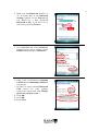
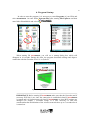
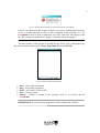
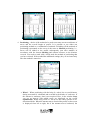
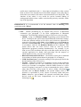
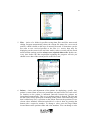
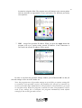
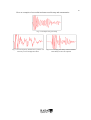
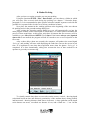
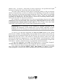
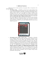
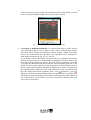
Software Package
Version 1.059
User’s Manual
Riga – 2010
1
Table of Contents
Name of Chapter
Page
1. Introduction ....................................................................................................................... 2
2. Brief Information on Georadar .......................................................................................... 3
3. Definition of Terms ........................................................................................................... 5
4. Examples of Displaying Radar Data ................................................................................. 6
5. Computer Program Installation ......................................................................................... 7
5.1 PDA Configuration for Connection with Georadar .................................................. 11
5.2. PDA Configuration for Connection with External Bluetooth GPS Receiver .......... 14
6. Program Startup ............................................................................................................... 16
7. Georadar Setup ................................................................................................................ 18
8. Radar Probing .................................................................................................................. 27
9. Additional Functions ....................................................................................................... 29
10. Our Recommendations .................................................................................................. 32
11. Format of Probing Data Files SEG-Y ........................................................................... 33
Contact Information............................................................................................................. 36
2
1. Introduction
We thank you for having purchased the Ground Penetrating Radar (Georadar)
manufactured by our company, and/or for your interest. Our company has over 40 years of
experience in this field of GPR. The scientific research was initiated by the Problem
Laboratory of Aviation Subsurface Radiolocation (PLAPR) whose successor is our
research-and-production company Radar Systems, Inc.
A modern georadar is a quite sophisticated radio engineering device. However,
thanks to the application of the microprocessors and computing technologies, to operate a
georadar today is much easier than it was with its earlier models. Actually, to know how to
operate a georadar means to know how to work competently with the software whose
description you are reading right now.
The software package PrismMobile is intended for a palmtop computer – personal
digital assistant (PDA) – guided by the operating system Windows Mobile® 6 (or newer
versions) and functioning as part of the georadar Zond-12e Advanced, Zonde-12e WiFi
Upgrade Kit or Python3.
IMPORTANT! To interface with the aforesaid devices, PDA must be equipped with
the wireless system WiFi.
The tasks of the package are as follows:
1. Control of all georadar modes and adjustment to specific working conditions.
2. Receiving of digital data from a georadar during radar probing and recording
thereof in the form of files (onto any data carriers that are PDA compatible).
The software package is designed in the format of the so-called integrated user
environment, i.e., a user starts one program – PrismMobile – and deals with this program
only. All other auxiliary programs start automatically, depending on user’s actions.
3
2. Brief Information on Georadar
Here is a very simplified georadar structure scheme which gives a general idea about
how the georadar works.
GPS
PDA
Georadar
Stroboscopic converter
Synchronizer
Transmitter
Receiver
Antenna
Antenna
Surface
Object
Fig. 2.1. Simplified georadar structure scheme
4
The antenna is excited by transmitter with very short electrical impulses. At that, the
transmitting antenna emits ultrabroadband 1.5-period electromagnetic waves the
approximate shape of which is shown on Fig. 2.2.
Fig. 2.2. Shape of an emitted electromagnetic wave
The electromagnetic waves propagate in the medium that is probed, reflecting from
various inhomogeneities (metals, voids, different subjects, borders of strata with different
parameters, etc.). Reflected waves are received by the receiver through the receiving
antenna and these waves carry information about the medium probed. Apart from the
reflected wave, by all means there is also a direct wave traveling from the transmitting
antenna to the receiving antenna along the shortest possible route. Therefore, an output
signal of the receiver represents an impulse of the transmitter (as shown on Fig. 2.2) and
subsequent reflected impulses. In order to determine the depth of the target location in the
medium, the reflected signal delay time is to be measured from the transmitter’s impulse.
Fig. 2.3. Example of an output signal of the receiver
The transmitter’s impulse is well seen on the left
The process presented on Fig. 2.3 is extremely fast; it lasts dozens to hundreds of
nanoseconds and is technically difficult to process. A stroboscopic converter is used to
“stretch” this process. The synchronizer controls all units of the georadar and, in its turn, is
controlled by PDA and the Software.
For the purpose of analysis of information received, it is necessary to take into
consideration that the velocity of propagation of electromagnetic waves in the probed
medium (other than air) is not equal to and is less than the speed of light by the coefficient
of retardation. The coefficient of retardation equals the square root of the dielectric
permittivity of the medium. The program automatically discounts this factor.
5
3. Definition of Terms
Here is a list of terms used in this text, whereas different resources give different
interpretation of these terms and some of them are not explained elsewhere.
1. Sample – unit value reflecting the amplitude of the signal at any given moment of
time.
2. Trace – an aggregate of samples containing one-dimensional information on reflected
signals. Examples of traces are shown on Fig. 2.3 and 4.1.
3. Profile – an aggregate of traces containing two-dimensional information on reflected
signals received as a result of some routing. Profile can consist of any number of
traces. Examples of a profile are shown on Fig. 4.2 and 4.3. The profile per say (or a
number of profiles) in the form of a file (files) is the end result of the probing. After
that follows processing (if necessary), printing (if necessary), and interpretation of
data.
4. Zero point – Trace sample corresponding to the transmitter’s emission maximum
instant. It is this very sample whereto the scale numbering zero falls along traces, i.e.
the delay time of a reflected signal should be counted from this sample. As it was
mentioned earlier, an impulse of the transmitter is approximately a 1.5-cycle (threelobe) signal. It means that the zero point should be aligned with the middle of the
second lobe of the impulse of the transmitter. The method of adjustment of the zero
point is described in chapter 10 of this manual. This is a very important parameter
taken into account in the calculation of signal time delays to determine the depth of the
target location in the probed medium. Examples of the location of the zero point are
shown on Fig. 4.1, 4.2 and 4.3.
5. Wiggle plot – a type of imaging a profile where traces are set vertically at some
distance from one another. Each trace is drawn as a curved line deflecting from the
middle line to the left or to the right, depending on the value of the sample in each
point of the trace. In addition, positive signal lobes are highlighted with the color
corresponding to the maximum positive level of the chosen color scale. Examples of
the wiggle plot are shown on Fig. 4.2.
6. Line scan – a type of imaging a profile where traces are set vertically, close to each
other, and they are drawn as vertical lines. Color in every point of the line depends on
the amplitude of a respective sample of traces according to the chosen color scale.
Examples of the line scan are shown on Fig. 4.3.
7. Mark – a distinguishing feature of a profile trace which denotes some uniqueness of
this trace and, consequently, uniqueness of this particular point of the probing route.
Marks serve to attach the profile to the location. When probing, you can by push of a
button enter marks when passing some locality landmarks or pegs that have been
placed for this purpose. Further on, when the profile is shown on the display, these
marks will be entered together with the profile. Examples of displaying marks are
shown on Fig. 4.3.
6
4. Examples of Displaying Radar Data
Fig. 4.1. Example of displaying the trace
Fig. 4.2. Example of displaying the color profile (in black-and-white and color scales)
Fig. 4.3. Example of displaying the line scan (in black-and-white and color scales)
Note: as our experience shows, the line scan in the black-and-white color scale is
the most informative type of displaying probing data (Fig. 4.3, on the left).
7
5. Computer Program Installation
The installation package of SP PrismMobile comes as a cabinet file
(PrismMobile.cab). CAB file is a compressed file containing components of the program
and instructions for the operating system to allocate them and register. In Windows
Mobile, this type of file is an executable file, i.e., when it is run, the program installation
module of the operating system is started.
In order to install SP, you need to connect your PDA to your desktop computer (PC)
that has a PDA connector (for synchronizing/data exchange) and carry out the following
operations:
IMPORTANT! It is recommended to use PDA for work only when it is
disconnected from PC because the programs used to do synchronizing/data exchange
(Microsoft ActiveSync) restrict the working capacity of the PDA wireless module
(i.e., they interrupt existing connection and disallow to connect to wireless LAN
(WiFi).
1. Connect your PDA to PC using USB connector. Wait until ActiveSync completes
initialization and in the opened window press the Explorer button. If ActiveSync has
in the
not started automatically, you can start it by double clicking on the icon
system tray (bottom right part of the screen). Explorer provides access to the entire
file structure of PDA.
Fig. 5.1. Explorer for PDA file structure
8
2. Open one more explorer on your PC and depending on where PrismMobile.cab is
located (either on the CD supplied with the software package or downloaded from the
site www.radsys.lv, section Downloads) choose a respective folder and open it. After
that, copy PrismMobile.cab to your PDA. To do that, you either drag PrismMobile.cab
from PC Explorer to PDA Explorer or right click on PrismMobile.cab, select Copy
from the dropdown menu and right click on any empty (white) space of PDA
Explorer and select Paste from the dropdown menu.
IMPORTANT! The root folder of PDA, which appears when File Explorer opens,
is the folder My Documents. If you copy PrismMobile.cab to other than root folder,
you should remember where it is located on PDA.
3.
Start File Explorer of PDA. To do that,
press the Start button, select File Explorer
or Programs and select File Explorer from
the opened window.
4. Go to My Documents folder or if you have
copied PrismMobile.cab to another folder,
go to that folder.
9
5. Click on PrismMobile.cab to start
installation. If it is a repeated installation,
skip this step and proceed to the following
one. During the first installation of
PrismMobile on your PDA you will see a
window warning that you are about to
install a program of an unknown publisher.
To continue, press Yes. Then proceed to
point 7.
6.
During repeated installation of PrismMobile
on your PDA, you will see a message that
the OS will remove the previous version of
PS. To allow that, press OK. Otherwise,
press Cancel.
7.
Choose a location to install PS on your PDA
– Device.
10
8.
The installation process will be shown as a
running line. Upon completion of
installation, a message will appear that PS
has been installed successfully.
IMPORTANT! If for some reason (to increase the storage space on the data carrier
or to install a newer version) you need to uninstall PS PrismMobile from your PDA,
do the following: Start → Remove programs from the Settings bar, System tag.
11
5.1 PDA Configuration for Connection with Georadar
In order for your PDA to be able to work as part of the georadar Zond-12e
advanced, Zonde-12e WiFi Upgrade Kit or Python3 you need to connect your PDA with
the georadar wireless network. For Windows Mobile 6, do the following steps:
1. Press Start, select Settings.
2. Then select Connections.
3. Press the Wi-Fi icon.
4.
If you have the IP-address set, proceed
to point 11.
12
5. In the opened window Configure
Network Adapters select Network
Adapters.
6. Select a respective wireless network
card from the list of devices (in case
with HP iPAQ 214 it should be
Marvell SDIO8686 Wireless Card).
7. Select Use specific IP Address.
8. In the field IP Address enter any
address for your PDA from the subnet
192.168.0.ххх
(where
«ххх»
corresponds to any number from 1 to
255,
except
for
10
because
192.168.0.10 is the address of the
Zond-12e or Python3 georadar), for
example, 192.168.0.1
9. In the field Subnet mask enter code
255.255.255.0.
10. Press OK.
11. If the Zond-12e (for Zond-12e
advanced
or
Zonde-12e
WiFi
Upgrade Kit) or Python (for Python3)
network has already been configured,
proceed to point 15.
12. Go to the Wireless tag and select the
network Zond-12e or Python (across
from which you will see the word
Available).
13. In the opened Zond-12e or Python
settings window select Next.
14. Press Next.
15. Press Finish.
13
16. Select Zond-12e or Python network
and click on Connect. Across from the
name of the Zond-12e or Python
network you will see the word
Connecting. Wait for the word
Connected to appear. The icon
will appear at the top of the screen. It
means that you have successfully
connected to the wireless network of
the Zond-12e or Python3 georadar.
17. Press ОK.
18. Press Close.
14
5.2. PDA Configuration for Connection with External Bluetooth GPS
Receiver
To use GPS receiver for work with the georadar, you have to make certain
adjustments to your PDA. For Windows Mobile 6, do the following steps:
1.
Press Start, select Settings.
2. Then select Connections.
3. Press the Bluetooth icon.
15
4. Make sure that Bluetooth interface is
on. It means that in the Bluetooth
Settings window in the General tag
you should see a blue inscription
Bluetooth is ON; if you don’t see it,
turn it on by pressing Turn on.
5. Go to Services and select Serial Port
from the list of service settings. Check
Enable service and press Advanced...
6. Enter 5 and 6 COM Ports as Inbound
COM Port and Outbound COM Port,
respectively.
7. In order to avoid selecting Bluetooth
GPS receiver for every probing,
remove the check mark from Display
the device selection screen ...
8. Press OK.
9. Press OK.
10. Press Close.
16
6. Program Startup
In order to start the program, it is necessary to enter Programs of your PDA and
select PrismMobile. Or enter folder Program Files after starting File Explorer and then
enter folder PrismMobile and select
Fig. 6.1 Programs
.
Fig. 6.2 File Explorer
When starting PS PrismMobile, you will see a startup dialog box which will
disappear in 10 seconds. During this time, the program downloads settings and aligns a
connection with the Georadar Zond-12е or Python3.
Fig. 6.3 Startup dialog box of PrismMobile
IMPORTANT! Before starting PS PrismMobile make sure that the Georadar (and if
necessary WiFi kit) is on, since the connection is established when PS PrismMobile
is started and it is broken upon exit from PS PrismMobile or when WiFi settings are
changed (see chapter 7 Georadar Setup). It is also necessary to take into
consideration that initialization of the wireless network takes up to 5 seconds after it
is turned on.
17
Fig. 6.4. Message about absence of connection with the control block
If there is no connection, the program will give a respective warning and will restrict
access to certain functions (receipt of data, alignment of the georadar, etc.). PS
PrismMobile will try to make a connection once more either after rebooting or when
the WiFi settings are modified (see chapter 7 Georadar Setup, paragraph 7).
The main window of the program is divided into two zones: zone of data displaying,
and zone of control buttons, such as Start, Stop, Mark, Exit, and SETUP).
Fig. 6.5. Main window of the program
•
•
•
•
•
Start – start of data acquisition.
Stop – stop of data acquisition.
Mark – put a marker in the profile.
Exit – exit the program.
SETUP – control of settings of the georadar Zond-12е or Python3 and PS
PrismMobile.
IMPORTANT! Any actions in the program are made with the help of Stylus.
18
7. Georadar Setup
Before you start probing, it is necessary to set up working modes of the georadar and
PS PrismMobile.
1. Assemble georadar Zond-12e Advanced or Python3 as explained in the User’s
Manual and turn it on.
When using Zond-12e WiFi Upgrade Kit, assemble WiFi Upgrade Kit according
to Zond-12e WiFi Upgrade Kit User’s Manual and turn it on.
2.
Turn on PDA and make sure that it is connected to the wireless network Zond-12e or
Python. The name of the network should appear on your PDA or in the dialog box
Wireless Manager. If connection is not established automatically, connect to the
network manually (see section 5.1 PDA Configuration for Connection with
Georadar).
Fig. 7.1. PDA desktop
3.
Fig. 7.2. Control of wireless networks
Start the program (see chapter 6 Program Startup) and after the startup dialog box
has disappeared press the SETUP button in the control section of the main program
window.
The window that appears is divided into three zones: zone of trace displaying, setup
pages, and tag box (every tag corresponds to its own settings page).
Current trace and battery status (for Zond-12e Advanced and Python3) are displayed
in the zone of trace displaying. The battery status is displayed graphically, in percentage
and voltage.
IMPORTANT! Keep an eye on the georadar internal battery status and use external
power resources (12 V DC) when the internal battery is low because it may cause
interruptions in georadar functioning (such as untimely shutdown, loss of the
wireless network, loss of antenna signal, etc.). To extend the life span of the internal
battery, it is recommended to fully recharge it after work with the georadar is
completed (see Georadar User’s Manual), since partial charging, regular use of the
battery when it is low, or incomplete charging result in its early failure.
19
Fig. 7.3. Georadar settings window
All kinds of settings are divided into several groups, and every group is located on
a certain setup page which has a respective tab on the tab ruler. To browse the tabs that are
not displayed on the screen, use the arrows
located in the bottom right part of the
screen. Setting groups are divided as follows:
IMPORTANT! Different versions of georadars have different amounts of settings.
The program automatically recognizes which georadar is connected and makes
available settings that are required for a connected georadar. Here and further we
refer to the Zond-12e Advanced version of the georadar. The differences from other
versions are not major and have fewer parameters to be set.
1. General – main georadar settings (see Fig. 7.3):
• Medium – here you install the medium you plan to probe. Choose the
medium from the list available that is closest to the medium you are dealing
with. Permittivity is shown for each medium. Adjusted permittivity (E=...)
which is used for calculations of depth is indicated to the right of the
medium dropdown window (see chapter 9 on adjusting of permittivity).
• Samples – a number of samples in a trace. In the current version, the
number is 512 and cannot be changed.
• Stacking – setting of the number of traces which will be summarized during
probing. Stacking helps suppress noises and interferences and increase the
depth of probing. But it should be remembered that it reduces the rate of
traces acquisition by PDA proportionally to the number of stackings and
may require slowing down of the movement of the antenna in order to avoid
loss of information. The minimum stacking possible is 2 because the
capability of today’s PDA does not support simultaneous acquisition,
display and saving of data without stacking.
• Channel (applies only to the Dual-Channel radar) – choice of a georadar
channel: Channel 1 – a single-channel operation mode with the antenna
20
connected to channel No. 1; Channel 2 – a single-channel operation mode
with the antenna connected to channel No. 2. Dual-channel operation mode
is not presented in this version of sotware.
• Show Battery – turn on/off the display of the status of the internal battery
(only in case with Zond-12e Advanced or Python3).
2. Antenna – settings of a connected antenna:
Fig. 7.4. Setup of connected antenna
Fig. 7.5. Automatic setup of pulse delay
• Antenna – select the antenna used in this channel from the offered list.
• Time Range – one of the most important parameters, to be chosen rather
carefully. You can select the range from a set of proposed values or set up
by yourself at the item Customized. When specifying the range there is
required to watch information appeared under the signal window. Should
you specify too wide range the legend Warning! Too small sample rate!
will appear. At the right side of the value of the range there is indicated in
nanoseconds its dimension in meters for the selected medium. It determines
the interval of investigated depths. The latter determines the interval of
investigated depths in selected media at absence of attenuation in it.
However, maximum penetration depth is defined by the level of attenuation
of the sounding signal and is different in different soils. Therefore, when
selecting this parameter there is not recommended to specify it to be higher
if required for resolving of your task.
• High Pass – choice of cut-off frequency of a hardware High Pass Filter in
the receiving path to supress low-frequency interferences that appears when
the antenna moves across uneven surface. Please follow instructions in the
bottom part of the settings page when you install the filter. If the surface of
the probing medium is even (asphalt, concrete, etc.) or if the antenna moves
in the air, you can turn off the filter; this way you can eliminate some slight
signal distortions caused by the filter.
• Pulse Delay – this option is meant for aligning a probing signal with the
probing time range. Initial pulse delay values are entered in the program
during its installation and do not reflect the optimal adjustment. The setup
should be done when the georadar is first turned on with this antenna for
21
this particular Time Range. The adjustment may be done either
automatically or manually. When using the automatic mode, after you press
the AutoDelay button the probing signal will be automatically aligned with
the beginning of the probing time range (see Fig. 7.5). To cancel or stop
automatic setup, press Cancel in the window that has appeared. When
setting in the manual mode, set the probing signal at the desired position in
. The optimal position is such
the probing time range by using buttons
position of the probing impulse in the probing time interval when the first
lobe is off from the beginning of the time axis by approximately 1/20 of its
length (see Fig. 7.15). After the initial adjustment, values of Pulse Delay
will be saved for each combination Antenna – Time Range and every time
you turn on the georadar henceforth you do not need to do this adjustment
again.
3. Gain – digital amplifying of received signals when they are displayed on the
screen as a radar profile. Since a signal weakens quickly when it moves
through the ground, the deeper the signal goes, the stronger the amplifying of it
must be. Therefore, amplifying of the signal at the end of the trace must be
stronger than at the beginning of the trace. You can apply any amplifying
function representing a broken line connecting 2, 3, 5 or 9 points where in each
of the points amplifying may be regulated with a slider within the range
between 0 to 84 dB. Under each slider, its accurate amplifying value is
indicated in dB. For the most part, it is sufficient to set 2 points with 0 dB at
the beginning and 48 dB at the end. If these settings are not optimal, you can
set other ones later.
IMPORTANT! Amplifying is a purely program function and is used only when data
is displayed. The signal itself is digitized and recorded without amplification.
Fig. 7.6. Gain in 2 points
Fig. 7.7. Gain in 3 points
22
Fig. 7.8. Gain in 5 points
Fig. 7.9. Gain in 9 points
4. Positioning – choice of the method to be used to measure current coordinates of
traces and the overall length of profile. It is possible to use either one
positioning method or a combination of methods. Switching off the methods of
positioning represented on the screen is the same as Manual positioning, i.e.,
traces will be added to the profile subsequently (one after another) in
accordance with the chosen Stacking and without reference to the distance
covered. You need to mark with a check mark the method of positioning that
you have selected. If the method has additional settings, they are activated only
after the method is turned on.
Fig. 7.10. Adjustment of positioning
• Wheel – When positioning with the help of a wheel, the covered distance
during movement is calculated and recorded in the header of each trace. If
the antenna is stationary, data is not acquired. Here, in the window Step,
you set an interval with which traces are displayed on the screen
equidistantly. When using Zond-12e Advanced, the wheel operates in bidirectional mode. When the antenna moves forward the profile on the screen
is displayed from left to right, but if the antenna moves backward, the
23
profile also is build backward, i.e., from right to left and has a white vertical
mark in front. If the antenna moves backward along the same path, then it
looks like a movement of the white vertical mark back over the profile. This
function of the wheel is very useful for precise location finding of
underground utilities when a white vertical mark precisely coincides with a
top of the hyperbola.
IMPORTANT! It is recommended to set the minimal value of Stacking when
positioning with a Wheel.
• GPS – satellite positioning by an external GPS receiver via Bluetooth
connection (see paragraph 5.2 for PDA configuration of Bluetooth
connection). The following settings for using a GPS receiver are provided:
o GPSID – using of a Windows Mobile 6 operating system internal GPS
driver. Turning on this option shuts down Bluetooth connection settings,
in this case internal settings of OS will be used, which are adjusted in a
respective OS window (press Start, select Settings, go to the System tag
and click on External GPS, it’s recommended to adjust further settings
in accordance with the OS Windows Mobile 6 User’s Manual). This
option allows that one GPS receiver could be used by several
applications (programs) running simultaneously. For example, if you
want to save GPS coordinates not only to the data profile but also by an
external application for further data processing (for the purpose of
enhancing the accuracy of received coordinates).
o Bluetooth Outbound COM Port – the number of this port is indicated
in accordance with the option chosen in paragraph 5.2 of chapter 6.
o COM Port Baud rate is selected according to the option specified in the
documentation of the GPS receiver.
o Logging – additional recording of coordinates not only in the profile but
also in a separate text file. All coordinates received from the GPS
receiver are recorded in compliance with the NMEA format as a GGA
record. If logging is activated, it is also recommended to select a folder
where these text files will be stored. To select a folder, click button
and then click on Browse Folder in the opened window where a file
structure is represented as a tree, choose a necessary folder and press
Select, otherwise, press Cancel. All external removable data storage
devices (such as SD Card, CompactFlash, etc.) are indicated by a
following icon .
24
Fig. 7.11. Folder search window
5. Files – choice of a folder for profiles saving (data files) and files name mask
editing. Program automatically shows the current file name (for a next saved
profile), which is build on the base of entered file mask. If sometimes you do
not want to save received profiles to the files (i.e. receive data only for
displaying on the screen in the real time mode), remove (switch off) the check
mark from the settings position Always save acquired data to file. In this case,
every time before the data acquisition beginning the program will ask you
should it save data of the current profile to the file or not.
Fig. 7.12. File recording setup window
6. Palette – choice and adjustment of the palette for displaying a profile. Any
palette is created from at least two (maximum ten) main colors. For each color,
its location on the palette is indicated. Intervals between the palettes are
interpolated automatically. This way a gradient palette is formed. The first and
the last colors always participate in forming of the palette. Each following color
that is added may have a position on the palette between the positions of two
closest colors included. Inclusion/exclusion of a color is done by pressing the
button with a respective number. To change a color, press the large button
located between the position slider and color numbers. You can change a color
25
location by using the slider. The program saves all changes to the current palette
and also provides an opportunity to save and retrieve six different previously
saved palettes.
Fig. 7.13. Palette setup window
7. WiFi – setup of the georadar IP address. When you press the Apply button the
program will try to connect using entered IP address. If the connection is
successful, the entered IP address will be stored.
Fig. 7.14. WiFi setup window
In order to exit from the georadar settings window, press Close or OK. At that, all
selected settings will be saved for further use.
Note: the program saves all georadar settings in special files (a separate settings file
is created for each georadar version). All parameters for all types of antennas are
saved. If you made some modifications to the parameters, then parameters get saved
on exit from setup. When the program is started next time, last parameters will be
used. If any settings file is corrupted, the program automatically loads default
settings for the current georadar version.
26
Here are examples of successful and unsuccessful setup and commentaries.
Fig. 7.15 Example of a good setup
Fig. 7.16. Low-frequency interference is present. It is
necessary to turn on High Pass Filter.
Fig. 7.17. Too large pulse delay of the transmitter.
Pulse Delay needs to be adjusted.
27
8. Radar Probing
After you have set up the georadar you can start probing.
Using the function SETUP / Files / Data Folder, you can choose a folder in which
you will store files received while doing the probing (see chapter 7 Georadar Setup,
paragraph 5). It is recommended to place profiles related to another separate work with the
georadar in a separate folder in order to avoid any confusion in future.
Now place the antenna in the working position at the beginning of the area chosen
for probing and exit the georadar settings dialog box.
After exiting the georadar settings dialog box you will automatically get into the
main program window in the bottom part of which there is a control panel to maintain the
process of data acquisition. At this point, only three lit buttons that are necessary will be
available to you: Start, Exit and SETUP. Press Start. If the button Always save acquired
data to file is not marked, the program will ask if it needs to save a received profile to the
file or not.
After a short delay (about one second), the computer will produce the sound signal
“Let’s go” and probing will start with displaying the radar line scan on the screen in real
time. It is important to note that data acquisition starts when the phrase “Let’s go” is
completed. It is done intentionally, taking into account the loss of time needed for an
operator to get ready to start moving.
Fig. 8.1. The program main window reflecting receipt of data
To visually control data, there are two scales on the screen: vertical – showing depth
(calculated based on time and dielectric permittivity of the medium that is being probed)
and horizontal – showing distance (both shown in meters). A large guideline on the depth
scale denotes one meter, a medium one denotes 10 cm, and a small one – 5 cm. On the
28
distance scale – 10 meters, 1 meter and 0.5 meter, respectively. On a profile itself, depth
horizons are displayed by yellow lines with one-meter intervals.
The name of the current file (if the option of saving the profile to a file was selected)
and the current position, in meters, in relation to the beginning of the profile are shown
under the profile, provided that positioning includes the wheel. If the wheel is not included
in the positioning, then the current number of traces is shown. Above the profile, GPS
coordinates are displayed (if the GPS option is selected for positioning) and the battery
status (only for Zond-12e Advanced or Python3).
We would like to remind you that if you carry out positioning using the wheel, data
acquisition to the current profile (and, respectively, displaying thereof on the screen)
is performed only during rotation of the wheel. In case of stop of the wheel data
acquisition is also stopped, and is resumed after beginning wheel rotation.
IMPORTANT! It is necessary to pay attention to messages generated by the
program and displayed at the bottom part of the profile, especially to those
highlighted in red. It will help you avoid irretrievable loss of data and waste of time.
As soon as you start data acquisition, the Stop and Mark buttons on the control
panel become available. If during probing when passing reference points on the profile you
need to insert special numbered marks into the data file, all you need to do is to press the
Mark button when the center of the antenna is passing the reference points. Every time
you press the button the computer gives a voice signal (“Mark”) and an aqua blue vertical
line appears on the screen. The first trace of the file is always automatically assigned the
mark with “0” number, while the last trace is assigned the maximum number.
To stop data acquisition, press Stop. The program gives a voice signal “Stopped”;
and Start, Exit and SETUP buttons on the control panel become available.
Now, if you have chosen saving of the profile to a file, it is already saved on the data
store in the folder you indicated SETUP / Files / Data Folder (see chapter 7 Georadar
Setup, paragraph 5). The next file will be automatically saved with an indexed filename.
29
9. Additional Functions
During the process of data acquisition, the program offers to an operator a few
additional functions:
• Zero depth setting – a possibility to correct the zero point position on the
scale of depth. Depending on the antenna, time range, ground permittivity, the
height to which the antenna is lifted above ground (for aerial antennas) and so
forth, the direct surface wave can change its position in relation to the
beginning of the trace, what, consequently, has an impact on the measured
depth. To incorporate these changes, the option provides correction of position
of the zero point on the scale of depth. To utilize it, double click on the depth
scale. You will see that a frame will appear around the scale.
Press on the depth scale and move the stylus up or down: the scale will move
along with it. When you withdraw the stylus, a new value for the zero depth
will be displayed. The program will remember this value and it will use it
afterwards for next profiles. If you are not satisfied with this value, you can
adjust it at any time.
Fig. 9.1. Zero depth setting
•
Determining precise depth of point target – a possibility to determine
precise (adjusted) depth of the point target. Because the georadar uses two
separated antennas (receiving antenna and transmitting antenna), simple
recalculation of the time scale into the depth scale gives an error. The error
results from the fact that when the antennas are separated by a gap, a distance
measured is slanting, not vertical and the time of a direct signal propagation
from the transmitting antenna to the receiving antenna is not taken into account
(see Fig. 2.1). Ignoring these parameters may lead to substantial errors,
especially when small depths are measured which are comparable to the
distance between the antennas. The Moveout correction function (which
includes digital processing of signals) is used to eliminate such an error. This
function recalculates the depth in such a way as if emission of a signal and
signal receiving are done from one point located between the antennas. Zero
depth point and dielectric permittivity must be defined correctly before
performance of this procedure.
30
Click on any point of the profile and in the bottom part of the profile you will
see the exact (recalculated) depth of the point you have chosen.
Fig. 9.1. Determining precise depth of the point target
•
Correction of medium permittivity. It is known that when a profile crosses
some diffracting objects, such as pipes, cables, stones, archaeological objects,
and zones where ground characteristics change sharply, signals from these
objects on a radar profile have the shape of a hyperbolic curve. Examples of
such signals are shown on Fig. 4.2, 4.3, and 9.3.
If you double click on the profile, the screen shows a hyperbolic line from a
theoretical local target in a theoretically homogeneous medium, and in the
bottom part of the profile you will see the value of the permittivity. Your task
is to align the theoretical hyperbola with the selected signal hyperbola on the
profile. To begin with, align tops of the hyperbolas, for which double click on
the top of the signal hyperbola, and then by single taps by stylus on branches of
the signal hyperbola adjust the slope of the branches. If you are satisfied with
how the aligned theoretical hyperbola looks, press ; otherwise, press .
When you confirm the theoretical hyperbola, the depth scale is reconfigured to
match the theoretical hyperbola. The program memorizes this value and it will
use it afterwards for next profiles. If you are not satisfied with this value, you
can correct it at any time.
31
Fig. 9.3. Correction of the medium permittivity
32
10. Our Recommendations
In this chapter, we offer several recommendations how to operate with the equipment
and the software. We do not claim that we have a monopoly on the truth, but if you are
new to working with this kind of equipment, we recommend you to read this chapter.
In our opinion, the line scan in the black-and-white color scale is the most informative
type of displaying probing data (see example on Fig. 4.3, on the left). It looks like
three-dimensional and weak signals are seen clearly.
Working with the program, pay attention to tips and messages.
Before you start working with the georadar on a separate task, it is useful to create a
separate folder where you will keep probing files in regard to this specific task versus
having all your information in one “pile”.
33
11. Format of Probing Data Files SEG-Y
The program PrismMobile uses the international SEG-Y format for geophysical data.
A name of a file starts with a 3200-byte EBCDIC descriptive reel header record
containing file service information. It is followed by a 400-byte binary reel header record
containing information about data:
Offset
from file
start
position, in
bytes
3200
Parameter
length in
bytes
Parameter
recording
format
4
int
Job identification number
3204
4
int
Line number
3208
4
int
Reel number
3212
2
short int
Number of data traces per record
3214
2
short int
Number of auxiliary traces per record
3216
2
short int
3220
2
short int
3222
2
–
Sample interval of this reel's data in
PICOseconds
Number of samples per trace for this reel's
data
Unused
3224
2
short int
3226
2
short int
3228
26
–
3254
2
short int
3256
344
–
Commentary
Data sample format code:
1 = 32-bit IBM floating point;
2 = 32-bit fixed-point (integer);
3 = 16-bit fixed-point (integer);
4 = 16-bit fixed-point with gain code
(integer).
CDP fold (expected number of data traces
per ensemble)
Unused
Measuring system:
1 = meters;
2 = feet.
Unused
Further, records of traces follow where each contains a 240-byte binary reel header
and data on traces. Offsetting from the file start point to record K equals
3600+K*(240+S*2), where S – a number of samples in a trace, K – trace record number
(counting starts from zero trace record, not from the first one). The header is followed by
data of probing which is recorded sequentially, sample after sample. No characters or
symbols are used between samples to divide them. Each sample is represented by data
sample format code from the binary reel header and takes 2 or 4 bytes. Thus, a trace
containing N samples is (2 or 4)*N bytes long. It is to be taken into account that samples
34
and traces are numbered starting with 0 and not 1. The header of the trace record is shown
in the table below:
Offset
from
beginning
of trace
record, in
bytes
0
Parameter
length in
bytes
Parameter
recording
format
4
int
Trace sequence number within line
4
4
–
Unused
8
4
int
Original field record number
12
4
int
16
4
–
Trace sequence number within original field
record
Unused
20
4
int
CDP ensemble number
24
4
int
28
2
short int
30
2
short int
32
2
short int
34
2
short int
36
4
–
Trace sequence number within CDP
ensemble
Trace identification code:
1 = seismic data;
2 = dead;
3 = dummy;
4 = time break;
5 = uphole;
6 = sweep;
7 = timing;
8 = water break;
9 = optional use.
Number of vertically summed traces
yielding this trace
Number of horizontally summed traces
yielding this trace
Data use:
1 = production;
2 = test.
Unused
40
4
float
44
26
–
70
2
short int
72
4
float
Scalar for coordinates:
+ = multiplier;
– = divisor.
X source coordinate
76
4
float
Y source coordinate
Commentary
Receiver group elevation
Unused
35
80
4
float
X receiver group coordinate
84
4
float
Y receiver group coordinate
88
2
short int
90
18
–
Coordinate units:
1 = length in meters or feet;
2 = arc seconds.
Unused
108
2
short int
110
4
–
114
2
short int
Number of samples in this trace
116
2
short int
118
118
–
Sample interval of this reel's data in
PICOseconds
Unused
236
2
short int
Marks indicator
238
2
short int
Mark number
Lag time between shot and recording start in
PICOseconds
Unused
36
Contact Information
We will be grateful for your feedback, please inform us regarding any deficiencies
you may find in functioning of our equipment or program and we also will appreciate any
suggestions as how to improve their parameters and performance criteria.
If you find any difficulties in operating with equipment, you can always contact us or
our representatives by phone, e-mail, or sending a letter.
We hope that using of the equipment manufactured by our company will help you
achieve successful results in your business.
Software:
S. Zelenkov
Radar Systems, Inc.
1-105 Darzauglu Street,
Riga, LV-1012, Latvia
Tel./fax:
E-mail:
Web:
(+371) 67141041
[email protected]
www.radsys.lv