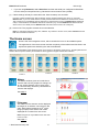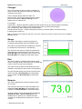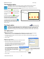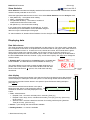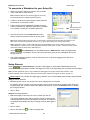
1
EasySense software manual (PC Windows version) Data Harvest Group Ltd. 1 Eden Court Leighton Buzzard Bedfordshire LU7 4FY Tel: +44 (0)1525 373666 Fax: +44 (0)1525 851638 e-mail: [email protected] [email protected] Website: www.data-harvest.co.uk Document No: DO 135 Revision 6 EASYSENSE software DO135 (6) Contents System requirements...................................................................................................................4 Installing the EASYSENSE software...........................................................................................4 Downloading the EASYSENSE software from our website.....................................................4 Connecting an Interface or Data logger.......................................................................................5 Starting the EASYSENSE program for the first time...................................................................5 The Home screen........................................................................................................................6 The Meters option .......................................................................................................................9 Changes .............................................................................................................................10 Gauge.................................................................................................................................10 Dial .....................................................................................................................................10 Numeric ..............................................................................................................................10 The Pictogram option ...............................................................................................................11 The EasyLog option..................................................................................................................13 The SnapShot option ................................................................................................................14 The Graph option ......................................................................................................................14 The logging wizard .................................................................................................................14 The Scope option ......................................................................................................................16 The Timing option .....................................................................................................................17 The Timing Wizard .................................................................................................................18 Measurements .......................................................................................................................21 Apparatus...............................................................................................................................22 The Counting option .................................................................................................................23 The Graph window...................................................................................................................25 The Toolbars ..........................................................................................................................25 Recording data.......................................................................................................................26 Selecting Data........................................................................................................................26 Use selection ......................................................................................................................27 Selection Wizard.................................................................................................................27 Previous Selection..............................................................................................................27 Analysing captured data.......................................................................................................28 Values.................................................................................................................................28 Interval................................................................................................................................28 Difference ...........................................................................................................................29 Gradient..............................................................................................................................29 Area ....................................................................................................................................29 Show Statistics ...................................................................................................................30 Displaying data .....................................................................................................................30 Data Value boxes ...............................................................................................................30 Axis display.........................................................................................................................30 Display Options ..................................................................................................................31 Number of Graphs ..........................................................................................................31 Graph type ......................................................................................................................31 Show Grid .......................................................................................................................31 X-Axis..............................................................................................................................31 Sensor settings ...............................................................................................................32 Colour .............................................................................................................................32 Show or Hide Channels......................................................................................................33 Zoom ..................................................................................................................................33 Auto scale...........................................................................................................................33 Title .....................................................................................................................................34 The Table display ...............................................................................................................34 © Data Harvest Group Ltd. 2 EASYSENSE software DO135 (6) The Comment column ........................................................................................................34 Using Tools on the data ........................................................................................................34 Notes ..................................................................................................................................34 Test Mode ..........................................................................................................................34 Smoothing ..........................................................................................................................34 Pre-log or Post-log Functions.............................................................................................35 Pre-set functions............................................................................................................. 35 Formula functions ........................................................................................................... 39 Best Fit ...............................................................................................................................40 Show Calculation................................................................................................................40 Predict ................................................................................................................................41 Add Text .............................................................................................................................41 Changing Settings ................................................................................................................42 Changing a sensor’s range ................................................................................................42 Calibrate Sensor.................................................................................................................42 Overlay ...............................................................................................................................44 Toolbar ...............................................................................................................................44 Set Language .....................................................................................................................44 Show Columns ...................................................................................................................44 Change Units......................................................................................................................44 Show Data as .....................................................................................................................44 Deleting data.........................................................................................................................45 Delete selected...................................................................................................................45 Edit a value.........................................................................................................................45 Merging data .........................................................................................................................45 Merge with file ....................................................................................................................45 Retrieve and Merge............................................................................................................45 Screen capture options ..........................................................................................................45 File menu option ....................................................................................................................46 Other Home options ..................................................................................................................47 Open File ...............................................................................................................................47 To open a Worksheet.............................................................................................................48 To open a Setup ....................................................................................................................49 To Save your own Setup file..................................................................................................49 To associate a Worksheet to your Setup file .........................................................................50 Setup Remote .......................................................................................................................50 Retrieve Remote ....................................................................................................................52 Altering the default configuration for data, setup files and images ...........................................53 Adding your own images ...........................................................................................................53 INDEX........................................................................................................................................54 EASYSENSE Software Multi-user Site Licence ....................................................................57 This manual may be freely copied for use with the EASYSENSE software. Copyright: all rights reserved. Data Harvest's policy is to continually improve products and services, so we reserve the right to make changes without notice. It is acknowledged that there may be errors or omissions in this publication for which responsibility cannot be assumed. No liability will be accepted for loss or damage resulting from use of information contained in this manual or from uses as described. © Data Harvest Group Ltd. 3 EASYSENSE software DO135 (6) System requirements Computer: IBM PC (or compatible) Operating System: Windows XP, Windows Vista and Windows 7 (32-bit and 64-bit compatible) Windows Installer 3.1* Microsoft .NET Framework 2* Microsoft Internet Explorer 8.0** Adobe Reader software (V7.0 or above)** Minimum 800 x 600 with 256 colours Recommended: 1024 x 768 with high colour - 16-bit Minimum Software: Display: * If Microsoft .NET Framework 2 or Installer 3.1 is not detected during the installation set up process, they will be automatically installed prior to the EASYSENSE application install. This will extend the installation time significantly. ** V8 minimum Internet Explorer is required to view documentation on the EasySense CD. To view and print PDF files you will need Adobe Reader installed. Installing the EASYSENSE software USB users: Make sure the EasySense logger is not connected to the USB port prior to, or while, the EASYSENSE software is being installed. • Log on as ADMINISTRATOR (or with equivalent access rights) on the system. • Close any open programs – you may need to restart your machine for configuration changes to be made. • Insert the EASYSENSE CD ROM into the CD Drive. Windows should detect the CD and automatically start up the EASYSENSE auto run program. If auto run fails to start, use Windows Explorer to navigate the CD ROM contents and double click on the Setup.exe file. • Follow the on-screen instructions to complete the installation of EASYSENSE and its associated files* onto the hard disk. • When the installation is complete, eject the CD ROM and store it safely. Restart your system. * Complete installs all, whereas a Custom install allows you to deselect the installation of logger manuals or to change their installation path. A Windows installer package (.msi) of the EASYSENSE software is available. The .msi package for • 32 bit systems is supplied in the i386 directory and for • 64 bit systems in the amd64 directory. (To check your system properties, click on Start, right click on Computer and select Properties). See page 53 for information on altering the default locations for data and setup files. Downloading the EASYSENSE software from our website The 4500 EASYSENSE software is available as a download from the Data Harvest website (www.dataharvest.co.uk). Save the compressed file to your computer, then ‘unzip’ it to extract all files before you run the setup.exe or msi. Note: The method used to unzip a file will depend on the computers operating system and the decompression program on your computer. For example: 1. 2. 3. Download the 4500 EasySense software zip file; select to Save it to a temporary directory on your computer. Right click on the zipped 4500 directory and select Extract All (or Compressed Decompressed Extract or Unzip). Select the extract destination as the temporary (unzipped) folder (zipped) folder directory. When the 4500 directory has decompressed the folder will appear minus its ‘zip’. From the unzipped folder either run the Setup.exe or select the appropriate Windows installer package (.msi). © Data Harvest Group Ltd. 4 EASYSENSE software DO135 (6) Connecting an Interface or Data logger • USB connection The first time an EASYSENSE unit (e.g. Vu, VISION, 1Link, 3Link, Q3+, Q5+, Q3, Q5, Qt Timer, QLink, or Q Advanced) is connected to a USB port on the computer, the USB drivers will need to install. Connect the EASYSENSE unit to the USB port on the computer. Windows will automatically detect a new device and install the drivers. • Bluetooth™ connection: Use the instructions provided in the EASYSENSE logger’s user manual. • Serial connection: Connect the interface/data logger to the serial port on the computer. Note which serial port you have connected to e.g. COM 1, as this information will be required when you start the EASYSENSE software. Starting the EASYSENSE program for the first time Start the EASYSENSE software e.g. Start ► Programs ► Data Harvest ► and click on EASYSENSE Software. Select the Language If a choice of language is available a Set Language window will open. To choose a different language, select from the drop-down menu and OK. The program will close. Restart to apply your choice. Select a User level The first time the EASYSENSE program is opened a ‘Select Program Level’ window will automatically open. Select a suitable user level. • • • Level 1 is aimed at ‘start’ level (e.g. up to 9 years old) Level 2 is aimed at ‘mid’ level (e.g. 9 – 15 years old) Level 3 is aimed at ‘exam’ level (e.g.15 years plus) Note: The program level can be altered by clicking on the Level icon and cycling through the levels (one bar for Level 1, two for Level 2 and 3 for Level 3). The currently selected level will be saved when the EASYSENSE program is closed. Select an Interface and Connection The first time EASYSENSE is opened a ‘Select Interface’ window will automatically open to allow the correct interface and connection to be selected. (a) Select the correct interface from the drop-down menu. • EasySense Range for an EASYSENSE data logger or interface • Flash Logger for the EASYSENSE Flash Logger (XP only) • Sense and Control for the Sense & Control or Sense & Control EasyLog. • Example Data for stored example data to show how sensor readings are displayed. If this option is selected you will not be able to collect data from your interface or data logger. (a) (b) (c) (b) Select the appropriate connection i.e. either Serial or USB Port. (d) • If you are connecting via a USB lead, select USB Port. • If you are using a serial lead, select Serial Port and then the number of the communication port used from the serial port drop-down list e.g. Communications Port (COM1). • If you are using a USB/serial adapter, select Serial Port and then the adapter from the serial port drop-down list e.g. AMC232USBDH USB Serial Port (COM4). © Data Harvest Group Ltd. 5 EASYSENSE software DO135 (6) • If you are using Bluetooth, select Serial Port and then the serial port configured for Bluetooth from the serial port drop-down list e.g. Bluetooth Communications Port (COM5). (c) If these settings will stay the same leave the ‘Show at startup’ box unticked. If the box is ticked (enabled) the ‘Select Interface’ window will automatically open when you next start EASYSENSE, so you can check that the currently selected Interface and method of connection are correct. This is useful if you use different types of interface (e.g. both Sense & Control and EASYSENSE Advanced units) or if the interfaces use different methods of connection (e.g. use both EASYSENSE Advanced units which connect via a serial port and EASYSENSE LINK units which connect via a USB port). (d) Click on OK. The program will save the current selection. Note: To change this selection at any time, CANCEL any ‘failure to connect’ errors, select Interface from the File menu and alter the selection. The Home screen Home is the main navigation screen, which contains the icons for all available options. The appearance of the Home screen and the complexity of the toolbars and functions in the experiment options are altered by the user level selected. Note: If the interface/data logger detected cannot use an option, it will appear greyed out e.g. the Setup Remote and Retrieve Remote options will only be available for data loggers that support remote data collection. Level 1 Level 2 Meters The Meters window gives an introduction to sensors and how they respond to change. Up to four section displays can be open at any one time and they can be any combination of sensors and displays. See page 9. Pictogram The value from the sensors can be displayed as images or an abstract colour block or bar chart. Each image represents a 10th of the range (or span) of the sensor and is also displayed as a number from zero to ten. Note: Pictogram is only available if the User level is set to Level 1. See page 11. © Data Harvest Group Ltd. 6 Level 3 EASYSENSE software DO135 (6) EasyLog The window will open pre-set to record sensor values continuously as a line graph until stopped. See page 13. Snapshot The window will open pre-set to record sensor values on demand (manual sampling) with a bar graph display. See page 14. Graph Use graph to record sensor values against a chosen time span as a line graph display. The window opens with a real time logging wizard from which the time span, interval between samples, start condition and triggers for the recording can be chosen. Note: Graph is only available for User level 2 or 3. See page 14. Scope A simple oscilloscope type display. The data from a sensor is redrawn continuously on the screen. Ideal for demonstrating fast events where there are rapid changes such as ECG traces, sound waveform, etc. Note: Scope is only available for User level 3. See page 16. Timing Timing is used to allow students to study Time, Velocity, Acceleration, Momentum and Kinetic Energy relationships using switchtype (digital) sensors such as Light gates. See page 17. © Data Harvest Group Ltd. 7 EASYSENSE software DO135 (6) Counting Use to count events by using switch-type (digital) sensors. The chart type can be displayed as images or a colour block or bar chart oriented either horizontally or vertically. Note: Counting is only available if the User level is set to Level 1 or 2. See page 23. Open File Used to load a previously saved .SSL or .SID file. Locate the correct file and click on open. See page 47. Open Setup To select and open an experimental setup file. This will pre-set the software for a specific operation. See page 49. Open Worksheet To select and open a worksheet and its accompanying experimental setup file. See page 48. Set up Remote Used for setting up the options to capture data while disconnected from the computer (remote). These options can include the duration of a recording, the time between each sample and triggers. See page 50. Retrieve Remote Use this option to retrieve a data set stored in your data logger’s memory. See page 52. © Data Harvest Group Ltd. 8 EASYSENSE software DO135 (6) The Meters option Start/Stop icon Menu bar User Level icon Toolbar Information window Close section window Section window Maximise window Sensor and its unit of measurement Right click Status bar When Meters is selected from the Home screen, the window will open with live data being displayed from a sensor in a Numeric window. Click on the Stop icon to stop data being recorded. To begin recording again click on the Start icon. • Up to four section windows can be open at any one time and they can be any combination of sensors and displays. • A section window can be opened either by clicking on the appropriate icon on the Toolbar or from the drop-down Display menu. • To alter the sensor displayed in a section, right click with the mouse in the section window and a Sensor Selection window will open. Select the sensor to display in that section from the list. • Click on the close button to close a section window. • A section window can be maximized to fill the whole window by selecting the maximize button, again to return to ¼ screen size. • Click on the Home icon click to return to the Home screen As soon as you open Meters or you click on the Start/Stop icon, the data is recorded ‘behind the scenes’. This data can be transferred into the Graph window for display and analysis using the Transfer to Graph icon (or select from the Edit menu). When in Graph click on the Back to Meters icon to return to the Meters window. © Data Harvest Group Ltd. 9 EASYSENSE software DO135 (6) Changes This is the simplest of all four sections. It displays a block of colour that changes to reflect the value being collected by the sensor. Colour changes happen within the span of a sensor’s limits. The minimum and maximum of these limits can be altered in Sensor Settings from the Display menu or Options icon. For example: Temperature - begins at light blue (coldest) and then works its way up to become dark red (hottest). Light - begins at black (no light), works through greys until it becomes white (full light). pH – simulates the colour change of universal indicator. Sound and other sensors – begin at dark green (minimum), becomes lighter until works through to bright green (maximum). Note: To alter the sensor displayed, right click in the section window and select the required sensor from the Sensor Selection window. Gauge This section will display a simple bar gauge that increases and decreases with the measured value. The scale on the left-hand side is divided into sections to correspond to the sensor it is representing. The maximum and minimum values recorded will be displayed on the right-hand axis by two short lines if Show Min Max from the Display menu is ticked. Use Reset Min Max from Display to reset these values. Dial This section displays a traditional dial whose pointer moves to the right as the measured value increases and moves to the left as the value decreases. The scale around the dial is automatically set by the software to correspond to the sensor it is representing. Two thin lines will display the maximum and minimum values recorded if Show Min Max from the Display menu is ticked. Use Reset Min Max to reset these values. Numeric This section displays the currently measured value as a number. The maximum and minimum value recorded will be displayed if Show Min Max from the Display menu is ticked. Use Reset Min Max to reset these values. Decimal numbers can be switched off by deselecting Display Decimals in Sensor Settings from the Display menu or Options icon. Without decimals selected, the reading will be rounded up to a whole number. © Data Harvest Group Ltd. 10 EASYSENSE software DO135 (6) Sensors The sensors are automatically identified when the Meter option is selected. To change sensors while Meters is logging, simply replace the sensor with a different type. Meters will automatically change the sensor settings so that the correct calibration scales are displayed. If not logging then the change will be detected once logging has started. To alter the sensor displayed in a section, right click with the mouse in the section window and a Sensor Selection window will open. Select the sensor to display in that section from the list. The display colour, decimals, name and the minimum and maximum limits of a sensor can be altered either from the Display menu or Options icon. See page 32. To change the range of a sensor e.g. to alter the range of a Heart Rate sensor from Waveform to Beats per minute select Sensor Config from the Settings menu (see page 42). User Level 1 The Pictogram option Menu bar Toolbar Information User Level icon Double left click in the area above the chart to enter a Title Right click within the graph area for Add Text and Title The program will open with values from the sensors displayed as images on the chart. Each image represents an assigned amount of data, a 10th of a total range (or span) of the sensor and displays the number from zero to 10. The block or bar icons can be used to change the images to abstract colour blocks or a bar chart. Charts can be oriented either horizontally or vertically . To capture a live reading from the sensors click on the Store icon. readings is 10. Stored data can be sorted either by its sample number or by the maximum or minimum value of each sensor. logging, select the Sort Data icon Stop and choose how you want the data organised. Sorted by sensors Max to Min © Data Harvest Group Ltd. 11 The maximum number of stored EASYSENSE software DO135 (6) The amount of data assigned to each image or block can be altered by changing the range of the sensor and/or its scale. For example with a Light sensor: • If its range is 0 – 1 k Lux (1,000 Lux) then each image will represent 1/10th of this range = 100 Lux. If the range was 0 – 10 k Lux (10,000 Lux) then each image will represent 1,000 Lux. • If the minimum to maximum scale of the 0 – 1,000 Lux range is reduced to 0 – 500 Lux then each image will represent 50 Lux. or Sensor Config (Settings menu). Select the To change the range of a sensor either use New sensors name, then Change Range. When the set range window opens select the required range, OK. To change the scale of the sensor select Options and Max value and type in the new number, OK. , Sensor Scale. Double click in the cell with the Min The name for the data channel can be changed in this window by double clicking in the cell with the sensors name and typing in a new name. The picture image can be altered by double clicking in the cell showing the current image and selecting a preferred image, OK. See page 53 on adding new images to those available. To reset to the original name or scale select the data channel and select Reset to default Min Max or Reset to default Name. Select New to set up a new recording. Deselect the tick next to any sensors from which readings are not required. 1 2 Select Next to show the orientations and display type of the chart or select Finish. © Data Harvest Group Ltd. 12 The range, picture or name of the sensor can also be changed from this window. Select the sensor first then the change option. EASYSENSE software DO135 (6) . Select a data point (a box will highlight the To display the ‘real’ sensor value select the Values icon selection), the value and its unit will be displayed in the information window. Click on the Values icon again to deselect. To change the background colour of the chart select the Background tab from the Options icon and select a new colour. To label a data point: • Right click in the chart area and select Add Text. • A dialogue box will open. Type in the required text and OK. • Move the curser over the data point you want to label, a highlight box will indicate the point selected and the label will appear as a ‘ghost’ box. • Click and the label will appear. To move, edit or delete a label, right click on the label and select the appropriate function. Tip: Long labels are best displayed when the chart is displayed horizontally. The EasyLog option If EasyLog is selected from the Home screen, the graph window will open pre-set to record sensor values continuously as a line graph until stopped. This makes it ideal for experiments when the time of the recording is unknown. EASYSENSE View, Q3 or 5 users: The New logging wizard will open, deselect the tick next to any sensors from which readings are not required. Click on the Start icon to begin recording. Click on a sensors name to change its range Logging will start with a time span of 30 seconds and when it has elapsed the time span will double automatically. This will continue until the recording is stopped by clicking on the Stop icon. To change a sensors range select New . Select the sensor’s name; when the set range window opens select the required range, OK and then Finish. Choose EasyLog when an X vs. Y graph is required (to plot the readings of one sensor against another). Alter the X-axis to display a sensor (rather than time) – see page 31. © Data Harvest Group Ltd. 13 EASYSENSE software DO135 (6) The SnapShot option If SnapShot is selected from the Home screen, the graph window will open pre-set to record sensor values on demand (manual sampling) with a bar graph display. EASYSENSE View, Q3 or 5 users: The New logging wizard will open, deselect the tick next to any sensors from which readings are not required. Click on the Start icon to begin recording. Click within the graph area to collect a sample. Click on the Stop icon recorded. to stop data being If you click on the Start icon again you will be given the option to add the new readings to the end of the existing data (if No is selected the existing data will be deleted). To change a sensors range select New . Select the sensor’s name; when the set range window opens select the required range, OK and then Finish. The Graph option User Level 2 & 3 If Graph is selected from the Home screen, the graph window will open pre-set to record sensor values against a chosen time span as a line graph display. The window will open with a real time logging wizard from which the time span, interval between samples, start condition and triggers for the recording can be chosen. When your selection has been made, click on Finish. The logging wizard Stage 1: Sensor selection • Deselect the tick next to any sensors from which readings are not required. If sensors have been altered after start up, click on the Redetect button to identify the change of sensor. • To change a sensor’s range, click on the sensor’s name, when the set range window opens select the required range, OK. • Click on Next. Stage 2: Recording duration • Select the length of time that you want to record from the list. • Select the interval between samples being taken. The number of samples will automatically alter when the total recording time and the interval between samples are selected. The range of recording times will vary according to which data logger is used. If a very short recording and intersample time are selected then the recording will be in FAST mode. In this mode there will be no screen display of the data until the recording ends. REAL TIME recording will change to FAST if a combination of very short recording and intersample times are selected Note: If you wish to view fast data as it is being recorded then use Scope – see page 16. • Click on Next. © Data Harvest Group Ltd. 14 EASYSENSE software DO135 (6) Stage 3: Select the Start condition as required. This is used to set the condition required for the recording to start. The choice of start conditions and triggers available on this page will depend on both the recording time selected and the data logger used. E.g. start conditions for QAdvanced if a FAST recording time is selected E.g. start conditions for REAL TIME recording time None - To begin recording as soon as you click on the Start icon . Trigger on Level - To begin recording when the selected sensor is ‘above’, ‘below’, ‘rises above’ or ‘falls below’ a set value. SET LEVEL Above To start recording when the value from a sensor is above a set level. SET LEVEL SET LEVEL Below To start recording when the value from a sensor is below the set level. Rises above Logging will not start until the value from a sensor rises up above the set level. SET LEVEL Falls below Logging will not start until the value from a sensor falls below the set level. Trigger on Digital Condition - to begin recording when a digital sensor, connected to input A or B, is On, Off, Rising to On or Falling to Off. Note: This option is only available with certain loggers when a FAST recording time is selected. If Falling to Off is selected, logging will start when an object has passed through the light beam If Rising to On is selected, logging will start when the first part of the object breaks the light beam Select any Pre Trigger requirements. Note: This option will only become available if a FAST recording time with a trigger on level or digital condition is selected. Pre-trigger will allow a percentage of samples to be stored before the trigger condition is met and the remainder to be taken afterwards. For example, if 1,000 readings are to be taken and a 25% pre-trigger is selected, 249 readings will be taken before the trigger condition is met and 750 on and after the trigger. © Data Harvest Group Ltd. 15 EASYSENSE software DO135 (6) Note: Sufficient time must be allowed to elapse for the pre-trigger samples to be taken e.g. at a relatively slow sample time of 100 milliseconds with 1,000 samples and a 25% pre-trigger, it will take 25 seconds to get to the pre-trigger position. • Click on Finish. • Click on the Start icon . Recording will start when the start condition you have selected is met. The recording will stop when the selected time span has passed. Note: If you want to stop recording before the time span has passed, click on the Stop icon. If None was the selected trigger then the recording will start as soon as the Start icon is clicked. If recording REAL TIME, with a trigger on level selected, a ‘Waiting for Trigger’ message will appear in the status bar (below the graph). When the trigger condition is reached the recording will begin. If recording FAST with a triggered start, a recording data message will display (if there is sufficient time!) until the trigger condition is met. The data collected will download as soon as the recording has finished. The Scope option User Level 2 & 3 Scope models many of the functions of a simple oscilloscope. It displays ‘real-time’ plots (as they occur) from the value of a sensor versus time. Unlike a graph that has a beginning and an end, the scope trace is refreshed or ‘redrawn’ continuously as long as data is being measured. Make your selection from the control panel on the right hand section of the Scope window and then to begin recording. click on the Start icon Once data has been recorded, it can be treated in the same manner as normal graph data e.g. the Xaxis altered from time Reading number. Note: Overlay and Pre-Log functions are not available. Timebase The duration / intervals that are available will depend on the method of connection to the computer and the type of interface connected. The fastest speeds (with an interval shorter than 20 ms) require both direct USB communication and an interface capable of fast logging. For example: • When an EASYSENSE Q Advanced is connected via Bluetooth the fastest interval between readings available is 20 ms. If connected via the USB port, the fastest interval is 20 μs. • When EASYSENSE Advanced is connected via the serial port or a USB serial adapter, the fastest interval between readings will be 20 ms. • The fastest interval between readings available for EASYSENSE Q3, Q3+ or Q5 is 20 ms. For Q5+ the fastest interval will be 1 ms. The timebase (interval between samples and duration) can be changed during logging. Use Faster to decrease and Slower to increase the time period between samples. Duration 5.12 ms 12.8 ms 25.6 ms 51.2 ms 128 ms 256 ms 512 ms 1.28 s 2.56 s Interval 20 μs 50 μs 100 μs 200 μs 500 μs 1 ms 2 ms 5 ms 10 ms 1 2 4 4 4 4 4 4 4 Max. no. of sensors © Data Harvest Group Ltd. 16 EASYSENSE software DO135 (6) Duration Roll mode Roll mode Roll mode Roll mode Roll mode Interval 20 ms 50 ms 100 ms 200 ms 500 ms When the interval between readings is 20 ms or slower, the timebase will be in roll mode. In this mode the graph trace is redrawn continuously. When you click on Stop the trace displayed will ‘freeze’ and the data will become visible in the table. If the interval between readings is 10 ms or faster, Scope will be in trigger mode. Trigger Mode • Normal – records a trace for the specified duration each time a specific starting condition (trigger) is met. • Auto - operates in a similar way to Normal, but if after a second the specified start condition is not activated, a trace will be recorded. This feature is useful in testing that the trigger settings for an experiment are correct. The trace will continue to be updated at a frequency of once per second. • Single Shot - records one single trace and then stops recording automatically. Trigger Edge • Positive - the reading from a channel has to rise above a set value to trigger a recording. • Negative – the reading from a channel has to fall through a set value to trigger a recording. Trigger Channel and Level • Select the Channel to be used for the trigger condition from the drop-down menu. • Click on the Higher or Lower buttons to change the threshold value for the trigger. An orange dotted line on the graph will mark the current level. Pretrigger Position • Allows a percentage of samples to be stored before the trigger condition is met and the remainder to be taken afterwards. When logging stops a brown dotted line will mark the pre-trigger position on the trace. The Timing option The diagram below shows a typical apparatus set up for use with Timing. This option is used to handle data from switch-type sensors such as Light gates and Timing mats which only have two states, ON or OFF. Connect the digital sensors being used to the interface. Measurements can be taken from either a single sensor connected to Input A, or from two sensors connected to both Input A and B. To perform calculations for Speed/Velocity, Acceleration, Distance, Momentum and Kinetic Energy, it is necessary to enter the parameters used in an experiment. For example, to calculate speed from A to B, enter the distance between the two digital sensors connected to A and B. In this set up Light gates are connected to Input A and B on the interface and are used to monitor the movement of a cart down a track. An interrupt card is fixed to the top of the cart. The card will cut through the Light gate’s infrared beam. © Data Harvest Group Ltd. 17 EASYSENSE software DO135 (6) When Timing is selected from the Home screen, the graph window will be pre-set to record as a bar graph display against reading number. The window will open with a timing wizard from which the measurements required, apparatus and its parameters, and units for display can be chosen (the options available will depend on the level you have selected to work at). When your selection has been made, click on Finish. The Timing Wizard User Level 1 has a simple wizard to record Time or Speed at A, Time or Speed from A to B, or Time from A to A (stopwatch). Step 1 • Time Step 2 at A Units and decimal places from A to B Units and decimal places from A to A (e.g. Stopwatch) Units and decimal places Step 1 • Speed Step 3 b Step 2 at A from A to B Step 3 a Step 3 b Enter the length of the single interrupt card in millimetres Units and decimal places Enter the distance from the Sensor at A to the Sensor at B in metres Units and decimal places Step 1: Select whether you want to record Time or Speed. Select Next. Step 2: Select whether you want to measure: Time • at A • from A to B • from A to A (e.g. Stopwatch) Speed • at A • from A to B Select Next. Step 3: If a Time option was selected then the next page will be units and decimals – see 3b. If Speed was selected, the next page will be for entering the measurement required for the calculation of speed. 3a: Velocity from A to B - enter the distance between the sensor connected to Input A and the sensor at Input B (in metres). Click on Next. © Data Harvest Group Ltd. Speed at A - enter the length of the single interrupt card that will pass through the sensor connected to Input A (in millimetres). Click on Next. 18 EASYSENSE software DO135 (6) 3b: Select the number of decimal places and the units for the display of calculated data from the drop-down menus. Select Finish. Click on the Start icon. When a signal change from the digital sensor/sensors is received, the timing measurement will automatically be entered into the table and graph. The vertical axis scale automatically adjusts to match the largest value collected. User Level 2 and 3 The pages in the Wizard will vary according to the choice made in the previous step. Step 1: Select how you want to record the data. Click on Next. Step 2: Select whether you want to measure at A, at A or B, from A to B, at A then B, etc. Click on Next. Step 3: Select the apparatus/interrupter you will be using in the experiment. Click on Next. Step 4: Enter the measurement of the apparatus/interrupter required by the calculation. Click on Next. Step 5: Select the number of decimal places and the units for the display of calculated data from the drop-down menus. Click on Next. Step 6: Select, if required, to display any of the columns of data used in the calculation of the final set of data. Acceleration at A = Change in Velocity Time Taken = Speed A2 – Speed A1 = Time A1 to A2 Note: The option to show these columns are also available from Show Columns in the Settings menu. Click on Finish. LEVEL 2 and 3 choices are: User Level Interrupter Measurement at A 1, 2, 3 - - from A to B 1, 2, 3 - - from A to A 1, 2, 3 - - at A or B 2, 3 - - at A then B 2, 3 - - period at A 2, 3 - - Measure Time e.g. Stopwatch e.g. Pendulum © Data Harvest Group Ltd. 19 EASYSENSE software Speed / Velocity at A from A to B Distance Acceleration Momentum and Kinetic Energy Raw Times (interrupt edge times) DO135 (6) 1, 2, 3 Single interrupt card - length of card (mm) 2, 3 Double interrupt card - segment length (mm) 2, 3 Picket fence 2, 3 Pulley - fence pitch (mm) - calculation increment - none 1, 2, 3 - - distance from A to B (m) at A or B 2, 3 Single interrupt card - length of card (mm) at A then B 2, 3 Single interrupt card - length of card (mm) at A 2, 3 Picket fence 2, 3 Pulley - fence pitch (mm) - calculation increment - 2, 3 Double interrupt card - segment length (mm) Picket fence Pulley - fence pitch (mm) - calculation increment - none at A at A or B 2, 3 Double interrupt card - segment length (mm) from A to B 2, 3 Single interrupt card - length of card (mm) at A then B 2, 3 Double interrupt card - segment length (mm) change from A to B 2, 3 Double interrupt card - segment length (mm) 3 Single interrupt card - length of card (mm) - mass of object passing through A (kg) 3 Double interrupt card 3 Picket fence 3 Pulley - segment length (mm) - mass of object passing through A (kg) - fence pitch (mm) - calculation increment - mass of object passing through A (kg) - mass of object passing through A (kg) at A or B 3 Single interrupt card from A to B 3 at A then A 3 Single interrupt card change from A to A 3 Single interrupt card at A then B 3 Single interrupt card change from A to B 3 Single interrupt card at A 3 - - at A or B 3 - - at A © Data Harvest Group Ltd. 20 - length of card (mm) - mass of object passing through A (kg) - mass of object passing through B (kg) - distance from A to B (m) - mass of object passing through A (kg) - length of card (mm) - mass of object passing through A (kg) - length of card (mm) - mass of object passing through A (kg) - length of card (mm) - mass of object passing through A (kg) - mass of object passing through B (kg) - length of card (mm) - mass of object passing through A (kg) - mass of object passing through B (kg) EASYSENSE software DO135 (6) Measurements Measurement at A Uses one digital sensor connected to Input A. Timing starts when the signal from Input A changes (ON) and stops when the signal reverts back (OFF). • If Light Gates are used with a single interrupt card, the time measured is for how long the card took to pass through the sensor. • For a Push Switch it will be the length of time that the switch is kept depressed. • For Timing mats it will be the length of time someone stands on the mat. Measurement from A to A E.g. stopwatch Uses one digital sensor connected to Input A. Timing will start when the signal at input A changes (ON) and will continue until the signal at A goes OFF and then ON again. Period at A E.g. pendulum Start the pendulum swinging, when it is moving freely click on the Start icon. Timing will start when the pendulum first passes through the Light Gate. When the pendulum passes back through, it will ignore the second signal change and will stop at the third change (when the pendulum arrives back at the Light Gate). The time shown will be for a complete period. ck Ba For w ard Point at which the pendulum starts and stops the recording A Measurement at A then A Uses one digital sensor connected to Input A. Time will be measured for a single interrupt card passing through a Light Gate (A1), and then returning back through (A2). E.g. for rebound collisions. Change from A to A Uses one digital sensor connected to Input A. The measurement will be for the change in value from A2 to A1 e.g. for a single interrupt card passing through a Light Gate and returning back through. Measurement from A to B Uses two sensors connected to Input A and B. A measurement is taken for the time an object takes to travel from the sensor at Input A to the sensor at Input B. Timing will start when the signal change at Input A is detected and stops when the signal at Input B changes. Measurement at A then B Uses two sensors connected to Input A and B. Three measurements are recorded of an object travelling from the sensor at Input A to the sensor at Input B. The measurements are: 1. Time to pass through Sensor A 2. Time to pass through Sensor B 3. Time to travel from A to B Measurement at A or B Uses two sensors connected to Input A and B. A measurement will be taken from whichever sensor detects the change in signal level. The measurement will be the time to pass through either sensor A or sensor B. © Data Harvest Group Ltd. 21 EASYSENSE software DO135 (6) Change from A to B Uses two sensors connected to Input A and B. A double interrupt card is used to measure the acceleration at A and then at B. The measurement shown will be the change in acceleration (Acceleration at B – Acceleration at A). Distance at A Use the Picket fence or Pulley, with a Light Gate connected to Input A, to measure the distance moved. Distance is calculated using the step size of the Data Harvest Pulley, or the pitch length of the Picket fence. Each time a new gap in the Pulley or the pitch of the Picket fence is reached; the distance moved is known. Raw Times Timing is usually started when the solid black part of an interrupt card blocks the infrared beam on a Light Gate and changes the logic level from 0 to 1. When the clear part of the card is reached, the infrared beam is restored and its logic state changes back to 0 and the event time is taken. Raw times show the logic levels as 0 and 1 values with the time of the event. 1 0 1 0 Apparatus Single Interrupt card Measure the solid part of the card that will pass through the Light Gate (mm). Speed is calculated using the length of the interrupt card divided by the time taken for the card to pass l Double Interrupt card The two segments of a double interrupt card must be equal in width. Measure the solid part of the card that will pass through the Light Gate (mm). l l Time taken for velocity to change V2 E.g. Average acceleration can be measured using a single Light Gate with a double interrupt card. Acceleration is calculated using the length of the segments on the double interrupt card. Acceleration = Change in Velocity = Time taken V1 V2 Length of segment Time - V1 Length of segment Time Time taken Picket fence The picket fence is a multi-segmented interrupt card so a sequence of measurements will be taken. l Measure from the start of one black edge to the start of the next black edge. © Data Harvest Group Ltd. 22 EASYSENSE software DO135 (6) To improve the accuracy of readings, a calculation increment can be applied to average the times over fewer pitches. Note: A calculation increment (of more than 1) will result in fewer measurements than the number of pitches on a fence might indicate. Pitch length (l) 60 mm or more 50 mm 40 mm 30 mm 20 mm *10 mm Suggested calculation increment 1 2 2 3 4 5-8 *Note: If a picket fence with a pitch length of 10 mm is used with buggy type investigations (which produce slower times than gravity investigations), the times can be averaged over less pitches so the calculation increment could be reduced to 5. When a Picket fence is used to measure speed or acceleration, the measurements shown are for instantaneous values i.e. it took this amount of time to travel this distance and the acceleration was. Spoked Pulley The measurements for the Data Harvest Spoked Pulley are pre-defined. The spokes on the pulley can easily interrupt the Light Gates beam to create false results. Wait until all is ready before you click on the Start icon. When a Spoked Pulley is used to measure speed or acceleration, the measurements shown are for instantaneous values i.e. at this distance, the speed was. The Counting option User Level 1 and 2 Menu bar Toolbar Information User Level icon Double left click in the area above the chart or right click within the graph area to enter a Title This option is used to count events using switch-type (digital) sensors such as Light gates or Timing mats which only have 2 states ON or OFF. © Data Harvest Group Ltd. 23 EASYSENSE software DO135 (6) The chart type can be changed to images vertically or a colour block oriented either horizontally or . Select the Sums icon to cycle through simple calculations based on the counting data (A + B, A – B, B – A, Difference), which will be displayed in the information window. Select New to set up a new recording. Deselect the tick next to any sensors from which readings are not required. 1 2 Select the sensor first then the change option. Select Next to select the orientations and display type of the chart or select Finish. To change the name of a data channel select the sensor then Change Name. Type in a new name, OK. To alter the picture image first select the sensor then Change Picture. Select the preferred image, OK. See page 53 on adding images to those available. To change the background colour of the chart select the Options icon and select a new colour. © Data Harvest Group Ltd. 24 EASYSENSE software DO135 (6) The Graph window EasyLog, SnapShot, Graph, Scope and Timing use the graph window to display and analyse readings. User level Menu bar Toolbar Information toolbar Data value boxes Double left click in this area to enter a Title Window dividers Y-axis Left click in the area left of the graph to alter the channel displayed. Right click Right click left of the graph area to alter the sensor settings (name, axis limits) Status bar The graph area The Toolbars Click on this icon to return to the Home window (Level 1, 2 & 3) Start or Stop icon (Level 1, 2 & 3) Overlay - adds a new set of data without the previous set being erased (Level 1, 2 & 3 Graph, Snapshot and EasyLog) New - to set up a new experiment (Level 1, 2 & 3) Left click below the graph area to alter the choice displayed X-axis Values - to find the value at a selected point Interval - find the time elapsed between two data points (Level 1, 2 & 3) Difference between the data at two points Area - calculates the area under a section of the graph (Level 1, 2 & 3) (Level 1, 2 & 3) Options - to change the way data is displayed Right click below the graph area for the X-Axis options (Level 3 only) Gradient calculates the rate of change (Level 2 & 3 only) (Level 1, 2 & 3) The Toolbars can be positioned at the top, bottom or left or right side of the graph. To move, position the mouse pointer over dotted line to the left of the toolbar, when it becomes a symbol, click, hold down and drag to its new position. © Data Harvest Group Ltd. 25 Notepad for entering information about an experiment (Level 1, 2 & 3) EASYSENSE software DO135 (6) With some logging options, the table area will automatically be exposed. If not, select Show Table from the Display menu. If it is not selected, then the graph will automatically fill the window. The table can still be exposed in this mode by dragging the window divider to the right i.e. position the mouse pointer over the window divider to the left of the screen, when it becomes a symbol, click, hold down the mouse button, and drag to the right to expose the table area. Window divider The table area The graph area Recording data To begin recording, simply click on the Start icon. During logging the Start/Stop icon will show a red square. Click on this icon to stop data being recorded before the selected duration has passed. If you want to repeat the last experiment (with all of the settings the same) simply click on the Start icon again. If you want to graph a new set of data, without the previous set of data being erased, select Overlay before you click on Start. (Not available in Scope or Timing). To set up a new investigation e.g. to change the duration of a recording in Graph, or to identify a change of sensors or change a sensor’s range, select the New experiment wizard. To go from one option to another e.g. from EasyLog to Snapshot, select the Home icon. Selecting Data To select individual readings: Click on the reading in the table or on the graph. The reading will be highlighted in the table and marked with a cursor on the graph. To deselect readings: Click with the left hand mouse button in the area above the graph. To select more than one reading in a series: • Click on the first reading of the series, hold down and drag the mouse to the last reading or • Click on the first reading of the series, hold down the SHIFT key and click on the last reading. The selected readings will be highlighted in the table and marked by a box in the graph. © Data Harvest Group Ltd. 26 EASYSENSE software DO135 (6) To select readings that are not in series: Hold down the CTRL key and click on each reading or point in turn. The selected readings will be highlighted in the table and marked with cursor lines in the graph. Use selection User Level 2 & 3 To display a selection of the recorded data, select the data required from the table or graph area (so it its highlighted). Click on Use Selection from the Edit menu and the graph will alter to use the selected data only. If you save while the selected part of the data is displayed, then only the selected data will be saved, (not the full data set). Selection Wizard User Level 2 & 3 Selection Wizard from the Edit menu can be used to select readings at specified intervals. Type in the first and last reading of the selection and the interval between the readings (e.g. every 10th reading). Click on OK and the selected readings will be highlighted in the table and graph. If the ‘Use the selection’ box is ticked the graph will automatically alter to display only the selected data. Previous Selection User Level 2 & 3 Use Previous Selection from the Edit menu to revert back to the previous selection. © Data Harvest Group Ltd. 27 EASYSENSE software DO135 (6) Analysing captured data There are a number of tools built into the graph window to allow the analysis of captured data. Note: Some of these tools will not be available when the X-axis is a data channel i.e. Interval, Difference, Gradient and Area. Click on Analysis in the menu bar to open the Analysis menu. Analysis menu at Users Level 1 Analysis menu at Users Level 2 Values Select the Values icon and move the mouse pointer into the graph area. A cursor will appear which can be moved around the graph using the mouse. Position the cursor at the point where information from the graph is needed. The corresponding value will be shown in the data value box and highlighted in the table. The information box will indicate the time of the selected data point. If the X-axis is a sensor, then cross hair cursor lines indicate what the value from the sensors would be if they crossed at the cursor point. Click on the Values icon again to deselect. Interval Select the Interval icon. Click on the first point on the graph, hold down and drag the mouse to the second point A box will be drawn around the section of graph and highlighted in the table. The information box will display the time of the first point, the time at the second point and the interval between them. Click on the Interval icon again to deselect. Click in the title area (just above the graph area) to deselect any selected readings. © Data Harvest Group Ltd. 28 Analysis menu at Users Level 3 EASYSENSE software DO135 (6) Difference Select the Difference icon. Click on the first reading to be used in the comparison, to give a fixed cursor at that point (shows as a brown or black line in the graph and table). Click on a second reading. Difference in the readings Note: Alternatively click on the first reading and then select the Difference icon. The values in the data boxes will show the difference between the data at the two points. While Difference is still selected it is possible to repeatedly select a second reading to compare with the first. st 1 Reading Click on the Difference icon again to deselect. Gradient nd 2 Reading User Level 2 & 3 This feature calculates the rate of change of data in the vicinity of the cursor. When the graph line is horizontal the gradient is zero and values are not changing. A positive gradient shows that values are increasing – the larger the gradient, the faster the change. The calculation is performed over two points either side of the cursor. Click on the Gradient icon and a vertical cursor with a small line will appear to indicate the slope of the graph for whichever data channel is currently selected on the Y-axis. The gradient value for all data channels will be shown in the data value boxes. Click on the Gradient icon again to deselect. A manual Best Fit line can be used to calculate the gradient between two points – see page 40. Area User Level 3 This feature is used to calculate and display the area under a chosen section of the graph. The calculation for area is performed on the data from all channels. The units correspond to the product of the Y and X-axis. Click on the Area icon. Click on the first reading, hold down and drag the mouse across the appropriate section of the graph. Shading lines will mark the section under the graph for whichever data channel is currently selected on the Y-axis. The values for area will be shown in the data value boxes. Click on the Area icon again to deselect. Click in the area above the graph to deselect any selected readings. © Data Harvest Group Ltd. 29 EASYSENSE software DO135 (6) User Level 2 & 3 Show Statistics Show Statistics calculates and displays statistical information about the data collected from the data channel currently selected on the Y-Axis. Select the appropriate data channel on the Y-Axis. Select Show Statistics from the Analysis menu. • Max (Maximum) – the highest value reading • Mean – the arithmetic mean. • SD (standard deviation) – the scatter of a series of measurements about their mean value • Min (Minimum) – the lowest value reading If only a part of the original graph is selected (e.g. by using Use selection) then the statistics will be calculated using the data from only the selected part of the graph. To switch statistics off, deselect Show Statistics from the Analysis menu. Displaying data Data Value boxes The value recorded by a sensor will be displayed in a data value box. The colour used in a data value box corresponds to the colour of the plotted line and the axis label on the graph. Each data channel is allocated a different colour i.e. channel one is red, channel two is blue, and channel three is green. These colours relate to the channel of data, not the type of sensor or the input number e.g. if Temperature sensors are used connected to Input 2 and 4 on the interface, they will be allocated to the first available data channels, Channel 1 (red), and Channel 2 (blue). See page 32 to change the channel colours. If ‘Example data’ is selected from the Interface menu, simulated data will be available. The data value box will be labelled as Sensor (%). The window divider can be used to resize the data value boxes i.e. position the mouse pointer over the window divider under the data boxes, when it becomes a symbol, click, hold down and drag downwards. Axis display Click with the left hand mouse button in the space to the left of the graph area to alter the data channel displayed. Subsequent clicks will cycle the Y-axis through all the data channels open. Click with the right hand mouse button in this space to open the Sensor Setting tab option (see page 32). Click with the left hand mouse button in the space below the graph area to cycle through the options available for whatever is currently displayed on the X-axis. 1. Time - select between: • Elapsed Time – from zero until that point in seconds [ Time (s) ], • Elapsed Time in days, hours, minutes and seconds [ Time (ss), (mm:ss), (hh:mm:ss), (d.hh:mm:ss) ]. • Absolute Time - the time & date from the start of recording until that point [ Absolute Time (hh:mm:ss), (d.hh:mm:ss) ]. 2. Sensor - cycle through the data channels available. 3. Reading Number - no choice is available © Data Harvest Group Ltd. 30 Window divider EASYSENSE software DO135 (6) Click with the right hand mouse button in the space below the graph area to open the X-Axis tab options. From this tab select whether you would like Time, Reading Number or Channel (e.g. sensor) displayed on the X-axis. Display Options The options to alter the overall graph display are available either from Display in the menu bar or from the Options icon. Note: Other display choices, e.g. Show or Hide Channels, Zoom, Title and Auto scale, which apply to an individual graph, are available by a right click in the graph area. See page 33. The Display menu in the graph window - Users Level 2 and 3 Number of Graphs Select the radio button next to the number of graphs that you want displayed in the graph area. Graph type Use this tab to customise the appearance of the collected data in the graph e.g. the graph type, thickness of line, point style and grid. Choose whether you want to display readings as a line or bar graph. • If Line Graph’ is selected, then individual readings are by default joined by a line. There is a choice of four different thickness of line or no line (none). The readings can be marked by a choice of symbols or remain unmarked (none). • If Bar Graph’ is selected then readings will be shown as bars of colour Show Grid If a grid is selected then a faint grating is marked on the graph. There is a choice between a fine and coarse grid. X-Axis From this tab select whether you would like Time, Reading Number or Channel (e.g. sensor) displayed on the X-axis. Time - the selected time span is used for the X-axis. Reading Number - the X-axis will be set to the number of single readings taken from a sensor, without any regular time interval between them. This axis is used for Snapshot data. Channel - the X-axis will be set to use one of the data channels e.g. a sensor. This axis is used for an X vs.Y plot. Note: To alter the data channel shown on the X-axis, click with the left hand mouse button in the space below the graph area to cycle through the data channels. © Data Harvest Group Ltd. 31 EASYSENSE software DO135 (6) Sensor settings From this tab the name and limits displayed for a data channel or sensor can be altered. Normally the full scale of a sensor is displayed on an axis e.g. the scale for a Temperature sensor will show a minimum of -30 to a maximum of 110˚C. If the scale of an axis is too large, the minimum and maximum limits displayed can be altered e.g. reduced to a minimum of 10 to a maximum of 50˚C. The name used for a data channel can also be changed e.g. from Temperature to Room Temperature. Name: Double click in the cell with the data channel/sensors name and type in the new name. The altered name will be marked by an asterisk. Minimum & Maximum: Double click on the cell with the Minimum or Maximum value and type in the new number. The altered number will be marked by an asterisk. To reset to the original name or scale, click to select the data channel and select Reset to Default Name or Reset to Default Min/Max. Click on OK to finish. Note: If the value from a sensor being recorded rises above the maximum or falls below the minimum limits that have been set, Graph will not be able to accurately display the true value. Display Decimals - Used to switch decimal numbers on and off from the display. If Display Decimals is not selected, the reading will be rounded up to a whole number. Note: While in Timing, the number of decimal places displayed can be altered - see Change Units on page 44. Colour From this tab the colour used by a data channel can be altered. Double click on the data channel/sensor name. A colour palette will open. Select the colour required and click on OK. Click on OK to finish. Individual graph choices Some display options i.e. Show or Hide Channels, Zoom, Auto scale and Title, are applied on an individual graph basis rather than to all graphs displayed. These are available by a right click in the graph area of the individual graph. ‘Right click’ context menu © Data Harvest Group Ltd. 32 EASYSENSE software DO135 (6) Show or Hide Channels The data from a channel or sensor can be hidden from view. Right click in the graph area and select Show or Hide Channels. Deselect the tick next to any sensors or channels you want to hide. Example: In this example two graphs are open. Show or Hide Channels has been used to deselect one of the sensors from each graph. Zoom An area of the graph can be magnified so that it can be seen in greater detail. Right click in the graph area and select Zoom In. Position the mouse pointer at the top corner of the area to be magnified. Click, hold down and drag the rectangular box over the area to be magnified. Release the mouse button to show the magnified area. To expand this magnified area further, right click, select Zoom in and repeat the above. Right click and select Zoom Out to zoom out by one step. Right click and select Zoom Off to return to the original graph. Auto scale This option scales the Y-axis by using the values of the data collected. Right click in the graph area and select one of the four choices. The graph will automatically be adjusted. Auto scale graph Min Max – applies the Auto scale to all the channels of data on the graph using the minimum and maximum limits of the data. Auto scale graph 0 to Max– applies the Auto scale to all the channels of data on the graph using a minimum value of zero with maximum of the maximum limit of the data. Auto scale channel Min Max – applies the Auto scale to whatever data channel is currently selected on the Y-axis using the minimum and maximum limits of the data. Auto scale channel 0 to Max - applies the Auto scale to whatever data channel is currently selected on the Y-axis using a minimum value of zero with maximum of the maximum limit of the data. Deselect to return to the original scale. © Data Harvest Group Ltd. 33 EASYSENSE software DO135 (6) Title To add a title to a graph, either right click in the graph area and select Title or double click with the left mouse button above the graph area. Type in the text for the title. The Table display Sensors/channels columns can be hidden from view. Right click in the table area. Deselect the tick next to any sensors/channels you want to hide. The width of the columns in the table can be increased or decreased. Position the mouse pointer over the line in the column heading. Click, hold down and drag to adjust the width. Line The Comment column Once some data has been collected, you can add text to the Comment column in the Table. Double click on the relevant cell in the Comment column. A dialogue box will appear for you to type in text or numbers from your keyboard. To Edit, double-click on the comment to re-open the dialogue box and alter as required. Using Tools on the data Click on Tools in the menu bar to open the Tools menu. Tools menu at Users Level 1 Note: Some tool options i.e. Predict, Delete Predictions and Add Text, which apply to an individual graph, are available by a right click in the graph area. See page 41. Tools menu at Users Level 2 & 3 Notes Select Notes from the toolbar or from the Tools menu to open the notes window, which has basic text editing facilities. The text written in this window is automatically saved in a data file. Use this window to write notes that would be useful when setting up the experiment, information about how the data was collected, or your conclusions to the experiment. Test Mode Select Test Mode from the Tools menu to test that your sensor is operating correctly. The current value from the sensor will appear in its data value box. The Test option will be active until it is deselected or a recording is started. Smoothing Used to ‘even out’ the data of a selected line by applying a moving average. Select Smoothing from the Tools menu. Select the data channel that you want to smooth from the drop-down menu. Click on the > button to smooth or < to reverse the process. The smooth level advances at one unit at a time for the > symbol and 5 units for the >> symbol. Click on OK when the smooth level is correct. © Data Harvest Group Ltd. 34 EASYSENSE software DO135 (6) User Level 2 & 3 Pre-log or Post-log Functions Functions are mathematical operations that can be applied to data. Functions can be applied to data as it is being collected using a Pre-log function or after the data has been collected using a Post-log function. For example: Select Pre-log function from the Tools menu to show both Velocity and Distance data from a Motion sensor as logging progresses. There maybe a slight delay (in most cases unseen) between collection of data and presenting the pre-log data on the screen e.g. 3 data points are needed before calculation of velocity can commence (acceleration would need 5 points). Note: Pre-log functions are not available in Scope. For example: Select Post-log function from the Tools menu to create a new set of data from data that has already been collected e.g. calculates Power from Voltage and Current data. • Select whether you want to use a pre-set function or formula to create the set of data. o Pre-set functions are described in words to make creating the data set simpler. o Formula - presents mathematical formula for generating data. Pre-set functions: 1. The top menu indicates the subject/topic area, click on the down arrow to view the options available and select the subject area from the drop-down list. The lower menu will indicate the function(s) available within the selected subject area, click on the down arrow to view the options available and then select the functions from the list. The white panel at the bottom of the window gives information about what the function will be calculating, what additional information will be needed for the calculation, units, etc. Click on Next. 2. Select the data channel(s) to be used as the source. Click on the arrow to reveal the list of sensors connected, it is presented in the order of the connected sensor ports. With Post-log functions the list will include any derived data channels. Click on Next. 3. Enter the details for the new set of data. A default name and units maybe already entered but they can be edited. Alter the number of decimal places to be displayed if required. Select whether the axis limits of this data should either expand to fit or use manual limits. Expand to fit - when the recording has finished, the axis will automatically redraw if data has exceeded the limits taken from the original data. Manual – use the limits of the axis as specified in the minimum and maximum boxes. Note: The default value is based on the default limits of the first source channel used in the calculation. If the maximum value calculated by the function is less than the source channel limits, apply Autoscale (see page 33) to find the limits of the calculated data. Enter any parameters required e.g. type in a multiplier, constant or scaler. Numbers can be negative or positive (make sure there isn’t a space between the + or – sign and the number). The action of the parameter is often indicated in the white panel. Click on Finish. 4. If you are using a Pre-log Function, click on the Start/Stop icon. Data will be calculated and displayed on the graph and table. Values will not be displayed in the data values boxes during logging. © Data Harvest Group Ltd. 35 EASYSENSE software DO135 (6) Pre-set functions SUBJECT FUNCTION INFORMATION Electricity Resistance Calculates resistance from Voltage and Current data. Current sensor values can be in units of A or mA, Voltage in mV or V. Identify the sensor’s units and select the correct multiplier (shown in the white information box). For low resistances set decimal places to 3. When Current is A and Volts is V, make Multiplier = 1 When Current is A and Volts is mV, make Multiplier = 0.001 When Current is mA and Volts is V, make Multiplier = 1000 When Current is mA and Volts is mV, make Multiplier = 1 Power Calculates power from Voltage and Current data. Current sensor values can be in units of A or mA, Voltage in mV or V. Identify the sensor units and select the correct multiplier (shown in the white information box). When Current is A and Volts is V, make Multiplier = 1 When Current is A and Volts is mV, make Multiplier = 0.001 When Current is mA and Volts is V, make Multiplier = 0.001 When Current is mA and Volts is mV, make Multiplier = 0.000001 SUBJECT FUNCTION INFORMATION Motion Velocity Velocity, calculated from position, distance or displacement data (first derivative) as dx where x is the distance data and t is the time data. dt Enter the units as appropriate e.g. Linear Motion – units (m) – m/s; (cm) – cm/s; (mm) – mm/s; (in) – in/s. Pendulum, units (deg) – deg/s. Acceleration from position data or distance data Acceleration calculated from position or distance data (second 2 2 derivative) as d s or d ϑ. 2 dt2 dt Enter the units as appropriate e.g. Linear Motion – units (m) – m/s/s; (cm) – cm/s/s; (mm) – mm/s/s; (in) – in/s/s. Pendulum – units Angular acceleration – deg/s/s. Acceleration from Velocity data (first derivative) Acceleration calculated as the first derivative of Velocity data (linear) Angular Acceleration from Angular Velocity data Angular Acceleration calculated from Angular Velocity data (first derivative) Displacement from a reference point Enter the units as appropriate e.g. Linear Velocity [m/s] – Linear Acceleration [m/s/s]. Enter the units as appropriate e.g. Angular Velocity (revs/s) – Angular Acceleration, units revs/s/s Angular Velocity (rads/s) – Angular Acceleration, units rads/s/s Displacement = the distance from a reference point. The distance value of the reference point is subtracted from the distance data to give the displacement. E.g. with an oscillating spring, the ‘reference point’ would be the distance value of the centre of the oscillation. The displacement required is the displacement from the centre of oscillation. Pendulum - Linear Displacement Calculates the linear displacement along the arc of the pendulum oscillation. It is calculated from the midpoint of the oscillation. Assumption; the angles are small (less than 20˚) and sinR = R in radians Displacement from Velocity © Data Harvest Group Ltd. Calculates the displacement from Velocity data. 36 EASYSENSE software Energy Gravitational Potential Energy (G.P.E.) DO135 (6) G.P.E. = Ep = mass (kg) x acceleration due to gravity (m/s/s) x distance (m). Use to calculate the change in potential energy of an object between two points in a gravitational field. E.g the GPE gained when a ball bounces to a certain height above the floor. ΔEp = m x g x Δh Kinetic Energy Kinetic Energy = [0.5 x mass (kg)] x velocity2 Pendulum – Potential Energy Calculates the difference in the potential energy of the pendulum bob between the centre of the oscillation and any other position in the oscillation. The angular displacement data must be in radians before this function is used (see the Conversion pre-set functions). Spring – Elastic Potential Energy Calculates the change in the elastic potential energy of the spring as a result of the displacement of the spring/mass system from the midpoint of the oscillation. Calculated as ½Fx (Joules) General Tare Use this function to subtract an offset from a sensors readings (typically used to zero the value from a sensor). Find the tare value before using this function. Note: Make the value negative or positive as appropriate e.g. (2) - (2) = 0, (-2) - (-2) = 0. Asks for Value (Snapshot Pre-log only) This pre-log function will only be available in SnapShot mode. Each time you click in the graph area to record a value, a dialogue box will appear for you to type in a number from your keyboard. Note: Enter a Name and Units as appropriate. Manual Entry Use this function to create a column full of zeros so that your own data can be entered via the keyboard. (To enter data, double click in a cell and type in your own data). Add a constant Use this function to add a number (constant) to each data point. Subtract a constant Use this function to subtract a number (constant) from each data point. Multiply by a constant Use this function to multiply each data point by a number (constant). Note: Alter the number of decimal places as appropriate. Divide by a constant Use this function to divide each data point by a number (constant). Note: Alter the number of decimal places as appropriate. Moving Average (simple) This is a smoothing function. Each value is the mean of the previous ‘a’ number of data points e.g. if a = 5, then the averages of data points 1 to 5, 2 to 6, 3 to 7 etc. will be taken. Mean (x,a) The sum of all the values in a set of ‘a’ data points divided by ‘a’ e.g. if a = 5, an mean will be calculated for each set of 5 data points, 1 to 5, 6 to 10, 11 to 15, etc. Average of 2 Channels Adds and divides the data from two Channels to show the average of both channels. Note: Alter the number of decimal places as appropriate. Average of 3 Channels Adds and divides the data from three Channels to show the average of all three channels. Note: Alter the number of decimal places as appropriate. © Data Harvest Group Ltd. 37 EASYSENSE software Titration Asks for the Volume added (Snapshot Pre-log only) DO135 (6) This pre-log function will only be available in SnapShot mode. Each time you click in the graph area to record a value from the pH Sensor, a dialogue box will appear for you to type in a number from your keyboard. Enter the TOTAL volume added so far. First derivative of pH Creates a sharp peak to identify the point of most rapid change in pH. Convert Drops to Volume Use this function to convert ‘number of drops’ to a volume measurement. This function needs a value for the volume of one drop. Divide the volume in cm3 by the number of drops required to fill this volume e.g. 3 3 1 cm = 27 drops, 1/27 = 0.037 cm per drop. Note: Alter the number of decimal places as appropriate. Spirometer Spirometer Air Flow to Volume This function converts Air Flow data from the Spirometer to Volume. Spirometer Volume drift correction This function corrects Volume data (which has already been calculated from the Air Flow data) for drift. (Post-log only) Note: Volume data must be available to select. The multiplier and constant values are pre-calculated. Volume units = Litres (l) Volume units = Litres (l) Channel Oxygen Multiply Channel by Channel This function multiples the data of two Channels together Divide Channel by Channel This function divides the data from Channel one by Channel two. Subtract Channel from Channel This function subtracts the data of Channel two from Channel one (Channel one – Channel two). Add two Channels together This function adds the data from two Channels together % Saturation to mg/l This function converts Oxygen % saturation data to Oxygen in mg/l. You will need to supply the Air Pressure (default 101.3 kPa) and the Temperature (˚C). Conversion Convert Degrees (angles) to Radians Converts Degrees to Radians. For Pendulum (±20˚) adjust the minimum channel limits to -0.4 and maximum channel limits to 0.4. Radians to Degrees Converts Radians to Degrees Celsius to Fahrenheit Converts Celsius to Fahrenheit Fahrenheit to Celsius Converts Fahrenheit to Celsius Celsius to Kelvin Converts Celsius to Kelvin © Data Harvest Group Ltd. 38 EASYSENSE software DO135 (6) Formula functions: 1. Click on the down arrow to view the formulae available and select from the list. The white panel at the bottom of the window will give information about what the function will be calculating. a Mean (x,a) a/(x^b) + c a exp(bt) + c ax + by ax2 a tx + b a log10(bx) + c ax - by a/x2 + c a t/x + b a loge(bx) + c axy ax2 + bx + c a sin(bx) + c a log10(bt) + c ax/y at2 + bt + c a cos(bx) + c a loge(bt) + c a/x + c a dy/dx a exp(bx) + c (x - a)/b a dx/dt a sin(bt) + c Moving average (simple) axb + c a cos(bt) + c Click on Next. 2. Select the data channel(s) to be used as the source of x or y. Click on the arrow to reveal the list of sensors connected (it’s presented in the order of the connected sensor ports). With Postlog functions the list will include any derived data channels. Click on Next. 3. Edit the default name and units for the new set of data. Alter the number of decimal places to be displayed if required. Select whether the axis limits of this data should either expand to fit or use manual limits. o o Expand to fit - when the recording has finished, the axis will automatically redraw if data has exceeded the limits taken from the original data. Manual – use the limits of the axis as specified in the minimum and maximum boxes. Note: The default value is based on the default limits of the first source channel used in the calculation. If the maximum value calculated by the function is less than the source channel limits, apply Autoscale (see page 33) to find the limits of the calculated data. Enter any parameters required e.g. a and b are constants i.e. a number or scaler, c is an offset or intercept number. Numbers can be negative or positive (make sure there isn’t a space between the + or – sign and the number). Click on Finish. Notes: A negative number multiplied by a positive number creates a negative. A negative number multiplied by a negative number creates a positive. Any number multiplied by zero = 0. To remove part of a function set the constant’s (a or b) number to zero. E.g. To multiplying a data set by a constant would require an ax function. The function ax + by can be altered to ax by setting b to 0 (0 multiplied by y = 0). A number multiplied by 1 gives the same number. To leave the value of a data set unchanged by a calculation then the value of a or b should be set as 1. E.g. when adding two data sets there is no function x + y but there is ax + by. By setting both a and b to 1 makes the function ax +by = 1x +1y = x + y. If you are using a Pre-log Function, click on the Start/Stop icon. Data will be calculated and displayed on the graph and table. Values will not be displayed in the data values boxes during logging. © Data Harvest Group Ltd. 39 EASYSENSE software DO135 (6) Best Fit User Level 2 & 3 Select Best Fit from the Tools menu to calculate and produce a straight line which fits most closely to the collected data. It can be applied to the whole set of data or to a selected part. Note: If you want to apply an automatic line of best fit to only a part of the collected data, make your selection before choosing Best Fit. • Select the method of Best Fit Automatic (computer calculated) - the line will be drawn automatically across the entire range of the selected data. Manual (drawn freehand) - lets you draw the line of best fit between any two points • Click on Next. • Select the Axes for the line of Best Fit Select Y-axis – select the data channel/sensor to which you want to fit to the line from the drop-down menu. Select X-axis – the current X-axis will be selected by default. If the X-axis is Channel, select the data channel to be used from the drop-down list. • If a part of the collected data was selected for an automatic line, choose whether you want to apply the Best Fit line to the selected data only. • Click on OK. If Automatic was selected, the line will be drawn automatically. If Manual was selected, click at the start point, move the mouse and a ‘rubber band’ line will follow, click at the end point. A manual best fit line can be adjusted. Click on the end point of the line, hold down and drag to its new position. To delete the best fit line, right click on the line and select Delete. Information shown Automatic: (y = bx + a), r2 = Manual: (y = bx + a) y = the data channel selected x = as selected (i.e. time, reading or a data channel) b is the constant of the slope (gradient between two points) a is the intercept b = constant a = the intercept r2 is a fraction between 0 and 1. A high r2 tells you the line came very close to the points of data. When r2 = 1, all points line up exactly on a straight line with no scatter (so knowing x would let you predict y perfectly). An r2 value of 0 means there is no linear relationship between x and y (so knowing x doesn’t not help you predict y). Note: The r2 value is only available if an Automatic line is drawn. Show Calculation Use to show how a result has been calculated for a reading in Timing. Timing only Select a reading from the table, and select Show Calculation from the Tools menu. The formula and measurements used in the calculation will be shown. © Data Harvest Group Ltd. 40 EASYSENSE software DO135 (6) Click on Next to see the calculation for the next reading or Cancel to finish. Note: A calculation will not be available for data collected using a Picket fence or Pulley. Individual graph choices Some tool options i.e. Predict, Delete Predictions and Add Text are applied on an individual graph basis rather than to all graphs displayed. These are available by a right click in the graph area of the individual graph. Predict Used to anticipate the effect of a change to the measured parameter before data is recorded e.g. moving a Temperature Sensor from hot to cold water. Predict lines can be drawn on a graph to predict where you think the graph line will go. To make a Prediction: • Right click in the graph area and select Predict. • Click at the start point, move the mouse and a thick black line will appear. Use the line to draw a prediction on the graph. Click with the mouse button at different points on the graph to fix the line in position. Right click to stop and deselect Predict. • Record the data as normal to test the validity of your prediction. Predict can be reselected to make up to twenty predictions on a time graph or up to ten for an XY graph. To delete any unwanted prediction lines right click in the graph area and select Delete Prediction. Use the forward and backward buttons to cycle through the prediction lines. As each line is selected it will turn red on the graph. Click on the Delete button to erase the prediction. Add Text Used to annotate the graph with ‘text boxes’ that can be placed in any position in the graph area. Each text box has a line which can be made to ‘point’ to a part of the graph to which it refers. • Right click in the graph area and select Add Text. • A dialogue box will open. Type in the required text and OK. Note: Select Enter on your keyboard to move to a new line. • Move the cursor to the point on the line that you want the label to refer to and click once. • A ‘ghost’ rectangular box will appear, move it to the required position for the label. Click and the label will appear. © Data Harvest Group Ltd. 41 EASYSENSE software DO135 (6) The label can be moved at any time - click on the label and drag using the mouse. To edit or delete a label, right click on the appropriate label and select Edit or Delete. Changing Settings Changing a sensor’s range Note: This option is specifically for use with Smart Q sensors and cannot be used with Sense & Control and EASYSENSE Interfaces. Some Smart Q sensors have multiple ranges e.g. a Light Level Sensor.The simplest way to change a sensor’s range to one suitable for an experiment is: • Select the New recording wizard icon . • Click on the sensor’s name (it will be listed using its current range). Click on Sensor’s name • A set sensor range window will open; the range currently selected will be highlighted. Note: If the sensor only has one range this window won’t open. • Select the required range, then OK. • Select Finish to exit the wizard. Or • Select Sensor Config from the Settings menu. • Select the sensor requiring configuration from the list. Click on the Change Range button. Note: If no choice is available a message to say ‘This Sensor does not have multiple ranges’ will be displayed. • Select the required range and click on OK. • Close Sensor Config. Select the New recording wizard icon range to be detected. .and then Finish for the change in The sensor range setting will be retained until changed by the user. Calibrate Sensor Note: This option is specifically for use with Smart Q sensors and cannot be used with Sense & Control and EASYSENSE Interfaces. All Smart Q Sensors are supplied calibrated but certain Sensors allow the user to adjust the calibration constants to the conditions of the experiment. This option allows the user to adjust the sensor reading at either two or three points in its range. The adjustments made will affect the whole Sensor range, between and beyond these points. The accuracy of the user calibration will depend upon the number of calibration points used and their spacing. For example: The pH Sensor has a default calibration set for operation at a temperature of 25˚C. If the samples being measured are at a lower or higher temperature, then this default calibration may be improved by a ‘User calibration’. Buffer solutions of a known pH are used to set the values for the calibration points. It is essential that the buffer solutions used are at the same temperature as the samples in the experiment and that the pH value entered is the value of the buffer at that temperature. For example, a buffer solution with a pH of 7.01 at 25˚C can change its value to 7.10 at 5˚C, or 6.98 at 40˚C. © Data Harvest Group Ltd. 42 EASYSENSE software DO135 (6) • Select Sensor Config from the Settings menu. • Select the Sensor requiring configuration from the list. • Click on the Calibrate Sensor button Note: If no choice is available a message to say ‘This sensor does not have User Calibration’ will be displayed. • If you are using 3 test solutions to set the calibration points, check the ‘Use Three point calibration’ box is ticked. If only 2 test solutions are available, deselect the tick in the ‘Use Three point calibration’ box. Only the First and Last calibration points will then be available. • Type in the test solution value of all the buffers that will be used and click on Next. • Rinse the electrode thoroughly with distilled water. • Place the Sensor in the test solution with the lowest value e.g. pH 4 buffer. Agitate then leave for a minute until the reading shown in the lower section of the Calibrate sensor window stabilizes, click on the Next button – check the ADC value is entered alongside the First Values box. Rinse the electrode thoroughly with distilled water. • Place the Sensor in the test solution with the mid range value e.g. pH 7 buffer. Agitate then leave for a minute until the reading shown in the lower section of the Calibrate sensor window stabilizes, click on the Next button – check the ADC value is entered alongside the Second Values box. Rinse the electrode thoroughly with distilled water. • Place the Sensor in the test solution with the highest value e.g. pH 10 buffer. Agitate then leave for a minute until the reading shown in the lower section of the Calibrate sensor window stabilizes, click on the Next button – check the ADC value is entered alongside the Last Values box. • A message to say ‘The User range has been programmed. Disconnect and reconnect the Sensor from the EASYSENSE unit ‘will be displayed. Unplug the pH sensor from the EASYSENSE unit and then plug back in. OK the message. • Click on Change Range button and select User Cal as the range and click on OK. • Close Sensor Config. Click on the New icon then Finish for the change in range to be detected. The User calibration values will be stored in the Smart Q Sensor and will be retained until recalibrated. The lower section of the Calibrate sensor window displays the current reading from the selected sensor. Default calibration – shows the current value recorded by the default calibration stored in the Sensor. Current User calibration – shows the current value recorded by using the calibration points last configured by the user. Raw ADC – shows the value from the analogue digital converter in the EASYSENSE unit in a range of 0 – 65535. This value is used by the software to calculate the calibration constants. Logger Information Click on the Logger information button to check the type and the firmware version number of the EASYSENSE unit being used. © Data Harvest Group Ltd. 43 EASYSENSE software DO135 (6) Overlay Select the Overlay icon from the toolbar or Overlay Mode from Settings, to add a new set of data to the graph without the previous set of data being erased - useful for repeating an experiment to compare data. Snapshot, EasyLog and Graph Note: This option is not available in Scope or Timing. Toolbar These options let you choose whether to see small or large icons, and whether the icons show text. Smaller icons without text can be useful on low resolution displays, as it gives more space to the main graph area. Set Language If a choice of language is available then Set Language will be listed in the Settings menu. To choose a different language, select from the drop-down menu and OK. The program will close. Restart to apply for your choice. Timing only Show Columns To show data used to calculate the final result select Show Columns from the Settings menu in Timing. Tick the box next to any columns you would like displayed from the list. The columns available will vary depending on the Timing mode selected. Timing only Change Units Select Change Units from the Settings menu to specify the units and number of decimal places displayed (0 to 0.000000) in Timing. Each measurement has its own drop-down menu. Time Distance Speed/Velocity Acceleration Momentum Kinetic Energy Units ms, s mm, cm, m mm/s, cm/s, m/s, mph, km/h mm/s2, cm/s2, m/s2 g m/s, kg m/s mJ, J Timing only Show Data as Data can be recalculated in another form without having to repeat an experiment using Show data as from the Settings menu. The Timing Wizard will open, select how you want to show the current data and enter any measurements required for the calculation. E.g. recalculate Distance data collected using a picket fence to show Speed. © Data Harvest Group Ltd. 44 EASYSENSE software DO135 (6) Deleting data Delete selected Select the data that you want to delete – see page 26. Select Delete selected from the Edit menu and confirm the deletion of the currently selected data. If the data is recorded with a constant time interval between readings (Graph and EasyLog), the data will be deleted but the time intervals will remain consistent. If readings are displayed as joined by a line, it will redraw between the data points. If data is recorded with an inconsistent time point (Snapshot), both the data and reading number will be deleted and the graph will redraw. Edit a value Double click on the appropriate reading in the table, edit the value and select Enter on your keyboard. Delete Data Sets Use Delete Data Set from the Edit menu to erase an entire set of data. User Level 2 & 3 Choose the channel of data to erase from the drop down menu. Click on Erase and confirm the permanent deletion of the data set from that channel. Note: Once a data set has been deleted there is no recover option. Merging data User Level 3 Merge with file Select Merge with file from the File menu to merge the current data with a saved .SSL file. The data must be recorded with a time base (not suitable for Snapshot data) and the intersample time of the data must be the same for both. Note: You may find it best to set up a recording using a method in which the intersample time for the recording is specified e.g. Graph rather than using EasyLog if you intend to merge the resulting files This option is not available at User Level 1 & 2. User Level 3 Retrieve and Merge Lets the current data merge with a data set retrieved from an EASYSENSE data logger. The data must be recorded with a time base (not suitable for Snapshot data) and the intersample time of the data must be the same for both. Note: You may find it best to set up a recording with a specified intersample time e.g. using Setup Remote, to ensure the interval between samples is the same (rather than EasyLog) if the intention is to merge the resulting data. This option is not available at User Level 1 & 2. Screen capture options Item Available in Description Copy Table EasyLog, Snapshot, Graph, Scope, Timer Used to copy the current Table onto the clipboard from where it can be pasted into spreadsheet, word processor or desktop publishing applications. Copy Graph EasyLog, Snapshot, Graph, Scope, Timer Used to copy the current Graph onto the clipboard from where it can be pasted into word processor or desktop publishing applications. © Data Harvest Group Ltd. 45 EASYSENSE software DO135 (6) Copy Window Meters, EasyLog, Snapshot, Graph, Scope, Timer Used to copy the current EASYSENSE window (as displayed on the screen) onto clipboard where it can be pasted into word processor or desktop publishing applications. Export Bitmap Meters, EasyLog, Snapshot, Graph, Scope, Timer Select Export Bitmap from the File menu to capture and save whatever is shown in the graph and/or table area as a bitmap image using a filename and destination of your choice [default location is to the currently logged on user’s My Documents directory\EasySense Files\Data Files]. Saved as .BMP type. File menu option Item Home Available in Description Meters, EasyLog, Snapshot, Graph, Scope, Timer To return to the Home screen. New EasyLog, Snapshot, Graph, Scope, Timer Use to set up a new recording e.g. opens Logging wizard. Open EasyLog, Snapshot, Graph, Scope, Timer Use to load previously saved data file. Locate the correct EasySense file (.SSL) or .SID file and click on Open. [Default location is to the currently logged on user’s My Documents directory\EasySense Files\Data Files]. Save EasyLog, Snapshot, Graph, Scope, Timer Provided the file has been saved previously, the data will be automatically saved, retaining the name given the first time it was saved. If you Save while only a selected part of the data is being used then only the selected data will be saved. Save As EasyLog, Snapshot, Graph, Scope, Timer A dialogue box will open to allow the captured data to be saved as an EasySense file using a filename and destination of your choice. Saved as .SSL type file. [Default location is to the currently logged on user’s My Documents directory\EasySense Files\Data Files]. Note: The Save or Save As options are not available in Meters as the data collected is live, but data recorded ‘behind the scenes’ can be transferred into the Graph window and then saved. Save Setup Meters, EasyLog, Snapshot, Graph, Scope, Timer The settings for an experiment can be saved as a Setup file. This allows the use of the same settings at a future date without going through the set-up process. • Set up the parameters for the experiment • Select Save Setup from the File menu. Enter a name for the experiment (which will be displayed in the Worksheet/Setup window) and click on OK. • Type in a file name for the EASYSENSE Setup file and Save to the currently logged on user’s My Documents directory\EasySense Files\Setup Files as an .SSS type file. See page 49 for further information. © Data Harvest Group Ltd. 46 EASYSENSE software Transfer to Excel EasyLog, Snapshot, Graph, Scope, Timer Transfers the collected data into Microsoft Excel, if it is installed on your computer. Excel will open a new worksheet with column headings and data imported from EASYSENSE. EasyLog, Snapshot, Graph, Scope, Timer Use to export (save) the collected data in a .SID or CSV file format. (User Level 2 and 3 only) Export as a .SID/CSV file DO135 (6) (User Level 2 and 3 only) From the dialogue box select the Type as either SID or CSV and enter a file name and destination of your choice. Notes: • Files saved in SID format contain information about units and measurements so allow free exchange of data between a variety of data logging software systems • Files saved in CSV format (comma-separated values) are a simple text format suitable for database/spreadsheet systems e.g. Microsoft Excel. Interface selection Meters, EasyLog, Snapshot, Graph, Scope, Timer Used to select the correct type of interface and the type of connection used. Note: If the ‘Example Data’ option is selected you will not be able to collect data from your interface or data logger. The example sensors will replicate data from four sensors working at different values. The program will save your selection so it will be automatically configured when EASYSENSE is next used. Printing Page Set-up Meters, EasyLog, Snapshot, Graph, Scope, Timer To set up the print output to suit your printer. Use to select whether to print in landscape or portrait format. Print Meters only To print out a copy of the current screen display Print Graph EasyLog, Snapshot, Graph, Scope, Timer To print out a copy of the current graph Print Table EasyLog, Snapshot, Graph, Scope, Timer To print out a copy of the current table. Note: A table can use multi-pages to print. Use Print Preview Table to establish the number of pages before you decide whether to print. Print Preview Meters only Use to view the printout before printing. Print Preview Graph EasyLog, Snapshot, Graph, Scope, Timer Used to view the printout of a graph before printing. Print Preview Table EasyLog, Snapshot, Graph, Scope, Timer Used to view the printout of a table before printing. Other Home options Open File Using then File from the Home screen menu is an alternative way to load a previously saved data file. Locate the correct EasySense (.SSL) or .SID file and click on Open. Note: The default location is the currently logged on user’s My Documents directory\EasySense Files\Data Files. © Data Harvest Group Ltd. 47 EASYSENSE software DO135 (6) To open a Worksheet Use then Worksheet from the Home screen menu to open an experimental worksheet together with the software pre-configured for an investigation. Experimental worksheets can be written by the user, or purchased as pre-prepared files. Some example pre-prepared files are included with this program. A workroom file has both a setup file and a directory (with the same file name), which contains an html file named index.html. Setup file Directory Contents of the 01 How noisy directory Index.html file To open pre-prepared files: • Open the Data Harvest Investigations directory (1). • Open the Workroom files directory (2). • Open the subject directory (3). • Locate the investigation and double click on its setup file (5). (1) (2) (3) (5) (4) To open user saved files: • Open the My Investigations directory (4). • Locate the investigation and double click on its setup file (5). The worksheet for the investigation will open. Set up the apparatus as required. Click on the Launch icon to open the logging option pre-set to record this investigation. Note: The Cancel icon can be used to close the worksheet and return to the directory window. Use the To Experiment or To Worksheet icons to swap between the worksheet and the experiment window. Note: The Forward and Back icons will remain inactive until a hyperlink in the text is selected. © Data Harvest Group Ltd. 48 EASYSENSE software DO135 (6) To open a Setup Use then Setup from the Home screen menu to open the software pre-configured for an investigation. Some pre-prepared setup files are included with this program. To open pre-prepared setup files: • Open the Data Harvest Investigations directory. • Open the Setup files directory. • Open the subject directory. • Locate the investigation and double click on its Setup file. One of the logging options e.g. Graph will open pre-set to record this investigation. To open user files: • Open the My Investigations directory or select the Open Setup icon. • Locate the investigation and double click on its Setup file. One of the logging options e.g. Graph will open pre-set to record this investigation. Note: A Setup that has an associated worksheet can still be opened using Open Setup – the logging option will open without opening the worksheet. To Save your own Setup file • Set up the parameters of an experiment using the appropriate logging option i.e. EasyLog, Meters, Snapshot, Graph, Scope or Timing. E.g. Select the Users level, recording times, interval between samples, any start conditions or pretriggers plus any options required for display i.e. show table, number of graphs, line thickness and point style, grid on/off, X-axis, name, minimum and maximum limits, title, predictions, deselected channels, pre-log functions, notes, overlay, etc. • Select Save Setup from the File Menu. • Type in a suitable name for the experiment - this is the name that will be displayed in the My Investigations list. Click on OK. • The Save EASYSENSE Setup file dialogue box will open. Alter the file name if required and Save to the currently logged on user’s My Documents directory\EasySense Files\Setup Files (.SSS type file). © Data Harvest Group Ltd. 49 EASYSENSE software DO135 (6) To associate a Worksheet to your Setup file • When you save the Setup file, make a note of the file name used and the save location. Note: Default location is the currently logged on user’s My Documents\EasySense Files\Setup Files directory. • Create a new directory with exactly the same name as the Setup file, in the same location. Saved Setup file • Load a word processor application capable of saving HTML format files e.g. Microsoft Office Word, Publisher or FrontPage. Create your worksheet document. New directory with the same name • Save the document as an index.html file into the directory that has the same name as the set up file. Note: Ensure that the file is saved as .html - some versions of Microsoft Word will save web pages as .htm files, which will not be recognised by the setup. If so, type in the missing l (so .htm becomes .html). Note: Applications used to create HTML files (such as MS Publisher) may want to create more than just the index.html file e.g. pictures to go on the page that have been saved as GIF or JPG’s. If this is the case, ensure that all of the files are saved in the same directory. • Select then Worksheet from the Home window in EASYSENSE. Select the appropriate directory and then investigation from the list (using the name given for the investigation during the saving process). • The HTML worksheet will open. Click on the Launch icon to open the logging option pre-set to record the investigation. Setup Remote Select then Setup Remote to program a data logger to collect data independently from the computer. The collected data is stored in the logger’s memory to be retrieved by the computer at a later stage. Note: The Set up Remote option is only available for data loggers that support remote data collection. If the interface selected does not have this facility, the Remote option will either not appear or will be ‘greyed out’. User Level 1 has a simple two stage logging wizard to set up the available options before capturing data. Stage 1: Sensor selection • Deselect the tick next to any sensors from which readings are not required. To change a sensor’s range, click on the sensor’s name, when the set range window opens select the required range, OK. If sensors have been altered after start up, click on the Redetect button to identify the change of sensor. • Click on Next. Stage 2: Recording duration • Select the length of time that you want to record from the list. The interval between each sample and the number of samples will automatically alter when the time duration is selected. The range of recording times available will vary according to which data logger is used. • Click on Finish. • Click on the Start icon © Data Harvest Group Ltd. to begin recording data. 50 EASYSENSE software DO135 (6) User Level 2 and 3 has a three stage recording wizard. Stage 1: Sensor selection • Deselect the tick next to any sensors from which readings are not required.If sensors have been altered after start up, click on the Redetect button to identify the change of sensor. To change a sensor’s range, click on the sensor’s name, when the set range window opens select the required range, OK. • Click on Next. Stage 2: Recording duration • Select the total recording time from the list. • Select the interval between samples being taken. The number of samples will automatically alter when the total recording time and the interval between samples are selected. The range of recording times will vary according to which data logger is used. • Click on Next. Stage 3: • Select the Start condition as required. This is used to set the condition required for the recording to start. The choice of start conditions and triggers available on this page will depend on both the recording time selected and the data logger used. When Enter Pressed - To begin recording as soon as you press Enter on the data logger. When you click on Finish the settings will be downloaded and a message will appear on the computer to inform that ‘The logger is now set up for remote logging’. Click on OK. The data logger can be taken away from the computer and placed in the recording position. It will not start logging until the Enter (or Go) button on the logger is pressed. Trigger on Level - To begin recording when the selected sensor is ‘above’, ‘below’, ‘rises above’ or ‘falls below’ a set value e.g. when the value from a temperature sensor rises above 15ºC. SET LEVEL Above For example: To start recording when the value from the temperature sensor is above 15ºC. © Data Harvest Group Ltd. SET LEVEL SET LEVEL Below For example: To start recording when the value from the temperature sensor is below 15ºC. Rises above For example: Logging will not start until the temperature value rises up above the set level. 51 SET LEVEL Falls below For example: Logging will not start until the temperature value falls down to below the set level. EASYSENSE software DO135 (6) Trigger on Digital Condition - to begin recording when a digital sensor, connected to input A or B, is On, Off, is rising to on or falling to off. E.g. when used with Light Gates If Falling to Off is selected, logging will start when the object has passed through the beam If Rising to On is selected, logging will start when the first part of the object breaks the beam Trigger on Time - to begin recording at the time and date specified. • Click on the Now button to set the current time and date using your computer’s clock. • Alter Trigger on Time to a time and date in the future: Click on the hour, minute, or second number and then use the up/down arrows to scroll the number up or down. Click on the date drop-down arrow and select a future date from the calendar. • Select any Pre Trigger requirements. Note: This option will only become available a trigger on level or digital condition selected. Pre-trigger will allow a percentage of samples to be stored before the trigger condition is met and the remainder to be taken afterwards. For example, if 1,000 readings are to be taken and a 25% pre-trigger is selected, 249 readings will be taken before the trigger condition is met and 750 on and after the trigger. Stage 4: • Click on Finish. Recording will start when the start condition you have selected is met. Recording will stop when the selected time span has passed. Retrieve Remote Select then Retrieve Remote from the Home page to retrieve remotely captured data. Retrieved data can be used in the same way as real-time data i.e. it can be analysed, saved and printed. Note: This option will only be available for data loggers that support remote logging operations. EASYSENSE VISION users: • Select Interface from VISION’s Home screen or its PC Connection menu. VISION’s screen will alter to show its USB connected. • Select Remote ► Retrieve Remote from the PC’s Home screen. A dialog box will open showing a list of the sets of data presently stored in VISION. • Select the required set of data and click on the Retrieve button. Note: If the ‘Erase the Data set from the Logger after Retrieve’ box is ticked, the data set selected will be deleted after retrieval. • When you’ve finished using VISION as an interface, disconnect VISION from the USB port and VISION will restart. © Data Harvest Group Ltd. 52 EASYSENSE software DO135 (6) EASYSENSE users: Connect the data logger to the computer. Select Remote ► Retrieve Remote from the Home screen. The Date and Time of recording is set by the data logger. Type indicates the method of recording e.g. Analogue, EasyLog, Snapshot, and Timing. Select the required set of data and click on the Retrieve button. EASYSENSE Q 3 or 5 users: EasyLog or Remote data: Deselect the tick next to any sensors from which readings are not required. Timing Data: The Timing Wizard will open. Select how you want to retrieve the collected time data, the type of interrupter that was used and any measurement required for the calculation of the data. Sense & Control users: • Connect Sense & Control to the computer. Ensure it is switched ON (Manual) and is not logging. • Select Retrieve Remote from the Home screen. Altering the default configuration for data, setup files and images The default locations for the local data, setup file or pictogram image directory can be altered by changing the AppConfig.txt file. For 32-bit users this is located at C:\Program Files\DHG\EasySense\Objects. For 64-bit users it’s at C:\Program Files (x86)\DHG\EasySense\Objects. The default locations are: DHGSetupDirectory=[ProgramFiles]\dhg\EasySense Setup Files DHGSetupDirectoryV2=[ProgramFiles]\dhg\EasySense Setup Files V2 LocalSetupDirectory=[MyDocuments]\EasySense Files\Setup Files LocalDataDirectory=[MyDocuments]\EasySense Files\Data Files DHGPictogramDirectory=[ProgramFiles]\dhg\Pictogram Images LocalPictogramDirectory=[MyDocuments]\EasySense Files\Pictogram Images Open the AppConfig.txt file into Notepad. Locate and change to point to the directory you wish to set as the new default. Once the AppConfig.txt file has been altered it should be saved. If the setup files are to be stored onto a shared area on your network (rather than the local machine) then the AppConfig.txt file must be altered on all computers running EASYSENSE. Adding your own images You can add pictogram images, saved in a *.jpg and *.png format to the selection available in either the DHG pictogram directory [default location [ProgramFiles]\dhg\Pictogram Images] or locally [MyDocuments]\EasySense Files\Pictogram Images]. © Data Harvest Group Ltd. 53 EASYSENSE software DO135 (6) INDEX Absolute time ................................................... 30 Acceleration ..................................................... 20 Acceleration functions...................................... 36 Add function............................................... 37, 38 Add text...................................................... 13, 41 Analysing data ................................................. 28 Apparatus ........................................................ 22 Area ................................................................. 29 Asks for Value function .................................... 37 Asks for Volume added.................................... 38 Auto Scale ....................................................... 33 Average ..................................................... 30, 34 Average functions ............................................ 37 Axis ................................................ 30, 31, 32, 33 Back to Meters................................................... 9 Background................................................ 13, 24 Bar gauge ........................................................ 10 Bar graph ................................................... 11, 31 Best fit .............................................................. 40 Bitmap file ........................................................ 46 Block graph................................................ 11, 24 Bluetooth connection ..................................... 5, 6 Calculation ........................................... 24, 35, 40 Calibrate sensor............................................... 42 Celsius to Fahrenheit function ......................... 38 Celsius to Kelvin function ................................ 38 Change from A to A ......................................... 21 Change from A to B ......................................... 22 Change range ............................................ 12, 42 Change units.................................................... 44 Changes .......................................................... 10 Channel colour................................................. 32 Channel name ..................................... 12, 24, 32 Collect data...................................................... 53 Colour change ................................................. 10 Colour palette .................................................. 32 Columns..................................................... 34, 44 Comment ......................................................... 34 Continuous recording................................. 13, 16 Conversion functions ....................................... 38 Copy Graph ..................................................... 45 Copy Table ...................................................... 45 Copy Window................................................... 46 Counting .......................................................... 23 CSV files .......................................................... 47 Customising Table ........................................... 34 Data channel.................................................... 30 Data entry column function.............................. 37 Data value boxes ............................................. 30 Decimal places .......................................... 19, 44 Decimals .................................................... 10, 32 Default calibration ............................................ 43 Degrees to Radians function ........................... 38 Delete comment............................................... 34 Delete data set................................................. 45 Delete predictions ............................................ 41 Delete selected ................................................ 45 Delete text.................................................. 13, 42 Deselect channel ....................................... 33, 34 Deselect data................................................... 26 Dial................................................................... 10 © Data Harvest Group Ltd. Difference .................................................. 24, 29 Digital condition ......................................... 15, 52 Digital sensor................................................... 17 Displacement functions ................................... 36 Display............................................................. 30 Display decimals.................................. 10, 12, 32 Display options .......................................... 12, 31 Distance..................................................... 20, 22 Divide function ........................................... 37, 38 Double Interrupt card....................................... 22 Drops to volume function................................. 38 EasyLog....................................................... 7, 13 Edit a value...................................................... 45 Edit comment................................................... 34 Edit data .......................................................... 45 Edit menu ........................................................ 45 Edit text...................................................... 13, 42 Elapsed time.................................................... 30 Elastic Potential Energy function..................... 37 Electricity functions.......................................... 36 Energy function................................................ 37 Enter data function .......................................... 37 Erase data from logger.................................... 52 Erase data set ................................................. 45 Example data......................................... 5, 30, 47 Excel................................................................ 47 Export as .SID ................................................. 47 Export as CSV file ........................................... 47 Export Bitmap .................................................. 46 Fahrenheit to Celsius function......................... 38 Fast mode.................................................. 14, 51 File menu......................................................... 46 First derivative of pH function.......................... 38 Formula ........................................................... 35 Frequency - average ....................................... 37 Functions ......................................................... 35 G.P.E function ................................................. 37 Gauge.............................................................. 10 Gradient..................................................... 29, 40 Graph........................................................... 7, 14 Graph type....................................................... 31 Graph window.................................................. 25 Grid.................................................................. 31 Hide sensor ............................................... 12, 33 Home screen ............................................... 6, 46 Horizontal axis ........................................... 30, 31 Horizontal graph ........................................ 11, 24 Icons ................................................................ 44 Image................................................... 12, 24, 53 Index.html ........................................................ 50 Interface................................................... 5, 6, 47 Interrupter ........................................................ 22 Interval............................................................. 28 Interval between samples.................... 16, 50, 51 Investigation .................................................... 48 Kinetic Energy ................................................. 20 Kinetic Energy function.................................... 37 Label.......................................................... 13, 41 Launch............................................................. 48 Level .................................................................. 5 Light gates ....................................................... 17 54 EASYSENSE software DO135 (6) Line graph........................................................ 31 Line of best fit .................................................. 40 Linear displacement function........................... 36 Logger information........................................... 43 Logging wizard ...... 12, 13, 14, 18, 24, 42, 50, 51 Magnify area.................................................... 33 Manual data entry function .............................. 37 Manual sampling ............................................. 14 Max/Min ............................................... 10, 30, 32 Maximize/Minimise ............................................ 9 Mean................................................................ 30 Measurement at A ........................................... 21 Measurement at A or B.................................... 21 Measurement at A then A................................ 21 Measurement at A then B................................ 21 Measurement from A to A................................ 21 Measurement from A to B................................ 21 Merge data file................................................. 45 Meters............................................................ 6, 9 Momentum....................................................... 20 Motion functions .............................................. 36 Multiply functions ....................................... 37, 38 Name ......................................................... 24, 32 New............12, 13, 14, 18, 24, 26, 42, 46, 50, 51 None .......................................................... 15, 51 Notes ............................................................... 34 Number ...................................................... 10, 32 Number of graphs............................................ 31 Number of samples ................................... 50, 51 Numeric ........................................................... 10 Offset function ................................................. 37 Open file ................................................ 8, 46, 47 Open Setup ................................................. 8, 49 Open Worksheet.......................................... 8, 48 Options ................................................ 12, 31, 47 Oscilloscope ................................................ 7, 16 Overlay ...................................................... 26, 44 Oxygen function............................................... 38 Pendulum......................................................... 21 Pendulum functions ................................... 36, 37 Period at A....................................................... 21 Picket fence ..................................................... 22 Pictogram......................................................... 11 Picture image....................................... 12, 24, 53 Pitch length...................................................... 23 Point style ........................................................ 31 Post-log functions ............................................ 35 Potential energy function ................................. 37 Power function................................................. 36 Precision .......................................................... 44 Predict.............................................................. 41 Pre-log functions.............................................. 35 Pre-trigger............................................ 15, 17, 52 Previous selection ........................................... 27 Printing............................................................. 47 Radians to Degrees function ........................... 38 Rate of change .......................................... 29, 40 Raw ADC ......................................................... 43 Raw Times................................................. 20, 22 Reading number axis................................. 30, 31 Recalculate data.............................................. 44 Record against chosen time span ............. 14, 51 © Data Harvest Group Ltd. Recording data ............................................ 9, 26 Recording wizard... 12, 13, 14, 18, 24, 42, 50, 51 Redetect ........................................ 11, 14, 50, 51 Remote wizard ................................................ 50 Reset Min Max ................................................ 10 Resistance function ......................................... 36 Retrieve ........................................................... 45 Retrieve and merge......................................... 45 Retrieve remote........................................... 8, 52 Retrieving fast data ......................................... 16 Save file........................................................... 46 Save Setup................................................ 46, 49 Scale................................................................ 12 Scale axis ............................................ 30, 32, 33 Scope .......................................................... 7, 16 Section window ................................................. 9 Selecting data.................................................. 26 Selection wizard .............................................. 27 Sensor ..................................... 11, 12, 14, 17, 50 Sensor axis................................................ 30, 31 Sensor colour .................................................. 32 Sensor Config.................................................. 42 Sensor name ....................................... 12, 24, 32 Sensor range............................................. 12, 42 Sensor selection.................................... 9, 11, 51 Sensor settings.............................. 10, 12, 30, 32 Sensor value boxes......................................... 30 Serial connection......................................... 5, 47 Settings ........................................................... 42 Setup Remote ............................................. 8, 50 Show calculation ............................................. 40 Show columns ................................................. 44 Show data as................................................... 44 Show Grid........................................................ 31 Show Min Max................................................. 10 Show or Hide channel ............................... 33, 34 Show Statistics ................................................ 30 Show Table ..................................................... 26 SID files ........................................................... 47 Single Interrupt card ........................................ 22 Small icons ...................................................... 44 Smart Q sensors ............................................. 42 Smoothing ....................................................... 34 Snapshot ..................................................... 7, 14 Sort data.......................................................... 11 Speed ........................................................ 18, 20 Spirometer functions ....................................... 38 Spoked Pulley ................................................. 23 Spring functions............................................... 37 Standard deviation .......................................... 30 Start condition Digital condition ..................................... 15, 52 None ...................................................... 15, 51 Sensor value.................................... 15, 17, 51 Time and date.............................................. 52 Start logging ................................................ 9, 26 Statistics .......................................................... 30 Stopwatch........................................................ 21 Store ................................................................ 11 Subject functions ....................................... 35, 39 Subtract an offset function .............................. 37 Subtract function ....................................... 37, 38 55 EASYSENSE software DO135 (6) Sums................................................................ 24 Table ................................................................ 26 Tare function.................................................... 37 Test Mode........................................................ 34 Text box ........................................................... 41 Time ........................................................... 18, 19 Time axis ......................................................... 31 Time interval .................................................... 28 Timebase ................................................... 16, 30 Timespan ................................................... 50, 51 Timing .......................................................... 7, 17 Timing card ...................................................... 17 Timing wizard............................................. 18, 19 Title .................................................................. 34 Toolbar....................................................... 25, 44 Tools ................................................................ 34 Transfer to Excel.............................................. 47 Transfer to Graph .............................................. 9 Trigger Channel level................................. 17, 51 © Data Harvest Group Ltd. Trigger when.............................................. 15, 51 Units .......................................................... 19, 44 USB connection........................................... 5, 47 Use selection ................................................... 27 User calibration................................................ 43 Users level......................................................... 5 Values........................................................ 13, 28 Values on demand .................................... 14, 37 Velocity ...................................................... 18, 20 Velocity functions............................................. 36 Vertical axis ..................................................... 30 Vertical graph ............................................ 11, 24 Volume added function.................................... 38 Worksheet ........................................... 48, 49, 50 X vs.Y ........................................................ 13, 31 X-axis......................................................... 30, 31 Y-axis................................................... 30, 32, 33 Zero column function....................................... 37 Zoom ............................................................... 33 56 EASYSENSE software DO135 (6) EASYSENSE Software Multi-user Site Licence Definitions The following expressions have the meanings given here: • ‘DHG’ means Data Harvest Group Limited, being owner of all intellectual property rights in the Software • ‘Documentation’ means both printed and electronic user documentation. • ‘Software’ means the program supplied. Licence This software package may be freely used, copied, and disseminated. This includes any associated documentation and user guides. The software may not be amended, changed or altered in anyway. Limited Warranty and Disclaimer of Liability The Software is supplied ‘as is’; DHG makes no warranty, whether express or implied, as to the merchant ability of the Software or its fitness for any particular purpose. In no circumstances will DHG be liable for any damage, loss of profits, goodwill or for any indirect or consequential loss arising out of your use of the Software, or inability to use the Software, even if DHG has been advised of the possibility of such loss. General These conditions supersede any prior agreement, oral or written, between the licensee and DHG relating to the software. © Data Harvest Group Ltd. 57