1
LITESTAR 4D v. 3.00
User Manual
Litecalc - Lighting Design Module
June 2015
Index
LITESTAR 4D ............................................................................................................................................................................................................ 6
Configuration.............................................................................................................................................................................................................. 7
Minimum computer configuration ............................................................................................................................................................................................................................ 7
Program limits ......................................................................................................................................................................................................................................................... 7
To start ....................................................................................................................................................................................................................... 8
Program installation and start up ............................................................................................................................................................................................................................ 8
Program start .......................................................................................................................................................................................................................................................... 8
Data structure and updating ....................................................................................................................................................................................... 9
The project step by step ........................................................................................................................................................................................... 10
Free project ........................................................................................................................................................................................................................................................... 11
Drag&Drop ............................................................................................................................................................................................................... 13
Introductory Notes.................................................................................................................................................................................................... 14
Basic Concepts ..................................................................................................................................................................................................................................................... 14
Cartesian references and luminaire aiming .............................................................................................................................................................. 15
Cartesian axes and design grid ........................................................................................................................................................................................................................... 15
Relative Cartesian Axes and Luminaires .............................................................................................................................................................................................................. 15
The photometric solid............................................................................................................................................................................................................................................ 16
Main screen.............................................................................................................................................................................................................. 17
Dropdown menu bar and icon bar ............................................................................................................................................................................ 18
File Menu............................................................................................................................................................................................................................................................... 18
File icon bar........................................................................................................................................................................................................................................................... 18
Mode Menu ........................................................................................................................................................................................................................................................... 19
Mode icons bar...................................................................................................................................................................................................................................................... 19
Edit Menu .............................................................................................................................................................................................................................................................. 19
Edit icon bar .......................................................................................................................................................................................................................................................... 20
Modify Menu.......................................................................................................................................................................................................................................................... 20
Vertical icon bar .................................................................................................................................................................................................................................................... 21
Create Menu ......................................................................................................................................................................................................................................................... 22
Create icon bar...................................................................................................................................................................................................................................................... 23
Calculation Menu .................................................................................................................................................................................................................................................. 23
Calculations icon bar............................................................................................................................................................................................................................................. 24
Results icon bar .................................................................................................................................................................................................................................................... 24
Tools Menu............................................................................................................................................................................................................................................................ 24
Page 2/94
View Menu............................................................................................................................................................................................................................................................. 25
Vertical icon bar .................................................................................................................................................................................................................................................... 25
Link Menu.............................................................................................................................................................................................................................................................. 26
Help Menu ............................................................................................................................................................................................................................................................. 26
Menu bar in the design area..................................................................................................................................................................................... 27
View Menu............................................................................................................................................................................................................................................................. 27
View Menu............................................................................................................................................................................................................................................................. 27
Result Menu .......................................................................................................................................................................................................................................................... 27
Project lists TAB....................................................................................................................................................................................................... 28
Scene .................................................................................................................................................................................................................................................................... 28
Luminaires............................................................................................................................................................................................................................................................. 28
Materials................................................................................................................................................................................................................................................................ 29
Results .................................................................................................................................................................................................................................................................. 29
Libraries and properties TAB.................................................................................................................................................................................... 30
Properties .............................................................................................................................................................................................................................................................. 30
Object Layers and Lightings.................................................................................................................................................................................................................................. 30
Library ................................................................................................................................................................................................................................................................... 31
Shortcuts .................................................................................................................................................................................................................. 32
Rapid selection keys for modifications .................................................................................................................................................................................................................. 32
Rapid selection keys for managing the operative design area ............................................................................................................................................................................. 32
Rapid selection keys for area design .................................................................................................................................................................................................................... 32
Operative design zone ............................................................................................................................................................................................. 33
Creation of calculation area...................................................................................................................................................................................... 34
Creation of an interior/exterior environment.......................................................................................................................................................................................................... 34
Inserting a curved wall .......................................................................................................................................................................................................................................... 35
Definition of room parameters............................................................................................................................................................................................................................... 35
Insertion of a 2D .DXF file ..................................................................................................................................................................................................................................... 36
Creating a working plane.......................................................................................................................................................................................... 37
Creating a rectangular or irregular working plane................................................................................................................................................................................................. 37
Modifying the area, extruded objects and working planes........................................................................................................................................ 38
Insertion of a window................................................................................................................................................................................................ 39
Insertion of an object ................................................................................................................................................................................................ 40
3D files management window ............................................................................................................................................................................................................................... 41
Objects and materials editor..................................................................................................................................................................................... 42
Object Editor ......................................................................................................................................................................................................................................................... 42
Material Editor ....................................................................................................................................................................................................................................................... 43
Page 3/94
Texture .................................................................................................................................................................................................................................................................. 44
Insertion of a luminaire ............................................................................................................................................................................................. 45
Luminaire and Light Filter Editor .............................................................................................................................................................................. 46
Light Editor ............................................................................................................................................................................................................................................................ 46
Change lamp......................................................................................................................................................................................................................................................... 47
Creating a list of favorite luminaires ......................................................................................................................................................................... 48
Linking an .OXL file to the 3D model of the luminaire .............................................................................................................................................. 49
3D Coordinates ..................................................................................................................................................................................................................................................... 49
Faces..................................................................................................................................................................................................................................................................... 50
OXL Editor............................................................................................................................................................................................................................................................. 50
Wizard for interiors/exteriors .................................................................................................................................................................................... 51
Setting the room parameters................................................................................................................................................................................................................................. 52
Inserting luminaire groups ........................................................................................................................................................................................ 53
Add luminaires by rows and columns ................................................................................................................................................................................................................... 54
Total flux method................................................................................................................................................................................................................................................... 55
Transformations ....................................................................................................................................................................................................... 56
Move...................................................................................................................................................................................................................................................................... 56
Rotate.................................................................................................................................................................................................................................................................... 57
Scale ..................................................................................................................................................................................................................................................................... 58
Aim ........................................................................................................................................................................................................................................................................ 59
Object Duplication .................................................................................................................................................................................................... 60
Duplicate ............................................................................................................................................................................................................................................................... 60
Grid position .......................................................................................................................................................................................................................................................... 60
Position in circle .................................................................................................................................................................................................................................................... 61
Position in line ....................................................................................................................................................................................................................................................... 62
Calculation of natural light ........................................................................................................................................................................................ 63
Orient North........................................................................................................................................................................................................................................................... 63
Insertion of a sensor................................................................................................................................................................................................. 64
Calculations.............................................................................................................................................................................................................. 65
Calculation Setup .................................................................................................................................................................................................................................................. 65
Inserting an observer ............................................................................................................................................................................................................................................ 66
List of available calculations.................................................................................................................................................................................................................................. 67
Results visualization................................................................................................................................................................................................. 69
Rendering................................................................................................................................................................................................................. 70
Dynamic Rendering............................................................................................................................................................................................................................................... 70
Page 4/94
Ray Tracing ........................................................................................................................................................................................................................................................... 71
Emergency lighting calculation................................................................................................................................................................................. 72
Emergency parameters settings ........................................................................................................................................................................................................................... 73
Inserting project elements ..................................................................................................................................................................................................................................... 74
Results calculation and visualization .................................................................................................................................................................................................................... 75
Automatic luminaire insertion (only with Emergency Plus license)....................................................................................................................................................................... 76
Roads calculation..................................................................................................................................................................................................... 77
Guided roads......................................................................................................................................................................................................................................................... 77
Advanced Roads - Roads ..................................................................................................................................................................................................................................... 80
Advanced Roads - Luminaires .............................................................................................................................................................................................................................. 82
Roads calculation..................................................................................................................................................................................................... 84
Print.......................................................................................................................................................................................................................... 85
Customizing printouts and choosing the logo ....................................................................................................................................................................................................... 86
Scripting ................................................................................................................................................................................................................... 87
Line structure ........................................................................................................................................................................................................................................................ 87
Creation instructions ............................................................................................................................................................................................................................................. 89
File instructions ..................................................................................................................................................................................................................................................... 89
Layer intructions .................................................................................................................................................................................................................................................... 89
Positioning instructions ......................................................................................................................................................................................................................................... 90
Output instruction .................................................................................................................................................................................................................................................. 91
Property instructions ............................................................................................................................................................................................................................................. 92
Visualization instructions....................................................................................................................................................................................................................................... 92
Calculation instructions ......................................................................................................................................................................................................................................... 92
Example ................................................................................................................................................................................................................................................................ 93
Bibliography – printed books................................................................................................................................................................................................................................. 94
Bibliography – open source material..................................................................................................................................................................................................................... 94
Page 5/94
LITESTAR 4D
Notes
LITESTAR 4D is a Suite of programs that includes the following modules:
Litecalc is the lighting engineering calculation program for interior and exterior environments (large areas, roads, tunnels)
with view functions of results tables, graphs and photo-realistic images of the environment from different viewpoints, by
means of dynamic rendering and ray Tracing.
Liswin is the estimate and operative catalog, where both commercial and photometric data can be found, with functions of
parametric and tree product search, updating via Internet, management of data sheets of products and accessories in
various languages exportable in PDF and RTF format.
Lisdat is the catalog data management module, and foresees manual entry or database import
Photoview is the photometry visualization module, with view and print functions for photometric tables and graphs in
different languages.
Webcatalog is the catalog management module via internet
LITESTAR 4D is supplied in 2 license forms, Open, freeware (free of charge) downloadable from WebOxy, the OxyTech site
and Professional, on payment.
LITESTAR 4D Open is the freeware version (free of charge) of LITESTAR 4D, downloadable from the site, which excludes
certain functions present in the Professional version, such as:
Advanced roads module
Complete Ray Tracing calculation
Electricity lines for road installations
Structure management (example: floodlight masts)
Calculation of vertical, cylindrical, semi-cylindrical illuminances and those in the direction of the TV camera
Manual entry of photometric data
Photometric data import from OxyTech goniophotometers types T1,T2, T3 and T4
Page 6/94
The Link menu, or icon bar, present in each of the
modules allow access to the various programs.
When Litecalc is opened, the Liswin module opens
automatically since the latter is necessary to
ensure the correct functioning of the calculation
program.
Configuration
Minimum computer configuration
Notes
It is advisable, before carrying out program installation, to verify that the configuration of your computer is at least of the following type
(minimum configuration):
Computer:
PC Pentium of latest generation with Open graphic libraries GL 2.0 or greater
RAM Memory:
1 Gb
Hard Disk:
With at least 100 Mb free for the program. The space for archives depends on the number of products loaded
Video:
Resolution preferable 1024x768 pixel
Mouse:
Windows compatible
Operating System:
Windows7® - Windows® Vista - Windows XP®
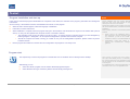
Program limits
The program has been configured according to the following limits:
Room/environment plan:
any with polygonal chain also used to approximate curved elements
Maximum dimensions:
X=5,000 m Y=5,000 m Z=5,000 m
Maximum number of luminaires:
Unlimited depending on RAM memory limits
Maximum number of luminaire types:
Unlimited depending on RAM memory limits
Page 7/94
To start
Program installation and start up
Notes
In the case of customized programs distributed from companies to the market, the activation of the program, photometric and catalog files
is automatic.
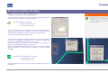
On the contrary, if the software has been downloaded from internet, run the program:
When the menu window appears, select the language of installation
Follow the on-screen instructions
When installation is complete, enter the program and type in the activation code received from Oxytech in the window that opens at
start up. To carry out this operation the computer must be connected to internet:
•
The Activation Code can only be used on one PC at a time. To use the program on another PC first you must deregister by
selecting Register + Deregister + Ok and repeat the Registration operation from the other computer
•
Should the computer be broken, leaving you unable to carry out the Deregistration operation, please contact OxyTech’s
Customer Service
Exit the program and relaunch to activate the new configuration: the program is now ready to use
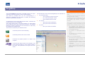
During installation both the program destination
folder and that of the data required for project
development will have to be defined.
Should these folders not be modified, the program
will use the default folders, visualized at the time of
installation.
More precisely, definition of the following folders is
required:
•
DATA, which is an installation folder with
write permission, for those operative systems
(e.g. Windows 7) that do not include the
possibility of writing in the PROGRAMS folder
•
DOCUMENT, where data related to the
projects and manufacturers’ catalogs is
gathered
Program start
The simplest way to launch the program is to double click on the LITESTAR 4D icon directly from the desktop.
When Litecalc is opened, the Liswin module will
also open automatically since it is necessary for
the correct functioning of the calculation program
and for selection of the manufacturers’ luminaires
in the Plug-ins.
Alternatively you can:
It is advisable never to close the application, but to
minimize it as an icon in the applications bar.
Select the Litecalc program from the window Start/All programs/Oxytech
Select Start/Run and type d:\Directory Name\LTS.EXE finally pressing Enter
Page 8/94
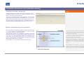
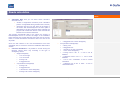
Data structure and updating
Notes
LITESTAR 4D is equipped with a single database (Oxydata.MDB),
differently from LITESTAR 10 in which there were 2 databases,
one catalog (MDB Access type) and one photometric
(Fotom.FDB).
The LITESTAR 4D database is the evolution of the LITESTAR 10
catalog database in which the functions for managing the
photometric files in the new OxyTech OXL format have been
integrated.
The OXL files are obtained by converting the photometric files into
international formats (e.g. EUL or IES), by means of the Photoview
module or using the Lisdat module.
For a more detailed explanation please refer to the Photoview
manual.
The MDB database is created by downloading the manufacturers’
Plug-ins (unmodifiable data) by means of the Liswin module or by
directly inserting the luminaire technical data into Liswin by means
of the Lisdat module, which can also be used to link the
photometries in OXL format to the sheets.
Inside the …\DB folder are found the data relating to each
individual manufacturer subdivided into subfolders.
The data structure consists of the following elements:
A series of non language sensitive documents, such as
product images
A group of folders named with the abbreviation of the
language (FRA for French, ING for English, ITA for Italian ….)
inside which all language sensitive files are saved, such as
catalog sections, instruction modules etc.
A Litepack folder inside which the OXL files are saved
Page 9/94
What OXL files are
The OXL file is an XML type file (files used in
many applications for data exchange) inside which
the following information is found:
•
the general lighting device data
•
the lamps data, including color
•
the dimensions and, if available, 3D file of the
luminaire
The technicaI data (catalog and photometries) of
the individual manufacturers present as Plug-ins,
are updated by means of the Liswin module, with
the command
Parametric product search via internet.
If the products you intend using are not present in
the Plug-ins, but you wish anyway to prepare a
catalog of your own, the Lisdat module should be
used to manually insert the data and link the
photometries.
The project step by step
Notes
The program allows essentially two project settings, as described below:
Free project: where each parameter is freely determined by the
designer.
In this case the designer is free to follow the project procedure that
he deems most suitable:
Create a calculation scene, that could be represented by any
object, such as:
•
•
An environment (interior/exterior), drawn in plan or in
3D view
An environment “traced” from a 2D .DXF imported as
background
Guided project: where the main parameters are “guided” by the
software and entered in the window.
This is the method used when for example it is necessary to
perform a calculation in accordance with the norms in force, as in
the case of tunnels and roads, or when simple, regular areas are
to be calculated.
In this case the procedure is as follows:
Select the type of calculation to be performed. The program
will then open a window to be completed
Enter the parameters required for the calculation
•
A working plane, or a number of working planes
Choose the luminaires
•
An object (furniture) inserted from the list
•
A complete 3D model imported from outside
Carry out calculations. In this case the software will
automatically set the parameters to be calculated
Enter and define the characteristics of the objects (materials,
reflectances, etc.)
Visualize the results and renderings
Configure the print outs
Insert luminaires
Perform calculations, setting the parameters to be verified
To access the various guided projects click on the relative icons:
Visualize the results and renderings
Configure the print outs
To access the roads module
To access the interiors module
To access the exteriors module
To access the exteriors module
Page 10/94
To carry out calculation it is no longer necessary,
as in the past, to draw a specific environment
(interior or exterior), where furniture and
luminaires are to be inserted.
More precisely, it is no longer necessary to have a
ceiling and a floor to verify a scene.
From this version of the program it is sufficient to
insert an object (furniture, working plane or room)
and a luminaire to be able to launch calculation.
All the objects belonging to the scene are in fact
evaluated in the same way, for example in the
visualization of Properties, and permit the same
transformations.
The project step by step
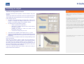
Free project
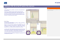
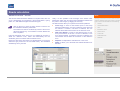
Once the program has been launched, to create a new
calculation scene it is essential to:
Select this icon if you wish to define an interior
environment.
By clicking with the left mouse button inside the operative area of
the design, it will be possible to draw the boundaries of the area
point by point and, using the Enter key, to close the room. The
program will then open a window in which to set the height of the
room and working plane, automatically extruding the walls and
ceiling. The reflection coefficients will be attributed in standard
mode but can always be modified by the user (for a more detailed
explanation see the chapter: Creation of an interior/exterior area).
Select this icon if you wish to define an exterior area.
By then clicking inside the operative area of the design, it will be
possible to draw the boundaries of the exterior area point by point
with the mouse and, using the Enter key, to close the perimeter. In
this case the program automatically removes the walls and ceiling
of the room, attributing standard reflection coefficients (for a more
detailed explanation see the chapter: Creation of an
interior/exterior area).
N.B.:
Once the area has been created, by selecting the area with the
right mouse button in the Scene TAB, on the left of the screen,
select Modify to access the Object Editor, where the surface
characteristics and reflection coefficients can be modified (for a
more detailed explanation see the chapter: Object Editor).
Notes
The objects may be inserted as:
Furniture present in the library. Insertion is made by
selecting the object and dragging it into the design area
(Drag&Drop)
3DS or OBJ Objects, created by the user, present in an
external folder. Also in this case insertion is made using
the Drag&Drop function
For a more detailed explanation see the chapters: Drag&Drop and
object insertion.
There is a third way of inserting objects:
By clicking on the extrude icon it is possible to extrude a
plan view object.
In this case, after selection the icon, click inside the operative area
of the design, the outlines of the plan view object can be drawn,
subsequently defining the height in the window which opens after
pressing the Enter key to close the object.
Also in this case, once the objects have been inserted it is possible
to access the Object Editor, by selecting the name of the object with
the right mouse button and selecting Modify.
Page 11/94
The program allows you to create an area by
“tracing“ a 2D DXF, imported into the design area
with the Drag&Drop function.
In this case once the .DXF file has been inserted,
you need to click on the icon corresponding to the
type of area you wish to create and trace the base
DXF (for a more detailed explanation see the
chapter: Insertion of a 2D .DXF file).
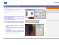
The project step by step
Notes
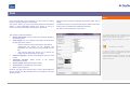
At this point, to insert the luminaires with which to verify
calculation, one of the following operations is possible:
Select the icon and drag the luminaire from the list of
favorites
Select the Liswin icon and drag into the project a
luminaire present in the list to which a photometry is
associated (FOT flag, in the relative column)
Select the Webcatalog icon and, after choosing the
manufacturer, drag the selected luminaire into the
project. In this case the luminaire will also be inserted
automatically into Liswin
Select the external folder icon and drag the photometric
file (.EUL or .IES)
Each luminaire may be rotated, moved, aimed and duplicated by
selecting the relative icons.
It will be possible at any time to edit a luminaire, so as to replace it
with another, change the flux, lamp or color filters, by selecting it
with the right mouse button inside the Scene TAB, on the left of the
screen, and selecting Modify (for a more detailed explanation see
the Chapter: Luminaires and color filters Editor).
Finally launch calculations and view the results:
As far as calculating luminaire flux is concerned, it
is important to underline that:
•
The luminaires inserted using the Liswin lists
are associated with a lamp. In this case
therefore the flux used in the calculation will
be that of the lamp (viewable in the part
related to lamps in the luminaires editor)
•
For photometries inserted as .IES or .EUL
instead, the program will use as default the
flux present in the photometric file
By clicking on the icon, the parameters to be calculated
can be set (with a flag) and then calculation can be
launched.
Once calculations are complete and the window is closed, the
results summary table automatically appears.
By selecting the individual items with the left mouse button and
clicking on the relative keys, the various graphs can be viewed.
The selected results will be inserted in the Results TAB on the left of
the screen.
Selection of View-Results in the design area will instead visualize
the dynamic rendering of the project .
By clicking on the Ray-Trace icon static images can be
created, and these will be saved in the ImpExp folder.
Finally, upon conclusion of the project, after all results have been
viewed and the renderings saved, the print module can be
accessed, using File/print, where the print logo and company data
can be set; select with a flag the data to be printed and view the print
preview.
For a more detailed explanation see the relative chapters:
Calculations, Results View, Rendering e Printouts.
Page 12/94
It will however be possible at any time to change
the flux, in the Luminaires Editor, either by typing a
new flux in the appropriate box, or by selecting
another lamp among those present in Liswin (for a
more detailed explanation see the chapter Change
lamp)
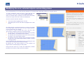
Drag&Drop
Notes
The term Drag&Drop means that it is possible to click on an object
and drag it into another position, where it will be released.
This means for example that if an icon corresponding to a
document is dragged from one folder to another, this will bring
about the transfer of the document.
To facilitate the use and make data insertion faster, LITESTAR 4D
includes extensive use of Drag&Drop.
This means that the files in the other modules or in other folders
can be selected, with a click of the left mouse button, and dragged
(keeping the button pressed) from the environment in which they
are situated into the design area.
“Environment in which they are situated” means:
The formats that can be used with Drag&Drop in the software are:
For photometric files:
•
.OXL, proprietary format of Oxytech
•
.EUL, standard European format
•
.IES, standard American format
For objects:
•
.3DS, open format of 3D Studio
•
.OBJ, open format of Wavefront
For plans:
•
.DXF, open format of Autodesk
Luminaires present in the Webcatalog
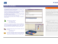
On an operative level to perform Drag&Drop you
need:
To open the origin environment (for example, as in
the figure alongside, a folder).
To select the file and keeping the left mouse
button pressed, drag it into the design area until
the forbidden sign becomes a broken line
rectangle.
As far as import of external objects is concerned it
is necessary to verify the accuracy of the 3D
models, before proceeding to import checking:
•
The orientation and conformity of the
perpendiculars (adjacent polygons must have
perpendiculars in the same direction [in-out)
•
The topological accuracy
•
The absence of superimposed faces and
vertices
•
The presence of uv coordinates in the case
of texture applications
Luminaires present in the Liswin module
Furthermore, it is always advisable:
Luminaires and objects present in a folder in the
computer
Luminaires and objects internal to the program, such
as the luminaire catalog or object catalog, stored in
the Library TAB, positioned on the right of the main
screen
Page 13/94
•
Not to import as a single file blocks of objects
that you want to manage separately, but to
separate them at origin.
•
To maintain the lowest number of polygons
possible with respect to the object you want
to represent.
•
In the case of conversion from parametric
objects (nurbs) to verify the accuracy of the
mesh generated and the number of polygons
generated
Introductory Notes
Notes
Calculation is based on the new, innovative
method of Photon Mapping, which replaces the
old method of Radiosity and is described in the
University of California site where it was
developed. For further information please consult
the site: http://graphics.ucsd.edu/~henrik/.
The Litecalc program is designed for the calculation of lighting
engineering parameters for lighting installations with luminaires
measured according to the C-Gamma system of CIE24 and CIE 27
Recommendations (road lights) and V-H (floodlights). The program
calculates the illuminances and luminances on all the surfaces
present in the calculation area, taking into consideration the
shadows created by them and natural light (if configured).
Calculation can be effected for interior and exterior environments,
roads and tunnels in accordance with the different norms.
Basic Concepts
In the figures alongside two luminaires are shown.
The red line represents gamma 0°. The origin of
this line represents the photometric barycenter.
Direct and Indirect Luminaires: A luminaire is normally
measured with the light emission plane perpendicular to the
luminous axis (Gamma 0°). The new data format instead allows
the composition of different photometric curves in the same
product and each of these can present an emitting surface directed
independently of the others.
To avoid mistakes of aiming, therefore, before use it is
recommendable to verify the type of data available.
Bounding Box: This is the parallelepiped box that encloses the
element under examination, whether a piece of furniture or a
lighting device. The environment itself can be visualized as a
bounding box.
Reflections: By reflection is meant the ability of the material to reemit the light it receives. In this program the reflections are no
longer evaluated only according to the Lambert method (perfectly
diffuse reflections), but also by means of the real functions of
material behavior BRDF (reflection, absorption, transmission) or
using the R and C reduced reflection factor tables (e.g. road
surfaces).
Page 14/94
Cartesian references and luminaire aiming
Cartesian axes and design grid
Notes
Objects are always associated with a triplet of Cartesian axes X, Y,
Z identified with the colors X=red Y=green and Z=blue which is
found in the center of the design area.
The area is characterized by a grid in which the space between
one intersection and the other is established as 1 m and at the
center of which the absolute origin of the Cartesian axes is fixed.
The snap step of the grid is fixed at 0.5 m by default, but may be
modified accessing the Settings window from the Tools menu.
Relative Cartesian Axes and Luminaires
Transformations (movements and rotations) of
individual objects are achieved using the absolute
axes of the object (these do not change as a result
of the rotations, but always remain oriented as the
absolute axes of the design).
Each luminaire is associated to its triplet of intrinsic Cartesian axes
x’, y’ and z’ relative to the absolute triplet X, Y and Z, on which
movements, rotations or aimings are based.
The photometric system of C- semiplanes, according to which the
photometry is referred, is integral with the system of intrinsic axes
x’,y’, and z’ of the luminaires, where the semiplane C-0°
corresponds with the plane formed by the axes z’ and the positive
part of y’. Each rotation around the intrinsic axes brings about the
rotation also of the group of C- planes.
The semiplane C-0° is, generally, perpendicular to the lamp.
If however the object should be rescaled, this
transformation would be carried out on the x’, y’
and z’ axes related to the object itself.
Therefore, should an item of furniture be rotated
on the absolute X axis by 90° and subsequently
rescaled on the relative z’ axis, the new
measurement would correspond graphically to the
absolute Y axis, by virtue of the previously effected
rotation.
The rotations of a luminaire or of an object
around the axes is considered positive when the
observer sees them take place in an anticlockwise
direction, seen from the positive side of the axis.
Page 15/94
Cartesian references and luminaire aiming
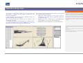
The photometric solid
To facilitate luminaire aiming, the program allows the photometric
solid of the single object to be viewed.
The photometric solid is the representation in 3D space of the
photometric emission of the luminaire. For this reason any
asymmetries can be represented.
The photometric solid on the left, shown in the illustration below,
represents a symmetrical photometry, whereas that on the right an
assymetrical photometry. In both cases the emission is downward.
The red line represents the direction of emission of the
photometry. The origin of this line is the photometric barycenter.
Notes
To view the photometric solid just click on the View menu (situated
on the left of each design frame) and select Photometric solid.
In the same menu by selecting Aiming, the direction is shown in
red.
Page 16/94
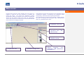
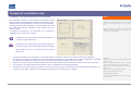
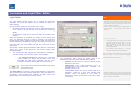
Main screen
Notes
Program launch opens the main operative area, from which it is
possible to access all the tools necessary for modeling and
viewing the project. The central area, dedicated to graphic
representation, allows four windows to be opened, for viewing the
objects from the different angles (front, side, top, perspective).
The two side windows on the other hand contain all the elements
and commands for managing the project.
Everything that concerns the construction of the calculation area is
considered an “element”: the elements, even if differing in nature
and geometry, maintain the same logical representation.
Thus whether they are environments, furniture or lighting devices,
the tools for handling them (properties table, transformations,
editor, etc.) will always be the same.
Dropdown menu bar
Operative area TAB
and icon bar
Module access
Project lists TAB
Operative design area
Object
insertion
and
properties TAB (dimension
and position)
Page 17/94
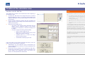
Dropdown menu bar and icon bar
Notes
The main operations can be performed by means of:
Dropdown menu bar: a click with the left mouse button on the reference menu (File, Edit, Modify, Create, Calculations, Tools, View,
Link, Help) and after scrolling with the pointer on the items (which will be highlighted in blue), a click on the command to be carried
out
Icon bar: to view
which commands are
represented by the icons on the bar, just position
the mouse pointer on them for a few seconds.
Icon bar: a click with the left mouse button on the command icon
In the lower part of the menu, the recent projects
are shown. Select one of the lines to open the
corresponding project.
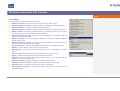
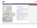
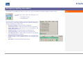
File Menu
For all operations linked with opening, exporting and saving a project:
New: to start a new project
Open: to open a project chosen from the archive
Save: to save the current project
Save as: to save the current project with name in a folder of the computer
Project Properties: to insert the data related to the project and the roads energy
certification data
Import: to import 3d models, such as .OBJ or .3DS, or to import a .DXF file
Save as package: to export a group of objects in a single file
Export GDF: to export the project in the proprietary format of the Politecnico of Milan
Export to PNT: to export the project and use the data in the estimate module
Printout: to print the project
Exit: to exit the program
Selection of Project Properties opens a window in
which you can insert the general data and the
roads energy certification data related to the
project
File icon bar
From left to right the commands are:
New: to start a new project
Open: to open a project chosen from the archive
Save: to save the current project in a folder of the computer
Printout: to print the current project
Page 18/94
Dropdown menu bar and icon bar
Notes
Mode Menu
To choose the program operation mode:
Free: to realize lighting engineering projects for interiors or exteriors
Emergency: to realize emergency lighting engineering projects in accordance with norms
Mode icons bar
From left to right the commands are:
Free: to realize lighting engineering projects for interiors or exteriors
Emergency: to realize emergency lighting engineering projects in accordance with norms
Rename: another way to rename the selected
object is to type the new name directly in the
properties window, on the right of the design area.
Edit Menu
For the general management functions of the project:
Undo: to cancel one or more operations (for example, to return a luminaire to its original
position after moving it etc.)
Redo: to refresh the project state after 1 or more cancellation operations
Duplicate: the object is duplicated and
superimposed on the original. To move it just
select it with the move command.
Undo/Redo: the command is shown as an icon
also on the right part of the screen between the
design area and the properties window.
Duplicate: to duplicate the selected object
Delete: to delete the selected objects
Rename: to change the name of a selected object
Group: to create a group of one or more objects, even of different types (lighting devices
or furniture). In this way the transformation of one or more objects will depend on a virtual
element (broken line), in whose barycenter the origin of the group axes is positioned
Parent: to associate two or more objects, in such a way that their transformation depends
on the object with which they have been associated and on which the origin of the axes is
positioned
Unparent: to separate the objects linked by the parent command
Page 19/94
Dropdown menu bar and icon bar
Notes
By selecting a number of objects present in the
tree, you can create a group by pressing the G key
or Parent by pressing the P key. In the second
case the reference object will be the first in the list.
Edit icon bar
From left to right the commands are:
Duplicate: to duplicate the selected object
Delete: to delete the selected objects
Rename: to change the name of a selected object
Group: to collect a number of objects in a group
Parent: to make the transformation of an object dependent on another object
Unparent: to separate the objects linked by the parent command
The modify commands can also be selected with
the keyboard:
Modify Menu
For all operations connected with modifying the objects (environments, luminaires, furniture,
etc.):
W: translation
E: rotation
Selection mode: to select an object
R: scale
Move: to move an object on the three Cartesian axes (x’,y’, z’)
Q: selection
Rotate: to rotate an object on the three Cartesian axes (x’,y’, z’)
T: aiming
Scale: to rescale an object on the three Cartesian axes (x’,y’, z’)
Aim: to orient the object in a direction (x’,y’, z’)
Capture aiming: to capture an object and orient it directing its axis to the destination
Reset transform: to cancel all transformations performed on the object
Object, Local, World: these represent the transformation reference system
Page 20/94
Dropdown menu bar and icon bar
Notes
Once the command has been selected:
Vertical icon bar
The same commands of the Modify menu are shown on the right of the screen between the
design area and the properties window. From top to bottom the commands are:
Selection mode: to select an object
Track: is obtained by pressing the left mouse
button in the design area. By moving the mouse
the drawing can then be moved in all directions.
Zoom in - Zoom out: is obtained by pressing the
left mouse button in the design area. By moving
the mouse upwards the drawing enlarges, by
moving it downwards it reduces.
Move: to move an object on the three Cartesian axes (x’,y’, z’)
Rotate: to rotate an object on the three Cartesian axes (x’,y’, z’)
Tumble: is obtained by pressing the left mouse
button on the design area. By moving the mouse
the drawing can then be rotated in all directions.
Scale: to rescale an object on the three Cartesian axes (x’,y’, z’)
Aim: to orient the object in a direction (x’,y’, z’)
Reset transform: to cancel all transformations performed on the object
Alternatively the commands can be performed with
the mouse and keyboard:
Undo: to cancel one or more operations
Track: CTRL + left mouse button, or mouse wheel
pressed.
Redo: to refresh the project state after one or more cancellation operations
Tumble: to rotate the perspective view
Zoom in - Zoom out: SHIFT + left mouse button
or mouse wheel zoom.
Track: to move the work area inside the window
Tumble: ALT left mouse button.
Zoom in - Zoom out: to zoom in and out inside the window
Toggle: to deselect the three previous commands (Tumble, Track, Zoom in - Zoom out)
Rescale: to fit the work area inside the window
Page 21/94
Dropdown menu bar and icon bar
Notes
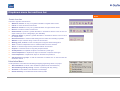
Create Menu
For all operations connected with creating a project:
Wizard for interiors: to create an interior environment (floor, walls, ceiling)
Advanced project for interiors: to open the wizard for creating an interior environment
Wizard for Exteriors: to create an external environment (floor)
Advanced project for exteriors: to open the wizard for creating an exterior environment
Wizard for roads: to perform a guided calculation in accordance with the norms in force
for simple roads (one or two carriageways, plus sidewalks)
Advanced projects for roads: to perform a guided calculation in accordance with the
norms in force for complex roads
Wizard for tunnels: to carry out a guided calculation in accordance with the simplified
tunnels norms in force
Advanced project for tunnels: to carry out a guided calculation in accordance with the
tunnels norms in force including Adrian diagram
Extruded furniture: to create a solid starting from the outline and extruding it upwards
Window: to open a window along a wall of the environment
Working plane: to add a working plane created by the user, of rectangular or irregular
shape
View: to create an independent view to visualize inside one of the windows
Sensor: to simulate a light sensor positioned inside an environment
Projector: to read the results on irregularly shaped surfaces. In this way the points are
projected on a reference surface grid
Duplicate with grid: to duplicate an object on the basis of a preset grid
Duplicate in circle: to duplicate an object on the basis of a preset circular grid
Duplicate in line: to duplicate an object on the basis of a preset line
Add luminaires to groups: to add the luminaires in tabular form or with the total flux
calculation method
Page 22/94
Dropdown menu bar and icon bar
Notes
Create icon bar
From left to right the commands are:
Wizard for interiors: to carry out a guided calculation of regular interior areas
Interior: to create an interior environment
Wizard for exteriors: to carry out a guided calculation of regular exterior areas
Exterior: to create an exterior environment
Roads Wizard: to perform a guided calculation in accordance with the norms in force for
simple roads (one or two carriageways, plus sidewalks)
Advanced Roads: to perform a guided calculation in accordance with the norms in force
for complex roads
Extruded furniture: to create a solid starting from the outline and extruding it upwards
Window: to open a window along a wall in the environment
Working plane, Custom: to insert a rectangular or irregular virtual working plane
View: to create an independent view to visualize inside one of the windows
Sensor: to simulate a light sensor positioned inside an environment
Projector: to read the results on irregularly shaped surfaces
Grid Duplication: to duplicate an object on the basis of a preset grid
Circular Duplication: to duplicate an object on the basis of a preset circular grid
Linear Duplication: to duplicate an object on the basis of a preset line
Add luminaires to groups: to add the luminaires in tabular form or with the total flux
calculation method
Calculation Menu
For all operations connected with calculating the lighting engineering values of a project:
Start Calculations: to launch value calculations (illuminances and luminances)
Start Rendering with Ray Tracing: to launch a rendering with Ray Tracing
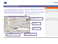
Set North: to orient North in the calculation of natural light
Results Summary: to visualize the results summary table
Page 23/94
Dropdown menu bar and icon bar
Notes
Calculations icon bar
From left to right the commands are:
Start Calculations: to launch calculation of the values (illuminances and luminances)
Cancel Calculations: to cancel previously calculated results
Start Rendering with Ray Tracing: to launch a rendering with Ray Tracing
Set North: to orient North in the calculation of natural light
Capture image: to save an image of the area in .BMP format. The image will be saved in
the ImpExp folder of the program
Results icon bar
From left to right the commands are:
Results Summary: to visualize the results summary table
View Pseudo Colors: to visualize rendering in color scale
Tone Mapping: to modify the perception of the image. This allows correction of any
discrepancies between what is expected and what the monitor or printer are able to
represent
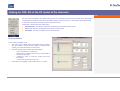
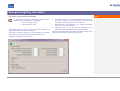
Selection of Print Settings opens the window
shown below where, by flagging the box alongside,
the following can be selected:
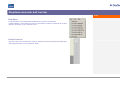
Tools Menu
For all operations connected with the creation, opening, export and saving of a project:
Show codes: to visualize the codes set by the
user relating to the luminaires, using the Rename
command
Measurement: to measure the length of a segment in the design area
Capture image: to save an image of the area in .BMP format
Pseudo colors: to visualize the rendering in color scale
Tone Mapping: to modify the perception of the image. This allows correction of any
discrepancies between what is expected and what the monitor or printer are able to
represent.
Scripting: to automate certain operations, by means of the Python language
Settings: to set the default working modes such as dimension, step and color of the design
grid
Print Settings: to set visualization of luminaire references in the print phase.
references will shown in the paragraph 2D plan View with references.
These
Oxl Editor: to link a photometric solid to the luminaire 3D
Page 24/94
Show Ids: to visualize the codes automatically
given by the program
Dropdown menu bar and icon bar
Notes
View Menu
For all operations connected with the visualization of windows in the work area.
It allows selection of the number and layout of the windows (vertical or horizontal) in the area
relative to the design, up to a maximum of four.
Vertical icon bar
The same View menu commands are shown on the right of the screen between the design area
and properties window, so as to always be visible.
Page 25/94
Dropdown menu bar and icon bar
Notes
It is also possible to access the individual modules
from the icons on the right of the screen in the
Libraries TAB
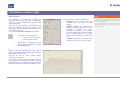
Link Menu
To access the other program modules:
Liswin: to access the catalog module
Photoview: to access the photometry view module
Lisdat: to access the data insertion module
Energy Calculation: to access the energy calculation window of the installation under
design
Help Menu
For all operations that may be of help in designing the project:
Language: to select the program language
Website: to access the OxyTech internet site
Norms and laws: to consult norms extracts on the OxyTech site
By selecting Program Path you can open three
different folders:
Encyclopedia: to access the concepts relative to lighting engineering measurements on
the OxyTech site
•
Program: to visualize the folders that contain
the files relating to program function
Tutorials: to download from Internet the automatic demonstration of the main program
functions
•
Configuration Data: to visualize the folders
that contain the files relating to program
configuration
•
Data: to visualize the folders that contain the
manufacturer data (.../DB) and the files saved
by the program (.../ImpExp e .../project)
Manual: to download manuals from the Oxytech site
Key Commands Help: to view the options that can be activated using key commands
Check license: to check license status
Update via Internet: to download the software updates via Internet
Communicate problem/report: to communicate a problem or report to OxyTech
Program Path: to open the folders relative to the program and the manufacturers’ data
About: for access to the window indicating the program version and any notes on
copyright
Page 26/94
Menu bar in the design area
Notes
These are the menus situated on the top left, in the window relating to the design views
View Menu
For all operations connected with viewing the project:
Fit View: to fit the view within the window
Wireframe, Flat, Smooth, Wire Solid: to view the design according to various graphic
options
Texture, Texture Result: to view the design and rendering complete with textures, if
connected
Results, Pseudo color: to view the rendering without texture or color scale once
calculation is complete
Grid, Axes, Ruler,Toggle draw compass: to view the grid, axes, ruler, or compass
Working Plane: to view the reference working plane
Photometric solid: to view the photometric solid of the luminaires
Surface labels: to view the number associated with each surface
Back-face-culling: to view the back-faces of an object
Aiming: this activates a red line on the luminaires that indicates where gamma 0° is
located
Normals: to view the normals of the objects’ surfaces
Display view information: this activates the view information on the bottom left
View Menu
To set the environment views:
Perspective: to view the design in three-dimensional perspective view
Front: to view the design in front view
Top: to view the design in plan view
Right, Left, Back, Bottom view:: to view the design in side views
Result Menu
In this window you can choose the results graphs previously selected in the results summary
window.
Page 27/94
If a graph is visualized in the design area, click on
the View menu to select the other graphs available
for the surface under examination.
Project lists TAB
Situated to the left of the work area, it shows all the information regarding the objects inserted in the project:
Scene
In this window, all the elements making up the environment (furniture, working planes,
luminaires, etc.). are found with tree structure
On selection of an object from the list with the left mouse button, the model in the design
area will be highlighted, while in the Properties window (to the right of the design area) the
properties regarding the object itself will appear
On selection of an object in the list with the right mouse button, it is possible both to edit its
properties (Modify) and to change its name (Rename). If the selected element is the area, it
will also be possible to modify the height of the working plane (Working Plane High
Definition), and to modify the perimeter of the room (Modify perimeter)
Luminaires
This allows the list of the different types of luminaires inserted in the project to be visualized
in the lower part of the window the characteristics of the luminaires are highlighted
the Select key allows selection of all the luminaires of the same type present in the project
Page 28/94
Notes
Another way to rename the selected object is to
type the new name directly in the Light Editor
window (for a more detailed explanation please
see the Light Editor paragraph), or by means of
the Edit/Rename menu.
By using the CTRL key plus the left mouse
button a number of objects can be selected
simultaneously.
By selecting a number of objects present in the
tree, a Group can be created by pressing G or a
Parent can be created by pressing P. In the
second case the reference object will be the first in
the list.
Project lists TAB
Notes
Materials
This allows the list of the materials present in the project assigned to the various surfaces of the
objects to be visualized.
Selecting a material present in the list with the right mouse button makes it possible to edit
its properties (Edit)
By modifying the characteristics of a single
material, automatically all the surfaces that refer to
that material will be updated, even if they belong to
different objects.
For example if the “Default” material is connected
to a surface of object A and to a surface of object
B, both present in the project, the two surfaces will
change
their
characteristics
automatically
according to the modifications made on the
“Default” material.
Once calculation is complete,
Summary automatically opens.
Results
This allows a list of the various results obtained through calculation to be visualized.
By selecting a result in the list with the right mouse button it is possible to open the relative
graph (Open), or close it (Close)
By clicking twice on the result the corresponding graph will be shown in the design area
The dropdown menu By Type allows you to choose the order of viewing:
Calc: for type of calculation performed (luminance, illuminance, etc.)
Obs: for observer, where calculations require the observer’s position
Surf: for the selected surface
In the lower part of the window the summary data relating to the calculated parameters are
visualized.
Page 29/94
the
Results
To insert the results obtained in the Results TAB
just select those of interest with the left mouse
button (to select more than one surface at a time
keep the CTRL button plus the left mouse button
pressed on the individual items) and click on the
keys of the graphs you wish to view.
Libraries and properties TAB
Properties
Notes
This allows the layers and properties of the selected object to be visualized and modified.
The Selection window permits the name of the object to be modified by typing the new
name directly in the box
The Modify key opens the window relating to the material characteristics of the object
The Transformation window allows modification of the dimensions, position and rotations
of the object by typing the value directly in the box
To display or hide a layer is important when there
are many objects in the project.
Object Layers and Lightings
The Object Layers and Lightings window allows a number of objects to be associated to a
determined layer, a new layer to be created or an existing one to be renamed or deleted and
luminaire lighting management.
Pressing with the right mouse button on a layer inside the window opens a window which
allows:
•
New Layer: to create a new layer, to which a new name will be given
•
Rename Layer: to rename an existing layer
•
Delete Layer: to delete an existing layer
•
Assign Selected Objects: to assign the layer to a selected object
Hiding the objects is a help in the modeling, in that
it frees the scene from unnecessary elements.
These objects can however still be selected and,
therefore, modified from the Scene tree on the left.
To block a layer instead allows you to avoid
“involuntary” transformations to the objects present
in the scene.
By clicking with the left mouse button on the symbols of the three columns you can:
•
display or hide the corresponding layer and the objects or luminaires associated to
it
•
block the objects associated to that layer, so they can no longer be modified or
moved (only objects)
•
exclude the objects or luminaires assigned to that layer by the calculation
•
change the color of the Tags assigned to the luminaires for lighting up.
Page 30/94
Excluding the objects from calculation instead
allows the calculation times to be reduced
especially during the preliminary verifications:
excluding certain pieces of furniture, therefore,
allows you to speed up calculation in this phase.
Libraries and properties TAB
Library
Notes
This allows viewing of the list of predefined objects and those of the most frequently used
luminaires.
To insert the objects in the project just select them
with the left mouse button and holding it pressed,
drag them into the design area (Drag&Drop). This
operation can be performed in all program
modules.
Clicking on the luminaires icon opens the library relative to the luminaires (image on the
left).
By clicking on the arrow of the dropdown menu, below the icons of the other program
modules it is possible to select the manufacturers present in the database.
To add new favorite luminaires to the list just access the luminaires TAB, on the left of the
screen, select the product and drag it with Drag&Drop into the library.
To do this it is important:
The Folder icon allows you to carry out
Drag&Drop operations from an external
folder, where photometric files or 3D
models have been saved.
that the luminaire library TAB on the right of the screen is selected
that the product is inserted in the current project
Clicking on the furniture icon opens the library relative to furniture (image on the right).
By clicking on the arrow of the dropdown menu, below the icons of the other program
modules, it is possible to open the different furniture archives present in the database.
Page 31/94
Flagging the List string allows you to view the list
of furniture and luminaires present in the library
and not the preview.
Shortcuts
Notes
The program allows certain operations to be speeded up using the keyboard.
To select an object just click on the object itself
with the left mouse button, inside the design area.
Rapid selection keys for modifications
These are the operations that allow object transformation. By pressing the associated key, the commands are activated, regardless of
whether the object to be transformed has been selected:
W: translation
E: rotation
R: scale
Q: selection
T: aiming
F: fit of the selected object or the bounding box of the scene
Space Bar: opens the rapid selection menu
More than one objects can be selected at a time
by keeping the CTRL key pressed and selecting
with the left mouse button the names of the objects
to be selected (in the Scene TAB on the left of the
screen).
Rapid selection keys for managing the operative design area
These are the operations that allow better management of the design area (e.g. zoom, pan, etc.). To activate them, the key associated
with the command and the left mouse button must be kept pressed in the design area:
Track: CTRL plus left mouse button, or mouse wheel pressed. Keeping the keys pressed and moving the mouse will enable you to move
the image
Zoom in - Zoom out: SHIFT plus left mouse button or mouse wheel. Keeping the keys pressed and moving the mouse will enable you to
enlarge the image
Tumble: ALT plus left mouse button. Keeping the keys pressed and moving the mouse will enable you to rotate the image
Rapid selection keys for area design
These are the operations that allow better management of the calculation area realization (they are active when an interior or exterior area
is being designed) . To activate them press the key associated with the command:
Back: to go back, that is cancel the last point fixed with the mouse
Enter: completes the step, that is it closes the environment and moves on to the next step
Esc: cancels everything and exits the environment creation tool
G: keeping the key pressed, the mouse pointer will position itself on the grid points (snaps) whose step can be defined in the
TOOLS/Settings window
O: keeping this key pressed, the mouse pointer moves orthogonally
X: if a background .DXF is being used, keeping this key pressed, the pointer will automatically position itself on the snap nearest the dxf
Page 32/94
When the area is edited, keeping the L key
pressed while inserting a new segment, the
segment will be created maintaining the wall
parallel to itself (for a more detailed explanation
see the Modify area and extruded objects chapter).
Operative design zone
Notes
The operative design zone consists of the area where the
environment is modeled and the objects necessary for the
calculation are inserted.
It also represents the area where the calculation results are
visualized, whether graphs or rendering.
The work environment can be divided into four windows, each
configurable separately.
To configure the number and arrangement of the design windows
just select the desired format from the Views menu or from the
vertical icon bar situated on the right of the operative area.
Each window has three dropdown menus which can be activated
with a click of the left mouse button:
View: this allows activation of the various types of
visualization of the object, both as regards the model view
and the results view
Camera: this allows configuration of a three-dimensional
view (Perspective) or 2D, Front, side and top views
To create an independent window you must select
Create in the menu and the command Camera.
Enter the camera menu from the selected window
and select the name of the camera just created.
At this point you can work from window to window:
for example it is possible to select a floodlight in
one window and aim it (with Pick Orient) in
another.
Results: this permits visualization of the calculated results
The View menu, inside the design area, allows
you to set visualization of the reference grid for the
design.
Select the Tools/Settings menu to access the grid
setup window.
In this way the dimension, step and reference grid
color of the design can be set.
Page 33/94
Creation of calculation area
Creation of an interior/exterior environment
Notes
Once the calculation area has been created it is
advisable to save the project using the File/Save
menu or the corresponding icon on the File icon
bar.
By environment we mean an external area of work (where only the
ground surface is represented) or an internal area (where the floor,
walls and ceiling are represented), in which to carry out calculation.
Creating an environment for interiors or exteriors allows us to view
the results graphs already subdivided in the summary into floor,
walls or ceiling.
To create an environment, in the first place, it is necessary to
establish the type of area to be modeled:
Remember that the central area of the drawing
allows the different Views to be visualized, with a
maximum of four windows
Selecting the icon with the left mouse button enables you
to draw an interior environment
Selecting the icon with the left mouse button enables you
to draw an exterior environment (without walls and ceiling)
After selecting the icon, and moving the mouse into the
design area:
The cursor will appear as a cross pointer, on which the X and Y coordinates of the point in which it is situated are highlighted
By clicking point by point, the single lines of the environment are drawn (for curved walls see the following paragraph). To facilitate
the creation of the perimeter, moving the cursor, the program will visualize the length of the line in meters
Clicking on the point of origin of the area will close the environment. Alternatively the environment can be closed with the Enter key
In this way the room height definition window will be shown, as explained in the following paragraph
Selecting the room with the right mouse button in the Scene TAB on the left of the screen and choosing Modify will enable you to
access the Object Editor, where surface characteristics and reflection coefficients can be modified
Commands that can be performed using the
keyboard:
Back: to go back, that is cancel the last point fixed
with the mouse
Enter: completes the step, that is it closes the
environment and moves on to the next step
Esc: cancels everything and exits the environment
creation tool
Space: opens the rapid choice menu
G: snap of 1/2 step on the grid
O: orthogonal movement
F: fit of the selected object or of the bounding box
of the scene
Page 34/94
Creation of calculation area
Inserting a curved wall
Notes
During area creation (whether interior or exterior) it is possible to
insert curved walls:
By positioning the pointer on the final point of the curve to be
created
By keeping the left mouse button pressed and moving the
pointer in the direction of the curve opening. In this way the
center coordinates and curve radius will be visualized
By releasing the right mouse button once the correct
dimensions of the curved element have been decided
Working plane height is set by default at 0.85m,
the standard height of a table.
Definition of room parameters
Often however, especially in exterior calculations,
the correct height should be moved to 0.10m.
Once room creation is complete, a window automatically opens in
which to type:
Room height in meters
To define the colors of the environment, click twice
with the left mouse button in the rectangle relating
to the surface color you wish to modify. In this
way the colors dialog window will open. The
program automatically proceeds to set the
reflection corresponding to the selected color. To
modify the value, just type the desired value in the
reflections box
Working plane height
Area reflections (walls, floor, ceiling)
Click on Ok with the left mouse button to close the window and the
previously defined window will appear.
The height of the room can however always be modified in the
Properties TAB, on the right of the design area, by typing the new
dimension in the field relating to Z, after selecting the area.
Page 35/94
Creation of the calculation area
Insertion of a 2D .DXF file
Notes
It is advisable to simplify the file before importing
it:
The simplest way to create a new environment is that of importing a
2D .DXF file to trace.
To import the .DXF file into the design area from an external
folder, Drag&Drop is used. To do this, just select the file in the
origin file and drag it into the program design area with the left
mouse button
Once it has been imported a window will open visualizing the
original dimensions of the design and the final dimensions in m
(used by the program)
At this point it is possible to set:
•
•
•
by removing all the parts that can weigh
down the file and that are unnecessary for the
comprehension of the drawing (crosshatching, shading, etc.)
•
by positioning the drawing origin directly on
0.0
•
by checking that the drawing scale is in
meters
The wrong import scale can cause serious errors
in the realization of the project, since the program
calculates the values using the metric scale.
the scale of the original design (remember that the
designs must be created in meters to be correctly
managed by the program), to rescale the design if not
in meters
Rescaling the drawing in the window will modify
the final dimensions of the drawing, shown in the
table, so as to verify that the set scale is correct.
the point of origin for inserting the file (Offset):
o None: to set the design as it is
o Bottom left: to position the left corner of the
design at the origin of the axes
o Centered axes X-Y: to center the design
where the axes intersect
o Customized: set directly by the user.
By flagging Use drop point the .DXF will be
inserted in the point at which the mouse has been
released in the design area
If a 3D .DXF is being imported, by flagging Use as
reference it will be possible to import the file as a
2D object.
By keeping the X key pressed, the pointer will
automatically position itself on the nearest snap in
the .DXF.
Leave the values in the window unchanged and click on the Ok
button to import the file without modifying it.
Subsequently you must select the type of environment you
want to realize (interior or exterior), in the way described in the
previous chapter
Finally just trace the perimeter of the background .DXF file to
produce the environment on which to perform calculation, and
set the height of the perspective view, in the case of an
interior, once the perimeter has been drawn
Page 36/94
Creating a working plane
Creating a rectangular or irregular working plane
Notes
By clicking with the right mouse button on the
name of the working plane in the Scene TAB it is
possible to rename the element or edit the
perimeter.
Selecting the Working plane icon with the left mouse
button allows you to create a regular working plane with
default size of 1x1m.
The dimensions can always be altered by editing the
fields in the Properties TAB.
Selecting the Custom icon instead allows the creation of a
working plane with customized shape and size, using the
same procedures as for area creation.
The working plane is assigned a default Layer on which all
operations described in the paragraph relating to the layer can be
performed.
All operations (e.g. movement and rotation) as described for objects
can be carried out on the working plane.
Page 37/94
Modifying the area, extruded objects and working planes
This command allows you to modify the area perimeter or an extruded object, eliminating, adding or moving the vertices.
Notes
Editing the perimeter opens the table with the
coordinates of the vertices and the height of the
object on the right-hand side of the screen.
To access modification, select the area or object with the right
mouse button, in the Scene TAB and select Modify Perimeter.
When an extruded object is selected, the model will be temporarily
moved to the origin of the axes to allow the modifications.
Click inside the boxes both to edit the vertices and
to modify the height.
After modifying the vertex coordinates, press the
TAB key to visualize the modifications in the
drawing.
Once the command has been selected:
The vertices will be highlighted with a red dot
The middle points of each side with be highlighted with a blue
square
When a vertex is selected, click on the Canc key
to delete it. On the contrary if you press the Ins
key, a new vertex will be inserted.
Click on the Ok key to accept the modifications, or
click on Canc to annul the modifications.
By keeping the left mouse button pressed on a vertex it is possible
to move the angle of the area; click on the blue square instead to
move the whole side in any direction.
If you click on a vertex or middle point, both a red and a blue
“ghost” will be visualized, as shown in the images beside:
The editable data are:
By selecting and moving (with the left mouse button pressed)
the blue square, a new segment will be inserted
By selecting and moving (with the left mouse button pressed)
the red dot, a new vertex will be created
By selecting and moving (with the right mouse button pressed)
the red dot, a new circular segment will be created, as shown
in the figure below
During modification the rapid selection keys for drawing the area
can be used, as explained in the Shortcuts chapter.
By pressing the L key during insertion of a new segment, the
segment will be created keeping the wall parallel
Finally press the Enter key to accept the modifications, whereas
pressing Canc the area or object will not be modified.
Page 38/94
•
Coordinates
and Y
•
Angle
between
two
segments
(during
modification the
previous segment
will
remain
constant and the
subsequent
segment will be
“moved”)
•
Segment length
•
Room height
X
Insertion of a window
Notes
So as to be able to calculate the contribution of natural light in the
interior environments, there is a tool that allows you to open a
window in a perimeter wall.
To create the opening the procedure below must be followed:
Select the relative icon (nel TAB o nel menù Crea) with
the left mouse button and move into the design area
The procedure requires the use of the Enter key to
confirm and if necessary Esc to annul the
command.
Select with a mouse click the wall in which to create the
opening. In this way a yellow rectangle will appear on the wall
Keep the left mouse button pressed inside the rectangle and
move the cursor up/down or left/right to create the dimensions
of the window
Press Enter to confirm the dimension
At this point, to position the window on the wall, keep the left
mouse button pressed and move the rectangle
Finally press Enter to confirm the position and open the
window
Page 39/94
Insertion of an object
Notes
The insertion of an object is effected with the Drag&Drop function in two different ways:
Selecting the icon of the object libraries in the right-hand
Library TAB and dragging the selected item of furniture
into the drawing.
Selecting the object from the Scene TAB tree on
the left, with a mouse click on the name, the object
will be selected also in the design area (the
surface lines will appear green).
Click on the dropdown menu (image on the right) to open the library
list, from which to choose the objects.
At this point just select the furniture with the left mouse button and,
keeping the button pressed, drag it into the design area
(Drag&Drop). When the mouse button is released the object will be
inserted in the object list in the Scene TAB and then it can be
repositioned, duplicated, rotated and scaled.
Furthermore, at the same time the properties will
be visualized in the right-hand Properties TAB,
where the object can be modified and rescaled.
By dragging the furniture as a .3DS or .OBJ file from an
external folder.
The object (.3DS or .OBJ) can also be inserted
using the File/Import menu. This function opens a
dialog window which allows you to choose the
object from inside the folders present in the
computer.
Once the file you want to import has been selected with the left
mouse button, you can drag it into the drawing.
At this point the management window described in the following
paragraph will open.
In this case the object will be inserted at the origin
of the absolute X, Y and Z axes.
The extruded object can be edited in the same
way as the area perimeter by clicking on the
furniture name in the Scene TAB with the right
button and selecting Modify Perimeter.
There is a third way of adding an object, selecting the
Extruded Furniture icon
•
in the Create icon bar
•
in the Create menu
In this way the object can be drawn directly in the design area,
clicking the vertices point by point, exactly as happens when
creating the environment (Creation of an interior/exterior
environment paragraph) and defining the height once the perimeter
has been closed.
Page 40/94
Inserting an object
3D files management window
Notes
Clearly, the more faces the model has, the longer
editing will be and also the calculation of the
model itself.
Once the model has been imported, a window divided in two parts
will open.
The first part called 3D Coordinates, shows the original dimensions
of the design and the final dimensions in m (used by the program).
In this TAB you can set:
By clicking in the area where the model is shown,
it is possible to perform all zoom, pan and rotation
operations already described:
the scale of the original design (remember that in order for the
program to manage the designs correctly they must be in
metres), to rescale the design if not realized in meters
Track: CTRL plus left mouse button, or pressed
mouse wheel. Keeping the keys pressed and
moving the mouse you can move the image.
the starting point for file insertion (Offset):
•
None: to position the model as it is
•
Bottom left: to position the left corner of the model at
the origin of the axes
•
Centred X-Y axes: to center the model at the
intersection of the axes
•
Customized: directly set by the user.
Zoom in - Zoom out: SHIFT plus left mouse button
or mouse wheel. Keeping the keys pressed and
moving the mouse you can enlarge the image.
Tumble: ALT plus left mouse button. Keeping the
keys pressed and moving the mouse you can
rotate the image
The rotation to be applied to the model on the X, Y, Z axes
Insertion using the Drop point, i.e. the point where the mouse
releases the model inside the design area when imported with
Drag&Drop.
In the Faces Tab it is possible to check the correct positioning of the
faces of the model.
When they are marked in white it means that the positioning is
correct, while if they are marked in yellow it means that the versors
are positioned in the opposite direction to that of observation. In
this case you will need to select the incorrect faces (either from the
list or by directly clicking on the model face) and click on the Invert
faces key, to change the position direction.
If you do not alter the values in the window, click on the Ok key to
import the file without variations.
The selected faces will be highlighted with blue
meshing on the model.
Page 41/94
Objects and materials editor
Object Editor
Notes
The object to be edited can be selected either by
clicking on the name in the Scene TAB, or directly
in the design area by clicking with the left mouse
button on the 3D element 3D.
The Object editor window allows you to modify the properties of the
individual surfaces relative to the furniture or environments. To
access the Editor, the object you want to edit must be selected.
At this point the window can be opened in two ways:
In both cases the name will be highlighted in blue
and the object in the drawing will have green
contours.
By clicking with the right mouse button on the name of the
object in the Scene TAB (on the left of the screen) and
selecting Modify
Selecting a surface in Editor, the faces of the
object of interest in the design area will be
meshed.
By clicking on Modify in the Properties TAB (on the right of the
screen)
Once the operation is complete, the window in the illustration
alongside opens, showing the list in which the surfaces contained
in the model and the material assigned to each of them can be
seen.
By keeping the Shift or Ctrl key pressed it is
possible to select multiple surfaces.
At this point, selecting the individual surface from the Surfaces
column, the material assigned to every single face can be modified.
If you select the material in the materials column, all those surfaces
which are associated with that material will be selected, so as to be
modified all together
To assign a material you can:
When an environment is created or an object is
inserted, Default materials are assigned. In the
case of 3D objects imported from outside often the
colors and materials will already be assigned.
Select Assign a new material, to create a new
material, typing the name of the new material in the
window that opens.
Click on the Ok key to open the material management
window (Editor) where the various parameters can be
set.
Example: if a tree is inserted, the surfaces relative
to the leaves are normally assigned in green, while
those of the trunk in brown.
Select Assign an existing material, to assign a material that is already present in the list to the selected surface
The name of the selected material, at this point appears in the Material Name box and its characteristics can be modified both in the
Material Editor window (following chapter), and in the Materials TAB on the left of the screen.
Page 42/94
Objects and materials editor
Material Editor
Notes
In color definition it is important to be careful to flag
not the Modulate color field, in case a colored
texture is assigned to the model.
The Edit Material icon allows you to open the
material modification window and set the
properties.
Otherwise the color of the texture and the default
color will be mixed.
The following operations can be performed in this window:
Modulating the color is important when a black and
which texture is assigned to a surface. In this way
the surface will take the previously assigned color.
Name: allows the material to be renamed by typing the new
name in the place of the existing one
Rename: allows the material name to be changed
Default color box: click twice to open the standard Windows
window that allows selection of a new color to be assigned to
the material
Select Texture: this allows you to assign a texture image to
the material, and to assign the main dimensions on X and Y
Remove texture: eliminates this association
Modulate color: by flagging the box the “transparency” of the
default color is set, so as to avoid mixing the set color with
that of the associated texture (selectable only if a texture has
previously been selected)
In defining the characteristics, the most important
data for calculation purposes is that of reflection,
since it can greatly influence the final results,
especially if a complete calculation is performed
(with inter-reflections)
Material type: allows you to select the type of material to
assign to the surfaces choosing between Generic,
Lambertian and R Table.
Reflections Properties Section: here you can set the
parameters that refer to the way in which the light interacts
with a material. More precisely they describe in what quantity
and form it is reflected, transmitted and absorbed
As regards the refraction index, reference can be
made to table data that can be found in various
sites, among which:
http://en.wikipedia.org/wiki/List_of_refractive_indic
es
As regards the other indices, currently no standard
reference tables exist.
Page 43/94
Objects and materials editor
Texture
Notes
It must be underlined that the texture is applied to
the material and not to the object itself. This
means that if there are a number of objects to
which the same material is assigned, by modifying
the parameters of an object, the parameters
relative to the other objects will automatically be
modified.
Click on Select Texture to open the dialog window in which to
select the image to be associated with the material.
In order to be used by the program, the files must be in the
following formats:
.JPG
.BMP
.TIF
The users can realize their own files, inserting them in the texture
management folder of the program Data/LibraryDB/Texture, where
new sub-folders can be created.
Once the material image file has been selected, return to the
general editor of the object to access the texture mapping editor
window, by clicking on Edit Projection.
To visualize the textures associated with the object
just click on the View/With texture menu situated
inside the design area.
The program tries to position the texture in the most suitable way.
The user can however at any time modify the position and
dimension of the surface texture of the object, by choosing from
the following options:
Repeat horizontally and vertically: flag the box to repeat
the image on the faces of the object, so as to cover all the
surfaces
Transpose: to transpose the image along the surfaces of the
object, vertically and horizontally. Click on the relative arrows
to change the number inside the box which in turn will change
the texture position
Scale: to scale the image, vertically and horizontally. Click on
the relative arrows to change the number inside the box
which in turn will change the texture position. Flag Uniform to
rescale the image both horizontally and vertically
Rotate: to rotate the image along the axes’ origin
Page 44/94
Insertion of a luminaire
The insertion of a luminaire takes place using the Drag&Drop function directly from the individual program modules:
If you select the object from the tree of the lefthand Scene TAB by clicking on the name with the
mouse, the object will also be selected in the
design area (the lines of the surfaces will appear
green).
By selecting the favorite luminaires icon from the righthand Library TAB and dragging the luminaire into the
drawing.
Click on the dropdown menu (image on the right) to open the list of
favorite manufacturers from which to choose the luminaires.
At this point just select the luminaire with the left mouse button and,
keeping the button pressed, drag it into the design area.
When the mouse button is released, the object will be inserted in
the object list in the Scene TAB on the left of the screen and then
can be repositioned, duplicated, rotated and scaled.
Furthermore, at the same time the properties will
be visualized in the right-hand Properties TAB,
where the object can be modified and rescaled.
By dragging the photometric file (.OXL) from the Liswin
module. The luminaire must be selected by clicking on the
photo of the photometry, relative to the chosen luminaire
By dragging the photometric file (.OXL) and catalog data
from the Webcatalog module
By dragging the photometric file (.OXL, .EUL or .IES) from
the Photoview module
By dragging the photometric file (.EUL or .IES) from an
external folder
Once the file you want to import has been selected with the left
mouse button, it will be possible to drag it into the drawing.
Also in this case when the mouse key is released, the object will be
inserted in the objects list of the Scene TAB and then can be
repositioned, duplicated, rotated and scaled.
Notes
Once the luminaires have been inserted they will be tagged with a
colored square which represents the lighting layer. To manage
the layers, see the Objects and Lightings Layers paragraph.
Page 45/94
Luminaire and Light Filter Editor
Light Editor
Notes
The object to be edited can be selected either by
clicking on the name in the Scene TAB, or directly
in the design area by clicking with the left mouse
button on the 3D element.
The Light Editor window allows you to modify the luminaire
properties. To access the Editor you must select the object you
intend editing.
At this point the window can be opened in two ways:
In both cases the name will be highlighted in blue
and the object in the drawing will have green
contours.
By clicking with the right mouse button on the luminaire name
in the Scene TAB (on the left of the screen) and selecting
Modify
By clicking on modify in the Properties TAB (on the right of the
screen)
When the operation is complete, the window shown beside will
open. The program gives the name by default to the luminaire
inserted in the project, visualized in the Scene TAB. This name can
however always be modified by clicking in the string on the top left
and typing the new name, which will then also be shown in the
Scene TAB.
The window contains all the information relative both to commercial
data (if the product is also present in the Liswin module), and
photometric data:
Changing a luminaire:
The commercial data regards the manufacturer, description,
code and image of the product and are not modifiable
•
The Change Luminaire key allows you to open the
Liswin module to change the luminaire. Once the
luminaire list has been visualized and the new
luminaire has been selected with a mouse click, just
Click on the icon to insert the luminaire in the place
of the previous one
The Other data key in the part of the window relating to commercial
data accesses the Liswin module while that in the part relative to
photometric data accesses the Photoview module, where the
graphs relative to the photometry can be viewed.
The photometric data include the polar graph of the
photometry and certain other editable data relative to:
•
Dimmer: this allows you to vary the intensity of light
between 0 and 100
•
Maint.Coeff.: with a value between 0 and 1, it
corresponds to the maintenance coefficient, the
default value is 0.85
•
Color Filter: allows the color of emitted light to be
modified. Select it to open the standard color
window, which will depend on the version of
Windows, in which to choose the color filter to apply
to the lamp
Page 46/94
•
If the beginning of the name of the luminaire
coincides with the code (that is it has not
been changed by the user) it will be
reassigned. If the names do not coincide, it
will be maintained.
•
The position and rotations of the previous
luminaire will always be maintained
Also in this case it is possible to change a luminaire
using the Drag & Drop function, dragging the
photometric file into the window.
When the color filter is selected, calculation is
performed taking into account the spectrometric
nature of light and the relative rendering will take
into account the interaction of the color of the light
with the color of the objects.
Luminaire and Color Filter Editor
Change lamp
Notes
The flux expressed in lumen represents
fundamental data for performing lighting
engineering calculation, without which verification
is impossible.
In the case of luminaires selected from Liswin, in the list, situated at
the bottom of the window, the lamps connected to the luminaire will
appear with the relative flux, inserted in the Flux box.
The program allows you to change the lamp associated with the
luminaire, or to associate a new one in the following way:
Select the lamp, shown in the table, with a mouse click
Click on Change lamp, accessing the Liswin module in the
lamps section
Select the desired lamp from the list, with a mouse click
Click on the icon to attach the new lamp, closing
the Liswin window and returning to the Editor
window.
When these operations are completed, the lamp will appear in the
Editor in place of the previous one.
The Total flux box shows the flux emitted by the
luminaire.
This means that, with traditional
sources, if two lamps are associated with a
luminaire, the Total Flux box will show the flux
shown in the Flux box, multiplied by two.
If, instead, you want to change not the lamp but only the luminous
flux, the desired value can be inserted directly in the Flux field
independently of lamp selection.
In this way the description of the attached lamp will not be modified
but only the reference flux for calculation will.
In this case, when modifying the flux by hand, care
must be taken to calculate the exact number of
lamps connected.
Page 47/94
Creating a list of favorite luminaires
Notes
From the right-hand Library TAB, select the favorite
luminaires icon to view the list of luminaires most used by
the user.
To be able to add a luminaire to a personal list you first need to
insert it in the project.
At this point, select it in the Luminaires TAB on the left of the screen
to be able to drag it into the list.
The luminaire will be visualized in a new archive, which will be
named according to the Manufacturer text in the photometric file
(which can be visualized and modified con Photoview).
In the case of an eulumdat file the image shown
as luminaire identification will have to be the
photometric curve.
To cancel a product from the lists must select it and click on the
Canc key.
If there was only one product in the list, at the next program start-up
the name will be eliminated from the list itself.
Instead in the case of an ,oxl file created with
Liswin to which a photo has also been attached,
the first image linked will be shown.
Page 48/94
Linking an .OXL file to the 3D model of the luminaire
Note
The .OXL file as described in the chapter Data structure and updating represents the file in which all the data related
to a luminaire are inserted. In this file it is possible to directly connect the .OBJ or .3DS model of the luminaire itself.
To do this first select the OXL Editor from the Instruments menu.
At this point a window with three TABs opens:
3D Coordinates: with which to define the coordinates and dimensions of the model
Faces: with which to correctly position the faces of the 3D model
OXL Editor: with which to link the l'OXL to the 3D model.
3D Coordinates
In this TAB it is possible to set:
The scale of the original design (remember that the designs
must be created in meters for the program to manage them
correctly),to rescale the design if not in meters
The axes starting point for inserting the file (Offset):
•
None: to position the model as it is
•
Bottom left: to position the left corner of the model at
the axes starting point
•
Centred X-Y axes: to center the model at the axes
intersection
•
Customized: set directly by the user.
The rotation to be applied to the model on the X, Y, Z axes.
Page 49/94
Linking an .OXL file to the 3D model of the luminaire
Faces
Notes
The selected faces will be highlighted with blue
meshing in the model.
In the Faces Tab it is possible to check the correct positioning of
the model faces.
When they are marked in white it means that the positioning is
correct, while if they are marked in yellow it means that the versors
are positioned in the opposite direction to that of observation. In
this case you will need to select the incorrect faces (either from the
list or by directly clicking on the model face) and click on the Invert
faces key, to change the position direction.
OXL Editor
This allows the model edited in the previous TABs to be linked to
the actual luminaire photometry.
Once the .OXL file has been imported using Drag&Drop, in this
section you can move and rotate the photometry, using the
Cartesian coordinates on the bottom left. In some cases movement
is necessary to correctly position the luminous center of the
photometry, in the central point of the luminaire luminous area.
A correct model should separate the surfaces of the luminous area
from the others. In this way by selecting these surfaces from the list
on the top left and clicking on Set as emitter, it will be possible to
“color” these surfaces white to simulate the illuminated parts.
Once these operations have been performed click on Save or Save
with Name and the .OXL file will be overwritten on the previous one
or saved with a new name.
Page 50/94
Wizard for interiors/exteriors
Notes
By means of this function you can insert a project step by step,
setting the area parameters (which may be rectangular or Lshaped), selecting a luminaire, entering the installation type data
(rows and columns), or the average illuminance value to be
attained (total flux calculation).
This procedure can be applied both to interior and to exterior
projects.
To access the window, you must select Wizard for interiors and
exteriors from the Create menu.
Or click on the interiors icon in the Create icon bar
Or on the exteriors icon
Selection of room type
(rectangular or L-shaped)
Room
dimensions
Room and working
plane height
Room
parameters
Page 51/94
reflectance
If the wizard for exteriors is selected it will not be
possible to set the area height and wall and ceiling
characteristics.
Wizard for interiors/exteriors
Setting the room parameters
Notes
After opening the window, you must:
select the room/area type, by clicking on the relative box,
choosing between:
•
Rectangular (dimensionsX,Y)
•
L-shaped (dimensions X, X1, Y, Y1)
set the dimensions of the selected room by typing in the
values inside the relative boxes on the right of the window (if
an L-shaped room is chosen, the fields relating to X1 and Y1
will also be activated);
set the value of the room height (only for interiors) and that of
the working plane.
Subsequently the parameters relating to the characteristics of the
area surfaces will need to be set:
by clicking with the left mouse button inside the colored box
relating to the floor (walls and ceiling). In this way the
windows dialog window for surface color selection will open.
After selecting the color, press the Accept key and the
program will also automatically update the reflectance factor
which will still be modifiable at any time;
by typing in the desired coefficient in the Reflectance box,
relative to the surface to be modified, if you do not wish to
change the color, but only the reflectance coefficient.
Once data entry is complete, click on the key:
Terminate to display the room inside the design area;
Cancel to interrupt the operation
Forwards to move to the luminaire entry window (for a more
detailed explanation regarding luminaire entry see the Insert
luminaires in groups chapter).
Page 52/94
Inserting luminaire groups
Notes
A fast way of inserting luminaires is the Add luminaires in groups
window. Using this window luminaires can be added automatically
whether by setting an illuminance value, or by typing the
installation data, interdistance, height, etc. as long as these are
regular. In the first case the luminaires will be automatically added
to the environment and the software will set the installation data
(interdistance) in relation to the number of luminaires calculated.
In the second instead the luminaires will be set out by row and
column in the environment, according to the parameters set in the
table.
The window can be accessed directly from the Wizard for interiors
or exteriors window. Alternatively, to access the window select
Add luminaires in groups from the Create menu
In order to use the window it is first necessary to
have created a reference environment for
calculation, unless you access the entry window
using the wizard procedure (for a more detailed
explanation see the Wizard for interiors/exteriors
chapter).
Or click on the icon in the Create icon bar
Inserting luminaires by row
and column
Luminaire
summary data
Lamp summary
data
Flag to delete luminaires present
in the project
Luminaire insertion with the
total flux method
Page 53/94
The Delete previous luminaires flag allows you to
delete the luminaires previously inserted in the
project. If you remove the flag the luminaires will
not be deleted and will contribute towards the
calculation.
Inserting luminaires in groups
Notes
To carry out the calculation a reference luminaire must be selected:
Pressing the Change Luminaire key accesses the Liswin module and the
luminaire can be selected, as explained in the Light Editor and Change Lamp
paragraph
If the photometry is not present in the Liswin lists it is however always possible to
import a luminaire using the Drag&Drop function from the other program modules
or from an external folder, dragging the reference file into the window
When luminaire selection is complete the type of insertion can be selected (by row and
column or with the total flux method).
Add luminaires by rows and columns
This function allows you to add the luminaires to the environment regularly by row and
column, by completing the table:
Luminaire Distance X-Y [m]: this is the interdistance between two consecutive
luminaires in the same row, both along the X and the Y axis
Height [m]: this is the height at which the luminaires are positioned, measured from
the floor to the luminous center of the luminaires
Relative Rotation Z [°]: this is the rotation of all the luminaires around their own
vertical axis passing through the luminous center
Number of Luminaires X-Y: this is the number of luminaires along the X and Y
axis
Position of First Luminaire X-Y [m]: this is the postion of the first luminaire with
respect to the order of the axes
Total Number of Luminaires: this is the total number of luminaires to be inserted
The data must be inserted in the left-hand column (with the white background fields) while in the right-hand column the program
reproduces them calculating and completing the remainder should those inserted be insufficient.
Should they be insufficient an error message is shown on the right (Insufficient Data). If instead the data inserted is incompatible the
program shows on the right the message Incompatible Data. This occurs when, for example, the number of luminaires defined along X and
Y are 2x2 whereas in the box the number of luminaires has been set at 6.
In the central part, between the two columns is the Flanked column with two boxes in correspondence with the two possible distances
between the luminaires (X and Y): if one of the two boxes is flagged the luminaires will be flanked in a continuous row in the environment.
Press the Ok key to position the luminaires in the environment so as to be able to carry out calculation (Calculations Chapter).
Page 54/94
Should the area under examination have irregular
geometry and one or more luminaires appear to
be outside the area, the program will automatically
delete them.
Inserting luminaires in groups
Total flux method
Notes
The luminaire number calculation is performed in
the parallelepiped (bounding box) that contains it;
it can therefore happen that, in irregular areas,
some luminaires may appear outside the area: in
this case the program will proceed to delete them
automatically.
This function allows you to determine the number of luminaires to be inserted in the
environment, given the average illuminance value to be obtained on the working plane
and to position them automatically and regularly by rows and by columns.
Average illuminance: this is the illuminance you want to achieve on the working
plane inside the area
The Norms key allows access to WebOxy where comments on the reference norms can
be found, from which to establish the illuminance values for the individual areas.
Pressing the Apply key, the program shows, at the bottom, the theoretical number of
luminaires required for calculation and the relative positioning by rows and columns.
If the calculated number of luminaires should not be divisible in a regular way by rows
and columns, the program will automatically add or delete luminaires to make the
configuration regular.
By flagging Delete Previous Luminaires, the luminaires present in the area will be
automatically deleted.
Once data insertion is complete, press the Ok key to position the luminaires in the area,
so as to be able to perform calculation (Calculations Chapter).
Simplified calculation is carried out according to the algorithm described in CIE 52 Recommendations (Total Flux) and therefore takes no
shadows or furniture into consideration and is only valid in the following conditions:
in parallelepiped rooms
in the case of not highly concentrating luminaires
when the area surfaces, particularly the floor, do not have a reflectance value greater than 75%
Applying this method outside the foreseen limits, although possible, may result in serious errors in the calculation of results.
It is therefore advisable to use this calculation in the initial project phases, given its high speed, but it cannot be considered the only
verification.
Page 55/94
Transformations
Move
Notes
There are two ways of moving an object (furniture or luminaire):
By manually editing the new position (Pos) on the X, Y and Z
absolutes in the properties TAB
Each object is associated to its triplet of intrinsic
Cartesian axes x’ (red), y’ (green) e z’ (blue), on
which to effect the transformations
By means of the Move icon:
•
Positioned on the vertical bar on the right of
the design area
•
In the Modify menu
The command can also be selected using the
keyboard by pressing the W (move) key
Once the command has been selected, a triplet of Cartesian axes
will appear on the object with an arrow on the ends and three
“pointers” on the planes of pertinence of two axes.
In this way two operations will be possible:
In order to activate the command, the object must
first be selected.
By clicking on one of the Cartesian axes (blue, green, red) and
dragging it, the object will be moved in the direction indicated
by the axis itself
By clicking on the pointer positioned between two axes and
dragging it, the object will be moved in the two directions
indicated while keeping the third fixed
Page 56/94
Transformations
Rotate
Notes
There are two ways of rotating an object (furniture or luminaire):
By manually editing the final rotation (Rot) in the properties
TAB
Each object is associated to its triplet of intrinsic
Cartesian axes x’ (red), y’ (green) e z’ (blue), on
which to effect the transformations
Using the Rotate icon:
•
positioned on the vertical bar on the right of
the design area
•
In the Modify menu
The command can also be selected using the
keyboard by pressing the W (move) key
Once the command has been selected, a triplet of Cartesian axes
will appear on the object in the form of an arch in the direction of
rotation:
In order to activate the command, the object must
first be selected.
By clicking on one of the axes (blue, green, red) and dragging
it, the object will be rotated in the direction indicated by the
axis itself
Page 57/94
Transformations
Scale
Notes
There are two ways of scaling an object (furniture or luminaire):
By manually editing the scale factors (Scale) in the properties
TAB
Each object is associated to its triplet of intrinsic
Cartesian axes x’ (red), y’ (green) e z’ (blue), on
which to effect the transformations.
Using the Scale icon:
•
positioned on the vertical bar on the right of
the design area
•
In the Modify menu
The command can also be selected using the
keyboard by pressing the W (move) key
Once the command has been selected, a triplet of Cartesian axes
will appear on the object with a cube on the ends and three pointers
on the planes of pertinence of two axes.
In this way two operations will be possible:
In order to activate the command, the object must
first be selected.
By clicking on one of the Cartesian axes (blue, green, red) and
dragging it, the object will be scaled in the direction indicated
by the axis itself
By clicking on the pointer positioned between two axes and
dragging it, the object will be scaled in the two directions
indicated keeping the third fixed
Page 58/94
Transformations
Aim
Notes
Each object is associated to its triplet of intrinsic
Cartesian axes x’ (red), y’ (green) e z’ (blue), on
which to effect the transformations.
To orient an object (furniture or luminaire) it is necessary to
Select the Aim icon positioned:
•
on the vertical bar on the left of the design
area
•
in the Modify menu
The command can be selected also using the
keyboard by pressing the T (aim) key.
In order to activate the command the object must
first be selected.
Once the command has been selected, a triplet of Cartesian axes
will appear with an arrow on the ends and three “pointers” on the
planes of pertinence of two axes. The origin of the axes is
positioned on the point “of arrival” of the aiming.
Two operations are thus possible:
By clicking on one of the Cartesian axes (blue, green, red) and
dragging it, the object will be oriented in the direction indicated
by the axis itself
By clicking on the pointer positioned between two axes and
dragging it, the object will be oriented in the two directions
indicated keeping the third fixed
Another way of orienting is to select the Capture Aiming command
from the Modify menu.
This command allows you to capture an object and orient it aiming
its axis towards a destination. It allows for example a luminaire to
be aimed towards an object.
To carry out the operation you must:
Click with the mouse on the object to be aimed so as to
“capture it”
Click on the destination surface to orient it. When you click on
the destination surface, a triplet of values appears near the
mouse, indicating the position of the final point
Press Enter to confirm the position
Page 59/94
Object Duplication
There are several ways of duplicating an object (luminaire, furniture or working plane) in the drawing:
Notes
Duplicate
By clicking on the icon (or selecting the command from the Edit
menu) the selected object will be copied on top of itself and it will
be possible to move it using the Move command.
By selecting with the right mouse button the
duplication request and clicking on Modify, the
duplication mask will be re-opened allowing you to
modify the duplication data of the inserted objects.
Grid position
By clicking on the icon (or selecting the command from the Create
menu) the selected object will be duplicated according to a grid,
where the total number of objects on the X and Y axes and their
inter-distance will have to be set.
The parameters in the table represent:
Num x: the number of objects on the x axis
Num y: the number of objects on the y axis
Step x: the distance between one object and the next on the x
axis
Step y: the distance between one object and the next on the y
axis
The parameters can also be modified by clicking on the wheel and
rolling the cursor.
Once duplication is complete, on the Scene TAB the new group
will appear in the list, which it will then be possible to modify, as a
group, selecting the name in the list, or as single objects, selecting
the object to be modified directly in the drawing and clicking on
Modify in the Properties TAB.
Page 60/94
Object Duplication
Notes
By selecting with the right mouse button the
duplication request and clicking on Modify, the
duplication mask will be re-opened allowing you to
modify the duplication data of the inserted objects.
Position in circle
By clicking on the icon (or selecting the command from the Create
menu) the selected object will be duplicated according to a grid,
where the total number of objects and the duplication radius must
be set.
The parameters in the table represent:
Num: total number of objects
Align: align to center
Radius: duplication radius
The parameters can also be modified by clicking on the wheel and
rolling the cursor.
Once duplication is complete, on the Scene TAB the new group
will appear in the list, which it will then be possible to modify, as a
group, selecting the name in the list, or as single objects, selecting
the object to be modified directly in the and clicking on Modify in
the Properties TAB.
Page 61/94
Object Duplication
Notes
By selecting with the right mouse button the
duplication request and clicking on Modify, the
duplication mask will be re-opened allowing you to
modify the duplication data of the inserted objects.
Position in line
By clicking on the icon (or selecting the command from the Create
menu) the selected object will be duplicated according to a grid,
where the total number of objects on the X and Y axes and their
inter-distance will have to be set.
The parameters of the table represent:
Num: total number of objects
Step: distance between one object and the other
Start: distance of the line starting point from the Cartesian
axes
Tilt: tilt of the luminaires on the X axis
The parameters can also be modified by clicking on the wheel and
rolling the cursor.
Once duplication is complete, on the Scene TAB the new group
will appear in the list, which it will then be possible to modify, as a
group, selecting the name in the list, or as single objects, selecting
the object to be modified directly in the drawing and clicking on
Modify in the Properties TAB.
Page 62/94
Calculation of natural light
Orient North
Notes
The calculation of natural light supplies the
parameters necessary for evaluating the contribution
of the sun, in terms of illuminance, inside the areas
under examination.
To have an accurate analysis, it is necessary first to
define the orientation of North with respect to the
environment and especially to set the position of the
sun throughout the day.
To access the Sun & sky settings window, select:
The Orient North icon positioned:
•
In the icon bar in Calculations
•
In the Calculations menu
The parameters to be set in the table are:
Orientation: this is the parameter that
identifies North, by means of angle
settings
Sunlight Settings: this activates the
setting of the day and time at which
calculation is desired, and allows
terrestrial coordinates to be defined.
Here the Latitude and Longitude positions
can be inserted directly, or the preset
values can be selected from Nation and
City
Turbidity: this allows the setting of the
clearness of the sky, from clear to cloudy
Alternatively it is possible to access
the calculations window by selecting
Sun & sky settings
When the values have been set in the table, click on
OK and the compass rose will appear with orientation
North inside the design area.
The sun will also be shown (yellow sphere)
positioned in the set hour.
At this point it will be possible to calculate with only
the contribution of natural light, without inserting
lighting devices, or to complete the project and verify
the levels of illuminance with the contribution of both.
Page 63/94
Leaving 0° as the value in the orientation box,
North will be oriented upwards (Y axis), looking at
the plan view drawing.
For positive angle values, North will rotate in an
anticlockwise direction, for negative values it will
rotate clockwise.
Insertion of a sensor
Notes
Since to all effects the sensor is an object, its
dimensions and position in the environment are
controlled with the keys of object Transformation
or in the Properties TAB window.
The “sensor” simulates a genuine illuminance sensor placed inside an
environment and can be associated to a number of lighting devices, so as to
check the variations in the quantity of light emitted in specific areas.
To access the Sensor Editor window it is first necessary to insert an sensor in
the environment using:
The Sensor icon positioned:
•
in the Create icon bar
•
in the Create menu
At this point to edit the sensor you must:
Select the sensor in the Scene TAB on the left of the design area and
select Edit
Click on Modify in the Properties TAB on the right of the design area
If the Value box shows the value -1 it indicates a
value outside the sensitivity range of the
instrument.
The first window Controlled lights allows a number of lighting devices to be
associated to the sensor, so as to realize a dynamic control system.
Association is performed by keeping the sensor properties window open and,
after selecting the luminaires (from the list on the left in the Scene TAB or
directly in the drawing), by pressing the Add key:
The Remove key deletes the selected luminaires from the list.
The Curve of response box allows the setting of data relating to the sensitivity
of the sensor, such as:
Curve Type peculiar to the sensor
Cone Angle that therefore identifies the area of reception of the sensor
Accuracy that is the precision with which the sensor reads the illuminance
The Measured value box shows the average value read by the sensor in the
Value box.
The position of the Sensor can be moved in the drawing and therefore the value
of illuminance in that point can be read by pressing the Recalculate key.
Page 64/94
Calculations
Calculation Setup
Notes
After completing insertion of the elements that go towards realizing
the lighting engineering verification, calculation can be started by
means of:
The icon Start Calculations positioned:
•
in the Calculations icon bar
•
in the Calculations menu
To select the calculations you wish to carry out
you must flag the box according to the type of
calculation desired.
When the Calculation Setup window is opened, calculation of the
illuminances is set by default.
In Mode definition two different types of calculations can be set:
The keys on the right allow management of the
observers in those calculations that require them
and represent:
Direct component: calculation of only direct illumination
Direct + Indirect component: complete calculation of
reflectances
The program automatically configures a results visualization grid.
Removing the flag from Automatic grid, it is however possible to
configure a customized grid in longitudinal and transversal
directions.
In this way it is also possible to decide how to position the grid in
the space:
Edit the observers inserted to modify the
data
Add an observer
Edit the observers inserted to modify the
data
inside: in which the first point of the grid is positioned in the
center of the surface
When a new observer has been inserted, the
coordinates will appear in the central part of the
window.
on edge: in which the first point of the grid is positioned on the
edge of the surface
According to the type of calculation, the modifiable
fields will be activated in the observer definition
window.
By pressing the Start key, calculations start up, showing the
progress in a percentage in the Calculation Progress bar.
On conclusion press the Done key to close the window.
Page 65/94
Calculations
Inserting an observer
Setting observers allows you to carry out those calculations in
which the position and direction of vision occupy a fundamental
role, such as for example luminance calculation of non Lambertian
surfaces or UGR calculation of interior areas.
Notes
To add a new observer, firstly the calculation to be effected must
be selected by flagging the appropriate box.
Secondly, click on the relative icon, thus opening the setting
window:
For a more detailed explanation of observer
settings for each individual calculation see the
chapter List of available calculations.
Press the icon to add an observer.
The icon is situated on the right of each type of calculation
in which an observer may be added
On the operative level, firstly the observer’s eyes
position must be set, obtaining it graphically from
the drawing, in relation to the X, Y and Z absolute
reference coordinates of the design.
The setup window is made up of three distinct sections:
General, which indicates:
•
the observer name, modifiable using the Rename key
•
the type of calculation (Luminance, Glare, etc.)
Secondly the observation point must be sent
using the Cartesian coordinates (for Place) and
angles (for Direction). In both cases to define the
correct coordinates reference must be made to the
absolute Cartesian axes.
Eyes position: which indicates the position of the observer in
Cartesian coordinates
Observation point: which indicates the direction of
observation, that is the point towards which the observer is
looking
To define the direction, one of the two following parameters must be
set by flagging the box to the side of the string:
In the first case, the calculation planes are all in
the direction of the observer, in the second the
planes in the various points are all oriented in the
same way according to the β (on the horizontal
plane) and α angles (tilt angle): this means that
the directions of observation are all parallel to
each other (infinity observer).
By Place: where to insert the x,y,z Cartesian coordinates of
vision. More simply we could say they represent the
coordinates of the point towards which the observer is looking
By Direction: where to insert a horizontal (Beta) and a vertical
(Alpha) angle of vision. In this case the point of observation is
calculated by setting two angles, where x and y are
represented by the horizontal angle (Beta) and z by the vertical
angle (Alpha)
Page 66/94
Calculations
List of available calculations
The program allows different types of calculation to be performed
such as:
Sun and sky settings: this allows you to calculate the
contribution of natural light (for a more detailed explanation
see the chapter: Calculating natural light)
Illuminance [lux]: on all surfaces
Vertical illuminance [lux]: these illuminances are calculated
in the 4 directions +X, -X, +Y and -Y parallel to the Cartesian
axes on vertical planes situated in the points of the calculation
grid at the height of the working plane
Light pollution: this allows you to verify the percentage of
quantity of light, in exterior installations, that is lost in the sky
Notes
Luminance [cd/m2]: Calculation of the luminance is
dependent on the type of reflection defined for the surface
whether diffuse reflection or Lambertian luminance (for the
surface only one reflection factor has been defined) or real (a
table of reduced reflection factors is defined for the surface
depending on the angle of observation and the incidence of
the luminous ray: these tables are used in the design of road
lighting installations). Definition of the position and direction
of observation makes sense in the calculation of the
luminances of road surfaces or non Lambertian surfaces. In
the other cases calculation of the luminance is independent
of the observer’s position
Cylindrical illuminance [lux]: these illuminances are
calculated on the cylinder situated in each of the calculation
grid points at the defined height. These illuminances do not
correspond, as may be thought, to the average of the 4 vertical
illuminances in the 4 directions but are proportional to them for
less than a factor of 2/π
Semi-cylindrical illuminance [lux]: these illuminances are
calculated on the semi-cylinder situated in each of the
calculation grid points at the defined height: by selecting the
calculation, the height will be automatically visualized in the
cylindrical illuminance box (1.5m), where it can be modified.
The semi-cylindrical illuminance is dependent on the position
of the observer and consequently, when it is selected, clicking
on the + key opens the observer settings window. Here you
can define, alternatively, either the position of the observer (in
this case the illuminances are calculated in the direction of the
latter) or the direction defined by means of the β [°] angle,
deviation angle (in this case the illuminances in the various
points are all parallel to each other according to the direction
defined). The rotations origin axis for evaluating the angle is
the X positive axis
Page 67/94
Luminance Calculation
Calculation of the luminances in road installations
in accordance with the norms is always effected
with the observer situated at the fixed height of
1.5 m.
Calculation Times
It is difficult to define a precise calculation time
since it depends on a series of factors, among
which:
•
the number of surfaces making up the
environment
•
the number of luminaires inserted
•
the number of pieces of furniture and their
surfaces
•
whether or not evaluation is made of the
shadows created both by possible recesses
in the walls and by the inserted furniture
Calculations
Notes
Glare: activating luminance calculation, it is also possible to
activate that of glare types which, depending on the kinds of
installation, are:
•
Interiors: the program carries out calculation of glare
evaluation parameters such as UGR (Unified Glare
Rating), VCP (Visual Comfort Probability) and CGI (in
accordance with CIE Recommendations 55). The
program allows the insertion of more than one observer
using the position insertion window (Cartesian
coordinates x, y, z) and observation direction window
(Cartesian coordinates x’, y’, z’ or β angles, for
deviation, and α for tilt). Access to the insertion window
is gained by clicking on the + key
•
Roads: the program in this case carries out calculation
of the parameters G (discomfort glare), Lv (veiling
luminance) and Ti (threshold increase) according to the
Recommendation selected, automatically positioning
the reference observers
•
General Exterior Areas: the program in this case
carries out calculation of the G parameter according to
the CIE Recommendations for sports areas where 19
observers are automatically defined with predefined
positions and directions of observation and calculation
of the GR parameter relative to the glare of floodlights
in general exterior areas with the observer in any
position and direction of observation
TV illuminances in the direction of the camera [lux]:
these illuminances are those in the direction of the camera or
cameras, since it is possible to define more than one. When
the function is selected (a √ appears beside the description)
the program presents the window with which to define either
the camera position coordinates (coordinates x, y, z) or the
direction of observation (β [°] angles of deviation on the
horizontal plane and α [°] of tilt) with the reference axis for
evaluation of the β angle corresponding to the positive X
axis, of the α angle corresponding to the negative Z axiso: in
the first case, the calculation planes are perpendicular to the
camera direction of observation – calculation point, in the
second the planes in the various points are considered all
directed in the same way according to the β angles (on the
horizontal plane) and α (tilt angle): that is to say that the
directions of observation are all parallel to each other
(observer to infinity).
Defining the calculation height in the left-hand window
(default is 1.5m), illuminance calculation can be effected with:
•
The UNI norm
•
The FIFA norm
by clicking inside the box to the side of the reference norm.
Page 68/94
Results visualization
Notes
When the Calculation window is closed, the results summary table appears automatically.
To select a number of lines at the same time,
press CTRL and the left mouse button.
The table illustrates the list of graphs available for visualization and
the parameters of visual comfort calculated.
Selecting the individual lines with the left mouse button and clicking
on the key of the graph you require (pseudo colors, iso curves,
values), the corresponding graph will be visualized.
The selected items will be inserted in the Results TAB, where they
can be deleted using the CANC key.
In this way the graphs can be opened at any time with a double
click of the mouse and visualized in the design area.
Once the summary has been closed, it will always be possible to
access it using:
When the graphs relative to the individual surfaces
are opened in the design area, the uniformity
ratios and reference values (minimum, medium,
maximum) are also shown.
When a surface graph is visualized in the window,
by entering the Views menu in the window, the
pseudo color graph of the plan can be visualized.
In the Results icon bar
The Pseudo Color Editor window allows setting
of the reference parameters for image
representation:
In the Calculations menu
•
By typing the illuminance values in the
boxes, a customized scale can be configured
•
Click on the color to choose the reference
color
the Summary icon positioned:
Another way of visualizing the calculation results is represented by
the pseudo color diagram. With this type of graph the environment
can be represented three-dimensionally and a color can be
associated to each level of illuminance, creating a scale of colors.
Alternatively in Recalculate Values a default scale
can be configured, selected from the dropdown
menu:
Colors: to set an image in color or black and white
Curve: to view the data in a linear or logarithmic
scale
It can be accessed using the View Pseudo Colors icon
positioned:
The Rescale window allows you to visualize and
modify the maximum and minimum illuminance
value the scale refers to, as well as the step.
in the Results icon bar
in the Tools menu
By means of the Capture image icon (in the Calculations
icon bar) it is possible to save the created image. This
image will automatically be saved in the /ImpExp folder.
Page 69/94
Rendering
Dynamic Rendering
Notes
Click
on
the
Visualization
management icon, in the Results icon
bar (or in the Tools/Visualization
management menu), to access the
management window of image
luminosity and contrast.
Dynamic rendering, also called Real Time Rendering, allows you to
walk in the environment, but does not permit visualization of the
Ray Tracing effects.
When the results window in the design area is closed, the visualized
area appears rendered, according to the results obtained with the
calculation. In this situation it is possible to move around inside the
area, so as to realize “shots” that can be saved and then printed.
To save the images thus created in the design, select:
the Capture image icon positioned:
in the Calculations icon bar
in the Tools menu
The Tone Mapping window includes the following
functions:
In this way the images are automatically saved in the ...\ImpExp
folder of the program.
• Type: this allows you to choose between
linear or logarithmic representation
Another way to access dynamic rendering visualization is to select
Results in the View dropdown menu. The rendering may be
represented in each Camera (Perspective, Front, Top, Side), but
not when inside the results table view.
Clearly, to be able to visualize the rendering, the results must first
be calculated.
• Min, Max: the minimum and maximum values
of the environment
• % of the Max: is the percentage of the
maximum value of image saturation
• Range (Gamma):
this is the correction of
image exposure (0 light image, 1 dark image).
Page 70/94
Rendering
Ray Tracing
Notes
This type of rendering generates an image of synthesis, where the
view set with dynamic rendering is associated with a higher quality
image with fixed observer in which all effects of specularity,
transparency and refraction are included.
Given the calculation times needed to generate an image with Ray
Tracing, it is not possible to realize dynamic renderings; to create
each image, a new observer position will have to be defined,
moving within the room, then launching a new visualization with Ray
Tracing.
To start Ray-Trace select the Start Rendering icon
positioned:
in the Calculations icon bar
in the Calculations menu
Once the rendering window has been started up, the image will be
composed, visualizing the progress in the percentage seen in the
line in the lower part of the window.
The images will be saved automatically in the …\ImpExp folder of
the program.
The various icons present in the window allow:
Click on this icon to open the settings
window where you can set:
Setup of rendering settings according to different
parameters
Rescaling of the image according to the size of the
window
Rescaling the image in 1:1 scale
Movement inside the image, using the Pan and
Zoom in - Zoom out commands
Page 71/94
•
the dimensions of the image (width x height)
•
image quality (Normal, Medium, High)
•
background color. Clicking the color box will
open the Windows colors window where you
can set the new color
Emergency lighting calculation
This function, only available with Litestar Pro, allows you to carry out calculation of emergency lighting according to norms.
To access the module select the Emergency icon
situated:
•
in the Modes icon bar
•
in the Modes menu
Once the Emergency mode is activated, a new menu will appear in the menu
and icon bars, in which all the functions that are useful for designing an
emergency lighting project can be found:
Emergency Settings: to set the calculation parameters
Create Escape Routes: to draw the escape routes in the environment
Create Safety Points: to add elements, such as extinguishers, that
require greater illuminances
Create Internal Exit: to define the safety exits inside the area
Create External Exit: to define the safety exits outside the area
Insert High Risk Area: to define smaller areas within the environment
where greater illuminance is required
Add Emergency Luminaires Automatically: to access the automatic
luminaire insertion mode (available only with the emergency plus
license)
Show Status: to visualize the results status window
Page 72/94
Notes
Emergency lighting calculation
Emergency parameters settings
To access the emergency parameters settings window
select the Emergency Settings icon situated:
•
in the Emergency icon bar
•
in the Emergency menu
The window allows you to set the main parameters necessary for
verifying the values calculated in the project.
The setting, performed according to norm UNI1838, is by default
but the user is free to modify the individual data at any time.
The table is subdivided into three parts:
Notes
Parameter definition, to set the parameters that will be used
as reference values, to be compared with those effectively
calculated in the project to verify their congruency
Perimeter belt, to set whether or not to exclude a perimeter
belt of 0.5 m from the calculation
Calculation type, to set the type of calculation to be
performed choosing between direct and direct+indirect
Clicking on the Ok key will set the values by default; clicking on the
Cancel key will return to the previously set values.
Page 73/94
Emergency lighting calculation
Inserting project elements
Notes
In order to perform calculation correctly and to verify that the
illuminance values obtained correspond to the parameters set, it is
necessary to define the main characteristics of the environment,
such as:
Escape routes
Safety exits both internal and external
Safety points (if present)
High risk areas (if present)
in the following way:
To confirm the inserted elements and exit the
command just press the Enter key.
Select this icon to activate the command to highlight the
escape routes in the area.
To mark the escape routes you must click near the safety
exit and “draw a line” clicking again at the end of the
escape route
Press the Esc key instead during execution of the
commands related to the escape routes and high
risk areas to exit the command without confirming.
The codes of the inserted objects will be
visualized in the list found in the Scene TAB.
Select this icon and click inside the area with the left
mouse button to position the internal emergency exits
To cancel the objects just select them with the left
mouse button (in the Scene TAB or in the area)
and press the Canc key.
Select this icon and click inside the area with the left
mouse button to position the external emergency exits
Select this icon and click inside the area with the left
mouse button to position the safety points, for example
the extinguishers (as represented with the red symbols in
the figure on the right)
Select this icon and click inside the area with the left
mouse button to draw an area in which to verify the values
set in the high risk area setting (as shown by the orange
rectangle in the figure on the far right)
Page 74/94
Emergency lighting calculation
Results calculation and visualization
Notes
Click on the Results icon situated in the
Results icon bar to visualize the results
summary table, from which to select the
graphs, as explained in the Visualization
of results chapter.
Once the elements required to complete the lighting engineering verification
have been inserted, calculation can be started using:
The Start Calculation icon situated:
•
in the Calculations icon bar
•
in the Calculations menu
The setup window (shown in the figure on the right) cannot be modified,
except the part related to the calculation grid, since the parameters to be
calculated have already been set in the Emergency Parameters table.
To start calculation just click on the Start key.
Once calculation is complete a number of windows will open in the drawing in
which the non-congruent parameters will be summarized (should the
calculation not correspond to the reference parameters).
Instead, the points in the area in which the values do not satisfy the
parameters will be highlighted graphically with an X.
Should the calculated parameters be correct however, a window will appear
saying Illuminance is correct, showing a summary of the main values
calculated.
By clicking on the Show Status icon situated:
•
in the Emergency icon bar
•
in the Emergency menu
it will be possible at any time to open the summary window of the calculated
parameters.
Page 75/94
Emergency lighting calculation
Automatic luminaire insertion (only with Emergency Plus license)
Notes
Should the automatic positioning not satisfy
project requirements, it is always possible to
modify the positioning manually directly inside the
work area and repeat calculations.
The automatic luminaire insertion module allows you to add
luminaires automatically, after selecting the type to be used, in the
various areas.
To access click on the Add emergency luminaires
Automatically icon, situated:
•
in the Emergency icon bar
•
in the Emergency menu
The window shows different TABS such as:
Escape Routes
Safety Points
General Illumination
Internal Exits
High Risk Areas
External Exits
Inside each TAB the height of installation of the luminaires can be
selected by typing the corresponding value in the Luminaire Height
field.
To add or modify the luminaires you can:
Click on the Change luminaire key and select a luminaire
from the list in Liswin (as explained in the Light Editor
paragraph)
Import a file using the Drag&Drop function (as explained in the
Drag&Drop chapter)
In both cases the luminous flux of the lamps and maintenance
factor can be modified by typing a new value in the respective
fields.
Once luminaire selection is complete, clicking on the Ok key will
automatically open up the calculation setup window in which
calculation can be started (as explained in the previous
paragraph).
Page 76/94
Roads calculation
Guided roads
Notes
When a particular norm is chosen, certain
parameters, such as the number and position of
the calculation points, will be automatically
inserted according to the reference norm, thus
preventing them from being changed or modified
by the user in any way.
This function allows to automatically define simplified roads,
according to the configurations set by the selected norm, with one
or two carriageways with sidewalks, central reservations and a
single type of luminaire.
Clicking on the icon opens a window like the one shown
on the right hand-side in which it is possible to set the
following parameters:
A road with double carriageways is considered by
default a two-way traffic system: should the double
carriageway road be one-way, you must select the
option ‘One Way’.
Norm: this option allows to choose the norm according to
which the calculation will be performed. It is subdivided in:
•
•
Norm: this allows you to choose one among the
available norms: CIE 30, UNI 10439, CIE 140, CEN
13201
Observer’s Age: this field, expressed in years, is
active for insertion when the norm so requires (norms
CIE 140 and CEN 13201). The estimated standard
age is 22
Carriageway Type: it is possible to choose among the
following options:
•
Single Carriageway: in this case the program creates
one carriageway and 2 sidewalks at its sides with the
dimensions defined in the Carriageway Data section
•
2 Symmetrical Carriageways: the program creates two
carriageways of equal width, a central reservation and
two sidewalks at the sides with the dimensions defined
in the Carriageway Data section
•
2 Asymmetrical Carriageways: the program creates
two carriageways of different widths, a central
reservation and 2 sidewalks at the sides with the
dimensions defined in the Carriageway Data section
One Way: this is a flag that allows you to define whether the
grouping of lanes (carriageway) is traveled in only one
direction (activated) or in 2 opposing directions (deactivated)
In this case the program considers circulation from
left to right.
Carriageway Data: these data are defined here for each
road element/component (sidewalk A, sidewalk B,
carriageway A, central reservation, carriageway B):
•
The width [m]
•
The number of transversal calculation points for the
calculation of illuminances (only modifiable when the
"Free" norm has been selected)
•
The number of lanes in each carriageway
•
The number of transversal calculation points
corresponding to the single lanes, for the calculation
of luminances and illuminances (for the calculation
of longitudinal uniformity, they must be an odd
number)
La classificazione
normativa
stradale
illuminotecnica
secondo
The reduced reflection factors (Tables R: C1, C2, R1, ….)
with the corresponding q0 factor, valid for carriageways
Page 77/94
In the case of sidewalks and central reservations
the program automatically assigns a regular
reflection to the surface defining it a pre-set
reflection factor.
Roads calculation
Notes
Calculation Data: here you can define certain calculation
elements such as:
•
Number of longitudinal calculation points: calculation
points in a longitudinal sense (parallel to the road axis)
•
Examined Area (XC) [m]: this refers to the length of
the section that will be analyzed if the Auto option is
deactivated. If the Auto option has been activated, the
program will consider the section of the road that lies
between two successive luminaires.
The program automatically adds to the column the number of
luminaires/poles that fit in 5 times the height of the installation
before the area and 12 times after the area in the case of one way
traffic, in 12 times both before and after the area in the case of two
way traffic
Once the data relative to the road characteristics have been
completed, click on Forward to access the installation data insertion
window:
Luminaire Distribution: it is possible to choose among the
following options which vary according to the type of
carriageway chosen:
•
Single Carriageway
1 row on the right
•
1 row on the left
•
2 facing rows
•
2 staggered rows
•
•
2 Symmetrical Carriageways
•
2 facing rows
•
2 staggered rows
•
1 central row in each carriageway
•
2 facing rows in each carriageway
•
•
2 staggered rows in each carriageway
2 Asymmetrical Carriageways
•
2 facing rows
•
2 staggered rows
•
1 central row in each carriageway
•
1 row in each carriageway
•
2 facing rows in carr. A – 1 row in carr. B
kerbside
•
2 staggered rows in carr. A – 1 row in carr.B
kerbside
•
1 row in carr. A kerbside– 2 rows in central
reservation
•
1 staggered row in carr. A. Kerb – 2 rows in
central reservation
Page 78/94
Roads calculation
Notes
Installation Data: here you define the data relative to luminaire
installation such as:
•
Luminaire-Carr.Edge Distance (LC) [m]: the distance
between the luminaire upright and the verge on which the
pole stands
•
Pole Setback (SK): the distance of the pole from the
carriageway
•
Arm (L) [m]: the projection length of the pole bracket on the
horizontal plane
•
Mounting Height (H) [m]: the height at which the luminaires
are positioned, taken as the height of the luminous center
from the road surface at height 0 m
•
Spacing Distance (D) [m]: the interdistance between two
consecutive poles/luminaires positioned on the same side
•
Tilting Angle (RY) [°]: this is the inclination according to
which the luminaire is rotated around the intrinsic y axis of
the luminaire itself and parallelly to the road axis. Inclination
is at 0° with the luminaire horizontal and the luminous axis
vertical, and rotation is positive when the luminaire rotates
anticlockwise with respect to the observer who has the pole
supporting the luminaire on his left
•
Arm Rotation Angle (ARZ) [°] This allows rotation of the
arm while maintaining unchanged that of the luminaire.
Rotation is carried out with respect to the 0 reference taken
on the positive x axis. By default the arm is rotated by + o 90°, that is to say in transversal direction to the road. ARZ
additional rotation depends also on the traffic direction: if an
additional rotation (for example 20°) is applied to a
configuration of 2 opposite rows in a single traffic direction
there will be a rotation of 90+20° for the right-hand row and
of 270+20° for the left-hand row; in the case of two way
traffic it will be 90+20° and 270+20°
•
Luminaire Rotation Angle (RZ) [°]: This allows
rotation of the luminaire maintaining unchanged
that of the arm. The same description applies
as for arm rotation
Lateral Tilt Angle (RX) [°]: this inclination allows
you to rotate the luminaire around its own
intrinsic x axis, that is around the axis parallel to
the lamp and passing through it
Change Luminaire button allows access to the Liswin
module in order to select the luminaire that will be used
in the calculation.
The Other Data key allows access to the Photoview
module to visualize the photometric data of the selected
luminaire.
It is however always possible to select a photometry using
the Drag&Drop function, dragging the luminaire in the
window (as explained in the Drag&Drop chapter).
For all other operations that can be carried out on the
luminaires please see the Luminaires Editor chapter.
Click on the End key to visualize the stretch of road under
examination inside the design area.
Instead click on the Access Advanced Project key to enable
access to the advanced roads editor.
Clicking on the Change Luminaire key gives
access to the Liswin module. Once the desired
luminaire has been selected, to import it into the
Litecalc window just press on the Select key on
the top right.
Page 79/94
Roads calculation
Advanced Roads - Roads
This function allows automatic definition of complex roads, with one
or two carriageways and pavements, central reservations, cycling
paths, etc., with different heights and luminaire types.
Click on the icon to open an empty window in which to set
the installation reference parameters.
The window can also be accessed by means of the Access
Advanced Project key, once insertion in Roads Wizard has
been completed.
Using the dropdown menu at the top, it is possible at any time to
select the reference norm, which will automatically set the
calculation grid in accordance with the selected norm.
Next to the drop-down menu there is a cell that allows you to set the
observer’s age (norms CIE 140 and CEN 13201). The estimated
standard age is 23 years old.
Notes
Lastly, it is also possible to set the length of the stretch under
examination which may be equal to the interdistance between the
two poles or even longer, by flagging the Auto key.
The buttons below allow you to perform these main operations:
Insert Copy: to insert a new element (zone or sub-zone)
above the selected one. If a zone is selected, a new zone will
be inserted. If instead a sub-zone is selected, the new
element will be added at the bottom of the reference zone.
Add at the Bottom: to insert a new element (zone or subzone) at the bottom of the list. If a zone is selected, a new
zone will be inserted. If instead a sub-zone is selected, the
new element will be added at the bottom of the reference
zone.
Duplicate: to duplicate the selected zone or sub-zone
Delete: it allows you to eliminate the selected element from
the table
Page 80/94
Clicking on the Add to zone or Add new zone key
opens a dropdown menu from which to choose the
type of zone to be inserted from the following:
•
Generic
•
Central Reservation
•
Lane
•
Emergency Lane
•
Parking Lane
•
Cycle Path
•
Pedestrian Path
•
Sidewalk
Roads calculation
Notes
The main element of the project list is called “zone”. The zone is
identified by the name that appears in the left hand column of the
grid. Each zone may be made up of a number of features
To define the different features of a zone or sub-zone the following
fields can be edited, characterized by the white box:
Description: the name we intend to give to each road element
Zone Type : it represents the main feature of the zone under
examination. The available zone types are as follows:
Secondary, Carriageable and Cycling/Pedestrian. Depending
on the zone type chosen, the calculation to be made will
automatically be set. If, for instance, we choose Carriageable,
the luminance calculation will be made following the
corresponding norm
Width (HC) [m]: it refers
lane/sidewalk/central reservation
to
the
width
of
the
y1 [m]: this represents the starting point of the zone/sub-zone,
with regard to the Y axis
y2 [m]: this represents the ending point of the zone/subzone,
with regard to the Y axis
Direction: this identifies the direction of the traffic
Zone Height (HC) [m]: it is the zone height with respect to the
reference plane of 0m height; the program in actual fact allows
calculation of road sections situated at different heights from
0m as happens with overpasses and sidewalks
R Table - q0/Refl.Factor: defines the type of reflection of the
surface under examination. In the case of Diffusive reflection
(Lambert’s Law of regular reflection is applicable), it is only
necessary to define the reflection factor (percentage value
between 0% and 100%). In the case of non Diffusive
reflection, it will be necessary to define the Reduced
Reflection Factors Table among tables C1, C2, R1 … R4 and
the reflection factor q0
Surround: sets the dimension for the calculation of the sr
lateral visibility parameter
In the case of non Diffusive surfaces it becomes
necessary to set the observer’s position (x with
respect to the origin and y with respect to the
right-hand verge of the carriageway) to allow the
calculation of luminance on the road section under
examination. Please be aware that the program
automatically sets the observer’s position
according to the norm that has been chosen.
In case of diffusive reflection it is not necessary to
define the observer since the luminance values
are independent from their position (all observers
see the same luminance values).
The Pt.Calc.Y and Num.Punti. Calc.Long. fields are only
editable if no reference norm is selected (option Free). In this case
the user will have to decide the number of longitudinal and
transversal calculation points
The modifiable fields (which are white as opposed to those that
cannot be edited, which are grey) may be of two types:
Editable: by clicking twice inside the box it is possible to
modify the value shown directly
Dropdown: clicking twice in the box opens a dropdown
menu, from which to choose among the various options
Lighting Class: it represents the different classes of project
references, to be verified and respected when carrying out the
calculation, according to norm EN13201
Color: this option offers the possibility of changing the colors
of the different surfaces. A cycling lane, for instance, could
have red asphalt. This option is particularly useful when we
wish to create a rendering after the calculation
Page 81/94
The field “width” - regarding the zone - indicates
the total width of the zone, as the sum of the
different elements that make it up. This field
cannot be edited.
Roads calculation
Advanced Roads - Luminaires
Selection of the Luminaires key opens the window in which to
define the position and type of luminaires to be used in the project.
In fact with the Advanced roads module it is possible to insert
different types of lighting devices in the individual calculations, and
globally verify the lighting engineering parameters, on the basis of
the norm chosen.
The below perform the main operations such as:
Add: this allows you to insert a new row of luminaires. The
program then proceeds to insert a new luminaire selecting it
from the Liswin module. It is however always possible to select
a photometry using the Drag&Drop function, dragging the
luminaire in the window (as explained in the Drag&Drop
chapter).
Notes
To define the various installation characteristics of a row of
luminaires, the following fields are editable:
Name: this is the name given to the row of luminaires to be
defined (example Row A or Row 1 …)
Position X – Y (XP-YP) [m]: these are the absolute X and Y
coordinates of the first pole in the row
Luminaire Height (H) [m]: this is the height of the luminaire
installation and corresponds to the distance between the
reference plane at 0 m height and the luminous center of the
luminaire
N.Poles: this represents the number of poles forecast inside
the area under examination
Delete: this eliminates the selected element from the table
To modify a luminaire that has already been
inserted just select the line of reference and click
on Change luminaire. This accesses the Liswin
module where you can choose the new luminaire.
It is however always possible to modify the
luminaire also using the Drag&Drop function by
dragging the file inside the luminaire area.
For all other possible operations on the luminaires
see the Luminaire Editor chapter.
Page 82/94
Roads calculation
Notes
Virtual Row:
•
if this option is active the program will extend the
row of luminaires outside the area under
examination to take into account the contribution of
all the luminaires; the number of luminaires added
is equal to the number of luminaires/poles that can
fit into 5 times the height of the installation before
the area and 12 after (according to the driver’s
direction) if the traffic is one way, 12 times both
before and after in the case of two way traffic. If
there are two or more rows of luminaires with
different numbers of poles and inter-distances, the
program takes into consideration the row with the
maximum total length
•
Lateral Tilt Angle (RX) [°]: this is the inclination (rotation) of
the luminaire around its own x axis
Also in this case to modify the data you must click twice inside the
editable boxes (white).
Clicking finally on the End key causes the stretch of road under
examination to be visualized in the design area.
Click instead on the Return to Wizard key to move to the guided
module.
If the Virtual Row option is deactivated the program
takes into consideration a stretch of road
corresponding to the number of poles defined in the N.
of Poles box without adding other elements either
before or after the area under examination
Spacing Distance (D) [m]: this is the inter-distance between 2
consecutive luminaires in the same row
Arm length (L) [m]: this this how long the arm of the pole
projects over the horizontal plane
Tilt Angle (RY) [°]: this is the inclination (rotation) of the
luminaire around its own y axis
Arm Rotation (RSZ) [°]: this is the rotation of the arm around
the vertical axis (z) while keeping luminaire rotation
unchanged, taking as 0 reference the positive X axis (as
explained in the roads guidelines)
Luminaire Rotation (RZ) [°]: this is the rotation of the
luminaire around the vertical axis (z) while keeping arm
rotation unchanged, taking as 0 reference the positive X axis
(as explained in the roads guidelines)
Once insertion is complete to reedit the area you must select the
element with the right mouse button in the Scene TAB and press
Modify.
Page 83/94
Roads calculation
Notes
When the insertion operations are completed and you have
returned to the main program screen, calculations can be launched
by clicking on the relative icon in the Calculations TAB or select
Start Calculations in the Calculations menu.
The program will automatically set the correct calculation
parameters according to the previously selected norm.
To launch calculations just click on the Start key .
When calculations are complete, click on the Close key to
automatically access the results table.
The upper part of the table will summarize the information related to
the
luminance
calculation
on
the carriageways.
The
correspondence or non-correspondence with the road classification
selected during the planning phase, in accordance with norm
EN13201, will be shown by these two symbols
.
By clicking on the TABs in the lower part on the other hand it will be
possible to access the illuminance and luminance values in the
various areas. Select the area of interest in the list and click on
one of the keys on the bottom right to visualize the relative graphs.
Click on the Installation Energy Classification TAB to visualize the
energy classification of the installation, in accordance with the Hera
Luce parameters or Spanish norms.
Select the observer line in the Observer
Luminance TAB and then click on one of the keys
on the bottom right to visualize the graph of the
entire carriageway, where an arrow shows the
observer position.
If instead one lane is selected, the graph relating
to a single lane will open.
Page 84/94
Print
Notes
From the drop-down menu File/Print you can access the dialog
window of project printing (Print manager).
This window allows you to print the whole project and associated
images, to insert information related to the project, to set up a
cover, to choose the elements of the project to be printed.
Moreover here the printout language and favorite printer can be
chosen.
To select the items to be printed just flag the relative boxes (the
window opens by default with all elements selected).
The data can be viewed in the print preview.
The results tables that are visualized and then
printed directly depend on the lists present in the
Results TAB, on the left of the screen.
The window contains the following:
Project information: here you enter the information relating to
the current project;
We remind you that to visualize the results you
must:
Cover image: here you configure the image to be entered on
the first page of the printout:
•
Click on the box to choose the image to be inserted
•
Alternatively the image can be dragged with
Drag&Drop from the window of origin directly into the
box
•
The Remove image key allows you to remove the
image from the preview and cover page
To select a number of results at the same time,
just keep the CTRL key pressed and click with the
mouse on the items of interest.
Printout Language: to choose the language in which you wish
to print
The selected results will be inserted in the relative
TAB and will be viewable in the design area with a
double mouse click.
Customize printouts:
customization window
allows
access
to
the
click on the Summary icon and select
the tables to be visualized
printout
Printer setting: allows default printer setting
Print Preview: to visualize the print preview
Print: to print the project
Finally on the right of the window there is a list of all the data that
can be printed: the flag indicates that the information has been
selected for print.
Page 85/94
Print
Customizing printouts and choosing the logo
Notes
Once the program has been installed, the printout
logo can be directly linked with the following
essential characteristics:
The Customize printouts key gives access to the window where you
can set:
The data relating to the designer and project notes
Printer margins, that is the margins of the printout sheet
Logo position:
•
Do not print: to print no logo
•
Left: to print the logo in the top left
•
Center: to print the logo in the top center
•
Right: to print the logo in the top right
•
Format: BMP
•
Recommended dimensions:
2cm, width max. 21cm
height max.
The logos that are not in scale will be
automatically rescaled by the software with the
risk of losing their proportions.
Print logo selection: to choose the print logo
Selection of the Print logo selection key opens a dialog window in
which to search for the folder containing the logo to be used.
Once the settings relating to the logo (selection and position),
printout margins and project data have been configured, they will be
maintained for all the program modules.
Page 86/94
Scripting
Notes
Litecalc 4D is enforced with a Python scripting module version
2.6.5 in order to have an automatic engine to drive some
operation.
Selecting Scripting from Tools menu will open a text window
divided in two parts: in the upper one there is the text of the script
(input window), in the lower one there is the output window.
At the bottom of the window some button allow to:
Run: Execute the code in the input window,
Load File: Open a File window in order to load a Python
script , usually with a .py extension.
Load Run: Open a file and execute it.
Physical lines
A physical line ends in whatever the current platform’s convention
is for terminating lines. On Windows, it is the ASCII sequence CR
LF (return followed by linefeed).
Comments
The hash character (#) mark the beginning of a comment that will
stop at the end of the line. It is not necessary that the comment
begin at first position of the line.
The structure of the language is the one described in the Python
Reference Manual, for a complete reference see in Bibliography.
Line structure
a = b + c
# a is the sum of b and c
Explicit line joining
Two or more physical lines may be joined into logical lines using
backslash characters (\), as follows: when a physical line ends in a
backslash that is not part of a string literal or comment, it is joined
with the following forming a single logical line, deleting the
backslash and the following end-of-line character. For example:
This will print the value of Π.
Or, if you want to print the current version of
Python, type:
import sys
v = sys.version[:3]
For a complete list of modules available please
see:
http://docs.python.org/library/
A Python program is composed by a number of logical lines.
if 1900 < year < 2100 and 1 <= month <= 12 \
and 1 <= day <= 31 and 0 <= hour < 24 \
Logical lines
and 0 <= minute < 60 and 0 <= second < 60:
return 1
The end of a logical line is represented by the token NEWLINE.
Statements cannot cross logical line boundaries except where
NEWLINE is allowed by the syntax (e.g., between statements in
compound statements). A logical line is constructed from one or
more physical lines by following the explicit or implicit line joining
rules.
In Python window are available all the modules
included in the standard language, hence if you
want to add math capabilities to your script just
type:
import math
print math.pi
# Beginning of the procedure
Clear Input: clear the input window
Clear Output: clear the output window
Commands should be invoked as methods of oxy
module.
# Looks like a valid date
A line ending in a backslash cannot carry a comment. A backslash
does not continue a comment. A backslash does not continue a
token except for string literals (i.e., tokens other than string literals
cannot be split across physical lines using a backslash). A
backslash is illegal elsewhere on a line outside a string literal.
Page 87/94
Scripting
Notes
Implicit line joining
Indentation
Expressions in parentheses, square brackets or curly braces can
be split over more than one physical line without using
backslashes. For example:
Leading whitespace (spaces and tabs) at the beginning of a logical
line is used to compute the indentation level of the line, which in
turn is used to determine the grouping of statements.
month_names = \
First, tabs are replaced (from left to right) by one to eight spaces
such that the total number of characters up to and including the
replacement is a multiple of eight (this is intended to be the same
rule as used by UNIX). The total number of spaces preceding the
first non-blank character then determines the line’s indentation.
Indentation cannot be split over multiple physical lines using
backslashes; the whitespace up to the first backslash determines
the indentation.
[’Januari’,’April’,’Juli’,’Oktober’,
# These are the
’Februari’,’Mei’,’Augustus’,’November’, # Dutch names
’Maart’,’Juni’,’September’,’December’] # for the months
# of the year
Implicitly continued lines can carry comments. The indentation of
the continuation lines is not important. Blank continuation lines are
allowed. There is no NEWLINE token between implicit continuation
lines.
Blank lines
A logical line that contains only spaces, tabs, formfeeds and
possibly a comment, is ignored (i.e., no NEWLINE token is
generated). During interactive input of statements, handling of a
blank line may differ depending on the implementation of the readeval-print loop. In the standard implementation, an entirely blank
logical line (i.e. One containing not even whitespace or a
comment) terminates a multi-line statement.
Page 88/94
Scripting
Creation instructions
createAmbient: create an Ambient
Parameters
•
sequence of vertices in x,y,z coordinates,
•
the height of the room if interior,
•
zero if interior, not zero if exterior.
oxy.createAmbient( ( (-4.0, -4.0, 0.0 ), \
( 4, -4, 0.0 ), ( 4.0, 4.0, 0.0 ), \
( -4.0, 4.0, 0.0 ) ), 3.5, 0 )
File instructions
Notes
loadProject: to load a stored project
Parameters
•
A fully qualified .prj project previously stored
oxy.loadProject( "C:\\...\\_house_v3.prj")
Remind that the backslash sign used to divide the
sequence of directories should be doubled.
saveProject: to store a project
Parameters
objPath="c:\\..Data\\libraryDB\\meshe
s\\"
oxlPath="c:\\..\\Oxl\\”
•
A fully qualified .prj file name
oxy.saveProject( "C:\\Doc…\\Prt…\\Doc…\\house.prj")
createElement: add a object to scene object list
Parameters
•
The object to be created
sensor add a sensor to the scene
•
•
importFile: to add external objects to scene objectlist
Parameters
•
projector add a projector to the scene
oxy.createElement("projector")
layer: manage the layers
Parameters
•
action activated
•
Create create a new layer
•
•
Type of file allowed to import:
Oxl – Litestar’s Litepack
•
Lms – Litestar 3D object library
•
3ds – Autodesk 3D studio file type
•
Obj – Wavefront .obj 3D geometry definition file
format
•
oxy.createElement( "sensor" )
Layer intructions
A good practice is to move local path information
to global variables.
•
A fully qualified file name
oxy.importFile( "oxl", oxlPath + " wallasher.oxl" )
oxy.importFile( "lms", objPath + "cube.lms" )
oxy.importFile( "3ds", objPath + "Siteplan_c.3ds" )
oxy.importFile( "obj", objPath + "Torre0x8x6.obj" )
Assign assign the specified the active object to
layer
specified the name of the layer
oxy.layer( "create", "ext_walls" )
oxy.layer( "assign", "ext_walls" )
Page 89/94
Scripting
Positioning instructions
rename: rename the selected object
Parameters
•
A valid name
Notes
orient: orient an object. Active on the current selection
Parameters
•
Values of the goal point in x, y, z
oxy.rename( "Light_4" )
oxy.orient(-98.167931,-51.276154 ,57.720081)
move: move an object. Active on the current selection
Parameters
scale: scale an object. Active on the current selection
Parameters
•
Values of translation in x, y, z
•
•
Type of translation (compulsory)
•
Absolute
•
Relative
•
Space – space of transformation (compulsory)
•
0 – object
•
1 – local
•
2 - word
•
•
x, y, z scale values
Type of translation (compulsory)
Absolute
•
Relative
•
Space – space of transformation (compulsory)
•
0 – object
•
1 – local
•
2 - word
oxy.move( 6.450, 2.0, 2.5, absolute=1 )
oxy.scale( 0.4, 0.4, 0.4, absolute=1 )
rotate: rotate an object. Active on the current selection
Parameters
select: select an object
Parameters
•
Values of translation in x, y, z
oxy.move( 0, 0, 180)
•
Values that identifies the object
oxy.select(167931)
Page 90/94
Scripting
Output instruction
doPrint: activate the printing procedure
Parameters
•
no parameters required
oxy.doPrint()
Notes
getSelection: returns the list of identification codes of objects
selected in the scene.
Parameters
•
no parameters required
oxy.getSelection()
output: activate the printing procedure
Parameters
•
no parameters required
oxy.output(s)
selectByName: select an object by name
Parameters
•
Value or name that identifies the object
oxy.selectByName(“Light_2”)
dumpInfo: store a file information of
Parameters
•
name of the object
•
Fully qualified txt file
•
Name of the sensor to be dumped
oxy.dumpInfo( "lightControl", " C-5.txt", "Snsr_1")
duplicate: duplicate an object. Active on the current
selection. The name of the object will increment the counter:
e.g. Light_1 will become Light_2, Light_3 and so on.
Parameters
•
no parameters required
oxy.duplicate()
Page 91/94
Scripting
Property instructions
setParameter: change the parameter of an active luminaire.
Parameters
•
•
Visualization instructions
pointCamera: set the viewpoint of the camera.
Parameters
“tnLight” – the properties of the luminaire
•
“Perspective” – the view type
Value being changed
SpectrumRGB
Rgb
The three values for RGB color
•
Dimmer
Real – the type of value
The value of dimming from 0 to 1
•
Coordinates x, y, z of the eye
•
Coordinates x, y, z of the target
•
oxy.setParameter("tnLight", "SpectrumRGB", "rgb",
( 0.45, 0.9, 0.45 ) )
oxy.setParameter("tnLight", "dimmer","real",0.0)
Calculation instructions
oxy.pointCamera(
1.0,-1.00,2.0) )
"Perspective",
•
Type of viewport
•
Resolution x
•
Resolution y
oxy.render(
resy=720 )
camera="Perspective",
Type of calculation
0 – do not calculate reflected light
•
1 – calculate reflected light
•
•
(3,6.0,1.7),
(-
render: start the raytracing procedure.
Parameters
startCalc: start the calculation procedure.
Parameters
•
Notes
Precision of calculation
0 – lower
•
1–
•
2 – medium
•
3–
•
4 – grater
•
oxy.startCalc( 0, 2 )
Page 92/94
resx=1280,
Scripting
Example
Notes
Commands should be invoked as methods of oxy module, as in the following example:
# Variables - should be changed according to LITESTAR 4D settings
oxlPath = "c:\\Programmi\\OxyTech\\LITESTAR 4D\\Data\\libraryDB\\lights\\"
lmsPath = "c:\\Programmi\\OxyTech\\LITESTAR 4D\\Data\\libraryDB\\meshes\\"
oxy.createAmbient( ( (-4.0, -4.0, 0.0 ), ( 4, -4, 0.0 ), ( 4.0, 8.0, 0.0 ), ( 0.0, 8.0, 0.0 ), \
( 0.0, 4.0, 0.0 ), ( -4.0, 4.0, 0.0 ) ), 3.5, 0 ) # Creation of an environment
oxy.pointCamera( "Perspective", (-4.0,0.0,2.0), (2.0,2.00,2.0) ) # set of a point of view
oxy.importFile( "oxl", oxlPath + "2834_70_Corona.OXL" )
oxy.rename( "Light_1" )
# import lights in the room
# rename light
oxy.move( 3.80, 1.50, 2.5, absolute=1 )
# move light in the room
oxy.duplicate() # duplicate automatically rename, so oxy.rename is of no use
oxy.move( 3.80, 2.0, 2.5, absolute=1 )
oxy.duplicate()
oxy.move( 3.80, 2.5, 2.5, absolute=1 )
oxy.importFile( "lms", lmsPath + "Couch04.lms" )
oxy.move( 3.45, 2.16, 0.0, absolute=1 )
oxy.rotate( 0, 0, -90)
oxy.importFile( "lms", lmsPath + "Potted plant01.lms" )
oxy.move( 3.45, 3.7, 0.0, absolute=1 )
oxy.scale( 1.4, 1.4, 3.4, absolute=1 )
# loop nine times making each time a calculation and producing a radiosity image
# see results in .....\LITESTAR 4D\Docs\ImpExp\
ciccio=0.1
while ciccio < 0.9:
oxy.selectByName( "Light_1")
# set the colors of the lights
oxy.setParameter("tnLight", "SpectrumRGB", "rgb", ( ciccio, 0.0, 1-ciccio) )
"Light_2")
oxy.selectByName(
oxy.setParameter("tnLight", "SpectrumRGB", "rgb", ( 0.0, ciccio, 0.0 ) )
oxy.selectByName( "Light_3")
oxy.setParameter("tnLight", "SpectrumRGB", "rgb", ( 1-ciccio, 0.0, ciccio ) )
oxy.startCalc(1, 2 )
ciccio=ciccio+0.1
oxy.render( camera="Perspective", resx=1280, resy=720 )
Page 93/94
Scripting
Bibliography – printed books
Mark Pilgrim - Dive Into Python
Alex Martelli - Python Cookbook
Allen B. Downey - Think Python - How to Think Like a
Computer Scientist - 2008
Mark Lutz - Learning Python: Powerful Object-Oriented
Programming
Mark Lutz - Programming Python by
David M. Beazley - Python Essential Reference (4th Edition)
Magnus Lie Hetland - Beginning Python: From Novice to
Professional
Alex Martelli - Python in a Nutshell, Second Edition
Bibliography – open source material
Python Documentation
http://www.python.org/
Alan Gauld - Beginner's Tutorial
http://www.freenetpages.co.uk/hp/alan.gauld/
Mark Pilgrim Dive Into Python - 2004
http://diveintopython.org/toc/index.html
Mark Pilgrim Dive Into Python 3 - 2011
http://diveintopython3.org/
Ascher - Python Cookbook: Martelli
Allen B. Downey - Think Python - How to Think Like a
Computer Scientist – 2008
http://greenteapress.com/thinkpython/thinkpython.html
Page 94/94
Notes