Download ME 566 Computational Fluid Dynamics for Fluids Engineering

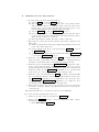
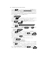
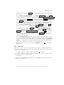
ME 566
Computational Fluid Dynamics for
Fluids Engineering Design
ANSYS CFX STUDENT USER
MANUAL Version 11 Upgrade
Gordon D. Stubley
Department of Mechanical Engineering, University of
Waterloo
c
G.D.
Stubley 2007
2007
iv
Contents
1
Introduction
1
2
Commands for Duct Bend Example
2.1 Geometry Model
2.2 Mesh Generation
2.3 Pre-processing
2.4 Solver Manager
2.5 Post-processing
2.6 Clean Up
v
3
3
7
9
13
13
15
1
Introduction
In these notes the basic steps in a CFD solution will be illustrated using
the professional software ANSYS Workbench Version 11 Upgradewhich includes
the components DesignModeler, Meshing, and Advanced CFD (all trademarks
of ANSYS). These notes are designed for students who have had some exposure
to ANSYS Workbench 10.
There are four significant differences between Versions 10 and 11:
Meshing: Besides the CFX-Mesh tool, Version 11 provides a range of meshing
tools for generating hexahedral and tetrahedral meshes. The emphasis in
these notes is on tetrahedral meshing with inflation as implemented in CFXMesh. By setting the ANSYS Workbench options, the default meshing tool
is set to CFX-Mesh.
CFX GUI/Mouse: The CFX-Pre and Post GUI’s and mouse actions have
been changed to make them compatible with the actions used in DesignModeler and CFX-Mesh. In particular, the rotation actions in CFX-Pre and
CFX-Post are now context sensitive. The coordinate system triad in CFXPre and Post remains inactive. To set standard directional views type x, y,
or z while the Viewer window is active to get views in the positive axis directions and type X, Y, or Y to get views in the negative axis directions. Other
standard key mappings can be seen by clicking on the Show Help Dialog
icon at the right of the lower row of icon buttons.
Tree View: CFX-Pre and CFX-Post now make use of the tree view of object
databases similar to that of DesignModeler and CFX-Mesh. In particular,
commands for modifying the database can be directly accessed from the tree
view. The implementation of boundary conditions for boundary surfaces is
an application of this new capability.
Default Settings: CFX-Pre uses more default settings to reduce the number
of details that the user must directly set to establish a solver definition file.
To illustrate these differences, the notes only provide the steps required to
complete the ductbend example program provided in the Version 10 Student
User Manual.
The following font/format conventions are used to indicate the various commands that should be invoked:
1
2
INTRODUCTION
Menu/Sub-Menu/Sub-Sub-Menu Item chosen from the menu hierarchy at the
top of a main panel or window,
Button/Tab Command Option activated by clicking on a button or tab,
Link description Click on the description to move by a link to the next step/page;
Name
value Enter the value in the named box,
Name H selection Choose the selection(s) from the named list,
Name Panel or window name,
Name On/off switch box, and
Name On/off switch circle (radio button).
2
Commands for Duct Bend
Example
2.1
Geometry Model
The first phase uses DesignModeler. The commands listed below will create a
solid body geometry that will represent the flow domain:
•
•
•
•
set up the project directory and page;
set up a plane for sketching on;
sketch in the flow path through the duct, Figure 2.1;
generate the solid body geometry;
To begin:
• Create a new folder N:/Ductbend1 to be the working directory for the
project files.
• Open ANSYS Workbench from
Start/Programs/Engineering/ANSYS 10.0/ANSYS Workbench. To open
a new project:
1. In the Start window, select Empty Project in the New panel,
2. From the menu bar choose File/Save As ... to create a project file in
your working directory, and
3. In the Save As window fill in File name: Ductbend.wbdb and click
the Save button.
• From the menu bar choose Tools/Options ... to change the length units and
meshing tool options:
∗ In the Options window expand the + DesignModeler entity and select
Grid Defaults (Meters) in the tree view on the left. Set Minimum
Axes Length 0.5 and Major Grid Spacing 0.1 .
∗ In the Options window expand the + Meshing entity and select Meshing. Set Default Physics Preference CFD and Default Method
CFX-Mesh .
1 When NEXUS network traffic is high, it is better to make the working directory on your
local machine, i.e. C:/Temp/Ductbend.
3
4
COMMANDS FOR DUCT BEND EXAMPLE
/.(0* *+,
$!%!
6.'1%* 2378
!
"#
&'$()* *+-,
&1* 2435+
Fig. 2.1 Wireframe of the final sketch of the duct bend flow path.
Click OK to save the options and close the window,
• Under Create DesignModeler Geometry, choose New Geometry,
• Check that the desired length unit is Meter is selected and click Ok in
the units window that appears,
• In the Tree View, select the XYPlane entity and then click the New Sketch
icon to create the Sketch1 entity as a component of the XYPlane.
• To start the sketching , select the Sketching tab
• To draw in the 2D sketch of the duct flow path (Figure 2.1)
1. Select the Sketching tab; and
GEOMETRY MODEL
5
2. Click on the Z coordinate of the triad in the lower right corner of the
Model View.
• Select the Draw toolbox and:
1. With the Arc by Center tool sketch the inner wall bend shape:
(a) Place the cursor over the origin (watch for the P constraint symbol)
and left mouse button click.
(b) Move the cursor to the left along the X axis. With the C constraint
visible click the left mouse button to put the start point of the arc
on the X axis.
(c) Sweep the cursor clockwise until the C constraint appears at the Y
axis. Click the left mouse button.2
2. Switch to the Dimensions toolbox to size the inner wall bend radius:
(a) Select the Radius tool;
(b) Select a point on the arc. Then move the cursor to the inside of the
arc near the origin. Click to complete a dimension which is labelled
R1.
(c) In the Details View notice that R1 is shown under the Dimensions
title.
(d) Change the value of R1 to 0.025 [m]. Notice the arc radius changes
automatically. If the dimension is poorly placed on your sketch you
can use the Move tool to correct the placement.
3. Switch back to the Draw toolbox to sketch the inner entrance wall:
(a) With the Line tool selected, place the cursor in the lower left
quadrant of the XY plane near the arc. Click the left mouse button.
Move the mouse cursor down to create a vertical line. Look for the
V constraint symbol and click the left mouse button;
(b) Switch to the Dimensions toolbox to size the inner entrance wall
length:
i. Select the General tool;
ii. Select a point near the centre of the line. Click and drag the cursor
to the right to form the dimension lines. Release the mouse button
where the label, V2, is to be placed.
iii. In the Details View change the value of V2 to 0.10 [m].
(c) To join the inner entrance wall and the inner wall bend switch to
the Constraints toolbox;
i. Select the Coincident tool;
ii. Select the upper end of the entrance inner wall with a left mouse
button click. The square end marker should be yellow;
iii. Select the square end marker of the arc that lies on the X axis
with a left mouse button click. The inner entrance wall should
join the inner wall bend.
2 Notice
that the drawing instruction steps are provided in the lower left corner.
6
COMMANDS FOR DUCT BEND EXAMPLE
4. To draw a line across the inflow (entrance):
(a) Use the Line tool in the Draw toolbox;
(b) Place the cursor over the bottom end point of the entrance inner
wall and notice that a P constraint symbol appears. Left mouse
button click to select this point and then move the cursor to the
left and click while the H constraint symbol is visible.
(c) Use the General tool in the Dimensions toolbox:
(d) Select a point near the centre of the line. Click and drag the cursor
to the bottom to form the dimension lines. Release the mouse button
where the label, H3, is to be placed.
(e) In the Details View change the value of H3 to 0.075 [m].
5. Repeat the procedure used for the entrance inner wall to draw the exit
inner wall:
(a) Draw a horizontal line in the upper right XY quadrant near the end
point of the inner wall bend;
(b) Set the length of the line to 0.20 [m] with the General tool from
the Dimensions toolbox;
(c) Join the exit inner wall to the inner wall bend with the Coincident
tool from the Constraints toolbox.
6. Draw the outer entrance wall with the Line tool. Start at the outer
(left) end point of the inflow edge (look for the P constraint symbol)
and draw a vertical line that is coincident (C) with the X axis;
7. Draw the outer bend wall with the Arc by Center tool. Put the centre
at the origin, make the start point at approximately 20◦ above the X
axis in the upper left quadrant, and make the end point coincident (C)
with the Y axis. Use the Coincident constraint tool to join the start
point of the arc to the end point of the outer entrance wall;
8. Draw the outer exit wall with the Line tool. Draw a horizontal (H)
line coincident (C) with the Y axis above its final desired location. Use
the Coincident constraint tool to join this line to the end of the outer
bend wall. Use the Equal Length constraint tool to make the outer
exit wall the same length as the inner exit wall; and
9. Draw a line from the end of the outer exit wall to the end of the inner
exit wall to form the outflow edge. Make sure that the end points are
coincident (P).
The sketch should now be an enclosed contour on the XYPlane.
• To create the three dimensional solid body:
1. Switch to the Tree View by selecting the Modeling tab;
2. Click on the Extrude button to create the Extrude1 feature . In the
Details View:
∗ Check Base Object Sketch1 ,
MESH GENERATION
7
∗ Select Operation H Add Material ,
∗ Select Direction Vector H None (Normal) ,
∗ Set FD1, Depth (> 0) 0.02 ,
∗ Select As Thin/Surface? H No , and
∗ Select Merge Topology? H Yes .
3. Click on the Generate button to create a Solid. Use the isometric view
in the Model View to check that you have a three dimensional solid grey
body.
• Choose File/Save As ... and set File name: Ductbend.agdb in the Save
As window. Click Save to close window.
• Return to the Project page by clicking on the Ductbend [Project] tab at
the top left corner of the window.
2.2
Mesh Generation
The second phase uses CFX-Mesh. The commands listed below will generate a
discrete mesh in the flow domain:
• name the surfaces (faces) of the solid geometry to ease boundary condition
specification;
• specify the properties of the mesh in the interior of the flow domain and
close to solid walls;
• preview the surface mesh to check for anomalies; and
• create the geometry file with volume mesh information.
• Choose the New Mesh DesignModeler Tasks; Notice the three primary areas:
Graphics View, Tree View, and Details View, in the CFX-Mesh window.
• The surfaces (faces) of the solid are labeled as regions for ease of attaching the boundary conditions . To attach a region entity at the inflow (see
Figure 2.1):
1. Orient the model so that the inflow surface can be easily picked with
the mouse cursor;
2. Right mouse click over Regions in the Tree View and select Insert H
Composite 2D Region to create a new region entity;
3. Left click over the new entity’s name, Composite 2D Region 1, and edit
the region name to inflow surface;
4. In the Graphics View put the mouse cursor over the inlet surface area
and left mouse click. The inlet surface area should turn green; and
5. In the Details View click on Location H Apply and the surface will
now turn red;
• Repeat to create a region entity called outflow surface. Notice that if you
left mouse button click on inflow surface or the outflow surface in the Tree
View that the resulting region in the Graphics View turns green.
8
COMMANDS FOR DUCT BEND EXAMPLE
• Create a region entity called inner wall. This region is composed of three
primitive surfaces. To select a set of surfaces or faces hold the ”Ctrl” key
down while clicking on the component surfaces in the Graphics View;
• Repeat to create an entity called outer wall;
• For a region called front surface use the Z view of the Graphics View when
selecting the surface. Notice that there are two parallel planes in the lower
left corner of the Graphics View. The front most of these planes should be
outlined in red.
• Lastly, create a region called back surface. Notice that when this region is
created the Default 2D Region disappears.
• In the Tree View, select Options to see the mesh options in the Details View:
∗ Set Surface Meshing H Advancing Front ,
∗ Set Meshing Strategy H Extruded 2D Mesh ,
∗ Set 2D Extrusion Option H Full , and
∗ Set Number of Layers H 1 ;
• In the Tree View, expand the + Spacing entity;
• Select the Default Body Spacing entity to open the Body Spacing Details
View. Set Maximum Spacing [m] 0.0075 .
• Left mouse click on the Extruded Periodic Pair entity;
∗ In the Graphics View select the front surface and then click Location
1 Apply in the Details View;
∗ In the Graphics View select the back surface (remember to use the
location planes in the lower left corner of the Graphics View) and then
click Location 2 Apply in the Details View; and
∗ Set Periodic Type H Translational ;
• In the Tree View, right mouse click on Inflation and select Insert/Inflated
Boundary to create an Inflated Boundary entity. Select the three surfaces
of the inner wall in the Graphics View for the Location and set Maximum
Thickness [m] 0.0075 ;
• Repeat to create an Inflated Boundary of Maximum Thickness [m] 0.0075
on the outer wall;
• In the Tree View right mouse click on + Preview entity and select Generate
Surface Meshes. Progress is shown in the lower left corner. After a short
time you should see a mesh of triangles and rectangles on the surfaces of
the solid;
• Click the Generate the volume mesh for the current problem icon on the
top row of icons/buttons. Again, progress is shown in the lower left corner.
When this process is completed, go to the Tree View and select Errors to
ensure that no errors are reported in the Details View.
• To close this phase, select File/Save As ... and set File name: Ductbend.cmdb .
PRE-PROCESSING
9
• Return to the Project page by clicking on the Ductbend [Project] tab at
the top left corner of the window.
2.3
Pre-processing
The first CFD phase is preprocessing. In this phase the complete CFD model
(mesh, fluids, flow processes, boundary conditions, etc.) is defined and saved in
a hierarchical database. After opening CFX-Pre, the commands listed below will
accomplish the following steps:
• link the mesh file to a CFX flow project,
• set simulation type to steady state,
• establish a fluid with nominal properties of water,
• specify the region through which the fluid will flow, the fluid (nominally
water), and the physical models (fluid flow, no heat transfer, turbulence,
standard k − ε model with scalable wall functions),
• set up and attach the rough wall boundary condition, the inlet boundary
condition, the outlet boundary condition, and the symmetry boundary conditions,
• set the global initial conditions,
• set the solver controls for discretization scheme, time step type, and convergence criteria,
• set the output variable list, and
• write the complete CFD model definition to a def file.
To accomplish these steps execute the following commands:
• Highlight the Mesh Model, Ductbend.cmdb, in the Project page and select
Create CFD Simulation with Mesh under Advanced CFD Tasks;
• After a short wait the CFX-Pre page will open. This page is similar to
the CFX-Post page. There are three main areas: the menus and command
buttons at the top, the Viewer window at the right, and the Outline view
of the database trees at the left;
• Right mouse click on the Materials entity in the Outline tree and select
Insert/Material to create a new material with the required water properties.
In the Insert Material panel, fill in Name Water nominal and click OK
to open a panel with two tabs:
∗ Click the Basic Settings tab and set:
∗ Option H Pure Substance ,
∗ Material Group H Constant Property Liquids ,
∗ Material Description off,
∗ Thermodynamic State on and Thermodynamic State H Liquid .
∗ Click the Material Properties tab and set:
∗ Option H General Material ,
∗ in the Equation of State area set,
10
COMMANDS FOR DUCT BEND EXAMPLE
∗ Option H Value ,
∗ Density
1000
H kgm− 3 ,
∗ expand Transport Properties + ,
∗ Dynamic Viscosity on and Dynamic Viscosity
0.001
H Pa · s ,
and then click Ok .
• In the Outline view, right mouse click the Simulation Type entity and select
Edit to open the Simulation Type panel. Check that Option H Steady State
is set and then click Ok .
• In the Outline view, double left mouse click the Default Domain entity to
open the Domain: Default Domain panel which will have several tabbed
sub-panels.
∗ On the General Options sub-panel, set:
◦ Location H B28 and notice that the geometry is highlighted in
green in the Viewer window,
◦ Domain Type H Fluid Domain ,
◦ Fluids List H Water nominal ,
◦ Particle Tracking off,
◦ Reference Pressure 1 H atm ,
◦ Buoyancy Option H Non Buoyant , and
◦ Domain Motion Option H Stationary .
∗ on the Fluid Models sub-panel set:
◦ Heat Transfer Model Option H None ,
◦ Turbulence Model Option H k-Epsilon ,
◦ Turbulent Wall Functions Option H Scalable ,
◦ Reaction or Combustion Model Option H None , and
◦ Thermal Radiation Model Option H None ,
∗ on the Initialization sub-panel ensure that Domain Initialization is
off and then click Ok to close the panel.
• To prepare for implementing the boundary conditions, expand the expand
+ Ductbend.cmdb mesh model to see the Principal 2D Regions of the geometry. Check that all 2D regions are highlighted.
• Right mouse click back surface and select Insert/Boundary to open the
boundary details panel. In this panel:
∗ under the Basic Settings tab set:
◦ Boundary Type H Symmetry , and
◦ Location H back surface ,
and then click Ok to close the panel and create the new boundary object.
PRE-PROCESSING
11
Notice that perpendicular red arrows appear on the back surface in the
Viewer window and the boundary object is listed in the Default Domain
entity. Clicking on back surface object in the Default Domain database causes
the back surface mesh to be outlined with green in the Viewer window. A
double mouse click will re-open the boundary details panel.
• Right mouse click front surface and select Insert/Boundary to open the
boundary details panel. In this panel:
∗ under the Basic Settings tab set:
◦ Boundary Type H Symmetry , and
◦ Location H front surface ,
and then click Ok to close the panel.
• Right mouse click inflow surface and select Insert/Boundary to open the
boundary details panel. In this panel:
∗ under the Basic Settings tab set:
◦ Boundary Type H Inlet , and
◦ Location H inflow surface ,
∗ and under the Boundary Details tab set:
◦ Flow Regime Option H Subsonic ,
◦ Mass and Momentum Option H Normal Speed ,
◦ Normal Speed H 3 H ms− 1 ,
◦ Turbulence Option H Intensity and Length Scale ,
◦ Value 0.05 ,
◦ Eddy Length Scale
0.0075
H m,
and then click Ok to close the panel and create the new boundary object.
• Right mouse click inner wall and select Insert/Boundary to open the boundary details panel. In this panel:
∗ under the Basic Settings tab set:
◦ Boundary Type H Wall , and
◦ Location H inner wall ,
∗ and under the Boundary Details tab set:
◦ Wall Influence on Flow Option H No Slip ,
◦ Wall Velocity off,
◦ Wall Roughness Option H Rough Wall ,
◦ Roughness Height
0.0001
H m,
and then click Ok to close the panel.
• Right mouse click outer wall and select Insert/Boundary to open the boundary details panel. In this panel:
12
COMMANDS FOR DUCT BEND EXAMPLE
∗ under the Basic Settings tab set:
◦ Boundary Type H Wall , and
◦ Location H outer wall ,
∗ and under the Boundary Details tab set:
◦ Wall Influence on Flow Option H No Slip ,
◦ Wall Velocity off,
◦ Wall Roughness Option H Rough Wall ,
◦ Roughness Height
0.0001
H m,
and then click Ok to close the panel.
• Right mouse click outflow surface and select Insert/Boundary to open the
boundary details panel. In this panel:
∗ under the Basic Settings tab set:
◦ Boundary Type H Outlet , and
◦ Location H outflow surface ,
∗ and under the Boundary Details tab set:
◦ Flow Regime Option H Subsonic ,
◦ Mass and Momentum Option H Average Static Pressure ,
◦ Relative Pressure
0
H Pa ,
and then click Ok to close the panel.
• Right mouse click on Solver Control entity and select Edit to open the Details
of Solver Control panel. Under the Basic Settings tab set:
∗ Advection Scheme Option H Upwind ,
∗ Timescale Control H Physical Timescale ,
∗ Physical Timescale 0.04 H s (30% of the average residence time of
a fluid parcel inside the flow domain),
∗ Max No. Iterations 50 ,
∗ Residual Type H MAX ,
∗ Residual Target 1.0e-3 ,
and then click Ok .
• Right mouse click on Output Control entity and select Edit to open the
Details of Output Control panel. Under the Results tab set:
∗ Option H Standard ,
∗ Output Variable Operators on and choose H All , and
∗ Output Boundary Flows on and choose H All ,
and then click Ok .
SOLVER MANAGER
13
• On the row of buttons below the menu bar above the Viewer window, click
the Write Solver File icon (last one in the row) to open the panel. Accept
the default filename, Ductbend.def and Operation H Start Solver Manager .
2.4
Solver Manager
The CFX-Solver window will open after CFX-Pre closes. In the Define Run
panel set:
• Definition File ductbend.def (NOTE: If restarting a partially converged
run, you would enter the name of the most current results file),
• Type of Run H Full , and
• Run Mode H Serial ,
and then click Start Run .
After a few minutes execution should begin. Diagnostics will scroll on the terminal output panel and the equation RMS residuals will be plotted as a function
of time step. After the first few time steps, the residuals should fall monotonically. Execution should stop within 40 time steps. In the ANSYS CFX Solver
Finished Normally window click Process Results Now .
2.5
Post-processing
The most interesting step is the analysis of the results. To illustrate this step the
commands listed in the next paragraph step through the following tasks:
•
•
•
•
•
•
•
•
create a vector plot on one of the symmetry boundary planes,
save an image of the plot,
create a vorticity variable,
create a fringe plot of the vorticity field,
create a line and export the velocity data along the line,
export the inner wall pressure and wall shear stress distribution,
probe the velocity field, and
save the visualization state.
To accomplish these tasks click the CFX-Post tab in bottom left corner and
then:
• Choose Insert/Vector, accept Name Vector 1 , and click OK to define a
vector object and open an edit panel. In the panel set:
∗ Locations H front surface ,
∗ Reduction Reduction Factor ,
∗ Factor 1 (plots vector at every mesh point),
∗ Variable H Velocity ,
∗ Hybrid on,
∗ Projection H None ,
14
COMMANDS FOR DUCT BEND EXAMPLE
and click Apply . The vector plot should appear in the 3D Viewer window
and the vector object is listed in the User Locations and Plots database tree.
Turn Default Legend View 1 off and back on to remove and then replace
the scale legend. Turn Wireframe off and on. Orthographic projection
will work best for two-dimensional views. Notice that if you double-click on
an object in the database tree then a details panel opens up for that object.
• Choose File/Print ... and in the Print panel set:
∗ File
vectorplot.png , and
∗ Format H PNG
followed by Print . The plot will printed to the file vectorplot.png in your
working directory. You can import this file into other documents.
• Choose Insert/Variable and in the New Variable definition window set
Name Vorticity and click OK . In Vorticity edit panel (lower left):
∗ set Method H Expression ,
∗ set Scalar on,
∗ fill in Expression Velocity v.Gradient X - Velocity u.Gradient Y , and
∗ click Apply .
• Choose Insert/Contour, accept Name Contour 1 , and click OK to define
a fringe/contour plot object and open an edit panel. In the panel set:
∗ Locations H front surface ,
∗ Variable H Vorticity
and click Apply . The fringe plot should appear in the 3D Viewer window.
• Choose Insert/Location/Line, accept Name Line 1 , and click OK to
define a line object and open an edit panel. Use Method H Two Points ,
set Point 1 to (0.0,0.1,0.01), set Point 2 to (0.0,0.025,0.01), set the number of
samples to 25, and click Apply to see the line (make sure that the visibility
of the contour plot, etc. is turned off).
• Choose File/Export ... to open the Export panel where you can:
∗
∗
∗
∗
set File velocity.csv ,
select Line 1 from the Locations list,
set Export Geometry Information on,
select (Ctrl key plus click) Velocity u and Velocity v from the Select
Variable(s) list, and
∗ click Save to write the data to a file in a comma-separated format that
can be imported into a conventional spreadsheet program for plotting
or further analysis. Notice that this file includes x, y, and z values.
• Choose Insert/Location/Plane, accept Name Plane 1 , and click OK to
define a plane object and open an edit panel. Use Method H XY Plane
CLEAN UP
15
with Z = 0[m] and click Apply (turn highlighting off to avoid clutter in
the view).
• Choose Insert/Location/Polyline, accept Name Polyline 1 , and click OK
to define a polyline object. In the edit panel use Method H Boundary Intersection
with Boundary List H inner wall and Intersect With H Plane 1 and then
click Apply . This creates a line that follows the inner wall. You can follow
the steps for export along a line to export the values of the pressure, total
pressure, and wall shear (stress) along this line into the data file wall.csv.
• Choose Insert/Location/Point, accept Name Point 1 , and click OK to
define a point object. Use Method H XYZ and initialize the point to
(0.10,0.04,0) before clicking Apply . Choose Tools/Function Calculator to
open the Function Calculator panel. Use Function H probe , Location H
Point 1 , Variable H Velocity u.Gradient X (Note: Use the ... to get a list
of all possible variables.) before clicking on the Calculate button. The result with units appears in the Result box. Move the point around to probe
other regions in the flow.
• Choose File/Save State and enter tutorial1.cst for the file name to save
all of the information associated with the visualization and post-processing
objects you have created in this session. You can load this state file (File/Load
State) to recreate these objects and images in later sessions. This facility
allows easy comparison of results between simulations.
• Return to the Project page and choose File/Exit. Select Yes to save highlighted files.
2.6
Clean Up
The last step is to remove unnecessary files created by CFX-5. This step is
necessary to ensure that you do not exceed your disk quota. At the end of each
session3 delete all files except:
• *.agdb, *.cmdat, *.cmdb, *.wbdb, *.def and * *.res files.
If you no longer need your results but would like to be able to replicate them
then you should delete all files except:
• *.def files.
After removing all unnecessary files, use the WinZip utility to compress the
contents of your directory.
3 If
you have used a local temp drive, remember to copy your work to your N: drive