Download DNM Product Specification Report

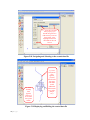
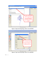
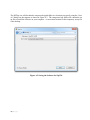
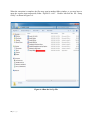
GFM:
Graphical Flow Model
User’s Manual
Developed by The University of Kentucky and KYPIPE LLC
Prepared for the
National Institute of Hometown Security
368 N. Hwy 27
Somerset, KY 42503
September 30, 2012
This research was funded through funds provided by the Department of Homeland Security,
administered by the National Institute for Hometown Security Kentucky Critical Infrastructure
Protection program, under OTA # HSHQDC-07-3-00005, Subcontract # 02-10-UK.
1|P a g e
Table of Contents
List of Figures ........................................................................................................................................ 4
1.0 INTRODUCTION .............................................................................................................................. 8
1.1 Background.................................................................................................................................. 8
1.2 GFM Functionality ....................................................................................................................... 8
1.3 Downloading the Software from the Internet .......................................................................... 12
1.4 Applying the Software ............................................................................................................... 12
2.0 GFM GRAPHICAL USER INTERFACE .............................................................................................. 13
2.1 Basic Functions .......................................................................................................................... 13
2.2 Opening an Existing Data File .................................................................................................... 15
2.3 Settings Menu/Loading a Background Map .............................................................................. 18
2.4 Editing the Elements of an Existing Data File ............................................................................ 22
2.5 Adding Pipe or Node Elements to an Existing Data File ............................................................ 22
2.6 Adding Valves or Hydrants to a Pipe ......................................................................................... 23
3.0 GENERATING A FLOW ANALYSIS .................................................................................................. 25
3.1 Error Checking ........................................................................................................................... 25
3.2 Flow Analysis Run ...................................................................................................................... 25
3.2.1 Display Flowrates ............................................................................................................... 27
3.2.2 Display Pressures ................................................................................................................ 28
3.2.3 Data Contours ..................................................................................................................... 29
3.2.4 Analysis Report .................................................................................................................. 32
3.3 Printing/Saving the Analysis Report .......................................................................................... 35
3.4 Printing/Saving an Analysis Image ............................................................................................ 36
4.0 Highlighting Critical Users/Infrastructure .................................................................................... 39
5.0 Importing KIA Datasets ................................................................................................................. 45
6.0 Exporting Data to KYPIPE .............................................................................................................. 55
APPENDIX A: INSTALLING THE SOFTWARE ......................................................................................... 57
2|P a g e
APPENDIX B: HOW TO ADD NEW ELEMENTS TO YOUR NETWORK FILE ............................................ 69
B.1 Network Elements ................................................................................................................... 69
B.2 Internal Nodes ........................................................................................................................... 70
B.3 End Nodes ................................................................................................................................. 72
APPENDIX C: USING KYPIPE FOR ADDITIONAL NETWORK ANALYSIS ................................................. 76
C.1 Laying Out a Pipe System .......................................................................................................... 77
C.2 Quick Start Example .................................................................................................................. 79
C.3 Additional KYPipe Demonstration Example .............................................................................. 84
3|P a g e
List of Figures
Figure 1.1 Example Network Model .................................................................................................... 9
Figure 1.2 GFM GUI with Network Schematic Super-imposed on Background Map ...................... 10
Figure 1.3 Network Schematic and Map with Critical Asset Icons .................................................... 11
Figure 2.1 Basic GFM Graphical User Interface ................................................................................ 13
Figure 2.2 File and Program Options Command Bar ......................................................................... 14
Figure 2.3 Map Function Menu .......................................................................................................... 14
Figure 2.4 Opening a New File ........................................................................................................... 15
Figure 2.5 Opening a New File (continued) ....................................................................................... 16
Figure 2.6 Example Water Distribution Network System Schematic ................................................ 17
Figure 2.7 Going to Settings Menu from Map View .......................................................................... 18
Figure 2.8 Settings Menu/Adding a Background Map ....................................................................... 19
Figure 2.9 Navigating to the Desired Map File (i.e. CITY_Map.bmp) .............................................. 20
Figure 2.10 Returning to Map View to See the Background Map ..................................................... 21
Figure 2.11 Pipe Data Menu ............................................................................................................... 22
Figure 2.12 Node Data Menu.............................................................................................................. 23
Figure 2.13 Adding a Valve to a Pipe ................................................................................................. 24
Figure 2.14 Valve Added to Pipe........................................................................................................ 24
Figure 3.1 Analyze Menu in the Program Command Bar .................................................................. 25
Figure 3.2 Operational Control Settings Dialog Box.......................................................................... 26
Figure 3.3 Results Menu from Analysis Run...................................................................................... 27
Figure 3.4 Flowrate Labels ................................................................................................................. 28
Figure 3.5 Pressures at System Nodes ................................................................................................ 29
Figure 3.6 Pressure Contours - Hatch ................................................................................................. 30
Figure 3.7 Pressure Contours - Gradient............................................................................................. 31
4|P a g e
Figure 3.8 Analysis Report Section (Data) ......................................................................................... 33
Figure 3.9 Analysis Report Section (Results) ..................................................................................... 34
Figure 3.10 Printing the Analysis Report ........................................................................................... 35
Figure 3.11 Saving the Analysis Report as a Document .................................................................... 36
Figure 3.12 Screen Capture of Flowrate Analysis (BMP File Image) ................................................ 37
Figure 3.13 Print Menu Window Box................................................................................................. 38
Figure 4.1 Locating Critical Users/Infrastructure with a Node Point ................................................. 39
Figure 4.2 Selecting the Critical Infrastructure Icon Image ............................................................... 40
Figure 4.3 Designating the Node Image Size ..................................................................................... 41
Figure 4.4 Node Image Sizes .............................................................................................................. 41
Figure 4.5 Showing the Node Image on the Map ............................................................................... 42
Figure 4.6 Reformatting the Node Label Box .................................................................................... 43
Figure 4.7 Moving the Node Image .................................................................................................... 44
Figure 5.1 Kentucky Infrastructure Authority (KIA) Website ........................................................... 45
Figure 5.2 Access Water Lines File by Clicking on the WRIS tab .................................................... 46
Figure 5.3 Downloading the KIA Water Lines Files .......................................................................... 46
Figure 5.4 Steps to Save the Downloaded File ................................................................................... 47
Figure 5.5 Steps to Extract the Zipped Files ....................................................................................... 47
Figure 5.6 Proceed with the File Extraction ....................................................................................... 48
Figure 5.7 Specify the Folder to put the Unzipped Files .................................................................... 48
Figure 5.8 Click the Finish Button Once Completed.......................................................................... 49
Figure 5.9 Start the GFM program and using the New File Option ................................................... 49
Figure 5.10 Access the PIPE2000 Utility Function through the File drop down Menu ..................... 50
Figure 5.11 Now Click on the Import KIA Database Button ............................................................. 50
Figure 5.12 Set the Program Import Options and then click on Start ................................................. 51
Figure 5.13 Select the File that you want to import into GFM ........................................................... 51
5|P a g e
Figure 5.14 The following menu will appear as the program processes the KIA database files ........ 52
Figure 5.15 The Program will download all the KIA Database Files ................................................. 52
Figure 5.16 The following menu will be displayed as the program processes the files ..................... 53
Figure 5.17 Opening the created data file ........................................................................................... 53
Figure 5.18 Navigating and Selecting to the created data file ............................................................ 54
Figure 5.19 Displaying and Editing the created data file.................................................................... 54
Figure 6.1 Step One in Exporting a File for Use in KYPIPE ............................................................. 56
Figure 6.2 Step Two in Exporting a File for Use in KYPIPE............................................................. 56
Figure A.1 KYPipe Page for Decon Version Download .................................................................... 57
Figure A.2 Saving the Software Set Up File....................................................................................... 58
Figure A.3 Extracting the Compressed Zip Files............................................................................... 59
Figure A.4 Run the Set Up File .......................................................................................................... 60
Figure A.5 Run the Set Up File ......................................................................................................... 61
Figure A.6 Click Next to Continue .................................................................................................... 62
Figure A.7 Select the License Agreement and Next to Continue ....................................................... 62
Figure A.8 Enter Your Information and Click Next to Continue ....................................................... 63
Figure A.9 Click Next and Yes to Create Folder ................................................................................ 63
Figure A.10 Click Install..................................................................................................................... 64
Figure A.11 Click Finish..................................................................................................................... 64
Figure A.12 Locating and Launching the Installed Software ............................................................. 65
Figure A.13 Notification Upon Launching Software. Click OK to Continue. ................................. 65
Figure A.14 KYPipe Information Box................................................................................................ 66
Figure A.15 Version Information Box. Click OK to Continue. ........................................................ 67
Figure A.16 New File Specification Box........................................................................................... 68
Figure C.1 Example Pipe System ....................................................................................................... 80
Figure C.2 Completed Pipe System Layout ........................................................................................ 81
6|P a g e
Figure C.3 Case 1 - Pressure and Flow .............................................................................................. 83
Figure C.4 Case 1 - Loss and HGL ..................................................................................................... 83
Figure C.5 Pipe System Layout for Demonstration Examples ........................................................... 84
Figure C.6 Results Labels, Case 0 ...................................................................................................... 85
Figure C.7 Contours, Case 2 ............................................................................................................... 86
Figure C.8 Profile, Case 0 ................................................................................................................... 87
7|P a g e
1.0 INTRODUCTION
1.1 Background
The Graphical Flow Model (GFM) has been developed for water utility managers as a first step
toward utilizing a computer model of their distribution system. The GFM is not a comprehensive
water system model, modeling all possible aspects of operations; however, for systems that have
little to no computer based representations of their system, the GFM is a great asset. First, it
provides a graphical representation of a system within an interactive interface, capable of storing and
manipulating data pertaining to many components of the system. Secondly, given certain hydraulic
operational control inputs, the GFM is capable of returning output for many important system
questions such as flow directions and magnitudes, pressures, hydraulic grade line contours, and
more.
The GFM has been designed to allow the use of pre-developed GIS datasets for use in constructing
graphical representations of water distribution systems. In particular, the model has been developed
to allow use of the Kentucky Infrastructure Authority (KIA) water distribution system database.
Finally, the GFM has an option that will allow the user to export any model developed within the
GFM graphical user interface (GUI) for possible subsequent use with comprehensively functional
water distribution network analysis software (i.e. KYPIPE).
1.2 GFM Functionality
The functionality of the model is summarized as follows:
1. One of the unique challenges of developing computer models for small utilities is the ability to
generate and assemble the required basic network data. The Kentucky Infrastructure Authority
(kia.ky.gov) has assembled extensive GIS data sets for all of the water distribution systems within
the state (http://kia.ky.gov/wris/data.htm). This information includes data on pipelines, water tanks,
water treatment plants, water meters, and pump stations. The GFM model includes functionality to
upload such data via a graphical user interface to permit the creation of a schematic of the water
distribution system. While this functionality will be initially applied to water utilities within
Kentucky, it should provide a framework for extension of such an approach to other states as well
(see Figure 1.1).
2. The existing infrastructure can be displayed in graphical form superimposed on a topographic
map. The topographic map can display the physical relationships that the existing system
infrastructure has with its surroundings in terms of elevations and natural and urban geographical
features. The GFM has been designed with the capability to upload a background map that would
contain such information (see Figure 1.2).
8|P a g e
Figure 1.1 Example Network Model
3. In addition to having a map of the network, it would also be helpful to have a feature that
would allow the user to immediately see locations of any critical users or infrastructure that
are on the distribution system. This functionality has been provided by allowing the user to
turn on infrastructure icons which can be readily seen and identified in the program GUI (see
Figure 1.3).
4. The pipe material and age of the pipe may be important in making system decisions and
planning. As a result, the GFM provides a summary of such material for use by the system
operator or management planner.
9|P a g e
Figure 1.2 GFM GUI with Network Schematic Super-imposed on Background Map
5. The analyze function of the GFM can provide a lot of information about the flow in the
system. The direction of the flow in the pipes is shown graphically on the schematic of the
distribution system by arrow pointers on the pipes. The rate of flow in a pipe is shown as a
label on the pipe and external demand withdrawals or external inputs is shown as a label on
the node. The former label is a yellow box and the latter label is a blue box.
6. The analyze function of the GFM can provide the pressure at each node using box labels.
7. The GFM can produce contours in the background of the schematic to show elevations,
node pressures, the hydraulic grade line, or the pressure head. These contours can be
displayed with a hatching, gradient, or solid fill.
10 | P a g e
Figure 1.3 Network Schematic and Map with Critical Asset Icons
8. The analyze function of the GFM can produce an analysis report. The report begins with
data summaries of regulatory valves, pipelines, and nodes. Then the report gives the analysis
results for the regulatory valves, pipelines, and nodes. The results for the regulatory valves
give upstream and downstream pressure and through flow. The results for the pipelines
includes flowrates, and the results for the nodes includes external demands, hydraulic grade,
and pressures. Finally the report provides a summary of system inflows and outflows.
9. In the event that system valves needed to be closed due to leakages, breaks, or
contamination, additional pipes may also become isolated and/or the pressures at different
parts of the system may be adversely impacted. By coupling a decision support system with
a water distribution model, the model can be used to evaluate the impacts of such closures
and alert system operators about potential operational problems. By performing off-line
analyses of the system for different closure scenarios, it is possible that such problems can be
avoided by taking actions to increase the number of valves in the system or by providing
pressure augmentation through the construction of new booster pumps or new parallel lines.
While some of this functionality can be accomplished by simply using a graphical
11 | P a g e
representation of the water distribution system, functionality to fully address all the needs
described above would require the utilization of some type of underlying hydraulic and water
quality model. Thus, a final functionality of the GFM would be the ability to upload the
assembled data into a fully functional water distribution system model (e.g. PIPE2010 by
KYPIPE LLC).
1.3 Downloading the Software from the Internet
Instructions for downloading the GFM software and installing it on your computer are
provided in Appendix A. In order to insure the maximum potential use of the software, a
free version of the program is provided with the capability of analyzing a water distribution
system with up to 250 pipes. In the event a utility has a system with greater than 250 pipes,
one may either skeletonize the system by excluding smaller pipes from the model or one may
contact KYPIPE directly for a software upgrade. In addition to the associated software, the
download will also include two example data files for use in explaining the basic
functionality of the GFM software. These files will include a background map (i.e.
CITY_Map.bmp) and a network model for a small water distribution system (decon
example.p2k). Both of these files will be used to illustrate the features of the GFM in the
following chapters.
1.4 Applying the Software
The basic features of the GFM graphical user interface are provided in Chapter 2. Instructions on
how to generate network analysis results are provided in Chapter 3. Chapter 4 contains instructions
on highlighting critical infrastructure and information on other advanced features of the GFM GUI.
Instructions on how to import network data from the Kentucky Infrastructure Authority (KIA)
Database are provided in Chapter 5. Finally, instructions on how to export a file generated in GFM
for possible application in the full KYPIPE program are provided in Chapter 6. The GFM also
contains the functionality of the Network Decontamination Model (NDM) software. See the NDM
user guide for instructions on using the NDM capabilities.
12 | P a g e
2.0 GFM GRAPHICAL USER INTERFACE
2.1 Basic Functions
The GFM software has been developed using the existing KYPIPE graphical user interface to allow
a more seamless migration of data files developed using GFM to KYPIPE to provide additional
analysis capabilities. The basic GFM GUI is shown in Figure 2.1. As can be seen from the figure,
the GUI is divided into five sections: 1) the File and Program Options Command Bar, 2) the
Map/Settings option buttons, 3) the Map Function Menu, 4) the Map Window, and 5) the Pipe and
Node Data Menu area. Additional details of the File and Program Options Command Bar are
provided in Figure 2.2 while additional details of the Map Function Menu are shown in Figure 2.3.
File and Program Options
Map Setting Options
Map
Function
Menu
Map Window
Pipe and Node
Data Menu
Figure 2.1 Basic GFM Graphical User Interface
13 | P a g e
Program Command Bar
Figure 2.2 File and Program Options Command Bar
Map Function Menu
Map Text Mode
Map Layout Mode
Fixed Mode 1 – Cannot move or add nodes
Select Multiple Nodes and Pipes
Attach a note to the map
View data tables
Add north arrow to map
Undo last map change
Zoom and pan functions
Shift map window functions
Fixed Mode 2 – Cannot move/Can add nodes
Select Nodes/Pipes using a polygon
Clear selections
Refresh map
Views
Redo last map change
Zoom and pan functions
Shift map window functions
Figure 2.3 Map Function Menu
(Note: Undo and Redo features do not work in the GFM Version of KYPIPE)
14 | P a g e
2.2 Opening an Existing Data File
Network schematics of water distribution systems may be input into GFM using pre-existing data
files, or constructed using data from the Kentucky Infrastructure Authority website. Instructions for
the latter are provided in Chapter 5. A new network model may be loaded into the Map Viewing
area at any time by clicking on the File drop-down menu (the first button in the Program Command
Bar, see Figure 2.2) and then selecting the Open command. At this point, the user will be asked
whether or not to save the existing file before loading a new one. For this tutorial, select no. A new
pop-up dialog box will appear which the user can use to select the new file. To load the example
file, [1] click on the Examples tab on the left side of the dialog box, and then [2] select the folder
named “8 Decon” in the directory window (see Figure 2.4).
Figure 2.4 Opening a New File
15 | P a g e
After selecting the “8 Decon” folder, the available files within that folder will appear in the window
at the right side of the dialog box. The file “decon example.p2k” may already be highlighted but if it
is not, [3] click the file’s name to highlight it, then [4] click “OK”. See Figure 2.5 below.
Figure 2.5 Opening a New File (continued)
16 | P a g e
Figure 2.6 below shows the example network schematic. The Open File dialog box can be used to
open any user network data file. The user should navigate to the drive/folder where the desired file
is stored, highlight the filename, and then click OK as was demonstrated for opening the example
file.
Figure 2.6 Example Water Distribution Network System Schematic
17 | P a g e
2.3 Settings Menu/Loading a Background Map
When the program is first executed, the program defaults to the map view. By clicking on the
Settings button, the user may also switch to the Settings Menu, which provides additional options for
controlling the features of the map view. One of the options in the Settings Menu allows the user to
upload a background map. To load a background map, [1] click on the Settings tab as shown in
Figure 2.7.
Figure 2.7 Going to Settings Menu from Map View
18 | P a g e
Once in the Settings Menu, [2] select the Backgrounds tab and then [3] click the “Add Map” button.
These steps are illustrated in Figure 2.8.
Figure 2.8 Settings Menu/Adding a Background Map
19 | P a g e
After this is done, the program will transfer back to the Map View and a popup dialog box will
appear that will allow the user to navigate to a specific folder which contains a background map.
The example map that comes with the program installation is called CITY_Map.bmp. [4] Scroll
down the dialog box window until you locate and select the file “CITY_Map”, and then [5] click
“Open.” Figure 2.9 below illustrates these steps.
Figure 2.9 Navigating to the Desired Map File (i.e. CITY_Map.bmp)
20 | P a g e
The view will revert to the Settings Menu and the name of the background map will appear in the
files window. To see the background map and return to the Map View, [6] click on the Map tab as
shown in Figure 2.10. The end result can be seen by referring back to Figure 1.3. A user can follow
the same process to load any background map that is desired. The user should use the dialog box to
navigate to the location and name of the desired file and select “Open.”
Figure 2.10 Returning to Map View to See the Background Map
21 | P a g e
2.4 Editing the Elements of an Existing Data File
Once a model has been either created or loaded into the map viewing area, the user can review or
edit the data associated with each element (pipe, node, or valve). This is done by moving the mouse
cursor over the element and then clicking the element with the mouse button. When clicking on an
element, the data associated with the element will be shown in the Element Information area of the
GUI. Figure 2.11 shows the Pipe Information area for a selected pipe and Figure 2.12 shows the
Node Information area for a selected node.
2.5 Adding Pipe or Node Elements to an Existing Data File
In addition to viewing the data associated with the different elements, the user may also add
elements to the model. Instructions for adding new pipe and node elements are provided in
Appendix B.
Figure 2.11 Pipe Data Menu
22 | P a g e
Figure 2.12 Node Data Menu
2.6 Adding Valves or Hydrants to a Pipe
Since the KIA database does not include valves and hydrants, a more common action will be to add
valves and hydrants to the existing model. Figure 2.13 illustrates how to add an “on/off” valve.
First, [1] the user clicks (left mouse button) on the pipe at the location which to add the valve or
hydrant. Next [2] the user should click (left mouse button) on the Insert [“Insrt”] button on the Pipe
Information Menu. This will bring up a drop down menu which includes possible options. In this
case, [3] the user should click on “On/Off Valve.” Figure 2.14 shows the newly added valve. All
selections have been cleared in the figure using the button shown (see also Figure 2.3 for this
function). A hydrant can be added following the same steps, with the exception of selecting
“hydrant” instead of “on/off valve.” Once an element has been added, the user may click on the
element and drag it to a new location along the line if desired. A valve or hydrant can also be
deleted by clicking the element to select it and then clicking the delete button [“Del”] which is found
in the same menu area as the Insert button.
23 | P a g e
Figure 2.13 Adding a Valve to a Pipe
Figure 2.14 Valve Added to Pipe
24 | P a g e
3.0 GENERATING A FLOW ANALYSIS
The primary purpose of the GFM is to generate a flow analysis. The flow analysis can provide both
graphical results and a detailed report. Based on operational control settings, the GFM determines
flow rates and pressures.
3.1 Error Checking
In the program command bar (see Figure 3.1 below) select “Analyze”. When the Analyze menu
appears, select “Error check.” This feature checks allows the user to check for errors before running
the program. An error check on the current example file should return “No Errors.” If this is the
case, select “OK.” In some cases the error check may return “System cannot have changes.” If this is
the case then select yes to removing the changes.
Program Command Bar
Figure 3.1 Analyze Menu in the Program Command Bar
3.2 Flow Analysis Run
The user wanting to get data for flow rates and pressures in the system network will run the flow
analysis. To run a flow analysis, select “Analyze” in the program command bar, and under the
Analyze menu, select “Analysis.” The Operational Control Settings dialog box will appear (see
Figure 3.2).
25 | P a g e
Figure 3.2 Operational Control Settings Dialog Box
At this point the user can see and control settings for reservoirs, elevated tanks, pumps, and demand.
The introductory version of the GFM allows only constant pumps and constant demand. When
satisfied with the operational control settings, select “Analyze Using Settings” at the bottom right
hand corner of the dialog box. The program will run. When the program has finished, a run results
menu will appear on the screen as shown in Figure 3.3.
26 | P a g e
Figure 3.3 Results Menu from Analysis Run
3.2.1 Display Flowrates
If “Display Flowrates” is selected, then flowrate labels will appear on the network schematic as
shown in Figure 3.4. Yellow boxed labels display flow through a pipe, while blue boxed labels
display inputs/outputs for the system. For example, there is a blue box label with 93.5 gpm input
from the south tank into the system, which then flows through the pipe as shown by the yellow box
label with 93.5 gpm. Then at the first downstream junction from the south tank there is a blue box
label showing a 7.2 gpm output demand at the node. The labels can be cleared by selecting “Labels”
from the program command bar, and then “Hide labels.” An additional helpful feature of the
“Display Flowrates” is that the direction of flow in the system network is graphically shown on the
schematic pipes by directed arrows.
27 | P a g e
Figure 3.4 Flowrate Labels
3.2.2 Display Pressures
To return to the results menu in order to display different results data, it is not necessary to run the
model again. By selecting “Analyze” in the program command bar and then “Quick Results”, the
results menu shown before in Figure 3.3 appears again on the screen. Selecting “Display Pressures”
will display the pressure (psi) at each node point in the network system as shown in Figure 3.5. To
clear the pressure labels, the user may hide the labels as described in the previous section on
flowrates.
28 | P a g e
Figure 3.5 Pressures at System Nodes
3.2.3 Data Contours
The results menu, or Results Display Options box, shown in Figure 3.3 gives two options for
displaying pressure contours on the network schematic, a hatch and a gradient mapping. Figure 3.6
shows the pressure contours using a hatch mapping and Figure 3.7 shows the pressure contours using
a gradient mapping. These same pressure contour displays can be obtained using the “Contours”
menu from the program command bar. Within the contours menu, you can select other styles for
displaying contours, from simple unfilled lines to a solid fill. The contours menu also offers to
display other kinds of information. The pressure head in feet can be contour mapped instead of the
pressure in psi. The user can also select from this menu to contour map elevation or the hydraulic
grade line (HGL). The contours can be cleared by selecting “Hide contours” in the contours menu.
29 | P a g e
Figure 3.6 Pressure Contours - Hatch
30 | P a g e
Figure 3.7 Pressure Contours - Gradient
31 | P a g e
3.2.4 Analysis Report
After running the GFM flow analysis, a complete analysis report can be obtained from the results
display options shown in Figure 3.3. The report contains all of the network system data and all of the
network flow properties. The data section provides data for the regulating valves, the pipelines, and
the nodes. Then the report provides the flow analysis result for each of those components. For the
regulating valves, the report specifies the upstream and downstream pressures at for each regulating
valve and the through flow. For each pipeline in the system, the flowrate is given. The flow
analysis results for each node consist of the external demand, the hydraulic grade, the pressure head,
and the node pressure in psi. Finally the report provides a summary of the system inflows and
outflows. Figures 3.8 and 3.9 show part of an analysis report.
32 | P a g e
Figure 3.8 Analysis Report Section (Data)
33 | P a g e
Figure 3.9 Analysis Report Section (Results)
34 | P a g e
3.3 Printing/Saving the Analysis Report
The analysis report can be printed by clicking “Print” at the top left corner of the contamination
report window box. A print set up window box will appear in which you can set up printing options
(see Figure 3.10). To save the contamination report as a document, click “Save as a DOC file” at the
top of the report window box; a save file dialog box will appear giving the user the option of where
to save the file and what to name the created file (see Figure 3.11).
Figure 3.10 Printing the Analysis Report
35 | P a g e
Figure 3.11 Saving the Analysis Report as a Document
3.4 Printing/Saving an Analysis Image
From the “Edit” menu in the Program Command Bar select “Copy Map to Clipboard.” Then you can
paste the map to PowerPoint or any other platform for the image.
Also from the “Edit” menu in the Program Command Bar you can select “Screen Capture (BMP).”
This option saves the image as a BMP file, giving it a default filename based on the current file’s
filename and saves the image in the same location as the current file. Figure 3.12 shows the screen
capture result for the map display of flowrates.
36 | P a g e
Figure 3.12 Screen Capture of Flowrate Analysis (BMP File Image)
To have control over the file name and file location of the saved map image, select “File” from the
Program Command Bar, and then select “Print.” A print menu window box will open as shown in
Figure 3.13. On the left side of the window, bottom-middle as indicated in the figure, there are print
options. In the print options, printer can be selected for a hard copy of the image, or the image can
be saved as a BMP, PDF, or JPG file. If BMP, PDF, or JPG is selected, then to create the file, click
“Create” at the bottom left corner of the print menu window box. After “create” is chosen, a dialog
box will appear which allows the user to stipulate the file name and file location of the image file.
37 | P a g e
Figure 3.13 Print Menu Window Box
38 | P a g e
4.0 Highlighting Critical Users/Infrastructure
Critical users or infrastructure can be highlighted so that they are immediately ascertainable in the
map view. This process will be illustrated by placing a school on the example map. Figure 4.1
shows the first three steps. 1. Select Text Mode. 2. Left-click on the map where the school is
located, this creates a new node point. 3. Click inside the text field within the Node Information area
and type “School.”
Figure 4.1 Locating Critical Users/Infrastructure with a Node Point
39 | P a g e
Figure 4.2 illustrates the next three steps. 4. Within the Node Information area, click “Load” under
the Node Image menu. 5. A file dialog box will appear in which an image named “school” can be
found by using the scroll bar. Select this image and click “Open.” 6. After clicking open, the dialog
box will disappear and the selected image will be shown under the Node Image menu. Go to
“Settings.”
Figure 4.2 Selecting the Critical Infrastructure Icon Image
40 | P a g e
Figure 4.3 illustrates the next three steps. 7. Select the “Colors/Sizes” Tab. 8. Enter the desired text
size; for this example enter 24 (Figure 4.4 shows the relative size for different node image sizes). 9.
Return to Map View.
Figure 4.3 Designating the Node Image Size
Figure 4.4 Node Image Sizes
41 | P a g e
Finally, Figure 4.5 shows the last step, which is to click “Show on Map” under the Node Image
menu in the Node Information area.
Figure 4.5 Showing the Node Image on the Map
42 | P a g e
The critical user/infrastructure label and image can be formatted differently or moved as desired. To
illustrate the possibilities, click on “Settings” (see step 6 in Figure 4.2). Figure 4.6 shows the first
three steps within the settings menu for a different format for the node label box. 1. Select the
“Labels” tab. 2. Select “Horizontal Text” 3. Then return to the Map view.
Figure 4.6 Reformatting the Node Label Box
43 | P a g e
The node image can be place in one of the four corner positions around the node location. It can be
moved to the desired location by selecting the “move” button within the Node Image menu in the
Node Information area as shown in Figure 4.7. In the example, the image may be in the way of the
label, and it can be moved to the lower right corner as seen in the figure.
Figure 4.7 Moving the Node Image
44 | P a g e
5.0 Importing KIA Datasets
In order to facilitate the development of a network model for use in GFM, the program has been
developed to allow the use of datasets developed by the Kentucky Infrastructure Authority.
Detailed steps for accessing and downloading files from the KIA online database are provided in
Figures 5.1 – 5.8. Additional steps for using these files to build a basic network in the GFM
environment are then summarized in Figures 5.9-5.16. Finally, the steps required to import the
developed data file into the GFM models are described in Figures 5.17-5.20.
1 – Go to http://kia.ky.gov
Figure 5.1 Kentucky Infrastructure Authority (KIA) Website
45 | P a g e
2 – Click on the WRIS tab
Figure 5.2 Access Water Lines File by Clicking on the WRIS tab
4
Click
Save
3 – Click on Water Lines
Figure 5.3 Downloading the KIA Water Lines Files
46 | P a g e
5 – Navigate to the folder
you want the files to be
saved – e.g. kia database
6 – Click Save
Figure 5.4 Steps to Save the Downloaded File
8 – Select the
Extract All…
Option
7 – Once the files have
been saved, navigate to the
folder and then click on
watlin.zip file
Figure 5.5 Steps to Extract the Zipped Files
47 | P a g e
9 – Unzip the files
Figure 5.6 Proceed with the File Extraction
10 – Select the folder to put
the unzipped files
Figure 5.7 Specify the Folder to put the Unzipped Files
48 | P a g e
11 – Click Finish
Figure 5.8 Click the Finish Button Once Completed
12 – Start KYPIPE Decon
GFM
and Open with a New File
Figure 5.9 Start the GFM program and using the New File Option
49 | P a g e
Figure 5.10 Access the PIPE2000 Utility Function through the File drop down Menu
14 – Click on the Import
KIA Database tab
Figure 5.11 Now Click on the Import KIA Database Button
50 | P a g e
15 – Make sure both boxes
are checked and then click
on Start
Figure 5.12 Set the Program Import Options and then click on Start
16 – Navigate to the folder
that contains the watlin
shapefile. Highlight the
file and then click on open.
Figure 5.13 Select the File that you want to import into GFM
51 | P a g e
Figure 5.14 The following menu will appear as the program processes the KIA database files
18 – Select the utility you
would like to create a
model for and then click
on the single step
conversion button
Figure 5.15 The Program will download all the KIA Database Files
(the user should now select a particular system to model)
52 | P a g e
19 - The following menu
will appear as the
program creates the
network data file for the
selected utility. Once the
program finishes, it will
end (close)
automatically.
Figure 5.16 The following menu will be displayed as the program processes the files.
Once the program finishes, it will close and control will be returned back to the GFM GUI.
20 – To open the network
data file that you have
just created, you will
need to now run the
Decon
GFM program, if it is
not already running.
Next you will need to
open the file. This is
done by clicking on the
File and then Open tabs
Figure 5.17 Opening the created data file
53 | P a g e
21 – Once the Open File
menu pops up, you
should navigate to the
folder where you saved
the new file. Next
highlight the file and
then click on the OK
button
Figure 5.18 Navigating and Selecting to the created data file
22. Once
the Map
View
appears,
click on Z
all to make
the system
visible.
23. Once
the system
map
appears,
you will
need to edit
the pipes
and nodes
to add
additional
information
(e.g. tanks,
pumps,
etc.)
Figure 5.19 Displaying and Editing the created data file
54 | P a g e
6.0 Exporting Data to KYPIPE
While the GFM has been developed to support flow analysis activities associated with a water
distribution network, some analyses will require the use of a full hydraulic/water quality network
analysis program (e.g. KYPIPE, EPANET, etc.). For example, as the result of closing different
valves, additional pipes may also become isolated and/or the pressures at different parts of the
system may be adversely impacted. By coupling a decision support system with a water distribution
model, the model can then be used to evaluate the impacts of such closures and alert system
operators about potential operational problems. By performing off-line analyses of the system for
different closure scenarios, it is possible that such problems can be avoided by taking actions to
increase the number of valves in the system or by providing pressure augmentation through the
construction of new booster pumps or new parallel lines. While some of this functionality can be
accomplished by simply using a graphical representation of the water distribution system,
functionality to fully address all the needs described above would require the utilization of some
type of underlying hydraulic and water quality model.
In order to be able to perform such analyses, the GFM has been developed to permit the exporting of
any network file created in GFM, (either from scratch or by using data imported from the KIA
database) for subsequent use by KYPIPE (see Figures 6.1 and 6.2). Once loaded into KYPIPE, the
file can then be subsequently exported using additional software formats (e.g. EPANET). More
detailed instructions about how to use KYPIPE to perform additional hydraulic analyses are
provided in Appendix C.
55 | P a g e
1 – Once a network model
has been created in the
Decon
GFM Program, the file
may be exported for use
in the regular KYIPIPE
program by simply saving
the file.
Figure 6.1 Step One in Exporting a File for Use in KYPIPE
2 – To save the file, specify
the name of the file and
the folder in which you
would like the file saved
Figure 6.2 Step Two in Exporting a File for Use in KYPIPE
56 | P a g e
APPENDIX A: INSTALLING THE SOFTWARE
The GFM can be conveniently downloaded from the internet. To download the KYPipe GFM, go to
www.kypipe.com/decon and left-click the “GFM” icon at the bottom middle of the page as shown
in Figure A.1.
Figure A.1 KYPipe Page for Decon Version Download
57 | P a g e
The KYPipe site will download a compressed zipped folder to a location you specify using the “Save
As” dialog box that appears as shown in Figure A.2. The compressed zip folder will contain the set
up file to install the software on your computer. A convenient location for this temporary set up file
is the desktop.
Figure A.2 Saving the Software Set Up File
58 | P a g e
You may have to wait a few minutes for the software set up files to download to your computer.
When the download is complete, open the compressed zip folder, named “Pipe2012—6.000”, and
select “Extract all files” at the top of the folder window as shown in Figure A.3.
Figure A.3 Extracting the Compressed Zip Files
59 | P a g e
When the extraction is complete, the files may open in another folder window, or you may have to
open the regular (non-compressed) folder “Pipe2012—6.00”. Double left-click the file “Setup
6.000y” as shown in Figure A.4.
Figure A.4 Run the Set Up File
60 | P a g e
When prompted by a Windows Operating System, select “Run” as shown in Figure A.5.
Figure A.5 Run the Set Up File
The Setup Wizard will proceed to guide the user through the steps of setup and installation. Figures
A.6 through A.11 illustrate the Setup Wizard process.
61 | P a g e
Figure A.6 Click Next to Continue
Figure A.7 Select the License Agreement and Next to Continue
62 | P a g e
Figure A.8 Enter Your Information and Click Next to Continue
Figure A.9 Click Next and Yes to Create Folder
63 | P a g e
Figure A.10 Click Install.
Figure A.11 Click Finish
64 | P a g e
When the download, set up, and installation is complete, you can launch the software from the
programs menu. Figure A.12 illustrates where to find the installed software. From the programs
menu, expand the Pipe 2012 folder. Next, expand the Applications folder. Finally left-click the
Graphical Flow Model. Figure A.13 shows the notification which appears when the software is
launched. Click OK to continue.
Figure A.12 Locating and Launching the Installed Software
Figure A.13 Notification Upon Launching Software. Click OK to Continue.
65 | P a g e
The KYPipe information box shown below in Figure A.14 will appear at some point as the program
opens. You can close the information box by clicking the “X” in the upper right-hand corner.
Figure A.14 KYPipe Information Box.
66 | P a g e
When KYPipe opens, a version information box will appear in the middle of the window as shown
in Figure A.15. This box announces the program version (Decon Version) and the licensed pipe size
(e.g. 250). Click OK to continue.
Figure A.15 Version Information Box. Click OK to Continue.
67 | P a g e
At the start of KYPipe, a New File Specification box will appear, allowing the user to choose to load
the current file (the file considered by KYPipe to be the current file is named at the bottom of the
box) or another file specified by the user. See Figure A.16.
Figure A.16 New File Specification Box.
68 | P a g e
APPENDIX B: HOW TO ADD NEW ELEMENTS TO YOUR NETWORK FILE
B.1 Network Elements
Pipe distribution systems are constructed using the following two elements:
1. Pipe Links
2. Nodes
All development is carried out using only these two elements. Important definitions are illustrated in
the picture below and the following descriptions:
Pipe Links
Pipe links are uniform sections of pipes (same basic properties) following any route. A pipe link
may be comprised of one or more pipe segments. A pipe segment is a straight run of pipe with no
internal nodes.
Nodes
Nodes are located at the ends of pipe segments and include all distribution system devices that are
modeled.
Internal nodes - are located between two pipe segments.
End nodes - are located at the ends of all pipe links and can connect other pipe links, represent a
dead end or a connection to a supply.
Text nodes - can be located anywhere on your map and are used for adding information to your
map.
69 | P a g e
*End nodes count as nodes used for your model while internal and text nodes do not.
B.2 Internal Nodes
Internal nodes are located between two pipe segments of identical properties. The intermediate node
is usually a point where a directional change occurs while the other internal nodes (valve, hydrant,
in-line meter, metered connections, and check valves) are devices or model elements located in a
pipe link. From the modeling viewpoint, internal nodes are essentially passive devices (they do not
directly affect the calculation), although they do provide added modeling capabilities. Internal node
types can be interchanged. They also can be changed to an end node at anytime. However, end
nodes can be changed to internal nodes only if there are exactly two connecting pipe links with
identical pipe properties.
1. Intermediate Node - No device at this location - usually represents a change of alignment. To
delete all intermediate nodes see Deleting Intermediate Nodes
2. Valve- Indicates location of cut-off valves. The minor loss for this inactive valve is not
automatically included in the network analysis or the report. To account for a minor loss due to a
valve, the user may enter the loss as a pipe fitting or using the active valve element.
3. Hydrant -Indicates location of fire hydrants.
4. In-line Meter - Indicates presence of an in-line meter for pipe link. It is used for EPS reports of
total flows.
70 | P a g e
5. Check Valve (Directional) Indicates device in pipe link that prevents flow reversal. The correct direction (flow allowed in
direction indicated) must be selected in the pipe link.
6. Metered Connections Indicates location of metered connections. Meter ID may be specified to interface with meter
records.
7. Customized Device - Two additional internal nodes can be used to represent any desired devices
(such as air release valves).
71 | P a g e
B.3 End Nodes
End nodes are located at each end of all pipe links. End nodes represent both passive connections,
such as junctions and connections to supplies, and active elements, such as pumps. One or more
pipe links can connect to a common end node. For non-directional end nodes (junctions, reservoirs,
tanks, variable pressure supplies, and sprinklers), pipe links can be connected in any manner. For
directional end nodes (pumps, loss elements, and regulators), an inlet and outlet connection point are
shown and pipe links must be connected to the appropriate side of the element so that the direction
indicated is correct. Pumps and loss elements (but not regulators) can connect (on one side) directly
to a reservoir. This condition is modeled when no pipe link connections are made to one side of the
element. This side is then modeled as a constant head reservoir and the reservoir head must be
specified with the input data. All end node types can be interchanged. If a change is made from a
non-directional to a directional node, the pipe links will connect arbitrarily. It is necessary to make
sure that the direction is correct and the pipe links are properly connected. However, an end node
can be changed to an internal node only if there are exactly two pipe links and the basic pipe link
properties are the same (except length and minor coefficients). If the properties are not the same, the
change to an internal node will be possible only if an option to utilize common properties is
accepted.
1. Junction - A connection of one (dead end junction) or more pipe links.
2. Reservoir - A connection of one or more pipe links to a constant level reservoir. During a
simulation, the reservoir level remains constant unless data is provided to change its value.
3. Tank - A connection of one or more pipe links to a variable level storage node. For EPS
(extended period simulations) level changes are calculated.
72 | P a g e
4. Variable Pressure Supply A connection of one or more pipe links to a supply where the supply pressure depends on the supply
flow and is determined by using pressure flow data provided.
5. Sprinkler (Pressure Dependent Outflow) A connection of one or more pipe links to a point where flow is discharged based on the pressure in
the distribution system. The characteristics of a connecting pipe may be defined (length, diameter,
elevation change). This device can model a leak or a pressure sensitive demand.
6. Pumps (Directional) A connection of one or more pipe links to a pump. The pump direction must be set and pipe links
connected to the appropriate sides.
73 | P a g e
7. Loss Element (Directional) An element identical to a pump except instead of a head gain, a head loss occurs.
8. Regulator (Directional) - A connection of one or more pipes is required to each side of the
device that maintains downstream pressure (pressure regulating valve), upstream pressure (pressure
sustaining valve) or flow (flow control valve). The direction must be set and the pipe links
connected to the appropriate side.
74 | P a g e
9. LE Library (Back Flow Preventer) A special loss element for which head flow data is provided based on manufacturer, model, and size.
See Loss Elements Library.
10. Active Valve - A valve which may be opened and closed and for which the minor loss is
included in the network analysis.
75 | P a g e
APPENDIX C: USING KYPIPE FOR ADDITIONAL NETWORK ANALYSIS
As discussed previously, KYPIPE can be used to perform additional hydraulic and water quality
analyses which may be useful in support of a graphical flow analysis with a water system. This
appendix provides additional instructions on how to build a network model in the KYPIPE
environment as well as perform basic hydraulic analyses. For additional support on should consult
the KYPIPE website: www.kypipe.com.
76 | P a g e
C.1 Laying Out a Pipe System
Pipe2010 is designed to provide a very simple, intuitive interface for your pipe system development.
All development is done in ‘Layout’ mode. When you are not developing or modifying your system,
you should select a different mode (usually ‘Fixed’) so you will not inadvertently modify the layout.
The layout and subsequent modifications are done with the following operations.
1. Select a Node or Pipe Link - Point mouse to node or pipe and LC (left click).
2. Add Pipe Segment and Node - Select starting node (existing) and point mouse to ending node
location (new) and RC (right click). NOTE - Right or left click AGAIN and the newly created node
will NOT automatically be made into an intermediate node if it will subsequently be made an in-line
node, it will remain as a junction.
3. Add Pipe Segment - Select starting node (existing) and point mouse to ending node location
(existing) and RC (right click).
4. Move Node - Point mouse to node and hold down left mouse button and drag to the new location.
5. Insert Node - Point mouse to desired location in pipe link and LC (left click). Click ‘Insrt’ (Pipe
Information Window) and select node type from pop-up list.
6. Change Node Type - Select node and click on current node type selector (below name) and select
from node type pop-up list (Node Information Window).
7. Delete Internal Node - Select internal node and click on ‘Del’ (delete) in the Node Information
Window. **** Note that this will combine the two connecting pipe segments into one segment
eliminating the internal node.
8. Delete End Node - Select end node and click on ‘Del’ (delete) in Node Information Window.
**** Note that this will also delete ALL the pipe links connecting the node. If you do not wish to do
this, change the intermediate node type to a junction.
9. Delete Pipe Link - Select pipe and click on ‘Del’ (delete) in Pipe Information Window.
10. Change Node Direction - For directional end nodes (pumps, loss elements and regulators),
select node and click on the button shown below in the Node Information Window. The symbol in
the node icon will change direction. You can do this to correct your model or to improve the
appearance of the directional node.
11. Change Pipe Direction - The positive pipe direction (for referencing flows, etc.) is from Node 1
to Node 2. To reverse this, click on the button shown below (Pipe Information Window). It is
necessary to ensure pipes with check valves are in the correct direction.
77 | P a g e
12. Change Pipe Link Connection - For pipe link connections to directional nodes, click the
symbol adjacent to the directional node (Pipe Information Window). You will see the link
connection change to the other side of the directional node.
As you lay out your system (using operation 2), intermediate nodes are automatically inserted at all
changes in alignment. These are automatically changed to junction nodes if only one or more than
two pipes are connected or if the properties of the two connecting segments differ. To automatically
lay out junctions instead of intermediate nodes, go to System Data tab and the Preferences Tab and
click on "Do Not Automatically Layout Intermediate Nodes".
78 | P a g e
C.2 Quick Start Example
Step 1 - Initial Preparation
Initial steps include file selection, background preparation and system data selections.
a. file selection
You can access an existing data file or, as for this demonstration, create a new one. Click on File
(top menu box) and select New.
b. system data selection
The New File setup screen appears. As a minimum you need to specify the flow units and head loss
equation to use.
Click on the Units drop down list and select GPM. The default head loss equation showing (HazenWilliams) and the defaults showing for data features are all acceptable.
Click on MAP to return to the Pipe2010 map.
c. background preparation
You can import a drawing map, utilize grid lines or choose not to use a background. For this
demonstration we will turn on a grid and use it to guide our layout letting Pipe2010 calculate pipe
lengths.
Click on Map Settings / Grids - The default grid settings of 1000 (major) and 100 (minor) are
good for our demonstration so we will use them.
Click on Major Grid and Minor Grid check boxes. This will display background grid lines.
Click on Map to return to the Pipe2010 map.
79 | P a g e
Step 2 - System Layout
The map area which appears on the screen will show a region approximately 1000 x 1000 feet with
the 100 foot grid lines displayed. This area will be appropriate for the demonstration. A larger or
smaller region can be displayed by clicking on the zoom in ( + ) or a zoom out ( - ) button on the
left side.
Figure C.1 Example Pipe System
The system we wish to lay out is shown above drawn on a 100 foot grid system. It is a loop fed by
Reservoir A which has a static water level or hydraulic grade line (HGL) = 300 and discharges into
Reservoir B which has a static water level or hydraulic grade line (HGL) = 250. The node
elevations are noted. This is followed by the reservoir HGL's at the two reservoirs. The pipe
material, diameter and roughness is noted for each pipe in a box. Points (a) and (b) are shown for
reference in the discussion below. The development of the pipe system model is accomplished in
three steps.
a.
layout pipes and nodes
The entire piping system can be laid out using the mouse and a right click (RC) to add pipes and
nodes and a left click (LC) to select a node. The following operations will produce the system
layout:
RC on gridline intersection to make first node
move mouse 300 feet (3 blocks) to right and RC (a)
move mouse 200 feet up and RC
move mouse 200 feet right and RC
move mouse 200 feet down and RC (a)
move mouse 200 feet left (back to existing node) and RC
select node at (b) and move 100 feet up and 100 feet to left and RC
80 | P a g e
Now all the pipes and nodes are laid out. Note all nodes are either junction or intermediate nodes
and Pipe2010 has assigned pipe and node names.
b.
change node types
Select any nodes which are different than shown and change to the correct node type. To do this
select the node and click on drop down node list (Node Information Window - below Name)
and select desired type from list.
Select node at Reservoir A (LC) and change node type to Reservoir
Select node at Reservoir B and change node type to Reservoir
The system should now look as shown below.
Figure C.2 Completed Pipe System Layout
c.
provide data
Select each pipe and end node and provide data
Select each pipe and click Pipe Type (Pipe Information Window) and select choice from drop
down list. Select ductile: 250:6 for pipe from Reservoir A and pvc: 150:4 for the rest. Note
that default roughness values are provided. Provide appropriate Fittings Data (elbow) for pipes
with 90o bend, for example
Select each Reservoir and provide values shown for Grade (HGL) and Elevation
Select each junction and intermediate node, enter Elevation
d.
save data file
81 | P a g e
Provide a name and save your data file. Click on File (Main Menu) and Save As and provide a file
name in the popup menu. Such as QSI (for Quick Start example 1).
Step 3 - Analyze System and Review Results
Note: GFM users will not be able to analyze their system with variable demands and inputs. In order
to do this they will need to run a version of KYPipe. The current KYPipe Demo mode is only
configured for a network with 50 pipes. To analyze a system larger than this, the user will need to
contact KYPIPE to purchase the regular KYPIPE software for analyzing a larger system.
a.
check data and run analysis
Click Analyze (Main menu) and select Error Check. If errors are flagged correct these. If the
message "No Errors" appears proceed.
Click Analyze (Main Menu) and select Analyze System and click Analyze on the popup menu to
accept the defaults (Analyze with KYPipe, Use Current Year)
b.
review results
The results can be reviewed on the schematic using Results Labels or by looking at the tabulated
output.
Click on Output (Main tabs) and scroll through the tabulated summary of data and results. If the
Page Up and Page Down keys don't work click anywhere on the screen to activate them. Click on
Maps (Main tabs) to go back to your system graphical display.
Click on Labels (Main menu) and select Pipe Results | Pipe Result A and Node Results | Node
Result A to show the results depicted in the Results Selection bar on the bottom right of the screen.
You can click on the P selector to change the pipe results (to Flow, for example) and the N
selector (Pressure for example) to change to the node results. A helpful selection is Loss (head loss)
for pipes and HGL for nodes because it provides a very useful view of the system operation.
Printouts based on these selections are shown (Figures C.3 and C.4).
82 | P a g e
Figure C.3 Case 1 - Pressure and Flow
Figure C.4 Case 1 - Loss and HGL
83 | P a g e
C.3 Additional KYPipe Demonstration Example
A simple pipe system representing the main pipes of a small municipal distribution system is shown
in Figure C.5. This system is used to demonstrate the use of KYPipe2010 for regular and *extended
period simulations and Surge for surge analysis. A number of modeling features may be
demonstrated using the data files provided in the DEMO subdirectory. We suggest that you run the
demonstration files with a screen resolution of 1024 by 768 or higher if possible.
Figure C.5 Pipe System Layout for Demonstration Examples
KYPipe - Regular Simulations
Click on File (Main Menu) and Open and select the file Demoreg (in the demo subdirectory) using
the browser. You should get the pipe system and map shown in Figure C.5. The Demoreg file sets
up the baseline analysis (Case 0) and two additional scenarios (Cases 1 and 2).
Case 0 - The pump is running with normal demands
Case 1 - The pump is off and the tanks supply the system
Case 2 - The pump is off and a fire demand of 650 g.p.m. is placed Junction J-13
You can see normal demand patterns specified by clicking on Labels (Main Menu) and selecting
Junction Demands and Type.
To run the analysis, click on Analysis (Main Menu), select Analyze System and make sure that
KYPipe is selected before you click Analyze. Once the analysis is complete, you can click on
84 | P a g e
Report to see the tabulated report. There are many advantages to viewing the results graphically
using several KYPipe2010 features.
1) Results Labels: Click on Labels, Pipe Results, and Pipe Result A and repeat for Node Results
and Node Results A. This will display flow rates (in g.p.m.) for each pipe and the pressure (in p.s.i.)
for each node for the baseline data (Case 0). Figure C.6 shows this display You can use the Results
Selector bar at the bottom of the screen to select different parameters for nodes (drop down list for N
(node) box) and pipes (drop down list for P (pipe) box) and look at Cases 1 and 2 using the arrows in
the A case/time selection box.
Figure C.6 Results Labels, Case 0
85 | P a g e
2) Contours: Contours are very effective means for showing results. Show pressure contours for
Case 2 to illustrate this feature. Make sure Pres (pressure) is selected in the N box and Case 2 in the
A box (Results Selector bar). Click on Map Settings and Emphasis/Contours and select Pressure
(parameter). The contour values should be set at 20, 30, 40, 50, and 60. Click on Show Contour,
then Map (top tabs) to return to the map. The pressure contours should be displayed (if not, click the
Refresh button). Figure C.7 shows this display.
Figure C.7 Contours, Case 2
86 | P a g e
3) Profiles: A profile plot showing the pipeline profile and head profiles provides a very useful tool.
To display this, click the Group button and select a starting node (J-13), upper center- dead end, and
an ending node (the clear well reservoir). Next, click Analyze (Main Menu) and Profile and Create
Profile from Leftmost Selected Node. The profile shown in Figure B.8 will be displayed. The
envelope of heads for the three cases will be displayed if Show Envelope is selected. Select
Time/Case A and Time/Case B and the profiles for the cases selected in A and B (Results Selector
bar) will be displayed. You can provide an Upper (or Lower) Head Limit to see if your heads
exceed the limits.
Figure C.8 Profile, Case 0
87 | P a g e