1
Implementation of an Underwater
Digital Acoustic Telemetry
Receiver
By
Raymond A. McAvoy
B.S. University of Maine, 1999
A THESIS
Submitted in Partial Fulfillment of the
Requirements for the Degree of
Master of Science
(in Electrical Engineering)
The Graduate School
The University of Maine
May, 2002
Advisory Committee:
Donald M. Hummels, Professor of Electrical and Computer Engineering,
Advisor
Bruce E. Segee, Associate Professor of Electrical and Computer Engineering
Duane Hanselman, Associate Professor of Electrical and Computer Engineering
LIBRARY RIGHTS STATEMENT
In presenting this thesis in partial fulfillment of the requirements for an
advanced degree at The University of Maine, I agree that the Library shall make
it freely available for inspection. I further agree that permission for “fair use”
copying of this thesis for scholarly purposes may be granted by the Librarian. It
is understood that any copying or publication of this thesis for financial gain shall
not be allowed without my written permission.
Signature:
Date:
Implementation of an Underwater
Digital Acoustic Telemetry
Receiver
By Raymond A. McAvoy
Thesis Advisor: Dr. Donald M. Hummels
An Abstract of the Thesis Presented
in Partial Fulfillment of the Requirements for the
Degree of Master of Science
(in Electrical Engineering)
May, 2002
This thesis presents the design and software implementation of an underwater acoustic modem receiver. Communication links in underwater environments
face several undesired effects. These include multipath signal reflections, intersymbol interference, and channel fading. This receiver design uses a combination
of time and spatial diversity inputs combined with an adaptive feedback equalizer
to counteract those effects.
The design is based on three modules. A front-end module demodulates and
Doppler-compensates the incoming data. A channel combiner module receives
data from one or more front ends for spatial diversity and combines repeated
transmissions for time diversity. The data from each input channel is time aligned
and stored in a ‘job’ structure. The channel combiner also calculates tap sizes and
locations for the feedback equalizer. Completed ‘job’ structures from the channel
combiner are then sent to an equalizer module.
The modules are implemented in C language code written and compiled for
Analog Devices SHARC digital signal processors. The hardware consists of several
processors that are interconnected via link ports. This allows each module to run
on a separate processor. It also allows for multiple instances of certain modules to
be run simultaneously to provide real-time operation.
ACKNOWLEDGMENTS
This work has been supported by the Naval Undersea Warfare Center
under a contract administered by the University of Maine Electrical Engineering
Department.
Many thanks to Don Hummels for making this work possible through his
guidance and assistance.
University of Maine MS Thesis
Raymond A. McAvoy, May, 2002
ii
TABLE OF CONTENTS
ACKNOWLEDGMENTS . . . . . . . . . . . . . . . . . . . . . . . . . . . . . . . . . . . . . . . . . . . . . . . .
ii
LIST OF TABLES . . . . . . . . . . . . . . . . . . . . . . . . . . . . . . . . . . . . . . . . . . . . . . . . . . . . . . . .
vi
LIST OF FIGURES . . . . . . . . . . . . . . . . . . . . . . . . . . . . . . . . . . . . . . . . . . . . . . . . . . . . . . vii
Chapter
1 Introduction . . . . . . . . . . . . . . . . . . . . . . . . . . . . . . . . . . . . . . . . . . . . . . . . . . . . . . . . . . .
1.1 Background . . . . . . . . . . . . . . . . . . . . . . . . . . . . . . . . . . . . . . . . . . . . . . . . . . . . . . . . . . . . . . .
1.2 Purpose of the Research . . . . . . . . . . . . . . . . . . . . . . . . . . . . . . . . . . . . . . . . . . . . . . . . . .
1.3 Thesis Organization . . . . . . . . . . . . . . . . . . . . . . . . . . . . . . . . . . . . . . . . . . . . . . . . . . . . . .
1
1
1
3
2 UDAT System Overview . . . . . . . . . . . . . . . . . . . . . . . . . . . . . . . . . . . . . . . . . . . . .
2.1 UDAT Receiver Modules . . . . . . . . . . . . . . . . . . . . . . . . . . . . . . . . . . . . . . . . . . . . . . . . .
2.2 Sensor, Channel, and Job Notation . . . . . . . . . . . . . . . . . . . . . . . . . . . . . . . . . . . . .
2.3 Data Frame/Modulation Format . . . . . . . . . . . . . . . . . . . . . . . . . . . . . . . . . . . . . . . .
2.3.1 TID Ping . . . . . . . . . . . . . . . . . . . . . . . . . . . . . . . . . . . . . . . . . . . . . . . . . . . . . . . . . .
2.3.2 Quiet Times . . . . . . . . . . . . . . . . . . . . . . . . . . . . . . . . . . . . . . . . . . . . . . . . . . . . . . .
2.3.3 Modulated Data . . . . . . . . . . . . . . . . . . . . . . . . . . . . . . . . . . . . . . . . . . . . . . . . . .
5
5
7
8
8
9
9
3 Receiver Front End . . . . . . . . . . . . . . . . . . . . . . . . . . . . . . . . . . . . . . . . . . . . . . . . . . .
3.1 Signal Format . . . . . . . . . . . . . . . . . . . . . . . . . . . . . . . . . . . . . . . . . . . . . . . . . . . . . . . . . . . . .
3.2 Front End Tasks . . . . . . . . . . . . . . . . . . . . . . . . . . . . . . . . . . . . . . . . . . . . . . . . . . . . . . . . . .
3.3 Front End Overview . . . . . . . . . . . . . . . . . . . . . . . . . . . . . . . . . . . . . . . . . . . . . . . . . . . . . .
3.4 Calculation of the Complex Representation . . . . . . . . . . . . . . . . . . . . . . . . . . . .
3.5 Doppler Tracking . . . . . . . . . . . . . . . . . . . . . . . . . . . . . . . . . . . . . . . . . . . . . . . . . . . . . . . . .
3.5.1 Complex Representations of Bandpass Signals . . . . . . . . . . . . . . . . .
3.5.2 Time Scaling of Signals . . . . . . . . . . . . . . . . . . . . . . . . . . . . . . . . . . . . . . . . . .
3.5.3 Nonuniform Sampling of x(t) . . . . . . . . . . . . . . . . . . . . . . . . . . . . . . . . . . . .
3.5.4 A Phase Locked Loop to Adjust the Sample Rate . . . . . . . . . . . . .
3.5.4.1 Selection of Loop Filter Coefficients . . . . . . . . . . . . . . . . . .
3.5.4.2 Doppler Tracking PLL Summary . . . . . . . . . . . . . . . . . . . . .
3.5.5 Nonuniform Sampler Implementation . . . . . . . . . . . . . . . . . . . . . . . . . . .
3.5.6 Filter Designs . . . . . . . . . . . . . . . . . . . . . . . . . . . . . . . . . . . . . . . . . . . . . . . . . . . . .
3.6 Lowpass and Matched Filters . . . . . . . . . . . . . . . . . . . . . . . . . . . . . . . . . . . . . . . . . . . .
3.7 Frame Synch Ping Correlation . . . . . . . . . . . . . . . . . . . . . . . . . . . . . . . . . . . . . . . . . . .
11
11
11
12
15
17
18
19
20
22
25
26
27
30
31
33
4 Adaptive Feedback Equalizer . . . . . . . . . . . . . . . . . . . . . . . . . . . . . . . . . . . . . . . . 37
4.1 General Equalizer Algorithm Overview . . . . . . . . . . . . . . . . . . . . . . . . . . . . . . . . . 38
4.2 Equalizer Implementation . . . . . . . . . . . . . . . . . . . . . . . . . . . . . . . . . . . . . . . . . . . . . . . . 47
University of Maine MS Thesis
Raymond A. McAvoy, May, 2002
iii
4.2.1 Vector and Matrix Storage . . . . . . . . . . . . . . . . . . . . . . . . . . . . . . . . . . . . . . .
4.2.2 Initializing Vectors and Matrices . . . . . . . . . . . . . . . . . . . . . . . . . . . . . . . .
4.2.3 Copying Sections of Vectors and Matrices . . . . . . . . . . . . . . . . . . . . . .
4.2.4 Dot Products . . . . . . . . . . . . . . . . . . . . . . . . . . . . . . . . . . . . . . . . . . . . . . . . . . . . .
4.2.5 Matrix - Vector Multiplication . . . . . . . . . . . . . . . . . . . . . . . . . . . . . . . . . .
4.2.6 RLS Correlation Matrix Update . . . . . . . . . . . . . . . . . . . . . . . . . . . . . . . . .
4.3 Equalizer Front End . . . . . . . . . . . . . . . . . . . . . . . . . . . . . . . . . . . . . . . . . . . . . . . . . . . . . .
4.4 Equalizer Testing and Verification . . . . . . . . . . . . . . . . . . . . . . . . . . . . . . . . . . . . . . .
4.5 RLS Equalizer Benchmarks . . . . . . . . . . . . . . . . . . . . . . . . . . . . . . . . . . . . . . . . . . . . . .
4.5.1 41 Taps . . . . . . . . . . . . . . . . . . . . . . . . . . . . . . . . . . . . . . . . . . . . . . . . . . . . . . . . . . . .
4.5.2 62 Taps . . . . . . . . . . . . . . . . . . . . . . . . . . . . . . . . . . . . . . . . . . . . . . . . . . . . . . . . . . . .
4.5.3 104 Taps. . . . . . . . . . . . . . . . . . . . . . . . . . . . . . . . . . . . . . . . . . . . . . . . . . . . . . . . . . .
4.5.4 Benchmark Summary . . . . . . . . . . . . . . . . . . . . . . . . . . . . . . . . . . . . . . . . . . . .
47
47
48
48
49
49
50
51
52
54
55
57
58
5 Channel Combiner . . . . . . . . . . . . . . . . . . . . . . . . . . . . . . . . . . . . . . . . . . . . . . . . . . . .
5.1 Interface to Front-End Modules . . . . . . . . . . . . . . . . . . . . . . . . . . . . . . . . . . . . . . . . .
5.2 Equalizer Job Queuing . . . . . . . . . . . . . . . . . . . . . . . . . . . . . . . . . . . . . . . . . . . . . . . . . . .
5.2.1 Equalizer Jobs . . . . . . . . . . . . . . . . . . . . . . . . . . . . . . . . . . . . . . . . . . . . . . . . . . . .
5.2.2 Job Queuing Methods . . . . . . . . . . . . . . . . . . . . . . . . . . . . . . . . . . . . . . . . . . . .
5.2.3 Common Memory Transfer Theory of Operation . . . . . . . . . . . . . .
5.2.4 Link Port Transfer Theory of Operation . . . . . . . . . . . . . . . . . . . . . . . .
5.3 State Machine Implementation . . . . . . . . . . . . . . . . . . . . . . . . . . . . . . . . . . . . . . . . . .
5.3.1 Overall Status. . . . . . . . . . . . . . . . . . . . . . . . . . . . . . . . . . . . . . . . . . . . . . . . . . . . .
5.3.2 Sensor State Machine . . . . . . . . . . . . . . . . . . . . . . . . . . . . . . . . . . . . . . . . . . . .
5.3.2.1 Ping Synchronization . . . . . . . . . . . . . . . . . . . . . . . . . . . . . . . . . .
5.3.2.2 Get Ping TID . . . . . . . . . . . . . . . . . . . . . . . . . . . . . . . . . . . . . . . . . .
5.3.2.3 Wait for Ping . . . . . . . . . . . . . . . . . . . . . . . . . . . . . . . . . . . . . . . . . . .
5.3.2.4 Watch for Detection . . . . . . . . . . . . . . . . . . . . . . . . . . . . . . . . . . .
5.3.2.5 Record Direct Path . . . . . . . . . . . . . . . . . . . . . . . . . . . . . . . . . . . .
5.3.2.6 Build Sparsing List. . . . . . . . . . . . . . . . . . . . . . . . . . . . . . . . . . . . .
5.3.2.7 Record Modulated Data . . . . . . . . . . . . . . . . . . . . . . . . . . . . . . .
5.3.3 Job State Machine . . . . . . . . . . . . . . . . . . . . . . . . . . . . . . . . . . . . . . . . . . . . . . . .
5.3.3.1 Abort Channels . . . . . . . . . . . . . . . . . . . . . . . . . . . . . . . . . . . . . . . .
5.3.3.2 Calculate Taps . . . . . . . . . . . . . . . . . . . . . . . . . . . . . . . . . . . . . . . . .
5.3.3.3 Check Send . . . . . . . . . . . . . . . . . . . . . . . . . . . . . . . . . . . . . . . . . . . . .
5.3.3.4 Send Job . . . . . . . . . . . . . . . . . . . . . . . . . . . . . . . . . . . . . . . . . . . . . . . .
5.4 Equalizer Tap Calculations . . . . . . . . . . . . . . . . . . . . . . . . . . . . . . . . . . . . . . . . . . . . . .
5.4.1 Tap Selection Theory of Operation. . . . . . . . . . . . . . . . . . . . . . . . . . . . . .
5.4.2 The Linked List Structure . . . . . . . . . . . . . . . . . . . . . . . . . . . . . . . . . . . . . . .
5.4.3 Maintaining the List. . . . . . . . . . . . . . . . . . . . . . . . . . . . . . . . . . . . . . . . . . . . . .
5.4.4 Selection of Sparse Tap Sizes and Locations. . . . . . . . . . . . . . . . . . . .
5.5 Channel Combiner Testing and Verification . . . . . . . . . . . . . . . . . . . . . . . . . . . .
5.5.1 Ping Synchronization Testing . . . . . . . . . . . . . . . . . . . . . . . . . . . . . . . . . . . .
5.5.2 Watch for Detection Testing . . . . . . . . . . . . . . . . . . . . . . . . . . . . . . . . . . . . .
5.5.3 Build Sparsing List Testing . . . . . . . . . . . . . . . . . . . . . . . . . . . . . . . . . . . . . .
60
61
63
63
65
66
67
67
68
70
70
73
73
73
74
76
76
77
77
79
79
80
80
81
83
83
86
86
88
88
89
University of Maine MS Thesis
Raymond A. McAvoy, May, 2002
iv
5.5.4
5.5.5
Calc Taps Testing . . . . . . . . . . . . . . . . . . . . . . . . . . . . . . . . . . . . . . . . . . . . . . . . 89
Overall Channel Combiner Testing . . . . . . . . . . . . . . . . . . . . . . . . . . . . . . 89
6 System Testing and Conclusions. . . . . . . . . . . . . . . . . . . . . . . . . . . . . . . . . . . . . 92
6.1 Test Setup Configuration. . . . . . . . . . . . . . . . . . . . . . . . . . . . . . . . . . . . . . . . . . . . . . . . . 92
6.2 System Testing Procedures and Results. . . . . . . . . . . . . . . . . . . . . . . . . . . . . . . . . 96
6.2.1 Front-End Module Testing . . . . . . . . . . . . . . . . . . . . . . . . . . . . . . . . . . . . . . . 96
6.2.2 Overall System Testing. . . . . . . . . . . . . . . . . . . . . . . . . . . . . . . . . . . . . . . . . . . 98
6.3 Conclusions and Future Work . . . . . . . . . . . . . . . . . . . . . . . . . . . . . . . . . . . . . . . . . . . 102
REFERENCES . . . . . . . . . . . . . . . . . . . . . . . . . . . . . . . . . . . . . . . . . . . . . . . . . . . . . . . . . . . 104
APPENDIX A. Memory Usage and Allocation . . . . . . . . . . . . . . . . . . . . . . . 105
A.1 Channel Combiner Memory Usage . . . . . . . . . . . . . . . . . . . . . . . . . . . . . . . . . . . . . . 105
A.2 RLS Equalizer Memory Usage . . . . . . . . . . . . . . . . . . . . . . . . . . . . . . . . . . . . . . . . . . . 107
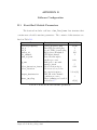
APPENDIX B. Software Configuration . . . . . . . . . . . . . . . . . . . . . . . . . . . . . . . 109
B.1 Front-End Module Parameters. . . . . . . . . . . . . . . . . . . . . . . . . . . . . . . . . . . . . . . . . . . 109
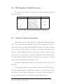
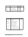
B.2 RLS Equalizer Module Parameters . . . . . . . . . . . . . . . . . . . . . . . . . . . . . . . . . . . . . . 110
B.3 Channel Combiner Parameters . . . . . . . . . . . . . . . . . . . . . . . . . . . . . . . . . . . . . . . . . . 110
BIOGRAPHY OF THE AUTHOR . . . . . . . . . . . . . . . . . . . . . . . . . . . . . . . . . . . . . 112
University of Maine MS Thesis
Raymond A. McAvoy, May, 2002
v
LIST OF TABLES
4.1
RLS equalization times without compiler optimization. . . . . . . . . . . . . . . . . . . 59
4.2
RLS equalization times with compiler optimization. . . . . . . . . . . . . . . . . . . . . . . 59
5.1
Elements of the sensor data structure. . . . . . . . . . . . . . . . . . . . . . . . . . . . . . . . . . . . . . 62
5.2
Elements of the front-end data sub-structure. . . . . . . . . . . . . . . . . . . . . . . . . . . . . . 62
5.3
Elements of the equalizer job structure. . . . . . . . . . . . . . . . . . . . . . . . . . . . . . . . . . . . 64
5.4
Elements of the equalizer scratch space structure. . . . . . . . . . . . . . . . . . . . . . . . . 65
A.1 Memory used by the equalizer job structure. . . . . . . . . . . . . . . . . . . . . . . . . . . . . . . 106
A.2 Memory used by the scratch space structure. . . . . . . . . . . . . . . . . . . . . . . . . . . . . . 106
A.3 Memory used by the front-end sub-structures. . . . . . . . . . . . . . . . . . . . . . . . . . . . . 106
A.4 Equalizer memory allocated on the heap. . . . . . . . . . . . . . . . . . . . . . . . . . . . . . . . . . . 108
B.1 Front-end module run-time parameters. . . . . . . . . . . . . . . . . . . . . . . . . . . . . . . . . . . . 109
B.2 RLS equalizer module run-time parameters. . . . . . . . . . . . . . . . . . . . . . . . . . . . . . . 110
B.3 Channel combiner module compile-time parameters. . . . . . . . . . . . . . . . . . . . . . 111
B.4 Channel combiner module run-time parameters. . . . . . . . . . . . . . . . . . . . . . . . . . . 111
University of Maine MS Thesis
Raymond A. McAvoy, May, 2002
vi
LIST OF FIGURES
2.1
Interconnection of UDAT receiver modules. . . . . . . . . . . . . . . . . . . . . . . . . . . . . . . .
6
2.2
Format of a single telemetry data frame. . . . . . . . . . . . . . . . . . . . . . . . . . . . . . . . . . .
8
3.1
Functional block diagram of the telemetry receiver front-end. . . . . . . . . . . . . 13
3.2
Magnitude response of the first FIR decimation filter, used to
reduce the sample rate by a factor of five. . . . . . . . . . . . . . . . . . . . . . . . . . . . . . . . . . . 16
3.3
Block diagram of the Doppler compensator and resampler. . . . . . . . . . . . . . . . 17
3.4
Complex representation of the phase-locked loop used for Doppler
tracking. . . . . . . . . . . . . . . . . . . . . . . . . . . . . . . . . . . . . . . . . . . . . . . . . . . . . . . . . . . . . . . . . . . . . . . . 23
3.5
Frequency-domain representation of the (linearized) phase-locked
loop. . . . . . . . . . . . . . . . . . . . . . . . . . . . . . . . . . . . . . . . . . . . . . . . . . . . . . . . . . . . . . . . . . . . . . . . . . . . 24
3.6
Magnitude response of the 6th order elliptical pilot tone filter. . . . . . . . . . . . 31
3.7
Magnitude response of the 800-coefficient FIR interpolation
filter used to implement the resampler. . . . . . . . . . . . . . . . . . . . . . . . . . . . . . . . . . . . . . 32
3.8
Magnitude response of the output FIR anti-aliasing filter. . . . . . . . . . . . . . . . . 33
4.1
Block diagram of the decision feedback equalizer - digital phase
locked loop (DFE-DPLL). . . . . . . . . . . . . . . . . . . . . . . . . . . . . . . . . . . . . . . . . . . . . . . . . . . . 40
4.2
Block diagram of the rth diversity feedforward section of the
DFE-DPLL. . . . . . . . . . . . . . . . . . . . . . . . . . . . . . . . . . . . . . . . . . . . . . . . . . . . . . . . . . . . . . . . . . . 41
4.3
Block diagram of the non-sparse feedback section of the DFEDPLL. . . . . . . . . . . . . . . . . . . . . . . . . . . . . . . . . . . . . . . . . . . . . . . . . . . . . . . . . . . . . . . . . . . . . . . . . 42
4.4
Block diagram of the spth sparse feedback section of the DFEDPLL. . . . . . . . . . . . . . . . . . . . . . . . . . . . . . . . . . . . . . . . . . . . . . . . . . . . . . . . . . . . . . . . . . . . . . . . . 42
4.5
RLS equalizer error from C version. . . . . . . . . . . . . . . . . . . . . . . . . . . . . . . . . . . . . . . . . 51
4.6
RLS equalizer error from MATLAB version. . . . . . . . . . . . . . . . . . . . . . . . . . . . . . . 52
4.7
RLS benchmark for 41 taps. . . . . . . . . . . . . . . . . . . . . . . . . . . . . . . . . . . . . . . . . . . . . . . . . 54
4.8
RLS benchmark for 41 taps with optimization. . . . . . . . . . . . . . . . . . . . . . . . . . . . 55
4.9
RLS benchmark for 62 taps. . . . . . . . . . . . . . . . . . . . . . . . . . . . . . . . . . . . . . . . . . . . . . . . . 56
4.10 RLS benchmark for 62 taps with optimization. . . . . . . . . . . . . . . . . . . . . . . . . . . . 56
4.11 RLS benchmark for 104 taps. . . . . . . . . . . . . . . . . . . . . . . . . . . . . . . . . . . . . . . . . . . . . . . . 57
University of Maine MS Thesis
Raymond A. McAvoy, May, 2002
vii
4.12 RLS benchmark for 104 taps with optimization. . . . . . . . . . . . . . . . . . . . . . . . . . . 58
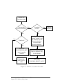
5.1
Channel combiner functional illustration. . . . . . . . . . . . . . . . . . . . . . . . . . . . . . . . . . 61
5.2
Channel combiner status flow chart. . . . . . . . . . . . . . . . . . . . . . . . . . . . . . . . . . . . . . . . 69
5.3
State flow diagram for the sensor state machine. . . . . . . . . . . . . . . . . . . . . . . . . . 71
5.4
Ping synchronization flow chart. . . . . . . . . . . . . . . . . . . . . . . . . . . . . . . . . . . . . . . . . . . . 72
5.5
Watch for detection flow chart. . . . . . . . . . . . . . . . . . . . . . . . . . . . . . . . . . . . . . . . . . . . . . 75
5.6
State flow diagram for the job state machine. . . . . . . . . . . . . . . . . . . . . . . . . . . . . . 78
5.7
Linked list of correlator values and corresponding pointers. . . . . . . . . . . . . . . 84
5.8
List construction and update flow chart. . . . . . . . . . . . . . . . . . . . . . . . . . . . . . . . . . . 85
5.9
Sparse feedback tap calculation flow chart. . . . . . . . . . . . . . . . . . . . . . . . . . . . . . . . . 87
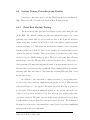
5.10 Sample of artificial testing demodulator (top) and correlator
(bottom) waveforms. . . . . . . . . . . . . . . . . . . . . . . . . . . . . . . . . . . . . . . . . . . . . . . . . . . . . . . . . 90
6.1
Test setup configuration. . . . . . . . . . . . . . . . . . . . . . . . . . . . . . . . . . . . . . . . . . . . . . . . . . . . . 93
6.2
Module arrangement on Morocco II for one input channel. . . . . . . . . . . . . . . 94
6.3
Module arrangement on Morocco II for two input channels. . . . . . . . . . . . . . 95
6.4
Sample of demodulator output waveform. . . . . . . . . . . . . . . . . . . . . . . . . . . . . . . . . . 97
6.5
Sample of correlator output waveform. . . . . . . . . . . . . . . . . . . . . . . . . . . . . . . . . . . . . 97
6.6
Equalization results from one input channel (no diversity). . . . . . . . . . . . . . . 98
6.7
Equalization results from one input channel with time diversity. . . . . . . . . 99
6.8
Equalization results from two input channels (spatial diversity). . . . . . . . . 99
6.9
Equalization results from four input channels (spatial and time
diversity). . . . . . . . . . . . . . . . . . . . . . . . . . . . . . . . . . . . . . . . . . . . . . . . . . . . . . . . . . . . . . . . . . . . . 100
University of Maine MS Thesis
Raymond A. McAvoy, May, 2002
viii
CHAPTER 1
Introduction
1.1
Background
Submarine warfare simulation exercises conducted by the Naval Undersea
Warfare Center (NUWC) have stimulated an interest in reliable underwater communication links. NUWC requires the ability to exchange data between submerged
submarines, surface ships, and seafloor hydrophone arrays in shallow water environments [1].
While acoustical signals propagate reasonably well in water, several issues
must be addressed when designing an underwater communications link. Tests
conducted for the Seaweb ’98 program [2] and NUWC [3] have revealed that
multipath signal spread is a major problem associated with underwater communications in shallow water environments. Inter-symbol interference and signal fading
are other issues that must be dealt with as well.
A study conducted by NUWC [4] has shown that a decision feedback
equalizer (DFE) coupled with a digital phase locked loop (DPLL) can compensate
for these undesired effects in underwater environments. The DPLL helps track
phase shifts that are too rapid for the DFE. The equalizer design proposed in [4]
also makes use of multiple diversity inputs to help combat problems due to channel
fading.
1.2
Purpose of the Research
The Test and Evaluation Department at the NUWC Newport Division origi-
nally developed and tested a prototype Underwater Digital Acoustic Telemetry
(UDAT) system using Texas Instruments TMS320C40 digital signal processors
University of Maine MS Thesis
Raymond A. McAvoy, May, 2002
1
[5, 1]. This thesis presents the design and implementation of an improved UDAT
system using Analog Devices SHARC processors.
NUWC’s prototype UDAT system, or modem, utilized two TMS3240C40
DSPs for each of its four functional blocks: (1) packet detection and synchronization, (2) Doppler estimation and compensation, (3) complex demodulation,
and (4) equalization. The modem presented in this thesis uses a redesigned Doppler
compensation algorithm that has been combined with a redesigned complex demodulation algorithm, thereby allowing the two to run on a single SHARC processor.
The packet detection and synchronization algorithms have also been redesigned,
allowing them to run real-time on a single SHARC DSP. The redesign of the
packet detection and synchronization includes two additional capabilities. First is
the ability to automatically choose equalizer parameters based on channel information. Second is the capability to handle multiple acoustic sensors.
A special initialization sequence and manual fine tuning were required to
select equalizer parameters in NUWC’s prototype modem. That design results in
fixed equalizer parameters that may not remain optimal as the channel changes
with time. The modem described in this thesis automatically gathers channel
characteristics from the synchronization pings and uses them to periodically update
the equalizer parameters.
The modem presented in this thesis is capable of handling signals from
multiple physically separated acoustic sensors. This spatial diversity technique
can help lower error rates. Another technique known as time diversity also lowers
error rates. Time diversity requires the transmitter to repeat the message several
times (usually twice). The modem described in this thesis is capable of using both
spatial and time diversity. In contrast, the prototype modem developed by NUWC
utilized time diversity operation only.
University of Maine MS Thesis
Raymond A. McAvoy, May, 2002
2
Tests of the UDAT system conducted by NUWC [5] revealed that strong
multipaths arriving several milliseconds after the main signal created problems
with equalization. Increasing the equalizer’s memory to include the late arriving
paths usually is not practical in real-time systems [5]. The equalizer used in the
modem presented in this thesis utilizes a sparse feedback section to include late
arriving signal paths without adding excessive computational complexity.
The modem implementation discussed in this thesis is expected to allow
a maximum data rate of 1800 bits/sec at a range of 2 nautical miles in shallow
water. It also has the capability to track Doppler shifts up to ±2% in order to
compensate for transmitters and receivers aboard moving submarines and ships.
1.3
Thesis Organization
Chapter 2 provides an introduction to the modules that make up the UDAT
system and shows how they are interconnected. The system’s data frame layout
is also be presented in Chapter 2. Descriptions of each module appear in greater
detail in later chapters.
In chapter 3, the front-end module is described. This module demodulates
and Doppler-compensates the incoming data. The front-end module also provides
channel information in the form of Target ID (TID) correlations.
Chapter 4 presents the implementation and benchmarking of the decision
feedback equalizer-phase locked loop (DFE-DPLL). The DFE-DPLL, or equalizer,
is used to correct for multipath channel and fading effects.
Chapter 5 discloses the channel combiner module that collects data and
channel information from one or more front-end modules. This module time aligns
the incoming data frames and submits them to an equalizer module. The channel
combiner also gathers information about the channel characteristics that are used
to configure the equalizer.
University of Maine MS Thesis
Raymond A. McAvoy, May, 2002
3
Testing procedures and results used to verify proper operation of the system
are discussed in Chapter 6. This chapter also presents recommendations for future
changes and improvements.
University of Maine MS Thesis
Raymond A. McAvoy, May, 2002
4
CHAPTER 2
UDAT System Overview
This chapter provides an overview of the three modules that comprise the
Underwater Digital Acoustic Telemetry (UDAT) receiver. It also introduces some
notation that will be used throughout the later chapters. A description of the data
frame format used by the UDAT receiver is also described in this chapter.
The software implementation of this receiver is implemented on Analog
Devices Super Harvard Architecture Computer (SHARC ) digital signal processors.
The modular design of the software makes use of link port interconnections to
exchange data between the various modules. That design allows for flexibility in
the system configuration. The original design was constructed and tested on a
Morocco II carrier board with 8 SHARC processors [6]. Work is currently under
way to move the system to a Hammerhead platform that supports four faster
SHARC processors [7].
2.1
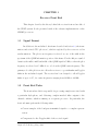
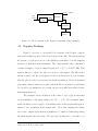
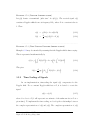
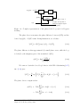
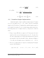
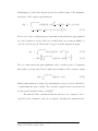
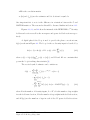
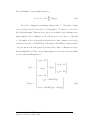
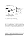
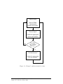
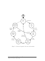
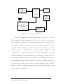
UDAT Receiver Modules
The UDAT receiver is comprised of one or more front-end modules, a
channel combiner module, and one or more equalizer modules. These modules
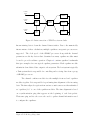
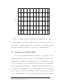
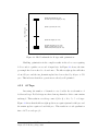
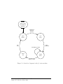
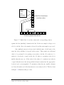
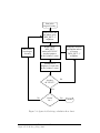
are connected as shown in Figure 2.1.
One front-end module is required for every acoustic input. Exploitation of
spatial diversity requires the use of multiple, physically separated, acoustic sensors
- each with a dedicated front-end module. Exploitation of time diversity can be
achieved with a single front-end module where repeated transmissions of the same
data helps combat time varying channel fading effects.
The equalizer modules implement the mathematical operations required to
determine and track dynamic channel characteristics. The equalizers make use of
University of Maine MS Thesis
Raymond A. McAvoy, May, 2002
5
Acoustic
sensor
Acoustic
sensor
Acoustic
sensor
Front
End
Equalizer
Front
End
Channel
Combiner
Front
End
Equalizer
Equalizer
Host
Figure 2.1: Interconnection of UDAT receiver modules.
known training data to learn the channel characteristics. Due to the numerically
intense nature of these calculations, multiple equalizers on separate processors are
supported. The clock speed of the SHARC processors along with the channel
parameters are the key factors that determine how many equalizer modules must
be used to provide real-time operation. Chapter 4 contains equalizer benchmarks
that give examples for some typical equalizer parameters. Each equalizer module
submits its demodulated data output to a host system. The host system is typically
a Unix system that is responsible for controlling and receiving data from a group
of SHARC processors.
The channel combiner module ties the multiple front-end and equalizer
modules together. It is responsible for performing time alignment of the incoming
data. The time-aligned receptions from various acoustic sensors are then submitted
as “equalizer jobs” to one of the equalizer modules. The time alignment is based
on a synchronization ping that appears at the beginning of each data packet.
That same ping and its echoes are also used to gather channel information used
to configure the equalizers.
University of Maine MS Thesis
Raymond A. McAvoy, May, 2002
6
2.2
Sensor, Channel, and Job Notation
As was presented in Section 1.2, the UDAT system uses both time and/or
spatial diversity to reduce reception errors. Time diversity is implemented by
combining two transmissions of the same data into two equalizer input “channels.”
Spatial diversity involves combining receptions of the same data frame from two
physically separated “sensors” into two equalizer input “channels.” It is necessary
at this time to distinguish between “sensors” and “channels”. Sensors are physical
input devices (such as hydrophones) which provide an acoustic input to a frontend module. The sensor outputs are demodulated and Doppler compensated by
the front end. Multiple copies of these outputs for the same transmitted data
(either from spatial or time diversity) are time aligned by the channel combiner
and submitted to an equalizer for demodulation. For a given equalizer job, each
copy of the time aligned receptions is known as a “channel”.
The equalizer’s input channels can come from any combination of time
and/or spatial diversity inputs. For example, two sensors could provide four
input channels to the equalizer when the system is operating in both time and
spatial diversity modes. Or, two sensors could provide two input channels when
operating in spatial diversity mode. Alternatively, one sensor could provide two
input channels when operating in time diversity mode.
In addition to time aligning the sensor waveforms, the channel combiner is
responsible for determining the dominant channel characteristics and passing this
information along to the equalizer. This information is stored in a structure called
an “equalizer job”. Equalizer jobs are written by the channel combiner and sent
to equalizers as described in Chapter 5.
University of Maine MS Thesis
Raymond A. McAvoy, May, 2002
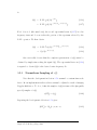
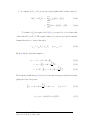
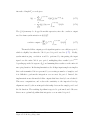
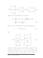
7
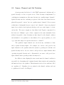
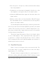
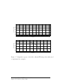
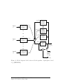
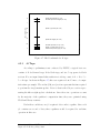
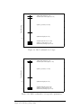
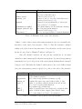
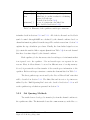
One Data "Frame" (one second)
42 msec
100 msec
SYNCH
Pulse
80 msec
720 msec
200
Training
Symbols
76−bit
DPSK Ping
541.33 usec/bit
58 msec
1800 Data Symbols
SYNCH
Pulse
QPSK Data
400 usec/symbol
Figure 2.2: Format of a single telemetry data frame.
2.3
Data Frame/Modulation Format
The UDAT system transmits data in a data frame format illustrated in
Figure 2.2. Each data frame is one second long and contains the following sections.
• 42 msec target identification (TID) ping
• 100 msec quiet time
• 800 msec modulated data
• 58 msec quiet time
2.3.1
TID Ping
The data frame is initiated using a synchronization pulse consisting of a
76-bit Differential Phase Shift Keyed (DPSK) ping. The receiver, described in
Chapter 3, supports the detection of two possible “target ID” bit sequences within
this synch pulse. To be compatible with tracking ping formats currently used by
NUWC, the DPSK modulation format for the synchronization ping is different
from that of the information portion of the frame. The bit duration within the
synchronization pulse is 541.33 µsec, giving a ping duration of 41.682 msec.
University of Maine MS Thesis
Raymond A. McAvoy, May, 2002
8
These TID pings are used by the channel combiner (described in Chapter
5) to time align the received data frames. These pings are also used to identify
data frame numbers when the system is operating in time diversity mode.
2.3.2
Quiet Times
The synchronization ping is followed by a 100 msec quiet time in which no
data is transmitted. The receiver utilizes this period to obtain possible multipath
delays for the channel. The channel combiner uses synchronization ping detections
within this time period to indicate the channel delays that are likely to include
significant energy for the following data. Further details of this operation appear
in Section 5.4. The channel combiner then passes this delay information on to the
equalizer.
The 58 msec quiet time at the end of the frame helps prevent echoes of one
frame from interfering with the next frame.
2.3.3
Modulated Data
The information period of the data frame consists of 2000 Quadrature
Phase Shift Keyed (QPSK) symbols, 200 “training symbols” followed by 1800 data
symbols. The training symbols are known by both the transmitter and receiver.
They are used to “train” the adaptive equalizer to “learn” the channel characteristics. Training data is included with each data frame to allow the equalizer to
“re-learn” the channel characteristics once every second, thereby compensating for
rapidly changing channels.
The symbol duration for this portion of the frame is 400 µsec, so that the
information portion of the frame lasts a total of 800 msec. As was stated above,
this information period is broken down into training and real data sections. The
University of Maine MS Thesis
Raymond A. McAvoy, May, 2002
9
200 symbols of training data occupy the first 80 msec, while the real data occupies
the last 720 msec of this interval.
Chapter 3 presents the UDAT receiver front-end module used to receive
this specialized signal format.
University of Maine MS Thesis
Raymond A. McAvoy, May, 2002
10
CHAPTER 3
Receiver Front End
This chapter describes the theory behind the receiver front-end module of
the UDAT system. It also presents details of the software implementation on the
SHARC processors.
3.1
Signal Format
In addition to the modulated data frame described in Section 2.3, the trans-
mitter sends a fixed CW “pilot tone”, which is exploited by the receiver to aid in
synchronization. The pilot tone frequency is selected as one of the nulls in the
spectrum of the QPSK information portion of the frame. For the 400 µsec symbol
duration, the null-to-null bandwidth of the QPSK signal is 5 kHz, so that the pilot
frequency is selected as 2.5 kHz above or below the QPSK carrier frequency. The
primary role of the pilot tone is to allow the receiver to cope with unknown Doppler
shifts in the modulated signal. The receiver has been designed to allow Doppler
shifts of up to ±2%, for carrier frequencies ranging from 10 kHz to 40 kHz.
3.2
Front End Tasks
The front-end module is responsible for processing samples associated with
a particular hydrophone, and delivering complex matched filter outputs to the
channel combiner, which is running on a separate processor. In particular, the
front end must perform the following tasks:
• Convert samples of the bandpass transmitted signal to a complex representation.
• Compensate for the Doppler shift of the received signal.
University of Maine MS Thesis
Raymond A. McAvoy, May, 2002
11
• Detect the presence of the pilot tone, which is an indication that telemetry
data is being transmitted.
• Normalize the received waveform by the magnitude of the pilot tone, so that
a fixed amplitude received signal is delivered to the channel combiner.
• Calculate the QPSK matched filter outputs, and deliver these values to the
channel combiner.
• Find the correlation of the received waveform with two different 76-bit target
ID’s. The maximum of the two correlations and the associated target ID are
delivered to the channel combiner.
Note that although the synchronization ping correlation is performed in the
front end, the actual detection and frame alignment is performed by the channel
combiner. The receiver front end produces a continuous output stream of correlation values and matched filter outputs, without any regard for the particular
data frame structure shown in Figure 2.2.
The front end output data streams are delivered to the channel combiner
at a rate of 5000 samples/sec. Each complex matched filter output symbol is
accompanied by a correlation value (indicating the larger of the two calculated
76-bit correlations), the ID associated with this maximum, and an indication of
whether the pilot tone has been detected.
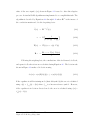
3.3
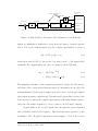
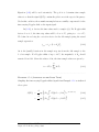
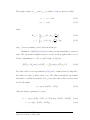
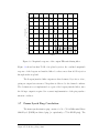
Front End Overview
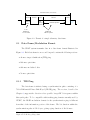
Figure 3.1 shows a block diagram of the receiver front-end module. The
receiver input consists of a stream of samples from an acoustic sensor using a
sample frequency of Fs = 104.4375 ksps.
The signal of interest is assumed modulated at a carrier frequency Ωc =
2πFc rad/sec, and has a null-to-null bandwidth of 5 kHz. For efficiency, bandpass
University of Maine MS Thesis
Raymond A. McAvoy, May, 2002
12
Sent to Channel
Combiner
Locked to transmitter clock
5 ksps
10 ksps
2
104.4375 ksps
20.8875 ksps
Lowpass Filter
Input
5
Match Filter Output
10 ksps
Doppler Compensation
and Resampler
Lowpass/Matched
Filter
Synch Correlation
2
Correlation Values
Maximum ID
Pilot Detected
exp(−j Ωct)
Figure 3.1: Functional block diagram of the telemetry receiver front-end.
signals are manipulated within the receiver front end using a complex representation. For a real bandpass signal x(t), the complex representation is given by
x̃(t) = L.P.P. x(t)e−jΩc t
(3.1)
where the notation L.P.P.{} denotes the “low pass portion” of the signal in the
argument. The original signal x(t) can be reconstructed from x̃(t) using
x(t) = 2Re x̃(t)e+jΩc t
= 2|x̃(t)| cos(Ωc t + 6 x̃(t))
(3.2)
(3.3)
The magnitude and phase of the complex representation x̃(t) provide the envelope
and phase of the corresponding bandpass signal. No information about x(t) is lost
in manipulating x̃(t), and reduced sample rates can be used to describe the complex
representation (saving computations). The mixer and lowpass filter portions of the
front end serve to extract the complex representation of the input sample sequence,
and reduce the sample frequency by a factor of five to 20.8875 ksps (complex).
Doppler shifts in the received signal cause the apparent carrier frequency
and bandwidth of the received signal to differ from the values generated by the
transmitter. The “Doppler Compensation and Resampler” block of the receiver
University of Maine MS Thesis
Raymond A. McAvoy, May, 2002
13
compensates for this effect by modifying the sample frequency implemented at the
receiver. In short, the receiver sampling frequency is adjusted until the transmitted
pilot tone is phase-locked to a locally generated pilot tone at the appropriate
frequency. This procedure effectively locks the receiver sample rate to that of the
transmitter. Since Doppler compensation requires resampling of the input signal,
it is straightforward to also implement an additional decimation by a factor of
(approximately) 2 within this stage. This relaxes the requirements of the first
decimation filter, saving computations. Doppler compensation implementation
using the complex representations are presented in Section 3.5.
The output of the Doppler Compensation block is a stream of complex
samples at sample rate of 10 ksps. A lowpass filter is used to limit the bandwidth
of this signal to approximately 2.5 kHz to avoid aliasing in the final decimation
stage. The QPSK matched filter output for a given time index involves summing
the filter outputs over the most recent four samples (400 µsec). This operation is
combined with the calculation of the lowpass filter output, so that a single filter is
used to implement both the lowpass and matched filter operations. This sequence
is then decimated (by 2) to form the “Matched Filter Output” that is provided to
the channel combiner.
“Synch Correlation” outputs of the receiver front end provide data frame
synchronization. The matched filter outputs are correlated with the known bit
sequences for the possible synchronization pings. Since phase ambiguity exists
between the transmit and receive clocks, the magnitude of the (complex) correlation is used to detect the presence of the synchronization ping. Correlation values
are calculated for every other matched filter output, giving an output sample rate
of 5 ksps. For each output sample, the maximum correlation value is reported,
along with the ping ID associated with the maximum.
University of Maine MS Thesis
Raymond A. McAvoy, May, 2002
14
The following sections provide additional details regarding the design and
implementation of the individual components of the receiver front-end module.
3.4
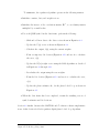
Calculation of the Complex Representation
The complex representation of the input signal is given in equation (3.1).
Samples of the complex representation are calculated from the sequence of input
samples by filtering the signal x(kTs )e−jΩc kTs , where Ts = 1/Fs . Values of the
exponential can be calculated recursively by setting
(3.4)
e0 = 1
ek = ek−1 exp(−jΩc Ts )
= e−jΩc kTs
k = 1, 2, . . .
(3.5)
(3.6)
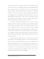
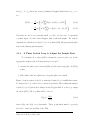
The transcendental function exp(−jΩc Ts ) can be evaluated once, so that calculation of the exponential portion of the sequence involves a single complex multiplication. The sequence ek x(kTs ) must then be filtered to produce samples of
x̃(t).
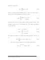
The null-to-null spectrum of x(t) occupies the band Fc − 2.5 kHz to Fc +
2.5 kHz. Doppler shifts may shift the apparent frequency at the receiver by up
to ±2%, so that for a carrier frequency of Fc = 40 kHz, the band of interest
occupies roughly Fc ± 3.3 kHz. The lowpass filter used to create x̃(t) must pass
frequencies below 3.3 kHz. To reduce the sample rate by a factor of five to 20.08875
kHz, the filter must eliminate frequencies within 3.3 kHz of 20.08875 kHz to avoid
the undesired signal from aliasing into the band of interest. A 25 coefficient FIR
lowpass filter was designed to provide 80 dB of stopband rejection. The magnitude
response of the filter is shown in Figure 3.2.
University of Maine MS Thesis
Raymond A. McAvoy, May, 2002
15
10
0
−10
Filter Gain (dB)
−20
−30
−40
−50
−60
−70
−80
−90
0
0.5
1
1.5
2
2.5
3
Frequency
3.5
4
4.5
5
4
x 10
Figure 3.2: Magnitude response of the first FIR decimation filter, used to reduce
the sample rate by a factor of five.
University of Maine MS Thesis
Raymond A. McAvoy, May, 2002
16
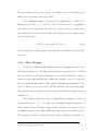
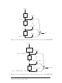
x̃(tk ) = y(kTy )
Input
x̃(kTx )
Pilot Tone p̃(kTx )
Filter
Resampler
tk
p̃(tk )
Phase
Comparison
Reference
Oscilator
Figure 3.3: Block diagram of the Doppler compensator and resampler.
3.5
Doppler Tracking
Figure 3.3 provides a conceptual block diagram of the Doppler compen-
sation and resampler portion of the receiver front-end module. The system exploits
the presence of a pilot-tone at one of the QPSK spectral nulls to lock the sampling
frequency to that used in the transmitter. The complex input for the compensator
consists of samples of x̃(t) at sample frequency Fx = Fs /5 = 20.08875 kHz. This
signal is filtered to extract the pilot-tone portion of the signal. (The filter is not
strictly required, and the development described in this section does not assume
that the pilot tone has been separated from the modulation. However, marginal
performance improvements were realized when the filter was included, particularly
for low pilot tone amplitudes. As a result, the pilot tone filter was included in the
final implementation.)
The resampler allows calculation of the values of x̃(t) or p̃(t) at times that
are not multiples of the input sample period Tx = 1/Fx . The resampler implemented in this receiver is capable of calculating values of these signals with approximately 1 µsec granularity in the sample time. (Note that changing the sample
rate for the complex representation is slightly more complicated than interpolating
the input signals, since the value of Ts used in (3.5) must also be modified—see
University of Maine MS Thesis
Raymond A. McAvoy, May, 2002
17
Section 3.5.3.) The goal of the Doppler compensation section is to generate a
sequence of input sample times tk so that the output signal sample rate is Fy = 10
ksps, locked to the transmitter clock. To accomplish this, the pilot-tone portion of
the transmitted signal is compared to a locally generated pilot tone. Phase errors
between the two signals are used to adjust the sampling clock.
The remainder of this section gives the mathematical development needed
to implement the resampler and Doppler compensation.
3.5.1
Complex Representations of Bandpass Signals
To develop the Doppler tracking algorithm, this subsection reviews the
complex representation notation used in this thesis, and gives a few examples of
signals that will prove useful. Let x(t) denote a bandpass signal of interest with
center frequency Ωc rad/s and bandwidth B Hz. The complex representation of
x(t) given by (3.1) is restated here
x̃(t) = L.P.P. x(t)e−jΩc t .
(3.7)
The original signal x(t) can be reconstructed from x̃(t) using
x(t) = 2Re x̃(t)e+jΩc t
= 2|x̃(t)| cos(Ωc t + 6 x̃(t))
(3.8)
(3.9)
..........................................................................
Example 3.5.1 (Pure cosine)
For x(t) = A cos(Ω1 t), we have
x̃(t) =
University of Maine MS Thesis
Raymond A. McAvoy, May, 2002
A
exp (j(Ω1 − Ωc )t) .
2
18
(3.10)
..........................................................................
Example 3.5.2 (Doppler Shifted cosine)
Let p(t) denote a transmitted “pilot tone” A cos(Ωp t). The received signal x(t)
contains a Doppler shifted tone at frequency DΩp , where D is a constant close to
1. Then
x(t) = p(Dt) = A cos(Ωp Dt)
(3.11)
A
exp (j(Ωp D − Ωc )t)
2
(3.12)
x̃(t) =
..........................................................................
Example 3.5.3 (Time Varying Doppler Shifted cosine)
Example 3.5.2 may be extended by assuming that the Doppler shift is time-varying.
This is represented mathematically by
Z
x(t) = p
t
Z t
D(λ)dλ = A cos Ωp
D(λ)dλ
0
(3.13)
0
This gives
Z t
A
x̃(t) = exp jΩp
D(λ)dλ − jΩc t .
2
0
3.5.2
(3.14)
Time Scaling of Signals
In our implementation, timescaling the signal x(t) compensates for the
Doppler shift. For a constant Doppler shift factor D, it is desired to create the
signal
y(t) = x(t/δ)
(3.15)
where δ is close to D (δ will represent our estimate of the unknown factor D at a
given time). To implement the time scaling, we develop the relationships between
the complex representations of x(t) and y(t). The complex representation of y(t)
University of Maine MS Thesis
Raymond A. McAvoy, May, 2002
19
is
ỹ(t) = L.P.P. x(t/δ)e−jΩc t
= L.P.P. x(t/δ)e−jΩc (t/δ) e−jΩc (t−t/δ) .
(3.16)
(3.17)
For δ close to 1 (the usual case), the second exponential term of (3.17) is a low
frequency term and does not alter the portion of the spectrum selected by the
L.P.P. operator. We then obtain
ỹ(t) = L.P.P. x(t/δ)e−jΩc (t/δ) e−jΩc (t−t/δ)
= x̃(t/δ)e−jΩc (t−t/δ) .
(3.18)
(3.19)
One can readily observe that the complex representation of y(t) cannot be
obtained by simply time scaling the signal x̃(t). The exponential factor in (3.19)
is required to obtain ỹ(t) for the desired center frequency Ωc .
3.5.3
Nonuniform Sampling of x(t)
Note that the development in Section 3.5.2 assumed a constant time-scale
factor. In our implementation the scale factor must be adjusted to track a changing
Doppler shift factor. To do so, define the samples of y(t) in terms of the (unequally
spaced) samples of x(t):
y(kTy ) = x(tk ).
(3.20)
Repeating the development of Section 3.5.2 gives
ỹ(kTy ) = x̃(tk )e−jΩc (kTy −tk ) .
University of Maine MS Thesis
Raymond A. McAvoy, May, 2002
20
(3.21)
Equation (3.21) will be used extensively. The goal is to determine time sample
values tk so that the signal ỹ(kTy ) contains the pilot tone at the expected frequency.
Under this condition, the nonuniform sampler has successfully compensated for the
time-varying Doppler shift on the input signal.
In (3.21), tk denotes the time values used to sample x(t). For Doppler shift
factors close to 1, the time step values will be close to Ty , giving tk+1 − tk ≈ Ty .
We define ∆k as being the correction factor for the kth sample giving the actual
sample separation:
tk+1 = tk + (1 + ∆k )Ty .
(3.22)
∆k is the (small) deviation in the sample step size from the kth sample to the
k + 1st sample. For Doppler shifts of up to ±2%, the magnitude of ∆k should
remain below 0.02. Given the values of ∆k , the time sample values are given by
tk = kTy +
k−1
X
∆` Ty
(3.23)
`=0
..........................................................................
Example 3.5.4 (Sampling of the Pilot Tone)
Sampling the time-varying Doppler shifted signal from Example 3.5.3 as indicated
above gives
Z tk
A
ỹ(kTy ) =
exp jΩp
D(λ)dλ − jΩc tk e−jΩc (kTy −tk )
2
0
Z tk
A
=
exp jΩp
D(λ)dλ − jΩc kTy
2
0
University of Maine MS Thesis
Raymond A. McAvoy, May, 2002
21
(3.24)
(3.25)
Let Dk = 1 − dk denote the average (unknown) Doppler shift factor for tk < t <
tk+1 .
k−1
X
A
(Ty (1 + ∆` )D` ) − jΩc kTy
ỹ(kTy ) =
exp jΩp
2
`=0
!
k−1
X
A
=
exp jTy Ωp
(1 + ∆` )(1 − d` ) − jΩc kTy
2
`=0
(3.26)
!
(3.27)
Note that ∆` and d` are generally small (< 0.02). In our case, d` represents
a system input—it is the actual Doppler shift at the kth sample. We wish to
determine ∆` such that (1 + ∆` )(1 − d` ) ≈ 1, so that ỹ(kTy ) will represent the pilot
tone at the (known) pilot frequency.
3.5.4
A Phase Locked Loop to Adjust the Sample Rate
To determine ∆` so that y(kTy ) contains the expected pilot tone at the
appropriate frequency, the following strategy is adopted:
1. measure the phase error between ỹ(kTy ) and the desired exp(j(Ωp − Ωc )kTy ))
terms.
2. Filter this result and adjust ∆` to keep this phase error small.
Figure 3.4 shows a phase-locked loop structure designed to accomplish these tasks.
To analyze the loop, each block is considered separately. The nonuniform sampler
described by (3.27) shows how changes in the Doppler shift dk or the loop output
∆k effect ỹ(kTy ). The loop filter will be denoted
HL (z) =
B(z)
.
A(z)
where B(z) and A(z) are polynomials.
selected to ensure the stability of the PLL.
University of Maine MS Thesis
Raymond A. McAvoy, May, 2002
22
(3.28)
These polynomials must be properly
exp(j(Ωp − Ωc )kTs )
Phase
Detector
Loop
Filter
Nonuniform
Sampler
ỹ(kTs )
∆k
Sample Rate Control
Doppler Compensated
Sampled Output Signal
ỹ(kTs )
x̃(t)
Figure 3.4: Complex representation of the phase-locked loop used for Doppler
tracking.
The phase detector measures the phase difference between ỹ(kTy ) and the
desired exp(j(Ωp − Ωc )kTy terms. In implementation, we calculate
γ̃(kTy ) = ỹ(kTy ) exp(−j(Ωp − Ωc )kTy )
(3.29)
The phase difference is then approximated (for small phase errors, while the loop
is locked) by the imaginary part of the normalized γ̃(kTy ):
φ(kTy ) = Im
γ̃(kTy )
|γ̃(kTy )|
(3.30)
We can now obtain the closed-loop behavior of the PLL. Substituting (3.27)
into (3.29) gives
!
k−1
X
A
γ̃(kTy ) = exp jTy Ωp
[(1 + ∆` )(1 − d` ) − 1]
2
`=0
(3.31)
The phase detector output is then
φ(kTy ) ≈ Ty Ωp
= Ty Ωp
k−1
X
`=0
k−1
X
`=0
University of Maine MS Thesis
Raymond A. McAvoy, May, 2002
23
[(1 + ∆` )(1 − d` ) − 1]
(3.32)
(∆` − d` − d` ∆` )
(3.33)
d(z)
Ωp Ts z −1
1−z −1
φ(z)
HL (z) =
B(z)
A(z)
∆(z)
Figure 3.5: Frequency-domain representation of the (linearized) phase-locked loop.
The cross-product term d` ∆` does not significantly influence the behavior of the
loop since ∆` and d` are both small. This term is dropped from the analysis, giving
φ(kTy ) ≈ Ωp Ty
k−1
X
(∆` − d` )
(3.34)
`=0
In difference equation form, we have
φ(kTy ) = φ((k − 1)Ty ) + Ωp Ty (∆k−1 − dk−1 ).
(3.35)
Taking the z-transform of this result gives a frequency domain description of the
phase detector combined with the nonuniform sampler:
φ(z) = (Ωp Ty )
z −1
(∆(z) − d(z)).
1 − z −1
(3.36)
Figure 3.5 gives a frequency domain depiction of the linearized phase-locked loop
just developed. The linearized model shows how external changes in the Doppler
shift of the sampled signal (dk ) are tracked by the sampler.
Successful loop
operation is indicated by small values of φ(kTy ) (small phase errors). The closedloop transfer function from the Doppler disturbance to the phase error is given by
φ(z)
−Ωp Ty A(z)
=
d(z)
(z − 1)A(z) − Ωp Ty B(z)
(3.37)
The loop filter polynomials A(z) and B(z) should be selected to make this small
at low input frequencies (near z = 1). A second transfer function of interest is the
University of Maine MS Thesis
Raymond A. McAvoy, May, 2002
24
relationship between dk and ∆k . The closed-loop relationship is given by
−Ωp Ty B(z)
∆(z)
=
d(z)
(z − 1)A(z) − Ωp Ty B(z)
(3.38)
This filter should be lowpass in nature, so that the (relatively low frequency)
changes in dk are accurately tracked by the loop, while portions of the re-sampled
signal not near the pilot tone frequency are rejected.
3.5.4.1
Selection of Loop Filter Coefficients
Selection of the loop filter coefficients was largely a trial and error process.
The following constraints are observed:
1. The loop must be stable. Given the poles and zeros of HL (z), the gain of
the filter may be modified while monitoring the magnitudes of the roots of
(z − 1)A(z) − Ωp Ty B(z). Gain values are identified so that these roots lie
within the unit circle under all expected values of Ωp Ty .
2. The steady-state phase error must be reasonable. The phase detector given
in (3.30) is based on an assumption that the phase error will be small. Phase
errors above ±π/2 violate the linearity assumptions used in the approximation given in (3.32). The nonlinearity will cause the loop to loose lock.
The steady-state phase error for a constant Doppler shift factor Dss = 1−dss
is obtained from the DC gain of the closed-loop response
φ(z) =
dss
d(z) z=ej0 =1
1
=
dss
HL (1)
φss
University of Maine MS Thesis
Raymond A. McAvoy, May, 2002
25
(3.39)
(3.40)
For example, to obtain a maximum phase error of ±π/3 for a maximum
Doppler shift of 2% (dss = 0.02) gives the requirement
π
0.02
≥
3
|HL (1)|
(3.41)
To meet this requirement, the DC gain of the loop filter must exceed -34 dB.
3. The roots of A(z) are selected close to z = 1, making HL (z) lowpass and
making
φ(z)
d(z)
small near z = 1.
4. The roots of B(z) are selected near the unit circle to control the bandwidth
of
∆(z)
.
d(z)
This transfer function should be lowpass, with bandwidth sufficient
to pass the Doppler drift frequencies, but narrow enough to reject any other
modulation present in the signal.
3.5.4.2
Doppler Tracking PLL Summary
For further reference, the iterative Doppler tracking PLL is summarized by
the equations (3.42) to (3.46), which are restated from the above development.
• Nonuniform Sampler
tk = tk−1 + (1 + ∆k−1 )Ty
(3.42)
ỹ(kTy ) = x̃(tk ) exp {−jΩc (kTy − tk )} .
(3.43)
γ̃(kTy ) = ỹ(kTy ) exp(−j(Ωp − Ωc )kTy )
(3.44)
• Phase Detector
University of Maine MS Thesis
Raymond A. McAvoy, May, 2002
26
φ(kTy ) = Im
γ̃(kTy )
|γ̃(kTy )|
(3.45)
• Loop Filter
HL (z) =
∆k =
B(z)
b0 + b1 z −1 + · · · + bn z −n
=
A(z)
1 + a1 z −1 + · · · + an z −n
n
X
bi φ((k − i)Ty ) −
i=0
3.5.5
n
X
ai ∆k−i
(3.46)
i=1
Nonuniform Sampler Implementation
Assume that samples of x̃(t) are available at sample frequency Fx samples
per second, and sample period Tx = 1/Fx . That is, x̃(t) has been uniformly
sampled, and x̃(`Tx ) is known. To implement the nonuniform sampler required by
(3.43), samples between times `Tx can be calculated using polyphase interpolators.
For an interpolation rate of I, samples at time `Tx + m(Tx /I) can be obtained as
follows:
1. Design a lowpass FIR filter at sample rate IFx that passes the desired
signal band and rejects (at least) frequencies above Fy − B, where Fy is
the desired output sample rate for ỹ(t) (possibly different from Fx ) and B is
the bandwidth of x̃(t). Select the number of filter coefficients as a multiple of
I. Let h(k) denote the impulse response of this filter (k = 0, 1, . . . , M I − 1).
2. The set of I polyphase filters are designed by decimating h(k). The impulse
response of the mth filter is
pm (j) = h(m + jI)
University of Maine MS Thesis
Raymond A. McAvoy, May, 2002
m = 0, 1, . . . , I − 1 j = 0, 1, . . . , M − 1
27
(3.47)
3. To evaluate x̃(`Tx + mTx /I), use the mth polyphase filter at time origin `Tx :
M
−1
X
x̃(`Tx + mTx /I) =
pm (j)x̃((` − j)Tx )
(3.48)
h(m + jI)x̃((` − j)Tx )
(3.49)
j=0
M
−1
X
=
j=0
To evaluate x̃(tk ) as required in (3.43), tk is rounded to a close time value
of the form `k Tx + mk Tx /I. The required values of `k and mk are found recursively.
Assume that the tk−1 value is known by
tk−1 = `k−1 Tx + rk−1 Tx
0 ≤ rk−1 < 1.
(3.50)
From (3.42) the next time sample is
tk = tk−1 + (1 + ∆k−1 )Ty
Ty
= tk−1 + (1 + ∆k−1 )
Tx
Tx
Ty
Tx
= `k−1 Tx + rk−1 + (1 + ∆k−1 )
Tx
(3.51)
(3.52)
(3.53)
The term in parenthesis in (3.53) can be broken into its integer and fractional part,
giving the desired step sizes:
Ty
rk−1 + (1 + ∆k−1 )
Tx
= ∆`k + rk ,
0 ≤ rk < 1.
tk = (`k−1 + ∆`k )Tx + (rk I) Tx /I
University of Maine MS Thesis
Raymond A. McAvoy, May, 2002
28
(3.54)
(3.55)
The required values of `k−1 and mk−1 to evaluate (3.49) are given by setting
`k = `k−1 + ∆`k
mk = brk Ic
(3.56)
(3.57)
where
∆`k
rk
Ty
=
rk−1 + (1 + ∆k−1 )
Tx
Ty
=
rk−1 + (1 + ∆k−1 )
− ∆`k
Tx
(3.58)
(3.59)
and b·c denotes rounding down to the nearest integer.
Evaluation of ỹ(kTy ) in (3.43) also requires an exponential phase correction
term. The exponential evaluation may be avoided in the polyphase filter case as
follows. Substituting tk = `k Tx + mk (Tx /I) into (3.43) gives
ỹ(kTy ) = x̃(tk ) exp {−jΩc (kTy − `k Tx )} exp {+jΩc Tx mk /I}
(3.60)
The value of the second exponential in (3.60) can be obtained from a lookup table,
since there are only I possible values of mk . The value of the middle exponential
term may be calculated recursively. Let ck denote the value of this correction term
for the kth sample:
ck = exp {−jΩc (kTy − `k Tx )}
(3.61)
Using the update equations for `k gives
ck = exp {−jΩc ((k − 1)Ty − `k−1 Tx )} exp {−jΩc (Ty − ∆`k Tx )}
= ck−1 exp {−jΩc (Ty − ∆`k Tx )}
University of Maine MS Thesis
Raymond A. McAvoy, May, 2002
29
(3.62)
(3.63)
The exponential term of (3.63) can also be tabulated, since (for small Doppler
shifts) only a few values of ∆`k are possible.
The nonuniform sampler given in (3.43) is implemented by using (3.56)
through (3.59) to find `k , mk , and ∆`k . These values are used to approximate
x̃(tk ) using (3.49). The integer ∆`k is used to obtain ck as in (3.63) (where the
exponential factor is obtained from a table). The Doppler corrected output sample
is then obtained from
ỹ(kTy ) = x̃(tk )ck exp {jΩc Tx mk /I}
(3.64)
where again the exponential term is found from an I-element table indexed by the
value of mk .
3.5.6
Filter Designs
A 6th order elliptical highpass filter was used to implement the pilot tone
filter shown in Figure 3.3. The filter passband includes frequencies above 1.7 kHz
(the lower limit for the Doppler shifted pilot tone location). This filter, combined
with the lowpass filter implemented within the resampler, serves to isolate the
pilot tone from the bulk of the modulated signal. The filter was implemented as a
cascade of three second-order sections. The filter allows 0.3 dB of passband ripple,
and attenuates the stopband by 40 dB. A plot of the filter characteristic is shown
in Figure 3.6.
The polyphase interpolator used to implement the resampler is based on
an interpolation rate of I = 50, giving an oversampled sampling frequency of
50Fx = 1044.375 ksps. The filter design described in Step 1 of Section 3.5.5 was
accomplished using a 800-coefficient FIR filter with 80 dB of stopband rejection.
The magnitude response of this interpolation filter is illustrated in Figure 3.7.
University of Maine MS Thesis
Raymond A. McAvoy, May, 2002
30
10
0
Filter Gain (dB)
−10
−20
−30
−40
−50
0
1000
2000
3000
4000
5000
6000
Frequency
7000
8000
9000
10000
Figure 3.6: Magnitude response of the 6th order elliptical pilot tone filter.
The filter impulse response was decimated as described in (3.47) to give a set of
50 separate 15-coefficient polyphase filters. Calculation of each resampled output
value involves finding the output of one of these 15-coefficient FIR filters.
3.6
Lowpass and Matched Filters
The output lowpass filter illustrated in Figure 3.3 is required to avoid
aliasing when the sample rate is reduced to 5 ksps. This filter was designed to pass
frequencies below 2.2 kHz, and reject frequencies above 2.8 kHz. Figure 3.8 shows
a plot of the magnitude response of this filter, obtained using a 40-coefficient FIR
filter. In implementation, this filter is combined with the QPSK matched filter by
convolving the designed impulse response with the impulse response of the matched
filter (a sequence of four 1’s). The resulting combined lowpass and matched filter
is a 43-coefficient FIR filter. Note that although the magnitude response shown in
University of Maine MS Thesis
Raymond A. McAvoy, May, 2002
31
Filter Gain (dB)
0
−20
−40
−60
−80
0
0.5
1
1.5
2
2.5
3
Frequency
3.5
4
4.5
5
5
x 10
Filter Gain (dB)
0
−20
−40
−60
−80
0
1000
2000
3000
4000
5000
Frequency
6000
7000
8000
9000
10000
Figure 3.7: Magnitude response of the 800-coefficient FIR interpolation filter used
to implement the resampler.
University of Maine MS Thesis
Raymond A. McAvoy, May, 2002
32
10
0
−10
Filter Gain (dB)
−20
−30
−40
−50
−60
−70
−80
−90
0
500
1000
1500
2000
2500
Frequency
3000
3500
4000
4500
5000
Figure 3.8: Magnitude response of the output FIR anti-aliasing filter.
Figure 3.8 shows less than 70 dB of stopband rejection, the combined magnitude
response of the lowpass and matched filter does have more than 80 dB rejection
throughout the stopband.
The Lowpass/matched filter outputs are then decimated by a factor of two,
giving an output data stream of 5 ksps that is delivered to the channel combiner.
The decimation is not implemented as a part of the lowpass/matched filter, since
the 10 ksps output is required for accurate implementation of the ping synchronization correlator.
3.7
Frame Synch Ping Correlation
The frame-synchronization ping consists of a Nb = 76-bit Differential Phase
Shift Keyed (DPSK) modulated ping (or equivalently, a 77-bit BPSK ping). The
University of Maine MS Thesis
Raymond A. McAvoy, May, 2002
33
ping may be described by
p(t) =
Nb
X
bk p0 (t − kTb )
(3.65)
k=0
where bk = ±1 indicates the transmitted bit, Tb = 541.33 µsec is the bit period,
and p0 (t) describes the transmitted waveform for each bit.
sin(Ωc t) 0 ≤ t ≤ Tb
p0 (t) =
0
(3.66)
elsewhere
Note that (3.66) describes a “phase jammed” signal, in which the phase of the
transmitted signal is reset for each transmitted bit. The complex representation
of p0 (t) is given by
p̃0 (t) = −(j/2)w(t)
1 0 ≤ t ≤ Tb
w(t) =
0 elsewhere
(3.67)
(3.68)
The complex representation for a frame synchronization ping that occurs at t = 0
is
p̃(t) =
Nb
X
bk (−j/2)w(t − kTb )e−jΩc kTb .
(3.69)
k=0
The desired correlator output for a received signal s(t) is given by
Z
t+(Nb +1)Tb
s(λ)p(λ − t)dλ.
c(t) =
t
University of Maine MS Thesis
Raymond A. McAvoy, May, 2002
34
(3.70)
Substituting (3.3) into this expression gives the result in terms of the magnitude
and phase of the complex representations
Z
c(t) =
t+(Nb +1)Tb
1
cos(6 s̃(λ) − 6 p̃(λ − t) + Ωc t)
2
t
1
6
6
+ cos( s̃(λ) + p̃(λ − t) + Ωc t + Ωc λ) dλ.
(3.71)
2
4|s̃(λ)||p̃(λ − t)|
The second cosine is a high frequency term with an integral that is approximately
zero (and equals zero for the ideal case in which there are an integer number of
cycles in each bit period). This term is dropped from the integration giving
Z
t+(Nb +1)Tb
c(t) =
t
( Z
2Re s̃(λ)p̃∗ (λ − t)ejΩc t dλ.
!
)
t+(Nb +1)Tb
= 2Re
s̃(λ)p̃∗ (λ − t)dλ ejΩc t
(3.72)
.
(3.73)
t
The ejΩc t term reflects the phase alignment of the correlation period. Comparing
this result to (3.2) gives the desired complex representation of the correlator output
Z
t+(Nb +1)Tb
c̃(t) =
s̃(λ)p̃∗ (λ − t)dλ
(3.74)
t
Frame synchronization is obtained by comparing the envelope of c(t) to a threshold,
or equivalently the value of 2|c̃(t)|. The correlator output for the receiver front end
are the actual calculated values of (2|c̃(t)|)2 .
The matched filter calculation that has already been completed can be
exploited in the evaluation of the above integral. Breaking the integration into
University of Maine MS Thesis
Raymond A. McAvoy, May, 2002
35
intervals of length Tb seconds gives
c̃(t) =
Nb Z
X
k=0
=
Nb
X
t+(k+1)Tb
s̃(λ)b∗k (j/2)ejΩc kTb dλ
(3.75)
t+kTb
b∗k (j/2)ejΩc kTb
Z
t+(k+1)Tb
s̃(λ)dλ
(3.76)
t+kTb
k=0
The (j/2) term may be dropped from this expression, since the correlator output
used for frame synchronization is (2|c̃(t)|)2 .
N
2
Z t+(k+1)Tb
b
X
correlator output = b∗k ejΩc kTb
s̃(λ)dλ
t+kTb
(3.77)
k=0
The matched filter outputs provide signal integration over a 400 µsec period,
which is slightly less than the 541.33 µsec bit period used in (3.77). Ideally,
synchronization ping correlation would be performed by integrating the input
signal over the entire 541.33 µsec period, multiplying these results by ±ejΩc kTb
depending upon the bit sequence (bk ), and summing these results over the entire 42
msec ping duration. In this implementation, the 10 ksps input sample rate implies
that each transmitted bit is represented by a non-integer number of samples, and
it is difficult to perform the integration over an exact bit period. Instead, the
implementation uses the matched filter outputs that have already been calculated.
This saves computations, and reduces the sensitivity to the imperfect bit-edge
alignment caused by the non-integral relationship between the sample period and
the bit duration. The resulting algorithm is expected to perform about 1 dB worse
than a more optimal algorithm that integrates over an entire bit period.
University of Maine MS Thesis
Raymond A. McAvoy, May, 2002
36
CHAPTER 4
Adaptive Feedback Equalizer
This chapter describes the UDAT system’s equalizer module. This module
consists of a front-end interface to the channel combiner module and a Recursive
Least Squares (RLS) equalizer.
Studies conducted by NUWC [4] have shown that an adaptive decision
feedback equalizer-digital phase locked loop (DFE-DPLL) works very well in terms
of reducing multipath effects, time varying inter-symbol interference, and channel
fading inherent in underwater environments. MATLAB prototypes of this equalizer
were written by Dr. Nixon A. Pendergrass, Susan M. Jarvis, and Fletcher Blackmon
at NUWC using both RLS and Fast Transversal Filters (FTF) weight update
algorithms.
Using the RLS algorithm to update the equalizer’s filter weights is relatively
computationally intensive. It is on the order of N 2 where N is the length of
the weight vector (Equation 4.3).
The FTF algorithm on the other hand is
more computationally efficient (on the order of N ). However, since this is a
prototype system being developed for the first time on SHARC processors it was
decided to start by implementing the equalizer with an RLS algorithm. The
straightforward nature of the RLS algorithm simplified the task of translating
the MATLAB equalizer code into a C version for the SHARC processors. It was
also expected that the increased processing power of the SHARC processors (as
compared to the C40 processors used in [1]) might be sufficient to handle the
increased computational burden of the RLS algorithm.
Discussion of the equalizer will begin by introducing the notation and
presenting the basics of the implemented algorithm. Next, key operations of the C
language implementation of the equalizer will be discussed and compared to their
University of Maine MS Thesis
Raymond A. McAvoy, May, 2002
37
MATLAB equivalents. Finally, a series of benchmarks will be presented to show
the equalizer’s calculation times for some typical tap weight counts.
4.1
General Equalizer Algorithm Overview
A block diagram of this diversity input adaptive DFE-DPLL is shown in
Figure 4.1. Note that this is the same equalizer presented in [4] except for the
addition of the sparse feedback sections (detailed in Figure 4.3).
Both the MATLAB and C implementations of this adaptive equalizer use
the following notation:
• n is the symbol counter
• training is the training symbol counter
• v is a matrix with columns of input data for each channel
• L, M , and M 2 are the number of feedforward, feedback, and sparse feedback
tap weights respectively
• M 2OF F is a vector of sparse feedback tap locations
• R is the number of diversity inputs (channels)
˜ are the feedforward, feedback, and sparse feedback tap weight
• ã, b̃, and b2
vectors respectively
• p(n), q(n), and q2(n) are the contributions of the feedforward, feedback, and
sparse feedback sections respectively
˜ (Equation 4.8)
• W̃ (n) is the weight vector formed from ã, b̃, and b2
• Ũ (n) is the input vector shown in Equation 4.8
University of Maine MS Thesis
Raymond A. McAvoy, May, 2002
38
• R is the correlation matrix
• d(n) and dbit (n) are the estimates and bit decisions for symbol n
One important fact to note is the difference in orientation between the C and
MATLAB matrices. The reasons for this will be discussed further in Section 4.2.1.
Figures 4.2, 4.3, and 4.4 show the internals of the DFE-DPLL’s rth diversity
feedforward section as well as the non-sparse and sparse feedback sections respectively.
A digital phase-locked loop is used to provide the phase correction term,
Θr (n) as shown in Figure 4.2. The loop for the rth diversity input is described by
Θr (n + 1) = Θr (n) + K1 · φr (n) + K2 ·
n
X
φr (i),
(4.1)
i=0
P
∗
where φr (i) = ={pr (n)[ R
r=1 pr (n) + ε(n)] }, and K1 and K2 are constants that
govern the loop’s tracking characteristics [4].
The received symbol estimate can be written as
d(n) =
R X
T
X
a∗r,i (n) · e−jΘr (n) · vr (2n − i)
r=1 i=−T
−
M
X
b∗` (n) · dbit (n − `)
`=1
−
2(sp)
SP MX
X
sp=1
b2∗sp,` (n) · dbit (n − M 2OF F (sp) − `),
(4.2)
`=1
where R is the number of diversity inputs, L = 2T + 1 is the number of tap weights
in each feedforward section, M is the number of tap weights in the feedback section,
and M 2(sp) are the numbers of taps in each of the SP sparse feedback sections.
University of Maine MS Thesis
Raymond A. McAvoy, May, 2002
39
Input 1
v1
Feedforward
Section 1
q21 (n)
Sparse
Feedback
Section 1
q2SP (n)
Sparse
Feedback
Section SP
p1 (n)
q(n) Feedback
Section
Input r
vr
Feedforward
Section r
pr (n)
+
d(n)
Decision
Rule
Output
dbit (n)
−
Input R
vR
Feedforward
Section R
+
Training
Signal
pR (n)
dref (n)
Error Signal ε(n)
Figure 4.1: Block diagram of the decision feedback equalizer - digital phase locked
loop (DFE-DPLL).
University of Maine MS Thesis
Raymond A. McAvoy, May, 2002
40
Input r
vr
a∗r,T (n)
x
vr (2n + T )
z −1
a∗r,T −1 (n)
x
a∗r,1 (n)
x
vr (2n + 1)
z −1
a∗r,0 (n)
x
vr (2n)
z −1
+
a∗r,−1 (n)
vr (2n − 1)
x
a∗r,−T +1 (n)
e−jΘr (n)
x
pr (n)
x
z −1
a∗r,−T (n)
T = (L − 1)/2
vr (2n − T )
x
Figure 4.2: Block diagram of the rth diversity feedforward section of the DFEDPLL.
University of Maine MS Thesis
Raymond A. McAvoy, May, 2002
41
dbit (n)
z −1
−b∗1 (n)
x
dbit (n − 1)
z −1
−b∗M −1 (n)
x
z −1
+
−b∗M (n)
dbit (n − M )
q(n)
x
Figure 4.3: Block diagram of the non-sparse feedback section of the DFE-DPLL.
dbit (n)
z −M 2OF F (sp)
−b2∗sp,1 (n)
x
dbit (n − M 2OF F (sp))
z −1
−b2∗sp,M 2(sp)−1 (n)
x
z −1
−b2∗sp,M 2(sp) (n)
dbit (n − M 2OF F (sp) − M 2(sp))
+
q2sp (n)
x
Figure 4.4: Block diagram of the spth sparse feedback section of the DFE-DPLL.
University of Maine MS Thesis
Raymond A. McAvoy, May, 2002
42
The total number of tap weights is given by
N =L·R+M +
SP
X
M 2(sp).
(4.3)
sp=1
In order to eliminate recalculating values in the z −1 delay lines, column
vectors ṽr (n) are used to store the 2n + T through 2n − T values of vr for each of
the R diversity inputs. Values in each ṽr (n) vector are shifted down each time a new
˜
input sample is added. Similarly, a vector d(n)
is used to store the n − 1 through
˜ sp (n)
n − M samples of dbit for use in the feedback section. And column vectors d2
are used to store the n−M 2OF F (sp)−1 through n−M 2OF F (sp)−M 2(sp) values
of dbit for use in each of the sparse feedback sections. These coefficient vectors are
shown in Equation 4.4. The corresponding weight vectors are also stored in column
vectors as shown in Equation 4.5.
vr (2n + T )
..
.
dbit (n − 1)
˜
..
ṽr (n) = vr (2n) d(n) =
.
..
.
dbit (n − M )
vr (2n − T )
dbit (n − M 2OF F (sp)
.
˜ sp (n) =
..
d2
dbit (n − M 2OF F (sp) − M 2(sp))
University of Maine MS Thesis
Raymond A. McAvoy, May, 2002
43
(4.4)
ar,T (n)
..
.
ãr (n) = ar,0 (n)
..
.
ar,−T (n)
−b1 (n)
..
b̃(n) =
.
−bM (n)
˜ sp (n) =
b2
−b2sp,1 (n)
..
.
−b2sp,M 2(sp) (n)
(4.5)
Equations 4.4 and 4.5 allow Equation 4.2 to be written as
d(n) =
R
X
H
˜
ãH
r · ṽr (n) + b̃ (n) · d(n) +
r=1
=
R
X
SP
X
˜ H (n) · d2
˜ sp (n)
b2
sp
sp=1
pr (n) + q(n) +
r=1
SP
X
q2(n)
(4.6)
sp=1
Equation 4.2 can also be written in terms of the entire W̃ (n) weight vector as
d(n) = W̃ H (n) · Ũ (n)
(4.7)
where
ã1 (n)
..
.
ṽ1 (n) · e−jΘ1 (n)
..
.
ã (n)
ṽ (n) · e−jΘR (n)
R
R
˜
W̃ (n) = b̃(n) Ũ (n) =
d(n)
b2
˜ 1 (n)
˜ 1 (n)
d2
..
..
.
.
˜ S P (n)
˜ SP (n)
b2
d2
(4.8)
In Equation 4.7, W̃ (n) represents the vector of all filter coefficients used in the
various systems shown in Figures 4.2, 4.3, and 4.4. To track changing channel
conditions, this vector must be modified while the receiver is operating. The
University of Maine MS Thesis
Raymond A. McAvoy, May, 2002
44
value of the error signal, ε(n), shown in Figure 4.1 is used to drive this adaptive
process. A standard RLS algorithm was implemented to accomplish this task. The
algorithm is described by Equations 4.9 through 4.12 where R−1 is the inverse of
the correlation matrix and λ is the forgetting factor.
P̃ (n) = R−1 · Ũ (n)
α = <
1
λ + Ũ (n)H · P̃ (n)
(4.9)
W̃ (n) = W̃ (n) + α · ε(n) · P̃ (n)
R−1 =
R−1 − α · P̃ (n) · P̃ H (n)
λ
(4.10)
(4.11)
(4.12)
Following the weight update, the contributions of the feedforward, feedback,
and sparse feedback sections are recalculated using Equation 4.6. The decision rule
shown in Figure 4.1 makes a bit decision using
dbit (n) = sign(<{d(n)}) + j · sign(={d(n)})
(4.13)
If the equalizer is still in training mode (first 200 symbols) the error is calculated
using ε(n) = dref (n) − d(n) where dref is a known reference symbol. However,
if the equalizer is in decision directed mode the error is calculated using ε(n) =
dbit (n) − d(n).
University of Maine MS Thesis
Raymond A. McAvoy, May, 2002
45
To summarize, the equalizer algorithm operates in the following manner:
• Initialize counters, data, and weight vectors.
• Initialize the inverse of the correlation matrix, R−1 , to an identity matrix
multiplied by a small scalar.
• For each QPSK symbol in the data frame, perform the following:
– Shift and add new data to the data vectors shown in Equation 4.4.
– Update the Ũ (n) vector as shown in Equation 4.8.
– Calculate the output, d(n), using the current weights.
– Form a temporary bit decision (Equation 4.13 and use it to calculate
the error, ε(n).
– Update the W̃ (n) weight vector using the RLS algorithm as described
in Equations 4.9 through 4.12.
– Recalculate the output using the new weights.
– Form the bit decision (Equation 4.13 and use it to calculate the error,
ε(n).
– Update the phase estimate, Θr , for the phase locked loop as shown in
Equation 4.1.
• When the data frame has been completed, return the resulting vectors of
symbol estimates and bit decisions.
Section 4.2 further discusses the MATLAB and C software software implementations of this decision feedback equalizer-digital phase locked loop algorithm.
University of Maine MS Thesis
Raymond A. McAvoy, May, 2002
46
4.2
Equalizer Implementation
The RLS equalizer used in this system is a C language implementation of
NUWC’s MATLAB version. The code performs an R input channel complex valued
exponentially weighted recursive least squares sparse adaptive filter algorithm for
a QPSK signal. The software implementations accept fractionally spaced input
samples with two samples per QPSK symbol. Therefore, k is used to denote the
sample index while n is used for the QPSK symbol index. Wideband libraries [8]
were used extensively to duplicate the functionality of the MATLAB code in C.
Examples of the Wideband library functions used in the equalizer are shown in the
following sections.
4.2.1
Vector and Matrix Storage
As was noted earlier in Section 4.1, both the MATLAB and C equalizer
code use the same notation. However, the column vectors in the MATLAB code
have been transposed in the C code for memory usage and indexing efficiency.
Matrices are stored in C as one long vector containing the matrices’ rows. This is
not only the optimal storage format but it also allows certain vector operations to
be used on matrices.
4.2.2
Initializing Vectors and Matrices
MATLAB uses the functions eye, ones, and zeros to initialize vectors and
matrices. The Wideband functions vfill and cvfill, which stand for vector fill
and complex vector fill, can be used as an equivalent replacement. To duplicate
the functionality of eye, the vector fill command is first used to fill the matrix with
zeros by treating the matrix as one long row vector. Then a loop is used to change
the diagonal elements to ones.
University of Maine MS Thesis
Raymond A. McAvoy, May, 2002
47
4.2.3
Copying Sections of Vectors and Matrices
The Wideband functions vmov and cvmov, which stand for vector move and
complex vector move, are used to copy sections of vectors and matrices. As an
example, the matrix v_k is used to store the ṽr vectors as defined in Equation 4.4
is formed in MATLAB using a statement of the form:
v_k(1:k,:) = v(k:-1:1,:);
to copy the first k rows of v into v_k in the reverse order. This functionality is
duplicated in C using the Wideband function cvmov within a for loop covering
the number of diversity inputs.
cvmov(&v[index][k-1],-1,&v_k[index][0],1,k);
The for loop accounts for all diversity input channels just as the colon operator
does in MATLAB. Note that the variables v and v_k are transposed from their
MATLAB orientation as was described in Section 4.2.1. The first argument of
cvmov is the address of the k’th column of v and the second is a stride of -1. This
takes the first k columns of v in the reverse order. The third argument is the
destination (columns of v_k) and the stride of 1 keeps them in order. The final
argument, k is an element count.
4.2.4
Dot Products
The Wideband function ccdotpr to calculate a complex conjugate dot
product, is also used in the equalizer code. For example, the received symbol
estimate (Equation 4.7) is calculated in MATLAB using:
d(n) = W_k’ * U_k;
Again, these vectors are transposed from their MATLAB orientation requiring the
Wideband equivalent to multiply them in the reverse order using:
ccdotpr(U_k,1,W_k,1,&d_tmp,taps);
University of Maine MS Thesis
Raymond A. McAvoy, May, 2002
48
Here, U_k and W_k are the two vectors to be multiplied and ones are used as the
strides. The variable taps has been initialized to the length of the vectors being
implemented.
4.2.5
Matrix - Vector Multiplication
Another useful Wideband function is cmvmul which performs a complex
matrix-vector multiplication. It is used to implement Equation 4.9. In MATLAB ,
this equation takes the form:
invR_Uk = inv_R * U_k;
Note that invR_Uk is the variable used to denote P̃ in the MATLAB and C code.
The Wideband equivalent of the above calculation uses:
cmvmul(&inv_R[0][0],taps,taps,U_k,invR_Uk);
The first argument is the start of the inv_R matrix. The next two arguments are
the row and columns of inv_R which are both taps since it is a square matrix. The
fourth argument is the source vector, U_k, which is followed by the destination,
invR_Uk .
4.2.6
RLS Correlation Matrix Update
Updating the correlation matrix (Equation 4.12) is performed using the
following MATLAB code:
inv_R = (inv_R - alfa * invR_Uk * invR_Uk’)/lmda;
However, the Wideband library does not provide a function that does both a matrix
subtraction and a multiplication. And storing a temporary copy of the invR_Uk
outer product requires more memory than is available on the SHARC processors.
Therefore, the matrix update is performed on a column by column basis.
A for loop is used to cycle through the columns. First, a scaling factor of
-alfa * invR_Uk[col_indx] is calculated. Then the Wideband function cvsma
University of Maine MS Thesis
Raymond A. McAvoy, May, 2002
49
is used to perform a complex vector-scalar multiply and add. Initially, this was
implemented using:
cvsma(invR_Uk,1,&scale,&inv_R[0][index],
&taps,&inv_R[0][index],taps,taps);
to calculate the entire column of inv_R. However, on the SHARC processors this
implementation had some numerical instability problems. So a second method was
used to ensure that the matrix would remain symmetric. The new method uses:
cvsma(&invR_Uk[index],1,&scale,&inv_R[index][index],
&taps,&inv_R[index][index],taps,taps-index);
followed by:
cvconj(&inv_R[index+1][index],taps,
&inv_R[index][index+1],1,taps-index-1);
inside a loop that covers all but the last two columns. This multiply and add
only operates on the upper triangular half of the matrix. The cvconj is then
used to generate the lower (conjugate) part of the matrix. Since most of the
Wideband vector functions have a minimum element count, this method requires
the last four elements (last two columns) to be calculated outside the loop.
Finally, the Wideband function vscmul is used to multiply the result by
1/lmda to take care of the division by lmda. vscmul is a vector-scalar multiply,
but the entire inv_R matrix is treated as one long vector since there is no “matrixscalar multiply” function in the Wideband library.
4.3
Equalizer Front End
Due to processing and memory requirements, real-time operation requires
several equalizers, each running on its own processor. As will be described in
Section 5.2.4, jobs are submitted to the equalizers via a link port transfer. This
requires a small job receiving front end to configure a link port and DMA in order
University of Maine MS Thesis
Raymond A. McAvoy, May, 2002
50
2
1.5
Re(Error)
1
0.5
0
−0.5
−1
−1.5
0
200
400
600
800
1000
1200
Sample Index
1400
1600
1800
2000
Figure 4.5: RLS equalizer error from C version.
to receive the job. After the DMA reception has been configured, the front end
enters a loop in which it polls the link port status. Once a complete job transfer
has finished, the equalizer function is called to perform the equalization. Then the
loop repeats by reinitializing another link port reception.
An alternative job sending method that uses the processor common memory
space to transfer jobs from the channel combiner to the equalizers is described in
Section 5.2.3. That job transfer method also requires a job receiving front end to
poll the queue in the common memory for a job to equalize.
4.4
Equalizer Testing and Verification
Proper operation of the RLS equalizer code was verified by comparing it to
the known MATLAB version provided by NUWC. Figures 4.5 and 4.6 show how
the equalizer errors compare between the C and MATLAB versions respectively.
Both plots were generated using the same set of testing data.
University of Maine MS Thesis
Raymond A. McAvoy, May, 2002
51
2
1.5
Re(Error)
1
0.5
0
−0.5
−1
−1.5
0
200
400
600
800
1000
1200
Symbol Index
1400
1600
1800
2000
Figure 4.6: RLS equalizer error from MATLAB version.
Due to the fact that MATLAB’s floating point precision is greater than
that of the SHARC processors, the two error waveforms are not exactly the same.
However, they both exhibit the same characteristic shape, indicating that the
C version is operating correctly. The actual equalized output vectors were also
compared and found to be very close. Again, there was some variation in the
exact magnitudes due to precision differences.
4.5
RLS Equalizer Benchmarks
Several benchmarking tests were performed on the RLS equalizer code to
determine the time required to equalize jobs with various tap counts. This equalizer
design applies the feedback and sparse feedback tap weights equally to all input
channels. Therefore, the equalizer’s computational complexity is strongly related
to the number of feedforward taps and the number of input channels.
University of Maine MS Thesis
Raymond A. McAvoy, May, 2002
52
The following benchmarks were performed on 40 MHz 21060 SHARC digital
signal processors on a Spectrum Morocco II carrier board [6]. The time lines in
Figures 4.7 through 4.12 were generated by measuring the time required to execute
each of the major steps within the equalizer algorithm. A PMC ADADIO board
[9] was connected to the Morocco II carrier board. The DAC on the ADADIO
board was monitored with an oscilloscope. The equalizer code was temporarily
modified to write a different value to the DAC upon completion of each of the
following events:
• entry into the main processing loop
• addition of new samples to the U_k input vector
• calculation of the output and error with current weights
• update of the filter weights, W_k
• update of the inv_R matrix
• calculation of the output with the new weights
• update of the DPLL phase estimate
The computation time required for each event showed up as a plateau on
the oscilloscope waveform. Data captured from the oscilloscope trace was used to
measure the width of those plateaus and generate the benchmarking timelines.
The above sequence occurs once for each sample. Therefore, a larger spike
was also written to the DAC at the completion of each job. Triggering the oscilloscope on the larger peak was used to determine the total equalization time required
per job. The total equalization time is also noted in each of the following benchmarks.
University of Maine MS Thesis
Raymond A. McAvoy, May, 2002
53
Update phase esitmate (17 µ sec)
Calculate output w/new weights (80 µ sec)
1.2
Time (milliseconds)
1
Update inv_R matrix (600 µ sec)
0.8
0.6
0.4
Update filter weights (346 µ sec)
0.2
Calculate output and error (76 µ sec)
Update U_k weight vector (46 µ sec)
Initialize main processing loop (42 µ sec)
0
Figure 4.7: RLS benchmark for 41 taps.
4.5.1
41 Taps
According to preliminary tests conducted by NUWC, a typical test case
consists of 21 feedforward taps, 10 feedback taps, and two 5 tap sparse feedback
sections. For one input channel this results in a total tap count of 21 + 10 + 5 +
5 = 41 taps. As shown in Figure 4.7, this case requires about 1.5 msec of computation time per sample. The widest (590 µsec) section represents the time required
to perform the inv_R matrix update. Prior to that is the 350 µsec section representing the filter weight update calculations. Since these two operations account
for the majority of the equalizer’s computation time, they were optimized using
Wideband library routines.
Under these conditions, one job requires 2.34 seconds to equalize. Since each
job contains one second of data, three equalizers would be required for real-time
operation in this case.
University of Maine MS Thesis
Raymond A. McAvoy, May, 2002
54
1
Update phase estimate (16 µ sec)
Calculate output w/new weights (22 µ sec)
Time (milliseconds)
0.8
Update inv_R matrix (562 µ sec)
0.6
0.4
Update filter weights (343 µ sec)
0.2
0
Calculate output and error (31 µ sec)
Update U_k weight vector (19 µ sec)
Initialize main processing loop (23 µ sec)
Figure 4.8: RLS benchmark for 41 taps with optimization.
Enabling optimization in the compiler results in the above case requiring
1.95 seconds to equalize one second of input data. As Figure 4.8 shows, the time
per sample has been reduced to about 1 msec. The filter weight update still takes
about 350 µsec and the inv_R matrix update has been reduced by 40 µsec to 550
µsec. This indicates that these operations are already well optimized.
4.5.2
62 Taps
Increasing the number of channels to two doubles the total number of
feedforward taps. Feedback taps are shared among channels so their count remains
unchanged. This results in a total tap count of (21 ∗ 2) + 10 + 5 + 5 = 62 taps.
Figure 4.9 shows that the filter weight update now requires just under 800 µsec and
the matrix update requires about 1200 µsec. This results in a total equalization
time of 4.75 seconds per job.
University of Maine MS Thesis
Raymond A. McAvoy, May, 2002
55
Update phase estimate (23 µ sec)
Calculate output w/new weights (129 µ sec)
2
Time (milliseconds)
Update inv_R matrix (1.23 m sec)
1.5
1
Update filter weights (756 µ sec)
0.5
Calculate output and error (137 µ sec)
Update U_k weight vector (77 µ sec)
Initialize main processing loop (61 µ sec)
Figure 4.9: RLS benchmark for 62 taps.
2
Time (milliseconds)
1.5
Update phase estimate (23 µ sec)
Calculate output w/new weights (31 µ sec)
Update inv_R matrix (1.17 m sec)
1
0.5
0
Update filter weights (756 µ sec)
Calculate output and error (54 µ sec)
Update U_k weight vector (30 µ sec)
Initialize main processing loop (31 µ sec)
Figure 4.10: RLS benchmark for 62 taps with optimization.
University of Maine MS Thesis
Raymond A. McAvoy, May, 2002
56
Update phase estimate (31 µ sec)
Calculate output w/new weights (236 µ sec)
5
4
Time (milliseconds)
Update inv_R matrix (3.14 m sec)
3
2
Update filter weights (1.62 m sec)
1
Calculate output and error (260 µ sec)
Update U_k weight vector (114 µ sec)
Initialize main processing loop (115 µ sec)
0
Figure 4.11: RLS benchmark for 104 taps.
Again, enabling optimization in the compiler helps slightly by reducing the
overall equalization time to 4.1 seconds per job. The computational details of this
case are shown in Figure 4.10.
This two diversity channel example represents operation in either time or
spatial diversity mode. Real-time operation with this tap count will require 5
equalizer modules.
4.5.3
104 Taps
On chip memory limits the channel combiner to four channels. This brings
the total tap count for this case to (21 ∗ 4) + 10 + 5 + 5 = 104 taps. Figures 4.11
and 4.12 show the timing details of this 104 taps case. Clearly, the filter weight
and matrix updates account for the majority of computational time per sample.
Considering the fact that equalization times with and without optimization
are 11.89 and 10.72 seconds respectively, it is obvious that the RLS equalizer is too
University of Maine MS Thesis
Raymond A. McAvoy, May, 2002
57
5
Update phase estimate (23 µ sec)
Calculate output w/new weights (68 µ sec)
4.5
4
Time (milliseconds)
3.5
Update inv_R matrix (3.04 m sec)
3
2.5
2
1.5
1
Update filter weights (1.93 m sec)
0.5
0
Calculate output and error (92 µ sec)
Update U_k weight vector (38 µ sec)
Initialize main processing loop (46 µ sec)
Figure 4.12: RLS benchmark for 104 taps with optimization.
computationally intensive for practical use in this case. Four channel operation is
still possible but it requires a tradeoff in the tap count. For example, as shown in
Table 4.2, the number of feedforward taps must be reduced to 11 (as opposed to 21)
to bring the equalization time down to a practical 4.59 seconds. Equalization times
over five seconds are not considered practical since there are only five available
SHARC processors on the Morocco II board when the other three are running
front-end and channel combiner modules.
4.5.4
Benchmark Summary
Table 4.1 lists the total equalization times required for the above bench-
marks without compiler optimization.
enabled are summarized in Table 4.2.
University of Maine MS Thesis
Raymond A. McAvoy, May, 2002
58
The times obtained with optimization
Input
Channels
1
2
4
Feedforward Feedback
Taps
Taps
21
10
21
10
21
10
Sparse Feedback Taps
10
10
10
Total Time (sec)
Taps
41
2.34
62
4.75
104
11.89
Table 4.1: RLS equalization times without compiler optimization.
Input
Channels
1
2
4
4
4
4
4
4
4
Feedforward Feedback
Taps
Taps
21
10
21
10
21
10
19
10
17
10
15
10
13
10
11
10
9
10
Sparse Feedback Taps
10
10
10
10
10
10
10
10
10
Total Time (sec)
Taps
41
1.95
62
4.1
104
10.72
96
9.28
88
7.97
80
6.75
72
5.63
64
4.59
56
3.67
Table 4.2: RLS equalization times with compiler optimization.
University of Maine MS Thesis
Raymond A. McAvoy, May, 2002
59
CHAPTER 5
Channel Combiner
This chapter presents the channel combiner module, the function of which
is tying the front-end and equalizer modules together. As such, it must perform
the following tasks:
• Time alignment of data frames
• Channel analysis (based on the target ID correlation waveform) to identify
dominant multipath components
• Formation of “equalizer jobs” for distribution to the equalizer modules
As was shown in Chapter 2, several front-end modules send time and/or
spatial diversity channels into the channel combiner. Since signals from physically
separated sensors (spatial diversity) do not all arrive at the same time, the channel
combiner must time align the data frames before presenting them to an equalizer
module. Figure 5.1 presents a pictorial view of how the channel combiner time
aligns signals from multiple sensors. The channel combiner must also calculate
equalizer tap sizes and locations based upon the channel information gathered
from the TID ping and its echoes as described in Sections 2.3.1 and 2.3.2.
The inner workings of the channel combiner module are presented by first
discussing the interface with front-end modules followed by methods of distributing
completed jobs to equalizer modules. Next, the state machines that make up the
channel combiner’s inner core are discussed. Finally, the equalizer tap calculations
are presented.
University of Maine MS Thesis
Raymond A. McAvoy, May, 2002
60
Acoustic
sensor
Acoustic
sensor
Front
end
Channel
combiner
Time aligned sensor responses
Front
end
Primary detection
(direct path signal)
Secondary detections
(multipath signals)
Figure 5.1: Channel combiner functional illustration.
5.1
Interface to Front-End Modules
Each front-end module runs on its own SHARC processor and is connected
to one acoustic sensor. The channel combiner also runs on its own processor
and receives data from the front-end modules via link ports. A set of ping pong
buffers is used in conjunction with a direct memory access (DMA) transfer to
bring data into the channel combiner. The ping pong buffers utilize a pointer
(buffer_to_process) to indicate the working buffer. While the CPU is processing
the working buffer, the other buffer is being filled by DMAs transferring data from
the front-end modules.
The channel combiner uses data structures to store information from the
input sensors (front-end modules). One of these sensor data structures is used
for every front-end module that is connected to the channel combiner. Table
5.1 lists the elements contained within each sensor data structure. Each sensor
data structure also contains the ping pong buffers mentioned above. Since these
University of Maine MS Thesis
Raymond A. McAvoy, May, 2002
61
Element Name
Description
front-end data sub-structure input data (ping pong buffers)
associated with this sensor
sensor state
(described in Section 5.3)
current job
pointer to the job associated with this sensor
(described in Section 5.2.1)
channel
channel (location) within the job where the
sensor data is to be written
transmission number
data frame number for use with time diversity
largest peak and age
used for ping synchronization
(described in Section 5.3.2)
TID_array[ ]
used to track past TIDs for channel alignment
Table 5.1: Elements of the sensor data structure.
“buffers” consist of three arrays plus status information, they are essentially substructures of the sensor data structure. Table 5.2 lists the elements contained
within each of the front-end sub-structures. Note that these are the same arrays
shown as being “Sent to Channel Combiner” in Figure 3.1.
Since the channel combiner can only perform calculations on one input
channel at a time it must rapidly alternate among them. A pointer (curr_sensor)
is maintained in order to keep track of the sensor (input channel) that is currently
being processed. Each time the channel combiner moves on to a new buffer of input
data, the curr_sensor pointer is updated to point to the sensor data structure
Element Name
length
td_present
sensor_id
corr[ ]
TID[ ]
demod[ ]
Description
length of the buffer being sent from the front-end module
to the channel combiner
pilot detected flag (switches telemetry on/off)
identifies the sensor associated with a buffer of data
buffer of correlation values from the front-end module
(to be used for ping synchronization
and equalizer tap calculations)
buffer of target ID associated with each correlation value
buffer of matched filter outputs (demodulated data)
(to be time aligned and sent to an equalizer)
Table 5.2: Elements of the front-end data sub-structure.
University of Maine MS Thesis
Raymond A. McAvoy, May, 2002
62
associated with the sensor (front-end module) supplying the data. So the channel
combiner makes use of a C code statement of the form:
curr_sensor -> buffer_to_process -> data
to access data associated with the working ping pong buffer within the appropriate
sensor data structure.
5.2
Equalizer Job Queuing
Real-time operation of the UDAT system requires that the data packets
generated by the channel combiner be equalized at a rate of one per second.
However, as was shown in Chapter 4, the equalizer algorithm often requires more
than one second to equalize a data packet. Therefore, real-time operation requires
several copies of the equalizer module to be run on separate processors. Multiprocessor equalizer operation requires a queuing scheme to distribute jobs among
the equalizers.
5.2.1
Equalizer Jobs
The channel combiner uses structures known as “equalizer jobs” to contain
all of the information required by an equalizer to process a packet of data. Elements
contained within each of the equalizer job structures are listed in Table 5.3. Two of
these job structures must be maintained by the channel combiner since data from
the various input sensors does not all arrive at the same time. For example, it is
possible for ‘sensor A’ to come to the end of a data frame before ‘sensor B’. The
job can’t be submitted to the equalizer until ‘sensor B’ has also reached the end
of its data frame. But in the meantime, ‘sensor A’ will be starting on a new data
frame which in turn requires a new job. Maintaining two job structures eliminates
this problem. Pointers known as actv_job and pend_job are utilized to keep track
of the active and pending jobs respectively. In the above example where ‘sensor
University of Maine MS Thesis
Raymond A. McAvoy, May, 2002
63
Element Name
pop[ ]
half[ ]
det[ ]
aborted[ ]
L
M
M2[ ]
sumM2
lenM2
M2OFF[ ]
v[ ][ ]
Description
vector of channel ‘fully populated’ flags
vector of channel ‘halfway populated’ flags
vector of channel detected flags
vector of aborted channel flags
feedforward symbol count
feedback symbol count
sparse feedback symbol count vector
sum of elements in the M2 vector
length of the M2 vector
sparse feedback delay/offset vector
demodulated signal vectors (data to be equalized)
Table 5.3: Elements of the equalizer job structure.
A’ finishes before ‘sensor B’, the two jobs allow ‘sensor A’ to start writing its new
data frame into the pending job while ‘sensor B’ is finishing up the current job.
When ‘sensor B’ has finished and the job has been submitted to the equalizer, the
actv_job and pend_job pointers are switched. Once a sensor has been assigned
a job as described in Section 5.3.2.4 it continues to use that job until it reaches
the end of a data frame. Therefore, the switching of the active and pending job
pointers does not cause a sensor to jump between jobs part way through a data
frame.
The channel population vector (pop) is used to signify that a channel is
fully populated with valid data to be used by the equalizer. This vector contains
FULL flags that correspond to valid demodulated signal vectors. Invalid signal
vectors (ones that do not contain data) are marked with an EMPTY flag in the
corresponding location in this population vector. Similarly, the halfway (half)
flags are used to indicate when a channel is half full of data. The det (detected)
flags are used to indicate that a signal has been detected on a particular channel.
The aborted flags are used to mark channels that were aborted due to the fact
that they hadn’t received a signal detection. The use of these flags is described
University of Maine MS Thesis
Raymond A. McAvoy, May, 2002
64
Element Name
dir_path[ ]
list
pointers[ ]
Description
storage space for the direct path signal
linked list of correlator values for calculating
sparse feedback taps
(described in Section 5.4.2)
vector of pointers into the linked list
(also described in Section 5.4.2)
Table 5.4: Elements of the equalizer scratch space structure.
in further detail in Sections 5.3.2 and 5.3.3. All of the feedforward and feedback
symbol counts L through M2OFF are calculated by the channel combiner based on
channel information gathered from the target ID correlation waveform. Section 5.4
explains the tap calculation procedures. Finally, the demodulated signal vectors
(v) contain the matched filter outputs (demod from Table 5.2) from each channel
that have been time aligned by the channel combiner.
Each equalizer job also has an associated scratch space for information that
is not passed on to the equalizer. Jobs and scratch space are separate for two
reasons. First, it allows them to be stored in different areas of on-chip memory.
Second, it prevents the needless transfer of the scratch space information to the
equalizer. Each scratch space structure contains the elements listed in Table 5.4.
The direct path storage area is used by the “Record Direct Path” state that
will be described in Section 5.3.2. The linked list and its vector of pointers are
utilized by the “Build Sparsing List” state also described in Section 5.3.2 as well
as the equalizer tap calculations presented in Section 5.4.
5.2.2
Job Queuing Methods
Two methods were developed to transfer jobs from the channel combiner to
the equalizer modules. The first method uses the common memory on the Morocco
University of Maine MS Thesis
Raymond A. McAvoy, May, 2002
65
II board as a queue where jobs are temporarily stored until an equalizer reads them.
The second method uses link port transfers to send jobs to the equalizers.
The common memory job queuing method allows equalizers to be run on
any processor without the need for any special configurations. However, it does
have some limitations. For example, the code used to read data from the ADADIO
(input/output) board [9] ties up the processor common bus making it unavailable
for use with this job queuing scheme. There are also plans to run this software on
platforms other than the Morocco II that do not have the same common memory
architecture. Therefore, it was necessary to develop the link port job transfer
method that is currently in use.
The link port method works very much like the link port transfer used to
bring front end data into the channel combiner. However, instead of using a ping
pong buffering scheme, the data is sent in one continuous block. An additional
link port status check is also performed prior to sending a job. The status check
insures that the equalizer on the receiving link port is ready to accept a new job.
5.2.3
Common Memory Transfer Theory of Operation
With this method, multiple job slots were set aside in the common memory.
This allowed new jobs to be continuously written into the queue without overwriting an unequalized job. The channel combiner would write out new jobs at a
rate of one per second. Each write consisted of a bus request, the data transfer,
and a bus release. Meanwhile each processor running an equalizer module was
also running a job scanning front-end routine. The job scanning front end would
request the common bus on regular intervals. While it had access to the bus
it would check for an available job by looking at a job status flag and copy the
first available job it found into the processor’s local memory. Once the check and
transfer (if applicable) were completed, the job’s status flag was changed and the
University of Maine MS Thesis
Raymond A. McAvoy, May, 2002
66
bus was released. When available jobs were found they were sent to the equalizer
and the front end stopped polling for jobs until the equalizer was finished.
5.2.4
Link Port Transfer Theory of Operation
Instead of submitting jobs to a queue in the common memory, the channel
combiner writes them directly to an equalizer via a link port transfer.
This
requires that the channel combiner be provided with a list of link ports that will be
connected to processors running equalizers. Under normal operating conditions,
the channel combiner cycles through the available link ports in sequence. However,
if an equalizer is busy (as determined by the link port status check) an error is
flagged and the job is sent to the next free equalizer in the sequence.
The required number of equalizers depends largely on the number of taps
selected. As long as a sufficient number of equalizers are in operation, the channel
combiner will function under normal operating conditions and no “busy equalizer”
error flags will be set. Busy equalizer errors are an indication that more equalizers are required to maintain real-time operation. Since the maximum number of
equalizers is limited by the SHARC processor’s 6 link ports, it may be necessary
to reduce the maximum tap limit. The benchmarks presented in Chapter 4 give
a more detailed account of the number of equalizers required to deal with various
tap counts.
5.3
State Machine Implementation
The inner core of the channel combiner consists of two state machines.
One state machine handles the various calculations associated with each of the
input sensors (front-end modules). The other state machine is used to maintain
the equalizer jobs and distribute them to the equalizer modules. The channel
University of Maine MS Thesis
Raymond A. McAvoy, May, 2002
67
combiner uses an overall status to cycle among gathering new input as described
in Section 5.1 as well as updating the appropriate state machines
5.3.1
Overall Status
The channel combiner’s overall status is one of three possibilities:
• Monitor Input
• Process Input
• Job Maintenance
Figure 5.2 presents a flowchart showing how the channel combiner cycles through
the above modes.
While in the “Monitor Input” mode, the link ports are monitored for
incoming data. This is done by looking at a pointer associated with the ping pong
buffers described in Section 5.1. New data is ready when the buffer_to_process
pointer associated with a front-end module changes, indicating that the DMA has
completed filling an input buffer. The actual pointer change takes place in an
interrupt service routine that handles the DMA transfers to the ping pong buffers.
Once a new input buffer has been collected, the status changes to “Process
Input”. The sensor state machine for the appropriate sensor (presented in Section
5.3.2) is executed for the new buffer of input samples. Then, if necessary, the “Job
Maintenance” state machine described in Section 5.3.3 is updated.
University of Maine MS Thesis
Raymond A. McAvoy, May, 2002
68
"Monitor Input"
Wait for DMA
interrupt and
transfer new buffer
"Process Input"
Update the appropriate
sensor state machine
Is at least
one channel
"halfway" ?
No
Yes
"Job Maintenance"
Update the appropriate
job state machine
Figure 5.2: Channel combiner status flow chart.
University of Maine MS Thesis
Raymond A. McAvoy, May, 2002
69
5.3.2
Sensor State Machine
The channel combiner has the capability to maintain multiple sensor state
machines. A separate sensor state machine is associated with each front-end
module that supplies data to the channel combiner. When the channel combiner
status is “Process Input”, the sensor state machine associated with a ping pong
buffer of new data is updated. A diagram of the sensor state machine is shown in
Figure 5.3. It contains the states discussed in the following subsections, namely,
Ping Synchronization, Get Ping TID, Wait for Ping, Watch for Detection, Record
Direct Path, Build Sparsing List, and Record Modulated Data.
5.3.2.1
Ping Synchronization
This is the start-up state for the sensor state machine. By looking for pings
spaced approximately one second apart, this “Ping Synchronization” state prevents
the UDAT receiver from triggering on echoes of pings or false ping detections. This
state examines the correlator outputs provided by the front-end modules to locate
dominant peaks that are close to one second apart. Since it is impractical to save
the correlator outputs for a full second, only the largest correlator peak over the
past 1.1 seconds is maintained in memory. A flow chart of the ping synchronization
logic is shown in Figure 5.4.
In this state, the sample from the correlator is compared to a detection
threshold. Synchronization occurs if the sample is above the threshold and the
largest peak is approximately one second old. Upon synchronization, the sensor’s
state is changed to “Get Ping TID”. Otherwise, the sample is compared to the
largest correlator peak and if appropriate used to replace the largest peak.
Once the sample has been processed, the age of the largest peak is incremented and then checked. A peak age that is significantly older than one second
is an indication of a missed ping. So, if the peak’s age is over 1.1 seconds, it is
University of Maine MS Thesis
Raymond A. McAvoy, May, 2002
70
START
PING
SYNC
Synchronized
RECORD
MODULATED
DATA
Finished
building
list
GET
PING
TID
Found TID
wait 950ms
Finished
recording
wait 50ms
BUILD
SPARSING
LIST
WAIT
FOR
PING
Timed Out
(not detected)
Finished
recording
Done
waiting
RECORD
DIRECT
PATH
WATCH
FOR
DETECTION
Detected
Figure 5.3: State flow diagram for the sensor state machine.
University of Maine MS Thesis
Raymond A. McAvoy, May, 2002
71
Read in new
correlator value
Is peak
approximately
one second old?
Greater than
Yes
detection threshold?
No
No
Increase age
of largest peak
No
No
Is peak
over one
second old ?
Is the
current sample
> largest peak?
Yes
Replace peak
with current
sample
Yes
Erase largest
peak
Reset peak
age to zero
Stay in the
"PING_SYNC"
state for another
iteration
Move on to
"GET_PING_TID"
Figure 5.4: Ping synchronization flow chart.
University of Maine MS Thesis
Raymond A. McAvoy, May, 2002
72
Yes
erased. This procedure prevents synchronization to a false correlator peak that is
not at the start of a data frame.
5.3.2.2
Get Ping TID
Once ping synchronization has been established, the sensor state machine
moves into the target ID detection (“Get Ping TID”) state. This state records the
target ID that corresponds to the synchronization ping. When the ping’s TID has
been established, it is entered into an array containing the TIDs of the past four
pings. The array of past TIDs is used to determine the data frame number of a
packet when operating in time diversity mode.
5.3.2.3
Wait for Ping
Following the “Get Ping TID” state, the state machine enters the “Wait
for Ping” state. This state simply waits a specified amount of time (determined
by a “wait counter”) before moving on to “Watch for Detection”.
“Wait for Ping” can follow either the “Get Ping TID” or “Record Modulated
Data” states. Each state sets the “wait counter” differently. “Get Ping TID” sets
the “wait counter” to just under one second. That causes “Wait for Ping” to stop
just short of the next ping that is due to arrive. “Record Modulated Data” sets
the “wait counter” for 50 msec causing “Wait for Ping” to wait out most of the
59 msec quiet time that follows each data frame. Once “Wait for Ping” is finished
the state is changed to “Watch for Detection”.
5.3.2.4
Watch for Detection
This state looks for the next detection threshold crossing in the correlator
waveform. Once the threshold has been exceeded, the detection is assigned a job
and a data channel within that job. This is where data from this detection will
University of Maine MS Thesis
Raymond A. McAvoy, May, 2002
73
be written. A detected flag is also set for this channel at this time. That flag
will later be used by the job state machine described in Section 5.3.3 to determine
which channels are being filled with valid data. Then the sensor state machine
continues on to the state “Record Direct Path”.
However, if a threshold crossing does not occur within a timeout limit the
sensor state machine is reset back to the “Ping Synchronization” state. Figure 5.5
contains a flow chart illustrating the “Watch for Detection” state.
5.3.2.5
Record Direct Path
The threshold crossing detected by “Watch for Detection” indicates the
start of the direct signal path. This state records the direct signal path section of
the correlator waveform for use in determining channel characteristics in the form
of feedforward and non-sparse feedback equalizer taps. Section 5.4 discusses the
calculations involved in determining the tap sizes based on this direct signal path
recording.
In addition, this state also locates the maximum peak of the target ID
correlation. The time at which the maximum peak occurs is used as the time
origin for this detection.
The target ID corresponding to the maximum peak is also recorded into the
array of past TIDs and used to determine the data frame number of this packet.
A check of the TID array is performed to ensure that the expected TID sequence
is being received. An out of sequence ID will set a TID_error flag that is used as
a warning that this may be a false detection.
Once the direct path (5 msec time window) has been recorded into the job
structure, the sensor’s state is changed to “Build Sparsing List”. In the event
that the direct path lasts longer than the 5 msec time window, the rest of the
University of Maine MS Thesis
Raymond A. McAvoy, May, 2002
74
Read in new
correlator value
Greater than
Yes
detection threshold?
Is pending
job full?
No
Yes
No
Identify current "job",
current "scratch", and
job "channel" for this
detection based on
the sensor and
detection numbers
Yes
Timed out?
No
Stay in the
"WATCH_FOR_DET"
state for another
iteration
Initialize sample counter
and set "detected" flag
for this channel
Reset to the
"PING_SYNC"
state
Move on to
"RECORD_DIRECT_PATH"
Figure 5.5: Watch for detection flow chart.
University of Maine MS Thesis
Raymond A. McAvoy, May, 2002
75
Flag job
full error
direct path will be picked up by the sparsing list and later merged with the direct
feedback path during the final tap calculations.
5.3.2.6
Build Sparsing List
Sensors in the “Build Sparsing List” state update the sparsing list (described
in Section 5.4.3). This list is later used to extract channel characteristics that are
fed into the equalizer in the form of sparse feedback tap sizes and locations. The
actual calculation of these sparse feedback taps is discussed in further detail in
Section 5.4.
This state lasts until the end of the 100 msec quiet time in the data frame.
When completed, the sensor enters the “Record Modulated Data” state.
5.3.2.7
Record Modulated Data
Sensors in this state record the demodulated (and Doppler compensated)
message portion of the data frame into an appropriate slot in the current job.
The appropriate slot and current job were determined while the sensor was in the
“Watch for Detection” state. Recording the demodulated data consists of copying
samples of demod (Table 5.2) into the appropriate row (slot) of v (Table 5.3). Since
the “Record Modulated Data” state is always entered exactly 100 msec after the
peak correlation with the synchronization ping this effectively time aligns the data.
As was described in Section 2.3, this section of data lasts for 800 msec. A
sample counter is used to set a halfway (half) flag at the 400 msec point. The
half flag is later used to see if the job state machine (described in Section 5.3.3)
is ready to be updated.
Once the sample counter has reached the 800 msec point, the sensor has
completed recording its demodulated data. At this point, the sensor is marked
complete by setting its pop flag in the job data structure. Then the sensor state
University of Maine MS Thesis
Raymond A. McAvoy, May, 2002
76
machine is returned to the “Wait for Ping” state to wait out the 59 msec quiet
time that follows each data frame.
Since all of the flags such as half, det, pop, and aborted reside within
the job structure (rather than the sensor structure) there is no need for the sensor
state machine to perform any sort of clean up or re-initialization at the end of
each data frame. Those tasks are performed at the end of the “Send Job” state
described in Section 5.3.3.4.
5.3.3
Job State Machine
Following each update of the sensor state machine, the half flags for each
channel are examined to see if the job state machine needs to be updated.
In the case of no time diversity, a set half flag on at least one of the channels
will cause the channel combiner’s status to change to “Job Maintenance” which in
turn updates the job state machine. When time diversity is being used, only the
channels associated with the second transmitted data frame are examined. A set
half flag on any one of those channels will move the channel combiner into the
“Job Maintenance” status where the job state machine will be updated.
Figure 5.6 presents a diagram of the job state machine. It takes on one of
four different states.
5.3.3.1
Abort Channels
While in this state, all the channels associated with the active job are
examined for detections. This is done using the detected flags that were set in
the “Watch for Detection” state of the sensor state machine (Section 5.3.2.4). Any
channels that have not been detected by this point are aborted by setting their
sensor state back to “Ping Sync” and setting their aborted flag.
University of Maine MS Thesis
Raymond A. McAvoy, May, 2002
77
START
when at least
one channel is
"halfway"
Undetected
channels
aborted
Abort
Chans
Calc
Taps
Job
sent
Taps
calculated
Not Ready to Send
Send
Job
Check
Send
Ready to Send
Figure 5.6: State flow diagram for the job state machine.
University of Maine MS Thesis
Raymond A. McAvoy, May, 2002
78
Since the job state machine is only updated after at least one channel has
been detected and reached the halfway point, any undetected channels can be
safely aborted at this point. Once this check has been performed and necessary
channels aborted, the job state machine moves on to “Calc Taps”.
5.3.3.2
Calculate Taps
The “Calc Taps” state performs the equalizer tap calculations as described
in Section 5.4. These calculations are based on the linked list of maximum correlator values described in Section 5.4.2. Following the calculations, the job state is
changed to “Check Send”.
5.3.3.3
Check Send
The “Check Send” state determines whether or not a job is ready to be
sent to an equalizer. First, the number of full and aborted channels are counted.
If the number of full channels plus the number of aborted channels does not add
up to the total number of channels, then there are still some channels being filled.
Note that for time diversity mode, only the channels associated with the second
transmitted data frame are checked in this manner.
In the event that there are still detected channels waiting to finish filling,
the job state machine is kept in the “Check Send” state and the channel combiner’s
status goes back to “Monitor Input”, which allows another buffer of input data to
be processed by the sensor state machine.
Upon returning to “Job Maintenance” status (after processing the new
buffer), the job state machine is now in the “Check Send” state where the above
check will be performed again.
University of Maine MS Thesis
Raymond A. McAvoy, May, 2002
79
Once the number of aborted plus full channels matches the total number of
channels it is time to send the job. The job is sent by moving into the “Send Job”
state.
5.3.3.4
Send Job
Upon entering the “Send Job” state, the job is submitted to the equalizer
module via a link port transfer as described in Section 5.2. The old common
memory job transfer method (also described in Section 5.2) required the “Send
Job” state to search for a free slot in the job queue prior to submitting the job.
After the job has been sent, some cleanup and bookkeeping are done. The
local copy of the sent job is re-initialized to prepare it for reuse. Reinitializing
the job clears all of the populated (pop), detected (det), halfway (half), and
aborted flags as well as clearing out the entries from the sparsing list. Then
any uncompleted sensors are returned to the state “Ping Sync”. In addition, the
active and pending jobs are switched. Finally, the job state machine returns to
the “Abort Chans” state.
Once the job state machine has been updated, the overall status of the
channel combiner is set back to “Monitor Input” to read in a new buffer of input
data.
5.4
Equalizer Tap Calculations
Section 2.3.2 mentioned that the quiet time between the synchronization
ping and the actual data can be used to gather information about the link’s channel.
This information must be presented to the equalizer in the form of tap locations
and sizes. Information recorded by the “Record Direct Path” and “Build Sparsing
List” states is used for just that purpose.
University of Maine MS Thesis
Raymond A. McAvoy, May, 2002
80
As was mentioned in Section 5.3.2.5 the detection threshold crossing in
the “Watch for Detection” state signifies the start of the direct signal path. The
feedforward section starts there and lasts until the peak in the correlator waveform.
Both of those points were determined in the “Record Direct Path” state so the
feedforward tap calculation is simply finding the distance between those two points.
A feedforward tap scaling factor is also included so the user can fine tune the
number of feedforward taps selected by this calculation. The center-tap equalizer
requires an odd number of taps in its feedforward section. Therefore, if the number
of taps turns out to be even, one is added to make it odd.
The non-sparse feedback section starts at the correlation peak and lasts
until the direct path signal has dropped below a certain threshold. Calculation of
the non-sparse feedback tap count involves searching through the recorded direct
path for that threshold crossing and determining how far it is from the correlation
peak. Again, a scaling factor is used to allow fine tuning of the non-sparse feedback
tap count.
The selection of sparse feedback tap locations and sizes is performed using
a linked list of the maximum correlator values. Whenever a sensor is in the “Build
Sparsing List” state, it updates this list. Once all sensors (for a given job) have
finished updating the list, it is then used to calculate the sparse feedback tap
information.
5.4.1
Tap Selection Theory of Operation
This method of building and parsing a linked list of correlator values to
determine tap locations was developed due to processing time constraints.
Input from the front-end module(s) arrives at a rate of 5000 samples/sec
in packets containing roughly 60 samples (12 msec) each. With only 12 msec to
process 60 samples (or 120 samples if receiving input from two front-end modules)
University of Maine MS Thesis
Raymond A. McAvoy, May, 2002
81
the channel combiner does not have much time available for a computationally
unbalanced tap calculation algorithm.
An example of a computationally unbalanced algorithm would be storing
the raw target ID correlation waveform and then searching through it for peaks.
Storing the values would be quick and have time per sample to spare. However,
searching the 100 msec (quiet time) vector would likely take longer than 12 msec
and result in data loss.
Building and parsing a linked list is a more computationally balanced
method. It spreads the processing time over a large number of samples. Updating
the list for each new sample makes use of the spare processing time that would be
wasted by just recording the sample into an array. The resulting list contains correlator peaks sorted by magnitude eliminating the need to search through a vector.
Therefore, the remaining calculations needed to extract the tap information will
not last long enough to result in data loss.
A benchmark similar to the ones performed on the equalizer was used to
verify that this tap calculation method would fit within the channel combiner’s
time constraints. The time required for the “Build Sparsing List” function to
process one sample was hardly measurable on an oscilloscope (well under the 200
µsec available per sample). A typical list containing 30 entries required 0.3 msec
to process. Again, well within the 12 msec available between input receptions.
The linked list of peak values also provides a memory savings over storing
the raw correlator waveforms. By having all sensors associated with a job maintain
the same list, it also provides a simple and effective way of combining the information from all channels.
University of Maine MS Thesis
Raymond A. McAvoy, May, 2002
82
5.4.2
The Linked List Structure
Each equalizer job scratch space (mentioned in Section 5.2.1) contains a
linked list of correlator values that were recorded during the “Build Sparsing
List” state. Each element of the linked list is a structure containing the following
elements.
• pointer to the previous element
• pointer to the next element
• index of the correlator value
• the correlator value
The previous and next pointers are used for list bookkeeping. The index
is used to keep track of the value’s original location in the input sequence. The
index is taken with reference to the center of the target ID correlation peak found
by “Record Direct Path”. This list is used to store a fixed number of the largest
peaks (over all sensors associated with a job) in their correlator waveforms.
In addition to the list, a vector of pointers into the list is also maintained
for bookkeeping purposes. These pointers are all initialized to NULL. When an
element from location N in the original input sequence is added to the list, the
N’th pointer is set to point to that list entry. This list of pointers will be used
to index into the list during the tap calculation process. Figure 5.7 illustrates the
relationship between the linked list and its corresponding vector of pointers.
5.4.3
Maintaining the List
This list of peaks in the correlator waveform is updated by sensors in the
“Build Sparsing List” state. As each new correlator sample arrives, it is checked
University of Maine MS Thesis
Raymond A. McAvoy, May, 2002
83
index
value
next
previous
Linked list of maximum
correlator values
NULL (default)
Vector of pointers into the list
Figure 5.7: Linked list of correlator values and corresponding pointers.
against the last (smallest) element in the list. If the new sample is larger, it is
added to the list. If not, the sample is discarded and the next sample is processed.
Since multiple sensors (each associated with the same job) all write to the
same list, the possibility of repeated indices arises. This requires an additional
check to be performed before writing a new value to the list. If a value is to be
written to an already occupied index, the old value is overwritten only if it is
smaller than the new one. If the index of the value to be written is not already
occupied then the new value (along with its index) is written into the appropriate
location based on its magnitude. To maintain a finite list size, smaller elements
are deleted from the end of the list whenever a new entry is added. The flow chart
in Figure 5.8 illustrates this procedure.
University of Maine MS Thesis
Raymond A. McAvoy, May, 2002
84
Read in the
current sample
No
Is the
current sample >
smallest in list?
Yes
Is there
already an entry
at this index?
No
Make room by
removing the old
"end" element
from the list
Yes
Is this
new sample
larger?
No
Add the new
element to
the list and
update the
"pointers" vector
Yes
Replace the
existing entry
at this index
and update the
"pointers" vector
Finished with this sample
Figure 5.8: List construction and update flow chart.
University of Maine MS Thesis
Raymond A. McAvoy, May, 2002
85
5.4.4
Selection of Sparse Tap Sizes and Locations
Once all sensors have finished writing to the list, the tap and location
calculations can begin. This is done when the job state machine of Section 5.3.3
is in the “Calc Taps” state. The feedforward and non-sparse feedback taps are
calculated as described at the beginning of this section. Then the sparse feedback
taps are calculated in the following manner.
First, a tap is centered at the index of the maximum value in the list.
The width of the tap is initially set to a minimum tap selection width called
MIN_SECT. These MIN_SECT elements are then deleted from the list along with
their corresponding pointers in the bookkeeping pointer array. The pointers array
is examined to see if the tap’s four neighbors (two on each side) are present in
the list. If any of them are present, the tap width is widened by four and those
entries are deleted from the list and pointers array as well. The widening continues
until there are no more list entries at the neighboring indices. Then, the process
repeats with the next tap location being set to the index at the top of the list.
New taps are added and widened until either the maximum number of taps are
allocated or the maximum number of tap locations are used. This sparse feedback
tap calculation procedure is illustrated in Figure 5.9.
5.5
Channel Combiner Testing and Verification
Since the UDAT system makes extensive use of link ports to transfer data
into and out of the channel combiner, it was imperative that the ping pong buffer
and link port status check routines be thoroughly tested. These tests involve
writing two pieces of test code, a sender and a receiver. The sender simply fills
a buffer full of easily recognizable data and sends it out a link port by calling
the link port sending code to set up a transfer. Meanwhile, the receiver test code
University of Maine MS Thesis
Raymond A. McAvoy, May, 2002
86
Start at the
largest list entry
Find its index and
the indices of its
"MIN_SECT−1"
neighbors
Remove these
MIN_SECT
entries and "NULL"
out their pointers
in the "pointers" vector
Move on to
next largest
list entry
Widen the selection
and find the indices
of its new
"MIN_SECT−1"
neighbors
Examine the 4
neighbors (2 each side)
in the "pointers" vector
Are they
all "NULL"?
No
Yes
No
End of
list ?
Yes
Finished
Figure 5.9: Sparse feedback tap calculation flow chart.
University of Maine MS Thesis
Raymond A. McAvoy, May, 2002
87
calls upon the link port ping pong buffer routines to receive the data. The Analog
Devices Visual DSP debugger [10] was used to set a break point in the receiver
test code and examine the contents of the ping pong buffers. The presence of the
easily recognizable test data in the ping pong buffers confirms that the link port
sending and receiving code operates correctly. Similarly, the link port status check
(used by the “Send Job” state) was also tested using the Visual DSP debugger.
This involves stopping the receiver and leaving the sender running. Examining the
status flag proved that the link port status check code functions correctly.
Testing of the channel combiner module was broken down into individual
testing of the key states as well as overall testing. The key states of the channel
combiner include “Ping Synchronization”, “Watch for Detection”, “Build Sparsing
List”, and “Calc Taps”.
5.5.1
Ping Synchronization Testing
The ping synchronization state of the sensor state machine was tested using
artificial test data as the input to the channel combiner. The Visual DSP debugger
was used to single step through the ping synchronization code and check for proper
operation. Due to memory limitations it was not possible to store several seconds
of artificial test data so the debugger was used to modify the peak age to simulate
peaks that have gotten “too old”. As desired, the sensor state would only advance
to “Get Ping TID” when two pings were approximately one second apart.
5.5.2
Watch for Detection Testing
Artificial testing data was also used to make sure the “Watch for Detection”
state was working correctly. This testing data consists of a buffer of correlator
values containing known peaks exceeding the detection threshold. Single stepping
University of Maine MS Thesis
Raymond A. McAvoy, May, 2002
88
through the code with the debugger was used to verify that the peaks are being
detected and assigned to jobs correctly.
5.5.3
Build Sparsing List Testing
The “Build Sparsing List” code described in Sections 5.3.2 and 5.4 was
thoroughly tested using a dedicated test routine. The test procedure involves
calling the “Build Sparsing List” function with artificial testing data. This testing
data consists of a vector populated with sparsely placed peaks. The resulting list
are then examined in the debugger to be sure that the peaks and their locations
are being stored correctly.
5.5.4
Calc Taps Testing
Sparse feedback tap calculation for the equalizer (Section 5.4) is based on
the list generated by “Build Sparsing List”. Therefore, the same artificial test
data and resulting list were also used to test the tap calculation code. Comparing
the resulting tap widths and locations to the artificial data shows that the “Build
Sparsing List” and “Calc Taps” routines are correctly centering appropriately sized
taps on the peak locations.
5.5.5
Overall Channel Combiner Testing
Normal operation of the channel combiner requires a minimum of several
seconds worth of input data to become synchronized and generate some equalizer
jobs. Therefore memory size constraints limit the degree of testing that can be
performed with artificial data.
Overall testing of the channel combiner involved writing an artificial data
source module to supply data in the same manner as the actual front-end module.
This data source stores one data frame (1 sec) worth of simulated target ID
University of Maine MS Thesis
Raymond A. McAvoy, May, 2002
89
Demodulator Output (Real Part)
300
200
100
0
−100
−200
−300
0
500
1000
1500
2000
2500
3000
Samples (5000 samp/sec)
3500
4000
4500
5000
0
500
1000
1500
2000
3500
4000
4500
5000
3000
Correlator Output
2500
2000
1500
1000
500
0
2500
3000
Figure 5.10: Sample of artificial testing demodulator (top) and correlator (bottom)
waveforms.
correlator and demodulator output waveforms in local on-chip memory. Those
waveforms are continuously transmitted through the link port to the channel
combiner. Figure 5.10 shows the simulated waveforms that were repeatedly sent
to the channel combiner for this test.
The output of the channel combiner was sent to an equalizer module and a
breakpoint was placed in the equalizer module, allowing the resulting equalizer jobs
to be analyzed for proper contents. The tap counts and locations in the resulting
jobs were compared to the peaks in the simulated correlator waveform to verify
that the channel combiner performs the tap calculations correctly. The simulated
data source placed zeros in the non-message portions of the demodulator waveform
making it easy to check that the channel combiner properly time aligns the data
frames.
However, since this test continuously repeated the same exact packet it did
not serve as a true test of the channel combiner’s synchronization and detection
University of Maine MS Thesis
Raymond A. McAvoy, May, 2002
90
capabilities. Those features can only be tested by feeding real data into the
complete system consisting of a front-end module, the channel combiner module,
and one or more equalizer modules. Sections 6.1 and 6.2.2 present the test setup
and procedures used for overall system testing.
University of Maine MS Thesis
Raymond A. McAvoy, May, 2002
91
CHAPTER 6
System Testing and Conclusions
This chapter outlines the hardware and software configuration used during
the development and testing stages of this underwater digital acoustic telemetry
(UDAT) system.
6.1
Test Setup Configuration
The system was developed and tested on a Spectrum Morocco II carrier
board [6] containing eight 21060 SHARC digital signal processors. The system uses
a modular design and makes extensive use of link ports to transfer data amongst
the processors. This allows the system to be relatively flexible when migrating to
other SHARC processor platforms.
These tests conducted on the UDAT system were performed on the setup
shown in Figure 6.1. A digital audio tape (DAT) of actual underwater signal
receptions (recorded aboard a submarine) is used to provide real data signals to the
system. A PMC ADADIO board [9] containing analog to digital converters (ADCs)
converts the DAT’s audio output and makes it available to the SHARC processors
on the Morocco II board. The ADADIO board also contains digital to analog
converters (DACs) that were connected to an oscilloscope to conduct the equalizer
benchmarks presented in Section 4.5. The front panel LEDs on the Morocco II
also proved useful as an additional debugging tool.
Also shown in Figure 6.1 is a Mountain ICE JTAG interface pod [11], which
provides the link between the Morocco II board and a PC running Visual DSP
development and debugging software. The Visual DSP debugging software was
used extensively to test the code for proper operation and store copies of various
data buffers.
University of Maine MS Thesis
Raymond A. McAvoy, May, 2002
92
DAT
L/R audio out
(digital audio tape)
player
analog output
analog input
Storage
Oscilloscope
PMC ADADIO
I/O board
PC running
VisualDSP
debugger
Front panel LEDs
PMC interface
Morocco II
V8 SHARC carrier board
in VME chassis
Mountan ICE
JTAG interface pod
JTAG interface
Figure 6.1: Test setup configuration.
Figure 6.2 illustrates the UDAT module layout on the Morocco II board.
This configuration makes maximum use of the Morocco II’s link port interconnection structure and allows for five equalizer modules and one front-end module.
An alternate configuration (used for two physical input channels) replaces the
equalizer on DSP 0, Cluster 3 with a front-end module. That layout is illustrated in Figure 6.3. The “Data Source” shown on DSP 0, Cluster 1 in both
configurations is a program (m2_drv_bb_sim.c) written by NUWC to read data
from the ADADIO board and distribute it (via a link port) to another processor.
Since m2_drv_bb_sim.c is limited to sending data out one link port, the front-end
module running on DSP 0, Cluster 2 in Figure 6.3 must use a send_to_back option
to pass the second channel of data along to another equalizer module on DSP 0,
Cluster 3. Software configuration parameters and their default settings for these
tests are listed in Appendix B.
University of Maine MS Thesis
Raymond A. McAvoy, May, 2002
93
Front Panel
Cluster 1
Cluster 2
DSP 0
Cluster 3
Cluster 0
DSP 0
"6"
DSP 1
"4"
DSP 1
LP 0
DSP 0
DSP 0
LP 4
LP 4
"7"
Equalizer
"5"
Link 0
Connector
Equalizer
LP 1
Equalizer
LP 5
LP 3
Front−End
"2"
DSP 1
LP 3
LP 5
LP 1
Data Source
LP 2
LP 4
LP 2
Equalizer
"0"
DSP 1
LP 5
Channel
Combiner
"3"
Connector
94
University of Maine MS Thesis
Raymond A. McAvoy, May, 2002
Equalizer
"1"
LP 0
Link 3
External Link Port Cable
Figure 6.2: Module arrangement on Morocco II for one input channel.
Front Panel
Cluster 1
Cluster 2
LP 4
Cluster 0
LP 5
DSP 0
"2"
DSP 1
LP 5
LP 1
Data Source
LP 2
LP 4
LP 3
LP 4
"4"
LP 5
LP 4
Cluster 3
DSP 0
Front−End
"6"
LP 0
DSP 1
"7"
DSP 1
LP 3
Equalizer
"5"
Link 0
Connector
Equalizer
LP 1
(send_to_back)
DSP 0
LP 2
DSP 0
Front−End
Equalizer
"0"
DSP 1
LP 5
Channel
Combiner
"3"
Connector
95
University of Maine MS Thesis
Raymond A. McAvoy, May, 2002
Equalizer
"1"
LP 0
Link 3
External Link Port Cable
Figure 6.3: Module arrangement on Morocco II for two input channels.
6.2
System Testing Procedures and Results
Several procedures were used to test the UDAT system for proper function-
ality. These tests will be described in detail in the following sections.
6.2.1
Front-End Module Testing
The front-end module (presented in Chapter 3) was tested using the data
on the DAT. The channel combiner module was temporarily replaced by a data
gathering test routine that recorded several seconds of the front-end module’s
output waveforms. A three second section of the demodulator output waveform
is shown in Figure 6.4. This waveform matches the structure of the data frame
format presented in Section 2.3. Since it was sampled at a random time it starts
out near the tail end of a frame. The region starting at around 0.2 sec and ending
around 1.0 sec is a QPSK message portion. There is a clear quiet time following
that message before the TID ping that occurs shortly after 1.0 sec. There is also a
clear quiet time following that ping and the start of another message near 1.2 sec.
However, this second message has a significant delayed multipath that obscures the
following quiet time and starts to blend with the following TID ping that occurs
shortly after 2.0 sec.
In addition to the demodulator output waveform, a corresponding three
second section of the correlator output waveform was also recorded. This waveform
is shown in Figure 6.5. As expected, the main detections show up as peaks one
second apart. Detections from multipath signals are also present and in the case
of the second detection (around 1.0 sec) they show up as a weaker peak in the
correlation waveform. The third detection in this waveform (around 2.0 sec) shows
a weaker main detection followed by a stronger delayed detection. The weakness of
the main detection is due to the interference caused by the long delayed multipath
signal present in the preceding frame.
University of Maine MS Thesis
Raymond A. McAvoy, May, 2002
96
20
15
Demodulator Output (Real Part)
10
5
0
−5
−10
−15
−20
0
0.5
1
1.5
Time (seconds)
2
2.5
3
Figure 6.4: Sample of demodulator output waveform.
5000
4500
4000
Correlator Output
3500
3000
2500
2000
1500
1000
500
0
0
0.5
1
1.5
Time (seconds)
2
2.5
Figure 6.5: Sample of correlator output waveform.
University of Maine MS Thesis
Raymond A. McAvoy, May, 2002
97
3
126 Bit Errors
Bit Decision = Bit Reference
No
1874 Correct Bit Decisions
Yes
0
200
400
600
800
1000
1200
Symbol Index
1400
1600
1800
2000
Figure 6.6: Equalization results from one input channel (no diversity).
6.2.2
Overall System Testing
Overall system tests were performed using the complete test setup that was
described earlier in this Chapter. The setup is shown in Figures 6.1 and 6.2.
The DAT contains receptions of a known data packet that is repeatedly
broadcast for several minutes. The debugger was used to place breakpoints in the
equalizer modules to observe and store their outputs. The stored equalizer outputs
were then compared against the known message in MATLAB. Figures 6.6 through
6.8 show the results of these tests.
The results of the single channel (no diversity) test shown in Figure 6.6
show that the system is working but the performance is rather poor with 126 bit
errors (out of 2000 bits). This poor performance can be attributed to the fact that
one input channel (no diversity) was used during that test. Figure 6.7 backs this up
by showing how time diversity lowers the number of bit errors to 63. However, 63
bit errors is still a rather high error rate, indicating the system would likely benefit
University of Maine MS Thesis
Raymond A. McAvoy, May, 2002
98
63 Bit Errors
Bit Decision = Bit Reference
No
1937 Correct Bit Decisions
Yes
0
200
400
600
800
1000
1200
Symbol Index
1400
1600
1800
2000
Figure 6.7: Equalization results from one input channel with time diversity.
32 Bit Errors
Bit Decision = Bit Reference
No
1968 Correct Bit Decisions
Yes
0
200
400
600
800
1000
1200
Symbol Index
1400
1600
1800
2000
Figure 6.8: Equalization results from two input channels (spatial diversity).
University of Maine MS Thesis
Raymond A. McAvoy, May, 2002
99
20 Bit Errors
Bit Decision = Bit Reference
No
1980 Correct Bit Decisions
Yes
0
200
400
600
800
1000
1200
Symbol Index
1400
1600
1800
2000
Figure 6.9: Equalization results from four input channels (spatial and time
diversity).
from the fine tuning of the various parameters involved with selecting equalizer
taps.
Testing the system’s functionality for spatial diversity involves utilizing the
DAT’s left and right channels that contain recordings from two physically separated
hydrophones (sensors). The test layout illustrated in Figure 6.3 utilizes a front-end
module on DSP 0, Cluster 2 to perform calculations for one sensor and pass the
raw data along to DSP 0, Cluster 3 using a send_to_back option in the link port
setup. The second front-end module on DSP 0, Cluster 3 performs calculations
for the second sensor. Both front-end modules send data to the channel combiner
module on DSP 1, Cluster 1. The results of a spatial diversity test are presented
in Figure 6.8. With only 32 bit errors, this is clearly an improvement over both
the single channel and time diversity results. Again, further fine tuning is likely
to result in even lower bit error rates.
University of Maine MS Thesis
Raymond A. McAvoy, May, 2002
100
Combining both spatial and time diversity serves to further lower bit errors.
Figure 6.9 shows that two spatial diversity inputs, each using time diversity, brings
the number of bit errors down to 20.
Further tests of the entire system were conducted using the Morocco II’s
front panel LEDs. Unlike the equalizer benchmark testing, these timing tests
could not be done using the ADADIO board’s DAC since the m2_drv_bb_sim.c
program being used to read incoming data ties up the processor common bus.
That leaves the front panel LEDs (one for each processor) as the only real-time
diagnostic output. The first test conducted with the LEDs involved having the
channel combiner turn its LED on whenever it entered the “peak too old” portion
of the “Ping Synchronization” state. This provided a visual representation of
how often the system was not detecting synchronization pings. As was expected,
the LED would occasionally flash when running the system with input from the
DAT. This indicates that every so often a ping was weak enough to fall below the
detection threshold. If the LED had been flashing more frequently there would
have been concern for lost detections and the detection threshold could have been
lowered to compensate.
A similar test was done using the LED to indicate whenever synchronization
had been lost, requiring the sensor to be sent back to the “Ping Synchronization”
state. Again, the LED would light occasionally but not often enough to indicate
a problem. As desired, playing a portion of the DAT without telemetry data kept
the LED constantly illuminated.
Another “LED test” involved turning on the LED whenever the “Watch for
Detection” state picked up a detection. The LED was then turned back off at the
beginning of a new input data buffer. This test resulted in the LED blinking on
once per second indicating that the system was indeed picking up detections at the
expected rate for one physical input channel. A very similar test was performed
University of Maine MS Thesis
Raymond A. McAvoy, May, 2002
101
with the LED being turned on whenever an equalizer job was submitted. Again,
the flashes were spaced at one second intervals as expected.
6.3
Conclusions and Future Work
The above tests verify that the UDAT system functions properly on the
Morocco II platform. However, there are still several variables such as the detection
threshold and tap size scaling factors that require fine tuning to achieve optimal
system performance.
One example of parameter fine tuning was discovered during the testing
disclosed in Section 6.2.2. It was found that it is desirable to place a limit on
the number of sparse feedback taps generated by the channel combiner. Since
the sparse feedback tap calculation algorithm (Section 5.4) utilizes peaks in the
correlator waveform to place taps, it is possible for it to start including “noise” if
the number of sparse feedback sections is too large. Observation of the target ID
correlation waveforms (such as those shown in Figure 6.5) indicate that one or two
sparse feedback sections should be sufficient for most situations.
As was discussed in the beginning of Chapter 4, the RLS algorithm was
chosen to update the equalizer weight vector in this prototype implementation.
Benchmarks conducted on this equalizer design (see Section 4.5) revealed that
the computational complexity of the RLS algorithm limits real-time operation to
about 64 taps. Recall from Table 4.2 that a 64 tap equalizer running on one of the
Morocco II board’s eight 40 MHz 21060 SHARC processors requires 4.59 seconds
per job. Therefore, real-time operation would require five equalizers (the maximum
available since the remaining three processors are being used by other modules).
The 64 tap limit is likely to result in performance limitations. To avoid
such limitations, a more computationally efficient algorithm such as the Fast
University of Maine MS Thesis
Raymond A. McAvoy, May, 2002
102
Transversal Filters (FTF) algorithm proposed in [4] must be implemented on a
SHARC processor.
Error-correction encoding and decoding should also help lower error rates.
Current receiver implementations all place error-correction decoding on a remote
host. A faster equalizer algorithm should also allow time for a convolutional
decoder to be integrated with the equalizer.
NUWC already has plans to move this system from the Morocco II 21060
platform to other SHARC platforms with faster processors. Faster processors will
help reduce the equalizer computation time but many of the other platforms such
as the Hammerhead [7] have fewer processors. So a faster equalizer algorithm will
still be required. The faster processors should allow multiple front-end modules to
be run on one processor. Such an arrangement would be beneficial in situations
utilizing spatial diversity as it would free up a processor that could then be used
to run another equalizer module.
University of Maine MS Thesis
Raymond A. McAvoy, May, 2002
103
REFERENCES
[1] S. M. Jarvis, The Underwater Digital Acoustic Telemetry (UDAT) System
User’s Manual. Naval Undersea Warfare Center, Newport, Rhode Island,
1997.
[2] J. A. Rice, “Telesonar signaling and seaweb underwater wireless networks,”
tech. rep., Space and Naval Warfare Systems Center, San Diego, California,
2000.
[3] D. Carvalho, F. Blackmon, and R. Janiesch, “The results of several acoustic
telemetry tests in both shallow and deep water,” tech. rep., Naval Undersea
Warfare Center, Newport, Rhode Island, 1995.
[4] S. M. Jarvis and N. A. Pendergrass, “Implementation of a multichannel
decision feedback equalizer for shallow water acoustic telemetry using a stabilized fast transversal filters algorithm,” tech. rep., Naval Undersea Warfare
Center and Dept of Electrical and Computer Engineering University of
Massachusetts, Dartmouth, Newport, Rhode Island, 1995.
[5] S. M. Jarvis, F. Blackmon, K. Fitzpatrick, and R. Morrissey, “Results from
recent sea trials of the underwater digital acoustic telemetry system,” tech.
rep., Naval Undersea Warfare Center, Newport, Rhode Island, 1998.
[6] Spectrum Signal Processing, #200-2700 Production Way Burnaby, B.C. V5A
4X1 Canada, Morocco 2 V8 Carrier Board Technical Reference, 1999.
[7] BittWare, Inc., 33 N Main St. Concord, NH 03301, Hammerhead-PCI User’s
Guide, 2000.
[8] Wideband Computers, Inc., 1350 Pear Avenue Mountain View, CA 94043,
ADSP-21K Optimized DSP Library User’s Manual, 1999.
[9] PLX Technology, Inc., 870 Maude Avenue Sunnyvale, California 94085, PCI
9080 Data Book, 2000.
[10] Analog Devices, Inc., One Technology Way P.O. Box 9106 Norwood, MA
02062-9106, Visual DSP ++ Getting Started Guide for ADSP-21xxx Family
Tools, 2000.
[11] White Mountain DSP, 20 Cotton Road Nashua, New Hampshire 03063,
Mountain-ICE Emulator Hardware User’s Guide, 2000.
University of Maine MS Thesis
Raymond A. McAvoy, May, 2002
104
APPENDIX A
Memory Usage and Allocation
A.1
Channel Combiner Memory Usage
The channel combiner must store two equalizer job structures, each of which
contains one second’s worth of data from up to four input channels. The memory
required to store each structure is listed in Table A.1. Storing two such structures
(for the current and pending jobs) requires a total of 64,080 words. The 21060 and
21160 SHARC processors have 4 Mbits of internal memory that is divided into
two 2 Mbit blocks. When used to store 32 bit words, these blocks have a capacity
of 64 K (65,536) words. Therefore, the Linker Description File (LDF) used in
conjunction with the channel combiner sets aside one complete block for the Data
Memory Data Area (DMDA) used to store the equalizer jobs.
In addition to the equalizer jobs, the channel combiner must also store
information required to calculate tap sizes and locations for the equalizer. That
data is stored in the scratch space structures described in Chapter 5. Table A.2
lists the memory used to store each scratch space. (*) Note that the list size of 31
entries is only a typical size.
Since each job structure (current and pending) is accompanied with a corresponding scratch space, two scratch spaces must be stored which requires 1,668
words.
The channel combiner is equipped to receive data from two physical sensors.
That data is transferred in ping pong buffers. The memory used by each front-end
sub-structure (ping pong buffer) is listed in Table A.3. These two ping pong buffers
(totaling 468 words) are stored within a sensor structure that also contains about
University of Maine MS Thesis
Raymond A. McAvoy, May, 2002
105
Variable Name
pop[ ]
half[ ]
det[ ]
aborted[ ]
L
M
M2[ ]
sumM2
lenM2
M2OFF[ ]
v[ ][ ]
Total
Data Type
int
int
int
int
int
int
int
int
int
int
cplx float
Size
Memory Words
1x4
4
1x4
4
1x4
4
1x4
4
1
1
1
1
1 x 10
10
1
1
1
1
1 x 10
10
4 x 4000
32000
32040
Table A.1: Memory used by the equalizer job structure.
Variable Name Data Type
dir_path[ ]
float
list
4-element
structure
pointers[ ]
int
Total
Size
Memory Words
1 x 210
210
1 x 31*
124
1 x 500
500
834
Table A.2: Memory used by the scratch space structure.
Variable Name
length
td_present
sensor_id
corr[ ]
TID[ ]
demod[ ]
Total
Data Type
int
int
int
float
int
cplx float
Size Memory Words
1
1
1
1
1
1
1 x 60
60
1 x 60
60
1 x 60
120
243
Table A.3: Memory used by the front-end sub-structures.
University of Maine MS Thesis
Raymond A. McAvoy, May, 2002
106
20 other scalar elements, some of which are listed in Table 5.1. Therefore, storing
two such sensor structures (one for each sensor) requires a total of 1,012 words.
Both the sensor data structure (1,012 words) and the scratch spaces (1,668
words) are stored in the Program Memory Data Area (PMDA). Since the LDF sets
aside 32 K words in the PMDA there is plenty of space to store these structures.
The LDF used with the channel combiner defines the following sizes:
• 16 K C code space on block 0
• 32 K PMDA on block 0
• 4 K stack on block 0
• 4 K heap on block 0
• 64 K DMDA on block 1
A.2
RLS Equalizer Memory Usage
Similarly, the RLS equalizer must also store large quantities of data. Storage
space for the raw input data and the correlation matrix, inv_R, account for the
majority of the equalizer’s memory usage.
Unlike the channel combiner, the
equalizer receives information that can be used to calculate the memory requirements of a particular job. Therefore, the equalizer is able to use dynamic memory
allocation to store most of its data on the heap. Table A.4 lists the items that the
equalizer allocates on the heap. Since the sizes of these elements are variable the
values in the table are calculated based on a typical maximum of 140 taps (L = 20
feedforward, M = 20 feedback, and 100 sparse feedback taps in 10 sections). The
equalizer’s LDF file sets aside a 56 K word heap to store this data.
The equalizer must also store a local copy of the incoming job which contains
the raw input data. As was shown in Table A.1, these equalizer jobs require 32,040
University of Maine MS Thesis
Raymond A. McAvoy, May, 2002
107
Variable Name
d_ref2[ ]
W_k[ ]
U_k[ ]
a[ ]
b[ ]
b2[ ]
inv_R[ ][ ]
invR_Uk[ ]
v_k[ ][ ]
d_k[ ]
d_k2[ ]
q2[ ]
err[ ] (optional)
Total
Data Type
cplx float
cplx float
cplx float
cplx float
cplx float
cplx float
cplx float
cplx float
cplx float
cplx float
cplx float
cplx float
cplx float
Size
Memory Words
lenM2 (10)
20
taps (140)
280
taps (140)
280
div * L (80)
160
M (20)
40
sumM2 (100)
200
taps x taps (19600)
39,200
taps (140)
280
div * L (80)
160
M (20)
40
lenM2 * maxM2 (400)
800
lenM2 (10)
20
lenV/2 (2000)
4000
45,480
Table A.4: Equalizer memory allocated on the heap.
words of storage space. Therefore, the equalizer’s LDF file creates a 40 K (40960)
word PMDA in which to store this data along with the equalizer’s output decision
(8000 words). The LDF used with the equalizer defines the following sizes:
• 16 K C code space on block 0
• 40 K PMDA on block 0
• 4 K DMDA on block 1
• 4 K stack on block 1
• 56 K heap on block 1
University of Maine MS Thesis
Raymond A. McAvoy, May, 2002
108
APPENDIX B
Software Configuration
B.1
Front-End Module Parameters
The front-end modules each have a Run_Time_Parms data structure that
contains user selectable run-time parameters. The contents of this structure are
listed in Table B.1.
Parameter Name
carrier_frequency
tid_A
tid_B
sensor_id
vic_channel
send_to_back
lp_xmt
pilot_detection_factor
pilot_location
output_destination
phase_jam_flag
Description
Carrier frequency (Hz)
First TID for synch ping
Second TID for synch ping
Hydrophone ID number
VIC input channel
Pass data through to
another processor
Link port to use with
send_to_back
Pilot detection factor
Pilot tone above/below
the carrier frequency
DSP ID of the channel
combiner processor
Phase jamming as described
in Section 3.7
Default Value
12,500
1
2
100
1
false
5
0.02
below (0)
Table B.1: Front-end module run-time parameters.
University of Maine MS Thesis
Raymond A. McAvoy, May, 2002
109
3
off (0)
B.2
RLS Equalizer Module Parameters
The equalizer modules also contain user selectable run-time parameters
shown in Table B.2.
Parameter Name
lmda
K1
K1
lp_rcv
Description
Default Value
RLS forgetting factor
0.995
Phase locked loop
tracking constant 1
0.01
Phase locked loop
tracking constant 2
0.001
Link port connected to
the channel combiner
2
Table B.2: RLS equalizer module run-time parameters.
B.3
Channel Combiner Parameters
The channel combiner software has both compile-time and run-time param-
eters. The compile-time flag TIME_DIV (found in chan_combiner.c) is used to
enable time diversity operation. When TIME_DIV is disabled, the channel combiner
operates only in spatial diversity mode and treats consecutive data frames as new
messages. When TIME_DIV is enabled, the channel combiner operates in time
diversity mode and treats pairs of consecutive data frames as time diversity pairs.
Note that when the channel combiner is operating in time diversity mode it is still
capable of handling spatial diversity inputs as well.
Additional compile-time parameters for the channel combiner are listed in
Table B.3.
The run-time parameters for the channel combiner are listed in Table B.4.
Note that num_sensors has a default value of either 1 or 2. One sensor can allow
the system to operate in time diversity mode. At least two sensors are required to
operate in spatial diversity (or both time and spatial diversity) mode.
University of Maine MS Thesis
Raymond A. McAvoy, May, 2002
110
Parameter Name
Description
TIMEOUT_LIMIT
Timeout limit used in
“Watch for Detection”
Element count of the list
used in “Build Sparsing List”
Minimum number of taps
in one sparse feedback section
LIST_SIZE
MIN_SECT
Default
Value
Defined In
File
50 msec
job.h
31
job.h
5
calc_taps.c
Table B.3: Channel combiner module compile-time parameters.
Parameter Name
det_thresh
tap_thresh
ff_scale
fb_scale
sp_fb_taps
num_sensors
num_equalizers
lp_rcv[]
lp_xmt[]
Description
Default Value
Detection threshold
2000
Tap threshold (see
Section 5.4
1000
Feedforward tap scaling factor
5
Feedback tap scaling factor
1
Upper limit on number of
sparse feedback sections
1
Number of diversity input
sensors supplying data to
the channel combiner
1 or 2
Number of equalizers connected
to the channel combiner
4
Vector of link ports connecting
the channel combiner to front-ends
[1 0]
Vector of link ports connecting
the channel combiner to equalizers
[2 3 4 5]
Table B.4: Channel combiner module run-time parameters.
University of Maine MS Thesis
Raymond A. McAvoy, May, 2002
111
BIOGRAPHY OF THE AUTHOR
Raymond McAvoy was born in Houlton, Maine on September 10, 1976. He
received his high school education from Katahdin High School in Sherman, Maine
in 1995.
He entered the University of Maine in 1995 and obtained his Bachelor of
Science degree in Electrical Engineering in 1999.
In June 1999, he was enrolled for graduate study in Electrical Engineering
at the University of Maine and served as a Research Assistant. Current research
interests include communications and signal processing. He is a member of Tau
Beta Pi, and Eta Kappa Nu, and his interests include metalworking and restoring
classic autos.
Raymond is a candidate for the Master of Science degree in Electrical
Engineering from The University of Maine in May, 2002.
University of Maine MS Thesis
Raymond A. McAvoy, May, 2002
112