Download jMPC Toolbox v3.11 User`s Guide

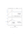
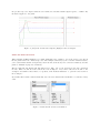
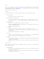
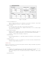
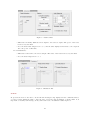
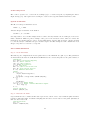
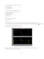
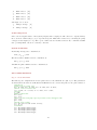
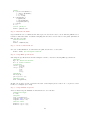
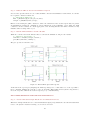
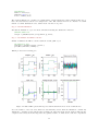
Industrial Information & Control Centre
jMPC Toolbox v3.11 User’s Guide
Jonathan Currie
AUT University
email: [email protected]
July 5, 2011
Contents
1 Introduction
1.1 Overview . . . . . . . . . . . . . . . . . . . . . . . . . . . . . . . . . . . . . . . . . . . . .
1.2 MPC Block Diagram . . . . . . . . . . . . . . . . . . . . . . . . . . . . . . . . . . . . . . .
1.3 Nomenclature . . . . . . . . . . . . . . . . . . . . . . . . . . . . . . . . . . . . . . . . . . .
2
2
2
3
2 Getting Started
2.1 Pre Requisites . . . . . . .
2.2 Installing the Toolbox . .
2.3 Compiling C-MEX Files .
2.4 Locating Documentation .
2.5 MPC Simulation GUI . .
2.6 Command Line Examples
.
.
.
.
.
.
4
4
4
4
4
5
5
3 Model Predictive Control Overview
3.1 Introduction . . . . . . . . . . . . . . . . . . . . . . . . . . . . . . . . . . . . . . . . . . . .
3.2 Linear MPC Algorithm . . . . . . . . . . . . . . . . . . . . . . . . . . . . . . . . . . . . .
3.3 The jMPC Controller . . . . . . . . . . . . . . . . . . . . . . . . . . . . . . . . . . . . . . .
6
6
6
6
.
.
.
.
.
.
.
.
.
.
.
.
.
.
.
.
.
.
.
.
.
.
.
.
.
.
.
.
.
.
.
.
.
.
.
.
.
.
.
.
.
.
.
.
.
.
.
.
.
.
.
.
.
.
.
.
.
.
.
.
.
.
.
.
.
.
.
.
.
.
.
.
.
.
.
.
.
.
.
.
.
.
.
.
.
.
.
.
.
.
.
.
.
.
.
.
.
.
.
.
.
.
.
.
.
.
.
.
.
.
.
.
.
.
.
.
.
.
.
.
.
.
.
.
.
.
.
.
.
.
.
.
.
.
.
.
.
.
.
.
.
.
.
.
.
.
.
.
.
.
.
.
.
.
.
.
.
.
.
.
.
.
.
.
.
.
.
.
.
.
.
.
.
.
.
.
.
.
.
.
.
.
.
.
.
.
.
.
.
.
.
.
.
.
.
.
.
.
.
.
.
.
.
.
.
.
.
.
.
.
4 Graphical User Interface (GUI)
4.1 GUI Overview . . . . . . . . .
4.2 Running An Example . . . . .
4.3 Using Matlab LTI Models . .
4.4 Using jNL Models . . . . . . . .
4.5 Auto Setup . . . . . . . . . . .
4.6 Loading and Saving Settings . .
4.7 Options . . . . . . . . . . . . .
.
.
.
.
.
.
.
.
.
.
.
.
.
.
.
.
.
.
.
.
.
.
.
.
.
.
.
.
.
.
.
.
.
.
.
.
.
.
.
.
.
.
.
.
.
.
.
.
.
.
.
.
.
.
.
.
.
.
.
.
.
.
.
.
.
.
.
.
.
.
.
.
.
.
.
.
.
.
.
.
.
.
.
.
.
.
.
.
.
.
.
.
.
.
.
.
.
.
.
.
.
.
.
.
.
.
.
.
.
.
.
.
.
.
.
.
.
.
.
.
.
.
.
.
.
.
.
.
.
.
.
.
.
.
.
.
.
.
.
.
.
.
.
.
.
.
.
.
.
.
.
.
.
.
.
.
.
.
.
.
.
.
.
.
.
.
.
.
.
.
.
.
.
.
.
.
.
.
.
.
.
.
.
.
.
.
.
.
.
.
.
.
.
.
.
.
.
.
.
.
.
.
.
.
.
.
.
.
.
.
.
.
.
.
.
.
.
.
.
.
.
.
.
.
.
.
.
.
.
.
.
8
8
14
14
15
16
17
18
5 Case Studies
5.1 Servomechanism Example . .
5.2 Quad Tank Example . . . . .
5.3 3DOF Helicopter Example . .
5.4 CSTR Example . . . . . . . .
5.5 Distillation Column Example
.
.
.
.
.
.
.
.
.
.
.
.
.
.
.
.
.
.
.
.
.
.
.
.
.
.
.
.
.
.
.
.
.
.
.
.
.
.
.
.
.
.
.
.
.
.
.
.
.
.
.
.
.
.
.
.
.
.
.
.
.
.
.
.
.
.
.
.
.
.
.
.
.
.
.
.
.
.
.
.
.
.
.
.
.
.
.
.
.
.
.
.
.
.
.
.
.
.
.
.
.
.
.
.
.
.
.
.
.
.
.
.
.
.
.
.
.
.
.
.
.
.
.
.
.
.
.
.
.
.
.
.
.
.
.
.
.
.
.
.
.
.
.
.
.
.
.
.
.
.
.
.
.
.
.
.
.
.
.
.
.
.
.
.
.
20
20
27
33
40
45
.
.
.
.
.
1
1
Introduction
1.1
Overview
This manual details the key functionality provided by the jMPC Toolbox. The toolbox is a collection of
m-files, Simulink models and compiled C-MEX functions for use in simulating and controlling dynamic
systems using Model Predictive Control. Key functionality offered by this toolbox includes:
• Easily build linear MPC controllers.
• Simulating controllers within linear and nonlinear environments.
• Applying linear inequality constraints to inputs and outputs.
• Various Quadratic Programming (QP) solvers are provided to solve the quadratic cost function.
• Implement advanced functionality such as state estimation, blocking and soft constraints.
• View real-time MPC control using the supplied Graphical User Interface (GUI).
• Connect the Simulink MPC block to real world dynamic systems using an A/D and D/A.
This work is the result of my research into embedded MPC during my time at AUT University. It is a
work in progress over the last two years and will continue to be upgraded as time allows.
1.2
MPC Block Diagram
Figure 1: jMPC Toolbox Block Diagram
The above figure illustrates the functionality provided by the jMPC Toolbox within an example application. The Plant represents a dynamic industrial process which is to be controlled to a setpoint by the
MPC controller. Two forms of disturbances can be added to the simulation, a load disturbance on the
input and/or measurement noise on the plant output. The measured output is then fed back to the MPC
controller in order to calculate the next control move. Also viewable within this toolbox are controller
model states and outputs for post analysis of model/plant mismatch.
The MPC controller is created as a jMPC object while the Plant can be a jSS object for linear simulations,
or a jNL object for nonlinear simulations. These classes are described in detail within this document
together with several examples illustrating their use.
2
1.3
Nomenclature
Several standard typographical and variable name conventions are used within this document and the
toolbox itself:
Typographical Conventions
t
Italic
Scalar
a
Lowercase Bold
Vector
A
Uppercase Bold
Matrix
Standard Variable Names
u
Input vector (Manipulated Variable)
x
State vector
y
Output vector (Measured Outputs)
MPC Variable Names
umdist
Unmeasured input disturbances
mdist
Measured input disturbances
noise
Output disturbances
up
Plant input
xm
Model states
xp
Plant states
ym
Model output
yp
Plant output
3
2
Getting Started
2.1
Pre Requisites
The jMPC Toolbox is designed to run independent of any other Matlab Toolbox, however several
toolboxes will significantly increase functionality. These include:
• Control Systems Toolbox (Transfer Functions & Manipulations → Highly Recommended)
• Optimization Toolbox (Using quadprog → Not Critical)
• Simulink 3D Animation (For 3D MPC Demos → Not Critical)
To run the supplied C-MEX functions you must also install the Microsoft VC++ 2010 runtime available
from the Microsoft website. Ensure you download the version (x86 or x64) suitable for your platform.
This runtime is required to run this toolbox.
2.2
Installing the Toolbox
Installing the jMPC Toolbox is simple with the supplied automated Matlab install script. Copy the
jMPC directory to a suitable permanent location and using Matlab browse to the contents of the jMPC
directory and run the install script:
>> jMPC_Install.m
The install script will perform the following steps based on user responses:
1. Uninstall previous versions of the jMPC Toolbox
2. Save the required jMPC Toolbox paths to the Matlab path
3. Run a post-installation self check
4. Display the read me file
Ensure you do not rename the jMPC directory from \jMPC\ as the name is used in automated MEX file
compilation.
2.3
Compiling C-MEX Files
All MEX files supplied are built using VC++ 2010 for both 32bit and 64bit systems and should work
‘out of the box’. If you do experience problems and wish to rebuild the C-MEX files supplied you can
run the supplied function jMPC MEX Install.m located within the Utilities directory. You will require
the Intel Math Kernel Library (MKL) [4] as well as the default BLAS & LAPACK libraries supplied
with Matlab to rebuild all files. This should only be conducted if you require changes to the original
source files.
2.4
Locating Documentation
The jMPC Toolbox is fully documented within the normal Matlab help browser. Simply type doc at
the command prompt and navigate to the jMPC Toolbox section. Supplementary help is also available
by typing help x where x is the name of the jMPC function, for example:
4
>> help jMPC
This PDF can also be used as reference guide or as a class handout.
2.5
MPC Simulation GUI
A nice way to get a feel for automatic control using MPC is using the supplied Graphical User Interface
(GUI). This allows real time interaction with an animated process such that tuning parameters, constraints and model-plant mismatch among other parameters can all be investigated. To start using the
GUI type the following at the Matlab command line:
>> jMPCtool
To load an example MPC setup click File → Load → Example Models and select a model and setup
from the list. Further details of the jMPC GUI will be presented later in this manual.
2.6
Command Line Examples
The ‘Examples’ folder within the jMPC directory contains a number of worked linear and non linear
MPC simulation examples using the jMPC Toolbox via objects. For example to open the linear MPC
examples supplied, type:
>> edit jMPC_linear_examples
These examples are described in detail within the jMPC documentation and later in this manual.
5
3
3.1
Model Predictive Control Overview
Introduction
Model Predictive Control (MPC) is an Advanced Process Control (APC) technology which is used
commonly in the Chemical Engineering and Process Engineering fields. MPC allows control of all plants
from Single Input Single Output (SISO) through to Multiple Input Multiple Output (MIMO) and nonsquare systems (different numbers of inputs and outputs). However its real advantage is the ability to
explicitly handle constraints, such that they are included when calculating the optimal control input(s)
to the plant. Among other attractive features, this has enabled MPC to be the preferred APC technology
for a number of years, and continues to this day.
Several variants of the MPC algorithm exist, including the original Dynamic Matrix Control (DMC),
Predicted Functional Control (PFC), Generalized Predictive Control (GPC) as well as nonlinear and
linear MPC. However all retain a common functionality; a model of the system is used to predict the
future output of the plant so that they controller can predict dead-time, constraint violations, future
setpoints and plant dynamics when calculating the next control move. This enables robust control which
has proved its use in industry and academia for over 20 years.
3.2
Linear MPC Algorithm
The MPC algorithm used within the jMPC Toolbox is a linear implementation, where a linear state space
model is used for the system prediction. This enables the controller to formulate the control problem as a
Quadratic Program (QP), which when setup correctly results in a convex QP, ensuring an optimal input
(global minimum). The fundamental algorithm characteristic is the system prediction and subsequent
control move optimization, shown below:
Viewable in Figure 2 is the standard MPC prediction plot, where the top plot shows the predicted plant
output for the prediction horizon, and the bottom plot shows the planned control inputs for the control
horizon. The linear model which is used to build the controller is used for the plant prediction, viewable
as the blue dots. With a good model of your system this prediction can be quite accurate, enabling
the control moves to optimally move the system to the setpoint. Also shown in the above plots are the
constraints available to MPC including maximum and minimum inputs and outputs, as well maximum
rate of change of the input.
3.3
The jMPC Controller
Referring to Figure 1 shows how the jMPC controller is included in a system. The jMPC controller uses
the current setpoint (setp) and measured disturbance (mdist), together with the current plant output
measurement (yp ) to calculate the optimal control input (u). For simulation purposes you can also
add an unmeasured disturbance (umdist) and measurement noise (noise) to the plant to test how the
controller responds. For analysis purposes you can also read the model states (xm ) and the model output
(ym ), which can be compared to the plant states (xp ) and plant output (yp ).
When running a simulation the plant is represented by either a jSS (State Space) linear plant, or a
collection of nonlinear (or linear but this is unusual as it should be converted to state space) Ordinary Differential Equations (ODEs) in a jNL plant. This enables you to perform linear and nonlinear
simulations using the same jMPC controller, and just changing the plant object.
6
Figure 2: MPC Prediction Overview
7
4
Graphical User Interface (GUI)
The jMPC Toolbox also contains a GUI to aid in understanding plant dynamics, running live demonstrations of MPC and classroom use. The GUI retains many of the features of the jMPC Class, and users
with find the GUI intuitive to migrate to.
4.1
GUI Overview
Figure 3: jMPC GUI Main Window
Past and Present Windows
These windows display the current and past data measured by the process. The top window displays the
process outputs, while the bottom window displays the process inputs. Using a custom Scrolling Object,
these plots scroll as the data is received, allowing only the most recent data to be viewed.
The window size is customizable through the advanced tab.
There are typically 3 lines plotted for each output; the output line itself (solid), the desired setpoint
(dash-dot), and the constraints (dotted). For the input the same rules apply but without the setpoint.
Prediction Windows
One of the main advantages of MPC is the predictive component. This window allows you to view in
Real Time the actual predicted response, as calculated using the supplied Model. The upper window is
8
the predicted process output, while the lower window is calculated future input sequence, of which only
the first is applied to the plant.
Figure 4: [Left] Past and Present Outputs, [Right] Predicted Outputs
Plant and Model Selection
When running an MPC simulation you must artificially select a Plant to act as the real process. In real
life the plant is the real continuous process, and is sampled discretely by the controller. In this software,
you load the Plant and Model separately, where the Model is used by the controller exclusively, and the
plant for simulation purposes exclusively.
The two lists will only display jSS, jNL and lti (ss, zpk, tf) objects, as these are the only compatible
models. These models are sourced from the base workspace. If you have added new models to the
workspace and wish for these lists to be updated, click ”Refresh Variables” to perform a new search of
the workspace.
By default this software will automatically select models called Plant and Model for each list, if they
exist.
Figure 5: Plant and Model Selection Window
9
Tabs
Due to space constraints, 3 tabs have been implemented on the GUI using the user generated function
tabpanel. Acknowledgements to Elmar Tarajan for creating this functionality! Note that the supplied
tabpanel function is covered by a BSD license.
Each of the tabs are described below:
Setup Tab
This is the main Tab used for setting up the MPC controller. It has the following elements:
• Prediction Horizon
– Length of the prediction of the model output
• Control Horizon or Blocking Moves
– Control Horizon (scalar) → Length of samples calculated as the future input sequence (or)
– Blocking Moves (vector) → Vector of samples calculated as blocking moves (i.e. [4 2 2 2])
• Tuning Weights
– These are used by the MPC Quadratic Program cost function
– Placing a higher number will increase the penalty cost as this variable deviates from the
setpoint, or for using that input
– Weights are squared in calculation
• Constraints
– The fundamental advantage of MPC is the ability to add constraints on the process
– This software allows constraints on the min and max input, max input change and the min
and max output
– Note all input constraints are hard constraints
• QP Solver
– In order to compare implementations, 5 QP solvers are available for use, including Matlab’s
built in quadprog (provided the Optimization Toolbox is installed)
• Default
– When starting out, this button automatically fills in default values within all settings, allowing
almost single click simulation
– Note these values are dependent on the Model size only, and no heuristics are used in choosing
values
Advanced Tab
These settings, although listed as advanced, will likely be required to be used in order to gain the desired
result. The properties are:
• State Estimation
– To account for Model - Plant mismatch and the affect of noise, state estimation allows the
plant states to be estimated
– The estimate is applied to the model states via a gain matrix, of which one is designed using
a gain supplied by the slider bar
10
Figure 6: Setup Tab
• Controller Sampling Period
– This is a highly important period, and must be chosen with consideration. Models with
different sampling periods will be re sampled at this frequency
• Window Length
– Determines the length of time visible on the past and present windows
– Note a maximum of 100 samples can be displayed in the window, so choose a window length
appropriate to the sample time
• Soft Output Constraints
– Enables a penalty weighting on the output constraints such that breaking the output constraints (due to for example a disturbance) does not render the QP problem infeasible
– Defaults to a small penalty term (100) for example use
• Initial Setpoints
– To prevent initial instability, or to start with a transient, use this table to set the setpoints at
sample k = 0
• Simulation Speed
– To slow down the execution of the simulation you can enable ‘Slow Mode’ which will run the
simulation at approximately 1/2 speed
Simulation Tab
This tab is automatically selected when Start is pushed, and allows editing of Real Time Setpoints and
Disturbances. The properties are:
• Setpoint
– With the correct output selected, you can modify in real time the setpoint value. Note due
to this being a real time implementation, setpoint look ahead cannot be used
– The setpoint ranges from -10 to 10, thus the system must be normalised for values outside
this range
• Measurement Noise
11
Figure 7: Advanced Tab
– This adds a normally distributed noise signal to the selected output. The power of the noise
is selected by the slider
– Note the slider value ranges from -5 to 5, and the value displayed and added to the output is
10 to the power of this value
• Load Disturbance
– This adds a bias term to the selected input. The value of the bias is selected by the slider
– Note the slider ranges from -5 to 5
Figure 8: Simulation Tab
Console
To prevent the need for the user to check run time messages being displayed in the command window,
a console is used within the GUI to alert the user of actions being undertaken on their behalf. It is
important to identify each message, as they will often lead to undesirable results if ignored.
12
Figure 9: Console Window
Description
This control is optional, and provided simply for adding a description to the current setup. This description is saved as part of the GUI object, and thus can help you identify objects at a later stage. Note this
only updates when an example is loaded, or the user enters information
Figure 10: Description Window
Buttons
• Start / Stop
– Simply starts or stops the simulation. Note the same button changes function depending on
whether the simulation is running or stopped
• Pause
– Pause execution of the simulation, without losing the current data
• Refresh Variables
– When you add new or change models / objects to the workspace, this button allows the GUI
to rescan the base workspace for changes. Any new models or changes will be identified and
populated within the respective lists
• Auto Load
– This button is covered in detail in the Auto Setup section
13
4.2
Running An Example
Provided with this software are several example setups which allow for new users to get familiar with
the software.
To load an example, click File → Load → Example Models.
Figure 11: Locating examples from the File menu
You will be presented with a new window, containing a list of currently saved examples.
Figure 12: Examples list
Each example is complete with a functional description, displayed as each example is selected. As this
software matures, expect this list to change. Click OK to select an example, which will be automatically
loaded into the GUI. At this point you can run the example as is, or modify existing settings as required.
4.3
Using Matlab LTI Models
When you have the Matlab Control Systems Toolbox installed, this tool can also load lti models for
use within MPC simulation. This is the intended purpose of this software, however jSS objects are also
provided for use without the Control Systems Toolbox.
Any Matlab lti model can be loaded into the GUI, including transfer function (tf), state space (ss),
and zero-pole-gain (zpk) models. All of these will appear in the plant and model lists automatically.
14
Figure 13: Plant and Model list
Continuous Models
As the underlying Model Predictive Controller is discrete, all models used will be converted to discrete.
If Auto Calculate Ts is selected, then the routine described here will calculate a suitable sampling rate,
and the model will be discretized using the Control Systems Toolbox function, c2d. If Auto Calculate
Ts is not selected, then the sampling period entered in the Controller Sampling Period edit box will be
used by c2d.
Discrete Models
When Auto Calculate Ts is selected, the Model’s sampling period will be used as the Controller Sampling
Period. If this option is not selected, and the Plant or Model’s sampling time is not the same as the
value in the Controller Sampling Period edit box, then it will be re-sampled using the Control Systems
Toolbox function, d2d. The same applies if the Plant and Model sampling periods are different.
Problems can occur using d2d on Models which have already been approximated using delay2z. This
is due to multiple poles at the origin, which is the effective dead time. In order to avoid this, make sure
you either supply discrete models with dead time at the correct sampling rate, or try reselecting the
model after changing Ts.
Models with Dead Time
As the original jMPC class does not handle dead time naturally, models supplied with dead time are
handled differently from those above. The Control Systems Toolbox function, delay2z, is used to
convert all dead time into leading zeros in the dynamics, which effectively adds dead time at integer
multiples of the sampling time. For continuous models, they are first discretized as above, before this
function is applied. This avoids using an approximation such as the function pade. The downside to
this method is greater computational load, especially as the dead time increases beyond 10 sampling
instants, as the state space matrices are increased in size.
Note the supplied Model object class, jSS, does not have a field for dead time, thus only lti models can
be used for dead time simulations.
4.4
Using jNL Models
In order to more accurately simulate a given process, you can use a jNL object as the Plant. This allows
you to use nonlinear Ordinary Differential Equations (ODEs) to represent the plant dynamics, while
15
retaining a simpler, linear state space model as the internal controller model. See the help section on
jNL objects on how to create the plant, and the limit of the associated object.
Note you must still supply a linear time invariant (lti) model for the controller, as the jMPC object does
not currently support nonlinear models.
Figure 14: Use of jNL objects in the GUI
Due to increased computation of the simulation (an ODE solver), on older machines you may experience
a noticeable performance slow down in the GUI.
4.5
Auto Setup
To speed up users familiar with the jMPC object and using scripts to run the simulation, this button
allows the GUI to check the workspace to find setup options with default variable names:
• Np
– Prediction Horizon (integer)
• Nc
– Control Horizon (integer) or Blocking Moves (vector)
• uwt
– Input tuning weights (vector)
• ywt
– Output tuning weights (vector)
• con
– Constraint structure in the form:
∗ con.u is [Umin Umax Delumax] (matrix)
∗ con.y is [Ymin Ymax] (matrix)
• setp
– Setpoints (matrix)
– Note only the first row of this is used (first setpoint)
• Ts
16
– Sampling time of the controller (scalar)
All variables must defined exactly as above. Note you must have a model loaded first before you can use
this feature. An example setup is listed below:
%Plant
G1p = tf({[1 -1],[1 2]},{[1 1],[1 4 5]});
%Model
G1m = tf({[1.2 -1.1],[1.5 2.2]},{[1.4 1.7],[1.2 4.4 5.1]});
Np = 10;
Nc = 5;
uwt = [0.1 0.2]’; %[in1 in2]
ywt = [0.1]’; %[out1]
con.u = [-5 5 2.5;
-5 5 2.5]; %[umin umax del_umax]
con.y = [-5 5]; %[ymin ymax]
setp = 1; %[setp1]
Ts = 0.1;
4.6
Loading and Saving Settings
In order to be able to save and load an MPC configuration, three methods are provided:
Import from / Export to Workspace
When you wish to use a setup locally, i.e. within the Matlab workspace only, this option allows the
use of jGUI objects, which are specific to this tool. They contain all options specified by the GUI, with
the exception of simulation data (which is only read during an active simulation).
Both of these options are available vai the respective File → Load / File → Save menus, and each will
launch a separate window for loading or saving.
Load From Workspace
This window is almost identical to the Load Example window, with the exception that this window scans
the base Matlab workspace for jGUI objects, rather than loading a pre-saved example.
Figure 15: Load from workspace interface
Save To Workspace
17
Use this method to save the current settings into a jGUI object, which will be saved to the base Matlab
workspace. Not you must have a working setup for this to work, as this option will rebuild a jMPC object
from the current settings to save.
Figure 16: Save to workspace interface
Load From / Save To File
When you wish to use a permanent setup, or permanently save your MPC configuration, use the Load
From / Save To File option to do so. Both of these options will open a standard file Window, and allow
the user to specify a file name and location. Files will be saved as a .mat file, and thus only these can
be loaded.
Note as above, only a working setup can be saved.
Export MPC Controller
To use a controller created within the GUI, i.e. within Simulink or a standard jMPC simulation, you
can export just the jMPC controller using this feature. A standard Save To Workspace window will be
presented to choose a variable name for the controller.
4.7
Options
To accommodate different user preferences, the following options are available from the options menu:
Auto Scaling
Auto scaling refers to the ability of the scrolling plots to resize in real time. When this option is enabled,
and the process is at steady state, the response windows will begin to rescale, such that window will
zoom back to the response lines. This is an advantage when a process has become unstable, and you
wish to zoom back to the detail of the plot.
Performing multiple small step changes will encourage the plot to rescale to smaller sizes. If you wish to
keep the plot size constant (i.e. it will get bigger but not smaller), then disable this option. This option
is enabled by default.
Auto Calculate Ts
The variable Ts is the sampling time of the controller, and must be chosen with consideration of the
speed of the model. To aid amateur users from selecting sample times too fast or slow for a given process,
18
this option will perform a step test of the model, and extract the sample time and length of simulation.
It will then use these values for choosing the Controller Sampling Period (Ts) and Window Length.
Disable this option to manually select these values. This option is enabled by default.
Note: You must have the Control Systems Toolbox to use this option.
Data Logging
If you wish to log the data displayed by the GUI, then enable this option. This can be useful for later
analysis, as you can view the entire simulation, not just the window size.
Note that not just the controller inputs and plant outputs are returned, but also the model output, plant
and model states, and the rate of change of the inputs.
With this option enabled, three objects are automatically created in the base workspace:
• plotvec
– This is a structure containing all the elements listed above, such that it can be accessed by a
user’s plotting function easily
• simresult
– This is a jSIM object, which contains the same information as plotvec, but within one of the
properties of the object. The advantage of this is the plot command is overloaded for this
object, so plotting MPC responses is simple
• MPC1
– This is a jMPC object, used for plotting the results, above
To plot the response using the jSIM object, use the following command:
>> plot(MPC1,simresult)
You can also call the function with an optional argument, to obtain detailed plots:
>> plot(MPC1,simresult,‘detail’)
Demo Mode
A visual feature only demo mode allows the GUI to automatically vary the setpoints every 100 samples,
such that it provides a live demonstration. The algorithm will randomly select an output to modify, and
randomly choose a new setpoint. The new setpoint will be on a normal distribution, with a mean of 1,
and a standard deviation of 2. The algorithm does not respect any constraints on the system.
19
5
Case Studies
The following examples are exercises to aid new users becoming familiar with the jMPC Toolbox.
5.1
Servomechanism Example
The completed example can be found in Examples/Documentation Examples/Servo Example.m
Reference: Matlab MPC Toolbox (2010) [7]
Figure 17: Servomechanism Schematic
Linear System Model
The continuous time state space equation of the servomechanism is as follows:




0
1
0
0
0
kθ
− kθ − βL

 0 
0


JL
ρJL

ẋ =  0JL
x + 
 0 u
0
0
1


kT
β +k2 /R
kθ
0
− ρ2kJθM − M JMT
RJM
ρJM
yp = 1 0 0 0 x
1 0
0
0
x
ym =
kθ 0 − kρθ 0
where we have defined the state vector, x, as:
x1
Load Angle
[rad]
x2
Load Angular Velocity
[rad/s]
x3
Motor Angle
[rad]
x4
Motor Angular Velocity
[rad/s]
and the output vector, y, as:
y1
Load Angle
[rad]
y2
Load Torque
[Nm]
and input, u, as:
u1
Motor Voltage
[V]
20
Control Objectives
The control objective is to control the Load Angle (y1 ) to a desired setpoint, by adjusting the Motor
Input Voltage (u1 ). We require the Load Angle to settle at the setpoint within around 10 seconds.
System Constraints
The Motor Voltage Constraint is set as:
-220V < u1 < 220V
And the Torque Constraint on the shaft is:
-78.5Nm < y2 < 78.5Nm
It is important to note in this example that we cannot directly measure the Load Torque, however we
must constrain it. This is a perfect example of the power of model based control, where we can use the
internal model outputs (ym ) in order to predict unmeasured outputs. The predicted outputs can then
be controlled and/or constrained as per a normal output. For this example we will constrain the Load
Torque only, and not control it to a setpoint.
Linear MPC Simulation
Step 1 - Create The Plant
The first step is to implement the model equations above into Matlab as a jSS object. The parameters
are first defined, then the model A, B, C and D matrices are created and passed to the jSS constructor:
%Parameters
k0 = 1280.2; %Torisional Rigidity
kT = 10; %Motor Constant
JM = 0.5; %Motor Inertia
JL = 50*JM; %Load Inertia
p = 20; %Gear Ratio
BM = 0.1; %Motor viscous friction
BL = 25; %Load viscous fraction
R = 20; %Armature Resistance
%Plant
A = [0 1 0 0;
-k0/JL -BL/JL k0/(p*JL) 0;
0 0 0 1;
k0/(p*JM) 0 -k0/(p^2*JM) -(BM+kT^2/R)/JM];
B = [0;
0;
0;
kT/(R*JM)];
C = [1 0 0 0]; %Plant Output
Cm = [1 0 0 0; %Model contains unmeasured outputs
k0 0 -k0/p 0];
D = 0;
%Create jSS Object
Plant = jSS(A,B,C,D);
Step 2 - Discretize the Plant
Object Plant is now a continuous time state space model, but in order to use it with the jMPC Toolbox,
it must be first discretized. A suitable sampling time should be chosen based on the plant dynamics, in
this case use 0.1 seconds:
%Discretize Plant
Ts = 0.1;
Plant = c2d(Plant,Ts);
21
Step 3 - Create Controller Model
Now we have a model of the system for the internal calculation of the controller, we also need a controller
model for the internal calculation of the controller. The plant does not have to be the same as the
controller model, and in real life will not be. However for ease of this simulation, we will define the plant
and model to be the same:
%Create jSS Model
Model = jSS(A,B,Cm,D);
Model = c2d(Model,Ts);
In order to assign the second model output (Torque) as unmeasured, we use the following method:
%Set Unmeasured Outputs in model
Model = SetUnmeasuredOut(Model,2);
Step 4 - Setup MPC Specifications
Following the specifications from this example’s reference, enter the following MPC specifications:
%Horizons
Np = 10; %Prediction Horizon
Nc = 2; %Control Horizon
%Constraints
con.u = [-220
con.y = [-inf
-78.5
%Weighting
uwt = [0.1]’;
ywt = [1 0]’;
220 1e2]; %in1 umin umax delumax
inf ; %out1 ymin ymax
78.5]; %out2 ymin ymax
%do not control the second output (Torque)
%Estimator Gain
Kest = dlqe(Model);
In this case we have chosen a prediction horizon of 10 samples (1 second at Ts = 0.1s) and a control
horizon of 2 samples (0.2 seconds). The control horizon must always be less than or equal to the prediction
horizon, based on the formulation of the MPC problem. The prediction horizon should be chosen based
on the dynamics of the system, such that it can predict past any system dead time and sufficient enough
for the controller to predict required constraint handling.
The constraints are specified exactly as above, noting a default rate of change of the input voltage has
been chosen as 100V/sample. This variable must be defined if the controller is constrained, however if
you are not concerned about the rate of change, you can use a suitably large value, such as done here.
Also note the output load angle (y1 ) is not constrained, such that minimum and maximum are defined
as -inf, and inf, which removes that output from constraint handling in the controller.
The weighting is the user’s main handle for tuning the controller performance. A larger number represents
a larger penalty for that input / output, where inputs are penalized based on a zero input (no plant
input), and outputs based on setpoint deviation. Penalizing inputs will discourage the controller from
using that input, and penalizing outputs will encourage the controller to move that output to the setpoint
faster.
A special function in this toolbox is the ability to set a weight to 0, as done in y2 . This tells the MPC
constructor this is an uncontrolled output, such that it is not fed-back, and it will not have a setpoint,
however you may still place constraints on it, as is done in this example.
The final line creates a discrete time observer using an overloaded version of the Matlab dlqe function,
assuming identity Q and R covariance matrices.
Step 5 - Setup Simulation Options
Next we must setup the simulation environment for our controller:
%Simulation Length
22
T = 300;
%Setpoint
setp = ones(T,1);
setp(1:50) = 0;
%Initial values
Plant.x0 = [0 0 0 0]’;
Model.x0 = [0 0 0 0]’;
The simulation length is always defined in samples, such that in this example it is set to 30 seconds (300
samples x 0.1s). The setpoint must be defined as T samples long, and is a user specified trajectory for
the controller to follow throughout the entire simulation. When their are multiple controlled outputs,
the setpoint must a matrix, with each column representing a different output.
Finally the initial states of the Plant and Model can be set individually, such that simulations where the
controller starts a state mismatch can be tested.
Step 6 - Set MPC Options
For advanced settings of the MPC controller or simulation you can use the jMPCset function to create
the required options structure. For this example we just wish to set the plot titles and axis:
%Set Options
opts = jMPCset(‘InputNames’,{‘Motor Voltage’},...
‘InputUnits’,{‘V’},...
‘OutputNames’,{‘Load Angle’,‘Load Torque’},...
‘OutputUnits’,{‘rad’,’Nm’});
Step 7 - Build the MPC Controller and Simulation Options
Now we have specified all we need to build an MPC controller and simulation environment, we call the
two required constructor functions:
%-- Build MPC & Simulation --%
MPC1 = jMPC(Model,Np,Nc,uwt,ywt,con,Kest,opts);
simopts = jSIM(MPC1,Plant,T,setp);
MPC1 is created using the jMPC constructor, where the variables we have declared previously are passed
as initialization parameters. Simulation options simopts is created similarly, except using the jSIM
constructor. Both constructors contain appropriate error checking thus the user will be informed of any
mistakes when creating either object
Step 8 - Run the MPC Simulation and Plot Results
With the controller and environment built, we can run the simulation, and plot the results:
%-- Simulate & Plot Result --%
simresult = sim(MPC1,simopts,‘Matlab’);
plot(MPC1,simresult,‘summary’);
The sim function will be familiar to most Matlab users, and is overloaded here for the jMPC Class.
Passing the controller and the simulation environment will allow a full MPC simulation to run, with
progress indicated by the progress bar. In this instance we have specified we wish to run a Matlab
simulation (default), rather than a Simulink or other MPC implementation.
The final command, plot, is once again overloaded for the jMPC Class, and allows us to pass the controller
(required for constraint listing), the simulation results, and specify the type of plot we wish to view. In
this instance, just a summary will do. The plot produced is shown below:
Viewable in the top left axis (Output), the controlled response of the load angle (blue line) is poor, and
the value oscillates for some time before we would expect to see it settle.
The next task is to tune the controller such that we achieve a settling period of the load angle within
around 10 seconds. Noting the physical constraints on the system, we can see the input voltage is less
23
Figure 18: Untuned MPC servo response
than a third of its maximum, such that we can reduce the weight on this input to encourage the controller
to use more voltage for a faster response. The torque is also much lower than the constrained value, such
that increasing the voltage shouldn’t be a problem.
Step 8 - Re Tune Controller Weights
Decrease the input weight and increase output 1 weight as follows, then rebuild the controller:
%Weighting
uwt = [0.05]’;
ywt = [2 0]’;
%Rebuild MPC
MPC1 = jMPC(Model,Np,Nc,uwt,ywt,con,Kest,opts);
Step 9 - Re Tune Controller Weights
With the new controller, run the simulation again using the existing simulation environment, and plot
the results using the detail switch:
%Re-Simulate & Plot
simresult = sim(MPC1,simopts,‘Matlab’);
plot(MPC1,simresult,‘detail’);
The detailed output result is shown below:
The top plot shows the Load Angle with respect to setpoint, and with the new tuning we can see we
achieve the desired settling time, while meeting the constraints on the Torque (bottom plot).
Linear Simulink Simulation
Step 1 - Re Run MPC Simulation with Simulink Switch
24
Figure 19: Tuned MPC servo response
In order to use the supplied Simulink MPC components, the simplest way to get started is to simply
use the ‘Simulink’ switch
%Re-Simulate & Plot
simresult = sim(MPC1,simopts,’Simulink’);
plot(MPC1,simresult,’detail’);
which, all going to plan, will give exactly the same results as the ‘Matlab’ simulation. This mode
populates the supplied jMPC simulink.mdl Simulink Model with the auto generated MPC components,
and calls Simulink to simulate it. The difference here is that the simulation is now running the jMPC S
Function, written in C and supplied as a Simulink block. This code is optimized for general MPC use
and thus will run much faster than the Matlab Simulation code. However the m-file algorithm is still
useful for those wishing to learn how to create their own MPC implementations (like me), and as such,
is still used.
Step 2 - Build a Simulink Model To Test the Controller
Fire up Simulink, and build the following Simulink model using the jMPC Toolbox and Standard
Simulink blocks:
Figure 20: MPC control of a Servo Simulink Model
25
Set the Simulink Solver configuration as follows:
- Fixed Step Discrete
- 0.1s Sampling Time
- 0 → 50s run time
Set the pulse generator configuration as follows:
- Sample based with a sample time of 0.1
- Period 400 samples
- Pulse width 200 samples
- Amplitude of 1
- Phase delay of 0
Set the Selector block as follows:
- Input port size of 2
- Index as 2
By default the MPC Controller and Plant will have variable names already used in the example above, but
you can customize these as you require. You can also use the completed model located in Examples/Servo Simulink.mdl.
Step 3 - Running the jMPC Simulink Simulation
Click Run to generate the following plot in the scope:
Figure 21: Tuned MPC servo response in Simulink
This example shows just how easy it is to create a jMPC MPC Controller in Matlab, import it to
Simulink, and then run a Simulink Simulation.
26
5.2
Quad Tank Example
The completed example can be found in Examples/Documentation Examples/QuadTank Example.m
Reference: J. Akesson (2006)[1] and Quanser [5]
Figure 22: Quad Tank Schematic
Linear System Model
The continuous time state space equation of the 4-tank system is as follows:
 γ1 k1


 1
A3
0
− T1
0
0
A1
A1 T3
γ2 k 2 

A4 
 0
0
− T12
0

A2
A2 T4  ∆x + 
∆ẋ = 
∆u

(1−γ
1
2 )k2 
 0
0
− T3
0 
0


A3
1
(1−γ1 )k1
0
0
0
− T4
0
A4


kc 0 0 0
 0 kc 0 0 

∆y = 
 0 0 kc 0  ∆x
0 0 0 kc
where we have defined the state vector, x, as:
x1
Tank 1 Level
x2
Tank 2 Level
x3
Tank 3 Level
x4
Tank 4 Level
and the output vector, y, as:
27
y1
Tank 1 Level
[cm]
y2
Tank 2 Level
[cm]
y3
Tank 3 Level
[cm]
y4
Tank 4 Level
[cm]
and input vector, u, as:
u1
Pump 1 Voltage
[V]
u2
Pump 2 Voltage
[V]
Control Objectives
Due to the non-square nature of the system (2 inputs and 4 outputs) we will control two outputs, namely
the bottom two tank levels (y1 , y2 ) to a specified setpoint. This will be achieved by controlling the pump
voltages via the inputs (u1 , u2 ). The top two tank levels are measured and are also constrained within
safe operating limits, but are not directly controlled.
System Constraints
Both Pump Voltages are constrained as:
-12V ≤ u[1−2] ≤ 12V
The Bottom Two Tank Levels are constrained as:
0cm ≤ y[1−2] ≤ 25cm
And The Top Two Tank Levels are constrained as:
0cm ≤ y[3−4] ≤ 10cm
Linear MPC Simulation
Step 1 - Create The Plant
The first step is to implement the model equations above into Matlab as a jSS object. The parameters
are first defined, then the model A, B, C and D matrices are created and passed to the jSS constructor:
%Parameters
%Tank cross sectional area
A1 = 15.5179; A2 = 15.5179; A3 = 15.5179; A4 = 15.5179;
%Outlet cross sectional area
a1 = 0.1781; a2 = 0.1781; a3 = 0.1781; a4 = 0.1781;
%Gravity
g = 981;
%Pump coefficients
k1 = 4.35;
k2 = 4.39;
%Ratio of allocated pump capacity between lower and upper tank
g1 = 0.36;
g2 = 0.36;
%Steady state values
x0 = [15.0751 15.0036 6.2151 6.1003];
u0 = [7 7];
%Constants
T1 = A1/a1*sqrt((2*x0(1)/g));
T2 = A2/a2*sqrt((2*x0(2)/g));
T3 = A3/a3*sqrt((2*x0(3)/g));
T4 = A4/a4*sqrt((2*x0(4)/g));
28
%Plant
A = [-1/T1 0 A3/(A1*T3) 0;
0 -1/T2 0 A4/(A2*T4);
0 0 -1/T3 0;
0 0 0 -1/T4];
B = [(g1*k1)/A1 0;
0 (g2*k2)/A2;
0 ((1-g2)*k2)/A3;
((1-g1)*k1)/A4 0];
C = eye(4);
D = 0;
%Create jSS Object
Plant = jSS(A,B,C,D)
Step 2 - Discretize the Plant
Object Plant is now a continuous time state space model, but in order to use it with the jMPC Toolbox,
it must be first discretized. A suitable sampling time should be chosen based on the plant dynamics, in
this case use 3 seconds
%Discretize Plant
Ts = 3;
Plant = c2d(Plant,Ts);
Step 3 - Create Controller Model
For ease of this simulation, we will define the plant and model to be the same:
Model = Plant; %no model/plant mismatch
Step 4 - Setup MPC Specifications
Following the specifications from this example’s reference, enter the following MPC specifications:
%Horizons
Np = 10; %Prediction Horizon
Nc = 3; %Control Horizon
%Constraints
con.u = [0 12 6;
0 12 6];
con.y = [0 25;
0 25;
0 10;
0 10];
%Weighting
uwt = [8 8]’;
ywt = [10 10 0 0]’;
%Estimator Gain
Kest = dlqe(Model);
In this case we have chosen a prediction horizon of 10 samples (30 seconds at Ts = 3s) and a control
horizon of 3 samples (6 seconds).
Step 5 - Setup Simulation Options
Next we must setup the simulation environment for our controller:
%Simulation Length
T = 250;
%Setpoint
setp = 15*ones(T,2);
setp(100:end,1:2) = 20;
setp(200:end,2) = 15;
%Initial values
Plant.x0 = [0 0 0 0]’;
Model.x0 = [0 0 0 0]’;
29
Step 6 - Build the MPC Controller and Simulation Options
Now we have specified all we need to build an MPC controller and Simulation environment, we call the
two required constructor functions:
%-- Build MPC & Simulation --%
MPC1 = jMPC(Model,Np,Nc,uwt,ywt,con,Kest);
simopts = jSIM(MPC1,Plant,T,setp);
MPC1 is created using the jMPC constructor, where the variables we have declared previously are passed
as initialization parameters. Simulation options simopts is created similarly, except using the jSIM
constructor. Both constructors contain appropriate error checking thus the user will be informed of any
mistakes when creating either object
Step 7 - Run the MPC Simulation and Plot Results
With the controller and environment built, we can run the simulation, and plot the results:
%-- Simulate & Plot Result --%
simresult = sim(MPC1,simopts,‘Matlab’);
plot(MPC1,simresult,‘summary’);
The plot produced is shown below:
Figure 23: Tuned MPC quad tank response
As shown in the top left plot (Outputs) the final step change at k = 200 causes one of the top tanks to
hit a constraint, limiting the flow into both bottom tanks. This results in the system being unable to
meet the setpoints, which is the desired response (obey constraints first).
Linear MPC Simulation with Unmeasured Disturbances
Step 1 - Add an Unmeasured Input Disturbance and Measurement Noise
This next example will show how to add an unmeasured input (load) disturbance as well as measurement
noise to the system. Add the following code in a new cell block:
30
%Disturbances
umdist = zeros(T,2);
umdist(80:end,1) = -1;
noise = randn(T,4)/30;
The variable umdist now contains a 2 column matrix of input disturbance values, which in this case u1
has a 1V bias subtracted from it for samples 80 to 100. The variable noise now contains a 4 column
matrix of normal distribution noise, with a mean of 0 and a low power.
Step 2 - Rebuild Simulation
Rebuild the simulation object as follows, this time including the disturbance matrices:
%Rebuild Simulation
simopts = jSIM(MPC1,Plant,T,setp,umdist,[],noise);
Step 3 - Re-Simulate the MPC Controller
Finally re-simulate the MPC controller with the rebuilt jSIM object:
%Re Simulate & Plot
simresult = sim(MPC1,simopts,’Matlab’);
plot(MPC1,simresult,’summary’);
Which produces the following plot:
Figure 24: Tuned MPC quad tank response with measurement noise and load disturbance
Note the addition of two new axes, which are automatically created when the simulation contains any
disturbance. Viewable in the Output axis at sample 80, when the input bias is applied, although the
outputs deviate briefly from their setpoints, they quickly return to normal, as the controller compensates
31
with a higher input voltage, viewable in the Input axis. Also note the measurement noise has a minimal
effect on the controlled response, in due partly to the filtering affect of the Kalman Filter and long plant
dynamics.
For those interested, re-run the simulation without state estimation and note how the control performance
substantially degrades after the input bias is applied, as the plant and model states deviate (enable the
plot model option).
32
5.3
3DOF Helicopter Example
The completed example can be found in Examples/Documentation Examples/Heli Example.m
Reference: J. Akesson (2006) [1] and Quanser [6]
Figure 25: 3DOF Helicopter Schematic [1]
Linear System Model
The continuous time state space equation of the 3DOF helicopter is as follows:




0
0
0 1 0 0
0
0
Kf la 
 Kf la
0 0 0 0
0
0
 Je

Je





0 0 0 1
0
0
0
0



x
+
ẋ = 

u
0 0 0 0 − Fg la 0
0
0




Jt

0 0 0 0
0 
 0

0
1
K f lh
Kf lh
−
0 0 0 0
0
0
Jp
Jp


1 0 0 0 0 0
y = 0 0 1 0 0 0 x
0 0 0 0 1 0
where we have defined the state vector, x, as:
x1
Elevation Angle
[rad]
x2
Elevation Angular Velocity
[rad/s]
x3
Rotation Angle
[rad]
x4
Rotation Angular Velocity
[rad/s]
x5
Pitch Angle
[rad]
x6
Pitch Angular Velocity
[rad/s]
and the output vector, y, as:
y1
Elevation Angle
[rad]
y2
Rotation Angle
[rad]
y3
Pitch Angle
[rad]
and input vector, u, as:
u1
Motor 1 Voltage
[V]
u2
Motor 2 Voltage
[V]
33
Control Objectives
The control objective is to control the Elevation and Rotation angles (y1 , y2 ) to their respective setpoints,
by adjusting Motor 1 and 2 Voltages (u1 , u2 ). The Pitch Angle (y3 ) is constrained but not controlled to
a setpoint.
System Constraints
Both Motor Voltages are constrained as:
-3V ≤ u[1−2] ≤ 3V
Each axis rotation angle is constrained as follows:
-0.6 ≤ y1 ≤ 0.6
-pi ≤ y2 ≤ pi
-1 ≤ y3 ≤ 1
Linear MPC Simulation
Step 1 - Create The Plant
The first step is to implement the model equations above into Matlab as a jSS object. The parameters
are first defined, then the model A, B, C and D matrices are created and passed to the jSS constructor:
%Parameters
Je = 0.91; % Moment of inertia about elevation axis
la = 0.66; % Arm length from elevation axis to helicopter body
Kf = 0.5; % Motor Force Constant
Fg = 0.5; % Differential force due to gravity and counter weight
Tg = la*Fg; % Differential torque
Jp = 0.0364; % Moment of inertia about pitch axis
lh = 0.177; % Distance from pitch axis to either motor
Jt = Je; % Moment of inertia about travel axis
%Plant
A = [0 1 0 0 0 0;
0 0 0 0 0 0;
0 0 0 1 0 0;
0 0 0 0 -Fg*la/Jt 0;
0 0 0 0 0 1;
0 0 0 0 0 0];
B = [0 0;
Kf*la/Je Kf*la/Je;
0 0;
0 0;
0 0;
Kf*lh/Jp -Kf*lh/Jp];
C = [1 0 0 0 0 0;
0 0 1 0 0 0;
0 0 0 0 1 0];
D = 0;
%Create jSS Object
Plant = jSS(A,B,C,D)
Step 2 - Discretize the Plant
Object Plant is now a continuous time state space model, but in order to use it with the jMPC Toolbox,
it must be first discretized. A suitable sampling time should be chosen based on the plant dynamics, in
this case use 0.12 seconds
34
%Discretize Plant
Ts = 0.12;
Plant = c2d(Plant,Ts);
Step 3 - Create Controller Model
For ease of this simulation, we will define the Plant and Model to be the same:
Model = Plant; %no model/plant mismatch
Step 4 - Setup MPC Specifications
Following the specifications from this example’s reference, enter the following MPC specifications:
%Horizons
Np = 30; %Prediction Horizon
Nc = 10; %Control Horizon
%Constraints
con.u = [-3 3 1e6;
-3 3 1e6];
con.y = [-0.6 0.6;
-pi pi;
-1 1];
%Weighting
uwt = [1 1]’;
ywt = [10 10 1]’;
%Estimator Gain
Kest = dlqe(Model);
Step 5 - Setup Simulation Options
Next we must setup the simulation environment for our controller:
%Simulation Length
T = 300;
%Setpoint
setp = zeros(T,3);
setp(:,1) = 0.3;
setp(125:250,1) = -0.3;
setp(:,2) = 2;
setp(200:end,2) = 0;
%Initial values
Plant.x0 = [0 0 0 0 0 0]’;
Model.x0 = [0 0 0 0 0 0]’;
Step 6 - Set MPC Options
For advanced settings of the MPC controller or simulation you can use the jMPCset function to create
the required options structure. For this example we just wish to set the plot titles and axis:
%Set Options
opts = jMPCset(‘InputNames’,{‘Motor 1 Voltage’,‘Motor 2 Voltage’},...
‘InputUnits’,{‘V’,‘V’},...
‘OutputNames’,{‘Elevation Angle’,‘Rotation Angle’,‘Pitch Angle’},...
‘OutputUnits’,{‘rad’,‘rad’,‘rad’});
Step 7 - Build the MPC Controller and Simulation Options
Now we have specified all we need to build an MPC controller and Simulation environment, we call the
two required constructor functions:
%-- Build MPC & Simulation --%
MPC1 = jMPC(Model,Np,Nc,uwt,ywt,con,Kest,opts);
simopts = jSIM(MPC1,Plant,T,setp);
35
MPC1 is created using the jMPC constructor, where the variables we have declared previously are passed
as initialization parameters. Simulation options simopts is created similarly, except using the jSIM
constructor. Both constructors contain appropriate error checking thus the user will be informed of any
mistakes when creating either object
Step 8 - Run the MPC Simulation and Plot Results
With the controller and environment built, we can run the simulation, and plot the results:
%-- Simulate & Plot Result --%
simresult = sim(MPC1,simopts,‘Matlab’);
plot(MPC1,simresult,‘summary’);
The plot produced is shown below:
Figure 26: Tuned MPC 3DOF helicopter response
We can also plot a detail plot using the ’detail’ switch to better view the output responses:
Viewable in the output responses the elevation angle and rotation angle both appear controlled, with
minimal overshoot and fast rise and fall times. Note the pitch angle is constrained as required at ± 1
rad when moving the helicopter around the rotation axis, as was specified.
Linear MPC with Nonlinear Simulation
In order to more accurately verify the controller tuning, we can also create the nonlinear model of the
plant, using the nonlinear differential equations of the helicopter system:
36
Figure 27: Tuned MPC 3DOF helicopter outputs
Kf la
Tg
(Vf + Vb ) −
Je
Je
Fg la
θ̈r = −
sin θp
Jt
Kf lh
θ̈p =
(Vf − Vb )
Jp
θ̈e =
Step 1 - Build Nonlinear ODE Callback Function
As detailed in creating a jNL object, the first step is to write an m-file which contains the above expressions, suitable for use with a Matlab integrator:
function xdot = nl_heli(t,x,u,param)
% Nonlinear Helicopter Model
%Assign Parameters
[Je,la,Kf,Fg,Tg,Jp,lh,Jt] = param{:};
xdot(1,1)
xdot(2,1)
xdot(3,1)
xdot(4,1)
xdot(5,1)
xdot(6,1)
=
=
=
=
=
=
x(2);
(Kf*la/Je)*(u(1)+u(2))-Tg/Je;
x(4);
-(Fg*la/Jt)*sin(x(5));
x(6);
(Kf*lh/Jp)*(u(1)-u(2));
end
The file, nl heli.m, is saved in a suitable folder on the Matlab path.
Step 2 - Build the jNL Object
The next step is to build the jNL object, passing the function above as a function handle:
37
%Non Linear Plant
param = {Je,la,Kf,Fg,Tg,Jp,lh,Jt}; %parameter cell array
Plant = jNL(@nl_heli,C,param);
Note we have passed the parameters as a cell array, and also retained the linear C output matrix for
now. This could also be a function handle to a nonlinear output function.
Step 3 - Linearize the jNL Object
In order to use the nonlinear plant with our linear MPC controller, we must linearize the ODE function
and generate the required linear state space model:
%Linearize Plant
u0 = [Tg/(2*Kf*la) Tg/(2*Kf*la)];
Model = linearize(Plant,u0);
In this instance we have chosen the linearize the ODE expression above the motor voltages of 0.5V.
We have not specified a state to linearize about, such that function will also automatically determine a
steady state to linearize about.
Step 4 - Rebuild jSS Object
The model returned from the linearize function is a Matlab lti object, and can be automatically
converted to a jSS object, and then converted to a discrete model:
%Build jSS object
Model = jSS(Model);
%Discretize model
Model = c2d(Model,Ts);
Step 5 - Rebuild and Re-Simulate the MPC Controller
The last step is to rebuild the MPC controller and simulation environment, and then re run the simulation:
%Rebuild MPC & Simulation
MPC1 = jMPC(Model,Np,Nc,uwt,ywt,con,Kest);
simopts = jSIM(MPC1,Plant,T,setp);
%Re-Simulate & Plot
simresult = sim(MPC1,simopts,’Matlab’);
plot(MPC1,simresult,’summary’);
The output result is shown below:
As viewable in the plot above, the controlled response of the nonlinear system is quite similar to the linear
system, however viewing the plots side by side shows the differences (specifically the nonlinearities):
From the nonlinear plot, it is now evident there is significantly more overshoot on the rotation setpoint.
This is attributed to the nonlinear equation governing the relationship between the rotation angle, and
the pitch angle (sine), which cannot be fully defined a single linearization point. However the control
is still reasonable, and would expect to function sufficiently well on a real plant. Note also that further
tuning may improve this response, which is left to the reader to implement.
38
Figure 28: Tuned MPC 3DOF helicopter response with nonlinear plant
Figure 29: Comparison of MPC 3DOF linear and nonlinear simulation responses
39
5.4
CSTR Example
The completed example can be found in Examples/Nonlinear Examples.m in the Henson CSTR cellblock.
Reference: M. Henson & D. Seborg (1997) [3]
Figure 30: CSTR Schematic
Nonlinear System Model
The continuous time, ordinary differential equations of the CSTR model are as follows:
−E
σ = k0 e RTr Ca
d Ca
q
= (Caf − Ca ) − σ
dt
V
q
H
UA
d Tr
= (Tf − Tr ) +
σ+
(Tc − Tr )
dt
V
Cp ρ
Cp ρV
The equations represent a continuously stirred tank reactor with a single reaction from A -¿ B, and a
complete mass and energy balance.
We have defined the state vector, x, as:
x1
Concentration of A in reactor (Ca )
[mol/m3 ]
x2
Temperature of reactor (Tr )
[K]
and the output vector, y, as:
y1
Concentration of A in reactor (Ca )
[mol/m3 ]
y2
Temperature of reactor (Tr )
[K]
and input vector, u, as:
u1
Concentration of A in feed (Ca f ) (Measured Disturbance)
[mol/m3 ]
u2
Temperature of feed (Tf ) (Measured Disturbance)
[K]
u3
Temperature of cooling jacket (Tc )
[K]
40
Control Objectives
The control objective is to control the temperature of the reactor by adjusting the temperature of the
cooling jacket. Both the concentration and temperature of the feed are measured disturbances, and
cannot be modified by the controller. The reactor concentration is constrained but not controlled to a
setpoint.
System Constraints
The jacket cooling temperature is set as:
278.15 ≤ u[3] ≤ 450K
And the reactor is constrained as:
0 ≤ y1 ≤ 3 mol/m3
278.15 ≤ y2 ≤ 450K
Linear MPC with Nonlinear Simulation
Step 1 - Build Nonlinear ODE Callback Function
As detailed in creating a jNL object, the first step is to write an m-file which contains the above expressions, suitable for use with a Matlab integrator:
function xdot = nl_cstr(t,x,u,param)
% Nonlinear CSTR model
%Assign Parameters
[q,V,k0,E,R,H,Cp,rho,UA] = param{:};
r = k0*exp(-E/(R*x(2)))*x(1);
xdot(1,1) = q/V*(u(1)-x(1)) - r;
xdot(2,1) = q/V*(u(2)-x(2)) + (H/(Cp*rho))*r + (UA)/(Cp*rho*V)*(u(3)-x(2));
end
The file, nl cstr.m, is saved in a suitable folder on the Matlab path.
Step 2 - Build the jNL Object
The next step is to build the jNL object, passing the function above as a function handle:
%Parameters
q = 100; % Volumetric flow rate [m^3/min]
V = 100; % Volume in reactor [m^3]
k0 = 7.2e10; % Pre-exponential nonthermal factor [1/min]
E = 7.2752e4;% Activation energy in the Arrhenius Equation [J/mol]
R = 8.31451; % Universal Gas Constant [J/mol-K]
H = 5e4; % Heat of Reaction [J/mol]
Cp = .239; % Heat capacity (J/g-K)
rho = 1000; % Density (g/m^3)
UA = 5e4; % Heat Transfer * Area [J/min-K]
%Output Matrix
C = eye(2);
%Nonlinear Plant
param = {Je,la,Kf,Fg,Tg,Jp,lh,Jt}; %parameter cell array
Plant = jNL(@nl_cstr,C,param);
Note we have passed the parameters as a cell array, and also retained the linear C output matrix for
now. This could also be a function handle to a nonlinear output function.
41
Step 3 - Linearize the jNL Object
In order to use the nonlinear plant with our linear MPC controller, we must linearize the ODE function
and generate the required linear state space model. The system is linearized about an unsteady operating
point as specified in the original reference:
%Initial U
CAf = 1; % Feed Concentration [mol/m^3]
Tf = 350; % Feed Temperature [K]
Tc = 300; % Coolant Temperature [K]
%Linearize Plant
u0 = [CAf Tf Tc]’;
xop = [0.5 350]’; %unstable operating point [Ca Tr]
Model = linearize(Plant,u0,xop,‘ode15s’)
Note in this instance we have specified to use ode15s for linearization. While this is not used in this
particular scenario (we are not solving for a steady state here), it will be used for all future simulations
of this jNL plant (instead of the default ode45).
Step 4 - Create Controller Model
Returned from linearize is a Matlab lti object containing the linearized model of our system. This
must be converted to a jSS object, and discretized to be used to build an MPC controller:
%Build jSS object & discretize
Model = jSS(Model);
Ts = 0.05;
Model = c2d(Model,Ts)
In order to assign the measured disturbances in the model, we use the following method:
%Set Measured Disturbances (Caf,Tf)
Model = SetMeasuredDist(Model,[1 2]); %Provide index of which inputs are mdist
Step 5 - Setup MPC Specifications
The MPC Controller is specified as follows:
%Horizons
Np = 30; %Prediction Horizon
Nc = [10 10 10]; %Blocking moves
%Constraints
con.u = [278.15 450 20];
con.y = [0 3;
278.15 450];
%Weighting
uwt = 1;
ywt = [0 5]’;
%Estimator Gain
Kest = dlqe(Model);
Step 6 - Setup Simulation Options
Next we must setup the simulation environment for our controller:
%Simulation Length
T = 300;
%Setpoint (CA)
setp = zeros(T,1);
setp(:,1) = xop(2);
setp(50:end,1) = xop(2)+25;
setp(200:end,1) = xop(2)-25;
%Measured Disturbances (Caf Tf)
mdist = zeros(T,2); mdist(:,1) = CAf; mdist(:,2) = Tf;
mdist(130:140,1) = CAf+0.1; %Step disturbance of Caf
42
mdist(220:260,2) = Tf-linspace(0,20,41); %Slow cooling of Tf
mdist(261:end,2) = Tf-20; %Tf final
%Set Initial values at linearization point
Plant.x0 = xop;
Model.x0 = xop;
Step 7 - Set MPC Options
For advanced settings of the MPC controller or simulation you can use the jMPCset function to create
the required options structure. For this example we wish to set the plot titles and axis, as well as setting
the initial control input (at k = 0) to the linearization point:
%Set Options
opts = jMPCset(‘InitialU’,u0,... %Set initial control input at linearization point
‘InputNames’,{‘Feed Concentration’,‘Feed Temperature’,‘Jacket Temperature’},...
‘InputUnits’,{‘mol/m^3’,‘K’,‘K’},...
‘OutputNames’,{‘Reactor Concentration’,‘Reactor Temperature’},...
‘OutputUnits’,{‘mol/m^3’,‘K’})
Step 8 - Build the MPC Controller and Simulation Options
Now we have specified all we need to build an MPC controller and Simulation environment, we call the
two required constructor functions:
%-- Build MPC & Simulation --%
MPC1 = jMPC(Model,Np,Nc,uwt,ywt,con,Kest,opts);
simopts = jSIM(MPC1,Plant,T,setp,[],mdist);
MPC1 is created using the jMPC constructor, where the variables we have declared previously are passed
as initialization parameters. Simulation options simopts is created similarly, except using the jSIM
constructor.
Step 9 - Run the MPC Simulation and Plot Results
With the controller and environment built, we can run the simulation, and plot the results. We use
Simulink as the evaluation environment as it runs significantly faster than Matlab for nonlinear simulations:
%-- Simulate & Plot Result --%
simresult = sim(MPC1,simopts,‘Simulink’);
plot(MPC1,simresult,‘detail’);
As shown in Figures 31 and 32 the system shows good control with minimal overshoot even for large
step changes. This particular problem presents a considerable challenge to linear MPC based on the
unstable operating point and significant nonlinearities of the system. However correct tuning can give
good results, even when responding to disturbances.
43
Figure 31: CSTR Simulation Output Responses
Figure 32: CSTR Simulation Inputs
44
5.5
Distillation Column Example
The completed example can be found in Examples/Nonlinear Examples.m in the Hahn Distillation
cellblock.
Reference: J. Hahn and T.F. Edgar (2002) [2]
Figure 33: Distillationmn Column Schematic
45
Nonlinear System Model
The continuous time, ordinary differential equations of the distillation column model are as follows:
Condenser:
dx1
1
=
V (y2 − x1 )
dt
Acond
Rectification Trays:
dxi
1
=
[L (xi−1 − xi ) − V (yi − yi+1 )]
dt
Atray
Feed Tray:
1
dxf
=
[Feedf xf eed + Lxf −1 − F Lxf − V (yf − yf +1 )]
dt
Atray
Stripping Trays:
dxi
1
=
[F L (xi−1 − xi ) − V (yi − yi+1 )]
dt
Atray
Reboiler:
1
dxn
=
[F Lxn−1 − (Feedf − D) xn − V yn ]
dt
Areboiler
Further Equations:
D = 0.5Feedf
L = Refluxr D
V =L+D
F L = Feedf + L
xα
y=
1 + (α − 1) x
The equations represent a binary distillation column with n trays and a feed tray which can be located
at any tray f. The model assumes a constant relative volatility to determine vapour flows.
We have defined the state vector, x, as:
x1
Reflux Drum Liquid Mole Fraction of A
[mol]
x2
Tray 1 Liquid Mole Fraction of A
[mol]
Feed Tray Liquid Mole Fraction of A
[mol]
xn−1
Tray n Liquid Mole Fraction of A
[mol]
xn
Reboiler Liquid Mole Fraction of A
[mol]
...
xf
...
and the output vector, y, as:
y1
Reflux Drum Liquid Mole Fraction of A
[mol]
y2
Feed Tray Liquid Mole Fraction of A
[mol]
y3
Reboiler Liquid Mole Fraction of A
[mol]
and input vector, u, as:
46
u1
Feed Flowrate (Measured Disturbance)
[mol/min]
u2
Feed Mole Fraction of A(Measured Disturbance)
[mol]
u3
Reflux Ratio
Control Objectives
The control objective is to control the mole fraction of A in the reflux drum by manipulating the reflux
ratio. Both the feed mole fraction and flow rate are measured disturbances, and cannot be modified by
the controller. The mole fractions on the other trays are not controlled but constrained within sensible
limits.
System Constraints
The reflux ratio is constrained as:
0 ≤ u[3] ≤ 10
And the tray mole fractions are constrained as:
0.98 ≤ y1 ≤ 1 mol
0.48 ≤ y2 ≤ 0.52 mol
0 ≤ y2 ≤ 0.1 mol
Linear MPC with Nonlinear Simulation
Step 1 - Build Nonlinear ODE Callback Function
As detailed in creating a jNL object, the first step is to write an m-file which contains the above expressions, suitable for use with a Matlab integrator:
function xdot = nl_distil(t,x,u,param)
% Nonlinear Distillation model
%Assign Parameters
[FT,rVol,aTray,aCond,aReb] = param{:};
xdot = NaN(size(x));
fFeed = u(1); aFeed = u(2); RR = u(3);
% Additional Eqs
D = 0.5*fFeed; % Distillate Flowrate [mol/min]
L = RR*D; % Flowrate of the Liquid in the Rectification Section [mol/min]
V = L+D; % Vapor Flowrate in the Column [mol/min]
FL = fFeed+L; % Flowrate of the Liquid in the Stripping Section [mol/min]
% Determine Vapour Flows + Delta Flows
y = x*rVol./(1+(rVol-1).*x); % Assume constant relative volatility to determine vapour flows
dx = -diff(x); dy = -diff(y); % Difference molar flow rates
%Calculate flowrates on each tray
xdot(1,1) = 1/aCond*V*(y(2)-x(1)); % Reflux Drum
xdot(2:FT-1,1) = (L*dx(1:FT-2) - V*dy(2:FT-1))/aTray; % Top section
xdot(FT,1) = 1/aTray*(fFeed*aFeed+L*x(FT-1)-FL*x(FT)-V*(y(FT)-y(FT+1))); % Feed tray
xdot(FT+1:end-1) = (FL*dx(FT:end-1)-V*dy(FT+1:end))/aTray; % Bottom section
xdot(end) = (FL*x(end-1)-(fFeed-D)*x(end)-V*y(end))/aReb; % Reboiler
end
The file, nl distil.m, is saved in a suitable folder on the Matlab path.
Step 2 - Build the jNL Object
47
The next step is to build the jNL object, passing the function above as a function handle:
%Parameters
nTrays = 32; % Number of Trays
feedTray = 17; % Feed tray location
rVol = 1.6; % Relative Volatility
aTray = 0.25; % Total Molar Holdup on each Tray
aCond = 0.5; % Total Molar Holdup in the Condensor
aReb = 1.0; % Total Molar Holdup in the Reboiler
%Output Matrix
C = zeros(3,nTrays);
C(1,1) = 1; C(2,feedTray) = 1; C(3,end) = 1;
%Nonlinear Plant
param = {feedTray,rVol,aTray,aCond,aReb,aFeed}; %parameter cell array
Plant = jNL(@nl_distil,C,param);
Note we have passed the parameters as a cell array, and also retained the linear C output matrix for
now. This could also be a function handle to a nonlinear output function.
Step 3 - Linearize the jNL Object
In order to use the nonlinear plant with our linear MPC controller, we must linearize the ODE function
and generate the required linear state space model:
%Initial U
fFeed = 24/60; % Feed Flowrate [mol/min]
aFeed = 0.5; % Feed Mole Fraction
RR = 3; % Reflux Ratio
%Linearize Plant
u0 = [fFeed aFeed RR]’;
x0 = []; %unknown operating point
[Model,xop] = linearize(Plant,u0,x0,‘ode15s’);
Note in this instance we have specified to use ode15s for linearization. As we do not know the states
at our linearization point the linearize function will also solve for the steady state using ode15s, if one
exists. This will be returned as xop which can be used for initial states later on.
Step 4 - Create Controller Model
Returned from linearize is a Matlab lti object containing the linearized model of our system. This
must be converted to a jSS object, and discretized to be used to build an MPC controller:
%Build jSS object & discretize
Model = jSS(Model);
Ts = 1;
Model = c2d(Model,Ts)
In order to assign the measured disturbances in the model, we use the following method:
%Set Measured Disturbances (fFeed,aFeed)
Model = SetMeasuredDist(Model,[1 2]); %Provide index of which inputs are mdist
Step 5 - Setup MPC Specifications
The MPC Controller is specified as follows:
%Horizons
Np = 25; %Prediction Horizon
Nc = 10; %Blocking moves
%Constraints
con.u = [0 10 1];
con.y = [0.92 1;
0.48 0.52;
0 0.1];
%Weighting
uwt = 1;
48
ywt = [10 0 0]’;
%Estimator Gain
Kest = dlqe(Model);
Step 6 - Setup Simulation Options
Next we must setup the simulation environment for our controller:
%Simulation Length
T = 200;
%Setpoint (Reflux Drum)
setp = zeros(T,1);
setp(:,1) = xop(1);
setp(10:end,1) = xop(1)+0.02;
%Measured Disturbances
mdist = zeros(T,2); mdist(:,1) = fFeed; mdist(:,2) = aFeed;
mdist(60:end,2) = aFeed+0.01; %Small increase in feed mole fraction
mdist(140:end,1) = fFeed+1; %Small increase in feed flow rate
%Set Initial values at linearization point
Plant.x0 = xop;
Model.x0 = xop;
Step 7 - Set MPC Options
For advanced settings of the MPC controller or simulation you can use the jMPCset function to create
the required options structure. For this example we wish to set the plot titles and axis, as well as setting
the initial control input (at k = 0) to the linearization point:
%Set Options
opts = jMPCset(‘InitialU’,u0,... %Set initial control input at linearization point
‘InputNames’,{‘Feed Flowrate’,‘Feed Mole Fraction’,‘Reflux Ratio’},...
‘InputUnits’,{‘mol/min’,‘Fraction’,‘Ratio’},...
‘OutputNames’,{‘Liquid Mole Fraction in Reflux Drum’,‘Liquid Mole Fraction in Feed Tray’,...
‘Liquid Mole Fraction in Reboiler},...
‘OutputUnits’,{‘Fraction’,‘Fraction’,‘Fraction’});
Step 8 - Build the MPC Controller and Simulation Options
Now we have specified all we need to build an MPC controller and Simulation environment, we call the
two required constructor functions:
%-- Build MPC & Simulation --%
MPC1 = jMPC(Model,Np,Nc,uwt,ywt,con,Kest,opts);
simopts = jSIM(MPC1,Plant,T,setp,[],mdist);
MPC1 is created using the jMPC constructor, where the variables we have declared previously are passed
as initialization parameters. Simulation options simopts is created similarly, except using the jSIM
constructor.
Step 9 - Run the MPC Simulation and Plot Results
With the controller and environment built, we can run the simulation, and plot the results. We use
Simulink as the evaluation environment as it runs significantly faster than Matlab for nonlinear simulations:
%-- Simulate & Plot Result --%
simresult = sim(MPC1,simopts,‘Simulink’);
plot(MPC1,simresult,‘detail’);
As shown in Figures 34 and 35 the linear MPC controller retains good control of the distillation column
even when faced with a large nonlinear system with multiple disturbances.
49
Figure 34: Distillation Column Simulation Output Responses
Figure 35: Distillation Column Simulation Inputs
50
References
[1] J. Akesson. MPCtools 1.0 - Reference Manual. 2006.
[2] Hahn, J. and Edgar, T.F. An improved method for nonlinear model reduction using balancing of
empirical gramians. Computers and Chemical Engineering, 26.
[3] Henson, M. and Seborg, D. Nonlinear Process Control. Prentice Hall PTR, 1997.
[4] Intel. Intel Math Kernel Library 10.3, 2011.
[5] Quanser. Coupled Water Tanks User Manual, 2003.
[6] Quanser. 3-DOF Helicopter Reference Manual, 2007.
[7] The Mathworks. MPC Toolbox v3.2.1, 2010.
51