Download RR-0-5430-P3 - CTIS - University of Texas at El Paso

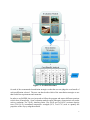
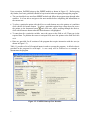
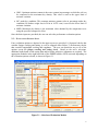
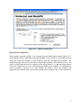
Expert System for Pavement
Remediation Strategies
(ExSPRS) User’s Manual
Product Number 0-5430-P3
TxDOT Project Number 0-5430
Conducted for:
Texas Department of Transportation
August 2008
Center for Transportation Infrastructure Systems
The University of Texas at El Paso
El Paso, TX 79968
(915) 747-6925
http://ctis.utep.edu
Expert System for Pavement Remediation Strategies
(ExSPRS) User’s Manual
by
Yaqi Wanyan, MSCE
Enrique Portillo,
Imad Abdallah, MSCE
and
Soheil Nazarian, PhD, PE
Research Project Number TX-0-5430
Conducted for
Texas Department of Transportation
Product Number 0-5430-P3
The Center for Transportation Infrastructure Systems
The University of Texas at El Paso
El Paso, TX 79968-0516
Disclaimers
The contents of this report reflect the view of the authors who are responsible for the facts and
the accuracy of the data presented herein. The contents do not necessarily reflect the official
views or policies of the Texas Department of Transportation. This report does not constitute a
standard, a specification or a regulation.
The material contained in this report is experimental in nature and is published for informational
purposes only. Any discrepancies with official views or policies of the Texas Department of
Transportation should be discussed with the appropriate Austin Division prior to implementation
of the procedures or results.
NOT INTENDED FOR CONSTRUCTION, BIDDING, OR PERMIT PURPOSES
Yaqi Wanyan, MSCE
Enrique Portillo,
Imad Abdallah, MSCE
Soheil Nazarian, PhD, PE (66495)
Table of Content
CHAPTER 1 INTRODUCTION......................................................................................... 1
1.1 - SYSTEM REQUIREMENT AND INSTALLATION .................................................................... 2
1.2 - DESCRIPTION OF PROGRAM.............................................................................................. 2
CHAPTER 2 INPUT MODULE ......................................................................................... 7
2.1 - BASIC INPUT .................................................................................................................... 7
2.2 - EVALUATION OPTIONS INPUT .......................................................................................... 9
2.3 - EXAMPLE ....................................................................................................................... 11
CHAPTER 3 EVALUATION MODULE ........................................................................ 13
3.1 - EVALUATION OPTIONS ................................................................................................... 13
3.2 - EVALUATION CHECKS OUTCOME................................................................................... 15
CHAPTER 4 REMEDIATION MODULE ...................................................................... 19
4.1 - REMEDIATION STRATEGIES FOR CONSIDERATION .......................................................... 20
4.2 - DETAILS OF REMEDIATION STRATEGIES TO CONSIDER ................................................... 20
CHAPTER 5 COST-BENEFIT MODULE ...................................................................... 33
5.1 - COST ANALYSIS ASSUMPTIONS ..................................................................................... 33
5.2 - BENEFIT INPUT............................................................................................................... 36
5.3 - COST-BENEFIT ANALYSIS RESULTS ............................................................................... 38
CHAPTER 6 -
REFERENCE .............................................................................................. 41
iii
iv
List of Tables
Table 1.1—List of Input Parameters Required in ExSPRS ............................................................ 5
Table 3.1—Summary of Example Input Data (Fort Worth Case Study) ...................................... 12
Table 5.1—Summary of Cost Analysis Assumptions (Fort Worth Case Study) .......................... 36
Table 5.2—Summary of Parameter Changing Trend for Remediation Strategies ....................... 37
v
vi
List of Figures
Figure 1.1—ExSPRS Flowchart ..................................................................................................... 3
Figure 1.2—ExSPRS Start-up User Interface................................................................................. 4
Figure 2.1—Selection of Evaluation Models.................................................................................. 9
Figure 3.1—Evaluation Options ................................................................................................... 14
Figure 3.2—Subgrade Shear Failure Check Input Structure ........................................................ 15
Figure 3.3—Evaluation Checks Outcome .................................................................................... 16
Figure 3.4—Longitudinal Cracking Check Graphical Result....................................................... 17
Figure 4.1— Logic Flowchart of Recommended Remediation Strategies ................................... 19
Figure 4.2—Selection of Remediation Strategies ......................................................................... 20
Figure 4.3—Stabilization Window of Remediation Module ........................................................ 21
Figure 4.4—Use of Geosynthetics ................................................................................................ 22
Figure 4.5—Hierarchy of Moisture Control Methods .................................................................. 23
Figure 4.6—Moisture Control Method of Using Moisture Barriers ............................................. 24
Figure 4.7—Moisture Control Method of Using Sloped Sections ............................................... 25
Figure 4.8—Moisture Control Method of Using Cross Drain Structures ..................................... 25
Figure 4.9—Moisture Control Method of Using Water Bars ....................................................... 26
Figure 4.10—Moisture Control Method of Dealing with Steep Grades ....................................... 26
Figure 4.11—Moisture Control Method of Using Inlets and Outlets ........................................... 27
Figure 4.12—Moisture Control Method of Using Root Barriers ................................................. 27
Figure 4.13—Moisture Control Method of Removing Vegetations ............................................. 28
Figure 4.14—Undercut and Backfill............................................................................................. 29
Figure 4.15—Deep Dynamic Compaction ................................................................................... 30
Figure 4.16—Decreasing Clay Content ........................................................................................ 31
Figure 5.1—Cost and Benefit Analysis ........................................................................................ 34
Figure 5.2—Pavement Parameters Modified for Each Remediation Strategy ............................. 39
Figure 5.3- Cost-Benefit Results for the Remediation Strategies ................................................. 40
vii
viii
CHAPTER 1 - INTRODUCTION
Rural, low-volume, farm-to-market access roads, roads connecting communities, and roads for
logging or mining are commonly referred as low-volume roads. Low-volume roads commonly
have an average daily traffic (ADT) of less than 400 vehicles per day, and usually have design
speeds less than 50 mph (80 kph) (AASHTO, 2002).
This research project was focused on low-volume roads over expansive clayey soils in Texas. In
spite of the over conservative pavement designs recommended and widely used in Texas for
roads in high PI clay areas, these costly pavements often fail prematurely. This failure occurs
primarily because of the highly variable properties of the clay throughout the year due to
moisture fluctuations. A significant amount of work is required to maintain and rehabilitate
these roads. The expansive nature of high PI clays, despite the fact that they are considered in
the design, is also of concern since they contribute to the roughness of the road, and as such the
loss of the functional serviceability of the roads. Therefore, it is imperative to improve the design
and laboratory procedures to address expansive subsoil conditions and then design pavements
accordingly to extend the life expectancy of these roads. The intent of this research project was
to cultivate the vital features of strategies for improving low-volume flexible pavement design
and thus improving the overall low-volume road performance. These include:
1). Identify the shortcomings of current design and construction practices associated with the
less than desirable performance of pavements in low-volume roads constructed on high
PI clays;
2). Identify the most significant soil parameters directly related to the performance of these
types of roads;
3). Propose practical and dependable laboratory test methods and analyzing models to
address the problem of premature failure of low-volume roads on high PI expansive
subgrade;
4). Qualify and quantify current remediation procedures, climatic effects and road condition
assessment (both successful and unsuccessful) used to mitigate the shrink-swell
problems;
5). Develop a user-friendly expert system design tool to guide the designers through the
process for more realistic designs and rehabilitations.
The results from this study offered a new design procedure that provides the following
information:
1




Identify most relevant soil properties and corresponding test procedures to characterize
and address highly expansive subgrade problems;
Propose quantitative analyzing models to predict flexible pavements failure on expansive
subgrade, specifically for low-volume roads;
Create an interactive expert system program to guide the user through design procedures
and provide realistic layer thicknesses for low volume roads;
Rank feasible design alternatives for rehabilitation and maintenance to minimize the cost
without compromise performance.
The design guideline for low classification roads over high PI clays developed to address the
issues summarized above is referred to as Expert System for Pavement Remediation Strategies
(ExSPRS). This program can be used to evaluate the structural and performance adequacy of
low-volume flexible pavement designs and to achieve cost-effective designs with appropriate
modifications. The program mimics human expert decision making process for this purpose.
Finally, cost-benefit comparisons are made between possible alternative modifications based on
modified inputs for each strategy. The goal is to help pavement engineers to design low-volume
roads that avoid costly over-designed yet underperforming roads over expansive subgrade.
This document provides a user’s guide to Version 1.0 of ExSPRS. Although the focus of this
research is for Texas, the new design guidelines will be helpful to other states with similar
problems. It is highly recommended to review research report 0-5430-1 and 2 before going any
further and using this program. The report provides a solid foundation regarding the theory,
models and processes used to develop this program.
1.1 - SYSTEM REQUIREMENT AND INSTALLATION
The program will work on a typical computer with Windows 9x, 2000, XP, Vista or NT
operating system. To install the program, execute the setup file ExSPRS.EXE and follow the
onscreen instructions. After installation, double click on the program icon on your desktop to
execute the program.
1.2 - DESCRIPTION OF PROGRAM
The Expert System for Pavement Remediation Strategies (ExSPRS) program has four main
modules: Input, Evaluation, Remediation and Cost-Benefit. Figure 1.1 shows the flowchart of
the program. ExSPRS uses an expert system approach which manages and incorporates concepts
derived from our study and uses structured knowledge to provide analysis to the user as an expert
would do. This program is specially developed for low-volume roads build over expansive
clayey subgrade.
The user needs to provide an initial pavement structure as an input. This pavement structure can
be obtained using common design software such as FPS19W. ExSPRS will check the candidate
pavement structure for several potential structural or functional distresses using its evaluation
models. If the input section experience premature distress, ExSPRS will use the expert system
approach to recommend feasible remediation strategies. Based on the remediation selected, the
modified pavement structure is re-evaluated. The cost-benefit analysis module will provide the
agency cost estimation of the original pavement section along with the additional agency costs
2
Figure 1.1—ExSPRS Flowchart
for each of the recommended remediation strategies so that the user can judge the cost-benefit of
each modification selected. The user can then decide which of the remediation strategies to use
that fits his/her requirements and constrains.
In order to use ExSPRS, the user just needs to follow the program and answer different questions
to their best of knowledge. Some evaluation models require laboratory characteristic test results
such as gradation (Tex-110-E), Atterberg limits (Tex-104-E and Tex-105-E), moisture density
tests (Tex-114-E), unconfined compressive strength (UCS, Tex-117-E) tests to quantify the
properties of the clayey subgrade material.
3
Upon execution, ExSPRS brings-up the INPUT module as shown in Figure 1.2. Before going
any further, four basic guidelines should be kept in mind when navigating through the program:
 The user should always start from INPUT module and follow the program steps through other
modules. It is best not to navigate to the next module before completing the information on
the current one.
 To select a particular option with check box or radio button, move the pointer to it and then
click with the left mouse button. To select a particular option from a drop-down list, move
and click once, while scrolling through the choices,
the pointer to the downward arrow
click with left mouse button when the desired answer is highlighted.
 To enter data for a particular variable, move the cursor to the field or cell. Then type in the
required data. To position the cursor to an input field, move the pointer to the field and click
on it.
 Hints are provided for all sections of the program that require interaction with the user (as
shown in Figure 1.2)
Table 1.1 provides a list of all required inputs in order to execute the program. A default value is
provided in the program for each input. A case study will be followed as an example to
demonstrate the program.
Figure 1.2—ExSPRS Start-up User Interface
4
Layer
Properties
Design Properties
Soil Properties
Table 1.1—List of Input Parameters Required in ExSPRS
Number of Layers
Description of layers (Layer Type)
Thickness (in.)
Modulus (ksi)
Poisson's ratio
Design ESALs (millions)
Analysis period (years)
Initial Serviceability index
Reliability (in decimal)
Design wheel load (kips)
Tire pressure (psi)
Road length (mile)
Total number of lanes
Lane width (ft)
Depth of treated subgrade (in.)
Percent of time pavement is exposed to saturation moisture level (%)
Pavement drainage quality
Subgrade Modulus during wet season (ksi)
PI
LL
P200
Optimum moisture content (%)
Maximum dry density(pcf)
Angle of internal friction from Triaxial tests
(degrees)
Cohesion of soil from Triaxial Test (psi)
Texas Triaxial Classification of soil
IDT at dry (psi)
PVR Limit (in.)
Sulfate Content (ppm)
5
6
CHAPTER 2 - INPUT MODULE
In this chapter, the following items are discussed as used in the INPUT module:
o
o
o
o
Layer properties
Design properties
Soil properties
Preliminary information regarding structural and performance evaluations
The ExSPRS INPUT module is developed through an interactive screen, which allows the user
to rapidly create the input data. The default values for a typical low-volume road build over high
PI clayey subgrade in Texas are displayed in the screen data input fields at the time the program
starts. These default values can be used as a starting point for the user to edit or use as desired.
At the bottom of the screen, two buttons are provided to recall data from an existing file or save
the input in a file for future use.
The “Load Input File” button is used to load a previously saved input file.
The “Save Input File”, allows the user to type in a file name “with no spaces”, and save the
current input file under the default program folder.
The INPUT module has four sections as shown in the left portion of the input screen. The right
part of the input screen is grayed out. That section is related to the evaluation options and is
activated when the required information is provided in the right hand portion. The following
section will discuss the INPUT module in detail.
2.1 - BASIC INPUT
Basic input includes layer properties, design properties and subgrade properties.
description of the basic design inputs are given below.
A brief
1). Layer Properties
 Number of layers: This program is restricted to three and four layer pavement systems
(including subgrade) since its specific target is the lower classification roads.
7
 Layer Property Table: Layer thickness in in., layer modulus in ksi and Poisson’s ratio for
each layer should be input. The representative moduli of materials can be obtained either
from the Falling Weight Deflectometer tests or laboratory tests. The user is advised to
make a reasonable input for each modulus because of the effects these values have on the
final solution.
 Layer Description: The type of layer being HMA, base or subgrade should be identified
for each layer. The first layer is HMAC by default. For surface-treatment a thickness of
0.5 in. and a modulus of 300 ksi are recommended. After the layer type is selected from
the drop-down list for each layer, the user needs to click “Update” button.
2). Design Properties
 ESAL: One direction cumulative 18-kip (80-kN) equivalent single axle load (ESAL)
applications in millions at the end of the design period (10 years in this case). This value
can be obtained from the Transportation Planning & Programming Division.
 Analysis Period: Length of analysis period in years, usually 10 years for low-volume
roads.
 Serviceability Index: This input pertains to the initial pavement serviceability index,
which is a function of pavement type and construction quality. Typical value ranges
between 4.0 and 4.2.
 Reliability: It is a means of incorporating some degree of certainty into the design process.
The level of reliability to be used for design of low-volume roads ranges from 50% to
80%. This number should be entered in decimal format.
 Design Wheel Load: Load on one single axle or a set of tandem axles in kips.
 Tire Pressure: Default value is 100 psi. Higher tire pressure is one of the reasons for
higher tensile strains and stresses within pavement.
 Road Length: This value is used to estimate cost. Unit length of 1 mile is recommended.
 Number of Lanes for both directions: This refers to the total number of lanes in both
directions. For low-volume roads, it is usually 2 or 4.
 Lane Width: This input is also used to estimate cost. The standard 12-ft lane is used as
default.
 Depth of Treated Subgrade: This is the thickness of the stabilized layer between the base
and subgrade in in.
3). Subgrade Properties
 PI: Plastic index in percentage (Tex-106-E). It is a measure of the range of water contents
where the soil exhibits plastic properties. The PI is the difference between the liquid limit
and the plastic limit. PI  LL  PL
 LL: Liquid limit in percentage (Tex-104-E).The liquid limit (LL) is the water content
where a soil changes from liquid to plastic behavior.
 P200: Percentage of materials passing the 75 μm (No 200) sieve. (Tex-110-E)
8
 OMC: Optimum moisture content is the water content in percentage at which the soil can
be compacted to the maximum dry density. This value is used as the upper limit of
moisture variation.
 MC under dry condition: This constant moisture content value in percentage under dry
condition (No further weight loss in 24-hr in 104oF oven) is used as the lower limit of
moisture variation.
 MDD: Maximum dry density is the maximum value obtained by the compaction curve
using the specified compactive effort.
Once the basic inputs are provided, the user can select the performance evaluation options.
2.2 - EVALUATION OPTIONS INPUT
Four evaluation options as depicted in the input screen are provided: 1) Structural checks that
consider fatigue cracking and rutting, as well as subgrade shear failure; 2) Performance checks
that consider longitudinal cracking and roughness. The user can deactivate any or all of the
options except the fatigue cracking and rutting check. Based on the user’s selections,
additional input based on lab testing data and/or his/her subjective judgments are required. The
appropriate modules in the right hand side of the INPUT module will be activated depending on
the evaluation options selected, as shown in Figure 2.1.
1
1
1
1
Figure 2.1—Selection of Evaluation Models
9
Fatigue Cracking and Rutting
A layered linear elastic model that computes pavement responses under static loads is
incorporated in the software to check for the pavement fatigue cracking and subgrade rutting.
The Asphalt Institute (1982) and Shell (1978) design methods, which relate the strains to the
allowable number of load repetitions as shown in the following equations are used:
N f  f 1 ( t )  f 2 ( E1 )  f 3
(2.1)
N d  f 4 ( c )  f 5
(2.2)
where Nf and Nd is the allowable number of load repetitions for fatigue cracking and rutting
respectively, c is the horizontal tensile strain at the bottom of the HMA, t is the vertical
compressive strain on top of the subgrade, E1 is the HMA modulus, f1 to f5 are empirical
coefficients.
If the loss of stiffness during wet season is a concern, the user is prompted to provide the
saturated subgrade modulus in ksi. This modulus will be used in the check to account for the
worst case scenario.
Subgrade Shear Failure
This option utilizes the Texas Triaxial Design method and LoadGage to check the subgrade shear
failure. If the user desires to check for the subgrade shear failure, the Texas Triaxial Test (Tex117-E) results will be required. However, if the test data is not available, default values are
assigned by the program based on some general questions. The user is strongly encouraged to
minimize the use of the default values for this purpose as much as possible.
Longitudinal Shrinkage Cracking
The longitudinal shrinkage cracking is believed to be initiated in the subgrade as a “bottom-up”
crack. The subgrade cracks under the combined action of shrinkage by drying and the resistance
to shrinkage due to base layer on one hand, and to the deeper, constant-moisture layers of the
clay, on the other hand. Resistance to the shrinkage results in shear stresses at the interface of
subgrade and base which in turn produce compression stress in the granular courses and tension
stress in the clay. When the tensile stress equals the tensile strength, cracking is initiated. Upon
further drying, the crack propagates through the base course towards the asphalt layer. If the
tensile strength of the asphalt layer is also inadequate, the crack may propagate through to the
surface, after which another new cracking cycle begins. (Uzan, et al., 1972; Bell and Wright,
1991)
During a dry weather cycle, subgrade shrinkage will cause lateral forces which may exceed its
tensile strength. The increase in the lateral shrinkage stress of soil is the main reason for the
development of longitudinal cracks. A finite element model is incorporated in ExSPRS to
estimate the threshold moisture contents for the initiation (MCI) and propagation (MCP) of the
longitudinal cracks in the pavement structure. This model also estimates the most likely location
for such cracking.
10
A thorough description of the theory and the model used in ExSPRS is provided in TxDOT
Research Report TX-0-5430-2.
To utilize this model, the user needs to either provide laboratory results of the shrinkage strain or
use the shrinkage strain vs. moisture content relationships (later referred to as shrinkage strain
model) developed under this research project. If the information regarding the shrinkage strain is
available and the user selects any of the first three test options, two inputs are required: 1) the
tensile stress under dry condition, and 2) the shrinkage strain value that can be obtained from a
shrinkage strain characterization test such as linear shrinkage bar test or the volumetric shrinkage
strain test. Means of estimating the tensile strength is provided in Research Report 0-5430-2.
If the user decides to use the built-in shrinkage strain model, no extra inputs are required as they
were already provided under the soil properties section.
Roughness
Environmental changes cause subgrade volume change induced by swelling and/or shrinking.
The roughness of pavement is the result of the cumulative deformation and differential
volumetric change of the problematic subgrade soils. The roughness model checks the potential
vertical rise (PVR) of subgrade and evaluates the international roughness index (IRI) of low
volume roads surface.
If the user reports the subgrade as highly expansive (Roughness portion on the bottom right
panel), PVR check will be evoked. The limit of tolerable PVR is also required. This value
typically varies between 1 to 2 inches. Also, if excessive roughness is known to be a concern in
the area, IRI check will be activated to estimate the expected IRI at the end of the design period.
2.3 - EXAMPLE
To understand the steps and modules in ExSPRS, an example is provided for the user to follow.
This also serves as a training exercise. Table 3.1 gives an example of summarized input
information to input into the program. This example will be used in the description of the
remaining modules so the user can use this manual to follow along for the remaining chapters.
Once the required data for all the evaluation checks are completed, the user may click the “Next”
button (at the bottom-right hand side of the INPUT module) to proceed to the EVALUATION
module.
11
Layer
Properties
Design Properties
Soil Properties
12
Table 3.1—Summary of Example Input Data (Fort Worth Case Study)
Number of Layers
3
Compacted
Description of layers
HMAC Flexible Base
Subgrade
Thickness (in.)
2
6
200
Modulus (ksi)
500
50
14
Poisson's ratio
0.35
0.35
0.4
Design ESALs (millions)
1
Analysis period (years)
10
Initial Serviceability index
4.0
Reliability (in decimal)
0.8
Design wheel load (kips)
18
Tire pressure (psi)
100
Road length (mile)
1
Total number of lanes
2
Lane width (ft)
12
Depth of treated subgrade (in)
12
Percent of time pavement is exposed to saturation moisture level (%)
1 to 5
Pavement drainage quality
Good
Subgrade Modulus during wet season (ksi)
9
PI
29
LL
61
P200
100
OMC (%)
24
Dry MC (%)
1.2
MDD (pcf)
92
Angle of internal friction (◦)
35
Cohesion of soil (psi)
3.6
Classification of soil
4
IDT at dry (psi)
15
PVR Limit (in)
2
Sulfate Content (ppm)
1000
CHAPTER 3 - EVALUATION MODULE
In this chapter, the following items are discussed as used in the EVALUATION module:
o Information regarding evaluation models
o Outcome of possible distresses and failures of the design being evaluated
Based on the district survey and literature review conducted under research project TX-0-5430,
the most prevailing distresses for low volume flexible pavements are longitudinal cracking,
rutting, shoving and excessive roughness. The main causes for these distress problems can be
categorized into two areas: 1) Inadequate support, which is caused by inadequate layer
thicknesses, poor constructions and improper stabilization; 2) Problematic soils susceptible to
moisture variation, which include subgrade volume change, shoulder problems, poor drainage or
other combined effects. The EVALUATION module is used to determine whether the userdefined pavement structure meets these criteria. The outcome from EVALUATION module
provides the user with the option to either modify the original design (use different cross-sections
or materials) and restart the analysis over or proceed to the REMEDIATION module to
determine suitable remediation alternatives.
3.1 - EVALUATION OPTIONS
In addition to the preliminary inputs required in the INPUT module, several specific questions
are also asked in the EVALUATION module window as shown in Figure 3.1. The details for
each type of evaluation are presented next.
Longitudinal Shrinkage Cracking Model
If the user selects to provide the shrinkage strain in the INPUT module, no additional
information is required. If the user decides to use the built-in shrinkage strain model, he/she
needs to select the index parameters to be used to estimate the shrinkage strain with the built-in
model. Figure 3.1 depicts the selection of soil parameters for inclusion under the top panel. The
development and validation of the shrinkage strain model used in ExSPRS is provided in TxDOT
Research Report TX-0-5430-1.
13
Figure 3.1—Evaluation Options
Subgrade Shear Failure Model
Figure 3.2 depicts the input structure for subgrade shear failure check. By default, the Texas
Triaxial method is used. The required cover depth from this method may be over-conservative in
districts where the climate is drier, or where the soils are not as moisture susceptible (Fernando,
et al., 2001). To account for this conservatism, the modified triaxial design method (MTRX) is
also provided as a choice to double-check the cases when the pavement structure fails the Texas
triaxial check. If triaxial test results are provided in the INPUT module, no further information
is required and the rightmost question in the EVALUATION module under the Subgrade Shear
Failure model is grayed. If on the contrary, the triaxial test results are not available, the subgrade
condition is used to estimate these parameters. The user also needs to select the analysis option
and axle load type in order to execute the MTRX ( also known as LoadGage) check. By default,
the LoadGage program runs a linear analysis to predict the stresses. However, for the advanced
user, a nonlinear option is included to permit modeling of the stress-dependency. The nonlinear
analysis option will provide a more realistic prediction of the stresses induced under loading
(Jooste and Fernando, 1995) for thin pavements. This analysis in MTRX uses equation with k1,
k2 and k3 material constants determined from resilient modulus testing (Uzan, 1985).
14
Figure 3.2—Subgrade Shear Failure Check Input Structure
Roughness Model
In order to estimate IRI and PVR more accurately, two environmental-related questions are
asked:
1). What is the percentage of time within a typical year that the pavement is exposed to wet
season (moisture level approaching saturation)?
2). What is the quality of the pavement drainage system?
The user needs to make appropriate selections according to his/her experience. Once all the
relevant information for the EVALUATION module is provided, the user can proceed to view
the Evaluation Outcome by clicking the “Perform Evaluation Checks” button at the bottom-right
hand side of the window.
3.2 - EVALUATION CHECKS OUTCOME
The “Evaluation Checks Outcome” window is divided into four panels to present the results for
the four Evaluation Options (see Figure 3.3). The top left portion presents the outcome of the
fatigue cracking and rutting check, the top right section presents the results for the subgrade
shear failure check, the bottom left section is for the roughness check results and finally the
bottom right portion shows the results for the longitudinal shrinkage cracking (LSC) check
15
Figure 3.3—Evaluation Checks Outcome
results. If an evaluation was not selected in the INPUT module, the designated results panel will
be blank.
For the fatigue cracking and rutting check, the corresponding allowable load repetitions are
reported in million ESALs. Fail/Pass flags are also shown for each one. The design traffic
provided by the user in the INPUT module is also reported here for comparison. An overall
Fail/Pass flag is also reported for this evaluation check. In the example used in this manual for
illustration, the section passed the fatigue cracking performance and failed the rutting. The
overall evaluation check is considered as failed, and therefore, remediation to prevent rutting is
required.
In this example, both the Texas triaxial (Tex-117-E) method and MTRX method were used. The
Texas triaxial check proposed a required cover depth of 15 in. MTRX check required a base
thickness of 13 in. The original design failed both checks.
Under the roughness check results, the total PVR was estimated to be 2.6 in. Since in this
example the acceptable PVR limit of 2 in. was provided, the PVR check also failed. The IRI
check gave 2.1 m/km, which passed the criteria for farm to market roads. Details of IRI criteria
can be found in Research Report TX-0-5430-2.
The longitudinal shrinkage cracking check estimated that at a moisture content of 21.6%, the
shrinkage cracking initiates, and at 16.8%, the longitudinal crack propagates up to surface. At
16
the bottom-right of the LSC results panel, there is a button “Graph of crack initiation at the top of
subgrade (across pavement section)” that provides the user with the location and distribution of
stresses. The user can click to see the distribution of critical points along a 12-ft lane (144 inches
in x-axis) cross-section view (depth of inches along y-axis) as shown in Figure 3.4. The critical
locations are near the 42 ± 18 in. (3.5 ± 1.5 ft) range from the pavement edge.
To proceed to the REMEDIATION module, the user needs to click the “Determine Remediation
Strategies” button in the bottom right of the screen. The REMEDIATION module is presented
in Chapter 4.
Figure 3.4—Longitudinal Cracking Check Graphical Result
17
18
CHAPTER 4 - REMEDIATION MODULE
In this chapter, the following items are discussed as used in the REMEDIATION module:
o Alternative ways to consider for overcoming structural inadequacy and performance
problems
o Description of each alternative on how to improve the pavement system
In the REMEDIATION module, six modification strategies grouped into two categories are
available for consideration: 1) To improve subgrade strength and stiffness; and 2) To minimize
moisture variation induced swell/shrink problems. ExSPRS will recommend appropriate
methods to consider from either or both categories following the logic flowchart shown in Figure
4.1 based on the evaluation results.
Figure 4.1— Logic Flowchart of Recommended Remediation Strategies
19
4.1 - REMEDIATION STRATEGIES FOR CONSIDERATION
Figure 4.2 shows the selection of remediation strategies. The user has the choice to decide which
one(s) out of the recommended modifications to be considered and analyzed for the original
candidate design. When a specific strategy is selected, the user will notice that a new tab is
activated. Figure 4.2 shows where both Stabilization and Undercut-Backfill are selected and
thereby their tabs are activated (see Figure 4.2). For demonstration purpose and the example
provided in this manual, all recommended remediation strategies are selected for further
illustration. This module shows the remediation strategies that resulted from the evaluation
check results. Once the user determines and selects which of the remediation strategies might be
suitable for consideration, the user can proceed to the COST-BENEFIT module where a cost
analysis is performed and the benefits of the selected remediation strategies are provided for
comparison.
1
1
1
1
Figure 4.2—Selection of Remediation Strategies
4.2 - DETAILS OF REMEDIATION STRATEGIES TO CONSIDER
To explore the details of each modification method, the user can click on the corresponding
highlighted tab. All activated remediation strategy tabs are parallel, and the user can explore any
of the solutions in any order.
20
Stabilization
Clayey soils are often stabilized with calcium based stabilizers to improve their engineering
properties including strength, volumetric change potential and permeability. Figure 4.3 depicts
the screenshot of stabilization window. Three questions are asked in this module. First, the user
is asked to locate their project using the map provided (see Figure 4.3) to decide whether the
location is susceptible to sulfate heave problem, which is one of the main factors that affects the
final stabilization method and stabilizer recommended. Second, the user is asked to provide the
laboratory tested sulfate concentration in ppm. (Tex-145-E). The default value for this question
will be set to no sulfate concentration, if the user answer for the first question is “Neither”, or
Tex-145-E is not carried out. Finally, the user should indicate whether the subgrade is an
organic-rich subgrade. To facilitate the responses to these questions, the user can take advantage
of the specially treatment recommendations, references and the recommended stabilizers
provided at the bottom-left part (see Figure 4.3).
Reference /
Recommendations
Stabilizers
Figure 4.3—Stabilization Window of Remediation Module
Geosynthetics
For the scope of this research, the geosynthetic reinforcement is assumed to be targeted for
subgrade improvements. The reinforcement is placed at the interface between base/subbase and
the subgrade. Figure 4.4 illustrates the usage of the geosynthetic reinforcement with some
additional references. At the bottom half of the window there are three questions regarding the
subgrade quality. These questions are used to decide the required depth of the pavement above
21
Evaluation Check
Figure 4.4—Use of Geosynthetics
the placement of the geosynthetic material. If has chosen to select this option as a remediation
strategy to consider, then the user should answer those questions. One option is to use the
subgrade resilient modulus, which requires no further action since that value was already
provided in the INPUT module. Further questions are only required if the user decides to use the
other two very approximate methods (the use of these two options is discouraged for project
level studies). Upon selecting one of the two lower radio buttons, the appropriate menu will be
activated.
To ensure that the geosynthetic material can be place at the recommended depth (middle graph in
Figure 4.4) directly without further construction modifications, the user needs to provide
maximum tolerable depth of rutting during the design life of the roadway in inches. Commonly
used value of 2-inch was provided as default. The “Update” button needs to be selected. The
program will show whether thicker layers above subgrade are required for the section with the
geosynthetic to be fully functional without losing it’s anchorage strength. To return to the main
remediation tab, select the “Return” button or directly click on the tab.
22
Moisture Control
Many pavement distress problems are caused by moisture variation and migration. The moisture
control remediation methods are offered in a hierarchical style as shown in Figure 4.5. This
remediation strategy focuses on measures that directly deal with minimizing moisture change in
the subgrade. These remediation strategies are grouped into three main categories: 1) use of
vertical moisture barriers, 2) improve drainage and 3) treat nearby vegetations.
Figure 4.5—Hierarchy of Moisture Control Methods
23
This portion of the program is illustrative rather than analytical. The user can explore useful
information, design methods and references for different methods by first selecting one of the
three moisture control groups, then further specifying a method if selection question shows up.
Figure 4.6 shows an example informational screen of using moisture barriers. The user can click
“Next Picture” button to read more. As presented in the flowchart in Figure 4.5, there are five
methods to improve the drainage. They are: use sloped sections, cross-drain structure, water bars,
inlets and outlets and to avoid steep grades. Figures 4.7 to 4.11 show example informational
screens of these drainage improvement methods. Figure 4.12 and 4.13 depicts example
informational screens of vegetation treatments.
Figure 4.6—Moisture Control Method of Using Moisture Barriers
24
Group
Method
Figure 4.7—Moisture Control Method of Using Sloped Sections
Figure 4.8—Moisture Control Method of Using Cross Drain Structures
25
Figure 4.9—Moisture Control Method of Using Water Bars
Figure 4.10—Moisture Control Method of Dealing with Steep Grades
26
Figure 4.11—Moisture Control Method of Using Inlets and Outlets
Figure 4.12—Moisture Control Method of Using Root Barriers
27
Figure 4.13—Moisture Control Method of Removing Vegetations
Undercut and Backfill
Poor subgrade soil can simply be removed and replaced with high quality fill. This method,
which is also called undercut and backfill, is a simple procedure that does not require any
specialized equipment. However, unless a suitable backfill material is available near the job site,
removal and replacement is generally a much more expensive operation than the use of additives.
For this reason, removal and replacement is mostly used in urban areas, where dust and
environmental impacts make the use of additives less desirable. Removal and replacement may
also be the best option in areas where deep deposits of peat and muck cannot be treated with the
use of additives. For lower classification roads, economic constrains have to be taken into
account. If this remediation is selected, the program calculates the recommended replacement
depth. Figure 4.14 provides an example of the calculated undercut and backfill depth in inches
provided by the program.
28
Figure 4.14—Undercut and Backfill
Deep Dynamic Compaction
Deep dynamic compaction (DDC) is an economical ground modification method (Figure 4.15).
This technique involves repeatedly raising and dropping a large weight in a prescribed pattern to
densify the potentially unstable or weak underlying materials with high-energy impacts. The
weight may range from 6 to 25 tons and the drop height typically varies from 30 to 60 ft. The
degree of densification achieved is a function of the energy input (i.e., weight and drop height) as
well as the saturation level, fines content and permeability of the material. As mentioned by
several researchers, (Mowafy et al., 1985; Rollins and Christie, 2002), this method is not
appropriate for saturated clayey soils and the solution may be temporary due to water infiltration.
29
Figure 4.15—Deep Dynamic Compaction
Decreasing Clay Content
When undercut and backfill is not economically feasible, another method which is referred to as
“decreasing clay content” provides an alternative. As the name implies, this process is to dilute
expansive soils with non-expansive fill. It is less time consuming and cheaper compared to
undercut and backfill when quantities of non-expansive fills are limited. When this method is
selected, the program provides the user with the equations based on literature review to quantify
required volume of mixing sand (see Figure 4.20).
The user is encouraged to explore all remediation strategies that are of interest. After studying
the feasible modification methods, the user can proceed to the COST-BENEFIT module by
selecting the button on the bottom right screen to determine which of the strategies are
economically feasible. As mentioned at the beginning of this chapter, this module was to
provide the user with the remediation option available to him/her based on the evaluation checks.
For each remediation strategy selected, the user needs to provide additional information in order
for that strategy to be analyzed and its benefit and cost determined. This is covered in the next
chapter.
30
Figure 4.16—Decreasing Clay Content
31
32
CHAPTER 5 - COST-BENEFIT MODULE
In this chapter, the following items are discussed as used in the COST-BENEFIT module:
o
o
o
o
Determination of unit costs for selected remediation strategies
Estimation of updated pavement input parameters for selected remediation strategies
Cost comparison of selected alternatives
Benefit comparison of selected alternatives
The COST-BENEFIT module is the last module in the program. It provides the user with cost
benefit comparison of the original design and selected remediation strategies. This module is
separated into two parts:
1) Input, which acquires assumptions to estimate unit costs and updated pavement
characteristic parameters to quantify benefit; and
2) Outcome, which compares cost and benefit among alternatives.
The input portion is shown first when the user first views this module. As shown in the top of
Figure 5.1, all remediation strategies selected by the user are active and their corresponding
treatments and unit are provided. Again if a remediation is not selected the corresponding
section is grayed out. The second portion of the input is associated with the updated parameters
of the pavement system that are impacted by the remediation strategies. These parameters are
listed in a tabular format (see Figure 5.1).
In the second portion of the COST-BENEFIT module the outcome identifies and compares the
cost and benefit of all eligible alternatives. Once all the inputs such as the detailed modification
activities, unit cost and modified pavement parameters are provided, the cost-benefit analysis is
computed. This outcome is presented in a similar tabular format at the bottom of the screen. In
this chapter, the inputs and outcome of the cost-benefit analysis is described.
5.1 - COST ANALYSIS ASSUMPTIONS
Before describing the COST-BENEFIT module there are some basic assumptions made to
simplify the procedure without compromising the results accuracy. These assumptions are
presented first.
33
Figure 5.1—Cost and Benefit Analysis
Basic Assumptions

For a typical lower classification pavement cost analysis, only the agency costs are
considered due to the fact that the low-volume roads typically experience low daily traffic.
The user costs are considered minimal and are omitted in cost estimates.
 Construction time estimation is also omitted assuming that the agency cost to be the
controlling parameter.
 The agency cost is estimated using unit cost approach. Unit price information was obtained
from the RS Means CostWorks Data for Heavy Construction (R.S. Means 2007). These unit
cost data can be easily updated with the most current information as they become available.
 RS Means differentiates unit costs for same construction activity with different lift thickness.
User defined layer thicknesses are interpolated/extrapolated based on available lift thickness
information.
 Cost analysis is only considered for road lanes, and shoulders are excluded. By default, the
roadway section being analyzed is a one-mile, two-lane low-volume road with 12-ft-wide
lanes.
 New pavement is assumed for planning construction activities. Only main construction
activities are considered, which include, but not limited to excavation, backfill, compaction,
34
and preparation of subbase, base, and AC layers. Minor activities such as underground utility
removal, drainage and manhole installation, bridge or culvert construction, surface detailing
and finishing are eliminated.
 One crew with one shift is used for all activities since expediting with more crew members or
shifts results higher unit cost. For each activity, normal or ideal set of working conditions are
considered. No variability is considered to account for changes in weather or other factors
during the construction.
 For each remediation strategy the cost is considered separately, since they are independent of
one another.
Cost Input
In Figure 5.1, the top portion of the COST-BENEFIT module shows the input needed for cost
estimation of selected remediation strategies. The user needs to either select from the drop-down
list or to enter numerical values for each activated remediation method. Unit cost for each
strategy will be provided at the right side for quick reference.
The following sections discuss these cost input for each remediation in detail.
 Stabilization: Recall that in the REMEDIATION module the appropriate stabilizer was
selected. For this example the stabilizer was lime. This information is passed and loaded in
this module. ExSPRS automatically loads accordingly cost information in a drop-down list
with different mix percentage. As an example, the user can select 4% mix. The unit cost for
4% lime stabilization of 12-inch lift is retrieved to be $11.3/yd2 (12-inch lift means the total
treatment depth that was entered in INPUT module). As a special note, for each remediation
strategy, there maybe more than one possible treatment activities available. To continue with
the lime stabilization example, the user is required to identify mix percentage, but not the lift
thickness. In construction however, it maybe achieved by stabilizing one single layer of 12inch, two layers of 6-inch each, or other lift thickness combinations. The rule of thumb used
in ExSPRS is always to select the cheapest one among possible pool of activities. In this case,
a single layer of 12-inch treatment is cheaper than 2 runs of 6-inch layer, and that is the reason
the unit cost of $11.3 is reported. If the costs need to be modified in the future, then the file
installed with the program called “CostAnalysis v2.xls” needs to be updated. An example for
each tab sheet in the excel file can be followed to update the proper unit cost.
 Undercut and backfill depth is automatically inputted from previous calculation. The cost
associated with this method includes excavation and backfill. No extra input is needed.
 Geosynthetics: The only information needed from the user is to select the tensile strength for
the geosynthetic. R.S. Means 2007 reports the tensile strength per fabric sheet in terms of
pounds (lb). The available options are 120-lb, 200-lb and 600-lb. Other associated
installation costs are not considered due to lack of information.
 Moisture control methods have three different categories which are identified as a) Moisture
Barriers; b) Drainage Improvement; and c) Vegetation Removal. All encountered costs will
be added up together for the final cost estimation of moisture control.
a). Moisture Barriers: Regular drainage geotextile is assumed. The user will be asked for
the geotextile film thickness.
35
b). Drainage Improvement: There may be several ways to improve drainage. Additional
costs considered by the program include grading sloped sections and the use of culvert
either to build cross-drain structures, water bars or as inlet and outlet. The user needs to
provide culvert diameter, spacing and slope description (gentle or steep).
c). Vegetation Removal: The user needs to select from drop-down lists of the following
information: diameter of big trees (meaning diameter bigger than 12-inch) to be removed
per road length (entered in INPUT module); number of small trees (diameter less than
12-inch) per acre; percentage of hardwoods and roadside width for small trees (ft./side)
 Due to the lack of cost data for deep dynamic compaction, airport subgrade compaction is
used as a substitute. The user needs to select the percentage of standard proctor density from
R.S. Means’ available pool of 80%, 85%, 90% and 95%.
 The agency cost for decreasing clay content method includes three parts: excavation, backfill
and mixing. Due to lack of information, it is estimated the same way as undercut and backfill,
with half the depth entered by the user (meaning a partial mix and replacement).
Table 5.1 gives an example of summarized cost analysis input that the user can follow to practice
with the program.
Table 5.1—Summary of Cost Analysis Assumptions (Fort Worth Case Study)
Stabilizer
Lime
Stabilization
Stabilization percent mix
4%
Geosynthetics tensile strength (psi)
600
Geosynthetics
Culvert Diameter (in)
12
Drainage
Culvert Spacing (ft)
500
Improvement
Sloped Section
Gentle
Barrier film thickness (in)
0.44
Barriers
Moisture
Big Tree Diameters (for trees bigger than 12")
12-24
Control
Number of big trees to be removed (per mile)
10
Vegetation
Number of trees less then 12" per acre
Up to 400
Removal
Percentage of hardwoods
0-25%
Roadside Width for smaller trees (ft./side)
6
Undercut and backfill depth (in.)
13
Undercut and Backfill
Compaction Depth (in.)
24
Deep Dynamic Compaction
Percentage of standard proctor density
95%
5.2 - BENEFIT INPUT
The benefit input portion of this module is based on comparing structural and performance
evaluation results for the original design and that after using a remediation strategy. These
changes in evaluation results are caused by changes in input parameters. The user will be asked
to provide new input for those changed parameters by either performing laboratory tests or use
their best estimation. The benefit input table will originally show the values of the original
design for cases being analyzed. First column automatically loads the user’s input from earlier
36
steps. The other columns are designated for remediation strategies as identified with
corresponding remediation keyword. The values in these columns need to be modified if the
corresponding remediation strategy was selected (in REMEDIATION. module). Parameters that
are likely to be impacted by the remediation strategy are bolded.
The following are some general discussions on changes of expansive subgrade soil properties
caused by each remediation strategy. The changing trend of the parameters under each treatment
is tabulated in Table 5.2 with “” meaning increase, “” meaning decrease, “” meaning either
increase or decrease is possible, and “—” meaning no change. The information can assist the
user as a guide to estimate the appropriate input values. Additional information can be found in
TxDOT Research Reports 0-5430-1 and 2.
Table 5.2—Summary of Parameter Changing Trend for Remediation Strategies
Remediation Strategies
Undercut Deep
Decrease
Parameters
GeoMoisture
Stabilization
&
Dynamic
Clay
synthetics Control
Backfill
Compaction Content
Mr_optimum





—
(ksi)






Mr_wet (ksi)



—
—
—
PI



—
—
—
LL




—
—
OMC (%)




—
—
MDD (pcf)
IDT_dry





—
(psi)
Triaxial





—
Test
Expansive clays are usually chemically stabilized with cement, lime or fly ash to reduce their
plasticity index, liquid limit, volume change potential, and maximum dry density and to improve
optimum water content, shrinkage limit, and shear and tensile strength properties. (Croft, 1967;
Little, 1999; Thompson, 1966; Bell, 1996; Basma and Tuncer, 1991) Different results are
reported by researchers on how much these parameters changed.
The use of geosynthetics as reinforcement for subgrade soils in both wet and dry conditions
increases tensile strength and initial stiffness of the subsoil, decreases long-term vertical and
horizontal deformation, reduces desiccation cracking, fatigue cracking and rutting, and helps in
holding the pavement system together better (Gurung, 2003; 1983; Abd El Halim et al., 1983;
Cicoff and Sprague, 1991; Steward et al., 1977; Giroud and Noiray, 1981; Montanelli, et al.,
1999). However, the benefits of using geosynthetics are more noticeable for future performance
rather than initial parameter values. Measured values of stresses, strains, deflections and other
parameters are highly case specific. As many researchers have suggested, an average design
improvement factor could be used. From literature review, this improvement factor ranges from
1.5 to 2.
37
Moisture control methods do not change soil properties, but rather minimize moisture migration
and fluctuation. Thus prevent or minimize the subgrade from expanding during wet seasons and
shrinking during dry periods. With moisture control remediation implemented, parameters such
as subgrade modulus, shrinkage strain and triaxial test results will be controlled in a much
smaller variation range for worst case scenarios.
Undercut and backfill method removes poor subgrade and replaces it with high quality fill. This
procedure changes every aspect of subgrade soil, thus new tests are required to identify soil
characteristic properties.
Deep dynamic compaction is a temporary method to densify unstable or weak subgrade. With
high-energy impacts, unit weight, dry density, strength, stiffness and swell/shrinkage potential of
subgrade soils are modified.
The main purpose of decreasing clay content method is to reduce problematic subgrade
volumetric change potential by diluting expansive soils with non-expansive fills. Similar to
undercut and backfill, every soil characteristic property will change.
For the purpose of this example, changes to the parameters required based on the remediation
strategies are made based on educated guess. Again, laboratory testing would need to be carried
out in order to obtain those values. The modified values are shown in the highlighted section of
Figure 5.2.
5.3 - COST-BENEFIT ANALYSIS RESULTS
Figure 5.3 represents the cost analysis results for our example case. The original design costs
about $347,000/mile, followed by the cost of all remediation strategies. For example, subgrade
stabilization using 4% lime costs $160,000/mile and to control moisture variation by using
drainage improvement, moisture barriers and vegetation removal requires an additional of
$110,000/mile. However, for the remaining four remediation strategies the cost was less than
$50,000/mile. To justify the benefit of each remediation method, before-after analysis results
should be carefully studied. The detailed results for evaluation models are presented in this
table, with a GREEN color for those that passed the criteria, and a RED color for those failed.
Cost-benefit analysis opens the door for more in-depth understanding regarding how to reach a
reasonable and satisfactory design for low-volume road. A good design relies on not one single
factor but many factors combined. ExSPRS program tries to identify a more critical combination
of considerations in hoping for a favorable alternative. Expertise is invaluable to apply the
findings to assist engineers in their decision making process. The following paragraph will
discuss how to compare cost estimations and benefit results based on the example presented in
this manual. As prevailing distress problems are different for each district, the concentration of
the design goal changes, which in turn will yield different user preferences. In the example case,
let’s assume longitudinal cracking is reported to be the main issue and thus decreasing subgrade
moisture susceptibility become more critical than other aspects. Computational results shown in
Figure 5.3 indicates placing a geosynthetic reinforcement layer near base-subgrade interface
provides the most benefits in keeping longitudinal cracking problem away. Also, by referring to
the cost estimation, using geosynthetics seems to be a very cost-effective choice. Thus, original
38
design with geosynthetic reinforcement is very favorable compared to other possibilities. Please
keep in mind that the values used in this example as benefit input were hypothetical and are for
demonstration purpose only.
After the analysis is complete, the program provides a “Save Results” button at the bottom of the
Cost-Benefit Analysis module, which allows the user to save the results in an Excel format.
Figure 5.2—Pavement Parameters Modified for Each Remediation Strategy
39
Figure 5.3- Cost-Benefit Results for the Remediation Strategies
40
REFERENCE

AASHTO (2002) “AASHTO Design Guide 2002 (NCHRP 1-37), The MechanisticEmpirical Design Guide” Federal Highway Administration

Abd El Halim, A.O., Haas, R., and Chang, W. A. (1983) “Geogrid Reinforcement of Asphalt
Pavements and Verification of Elastic Layer Theory” TRB Research Board Record No. 949
pp.55-65

Basma, A.A., Tuncer, E.R. (1991) “Effect of Lime on Volume Change and Compressibility
of Expansive Clays” Transportation Research Board, TRR No. 1296, Washington DC. pp.
54-61.

Bell, D.O. and Wright, S.G. (1991) “Numerical Modeling of the Response of Cylindrical
Specimens of Clay to Drying” FHWA/TX-92-1195

Bell, F.G. (1996) “Lime Stabilization Of Clay Minerals And Soils”. Engineering Geology 42
pp.223-237.

Cicoff, G.A. and Sprague, C.J. (1991) “Permanent Road Stabilization: Low-Cost Pavement
Structures and Lightweight Geotextiles” Transportation Research Record 1291. pp.294-310

Croft, J.B. (1967) The Influence of Soil Mineralogical Composition on Cement Stabilization
Geotechnique vol. 17, London, England, pp.119–135.

Fernando, E., Liu W. and Lee T. (2001) “ User’s Guide to the Texas Modified Triaxlial
(MTRX) Design Program”

Giroud, J.P. and Noiray, L. (1981) “Geotextile-Reinforced Unpaved Road Design” Journal
of Geotechnical Engineering Division, Proceedings of the ASCE Vol. 107, No. GT9, pp.12331254

Gurung, N. (2003) “ A Laboratory Study on the Tensile Response of Unbound Granular base
Road Pavement Model Using Geosynthetics” Geotextiles and Geomembranes 21 pp.59-68

Jooste, F. J. and E. G. Fernando. Development of a Procedure for the Structural Evaluation of
Superheavy Load Routes. Research Report 1335-3F, Texas Transportation Institute, Texas
A&M University, College Station, Texas, 1995.
41

Little, D.N.(1999) “Evaluation of Structural Properties of Lime Stabilized Soils and
Aggregates, Vol. I. Summary of Findings” National Lime Association Publication

Montanelli, F., Zhao, A.G. and Rimoldi, P. (1999) “Geosynthetic-Reinforced Pavement
System: Testing & Design” (http://www.tenax.net/)

Mowafy, Y.M., Bauer, G.E. and Sakeb, F.H. (1985b) “Treatment of Expansive Soils: A
Laboratory Study” Transportation Research Record 1032. pp.34-39

Rollings, K.M. and Christie, R. (2002) “Pavement and Subgrade Distress-Remedial
Strategies for Construction and Maintenance (I-15 Mileposts 200-217)” Utah DOT research
and development report No. UT-02.17.

R.S. Means (2007) The 2008 RS Means Heavy Construction Cost Data on CD-ROM

Shell (1978) Shell Pavement Design Manual-Asphalt Pavements and Overlays for Road
Taffic, London, England.

Steward, J., Williamson, R. and Mohney, J. (1977) “Guidelines for Use of Fabrics in
Construction and Maintenance of Low-Volume Roads” FHWA TS-78-205

The Asphalt Institute (1982) Research and Development of the Asphalt Institute’s Thickness
Design Manual (MS-1). 9th Ed. Research Report 82-2 (RR-82-2), Maryland, 204 p.

Thompson, M.R., (1966), “Lime Reactivity of Illinois Soils,” Journal of the Soil Mechanics
and Foundations Division, ASCE, Vol. 92, No. SMS.

Uzan, J., (1985), “Granular Material Characterization”, Transportation Research Record
1022, Transportation Research Board, Washington, D. C., pp. 52 – 59

Uzan J., Livneh, M. and Shklarsky, E. (1972) “Cracking Mechanism of Flexible Pavements”
Transportation Engineering Journal, Proceedings of the American Society of Civil
Engineers, February, pp. 17-36
42