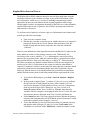
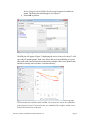
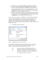
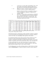
Download Chapter 1 Survival Analysis in Partek® Genomics Suite™ 6.6

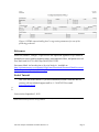
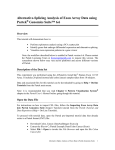
Chapter 1 Survival Analysis in Partek® Genomics
Suite™ 6.6
This tutorial will illustrate how to:
 Compare the survival rates in two groups
 Visualize the Kaplan-Meier survival curves
 Assess the impact of gene expression values on survival probabilities by
Cox regression
Survival analysis is a branch of statistics which deals with modeling of time-toevent. In the context of “survival,” the most common event studied is death
although any other important biological event could be analyzed in a similar
fashion (e.g., spreading of the primary tumor or occurrence/relapse of disease). It is
important to emphasize that the significant event should be well-defined and occur
at a specific time. As the primary outcome event is typically unfavorable (e.g.,
death, metastasis, relapse, etc.), the event is called a “hazard.”
In the other words, survival analysis tries to answer questions such as: What is the
proportion of a population who will survive past a certain time (i.e., what is the 5year survival rate)? What is the rate at which the event occurs? Do particular
characteristics of participants have an impact on survival rates (e.g., are certain
genes associated with survival?? Is the 5-year survival rate improved in patients
treated by a new drug?
An important feature of survival analysis is the presence of “censored” data. For
instance, medical studies often focus on survival of patients after treatment so the
survival times are recorded. At the end of the study period, some patients are still
alive, some have died (and survival data should be available for those), and the fate
of some patients is not known because they dropped out of the study. One possible
reason for drop-out could be that the patient moved to a different geographical area,
but it is also possible that the patient felt so much better that he felt that no further
intervention is needed. Censored data represent the last group (study drop-outs or
unknown status). The information from censored data is valuable because while it
does not measure the actual survival time, it does measure a minimum length of
survival to the time the study ends or the subject drops out of the study. Within the
field of survival analysis, special tests are developed to correctly use both censored
and uncensored observations. The details of the tests implemented in Partek®
Genomics Suite™ (PGS) could be found in the user's manual (available under Help
> User's Manual).
Please note: The following tutorial was written using Partek® Genomics Suite™
version 6.6. As PGS is a rapidly evolving software application, future versions of
PGS may be different from the screenshots displayed in this tutorial. To ensure that
Survival Analysis in Partek® Genomics Suite™ 6.6
Page 1
you are using the most current version of PGS, please visit Help > Check for
Updates.
Tutorial Data Set
This example data set (236 samples) is a subset of fresh-frozen breast tumor
specimens from a population-based cohort of 315 women with breast cancer. The
clinicopathological characteristics accompanying each tumor include p53 status
(mutant or wild-type), estrogen receptor (ER) status, progesterone receptor (PgR)
status, lymph node status, tumor size, and patient age. Gene expression of all the
samples was assessed on Affymetrix® U133A and U133B arrays (Miller LD et al.,
GSE3494). Please note that Affymetrix data have been chosen for the illustration
purposes only, and that the same functionality can be used to analyze data generated
by any vendor.
The raw data files (.CEL) have already been imported into PGS; samples with no
survival time data as well as sample attributes irrelevant for the survival analysis
were removed, and the final spreadsheet was saved in PGS (Survival_Tutorial.fmt
and Survival_Tutorial.txt). The files in a .zip folder are provided on Partek’s
tutorials page (under the Gene Expression tab) and are easily found by selecting
Help > On-line Tutorials in the PGS main menu. To proceed with the exercise,
download the .zip folder to your computer and unzip it.
To open the data file, use File > Open…, browse to the folder containing the
tutorial data set, and select the file Survival_Tutorial.fmt. PGS will open the data
spreadsheet where each row represents one tumor sample. Sample attributes are in
columns 1 – 8, while columns 9+ are gene expression levels (probesets on columns)
(Figure 1).
Figure 1: Viewing the sample data (one sample per row) for survival analysis
Survival Analysis in Partek® Genomics Suite™ 6.6
Page 2
Kaplan-Meier Survival Curves
The Kaplan–Meier (KM) estimator shows the survival from study data when the
incidence of disease is not constant over time. A plot of the KM estimate of the
survival function, a KM curve, is a series of declining horizontal steps which
approaches the true survival function for the original population when a large
enough sample is taken. An important advantage of the KM curve is that it handles
censored data which occur if a patient is lost to follow-up (drops out) before the
final outcome is observed.
To perform survival analysis, at least two pieces of information (one column each)
must be provided for each sample:


Time-to-event: a numeric factor
Whether the event has occurred or not or whether the time was censored: a
categorical factor with two levels. Patients who participate in the full
length of study and who do not experience the event are considered
“censored”
Time-to-event indicates the time elapsed between the enrollment of a subject in the
study and the occurrence of the primary outcome event. Traditionally, the
occurrence of the event is coded as “1” (i.e., indicating the event occurred for a
patient at the given time point), while the censored data (e.g. patient lost to followup or patient still alive at the end of the study) is coded by “0”. Please note that
PGS does not impose any limitation on the labels used for the two categories (do
not have to be 0 and 1); in this tutorial, the events are coded as either death or
censored. If a patient is still alive at the end of the study, then the event time should
indicate the period between enrollment and the study end. If a patient is lost to
follow-up, then the time-to-event should indicate the period between enrollment
and the last known time point at which the patient had not experienced the event.




To invoke the KM analysis, go to Stat > Survival Analysis > KaplanMeier
In the present example (Figure 1), column #1 (Survival (years)) indicates
the survival time of each patient (in years), while column #2 (Event)
specifies the outcome for each patient: death or censored. Consequently,
at the top of the Kaplan-Meier dialog box, set Time Variable to 1.
Survival (years) and the Event Variable to 2. Event. Note that only
variables with two categories are displayed in the Event Variable list, and
only numeric data are displayed in the Time Variable pull-down list
Select death from the Event Status drop-down list to indicate the primary
outcome which automatically tell PGS that the censored outcome is coded
as the other variable (in this example, censored)
To test the difference in survival rates between the p53 mutants (mutant)
and samples with wild-type p53 gene (wt), select 3. p53 status in the
Candidates list and click on the Add Factor > button to transfer it to the
Survival Analysis in Partek® Genomics Suite™ 6.6
Page 3

Strata (Categorical) list (PGS will only accept categorical variables as
strata). The dialog box should appear as in Figure 2
Select OK to proceed
Figure 2: Configuring the Kaplan-Meier dialog
The KM plot will appear (Figure 3) displaying the survival curves for the p53 wildtype and p53 mutant groups. Each curve shows the survival probability at a given
time point with censored outcomes indicated by triangles, and events (death in this
tutorial) occurring wherever there is a downward step.
Figure 3: Kaplan-Meier plot comparing the survival curves between two groups.
The horizontal axis indicates time to death; the vertical axis shows the cumulative
proportion of survival. Censored events are symbolized by triangles; death occurs
at each downward step in the plot
Survival Analysis in Partek® Genomics Suite™ 6.6
Page 4
PGS performs two statistical tests to compare the survival curves: the log-rank test
and the Wilcoxon-Gehan (Breslow’s) test. Both tests work well with censored data.
Low p-values indicate that the groups have significantly different survival times.
See the legend for Figure 5.
In addition to the plot, a new spreadsheet (KM) is created (Figure 4).
Figure 4: Viewing the KM spreadsheet, detailing the results of Kaplan-Meier
survival analysis. Each row represents occurrence of at least one significant event
The spreadsheet is organized into two sections: the analysis of the p53 mutant
group is followed by the p53 wild type group. Each row represents a time point at
which at least one event occurred whereas the columns provide the following pieces
of information:
1:
2:
3:
4:
5:
6:
7:
8:
9:
Identifies the group membership (according to the strata)
Survival time corresponds to the entries in column #1 of the
original (Survival_Tutorial) spreadsheet. At each given time, at
least one event, either death or censored, was recorded
Probability of survival: cumulative probability of survival at a
given time point (also known as KM survival estimate).
(Cumulative probability is the probability of surviving all of the
intervals before this time point.) As time increases, the cumulative
survival probability decreases as events occur
Number of group members at risk (have not experienced the event).
The count in each row is calculated by subtracting the number of
deaths and censored events in the row above from the number at
risk in the row above
Count of deaths at this time in the group
Count of censored events at the given time in the group
Total number of deaths in all groups at the given time
Total number of participants at risk in all groups. The count in each
row is calculated by subtracting the number of deaths and censored
events at the previous time point in both groups from the total
number at risk at the previous time point
Natural logarithm of column #3; also noted as ln(KM)
Survival Analysis in Partek® Genomics Suite™ 6.6
Page 5
10:
Natural logarithm of the negative value of column #9, i.e., ln(–
ln(KM)). A plot of ln(-ln(KM)) vs. ln(t) is often used to test the
proportional hazards assumption. To visualize the risk, select this
column and select View > Log Log S Plot (Figure 5)
Figure 5: Log Log S plot of KM data. As the lines are mostly parallel and do not
cross, the log-rank test assumptions are valid. The Wilcoxon-Gehan test has more
power if the lines had crossed or were not parallel but performs less well when
there is extensive censored data
Cox Regression
The Kaplan-Meier method is useful for comparing survival curves in two or more
groups with a primary exposure variable whereas the Cox regression (Cox
proportional-hazards model) enables assessing the effect of several factors
(predictors) on the outcome. Predictors that lower the probability of survival are
called risk factors; protective factors are predictors that improve the survival
probability. The Cox proportional-hazards model like similar to multiple logistic
regression that considers time-to-event rather than simply whether an event
occurred or not. Cox regression in PGS is accessed from the Stat menu.
Survival Analysis in Partek® Genomics Suite™ 6.6
Page 6


Select the Survival_Tutorial spreadsheet in the spreadsheet navigator
Select Stat > Survival Analysis > Cox Regression. The resulting dialog
(Figure 6) resembles the Kaplan-Meier configuration dialog. Be sure to
specify 1. Survival (years) for Time Variable, 2. Event for Event Variable,
and death for Event Status. PGS will automatically select all the response
variables (in this example: probesets) as Predictor.
Optional Co-predictor(s) are numeric or categorical factors to be included
in the regression model. To evaluate the association between tumor size and
gene expression, select 7. tumor size (mm) in the list of Candidate(s) and
use Add Factor > to move it to the list of Co-predictor(s)

To access the advanced options, select Model... The resulting dialog (not shown)
enables the inclusion of interactions between predictors and co-predictors in the
regression model. The Results… button invokes the dialog through which
additional output (Chi-square values, coefficient, degrees of freedom, model
parameters, etc.) can be included in the output spreadsheet. Neither of these steps is
needed in this tutorial.

Select OK to start the computation
Figure 6: Configuring the Cox regression dialog
The spreadsheet generated by the Cox regression procedure (Cox) is shown in
Figure 7. Each row of the spreadsheet corresponds to one of the predictors
(probesets). The description of the columns is provided below.
1 & 2:
3:
4 & 5:
Column # and Probeset ID. Identify the predictor
HRatio(gene). Hazard ratio of the predictor in column #2
LowCI(gene) and UpCI(gene). The 95% confidence
boundaries of the hazard ratio. LowCI and HighCI are the
lower and upper boundary, respectively.
Survival Analysis in Partek® Genomics Suite™ 6.6
Page 7
6:
7 – 10:
11:
p-value(gene). P-value of the corresponding χ2-test. A low
value in this column indicates that the predictor poses a
large hazard or is associated with shortened survival time
HRatio(co-predictor), LowCI(co-predictor), UpCI(copredictor), p-value(co-predictor). Effects of the copredictor on the survival time; corresponds to columns 3 –
6. For each additional co-predictor, a similar block of
columns is added
modelfit(0). P-value of the test assessing the overall model
fit, i.e.., the relationship between survival time, predictors,
and co-predictors in the model. A modelfit value > 0.05
indicates a poor association between the predictor and/or
co-predictors and the survival time
Figure 7: Viewing the result of the Cox regression procedure. Each row
corresponds to one predictor variable
The hazard ratio Hratio is also known as relative risk and is an effect size measure
used to assess the direction and magnitude of the effect of a predictor variable on
relative risk of the event, controlling for other predictors in the model.
For continuous predictors (such as gene expression values and tumor size), the
hazard ratio is the predicted change in the hazard for a unit increase in the
predictor. A hazard ratio greater than 1.0 indicates that the predictor is associated
with the event (shorter survival time), hazard ratios below 1.0 are associated with
the decreased hazard of the event, and a hazard ration of 1 indicates that the
predictor has no effect on the survival time. Categorical predictors, on the other
hand, should be interpreted relative to the reference category.
For a detailed result on one of the predicting probesets, right-click the row header
and select HTML Report. The report will open in a browser window (Figure 8).
Survival Analysis in Partek® Genomics Suite™ 6.6
Page 8
Figure 8: HTML report detailing the Cox regression parameters for one of the
predicting probesets
References
Miller LD, Smeds J, George J, Vega VB et al. An expression signature for p53 status in
human breast cancer predicts mutation status, transcriptional effects, and patient survival.
Proc Natl Acad Sci U S A 2005 Sep 20;102(38):13550-5
Stevenson, Mark. An Introduction to Survival Analysis. Available at:
http://epicentre.massey.ac.nz/Portals/0/EpiCentre/Downloads/Personnel/MarkStevenson/
Stevenson_survival_analysis_241109.pdf
End of Tutorial
This is the end of the tutorial. If you need additional assistance with this data set,
you may call our technical support staff at +1-314-878-2329 or email
[email protected].
a.
b.
Last revision: September 5, 2012
Copyright  2012 by Partek Incorporated. All Rights Reserved. Reproduction of this material without express written
consent from Partek Incorporated is strictly prohibited.
Survival Analysis in Partek® Genomics Suite™ 6.6
Page 9