1
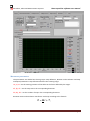
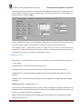
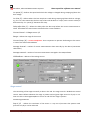
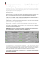
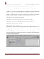
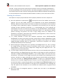
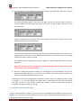
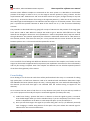
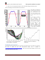
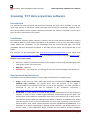
Particulars, Advanced Measurement Systems Data acqusition software user manual Scanning TCT data acqusition software Introduction The software for Data Acquisition with Particulars Scanning TCT gives user a possibility to take and store large amount of waveforms usually associated with scanning TCT technique. Together with a laser control software (and a separate temperature controller if it requires a computer control at all) it gives the user a total control of the system. Installation Data acquisition software (DAQ) is written in Labview and runs under Microsoft Windows. It requires the LabView 2010 Run Time Engine (LV2010RTE) to be installed on the PC. The executable program (called 3DTCT) and LV2010RTE can be downloaded from the Particulars web page. First install LV2010RTE and then decompress the 3DTCT in the folder of your choice. You should be able to run 3DTCT. The software can be downloaded from www.particulars.si/downloads/PSTCT.zip and LVRTE from www.particulars.si/downloads/LV2010RTE.zip or from National Instruments web page (http://ni.com). Notation used in this manual: Italic font – name of commands in the GUI of the program, controls (logically) belonging to the same group can be in the same color Bold font – important Red bold font – very important, not obeying the rules can result in damage to the equipment. Requirements and interfaces The software controls different devices: moving stages, oscilloscope and voltage sources. Stages: usually the setup comes with stages which are controlled over uSMC or XIlab (after 09/2014) stage controller. The original driver from the producer of the stages is recommended to be installed as well (CD is a part of the shipment). The stage controller is connected to the PC via USB as indicated in the installation instructions ( http://www.particulars.si/downloads/ScanTCT_Install.pdf ). Osciloscope: It is very difficult to include all the possible oscilloscopes in the data acquisition software. In order to cover as wide range of different oscilloscopes the generic driver was written which covers different oscilloscopes from LeCroy and Textronix. All of them need to communicate with the DAQ over GPIB interface (GPIB). In addition to GPIB Particulars added (and will continue to do so) more oscilloscopes also from other producers in the future for which NI-VISA is used, which supports different interfaces (GPIB/Ethernet/USB/RS232). If an adaptation to a specific oscilloscope is required please contact us. The default option is a 4 channel 1GHz, 5 GS/s digitization board provided by Paul Scherer Institute, Villingen, Version 1.2, September 2014 Page 1 Particulars, Advanced Measurement Systems Data acqusition software user manual Switzerland (http://www.psi.ch/drs/evaluation-board) which is a low cost substitution to an oscilloscope, but has also some advantages over the ordinary oscilloscopes in terms of acquisition rate and portability. Voltage sources: the data acquisition program controls/perform scans with one or two voltage sources used for biasing detectors/samples. The list of voltage sources built in the software includes most widely used models by Keithley: 228, 237,487,617,2410,6487,6517. As in the case of oscilloscopes please contact us for adaptation to another voltage source. Again the GPIB interface is used for communication with the PC. Structure of the software The software is written in such a way that it should be as easy as possible to operate it. Different functionalities are grouped in the individual tabs: General, Movement Parameters, Voltage Source 1, Voltage Source 2, Stage Control and Oscilloscope (Laser control is foreseen in the 3DTCT but not yet implemented). Apart from the “General“ tab all other tabs are designated to control and setup specific piece of hardware. In “Voltage Source 1” for example one sets the stepping parameters for the bias voltage scan, initializes the source, sets the current compliance parameters etc. The review of the functions of individual tabs will follow. General parameters Description of controls: Init devices – initializes the stage drivers, voltage sources, DRS board (if chosen). Initialization is a requirement to be able to start scanning acquisition. It is usually performed right after the start of the program. Save, Load – saves/loads the set of parameters of the control panels to/from a file. This is very useful as it saves time to setup parameters and prevent small mistakes each time the program starts. For example, the parameters for a certain type of scan can be saved and then reloaded. Save: Yes/No – enables the saving of the taken waveforms to the disk. Usually “no” is chosen only to test if everything works. Byte order – data are stored in the binary form and this parameter controls the byte order in which bytes of a float variable are written (0=decided by the OS, 1=Little Endian,2=Big endian). It is recommended to use option 2 which is also set as default. Oscilloscope – selects the appropriate oscilloscope connected to the computer NI-VISA resource name – selects the oscilloscope’s VISA address Scope GPIB – GPIB address of the oscilloscope (only if GPIB without NI-VISA is used) Record Channels – Select which channels of the oscilloscope you would like to record. This is useful for a multi-channel TCT, where more amplifiers are connected to the same detector. Up to 4 channels can be simultaneously recorded. Version 1.2, September 2014 Page 2 Particulars, Advanced Measurement Systems Data acqusition software user manual Stage Controller – select the stage controller (uSMC is default) Switch off motors – disconnects the power to the motors after the scan is finished. This serves to prolong the lifetime of the motors; e.g. for a scan started on Friday and completed on Saturday it makes no sense to have motors powered for additional day without doing anything. Init motors at start – initializes motors at the start. User – user taking the data Sample name – name of the sample Type of generation – laser used T - temperature Comment – all the additional info that needs to be stored The above information will be stored in the header of the data file. Make sure that you enter all the information before you start DAQ. Information string – message display for the data from the devices. Clears with botton “C” next to it. Config filename – name of the configuration file Data file – name of the data file START - starts the data acquisition STOP DAQ – stops the data acquisition. If pressed the missing data in the file will be replaced with 0, so that the file will still be useable. Waveforms - shows the last taken waveform during data acquisition. x,y,z – current positions of the stages Voltage 1, Voltage 2, Current 1, Current 2 – bias voltage and current for both sources Progress - shows the progress of the acquisition and the estimated time until it is finished. Version 1.2, September 2014 Page 3 Particulars, Advanced Measurement Systems Data acqusition software user manual Movement parameters The parameters are divided into three groups. Step definition, Rotation and translation and Step and Speed parameters. Step definitions defines the scanning range: x0, y0, z0 - are the starting positions of the tables in the frame defined by the stages dx, dy, dz – are the step sizes in the corresponding directions Nx, Ny, Nz – are the number of step in the corresponding directions Rotation matrix and translation transforms each step according to the formula ⃗ , 𝑅⃗ = 𝑴𝑟 + 𝑇 Version 1.2, September 2014 Page 4 Particulars, Advanced Measurement Systems Data acqusition software user manual where R represents the position in the detector frame M rotation matrix and T translation vector. This is useful if coordinate system of the detector is not the same as the one of the stages. The default seting is T=(0,0,0) and M=1. Movement speed and movement step define the speed and step of the stages during the scan. Usually the default settings are recommended. If large areas are scanned some time can be saved by increasing the speed of the movement at the expense of more accurate positioning. Time between steps – determines the time the stages are at rest after the move before the waveforms are taken. Ideally this value can be 0 s, but 0.1 s would be recommended to be certain that stages to be really at rest when the waveforms are taken. Voltage Source 1,2 Bias Source 1 – controls whether the source is connected. If not all the other options are ignored in the program. Voltage Source – selects the device used as bias source Initialize at start – decides whether the device is initialized when Init Devices is pressed. Output bias [V] – set the desired bias voltage. The value will be applied after Apply bias now is pressed Initialize now - initializes device (reconfigures if some configuration settings have been changed manually) Steping control – Voltage source 1,2 The first array of three fields (start bias, stop bias, number of voltages in-between) determines the stepping in certain voltage interval. Several intervals can be defined by using the array. Please read section on running the software for clarification. Mode – determines how the array of voltage steps will be defined (linear, exponential and both options with hysteresis) Version 1.2, September 2014 Page 5 Particulars, Advanced Measurement Systems Data acqusition software user manual Inc.speed [s] – defines the speed with which the voltage is changed during ramping up/down the bias voltage. Inc. bias [V] – defines what is the bias step that is used during ramping up/down the bias voltage; e.g. if it is 5 V that means that the bias step of 20 V will be done in 4 steps, each 5 V with a delay of determined by “Inc. speed [s]” between each step. Delay after bias [s] – defines the delay after the bias step before the current measurement is taken. Some detectors need certain time before the current stabilizes. Current Control – Voltage source 1,2 Range – defines the range of the current Current Comp. [A] – current compliance. That is important to prevent the damage to the sensor in case of the electrical breakdown. Average internal – number of current measurements done internally by the device (sometimes called filter) Average external – number of current measurements averaged in the DAQ software. GPIB address – address of the voltage source Stage control The controlling of the stages manually is done in this tab. The stage control is divided into several sectors. Status defines wheatear the stage is present and on (green light turned on if yes) or not. One can click on the StageX ON/OFF to turn it on and off if the stage is present. Positioning parameters Step X,Y,Z - defines the resolution of the motor i.e. step size 1/8 means that position with precision of 1/8 m can be achieved. Version 1.2, September 2014 Page 6 Particulars, Advanced Measurement Systems Data acqusition software user manual Speed X,Y,Z [mm/s] – defines the speed of rotation. Usually values equal or below 0.78 mm/s are suitable for stage of that range Limit SW – limit switch. At extreme positions the stages have micro switches with break the contact and prevent further rotations of the stepping motors. When the switch breaks the contact the green light turns on the corresponding side. Positioning control There are two ways of moving the tables manually. Either the destination position is entered in Set pos. X,Y,Z or uses the < and > buttons to move for the value of Step move X left and right. reset pos. X - the current position can be reset to become reference position (0 microns) by pressing it. Beware that you lose absolute calibration in this case. Default speed – if selected the value of the speed as it will be used in the scan (see Movement parameters) will override Speed X,Y,Z [mm/s]. Refresh scope – it will perform acquisition of the waveform after the movement of the stages Set as Start – when pushed, the values of current x,y and z positions are written to Movement Parameteres/Step definitions/x0,y0 and z0. Stage move – after setting the destination Set pos.X,Y,Z pushing the button moves the stages to the designated positions, starting with x-axis then y-axis and finally z-axis. Oscilloscope The oscilloscope tab is mostly used when PSI-DRS board is used. When using the classical oscilloscope the data acquisition software only transfers the waveform shown in the oscilloscope to the PC. All the settings regarding trigger, averaging, dynamic range, time scale etc. should be done in the oscilloscope. Only the waveforms to be taken are indicated in the software. In case of DRS is used, which unlike the oscilloscope, has no display all the required settings are done within the DAQ software. Version 1.2, September 2014 Page 7 Particulars, Advanced Measurement Systems Data acqusition software user manual Connected – indicates that DRS board has been identified and that it is connected. Frequency – sets the sampling frequency in GHz (5 GHz=200ps between the time points) Range – range of the ADC converter (0=-0.5 V to 0.5 V, 1=0 V – 1 V) Timeout [s] – if no trigger is received the DRS goes in the timeout and returns the control to the program. The program is irresponsive for that amount of time without triggers arriving. Average – number of averages. The speed of averaging depends on both laser pulse repetition frequency DRS board. The DRS is capable of taking around 300 waveforms per second. Select Channel – select the channels to be acquired. Trigger delay – interval stored to the memory before the arrival of the trigger in ns Trigger level – the only option is edge trigger with threshold given by the level in V Trigger edge – trigger on falling or rising edge. Trigger channel – channel to trigger on DRS has a feature that the time jitter (shift of pulse left and right for individual triggers) can be of the order of up to 1 ns (peak-to-peak) which spoils the measured rise time of the pulses when averaging is used. In order to cope with that the absolute time scale is referenced to the trigger pulse. The trigger signal is very sharp and its edge can determine absolute arrival time (wrt to t=0 at the start of the buffer) for each individual pulse. t0 can be set with CT and trigger threshold by CThr. Time correction can be switched on/off by Time corr. All the settings set in the Oscilloscope tab are used for DAQ during the scans. Run oscilloscope – since the application is a single threading one control to the main program should be returned by the DRS after the acquisition. Therefore when running no other user operation dealing with other parts of the software is possible (tabs disappear). Only when the DRS board has stopped the control of the program is returned to user. Version 1.2, September 2014 Page 8 Particulars, Advanced Measurement Systems Data acqusition software user manual Take WF – during running of the oscilloscope the waveform shown of the display ( Waveforms ) can be recorded/taken to an ascii file (text file). You will be prompted for the filename. In the first line of the file there are data and time. Starting time and time difference between the data points are in the second line. Then the taken waveforms follow in columns, one for each active channel. Running the software This chapter is a step by step introduction how to prepare parameters and run a simple scan. 1.) Once the application is opened press in the top left corner of the window. This start the program. The first step would usually be the initialization of the devices (General/Init Devices). Make sure that the devices you want to initialize have initialization at start switched on (voltage sources, DRS board, stages). If initialization was successful you can setup the scanning and data acquisition parameters. It is recommended that if you frequently do similar/equal scans that you record the parameters to a file (General/Save , General/Load). Two examples of classic TCT measurement (defocused beam on a pad detector without position scanning) and position scan with a single voltage source are included in the distribution ( Parameters_ClassicalTCT.dat, Parameters_ScanningTCT.dat ). Have a look at the files to understand the configuration syntax. 2.) It is always advisable to check that waveform acquisition works Oscilloscope/Run Oscilloscope. For what you are going to record is exactly what is shown in Waveforms. If DRS is used you can also adjust the parameters within the program. These options are disabled (trigger/averaging settings) when an oscilloscope is selected for acquisition. The settings should be done directly on the oscilloscope. 3.) When changing the voltage please use, if possible, the Voltage source 1,2 tabs. To change the voltage during the manual tuning of parameters (focus search, setting up the laser power/duration, ) enter the value in Output bias voltage and press Apply bias now. The voltage source must be initialized first. 4.) To move stages to desired location before the start of the scan and manually check signals at different positions use Stage Control tab. First make sure that stages you want to operate are switched on (Stage Control/StageX ON/OFF). If you initialize stages at the start then they should be on. The position of the stages returned by the software upon initialization can be arbitrary. Therefore it is always advisable to set the reference position before performing any scans. See instruction for “Setting reference position”. If stages are in appropriate position already one can use either Stage Control/<> buttons or put the required position in microns and move the tables. It is generally good idea to have Stage Control/Refresh scope turned on so that the effect of the movement to the signal can be immediately seen. Although the step and speed of the movement can be controlled the default values are general found acceptable. 5.) Once the range of investigated positions is located enter the data in the Movement Parameters tab. Version 1.2, September 2014 Page 9 Particulars, Advanced Measurement Systems Data acqusition software user manual 6.) If you intend to do the voltage scan enter the voltage scan parameters. How does it work? The above setting will make 11 steps from 0 to 100 in step of 10 V if linear mode is chosen. If you would like to continue with steps of 20 V from 120 V to 500 V open a new entry in the array and enter When no voltage scan is required and you would simply want detector at given bias use the following setting (in this case 80 V only) It is important that number of steps is 0 and start level the desired voltage. If you don’t care of voltage settings at all you can also disable voltage sources, but then no current and voltage information will be written to the file. The default setting for applying the bias (Inc. speed, Inc. bias, Delay after bias) are usually adequate. Please pay attention to current compliance setting as too high value can lead to destruction of the sensor in case of the breakdown. 7.) Once the voltage and position stepping has be determined, DRS/oscilloscope set one can proceed with data acquisition. To do than press START. You will be able to monitor the progress and taken waveforms during the scan. The direction of the scan (changing the parameters) is always done in the following order: voltage 1, voltage 2, z, y,x . After the whole scan range is done in x direction the y-direction will change and after it is done z then voltage 2 and finally voltage 1. Beware as the total number of waveforms can quickly become very large. Setting the reference position If only a relative position is relevant you can at any time use Stage Control/Reset to set the current position as a reference ie. 0. All the moves of any of the stages will be done relative to this position. So 100 will mean 100 microns to the right. Version 1.2, September 2014 Page 10 Particulars, Advanced Measurement Systems Data acqusition software user manual However when different samples are measured on the same system it is advisable to use absolute position of the stage. In order to do so, run the stage to extreme position by using < button. Use the steps between 100 - 1000 microns and once the limit switch turns green, change the step to very low value of e.g. 10. Press the button for moving in the opposite position (>). After one or two pushes the limit switch light should disappear. That indicates that the stage is in its extreme position. If the “reset pos” is pressed this position becomes 0. Now all the moves are to +/- few 10 microns absolutely accurate. The procedure is described below. By going left in steps of 100 microns the position of the stage goes from -300 to -400 to -500. When an attempt was made to go to -600 the Limit SW turns on. Step move X was changed to 10 microns and a (sometimes > needs to be pushed twice) step was made in the right direction. The position reported by the software is -493 which means that at ~503 microns is the extreme position. After that the reset pos. X was pressed and the current location of the table becomes position 0 in x. The same should be repeated for all axis. This is useful for focus finding with different detectors mounted. If the samples are of similar size the stages can be moved to approximate focus position (see installation instruction for focus information) and only fine tuning is required. Even if the samples are different one can calculate expected position of the focus from geometry of the mount. Focus finding Focus finding is one of the main tasks that will be performed with the setup. It is essential for taking high quality data. To find focus detectors need to be metalized with metallization dimensions larger than FWHM of the beam (almost always the case) or during Edge-TCT scans with well-defined edge of the detector (in the sense that light is not reflected from the surface serving as support for the detector) . Let us assume that we want to find focus on a strip detector with pitch of 50 m and strip width 10 m. For the purpose of the study all strips are connected together (not always the case) 1.) Crude focus finding : position the laser in x direction so that the signal at given z is minimal. That should happen when you hit the metalized strip. If you are completely out of focus there will be no dependence at all. Move in crude steps the optics (z-axis) and look for it. 2.) Once you see the change in the signal as you move along the x-axis (or y if differently oriented) start changing in smaller step position of the optics. The point where the minimal signal is observed has the correct focal distance. Version 1.2, September 2014 Page 11 Data acqusition software user manual Particulars, Advanced Measurement Systems 3.) Run a scan in very appropriate steps in x and z with fixed voltage to find precise focus. What you should get is illustrated below for the red laser. x-axis The signal as a function of the laser position along the axis perpendicular to the strips with detector place in the focus of the red laser. If the optics is moved in any directions the transitions become less sharp as shown below. The error function is usually fit to the signal in the transition region from which the FWHM of the beam is calculated. FWHM of the beam at different positions of the optics shows a nice Gaussian profile of the beam with FWHM of around 6 m. Error function fit to the charge collection plots at different z coordinates FWHM of the beam at at different z coordinates Reading the measurements The data is stored in the binary form for compactness and speed reasons. The software for reading in the data is based on the root (root.cern.ch) library and is available in http://www.particulars.si/TCTAnalyse/index.html . There you will also find examples of how to read and do some analysis on taken scans. Version 1.2, September 2014 Page 12 Particulars, Advanced Measurement Systems Data acqusition software user manual Warning Please note that the software is in large parts in the development phase so expect some unexpected behavior and treat bugs with patience. We will fix them as soon as we get them. Use it only with Particulars Scanning TCT system.. Version 1.2, September 2014 Page 13