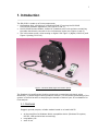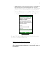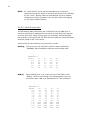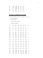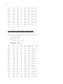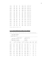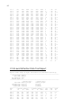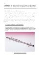
1
GK-604D Inclinometer Readout Application User’s Manual No part of this instruction manual may be reproduced, by any means, without the written consent of Geokon, Inc. The information contained herein is believed to be accurate and reliable. However, Geokon, Inc. assumes no responsibility for errors, omissions or misinterpretation. The information herein is subject to change without notification. Copyright © 2015 by Geokon, Inc. (Doc Rev M, 12/2015) Warranty Statement Geokon, Inc. warrants its products to be free of defects in materials and workmanship, under normal use and service for a period of 13 months from date of purchase. If the unit should malfunction, it must be returned to the factory for evaluation, freight prepaid. Upon examination by Geokon, if the unit is found to be defective, it will be repaired or replaced at no charge. However, the WARRANTY is VOID if the unit shows evidence of having been tampered with or shows evidence of being damaged as a result of excessive corrosion or current, heat, moisture or vibration, improper specification, misapplication, misuse or other operating conditions outside of Geokon's control. Components which wear or which are damaged by misuse are not warranted. This includes fuses and batteries. Geokon manufactures scientific instruments whose misuse is potentially dangerous. The instruments are intended to be installed and used only by qualified personnel. There are no warranties except as stated herein. There are no other warranties, expressed or implied, including but not limited to the implied warranties of merchantability and of fitness for a particular purpose. Geokon, Inc. is not responsible for any damages or losses caused to other equipment, whether direct, indirect, incidental, special or consequential which the purchaser may experience as a result of the installation or use of the product. The buyer's sole remedy for any breach of this agreement by Geokon, Inc. or any breach of any warranty by Geokon, Inc. shall not exceed the purchase price paid by the purchaser to Geokon, Inc. for the unit or units, or equipment directly affected by such breach. Under no circumstances will Geokon reimburse the claimant for loss incurred in removing and/or reinstalling equipment. Every precaution for accuracy has been taken in the preparation of manuals and/or software, however, Geokon, Inc. neither assumes responsibility for any omissions or errors that may appear nor assumes liability for any damages or losses that result from the use of the products in accordance with the information contained in the manual or software. Table of Contents: 1. Introduction .............................................................................................. 1 1.1 Features ...........................................................................................1 1.2 GK-604D Inclinometer Readout Application ...........................................3 1.2.1 Tiltmeter and Compass Probes ...............................................................................5 1.3 Before using the GK-604D Inclinometer Readout ..................................6 2. Installation and Operation......................................................................... 7 2.1 Initial Quick Start Sequence ................................................................7 2.2 Establishing Contact with the Remote Module ..................................... 12 2.3 Installing the GK-604D IRA ............................................................... 15 2.3.1 Launching the GK-604D Installer ........................................................................ 17 2.4 Starting the Inclinometer Readout the first time .................................. 21 3. User Interface ..........................................................................................26 3.1 Overview ........................................................................................ 26 3.2 Project Explorer ............................................................................... 27 3.2.1 Context Menu .............................................................................................................. 28 3.3 Application Menu ............................................................................. 29 3.3.1 Live Readings .............................................................................................................. 29 3.3.2 Edit Settings ................................................................................................................ 36 3.3.3 Terminal Window ....................................................................................................... 36 3.3.4 About GK-604D .......................................................................................................... 38 3.3.5 System Configuration .............................................................................................. 40 3.4 File Menu ........................................................................................ 48 3.4.1 Export Menu ................................................................................................................ 48 3.4.2 Import Menu................................................................................................................ 51 3.4.3 View Data ...................................................................................................................... 54 3.4.4 Delete/Restore Menu ................................................................................................ 57 3.4.5 Exit Tapping on this menu item will cause the program to cease execution. ................................................................................................................................. 58 4. Configuring Project Explorer Elements ..................................................... 59 4.1 Hole Configuration ........................................................................... 60 4.2 Probe Configuration ......................................................................... 61 4.3 Project Configuration ..................................................................... 63 5. Files, Folders and Transferring Data ......................................................... 64 5.1 File Transfer ................................................................................... 65 5.2 Backing up configurations ................................................................ 65 6. Maintenance............................................................................................ 66 .................................................................................................................... 66 APPENDIX A. Inclinometer Theory ............................................................... 68 A.1. Inclinometer Theory ....................................................................... 68 A.2 Conducting the survey .................................................................... 71 A.3 Checksums and “Face Errors” on Inclinometer Probes ......................... 72 A.3.1 Effect of “Face Error” on reading accuracy..................................................... 73 A.3.2 Measurement of “Face Error” .............................................................................. 74 A.3.3 Setting of the “Face Error” to zero .................................................................... 74 A.3.4 Conclusion .................................................................................................................... 75 APPENDIX B. Data File Format ..................................................................... 76 B.1 Hole Data File Format ...................................................................... 76 APPENDIX C. Text Reports ........................................................................... 78 C.1 Raw Data Text Report ...................................................................... 78 C.2 A-axis Profile Data Text Report.......................................................... 79 C.3 B-axis Profile Data Text Report.......................................................... 80 C.4 A-axis Deflection Data Text Report .................................................... 81 C.5 B-axis Deflection Data Text Report .................................................... 82 APPENDIX D. Remote Module Command Structure ......................................84 APPENDIX E. Data Reduction Formulas........................................................86 E.1. Deflection Calculation ...................................................................... 86 E.2. Profile Calculation ........................................................................... 88 E.3. GTILT Users ................................................................................... 89 APPENDIX F. Technical Specifications ....................................................................................................................90 F.1. GK-604D Digital System Specifications .............................................. 90 F1.1 Compass Sensor Specifications ............................................................................. 91 F.2. Analog Probe System Specifications .................................................. 92 F.3. Field PC (FPC-1) Specifications ......................................................... 93 APPENDIX G. Portable Tiltmeter Operation .................................................94 G.1 Single Channel Tiltmeter (Model 6101) .............................................. 94 G.2. Tiltmeter Data Format .................................................................... 99 G.3 Dual Channel Digital Tiltmeter (Model 6101D) ................................... 100 G.4. Dual-Axis Tiltmeter Data Format .................................................... 103 APPENDIX H. Spiral and Compass Probe Operation ................................... 104 H.1 Spiral Indicator Probe (6005-3) ....................................................... 104 H.2 Inclinometer/Compass Probe (6100D-X) .......................................... 107 H.2.1 Calibrate Compass .................................................................................................. 110 H.4 Compass Survey Data ................................................................... 112 Table of Figures: Figure 1 – Model GK-604D, Digital Inclinometer System .......................................................................1 Figure 2 - Model 6000-2 Control Cable (top) ..........................................................................................2 Figure 3 - FPC-1 running GK-604D IRA ....................................................................................................3 Figure 4 - 6000/6100 type probe ............................................................................................................4 Figure 5 - GK-604-4 Interface ..................................................................................................................4 Figure 6 - GK-604-3 Reel System (shown with the Archer unit and carrying case) ................................5 Figure 7 - Probe Settings Mismatch ........................................................................................................9 Figure 8 - Initial Probe Settings ............................................................................................................ 10 Figure 9 - No probe association window ............................................................................................. 10 Figure 10 - ActiveSync Window showing active connection ............................................................... 15 Figure 11 - Windows Mobile Device Center ........................................................................................ 16 Figure 12 - Windows Explorer window displaying HHD root folder .................................................... 17 Figure 13 - Hand-held device root folder contents.............................................................................. 18 Figure 14 - Installation Folder Contents .............................................................................................. 18 Figure 15 - GK-604D Installer at root of HDD....................................................................................... 19 Figure 16 - GK-604D Install Screen....................................................................................................... 20 Figure 17 - GK-604D IRA Icon in Start->Program ................................................................................. 20 Figure 18 - Select Workspace Name .................................................................................................... 21 Figure 19 - Select Workspace Folder ................................................................................................... 22 Figure 20 - Workspace Exists ............................................................................................................... 22 Figure 21 - Select Probe Library Name ................................................................................................ 23 Figure 22 - Select Probe Library Folder ................................................................................................ 24 Figure 23 - Probe Library Exists ............................................................................................................ 24 Figure 24 - Empty Workspace and Probe Library ................................................................................ 25 Figure 25 - User Interface ..................................................................................................................... 26 Figure 26 – Context Menu .................................................................................................................... 28 Figure 27 - Application Menu ............................................................................................................... 29 Figure 28 - Remote Module Connection Problem................................................................................ 30 Figure 29 - Temporary File Data Prompt .............................................................................................. 30 Figure 30 - View Save Data ................................................................................................................... 31 Figure 31 - Load Previous Data ............................................................................................................. 31 Figure 32 - Live Readings Screen .......................................................................................................... 32 Figure 33 - Unsaved Data Prompt ........................................................................................................ 32 Figure 34 - Auto Increment Save .......................................................................................................... 32 Figure 35 - Save File Screen .................................................................................................................. 33 Figure 36- Menu option (Live Readings screen) ................................................................................... 34 Figure 37 - Viewing Inclinometer Data ................................................................................................. 35 Figure 38 - Viewing Compass Data ....................................................................................................... 35 Figure 39 - Terminal Window ............................................................................................................... 36 Figure 40 - About GK-604D IRA ............................................................................................................ 38 Figure 41 - Ready for Connection? ....................................................................................................... 38 Figure 42 - Remote Module/Probe Status............................................................................................ 39 Figure 43 - System Configuration ......................................................................................................... 40 Figure 44 - Stable Indication ................................................................................................................. 41 Figure 45 - Unstable Indication ............................................................................................................ 41 Figure 46 – Auto Record Enabled ......................................................................................................... 43 Figure 47 - Auto Record Active ............................................................................................................. 43 Figure 48 - Auto record paused, Dataset 2 selected ............................................................................ 45 Figure 49 - Male DB-9 housing (female pins) ....................................................................................... 47 Figure 50 - File Menu Figure 51 - Export Menu................................................................................. 48 Figure 52- Export Data Window Figure 53 - Save Data File ............................................................. 49 Figure 54 - Export Path Selection Figure 55 - Probe Selection Window .......................................... 50 Figure 56 - Import Menu Figure 57 - Select Hole Export File ......................... 51 Figure 58 - Select Project Export File Figure 59 - Select Probe Export File ....................................... 52 Figure 60 - Select Probe Library Export File Figure 61 - Probe Library Switch after Import ............. 53 Figure 62 - Select View Options Window Figure 64 - Menu Options for Reports Figure 63 - View Option List .......................................... 54 Figure 65 - Raw Data Report ............................................... 55 Figure 66 - Axis Profile Report Figure 67 - Axis Deflection Report ................................................... 55 Figure 68 - Profile Plot Figure 69 - Profile Plot - Marker On ............................................................ 56 Figure 70 - Deflection Plot ................................................................................................................... 57 Figure 71 - Delete / Restore Window Figure 72 - Hole Delete / Restore Window .......................... 58 Figure 73 - Hole General Settings ........................................................................................................ 60 Figure 74 - Hole Parameters ................................................................................................................ 60 Figure 75 - Probe General Settings ...................................................................................................... 61 Figure 76 - Probe Coefficients .............................................................................................................. 61 Figure 77 - Project Settings .................................................................................................................. 63 Figure 78 - Inclinometer Casing (end view) ......................................................................................... 68 Figure 79 - Inclinometer Probe ............................................................................................................ 69 Figure 80 - Inclinometer Survey Description ....................................................................................... 70 Figure 81 - Plot of Borehole Deflection................................................................................................ 70 Figure 82 - Model 6101 Tiltmeter with 6201-3 Interface Cable .......................................................... 94 Figure 83 - Tiltplates: 6201-1C (ceramic), 6201-1A (Copper plated Aluminum), 6201-1S (stainless) . 95 Figure 84 - Live Readings (Tiltmeter) ................................................................................................... 97 Figure 85 - Saving data query............................................................................................................... 97 Figure 86 - Save File Dialog .................................................................................................................. 98 Figure 87 - File Exists Dialog ................................................................................................................. 98 Figure 88- Model 6101D Digital Tiltmeter .......................................................................................... 100 Figure 89 - Live Readings (Tiltmeter) .................................................................................................. 102 Figure 90 - Spiral Indicator Probe (6005-3) ........................................................................................ 104 Figure 91 - Live Readings for Spiral Data ............................................................................................ 105 Figure 92 - Saving Compass Survey Data ............................................................................................ 106 Figure 93 – Digital Inclinometer/Compass Probe (6100D-X) ............................................................. 107 Figure 94 – Compass Enable Message................................................................................................ 108 Figure 95 - Live Compass Data............................................................................................................ 109 Figure 96 - Initial Calibration Screen .................................................................................................. 110 Figure 97 - Calibration Routine........................................................................................................... 111 1 1. Introduction The GK-604D is made up of three components: the Readout Unit, consisting of a hand-held field PC running the GK-604D Inclinometer Readout Application (see Figures 1 and 3). the GK-604D Remote Module, housed in a weather-proof reel enclosure containing the cable that directly connects to the inclinometer probe (see Figures 1 and 6) The inclinometer probe, either analog or digital. See Figure 1 (digital, 6100D-X) and Figure 4 (analog, 6100-1X). Figure 1 – Model GK-604D, Digital Inclinometer System The Readout Unit and Remote Module components communicate wirelessly using Bluetooth®, a reliable digital communications solution. This simplifies the handling of the system in the field as well as simplifying the transfer of data to your PC workstation for final analysis. 1.1 Features Rugged, general purpose, reliable readout based on a hand-held PC: all the benefits of a Windows Mobile compatible device (Windows file system, RS-232, USB and wireless connectivity) long battery life ease of use 2 Lightweight and simple Remote Module: lithium battery (8 + hours of continuous use) one button operation; automatic power down when Bluetooth connection is dropped or after several minutes of inactivity rugged reliable connection to standard inclinometer probes (Figures 1 and 4) is accomplished via model 6000-2 control cable which features a lightweight, polyurethane jacket and is less than 7 mm in diameter (see Figure 2). The control cable contains a central Kevlar® strand with a breaking strength of 150 kg Figure 2 - Model 6000-2 Control Cable (top) 3 1.2 GK-604D Inclinometer Readout Application The GK-604D Inclinometer Readout Application (GK-604D IRA) installs and runs on a ruggedized hand-held PC (FPC-1) (see Figure 3) and is designed to communicate via Bluetooth with Remote Modules connected to analog or digital probes (see Figure 4), both MEMS and force-balance type. For digital probes the Remote Module is fully contained within the reel as depicted by Figure 1. For analog probes an interface unit, GK-604-4 (see Figure 5), connects directly to the probe (analog MEMS and force-balance type) and can be purchased as a separate unit or as part of the GK-604-3 reel system (see Figure 6). Figure 3 - FPC-1 running GK-604D IRA 4 Figure 4 - 6000/6100 type probe Figure 5 - GK-604-4 Interface 5 Figure 6 - GK-604-3 Reel System (shown with the Archer unit and carrying case) Note: The GK-604D Inclinometer Readout Application will also operate on the Archer Field PC from Juniper Systems (shown in Figure 6) as well as the newer Archer2. 1.2.1 Tiltmeter and Compass Probes In addition to standard inclinometer probes, the GK-604D IRA also can be used with Geokon Tiltmeter and Compass Probes. See Appendices G and H for more information on these probe types. 6 1.3 Before using the GK-604D Inclinometer Readout The readout software runs as an application under Windows Mobile 6 operating system installed on a hand-held PC (FPC-1). The user should familiarize themselves with the FPC-1 and the Windows Mobile OS. It is assumed in the instructions below that the user can launch applications from the Start button including File Explorer and the Bluetooth Settings manager. It is assumed that the user can tap the keyboard icon as needed and use the onscreen keyboard to enter text and numbers. Check out the Maintenance requirements in Section 6 7 2. Installation and Operation The steps described in section 2.1 are an attempt to guide the user through the process of launching the GK-604D IRA, connecting to the probe and taking a survey. If all parts of the GK-604D are purchased as a system, Geokon makes every effort to ensure that the system is completely set up and working before it leaves the factory. Other times, the user may already own the hand-held PC and are setting up their hardware and software for the very first time. The steps below attempt to cover all cases and refer the user to the appropriate section when more information is needed. For those users that have purchased a complete GK-604D system, a workspace with the name of “GK604D” and a probe library called “ProbeLibrary” will have been pre-defined and the FPC-1 unit will already be paired with the Remote Module. Note that the workspace and probe library names can be changed at any time or new ones can be created (see section 3.2.1). When purchasing a GK-604D system, sections 2.2 through 2.4 can possibly be skipped but a quick review is recommended. NOTE: Always make sure that the inclinometer probe is attached to the reel before attempting the quick start sequence below. 2.1 Initial Quick Start Sequence The following steps are a guide to the typical operation of the GK-604D and, if followed, should result in a successful “hole” survey being taken: A) If the Remote Module was purchased separately from the FPC-1 unit or if a new Bluetooth pairing is needed, see section 2.2 (Establishing Contact with the Remote Module). B) Launch the GK-604D IRA by tapping on “Start” from the FPC-1 main window, tap “Programs”, then tap the GK-604D IRA icon. If the GK-604D Inclinometer Readout Application has not been installed, please see section 2.3 (Installing the GK-604D IRA). C) If the window shown in Figure 18 is displayed instead of the Main Window (see Figure 25), please refer to section 2.4, “Starting the Inclinometer Readout the First Time”. D) If the Inclinometer System is an analog system (probe model numbers 6100-1E and 6100-1M) then a “probe” must be defined in the Project Explorer Probe Library (see section 3.2 and 4.2 for more information regarding adding and configuring a new probe). After adding a new analog probe configuration, skip to step F. 8 E) If the Inclinometer System is a digital system (probe model numbers 6100D-E and 6100D-M), any new “probe” will be discovered upon connection to the Remote Module (covered in later steps). F) If launching the GK-604D IRA for the first time, a “project” and a “hole” must be defined before connecting to the Remote Module (see sections 3.2, 4.4 and 4.1 for more information regarding adding and configuring Project Explorer elements). NOTE: If preparing to connect to a digital system the first time, please select “UNKNOWN” for the hole parameter, “Probe Name:”. G) If it’s not selected already, select the new hole (by tapping on the hole icon in the Project Explorer) created in step F. Press the button labeled “POWER ON (BLUETOOTH)” on the Remote Module. A blue light should come on and start to blink, signifying that the Remote Module is waiting to connect to the FPC-1 unit. H) To start the connection process, tap on the Application Menu (see section 3.3) then tap “Live Readings”. By default the application will look for a Bluetooth connection on “COM5”. If the Remote Module fails to connect with the FPC-1, then the window shown in Figure 28 will be displayed, indicating that either the Remote Module is no longer trying to connect (timed out) or that the Bluetooth pairing is associated with another COM port. Make sure that the proper COM port is selected and tap “Reconnect”. If connecting to an analog system, after a few seconds, the blue light on the Remote Module should change to a steady state blue (lit but not flashing) and the Live Readings Window will be displayed (see Figure 29). Skip to step I. If connecting to an digital system, after few seconds, the blue light on the Remote Module should change to a steady state blue (lit but not flashing) and one of two windows will be displayed: a. If the window shown in Figure 7 is displayed, then the probe has not been previously detected by the GK-604D IRA (digital systems only). In this case, tap “ok” and the probe will be added to the Probe Library and the window shown in Figure 8 will be displayed. This allows an opportunity to give the new newly detected probe a user friendly name and description. See section 4.2, Probe Configuration for more information on probe settings. When satisfied with the settings, tap “Menu->Save Settings” to exit the Probe Settings Window (see Figure 8). If the probe name was set to “UNKNOWN” in step F, the window in figure 9 will be displayed, allowing the name of the probe just found to be saved into the current hole configuration. 9 b. The Live Readings Window will be displayed (see Figure 29). This indicates that the GK-604D IRA has recognized the probe as one it has connected to before. Figure 7 - Probe Settings Mismatch 10 Figure 8 - Initial Probe Settings Figure 9 - No probe association window 11 I) Refer to section 3.3.1 for more information about taking a survey using the Live Readings window. Also refer section A.2 for information regarding the mechanical process of taking a survey. J) After performing a survey, any saved data corresponding to a particular hole survey may be reviewed and/or reports generated by tapping the “File” menu then “View Data”. See section 3.4.3 for more information about the View Data option. K) Raw data files may be exported to a file system folder of the user’s choosing by tapping on “File”, then “Export”, then “Data”. See section 3.4.1.1 for more information regarding data export options. L) To close the GK-604D IRA, tap “File” then “Exit”. 12 2.2 Establishing Contact with the Remote Module In general this should only need to be done once and is typically done before it leaves the factory. Follow the steps below to ensure the ‘partnership’ with the remote is established before using the readout software: 1. Use the Bluetooth Settings Manager on the hand-held PC to set up the link to the remote. Read about setting up a Bluetooth “partnership” in Chapter 9 of the Field PC’s Reference Guide. Several ways to start the Bluetooth Manager. 2. Once in the Bluetooth Settings Manager, click on the “Mode” tab and then make sure that the box next to “Turn on Bluetooth” is checked. 3. Click on the “Devices” tab. If it shows a “Geokon” device (name will start with “GK604” and contain the remote’s serial number), go to step 6. Otherwise turn on the remote module (should see a flashing blue indicator on the remote) and select “Add new device…”. 13 4. When a suitable remote is discovered, highlight the device and tap “Next”. 5. A prompt will be displayed for a password; enter “default” and tap “Next” again. If a partnership with the device is successfully established the screen will momentarily display the prompt to the right and then return to the Bluetooth Devices screen. 6. Click on the COM Ports tab. If the “Geokon” device is already assigned to a COM Port, skip to step 9. If no COM port is assigned, select “New Outgoing Port”. In the example to the right there is no COM Port assigned to a “GK604” device. 14 7. The screen-shot to the right shows the devices that a COM Port may be selected for. Select the appropriate “Geokon” device from the list and tap “Next”. 8. From the “Port:” drop-down list, select a COM port (COM5 is the default). Be sure to remember the number of the COM port as you may have to select it later in the readout software (see sections 3.3.1 and 3.3.3, as well as Figure 28). Make sure to “uncheck” the “Secure Connection” check-box. Tap “Finish” when done to return to the Bluetooth Settings “COM Ports” screen. 9. Lastly verify that the Bluetooth device is set for Serial Port operation. From the “Devices” tab of the Bluetooth Settings manager, tap the device to be used to communicate with the remote. The screen to the right will be displayed. Ensure that the “Serial Port” checkbox is checked. Tap “Save” to complete the Bluetooth Settings. 15 2.3 Installing the GK-604D IRA The installation of the GK-604D IRA requires the following: Hand-held device (HHD) running Windows Mobile Classic 6.0 or higher with at least 50 Mbytes of free memory. HHD must be Bluetooth enabled and be able to assign a Bluetooth connection to a COM port. Windows .NET 3.5 Compact Framework (CF) and .NET framework English-language Messages package installed on HHD. Both “CAB” file installers are included in the GK-604D IRA installer “Zip” file, available on Geokon’s web-site (http://www.geokon.com/digital-inclinometer-system/). Microsoft ActiveSync version 4.5.0 or higher running on the host PC (see Figure 10) or Windows Mobile Device Center if PC is running Windows 7 (see Figure 11) as well as the HHD. An active connection between the two must be established either via a physical link or Bluetooth. Figure 10 - ActiveSync Window showing active connection 16 Figure 11 - Windows Mobile Device Center 17 2.3.1 Launching the GK-604D Installer From the Windows Mobile Device Center window on a desktop PC (see Figure 11) click on the folder icon labeled “Browse the contents of your device” to call up an Explorer Window for the HHD (see Figure 12). The procedure for ActiveSync is very similar. Figure 12 - Windows Explorer window displaying HHD root folder In the Figure 11 above, double-click the icon labeled “\” to navigate to the hand-held PC’s system root shown in Figure 13. 18 Figure 13 - Hand-held device root folder contents Next, unzip the GK-604D Installer (downloaded from Geokon’s web-site), open a Windows Explorer window and then navigate to the root folder of the Installation folder (see Figure 14). Figure 14 - Installation Folder Contents 19 Copy the file, “GK604D_Installer.CAB” from the installation folder to the HHD system root folder. From the HDD, navigate to the system root folder using File Explorer (see Figure 15) and tap the file, “GK604D_Installer” to execute the installer. Figure 15 - GK-604D Installer at root of HDD If there is a storage card installed in the HHD then the user will be prompted to choose the location for the installation (see Figure 16). It is recommended that “Device” be selected then tap “Install” with the stylus to initiate the install process. 20 Figure 16 - GK-604D Install Screen The file, GK604D_Installer.CAB can be now deleted from the system root folder to free up memory. The GK-604D IRA is now installed and its icon should appear in “Start->Programs” (see Figure 17). Figure 17 - GK-604D IRA Icon in Start->Program 21 2.4 Starting the Inclinometer Readout the first time The readout software is launched by tapping the Start button and selecting the icon (to the right) from the drop down list or clicking on Programs and then clicking the icon (to the right). If the application fails to launch and the message, “This application requires a newer version of the Microsoft .NET Compact Framework than the version installed on this device”, is displayed then the .NET Compact framework that is included in the installer “Zip” file should be installed. The .NET Compact Framework installer is called “NETCFv35.wm.arm4i.cab” and is located in a folder called “dotNET 3.5 CF” (see Figure 14). Installation is very similar to installing the GK-604D IRA. A companion package for the .NET Framework, “NETCFv35.Messages.EN.wm.cab”, should also be installed at this time and is located in the same folder. When starting the GK-604D Inclinometer Readout Application (GK-604D IRA) for the first time, you will be prompted to create a workspace name. The workspace name can be any combination of letters and numbers and should be descriptive in nature. After creation, this name will be displayed in the Project Explorer window. Figure 18 - Select Workspace Name Once the name for your workspace is selected, you will be prompted to choose or create a folder on your PC where all the workspace elements will be stored. As can be seen below, the default workspace location is in a folder name the same as the workspace name under a special shared folder reserved for workspaces. For Windows Mobile devices, this folder is located at: \Application Data\Geokon\GK-604D\Workspaces. GK-604D IRA appends the name of the new workspace to this shared folder and uses it as the default location for the new workspace. The user is free to select their own location, either by entering it directly, or the Browse [ … ] button may be 22 used to navigate to a different folder location or to create a new folder (see Figure 19). This workspace location will be stored in the GK-604D IRA configuration for subsequent application access. After workspaces are created, all future user access to workspaces is always by name. Figure 19 - Select Workspace Folder Note: If the newly selected workspace folder contains an existing workspace, GK-604D IRA will display a dialog prompt asking the user if they want to import the workspace as is or to rename it with the previously specified new workspace name. Figure 20 - Workspace Exists 23 Much like what was done for the initial workspace, a probe library also needs to be created before the application can fully launch. After specifying the workspace folder, you will be prompted to create a probe library name. The probe library name can be any combination of letters and numbers and should be descriptive in nature. After creation, this name will be displayed in the Project Explorer window. Figure 21 - Select Probe Library Name Once you've selected the name for your probe library, you will be prompted to choose or create a folder on your PC where all the probe library elements will be stored. As can be seen below, the default probe library location is in a folder name the same as the probe library name under a special shared folder reserved for probe libraries. For Windows Mobile devices this folder is located at: \Application Data\Geokon\GK-604D\Probe Libraries GK-604D IRA appends the name of the new probe library to this shared folder and uses it as the default location for the new probe library. The user is free to select their own location, either by entering it directly, or the Browse [ … ] button may be used to navigate to a different folder location or to create a new folder (see Figure 22). This probe library location will be stored in the GK-604D IRA configuration for subsequent application access. After probe libraries are created, all future user access to probe libraries is always by name. 24 Figure 22 - Select Probe Library Folder Note: If the newly selected probe library folder contains an existing probe library, GK-604D IRA will display a dialog prompt asking the user if they want to import the probe library as is or to rename it with the previously specified new workspace name. Figure 23 - Probe Library Exists 25 After the initial workspace and probe library are created the GK-604D IRA will open with the newly created workspace and probe library displayed (see Figure 24). New project(s) and hole configurations may be added to your workspace as well as adding new probes (settings) to the new probe library. Figure 24 - Empty Workspace and Probe Library 26 3. User Interface 3.1 Overview The GK-604D IRA user interface contains a number of navigation controls designed to make job of selecting application elements and functions easier. These navigation controls present an organizational view of the active workspace, inform the user about the state of the application, and provide the user with tools to configure and control Geokon devices. Figure 25 - User Interface The GK-604D IRA User Interface is comprised of several core components: Project Explorer Element selection tool. Context (drop-down) menu. Application Menu Allows display changes, project, hole and probe configuration and connection to the remote module. File Menu File and project explorer element exporting, importing and restoration. Data view/reporting options. 27 Status Area Displays the currently selected hole and probe as well as application status. 3.2 Project Explorer The Project Explorer is the primary navigation mechanism for moving around the GK-604D IRA workspace and probe library. The Project Explorer presents a view of the workspace including projects and holes and a view of the probe library that includes available probes. These views reflect the hierarchical relationship between these elements. The highest element in the workspace hierarchy tree is a project. Projects allow a GK-604D IRA user to group holes into organizational units based on the user's preference. A project can reflect a specific site where holes have been drilled such as a construction project. This organizational feature makes it easy to find hole configurations along with related data files. The list of holes defined under the project can be viewed by selecting a specific project and expanding its branch in the explorer view (click on + sign preceding project name) (see Figure 25). In the hierarchy of the project explorer, holes are child elements of a project. Hole settings can be edited by selecting the desired hole in the explorer tree. Once selected, hole settings can be displayed using “Edit Settings” from the Application Menu (Figure 27) or by using the context menu (Figure 26). Much as a project is a child element of a workspace, a probe is a child element of a probe library. 28 3.2.1 Context Menu From the Project Explorer, new workspace elements can be added using the context menu. Access the drop-down menu by tapping and holding the explorer element that is to be operated on. The context menu is context sensitive in that, based on the current selection, the appropriate elements will be enabled and others will be disabled. Figure 27 below shows the drop-down menu with the menu item, “Add Hole”, enabled (not grayed out) since a “project” element is selected in the Project Explorer. Figure 26 – Context Menu As can be seen from Figure 26, the settings for a project explorer element can also be edited from the context menu. Note that certain explorer elements can be sorted by newest or oldest first. The elements that can be sorted in a project explorer list are: Holes, Projects, and Probes. 29 3.3 Application Menu The GK-604D IRA Application Menu provides access to high level application functionality. It is located in the lower, right corner of the main window frame. The “Edit Settings” menu sub-item of this menu can also be accessed via the context menu. The Application Menu sub-items are further described below: Figure 27 - Application Menu 3.3.1 Live Readings Tapping on this menu item initiates the Remote Module connection process and after a successful connection, the Live Readings screen will be displayed (see Figure 32). Should the connection attempt fail, the window shown in Figure 28 will be displayed with suggestions for correcting any issues before re-trying. Note: When attempting to connect to the Remote Module, please ensure that the “Power On” button on the Remote Module has been pressed (blue light will be blinking) before tapping on the “Live Readings” menu item. 30 Figure 28 - Remote Module Connection Problem After the Remote Module successfully connects to the FPC-1, the blue “POWER ON” indicator will transition from blinking to steadily lit and one of two possible screens will be displayed: 1) Figure 29 shows the message displayed if the GK-604D detects that a previous survey wasn’t saved. Tapping “Yes” displays the temporary data (see Figure 30). Tapping “No” displays the “Load previous data” prompt (see Figure 31) Figure 29 - Temporary File Data Prompt 31 Figure 30 - View Save Data To dismiss the “View saved data” window tap on “ok” which will then display the “Load previous data” prompt (see Figure 31). Tapping “Yes” on the Load previous data” window will load the temporary data into memory and then display “Live Readings” (see Figure 32). Tapping “No” will load “Live Readings” as normal (see Figure 32). Figure 31 - Load Previous Data 32 2) The “Live Readings” screen is displayed (Figure 32). Readings are continuously updated from the Remote Module. The data set always starts with ‘Dataset 1’ but can be switched at any time to ‘Dataset 2’ (usually after rotating the probe 180 degrees). At the start of a survey, the ‘Level’ is set to the “Starting Level” configured for a particular hole. Pressing either of the “Record Data” buttons (with a finger or tap of the stylus) records that set of A and B values and automatically changes the ‘Level’ (on screen) by the amount based on the hole configuration “Interval” value (see section 4.1). The “Record Data” option can also be activated by pressing the “Enter” key on the lower-right side of the keypad. A “beep” sound should be heard, confirming that the reading has been stored. If no beep is heard, tap the “volume” control at the top of the screen and adjust the volume. Be sure to move the probe to the new level and wait for the readings to stabilize before recording the next reading. At any point you can scroll the ‘Level’ using the green up and down arrow buttons on the screen and view data stored and checksums (lower half of the screen). When done taking readings, tap “Menu” (lower-left corner of the screen), followed by “Exit Live Readings”. You will be given the option to save the readings to a file (see Figure 33). o Even if you select No, the readings will be saved to a temporary file and can be restored the next time “Live Readings” is entered. Figure 32 - Live Readings Screen Figure 33 - Unsaved Data Prompt Figure 34 - Auto Increment Save 33 o If Yes is selected, you then will be given the choice of saving with the auto-increment suffix on the standard filename (see Figure 34). Selecting Yes again causes the save operation to be carried out using a filename of the form: [Hole_Name][3 digit AutoIncr_Suffix].GKN o If you select No (to the auto incrementing option) you will be shown the standard File Save As screen and you can modify the file name to anything you choose. Use the stylus to click on the keyboard icon (bottom) and make the changes you desire (see Figure 35). Figure 35 - Save File Screen See section 3.3.5 (System Configuration) for more information about options that affect Live Readings and taking surveys. 3.3.1.1 Live Readings Screen Menu Options Figure 36 shows the available options from the Live Readings “Menu” item when a Digital Inclinometer/Compass probe is detected. These options are described below: 34 Figure 36- Menu option (Live Readings screen) Enable Compass Survey For GK-604D systems with a reel firmware version of V2.7 (or greater) AND a probe firmware version of V2.7 (or greater), capability exists to take a Compass Survey of the selected hole at the same time as the inclinometer survey. This menu item is only shown if a compass probe is detected. See Appendix H for a complete description of the Compass and Spiral Probes. Calibrate Compass Tapping this item causes the Compass Calibration dialog to be displayed where a procedure to calibrate the Digital Inclinometer/Compass probe can be followed. See Appendix H for a complete description of the Compass Calibration procedure. View Compass Data When a compass survey is enabled, this menu item is enabled and allows the compass heading to be displayed in place of inclinometer “A” data. This item toggles between “View Compass Data” and “View Inclinometer Data” depending on that data currently being viewed (see Figures 37 and 38). This menu item is only shown if a compass probe is detected. See Appendix H for a complete description of the Compass and Spiral Probes. 35 View Previous Survey Data Allows viewing (and loading) of previous survey data. When tapped, the user must first select the previous survey file to view. After selecting a file a window very similar to Figure 30 will be displayed. After dismissing this window by tapping “ok” another prompt is displayed similar to Figure 31 is displayed. Tap “Yes” to load the data or “No” to continue with the current survey. Exit Live Readings When tapped, causes the GK-604D to prompt to save survey data, shuts down the Remote Module (reel) then exits the Live Readings screen. Figure 37 - Viewing Inclinometer Data Figure 38 - Viewing Compass Data 36 3.3.2 Edit Settings As with the Context Menu (see section 3.2.1), tapping the “Edit Settings” menu will invoke the Settings Editor for the currently selected Project Explorer element (See the section 4 for more information on settings). 3.3.3 Terminal Window This feature requires an active connection to a Remote Module and will attempt to connect when invoked. If a connection cannot be made, the window shown in Figure 28 will be displayed. If a connection can be made, the window shown in Figure 39 is displayed. Using the “Terminal Window” requires the use of the on-screen keyboard to enter simple one or two character commands to the Remote Module. See Appendix D for more information regarding the Remote Module command structure. After typing in a command, tapping the “Return” (Enter) key will cause the command to be sent to the Remote Module. Figure 36 shows the response to a Firmware Version command (4). Figure 39 - Terminal Window 37 Alternately, tapping the “Send” menu gives the user the ability to send a character to the Remote Module with or without a Carriage Return (CR) appended to the character string (see Figure 39). This is useful when a confirmation character is required (such as for the calibration routine) but no carriage return. 38 3.3.4 About GK-604D This displays an information panel giving copyright information as well as the application version (see Figure 40). Tapping on the “Remote Module Status” button will display another screen asking if a probe is connected to a Remote Module and is the Remote Module ready to connect (blue light blinking) (see Figure 41). Figure 40 - About GK-604D IRA Figure 41 - Ready for Connection? Tapping on the “Yes” button causes the GK-604D IRA to initiate the connection 39 process with the Remote Module. If the connection is successful then the following is displayed (see Figure 42), giving status about the Remote Module Figure 42 - Remote Module/Probe Status Figure 42 depicts the status available for a digital Remote Module and probe. For analog systems, only the Remote Module version and battery voltage is listed. 40 3.3.5 System Configuration This screen allows selecting options that affect how the system works and how a survey is taken (see Figure 43). The sub-sections that follow describe each parameter in detail. Figure 43 - System Configuration 3.3.5.1 Stable Indication Valid choices for this selection include: None On the Live Readings Screen, the only indication of stability will be to monitor the A and B readings (see Figure 32). Visual Only When this stability indication is selected an icon is displayed on the Live Readings Screen, indicating whether the reading is stable or not (see Figures 44 and 45). Visual/Audible When this stability indication is selected, in addition to the icon described above, an audible indication is played indicating readings stability or instability (see Figures 44 and 42, as well as sections 3.3.5.3 and 3.3.5.4). 41 Figure 44 - Stable Indication Figure 45 - Unstable Indication 42 3.3.5.2 Stability Filter If the “Stable Indication” (see section 3.3.5.1) selection is set to something other than “None”, this parameter will be enabled and a drop-down list will facilitate the entry of a number that is used to determine readings stability (a value less than 10 is recommended). When taking live readings, if the difference between two subsequent readings of the A and B channels are less than or equal to the “Stability Filter” then the reading will be deemed stable and, if enabled, the “Stability Indication” icon (see Figures 44 and 45) will be set accordingly. 3.3.5.3 Stable Sound If the “Stable Indication” (see section 3.3.5.1) selection is set to “Visual/Audible”, this parameter will be enabled and a drop-down list will display the choices of “sounds” that the HHD can make when a stable reading is achieved in the “Live Readings” screen (see Figure 44). Tapping on the icon to the right of the “Stable Sound” selection plays a preview of the actual sound heard. 3.3.5.4 Unstable Sound If the “Stable Indication” (see section 3.3.5.1) selection is set to “Visual/Audible”, this parameter will be enabled and a drop-down list will display the choices of “sounds” that the HHD can make when the readings achieved in the “Live Readings” screen are determined to be unstable (see Figure 45). Tapping on the icon to the right of the “Unstable Sound” selection plays a preview of the actual sound heard. 3.3.5.5 Auto Record Data If this selection is set to “Enable”, upon entry into the “Live Readings” screen, the “Auto Record” feature will be enabled (see Figure 46). 43 Figure 46 – Auto Record Enabled To activate the “Auto Record” feature, tap on the “Play” icon to the right of the “A” reading text box. The “Play” icon will be replaced with the “Pause” icon, the red text status message will change to “Auto record mode is active” and, if the readings are stable, the first reading will automatically be recorded (see Figure 47). Figure 47 - Auto Record Active 44 The list of steps below illustrates the proper way to utilize the “Auto Record” feature. For the purpose of this example the following is assumed: the hand-held device is connected via Bluetooth to the Remote Module in System Configuration, the “Stable Indication” parameter is set to “Visual/Audible” the “Auto Record Data” parameter is set to “Enable” (see Figure 40). at the start of an “Auto Record” sequence, the probe should be down the casing at the starting level, in the “A+” orientation. 1. Tapping on the “Live Readings” menu item displays the screen shown in Figure 46). 2. As in the normal operation, readings are continuously updated from the remote. The data set always starts with ‘Dataset 1’ (can be switched at any time to ‘Dataset 2’). At the start, the “Level” is set to the “Starting Level”, previously set in the Hole Settings screen (see section 4.1, Figure 73). 3. Tap on the “Play” icon to activate the “Auto Record” feature. The red status text message will change to “Auto record mode is active” and the green “Play” icon will change to the red “Pause” icon. If the readings are stable, the initial A & B readings will be taken and a “beep” sound should be heard, confirming that the readings have been stored. If no beep is heard, tap the “volume” control at the top of the screen and adjust the volume. 4. By pulling on the inclinometer cable, move the probe to the next level, ensuring that the cable marker/ferrule sits securely in the cable hold. Approximately 1 second after moving the probe, the system will determine that the readings are no longer stable. The stability icon will be set to its unstable state and the “Unstable” sound selected in the “System Configuration” screen (see Figure 43) will be played. Approximately 2 seconds after the cable marker/ferrule is locked in the cable hold, the system will determine that the readings are again stable and respond by setting the stability icon to its stable state and playing the selected “Stable” sound (see Figure 44). Immediately following the stable sound, the current readings are stored, the record “beep” is heard and the level is decremented by the pre-selected interval. 5. Repeat step 4 until all the “A+” readings have been taken. 45 6. Tap the “Dataset 1” icon and observe that the red status text message will change to “Auto record mode is paused” and the “Pause” icon will change to the “Play” icon while “Dataset 1” becomes “Dataset 2” (see Figure 48). Figure 48 - Auto record paused, Dataset 2 selected 7. After rotating the probe 180 degrees, lower it back to the “Starting Level” appropriate for this hole. Repeat step 3. 8. Repeat step 4 until all the “A-” readings have been taken. 9. When done taking readings, tap the “Menu” item (bottom-left corner of the screen), followed by “Exit Live Readings”. You will be given the option to save the readings to a file (see Figure 33). 10. Even if “No” (see Figure 33) is selected, the readings will be saved to a temporary file and can be restored the next time the Live Readings screen is entered. 11. If “Yes” (see Figure 33) is selected, then another dialog box will be displayed giving the choice of saving with the auto-increment suffix on the standard filename (see Figure 34). Selecting “Yes” again causes the save operation to be carried out using a filename of the form: [Hole_Name][3 digit AutoIncr_Suffix].GKN 12. If “No” is selected (to the auto incrementing option) the standard File Save As screen will be shown giving the option of modifying the file name to another name of the user’s choosing. Use the stylus to click on the keyboard icon (bottom) and make the changes desired (see Figure 35). 46 NOTE: An “Auto Record” survey can be paused at any time and restarted as long as the probe is moved to the proper level reflected by the “Level:” display. When an Auto Record survey is paused, the data can still be recorded in the “normal” fashion by tapping on the “Record Data” buttons. 3.3.5.6 Finish Survey with: This parameter deals exclusively with “unfinished” survey data files. A survey is unfinished if readings were not taken at each level from starting up to the zero level. Many surveys may not completely finished because the geometry of the probe will not allow the last reading or two to be taken while the probe is still in the casing. Valid choices for this selection (see Figure 43) include: Nothing The survey will not be filled in and will remain unfinished. “READINGS” will be modified to reflect the actual number taken. : : : #READINGS:5 FLEVEL, A+, 5.0, 45, 4.5, 46, 4.0, 44, 3.5, 46, 3.0, 44, NaN(s) A-, 12, 12, 12, 13, 13, B+, -87, -84, -85, -85, -86, B81 81 82 82 82 Each missing level “row” of the survey will be filled in with “NaN(s)” which is the floating point representation of a nonnumerical value. NaN is an abbreviation for ”Not a Number”. : : : #READINGS:11 FLEVEL, A+, 5.0, 32, 4.5, 33, 4.0, 30, 3.5, 30, 3.0, 29, 2.5, 29, 2.0, 30, 1.5, NaN, 1.0, NaN, 0.5, NaN, 0.0, NaN, A-, 25, 24, 24, 24, 24, 24, 24, NaN, NaN, NaN, NaN, B+, -81, -81, -81, -80, -80, -81, -83, NaN, NaN, NaN, NaN, B82 82 82 81 81 81 81 NaN NaN NaN NaN 47 Blanks Each missing level “row” of the survey will be filled in with blank characters : : : #READINGS:11 FLEVEL, A+, 5.0, 46, 4.5, 46, 4.0, 46, 3.5, 42, 3.0, 50, 2.5, 45, 2.0, , 1.5, , 1.0, , 0.5, , 0.0, , A-, 17, 17, 14, 19, 18, 12, , , , , , B+, -86, -86, -86, -86, -86, -86, , , , , , B80 82 81 80 80 80 3.3.5.7 Remote Record Switch: If this parameter is “Enabled”, an auxiliary switch can be used to record data points without having to tap the “Record Data” buttons on the Nautiz screen. A “remote” “Record Data” event is triggered by shorting pins 7 and 8 of the RS-232, DB-9 connector (see Figure 49) on the Nautiz. Figure 49 - Male DB-9 housing (female pins) 48 3.4 File Menu The file menu is used to import and export Project Explorer element settings along with data export, viewing and report generation. It also is used to fully delete and/or restore previous deleted Project Explorer elements (see Figure 50). Figure 50 - File Menu Figure 51 - Export Menu 3.4.1 Export Menu The Export menu is used to export hole data and Project Explorer element settings to a folder of the user’s choosing (see Figure 51). 3.4.1.1 Export Data Menu The Export Data menu allows exporting of data from the current hole selected either via the Project Explorer or listed in the status area. Figure 52 shows the files available for hole, “Hole1”. A file may be selected by tapping and holding on the file name. When a context menu is displayed, tap on “Select” to select the file for exporting. Multiple files may be selected. Once all the desired files are selected, tap “Export” to display the Save File window (Figure 53) where a new name and folder may be specified for each file. 49 Figure 52- Export Data Window Figure 53 - Save Data File 3.4.1.2 Export Hole Settings Clicking on this menu item displays the “Select Export Path” window (see Figure 54), from which a path to export the hole settings file can be selected. All files within the hole element folder are compressed into a single export file. The naming format for the hole export file is: <Selected Path> + <Hole Name> + “.lvhe” 3.4.1.3 Export Project Settings Clicking on this menu item displays the “Select Export Path” window (see Figure 54), from which a path to export the project settings file can be selected. All files within the project are compressed into a single export file. The naming format for the project export file is: <Selected Path> + <Project Name> + “.lvpe” 3.4.1.4 Export Probe Settings Clicking on this menu item displays the “Select… …Probe” window (see Figure 55), from which a probe can be selected. After selecting a probe, the “Select Export Path” window (see Figure 54) is displayed, from which a path to export the probe settings file can be selected. The naming format for the probe export file is: <Selected Path> + <Probe Name> + “.gkpe” 50 3.4.1.5 Export Probe Library Clicking on this menu item displays the “Select Export Path” window (see Figure 54), from which a path to export the probe library files can be selected. All files and folders within the probe library are compressed into a single export file. The naming format for the probe library export file is: <Selected Path> + <Probe Library Name> + “.gple” Figure 54 - Export Path Selection Figure 55 - Probe Selection Window 51 3.4.2 Import Menu The Import Menu is used to import Project Explorer element settings (see Figure 56) that were previously exported using the Export Menu functions (see Figure 51). 3.4.2.1 Import Hole Settings Clicking on this menu item displays the “Select .LVHE File” window (see Figure 57), from which a hole export file can be selected (see section 3.4.1.2). After selection, a new “Hole” will be created in the currently selected project. This new “Hole” will contain all the settings and any data files that were contained in the hole export file. If a hole with the same name already exists in the currently selected project a message will be displayed and the hole import will be cancelled. Figure 56 - Import Menu Figure 57 - Select Hole Export File 3.4.2.2 Import Project Settings Clicking on this menu item displays the “Select .LVPE File” window (see Figure 58), from which a project export file can be selected (see section 3.4.1.3). After selection, a new “Project” will be created in the current workspace. This new project will contain all the settings and any “holes” that were contained in the project export file. If a project with the same name already exists in the current workspace a message will be displayed and the project import will be cancelled. 52 3.4.2.3 Import Probe Settings Clicking on this menu item displays the “Select .GKPE File” window (see Figure 59), from which a probe export file can be selected (see section 3.4.1.4). After selection, a new “Probe” will be created in the current probe library. This new probe will contain all the settings that were contained in the probe export file. If a probe with the same name already exists in the current probe library a message will be displayed and the probe import will be cancelled. Figure 58 - Select Project Export File Figure 59 - Select Probe Export File 53 3.4.2.4 Import Probe Library Clicking on this menu item displays the “Select .GPLE File” window (see Figure 60), from which a probe library export file can be selected (see section 3.4.1.5). After selection, a message query will be displayed (see Figure 61) asking the user if they would like to make the imported probe library the current one. Answering “Yes” to the query will replace the current probe library with the imported probe library. Answering “No” will simply add the new probe library to the list of probe libraries that the GK604D IRA keeps track of. The new probe library can be “switched” to at a later date. Figure 60 - Select Probe Library Export File Figure 61 - Probe Library Switch after Import 54 3.4.3 View Data When the View Data Menu is clicked the screen displayed in Figure 62 is shown. The Select View Options screen is used to select a view option (see Figure 63) and data files to view a graphical or tabular report. Figure 62 - Select View Options Window Figure 63 - View Option List The available “View” options are: 3.4.3.1 Raw Data File as Table This selection will cause the selected “hole” raw data to be displayed or saved in tabular form. Figure 64 shows the available options for any report. Figure 65 illustrates the report as viewed on the FPC-1 unit. See Appendix C for examples of reports saved in text form. Tabular reports may also be saved in comma-separated value (.csv) or “Text” (.txt) format. 3.4.3.2 Axis Profile Data as Table Selecting this option allows viewing or saving hole profile data for the A or B axis. The profile is calculated from the magnitude of the readings at each level (see Figure 66). This report lists the profile of the casing as calculated from the bottom of the casing upward or from the top down (see the Options pane in Figure 64). See Appendix C for an example of a profile report saved in text form. Tabular reports may also be saved in commaseparated value (.csv) or “Text” (.txt) format. 55 Figure 64 - Menu Options for Reports Figure 66 - Axis Profile Report Figure 65 - Raw Data Report Figure 67 - Axis Deflection Report 3.4.3.3 Axis Deflection Data as Table Selecting this option allows viewing or saving hole deflection data for the A or B axis. Deflection is determined from the accumulated change in 56 deflection between the two selected data files at each level. This report lists the deflection of the casing as accumulated from the bottom of the casing upward or from the top down (see Figure 67). See Appendix C for an example of a deflection report saved in text form. Tabular reports may be saved in comma-separated value (.csv) or “Text” (.txt) format. 3.4.3.4 Axis Profile Data as Graph Selecting this option allows a graphical view of hole profile data and is useful for visualizing the actual installed characteristics (inclination, couplings, anomalies, etc.) of the casing. Figure 68 show a typical profile plot. Tapping on the icon in the upper-left corner of the plot (a circle with a vertical line) enables a “marker” line on the plot. Moving the marker line by tapping and dragging shows corresponding X and Y values below the plot (see Figure 69). “Screen-shots” of graphical reports may be saved in “.bmp” format”. Figure 68 - Profile Plot Figure 69 - Profile Plot - Marker On 3.4.3.5 Axis Deflection Data as Graph Selecting this option allows a graphical view of hole deflection data for either axis and is useful for visualizing magnitude and direction of any movement of the borehole (see Figure 70). “Screen-shots” of graphical reports may be saved in “.bmp” format”. 57 Figure 70 - Deflection Plot 3.4.4 Delete/Restore Menu This menu Project Explorer elements to be permanently deleted or restored back to their original location. A special folder is reserved for storing project explorer elements that are deleted from a workspace. Data files from the currently selected hole can also be deleted. Tapping the Delete/Restore menu causes the GK-604D IRA to search this folder to see which elements are available for restoring or permanent deletion. As can be seen in Figure 71, in the example below there are holes, projects, probes and probe libraries that are stored in the special folder that can be either restored or permanently deleted. Figure 72 shows the window that is created when the “Holes” button is tapped in Figure 71. In each element delete/restore window, an element may be selected by tapping and holding on the element name. When a context menu is displayed, tap on “Select” to select the file for deleting or restoring. Multiple files may be selected. Once all the desired files are selected, tap either “Delete” or “Restore” from the “Menu” options. WARNING: Selecting “Delete” will permanently delete the selected element and later restoration will NOT be possible. 58 Figure 71 - Delete / Restore Window Figure 72 - Hole Delete / Restore Window 3.4.5 Exit Tapping on this menu item will cause the program to cease execution. 59 4. Configuring Project Explorer Elements Each project explorer element has settings that can be configured. For some, like Workspace, Probe Library and Project the settings consist only of a name and description. Elements such as Holes and Probes require more configuration parameters such as English/metric units, initial level, and gage factors. These settings can be adjusted to meet the user’s needs and the specifications of the probe. The software currently supports 3 different probe types and as many probe and hole configurations as the Field PC can store in memory. All these can be adjusted using the Edit Settings option from the Context or Application Menu. 60 4.1 Hole Configuration Figure 73 depicts the Hole General Settings, the first screen of the Edit Hole Settings dialog: - Hole ID Read-only value, generated when the hole was created. Used internally by the GK-604D IRA. - Hole name Tap on the keyboard icon (bottom of the screen) to bring up the on-screen keyboard. Use it to enter a unique and descriptive hole name. - Description Optional parameter. Using the on-screen keyboard, enter a brief description pertaining to the hole’s location and purpose. - Probe Name Select the Probe Name from the drop down list. This associates a hole with a particular probe. Enter “UNKNOWN” if the probe has not yet been “found”. Figure 73 - Hole General Settings - Hole Units The units for the hole level and interval. Select either meters or feet from the drop-down list. - Created On Read-only date and time value, generated when the hole was created. - Starting Level Using the on-screen keyboard, enter a value for the initial level of the survey for this hole (see Figure 74). - Interval Enter an interval to be used for the survey. This value is dependent on Hole Units and is typically .5 meters or 2 feet. - Top Elevation This optional parameter corresponds to the elevation at the top of the hole. - Azimuth Angle This optional parameter allows correction of any casing deviation from the appropriate A+ direction. Figure 74 - Hole Parameters 61 When done editing, the settings can be saved via the “Menu->Save Settings” option. 4.2 Probe Configuration Figure 75 depicts the General Probe Settings, the first screen of the Edit Probe Settings dialog: - Probe ID Read-only value, generated when the probe was created. Used internally by the GK-604D IRA. - Serial number Read-only parameter for digital inclinometer probes, read/write parameter for analog and compass probes. - Probe name Use the on-screen keyboard to enter a friendly name for the probe - Description Optional parameter. Enter a brief description pertaining to the probe - Probe type Select a probe type from drop-down list. Choices are: Analog, Digital, Compass and Tiltmeter. Compass mode selects the Geokon 6005-3 Spiral Indicator Probe which requires the GK-604-3 Analog Reel System or the GK-604-4 Interface Module. In this mode, the GK-604D IRA will rescale the output to properly display 0-360 degrees on the Live Readings screen. In Compass and Tiltmeter mode, only one channel (A) is read and displayed on the Live Readings screen and only the A readings are stored in the data file. - Date created Read-only date and time value, generated when the probe was created. - Last edited Read-only data and time value, updated whenever the probe settings are modified. Figure 75 - Probe General Settings Figure 76 - Probe Coefficients 62 - A and B Channel Zero Shift To compensate for any offset at zero enter appropriate values for the Zero Shift values (see the Inclinometer Probe manual and Calibration sheet for more information). Digital probes may have these values programmed at the factory. When the probe type is set to Compass, the Zero Shift A value should be set to 200 (see Figure 76). See Appendix H for more information regarding Spiral Indicator Probe operation. - A and B Channel Gage Factors Using the on-screen keyboard, enter appropriate numbers for the 2 gage factors (see the Inclinometer Probe manual and Calibration sheet for more information). Digital probes may have these values programmed at the factory. When the probe type is set to Compass, the Gage Factor A value should be set to 0.1 (see Figure 76). See Appendix H for more information regarding Spiral Indicator Probe operation. - A and B Channel Gage Offsets These values are typically “0” and are occasionally needed to remove an offset from a Compass probe. Offsets are entered in engineering units using the onscreen keyboard (see Figure 76). For a Compass probe there will be no “B” channel and the B Channel value should be left at “0”. Digital probes may have these values programmed at the factory. When the probe type is set to Compass, the offset can be determined by taking readings (using the Live Readings screen) and determining if the compass value is ever greater than 360. If so then the Gage Offset A value should be set to 360 – (current reading > 360). For example, if the current compass probe reading is 365 then the Gage Offset A value = (360 – 365) = -5. See Appendix H for more information regarding Spiral Indicator Probe operation. If the probe “Type” is set to Tiltmeter, the “B Channel” parameters are not used and can be left at 0. When done editing, the settings can be saved via the “Menu->Save Settings” option. If connected to a digital Remote Module and digital probe, Zero Shift, Gage Factor and Gage Offset changes can be uploaded to the probe via the “Menu->Save and Upload Settings” option. After tapping “Save and Upload Settings”, the reminder window shown in Figure 41 will be displayed to ensure that the Remote Module is ready to connect. 63 4.3 Project Configuration Figure 77 depicts the Projects Settings dialog: - Project ID Read-only value, generated upon project creation. Used internally by the GK-604D IRA. - Project Name Use the on-screen keyboard to enter a unique and descriptive project name. - Description Optional parameter. Use the on-screen keyboard to enter a brief description pertaining to the project. - Created On Read-only date and time value, generated when the project was created. Figure 77 - Project Settings When done editing, project settings are saved via “Menu->Save Settings” options. 64 5. Files, Folders and Transferring Data The GK-604D IRA uses several types of files and dedicated folder locations to keep track of Workspaces and Project Explorer element configuration files, such as hole and probe configuration files and data files. The default locations and names for most of these appear in Table 1: Purpose Default Folder Filename GK-604D IRA preferences and configuration \Application Data\Geokon\GK-604D\ Config.xml Workspace repository \Application Data\Geokon\GK604D\Workspaces\ N/A Probe Library repository \Application Data\Geokon\GK604D\Probe Libraries\ N/A Project repository (Workspace) \Application Data\Geokon\GK604D\Workspaces\<WRK_SPC_FLDR>\1 .wkspc Hole repository (Project) \Application Data\Geokon\GK-604D\ Workspaces\<WRK_SPC_FLDR>\ <PROJECT ID>\ .proj Hole configuration \Application Data\Geokon\GK-604D\ Workspaces\<WRK_SPC_FLDR>\ <PROJECT ID>\<Hole ID>\ .hole Data Files (per Hole) \Application Data\Geokon\GK-604D\ Workspaces\<WRK_SPC_FLDR>\ <PROJECT ID>\<Hole ID>\data\ *.gkn Probe repository (Probe Library) \Application Data\Geokon\GK604D\Probe Libraries\ <PRB_LIB_FLDR>\2 .prblib Probe configuration \Application Data\Geokon\GK604D\Probe Libraries\ <PRB_LIB_FLDR>\<Probe ID>\ .probe Table 1 – Folder paths and File Names 1. <WRK_SPC_FLDR> is usually the same as the workspace name but is not required to be. 2. <PRB_LIB_FLDR> is usually the same as the probe library name but is not required to be. NOTE: Manual editing any of the configuration files or renaming folders above may result in data loss or unexplained operation and is strongly discouraged! 65 5.1 File Transfer In general, the only files generated by the GK-604D IRA that will have to be transferred are the “hole” data files, although periodically archiving others on a “master” PC is recommended. Connecting the Field PC to a desktop or laptop PC using the supplied USB cable (Type A to mini B) is straight forward and allows the user to view the Field PC’s storage as a flash drive on the desktop/laptop; you can then simply drag the files around to any folder on the desktop/laptop. If you are using Windows XP you will need to download and install the program, “ActiveSync”. This application is available for free from the Microsoft site (www.microsoft.com and search for “Active Sync download”). Once installed (generally requires a reboot), simply connect the USB cable from the Field PC and then open “My Computer” on the XP machine and see a “PDA” entry under drives. Just double click on it to see the folders in the Field PC. If you are using Windows Vista or Windows 7, a free application called “Windows Mobile Device Center” is available on Microsoft’s website. Once installed, a hardware connection between the Field PC and the desktop/laptop typically initiates the software connection. It is not necessary to set up any ‘syncing’ options although it can easily be accomplished. Another Bluetooth partnership can also be set up from your desktop/laptop (assuming they have Bluetooth modules) to the Field PC and transfer files that way. All of these options (and more) are described in the reference guide of the FPC-1 Field PC, available in the Inclinometer section of the Geokon manuals webpage: http://www.geokon.com/manuals/ 5.2 Backing up configurations To guard against accidental data loss and as a matter of good computer technique, critical data and configuration files should be periodically backed up. Entire projects can be backed up using the Project Export function from the File menu. After exporting, the resulting “.lvpe” file should be transferred to a desktop PC using the techniques described in section 5.1 Probe Libraries can be backed up using the Probe Library Export function from the File menu. After exporting, the resulting “.gple” file should be transferred to a desktop PC using the techniques described in section 5.1 Although backing up a project automatically includes any data files stored as part of the project element “hole” structure, data files can be individually backed up per hole using the Data Export function from the File menu. After exporting, the resulting “.gkn” file should be transferred to a desktop PC using the techniques described in section 5.1 66 6. Maintenance The inclinometer probe is a totally sealed unit and, as such, field adjustments are not required. 6.1 Maintenance of the ‘O’ ring on the connector requires that it be kept clean and free of cuts and knicks. Periodic greasing with ‘O’ lube is recommended. A worn or damaged ‘O’ ring should be replaced with a new one (five ‘O’ rings are supplied with each new probe). 6.2 Wheel assemblies should be kept dry when in storage. They should be kept free of dirt by using a compressed air gun to blow away grit. After every survey spray the springs, pivots and axles with light oil. This is very important and should not be neglected. Geokon recommends lubricating the wheel bearings after each use as shown below. This practice forces out any water or contaminates that may be present thus extending the service life. ADH-106 Belray Waterproof Grease Type 99540 Grease wheels through the grease port in the wheel hub after each use. 67 6.3 One of the main problems encountered is failure to keep the connectors dry. Often this is caused by failure to fully tighten the cable connector to the probe connector. This connection must be made up tight in order to compress the O-ring in the end of the probe connector. Periodically the pins of the probe connector must be sprayed with DEOXIT #DN5 spray contact cleaner and rejuvenator. A small spray can of this is supplied with each inclinometer probe. After each daily use always make sure that the connectors are completely dry before replacing the protective caps. Otherwise corrosion could result. 6.4 If the zero offset changes due to aging or rough handling this will not affect the quality or accuracy of the readings because the offset is removed by taking two sets of readings in the A and A directions. However, if the zero offset changes by more than 5000 digits then the probe should be returned to the factory for repairs. Zero offset can be set to zero at any time using the software inside the GK-604 readout instrument (see Page 62 of the GK-604D Manual). 6.5 It is good practice to have a piece of inclinometer casing permanently fastened to a fixed immovable structure in the laboratory. This casing is used as a periodic check on the calibration of the probe. Placing the probe in the casing should give a reading that does not change with time. 6.6 Remember, from time to time, to backup and remove the survey data from the Handheld. Failure to do this can cause the physical memory to run out and corrupt the system. 68 APPENDIX A. Inclinometer Theory A.1. Inclinometer Theory In the geotechnical field inclinometers are used primarily to measure ground movements such as might occur in unstable slopes (landslides) or in the lateral movement of ground around on-going excavations. They are also used to monitor the stability of embankments, slurry walls, the disposition and deviation of driven piles or drilled boreholes and the settlement of ground in fills, embankments, and beneath storage tanks. A+ (reference direction) In all these situations it is normal to either install a casing in a borehole drilled in the ground, to cast it inside a concrete structure, to bury it beneath an embankment, or the like. The inclinometer casing has four orthogonal grooves (Figure 78) designed to fit BB+ the wheels of a portable inclinometer probe (Figure 79). This probe, suspended on the end of a cable connected to a readout device, is used to survey the inclination of the casing with respect to vertical (or horizontal) and in this way to detect any changes in inclination Acaused by ground movements. Figure 78 - Inclinometer Casing (end view) The probe itself contains two MEMS, (Micro Electro-Mechanical Sensor), accelerometers, which flex when acted on by the force of gravity. Since the output voltage is proportional to the sine of the angle of inclination, the output is also proportional to horizontal deviation of the borehole (or the vertical deviation of a horizontal borehole). In order to obtain a complete survey of the ground around the installed inclinometer casing it is necessary to take a series of tilt measurements along the casing. Typically an inclinometer probe has 2 sets of wheels separated by a distance of 2 feet (English system) or .5 meter (Metric system). A casing survey would begin by lowering the probe to the bottom of the casing and taking a reading. The probe would then be raised at 2 foot (English system) or .5 meter (Metric system) intervals and a reading taken at each interval until the top of the casing is reached. The set of readings thus generated is called the A readings. Marks on the cable at 2 foot (English) or .5 meter (Metric) spacing facilitate the process. The probe is then removed from the casing, rotated through 180, replaced in the casing, lowered to the bottom of the borehole and a second set of readings (the A set) obtained as the probe is raised at the reading interval. 69 Cable Cable Fitting A+ Wheel Assembly A- Accelerometer Housing Wheel Assembly Bottom Cushion Figure 79 - Inclinometer Probe Inclinometer probes usually contain two accelerometers with their axes oriented at 90 to each other. The A axis is in line with the wheels (Figure 79 illustrates) with the B axis orthogonal to it. Thus, during the survey, as the A, A readings are obtained, the B, B readings are also recorded. During the data reduction these two sets of readings (A, A and B, B) are combined (by subtracting one set of readings from the other) in such a way that the effect of any zero offset of the force balance accelerometer is eliminated. [This zero offset is the reading obtained from the inclinometer probe when it hangs vertical. Ideally the offset (or bias) would be zero, but usually there is a zero offset which can change during the life of the probe due to drift of the transducer, wear and damage of the wheels or most likely due to a sudden shock to the transducer caused by dropping or allowing it to hit too hard against the bottom of an installed inclinometer casing.] Subsequent surveys of the inclinometer casing, when compared with the original survey, will reveal any changes of inclination of the casing and locations at which these changes are taking place. Analysis of the change of inclination is best performed by computing the horizontal offset of the upper wheels relative to the lower wheels which has produced the tilting () over the reading interval (L) of the survey (usually the wheel base of the probe, 2 feet for English systems, .5 meter for Metric). At each position of the inclinometer the two readings taken on each axis (A , A and B, B) are subtracted from each other leaving a measure of sine. This value is then multiplied by the reading interval (L) and the appropriate factor to output horizontal deflection in engineering units (inches for English, centimeters or millimeters for Metric) (see Figure 80). 70 GK-603 Readout L sin Electrical Cable Inclinometer Casing Casing Alignment (exaggerated) L s in Probe Borehole Reading Interval L True Vertical Coupling Backfill Probe Guide Wheels Bottom Cap Figure 80 - Inclinometer Survey Description When all these incremental horizontal deflections are accumulated and plotted beginning at the bottom of the borehole the net result is to produce a plot of the change in horizontal deflection between the time of the initial survey and the time of any subsequent survey (see Figure 81). From such a deflection plot it is easy to see at which depth the movement is occurring and its magnitude. Deflection Change - + Borehole Top Zone of Movement Borehole Bottom Figure 81 - Plot of Borehole Deflection Other methods of analysis can be used but generally add little to the overall understanding of the situation. For example, using a single set of data, a profile of the borehole can be created. Also, a plot can be made of the actual change in reading (inclination) at each measurement depth increment. A plot of this nature reveals the depths at which movement is occurring. But this information can be obtained from the change in deflection curve with little difficulty. 71 One other analysis is the Check Sum (or Instrument Check) which can be used to measure the quality of the survey data. The quality of the data can be impaired by any or all of the following; Skipping over or duplicating a reading. Not allowing the inclinometer sufficient time to come to rest before taking a reading. Not allowing sufficient time to allow the probe to reach temperature equilibrium before commencing the survey. Malfunction of the probe, cable or readout device. This may be the result of shock, moisture, low battery conditions, opens or shorts in the cable or probe, etc. Carelessness in positioning the wheels so that the probe wheels do not rest on the same part of the casing from one survey to the next. Positioning the wheels so that they fall right on top of a casing joint so that the reading is unstable or simply erroneous. The Check Sum analysis is performed by adding the A+, A- readings and the B+, Breadings. When this is done the part of the reading due to the tilt is eliminated leaving only a value which is equivalent to twice the zero offset of the inclinometer transducer. A.2 Conducting the survey The following is a synopsis of the steps involved in taking a survey (see section 3.3.1 for more details): 1) Attach the cable to the probe making sure that the connector is clean and the Oring undamaged. Tighten the connector to ensure that the O-ring is compressed and watertight. 2) Twist the probe so that the uppermost wheel fits into the casing groove that faces the direction of the anticipated movement, (In the case of a slope this would be downhill, or, in the case of a foundation wall in the direction of the opening. This guarantees that the measured deflections will be positive. Lower the inclinometer probe to the bottom of the casing. To avoid damage to the probe be careful not to let the probe strike hard against the bottom of the hole. 3) Select the size of cable hold that matches the inclinometer casing and place it inside the top of the casing. Lift the inclinometer until the first cable marker sits in the cable hold. 4) Switch on the FPC-1, turn on the Remote Module (blue light blinking) then launch the GK-604D IRA. After verifying that the hand-held unit has connected to the probe, click on the “Live Readings” menu and observe the inclinometer reading. Wait until the probe temperature has stabilized and the reading doesn’t change. 72 5) Make sure that the GK-604D IRA is set to Data Set 1.Take the first reading, pull up on the cable until the next cable marker sits in the cable hold and, after a short pause, take another reading. 6) Continue in this way until the top marker is reached, then remove the cable hold and pull the inclinometer out of the hole. 7) Twist the probe through 180 degrees then lower it to the bottom of the hole. Tap the “Dataset 1” button to select data set 2. 8) Repeat steps 3 to 6. 9) Tap on “Menu->Exit Live Readings” to save the data. A.3 Checksums and “Face Errors” on Inclinometer Probes Many users have expressed concern about checksums or “face errors” on inclinometer probes. They are concerned with the effect of the “face error” on the accuracy of the readings. The purpose of this section is to show that under normal circumstances the effect of the “face error” or checksum is negligible even with checksums as large as 2000. The only time a problem would arise is if the face error or checksum was to change between the two halves of a survey. This is why it is extremely important to not bang the probe on the bottom of the borehole between survey halves, and to not handle the probe roughly while out of the hole. The term “face error” comes from surveying terminology. It is normal for all theodolites to have a “face error” which is caused by imperfections of alignment of the collimation axis and other misalignments. These “face errors” are removed routinely by taking two readings of the theodolite: one angle is measured with the face of the vertical scale on the left of the theodolite and another with the face of the vertical scale on the right of the theodolite. The average of the two readings “face right” and “face left” gives the true angle since the “face error” cancels out. Similarly with the inclinometer probe: the “face error” arises from the fact that the axis of the inclinometer probe is not parallel with the electrical axis of the internal, force-balance, servo- accelerometer transducer. Once again the “face error” is eliminated by taking two surveys of inclinometer readings one with the wheels of the inclinometer probe pointing in one direction and another with the wheels of the probe at 180 to the first direction. If the first set of readings are all too large by the amount of the “face error” then the second set of readings will be too small by the amount of the “face error” and the average or sum of the two readings will be a measure of the true inclination since the effect of the face error will be totally eliminated. 73 A.3.1 Effect of “Face Error” on reading accuracy The “face error” or check-sum can only affect the accuracy of the readings if it affects the calibration of the probe. This is possible because the output of the probe transducer is proportional to the sine of the inclination from the vertical and the sine function is non-linear. Imagine, for a moment, that the electrical axis of the transducer is five degrees away from being parallel with the axis of the inclinometer. This would give rise to a “face error” of 01743. (The inclinometer reader displays 20,000 sin ). So, one set of readings would be all too large by this amount and the other set of readings from a normal inclinometer survey would be too small by this amount, but the sum of the two readings would be accurate. The “face errors” having canceled out. However, if we assume that the hole is almost vertical then the transducer will be tilted at an angle of 5 . The difference in the slope of the sine function at any point is equal to the cosine of the angle at that point. The cosine of 0 is 1.0000 the cosine of 5 is 0.996 so that the effect of this “face error” on the calibration of the probe is to increase it by a factor of 1/0.996 = 1.004. The practical implication of this would mean that if the apparent deflection of a borehole was 100 mm, the true deflection would be 100.4 mm. For practically all applications, in the real world, the difference is insignificant and is a lot less than the differences which normally occur from survey to survey i.e. a lot less than the precision of the inclinometer probe survey. (Lack of precision is caused by a failure to position the wheels of the probe in exactly the same place from survey to survey; failure to wait sufficiently long to allow the probe transducer to come to rest before reading; and random dirt in the inclinometer casing). Note that the normal system accuracy of an inclinometer probe is 7 mm in 30 meters. By comparison it can be seen that the normal system accuracy or precision is very much larger than the calibration error caused by the “face error” and that for all practical purposes the “face error” is of no consequence and can be completely discounted if it is less than 2000 digits. (As another example, supposing the check-sum was as large as 5000 digits. This is equivalent to a gross angular error of misalignment of almost 15 degrees. The effect on the calibration would be a little over 3 % so that the apparent deflection of 100 mm would be out by 3 mm which again is smaller than the normal data spread due to imprecision). 74 A.3.2 Measurement of “Face Error” The “face error” is the reading shown by the inclinometer probe when it is perfectly vertical. In practice, the easiest way to obtain the “face error” is to run a normal inclinometer survey, with the two sets of readings at 180, and then to run a profile or deflection report (see section C.2 and C.3, the column labeled “Diff”). Examination of the data will reveal the average checksum which is equal to twice the “face error.” A.3.3 Setting of the “Face Error” to zero There are three ways of setting the “face error” to zero. None of them are necessary from the point of view of improving accuracy. A.3.3.1 Mechanically At the time of manufacture the electrical axis of the transducer is adjusted by means of shims etc., until it points parallel to the axis of the inclinometer probe. This method suffers from the disadvantage that if the ”face error” changes due to wear and tear on the probe and rough handling, or shock loading of the transducer then the probe needs to be returned to the factory for dismantling and re-adjustment. A.3.3.2 Electrically Electronic circuitry can be included in the probe so that the output of the transducer can be adjusted to zero when the probe is vertical. The disadvantage of this method is that it introduces electronic components into the inside of the probe which may alter with time, temperature and humidity and which, if the “face error” changes due to wear and tear or rough handling, will require the probe to be dismantled and the electronic circuitry readjusted. Also, this form of correction only masks the “face error”. It does not really remove it and if the “face error” is very large the calibration will be affected. A.3.3.3 By software The best way for setting the “face error” to zero is by applying an automatic correction to the measured readings using the software capabilities of the inclinometer readout box. 75 The procedure for setting the face error to zero is described in section 4.2 which covers the subject of “Zero shifts” which are the same as “face errors”. The advantage of this method lies in its simplicity and the ability to set the “face error” to zero at any time without dismantling the probe. This is the method chosen by Geokon. Another advantage of this method is that it is possible by judicious choice of the “face error” entered into the software program to make one probe give exactly the same digits output as another probe. This is sometimes thought to be desirable where probes are switched and unbroken continuity of the raw data is desired. It is not necessary for reason of accuracy as has already been explained. The disadvantage of this method is that, if the probe is changed, the operator must remember to change the zero shift offset in the program to accommodate the “face error” of the new probe. A.3.4 Conclusion It has been shown that for most practical purposes check-sums of less than 2000 digits are of no consequence and can be completely ignored providing the inclinometer survey is conducted in the normal way. (i.e., 2 sets of readings at 180) It has further been shown that the best method by far, for setting the “face error” to zero, is by means of the software capabilities in the inclinometer reader. This is the method chosen by Geokon. 76 APPENDIX B. Data File Format B.1 Hole Data File Format *** GK 604M(v1.0.1.0,01/13);2.0;FORMAT II PROJECT :myHoles HOLE NO. :newHole DATE :01/02/13 TIME :14:32:13 PROBE NO.:testProbe FILE NAME:newHole_001.gkn #READINGS:61 FLEVEL, A+, A-, B+, B30.0, 1013, -1052, -380, 320 29.5, 945, -985, -377, 315 29.0, 946, -981, -346, 290 28.5, 945, -978, -331, 276 28.0, 995, -1048, -337, 278 27.5, 1014, -1050, -318, 263 27.0, 1034, -1068, -316, 265 26.5, 1046, -1078, -348, 288 26.0, 1037, -1075, -376, 326 25.5, 1042, -1075, -415, 366 25.0, 1079, -1116, -430, 366 24.5, 1053, -1087, -440, 378 24.0, 1027, -1066, -449, 385 23.5, 1024, -1061, -477, 413 23.0, 1020, -1054, -474, 422 22.5, 1029, -1063, -500, 448 22.0, 1099, -1131, -485, 437 21.5, 1080, -1116, -503, 439 21.0, 1047, -1082, -514, 462 20.5, 1043, -1075, -518, 454 20.0, 1042, -1077, -527, 469 19.5, 1062, -1096, -542, 480 19.0, 1074, -1105, -551, 487 18.5, 1085, -1118, -553, 490 18.0, 1104, -1140, -572, 513 17.5, 1097, -1128, -541, 483 17.0, 1090, -1125, -549, 500 16.5, 1069, -1105, -545, 493 16.0, 1103, -1139, -567, 497 15.5, 1082, -1129, -566, 506 15.0, 1065, -1100, -553, 495 14.5, 1052, -1086, -529, 467 14.0, 1009, -1045, -519, 452 13.5, 956, -991, -534, 468 13.0, 899, -933, -558, 492 12.5, 841, -874, -557, 493 12.0, 800, -836, -568, 499 11.5, 778, -808, -547, 482 11.0, 755, -789, -522, 464 10.5, 752, -785, -489, 440 10.0, 754, -789, -465, 409 9.5, 766, -802, -433, 378 9.0, 769, -804, -429, 371 8.5, 765, -800, -435, 372 8.0, 762, -795, -442, 379 77 7.5, 7.0, 6.5, 6.0, 5.5, 5.0, 4.5, 4.0, 3.5, 3.0, 2.5, 2.0, 1.5, 1.0, 0.5, 0.0, 785, 811, 809, 802, 786, 776, 788, 777, 707, 707, 686, 647, 608, 559, 564, 565, -819, -844, -842, -837, -817, -809, -818, -808, -757, -739, -721, -680, -643, -599, -600, -600, -441, -456, -450, -472, -464, -475, -468, -447, -435, -408, -407, -413, -412, -359, -361, -359, 386 388 394 414 398 412 404 381 375 354 359 356 357 298 300 300 78 APPENDIX C. Text Reports C.1 Raw Data Text Report Hole Survey Raw Data Report ---------------------------------------------------------------Project Name: myHoles Hole Name: newHole Top Elevation: 186.6 File Name: newHole_001.gkn Reading Date: 01/02/13 Reading Time: 14:32:13 Probe Name: testProbe ---------------------------------------------------------------Level A+ AB+ BElev. (m) (dig.) (dig.) (dig.) (dig.) (m) ---------------------------------------------------------------0.5 564 -600 -361 300 186.1 1 559 -599 -359 298 185.6 1.5 608 -643 -412 357 185.1 2 647 -680 -413 356 184.6 2.5 686 -721 -407 359 184.1 3 707 -739 -408 354 183.6 3.5 707 -757 -435 375 183.1 4 777 -808 -447 381 182.6 4.5 788 -818 -468 404 182.1 5 776 -809 -475 412 181.6 5.5 786 -817 -464 398 181.1 6 802 -837 -472 414 180.6 6.5 809 -842 -450 394 180.1 7 811 -844 -456 388 179.6 7.5 785 -819 -441 386 179.1 8 762 -795 -442 379 178.6 8.5 765 -800 -435 372 178.1 9 769 -804 -429 371 177.6 9.5 766 -802 -433 378 177.1 10 754 -789 -465 409 176.6 10.5 752 -785 -489 440 176.1 11 755 -789 -522 464 175.6 11.5 778 -808 -547 482 175.1 12 800 -836 -568 499 174.6 12.5 841 -874 -557 493 174.1 13 899 -933 -558 492 173.6 13.5 956 -991 -534 468 173.1 14 1009 -1045 -519 452 172.6 14.5 1052 -1086 -529 467 172.1 15 1065 -1100 -553 495 171.6 15.5 1082 -1129 -566 506 171.1 16 1103 -1139 -567 497 170.6 16.5 1069 -1105 -545 493 170.1 17 1090 -1125 -549 500 169.6 17.5 1097 -1128 -541 483 169.1 18 1104 -1140 -572 513 168.6 18.5 1085 -1118 -553 490 168.1 19 1074 -1105 -551 487 167.6 19.5 1062 -1096 -542 480 167.1 20 1042 -1077 -527 469 166.6 20.5 1043 -1075 -518 454 166.1 21 1047 -1082 -514 462 165.6 21.5 1080 -1116 -503 439 165.1 22 1099 -1131 -485 437 164.6 22.5 1029 -1063 -500 448 164.1 23 1020 -1054 -474 422 163.6 23.5 1024 -1061 -477 413 163.1 24 1027 -1066 -449 385 162.6 24.5 1053 -1087 -440 378 162.1 25 1079 -1116 -430 366 161.6 79 25.5 26 26.5 27 27.5 28 28.5 29 29.5 30 1042 1037 1046 1034 1014 995 945 946 945 1013 -1075 -1075 -1078 -1068 -1050 -1048 -978 -981 -985 -1052 -415 -376 -348 -316 -318 -337 -331 -346 -377 -380 366 326 288 265 263 278 276 290 315 320 161.1 160.6 160.1 159.6 159.1 158.6 158.1 157.6 157.1 156.6 C.2 A-axis Profile Data Text Report Report: A-Axis Digits and Profile in Centimeters (Bottom Up) ---------------------------------------------------------------Project Name: myHoles Hole Name: newHole Top Elevation: 186.6 Azimuth Angle: 0.0 File Name: newHole_001.gkn Reading Date: 01/02/13 Reading Time: 14:32:13 Probe Name: testProbe ---------------------------------------------------------------Elev A+ ASum Diff Diff/2 Defl Level (m) (dig.) (dig.) (dig.) (dig.) (dig.) (cm) (m) ---------------------------------------------------------------186.1 564 -600 -36 1164 582 139.79 0.5 185.6 559 -599 -40 1158 579 138.34 1 185.1 608 -643 -35 1251 626 136.89 1.5 184.6 647 -680 -33 1327 664 135.33 2 184.1 686 -721 -35 1407 704 133.67 2.5 183.6 707 -739 -32 1446 723 131.91 3 183.1 707 -757 -50 1464 732 130.10 3.5 182.6 777 -808 -31 1585 793 128.27 4 182.1 788 -818 -30 1606 803 126.29 4.5 181.6 776 -809 -33 1585 793 124.28 5 181.1 786 -817 -31 1603 802 122.30 5.5 180.6 802 -837 -35 1639 820 120.30 6 180.1 809 -842 -33 1651 826 118.25 6.5 179.6 811 -844 -33 1655 828 116.19 7 179.1 785 -819 -34 1604 802 114.12 7.5 178.6 762 -795 -33 1557 779 112.11 8 178.1 765 -800 -35 1565 783 110.17 8.5 177.6 769 -804 -35 1573 787 108.21 9 177.1 766 -802 -36 1568 784 106.24 9.5 176.6 754 -789 -35 1543 772 104.28 10 176.1 752 -785 -33 1537 769 102.35 10.5 175.6 755 -789 -34 1544 772 100.43 11 175.1 778 -808 -30 1586 793 98.50 11.5 174.6 800 -836 -36 1636 818 96.52 12 174.1 841 -874 -33 1715 858 94.48 12.5 173.6 899 -933 -34 1832 916 92.33 13 173.1 956 -991 -35 1947 974 90.04 13.5 172.6 1009 -1045 -36 2054 1027 87.61 14 172.1 1052 -1086 -34 2138 1069 85.04 14.5 171.6 1065 -1100 -35 2165 1083 82.37 15 171.1 1082 -1129 -47 2211 1106 79.66 15.5 170.6 1103 -1139 -36 2242 1121 76.90 16 170.1 1069 -1105 -36 2174 1087 74.10 16.5 169.6 1090 -1125 -35 2215 1108 71.38 17 169.1 1097 -1128 -31 2225 1113 68.61 17.5 168.6 1104 -1140 -36 2244 1122 65.83 18 168.1 1085 -1118 -33 2203 1102 63.02 18.5 167.6 1074 -1105 -31 2179 1090 60.27 19 167.1 1062 -1096 -34 2158 1079 57.55 19.5 166.6 1042 -1077 -35 2119 1060 54.85 20 166.1 1043 -1075 -32 2118 1059 52.20 20.5 80 165.6 165.1 164.6 164.1 163.6 163.1 162.6 162.1 161.6 161.1 160.6 160.1 159.6 159.1 158.6 158.1 157.6 157.1 156.6 1047 1080 1099 1029 1020 1024 1027 1053 1079 1042 1037 1046 1034 1014 995 945 946 945 1013 -1082 -1116 -1131 -1063 -1054 -1061 -1066 -1087 -1116 -1075 -1075 -1078 -1068 -1050 -1048 -978 -981 -985 -1052 -35 -36 -32 -34 -34 -37 -39 -34 -37 -33 -38 -32 -34 -36 -53 -33 -35 -40 -39 2129 2196 2230 2092 2074 2085 2093 2140 2195 2117 2112 2124 2102 2064 2043 1923 1927 1930 2065 1065 1098 1115 1046 1037 1043 1047 1070 1098 1059 1056 1062 1051 1032 1022 962 964 965 1033 49.55 46.89 44.15 41.36 38.74 36.15 33.54 30.93 28.25 25.51 22.86 20.22 17.57 14.94 12.36 9.81 7.40 4.99 2.58 21 21.5 22 22.5 23 23.5 24 24.5 25 25.5 26 26.5 27 27.5 28 28.5 29 29.5 30 Average Channel A Offset: -17.5 C.3 B-axis Profile Data Text Report Report: B-Axis Digits and Profile in Centimeters (Bottom Up) ---------------------------------------------------------------Project Name: myHoles Hole Name: newHole Top Elevation: 186.6 Azimuth Angle: 0.0 File Name: newHole_001.gkn Reading Date: 01/02/13 Reading Time: 14:32:13 Probe Name: testProbe ---------------------------------------------------------------Elev B+ BSum Diff Diff/2 Defl Level (m) (dig.) (dig.) (dig.) (dig.) (dig.) (cm) (m) ---------------------------------------------------------------186.1 -361 300 -61 -661 -330 -65.30 0.5 185.6 -359 298 -61 -657 -328 -64.48 1 185.1 -412 357 -55 -769 -384 -63.65 1.5 184.6 -413 356 -57 -769 -384 -62.69 2 184.1 -407 359 -48 -766 -383 -61.73 2.5 183.6 -408 354 -54 -762 -381 -60.77 3 183.1 -435 375 -60 -810 -405 -59.82 3.5 182.6 -447 381 -66 -828 -414 -58.81 4 182.1 -468 404 -64 -872 -436 -57.77 4.5 181.6 -475 412 -63 -887 -443 -56.68 5 181.1 -464 398 -66 -862 -431 -55.58 5.5 180.6 -472 414 -58 -886 -443 -54.50 6 180.1 -450 394 -56 -844 -422 -53.39 6.5 179.6 -456 388 -68 -844 -422 -52.34 7 179.1 -441 386 -55 -827 -413 -51.28 7.5 178.6 -442 379 -63 -821 -410 -50.25 8 178.1 -435 372 -63 -807 -403 -49.22 8.5 177.6 -429 371 -58 -800 -400 -48.21 9 177.1 -433 378 -55 -811 -405 -47.21 9.5 176.6 -465 409 -56 -874 -437 -46.20 10 176.1 -489 440 -49 -929 -464 -45.11 10.5 175.6 -522 464 -58 -986 -493 -43.94 11 175.1 -547 482 -65 -1029 -514 -42.71 11.5 174.6 -568 499 -69 -1067 -533 -41.43 12 174.1 -557 493 -64 -1050 -525 -40.09 12.5 173.6 -558 492 -66 -1050 -525 -38.78 13 173.1 -534 468 -66 -1002 -501 -37.47 13.5 172.6 -519 452 -67 -971 -485 -36.21 14 172.1 -529 467 -62 -996 -498 -35.00 14.5 171.6 -553 495 -58 -1048 -524 -33.76 15 81 171.1 170.6 170.1 169.6 169.1 168.6 168.1 167.6 167.1 166.6 166.1 165.6 165.1 164.6 164.1 163.6 163.1 162.6 162.1 161.6 161.1 160.6 160.1 159.6 159.1 158.6 158.1 157.6 157.1 156.6 -566 -567 -545 -549 -541 -572 -553 -551 -542 -527 -518 -514 -503 -485 -500 -474 -477 -449 -440 -430 -415 -376 -348 -316 -318 -337 -331 -346 -377 -380 506 497 493 500 483 513 490 487 480 469 454 462 439 437 448 422 413 385 378 366 366 326 288 265 263 278 276 290 315 320 -60 -70 -52 -49 -58 -59 -63 -64 -62 -58 -64 -52 -64 -48 -52 -52 -64 -64 -62 -64 -49 -50 -60 -51 -55 -59 -55 -56 -62 -60 -1072 -1064 -1038 -1049 -1024 -1085 -1043 -1038 -1022 -996 -972 -976 -942 -922 -948 -896 -890 -834 -818 -796 -781 -702 -636 -581 -581 -615 -607 -636 -692 -700 -536 -532 -519 -524 -512 -542 -521 -519 -511 -498 -486 -488 -471 -461 -474 -448 -445 -417 -409 -398 -390 -351 -318 -290 -290 -307 -303 -318 -346 -350 -32.45 -31.11 -29.78 -28.48 -27.17 -25.89 -24.53 -23.23 -21.93 -20.65 -19.41 -18.19 -16.97 -15.79 -14.64 -13.46 -12.34 -11.22 -10.18 -9.16 -8.16 -7.19 -6.31 -5.52 -4.79 -4.06 -3.29 -2.54 -1.74 -.88 15.5 16 16.5 17 17.5 18 18.5 19 19.5 20 20.5 21 21.5 22 22.5 23 23.5 24 24.5 25 25.5 26 26.5 27 27.5 28 28.5 29 29.5 30 Average Channel B Offset: -29.6 C.4 A-axis Deflection Data Text Report Report: A-Axis Change in Digits and Deflection in Centimeters (Bottom Up) ----------------------------------------------------------------------------Project Name: myHoles Hole Name: newHole Top Elevation: 186.6 Azimuth Angle: 0.0 ------------------------------------------------------------------------------Initial Data---Current Data-File Name: newHole_001.gkn newHole_002.gkn Reading Date: 01/02/13 01/03/13 Reading Time: 14:32:13 13:54:50 Probe Name: testProbe testProbe ----------------------------------------------------------------------------Elev. --Initial (digits)-- --Current (digits)-- Corr. Defl. Level (m) A+ ADiff. A+ ADiff. Diff. (cm) (m) ----------------------------------------------------------------------------186.1 564 -600 1164 508 -657 1165 1 -.09 0.5 185.6 559 -599 1158 510 -656 1166 8 -.09 1 185.1 608 -643 1251 541 -698 1239 -12 -.10 1.5 184.6 647 -680 1327 591 -736 1327 0 -.08 2 184.1 686 -721 1407 631 -776 1407 0 -.08 2.5 183.6 707 -739 1446 650 -796 1446 0 -.08 3 183.1 707 -757 1464 666 -809 1475 11 -.08 3.5 182.6 777 -808 1585 719 -865 1584 -1 -.10 4 182.1 788 -818 1606 728 -874 1602 -4 -.09 4.5 181.6 776 -809 1585 719 -865 1584 -1 -.09 5 181.1 786 -817 1603 730 -873 1603 0 -.09 5.5 180.6 802 -837 1639 747 -893 1640 1 -.09 6 180.1 809 -842 1651 753 -898 1651 0 -.09 6.5 179.6 811 -844 1655 755 -898 1653 -2 -.09 7 179.1 785 -819 1604 729 -874 1603 -1 -.09 7.5 178.6 762 -795 1557 706 -851 1557 0 -.09 8 178.1 765 -800 1565 710 -855 1565 0 -.09 8.5 177.6 769 -804 1573 714 -859 1573 0 -.09 9 82 177.1 176.6 176.1 175.6 175.1 174.6 174.1 173.6 173.1 172.6 172.1 171.6 171.1 170.6 170.1 169.6 169.1 168.6 168.1 167.6 167.1 166.6 166.1 165.6 165.1 164.6 164.1 163.6 163.1 162.6 162.1 161.6 161.1 160.6 160.1 159.6 159.1 158.6 158.1 157.6 157.1 156.6 766 754 752 755 778 800 841 899 956 1009 1052 1065 1082 1103 1069 1090 1097 1104 1085 1074 1062 1042 1043 1047 1080 1099 1029 1020 1024 1027 1053 1079 1042 1037 1046 1034 1014 995 945 946 945 1013 -802 -789 -785 -789 -808 -836 -874 -933 -991 -1045 -1086 -1100 -1129 -1139 -1105 -1125 -1128 -1140 -1118 -1105 -1096 -1077 -1075 -1082 -1116 -1131 -1063 -1054 -1061 -1066 -1087 -1116 -1075 -1075 -1078 -1068 -1050 -1048 -978 -981 -985 -1052 1568 1543 1537 1544 1586 1636 1715 1832 1947 2054 2138 2165 2211 2242 2174 2215 2225 2244 2203 2179 2158 2119 2118 2129 2196 2230 2092 2074 2085 2093 2140 2195 2117 2112 2124 2102 2064 2043 1923 1927 1930 2065 711 699 682 698 720 746 782 843 900 931 996 1008 1038 1046 1014 1034 1041 1048 1029 1019 1006 985 987 991 1025 1041 974 965 969 972 998 1023 985 982 989 977 958 937 889 888 889 956 -857 -845 -840 -844 -865 -892 -929 -989 -1047 -1100 -1142 -1156 -1185 -1193 -1161 -1180 -1184 -1196 -1174 -1164 -1150 -1133 -1131 -1138 -1171 -1187 -1119 -1110 -1117 -1119 -1143 -1171 -1131 -1130 -1134 -1125 -1105 -1093 -1022 -1037 -1039 -1107 1568 1544 1522 1542 1585 1638 1711 1832 1947 2031 2138 2164 2223 2239 2175 2214 2225 2244 2203 2183 2156 2118 2118 2129 2196 2228 2093 2075 2086 2091 2141 2194 2116 2112 2123 2102 2063 2030 1911 1925 1928 2063 0 1 -15 -2 -1 2 -4 0 0 -23 0 -1 12 -3 1 -1 0 0 0 4 -2 -1 0 0 0 -2 1 1 1 -2 1 -1 -1 0 -1 0 -1 -13 -12 -2 -2 -2 -.09 -.09 -.09 -.07 -.07 -.06 -.07 -.06 -.06 -.06 -.03 -.03 -.03 -.05 -.04 -.04 -.04 -.04 -.04 -.04 -.05 -.05 -.04 -.04 -.04 -.04 -.04 -.04 -.04 -.05 -.04 -.04 -.04 -.04 -.04 -.04 -.04 -.04 -.02 -.01 -.01 .00 9.5 10 10.5 11 11.5 12 12.5 13 13.5 14 14.5 15 15.5 16 16.5 17 17.5 18 18.5 19 19.5 20 20.5 21 21.5 22 22.5 23 23.5 24 24.5 25 25.5 26 26.5 27 27.5 28 28.5 29 29.5 30 C.5 B-axis Deflection Data Text Report Report: B-Axis Change in Digits and Deflection in Centimeters (Bottom Up) ----------------------------------------------------------------------------Project Name: myHoles Hole Name: newHole Top Elevation: 186.6 Azimuth Angle: 0.0 ------------------------------------------------------------------------------Initial Data---Current Data-File Name: newHole_001.gkn newHole_002.gkn Reading Date: 01/02/13 01/03/13 Reading Time: 14:32:13 13:54:50 Probe Name: testProbe testProbe ----------------------------------------------------------------------------Elev. --Initial (digits)-- --Current (digits)-- Corr. Defl. Level (m) B+ BDiff. B+ BDiff. Diff. (cm) (m) ----------------------------------------------------------------------------186.1 -361 300 -661 -361 300 -661 0 .05 0.5 185.6 -359 298 -657 -361 300 -661 -4 .05 1 185.1 -412 357 -769 -413 358 -771 -2 .06 1.5 184.6 -413 356 -769 -412 355 -767 2 .06 2 184.1 -407 359 -766 -412 357 -769 -3 .06 2.5 183.6 -408 354 -762 -408 356 -764 -2 .06 3 83 183.1 182.6 182.1 181.6 181.1 180.6 180.1 179.6 179.1 178.6 178.1 177.6 177.1 176.6 176.1 175.6 175.1 174.6 174.1 173.6 173.1 172.6 172.1 171.6 171.1 170.6 170.1 169.6 169.1 168.6 168.1 167.6 167.1 166.6 166.1 165.6 165.1 164.6 164.1 163.6 163.1 162.6 162.1 161.6 161.1 160.6 160.1 159.6 159.1 158.6 158.1 157.6 157.1 156.6 -435 -447 -468 -475 -464 -472 -450 -456 -441 -442 -435 -429 -433 -465 -489 -522 -547 -568 -557 -558 -534 -519 -529 -553 -566 -567 -545 -549 -541 -572 -553 -551 -542 -527 -518 -514 -503 -485 -500 -474 -477 -449 -440 -430 -415 -376 -348 -316 -318 -337 -331 -346 -377 -380 375 381 404 412 398 414 394 388 386 379 372 371 378 409 440 464 482 499 493 492 468 452 467 495 506 497 493 500 483 513 490 487 480 469 454 462 439 437 448 422 413 385 378 366 366 326 288 265 263 278 276 290 315 320 -810 -828 -872 -887 -862 -886 -844 -844 -827 -821 -807 -800 -811 -874 -929 -986 -1029 -1067 -1050 -1050 -1002 -971 -996 -1048 -1072 -1064 -1038 -1049 -1024 -1085 -1043 -1038 -1022 -996 -972 -976 -942 -922 -948 -896 -890 -834 -818 -796 -781 -702 -636 -581 -581 -615 -607 -636 -692 -700 -434 -447 -468 -474 -464 -469 -450 -454 -437 -442 -435 -430 -438 -464 -489 -523 -546 -566 -557 -557 -533 -519 -526 -554 -564 -566 -540 -551 -540 -571 -553 -550 -541 -529 -517 -513 -502 -486 -499 -475 -476 -448 -440 -423 -416 -377 -349 -316 -316 -338 -329 -350 -377 -379 376 382 404 411 406 411 393 386 379 378 371 369 376 408 439 460 481 502 494 491 470 451 468 496 505 508 492 499 481 513 491 487 481 469 454 449 439 437 447 422 414 384 377 364 366 324 290 266 263 275 272 293 315 319 -810 -829 -872 -885 -870 -880 -843 -840 -816 -820 -806 -799 -814 -872 -928 -983 -1027 -1068 -1051 -1048 -1003 -970 -994 -1050 -1069 -1074 -1032 -1050 -1021 -1084 -1044 -1037 -1022 -998 -971 -962 -941 -923 -946 -897 -890 -832 -817 -787 -782 -701 -639 -582 -579 -613 -601 -643 -692 -698 0 -1 0 2 -8 6 1 4 11 1 1 1 -3 2 1 3 2 -1 -1 2 -1 1 2 -2 3 -10 6 -1 3 1 -1 1 0 -2 1 14 1 -1 2 -1 0 2 1 9 -1 1 -3 -1 2 2 6 -7 0 2 .07 .07 .07 .07 .06 .07 .07 .07 .06 .05 .05 .04 .04 .05 .04 .04 .04 .04 .04 .04 .04 .04 .04 .03 .04 .03 .05 .04 .04 .04 .03 .04 .03 .03 .04 .04 .02 .02 .02 .02 .02 .02 .01 .01 .00 .00 .00 .01 .01 .00 .00 -.01 .00 .00 3.5 4 4.5 5 5.5 6 6.5 7 7.5 8 8.5 9 9.5 10 10.5 11 11.5 12 12.5 13 13.5 14 14.5 15 15.5 16 16.5 17 17.5 18 18.5 19 19.5 20 20.5 21 21.5 22 22.5 23 23.5 24 24.5 25 25.5 26 26.5 27 27.5 28 28.5 29 29.5 30 84 APPENDIX D. Remote Module Command Structure COMMAND 0 1 2 3 4 5 6 7 8 9 D G G T V # #sn FUNCTION TAKE VA READING TAKE VB READING TAKE BATTERY READING TAKE -12V READING 1 FIRMWARE VERSION 4 (see Note 2) (see Note 2) TAKE +12V READING 1 TAKE +5V REFERENCE READING TAKE 3.3V READING 1 LOAD PROBE DEFAULTS 3 DISPLAY GAGE PARAMETERS ENTER GAGE PARAMETERS 3 SYNTAX 0 1 2 3 4 5 6 7 8 3 PROBE TEMPERATURE (°C) 3 FIRMWARE VERSION (Remote Module) 3 DISPLAY PROBE SERIAL # 3 ENTER PROBE SERIAL # 3 RETURN VALUE (+/-)##### (+/-)##### <sp><sp>+#.# <sp>-12.0 VER#.# <CR> 000<sp><sp><sp> <sp>+12.0 <sp><sp>+#.# 9 D G G70A/(LorP)/#/#/# or G70B/(LorP)/#/#/# See example G below T V <sp><sp>+3.3 See Example D See Example G2 See Example G1 # #sn(16 alphanumeric characters or symbols) See example # See example #sn (+/-)##.#### VER #.# Notes: 1. These commands exist only for GK-604 analog systems and are included in the digital system for compatibility. 2. Like Note 1 but are for internal use only. 3. These commands exist only for GK-604D digital system. 4. Firmware Version (Command 4) returns the Remote Module version for analog systems and the probe firmware version for digital systems. Example 1: LOAD PROBE DEFAULTS Loads probe default gage parameters (calibration factors): Command: D<CR> Response: GT:70A ZR:0.0000 GF:1.0000 GO:0.0000 GT:70B ZR:0.0000 GF:1.0000 GO:0.0000 Channels VA and VB: Linear Conversion Zero Read Offset = 0 Gage Factor = 1 Gage Offset = 0 Results in digits display = 2500(Vout) 85 Example 2: Enter Gage Parameters: Enter and store gage parameters for each axis: A axis: Linear conversion Zero Read Offset = 0 Gage Factor = .62 Gage Offset = 0 Command: G70A/L/0/.62/0<CR> Response: GT:70A ZR:0.0000 GF:0.6200 GO:0.0000 GT:70B ZR:0.0000 GF:1.0000 GO:0.0000 B axis: Linear conversion Zero Read Offset = 0 Gage Factor = 1.005 Gage Offset = 0 Command: G70B/L/0/1.005/0<CR> Response: GT:70A ZR:0.0000 GF:0.6200 GO:0.0000 GT:70B ZR:0.0000 GF:1.005 GO:0.0000 Example 3: Display Gage Parameters: Display gage parameters stored in the probe: Command: G<CR> Response: GT:70A ZR:0.0000 GF:0.6200 GO:0.0000 GT:70B ZR:0.0000 GF:1.005 GO:0.0000 Example 4: Display Probe Serial Number: Display the serial number that is stored in the probe: Command: #<CR> Response: 6001-E,126543 Example 5: Enter Probe Serial Number: Enter and store probe serial number. Up to 16 alphanumeric characters and symbols may be stored. Command: #sn6001-E,126543<CR> Response: 6001-E,126543 (1) NOTES: 1. The GK-604D IRA uses the serial number to determine the inclinometer probe units (metric or English) by reading the model number portion of the serial number string (the part to the left of the comma). If the model number does not contain an “-E” or a “–M” then unpredictable results may occur. 86 APPENDIX E. Data Reduction Formulas E.1. Deflection Calculation Label ZZ RINT Description Correction Angle (usually 0). Absolute Reading Interval in feet or meters. IA,IA Initial A Axis Data in Digits (2sin=10000 @ 30, 2.5sin=12500 @ 30). PA,PA Present A Axis Data in Digits (2sin=10000 @ 30, 2.5sin=12500 @ 30). IB,IB Initial B Axis Data in Digits (2sin=10000 @ 30, 2.5sin=12500 @ 30). PB,PB Present B Axis Data in Digits (2sin=10000 @ 30, 2.5sin=12500 @ 30). SA Calculated Digit Change for A Axis. SB Calculated Digit Change for B Axis. M Multiplier, where: Probe configuration Sinco Probe 2sin, 2.5sinθ. Metric units, millimeters, 0.05 0.04 Metric units, centimeters, 0.005 0.004. 0.0006 0.00048 Imperial units, inches CA Geokon probe Deflection A (in inches, English units, not corrected). Deflection A (in centimeters or millimeters, Metric units, not corrected). CB Deflection B (in inches, English units, not corrected). Deflection B (in centimeters or millimeters, Metric units, not corrected). DA Deflection A (in inches, English units, corrected for angle). Deflection A (in centimeters or millimeters, Metric units, corrected for angle). DB Deflection B (in inches, English units, corrected for angle). Deflection B (in centimeters or millimeters, Metric units, corrected for angle). cos Cosine function. sin Sine function . Table E-1 Data Reduction Variables (Deflection) 87 SA = ((PA+)-(PA-))/2 - ((IA+)-(IA-))/2 SB = ((PB+)-(PB-))/2 – ((IB+)-(IB-))/2 Equation E-1 Change in Digits Calculation (Deflection) CA = M RINT SA CB = M RINT SB DA = (CA cos(ZZ))-(CB sin(ZZ)) DB = (CA sin(ZZ))+(CB cos(ZZ)) Equation E-2 Deflection Calculation Note: Accumulate () DA and DB results at each depth increment (from the bottom up or the top down) to obtain the deflection change (Figure 67). 88 E.2. Profile Calculation Label ZZ RINT Description Correction Angle (usually 0). Absolute Reading Interval in feet or meters. A, A A Axis Data in Digits (2sin=10000 @ 30, 2.5sin=12500 @ 30). B, B B Axis Data in Digits (2sin=10000 @ 30, 2.5sin=12500 @ 30). SA Calculated Digit Change for A Axis. SB Calculated Digit Change for B Axis. M Multiplier, where: Probe configuration Sinco Probe 2sin, 2.5sinθ. Metric units, millimeters, 0.05 0.04 Metric units, centimeters, 0.005 0.004. 0.0006 0.00048 Imperial units, inches CA Geokon probe Deflection A (in inches, English units, not corrected). Deflection A (in centimeters or millimeters, Metric units, not corrected). CB Deflection B (in inches, English units, not corrected). Deflection B (in centimeters or millimeters, Metric units, not corrected). DA Deflection A (in inches, English units, corrected for angle). Deflection A (in centimeters or millimeters, Metric units, corrected for angle). DB Deflection B (in inches, English units, corrected for angle). Deflection B (in centimeters or millimeters, Metric units, corrected for angle). cos Cosine function. sin Sine function . Table E-2 Data Reduction Variables (Profile) SA = ((A+)-(A-))/2 SB = ((B+)-(B-))/2 Equation E-3 Change in Digits Calculation (Profile) 89 CA = M RINT SA CB = M RINT SB DA = (CA cos(ZZ))-(CB sin(ZZ)) DB = (CA sin(ZZ))+(CB cos(ZZ)) Equation E-4 Profile Calculation Note: Accumulate () DA and DB results at each depth increment (from the bottom up or the top down) to obtain the profile. E.3. GTILT Users When using GTILT with the GK-604D use a Probe Constant of 10000 for both English and Metric probes when using 2.0sin Units! For 2.5sin Units use a Probe Constant of 12500. 90 APPENDIX F. Technical Specifications F.1. GK-604D Digital System Specifications Standard Range Sensors 30 + MEMS accelerometers 2 MEMS Output Differential 4 VDC 6100D Probe Output Digital Data Stream Probe Resolution 24-bit System Resolution1 0.025 mm/500 mm ( 0.0001 ft/2 ft) Accuracy 0.05% Full Scale (F.S.) Linearity 0.02% F.S., up to 10 Repeatability 1 mm/30 m Total System Accuracy2 3 mm/30 m ( 0.125 in/100 ft) Temperature Range (Probe) 0C to 50C Temperature Range (Remote Module) -30C to 50C Temperature Coefficient 0.002% F.S./C Wheel Base 0.5 m, 1m or 2 ft Length x Diameter Casing Size I.D. 3 4 700 x 25 mm, 1200 x 25 mm or 32 x 1 in 51 to 89 mm (2.0 to 3.5 in) Weight (with case) 7.5 kg (16 lb) Shock Survival5 2000 g Battery (Remote Module) Li-Ion, 7.4 V, 2600 mAh; >40 hours continuous operation per charge Notes: 1. 10 arc seconds. This resolution is true only in the range of 5 from vertical. Beyond this, the resolution is diminished by the cosine of the angle from vertical. 2. Within 3 of vertical. This takes into account the accumulation of the error inherent with each reading and normal placement errors in positioning the probe inside the casing; also the effect of debris in the casing or casing damage. 3. The cable connector adds 150 mm to the length of the probe. The wheel diameter is 30mm. 4. The probe is designed for use in all standard inclinometer casing up to a maximum diameter of 89 mm (3.5 inches). 5. The Inclinometer Probe is a highly sensitive device and should be treated with great care at all times in order to maintain calibration. In particular, the probe should be prevented from impacting the bottom of the casing with any force. 91 F1.1 Compass Sensor Specifications The following table contains specifications for the Digital Compass sensor embedded in digital inclinometer probes. Compass Sensor Anisotropic Magnetoresistive MEMS Output 4 VDC 1 Compass Sensor Resolution 12 bit Remote Module Resolution 16 bit Compass Sensor Accuracy 2 degrees Operating Temperature 30C to 85C (22 to 185F) 92 F.2. Analog Probe System Specifications The following table contains specifications for the analog probe system which is comprised of a probe (6100-1M or 6100-1E) and the Remote Module. The Remote Module can be either a GK-604-3 (reel system) or a GK-604-4 (probe interface). Probe Range (100% F.S.) 30 Remote Module Input Range 8 VDC Sensors 2 MEMS accelerometers MEMS Output 4 VDC 1 Probe Resolution .025 mm /500mm (.0001 ft/ 2 ft) 2 Remote Module Resolution 16 bit Repeatability 1mm/30m ( 0.05in/100ft) 3 Total System Accuracy 4 4 mm/ 30 m ( 0.17 inch/ 100 ft) Remote Module Accuracy 0.1% F.S. Probe Temperature Range 20C to 50C (4 to 122F) Remote Module Temp. Range -30C to 50C Temperature Coefficient <.0002% F.S./ C (<.0002% F.S./ F) Wheel Base 0.5m or 1.0m (2 ft) Probe Length x Diameter5 700 25 mm dia. (32 1 in dia.) GK-604-3 Dimensions (L x W x H): 380 x 280 x 490 mm GK-604-4 Dimensions (L x W x H): 160 x 75 x 75 mm Weight (with case) (GK-604-1) 7.5 kg (16 lb) Shock Survival 2000g Battery (Remote Module) Li-Ion, 7.4 V, 2600 mAh; >16 hours continuous operation per charge Notes: 1. The probe outputs +/-4 volts at an inclination of +/-30 to the vertical. These parameters are referred to as full scale. Operation beyond this inclination is not possible with a standard MEMS probe. 2. The resolution shown in the table above is only true in the range of 5 from the vertical. Beyond this the resolution is reduced by a factor equal to 1/cosine of the angle from the vertical. For instance the resolution at 0 degrees from vertical is 10.3 arc seconds and the resolution at 15 degrees from the vertical is 10.3 x 1/0.966 = 10.7 arc seconds. The figures given assume that the readout box can detect a change of output of 0.0005 VDC. 3. The figure shown applies to the use of a single probe used repeatedly over a short space of time in a single borehole. 4. In practice, system accuracy is controlled mainly by the precision with which the inclinometer can be positioned at exactly the same depth, in the casing, from survey to survey. Factors such as debris in the casing or casing damage also have an effect. The stated accuracy assumes that the surveys are conducted over a period of time in a proper manner and that the casing is within 5 degrees off the vertical. Accuracy is 93 improved by allowing the probe to reach equilibrium at each depth level before taking a reading. 5. The probe is designed for use in all casing sizes up to 85mm ID (3.34in.). The wheel diameter is 30mm. The cable connector adds 150mm to the length of the probe. F.3. Field PC (FPC-1) Specifications Processor 806 MHz PXA310 Operating System Windows Mobile® 6.1 Classic Included Software Microsoft® Office Mobile; multiple languages Memory 88.99 MB RAM Data Storage 4 GB internal data storage; compact Flash slot (Type I or II); SD/SDHC slot; SDIO supported; user accessible CF and SD slots Color Display 480 x 640 pixel, Anti-glare 3.5” VGA resolution, sunlight readable, 262K color (18 bit), TMR Technology with LED backlight Keyboard Dedicated backlit numeric keypad; Four-way directional buttons using function key (Fn); discrete keys for Start, Menu Left, Menu Right, Camera, “ok”, Return and Power/Suspend Ports RS-232C 9-pin “D” connector; 1 x USB host and client (Mini AB USB OTG, 1.2 host, 2.0 client); 12 VDC @ 4.1 Amps Max power in; Case IP67 waterproof Environmental Tested to MIL-STD810F for water, humidity, sand, dust vibration, altitude, shock and temperature Power Intelligent 5600 mAh Li-Ion battery; battery easily changed in the field without tools Wireless Connectivity Internal Bluetooth® wireless technology option, 2.0 +EDR, Class 1, range 20 m; WLAN: Integrated 802.11b/g supports AES TKIP, WEP, WPA and WPA2 Certification & Standards FCC Class B; CE Mark; EN60950; RoHS compliant; FM approved Class I, Div 2 Operating Temperature -30C to 60C Storage Temperature -40C to 70C Shock Survival Multiple drops from 1.22 m onto concrete Dimensions (L x W x H) 179 mm (7") x 97 mm (3.8") x 37 mm (1.5") Weight 490 g, with battery 94 APPENDIX G. Portable Tiltmeter Operation G.1 Single Channel Tiltmeter (Model 6101) When connected to the GK-604-4 Probe Interface Module (see Figure 5), the Model 6101 Tiltmeter (see Figure 82) can be read with the FPC-1 using the GK-604D IRA. Figure 82 - Model 6101 Tiltmeter with 6201-3 Interface Cable The Model 6101 Portable Tiltmeter is designed to be placed on an alignment plate (Tiltplates, 6201-1X, see Figure 83) that has been permanently attached to the structure being monitored. Measurements can be made on horizontal or vertical surfaces. The readings are taken in pairs, 180 degrees apart from each other, to eliminate any instrument bias and thereby obtain true tilt. 95 Figure 83 - Tiltplates: 6201-1C (ceramic), 6201-1A (Copper plated Aluminum), 6201-1S (stainless) It is assumed that a valid Bluetooth pairing exists between the GK-604-4 Interface Module and the FPC-1 (see section 2.2 for more information about establishing communication with the Interface Module). The recommended steps for connecting to and taking a reading with the Model 6101 Tiltmeter are as follows: 1. Connect one end of the 6201-3 cable to the Tiltmeter 2. Connect the other end of the 6201-3 cable to the GK-604-4 Interface Module. 3. On the FPC-1, launch the GK-604D IRA and create a new probe configuration: 4. Using the Context Menu (see section 3.2.1), after highlighting the Probe Library, select the “Add Probe” menu item to create a new probe. Name the new probe and select “Tiltmeter” for probe type. Using the calibration sheet as a guide, enter the “Zero Shift A” and “Gage Factor A” parameters. Leave the B channel parameters at zero. Tap “Save Settings” to save the new probe configuration. See section 4.2 for more information about probe configuration. Create a new hole configuration for every unique location where tilt is to be measured: 96 Using the Context Menu (see section 3.2.1), after highlighting the Project element, select the “Add Hole” menu item to create a new hole configuration. Since the “hole” corresponds to a physical location, be sure to name it appropriately, such as, “Location1”. Additional information may be entered in the “Description” field. For each new hole created, select the probe created in step 3. The hole parameters such as “Starting Level”, “Interval”, “Top Elevation” and “Azimuth Angle” are not applicable for Tiltmeter operation and can be left blank. Tap “Save Settings” to save the new hole configuration. See section 4.1 for more information about hole configuration. 5. Make sure that the “hole” corresponding to the location to be measured is selected in the Project Explorer. 6. Press the “POWER ON” button on the GK-604-4 interface and ensure that the blue indicator is blinking. 7. Tap the Live Readings menu item from the Application menu to start the reading process. If a valid Bluetooth connection can be established, a Tiltmeter specific Live Readings screen will be displayed (see Figure 84). Note the drop-down control in Figure 84, located just to the right of the “A” value display. This allows the “A” value to be displayed in 3 different units, described below: Digits Digit values are calculated as follows: R1 = Probe Voltage (PV) * 2000 [R1 is read from the Remote Module] R0 = Zero Shift A [from probe configuration] GF = Gage Factor A [from probe configuration] GO = Gage Offset A [from probe configuration – usually zero (0)] DIGITS = ((R1 – R0) * GF) + GO Volts PV = (R1 – R0) / 2000 [for Geokon probes: +4V ≈ +15 degrees] Degrees DEGREES = arcsin( DIGITS / 20000) [multiply by 180/Pi if arcsin produces angles in radians] 97 Figure 84 - Live Readings (Tiltmeter) 8. Align the Tiltmeter on the tiltplate in the A+ orientation, then tap “Record Data” to take the “A+” reading (see the 6101 User’s Manual). 9. Tap the “Dataset” icon and observe that the dataset number changes to “2”. 10. Reverse the Tiltmeter orientation to A- and, again, tap “Record Data” to take the “A-” reading. Tapping “Menu-›Exit Live Readings” will display the window in Figure 85. Figure 85 - Saving data query 98 11. Tap the “Yes” button to start the data saving process. The “Save File” dialog (Figure 86) will be displayed, allowing the user to name the data file to save. Figure 86 - Save File Dialog 12. After tapping “Save” the GK-604D IRA will determine if the file exists. If this is a new file then the data will be written to it in a format similar to the standard Inclinometer format. If a file of the same name already exists then the dialog shown in Figure 87 will be displayed. Figure 87 - File Exists Dialog 99 13. Tapping “Yes” on the “File exists” dialog allows multiple reads for this location to be stored in a single data file. See section G.1 for an example of Tiltmeter data format. 14. Tapping “No” at the “File exists” dialog will again call up the “Save File” dialog (see Figure 86) and another opportunity will be given to select a new file. G.2. Tiltmeter Data Format *** GK 604E(v1.2.0.0,07/14);2.0;FORMAT II PROJECT :Site 1 LOCATION :Loc1 DATE :07/16/14 TIME :11:43:37 PROBE NO.:tiltMeter UNITS :DIGITS FILE NAME:Loc1_Tiltmeter.gkn A+, A-, Date/Time -1358, 1587, 07/16/14 11:43:37 -1477, 964, 07/16/14 11:48:13 1003, -1552, 07/16/14 14:01:44 -1555, 1696, 07/16/14 14:13:23 -2021, 1888, 07/16/14 14:58:51 100 G.3 Dual Channel Digital Tiltmeter (Model 6101D) The Model 6101D Tiltmeter (Figure 88) contains an integral battery and Bluetooth module, allowing the tiltmeter to be read directly with the FPC-1 running the GK604D IRA. No external Interface Module is needed. The Model 6101D can also measure tilt in 2 axes: A and B. Figure 88- Model 6101D Digital Tiltmeter The Model 6101D Portable Tiltmeter is designed to be placed on an alignment plate (Tiltplates, 6201-1X, see Figure 83) that has been permanently attached to the structure being monitored. Measurements can be made on horizontal or vertical surfaces. The readings are taken in pairs, 180 degrees apart from each other, to eliminate any instrument bias and thereby obtain true tilt. 101 It is assumed that a valid Bluetooth pairing exists between the 6101D and the FPC1 (see section 2.2 for more information about establishing Bluetooth pairings). The recommended steps for connecting to and taking a reading with the Model 6101D Tiltmeter are as follows: 1. Create an initial “hole” configuration corresponding to the unique location where tilt is to be measured: Using the Context Menu (see section 3.2.1), after highlighting the Project element, select the “Add Hole” menu item to create a new configuration. Since the “hole” corresponds to a physical location, be sure to name it appropriately, such as, “Location1”. Additional information may be entered in the “Description” field. For the first location (hole) created, select “UNKNOWN” for “Probe name:”. The hole parameters such as “Starting Level”, “Interval”, “Top Elevation” and “Azimuth Angle” are not applicable for Tiltmeter operation and can be left blank. Tap “Save Settings” to save the new location (hole) configuration. See section 4.1 for more information about hole configuration. 2. Make sure that the “hole” corresponding to the location to be measured is selected in the Project Explorer. 3. Press the “ON/OFF” button on the 6101D and ensure that the blue indicator light is blinking. 4. Tap the “Live Readings” menu item from the “Application” menu to start the reading process. If a valid Bluetooth connection can be established, a dual axis, tiltmeter specific, Live Readings screen will be displayed (see Figure 89). Note the drop-down control in Figure 89, located just to the right of the “A” value display. This allows the “A” and “B” values to be displayed in 3 different units, described below: Digits Digit values are read directly from the 6101D Tiltmeter and are internally calculated as follows: R1 = internal MEMS module voltage, (volts) R0 = Zero Shift A [from internal probe configuration] GF = Gage Factor A [from internal probe configuration] GO = Gage Offset A [from internal probe configuration – usually zero] DIGITS = (((2500 * R1) – R0) * GF) + GO 102 Volts PV = DIGITS / 2500 [for Geokon Tiltmeters: +4V ≈ +15 degrees] Degrees DEGREES = arcsin( DIGITS / 38637.03305) [multiply by 180/Pi if arcsin produces angles in radians] Figure 89 - Live Readings (Tiltmeter) 5. Align the Tiltmeter on the tiltplate in the A+ orientation, then tap “Record Data” to take the “A+” reading (see the 6101 User’s Manual). For the Model 6101D, the “B+” reading is taken at the same time as “A+”. 6. Tap the “Dataset” icon and observe that the dataset number changes to “2”. 7. Reverse the Tiltmeter orientation to A- and, again, tap “Record Data” to take the “A-” reading. For the Model 6101D, the “B-” reading is taken at the same time as “A-”. Tapping “Menu-›Exit Live Readings” will display the window in Figure 85. 8. Tap the “Yes” button to start the data saving process. The “Save File” dialog (Figure 86) will be displayed, allowing the user to name the data file to save. 9. After tapping “Save” the GK-604D IRA will determine if the file exists. If this is a new file then the data will be written to it in a format similar to the standard Inclinometer format. If a file of the same name already exists then the dialog shown in Figure 87 will be displayed. 103 10. Tapping “Yes” on the “File exists” dialog allows multiple reads for this location to be stored in a single data file. See section G.4 for an example of Dual Axis Tiltmeter data format. 11. Tapping “No” at the “File exists” dialog will again call up the “Save File” dialog (see Figure 86) and another opportunity will be given to select a new file. G.4. Dual-Axis Tiltmeter Data Format *** GK 604E(v1.3.0.0,02/15);2.0;FORMAT II PROJECT :Site 1 LOCATION :Loc1 DATE :02/19/15 TIME :14:54:17 PROBE NO.:tiltMeter UNITS :DIGITS FILE NAME:Loc1_Tiltmeter.gkn A+, A-, B+, B-, Date/Time -1358, 1587, 55, -58, 2/19/15 14:50:25 -1477, 1600, 55, -58, 2/21/15 14:45:07 -1458, 1557, 53, -56, 2/23/15 14:30:15 -1555, 1696, 57, -51, 2/25/15 14:37:33 104 APPENDIX H. Spiral and Compass Probe Operation The GK-604D IRA supports two different compass probes: 1) The analog Spiral Indicator Probe (6005-3), requiring the GK-604-3 Analog Reel System or the GK-604-4 Interface Module. 2) The digital Inclinometer/Compass Probe (6100D-X, Firmware Version V2.5), requiring a GK-604D-X Digital Reel System with a firmware version of V2.5 or higher. While both probes can provide spiral survey data, there are significant differences in their features and operation. The two probes are individually described in the sections that follow. H.1 Spiral Indicator Probe (6005-3) The Spiral Indicator Probe (see Figure 90) connects to a GK-604-3 Analog Reel System (see Figure 6) or the GK-604-4 Interface Module (see Figure 5). In general, operation of the Spiral probe is similar to the standard 6100-1X probe with a few exceptions. The steps below provide basic instruction on how to perform a spiral survey: Figure 90 - Spiral Indicator Probe (6005-3) 105 1. Connect the 6005-3 probe to the Remote Module and ensure that a Bluetooth pairing exists between the Remote Module and the FPC-1 Field PC. See Section 2.2 for more information regarding Bluetooth pairing. 2. Launch the GK-604D IRA. 3. Create a new probe in the Probe Library and configure it for a probe type of “Compass”. Enter “200” for “Zero Shift A” and “.1” for “Gage Factor A” parameters (see Section 4.2, Probe Configuration). Save the settings. 4. Create a new hole to represent the physical hole, shaft or well that a spiral survey is to be performed on. Select the compass probe created in item #3 as the probe to be assigned to this hole. Set the “Azimuth Angle” parameter to “0” then save settings (see Section 4.2, Hole Configuration). 5. Press the “POWER ON (BLUETOOTH)” button on the reel and ensure that the blue light is blinking. 6. From the main screen, tap the “Application” menu (Figure 27) then “Live Readings” (Section 3.3.1) to display the “Live Readings” screen for compass headings (see Figure 91). Figure 91 - Live Readings for Spiral Data 106 7. Unlike an inclinometer survey, a spiral survey only requires A+ data so a second pass is not necessary (do not tap Dataset after first pass). 8. When done the survey, tap “Menu->Exit Live Readings” and the screen shown in Figure 92 will be displayed. Tap “Yes” to save the compass survey data. Figure 92 - Saving Compass Survey Data 9. The survey data is saved into a “.gkn” file with a slightly different format than for an inclinometer survey (see Section H.3, Spiral Indicator Data). This data file can be viewed (select “Raw Data as Table”) and/or exported for later use in analysis. 107 H.2 Inclinometer/Compass Probe (6100D-X) As of probe firmware version V2.5, coupled with the GK-604D reel assembly (also V2.5), all digital inclinometer probes now include a 3-axis, magneto-resistive, compass sensor survey (see Figure 93). The compass sensor coupled with 2 axes of MEMS, allow a spiral survey to be performed at the same time as the inclinometer survey. Figure 93 – Digital Inclinometer/Compass Probe (6100D-X) Follow the steps below to perform a compass survey with the Digital Inclinometer/Compass Probe: 1. Connect the 6100D-X probe to the Remote Module and ensure that a Bluetooth pairing exists between the Remote Module and the FPC-1 Field PC. See Section 2.2 for more information regarding Bluetooth pairing. 2. Launch the GK-604D IRA. 3. If one does not already exist, create a hole to represent the physical hole, shaft or well where the inclinometer/compass survey is to be performed. If a probe configuration exists for the Inclinometer/Compass probe, then select the name of the probe to be assigned to this hole, otherwise set the “Probe” to “UNKNOWN”. Set the “Azimuth Angle” parameter to “0” then save settings. 4. Press the “POWER ON (BLUETOOTH)” button on the reel and ensure that the 108 blue light is blinking. 5. From the main screen, tap the “Application” menu (Figure 27) then “Live Readings” (Section 3.3.1). If the probe serial number matches a probe configuration serial number from the Probe Library then the “Live Readings” screen will be displayed (see Figure 32). Proceed to step 6. If the probe has never been detected before, a screen similar to the one in Figure 7 will be displayed. Tap “ok” to continue and the GK-604D IRA will display a probe editing screen to allow the probe to be named (see Figure 8). After entering a name, tap “Menu->Save Settings”. If the hole to be surveyed has an “UNKNOWN” probe assigned to it then the GK-604D IRA will ask if this newly discovered probe should be assigned to this hole (see Figure 9). Selecting “Yes” will cause the GK-604D IRA to display the screen shown in Figure 32. 6. If the GK-604D IRA has detected an inclinometer with the integral compass, tapping the “Menu” option will the display the menu shown in Figure 36. Tapping the menu option, “Enable Compass Survey”, will display the message shown (in red) in Figure 94 for approximately 5 seconds and will enable the compass survey option. This message informs the user that, with the compass enabled, an inclinometer survey will take approximately 30% longer. Figure 94 – Compass Enable Message 109 7. With the compass enabled, a survey is performed as normal (see Section 3.3.1) and the compass heading can be displayed at any level by tapping on “Menu->View Compass Data”, displaying the screen shown in figure 95. Figure 95 - Live Compass Data 8. While live compass data is being shown, “Live Inclinometer Data” can be redisplayed at any time by tapping on “Menu->View Inclinometer Data”. 9. When done the survey, tap “Menu->Exit Live Readings” and the “Unsaved data” prompt (see Figure 33) will be displayed. Tap “Yes” to save the inclinometer/compass survey data. 10. The inclinometer survey data is saved into a “.gkn” file as normal while the compass survey data is saved into a “.gks” file. The “.gks” file format is supported by SiteMaster inclinometer analysis software and is very similar to standard inclinometer survey data with the following exceptions: A+ data is always in degrees. A- and B- are always zero (0) B+ data is always 90 degrees greater than A+ 11. The compass data file can be viewed (select “Raw Data as Table”) and/or exported for later use in analysis. See Section H.4 for an example “.gks” file. 110 H.2.1 Calibrate Compass For optimum accuracy, the digital inclinometer/compass probe should be calibrated for each site. The GK-604D IRA provides a dialog to facilitate this (see Section 3.2.1.1 and Figure 36). A compass survey does not need to be enabled to perform the calibration. While the GK-604D IRA is connected to the probe and displaying the “Live Readings” screen, tap on “Menu->Calibrate Compass” to display the initial calibration screen (see Figure 96). Figure 96 - Initial Calibration Screen Tapping “Start” begins the calibration process (see Figure 97). 111 Figure 97 - Calibration Routine As the instructions state, the probe should be held in an upright position and slowly rotated through at least 360 degrees. The large rotating blue “arrow” serves 2 purposes: one, it indicates to the user that the probe should be turned and two, it provides feedback that the calibration routine is still running. Tapping “Done” sends a command to the probe that calibration is finished and the Live Readings screen is re-displayed. 112 H.3 Spiral Indicator Data *** GK 604E(v1.2.0.0,07/14);2.0;FORMAT II PROJECT :testProj HOLE NO. :cmpsHole DATE :7/21/14 TIME :15:12:03 PROBE NO.:compass FILE NAME:cmpsHole_Compass001.gkn #READINGS:51 FLEVEL, HEADING 100.0, -14.5 98.0, -14.5 96.0, -14.5 94.0, -14.4 92.0, -14.4 90.0, -14.5 88.0, -14.5 86.0, -14.6 84.0, -14.5 82.0, -14.6 80.0, -14.5 78.0, -17.5 H.4 Compass Survey Data *** GK 604M(v1.2.0.0,07/14);2.0;FORMAT II PROJECT :testProj HOLE NO. :testHole DATE :7/22/14 TIME :11:30:57 PROBE NO.:incloCompass FILE NAME:testHole_012_Compass.GKS #READINGS:71 FLEVEL, A+, A-, B+, B35.0, 164, 0, 254, 0 34.5, 164, 0, 254, 0 34.0, 168, 0, 258, 0