Download INTREPID spatial and time domain filters and transformations (R13)

INTREPID User Manual
Library | Help | Top
INTREPID spatial and time domain filters and transformations (R13)
1
| Back |
INTREPID spatial and time domain filters and
transformations (R13)
Top
INTREPID tools use a range of filters and transformations in the spatial and time
domains. This appendix summarises the filters and transformations and gives
details about their parameters. Some tools allow you to change parameters, whereas
for other tools their values are fixed. This appendix shows which parameters may be
set for each tool. See the chapter corresponding to the tool for further details about
this.
INTREPID tools use the following spatial / time filters and transformations
Library | Help | Top
•
User defined convolution kernel
•
Fuller filter
•
Naudy filter
•
4th difference function
•
Gradient
•
Automatic gain control
•
Contrast normalisation
•
Hilbert transform
•
Phillips auto depth estimation
•
Gravity Inversion
•
Strip gravity layer
•
Butterworth
•
Recursive RC filter
•
Hilbert Pair convolutions for Falcon
•
Spectral derivatives and integrations
•
Quaternions, as a linear method for manipuating and filtering rotations
•
2d/3d complex tensor filters
•
Infinite Impulse and Finite impulse methods are used as required.
•
Isostatic correction uses the Bessel function integral.
© 2012 Intrepid Geophysics
| Back |
INTREPID User Manual
Library | Help | Top
INTREPID spatial and time domain filters and transformations (R13)
2
| Back |
Availability in INTREPID tools
Y
Levelling (crossovers calculation)
Y
Y
Y
Y
Decorrugation
Y
Y
Microlevelling
Y
Y
Line Filter
Y
Spatial Convolution Grid Filters
Y
Equivalent Layer
Y
Y
Y
Y
Y*
Y
Y
Y
Y
Y
Y
Y
Isostatic
Y
Spectral grid filtering
Y
Y
Spectral Voxet filtering
Y
Y
Y
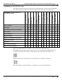
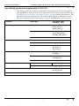
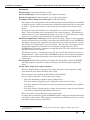
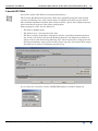
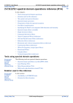
* The local mean filter is available as one of the user defined kernels
The filters listed in this section carry one or two icons denoting whether they are
available in the Spectral Domain Grid Filters tool and/or the Line Filter tool.
This icon indicates that the filter is available for use with line datasets.
This icon indicates that the filter is available for use with grid datasets.
Library | Help | Top
Bessel
Contrast normalisation
Y
Phillips auto depth
Y
Hilbert transform
Gridding
Automatic gain control
Y
Local maximum filter
Y
Local median filter
Gradient
Y
Local mean filter
4th Difference
Profile Editor
Naudy Filter
Fuller filter
Availability of spatial filters in
INTREPID tools
User defined kernel
The following table shows the filters and transformations used in each INTREPID
tool. The notation 'Y' indicates that the tool uses the filter or transformation
© 2012 Intrepid Geophysics
| Back |
INTREPID User Manual
Library | Help | Top
INTREPID spatial and time domain filters and transformations (R13)
3
| Back |
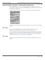
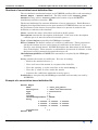
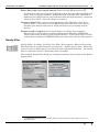
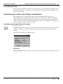
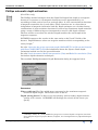
Standard spatial / time filter / transformation dialog boxes
Some INTREPID tools now use a standard dialog box to configure each filter or
transformation. With new versions of INTREPID, more tools will use these standard
dialog boxes as appropriate.
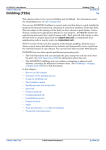
A typical standard spatial / time filter / transformation dialog box appears below.
Certain features are common to all of these dialog boxes as described in the following
sections.
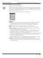
Filter name
For standard INTREPID filters and transformations configured directly in
interactive or batch mode, the Name text box shows the filter type.
In the Line Filter tool, for filters configured using a filter definition file, the Name
text box shows the name of the filter definition file ahd is used for saving the filter
specifications. See "Standard filter names" in Line Filtering (T31) and "Loading and
saving filter definitions" in Line Filtering (T31) for details.
Filter space
For spatial and time domain filters and transformations, INTREPID shows this as
'Spatial'.
Library | Help | Top
© 2012 Intrepid Geophysics
| Back |
INTREPID User Manual
Library | Help | Top
INTREPID spatial and time domain filters and transformations (R13)
4
| Back |
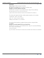
Detrending and replacing trends
Before applying a filter, INTREPID removes first order trends (overall slope) in the
data. If it makes sense to restore the trend after application of the filter, INTREPID
will either automatically replace the trend or include a Replace Trend option in the
filter properties dialog box. INTREPID will normally replace the trend unless you
turn off the Replace Trend check box.
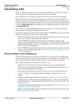
Creating the extended region for filters
To prevent loss of data at the line ends, filters use an extended region at each end of
the line, where the values of the first or last original data point can be rolled off to
zero.
This is particularly important for the Fuller filter, Hilbert transform and Phillips
auto depth estimation.
The properties dialog boxes for these filters contain parameters for specifying the
extended region.
INTREPID calculates initial Signal values for the data points in the extended region.
These can be based on nearby original data values. See Extended region size and
Data extension method for information.
Library | Help | Top
© 2012 Intrepid Geophysics
| Back |
INTREPID User Manual
Library | Help | Top
INTREPID spatial and time domain filters and transformations (R13)
5
| Back |
Extended region size
(Hilbert transformation only)
INTREPID automatically calculates the length of the extended region for the Hilbert
transform using the formula
w – 1)
p = (----------------2
where
p = length (data points) of extended region
w = filter window length
INTREPID automatically calculates a suitable extended region size for the other
filters.
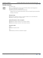
Data extension method
(Fuller filter, Hilbert transformation, Phillips automatic depth estimation only)
INTREPID has three options for extended region values, as described below. In the
dialog box for the filter, select the Data Extension Method option as required.
Zero Pad INTREPID sets all extended region values to zero.
Mirror Pad Data INTREPID extrapolates values so that the profile of the extended
region Signal values is a Y reflection of the profile of the Signal values of the same
number of original data points at that end of the line.
Flipped Mirror Pad Data INTREPID extrapolates values so that the profile of the
extended region Signal values is a Y reflection then an X reflection of the profile of
the Signal values of the same number of original data points at that end of the
line. This is the default option for spatial domain filters.
Filter definition (.fdf) vs kernel (.ker) files
Filter definition (.fdf) files
Using the Line Filter tool you can save and load filter definition files which specify
the type and parameters for a filter. These files have the extension .fdf and reside
in the install_path/filters directory (where install_path is the location of
your INTREPID installation). Filter definition files can specify spatial or spectral
domain filters.
The name of the filter definition file will show in the Name text box of the filter
properties dialog box.
See "Loading and saving filter definitions" in Line Filtering (T31) for details.
User defined convolution kernel (.ker) files
You can specify a convolution filter using a set of coefficients for multiplying
neighbouring data points or grid cells, combining the results and calculating a new
value for the target point or cell. INTREPID stores the coefficients in a user defined
convolution kernel file with the extension .ker, residing in the install_path/
kernels directory (where install_path is the location of your INTREPID
installation). See User defined convolution kernelsfor details.
Library | Help | Top
© 2012 Intrepid Geophysics
| Back |
INTREPID User Manual
Library | Help | Top
INTREPID spatial and time domain filters and transformations (R13)
6
| Back |
User defined convolution kernels
(Line Filter, Spatial Convolution Grid Filters, Equivalent Layer only)
When you apply a convolution filter, INTREPID replaces the Signal value of each
data point (line datasets), or each grid cell (grid datasets) with a weighted
combination of its original value and those of its neighbours, using a set of
coefficients. A user defined convolution kernel contains a set of coefficients.
In an INTREPID revision to be released soon you will be able to apply user defined
convolution kernels to line datasets using the Line Filter tool (See "Filter operations"
in Line Filtering (T31)).
In the current version of INTREPID you can apply user defined convolution kernels
to grid datasets using the Spatial Convolution tool (See Spatial Convolution Grid
Filters (T34)).
The Weiner Filter tool automatically produces kernels for grid datasets. The
Equivalent Layer tool uses these kernel for its operation. See Creating Weiner
convolution kernels (T35) and Equivalent Layer corrections (T36) for details.
Library | Help | Top
© 2012 Intrepid Geophysics
| Back |
INTREPID User Manual
Library | Help | Top
INTREPID spatial and time domain filters and transformations (R13)
7
| Back |
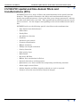
User defined grid kernels supplied with INTREPID
The following table describes the predefined convolution kernels typically supplied
with INTREPID. Many of these are designed to emulate spectral domain filters (See
INTREPID spectral domain operations reference (R14) for further information). The
predefined convolution kernels are all standard Earth Resource Mapping kernels.
For more information about these kernels, refer to the ERMapper documentation.
Purpose
Kernel type
File names (with
extension .ker)
Enhancing peaks and troughs
Downward continuation
down_cont_half
down_cont_1
down_cont_2
Horizontal derivative
hz10_2nd_deriv
hz13_2nd_deriv
hz1960_2nd_deriv
Second vertical derivative
secondvertical
Averaging
3x3ave
Low pass
low_pass_4
Upward continuation
up_cont_half
up_cont_1
up_cont_2
Horizontal edge enhance
h_edge
h_edge_5
Residual
residual_1
residual_2
Sharp Edge
sharpedge
Band pass
bandpass_3_5
High pass
high_pass_4
Directional filter
Sun filter
East_West
North_South
Magnetic susceptibility
Weiner
wiener
Smoothing
Enhancing edges
Extracting particular frequencies
Library | Help | Top
© 2012 Intrepid Geophysics
| Back |
INTREPID User Manual
Library | Help | Top
INTREPID spatial and time domain filters and transformations (R13)
8
| Back |
Structure of convolution kernel definition files
The user defined convolution kernels are INTREPID auxiliary files each containing a
Kernel Begin – Kernel End block. The files reside in the install_path/
kernel directory (where install_path is the location of your INTREPID
installation) and have extension .ker.
The kernel definition file contains definitions of seven parameters. Earth Resource
Mapping developed this format as an open standard. INTREPID does not use some of
the parameters in the format, but requires them to be present in order for the
definition to conform to the standard.
Name contains the name of the filter enclosed in double quotes.
Description contains the description of the kernel. If the text of the description
contains spaces it must be enclosed in double quotes "".
Type = Convolution required by the ERMapper standard.
Rows, Columns The kernel consists of a matrix of coefficients. These parameters
specify the number of rows and columns of coefficients in the kernel. If you
specify a user defined kernel, INTREPID displays the dimensions in the Status
area of the display. There must be an odd number of rows and of columns, so that
the kernel can be symmetrical around the target cell.
OkOnSubsampledData = FALSE This statement is required by the ERMapper
standard.
Array contains the matrix of coefficients. For ease of reading:
•
Enclose the matrix in braces { }.
•
Place each row of the matrix in a separate line of the file.
•
Place the opening '{' on the same line as the words Array =
•
Place the '}' alone on a line under the matrix.
•
Separate the coefficients within the rows by spaces.
Scalefactor = 1 required by the ERMapper standard and currently not used by
INTREPID.
Example of a convolution kernel definition file
Kernel Begin
Name
= "hz13_2nd_deriv"
Description
= "HZ13 2nd Derivative"
Type
= Convolution
Rows
= 3
Columns
= 3
OkOnSubsampledData = FALSE
Array
= {
0.500000 –2.000000 0.500000
2.000000 6.000000 –2.000000
0.500000 –2.000000 0.500000
}
Scalefactor
= 1
Kernel End
Library | Help | Top
© 2012 Intrepid Geophysics
| Back |
INTREPID User Manual
Library | Help | Top
INTREPID spatial and time domain filters and transformations (R13)
9
| Back |
Fuller filter
(Gridding, Levelling, Line Filter, Decorrugation, Microlevelling tools)
The moving average Fuller convolution filter1 detects high frequency data and passes
or rejects it. See User defined convolution kernels for a general explanation of
convolution filters. INTREPID can apply the Fuller filter to line or grid data.
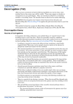
The standard Fuller filter dialog box appears below.
Parameters
Window Size (data points) (standard parameter name)
Streak Width (m) ( in Decorrugation first (high pass) filter)
Streak Length (m) (in Decorrugation second (low pass) filter)
Secondary filter along correction (m) (in Microlevelling)
The window size ('wavelength') corresponds to the maximum width of anomalies
to be processed by the Fuller filter (i.e., identified as high frequency).
In the Decorrugation and Microlevelling tools this is measured in metres. In the
other tools it is measured as the number of data points.
The window size also corresponds to the number of coefficients used in the Fuller
convolution process (one per data point or grid cell in the window).
Normalise filter weights The Fuller filter is a convolution filter with a set of
coefficients. You can ensure that the filter does not cause an overall change in the
mean of the data by normalising the filter weights (making the coefficients add up
to 1).
1. D.C. Fraser, B.D. Fuller and S.H. Ward, Some Numerical Techniques for Application in
Mining Exploration, Geophysics, vol. XXXI, NO. 6, December, 1966.
Library | Help | Top
© 2012 Intrepid Geophysics
| Back |
INTREPID User Manual
Library | Help | Top
INTREPID spatial and time domain filters and transformations (R13)
10
| Back |
Fuller filter high / low output options (fixed in Profile Editor (high pass),
Levelling (low pass), Decorrugation1 (high pass then low pass), Microlevelling (low
pass)) You can specify whether a Fuller filter will output the data identified as
high frequency (High Pass) or output the data with the high frequency component
removed (Low Pass). Select the option as required.
Output residuals This option reverses the action of the High Pass / Low Pass
options above. If you turn it on, INTREPID will reject the data that it would
normally pass and pass the data it would normally reject according to these
options.
Replace trend in output (fixed in Profile Editor, Levelling, Decorrugation,
Microlevelling—all turned on) Before applying the Fuller filter, INTREPID
removes first order trends (overall slope) in the data. If this check box is on (this
is the default condition), INTREPID will restore this trend after the filter process.
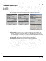
Naudy filter
(Profile Editor, Gridding, Levelling, Line Filter, Decorrugation, Microlevelling tools)
This filter detects sudden changes in your data (i.e., high frequency data). These may
be due to noise or spikes that are not characteristic of potential field data. The Naudy
filter is commonly used for eliminating noise and spikes.
The standard Naudy filter dialog box and the parameters box from the Profile Editor
appear below.
1. INTREPID normally uses a Fuller filter for the second, low pass filter process in
Decorrugation
Library | Help | Top
© 2012 Intrepid Geophysics
| Back |
INTREPID User Manual
Library | Help | Top
INTREPID spatial and time domain filters and transformations (R13)
11
| Back |
Parameters
Window Size (standard parameter name)
Streak Width (m) (in Decorrugation first (high pass) filter)
Streak Length (m) (in Decorrugation second (low pass) filter)
Secondary filter along correction (m) (in Microlevelling)
The window size corresponds to the maximum width of anomalies to be identified
as high frequency. In the Decorrugation and Microlevelling tools this is measured
in metres. In the other tools it is measured as the number of line dataset data
points.
In 'spectral' terms the window size corresponds to a cutoff wavelength for the
filter. Thus 1/(window size) corresponds to the cutoff frequency. The minimum
window size is 2, so the maximum frequency is 1/2, or 0.5. Thus frequencies range
from 0 to 0.5, and the cutoff frequency lies within this range.
Minimum amplitude, Tolerance (fixed in Microlevelling, change in Decorrugation
task specification files only) When calculating the Naudy filter result INTREPID
will ignore changes with amplitude less than the value of this parameter. Specify
the Tolerance in Signal units or grid cell units. The tolerance corresponds to the
minimum amplitude of anomalies to be identified as high frequency data.
INTREPID will identify an anomaly as high frequency if it has amplitude higher
than the tolerance you specify.
The default value 0.1 corresponds to 0.1 nT, the current documented accuracy of
magnetometers. This ensures that INTREPID will not waste time attempting to
smooth out the normal fluctuations associated with the precision limits of the
instrument.
Wavelength (Profile Editor) When calculating the Naudy filter result INTREPID
will only examine sequences of data points up to the Wavelength as potential
noise.
Naudy filter high / low output options
(Fixed in Profile Editor (high pass), Levelling (low pass), Decorrugation1 (high
pass then low pass), Microlevelling (low pass));
(Notch output only available in Line Filter and Gridding)
You can specify whether a Naudy filter will output:
•
The data identified as high frequency (High Pass),
•
The data with the high frequency component removed (Low Pass),
•
The data within a band (notch or range of frequencies) related to the window
size (Notch),
•
The data outside a band (notch or range of frequencies) related to the window
size (Notch) with Output Residuals turned on).
Select the option corresponding to your requirement.
To apply the band (notch) option INTREPID applies a high pass Naudy filter then
a low pass to the results. This outputs (or rejects) data with frequency close to the
specified cutoff frequency of the filter.
1. INTREPID normally uses a Naudy filter for the first, high pass filter process in
Decorrugation
Library | Help | Top
© 2012 Intrepid Geophysics
| Back |
INTREPID User Manual
Library | Help | Top
INTREPID spatial and time domain filters and transformations (R13)
12
| Back |
Output residuals This option reverses the action of the High Pass/Low Pass/Notch
options above. If you turn it on, INTREPID will reject the data that it would
normally pass and pass the data it would normally reject according to these
options.
Replace trend in output (fixed in Profile Editor, Levelling, Decorrugation,
Microlevelling—all turned on) Before applying the Naudy filter, INTREPID
removes first order trends (overall slope) in the data. If this check box is on (this
is the default condition), INTREPID will restore this trend after the filter process.
4th Difference noise detection
(Profile Editor and Spreadsheet editor only)
This filter calculates the 4th difference of the Signal data. Non-zero 4th difference
results indicate sudden changes in the data. See the description of the diffn()
function in Section "INTREPID Functions" in INTREPID expressions and functions
(R12) for information about the 4th difference calculation (diff4()).
Gradient filter
(Profile Editor only)
The gradient filter calculates the slope of the Signal field with respect to time
(fiducial). This is a useful indicator of rapid change and therefore a method of
identifying noise.
Library | Help | Top
© 2012 Intrepid Geophysics
| Back |
INTREPID User Manual
Library | Help | Top
INTREPID spatial and time domain filters and transformations (R13)
13
| Back |
Local mean / median filters
(Mean: Line Filter only; Median: Line Filter and Spatial Convolution Grid Filters
only, Local mean-Tensor: Profile Editor) These filters adjust the value of the target
cell based on the mean or median value of the cell and its neighbours in a window.
For line data this window is a number of data points surrounding the target point.
For grid data the window is square with the target cell in the centre.
The standard Local Mean and Local Median filter dialog boxes appear below.
Parameters
Window length Use this text box to specify the width of the filter window. For
example, if the width of the filter window is 21, then the new cell value will be
calculated from the value of the cell and its 10 neighbours in each direction (Line
data: 10 data points on either side of the target point, Grid data: block of cells 10 x
10 with target cell in the centre). The value of parameter cannot be less than 3.
Low Pass, High Pass Contact technical support for information.
Normalise filter weights Contact technical support for information.
Output Residuals (fixed in Spatial Convolution Grid Filters—turned off) If you
turn on this check box, INTREPID will output the difference between the filter
results and the original data.
Replace trend in output (fixed in Spatial Convolution Grid Filters—turned on)
Before applying the local mean / median filter, INTREPID removes first order
trends (overall slope) in the data. If this check box is on (this is the default
condition), INTREPID will restore this trend after the filter process.
Library | Help | Top
© 2012 Intrepid Geophysics
| Back |
INTREPID User Manual
Library | Help | Top
INTREPID spatial and time domain filters and transformations (R13)
14
| Back |
Local Maximum filter
The local maximum filter operates in a similar way to the existing Local Mean and
Local Median filters. It sets the value of the target data point to the maximum value
found in the window.
Automatic gain control and contrast normalisation
The automatic gain control (AGC) and contrast normalisation filters uses an
averaging process to reduce the amplitude variance of the data. This can amplify
smaller anomalies and dampen larger anomalies so that all anomalies appear more
similar. This is useful for enhancing smaller anomalies and reducing any tendency of
larger anomalies to 'drown out' the signal.
Automatic gain control filter for line data
(Line Filter only)
INTREPID processes each data point input value using the values in a surrounding
window. It divides the input value by the root mean square of the points in the
window.
The AGC filter dialog box appears below.
Parameters
AGC 1/2 Window size Number of data points in the AGC window. The default value
is 5.
Library | Help | Top
© 2012 Intrepid Geophysics
| Back |
INTREPID User Manual
Library | Help | Top
INTREPID spatial and time domain filters and transformations (R13)
15
| Back |
Contrast normalisation filter for grid data
(Spatial Convolution Grid Filters only)
The Contrast Normalisation filter is a non-linear space variant stretch filter that will
enhance the low amplitude, high frequency content, and dampen the high amplitude
content. It has a similar effect to an automatic gain control filter (See Automatic gain
control and contrast normalisation).
The Contrast Normalisation filter dialog box appears below.
Parameters
Window Use this text box to specify the width of the filter window. For example, if
the width of the filter window is 21, then the new target cell value will be
calculated from the value of the cell and its 10 neighbours in all directions.
Mean Use this text box to specify the desired mean of the output.
Stddev Use this text box to specify the desired standard deviation of the output.
Weight for Means Use this text box to specify the weighting to apply to the desired
mean versus the local mean of the window.
The closer the weighting to 0, the more biassed result will be towards the local
mean of the window. If the weighting is equal to 0 the filter will use the local
mean of the window and ignore your desired mean.
The closer the weighting to 1, more biassed the results will be towards the desired
mean. If the weighting is equal to 1 the filter will use your desired mean and
ignore the local mean of the window.
Essentially this has the effect of dampening regional trends when you use a value
closer to 1. Setting the value to 0 preserves the regional component.
MaxGain The maximum gain is an amplification limit for data output by the filter.
A cell may not deviate more than the value of this parameter from the mean of the
cells in the window.
Library | Help | Top
© 2012 Intrepid Geophysics
| Back |
INTREPID User Manual
Library | Help | Top
INTREPID spatial and time domain filters and transformations (R13)
16
| Back |
Hilbert transform
(Gridding, Line Filter only)
The Hilbert Transform filter uses a finite difference operator to calculate an
imaginary component of the input (Quadrature). It uses this as the filter result or
combines it with the existing real component to give the Instantaneous Phase or
Instantaneous Frequency.
The standard Hilbert transform dialog box appears below.
Parameters
Filter Properties
Filter Window Length The number of data points used by the Hilbert Transform
finite difference operator. The default value is 19 (i.e., 9 points on each side of the
target point). The value of parameter cannot be less than 9.
Output Options
Quadrature This is the imaginary component of the input signal derived using the
Hilbert transform. The Hilbert Transform includes a detrending process. You can
choose whether to replace the trend in the filter results using the two Quadrature
options:
Quadrature—(local) trend replaced
Quadrature—(local) trend removed
Even though the Hilbert transform is not connected with the spectral domain, you
can find a relevant discussion of detrending in section"Detrending data values" in
INTREPID spectral domain operations reference (R14)
Complex Amplitude This is the magnitude of sum of the input data (real
component) and the Quadrature results (imaginary component).
complex amplitude =
Library | Help | Top
2
real + imaginary
2
© 2012 Intrepid Geophysics
| Back |
INTREPID User Manual
Library | Help | Top
INTREPID spatial and time domain filters and transformations (R13)
17
| Back |
Instantaneous Phase This is derived by combining the input data (real component)
and the Quadrature results (imaginary component) using the formula
imaginary
instantaneous phase = atan ⎛ ------------------------⎞
⎝ real ⎠
Instantaneous Phase can show continuity for subtle features often lost when you
only examine the real component. See the articles Taner, Koehler and Sheriff
(1979)1 and Fitzgerald, Yassi, and Dart (1997)2 for further discussion of this
technique.
Unwound Instantaneous phase results have data jumps due to the spiralling nature
of the filter. INTREPID can correct this using a surface consistent partial
unwrapping algorithm. Select this option to produce unwrapped instantaneous
phase results.
Instantaneous Frequency This is a measure of change in the Instantaneous Phase
(see previous section), comparing adjacent values of Instantaneous Phase results.
It uses the formula
instantaneous frequency = diff1(instantaneous phase)
See "DIFF function example" in INTREPID expressions and functions (R12)for an
illustration of this function.
1. Taner, M.T., Koehler, F. and Sheriff, R.E., 1979, Complex seismic trace analysis:
Geophysics 44, 1041–1063.
2.Fitzgerald, D., Yassi, N. and Dart, P., 1997, A case study on geophysical gridding
techniques: INTREPID perspective: Exploration Geophysics, 28, 1–
Library | Help | Top
© 2012 Intrepid Geophysics
| Back |
INTREPID User Manual
Library | Help | Top
INTREPID spatial and time domain filters and transformations (R13)
18
| Back |
Phillips automatic depth estimation
(Line Filter only)
The Phillips method estimates from the Signal field signal the depth to a magnetic
basement. It assumes a 2-D magnetic basement can be approximated by an
assemblage of thin vertical (or near-vertical) dykes. It uses autocorrelation functions
of magnetic anomalies due to such dykes. These functions are in a form that is
independent of magnetic inclination and dip. Depth estimates are calculated using
combinations of autocorrelation functions at various lags.Consistent depth estimates
using a range of different lags are interpreted to mean a valid depth estimate.
The best results occur when the window length matches the wavelength of the
magnetic responses.
INTREPID expresses the results in the same units as the X and Y fields of the
dataset. Depth Estimate values are negative numbers with 0 corresponding to the
survey height.1
See also "Querying the power spectrum graph (OldGridFFT)" in Old spectral domain
grid filters (OldGridFFT) (T38)for information about the Spector Grant depth
estimation method used in the spectral domain.
See also Naudy Automatic Model interpretation (T43) and Euler Deconvolution (T44)
for further depth estimation techniques.
The standard Phillips Automatic Depth Estimation dialog box appears below.
Parameters
Filter width (m) The filter width must correspond to the maximum magnetic
basement depth sought. The default value is 290 m.
Depth tuning factor Use this to vary the primary and secondary depth estimate
'quality of fit' criteria. INTREPID will multiply the criteria by the factor you
specify.
1. Phillips, Jeffrey D., (1979) ADEPT: A program to estimate depth to magnetic basement
from sampled magnetic profiles Reston, Virginia, U.S. Geological Survey Open File Report
79–367.
Library | Help | Top
© 2012 Intrepid Geophysics
| Back |
INTREPID User Manual
Library | Help | Top
INTREPID spatial and time domain filters and transformations (R13)
19
| Back |
Lacoste RC filter
(Line Filter and Profile Editor (compound data filters)
The Lacoste RC (Resistive/Capacitive) filter was originally designed using analog
circuits, for filtering very noisy marine data. Its digital equivalent can be used to
filter stabilised platform monitor data which contains a great deal of high frequency
noise from the movement of the ship acquiring data.
Some properties of the Lacoste filter are:
•
The filter is highly linear
•
The filter leaves a local trend in the data
•
The first 3 stages of the filter compensate for the acquisition instrument phase
lag. In the case of the LaCoste and Romberg S-meter, the firmware performs 3
stages of 20 second forward lag filtering only. The Lacoste filter compensates for
this by performing 3 stages of 20 second reverse lag only. Successive filter stages
are then run in pairs, to eliminate any phase lag.
If you select the curvature version, INTREPID displays a further dialog box
Library | Help | Top
© 2012 Intrepid Geophysics
| Back |
INTREPID User Manual
Library | Help | Top
INTREPID spatial and time domain filters and transformations (R13)
20
| Back |
Parameters
Filter Stages Number of stages in the filter
RC Times in seconds Time in seconds for each filter stage.
Example 1 Lacoste 9-stage RC noise filter.
This filter does 3 stages of 1 way backwards, then 3 stages of 2-way filtering
20.0, 20.0, 20.0, 27.0, 27.0, 27.0, 27.0, 27.0, 27.0,
eg 20 sec back, 20 sec back, 20 sec back, (27 sec forward, 27 sec back) x 3
To calculate the length of the filter, add the numbers up (they are in seconds).
so 20+20+20 = 60 sec, one minute,
and 6 * 27 = 162 sec, about 2.7 minute,
making a total of 222 sec, or 3.7 minutes.
If you don’t wish to introduce any phase lag into your data, design the filter
accordingly.
Example 2 Lacoste 6-stage RC 106 second noise filter.
This filter does 3 stages of 1 way backwards, then 1 stage of 1-way forward filtering,
then 1 stage of 2-way filtering.
10 10 10, 30, 23 23
(eg: 10 sec back, 10 sec back, 10 sec back, 30 sec forward, 23 sec back, 23 sec forward)
Library | Help | Top
© 2012 Intrepid Geophysics
| Back |
INTREPID User Manual
Library | Help | Top
INTREPID spatial and time domain filters and transformations (R13)
21
| Back |
Gravity Inversion
(Line Filter only)
This is an implementation of the paper by Murthy & Rao, from Computers &
Geosciences, Vol 15 No. 7 pp1149-1156
A profile of gravity data is inverted to yield either:
•
Depths to the top of the basement surface below each point of gravity anomalies
•
Anomaly of structure
Parameter input
Z Depth above which the structure or density Surface is to be calculated, km
Dc Density contrast, gm/cc, default is 400
Optional Parameters to aid convergence
Ztlt Minimum depth to interface, km, default is 1000 m.
Zblt Maximum depth to interface, km, default is 4000 m.
Parameter output
Either
Zt Depth to interface in km
OR
Gcal Anomaly of structure calculated, in mgals
Library | Help | Top
© 2012 Intrepid Geophysics
| Back |
INTREPID User Manual
Library | Help | Top
INTREPID spatial and time domain filters and transformations (R13)
22
| Back |
Strip Gravity Layer
(Line Filter only)
A simple filter to calculate the gravitational effect of a layer of variable thickness.
It is based upon using the formula for the gravitational effect for a Prism
Parameter input
Zbot Depth to bottom of layer
Ztop Depth to top of layer, default is 0.0
Dc Density contrast, gm/cc
Library | Help | Top
© 2012 Intrepid Geophysics
| Back |