Download USER MANUAL

Digital Photogrammetric System
Version 5.21
USER
MANUAL
Project Processing
PHOTOMOD 5.21
1. Block processing ......................................................................................................................................... 7
2. Main windows............................................................................................................................................... 7
2.1. 2D Window .............................................................................................................................................. 7
2.1.1. Image displaying tools...................................................................................................................... 9
2.1.2. Brightness and contrast adjustment............................................................................................... 10
2.1.3. Saving 2D window image ............................................................................................................... 10
2.2. 3D Window ............................................................................................................................................ 12
2.2.1. 3D window properties..................................................................................................................... 14
2.3. Navigation window ................................................................................................................................ 17
2.4. Layer manager ...................................................................................................................................... 17
2.5. Status panel .......................................................................................................................................... 20
2.6. Object list window.................................................................................................................................. 20
2.7. Raster map window............................................................................................................................... 21
3. Stereomeasurements................................................................................................................................. 23
3.1. Stereomodes ......................................................................................................................................... 23
3.1.1. Anaglyph glasses ........................................................................................................................... 23
3.1.2. Shutter glasses............................................................................................................................... 23
3.2. Stereopair selection............................................................................................................................... 24
3.3. Operating marker .................................................................................................................................. 25
3.3.1. Moving marker mode...................................................................................................................... 25
3.3.2. Fixed marker mode ........................................................................................................................ 25
3.3.3. Marker = mouse mode ................................................................................................................. 26
3.3.4. Snap-to-ground mode .................................................................................................................... 26
3.3.5. Streamline mode ............................................................................................................................ 26
3.3.6. Fixed Z mode ................................................................................................................................. 27
3.3.7. Marker window............................................................................................................................... 27
3.3.8. Type of snapping............................................................................................................................ 28
3.4. Adjusting stereoimage........................................................................................................................... 28
3.5. Measurements over the model.............................................................................................................. 29
4. Vector objects............................................................................................................................................. 30
4.1. Vector layer ........................................................................................................................................... 31
4.2. Vector layer with classifier..................................................................................................................... 31
4.2.1. Creating vector layer with classifier ............................................................................................... 31
4.2.2. Classifier......................................................................................................................................... 31
4.2.2.1. Classifier creation ...................................................................................................................................................... 34
4.2.2.2. Classifier editing........................................................................................................................................................ 36
4.2.2.3. Import of classifier..................................................................................................................................................... 36
4.2.2.4. Adding attributes ....................................................................................................................................................... 37
4.2.2.5. Additional attributes .................................................................................................................................................. 40
4.2.2.6. Labels creation........................................................................................................................................................... 41
4.2.2.7. Attaching vector objects to classifier......................................................................................................................... 42
4.2.2.8. Object list .................................................................................................................................................................. 42
4.3. Vector objects creation.......................................................................................................................... 43
4.3.1. Vector object types......................................................................................................................... 43
4.3.2. Vector objects creation................................................................................................................... 43
4.3.2.1. Point creation............................................................................................................................................................. 44
4.3.2.2. Polyline creation........................................................................................................................................................ 44
4.3.2.3. Polygon creation........................................................................................................................................................ 45
4.3.2.4. Creating orthogonal vector objects........................................................................................................................... 45
4.3.2.5. CAD-objects creation ................................................................................................................................................ 45
4.3.3. Loading vector data........................................................................................................................ 47
4.3.4. Saving vector data.......................................................................................................................... 47
4.3.5. Switching between stereopairs ...................................................................................................... 47
4.4. Editing of vector objects ........................................................................................................................ 48
4.4.1. Objects selection ............................................................................................................................ 48
4.4.1.1. Selection tools ........................................................................................................................................................... 48
4.4.1.2. Selection modes......................................................................................................................................................... 48
4.4.1.3. Selecting all objects in layer...................................................................................................................................... 49
4.4.1.4. Selecting objects of the same code ............................................................................................................................ 49
4.4.2. Point editing.................................................................................................................................... 49
© 2011
2
Project processing
2011
4.4.3. Polyline/polygon editing ................................................................................................................. 50
4.4.3.1. Vertex editing ............................................................................................................................................................ 50
4.4.3.2. Vertex adding ............................................................................................................................................................ 50
4.4.3.3. Polyline continuing.................................................................................................................................................... 50
4.4.3.4. Converting objects to figures..................................................................................................................................... 51
4.4.3.5. Interpolating polyline ................................................................................................................................................ 51
4.4.3.6. Interpolation of polyline elevations ........................................................................................................................... 51
4.4.3.7. Rounding off corners ................................................................................................................................................. 52
4.4.3.8. Moving polyline ........................................................................................................................................................ 52
4.4.3.9. Deleting polyline ....................................................................................................................................................... 52
4.4.3.10. Building buffer zone................................................................................................................................................ 53
4.4.3.11. Creating profiles through vector objects.................................................................................................................. 53
4.4.3.12. Circles around points ............................................................................................................................................... 54
4.4.3.13. Project on stereomodel ............................................................................................................................................ 55
4.4.3.14. Projection on TIN .................................................................................................................................................... 55
4.4.3.15. Quick interpolate ..................................................................................................................................................... 56
4.4.3.16. Deleting pickets around line objects........................................................................................................................ 56
4.4.3.17. Converting polygons to points................................................................................................................................. 56
4.4.3.18. Merging point objects by attribute........................................................................................................................... 57
4.4.3.19. Searching objects by attribute value ........................................................................................................................ 57
4.4.3.20. Collating objects...................................................................................................................................................... 58
4.4.3.21. Copying to layer ...................................................................................................................................................... 59
4.4.3.22. Copying/pasting using clipboard ............................................................................................................................. 60
4.4.3.23. Operations with group of objects............................................................................................................................. 60
4.4.3.24. Object type conversion ............................................................................................................................................ 61
4.4.4. Curves editing ................................................................................................................................ 61
4.4.4.1. Curves creating mode ................................................................................................................................................ 62
4.4.4.2. Polylines to curves conversion .................................................................................................................................. 62
4.4.4.3. Curves to polylines conversion.................................................................................................................................. 62
4.4.4.4. Automatic smoothing adjustment .............................................................................................................................. 63
4.4.4.5. Curve segments editing ............................................................................................................................................. 63
4.4.4.6. Smoothing control ..................................................................................................................................................... 63
4.4.5. Topology......................................................................................................................................... 64
4.4.5.1. Segment deleting ....................................................................................................................................................... 64
4.4.5.2. Merging polylines...................................................................................................................................................... 64
4.4.5.3. Merging polygons...................................................................................................................................................... 65
4.4.5.4. Closing polyline......................................................................................................................................................... 65
4.4.5.5. Unclosing polyline..................................................................................................................................................... 65
4.4.5.6. Splitting polyline ....................................................................................................................................................... 65
4.4.5.7. Connection to point ................................................................................................................................................... 65
4.4.5.8. Connection to polyline .............................................................................................................................................. 65
4.4.5.9. Continuing along polyline ......................................................................................................................................... 65
4.4.5.10. Closing along polyline............................................................................................................................................. 66
4.4.5.11. Topology control ..................................................................................................................................................... 67
4.4.6. Undoing the editing operations ...................................................................................................... 68
5. Creation of digital terrain model (DTM).................................................................................................... 69
5.1. Types of DEM representation ............................................................................................................... 69
6. TIN................................................................................................................................................................ 70
6.1. Initial data for TIN building..................................................................................................................... 71
6.2. Workflow................................................................................................................................................ 71
6.3. Preparing of base layers for TIN creation ............................................................................................. 71
6.3.1. Pre-regions..................................................................................................................................... 72
6.3.2. Pickets creation .............................................................................................................................. 73
6.3.2.1. Modes and methods for creating pickets ................................................................................................................... 73
6.3.2.2. Grid creation.............................................................................................................................................................. 73
6.3.2.3. Automatic computation of points .............................................................................................................................. 76
6.3.2.3.1. Computation of points ................................................................................................................................... 76
6.3.2.3.2. Correlator presets .......................................................................................................................................... 80
6.3.2.3.3. Settings of correlator preset........................................................................................................................... 81
6.3.2.3.4. More settings of pass..................................................................................................................................... 85
6.3.2.3.5. First approximation settings .......................................................................................................................... 86
6.3.2.3.6. Computing points in distributed processing mode......................................................................................... 87
6.3.2.4. Creation of pickets in pathway mode ........................................................................................................................ 88
6.3.2.5. Points editing ............................................................................................................................................................. 89
6.3.2.6. Filter by Z-range........................................................................................................................................................ 90
3
RACURS Co., Ul. Yaroslavskaya, 13-A, office 15, 129366, Moscow, Russia
PHOTOMOD 5.21
6.3.2.7. Median Z filter........................................................................................................................................................... 90
6.3.2.8. Filter adjacent point objects....................................................................................................................................... 91
6.3.2.9. Filter of buildings and vegetation .............................................................................................................................. 91
6.3.2.9.1. Setting up parameters of filter ....................................................................................................................... 95
6.3.2.9.2. Recommendations on using the filter ............................................................................................................ 97
6.3.2.10. Considering operator personal difference ................................................................................................................ 98
6.3.3. Using triangulation points............................................................................................................... 99
6.3.4. Opening of base layers .................................................................................................................. 99
6.4. Building TIN .........................................................................................................................................100
6.4.1. Create TIN window ......................................................................................................................100
6.4.2. Building of TIN boundaries...........................................................................................................102
6.4.3. Viewing TIN ..................................................................................................................................104
6.4.4. Saving TIN....................................................................................................................................105
6.4.5. Loading TIN..................................................................................................................................105
6.4.6. Closing TIN...................................................................................................................................105
6.5. TIN editing ...........................................................................................................................................105
6.5.1. TIN topology verification...............................................................................................................105
6.5.2. Filtering.........................................................................................................................................106
6.5.2.1. Simplifying .............................................................................................................................................................. 107
6.5.2.2. Peak filtering ........................................................................................................................................................... 107
6.5.2.3. Filter by Z-range...................................................................................................................................................... 109
6.5.3. Rebuilding of TIN..........................................................................................................................109
6.6. TIN control against triangulation points...............................................................................................110
6.7. Calculating TIN area............................................................................................................................111
6.8. Statistics ..............................................................................................................................................112
7. Contour lines ............................................................................................................................................113
7.1. Building contour lines from TIN ...........................................................................................................113
7.2. Building contour lines from DEM.........................................................................................................114
7.3. Creating smooth model contours ........................................................................................................116
7.4. Saving contour lines ............................................................................................................................118
7.5. Loading contour lines ..........................................................................................................................118
7.6. Operations on contour lines ................................................................................................................118
7.6.1. Controlling contours intersections ................................................................................................119
7.6.2. Checking contours by points ........................................................................................................119
7.6.3. Merging contours..........................................................................................................................120
7.6.4. Checking contours merging .........................................................................................................122
8. Digital Elevation Model (DEM).................................................................................................................122
8.1. DEM building .......................................................................................................................................122
8.1.1. Building DEM using TIN ...............................................................................................................122
8.1.2. Building DEM using pickets..........................................................................................................124
8.1.3. Building DEM using regular pickets .............................................................................................126
8.1.4. Creating smooth model DEM .......................................................................................................127
8.1.5. Creation of DTM by dense model ................................................................................................128
8.1.5.1. Building parameters of DTM by dense model......................................................................................................... 129
8.1.6. Batch DTM creation......................................................................................................................132
8.2. DEM rebuilding by TIN ........................................................................................................................134
8.3. DEM recovering...................................................................................................................................134
8.4. DEM saving .........................................................................................................................................135
8.5. DEM loading ........................................................................................................................................135
8.6. DEM filtration .......................................................................................................................................135
8.6.1. Buildings and vegetation filter ......................................................................................................135
8.7. Operations on DEM.............................................................................................................................137
8.7.1. Merging DEMs..............................................................................................................................137
8.7.2. Flattening DEM fragment .............................................................................................................137
8.7.3. Transposing DEM.........................................................................................................................138
8.7.4. Converting DEM to another coordinate system ...........................................................................138
8.7.5. Transforming DEM by a set of points...........................................................................................139
8.7.6. Filtration........................................................................................................................................139
8.7.6.1. Median filter ............................................................................................................................................................ 139
8.7.6.2. Smooth filter............................................................................................................................................................ 139
8.7.7. Converting DEM into points .........................................................................................................140
8.7.8. Difference DEM creating ..............................................................................................................140
© 2011
4
Project processing
2011
8.7.9. Filling void cells ............................................................................................................................141
8.7.10. Conversion cells to void .............................................................................................................145
8.8. DEM accuracy control .........................................................................................................................145
8.8.1. DEM accuracy control by TIN ......................................................................................................145
8.8.2. DEM accuracy control by vector objects......................................................................................147
8.8.3. DEM accuracy control by triangulation points..............................................................................148
8.8.4. Void cells searching .....................................................................................................................149
8.8.5. DEM’s comparing .........................................................................................................................149
8.9. LIDAR data loading .............................................................................................................................149
9. Import-Export............................................................................................................................................149
9.1. Import vector objects ...........................................................................................................................149
9.1.1. Coordinates conversion during import .........................................................................................150
9.1.2. Importing attributes.......................................................................................................................151
9.1.3. Import from ASCII format. ............................................................................................................151
9.1.3.1. ASCII format description ........................................................................................................................................ 152
9.1.4. Import from ASCII-A format..........................................................................................................152
9.1.4.1. ASCII-A format description .................................................................................................................................... 153
9.1.5. Import from CSV format ...............................................................................................................154
9.1.6. Import from DGN format...............................................................................................................156
9.1.7. Import from DXF format................................................................................................................157
9.1.8. Import from Generate format........................................................................................................158
9.1.9. Import from ATLAS KLT format....................................................................................................159
9.1.10. Import from LAS format ..............................................................................................................159
9.1.11. Import from LIG format ...............................................................................................................160
9.1.12. Import from MIF/MID format .......................................................................................................161
9.1.13. Import from Shape format ..........................................................................................................163
9.1.14. Import from VectOr format..........................................................................................................164
9.1.15. Import pickets from VectOr format .............................................................................................164
9.2. Export ..................................................................................................................................................165
9.2.1. Coordinates conversion during export .........................................................................................165
9.2.2. Export to ASCII format .................................................................................................................166
9.2.3. Export to ASCII-A format..............................................................................................................166
9.2.4. Export to CSV format ...................................................................................................................167
9.2.5. Export to DGN format...................................................................................................................168
9.2.5.1. DGN format peculiarities ........................................................................................................................................ 169
9.2.6. Export to DXF format....................................................................................................................169
9.2.7. Export to Generate format............................................................................................................171
9.2.8. Export to ATLAS KLT format........................................................................................................172
9.2.9. Export to LIG format .....................................................................................................................172
9.2.10. Export to MIF/MID format ...........................................................................................................173
9.2.11. Export to Shape format ..............................................................................................................175
9.2.12. Export to VectOr format..............................................................................................................175
9.3. Import of DEM .....................................................................................................................................176
9.3.1. Batch DEM import ........................................................................................................................177
9.4. Export of DEM .....................................................................................................................................177
10. Parameters and settings .......................................................................................................................178
10.1. Windows settings ..............................................................................................................................178
10.2. Marker settings..................................................................................................................................180
10.3. Control settings .................................................................................................................................181
10.4. Settings of modules starting..............................................................................................................183
10.5. Settings of block layout .....................................................................................................................183
10.5.1. Parameters of loading and displaying images ...........................................................................184
10.6. Stereo settings ..................................................................................................................................185
10.7. Correlator settings .............................................................................................................................186
10.8. DEM settings .....................................................................................................................................188
10.9. TIN settings .......................................................................................................................................189
10.10. Grid settings ....................................................................................................................................191
10.11. Pathway mode settings ...................................................................................................................191
10.12. Vector objects settings ....................................................................................................................192
10.12.1. Settings of labels displaying.....................................................................................................193
10.12.2. Settings of elevation labels displaying .....................................................................................194
5
RACURS Co., Ul. Yaroslavskaya, 13-A, office 15, 129366, Moscow, Russia
PHOTOMOD 5.21
10.12.3. Settings for display of points numbers .....................................................................................195
10.12.4. Coordinates transformation......................................................................................................197
10.13. Parameters of images and DEM loading ........................................................................................198
10.14. Orientation settings .........................................................................................................................199
10.15. Undo settings ..................................................................................................................................199
10.16. Settings for resource backups.........................................................................................................200
10.17. Auto-save settings...........................................................................................................................201
10.18. System settings ...............................................................................................................................202
10.19. Mouse settings ................................................................................................................................203
11. Three-dimensional modeling – 3D-Mod ...............................................................................................203
11.1. Main menu of 3D-Mod program ........................................................................................................204
11.2. Texture mapping to 3D objects .........................................................................................................209
11.2.1. Texture mapping to 3D objects ..................................................................................................209
11.2.2. Objects editing in 3D Mod ..........................................................................................................214
11.2.2.1. Removing of the stereo-plotting errors of the initial 2D vector objects................................................................. 214
11.2.2.2. Editing of 3D objects............................................................................................................................................. 217
11.3. Appendix A. Description of ASCII format ..........................................................................................218
11.4. Appendix B. Description of ASCII-A format.......................................................................................218
© 2011
6
Project processing
2011
1. Block processing
As soon as the block adjustment operation is complete (see Block adjustment User
manual) you can start with block processing, which includes the following capabilities:
 3D vectorization in stereo mode – (see the chapter Vector objects creation )
 Creating DTM as an irregular network of triangles TIN (see the chapter TIN)
 Creating DTM as a regular grid DEM (see the chapter DEM)
 Creating smooth contour lines with given z-interval (see the chapter Contours)
 Orthomosaicking (see the Orthomosaic building User Manual)
2. Main windows
There are two types of windows mainly used on block processing stage for viewing and
editing DTM and other data - 2D and 3D
2D window is used for viewing and editing of DTM, 3D vectors and contour lines in stereo or
mono modes (see the chapter 2D Window)
3D window is used for viewing DTM and vector objects at different angles in 3D space (see
the chapter 3D Window)
According to the corresponding option on the Windows tab in the Settings window (Service
/ Settings menu command), a 2D window is opened automatically after starting
PHOTOMOD Core.
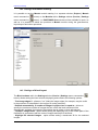
2.1. 2D Window
2D window is the main window used for creation and editing of 3D vector objects, TIN and
DEM. Once PHOTOMOD Сore is started 2D window displays the full scheme of the block.
The window content is managed by the Layer manager window (see the chapter Layer
manager)
There are two types of 2D windows - a window with full block scheme and a window with a
single stereopair. In order to open a new 2D window with block scheme use menu command
Windows | New 2D window (block); for a new 2D windows with stereopair - Windows |
New 2D window (stereopair) or the
button on the PHOTOMOD Core main toolbar.
Thus it is possible to work with several windows simultaneously if needed. Use command
Window | Refresh all 2D- windows to refresh all opened 2D windows contents.
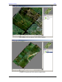
7
RACURS Co., Ul. Yaroslavskaya, 13-A, office 15, 129366, Moscow, Russia
PHOTOMOD 5.21
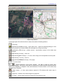
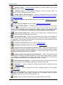
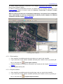
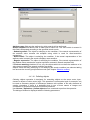
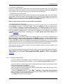
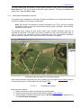
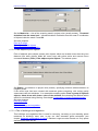
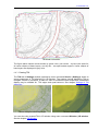
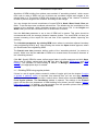
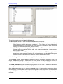
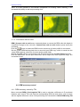
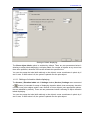
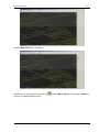
2D window with a block scheme and a block-wide DEM displayed
2D window for a stereopair with a TIN displayed
© 2011
8
Project processing
2011
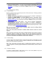
There are following icons in the 2D window tool bar:

(marker == mouse / F4 hot key) – turns on marker == mouse mode, in this case
mouse cursor is not displayed and only the stereomarker is used for work (see the
chapter marker == mouse mode).

(center on marker / F7 hot key) – scrolls image in such a way that the marker is
located in the middle of screen

(fixed marker / F6 hot key) – turns on/off the mode when marker is always located
in the middle of screen and while moving the mouse the image “moves” (see the chapter
Fixed marker mode).

(fixed marker parallax mode / Shift+F7 hot key) – toggles fixed parallax mode. The
command is available for the selected stereopair in 2D window.

(stereo mode / F9 hot key) – turns on/off stereomode. You can also change the
type of stereo by using (Service | Settings | Stereo option). Page-flipping and analog
stereomodes are available. See the chapter Stereomode. Icon is available for 2D window
for selected stereopair.

(change phase / F11) – for mono-mode loads left or right image of stereopair For
steromode changes the phase - replace left and right image in the window. Icon is
available for 2D window for selected stereopair

(adjust depth / F2 hot key) – adjusts stereopicture so that the X-parallax for marker
is equal to 0. See the chapter Stereoimage settings. Icon is available for 2D window for
selected stereopair.

(restore depth / F3 hot key) – cancels “adjust depth” operation (see above). See the
chapter Stereoimage settings. Icon is available for 2D window for selected stereopair.

– shows / hides Navigation and Manager windows, located to the right from the
main window (see the chapters Navigation window and Layer manager).

– shows / hides Navigation window (see the chapter Navigation window)

– (duplicated by the Ctrl+F8) shows / hides scrollbars
The rest of 2D window toolbar icons are used for image displaying (zooming, panning,
scrolling, etc (See the chapter Image displaying tools)
Shift+F8 hot keys open the panel used to setup image radiometric properties
See the chapter Brightness and contrast settings.
There are two common ways to select images for opening a stereopair in a 2D window from
the Block editor or Block scheme window:
 Select two overlapping images.

Select single image – in this case, a stereopair window is opened for the stereopair
formed by the selected image and the next image in strip, if there is one – or with the
previous image, if selected image is the last one in its strip.
2.1.1. Image displaying tools
Following icons of 2D window are used to zoom in / zoom out the image:

9
(* hot key) – one step zoom in;
RACURS Co., Ul. Yaroslavskaya, 13-A, office 15, 129366, Moscow, Russia
PHOTOMOD 5.21

(/ hot key) – one step zoom out;

(Alt-Enter hot key) – fit image to the window;

(Alt-1 hot key) – 1:1 zoom, when image cell corresponds to screen pixel.
For convenient image zooming in 2D window use the following hot keys:
 Alt-2 – 200% zoom
 Alt-3 – 300% zoom
 Alt-4 – 400% zoom
In order to change the current zoom level you can also use a slider
, for
selecting given zoom value. Mouse click along with Ctrl-Alt or Ctrl-Alt-Shift can be also
used to zoom in and zoom out respectively.
Besides, you can zoom in by zoom box along with pressed Ctrl-Alt and zoom out by zoom
box along with pressed Ctrl-Alt-Shift. For “panning” over the image move the mouse with
pressed Alt key and left mouse button, or use the scroll bars.
Navigation window is used for fast navigating into the needed part of the image.
2.1.2. Brightness and contrast adjustment
To change image brightness, contrast and gamma use sliders
,
,
bottom of 2D window. The panel is show or hidden by Shift - F8 hot keys.
located at the
A set of buttons located to the right from sliders is used for adjustment of image brightness,
contrast and gamma for color channels (red, green, and blue). You can adjust the
parameters either for each selected channel (the button corresponding to the channel color
should be pushed), or for all channels at the same time (when the button
is pushed).
When working in stereo mode (turned on by pushing the button
on 2D window toolbar
or by F9 hotkey) these operations may be performed either for each image of stereopair (to
turn on the right or the left image the button
or
or for the whole stereopair (when the button
is pushed).
correspondingly should by pushed),
To restore default BCG settings select the command Restore settings in context menu of
BCG panel.
These settings are kept only for current session; they are reset when either PHOTOMOD is
restarted or the 2D window is closed.
2.1.3. Saving 2D window image
The system provides the ability to save the 2D window scenes to TIFF file format (with the
pyramid). Full scene (not only the part visible inside the window) is saved, with regard to
settings in the Layer manager, current zoom and images order (set with the use Images zorder toolbar). For the 2D window (block scheme), besides the image, the tab data file with
the georeference data is also stored in the current geo coordinate system of block scheme.
© 2011
10
Project processing
2011
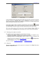
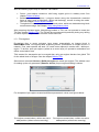
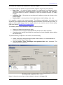
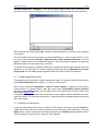
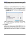
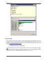
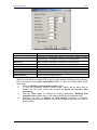
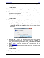
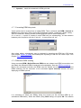
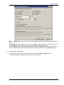
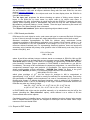
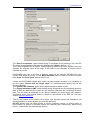
Use the Service | Save image menu command to save the scene. The Save scene window
is opened.
Settings for saving 2D window scene
Choose the window to save from the drop down list of all open 2D windows.
and
buttons are used to set needed window zoom. Set image resolution in dpi – to obtain
acceptable image print size.
To open and (optionally) print the image immediately after saving, use the Open created
image checkbox.
To save the scene, press OK button and select path and TIFF file name. At that, it saves the
whole scene, not just the visible fragment in a 2D window. Note that the bigger the zoom, the
larger the file and the longer it takes to save the scene.
Notes:
1. At least a small part of 2D window should be visible to save the scene.
2. In order to save stereo image, anaglyph stereo mode should be chosen (see the
chapter Stereo settings). It is also possible to save either left or right frame in mono
mode using the
Change phase button of the 2D window.
Image order in block scheme window may be adjusted with the Images z-order toolbar:
The toolbar contains the following tools:

11
– reset images order – set block to initial look;
RACURS Co., Ul. Yaroslavskaya, 13-A, office 15, 129366, Moscow, Russia
PHOTOMOD 5.21

– invert images order (invert order of images in all strips, and the strips order as
well;

– bring selected images to front;

– bring selected strips to front;

– invert images order in selected strips;

– invert strips order.
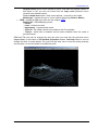
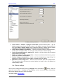
2.2. 3D Window
3D window is opened by Windows | 3D window command and used to 3D displaying of
DEM, TIN and vector objects at different angles. You can view the model in mono and
anaglyph or page-flipping stereomodes. Besides moving and rotation you can change Zscale of the model and use it for animated presentations. See also the chapters Vector
objects, DEM creation.
3D window uses OpenGL interface for objects displaying.
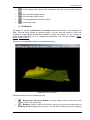
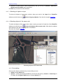
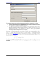
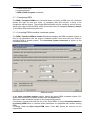
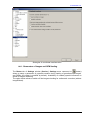
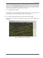
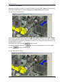
DEM shown in 3D window
3D window tool bar includes following icons:

– Moving (Alt- left mouse button hot keys). Used to move view area by left
mouse button or by arrow keys.

– Rotation. Used to rotate view area by using left mouse button along with an
Auxiliary round displayed on the screen. You can show / hide this round by pressing
© 2011
12
Project processing
2011
on the
icon by right mouse button. If the cursor is located inside the round the
model is rotated around global XY axes. Otherwise - around Z axis.

– Camera focal length. Used to change camera focal length.

– Perspective projection. Used to view the model in perspective projection.

– Orthogonal projection. Used to view the model in orthogonal projection.

– Scaling. One step zoom in / zoom out (duplicated by the mouse wheel).

– Scene center moving. Used to move scene center by moving the mouse along
with its left button pressed..

– Scaling along object’s Z-axis. Used to expand / constrain model along Z-axis
(duplicated by +/- hot keys respectively). The model is changed by moving the mouse
along with its left button pressed.

– Select. Used to select a model part by moving the mouse along with its left
button pressed. Duplicated by Ctrl and left mouse button) The selection is used for
detailed viewing

– opens pull-down menu used to manage modes of model or its part viewing:
– Full layer – total model displaying;
– Show selected – displaying of model selected part;
– Points – displaying model part as points;
– At least one point is selected – displaying the selected part of model in
such a way that all model elements belonging to the selection even
partially will be selected (for example is selected area includes a part of
vector object the total object will be selected).
– Fully selected – displaying selected part of model which includes only
elements fully covered by the selected area.

– animation Used to view the 3D model from all sides. The slider
is
used to change the speed of model rotation. Right mouse button click on the
icon
opens pull-down menu containing the items related to rotation modes and turning on /
off animation
– On/Off animation;
– Around X-axis – rotation around Х-axis;
– Around Y-axis – rotation around Y-axis;
– Around Z-axis – rotation around Z-axis;
– Change the direction – changing the direction of rotation;

– Mono. Monomode on-off (by default).

– Anaglyph stereo. Anaglyph stereomode on-off.


13
– Page-flipping stereo. Page-flipping stereomode on-off. Slider
, is
used to setup the depth. Use right mouse button to change the stereo phase
(Exchange buffers for stereopair).
– Default. Used to go back to preliminary settings.

– Refresh. Refreshes model state in case of changes in 2D window (automatic in
perspective projection mode).

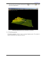
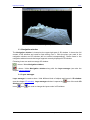
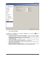
– Show point coordinates. Shows coordinates of a model point picked by
mouse. Besides you can measure distances in this mode. First and last point of the
line are selected by double mouse click. Current cursor coordinates are shown at the
upper left corner as well as the straight distance and the distance over relief. Also you
RACURS Co., Ul. Yaroslavskaya, 13-A, office 15, 129366, Moscow, Russia
PHOTOMOD 5.21
can set the first and last points coordinates by the
the current measured line.
icon. Use icon
to delete
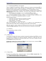
Measuring distances and cursor coordinates in 3D window
2.2.1. 3D window properties
3D window properties window is used to manage displaying layers. This window is
opened automatically when opening 3D window.
© 2011
14
Project processing
2011
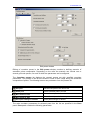
Use On option, to show / hide following objects and layers in 3D window, as well as for some
other settings:


15
TIN – TIN layer managing (see also the chapter Triangulated Irregular Network (TIN):
All – shows / hides all TIN layers;
Model type – TIN displaying mode:
– Points;
– Lines - wireframe model;
– Hypsometry - hypsometrical model;
– Texture - model with a rendered source raster (available when the raster is
georeferenced)
Imaging – changes layer color;
– Shows the layer as monochrome (Lightning) or by colors in accordance with
the Z-range (Color fill) When using Lightning mode you can change TIN color
from pull-down menu Layer color after TIN selection;
Objects – managing vector layers (See also the chapter Vector objects creation):
All – shows/hides all vector layers and objects;
RACURS Co., Ul. Yaroslavskaya, 13-A, office 15, 129366, Moscow, Russia
PHOTOMOD 5.21

Original colors shows vector objects by colors used while the objects creation. If
this option is Off, you can use colors from the Layer color pull-down menu
located at the window bottom;
Turn on depth test shows / hides vector objects, “covered” by the model.
Model type – selects the type of vector objects displaying (Vectors, Bezier);
DEM – managing DEM layer (see also the chapter DEM):
Model type – DEM displaying mode:
– Points;
– Lines - wireframe model;
– Hypsometry - hypsometrical model;
– Color fill - the model colored in accordance with Z-coordinate;
– Texture - model with a rendered source raster (available when the raster is
georeferenced).
DEM and TIN color can be changed by using the color you need fron the pull-down menu
(Layer color) in the bottom of 3D window properties window. Grid step slider is used to
change the level of model details. Thus use low grid step value to see the model generally
and increase it to see the details of its different parts.
Minimal grid step value
© 2011
16
Project processing
2011
Maximal grid step value
2.3. Navigation window
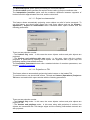
The Navigation window is located at the upper-right part of 2D window. It shows the full
content of 2D windiow and used for fast moving over it. Click the place you need in the
navigation window and 2D window will be scrolled correspondingly. Green frame in the
navigation window bounds the image fragment currently displayed in 2D window
Following icons are used to manage 3D window:
– shows / hides Navigation window;
– shows / hides Navigation window along with the Layer manager (see also the
chapter Layer manager).
2.4. Layer manager
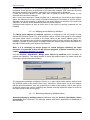
Layer manager is used to show / hide different kinds of objects and layers in 2D window
(see the chapter 2D window). Layer manager window is opened by
window tool bar.
Icons
17
and
icon of the main 2D
are used to change the layers order in 2D window.
RACURS Co., Ul. Yaroslavskaya, 13-A, office 15, 129366, Moscow, Russia
PHOTOMOD 5.21
Manager Layer
Use icon
, to show / hide following layers and objects in 2D window:
 Raster – shows / hides block images. See the chapter Project forming в in Project
creation User Manual.
 Block scheme – shows / hides the block scheme containing following objects:
- Names – names of project images;
- Stereopairs – stereopair outlines (red color);
- Strip outlines ;
- Images outlines.
 Triangulation points – shows / hides point of aerial triangulation (tie, check and ground
control points). See also Aerial triangulation User Manual. The aerial triangulation
points are displayed by using Orientation | Show as vector objects option, after that
you can save them as an ordinary vector file and use for example for DTM creation. See
also the chapter Creation of digital terrain model (DTM).
 Pre-regions – shows / hides pre-regions. Pre-regions are also the vector objects and can
be edited in a standard way. See the chapter Pre-regions.
 Grid – shows / hides regular grid used for DTM creation (see the chapter Grid creation),
including the following:
- Limits – shows/hides grid extents (red color)
- Nodes – shows/hides grid nodes (green color)
 TIN – shows / hides TIN (see the chapter TIN).
 DEM – shows / hides DEM (See the chapter DEM), including following items:
- Selection – selected fragment of DEM (if any)
- Frame – rectangular DEM border
- Raster – DEM itself.
 Vector – shows / hides vector objects (see the chapter Vector objects creation),
including following object types:
- Selected objects – selected vector objects;
- Labels – labels;
- Objects – all vector objects belonging to the current layer.
© 2011
18
Project processing


2011
Contours – smooth contour lines (see the chapter Contour lines). Contours layer in fact
is an ordinary vector layer and consist of the same object types.
Marker
You can setup displaying parameters of different object types by using Service / Settings.
See the chapter Parameters and settings.
Vector layers have an extension x-data, grid layers – x-grid, DEM layers – x-dem.
Symbol
, appeared by the mouse click on the layer name makes the layer “active” and
editable in 2D window. Symbol
means that layer is active but not-editable.
Symbol
shows “main” color of layer object. Double mouse click on the layer name opens
a window to set the parameters of layer displaying.
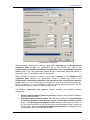
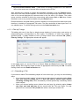
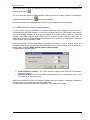
Color settings for the vector layer
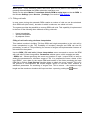
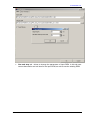
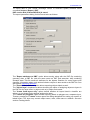
Right mouse button click on the layer name opens following pull-down menu:
Information – layer related information;
Close – closing selected layer.
19
RACURS Co., Ul. Yaroslavskaya, 13-A, office 15, 129366, Moscow, Russia
PHOTOMOD 5.21
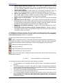
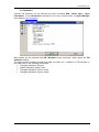
TIN related information
Vector pickets related information
2.5. Status panel
Status panel is located in the bottom part of PHOTOMOD Core window and shows
 Current marker coordinates in the project coordinate system.
 Error messages or messages about successful operation completing. For example –
«Bad point» or «Ready» when “placing” a marker on the surface by correlator (spacebar
hot key).
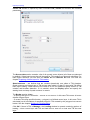
2.6. Object list window
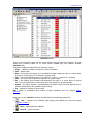
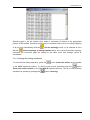
The list of vector objects loaded into a layer with classifier can be displayed in the Object list
window (Windows / Object list menu).
© 2011
20
Project processing
2011
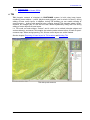
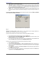
Selecting object in 2D window and in the list
Following objects are displayed in the Object list window: object numbers, codes, types,
attributes. If Select object on image option is On the mouse click on the record in the object
list selects the corresponding object on the image.
Object list can be saved to .dbf file by using
icon in the upper part of the window
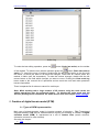
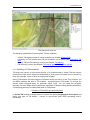
2.7. Raster map window
While the stereovectorization process you can load a map in a raster format which can help
for objects type identification.
Raster map window can be shown / hide by using Windows | Raster map option.
Any georeferenced raster image could be opened in the window in the following formats:
GeoTIFF, ERDAS Imagine, PCIDSK, and also TIFF, BMP, JPEG, NITF, GIF, JPEG2000,
accompanying by georeferencing text files PHOTOMOD GEO, ArcWorld (TFW, BPW,
JPW,…) or MapInfo TAB.
The initial raster image is georeferenced using known ground control points in Georeference
window of PHOTOMOD Montage Desktop module, see an appropriate User Manual.
21
RACURS Co., Ul. Yaroslavskaya, 13-A, office 15, 129366, Moscow, Russia
PHOTOMOD 5.21
Raster map window
In the upper part of the window there is button bar with the following buttons:
- close map
(duplicated by Ctrl-O hot keys) - open raster map – opens file selecting dialogue. If the
map to be opened is not located within the stereopair you will get a warning
(duplicated by F5 hot key) - refresh vectors – synchronize vectors on the raster map
and stereopair
(duplicated by / hot key) - zoom out
(duplicated by Alt-1 hot keys) - 1:1 zoom, when image cell corresponds to screen pixel
(duplicated by * hot key) - zoom in
(duplicated by Alt-Enter hot keys) - fit to page
- zoom scale
- relative thickness of the vector objects – the field is used for vector lines
thickness changing. The value in this field is a coefficient by which absolute object thickness
taken from Classifier is multiplied. Color and thickness of vectors shown on the raster map
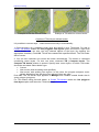
are taken from Classifier
- show vectors – to view vector objects (opened in 2D window) with raster map in
background
- grayscale – transfer color raster image into grayscale
- no raster – closes raster image but preserves vector objects if any
© 2011
22
Project processing
2011
- synchronize windows – synchronizes marker movement in 2D window and raster
image window. At that when marker is moving in one of these windows it is moving in
another too.
In most cases stereopair orientation is not the same as coordinate system orientation (on
raster map). That is why for more convenient work the map could be rotated in the following
ways:
- without rotation,
- turn at 90 degrees,
- turn at 180 degrees and
turn at 270 degrees. At that raster file is not changed and the rotation is executed “on the fly”.
All view settings, path to loaded map, and also Raster map window visibility, size and
location are saved automatically and restore at next PHOTOMOD session. At that map file
name is associated with stereopair name and thus different stereopairs will be opened with
appropriate raster maps.
3. Stereomeasurements
3.1. Stereomodes
To switch between stereomodes (Anaglyph or Page-flipping), described below use Service
| Settings | Stereo menu. Open 2D window for selected stereo pair using the
button of
the main PHOTOMOD Core tool bar or use the Window | New 2D-window (stereopair).
The icon
(Open new 2D-window for selected stereopair) of the main PHOTOMOD
tool bar is used to open a stereopair for stereoprocessing.
To turn ON/OFF stereomode in 2D window click the icon
in upper menu of 2D window
or F9 hot key. See the details on hardware settings of your PC for convenient working in
stereomode in PHOTOMOD Overview User Manual.
3.1.1. Anaglyph glasses
Anaglyph stereoimage is formed by visualization of the left and right images of the stereopair
“beyond” red and blue filters. To view such a picture you should use special anaglyph
spectacles with red and blue glasses. Anaglyph stereomode requires no special equipment
but it is not completely good for working with color images. Another disadvantage is that the
picture gets a bit darker when viewing through the filters.
Note. Anaglyph stereo is available only for HighColor or TrueColor display mode of
your monitor
3.1.2. Shutter glasses
Shutter glasses are liquid crystal glasses synchronized with the vertical refresh rate of the
monitor. PHOTOMOD system supports page-flipping stereomode when working with shutter
glasses. Refer to PHOTOMOD Overview User Manual for the details about using stereo
glasses and other special equipment for stereoprocessing.
Page flipping (“frame by frame”) display mode provides the most high quality stereo picture
because it uses full frames instead of semi-frames. Left and right images of the stereopair
are displayed one by one synchronously with the frames switching. The shutter glasses are
23
RACURS Co., Ul. Yaroslavskaya, 13-A, office 15, 129366, Moscow, Russia
PHOTOMOD 5.21
synchronized with the monitor vertical refresh rate and allow you to see them
“simultaneously” and make stereo measurements. For working in page-flipping mode you
should use a monitor with a good enough vertical refresh rate (at least 120 Hz) and an
appropriate video card.
3.2. Stereopair selection
To open new stereopair 2D-window select images which make a stereopair using block
scheme or Block editor window. If only one image is selected the stereopair composed of
the selected image and the left adjacent one in the strip (if the last image of the strip is
selected, right adjacent image will be opened) will be opened in the stereopair 2D-window.
Execute the menu command Windows | New 2D window (stereopair) or press the button
on the main toolbox PHOTOMOD Core. Stereopair 2D window will open.
The following ways to change the stereopair are provided in the stereopair 2D-window:
– toolbox Change stereopair (menu Windows | Toolbars | Change stereopair), which
contains following tools:

– open stereopair one image backward in the strip (duplicated by the menu
command Windows | Previous stereopair).

– open stereopair one image forward in the strip (duplicated by the menu
command Windows | Next stereopair).

– open stereopair one strip upward (duplicated by the menu command Windows
| Stereopair up).

– open stereopair one strip downward (duplicated by the menu command
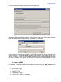
Windows | Stereopair down).

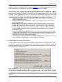
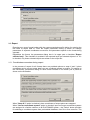
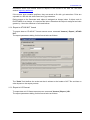
– select an arbitrary stereopair (duplicated by the menu command Windows |
Select stereopair). It opens arbitrary stereopair selection window, where on the Tab
Adjacent Stereopairs the list of all possible adjacent stereopairs is displayed
(including stereopairs composed of non-adjacent images or images from different
strips provided that they are overlapping), the tab All images displays the list of all
images in the project. The images of the opened stereopair are checked. Select the
stereopair using one of the tabs and press OK.
© 2011
24
Project processing
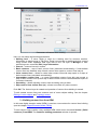
2011
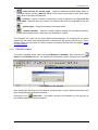
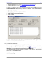
Arbitrary stereopair selection
The menu command Windows | Open inverted stereopair allows swapping opened
stereopair images (upper down, lower up).
3.3. Operating marker
3.3.1. Moving marker mode
icon (fixed marker) or F6 hot
Moving and fixed marker modes are turned on/off by the
key.
Use mouse or keys with arrows to move the marker in XY plane and PgDn, PgUp keys or
the mouse wheel to move it along Z axis.
Use spacebar key to place the marker on the model surface automatically by the correlator.
If the correlator fails a message Bad point appears in the Status bar accompanied with a
sound (see the chapter Correlator parameters).
Note that the step of marker moving along Z axis is discrete and defined directly by the
current zoom level. For fast marker moving along Z axis use mouse wheel along with
pressed Alt key.
Use Service | Settings | Marker (stereopair) window to setup marker shape, size and color,
see the chapter Marker settings.
3.3.2. Fixed marker mode
25
RACURS Co., Ul. Yaroslavskaya, 13-A, office 15, 129366, Moscow, Russia
PHOTOMOD 5.21
Moving and fixed marker modes are turned on/off by the
icon (fixed marker) or F6 hot
key. In case of fixed marker the marker is always located in the center of screen and its X
parallax is equal to 0.
During vectorization you move the images of stereopairs by the mouse or arrow keys (, ,
, ) in plane and by PgDn, PgUp keys or the mouse wheel by Z. Use spacebar key to
place the marker on the model surface automatically by the correlator. If the correlator fails a
message Bad point appears in the Status bar accompanied with a sound (see the chapter
Correlator parameters).
This mode is familiar for operators experienced in working with analytical stereo devices.
Another advantage is a smooth roam vectorization with a constant image auto scrolling.
Use Service | Settings | Marker (stereopair) window to setup marker shape, size and color,
see the chapter Marker settings.
3.3.3. Marker = mouse mode
This mode (turned on by clicking the icon
marker == mouse or F4 hot key) “removes”
mouse cursor from the screen. In this case any mouse movement causes the corresponding
stereomarker moving without mouse click. The mode is useful for digitizing polylines and
polygons.
Use Service | Settings | Marker (stereopair) window to setup marker shape, size and color,
see the chapter Marker settings.
3.3.4. Snap-to-ground mode
Marker may automatically follow the relief elevation in Snap to ground mode during
vectorization. The snap-to-ground mode is toggled with toolbar button
toolbar, Т hotkey or Edit | Snap to ground menu command.
of the Vectors
In this mode, the operator moves the marker in XY-plane, and marker height is adjusted
automatically by the correlator (see the chapter Correlator settings). If correlation in the given
point fails, the marker may be positioned manually with mouse wheel or PgUp, PgDn keys.
3.3.5. Streamline mode
Objects in 2D window may be created by freehand drawing with left mouse button pressed,
adding points automatically when distance from the previous point exceeds the given
threshold (see the chapter Settings of vector objects displaying). The mode is toggled by the
button on Vectors toolbar, Y hotkey or Edit | Streamline mode menu command. The
first point of the line is created with Insert key, further points are added automatically when
either the marker is moved with left mouse button pressed, or each time the mouse button is
clicked, given the above-mentioned threshold condition.
In order for this mode to work, the line or polygon drawing mode must be chosen (line (L) or
polygon (C) code selected in the classifier in case it is used).
© 2011
26
Project processing
2011
3.3.6. Fixed Z mode
If you need to draw a vector line at a constant Z level use Fixed Z mode. To set a Z value,
place the marker to a correct position and select menu command Edit | Fix marker by Z or
press Alt-Z shortcut or click the icon
in the Marker window opened by the icon
of
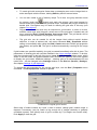
the main panel or by the command Windows | Marker window. You can also enter the Z
value in Z field of Marker window in order to move marker appropriately.
This mode is useful for example for digitizing the contour lines
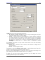
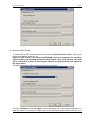
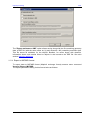
3.3.7. Marker window
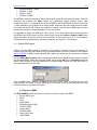
Marker window (opened by the icon
Marker window of the main panel or by main
menu command Windows | Marker window) shows marker coordinate in the project
coordinate system and in WGS 84 latitude-longitude. Besides viewing the values you can
enter them from the keyboard and the marker will be moved accordingly after pushing the
Apply button.
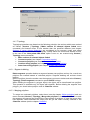
Marker window
There are the following icons at Marker window button bar:

- apply immediately – change marker position right after entering coordinate values
without pressing Enter key

- apply – moving marker in accordance with entered coordinate values

- canceling coordinate values input

- more decimal places – increasing number of decimal places in coordinate values
at 1

- less decimal places – decreasing number of decimal places in coordinate values
at 1

27
- fix marker by Z – Duplicated by Alt-Z shortcut. In this case Z-marker coordinate
can not be changed. See the chapter Fixed Z mode.
RACURS Co., Ul. Yaroslavskaya, 13-A, office 15, 129366, Moscow, Russia
PHOTOMOD 5.21
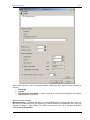
Marker latitude / longitude on the WGS 84 ellipsoid are displaying at the bottom part of the
window. There are flowing icons in there:

– coordinate display format - changing the format of latitude-longitude values

– increase display precision – more decimal places in coordinate values

– decrease display precision – less decimal places in coordinate values

– format for units and hemisphere display

– copy coordinates to clipboard
3.3.8. Type of snapping
When working in the snap mode the marker is moving only “along” the existing vector
objects (points, vertices or segments). It is useful when you need to create an object that
spatially coincides with some existing objects. For example when you vectorize electric
power line connecting existing piers (point objects). Snapping can be applied to the vector
objects belonging to all layers displaying on the screen (not only to the active one). Use
options of Edit / Snapping menu to switch between following snapping modes:
 3D snapping to vertex (the
icon or V hot key). In this mode the marker “jumps” from
one vertex to another. When you click somewhere on the image, the marker moves to the
nearest vertex or point.
 2D snapping to vertex (the
icon or B hot key). In this mode the marker “jumps” from
one vertex to another and XY marker coordinates coincide with XY coordinates of the
vertex. Marker Z coordinate at that will be preserved.
 3D snapping to line (the
icon or N hot key). In this mode the marker moves along
existing vector objects lines (segments) keeping all XYZ coordinates. When you click
somewhere on the image, the marker moves to the nearest vector object.
 2D snapping to line (the
icon or M hot key). In this mode the marker moves along
existing vector objects lines (segments) just in XY plane. Marker Z coordinate at that will
be preserved.
2D snapping is used when the creating object must spatially coincide with an existing one
only in XY plane. For example you want to “draw” an extension to some building at the other
Z level.
Hot keys listed above are used for quick setting snapping on (the key is pressed down) and
off (the key is released).
Note: It is possible to draw part of the object (for example, part of the polyline) on the
existing object if the snapping mode is turned on during the object creation. As a
result, two (or more) of the object will have the geometrically coincided parts of
objects.
3.4. Adjusting stereoimage
No matter which kind of stereomode you use, you need to adjust the stereo image to get the
best stereo effect in some particular image region. This is especially important when you
work with “deep” images, i.e. those having big variations in X parallax. To adjust the stereo
image, do the following:
 place the stereo marker on some point of the region of interest manually or by snap to
ground operation (see the chapter Operating marker);
© 2011
28
Project processing
2011
 press F2 key or click the
icon of 2D window.
The program will rebuild the stereo image to set X parallax in the point of stereo marker to
zero value. So the best stereo picture is in the area around the marker.
Press F3 key or click the
icon of the main panel to restore the stereo depth.
You can change stereomode phase (i.e. swap over left and right images) using F11 key or
the button
in 2D window.
Besides, you can use Shift-PgUp/PgDn or Shift-mouse wheel shortcuts to change stereo
image depth.
3.5. Measurements over the model
of the main panel or by
The mode of measurements (turned on by pushing the icon
selecting menu item Windows | Measure mode) is useful for some temporary stereomeasurements – when for example you need to know the height of a building or a tree.
There are exactly the same tools as for the 3D line creation – Insert key to add a vertex,
PgUp, PgDn keys or mouse wheel to move marker by Z and the mouse or arrow keys to
move marker in plane. The line appeared is a temporal one: it disappears after you quit
measurements mode (by releasing the same icon
See also the chapter Vector objects creation.
29
or turning off the menu item).
RACURS Co., Ul. Yaroslavskaya, 13-A, office 15, 129366, Moscow, Russia
PHOTOMOD 5.21
Measurements window
Measurements window displays following values:












X – marker X geodetic coordinate
Y – marker Y geodetic coordinate
Z – marker Z geodetic coordinate
Xp – marker geodetic X-coordinate in previous point
Yp – marker geodetic Y-coordinate in previous point
Zp – marker geodetic Z-coordinate in previous point
dX – marker geodetic delta X when drawing a “rubber line”
dY – marker geodetic delta Y when drawing a “rubber line”
dZ – marker geodetic delta Z when drawing a “rubber line”
S – length of the current segment of the “rubber line”
D – length of the current segment projection on XY plane
dZ/D – the value of the current segment slope

– direction of the current segment relatively to X axis

– direction of the current segment relatively to the previous one

– vertical angle of the current segment
If necessary you can input geodetic coordinates X, Y or Z into appropriate fields of
Measurement window and marker will move into the point with specified coordinates after
pressing Enter.
4. Vector objects
© 2011
30
Project processing
2011
Vector objects (points, lines or polygons) are contained in a vector layer of two possible
types: vector layer and vector layer with classifier.
4.1. Vector layer
A vector layer containing vector objects that have no attributes attached. In order to create
vector layer use command Vectors | Create layer. As a result a new layer called Vectors
appears in the Layer manager panel. Vector layer has a number and an extension “x-data”
See also the chapter Layer manager.
4.2. Vector layer with classifier
4.2.1. Creating vector layer with classifier
Vector layer with classifier contains vector objects attached to PHOTOMOD hierarchical
classifier (in fact it is kind of database table). In order to create vector layer with a classifier
you should use Vectors | Create layer with classifier command. As a result As a result a
new layer called Vectors appears in the Layer manager panel. Vector layer has a number
and an extension “x-data”. The classifier window will be opened automatically. See also the
chapters Layer manager and Classifier
4.2.2. Classifier
All vector objects created in the vector layer with a classifier are attached to the classifier
records. The classifier is a database table, containing codes and attributes used to thematic
classification of the vector objects. Use Windows | Classifier option to open Classifier
window.
31
RACURS Co., Ul. Yaroslavskaya, 13-A, office 15, 129366, Moscow, Russia
PHOTOMOD 5.21
Classifier window
There is a list of thematic layers of the current project in the left part of the window. The right
window part contains codes list of vector objects (Codes tab) and objects attributes
(Attributes tab).
Codes tab contains the table with the following columns:
 Visible – visibility of objects with given code in 2D window
 Code – object code
 Name – the unique text string up to 64-character length created to refer to a vector object
or group of vector objects. For example “Unpaved road”
 Type – one of the following types of an object: P – point, L – polyline, C – polygon
 Color – the color used to show the object on the raster image
 Size – the floating point number that determines the size of a vector object in ground
units. For points this feature controls the size of the symbol on a raster image;
 Symbol – the ASCII symbol, corresponding to the object code (for point objects only), it
could be selected from the standard symbol library
 Q-ty – quantity of objects of given code
Attr. – option of availability and number of object attributes (see the chapter Adding
attributes
Upper icons of the Classifier window are intended for the following operations:

- new – creates new Classifier after closing the loaded one (see the chapter
Classifier creation)

- open – opens existing classifier

- save as – saves changes
© 2011
32
Project processing
2011

- classifer import – opens standard dialogue for import codes to the current
Classifier (see the chapter Classifer import)

- classifier export – opens standard dialogue to input file name (with *.rsc
extension) for export classifier to VectOr format

- assign code to selected objects – allows to change the code of the objects
selected in 2D window (see the chapters Attaching vector objects to classifier records и
Changing object types)

- select all objects with current code (see the chapter Selecting objects with
current code)

- select all group objects (see the chapter Selection of all layer objects)

- select all visible objects – if visibility of some objects is OFF (by mouse click on
the “eye”
icon rightward from code or layer name) you can select the rest visible
objects using this button. Use such selection to export a group of all selected objects
using menu command Objects | Import/Export | Format | Export selected objects

- show selected object code – allows to show object code in Classifier when an
appropriate vector object is selected in 2D window

- show selected code – used to scroll down the list of codes in the Classifier in
such a way that the code of the object selected in 2D window is shown in the Classifier.
This operation is useful when selected code is at the bottom of the long Classifier list and
is invisible without scrolling down the list

- set label for current code (see the chapter Labels creation)

- set label for all group codes (see the chapter Labels creation)

- assign elevation from attribute to selected code – if after vector objects import
their heights are located in Classifier attributes, you can assign these heights to object
vertices, by pushing this button. The operation is used during contours import from
MIF/MID and SIT (Map 2005, VectOr) formats

- assign elevation from attribute to selected layer – if after vector objects import
their heights are located in Classifier attributes, you can assign these heights to vertices
of all objects in selected layer, by pushing this button. The operation is used during
contours import from MIF/MID and SIT (Map 2005, VectOr) formats

- show codes from sublayers – if pushed and some layer in Layers list is selected
then all vector objects codes available on this layer is shown in codes list

- edit code… – opens a window for editing selected code or attribute (see the
chapter Classifier editing)

- add code… – opens a window for new code or attribute creation (see the chapter
Classifier editing)

- add code to favorites – adds selected code to another codes list, which simplifies
searching for frequently used codes. Favorites list is visualized when the option
Favorites in lower left corner of the Codes table is ON

33
- delete – allows to delete selected code or attribute after some warning
RACURS Co., Ul. Yaroslavskaya, 13-A, office 15, 129366, Moscow, Russia
PHOTOMOD 5.21

- select hot key for current code – opens an additional window which allows to
associate chosen hot key (Shift-1,2,3,4,5) to the current vector object code, that makes
easy quick code call in the Classifier

- find text – opens a window of searching record in selected mode: By code, By
code name. Type the value you need in the selected text field and push OK to start the
search


- search again – further code search in selected mode
- default classifier – sets the currently loaded classifier as the default classifier,
loaded automatically when a new layer with classifier is created.
The Classifier is a useful tool for vector objects systematization. For example you can select
objects with the same code and delete them or show them with some particular color. Vector
objects codes are using also for vectors export to exchange formats see the chapter Export
of vector objects
4.2.2.1. Classifier creation
To create a classifier select menu command Windows | Classifier, then click the icon
(New) in the Classifier window. You should start with layers creation (left part of the window)
Creating layers in the classifier
After creating the list of layers of the objects, create the list of vector objects included to each
layer along with their codes and attributes.
Pushing the icon
(Add code…) for adding records to the classifier (in the right part of
the window) opens the following window:
© 2011
34
Project processing
2011
New code creation
Use Code field to input the unique object code, then Code name field for object name and
also assign to the object its type and following features to display it in 2D window:
• For point object (P type) – symbol (from popped up standard symbol library) symbol
color (from popping up standard MS Windows palette (Win button) or from AutoCAD
palette (ACI button)) and size (in point units in the appropriate field). Please note that
symbol size could be changed only for True Type fonts.
• For polyline (L type) and polygon (С type) – line color (from popped up standard MS
Windows palette (Win button) or from AutoCAD palette (ACI button)) and its style in
the window appearing by pushing the appropriate button:
Layer style selection
Here select line type, style of its filling, its width and shape of its end using appropriate
options. Selected line style is preserved during line objects export into DXF and DGN
formats, see the chapter Export of vector objects.
When all necessary options are set, push OK and object code will be added to the layer
which name is selected in the Layers list or to the root directory if the objects are not divided
into layers.
So you can create codes for different objects which supposed to be extracted and add them
to the Classifier with possible classification into thematic layers.
Once the Classifier is created save it using the icon
(Save as) to the resource with
specified name. The classifer will be opened automatically for all PHOTOMOD further
sessions. If you need to open another classifier click the icon
(Open) to get a list of
available resources with classifier. Also you can create new classifier using an imported one
(see the chapter Classifier import).
35
RACURS Co., Ul. Yaroslavskaya, 13-A, office 15, 129366, Moscow, Russia
PHOTOMOD 5.21
Besides, while importing vector objects to PHOTOMOD from exchange formats their codes
could be also imported into a new classifier or added to the existing one depending on the
appropriate options, see the chapter Import of vector objects.
4.2.2.2. Classifier editing
In open Classifier, you can edit Layers list in the left panel and Codes and attributes list in
the right one. Layers list editing is described in the chapter Adding attributes.
Use the tool bar above the Layers list for the following operations:

(duplicated by F2 key) edit layer name… – allows to change selected layer (folder)
name. Press Enter to save changed name or Esc to cancel editing

add layer… – opens a window for new layer (folder) name input

delete layer – deletes selected layer (folder) from Layers list
Use the same buttons of upper button bar for Classifier editing in the right part of window:

show layer with sublayers – shows objects in layer including those in sub-layers

hide layer with sublayers – hides objects in layer including those in sub-layers

edit code… – (or double click on the code record selected) opens a dialogue
described in the chapter Classifier creation


add code… – opens a dialogue used to create a new record in classifier
add code to favorites – adds selected code to another codes list that simplifies
searching for frequently used codes. Favorites list is visualized when the option
Favorites in lower left corner of the Codes table is ON

delete code – deletes selected classifer record
Popup menu opened by right mouse button click on Layer list allows to perform the following
operations with the list:




Copy layer – copies the layer selected to the clipboard
Paste layer – pastes the layer copied from clipboard into Layers list
Move layer – moves the layer taken from clipboard into Layers list or inside selected
layer (as a sublayer) and removes it from the previous location
Show layer with sublayers – opens in 2D window objects with codes, which belong

to the active layer (the icon
leftwards from layer name becomes active at that)
Hide layer with sublayers – hides in 2D window objects with codes, which belong to
the active layer (the icon
leftwards from layer name becomes inactive at that).
4.2.2.3. Import of classifier
In order to import the classifier use the icon
(Classifier import) which opens the
dialogue for file selection. There are several possibilities of vector objects codes import when
creating the classifier or adding codes to the current one:
- import of PHOTOMOD VectOr classifier (.rsc files). PHOTOMOD VectOr uses a
library of map symbols (classifier) to display and print out digital map objects. The set
© 2011
36
Project processing
2011
of standard classifiers (.rsc files) related to different map scales is included to
PHOTOMOD distribution file set and stored in \VectOr\RSC directory by default. Use
the PHOTOMOD classifier, corresponding to the VectOr selected classifier to
associate the objects created in PHOTOMOD with the appropriate symbols in
PHOTOMOD VectOr. In that case the table code will be equivalent to the classifier
code for the exact object type. If you want to automatically create a PHOTOMOD
classifier based on the VectOr classifier you should select type of file as RSC and
select source classifier in the Import window.
import of PHOTOMOD VectOr classifier, associated with existing map (.sit and .map
files) to PHOTOMOD classifier (see also the chapter Import from VectOr).
-
After selecting the file to be imported define the name and path for the output resource with
classifier in PHOTOMOD format.
Besides, while importing vector objects to PHOTOMOD from exchange formats their codes
could be also imported into a new classifier or added to the existing one depending on the
appropriate options, see the chapter Import of vector objects.
4.2.2.4. Adding attributes
For each vector object code you can add some auxiliary attributes using the Attributes tab in
the Classifier window with the following parameters:
 Name – field name
 Type – field type (see below)
Text
Integer
Smallint
Decimal
Float
Data
Logical


- text attribute either without parameters (in this case the length of the
attribute is the length of its value, but not greater than 32767) or with one
parameter, specifying the fixed length of the text;
- 4 byte integer (without parameters);
- 2 byte integer (without parameters);
- fixed decimal point attribute with two parameters. The first parameter is the
total attribute length in bytes, the second - the number of digits after the
decimal point;
8 bytes float attribute (without parameters);
unformatted attribute with one parameter specifying the attribute length in
bytes;
logical attribute with possible values 0 or 1 (without parameters).
Size (bytes) – for numeric fields is defined automatically, otherwise should be defined by
user (for text fields for example)
Precision – number of decimal places for “float” attributes
To edit or create attribute table click the icon
(Edit attribute) of the upper button bar in
Classifier window, when Attributes tab is selected. After that you will get the window for
editing the parameters of attributes of record selected:
37
RACURS Co., Ul. Yaroslavskaya, 13-A, office 15, 129366, Moscow, Russia
PHOTOMOD 5.21
Adding the attribute
To assign attribute value to attribute with integer type use the panel Values list:
Following icons are used to:
- add – opens a window for input of attribute name and value
- delete – deletes attribute value from the list
- edit – opens a window for editing of attribute name and value
- clear – deletes all attributes values from the list.
Besides, on Attributes tab you can use the following operations:

© 2011
- add attribute – opens a window for creating a new attribute record
38
Project processing

2011
- delete attribute – deletes current attribute field
Use the buttons on the left side of Attributes tab to perform the following operations with
object’s attributes:
- move up – moves the record to the topmost position
- upper – moves the record on one position up
- lower – moves the record on one position down
- move down – moves the record to the bottommost position
- invert attributes order – rearranges the list in the reverse order.
On the Attributes tab of classifier use popup menu opened by right mouse button click,
which contains the following commands:
Copy attribute – copies selected attribute to the clipboard
Copy all code attributes – copies all attributes of the current code to the clipboard
Paste attribute – pastes attribute(s) from the clipboard to the attributes list of the current
code. It is used to remove unnecessary attributes from other codes of the Classifier. If
you need to move attributes from one Classifier to another, paste the attribute from
clipboard to text file. Then open another Classifier, select the code and paste the attribute
into code selected.
▪ Get Z from attribute – assigns Z coordinate to the objects of selected code. The
coordinate is either taken from imported file or input by the user.
To enter the attribute values use the command Windows | Objects attributes. Select
Attributes tab in the Object attributes window appeared and enter attribute values in the
Values column after clicking the grey field.
▪
▪
▪
39
RACURS Co., Ul. Yaroslavskaya, 13-A, office 15, 129366, Moscow, Russia
PHOTOMOD 5.21
Vector object attributes
To start editing the attribute value in table cell, select it by mouse. To complete editing and
save the input value, press Enter or just click the next cell with attribute value. Press Esc to
cancel editing and exit.
The following operations are available for attribute’s values:


Copy to clipboard – allows to copy attribute’s values of the object to the clipboard using
menu command Edit | Objects | Copy attributes values if the object is selected in the
current layer
Paste from clipboard – object’s attribute value, which was copied to the clipboard by
previous operation, could be assigned to the one or several selected objects of active
vector layer. Use menu command Edit | Objects | Paste attributes values to add
attribute’s values to the attributes with the same names.
In Object attributes window you can create an additional attributes for the objects selected,
using Additional attributes tab (see the chapter Adding additional attributes).
4.2.2.5. Additional attributes
Besides the attributes associated with a code in the classifier (see the chapter Adding
attributes) the unique attributes for the selected object could be created. At that all objects
associated with some code in the classifier will have common attributes defined in the
classifier, but each of them may have some additional unique attributes. To create a table of
additional attributes you should do the following:
 select vector object or group of objects (see the chapter Objects selection)
 select menu command Windows | Object attributes. First two tabs of Object attributes
window show a record in the classifier and object attributes
© 2011
40
Project processing

2011
select the Additional attributes tab and create a table of additional attributes in exactly
the same way as for classifier attributes (see the chapter Adding attributes).
Following icons are used to create additional attributes table:

- delete all additional attributes for selected objects – deletes all
additional attributes for selected objects

- delete same additional attributes for selected objects – deletes
additional attributes which are common for selected objects

- add additional attribute – opens a window for creating a new additional
attribute

- delete additional attribute – deletes current additional attribute
- edit additional attribute – opens a window for editing current additional
attribute
select the fields by the mouse and enter the attribute values to associate the additional
attributes with the selected vector object.


Additional attributes
To start editing the attribute value in table cell, select it by mouse. To complete editing and
save the input value, press Enter or just click the next cell with attribute value. Press Esc to
cancel editing and exit.
Note. Additional attributes could not be exported in PHOTOMOD VectOr module unlike
usual object attributes
4.2.2.6. Labels creation
Each vector object could be supplied with special sign (label) displayed in 2D window as a
label to the point object or to the linear object vertex (if the appropriate option in module
settings is ON, see the chapter Labels displaying settings). This label could be also exported
to DXF file of AutoCAD system. To assign the label, select object code in Classifeir and
push the icon
41
(set label for current code) in the upper button bar.
RACURS Co., Ul. Yaroslavskaya, 13-A, office 15, 129366, Moscow, Russia
PHOTOMOD 5.21
Label creation
In the list appeared choose the label source (taken from the values of columns of the layer
selected in codes list). If Attribute value is selected, Attributes pop down list is available to
select the label content, which will be visualized in 2D window or AutoCAD program after
export of the objects of selected code to DXF file.
If you need to assign a label to all objects of selected layer push the button
(set label
for all group codes). At that the label is assigned to all objects in selected layer, that is why
you should assign it only after creation of all layer objects just prior their export to DXF.
After vector objects export to DXF format (menu command Vectors | Export | DXF) and
opening this layer in AutoCAD system these objects will be shown with the label assigned.
4.2.2.7. Attaching vector objects to classifier
The classifier records may be attached to vector objects in two ways:
 while the vector object creating. Select the record you need in the Classifer window
and start the vectorization. The code will be assigned automatically
 attaching record to an existing object. Select an object or a group of objects in 2D
window and code to be assigned in the Classifier and click the icon
selected objects). See the chapter Objects selection.
(assign code to
See also the chapter 6 Creating vector objects and Changing object type.
4.2.2.8. Object list
The list of vector objects of the current project can be displayed in the Object list window
(Windows / Object list menu).
© 2011
42
Project processing
2011
Selecting object in 2D window and in the list
Following objects are displayed in the Object list window: object numbers, codes, types,
attributes. If Select object on image option is On the mouse click on the record in the object
list selects the corresponding object on the image.
Object list can be saved to .dbf file by using
icon in the upper part of the window
4.3. Vector objects creation
3D vector objects (points, lines, polygons and CAD-objects) are used for both vector maps
and DTM creation. There is also a special automatically created vector object - pre-regions)
4.3.1. Vector object types
PHOTOMOD works with 3D vector objects of the following types:
 point – a point in space, defined by X, Y, Z coordinates
 line (polyline) – a set of XYZ points (vertices) connected by straight lines (segments).
The polyline may be either closed or unclosed. In case of closed polyline its first and last
vertices are spatially coinciding
 polygon – an area object. The polygon is closed automatically after finishing its creation.
During polygon creation its first and last vertices are coincide spatially and are edited
simultaneously.
 CAD objects – standard geometric figures, see the chapter Creating CAD-objects.
4.3.2. Vector objects creation
43
RACURS Co., Ul. Yaroslavskaya, 13-A, office 15, 129366, Moscow, Russia
PHOTOMOD 5.21
All marker related operations, described in the chapter Operations with marker are used
during vector objects creation.
In order to start the vectorization process you should select an existing vector layer in the
Layer manager window or create a new one (Vectors | Create layer or Vectors | Create
layer with classifier)
Note: In order to increase the vectorization productivity, use special 3D or multibutton
mice, hand wheels as well as programming of ordinary mouse buttons for different
operations (see the chapter Mouse settings)
Creating vector objects
4.3.2.1. Point creation




If the classifier is available select the point object you need in the classifier
If you work with a layer without classifier activate point creation mode (by pressing P (point object creation);
key or using the icon
locate the marker in 2D window to the position you need (see the chapter Operations with
marker);
press Insert to add a point.
4.3.2.2. Polyline creation


If the classifier is available select the polyline-type code you need in the classifier
If you work with a layer without classifier activate point creation mode (by pressing L key or using the icon
© 2011
(polyline object creation);
44
Project processing
2011

for each polyline vertex:
-locate the marker in 2D window to the position you need (see the chapter Operations
with marker);
-press Insert key to add the vertex;
 press Enter or Esc to finish polyline creation.
Use the Vectors | Topology | Close polyline menu command (duplicated by the Shift-C
keyboard shortcut) after the last vertex entering to close polyline in the process of its
creation. Description of orthogonal polyline creating see chapter Orthogonal objects creation
mode.
4.3.2.3. Polygon creation


If the classifier is available select the polyline object you need in the classifier
If you work with a layer without classifier activate point creation mode (by pressing G -
(polygon object creation);
key or using the icon
for each polygon vertex:
-locate the marker in 2D window to the position you need (see the chapter Operations
with marker);
-push Insert to add the vertex;
 press Enter or Esc to finish polygon creation.
See also the chapter Orthogonal objects creation mode about buildings vectorization.

4.3.2.4. Creating orthogonal vector objects
Vectorization of some objects (buildings, for instance) requires drawing line segments at the
right angle. To turn on such rectangle mode use the following ways:
 Press the A key if you would like to draw some part of polyline in rectangle mode.
Press and keep holding down the A key before adding next segment and release this
key to continue the line in usual mode

Push the icon
vectorization mode.
of the main panel to turn on the constant “orthogonal”
Rectangle mode is used for creating both polylines and polygons (see the chapters Polyline
creation and Polygon creation).
If you need to create a closed orthogonal polyline, use Vectors | Topology | Close polyline
command (Shift-С hot key) after entering last polyline vertex, and next press Esc key.
4.3.2.5. CAD-objects creation
In order to create vector objects of standard geometric shape, use a menu, opened by the
command Edit | Vectors create mode | CAD objects.
CAD objects creation window
45
RACURS Co., Ul. Yaroslavskaya, 13-A, office 15, 129366, Moscow, Russia
PHOTOMOD 5.21
Push the button
in this menu to open lower part of the window containing settings for
each object type. The drop-down list is used for parameters selection, described below.
The following buttons are used to choose the type of the object to be created:
▪
Ellipse – if the button is pushed, you can start ellipse creating. Press Insert,
then drag ellipse’s semi-axis by mouse to needed size and click Insert once more to
create ellipse.
▪
Circle – if the button is pushed, you can start circle creating. Press Insert. If the
circle is build by two points, second press of Insert indicates the diameter of the
circle. If the option Center, radius is selected, second press of Insert indicates the
radius of the circle. If the circle is build by two points, press Insert three times to
indicate three points, lying on the circle.
▪
Arc – if the button is pushed, you can start arc creating. Press Insert, and then
move the marker to specify the arc’s radius. Press Insert once more, then drag a
polygon of needed size by mouse.
▪
Sector – if the button is pushed, you can start sector creating by pressing Insert.
The second pressing of Insert specifies sector’s radius, which could be both fixed
and changeable, depending on the option selected in drop-down list. Then drag a
polygon of needed size by mouse.
▪
Segment – if the button is pushed, you can start segment creating by pressing
Insert. The second pressing of Insert specifies the beginning and the end of
segment’s arc or another parameter depending on the option selected in drop-down
list. Then drag a polygon of needed size by mouse.
▪
Rectangle – if the button is pushed, you can start rectangle creating by pressing
Insert. Then indicate three rectangle vertices by Insert, or another points of the
rectangle depending on the option selected in the drop-down list. Then drag a
polygon of needed size by mouse.
▪
Polygon – if the button is pushed, you can start polygon creating (regular convex
figure) by pressing Insert. Then drag a polygon of needed size by mouse. Number of
vertices should be input into appropriate field (3 – by default, possible values from 3
to 500).
Since broken lines approximate CAD-objects in PHOTOMOD system, you can change the
object’s curvature by changing the maximal distance from segment of broken line to curve
between two closest vertices. This distance is called precision and could be adjusted for
CAD-objects with curved segments (ellipse, circle, arc, sector, segment). Default value of this
parameter is 0.5, in units defined by the user for the current project.
Note. Prior to creating of the CAD-objects (arcs) you should select the appropriate
object type in the Classifer if the latter is used: (L) for linear CAD-objects (arcs), and
(С) – for areal objects, see the chapter Classifier.
Once the object type and parameters are selected, start its creation in 2D window. To
confirm the creation press Enter at the end. Or press Esc to cancel object creation.
You can also transform existing vector object(s) into geometric figures, as described in the
chapter Transforming object to CAD-figure.
© 2011
46
Project processing
2011
4.3.3. Loading vector data
Use Vectors | Load menu option to load existing vector objects to 2D window. This
command opens a list of vector datasets available in the current profile (they have *.x-data extension). If you select several vector datasets you can load them into one or several layers
(by using the appropriate options). Corresponding vector layers appears in the Layer
manager panel.
If there are some vectors already loaded you have several choices when loading new ones.



Clear layer and continue loading into it – vector data of the active layer are replaced
with selected new ones.
Create new layer and load data into it – vectors are added into a new layer.
Add new data to Vectors without unloading existing data – vector data are added to
the currently exiting vector objects of the active layer.
Vectors | Recent menu option is used for fast opening vector resources, you worked on last
time.
4.3.4. Saving vector data
Vectors | Save and Vectors | Save as commands are use to save vector data to the source
or another dataset correspondingly.
You can also go back to the last saved data by using Vectors | Revert command of the main
system menu.
4.3.5. Switching between stereopairs
For vectorization of long objects continuing along the whole block of images (roads for
example) it is convenient to digitize them going through all stereopairs without breaking. To
pass to adjacent stereopairs use following commands:

Windows | Next stereopair or main menu icon
stereopair in the strip (Ctrl-Alt + right arrow key)

Windows | Previous stereopair or main menu icon
previous stereopair in the strip (Ctrl-Alt + left arrow key)
– allows to pass to the next
– allows to pass to the
Note that PHOTOMOD keeps zoom, parallax and marker position when switching between
stereopairs for immediate and comfortable continuing the vectorization.
47
RACURS Co., Ul. Yaroslavskaya, 13-A, office 15, 129366, Moscow, Russia
PHOTOMOD 5.21
4.4. Editing of vector objects
4.4.1. Objects selection
Editing operations are applied to the selected vector object (group of objects). Objects may
be selected manually (see the chapters Selection tools and Selection modes) or by a query
in the classifier - by code, by layer etc. (see the chapter Classifier).
Use Edit | Group selection option of the main menu to access the vector selection tools.
4.4.1.1. Selection tools
Following tools are used to select vector objects:
 double click or S hot key to select a single polyline or polygon or single mouse click to
select a single point/vertex (you should place the marker near the objects beforehand)

rectangle (the icon
of the main panel or menu command Edit | Selection |
Rectangle). Allows to select vector objects inside the rectangle “drawn” by mouse along
with pressed Shift key

polygon (the icon
of the main panel or menu command Edit | Selection |
Polygon). Allows to select vector objects inside the polygon of an arbitrary shape. Press
left mouse button and Shift key to start polygon drawing. As a result you have a first
vertex and a rubber-line to the current cursor position. Use left mouse button for adding
vertices, and finally double click left mouse button to finish objects selection by polygon.
4.4.1.2. Selection modes
You can set a selection mode using Edit | Group selection menu items or corresponding
icons of the main panel:


(normal) – selects objects and deselects currently selected objects
(add to selected) – adds objects to a group. Each new selected object (or group of
objects) is added to the current group of selected objects

(subtract from selected) – cancels object (or group of objects) selection

(invert selected) – invert operation. Selected objects are removed from a group if
they are currently included and are added to a group if they are not currently included
 Fully inside - vector objects selection mode used to select objects which were fully inside
in selection frame.
 Partially inside - This mode allows to select objects which are either entirely inside
selection frame or intersect it, not necessarily having any points inside the frame.
 At least one point inside - vector objects selection mode used to select objects having at
least one vertex inside the selection frame.
To select vector objects and their vertexes in consecutive order use Vectors | Selection
menu command which opens the following submenu:
 Selection of previous object duplicated by the Ctrl-< keyboard shortcut or Vectors |
Selection | Select previous object menu command.
 Selection of next object duplicated by the Ctrl-> keyboard shortcut or Vectors |
Selection | Select next object menu command.
 Select of previous polyline vertex duplicated by the (<) hot key or Vectors | Selection |
Select previous line vertex menu command.
© 2011
48
Project processing
2011

Selection of next polyline vertex duplicated by the (>) hot key or Vectors | Selection |
Select next line vertex menu command.
Use Esc key to cancel current selection.
4.4.1.3. Selecting all objects in layer
To select all objects of some layer, select a layer you need in the Layer list of Classifier
window and click the icon
(select all group objects). See also the chapter Classifier.
4.4.1.4. Selecting objects of the same code
To select all objects of the same code, select a code you need in Codes list of the Classifier
window and click the icon
(select all objects with current code). After that the objects
with selected code will be highlighted in 2D window.
See also the chapter Classifier.
Selecting objects of the same code
4.4.2. Point editing
Once a point object is selected (by mouse click) you can:
 delete it using Delete key
 move it – press and hold down Ctrl key and move the point by mouse or arrow keys in
XY plane and by PgUp, PgDn keys or mouse wheel by Z
49
RACURS Co., Ul. Yaroslavskaya, 13-A, office 15, 129366, Moscow, Russia
PHOTOMOD 5.21

move it to marker position – use menu command Vectors | Operations | Move point
to marker or J hot key. You can position marker manually (set the chapter Operations
with marker) or by entering its coordinates in Marker window (see the chapter Marker
window)
4.4.3. Polyline/polygon editing
4.4.3.1. Vertex editing
Polyline or polygon vertex is selected by the click of left mouse button. Following operations
are available for selected vertex:
 deleting - Delete key
 moving – press and hold down Ctrl key and move the point by mouse or arrow keys in
XY plane and by PgUp, PgDn keys or mouse wheel by Z
 moving it to marker position – use menu command Vectors | Operations | Move
point to marker or J hot key. You can position marker manually (set the chapter
Operations with marker) or by entering its coordinates in Marker window (see the chapter
Marker window)
 line orthogonalization on the vertex – menu command Vectors | Operations |
Orthogonalization forward (duplicated by Ctrl-F) and Vectors | Operations |
Orthogonalization backward (duplicated by Ctrl-B) causes moving the next (preceding)
vertex in such a way that the angle at the selected vertex becomes equal to 90 or 180.
See also the chapter Creating orthogonal objects
Note: you can select a single vertex of polyline object vertex for editing (without
selection of the object itself)
Note: if the Joint points edit mode is enabled, linked common vertices are moved
together.
Note: if the Joint points edit mode option is enabled and the some number of vertices
of different objects is already has "linked", then for their following simultaneous
editing is necessary to use snapping to vertices (see chapter Types of snapping), and
the Vectors | Operations | Move point to marker menu command.
4.4.3.2. Vertex adding
To insert a vertex to the selected polyline / polygon place the marker to the position you need
and press Insert. If you select a vertex of polyline by Alt-S hot keys the Insert operation
inserts a new vertex after the selected one.
Note: if the Joint points edit mode option is enabled then inserting a vertex in the
common segment of several polylines between two linked vertexes, inserts it into all
of them.
4.4.3.3. Polyline continuing
To continue a selected polyline, make “active” its first or last vertex (Alt-S hot keys) and
continue vectorization process in a standard way.
© 2011
50
Project processing
2011
4.4.3.4. Converting objects to figures
To convert selected or all objects of the current layer into geometric figure use menu
command Vectors | Operations | Convert to figure:
Conversion parameters
In the window appeared select figure type (ellipse, circle, rectangle, square) and setup
conversion precision in appropriate fields. Vector objects presented in the curves form are
approximated by polylines in the PHOTOMOD system.
The approximation accuracy that is the maximum distance from the polyline segment up to
the curve at the section between the two nearest vertices, is set by user. By default it is equal
to 0.5 in units of the current project (usually in meters).
4.4.3.5. Interpolating polyline
Polyline (polygon) interpolation (Vectors | Operation | Interpolate) is used to smooth
polylines by adding vertices along calculated invisible Bezier curve. The typical application of
smoothing is vectorization of road junctions. Interpolation parameters are as follows:



Curvature – the degree of the curvature (recommended range of values 0.1 – 1.0)
Step – is a distance between vertices in output smoothed polyline
Precision – defines whether to add vertices into some fragments of the output polyline. If
the distance between the Bezier curve and output polyline is greater than Precision
value, there will be more vertices added unless the criteria is satisfied.
Interpolate operation may by applied to all objects or to selected ones by using the
appropriate option.
4.4.3.6. Interpolation of polyline elevations
During lines vectorization on monotonous relief you can interpolate Z-values of polyline
vertices. For that press Z key or select the command Vectors | Operations | Interpolate
elevations) when creating polyline. At that heights of vertices located between first and last
51
RACURS Co., Ul. Yaroslavskaya, 13-A, office 15, 129366, Moscow, Russia
PHOTOMOD 5.21
vertices are interpolated proportionally to the distance between intermediate vertices and
depending on the heights difference between first and last vertices.
You can also interpolate elevations of vertices in existing line if it is selected in 2D window.
4.4.3.7. Rounding off corners
To round off (smooth) the corners at vertices of vector objects (polylines and polygons) use
menu command Vectors | Operations | Round off corners.
Smoothing parameters
Process parameters are as following:
 Curvature radius – the less the value the closer smoothing curve to the vertex of the
initial broken line.
 Precision – you can change the object corner curvature by changing the maximal
distance from segment of source broken line to curve between two closest vertices. This
distance is called precision. Default value of this parameter is 0.5, in units defined for the
current project (usually meters).
The operation can be applied to all objects, selected object and selected vertex in
accordance with corresponding option.
4.4.3.8. Moving polyline
In order to move a polyline select it (e.g. by mouse double click), and move it by mouse
along with held down Ctrl key and left mouse button, or with arrow keys and held down Ctrl
key. To move polyline along Z use Ctrl-PgUp, PgDn hot keys or mouse wheel rotation with
Ctrl key held down. There should be no selected vertices in the polyline.
4.4.3.9. Deleting polyline
Use Delete key to delete a selected polyline. If the polyline contains a selected vertex, first
pressing the Delete key will delete the vertex and the second pressing will delete the whole
polyline.
© 2011
52
Project processing
2011
4.4.3.10. Building buffer zone
The buffer zone building operation (menu command Vectors | Operations | Buffer zone)
creates a polyline or polygon, which is parallel to the source vector object (selected in 2D
window) and is located at the selected distance from it.
Buffer zone creation parameters
Buffer zone can be created both for line and area objects. If the object of polyline type is
selected in 2D window then in the window opened the Polylines check box is marked and
you can select an option of location of buffer zone relatively to the object selected:
- Left – the polyline is created “leftward” from the source one correspondingly to its
vertices numbering
- Right – the polyline is created “rightward” from the source one correspondingly to its
vertices numbering
- Both – two polylines are created on both sides of the object selected
If the object of polygon type is selected in 2D window, then in settings window the
appropriate check box is marked and you can select one of the following options:



Outside – outside of initial polygon
Inside – inside of initial polygon
Both – two polygons are created on both sides of the object selected.
Distance – distance in meters from selected polyline (buffer zone width)
Z offset – moving polyline vertices at selected offset by height
When buffer zone is created the initial object could be deleted if the appropriate option is
selected.
4.4.3.11. Creating profiles through vector objects
You can create profile lines perpendicular to the group of linear objects. This is a good way
to describe for instance, the dam, which “consists of” two lines at both feet and edges. In
case of using layer with classifier the resulting profiles (linear or point vector objects) are
attached to the selected codes in Classifier and can be used for various applications.
53
RACURS Co., Ul. Yaroslavskaya, 13-A, office 15, 129366, Moscow, Russia
PHOTOMOD 5.21
Profiles through vector objects
Prior to create profiles select vector objects in “add to selection” mode (for example, road
edges), then select one of them (it will be shown in bold) and call menu command Vectors |
Operations | Vectors profiles. In the window opened set the step between profile lines (in
meters), which will be created at right angle to highlighted vector object (in the Distance
between profiles field). You may save profile lines and/or intersection points of profiles with
selected objects as polylines and pickets codes, by selecting the options Create pickets
with code or Create polylines with code and input code names. At that the pickets and
polylines will be attached to Classifier table as codes of linear (L) and point (P) objects, and
placed to the its root directory.
4.4.3.12. Circles around points
This feature is designed to create circles with the given radius around vertices of vector
objects. To use this feature, required objects should be selected (or not, if it is necessary to
process all objects) and then the Vectors | Operations | Circle around points menu
command is called, which opens window with the following parameters:
© 2011
54
Project processing
2011
The Selected objects option allows processing all or selected objects.
The Circle radius option specifies the required circles radius in project coordinate units.
The Interpolation precision option sets the maximum difference between segments of
broken line which approximates the circle, and the circle itself.
4.4.3.13. Project on stereomodel
This feature allows automatically projecting vector objects on relief of active stereopair. To
use this feature, one should open stereo pair, load vector objects and use the Vectors |
Operations | Project on stereomodel menu command which opens window with the
following parameters:
There are two projection modes:
• The Vertices only mode - in this case the vector objects vertices and point objects are
projected.
• The Vertices and polylines with step mode - in this case, along with the vertices
projection is performed by splitting linear objects into segments with a given step and
projecting resulting intermediate vertices.
The Correlation parameters button calls a standard window of correlator parameters, see
chapter Correlator parameters.
4.4.3.14. Projection on TIN
This feature allows to automatically project the loaded vectors on the loaded TIN.
To use this feature, one should load vectors, TIN and use Vectors | Operations | Project on
TIN menu command which opens window with the following parameters:
There are two projection modes:
• The Vertices only mode - in this case, the vector objects vertices and point objects are
project on TIN.
• The Vertices and polylines mode - in this case, along with projection of vertices, line
objects are intersected with TIN triangle edges and the resulting intermediate vertexes are
also projected.
55
RACURS Co., Ul. Yaroslavskaya, 13-A, office 15, 129366, Moscow, Russia
PHOTOMOD 5.21
4.4.3.15. Quick interpolate
The Quick interpolate operation is designed for quick smoothing corners of linear vector
objects and can be applied in cases where the accuracy and quality of the result does not
really matter. The operation consists in replacing the vertex of each polyline by he middles of
polyline edges. To perform the operation use the Vectors | Operations | Quick interpolate
menu command. It will be prompted to choose whether to perform interpolation for all linear
objects or only for selected ones.
4.4.3.16. Deleting pickets around line objects
The Delete pickets around line objects operation is designed to "cleanse" of pickets which
are designed for TIN building, in case the pickets which are located close to the linear
objects, are in conflict with these linear objects. To perform the operation use the Vectors |
Operations | Delete pickets around line objects menu command which opens window with
the following parameters:
If the TIN layer is active, then the basic vector layers are selected by default in the Delete
pickets around breaklines window. If the vector layer is active, then it is selected by
default. Otherwise, all layers are selected by default
All the layers selected are processed simultaneously, i.e. for each linear object of each layer
the pickets which located closer then specified distance are removed from all the processed
layers.
4.4.3.17. Converting polygons to points
The Convert polygons to points operation is designed to convert all or selected closed
polylines (polygons) to point objects. For example, the operation can be used to convert
settlements represented by polygons to point objects.
© 2011
56
Project processing
2011
To perform the operation use the Vectors | Operations | Convert polygons to points menu
command. If the operation is performed on the layer with classifier, then code type P (point)
should be selected in the classifier, otherwise error message will be displayed.
If there are selected objects in layer, then user is invited to select if all objects or only
selected ones should be changed.
After running this command, closed polylines (all or selected) are converted to point objects
which are placed at the mass center of points constituting the boundary of source objects.
Selected code in the classifier is assigned to new point objects (in the case of the layer with
classifier), as well as all the attributes of the source linear objects.
Unclosed linear objects as well as point ones in the result of running command are not
modified.
4.4.3.18. Merging point objects by attribute
The Merge point objects by attribute operation is designed to find all groups of point
objects with identical values of a given attribute, and to convert each group of point objects
into point object which is located at the mass center of the source objects group. For
example, this operation can be used to generalize the map on which various real objects are
marked by groups of point objects, and object attributes of each group contain the name of a
real object, which these point objects are related to.
Note: If it is necessary to merge groups of closed polygons following the same
principle, it is possible to first use the Convert polygons to points command, see the
chapter Converting polygons to points.
Use the Vectors | Operations | Merge point objects by attribute menu command to
perform the operation. The dialog window to select the attribute name, by which values will
be merged, opens before the operation.
The appropriate message is displayed if there is no point object which has an attribute with
the specified name in the current vector layer. Otherwise, search starts for all point objects
with the specified attribute; they are grouped by the value of this attribute, then in each group
all objects except one (chosen randomly) are deleted, and this remainder object is moved to
the mass center of the source group.
4.4.3.19. Searching objects by attribute value
Searching objects by attribute value is performed using the Vectors | Operations | Select
by attribute menu command. The dialogue window with search parameters is displayed on
this command:
57
RACURS Co., Ul. Yaroslavskaya, 13-A, office 15, 129366, Moscow, Russia
PHOTOMOD 5.21
Attribute name field sets the attribute by which search will be performed.
Search template field allows user to enter text to search for. The value which is entered in
this field is interpreted according to the specified search mode:
• Substring match. The object is satisfying to the condition, if the textual representation of
the attribute value contains the template string which is used for case-insensitive
comparison.
• Exact match. The object is satisfying the condition, if the textual representation of the
attribute value is exactly the search template, case sensitive.
• Regular expression. The object is satisfying the condition, if the textual representation of
the attribute value matches the regular expression entered in Search template field.
If Find not matching checkbox is set, only the objects which do not have the attribute or its
value does not satisfy the search condition are shown.
Objects found this way (satisfying or not satisfying the search condition) are selected taking
into account the current group selection mode (see chapter Selection modes).
4.4.3.20. Collating objects
Collating objects operation is designed for searching objects at the same vector layer,
closest to objects of other vector layer. This operation is quite special and, for example, can
be used to automate analysis of differences between two variants of file with elements of
exterior orientation, if there is a probability that in one of them names of images and
coordinates of projection centers are incorrectly matched.
Use Vectors | Operations | Collate objects menu command to perform the operation.
The dialogue window is displayed with the following parameters:
© 2011
58
Project processing
2011
The performed operations are defined by parameters specified in this window, as follows:
 For each object of layer, set by Working layer field, the closest object of the layer,
set in the Reference layer field, is matched, and the search is performed in the area
with radius which is specified in Search range field.
 If an object of reference layer is found containing a string attribute with object's name
(Attribute containing reference object name field is source), then the value of this
attribute is saved into a given attribute of an object of working layer (Attribute
containing reference object name field is target).
As a result of performing operation, every object of working layer contains attribute with a
name of a closest object of reference layer; for further analysis a working layer can be
exported into a format supporting tabular representation of attributes (for example, as DBF
file - see chapter Import-Export) to create a list of correspondence between objects of one
layer and objects of another.
4.4.3.21. Copying to layer
Use Vectors | Operations | Copy to layer menu command to copy vector objects from one
layer to another. The dialogue window with copying parameters is displayed on this
command:
59
RACURS Co., Ul. Yaroslavskaya, 13-A, office 15, 129366, Moscow, Russia
PHOTOMOD 5.21
Copy option allows user to copy All or Selected vector objects.
Types option allows user to select objects to copy depending on their type.
Destination option specifies the layer to which the vector objects will be copied. This may be
an Existing layer or a New layer.
4.4.3.22. Copying/pasting using clipboard
Selected vector objects can be copied to clipboard by pressing Ctrl-C keyboard shortcut or
Vectors | Clipboard | Copy menu command. Vector objects from clipboard may be pasted
by pressing Ctrl-V keyboard shortcut or Vectors | Clipboard | Paste menu command. Thee
Vectors | Clipboard | Cut menu command or Ctrl-X keyboard shortcut are used to move the
object, for example, to the other layer (with cut and consecutive paste operation). Vectors |
Clipboard | Paste into marker position menu command or Ctrl-Shift-V keyboard shortcut
is designed to move object, for example, within the bounds of one layer. Marker position is
used as a reference point while pasting the vector objects. Thus, in the case if marker is not
moved between the copying and pasting operations the objects will be pasted in the same
coordinates as the source; otherwise they will be shifted by the vector, which connects the
marker positions at the moments of copying and pasting.
4.4.3.23. Operations with group of objects
Following operations with a group of selected objects (see chapter Objects selection) are
available:
 Deleting (Delete key)
 Moving – press Ctrl key and move objects in XY-plane by mouse or arrow-keys and
along Z-axis by Ctrl-PgUp, PgDn keys or the mouse wheel with Ctrl pressed.
 Converting object type (see chapter Object type conversion)
 Building buffer zone (see chapter Buffer zone)
 Interpolating (see chapter Polyline interpolation)
 Profiling (see chapter Building profile through selected objects).
 Building circles around points (see chapter Circle around points).
 Projection on stereomodel (see chapter Project on stereomodel).
 Quick interpolate (see chapter Quick interpolate).
 Converting polygons to points (see chapter Converting polygons to points).
 Deleting pickets around line objects (see chapter Deleting pickets around line objects).
 Merging point objects by attribute (see chapter Merging point objects by attribute).
© 2011
60
Project processing


2011
Selection by attribute (see chapter Searching objects by attribute value).
Collating objects (see chapter Collating objects).
In addition, it is possible to look at some properties of an object selected in 2D window using
the Object properties window, which is displayed by Vectors | Line object properties
menu command (duplicated by I hot key):





The number of vertices
The maximum and minimum object coordinates
Length/perimeter
Area in plane (in case of closed polygon)
Length in plane.
In bottom window there is a table with X, Y and Z coordinates of the object vertices,
numbered according to their vectorization order.
4.4.3.24. Object type conversion
You can convert vector polygons to vector polylines and vice versa.
Select a polyline or a group of polylines (see the chapter Objects selection), select in the
Classifer window a polygon code and click the icon
(assign code to selected
objects). As a result the polylines get closed and their code is changed.
The opposite operation converts polygons to polylines. In this case you have to select
polyline code in the Classifier window
4.4.4. Curves editing
61
RACURS Co., Ul. Yaroslavskaya, 13-A, office 15, 129366, Moscow, Russia
PHOTOMOD 5.21
4.4.4.1. Curves creating mode
Curves creation mode is toggled by using Edit | Vectors create mode | Curves option
(duplicated by
icon of Vectors toolbar)
For the layer with classifier you should:
 select an appropriate polyline or polygon code (L or C type)
 add curve vertices one by one by Insert key
 press Enter to finish the curve creation.
When working without classifier you should select a polyline or polygon object type in
Vectors editing toolbar.
4.4.4.2. Polylines to curves conversion
Use Edit | Curve transforms | Convert polylines to curves command to convert selected
polylines to curves (duplicated by
icon).
4.4.4.3. Curves to polylines conversion
Use Edit | Curve transforms | Convert curves to polylines command to convert selected
curves to polylines (duplicated by
© 2011
icon).
62
Project processing
2011
4.4.4.4. Automatic smoothing adjustment
PHOTOMOD allows you to adjust smoothing level for each added curve vertex automatically
(Edit | Curve transforms | Resmooth on editing option (duplicated by
icon)). Any
operation of the curve editing in this case keeps the smoothing level equal to the value
entered in Service | Settings | Vectors | Default curve smoothing text field.
4.4.4.5. Curve segments editing
To start editing the segments of curve, use the Edit | Curve transforms | Edit control
toolbar
nodes menu command (the mode is activated by pushing the X hot key or
button). Using the Ctrl key and left mouse button user can edit the position of segments of
the smooth curves created, «pulling» the curve nodes.
Control markers (in the figure in blue)
The Smooth editing of curve control nodes option (duplicated by pushing the
toolbar
button) turns on/off the possibility of the angles formation during editing segments of curve.
4.4.4.6. Smoothing control
Method of controlling the smoothing is activated by the Edit | Curve transforms | Curves
smoothing menu command. The degree of smoothing is determined using the like-named
slider. The operation of smoothing can be applied to all objects and selected objects by
selecting the appropriate radio button.
63
RACURS Co., Ul. Yaroslavskaya, 13-A, office 15, 129366, Moscow, Russia
PHOTOMOD 5.21
The degree of curves smoothing
4.4.5. Topology
Topological operations are based on the following principle: the vertices which were marked
as "linked" (Vectors | Topology | Make vertices of selected objects linked menu
command) and located closer to one another than the specified distance (see chapter
Settings of vector objects displaying) are considered to be common vertex and edited
simultaneously. Linked vertices (topologically united) which are moved and deleted as one,
in the case if the Joint points edit mode option is turn on; are created using Vectors |
Topology menu commands:
 Make vertices of selected objects linked
 Connect to point (see chapter Connection to point)
 Connect to polyline (see chapter Connection to polyline)
 Continue along polyline (see chapter Continuing along polyline)
 Auto-close along polyline (see chapter Closing along polyline)
4.4.5.1. Segment deleting
Delete segment operation deletes a segment between two polyline vertices. As a result two
polylines are created instead of unclosed polyline. Segment deleting will unclose closed
polyline.
Select a polyline, place the marker near the segment you want to delete and select Vectors |
Topology | Delete segment command or press Shift-D hot keys.
When deleting the segment in polygon object, the object will be transformed into polyline.
This operation is available only for layers with classifier. Before deleting the segment from
polygon, you should select polyline code in Classifier window.
4.4.5.2. Merging polylines
To merge two unclosed polylines, select them (see the chapter Object selection) and use
menu command Vectors | Topology | Merge two polylines or hot keys Shift-P. As a result
the segment will connect two closest first or last vertices of polylines. In case the source lines
have different codes attached the output line will get the code currently selected in the
Classifier window (see the chapter Classifier)
© 2011
64
Project processing
2011
4.4.5.3. Merging polygons
To merge two overlapping or having common border polygons, select them (see the chapter
Object selection) and use menu command Vectors | Operations | Polygons merging or hot
keys Shift-G. In case if the source polygons have different codes attached the output
polygon will get the code currently selected in the Classifier window (see the chapter
Classifier), otherwise the output polygon retains the code of source polygons.
4.4.5.4. Closing polyline
In order to close polyline you should select it and press Shift-C or use a command from the
main menu: Vectors | Topology | Close polyline. In case of layer with classifier, a polygon
code (type C) must be selected beforehand in the Classifier window.
4.4.5.5. Unclosing polyline
Use Vectors | Topology | Unclose polyline menu item or hot keys Shift-B to unclose a
selected polyline. As result the segment connecting the first and last vertices will be deleted.
In case of layer with classifier you should select a polyline code beforehand in the Classifier
window.
4.4.5.6. Splitting polyline
To split polyline into two polylines, place the marker to the needed break position and select
menu command Vectors | Topology | Split polyline (or hot keys Shift-X). You can simply
split polygon object in non-classifier layer. In case of layer with classifier you should select a
polyline (type C) code in the Classifier window beforehand.
4.4.5.7. Connection to point
To connect the polyline being created to the existing one at a vertex, use the Vectors |
Topology | Connect to point menu command (duplicated by the Shift-V hot keys). As a
result both lines have common vertex and editing of it causes simultaneous modification of
both objects (see chapter Topology).
4.4.5.8. Connection to polyline
To connect the polyline being created to the existing one in arbitrary point of its segment, use
the Vectors | Topology | Connect to polyline menu command (duplicated by the Shift-L
hot keys). The new vertex is created on the intersection of existing line segment and “rubber”
continuation of new line. As a result both lines have common vertex and editing of it causes
simultaneous modification of both objects (see chapter Topology).
4.4.5.9. Continuing along polyline
The operation is especially important for vectorization of objects, boundaries of which should
coincide precisely, land parcels for instance.
When you draw a polyline along the existing one you can start and complete the common
part of new and existing polylines using the following two ways.
How to create the first common vertex of two linear objects
65
RACURS Co., Ul. Yaroslavskaya, 13-A, office 15, 129366, Moscow, Russia
PHOTOMOD 5.21
• In a vertex of existing line
If there is existing polyline along which new object should be drawn start new linear object
vectorization. Place the marker near the vertex of the existing object and press Shift-V hot
keys, after that the vertex becomes the first common point of both lines.
• In arbitrary point of existing line
If there is existing polyline along which new object should be drawn start new linear object
vectorization. Place the marker near arbitrary point (not vertex) of the existing line and press
Shift-L hot keys (or select the command Edit | Topology | Connect to line), after that this
point becomes a vertex and the first common point of both lines.
How to create the last common vertex of two linear objects
• To selected vertex of existing line
Place the marker near the vertex supposed to be the last common point for both lines and
press Shift-S hot keys to select this vertex. Then use Shift-F hot keys (or select menu
command Edit | Topology | Continue along polyline | To selected vertex). After that the
existing and newly created lines will coincide topologically on the selected part. At that both
lines are editable independently. In this case the vertexes of both objects can be edited
separately and simultaneously, depending on the Joint points edit mode option (see
chapter Topology).
• To arbitrary point of existing line
Place the marker to an arbitrary point near existing polyline (near the point supposed to be
the last common vertex of both lines) and press Shift-A hot keys (or select the command
Edit | Topology | Continue along polyline | To marker position). The last common vertex
of two lines will be created in cross-point of existing line and its projection on it. If the marker
is placed so that there is no it’s projection on any polyline segments, the additional segment
will be created on the line and new polyline will be continued to the closest vertex.
After creating the last common vertex of two linear objects continue new line creation, and
press Enter to complete it.
As a result two polylines have common part bounded by two consequently selected vertices.
When editing the vertex belonging to several objects, all these objects are changed
simultaneously, in the case if Joint points edit mode option is turn on (see chapter
Topology).
4.4.5.10. Closing along polyline
You can create a new polygon, which will have the part of the border topologically
coinciding with existing polyline or polygon, using the Close along polyline operation.
- place the marker near the vertex of the existing object which will be the last point of the
common fragment and press Insert.
- continue vectorization by adding new vertices
- place the marker near the vertex of the existing object which will be the first point of the
common fragment and press Insert.
- Press the Shift-M hot keys or select Edit | Topology | Auto-close along polyline
menu command so that the boundary of the polygon being created will be drawn along
existing one within the user-defined extents.
- press Enter to complete the operation.
© 2011
66
Project processing
2011
4.4.5.11. Topology control
Spatial topological relations between objects imply the coincidence of their common borders
during the continuing polyline along another one, as well as the coincidence of vertices
during the snapping. In some cases, as a result of operator error the corresponding vertices
do not match that is, one vertex can be digitized as two which are very close to each other.
The parameters of search process of such duplicate vertices (topology verification) are
Metrics and Max. distance in meters. Pair of points is wrong in that case, if they are from
each other closer than Max. distance specified parameter. During the topology verification
process 2D as well as 3D distances (Metrics) can be measured. Selected objects option is
used to verify topology of selected objects. Above-mentioned parameters of topology
verification process are specified in the Parameters window which is displayed on Vectors |
Topology | Verify topology menu command.
Parameters of topology verification
Set the Search neighbour points checkbox to search for coinciding neighbor vertices in a
line during the topology verification process.
Set the Search near points checkbox to search for coinciding vertices on different lines
during the topology verification process.
Set the Search invalid polylines (polygons) to search for line objects, which have less than
two vertices – for non-closed objects and less than three – for closed objects during the
topology verification process.
Set the Search duplicate objects to search for line and point objects, which have fully
coinciding vertices, during the topology verification process.
Wrong coding option (only applied to vector layers with classifier) allows revealing the point
objects matched to linear code and vice versa during the topology verification process. Also
revealed are non-closed objects matched to linear code with mandatory closure (code type
C).
Upon setting parameters and pressing OK button, the topology verification process is
started. If errors are detected, a list of coordinates of erroneous points is displayed.
In case any of the above listed errors have been found, the Topology correction window
opens for review and correction. Each string of coordinates list of erroneous points includes
name of error and its plane coordinates.
67
RACURS Co., Ul. Yaroslavskaya, 13-A, office 15, 129366, Moscow, Russia
PHOTOMOD 5.21
Selecting point in the list (double click) leads to movement of marker in the appropriate
position of 2D window. Erroneous points may be corrected either one by one using snapping
or all at once automatically with the
Correct topology button, or all selected at once
Correct topology of selected points button. As a result of automatic topology
with the
correction the erroneous point are shifted to the same point with average values of
coordinates.
4.4.6. Undoing the editing operations
To undo the last editing operation, press the
button (Undo last action) on the toolbar
button
or the Ctrl-Z keyboard shortcut. To redo the last undone operation press the
(Redo last undone action) or the Ctrl-Shift-Z keyboard shortcut. The list of recent editing
operations is opened by pressing the
© 2011
button (Undo log).
68
Project processing
2011
Action Log
To undo the last editing operation, press the
button (Undo last action) on the toolbar
button (Redo last undone
of the window. To redo the last undone operation press the
action). To cancel the group of actions, double-click the left mouse button on the line with
the action, to which you want to roll back the changes. Fields with an undone action are
marked in italics (see the screenshot). To redo the undone changes, double-click the left
mouse button on the field which changes you want to revert. Pushing the Clear undo log
button leads to the removal list of operations and as result the undo and redo operations
become impossible.
There is separate list of actions to cancel for each layer.
Note: While working with a large number of 3D vectors using the undo mode, the
editing operations may be performed slowly. To disable the undo mode use the
Service | Settings menu command, the Undo section (see also chapter Undo settings).
5. Creation of digital terrain model (DTM)
5.1. Types of DEM representation
Main type of digital elevation model is irregular network of triangles – TIN (Triangulated
Irregular Network). TIN may be transformed into regular grid resulting in creation of digital
elevation model (DEM) or represented as a set of contour lines (terrain contours,
submarine contours or other isolines).
See also the chapter:
 TIN
69
RACURS Co., Ul. Yaroslavskaya, 13-A, office 15, 129366, Moscow, Russia
PHOTOMOD 5.21


Contour lines
Digital Elevation Model (DEM).
6. TIN
TIN (irregular network of triangles) in PHOTOMOD system is built using base layers,
containing vector objects – points, polylines and polygons, and is re-built “on-the-fly” during
editing of base vector layers. In addition, during TIN building you can enable creating of
quasi-contours – isolines with specified step, passing through TIN triangles edges. Quasicontours are integral part of TIN and are also rebuild dynamically along with TIN during
editing of vector objects of base layers.
I.e. TIN could not exist without “vectors” and it could not be edited (triangles edges and
vertices directly), and saved TIN contains just relative paths to base layers, as well as quasicontours step. When saving/opening TIN, all base vector layers are saved /loaded.
See the chapter Preparing of base layers for TIN creation and Building TIN.
TIN with quasi-contours
© 2011
70
Project processing
2011
6.1. Initial data for TIN building
Initial data for TIN building are spatial vector objects (points, polylines and polygons), created
using stereovectorization. See the chapter Vector objects. Pickets may be also used as
base data for TIN, they are point vector objects, without semantic meaning, created on
terrain relief using regular grid or in arbitrary order, and covered area selected of TIN
creation. See the chapter Pickets creation.
TIN is created considering all objects of all selected vector layers (base layers) and is rebuild dynamically during any base layers changing – adding/deleting/editing of “vectors” on
the layers.
In order to create good TIN it is recommended to use breaklines – vector polylines created
along continuous relief features (such as ridges or canyons), as well as manmade objects
such as roads.
Initial data for TIN building – vector objects
6.2. Workflow
There is the following work procedure of creating an irregular network of triangles (TIN):
1. Forming of base vector layers. See the chapter Preparing of base layers for TIN creation.
2. Defining of TIN boundaries. See the chapter Building of TIN boundaries.
3. Building TIN. See the chapter Building TIN.
4. TIN viewing and editing. See the chapter TIN displaying, TIN control against triangulation
points and TIN editing.
6.3. Preparing of base layers for TIN creation
Preparing base layers for TIN creation consists in selection of a set of layers with vector
objects (points, polylines and polygons), obtained during the stereo vectorization. See
chapter Vector objects creation.
71
RACURS Co., Ul. Yaroslavskaya, 13-A, office 15, 129366, Moscow, Russia
PHOTOMOD 5.21
Also the following layers may be used for TIN creation:



Points - point objects created on relief using regular grid or in arbitrary order. See
chapter Pickets creation.
Breaklines - vector polylines / polygons drawn along the characteristic extended
forms of relief (such as shoulders, ridges and thalwegs), as well as along the roads.
See also chapter Vector objects creation.
Triangulation Points - tie/ground control/check points, which are obtained during block
measurement stage. See chapter Using triangulation points.
After preparing the base layers, determining borders of TIN, one can proceed to create the
TIN (see chapter Building TIN). The TIN will be reconstructed dynamically during any editing
of vector objects in layers based on which it has been built.
6.3.1. Pre-regions
Pre-regions form a vector polygons layer drawn automatically on images block in
PHOTOMOD Core. Pre-regions allow organizing stereo vectorization of images block in a
network. Thus, each operator will work (i.e. create vector objects) in certain area – within preregion. To do this, open pre-regions (saved as a vector layer) on operator’s workstation and
define vectorization area.
TINs created for stereopairs can be merged then using pre-regions borders into global TIN
for the whole block of images. See the chapter Building TIN.
Select menu command Vectors | Build pre-regions to create pre-regions. The window used
for setting up the only parameter (Remove slivers) for pre-regions building is shown.
For examples of pre-regions created at different parameter’s values, see figures below.
Pre-regions created when a slider was set to
min position (without slivers removing)
© 2011
Pre-regions created when a slider was set to
max position (with slivers removing)
72
Project processing
2011
Pre-regions form a usual vector layer of polygons, which you can edit, save, close and open.
For pre-regions editing use tools of vector objects editing. See the chapter Editing of vector
objects.
To save pre-regions make active the Pre-regions layer in Manager and select menu
command Vectors | Save or Vectors | Save as and save the pre-regions as a usual vector
layer in profile resources.
Use menu command Vectors | Load to load pre-regions available.
To close pre-regions make active the Pre-regions layer in Manager and select menu
command Vectors | Close or right click the Pre-regions layer and select Close.
6.3.2. Pickets creation
6.3.2.1. Modes and methods for creating pickets
Pickets are 3D point vector objects, created on the terrain surface. Pickets, along with other
vector layers, are used as base layers for TIN building. Pickets can be created using the
correlator. The PHOTOMOD system provides for three modes of pickets creation:

Manually in stereo (without or with correlator). To add a point, position marker
anywhere on the model surface and press Insert key (see also chapter Point
creation). To add a point with correlator, press spacebar, check correlation result (in
the status bar), and add the picket (Insert). Correlator settings are tuned in the
Settings window (Service | Settings | Correlator). See chapter Correlator settings.

In semi-automatic pathway mode (without or with correlator), which involves
preliminary construction of regular grid and passing all the nodes of regular grid one
by one for manual pickets adding using the correlator or without, or bypassing nodes
(see chapter Creation of pickets in pathway mode). Correlator parameters for the
pathway mode are also specified in the Settings window. See chapter Correlator
settings.
In automatic mode using the correlator. This method also involves creating a
regular grid of nodes, in neighborhood of which the correlator tries to calculate spatial
coordinates and create pickets. Automatic mode provides wide range of
opportunities: setting from one to three nodes processing passes with different
correlator parameters, precision control, screening and filtering of pickets, saving
quality assessment. Correlator settings for automatic pickets computing are set in the
Compute points automatically window. See chapter Automatic computation of
points.

6.3.2.2. Grid creation
Creating pickets automatically with correlator or in semi-automatic pathway mode requires a
regular grid with a given step (nodes frequency); spatial coordinates are computed and
pickets are created in the vicinity of these nodes. See also chapters Automatic computation
of points and Creation of pickets in pathway mode.
The grid can be created on block of images, on any part of the block or on selected stereo
pair. Grid border can have any form - rectangle or arbitrary polygon.
Use the Grid | Create menu command to create grid (duplicated by the
button in the
PHOTOMOD Core toolbar). This makes a new layer Grid to appear in the Layer manager.
Next, it is necessary to define the grid area:
73
RACURS Co., Ul. Yaroslavskaya, 13-A, office 15, 129366, Moscow, Russia
PHOTOMOD 5.21

To create grid with rectangular frame draw a rectangular area on the image block or
active stereopair with the mouse, holding Shift key and left mouse button.

You can also create a grid of arbitrary shape. To do that, use group selection mode


by polygon (push the
button) and mark the polygon (grid area) apexes by
mouse clicks along with Shift key pressed down. Complete the polygon creation by
double click. Pre-regions may be used for defining the grid area in this way (see
chapter Pre-regions).
Polygons from a vector layer may be imported as grid borders. In order to do this,
activate vector layer with polygons, select some of the polygons if needed and call
menu command Grid | Create borders from vector layer. The grid border will be
imported from the selected or all polygons of the layer.
The grid also can be created for all the images block without explicit borders
definition. In order to achieve this, call menu command Grid | Properties without
calling or immediately after calling the Grid | Create command. Define grid properties
(see below) and press ОК. The grid is created automatically covering all the image
block.
If grid borders are specified explicitly, the grid is created immediately after this is done. The
parameters of showing grid are could be modified in the Layer manager window. To do this,
click the colored square to the left of the layer. Layer display settngs window opens, which
allows to set the nodes and grid boundaries color, and also the type and size of the symbol
to display the grid nodes. Additional settings – showing grid as a semitransparent fill and
nodes size – can be changed in the Settings window on the Grid tab (Service | Settings).
See chapter Settings of grid displaying.
To change the grid properties for the current grid layer, use the Grid | Properties menu
command. The Grid properties window is opened.
Parameters of regular grid of nodes
Select step of nodes creation by X and Y axes in meters, change grid’s rotation angle in
degrees if necessary (may be useful at big enough tilt of images relatively to geodetic
coordinate system). And specify level of grid in meters by Z (its height over terrain relief).
Push Apply to view the grid.
© 2011
74
Project processing
2011
Grid created from pre-regions, with rotation applied.
Creation of regular grid for the whole images block
75
RACURS Co., Ul. Yaroslavskaya, 13-A, office 15, 129366, Moscow, Russia
PHOTOMOD 5.21
The grid created may be saved in current profile resources, using menu command Grid |
Save (Save as). The grid is saved to file with x-grid extension. To open an available grid
select menu command Grid | Load.
6.3.2.3. Automatic computation of points
The system has a capability of automatic 3D points calculation in the regular grid nodes by
using the correlator in the images overlap areas
Note: this function is available for oriented stereopairs only. Thus, you have to adjust
the block (at least in the free model) before starting points calculation. See the Block
adjustment User manual.
The process goes through all grid nodes inside every oriented stereopair and tries to
calculate Z-coordinate in the point of the best correlation in the node surrounding area. In
case of success (all calculated process parameters meet the user-defined acceptable
values) the point is added to the output vector layer. Otherwise it is skipped.
Automatic points calculation for selected stereopair
After points automatic computing they can be edited (see the chapter Points editing) and be
used as a base layer for TIN creation (see the chapter TIN)
6.3.2.3.1.
Computation of points
Before process starting:
1. Define search area used for automatic points computation
2. Create regular grid for the search area (See the chapter Grid creation)
3. Select images included to the search area in 2D window or open the stereopair you
need (2D window (stereopair))
© 2011
76
Project processing
2011
In order to start the process select Vectors | Compute points automatically menu item. If
the grid layer was created before Compute points window is opened immediately.
Otherwise you will need to setup the grid parameters in the Grid properties window (see the
chapter Grid creation). In this case the grid covers the images block totally.
Compute points window
Compute points window consists of following parameter panels:
Parameters
Correlator presets
used to setup the correlator in
accordance with the type of
territory and type of sensor
User actions
Following pre-defined presets are available:
 mountainous terrain
 mountainous terrain (satellite)
 urban area
 rural area
to view or edit the preset parameters or create or
Use button
own preset. See the chapter Preset editing.
Search area
used to define process area
Following options are available:
 All images - to use all block images;
 Selected images - to use images selected in 2D window
(block);
 Active stereopair – to start process for active stereopair
– stereopair opened in 2D window (stereopair).
77
RACURS Co., Ul. Yaroslavskaya, 13-A, office 15, 129366, Moscow, Russia
PHOTOMOD 5.21
Use button
to select another group of block images.
By default the process works for in-strip stereopairs. And in very
most cases it is enough to get good results. Use option Process
interstrip stereopairs if you want to include them to process.
Grid
used to view and edit the grid
parameters.
Following grid parameters are displayed:
 Area (sq. meters.);
 Approximate nodes number.
Use Properties button to change grid parameters (see the
chapter Grid creation).
Initial approximation
used to define the initial
approximation for the correlator.
This parameter sets up the
approximate value of Zcoordinate for every grid node
used as a first approach for
searching the point on the left
and right stereopair images
Following options are available:
 Mean stereopair elevation. Calculated from the exterior
orientation parameters;
 Fixed elevation. User-defined Z-value;
 DEM. DEM selected by user. For possible NULL-cells the
mean stereopair elevation is used.
in order to select the DEM in the active
Use button
profile.
You can also set the deviation in meters from the initial
approximation model by using the Precision parameter.
Additional
used to setup additional
process parameters.
Following options can be used if needed:
 Save quality assessment to attributes (see Note 1 in
this chapter).
 Delete redundant points to thin out the points obtained
from different stereopairs on the same grid nodes and,
thus, located very close to each other. Process takes into
account the minimum distance between the points defined
in the current preset parameters (see the chapter Preset
editing). If the option Save quality assessment to
attributes is on the system will keep the point with the
highest correlation value (“corr" attribute) and deletes the
rest of points.
 Random points distribution causes random points
location in the area of ½ grid cell size.
Destination
used to load or save calculated
points
Available options are as follows:
 Load into vector layer to display the output points. If
there is no vector layer loaded it is created.
 Save into resources to save output points to vector
resources without displaying. Use Settings button to
select output resources. See Note 2 of this chapter for
details.
Distributed processing, OK,
Cancel buttons
Push Distributed processing button to start points computation
in distributed processing mode. It is very useful for big projects.
See the chapter Computing points in distributed processing mode.
Use OK button to start processing and Cancel button to stop it.
Note 1
Save quality assessment to attributes option allows saving the following attributes
(regardless of classifier been assigned to vector layer or not, see chapter Vector objects:
 "corr" (double) – correlation coefficient, a floating point number in range [0;1] (with
normalized correlation threshold been the actual lower boundary);
© 2011
78
Project processing



2011
"aq" (double) – autocorrelation sigma;
"std_dev" (double) – nominal std. deviation of point geometry, equal to relative pixel
size of the pyramid level chosen for the correlator pass which resulted in the point
(i.e. it is 1 for the zero pyramid level, 2 - for the first one, 4 for the second, etc.). It
actually reflects accuracy of the measurement;
"pass" (int) – correlator pass number which resulted in the point measurement, may
be used for further analysis of preferable strategy for the given relief type (equals 1,2
or 3).
In order to view attribute values you should select the point and open Object attributes
window (Windows | Object attributes).
Quality assessment for a computed point
Note 2
Settings for saving points window allows to save points into one output resource or
distribute them into several resources of the active profile.
In order to save points into one vector resource of the active profile you should:
1. Select Save into one resource option and push
button.
2. Select the folder in the opened Open window and enter the resource name in the
Resource name text field. Push OK button.
3. As a result the output path and resource name are displayed in the appropriate text
field. Push OK button to get back to the Compute points window.
In order to save output points into several vector resources you should:
1. Select Split into parts option.
2. Choose between By stereopairs and By rectangular sheets options depending on
how do you want to divide the points. In second case set the size of the rectangular
area in meters.
3. Click
button rightward to and save in folder text filed and select output folder to
be used for saving resources.
4. As a result the output path is displayed in the appropriate text field. Push OK button
to get back to the Compute points window.
79
RACURS Co., Ul. Yaroslavskaya, 13-A, office 15, 129366, Moscow, Russia
PHOTOMOD 5.21
Settings for saving points window
6.3.2.3.2.
Correlator presets
Correlator presets window is used to form the correlator presets list. To open the window
push the
button in the Correlator preset panel of the Compute points window.
Correlator presets window
The list of all created correlator presets is displayed in the left side of current window. The list
contains the standard correlator presets by default with parameters tuned for the following
terrain types:
 Mountainous terrain
 Desert
© 2011
80
Project processing

2011
Rural area
The right panel of the window contains the following buttons for managing the correlator
presets:
Button
Description
Creating new correlator presets.
The Create preset window opens by pushing the appropriate button.
Enter the new preset name and push the OK button. The Edit preset
window opens. Edit the parameters and push the OK button. New preset
is saved and displayed in the list of Correlator presets window.
Editing correlator preset selected in the list.
Select the preset in the list and push the Edit button. The Edit preset
window opens. Edit the parameters of the selected preset and push the
OK button to save the changes made.
Copying correlator preset selected in the list.
Select the preset in the list and push the Copy button. The Create preset
window opens. Enter the new preset name and push the OK button. The
copy of selected preset appears in the list of Correlator presets window.
Renaming correlator preset selected in the list.
Select the preset in the list and push the Rename button. The Create
preset window opens. Enter the new preset name for selected preset and
push the OK button. The new name of selected preset is displayed in the
list of Correlator presets window.
Deleting correlator preset selected in the list.
Select the preset in the list and push the Delete button. The deletion
request of selected preset is appear. Push the OK button. The selected
preset will be deleted from the list of Correlator presets window.
6.3.2.3.3.
Settings of correlator preset
The Edit preset window is used to viewing and setting the correlator preset, which is
available for opening in following cases:
 Editing of current preset. Select the preset in the list of Correlator presets window
and push the Edit button.
 Creating of new preset. Push the Create new button. Enter the new name of preset
and push the OK button.
81
RACURS Co., Ul. Yaroslavskaya, 13-A, office 15, 129366, Moscow, Russia
PHOTOMOD 5.21
Edit preset window
Editing of correlator preset in the Edit preset window consists in defining scenario of
automatic points computation. Depending on the relief the scenario can include one or
several grid node passes, for each of which the parameters set is configured.
The Correlator passes list displays the created passes set with specified correlator
parameters. The passes in the list are located in order of their usage during the automatic
computation of points. The following buttons are provided to form the passes list:
Button
Description
New pass
Add the new pass to the end of list
Delete pass
Delete selected pass in the list
Move further to end
Move selected pass in list to bottom
Move closer to start
Move selected pass in list to top
Reset pass settings to defaults
Reset pass settings to default
The main correlator parameters for selected pass from the list are specified in the Pass
panel. Pass panel contains the following parameters:
© 2011
82
Project processing





2011
Correlation mask halfsize – half of correlation mask linear size in pixels along X and
Y axes (the mask has a rectangular form). Default value - 12x12 pixels. Increasing
the size of the mask increases the recognition accuracy for smoothly varying terrain
and reduces the impact of small parts on the surface, but reduces the total outcome
of points. It should also be noted that working on material with low-contrast areas,
corresponding to oblique forms of relief (for example, fields or lawns on the hills),
points may be added corresponding not to the center but the edge of the mask.
Increase search area. Parameter is intended to remedy the situation, when
estimated search area of the corresponding point on the right image derived from the
orientation data of the stereo pair is too small (e.g. not enough tie points on highaltitude objects or in the corners of a stereo pair). Typically, in this case we are talking
about tens or hundreds of pixels (along X axis). The requirement to increase the
search area along Y can occur when the accuracy of the relative orientation stereo
pair is low.
Correlation threshold – the minimum allowed value of the correlation coefficient.
The value essentially depends on the quality of the material, as well as on other
parameters. However, it is generally recommended to set the value not less than 0.7.
Contrast point search area. Determines the size of the area (in pixels) around the
initial approximation (a grid node), in which point of maximum contrast is searched for
before the correlation is performed. It is recommended to increase the value for
images with clear contours of objects, reduce for low-contrast areas, where the
probability of correlator error is high.
Control autocorrelation and Maximum autocorrelation radius. Option allows to
control the autocorrelation of point, i.e. degree of point uniqueness within some
neighborhood on the left image. The higher the value of the autocorrelation radius,
the less precise is the point and the greater the likelihood of incorrect matching with
the right image, even with high correlation coefficient.
Note:
The autocorrelation is controlled as follows: the two-dimensional function of
correlation of the mask with the regions on the same image with shift relative to the
mask up to given number of pixels (the maximum is obviously equal to 1 at point with
zero displacement), and then the coefficient σ is calculated in the formula for twodimensional surface, which is described by a Gaussian function:
f (r )  e

r2
2 2
,
where r - the shift of the area relative to the mask, so that the f(r) graph describes
the distribution of the correlation coefficient above. Thus, σ - radius of the area,
beyond which the correlation mask coefficient is not greater than 0.5. The smaller σ,
the more sharp peak forms by the autocorrelation function at 0, and the more the
mask is precise and the less likely that the area on the right image with the
maximum correlation coefficient actually corresponds to the shifted mask.
83
RACURS Co., Ul. Yaroslavskaya, 13-A, office 15, 129366, Moscow, Russia
PHOTOMOD 5.21
Filter by the autocorrelation radius rejects the point which having the parameter σ greater
than this radius. Thus, in particular, points on vector objects are "rejected".
On the contrast material (such as urban area in the serene atmosphere at digital imaging)
values of radius may be set to 8-9 pixels, in case of survey with a "smear" (or in the case of
rural areas on the aerial survey) - about 30 pixels.
More button allows to configure additional settings for the selected pass. See the
description in chapter More settings of pass.






© 2011
Miscellaneous panel contains the following options:
Limit points Z range. Parameter specifies the criterion of rejection by Z-range, which
is applied to each calculated point. Set the radio-button to one of the following
positions:
– Project elevation range, defined by user in the project properties;
– Stereopair elevation range, calculated during the adjustment of block images.
Redundant points filter radius. The option is used to filter adjacent pickets created
by passing through the same grid nodes on different stereo pairs. The thinning of
pickets is carried out after pickets computation is complete, based on the specified
radius in meters.
Compute first approximation. Option allows to perform a preliminary calculation of
the pickets, which settings are specified using the Settings button (it is located on the
right). A preliminary calculation is recommended to perform for the scanner imagery.
See the description in chapter Preliminary calculation settings of the first
approximation.
Additional pass with reverse stereopair. Option enabled the additional pass during
the computing of the pickets, using which the search is done for the corresponding
points on the left image for points on the right image (during the main pass the points
on the right image which correspond to the points on the left image are searched).
Unused image border, %. Option allows to not take into account during the
computing of the pickets area of image.
Maximum vertical parallax. Option is designed for rejection points to set limits on
the vertical parallax (in pixels).
Note:
The point generated by correlation has 4 coordinates - XL, YL on the left image and
XR, YR, on the right image. To calculate the vertical parallax is performed the
coordinate transformation from image to the coordinate system of the project and vice
84
Project processing
2011
versa, two pairs of new coordinates (XL2, YL2) and (XR2, YR2) are obtained as the
result, and then the parallax is calculated as:
YPAR= (YR-YL)-(YR2-YL2),
and the point are rejected with the value | YPAR | greater than the specified value.
This option should be selected experimentally, especially in the case of scanner
imagery.
6.3.2.3.4.
More settings of pass
To configure the additional correlation parameters for the selected pass in the Edit preset
window the More button is used, which opens the Additional settings: Pass № window.
Additional settings for selected pass
Autocorrelation settings panel allows to set the additional settings for autocorrelation:
 Mask halfsize – half of correlation mask linear size in pixels along X and Y axes.
Default value - 12x12 pixels.
 Search area halfsize – half of area size, in which autocorrelation surface is created.
Contrast settings panel allows to take into account the contrast for low-contrast images.
Check the Minimum mask contrast option and set the followings settings:
 Mask halfsize – half of area size around of point, in which the contrast calculation is
carried out (rms deviation of points brightness of the mean).
 Minimum contrast – the value in a range of 0 to 256.
Overview level parameter allows to perform the correlation between the subsampled
images. 0 value corresponds the based level of epipolar images (it is corresponds to 1:1
zoom in stereo window), 1 – subsampled twice, 2 – subsampled fourthly, etc. Using the
Overview parameter useful in the following cases:
85

On the grainy film imagery, which interfere with the reliable operation of the
correlator.

On the relief surface of type the field, which has in a base detail level the random
irregular items (grass and small shrubs), or conversely the regular figure (a freshly
plowed field), on which the comparable textures are appear on the left and right
images if the scale is decreased.
RACURS Co., Ul. Yaroslavskaya, 13-A, office 15, 129366, Moscow, Russia
PHOTOMOD 5.21

In cases when it is necessary to exclude small objects on the relief (bushes /
separate trees / houses). In this case, subsampling jointly with increasing the mask
size leads to the fact that, even if the center of mask falls on the outshot object, the
resulting point elevation corresponds to the surrounding terrain.
In any case, the increase percentage of good point obtainment is accompanied by a
decrease of accuracy in proportion to the used scale (twofold to first overview level, etc.).
Nevertheless, for the relatively flat relief, or not too high demands on result accuracy, this
"diminution of accuracy" can be justified.
It should be used the correlator settings, which differ by no greater than one level of the
overview (for example, 0 and 1; 2 and 3) as the passes of the same calculation process,
otherwise, in areas with small details (such as houses), may appear the «staggered» grids of
interleaved points at the height of the object and at the height of the terrain.
6.3.2.3.5.
First approximation settings
"DTM first approximation" is represented by a TIN built over the subsampled set of points.
Creating such DTM allows to narrow search area for each point of the main process and thus
reduce the total search time and likelihood of appearing of erroneous points.
First approximation for window is used to set the process settings of first approximation
calculating, which opens by pushing on the Settings button in the Edit preset widow.
First approximation settings
First approximation for window allows to specify the following parameters:
 First approximation DTM step – to specify DEM step;
 First approximation DTM filter threshold – the TIN filter threshold for the minimal
angle of slope of a normal, normalized to the range (0; 1) (see chapter about TIN
filtering);
© 2011
86
Project processing

2011
Increase search area – additional increase of search area beyond values specified
by the correlator pass parameters.
The list Correlator passes and parameters in the Pass panel allow to specify the correlator
preset for preliminary pickets calculation. See description of main parameters in the chapter
Settings of correlator preset. The More button serves to specify additional parameters for the
pass selected. See description in chapter More settings of pass.
6.3.2.3.6.
mode
Computing points in distributed processing
For starting points computation in distributed processing mode, press the Distributed
processing button in the Compute points window (Vectors | Compute points
automatically menu command). The following window opens:
Note:
Each distributed processing task saves its result in a separate resource in the
specified working folder of the profile resources. As the corresponding warning
message states, the working folder is cleared (including deleting of all subfolders)
when the tasks are posted. So using any project folder with existing data leads to
loosing all this data, and is strictly not recommended, especially when there are no
backup copies of such data.
The computing job may be split in distributed processing tasks in two ways:
 By stereopairs. Each stereopair is processed as a separate task. It is supposed that
the data would be further edited manually (in stereomode). Points computed for the
same grid nodes from different stereopairs are not filtered, because tasks work
independently of each other. The computed points are saved in resources named
after the stereopairs in the working folder.
 By rectangular sheets. The rectangle circumscribed around the grid area in the
coordinate system of the project, is split into rectangular sheets of the given size;
each sheet is collected from all stereopairs it intersects with. Adjacent points are
filtered. The result is saved for each sheet in a resource named Sheet_X_Y.x-data
where X and Y are sheet numbers along X and Y axes respectively. This strategy
implies further automated processing, e.g for batch creation of DEM (see chapter
Batch DTM creation).
87
RACURS Co., Ul. Yaroslavskaya, 13-A, office 15, 129366, Moscow, Russia
PHOTOMOD 5.21
6.3.2.4. Creation of pickets in pathway mode
Pickets could be collected in semi-automatic way with linking their XY coordinates to regular
grid nodes on a stereopair, using Pathway mode.
In this mode the operator can set Z coordinate of each picket manually or using correlator.
After that the operator adds or skips the picket in current grid node and passes to the next
one. During marker positioning in first node the initial Z coordinate of marker is setup
regarding to grid Z-level specified in the Grid properties window, see the chapter Grid
creation. Marker Z level after jumping to subsequent node is defined by settings (see below).
Adding points in pathway mode is performed in stereo mode in the stereopair 2D window. At
that, a global grid for all the project may be used, and automatic switching between
stereopairs during passing through grid nodes may be set up.
Preliminary settings are defined in the Settings window (menu command Vectors | Pathway
| Settings which opens Pathway mode tab of the Settings window). This window allows
setting Z level for marker after jumping from node to node, limit grid traversing by the active
stereopair regardless of the grid limits, or on the contrary traverse all the grid with automatic
stereopair switching in 2D window. See detailed description in chapter Pathway mode
settings.
Before starting pathway mode, grid for the area of interest and target vector layer (new or
with existing data) for points could be created beforehand. If the necessary layers have not
been prepared before, they are created automatically when pathway mode is activated (see
below).
To start creating points in pathway mode:
 Turn the pathway mode on. Execute Vectors | Pathway | Activate menu command.
A grid layer and a vector layer are created automatically in case they have not been
created before, the vector layer is made active and marker moves to the starting node
(lower left grid node in the project coordinate system).
 Define the traversing direction of the grid with Vectors | Pathway menu command or
Pathway mode toolbar (see details below): scan grid rows or columns, or "zigzag"
over rows or columns. Besides, more control over grid traversing mode is given by
possibility of negative values for grid step (by X,Y) in the Grid properties window (see
chapter Grid creation).

Open a stereopair, using the
main toolbar button (Open new 2D window for
(Toggle stereo)
the selected stereopair). Turn on the stereo mode with the
button on the 2D window toolbar. make sure the 2D window has focus, and points

entering mode (
) is chosen in Vectors toolbar.
Enter the points. In pathway mode, points are added by pressing Enter key. Points
can be settled on surface with correlator, by pressing Spacebar key. If the correlation
succeeds, the status bar displays correlation coefficient, otherwise it displays "bad
point" warning. Press Enter to add the points. Press Delete to bypass the grid node
without adding point and jump to the next node. Correlator parameters, as well as
beep on unsuccessful correlation attempt, are set up in the Settings window
(Service | Settings | Correlator), see chapter Correlator settings. To return to the
previous grid node, use the Backspace key. Last added point may be deleted with
Ctrl-Z shortcut – the standard undo function (see chapter Undoing the editing
operations), if undo is active in the system settings (see chapter Undo settings).
To turn the pathway mode off, call the Vectors | Pathway | Activate command once more
(the menu entry is unchecked).
© 2011
88
Project processing
2011
Current grid node is saved when the grid is saved, so pathway grid traversing may be
interrupted and afterwards restarted from the same node.
After all grid nodes have been passed, the "Pathway complete" message is displayed. The
vector layer may be saved with the standard Vectors | Save command.
The following commands in Vectors | Pathway menu and Pathway mode toolbar are
available for the pathway mode:




Activate (
) – toggle pathway mode on/off.
Add point (Enter key) – add a point in current marker position.
Bypass point (Delete key) – bypass node (without adding point) and jump to the
next node.
Return (Backspace key) – return to the previous node (without deleting point).

Marker to current grid node (

To nearest grid node (
) – move marker to the nearest grid node and make it
current. This command works only when marker is within grid border (in project
coordinate system), and is designated for setting pathway starting node manually.

To first grid node (
current.

Mode: scan rows (

Mode: scan columns (

Mode: "zigzag" by rows (


Mode: "zigzag" by columns (
)
Settings – open the system Settings window on the Pathway mode tab, See chapter
Pathway mode settings.
) – move marker to the current grid node.
) – move marker to the first (lower left) node and make it
)
)
)
6.3.2.5. Points editing

Points deleting, adding, moving
Operations of points editing are applicable to selected point or group of points. Selecting and
editing points requires activating vector layer containing points in Layer Manager. Double
click the point to select it or use the Selection modes toolbar to select a group of points.
Since points are vector objects you can apply all operations of vector editing to them. See
also chapters Point editing and Objects selection.
To add a new point to active vector layer, it is necessary to set point entering mode (Edit |
Vectors create mode | Points), place the marker into needed position and press Insert key.
To add new point using correlator (on the stereopair), use Spacebar to assess the
correlation (shown in status bar). Press Insert if the correlation result is satisfactory.
Parameters and sound for correlation are set up in the settings window (Service | Settings |
Correlator). See chapter Correlator settings.
Also there is a command Vectors | Operations | Delete points around polylines, which
allows (for several layers as a one) deleting all points located within the given range from
polylines. See chapter Deleting pickets around line objects.

Filtering points
There are several filters available for point objects:
Filter by Z-range – filter out points and polyline/polygon vertices, Z coordinate of which falls
outside the given absolute range.
89
RACURS Co., Ul. Yaroslavskaya, 13-A, office 15, 129366, Moscow, Russia
PHOTOMOD 5.21
Median Z filter – filter out points and polyline/polygon vertices, Z coordinate of which falls
outside the given range from median Z value for a certain area.
Filter adjacent point objects – filter out points situated closer than the given range from one
another.
Filter of buildings and vegetation – filter points set on elevated objects (buildings, trees) or in
pits, to obtain layer of points describing the relief.

Verifying points topology
Vectors | Topology | Verify topology command may also be used for finding points coinciding
with line object vertices. See chapter Topology control.
6.3.2.6. Filter by Z-range
For filtering objects of the active vector layer, execute the Vectors | Filter | Filter by Z-range
command. The Z-range filter window opens:
The window displays the name of the active vector layer and range of Z coordinates for all
objects in the layer. This range also is used for default values in the Filter range section.
Adjust these values and press OK. All points and polyline/polygon vertices having Z
coordinates outside the specified range, are deleted.
Z-range filtering is also available in automatic points computing (see chapter Computation of
points.
See also chapters
Median Z filter
Filter adjacent point objects
Filter of buildings and vegetation.
6.3.2.7. Median Z filter
This filter consists in sequential scanning of the vector layer area by a window (mask) of the
given size (with step equal to ½ of the mask size) and deleting points and vertices, Z
coordinate of which falls outside the given threshold from the median Z value of all objects
inside the mask. This filter suits for cleaning points layer from sharp surges on the smooth
relief.
To apply the filter, execute the Vectors | Filter | Median Z filter command. The
corresponding window is opened:
© 2011
90
Project processing
2011
Set the Mask size – size of the scanning mask in project units (usually meters), Threshold
deviation from the mean level – allowed deviation of altitudes from the mean Z coordinates
of objects inside the mask. Press OK.
See also chapters
Filter by Z-range
Filter adjacent point objects
Filter of buildings and vegetation.
6.3.2.8. Filter adjacent point objects
Filter of adjacent point objects erases point objects which are located closer than the given
distance from other objects. Make the vector layer with points active and execute menu
command Vectors | Filter | Filter adjacent point objects. The window opens:
Set Radius – the distance in project units (meters), specifying minimum allowed distance to
neighbor points.
If the vector layer has been created with automatic points computing, with saving quality
assessment data into attributes, it is reasonable enabling option From a group of adjacent
objects, delete those with lesser value of the attribute and choosing the attribute which
would be considered during filtering. See chapter Computation of points (extended mode).
See also chapters
Filter by Z-range
Median Z filter
Filter of buildings and vegetation.
6.3.2.9. Filter of buildings and vegetation
This buildings and vegetation filter is used for removing, correcting or just detecting points
measured on buildings, trees, cars, in pits, etc. after automatic points calculation (see
chapter Automatic computation of points). Random surges are also filtered out. Only points
describing the relief are left.
91
RACURS Co., Ul. Yaroslavskaya, 13-A, office 15, 129366, Moscow, Russia
PHOTOMOD 5.21
We further call all points not measured on relief as "surges".
It is recommended (as default) to apply three filter stages in sequence (three passes):
 Basic filter – for removing points standing out significantly from adjacent points.
These may be points on freestanding trees as well as in forest areas. This stage also
can detect majority of points on buildings as well as correlator blunders (i.e. sharp
surges);
 Additional filter – filter points not consistent with adjacent points and missed on the
previous stage;
 Detailed filter – remove points on low-height objects (small buildings, cars, etc).
It is possible to create new custom presets. The different combinations of presets and
sequence of their application allows producing optimum filtration results for the given area, in
order to obtain points laying strictly on terrain, which in turn can be used to create quality
DEM (see chapter Digital Elevation Model(DEM).
The following actions are available for detected erroneous points:



Removal of points from the source layer;
Correction of found surges (height adjustment) in the source layer of points;
Checking points (saving found points to new layers for further analysis without editing
the source layer).
To perform filtering of objects on the surface, do the following:
1. Load a vector layer with point objects (layer must be active). It is recommended to
create a backup copy of layer data.
2. Use the Vectors | Filter | Buildings and vegetation filter menu command. The
following window is opened:
Buildings and vegetation filter window
Name of the active vector layer of point objects is shown in the Layer field.
© 2011
92
Project processing
2011
Filter selected objects only option allows applying filtering only to selected objects, for
example, if it is required to reprocess only a certain area after the filtration is mainly complete
for all points. In this case it is recommended to uncheck the Remove untestable points
located from the boundary option in the Untestable points field.
Copy points to new layers section is used for saving the filtered out, corrected or
untestable points in the new vector layers for analysis of found surges. Besides, these layers
can be used to restore the base points layer (by merging layers), in case there is no backup
copy of the source points layer. Some points may appear untestable during filtering. Usually
these are points, neighborhood of which contains not enough other points – on the layer
boundary or in areas where the correlator has found fewer points (fields, forests, water, etc).
Untestable points field allows to specify the actions with found untestable points:
 Remove all – allows to remove all the found untestable points;
 Remove near the border – allows to enter the distance from the edge of layer (not
stereo pair, but all loaded layer data), which defines the untestable points to be
removed;
 Mark only – allows to save untestable points into the separate layer.
Number of used threads parameter allows to use the multiple CPU’s cores for
implementation of distribution processing. Specify the number of CPU’s cores in the input
field to distribute into the threads.
The Use section allows implementing two approaches to the objects filtration and contains
the following options:
 Presets – allows using the existing pre-defined or user-created presets to filter in any
combination and sequence of their application. Creating and configuring the
parameter presets is implemented in the Parameters and presets window (called by
pressing the appropriate button). By default, the list contains three pre-defined
parameters presets by default - the Basic filter, the Additional filter, the Detailed
filter. Filter scenario is created with the help of the Presets in application order
table, in which the presets list is formed and actions for found errors (Delete, Correct
or Check) are defined.
 Parameters – allows implementing only one pass with the specified parameters (in
the Parameters and presets window). At that it is possible to use parameters of any
existing preset in the list or set custom ones. After confirming parameters it is just
necessary to choose actions for surges, which are found during filtration, in the
Actions section: Delete, Correct or Check surges.
The Parameters and presets button opens the Filter’s parameters and presets window
for setting parameters, creating presets as well as importing / exporting the presets (see
chapter Setting up parameters of filter).
The Automatically recalculate parameters and presets for the current space between
points (recommended) option is used to automatically calculate the mean distance between
points of the active layer and recalculating current parameters in accordance with the
calculated step. It may be applied to existing presets.
The Presets in application order table is available if the Presets option in the Use section
is selected. It is used to select preinstalled or custom presets (created in the Parameters and
presets window), determine its application sequence (quantity of passes) and actions for
error points detected during the filtering for each pass/preset. I.e. the table allows defining
the filter scenario.
93
RACURS Co., Ul. Yaroslavskaya, 13-A, office 15, 129366, Moscow, Russia
PHOTOMOD 5.21
The table contains the following fields:
 Pass number;
 Use – it is possible to exclude the preset (empty field) from the list or include (the
green check mark) with mouse click;
 Name – name of the preset, which is selected from the drop-down list of pre-defined
or custom presets
 Reliable surges – this field defines actions for the reliably detected surges; the
action is selected from the drop-down list (Delete, Correct or Check the points).
When either Delete or Correct action is chosen, the active points layer is edited;
copies of deleted or corrected points may be saved into new layers (if the
corresponding option in Copy points to new layers before removing or correcting
section is checked). If the Check action is chosen, the source points layer is left
unmodified, and found surges are copied to a new layer Surge points. Surge points
are treated as reliable when they satisfy all filtering criteria.
 Doubtful surges – this field defines actions for doubtful (uncertain) surges. Available
actions are similar to those in the Reliable surges field. Points are treated as
doubtful surges when there is not enough data in their neighborhood to make
unambiguous analysis.
A toolbar on top contains the following buttons:

– add a preset to the list (add a new row for the new preset);

– remove selected preset from the list;

– clear the list;

– move the selected preset upwards;

– move the selected preset downwards.
All these actions operate only on links to presets, and do not affect the presets themselves.
In particular, clearing the list does not delete the presets.
The Actions section is available when the Parameters option in the Use section is checked;
it also allows defining actions for reliably detected and doubtful points, found as a result of
one-pass filtering with the given parameters.
Workflow for multi-pass filtration using
combination of presets:
© 2011
Workflow for single-pass filtration with given
parameters:
94
Project processing
2011

Choose the Presets option in step 1.

In step 2, press the Parameters and
presets button to open the
corresponding window for viewing
existing or creating new presets.
Existing preset parameters cannot be
edited manually, but it is possible to
automatically recalculate settings of all
presets based on current mean distance
between points (when Automatically
recalculate parameters… option is on).

 Determine the filter scenario in step 3 –
the combination of presets, order of their
application and actions for found surges.
See also chapter Recommendations on using the filter.


6.3.2.9.1.
Choose the Parameters option in step 1.
Press the Parameters and presets
button in step 2 for settings the
parameters for the single pass. In this
case it is possible to set/edit any
parameter, as well as determine
parameters automatically (when
Automatically recalculate parameters…
option is on). See chapter Setting up
parameters of filter.
Choose action for found surges in step 3.
Setting up parameters of filter
The Filter’s parameters and presets window is opened by pressing the Parameters and
presets button in the Buildings and vegetation filter window. It is used for defining
parameters and creating, exporting and importing parameter presets.
95
RACURS Co., Ul. Yaroslavskaya, 13-A, office 15, 129366, Moscow, Russia
PHOTOMOD 5.21
Parameters and presets
When filtering by parameters is chosen (option Use / Parameters in the Buildings and
vegetation filter window), the parameters set in this window are used. If the
Automatically recalculate parameters and presets for the current space between
points option is on, the parameters appear already recalculated when the window is
displayed. Then, it is possible to edit any parameters.
When filtering by presets is chosen (option Use / Presets in the Buildings and
vegetation filter window), the parameters saved in presets are used. If the
Automatically recalculate parameters and presets for the current space between
points option is on, the recalculated parameters are used (the presets themselves are
still not modified). I.e. it is not possible to edit the existing preset parameters, but the
preset may be used as a base to create another preset.
The Filter’s parameters and presets window contains the following filtration
parameters:


© 2011
Average space between points in the layer: displays mean distance between
points in the active layer.
Calculation space between points: the field can be edited if the Automatically
recalculate parameters and presets for the current space between points
option in the Buildings and vegetation filter window is off; when this option is
on, the value of this field is equal to the mean space between points (rounded to
integer value). When the Calculation space between points is changed, the rest
of parameters are recalculated automatically.
96
Project processing







2011
Points mutual influence distance (m) - circle radius, in which area the values
pickets heights will be analyzed for errors. It is recommended to set the value of
3-5 the average distances between the pickets for the near distance (the
minimum circle radius).
Filter surges (up/down): if either option is on, the filtering is performed. If only up
option is on, the program ignores surges directed downwards, and vice versa.
Spikes only (up/down): if the option is on, the points are filtered by two criteria
only: slope angle to search spikes and points mutual influence distance (see
below). The rest of parameters are not used (and are disabled).
Slope angle to search spikes – this angle is counted off from the horizontal
plane.
Maximum area of flat surges – the groups of points forming smooth surfaces
and displaced from some mean adjacent points plane are detected given the area
of such surfaces is less than this parameter. Usually, these are points on flat roofs
of buildings. Surfaces with larger areas are not treated as surges.
Radius of intermediate smoothing – radius of the sphere defining the surface
smoothing.
Permissible point's deviation from the smoothed surface – defines a criterion,
according to which points, having distance larger than the given value from the
smoothed surface, are filtered.
The Preset list contains a drop-down list of all presets (pre-defined and custom). Any preset
is a combination of defined parameter settings, which are recalculated when the Calculation
space between points parameter is changed.
The following toolbar buttons are used for managing the presets:
– add a new preset to the list. The button should be pressed after the parameters for a
new preset are ready, to open a window for naming the preset. After the name is specified,
the preset is created from current parameters, and it's name appears in the presets list.
– delete the selected preset from the list
– clear the presets list
– export all presets from the list into a file
– import presets from a file into the list
– reset to the initial state – delete all custom presets and reset the pre-defined presets
to their default settings.
6.3.2.9.2.
Recommendations on using the filter
The following should be taken into account when setting up the filter:
1.
2.
3.
4.
97
It is preferable to use stagewise filtering (several passes with different parameter
presets).
The presets should be formed in the order of increase of the following parameters:
points mutual influence distance, radius of intermediate smoothing, and permissible
point's deviation from the smoothed surface.
The radius of intermediate smoothing directly describes the terrain feature, thus it
should not be set too large (more than 1500 m)
It is recommended to analyze beforehand the maximum area of flat surges in the
area of interest (e.g. measure in stereopair window) and compare it to the value in
preset parameters. In case the latter is less than measured area, the parameter
should be increased.
RACURS Co., Ul. Yaroslavskaya, 13-A, office 15, 129366, Moscow, Russia
PHOTOMOD 5.21
5.
Points mutual influence distance should not be set more than 20 times larger than
the mean distance between points. It may lead to significant filtering time increase.
6.3.2.10. Considering operator personal difference
In practice, heights measurement accuracy in stereo mode depends on individual features of
operator’s vision. It is expressed in the fact that, along with random errors, the result of each
operator work contains some permanent shift by Z coordinate that is specific just for this
individual. Such effect is called "operator personal difference" and PHOTOMOD system
provides it’s considering and eliminating.
On the first step a set of pickets is created, which has its Z coordinate determined with the
greatest accuracy. To do this, you must create or download from the resources set some
pickets with quite accurate location on the surface. Then choose menu item Vectors |
Operator bias | Master points to open the Master points window.
In this window a maximum shift on Z coordinate is set so, that it includes a guaranteed
"ideal" position of every picket of the layer. Acceptable error is calculated as maximum
difference between real and "ideal" location of each picket. Push the Start button. After that
pickets no longer appear, and marker starts being set at coordinates of each picket, while
height is being increased by random offset not exceeding Maximal Z shift parameter. An
experienced operator should move the marker in height to the most accurate location
(according to his point of view) and save this position using the Enter key (marker's XY
coordinates are fixed then and can not be changed). Totally two passes for all pickets are
made. Then passes are repeated only for those pickets which have measurement errors
exceeding acceptable. After all the pickets have been measured with sufficient accuracy, the
operator is proposed to save them as a vector resource of PHOTOMOD system.
On the second phase calibration of each operator by set of master points is performed. To do
it you need to download master points and choose menu item Vectors | Operator bias |
Operator difference measurement. You will see appropriate window.
In this window the maximum shift on Z coordinate is set in such a way that it is guaranteed to
overlap a constant error of operator being calibrated. Number of measurements for each
point can vary from 1 to 1000. Then push the Start button. After that pickets no longer
appear, and marker starts being set at coordinates of each picket, while height is being
increased by random offset not exceeding Maximal Z shift parameter. Operator being
calibrated should move the marker in height to the most accurate location (according to his
point of view) and save this position using the Enter key (marker's XY coordinates are fixed
then and can not be changed). Upon completion of all the passes a message appears:
© 2011
98
Project processing
2011
"Operator difference: <number>". After that a window appears with a list of operators, and
you should enter a personal difference of operator being calibrated with his name specified.
After entering name and clicking OK, operator personal difference is stored in the database
of operators.
The third phase includes accounting of personal difference in stereo mode process. To do
so, select menu command Vectors | Operator bias | Select operator difference. This will
display a window with a list of calibrated operators. After choosing the operator, his personal
difference appears in the Status bar in red color.
To cancel the accounting of personal difference, double-click the line with operator personal
difference in the Status bar. In window opened disable the option Adjustment in current
zoom pixels and click OK. Operator personal difference will be equal to 0 after that.
6.3.3. Using triangulation points
Triangulation points acquired on aerial triangulation stage can be also used for DTM creation
(see Aerial triangulation User Guide), i.e. used as a vector layer.
Select menu command Orientation | Load as vector objects to display tie and ground
control points on a block scheme. After that vector layer Triangulation points (Vectors)
appears in Layer Manager and you can select it as one of base layers for TIN creation. See
the chapter Building TIN.
Triangulation points are loaded as conventional vector objects without classifier with their
names as labels. The layer may be saved to .x-data resource by standard means for working
with vector layers.
6.3.4. Opening of base layers
In order to open base vector layers, needed for TIN creation, use menu command Vectors |
Load. Select a file with vector data in profile resources (file with x-data extension). Push the
Open button. If some vector layers are already opened, the Loading window appears, that is
used to specify the layer where to open the vector objects.
99
RACURS Co., Ul. Yaroslavskaya, 13-A, office 15, 129366, Moscow, Russia
PHOTOMOD 5.21
There are the following options for data loading:



Clear layer and continue loading into it – active vector layer is cleared from data
and objects of selected file are loaded to it instead. At that the layer is renamed
according to a name of loaded file. If no one of previously opened vector layers is
active during loading, the last opened vector layer is suggested to use.
Create new layer and load data into it – for objects of selected file is created a new
layer with name, which is organized in the following way: <selected file name.x-data
(Vectors(N))>, where N – is a number of regular vector file.
Add new data to Vectors layer without unloading existing data – does not clear
an active vector layer number N, but adds there vector objects from selected layer. If
no one of previously opened vector layers is active during loading, the last opened
vector layer is suggested to use.
When loading several files with vector objects at once, the program suggests to load all
vector objects of all vector files into one new layer or to create separate layers for each
vector file.
6.4. Building TIN
After forming and opening of all base vector layers you can proceed to TIN creation. See the
chapter Preparing of base layers for TIN creation. At that, you can specify in advance
boundaries of future TIN. See the chapter Building of TIN boundaries.
For TIN creation use menu command TIN | Create, that opens the Create TIN window.
6.4.1. Create TIN window
© 2011
100
Project processing
2011
Create TIN window is opened by menu command TIN | Create and contains the following
parameters:
The Source data section contains a list of all opened vector objects (all of them are selected
by default). Select base layers that will be used for TIN creation and dynamic rebuilding. For
base layers selection you can also use Select all and Unselect all tools. See also the
chapter Preparing of base layers for TIN creation.
Quasi-contours – are isolines that are created dynamically over sides of TIN triangles.
Quasi-contours are integral part of TIN and are also rebuild “on-the-fly” along with TIN during
base layers editing. Quasi-contours are used as a rule for additional quality control of TIN
creation and blunders detection. If it is needed, select the Display option and specify the
starting level and step of quasi-contours in meters.
The Border section allows:
– to specify the type of TIN border – convex or non-convex. In this case TIN covers all vector
objects of base layers.
– to create TIN using specified border – polygon(s) of defined vector layer. In this case TIN is
calculated just in boundaries of specified polygons. TIN created by the polygons has convex
border. See the chapter Building of TIN boundaries.
Click OK. If there is TIN in Manager, the Loading window is opened containing options of
loading – clear current layer with TIN and load there a new one or load new TIN into new
layer.
101
RACURS Co., Ul. Yaroslavskaya, 13-A, office 15, 129366, Moscow, Russia
PHOTOMOD 5.21
TIN with quasi-contours
The following capabilities for working with TIN are available:
-
various TIN display modes for visual analysis (see chapter Viewing TIN).
calculation of TIN surface area (3D and projection on XY plane, see Calculating TIN
area
filtering TIN and TIN topology control (see chapter TIN editing).
TIN accuracy control (see chapter TIN control against triangulation points).
6.4.2. Building of TIN boundaries
TIN may have convex or non-convex border. It is recommended to create TIN with convex
border if the initial vector objects are distributed so, that a part of a model is not “covered” by
them (for example, rivers or lakes on large scale images).
During TIN creation all vector objects of all base layers are built-in to the TIN. However you
can define explicitly the area of TIN creation – by specifying the TIN border. To do that you
should create polygons-areas on particular vector layer. You can draw the polygons
manually, but also obtain them by automatic calculation of borders using specific parameters.
Created polygons may be edited and used as TIN borders.
Creation of TIN without pre-defined border
In Create TIN window in Border section unselect the option Use polygons from layers and
select only type of TIN border – convex or non-convex (with some smoothing level if
necessary).
© 2011
102
Project processing
2011
Example of TIN with convex border
Example of TIN with non-convex border
Creation of TIN with pre-defined border
It is possible to use two ways – create borders manually or automatically:
1. Draw polygon(s) on a separate vector layer and specify it as a TIN border. For that in
Create TIN window enable the Use polygons from layers option and select a layer with
created border. You can also use only selected objects of the layer (by enabling the
appropriate checkbox). Push OK. TIN will be created within specified border. The TIN border
will be convex.
2. You can also calculate and create the border automatically. The border is calculated
considering vector layers. For that, use menu command TIN | Compute border. The
Compute TIN border window is opened. Specify base vector layers, for which TIN border
should be calculated. Select border type:
 Convex
 Non-convex (with smoothing level specified)
 Non-convex with splitting into regions. In this case, the program analyses vector
objects distribution and split them into regions if there are gaps.
Push OK. The TIN border layer appears in Manager and contains created border that is
vector polygon (polygons).
For TIN creation using pre-build border, in Create TIN window enable the Use polygons
from layers option and select the TIN border layer.
103
RACURS Co., Ul. Yaroslavskaya, 13-A, office 15, 129366, Moscow, Russia
PHOTOMOD 5.21
TIN border calculation
The figure above shows convex border by green color, non-convex – by blue (the same for
all vector objects of base layers), and by red – two split borders-regions. Vector objects of
base layers are displayed in grey color.
6.4.3. Viewing TIN
The TIN tab of Settings window (opened by menu command Service | Settings) allows to
setup parameters of TIN displaying in 2D window. The settings include displaying TIN as
triangles colored by elevation, or solid fill. Also for enhanced visual experience, antialiased
display may be enabled for TIN edges and quasi-contours. See chapter Settings of TIN
displaying.
TIN as triangles colored by height
TIN as a solid filling
You can also view created TIN in 3D window using menu command Window | 3D window.
See the chapter 3D Window.
© 2011
104
Project processing
2011
6.4.4. Saving TIN
For TIN saving use menu command TIN | Save or TIN | Save as. TIN is saved in profile
resources in file with .x-tin extension, which contains relative paths to vector resources –
base layers, and also step of quasi-contours. If base layers are not saved, they are saved
automatically during TIN saving.
6.4.5. Loading TIN
For TIN loading use menu command TIN | Load. Select TIN to be loaded (file with .x-tin
extension) in profile resources and push the Open button. TIN is loaded along with base
vector layers (if they are not opened yet).
You can load several TIN’s placing them to separate layers. But you can also replace
existing TIN during loading of next one.
6.4.6. Closing TIN
Prior to closing of selected TIN (using menu command TIN | Close) you will be suggested to
save it to profile resources, and then to close its accompanying base layers too.
At closing of one of base layers, the TIN itself is also closed. Before closing it is suggested to
save it to profile resources.
6.5. TIN editing
In PHOTOMOD system TIN does not exist without vectors, and it is impossible to edit it (i.e.
its nodes and edges), since TIN contains just relative paths to base vector layers, and step of
quasi-contours. You can change a net of triangles (TIN) only when editing the base – vector
objects of base layers. TIN along with quasi-contours is re-built “on-the-fly” during editing of
base layers. See the chapter Editing of vector objects.
The following means for TIN editing are available in PHOTOMOD:
 Filtering – simplifying, peak filter and Z-range filter, which are applied to objects of
base vector layers. See chapter Filtering.
 Topology verification – search for adjacent TIN nodes (i.e. points and line vertices
of base vector layers) and topology correction. See chapter TIN topology verification.
6.5.1. TIN topology verification
TIN topology verification consists in searching for adjacent TIN nodes, i.e. adjacent vector
points and polyline/polygon vertices of base layers, which form the TIN triangle vertices.
Topology correction consists in deleting or aligning found adjacent points (i.e. editing points
or vertices of vector objects). Aligning (joining) points consists in moving adjacent points to
from a single point.
105
RACURS Co., Ul. Yaroslavskaya, 13-A, office 15, 129366, Moscow, Russia
PHOTOMOD 5.21
Execute the TIN | Verify topology menu command. The Parameters window is opened:
Select metrics to search for adjacent points either in plane – XY (2D) or considering the Z
coordinate – XYZ (3D). Set the maximum distance between points which are considered
adjacent. The process started by pressing OK button results in the Topology correction
window containing the list of found points, or a message informing that no topology errors
have been found.
The window allows correcting the topology (erasing or aligning points) for all points in the list
at once (
button) or for the selected point only (
button). When a point is selected in
the list, the marker automatically moved to its position in 2D window. The issue may be fixed
manually (see chapter Editing of vector objects). Consecutive review of each point in 2D
window is recommended to avoid loss of valuable data acquired during stereovectorization.
TIN topology correction
6.5.2. Filtering
For TIN editing there are three filters available – simplifying, peak filtering and filter by Zrange. In case you apply simplifying and peak filtering you will delete “bad” pickets (point
vector objects), which are TIN nodes. I.e. a deleting of TIN node means deleting of
© 2011
106
Project processing
2011
corresponding vector point. If filtering by Z is applied the program deletes point objects and
vertices of polylines/polygons, Z-coordinate of which lies outside of specified range. See also
chapters Simplifying, Peak filtering and Filter by Z-range.
6.5.2.1. Simplifying
Simplifying of nodes of TIN triangles means filtering of point vector objects in base layers. To
start simplifying select menu command TIN | Filter | Simplify. You will get the Simplify TIN
dialogue opened, that contains initial TIN statistics and allows to setup the simplifying
parameters.
The statistics includes information on the number of TIN nodes and mean distance between
nodes (average length of edges). There are the following simplifying parameters:
 Maximum deviation from the source model – maximal deviation of source model
from resulting one by Z.
 Mean distance between nodes – used to setup the distance between nodes in
meters.
Push OK. After simplifying is finished you will get a message about number of deleted nodes.
Please remember, that deletion of TIN nodes means deletion of vector points from base
layers. The filter works with all base layers as with one editable layer. To cancel filtering
results use the Undo last action tool.
6.5.2.2. Peak filtering
Peak filtering operation (called using menu command TIN | Filter | Peak filtering) consists in
searching for TIN nodes, which differ significantly from neighbor nodes by Z value. I.e. the
system detects nodes of sharp local spikes. The filter is applied not for TIN nodes
themselves, but directly to point objects (pickets) containing in base layers, that used for
creating TIN nodes.
The Peak filtering window allows to delete a part of nodes, which form the most «peaked»
pyramids.
107
RACURS Co., Ul. Yaroslavskaya, 13-A, office 15, 129366, Moscow, Russia
PHOTOMOD 5.21
Peak filtering
Relative distribution of TIN nodes with different peak factor is displayed on the histogram.
The relative distribution of TIN nodes with different peak factor is displayed in the blue
histogram. The node with peak factor equal to 0 is considered as “error-free”. The node of
minimum reliability calculated in accordance with the selected method has peak factor value
equal to 100. In order to filter TIN nodes move vertical red line by mouse or just enter the
Peak factor threshold value from the keyboard.
The peak factor is calculated by one of the following methods (selected in the Factor
calculation method drop-down list):
 By minimum normal inclination – peak factor is proportional to minimum angle value
between the normal to triangle plane and the plane of Z = const for all triangles “around”
the TIN node.
 By maximum normal inclination – peak factor is proportional to maximum angle value
between the normal to triangle plane and the plane of Z = const for all triangles “around”
the TIN node.
 By mean normal inclination – peak factor is proportional to mean angle value between
the normal to triangle plane and the plane of Z = const for all triangles “around” the TIN
node.
 By sum normal projection – peak factor is inversely proportional to the absolute value
of projection of the vector sum of normal lines to triangles on the Z axis.
© 2011
108
Project processing

2011
By sum normal absolute value – peak factor is inversely proportional to the absolute
value of the vector sum of normal lines to triangles on the Z axis.
After selecting the method for peaks and threshold calculating, push the Refresh button,
after that in the lower window appears TIN nodes list according to these parameters. Mouse
click on list record highlights the selected node in this list and in 2D window. The nodes
group could be selected in the list by mouse along with pressed Ctrl or Shift keys. Nodes
selected in such a way could be deleted using the Delete button.
Please remember, that peak filtering results in deletion of vector points from base layers and,
therefore, in deletion of appropriate TIN nodes. The filter works with all base layers as if it is
one editable layer. To cancel filtering results use the Undo last action tool.
6.5.2.3. Filter by Z-range
TIN editing with use of the filter by height means deleting of vector points, and vertices of
polylines/polygons (corresponding to TIN nodes), Z-coordinate of which lies outside of
specified range. To apply filtration of TIN by Z-range select menu command TIN | Filter |
Filter by Z-range. The appropriate window will appear.
In the Layer panel you see the TIN to be filtered. Zmin and Zmax fields show TIN height
range. Specify filter range by height in meters in appropriate section and push OK. To cancel
filtering results use the Undo last action tool.
6.5.3. Rebuilding of TIN
If you need to rebuild TIN considering objects of new vector layer, you may use the following
ways:
 If you choose to load “vectors” of new layer into base layer (by selecting option Clear
layer and continue loading into it or Add new data to Vectors layer without
unloading existing data) TIN is immediately re-build dynamically considering added
vector objects.
 When you choose loading vector objects into new layer (by selecting option Create
new layer and load data into it) you should build the TIN once again. For that
perform menu command TIN | Create and select a new layer as base one.
109
RACURS Co., Ul. Yaroslavskaya, 13-A, office 15, 129366, Moscow, Russia
PHOTOMOD 5.21
Loading of new vector data
During closing of one of the base vector layers which is the TIN base, the TIN itself is closed
too.
After TIN editing (i.e. editing of base layers objects) for final TIN re-creation perform menu
command TIN | Rebuild.
Besides, the Rebuild command allows to change a level of smoothing of non-convex border
of created TIN. Layer with TIN should be active (marked in Layer manager by
or
sign).
6.6. TIN control against triangulation points
If quasi-contours were built duting TIN creation, their analysis in stereo mode may reveal
blunders in TIN model. See chapter TIN editing.
If triangulation points were not used as one of the base layers for TIN creation (see chapter
Using triangulation points), it is feasible performing TIN checking against the triangulation
points – analysis of TIN deviation by Z. In order to do it, execute the menu command TIN |
Check against adjustment points. The Accuracy control window opens containing the list
of all points (ground control/check/tie) obtained during the block triangulation stage (see the
Aerial triangulation user manual).
© 2011
110
Project processing
2011
Accuracy control against triangulation points
The top panel of the window is used to control visibility of different kinds of points in the list
and allows displaying ground control, check, tie and/or targeted points, as well as used
(falling within the TIN border, having the Z discrepancy computed) only points. Also the
quantity of used points is displayed in the panel.
Each point in the list has the following data in the corresponding columns:
 point Name and Type;

whether the point is used in TIN Z discrepancy control (
- not used,
used);
 adjusted coordinates of the point (X,Y and Z);
 TIN discrepancy by Z (Ez).
Besides, the RMS and Maximum error by Z is displayed in the bottom panel.
The button
-
is used to find and select in the list the point with maximum discrepancy.
The button
is used to open and print the detailed accuracy report.
The Name, Type, Use and Ez columns may be sorted in ascending or descending order (by
clicking the column title).
6.7. Calculating TIN area
The system allows calculating area of all the TIN (surface and projection on XY plane), as
well as area of TIN surface within a given polygon.
To do such calculations, execute the TIN | Compute area menu command. The system
outputs areas of 3D TIN surface and TIN projection on XY plane in sq.m.
To compute area of the TIN surface within a polygon, select the polygon (create new or use
existing in any vector layer) and execute menu command TIN | Polygon area on surface.
111
RACURS Co., Ul. Yaroslavskaya, 13-A, office 15, 129366, Moscow, Russia
PHOTOMOD 5.21
6.8. Statistics
Concise TIN summary can be retrieved by menu command Edit | Active layer | Layer
information, or the Information command in the layer context menu on Layer Manager
(see chapter Layer manager).
More details can be retrieved with TIN | Statistics menu command, which opens the TIN
statistics window.
The upper section contains general layer data, the lower one – statistics on TIN triangles in
bar chart form for the following parameters:
 Triangles distribution by area
 Nodes distribution along Z axis
 Triangles distribution by min. angle
 Triangles distribution by max. angle
© 2011
112
Project processing
2011
7. Contour lines
Source data for contour lines creation is relief model, represented as irregular network of
triangles (TIN) or as regular digital elevation model (DEM). Apart from that, there is a
capability of creating smooth-model contours from vector layers with given precision (see
chapter Creating smooth model contours.
7.1. Building contour lines from TIN
In this case created TIN is used as a source data for contour lines building (see the chapter
TIN).
To start contour lines creation using available TIN select menu command Vectors | Build
contours | From TIN. The Build contours from TIN window is opened.
113
RACURS Co., Ul. Yaroslavskaya, 13-A, office 15, 129366, Moscow, Russia
PHOTOMOD 5.21
Parameters of contour lines creating
Here you can setup the following parameters:
 Starting level – Z value, which is used as a starting level for contours creation.
Information on height range of TIN (Zmin, Zmax) you can see in statistics window, opened
using context menu appeared after right click on the TIN layer in Manager or after
performing menu command Edit | Layer information.
 Interval – contours interval in meters.
 Basic contours – step of basic contour lines (calculated automatically). If intermediate
contour lines are disabled, step of basic contour lines equals to contour lines interval.
 Index contour lines – allows to create index contour lines with step equals to 5 steps of
basic contour lines (calculated automatically).
 Intermediate contour lines – to create intermediate contour lines with step equals to
step of basic contour lines (at that step of basic contour lines is recalculated and equals to
2 contours intervals).
 Smoothing – allows adjusting contour lines smoothing using a slider.
 Skip contour lines shorter than (m) – allows to exclude very short contours.
Push OK. The Vectors layer is created and operation of contour lines building is started.
To edit created contour lines use common tools of vector objects editing. See the chapter
Editing of vector objects and Topology control.
7.2. Building contour lines from DEM
In this case digital elevation model (DEM) is used as a source data for contour lines building
(see the chapter Digital Elevation Model (DEM)).
To start contour lines creation using available DEM select menu command Vectors | Build
contours | From DEM. The Contours building parameters window is opened.
© 2011
114
Project processing
2011
Parameters of contour lines creating by DEM
In DEM panel you can setup the following parameters:
 Min. elevation and Max. elevation fields show a range of DEM heights, that allows
to estimate heights range for contours creation.
 Smooth – enables smoothing of initial DEM prior to contours building, considering
the settings specified below. Algorithm of DEM smoothing in some node considers
the information about its adjacent nodes, their number is defined by the Aperture
size parameter. Smoothing level is defined by the Smooth level parameter, which
can possess the value from 0 to 1, where the value 1 corresponds to maximal
smoothing.
The Contours panel allows to setup contour lines features. There are the following
obligatory parameters:
 Starting level – minimum Z value of contour, which used as a starting level for
contours creation.
 Interval – contours interval in meters.
If necessary you can select Minimal nodes number – used to delete contour lines with a
number of nodes less than the selected (the default value is 5).
Enable the option Thick contours to create thick contours according to the settings of this
panel: starting level and the interval of thick contours (5 – by default).
In addition you can setup contours filtering parameters (by noise RMS) and contours
smoothing parameters (by curvature threshold).
115
RACURS Co., Ul. Yaroslavskaya, 13-A, office 15, 129366, Moscow, Russia
PHOTOMOD 5.21
If the Smooth option is on, the smooth curves are created with given curvature.
Push OK. The Vectors layer is created and operation of contour lines building is started
according to your settings.
To edit created contour lines use common tools of vector objects editing (see the chapter
Editing of vector objects, and Curves editing).
7.3. Creating smooth model contours
Creating smooth model contours allows creating contours as smooth curves with given
precision. This type of contours creation guarantees absence of intersections, thus excluding
the operation of contours intersection control.
The source data are any vector objects obtained as a result of stereovectorization. If needed,
vector polygons may be defined to use them as borders of area of interest for creating the
contours. See also chapter Vector objects creation.
To create the contours, load vector layers and execute the menu command Vectors | Build
contours | Smooth model. The following window opens:
© 2011
116
Project processing
2011
Select base layers to use for contours creation among the open layers. Define the area of
interest:
 Rectangle
 Convex
 Use polygons from layers – select vector layer, all or selected polygons from which
should be used as borders.
Define accuracy settings:
Model accuracy - maximum deviation of internal DEM along Z axis from base vectors. It
should be set reasoning from the accuracy of vectors creation in stereomode. As a rule, this
accuracy is about 1 pixel (GSD). The GSD can be found out e.g. in the grid properties
window (Grid | Properties).
117
RACURS Co., Ul. Yaroslavskaya, 13-A, office 15, 129366, Moscow, Russia
PHOTOMOD 5.21
Contours accuracy – maximum deviation of contours along Z axis from internal DEM, which
is used to create the smooth contours.
Next, specify the contours parameters (in project units): obligatory – starting level and
interval of basic contours; if needed, enable creation of index and intermediate contour lines.
Minimum points number in a contour option allows to reject the contours, the number of
nodes in which less then set value.
7.4. Saving contour lines
Contour lines are usual vector objects – polylines, created in separate Vectors layer. That is
why for saving the layer with contour lines make it active in Manager and perform menu
commands Vectors | Save to rewrite a current file or Vectors | Save as to input new file
name and path to save them in profile resources.
7.5. Loading contour lines
Use menu command Vectors | Load to open contour lines available. In opened window with
profile resources select vector file containing contour lines. Vector resources have x-data
extension. You can open several resources with contour lines at the same time, by placing
them into different layers.
There are the following options for contour lines loading:
 Clear layer and continue loading into it – active vector layer is cleared from data
and selected contour lines are loaded to it instead. At that the layer is renamed
according to a name of loaded file. If no one of previously opened vector layers is
active during loading, the last opened vector layer is suggested to use.
 Create new layer and load data into it – for contour lines is created a new layer
with name, which is organized in the following way: <selected file name.x-data
(Vectors(N))>, where N – is a number of regular vector file.
 Add new data to Vectors layer without unloading existing data – adds to an
active vector layer contour lines from selected layer. If no one of previously opened
vector layers is active during loading, the last opened vector layer is suggested to
use.
You can also open empty contour lines layer in Manager window using menu command
Vectors | Create layer and then import there contours from exchange format using menu
command Vectors | Import. Use Vectors | Export command to export created contour lines
to format selected from a list.
7.6. Operations on contour lines
The created contours are in fact vector polylines consisting of straight segments (broken
lines) or smoothed segments (curves), so they are subject to all editing operations on vector
polylines and curves. See chapters Editing of vector objects, including Polyline/polygon
editing and Curves editing.
Besides, the following special operations are available for contours:
 Control of intersections and self-intersections of contours (see chapter Controlling
contours intersections)
 Checking contours against points of loaded vector layer (see chapter Checking
contours by points)
 Automatic merging of contours (see chapter Merging contours)
 Control of contours merging (see chapter Checking contours merging) – searching
and eliminating gaps between contours.
© 2011
118
Project processing
2011
7.6.1. Controlling contours intersections
Smoothing of contours may lead to appearance of their intersections and self-intersections.
To check the contours for intersections, execute the menu command Vectors | Contour
operations | Search for contours intersections. If it is necessary to check only
neighboring contours, check the Neighbor contours only option. When the search process
is complete, the list of coordinated of found intersections is opened.
Selecting the point in the list makes marker jump to the point, for consequent editing of the
intersection (see chapter Editing of vector objects).
Controlling contours intersections
7.6.2. Checking contours by points
After the contours have been built, they can be verified by comparing with existing pickets for
the same area. To perform the verification, open contours and pickets in the different layers
and execute the menu command Vectors | Contour operations | Check contours by
points. In consecutive windows, select the contours layer, points layer and enter maximum Z
deviation.
The checking operation is based on the following principle. An internal temporary TIN is build
over contour nodes, and each point is compared to the Z coordinate of TIN surface in the X,Y
coordinates of the point.
After the process is complete, a list of found error is shown. The list contains the ordinal
number N and X, Y, Z coordinates of the point, Z range (Ext) of the neighbor contours,
between which the point is found. The last field contains errors found as the result of the
verification. The errors belong to one of the two types:
119
RACURS Co., Ul. Yaroslavskaya, 13-A, office 15, 129366, Moscow, Russia
PHOTOMOD 5.21


The point "overflies" (it's Z falls out of the Z range of neighbor contours). In this case
the errors field is left empty.
The difference between the internal TIN and the point is larger than the given
maximum value. In this case, the error field shows the computed Z-coordinate of the
TIN (Z').
Errors found with maximum deviation set to 1 m
Selecting a row in the list moves marker to the point and centers 2D window on it to make
possible editing of contours in stereo mode. See chapter Polyline/polygon editing.
Use the
button to save the list to a text file.
7.6.3. Merging contours
To merge contours manually, open a vector file with additional contours (e.g. from the next
stereopair), adding it to the current layer with contours: check the Add new data to layer
option when opening the resource.
Use vector objects editing tools to perform stitching, in particular snapping (see chapters
Polyline continuing and Type of snapping), and Merging polylines tool.
Contour fragments created for different stereopairs of the block may be stitched together
automatically. The command Vectors | Contour operations | Merge contours is used for
doing that. It opens the corresponding Parameters window on the Source contours tab to
select resources with the contours for merging.
© 2011
120
Project processing
2011
Select contour fragments for merging
In the bottom left list of the window, select the source vector resources containing contour
fragments created from TIN for adjacent stereopairs, and with mouse doubleclick (or the
button) add the to the right window pane.
On the Parameters tab, define the maximum size of gap between contours which should be
stitched; allowed deleted contour part (for overshoot intersections) and smoothing level.
Intersecting contours will be stitched at the intersection point deleting the ends.
121
RACURS Co., Ul. Yaroslavskaya, 13-A, office 15, 129366, Moscow, Russia
PHOTOMOD 5.21
Press ОК. A new layer with merged contours is created in the Layer Manager.
7.6.4. Checking contours merging
Quality of automatic or manual contours merging may be verified with the operation of
checking the merging (Vectors | Contour operation | Check of contours merging menu
command). The parameter is the check distance – maximum size of the distance between
contours which is considered the gap. A list of coordinates of found gaps is shown
(coordinates of the gap center and its size DL for each gap). Selecting a row in the list moves
marker to the gap center point for editing the contours.
List of contour gaps after merging
When a gap is selected, it can be fixed by pressing the
fixed by pressing the
(Merge) button. All gaps can be
(Merge all) button.
8. Digital Elevation Model (DEM)
8.1. DEM building
Initial data for regular grid – DEM (Digital Elevation Model) – creation are relief models,
represented as irregular network of triangles (TIN) or points as well as any vector objects.
See the chapter Building TIN and Pickets creation. All ways of DEM building are described
below.
8.1.1. Building DEM using TIN
When operation of DEM creation from TIN (using menu command DEM | Build | From TIN),
is started, the Create DEM dialog for parameters selection is opened.
© 2011
122
Project processing
2011
DEM creation parameters from TIN
You can change the bounds coordinates of output DEM in North, West, South, East text
fields. To do that input new coordinate values there. The defaults are the coordinates of the
corners of the rectangle, which describes an area of the source TIN. In the Height and
Width fields you can see calculated sizes of DEM border in meters.
Use the DEM cell size parameter to set a size of DEM cell in meters. This value should be
commensurable with the size of grid cell used for TIN creation or with the size of the smallest
TIN triangle. Too small DEM cell size just causes increasing of the output file size and time of
the operation without improving the accuracy. Number of cells for width and height and
approximate size of DEM file is calculated using the cell size specified here.
Click OK. Specify DEM file name, define target folder in profile resources and click Save.
Select one of loading options and click OK (see also the chapter DEM saving and DEM
loading). The operation of DEM building is started. In Manager (see the chapter Layer
manager) the appropriate layer is created.
123
RACURS Co., Ul. Yaroslavskaya, 13-A, office 15, 129366, Moscow, Russia
PHOTOMOD 5.21
Digital Elevation Model for the whole block, created from TIN
During moving marker over DEM you can see DEM points coordinates and heights in Status
bar.
Use the DEM | Rebuild by TIN menu command to refresh DEM in case of changing the
initial TIN.
8.1.2. Building DEM using pickets
To start DEM building using available pickets (point objects with XYZ-coordinates) use menu
command DEM | Build | From pickets. The Parameters window is opened, where you can
select source data from profile resources – files with pickets, and setup parameters of output
DEM.
See also the chapter Pickets creation.
© 2011
124
Project processing
2011
Selection of source pickets
Proceed to the Parameters tab and adjust parameters of algorithm of DEM building.
125
RACURS Co., Ul. Yaroslavskaya, 13-A, office 15, 129366, Moscow, Russia
PHOTOMOD 5.21
Parameters of output DEM
Algorithm of DEM building from pickets uses method of “smoothing window”, which moves
from node to node of DEM over set of pickets and considers heights and weights of the
pickets fallen in it. The height of DEM node located in the center of the “window” is defined
as total of picket’s heights in the “window” according to their weight.
You can change the bounds coordinates of output DEM in North, West, South, East text
fields. To do that input new coordinate values there. The defaults are the coordinates of the
corners of the rectangle, which describes an area of the source TIN. In the Height and
Width fields you can see calculated sizes of DEM border in meters.
Use the Cell size parameter to set a size of DEM cell in meters. This value should be
commensurable with the average distance between pickets. Too small DEM cell size just
causes increasing of the output file size and time of the operation without improving the
accuracy.
The Calculate parameters by existing DEM button allows to calculate adjacent boundary
using neighboring DEM (if any). After pushing the button the Open window appears, where
you should select the neighboring DEM.
The Search area size parameter defines radius of the “smoothing window” (in meters on
terrain). Make sure that the cell size of DEM to be created does not exceed a diameter of
the “smoothing window”.
Click OK. Specify DEM file name, define target folder in profile resources and click Save.
Select one of loading options and click OK (see also the chapter DEM saving and DEM
loading). The operation of DEM building is started. In Manager (see the chapter Layer
manager) the appropriate layer is created
8.1.3. Building DEM using regular pickets
If there is a set of regular pickets created in nodes of regular grid (see the chapter Creation
of pickets in pathway mode) or imported from external files, you can use them for DEM
building. Load pickets to separate layer, make it active. Select menu command DEM | Build |
From regular pickets. The Parameters window is opened. The settings in the Extents
panel are the same as parameters of DEM building from pickets (see the chapter Building
DEM using pickets). In addition, you can exclude from the operation pickets with specified
height (by enabling the option Exclude Z values).
© 2011
126
Project processing
2011
Parameters of DEM creation from regular pickets
Click OK. Specify DEM file name, define target folder in profile resources and click Save.
Select one of loading options and click OK (see also the chapter DEM saving and DEM
loading). The operation of DEM building is started. In Manager (see the chapter Layer
manager) the appropriate layer is created.
DEM created from regular pickets
8.1.4. Creating smooth model DEM
A DEM can be created as smooth model from objects of selected vector layers. The smooth
model implies creation of DTM with the given precision.
127
RACURS Co., Ul. Yaroslavskaya, 13-A, office 15, 129366, Moscow, Russia
PHOTOMOD 5.21
To create DEM, open vector layers and execute menu command DEM | Build | Smooth
model. The Build DEM from smooth DTM dialog appears.
In Source layers section select base vector layers by checking them in the list.
The Working area border allows settings the DEM border:
 Rectangle
 Convex
 Use polygons from layer – use all or selected polygons from the chosen layers
The Model accuracy setting defines maximum Z deviation of DEM from points and vertices
of vector objects, judging from the accuracy of vectorization in stereo mode with the help of
correlator. As a rule, the precision is about 1 pixel. Pixel size (GSD) can be seen e.g. in the
grid properties dialog (Grid | Properties).
The DEM parameters section allows setting the output DEM limits and size. The Cell size
section is used to set the DEM cell size and assess the number of cells and DEM file size.
8.1.5. Creation of DTM by dense model
The system provides for the possibility of building a DTM by dense model, cell size of which
corresponds to one pixel of the image.
Warning: The procedure of building a DTM by dense model is performed only for
adjusted stereo pairs. I.e it is necessary to adjust the stereo pairs in the free or
georeferenced model previously (see Aerial triangulation User Manual). Otherwise, the
DTM will not be generated or will be generated incorrectly.
Follow these steps to build the DTM by dense model:
1. Specify the DEM building area using the grid. Since the calculation of the coordinates
will be implemented in each pixel of the selected area, then the grid nodes are not
taken into account, grid only specifies the boundary of the DEM. Select the Grid |
Create menu command to create a grid (see chapter Grid creation).
2.
Perform the DEM | Build | Dense DTM menu command. If the grid was not built
previously, then on performing the command the grid is created on the entire block of
© 2011
128
Project processing
2011
images and Grid properties window will be opened. Push the OK button if you intend
to build the DEM at all the stereopairs of block. Push the Cancel button to create the
grid with other boundaries, using Grid | Create and repeat the DEM | Build | Dense
DTM menu command. Next, the Save window opens.
3. Define the folder of active profile and enter the file name of output DEM. Push the
Save button. Create dense DTM window opens.
4. Specify the building area (if necessary). Set the parameters of DTM by dense model,
if necessary, set the filtering options, as well as boundaries and / or cell size for the
output DEM. See the detailed description in chapter Building parameters of DTM by
dense model. Push the OK button. Process of DEM building starts, which depending
on the size of the building area can take a long time. In the presence of NVIDIA
CUDA processor provides the possibility of using the GPU to accelerate the building
of
DEMs.
See
detailed
information
on
the
site
http://www.nvidia.ru/object/cuda_gpus_ru.html.
8.1.5.1. Building parameters of DTM by dense model
Create dense DTM window contains two main parts. The Actions panel is located on the
left side, which allows to perform the following steps:
 Building of DTM by dense model;
 Applying the Buildings and vegetations filter to built of DTM by dense model
(optional);
 Creation output DEM with the specified cell size and / or with the DEM boundaries
(optional).
The right panel allows to specify the building area of DTM by dense model, and set also the
parameters of output DEM.
129
RACURS Co., Ul. Yaroslavskaya, 13-A, office 15, 129366, Moscow, Russia
PHOTOMOD 5.21
To create of DTM by dense model, follow these steps:
1.
2.
3.
4.
5.
6.
7.
© 2011
Specify the building area in the Search area panel: All images, Selected images, or
Active stereo pair.
To save DTM by dense model into the active profile, specify the file name and its
location in the Save into resource entry line and uncheck the Delete the resource
after processing.
Specify the hardware resource, which to be used for calculations: the central
processor (CPU) or NVIDIA CUDA processor (GPU). Usage the NVIDIA CUDA
processor (if any) is significantly reducing the processing time.
Switch on the Check correlation and Check auto-correlation options to verify the
correlation on specifying limits in parameters and autocorrelation, respectively.
Specify the Sigma radius and Sigma threshold parameters. Filter on the radial
autocorrelation rejects the points, which has the σ parameter greater than specified
radius. Thus, in particular, the points on the vector objects are "rejected». See also
the description of the autocorrelation parameters in chapter Settings of correlator
preset.
Define the Correlation threshold - the minimum allowed value of the correlation
coefficient for the matched image pixels. The Correlation threshold is set to 0,1 by
default.
Push the More button to define the additional parameters. Correlation parameters
window opens.
130
Project processing
2011
Additional correlation parameters window
Parameter
Images smoothing
Search by X
Search by Y
Mask halfsize
Micro tile size
Macro tile size
Coarse threshold
Dispersion threshold
Output statistics
Description
The slider serves to define the smoothing degree of images.
The size of search area along X axis with respect to initial
approximation, calculated on the basis of orientation data.
The size of search area along Y axis with respect to initial
approximation, calculated on the basis of orientation data.
Half of correlation mask linear size in pixels along X and Y axes.
Micro tile size - the size of area in macro-tile to match the pixels.
Macro tile size – the size of image area.
The value of correlation coefficient when matching the micro-tiles.
The value of contrast during the matching of the images pixels.
Check box to display the information about the building of DTM by
dense model in progress window.
Ability the processing of created DTM by dense model using the Buildings and vegetation
filter is provided in the Create dense DTM window. To filter the created DEM, follow
these steps:
1.
Check the Buildings and vegetations filter option.
2.
To save the processed DTM by dense model, specify the file name and its
location into the active profile and uncheck the Delete the resource after
processing.
3.
Push the Filter setup for settings the filtering parameters. Buildings and
vegetation filter window opens. See chapter Buildings and vegetation filter.
4.
Determine the value of Number of used threads parameter to distribute
processing between the processor cores (If the computer has multi-core CPU or
several CPUs).
131
RACURS Co., Ul. Yaroslavskaya, 13-A, office 15, 129366, Moscow, Russia
PHOTOMOD 5.21
Filtering settings
Ability the specifying of parameters for output DEM: boundaries and cell size, also is
provided in the Create dense DTM window.
To save the output DEM, follow these steps:
1. Set the parameters of output DEM in the Output DEM parameters panel: specify the
boundaries and / or cell size of the DEM.
2. Check the Create output DEM option and specify the file name and its location into the
active profile to save the output DEM.
Push the OK button in the Create dense DTM window after the defining all parameters. The
process of building the DTM by dense model starts.
8.1.6. Batch DTM creation
Batch creation allows creating DTM (in TIN or DEM form) in case the volume of source data
(millions of points/vertices) surpasses the capabilities of the hardware for immediate DTM
creations.
The batch DTM creation approach is as follows: the source vector resources are "cut" into
sheets, each of the sheets is used to build TIN and DEM, which in turn are merged into
output DEM.
Execute the DEM | Batch DTM creation command. The Create batch DTM window
appears, open on the tab Step 1: Source data. Select vector resources. Using buttons with
arrows, create the list of all data form DTM creation. Press Next.
© 2011
132
Project processing
2011
Creating source vector data list for batch DTM creation
The window switches to the Step 2: Options tab.
The Processing section is used to set the tasks which are executed:
1. Split input data into sheets – define maximum number of points/vertices in each list (1
million points by default) and sheets overlap in %. The number of sheets is deduced
from this parameters; in output folder a vector resource is created for each sheet with
extension .x-data and name sheet_(sheet number).
2. Build TIN by created sheets – turn this on to create TIN resources for each sheet.
This task leads to creating TIN files with .x-tin extension and sheet_(sheet number)
name in output folder.
3. Build DEM by created TIN – turn this option on to build united DEM from all the TINs
created from vector sheets. Checking this option also turns on the Build TIN option.
This task results in the dem.x-dem resource created in the output folder.
In the Working folder section define an empty folder for placing output data.
The Filtering section allows applying filtration of vector points and respective TIN by Z
range. This means ignoring in TIN creation of vector points and polyline/polygon vertices, Z
coordinate of which falls outside the given range.
The DEM parameters section allows changing limits and cell size of the united DEM and
assessing its number of cells and approximate file size.
After all the parameters are set, press the Execute button. A confirmation message is shown
about deleting all existing data in the output working folder. After the process is complete, the
output DEM (if the corresponding options is checked) is loaded into a new layer in Layer
manager.
133
RACURS Co., Ul. Yaroslavskaya, 13-A, office 15, 129366, Moscow, Russia
PHOTOMOD 5.21
8.2. DEM rebuilding by TIN
DEM | Rebuild by TIN menu command allows to refresh DEM in case of changing the initial
TIN (see the chapter TIN editing).
8.3. DEM recovering
The system provides the ability to recover the DEM integrity, which may be corrupted as a
result of various operations or the DEM filtering.
Use the DEM | Recover menu command to recover the DEM. The Open window opens.
Determine the name and location of the recovered output DEM into the active profile
resources and push the Open button. The Rebuild DEM pyramid window opens.
Window consists of following parameters:
 Rebuild fragment pyramids – allows to rebuild the DEM by fragments, in case the
DEM consists of these;
 Rebuild common pyramid – allows to rebuild the common DEM pyramid;
© 2011
134
Project processing

2011
Recalculate elevation bounds – allows to “repaint” the DEM after the changing of its
bounds by Z-range.
8.4. DEM saving
DEM is saved to file with x-dem extension. File name and target folder in profile resources is
defined prior to DEM creation, so the DEM is saved automatically to file specified just after
creation is complete.
The DEM menu item contains the following commands:
 Save copy – allows creating a copy of active DEM – i.e. to save current DEM to
specified file in profile resources.
 Save selection – allows to save selected (using the Rectangle selection mode tool)
DEM area to specified file in profile resources.
 Export – allows exporting created DEM to external files of different formats.
8.5. DEM loading
For DEM loading you can use the following commands of DEM menu item:
 Load – allows to open DEM saved in profile resources (file with x-dem extension).
After that the Loading window is opened where you can select one of the loading
options, if there is DEM layer in Manager:
– Clear layer and continue loading into it – loads DEM to active (or last
opened) layer with DEM, after clearing the layer from existing data.
– Create new layer and load data into it – creates new layer with file name for
DEM loading.
Options of DEM loading



Open from file – allows to open DEM directly from external source, without
conversion to internal format (x-dem). At that, if there is DEM layer in Manager, you
should select one of the following loading options – Clear layer and continue
loading into it and Clear layer and continue loading into it. You can save opened
DEM to internal format x-dem in profile resources.
Import – allows to import DEM from external files of different formats. See the
chapter Import of DEM.
Load LIDAR data – allows to transform the LIDAR data to DEM. See chapter LIDAR
data loading.
8.6. DEM filtration
8.6.1. Buildings and vegetation filter
135
RACURS Co., Ul. Yaroslavskaya, 13-A, office 15, 129366, Moscow, Russia
PHOTOMOD 5.21
Buildings and vegetation filter is provided for DEM. The operation principle of the filter is as
follows. Base points with a given decimation ratio are computed for DEM. Filter is applied to
this set of points to remove the points, which fall onto the houses, trees, cars etc. At that,
random peaks are also filtered. As a result, there are only the points, describing the terrain.
Next, editing of the DEM is performed on the basis of the "relief" points, and the DEM is
saved in a new layer.
Use the DEM | Buildings and vegetation filter menu command to filter the buildings and
vegetation from DEM. The corresponding window opens.
Buildings and vegetation filtration from DEM
Since the filter is applied to the points, which computed from DEM, the detailed description of
the filter parameters, see chapter Filter of buildings and vegetation. In the case of DEM
filtering by default it is proposed the serial passage only the two stages of filtration: the basic
and additional filtration.
The thinout coefficient for finding the basic pickets from DEM is given in the Filter's
parameters and presets window.
© 2011
136
Project processing
2011
Determination of thinning parameters for finding the basis points
The detailed description of other window options, see chapter Setting up parameters of filter.
8.7. Operations on DEM
8.7.1. Merging DEMs
For merging of two adjacent DEM’s, which have overlap area, use menu command DEM |
Merge. After selecting the command the DEM merging window is opened that is used for
selecting of initial DEM’s (files with x-dem extension) from profile resources, and also for
defining of output DEM parameters (see the chapter Building DEM using pickets). In addition,
you can specify actions in overlap areas during merging:
– use data from top DEM;
– use data from bottom DEM;
– calculate and use average values of adjacent DEM’s points in overlap area.
8.7.2. Flattening DEM fragment
DEM | Flatten fragment menu command allows to flatten the selected DEM fragment by
height. I.e. DEM height mean value of current fragment will be assigned to all cells of
selected DEM fragment.
Selection of DEM fragment is performed by polygons. Perform the following to flatten
DEM fragment:
137
RACURS Co., Ul. Yaroslavskaya, 13-A, office 15, 129366, Moscow, Russia
PHOTOMOD 5.21
1. Create vector layer;
2. Create polygons;
3. DEM | Flatten fragment command.
8.7.3. Transposing DEM
The DEM | Transpose DEM menu command allows converting a DEM from left coordinate
system into right one and vice versa, i.e. swapping rows and columns, to bring it into
compliance with the project. The left/right DEM mismatch may be caused by source vectors,
which were used to build the DEM, which should have been XY-swapped (Vectors | Swap X
<–>Y) before DTM creation but were not.
8.7.4. Converting DEM to another coordinate system
The DEM | Transform DEM to another CS allows changing the DEM coordinate system to
bring it into compliance with the project coordinate system. Also such need may arise for
exporting DEM to another system. The Coordinate system conversion is shown on the
command execution:
DEM conversion
In the Input coordinate system section, specify the actual DEM coordinate system (if it
differs from the project coordinate system) with the Select button.
Select the output coordinate system in the corresponding section.
If necessary, change limits and cell size of the output DEM, or press Calculate parameters
by existing DEM button to calculate these parameters as compatible with another existing
DEM.
If needed, check the Open output DEM option. Press OK. Specify the resource for the
output DEM.
© 2011
138
Project processing
2011
8.7.5. Transforming DEM by a set of points
There is capability of transforming a DEM by existing set of points by referencing DEM to
points coordinates. At that, if points are given by 2 coordinates X and Y, the 2D (plane)
transform is used, if they are given by 3 coordinates X,Y,Z – the 3D transform is used.
To perform the transformation, a text file must be prepared containing points coordinates in
DEM and corresponding target coordinates. The text file must contain data in either of the
following forms:
 lines containing 4 coordinates X Y X* Y* to transform DEM in XY plane;
 lines containing 6 coordinates X Y Z X* Y* Z* to transform DEM in 3D space.
Here, X Y Z are coordinates of a point in DEM, X* Y* Z* are the target coordinates of the
same point. The fields can be separated by spaces or commas.
2D transformation implies:
 shift, when only one line with point coordinates is present;
 shift, scale and rotation – when two points are given;
 affine transform – for 3 points;
 projective transform – for 4 points or more.
When 3D coordinates are given, the shift by Z is added to the corresponding 2D
transformation (the Z delta value is calculated as mean delta for all the points).
When the text file is ready, activate the DEM layer and execute menu command DEM |
Transform DEM by points set. Select the text file with points coordinates and press OK.
8.7.6. Filtration
There are two filters available for DEM:
 Median filter
 Smooth filter
8.7.6.1. Median filter
The principle of median filter function consists in sequential scanning of the DEM by a mask
of a given size, defined by the Aperture parameter (measured in DEM grid cells) and
replacing Z value in a DEM cell by the mask median value, if the source Z differs more then
the Threshold from this median value.
To apply the median filter, activate the DEM layer and execute menu command DEM |
Median filter. Set the parameters and press OK.
8.7.6.2. Smooth filter
To apply the smoothing filter, execute the menu command DEM | Smooth filter. The
Parameters window opens with the following fields:
 Level – filtration strength in the range from 0 to 1;
139
RACURS Co., Ul. Yaroslavskaya, 13-A, office 15, 129366, Moscow, Russia
PHOTOMOD 5.21

Aperture – mask size measured in DEM grid cells.
8.7.7. Converting DEM into points
Vector points can be created from a loaded DEM. This is achieved with DEM | Convert to
points menu command, which opens the Parameters window, containing a single setting –
Thin out coefficient, defining number of DEM grid cells used to create each point.
If it is set to 1, a point is created in each DEM cell (no subsampling), so that distance
between point is equal to cell size; if set to 2 – in every other cell, etc.
Also points without subsampling may be obtained by exporting the DEM into CSV format
(see chapter Export of DEM) and subsequent importing of this file into vector layer. See
chapter Import from CSV format.
8.7.8. Difference DEM creating
Using command DEM | Build difference DEM one can subtract one DEN from another one
and obtain the difference DEM for analysis and investigation. See also DEM’s comparing.
Before the command execution the DEMs must be loaded and minuend and subtrahend
DEMs selected. On the execution of the command Layers selection window will open
displaying all DEMs opened.
It is necessary to select two DEMs. Using the arrows put the minuend DEM up (or
subtrahend DEM down). Select the DEMs (using Shift hotkey) and press OK. The window
© 2011
140
Project processing
2011
Save opens – input difference DEM’s name and point out its place in the resources. On
pressing the button Save the DEMs subtraction operation runs.
Switch on the option Marker Z coordinate follows DEM in active layer on the tab DEM in
the Window Settings (menu Service | Settings). See section DEM settings.
8.7.9. Filling void cells
In most cases, during the automatic DEM creation a number of cells can not be calculated.
Such DEM cells (the "holes"), elevation in which is unknown, are called void cells.
The system provides the possibility to recover DEM void cells. This capability is implemented
in the form of the following three methods of filling void cells:
•
•
•
Linear interpolation
Smooth interpolation
By adjacent values
Filling of void cells using the linear interpolation
This method consists in building TIN from DEM and height computation to the void cell by
linear interpolation by this TIN. Possibility of boundary changes and DEM cell size for
processing, as well as TIN pre-filtering for removal of surges are implementation features of
this method in the system.
Use the DEM | Fill void cells | Linear interpolation menu command to recover the DEM
with void cells by linear interpolation. Parameters window opens, which contains two tabs:
• DEM's tab - allows specifying the name and location of input / output DEM, as well as
setting the parameters for exclusion surges of TIN. It is proposed the name <name of the
input DEM> _corr.x-dem for the output DEM and location in the folder containing the input
DEM file by default. Peak filtering checking allows to obtain the more "smooth" TIN, but it
will perform to recomputation the known heights values of non-void cells. Window of
additional parameters for searching of surges from TIN to remove - the maximum edge
length and the maximum elevation shift up more than - opens by pushing the
141
button.
RACURS Co., Ul. Yaroslavskaya, 13-A, office 15, 129366, Moscow, Russia
PHOTOMOD 5.21

© 2011
Size and step tab - allows to change the parameters of input DEM. In this tab user
can set boundaries and cell size for the input DEM, as well as use the existing DEM.
142
Project processing
2011
Filling void cells using the smooth interpolation
This method consists in automatic calculation of the thin out coefficient of input DEM for
auxiliary DEM, by which will be calculated elevation values for the void cells by smooth
interpolation. This method is recommended for the sufficiently dense DEM. Feature of this
method is that the computation of the heights is carried out exclusively for the void cells, i.e
the known heights of the input DEM cells are do not change. Output DEM parameters
(boundary and cell size) would fully correspond with the input DEM.
Use the DEM | Fill void cells | Smooth interpolation menu command to recover the DEM
with void cells by smooth interpolation. Filling holes in DEM window opens. The window is
used to specify the name and location of input / output DEM, as well as to set the parameters
of the auxiliary DEM.
For the output DEM the name <input DEM name> _filled.x-dem and location in the folder,
containing the input DEM file are proposed by default. Push the Parameters button to open
the Hole filling parameters window, which displays the GSD of input DEM, as well as
automatically calculated values of the auxiliary DEM - thin out coefficient and GSD.
143
RACURS Co., Ul. Yaroslavskaya, 13-A, office 15, 129366, Moscow, Russia
PHOTOMOD 5.21
Auxiliary DEM parameters
Filling void cells by adjacent values
Filling void cells with the nearest value method is based on the analysis of cells surrounding
the void one. Use the DEM | Fill void cells | By adjacent values menu command to recover
DEM by this method. Parameters window opens, which contains the following settings:
Параметры восстановления пустых ячеек матрицы высот


Input DEM – select from the resources the DEM the NULL values to be restored in.
Ouput DEM – point out the name and place in the profile resources of the output
DEM.

Pre-filtering – optional step which comprises values over small neighboring area
using main layer of the DEM pyramid. Aperture size defines the area. The step
allows effective closing the gaps which are the main part of the missing values.
Filtering – mandatory step, to perform which it is necessary to select pyramid layer for
output DEM (the main layer is number 0). If the input DEM is too detailed one can thin it out
(to set non-zero layer number). The analysis is usually performed with rather large aperture
© 2011
144
Project processing
2011
value. It is also possible to use bilinear interpolation for missing values restoring. It will
increased the quality as well as processing time.
DEM, which contains void cells
Recovered DEM
8.7.10. Conversion cells to void
DEM | Convert cells to void menu command allows to convert the DEM cells with height in
a specifed Z-range to the void cells. Convert Dem cells to void window opens during the
command.
Push the
button to select the DEM from the resources of active profile for conversion.
Set the Create DEM backup check box to save the input DEM copy, which is saved into the
<input DEM>.backup.x-dem file of current active profile folder.
Specify the DEM cells for conversion to void. Set its Z-range into the Zmin, Zmax input box.
Push the OK button. All the input DEM cells, which height falls within specified range, are
converted to void.
8.8. DEM accuracy control
8.8.1. DEM accuracy control by TIN
Menu command DEM | Check against TIN is used to calculate a difference in Z coordinate
between each source TIN node and the corresponding DEM cell and opens a list of points
with the highest difference values. After performing the command the Check DEM using TIN
145
RACURS Co., Ul. Yaroslavskaya, 13-A, office 15, 129366, Moscow, Russia
PHOTOMOD 5.21
window is opened, allowing to specify maximal number of TIN nodes, where this difference
will be calculated.
Operation of DEM accuracy control by TIN is used to “compare” the output DEM and the
source TIN. The program calculates a difference in Z coordinate between each TIN vertex
and corresponding DEM cell. After the completion of accuracy control operation the Check
DEM using TIN window is opened, that contains a list with TIN vertices and corresponding
deviations.
The list displays X,Y,Z coordinates and value of Z-residual between DEM and TIN for each
vertex. The status line shows errors – maximal, mean absolute and RMS.
Results of DEM accuracy control using TIN
Select the vertex in the list to place the marker to appropriate TIN vertex in 2D window to
view and edit the TIN. Since each TIN vertex corresponds to picket (point vector object) or
node of polyline/polygon of base layers, TIN editing means deletion or editing of the pickets
or nodes of vector objects that are the base of TIN. See the chapter TIN editing.
In order to delete vertex of TIN selected in the list, use the Delete key or the
button.
You can also delete all vertices with the residuals more or equals the selected one using the
button.
Thus, the operation of DEM accuracy control is one more tool of searching of erroneous TIN
vertices – spikes.
© 2011
146
Project processing
2011
Once insufficient vertices are deleted from the list you can re-build the DEM immediately by
pushing the button
.
You can save the results of DEM accuracy control (the list of vertices with their coordinates)
to the text file by clicking the
button in this window.
Erroneous vertices list includes those located on all stereopairs of current project.
8.8.2. DEM accuracy control by vector objects
In some cases may be necessary to compare DEM with vector objects, which are not a
source data for the DEM creation, i.e. they are not base layers for TIN building, that used in
turn for the DEM creation, or they are not regular or irregular pickets used for the DEM
creation. The DEM may be also obtained from external sources and you may want to
estimate its accuracy using available vector objects. Or vice versa, you may want to estimate
vector objects using “reference” DEM.
During comparing ”vectors” with DEM Z-coordinate of pickets or vector objects nodes are
comparing with heights of corresponding DEM points. In order to perform such a comparing
select menu command DEM | Check against vector objects.
The parameters window opens:


Limit number of vertices – only given number of points with maximum Z deviations
is shown in the list
Value more than – the list will contain all points and vertices, deviation of which from
Z is larger than the given value.
When the calculation process is complete, window with the list opens, containing coordinates
of points/vertices and their deviation from DEM (DZ).
The status bar shows maximum, mean absolute Z deviation and its RMS.
147
RACURS Co., Ul. Yaroslavskaya, 13-A, office 15, 129366, Moscow, Russia
PHOTOMOD 5.21
When a point is selected in the list, marker in the 2D window is moved to its coordinates.
You can save the results of DEM accuracy control (the list of vertices with their coordinates)
to the text file by clicking the
button in this window.
8.8.3. DEM accuracy control by triangulation points
If triangulation points have not been used at some point of DEM creation, it is feasible
analyzing the DEM deviation by Z from the triangulation points. The menu command DEM |
Check against adjustment points is used for this purpose. There is no need to load the
points into a vector layer. After the calculation process is complete, the Accuracy control
window opens containing all points (ground controls/check/tie) obtained on the block
measurement stage (see Aerial Triangulation user manual).
Accuracy control by triangulation points
The top panel of the window is used to control visibility of different kinds of points in the list
and allows displaying ground control, check, tie and/or targeted points, as well as used
© 2011
148
Project processing
2011
(falling within the DEM border, having the Z discrepancy computed) only points. Also the
quantity of used points is displayed in the panel.
Each point in the list has the following data in the corresponding columns:
 point Name and Type;

whether the point is used in DEM Z discrepancy control (
- not used,
- used);
 adjusted coordinates of the point (X,Y and Z);
 DEM discrepancy by Z (Ez).
Besides, the RMS and Maximum error by Z is displayed in the bottom panel.
The button
is used to find and select in the list the point with maximum discrepancy.
The button
is used to open and print the detailed accuracy report.
The Name, Type, Use and Ez columns may be sorted in ascending or descending order (by
clicking the column title).
8.8.4. Void cells searching
Feature of void cells searching in DEM (“holes”) is provided in the system to analize the DEM
building quality.
Select DEM | Search for void cells menu command to start search for void cells (“holes”) in
DEM. Then the window containing the Search for DEM fragments parameter is opened.
Push the OK button. The operation of searching for void cells starts. Once the search is
completed you will get opened the list of found void cells with its X, Y-coordinates centers.
When the element is selected in the list, the marker moves to appropriate DEM cell. You can
save the list to the text file by clicking the
button.
The following features to edit DEM with void cells are provided:



There are three methods of filling void cells (see chapter Filling void cells);
Flattening fragment;
Edition of vector objects and DEM rebuilding, in the case if the source vector layers
are used during the DEM building.
8.8.5. DEM’s comparing
To perform a comparing of two DEM’s for the same territory in order to find deviations by Zaxis between them, use menu command DEM | Compare DEM’s. After selecting the
command the Select layer window is opened, that is used to choose two DEM’s. You can
specify a limit of points number to be displayed in the list. The list displays first of all points
with maximal difference in Z values.
8.9. LIDAR data loading
See Using the LIDAR data in the system User Manual.
9. Import-Export
9.1. Import vector objects
For importing and exporting vector objects, submenus Vectors | Import and Vectors |
Export are used respectively.
149
RACURS Co., Ul. Yaroslavskaya, 13-A, office 15, 129366, Moscow, Russia
PHOTOMOD 5.21
During import of the objects with classifier from external exchange formats, the objects are
linked to current Code table (see the chapter Classifier). For this the information, stored in
main imported file or in DBF-file accompanying main imported file, is used.
Importing any vector format begins with the system standard open file dialog for selecting
one or more files to import. Then the import parameters dialog is shown for settings
parameters of imported coordinates conversion, and parameters specific to the format being
imported. Finally, depending on one or several files are imported, whether there is an open
vector layer on PHOTOMOD, etc. there may be shown a list of options, containing a subset
of the following set of actions, in similar fashion to loading vector data from resources:
 Load into one layer – (if there is no loaded vector layer) create new vector layer and
load all selected files into it
 Create separate layer for each file – create a new separate layer for each of the
files being imported
 Batch import – if this option is selected, on the next step a folder in the resources
system must be selected, then in the process of import each of the selected files is
loaded, saved to the given folder, and closed. This way can be used to load large
amount of data split into lots of moderately-sized files, while the total amount of data
or the processing workflow makes it undesirable or impossible to load into single
PHOTOMOD layer
 Clear layer and continue loading into it – when there is loaded vector layer, purge
it (with saving confirmation if there are unsaved data) and load all imported files into it
 Load all into one new layer – (when there is loaded vector layer) create one new
vector layer and import all selected files into it
 Load all layers into layer without unloading existing data – when there is a vector
layer with data, load all files into it without purging existing data.
9.1.1. Coordinates conversion during import
For all import formats, there are options during import process to swap X and Y plane
coordinates, of imported points, and convert vector data from one coordinate system to
another. A standard panel at the bottom of all import parameter dialogs is used to control this
process, shown on the illustration:
When "Swap X Y" option is checked, plane coordinates of input points are swapped.
When "Convert coordinate system" option is checked, input and output coordinate systems
are assigned in a fashion common to all PHOTOMOD system – the "Select" button provides
for selecting a coordinate system from preinstalled database, from file or from resource. The
default setting for input and output coordinate systems is the coordinate system of the loaded
project.
© 2011
150
Project processing
2011
Note that if both options ("Swap X Y" and "Convert coordinate system") are checked, first
of all plane coordinates of points are swapped and then the result is converted between
coordinate systems.
9.1.2. Importing attributes
In order to use classifier and import attribute values for the loaded vector data, the target
layer must have been assigned a classifier beforehand (i.e. created with Vectors | Create
layer with classifier command or loaded from resource containing data with classifier).
During import into layer without classifier, objects semantics may be partially or totally
discarded.
When objects attached to an external classifier are imported, they are linked to currently
loaded classifier. For correct linking, information is used which is contained in the primary file
being imported or in accompanying DBF file.
The latter DBF file contains a database table in dBASE format, containing rows (records) and
columns (fields).
Database fields describe attribute data. In particular, first 4 fields of DBF file, created when
exporting vector data to external format, contain the following information:
 NAME – unique object name, which is stored in an attribute with fixed name "Name",
if this attribute is defined in classifier
 CODE – classifier code, which the object is assigned to
 CODENAME – classifier code name, which the object is assigned to
 LAYER – classifier layer name, which the object code is stored in.
Fifth and further fields contain main and additional attributes of vector objects.
The following schematic example illustrates the DBF file structure used by PHOTOMOD. Let
there be several vector objects:
Object A has attributes - a, b, c
Object B has attributes - b, c
Object C has attributes - b, k
This set would be saved to and loaded from the following DBF table:
A
B
C
NAME
CODE






CODENAME LAYER






a

attributes
b
c





k

Some formats (e.g. ASCII-A) store objects attributes not in a separate DBF file but inside the
main file. In such case attributes of vectors objects during import would be loaded and linked
to classifier using main file only.
The following procedure is used to link imported objects to existing classifier: code, code
name and object type (point, polyline or polygon) are read from DBF or main file, and code
entry with such characteristics is checked to exist in the classifier. If the entry exists, the
object is linked to it. Otherwise, a new layer is created, and a code entry possessing the said
code, code name and type is created, with imported object linked to it.
9.1.3. Import from ASCII format.
To import data from PHOTOMOD ASCII format (see format description below), execute
menu command Vectors | Import | ASCII. Files in this format have ".txt" extension. "Simple"
ASCII format is designed to store only vector geometry data without semantics, attributes
data can be stored separately in a DBF files. The format does not imply storing 2D objects.
The import parameters dialog for this format looks as follows:
151
RACURS Co., Ul. Yaroslavskaya, 13-A, office 15, 129366, Moscow, Russia
PHOTOMOD 5.21
If a DBF file is present, vector objects are linked to classifier in a manner described in
Importing attributes section. In order for this to work, DBF file must be placed in the same
folder as .txt file and have the same name and extension .dbf, and the Use DBF file option
must be checked in parameters dialog.
If no DBF file is used during import, entries for codes stored in the ASCII file itself will be
created in the classifier root layer, and imported objects will be linked to these code entries.
9.1.3.1. ASCII format description
This format represents each vector object as a sequence of points defined by 3D
coordinates.
Formally the file consists of records of variable length separated by the "*" (asterisk) symbol.
Each record defines an object which may be either point or polyline.
The record consists of object code and a sequence of lines with comma-separated 3D
coordinates of points. Example of such file:
Road
1234.67,4567.67,565.453
1245.6,7439.570,860.958
*
Point
1257.85,2198.76,459.56
*
9.1.4. Import from ASCII-A format
To import data from PHOTOMOD ASCII-A format (see format description below), execute
menu command Vectors | Import | ASCII-A. Files in this format have ".txt" extension. ASCIIA format contains objects attributes along with geometry information, thus objects attributes
are loaded directly from the ASCII-A file. The format does not imply storing 2D objects. The
import parameters dialog for this format contains only standard coordinate conversion
settings, there are no format-specific options.
© 2011
152
Project processing
2011
9.1.4.1. ASCII-A format description
ASCII-A format, aside from coordinates of vector objects, contains information about objects
type, layer numbers, as well as attributes names and values. This format is an extension of
"simple" ASCII file (see section ASCII format description), with object definition
complemented by lines describing type and attributes of the object.
See notes below describing the following example:
L 101 1 15 7
OBJECT_NAME=Railway
OBJECT_COLOR=3
OBJECT_SYMBOL=#
OBJECT_SIZE=5.5
WIDTH=7.2
ROADNAME=London-Paris
545566.505,473671.817,77.850
545715.103,473656.072,78.310
545782.001,473567.393,78.156
545860.428,473463.139,77.974
545847.506,473339.305,77.380
545795.032,473249.288,76.795
545517.126,473365.500,76.318
545269.605,473463.426,75.869
*
The first line of the object definition contains fields:
[Type] [Code] [Layer] [N1] [N2],
where:
• Type – symbol defining the object type (L, P, C);
• Code – object code;
• Layer – layer number;
• N1 – total number of lines taken by object definition;
• N2 – number of lines taken by attributes listing.
Next lines contain attributes description in the form of:
Name=Value
There are for fixed attributes:
153
RACURS Co., Ul. Yaroslavskaya, 13-A, office 15, 129366, Moscow, Russia
PHOTOMOD 5.21
• OBJECT_NAME – object name;
• OBJECT_COLOR – object color code;
• OBJECT_SYMBOL – object symbol;
• OBJECT_SIZE – object size.
These attributes got to the properties Name, Color, Symbol and Size of code entry.
Attribute lines are followed by lines with coordinates of object points, in the same form as for
the ASCII format (see section ASCII format description). Object definitions are separated by
an "*" (asterisk) symbol.
9.1.5. Import from CSV format
CSV format is a rather flexible exchange data format to one degree or another supported by
vast variety of programs of different profiles, and also easily human-editable. Due to this fact
it can be used as an exchange format in case when specialized geospatial formats cannot be
used for some reason. In particular, CSV is often used as an exchange format for orthophoto
sheet frames specification data. CSV import function in PHOTOMOD is primarily oriented to
the latter use, but may be as well used for a broad spectrum of other tasks.
To import data from CSV format, execute menu command Vectors | Import | CSV. The
import parameters dialog for this format looks as follows:
The Line template field is used for defining the sequence of fields contained in each line of
the imported CSV file. The following field types may be listed, separated by commas:
 Name – object name
© 2011
154
Project processing
2011

Xn, Yn, Zn, where n is an integer number starting from 1 – coordinates of the object
point no. n respectively
 * - field to bypass
All objects stored in the file must follow the same template, i.e. each CSV line must contain
the same number of fields, corresponding to number of fields in the template. Lines not
matching the template are ignored. For all points, 2 (for 2D objects import) or 3 coordinates
must be available.
When the "ОК" button is pressed, active template is saved, and when the command is called
next time, added to the drop down list containing history of templates. The "Clear list" button
may be used to clear this history list.
The "Build template" button calls the CSV template editor window, which can be used to
visually construct the template for importing objects containing up to 4 points:
This window allows setting total number of fields in line and position of each field. When the
"OK" button is pressed, the "Line template" field in import parameters dialog receives the
resulting template.
The default template:
Name, X1, Y1, X2, Y2, X3, Y3, X3, Y4
Matches lines containing for each object its name and 2D coordinates of 4 points, i.e.
standard record for orthophoto sheet frame specification.
The "Field separators" group is used to define list of symbols separating fields in the CSV
file.
The "Decimal separator" option defines whether only decimal point may be used to
separate fractional part of a number from the integer part, or there may be either point or
comma used (situation incidental to files created by programs respecting operating system
locale setting in Russia and several other countries). In the latter case a comma cannot be
used as a field separator, or create objects would have erroneous coordinates or the import
process may fail at all.
The field defined as an object name is assigned to attribute "Name" of the created objects.
155
RACURS Co., Ul. Yaroslavskaya, 13-A, office 15, 129366, Moscow, Russia
PHOTOMOD 5.21
9.1.6. Import from DGN format
PHOTOMOD supports import from DGN V7 format (also known as ISFF DGN or Intergraph
DGN), used in MicroStation J / 7. DGN V8 format, used by default in MicroStation 8 and
later, is not supported. To import DGN data from such system, it is necessary to save DGN
as V7 by the means of MicroStation before loading it into PHOTOMOD.
To import data from DGN format execute menu command Vectors | Import | DGN. The
import parameters dialog for this format looks as follows:
The "Coordinates conversion" field makes it possible to multiply all coordinates in the file
by the same factor during import (1.0 by default – i.e. no change).
2D DGN objects are converted to 3D during import. The way to obtain Z coordinates for
object points may be chosen from the following options (in "Z for 2D objects" pane):
 Constant elevation – all objects are assigned the same Z value
 DEM from resources – allows to select a resource with DEM to peek Z values from
 Use for unknown elevations field defines the Z value to be used for points falling
into DEM void cells (cells with no elevation assigned)
When "Use DBF file" option is checked and there exists corresponding DBF file in the folder
with DGN file, imported vector objects are linked to classifier as described in section
Importing attributes.
If no DBF file is used for import, objects are linked to classifier in the following manner: in the
classifier root layer layers and code entries corresponding to layers and codes of DGN file
are created, and objects are linked to these code entries.
© 2011
156
Project processing
2011
If "Import text as points" is set, DGN text objects are imported as point objects with "Label"
attribute containing text of the source object (see section Creating labels).
Some peculiarities of the DGN V7 format are described in section Export to DGN format.
9.1.7. Import from DXF format
To import data from DXF format (an AutoCAD exchange format) execute menu command
Vectors | Import | DXF.
DXF R14 (AutoCAD R14 format) is supported. Import of newer versions of DXF is not
supported.
The import parameters dialog for this format looks as follows:
The "Scale" field allows multiplying all coordinate values in file by the same factor (1.0 by
default – i.e. no change).
The "Use blocks as points" options allows importing origins of AutoCAD blocks as point
objects.
157
RACURS Co., Ul. Yaroslavskaya, 13-A, office 15, 129366, Moscow, Russia
PHOTOMOD 5.21
The "Origin" panel is used to set origin of coordinates during import. Default values – (0.0,
0.0, 0.0).
The "Import 2D objects" option defines whether 2D objects are imported and converted to
3D. The way to obtain Z coordinates for object points may be chosen from the following
options (in "Z for 2D objects" pane):
 Constant elevation – all objects are assigned the same Z value
 DEM from resources – allows to select a resource with DEM to peek Z values from
 Use for unknown elevations field defines the Z value to be used for points falling
into DEM void cells (cells with no elevation assigned)
 Z from "Elevation" code instructs the system to import Z from the Elevation attribute
of DXF file
 Elevation from attribute – use an attribute in DXF file (name of which is entered in
the field) to obtain Z from.
"Curves interpolation precision ": when objects containing smooth curves are imported,
the latter are approximated by polylines. Value in this field defines precision (maximum
distance from source curve to the polyline), thus influencing the number of nodes created.
When "Use DBF file" option is checked and there exists corresponding DBF file in the folder
with DXF file, imported vector objects are linked to classifier as described in section
Importing attributes.
If no DBF file is used for import, objects are linked to classifier in the following manner: in the
classifier root layer layers and code entries corresponding to layers and codes of DXF file are
created, and objects are linked to these code entries.
9.1.8. Import from Generate format
To import data from ArcINFO Generate format execute menu command Vectors | Import |
Generate. Common extensions for this type of files are .gnp, .pnt for files with points and
.gnl, .lin for files with polylines.
The import parameters dialog for this format looks as follows:
© 2011
158
Project processing
2011
If no DBF file is used during import, i.e. the only additional information about object is its type
(point, polyline, polygon) from the main file, the objects are linked to codes created in the root
layer of classifier for the type of objects in the file (either points or polylines, or polygons).
When "Use DBF file" option is checked and there exists corresponding DBF file in the folder
with Generate file, imported vector objects are linked to classifier as described in section
Importing attributes.
9.1.9. Import from ATLAS KLT format
To import data from ATLAS KLT format execute menu command Vectors | Import | ATLAS
KLT.
The import parameters dialog for this format looks as follows:
"Curves approximation precision" parameter influences import of arc and circle objects:
the higher the precision (smaller value) the more nodes are added to polylines approximating
these curves.
When "Use DBF file" option is checked and there exists corresponding DBF file in the folder
with KLT file, imported vector objects are linked to classifier as described in section Importing
attributes.
If no DBF file is used for import, objects are linked to classifier in the following manner: in the
classifier root layer layers and code entries corresponding to layers and codes of KLT file are
created, and objects are linked to these code entries.
9.1.10. Import from LAS format
To import data from LIDAR LAS format execute menu command Vectors | Import | LAS.
The import parameters dialog for this format looks as follows:
159
RACURS Co., Ul. Yaroslavskaya, 13-A, office 15, 129366, Moscow, Russia
PHOTOMOD 5.21
MinX … MaxZ labels show the range of coordinates of points contained in the LAS file to
import.
The "Reflection" drop-down list is used to specify which reflection numbers should be
loaded. "All" is chosen by default, i.e. import all points contained in the file.
The "Thinning" option allows lessening of the number of imported points by thinning them to
the given density with minimum distance between points specified in the "grid step" field.
9.1.11. Import from LIG format
To import data from LIG format execute menu command Vectors | Import | LIG.
The import parameters dialog for this format looks as follows:
© 2011
160
Project processing
2011
When "Use DBF file" option is checked and there exists corresponding DBF file in the folder
with LIG file, imported vector objects are linked to classifier as described in section Importing
attributes.
If no DBF file is used for import, objects are linked to classifier in the following manner: in the
classifier root layer layers and code entries corresponding to layers and codes of LIG file are
created, and objects are linked to these code entries.
9.1.12. Import from MIF/MID format
To import data from MapInfo MIF/MID format execute menu command Vectors | Import |
MIF/MID. In the open file dialog, files with extension .mif should be selected.
The import parameters dialog for this format looks as follows:
161
RACURS Co., Ul. Yaroslavskaya, 13-A, office 15, 129366, Moscow, Russia
PHOTOMOD 5.21
MIF/MID format is essentially 2D, but Z coordinates may be still obtained from it, a single Z
value for all points of an object, which is commonly used to import contours. The general
source of Z coordinates is defined in "Z for 2D objects" panel:






Constant elevation – all objects are assigned the same Z value
DEM from resources – allows to select a resource with DEM to peek Z values from
Elevation from attribute – if Z coordinates are stored in an attribute in MID file as
mentioned above, the name of this attribute must be entered in this field in order to
use these elevation values.
Use numeric symbols only – if this is checked, values of the attribute specified in
the Elevation from attribute field are filtered so that only digits, point, comma and
minus sign are left, and then comma if present is treated as a decimal point (this is
essential working in Russian and some other locales using comma as the decimal
separator). Thus, it becomes possible to read Z from the attribute string
"elev:90.6:note::". Still in case the Z attribute is supposed to be of proper
floating point format, this options should be unchecked to avoid some ambiguousness
brought by such kind of parsing.
Use for unknown elevations – Z coordinates which could not be obtained with
preceding methods are assigned the value entered in this field
Skip objects with elevation – when an attribute is used as a source of elevation
data, if it is equal to the value entered in this field, then the corresponding object is
considered invalid and is not imported.
If "Import text as points" is set, MIF/MID text objects are imported as point objects with
"Label" attribute containing text of the source object (see section Creating labels).
© 2011
162
Project processing
2011
9.1.13. Import from Shape format
To import data from ArcINFO Shape format execute menu command Vectors | Import |
Shape.
Files in this format usually have .shp extension. One file may contain objects of a single type
(either points or polylines, or polygons).
The import parameters dialog for this format looks as follows:
To import 2D shape file, check the option "Import 2D objects".
The way to obtain Z coordinates for object points may be chosen from the following options
(in "Z for 2D objects" pane):
 Constant elevation – all objects are assigned the same Z value
 DEM from resources – allows to select a resource with DEM to peek Z values from
 Use for unknown elevations field defines the Z value to be used for points falling
into DEM void cells (cells with no elevation assigned)
Each Shape file has accompanying DBF file, which is used for linking objects to classifier,
see section Importing attributes.
The "Base attributes" panel is used to define which fields in DBF correspond to basic
attributes of the objects: object name, code, code name and layer name.
163
RACURS Co., Ul. Yaroslavskaya, 13-A, office 15, 129366, Moscow, Russia
PHOTOMOD 5.21
9.1.14. Import from VectOr format
To import data from PHOTOMOD VecrOtr format execute menu command Vectors | Import
| VectOr. Files with extensions .sit or .map may be imported.
The import parameters dialog for this format looks as follows:
The "Import RSC file" option allows converting VectOr classifier used by the imported map
to PHOTOMOD classifier, preserving links between objects and code entries.
The "Import 2D objects" option defines whether 2D objects are imported and converted to
3D. The way to obtain Z coordinates for object points may be chosen from the following
options (in "Z for 2D objects" pane):
 Constant elevation – all objects are assigned the same Z value
 DEM from resources – allows to select a resource with DEM to peek Z values from
 Use for unknown elevations field defines the Z value to be used for points falling
into DEM void cells (cells with no elevation assigned)
Note: VectOr maps support storing code, code name, object type, layer name, as well as
attributes for each object. But the semantic structures of Vector and PHOTOMOD are not
fully equivalent, thus export/import operations with VectOr data may lead to loss of certain
data.
9.1.15. Import pickets from VectOr format
If data in a VectOr map is needed for DTM creation only, in order to speed up import and
decrease the amount of needed RAM, it is advisable to import point objects and line vertices
only, without semantic data. This is achieved by using menu command Vectors | Import |
Vector (pickets only). Imported pickets are not linked to classifier.
The import parameters dialog has no format-specific options:
© 2011
164
Project processing
2011
9.2. Export
Exporting any vector format begins with the system standard save file dialog for entering the
file name to export data to. Then the export parameters dialog is shown for settings
parameters of exported coordinates conversion, and parameters specific to the format being
exported.
Regardless the format, the parameters dialog has in its upper part a checkbox "Export
selected only". This checkbox is enabled if the exported layer has selected objects in it. If it
is checked, only these selected objects are written to the output file.
9.2.1. Coordinates conversion during export
In the process of export for all formats there are provided options to swap X and Y plane
coordinates and to convert vector data from one coordinate system to another. For setting up
this conversion, parameters dialog for each format contains in its bottom part a panel as
shown on the illustration:
When "Swap X Y" option is checked, plane coordinates of output points are swapped.
When "Convert coordinate system" option is checked, input and output coordinate systems
are assigned in a fashion common to all PHOTOMOD system – the "Select" button provides
for selecting a coordinate system from preinstalled database, from file or from resource. The
165
RACURS Co., Ul. Yaroslavskaya, 13-A, office 15, 129366, Moscow, Russia
PHOTOMOD 5.21
default setting for input and output coordinate systems is the coordinate system of the loaded
project.
Note that if both options ("Swap X Y" and "Convert coordinate system") are checked, first
of all coordinates of points are converted between coordinate systems and then the plane
coordinates of result is swapped.
9.2.2. Export to ASCII format
To export data to ASCII format execute menu command Vectors | Export | ASCII. Files in
this format have default extension .txt. See also format description in section ASCII format
description.
The export parameters dialog for this format looks as follows:
The "Export attributes to DBF" option allows saving along with the ASCII file containing
geometry data, a DBF file (with the same name as ASCII and extension .dbf) containing
semantic data. This file stores all attributes for the objects. Besides, for vector layers with
classifier, information about code entries linked to objects is also saved to the DBF file.
9.2.3. Export to ASCII-A format
To export data to ASCII-A format execute menu command Vectors | Export | ASCII-A. Files
in this format have default extension .txt. See also format description in section ASCII-A
format description.
The export parameters dialog for this format does not contain any format-specific options:
© 2011
166
Project processing
2011
9.2.4. Export to CSV format
To export data to CSV format execute menu command Vectors | Export | CSV. Files in this
format have default extension .csv.
Export to CSV format in the current PHOTOMOD version is designated for exporting
objects actually representing orthophoto sheet frames. Only 4 first vertices (and only
X & Y coordinates of them) of each polyline objects are exported along with (optional)
the object name.
The export parameters dialog for this format looks as follows:
The field "Attribute to use as name" contains dropdown list of all existing attributes in a
layer the one to be used as an object name in the first field of each line of CSV file. If an
167
RACURS Co., Ul. Yaroslavskaya, 13-A, office 15, 129366, Moscow, Russia
PHOTOMOD 5.21
object does not have the attribute with the chosen name, an empty field is saved (i.e. the line
would start with the field separator – a comma).
Corresponding import templates (see chapter Import from CSV format) are:
 For checked option " Attribute to use as name ":
Name, X1, Y1, X2, Y2, X3, Y3, X3, Y4
 For unchecked option " Attribute to use as name ":
X1, Y1, X2, Y2, X3, Y3, X3, Y4
9.2.5. Export to DGN format
PHOTOMOD support export to DGN V7 format (also known as ISFF DGN or Intergraph
DGN), the default format for MicroStation J / 7. DGN V8 format, native for MicroStation 8
and newer, is not supported. Exported form PHOTOMOD DGN V7 file can be opened in
any MicroStation version, but the format specifics places some limitations on the
completeness of data exchange (see section DGN format peculiarities below).
To export data to DGN format execute menu command Vectors | Export | DGN.
The export parameters dialog for this format looks as follows:
Settings grouped in the "Linear units" panel (Master units, Sub Units, MU / SU, SU / DGN
Pos. Units), are described in section DGN format peculiarities below.
The "Origin" allows either manual setting of DGN coordinate system origin or automatic
calculation ("Auto selection" option).
© 2011
168
Project processing
2011
The "Export attributes to DBF" option allows saving DBF file (with the same name as DGN
file and extension .dbf) with all objects attributes along with the main DGN file, see also
section Importing attributes.
Line styles are also saved for line objects and used for data display when the DGN file is
opened in MicroStation.
The "As layer use" dropdown list allows choosing an option of linking vector objects to
layers in the DGN file: by layer name, by object code or by object code name. A
supplementary file with .lvl extension is saved along with the DGN file, containing the layer
names. When opening DGN in MicroStation, this level file may be also imported using
MicroStation command Settings | Level | Names. Then the layer names may be saved into
DGN by the File | Save Settings menu command.
The "Export Label attribute" option allows exporting objects labels as well.
9.2.5.1. DGN format peculiarities
DGN stores for each object its code, code name and type in a reserved file block 512 bytes
in size. If there is enough free space left, object attributes are written to this block as well.
Standard coordinate representation for DGN file (without using undisclosed format
extensions available to MicroStation application only) contains 32-bit integer values, i.e. all
objects coordinates in file are constrained to the range 0 to 4*109 (or –2*109 to 2*109),
moreover without fractional part. For representing fractional numbers, there are introduced
secondary units: besides the primary units (position units in DGN terms), sub units (SU) and
master units (MU), and
1 SU = N Pos.units
1 MU = M SU,
where N and M are arbitrary integer numbers stored as constants in DGN file. MU and SU
(but not Pos. units) may be assigned any two-character names (fields "Master Units (MU)" и
"Sub Units (SU)" in dialog). Thus there is a capability of representing coordinates as fixedpoint fractional numbers (export procedure in PHOTOMOD is hard-coded to use MU for
coordinates). The range of this coordinates is respectively diminished, i.e. each DGN file is a
compromise between range and precision of coordinates. The export parameters dialog
allows explicit setting of both multipliers: "SU/DGN Pos. Units" (N factor in the given
formula) and "MU/SU" (M factor). For the dialog sample shown in the screenshot,
1 MU=(M*N)=105 Pos. units,
-5
which gives precision of 10 , but the range for changes in MU is constrained to
approximately –2*104 to 2*104, which is usually not sufficient for real-world data. That is why
the specification of "Origin" is also introduced. It is a set of 3 coordinates (X,Y,Z), this time in
floating-point format, i.e. without significant limitations, which is added to all coordinates in
file expressed in MU. If (X0,Y0,Z0) standing for the origin, resultant coordinates stored in one
DGN file may take any values in range
from (X0 - 2*109 / M / N ; Y0 - 2*109 / M / N ; Z0 - 2*109 / M / N)
to (X0 + 2*109 / M / N ; Y0 + 2*109 / M / N ; Z0 + 2*109 / M / N).
In PHOTOMOD, this origin may be specified manually, or its calculation may be left for the
system (checking the "Auto selection" option), which defines it as a center of 3D box
circumscribed about all the objects.
Considering export of classifier layers, each layer is assigned a unique integer index greater
then 0. Objects saved to DGN file are assigned a DGN layer with the same index. Layer
names are not used inside DGN.
9.2.6. Export to DXF format
169
RACURS Co., Ul. Yaroslavskaya, 13-A, office 15, 129366, Moscow, Russia
PHOTOMOD 5.21
To export data to DXF format (exchange format of AutoCAD system) execute menu
command Vectors | Export | DXF.
DXF version R14 (of AutoCAD R14) is saved.
The export parameters dialog for this format looks as follows:
The "Export attributes to DBF" option allows saving along with the DXF file containing
geometry data, a DBF file (with the same name as DXF and extension .dbf) containing
semantic data. This file stores all attributes for the objects. Besides, for vector layers with
classifier, information about code entries linked to objects is also saved to the DBF file. See
also section Importing attributes.
The "Export Label attribute" option allows exporting objects labels as well.
The "Use as layer" dropdown list allows choosing the option of assigning objects to layers in
the DXF file: by layer name, by object code or by object code name.
The "Create used layers only" option defines whether all layers listed in classifier are
written, or only those having objects assigned to them.
The "Labels for polygons" option allows exporting labels to polygons as a separate layer.
Thereat, pressing the "Labels" button opens the dialog designated for setting up creation of
labels layers. The layer may contain object name, code, code name or attribute. See also
section Creating labels.
© 2011
170
Project processing
2011
The "Convert line objects to Polygon Mesh" option allows converting all line objects (if
"Convert all" is checked) or only line objects with a certain attribute ("Convert objects with
attributes") into AutoCAD 3D objects of Polygon Mesh type. Each of such objects is created
from the corresponding source line object and its orthogonal projection on a horizontal plane
defined by the "Default base elevation" field. This feature may be used, for example, for
obtaining 3D models of fences having vectorized their upper edges only.
Line styles are preserved during export, and are used for displaying exported objects in
AutoCAD.
9.2.7. Export to Generate format
To export data to ArcINFO Generate format execute menu command Vectors | Export |
Generate.
The export parameters dialog for this format looks as follows:
The "Export attributes to DBF" option allows saving along with the file containing geometry
data, a DBF file (with the same name as .gnp/.gnl and extension .dbf) containing semantic
data. This file stores all attributes for the objects. Besides, for vector layers with classifier,
171
RACURS Co., Ul. Yaroslavskaya, 13-A, office 15, 129366, Moscow, Russia
PHOTOMOD 5.21
information about code entries linked to objects is also saved to the DBF file. See also
section Importing attributes.
If the source layer contains polylines, they are saved to file with .gnl extensions. Point are
exported to a file with the same name and .gnp extension.
During export to Arc Generate each object is assigned an integer index. If object code in
PHOTOMOD is an integer, it is used as this index. Otherwise the object is assigned an index
greater by 1 then the maximum of all used indices.
9.2.8. Export to ATLAS KLT format
To export data to ATLAS KLT format execute menu command Vectors | Export | ATLAS
KLT.
The export parameters dialog for this format looks as follows:
The "Scale" field defines the scale text that is written to the header of KLT file and has no
other impact on the export process.
9.2.9. Export to LIG format
To export data to LIG format execute menu command Vectors | Export | LIG.
The export parameters dialog for this format looks as follows:
© 2011
172
Project processing
2011
The "Export attributes to DBF" option allows saving along with the file containing geometry
data, a DBF file (with the same name as .lig and extension .dbf) containing semantic data.
This file stores all attributes for the objects. Besides, for vector layers with classifier,
information about code entries linked to objects is also saved to the DBF file. See also
section Importing attributes.
9.2.10. Export to MIF/MID format
To export data to MIF/MID format (MapInfo exchange format) execute menu command
Vectors | Export | MIF/MID.
The export parameters dialog for this format looks as follows:
173
RACURS Co., Ul. Yaroslavskaya, 13-A, office 15, 129366, Moscow, Russia
PHOTOMOD 5.21
The "Save Z as attribute" option allows saving Z coordinate as an attribute in the .mid file.
The name of the attribute is defined in the adjacent field "Name" (default – "Z").
The "Create separate files for layers" allows exporting objects from each classifier layer into
separate file with the name of this layer. If this option is not checked, all objects will be
exported to one file.
PHOTOMOD may use a text line of arbitrary length as an attribute. MIF/MID files may
contain fixed length lines only. So the Base attributes panel is used to set sizes for basic
fields Code and Code name (default value is 64).
If there are PHOTOMOD objects with codes not being integers numbers, it is necessary to
turn the option "Export code as integer value" on, otherwise these objects may be not
shown in MapInfo.
The "Export Label attribute" option allows exporting objects labels as well.
The "Export attributes to DBF" option allows saving along with the file containing geometry
data, a DBF file (with the same name as .mif/.mid and extension .dbf) containing semantic
data. This file stores all attributes for the objects. Besides, for vector layers with classifier,
information about code entries linked to objects is also saved to the DBF file. See also
section Importing attributes.
Two file are created as the result of the export: with identical names and extensions .mif
storing geometry of vector objects, and .mid with attributes.
MIF/MID format does not allow spaces in column (attribute) names, so during export in
PHOTOMOD all spaces in attribute names are replaced with underscores, while during
import – underscores are replaced with spaces.
© 2011
174
Project processing
2011
9.2.11. Export to Shape format
To export data to ArcINFO Shape format execute menu command Vectors | Export |
Shape.
The export parameters dialog for this format looks as follows:
The "Objects type" dropdown list: Shape format allows storing of different types of objects in
separate files, and the export must be performed for different object types separately,
selecting the corresponding type (points, polylines, polygons).
Format specifics:
Each set of Shape files contains at least three files with the same name and different
extensions.
*.shp – main file containing objects geometry. One .shp file contains only either points or
lines, or polygons.
*.shx – an optional index file containing information on placement of objects in the main file.
Is used to speed up reading of the main file.
*.dbf – file containing DBF table. See section Importing attributes.
The "Base attributes" panel is used to assign DBF field names for basic PHOTOMOD
attributes: object name, code, code name and layer name.
9.2.12. Export to VectOr format
To export data to PHOTOMOD VectOr format execute menu command Vectors | Export |
VectOr.
175
RACURS Co., Ul. Yaroslavskaya, 13-A, office 15, 129366, Moscow, Russia
PHOTOMOD 5.21
The export parameters dialog for this format looks as follows:
If a new SIT file (new map) is being created, after the "ОК" button is pressed in the main
parameters dialog, an additional dialog is opened to enter map scale, district name (arbitrary
text) and RSC file name (classifier name) – a file with *.rsc extension.
Several common classifiers are included in PHOTOMOD distribution and are located in the
VectOr subfolder of PHOTOMOD main program folder. See also PHOTOMOD VectOr User
Manual. If codes in VectOr and PHOTOMOD classifiers match, the objects are assigned to
the VecrOt classifier codes and will be displayed in VectOr with styles defined in the RSC
file. See also Importing classifier section.
9.3. Import of DEM
It is possible to import the DEM from the raster format files using the DEM | Import menu
command:






© 2011
Surfer grid (*.GRD)
ArcInfo grid (*.GRD)
GeoTIFF (*.TIF)
USGS DEM (*.DEM)
VectOr MTW (*.MTW)
DTED (*.DT?, where ? – character)
176
Project processing




2011
ERDAS Imagine (*.IMG)
PCIDSK (*.PIX)
SRTM (*.HGT)
GTOPO (*.DEM)
The DEM file selection window of above-listed types opens on command execution. After file
selecting and pushing the Open button the parameters import window opens, after
configuring which, it is suggested to save the DEM in the PHOTOMOD internal format with
*.x-dem extension in the resources of active profile. Select the file name and resources folder
for saving and press OK. Define the method of loading - into the active DEM layer (if there
already is such layer in Layer Manager) or into a new layer.
It is possible to import the DEM as a set of points. To do this, import the file which contains
the DEM in the ASCII format, into the Vectors layer using the Vectors | Import | ASCII main
menu command. At that the source file may also be in csv format (set of X, Y, Z coordinates
of DEM elements, separated by commas or spaces), but with the *.txt extension.
9.3.1. Batch DEM import
Feature of batch DEM import is provided in the system. It allows in the same session to
transform the few files with DEMs of any supported format (see list of formats in the chapter
Import of DEM) to DEM internal formats files, which are saved into the resources of active
profile.
Use the DEM | Batch import menu command to batch import. Open window opens to select
the files with DEMs. Select the files with DEMs and push the OK button. Parameters window
opens, which allows to set the parameters for output DEMs, namely the cells with given Z
value transformation to void cells.
Push the OK button. Window of selection the active profile folder to saving the files with
output DEMs. The name of output DEMs files is the same as of sources files except for the
extension which is replaced with x-dem.
9.4. Export of DEM
The PHOTOMOD system supports a number of formats to export the DEM:
 ArcInfo ASCII grid
 ASCII
 CSV
 DTED DEM
 ERDAS Imagine DEM
 GeoTIFF DEM
 VectOr MTW
 PCIDSK DEM
 Surfer ASCII grid
 USGS DEM
177
RACURS Co., Ul. Yaroslavskaya, 13-A, office 15, 129366, Moscow, Russia
PHOTOMOD 5.21
Select the DEM for export from the Layer Manager (make this layer active), and then use
Vectors | Export | (export format) menu command. The dialog appears for choosing file
name (outside the resource profile) to save exported DEM to. Press the Save button. The
export parameters window opens. Set the parameters and press OK.
10. Parameters and settings
Settings window, which contains tabs set, which allow to adjust the PHOTOMOD system
parameters for various steps performing of project processing, opens by the Service |
Settings command (or by pushing the
button of PHOTOMOD Core main toolbar).
The Settings window
10.1. Windows settings
The tab Windows in the Settings window (menu Service | Settings or the
allows setting 2D-windows parameters.
© 2011
button)
178
Project processing
2011
2D-window parameters



Automatically open 2D window (switched on by default) – provided it is switched off
during the next PHOTOMOD session only main menu and toolbars used in previous
session will be opened;
Allow pseudo-stereo in block 2D window – allows to enable stereo mode in block
scheme window. After selecting the option you should close and then re-open the
block scheme window – you will be allowed to turn on the stereo mode there, at that
for the left eye an orthogonal projection is used, and for the right one – parallel
projection with some angle to normal line. The angle is defined by the Separation
parameter.
Background color in 2D window – allows changing colour of the background of all
opened 2D-windows (using mouse double-click)
The section Stereopair window contains the following options:
 Limit displayed area in the stereopair window – allows displaying only that parts of
vector layers that fall into stereopair limiting parallelepiped (with respect to the project
reference system) which accelerates the objects displaying.
 Accelerated coordinates transforms for display with the accuracy – allows
accelerating displaying working area of the stereopair window (the system tries to
approximate transforming from the project reference system to pixels using
piecewise-projective transformation with accuracy specified in pixels).
In the section Zoom text style it is possible to select one of the three available scale
displaying styles.
The section Additional indicators in 2D window contains the following options:
179
RACURS Co., Ul. Yaroslavskaya, 13-A, office 15, 129366, Moscow, Russia
PHOTOMOD 5.21




Compass – allows displaying orientation of the axes of the project reference
system at the marker position at the left bottom corner of the 2D-window.
Grid – allows displaying coordinate grid in the 2D-windows of the block and/or
stereopair. In the stereowindow the grid will be displayed approximately at the
marker height.
Linear scale – allows displaying of the scale (using the marker coordinates) in
the left bottom corner of the 2D-window.
Display overlap in stereopair 2D window – allows displaying the images
overlapping area in the stereopair 2D-window
Remark: Compass, Linear scale and Grid are placed in the Marker layer, and they
could be hidden (along with the marker) by switching off the layer visibility. See
chapter Layer manager.



The option Set previous marker position in a new 2D window – when new 2Dwindow is opened using menu commands Windows | New 2D-window (block) and
Windows | New 2D-window (stereopair) the marker will be placed at the same
position on the image as in the previous window.
The option Disable intermediate overview display in stereopair 2D window –
allows accelerating stereopairs changing with possible loss of visual comfort.
The option Status panel in 2D window – allows displaying/hiding status panel at the
bottom of 2D-window.
See also the chapter Main windows.
10.2. Marker settings
button allows
Windows | Marker tab in Settings window (Service | Settings) or the
setting the following parameters of marker displaying on a block scheme or on a stereopair:
© 2011
180
Project processing
2011
Marker displaying parameters
You can change the following parameters of marker displaying:
 Type – marker shape (Cross, T (four types), Aim, Rectangle (four types))
 Width – marker width in pixels
 Height – marker height in pixels
 Color – marker color
See also the chapter Operating marker.
10.3. Control settings
Control parameters are set up on the tab Control in the window Parameters (menu Service
| Parameters or the button
):
181
RACURS Co., Ul. Yaroslavskaya, 13-A, office 15, 129366, Moscow, Russia
PHOTOMOD 5.21
Control settings


Z movement step – allows to set Z step of mouse movement using scroller (in pixels
in the current scale)
Mouse sensitivity in roam mode – allows adjusting work in still marker mode,
defining the rate of image shifting in block or stereopair 2D windows in response to
mouse movement.
Autoscrolling section – allows marginal zone defining (in pixels), on entering which
autoscrolling starts.
Automatically adjust parallax in stereo mode section – allows defining threshold value (in
pixel) to perform automatic parallax adjustment in stereo mode.
Section Automatically change stereopair – allows adjusting of automatic stereopair
change – by defining the marginal zone (distance from overlapping area margin in percents
of image size), on entering which the next stereopair will be made active as well as enabling
automatic stereopair change for different modes or operations:
– In the vector object creating/editing mode (For editing option);
– In filtering and checking of vector objects, contour lines, TIN, DEMs (For filter and
control operations options);
Note: Automatic stereopair change in pickets creating in profiling mode (see chapter Creation
of pickets in pathway mode) is adjusted on the appropriate tab (see chapter Pathway mode
settings).

© 2011
Use fixed marker parallax mode as default – allows setting the mode by default.
182
Project processing
2011
10.4. Settings of modules starting
It is possible to set the Mosaic module starting in a separate window (Project | Mosaic
menu command or
button) on the Modules tab in Settings window (Service | Settings
button); i.e. PHOTOMOD Core window will be available for work, as
menu command or
well as it is possible to define the precision in Mosaic module during the georeference,
import/export and other operations.
10.5. Settings of block layout
The Block scheme tab in the Settings window (Service | Settings menu command or
button) allows setting the block scheme displaying and contains the following options:
- Trim image edges % - allows to "cut" (hide) the image edges (for example, may be useful
in the presence of brownfields in the images of analog cameras);
- Refresh automatically, if number of images in project less or equal to - allows to
specify the maximum number of images with the which the block scheme will be
automatically updated (for example, after editing the tie points or block adjustment);
- "Opaque" image frame - option allows setting the displaying only of the visible parts of the
framework in accordance with the order of images and strips in the block;
- Highlight fill selected images - option allows setting a translucent fill for the selected
images;
183
RACURS Co., Ul. Yaroslavskaya, 13-A, office 15, 129366, Moscow, Russia
PHOTOMOD 5.21
- Highlight fill selected stripes - option allows setting a translucent fill for the selected
strips;
Minimum images overlap for forming interstrip stereopairs (this setting is local for the
current project) – it is recommended to set the value not less then 20% for large projects
with "good" overlap - 40-50%
Parameters of block scheme displaying
10.5.1. Parameters of loading and displaying images
Raster tab in the Settings window (Service | Settings menu command or
allows to set the loading rasters parameters in 2D windows.
© 2011
button)
184
Project processing
2011
Loading rasters pameters






Load rasters if number of images is less then specified values option – do not
display rasters (only frames) if their number in the project is greater then specified in
this field. Block | Show images menu command allows to display all the rasters
regardless of their quantity, though it slows down working with the project.
Load cached images in portions of – allows to set the number of cached images (
small copies of images, which are storing in cache) during the rasters loading.
Load non-cached images in portions of – allows to set the number of non-cached
images during the loading.
Show true images in zoom greater then – allows to set the threshold zoom, greater
which the rasters will be displayed.
Cached images transparency – allows to set the transparency range during the
displaying of cached rasters (small copies of images) using the slider.
Maximum cached image size – allows to set the size in pixels for cached raster.
The less is the value, the faster are rasters display; the larger is value, the higher the
raster display quality.
10.6. Stereo settings
button) allows to
Stereo tab in Settings window (Service | Settings menu command or
select the stereomode – Anaglyph or Page-flipping, as well as set and start automatically
IBIK shutter glasses driver in case of its usage.
See also chapter Stereomodes.
185
RACURS Co., Ul. Yaroslavskaya, 13-A, office 15, 129366, Moscow, Russia
PHOTOMOD 5.21
Stereo mode selection
10.7. Correlator settings
For automatic projecting of marker on the terrain surface (see chapter Snap-to-ground mode)
PHOTOMOD system uses correlation algorithm. The Correlator tab of Settings window
(Service | Settings menu command or
parameters.
© 2011
button) allows to setup the following correlator
186
Project processing
2011
Correlator settings


187
Correlation matrix half-size – half-sizes of the matrix of searching the
corresponding points on the left and right images (the default value is 10x10). In most
cases it is not recommended to increase the matrix size because of slowing down the
processing.
Increase search area
± X – allows to increase the searching area by X parallax (in pixels). These values may
be increased when tie points, used in the relative orientation process, do not “cover” the
whole range of Z coordinates for the model (tie points are not located on the very high
and very low relief elements).
± Y – allows to increase the searching area by Y parallax (in pixels). Usually Y-parallax
after the relative orientation is not greater than 1 pixel so in most cases the increasing of
this parameter just slows down the process without the results improving.
 Correlation threshold – minimum acceptable correlation value. All points with the
correlation less than the selected value are rejected. If you decrease this value the
correlator will find more points, but the number of erroneous points also increases.
The default value is 90 percent.
 Autocorrelation threshold – for contrast material (e.g. digital imagery of urban area
in cloudless weather), this parameter may be set to 8-9; when images have motion
blur artifacts or for processing rural area, optimum value is about 30.
 Minimum mask StdDev – defines minimum std. deviation of brightness over the
correlation mask (no-contrast, single color surface has std. deviation of zero). There
is no direct relationship between this threshold and overall resulting quality. Still,
masks with low std.dev. tend to have higher amount of noise relative to real details. In
majority of cases it is recommended to leave default value (5). If the imagery has
extremely low contrast, the limit may be decreased to 1. If there are enough contrast
RACURS Co., Ul. Yaroslavskaya, 13-A, office 15, 129366, Moscow, Russia
PHOTOMOD 5.21

objects and correlator produces erroneous points on monotonous areas, it may be
worth increasing a bit.
 Contrast point search area – defines whether the system should first search for the
most contrast point within given range (in pixels). It is recommended to increase this
parameter for imagery having objects with contrast edges and decrease for lowcontrast images with shadows, where otherwise majority of points would tend to
shadow edges, leading to errors.
Search area – search area of the appropriate point on the neighbor image:
From project data – searching will be performed within the range of min and max
elevation, measured for each project stereopair.
Within range of defined value in meters from initial approximation – surface
searching within the range of defined value from marker position.
 Beep on correlation failure – select this option to enable a sound signal (and “bad
point” message in the Status line), if correlator fails.
10.8. DEM settings
button) allows
The DEM tab of Settings window (Service | Settings menu command or
to setup DEM displaying parameters using the following sliders:
 Transparency – allows to setup a level of DEM transparency
 Texture size – allows to specify a size of texture used to simulate more or less
realistic terrain surface (relief illusion). Moving slider to the right increases detail level
and visual quality, but slows down the DEM loading process.
 Interpolation grid size – influences on displaying in stereo window (see the chapter
Stereomeasurements), allows to define a size of regular grid, that is used for DEM
“pulling on” (to comply relief in non-orthogonal projection).
When Marker Z coordinate follows DEM in active layer option is on, the marker is settled
on DEM surface, i.e. marker Z coordinate is set to corresponding DEM Z in the marker
position, if DEM is active layer in Layer manager.
© 2011
188
Project processing
2011
DEM settings
See also the chapter Digital Elevation Model (DEM).
10.9. TIN settings
You can setup TIN displaying parameters in 2D window using Settings window (opened by
Service | Settings menu command or
189
button) on the TIN tab. See also the chapter TIN.
RACURS Co., Ul. Yaroslavskaya, 13-A, office 15, 129366, Moscow, Russia
PHOTOMOD 5.21
Settings of TIN displaying
The Color TIN by elevation option (enabled by default) allows to show TIN as a triangles
colored by height or as a solid filling in cases if the TIN contains more than pre-defined
number of triangles or when zoom to scale, at which the window contains more number of
triangles than specified here.
When displaying TIN as a solid filling, quasi-contours are not shown.
If the Color TIN by elevation option is disabled all triangles of TIN are displayed by the
same color, defined for the TIN layer in Manager (see also the chapter Layer manager).
TIN as triangles colored by height
© 2011
TIN as a solid filling
190
Project processing
2011
The Antialiased display option is used for enhanced visual representation of TIN and quasicontours.
Changing the Triangulation precision may help eliminate TIN creation errors from vectors,
containing almost coinciding points. This value defines minimum distance between points
which become different TIN nodes, not the single node.
10.10. Grid settings
button) allows
The Grid tab of Settings window (Service | Settings menu command or
setting up parameter of displaying the regular nodes grid (see also chapter Grid creation):
 Display grid as solid fill instead of separate points, if number of nodes in the window
at current zoom is more than specified value.
 Set grid node visible size.
Settings of grid displaying
10.11. Pathway mode settings
The Pathway mode tab of the Settings window (Service | Settings menu command or
button) defines parameters for semiautomatic creating of points in pathway mode.
Set marker Z when jumping to next grid node:
 Do not change, i.e. Z is left as it was in previous grid node;
 Z from grid – equal to Z set in grid properties window (see chapter Grid creation);
 Given value.
191
RACURS Co., Ul. Yaroslavskaya, 13-A, office 15, 129366, Moscow, Russia
PHOTOMOD 5.21
When the Limit grid area in stereopair 2D window option is on, the grid traversing is
limited to the stereopair limits, regardless of the total grid size. When this option is on, the
Automatically change stereopair option should be turned off.
To traverse the "global" grid with changing stereopairs automatically, it is necessary to turn
off the Limit grid area in stereopair 2D window option and turn on the Automatically
change stereopair option. At that, automatic stereopair change is affected by the Threshold
parameter value, defining the border part of stereopair in percent, when reaching which in
pathway mode, the stereopair in 2D window is changed. The Threshold value is edited on
the Control tab.
See also chapter Creation of pickets in pathway mode.
Pathway mode settings
10.12. Vector objects settings
button)
The Vectors tab of the Settings window (Service | Settings menu command or
allows settings the following parameters:
 Default curve smoothing - from 0 to 1;
 Points joint swath for topological operations (relating menu – Vectors |
Topology). See also chapter Editing of vector objects.
 Streamline step (in project units, usually meters). See chapter Streamline mode.
The Selection section allows settings the following vector objects selecting options:
 Select vertices when marker moves over them – if on, moving the marker selects
point/vertex inside range of Swath screen pixels at current zoom.
© 2011
192
Project processing

2011
Move marker to selected vertex – if on, marker moves to the newly selected vertex
(thus displaying X,Y,Z coordinates of the vertex in status panel).
The Polygon selection subsection allows choosing the polygon selection mode – either
polygon with border closest to marker, or polygon, inside which the marker is positioned. See
also chapter Objects selection.
Finally, the radius of searching for nearest points/vertices or lines may be specified for
snapping (see chapter Type of snapping) or manual selection operations (see chapter
Objects selection) with Snapping swath and Manual selection swath fields respectively.
Manual selection swath defines the range around the marker, in which search is performed
when manual selection of vector points is done.
Settings of vector objects displaying
10.12.1. Settings of labels displaying
The Vectors | Labels tab of Settings window (Service | Settings menu command or
button) is intended for setup of displaying labels that accompany point vector objects or
vertices of linear and areal objects. At that a value from Label code (from Code table) of the
appropriate 3D object will be used as a label. See the chapter Labels creation.
193
RACURS Co., Ul. Yaroslavskaya, 13-A, office 15, 129366, Moscow, Russia
PHOTOMOD 5.21
Settings of labels displaying
The Show object labels option is enabled by default. There are two parameters below it
allowing to adjust labels displaying: to display labels if a number of objects at any zoom less
then value specified, otherwise if the scale exceeds the specified one.
You can also setup the label shift relatively to the object’s center coordinates in pixels by X
and Y axes. If offset value is 0, the symbol is placed over the point object.
10.12.2. Settings of elevation labels displaying
The Vectors | Elevation labels tab of Settings window (Service | Settings menu command
or
button) is intended for setup of displaying elevation labels, that accompany elevation
numbers near point objects and/or near vertices of linear objects (see appropriate options,
that are disabled by default). There are two parameters below it allowing to adjust elevation
labels displaying.
You can also setup the label shift relatively to the object’s center coordinates in pixels by X
and Y axes. If offset value is 0, the symbol is placed over the point object.
© 2011
194
Project processing
2011
Settings of elevation labels displaying
10.12.3. Settings for display of points numbers
The Vectors | Point numbers tab of the Settings window (Service | Settings menu
command or
button) allows configuring the displaying of point numbers of selected
vector object (polyline or polygon). Enable the corresponding option and define settings:
 Zoom, starting from which the numbers are shown;
 Shift by X and Y of the number label relative to vector object vertex.
195
RACURS Co., Ul. Yaroslavskaya, 13-A, office 15, 129366, Moscow, Russia
PHOTOMOD 5.21
Settings for displaying numbers of selected object vertices
© 2011
196
Project processing
2011
Display of vector objects vertices numbers in 2D window
10.12.4. Coordinates transformation
The Vectors | Coordinates transform tab of Settings window (Service | Settings menu
command or
button) allows to perform coordinates transformation between blocks
through pixel or geodetic coordinates. In case of using geodetic coordinates, you can
perform transformation via latitude/longitude, or using equating of coordinates numerical
values. The option below allows to use another strategy of coordinates transformation.
197
RACURS Co., Ul. Yaroslavskaya, 13-A, office 15, 129366, Moscow, Russia
PHOTOMOD 5.21
Strategies of coordinate transformation
10.13. Parameters of images and DEM loading
button)
The Raster tab of Settings window (Service | Settings menu command or
allows to setup a parameter of pyramids creation during loading of georeferenced images,
and DEM’s (the option is enabled by default). Availability of created pyramid influences on
speed of images refreshing.
The option below allows to switch off the images checking for radiometric correction (without
ImageWizard).
© 2011
198
Project processing
2011
Parameter of images loading
10.14. Orientation settings
The Orientation tab in the Settings window (Service | Settings menu command or
button) allows to set whether all images are selected automatically for automatic tie points
measurements when the corresponding window is opened; otherwise only those images
selected in the block layout 2D window are chosen.
10.15. Undo settings
button) is
The Undo tab of Settings window (Service | Settings menu command or
used to enable or disable undo/redo functionality and to set up the depth of undo actions
stack (stored number of undo/redo actions).
See the chapter Undo.
199
RACURS Co., Ul. Yaroslavskaya, 13-A, office 15, 129366, Moscow, Russia
PHOTOMOD 5.21
Undo settings
10.16. Settings for resource backups
The Backups tab of the Settings window (Service | Settings menu command or
button) allows defining the number of stored backup copies of primary project resources and
vector resource. When the numbers set here are exceeded, the oldest backup copies are
deleted. The backup copies are stored in the backup subfolder of the folder containing the
resource being saved (e.g. for data/vectors.x-data resource, the backup copies are placed in
the data/backup subfolder).
© 2011
200
Project processing
2011
Resource backups settings
10.17. Auto-save settings
The Auto-save tab in the Settings window (Service | Settings menu command or
button) allows configuring periodic automatic saving of vector data being edited. Turn on the
corresponding option and set the following auto-save parameters:
 Interval (in minutes) between consequent auto-saving of edited objects (in case this
option is disabled, see the option below)
 Disk space limit (in GB) which is used for auto-save data (in
PHOTOMOD5.VAR\AutoSave folder). When this limit is exceeded, the oldest data
files are deleted.
 Minimum inactivity period (in seconds) – minimum system idle time, after which the
auto-save is performed if Interval minutes have lapsed since the previous auto-save.
This function ensures that auto-saving is executed when there is no mouse or
keyboard activity, so that this does not bring any discomfort to operator.
The vector data files are stored in PHOTOMOD5.VAR \ AutoSave folder. Resource
name with appended date is used as the file name. Autosave is activated only after the
layer has been modified (and it's name marked with an asterisk in the layer manager
window). When the set limits of disk space is exceeded by the autosave files, the oldest
files are automatically erased on PHOTOMOD Core start or autosave initiation. The
Vectors | Restore menu command opens the Restore files window listing the contents
of the Autosave folder and allowing to load any of these files.
201
RACURS Co., Ul. Yaroslavskaya, 13-A, office 15, 129366, Moscow, Russia
PHOTOMOD 5.21
10.18. System settings
button)
The System tab of Settings window (Service | Settings menu command or
allows to setup system settings:
 Do not use textures for precision raster display – enable this option to speed up
graphics output when using old video adapter, but this will not allow to position
marker with sub-pixel accuracy (e.g., in fixed marker mode).
 Compatibility mode for TIN display – enable this option only if you can see artifacts
during TIN displaying.
 Tile size for reading and displaying images – try to change a size of tile, if during
image displaying in 2D window you experience noticeable delays.
 Tile size for writing MS-TIFF – allows to setup a tile size for files of MS-TIFF and
MegaTIFF formats to be created.
 Memory cash buffer for project images – when working with big volume of vector
data, reduce memory cash buffer (free memory), in other cases increase it.
© 2011
202
Project processing
2011
System settings
10.19. Mouse settings
The time consuming processes such as break lines vectorization or TIN editing requires the
system to be as ergonomic as possible. Besides using hot keys (see the chapter Hot keys)
and toolbar icons instead of the main menu, there is a very useful capability to setup mouse
buttons for different operations. At that you can use either ordinary 3-button or 5-button mice
or special devices: 3D mice, hand wheels and foot pedals. In fact you can setup any mouse
which emulates the standard 5-button one. To setup the mouse use menu command Service
| Mouse setup to open Mouse settings window. See General information User Guide for
details of mouse configuration and special devices and 3D mice usage.
11. Three-dimensional modeling – 3D-Mod
3D-MOD module is intended for building of 3D-objects using vectors with classifier created in
PHOTOMOD system (see the chapter Vector layer with classifier), editing, texture mapping
and for subsequent export of resulting file to the necessary data format for further use in
other software. There is the following workflow:
 Export vectors with attributes to ASCII-A format (see the chapter Export to ASCII-A);
 Start 3D-Mod program;
 Import of vectors from ASCII-A-file and transforming them to the 3D-Mod native format
(*.tx3);
 3D modeling (including the editing and texture mapping of 3D objects);
 Export to the necessary data format.
203
RACURS Co., Ul. Yaroslavskaya, 13-A, office 15, 129366, Moscow, Russia
PHOTOMOD 5.21
11.1. Main menu of 3D-Mod program
The File menu is used for import of vector objects from ASCII-A-file to 3D-Mod and export of
resulting objects of 3D-Mod system to the necessary data format for further use in other
software. Menu consists of the following items:
 Open – opens the file of vector objects in the 3D-Mod native format (*. tx3).
 Save – allows saving the current file or changes of the current file to the 3D-Mod
native format.
 Save as – allows saving the current file or changes of the current file under a new
name in the 3D-Mod native format.
 Import – allows to import vector objects from ASCII-A-file and to transform them to
native format of 3D-Mod. The command opens a window for ASCII-A-file (*.txt)
selection. Format ASCII-A allows to store vector objects attributes along with their
metrics (see Appendix B). After selection of .txt file, push the Open button to specify
parameters in the Parameters of import and building window:
© 2011
204
Project processing
2011
Import parameters
The Parameters of import and building window consists of 4 sections, where you can
specify settings of coordinate system (which is defined in PHOTOMOD project), setup
parameters of objects building, specify reference DXF-file (path to DXF-file that contains a
description of point objects geometry) and level:
Import section:
- Coordsystem – specify Left or Right coordinate system according to
parameters of coordinate system defined in PHOTOMOD project;
- Build 3D objects – enable this option to build 3D objects;
3D modeling section:
-
205
Join vertices tolerance – allows to merge vertices, if the distance between
them is less than specified value;
Overlapped vertices mode sets the processing rule for vertices with the
same XY during the 3D-models building;
Use objects without assignment – allows to use lines (Build objects from
closed lines) and contours (Include points to 3D modeling) without
attributes, just as a bounding contours;
Planar geometry – enables algorithm used to eliminate self-crossing of vector
objects and bounding contours in XY plane.
Process by layers mode allows to process elements (closed contours, lines)
during the 3D-model building independently for each layer, to remove
unwanted interaction between elements from different layers and accelerate
processing;
RACURS Co., Ul. Yaroslavskaya, 13-A, office 15, 129366, Moscow, Russia
PHOTOMOD 5.21
Reference DXF-file section:
- Link by code – allows to link point objects with geometry containing in DXFfile by code of object (see Appendix B).
- Link by codename – allows to link point objects with geometry containing in
DXF-file by name of object code (see Appendix B).
- Path – allows to specify path to DXF-file that contains a description of point
objects geometry. Push the
button to specify a path, after that a
dialogue for DXF-file selection is opened. Once DXF-file is selected, push the
Accept button to perform import.
Level section:
-




Level – set the level of height, on which the side faces of objects will be
projected;
Grid – specifies path to the DEM, which sets a lower limit during the 3D
objects creating.
Export – used to export objects of 3D-MOD system to the necessary data format for
further use in other software. To perform data export to DXF format (exchange format
of AutoCAD system) select menu command File | Export, resulting in opening of the
Export window which allows to create output file with selected extension (*.dxf, *.txt,
*.tx3, *.dae, *.3ds).
Export selected – used to export selected objects of 3D-MOD system to selected
format – opens the window for format file selection (Export).
Close – closes the current file with the ability of data saving.
Exit – closes 3D-Mod program.
The Edit menu is used for work with objects imported from PHOTOMOD system. Menu
consists of the following items:

Select – (is duplicated by pushing the
allows to select objects in view area.

Select by name – (is duplicated by pushing the
button on toolbar or by Ctrl-N
shortcut) – allows to select objects in view area using a list. After selecting the
command the Select objects window is opened. It contains a list of names shown as
a table, the Filter panel and three buttons below the panel, used for managing of
objects list.
© 2011
button on toolbar or by Ctrl-S shortcut) –
206
Project processing
2011
The list of objects names of 3D-MOD system
The list of names contains the following columns:
Name – unique name with length not exceeding 64 symbols, which is assigned to each
object;
Type – object type. May have following values: Geometry, Contour, Line, Point.
Assignment – attribute, that defines a way of using of imported objects during creating 3Dobjects (LibPoint, Break, Object).
State – Used/Free – status of imported objects during 3D-objects creation – used/not used.
The Filter panel is used to select the following filters:
Assigned points/Free points –
Assigned lines/Free lines –
Buildings – 3D-objects created using objects imported from StereoDraw module.
Library – 3D-objects created using point objects imported from StereoDraw module and
DXF-file that contains a description of objects geometry.
There are the following buttons that allow to manage the objects list:
- Select all – selects all items in the list;
- Inverse – inverts selection (all selected objects become deselected and all
deselected objects become selected);
- Clear – cancels selection of all items of the list;
When you selected all necessary filters, click the Select button.
207

Select dependent menu command (is duplicated by pushing the
button on
toolbar) allows to select both the whole object and all elements (contours, breaklines),
used to create objects in 3D-MOD system.

Select unused objects menu command (is duplicated by pushing the
button
on toolbar) allows to select elements (contours, breaklines), that are not used to
create objects in 3D-MOD system.
RACURS Co., Ul. Yaroslavskaya, 13-A, office 15, 129366, Moscow, Russia
PHOTOMOD 5.21





Edit texture coordinates menu command activates the editing mode of the texture
coordinates of 3D objects (see chapter Texture mapping to 3D objects).
New material menu command allows specifying the unique texture for the selected
object.
Some objects of 3D scenes can have the common texture. Changing the texture of
one of the objects makes it automatically changed for the other objects. To define the
unique texture for selected object of 3D scene it’s necessary previously to define the
new material for it.
Edit menu command activates the editing mode of vertices, edges and faces of 3D
object (see chapter Objects editing in 3D Mod).
Delete menu command (is duplicated by the Del key) – deletes selected objects.
Delete all menu command – deletes all objects.
The View menu is used to manage view area. It contains the following items:
 Tools shows/hides the following toolbars:
-
View
control
tools
-
shows/hides
toolbar
visualization area and to stereo mode selection.
-
Objects
control
tools
-
the
, used to manage
shows/hides
the
toolbar
, intended for objects management.
-
Object
hidden
tolls
-
toolbar
manage visualization mode of different objects types.
shows/hides
,
intended
the
to

Move - (is duplicated by pushing the
button on toolbar or by Ctrl-Alt-M
shortcut) – allows to move view area by mouse using drag-and-drop mode.

Approach/Distance - (is duplicated by pushing the
button on toolbar or by
Ctrl-Alt-F shortcut) – allows to move view area closer or farther from user.

Rotate - (is duplicated by pushing the
button on toolbar or by Ctrl-Alt-R
shortcut) – allows to rotate view area by mouse with pressed left mouse button.

Zoom - (is duplicated by pushing the
allows to change view area scale.

Select region - (is duplicated by pushing the
button on toolbar or by Ctrl-Alt-S
shortcut) – defines borders of view area.
Edges – viewing 3D objects in a wireframe model.
Textures – viewing 3D objects with the mapped texture.
Anaglyph stereo – enables/disables anaglyph stereomode.
Frame stereo – enables/disables page-flipping stereomode.
The View direction option allows to specify 6 basic orthogonal and one perspective
projection (Front, Back, Left, Right, Top, Bottom, Perspective).






© 2011
button on toolbar or by Ctrl-Z shortcut) –
Four views – (is duplicated by pushing the
view area in four projections.
button on toolbar) allows to see
208
Project processing
2011
The Objects menu is used to enable or disable visualization of specific sets of objects and
contains the following items:

Show points menu command (is duplicated by pushing the
shows/hides all points.
button on toolbar)

Show lines menu command (is duplicated by pushing the
shows/hides all points lines and contours.
button on toolbar)

Show buildings menu command (is duplicated by pushing the
toolbar) shows/hides all buildings.

Show library menu command (is duplicated by pushing the
button on toolbar)
shows/hides all objects containing in DXF-file, which is added during import of data
from PHOTOMOD system.

Hide selected menu command (is duplicated by pushing the
allows to hide selected objects.
button on toolbar)

Hide by name menu command (is duplicated by pushing the
allows to hide objects selected by name.
button on toolbar)

Hide unselected menu command (is duplicated by pushing the
toolbar) allows to show selected objects.
button on

Unhide by name menu command (is duplicated by pushing the
toolbar) allows to show objects selected by name.
button on

Unhide all menu command (is duplicated by pushing the
button on toolbar)
shows all objects.
Build menu command allows building 3D objects by selected vectors.

button on
11.2. Texture mapping to 3D objects
The capability of texture mapping to 3D objects for the most realistic visualization: possibility
of making necessary shading and/or illusion of relief is implemented in the 3D Mod program.
The process of texture mapping to 3D-objects can be divided into the following steps:
-
Load or import vector objects in ASCII3D, ASCII or 3DS formats with the *. txt, *. 3ds
and *. tx3 extensions, respectively;
The process of texture mapping includes: loading texture and editing of the texture
coordinates;
Saving of 3D objects with the mapped texture to the 3D Mod native format or export
to the necessary data format for further use in other software.
11.2.1. Texture mapping to 3D objects
209
RACURS Co., Ul. Yaroslavskaya, 13-A, office 15, 129366, Moscow, Russia
PHOTOMOD 5.21

Load the file of 3D objects in working area using the File | Open menu command (the
dialog selection of datafile in the 3D Mod native format is opened when the
command) or the File | Import menu command (the dialog selection of supported
formats is opened when the command).
General view of 3D scene

Set the object in the working area of 3D window in a comfortable view to texture
mapping using the Toolbar (see chapter Main menu of 3D Mod program).

Select object using the mouse click.
© 2011
210
Project processing
2011
Start working using the Edit | Edit texture coordinates menu command in case, if the
texture was not initially been mapped to the object.
In that case, if the texture initially has been mapped to object, use the sequence of menu
command: Edit | New material, Edit | Edit texture coordinates. Some objects of 3D
scenes can have the common texture. Changing the texture of one of the objects makes it
automatically changed for the other objects. To define the unique texture for selected object
of 3D scene it’s necessary previously to define the new material for it.
The working area of 3D window divides into 2 parts (3D and 2D).
The control panel of 2D window is on the right side of the screen. The 2D window is used for
editing of texture coordinates, loading and displaying of texture, as well as displaying the
polygonal frame of object.

211
Load the texture using the
button in the control panel of 2D window. The
dialog selection of raster file with *.bmp extension opens. Select necessary file.
RACURS Co., Ul. Yaroslavskaya, 13-A, office 15, 129366, Moscow, Russia
PHOTOMOD 5.21

Start the process of the texture mapping by editing texture coordinates. This process
is performed by “binding” raster images to the vertices of faces of the polygonal frame. And it
is showed in the 3D window in real time, with corresponding vertices, which are displayed
simultaneously (in the form of the origin of coordinates icon), for the most correctly mapping
of the texture on the object.
Select the part of object (face) in the F (faces) mode using the left mouse key and Shift
button and push the
button for mapping the selected fragment of texture to
button (Move object) on the main Toolbar.
corresponding face of 3D object. Push the
Point the selected face of polygonal frame with the marker in 2D window. Drag the face by
moving the mouse along with its left button pressed and pull toward to the corresponding
raster image.
Then, it is necessary “to bind” the texture to the vertices of selected face of the polygonal
frame. Activate the P (point) mode. Push the
button (Move object) on the main Toolbar.
Select one of the vertices by clicking and dragging it using the left mouse button, move it to
the needed position on a raster image (3D window shows in real time the vertice of a face
which a fragment of texture is bound to).
© 2011
212
Project processing
2011
Select the next face of object and continue the process of texture mapping.
During the texture coordinates editing the necessity to change position of edited face in the
2D window may occur to texture mapping correctly. Use the
button. Set the
editable face in the working area of 3D window in a comfortable view and push the
button. Editable face displays in the 2D window in the same view.
Activate the F (faces) mode and push the
button (Move object) on the main Toolbar for
the polygonal frame movement in the 2D window. Select the polygonal frame by clicking and
dragging it using the left mouse button, point it with the marker, move it to the needed
position the same way.
button is performed to change size of polygonal frame or its faces. Activate
The
the P (point) mode. Select the polygonal frame or face by clicking and dragging it using the
left mouse button and push the
button. The zoom tool displays around the object.
Pull one of the frame corners to change size.
213
RACURS Co., Ul. Yaroslavskaya, 13-A, office 15, 129366, Moscow, Russia
PHOTOMOD 5.21
Use the File | Save menu command to save the changes in the 3D scene in the 3D Mod
native format or the File | Save as menu command to save changes in the current file under
a new name. Use the File | Export selected menu command to save and export changes of
selected object to the necessary data format for further use in other software (the dialog
selection of supported formats is opened when the command).
11.2.2. Objects editing in 3D Mod
The editing feature in the 3D Mod program is implemented for removing stereo-plotting errors
of the initial 2D vector objects and editing of already created 3D objects.
11.2.2.1. Removing of the stereo-plotting errors of the initial 2D vector objects
Import the layer of initial 2D vector objects for editing using the File | Import menu
command.
Select the editable object by mouse clicking.
© 2011
214
Project processing
2011
Use the Edit | Edit menu command.
Activate the P (point) mode and push the
removing of stereo-plotting errors.
215
button (Move object) on the main Toolbar for
RACURS Co., Ul. Yaroslavskaya, 13-A, office 15, 129366, Moscow, Russia
PHOTOMOD 5.21
Point the reference system origin icon with the marker the way that one of the planes is
highlighted in yellow. Pull it using the left mouse button and edit the object.
Use the Objects | Build menu command for creating 3D object from edited vectors.
Use the File | Save menu command to save the changes in the 3D scene in the 3D Mod
native format or the File | Save as menu command to save changes in the current file under
a new name. Use the File | Export selected menu command to save and export changes of
selected object to the necessary data format for further use in other software (the dialog
selection of supported formats is opened when the command) or the File | Export menu
command to save and export changes from the whole 2D objects layer.
© 2011
216
Project processing
2011
11.2.2.2. Editing of 3D objects
Open the necessary 3D object or scene for editing using the File | Open menu command.
Select the editable object by mouse clicking. Use the Edit | Edit menu command.
For 3D objects vertices editing:
Activate the P (point) mode and push the
button (Move object) on the main Toolbar.
Select the appropriate vertex to edit. Point the reference system origin icon with the marker
the way that one of the planes is highlighted in yellow. Pull it using the left mouse button and
edit the position of vertex.
Select the vertex and push the
button to delete.
Select the vertices and push the
Use the
button to join topologycally the several vertices.
button to divide vertices.
For 3D objects faces editing:
217
RACURS Co., Ul. Yaroslavskaya, 13-A, office 15, 129366, Moscow, Russia
PHOTOMOD 5.21
button (Move object) on the main Toolbar.
Activate the F (faces) mode and push the
Select the appropriate face to edit. Point the reference system origin icon with the marker the
way that one of the planes is highlighted in yellow. Pull it using the left mouse button and edit
the position of face.
Select the face and push the
button to delete.
Select the face and push the
button to split the 3D object into faces. Point the
reference system origin icon with the marker the way that one of the planes is highlighted in
yellow. Pull it using the left mouse button and detach the face.
Use the
button to create the face. Point the first vertex of face being created with
the marker. Create the face, successively selecting three vertices counterclockwise.
The Delete free points check box removes the vertices that are not attached with any faces.
Note: The front side of face defined by a sequence of vertices counterclockwise.
Use the File | Save menu command to save the changes in the 3D scene in the 3D Mod
native format or the File | Save as menu command to save changes in the current file under
a new name. Use the File | Export selected menu command to save and export changes of
selected object to the necessary data format for further use in other software (the dialog
selection of supported formats is opened when the command) or File | Export menu
command to save and export changes from the whole 2D objects layer.
11.3. Appendix A. Description of ASCII format
In this format each vector object is represented as a sequence of vertices described by their
3D coordinates. The file of this format is a sequence of records separated by “*” symbol.
Each record describes an object, which can be a point or a polylines.
Each record consists of a type of an object and rows with 3D coordinates of its vertices. If an
object is a point, its name (text string) may follow its coordinates. The example of ASCII file is
shown below.
Road
- type - text string;
1234.67,4567.67,565.453
- X1,Y1,Z1 - 1-st vertex coordinates;
1245.6,7439.570,860.958
- X2,Y2,Z2 - 2-nd vertex coordinates;
...
- ...
*
- separator of object descriptions;
Point
- type - text string;
1257.85,2198.76,459.56,Point1
- X, Y, Z - point coordinates and name (arbitrary
text);
*
- ...
...
- ...
11.4. Appendix B. Description of ASCII-A format
In addition to vertices coordinates the extended ASCII-A format contains the following
information: an object type, a layer number, names and values of an object attributes. The
structure of this format file is mainly the same as of ASCII format file. But the header of the
file contains several lines, describing an object type and attributes.
Below is an example of an object description section with explanation:
L 101 1 15 6
OBJECT_NAME=Highway
OBJECT_COLOR=3
OBJECT_SYMBOL=R
© 2011
218
Project processing
2011
OBJECT_SIZE=5.5
WIDTH=7.2
ROADNAME= Highway_1234
545566.505,473671.817,77.850
545715.103,473656.072,78.310
545782.001,473567.393,78.156
545860.428,473463.139,77.974
545847.506,473339.305,77.380
545795.032,473249.288,76.795
545517.126,473365.500,76.318
545269.605,473463.426,75.869
*
The first line of an object description has the following structure:
Type Code Layer N1 N2,
where:
 Type - the symbol describing an object type (L, P, C, R);
 Code - the code of an object;
 Layer - the layer number;
 N1 - the total number of lines of an object description;
 N2 - the number of lines describing object attributes.
Then lines with descriptions of attributes follow. An attribute description line looks like:
Name=Value
There are four following attributes with reserved names:
 OBJECT_NAME – name of object;
 OBJECT_COLOR – number of object color;
 OBJECT_SYMBOL – symbol assigned to object;
 OBJECT_SIZE – size of object.
During import values of these attributes are assigned to the Name, Color, Symbol and Size
properties respectively.
Lines with an object attributes description are followed by the lines with coordinates of object
vertices. The coordinate description lines have the same format as described above for the
ASCII format without attributes. Groups of lines corresponding to objects descriptions are
separated by lines with the “*” symbol, but unlike the previous case, these lines are not
obligatory because the beginning of an object description is recognized by its first line.
The main role in recognizing of the beginning of objects description plays the first string.
In addition to standard some attributes are used during 3D-objects creation. These objects
have the following default names and appropriate function:
object=
-
contour or line with this attribute is bounding contour;
-
contour, line or point with this attribute is break line;
-
point with this attribute specifies a height of library object;
-
contour, line or point with this attribute is not used for objects creation.
break=
library=
none=
219
RACURS Co., Ul. Yaroslavskaya, 13-A, office 15, 129366, Moscow, Russia