Download Java Modelling Tools users manual

114
CHAPTER 5. JABA (ASYMPTOTIC BOUND ANALYSIS)
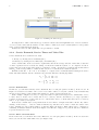
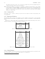
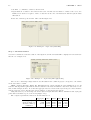
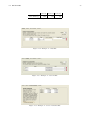
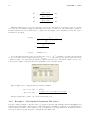
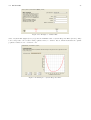
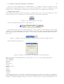
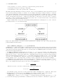
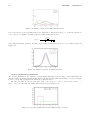
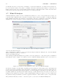
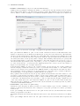
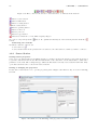
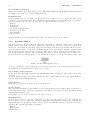
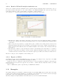
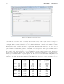
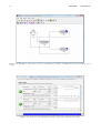
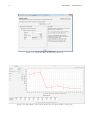
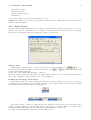
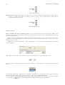
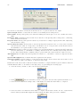
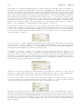
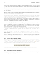
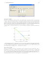
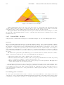
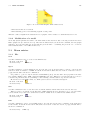
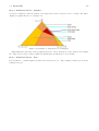
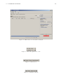
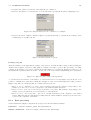
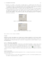
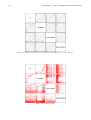
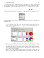
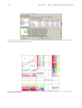
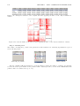
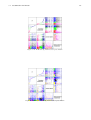
Figure 5.10: Saturation Sector Graphic
In this example Figure 5.10 we can observe a big area,on the top of the triangle, that rapresents the range
of mix population where Station4 is a bottleneck. In the center of the triangle there is a little red area that
rapresent the range of mix population where Disk1, Disk2 and Station4 are all bottleneck.
This graph is useful for understanding what station begin bottlenek and when but it is not simple to recornize
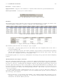
the exat value of the swiching segment. In order to obtain the exact value select the “Saturation Sector - Text”
tab subsection 5.2.8.
5.2.7
Convex Hull - Graphic
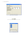
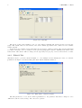
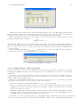
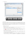
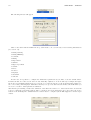
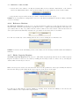
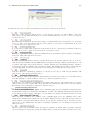
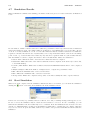
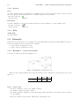
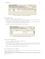
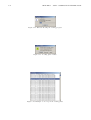
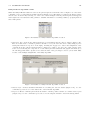
Using the Solve command and selecting the “Convex Hull - Graphic” tab the Convex Hull graphic is show.
Overview
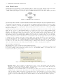
The Convex Hull graphic implements the polyhedral analysis technique. The polyhedral analysis technique
implemented in JABA is limited to queueing networks with customers grouped in two classes. The points in
the graph are obtained from the service demand matrix as follows. Each station corresponds to a point on the
graph whose co-ordinates are represented by the service demand of the two customer classes. For example, a
queue with service demands 10 sec for class 1, and 15 sec for class 2 is represented as a point with coordinates
(10,15). Then JABA builds the convex hull of this set of points, that is the smallest convex set containing all
the points.
The distinction of queues among the different types of bottleneck and non-bottleneck classes can be immediately operated from the knowledge of the convex hull using the following rules:
• All potential bottlenecks lie on the boundary of the convex polytope.
• All dominated station are interior points P of the convex polytope such that there is at least one point Q
whose co-ordinates are all higher or equal in value than those of P;
• All non-dominated stations in the interior of the convex polytope are masked-off stations. The application
of these rules is described below in the case study.
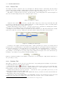
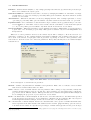
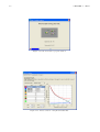
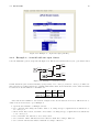
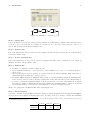
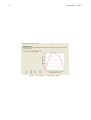
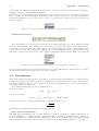
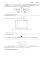
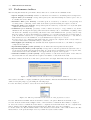
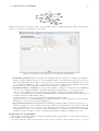
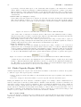
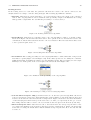
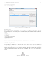
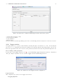
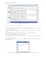
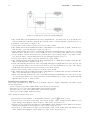
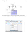
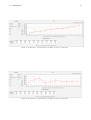
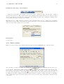
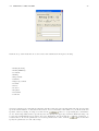
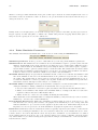
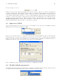
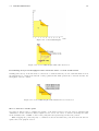
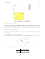
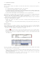
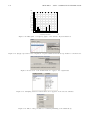
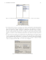
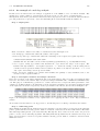
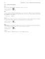
¿From this plot,Figure 5.11 we can see that Disk1 and Disk2 (depicted in red) lie on the boundary of the
convex hull, thus are potential bottlenecks. CPU (green) is instead a dominated non-bottleneck station, since
it is dominated by Sation4 and Disk1. Sation4 (blue) is also in the interior of the convex hull, but it is a
non-bottleneck station as there is no other point with all coordinates greater than those of Sation4 so it is a
masked-off station.
Determining points coordinates
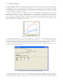
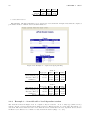
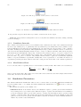
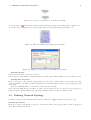
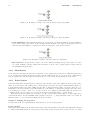
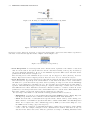
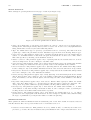
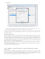
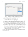
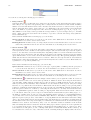
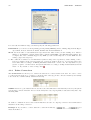
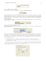
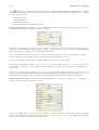
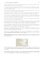
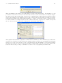
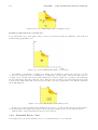
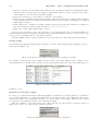
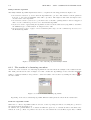
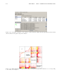
In order to gain exact information about the coordinates of a point it is sufficient to click, using the left button
of the mouse, on the point and additional information will appear after the point’s name. If the clicked point is
a dominated one, then it will be possible to see by which point (there could be more than one) it is dominated.