1
Performance Evaluation Lab
Dipartimento di Elettronica e Informazione
Politecnico di Milano - Italy
JMT
Java Modelling Tools
users manual
Version 0.5
ii
c
Copyright °2008
Performance Evaluation Lab - Dipartimento di Elettronica e Informazione - Politecnico di Milano.
All rights reserved.
Java Modelling Tools is free; you can redistribute it and/or modify it under the terms of the GNU General Public
License as published by the Free Software Foundation; either version 2 of the License, or (at your option) any later
version.
Java Modelling Tools is distributed in the hope that it will be useful, but WITHOUT ANY WARRANTY; without
even the implied warranty of MERCHANTABILITY or FITNESS FOR A PARTICULAR PURPOSE. See the GNU
General Public License for more details.
You should have received a copy of the GNU General Public License along with Java Modelling Tools; if not, write
to the Free Software Foundation, Inc., 675 Mass Ave, Cambridge, MA 02139, USA.
Contents
Contents
iii
1 Introduction
1.1 Starting with the JMT suite . . . . . . . . . . . . . . . . . . . . . . . . . . . . . . . . . . . . . . .
1
2
2 JMVA
2.1 Overview . . . . . . . . . . . . . . . . . . . . . . . . . . . . . . .
2.1.1 Starting the alphanumeric MVA solver . . . . . . . . . . .
2.2 Model definition . . . . . . . . . . . . . . . . . . . . . . . . . . .
2.2.1 Defining a new model . . . . . . . . . . . . . . . . . . . .
2.2.2 Classes Tab . . . . . . . . . . . . . . . . . . . . . . . . . .
2.2.3 Stations Tab . . . . . . . . . . . . . . . . . . . . . . . . .
2.2.4 Service Demands, Service Times and Visits Tabs . . . . .
2.2.5 What-if Tab . . . . . . . . . . . . . . . . . . . . . . . . . .
2.2.6 Comment Tab . . . . . . . . . . . . . . . . . . . . . . . .
2.2.7 Expression Evaluator . . . . . . . . . . . . . . . . . . . . .
2.2.8 Model Solution . . . . . . . . . . . . . . . . . . . . . . . .
2.2.9 Model Solution - What-if analysis . . . . . . . . . . . . .
2.2.10 Modification of a model . . . . . . . . . . . . . . . . . . .
2.3 Menu entries . . . . . . . . . . . . . . . . . . . . . . . . . . . . .
2.3.1 File . . . . . . . . . . . . . . . . . . . . . . . . . . . . . .
2.3.2 Action . . . . . . . . . . . . . . . . . . . . . . . . . . . . .
2.3.3 Help . . . . . . . . . . . . . . . . . . . . . . . . . . . . . .
2.4 Examples . . . . . . . . . . . . . . . . . . . . . . . . . . . . . . .
2.4.1 Example 1 - A model with a single closed class . . . . . .
2.4.2 Example 2 - A model with two open classes . . . . . . . .
2.4.3 Example 3 - A model with a load dependent station . . .
2.4.4 Example 4 - A model with one open and one closed class
2.4.5 Example 5 - Find optimal Population Mix values . . . . .
.
.
.
.
.
.
.
.
.
.
.
.
.
.
.
.
.
.
.
.
.
.
.
.
.
.
.
.
.
.
.
.
.
.
.
.
.
.
.
.
.
.
.
.
.
.
.
.
.
.
.
.
.
.
.
.
.
.
.
.
.
.
.
.
.
.
.
.
.
.
.
.
.
.
.
.
.
.
.
.
.
.
.
.
.
.
.
.
.
.
.
.
.
.
.
.
.
.
.
.
.
.
.
.
.
.
.
.
.
.
.
.
.
.
.
.
.
.
.
.
.
.
.
.
.
.
.
.
.
.
.
.
.
.
.
.
.
.
.
.
.
.
.
.
.
.
.
.
.
.
.
.
.
.
.
.
.
.
.
.
.
.
.
.
.
.
.
.
.
.
.
.
.
.
.
.
.
.
.
.
.
.
.
.
.
.
.
.
.
.
.
.
.
.
.
.
.
.
.
.
.
.
.
.
.
.
.
.
.
.
.
.
.
.
.
.
.
.
.
.
.
.
.
.
.
.
.
.
.
.
.
.
.
.
.
.
.
.
.
.
.
.
.
.
.
.
.
.
.
.
.
.
.
.
.
.
.
.
.
.
.
.
.
.
.
.
.
.
.
.
.
.
.
.
.
.
.
.
.
.
.
.
.
.
.
.
.
.
.
.
.
.
.
.
.
.
.
.
.
.
.
.
.
.
.
.
.
.
.
.
.
.
.
.
.
.
.
.
.
.
.
.
.
.
.
.
.
.
.
.
.
.
.
.
.
.
.
.
.
.
.
.
.
.
.
.
.
.
.
.
.
.
.
.
.
.
.
.
.
.
.
.
.
.
.
.
.
.
.
.
.
.
.
.
.
.
.
.
.
.
.
.
.
.
.
.
.
.
.
.
.
.
.
.
.
.
.
.
.
.
.
.
.
.
.
.
.
.
.
.
.
.
.
.
3
3
3
4
4
5
5
6
8
10
10
10
11
14
14
14
14
15
15
15
19
20
22
24
3 JSIMgraph
3.1 Overview . . . . . . . . . . . . . . . . .
3.2 The home window . . . . . . . . . . . .
3.3 Working with the graphical interface . .
3.3.1 Defining a new model . . . . . .
3.3.2 Defining the classes of customers
3.4 Distributions . . . . . . . . . . . . . . .
3.5 Performance indices . . . . . . . . . . .
3.5.1 Confidence Intervals . . . . . . .
3.5.2 Max Relative Error . . . . . . . .
3.6 Simulation Parameters . . . . . . . . . .
3.7 What-If Analysis . . . . . . . . . . . . .
3.8 Finite Capacity Region (FCR) . . . . .
3.9 Defining Network Topology . . . . . . .
3.9.1 Source Station . . . . . . . . . .
3.9.2 Sink Station . . . . . . . . . . . .
3.9.3 Delay Station . . . . . . . . . . .
3.9.4 Fork Station . . . . . . . . . . .
.
.
.
.
.
.
.
.
.
.
.
.
.
.
.
.
.
.
.
.
.
.
.
.
.
.
.
.
.
.
.
.
.
.
.
.
.
.
.
.
.
.
.
.
.
.
.
.
.
.
.
.
.
.
.
.
.
.
.
.
.
.
.
.
.
.
.
.
.
.
.
.
.
.
.
.
.
.
.
.
.
.
.
.
.
.
.
.
.
.
.
.
.
.
.
.
.
.
.
.
.
.
.
.
.
.
.
.
.
.
.
.
.
.
.
.
.
.
.
.
.
.
.
.
.
.
.
.
.
.
.
.
.
.
.
.
.
.
.
.
.
.
.
.
.
.
.
.
.
.
.
.
.
.
.
.
.
.
.
.
.
.
.
.
.
.
.
.
.
.
.
.
.
.
.
.
.
.
.
.
.
.
.
.
.
.
.
.
.
.
.
.
.
.
.
.
.
.
.
.
.
.
.
.
.
.
.
.
.
.
.
.
.
.
.
.
.
.
.
.
.
.
.
.
.
.
.
.
.
.
.
.
.
.
.
.
.
.
.
.
.
.
.
.
.
.
.
.
.
.
.
.
.
.
.
.
.
.
.
.
.
.
.
.
.
.
.
.
.
.
.
.
.
.
.
.
.
.
.
.
.
.
.
.
.
.
.
.
.
.
.
.
.
.
.
.
.
.
.
.
.
.
.
.
.
.
29
29
30
31
31
32
34
41
42
42
42
44
46
47
48
50
50
53
.
.
.
.
.
.
.
.
.
.
.
.
.
.
.
.
.
.
.
.
.
.
.
.
.
.
.
.
.
.
.
.
.
.
.
.
.
.
.
.
.
.
.
.
.
.
.
.
.
.
.
.
.
.
.
.
.
.
.
.
.
.
.
.
.
.
.
.
iii
.
.
.
.
.
.
.
.
.
.
.
.
.
.
.
.
.
.
.
.
.
.
.
.
.
.
.
.
.
.
.
.
.
.
.
.
.
.
.
.
.
.
.
.
.
.
.
.
.
.
.
.
.
.
.
.
.
.
.
.
.
.
.
.
.
.
.
.
.
.
.
.
.
.
.
.
.
.
.
.
.
.
.
.
.
.
.
.
.
.
.
.
.
.
.
.
.
.
.
.
.
.
.
.
.
.
.
.
.
.
.
.
.
.
.
.
.
.
.
.
.
.
.
.
.
.
.
.
.
.
.
.
.
.
.
.
.
.
.
.
.
.
.
.
.
.
.
.
.
.
.
.
.
.
.
.
.
.
.
.
.
.
.
.
.
.
.
.
.
.
iv
CONTENTS
3.10
3.11
3.12
3.13
3.9.5 Join Station . . . . . . . . . . . . . . . . . . . . . . . . . . . . . . . .
3.9.6 Routing Station . . . . . . . . . . . . . . . . . . . . . . . . . . . . .
3.9.7 Queueing Station . . . . . . . . . . . . . . . . . . . . . . . . . . . . .
3.9.8 Logger station . . . . . . . . . . . . . . . . . . . . . . . . . . . . . .
Modification of the Parameters . . . . . . . . . . . . . . . . . . . . . . . . .
3.10.1 Modifying Simulation Parameters . . . . . . . . . . . . . . . . . . . .
3.10.2 Modifying station parameters . . . . . . . . . . . . . . . . . . . . . .
3.10.3 Modifying the default values of parameters . . . . . . . . . . . . . .
Error and Warning Messages . . . . . . . . . . . . . . . . . . . . . . . . . .
Results of simulation . . . . . . . . . . . . . . . . . . . . . . . . . . . . . . .
3.12.1 Results from a single simulation run . . . . . . . . . . . . . . . . . .
3.12.2 Result of What-If Analysis simulation run . . . . . . . . . . . . . . .
3.12.3 Export to JMVA . . . . . . . . . . . . . . . . . . . . . . . . . . . . .
Examples . . . . . . . . . . . . . . . . . . . . . . . . . . . . . . . . . . . . .
3.13.1 Example 1 - A model with single closed class . . . . . . . . . . . . .
3.13.2 Example 2 - What-If Analysis of a system with multiclass customers
4 JSIMwiz
4.1 Overview . . . . . . . . . . . . . . . . . . .
4.1.1 Starting the discrete-event simulator
4.2 Defining a new model . . . . . . . . . . . .
4.2.1 Define Classes . . . . . . . . . . . .
4.2.2 Define stations . . . . . . . . . . . .
4.2.3 Define Connections . . . . . . . . . .
4.2.4 Station Parameters . . . . . . . . . .
4.2.5 Define Performance Indices . . . . .
4.2.6 Reference Stations . . . . . . . . . .
4.2.7 Finite Capacity Regions . . . . . . .
4.2.8 Define Simulation Parameters . . . .
4.2.9 Define what if analysis . . . . . . . .
4.3 Import in JMVA . . . . . . . . . . . . . . .
4.4 Modify default parameters . . . . . . . . . .
4.5 Modify the Current Model . . . . . . . . . .
4.6 Error and warning messages . . . . . . . . .
4.7 Simulation Results . . . . . . . . . . . . . .
4.8 Start Simulation . . . . . . . . . . . . . . .
.
.
.
.
.
.
.
.
.
.
.
.
.
.
.
.
.
.
.
.
.
.
.
.
.
.
.
.
.
.
.
.
.
.
.
.
.
.
.
.
.
.
.
.
.
.
.
.
.
.
.
.
.
.
.
.
.
.
.
.
.
.
.
.
.
.
.
.
.
.
.
.
.
.
.
.
.
.
.
.
.
.
.
.
.
.
.
.
.
.
.
.
.
.
.
.
.
.
.
.
.
.
.
.
.
.
.
.
.
.
.
.
.
.
.
.
.
.
.
.
.
.
.
.
.
.
.
.
.
.
.
.
.
.
.
.
.
.
.
.
.
.
.
.
.
.
.
.
.
.
.
.
.
.
.
.
.
.
.
.
.
.
.
.
.
.
.
.
.
.
.
.
.
.
.
.
.
.
.
.
.
.
.
.
.
.
.
.
.
.
.
.
54
55
56
57
58
58
59
59
62
64
64
66
66
66
67
69
.
.
.
.
.
.
.
.
.
.
.
.
.
.
.
.
.
.
.
.
.
.
.
.
.
.
.
.
.
.
.
.
.
.
.
.
.
.
.
.
.
.
.
.
.
.
.
.
.
.
.
.
.
.
.
.
.
.
.
.
.
.
.
.
.
.
.
.
.
.
.
.
.
.
.
.
.
.
.
.
.
.
.
.
.
.
.
.
.
.
.
.
.
.
.
.
.
.
.
.
.
.
.
.
.
.
.
.
.
.
.
.
.
.
.
.
.
.
.
.
.
.
.
.
.
.
.
.
.
.
.
.
.
.
.
.
.
.
.
.
.
.
.
.
.
.
.
.
.
.
.
.
.
.
.
.
.
.
.
.
.
.
.
.
.
.
.
.
.
.
.
.
.
.
.
.
.
.
.
.
.
.
.
.
.
.
.
.
.
.
.
.
.
.
.
.
.
.
.
.
.
.
.
.
.
.
.
.
.
.
.
.
.
.
.
.
.
.
.
.
.
.
.
.
.
.
.
.
.
.
.
.
.
.
.
.
.
.
.
.
.
.
.
.
.
.
.
.
.
.
.
.
.
.
.
.
.
.
.
.
.
.
.
.
.
.
.
.
.
.
.
.
.
.
.
.
.
.
.
.
.
.
.
.
.
.
.
.
.
.
.
.
.
.
.
.
.
.
.
.
.
.
.
.
.
.
.
.
.
.
.
.
.
.
.
.
.
.
.
.
.
.
.
.
.
.
.
.
.
.
.
.
.
.
.
.
.
.
.
.
.
.
.
.
.
.
.
.
.
.
.
.
.
.
.
.
.
.
.
.
.
.
.
.
.
.
.
.
.
.
.
.
.
.
.
.
.
.
.
.
.
.
.
.
.
.
.
.
.
.
.
.
.
.
.
.
.
.
.
.
.
.
.
.
.
.
.
.
.
.
.
.
.
.
.
.
.
.
.
.
.
.
.
.
.
.
.
.
.
.
.
.
81
81
82
82
83
85
94
95
95
97
97
98
99
101
101
104
104
106
106
5 JABA (Asymptotic Bound Analysis)
5.1 Overview . . . . . . . . . . . . . . . . . . . . . . . . . .
5.1.1 Starting the alphanumeric JABA solver . . . . .
5.2 Model definition . . . . . . . . . . . . . . . . . . . . . .
5.2.1 Defining a new model . . . . . . . . . . . . . . .
5.2.2 Classes Tab . . . . . . . . . . . . . . . . . . . . .
5.2.3 Stations Tab . . . . . . . . . . . . . . . . . . . .
5.2.4 Service Demands, Service Times and Visits Tabs
5.2.5 Comment Tab . . . . . . . . . . . . . . . . . . .
5.2.6 Saturaction Sector - Graphic . . . . . . . . . . .
5.2.7 Convex Hull - Graphic . . . . . . . . . . . . . . .
5.2.8 Saturation Sector - Text . . . . . . . . . . . . . .
5.2.9 Modification of a model . . . . . . . . . . . . . .
5.3 Menu entries . . . . . . . . . . . . . . . . . . . . . . . .
5.3.1 File . . . . . . . . . . . . . . . . . . . . . . . . .
5.3.2 Action . . . . . . . . . . . . . . . . . . . . . . . .
5.3.3 Help . . . . . . . . . . . . . . . . . . . . . . . . .
5.4 Examples . . . . . . . . . . . . . . . . . . . . . . . . . .
5.4.1 Example 1 - A two class model . . . . . . . . . .
5.4.2 Example 2 - A three class model . . . . . . . . .
.
.
.
.
.
.
.
.
.
.
.
.
.
.
.
.
.
.
.
.
.
.
.
.
.
.
.
.
.
.
.
.
.
.
.
.
.
.
.
.
.
.
.
.
.
.
.
.
.
.
.
.
.
.
.
.
.
.
.
.
.
.
.
.
.
.
.
.
.
.
.
.
.
.
.
.
.
.
.
.
.
.
.
.
.
.
.
.
.
.
.
.
.
.
.
.
.
.
.
.
.
.
.
.
.
.
.
.
.
.
.
.
.
.
.
.
.
.
.
.
.
.
.
.
.
.
.
.
.
.
.
.
.
.
.
.
.
.
.
.
.
.
.
.
.
.
.
.
.
.
.
.
.
.
.
.
.
.
.
.
.
.
.
.
.
.
.
.
.
.
.
.
.
.
.
.
.
.
.
.
.
.
.
.
.
.
.
.
.
.
.
.
.
.
.
.
.
.
.
.
.
.
.
.
.
.
.
.
.
.
.
.
.
.
.
.
.
.
.
.
.
.
.
.
.
.
.
.
.
.
.
.
.
.
.
.
.
.
.
.
.
.
.
.
.
.
.
.
.
.
.
.
.
.
.
.
.
.
.
.
.
.
.
.
.
.
.
.
.
.
.
.
.
.
.
.
.
.
.
.
.
.
.
.
.
.
.
.
.
.
.
.
.
.
.
.
.
.
.
.
.
.
.
.
.
.
.
.
.
.
.
.
.
.
.
.
.
.
.
.
.
.
.
.
.
.
.
.
.
.
.
.
.
.
.
.
.
.
.
.
.
.
.
.
.
.
.
.
.
.
.
.
.
.
.
.
.
.
.
.
.
.
.
.
.
.
.
.
.
.
.
.
.
.
.
.
.
.
.
.
.
.
.
.
.
.
.
.
.
.
.
.
.
.
.
.
.
.
.
.
.
.
.
.
.
.
.
.
.
.
.
.
.
.
.
.
.
.
.
.
.
.
.
.
.
.
.
.
.
.
.
.
.
.
.
.
.
109
109
109
110
110
111
111
111
112
112
114
116
117
117
117
118
118
118
118
121
.
.
.
.
.
.
.
.
.
.
.
.
.
.
.
.
.
.
.
.
.
.
.
.
.
.
.
.
.
.
.
.
.
.
.
.
.
.
.
.
.
.
.
.
.
.
.
.
.
.
.
.
.
.
.
.
.
.
.
.
.
.
.
.
.
.
.
.
.
.
.
.
.
.
.
.
.
.
.
.
.
.
.
.
.
.
.
.
.
.
.
.
.
.
.
.
.
.
.
.
.
.
.
.
.
.
.
.
CONTENTS
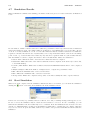
6 JWAT - Workload Analyzer Tool
6.1 Workload analysis . . . . . . . . . . . . . . . . . .
6.1.1 A workload characterization study . . . . .
6.1.2 Input definition . . . . . . . . . . . . . . . .
6.1.3 Data processing . . . . . . . . . . . . . . . .
6.1.4 Clustering algorithms . . . . . . . . . . . .
6.1.5 The results of a clustering execution . . . .
6.1.6 An example of a web log analysis . . . . . .
6.1.7 Menus description . . . . . . . . . . . . . .
6.2 Format definition . . . . . . . . . . . . . . . . . . .
6.2.1 Example of a format definition . . . . . . .
6.2.2 Example of the definition of the Apache log
v
.
.
.
.
.
.
.
.
.
.
.
.
.
.
.
.
.
.
.
.
.
.
.
.
.
.
.
.
.
.
.
.
.
.
.
.
.
.
.
.
.
.
.
.
.
.
.
.
.
.
.
.
.
.
.
.
.
.
.
.
.
.
.
.
.
.
.
.
.
.
.
.
.
.
.
.
.
.
.
.
.
.
.
.
.
.
.
.
.
.
.
.
.
.
.
.
.
.
.
.
.
.
.
.
.
.
.
.
.
.
.
.
.
.
.
.
.
.
.
.
.
.
.
.
.
.
.
.
.
.
.
.
.
.
.
.
.
.
.
.
.
.
.
.
.
.
.
.
.
.
.
.
.
.
.
.
.
.
.
.
.
.
.
.
.
.
.
.
.
.
.
.
.
.
.
.
.
.
.
.
.
.
.
.
.
.
.
.
.
.
.
.
.
.
.
.
.
.
.
.
.
.
.
.
.
.
.
.
.
.
.
.
.
.
.
.
.
.
.
.
.
.
.
.
.
.
.
.
.
.
.
.
.
.
.
.
.
.
.
.
.
.
.
.
.
.
.
.
.
.
.
.
.
.
.
.
.
.
.
.
.
.
.
.
.
.
.
.
.
.
.
.
.
.
.
.
.
.
.
.
.
.
.
.
.
.
125
126
126
128
131
135
138
143
146
147
148
149
A Basic Definitions
151
B List of Symbols
153
Bibliography
155
vi
CONTENTS
Chapter 1
Introduction
The Java Modelling Tools (JMT) is a free open source suite consisting of six tools for performance evaluation,
capacity planning, workload characterization, and modelling of computer and communication systems. The
suite implements several state-of-the-art algorithms for the exact, asymptotic and simulative analysis of queueing
network models, either with or without product-form solution. Models can be described either through wizard
dialogs or with a graphical user-friendly interface. The workload analysis tool is based on clustering techniques.
The suite incorporates an XML data layer that enables full reusability of the computational engines.
The JMT suite is composed by the following tools:
JSIMwiz : a wizard-based interface for the discrete-event simulator JSIM for the analysis of queueing
network models. A sequence of wizard windows helps in the definition of the network properties. The JSIM
simulation engine supports several probability distributions for characterizing service and inter-arrival times.
Load-dependent strategies using arbitrary functions of the current queue-length can be specified. JSIMwiz supports state-independent routing strategies, e.g., Markovian or round robin, as well as state-dependent strategies, e.g., routing to the server with minimum utilization, or with the shortest response time, or with minimum
queue-length. The simulation engine supports several extended features not allowed in product-form models,
namely, finite capacity regions (i.e., blocking), fork-join servers (i.e., parallelism), and priority classes. The
JSIM performs automatically the transient detection, based on spectral analysis, computes and plots on-line
the estimated values within the confidence intervals. What-if analyses, where a sequence of simulations is run
for different values of control parameters, are also supported.
JSIMgraph: a graphical user-friendly interface for the same simulator engine JSIM used by JSIMwiz.
It integrates the same functionalities of JSIMwiz with an intuitive graphical workspace. This allows an easy
description of network structure, as well as a simplified definition of the input and execution parameters.
Network topologies can be exported in vectorial or raster image formats.
JMVA: for the exact analysis of single-class or multiclass product-form queueing networks, processing
open, closed or mixed workloads. A stabilized version of the Mean Value Analysis MVA algorithm is used.
Network structure is specified by textual wizards. What-if analyses and graphical representation of the results
are provided.
JMCH: it applies a simulation technique to solve a single station model, with finite (M/M/1/k) or infinite
queue (M/M/1), and shows the underlying Markov Chain. It is possible to dynamically change the arrival rate
and service time of the system.
JABA: for the identification of bottlenecks in multiclass closed product-form networks using efficient convex
hull algorithms. Up to three customer classes are supported. It is possible to identify potential bottlenecks
corresponding to the different mixes of customer classes in execution. Models with thousands of queues can
be analyzed efficiently. Optimization studies (e.g., throughput maximization, minimization of response time,
identification of the optimal load) can be performed through the identification of the saturation sectors, i.e.,
the mixes of customer classes in execution that saturate more than one resource simultaneously.
JWAT: supports the workload characterization process. Some standard formats for input file are provided
(e.g., Apache HTTP and IIS log files), customized formats may also be specified. The imported data can
initially be analyzed using descriptive statistical techniques (e.g, means, correlations, histograms, boxplots,
scatterplots), either for univariate or multivariate data. Algorithms for data scaling, sample extraction, outlier
filtering, k-means and fuzzy k-means clustering for identifying similarities in the input data are provided. These
1
2
CHAPTER 1. INTRODUCTION
techniques allow the identification of cluster of customers having similar characteristics. The clusters centroids
represent the mean values of the parameters of the classes (e.g., CPU time, n.o of I/Os, n.o of web pages pages
accessed) that can be used for the workload parameterization.
1.1
Starting with the JMT suite
Double click on the JMT icon
on your program group or on the desktop, or open the command prompt and
type from the installation directory:
java -jar JMT.jar
The window of Figure 1.1 will be shown.
Figure 1.1: The JMT suite Starting Screen
This starting screen is used to select the application of the suite to be executed by clicking on the corresponding button. The flow chart should help the user to select the application that best fits its needs.
In the following chapters the tools will be examined in details and some examples are given. This manual
is intended for the general user that wants to learn how to interact with JMT. Advanced users that want to
learn details on internal data structures, computational engines and XML interfaces should refer to JMT system
manual.
Several other documents related to JMT description and applications are provided with the suite. Click on
Online Documentation button to access the library. An exercise book is also available.
Chapter 2
JMVA
2.1
Overview
JMVA solves open, closed and mixed product form [BCMP75] queueing networks with the exact MVA algorithm
[RL80]. In order to avoid fluctuations of the solutions when the model contains load dependent stations, the
implemented algorithm is a stabilized version [BBC+ 81] of the classic MVA algorithm.
Resources may be of two types: queueing (either with load independent or load dependent service times)
and delay. The model is described in alphanumeric way: user is guided through the definition process by steps
of a wizard interface (5 or 6 steps). What-if analyses, where a sequence of model are solved for different
values of parameters, are also possible (see subsection 2.2.5). A graphical interface to describe the model in a
user-friendly environment is also available, see JSIMgraph for details.
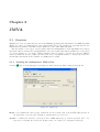
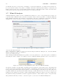
2.1.1
Selecting
Starting the alphanumeric MVA solver
button on the starting screen, Figure 2.1 window shows up. Three main areas are shown:
Figure 2.1: Classes tab
Menu : it is organized into three groups of functions. To use a menu, click on the menu heading and choose
the appropriate option. For the description of menu entries, see section 2.3
Toolbar : contains some buttons to speed up access to JMVA functions (e.g. New model, Open, Save. . . See
section 2.3 for details). If you move the mouse pointer over a button a tooltip will be shown up.
3
4
CHAPTER 2. JMVA
Page Area : this is the core of the window. All MVA parameters are grouped in different tabs. You can
modify only a subset of them by selecting the right tab, as will be shown later.
2.2
Model definition
Models with one or multiple customer classes provide estimates of performance measures. For a brief description
of basic terminology please refer to Appendix A.
In the case of single class models, the workload is characterized by two inputs: the set of service demands,
one for each resource, and the workload intensity. On the other hand, in multiple class models, a matrix of
service demands is requested [LZGS84].
2.2.1
Defining a new model
To define a new model select toolbar button
must be defined:
or the New command from File menu. The following parameters
1. Classes with their workload intensities (number of customer N for closed classes and arrival rate λ for
open classes)
2. Stations (service centers)
3. Service demands (or Service Times and Visits)
4. Optional short Comment
The execution of JMVA provides, for each class and each station, the following performance indices:
•
•
•
•
Throughput
Queue Length
Residence Time
Utilization
The following aggregate indices are provided:
• System Throughput
• System Response Time
• Average number of customers in the system
Input tabs
As can be seen in Figure 2.1, the parameters that must be entered in order to define a new model are divided
in four tabs: Classes, Stations, Service Demands and Comment.
Tabs number can become five, if you click Service Times and Visits button in Service Demands Tab. As
will be discussed in subsection 2.2.4, the Service Demands Tab will be hidden and it will appear Service
Times Tab and Visit Tab. You can navigate through tabs:
• using sequential wizard buttons, if enabled, at the bottom of the window (Figure 2.2)
• using sequential buttons located in menu
• using the tab selector, clicking on the corresponding tab (Figure 2.3)
Figure 2.2: Wizard buttons
Figure 2.3: Tab selector
2.2. MODEL DEFINITION
2.2.2
5
Classes Tab
An example screenshot of this tab can be seen in Figure 2.1. This tab allows to characterize customer classes
of the model. Your model will be a single class model if and only if there will be only one class, closed or open.
On the contrary multiple class models will have at least two classes, closed and/or open.
The number of classes in the model can be specified in the corresponding input area, shown in Figure 2.4
and can be modified using the keyboard or using the spin controls.
Figure 2.4: Number of classes
Using the delete button
associated to a specific class, a class can be removed provided that there will
be at least one class after the deletion. Similar result may be obtained using spin controls, decreasing classes
number; in this case last inserted class will be removed.
Default class names are Class1, Class2, . . . ClassN. A model can be customized by changing these names:
this can be done by clicking directly on the name that should be changed.
In Figure 2.5 there are three classes of customers, two closed and one open. The third class has the default
name Class3 while the other two classes have customized names, namely ClosedClass and OpenClass.
Figure 2.5: Defining the classes types
A class type can be Open or Closed. It is important to define each class type because a closed class workload
is described by a constant number of customers in each class, while the open classes workload is described by
the customer arrival rate for each class which does not imply limits on the maximum number of customers.
As can be seen in Figure 2.5, a class type can be selected in a combo-box. The input boxes No. of Customers
(N ) referring to closed classes accept only positive integer numbers; the input boxes of the Arrival Rate (λ)
referring to open classes, accept positive real numbers (Figure 2.6).
Figure 2.6: Workload definition of the number of customers of a closed class (N = 100) and the arrival rate of
an open class (λ = 3.14)
2.2.3
Stations Tab
The number of stations of the model can be specified in the corresponding input area (Figure 2.7) and can be
modified using the keyboard or the spin controls.
Using the delete button
associated to a specific station, a station can be removed provided that there
will be at least one station after the deletion. Similar result may be obtained using spin controls, decreasing
stations number; in this case last inserted station will be removed.
Default station names are Station1, Station2, . . . StationN. In order to personalize your model, you can
change and give names other than default ones.
In Figure 2.8 there is only one station with default name Station4 and there are three stations with customized names: CPU, Disk1 and Disk2.
A station type can be Load Independent, Load Dependent or Delay. You can insert in your model a Load
Depend center only if there is a unique closed class1 ; in all other cases the combo-box will be disabled.
1 Multiclass,
open and mixed models with load dependent stations are not supported yet
6
CHAPTER 2. JMVA
Figure 2.7: Number of stations
Figure 2.8: Defining the stations type
It is important to define each station type because if a station is Load Dependent a set of service demand or a set of service times and the number of visit - must be defined (one service demand/time for each possible
value of queue length inside the station).
In subsection 2.2.4 we will explain this concept with more details.
2.2.4
Service Demands, Service Times and Visits Tabs
Service Demands can be defined in two ways:
• directly, by entering Service Demands (Dkc )
• indirectly, by entering Service Times (Skc ) and Visits (Vkc )
Service demand Dkc is the total service requirement, that is the average amount of time that a customer
of class c spends in service at station k during one interaction with the system, i.e. it completes execution.
Service time Skc is the average time spent by a customer of class c at station k for a single visit at that station
while Vkc is the average number of visits at that resource for each interaction with the system.
Remember that Dkc = Vkc ∗ Skc so it is simple to compute service demands matrix starting from service
times and visits matrixes. Inverse calculation is performed with the following algorithm:
½
1 if Dkc > 0
Vkj =
0 if Dkc = 0
½
Dkc if Dkc > 0
Skc =
0
if Dkc = 0
Service Demands Tab
In this tab, you can insert directly Service Demands Dkc for each pair {station k-class c} in the model. In
Figure 2.9 a reference screenshot can be seen: notice that a value for every Dkc element of the D-matrix has
already been specified because default value assigned to newly created stations is zero.
In the example of Figure 2.9, each job of type ClosedClass requires an average service demand time of 6 sec
to CPU, 10 sec to Disk1, 8 sec to Disk2 and 2.5 sec to Station4. On the other hand, a job of type OpenClass
requires on average 0.1 sec of CPU time, 0.3 sec of Disk1 time, 0.2 sec of Disk2 time and 0.15 sec of Station4
time to be processed by the system.
If the model contains any load dependent station, the behavior of Figure 2.10 will be shown. By doubleclicking on LD Settings. . . button a window will show up and that can be used to insert the values of the
service demands for each possible number of customer inside the station. That values can be computed by
evaluating an analytic function as shown in Figure 2.11. The list of supported operators and more details are
reported in subsection 2.2.7.
Service Times and Visits Tabs
In the former tab you can insert the Service Times Skc for each pair {station k-class c} in the model, in the
latter you can enter the visits number Vkc (See Figure 2.12).
2.2. MODEL DEFINITION
7
Figure 2.9: The Service Demands Tab
Figure 2.10: Defining a load dependent station service demand
Figure 2.11: Load Dependent editing window
8
CHAPTER 2. JMVA
Figure 2.12: Visits Tab
The layout of these tabs is similar to the one of the Service Demand Tab described in the previous paragraph. The default value for each element of the Service Times (S) matrix is zero, while it is one for Visits’
matrix elements.
In current model contains load dependent stations, the behavior of Service Times Tab for their parametrization will be identical to the one described on the previous paragraph for Service Demands Tab. On the other
hand Visits Tab behavior will not change as load dependency is a property of service times and not of visits.
2.2.5
What-if Tab
This Tab is used to perform a what-if analysis, i.e. solve multiple models changing the value of a control
parameter. In Figure 2.13 is shown this panel when what-if analysis is disabled.
Figure 2.13: What-if Tab - Disabled analysis
The first parameter to be set is the control parameter i.e. the parameter that will be changed to solve
different models in a selected range. Five choices are possible:
2.2. MODEL DEFINITION
9
Disabled : disables what-if analysis, so only a single queueing network model, specified in the previous steps,
will be solved. This is the default option.
Customer Numbers : different models will be executed by changing the number of customers of a single
closed class or of every closed class proportionally. This option is available only when current model has
at least one closed class.
Arrival Rates : different models will be executed by changing arrival rate of a single open class or of every
open class proportionally. This option is available only when current model has at least one open class.
Population Mix : the total number of customers will be kept constant, but the population mix (i.e. the ratio
between number
of customers of selected closed class i and the total number of customers in the system
P
βi = Ni / k Nk ). This option is available only when current model has two closed classes.
Service Demands : different models will be solved changing the service demand value of a given station for
a given class or for all classes proportionally. This option is available only for load independent and
delay stations.
Whenever a control parameter is selected, the window layout will be changed to allow the selection of a
valid range of values for it. For example in Figure 2.14 Service Demands control parameter was selected. On
the bottom of the window, a riepilogative table is presented: depending on selected control parameter, that
table is used to show the initial state of involved parameters. Every class currently selected for what-if analysis
is shown in red.
Figure 2.14: What-if Tab - Service Demands
A brief description of each field is now presented:
Station : available only with Service Demands control parameter. This combo box allows to select at which
station service demand values will be modified.
Class : allows to select for which class the selected parameter will be changed. A special value, namely All
classes proportionally, is used to modify the control parameter for each class keeping constant the
proportion between different classes2 . This special value is not available in Population Mix analysis as
we are changing the proportion of jobs between two closed classes.
From : the initial value of what-if analysis. It was chosen to leave this value fixed to the initial value specified
by the user in the previous steps to avoid confusions, so this field acts as a reminder. The only exception
is when Population Mix is changed, in that case it is allowed to modify this value too.
To : the final value of what-if analysis. Please notice that this value can be greater or smaller than From value
and is expressed in the same measure unit. Whenever All classes proportionally option is selected,
both From and To values are expressed as percentages of initial values (specified in the previous steps
2 for example, in a model with two closed classes with population vector (2,6), the following models can be executed: (1,3),
(2,6), (3,9), (4, 12), . . .
10
CHAPTER 2. JMVA
and reminded in the table at the bottom of the panel, see Figure 2.14), in the other situations they are
considered as absolute values for the chosen parameter.
Steps : this is chosen number of executions i.e. the number of different models that will be solved. When
control parameter is Customer Numbers or Population Mix, the model can be correctly specified only
for integer values of population. JMVA will perform a fast computation to find the maximum allowed
number of executions given current From and To values: if user specifies a value bigger than that, JMVA
will use the computed value.
2.2.6
Comment Tab
In this Tab, a short - optional - comment about the model can be inserted; it will be saved with the other
model parameters.
2.2.7
Expression Evaluator
An expression evaluator is used for the definition of service demands or service times of a load dependent
station. It allows to specify times as an analytic function of n where n is the number of customer inside the
station.
Expression are evaluated using JFEP 3 (Java Fast Expression Parser) package which supports all operators
enumerated in Table 2.1 and all functions enumerated in Table 2.2.
Operator
Symbol
∧
Power
Unary Plus, Unary Minus +n, −n
Modulus
%
Division
/
Multiplication
∗
Addition, Subtraction
+, −
Table 2.1: List of all supported operators ordered by priority
Function
Symbol
Sine
sin()
Cosine
cos()
Tangent
tan()
Arc Sine
asin()
Arc Cosine
acos()
Arc Tangent
atan()
Hyperbolic Sine
sinh()
Hyperbolic Cosine
cosh()
Hyperbolic Tangent
tanh()
Inverse Hyperbolic Sine
asinh()
Inverse Hyperbolic Cosine
acosh()
Inverse Hyperbolic Tangent atanh()
Natural Logarithm
ln()
Logarithm base 10
log()
Absolute Value / Magnitude
abs()
Random number [0, 1]
rand()
Square Root
sqrt()
Sum
sum()
Table 2.2: List of supported functions for the load dependent service times
2.2.8
Model Solution
Use Solve command to solve the model. If the model specifies a what-if analysis, please refer to subsection 2.2.9.
Model results will be shown on a separate window, like the one of Figure 2.15.
3 http://jfep.sourceforge.net/
2.2. MODEL DEFINITION
11
Figure 2.15: Model Solution (Throughput Tab)
Using the tab selector, all the other computed performance indices can be seen: Throughput, Queue lengths,
Residence Times, Utilizations and a synopsis panel with schematic report of input model. Both results and
synopsis tab data can be copied to clipboard with the standard CTRL+C keyboard shortcut.
When open classes are used, the resource saturation control is performed. For multiple class models, the
following inequality must be satisfied:
X
λc ∗ Dkc < 1
max
k
c
This inequality ensures that no service center is saturated as a result of the combined loads of all the classes. Let
us consider, as example, the model with the classes shown in Figure 2.5 with the D-matrix shown in Figure 2.9
Since λ = 3.14 < 3.33 = 1/0.3 = 1/Dmax the model is not in saturation and the Solve command will be
executed correctly.
In this example, substituting DDisk1-OpenClass with values ≥ 1/3.14 ≈ 0.318 will cause the saturation of
resource Disk1 and the error message of Figure 2.16 will appear.
Figure 2.16: Input data error message
2.2.9
Model Solution - What-if analysis
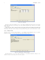
Use Solve command to solve the model. During model solution, a progress window, see Figure 2.17, shows up.
It displays the cumulative number of models currently solved, the total number of models to be solved and the
elapsed time.
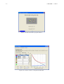
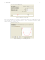
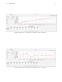
At the end of the solution, results will be shown in a separate window, see Figure 2.18. This tab allows to
show in a plot the relation between the chosen control parameter (see subsection 2.2.5) and the performance
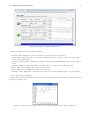
indices computed by the analytic engine.
The combo box Performance Index allows to select the performance index to be plotted in the graph, while
in the table below, users can select the resource and the class considered.
• The first column is fixed and lists all available colors to be used in the graph.
• The second column, named Class, is used to select the class considered in the graph. The special value
Aggregate is used for the aggregate measure for all classes. If input model is single-class, the class is
selected by default for each row.
• The final column, named Station, is used to select the station considered in the graph. The special value
Aggregate is used for the aggregate measure for the entire network. Note that the Aggregate value is
not valid when the Utilization performance index is selected.
In addition to the center performance indices (i.e. Throughput, Queue length, Residence Times, Utilization),
three system performance indices are provided in the Performance Index combo box (System Response Time,
12
CHAPTER 2. JMVA
Figure 2.17: Model Solution progress window
Figure 2.18: Model Solution - Graphical Results Tab
2.2. MODEL DEFINITION
13
System Throughput, Number of Customers). This system indices can be easily obtained by selecting the special Aggregate value for both Class and Station columns of the corresponding center indices (see Appendix A
for the definition of the performance indices), but they were provided here as a shortcut. As we are referring
to aggregate measures, the selection of reference class and station is not significant and, in this case, the table
in the left of Figure 2.18 will not be shown.
On the bottom-left corner of the window, users can modify minimum and maximum value of both the
horizontal and vertical axes of the plot. JMVA is designed to automatically best-fit the plot in the window but
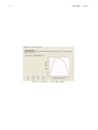
this controls allow the user to specify a custom range or zoom on the plot. Another fast method to perform a
zoom operation is to left-click and drag a rectangle on the graphic window (see Figure 2.19) or right-click on it
and select Zoom in or Zoom out options. To automatically reset the best-fit scale users can right-click on the
graphic window and select Original view option.
Figure 2.19: Zoom operation on the plot
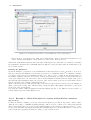
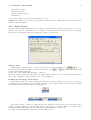
The graphic window allows to export plots as image to be included in documents and presentations. To
save current graph as image, right-click on the graphic and select Save as... option. A dialog will be shown
to request the name of the file and the format. Currently supported format are Portable Network Graphics PNG - (raster) and Encapsulated PostScript - EPS - (vectorial, currently only black and white).
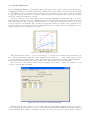
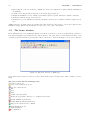
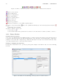
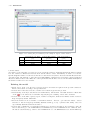
The second tab of the solution window, shown in Figure 2.20, is used to display the solutions of each
execution of the analytic algorithm.
Figure 2.20: Model Solution - Textual Results Tab
This Tab has the same structure of the results window without What-if analysis (described in subsection 2.2.8) but allows to select the execution to be shown in the field Execution Number. By entering requested
execution number in the spinner, or using the up and down arrows, user can cycle between all the computed
14
CHAPTER 2. JMVA
performance indices for each execution. Just below the spinner, a label gives information on the value of the
control parameter for the currently selected execution.
2.2.10
Modification of a model
To modify system parameters return to the main window and enter new data. After the modifications, if you
use Solve command, a new window with model result will show. You can save this new model with the
previous name - overwriting the previous one - or save it with a different name or in a different directory.
2.3
2.3.1
Menu entries
File
New
Use this command in order to create a new JMVA model.
Shortcut on Toolbar:
Accelerator Key:
CTRL+N
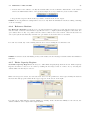
Open
Use this command to open an existing model. You can only open one model at time, to edit two or more models
start more than one instance of JMVA. If current model was modified since its creation or last save action, a
popup window will be shown for confirmation.
It is possible to open not only models saved with JMVA (*.jmva), but also with other programs of the suite (for
example JABA *.jaba, JSIM *.jsim and JMODEL4 *.jmodel). Whenever a data file of another tool is opened,
a conversion is performed and error/warnings occurred during conversion will be reported in a window.
Models are stored in XML format, see JMT system manual for a detailed description.
Shortcut on Toolbar:
Accelerator Key:
CTRL+O
Save
Use this command in order to save the active document with its current name in the selected directory.
When you save a document for the first time, JMVA displays the Save As dialog box so you can rename
your document. If you save a model after its resolution, results are stored with model definition data.
Shortcut on Toolbar:
Accelerator Key:
CTRL+S
Exit
Use this command in order to end a JMVA session. You can also use the Close command on the application
Control menu. If current model was modified since its creation or last save action, a popup window will be
shown for confirmation.
Accelerator Key:
2.3.2
CTRL+Q
Action
Solve
Use this command when model description is terminated and you want to start the solution of the model. At
the end of the process the window in Figure 2.15 will popup.
Shortcut on Toolbar:
Accelerator Key:
CTRL+L
4 In previous versions of the JMT suite, JMODEL was the name of the JSIMgraph application. Thus, *.jmodel files are files
saved in previous versions of the tool.
2.4. EXAMPLES
15
Randomize
Use this command in order to insert random values into Service Demands - or Service Times - table. Generated
values are automatically adjusted to avoid saturation of resources.
Shortcut on Toolbar:
Accelerator Key:
CTRL+R
Import in JSIM
This command will import current model into JSIM to solve it using simulator. A simple parallel topology is
derived from number of visits at each station and generated model is equivalent to original one.
Shortcut on Toolbar:
Accelerator Key:
2.3.3
CTRL+G
Help
JMVA Help
Use this command to display application help. From the initial window, you can jump to step-by-step instructions that show how use JMVA and consult various types of reference information.
Once you open Help, you can click the Content button whenever you want to return to initial help window.
Shortcut on Toolbar:
Accelerator Key:
CTRL+Q
About
Use it in order to display information about JMVA version and credits.
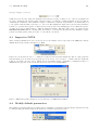
2.4
Examples
In this section we will describe some examples of model parametrization and solution using MVA exact solver.
Step-by-step instructions are provided in five examples:
1. A single class closed model with three load independent stations and a delay service center (subsection 2.4.1)
2. A multiclass open model with two classes and three load independent stations (subsection 2.4.2)
3. A single class closed model with a load dependent station and a delay (subsection 2.4.3)
4. A multiclass mixed model with three stations (subsection 2.4.4)
5. A multiclass closed model where a what-if analysis is used to find optimal Population Mix values (subsection 2.4.5)
2.4.1
Example 1 - A model with a single closed class
Solve the single class model specified in Figure 2.21. The customer class, named ClosedClass has a population
XDisk1
Users
XCPU
Disk1
CPU
XDisk2
Disk2
Figure 2.21: Example 1 - network topology
of N = 3 customers.
16
CHAPTER 2. JMVA
There are four stations, three are of load independent type (named CPU, Disk1 and Disk2 ) and one is of
delay type (named Users). Users delay station represents user’s think time (Z = 16 s) between interaction
with the system. Service times and visits for stations are reported in Table 2.3.
CPU
Disk1
Disk2
Users
Service Times [s]
0.006
0.038
0.030 16.000
Visits
101.000 60.000 40.000
1.000
Table 2.3: Example 1 - service times and visits
Step 1 - Classes Tab
•
•
•
•
use New command to create a new jMVA document
by default, you have already a Closed class
if you like, substitute default Class1 name with a customized one (ClosedClass in our example)
complete the table with workload intensity (number of customers). Remember that intensity of a closed
class N must be a positive integer number; in this case, 3
At the end of this step, the Classes Tab should look like Figure 2.22.
Figure 2.22: Example 1 - input data (Classes Tab)
Step 2 - Stations Tab
• use Next > command to switch to Stations Tab
• digit number 4 into stations number textbox or select number 4 using spin controls or push New Station
button three times. Now your model has four Load Independent stations with a default name
• if you want you can change station names. Substitute CPU for default name Station1, substitute Disk1
for default name Station2, substitute Disk2 for default name Station3 and substitute Users for default
name Station4
• change the type of last inserted station; Users station is a Delay (Infinite Server)
At the end of this step, the Stations Tab should look like Figure 2.23.
Step 3 - Service Times and Visits Tabs
• use Next > command to switch to Service Demands Tab
• press Service Time and Visit button as you don’t know the Service Demands of the three stations: in this
case Service Times and number of Visits should be typed. After button pressure, the Service Demands
Tab will be hidden and Service times Tab and Visit Tab will appear
• you can input all Service Times in the table. Remember that Service Time of the Users station, of delay
type, is think time Z, in this case 16 s
At this point, the Service Times Tab should look like Figure 2.24.
2.4. EXAMPLES
17
Figure 2.23: Example 1 - input data (Stations Tab)
Figure 2.24: Example 1 - input data (Service Times Tab)
18
CHAPTER 2. JMVA
• use Next > command to switch to Visits Tab
• input numbers of visits for all centers in the table. In this case the number of visits of the Users, the
infinite server station, is equal to 1 since a customer at the end of an interaction with the system visits
this station.
At the end of this step, the Visits Tab looks like Figure 2.25.
Figure 2.25: Example 1 - input data (Visits Tab)
Step 4 - Model Resolution
Use Solve command to start the solution of the input model. Model results will be displayed in a new window
like the one of Figure 2.26.
Figure 2.26: Example 1 - output data (Throughput Tab)
Since we are considering a single-class model, all results in the column Aggregate correspond to the results
in the ClosedClass column.
JMVA computes Residence Times Wk , Throughputs Xk , Queue lengths Qk and Utilizations Uk for all
stations. The algorithm begins with the known solution for the network with zero customers, and iterates on N
that, in this example, is three. Note that the aggregate Residence Time is the System Response Time measure
and the aggregate Queue Length is the average number of customers in the system.
Using tab selector, you can change tab and see Queue length, Residence Times, Utilizations and a synopsis
panel with a schematic report of the model (Figure 2.27).
The computed performance indices are shown in Table 2.4.
Aggregate
Throughput [job/s]
0.144
Queue Length [job]
3.000
Residence Time [s]
20.839
Utilization
Table 2.4: Example
CPU
Disk1 Disk2
14.540 8.637 5.758
0.193 0.410 0.194
0.643 2.847 1.349
0.087 0.328 0.172
1 - model outputs
Users
0.144
2.303
16.000
2.303
2.4. EXAMPLES
19
Figure 2.27: Example 1 - output data (Synopsis Tab)
2.4.2
Example 2 - A model with two open classes
Solve the multiclass open model specified in Figure 2.28. The model is characterized by two open classes A and
XDisk1
λA, λ B
S
Source
XCPU
Disk1
CPU
XDisk2
λA, λB
Disk2
Figure 2.28: Example 2 - network topology
B with arrival rate (the workload intensity λ) respectively of λA = 0.15 job/s and λB = 0.32 job/s. There are
three stations of load independent type, identified with names CPU, Disk1 and Disk2. Service times and visits
for stations are shown in Table 2.5 and Table 2.6.
CPU Disk1 Disk2
Class A [s] 0.006 0.038 0.030
Class B [s] 0.014 0.062 0.080
Table 2.5: Example 2 - service times
Since this model is similar to the network of Figure 2.21 solved in subsection 2.4.1, we will show how to
easily create it from a saved copy of Example 1:
1. Open the saved instance of Example 1 model
2. Go to Classes Tab, change ClosedClass name to A, change its type to Open and set its arrival rate to
λA = 0.15 job/s.
3. Click on New Class button, sets name of new class to B, change its type to Open and set its arrival rate
to λB = 0.32 job/s.
4. Go to Stations Tab and remove Users delay center.
5. Go to Service Times Tab and sets service times for Class B according to Table 2.5.
6. Go to Visits Tab and sets visits for Class B according to Table 2.6.
20
CHAPTER 2. JMVA
CPU
Class A 101.0
Class B
44.0
Table 2.6: Example 2
Disk1 Disk2
60.0
40.0
16.0
27.0
- number of visits
7. Select Solve action.
The Synopsis Tab with a schematic report of the model created is shown on Figure 2.29, while the computed
performance indices of this model are shown in Table 2.7.
Figure 2.29: Example 2 - output data (Synopsis Tab)
Throughput [job/s]
Queue Length [job]
Residence Time [s]
Utilization
Aggregate
0.150
2.529
16.863
-
Class A
CPU
Disk1
15.150 9.000
0.128 1.004
0.851 6.695
0.091 0.342
Class B
Aggregate
CPU
Disk1
Throughput [job/s]
0.320 14.080 5.120
Queue Length [job]
6.575
0.277 0.932
Residence Time [s]
20.548
0.865 2.913
Utilization
0.197 0.317
Table 2.7: Example 2 - model outputs
2.4.3
Disk2
6.000
1.398
9.317
0.180
Disk2
8.640
5.366
16.770
0.691
Example 3 - A model with a load dependent station
The network is shown in Figure 2.30. It comprises only two stations: one is of delay type (named Users)
and the other is a load dependent station (named Station). This model has one closed class only with N = 8
customers. The user’s think time is Z = 21 s, while the service demands for the load dependent Station, shown
in Table 2.8, are function of n: number of customers in the station (D(n) = n + 1/n).
2.4. EXAMPLES
21
Users
Station
Figure 2.30: Example 3 - network topology
n
1
2
3
4
5
6
7
8
D(n) [s] 2.00 2.50 3.33 4.25 5.20 6.17 7.14 8.13
Table 2.8: Example 3 - service demands for Station, a load-dependent service center
Step 1 - Classes Tab
The instructions that are the same given in Step 1 of subsection 2.4.1; in this case N must be 8.
Step 2 - Stations Tab
The instructions are given in Step 2 of subsection 2.4.1; in this case the model has two stations: a Load
Dependent station and a Delay Center.
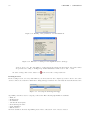
Step 3 - Service Demands Tab
1. use Next > command to switch to Service Demands Tab
2. double-click on cell with text LD Setting. . . to open the editor of load dependent service demands in a
separate window, shown in Figure 2.31.
3. it is not mandatory to insert all values one-by-one. You can click or drag to select cells, enter the expression
n + 1/n into the textbox at the bottom of the window and click the Evaluate button.
4. at the end of this phase, editor window looks like Figure 2.32. Now you may press OK button to confirm
changes and return to JMVA main window.
Figure 2.31: Example 3 - editor for the description of service demands for a load dependent station corresponding
to the different number of customers before the parametrization
Step 4 - Model Resolution
Use Solve command to resolve the model, results are shown in Table 2.9.
22
CHAPTER 2. JMVA
Figure 2.32: Example 3 - editor for the description of service demands for a load dependent station. In this
case an arithmetic function has been defined: S(n) = n + 1/n
Aggregate Station Users
Throughput [job/s]
0.234
0.234
0.234
Queue Length [job]
8.000
3.080
4.920
Residence Time [s]
34.149
13.149 21.000
Utilization
0.810
0.973
Table 2.9: Example 4 - model outputs
2.4.4
Example 4 - A model with one open and one closed class
The mixed queueing network model is shown in Figure 2.33. Workload intensities: the open class has an arrival
S
λopen
λ open
Station1
Station2
Station3
Figure 2.33: Example 4 - network topology
rate λ = 1 job/s, the closed class has a customers number N = 57. Service demands are shown in Table 2.10.
Step 1 - Classes Tab
Follow the instructions of Step 1 in the previous examples; the Classes Tab is shown in Figure 2.34.
Step 2 - Stations Tab
Follow the instructions of Step 2 in the previous examples; in this case the model has three Load Independent
stations (see Figure 2.35).
Step 3 - Service Demands Tab
Follow the instructions of Step 3 in the previous examples and define service demands for both classes as
illustrated in Table 2.10 (see Figure 2.36).
Step 4 - Model Solution
Use Solve command. Results can be verified by computing the equivalent model, where the open class “slows
down” the closed class by subtracting utilization to it:
2.4. EXAMPLES
23
Station1 Station2 Station3
OpenClass [s]
0.5
0.8
0.6
ClosedClass [s]
10.0
4.0
8.0
Table 2.10: Example 4 - service demands
Figure 2.34: Example 4 - Class Tab
Figure 2.35: Example 4 - Stations Tab
Figure 2.36: Example 4 - Service Demands Tab
24
CHAPTER 2. JMVA
D1eq
=
D2eq
=
D3eq
=
D1,ClosedClass
= 20s
1 − λ ∗ D1,OpenClass
D2,ClosedClass
= 20s
1 − λ ∗ D2,OpenClass
D3,ClosedClass
= 20s
1 − λ ∗ D3,OpenClass
MVA algorithm is used to solve the equivalent closed model. The number of customers of the closed class
is 57, and the exact MVA technique should require the solution of other 56 models with smaller population.
In this particular case, the formula used to compute the throughput can be simplified because the Service
Demands are all equals:
X eq (N )
=
=
=
X eq (57) =
P3
eq
k=1 Dk
+
P3
N
k=1
[Dkeq ∗ Qeq
k (N − 1)]
N
P3
60 + 20 ∗ k=1 Qeq
k (N − 1)
N
60 + 20 ∗ (N − 1)
0.048305 job/s
So the throughput measure for the closed class is XClosedClass = X eq = 0.048305 job/s while the throughput
for the open class coincide with its arrival rate XOpenClass = λ. As visits were not specified, they have been
considered equal to one: that’s why throughput is equal at each station for each class (see Figure 2.37), i.e. the
solved model consists of 3 stations that are sequentially connected with feedback.
Figure 2.37: Example 4 - throughput
Queue lenghts can be computed with the following formulas:
Qk,ClosedClass (N ) =
Qk,OpenClass (N ) =
Qeq
k (N )
λ ∗ Dk,OpenClass ∗ [1 + Qk,ClosedClass (N )]
1 − λ ∗ Dk,OpenClass
And the results will be equal to the ones shown in Figure 2.38.
2.4.5
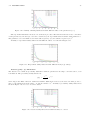
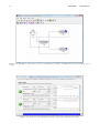
Example 5 - Find optimal Population Mix values
Perform a what-if analysis to find the value of population mix that will maximize System Throughput and
minimize System Response Time in the model shown in Figure 2.39. This model has two closed classes (named
Class1 and Class2 ) with a total population of N = 20 and three load independent stations (named Station1,
Station2 and Station3 ) with the service demands shown in Table 2.11.
2.4. EXAMPLES
25
Figure 2.38: Example 4 - queue lengths
Station1
Station2
Station3
Figure 2.39: Example 5 - network topology
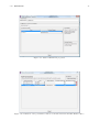
Step 1 - Classes Tab
Follow the instructions of Step 1 in the previous examples; as we will change population mix, initial allocation
of the N = 20 jobs is irrelevant. For example we can allocate N1 = 10 jobs to Class1 and N2 = 10 jobs to
Class2. The Classes Tab is shown in Figure 2.40.
Step 2 - Stations Tab
Follow the instructions of Step 2 in the previous examples; in this case the model has three Load Independent
stations (see Figure 2.41).
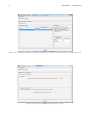
Step 3 - Service Demands Tab
Follow the instructions of Step 3 in the previous examples and define service demands for both classes as
illustrated in Table 2.11 (see Figure 2.42).
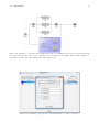
Step 4 - What-if Tab
1. use Next > command to switch to What-if Tab
2. Select Population Mix as a control parameter of the analysis in the combo box, several fields will be
shown below.
3. Class1 is already selected, by default, as reference class for the what-if analysis. This means that βi
values in From and To fields are referred to Class1.
4. By default, JMVA suggests the minimum allowed value of β1 in the From field and its the maximum value
in the To field5 . Since we want to find the optimal value in the entire interval, we leave this unchanged.
5. we want to perform the maximum number of allowed executions, so we enter a big number in the Steps
field (100 for example). JMVA will automatically calculate the maximum number of allowed executions
provided that number of customers for each class must be an integer and will report 19.
At the end of this phase, the What-if Tab will look like Figure 2.43.
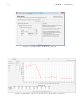
Step 5 - Model Solution
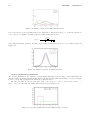
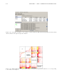
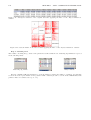
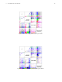
Use Solve command. In the Graphical Results Tab select System Response Time and System Throughput
as Performance Index (Figure 2.44 and Figure 2.45). Zooming on the plot, allows to identify the maximum
5 Since it is requested that one class has at least one job and customer number must be integer, the minimum value is 1/N and
the maximum value is (N − 1)/N .
Station1 Station2 Station3
Class1 [s]
1.0
5.0
1.0
Class2 [s]
5.0
1.0
5.0
Table 2.11: Example 5 - service demands
26
CHAPTER 2. JMVA
Figure 2.40: Example 5 - Class Tab
Figure 2.41: Example 5 - Stations Tab
Figure 2.42: Example 5 - Service Demands Tab
2.4. EXAMPLES
27
Figure 2.43: Example 5 - What-if Tab
value of System Throughput (0.32 job/s) and the minimum value of System Response Time (62.50 s). They
both corresponds to the execution with population mix β1 = 0.40 for Class1, which means that the optimal
population values are N1 = 8 and N2 = 12.
Figure 2.44: Example 5 - System Response Time
28
CHAPTER 2. JMVA
Figure 2.45: Example 5 - System Throughput
Chapter 3
JSIMgraph
3.1
Overview
In the JMT suite a discrete-event simulator for the analysis of queueing network models is provided. It can be
used through two interfaces: alphanumerical (JSIMwiz ) and graphical (JSIMgraph).
JSIMgraph is the GUI front-end to JMT simulation engine. It helps the users to perform an evaluation study
in two ways. Firstly, critical statistical decisions, such as transient detection and removal, variance estimation,
and simulation length control, have been completely automated, thus freeing the users from taking decisions
about parameters s/he may not be familiar with. The simulation is automatically stopped when all performance
indexes can be estimated with the required accuracy. Secondly, a user-friendly graphical interface allows the
user to describe, both the network layout and the input parameters. Furthermore, the graphical interface
also provides support for the use of advanced features (several of them are for networks with very general
characteristics, usually referred to as non-product-form networks) like fork and join of customers, blocking
mechanisms, regions with capacity constraints on population, state-dependent routing strategies, user-defined
general distributions, import and reuse of log data. A module for What-If Analysis, where a sequence of
simulations is run for different values of control parameters, particularly useful in capacity planning, tuning
and optimization studies, is also provided.
The simulation engine performs on-line the statistical analysis of measured performance indices, plots the
collected values, discards the initial transient periods and computes the confidence intervals.
Network topologies implemented and solved using JSIMgraph can be exported in vector (e.g., eps, pdf) or raster
(e.g., jpeg, png) image formats.
Main Features
Arrival rates for open classes of customers generated by Source stations and station service times (for any type
of station in open and closed models) can be generated according to the following distributions: Burst (General), Constant, Erlang, Exponential, Gamma, Hyperexponential, Normal, Pareto, Poisson, Student-T, Uniform
Queueing discipline: the following strategies are available: First Come First Served, FCFS with priority,
Last Come First Served, LCFS with priority
Routing of the customers in the network, i.e., the path followed by the requests among the resources, can
be described either probabilistically or according to the following strategies: Fastest service, Least utilization,
Random, Round robin, Join the Shortest Queue, Shortest response time (the values of the control parameters
are evaluated on the stations connected in output to the considered one). These strategies can be further
combined among themselves through the use of a routing station.
Other peculiar features of the simulator are:
•
•
•
•
•
•
Load dependent service time strategies
Fork-and-join stations to model parallelism
Simulation of complex traffic pattern and service times (e.g., burst)
Blocking regions (in which the number of customer is limited)
What-if analysis (with various control parameters)
Customization of default values
29
30
CHAPTER 3. JSIM GRAPH
• Import/Export of the model from/to JMVA, the exact solver (when the required analytic assumptions
are satisfied)
• Logging of the data flowing in any part of the model (Logger station)
• Graphical visualization of the evaluated performance indices together with their confidence intervals
• automatic transient detection and removal
• automatic stop of the simulation when all performance metrics can be estimated with the required accuracy.
JSIMgraph has a modular Java-based architecture that allows the introduction of new Java classes in the
simulation engine without any modification to the source codes of the other classes.
3.2
The home window
In the initial window of the JSIMgraph (Figure 3.1), all the icons in the toolbar except the first two (Create a
new model and Open a previously saved model) are inactive. Choosing Create a new model from the toolbar
or New from the File menu bar activates the other icons in the toolbar. From Figure 3.1, we can see that the
Figure 3.1: The home window of JSIMgraph
home window has a menu bar and two toolbars. The menu bar has 5 menus: File, Edit, Define, Solve,
Help.
The first toolbar has the following icons:
Create a new model
Open a previously saved model
Save the current model
Cut
Copy
Paste
Define customer classes
Define the performance indices to be evaluated and plotted
Define simulation parameters
Define What-if analysis parameters
Export the current model to JMVA
Start simulation model
Pause simulation
Stop simulation
3.3. WORKING WITH THE GRAPHICAL INTERFACE
31
Show simulation results window
Define new default values of model parameters
The second toolbar has the following icons:
Select
Insert a source station
Insert a sink station
Insert a routing station
Insert a delay station
Insert a queueing station
Insert a fork node
Insert a join node
Insert a logger station
Connect two elements
Add selected stations to a new Finite Capacity Region
Rotate the component
Optimize the graph
3.3
3.3.1
Working with the graphical interface
Defining a new model
To define a new model the following steps have to be performed.
1. Draw the network (click and drop)
2. Define Customer Classes and select the Reference Station for each class
3. Set the parameters for each object
4. Select the performance indices to be collected and evaluated
5. If needed, insert one or more Finite Capacity Regions (FCR)
6. Choose or change the simulation parameters
7. Enable What-If Analysis and set its parameters, if required
8. Start the simulation
9. If diagnostic errors are detected, click on them and the related window that allows immediately to fix them
will be shown.
Step 1: Create the new model
To draw a new network, select or choose New from File menu. A white area in which the model should
be drawn will be shown. Utilize the pre-defined objects like queueing station, delay, source, sink, logger,
connection, routing station and fork/join.
Step 2: Define customer classes
In all the networks implemented, one or more Customer Classes must be defined. To describe them, see
subsection 4.2.1 - ”Defining Customers Classes” and parameterize the classes to use.
For each class of customers, a Reference Station should be set. This station is used to compute the system
throughput for each class (i.e., the number of customers of that class that flow through the system in a time
unit). It is a required parameter in order to compute correctly the simulation results. If a simulation is started
without its prior definition, an error message will appear.
Step 3: Define station parameters
All the stations have default parameters. The proper parameters of the objects should be defined: either
the numeric values or the qualitative parameters such as routing strategy, queueing policy, maximum number
of customers in a FCR region, etc. See section 3.9 - ”Defining Network Topology” for details.
Step 4: Define performance indices
The performance indices that will be evaluated during the simulation should be selected. Select the indices
and set the class and the station which each index refers to. See section 3.5 - ”Performance Indices” for details.
Step 5: Define a Finite Capacity Region
32
CHAPTER 3. JSIM GRAPH
A F inite C apacity Region (FCR) is a section of the model, that may consists of one or more stations, in
which the number of customers is limited. Several FCRs can be defined in a network, provided that they do
not overlap. See section 3.8 ”Finite Capacity Region (FCR)” to learn how to set this type of region.
Step 6: Setting simulation parameters
The parameters that control the simulation and the initial state of the network should be defined. See
section 3.10 ”Modification of the parameters” for details.
Step 7: Enabling a What-If Analysis
If you decide to set up a What-If Analysis read section 3.7.
Step 8: Start the simulation
Press
or select Simulate from the Solve menu to start the simulation. Before starting the simulation, a
check if the defined network is correct is performed, and the errors detected (fatal or warning) are shown. The
results of a simulation are described in section 3.12.
Step 9: Fatal Errors and Warning Messages
The detected errors and warning messages are shown in section 3.11.
3.3.2
Defining the classes of customers
The workload intensity is described by one of the following parameters:
λ the arrival rate (for open models)
N the population size (for closed models).
In open models the workload intensity is specified by the parameter λ, i.e., the rate at which requests (customers)
arrive at the system. In these type of models there is an infinite stream of arriving customers and the customer
population, i.e., the number of customers in execution, varies over time. Customers that have completed their
execution leave the system (and reach a sink station). The class of customers of an open model is also referred
to as Open Class.
In closed models the workload intensity is specified by a parameter N, indicating the average number of jobs
(customers) in execution. In these models the population is fixed, i.e., N is kept constant. Customers that
have completed their service are considered as if they left the model and have been replaced immediately by a
new customer. The class of customers in execution in a closed model is also referred as Closed Class. Multiple
class models consist of N customer classes, each of which has its own workload intensity and its own service
demand at each center. Within each class, the customers are indistinguishable, i.e., statistically equal. Models,
in which the customers belong to both of the two types of classes, open and closed, are referred to as Mixed
models. The parameters defining the two types of classes are given below.
• Open Classes parameters: priority, interarrival time distribution, reference station, service time distributions of the stations
• Closed Classes parameters: priority, population value, reference station, service time distributions of
the stations.
The classes of customers identify different customer behavior and characteristics, such as the type (closed
or open), the size of the customer population (for closed classes) or the interarrival time distribution (for open
classes), the path among the resources, the service time required.
They can be set from the Define menu by choosing Customer Classes. The following panel will be shown.
Figure 3.2: Window for the definition of the classes of customers
Classes must be explicitly added to the model, either one at a time by clicking the Add Class button, or by
selecting directly the desired final number of classes from the Classes counter. The newly added classes will
be listed with default parameters.
3.3. WORKING WITH THE GRAPHICAL INTERFACE
33
Double click on the default name (i.e., Class0, Class1, etc.) to change it. Each new class has a priority
in the system. A smaller number indicates a lower priority. Default value is 0, it can be changed by double
clicking on the corresponding area. In this panel you can insert either one or multiple customer classes.
Defining Open Classes
After adding a class and set its name and priority, you must select the type of the class. Classes are created
Closed by default, so if you want an Open class, select the type Open from the Type menu.
Figure 3.3: Selection of the type of the class
Now the class characteristics should look like Figure 3.4.
Figure 3.4: Class characteristics window
Open classes describe customer populations that vary over time. They are characterized by the probability
distribution of the interarrival time of customers arriving at the system. The default Interarrival Time Distribution is exp(1) (Exponential Distribution with λ =1). To change the Interarrival Time Distribution, click the
Edit button.
Figure 3.5: Definition of the interarrival time distribution and its parameters (Edit button)
The following window will appear:
Figure 3.6: Window for the editing of the distribution of interarrival times
Click on the Selected Distribution drop down menu to choose one of the following distributions:
Burst (General)
Burst (MMPP2)
Constant
Erlang
Exponential
Gamma
Hyperexponential
Normal
Pareto
Poisson
Replayer
StudentT
Uniform.
For each distribution the correct values of the parameters should be described, default values can eventually be
used. Parameters that are related each others are automatically updated when one of them is modified. For
example, for an Erlang distribution, when you set the (α, r) pair, the (mean, c) pair is automatically set to the
34
CHAPTER 3. JSIM GRAPH
correct values. The Replayer distribution allows the user to use trace of data collected from real experiments.
Click OK to return to Class parameters definition.
The final step of a class definition is the identification of the Reference Station, i.e., the station of the model
used to compute the system throughput and response time of a class. It can be selected from the Reference
Station menu (Figure 3.7). For Open Classes, only one of the stations of Source type can be selected as
Reference Station.
Figure 3.7: Selection of the Reference Station for an open class of customers
Defining Closed Classes
Figure 3.8: Closed class definition parameters
By default Classes are created as Closed. Priority can be changed as in the case of Open class (the default
value is 0, the minimum). The population size (also referred to as N ) is the parameter that characterizes a
closed class. For a closed class N is constant and does not change during the execution of the simulation. Its
default value is 1 and it may be changed by clicking on the corresponding area in the class properties matrix.
A Reference Station for the class must be selected from the Reference Station menu. With a closed class all
Figure 3.9: Selection of a Reference Station for a closed class of customers
the type of stations can be selected but neither a Source nor a Sink. The Reference Station is used to compute
the system throughput and response time for the class considered.
3.4
Distributions
Open class models are workloads where the number of requests in the system fluctuates over time and new
requests arrive at the system as if generated by an infinite source. The arrival pattern can be described by a
probability distribution simple or very complex. It is often used the distribution of the inter-arrival times of
consecutive requests, or customers.
A probability distribution f (x) can be characterized by:
Mean (if it exists):
Z
∞
E[X] =
x f (x) dx
−∞
Variance (if it exists):
Z
∞
V ar[X] =
(x − E[X])2 f (x) dx = E[X 2 ] − E[X]2
−∞
Coefficient of variation c (when mean and variance exist and mean is not 0):
√
variance
c =
mean
The following probability distributions are currently supported.
Burst (General) distribution
The Burst (General) distribution is a complex distribution obtained combining two different distributions. It
allows the simulation of complex patterns of arrivals and may be suitable for simulating the load generated
by web 2.0 applications. A Burst (General) distribution consists of two different types of intervals (A and B)
independent among each other. For both the interval types the following parameters have to be specified:
3.4. DISTRIBUTIONS
35
• the probability of occurrence of that type of interval in the generated stream
• the length distribution for that type of intervals
• the distribution of the values generated into each interval.
The Burst (General) distribution behaves as follows. As soon as the simulation starts, an interval is chosen
based on the specified probability of occurrence. If, for example, interval type A has probability of occurrence
of 0.7 and interval B has 0.3, then an interval of type A is chosen with 70% probability. In order to determine
the duration of an interval, an event from the interval-length distribution is obtained. The distribution of the
events of an interval is then used to compute the arrival time of customers or the service time of a station,
depending on where the Burst (General) distribution is used. As soon as the interval ends, a new interval is
chosen based on the given probability as before.
Figure 3.10 shows the concept idea of the Burst (General) distribution, clarifying the role of the occurrence
probability and the role of the interval length.
Figure 3.10: Main structure of the Burst (General) distribution consisting of two type of intervals with independent statistical characteristics
Burst (MMPP2) (mmpp2(σ0 , σ1 , λ0 , λ1 )) distribution
A MMPP(2) is a continuous-time Markov chain that jumps between two states and the active state determines
the current rate of service. For example, one state may be associated with slow inter-arrival times (state 0), the
other may have fast inter-arrival times (state 1). As time passes, the MMPP(2) jumps several times between
the slow state 0 and the fast state 1.
In JMT, the MMPP(2) is parameterized by four rates: σ0 , σ1 , λ0 , and λ1 (see Figure 3.11). While in state
0, the MMPP(2) generates arrivals with rate λ0 or jumps to state 1 with rate σ0 ; in state 1 the arrival and
jump rates are λ1 and σ1 , respectively. This can be equivalently stated as follows: in state 0 a random number
with exponential distribution having rate λ0 + σ0 is drawn, then with probability λ0 /(λ0 + σ0 ) is the arrival
of a new job (or equivalently the completion of its service if the MMPP(2) is used as a service process), while
with probability σ0 /(λ0 + σ0 ) without any job arrival or service completion; the case of state 1 is similar.
A MMPP(2) can be parameterized to have a predefined mean, c2 , skewness, decay rate of the autocorrelation.
Given these four parameters, there are closed-form formulas to obtain the corresponding values of σ0 , σ1 , λ0 ,
and λ1 . For example the mean is related to the rates of the MMPP(2) by
mean =
σ0 + σ1
λ0 σ1 + σ0 λ1
while the decay rate of the autocorrelation that controls the burstiness is
decay rate =
λ0 λ1
.
λ0 λ1 + λ0 σ1 + σ0 λ1
In particular, a large decay rate (> 0.9) creates large bursts of arrivals/service completions. The reader
could find additional details on how to fit a MMPP(2) for example in [CZS07] and references therein.
example 1)λ0 = λ1 = 5 is an exponential distribution for all choices of σ0 and σ1
example 2)λ0 = 1.4346, λ1 = 0, σ0 = 0.0139, σ1 = 0.0319 is an hyperexponential with mean= 1, c2 = 20,
p = 0.99. since the hyperexponential has no burstiness, here the autocorrelation coefficients are equal to zero.
36
CHAPTER 3. JSIM GRAPH
example 3) λ0 = 12, λ1 = 0.0879, σ0 = 0.0010, σ1 = 0.0001 is a MMPP(2) with burstiness. The mean is
1, c2 =20, skewness= 7.31, lag-1 autocorrelation coefficient is 0.4745. Since for a MMPP(2) the autocorrelation
is always less than 0.5, this is an example of a process with very large burstiness.
Figure 3.11: Main structure of the Burst (MMPP2) distribution
Constant (Const(k)) distribution
This distribution describes a constant (deterministic) flow of customers, arriving exactly every k time units.
The probability density function is:
½
1 x=k
f (x) =
0 x 6= k
The only parameter that should be specified is the mean, equal to k.
Figure 3.12: Constant distributions for two different mean values
Erlang (erl(α,r)) distribution
The Erlang distribution is a continuous distribution, with two parameters: the shape r, an integer value, and
the rate α, a real value. It is a special case of a Gamma distribution with integer shape parameter. The
probability density function is:
αr r−1 −αx
f (x) =
x
e
Γ(r)
Γ(r) is called Eulero function and when r is a non null positive integer, as in the case of the Erlang distribution,
the Eulero function reduces to Γ(r) = (r − 1)!.
A random variable with Erlang distribution of order r can be obtained as a sum of r exponentially distributed
random variables with mean 1/rα (see Figure 3.13). When the values of α and r are changed, the system
Figure 3.13: Simulation of an Erlang distribution with a sequence of exponential stages
will automatically recompute the mean = r/α and the variance V ar = r/α2 . A family of probability density
functions that illustrate the impact of various (α, r) pairs is shown in Figure 3.14.
Exponential (exp(λ)) distribution
This is a continuous probability distribution where λ > 0 is the distribution parameter, often called the rate
parameter; the distribution is defined in the interval [0,∞). The probability density function is:
½
λe−λx x ≥ 0
f (x) =
0
x<0
3.4. DISTRIBUTIONS
37
Figure 3.14: A family of Erlang distributions with different values of the parameters (α, r )
The exponential distribution is used to model Poisson processes. The time interval between two consecutive
events generated by a Poisson process can be described by an exponential random variable with parameter λ.
The parameter λ is a real number, the mean value is given by 1/λ, the variance is given by 1/λ2 .
A family of exponential density functions with different values of λ is shown in Figure 3.15.
Figure 3.15: Exponential density functions with different mean (1/λ) values)
Gamma (gam(α, λ)) distribution
The Gamma is a continuous probability distribution with two parameters: the shape α and the scale λ, both
real numbers. The probability density function is:
f (x) =
xα−1
e−x/λ
Γ(α)λα
where Γ(t) is the Eulero function. When the Gamma distribution is selected, the user can either provide α
and λ or the distribution mean equal to αλ and the variance αλ2 . A family of probability density functions is
shown in Figure 3.16, for a set of α and λ values.
Figure 3.16: Gamma density functions for different values of α and λ
38
CHAPTER 3. JSIM GRAPH
Hyperexponential (hyp(p,λ1 , λ2 )) distribution
A hyperexponential distribution describes a random variable characterized by a variability higher with respect
to an exponential one with the same mean. It is the result of a weighted sum of two independent exponentially
distributed random variables, with parameters λ1 and λ2 respectively. The weight p is the probability that
the random variable behaves like the exponential variable with parameter λ1 and 1-p that it behaves like the
exponential variable with parameter λ2 . The probability density function is:
f (x) = p λ1 e−λ1 x + (1 − p) λ2 e−λ2 x
When this distribution is used to model customer interarrival time or a station service time, with probability p
Figure 3.17: Generation of the values of an hyperexponential function through two exponential stages in parallel
the next interval before a new arrival (or the next service time) is distributed like the upper server in Figure 3.17
the figure above while with probability 1-p it will be distributed like the lower server.
A family of hyperexponential density functions is shown in Figure 3.18. Note that when λ1 = λ2 , the
hyperexponential reduces to a simple exponential.
Figure 3.18: Family of hyperexponential density functions
Normal (norm(µ, σ)) distribution
The Normal distribution is also called Gaussian since its probability density function is the Gaussian function.
It is well known for its bell-shaped density function.
The two parameters are µ = location (real number, it is the mean of the distribution), and σ = scale (real
number, it is the standard deviation of the distribution, i.e., the square root of the variance). The density is
symmetrical around the mean and the variance. The probability density function is:
f (x) = √
(x−µ)2
1
e− 2σ2
2πσ
The standard normal distribution is the normal distribution with µ = 0 (mean equal 0) and σ = 1 (variance
and standard deviation equal 1). A family of normal density functions is shown in Figure 3.19.
Pareto (par(α,k)) distribution
This distribution is usually utilized to describe the behavior of social and economical phenomena (e.g., the
distribution of wealth, where a small portion of the people owns the larger part of the wealth). It is characterized
by the parameters k > 0, location (real), and α > 0, shape (real). The probability density function is:
f (x) = αk α x−(α+1)
3.4. DISTRIBUTIONS
39
Figure 3.19: Family of normal density functions. The standard normal density is the green colored.
If k and α are provided as input parameters, the simulator compute the mean kα/(α − 1) for k > 1 and the
variance
α2 x
(x − 1)2 (x − 2)
A family of Pareto density functions is shown in Figure 3.20.
Figure 3.20: Family of Pareto density functions.
Poisson (poisson(λ)) distribution
The Poisson distribution describes the number of events occurring in a time interval, when such events are
independent of the amount of time elapsed and they occur at a fix rate. It is a discrete probability distribution
characterized by a single parameter, λ, a positive real number, which is the average number of events in a time
interval and its variance. The probability of having an arrival in a time interval (t, t+∆t) is λ∆t+o(∆t)2 , while
the probability of more than one arrival in the same interval is o(∆t).
For large time intervals T, the distribution is near the mean value, thus the number n of arrivals over the
interval is given by n = λT. The time intervals between two consecutive events having a Poisson distribution
are exponentially distributed with average value equal to 1/λ. The probability mass function is:
f (x) =
λx −λ
e
x!
A family of Poisson probability mass functions is shown in Figure 3.21.
Replayer (replayer(”filename”)) distribution
When Replayer is chosen, a trace of data provided by the users can be reused as interarrival times or service
times. The file format should be text/binary with values separated by CR (”Carriage Return”). In order to
use this user-supplied file of data, the user should provide in the input window the absolute path name of the file.
Student-T (studT(ν)) distribution
The T -distribution, or StudentT distribution, is a continuous distribution characterized by the single parameter
ν, a real positive number. It is used when the mean of a normally distributed population must be estimate
using only a small sample size. It is the basis of the Student-t’s test that is used to evaluate the statistical
significance of the difference between two sample means and for the difference between two population means.
40
CHAPTER 3. JSIM GRAPH
Figure 3.21: Family of Poisson probability mass functions.
It is a special case of the generalized hyperbolic distribution. The mean is 0 for ν > 1 and the variance is
ν/(ν − 2) for ν > 2 (infinite otherwise). The probability density function is:
f (x) = √
Γ( ν+1
2 )
νπ Γ( ν2 ) (1 +
x2 ν+1
2
ν )
where Γ(t) is the Eulero function. A family of probability density functions for a set of ν values is shown in
Figure 3.22.
Figure 3.22: Family of Student-T density functions.
Uniform (U(min,max)) distribution
The Uniform distribution, also referred to as Rectangular distribution due the shape of its density function,
describes a random variable that may assume all the values in the range (min, max) with the constant probability
1/(max − min). The probability is 0 outside the considered range.
The user can either provide the pair (min, max) or the mean m = (max + min)/2 and variance c =
(max − min)2 /12. Two uniform density functions are plotted in Figure 3.23.
Figure 3.23: Uniform density functions with different range of values.
3.5. PERFORMANCE INDICES
3.5
41
Performance indices
The following list include the performance indices that can be obtained from a simulation run.
• Queue Length (of a station): number of customers N at a station, both waiting and receiving service.
• Queue Time (of a station): average time spent by the customers waiting in a station queue. It does
not include the Service Time.
• Residence Time (of a station): total time spent at a station by a customer, both queueing and
receiving service, considering all the visits at the station performed during its complete execution.
• Response Time (of a station): average time spent in a station by a customer for a single visit (sum
of Queue time and Service time).
• Utilization (of a station): percentage of time a station is used (i.e., busy) evaluated over all the
simulation run. It ranges from 0 (0%), when the station is always idle, to a maximum of 1 (100%), when
the station is constantly busy servicing customers for the entire simulation run. Queueing stations may
have more than one server, their number is a parameter to be specified (default is 1). It is important to
point out that the utilization U of a queueing station with a single server is given by U = λS, and in a
station with mservers the utilization of any individual server is given by U = λS/m.
In delay stations, for consistency with Little’s law, the utilization is computed as the average number of
customers in the station, and thus it may be greater than 1.
• Throughput (of a station): rate at which customers departs from a station, i.e., the number of requests
completed in a time unit.
• System Throughput (of the system): rate at which customers departs from the system.
• System Response Time (of the system): average time a customer spends in the system in order to
receive service from the various stations it visits. It corresponds to the intuitive notion of response time,
as the interval between the submission of a request and the reception of the response.
• Customer Number (of the system): average number of customers in the system. If the index is
associated with a closed class, then it is equal to the number of customers in the class.
Any subset of indices from the above list can be plotted as model output. Each index is associated with a class
Figure 3.24: The window for the selection of the performance indices.
and a station and will be computed within the given Confidence Interval and Maximum Relative Error, both
defined on the (0-1) range, by performing the following steps:
1. Select the index you want to add to the model from this menu:
Figure 3.25: The drop-down list for the selection of the performance indices.
2. Select Add Selected Index and the index will be added to the panel. Then the index must be set.
3. Select from the Class menu a Single class, or All Classes, for which the index must be computed.
4. Select the Station for which the index must be computed from Station menu. In case of system wide
indices, namely, System Throughput and System Response Time, this option is not available.
5. Double click to modify the default values for the Confidence Interval size of the solution and for the Max
Relative Error of the greatest sample error, if you want more/less accurate results.
42
CHAPTER 3. JSIM GRAPH
Figure 3.26: The drop-down list for the selection of the Class.
Figure 3.27: The drop-down list for the selection of the Station.
Figure 3.28: Definition of the Confidence Interval and Max.Relative Error.
6. Repeat these steps for all the indices you want to include in the model output.
NOTE: Errors in parameter settings will be detected only when the simulation is started, raising a warning
or an error message.
3.5.1
Confidence Intervals
The confidence interval shown at the end of a simulation run contains the true value of the estimated index with
the selected probability (1-α) or, equivalently, if an experiment is repeated many times, in (1-α)*100% of cases.
Various difficulties in meeting theoretical assumptions can cause that the real percentage of the confidence
intervals containing the true parameter differs significantly from (1-α). The robustness of the above methods of
data collection and analysis is usually measured by the coverage of confidence intervals, defined as the frequency
with which the intervals (X(n)-∆x, X(n)+∆x) contain the true parameter value µx , at a given confidence level
(1-α), 0< α <1. The coverage analysis can be applied only to systems with a theoretical well-known behavior,
since the value of µx has to be known. Any analyzed method must be applied in a statistically significant
number of repeated simulation experiments, usually 200 or more replications, to determine the fraction of
experiments producing the final confidence intervals covering the true mean value of the estimated parameter.
3.5.2
Max Relative Error
Let x be the true value of a quantity and xi be the measured or inferred value. The relative error is defined by:
|X(n) − µx |
|µx |
where
X(n) =
n
X
xi
i=1
n
where µx is the mean value. The relative error is the sum of the deviations between the sample values and the
mean value, divided for the mean value.
3.6
Simulation Parameters
The Define Simulation Parameters window can be reached either by selecting Simulation Parameters
from the Define menu or by clicking the Define Simulation Parameters icon
Figure 3.30).
The parameters required by the simulator are:
from the toolbar (see
• Simulation Seed: is the number used by the simulation engine to generate pseudo-random numbers.
If you change the seed, you will obtain a different sequence of pseudo-random numbers. If a simulation
is repeated using the same seed, the same sequence of pseudo-random numbers will be generated, thus
leading to identical results. The default value is random, which indicates that the simulation engine will
pick a seed of its choice in a pseudo-random fashion each time it is started; deselect random and insert a
number if you want a custom simulation.
3.6. SIMULATION PARAMETERS
43
Figure 3.29: Confidence intervals for the correct parameter value µx evaluated in 10 runs. The coverage is 80%
since two of them do not include the correct value.
Figure 3.30: Window for the definition of the Simulation Parameters
• Maximum duration (sec): It represents the maximum amount of time in seconds that the simulation
will run. If the simulation ends before the maximum duration, the parameter is ignored and does not
affect the results. The default value is infinite, deselect it and specify the preferred maximum time if you
do not want the simulation to run for a possibly very long time. In this case, the simulation stops when
the time limit is reached, although a reliable solution may not be available yet.
• Maximum number of samples: It is the greatest number of samples for each index that JSIMgraph
collects before ending the simulation. During a simulation, measurements can be stopped in case of:
- Success, if the results have reached the required Confidence Interval and the Max Relative Error
- Failure, if the simulation has analyzed the maximum number of samples but has not reached the required
Confidence Interval or Max Relative Error
- Failure, if timeout occurs before successfully calculating the final results.
The default value for the maximum number of samples is 500,000; you may increase it (for a more accurate
simulation) or decrease it (for a faster simulation).
• Representation Interval (sec): This is the granularity at which results are plotted on the screen, i.e.,
the time interval before a new point is added to the graphs, as the simulation proceeds. A large value will
make the simulation to proceed slower, as the graphs are updated less often. Small values will provide
an impression of better ”responsiveness” from the simulation, as graphs are updated more frequently.
Animation checkbox is used to enable or disable queue animation during the simulation process.
Initial state of a simulation
The Initial state is the model state at time 0, typically described by the number of customers in each station
at the beginning of the simulation.
For closed customer classes, all customers are allocated by default to their reference stations. You can
44
CHAPTER 3. JSIM GRAPH
modify this allocation, as long as the total number of customers remains the one defined in the Classes tab.
For open customer classes, it is possible to initialize each station with any desired number of customers. In
Figure 3.30 the initial state of a model with four stations and two classes (ClosedClass with 3 customers in the
CPU station and Class0 with 10 customers in the Users station) is shown.
3.7
What-If Analysis
A What-If Analysis consists of a series of simulations in which one or more control parameters are varied over
a specified range. This allows the observation of system behavior under a spectrum of conditions, unlike the
single simulation run where the system is observed under a fixed set of parameters. By default the What-If
Analysis is not enabled. It must be activated explicitly and its parameters should be defined.
Figure 3.31: The window for What-If Analysis definition.
Activating the What-If Analysis
After completing the definition of the model and selecting the What-If Analysis tab, check the Enable
what-if analysis checkbox to activate it.
Selecting the What-If Analysis
After enabling the What-If Analysis, it is possible to select the parameter to control the sequence of simulation
runs using the menu of Figure 3.32. When you select a What-If Analysis parameter, the bottom section of
Figure 3.32: Selection of the parameter for the control of a What-If Analysis.
the window of Figure 3.31 will change depending upon the parameter. In the right portion a Description is
provided of the selected parameter and of the impact of its variation. In the left portion the details of the parameter range (From and To fields) and the number of executions (Steps) on the range are provided. The set of
modifiable parameters depends upon the number and type of classes in the model: in a single class model, you
simply select the parameters you want to change during simulation while in a multiclass model, you must select
the parameter and specify whether you want to apply the variation to all the classes or just to one specific class.
The parameters that may be used to control the sequence of executions in a What-If Analysis are:
3.7. WHAT-IF ANALYSIS
45
• Number of Customers: (only for models with closed classes)
JSIM repeats the simulation changing the number of customers in each run, starting from the number
inserted in the From N field, to the value inserted in the To N field. The simulation is repeated Steps(n.of
exec.) number of times. In Figure 3.33 a What-If Analysis is planned on a single closed class model.
Figure 3.33: Selection of the Type of population growth in a What-If Analysis.
The option Increase number of jobs of one closed class has been selected. The initial value of the
number of customers is not modifiable from this window, as it is part of the Classes tab. The final value
should be specified in the field To N. In this case, with a final value of 20 and 6 Steps, simulations are run
for 10, 12, 14, 16, 18 and 20 customers, respectively. Only the customer number in the class selected in
the Class (ClosedClass, in the picture) will be changed. The remaining classes (if they are present) will
keep their initial number of customers. The simulator control that the sum of the percentages of jobs of
the various classes (represented by the components βi of vector β) evaluated over the global population
N of the model add up to 1, as shown in the Population mix table on the bottom of the window of
Figure 3.33 in the simple case of a single class model.
If the Increase number of jobs of all closed classes option is selected, the overall population is
increased keeping constant the relative proportion of jobs in the various classes, i.e., the values βi (also
referred to as population mix ). Because in the JSIM the number of customers in each class can only be
integer numbers, only the population vectors with all integer components can be considered. Therefore,
the actual number of executions may be smaller than the one specified.
The population mix describes the way the global population is subdivided between the classes, i.e., the
percentage of customers in each class (βi values) over the total population. The population mix can be
modified extensively selecting the way we want to change it with the increasing of the global population
of customers: all classes increase proportionally or only one class increases keeping constant the jobs
of the other classes (select the option Increase number of jobs of one closed class in this case).
Mixed models can be analyzed too. Remember that only models with closed classes (at least one) will be
considered in this What-If Analysis.
• Arrival Rate: (only if there are open classes)
Arrival rate is the frequency at which jobs arrive at a station during a period of time. Similarly to the
number of customers, the arrival rate can be changed for one specific open class or for all the open classes
in the model.
If the option Change the arrival rate of one open class is selected, the final arrival rate and the
number of steps must be specified.
The initial arrival rate is specified in the Arrival Rate section of the Classes tab and it is not modifiable
here.
If the option Change arrival rates for all open classes is selected, the final value is expressed as
46
CHAPTER 3. JSIM GRAPH
a percentage of increase with respect to the actual value that is applied to the arrival rates of all the
classes. Figure 3.31 shows the settings for a What-If Analysis of the arrival rate of all the open classes.
The To field is set to 150%, which means that for each class the final arrival rate will be 1.5 times greater
than the initial value. 10 runs will be executed with equally spaced (in percentage) intermediate values
of arrival rates.
• Service time: (for all types of classes)
Service Time is the time required by a customer at each visit of a station. In this case, besides the final
value and the number of runs to be executed, the station and the customer’s class (or all the classes)
whose service time will be varied must be specified. Figure 3.34 shows the settings for a What-If Analysis
Figure 3.34: Selection of the final value of service time in a What-If Analysis.
of the service time of class Class1 at station Server1. The service time distribution will not change.
Only its average will be modified to span the range defined by the initial value (specified in the Station
Parameters tab) and the final value specified here in the To field.
If the Change service time of all classes option is selected, the range of service time to explore is
expressed in percentage, starting from the initial value specified at model definition (which is considered
as 100%). The station whose service time should be modified must be specified.
• Seed: (for all types of classes)
Unlike the previous cases, where the analysis is performed for a range of values of one of the model
parameters in order to investigate the system behavior under a variety of conditions, a What-If Analysis
on the seed aims at evaluating the sensitivity of the simulation engine to numerical conditions, in particular
to the numerical value used by the pseudo-random number algorithm to generate the sequence of numbers,
i.e., the seed. The simulation engine uses a pseudo-random number generator to generate the sequence
Figure 3.35: Selection of the number of repeated executions with different seeds in a What-if analysis.
of values used in each execution. By changing the seed, a different sequence of values is produced, thus
leading to different numerical results. The first seed is the one defined in the Simulation Parameters
tab. The number of executions is specified in the panel of Figure 3.35 and the simulation engine generates
as many pseudo-random seeds to be used (one for each execution).
3.8
Finite Capacity Region (FCR)
A Finite Capacity Region is a region of the model where the number of customers is controlled. It is possible
to define two types of FC region capacity constraints:
• Shared : an upper bound for the number of customers that are in the region, regardless of the classes they
belongs to.
• Dedicated : an upper bound for the number of jobs for a specific customer class in the region
During the simulation the most restrictive constraint is applied. For example consider a multiclass model
with two classes (Class1 and Class2 ) with a shared constraint of 100 customers, a dedicated constraint of 30
customers for Class1 and no dedicated constraint for Class2. If during the simulation the queue contains 30
customers belonging to Class1 and 60 customers belonging to Class2, an incoming job of Class1 will be rejected
(as it’s dedicated constraint is violated) while an incoming job of Class2 will be accepted (as it will not exceed
the shared constraint). If the initial state was 20 jobs of Class1 and 80 jobs of Class2 an incoming job will
always be rejected, despite of its class, as it would violate the shared constraint.
How to define a FCR:
1. Select the stations to include in the region with the mouse: left-click with the mouse and hold it pressed
until all the elements are included. The selected stations are framed with green dashed lines, as shown in
Figure 3.36.
3.9. DEFINING NETWORK TOPOLOGY
47
Figure 3.36: Selection of the stations to be included in a FCR.
2. Select the icon
and the Finite Capacity Region will appear with a blue background, see Figure 3.37.
3. Double click on FCRegion to set the properties. The properties panel will appear, Figure 3.38.
Figure 3.37: The area with the blue background is the FRC.
Figure 3.38: Window for the definition of the FCRegion properties.
Global Properties
Region Name: the name of the region created
Region Capacity: max number of customers that can be in the region. Enable Infinite if you don’t want a bound.
Class Specific Properties
In the bottom part of the panel the class specific properties can be defined. Here you can define each class
capacity as infinite or as defined, in same way stated above for FCR capacity, and choose the dropping property
of the class.
Capacity: maximum number of customers of that class into the FCR.
Drop: when the FCR is busy, and Drop is ”false”, the incoming jobs are not dropped but are put into a
temporary queue, until the FCR can accept them, otherwise they are dropped from the network.
3.9
Defining Network Topology
To define a new model select New from File menu or click the icon
and draw the network topology.
Selecting the stations
From the second toolbar (Figure 3.39), select a station and click on the model panel to insert it (drag and
drop). The available stations are:
48
CHAPTER 3. JSIM GRAPH
Figure 3.39: The toolbar for the selection of the stations to be inserted in the network.
Insert a source station
Insert a sink station
Insert a routing station
Insert a delay station
Insert a queueing station
Insert a fork node
Insert a join node
Insert a logger station
Add selected stations to a new Finite Capacity Region
To rotate a component press the
button. To optimize the final layout of the network press the Press the
button.
Connecting two elements
To link two stations of the model:
1. Select the icon
2. Select and hold the mouse pressed from one station to the other station to which you want to connect to.
3.9.1
Source Station
Setting station properties
Open classes are characterized by an infinite stream of jobs that can enter the system. Source stations are used
to generate customers in the model. The interarrival time of the customers of each class should be defined as a
parameter of the class. The routing strategy defines the first station a newly created customer will visit. Only
open class customers can be routed from source stations.
Setting or changing the properties
Double click on the station icon to open the properties panel of Figure 3.40. There is only one section: Routing
Section.
Figure 3.40: Window for the Editing of the properties of a Source station.
3.9. DEFINING NETWORK TOPOLOGY
49
Routing Section
In the routing section, for each class, the generated customers are routed to the devices connected to the
analyzed station according to various routing strategies. The following algorithms are available:
• Random: Customers are routed randomly to one of the stations connected in output to the considered
station. The outgoing links are selected with the same probability. Figure 3.41 illustrates the routing
strategy with 3 output links. For each link the probability to be selected is 1/3.
Figure 3.41: Routing with Random algorithm.
• Round Robin: Customers are cyclically routed to the outgoing links according to a circular routing.
As shown in Figure 3.42, the first customer is sent to the top station, the second customer is sent to the
central station, and the third customers is sent to the bottom station. The next customers would be sent
to the top station again, and so on.
Figure 3.42: Routing with Round Robin algorithm.
• Probabilities: The routing probability for each outgoing link must be defined. The sum of all probabilities must be equal 1 (Figure 3.43 and Figure 3.44). If the values provided do not satisfy the constraint,
JSIM automatically normalizes the values before the simulation starts. The probability for each output
link may be set in the panel on the bottom right of the window shown in Figure 3.40.
Figure 3.43: Definition of the probability of the outgoing links.
Figure 3.44: Routing according to the Probability algorithm.
• Join the Shortest Queue, JSQ: (sometimes referred to as Shortest Queue Length) Each customer is
routed to the station connected in output that has the smallest number of customers either in queue and
in service at the time the customer leaves the routing station. Figure 3.45 shows a case where the number
of customers (in queue and in service) at the devices are 3, 2, and 1 job, respectively, from top to bottom.
The exiting customer will be routed to the bottom station, since its queue is the shortest (1 customer).
• Shortest Response time: Customers are sent to the station where the average response time for the
job’s class is the smallest at the moment a customer leaves the routing station. Figure 3.46 shows that
at the time of routing, the middle station has the smallest average response time, R, so the customer will
be sent to it.
50
CHAPTER 3. JSIM GRAPH
Figure 3.45: Routing according to the Join the Shortest Queue algorithm.
Figure 3.46: Routing according to the Shortest Response Time algorithm.
• Least Utilization: The destination station is chosen as the one with the smallest average utilization
at the time routing is performed. In the example, shown in Figure 3.47 depicted in the picture, the top
station is the least utilized, so it will receive the next customer to leave the blue station.
Figure 3.47: Routing according to the Least utilization algorithm.
• Fastest Service: A customer is routed to the device with the smallest average service time, S, for the
job’s class. In Figure 3.48 the exiting customer will be routed to the top station since its service time is
the minimum among the three.
3.9.2
Sink Station
Open class customers leave the system once they have received all the services they need. Sink stations are used
to model customers leaving the system, as they enter the sink station but do not ever leave it. Sink stations
have no parameters, only incoming connections from one or more stations, depending upon the model.
3.9.3
Delay Station
Customers that arrive at this station are delayed for the amount of time that defines the station service time.
They do not experience any queuing, since a delay station is modelled as a station with an infinite number of
servers with the same service time. Thus response time of delay stations is equal to the service time, Ri = Si .
Furthermore, the queue length corresponds in this case to the number of customers receiving service since there
is no waiting: Qi = Ri Xi = Si Xi = Ui . In delay stations, for consistency with Little’s law, the utilization is
computed as the average number of customers in the station, and thus it may be greater than 1.
Delay stations are used when it is necessary to produce some known average delay. A common application
of delay stations is to model transmission time (download, upload, ...) of large amounts of data over a network
(Internet, lans, ...) or to model users think time at the browsers.
Setting or changing the properties
Double click on the icon representing the delay station to see the property panel.
Service Section
Delay stations are infinite servers with the same service time characteristics; the service time distribution should
be defined. The infinite numbers of servers provide the same average response time for all jobs, as no job waits
3.9. DEFINING NETWORK TOPOLOGY
51
Figure 3.48: Routing according to the Fastest Service algorithm.
Figure 3.49: Windows for the editing of delay properties.
in queue for service. The load dependent or independent characteristic of the service time must be specified for
each class of customers through the menus of Figure 3.49 and Figure 3.50.
Figure 3.50: Selecting load dependency.
• Load Independent: A load independent service indicates that, regardless of the number of customers
that are in the station, the system will serve all the customers following a fixed policy modelled by
the chosen statistical distribution. To choose the Distribution press the Edit button and insert all the
parameters from the window of Figure 3.51.
The following service time distributions (see section 3.4) are supported: Burst (General), Constant,
Erlang, Exponential, Gamma, Hyperexponential, Normal, Pareto, Poisson, Student-T, Uniform.
• Load Dependent: A load dependent service time indicates that the amount of time the server spends
with each customer depends upon the current number of customers in the station. A set of intervals for
the number for jobs in the station is specified, either by adding one range at a time via the Add Range
button or by specifying the total number at once. For each range its lower (From button) value must be
specified. Automatically its upper value (To field) is computed. Each range of values can be associated
with different service times, distribution, mean and coefficient of variation, or a subset of them. To set the
parameters of a Load Dependent service time, click the Edit button to edit the Service Time Distribution.
The panel of Figure 3.52 appears, then specify the parameters for each range.
For each range of the number of customers the following parameters must be described:
– Distribution: you can choose among Burst (General), Burst (MMPP2), Pareto, Erlang, Exponential, Hyperexponential, Poisson, Uniform, Constant, Gamma and Normal distribution.
– Mean: the mean value of each distribution is specified in the ”Mean” form by double clicking on it.
Insert a number or an arithmetic expression that will be evaluated with JFEP - Java Fast Expression
Parser. For a complete list of the command supported by JFEP you can read the Help tab or see
the JFEP web site at http://jfep.sourceforge.net/
– c: The coefficient of variation of each distribution (when c exists) can be specified by double clicking
on the c form. For example, in Figure 3.52 two distributions are defined: when there is only one
customer in the station the service times are generated according to an Erlang distribution with
52
CHAPTER 3. JSIM GRAPH
Figure 3.51: Editing of the parameters of a distribution.
Figure 3.52: Window for editing a load dependent service strategy.
mean=1 and c=0.5. For any number of customers greater than 1 in the station, the service times
are generated according to an Hyperexponential distribution with mean=1 and c = 1.19.
To delete a range click on the delete icon
at the end of the correspondent row.
Routing Section
In the routing section, for every class defined, you can decide how the completed jobs are routed to the other
devices connected to station for which the routing strategy is defined. For each class, the user should select the
Figure 3.53: Selecting the Routing Strategy.
algorithm you want to use for outgoing connections. The following algorithms are available:
- Random
- Round Robin
- Probabilities
- Join the Shortest Queue
- Shortest Response time
- Least Utilization
- Fastest Service.
To know details about these algorithms, please refer to subsection 3.9.1 of Source Station.
3.9. DEFINING NETWORK TOPOLOGY
3.9.4
53
Fork Station
A Fork station is a station where jobs are split into tasks. No service is provided; therefore there is no service
time specification. Tasks are then routed along the Fork station outgoing links (see Figure 3.54).
Unlike classical queueing theory fork-join queues, a JSIM Fork station is not associated with a join station
Figure 3.54: The Fork and Join stations.
automatically. Any combination of queueing stations, Finite Capacity Regions, fork-join, routing stations, loggers, etc., is possible after a Fork station. This feature allows the modelling of very general parallel behaviors,
of which the traditional Fork-Join one is a special case. In JSIM the classical queueing theory fork-join queue
behavior is obtained by connecting the Fork station to as many queueing stations as the degree of parallelism
requested, with one task per outgoing link. Each queueing station is then connected to a Join station, where
the job is recomposed.
A Fork station is characterized by the forking degree, i.e., the number of tasks routed on each one of its outgoing
links, and the capacity, i.e., the maximum number of jobs that can be served by the station simultaneously.
Therefore, the number of sibling tasks a job is split into is given by the product of the number of outgoing
links from the Fork station times the forking degree. Note that a finite station capacity makes sense only
when there is a Join station downstream from the Fork station that can recompose the split jobs. Otherwise,
inconsistencies in the model and subsequent simulation error, such as out-of-memory, may occur. No automatic
checks to identify such critical conditions have been implemented since it may happen that users are required
to simulate special conditions purposely. Both the forking degree and the capacity are section parameters to
be specified in the model. As an example, a Fork station with forking degree 1, connected to three queueing
stations, would split a job into 3 sibling tasks (this is a traditional Fork-Join like behavior). If no Join station
is connected to any of the three Servers, a warning message is displayed since the model could quickly saturate
due to the extra load (3 more customers) created in addition to each job entering the Fork station.
Set or change of properties
The station has two sections: Fork Section and Queue Section.
Fork Section: In this section the user can define the station forking degree, i.e., the number of tasks created
for each job arriving at the fork station, and its capacity, i.e., the maximum number of jobs that can be in a
fork-join section (when a join is present):
Figure 3.55: Setting of the Fork degree and the Fork capacity.
• Forking degree: It is the number of tasks that are routed on each outgoing link of the fork station.
Therefore, each customer is split into (forking degree)x(number of outgoing links) tasks. By default the
forking degree is 1, it can be modified as shown in Figure 3.55.
• Capacity: It is the maximum number of customers (jobs) that can be served by a Fork-Join section
simultaneously. It makes sense only if there is a Join station matching the Fork one. It can be finite, in
this case when the limit is reached the jobs wait in the queue of the Fork station. A job is removed from
the queue and serviced (i.e., split into tasks) when a job is recomposed at the matching Join station and
leaves it. Capacity is defined using the form shown in Figure 3.56, after checking the Finite capacity...
box.
54
CHAPTER 3. JSIM GRAPH
Queue Section
The Queue section allows the specification of the queueing capacity (finite or infinite) and policy. Different
classes of customers may have different policies associated with them.
Figure 3.56: Window for the editing of the Fork properties.
• Capacity: a station can accept any customer and let them wait in queue, in which case its capacity is
considered infinite, or it can only accept a finite number of customers. In this case its capacity is finite,
the max number of customers is to be specified in the field length.
• Queue policy: it is the algorithm used to decide which customer to serve next. A variety of factors can
contribute to the order in which customers are served, such as arrival order, priorities associated with a
class, the amount of service already provided to customers, etc. In JSIM queuing disciplines based on
arrival order and priority are the only available, namely:
– FCFS: under the First Come First Served queuing discipline, customers are served in the order
in which they arrive at the station. If the model is exported to MVA, the following constraint is
enforced in the exported model. Since all customer classes must have the same average service time
at a FCFS station, the total number of visits to the station (Vc , k) is adjusted in order to comply
with the constraint and at the same time allow for distinct service demands (Dc , k).
– FCFS (Priority): under this policy, customers are ordered according to their arrival time but
customers with higher priority jump ahead of customers with lower priority (conventionally a small
priority number = low priority). Customers with the same priority are served FCFS.
– LCFS: under the Last Come First Served queuing discipline, an arriving job jumps ahead of the
queue and will be served first, unless other jobs arrive before the one currently in service finishes.
The LCFS discipline implemented in JSIM is not the preemptive-resume type.
– LCFS (Priority): under this policy, the next customer to be served is one with the highest priority
(conventionally a small priority number = low priority), so an arriving customer can only jump ahead
of the queue of the other jobs with the equal or smaller priority. Customers with the same priority
are served LCFS.
• Drop Rule: it is not active when infinite capacity is selected. For each class you can select a rule to
apply when a customer cannot enter a station since the max number of customers allowed is reached.
3.9.5
Join Station
Join stations are complementary to fork stations (see Figure 3.54). In classical queueing network theory, a task
arrives at a join station from the corresponding Fork station.
In JSIM, a Join station may have incoming links from stations other than the corresponding Fork one. A
Join station has no service time, as it is only used to recombine the tasks a job had been previously split into
and then route the job to some other station(s). When a task arrives at a join station, it waits until all its
sibling tasks have arrived. At this time, the original job is recomposed and routed to the next station. If a job
arrives from a station other than the corresponding Fork, i.e., a job that was not split, it is simply routed to
the next station. In this case the Join station operates as a routing station
3.9. DEFINING NETWORK TOPOLOGY
55
Set or change of properties
It has only the Routing section.
Figure 3.57: Editing of the Routing Strategy.
Routing Section:
In the routing section, for each class defined, you can decide how the completed jobs are routed to the other
devices connected to the station for which the routing strategy is defined. For each class, the user should select
the algorithm applied to determine the path followed by the outgoing customers. The following algorithms are
available:
- Random
- Round Robin
- Probabilities
- Join the Shortest Queue JSQ
- Shortest Response time
- Least Utilization
- Fastest Service.
To know details about these algorithms, please refer to the subsection 3.9.1 Source Station.
3.9.6
Routing Station
A routing station is a dummy station, with service time equal 0, which is used to create more sophisticated
routing strategies by sending customers through one or more such stations. For example, if we want that two
thirds of the incoming traffic at station Z to be randomly routed to either station A or B or the remaining third
to go either to station C or D, depending on the shortest queue at the two stations, we could implement the
following. Add a routing station, Y, to the output of Z station and define random routing for the three stations
connected in output (namely, A, B, Y). Then connect Y to C and D and define shortest queue routing JSQ for
C and D.
Figure 3.58: The Routing Station.
56
CHAPTER 3. JSIM GRAPH
Set or change of properties
With a double click on the routing station icon, the Editing Routing Station Properties window is shown
(see Figure 3.57). It has only one tab Routing Section.
Routing Section:
In the routing section, for each class, you can decide how the completed jobs are routed to the other devices
connected to the considered station. For each class, the user should select the algorithm applied to determine
the path followed by the outgoing customers. The following algorithms are available:
- Random
- Round Robin
- Probabilities
- Join the Shortest Queue JSQ
- Shortest Response time
- Least Utilization
- Fastest Service.
To know details about these algorithms, please refer to the subsection 3.9.1 Source Station.
3.9.7
Queueing Station
The Queueing Station is one of the most important components in a queueing network model. A queueing
station consists of two main components: a queue and a server (one or more) to execute the requests. If all
the servers of the station are busy when a new customer arrives at the station, the arriving customer join the
queue and waits its turn to receive service from the first idle server. The queueing discipline determine which
customer is served next when a server becomes free. The response time at queueing stations includes service
time and queueing time. Queueing stations may have more than one server, their number is a parameter to be
specified (default is 1). It is important to point out that the utilization U of a queueing station with a single
Figure 3.59: The Queueing Station icon.
server (i.e., the fraction of time in which the server is busy) is given by U = λS, and in a station with mservers
the utilization of any individual server is given by U = λS/m.
Set or change of the properties
Double click on the Queueing Station icon and the Editing Server Properties window will open (see Figure 3.60).
Station name is the name of the station that the user like to assign. There are three tabs: Queue Section,
Service Section and Routing Section.
Queue Section
Please refer to Queue Section of subsection 3.9.4 Fork Station
Service Section
The service time distribution and the number of servers (default is 1) should be defined. The load dependent or
independent characteristic of the service times must be specified for each class of customers through the menus
of Figure 3.49 and Figure 3.50.
Please refer to Service Section of subsection 3.9.3 Delay Station.
Routing Section
In the routing section, for each class of customers, you can decide the path followed by the completed jobs
are routed to the devices connected to station for which the routing strategy is defined. For each class, the
user should select the algorithm you want to use in order to determine the outgoing connection followed by a
customer. The following algorithms are available:
- Random
- Round Robin
- Probabilities
3.9. DEFINING NETWORK TOPOLOGY
57
Figure 3.60: Window for editing the Queueing (server) Station properties.
- Join the Shortest Queue - JSQ
- Shortest Response Time
- Least Utilization
- Fastest Service.
To know details about these algorithms, please refer to the Routing Section of subsection 3.9.1-Source Station.
3.9.8
Logger station
A logging station (i.e., logger ) reads information flowing through it and writes it to a file. In the simplest
way, it is a tool to understand and debug the traffic flow moving through the interesting part(s) of the model.
Place the logger station into the model, choose the parameters, and trace the data as it passes through the model.
Set or change of the properties
Double click on the Logger Station icon
to open the Editing Logger Properties station’s configuration
dialog (see Figure 4.2). There are two sections: Logger Section and Routing Section.
Figure 3.61: Window for the Logger Station configuration.
Logger Section
The configuration properties of the Logger Section are:
• Logging Options:
58
CHAPTER 3. JSIM GRAPH
– The Logfile’s name to use, either individual or merged (Logger0.csv or global.csv, respectively).
– The information to log (fields): Logger Name, Job Arrival Time (simulation units), unique Job ID,
defined Class ID, Interarrival time of same class, Interarrival time of any class. These fields are found
in the next section.
• Logfile Options:
– Browse button: allows changing the directory where logfiles are stored.
– Overwrite method to use when the logfile exists, and a new simulation needs to overwrite the file.
Replace overwrites the file, append adds data to the end of the file.
– Delimiter chooses the character to separate between.
• Status displays the path and file-status of the logfile that is going to be written.
As messages flow through the Logger from one station to another, the following information can be logged:
• Logger Name, the name of the logger where the message occured (e.g., Logger0 )
• Job arrival time, this timestamp marks the current simulation time from start of simulation (not
seconds)
• Job ID, the auto-generated unique sequence number of the message (e.g. 1,2,3...).
• Class ID, the name of customer class of message (e.g., Class0 )
• Interarrival time (same class), is a time difference between customer of the same class that passes
through the logger
• Interarrival time (any class), is a time difference between customers of any class that passes through
the logger.
Once a Logger is configured, running a simulation produces a logfile with the chosen fields. An example of
logfile output is:
LOGGERNAME;TIMESTAMP;JOBID;JOBCLASS;TIMEELAPSED SAMECLASS; TIMEELAPSED ANYCLASS
Logger0;0.199;1;Class0;0.000;0.199
Logger0;0.559;2;Class0;0.341;0.341
Routing Section
For each class of customers, the user should select the algorithm that want to apply in order to determine the
outgoing connection (i.e., the routing strategy) followed by a customer that completed its service in the current
station. The following algorithms are available:
- Random
- Round Robin
- Probabilities
- Join the Shortest Queue - JSQ
- Shortest Response Time
- Least Utilization
- Fastest Service.
To know details about these algorithms, please refer to the Routing Section of subsection 3.9.1-Source Station.
3.10
Modification of the Parameters
3.10.1
Modifying Simulation Parameters
To modify the simulation or initial state parameters , the user has to select Simulation Parameters (icon
from the Define menu and change the values. From Simulation Parameters the user can:
1.
2.
3.
4.
5.
)
change the Initial state, i.e., the location of the customers at the beginning of the simulation
change or confirm the seed of the random number algorithm in order to have different run of the simulation
change the maximum number of samples
change the time interval used in the graphical representation of the indices
change or confirm the maximum duration of the simulation.
For more details about these parameters see the Section Simulation Parameters of subsection 3.10.3.
3.10. MODIFICATION OF THE PARAMETERS
3.10.2
59
Modifying station parameters
To modify the parameters of a station select the icon
and double click on the station to modify. The
properties panel of a station will be opened and the modifications could be applied.
To see a complete list of properties of each station see section 3.9 Defining Network Topology.
3.10.3
Modifying the default values of parameters
The simulator default settings for Class, Station, Simulation, and Finite Capacity Region parameters can be
changed from the Define menu in the menu bar. At first the user need to select Default parameters from
the Define menu. Alternatively, the user can select the
(Define default values of model parameters)
Figure 3.62: Selection of the Default parameters from the Define menu.
button. In JSIMgraph all the parameters have default values. Such values can be changed to suit the user’s
most common modelling activities. The default values of Class, Station, Simulation, Finite Capacity Region
(FCR) and their possible modifications are described in the following sections.
Class Parameters
These settings define the default values of class parameters assigned to a new class (see Figure 3.63).
Figure 3.63: The Class parameters modification window.
• Name: The default name for each newly created class of customers is ”Class”, followed by a progressive
integer, starting from 1, indicating how many classes you have created so far. It can be set to any
alphanumerical string, which automatically will be followed by the same numbering scheme.
• Type: The default class type is ”Closed ”. If open classes are used more often, you may want to change
to Open as default, so as to minimize the type changes in the class definition section.
• Priority: The default class priority is 0. Higher numbers correspond to higher priority.
• Population: This parameter applies only to closed classes; the default value is 1, i.e., all closed classes are
created with 1 customer each. Change the value if you want larger populations by default in each closed
class.
• Distribution: This parameter applies only to open classes; the default value is Exponential since it is the
most popular distribution that characterizes customer interarrival times at a system. Change it to any of
the distributions available if most of your customer interarrival times follow a non-exponential pattern.
60
CHAPTER 3. JSIM GRAPH
Station Parameters
These settings are general parameters for any type of station (see Figure 3.64).
Figure 3.64: Station parameters modification window.
• Name: the default name of each newly created station is ”Station”, followed by a progressive integer,
starting from 1, indicating how many classes you have created so far. It can be set to any alphanumerical
string, which will be followed by the same numbering scheme.
• Type: the default station type is ”Queueing” (sometimes referred to as Server), since this is the most
popular type of station in performance models. Alternative types are Fork, Join, Routing, Delay, Logger.
• Queue Capacity: this parameter applies only to Queueing and Fork station types; the default value is
infinite, i.e., an infinite number of customers can queue at such stations. It can be set to finite, with a
finite value specified, by checking out the Infinite checkbox.
• Number of Servers: this parameter applies only to Queueing stations; the default value is 1, as most
devices are single server. It can be changed to any finite value.
• Queue Strategy: this parameter applies only to Queue and Fork station types; the default value is FCFS
and can be changed to LCFS. In both cases, a priority version of the discipline is also available.
• Service Distribution: this parameter applies only to Queueing Stations; the default value is Exponential.
It can be changed to any of the available distributions if most of the devices modelled are non-exponential.
• Delay Service Distribution: this parameter applies only to Delay stations; the default value is Exponential
but i can be changed to any of the distributions available.
• Routing Strategy: this parameter applies only to Delay, Queueing, Join, and Routing stations; the default
value is Random and it can be changed to any of the available routing strategies, namely Random, Round
robin, Probabilities, Join the Shortest Queue, Shortest Response time, Least utilization, and Fastest
service.
• Drop Rule: this parameter applies only to Fork stations. When a finite capacity is defined, the default
value of the Drop Rule is Drop, i.e., all customers exceeding the station capacity are discarded. Two
other policies are possible. When the capacity is infinite, the Drop Rule is disabled by default.
• Fork Capacity: this parameter applies only to Fork stations; the default value is infinite, i.e., no limit
on the number of customers entering a Fork station exists. It can be changed to finite, by checking the
blocking checkbox and a finite number must then be specified.
• Forking Degree: this parameter applies only to Fork stations; the default value is 1, i.e., one task is
generated for each outgoing link of the Fork station. It can be changed to any finite value, thus increasing
the degree of parallelism a job has (and the number of tasks it is split into).
Simulation Parameters
These parameters define the simulation run from a statistical point of view. More details on Confidence Interval
and Max Relative Error are reported in subsection 3.5.1 and subsection 3.5.2.
• Confidence Interval Measure: This parameter is set by default at 90%, a commonly used value as it
provides a good trade-off between results accuracy and simulation time. Larger values will lead to more
3.10. MODIFICATION OF THE PARAMETERS
61
Figure 3.65: Parameters for the control of the simulation.
•
•
•
•
•
•
accurate results at the expenses of an increase in the time the simulation takes to complete, smaller values
will achieve the opposite effect.
Max Relative Error Measure: This parameter is set by default at 10%; smaller values will increase results
accuracy while bigger values allow for larger errors in the samples.
Simulation Seed: This parameter is used to initialize the pseudo-random number generator. It should
be changed very cautiously, since the statistical quality of the sequence of pseudo-randomly generated
numbers is affected by the seed choice.
Maximum Duration: This parameter is set to infinite by default, so that even lengthy simulations can
complete and satisfy even narrow confidence intervals; finite values (in seconds) may force termination
before the end of the simulation.
Maximum Number of Samples: this parameter is set by default to 500,000. With a smaller number of
samples it may not be possible to achieve the requested confidence interval, a larger number may not
necessarily increase the results accuracy and simply extend the simulation time. It should be tuned
depending on the objectives of the simulation study performed.
Animation Update Interval: this parameter indicates the time interval between consecutive graph updates
on the screen; the default value is 2 sec, as it provides for a smooth progression of the graphs on the screen.
Larger values will make the evolution of the simulation appear jerky.
Number of classes in queue animation: this parameter controls the number of classes for which graphs
will be plotted for the selected performance indices. By setting the default value to 10, all classes are
represented in most models. Graph animation is enabled by default but can be disabled.
Finite Capacity Region (FCR) Parameters
These parameters define the default values for newly created Finite Capacity Regions.
Figure 3.66: Parameters of a Finite Capacity Region.
• Name: The default name of each newly created Finite Capacity Region is ”FCRegion”, followed by a
progressive integer, starting from 1, indicating how many classes you have created so far. It can be reset
to any alphanumerical string, which will be followed by the same numbering scheme.
• Global Region Capacity: The default value of this parameter is infinite, i.e., there is no upper limit to the
total number of customers allowed in the region; the value can be changed to finite, and a number must
be specified. Region Capacity per Class: the default value of this parameter is infinite, i.e., there is no
upper limit to the per class total number of customers allowed in the region; the value can be changed to
finite and a number must be specified.
• Drop: the default value of this parameter is ”False”, i.e., no customer is ever discarded when arriving at
the region; it can be changed to ” True”, in which case customers in excess of the region capacity are
discarded.
62
CHAPTER 3. JSIM GRAPH
Reset to Default Parameters
If you have modified the default parameter and you want to restore the original values press the Reset button
at the bottom of the panel.
3.11
Error and Warning Messages
JSIMgraph analyzes the network before starting the simulation. If errors or warnings are found, a window
reporting the description of the errors, like the one of Figure 3.67, is shown.
Click on an error or warning message to open the panel where you can fix it (modifying the wrong parameters
or changing the network).
In the following table the diagnostic messages of the most common errors and the suggested actions to fix them
are shown.
3.11. ERROR AND WARNING MESSAGES
Station X is not forward
linked
Error
Station X is not backward
linked
Error
No reference station defined for Class X
Error
No performance indices defined
Error
Fork found but no join
Warning
Join without fork
Error
Source X without
classes associated
open
Error
No classes defined
Error
A performance index is defined more than once
Error
Closed class Class X routed
to a station linked only to
sink
Error
Undefined station in performance index
Error
No station defined
Error
Open class found but no
source defined
Error
Closed class ClassX at station Server0 is routed to a
sink with p=1
Error
Open classes were found
but no sink have been defined
Error
Sink without open classes
Error
More than one sink defined, measures may not be
accurate
What-if analysis model
modified
Warning
Warning
Finite Capacity Region RegionX is empty
Error
Preloading of stations inside a finite capacity region
is not supported
Error
63
This error occurs when the station (source or join) has not outgoing, or
forward, links to any other station in the model. Only Sink stations do
not have forward links.
Each station must have at least an incoming, or backward, link from
other stations, for open class jobs to be able to leave the system. Only
the Source station does not have a backward link.
For each class you must define a Reference Station that is used to estimate system throughput and response time. Click on this error to open
and set the missing reference station.
This error occurs when you try to start the simulation but no performance index is defined.
Fork and Join stations should be inserted together in the model. If you
have inserted only one of the two stations, when the simulation is run
JSIM will show a diagnostic message. Having a Fork without a Join is
possible, although it may lead the system to saturate quickly.
Having a Join without a Fork is a mistake, hence the Error message.
The missing station must be added with the corresponding links.
Insert in the network a Source only if you have an open class. If you
have only a closed class, the source cannot be defined. But if you have
open and closed classes you have to define a Source and a Sink in the
network. This error appears when you have built a model with a source
but without open customer classes.
The definition of at least one class of customers is required in order
to solve a model. Customer classes are a mandatory parameter of any
model.
In the definition of the model output, the same index has been added
more than once for the same station and class. Multiple occurrences
must be removed.
Customers of closed classes keep circulating in the system. They may
not visit a Sink station or a station that is connected on the outgoing
link only to the Sink, since this would cause them to leave the system.
The station connections must be changed.
When a new performance index is defined, a connected station should
also be selected. Click on Performance Index from Define menu and
select the correct station.
You have to insert at least one station in the model.
When an open customer class is defined, a Source and a Sink must be
added to the network (to generate and collect the jobs). Add a source
to the network.
In the routing section of station Server0, the routing probability of a
closed class job to a sink is one. This is an error because jobs cannot
leave a closed model. Add another link to connect the station with other
components of the network and set the new routing probabilities.
When an open customer class is defined, a Source and a Sink must be
added to the network (to generate and collect the jobs). Add a sink to
the network.
A sink is only used to collect customers of open classes. This means that
a sink without any closed class is useless.
The evaluation of System Throughput performance index may be inaccurate with multiple sinks. We recommend to use one sink only.
One What-if analysis has been defined but after the model has been
modified adding a station. The analysis may not work properly. Redefine
the What-if Analysis
You have defined a Finite Capacity Region that is empty. A Finite
Capacity Region must contain least one station.
This error appears because you have defined some initial states for the
stations in the Finite Capacity Region. All Stations in a FCR must have
initial state equal to 0 otherwise this error will appear. Preloading is not
supported in FCR.
When you try to Export model defined with JSIM to JMVA some additional errors can appear due to the
assumptions that must hold in order to apply the MVA algorithm.
64
CHAPTER 3. JSIM GRAPH
Figure 3.67: Window with some diagnostic errors found by the simulator.
XXX routing strategy in
ClassX for Source is not allowed. This was considered
as RandomRouting
Warning
A state dependent routing
strategy was found
Warning
ServerX with non valid service time distribution
Warning
What-If
Analysis
(WIA)not available
Warning
Different per-class queueing strategy found at StationX
Warning
Non uniform service strategy inside FCFS station
StationX
Warning
Non exponential service
time inside FCFS station
StationX
Warning
3.12
A few constraints apply as for the admissible routing strategies. Round
Robin routing is not implemented in JMVA, so it will be automatically
transformed into Random, if you click the ”Continue” button. Otherwise, you can change it following the link.
You have defined a Routing strategy that doesn’t match the one of the
BCMP theorem. Click on the warning message and choose if you want to
convert all non state independent routing strategies to Random routing
or change the routing strategy manually.
You have defined a service time distribution not accepted by MVA. Modify the service time distribution to an exponential one. If ”Continue”
button is pressed, this distribution is considered as an Exponential with
the same mean value of the original one.
When you have defined a WIA and you want to export the model in
JMVA, this error appears because the JMVA can’t support WIA. If
”Continue” button is pressed, WIA is ignored.
This error appears during the export in JMVA because you have defined,
for the stationX, a queue strategy different for the various classes. To
export in JMVA, all queue strategies must be equal for all the classes.
If ”Continue” button is pressed, each queue strategy is considered as
”Processor Sharing”
A few constraints apply as for the admissible service time distributions.
A FCFS station must have exponentially distributed service time with
the same mean for all the classes of customers that visit the station. If
you click the ”Continue” button, this issue is ignored.
A few constraints apply as for the admissible service time distributions.
A FCFS station must have exponentially distributed service time with
the same mean for all the classes of customers that visit the station. If
you click the ”Continue” button, this issue is ignored.
Results of simulation
Two types of results are generated depending on the type of simulation executed: single simulation run and
What-If Analysis run.
3.12.1
Results from a single simulation run
At the end of a simulation, a panel with several tabs corresponding to the performance indices previously
selected is shown (see Figure 3.68).
If there are more indices of the same type, for example one index is referred by two or more different stations
or different classes, you can see the graphs under the same tab.
In each window, results for all the stations for which the performance index is specified are listed. Numerical
values and graphs are given. Successful results (i.e. if the confidence interval has been computed with the
precision set by the user) are indicated by the checkmark sign
(see, e.g., Figure 3.68). In case of errors or
indicates that the results obtained are not within the requested confidence
of early termination, the sign
interval.
In case of a syntactically correct network with some connections that make no sense from a modelling point
of view, e.g., a station that is never visited by any customer, a question mark
indicates that the simulator
could not compute the index for lack of measurements.
3.12. RESULTS OF SIMULATION
65
Figure 3.68: Results of a single simulation run.
Values are available for the following parameters:
• Station Name: This is the name of the station for which the index is computed
• Class Name: This is the name of the class for which the index is computed at the station (it could be
”All”, to mean All Classes)
• Conf.In / Max Rel.Err.: This is the Confidence Interval and Maximum Relative Error of the computed
index
• Analyzed Samples: This is the number of samples used to compute the performance index
• Min.: This is the minimum value observed for the index
• Max.: This is the maximum value observed for the index
• Average Value: This is the computed average value of the index, usually the value of greater interest.
Click on the graph to magnify it.
Each graph plotted represents the values of the corresponding index (blue line) with the Confidence Interval
(red lines), see Figure 3.69.
Figure 3.69: Plots representing the value of a performance index and its Confidence Interval.
66
CHAPTER 3. JSIM GRAPH
3.12.2
Result of What-If Analysis simulation run
At the end of a What-If Analysis simulation run, a panel showing the statistical values of the indices, a plot of
the indices behavior with respect to the control variable of the What-If Analysis and a table are shown. The
panel shows a number of tabs corresponding to the number of indices inserted.
For each tab, i.e., each performance index, the results are grouped into three parts:
Figure 3.70: Results of a What-If-Analysis.
• The first part consists of the names of the index, of the station, and of the Class, the number of samples
executed, the confidence interval and the maximum relative error, and the minimum and maximum values
of the index.
• The second part is represented by a graph with a grid to facilitate the reading and the X and Y axes
with their measure unit and scale. By default, on the graph are plotted the confidence interval range for
all the executions with different values of the What-if analysis control variable, that can disabled through
the checkbox.
• The third part consists of a table showing the results of each simulation run. The number of columns of
the table corresponds to the number of steps executed. When the simulation engine cannot compute the
confidence interval or the max relative error with the required probabilities, the values are written in red.
The size of each plot can be magnified double-clicking on it.
3.12.3
Export to JMVA
A simulation model created with JSIMgraph can be exported to the analytic solver component of the JMT
suite, namely JMVA. In the Action menu, click Export to MVA.
If there are errors or conditions not allowed in models to be solved by analytical techniques, a dialog window
with information about such errors appears. If you want to continue with the analytical solution, you must
correct the errors.
Refer to JMVA user’s guide for specific help on JMVA functionalities.
3.13
Examples
Two simple examples of performance evaluation studies executed using JSIMgraph are shown. We believe that
readers could benefit from their analysis by concentrating on the abstraction process and on the model design
rather than on the actual quantitative results presented in the projects.
The first example is a single simulation run whereas the second one is a What-If Analysis.
3.13. EXAMPLES
67
CPU Disk1 Disk2 Users
Service time [sec] 0.006 0.038 0.030
16
Visits
101
60
40
1
Table 3.1: The parameters for the single class model of Example 1.
3.13.1
Example 1 - A model with single closed class
For teaching purposes we are considering here the same Example 1 presented in the JMVA user manual. We will
see that the results obtained with JSIMgraph include in their confidence intervals the correct values obtained
with the exact solver JMVA.
The model
The digital infrastructure of a company consists of a computing server and a storage server equipped with two
large disks arrays. The user requirements are homogeneous and the workload generated may be considered as
a single class. The layout of the digital infrastructure is shown in Figure 3.71. The customer class, referred to
as ClosedClass, has a population of N = 3 customers. There are four stations (CPU, Disk1 and Disk2 ), three
Figure 3.71: The system of Example 1.
are of queueing type load independent and one is of delay type (Users). Users delay station represents user’s
think time (Z = 16s) between interaction with the system. Service times, distributed exponentially, and the
visits at the stations are reported in Table 3.1.
Drawing the graph
• Select File -> New or click on the
icon from the first toolbar.
• Insert a Queueing station in the drawing window by at first clicking the
icon and then clicking on
the drawing window. Perform this task 3 times in order to add 3 stations.
• Double click on a Queueing station. You will find a textbox to modify Station Name. By clicking each
of the queueing stations, rename Station Names as CPU, Disk1, and Disk2.
• Insert a Delay Station by selecting the
Station Name as Users.
icon from the toolbar. Double click on it and rename the
• By selecting the
icon, connect the queueing stations and the delay station as given in the problem.
The graph should look like Figure 3.72.
Now we have to describe the values of the parameters.
Defining customer class
• Select Define -> Customer Classes from the menu bar or click on the
icon.
• Click on Add Class. Set Population as 3 and Reference Station as Users. Note that that reference
station is the station which initiates and completes the flow of customers in the network.
Setting the values of the parameters
• Double click on Users delay station.
• Click on Edit.
68
CHAPTER 3. JSIM GRAPH
Figure 3.72: The system represented with JSIMgraph
• The default Selected Distribution should be Exponential. Set Mean value as 16 (recall that the
Customer think time is Z=16s). Click OK. Note that the value of λ is automatically computed by the tool.
• Click Done on the window of Figure 3.74.
• Double click on CPU. Click on Service Section tab. Click on Edit.
• The default Selected Distribution should be Exponential. Set Mean value as 0.006. Click OK. Note
that the value of λ is automatically computed by the tool.
• Click on the Routing Section tab. Set Routing Strategies as Probabilities. As there are 3 outgoing
links from CPU, we have to set a job’s probability to choose each of these paths. This is done by setting
the probabilities of Disk1, Disk2 and Users as 60, 40 and 1 respectively (see Figure 3.75). Click on Done.
Note that the values of the Probabilities are automatically adjusted by the tool.
• Double click on Disk1. Click on Service Section tab. Click on Edit.
• The default Selected Distribution should be Exponential. Set Mean value as 0.038s. Click OK. The
value λ is automatically computed by the tool.
• Click on the Routing Section tab. Choose Routing Strategies as Probabilities. Since there is only
one outgoing link, which goes to the CPU, from Disk1 so select the Probability of going to CPU (under
the Routing Options subsection) as 1 (see Figure 3.76). Click on Done.
• Double click on Disk2. Click on Service Section tab. Click on Edit.
• The default Selected Distribution should be Exponential. Set Mean value as 0.030. Click OK. The
value of λ is automatically computed by the tool.
• Click on the Routing Section tab. Choose Routing Strategies as Probabilities. Since there is only
one outgoing link, which goes to CPU from Disk2, set the Probability of going to CPU (in the Routing
Options subsection) to 1. Click on Done.
Defining the Performance Indices
Before start the simulation we must select the performance indices to analyze. In Example 1 we want to study
the following indices:
– Queue length [jobs] (for CPU, Disk1, Disk2, Users and the global System)
– Throughput [jobs/sec] (for CPU, Disk1, Disk2, Users and the System)
– Residence time [sec] (for CPU, Disk1, Disk2, Users and the System)
– Utilization (for CPU, Disk1, Disk2 and Users)
The following actions should be done:
• From menu bar select Define -> Performance Indices or select
from the toolbar.
• From the drop down menu at the right, select Queue Length. Click on Add Selected Index for four
times. Change State/Region of these Indices to CPU, Disk1, Disk2 and Users.
• From the drop down menu at the right, select Throughput. Click on Add Selected Index for four times.
Change State/Region of these Indices to CPU, Disk1, Disk2 and Users.
• From the drop down menu at the right, select Residence Time. Click on Add Selected Index for four
times. Change State/Region of these Indices to CPU, Disk1, Disk2 and Users.
3.13. EXAMPLES
69
Figure 3.73: Setting the mean value of Users think time for the delay station
• From the drop down menu at the right, select Utilization. Click on Add Selected Index for four
times. Change State/Region of these Indices to CPU, Disk1, Disk2 and Users.
The Define Performance Indices window should look like Figure 3.78. It should be noted that we can change
the Confidence Interval and/or Maximum Relative Error for any performance index from this window. At
the end click on Done.
Running the Simulation
To run the simulator - press Alt+s or select Simulate from the Solve menu or press
from the toolbar. Note
that if you had run the simulation for the same program before, JSIMgraph asks for a confirmation whether
you want to replace the previous simulation results or not. Choose yes to confirm. In the drawing window of
the Simulator (Figure 3.79), the colored parts of a station represents the percentages of station busy time and
of the queue length due to the customers of Class0. In the Simulation Results window, Figure 3.80, opened
automatically when simulation starts, the progress of the average values of the selected performance indices
and the extremes of the confidence intervals are shown.
Table 3.2 shows the average, min and max values of the indexes at the station level at the end of the simulation.
Table 3.3 shows the average, min, and max values of Response Time, Throughput, and number of customers
at the level of the global system.
Note that the results of different simulation runs may slightly vary due to the differences in the sequence of
random numbers generated with different seeds.
3.13.2
Example 2 - What-If Analysis of a system with multiclass customers
The problem
Consider an intranet consisting of a storage server and an Apache server. The storage server consists of three
disks used according to a RAID0 algorithm (striping). The web server consists of two independent systems
that for performance issue can accept globally a limited number of customers in concurrent execution, i.e., they
are allocated in a Finite Capacity Region with the maximum number of customers MaxClients = 100. A load
balancer split the requests among them according to policies described later.
70
CHAPTER 3. JSIM GRAPH
Figure 3.74: The Users properties window
The customers are subdivided into two open classes, Class0 and Class1 : the first class access only the Apache
server while the customers of the second class visit either the storage or the Apache server according to a
probabilistic algorithm. All Class0 customers go to the Load Balancer and their interarrival times are hyperexponentially distributed with parameters (p, λ1 , λ2 ) = (0.291, 0.182, 0.442), see Figure 3.82, resulting in a mean
value equal to 3.2 sec and coefficient of variation equal to 1.192.
The interarrival times of Class1 customers are exponentially distributed with mean 5 sec. In order to model
the RAID0 striping algorithm a Fork station is used. When a request arrive at the Fork station RAID0 it is
splitted in three requests sent in parallel to all the disks of the storage server. Fork degree at RAID0 station
is 3, that is, for each incoming request three requests are generated in each outgoing link. Service times for
all the disks - Disk1, Disk2 and Disk3 are 5 for Class0 and 0.5 for Class1 customers respectively. An FCR is
used in order to model the Apache server, which contains two web servers - Web Server 1 and Web Server 2,
that accept a maximum number of requests equal to 100. The load balancer station in this FCR split the load
among the two web servers with the following algorithms: Class0 customers with Join the Shortest Queue
and Class1 customers with Shortest Response Time. The service times for both Web Servers are 1 sec for
CPU
Users
(delay)
Disk1
Disk2
Queue length Residence time Utilization Throughput
[jobs]
[sec]
[%]
[jobs/sec]
min
0.080
0.882
0.076
13.067
max
0.096
1.019
0.089
15.014
avg
0.088
0.950
0.082
13.973
min
2.157
15.681
2.157
7.496
max
2.463
17.302
2.463
8.606
avg
2.310
16.492
2.310
8.013
min
0.373
2.836
0.276
4.996
max
0.434
3.327
0.318
5.713
avg
0.403
3.082
0.297
5.331
min
0.181
1.326
0.159
0.135
max
0.216
1.495
0.185
0.149
avg
0.199
1.410
0.172
0.141
Table 3.2: The results of the simulation at the stations level.
3.13. EXAMPLES
71
Figure 3.75: Setting the probabilities (or the visits) in output of CPU station
Min
Max
Avg
System Response Time System Throughput Customers number
[sec]
[job/sec]
[jobs]
20.510
0.134
2.952
21.413
0.149
3.047
20.961
0.141
3.000
Table 3.3: The results of the simulation at the system level.
both the classes.
According to some enterprise objectives, we need to study the behavior of this system when the Service Times
for all classes of WebServer1 increase from current values to 150%. Particularly, we want to forecast the
System Response Time for both Class0 and Class1 customers at Confidence Interval 0.99 and Maximum Relative Error 0.05. We want also to know the global throughput of WebServer1 at Confidence Interval 0.90 and
Maximum Relative Error 0.10. Thus, the control parameter that should be selected in the What-If Analysis is
the Service Times for all classes.
Defining the model
• Insert Source, Fork, Join, Routing, Queueing Stations and Sink as required in the problem considered.
Then connect them according to the specifications.
• Double click on the added resource, rename each of them as given in the problem.
• Hold Ctrl key on the keyboard and select Load Balancer, Web Server 1 and Web Server 2. Then click
on the
icon. It will create a new Finite Capacity Region consisting of those three elements.
• Double click on the finite capacity region, rename it as Apache, uncheck the infinite checkbox and set
Region Capacity as 100. Click Done.
• From the menu bar choose Define -> Customer Classes. Add two open customer classes - Class0
and Class1. Class0 is hyperexponentially distributed with (p, λ1 , λ2 ) = (0.291, 0.182, 0.442). Class1 is
exponentially distributed with mean value 5.
• Double click on Requests. Set routing strategy for both Class0 and Class1 as Probabilities. Since all
Class0 customers go to the LoadBalancer, set Probability of the LoadBalancer as 1. Whereas, since
the Class0 customers may go either to the LoadBalancer or to the RAID0 station, set the Probability
72
CHAPTER 3. JSIM GRAPH
Figure 3.76: Setting the routing probabilities (or the visits) in output of Disk1 station
of both LoadBalancer and RAID0 as 0.5. Then Click on Done (see Figure 3.83).
• Double click on RAID0 and set Fork degree at 3 (see Figure 3.84).
• Double click on the disks, then, clicking Edit in the Service Section tab, set the mean values for all
the disks - Disk1, Disk2 and Disk3 as 5 for Class0 and 0.5 for Class1.
• Double click on the LoadBalancer. Set the Routing Strategy of Class0 to Shortest Queue length,
and that of Class1 to Shortest Response Time (see Figure 3.85).
• By double clicking on the Web Servers, then under the Service Section tab, by clicking Edit, set the
mean values for all the web servers - WebServer1 and WebServer2 as 1 for both the classes.
• From the menu bar Define -> Performance Indices add the index System Response Time twice - the
first one for Class0 and the second one for Class1. Change the Confidence Interval to 0.99 and Maximum
Relative Error to 0.05. Then add the index Throughput. Set its Station/Region as WebServer1 (see
Figure 3.86).
• From the menu bar choose Define -> What-if analysis. Check the checkbox Enable What-if analysis.
Select the Service Times parameter. Set To(%) as 150, Steps (n. of exec.) as 10 and Station as
WebServer1. Keep the values of the Arrival Rates parameter as it is (To should be 150 and Steps
should be 10). Steps in the Seed parameter should remain 10 by default. Click Done (see Figure 3.87).
• To run the simulator - press Alt+s or select Simulate from the Solve menu or press
from the toolbar.
Note that if you had run the simulation for the same program before, JSIMgraph asks for your confirmation
whether you want to replace the previous simulation results or not. Choose yes to carry on. If we look
the drawing window of the Simulator, we can see the simulation going on.
The windows of Figure 3.88, Figure 3.89 and Figure 3.90 show the results of the What-If Analysis. Note that the
results of different simulation runs may slightly vary due to the differences in the sequence of random numbers
generated with different seeds.
3.13. EXAMPLES
73
Figure 3.77: Setting the Queue length performance index
Figure 3.78: The Define Performance Indices window at the end of the selection of the indices
74
CHAPTER 3. JSIM GRAPH
Figure 3.79: Example 1 - The layout of the model with the percentage of utilization and queue length (colored
areas)
Figure 3.80: Progress of the simulation (average values and confidence intervals)
3.13. EXAMPLES
75
Figure 3.81: Example 2 - A system with a multiclass workload, a RAID0 storage server (modelled with Fork
and Join Stations), and a web server consisting of two systems used in parallel, with a limited number of
requests in execution (modelled with a Finite Capacity Region)
Figure 3.82: Definition of the hyperexponential distribution of Class0 customers
76
CHAPTER 3. JSIM GRAPH
Figure 3.83: Setting the Routing strategy (probabilities) in output of station Requests for Class1 customers
Figure 3.84: Setting the RAID0 Fork station properties
3.13. EXAMPLES
77
Figure 3.85: Edit Loadbalancer properties
Figure 3.86: Definition of the performance indices, Confidence Interval, and Max Relative Error.
78
CHAPTER 3. JSIM GRAPH
Figure 3.87: Setting the What-If-Analysis parameters.
Figure 3.88: Throughput of the station WebServer1 for all the classes of customers.
3.13. EXAMPLES
79
Figure 3.89: Behavior of System Response Time for Class0 customers.
Figure 3.90: Behavior of System Response Time for Class1 customers.
80
CHAPTER 3. JSIM GRAPH
Chapter 4
JSIMwiz
4.1
Overview
Simulation can be applied when the characteristics of the network to be analyzed make analytical techniques
no longer useful for its performance evaluation. A simulator is a dynamic model able to follow the evolution in
time of both the system complexity it represents and the pattern of arrival requests to be executed.
In the JMT suite a discrete-event simulator JSIM for the analysis of queueing network models is provided. It
can be used through two interfaces: alphanumerical (JSIMwiz ) and graphical (JSIMgraph). The manual of
JSIMgraph is more detailed than this one. If some information are omitted or unclear in the
present manual you may consult it.
An intuitive user interface allows even an unexperienced user to build with JSIMwiz system models with
sophisticated characteristics. It helps the users to perform an evaluation study in two ways. Firstly, critical
statistical decisions, such as transient detection and removal, variance estimation, and simulation length control,
have been completely automated, thus freeing the users from taking decisions about parameters s/he may not
be familiar with. The simulation is automatically stopped when all performance indexes can be estimated
with the required accuracy. Secondly, a user-friendly graphical interface allows the user to describe, both the
network layout and the input parameters. Furthermore, the graphical interface also provides support for the
use of advanced features (several of them are for networks with very general characteristics, usually referred
to as non-product-form networks) like fork and join of customers, blocking mechanisms, regions with capacity
constraints on population, state-dependent routing strategies, user-defined general distributions, import and
reuse of log data. A module for What-If Analysis, where a sequence of simulations is run for different values of
control parameters, particularly useful in capacity planning, tuning and optimization studies, is also provided.
The simulation engine performs on-line the statistical analysis of measured performance indices, plots the
collected values, discards the initial transient periods and computes the confidence intervals.
All the plots generated by a simulation can be exported in vector (e.g., eps, pdf) or raster (e.g., jpeg, png)
image formats.
Main Features
Arrival rates for open classes of customers generated by Source stations and station service times (for any
type of station in open and closed models) can be generated according to the following distributions: Burst
(general), Burst (MMPP2), Constant, Erlang, Exponential, Gamma, Hyperexponential, Normal, Pareto, Poisson, Student-T, Uniform
Queueing discipline: the following strategies are available: First Come First Served, FCFS with priority,
Last Come First Served, LCFS with priority
Routing of the customers in the network, i.e., the path followed by the requests among the resources, can
be described either probabilistically or according to the following strategies: Fastest service, Least utilization,
Random, Round robin, Join the Shortest Queue, Shortest response time (the values of the control parameters
are evaluated on the stations connected in output to the considered one). These strategies can be further
combined among themselves through the use of a routing station.
Other peculiar features of the simulator are:
• Load dependent service time strategies
81
82
CHAPTER 4. JSIM WIZ
•
•
•
•
•
•
•
•
•
•
Fork-and-join stations to model parallelism
Simulation of complex traffic pattern and service times (e.g., burst)
Blocking regions (in which the number of customer is limited)
What-if analysis (with various control parameters)
Customization of default values
Import/Export of the model from/to JMVA, the exact solver (when the required analytic assumptions
are satisfied)
Logging of the job flows in any part of the model (Logger station)
Graphical visualization of the evaluated performance indices together with their confidence intervals
automatic transient detection and removal
automatic stop of the simulation when all performance metrics can be estimated with the required accuracy.
JSIMwiz has a modular Java-based architecture that allows the introduction of new Java classes in the simulation engine without any modification to the source codes of the other classes.
4.1.1
Starting the discrete-event simulator
Selecting
button on the starting screen, Figure 4.1 window shows up. Three main areas are shown:
Figure 4.1: The home window of JSIMwiz simulator
Menu : it is organized into three groups of functions. To use a menu, click on the menu heading and choose
the appropriate option. For the description of menu entries, see section 2.3
Toolbar : contains some buttons to speed up access to JSIM functions (e.g. New model, Open, Save. . . ). If
you move the mouse pointer over a button a tooltip will be shown up.
Page Area : this is the core of the window. All JSIM parameters are grouped in different tabs. You can
modify only a subset of them by selecting the right tab, as will be shown later.
4.2
Defining a new model
To define a new model, select the New command from the File menu, or the button
CTRL+N. A new model is automatically created every time JSIM is started.
The following parameters must be defined in order to complete the new model:
•
•
•
•
Classes
Stations
Connections
Station parameters *
or use the shortcut
4.2. DEFINING A NEW MODEL
•
•
•
•
83
Performance indices
Reference stations
Finite capacity regions *
Simulation *
To set each parameter, follow the user manual step by step.
NOTE: if no values are provided for the parameters marked with *, default values will be used and the
simulation will run anyway.
4.2.1
Define Classes
Customer classes identify different customer behavior and characteristics, such as the type (closed or open),
the size of the customer population (for closed classes) or the interarrival time distribution (for open classes).
They can be set using the Classes tab during the creation of a new model.
Adding a Class
Classes must be explicitly added to the model, either one at a time by clicking the
button, or
by selecting directly the final number of classes desired in the form
. The newly added classes will
be listed with deafult parameters.
Double click on the default name (ClassN) to change it.
Each new class has a priority in the system. A smaller number indicates a lower priority. Default value is 0
and it can be changed by double clicking on the corresponding area.
Defining the Class Type: Open Classes
After adding a class and possibly changing its name and priority, you must choose the type of customers
comprising the class. Classes are created Closed by default, so if you want an Open class, select the type Open
in the menu. The class characteristics looks like this now
Open classes describe customer populations that vary during time, therefore they are best characterized
by the probability distribution of the interarrival time, rather than by a constant number of customers. The
default Interarrival Time Distribution is exp(1) (Exponential Distribution with λ =1).
To change the Interarrival Time Distribution click the Edit button
84
CHAPTER 4. JSIM WIZ
The following window will appear
Click on the Selected Distribution drop down menu to choose from any of the following distributions
(see section 3.4):
•
•
•
•
•
•
•
•
•
•
•
•
•
Burst (General)
Burst (MMPP2)
Constant
Erlang
Exponential
Gamma
Hyperexponential
Normal
Pareto
Poisson
Replayer
StudentT
Uniform
In each case, it is possible to configure the distribution parameters as you wish, or use the default values.
Parameters that are related each other are automatically adjusted if one is modified (for example,the figure
shows how for an Erlang distribution, if you set the (α, r) pair, the (mean, c) pair is automatically adjusted to
the correct value). The Replayer distribution allows you to provide data traces from files. Click OK when you
are done to return to Class parameters definition.
The final step in defining a class is the definition of the Reference Station, i.e., that station in the model with
respect to which the performance indices will be computed. For Open classes there is no choice since the Source
station is the unchangeable default Reference Station used to compute System Throughput for all the Open
classes.
4.2. DEFINING A NEW MODEL
85
Defining the Class Type: Closed Classes
Classes are created Closed by default, so there is not need to change the Type. Priority can be changed
as in the Open class case. The population size is the parameter that characterizes a Closed class. It is fixed
and does not change for the entire life of the system. By default is 1 and it can be changed by clicking on the
corresponding area in the class properties matrix.
The final step is to define a Reference Station for the class that will be used to compute the performance
indices selected for the class. Use the Reference Station tab menu to select the Station.All stations but the sink
can be used as reference station for a closed class.
Distributions
See section 3.4
4.2.2
Define stations
When you create a new model, you must define the Stations from the Stations page of the tabs menu.
You can insert one station at a time, by pressing the
button, or multiple stations all at once,
by choosing the desired number in the input form
The added stations will be listed in the page.
Various types of stations are available, the default type being server. If you want to remove any of the stations,
select the target and press the corresponding delete button. Stations are name Station1, Station2, and so on
by default. If you want to assign model-relevant names, left-clik on a name to change and replace it. Similarly,
if the default station type Server is not what you need, select from the drop down menu of each station the
correct type.
86
CHAPTER 4. JSIM WIZ
You can choose among the following types of station:
1. Delay station:
Customers that arrive at this station are delayed for the amount of time that defines the station service
time. They do not experience any queueing, since a delay station is modelled as a station with an infinite
number of servers with identical service time. Because customers never have to wait for service, response
time at delay stations is equal to service time, Ri = Si . Furthermore, the queue length corresponds in this
case to the number of jobs receiving service since there is no waiting in queue: Qi = Ri Xi = Si Xi = Ui .
The utilization of the delay center represents the average number of jobs receiving service (i.e., in think
state). Delay centers are used when it is necessary to reproduce some known average delay (with the
selected distribution).
In the Station Parameters tab menu page, you can modify:
Service Section: in this section you can choose the service time distribution for the station. For more
information, see Service section section 4.2.2.
Routing Section: in this section you can specify how serviced customers should be routed to the next
station they will visit in the model. For more information, see Routing section section 4.2.2.
2. Server station:
The Server station is one of the most important components in a queuing network model. Service stations represent the service facilities of the system being modelled. A server station provides the required
service to its customers. Server stations may have any (finite) number of servers. If all the servers in the
service station are busy when a customer arrives at the station, the arriving customer is put in a waiting
queue until its turn to receive service from the first available server is up. The queueing discipline decides
which customer is served next when a server becomes free. Therefore, the response time at server stations
includes service time and queuing time. Server stations may have more than one server. Their number is
a parameter to be specified (default is 1).
In the Station Parameters tab menu page, you can modify:
Queue Section: in this section you can choose the type of queue (finite or infinite) and the policy used
to select the next customer to be served. For more information, see Queue section section 4.2.2.
Service Section: in this section you can choose the service time distribution for the station. For more
information, see Service section section 4.2.2.
Routing Section: in this section you can specify how serviced customers should be routed to the next
station they will visit in the model. For more information, see Routing section section 4.2.2.
3. Fork station:
A JSIM Fork station is simply a station where jobs are split into tasks. No service is
provided, therefore there is no service time specification. Tasks are then routed along the Fork station
outgoing links. Unlike classical queueing theory fork-join queues, a JSIM Fork station is not associated
with a join station automatically. Any combination of server stations, finite regions, fork-join, routing
stations, etc., is possibile after a Fork station. This feature allows the modeling of very general parallel
behaviors, of which the traditional Fork-Join one is a special case. In JSIM the classical queueing theory
Fork-Join queue behavior is obtained by connecting the Fork station to as many Server stations as the
degree of parallelism requested, with one task per outgoing link. Each Server station is then connected
to a Join station, where the job is recomposed. A Fork station is characterized by the forking degree, i.e.,
the number of tasks routed on each one of its outgoing links, and the capacity, i.e., the maximum number
of jobs that can be served by the station simultaneously. Therefore, the number of sibling tasks a job is
split into is given by the product of the number of outgoing links from the Fork station times the forking
degree. Note that a finite station capacity makes sense only when there is a join station downstream from
the fork station that can recompose the split jobs. Otherwise, inconsistencies in the model and subsequent
simulation error, such as out-of-memory, may occur. No automatic checks are available at the moment
that can identify such critical conditions. Both the forking degree and the capacity are section parameters
to be specified in the model. As an example, a Fork station with forking degree 1, connected to three
Server stations, would split a job into 3 sibling tasks (this is a traditional Fork-Join like behavior). If
no Join station is connected to any of the three Servers, a warning message is displayed since the model
4.2. DEFINING A NEW MODEL
87
could quickly saturate due to the extra load (3 more jobs) created in addition to each job entering the
Fork station.
In the Station Parameters page of the tabs menu,you can modify:
Fork Section: in this section you can choose the forking degree of a job on each outgoing link and the
fork station capacity, i.e., the maximum number of jobs that can be served in parallel by the station.
For more information, see Fork section section 4.2.2.
Queue Section: in this section you can choose the type of queue (finite or infinite) of the fork station
in case its capacity is finite and jobs must wait before proceeding through the fork station. For more
information, see Queue section section 4.2.2.
4. Join station:
Join stations are complementary to fork stations. In classical queueing network theory,
a task arrives at a join station from the corresponding Fork station. In JSIM, a Join station may have
incoming links from stations other than the corresponding Fork one. A Join station has no service time,
as it is only used to recombine the tasks a job had been previously split into and then route the job to
some other station(s). When a task arrives at a join station, it waits until all its sibling tasks have arrived.
At this time, the original job is recomposed and routed to the next station. If a job arrives from a station
other than the corresponding Fork, i.e., a job that was not split, it is simply routed to the next station.
In this case the Join station operates as a routing station.
In the Station Parameters tab menu page, you can modify:
Routing Section: in this section you can specify how serviced customers should be routed to the next
station they will visit in the model. For more information, see Routing section section 4.2.2.
5. Routing station:
A routing station is a dummy station, with service time equal 0, that is used
to create more complex and sophisticated routing strategies by sending jobs through one or more such
stations. For example, if we wanted two thirds of the incoming traffic at station Z to be randomly routed
to either station A or B and the remaining third to go either to station C or D, depending on the shortest
queue at the two stations, we could implement the following. Add a routing station, Y, among Z’s output
stations and define random routing for the three of them (A, B, Y). Then connect Y to C and D and
define Join the Shortest Queue routing to C and D.
In the Station Parameters tab menu page, you can modify:
Routing Section: in this section you can specify how serviced customers should be routed to the next
station they will visit in the model. For more information, see Routing section section 4.2.2.
6. Source station:
If the model comprises at least an open class, a sink and a source stations are
created by default, as they are necessary for the simulation and cannot be removed
Open classes are characterized by an infinite stream of jobs that can enter the system. Source stations
are used to introduce jobs in the model. Their service time is the interarrival time of each customer class
and as such, it is defined as a parameter of the class the job belongs to. The routing strategy defines the
first station a newly created job will visit. Only open class jobs can be routed from source stations.
In the Station Parameters tab menu page, you can modify:
Routing Section: in this section you can specify how newly created customers should be routed to the
next station they will visit in the model. For more information, see Routing section section 4.2.2.
7. Sink Station:
Open class customers leave the system once they have received all the service the need. Sink stations are
used to model customers leaving the system, as they enter the sink station but do not ever leave it. Sink
stations have no parameters, only incoming connections from one or more stations, depending upon the
model.
8. Logger station A logging station (i.e., logger ) reads information flowing through it and writes it to a file.
In the simplest way, it is a tool to understand and debug the traffic flow moving through the interesting
88
CHAPTER 4. JSIM WIZ
part(s) of the model. Place the logger station into the model, choose the parameters, and trace the data
as it passes through the model.
Set or change of the properties
Double click on the Logger Station icon
to open the Editing Logger Properties station’s configuration dialog (see Figure 4.2). There are two sections: Logger Section and Routing Section.
Figure 4.2: Window for the Logger Station configuration.
Logger Section
The configuration properties of the Logger Section are:
• Logging Options:
– The Logfile’s name to use, either individual or merged (Logger0.csv or global.csv, respectively).
– The information to log (fields): Logger Name, Job Arrival Time (simulation units), unique Job
ID, defined Class ID, Interarrival time of same class, Interarrival time of any class. These fields
are found in the next section.
• Logfile Options:
– Browse button: allows changing the directory where logfiles are stored.
– Overwrite method to use when the logfile exists, and a new simulation needs to overwrite the
file. Replace overwrites the file, append adds data to the end of the file.
– Delimiter chooses the character to separate between.
• Status displays the path and file-status of the logfile that is going to be written.
As messages flow through the Logger from one station to another, the following information can be logged:
• Logger Name, the name of the logger where the message occured (e.g., Logger0 )
• Job arrival time, this timestamp marks the current simulation time from start of simulation (not
seconds)
• Job ID, the auto-generated unique sequence number of the message (e.g. 1,2,3...).
• Class ID, the name of customer class of message (e.g., Class0 )
• Interarrival time (same class), is a time difference between customer of the same class that
passes through the logger
• Interarrival time (any class), is a time difference between customers of any class that passes
through the logger.
Once a Logger is configured, running a simulation produces a logfile with the chosen fields. An example
of logfile output is:
LOGGERNAME;TIMESTAMP;JOBID;JOBCLASS;TIMEELAPSED SAMECLASS; TIMEELAPSED ANYCLASS
Logger0;0.199;1;Class0;0.000;0.199
Logger0;0.559;2;Class0;0.341;0.341
Fork section
How to define the Forking Behavior This section is characteristic only of fork stations. It defines the
parallelism degree of a job, in terms of the number of tasks it is split into and how many jobs can be serviced
concurrently.
4.2. DEFINING A NEW MODEL
89
In this section you can define the station forking degree, i.e., the number of tasks created for each job
arriving at the fork station, and its capacity, i.e., the maximum number of of jobs that can be in a fork-join
section (when a join is present):
Forking degree: it is the number of tasks that are routed on each outgoing link of the fork station. Therefore,
each job is split into (forking degree)*(number of outgoing links) tasks. By default the forking degree is 1 and
it can be modified using this form:
Capacity: it is the maximum number of jobs that can be served by a fork-join section simultaneously. It makes
sense only if there is a join station matching the fork one. It can be finite, in which case once the limit is
reached, jobs wait in the queue of the fork station. A job is removed from the queue and serviced (i.e., split
into tasks) when a job is recomposed at the matching join station and leaves it. Capacity is defined using the
form below, after checking the Finite capacity... box:
Queue section
How to Define the Queue Strategy
The Queue section is part of the Station Parameters definition page; it is present only for server and fork
stations.
The Queue section allows the specification of the queueing capacity (whether finite or infinite) and policy.
Different classes may have different policies associated with them.
Capacity: a station can accept any customer and let them wait in queue, in which case its capacity is considered
infinite, or it can only accept a finite number of customers. In this case its capacity is finite, with a length to
be specified in the form
Queue policy:it is the algorithm used to decide which customer to serve next. A variety of factors can contribute
to the order in which customers are served, such as arrival order, priorities associated with a class, the amount
of service already provided to customers, etc.
In JSIM queueing disciplines based on arrival order and priority are the only available, namely:
FCFS: under the First Come First Served queueing discipline, customers are served in the order in which
they arrive at the station. If the model is exported to MVA, the following constraint is enforced in the
exported model. Since all customer classes must have the same average service time at a FCFS station,
the total number of visits to the station (Vc,k) is adjusted in order to comply with the constraint and at
the same time allow for distinct service demands (Dc,k).
90
CHAPTER 4. JSIM WIZ
FCFS (Priority): under this policy, customers are ordered according to their arrival time but customers with
higher priority jump ahead of customers with lower priority (conventionally a small priority number =
low priority). Customers with the same priority are served FCFS.
LCFS: under the Last Come First Served queueing discipline, an arriving job jumps ahead of the queue and will
be served first, unless other jobs arrive before the one currently in service finishes. The LCFS discipline
implemented in JSIM is not the preemptive-resume type.
LCFS (Priority): under this policy, the next customer to be served is one with the highest priority (conventionally a small priority number = low priority), so an arriving customer can only jump ahead of the
queue of the other jobs with the equal or smaller priority. Customers with the same priority are served
LCFS.
Routing section
How to Define the Routing Strategy The Routing section is part of the Station Parameters definition
page defined for all stations, except for fork and sink stations. In the routing section, for every class defined,
you may decide how the completed jobs are routed to the other devices connected to station for which the
routing strategy is defined.
For each class, the routing algorithm to be used on the outgoing links of the station is selected from this menu:
By clicking an algorithm, a brief explanation of the selected algorithm is shown and routing options can be
specified,where necessary:
You can choose among the following algorithms (NOTE: in each of the pictures illustrating the algorithms, the
blue station implements the routing strategy to the other devices):
Random: with this strategy, jobs are routed randomly to one of the stations connected to the routing device.
The outgoing links are selected with the same probability.The figure illustrates the routing strategy with
3 output links. For each link the probability to be selected is 1/3.
4.2. DEFINING A NEW MODEL
91
Round Robin: with this algorithm, jobs are cyclically routed to the outgoing links according to a circular
routing. As the figure shows, the first job is sent to the top station, the second job is sent to the central
station, and the third job is sent to the bottom station. The next job would be sent to the top station
again, and so on.
Probabilities: with this algorithm, you can define the routing probability for each outgoing link.The sum of
all probabilities must equal 1. If the values provided do not satisfy the constraint, JSIM automatically
normalizes the values before the simulation starts.
This strategy requires that you define the probability for each output link via the panel on the bottom
right of the window.
Join the Shortest Queue: with this strategy, each job is routed to the device that has the smallest queue
length, i.e., number of jobs waiting, at the time the job leaves the routing station. The figure shows a
case where the queue lengths at the devices are 3, 2, and 1 jobs, respectively, from top to bottom. The
exiting job will be routed to the bottom station, since its queue is the shortest(1 job).
Shortest Response Time: with this algorithm, jobs are sent to the station where the average response time
for the job’s class is the smallest at the moment a job leaves the routing station.The figure shows that at
the time of routing, the middle station has the smallest average response time, R, so the job will be sent
to it.
Least Utilization: with this strategy, the destination device is chosen as the one with the smallest average
utilization at the time routing is performed. In the example depicted in the picture, the top station is the
least utilized, so it will receive the next job to leave the blue station.
92
CHAPTER 4. JSIM WIZ
Fastest Service: with this strategy, a job is routed to the device with the smallest average service time, S,
for the job’s class. In the figure, the exiting job will be routed to the top station since it service time is
the minimum among the three.
Service section
How to Define the Service Strategy This section is present in server and delay stations. This section
allows the specification of the number of servers, for server stations, and the service time distribution, for both
server and delay stations.
Delay stations are infinite servers with identical service time, therefore they only need the service time
distribution. The infinite number of servers provides for equal average response time for all jobs, as no job
waits in queue for service.
In this section, the load dependent or independent nature of the service time is also specified for each class
in server stations:
The number of servers in a server station can be modified using the corresponding input area:
For each class, you must specify whether the service time is Load Dependent or Load Independent using this
menu:
A load independent service indicates that, regardless of the number of jobs that are in the station, the system
will serve all jobs following a fixed policy modelled by the chosen statistical distribution.
For each class, the Service Time Distribution is set to Exponential with average equal to 1. It can be modified
button and inserting all the required parameters from this window:
by clicking the
4.2. DEFINING A NEW MODEL
93
Click the drop down menu and choose the service time distribution among the following:
•
•
•
•
•
•
•
•
•
•
•
•
•
Burst (General)
Burst (MMPP2)
Constant
Erlang
Exponential
Gamma
Hyperexponential
Normal
Pareto
Poisson
Replayer
StudentT
Uniform
A load dependent service time indicates that the amount of time the server spends with each customer depends
upon the current number of customers in the station. A set of intervals for the number of jobs in the station is
button or by specifying the total number
specified, either by adding one range at a time via the
at once. Each range must them be specified by its lower (From) and upper (To) extremes. Each such range can
be associated with different service times, as for the distribution, the mean and the coefficient of variation, or
button and then
a subset thereof. To set the parameters of a Load Dependent service time, click the
specify the parameters for each added range.
94
CHAPTER 4. JSIM WIZ
For each customer number range you must specify the following parameters:
Distribution: you can choose among Burst (general), Burst (MMPP2), Pareto, Erlang, Exponential, Hyperexponential, Poisson, Uniform, Constant, Gamma and Normal distribution.
Mean: the mean value of each distribution is specified in the Mean form by double clicking on it. Insert a
number or an arithmetic expression that will be evaluated with JFEP - Java Fast Expression Parser. For
a complete list of the command supported by JFEP you can read the Help tab or see the JFEP web site
at http://jfep.sourceforge.net/
c: The coefficient of variation of each distribution (when C exist) can be specified by double clicking on the c
form. For example, in the previous picture two policies are defined: From 1 to 4 jobs in the station, the
server will behave according to an Erlang distribution with mean = 1 and c=0.5. For any number of jobs
greater or equal to 5 in the station, the system will behave according to an Exponential distribution with
mean = 1. If you want to delete a range click
4.2.3
Define Connections
The Connections tab allows you to define how stations are connected with each other. In order to create
a connection from station i to a station j, check the table entry (i,j) in the connection matrix (rows identify
source stations, columns identify destination stations)
NOTE: if there are open classes in the model, the Source and Sink station automatically created by the system
appear in the connection matrix. A Source station may have only outgoing links, a Sink station may have only
incoming links.
To define a consistent model a Source station must have at least one outgoing connection and a Sink station
must have an incoming connection.
Example 1: if you want to connect station1 to station2 in this way
must check this box
you
4.2. DEFINING A NEW MODEL
Example2: if you want to connect station1 to station2 in this way
must check this box
Example3: if you want to connect station1 to itself (with a feedback loop)
this box
95
you
you must check
NOTE: if connections among the stations are inconsistent, the system displays error-warning messages. For
more information about connection errors, read ref.
4.2.4
Station Parameters
The Station Parameters tab allows you to define the characteristic parameters of each station. For each
station, a different menu is presented depending upon the station type. Queuing, service, routing and forking,
or subsets thereof, are the characteristics to be defined through a series of tabs. Default settings are provided
that can be modified at the user’s need. The Sink station does not have any parameter.
Example (with a server station):
NOTE: You can find detailed information about station parameters subsection 4.2.2.
4.2.5
Define Performance Indices
Performance Indices are selected using the Performance Indices tab.
96
CHAPTER 4. JSIM WIZ
You can choose any subset of indices from the list below to be plotted as the model output:
Queue Length Number of customers at a station, both waiting and receiving service.
Queue Time Average time spent by the customers waiting in a station queue. It does not include the Service
Time.
Residence Time Total time spent at a station by a customer, both queueing and receiving service, considering
all the visits at the station.
Response Time Average time spent in a station by a customer for a single request (it is the sum of Queueing
time and Service time).
System Response Time Average time a customer spends in the system in order to receive service from the
various stations it visits. It corresponds to the intuitive notion of response time, as the interval between
the submission of a request and the reception of the response.
Utilization Percentage of time a resource is used w.r.t. the system lifetime; it varies from 0 (0%), when the
station is always idle, to a maximum of 1 (100%), when the station is constantly busy serving customers
for the entire system lifetime. Utilization may be greater than 1 if a station has more than one server.
Throughput Rate at which customers departs from a station, i.e., the number of services completed in a time
unit.
System Throughput Rate at which customers departs from the system.
Customer Number Average number of customers in the system. If the index is associated with a closed
class, then it is equal to the number of customers in the class.
Each index is associated with a class and a station and will be computed within a given Confidence Interval
and Max Relative Error, both defined on the (0-1) range, by performing the following steps:
1. Select the index you want to add to the model from this menu:
2. Click
and the index will be added to the panel. Next the index parameters must be set.
3. Select from the Class menu a single class, or All Classes, for which the index must be computed.
4. Select the Station for which the index must be computed from Station menu. In case of system wide
indices, namely, System Throughput and System Response Time, this option is not available.
4.2. DEFINING A NEW MODEL
97
5. Double click on the values to modify the default values for the Confidence Interval size of the solution
and for the Max Relative Error of the greatest sample error, if you want more/less accurate results.
6. Repeat these steps for all the indices you want to include in the model output.
NOTE: erroneous parameter settings will be detected only when the simulation is started, raising a warning
or an error message.
4.2.6
Reference Stations
The Reference Stations tab allows you to specify the Reference Station for each customer class. For each
customer class, a reference station must be specified in order to compute system throughput for that class. For
open classes, there is only one possible reference station, that is, the Source station. Such an association is
done by the system automatically each time an open class is created and cannot be modified.
For each closed class, any of the existing stations can be selected using the scroll menu below
NOTE: if a reference station is missing for any of the classes, an error message is returned when the simulation
will start.
4.2.7
Finite Capacity Regions
The Finite Capacity Regions tab allows you to define Finite Capacity Regions in the model. Finite Capacity
Regions can either be added one at a time by clicking the Add Region button or all at once by selecting the
desired number in the Regions selector.
When a new region is created, two new sub areas devoted to the parameters of the region, namely the stations
involved and class properties when in the region, appear on the screen on the right.
For each region, define first the capacity (infinite by default). If the check in the Infinity box is removed, the
desidered number can be input in the Capacity field.
98
CHAPTER 4. JSIM WIZ
Then for each region define which stations are part of that region. Stations are added in alphabetical order on
their names. If the model has more than one station, a drop down menu from the station name allows you to
change the station to add.
Finally, in the bottom right panel, you can define class specific properties for the finite capacity region selected.
Region capacity for that class (finite or infinite -the default value) and the dropping characteristic (true or
false) in case the capacity is exceeded are defined here.
4.2.8
Define Simulation Parameters
The Simulation Parameters and Initial State of the model are defined using the Simulation tab.
Simulation parameters: In the top section of this windows you can edit general simulation parameters.
Simulation Seed: The simulation seed is a number used by the simulation engine to generate pseudo-random
numbers. As this numbers are pseudo-random, if you change the seed, you will obtain a different sequence
of pseudo-random numbers. If a simulation is repeated using the same seed, the same sequence of pseudorandom numbers will be generated, thus leading to identical results. The default value is random, which
indicates that the simulation engine will pick a seed of its choice in a pseudo-random fashion each time it
is started; deselect random and insert a number if you want a custom simulation.
Maximum duration (sec): It represents the maximum amount of time in seconds that the simulation will
run. If the simulation ends before the maximum duration, the parameter is ignored and does not affect
the results. The default value is infinite deselect it and specify the preferred maximum time if you do
not want the simulation to run for a possibly very long time. In this case, the simulation stops when the
time limit is reached, although a solution may not be available yet.
Maximum number of samples: It is the greatest number of samples for each index that JSIM collects before
ending the simulation. During a simulation, measurements can be stopped in case of:
• Success, if the results have reached the required Confidence Interval and the Max Relative Error
• Failure, if the simulation has analyzed the maximum number of samples but has not reached the
required Confidence Interval or Max Relative Error
• Failure, if timeout occurs before successfully calculating the final results.
The default value for the maximum number of samples is 500,000; you may increase it (for a more accurate
simulation) o decrease it (for a faster simulation).
Representation Interval (sec): This is the granularity at which results are plotted on the screen, i.e., the
time interval before a new point is added to the graphs, as the simulation proceeds. A large value will
make the simulation to proceed slower, as the graphs are updated less often. Small values will provide an
impression of better responsiveness from the simulation, as graphs are updated more frequently.
Initial state: Initial state is the model situation at time 0, typically expressed by the number of customers in
each station before starting the simulation. For closed customer classes, all jobs are initially allocated to their
reference station. You can modify this allocation, as long as the total number of jobs remains the one defined
in the Classes (subsection 4.2.1) tab. For open customer classes, it is possible to initialize each station with
any desired number of jobs. The following table represents an example of an initial state of a model with three
stations and two classes.
4.2. DEFINING A NEW MODEL
4.2.9
99
Define what if analysis
The parameters of a what-if analysis are defined using the What-if-analysis tab.
A What-If Analysis consists of a series of simulations in which one or more parameters are varied over a specified
range. This allows the observation of system behavior under a spectrum of conditions, unlike the single JSIM
simulation run where the system is observed under a specific set of configuration parameters. By default the
what-if-analysis is not enabled. It must be activated explicitly and its parameters defined. Activating the
What-If Analysis
After completing the definition of the model and selecting the What-if analysis tab, check the Enable what-if
analysis checkbox to activate it.
Selecting the What-If Analysis Parameter
After enabling the what-if analysis, it is possible to select the parameter to control the series of simulation runs
using the menu below:
When you select a what-if analysis parameter, the bottom section of the window will change depending upon
the parameter. In the right portion a description is provided of the selected parameter and of the impact of
its variation. In the left portion the details of the parameter range (From and To fields) and the number of
executions (Steps) on the range are provided. The set of modifiable parameters depends upon the number and
type of classes in the model:
• In a single class model, you simply select the parameters you want to change during simulation.
• In a multiclass model, you select the parameter and specify whether you want to apply the variation to
all classes or just to one class.
Number of Customers (only for models with closed classes) JSIM repeats the simulation changing the number
of jobs in each run, starting from the number inserted in the From N field, to the value inserted in the To N
field. The simulation is repeated Steps (n. of exec.) number of times.
100
CHAPTER 4. JSIM WIZ
In the figure above a what-if analysis is planned on a single class model. The initial value of the number of
customers is not modifiable from this window, as it is part of the Classes tab. The final value is specified in
the field To N. In this case, with a final value of 20 and 6 Steps, simulations are run for 10, 12, 14, 16, 18 and 20
customers, respectively. Only the customer number in the class selected in the Class (Chiusa, in the picture)
will be changed. The remaining classes will keep their initial number of customers. The simulator makes sure
that the sum of the percentages of customers in various classes add up to 1, as shown in the Population mix
table on the bottom of the window. If the all-classes option is selected, the overall population is increased while
keeping the relative proportion of jobs in the various classes constant. Because the number of customers in each
class can only be an integer number, only the population vectors with integer components can be considered.
Therefore, the actual number of executions may be smaller than the one specified.
Population Mix: (only for models with two closed classes) The population mix describes the way the population is divided between the two class, i.e., the percentage of customers in each class over the total population.
Because of the complexity of the underlying modelling, this type of analysis is possible only for models with
two closed classes. Mixed class models can be analyzed too, as long as there are two closed classes. Only the
closed classes will be considered.
In order to allow for a complete analysis of the population mix, in this case the initial value of the percentage
of customers in one of the two classes, the one selected through the Class field, can be modified. Its default
value is the ratio of the class population to the total population of closed customers, defined in the Class tab.
Both the final and the initial beta are numbers on the range [0-1].
Arrival Rate: (only if there are open classes) Arrival rate is the frequency at which jobs arrive at a station during a period of time. Similarly to the number of customers, the arrival rate can be changed for one
specific open class or for all the open classes in the model. If a single class is selected, the final arrival rate and
the number of steps must be specified. The initial arrival rate is specified in the Arrival Rate section of the
Classes tab and it is not modifiable here. If the arrival rate is to be changed for all classes, the final value is
expressed as a percentage, which is applied to all classes.
The figure above shows the settings for a what-if analysis on the arrival rate of all the open classes. The To
field is seto to 150%, which means that for each class the final arrival rate will be one and a half times the
initial value. 10 runs will be exectued with equally spaced (in percentage) intermediate values.
Service time (for all types of classes) Service Time is the time required by a customer class at each visit
at a station. In this case, besides the final value and the number of runs to be executed, the station and the
customer class (or all the classes) whose service time will be varied must be specified.
The figure above shows the settings for a what-if analysis of the service time of class Class1 at station Server1.
The service time distribution will not change. Only its average will be modified to span the range defined by
the intial value (specified in the Station Parameters tab) and the final value specified here in the To field. If
the All classes option is selected, the range of service time to explore is expressed in percetange, starting from
the initial value specified at model definition (100%). The station where the service time change is applied
must be specified.
4.3. IMPORT IN JMVA
101
Seed (for all types of classes)
Unlike the previous cases, where the analysis is performed for a range of values of one of the model parameters
in order to investigate the system behavior under a variety of conditions, a what-if analysis on the seed aims at
evaluating the sensitivity of the simulation engine to numerical conditions, in particular to the initial value fed
to the pseudo-random number generator, i.e., the seed. The Simulation engine uses a pseudo-random number
generator to generate the sequence of values used in each execution. By changing the seed, a different sequence
of values is produced, thus leading to different numerical results. The first value is the one defined in the
Simulation Parameters tab. In this panel, the number of executions is specified and the simulation engine
generates as many pseudo-random seeds to be used in the executions.
4.3
Import in JMVA
After creating a simulation model, you can export it to the analytic solver component of the JMT suite, namely
JMVA. In the Action menu, click Export to MVA.
If there are errors in the model, i.e., conditions not allowed in models with analytical solution, a dialog window
with information about such errors appears (See section 4.6). If you want to continue with the analytical
solution, you must corret the errors. When the model satisfies all the constraints for analytical solution, a
JMVA window appears on the screen and the model can be solved with JMVA.
Refer to JMVA user’s guide (chapter 2) for specific help on JMVA functionalities.
4.4
Modify default parameters
The simulator default settings as for Class, Station, Simulation, and Finite Capacity Region parameters, may
be changed using the Define menu in the menu bar. Click the Default parameters
102
CHAPTER 4. JSIM WIZ
or the
Define default values of model parameters button. In JSIM all parameters have predefined, or default,
values. Such values can be change to suit the user’s most common modelling activities. Defaults can be modified
for the following sections:
•
•
•
•
Class Parameters
Station Parameters
Simulation Parameters
Finite Capacity Region (FCR) Parameters
Class Parameters These settings define the default class parameters used when a new class is created. For
detailed information about classes, see subsection 4.2.1.
Name: the default name for each newly created class of customers is Class, followed by a progressive integer,
starting from 1, indicating how many classes you have created so far. It can be reset to any alphanumerical
string, which will be followed by the same numbering scheme.
Type: the default class type is Closed. If open classes are used more often, you may want to change to
Open as default, so as to minimize the type changes in the class definition section.
Priority: the default class priority is 0. Higher numbers correspond to higher priority.
Population: this parameter applies only to closed classes; the default value is 1, i.e., all closed classes are
created with 1 customer in each of them. Change the value if you want larger populations by default in each
closed class.
Distribution: this parameter applies only to ¡em¿open classes; the default value is Exponential since it is
the most popular distribution that characterizes customer interarrival times at a system. Change it to any of
the distributions available if most of your customer interarrival times follow a non-exponential pattern.
Station Parameters These settings are general parameters for every type of station. For a detailed description of station types, see subsection 4.2.2
Name: the default name of each newly created station is Station, followed by a progressive integer, starting
from 1, indicating how many classes you have created so far. It can be reset to any alphanumerical string,
which will be followed by the same numbering scheme.
4.4. MODIFY DEFAULT PARAMETERS
103
Type: the default station type is Server, since this is the most popular type of station in performance models.
Alternative types are Server, Fork, Join, Routing, Delay.
Queue Capacity: this parameter applies only to Server and Fork station types; the default value is infinite,
i.e., an infinite number can queue at such stations. It can be reset to finite, with a finite value specified, by
checking out the Infinite checkbox.
Number of Servers: this parameter applies only to ¡em¿Server stations; the default value is 1, as most devices are single server. It can be changed to any finite value.
Queue Strategy: this parameter applies only to ¡em¿Server and ¡em¿Fork station types; the default value
is FCFS and can be changed to LCFS. In both cases, a priority version of the discipline is also available.
Service Distribution: this parameter applies only to ¡em¿Server stations; the default value is Exponential,
as it is the most popular when modelling device service time. It can be changed to any of the available distributions if most of the devices modelled are non-exponential.
Delay Service Distribution: this parameter applies only to Delay stations; the default value is Exponential
but i can be changed to any of the distributions available.
Routing Strategy: this parameter applies only to ¡em¿Delay, Server, Join, and Routing stations; the default
value is Random and it can be changed to any of the available routing strategies, namely Random, Round
robin, Probabilities, Join the Shortest Queue, Shortest R time, Least utilization, and Fastest service.
Drop Rule: this parameter applies only to Fork stations. When a finite capacity is defined, the default value of
the Drop Rule is Drop, i.e., all customers exceeding the station capacity are discarded. Two other policies are
possible. When the capacity is infinite, the Drop Rule is disabled by default.
Fork Capacity: this parameter applies only to Fork stations; the default value is infinite, i.e., no limit on
the number of customers entering a Fork station exists. It can be changed to finite, by checking the blocking
checkbox and a finite number must then be specified.
Forking Degree: this parameter applies only to Fork stations; the default value is 1, i.e., one task is generated for each outgoing link of the Fork station. It can be changed to any finite value, thus increasing the
degree of parallelism a job has (and the number of tasks it is split into).
Simulation Parameters These parameters define the simulation behavior from a statistical point of view.
For more information, see subsection 4.2.8 for simulation parameters or subsection 4.2.8 for Confidence Interval
and Max Relative Error.
Confidence Interval Measure: this parameter is set by default at 90%, a commonly used value as it provides
a good trade-off between results accuracy and simulation time; larger values will lead to more accurate results
at the expenses of an increase in the time the simulation takes to complete, smaller values will achieve the
opposite effect.
Max Relative Error Measure: this parameter is set by default at 10%; smaller values will increase results
accuracy while bigger values allow for larger errors in the samples. This metric is intended as the maximum
ratio between the half-width of the confidence interval and the estimated mean.
104
CHAPTER 4. JSIM WIZ
Simulation Seed: this parameter is used to initialize the pseudo-random number generator; it should be changed
very cautiously, since the statistical quality of the sequence of pseudo-randomly generated numbers is affected
by the seed choice.
Maximum Duration: this parameter is set to infinite by default, so that even lengthy simulations can complete and satisfy even narrow confidence intervals; finite values (in seconds) may force termination before the
end of the simulation.
Maximum Number of Samples: this parameter is set by default to 500,000; with a smaller number of samples it
may not be possible to achieve the requested confidence interval, a larger number may not necessarily increase
the results accuracy and simply extend the simulation time.
Animation Update Interval: this parameter indicates the time interval between consecutive graph updates
on the screen; the default value is 2 sec, as it provides for a smooth progression of the graphs on the screen.
Larger values will make the evolution of the simulation appear jerky.
Number of classes in queue animation: this parameter controls the number of classes for which graphs will be
plotted for the selected performance indices; by setting the default value to 10, all classes are represented in
most models. Graph animation is enabled by default but can be disabled.
Finite Capacity Region (FCR) Parameters These parameters define the default values for newly created Finite Capacity regions. For information about Finite Capacity Regions, see subsection 4.2.1
Name: the default name of each newly created Finite Capacity Region is FCRegion, followed by a progressive
integer, starting from 1, indicating how many classes you have created so far. It can be reset to any alphanumerical string, which will be followed by the same numbering scheme.
Global Region Capacity: the default value of this parameter is infinite, i.e., there is no upper limit to the
total number of customers allowed in the region; the value can be changed to finite, and a number must be
specified.
Region Capacity per Class: the default value of this parameter is infinite, i.e., there is no upper limit to
the per class total number of customers allowed in the region; the value can be changed to finite and a number
must be specified.
Drop: the default value of this parameter is False, i.e., no customer is ever discarded when arriving at the
region; it can be changed to True, in which case customers in excess of the region capacity are discarded.
4.5
Modify the Current Model
After creating a model and possibly running a simulation, you can go back to the model and modify it. To
modify the current model parameters after a simulation, close the simulation windows with the
button and
select the tab of the feature you wish to modify. No constraints on the order apply in this case, since all the
model parameters are already defined. If no simulation was run, simply select the tab of interest.
Parameters are changed the same way they were set when creating the model the first time section 4.2.
4.6
Error and warning messages
When you start the simulation, JSIM analyzes the model and if there are errors or inconsistencies, a diagnostic
window will pop up, describing the problems found.
4.6. ERROR AND WARNING MESSAGES
105
In what follows, a list of common problems and the respective solutions are presented:
•
This error occurs when the station (source or join) has not outgoing, or forward, links to any other
station in the model. Only Sink stations do not have forward links. To see how to connect two stations,
see subsection 4.2.3.
•
Each sink station must have at least an incoming, or backward, link from other stations, for open class
jobs to be able to leave the system. Only the Source station does not have a backward link. To see how
to connect stations, see subsection 4.2.3.
•
For each class you must define a Reference Station that is used to compute the performance indices for
the class. To see how to define a reference station, see subsection 4.2.6.
•
This error occurs when you try to start the simulation but no performance index is defined. Performance
indices are defined through subsection 4.2.5.
•
Fork and Join stations should be inserted together in the model. If you have inserted only one of the two
stations, when the simulation is run JSIM will show a diagnostic message. Having a Fork without a Join
is possible, although it may lead the system to saturate quickly, hence the Warning message. Having a
Join without a Fork is a mistake, hence the Error message. The missing station must be added with the
corresponding links, see subsection subsection 4.2.2 and subsection subsection 4.2.3 respectively.
•
Customer classes are a mandatory parameter of a model. If you forget to define any, the simulator will
raise an error. Add classes as described in ??.
•
In the definition of the model output, the same index has been added more than once for the same station
and class. Multiple occurrences must be removed, see subsection subsection 4.2.5.
•
Customers of closed classes keep circulating in the system. They may not visit a Sink station or a station
that is connected on the outgoing link only to the Sink, since this would cause them to leave the system.
The station connections must be changed, see subsection 4.2.3.
•
When exporting a JSIM model to JMVA, a few constraints apply as for the admissible routing strategies.
Round Robin routing is not implemented in JMVA, so it will be automatically transformed into Random,
if you click the Continue button. Otherwise, you can change it as described in subsetion subsection 4.2.4.
•
When exporting a JSIM model to JMVA, a few constraints apply as for the admissible service time
distributions. A FCFS station must have exponentially distributed service time with the same mean for
all the classes of customers that visit the station. If you click the Continue button, the station service
time is reset to the default value, the same for all classes. Otherwise, you can change it as described in
subsection 4.2.4.
•
When you add a new performance index, the station for which it is defined must be specified, otherwise
the error message above appears. Specify the missing station as described in subsection subsection 4.2.5.
106
CHAPTER 4. JSIM WIZ
4.7
Simulation Results
When a simulation terminates successfully, performance indices are plotted on tabbed windows, as illustrated
below.
In each window, results for all the stations for which the performance index is specified are listed. Numerical
values and graphs are given. Successful results are indicated by a checkmark sign on a green bullet. In case
of errors or of early termination, a cross on a red bullet indicates that the results obtained are not within the
requested confidence interval. In case of syntactically correct components that make no sense from a modelling
point of view, e.g., a station that is never visited by any customer, a question mark on a yellow bullet indicates
that the simulator could not compute the index for lack of measurements. Values are available for:
• Station Name: This is the name of the station for which the index is computed.
• Class Name: This is the name of the class for which the index is computed at the station (it could be All,
to mean All Classes).
• Conf.In / Max Rel.Err.: This is the Confidence Interval and Maximum Relative Error of the computed
index.
• Analyzed Samples: This is the number of samples used to compute the performance index.
• Min.: This is the minimum value observed for the index.
• Max.: This is the maximum value observed for the index.
• Average Value: This is the computed average value of the index, usually the value of greater interest.
4.8
Start Simulation
When a model is complete and the Simulation Parameters have been defined, you can start the simulation
clicking the
button or selecting Start Simulation from the Simulation menu
If there are errors and/or potentially critical conditions, error and/or warning messages will appear, see ??.
In case of errors, the simulation may not start and errors must be corrected. In case of warnings, you can
still start the simulation but the results may not be consistent. If another simulation was executed before the
current one, JSIM will warn you that previous simulation results will be overwritten if you continue. Click Yes
if you do not care about previous results, click No if you wish to save previous results first and then restart the
simulation.
4.8. START SIMULATION
107
After the simulation has started, the results window appears, with partial values. In particular, for each
performance index and for each station the index has been selected, the current number of analyzed samples,
the current average value and the graph of the latter are constantly updated. The graph plots in blue the current
average value estimated by the simulator and in red the confidence intervals. Confidence intervals appear in the
graph when the simulator has gather sufficient samples to compute a reasonably accurate confidence interval:
note that the number of samples required for the confidence intervals to appear is not constant and depends
also on other factors such as the degree of fluctuation of the average value estimate.
An hourglass indicates that the computation of that index is not finished yet. A checkmark in a green bullet indicates that the computation of that index has successfully terminated. In this case, the minimum and maximum
average are reported as well. At the bottom of the result window are the simulation control buttons, namely
the pause button (double bar), the start button (right pointing triangle), and the stop button (square).The
status bar indicates the percentage of simulation executed so far, both graphically and numerically.
108
CHAPTER 4. JSIM WIZ
Chapter 5
JABA (Asymptotic Bound Analysis)
5.1
Overview
Product-form queueing network models are used for modelling the performance of many type of systems, from
large computing infrastructures to distributed applications. The complexity of modern systems makes the application of exact solution techniques, such as the convolution algorithm or the MVA, prohibitively expensive
in terms of computational resource requirements. Also approximate solution techniques become less accurate
or more expensive with the growing complexity of the models. The alternative is represented by asymptotic
techniques that can efficiently determine asymptotic values for several performance indices such as throughput,
response time and queue lengths. The asymptotic techniques are particularly useful in tuning studies where
one needs to evaluate the performance gains of different tuning alternatives. The key to determine the asymptotic performances is the knowledge of the queueing center(s) with the highest utilization, i.e. the bottleneck
station(s). Multiclass models can exhibit multiple simultaneous bottlenecks depending of the population mix.
While identifying the bottleneck stations under a single-class workload is a well-established practice, no simple
methodology for multiclass models has yet been found. JABA provides such a technique, called Polyhedral
Analysis, using convex polytopes based approach presented in [CS04].
Among the no-bottleneck station, we distinguish two different centers: dominated and masked-off stations.
This distinction is important since the masked-off stations, despite having lower utilization than the bottleneck
center(s), may still exhibit the largest queue-length and hence the highest response times. Dominated stations, instead, typically play a marginal role in determining system performance, and have always the smallest
utilization and queue-lengths.
5.1.1
Selecting
Starting the alphanumeric JABA solver
button on the starting screen, Figure 5.1 the JABA window shows up.
Figure 5.1: Classes tab
Three main areas are shown:
109
110
CHAPTER 5. JABA (ASYMPTOTIC BOUND ANALYSIS)
Menu : it is organized into three groups of functions. To use a menu, click on the menu heading and choose
the appropriate option. For the description of menu entries, see section 5.3
Toolbar : contains some buttons to speed up access to JABA functions (e.g. New model, Open, Save. . . See
section 5.3 for details). If you move the mouse pointer over a button a tooltip will be shown up.
Page Area : this is the core of the window. All JABA parameters are grouped in different tabs. You can
modify only a subset of them by selecting the proper tab, as will be shown later.
5.2
Model definition
Models with two or three customer classes provide estimates of wich stations are potential bottleneck. For a
brief description of basic terminology please refer to Appendix A.
The workload is characterized for each station by the service demands of every customer class. Al least
JABA works with 2 classes of custumers therefore a matrix of service demands is required [LZGS84].
5.2.1
Defining a new model
To define a new model select toolbar button
must be defined:
1.
2.
3.
4.
or the New command from File menu. The following parameters
Classes
Stations (service centers)
Service demands (or Service Times and Visits)
Optional short Comment
The execution of JABA produces the following graph:
• Saturation Sector - Graphics
• Convex Hull - Graphics
And a textual report about the saturation sectors:
• Saturation Sectors - Text
Input tabs
As shown in Figure 5.1, the parameters that must be entered in order to define a new model are divided in four
tabs: Classes, Stations, Service Demands and Comment.
The number of tabs become five, if you click Service Times and Visits button in Service Demands Tab.
As will be discussed in subsection 5.2.4, the Service Demands Tab will be hidden and it will appear Service
Times Tab and Visit Tab. You can navigate across tabs:
• using sequential wizard buttons, if enabled, at the bottom of the window (Figure 5.2)
• using sequential buttons located in menu
• using the tab selector, clicking on the corresponding tab (Figure 5.3)
Figure 5.2: Wizard buttons
Figure 5.3: Tab selector
5.2. MODEL DEFINITION
111
Figure 5.4: Number of classes
5.2.2
Classes Tab
An example screenshot of this tab can be seen in Figure 5.1. This tab allows to set the number of custumer
classes. It’s possible to set two or three clesses.
The number of classes in the model can be specified in the corresponding input area, shown in Figure 5.4
and can be modified using the keyboard or the spin controls.
Using the delete button
associated to a specific class, a class can be removed provided that there will
be at least one class after the deletion. Similar result may be obtained using spin controls, decreasing classes
number; in this case last inserted class will be removed.
Default class names are Class1, Class2, . . . ClassN. The model can be personalized by changing these names.
5.2.3
Stations Tab
The number of stations of the model can be specified in the corresponding input area (Figure 5.5) and can be
modified using the keyboard or the spin controls.
Figure 5.5: Number of stations
Using the delete button
associated to a specific station, a station can be removed provided that there
will be at least one station after the deletion. Similar result may be obtained decreasing stations number using
spin controls; in this case last inserted station will be removed.
Default station names are Station1, Station2, . . . StationN. In order to personalize your model, you can
change and give names other than default ones.
In Figure 5.6 there is only one station with default name Station4 and there are three stations with personalized names: CPU, Disk1 and Disk2.
Figure 5.6: Defining the stations name
5.2.4
Service Demands, Service Times and Visits Tabs
Service Demands can be defined in two ways:
• directly, by entering Service Demands (Dkc )
112
CHAPTER 5. JABA (ASYMPTOTIC BOUND ANALYSIS)
• indirectly, by entering Service Times (Skc ) and Visits (Vkc )
Service demand Dkc is the total service requirement, that is the average amount of time that a customer
of class c spends in service at station k during one interaction with the system, i.e. it’s complete execution.
Service time Skc is the average time spent by a customer of class c at station k for a single visit at that station
while Vkc is the average number of visits at that resource for each interaction with the system.
Remember that Dkc = Vkc ∗ Skc so it’s simple to compute service demands matrix starting from service
times and visits matrixes. Inverse calculation is performed with the following algorithm:
½
1 if Dkc > 0
Vkj =
0 if Dkc = 0
½
Skc =
Dkc
0
if Dkc > 0
if Dkc = 0
Service Demands Tab
In this tab you can insert directly Service Demands Dkc for each pair {station k-class c} in the model. Figure 5.7
shown a reference screenshot can be seen: notice that a value for every Dkc element of the D-matrix has already
been specified because the default value assigned to newly created stations is zero.
Figure 5.7: The Service Demands Tab
In Figure 5.7, each job of Class1 requires an average service demand time of 6 sec to CPU, 16.53 sec to
Disk1, 8 sec to Disk2 and 9.75 sec to Station4.
Service Times and Visits Tabs
In the former tab you can insert the Service Times Skc for each pair {station k-class c} in the model, in the
latter you can enter the visits number Vkc (See Figure 5.8).
The layout of these tabs is similar to the one of the Service Demand Tab described in the previous paragraph. The default value for each element of the Service Times (S) matrix is zero, while it’s one for Visits’
matrix elements.
5.2.5
Comment Tab
In this Tab, a short - optional - comment about the model can be inserted; it will be saved with the other
model parameters.
5.2.6
Saturaction Sector - Graphic
Using the Solve command the Saturaction Sector graphic appears.
5.2. MODEL DEFINITION
113
Figure 5.8: Visits Tab
Two Classes graphic
We indicate a certain mix population with the couple (N1,N2) where N1 is the percentage of the customers
belong to class1 and N2 is the percentage of the customers of class2. Because the sum of N1 and N2 must
be 100% we will only consider N1 (N2 can be calculated subtrahend N1 at 100). In the hypothesis that the
number of customers in the system is constant (and high) it is possible to find an interval [N1 to N1’] where the
same two stations are bottleneck. We define this interval saturation sector and its extremity switching points
that are the value in with the station change from non-bottleneck to bottleneck or viceversa.
It is possible to represent a saturation sector and the switching points using a bidimentional graphic Figure 5.9.
Figure 5.9: Saturation Sector Graphic
In this example we can observe that Disk1 is a bottleneck for a mix population among (0;1) and (0.499,0.501).
At the point (0.499,0.501) color switches from green to blue because this point is a switching point. In fact
for a mix population from (0.499,0.501) to (0.757,0.243) Disk1 and Disk2 are both bottleneck. After the point
(0.757,0.243), that is a swiching point too, only Disk2 is a bottleneck.
Three Classes graphic
Suppose we can split the customers of our system in 3 class of customers, a specific population mix could be
represented by a point whose coordinates are the percentage of customers of a specific class. on a triangle that
has the vertex in the points (1,0,0), (0,1,0) e (0,0,1). The triangle area represent every possible population mix.
So we can divide the triangle in different sub-areas and each area rapresent a population mix range where one,
two or more stations are bottleneck at the same time. It is clearly understandable that we have no more a
switching point (such as in the two classes graph) but a switching segment.
114
CHAPTER 5. JABA (ASYMPTOTIC BOUND ANALYSIS)
Figure 5.10: Saturation Sector Graphic
In this example Figure 5.10 we can observe a big area,on the top of the triangle, that rapresents the range
of mix population where Station4 is a bottleneck. In the center of the triangle there is a little red area that
rapresent the range of mix population where Disk1, Disk2 and Station4 are all bottleneck.
This graph is useful for understanding what station begin bottlenek and when but it is not simple to recornize
the exat value of the swiching segment. In order to obtain the exact value select the “Saturation Sector - Text”
tab subsection 5.2.8.
5.2.7
Convex Hull - Graphic
Using the Solve command and selecting the “Convex Hull - Graphic” tab the Convex Hull graphic is show.
Overview
The Convex Hull graphic implements the polyhedral analysis technique. The polyhedral analysis technique
implemented in JABA is limited to queueing networks with customers grouped in two classes. The points in
the graph are obtained from the service demand matrix as follows. Each station corresponds to a point on the
graph whose co-ordinates are represented by the service demand of the two customer classes. For example, a
queue with service demands 10 sec for class 1, and 15 sec for class 2 is represented as a point with coordinates
(10,15). Then JABA builds the convex hull of this set of points, that is the smallest convex set containing all
the points.
The distinction of queues among the different types of bottleneck and non-bottleneck classes can be immediately operated from the knowledge of the convex hull using the following rules:
• All potential bottlenecks lie on the boundary of the convex polytope.
• All dominated station are interior points P of the convex polytope such that there is at least one point Q
whose co-ordinates are all higher or equal in value than those of P;
• All non-dominated stations in the interior of the convex polytope are masked-off stations. The application
of these rules is described below in the case study.
¿From this plot,Figure 5.11 we can see that Disk1 and Disk2 (depicted in red) lie on the boundary of the
convex hull, thus are potential bottlenecks. CPU (green) is instead a dominated non-bottleneck station, since
it is dominated by Sation4 and Disk1. Sation4 (blue) is also in the interior of the convex hull, but it is a
non-bottleneck station as there is no other point with all coordinates greater than those of Sation4 so it is a
masked-off station.
Determining points coordinates
In order to gain exact information about the coordinates of a point it is sufficient to click, using the left button
of the mouse, on the point and additional information will appear after the point’s name. If the clicked point is
a dominated one, then it will be possible to see by which point (there could be more than one) it is dominated.
5.2. MODEL DEFINITION
115
Figure 5.11: Convex Hull Graphic
Figure 5.12: Convex Hull Graphic while CPU is selected
Determining heavy-load throughputs and bottlenecks under a certain workload mix
Clicking (left button) on the line that it connects two bottleneck stations you can obtain information about
the saturation sector such as the interval of mix population that make possible the bottleneck and also the
throughput of the two classes.
Figure 5.13: Convex Hull Graphic while saturation sector is selected
Move a station to another point
Now suppose that we have to analyze the upgrade of the station Station4, the new Station4 will have half
demand for both the customer’s classes compared to the old one. In order to do this we can change the value
in the demand’s table of JABA or click on the point (left button) and drag it in the new position.
While dragging the point temporary co-ordinates are shown and when the point is released all data are
update and a new graph is created.
116
CHAPTER 5. JABA (ASYMPTOTIC BOUND ANALYSIS)
Figure 5.14: Convex Hull Graphic while is dragging a point
Identify a point’s label in a crowded area
It is possible that a area of the graph could be crowded of points whose names are difficult to read as showed
in thefollowing graph Figure 5.15.
Figure 5.15: Convex Hull Graphic whith a crowded area
It is difficult to understand - or simply read - which of the dominated point the label belongs to; at first
we can try to change the zoom, we can therefore zooming in by a double click on the mouse’s left button or
zooming out by a double click on the mouse’s right button. If the zooming is no enough we can try filtering
the zone and freeing only some points. In order to filter the area is enough to select it keeping the mouse’s left
button pressed. The background of the selected area will become grey, points will become dark grey and their
labels will disappear.
Figure 5.16: Convex Hull Graphic whith a filtered area
Now we try to reduce the filtered area adding some free area; to do that we select the area that we wish to
free keeping the mouse’s right button pressed. In the following example we have set the tallest point free.
Only the name of the station that is in the free area is showed.
5.2.8
Saturation Sector - Text
It’s a simple report about the saturation sector, for each saturation sector you can find:
5.3. MENU ENTRIES
117
Figure 5.17: Convex Hull Graphic whith a filtered area
• The station that are bottleneck
• The switching point or the switching segment bound points.
This tab could be helpful in the Saturation Sector graphic of three classes of costumers.subsection 5.2.6
5.2.9
Modification of a model
To modify system parameters return to the main window and enter new data or moving a station in Convex
Hull - graphic tab (see subsection 5.2.7). After the modifications, if you use Solve command, the new graphs
will show. You can save this new model with the previous name - overwriting the previous one - or save it
with a different name or in a different directory.
5.3
5.3.1
Menu entries
File
New
Use this command in order to create a new JABA model.
Shortcut on Toolbar:
Accelerator Key:
CTRL+N
Open
Use this command to open an existing model. You can only open one model at time, to edit two or more models
start more than one instance of JABA. If current model was modified since its creation or last save action, a
popup window will be shown for confirmation.
It’s possible to open not only models saved with JABA (*.jaba), but also with other programs of the suite
(for example JMVA *.jmva, JSIM *.jsim and JMODEL *.jmodel). Whenever a foreign data file is opened, a
conversion is performed and error/warnings occurred during conversion will be reported in a window.
Models are stored in XML format, see JMT system manual for a detailed description.
Shortcut on Toolbar:
Accelerator Key:
CTRL+O
Save
Use this command in order to save the active document with its current name in the selected directory.
When you save a document for the first time, JABA displays the Save As dialog box so you can rename
your document. If you save a model after its resolution, results are stored with model definition data.
Shortcut on Toolbar:
Accelerator Key:
CTRL+S
Exit
Use this command in order to end a JABA session. You can also use the Close command on the application
Control menu. If current model was modified since its creation or last save action, a popup window will be
shown for confirmation.
Accelerator Key:
CTRL+Q
118
CHAPTER 5. JABA (ASYMPTOTIC BOUND ANALYSIS)
5.3.2
Action
Solve
Use this command when model description is terminated and you want to start the solution of the model. At
the end of the process the Saturation Sector - Graphic subsection 5.2.6 will show.
Shortcut on Toolbar:
Accelerator Key:
CTRL+L
Randomize
Use this command in order to insert random values into Service Demands - or Service Times - table.
Shortcut on Toolbar:
Accelerator Key:
5.3.3
CTRL+R
Help
JABA Help
Not still avaiable.
5.4
Examples
In this section we will describe some examples of model parametrization and solution using JABA exact solver.
Step-by-step instructions are provided in two examples:
1. A two class model (subsection 5.4.1)
2. A three class model (subsection 5.4.2)
5.4.1
Example 1 - A two class model
Solve the two class model specified in Figure 5.18.
Figure 5.18: Example 1 - network topology
There are three stations (named CPU, Disk1 and Disk2 ). Service demands for each station are reported in
Table 5.1.
CPU Disk1 Disk2
FirstClass
2.60
7.02
4.81
SecondClass
7.02
4.51
5.70
Table 5.1: Example 1 - service demand
Step 1 - Classes Tab
• use New command to create a new JABA document
• by default, you have already two classes
• if you like, substitute default Class1 and Class2 name with a customized one (FirstClass and SecondClass
in our example)
At the end of this step, the Classes Tab should look like Figure 5.19.
5.4. EXAMPLES
119
Figure 5.19: Example 1 - input data (Classes Tab)
Step 2 - Stations Tab
• use Next > command to switch to Stations Tab
• digit number 3 into stations number textbox or select number 3 using spin controls or push New Station
button twice. Now your model has three stations with a default name
• if you want you can change station names. Substitute CPU for default name Station1, substitute Disk1
for default name Station2, substitute Disk2 for default name Station3
At the end of this step, the Stations Tab should look like Figure 5.20.
Figure 5.20: Example 1 - input data (Stations Tab)
Step 3 - Service Demand Tabs
• use Next > command to switch to Service Demands Tab
• you can input all Demands in the table.
• press Service Time and Visit button if you don’t know the Service Demands of the three stations. After
button pressure, the Service Demands Tab will be hidden and Service times Tab and Visit Tab will
appear. Now Service Times and number of Visits should be typed.
At this point, the Service Demands Tab should look like Figure 5.21.
Step 4 - Saturation Sectors - Graphics
Use Solve command to start the solution of input model. In the Saturation Sector - Grlaphic Tab will be
displayed a graphic like the one of Figure 5.22.
This graphic show the range of mix population where two or more stations are both bottleneck. In this
example Disk1 and Disk2 are both bottleneck when FirstClass is among 0.545 - 0.689 and SecondClass is
among 0.311 - 0.455
120
CHAPTER 5. JABA (ASYMPTOTIC BOUND ANALYSIS)
Figure 5.21: Example 1 - input data (Service Demand Tab)
Figure 5.22: Example 1 - Saturation Sectors Graphics
5.4. EXAMPLES
121
Figure 5.23: Example 1 - Convex Hull - Graphics
Step 5 - Convex Hull - Graphics
Using Next > command to switch to Convex Hull - Graphics and a graphic like Figure 5.23 will be shown.
This graphic implements the polyhedra analysis technique. The points on this graphic represent the stations.
Dominated stations are green, masked-off ones are blue and bottlenek ones are red. If you click on a station,
additional information will be shown, otherwise you can drag a station and see what will change in your model.
Step 6 - Saturation Sectors - Text
If you use Next > command again you will see the Saturation Sectors - Text, a simple textual report about the
Saturation Sectors.
5.4.2
Example 2 - A three class model
Solve the multiclass open model specified in Figure 5.24. The model is characterized by three A , B and C.
Figure 5.24: Example 2 - network topology
There are three stations, identified with names CPU, Disk1 and Disk2. Service times and visits for stations are
shown in Table 5.2 and Table 5.3.
CPU Disk1 Disk2
Class A [s]
0.01
0.38
0.30
Class B [s]
0.02
0.62
0.80
Class C [s]
0.09
0.42
0.50
Table 5.2: Example 2 - service times
122
CHAPTER 5. JABA (ASYMPTOTIC BOUND ANALYSIS)
CPU
Class A 101.0
Class B
44.0
Class C
63.0
Table 5.3: Example 2
Disk1 Disk2
60.0
40.0
16.0
27.0
21.0
35.0
- number of visits
Step 1 - Classes Tab
It is the same procedure of the Example 1 (subsection 5.4.1). You have only to add one more class.
Step 2 - Stations Tab
It is the same procedure of the Example 1 (subsection 5.4.1).
Step 3 - Service Times and Visits Tabs
• use Next > command to switch to Service Demands Tab
• press Service Time and Visit button if you don’t know the Service Demands of the three stations, Now
Service Times and number of Visits should be typed. After button pressure, the Service Demands Tab
will be hidden and Service times Tab and Visit Tab will appear
• you can input all Service Times in the table.
At this point, the Service Times Tab should look like Figure 5.25.
Figure 5.25: Example 2 - input data (Service Times Tab)
• use Next > command to switch to Visits Tab
• input number of visits for each center in the table.
At the end of this step, the Visits Tab looks like Figure 5.26.
Figure 5.26: Example 2 - input data (Visits Tab)
5.4. EXAMPLES
123
Step 4 - Saturation Sectors - Graphics
Use Solve command to start the solution of the input model. In the Saturation Sector - Graphic Tab will be
displayed a graphic like the one of Figure 5.27.
Figure 5.27: Example 2 - Saturation Sectors Graphics
This graphic show the range of mix population where two or more stations are both bottleneck. For example
the orange area is a renge of mix population in which Disk1 and Disk2 are both bottlenek.
Step 5 - Saturation Sectors - Text
If you use Next > command again you will see the Saturation Sectors - Text, a simple textual report about the
Saturation Sectors.
124
CHAPTER 5. JABA (ASYMPTOTIC BOUND ANALYSIS)
Chapter 6
JWAT - Workload Analyzer Tool
A computer system can be viewed as a set of hardware and software resources that are used in a time-variant
fashion by the processing requests generated by the user. During any given time interval, the users submit their
processing requests to the systems by inputting sets of programs, data, commands, requests for web sites or file
downloads, etc. All this input requests are usually designated by the collective term of workload. Every time
the value of a system or network performance index is given, the workload under which that values obtained
must be reported or, at any rate, known, since performance cannot be expressed by quantities independent of
the system’s workload. Thus, no evaluation problem can be adequately solved if the workloads to be processed
by the systems or transmitted over a network are not specified.
The quantitative description of a workload’s characteristics is commonly called workload characterization. A
characterization is usually done in terms of workload parameters that can affect system behavior and are defined
in a form suitable for a desired use. Thus, a workload is characterized correctly if, and only if, its result is
a set of quantitative parameters selected according to the goals of the characterization operation. Workload
characterization is fundamentally important in all performance evaluation studies and is indispensable for
designing useful workload models.
A workload may be regarded as a set of vectors in a space with a number of dimensions equal to the number of the
workload parameters used to describe each element considered. Since the amount of resulting data is generally
considerable, their analysis for the purpose of identifying groups of components with similar characteristics will
have to be performed by statistical techniques that can handle multidimensional samples, that is, techniques
that deal with multiple factors.
The JWAT tool is based on the application of a set of statistical techniques oriented towards the characterization of log data representing resource utilizations, traffic of requests, user web paths, etc. Its application
provides the input data for the models to be used in all types of performance evaluation studies.
The main window of JWAT (Figure 6.1) is opened pressing the
button in the JMT suite main window.
Through this window, it is possible to select one of the three main components of JWAT:
Traffic Analysis: Characterization of the arrival traffic of requests analyzing the timestamp in a log file
and deriving the parameters that refer to the burstiness of requests
Workload Analysis: Characterization of the workload of a system through the analysis of the log files
applying a clustering algorithm (k-Means or Fuzzy k-Means) and other statistical techniques. The input
data can be loaded directly from standard log files (e.g., Apache log files, IIS) or from files with any
format described by the users. Several graphical representations of the results are also provided for their
statistical comparison (histograms, pie-charts, dispersion matrix, QQ-Plot, QQ-Plot matrix, scatter plots,
...).
Path Analysis: The navigation paths followed by the users of a web site allow the identification of the
access paths that should be considered as representatives of the workload analyzed.
125
126
CHAPTER 6. JWAT - WORKLOAD ANALYZER TOOL
Figure 6.1: Main window of JWAT - Workload Analyzer Tool
6.1
Workload analysis
To perform a workload analysis press the button
of the JWAT window and the window of Figure 6.2
will be opened. This application help the user to perform in the proper sequence the various steps of the
workload characterization from the data loading to the statistical analysis, to the results visualization and to
their evaluation. The main components of the workload analysis window are:
• Men: three groups of functions are available: File, Action, Help. To utilize the menu select the desired
option. For the description of menu options see Section subsection 6.1.7.
• Toolbar : several buttons are available to facilitate and to speed up the access to the functions (e.g, New
input file, Help ... see Section subsection 6.1.7). When the cursor is over a button tooltips appear.
• Tabbed pane: It concerns the main functions of the application. All the operations that can be performed
on the input data are shown in four navigable tabs: input, statistics, clustering, clustering information
(Figure 6.4).
• Navigation buttons: used for navigate between panels. The buttons are enabled and disabled automatically
depending on the operations to be performed in the actual step (Figure 6.5).
In the following sections the utilization of the panels will be described in detail together with the available
options.
6.1.1
A workload characterization study
In this section the main operations to be performed in a workload characterization study are described. The
definition of the workload basic components, that is, the identification of the smallest level of detail that is
to be considered and of the set of variables to be used for their description, is among the first operations to
be performed. Depending on the intended use of the study, as workload basic components one may select
interactive commands, database queries and updates, web site requests, web downloads, programs, scripts,
servlets, applets, traffic intensity, source level instructions, etc. In the following we will refer to a workload
basic component as an observation (i.e., an item in the input file) and to the parameters that describe each
component as variables.
1. The first step consists of the selection of the file containing the data that are to be considered as input,
of the variables to load and of their format (see section 6.1.2). Let us remark that each observation may
be described in the input file by n variables but that the number of variables that are considered in the
actual statistical analysis may be less than n. It is also possible to decrease the number of observations
of the original input file (decrease its size) that will be loaded (considered) in the characterization study.
6.1. WORKLOAD ANALYSIS
127
Figure 6.2: Main window for the Workload analysis
Figure 6.3: Men and application toolbar
Figure 6.4: Tabs selector
Figure 6.5: Navigation buttons
128
CHAPTER 6. JWAT - WORKLOAD ANALYZER TOOL
Several filtering criteria for the construction of a sample of data are available: random selection of a given
number of observations, selection of the observations that belong to a given interval of their sequence
number. At the end of the data loading a panel describing the errors found in the data is shown. A user
may decide to stop the analysis and verify the input data or may continue with the following steps.
2. Computation and visualization for each variable of the descriptive statistics univariate and bivariate, of
the frequency graphs, of the scatter plots, and of the QQ-plot compared to a normal or exponential
distribution (section 6.1.3).
It is important to observe that usually the variables are expressed in nonhomogeneous units. To make
them comparable a scale change must be performed. The following statistical analysis of the original
data, especially of the histograms of their parameters, allows us to determine when it would be useful to
apply to them a logarithmic or another transformation. Very often the density functions of some variables
are highly positively skewed and have high values of kurtosis too. Applying a logarithmic transformation
of highly skewed variable densities it is possible to avoid or to reduce correlations among means and
variances of the clusters that will be identified. Several transformations may be applied to the numeric
variables (attention, ONLY to the numeric variables) .
A sample may be extracted from input file by using different criteria. The distributions of two variables
may be compared through QQ-plots and scatter plots selected in the corresponding matrix.
3. Selection of the clustering algorithm to apply and of the variables to be considered in the cluster analysis
(see section 6.1.4). The basic idea is to partition the given set of observations into classes of components
having homogeneous characteristics. Among the various clustering algorithms the most commonly applied
to workload characterization problems belong to the non-hierarchical k-means family. The algorithm
produces a number of classes ranging from 1 to k, where k is a parameter that must be specified by the
user. The observations are assigned to a class so that the sum of the distances between all the elements
and the centroid of the class is minimized. A set of representative components will then be selected from
the classes according to some extraction criteria (usually the centroids of the clusters) and used in the
construction of the workload model.
4. A panel is available for the visualization of the results of the clustering analysis. Several graphics and
tables are reported in order to describe the clusters composition and the goodness of a partition. Scatter
plots are available for all the variables considered (see section 6.1.5).
6.1.2
Input definition
The panel for the description of the input data (Figure 6.2) is a very important one since it allows the selection
of the input file that contains the data to be analyzed and the description of their structure. In such a way
we may take into consideration the log files generated by different systems and tools. The format definition
structure of the input file is described in detail in Section section 6.2.
Input file selection
To select the input file use the panel shown in Figure 6.6. The Browse... option for the selection of the input
file is available (Figure 6.6). Once a file has been selected its name is added to the list of the files available for
following analyses. A panel showing the number of observations loaded and the file name will automatically
Figure 6.6: Panel for the selection of the input file
appears (Figure 6.7).
Figure 6.7: Panel with information about the selected file
6.1. WORKLOAD ANALYSIS
129
Format definition
The next operation consists of the definition of the data format. The format of the input data is required by
the application:
• to recognize the number of variables that belongs to each observation
• to recognize the type (string, numeric or data) of each variable
• to the right interpretation of the meaning of each data element that belong to a single observation. For
the definition of the elements regular expressions Perl5 (Section section 6.2) are used. The defined formats
are stored in a library and can be browsed and reused.
• to select a subset of the variables of the observations that are in the original input file.
We will describe a very simple example of the format definition of an ’observation, i.e., a single element in the
input log file. The considered log file contains several data, e.g., IP client address that submits the request for
a resource to a web server, request timestamp, etc...) that are called variables.
After the selection of the input file, the format definition table is empty, see Figure 6.2, since no information
regarding current format has already been defined.
Two types of format definition are available:
• Manual, that consists of the definition of the format of each single variable through relative table and
relative commands
• Automatic, that load one of the predefined standard formats previously defined and loaded in files ‘.jwatformat’.
Manual definition
At the beginning, the correct number of variables of each observation in the log file is to be set (use the spinner
‘Number’ ). By using the ‘New var ’ button a new variable is added to the format table. The same result is
obtained using the spinner ‘Number’ at the right top of the table (see Figure 6.8).
To remove one or more variables by a format table we can utilize:
• the button
at the end of each row of the table. The result is the deletion of the concerning variable
• turned arrow towards the bottom of the spinner. The result is the deletion of the last variable of the table
• the right button of the mouse on a single selected variable, or on a set, to delete them from the format
table (Figure 6.9).
Figure 6.8: Format table
Figure 6.9: Deletion of selected variables
Once the correct number of variables in a observation is defined the next step is their description. The columns
of the format table have the following meaning:
• Name: as default, to each new added variable it is assigned the standard name Variable X. In order to
facilitate the analysis of the results it is recommended to change these names with new ones related with
the meaning of the variables.
• Type: it identifies the type of the variable. Possible choices are number, string and data. The type
definition is fundamental for the right interpretation of the results.
130
CHAPTER 6. JWAT - WORKLOAD ANALYZER TOOL
• Selection: it allows to specify which of the variables of the observations registered in the input file will be
effectively loaded. In any case, it is necessary to define all the variables of each observation, also if some
of them will not be selected for the statistical analysis.
• Comment: it is allowed to add a string of comment to each variable.
• Delimiter [Sep]: it identifies the character used (if it exists) in the input file to delimit the field identified
by the current variable. For example in the Apache server log file the variable ”timestamp” is contained
within square brackets.
• Regular Expression : definition of regular expression (Perl 5) that defines the variable. For example in
case of IP variables a possible regular expression is: ‘\d+\.\d+\.\d+\.\d+’.
• Delete: the corresponding variable will be deleted.
In order to help the users for each of the types the tool sets automatically some of the fields (delimiter of
field and regular expression) supplying standard settings as shown in Figure 6.8 where for for the type string
it is proposed ” as delimiter and \w+ as regular expression.
A format definition may be saved by using the ‘Save format’ button so that it may reused in the future.
Format loading
If a standard log file (Apache, IIS) is used it is possible to load the corresponding format by using the combobox
in the panel of Figure 6.10.
Figure 6.10: Panel for the loading of standard and previously saved format
For example, by selecting the option “Apache log file format”, the format definition table of Figure 6.11 is
automatically loaded. At this point, the user can select through the format table selection field the subset of
Figure 6.11: Format definition table
variables to load.
Methods for extracting a sample
In order to process the data from real log files, that usually are constituted by a very large number of observations
(e.g., several Gigabytes), by a cluster algorithm with a reasonable amount of processing time and storage
dimensions, the size of the original data set has to be reduced. Thus, only a sample drawn from the original
set of data is often submitted as input to the clustering algorithm.
After the definition of the data format it is possible through the panel Workload sampling method of
Figure 6.12 to select one of the following extraction criteria:
Figure 6.12: Extraction criteria for the sample construction
6.1. WORKLOAD ANALYSIS
131
• Complete file: all the observations of the input file are considered.
• Random: the number of observations to be loaded should be specified in the panel of Fig.Figure 6.13.
Figure 6.13: Random method for the construction of a sample
• Interval: the panel of Figure 6.14 that requires to specify the interval of observations (according to their
id numbers) to load will be shown.
Figure 6.14: Interval method options
Loading of log file
After the definition of the input file the loading of the selected observations will be started. After pressing the
‘LOAD’ button (Figure 6.15) the loading window of Figure 6.16 will be opened. The percentage of loading
completion, the number of processed observations and the number of observations discarded because not consistent with the specified format are shown. At the end of the load a window summarizing the total number
Figure 6.15: Button for the loading of the input data.
of observations loaded and the total number of observations loaded correctly (Figure 6.17) is shown. It is
possible to visualize the log file that contains the description of the errors found during the loading operation
(Figure 6.18). The error messages that are contained in the log file are:
• Error in row xx : Element y is wrong: (if you defined separators) the element corresponding to the
variable y, for the row xx, does not correspond to the defined regular expression.
• Error in row xx : Line does not match format (element y not found): The element corresponding to the
variable y is not present in the row (observation) xx of the input file.
• Error in row xx : Too many fields : the row xx contains elements in excess compared to the defined
format. This may indicate with high probability that the format definition described by the user is not
correct for the considered observation.
6.1.3
Data processing
A tabs substructure (Figure 6.19) shows the groups of the various statistics available:
Univariate:
descriptive statistics, graphs and transformations.
Sample construction:
methods of sample construction and data filtering.
132
CHAPTER 6. JWAT - WORKLOAD ANALYZER TOOL
Figure 6.16: Window showing the loading progress
Figure 6.17: Loading phase results
Figure 6.18: Example of error log in the loading phase
6.1. WORKLOAD ANALYSIS
Bivariate:
133
bivariate statistics.
QQ-plot matrix:
QQ-plots of the variables for comparison with normal and exponential distributions
Scatter plot matrix:
Scatter plots of all the variables.
Figure 6.19: Tabs structure for the processing of the data
Statistics
The univariate and bivariate panels show respectively several statistical indexes concerning each variable of the
observations (Figure 6.20) and the correlation coefficients of the variables (Figure 6.21).
Figure 6.20: Descriptive statistics of the variables
Figure 6.21: Correlation coefficients of the variables
The univariate panel shows also the following two types of graphs:
• a histogram, or frequency graph, preview for each variable, that can be magnified with a double click on
the preview (Figure 6.22).
• a preview of the QQ-plot graph of the variable quantiles compared with the normal distribution quantiles
with the same average and variance or the exponential distribution with the same average. Also this
preview can be magnified with a double click (Figure 6.23).
Both magnified graphs can be saved in eps (Encapsulated PostScript) and png (Portable Network Graphics)
formats.
Transformations and sample extraction
The panel of univariate statistics allows also to perform some variables transformations. To apply a transformation select the variable in the table of Figure 6.20; if it is of a numeric type the panel of Figure 6.24 that allows
the selection of the type of transformation (logarithmic, min-max and standard deviation) will be shown and
press the ‘Apply transformation’ button. It is possible to undo the last transformation by pressing the ‘Undo
transformation’ button. The list of the variables with the transformations applied is reported in the table. If
the selected variable is not numeric, the following message is shown: “This variable could not be transformed
since it is not numeric”.
To extract a sample from the original input file press on tab ‘Sample construction’. The panel of Figure 6.25
shows the possible criteria that can be applied to the loaded variables that depends on the selected method
and on the type of the variables.
• Random and Obsev. # interval methods are similar to those available in input window and allow to select
randomly n observations from the input file or to extract the observations whose numerical identifiers are
included into the interval defined by the user.
134
CHAPTER 6. JWAT - WORKLOAD ANALYZER TOOL
3
x10
2.2
2.0
F
r
e
q
u
e
n
c
i
e
s
1.8
1.6
1.4
1.2
1.0
0.8
0.6
0.4
0.2
0.0
0.0
0.5
1.0
1.5
2.0
2.5
3.0
Variable Bytes transferred
3.5
4.0
4
x10
Figure 6.22: Histogram, or frequency graph, of the variable ”Bytes transferred”
Figure 6.23: QQ-plot preview for the comparison of a given distribution with an exponential or a normal ones.
Figure 6.24: Selection of the transformation to apply to the original data
Figure 6.25: Sampling extraction criteria that can be applied on the selected variables
Figure 6.26: Filter of the percentiles of a variable (trimming of the distribution)
6.1. WORKLOAD ANALYSIS
135
• Trimming : the outliers, i.e., those values of a variable that are too distant from the other values of the
same variable, may distort the transformation and the statistical analysis by causing the other observations
to be assigned too much or too little weight should be removed. To filter a variable distribution (trimming
operation) the percentiles that should be removed can be specified (Figure 6.26).
• Interval operation applies a filter on a variable’s values. Depending on the type of the variable different
options panels will be shown. If the selected variable is numeric the panel is similar to that of Figure 6.27:
the minimum and maximum values of the variable should be specified. If the selected variable is of data
type the panel is similar to that of Figure 6.28: the dates of start and end of observations should be
specified. If the variable is of string type, it is possible to specify a substring that has to be contained in
the selected observations.
Figure 6.27: Filter on the values of a numeric variable
Figure 6.28: Filter on the values of a data variable
The operation of ‘Undo sampling’ is available.
Graphs
The last two panels of the statistics tab concern a preview of QQ-plot graphs and of scatter plots for all the
variables, respectively. Both allow to save graphs in the most common formats(.png, .eps). Previews can be
magnified with a left double click of the mouse. Several functions are available for the graphs: portions zoom,
points dimension, by clicking the right button of the mouse on a graph various formats are available for export
the graph as image.
6.1.4
Clustering algorithms
The next step of the characterization process is the choice of the clustering algorithm to be used ad of the options
available. Two clustering algorithms are actually implemented in the tool (k-Means and Fuzzy k-Means), see
Figure 6.31. Depending on the selected algorithm, in the right panel of tab the available options are listed.
The execution of a clustering algorithm will start when the buttons ‘Solve’ or
are pressed. During the
execution, the window of Figure 6.32 that report the progress state and allows to interrupt the execution is
shown.
K-Means algorithm
The non-hierarchical k-Means algorithm implemented in the tool requires the specification of the following
parameters, Figure 6.33:
• the maximum number k of clusters that the algorithm has to produce. Note that the algorithm produces
the results for all partitions from 1 to k clusters
136
CHAPTER 6. JWAT - WORKLOAD ANALYZER TOOL
Figure 6.29: QQ-plot matrix for the comparison of the distributions of two variables
Figure 6.30: Scatter matrix
6.1. WORKLOAD ANALYSIS
137
Figure 6.31: Clustering algorithm used and variables selected that will be considered in the analysis.
Figure 6.32: Clustering progress panel
• the maximum number of iterations to perform in order to find the optimal partition. The initial subdivision
into k clusters is iteratively improved by shifting, based on the selected criterion (in this case the Euclidean
distance), the elements of a cluster to another and computing after each assignment the new center of
mass of the clusters. The optimum configuration is obtained when points can no longer be reassigned.
The selected value is an upper limit of the number of interactions for each partition. Experiences suggest
the value of 4 interactions as a reasonable choice: the results are obtained in a short time and are enough
accurate. To obtain more accurate results higher values should be used, this involves a higher computation
time
• the transformation type to apply to selected variables (if needed). Transformations of the values are applied
before the execution of the algorithm and at the end of the execution the results can be transformed back
to their original values. The transformation of the values is often required since the variables are usually
expressed in different units and their ranges are very different. Since the algorithm uses the Euclidean
distance function as comparison metric to determine if an observation belongs to a cluster, the results
could be not reliable if the values differ of one or more order of magnitude.
Figure 6.33: Parameters of the clustering algorithm k-Means
138
CHAPTER 6. JWAT - WORKLOAD ANALYZER TOOL
Fuzzy k-Means algorithm
The fuzzy k-Means algorithm implemented in the tool requires the following parameters, Figure 6.34:
• the maximum number k of clusters that the algorithm has to produce. The results for all the partitions
from two to the selected maximum value will be provided. The higher is this value the higher is the
execution time of the algorithm
• the maximum number of iterations to perform in order to find the optimal partition. Four is a suggested
value. See the comments reported above for the K-means algorithm.
• the fuzziness level to apply during the algorithm execution. It is the value used by algorithm to determine
the fuzziness degree of final solution. It ranges from 2 to 100
• the transformation type to apply to selected variables (if needed). See the comments reported above for
the K-means algorithm.
Figure 6.34: Parameters of the clustering algorithm Fuzzy k-Means
6.1.5
The results of a clustering execution
At the end of the execution of a clustering algorithm the tab that allows the analysis of the results is shown.
The main panel shows the table in Figure 6.35 that contains the algorithm(s) executed and the maximum
number of clusters identified. It is possible to delete the results of an execution by clicking the button
the last column.
in
Figure 6.35: List of executed clustering algorithms
Depending on the selected clustering algorithm different results panels are shown in the results table.
K-Means algorithm results
When the k − M eans algorithm results are selected, a table reporting the indices concerning the goodness of
the partitions is shown, Figure 6.36.
To estimate the optimal number k of clusters in which the given set of observations will be subdivided two
indicators of the goodness of a partition are used. For each variable the Overall Mean Square Ratio, OMSR,
6.1. WORKLOAD ANALYSIS
139
i.e., a measure of the reduction of within-cluster variance between partitions in k and in k + 1 clusters, and
the ratio of the variance among the clusters and the within-cluster variance have been used. Large values of
the OM SR justify increasing the number of clusters from k to k + 1. An optimal partition should also be
characterized by values greater than 1 of the ratios of the variances among the clusters and within the clusters
for each variable.
A visual indication of the goodness of a partition is given with the icons
and
representing good and
bad results respectively. The values of OMSR and of the ratio are also reported in the table.
By selecting one of the rows of the table in Figure 6.36 the panel is updated and in the right side a tabs
structure concerning the visualization of the results is shown. Three main panels are available (Figure 6.37):
Figure 6.36: Indicators of the goodness of a partition (Overall Mean Square Ratio and ratio indices) for the
K-Means algorithm
• Clustering Info: It shows some statistical information concerning the clusters. For each cluster the number
of its components and its weight with respect to the total population are reported. Pie-charts are also
used to visualize these data. The panel at the bottom shows for each variable the distribution (in %) of
its values among the clusters.
Figure 6.37: Characterization of the clusters
• Clusters Info: It shows statistics concerning the clusters (Figure 6.38). Besides the classic descriptive
univariate statistics, the ISC, that indicates which variables have been used for the clustering, and the
center values, that refer to the centroid coordinates of each cluster, are reported. The panel at the bottom
shows a preview (it can be magnified by a left double click of the mouse) of the graph concerning the
comparisons of the distributions of the variables used in each cluster. It is also possible to visualize the
list of observations that belong to a cluster through the ‘Show Observations’ button (attention! this
operation may requires several minutes).
• Dispersion Matrix: this panel shows the matrix of all the possible variable vs variable scatter plots
(Figure 6.39). These graphs allows a visual interpretation of the compositions of the clusters since the
observations are represented with the color corresponding to the cluster it is assigned. With a left double
click of the mouse on a preview, the graph is magnified and several options can be selected with a right
click on the graph.
140
CHAPTER 6. JWAT - WORKLOAD ANALYZER TOOL
Figure 6.38: Descriptive statistics of the clusters obtained with the k-means algorithm and their visual characterization through the dispersion matrix
Figure 6.39: K-Means scatter plots matrix. Each observation is represented with the color corresponding to
the cluster it is assigned.
6.1. WORKLOAD ANALYSIS
141
Fuzzy K-Means algorithm results
When the fuzzy k-Means results are selected, the panel is uploaded and in the table of Figure 6.35 a new table
containing a row for each partition identified is shown (Figure 6.36). The number of clusters, the Entropy index
and the ratio are shown. By selecting one of the rows of table in Figure 6.40 the panel is updated and appears
in the right side a tabs structure that permits to visualize information concerning results, by grouping them in
three main panels:
Figure 6.40: Results of a fuzzy k-Means algorithm execution
• Clustering Info: It shows the clusters that have been identified and the entropy values ( Figure 6.41).
The error value used to identify a partition should be set by the user and can be easily changed (error
setting information are reported on the right). Pressing the ‘Apply error ’ button the assignment of the
observations in the current partitions will be changed according to the new error value and the table
at the bottom showing the composition of each cluster (and the statistical and graphic information) of
the following panels will be updated. Note that the sum of the percentages could be greater than 100%
because of the multiple assignments of the fuzzy algorithm.
Figure 6.41: Results of a fuzzy k-means algorithm execution
• Clusters Info: It shows statistical information concerning the selected cluster (Figure 6.42). See the
comments reported above for the cluster info of the k-means algorithm.
• Dispersion Matrix: this last panel shows the matrix of all the possible variable vs. variable scatter plots
( Figure 6.43). See the comments reported above for the dispersion matrix of the k-means algorithm.
142
CHAPTER 6. JWAT - WORKLOAD ANALYZER TOOL
Figure 6.42: Descriptive statistics of the clusters obtained with the fuzzy k-means algorithm and their visual
characterization through the dispersion matrix
Figure 6.43: Fuzzy k-Means scatter plot matrix. Each observation is represented with the color corresponding
to the cluster it is assigned
6.1. WORKLOAD ANALYSIS
6.1.6
143
An example of a web log analysis
In this section we will describe an example of application of the JWAT tool for a workload analysis. The
analyzed set of data consists of observations stored in the log file of a web server of a university site.
The input file Demo1Data.jwat and its format Demo1Format.jwatformat can be found in the subfolders Examples and jwatFormats, respectively, of the Java Modelling Tools folder installed with the JMT tools.
Step 1 - Input panel
Figure 6.44: Example of observations in the input file considered.
Figure 6.45: Input format example
Each observation consists of the values of 4 variables described in Figure 6.45:
• IP : String type variable that defines IP address of the request.
• Timestamp: Date type variable that defines the timestamp of the request, the regular expression
"\d\d/\w\w\w/\d\d\d\d:\d\d:\d\d:\d\d"’
identifies that the data will be in the format dd/mmm/yyyy:hh:mm:ss (e.g., 12/Jun/2000:12:21:45).
• Access request: String type variable that identifies the object that is the target of the request. The
definition through delimiter ” and regular expression ”‘.*”’ allows the reading of all the string that is
contained between quotation marks; if it is necessary it is possible to modify the expression ”‘.*”’ to read
only a part of the string between quotation marks.
• Bytes transferred : Numeric type variable that identifies the quantity of bytes transferred due to the
execution of the request submitted.
Step 2 - Descriptive statistics and sample extraction
Before the execution of the cluster analysis the size of the input data set has been reduced executing the filter
Interval to the values of the variable Bytes transferred setting a maximum value of 20000 and a minimum value
of 0. The purpose of this filtering operation is to obtain a data set more compact but still representative of the
original one. In Tables Figure 6.46 and Figure 6.47 the descriptive statistics before and after applying the filter
on the input data are shown, respectively. Scatter plot matrix of the filtered data are shown in Figure 6.48.
Figure 6.46: Descriptive statistics of the original data before applying the filter on the ”Bytes transferred”
variable
About 2500 observations have been dropped due to the filtering action, reducing considerably the variance.
Step 3 - Clustering panel
The k-Means algorithm and the variables timestamp and Bytes transferred have been selected in the clustering
panel together with the following options: number of clusters 7, interactions 50 and transformation Max-Min.
The clustering results panel is opened automatically. Through the ‘Back’ button we went back to the previous
panel to execute a new clustering algorithm. The fuzzy k-Means algorithm and the variables timestamp and
Bytes transferred have been selected together with the following options: number of clusters 6, interactions 20,
fuzziness level 2.0.
144
CHAPTER 6. JWAT - WORKLOAD ANALYZER TOOL
Figure 6.47: Descriptive statistics of the original data after applying the filter on the ”Bytes transferred”
variable
Figure 6.48: Scatters matrix on the data set after applying the filter on the ”Bytes transferred” variable.
Step 4 - Results panel
The results concerning the goodness of the partitions obtained with the two clustering algorithms are reported
in the following tables:
Clustering algorithms
k-Means
Fuzzy k-Means
We have visualized different statistics for each algorithm by varying the number of clusters, in particular
we show the scatter plots matrix for the partition with 5 clusters (as can be seen from the OMSR values this
partition has been evaluated as a good one).
6.1. WORKLOAD ANALYSIS
Figure 6.49: K-Means algorithm scatter plots matrix
Figure 6.50: Fuzzy k-Means algorithm scatter plots matrix
145
146
6.1.7
CHAPTER 6. JWAT - WORKLOAD ANALYZER TOOL
Menus description
File
New Use this command to start a new analysis selecting a new log file.
Shortcut on Toolbar:
Accelerator Key:
CTRL+N
Exit
Use this command to terminate the JWAT current session. It is possible to utilize ‘Exit’ button in the buttons
bar of application. If the session has been modified after its creation or after its last saving, a popup window
asks confirmation to save session.
Accelerator Key:
CTRL+Q
Action
Solve Use this command, when enabled, to start the algorithm selected in the clustering panel. It is possible
to obtain the same result by using ‘Solve’ button in the buttons bar of the application.
Shortcut on Toolbar:
Accelerator Key:
CTRL+L
Help
JWAT Help Use this command to visualize the help. Suggestions concerning the single tab in the application
are also available by using the ‘Help’ button in the buttons bar of application.
Shortcut on Toolbar:
Accelerator Key:
CTRL+Q
About
Use this command to visualize information concerning JWAT application.
6.2. FORMAT DEFINITION
6.2
147
Format definition
In this section we will describe the format definition of the file in input to the application. We will introduce
the basic concepts on which the format specific is based and then we will describe some examples with different
files.
The application allows, by using regular expression, to utilize as input either log files of standard formats,
as Apache and IIS, or log files modified by the user. The only important requirement on the input file structure
is that every observation (i.e., the set of the variables that refer to one element/item considered) must end with
‘\n’ character (new line).
To allow the application to be able to process correctly a log file, the user must describe:
• the observation structure, that is the number of variables that compose it.
• and for each variable the name, the type and the ‘structure’.
These information are specified by the user through the input panel described in section 6.1.2.
Regarding the number of variables it is enough to insert in the format table a number of rows equal to
the number of elements that compose the observation (see section 6.1.2). In Figure 6.51 the observation is
composed of 6 variables.
Figure 6.51: Format table after the insertion of the number of variables
The definition of the single variable requires, in addition to the name, a comment, its selection in order to
be considered in the analysis or not, its type, the description of the possible delimiter (Separator) and of the
regular expression that characterizes it.
The type has to be chosen among the numeric, string o data. The delimiter defines (if it exists) the character
or the characters that delimit the variable’s value. The regular expression (Perl 5) defines the format with which
the variable value is recorded in the log file.
A concise description of the format used for the regular expressions (Perl 5) follows. The purpose of the
definition of the regular expression is to specify the pattern that the variable values must have and therefore
(together with selected type) to allow the application to process correctly its value. For a complete description
of the regular expressions see a Mastering regular expressions book. In this section we will describe some options
useful to define in a simple way the pattern of the variables values. A list of operators follows:
+ : it indicates that there are one or more instances of the preceding character ( a+ ⇒ a,aa,aaa,...)
[ ]: it defines a pattern that allows to utilize as match element one of the values within square brackets ( a[bcd]e
⇒ abe, ace, ade)
* : it indicates that there are zero or more instances of the preceding character ( ba* ⇒ b,ba,baa,baaa,...)
? : it indicates that there are zero or one instance of the preceding character ( ba? ⇒ b,ba)
ˆ : it has two different meanings depending on the use. The former permits to require that a pattern starts with
a particular character (ˆabc ⇒ abcdef,abc fg,...). If it is utilized within square brackets as first character,
it allows to match any character that doesn’t belong to the defined group ([ˆa] ⇒ bcd,wedfgr,...)
() : it defines a pattern that permits to use as match element the string that is contained between brackets
((ab)+ ⇒ ab,abab,ababab,...).
A list of Escape Sequences used to identify intervals of characters follows:
\d : it identifies whichever number [0-9].
\D : it identifies whichever thing except a number [ˆ0-9].
\w : it identifies whichever character or number [0-9a-zA-Z].
\W : it identifies whichever thing except a character or a number [ˆ0-9a-zA-Z].
\s : it identifies a white space character [\t\n\r\f].
\S : it identifies whichever thing except a white space character [ˆ\t\n\r\f].
148
CHAPTER 6. JWAT - WORKLOAD ANALYZER TOOL
. : it identifies whichever character except the new line character ‘\n’.
Combining in an opportune way the characters, the options and the Escape Sequences it is possible to define
correctly the regular expression for each variable.
In the specific of regular expressions in Perl 5 there are some characters that are considered metacharacters.
Some of them are the same operators defined before. In this case, to use such characters as elements in the
expression is enough to precede them with the \ character.
The delimiter identifies one or more characters that delimit the value of a variable. In the log file of the
Apache format the page URL requested by the user contains characters and spaces and is delimited by “”. A
simple definition of the \w+ type regular expression could produce a wrong result because the value recovered
by application would finish at the first met space and not at the closure ”. To avoid this problem it is possible to
utilize the delimiters so that by using the expression .+ and specifying as delimiter ” the result will be correct.
Concerning the Apache log file, and more precisely the timestamp field, it is possible to show another use
of the delimiter. The value is contained between characters ‘[’ e ‘]’ (e.g, [12/Dec/2001:00:00:03 +0100] ) and
by using the field delimiter it is possible to specify as regular expression the following:
\d\d/\w\w\w/ \d\d\d\d:\d\d:\d\d:\d\d
This expression doesn’t specify the last part of the field (+0100 ) but it is correct in any case because specifying
the delimiters it is possible to define the regular expression in order to match only a part of the variable value.
6.2.1
Example of a format definition
Let’s consider a file to be analyzed with the following structure of the observations:
String without spaces 1000 0.0876 -12.663 “String with spaces” [12/Dec/2001:00:00:03 +0100]
The variables are 6 and their definition ( Figure 6.52) is the following:
String without spaces : we can define the regular expression in different ways, as for example [a-zA-Z]+ if
the string doesn’t contain numbers or \w+ to indicate whichever string of numbers and characters.
Integer number : we define the regular expression as a sequence of one or more numbers and therefore as
\d+.
Positive decimal : in this case there is the possibility to have decimal digits so that we define the regular
expression as a sequence of one or more digits (\d+) that may have the decimal separator and a further
succession of one or more digits. The result is therefore \d+([\.]\d+)?.
Decimal with sign : in this case in comparison to the previous case there is the possibility that at the
beginning of the number there is a sign +, - or no sign. Therefore it is enough to add at the beginning of
the regular expression ([+-])?.
String with spaces : if we utilize the regular expression previously defined \w+ we would have a problem
because the value recovered from the log file would be ”String that is not correct. The best solution is to
utilize the delimiter, in this case ”, and to utilize therefore the definition .+.
Date : even in this case by using the delimiter ([] ) we can define the following regular expression \d\d/\w\w\w/
\d\d\d\d:\d \d:\d\d:\d\d that may be used to recover the only information “12/Dec/2001:00:00:03”
leaving out the remaining part.
Figure 6.52: Example of the definition of a file format
6.2. FORMAT DEFINITION
6.2.2
149
Example of the definition of the Apache log
Now we will describe the format of the Apache log. Each observation has the following structure:
151.29.12.105 - - [12/Dec/2001:00:00:10 +0100] “GET /mappe HTTP/1.1” 200 313 www.polimi.it “http://www.polimi.it/”
“Mozilla/4.0 (compatible; MSIE 5.0; Windows 98; DigExt)” “-”
A brief explanation of the regular expressions used (Figure 6.53) follows:
1. for the Ip address of the request we define a sequence of one or more digits separated by a point and
therefore the regular expression is \d+\.\d+\.\d+\. \d+.
2. in most cases no value is set, and therefore it is possible to define exactly the string that we want to
recover from the file through - - (it is advisable not to select this variable at the moment of loading).
3. for the date we use the same definition described in the previous example or more simply by selecting the
date type in the concerning box, the application supplies a default definition that is correct too.
4. it is a string, delimited by ”, that can contains within some spaces characters and numbers. The best
definition uses the delimiter and the regular expression .+.
5. it is an integer number and as we have seen before we can utilize a more simple regular expression \d+ o
([+-])?\d+([\.] \d+)?.
6. even in this case it is an integer number and as we have seen before we can utilize the regular expression
\d+ o ([+-])?\d+([\.] \d+)?.
7. in this case the string is not delimited by any particular character and it doesn’t contain any spaces so
that we can utilize a simple regular expression \w+ or ones little bit different as [ˆ\s]+.
8. these last three strings are all delimited by the character ” and they can contain some spaces, characters
or numbers and therefore we must utilize the regular expression .+.
Figure 6.53: Apache log file format definition
150
CHAPTER 6. JWAT - WORKLOAD ANALYZER TOOL
Appendix A
Basic Definitions
Arrival Rate (λ). Rate at which customers of a given open class arrive in the system.
Batch workload. Closed workload class composed of customers that do not require interaction with delay
stations during their execution (i.e., the users think time is zero).
Bottleneck Station(s). The station(s) with the highest utilization in the system.
Class of customers. A group of customers with service demands on the different stations statistically equal.
Open classes are specified by an arrival rate (job/s), closed classes are composed by a fixed number of
jobs specified as a population (job).
Closed Class. Workload class in which customers that have completed service leave the system and are instantaneously replaced by a new customer. A closed model has thus a fixed population of requests.
Customer or Job or Transaction or Request. It is the element that will require service from network
stations. For example, it can be an http request, a database query,a ftp download command, or an I/O
request.
Delay station. Customers at a delay station are each (logically) allocated their own server, so there is no
competition for service (no queue). The time spent by a customer at a delay station is exactly its service
demand. In delay stations, for consistency with Little’s law, the utilization is computed as the average
number of customers in the station, and thus it may be greater than 1
Dominated Stations. A station P is dominated if exist al least one station Q whose service demands for each
class of customer are highest or equal (but at least one highest) than those of P.
Interactive workload (terminal workload). Its intensity is specified by two parameters: the number of
active terminals (customers), and the average length of time that customers use terminals (”think time”)
between interactions.
Load Dependent Resource (station). A load dependent service station can be thought of as a service
station whose service rate (the reciprocal of its service time) is a function of the customer population in
its queue.
Masked-off Stations. a station that is not a Potential Bottleneck or a Dominated station. A Masked-off
station may exhibit the largest queue-length and hence the highest response time.
Mean Value Analysis (MVA). Iterative technique used to evaluate closed queuing networks.
Multiple class models. Models with several customer classes, each of which has its own workload intensity
and its own service demand at each center. Within each class, the customers are indistinguishable.
Number of customers at a resource i (Qi ). The average queue length at station i include all customers
at that center, whether waiting in queue or receiving service.
Number of customers in the system. It is the aggregate measure of Queue Length over all stations.
Number of visits. The average number of visits that a customer makes to each resource during a complete
execution.
Open Class or Transaction Workload. Workload class in which there is an external source with an arbitrary
number of customers that are sent to the system according to a given distribution. The number of
customers in the model varies over time and can be arbitrarily large depending on the congestion level of
the resources and on the arrival process.
Global Population (N ). Constant number of requests belonging to a closed class.
Population Mix (βi ). The ratio between P
Ni , the number of customers of closed class i, and the total number
of customers in the system: βi = Ni / k Nk
151
152
APPENDIX A. BASIC DEFINITIONS
Potential Bottleneck Station. a station that can become bottleneck for some feasible combination of population
Queue length (Qk ), also referred to as Customer number. average number of customers at station k,
either waiting in queue and receiving service.
Queueing network model. A network of queues is a collection of service resources, which represent system
resources, and customers, which represent users or transactions.
Queueing station. A resource consisting of two components: queue and server. Customers at a queueing
resource compete for the use of the server. The time spent by a customer at a queueing resource has two
components: time spent waiting in queue and time spent receiving service.
Reference Station. User-specified station where a customer flow through when it has completed its execution,
i.e., it has performed an entire cycle of service in the system. The system throughput, system response
time, and the visits Vk are computed with respect to the visits at the reference station (usually assumed
as 1).
Residence Time (Wk ). Average time that a customer spent at station k during its complete execution. It
includes time spent queueing and time spent receiving service. It does not correspond to Response Time
Rk of a station since Wk = Rk ∗ Vk .
Response Time (Rk ). Average time required by a customer to flow through a station k (includes queue time
and service time).
Saturated Resource. When the arrival rate at a resource is greater than or equal to the maximum service
rate, the resource is said to be saturated (i. e., its utilization is equal to 1).
Saturation Sector. a interval of Population Mix in witch one, two ore more stations are both bottleneck.
Server Utilization (U ). The utilization of a queuing center is the proportion of time the resource is busy or,
equivalently, the average number of customers in service there (definition valid also for delay centers).
Service Demand (Dk ). average service requirement of a customer, that is the total amount of service required
by a complete execution at resource k. In the model it is necessary to provide separate service demand
for each pair service center-class. It is given by Dk = Vk ∗ Sk .
Service Time (Sk ). Average service requirement of a request of a given class per visit at resource k.
Station or Service Center or Resource. It represents a unit of the network. Customers arrive at the station
and then, if necessary, wait in queue, receive service from server, and eventually depart from the station.
System Response Time (R). Correspond to the intuitive notion of response time perceived by users, that
is, the time interval between the instant of the submission of a request to a system and the instant the
corresponding
reply arrives completely at the user. It is the aggregate measure of Residence Times:
P
R = k Wk .
System Throughput (X). Rate at which customers perform an entire interaction with the system. It is the
throughput observed at a user-defined reference station.
Throughput (Xk ). Rate at which customers are executed by station k accounting also periods where the
server is idle. That is Xk is the mean number of completions in a time unit.
Utilization (Uk ). Proportion of time in which the station k is busy or, in the case of a delay center. For single
server stations it may be interpreted as the average number of customers in the station (see Little Law
[Lit61]).
Visit (number of -) (Vk ). Average number of visits that a customer makes at station k during a complete
execution; it is computed as the ratio of the number of completions at resource k to the number of system
completions as observed at a user-defined reference station. If resource k is a delay center representing a
client station, it is a convention assign a unitary value to number of visits to this station.
Appendix B
List of Symbols
λi Arrival rate of class i
N Global population
Ni Population of class i
P
βi Population Mix βi = Ni / k Nk
Qk queue-length at station k
Vk average number of visits at station k
Wk residence time at station k, Wk = Rk ∗ Vk
Rk response time at station k
Uk utilization of station k
Dk service demand at station k (single class)
Dk,i service demand at station k of class i
P
R response time of the system, R = k Wk
X system throughput
Xk throughput at station k
153
154
APPENDIX B. LIST OF SYMBOLS
Bibliography
[BBC+ 81] G. Balbo, S.C. Bruell, L. Cerchio, D. Chialberto, and L. Molinatti. Mean value analysis of closed
load dependent queueing networks. Dipartimento di Informatica, Universit di Torino, Oct. 1981.
[BCMP75] F. Baskett, K.M. Chandy, R.R. Muntz, and F.G. Palacios. Open, Closed and Mixed Networks of
Queues with Different Classes of Customers. J. ACM, April 1975.
[CS04]
G. Casale and G. Serazzi. Bottlenecks identification in multiclass queueing networks using convex
polytopes. In Proc. of IEEE MASCOTS Symposium, pages 223–230. IEEE Press, 2004.
[CZS07]
G. Casale, E.Z. Zhang, and E. Smirni. Characterization of moments and autocorrelation in MAPs.
ACM Perf. Eval. Rev., Special Issue on MAMA Workshop, 35(1):27–29, 2007.
[Lit61]
John D. C. Little. A Proof of the Queueing Formula L= λW. Operations Research, 9:383–387, 1961.
[LZGS84] E.D. Lazowska, J. Zahorjan, G.S. Graham, and K. Sevcik. Quantitative System Performance.
Prentice-Hall, 1984.
[RL80]
M. Reiser and S.S. Lavenberg. Mean-Value Analysis of Closed Multichain Queuing Networks. J.
ACM, Vol 27, No 2, pp 313-322, April 1980.
155