Download Parsian - Small Size Robot League

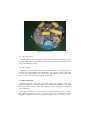
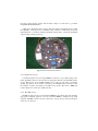
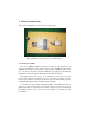
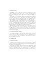
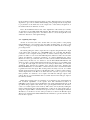
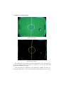
Parsian
(Amirkabir Univ. of Technology Small Size Team)
Team Description Paper for Robocup 2006
Amir Amjad Amir Ghiasvand, Mehdi Hooshyari Pour, Mohammad Korjani,
Mohsen Roohani, Shokoofeh Pourmehr, Farzaneh Rastgari, Vali Allah Monajjemi,
Moeen Nikzaad Larijani, Sepehr Saadatmand, Mani Milani
Electrical Engineering Department, Amirkabir University of Technology (Tehran
Polytechnic)
424 Hafez Ave. Postal Code 158754413, Tehran, Iran
[email protected]
Abstract. This document Describes, Parsian Robotic Small Size team activities
for preparing for Robocup 2006 Small Size League. It’s an overview of all
activities since November 2005. Parsian Robotic is a new comer to Small Size
league and this document describes the major activities they made to start
building Small Size Robots. Our robots mechanical and electrical design,
wireless communication, image processing and AI algorithms are described in
this paper.
1 Introduction
Parsian Robotic is a robotic research group working in Electrical Engineering
department of Amirkabir University of technology. The team now consists of 10
active members. Robocup 2006 is the opening tournament for this team to get
participated in a Small Size League.
2 Hardware Architecture
2.1 Mechanical Design
The robot mechanical structure consists of motors, wheels, robot body and the gears.
Each robot has 3 wheels, with relative polar angle of 120 degrees. The motors' power
is transferred to the wheels through the gears placed on the body of the robot, while
giving out 10 times more power. The motors are "Teac DC motors" and the wheels
are omni-directional for the purpose of omni-directional movement.
Fig. 1. Mechanical Design
2.1.1 Shooting system
The shooting operation is done by a solenoid with a metal core which is drawn to
the front of the robot to hit the ball. The solenoid moves the metal core radically when
it is given a 100v input voltage.
2.1.2 The spinner
The spinner axis is parallel to the ground plain. The roller is covered by rubber to
catch and covers the ball fully when the ball hits it. The spinner is placed at the height
of 2.3cm (the ball diameter) at the front of the robot, fixed by two holders. The
spinner motor rotates the roller through the related gears.
2.2 Electrical Design
We have followed 2 important goals in the design and production of the main
Printed Circuit Board on each robot. First, the maximum task capabilities of the main
board. Second, the least as possible the complexity of the board and its elements for
easier debugging.
The main controlling job is carried out by an AVR ATmega128 microcontroller.
The AVR microcontroller receives data from the wireless communication system
using the serial Rx port. Then the generated signal is sent to the motor drivers,
shooting system and the spinner. The decided voltage for each motor is produced
using Pulse Width Modulation.
A DC motor driver IC L-298 is used to drive the wheels' and spinner motors. It has
the capability of driving 2 motors simultaneously, if biased correctly with diodes and
right capacitors, to avoid the unwanted feedback current and to control the maximum
output voltage swing respectively.
Fig. 2. Robot main electrical board
2.2.1 Quadrature encoder
A feedback signal of the real output RPM of each motor is produced using a selfmade quadrature shaft encoder. We have designed the shaft encoder manually. There
are two IR-receivers and one IR-transmitter used on the opposite sides of a latticed
circular tape placed on the wheel's outside lap. An 89C2051 microcontroller counts
the number of pulses generated by the IR sensors circuit. The motor's RPM and
rotation direction is sent to the AVR controller.
2.2.2 The PID system
The PID system uses the encoder-measured RPM of each wheel and sends back the
appropriate feedback signal in case the measured RPM is different from what
expected. The PID system is used for each motor, to keep the speed and acceleration
of the robot as desired.
2 Wireless Communication
The wireless communication system consists of 3 main parts:
Fig. 3. Transmitter board, Designed based on AUREL XTR-434
2.1 Transceiver module
We use an AUREL XTR-434 transceiver module for data transmission and
reception. The XTR-434 uses the carrier frequency of 433.92 MHz. It's bandwidth is
150 KHz. It can work in data frequencies between 9600 - 100,000 bps, but it is said
not to be used for frequencies less than 57600 when not applying any bit-balancing
algorithms to the data, though the data must be byte-balanced otherwise.
The XTR-434 transceiver can be set to transmitter, receiver and power-down
modes. When switching to transmitter or receiver, the device needs 2ms to switch to
the new mode. And for 1ms after it should not be used for data transmission, but a
rectangular pulse signal must be transmitted in the meantime.
As we did not use the available manufactured PCBs of the XTR-434 module, we
came across some problems using our self-made circuit board. The correct way of
placing the module on a circuit board, the antenna connection, the ground circuits and
the antenna which is used, as said in the user's manual, is noticeable for better
performance!
2.2 Data flow control
Transmitter: there is an AVR microcontroller in the transmitter circuit of the
wireless communication board which is used to read the original data from the
Control unit computer and to create a packet of processed data for the XTR-434 to
transmit.
The serial Rx port of the AVR microcontroller has an interrupt subroutine which is
called anytime it receives one byte of data. When we receive 30 bytes of data, 5 bytes
for each robot, we apply the bit-balancing algorithm to the 30 original-data-bytes
giving out 60 bytes of processed data with equal number of 1s and 0s in each byte.
The "rf_transmit" function is then called to create a packet containing 1ms of
rectangular pulse signal plus one start-byte plus two bytes containing the number of
the bytes to be transmitted. Then the bit-balanced data followed by two ending bytes
are added to the created packet. The whole packet is sent to the XTR-434 Tx port,
using the serial Tx port of the AVR microcontroller for transmission.
Receiver: there is an AVR microcontroller on the receiver circuit board of the
wireless communication system on each robot which gets the received packet from
the XTR-434 Rx port. It then decodes the received packet in order to reconstruct the
original data. The data is checked for any errors using 3 different procedures, before
being passed to the next unit.
3.3 Serial connection to the computer
The serial RS232 COM port of the Control unit computer is used to send data to
and receive any needed data from the AVR microcontroller. A MAX-232 IC is used
to convert the +12 and -12 volts of the COM port to the operating logic voltages of
the circuit elements, that is 0 and 5.
4 Vision System
4.1 Global vision system
Studying some different documents and data -sheets and parameters of different
cameras, we decided to use a CCD-Analogue camera. Some important parameters of
the camera to use are discussed below.
The resolution of the camera output video must be at least 640x480 pixels so that
the image-processing algorithm can give a better and more delicate output. The
resolution of the grabbed frames sets a minimum limit to the capture device
specifications which is discussed later. The more the shutter speed of the camera is,
the more blur-less will be the image that it provides. This helps2 the noise-reduction
algorithm, to give a more definite understanding of the playing field. It was important
to pay attention to the frame-rate of the output video of the camera, though most of
the studied cameras would meet our need.
Due to the insufficient field of view of the original lens of the camera (f = 3.6 mm),
we decided to use an additional 0.42X wide lens. The added Lens would provide even
a wider view of field of play and so it would be easier to correct and repair the corner
and border distortions of the captured image.
4.2 Capturing video input
At first we recorded some video streams and took some pictures of the playing
field including the colored circles and other white boundary lines, in order to start
working on image-processing algorithms. It will be more talked about in the imageprocessing section.
We started getting the camera output into the computer using the Firewire output
of the camera and connecting it to a PCI IEEE 1394 port on the PC. The Firewire
connection to the computer would provides us with a noiseless input video and a
picture resolution of even more than 640x480 pixels. When we made sure about the
camera and Firewire connection parameters, we started challenging the VC++
libraries in order to get a real-time video from the connected camera and with the least
possible delay. In that case, we decided to use the DirectX9.0 SDK libraries and
drivers in order to get the grabbed frames directly into the VC++ project. While doing
so, to grab the video input, we came across two main problems. First, we noticed a
significant delay between the real-time video and the input video. Studying the
DirectX SDK libraries we found that a software-based decoder is used after the frame
is grabbed from the DV input. This would produce the delay. Second, we couldn't
find the needed extension repeaters for the Firewire cable, so that we could connect a
4meters high camera to the PC. As we didn’t have the very time to spend on solving
these problems, we decided to use a capture card with the analogue output of the
camera. We use a coaxial shielded cable to transfer data from the analogue output of
the camera to the PC.
When using a capture card, we would have to pay attention to the output frame-rate
and resolution capabilities of the capture card. The maximum resolution of
640x480px of the capture card would limit the video input maximum frame-rate to 30
fps. When using a capture card, another way to get the grabbed frame into the VC++
codes is to read the capture card’s memory. This can be done by directly reading the
memory without using the computer CPU in the overlay mode of the capture card, or
using the computer CPU to read data in the preview mode. Considering the different
alternatives, we decided to use the same procedure as we did for the Firewire input.
Thus we are using the DirectX9.0 SDK directshow libraries to get the real-time video
into the VC++ project.
4.3 Image-processing strategies:
Fig 4. Camera Output
Fig. 5. Rendered Image
After studying the other and previous teams’ documents and some other references
about the image-processing procedures we decided to use the color threshold
algorithms in the RGB color applet.
As the first attempt, we tested the tow-state thresholds for RGB colors and so we
reduced the total colors to only 8, out of 24bits. We did this, using the recorded video
streams and captured pictures in the MATLAB 6.5 environment. Afterwards we
examined and tested some different colors and environmental parameters affecting the
delicacy of the algorithm. We found out that the tow-state thresholds for all basic
RGB colors would not produce as many colors as we would need. So we decided to
use three-state color thresholds for at least one of the basic RGB colors. Using this we
are able to produce at least 12 easily distinguishable colors.
In order to identify each robot distinctively, we used some different patterns of
circles that we painted in one of those 12 colors. Each robot is distinctively identified
by these colored circles that are placed on top of each robot, considering the
arrangement of the circles.
In order to locate the circles of each color we thought of some different ways of
processing the matrix of the image among which I will briefly explain two most
inspiring ones.
•
•
One way of locating the circles is to read all the pixels of the grabbed frame
without bypassing any important or redundant pixels. In this case, a chosen
pattern that best represents a circle will scan the whole image and find all the
circles and finally drop the invalid circles found. Note that in this procedure
quite a lot of CPU usage and memory space will be used. This will cause the
program not to be able to produce as many new frame data as we need.
Another way of locating the circles is to read not ALL the pixels of the
image matrix. In this case a different pattern will sweep the whole picture,
but dropping about 95% of the pixels, if they don’t contain important
material. This is the procedure we are using now.
To identify each robot and find the angles needed, the algorithm goes through
some routine mathematical calculations then. As the last job of the image-processing
unit all the needed locations and angles and traces are passed to the control unit which
will control the robot movements.
NOTE: As an image-processing algorithm proposal, I would like to explain
another way to identify and locate the robots. In this procedure, a complete gradient
of the most distinguishable RGB basic color (such as green) is printed on a ring-paper
and placed on top of the robot. To identify each robot, a threshold color of another
basic RGB color (such as blue) is added to the gradient also. When using this
algorithm, there is no need to seek for any other circles more than central team circles.
When a radial line of one color is found in the near vicinity of the central tam circles,
the identity and angle of the robot is found at the same time. The gradient color tells
the angle, and the added color the ID.
5 Artificial intelligence subsystem
Artificial intelligence subsystem is divided into two parts. In “Beginner Layer” AI
each robot can do any activity such as going to new target, kicking, and passing. It
takes current game state and target game state (robots and ball position, velocities,
and robot orientation) as input from expert_ layer AI and generate the tasks to switch
current state to target state.
“Expert Layer” AI use reinforcement learning to select best activities. It gets robots
and ball position, velocities, and robot orientation as state current state and generates
target state. And submit the current and beginner state of robots to switch to target
state with beginner _layer AI.
5.1 Beginner Layer AI
This layer takes current and target state of robots, and reach the destination is it
job. The current state of a robot consists of the robot X and Y, coordinates,
orientation, and velocity. A desired target state consists of the final X and Y,
coordinates, final orientation, final velocity or power of kicking. In this section
obstacle avoidance is solved by minimizing the energy using Hopfield neural
networks.
5.2 Expert Layer AI
Expert Layer AI takes robot coordinates, orientation, and velocities as input from
vision system.
Expert _layer AI divided the field of play into squares and initialized a list of
activities by position of it to each square. In this section, game divided to three states
(defensive, offensive, and general). And arrange the activities by priority of each
activity. Then deleted each of them that completely infeasible. Finally, expert layer AI
choose the most suitable activity from top of the list. For example in 1/3 defensive
area of play kicking has best priority and dripping has lowest priority.
References:
1.
2.
Siegwart , Roland : Introduction to Autonomous Mobile Robots , 2004, MIT Press
Nils J. Nilsson : Introduction to Machine Learning, Department of Computer
Science, Stanford University