Download Groundwater Modeling System GMS v3.0 REFERENCE

16-58 GMS Reference Manual
Temporal Discretization
Many of the parameters associated with feature objects can be specified as
either constant or transient values. Transient values are defined as a simple
list of time/data pairs using the XY Series editor. The time series represents a
piece-wise linear curve indicating how the parameter varies with time. When
the Map -> MODFLOW command is selected, these curves must undergo
temporal discretization. Temporal discretization is a process of converting
general time series into discrete values that apply over specific time ranges
(stress periods).
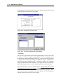
Transient parameters associated with feature objects are stored in an xy series.
An xy series is a general-purpose object used in GMS to represent curves of
data (in this case a time series). xy series are described in more detail in
Chapter 22. An xy series is manipulated by GMS with regards to feature
objects in three different ways: extrapolation, interpolation, and integration.
Extrapolation
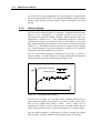
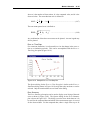
Because the user is free to enter any time values for the x parameter of an xy
series, it is possible that the xy series as entered does not cover the same time
range as the stress periods. In this case it may be necessary to extrapolate a
value for the xy series at a time before or after the first or last entered value.
In GMS the simplest approach has been used. If a value is required for a time
previous to the times defined by the xy series, the first value is used. Likewise
for a time that is later than the all of the times in the xy series, the last value is
used. Since this behavior might hide an error in the input parameters, GMS
will warn the user if any xy series does not cover the time range defined by the
stress periods.
Interpolation
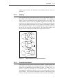
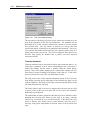
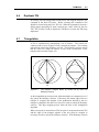
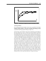
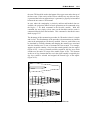
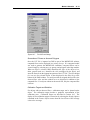
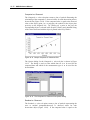
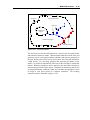
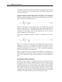
It is also sometimes necessary to create an xy series that is a composite of two
other xy series. This is the case when obtaining transient values for an
intermediate point along an arc segment that has differing transient parameters
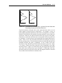
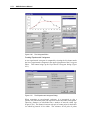
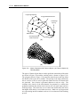
at both nodes at the ends of the arc. To perform this type of interpolation, a
new xy series is constructed that is the union of the x times from the two
original series. The y values that correspond to each of these new x values are
obtained by evaluating the original series at the x value to get two y values and
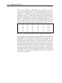
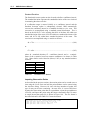
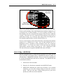
then interpolating these two y values using the following equation (illustrated
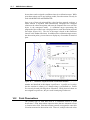
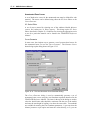
in Figure 16.29).
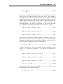
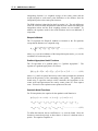
y n = F0 ( x n ) ⋅ (10
. − t ) + F1 ( x n ) ⋅ (t ) ................................................. (16.9)
Where xn and yn are the points along the new xy series, F0 and F1 are the two
original xy series and t is the interpolation weighting parameter.