Download User`s Manual POLARIS

time invariant (the lengths are the same for all pulses) filters. Traditional analog filters
are time invariant. The concept behind time variant filters is that, since the γ-rays arrive
randomly and the lengths between them vary accordingly, one can make maximum use of
the available information by setting Length to the interpulse spacing.
In principal, the very best filtering is accomplished by using cusp-like weights and time
variant filter length selection. There are serious costs associated with this approach
however, both in terms of computational power required to evaluate the sums in real time
and in the complexity of the electronics required to generate (usually from stored
coefficients) normalized {wi} sets on a pulse by pulse basis.
The Polaris takes a different approach because it was optimized for very high speed
operation. It implements a fixed length filter with all wi values equal to unity and in fact
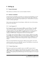
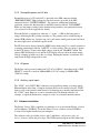
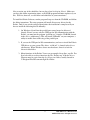
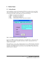
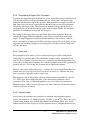
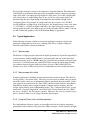
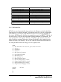
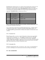
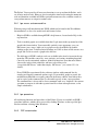
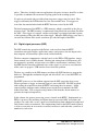
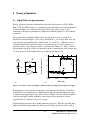
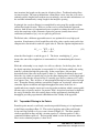
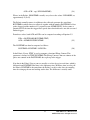
computes this sum afresh for each new signal value k. Thus the equation implemented is:
k − L −G
LV x , k = −
k
∑ Vi +
∑V
i
(5.2)
i = k − 2 L −G +1 i = k − L +1
where the filter length is L and the gap is G . The factor L multiplying Vx ,k arises
because the sum of the weights here is not normalized. Accommodating this factor is
trivial.
While this relationship is very simple, it is still very effective. In the first place, this is
the digital equivalent of triangular (or trapezoidal if G ≠ 0) filtering which is the analog
industry’s standard for high rate processing. In the second place, one can show
theoretically that if the noise in the signal is white (i.e. Gaussian distributed) above and
below the step, which is typically the case for the short shaping times used for high signal
rate processing, then the average in Eqn. 5.2 actually gives the best estimate of Vx in the
least squares sense. This, of course, is why triangular filtering has been preferred at high
rates. Triangular filtering with time variant filter lengths can, in principle, achieve both
somewhat superior resolution and higher throughputs but comes at the cost of a
significantly more complex circuit and a rate dependent resolution, which is unacceptable
for many types of precise analysis. In practice, XIA’s design has been found to duplicate
the energy resolution of the best analog shapers while approximately doubling their
throughput, providing experimental confirmation of the validity of the approach.
5.2
Trapezoidal Filtering in the Polaris
From this point onward, we will only consider trapezoidal filtering as it is implemented
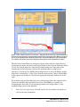
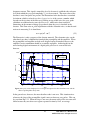
in the Polaris according to Eqn. 5.2. The result of applying such a filter with Length
L=1µs and Gap G=0.4µs to a γ-ray event is shown in Figure 5.3. The filter output is
clearly trapezoidal in shape and has a risetime equal to L, a flattop equal to G, and a
symmetrical falltime equal to L. The basewidth, which is a first-order measure of the
filter’s noise reduction properties, is thus 2L+G.
26
POLARIS User’s Manual V3.40
 XIA LLC 2009. All rights reserved.